minimally resolution biased electron-density maps

research papers

326 doi:10.1107/S0108767308004303 Acta Cryst. (2008). A64, 326–336

Acta Crystallographica Section A

Foundations ofCrystallography

ISSN 0108-7673

Received 15 November 2007

Accepted 10 January 2008

# 2008 International Union of Crystallography

Printed in Singapore – all rights reserved

Minimally resolution biased electron-density maps

Angela Altomare,a Corrado Cuocci,b Carmelo Giacovazzo,a,b* Gihan Salah Kamel,c

Anna Moliternia and Rosanna Rizzia

aIC, Bari, via Amendola 122/o, 70126 Bari, Italy, bDipartimento Geomineralogico, Universita di

Bari, Campus Universitario, Via Orabona 4, 70125 Bari, Italy, and cDepartment of Physics, Faculty

of Science, Helwan University, Cairo, Egypt. Correspondence e-mail: [email protected]

Electron-density maps are calculated by Fourier syntheses with coefficients

based on structure factors. Diffraction experiments provide intensities up to a

limited resolution; as a consequence, the Fourier syntheses always show series-

termination errors. The worse the resolution, the less accurate is the Fourier

representation of the electron density. In general, each atomic peak is shifted

from the correct position, shows a deformed (with respect to the true

distribution of the electrons in the atomic domain) profile, and is surrounded

by a series of negative and positive ripples of gradually decreasing amplitude.

An algorithm is described which is able to reduce the resolution bias by

relocating the peaks in more correct positions and by modifying the peak profile

to better fit the real atomic electron densities. Some experimental tests are

performed showing the usefulness of the procedure.

1. Notation

fj scattering factor of the jth atom, thermal factor included

f 0j scattering factor of the jth atom at rest

N number of atoms in the unit cell

s 2 sin�=�Fh structure factor with vectorial index h

Eh normalized structure factor

Bj isotropic thermal parameter of the jth atom

RES experimental data resolution (in A)

2. Introduction

Let

�ðrÞ ¼PNj¼1

�jðr� rjÞ

be the electron density of a crystal structure constituted by N

atoms: rj is the atomic position of the jth atom and �jðrÞ is its

electron density. For X-rays, �ðrÞ is a non-negative definite

function [i.e. �ðrÞ � 0 at any point of the unit cell]. When

calculated via structure-factor amplitudes, �ðrÞ should co-

incide with

�0ðrÞ ¼1

V

Xh

Fh expð�2�ih � rÞ

provided the summation is extended to an infinite number of

Miller indices and hjFhji ! 0 when RES! 0. In practice, the

summation is limited to the measured domain of the reciprocal

space, represented by the shape function �ðr�Þ [�ðr�Þ ¼ 1

inside the measured domain, �ðr�Þ ¼ 0 outside it]. Corre-

spondingly, the electron-density map available in practice, say

�0ðrÞ, is based on the structure factors F 0h ¼ Fh�ðr�Þ rather

than on Fh, where

�0ðrÞ ¼ �0ðrÞ � T½�ðr�Þ� ¼ �ðrÞ � �ðrÞ ¼PNj¼1

�jðr� rjÞ � �ðrÞ:

ð1Þ

�ðrÞ is the Fourier transform of �ðr�Þ and � represents the

convolution operation.

The main features of �0ðrÞ are the following: (a) it can be

negative in more or less extended regions of the unit cell; (b)

the atomic peaks are broadened and are surrounded by a

series of negative and positive ripples of gradually decreasing

amplitude; (c) since ripples may overlap with other ripples and

with atomic peaks, the maxima of the electron density �0ðrÞ are

at r0j, not perfectly coinciding with the atomic positions rj;

(d) the modification of the peak profiles and the displacements

of the atomic peaks are resolution dependent; (e) �0ðrÞ will

usually show more maxima and minima than �ðrÞ; in favour-

able conditions, it may be approximated by the main N

maxima in the map:

�0ðrÞ �PNj¼1

�0jðr� r0jÞ; ð2Þ

where �0jðrÞ, j = 1, . . . , N, are suitable peak profiles.

Returning from �0ðrÞ to �ðrÞ via deconvolution procedures

offers several advantages: peaks should move in more correct

positions, false peaks due to the limited experimental data

resolution may be eliminated, and peak broadening may be

reduced.

It is a common belief that resolution bias in crystallographic

electron-density maps is an unavoidable cost to pay: it is

generally considered an intrinsic unavoidable characteristic of

the electron-density maps, generated by the physics of the

diffraction experiment. This is rather unexpected if one

considers that the resolution bias is precisely described by the

basic diffraction theory. At non-atomic resolution, the bias is

larger and any current attempt to interpret the electron-

density maps in terms of molecular models is performed by

using the prior information on the molecular geometry rather

than by reducing the resolution bias. Correcting the bias

should increase the efficiency of any cyclic procedure based on

the electron-density modification, where the usefulness of the

(n + 1)th map is based on the quality of the phases derived

from the inversion of the nth map. The current electron-

density-modification procedures (Cowtan & Main, 1993;

Abrahams, 1997; Cowtan, 1999; Terwilliger, 1999, 2003; Hunt

& Deisenhofer, 2003) aim at fitting the expected character-

istics of the electron-density function by suitable restraints in

direct or reciprocal space. E.g. solvent flattening tries to fit the

positivity of the map in direct space, histograms in one or more

dimensions, in direct and/or reciprocal space, try to capture

the stereochemical information and improve the phase esti-

mates. None of these approaches is used to gain resolution and

to relocate peaks.

Traditional Patterson search methods often suppress (in the

reciprocal space) the ripples generated by the origin peak, by

calculating ðjEj2 � 1Þ Patterson maps. In contrast, the

correction for the series-termination effects is usually not

applied to observed electron-density maps. The only exception

we know is reported in a recent paper by Burla et al. (2006),

where an algorithm is described that allows the elimination of

the bias in a region around the heavy-atom peak. The algor-

ithm allowed the complexity limit for proteins solvable ab

initio to extend from 2268 (value attained by Mooers &

Matthews, 2006) to 6319 non-H atoms in the asymmetric unit

(provided RES is better than 1.2 A).

However, a perfect deconvolution procedure allowing the

return from �0ðrÞ to �ðrÞ may be applied only if �ðrÞ and the

atomic positions rj are a priori known. Luckily, the function

�ðrÞ, i.e. the supplementary information which will be explicitly

used by our algorithm, may be deduced from the experimental

data; in contrast, we have experimental access only to the

vectors r0j. In this paper, we describe a mathematical approach

leading, from �0ðrÞ, to a modified electron-density map [say

�0modðrÞ] which is expected to be closer to �ðrÞ than �0ðrÞ.We will first apply the approach to point-atom structures

(see xx3–5). This case is approximately (i.e. the displacement

factor blurs the exact theoretical shape of the scattering

factor) met when neutron diffraction data are available. Point

atoms are also simulated in X-ray or in electron crystal-

lography when E maps are considered. Indeed, the normal-

ization procedure replaces the usual atomic scattering factors

fj, monotonically decreasing with s, by their normalized scat-

tering factors �j ¼ fj=ðPN

j¼1 f 2j Þ

1=2, which are nearly constant

versus the diffraction angle. In this way, point-like atoms (the

effects of the displacement factor is analysed in x5 and in

Appendix A) replace electron clouds: the atomic peaks in the

corresponding electron densities are sharper but the quality of

the map is degraded by strong truncation effects (which are a

function of RES).

In x5, the usual electron-density maps employed in X-ray

crystallography will be considered.

In this pilot study, we will apply the theory to some selected

cases to show that peaks in the �0modðrÞ maps are closer to the

true atomic positions than peaks of the �0ðrÞmaps, and that the

�0mod’s are more interpretable in terms of molecular models.

The full potential of the theory will be revealed as soon as

massive applications are made to X-ray, neutron and electron

diffraction, single-crystal or powder data, small molecules as

well as macromolecules, at different resolutions and when

structure factors are still affected by phase errors. These

applications are deferred to forthcoming papers.

3. Peak deconvolution for a ‘one-point-atom’ and for a‘two-point-atom’ structure: one-dimensional case,atoms at rest

As a didactical example, let us first consider a one-dimensional

unit cell with period a, containing only a ‘one-point-atom’,

located at the origin: its electron density may be written as

�ðxÞ ¼ c�ðxÞ, where � is the Dirac delta function and c is a

suitable constant. If we calculate the structure factors up to

RES (i.e. Fh ¼ c for any h) and, from them, the electron

density �0ðxÞ by Fourier inversion, we should obtain

�0ðxÞ ¼ c�ðxÞ � �ðxÞ ¼ c�ðxÞ:

�ðxÞ is equal to ½sinð2hmax þ 1Þ�x�=sin�x, the function theor-

etically expected to describe the effect of the resolution in the

one-dimensional case, hmax ¼ intða RES�1Þ is the maximum

index used in the electron-density calculation. The maximum

value of �ðxÞ is ð2hmax þ 1Þ, attained at the origin.

Suppose that we have observed the electron density

�0ðxÞ ¼ c sinð2hmax þ 1Þ�x=sin�x. Can we return back to the

correct density �ðxÞ given �0ðxÞ and the prior knowledge that

�ðxÞ is a delta function? In Fig. 1, we plot �0ðxÞ when a = 20 A,

c = 6 and RES = 1.2, 1.8 and 2.2 A. While both �0ðxÞ and �ðxÞhave their maximum at the origin, relevant differences can be

found between them: the main peak of �0 is no longer a delta

Acta Cryst. (2008). A64, 326–336 Angela Altomare et al. � Minimally resolution biased electron-density maps 327

research papers

Figure 1�0ðxÞ for a one-point-atom structure. The point atom is a delta functionlocated at the origin ½�ðxÞ ¼ 6�ðxÞ� and represented by a red vertical bar.Blue line: RES = 1.2 A; red line: RES = 1.8 A; black line: RES = 2.2 A.

function, positive and negative ripples, with gradually

decreasing amplitude, surround it. The lower the resolution,

the smaller are the ripple intensities and their frequency.

In this simple example, recovering �ðxÞ given �0ðxÞ is quite

immediate. If the experimental fits with the function

c sinð2hmax þ 1Þ�x=sin�x, one can immediately deduce that

�ðxÞ is a delta function centred on the origin.

It may be worthwhile noting that recovering �ðxÞ does not

imply any peak shift; indeed, the main maximum in �0ðxÞ is

located in the origin as is the delta function. That does not

occur if a ‘two-point-atom’ structure is considered. Suppose

the electron density �0ðxÞ is given by

�0ðxÞ ¼ ½c1�ðx� x1Þ þ c2�ðx� x2Þ� � �ðxÞ

¼ c1�ðx� x1Þ þ c2�ðx� x2Þ: ð3Þ

In Fig. 2(a), for a = 20 A, c1 = c2 = 6, x1 = 0.0, x2 = 0.15, RES =

1.8 A, we show the delta functions by two red vertical bars,

c1�ðx� x1Þ by a blue line, c2�ðx� x2Þ by a green line. In

Fig. 2(b), �0ðxÞ is plotted by a black line and is overlapped with

research papers

328 Angela Altomare et al. � Minimally resolution biased electron-density maps Acta Cryst. (2008). A64, 326–336

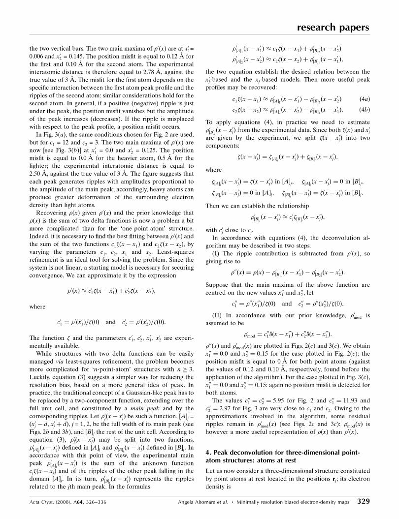
Figure 2Two-point-atom structure: the two point atoms are located atx1 ¼ 0:0; x2 ¼ 0:15 and are represented by 6�ðx� x1Þ and 6�ðx� x2Þ,respectively (red vertical bars). RES = 1.8 A. (a) Blue line: 6�ðx� x1Þ;green line: 6�ðx� x2Þ. (b) �0ðxÞ ¼ c1�ðx� x1Þ þ c2�ðx� x2Þ (black line).The two main maxima of �0ðxÞ are at x01 ¼ 0:06 and x02 ¼ 0:145. (c) �00ðxÞ(blue line) and �0modðxÞ (red vertical bars).

Figure 3Two-point-atom structure: the two point atoms are located atx1 ¼ 0:0; x2 ¼ 0:15 and are represented by 12�ðx� x1Þ and 3�ðx� x2Þ,respectively (red vertical bars). RES = 1.8 A. (a) Blue line: 12�ðx� x1Þ;green line: 3�ðx� x2Þ. (b) �0ðxÞ ¼ c1�ðx� x1Þ þ c2�ðx� x2Þ (black line).The two main maxima of �0ðxÞ are at x01 ¼ 0:0 and x02 ¼ 0:125. (c) �00ðxÞ(blue line) and �0modðxÞ (red vertical bars).

the two vertical bars. The two main maxima of �0ðxÞ are at x01=

0.006 and x02 = 0.145. The position misfit is equal to 0.12 A for

the first and 0.10 A for the second atom. The experimental

interatomic distance is therefore equal to 2.78 A, against the

true value of 3 A. The misfit for the first atom depends on the

specific interaction between the first atom peak profile and the

ripples of the second atom: similar considerations hold for the

second atom. In general, if a positive (negative) ripple is just

under the peak, the position misfit vanishes but the amplitude

of the peak increases (decreases). If the ripple is misplaced

with respect to the peak profile, a position misfit occurs.

In Fig. 3(a), the same conditions chosen for Fig. 2 are used,

but for c1 = 12 and c2 = 3. The two main maxima of �0ðxÞ are

now [see Fig. 3(b)] at x01 = 0.0 and x02 = 0.125. The position

misfit is equal to 0.0 A for the heavier atom, 0.5 A for the

lighter; the experimental interatomic distance is equal to

2.50 A, against the true value of 3 A. The figure suggests that

each peak generates ripples with amplitudes proportional to

the amplitude of the main peak; accordingly, heavy atoms can

produce greater deformation of the surrounding electron

density than light atoms.

Recovering �ðxÞ given �0ðxÞ and the prior knowledge that

�ðxÞ is the sum of two delta functions is now a problem a bit

more complicated than for the ‘one-point-atom’ structure.

Indeed, it is necessary to find the best fitting between �0ðxÞ and

the sum of the two functions c1�ðx� x1Þ and c2�ðx� x2Þ, by

varying the parameters c1, c2, x1 and x2. Least-squares

refinement is an ideal tool for solving the problem. Since the

system is not linear, a starting model is necessary for securing

convergence. We can approximate it by the expression

�0ðxÞ � c01�ðx� x01Þ þ c02�ðx� x02Þ;

where

c01 ¼ �0ðx01Þ=�ð0Þ and c02 ¼ �

0ðx02Þ=�ð0Þ:

The function � and the parameters c01, c02, x01, x02 are experi-

mentally available.

While structures with two delta functions can be easily

managed via least-squares refinement, the problem becomes

more complicated for ‘n-point-atom’ structures with n � 3.

Luckily, equation (3) suggests a simpler way for reducing the

resolution bias, based on a more general idea of peak. In

practice, the traditional concept of a Gaussian-like peak has to

be replaced by a two-component function, extending over the

full unit cell, and constituted by a main peak and by the

corresponding ripples. Let �0jðx� x0jÞ be such a function, ½A�j =

ðx0j � d; x0j þ dÞ, j = 1; 2, be the full width of its main peak (see

Figs. 2b and 3b), and ½B�j the rest of the unit cell. According to

equation (3), �0jðx� x0jÞ may be split into two functions,

�0½A�jðx� x0jÞ defined in ½A�j and �0½B�jðx� x0jÞ defined in ½B�j. In

accordance with this point of view, the experimental main

peak �0½A�j ðx� x0jÞ is the sum of the unknown function

cj�ðx� xjÞ and of the ripples of the other peak falling in the

domain ½A�j. In its turn, �0½B�jðx� x0jÞ represents the ripples

related to the jth main peak. In the formulas

�0½A�1ðx� x01Þ � c1�ðx� x1Þ þ �0½B�2ðx� x02Þ

�0½A�2ðx� x02Þ � c2�ðx� x2Þ þ �0½B�1ðx� x01Þ;

the two equation establish the desired relation between the

x0j-based and the xj-based models. Then more useful peak

profiles may be recovered:

c1�ðx� x1Þ � �0½A�1ðx� x01Þ � �

0½B�2ðx� x02Þ ð4aÞ

c2�ðx� x2Þ � �0½A�2ðx� x02Þ � �

0½B�1ðx� x01Þ: ð4bÞ

To apply equations (4), in practice we need to estimate

�0½B�j ðx� x0jÞ from the experimental data. Since both �ðxÞ and x0jare given by the experiment, we split �ðx� x0jÞ into two

components:

�ðx� x0jÞ ¼ �½A�jðx� x0jÞ þ �½B�j ðx� x0jÞ;

where

�½A�jðx� x0jÞ ¼ �ðx� x0jÞ in ½A�j; �½A�j ðx� x0jÞ ¼ 0 in ½B�j;

�½B�jðx� x0jÞ ¼ 0 in ½A�j; �½B�jðx� x0jÞ ¼ �ðx� x0jÞ in ½B�j:

Then we can establish the relationship

�0½B�jðx� x0jÞ � c0j�½B�jðx� x0jÞ;

with c0j close to cj.

In accordance with equations (4), the deconvolution al-

gorithm may be described in two steps.

(I) The ripple contribution is subtracted from �0ðxÞ, so

giving rise to

�00ðxÞ ¼ �ðxÞ � �0½B1�ðx� x01Þ � �

0½B2�ðx� x02Þ:

Suppose that the main maxima of the above function are

centred on the new values x001 and x002 , let

c001 ¼ �00ðx001Þ=�ð0Þ and c002 ¼ �

00ðx002Þ=�ð0Þ:

(II) In accordance with our prior knowledge, �0mod is

assumed to be

�0mod ¼ c001�ðx� x001Þ þ c002�ðx� x002Þ:

�00ðxÞ and �0modðxÞ are plotted in Figs. 2(c) and 3(c). We obtain

x001 ¼ 0:0 and x002 ¼ 0:15 for the case plotted in Fig. 2(c): the

position misfit is equal to 0 A for both point atoms (against

the values of 0.12 and 0.10 A, respectively, found before the

application of the algorithm). For the case plotted in Fig. 3(c),

x001 ¼ 0:0 and x002 ¼ 0:15: again no position misfit is detected for

both atoms.

The values c001 ¼ c002 ¼ 5:95 for Fig. 2 and c001 ¼ 11:93 and

c002 ¼ 2:97 for Fig. 3 are very close to c1 and c2. Owing to the

approximations involved in the algorithm, some residual

ripples remain in �0modðxÞ (see Figs. 2c and 3c): �0modðxÞ is

however a more useful representation of �ðxÞ than �0ðxÞ.

4. Peak deconvolution for three-dimensional point-atom structures: atoms at rest

Let us now consider a three-dimensional structure constituted

by point atoms at rest located in the positions rj; its electron

density is


research papers

�ðrÞ ¼PNj¼1

cj�ðr� rjÞ: ð5Þ

The experimental electron density will be

�0ðrÞ ¼PNj¼1

cj�ðr� rjÞ � �ðrÞ ¼PNj¼1

cj�ðr� rjÞ; ð6Þ

where �ðrÞ may be obtained as follows:

(a) a point atom with weight c = 1 is put at the origin;

(b) it is assumed Fh ¼ 1 for any h belonging to the observed

set of reflections;

(c) �ðrÞ ¼ ð1=VÞP

h Fh expð�2�ih � rÞ is calculated where

the summation goes over the set of observed reflections,

Friedel-related included.

If � is a sphere, �ðrÞ will have a spherical symmetry: the

expected function is

�ðrÞ ¼ 43�r3

maxy; ð7Þ

where

y ¼ 3sinð2�r�maxrÞ � ð2�r�maxrÞ cosð2�r�maxrÞ

ð2�r�maxrÞ3

and r�max ¼ RES�1.

The maxima of �0ðrÞ will be located at positions r0j, usually

not coincident with the positions rj. We want to find an elec-

tron density �0modðrÞ which better approximates �ðrÞ, given �0ðrÞand the prior knowledge that �ðrÞ is a sum of N delta functions.

In accordance with x3, an approximate solution of the problem

may be found by replacing the traditional concept of a three-

dimensional Gaussian-like peak by a two-component function:

i.e. �0jðr� r0jÞ extends over the full unit cell and is constituted

by a main peak and by the corresponding ripples. Let ½A�j be

the domain containing all the unit-cell points belonging to the

jth main peak and ½B�j the rest of the unit cell (see Fig. 4).

According to x3, �0jðr� r0jÞ is split into two functions,

�0½A�jðr� r0jÞ defined in ½A�j, representing the jth main peak, and

�0½B�jðr� r0jÞ, defined in ½B�j and describing its ripples. I.e.

�0jðr� r0jÞ ¼ �0½A�jðr� r0jÞ þ �

0½B�jðr� r0jÞ:

Accordingly, �ðr� r0jÞ is split into two components, e.g.

�ðr� r0jÞ ¼ �½A�j ðr� r0jÞ þ �½B�jðr� r0jÞ;

where

�½A�jðr� r0jÞ ¼ �ðr� r0jÞ in ½A�j; �½A�jðr� r0jÞ ¼ 0 in ½B�j;

�½B�jðr� r0jÞ ¼ 0 in ½A�j; �½B�jðr� r0jÞ ¼ �ðr� r0jÞ in ½B�j;

from which we can establish the relationship

�0½B�jðr� r0jÞ � c0j�½B�j ðr� r0jÞ: ð8Þ

c0j ¼ �0ðr0jÞ=�ð0Þ is expected to be close to cj. Equation (8)

estimates �0½B�jðr� r0jÞ in terms of experimental quantities.

We can now consider the experimental main peak

�0½A�jðr� r0jÞ as the sum of the unknown function cj�ðr� rjÞ and

of the ripples of the other peaks falling in the domain ½A�j:

�0½A�j ðr� r0jÞ � cj�ðr� rjÞ þPN

i6¼j¼1

�0½B�i ðr� r0iÞ:

Since �0½B�j ðr� r0jÞ vanishes in ½A�j, we can rewrite the above

equation in the form

�0½A�j ðr� r0jÞ � cj�ðr� rjÞ þPNi¼1

�0½B�i ðr� r0iÞ;

from which

cj�ðr� rjÞ � �0½A�jðr� r0jÞ �

PNi¼1

�0½B�iðr� r0iÞ

may be derived. The algorithm may now be described in two

steps.

(I) the overall ripple contribution is subtracted from �0ðrÞ,so giving rise to the electron-density map

�00ðrÞ ¼ �0ðrÞ �PNj¼1

�0½B�jðr� r0jÞ � �0ðrÞ � c0j�½B�j ðr� r0jÞ:

(II) Let the main maxima of �ðrÞ be centred on the values r00j .

Then �0mod is assumed to be

�0mod ¼PNj¼1

c00j �ðr� r00j Þ;

where c00j ¼ �ðr00j Þ=�ð0Þ.

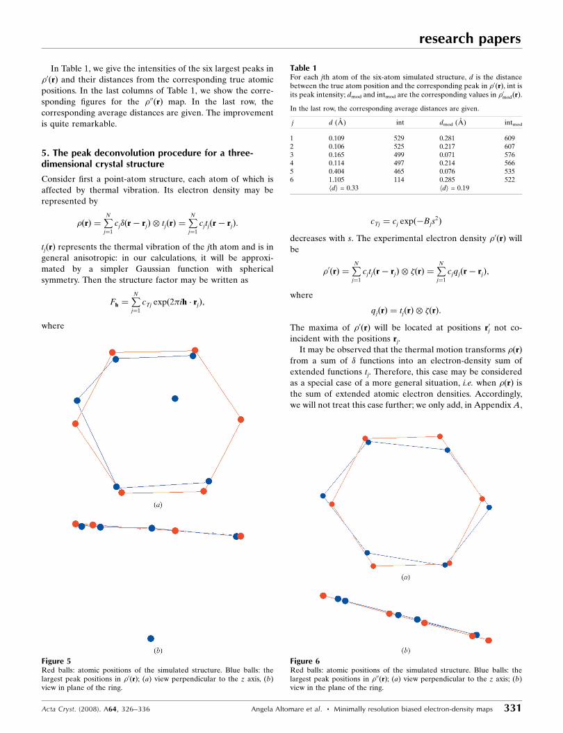
To check the usefulness of the above algorithm, we simu-

lated in P1 a simple point-atoms crystal structure constituted

by a benzene ring in a unit cell with parameters a = 3.848, b =

11.005, c = 12.727 A, � ¼ 106; ¼ 95; ¼ 80, RES = 1.54 A.

All the atoms were located in the plane z = 0: in Figs. 5(a), (b),

we show the true atomic positions by red balls. In the same

figures, the positions of the largest six maxima of �0ðrÞ are

shown by blue balls: Fig. 5(a) is plotted perpendicular to the z

axis, Fig. 5(b) is in the ring plane. If we apply the two-step

algorithm described above, we obtain the new positions r00j ,

drawn in Fig. 6(a) (perpendicular to z) and in Fig. 6(b) (in the

ring plane) by blue balls. One �0ðrÞ peak is far from the correct

position and is remarkably out from the benzene plane: its

position is well recovered in �0mod, which is also able to

maintain the planarity of the ring.

research papers


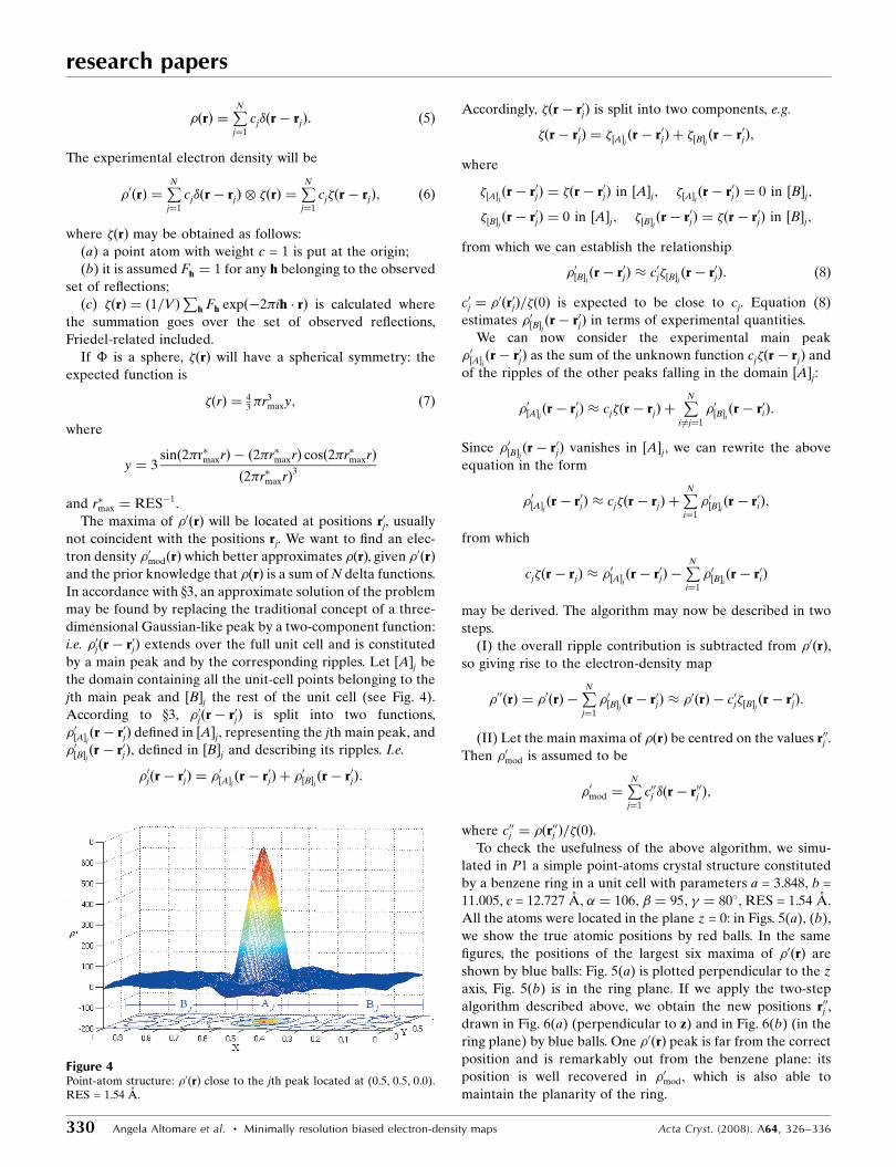
Figure 4Point-atom structure: �0ðrÞ close to the jth peak located at (0.5, 0.5, 0.0).RES = 1.54 A.

In Table 1, we give the intensities of the six largest peaks in

�0ðrÞ and their distances from the corresponding true atomic

positions. In the last columns of Table 1, we show the corre-

sponding figures for the �00ðrÞ map. In the last row, the

corresponding average distances are given. The improvement

is quite remarkable.

5. The peak deconvolution procedure for a three-dimensional crystal structure

Consider first a point-atom structure, each atom of which is

affected by thermal vibration. Its electron density may be

represented by

�ðrÞ ¼PNj¼1

cj�ðr� rjÞ � tjðrÞ ¼PNj¼1

cjtjðr� rjÞ:

tjðrÞ represents the thermal vibration of the jth atom and is in

general anisotropic: in our calculations, it will be approxi-

mated by a simpler Gaussian function with spherical

symmetry. Then the structure factor may be written as

Fh ¼PNj¼1

cTj expð2�ih � rjÞ;

where

cTj ¼ cj expð�Bjs2Þ

decreases with s. The experimental electron density �0ðrÞ will

be

�0ðrÞ ¼PNj¼1

cjtjðr� rjÞ � �ðrÞ ¼PNj¼1

cjqjðr� rjÞ;

where

qjðrÞ ¼ tjðrÞ � �ðrÞ:

The maxima of �0ðrÞ will be located at positions r0j not co-

incident with the positions rj.

It may be observed that the thermal motion transforms �ðrÞfrom a sum of � functions into an electron-density sum of

extended functions tj. Therefore, this case may be considered

as a special case of a more general situation, i.e. when �ðrÞ is

the sum of extended atomic electron densities. Accordingly,

we will not treat this case further; we only add, in Appendix A,


research papers

Figure 6Red balls: atomic positions of the simulated structure. Blue balls: thelargest peak positions in �00ðrÞ; (a) view perpendicular to the z axis; (b)view in the plane of the ring.

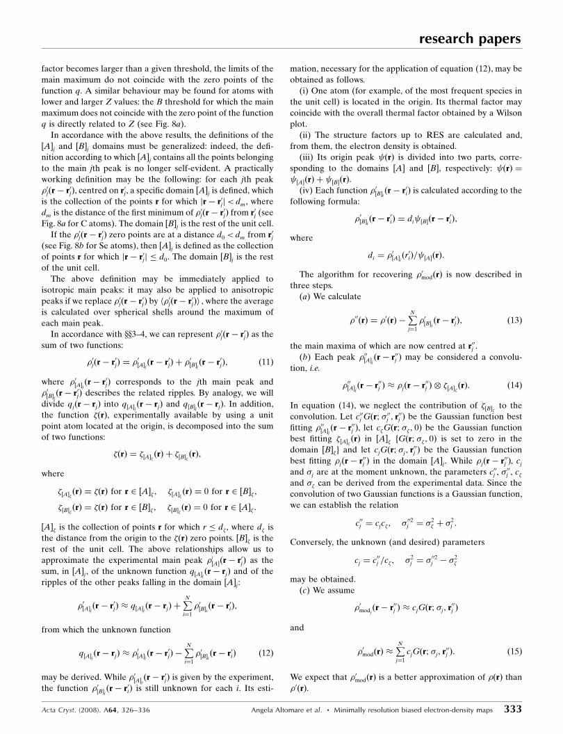
Table 1For each jth atom of the six-atom simulated structure, d is the distancebetween the true atom position and the corresponding peak in �0ðrÞ, int isits peak intensity; dmod and intmod are the corresponding values in �0modðrÞ.

In the last row, the corresponding average distances are given.

j d (A) int dmod (A) intmod

1 0.109 529 0.281 6092 0.106 525 0.217 6073 0.165 499 0.071 5764 0.114 497 0.214 5665 0.404 465 0.076 5356 1.105 114 0.285 522

hdi = 0.33 hdi = 0.19

Figure 5Red balls: atomic positions of the simulated structure. Blue balls: thelargest peak positions in �0ðrÞ; (a) view perpendicular to the z axis, (b)view in plane of the ring.

some considerations concerning the applicability of our

algorithm to usual point-atom structures described by X-ray

E maps or to neutron diffraction data.

Let us now consider a three-dimensional crystal structure

constituted by atoms located at rj, j ¼ 1; . . . ;N. Its electron

density is

�ðrÞ ¼PNj¼1

�jðr� rjÞ

and the observed electron density is

�0ðrÞ ¼PNj¼1

�jðr� rjÞ � �ðrÞ ¼PNj¼1

qjðr� rjÞ: ð9Þ

The position of the jth main peak in �0ðrÞ, say �0jðr� r0jÞ, is

influenced by the superposition of the functions

qiðr� riÞ; i ¼ 1; . . . ;N; i 6¼ j: ð10Þ

In accordance with xx3–4, returning back to �jðr� rjÞ requires

the elimination of the ripples of the main peaks and a suitable

modification of the mean peak profiles. That may be

attempted as soon as the following points are clarified.

(a) In the case of real atoms, each peak of �0ðrÞ arises from

the convolution of two broad functions, the first of which (say

�j) is atom dependent, the second (say �) is resolution

dependent. As a consequence, each main peak will generally

be wider than both the corresponding �j and the main peak of

�ðrÞ. Furthermore, each main peak may show, at a given

resolution, a proper broadness, depending on the atomic

species; in this case, the practical application of the decon-

volution procedure would require ½A� and ½B� domains of

different sizes, each size specific for each atomic species (in

contrast, for point atoms at rest the ½A� size was constant).

(b) The location of the ripples depends on the resolution; if

it was influenced also by the thermal factor of the peak-related

atom, then the functions �ðrÞ and qjðrÞ would show, at a given

data resolution, a different peak location. In this case, the

deconvolution procedure should face additional difficulties;

indeed, the atomic species associated with a main peak and the

corresponding atomic thermal factor often are not a priori

known. Correspondingly, the specific function qjðrÞ to

associate to the jth atom would remain ambiguous.

For assessing point (a), we plot in Fig. 7, for a = 20 A and

RES = 1.8 A, the electron density of C, Mn, Br and Hg atoms

when located at the origin and at rest. The Fourier coefficients

of such a simple �0ðrÞ function are

Fh ¼ f 0ðsÞ:

It may be observed that the domain ½A� does not substantially

vary with the atomic species, the ripple intensity is propor-

tional to Z, the ripple frequency and location remain practi-

cally constant.

For assessing point (b), we plot in Fig. 8(a), for a = 20 A and

RES = 1.8 A, the electron density of the C atom for different

values of the thermal factor B. We observe: (i) the main peak

intensity is inversely related to the B value; (ii) the size of the

domain ½A� increases with B; (iii) the ripple intensities are

inversely related to B but their frequency and location are

roughly constant (a mathematical basis for this practical

invariance is given in Appendix B); (iv) when the thermal

research papers


Figure 7One-atom structure. �0ðxÞ when C, Mn, Br and Hg atoms, at rest, arelocated at the origin. RES = 1.8 A.

Figure 8One-atom structure. �0ðxÞ at RES = 1.8 A: (a) when the C atom is locatedat the origin with different values of the thermal factor B (blue: B = 0 A2;green: B = 5 A2; red: B = 15 A2); (b) the corresponding curves when theSe atom is located on the origin.

factor becomes larger than a given threshold, the limits of the

main maximum do not coincide with the zero points of the

function q. A similar behaviour may be found for atoms with

lower and larger Z values: the B threshold for which the main

maximum does not coincide with the zero point of the function

q is directly related to Z (see Fig. 8a).

In accordance with the above results, the definitions of the

½A�j and ½B�j domains must be generalized: indeed, the defi-

nition according to which ½A�j contains all the points belonging

to the main jth peak is no longer self-evident. A practically

working definition may be the following: for each jth peak

�0jðr� r0jÞ, centred on r0j, a specific domain ½A�j is defined, which

is the collection of the points r for which jr� r0jj< dm, where

dm is the distance of the first minimum of �0jðr� r0jÞ from r0j (see

Fig. 8a for C atoms). The domain ½B�j is the rest of the unit cell.

If the �0jðr� r0jÞ zero points are at a distance d0 < dm from r0j(see Fig. 8b for Se atoms), then ½A�j is defined as the collection

of points r for which jr� r0jj d0. The domain ½B�j is the rest

of the unit cell.

The above definition may be immediately applied to

isotropic main peaks: it may also be applied to anisotropic

peaks if we replace �0jðr� r0jÞ by h�0jðr� r0jÞi , where the average

is calculated over spherical shells around the maximum of

each main peak.

In accordance with xx3–4, we can represent �0jðr� r0jÞ as the

sum of two functions:

�0jðr� r0jÞ ¼ �0½A�jðr� r0jÞ þ �

0½B�jðr� r0jÞ; ð11Þ

where �0½A�jðr� r0jÞ corresponds to the jth main peak and

�0½B�jðr� r0jÞ describes the related ripples. By analogy, we will

divide qjðr� rjÞ into q½A�jðr� rjÞ and q½B�jðr� rjÞ. In addition,

the function �ðrÞ, experimentally available by using a unit

point atom located at the origin, is decomposed into the sum

of two functions:

�ðrÞ ¼ �½A�� ðrÞ þ �½B�� ðrÞ;

where

�½A�� ðrÞ ¼ �ðrÞ for r 2 ½A��; �½A�� ðrÞ ¼ 0 for r 2 ½B��;

�½B�� ðrÞ ¼ �ðrÞ for r 2 ½B��; �½B�� ðrÞ ¼ 0 for r 2 ½A��:

½A�� is the collection of points r for which r d�, where d� is

the distance from the origin to the �ðrÞ zero points. ½B�� is the

rest of the unit cell. The above relationships allow us to

approximate the experimental main peak �0j

½A�ðr� r0jÞ as the

sum, in ½A�j, of the unknown function q½A�j ðr� rjÞ and of the

ripples of the other peaks falling in the domain ½A�j:

�0½A�j ðr� r0jÞ � q½A�jðr� rjÞ þPNi¼1

�0½B�iðr� r0iÞ;

from which the unknown function

q½A�jðr� rjÞ � �0½A�jðr� r0jÞ �

PNi¼1

�0½B�i ðr� r0iÞ ð12Þ

may be derived. While �0½A�j ðr� r0jÞ is given by the experiment,

the function �0½B�iðr� r0iÞ is still unknown for each i. Its esti-

mation, necessary for the application of equation (12), may be

obtained as follows.

(i) One atom (for example, of the most frequent species in

the unit cell) is located in the origin. Its thermal factor may

coincide with the overall thermal factor obtained by a Wilson

plot.

(ii) The structure factors up to RES are calculated and,

from them, the electron density is obtained.

(iii) Its origin peak ðrÞ is divided into two parts, corre-

sponding to the domains ½A� and ½B�, respectively: ðrÞ ¼ ½A�ðrÞ þ ½B�ðrÞ.

(iv) Each function �0½B�i ðr� r0iÞ is calculated according to the

following formula:

�0½B�i ðr� r0iÞ ¼ di ½B�ðr� r0iÞ;

where

di ¼ �0½A�iðr0iÞ= ½A�ðrÞ:

The algorithm for recovering �0modðrÞ is now described in

three steps.

(a) We calculate

�00ðrÞ ¼ �0ðrÞ �PNj¼1

�0½B�j ðr� r0jÞ; ð13Þ

the main maxima of which are now centred at r00j .

(b) Each peak �00½A�jðr� r00j Þ may be considered a convolu-

tion, i.e.

�00½A�jðr� r00j Þ � �jðr� r00j Þ � �½A�� ðrÞ: ð14Þ

In equation (14), we neglect the contribution of �½B�� to the

convolution. Let c00j Gðr; �00j ; r00j Þ be the Gaussian function best

fitting �00½A�j ðr� r00j Þ, let c�Gðr; ��; 0Þ be the Gaussian function

best fitting �½A�� ðrÞ in ½A�� {Gðr; ��; 0Þ is set to zero in the

domain ½B��} and let cjGðr; �j; r00j Þ be the Gaussian function

best fitting �jðr� r00j Þ in the domain ½A�j. While �jðr� r00j Þ, cj

and �j are at the moment unknown, the parameters c00j , �00j , c�and �� can be derived from the experimental data. Since the

convolution of two Gaussian functions is a Gaussian function,

we can establish the relation

c00j ¼ cjc�; �002j ¼ �2� þ �

2j :

Conversely, the unknown (and desired) parameters

cj ¼ c00j =c�; �2j ¼ �

002j � �

2�

may be obtained.

(c) We assume

�0modjðr� r00j Þ � cjGðr; �j; r00j Þ

and

�0modðrÞ �PNj¼1

cjGðr; �j; r00j Þ: ð15Þ

We expect that �0modðrÞ is a better approximation of �ðrÞ than

�0ðrÞ.


research papers

6. A minimally resolution biased Fourier synthesis

So far we have described an algorithm which modifies the

experimental electron-density map to obtain a new map in

which the resolution bias has been minimized. It may be

worthwhile assessing if the modified map may be obtained via

a Fourier synthesis using modified (RES-dependent) structure

factors as coefficients. Let us rewrite equation (13) as follows:

�00ðrÞ ¼PNj¼1

�00j ðr� r00j Þ

�PNj¼1

½�0jðr� r0jÞ � �0½B�jðr� r0jÞ�

�PNj¼1

½�0jðr� r0jÞ � c0j�½B�� ðr� r0jÞ�: ð16Þ

The inverse Fourier transform of equation (16), say

F 00h ¼ Fh � F½B��h ;

should provide the coefficients of the minimally biased elec-

tron-density synthesis, where

F 00h ¼ T�1½�ðrÞ�; ð17aÞ

Fh ¼ T�1½�0ðrÞ� ¼ T�1

hPNj¼1

�0jðr� r0jÞi¼PNj¼1

fj expð2�ih � rjÞ

ð17bÞ

F½B�� ¼ T�1½c0j�½B�� ðr� r0jÞ� ¼PNj¼1

c0jf½B�� expð2�ih � rjÞ; ð17cÞ

f½B�� ¼ T�1½�½B�� :

While equations (17a) and (17b) are not ambiguous (the first is

a definition, the second is supported by our previous analysis),

equation (17c) is doubtful. Indeed, �½B�� has a profile quite

different from the atomic profiles �j so that it is not guaran-

teed that the functionPN

j¼1 �0½B�jðr� r0jÞ may be reproduced by

using pseudo-atoms in rj. Even in the most favourable case

that it cancels the ripples generated by the atoms, it should

introduce its own ripples. Since the problem requires a deeper

analysis, we prefer to apply the algorithm described in x5 to

the practical case examined in x7.

It may be worthwhile noticing that the application of our

algorithm allows the extension of the resolution. The more

�0modðrÞ approximates �ðrÞ, the more the structure factors,

calculated from �0modðrÞ beyond RES, will approximate the

true ones: in the ideal case in which �0modðrÞ � �ðrÞ, extra-

polation up to RES = 0 is allowed. The practical use of the

extrapolation feature will be the object of our next study.

7. A first application to a real case

We decided to apply the algorithm to a particularly difficult

case, in which the resolution bias adds its effects to non-

negligible phase errors (e.g. arising from the application of

direct methods) and to errors in the structure-factor moduli

(e.g. the unavoidable consequence of the full-pattern-decom-

position process in powder crystallography). We choose the

crystal structure CAINE (Nowell et al., 2002), P�11 space group,

a = 7.40, b = 8.57, c = 13.69 A, � = 106.2, = 90.8, = 98.7;

chemical content in the asymmetric unit: C15H25Cl1N2O2, RES

= 1.46 A; number of observed reflections in the observed

2� range NREFL = 546. Only powder diffraction data are

experimentally available and they were used in the applica-

tions described below. All the calculations were performed by

a modified version of the program EXPO2004 (Altomare et

al., 2004). The structure-factor moduli were estimated via the

Le Bail method (Le Bail et al., 1988); owing to various physical

factors (e.g. peak overlapping, difficulty of defining the

background etc.), the process ended with the value Rmod =

0.38, where Rmod is the classical crystallographic residual

between true and Le Bail-estimated structure-factor moduli.

The phase problem was faced by applying direct methods:

the best trial solution showed an average phase error for the

NREFL reflections equal to h��i = 51. The map �0ðrÞ is just

the structure-factor Fourier transform. Peaks in �0ðrÞ were

automatically located and their connectivity established by the

standard EXPO2004 routines. The map was very poor and was

not interpretable, essentially because the peaks were far from

their correct positions. Only NP = 10 peaks were at a distance

less than 0.6 A from the true atomic positions: their average

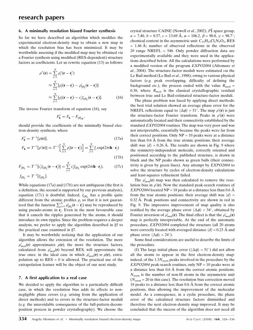
shift was hdi = 0.26 A. The results are shown in Fig. 9 where

the symmetry-independent molecule, correctly oriented and

positioned according to the published structure, is drawn in

black and the NP peaks shown as green balls (their connec-

tivity is given by green lines). Any attempt by EXPO2004 to

solve the structure by cycles of electron-density calculations

and least-squares refinement failed.

The �0modðrÞ map was then calculated to remove the reso-

lution bias in �0ðrÞ. Now the standard peak-search routines of

EXPO2004 located NP = 18 peaks at a distance less than 0.6 A

from the true atomic positions: their average shift was hdi =

0.32 A. Peak positions and connectivity are shown in red in

Fig. 9. The impressive improvement of map quality is also

testified by the average phase error h��i = 34, obtained by

Fourier inversion of �0modðrÞ. The final effect is that the �0modðrÞ

map is perfectly interpretable. At the end of the automatic

procedure, EXPO2004 completed the structure (all 20 atoms

were correctly located with averaged distance hdi = 0.23 A and

phase error h��i = 24).

Some final considerations are useful to describe the limits of

the procedure.

(I) The large initial phase error (h��i = 51) did not allow

all the atoms to appear in the first electron-density map:

indeed, of the 1.3Nasym peaks involved in the procedure by the

EXPO2004 peak-search routines, only NP = 10 peaks were at

a distance less than 0.6 A from the correct atomic positions.

Nasym is the number of non-H atoms in the asymmetric unit

(Nasym = 20 in this case). The resolution bias correction moved

18 peaks to a distance less than 0.6 A from the correct atomic

positions, thus allowing the improvement of the molecular

model. As a consequence, in a cyclic procedure, the phase

error of the calculated structure factors diminished and

therefore the next electron-density map improved. It may be

concluded that the success of the algorithm does not need all

research papers


the peaks to be close to the correct atomic positions: good and

wrong peaks can initially coexist without causing the failure of

the procedure.

(II) The value of RES for our test structure is 1.46 A. One

of the conditions for the success of the algorithm is that atoms

separated by distances in the interval 1.4–1.5 A (typical C—C

distances) give rise to electron-density peaks which may be

split in single peaks. It is guessed that structures with RES =

1.6–1.7 A are within the limits of the algorithm.

8. Conclusions

We have described an algorithm which curtails the resolution

bias in electron-density maps. The algorithm has been

successfully checked in some simulated and in one real case;

dramatic improvements of the experimental maps have been

obtained. We are not able to assess its full potential: extensive

tests are necessary. It is expected that the method may be

applied both during the phasing procedure for accelerating the

phasing process and in the refinement steps to both small and

macromolecules, to neutron as well as to electron and X-ray

data, and for variable data resolution. It seems also able to

extend the resolution. The eventual success of the next

applications will make available a new powerful tool for

modern crystallography, for which resolution is still a quite

limiting factor.

APPENDIX A

Useful approximations to point-atom structures are the so-

called E maps: they are obtained by using the normalized

structure factors

Eh ¼ Fh

.�PNj¼1

f 2j

�1=2

ð18Þ

as coefficients of the Fourier synthesis. The atomic scattering

factor fj includes the effect of the thermal vibration:

fj ¼ f 0j expð�Bjs

2=4Þ:

The use of (18) replaces physical atoms by point atoms but

does not completely eliminate the effects of the temperature

factors. Indeed, in the absence of any prior information, it is

usual to employ in the normalization process the overall

thermal factor provided by the Wilson plot, i.e.

fj ¼ f 0j expð� �BBs2=4Þ:

Then the structure factor may be modelled by


research papers

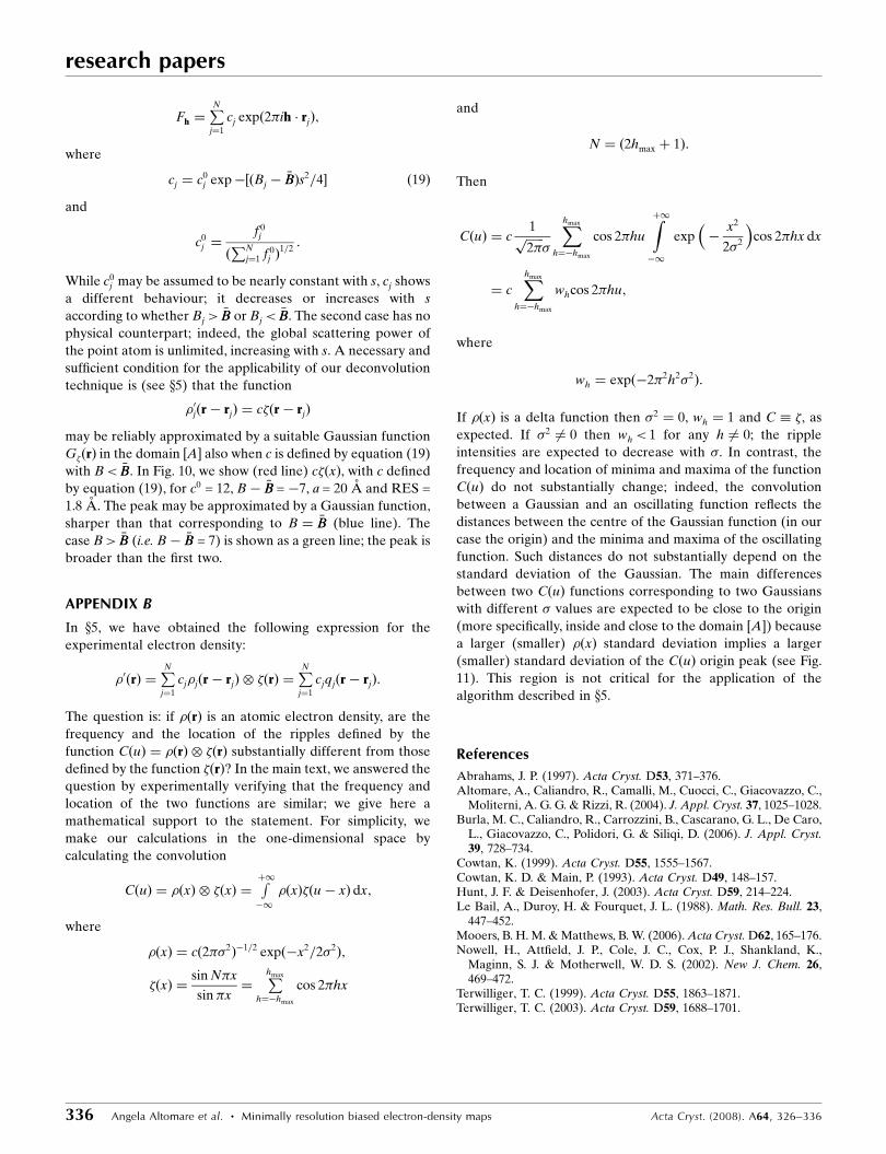
Figure 11The function C(u) is plotted: � = 0 (red line); � = 0.05 (blue line); � = 0.1(green line); � = 0.2 (black line);

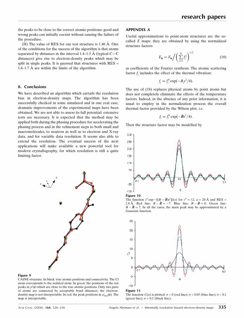
Figure 10The function c0 exp�½ðB� �BBÞs2��ðxÞ for c0 ¼ 12, a = 20 A and RES =1.8 A. Red line: B� �BB ¼ �7. Blue line: B� �BB ¼ 0. Green line:B� �BB ¼ 7. In all the cases, the main peak may be approximated by aGaussian function.

Figure 9CAINE structure. In black: true atomic positions and connectivity. The Clatom corresponds to the isolated atom. In green: the positions of the tenpeaks in �0ðrÞ which are close to the true atomic positions. Only two pairsof atoms are connected by acceptable bond distances; the electron-density map is not interpretable. In red: the peak positions in �0modðrÞ. Themap is interpretable.

Fh ¼PNj¼1

cj expð2�ih � rjÞ;

where

cj ¼ c0j exp�½ðBj �

�BBÞs2=4� ð19Þ

and

c0j ¼

f 0j

ðPN

j¼1 f 0j Þ

1=2:

While c0j may be assumed to be nearly constant with s, cj shows

a different behaviour; it decreases or increases with s

according to whether Bj > �BB or Bj < �BB. The second case has no

physical counterpart; indeed, the global scattering power of

the point atom is unlimited, increasing with s. A necessary and

sufficient condition for the applicability of our deconvolution

technique is (see x5) that the function

�0jðr� rjÞ ¼ c�ðr� rjÞ

may be reliably approximated by a suitable Gaussian function

G�ðrÞ in the domain ½A� also when c is defined by equation (19)

with B< �BB. In Fig. 10, we show (red line) c�ðxÞ, with c defined

by equation (19), for c0 = 12, B� �BB = �7, a = 20 A and RES =

1.8 A. The peak may be approximated by a Gaussian function,

sharper than that corresponding to B ¼ �BB (blue line). The

case B> �BB (i.e. B� �BB = 7) is shown as a green line; the peak is

broader than the first two.

APPENDIX B

In x5, we have obtained the following expression for the

experimental electron density:

�0ðrÞ ¼PNj¼1

cj�jðr� rjÞ � �ðrÞ ¼PNj¼1

cjqjðr� rjÞ:

The question is: if �ðrÞ is an atomic electron density, are the

frequency and the location of the ripples defined by the

function CðuÞ ¼ �ðrÞ � �ðrÞ substantially different from those

defined by the function �ðrÞ? In the main text, we answered the

question by experimentally verifying that the frequency and

location of the two functions are similar; we give here a

mathematical support to the statement. For simplicity, we

make our calculations in the one-dimensional space by

calculating the convolution

CðuÞ ¼ �ðxÞ � �ðxÞ ¼Rþ1�1

�ðxÞ�ðu� xÞ dx;

where

�ðxÞ ¼ cð2��2Þ�1=2 expð�x2=2�2

Þ;

�ðxÞ ¼sin N�x

sin�x¼

Phmax

h¼�hmax

cos 2�hx

and

N ¼ ð2hmax þ 1Þ:

Then

CðuÞ ¼ c1ffiffiffiffiffiffi2�p

�

Xhmax

h¼�hmax

cos 2�hu

Zþ1

�1

exp��

x2

2�2

�cos 2�hx dx

¼ cXhmax

h¼�hmax

whcos 2�hu;

where

wh ¼ expð�2�2h2�2Þ:

If �ðxÞ is a delta function then �2 ¼ 0, wh ¼ 1 and C � �, as

expected. If �2 6¼ 0 then wh < 1 for any h 6¼ 0; the ripple

intensities are expected to decrease with �. In contrast, the

frequency and location of minima and maxima of the function

CðuÞ do not substantially change; indeed, the convolution

between a Gaussian and an oscillating function reflects the

distances between the centre of the Gaussian function (in our

case the origin) and the minima and maxima of the oscillating

function. Such distances do not substantially depend on the

standard deviation of the Gaussian. The main differences

between two CðuÞ functions corresponding to two Gaussians

with different � values are expected to be close to the origin

(more specifically, inside and close to the domain [A]) because

a larger (smaller) �ðxÞ standard deviation implies a larger

(smaller) standard deviation of the CðuÞ origin peak (see Fig.

11). This region is not critical for the application of the

algorithm described in x5.

References

Abrahams, J. P. (1997). Acta Cryst. D53, 371–376.Altomare, A., Caliandro, R., Camalli, M., Cuocci, C., Giacovazzo, C.,

Moliterni, A. G. G. & Rizzi, R. (2004). J. Appl. Cryst. 37, 1025–1028.Burla, M. C., Caliandro, R., Carrozzini, B., Cascarano, G. L., De Caro,

L., Giacovazzo, C., Polidori, G. & Siliqi, D. (2006). J. Appl. Cryst.39, 728–734.

Cowtan, K. (1999). Acta Cryst. D55, 1555–1567.Cowtan, K. D. & Main, P. (1993). Acta Cryst. D49, 148–157.Hunt, J. F. & Deisenhofer, J. (2003). Acta Cryst. D59, 214–224.Le Bail, A., Duroy, H. & Fourquet, J. L. (1988). Math. Res. Bull. 23,

447–452.Mooers, B. H. M. & Matthews, B. W. (2006). Acta Cryst. D62, 165–176.Nowell, H., Attfield, J. P., Cole, J. C., Cox, P. J., Shankland, K.,

Maginn, S. J. & Motherwell, W. D. S. (2002). New J. Chem. 26,469–472.

Terwilliger, T. C. (1999). Acta Cryst. D55, 1863–1871.Terwilliger, T. C. (2003). Acta Cryst. D59, 1688–1701.

research papers


minimally resolution biased electron-density maps

Documents