minimally-invasive wearable sensors and data processing
TRANSCRIPT

MINIMALLY-INVASIVE WEARABLE SENSORS AND
DATA PROCESSING METHODS FOR MENTAL STRESS DETECTION
A Dissertation
by
JONGYOON CHOI
Submitted to the Office of Graduate Studies of Texas A&M University
in partial fulfillment of the requirements for the degree of
DOCTOR OF PHILOSOPHY
December 2011
Major Subject: Computer Science

Minimally-invasive Wearable Sensors and
Data Processing Methods for Mental Stress Detection
Copyright 2011 Jongyoon Choi
MINIMALLY-INVASIVE WEARABLE SENSORS AND
DATA PROCESSING METHODS FOR MENTAL STRESS DETECTION
A Dissertation
by
JONGYOON CHOI
Submitted to the Office of Graduate Studies of Texas A&M University
in partial fulfillment of the requirements for the degree of
DOCTOR OF PHILOSOPHY
Approved by: Chair of Committee, Ricardo Gutierrez-Osuna Committee Members, Louis G. Tassinary Yoonsuck Choe Dezhen Song Head of Department, Hank Walker
December 2011
Major Subject: Computer Science
iii
ABSTRACT
Minimally-invasive Wearable Sensors and Data Processing Methods for Mental Stress Detection.
(December 2011)
Jongyoon Choi, B.S., Sungkyunkwan University;
M.S., Gwangju Institute of Science and Technology
Chair of Advisory Committee: Dr. Ricardo Gutierrez-Osuna
Chronic stress is endemic to modern society. If we could monitor our mental state, we
may be able to develop insights about how we respond to stress. However, it is unfeasible to
continuously annotate stress levels all the time. In the studies conducted for this dissertation, a
minimally-invasive wearable sensor platform and physiological data processing methods were
developed to analyze a number of physiological correlates of mental stress.
We present a minimally obtrusive wearable sensor system that incorporates embedded
and wireless communication technologies. The system is designed such that it provides a balance
between data collection and user comfort. The system records the following stress related
physiological and contextual variables: heart rate variability (HRV), respiratory activity,
electrodermal activity (EDA), electromyography (EMG), body acceleration, and geographical
location.
We assume that if the respiratory influences on HRV can be removed, the residual HRV
will be more salient to stress in comparison with raw HRV. We develop three signal processing
methods to separate HRV into a respiration influenced and residual HRV. The first method
consists of estimating respiration-induced portion of HRV using a linear system identification
iv
method (autoregressive moving average model with exogenous inputs). The second method
consists of decomposing HRV into respiration-induced principal dynamic mode and residual
using nonlinear dynamics decomposition method (principal dynamic mode analysis). The third
method consists of splitting HRV into respiration-induced power spectrum and residual in
frequency domain using spectral weighting method. These methods were validated on a binary
discrimination problem of two psychophysiological conditions: mental stress and relaxation. The
linear system identification method, nonlinear dynamics decomposition method, and spectral
weighting method classified stress and relaxation conditions at 85.2 %, 89.2 %, and 81.5 %
respectively. When tonic and phasic EDA features were combined with the linear system
identification method, the nonlinear dynamics decomposition method, and the spectral weighting
method, the average classification rates were increased to 90.4 %, 93.2 %, and 88.1 %
respectively.
To evaluate the developed wearable sensors and signal processing methods on multiple
subjects, we performed case studies. In the first study, we performed experiments in a laboratory
setting. We used the wearable sensors and signal processing methods to discriminate between
stress and relaxation conditions. We achieved 81 % average classification rate in the first case
study. In the second study, we performed experiments to detect stress in ambulatory settings. We
collected data from the subjects who wore the sensors during regular daily activities. Relaxation
and stress conditions were allocated during daily activities. We achieved a 72 % average
classification rate in ambulatory settings.
Together, the results show achievements in recognizing stress from wearable sensors in
constrained and ambulatory conditions. The best results for stress detection were achieved by
removing respiratory influence from HRV and combining features from EDA.

v
DEDICATION
I dedicate this achievement to my wife, for her unceasing support and encouragement.

vi
ACKNOWLEDGMENTS
I would like to sincerely thank Dr. Ricardo Gutierrez-Osuna for his support of,
dedication to, and patience during my research and graduate studies at Texas A&M University.
Many of the contributions presented in this dissertation originated from his mentorship. I am
grateful for his guidance and enthusiasm for research. He encouraged me to be a better
independent researcher.
I thank my committee members, Dr. Louis G. Tassinary, Dr. Yoonsuck Choe, and Dr.
Dezhen Song for their interest and guidance to my work. I am grateful to Dr. Beena Ahmed for
collaboration in performing several experiments.
I would also like to thank all of the members of the Pattern Recognition and Intelligent
Sensor Machines (PRISM) Lab for the friendship. I would like to especially thank Jobany and
Daniel who have been excellent colleagues and friends over the last 7 years. I would also like to
thank Rakesh and Folami for helping and encouraging me when I was in the moments of
“fragile”.
Finally, I would like to thank my wife Shinae for her unconditional love and support.
Her patience helped to overcome difficulties of Ph.D. study. I thank my parents for their faith in
me and allowing me to study abroad to pursue my dream. Also, I thank Shinae’s parents. They
provided me with unending encouragement.

vii
TABLE OF CONTENTS
Page
ABSTRACT .................................................................................................................................. iii
DEDICATION ............................................................................................................................... v
ACKNOWLEDGMENTS ............................................................................................................. vi
TABLE OF CONTENTS ............................................................................................................. vii
LIST OF FIGURES ....................................................................................................................... xi
LIST OF TABLES ...................................................................................................................... xix
1. INTRODUCTION ............................................................................................................. 1
1.1 Organization of this dissertation ........................................................................... 4
2. BACKGROUND ............................................................................................................... 6
2.1 Influences of stress on body ................................................................................. 6 2.1.1 Mental stress and its consequences .......................................................... 6 2.1.2 Stress and the autonomic nervous system ................................................ 8
2.2 Physiological variables used for stress monitoring ............................................ 11 2.2.1 Cardiac activity ....................................................................................... 11 2.2.2 Electrodermal activity ............................................................................ 13 2.2.3 Respiration activity ................................................................................. 14 2.2.4 Muscle activity ....................................................................................... 15 2.2.5 Brain activity .......................................................................................... 16 2.2.6 Pupillary response .................................................................................. 17 2.2.7 Body movement ..................................................................................... 18
2.3 The cardiovascular system as a robust measure of ANS activity ....................... 19 2.3.1 Heart rate variability ............................................................................... 19 2.3.2 Limitations of HRV as a psychological marker ..................................... 22 2.3.3 Various factors influencing HRV ........................................................... 23
3. LITERATURE REVIEW ................................................................................................ 26
3.1 Wearable hardware prototypes ........................................................................... 26 3.1.1 Information vs. comfort .......................................................................... 26

viii
Page
3.1.2 Wireless communication ........................................................................ 27
3.2 Applications of wearable sensors ....................................................................... 29 3.2.1 User monitoring ...................................................................................... 29 3.2.2 Healthcare ............................................................................................... 30
3.3 Stress monitoring ................................................................................................ 31 3.3.1 Self-reporting .......................................................................................... 31 3.3.2 Biological samples.................................................................................. 32 3.3.3 Neuroimaging ......................................................................................... 33 3.3.4 Physiological variables ........................................................................... 34
3.4 Elicitation of mental stress for experimental purposes ....................................... 35 3.4.1 Reaction time .......................................................................................... 35 3.4.2 Working memory.................................................................................... 35 3.4.3 Selective attention .................................................................................. 36 3.4.4 Physical pressure .................................................................................... 37 3.4.5 Social stress ............................................................................................ 37
3.5 Computational modeling of physiological signals ............................................. 38
4. A WEARABLE SENSOR SYSTEM FOR AMBULATORY MONITORING OF MENTAL STRESS ................................................................................................... 41
4.1 System specifications ......................................................................................... 41 4.2 Physiological sensors ......................................................................................... 44 4.3 Holster unit ......................................................................................................... 47 4.4 Wireless nodes and communication ................................................................... 50 4.5 Sensor validation experiments ............................................................................ 52
4.5.1 Cardiovascular sensor validation ............................................................ 53 4.5.2 EDA sensor validation ............................................................................ 54 4.5.3 Respiration sensor validation ................................................................. 56
4.6 Summary ............................................................................................................ 58
5. REMOVING RESPIRATORY INFLUENCE FROM HRV .......................................... 59
5.1 Introduction ........................................................................................................ 60 5.2 Linear system identification ............................................................................... 63
5.2.1 Modeling cardio-respiratory relationships with ARMAX ...................... 63 5.2.2 Compensating differences in ventilation ................................................ 65
5.3 Nonlinear dynamics decomposition ................................................................... 67 5.3.1 Principal dynamic modes ....................................................................... 67 5.3.2 PDM decomposition without respiratory signals ................................... 69 5.3.3 Estimation of Volterra kernels ................................................................ 70
5.4 Spectral weighting .............................................................................................. 72 5.5 Summary of the proposed methods .................................................................... 73
ix
Page
6. EXPERIMENTS: COMPARISON OF THE RESPIRATORY INFLUENCE REMOVAL METHODS ................................................................................................. 75
6.1 Experimental ...................................................................................................... 76 6.2 Preliminary analysis and data preprocessing ...................................................... 80 6.3 Results from the linear system identification method ........................................ 82
6.3.1 Magnitude of the transfer function ......................................................... 82 6.3.2 Scaling factors ........................................................................................ 84 6.3.3 Power spectral density ............................................................................ 86
6.4 Results from the nonlinear dynamics decomposition method ............................ 87 6.4.1 Laguerre basis function .......................................................................... 88 6.4.2 Kernel estimation.................................................................................... 89 6.4.3 Power spectral density ............................................................................ 92
6.5 Results from the spectral weighting method ...................................................... 94 6.6 Logistic regression ............................................................................................. 95 6.7 Classification performance comparisons ............................................................ 97 6.8 Discussion ........................................................................................................ 102
7. INCREASING STRESS RECOGNITION BY COMBINING EDA FEATURES WITH RESPIRATORY INFLUENCE REMOVAL METHODS ................................ 107
7.1 Signal decomposition ....................................................................................... 107 7.1.1 Experimental results ............................................................................. 110
7.2 Combining EDA and HRV features ................................................................. 112 7.3 Discussion ........................................................................................................ 117
8. CASE STUDIES: EXPERIMENTS AT TEXAS A&M UNIVERSITY AT QATAR ......................................................................................................................... 121
8.1 Study 1: Stress elicitation in laboratory settings .............................................. 121 8.1.1 Experimental ........................................................................................ 121 8.1.2 Results .................................................................................................. 125 8.1.3 Summary .............................................................................................. 130
8.2 Study 2: Stress elicitation in ambulatory settings and removal of subject-to-subject variation ........................................................................................... 131 8.2.1 Experimental ........................................................................................ 131 8.2.2 Results of stress elicitation in ambulatory settings ............................... 135 8.2.3 Removal of subject-to-subject variation ............................................... 139 8.2.4 Results of subject-to-subject variation removal ................................... 141 8.2.5 Summary .............................................................................................. 142
9. DISCUSSION AND CONCLUSION ........................................................................... 144

x
Page
9.1 Future work ...................................................................................................... 147
REFERENCES ........................................................................................................................... 150
APPENDIX A ............................................................................................................................ 166
APPENDIX B ............................................................................................................................. 178
APPENDIX C ............................................................................................................................. 181
APPENDIX D ............................................................................................................................ 189
APPENDIX E ............................................................................................................................. 190
APPENDIX F ............................................................................................................................. 193
VITA ....................................................................................................................................... 203
xi
LIST OF FIGURES
Page
Figure 1. General adaptation syndrome model (Santrock, 2007). Hormone production takes place during stress adaptation, which alerts the body to respond to stress. The body returns to a normal state when the hormone production stops. ........................................................................................................................... 7
Figure 2. Hierarchy of the human nervous system. The nervous system is used to transmit signals between different parts of the body when the body perceives stress. ........................................................................................................................... 9
Figure 3. The ANS innervation divided into sympathetic and parasympathetic nervous system (Reece et al., 2010). ...................................................................................... 10
Figure 4. Influences of the two autonomic branches on heart. The two branches of ANS release norepinephrine and acetylcholine to control heart rate. ....................... 11
Figure 5. ECG and PPG. (a) QRS complex of ECG. (b) Photoplethysmography and pulse oximeter (courtesy of Nellcor Puritan Bennett Corp., Pleasanton, CA.). .......................................................................................................................... 12
Figure 6. Placements for EDA recording and examples of EDA signal. (a) Three electrode placements for EDA monitoring on the hand (Dawson et al., 2007). (b) Two hypothetical EDA signals under stimuli (Dawson and Nuechterlein, 1984). .................................................................................................. 14
Figure 7. Respiration measurement by monitoring the expansion and contraction of chest (Peratech, 2011). (a) The RIP or piezo sensor belts are tied to the thorax and abdomen of upper body. (b) The IP flows current through electrodes attached to chest. ...................................................................................... 15
Figure 8. Muscles measured for stress detection. (a) Trepezious (Zhao et al., 2003) (b) The facial EMG signals of the frontalis (1-2), corrugator supercilii(3-4), and zygomaticus major(5-6) (van den Broek et al., 2006). ............................................. 16
Figure 9. EEG placement and brainwaves. (a) EEG electrodes are placed on scalp (Wang et al., 2010b) (b) brain waves and the corresponding mental conditions (Mason, 2001). ........................................................................................ 17
xii
Page
Figure 10. Measuring pupillary response using an eye tracker. (a) Eye tracker is used to measure the size of pupils. (b) Pupillary response during a mental multiplication task (Ahern and Beatty, 1979). The pupil size increases as the subject performs arithmetic multiplication. .............................................................. 18
Figure 11. ECG, PPG and fluctuation of R-R interval. (a) The HRV is calculated from R to R duration on the ECG. (b) The HRV is calculated from peak to peak duration on the PPG. (c) The beat-to-beat periods show fluctuations. ..................... 20
Figure 12. Power spectral density of HRV. (a) The low and high frequency bands in the frequency domain. (b) PNS is dominant during supine posture, and (c) SNS is dominant during tilt posture. ................................................................................. 21
Figure 13. Different activation modes and psychological markers. (a) ANS branches exhibit four different activation modes. (b) Marker can map physiological response into psychological state in one-to-one mapping (Cacioppo et al., 2007). ........................................................................................................................ 23
Figure 14. Architecture of the wearable sensor system. The holster unit integrates a sensor hub and an embedded-Linux motherboard. The sensor hub contains various context sensors and a 2.4GHz transceiver that communicates with an array of wireless sensor modules, each consisting of a physiological sensor and a wireless transmitter. ......................................................................................... 42
Figure 15. Wearable sensor prototype. The system consists of a holster unit, a chest strap combining HRM and respiration sensors and wireless EMG and EDA modules. A USB transducer displays sensor data in real-time on a PC monitor during sensor calibration. ............................................................................ 43
Figure 16. Deployment of the chest strap which contains HRM and respiration sensor. (a) the HRM is located on the center of the chest. (b) Respiration sensor and transmitter is located on the left side of the chest. (c) The length of the chest strap is adjustable from behind. (d) HRM and respiration sensors are integrated into a single strap. .................................................................................... 45
Figure 17. Deployment of the EDA sensor and wireless node. (a) wireless EDA node is placed on the wrist band, and (b) Two electrodes are placed on index and middle finger. ............................................................................................................ 46
Figure 18. Deployment of the EMG sensor and wireless nodes. (a) Three electrodes are placed along the muscle fiber of the trapezius muscle, and (b) wireless EMG node is placed on the armband. ................................................................................. 47
xiii
Page
Figure 19. The holster unit. Accelerometer, GPS, HRM, power supply, and wireless transceiver circuits are integrated with the Verdex Pro. The accelerometer is located under the Verdex Pro. ................................................................................... 49
Figure 20. Wearing the final prototype. ..................................................................................... 49
Figure 21. Number of missing packets and recovery time. Results of (a) average number of missing packets per hour and (b) average time to reconnect to the holster unit were collected from 12 subjects. ............................................................ 52
Figure 22. Comparison of signal between ECG and HRM. This figure reflects data collected from subject #1. ......................................................................................... 54
Figure 23. Comparison of signal between commercial and custom EDA sensors. This figure reflects data collected from subject #2. .......................................................... 55
Figure 24. Comparison of signals between RIP, piezo, and pressure sensor in (a) no motion artifacts and (b) motion artifacts on respiration sensors. This figure reflects data collected from subject #4. ..................................................................... 57
Figure 25. Transfer magnitude of RSA as a function of respiratory frequency (Berntson et al., 1993b). ............................................................................................................ 61
Figure 26. Power spectra for HRV and respiration with (a) fixed breathing period of 10 seconds, (b) fixed breathing period of 3.5 seconds, and (c) broadband breathing. The subject breathed following pacing sounds. Data corresponds to subject #1. ............................................................................................................. 62
Figure 27. Android smartphone platform based Stroop color word test. The subjects were to respond to a question depending on either (a) word meaning or (b) font color. .................................................................................................................. 77
Figure 28. Android application that gave instructions to the subjects to help in spontaneous deep breathing. The elapsed experimental time was displayed on the top left corner of the screen. ........................................................................... 78
Figure 29. Experimental protocol - each of the three conditions (relaxation, stress, and calibration) lasted five minutes. The subjects were asked to repeat the relaxation and stress conditions three times. ............................................................. 79
Figure 30. Example of the collected physiological signals. Data corresponds to subject #9. The data show variations in (a) respiration, (b) R-R periods, and (c) EDA signal during calibration phase (the green segment), stress conditions (the red segments), and relaxation conditions (the blue segments). ......................... 81
xiv
Page
Figure 31. Average magnitude of the transfer function for broadband breathing. Blue solid line is the transfer gain averaged over 12 subjects, and the red dotted lines correspond to ±1 standard deviations. .............................................................. 83
Figure 32. Average magnitude of the transfer function for (a) relaxation and (b) stress conditions. Gains are calculated from coefficients of the online-linear method. Blue solid line is the transfer gain averaged over 12 subjects, and the red dotted lines correspond to ±1 standard deviations. ....................................... 83
Figure 33. Scale factor for relaxation condition. (a) Root mean squared prediction error as a function of the scaling factor. (b) Unscaled (α=1.0) and scaled (α=4.8)
predictions. This figure reflects data collected from subject #1. .............................. 85
Figure 34. Scale factor for stress condition. (a) Root mean squared prediction error as a function of the scaling factor. (b) Unscaled (α=1.0) and scaled (α=8)
predictions. This figure reflects data collected from subject #1. .............................. 85
Figure 35. Power spectrum of the signals involved in the linear system identification method. Relaxation (blue line) and stress (red line) conditions are compared on (a) HRV, (b) respiration, (c) estimated respiration influence HRV using offline estimation, (d) residual HRV using offline estimation, (e) estimated respiration influence HRV using online estimation, and (f) residual HRV using online estimation. This figure reflects data collected from subject #3. ........... 87
Figure 36. Comparison of weighting parameter of Laguerre basis. Smaller gives more weights to the more recent inputs. ................................................................... 88
Figure 37. Estimated first-order Volterra kernel for relaxation and stress conditions with a memory of M = 100 (25 seconds), Laguerre coefficient α = 0.7, and
order L = 6 (averaged over the entire dataset for each subject). Blue lines represent average kernels and the red lines represent standard deviation bounds.. Kernels from (a) the calibration condition of offline-nonlinear method, (b) relaxation and (c) stress conditions of online-nonlinear method, and (d) relaxation and (e) stress conditions of nonlinear-delayed-HRV-input method. ..................................................................................................................... 90
Figure 38. Estimated second-order Volterra kernel for relaxation and stress conditions with a memory of M = 100 (25 seconds), Laguerre coefficient α = 0.7, and
order L = 6 (averaged over the entire dataset for each subject). Kernel from (a) the calibration condition of offline-nonlinear method, (b) relaxation and (c) stress conditions of online-nonlinear method, and (d) relaxation and (e) stress conditions of nonlinear-delayed-HRV-input. .................................................. 91
xv
Page
Figure 39. Power spectrum of the nonlinear system identification method. Relax (blue line) and stress (red line) conditions are compared on (a) HRV, (b) respiration, (c) respiration influence on offline estimation, (d) residual on offline estimation, (e) respiration influence on online estimation, (f) residual on online estimation, (g) respiration influence on nonlinear-delayed-HRV-input method, and (h) residual on nonlinear-delayed-HRV-input. This figure reflects data collected from subject #3. ..................................................................... 93
Figure 40. Power spectrum of the spectral weighting method. Relax (blue line) and stress (red line) conditions are compared on (a) HRV and (b) respiration. Weighting function for (c) relaxation condition and (d) stress conditions were calculated from corresponding respiration signal. Results of the spectral weighting method for (e) respiratory-driven HRV and (f) residual HRV. This figure reflects data collected from subject #3. ........................................ 95
Figure 41. The logistic function with z on the horizontal axis and ƒ(z) on the vertical
axis. ........................................................................................................................... 96
Figure 42. PCA score plots using the first two components for all 12 subjects. Blue and red dots correspond to relaxation and stress conditions respectively...................... 100
Figure 43. Comparison of classification performances. Offline-nonlinear and offline-linear showed better classification performances than other methods. ................... 102
Figure 44. Decomposition of EDA into (a) SCL and (b) SCR ( ). This figure reflects data collected from subject #9. ................................................................... 111
Figure 45. Features extracted from EDA response. (a) mean SCL and (b) standard deviation of SCR ( ). Data corresponds to subject #9. ............................. 112
Figure 46. PCA score plots for 12 subjects. Blue and red dots correspond to relaxation and stress conditions respectively. .......................................................................... 115
Figure 47. Classification performance of the respiratory influence removal methods compared against the same methods when EDA features are included. ................. 117
Figure 48. Stress protocols used to induce mental stress. (a) The subjects were asked to track a moving target in a computer screen using a mouse and to click whenever one of three target letters appeared on the screen. (b) The subjects were shown one of four words (red, green, blue, yellow) displayed in different ink colors, and had to press on one of four buttons according to the ink color. (c) The subjects were told to memorize a set of words presented in sequence, and then recall them under time pressure. (d) The subjects had to manually trace a pattern on a paper printout by looking through a mirror. ............ 123
xvi
Page
Figure 49. Sequence of tests. The subjects performed MS (5 min), CW (5 min), DT (5 min), MT (5min), and PS (10 min). 3 minutes DBs were interleaved between stress tests. Note that the first DB lasted 5 minutes. ................................. 125
Figure 50. EDA, RR tachogram and respiratory signals for subject #5. .................................. 126
Figure 51. Optimized logistic regression coefficients. Four features are chosen from a forward feature selection procedure. ....................................................................... 127
Figure 52. Classification result using logistic regression. Mean SCL, standard deviation of SCR, PNS/SNS ratio (spectral weighting), and AVNN were used for features. ................................................................................................................... 128
Figure 53. EDA for subject #9 shows strong SCRs during the relaxation segments. .............. 129
Figure 54. Comfort rating of the wearable sensor (lower scores are better). ........................... 130
Figure 55. Screenshots of the ambulatory stress monitoring software in Android platform. (a) Android main screen for the four apps, (b) easy Stroop color word test, (c) hard Stroop color word test, (d) spontaneous deep breathing task, (e) questionnaires for the subject’s context, and (f) questionnaires for
the subject’s stress level. ......................................................................................... 133
Figure 56. Schedules are created as an iCal file and uploaded to Google calendar as notifications............................................................................................................. 134
Figure 57. Flow of ambulatory stress monitoring experiment. ................................................ 135
Figure 58. EDA, RR tachogram and respiratory signals; data corresponds to subject #11. ......................................................................................................................... 136
Figure 59. Classification results using logistic regression. Mean SCL, standard deviation of SCR, PNS/SNS ratio (spectral weighting), and AVNN were used for features. ..................................................................................................... 138
Figure 60. EDA and HRV for subject #5 shows increased SCLs during the relaxation segments and decreased SCLs during the stress segments. .................................... 139
Figure 61. Classification rates for subject-to-subject variability removal methods. ................ 142
Figure 62. Improvement in classification performances of the mental stress detection problem. The results of the linear and nonlinear methods correspond to online coefficient estimation method which gave best performance. ..................... 146
xvii
Page
Figure 63. Hirose 60 pin connector for Verdex Pro. ................................................................ 166
Figure 64. Power supply and voltage regulator modules for the holster unit. .......................... 168
Figure 65. Real-time clock module and backup battery. RTC module is accessible from Verdex Pro using I2C bus. ...................................................................................... 168
Figure 66. Heart rate monitor and comparator module. ........................................................... 169
Figure 67. GPS module. ........................................................................................................... 170
Figure 68. Wireless transceiver module. .................................................................................. 170
Figure 69. Accelerometer module. ........................................................................................... 171
Figure 70. Top and bottom layers of the designed PCB on No-Bluetooth prototype in real size. .................................................................................................................. 172
Figure 71. Final no-Bluetooth holster unit prototype . ............................................................. 173
Figure 72. Hirose 60 pin connection on Bluetooth prototype. ................................................. 175
Figure 73. Top and bottom layers of the designed PCB on Bluetooth prototype in real size. ......................................................................................................................... 176
Figure 74. Fianl Bluetooth holster unit prototype. ................................................................... 177
Figure 75. Locations of important files and directories in the holster unit. ............................. 185
Figure 76. Locations of important files and directories in the Bluetooth enabled holster unit. ......................................................................................................................... 188
Figure 77. Pin connections of the respiration node’s wireless transmitter. .............................. 193
Figure 78. Respiration sensor amplification circuit. ................................................................ 194
Figure 79. Power supply modules of the respiration node. ...................................................... 194
Figure 80. From 3.6V to 7V DC/DC step-up circuit. ............................................................... 195
Figure 81. PCB design of the respiration node......................................................................... 195
Figure 82. Pin connections of the EDA node’s wireless transmitter. ....................................... 197
xviii
Page
Figure 83. EDA sensor circuit. The circuit is a non-inverting amplifier. ................................. 197
Figure 84. Power supply circuit for the EDA node. ................................................................. 198
Figure 85. PCB layout of the EDA node. ................................................................................. 198
Figure 86. Pin connections of the EMG node’s wireless transmitter. ......................................199
Figure 87. Power supply circuit of the EMG node. .................................................................. 200
Figure 88. A circuit to generate negative 3.6V from positive 3.6V. ........................................ 200
Figure 89. EMG sensor circuit. ................................................................................................ 201
Figure 90. PCB layout of the EMG node. ................................................................................ 201

xix
LIST OF TABLES
Page
Table I. Respiratory influence removal methods. .................................................................. 75
Table II. Selected features for each method. Each method in the left column used the three corresponding features in right column ........................................................... 99
Table III. Comparison of two groups based on incorporation of respiration signal. .............. 103
Table IV. Comparison of online and offline coefficient estimation approaches. .................... 104
Table V. Comparison of linear and nonlinear methods. ........................................................ 105
Table VI. Combined EDA and HRV features used for comparison. Each method in the left column used the corresponding features in right column. ................................ 113
Table VII. Combined EDA and HRV features used for comparison when respiration signal is not available. ............................................................................................. 119
Table VIII. Combined EDA and HRV features used for comparison when respiration signal is available. ................................................................................................... 120
Table IX. Comfort rating questionnaires (Knight and Baber, 2005). ..................................... 130
Table X. Gumstix Verdex Pro XM4 COM pin connectors. ................................................... 167
Table XI. List of components for the holster unit. .................................................................. 174
Table XII. List of components for the respiration node. .......................................................... 196
Table XIII. List of components for the EDA node. ...................................................................199
Table XIV. List of components for the EMG node. ................................................................... 202

1
1. INTRODUCTION
Stress is the term used to describe bodily reactions to perceived physical or
psychological threats. It can be beneficial in keeping us alert and focused in any indication of
impending danger or to overcome a challenge. However, a frequent occurrence and/or the
extended duration of stress will have detrimental effects on a person’s health. As a result, stress
is a major risk factor for a number of illnesses, including diabetes, asthma, depression, and heart-
related diseases (1982). Since stress in modern life has become endemic, stress management is
an important part of personal healthcare.
Monitoring stress requires the maintenance of detailed logs of one’s perceived stress
level throughout the day which, however, is impractical for most people. Thus, a system that can
objectively monitor a person’s stress levels over extended periods (weeks or months) will be an
invaluable tool. A number of physiological indicators can be used to detect stress, including
voice pitch, facial expressions, body gestures, and physiological variables. Among these, and
unlike speech and facial expressions, physiological responses to stress are considered to be a
more reliable measure of a person’s stress-state (Luneski et al., 2010). Moreover, recent
advances in mobile computing and wearable sensors have made it possible to record
physiological variables 24 hours a day.
To determine stress levels from physiological variables, two elements are required: a
device to record physiological variables, and an algorithm to infer stress-state from physiological
variables. The first element, which records stress salient physiological variables, should be
This dissertation follows the style of International Journal of Human-Computer Studies.

2
unobtrusive to ensure minimal (if any) discomfort to the user. The use of several sensors
facilitates the collection of more physiological variables with the advantage of providing
information about stress. However, the use a large number of sensors amounts to a higher level
of discomfort and restriction of the users’ regular daily activities, and may culminate in the
collation of unreliable or biased data. Hence, the design of wearable sensor system requires a
balance between data collection and user comfort. Secondly, collected physiological variables
should be processed to infer a users’ stress-state. This requires signal processing methods to
extract stress salient features from the physiological variables, which can be influenced by
factors other than stress. For example, respiratory activity and body movement influence
physiological responses and can, in some cases, dominate the influence of stress in physiological
variables. Consequently, the absence of a method to address these additional influences makes
mental stress detection through physiological variables difficult and unreliable.
The two challenges identified above, wearable hardware and signal processing, form the
core motivation for this dissertation; the main objectives of which are to (1) design a wearable
prototype and (2) develop signal processing methods to detect mental stress.
As a step towards the first objective, we have design a wearable sensor system to capture
stress-relevant physiological variables as well as likely confounders. Namely, the system records
the following physiological variables: heart rate variability (HRV), respiration, electrodermal
activity (EDA), electromyography activity (EMG), body acceleration, and geographical location.
The system was designed with the goal of minimizing obstruction to the users’ regular daily
activities; this was achieved by judicious use of embedded and wireless communication
technologies, which helped keep the wearable sensor system footprint to a minimum.
As a step towards the second objective, we hypothesized that if the respiratory
influences on HRV could be removed, the residual HRV would make stress-driven responses
3
more salient in comparison with raw HRV. Based on this hypothesis, we have developed three
signal processing methods to separate HRV into a respiration influenced component and a
residual component, the latter of which can be used as a marker of stress. The first method
consists of estimating the respiration-induced portion of HRV using a linear system
identification method (autoregressive moving average model with exogenous inputs). The
second method decomposes HRV into a respiration-induced principal dynamic mode and a
residual by means of a nonlinear dynamics decomposition method (principal dynamic mode
analysis). The third method separates the respiration-induced component and the residual
component of HRV using a spectral weighting method based on the spectral content of the
respiratory signal.
The wearable sensor system and signal processing methods have been tested on multiple
subjects through a series of case studies. In the first study, we performed experiments in a
laboratory setting using the wearable sensors and signal processing methods to discriminate
between conditions in which stress was induced using several stress elicitation protocols and
relaxation conditions. The second study focused on stress detection in an ambulatory setting.
This involved the collection of data from the subjects who wore the sensors during regular daily
activities. Specific relaxation and stress elicitation activities were allocated periodically during
daily activities, and signal processing methods were applied to discriminate stress conditions
from relaxation conditions.
The contributions of this dissertation include:
The design of a wearable sensor prototype to collect stress salient physiological
variables with minimal obtrusiveness to the user.
The development of signal processing methods capable of separating HRV into
respiration influenced and residual signal.
4
Case studies performed to test the developed system and signal processing methods in
laboratory and ambulatory settings.
1.1 Organization of this dissertation
The remainder of this dissertation is organized as follows: Section 2 provides a
background in the area of psycho-physiological monitoring, including fundamentals of stress and
body responses, physiological variables as the main tools for stress monitoring, and a description
of cardiac activity as an indirect measure of stress. Section 3 reviews relevant research in
wearable sensor design and applications, stress monitoring and stress elicitation protocols, and
computational modeling of the Autonomic Nervous System (ANS). Section 4 describes the
hardware prototype developed as part of this dissertation, including the embedded system,
wireless communications and physiological sensors, and a validation of the instrument against
commercial sensors. Section 5 describes theoretical aspects of the proposed methods to separate
HRV into respiratory-influenced and residual signal. The section describes linear system
identification, nonlinear dynamics decomposition, and spectral weighting methods used to
separate respiration influence from HRV. Section 6 describes the experimental setup and
validation results for the suggested respiration influence separation methods in terms of their
ability to discriminate between stress and relaxation conditions. Section 7 introduces a method to
separate EDA response into tonic and phasic responses, and describes the classification
performance when these EDA features are combined with features from the respiration-
separation methods discussed in section 6. Section 8 describes two case studies which we
performed to validate our choice of the adopted hardware and signal processing methods. The
first study was performed to detect stress in laboratory settings using several stress elicitation

5
protocols and the second, to detect stress in ambulatory settings. Section 9 discusses the results
of this dissertation and offers suggestions for future research.
All the experiment protocols in this dissertation were approved by the Institutional
Review Board at Texas A&M University. All subjects provided written informed consent for the
study.
6
2. BACKGROUND
This section provides an overview of fundamental principles in stress monitoring. The
section starts with a description of the physiology of stress: the response of the human body
responses to stress, and the relationship with the autonomic nervous system. Next, the section
describes methods used to detect those body responses in the areas of psychophysiological
sensing. The section concludes with a review of cardiac activity as a robust measure of stress.
2.1 Influences of stress on body
2.1.1 Mental stress and its consequences
Stress generally refers to moments of unpleasant feelings aroused by external stimuli.
Selye (1982) defines it as the nonspecific result of any demand upon the body. Stress triggers a
cascade of physiological reactions aimed at preserving the integrity of the individual (Kasl,
1984). The human body typically reacts to a stressor (a stimulus causing stress) in three phases:
alarm, adaptation, and exhaustion (Selye, 1950). Selye (1946) refers to this process as the
general adaptation syndrome, and this process is shown in Figure 1. During the initial stage,
when the stressor is perceived, the body reacts by producing hormones. In the second stage, the
hormonal release causes the body to adapt to the stressor by employing a coping mechanism.
After a while, hormonal production is gradually reduced as the body cannot sustain hormonal
production indefinitely. During the final stage, these reactive hormonal production processes are
halted. Once the threat is averted, the body returns to a “normal” state. However, if the threat is
not averted, the stress response can be repeated.
7
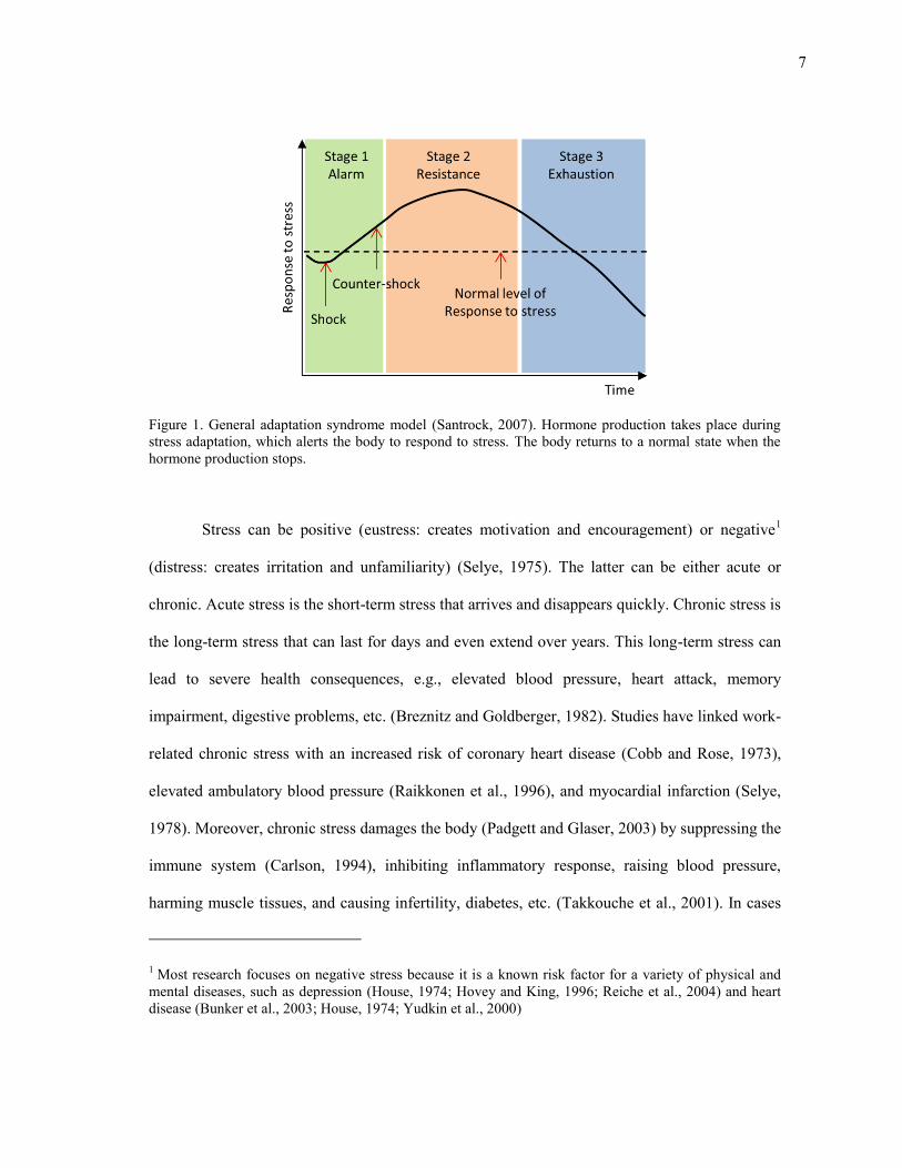
Figure 1. General adaptation syndrome model (Santrock, 2007). Hormone production takes place during stress adaptation, which alerts the body to respond to stress. The body returns to a normal state when the hormone production stops.
Stress can be positive (eustress: creates motivation and encouragement) or negative1
(distress: creates irritation and unfamiliarity) (Selye, 1975). The latter can be either acute or
chronic. Acute stress is the short-term stress that arrives and disappears quickly. Chronic stress is
the long-term stress that can last for days and even extend over years. This long-term stress can
lead to severe health consequences, e.g., elevated blood pressure, heart attack, memory
impairment, digestive problems, etc. (Breznitz and Goldberger, 1982). Studies have linked work-
related chronic stress with an increased risk of coronary heart disease (Cobb and Rose, 1973),
elevated ambulatory blood pressure (Raikkonen et al., 1996), and myocardial infarction (Selye,
1978). Moreover, chronic stress damages the body (Padgett and Glaser, 2003) by suppressing the
immune system (Carlson, 1994), inhibiting inflammatory response, raising blood pressure,
harming muscle tissues, and causing infertility, diabetes, etc. (Takkouche et al., 2001). In cases
1 Most research focuses on negative stress because it is a known risk factor for a variety of physical and mental diseases, such as depression (House, 1974; Hovey and King, 1996; Reiche et al., 2004) and heart disease (Bunker et al., 2003; House, 1974; Yudkin et al., 2000)
8
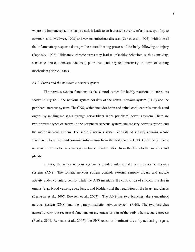
where the immune system is suppressed, it leads to an increased severity of and susceptibility to
common cold (McEwen, 1998) and various infectious diseases (Cohen et al., 1993). Inhibition of
the inflammatory response damages the natural healing process of the body following an injury
(Sapolsky, 1992). Ultimately, chronic stress may lead to unhealthy behaviors, such as smoking,
substance abuse, domestic violence, poor diet, and physical inactivity as form of coping
mechanism (Noble, 2002).
2.1.2 Stress and the autonomic nervous system
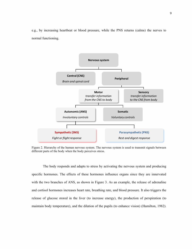
The nervous system functions as the control center for bodily reactions to stress. As
shown in Figure 2, the nervous system consists of the central nervous system (CNS) and the
peripheral nervous system. The CNS, which includes brain and spinal cord, controls muscles and
organs by sending messages through nerve fibers in the peripheral nervous system. There are
two different types of nerves in the peripheral nervous system: the sensory nervous system and
the motor nervous system. The sensory nervous system consists of sensory neurons whose
function is to collect and transmit information from the body to the CNS. Conversely, motor
neurons in the motor nervous system transmit information from the CNS to the muscles and
glands.
In turn, the motor nervous system is divided into somatic and autonomic nervous
systems (ANS). The somatic nervous system controls external sensory organs and muscle
activity under voluntary control while the ANS maintains the contraction of smooth muscles in
organs (e.g., blood vessels, eyes, lungs, and bladder) and the regulation of the heart and glands
(Berntson et al., 2007; Dawson et al., 2007) . The ANS has two branches: the sympathetic
nervous system (SNS) and the parasympathetic nervous system (PNS). The two branches
generally carry out reciprocal functions on the organs as part of the body’s homeostatic process
(Backs, 2001; Berntson et al., 2007): the SNS reacts to imminent stress by activating organs,
9
e.g., by increasing heartbeat or blood pressure, while the PNS returns (calms) the nerves to
normal functioning.
Figure 2. Hierarchy of the human nervous system. The nervous system is used to transmit signals between different parts of the body when the body perceives stress.
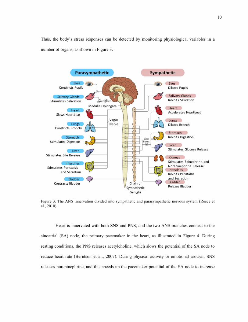
The body responds and adapts to stress by activating the nervous system and producing
specific hormones. The effects of these hormones influence organs since they are innervated
with the two branches of ANS, as shown in Figure 3. As an example, the release of adrenaline
and cortisol hormones increases heart rate, breathing rate, and blood pressure. It also triggers the
release of glucose stored in the liver (to increase energy), the production of perspiration (to
maintain body temperature), and the dilation of the pupils (to enhance vision) (Hamilton, 1982).
10
Thus, the body’s stress responses can be detected by monitoring physiological variables in a
number of organs, as shown in Figure 3.
Figure 3. The ANS innervation divided into sympathetic and parasympathetic nervous system (Reece et al., 2010).
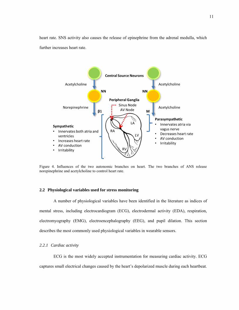
Heart is innervated with both SNS and PNS, and the two ANS branches connect to the
sinoatrial (SA) node, the primary pacemaker in the heart, as illustrated in Figure 4. During
resting conditions, the PNS releases acetylcholine, which slows the potential of the SA node to
reduce heart rate (Berntson et al., 2007). During physical activity or emotional arousal, SNS
releases norepinephrine, and this speeds up the pacemaker potential of the SA node to increase
11
heart rate. SNS activity also causes the release of epinephrine from the adrenal medulla, which
further increases heart rate.
Figure 4. Influences of the two autonomic branches on heart. The two branches of ANS release norepinephrine and acetylcholine to control heart rate.
2.2 Physiological variables used for stress monitoring
A number of physiological variables have been identified in the literature as indices of
mental stress, including electrocardiogram (ECG), electrodermal activity (EDA), respiration,
electromyography (EMG), electroencephalography (EEG), and pupil dilation. This section
describes the most commonly used physiological variables in wearable sensors.
2.2.1 Cardiac activity
ECG is the most widely accepted instrumentation for measuring cardiac activity. ECG
captures small electrical changes caused by the heart’s depolarized muscle during each heartbeat.
12
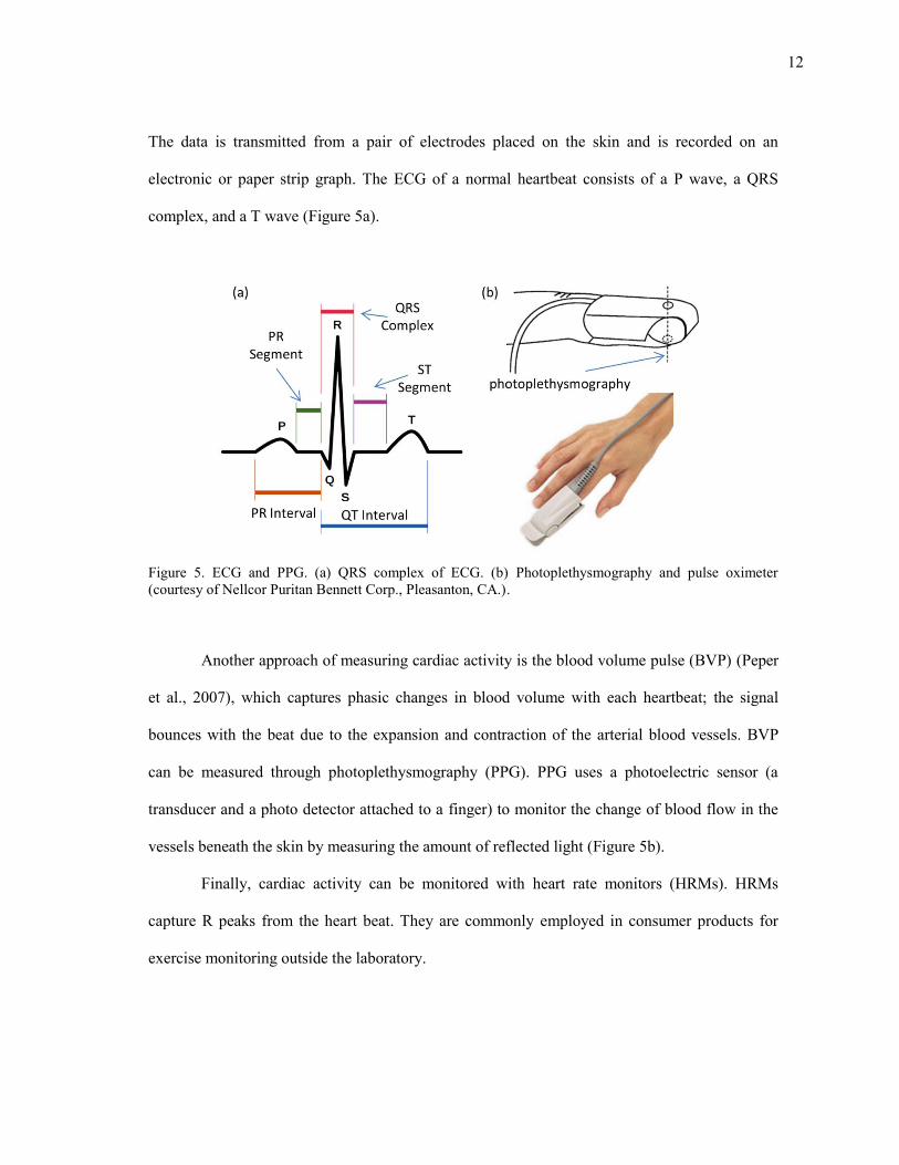
The data is transmitted from a pair of electrodes placed on the skin and is recorded on an
electronic or paper strip graph. The ECG of a normal heartbeat consists of a P wave, a QRS
complex, and a T wave (Figure 5a).
Figure 5. ECG and PPG. (a) QRS complex of ECG. (b) Photoplethysmography and pulse oximeter (courtesy of Nellcor Puritan Bennett Corp., Pleasanton, CA.).
Another approach of measuring cardiac activity is the blood volume pulse (BVP) (Peper
et al., 2007), which captures phasic changes in blood volume with each heartbeat; the signal
bounces with the beat due to the expansion and contraction of the arterial blood vessels. BVP
can be measured through photoplethysmography (PPG). PPG uses a photoelectric sensor (a
transducer and a photo detector attached to a finger) to monitor the change of blood flow in the
vessels beneath the skin by measuring the amount of reflected light (Figure 5b).
Finally, cardiac activity can be monitored with heart rate monitors (HRMs). HRMs
capture R peaks from the heart beat. They are commonly employed in consumer products for
exercise monitoring outside the laboratory.
13
2.2.2 Electrodermal activity
EDA, also known as galvanic skin response (GSR), refers to changes in electrical
conductivity of the skin due to perspiration. EDA is influenced by changes in hydration in the
eccrine sweat glands (the major sweat glands of the body). Under stress conditions, the sweat
glands produce an odorless substance consisting of water and Na-Cl, which increases the
conductivity of the skin. As a consequence, a measurement of skin conductance (or resistance) is
often used as an indicator of psychological arousal (e.g., startle response, fear, anger) (Picard and
Scheirer, 2001).
EDA can be captured by measuring the electrical conductance between two points on the
surface of the skin. In general, Ag/Ag-Cl-type electrodes are attached to the skin’s surface.
Changes in conductance are dependent on the density of eccrine glands. For this reason, EDA is
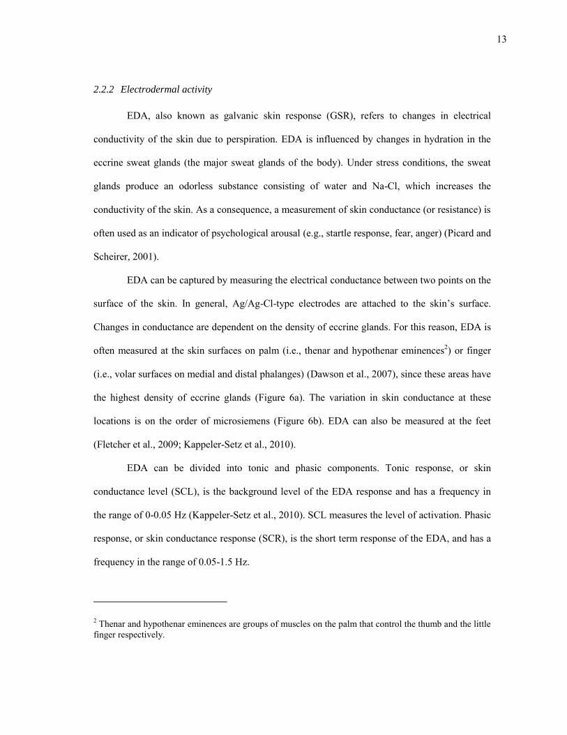
often measured at the skin surfaces on palm (i.e., thenar and hypothenar eminences2) or finger
(i.e., volar surfaces on medial and distal phalanges) (Dawson et al., 2007), since these areas have
the highest density of eccrine glands (Figure 6a). The variation in skin conductance at these
locations is on the order of microsiemens (Figure 6b). EDA can also be measured at the feet
(Fletcher et al., 2009; Kappeler-Setz et al., 2010).
EDA can be divided into tonic and phasic components. Tonic response, or skin
conductance level (SCL), is the background level of the EDA response and has a frequency in
the range of 0-0.05 Hz (Kappeler-Setz et al., 2010). SCL measures the level of activation. Phasic
response, or skin conductance response (SCR), is the short term response of the EDA, and has a
frequency in the range of 0.05-1.5 Hz.
2 Thenar and hypothenar eminences are groups of muscles on the palm that control the thumb and the little finger respectively.
14
Figure 6. Placements for EDA recording and examples of EDA signal. (a) Three electrode placements for EDA monitoring on the hand (Dawson et al., 2007). (b) Two hypothetical EDA signals under stimuli (Dawson and Nuechterlein, 1984).
2.2.3 Respiration activity
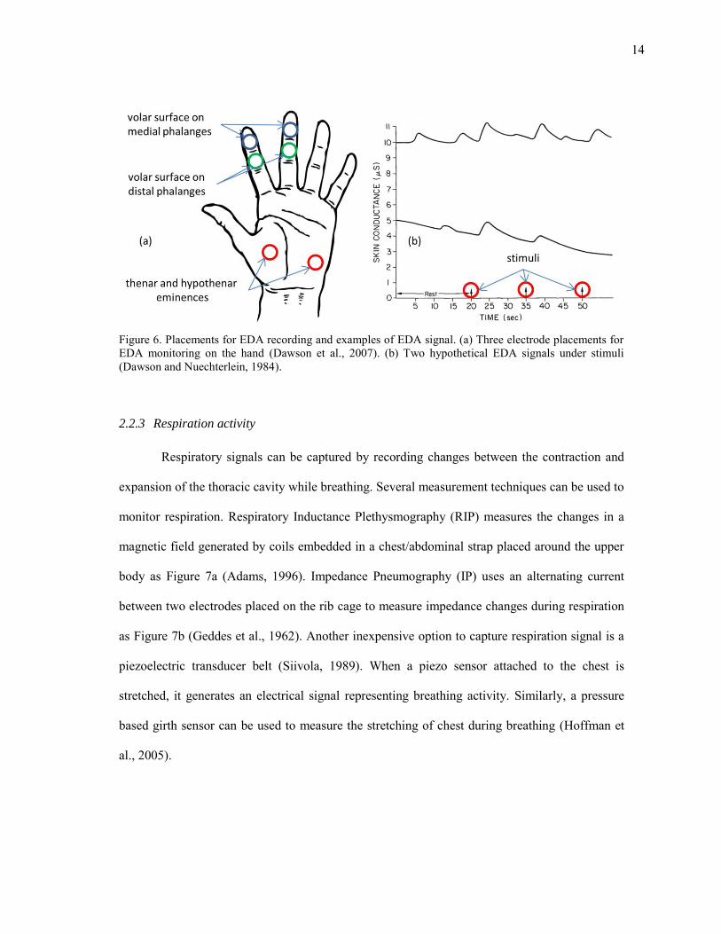
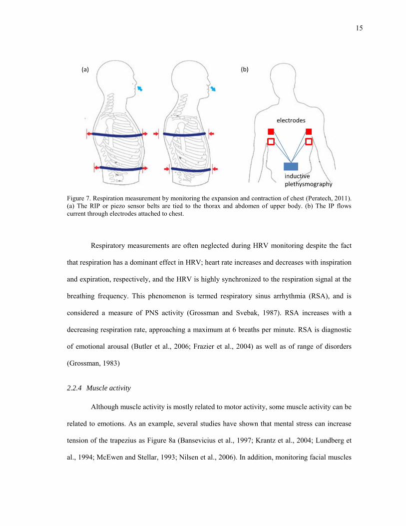
Respiratory signals can be captured by recording changes between the contraction and
expansion of the thoracic cavity while breathing. Several measurement techniques can be used to
monitor respiration. Respiratory Inductance Plethysmography (RIP) measures the changes in a
magnetic field generated by coils embedded in a chest/abdominal strap placed around the upper
body as Figure 7a (Adams, 1996). Impedance Pneumography (IP) uses an alternating current
between two electrodes placed on the rib cage to measure impedance changes during respiration
as Figure 7b (Geddes et al., 1962). Another inexpensive option to capture respiration signal is a
piezoelectric transducer belt (Siivola, 1989). When a piezo sensor attached to the chest is
stretched, it generates an electrical signal representing breathing activity. Similarly, a pressure
based girth sensor can be used to measure the stretching of chest during breathing (Hoffman et
al., 2005).
15
Figure 7. Respiration measurement by monitoring the expansion and contraction of chest (Peratech, 2011). (a) The RIP or piezo sensor belts are tied to the thorax and abdomen of upper body. (b) The IP flows current through electrodes attached to chest.
Respiratory measurements are often neglected during HRV monitoring despite the fact
that respiration has a dominant effect in HRV; heart rate increases and decreases with inspiration
and expiration, respectively, and the HRV is highly synchronized to the respiration signal at the
breathing frequency. This phenomenon is termed respiratory sinus arrhythmia (RSA), and is
considered a measure of PNS activity (Grossman and Svebak, 1987). RSA increases with a
decreasing respiration rate, approaching a maximum at 6 breaths per minute. RSA is diagnostic
of emotional arousal (Butler et al., 2006; Frazier et al., 2004) as well as of range of disorders
(Grossman, 1983)
2.2.4 Muscle activity
Although muscle activity is mostly related to motor activity, some muscle activity can be
related to emotions. As an example, several studies have shown that mental stress can increase
tension of the trapezius as Figure 8a (Bansevicius et al., 1997; Krantz et al., 2004; Lundberg et
al., 1994; McEwen and Stellar, 1993; Nilsen et al., 2006). In addition, monitoring facial muscles

16
can facilitate with recognition of emotions as Figure 8b (Fridlund et al., 1984; Lanzetta and
Englis, 1989; Tassinary and Cacioppo, 1992; Vrana, 1993).
Figure 8. Muscles measured for stress detection. (a) Trepezious (Zhao et al., 2003) (b) The facial EMG signals of the frontalis (1-2), corrugator supercilii(3-4), and zygomaticus major(5-6) (van den Broek et al., 2006).
Muscle activity is generally measured through electromyography (EMG). There are two
different types of measurements used in EMG: intramuscular and surface EMG. For
intramuscular measurements, a needle electrode is inserted into the contracting muscle. This
method is commonly used when measuring activity of nerves and muscle fibers. In contrast,
surface EMG captures muscle activity via electrodes attached to the surface of the contracting
muscle.
2.2.5 Brain activity
Electroencephalography (EEG) is the measurement of electrical activity in the brain
through electrodes placed on the scalp or on the cortex (Figure 9a). The resulting signals,
commonly referred to as “brainwaves”, display activity in four major frequency bands (Figure
17
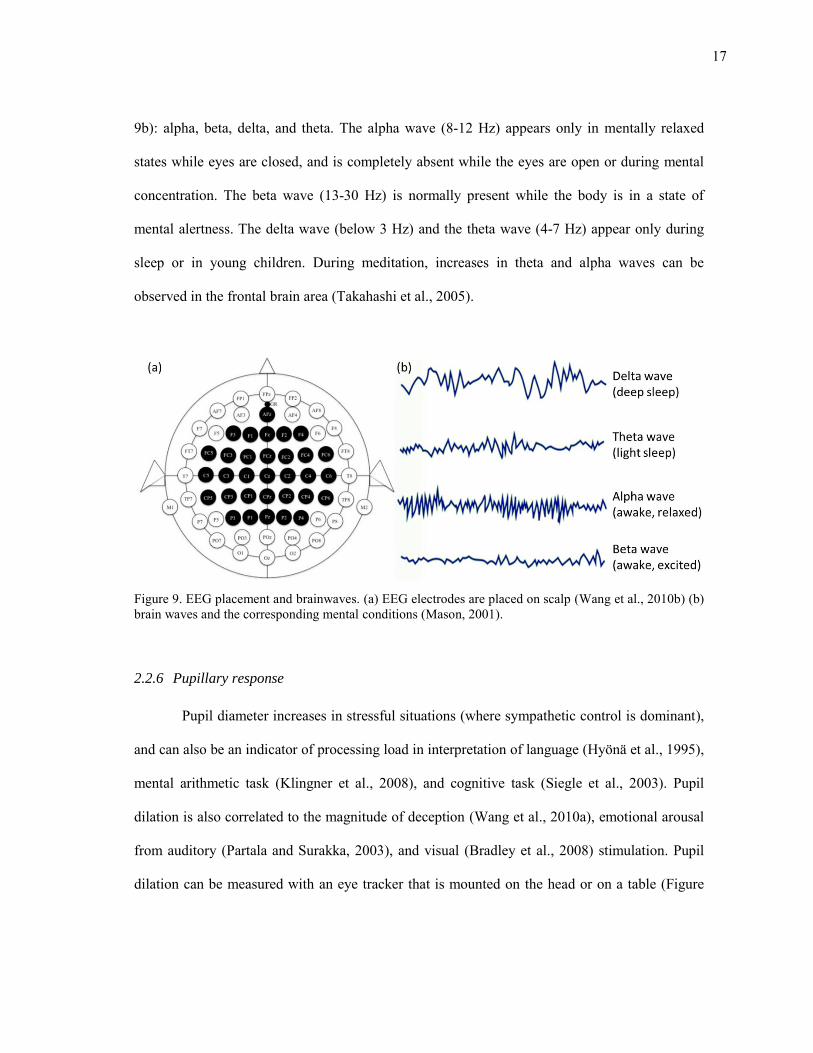
9b): alpha, beta, delta, and theta. The alpha wave (8-12 Hz) appears only in mentally relaxed
states while eyes are closed, and is completely absent while the eyes are open or during mental
concentration. The beta wave (13-30 Hz) is normally present while the body is in a state of
mental alertness. The delta wave (below 3 Hz) and the theta wave (4-7 Hz) appear only during
sleep or in young children. During meditation, increases in theta and alpha waves can be
observed in the frontal brain area (Takahashi et al., 2005).
Figure 9. EEG placement and brainwaves. (a) EEG electrodes are placed on scalp (Wang et al., 2010b) (b) brain waves and the corresponding mental conditions (Mason, 2001).
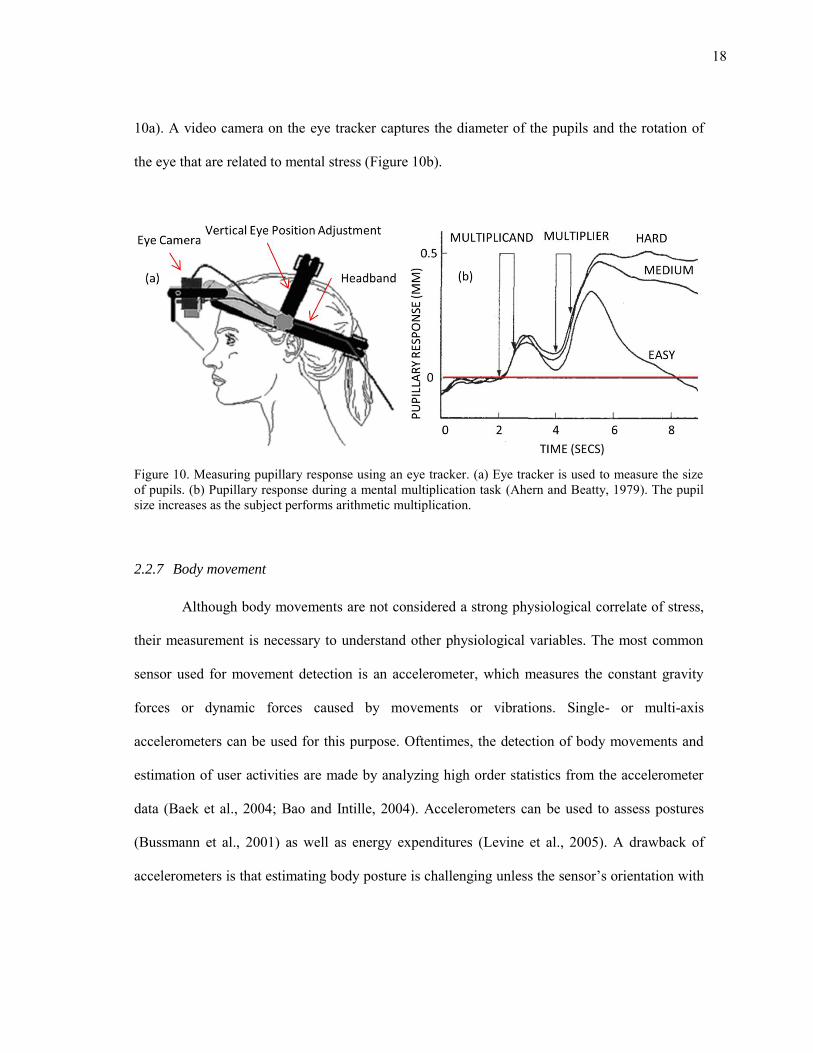
2.2.6 Pupillary response
Pupil diameter increases in stressful situations (where sympathetic control is dominant),
and can also be an indicator of processing load in interpretation of language (Hyönä et al., 1995),
mental arithmetic task (Klingner et al., 2008), and cognitive task (Siegle et al., 2003). Pupil
dilation is also correlated to the magnitude of deception (Wang et al., 2010a), emotional arousal
from auditory (Partala and Surakka, 2003), and visual (Bradley et al., 2008) stimulation. Pupil
dilation can be measured with an eye tracker that is mounted on the head or on a table (Figure
18
10a). A video camera on the eye tracker captures the diameter of the pupils and the rotation of
the eye that are related to mental stress (Figure 10b).
Figure 10. Measuring pupillary response using an eye tracker. (a) Eye tracker is used to measure the size of pupils. (b) Pupillary response during a mental multiplication task (Ahern and Beatty, 1979). The pupil size increases as the subject performs arithmetic multiplication.
2.2.7 Body movement
Although body movements are not considered a strong physiological correlate of stress,
their measurement is necessary to understand other physiological variables. The most common
sensor used for movement detection is an accelerometer, which measures the constant gravity
forces or dynamic forces caused by movements or vibrations. Single- or multi-axis
accelerometers can be used for this purpose. Oftentimes, the detection of body movements and
estimation of user activities are made by analyzing high order statistics from the accelerometer
data (Baek et al., 2004; Bao and Intille, 2004). Accelerometers can be used to assess postures
(Bussmann et al., 2001) as well as energy expenditures (Levine et al., 2005). A drawback of
accelerometers is that estimating body posture is challenging unless the sensor’s orientation with
19
respect to the body is kept constant. To overcome this problem, a MEMS gyroscope is often used
in combination with an accelerometer (Takeda et al., 2009; Zhou et al., 2006).
2.3 The cardiovascular system as a robust measure of ANS activity
As described 2.1.2, the cardiovascular system is innervated by two ANS branches, which
make cardiac response sensitive to stress. This section provides a detailed description of heart
rate variability and its use as a physiological marker. Features of HRV are explained followed by
explanation of possibility and limitation of HRV. Finally, factors that influence HRV are
enumerated.
2.3.1 Heart rate variability
Autonomic influences on the heart rate suggest that hart rate could be used to estimate
the activation level of both autonomic branches and, indirectly, to predict psychological state.
Unfortunately, changes in the SNS and PNS activities are potentially indistinguishable solely
based on changes in heart rate, e.g., an increase in heart rate can result from an increased SNS
activity and/or a decreased PNS activity. Instead, one must rely on one important difference
between both branches: PNS influences on heart rate tend to occur faster. Hence, by analyzing
fluctuations in beat-to-beat periods, one can begin to separate the contributions from both
branches. This is known as heart rate variability (HRV) analysis.
HRV is broadly employed in diverse areas ranging from psychological studies to clinical
risk assessment (Malik et al., 1996). ECG is ideal for HRV analysis because it captures the
complete QRS waveform, which makes it simple to exclude heartbeats that do not originate from
20
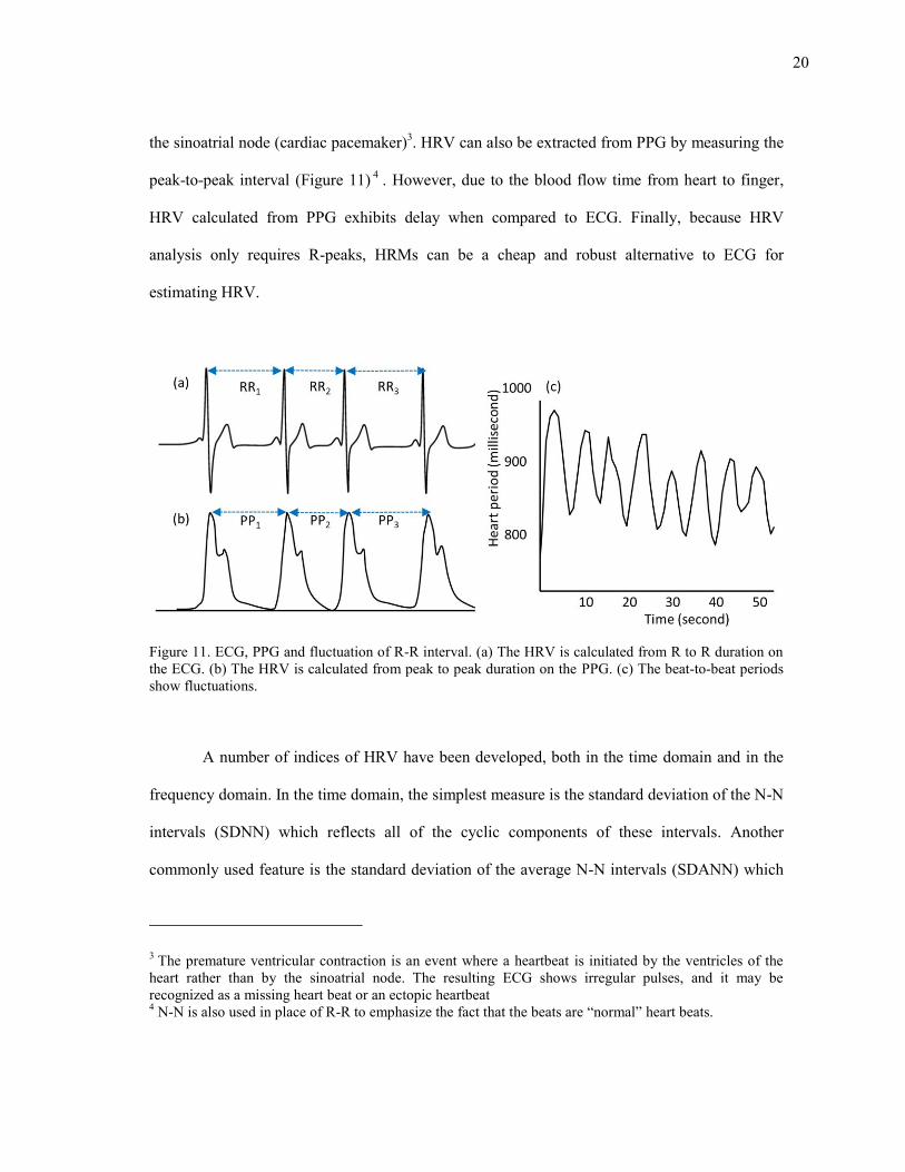
the sinoatrial node (cardiac pacemaker)3. HRV can also be extracted from PPG by measuring the
peak-to-peak interval (Figure 11) 4 . However, due to the blood flow time from heart to finger,
HRV calculated from PPG exhibits delay when compared to ECG. Finally, because HRV
analysis only requires R-peaks, HRMs can be a cheap and robust alternative to ECG for
estimating HRV.
Figure 11. ECG, PPG and fluctuation of R-R interval. (a) The HRV is calculated from R to R duration on the ECG. (b) The HRV is calculated from peak to peak duration on the PPG. (c) The beat-to-beat periods show fluctuations.
A number of indices of HRV have been developed, both in the time domain and in the
frequency domain. In the time domain, the simplest measure is the standard deviation of the N-N
intervals (SDNN) which reflects all of the cyclic components of these intervals. Another
commonly used feature is the standard deviation of the average N-N intervals (SDANN) which
3 The premature ventricular contraction is an event where a heartbeat is initiated by the ventricles of the heart rather than by the sinoatrial node. The resulting ECG shows irregular pulses, and it may be recognized as a missing heart beat or an ectopic heartbeat 4 N-N is also used in place of R-R to emphasize the fact that the beats are “normal” heart beats.
21
is calculated over short periods (usually 5 minutes). SDNN represents an estimate of overall
HRV while SDANN represents long-term components in HRV (Malik et al., 1996). Other
features include the square root of the mean squared differences of successive N-N intervals
(RMSSD), the number of interval differences of successive N-N intervals greater than 50 ms
(NN50; other durations can be used), and the proportion derived by dividing NN50 by the total
number of N-N intervals (pNN50; other durations can be used). RMSSD, NN50, and pNN50 are
highly correlative, and they reflect the high-frequency variations in HRV (Malik et al., 1996).
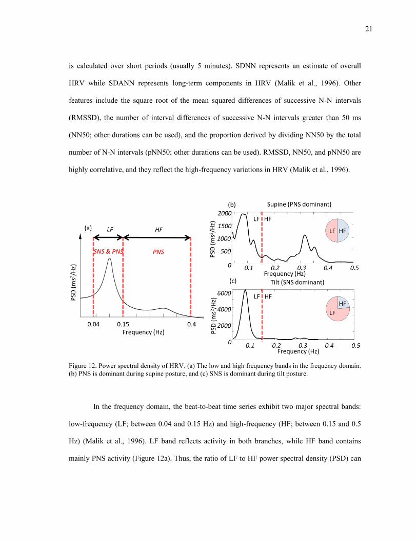
Figure 12. Power spectral density of HRV. (a) The low and high frequency bands in the frequency domain. (b) PNS is dominant during supine posture, and (c) SNS is dominant during tilt posture.
In the frequency domain, the beat-to-beat time series exhibit two major spectral bands:
low-frequency (LF; between 0.04 and 0.15 Hz) and high-frequency (HF; between 0.15 and 0.5
Hz) (Malik et al., 1996). LF band reflects activity in both branches, while HF band contains
mainly PNS activity (Figure 12a). Thus, the ratio of LF to HF power spectral density (PSD) can
22
serve as an indicator of autonomic balance5. As an example, the PNS component is dominant in
supine position, whereas the SNS component is dominant in a tilted posture, as illustrated in
Figure 12b-c.
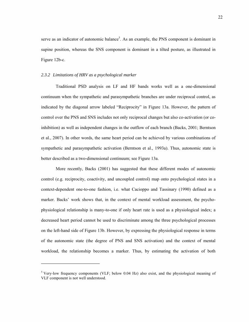
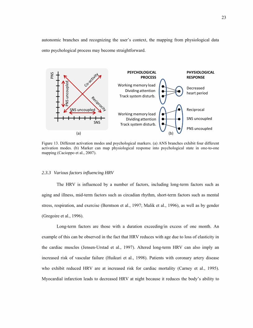
2.3.2 Limitations of HRV as a psychological marker
Traditional PSD analysis on LF and HF bands works well as a one-dimensional
continuum when the sympathetic and parasympathetic branches are under reciprocal control, as
indicated by the diagonal arrow labeled “Reciprocity” in Figure 13a. However, the pattern of
control over the PNS and SNS includes not only reciprocal changes but also co-activation (or co-
inhibition) as well as independent changes in the outflow of each branch (Backs, 2001; Berntson
et al., 2007). In other words, the same heart period can be achieved by various combinations of
sympathetic and parasympathetic activation (Berntson et al., 1993a). Thus, autonomic state is
better described as a two-dimensional continuum; see Figure 13a.
More recently, Backs (2001) has suggested that these different modes of autonomic
control (e.g. reciprocity, coactivity, and uncoupled control) map onto psychological states in a
context-dependent one-to-one fashion, i.e. what Cacioppo and Tassinary (1990) defined as a
marker. Backs’ work shows that, in the context of mental workload assessment, the psycho-
physiological relationship is many-to-one if only heart rate is used as a physiological index; a
decreased heart period cannot be used to discriminate among the three psychological processes
on the left-hand side of Figure 13b. However, by expressing the physiological response in terms
of the autonomic state (the degree of PNS and SNS activation) and the context of mental
workload, the relationship becomes a marker. Thus, by estimating the activation of both
5 Very-low frequency components (VLF; below 0.04 Hz) also exist, and the physiological meaning of VLF component is not well understood.
23
autonomic branches and recognizing the user’s context, the mapping from physiological data
onto psychological process may become straightforward.
Figure 13. Different activation modes and psychological markers. (a) ANS branches exhibit four different activation modes. (b) Marker can map physiological response into psychological state in one-to-one mapping (Cacioppo et al., 2007).
2.3.3 Various factors influencing HRV
The HRV is influenced by a number of factors, including long-term factors such as
aging and illness, mid-term factors such as circadian rhythm, short-term factors such as mental
stress, respiration, and exercise (Berntson et al., 1997; Malik et al., 1996), as well as by gender
(Gregoire et al., 1996).
Long-term factors are those with a duration exceeding/in excess of one month. An
example of this can be observed in the fact that HRV reduces with age due to loss of elasticity in
the cardiac muscles (Jensen-Urstad et al., 1997). Altered long-term HRV can also imply an
increased risk of vascular failure (Huikuri et al., 1998). Patients with coronary artery disease
who exhibit reduced HRV are at increased risk for cardiac mortality (Carney et al., 1995).
Myocardial infarction leads to decreased HRV at night because it reduces the body’s ability to
24
activate vagal dominance during sleep, which in turn is associated with a lower risk of cardiac
failure (Malik et al., 1990). Lower HRV can also be a sign of autonomic dysregulation in early
stages of hypertension (Singh et al., 1998). Finally, some studies link lower HRV to several
mental disorders, e.g., phobic anxieties (Kawachi et al., 1995) and depression (Rechlin et al.,
1994).
Mid-term factors are those with duration of a day. For example, circadian rhythms
influence HRV. Huikuri et al. analyzed HRV over periods of 24 hours and found a high
variability before subjects awake (reflecting a high vagal tone) and low values after awakening
(Huikuri et al., 1992). Malpas and Purdie (1990) observed that HRV rises during sleep and that
the absence of this phenomenon can be an indication of cardiac failure. Ischemic stroke patients
do not display the cycles due to cardiovascular autonomic dysregulation (Korpelainen et al.,
1997). In contrast, individuals undergoing rigorous physical training show significantly more
rhythm in parasympathetic activity during both day and night (Mølgaard et al., 1991).
Parasympathetic activity is lower in NREM6 sleep than in REM sleep, while the opposite occurs
in sympathetic activity (Berlad et al., 1993).
Short-term factors such as mental stress, respiration, and physical activity have a heavy
influence on HRV. Stressors such as public speaking, mental arithmetic, and reaction-time tests
can cause increased sympathetic activity and decreased parasympathetic activity (Berntson et al.,
1997). Emotions such as anger produce sympathetic activation, while appreciation produces a
shift in the HRV power spectrum towards the HF band; earlier studies suggest that positive
emotions lead to alterations in HRV (McCraty et al., 1995). Another short-term predominant
6 Non-rapid eye movement (NREM) refers sleep stage where there is usually little or no eye movement. In contrast, Rapid eye movement sleep (REM) is a normal sleep stage characterized by the random movement of the eyes.
25
factor which influences HRV is respiration. At normal breathing rates, the effect of respiration
on HRV begins during expiration and progresses slowly, although these influences are not
clearly evident at faster breathing rates (Eckberg, 1983). This relationship between breathing and
HRV is maximized at slow breathing rates of around 0.1 Hz (Malpas and Purdie, 1990). Given
the magnitude of its influence, the removal of respiration from HRV is likely to increase the
prominence of other factors. Physical activity is another dominant factor of HRV. During
exercise, the HF component reflects an increased respiratory rate and the LF peak changes with
the baroreceptor reflex (Perini et al., 1990). In addition, exercise and passive tilt result in a short-
term increase of HRV, which is related to increased HF power (Sandercock et al., 2005; Tulppo
et al., 2001).
HRV has considerable potential for assessing various influential factors of the
cardiovascular system. HRV has been reported as a tool for assessing the integrity of the ANS
(Berntson et al., 1997; Malik et al., 1996). More importantly, HRV can be derived from
unobtrusive cardiac sensors, and it provides easy access to physical and psychological state.

26
3. LITERATURE REVIEW
This section provides a review of wearable sensors, mental stress monitoring, and
computational methods for physiological signals. The first part of the section describes the
challenges of developing wearable sensor systems and the applications of these systems. Then,
we review approaches used for stress monitoring and discuss different experimental protocols
used in literature for inducing mental stress for experimental purposes. The final section of the
section reviews computational methods that have been proposed for the modeling of
physiological signals.
3.1 Wearable hardware prototypes
There are two important design issues that must be addressed while developing a
wearable sensor system. As discussed in the previous section, the design of wearable system
should consider a trade-off between the amount of information collected from the user and the
user’s comfort level. Second, the system must have the ability to transmit and store data
collected from the subjects for later use. Recent advances in communication technologies help us
address the second design issue; namely, the sensors can be equipped with wireless
communication systems to transfer and store the collected data.
3.1.1 Information vs. comfort
The argument that “more sensors are better” is not always true not only from a statistical
perspective (Hines, 1936; Jimenez and Landgrebe, 1998), but also in terms of design for
wearability (Gemperle et al., 1998). The first generation of wearable sensor systems focused on
27
information rather than user comfort. These systems had multiple physiological sensors wired
into the recording unit which digitized and stored the signals. One of the earliest wearable
systems, MIThril (DeVaul et al., 2003) wired ECG, EMG, EDA, and temperature sensors to a
Linux-based PDA. Wired connections are robust and reduce the need for separate power
supplies, but the user must get used to the dangling wires that hinder mobility. As an alternative,
Luprano et al. (2006) and Pacelli et al. (2006) designed e-textiles to hide the wire connections.
However, e-textiles require the subjects to wear specially-designed outfits rather than their
normal clothing.
Over the last decade, a number of commercially wearable systems have been developed
for fitness and healthcare markets (e.g., Fitbit™ (Fitbit Inc.), WakeMate™ (Perfect Third Inc.),
and Nike+™ (Nike Inc.)). These systems were designed to meet with the requirements of a
specific target group. Therefore, they contain only a few sensors (for e.g., an HRM and an
accelerometer) making them relatively affordable and conveniently sized. However, these
systems cannot be used for a complex problem such as stress management, which requires
information from various sensing modalities.
3.1.2 Wireless communication
The second major design aspect of a wearable system is the technology used for
transmitting and storing data. Wireless communications have become the standard technology
for data transmission. When developing a wearable sensor system, wireless protocols should be
chosen based on the transmission distance, speed, stability, and power consumption. Designers
should not only consider the wireless protocol but also the network architecture. The architecture
should be determined based on what data transmission strategy is to be adopted.
A wide variety of technologies are available for wireless communication, ranging from
wide area networks (i.e., cellular) to short-range protocols (i.e., Bluetooth, ZigBee)
28
(Pantelopoulos and Bourbakis, 2009). Cellular networks have been used to transmit data to
remote servers, and provide a high degree of freedom and mobility to the user. For example,
Anliker et al. (2004) developed AMON, a wearable sensor system that transmits a patient’s
electrocardiographic and pulse oximetry data to a remote server using a cell phone. However,
cellular networks are too expensive for long-term transmission of physiological data. For short-
range data transfer, Bluetooth is one of the most widely used communication protocol. As an
example, Mundt et al. (2005) developed a wearable sensor system for space and terrestrial
applications that integrates ECG, impedance plethysmography, pulse oximetry, and body
temperature and uses Bluetooth to transmit the sensor signals to a data logger. Recently, the
sensor network protocol ZigBee has become a popular alternative for wireless communication
due to its power efficiency. As an example, Shnayder et al. (2005) integrated a custom
physiological sensor board with commercially available ZigBee motes (Micaz™ and Telos™;
XBow Inc.) on CodeBlue.
ZigBee protocol can be combined with different network topologies to transmit data
from the nodes to the recording unit. One common topology is for each sensor node to transmit
data to a remote server through an ad hoc network. iCalm (Fletcher et al., 2009) used this
topology to connect EDA and PPG sensors to a remote base station. This ad hoc network
topology provides comfort to the subject by eliminating the need for them to carry a recording
unit. However, this topology requires that the sensor network always be within the reach of a
remote base station. Another possible network topology uses a body-worn hub that records the
data transmitted from the sensor nodes. This is known as a star topology. As an example, the
ubiquitous fashionable computer (UFC) (Lee et al., 2007) used a wireless hub to communicate
data from an accelerometer node attached to a single finger. The accelerometer node was
designed to recognize gestures to control ubiquitous devices such as a kiosk or a display.

29
Similarly, a body area network (BAN) developed by Monton et al. (2008) employed a mobile
hub to communicate with sensor modules (ZigBee™ protocol). The data collected from the
sensor modules was used to detect wakefulness, fatigue, and stress.
3.2 Applications of wearable sensors
In this section, we review applications of wearable sensors in the fields of engineering
and healthcare. In the field of engineering, wearable sensors have been used to monitor a user’s
internal state or a user’s external surroundings. In the field of healthcare, they have been used for
both clinical monitoring and behavioral monitoring (e.g., exercise monitoring).
3.2.1 User monitoring
From the early stages, research in wearable sensors have focused on addressing two
problems; (1) affect detection (Picard, 1997) and (2) context awareness (Schilit et al., 1994). The
problem of affect detection involves interpreting a user’s emotional status from physiological
signals. On the other hand, context awareness deals with detecting a user’s environment or the
user’s interaction with it. As an example, Picard and Healey (2001) were able to distinguish
among eight different emotional states (no emotion, anger, hate, grief, platonic love, romantic
love, joy, and reverence) of a single subject using a few weeks of physiological data. They
employed a forward feature selection strategy (Bishop, 2007) to extract the most relevant
features from the data. Similarly, Kim et al. (2004) classified surprise, sadness, anger, and stress
using features from ECG, skin temperature variation and electrodermal activity with a support
vector machine. Likewise, Lee et al. (2005) classified the emotions of calmness and excitement
using electrodermal activity and HRV with a neural network. For the problem of context
awareness, researchers have used audio, video, motion, and positioning sensors (e.g.
30
microphone, camera, accelerometer, gyroscope, and GPS receiver). In context awareness, the
term “context” commonly refers to physical location (e.g. at work, at home) of the user, which
presumably determines his or her activity. However, context sometimes may refer to social
situations, such as a meeting or a meal, or physical activities, such as laying down, walking, or
running. To capture these diverse notions of context, different sensors have been used: GPS
(Ashbrook and Starner, 2002, 2003), location beacons (Lee and Mase, 2002), video cameras
(Gemmell et al., 2004), microphones (Ellis and Lee, 2004), and accelerometers (Tapia et al.,
2004).
3.2.2 Healthcare
Wearable sensors have also been widely used for clinical applications, including cardio
vascular diseases (Malik et al., 1990; Mølgaard et al., 1991; Nolan et al., 1998), rehabilitation
(Sung et al., 2005), Parkinson’s disease (Kallio et al., 2002; Pursiainen et al., 2002), post-stroke
assessment (Hester et al., 2006; Korpelainen et al., 1997), and emergency reports (Shnayder et
al., 2005). We can broadly classify the clinical applications into two categories (1) detection of
critical events (e.g., heart attack) or (2) monitoring behavioral patterns (e.g., gait monitoring).
For applications such as detecting heart failure, the subjects should be monitored continuously.
In such applications, precision and durability of the wearable system takes precedence over
comfort. Barr et al. (1994) and Tomaselli et al. (1994) used ECG sensors for predicting heart
failure. Noury (2002) and Sixsmith and Johnson (2004) demonstrated the use of posture sensors
(i.e., accelerometer and gyro) for fall detection in older adults. For applications that monitor
patterns, the wearable system requires comfort over precision. Morris and Paradiso (2002) used a
shoe-mounted sensor for real-time gait monitoring, where the system collected motion, position,
and pressure data from the subject’s foot.. Similarly Hester et al. (2006) used wearable sensors to
assess and guide motor abilities of post-stroke rehabilitation patients. Body postures (i.e., sitting,

31
standing, and laying down) and periods of walking in elderly persons were monitored using a
chest attached kinematic sensor (Najafi et al., 2003). Along the same lines, accelerometers and
HRMs have been used to track energy expenditure for the purpose of exercise training (Fruin
and Rrankin, 2004; Strath et al., 2001) or for resting (Malavolti et al., 2007).
3.3 Stress monitoring
In this section, we discuss four methods that have been used in psychology for
monitoring mental stress in human subjects. The simplest of these methods is that of a self-
report, where the subject regularly answers questionnaires to track his/her stress levels based on
a predefined stress scale. The second approach involves using subject’s blood or urinal samples
to measure hormonal content that reflects mental stress. The third approach has developed more
recently, with the advancement of neural imaging devices where 3D snapshots of the subject’s
brain are obtained to measure stress. The fourth approach involves using physiological sensors.
3.3.1 Self-reporting
The perceived stress scale (PSS) (Cohen et al., 1983) was designed to measure the
degree of stress, and the scale includes queries about current levels of experienced stress. The
questions are independent of subject’s age, sex, etc., and ask about feelings and thoughts during
the last month. Holmes and Rahe (1967) developed a stress scale for long term stress
measurement. They identified 43 stressful life events that could result in long term illness. A
positive correlation of 0.118 was found between stress from the subjects’ life events and
illnesses. Using the same scale, Rahe and Mahan (1970) developed a number of "Life Change
Units" that measure the effects of stress on health. By narrowing down target population, the
questions and stress scales can be tailored to improve obtain more relevant information. For

32
example, the feminine gender role stress (FGRS) (Gillespie and Eisler, 1992) focused on
maladaptive stress responses which are salient in women such as fear of unemotional
relationships, being unattractive, victimization, and behaving assertively. Similarly, the parental
stress scale (Berry and Jones, 1995) was developed to measure emotions and role satisfaction
(e.g. loneliness, marital satisfaction, and guilt.). The results were shown to be consistent across
parents of different personalities. Also job specific scales were developed to measure stress at
the work place (Cushway et al., 1996; Gray-Toft and Anderson, 1981).
3.3.2 Biological samples
The second method of stress measurement involves the detection of biological responses
such as hormones, acid, and neurotransmitter. These tests usually measure for catecholamines,
corticosteroids, opioid peptides and serotonin in the subject’s blood or urine samples7.
Catecholamines are "fight-or-flight" hormones released by the adrenal glands in
response to stress (Schildkraut, 1965); they increase heart rate, blood pressure, breathing rate,
muscle strength, and alertness. Catecholamines are produced mainly by the cells and fibers of the
sympathetic nervous system. The major catecholamines are adrenaline (epinephrine),
noradrenaline (norepinephrine), and dopamine. For example, epinephrine levels are significantly
different prior to and during public speaking events (Dimsdale and Moss, 1980). Corticosteroids
are steroid hormones also involved in stress response, immune response and regulation of
inflammation, carbohydrate metabolism, protein catabolism, and blood electrolyte levels.
Opioid peptides are short sequences of amino acids that bind to opioid receptors in the
brain. Brain opioid peptide systems are known to play an important role in motivation, emotion,
7 Catecholamines and corticosteroids are hormones. Opioid peptides is an acid and serotonin is a neurotransmitter.
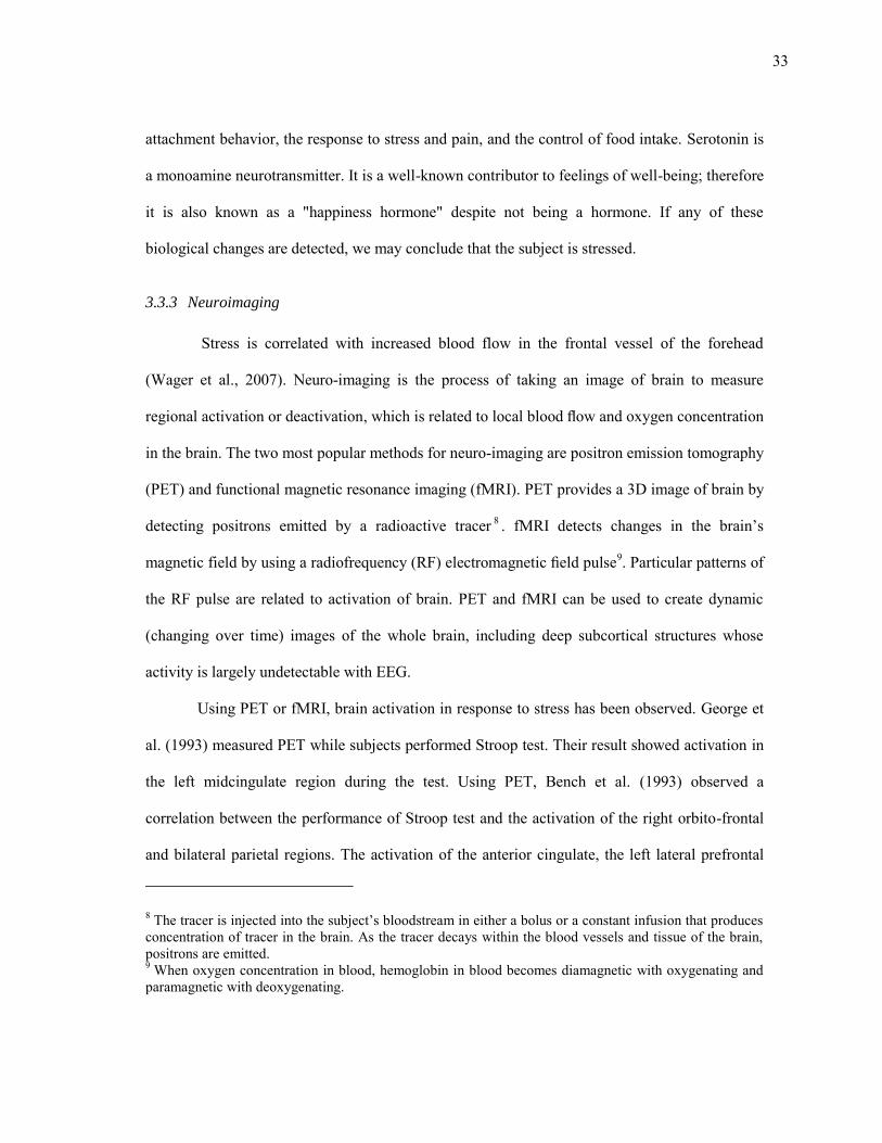
33
attachment behavior, the response to stress and pain, and the control of food intake. Serotonin is
a monoamine neurotransmitter. It is a well-known contributor to feelings of well-being; therefore
it is also known as a "happiness hormone" despite not being a hormone. If any of these
biological changes are detected, we may conclude that the subject is stressed.
3.3.3 Neuroimaging
Stress is correlated with increased blood flow in the frontal vessel of the forehead
(Wager et al., 2007). Neuro-imaging is the process of taking an image of brain to measure
regional activation or deactivation, which is related to local blood flow and oxygen concentration
in the brain. The two most popular methods for neuro-imaging are positron emission tomography
(PET) and functional magnetic resonance imaging (fMRI). PET provides a 3D image of brain by
detecting positrons emitted by a radioactive tracer 8 . fMRI detects changes in the brain’s
magnetic field by using a radiofrequency (RF) electromagnetic field pulse9. Particular patterns of
the RF pulse are related to activation of brain. PET and fMRI can be used to create dynamic
(changing over time) images of the whole brain, including deep subcortical structures whose
activity is largely undetectable with EEG.
Using PET or fMRI, brain activation in response to stress has been observed. George et
al. (1993) measured PET while subjects performed Stroop test. Their result showed activation in
the left midcingulate region during the test. Using PET, Bench et al. (1993) observed a
correlation between the performance of Stroop test and the activation of the right orbito-frontal
and bilateral parietal regions. The activation of the anterior cingulate, the left lateral prefrontal
8 The tracer is injected into the subject’s bloodstream in either a bolus or a constant infusion that produces
concentration of tracer in the brain. As the tracer decays within the blood vessels and tissue of the brain, positrons are emitted. 9 When oxygen concentration in blood, hemoglobin in blood becomes diamagnetic with oxygenating and paramagnetic with deoxygenating.
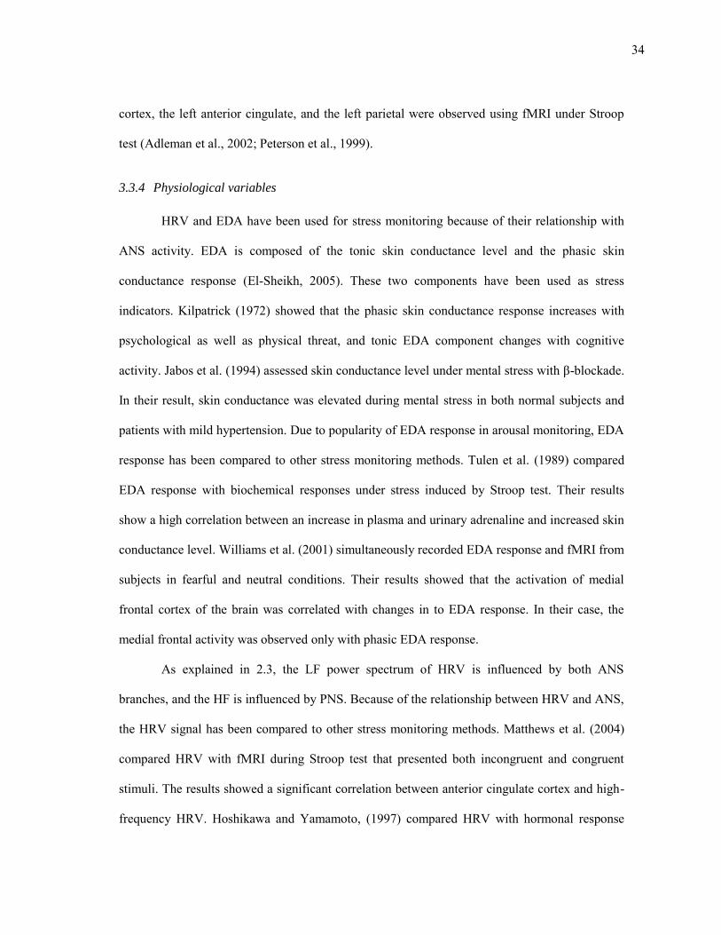
34
cortex, the left anterior cingulate, and the left parietal were observed using fMRI under Stroop
test (Adleman et al., 2002; Peterson et al., 1999).
3.3.4 Physiological variables
HRV and EDA have been used for stress monitoring because of their relationship with
ANS activity. EDA is composed of the tonic skin conductance level and the phasic skin
conductance response (El-Sheikh, 2005). These two components have been used as stress
indicators. Kilpatrick (1972) showed that the phasic skin conductance response increases with
psychological as well as physical threat, and tonic EDA component changes with cognitive
activity. Jabos et al. (1994) assessed skin conductance level under mental stress with β-blockade.
In their result, skin conductance was elevated during mental stress in both normal subjects and
patients with mild hypertension. Due to popularity of EDA response in arousal monitoring, EDA
response has been compared to other stress monitoring methods. Tulen et al. (1989) compared
EDA response with biochemical responses under stress induced by Stroop test. Their results
show a high correlation between an increase in plasma and urinary adrenaline and increased skin
conductance level. Williams et al. (2001) simultaneously recorded EDA response and fMRI from
subjects in fearful and neutral conditions. Their results showed that the activation of medial
frontal cortex of the brain was correlated with changes in to EDA response. In their case, the
medial frontal activity was observed only with phasic EDA response.
As explained in 2.3, the LF power spectrum of HRV is influenced by both ANS
branches, and the HF is influenced by PNS. Because of the relationship between HRV and ANS,
the HRV signal has been compared to other stress monitoring methods. Matthews et al. (2004)
compared HRV with fMRI during Stroop test that presented both incongruent and congruent
stimuli. The results showed a significant correlation between anterior cingulate cortex and high-
frequency HRV. Hoshikawa and Yamamoto, (1997) compared HRV with hormonal response

35
under Stroop test. Their results showed a significant decrease in RR interval with an increase in
norepinephrine and epinephrine concentrations.
3.4 Elicitation of mental stress for experimental purposes
In this section we review stress elicitation protocols that have been used in the literature.
These protocols are commonly based on five different stress drivers: (1) pressure on reaction
time (Luce, 1991), (2) working memory (Baddeley, 1992), (3) selective attention (Deutsch and
Deutsch, 1963), (4) physical pressure (Menkes et al., 1989), and (5) social stress (Kirschbaum et
al., 1993).
3.4.1 Reaction time
Pressure on reaction time has been a well-known driver in psychological tests (Welford,
1980). In these tests, subjects are asked to respond to stimulus as soon as possible, and this time
pressure induces stress in the subjects. A simple reaction time protocol would have one stimulus
expecting one response from the subject. For example, the subject is asked to press a key when
he/she hears a sound (Boer, 1995). A more elaborate protocol would require the subject to react
to only to a set of targets and avoid other distracters; the subject should respond to the stimuli by
choosing a corresponding reaction. For example, in a tracking test, the subjects are asked to
perform continuous adjustments to maintain the position of a moving target which is inherently
unstable (Jex et al., 1966).
3.4.2 Working memory
Working memory refers to a part of the brain used to store up and manipulate temporary
information. Complex cognitive tasks that require subjects to use working memory induce stress.
36
For example, the Sternberg memory search test (Sternberg, 1966, 1975) requires subjects to
memorize a small group of items (e.g., numbers or letters). Then, subjects are presented with a
series of items and determine if they have seen the items before (with a ‘yes’ or ‘no’ answer). By
increasing the number of items to be memorized, the difficulty of the task can be increased.
Hitch (1978) designed a mental arithmetic test that measures the subjects’ ability to manipulate
information in working memory using mathematical operands. Here, the subjects are required to
memorize numbers and answer to a query by applying the given arithmetic operator to the
memorized numbers. Baddeley (1968) showed that grammatical reasoning could be used to
induce stress. During the test, subjects were asked to compare the veracity of the description in
several sentences by manipulating the grammatical information in their working memory.
Several types of grammatical reasoning tasks have also been reported in the literature (Wason,
1968; Wason and Johnson-Laird, 1972). Reid et al. (1981) developed spatial processing test
where the subjects were asked to memorize an image and respond to a question by matching the
rotated image.
3.4.3 Selective attention
When subjects concurrently handle multiple sources of information, they tend to focus
on relevant sources and ignore the rest. Therefore, a task that requires a subject’s attention on
multiple sources of information simultaneously is likely to induce metal stress (Carter et al.,
1995). For example, during the standard Stroop test, subjects are asked to respond to the “color”
of the given text that is painted with inconsistent color (i.e., “red” is painted with blue color).
Major stress comes from cognitive interference between the subject’s ability to read words more
quickly than to name colors (Jensen and Rohwer Jr, 1966). Likewise, a dual-task test requires
subjects to perform two tasks simultaneously. When subjects are asked to perform the two tasks

37
(e.g., tracking and memory search tasks) at the same time, stress arises from the conflict of
selective attention since individuals tend to allocate equal priority to tasks.
3.4.4 Physical pressure
Physical discomfort has also been used as a stress inducing protocol. Lowery (2003)
devised a protocol based on the classic cold-pressor test (Hines, 1936), where subjects were
asked to place their hand in cold water for as long as they could. This test was used to measure
the subject’s threshold and tolerance to stress. Subjects reported the exact moment when they
first felt stress (threshold of stress) and at what point the stress became unbearable (tolerance to
stress). Menkes (1989) used a similar protocol to measure cardiovascular reactivity to stress.
Their results also demonstrated that stress could be a predictor of hypertension. Streff et al.
(2010) used a similar protocol, though in this case subjects had their hand immersed in hot water.
3.4.5 Social stress
Lastly, pressure from social evaluation can be used as a driver to induce stress. For
example, speaking in front of audiences (or cameras) often causes significant increases in the
release of stress hormones (Clow et al., 1997; Kirschbaum et al., 1993). During the test, a topic
sentence is given to the subjects and they are each asked to prepare a speech, express their
opinion, and answer questions from the public/audience. The Trier Social Stress Test (TSST),
one of the most frequently used protocols was proposed by Kirschbaum (1993). It consists of a
preparation period (3 minutes), a speech period (5 minutes), and an arithmetic period (5 minutes)
in front of an audience.
38
3.5 Computational modeling of physiological signals
Several computational modeling methods have been proposed to explore the dynamic
relation between ANS and the cardiorespiratory system. These methods have focused on
decoupling SNS and PNS influences on HRV by modeling the interaction of other physiological
signals such as respiration and arterial blood pressure (ABP). They are based on system
identification methods such as transfer functions, non-linear models, integral pulse frequency
modulation (IPFM), stochastic models, adaptive filtering, and independent component analysis
(ICA).
Linear analysis of cardio-respiratory system has been used to explain regulation
mechanisms that are driven by the ANS. Using respiration and ABP as a driver of PNS and SNS
activity respectively, the transfer function analysis from both signals to HRV can give an
estimate of balance between the two autonomic branches. In Saul et al.’s seminal work (Saul et
al., 1989), thea authors developed a transfer function model to characterize respiratory sinus
arrhythmia (RSA) using heart rate and respiration. Their results show that the gain of the transfer
function from respiration to heart rate is larger for the LF band than for the HF band and that the
gain is maximized at a respiratory frequency of 0.1 Hz. More importantly, their work identified
shifts in autonomic balance as a result of supine and tilt postures. Later, the authors extended the
model to use ABP as an additional input to the regulatory model (Chon et al., 1996; Saul et al.,
1991). Along the similar lines, Yana et al. (1993) estimated parameters of the transfer function
between instantaneous lung volume (ILV) and heart rate by means of a linear model. In this
model, the current heart rate was expressed as a linear combination of past ILV values; model
coefficients were estimated by least squares. More recently, Chen and Mukkamala (2008)
proposed linear-time-invariant (LTI) techniques to model the transfer function from respiration
and arterial blood pressure to heart rate. Knowing that SNS influences are sluggish and PNS
39
influences are rapid, the authors extract the slow and fast components of the transfer functions
and use them to estimate SNS and PNS activation, respectively.
More elaborate techniques based on non-linear system identification methods have also
been used to model the complex dynamics between physiological signals. Particularly relevant to
this dissertation is the work of Marmarelis (1997), who developed the so-called principal
dynamic mode (PDM). The PDM method uses the Volterra series (Schetzen, 1980) to model the
nonlinear relationships between a stimulus signal and corresponding response signal. In the
PDM method, the model is expressed using a reduced number of expansion bases, those that
contribute the most to the dynamics of the system. Marmarelis (1997) termed these minimum set
of bases functions as the “principal dynamic modes” of the nonlinear system. Later, Chon et al.
(1996) used the PDM method to perform nonlinear system analysis of the ANS. In their model,
ILV and ABP signals were used as inputs and HRV was used as an output. In their result, a non-
causal relationship between ILV and HR was found in the first and the second order kernels, and
this explained 80% of the fluctuations in HRV. More recently, Zhong et al. (2006; 2004) used
PDM to decouple the activation level of the two autonomic branches. They modified the PDM
method to use only a single output signal of HRV, whereas the original PDM required both input
and output. The result shows that the first two dominant PDMs correspond to the two autonomic
nervous activities.
Other than the linear and nonlinear system identification methods, alternate methods for
modeling the interventions of ANS branches have been used, such as integral pulse frequency
modulation, stochastic models, adaptive filtering, and independent component analysis. Integral
pulse frequency modulation (IPFM) discretizes a continuous signal into a discrete series of
pulses. Scheff (2011) used IPFM to model autonomic influence on cardiac dynamics. The
autonomic modulation was modeled as a sum of contributions from circadian variability,
40
sympathetic variations, parasympathetic variations, and a constant activity level. It was also
shown that a sequence of inter heartbeat intervals could be captured using a stochastic model.
Amaral et al. (1999) assumed that the heart rate is set by the competing inputs of different
sources that bias the heart rate towards specific direction (i.e., heart rate increase or decrease). In
the model, changes in the inter-beat interval are set as random stimuli; the SA node is
responsible for the initiation of heartbeat, the PNS increases the inter-heartbeat intervals, and the
SNS decreases the inter-heartbeat intervals. Then, each interval is set as a random function of
time. Adaptive filtering has also been used to separate parasympathetic influences from HRV
(Jan et al., 1991; Keenan and Grossman, 2005; Seyedtabaii and Seyedtabaii, 2008). Using the
simultaneously recorded respiration signal as a reference input, the HRV signal can be separated
into two components, RSA and other influences. Lastly, Vetter et al. (1999) propose a blind-
source-separation technique to estimate SNS and PNS activation from measures of heart rate and
arterial blood pressure. The method assumes that SNS and PNS exert independent influences on
HRV, and extracts relative contributions of each branch using independent components analysis.
41
4. A WEARABLE SENSOR SYSTEM
FOR AMBULATORY MONITORING OF MENTAL STRESS
This section provides a detailed description of the design and implementation of a
portable wearable sensor system for stress monitoring in ambulatory settings. The technical
details of this instrument are included in Appendix A (circuit schematics) and Appendix C
(software architecture) of this dissertation. This section is organized as follows. The first section
gives an overview of the system requirements and specifications. The next section gives a
detailed description of the integrated physiological sensors and the holster unit. In the subsequent
section, a description of the wireless communication protocol between the physiological sensors
and the holster unit is given. The section concludes with an experimental validation of our
custom sensor system against commercial sensors.
4.1 System specifications
The wearable sensor system was designed for use over prolonged periods of
uninterrupted data collection in ambulatory settings with minimal impact on the user’s normal
activity. The system was designed to meet the following requirements:
Open: to provide access to raw sensor data for full control of data acquisition
Modular: to facilitate the integration of additional sensor units
Unobtrusive: for minimal impact on user’s normal activity
Informative: to capture data that is relevant to mental stress detection
Appearance/design: small and lightweight
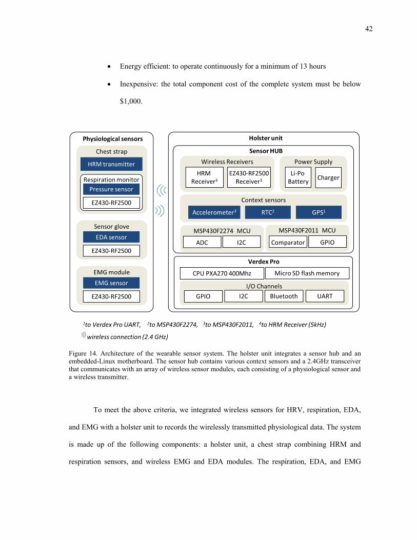
42
Energy efficient: to operate continuously for a minimum of 13 hours
Inexpensive: the total component cost of the complete system must be below
$1,000.
Figure 14. Architecture of the wearable sensor system. The holster unit integrates a sensor hub and an embedded-Linux motherboard. The sensor hub contains various context sensors and a 2.4GHz transceiver that communicates with an array of wireless sensor modules, each consisting of a physiological sensor and a wireless transmitter.
To meet the above criteria, we integrated wireless sensors for HRV, respiration, EDA,
and EMG with a holster unit to records the wirelessly transmitted physiological data. The system
is made up of the following components: a holster unit, a chest strap combining HRM and
respiration sensors, and wireless EMG and EDA modules. The respiration, EDA, and EMG
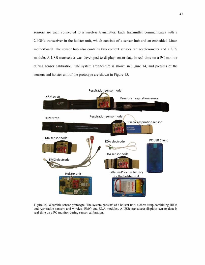
43
sensors are each connected to a wireless transmitter. Each transmitter communicates with a
2.4GHz transceiver in the holster unit, which consists of a sensor hub and an embedded-Linux
motherboard. The sensor hub also contains two context sensors: an accelerometer and a GPS
module. A USB transceiver was developed to display sensor data in real-time on a PC monitor
during sensor calibration. The system architecture is shown in Figure 14, and pictures of the
sensors and holster unit of the prototype are shown in Figure 15.
Figure 15. Wearable sensor prototype. The system consists of a holster unit, a chest strap combining HRM and respiration sensors and wireless EMG and EDA modules. A USB transducer displays sensor data in real-time on a PC monitor during sensor calibration.
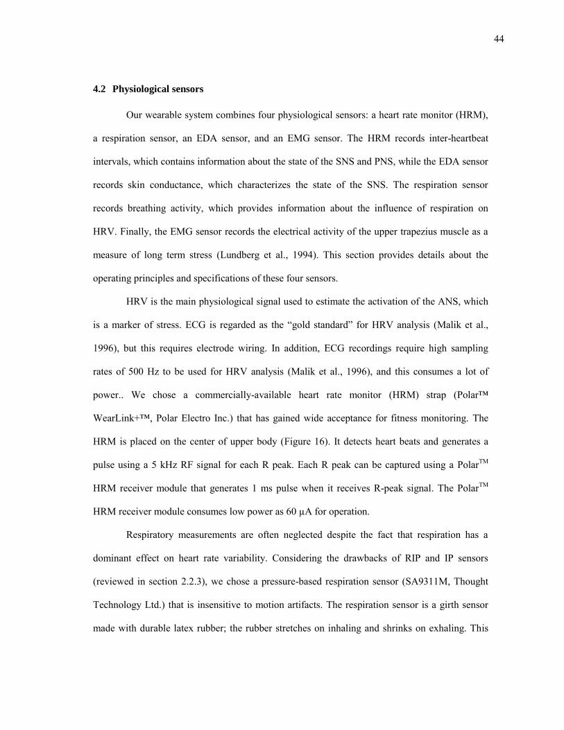
44
4.2 Physiological sensors
Our wearable system combines four physiological sensors: a heart rate monitor (HRM),
a respiration sensor, an EDA sensor, and an EMG sensor. The HRM records inter-heartbeat
intervals, which contains information about the state of the SNS and PNS, while the EDA sensor
records skin conductance, which characterizes the state of the SNS. The respiration sensor
records breathing activity, which provides information about the influence of respiration on
HRV. Finally, the EMG sensor records the electrical activity of the upper trapezius muscle as a
measure of long term stress (Lundberg et al., 1994). This section provides details about the
operating principles and specifications of these four sensors.
HRV is the main physiological signal used to estimate the activation of the ANS, which
is a marker of stress. ECG is regarded as the “gold standard” for HRV analysis (Malik et al.,
1996), but this requires electrode wiring. In addition, ECG recordings require high sampling
rates of 500 Hz to be used for HRV analysis (Malik et al., 1996), and this consumes a lot of
power.. We chose a commercially-available heart rate monitor (HRM) strap (Polar™
WearLink+™, Polar Electro Inc.) that has gained wide acceptance for fitness monitoring. The
HRM is placed on the center of upper body (Figure 16). It detects heart beats and generates a
pulse using a 5 kHz RF signal for each R peak. Each R peak can be captured using a PolarTM
HRM receiver module that generates 1 ms pulse when it receives R-peak signal. The PolarTM
HRM receiver module consumes low power as 60 µA for operation.
Respiratory measurements are often neglected despite the fact that respiration has a
dominant effect on heart rate variability. Considering the drawbacks of RIP and IP sensors
(reviewed in section 2.2.3), we chose a pressure-based respiration sensor (SA9311M, Thought
Technology Ltd.) that is insensitive to motion artifacts. The respiration sensor is a girth sensor
made with durable latex rubber; the rubber stretches on inhaling and shrinks on exhaling. This
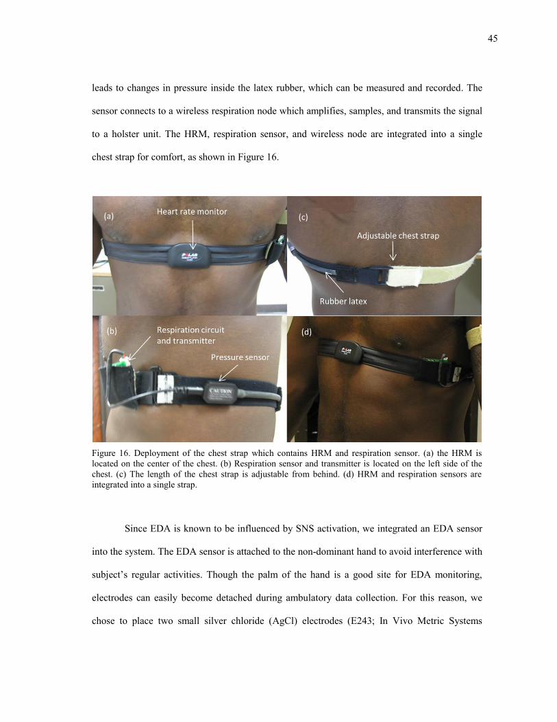
45
leads to changes in pressure inside the latex rubber, which can be measured and recorded. The
sensor connects to a wireless respiration node which amplifies, samples, and transmits the signal
to a holster unit. The HRM, respiration sensor, and wireless node are integrated into a single
chest strap for comfort, as shown in Figure 16.
Figure 16. Deployment of the chest strap which contains HRM and respiration sensor. (a) the HRM is located on the center of the chest. (b) Respiration sensor and transmitter is located on the left side of the chest. (c) The length of the chest strap is adjustable from behind. (d) HRM and respiration sensors are integrated into a single strap.
Since EDA is known to be influenced by SNS activation, we integrated an EDA sensor
into the system. The EDA sensor is attached to the non-dominant hand to avoid interference with
subject’s regular activities. Though the palm of the hand is a good site for EDA monitoring,
electrodes can easily become detached during ambulatory data collection. For this reason, we
chose to place two small silver chloride (AgCl) electrodes (E243; In Vivo Metric Systems
46
Corporation) on the proximal phalange of the index and middle fingers of the wearer’s non-
dominant hand. As with the respiration sensor, the electrodes are connected to a wireless node
which amplifies, samples, and transmits the signal to the holster unit. The wireless EDA node
can be worn on a wrist band, as shown in Figure 17.
Figure 17. Deployment of the EDA sensor and wireless node. (a) wireless EDA node is placed on the wrist band, and (b) Two electrodes are placed on index and middle finger.
The system also contains an EMG wireless node, which allows us to record activation in
the trapezius muscle for long-term stress monitoring. To measure EMG, we place two AgCl
electrodes (TDE205; Bio-Medical Instruments, Inc.) along the fibers of the trapezius muscle of
the non-dominant hand and a third reference electrode near the acromion. The electrodes connect
to a wireless node, as shown in Figure 18, which transmits the data to the holster unit.
The HRM and the respiration sensor are commercially-available products. We modified
the HRM sensor configuration by integrating its receiver circuit into the holster unit. A wireless
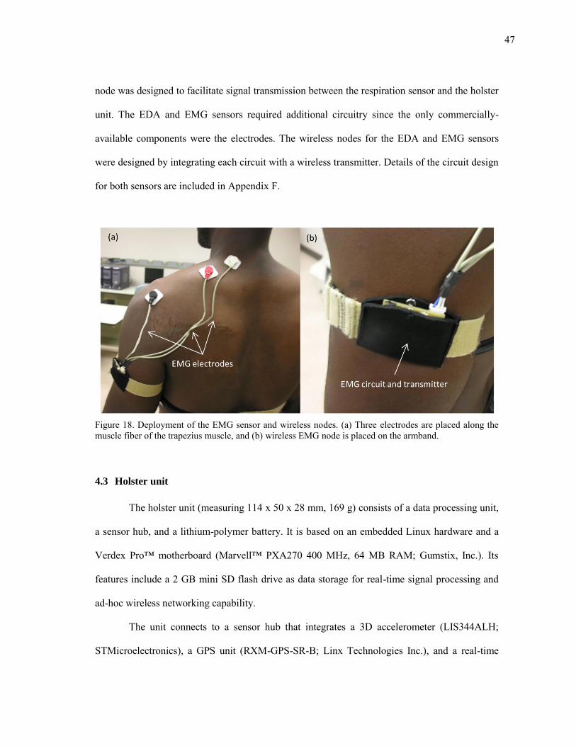
47
node was designed to facilitate signal transmission between the respiration sensor and the holster
unit. The EDA and EMG sensors required additional circuitry since the only commercially-
available components were the electrodes. The wireless nodes for the EDA and EMG sensors
were designed by integrating each circuit with a wireless transmitter. Details of the circuit design
for both sensors are included in Appendix F.
Figure 18. Deployment of the EMG sensor and wireless nodes. (a) Three electrodes are placed along the muscle fiber of the trapezius muscle, and (b) wireless EMG node is placed on the armband.
4.3 Holster unit
The holster unit (measuring 114 x 50 x 28 mm, 169 g) consists of a data processing unit,
a sensor hub, and a lithium-polymer battery. It is based on an embedded Linux hardware and a
Verdex Pro™ motherboard (Marvell™ PXA270 400 MHz, 64 MB RAM; Gumstix, Inc.). Its
features include a 2 GB mini SD flash drive as data storage for real-time signal processing and
ad-hoc wireless networking capability.
The unit connects to a sensor hub that integrates a 3D accelerometer (LIS344ALH;
STMicroelectronics), a GPS unit (RXM-GPS-SR-B; Linx Technologies Inc.), and a real-time
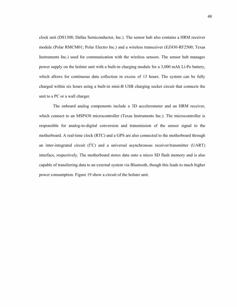
48
clock unit (DS1308; Dallas Semiconductor, Inc.). The sensor hub also contains a HRM receiver
module (Polar RMCM01; Polar Electro Inc.) and a wireless transceiver (EZ430-RF2500; Texas
Instruments Inc.) used for communication with the wireless sensors. The sensor hub manages
power supply on the holster unit with a built-in charging module for a 3,000 mAh Li-Po battery,
which allows for continuous data collection in excess of 13 hours. The system can be fully
charged within six hours using a built-in mini-B USB charging socket circuit that connects the
unit to a PC or a wall charger.
The onboard analog components include a 3D accelerometer and an HRM receiver,
which connect to an MSP430 microcontroller (Texas Instruments Inc.). The microcontroller is
responsible for analog-to-digital conversion and transmission of the sensor signal to the
motherboard. A real-time clock (RTC) and a GPS are also connected to the motherboard through
an inter-integrated circuit (I2C) and a universal asynchronous receiver/transmitter (UART)
interface, respectively. The motherboard stores data onto a micro SD flash memory and is also
capable of transferring data to an external system via Bluetooth, though this leads to much higher
power consumption. Figure 19 show a circuit of the holster unit.
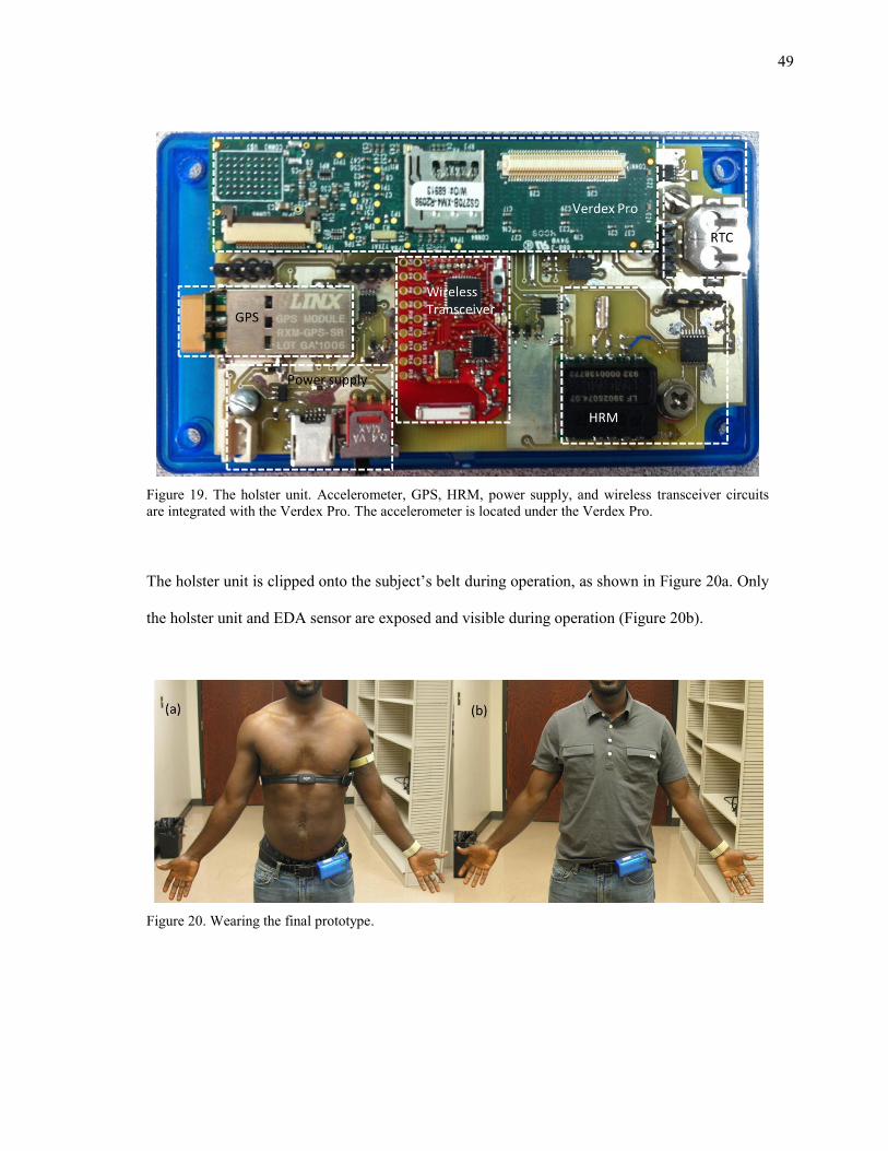
49
Figure 19. The holster unit. Accelerometer, GPS, HRM, power supply, and wireless transceiver circuits are integrated with the Verdex Pro. The accelerometer is located under the Verdex Pro.
The holster unit is clipped onto the subject’s belt during operation, as shown in Figure 20a. Only
the holster unit and EDA sensor are exposed and visible during operation (Figure 20b).
Figure 20. Wearing the final prototype.
50
4.4 Wireless nodes and communication
Each wireless sensor node contains a transceiver module (EZ430-RF2500; Texas
Instruments Inc.). The transceiver module consists of a MSP430F2274 microcontroller (Texas
Instruments Inc.) and a CC2500 radio module (Texas Instruments Inc.). The CC2500 radio
module provides a wireless detection range of 15-20 meters indoors, which is sufficient for
wearable sensors, using a 5 dB chip antenna. The transceiver module has eight 10-bit A/D ports
for interfacing with the sensor module. Wireless communication are based on SimpliciTI™
(Texas Instruments Inc.), a low-power lightweight sensor network protocol suited for small radio
frequency (RF) networks.
The wireless sensors are connected to the holster unit using a star-topology wireless
network architecture, wherein the sensor hub is used as the root node while the sensor nodes are
connected to the sensor hub as leaf nodes. We considered alternative architecture designs such as
multi-hop routing and mesh networking, but in the end chose a star topology because it
minimizes power consumption resulting from ad hoc communication. This architecture is
sufficient for communication between the holster unit and the wireless nodes but does not permit
peer-to-peer communication between nodes. The transmitter operates at a frequency of 2.4 GHz
which, because of the shorter wavelength, gives better radio transmission indoors (Fletcher et al.,
2009).
We implemented a wireless transmission recovery subroutine to handle transmission
failures resulting from unforeseen events such as accidental power failures on the holster unit.
To prevent permanent disconnection, the communication protocol uses message
acknowledgement packets (ACK) to increase the reliability of the wireless data transmission.
When a wireless sensor node sends a packet to the holster unit, it requests an ACK. If the node
doesn’t receive an ACK packet from the sensor hub, it tries to re-send the packet for a
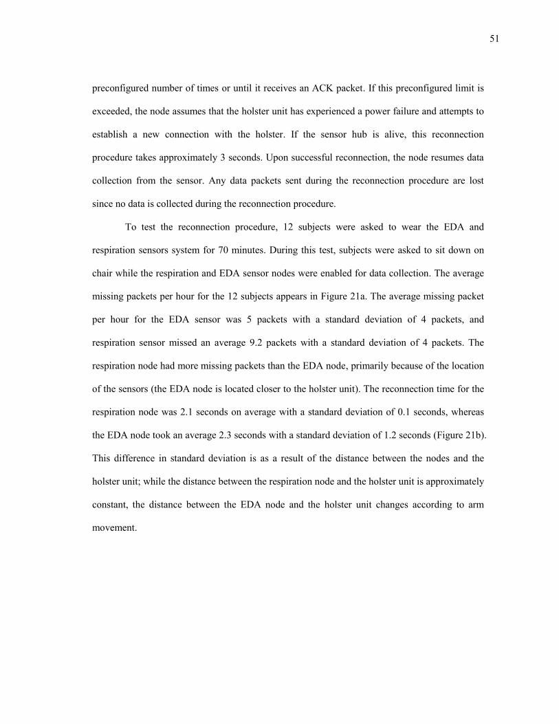
51
preconfigured number of times or until it receives an ACK packet. If this preconfigured limit is
exceeded, the node assumes that the holster unit has experienced a power failure and attempts to
establish a new connection with the holster. If the sensor hub is alive, this reconnection
procedure takes approximately 3 seconds. Upon successful reconnection, the node resumes data
collection from the sensor. Any data packets sent during the reconnection procedure are lost
since no data is collected during the reconnection procedure.
To test the reconnection procedure, 12 subjects were asked to wear the EDA and
respiration sensors system for 70 minutes. During this test, subjects were asked to sit down on
chair while the respiration and EDA sensor nodes were enabled for data collection. The average
missing packets per hour for the 12 subjects appears in Figure 21a. The average missing packet
per hour for the EDA sensor was 5 packets with a standard deviation of 4 packets, and
respiration sensor missed an average 9.2 packets with a standard deviation of 4 packets. The
respiration node had more missing packets than the EDA node, primarily because of the location
of the sensors (the EDA node is located closer to the holster unit). The reconnection time for the
respiration node was 2.1 seconds on average with a standard deviation of 0.1 seconds, whereas
the EDA node took an average 2.3 seconds with a standard deviation of 1.2 seconds (Figure 21b).
This difference in standard deviation is as a result of the distance between the nodes and the
holster unit; while the distance between the respiration node and the holster unit is approximately
constant, the distance between the EDA node and the holster unit changes according to arm
movement.
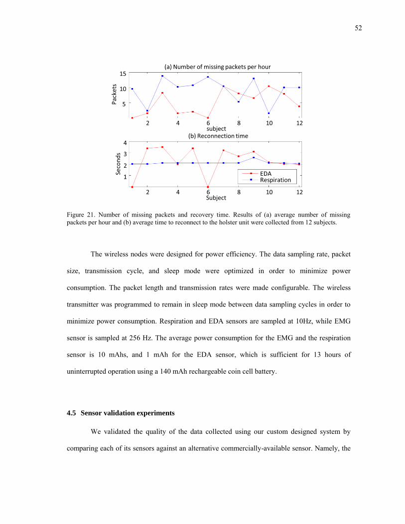
52
Figure 21. Number of missing packets and recovery time. Results of (a) average number of missing packets per hour and (b) average time to reconnect to the holster unit were collected from 12 subjects.
The wireless nodes were designed for power efficiency. The data sampling rate, packet
size, transmission cycle, and sleep mode were optimized in order to minimize power
consumption. The packet length and transmission rates were made configurable. The wireless
transmitter was programmed to remain in sleep mode between data sampling cycles in order to
minimize power consumption. Respiration and EDA sensors are sampled at 10Hz, while EMG
sensor is sampled at 256 Hz. The average power consumption for the EMG and the respiration
sensor is 10 mAhs, and 1 mAh for the EDA sensor, which is sufficient for 13 hours of
uninterrupted operation using a 140 mAh rechargeable coin cell battery.
4.5 Sensor validation experiments
We validated the quality of the data collected using our custom designed system by
comparing each of its sensors against an alternative commercially-available sensor. Namely, the
53
HRM sensor was compared against a commercial ECG, the EDA sensor was compared with a
commercial EDA sensor, and the integrated pressure respiration sensor was compared with a
piezo and an RIP respiration sensor. This section provides a detailed description of the
experiments conducted during the validation process along with a discussion of the results that
were obtained.
4.5.1 Cardiovascular sensor validation
The goal of this experiment was to validate the accuracy of heart rate variability
measurements obtained using a heart rate monitor. This was achieved by comparing the heart
rate variability measurements obtained using a heart rate monitor with the measurements
obtained using an electrocardiogram. For this experiment, we used the PolarTM HRM receiver
(RMCM01, Polar Electro Inc.) and transmitter (WearLink+™, Polar Electro Inc.) module as the
HRM sensor and the Thought Technologies ECG/EKG (SA9306; Thought Technologies Inc.) as
the ECG sensor.
The PolarTM HRM receiver module generates 1 ms pulse when it receives R-peak signal
from the transmitter, which gives an approximate measure of heart beat intervals, whereas the
Thought Technologies sensor measures the full ECG signal. For accurate comparison, 4 subjects
were outfitted with both sensors simultaneously. For this experiment, we induced variations in
HRV by having subjects perform a paced breathing exercise. To induce fluctuations in the R-R
tachogram, subjects were asked to modify their breathing pattern to match an audio prompt
designed for paced breathing. The audio prompt is a custom developed AndroidTM application
that gives periodic voice prompts which instruct the user to either inhale or exhale at intervals of
2, 4, 6 or 10 seconds. The sequence of these intervals was varied randomly thereby causing
alterations in the subjects breathing pattern. The paced breathing exercise was repeated twice for
each subject, for a duration of 150 seconds per iteration per subject.
54
Figure 22. Comparison of signal between ECG and HRM. This figure reflects data collected from subject #1.
The HRM module and the ECG sensor were simultaneously connected to a data logger
(Infiniti FlexComp™; Thought Technology Inc.), which recorded data from each sensor at a
frequency of 2 kHz. The R-peaks were extracted from the collected signal using a peak-detection
algorithm (Kohler et al., 2002), and R-R intervals were calculated for each sensor. Figure 22
compares the ECG and the HRM tachogram from one of the subjects in this experiment. The
average Pearson's correlation coefficient of 4 subjects between the data collected from both
sensors was 0.9654 with a standard deviation of 0.0204. These results show that the heart rate
monitor provides a sufficiently accurate measure of heart rate variability.
4.5.2 EDA sensor validation
The goal of this experiment was to validate the accuracy of skin conductance
measurements obtained using our custom EDA sensor. This was achieved by comparing the
EDA measurements obtained using our developed EDA sensor with the measurements obtained
using a commercial EDA sensor. For this experiment, we used the Thought Technologies EDA
sensor (SA2659; Thought technology Inc.) as the commercial EDA sensor.
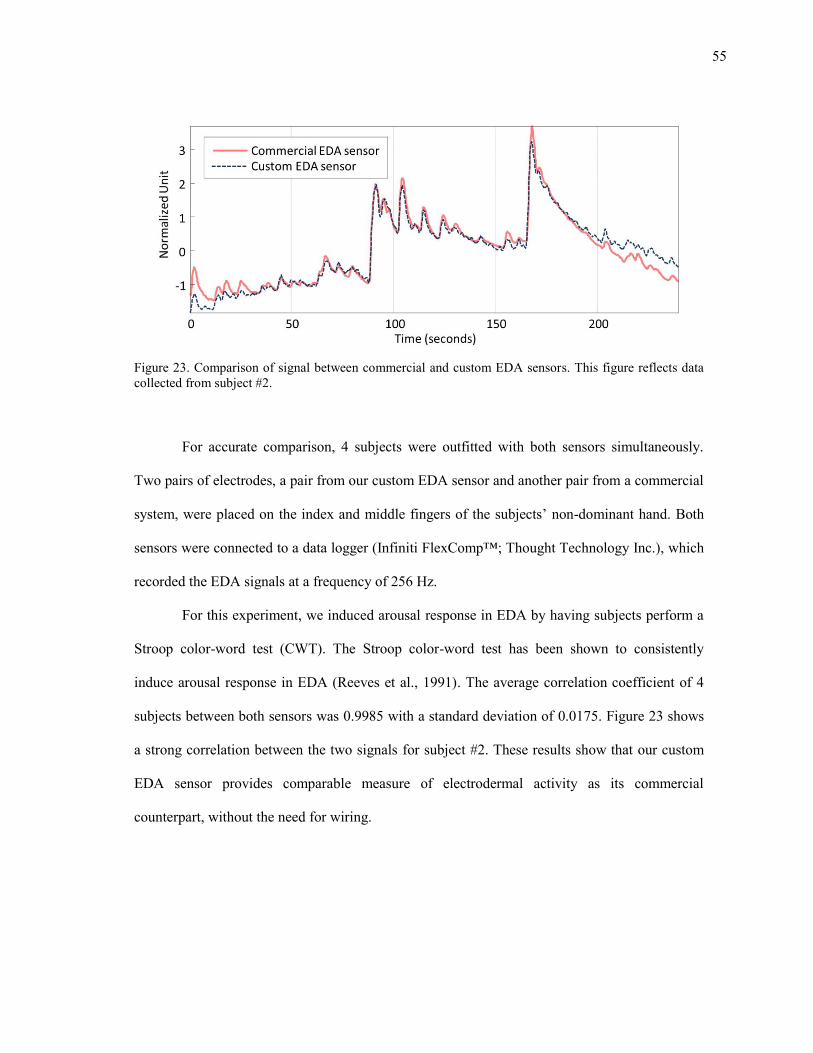
55
Figure 23. Comparison of signal between commercial and custom EDA sensors. This figure reflects data collected from subject #2.
For accurate comparison, 4 subjects were outfitted with both sensors simultaneously.
Two pairs of electrodes, a pair from our custom EDA sensor and another pair from a commercial
system, were placed on the index and middle fingers of the subjects’ non-dominant hand. Both
sensors were connected to a data logger (Infiniti FlexComp™; Thought Technology Inc.), which
recorded the EDA signals at a frequency of 256 Hz.
For this experiment, we induced arousal response in EDA by having subjects perform a
Stroop color-word test (CWT). The Stroop color-word test has been shown to consistently
induce arousal response in EDA (Reeves et al., 1991). The average correlation coefficient of 4
subjects between both sensors was 0.9985 with a standard deviation of 0.0175. Figure 23 shows
a strong correlation between the two signals for subject #2. These results show that our custom
EDA sensor provides comparable measure of electrodermal activity as its commercial
counterpart, without the need for wiring.
56
4.5.3 Respiration sensor validation
The goal of this experiment was to compare three commercial respiration sensors. For
this comparison, we evaluated the accuracy of the data collected by each sensor and we
evaluated the robustness of each sensor to motion artifacts. We also collected feedback from
each subject on the amount of comfort or discomfort experienced while wearing each sensor. For
these experiments, the following sensors were used: a pressure-based sensor, a piezo respiration
effort sensor (Ultra-Piezo™; Gereonics Inc.), and a RIP sensor (XactTrace™; Embla systems
Inc.)
The piezo and the RIP respiration monitoring technologies were used because both are
widely used as respiration sensors. The piezo respiration effort sensor is generally accepted
because it is comfortable and easy to use. The RIP sensor is the gold-standard for capturing
respiratory signals. These two sensors, along with a pressure based sensor, were simultaneously
attached to the subject’s thorax, connected to a data logger (Infiniti FlexComp™; Thought
Technology Inc.), and sampled at a frequency of 256 Hz.
The objective of the first experiment was to validate the accuracy of the pressure
respiration sensor. For this experiment, we used the paced breathing exercise described in
section 4.5.1. Figure 24 shows a comparison between the data collected from the RIP, piezo and
the pressure sensor. The average correlation coefficient was 0.9760 (σ =0.0269). The average
correlation between the RIP and the piezo sensor was 0.6407 (σ=0.0637). The average
correlation between the RIP and the piezo sensor is low in comparison to the correlation between
the RIP and the pre because the output of the piezo sensor is phase shifted (i.e. it relates to the
derivative of the respiration signal.)
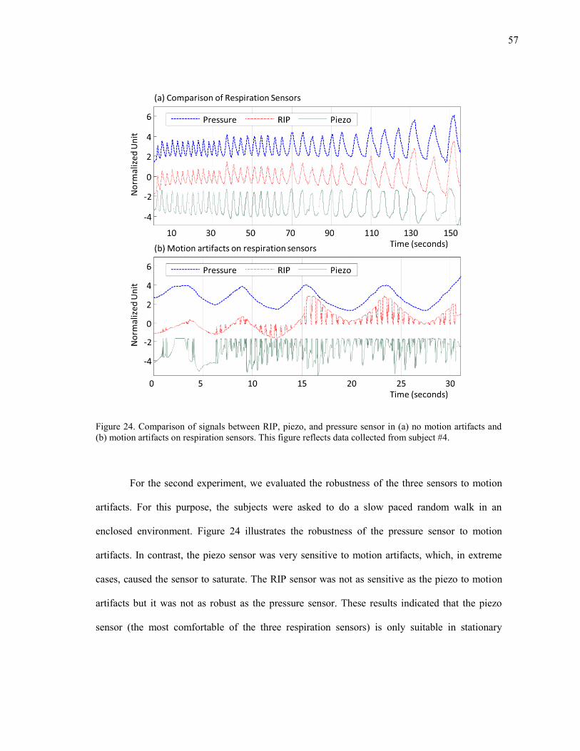
57
Figure 24. Comparison of signals between RIP, piezo, and pressure sensor in (a) no motion artifacts and (b) motion artifacts on respiration sensors. This figure reflects data collected from subject #4.
For the second experiment, we evaluated the robustness of the three sensors to motion
artifacts. For this purpose, the subjects were asked to do a slow paced random walk in an
enclosed environment. Figure 24 illustrates the robustness of the pressure sensor to motion
artifacts. In contrast, the piezo sensor was very sensitive to motion artifacts, which, in extreme
cases, caused the sensor to saturate. The RIP sensor was not as sensitive as the piezo to motion
artifacts but it was not as robust as the pressure sensor. These results indicated that the piezo
sensor (the most comfortable of the three respiration sensors) is only suitable in stationary
58
experiments where movement is restricted. These results also indicate that the pressure sensor is
the most suitable of the three.
4.6 Summary
This section provided a detailed description of a minimally-obtrusive wearable sensor
system designed for long-term ambulatory monitoring of mental stress. The system consists of
EDA, respiration, HRM, and EMG sensors to collect stress related physiological data. The
integrated HRM, EDA, and respiration sensors were compared to commercially available
sensors for validation. The results of this comparison showed that our sensor system is capable
of collecting data and exhibits a robustness to motion artifacts in a manner comparable with
commercial systems, without the need for wiring. The next section describes the signal
processing methods applied to the data collected using the sensor system described in this
section. The focus will be on removing respiratory influences on heart rate variability.
59
5. REMOVING RESPIRATORY INFLUENCE FROM HRV
Changes in HRV provide information about the activation of each ANS branch, which
can serve as indices of mental stress (Berntson et al., 1997). However, HRV can be influenced
by factors other than mental stress, and one of the most influential short-term factors is
respiration (Berntson et al., 1997). As an example, in situations where a subject breathes slowly
(below 10 breaths per minute), both respiratory changes and mental stress contribute to the LF
energy in the HRV power spectrum, which yields the traditional LF/HF ratio ineffective. Thus,
when using HRV as a measure of stress it is particularly important to have information about
respiration. Despite this fact, however, respiratory influences are rarely considered in studies of
HRV. To address this issue, this dissertation proposes three methods to detect mental stress from
HRV that account for respiratory influences.
The purpose of this section is to describe proposed methods for the removal of
respiratory influence on changes in heart rate variability. We hypothesize that if the respiratory
influence in HRV can be removed, the residual HRV will provide more salient information about
stress than the original HRV.
The section is organized as follows. First, we describe the relationship between
respiration and HRV, followed by a brief description of three suggested methods for removing
respiratory influence. Next, we provide detailed descriptions of each method: linear system
identification, nonlinear dynamics decomposition, and HRV spectral weighting.
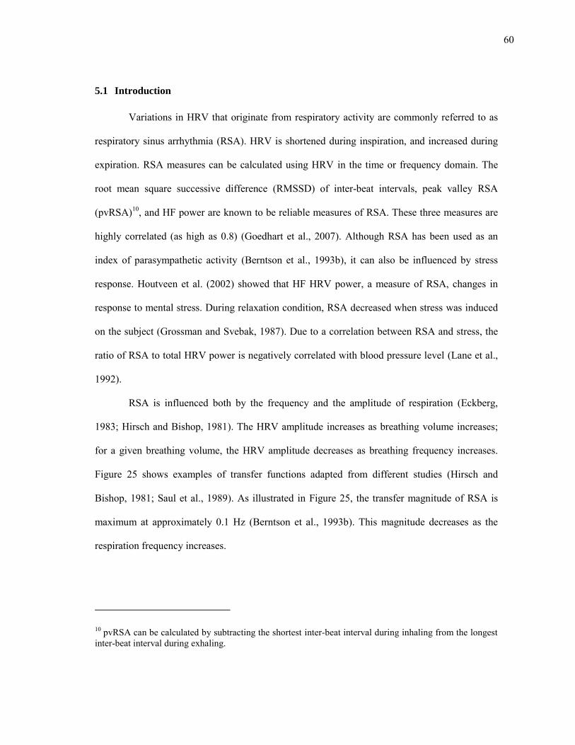
60
5.1 Introduction
Variations in HRV that originate from respiratory activity are commonly referred to as
respiratory sinus arrhythmia (RSA). HRV is shortened during inspiration, and increased during
expiration. RSA measures can be calculated using HRV in the time or frequency domain. The
root mean square successive difference (RMSSD) of inter-beat intervals, peak valley RSA
(pvRSA)10, and HF power are known to be reliable measures of RSA. These three measures are
highly correlated (as high as 0.8) (Goedhart et al., 2007). Although RSA has been used as an
index of parasympathetic activity (Berntson et al., 1993b), it can also be influenced by stress
response. Houtveen et al. (2002) showed that HF HRV power, a measure of RSA, changes in
response to mental stress. During relaxation condition, RSA decreased when stress was induced
on the subject (Grossman and Svebak, 1987). Due to a correlation between RSA and stress, the
ratio of RSA to total HRV power is negatively correlated with blood pressure level (Lane et al.,
1992).
RSA is influenced both by the frequency and the amplitude of respiration (Eckberg,
1983; Hirsch and Bishop, 1981). The HRV amplitude increases as breathing volume increases;
for a given breathing volume, the HRV amplitude decreases as breathing frequency increases.
Figure 25 shows examples of transfer functions adapted from different studies (Hirsch and
Bishop, 1981; Saul et al., 1989). As illustrated in Figure 25, the transfer magnitude of RSA is
maximum at approximately 0.1 Hz (Berntson et al., 1993b). This magnitude decreases as the
respiration frequency increases.
10 pvRSA can be calculated by subtracting the shortest inter-beat interval during inhaling from the longest inter-beat interval during exhaling.
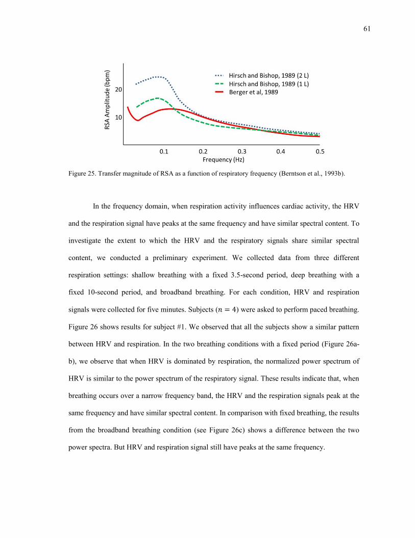
61
Figure 25. Transfer magnitude of RSA as a function of respiratory frequency (Berntson et al., 1993b).
In the frequency domain, when respiration activity influences cardiac activity, the HRV
and the respiration signal have peaks at the same frequency and have similar spectral content. To
investigate the extent to which the HRV and the respiratory signals share similar spectral
content, we conducted a preliminary experiment. We collected data from three different
respiration settings: shallow breathing with a fixed 3.5-second period, deep breathing with a
fixed 10-second period, and broadband breathing. For each condition, HRV and respiration
signals were collected for five minutes. Subjects ( ) were asked to perform paced breathing.
Figure 26 shows results for subject #1. We observed that all the subjects show a similar pattern
between HRV and respiration. In the two breathing conditions with a fixed period (Figure 26a-
b), we observe that when HRV is dominated by respiration, the normalized power spectrum of
HRV is similar to the power spectrum of the respiratory signal. These results indicate that, when
breathing occurs over a narrow frequency band, the HRV and the respiration signals peak at the
same frequency and have similar spectral content. In comparison with fixed breathing, the results
from the broadband breathing condition (see Figure 26c) shows a difference between the two
power spectra. But HRV and respiration signal still have peaks at the same frequency.
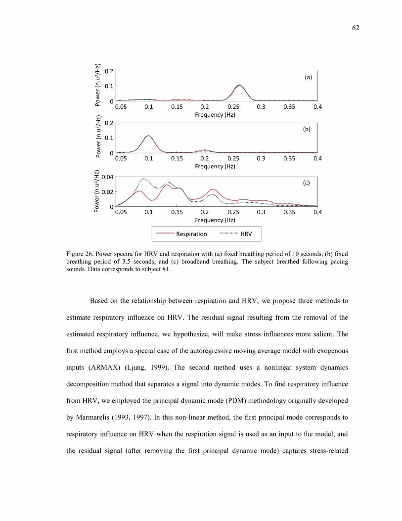
62
Figure 26. Power spectra for HRV and respiration with (a) fixed breathing period of 10 seconds, (b) fixed breathing period of 3.5 seconds, and (c) broadband breathing. The subject breathed following pacing sounds. Data corresponds to subject #1.
Based on the relationship between respiration and HRV, we propose three methods to
estimate respiratory influence on HRV. The residual signal resulting from the removal of the
estimated respiratory influence, we hypothesize, will make stress influences more salient. The
first method employs a special case of the autoregressive moving average model with exogenous
inputs (ARMAX) (Ljung, 1999). The second method uses a nonlinear system dynamics
decomposition method that separates a signal into dynamic modes. To find respiratory influence
from HRV, we employed the principal dynamic mode (PDM) methodology originally developed
by Marmarelis (1993, 1997). In this non-linear method, the first principal mode corresponds to
respiratory influence on HRV when the respiration signal is used as an input to the model, and
the residual signal (after removing the first principal dynamic mode) captures stress-related
63
information. The third method estimates the power spectrum of the respiratory-induced HRV
using a spectral weighting method. Namely, the spectral weighting attenuates the HRV power
spectrum according to the (normalized) respiration spectrum. As a result, the residual HRV
power spectrum is assumed to correlate to stress. A detailed description of each method is
provided in the following subsections.
5.2 Linear system identification
The linear system identification method estimates the respiratory influence on HRV by
using an ARMAX model. The estimated respiratory influence is then subtracted from the HRV
signal resulting in a residual signal that makes stress influences more salient. To accurately
estimate the coefficients of respiratory influence, the input respiration signal should exhibit
broadband characteristics. This broadband respiration signal can be obtained from a paced
respiration signal. To account for differences in ventilation between paced and spontaneous
breathing, we introduce a scale factor.
5.2.1 Modeling cardio-respiratory relationships with ARMAX
In statistcal analysis and signal processing, the ARMAX model is a tool for
understanding and predicting future values in time-series data. The model estimates the output of
a system as a linear combination of previous known inputs, unknown errors, and outputs. The
model equation (1) is made up of three parts: an autoregressive (AR) part, a moving average
(MA) part, and an exogenous input (X) part (Ljung, 1999). The AR part predicts the output of a
system based on its previous outputs. The MA part predicts the current value of the series based
on previous random shocks or error terms. The error terms are assumed to be white noise
originating from an unknown source. The X term is a known external time series.
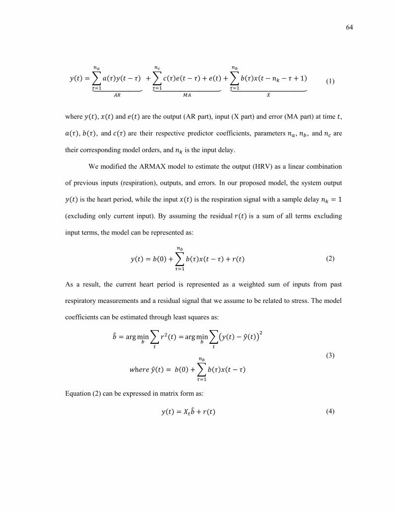
64
( ) ∑ ( ) ( )
⏟
∑ ( ) ( ) ( )
⏟
∑ ( ) ( )
⏟
(1)
where ( ), ( ) and ( ) are the output (AR part), input (X part) and error (MA part) at time ,
( ), ( ), and ( ) are their respective predictor coefficients, parameters , , and are
their corresponding model orders, and is the input delay.
We modified the ARMAX model to estimate the output (HRV) as a linear combination
of previous inputs (respiration), outputs, and errors. In our proposed model, the system output
( ) is the heart period, while the input ( ) is the respiration signal with a sample delay
(excluding only current input). By assuming the residual ( ) is a sum of all terms excluding
input terms, the model can be represented as:
( ) ( ) ∑ ( ) ( ) ( )
(2)
As a result, the current heart period is represented as a weighted sum of inputs from past
respiratory measurements and a residual signal that we assume to be related to stress. The model
coefficients can be estimated through least squares as:
∑ ( )
∑( ( ) ( ))
( ) ( ) ∑ ( ) ( )
(3)
Equation (2) can be expressed in matrix form as:
( ) ( ) (4)
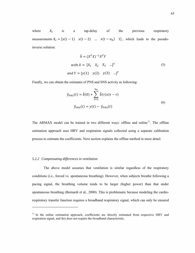
65
where is a tap-delay of the previous respiratory
measurements [ ( ) ( ) ( ) ] , which leads to the pseudo-
inverse solution:
( )
[ ]
[ ( ) ( ) ( ) ]
(5)
Finally, we can obtain the estimates of PNS and SNS activity as following:
( ) ( ) ∑ ( ) ( )
( ) ( ) ( )
(6)
The ARMAX model can be trained in two different ways: offline and online11. The offline
estimation approach uses HRV and respiration signals collected using a separate calibration
process to estimate the coefficients. Next section explains the offline method in more detail.
5.2.2 Compensating differences in ventilation
The above model assumes that ventilation is similar regardless of the respiratory
conditions (i.e., forced vs. spontaneous breathing). However, when subjects breathe following a
pacing signal, the breathing volume tends to be larger (higher power) than that under
spontaneous breathing (Bernardi et al., 2000). This is problematic because modeling the cardio-
respiratory transfer function requires a broadband respiratory signal, which can only be ensured
11 In the online estimation approach, coefficients are directly estimated from respective HRV and respiration signal, and this does not require the broadband characteristic.
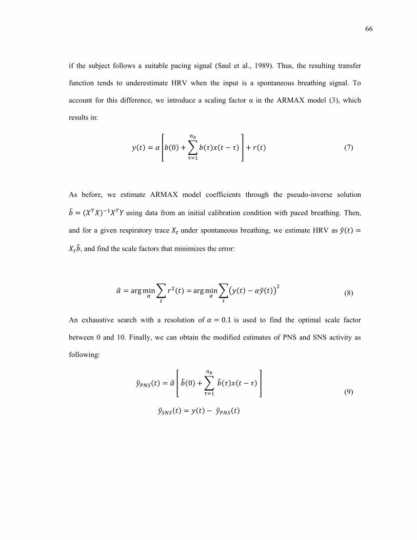
66
if the subject follows a suitable pacing signal (Saul et al., 1989). Thus, the resulting transfer
function tends to underestimate HRV when the input is a spontaneous breathing signal. To
account for this difference, we introduce a scaling factor α in the ARMAX model (3), which
results in:
( ) [ ( ) ∑ ( ) ( )
] ( ) (7)
As before, we estimate ARMAX model coefficients through the pseudo-inverse solution
( ) using data from an initial calibration condition with paced breathing. Then,
and for a given respiratory trace under spontaneous breathing, we estimate HRV as ( )
, and find the scale factors that minimizes the error:
∑ ( )
∑( ( ) ( ))
(8)
An exhaustive search with a resolution of is used to find the optimal scale factor
between 0 and 10. Finally, we can obtain the modified estimates of PNS and SNS activity as
following:
( ) [ ( ) ∑ ( ) ( )
]
( ) ( ) ( )
(9)
67
5.3 Nonlinear dynamics decomposition
We also explore a nonlinear system-identification technique based on the principal
dynamic mode (PDM) method (Marmarelis et al., 1999). A study by Chon et al. (1996)
suggested that PDM can be used to estimate influences to HRV from dual inputs: instantaneous
lung volume (ILV) and arterial blood pressure (ABP). In their study, Chon et al. showed that the
two dominant dynamic modes correspond to ILV and ABP. We modified their method by using
respiration signal as a single source input to HRV; in this case, the first principal dynamic mode
corresponds to respiratory influenced dynamics12. Additionally, Zhong et al. (2004) have shown
that PDM may be used to predict the activation level of two autonomic branches without using
the respiration input signal. Their model used a delayed HRV signal as an input to the PDM
model. We also modified this method by assigning sum of positive and negative dynamic modes
to respiratory influenced dynamics and residual.
5.3.1 Principal dynamic modes
A nonlinear time-invariant dynamic system can be modeled using a discrete-time
Volterra series as:
( ) ∑ ( ) ( )
∑ ∑ ( ) ( ) ( )
(10)
where ( ) is the system output, ( ) is the system input with a delay of , M is the memory
of the model, and ( ) are the Volterra kernels describing the dynamics of the system.
When modeling physiological systems, second-order series are used to provide a balance
12 Both the offline and online coefficient estimation approaches are applied to calculate the coefficients of the nonlinear method, similar to the approach used in the linear method.
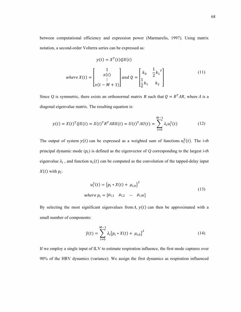
68
between computational efficiency and expression power (Marmarelis, 1997). Using matrix
notation, a second-order Volterra series can be expressed as:
( ) ( ) ( )
( ) [
( )
( )
] [
] (11)
Since Q is symmetric, there exists an orthonormal matrix R such that , where is a
diagonal eigenvalue matrix. The resulting equation is:
( ) ( ) ( ) ( ) ( ) ( ) ( ) ∑ ( )
(12)
The output of system ( ) can be expressed as a weighted sum of functions ( ). The i-th
principal dynamic mode ( ) is defined as the eigenvector of Q corresponding to the largest i-th
eigenvalue , and function ( ) can be computed as the convolution of the tapped-delay input
( ) with :
( ) ( )
[ ] (13)
By selecting the most significant eigenvalues from, ( ) can then be approximated with a
small number of components:
( ) ∑ ( )
(14)
If we employ a single input of ILV to estimate respiration influence, the first mode captures over
90% of the HRV dynamics (variance). We assign the first dynamics as respiration influenced
69
HRV and assign residuals as stress influenced. The estimates of the PNS activity and the SNS
activity are separated as:
( ) ( )
( ) ( ) ( ) (15)
To account for the difference in ventilation between paced and spontaneous breathing in the
offline coefficient estimation, as was described in section 0 for the linear system identification
method, we introduce a scaling factor α in the model (14), which results in:
( ) ∑ ( )
( ) ( )
( ) ( ) ( )
(16)
5.3.2 PDM decomposition without respiratory signals
PDM was introduced as a method for characterizing physiological systems using
relationship between input and output signal of the system. Zhong et al. (2004) showed that the
PDM method can be used to predict the activation of both autonomic branches using only heart
rate measurements. We apply a similar methodology by using the delayed HRV signal was used
as an input instead of respiration signal. The authors noted that the first two PDMs had spectral
characteristics similar to PNS and SNS activity; one mode contained both LF and HF power, and
the other contained mainly HF power, and that they explained over 90% of the variance in the
system dynamics.
In our studies, the first two PDM eigenvalues only capture 60% of the variance, which
suggests that additional modes are required to capture the system’s dynamics. Here we propose
70
an alternative selection criterion. First, we discard any eigenvalues whose magnitude | | is
lower than 5% of the total energy ∑| |. Next, we assign negative eigenvalues to SNS activation,
since they reduce heart periods, and assign positive eigenvalues to PNS activity, since they
increase heart periods. Finally, we sum the positive and negative dynamics separately to obtain
the estimates of PNS and SNS activity:
( ) ∑ ( )
( ) ∑ ( )
(17)
5.3.3 Estimation of Volterra kernels
Because of the coefficients of the nonlinear terms, estimation of the Volterra kernels is a
computationally challenging problem. Several estimation methods are available, such as cross-
correlation (Schetzen, 1981), fast orthogonal (Korenberg et al., 1988), and differential sampling
(van Hemmen et al., 2000) methods. We used the so-called Wiener’s method (Wiener, 1958) for
coefficient estimation because it yields accurate low-order kernel estimates from short
experimental data recordings and is robust to noise (Marmarelis, 1993). The key element of this
method is the assumption that the Volterra kernels have a block structure in which the input ( )
is passed through a filter bank ( ) :
( ) ∑ ( ) ( )
(18)
and the corresponding outputs ( ) are then combined through a static nonlinearity:
( ) ( ( ) ( ) ( ) ( )) (19)
Under this assumption, the Volterra series in equation (1) becomes a multinomial expansion:

71
( ) ∑ ( ) ( )
∑ ∑ ( ) ( )
( )
(20)
Using matrix notation, the multinomial expansion (20) can be expressed as:
( ) ( ) ( ) ( ) ( ) ( )
( ) ( ) ( ) ( ) ( )
( ) ( ) ( ) ( ) ( ) ( ) ( ) ( )
( ) ( ) ( ) ( ) ( ) ( ) ( ) ( ) ( )
( )
(21)
If the matrix is full-rank, then the coefficient vector can be estimated by means of least-squares
as
[ ] (22)
As a result, matrix Q in equation (2) can be constructed from the estimated multinomial kernels
as:
[
] [
]
[
( ) ( ) ( )
( ) ( ) ( )
( ) ( ) ( )
]
(23)
As suggested by Wiener (Schetzen, 1980), a suitable orthonormal basis for the impulse
responses ( ) in equation (18) is the family of Laguerre polynomials. These are exponentially
decaying functions suitable for modeling physiological systems. Laguerre functions are defined
as:
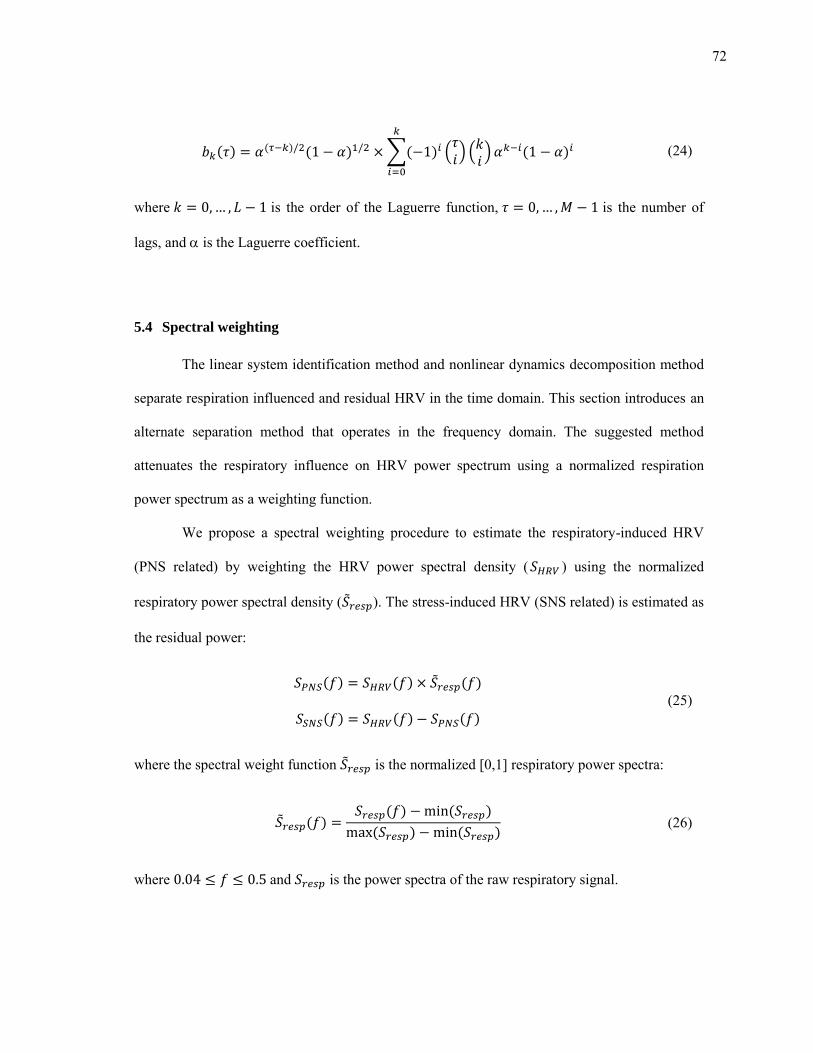
72
( ) ( ) ( ) ∑( )
( ) (
) ( ) (24)
where is the order of the Laguerre function, is the number of
lags, and is the Laguerre coefficient.
5.4 Spectral weighting
The linear system identification method and nonlinear dynamics decomposition method
separate respiration influenced and residual HRV in the time domain. This section introduces an
alternate separation method that operates in the frequency domain. The suggested method
attenuates the respiratory influence on HRV power spectrum using a normalized respiration
power spectrum as a weighting function.
We propose a spectral weighting procedure to estimate the respiratory-induced HRV
(PNS related) by weighting the HRV power spectral density ( ) using the normalized
respiratory power spectral density ( ). The stress-induced HRV (SNS related) is estimated as
the residual power:
( ) ( ) ( )
( ) ( ) ( ) (25)
where the spectral weight function is the normalized [0,1] respiratory power spectra:
( ) ( ) ( )
( ) ( ) (26)
where and is the power spectra of the raw respiratory signal.
73
5.5 Summary of the proposed methods
Respiratory activity is the dominant factor influencing heart rate variability. At normal
breathing rates (12-20 breaths per minute on average), respiratory influences to HRV fall within
the HF band. In a few cases of slow breathing, however, respiratory influences fall within the LF
band. In these cases the LF/HF ratio loses its diagnostic value and this is further compounded by
evidence that the cardiorespiratory system has a resonant frequency at approximately 0.1 Hz.
Thus, when breathing frequency falls within the LF band, the effects of respiration are amplified
and consequently, the LF band is confounded by the influence of both stress and respiratory
activity. The three suggested methods address this confounding problem by separating HRV into
a respiratory influenced HRV and residual HRV.
The main difference between the linear system identification method and the nonlinear
dynamics decomposition method is higher order (n ≥ 2) terms which are nonexistent in the linear
method. If the nonlinear coefficients approach zero, the equations for the two methods become
identical. Conversely, where the nonlinear coefficients are dominant, it supports the existence of
interactions in high order terms. Another difference is seen in the mapping of respiratory
influenced HRV. The estimated signal is the respiratory influenced HRV in the linear method
whereas the first principal dynamic mode is the respiratory influenced HRV in the nonlinear
method map.
Both the linear and nonlinear model coefficients can be estimated using two methods:
offline estimation and online estimation. In the offline estimation method, the coefficients are
trained using a broadband respiration signal and the resulting coefficients represent a general
transfer function between respiration and HRV. The coefficients obtained using this method are
sufficient for estimating respiratory influence on HRV in stress or relaxation conditions.
However, to generate a broadband respiration signal requires that the subjects perform a paced
74
breathing exercise, which leads to ventilation differences between paced breathing and
spontaneous breathing; thus requiring a scaling factor. The online model estimates coefficients
for each condition using a narrow band respiration signal, and although this approach is suitable
when broadband signal is not available, it leads to over fitting because the coefficients are
estimated using a narrow band respiration signal.
The third method, spectral weighting, estimates respiration influence in the frequency
domain. The spectral weighting approach can be interpreted as a decomposition of the HRV
power spectra into two orthogonal components: the first component is correlated with respiratory
behavior, while the second component is the residual signal assumed to capture stress influences.
In contrast with the traditional LF/HF ratio, this method does not rely on a fixed frequency band
but instead adapts to the respiration rate of each individual subject. In addition, this method does
not require a broadband calibration signal. These similarities and differences have an effect on
the performance of each method. The next section describes the validation experiments
conducted using the three methods, results obtained, and a discussion about the impact of these
results on mental stress detection.
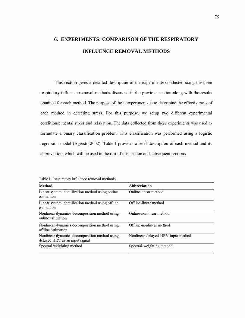
75
6. EXPERIMENTS: COMPARISON OF THE RESPIRATORY
INFLUENCE REMOVAL METHODS
This section gives a detailed description of the experiments conducted using the three
respiratory influence removal methods discussed in the previous section along with the results
obtained for each method. The purpose of these experiments is to determine the effectiveness of
each method in detecting stress. For this purpose, we setup two different experimental
conditions: mental stress and relaxation. The data collected from these experiments was used to
formulate a binary classification problem. This classification was performed using a logistic
regression model (Agresti, 2002). Table I provides a brief description of each method and its
abbreviation, which will be used in the rest of this section and subsequent sections.
Table I. Respiratory influence removal methods.
Method Abbreviation
Linear system identification method using online estimation
Online-linear method
Linear system identification method using offline estimation
Offline-linear method
Nonlinear dynamics decomposition method using online estimation
Online-nonlinear method
Nonlinear dynamics decomposition method using offline estimation
Offline-nonlinear method
Nonlinear dynamics decomposition method using delayed HRV as an input signal
Nonlinear-delayed-HRV-input method
Spectral weighting method Spectral-weighting method
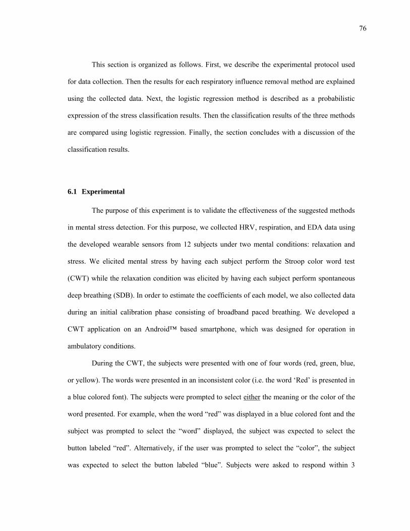
76
This section is organized as follows. First, we describe the experimental protocol used
for data collection. Then the results for each respiratory influence removal method are explained
using the collected data. Next, the logistic regression method is described as a probabilistic
expression of the stress classification results. Then the classification results of the three methods
are compared using logistic regression. Finally, the section concludes with a discussion of the
classification results.
6.1 Experimental
The purpose of this experiment is to validate the effectiveness of the suggested methods
in mental stress detection. For this purpose, we collected HRV, respiration, and EDA data using
the developed wearable sensors from 12 subjects under two mental conditions: relaxation and
stress. We elicited mental stress by having each subject perform the Stroop color word test
(CWT) while the relaxation condition was elicited by having each subject perform spontaneous
deep breathing (SDB). In order to estimate the coefficients of each model, we also collected data
during an initial calibration phase consisting of broadband paced breathing. We developed a
CWT application on an Android™ based smartphone, which was designed for operation in
ambulatory conditions.
During the CWT, the subjects were presented with one of four words (red, green, blue,
or yellow). The words were presented in an inconsistent color (i.e. the word ‘Red’ is presented in
a blue colored font). The subjects were prompted to select either the meaning or the color of the
word presented. For example, when the word “red” was displayed in a blue colored font and the
subject was prompted to select the “word” displayed, the subject was expected to select the
button labeled “red”. Alternatively, if the user was prompted to select the “color”, the subject
was expected to select the button labeled “blue”. Subjects were asked to respond within 3
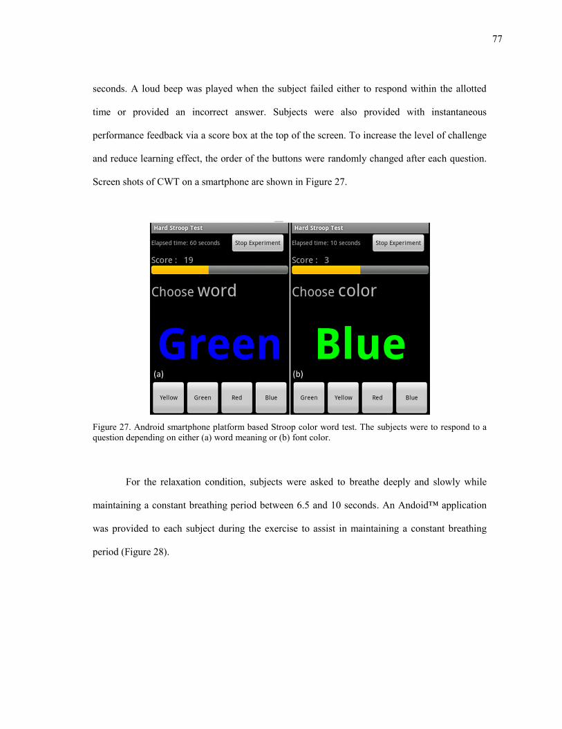
77
seconds. A loud beep was played when the subject failed either to respond within the allotted
time or provided an incorrect answer. Subjects were also provided with instantaneous
performance feedback via a score box at the top of the screen. To increase the level of challenge
and reduce learning effect, the order of the buttons were randomly changed after each question.
Screen shots of CWT on a smartphone are shown in Figure 27.
Figure 27. Android smartphone platform based Stroop color word test. The subjects were to respond to a question depending on either (a) word meaning or (b) font color.
For the relaxation condition, subjects were asked to breathe deeply and slowly while
maintaining a constant breathing period between 6.5 and 10 seconds. An Andoid™ application
was provided to each subject during the exercise to assist in maintaining a constant breathing
period (Figure 28).

78
Figure 28. Android application that gave instructions to the subjects to help in spontaneous deep breathing. The elapsed experimental time was displayed on the top left corner of the screen.
During the calibration stage, subjects were asked to modify their breathing pattern to match an
audio prompt designed for paced breathing. The audio prompt was a custom developed
AndroidTM application that provided periodic voice prompts to instruct the user to either inhale
or exhale at intervals randomly drawn from a modified Poisson process (Saul et al., 1989). This
ensured that the breathing signal had an approximately flat power spectrum over a broad range
of respiratory frequencies. In a Poisson process, the distribution function, equation (27),
describes the probability of observing k events within a given time interval τ assuming the events
are independent and identically distributed (IID) and occur at an average rate λ:
( ) ( )
(27)
The interval τ between two consecutive events in the Poisson process can be shown to follow the
exponential density function in equation (28):
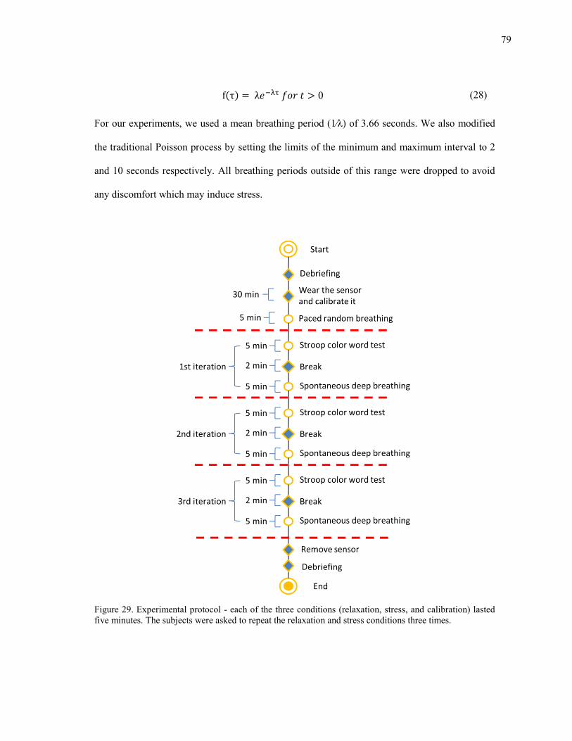
79
( ) (28)
For our experiments, we used a mean breathing period (1⁄λ) of 3.66 seconds. We also modified
the traditional Poisson process by setting the limits of the minimum and maximum interval to 2
and 10 seconds respectively. All breathing periods outside of this range were dropped to avoid
any discomfort which may induce stress.
Figure 29. Experimental protocol - each of the three conditions (relaxation, stress, and calibration) lasted five minutes. The subjects were asked to repeat the relaxation and stress conditions three times.
80
Each subject was asked to perform the calibration stage once and the CWT and SDB
three times each with a break between each test. A diagram illustrating the entire experimental
protocol is shown in Figure 29. The respiratory signal and the EDA signal were recorded at a
sampling rate of 10 Hz, whereas the HRM recorded the timestamps of each R peak.
6.2 Preliminary analysis and data preprocessing
A sample of the raw sensor signals collected from a subject during calibration phase and
a full sequence of the arousal response tests are shown in Figure 30. Irregularities and variance
in the respiratory signal and RR intervals are more evident during the stress conditions in
comparison with the relaxation conditions. The EDA signal shows a decaying trend during deep
breathing and distinct peaks during the stress segments.
From the respiratory signals illustrated in Figure 30, we observe that subjects exhibited
different breathing patterns for the two experimental conditions: a slow breathing pattern when
the subject relaxed and a faster breathing pattern when the subject became stressed. Although
this result shows that the respiratory signal itself may contain a significant amount of
discriminatory information, we note that respiratory activity can be under voluntary control. This
raises a question about the validity of the respiration signal as an objective measure of stress.
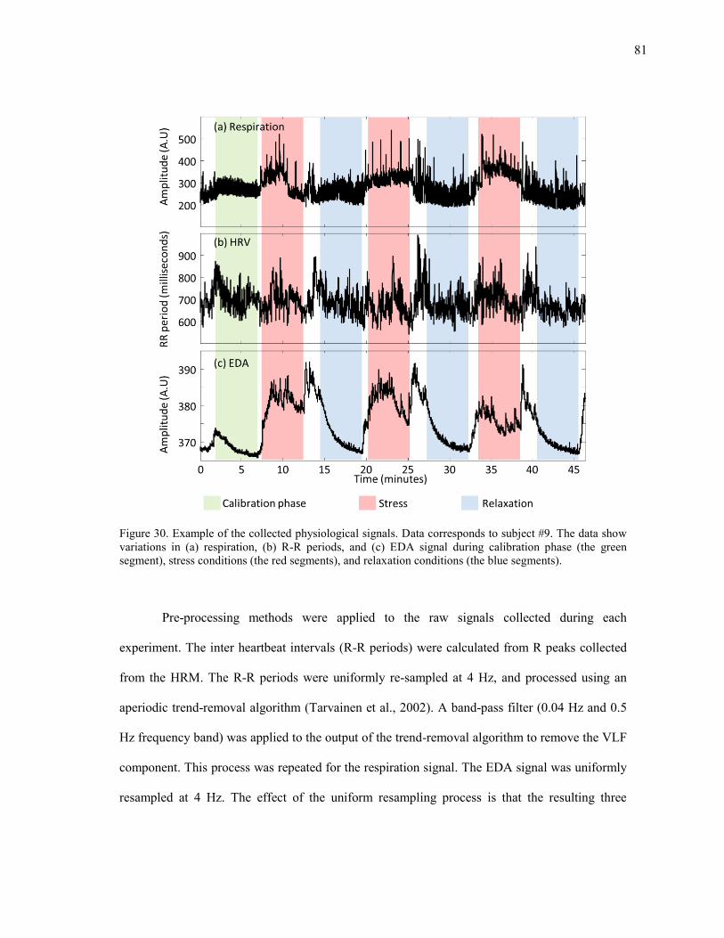
81
Figure 30. Example of the collected physiological signals. Data corresponds to subject #9. The data show variations in (a) respiration, (b) R-R periods, and (c) EDA signal during calibration phase (the green segment), stress conditions (the red segments), and relaxation conditions (the blue segments).
Pre-processing methods were applied to the raw signals collected during each
experiment. The inter heartbeat intervals (R-R periods) were calculated from R peaks collected
from the HRM. The R-R periods were uniformly re-sampled at 4 Hz, and processed using an
aperiodic trend-removal algorithm (Tarvainen et al., 2002). A band-pass filter (0.04 Hz and 0.5
Hz frequency band) was applied to the output of the trend-removal algorithm to remove the VLF
component. This process was repeated for the respiration signal. The EDA signal was uniformly
resampled at 4 Hz. The effect of the uniform resampling process is that the resulting three
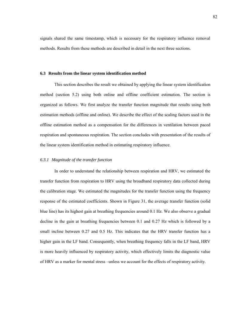
82
signals shared the same timestamp, which is necessary for the respiratory influence removal
methods. Results from these methods are described in detail in the next three sections.
6.3 Results from the linear system identification method
This section describes the result we obtained by applying the linear system identification
method (section 5.2) using both online and offline coefficient estimation. The section is
organized as follows. We first analyze the transfer function magnitude that results using both
estimation methods (offline and online). We describe the effect of the scaling factors used in the
offline estimation method as a compensation for the differences in ventilation between paced
respiration and spontaneous respiration. The section concludes with presentation of the results of
the linear system identification method in estimating respiratory influence.
6.3.1 Magnitude of the transfer function
In order to understand the relationship between respiration and HRV, we estimated the
transfer function from respiration to HRV using the broadband respiratory data collected during
the calibration stage. We estimated the magnitudes for the transfer function using the frequency
response of the estimated coefficients. Shown in Figure 31, the average transfer function (solid
blue line) has its highest gain at breathing frequencies around 0.1 Hz. We also observe a gradual
decline in the gain at breathing frequencies between 0.1 and 0.27 Hz which is followed by a
small incline between 0.27 and 0.5 Hz. This indicates that the HRV transfer function has a
higher gain in the LF band. Consequently, when breathing frequency falls in the LF band, HRV
is more heavily influenced by respiratory activity, which effectively limits the diagnostic value
of HRV as a marker for mental stress –unless we account for the effects of respiratory activity.
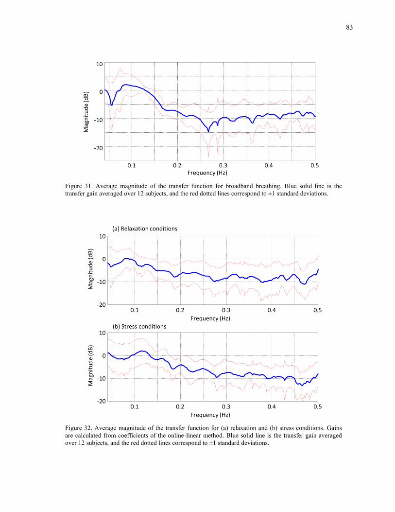
83
Figure 31. Average magnitude of the transfer function for broadband breathing. Blue solid line is the transfer gain averaged over 12 subjects, and the red dotted lines correspond to ±1 standard deviations.
Figure 32. Average magnitude of the transfer function for (a) relaxation and (b) stress conditions. Gains are calculated from coefficients of the online-linear method. Blue solid line is the transfer gain averaged over 12 subjects, and the red dotted lines correspond to ±1 standard deviations.
84
Figure 32 shows the transfer magnitude for the relaxation and stress conditions obtained
using online estimation. We observe similar transfer gain characteristics as in the offline
estimation method, and no apparent differences between relaxation and stress conditions. In both
conditions, the transfer gain is similar to that of paced broadband breathing. The gain is
maximum around 0.1 Hz.
6.3.2 Scaling factors
When ARMAX coefficients are estimated offline, a scale factor is needed to compensate
for ventilation differences between spontaneous breathing (relaxation and stress condition) and
paced broadband breathing (calibration phase). The effects of the scaled gain on HRV prediction
for a relaxation condition are illustrated in Figure 33 (data corresponds to subject #1). In the
absence of scaling (α=1), the model under-predicts the HRV value for the relaxation condition
since the coefficients of the linear model were estimated based on a paced broadband respiratory
condition. Introducing the multiplicative scaling factor addresses this issue. Figure 33a illustrates
the sensitivity of the root-mean-square (RMS) error with respect to the scaling factor; a
minimum RMS error prediction is obtained for α=4.8. The differences between the scaled and
unscaled models are shown in Figure 33b.
Figure 34 illustrates the effects of the scaling factor on a stress condition. A minimum
mean-squared prediction error is obtained for α=8. In stress condition, the amplitude of the
respiration signal is smaller and therefore the optimal scale factor is larger than that of relaxation
condition.
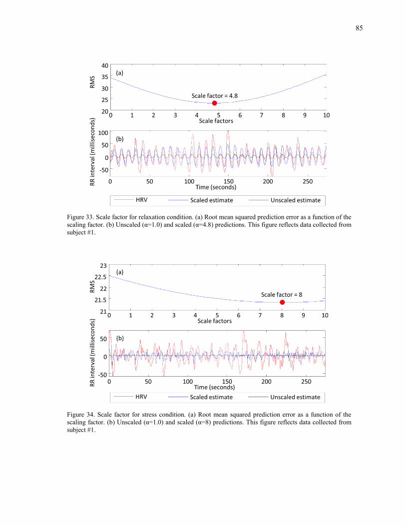
85
Figure 33. Scale factor for relaxation condition. (a) Root mean squared prediction error as a function of the scaling factor. (b) Unscaled (α=1.0) and scaled (α=4.8) predictions. This figure reflects data collected from subject #1.
Figure 34. Scale factor for stress condition. (a) Root mean squared prediction error as a function of the scaling factor. (b) Unscaled (α=1.0) and scaled (α=8) predictions. This figure reflects data collected from subject #1.
86
6.3.3 Power spectral density
As shown in Figure 35a-b, the HRV power in the LF band during the relaxation
condition (blue line) is larger than the LF power for the stress condition (red line). This is
because respiration during the relaxation condition occurs in the LF band. These results indicate
that, on the basis of the HRV signal alone (e.g., LF/HF ratio), it is difficult to discriminate
between the two experimental conditions (stress vs. relaxation) with a reasonable degree of
accuracy.
Next, we applied the offline ARMAX model to estimate the respiratory-driven HRV
signal for both conditions (stress and relaxation). PSDs for the respiratory-driven HRV (i.e.,
ARMAX model predictions) and residual HRV are shown in Figure 35c-d. As expected, the
respiratory-driven HRV for the relaxation condition shows a dominant LF peak, while the stress
condition shows a peak in the HF bands (Figure 35c). In contrast, the residual HRV for the stress
condition has higher LF power in comparison with the relaxation condition (Figure 35d). This
supports our hypothesis that residual analysis is more discriminatory than HRV analysis.
Results for the online ARMAX model are illustrated in Figure 35e-f. As with the offline
approach, the respiratory-driven HRV and residual HRV show a difference between relaxation
and stress conditions. Note that the online and the offline estimation methods show differences
in the LF power of respiratory-driven HRV for the relaxation condition (Figure 35c and e).
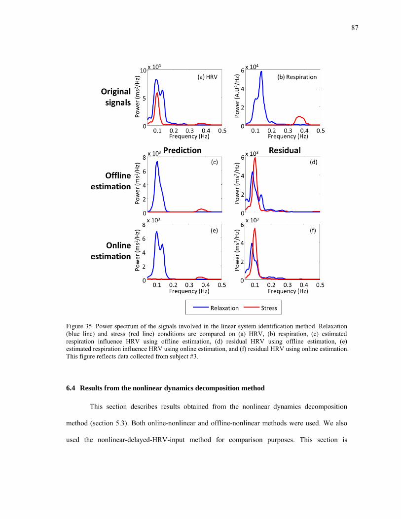
87
Figure 35. Power spectrum of the signals involved in the linear system identification method. Relaxation (blue line) and stress (red line) conditions are compared on (a) HRV, (b) respiration, (c) estimated respiration influence HRV using offline estimation, (d) residual HRV using offline estimation, (e) estimated respiration influence HRV using online estimation, and (f) residual HRV using online estimation. This figure reflects data collected from subject #3.
6.4 Results from the nonlinear dynamics decomposition method
This section describes results obtained from the nonlinear dynamics decomposition
method (section 5.3). Both online-nonlinear and offline-nonlinear methods were used. We also
used the nonlinear-delayed-HRV-input method for comparison purposes. This section is
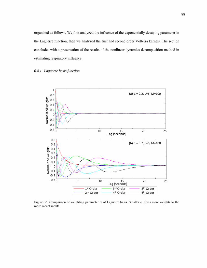
88
organized as follows. We first analyzed the influence of the exponentially decaying parameter in
the Laguerre function, then we analyzed the first and second order Volterra kernels. The section
concludes with a presentation of the results of the nonlinear dynamics decomposition method in
estimating respiratory influence.
6.4.1 Laguerre basis function
Figure 36. Comparison of weighting parameter of Laguerre basis. Smaller gives more weights to the more recent inputs.
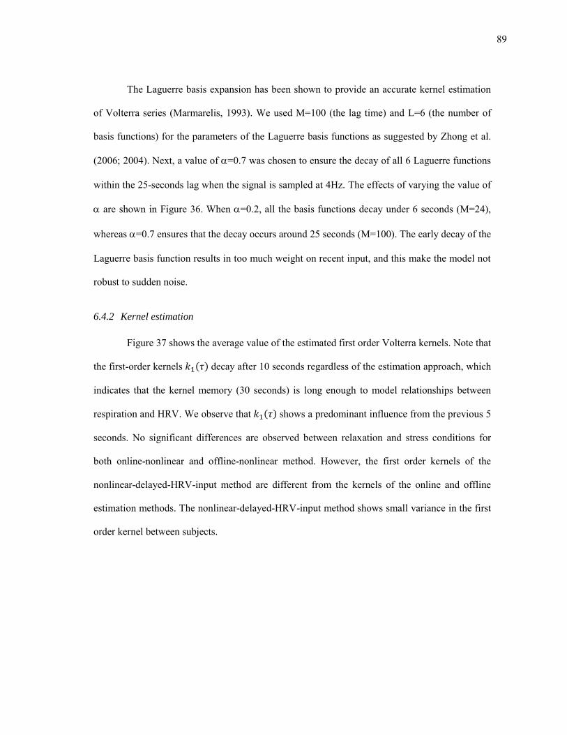
89
The Laguerre basis expansion has been shown to provide an accurate kernel estimation
of Volterra series (Marmarelis, 1993). We used M=100 (the lag time) and L=6 (the number of
basis functions) for the parameters of the Laguerre basis functions as suggested by Zhong et al.
(2006; 2004). Next, a value of =0.7 was chosen to ensure the decay of all 6 Laguerre functions
within the 25-seconds lag when the signal is sampled at 4Hz. The effects of varying the value of
are shown in Figure 36. When =0.2, all the basis functions decay under 6 seconds (M=24),
whereas =0.7 ensures that the decay occurs around 25 seconds (M=100). The early decay of the
Laguerre basis function results in too much weight on recent input, and this make the model not
robust to sudden noise.
6.4.2 Kernel estimation
Figure 37 shows the average value of the estimated first order Volterra kernels. Note that
the first-order kernels ( ) decay after 10 seconds regardless of the estimation approach, which
indicates that the kernel memory (30 seconds) is long enough to model relationships between
respiration and HRV. We observe that ( ) shows a predominant influence from the previous 5
seconds. No significant differences are observed between relaxation and stress conditions for
both online-nonlinear and offline-nonlinear method. However, the first order kernels of the
nonlinear-delayed-HRV-input method are different from the kernels of the online and offline
estimation methods. The nonlinear-delayed-HRV-input method shows small variance in the first
order kernel between subjects.
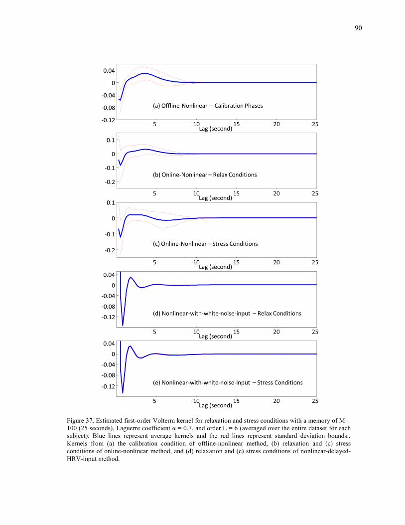
90
Figure 37. Estimated first-order Volterra kernel for relaxation and stress conditions with a memory of M = 100 (25 seconds), Laguerre coefficient α = 0.7, and order L = 6 (averaged over the entire dataset for each subject). Blue lines represent average kernels and the red lines represent standard deviation bounds.. Kernels from (a) the calibration condition of offline-nonlinear method, (b) relaxation and (c) stress conditions of online-nonlinear method, and (d) relaxation and (e) stress conditions of nonlinear-delayed-HRV-input method.
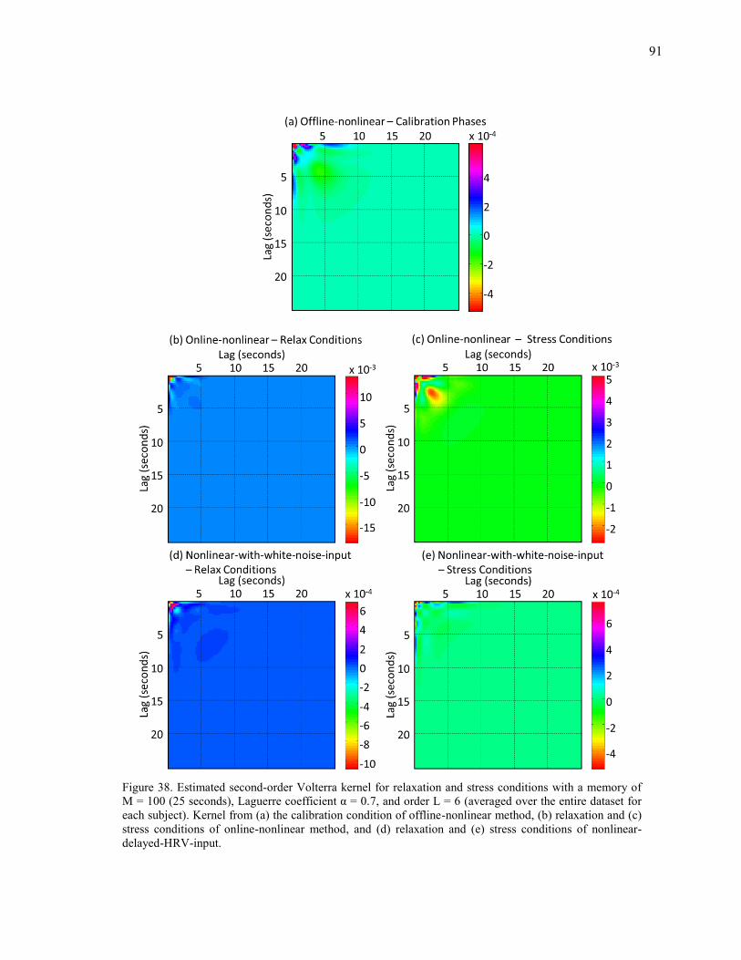
91
Figure 38. Estimated second-order Volterra kernel for relaxation and stress conditions with a memory of M = 100 (25 seconds), Laguerre coefficient α = 0.7, and order L = 6 (averaged over the entire dataset for each subject). Kernel from (a) the calibration condition of offline-nonlinear method, (b) relaxation and (c) stress conditions of online-nonlinear method, and (d) relaxation and (e) stress conditions of nonlinear-delayed-HRV-input.
92
The second-order kernel ( ) shows an influence between close terms (the
diagonal block in Figure 38). The online-nonlinear, offline-nonlinear, and nonlinear-delayed-
HRV-input methods show a different decay trend. The offline-nonlinear and nonlinear-delayed-
HRV-input methods decay after 5 seconds while the online-nonlinear method decays after 10
seconds. No significant difference was observed between the relaxation and stress conditions for
both online-nonlinear and nonlinear-delayed-HRV-input methods. These results suggest that the
two physiological conditions cannot be discriminated based on the kernels.
6.4.3 Power spectral density
The results of the nonlinear dynamics decomposition method are illustrated in Figure
39.For the offline-nonlinear method (Figure 39c-d), the respiratory-driven HRV for the
relaxation condition shows a dominant LF peak, while the stress condition shows a small peak in
the HF bands (Figure 35c). In contrast, the residual HRV for the stress condition has more LF
power than the residual HRV for the relaxation condition (Figure 35d).
Similar to the results obtained using the linear method in section 6.3.3, the residual HRV
for the stress condition has more power than respiratory-driven HRV for the offline-nonlinear
method (Figure 39d). The offline-nonlinear method results in a smooth spectral envelop when
applied to the respiratory-driven HRV for the relaxation condition.
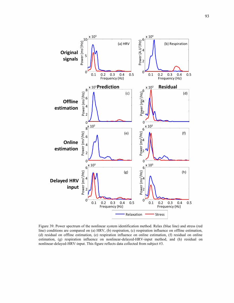
93
Figure 39. Power spectrum of the nonlinear system identification method. Relax (blue line) and stress (red line) conditions are compared on (a) HRV, (b) respiration, (c) respiration influence on offline estimation, (d) residual on offline estimation, (e) respiration influence on online estimation, (f) residual on online estimation, (g) respiration influence on nonlinear-delayed-HRV-input method, and (h) residual on nonlinear-delayed-HRV-input. This figure reflects data collected from subject #3.
94
Without the respiration signal, the nonlinear-delayed-HRV-input shows a different result
(Figure 39g-h) from the offline-nonlinear and online-nonlinear method. The estimated
respiratory-driven HRV for the stress condition shows a peak in the LF bands which is not
correlated with respiration signal.
6.5 Results from the spectral weighting method
Results from the spectral-weighting method are illustrated in Figure 40. Each weighting
function (Figure 40c-d) was calculated by normalizing corresponding respiratory PSD in Figure
40b. We applied the respective weighting functions and observed that the predictions show that
the residual energy lies primarily in the LF band (Figure 40e-f). More importantly, the results in
Figure 40e-f suggest an alternative interpretation of our model. The traditional HRV analysis
decomposes the power spectral density into two fixed spectral bands (LF vs. HF) whereas our
model suggests that HRV can be decomposed into two components: one that correlates with
respiratory activity (the energy observed in Figure 40e), and one that is orthogonal to respiratory
activity (the energy observed in Figure 40f). This decomposition using our model is
advantageous because, unlike the LF/HF ratio, it is not affected by the subject’s breathing rate.
This suggests that the ratio between HRV energy correlated with respiration and HRV energy
uncorrelated with respiration is a more meaningful index than the traditional LF/HF ratio.
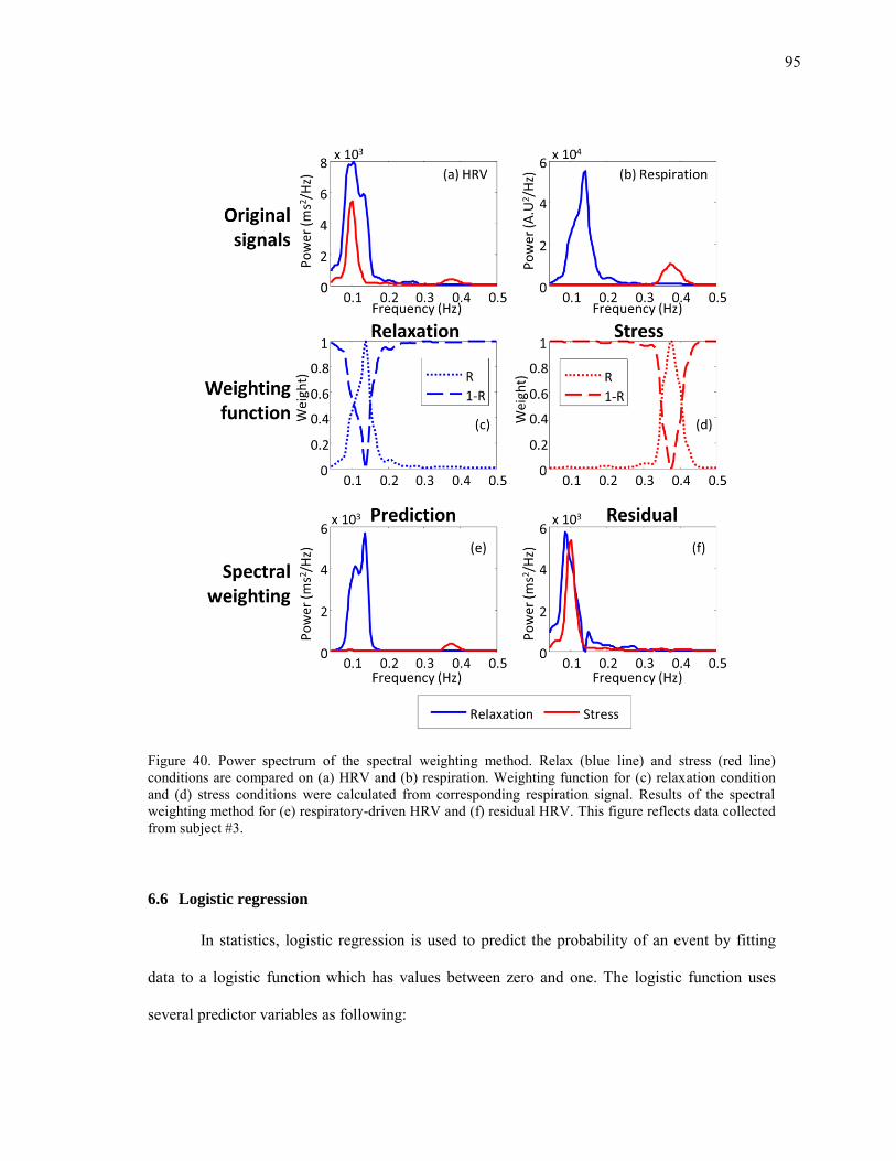
95
Figure 40. Power spectrum of the spectral weighting method. Relax (blue line) and stress (red line) conditions are compared on (a) HRV and (b) respiration. Weighting function for (c) relaxation condition and (d) stress conditions were calculated from corresponding respiration signal. Results of the spectral weighting method for (e) respiratory-driven HRV and (f) residual HRV. This figure reflects data collected from subject #3.
6.6 Logistic regression
In statistics, logistic regression is used to predict the probability of an event by fitting
data to a logistic function which has values between zero and one. The logistic function uses
several predictor variables as following:
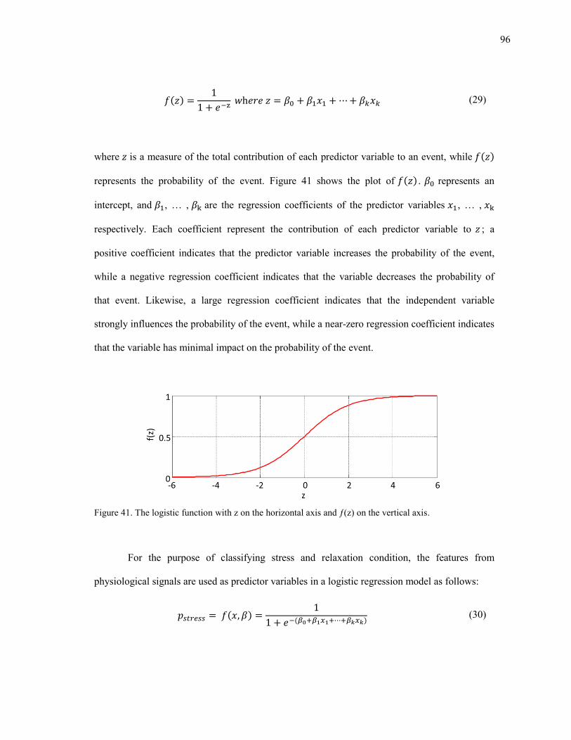
96
where is a measure of the total contribution of each predictor variable to an event, while ( )
represents the probability of the event. Figure 41 shows the plot of ( ) . represents an
intercept, and , … , are the regression coefficients of the predictor variables , … ,
respectively. Each coefficient represent the contribution of each predictor variable to ; a
positive coefficient indicates that the predictor variable increases the probability of the event,
while a negative regression coefficient indicates that the variable decreases the probability of
that event. Likewise, a large regression coefficient indicates that the independent variable
strongly influences the probability of the event, while a near-zero regression coefficient indicates
that the variable has minimal impact on the probability of the event.
Figure 41. The logistic function with z on the horizontal axis and ƒ(z) on the vertical axis.
For the purpose of classifying stress and relaxation condition, the features from
physiological signals are used as predictor variables in a logistic regression model as follows:
( )
(29)
( )
( ) (30)

97
where is the probability of stress, and is a vector of predictor variables. We estimate
these coefficients following a maximum-likelihood criteria by means of iteratively reweighted
least squares (IRLS) (McCullagh and Nelder, 1989). IRLS is used to find the maximum
likelihood estimates of the generalized linear model:
( ) ∑( ( ( )) ( ) ( ( )))
( ) (31)
where is a stress indicator variable for the ith event in a training set ( if stress;
otherwise).
6.7 Classification performance comparisons
In order to compare the performance of the proposed respiratory separation methods, we
formulated a binary classification problem. The goal was to distinguish between the stress
condition and the relaxation condition. We compared the stress classification performance of the
following methods:
1) HRV,
2) Respiration,
3) Two linear methods (online-linear estimation method and offline-linear estimation
method),
4) Three nonlinear methods (online-nonlinear method, offline-nonlinear method, and
nonlinear-delayed-HRV-input method), and
5) Spectral-weighting.
98
We used experimental data collected from 12 subjects to extract features for each
method. For each condition, the collected signals were analyzed with a 2.5 minute window
sliding at increments of 10 seconds, i.e. 15 analysis windows per test. Each window was treated
as a different sample, resulting in 105 windows for each subject including the calibration phase.
For classification purposes, we extracted three features (LF power, HF power, and LF/HF ratio)
for HRV and respiration, and three different features (LF and HF power of residual HRV, and
ratio of total power of respiratory-driven HRV to total power of residual HRV) for the
respiratory influence removal methods. Each feature was normalized to a zero mean and unit
standard deviation for each subject. The features used for each method are summarized in Table
II.
As indicated in 5.1, RSA is capable of reflect stress response. Thus, we can incorporate
respiratory-derived HRV features to detect stress response if RSA has information about stress.
However, the change of respiratory rate is used to induce relaxation in this experiment. As a
result of this, respiratory-driven HRV will easily differentiate between stress and relaxation
conditions, and this will result in an inflated classification rate for the two conditions. This is
problematic because this result is not the discrimination between stress and relaxation response
but between respiration activities. For this reason, we do not include respiratory-driven HRV
features for classification. Respiratory-driven HRV is only used in the feature of ratio between
respiration and stress induced power to represent the balance between SNS and PNS activation.
However, if respiration is not controlled during experiments, dropping RSA related features may
result in a loss of information. In this case, RSA related features should be included in the
analysis of stress detection.
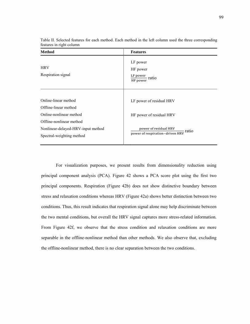
99
Table II. Selected features for each method. Each method in the left column used the three corresponding features in right column
Method Features
HRV
Respiration signal
LF power
HF power
ratio
Online-linear method
Offline-linear method
Online-nonlinear method
Offline-nonlinear method
Nonlinear-delayed-HRV-input method
Spectral-weighting method
LF power of residual HRV
HF power of residual HRV
ratio
For visualization purposes, we present results from dimensionality reduction using
principal component analysis (PCA). Figure 42 shows a PCA score plot using the first two
principal components. Respiration (Figure 42b) does not show distinctive boundary between
stress and relaxation conditions whereas HRV (Figure 42a) shows better distinction between two
conditions. Thus, this result indicates that respiration signal alone may help discriminate between
the two mental conditions, but overall the HRV signal captures more stress-related information.
From Figure 42f, we observe that the stress condition and relaxation conditions are more
separable in the offline-nonlinear method than other methods. We also observe that, excluding
the offline-nonlinear method, there is no clear separation between the two conditions.
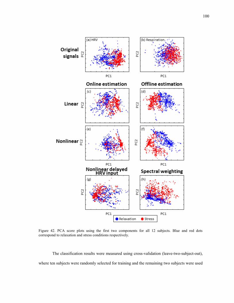
100
Figure 42. PCA score plots using the first two components for all 12 subjects. Blue and red dots correspond to relaxation and stress conditions respectively.
The classification results were measured using cross-validation (leave-two-subject-out),
where ten subjects were randomly selected for training and the remaining two subjects were used
101
for testing. This procedure allowed us to determine whether the classifier generalizes across
subjects. For each combination of training and test set (66 splits), the logistic regression model
coefficients were estimated from training data and used to estimate the probability for
samples in the test set. Next, we used a threshold as the decision boundary to label
an event as stressful. Classification results were averaged across the 66 splits and are
summarized in Figure 43. The average classification rate of the HRV signal and the respiration
signal were 77.1 % and 70.5 % respectively (Figure 43). Thus, HRV captured more information
about stress than respiration signal.
Average classification rates for the linear system identification method were 76.7 % and
85.2 % for the online-linear and offline-linear methods, respectively. The average classification
rates for the nonlinear dynamics decomposition method were 75.9 % and 89.2 % for the online-
nonlinear and offline-nonlinear methods, respectively. In both linear and nonlinear methods, the
results of online coefficients are not different from the results obtained using HRV. In contrast,
the offline coefficient estimation improved classification accuracy by 8.5 – 12.1 % compared
with HRV in both linear and non-linear methods. The classification performance of nonlinear-
delayed-HRV-input method was 77.2%, comparable to that obtained using HRV. This indicates
the limitation of the decomposition of the HRV signal without the respiration signal. Finally, the
performance of the spectral weighting method was 81.5 %.
In summary, the offline methods (both linear and non-linear) outperformed their online
counterparts. The spectral-weighting method also improved classification performance compared
to HRV analysis.
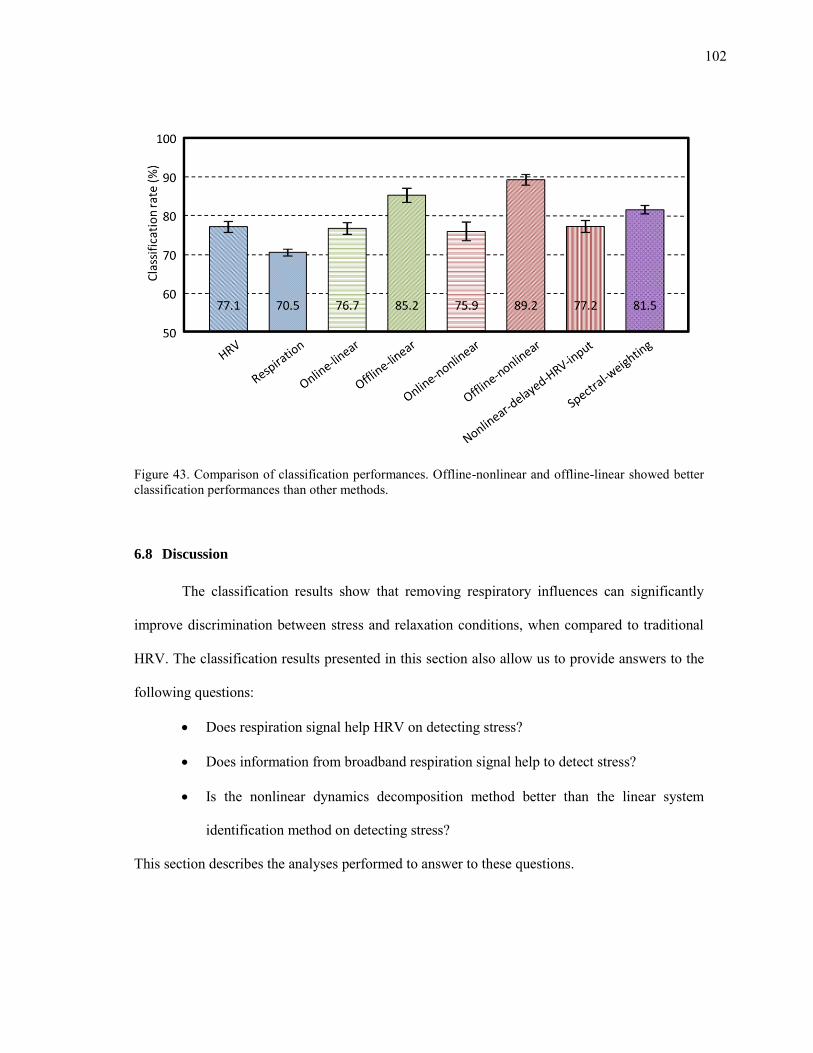
102
Figure 43. Comparison of classification performances. Offline-nonlinear and offline-linear showed better classification performances than other methods.
6.8 Discussion
The classification results show that removing respiratory influences can significantly
improve discrimination between stress and relaxation conditions, when compared to traditional
HRV. The classification results presented in this section also allow us to provide answers to the
following questions:
Does respiration signal help HRV on detecting stress?
Does information from broadband respiration signal help to detect stress?
Is the nonlinear dynamics decomposition method better than the linear system
identification method on detecting stress?
This section describes the analyses performed to answer to these questions.
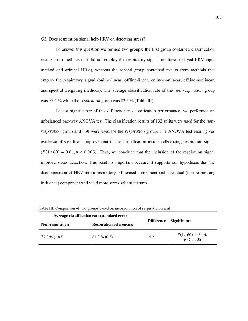
103
Q1. Does respiration signal help HRV on detecting stress?
To answer this question we formed two groups: the first group contained classification
results from methods that did not employ the respiratory signal (nonlinear-delayed-HRV-input
method and original HRV), whereas the second group contained results from methods that
employ the respiratory signal (online-linear, offline-linear, online-nonlinear, offline-nonlinear,
and spectral-weighting methods). The average classification rate of the non-respiration group
was 77.5 % while the respiration group was 82.1 % (Table III).
To test significance of this difference in classification performance, we performed an
unbalanced one-way ANOVA test. The classification results of 132 splits were used for the non-
respiration group and 330 were used for the respiration group. The ANOVA test result gives
evidence of significant improvement in the classification results referencing respiration signal
( ( ) ). Thus, we conclude that the inclusion of the respiration signal
improve stress detection. This result is important because it supports our hypothesis that the
decomposition of HRV into a respiratory influenced component and a residual (non-respiratory
influence) component will yield more stress salient features.
Table III. Comparison of two groups based on incorporation of respiration signal.
Average classification rate (standard error)
Difference Significance Non-respiration Respiration referencing
77.2 % (1.03) 81.3 % (0.8) + 4.2 ( )
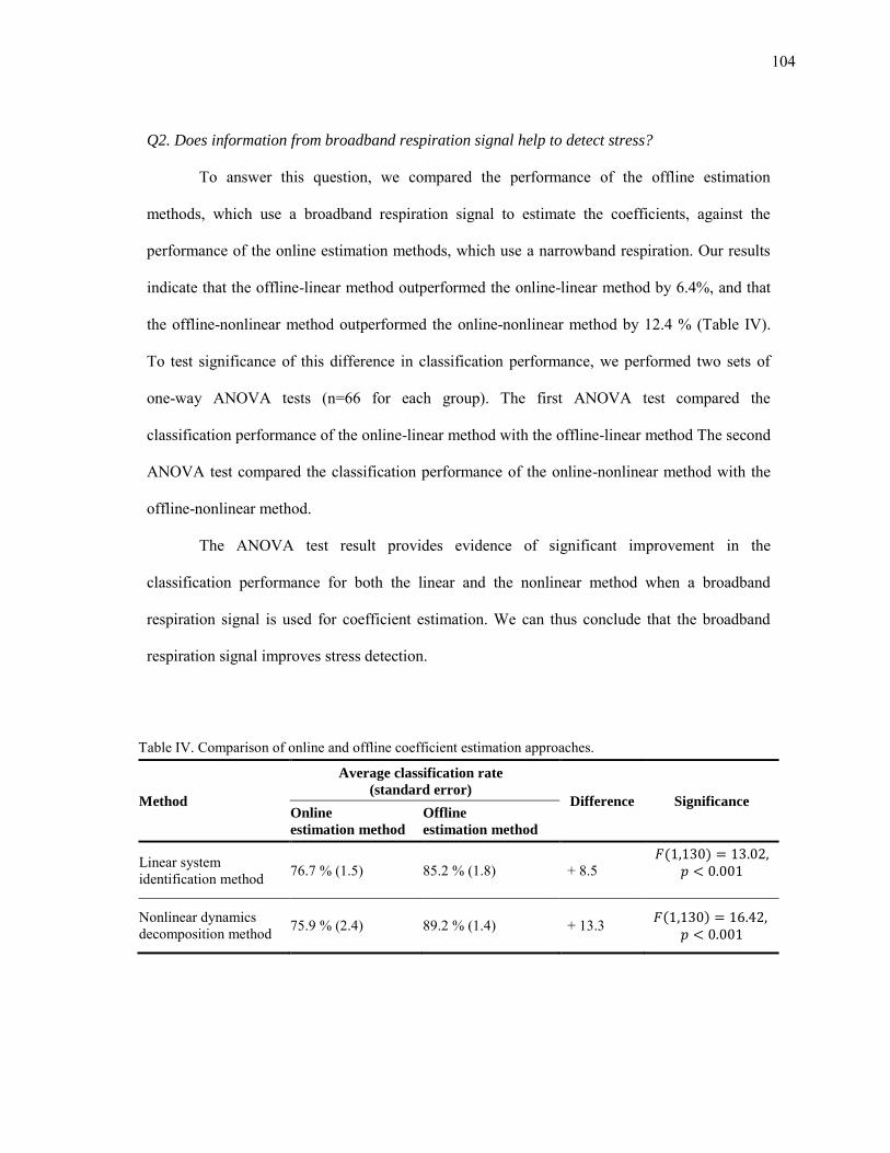
104
Q2. Does information from broadband respiration signal help to detect stress?
To answer this question, we compared the performance of the offline estimation
methods, which use a broadband respiration signal to estimate the coefficients, against the
performance of the online estimation methods, which use a narrowband respiration. Our results
indicate that the offline-linear method outperformed the online-linear method by 6.4%, and that
the offline-nonlinear method outperformed the online-nonlinear method by 12.4 % (Table IV).
To test significance of this difference in classification performance, we performed two sets of
one-way ANOVA tests (n=66 for each group). The first ANOVA test compared the
classification performance of the online-linear method with the offline-linear method The second
ANOVA test compared the classification performance of the online-nonlinear method with the
offline-nonlinear method.
The ANOVA test result provides evidence of significant improvement in the
classification performance for both the linear and the nonlinear method when a broadband
respiration signal is used for coefficient estimation. We can thus conclude that the broadband
respiration signal improves stress detection.
Table IV. Comparison of online and offline coefficient estimation approaches.
Method
Average classification rate
(standard error) Difference Significance
Online
estimation method
Offline
estimation method
Linear system identification method 76.7 % (1.5) 85.2 % (1.8) + 8.5
( )
Nonlinear dynamics decomposition method 75.9 % (2.4) 89.2 % (1.4) + 13.3 ( )
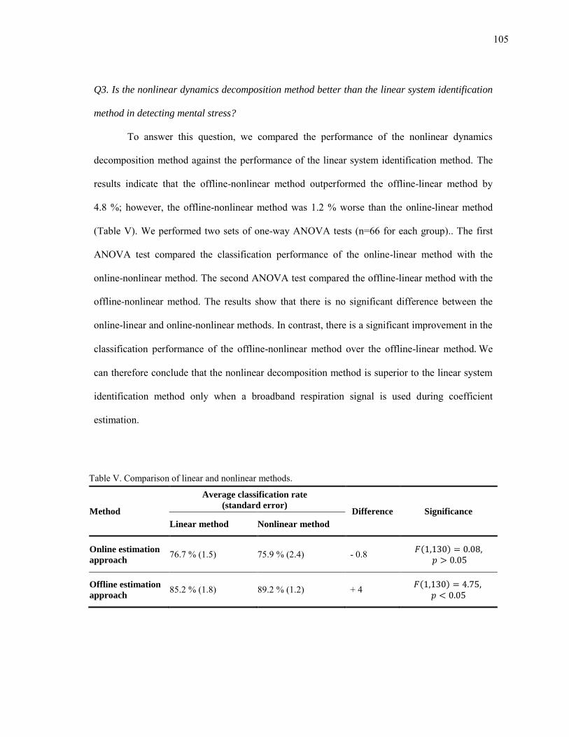
105
Q3. Is the nonlinear dynamics decomposition method better than the linear system identification
method in detecting mental stress?
To answer this question, we compared the performance of the nonlinear dynamics
decomposition method against the performance of the linear system identification method. The
results indicate that the offline-nonlinear method outperformed the offline-linear method by
4.8 %; however, the offline-nonlinear method was 1.2 % worse than the online-linear method
(Table V). We performed two sets of one-way ANOVA tests (n=66 for each group).. The first
ANOVA test compared the classification performance of the online-linear method with the
online-nonlinear method. The second ANOVA test compared the offline-linear method with the
offline-nonlinear method. The results show that there is no significant difference between the
online-linear and online-nonlinear methods. In contrast, there is a significant improvement in the
classification performance of the offline-nonlinear method over the offline-linear method We
can therefore conclude that the nonlinear decomposition method is superior to the linear system
identification method only when a broadband respiration signal is used during coefficient
estimation.
Table V. Comparison of linear and nonlinear methods.
Method
Average classification rate
(standard error) Difference Significance
Linear method Nonlinear method
Online estimation
approach 76.7 % (1.5) 75.9 % (2.4) - 0.8 ( )
Offline estimation
approach 85.2 % (1.8) 89.2 % (1.2) + 4 ( )

106
In conclusion, the additional information from the respiration signal improves stress
detection when used in combination with HRV. Both linear and nonlinear models should be
trained using a broadband respiration signal. Using identical calibration methods, the nonlinear
method outperforms the linear method in differentiating between conditions of stress and
conditions of relaxation.
107
7. INCREASING STRESS RECOGNITION BY COMBINING EDA
FEATURES WITH RESPIRATORY INFLUENCE REMOVAL METHODS
Electrodermal activity is known to be a strong indicator of SNS activation, and is not
influenced by PNS. The purpose of this section is to determine whether the information
contained in EDA can supplement information contained in HRV in terms of detecting stress.
For this purpose, we propose a method to decompose EDA into features that reflect the tonic and
phasic responses. These EDA features are then combined with the features from the respiratory
influence removal methods and tested on a classification problem of stress and relaxation
conditions.
This section is organized as follows. First, we describe the methods used to decompose
the EDA response into the tonic and the phasic components. Second, we describe the results
obtained from the application of this decomposition method on previously collected data. We
provide an analysis of the stress classification results obtained from three respiratory influence
removal methods using a combination of features extracted from EDA, respiratory influenced
HRV and the residual HRV. The section concludes with an analysis and discussion of the results.
7.1 Signal decomposition
EDA consists of two components: a slow changing offset known as the skin conductance
level (SCL), and a series of transient peaks known as skin conductance responses (SCR) (El-
Sheikh, 2005). SCRs are observed in reaction to startle events such as an unexpected loud noise.
A variant of SCRs, non-specific skin conductance responses (NS-SCR), occurs without any
108
external stimulus. NS-SCR can also be elicited by deep breathing and certain types of body
movement. It is not possible to identify NS-SCRs without reference to respiration and movement
signals (Dawson et al., 2007).
Several approaches have been proposed to decouple these two components. Lim et al.
(1997) proposed a curve-fitting method with sigmoidal/exponential functions that decomposed
the EDA signal into discrete SCRs and the residual SCL. Alexander et al. (2005) proposed a
similar computationally efficient algorithm for the same approach to decouple the two EDA
components. The method models the EDA time series as the convolution of an impulsive spike
train, which controls the timing of SCRs, and a second-order differential equation, which
controls the rise time and decay of individual SCRs (i.e., a bi-exponential function). Benedek
and Kaernbach (2010) improved on this work by modeling EDA as a driver function convolved
with an impulse response. Under the assumption that the driver function represents sudomotor
neuron activity (i.e., either spiking or at rest), the decomposition was performed using a non-
negative deconvolution procedure. These methods provide a fine decomposition into individual
SCRs but tend to be computationally heavy (Alexander et al., 2005). An alternative approach
proposed by Frantzidis et al. (2009) was to detect individual SCRs from the EDA derivative
based on a peak-picking algorithm; the approach was also able to extract various SCR
parameters such as latency and rise time.
After the two EDA components were decoupled, both components can be used as
features to quantify EDA. The duration, amplitude and occurrence of SCL and SCR have been
used as measures of EDA (Dawson et al., 2007). The most commonly reported measures are
amplitude of SCL, amplitude of SCR, and the number of occurrences of SCRs. These three
measures are known to be independent of each other, offering supplementary information about
stress (Dawson et al., 2007). The amplitude of SCL represents the tonic level of EDA that ranges
109
between 2 and 20 μS, and has been reported as a stable index of autonomic arousal in clinical
trials (Jacobs et al., 1994). When a stimulus is repeated several times, the amplitude of SCR
represents the phasic level that ranges between 0.1 and 1.0 μS. The number of occurrence of
SCRs has also been recommended as a measure of SCR (Dawson et al., 2007). The amplitude of
SCR decreases with each repetition of the stimulus. This SCR habituation can be evaluated by
counting the number of peaks to reach some predetermined level of habituation.
The aforementioned decomposition methods rely on a scoring procedure to validate each
SCR peak, and this procedure has a high computational complexity. For this reason we
employed a heuristic method using the regularized least-squares de-trending method (Tarvainen
et al., 2002). This heuristic approximates SCL as the aperiodic trend while SCR is approximated
using the residual.
( )
(32)
where is the raw EDA signal, is the SCL trend, and is the SCR component. The
regularization term biases the solution towards a smooth trend , where is the
identity matrix, and is a discrete approximation of the second derivative operator:
[
] (33)
By increasing the regularization parameter λ, this formulation allows us to generate increasingly
smoother SCL components. This method is advantageous because it is computationally lighter
110
than the previously described decomposition methods. It does not rely on a manual scoring of
each SCR peak. Because of these, the suggested decomposition method can be used to give real
time feedback to users from EDA signal. However, this decomposition method is a heuristics
with a few drawbacks. These include: 1) the estimated SCR component tends to correlated to
SCL13 and 2) the suggested method underestimates SCR component.
Once the EDA signal has been decomposed into SCL and SCR, one feature was selected
from each of SCL and SCR:
∑ ( )
(
∑
( )
)
(34)
where t represents time. The feature is the average SCL trend over the past N samples and
represents the tonic or baseline EDA, and the feature captures the standard deviation in the
residual ( ), which will be high in the presence of phasic EDA responses.
7.1.1 Experimental results
Results from the decomposition of EDA response into the SCL and SCR components are
shown in Figure 44. For this experiment, we use data collected from 12 subjects during the
studies discussed in section 6. During stress conditions, we observed that EDA signal level
increased and showed fluctuations. In contrast, during relaxation conditions, we observed that
the signal decayed uniformly with minimal fluctuations. Similar trend was observed across all 12
subjects.
13 The correlations among the EDA components are generally less than .60 (Schell et al., 1988).
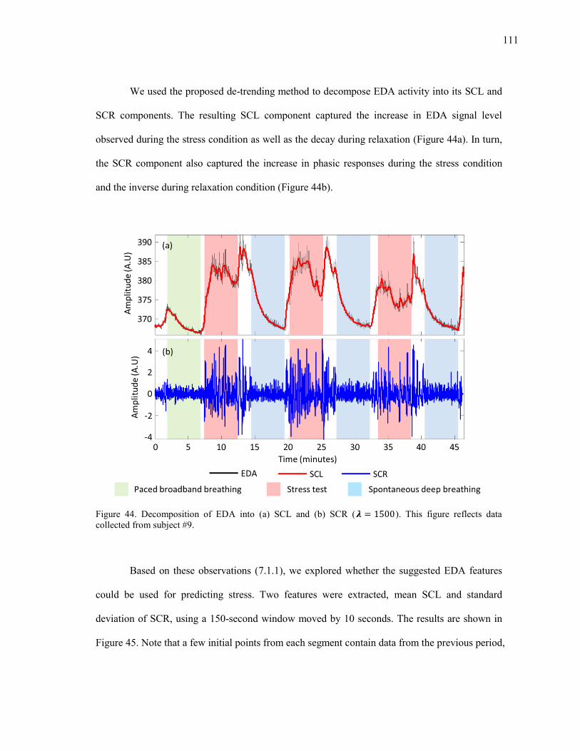
111
We used the proposed de-trending method to decompose EDA activity into its SCL and
SCR components. The resulting SCL component captured the increase in EDA signal level
observed during the stress condition as well as the decay during relaxation (Figure 44a). In turn,
the SCR component also captured the increase in phasic responses during the stress condition
and the inverse during relaxation condition (Figure 44b).
Figure 44. Decomposition of EDA into (a) SCL and (b) SCR ( ). This figure reflects data collected from subject #9.
Based on these observations (7.1.1), we explored whether the suggested EDA features
could be used for predicting stress. Two features were extracted, mean SCL and standard
deviation of SCR, using a 150-second window moved by 10 seconds. The results are shown in
Figure 45. Note that a few initial points from each segment contain data from the previous period,
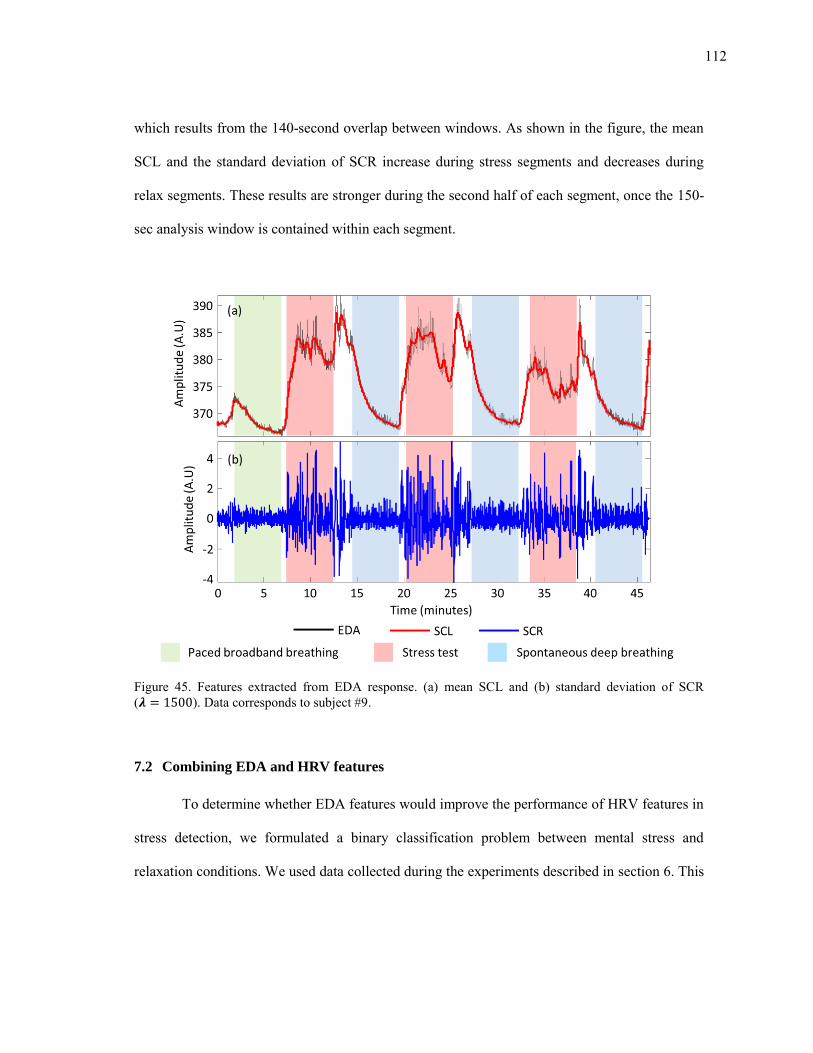
112
which results from the 140-second overlap between windows. As shown in the figure, the mean
SCL and the standard deviation of SCR increase during stress segments and decreases during
relax segments. These results are stronger during the second half of each segment, once the 150-
sec analysis window is contained within each segment.
Figure 45. Features extracted from EDA response. (a) mean SCL and (b) standard deviation of SCR ( ). Data corresponds to subject #9.
7.2 Combining EDA and HRV features
To determine whether EDA features would improve the performance of HRV features in
stress detection, we formulated a binary classification problem between mental stress and
relaxation conditions. We used data collected during the experiments described in section 6. This
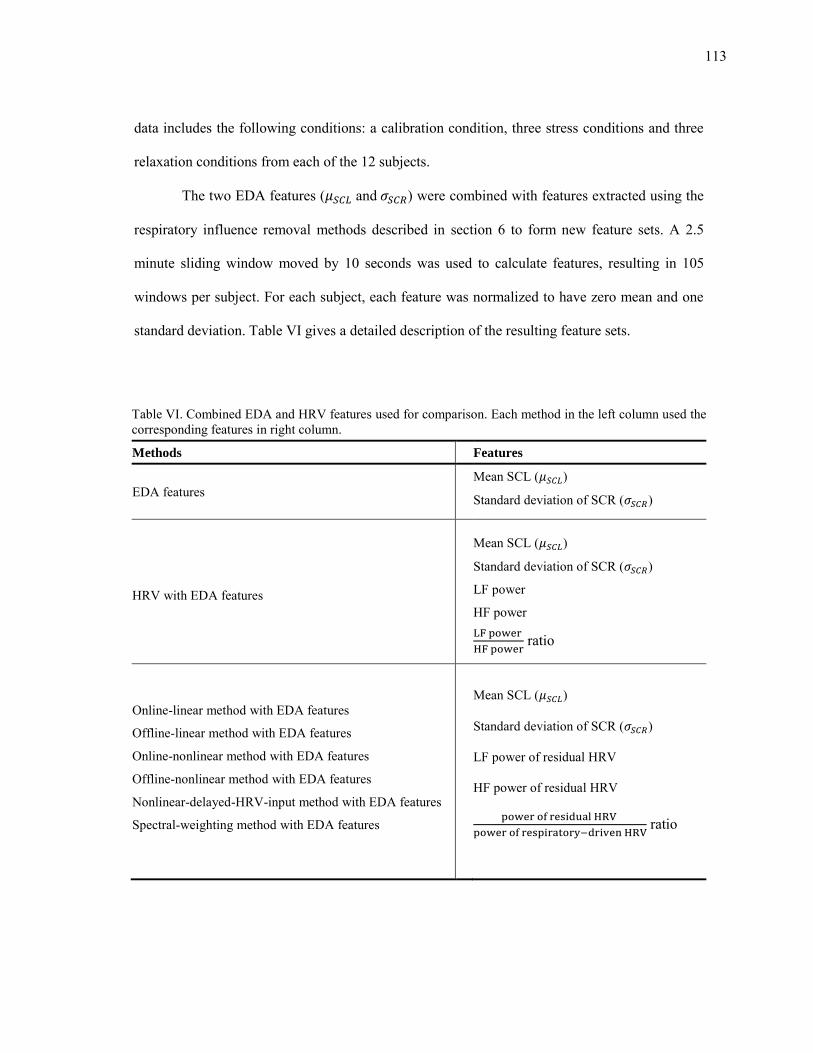
113
data includes the following conditions: a calibration condition, three stress conditions and three
relaxation conditions from each of the 12 subjects.
The two EDA features ( and ) were combined with features extracted using the
respiratory influence removal methods described in section 6 to form new feature sets. A 2.5
minute sliding window moved by 10 seconds was used to calculate features, resulting in 105
windows per subject. For each subject, each feature was normalized to have zero mean and one
standard deviation. Table VI gives a detailed description of the resulting feature sets.
Table VI. Combined EDA and HRV features used for comparison. Each method in the left column used the corresponding features in right column.
Methods Features
EDA features Mean SCL ( )
Standard deviation of SCR ( )
HRV with EDA features
Mean SCL ( )
Standard deviation of SCR ( )
LF power
HF power
ratio
Online-linear method with EDA features
Offline-linear method with EDA features
Online-nonlinear method with EDA features
Offline-nonlinear method with EDA features
Nonlinear-delayed-HRV-input method with EDA features
Spectral-weighting method with EDA features
Mean SCL ( )
Standard deviation of SCR ( )
LF power of residual HRV
HF power of residual HRV
ratio
114
For visualization purposes, we use PCA for dimensionality reduction for each feature
set. Figure 46 shows a scatterplot of the first two principal components for each feature set.
Although a clear boundary is not evident, the EDA features give some degree of separation
between the stress condition and relaxation condition. In Figure 46a, we also observe that the
stressor leads to an increase in and in comparison with the relaxation conditions. In
Figure 46b, we observe that the combination of EDA features with the traditional HRV features
improves the separation between the two conditions in comparison with the feature set
containing only the EDA features (Figure 46a). When we use features derived from the
respiratory influence removal methods, we observe a better separation between the two
conditions. Both the linear system identification methods (Figure 46c-d) and the nonlinear
dynamics decomposition methods (Figure 46e-f) separate the two conditions. When we apply the
broadband respiration signal to estimate model coefficients (offline method; Figure 46d and f),
both linear and nonlinear method show a better separation in comparison with their online
counterparts (Figure 46c and e). Overall, simple visual inspection of Figure 3 suggests that the
stress condition and relaxation conditions are most separable in the offline-nonlinear method
(Figure 46f).
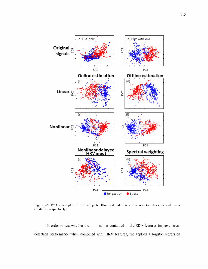
115
Figure 46. PCA score plots for 12 subjects. Blue and red dots correspond to relaxation and stress conditions respectively.
In order to test whether the information contained in the EDA features improve stress
detection performance when combined with HRV features, we applied a logistic regression
116
model using leave-two-out cross validation with data from 12 subjects (same as section 6). For
each combination of training and test set (66 unique splits), the logistic regression model
coefficients were estimated from the training data and used to estimate the probability for
samples in the test set. The results are summarized in Figure 47.
The average classification rate obtained using the features extracted from EDA and HRV
with EDA were 83.2% and 84.5%, respectively. We observed that the addition of EDA features
improved the performance of the respiration removal method by 4 – 8.5 %. The best
classification rates observed in section 6 (offline-nonlinear and offline-linear methods) were
increased from 85.2 and 89.2 % to 90.4 and 93.2%, respectively. The third best performance
from section 6, the spectral-weighting method, was improved from 81.5% to 88.1 %. This
improvement was observed on all previous methods including the poor performing methods
(nonlinear-delayed-HRV-input method).
In summary, adding EDA features improved performance for every respiratory influence
removal methods, which supports the notion that EDA captures complementary information that
can be used to identify stressful events.
.
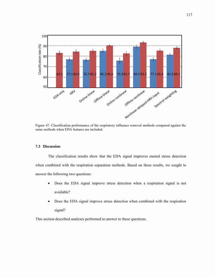
117
Figure 47. Classification performance of the respiratory influence removal methods compared against the same methods when EDA features are included.
7.3 Discussion
The classification results show that the EDA signal improves mental stress detection
when combined with the respiration separation methods. Based on these results, we sought to
answer the following two questions:
Does the EDA signal improve stress detection when a respiration signal is not
available?
Does the EDA signal improve stress detection when combined with the respiration
signal?
This section described analyses performed to answer to these questions.
118
Q1. Does the EDA signal improve stress detection when a respiration signal is not available?
Previously, we hypothesized that the respiratory signal would help improve the detection
of stress if respiratory influences were separated from HRV. In the results obtained in section 6,
the traditional HRV and nonlinear-delayed-HRV-input method were the only two methods that
did not use the respiration signal for mental stress detection; both methods showed the worst
classification performance.
Table VII summarizes results when both methods are combined with EDA features. In
both cases, the addition of EDA features yields a noticeable improvement in classification
performance, 7.4% for HRV and 8.2% for the nonlinear-delayed-HRV-input method. In order to
test the significance of this difference, we performed two sets of one-way ANOVA tests. The
first ANOVA test compared the classification performance of the combined EDA and traditional
HRV features against the traditional HRV features. The second ANOVA test compared the
classification performance of the combined EDA and nonlinear-delayed-HRV-input method
against the nonlinear-delayed-HRV-input method. The classification result of 66 splits were used
to verify the difference (n=66 for each group).
In Table VII, the ANOVA test result provides evidence of a significant difference in the
classification results for both HRV and nonlinear-delayed-HRV-input method. From these
results, we can infer that the EDA signal improves stress detection when it is combined with
HRV features, even in cases where the respiration signal is not available.
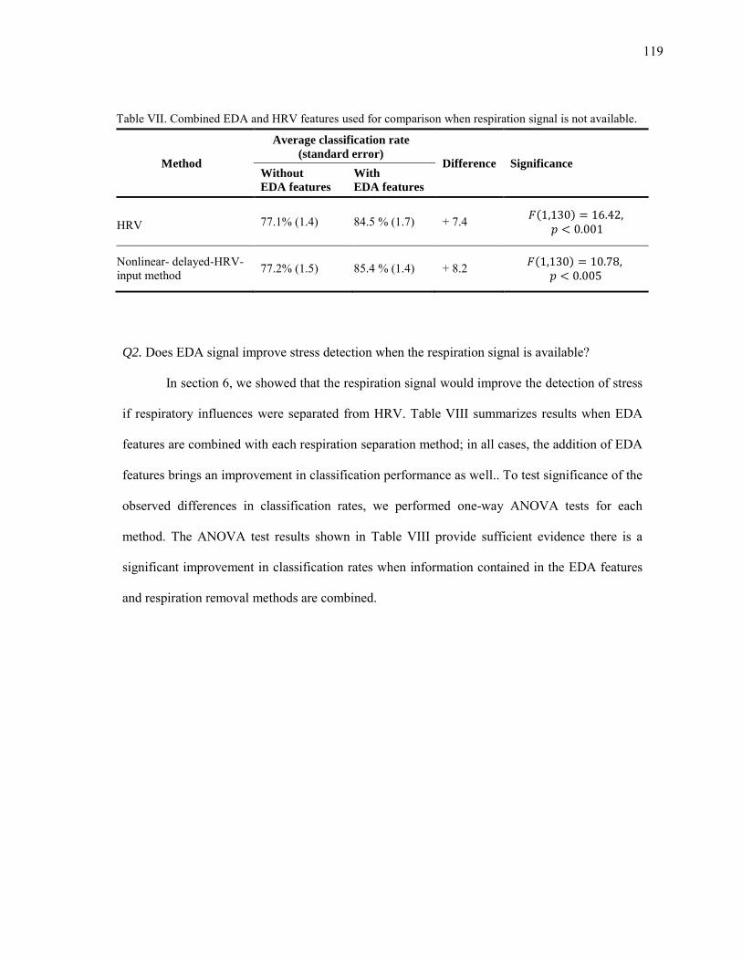
119
Table VII. Combined EDA and HRV features used for comparison when respiration signal is not available.
Method
Average classification rate
(standard error) Difference Significance
Without
EDA features
With
EDA features
HRV 77.1% (1.4) 84.5 % (1.7) + 7.4 ( )
Nonlinear- delayed-HRV-input method 77.2% (1.5) 85.4 % (1.4) + 8.2 ( )
Q2. Does EDA signal improve stress detection when the respiration signal is available?
In section 6, we showed that the respiration signal would improve the detection of stress
if respiratory influences were separated from HRV. Table VIII summarizes results when EDA
features are combined with each respiration separation method; in all cases, the addition of EDA
features brings an improvement in classification performance as well.. To test significance of the
observed differences in classification rates, we performed one-way ANOVA tests for each
method. The ANOVA test results shown in Table VIII provide sufficient evidence there is a
significant improvement in classification rates when information contained in the EDA features
and respiration removal methods are combined.
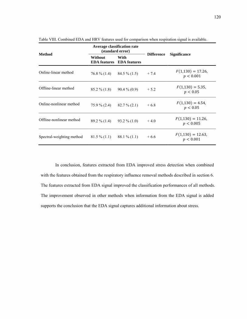
120
Table VIII. Combined EDA and HRV features used for comparison when respiration signal is available.
Method
Average classification rate
(standard error) Difference Significance
Without
EDA features
With
EDA features
Online-linear method 76.8 % (1.4) 84.5 % (1.5) + 7.4 ( )
Offline-linear method 85.2 % (1.8) 90.4 % (0.9) + 5.2 ( )
Online-nonlinear method 75.9 % (2.4) 82.7 % (2.1) + 6.8 ( )
Offline-nonlinear method 89.2 % (1.4) 93.2 % (1.0) + 4.0 ( )
Spectral-weighting method 81.5 % (1.1) 88.1 % (1.1) + 6.6 ( )
In conclusion, features extracted from EDA improved stress detection when combined
with the features obtained from the respiratory influence removal methods described in section 6.
The features extracted from EDA signal improved the classification performances of all methods.
The improvement observed in other methods when information from the EDA signal is added
supports the conclusion that the EDA signal captures additional information about stress.
121
8. CASE STUDIES: EXPERIMENTS AT TEXAS A&M UNIVERSITY AT
QATAR
This section gives an overview of the case studies that we performed in collaboration
with researchers from Texas A&M University at Qatar. The purpose of the case studies was to
verify the validity of wearable sensor prototype and signal processing methods. The section is
organized as follows. First, we describe a study performed in summer 2010 that was aimed at
classifying stress and relaxation conditions in laboratory settings. Next, we describe results from
a study performed in summer 2011, which was intended to classify stress and relaxation
conditions in ambulatory settings.
8.1 Study 1: Stress elicitation in laboratory settings
The purpose of this experiment was to recognize stress and relaxation conditions in
laboratory settings. Mental stress was elicited using a set of mental stress inducement tests. The
experiment was performed using the EDA, HRM, respiration, and EMG sensors. We collected
data from 10 subjects, and classification was performed using logistic regression by leave-one-
subject-out cross validation. After the experiments, the subjects were asked to provide feedback
regarding the comfort level of the wearable sensors for future improvement.
8.1.1 Experimental
The data collected for this experiment was grouped in two categories: mental stress and
relaxation. The stress condition consisted of a battery of tests. The tests included dual tracking
(DT), Stroop color word test (CT), memory search (MS), mirror tracing (MT), and public speech
122
(PS). The relaxation condition consisted of a deep breathing exercise (DB) where the subjects
were asked to breathe deeply at a pace of 0.1 Hz (slowly inhaling for 4 seconds followed by a
slowly exhaling for 6 seconds). A pacing auditory signal (a metronome with second ticks) was
played to help the subjects maintain breathing pace.
Dual tracking test (DT). At the beginning of this test, subjects were asked to memorize
three target letters. During the test, subjects were asked to track a moving target using the
computer mouse. While tracking the target, subjects were also required to click the left-mouse
button when one of three target letters was displayed on the screen. Distractor letters would also
appear during the experiment, which the subjects had to ignore. Subjects were provided
instantaneous visual feedback about their overall performance by means of three error bars
displayed on the screen. A screen shot of the dual tracking test is shown in Figure 48a.
Stroop color word test (CW): During this test, one of four words (red, green, blue, or
yellow) was displayed in different colored font. Subjects were asked to press one of four buttons,
each labeled with a color, in response to the color of the word being displayed. For example,
when presented with the word “red” in blue colored font, the subjects were expected to select the
button labeled as “blue”. A screen shot of the CW is shown in Figure 48b. Each word was
presented for 1000 ms, after which subjects had an additional 300 ms to respond; failure to
respond within the given response time (1300 ms) was equivalent to selecting the wrong button.
To increase difficulty, the test switched between two modes (congruent and incongruent) every
thirty seconds. In the congruent mode, each word expressing a specific color was displayed with
a matching color font, e.g., the word “red” was be displayed in red-colored font. In the
incongruent mode, the words were displayed in a different colored font, e.g., the word “blue”
would be displayed in red-colored font. Subjects were provided with instantaneous feedback on

123
their performance at the top of the screen. Subjects were asked to respond to questions by
pressing on the screen of a touchpad PC.
Figure 48. Stress protocols used to induce mental stress. (a) The subjects were asked to track a moving target in a computer screen using a mouse and to click whenever one of three target letters appeared on the screen. (b) The subjects were shown one of four words (red, green, blue, yellow) displayed in different ink colors, and had to press on one of four buttons according to the ink color. (c) The subjects were told to memorize a set of words presented in sequence, and then recall them under time pressure. (d) The subjects had to manually trace a pattern on a paper printout by looking through a mirror.
Memory search test (MS): During the MS, subjects were asked to memorize a sequence
of 5 target words. The experiment started by displaying each of the 5 target words individually
for duration of 1 second. Next, a matrix of 10 probe words was displayed, as shown Figure 48c.
The matrix contained a combination of 5 target words and 5 distractor words. To increase the

124
difficulty of the task, each distractor word was selected such that its spelling closely resembled
one of the target words. This word matrix was displayed for 5 seconds, and subjects were asked
to select those words that were members of the target word set. Subjects were allowed to select a
maximum of 5 letters and all selections were final. Each iteration in this process lasted 10
seconds and was repeated 30 times for making a total of 5 minutes. A touchpad PC was used for
this test as well.
Mirror-tracing test (MT): During this test, subjects were asked to trace the outline of a
shape (i.e. star) by hand while keeping the pencil within the boundaries of the outline. A
cardboard was used to block the subjects from having a direct view of their hand, who instead
could only see the reflection of their hand in a mirror (see Figure 48d). Once the tracing began,
the subjects were not allowed to lift pencil off the drawing paper at any time. If the pencil
exceeded the given line boundaries (boundary error), the subjects were told to bring it back
within the lines and as close as possible to the point where exited. All subjects used the same
starting shape in Figure 48d, but subsequent shapes were selected at random.
Public speech test (PS): During the test, subjects were asked to prepare a short speech on
a topic (3 min), deliver the speech to an audience (4 min), and address questions (3 min).
Subjects were asked to deliver speeches for opposite sides of the argument (2 minutes for each),
one in favor of and one against the following topic: "In many countries people no longer wear
their national costumes. People should be encouraged to wear their costumes every day."
Subjects were asked to use the 4 minutes delivery time in full. The target audience made up of
two people: one with a pro stance on the topic and the other with against stance on the topic.
Each member of the audience was provided with questions corresponding to their side of the
argument. Members of the audience were asked to question each subject in a cold demeanor,
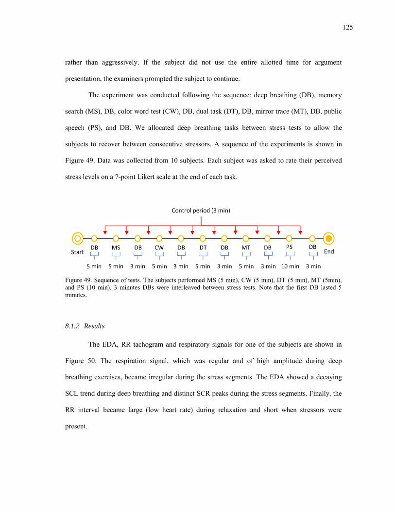
125
rather than aggressively. If the subject did not use the entire allotted time for argument
presentation, the examiners prompted the subject to continue.
The experiment was conducted following the sequence: deep breathing (DB), memory
search (MS), DB, color word test (CW), DB, dual task (DT), DB, mirror trace (MT), DB, public
speech (PS), and DB. We allocated deep breathing tasks between stress tests to allow the
subjects to recover between consecutive stressors. A sequence of the experiments is shown in
Figure 49. Data was collected from 10 subjects. Each subject was asked to rate their perceived
stress levels on a 7-point Likert scale at the end of each task.
Figure 49. Sequence of tests. The subjects performed MS (5 min), CW (5 min), DT (5 min), MT (5min), and PS (10 min). 3 minutes DBs were interleaved between stress tests. Note that the first DB lasted 5 minutes.
8.1.2 Results
The EDA, RR tachogram and respiratory signals for one of the subjects are shown in
Figure 50. The respiration signal, which was regular and of high amplitude during deep
breathing exercises, became irregular during the stress segments. The EDA showed a decaying
SCL trend during deep breathing and distinct SCR peaks during the stress segments. Finally, the
RR interval became large (low heart rate) during relaxation and short when stressors were
present.
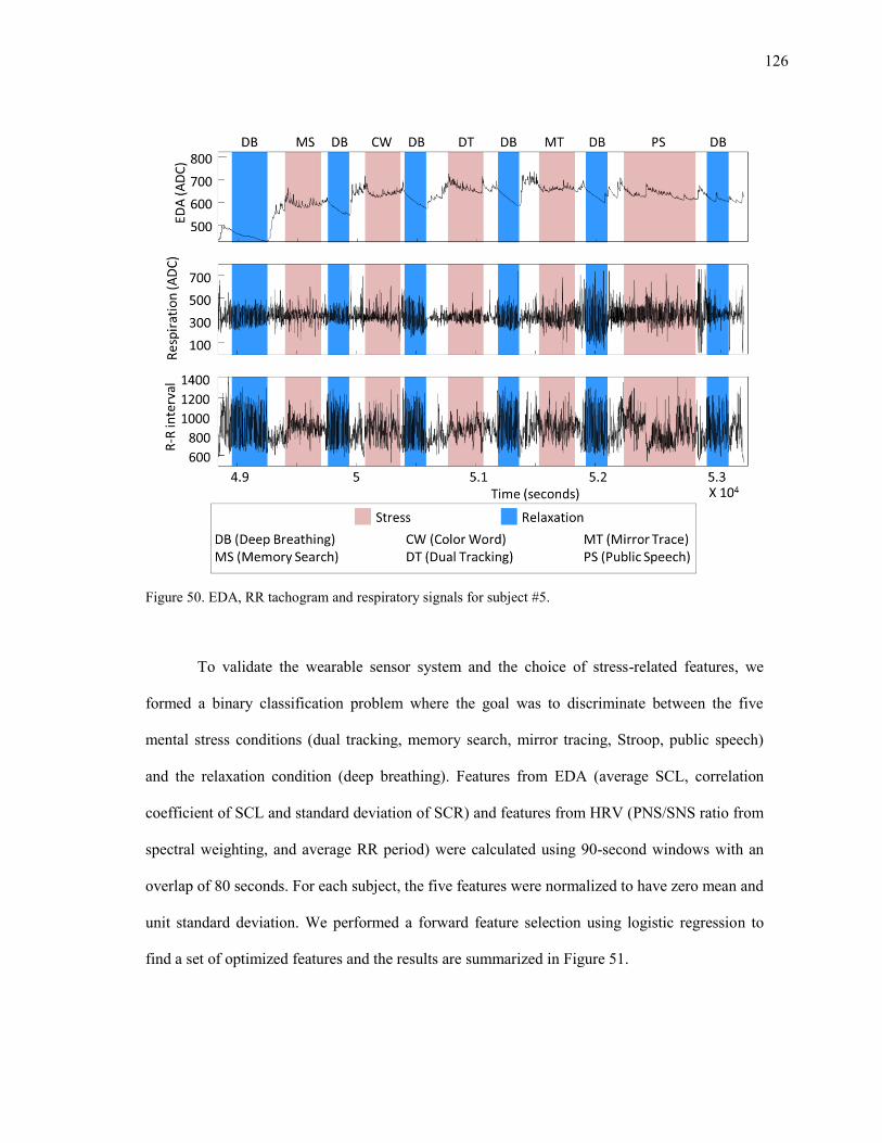
126
Figure 50. EDA, RR tachogram and respiratory signals for subject #5.
To validate the wearable sensor system and the choice of stress-related features, we
formed a binary classification problem where the goal was to discriminate between the five
mental stress conditions (dual tracking, memory search, mirror tracing, Stroop, public speech)
and the relaxation condition (deep breathing). Features from EDA (average SCL, correlation
coefficient of SCL and standard deviation of SCR) and features from HRV (PNS/SNS ratio from
spectral weighting, and average RR period) were calculated using 90-second windows with an
overlap of 80 seconds. For each subject, the five features were normalized to have zero mean and
unit standard deviation. We performed a forward feature selection using logistic regression to
find a set of optimized features and the results are summarized in Figure 51.
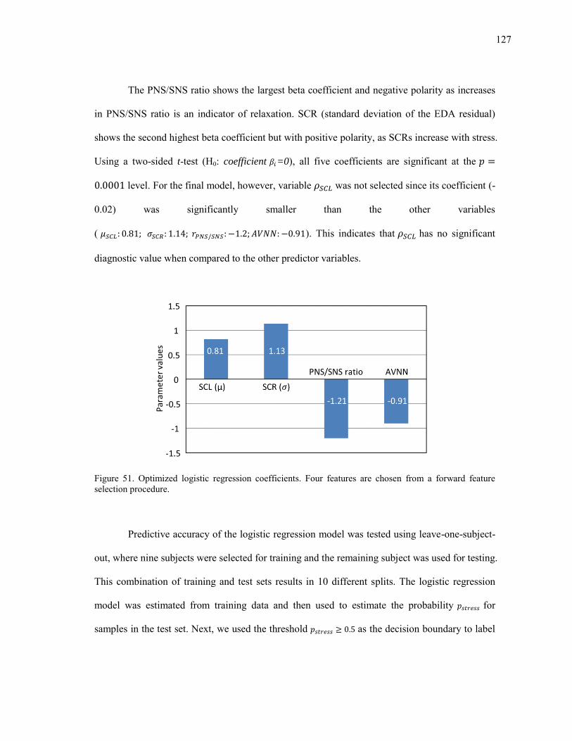
127
The PNS/SNS ratio shows the largest beta coefficient and negative polarity as increases
in PNS/SNS ratio is an indicator of relaxation. SCR (standard deviation of the EDA residual)
shows the second highest beta coefficient but with positive polarity, as SCRs increase with stress.
Using a two-sided t-test (H0: coefficient =0), all five coefficients are significant at the
level. For the final model, however, variable was not selected since its coefficient (-
0.02) was significantly smaller than the other variables
( ). This indicates that has no significant
diagnostic value when compared to the other predictor variables.
Figure 51. Optimized logistic regression coefficients. Four features are chosen from a forward feature selection procedure.
Predictive accuracy of the logistic regression model was tested using leave-one-subject-
out, where nine subjects were selected for training and the remaining subject was used for testing.
This combination of training and test sets results in 10 different splits. The logistic regression
model was estimated from training data and then used to estimate the probability for
samples in the test set. Next, we used the threshold as the decision boundary to label
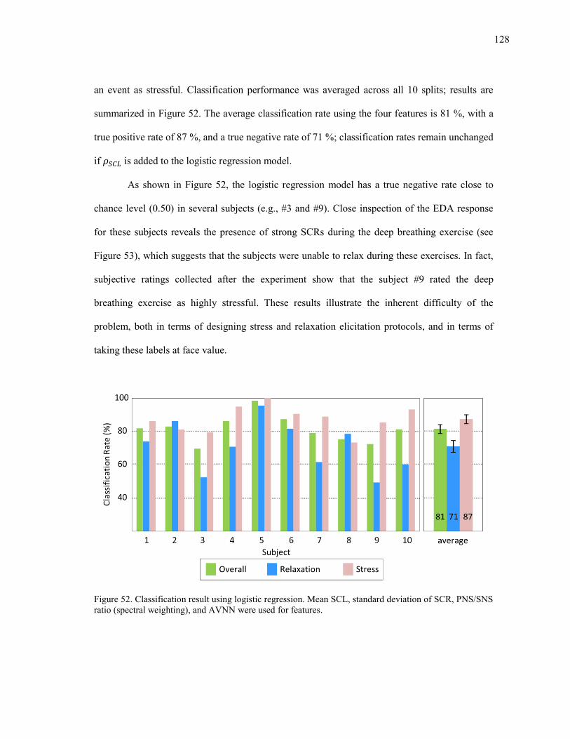
128
an event as stressful. Classification performance was averaged across all 10 splits; results are
summarized in Figure 52. The average classification rate using the four features is 81 %, with a
true positive rate of 87 %, and a true negative rate of 71 %; classification rates remain unchanged
if is added to the logistic regression model.
As shown in Figure 52, the logistic regression model has a true negative rate close to
chance level (0.50) in several subjects (e.g., #3 and #9). Close inspection of the EDA response
for these subjects reveals the presence of strong SCRs during the deep breathing exercise (see
Figure 53), which suggests that the subjects were unable to relax during these exercises. In fact,
subjective ratings collected after the experiment show that the subject #9 rated the deep
breathing exercise as highly stressful. These results illustrate the inherent difficulty of the
problem, both in terms of designing stress and relaxation elicitation protocols, and in terms of
taking these labels at face value.
Figure 52. Classification result using logistic regression. Mean SCL, standard deviation of SCR, PNS/SNS ratio (spectral weighting), and AVNN were used for features.
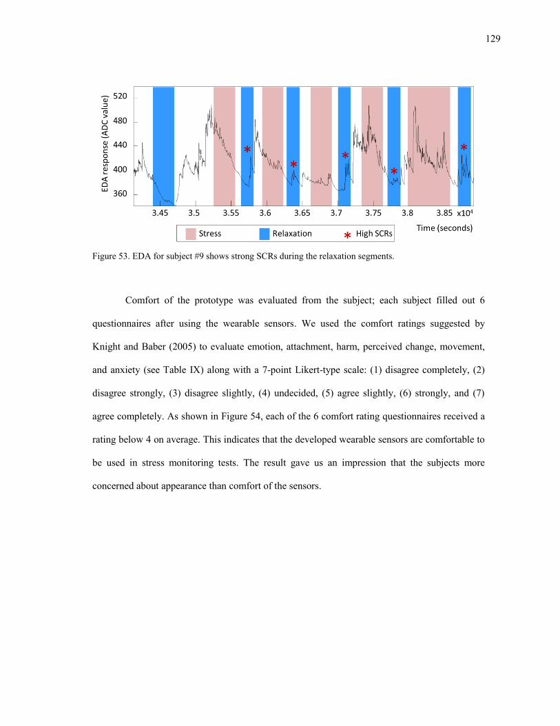
129
Figure 53. EDA for subject #9 shows strong SCRs during the relaxation segments.
Comfort of the prototype was evaluated from the subject; each subject filled out 6
questionnaires after using the wearable sensors. We used the comfort ratings suggested by
Knight and Baber (2005) to evaluate emotion, attachment, harm, perceived change, movement,
and anxiety (see Table IX) along with a 7-point Likert-type scale: (1) disagree completely, (2)
disagree strongly, (3) disagree slightly, (4) undecided, (5) agree slightly, (6) strongly, and (7)
agree completely. As shown in Figure 54, each of the 6 comfort rating questionnaires received a
rating below 4 on average. This indicates that the developed wearable sensors are comfortable to
be used in stress monitoring tests. The result gave us an impression that the subjects more
concerned about appearance than comfort of the sensors.
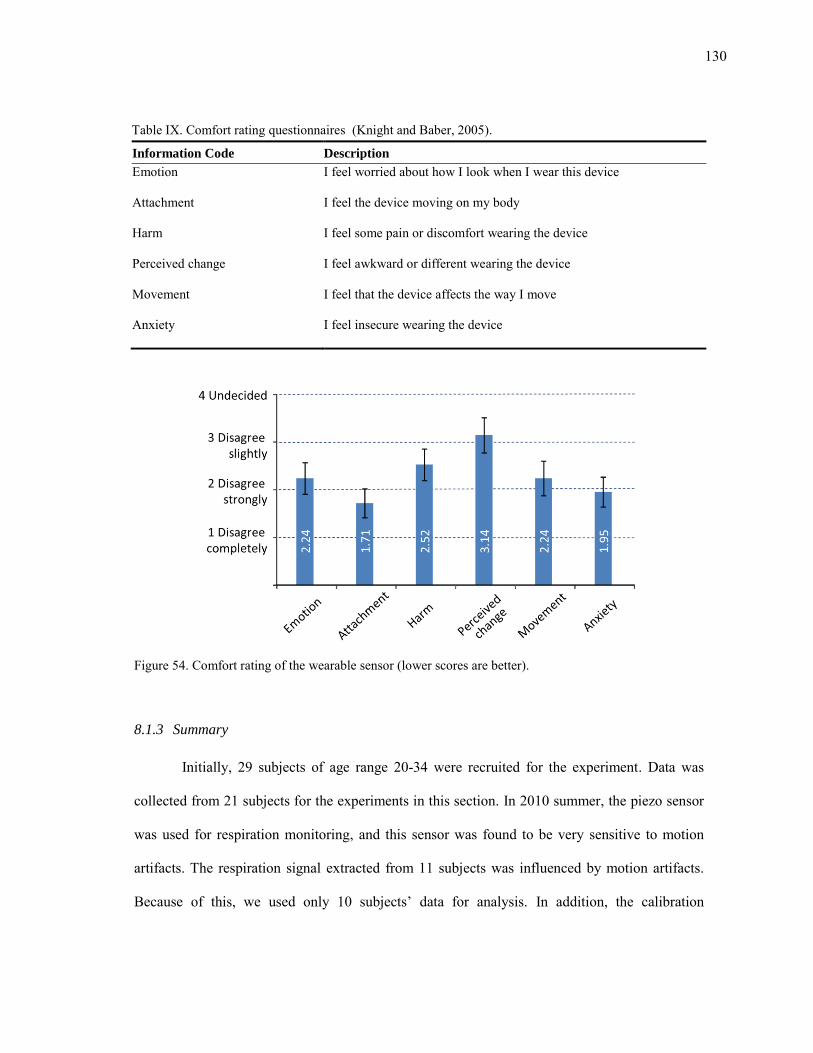
130
Table IX. Comfort rating questionnaires (Knight and Baber, 2005).
Information Code Description
Emotion I feel worried about how I look when I wear this device
Attachment I feel the device moving on my body
Harm I feel some pain or discomfort wearing the device
Perceived change I feel awkward or different wearing the device
Movement I feel that the device affects the way I move
Anxiety I feel insecure wearing the device
Figure 54. Comfort rating of the wearable sensor (lower scores are better).
8.1.3 Summary
Initially, 29 subjects of age range 20-34 were recruited for the experiment. Data was
collected from 21 subjects for the experiments in this section. In 2010 summer, the piezo sensor
was used for respiration monitoring, and this sensor was found to be very sensitive to motion
artifacts. The respiration signal extracted from 11 subjects was influenced by motion artifacts.
Because of this, we used only 10 subjects’ data for analysis. In addition, the calibration
131
procedure for the piezo respiration sensor was tedious and time consuming. After this experience,
we replaced the piezo sensor with a pressure sensor described in section 4.214.
8.2 Study 2: Stress elicitation in ambulatory settings and removal of subject-to-subject
variation
The objective of this study 2 was to detect stress in ambulatory settings. The experiment
was performed during the summer 2011 in Doha, Qatar and used EDA, HRM, and respiration
sensors. In this section, we suggest two methods to remove subject-to-subject variation in
ambulatory settings for improved stress detection: orthogonal signal correction (OSC) and linear
discriminant analysis (LDA). The section is organized as follows. An overview of the
ambulatory experiment is given, followed by the results obtained from ambulatory stress
monitoring. Then, two methods for subject-to-subject variation removal are described in detail.
Finally, the section concludes with an analysis of the classification results of both methods.
8.2.1 Experimental
The purpose of this experiment was to recognize stress and relaxation conditions in
ambulatory settings. We collected data from 13 subjects under three experimental conditions: a
hard CWT, an easy CWT and a relaxation exercise. Subjects were outfitted with the wearable
sensors in the morning by the experimenter. After calibration, subjects were asked to perform
each test in a controlled lab environment. Then subjects were allowed to leave the lab, and
resumed their respective regular daily activities. During the day, the subjects were asked to
perform three tasks two additional times (a randomly selected time in the morning and a
14 We compared piezo sensor and pressure sensors in section 4.5.3.
132
randomly selected time in the afternoon). The experiment was scheduled from 8:30 AM and 4:30
PM.
The test was conducted using mobile applications developed for Android™ smartphones
(Figure 55). Subjects were given a mobile phone to carry with them for the duration of the
experiment. During the easy CWT (Figure 55b), the device displayed a rectangle painted with
red, green, blue, or yellow colors. The subjects were asked to respond within the allotted time (7
seconds) by selecting the correct color. This test was designed to be less stressful (no beeping
sounds or other distractions were presented to the user). The hard CWT and relaxation
application used for this experiment were similar to the tests used in section 6 (Figure 55c and
Figure 55d). After each test, each subject was asked to complete a self-reporting questionnaire
about the environment in which the test was taken (Figure 55e) and the difficulty of the test
(Figure 55f).
Subjects were also asked to complete the self-reporting questionnaire 20 times during
the course of the day. The questionnaires were randomly scheduled (3 per hour), and notified to
the subject using an Android phone .
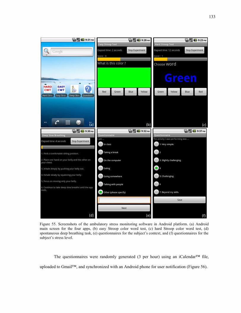
133
Figure 55. Screenshots of the ambulatory stress monitoring software in Android platform. (a) Android main screen for the four apps, (b) easy Stroop color word test, (c) hard Stroop color word test, (d) spontaneous deep breathing task, (e) questionnaires for the subject’s context, and (f) questionnaires for the
subject’s stress level.
The questionnaires were randomly generated (3 per hour) using an iCalendar™ file,
uploaded to Gmail™, and synchronized with an Android phone for user notification (Figure 56).
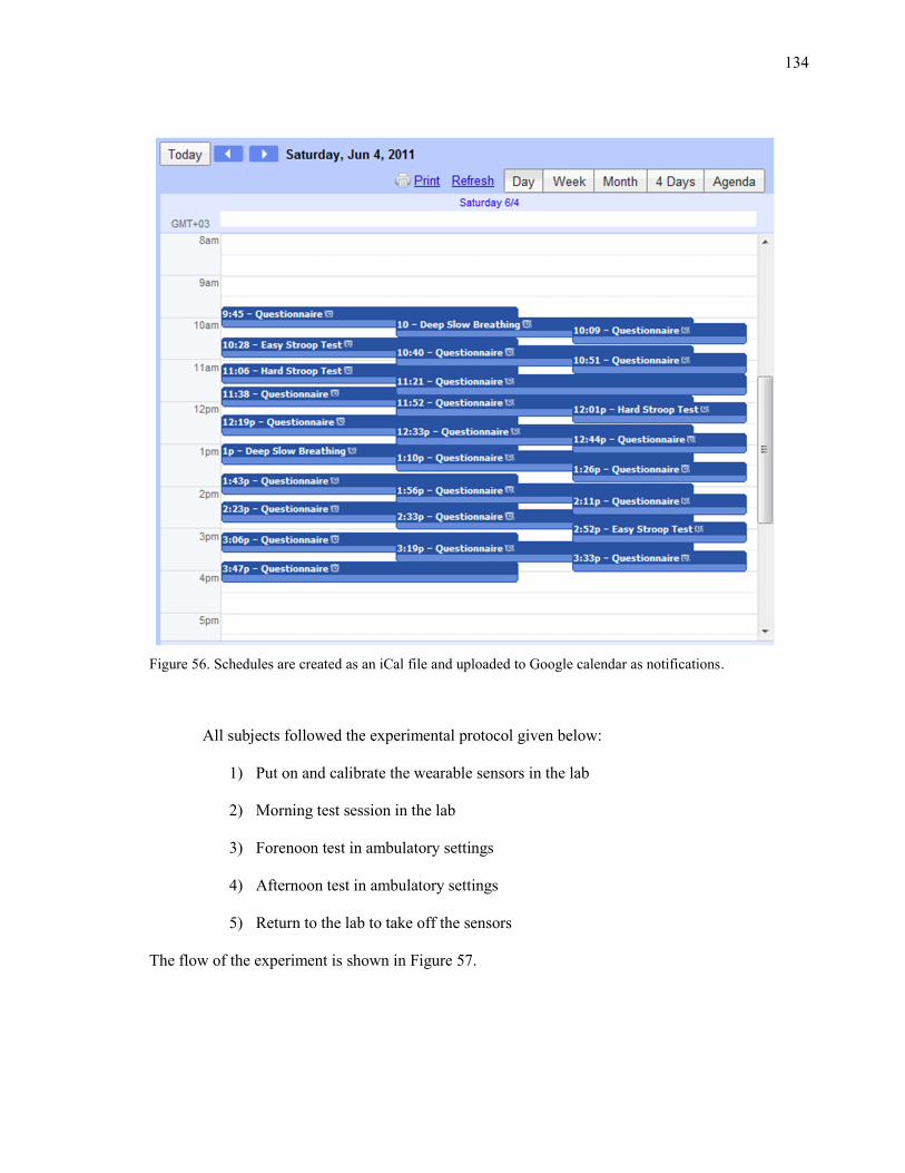
134
Figure 56. Schedules are created as an iCal file and uploaded to Google calendar as notifications.
All subjects followed the experimental protocol given below:
1) Put on and calibrate the wearable sensors in the lab
2) Morning test session in the lab
3) Forenoon test in ambulatory settings
4) Afternoon test in ambulatory settings
5) Return to the lab to take off the sensors
The flow of the experiment is shown in Figure 57.
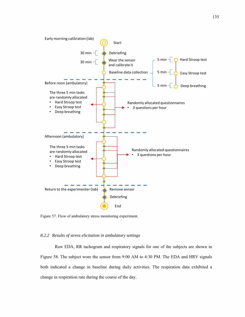
135
Figure 57. Flow of ambulatory stress monitoring experiment.
8.2.2 Results of stress elicitation in ambulatory settings
Raw EDA, RR tachogram and respiratory signals for one of the subjects are shown in
Figure 58. The subject wore the sensor from 9:00 AM to 4:30 PM. The EDA and HRV signals
both indicated a change in baseline during daily activities. The respiration data exhibited a
change in respiration rate during the course of the day.
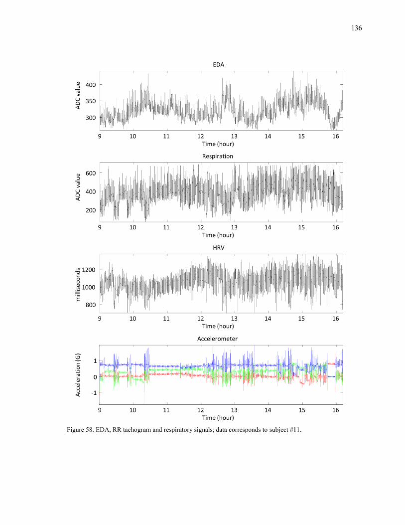
136
Figure 58. EDA, RR tachogram and respiratory signals; data corresponds to subject #11.
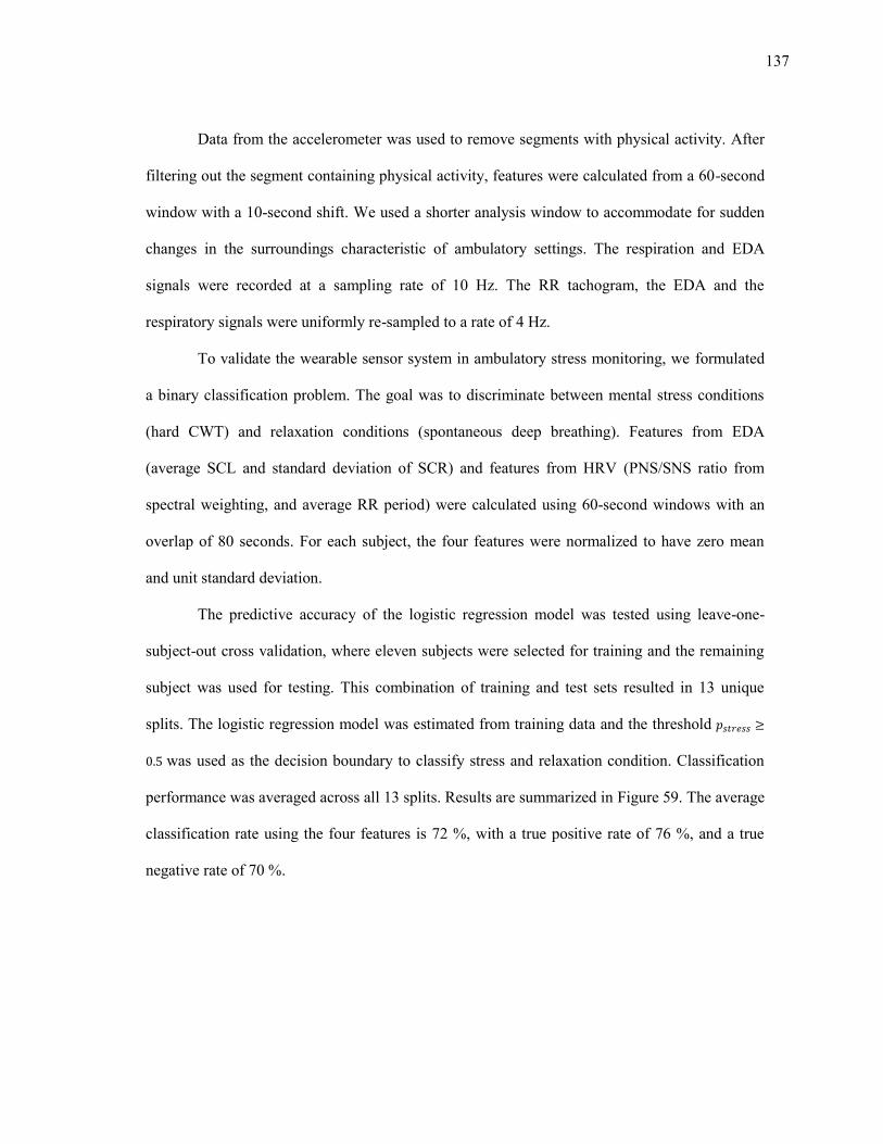
137
Data from the accelerometer was used to remove segments with physical activity. After
filtering out the segment containing physical activity, features were calculated from a 60-second
window with a 10-second shift. We used a shorter analysis window to accommodate for sudden
changes in the surroundings characteristic of ambulatory settings. The respiration and EDA
signals were recorded at a sampling rate of 10 Hz. The RR tachogram, the EDA and the
respiratory signals were uniformly re-sampled to a rate of 4 Hz.
To validate the wearable sensor system in ambulatory stress monitoring, we formulated
a binary classification problem. The goal was to discriminate between mental stress conditions
(hard CWT) and relaxation conditions (spontaneous deep breathing). Features from EDA
(average SCL and standard deviation of SCR) and features from HRV (PNS/SNS ratio from
spectral weighting, and average RR period) were calculated using 60-second windows with an
overlap of 80 seconds. For each subject, the four features were normalized to have zero mean
and unit standard deviation.
The predictive accuracy of the logistic regression model was tested using leave-one-
subject-out cross validation, where eleven subjects were selected for training and the remaining
subject was used for testing. This combination of training and test sets resulted in 13 unique
splits. The logistic regression model was estimated from training data and the threshold
was used as the decision boundary to classify stress and relaxation condition. Classification
performance was averaged across all 13 splits. Results are summarized in Figure 59. The average
classification rate using the four features is 72 %, with a true positive rate of 76 %, and a true
negative rate of 70 %.
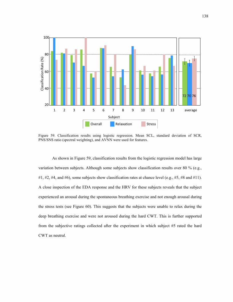
138
Figure 59. Classification results using logistic regression. Mean SCL, standard deviation of SCR, PNS/SNS ratio (spectral weighting), and AVNN were used for features.
As shown in Figure 59, classification results from the logistic regression model has large
variation between subjects. Although some subjects show classification results over 80 % (e.g.,
#1, #2, #4, and #6), some subjects show classification rates at chance level (e.g., #5, #8 and #11).
A close inspection of the EDA response and the HRV for these subjects reveals that the subject
experienced an arousal during the spontaneous breathing exercise and not enough arousal during
the stress tests (see Figure 60). This suggests that the subjects were unable to relax during the
deep breathing exercise and were not aroused during the hard CWT. This is further supported
from the subjective ratings collected after the experiment in which subject #5 rated the hard
CWT as neutral.
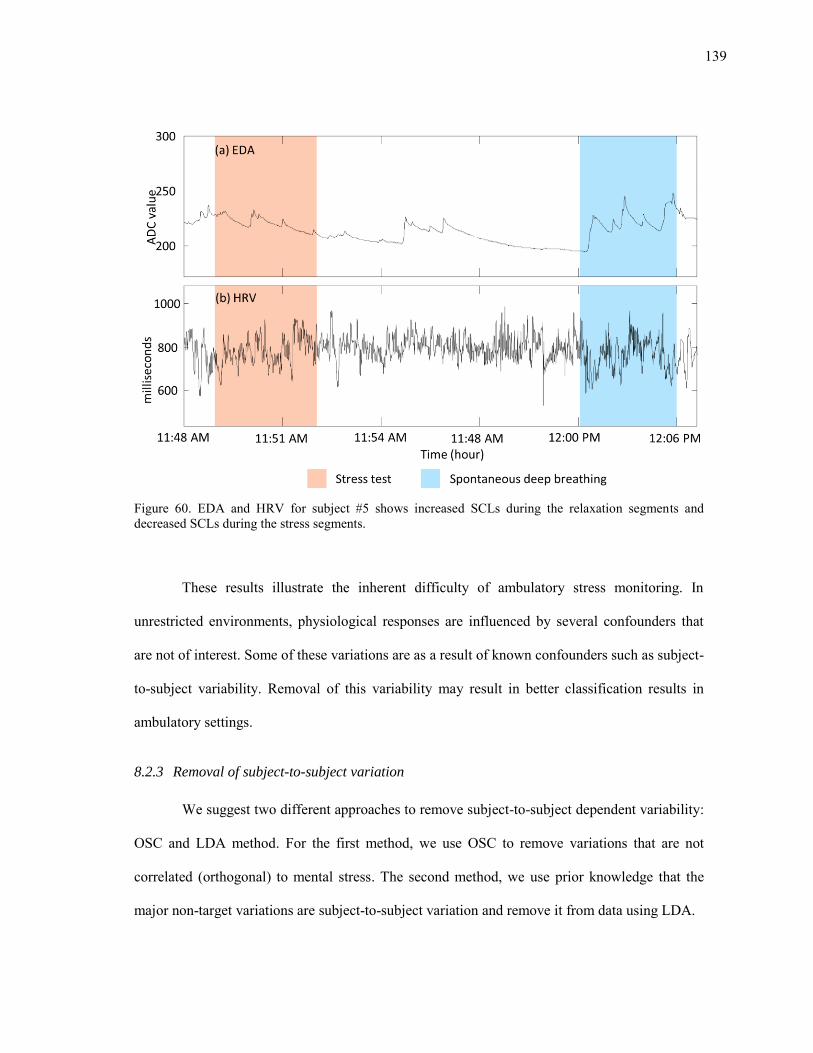
139
Figure 60. EDA and HRV for subject #5 shows increased SCLs during the relaxation segments and decreased SCLs during the stress segments.
These results illustrate the inherent difficulty of ambulatory stress monitoring. In
unrestricted environments, physiological responses are influenced by several confounders that
are not of interest. Some of these variations are as a result of known confounders such as subject-
to-subject variability. Removal of this variability may result in better classification results in
ambulatory settings.
8.2.3 Removal of subject-to-subject variation
We suggest two different approaches to remove subject-to-subject dependent variability:
OSC and LDA method. For the first method, we use OSC to remove variations that are not
correlated (orthogonal) to mental stress. The second method, we use prior knowledge that the
major non-target variations are subject-to-subject variation and remove it from data using LDA.

140
Orthogonal Signal Correction based method: OSC is a preprocessing technique used for
removing systematic variations, which are unrelated (orthogonal) to the target variables ( ),
from data ( ) (Wold et al., 1998). If we assume that data contains both orthogonal variations
( ) and correlated variations ( ) to the target variables (Y), we can express as following:
(35)
If we represent as a product of scores ( ) and loadings ( ), can be represented
as follows:
(36)
The OSC method, introduced by Wold et al. (1998), identifies using an iterative procedure.
Initially any suitable vector ‘t’ can be orthogonalized to Y as shown below:
( ( ) )
( )
(37)
The initial is the first principal component (PC) score vector t in X, orthogonalized to .
After each iteration, the convergence is checked by comparing difference between the newly
predicted and the previous (Wold et al., 1998). The target value for is obtained
when this difference converges to a value below a predetermined threshold. Then we compute
the residual as using the equation below:
(38)
Linear Discriminant Analysis based method: In this method, we focus on removing the
variation of interest (subject variation) by projecting the physiological data onto a space that
maximizes difference between subjects. This can be achieved by performing a LDA

141
transformation using the subject ID as the class label. We perform a linear regression between
the transformed data and original data to estimate the subject-dependent variation. By
subtracting the variation estimate from the original data, the residual data is free from cross
subject variation. The LDA projection to maximize the subject variation is defined by the
following equation:
( ) (39)
where represents the data, represents the scores, and represents the loading. We define
the regression model between and as follows :
(40)
where is the linear regression coefficients. can be estimated by
( ) (( ) ( ))
( ) (41)
The residual acquired by subtracting is free from subject dependency:
(42)
8.2.4 Results of subject-to-subject variation removal
We tested the predictive accuracy of the subject variation removal algorithm using
leave-two-out cross-validation by selecting 11 subjects for training and the remaining two
subjects for testing. For each combination of training and test sets, a logistic regression classifier
was trained and tested on each split. The classification performances were averaged across the
78 splits; Figure 61 shows the classification results. The average classification rate before subject
variation removal was 70.7%. After the OSC subject variation removal, the average
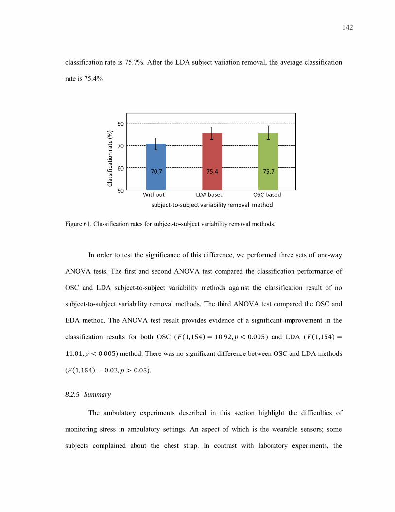
142
classification rate is 75.7%. After the LDA subject variation removal, the average classification
rate is 75.4%
Figure 61. Classification rates for subject-to-subject variability removal methods.
In order to test the significance of this difference, we performed three sets of one-way
ANOVA tests. The first and second ANOVA test compared the classification performance of
OSC and LDA subject-to-subject variability methods against the classification result of no
subject-to-subject variability removal methods. The third ANOVA test compared the OSC and
EDA method. The ANOVA test result provides evidence of a significant improvement in the
classification results for both OSC ( ( ) ) and LDA ( ( )
) method. There was no significant difference between OSC and LDA methods
( ( ) ).
8.2.5 Summary
The ambulatory experiments described in this section highlight the difficulties of
monitoring stress in ambulatory settings. An aspect of which is the wearable sensors; some
subjects complained about the chest strap. In contrast with laboratory experiments, the
143
ambulatory experiments required that the subjects wear the sensors for an extended period
(approximately 7.5 hours). We observed that after few hours, the stretchable fabric of the chest
strap loses tension. As a temporary solution, we used a medical tape to fix the strap on subjects’
chest. Future experiments will require an improved design of the chest strap.
In uncontrolled environments, data loss is inevitable because we are unable to control
subjects’ behavior during ambulatory experiments. In addition, physiological data in ambulatory
settings contains more variability than data in controlled laboratory settings. One of the known
reasons for this difference is the variability between subjects. To overcome this problem, we
explored the possibility of subject-to-subject variability removal. The results from removal of
subject-to-subject variability indicate that these methods can improve predictive power in stress
detection. The first method removed all components which are orthogonal to target variations of
interest. The second method removed major non-target variations leaving only target variations
of interest.
144
9. DISCUSSION AND CONCLUSION
The studies in this dissertation lie at the intersection of several disciplines, including
sensors, embedded systems, psychophysiology, biomedical signal processing, and pattern
recognition. Its focus has been the development of wearable sensors and signal processing
methods for detection of mental stress.
The contributions of this dissertation are three-fold. First, we have developed a wearable
sensor system prototype that can be used to detect mental stress in ambulatory settings. As part
of the system, we designed a number of wireless sensor nodes (EDA, respiration, HRM, and
EMG) and integrated them with a centralized holster unit. The system design was guided by the
need to find a balance between information content and user comfort, to allow subjects to
perform daily activities outside a laboratory environment. The reliability of the physiological
signals obtained from the prototype was validated against commercially-available sensors.
The second contribution of this dissertation has been the development of methods to
reduce respiratory influences in HRV. We hypothesized that if the respiratory influences on
HRV could be removed, the residual HRV will make stress-driven responses more salient in
comparison with raw HRV. Based on this hypothesis, we have developed three signal processing
methods (the linear system identification method, the nonlinear system dynamics decomposition
method, and the spectral weighting method) to separate HRV into a respiration-driven
component and a residual, stress salient component. Each method was thoroughly tested on
mental stress classification problems.
145
The third contribution lies in multiple case studies that were performed to evaluate the
sensor system and stress indices; as part of these studies, we evaluated a number of stress
elicitation methods and tested the system in laboratory as well as ambulatory settings.
To test our working hypothesis, which stated that separating HRV into the respiratory-
driven and residual HRV would improve stress detection, we developed three signal processing
methods. Using logistic regression for classification, the traditional HRV analysis can
discriminate stress and relaxation conditions with a 77.1 % success rate across subjects. In
contrast, the suggested linear system identification method, nonlinear dynamics decomposition
method, and the spectral weighting method provide classification rates of 85.2 %, 89.2 %, and
81.5 % respectively. Both linear and nonlinear methods yield optimal performance when the
coefficients are estimated using a broadband respiration signal.
Our studies also indicate that classification performance can be improved by combining
EDA features with those obtained from the respiratory influence separation methods. Our
experimental results show that the EDA signal can discriminate between stress and relaxation
conditions with 83.2% success rate. When these features are combined with traditional HRV
analysis, the resulting classification was 84.5%. This result indicates an improvement of 7.4% to
the classification rate for raw HRV but only a 1.3% improvement to EDA. The poor
improvement is as a result of the influence of breathing on raw HRV. The respiratory influence
imposed on the LF HRV bands degrades the performance of HRV. In contrast, breathing
influence did not degrade the performance of EDA. As a result, EDA showed better
classification rates than HRV in our experiments, and HRV did not help EDA features.
In contrast, when EDA features are combined with those from the respiratory influence
separation methods, classification rates increase to 90.4 % for the linear system identification
method, 93.2 % for the nonlinear dynamics decomposition method and 88.1 % for the spectral
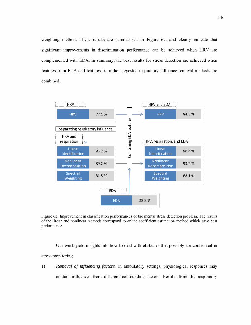
146
weighting method. These results are summarized in Figure 62, and clearly indicate that
significant improvements in discrimination performance can be achieved when HRV are
complemented with EDA. In summary, the best results for stress detection are achieved when
features from EDA and features from the suggested respiratory influence removal methods are
combined.
Figure 62. Improvement in classification performances of the mental stress detection problem. The results of the linear and nonlinear methods correspond to online coefficient estimation method which gave best performance.
Our work yield insights into how to deal with obstacles that possibly are confronted in
stress monitoring.
1) Removal of influencing factors. In ambulatory settings, physiological responses may
contain influences from different confounding factors. Results from the respiratory

147
influence removal methods and the subject-to-subject variability removal methods show
that we can minimize the effects of some confounding factors that may degrade the
ability to detect stress. This scheme possibly extended to other confounders such as
physical activity in the level of signal (i.e., the respiratory influence removal method) or
feature (i.e., the subject-to-subject variability removal methods).
2) Classification across subjects. A large volume of training data is necessary to
understand the mental state of a person. However, collecting this training data from a
single person requires a lot of time and effort. To deal with this problem, we need to be
able detect a person’s mental state using not only his/her training data but also training
data obtained from other subjects. We believe this can be achieved by normalizing the
data and removing confounding factors that are of no interest. Our classification results
provide preliminary evidence to support this claim, where stress and relaxation
conditions were classified across subjects.
We believe that monitoring of stress has the potential to transform long-term management of our
mental health. The suggested hardware and signal processing methods can potentially be used to
achieve this goal.
9.1 Future work
Wearable sensors and respiratory influence removal methods can potentially be used for
stress detection during regular daily activities. Future expansion on this work can be categorized
in two: hardware and signal processing. The hardware used for data collection can be redesigned
to improve user comfort and experience as follows:
Improve calibration procedures. The current prototype requires a lengthy calibration
procedure that the experimenter needs to perform prior to each experiment. Errors
148
during the calibration process result in noisy, often unusable data (i.e., saturation, small
gain, very low baseline). The calibration process can be improved in one of two ways:
simplification or automation. Simplifying the calibration process will make it possible
for the subject to perform the calibration independently. This can be achieved by
developing interactive software to guide the user during the calibration process. Then the
application verifies the calibrated sensor values and provides feedback to the user. The
respiration and EDA sensor module requires careful manual calibration of offset and
gain. Automation of the calibration process can eliminate the possibility of human errors,
and it can be achieved by an auto-calibration circuit that replaces each potentiometer
with a programmable resistor controlled by the microcontroller, so that both values can
be adjusted in real time.
Improve aesthetics. Feedback from subjects revealed the need for aesthetic
improvements for comfort and appearance. For instance, the chest strap for the prototype
tends to lose tension after a few hours of use. This caused discomfort to most subjects.
As shown in comfort rating scales in section 8.1.2, subjects worried about any perceived
change in personal appearance caused by the visible components (the holster unit worn
on the waist and the EDA electrodes worn on the hands). To improve user experience,
the next version of the prototype should make the holster unit smaller, provide a more
stable chest strap, and modifying the EDA electrodes to be less conspicuous by
integrating the electrodes and circuits into a fashionable wristband.
Sensor monitoring and control in real time. A smartphone may be used as a control
console for the wearable sensors. While we developed a Bluetooth-enabled holster unit
which can communicate with smartphones, in its present configuration the system only
offers clock synchronization between the holster unit and an Android™ smartphone. The
149
addition of real-time data visualization capabilities would provide subjects with
immediate biofeedback.
Signal processing improvements should focus on:
Improve the performance of the online methods. We observed that the offline methods,
which use broadband calibration signal to estimate coefficients, performed better than
online methods. If the broadband calibration signal is not available, it restricts the use of
offline methods. To improve the performance of the online method, we need a method to
prevent over fitting. First, the ratio between respiration-driven HRV and residual HRV
can be estimated using the spectral weighting method. This estimate can be used as a
weighting factor to reduce overestimation of respiratory influenced HRV in online
methods.

150
REFERENCES
Adams, J.A., 1996. Respiratory inductive plethysmography, In: Stocks, J., Sly, P.D., Tepper, R.S., Morgan W.J. (Eds.), Infant Respiratory Function Testing. John Wiley and Sons, Hoboken, NJ, pp. 139-163.
Adleman, N.E., Menon, V., Blasey, C.M., White, C.D., Warsofsky, I.S., Glover, G.H., Reiss, A.L., 2002. A developmental fMRI study of the Stroop color-word task. Neuroimage 16 (1), 61-75.
Ahern, S., Beatty, J., 1979. Pupillary responses during information processing vary with scholastic aptitude test scores. Science 205 (4412), 1289-1292.
Alexander, D.M., Trengove, C., Johnston, P., Cooper, T., August, J.P., Gordon, E., 2005. Separating individual skin conductance responses in a short interstimulus-interval paradigm. Journal of Neuroscience Methods 146 (1), 116-123.
Amaral, L.A.N., Goldberger, A.L., Ivanov, P.C., Stanley, H.E., 1999. Modeling heart rate variability by stochastic feedback. Computer Physics Communications 121 (1), 126-128.
Anliker, U., Ward, J., Lukowicz, P., Troster, G., Dolveck, F., Baer, M., Keita, F., Schenker, E., Catarsi, F., Coluccini, L., 2004. AMON: a wearable multiparameter medical monitoring and alert system. IEEE Transactions on Information Technology in Biomedicine 8 (4), 415-427.
Ashbrook, D., Starner, T., 2002, Learning significant locations and predicting user movement with GPS, In: IEEE International Symposium on Wearable Computers, pp. 101-108.
Ashbrook, D., Starner, T., 2003. Using GPS to learn significant locations and predict movement across multiple users. Personal and Ubiquitous Computing 7 (5), 275-286.
Backs, R.W., 2001. An autonomic space approach to the psychophysiological assessment of mental workload, In: Hancock, P., Desmond, P. (Eds.), Stress, Workload, and Fatigue Lawrence Erlbaum Associates, Mahwah, NJ, pp. 279-289.
Baddeley, A., 1968. A three-minute reasoning test based on grammatical transformation. Psychonomic Science 10 (10), 341-342.
Baddeley, A., 1992. Working memory. Science 255 (5044), 556-559.
Baek, J., Lee, G., Park, W., Yun, B.-J., 2004. Accelerometer signal processing for user activity detection, Lecture Notes in Computer Science 3215, 610-617.
Bansevicius, D., Westgaard, R.H., Jensen, C., 1997. Mental stress of long duration: EMG activity, perceived tension, fatigue, and pain development in pain free subjects. Headache: The Journal of Head and Face Pain 37 (8), 499-510.

151
Bao, L., Intille, S.S., 2004, Activity recognition from user-annotated acceleration data, In: International Conference on Pervasive Computing, pp. 1-17.
Barr, C., Naas, A., Freeman, M., Lang, C., Struthers, A., 1994. QT dispersion and sudden unexpected death in chronic heart failure. Lancet 343 (8893), 327-329.
Bench, C.J., Frith, C., Grasby, P., Friston, K., Paulesu, E., Frackowiak, R., Dolan, R., 1993. Investigations of the functional anatomy of attention using the Stroop test. Neuropsychologia 31 (9), 907-922.
Benedek, M., Kaernbach, C., 2010. Decomposition of skin conductance data by means of nonnegative deconvolution. Psychophysiology 47 (4), 647-658.
Berlad, I., Shlitner, A., Ben-Haim, S., Lavie, P., 1993. Power spectrum analysis and heart rate variability in stage 4 and REM sleep: evidence for state-specific changes in autonomic dominance. Journal of Sleep Research 2 (2), 88-90.
Bernardi, L., Wdowczyk-Szulc, J., Valenti, C., Castoldi, S., Passino, C., Spadacini, G., Sleight, P., 2000. Effects of controlled breathing, mental activity and mental stress with or without verbalization on heart rate variability. Journal of the American College of Cardiology 35 (6), 1462-1469.
Berntson, G.G., Cacioppo, J.T., Quigley, K.S., 1993a. Cardiac psychophysiology and autonomic space in humans: empirical perspectives and conceptual implications. Psychological Bulletin 114, 296-322.
Berntson, G.G.., Cacioppo, J.T., Quigley, K.S., 1993b. Respiratory sinus arrhythmia: autonomic origins, physiological mechanisms, and psychophysiological implications. Psychophysiology 30 (2), 183-196.
Berntson, G.G., Bigger, J.T., Eckberg, D.L., Grossman, P., Kaufmann, P.G., Malik, M., Nagaraja, H.N., Porges, S.W., Saul, J.P., Stone, P.H., Molen, M.W.V.D., 1997. Heart rate variability: origins, methods, and interpretive caveats. Psychophysiology 34 (6), 623-648.
Berntson, G.G., Quigley, K.S., Lozano, D., 2007. Cardiovascular psychophysiology, In: Cacioppo, J.T., Tassinary, L.G., Berntson, G. (Eds.), Handbook of Psychophysiology, 3ed. Cambridge University Press, Cambridge, UK, pp. 182-210.
Berry, J.O., Jones, W.H., 1995. The parental stress scale: initial psychometric evidence. Journal of Social and Personal Relationships 12 (3), 463-472.
Bishop, C.M., 2007. Pattern Recognition and Machine Learning, 2 ed. Springer, New York, NY, pp. 138-147.
Boer, L.C., 1995. Taskomat: Evaluation of a computerized test battery. International Journal of Selection and Assessment 3 (2), 105-114.
Bradley, M.M., Miccoli, L., Escrig, M.A., Lang, P.J., 2008. The pupil as a measure of emotional arousal and autonomic activation. Psychophysiology 45 (4), 602-607.

152
Breznitz, S., Goldberger, L., 1982. Stress research at a crossroads, In: Goldberger, L., Breznitz, S. (Eds.), Handbook of Stress: Theoretical and Clinical Aspects, 1 ed. Free Press, New York, NY, pp. 7-17.
Bunker, S.J., Colquhoun, D.M., Esler, M.D., Hickie, I.B., Hunt, D., Jelinek, V.M., Oldenburg, B.F., Peach, H.G., Ruth, D., Tennant, C.C., 2003. "Stress" and coronary heart disease: psychosocial risk factors. The Medical Journal of Australia 178 (6), 272-276.
Bussmann, J.B.J., Martens, W.L.J., Tulen, J.H.M., Schasfoort, F.C., Berg-Emons, H.J.G.V.D., Stam, H.J., 2001. Measuring daily behavior using ambulatory accelerometry: the activity monitor. Behavior Research Methods, Instruments, and Computers 33 (1), 349-356.
Butler, E., Wilhelm, F., Gross, J., 2006. Respiratory sinus arrhythmia, emotion, and emotion regulation during social interaction. Psychophysiology 43 (6), 612-622.
Cacioppo, J.T., Tassinary, L.G., 1990. Inferring psychological significance from physiological signals. The Americal Psychologist 45 (1), 16-28.
Cacioppo, J.T., Tassinary, L.G., Berntson, G., 2007. Psychological science: interdisciplinary approaches to classic questions about the mind, In: Cacioppo, J.T., Tassinary, L.G., Berntson, G. (Eds.), Handbook of Psychophysiology, 3ed. Cambridge University Press, Cambridge, UK, pp. 1-14.
Carlson, N., 1994. Physiology of Behavior. Allyn and Bacon, Needham Heights, MA, pp. 512-538.
Carney, R.M., Saunders, R.D., Freedland, K.E., Stein, P., Rich, M.W., Jaffe, A.S., 1995. Association of depression with reduced heart rate variability in coronary artery disease. The American Journal of Cardiology 76 (8), 562-564.
Carter, C.S., Mintun, M., Cohen, J.D., 1995. Interference and facilitation effects during selective attention: an H215O PET study of Stroop task performance. Neuroimage 2 (4), 264-272.
Chen, X., Mukkamala, R., 2008. Selective quantification of the cardiac sympathetic and parasympathetic nervous systems by multisignal analysis of cardiorespiratory variability. American Journal of Physiology - Heart and Circulatory Physiology 294 (1), 362-371.
Chon, K., Mullen, T., Cohen, R., 1996. A dual-input nonlinear system analysis of autonomic modulation of heart rate. IEEE Transactions on Biomedical Engineering 43 (5), 530-544.
Clow, A., Patel, S., Najafi, M., Evans, P., Hucklebridge, F., 1997. The cortisol response to psychological challenge is preceded by a transient rise in endogenous inhibitor of monoamine oxidase. Life Sciences 61 (5), 567-575.
Cobb, S., Rose, R., 1973. Hypertension, peptic ulcer, and diabetes in air traffic controllers. Journal of the American Medical Association 224 (4), 489-492.
Cohen, S., Kamarck, T., Mermelstein, R., 1983. A global measure of perceived stress. Journal of Health and Social Behavior 24 (4), 385-396.

153
Cohen, S., Tyrrell, D., Smith, A., 1993. Negative life events, perceived stress, negative affect, and susceptibility to the common cold. Journal of Personality and Social Psychology 64, 131-140.
Cushway, D., Tyler, P.A., Nolan, P., 1996. Development of a stress scale for mental health professionals. British Journal of Clinical Psychology 35 (2), 279-295.
Dawson, M.E., Nuechterlein, K.H., 1984. Psychophysiological dysfunctions in the developmental course of schizophrenic disorders. Schizophrenia Bulletin 10 (2), 204-232.
Dawson, M.E., Schell, A.M., Filion, D.L., 2007. The electrodermal system, In: Cacioppo, J.T., Tassinary, L.G., Berntson, G. (Eds.), Handbook of Psychophysiology, 3ed. Cambridge University Press, Cambridge, UK, pp. 159-181.
Deutsch, J.A., Deutsch, D., 1963. Attention: some theoretical considerations. Psychological Review 70 (1), 80-90.
DeVaul, R., Sung, M., Gips, J., Pentland, A., 2003, MIThril 2003: applications and architecture, In: IEEE International Symposium on Wearable Computers, pp. 4-11.
Dimsdale, J.E., Moss, J., 1980. Short-term catecholamine response to psychological stress. Psychosomatic Medicine 42 (5), 493-497.
Eckberg, D.L., 1983. Human sinus arrhythmia as an index of vagal cardiac outflow. Journal of Applied Physiology 54 (4), 961-966.
El-Sheikh, M., 2005. The role of emotional responses and physiological reactivity in the marital conflict–child functioning link. Journal of Child Psychology and Psychiatry 46 (11), 1191-1199.
Ellis, D.P.W., Lee, K., 2004, Features for segmenting and classifying long-duration recordings of "personal" audio, In: ISCA Tutorial and Research Workshop on Statistical and Perceptual Audio Processing.
Fletcher, R., Dobson, K., Goodwin, M., Eydgahi, H., Wilder-Smith, O., Fernholz, D., Kuboyama, Y., Hedman, E., Poh, M., Picard, R., 2009. iCalm: wearable sensor and network architecture for wirelessly communicating and logging autonomic activity. IEEE Transactions on Information Technology in Biomedicine 14 (2), 215-223.
Frantzidis, C., Konstantinidis, E., Pappas, C., Bamidis, P., 2009. An automated system for processing electrodermal activity. Studies in Health Technology and Informatics 150, 787-787.
Frazier, T., Strauss, M., Steinhauer, S., 2004. Respiratory sinus arrhythmia as an index of emotional response in young adults. Psychophysiology 41 (1), 75-83.
Fridlund, A.J., Schwartz, G.E., Fowler, S.C., 1984. Pattern recognition of self reported emotional state from multiple site facial EMG activity during affective imagery. Psychophysiology 21 (6), 622-637.

154
Fruin, M.L., Rrankin, J.W., 2004. Validity of a multi-sensor armband in estimating rest and exercise energy expenditure. Medicine and Science in Sports and Exercise 36 (6), 1063-1069.
Geddes, L., Hoff, H., Hickman, D., Moore, A., 1962. The impedance pneumography. Aerospace Medicine 33, 28-33.
Gemmell, J., Williams, L., Wood, K., Lueder, R., Bell, G., 2004, Passive capture and ensuing issues for a personal lifetime store, In: ACM Workshop on Continuous Archival and Retrieval of Personal Experences, pp. 48-55.
Gemperle, F., Kasabach, C., Stivoric, J., Bauer, M., Martin, R., 1998, Design for wearability, In: IEEE International Symposium on Wearable Computers, pp. 116-122.
George, M., Ketter, T., Parekh, P., Rosinsky, N., Ring, H., Casey, B., Trimble, M., Horwitz, B., Herscovitch, P., Post, R., 1993. Regional brain activity when selecting a response despite interference: an H215O PET study of the Stroop and an emotional Stroop. Human Brain Mapping 1 (3), 194-209.
Gillespie, B.L., Eisler, R.M., 1992. Development of the feminine gender role stress scale. Behavior Modification 16 (3), 426-438.
Goedhart, A.D., Van Der Sluis, S., Houtveen, J.H., Willemsen, G., De Geus, E.J.C., 2007. Comparison of time and frequency domain measures of RSA in ambulatory recordings. Psychophysiology 44 (2), 203-215.
Gray-Toft, P., Anderson, J.G., 1981. The nursing stress scale: development of an instrument. Journal of Psychopathology and Behavioral Assessment 3 (1), 11-23.
Gregoire, J., Tuck, S., Hughson, R., Yamamoto, Y., 1996. Heart rate variability at rest and exercise: influence of age, gender, and physical training. Applied Physiology, Nutrition, and Metabolism 21 (6), 455-470.
Grossman, P., 1983. Respiration, stress, and cardiovascular function. Psychophysiology 20 (3), 284-300.
Grossman, P., Svebak, S., 1987. Respiratory sinus arrhythmia as an index of parasympathetic cardiac control during active coping. Psychophysiology 24 (2), 228-235.
Hamilton, V., 1982. Cognition and stress: an information processing model, In: Goldberger, L., Breznitz, S. (Eds.), Handbook of Stress: Theoretical and Clinical Aspects, 1 ed. Free Press, New York, NY, pp. 156-189.
Hester, T., Hughes, R., Sherrill, D.M., Knorr, B., Akay, M., Stein, J., Bonato, P., 2006, Using wearable sensors to measure motor abilities following stroke, In: International Workshop on Wearable and Implantable Body Sensor Networks, pp. 4-8.
Hines, E.A., 1936. The cold pressor test for measuring the reactibility of the blood pressure: data concerning 571 normal and hypertensive subjects. American Heart Journal 11 (1), 1-9.

155
Hirsch, J., Bishop, B., 1981. Respiratory sinus arrhythmia in humans: how breathing pattern modulates heart rate. American Journal of Physiology - Heart and Circulatory Physiology 241 (4), 620-629.
Hitch, G.J., 1978. The role of short-term working memory in mental arithmetic. Cognitive Psychology 10 (3), 302-323.
Hoffman, A.M., Swanson, L.G., Bruns, S.J., Kuehn, H., Bedenice, D., 2005. Effects of tension of the girth strap on respiratory system mechanics in horses at rest and during hyperpnea induced by administration of lobeline hydrochloride. American Journal of Veterinary Research 66 (7), 1167-1174.
Holmes, T.H., Rahe, R.H., 1967. The social readjustment rating scale. Journal of Psychosomatic Research 11 (2), 213-218.
Hoshikawa, Y., Yamamoto, Y., 1997. Effects of Stroop color-word conflict test on the autonomic nervous system responses. American Journal of Physiology - Heart and Circulatory Physiology 272 (3), 1113-1121.
House, J.S., 1974. Occupational stress and coronary heart disease: a review and theoretical integration. Journal of Health and Social Behavior 15 (1), 12-27.
Houtveen, J.H., Rietveld, S., Geus, E.J.C., 2002. Contribution of tonic vagal modulation of heart rate, central respiratory drive, respiratory depth, and respiratory frequency to respiratory sinus arrhythmia during mental stress and physical exercise. Psychophysiology 39 (4), 427-436.
Hovey, J.D., King, C.A., 1996. Acculturative stress, depression, and suicidal ideation among immigrant and second-generation latino adolescents. Journal of the American Academy of Child & Adolescent Psychiatry 35 (9), 1183-1192.
Huikuri, H., Makikallio, T., Airaksinen, K., Seppanen, T., Puukka, P., Raiha, I., Sourander, L., 1998. Power-law relationship of heart rate variability as a predictor of mortality in the elderly. Circulation 97 (20), 2031-2036.
Huikuri, H.V., Linnaluoto, M.K., Seppänen, T., Airaksinen, K.E., Kessler, K.M., Takkunen, J.T., Myerburg, R.J., 1992. Circadian rhythm of heart rate variability in survivors of cardiac arrest. The American Journal of Cardiology 70 (6), 610-615.
Hyönä, J., Tommola, J., Alaja, A.M., 1995. Pupil dilation as a measure of processing load in simultaneous interpretation and other language tasks. The Quarterly Journal of Experimental Psychology 48 (3), 598-612.
Jacobs, S.C., Friedman, R., Parker, J.D., Tofler, G.H., Jimenez, A.H., Muller, J.E., Benson, H., Stone, P.H., 1994. Use of skin conductance changes during mental stress testing as an index of autonomic arousal in cardiovascular research. American Heart Journal 128 (6), 1170-1177.

156
Jan, K., Nagel, J.H., Hurwitz, B.E., Schneiderman, N., 1991, Decomposition of heart rate variability by adaptive filtering for estimation of cardiac vagal tone, In: International Conference of the IEEE Engineering in Medicine and Biology Society, pp. 660-661.
Jensen-Urstad, K., Storck, N., Bouvier, F., Ericson, M., Lindblad, L., Jensen-Urstad, M., 1997. Heart rate variability in healthy subjects is related to age and gender. Acta Physiologica Scandinavica 160 (3), 235-241.
Jensen, A.R., Rohwer Jr, W.D., 1966. The Stroop color-word test: a review. Acta Physiologica 25 (1), 36-93.
Jex, H.R., McDonnell, J.D., Phatak, A.V., 1966. A critical tracking task for manual control research. IEEE Transactions on Human Factors in Electronic 7 (4), 138-145.
Jimenez, L.O., Landgrebe, D.A., 1998. Supervised classification in high-dimensional space: geometrical, statistical, and asymptotical properties of multivariate data. IEEE Transactions on Systems, Man, and Cybernetics, Part C: Applications and Reviews 28 (1), 39-54.
Kallio, M., Suominen, K., Bianchi, A.M., Mikallio, T., Haapaniemi, T., Astafiev, S., Sotaniemi, K.A., Myllyl, V.V., Tolonen, U., 2002. Comparison of heart rate variability analysis methods in patients with Parkinson's disease. Medical and Biological Engineering and Computing 40 (4), 408-414
Kappeler-Setz, C., Schumm, J., Kusserow, M., Arnrich, B., Tröster, G., 2010, Towards long term monitoring of electrodermal activity in daily life, In: International Conference on Ubiquitous Computing.
Kasl, S., 1984. Stress and health. Annual Review of Public Health 5 (1), 319-341.
Kawachi, I., Sparrow, D., Vokonas, P.S., Weiss, S.T., 1995. Decreased heart rate variability in men with phobic anxiety (data from the Normative Aging Study). The American Journal of Cardiology 75 (14), 882-885.
Keenan, D., Grossman, P., 2005. Adaptive filtering of heart rate signals for an improved measure of cardiac autonomic control. International Journal of Signal Processing 2 (1), 52-58.
Kilpatrick, D.G., 1972. Differential responsiveness of two electrodermal indices to psychological stress and performance of a complex cognitive task. Psychophysiology 9 (2), 218-226.
Kim, K.H., Bang, S.W., Kim, S.R., 2004. Emotion recognition system using short-term monitoring of physiological signals. Medical and Biological Engineering and Computing 42 (3), 419-427
Kirschbaum, C., Pirke, K.M., Hellhammer, D.H., 1993. The ‘Trier Social Stress Test’—a tool for investigating psychobiological stress responses in a laboratory setting. Neuropsychobiology 28 (1-2), 76-81.
Klingner, J., Kumar, R., Hanrahan, P., 2008, Measuring the task-evoked pupillary response with a remote eye tracker, In: Symposium on Eye Tracking Research and Applications, pp. 69-72.

157
Knight, J., Baber, C., 2005. A tool to assess the comfort of wearable computers. Human Factors: The Journal of the Human Factors and Ergonomics Society 47 (1), 77-91.
Kohler, B., Hennig, C., Orglmeister, R., 2002. The principles of software QRS detection. IEEE Engineering in Medicine and Biology Magazine 21 (1), 42-57.
Korenberg, M.J., Bruder, S.B., Mcllroy, P.J., 1988. Exact orthogonal kernel estimation from finite data records: extending Wiener's identification of nonlinear systems. Annals of Biomedical Engineering 16, 201-214.
Korpelainen, J., Sotaniemi, K., Huikuri, H., Myllyla, V., 1997. Circadian rhythm of heart rate variability is reversibly abolished in ischemic stroke. Stroke 28 (11), 2150-2154.
Krantz, G., Forsman, M., Lundberg, U., 2004. Consistency in physiological stress responses and electromyographic activity during induced stress exposure in women and men. Integrative Psychological and Behavioral Science 39 (2), 105-118.
Lane, J., Adcock, R., Burnett, R., 1992. Respiratory sinus arrhythmia and cardiovascular responses to stress. Psychophysiology 29 (4), 461-470.
Lanzetta, J.T., Englis, B.G., 1989. Expectations of cooperation and competition and their effects on observers' vicarious emotional responses. Journal of Personality and Social Psychology 56 (4), 543-554.
Lee, C., Yoo, S., Park, Y., Kim, N., Jeong, K., Lee, B., 2005, Using neural network to recognize human emotions from heart rate variability and skin resistance, In: International Conference of the IEEE Engineering in Medicine and Biology Society, pp. 5523-5525.
Lee, J., Lim, S., Yoo, J., Park, K., Choi, H., Park, K., 2007, A ubiquitous fashionable computer with an i-throw device on a location-based service environment, In: International Conference on Advanced Information Networking and Applications Workshops, pp. 59-65.
Lee, S.-W., Mase, K., 2002. Activity and location recognition using wearable sensors. IEEE Pervasive Computing 1 (3), 24-32.
Levine, J.A., Lanningham-Foster, L.M., McCrady, S.K., Krizan, A.C., Olson, L.R., Kane, P.H., Jensen, M.D., Clark, M.M., 2005. Interindividual variation in posture allocation: possible role in human obesity. Science 307 (5709), 584-586.
Lim, C.L., Rennie, C., Barry, R.J., Bahramali, H., Lazzaro, I., Manor, B., Gordon, E., 1997. Decomposing skin conductance into tonic and phasic components. International Journal of Psychophysiology 25 (2), 97-109.
Ljung, L., 1999. System Identification: Theory for the User, 2 ed. Prentice Hall, Upper Saddle River, NJ, pp. 345-368.
Lowery, D., Fillingim, R.B., Wright, R.A., 2003. Sex differences and incentive effects on perceptual and cardiovascular responses to cold pressor pain. Psychosomatic Medicine 65 (2), 284-291.

158
Luce, R.D., 1991. Response Times: Their Role in Inferring Elementary Mental Organization. Oxford University Press, New York, NY, pp. 57-86.
Lundberg, U., Kadefors, R., Melin, B., Palmerud, G., Hassmen, P., Engstrom, M., Dohns, I., 1994. Psychophysiological stress and EMG activity of the trapezius muscle. International Journal of Behavioral Medicine 1 (4), 354-370.
Luneski, A., Konstantinidis, E., Bamidis, P., 2010. Affective medicine: a review of affective computing efforts in medical informatics. Methods of Information in Medicine 49 (3), 207-218.
Luprano, J., Sola, J., Dasen, S., Koller, J.M., Chetelat, O., 2006, Combination of body sensor networks and on-body signal processing algorithms: the practical case of MyHeart project, In: International Workshop on Wearable and Implantable Body Sensor Networks.
Malavolti, M., Pietrobelli, A., Dugoni, M., Poli, M., Romagnoli, E., De Cristofaro, P., Battistini, N.C., 2007. A new device for measuring resting energy expenditure (REE) in healthy subjects. Nutrition, Metabolism and Cardiovascular Diseases 17 (5), 338-343.
Malik, M., Camm, A.J., J. Thomas Bigger, J., Breithardt, G., Sergio Cerutti, Cohen, R.J., Coumel, P., Fallen, E.L., Kennedy, H.L., Kleiger, R.E., Lombardi, F., Malliani, A., Moss, A.J., Rottman, J.N., Schmidt, G., Schwartz, P.J., Singer, D.H., 1996. Heart rate variability: standards of measurement, physiological interpretation and clinical use. Circulation 93 (5), 1043-1065.
Malik, M., Farrell, T., Camm, A., 1990. Circadian rhythm of heart rate variability after acute myocardial infarction and its influence on the prognostic value of heart rate variability. The American Journal of Cardiology 66 (15), 1049-1054.
Malpas, S., Purdie, G., 1990. Circadian variation of heart rate variability. Cardiovascular Research 24 (3), 210-213.
Marmarelis, V.Z., 1993. Identification of nonlinear biological systems using laguerre expansions of kernels. Annals of Biomedical Engineering 21 (6), 573-589.
Marmarelis, V.Z., 1997. Modeling methodology for nonlinear physiological systems. Annals of Biomedical Engineering 25, 239-251.
Marmarelis, V.Z., Chon, K.H., Holstein-Rathlou, N.-H., Marsh, D.J., 1999. Nonlinear analysis of renal autoregulation in rats using principal dynamic modes. Annals of Biomedical Engineering 27 (1), 23-31.
Mason, R., 2001. 200 mg of Zen: L-theanine boosts alpha waves, promotes alert relaxation. Alternative and Complementary Therapies 7 (2), 91-95.
Matthews, S.C., Paulus, M.P., Simmons, A.N., Nelesen, R.A., Dimsdale, J.E., 2004. Functional subdivisions within anterior cingulate cortex and their relationship to autonomic nervous system function. Neuroimage 22 (3), 1151-1156.

159
McCraty, R., Atkinson, M., Tiller, W.A., Rein, G., Watkins, A.D., 1995. The effects of emotions on short-term power spectrum analysis of heart rate variability. The American Journal of Cardiology 76 (14), 1089-1093.
McCullagh, P., Nelder, J.A., 1989. Generalized Linear Models. Chapman & Hall/CRC, Boca Raton, FL, pp. 235-251.
McEwen, B., 1998. Protective and damaging effects of stress mediators. New England Journal of Medicine 338 (3), 171-179.
McEwen, B.S., Stellar, E., 1993. Stress and the individual: mechanisms leading to disease. Archives of Internal Medicine 153 (18), 2093-2101.
Menkes, M., Matthews, K.A., Krantz, D.S., Lundberg, U., Mead, L.A., Qaqish, B., Liang, K.Y., Thomas, C.B., Pearson, T.A., 1989. Cardiovascular reactivity to the cold pressor test as a predictor of hypertension. Hypertension 14 (5), 524-530.
Mølgaard, H., Sørensen, K.E., Bjerregaard, P., 1991. Circadian variation and influence of risk factors on heart rate variability in healthy subjects. The American Journal of Cardiology 68 (8), 777-784.
Monton, E., Hernandez, J., Blasco, J., Herve, T., Micallef, J., Grech, I., Brincat, A., Traver, V., 2008. Body area network for wireless patient monitoring. IET Communications 2 (2), 215-222.
Morris, S.J., Paradiso, J.A., 2002. A compact wearable sensor package for clinical gait monitoring. Motorola Journal 1 (1), 7–15.
Mundt, C., Montgomery, K., Udoh, U., Barker, V., Thonier, G., Tellier, A., Ricks, R., Darling, R., Cagle, Y., Cabrol, N., 2005. A multiparameter wearable physiologic monitoring system for space and terrestrial applications. IEEE Transactions on Information Technology in Biomedicine 9 (3), 382-391.
Najafi, B., Aminian, K., Paraschiv-Ionescu, A., Loew, F., Bula, C., Robert, P., 2003. Ambulatory system for human motion analysis using a kinematic sensor: monitoring of daily physical activity in the elderly. IEEE Transaction on Biomedical Engineering 50 (6), 711-723.
Nilsen, K., Westgaard, R., Stovner, L., Helde, G., R , M., Sand, T., 2006. Pain induced by low-grade stress in patients with fibromyalgia and chronic shoulder/neck pain, relation to surface electromyography. European Journal of Pain 10 (7), 615-627.
Noble, R., 2002. Diagnosis of stress. Metabolism 51 (6), 37-39.
Nolan, J., Batin, P., Andrews, R., Lindsay, S., Brooksby, P., Mullen, M., Baig, W., Flapan, A., Cowley, A., Prescott, R., 1998. Prospective study of heart rate variability and mortality in chronic heart failure: results of the United Kingdom heart failure evaluation and assessment of risk trial (UK-heart). Circulation 98 (15), 1510-1516.

160
Noury, N., 2002, A smart sensor for the remote follow up of activity and fall detection of the elderly, In: International IEEE-EMB Special Topic Conference on Microtechnologies in Medicine and Biology, pp. 314-317.
Pacelli, M., Loriga, G., Taccini, N., Paradiso, R., 2006, Sensing fabrics for monitoring physiological and biomechanical variables: e-textile solutions, In: International Summer School and Symposium on Medical Devices and Biosensors, pp. 1-4.
Padgett, D., Glaser, R., 2003. How stress influences the immune response. Trends in Immunology 24 (8), 444-448.
Pantelopoulos, A., Bourbakis, N., 2009. A survey on wearable sensor-based systems for health monitoring and prognosis. IEEE Transactions on Systems, Man, and Cybernetics, Part C: Applications and Reviews 40 (1), 1-12.
Partala, T., Surakka, V., 2003. Pupil size variation as an indication of affective processing. International Journal of Human-Computer Studies 59 (1-2), 185-198.
Peper, E., Harvey, R., Lin, I., Tylova, H., Moss, D., 2007. Is there more to blood volume pulse than heart rate variability, respiratory sinus arrhythmia, and cardio-respiratory synchrony. Biofeedback 35 (2), 54-61.
Peratech, 2011. Force pressure touch: sensig solutions. URL: (http://www.peratech.com).
Perini, R., Orizio, C., Baselli, G., Cerutti, S., Veicsteinas, A., 1990. The influence of exercise intensity on the power spectrum of heart rate variability. European Journal of Applied Physiology and Occupational Physiology 61 (1), 143-148.
Peterson, B.S., Skudlarski, P., Gatenby, J.C., Zhang, H., Anderson, A.W., Gore, J.C., 1999. An fMRI study of Stroop word-color interference: evidence for cingulate subregions subserving multiple distributed attentional systems. Biological Psychiatry 45 (10), 1237-1258.
Picard, R.W., 1997. Affective Computing. MIT Press, Cambridge, MA, pp. 5-17.
Picard, R.W., Healey, J., 2001. Toward machine emotional intelligence: analysis of affective physiological state. IEEE Transactions on Pattern Analysis and Machine Intelligence 23 (10), 1175-1191.
Picard, R.W., Scheirer, J., 2001, The Galvactivator: a glove that senses and communicates skin conductivity, In: International Conference on Human-Computer Interaction, pp. 1538-1542.
Pursiainen, V., Haapaniemi, T.H., T.Korpelainen, J., V.Huikuri, H., A.Sotaniemi, K., Myllylä, V.V., 2002. Circadian heart rate variability in Parkinson’s disease. Journal of Neurology 249
(11), 1535-1540.
Rahe, R.H., Mahan, J.L., 1970. Prediction of near-future health change from subjects' preceding life changes. Journal of Psychosomatic Research 14 (4), 401-406.

161
Raikkonen, K., Lassila, R., Keltikangas-Jarvinen, L., Hautanen, A., 1996. Association of chronic stress with plasminogen activator inhibitor–1 in healthy middle-aged men. Arteriosclerosis, Thrombosis, and Vascular Biology 16 (3), 363-367.
Rechlin, T., Weis, M., Spitzer, A., Kaschka, W., 1994. Are affective disorders associated with alterations of heart rate variability? Journal of Affective Disorders 32 (4), 271-275.
Reece, J.B., Urry, L.A., Cain, M.L., Wasserman, S.A., Minorsky, P.V., Jackson, R.B., 2010. Campbell Biology, 9 ed. Benjamin Cummings, Upper Saddle River, NJ, pp. 435-436.
Reiche, E.M.V., Nunes, S.O.V., Morimoto, H.K., 2004. Stress, depression, the immune system, and cancer. The Lancet Oncology 5 (10), 617-625.
Reid, G.B., Shingledecker, C.A., Eggemeier, F., 1981, Application of conjoint measurement to workload scale development, In: Annual Meeeting of Human Factors Society, pp. 522-526.
Sandercock, G., Bromley, P., Brodie, D., 2005. Effects of exercise on heart rate variability: inferences from meta-analysis. Medicine and Science in Sports and Exercise 37 (3), 433-439.
Santrock, J., 2007. Adolescence, 12 ed. McGraw-Hill, Columbus, OH, pp. 213-224.
Sapolsky, R., 1992. Stress, the Aging Brain, and the Mechanisms of Neuron Death. The MIT Press, Cambridge, MA, pp. 432-451.
Saul, J.P., Berger, R.D., Albrecht, P., Stein, S.P., Chen, M.H., Cohen, R.J., 1991. Transfer function analysis of the circulation: unique insights into cardiovascular regulation. American Journal of Physiology - Heart and Circulatory Physiology 261 (4), 1231-1245.
Saul, J.P., Berger, R.D., Chen, M.H., Cohen, R.J., 1989. Transfer function analysis of autonomic regulation. II. Respiratory sinus arrhythmia. American Journal of Physiology - Heart and Circulatory Physiology 256 (1), 153-161.
Scheff, J.D., Mavroudis, P.D., Calvano, S.E., Lowry, S.F., Androulakis, I.P., 2011. Modeling autonomic regulation of cardiac function and heart rate variability in human endotoxemia. Physiological Genomics 40, 951-964.
Schell, A.M., Dawson, M.E., Filion, D.L., 1988. Psychophysiological correlates of electrodermal lability. Psychophysiology 25 (6), 619-632.
Schetzen, M., 1980. The Volterra and Wiener Theories of Nonlinear Systems. Krieger Publishing Company, Malabar, FL, pp. 323-354.
Schetzen, M., 1981. Nonlinear system modeling based on the Wiener theory. Proceedings of the IEEE 69 (12), 1557-1573.
Schildkraut, J.J., 1965. The catecholamine hypothesis of affective disorders: a review of supporting evidence. American Journal of Psychiatry 122 (5), 509-522.

162
Schilit, B., Adams, N., Want, R., 1994, Context-aware computing applications, In: IEEE Workshop on Mobile Computing Systems and Applications, pp. 85-90.
Selye, H., 1946. The general adaptation syndrome and the diseases of adaptation. Journal of Clinical Endocrinology and Metabolism 6 (2), 117-230.
Selye, H., 1950. Stress and the general adaptation syndrome. British Medical Journal 1 (4667), 1383-1392.
Selye, H., 1975. Confusion and controversy in the stress field. Journal of Human Stress 1 (2), 37-44.
Selye, H., 1978. The Stress of Life, 2 ed. McGraw-Hill, Columbus, OH, pp. 7-22.
Selye, H., 1982. History and present status of the stress concept, In: Goldberger, L., Breznitz, S. (Eds.), Handbook of Stress: Theoretical and Clinical Aspects, 1 ed. Free Press, New York, NY, pp. 18-47.
Seyedtabaii, S., Seyedtabaii, R., 2008, Adaptive filtering of heart rate variation signal based on an efficient model, In: International Conference on Signal Processing, Robotics and Automation, pp. 256-260.
Shnayder, V., Chen, B., Lorincz, K., Fulford-Jones, T., Welsh, M., 2005, Sensor networks for medical care, In: International Conference on Embedded Networked Sensor Systems, pp. 314–
314.
Siegle, G.J., Steinhauer, S.R., Stenger, V.A., Konecky, R., Carter, C.S., 2003. Use of concurrent pupil dilation assessment to inform interpretation and analysis of fMRI data. Neuroimage 20 (1), 114-124.
Siivola, J., 1989. New noninvasive piezoelectric transducer for recording of respiration, heart rate and body movements. Medical and Biological Engineering and Computing 27 (4), 423-424.
Singh, J., Larson, M., Tsuji, H., Evans, J., O'Donnell, C., Levy, D., 1998. Reduced heart rate variability and new-onset hypertension: insights into pathogenesis of hypertension: the Framingham heart study. Hypertension 32 (2), 293-297.
Sixsmith, A., Johnson, N., 2004. A smart sensor to detect the falls of the elderly. IEEE Pervasive Computing 3 (2), 42-47.
Sternberg, S., 1966. High-speed scanning in human memory. Science 153 (3736), 652-654.
Sternberg, S., 1975. Memory scanning: new findings and current controversies. The Quarterly Journal of Experimental Psychology 27 (1), 1-32.
Strath, S.J., Bassett, D.R., Swartz, A.N.N.M., Thompson, D.L., 2001. Simultaneous heart rate-motion sensor technique to estimate energy expenditure. Medicine and Science in Sports and Exercise 33 (12), 2118-2123.

163
Streff, A., Kuehl, L.K., Michaux, G., Anton, F., 2010. Differential physiological effects during tonic painful hand immersion tests using hot and ice water. European Journal of Pain 14 (3), 266-272.
Sung, M., Marci, C., Pentland, A., 2005. Wearable feedback systems for rehabilitation. Journal of NeuroEngineering and Rehabilitation 2 (17), pp. 1-12.
Takahashi, T., Murata, T., Hamada, T., Omori, M., Kosaka, H., Kikuchi, M., Yoshida, H., Wada, Y., 2005. Changes in EEG and autonomic nervous activity during meditation and their association with personality traits. International Journal of Psychophysiology 55 (2), 199-207.
Takeda, R., Tadano, S., Natorigawa, A., Todoh, M., Yoshinari, S., 2009. Gait posture estimation using wearable acceleration and gyro sensors. Journal of Biomechanics 42 (15), 2486-2494.
Takkouche, B., Regueira, C., Gestal-Otero, J., 2001. A cohort study of stress and the common cold. Epidemiology 12 (3), 345-349.
Tapia, E., Intille, S., Larson, K., 2004. Activity recognition in the home using simple and ubiquitous sensors. Lecture Notes in Computer Science 3001, 158-175.
Tarvainen, M.P., Ranta-aho, P.O., Karjalainen, P.A., 2002. An advanced detrending method with application to HRV analysis. IEEE Transactions on Biomedical Engineering 49 (2), 172-175.
Tassinary, L., Cacioppo, J., 1992. Unobserable facial actions and emotion. Psychological Science 3 (1), 28-33.
Tomaselli, G.F., Beuckelmann, D.J., Calkins, H.G., Berger, R.D., Kessler, P.D., Lawrence, J.H., Kass, D., Feldman, A.M., Marban, E., 1994. Sudden cardiac death in heart failure. The role of abnormal repolarization. Circulation 90 (5), 2534-2539.
Tulen, J., Moleman, P., Van Steenis, H., Boomsma, F., 1989. Characterization of stress reactions to the Stroop color word test. Pharmacology Biochemistry and Behavior 32 (1), 9-15.
Tulppo, M., Hughson, R., Makikallio, T., Airaksinen, K., Seppanen, T., Huikuri, H., 2001. Effects of exercise and passive head-up tilt on fractal and complexity properties of heart rate dynamics. American Journal of Physiology - Heart and Circulatory Physiology 280 (3), 1081-1087.
van den Broek, E., Schut, M., Westerink, J., van Herk, J., Tuinenbreijer, K., 2006. Computing emotion awareness through facial electromyography. Lecture Notes in Computer Science 3979, 52-63.
van Hemmen, J.L., Kistler, W.M., Thomas, E.G.F., 2000. Calculation of Volterra kernels for solutions of nonlinear differential equations. SIAM Journal on Applied Mathematics 61, 1-21.
Vetter, R., Vesin, J., Celka, P., Scherrer, U., 1999. Observer of the human cardiac sympathetic nerve activity usingnoncausal blind source separation. IEEE Transactions on Biomedical Engineering 46 (3), 322-330.

164
Vrana, S.R., 1993. The psychophysiology of disgust: differentiating negative emotional contexts with facial EMG. Psychophysiology 30 (3), 279-286.
Wager, T.D., Hernandez, L., Jonides, J., Lindquist, M., 2007. Elements of functional neuroimaging, In: Cacioppo, J.T., Tassinary, L.G., Berntson, G. (Eds.), Handbook of Psychophysiology, 3ed. Cambridge University Press, Cambridge, UK, pp. 19-55.
Wang, J.T., Spezio, M., Camerer, C.F., 2010a. Pinocchio's pupil: using eyetracking and pupil dilation to understand truth telling and deception in sender-receiver games. The American Economic Review 100 (3), 984-1007.
Wang, P.T., King, C., Chui, L.A., Nenadic, Z., Do, A., 2010b, BCI controlled walking simulator for a BCI driven FES device, In: Rehabilitation Engineering and Assistive Technology Society of North America .
Wason, P.C., 1968. Reasoning about a rule. The Quarterly Journal of Experimental Psychology 20 (3), 273-281.
Wason, P.C., Johnson-Laird, P.N., 1972. Psychology of Reasoning: Structure and Content. Harvard University Press, Cambridge, MA, pp. 121-149.
Welford, A., 1980. Reaction Times, Academic Press, London, UK, pp. 73–128.
Wiener, N., 1958. Nonlinear Problems in Random Theory. The MIT Press, Cambridge, MA, pp. 324-333.
Williams, L.M., Phillips, M.L., Brammer, M.J., Skerrett, D., Lagopoulos, J., Rennie, C., Bahramali, H., Olivieri, G., David, A.S., Peduto, A., 2001. Arousal dissociates amygdala and hippocampal fear responses: evidence from simultaneous fMRI and skin conductance recording. Neuroimage 14 (5), 1070-1079.
Wold, S., Antti, H., Lindgren, F., Öhman, J., 1998. Orthogonal signal correction of near-infrared spectra. Chemometrics and Intelligent Laboratory Systems 44 (1-2), 175-185.
Yana, K., Saul, J., Berger, R., Perrott, M., Cohen, R., 1993. A time domain approach for the fluctuation analysis of heart rate related to instantaneous lung volume. IEEE Transactions on Biomedical Engineering 40 (1), 74-81.
Yudkin, J.S., Kumari, M., Humphries, S.E., Mohamed-Ali, V., 2000. Inflammation, obesity, stress and coronary heart disease: is interleukin-6 the link? Atherosclerosis 148 (2), 209-214.
Zhao, C., Kung, J., Adachi, N., 2003. Effect of local injection of steroid and anesthetics on electroacupuncture: prevention of immediate analgesia and induction of hyperalgesia. Acupuncture in Medicine 14, 41-44.
Zhong, Y., Jan, K.-M., Ju, K.H., Chon, K.H., 2006. Quantifying cardiac sympathetic and parasympathetic nervous activities using principal dynamic modes analysis of heart rate variability. American Journal of Physiology - Heart and Circulatory Physiology 291 (3), 1475–
1483.

165
Zhong, Y., Wang, H., Ju, K.H., Jan, K.-M., Chon, K.H., 2004. Nonlinear analysis of the separate contributions of autonomic nervous systems to heart rate variability using principal dynamic modes. IEEE Transactions on Biomedical Engineering 51 (2), 255-262.
Zhou, H., Hu, H., Harris, N.D., Hammerton, J., 2006. Applications of wearable inertial sensors in estimation of upper limb movements. Biomedical Signal Processing and Control 1 (1), 22-32.
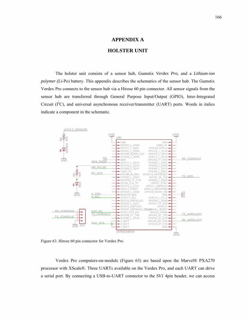
166
APPENDIX A
HOLSTER UNIT
The holster unit consists of a sensor hub, Gumstix Verdex Pro, and a Lithium-ion
polymer (Li-Po) battery. This appendix describes the schematics of the sensor hub. The Gumstix
Verdex Pro connects to the sensor hub via a Hirose 60 pin connector. All sensor signals from the
sensor hub are transferred through General Purpose Input/Output (GPIO), Inter-Integrated
Circuit (I2C), and universal asynchronous receiver/transmitter (UART) ports. Words in italics
indicate a component in the schematic.
Figure 63. Hirose 60 pin connector for Verdex Pro.
Verdex Pro computers-on-module (Figure 63) are based upon the Marvel® PXA270
processor with XScale®. Three UARTs available on the Verdex Pro, and each UART can drive
a serial port. By connecting a USB-to-UART connector to the SV1 4pin header, we can access

167
the embedded Linux of Verdex Pro with terminal software. GREEN is a green indicator light-
emitting diode (LED) which turns on when the power is on. Other pin outs are summarized in
Table X.
Table X. Gumstix Verdex Pro XM4 COM pin connectors. I/O pin Description
GPS_EN Connected to the GPS module HR_PULSE Connected to MSP430 for the HRM RX_GPS/TX_GPS Read/Write to the GPS module X_SDA/X_SCL Data/Clock line of the I2C bus SYS_EN Connected to the two voltage regulator modules TX_CONSOLE/RX_CONSOLE Read/Write to the Verdex Pro console VCC_SYS VCC for the Verdex Pro GND Ground TX_WIRELESS/RX_WIRELESS Read/Write to the wireless transmitter
The holster unit uses a single 3000mAh Li-Po battery as a power source. The Li-Po
battery can be recharged using a USB wire which connected to a PC or charger with a 500mAh
charging rate. While charging, the BLUE LED will be on(off when fully charged). When
charging, MCP73831 supplies 4.2V to the Li-Po battery. MCP73831also protects the battery
from over-charging and under-discharging during the charge cycle. The Li-Po battery has two
voltage regulators and supplies nominal 3.7V to the Verdex Pro which has its own internal
voltage regulator. VRM_WIRELESS supplies 3.3V to the wireless transceiver and GPS module
and the VRM_SENSOR supplies 3.3V to the HRM, RTC and accelerometer modules. MIC5219
is used for both, and it requires C12, C22, C24, and C25 (Figure 64) to be a tantalum capacitor.
SYS_EN on both regulators (Figure 64) connect to the VERDEX60H4 in Figure 63, and the
voltage regulators work only when SYS_EN is on. Thus, the sensor hub starts to work after the
Verdex Pro starts up.
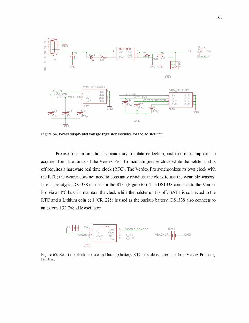
168
Figure 64. Power supply and voltage regulator modules for the holster unit.
Precise time information is mandatory for data collection, and the timestamp can be
acquired from the Linux of the Verdex Pro. To maintain precise clock while the holster unit is
off requires a hardware real time clock (RTC). The Verdex Pro synchronizes its own clock with
the RTC; the wearer does not need to constantly re-adjust the clock to use the wearable sensors.
In our prototype, DS1338 is used for the RTC (Figure 65). The DS1338 connects to the Verdex
Pro via an I2C bus. To maintain the clock while the holster unit is off, BAT1 is connected to the
RTC and a Lithium coin cell (CR1225) is used as the backup battery. DS1338 also connects to
an external 32.768 kHz oscillator.
Figure 65. Real-time clock module and backup battery. RTC module is accessible from Verdex Pro using I2C bus.
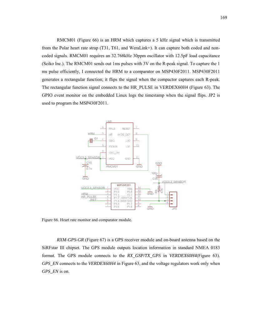
169
RMCM01 (Figure 66) is an HRM which captures a 5 kHz signal which is transmitted
from the Polar heart rate strap (T31, T61, and WeraLink+). It can capture both coded and non-
coded signals. RMCM01 requires an 32.768kHz 30ppm oscillator with 12.5pF load capacitance
(Seiko Inc.). The RMCM01 sends out 1ms pulses with 3V on the R-peak signal. To capture the 1
ms pulse efficiently, I connected the HRM to a comparator on MSP430F2011. MSP430F2011
generates a rectangular function; it flips the signal when the compactor captures each R-peak.
The rectangular function signal connects to the HR_PULSE in VERDEX60H4 (Figure 63). The
GPIO event monitor on the embedded Linux logs the timestamp when the signal flips. JP2 is
used to program the MSP430F2011.
Figure 66. Heart rate monitor and comparator module.
RXM-GPS-GR (Figure 67) is a GPS receiver module and on-board antenna based on the
SiRFstar III chipset. The GPS module outputs location information in standard NMEA 0183
format. The GPS module connects to the RX_GSP/TX_GPS in VERDEX60H4(Figure 63).
GPS_EN connects to the VERDEX60H4 in Figure 63, and the voltage regulators work only when
GPS_EN is on.
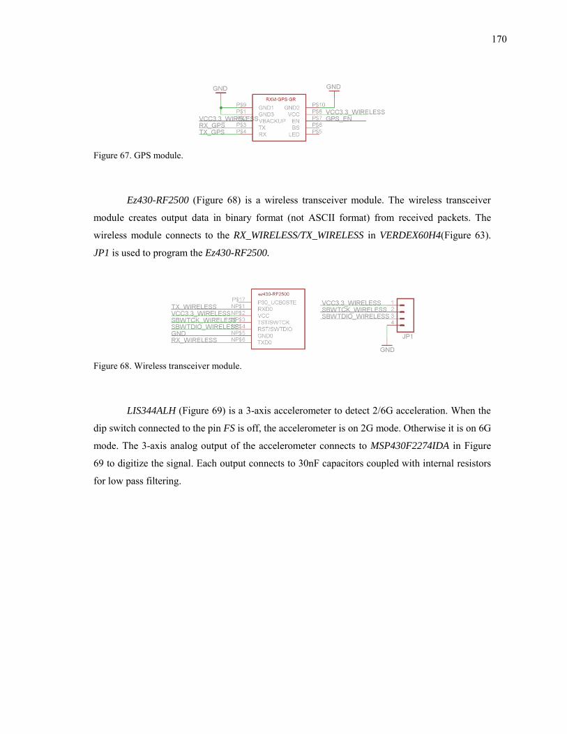
170
Figure 67. GPS module.
Ez430-RF2500 (Figure 68) is a wireless transceiver module. The wireless transceiver
module creates output data in binary format (not ASCII format) from received packets. The
wireless module connects to the RX_WIRELESS/TX_WIRELESS in VERDEX60H4(Figure 63).
JP1 is used to program the Ez430-RF2500.
Figure 68. Wireless transceiver module.
LIS344ALH (Figure 69) is a 3-axis accelerometer to detect 2/6G acceleration. When the
dip switch connected to the pin FS is off, the accelerometer is on 2G mode. Otherwise it is on 6G
mode. The 3-axis analog output of the accelerometer connects to MSP430F2274IDA in Figure
69 to digitize the signal. Each output connects to 30nF capacitors coupled with internal resistors
for low pass filtering.
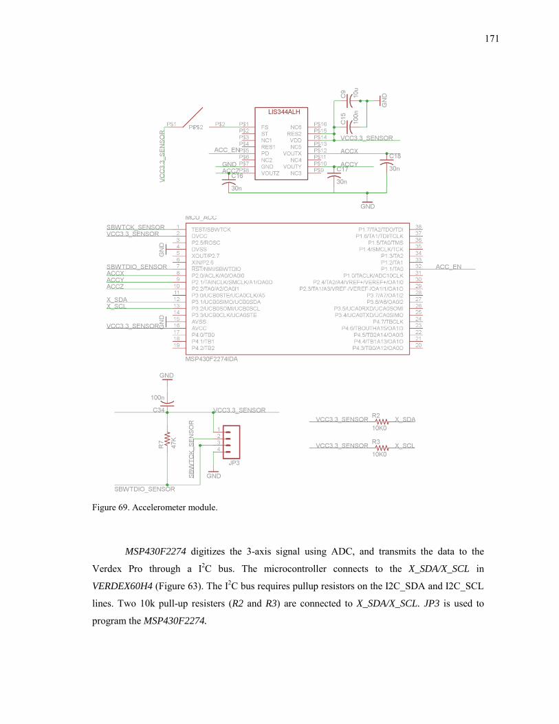
171
Figure 69. Accelerometer module.
MSP430F2274 digitizes the 3-axis signal using ADC, and transmits the data to the
Verdex Pro through a I2C bus. The microcontroller connects to the X_SDA/X_SCL in
VERDEX60H4 (Figure 63). The I2C bus requires pullup resistors on the I2C_SDA and I2C_SCL
lines. Two 10k pull-up resisters (R2 and R3) are connected to X_SDA/X_SCL. JP3 is used to
program the MSP430F2274.
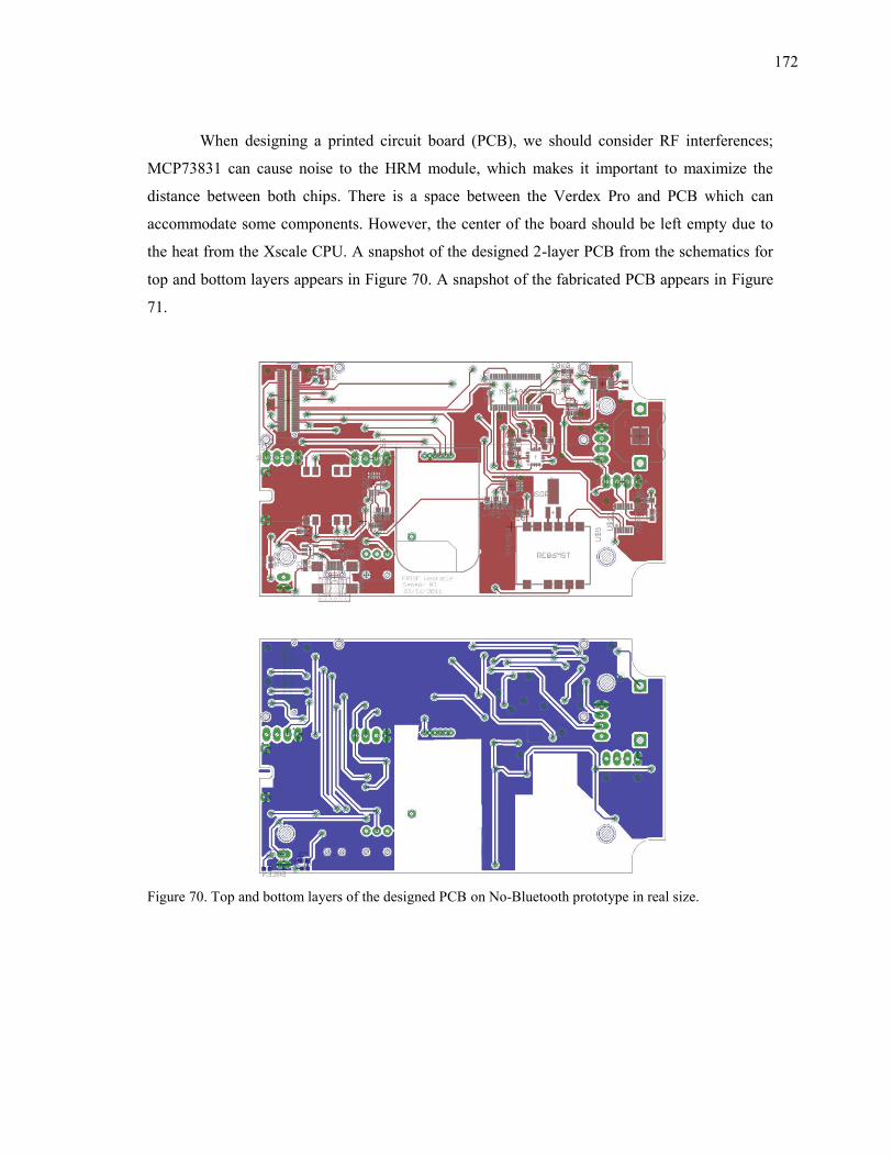
172
When designing a printed circuit board (PCB), we should consider RF interferences;
MCP73831 can cause noise to the HRM module, which makes it important to maximize the
distance between both chips. There is a space between the Verdex Pro and PCB which can
accommodate some components. However, the center of the board should be left empty due to
the heat from the Xscale CPU. A snapshot of the designed 2-layer PCB from the schematics for
top and bottom layers appears in Figure 70. A snapshot of the fabricated PCB appears in Figure
71.
Figure 70. Top and bottom layers of the designed PCB on No-Bluetooth prototype in real size.
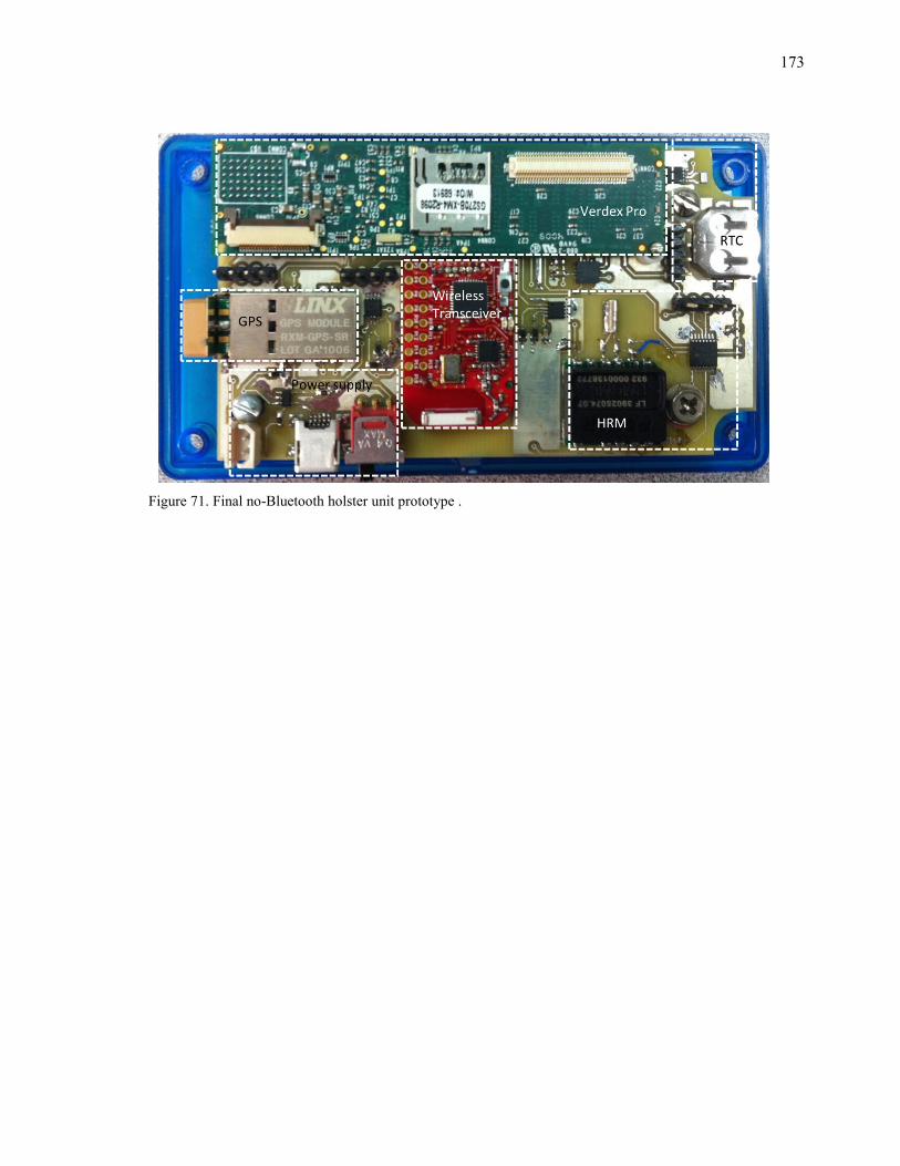
173
Figure 71. Final no-Bluetooth holster unit prototype .
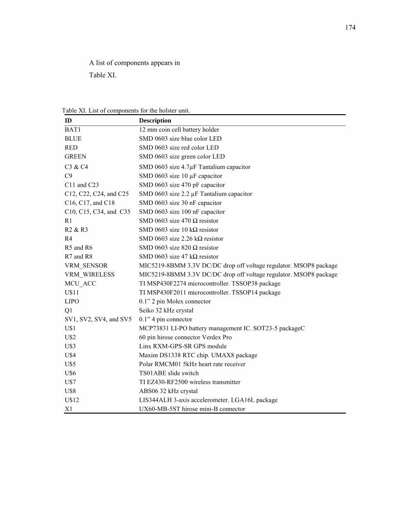
174
A list of components appears in
Table XI.
Table XI. List of components for the holster unit. ID Description
BAT1 12 mm coin cell battery holder BLUE SMD 0603 size blue color LED RED SMD 0603 size red color LED GREEN SMD 0603 size green color LED C3 & C4 SMD 0603 size 4.7µF Tantalium capacitor C9 SMD 0603 size 10 µF capacitor C11 and C23 SMD 0603 size 470 pF capacitor C12, C22, C24, and C25 SMD 0603 size 2.2 µF Tantalium capacitor C16, C17, and C18 SMD 0603 size 30 nF capacitor C10, C15, C34, and C35 SMD 0603 size 100 nF capacitor R1 SMD 0603 size 470 Ω resistor R2 & R3 SMD 0603 size 10 kΩ resistor R4 SMD 0603 size 2.26 kΩ resistor R5 and R6 SMD 0603 size 820 Ω resistor R7 and R8 SMD 0603 size 47 kΩ resistor VRM_SENSOR MIC5219-8BMM 3.3V DC/DC drop off voltage regulator. MSOP8 package VRM_WIRELESS MIC5219-8BMM 3.3V DC/DC drop off voltage regulator. MSOP8 package MCU_ACC TI MSP430F2274 microcontroller. TSSOP38 package U$11 TI MSP430F2011 microcontroller. TSSOP14 package LIPO 0.1” 2 pin Molex connector Q1 Seiko 32 kHz crystal SV1, SV2, SV4, and SV5 0.1” 4 pin connector U$1 MCP73831 LI-PO battery management IC. SOT23-5 packageC U$2 60 pin hirose connector Verdex Pro U$3 Linx RXM-GPS-SR GPS module U$4 Maxim DS1338 RTC chip. UMAX8 package U$5 Polar RMCM01 5kHz heart rate receiver U$6 TS01ABE slide switch U$7 TI EZ430-RF2500 wireless transmitter U$8 ABS06 32 kHz crystal U$12 LIS344ALH 3-axis accelerometer. LGA16L package X1 UX60-MB-5ST hirose mini-B connector
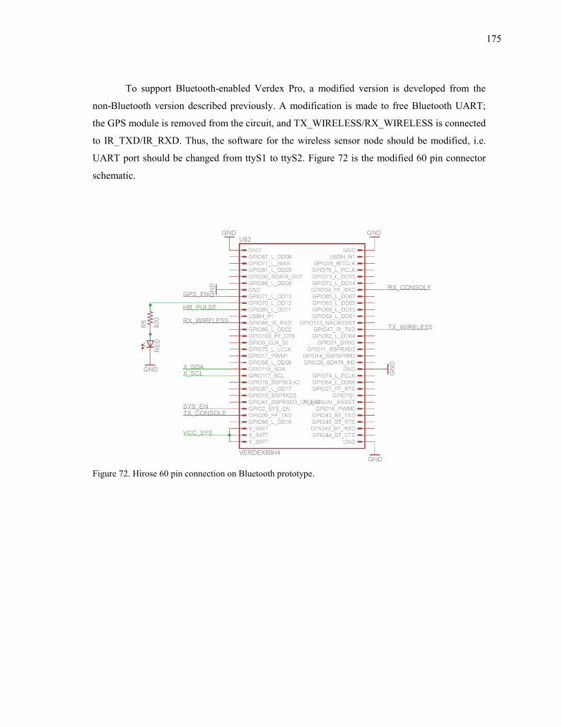
175
To support Bluetooth-enabled Verdex Pro, a modified version is developed from the
non-Bluetooth version described previously. A modification is made to free Bluetooth UART;
the GPS module is removed from the circuit, and TX_WIRELESS/RX_WIRELESS is connected
to IR_TXD/IR_RXD. Thus, the software for the wireless sensor node should be modified, i.e.
UART port should be changed from ttyS1 to ttyS2. Figure 72 is the modified 60 pin connector
schematic.
Figure 72. Hirose 60 pin connection on Bluetooth prototype.
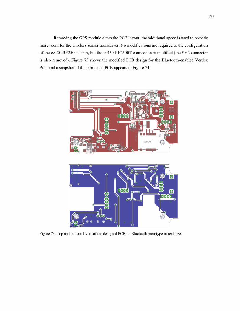
176
Removing the GPS module alters the PCB layout; the additional space is used to provide
more room for the wireless sensor transceiver. No modifications are required to the configuration
of the ez430-RF2500T chip, but the ez430-RF2500T connection is modified (the SV2 connector
is also removed). Figure 73 shows the modified PCB design for the Bluetooth-enabled Verdex
Pro, and a snapshot of the fabricated PCB appears in Figure 74.
Figure 73. Top and bottom layers of the designed PCB on Bluetooth prototype in real size.
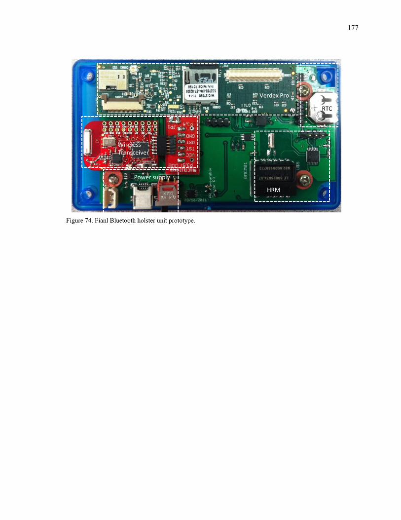
177
Figure 74. Fianl Bluetooth holster unit prototype.
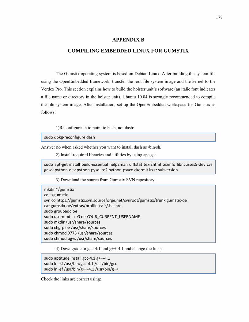
178
APPENDIX B
COMPILING EMBEDDED LINUX FOR GUMSTIX
The Gumstix operating system is based on Debian Linux. After building the system file
using the OpenEmbedded framework, transfer the root file system image and the kernel to the
Verdex Pro. This section explains how to build the holster unit’s software (an italic font indicates
a file name or directory in the holster unit). Ubuntu 10.04 is strongly recommended to compile
the file system image. After installation, set up the OpenEmbedded workspace for Gumstix as
follows.
1)Reconfigure sh to point to bash, not dash:
Answer no when asked whether you want to install dash as /bin/sh.
2) Install required libraries and utilities by using apt-get.
3) Download the source from Gumstix SVN repository,
4) Downgrade to gcc-4.1 and g++-4.1 and change the links:
Check the links are correct using:
sudo dpkg-reconfigure dash
sudo apt-get install build-essential help2man diffstat texi2html texinfo libncurses5-dev cvs gawk python-dev python-pysqlite2 python-psyco ckermit lrzsz subversion
mkdir ~/gumstix cd ~/gumstix svn co https://gumstix.svn.sourceforge.net/svnroot/gumstix/trunk gumstix-oe cat gumstix-oe/extras/profile >> ~/.bashrc sudo groupadd oe sudo usermod -a -G oe YOUR_CURRENT_USERNAME sudo mkdir /usr/share/sources sudo chgrp oe /usr/share/sources sudo chmod 0775 /usr/share/sources sudo chmod ug+s /usr/share/sources
sudo aptitude install gcc-4.1 g++-4.1 sudo ln -sf /usr/bin/gcc-4.1 /usr/bin/gcc sudo ln -sf /usr/bin/g++-4.1 /usr/bin/g++
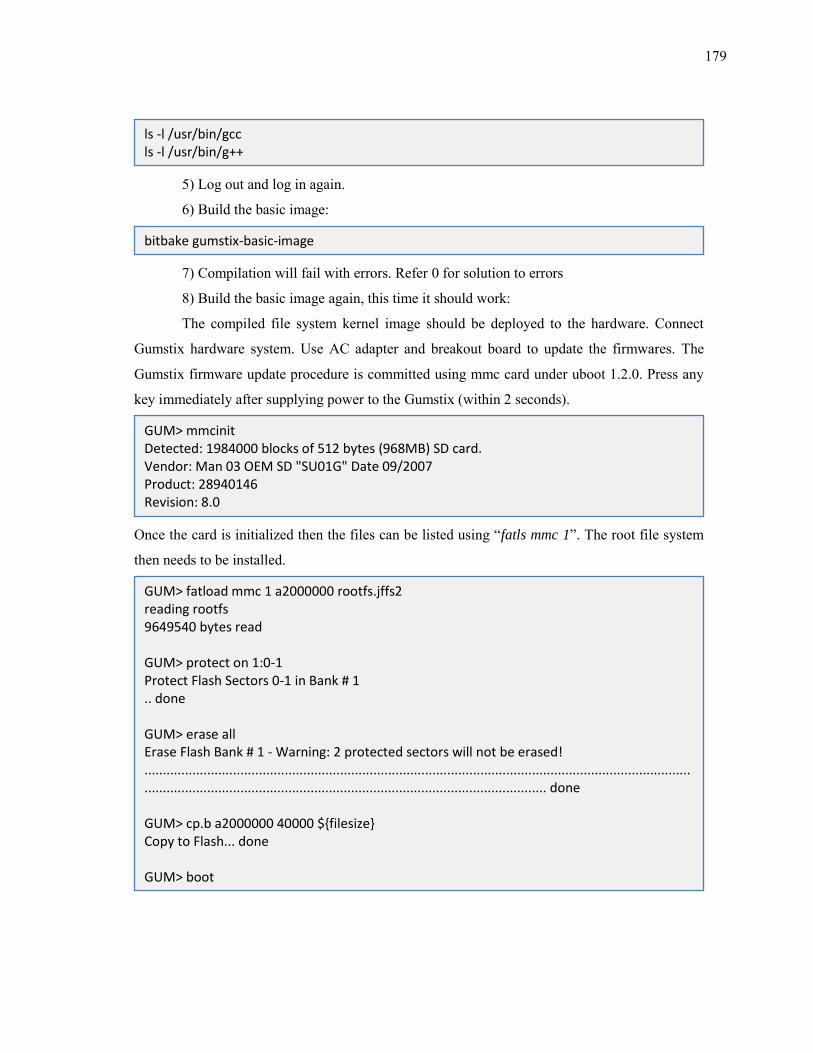
179
5) Log out and log in again.
6) Build the basic image:
7) Compilation will fail with errors. Refer 0 for solution to errors
8) Build the basic image again, this time it should work:
The compiled file system kernel image should be deployed to the hardware. Connect
Gumstix hardware system. Use AC adapter and breakout board to update the firmwares. The
Gumstix firmware update procedure is committed using mmc card under uboot 1.2.0. Press any
key immediately after supplying power to the Gumstix (within 2 seconds).
Once the card is initialized then the files can be listed using “fatls mmc 1”. The root file system
then needs to be installed.
ls -l /usr/bin/gcc ls -l /usr/bin/g++
bitbake gumstix-basic-image
GUM> mmcinit Detected: 1984000 blocks of 512 bytes (968MB) SD card. Vendor: Man 03 OEM SD "SU01G" Date 09/2007 Product: 28940146 Revision: 8.0
GUM> fatload mmc 1 a2000000 rootfs.jffs2 reading rootfs 9649540 bytes read GUM> protect on 1:0-1 Protect Flash Sectors 0-1 in Bank # 1 .. done GUM> erase all Erase Flash Bank # 1 - Warning: 2 protected sectors will not be erased! ................................................................................................................................................................................................................................................................. done GUM> cp.b a2000000 40000 $filesize Copy to Flash... done GUM> boot
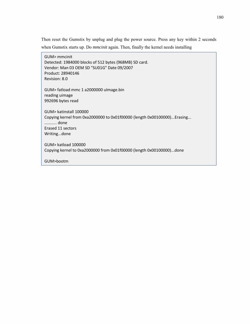
180
Then reset the Gumstix by unplug and plug the power source. Press any key within 2 seconds
when Gumstix starts up. Do mmcinit again. Then, finally the kernel needs installing
GUM> mmcinit Detected: 1984000 blocks of 512 bytes (968MB) SD card. Vendor: Man 03 OEM SD "SU01G" Date 09/2007 Product: 28940146 Revision: 8.0 GUM> fatload mmc 1 a2000000 uImage.bin reading uimage 992696 bytes read GUM> katinstall 100000 Copying kernel from 0xa2000000 to 0x01f00000 (length 0x00100000)...Erasing... ........... done Erased 11 sectors Writing...done GUM> katload 100000 Copying kernel to 0xa2000000 from 0x01f00000 (length 0x00100000)...done GUM>bootm
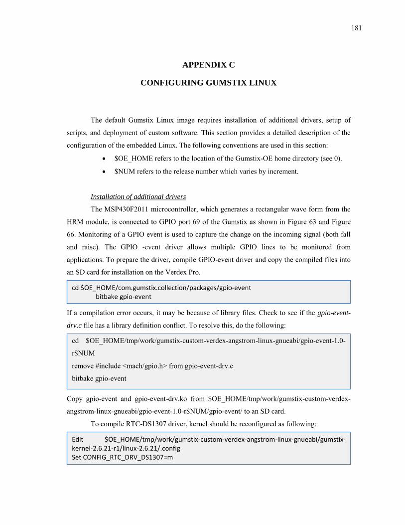
181
APPENDIX C
CONFIGURING GUMSTIX LINUX
The default Gumstix Linux image requires installation of additional drivers, setup of
scripts, and deployment of custom software. This section provides a detailed description of the
configuration of the embedded Linux. The following conventions are used in this section:
$OE_HOME refers to the location of the Gumstix-OE home directory (see 0).
$NUM refers to the release number which varies by increment.
Installation of additional drivers
The MSP430F2011 microcontroller, which generates a rectangular wave form from the
HRM module, is connected to GPIO port 69 of the Gumstix as shown in Figure 63 and Figure
66. Monitoring of a GPIO event is used to capture the change on the incoming signal (both fall
and raise). The GPIO -event driver allows multiple GPIO lines to be monitored from
applications. To prepare the driver, compile GPIO-event driver and copy the compiled files into
an SD card for installation on the Verdex Pro.
If a compilation error occurs, it may be because of library files. Check to see if the gpio-event-
drv.c file has a library definition conflict. To resolve this, do the following:
Copy gpio-event and gpio-event-drv.ko from $OE_HOME/tmp/work/gumstix-custom-verdex-
angstrom-linux-gnueabi/gpio-event-1.0-r$NUM/gpio-event/ to an SD card.
To compile RTC-DS1307 driver, kernel should be reconfigured as following:
cd $OE_HOME/com.gumstix.collection/packages/gpio-event bitbake gpio-event
cd $OE_HOME/tmp/work/gumstix-custom-verdex-angstrom-linux-gnueabi/gpio-event-1.0-
r$NUM
remove #include <mach/gpio.h> from gpio-event-drv.c
bitbake gpio-event
Edit $OE_HOME/tmp/work/gumstix-custom-verdex-angstrom-linux-gnueabi/gumstix-kernel-2.6.21-r1/linux-2.6.21/.config Set CONFIG_RTC_DRV_DS1307=m
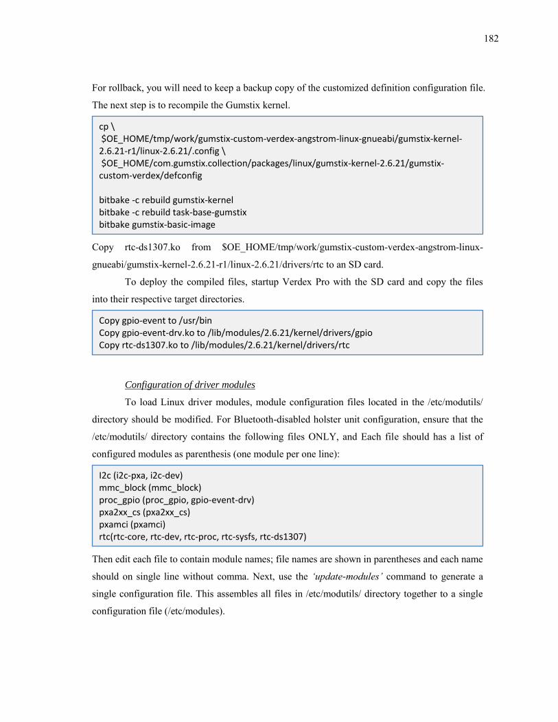
182
For rollback, you will need to keep a backup copy of the customized definition configuration file.
The next step is to recompile the Gumstix kernel.
Copy rtc-ds1307.ko from $OE_HOME/tmp/work/gumstix-custom-verdex-angstrom-linux-
gnueabi/gumstix-kernel-2.6.21-r1/linux-2.6.21/drivers/rtc to an SD card.
To deploy the compiled files, startup Verdex Pro with the SD card and copy the files
into their respective target directories.
Configuration of driver modules
To load Linux driver modules, module configuration files located in the /etc/modutils/
directory should be modified. For Bluetooth-disabled holster unit configuration, ensure that the
/etc/modutils/ directory contains the following files ONLY, and Each file should has a list of
configured modules as parenthesis (one module per one line):
Then edit each file to contain module names; file names are shown in parentheses and each name
should on single line without comma. Next, use the ‘update-modules’ command to generate a
single configuration file. This assembles all files in /etc/modutils/ directory together to a single
configuration file (/etc/modules).
cp \ $OE_HOME/tmp/work/gumstix-custom-verdex-angstrom-linux-gnueabi/gumstix-kernel-2.6.21-r1/linux-2.6.21/.config \ $OE_HOME/com.gumstix.collection/packages/linux/gumstix-kernel-2.6.21/gumstix-custom-verdex/defconfig bitbake -c rebuild gumstix-kernel bitbake -c rebuild task-base-gumstix bitbake gumstix-basic-image
Copy gpio-event to /usr/bin Copy gpio-event-drv.ko to /lib/modules/2.6.21/kernel/drivers/gpio Copy rtc-ds1307.ko to /lib/modules/2.6.21/kernel/drivers/rtc
I2c (i2c-pxa, i2c-dev) mmc_block (mmc_block) proc_gpio (proc_gpio, gpio-event-drv) pxa2xx_cs (pxa2xx_cs) pxamci (pxamci) rtc(rtc-core, rtc-dev, rtc-proc, rtc-sysfs, rtc-ds1307)
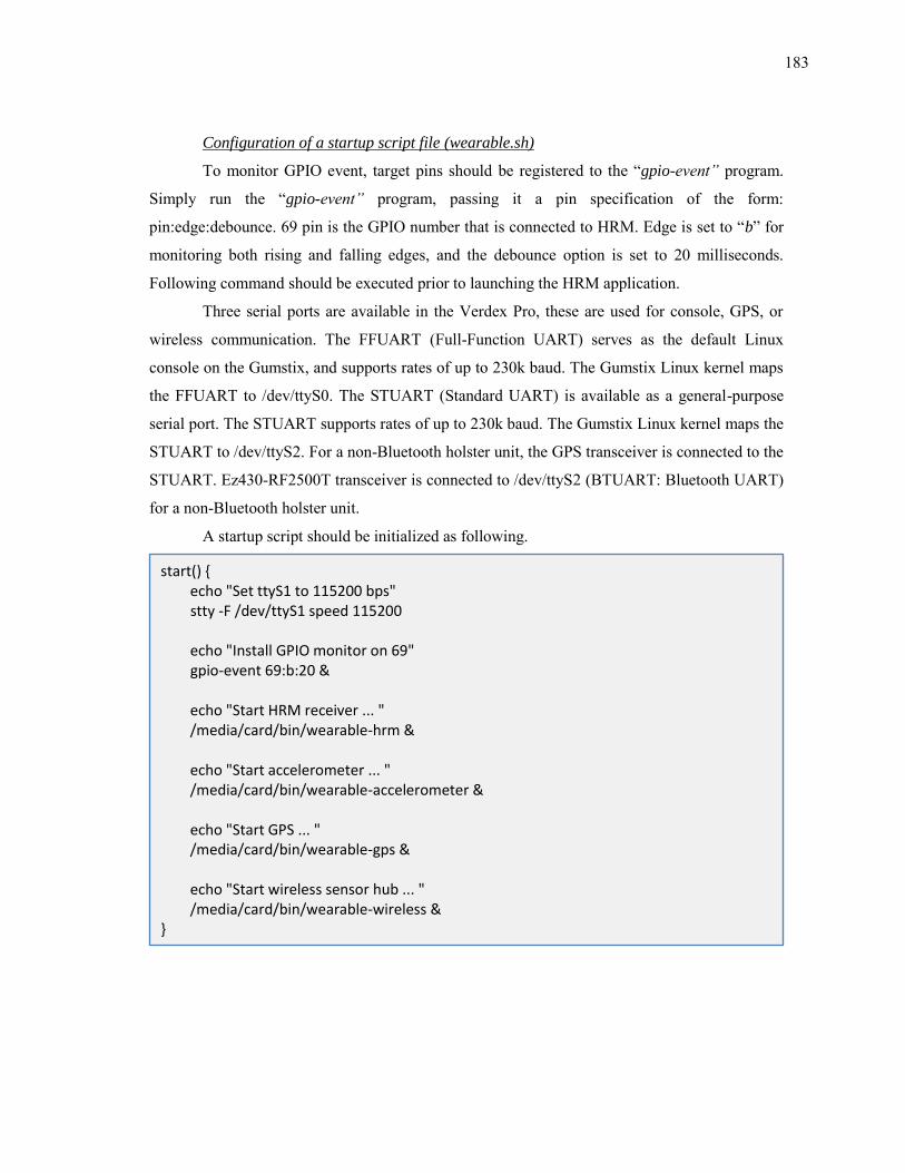
183
Configuration of a startup script file (wearable.sh)
To monitor GPIO event, target pins should be registered to the “gpio-event” program.
Simply run the “gpio-event” program, passing it a pin specification of the form:
pin:edge:debounce. 69 pin is the GPIO number that is connected to HRM. Edge is set to “b” for
monitoring both rising and falling edges, and the debounce option is set to 20 milliseconds.
Following command should be executed prior to launching the HRM application.
Three serial ports are available in the Verdex Pro, these are used for console, GPS, or
wireless communication. The FFUART (Full-Function UART) serves as the default Linux
console on the Gumstix, and supports rates of up to 230k baud. The Gumstix Linux kernel maps
the FFUART to /dev/ttyS0. The STUART (Standard UART) is available as a general-purpose
serial port. The STUART supports rates of up to 230k baud. The Gumstix Linux kernel maps the
STUART to /dev/ttyS2. For a non-Bluetooth holster unit, the GPS transceiver is connected to the
STUART. Ez430-RF2500T transceiver is connected to /dev/ttyS2 (BTUART: Bluetooth UART)
for a non-Bluetooth holster unit.
A startup script should be initialized as following.
start() echo "Set ttyS1 to 115200 bps" stty -F /dev/ttyS1 speed 115200 echo "Install GPIO monitor on 69" gpio-event 69:b:20 & echo "Start HRM receiver ... " /media/card/bin/wearable-hrm & echo "Start accelerometer ... " /media/card/bin/wearable-accelerometer & echo "Start GPS ... " /media/card/bin/wearable-gps & echo "Start wireless sensor hub ... " /media/card/bin/wearable-wireless &

184
Configuration of real time clock and timezone
The RTC driver should be loaded after I2C driver. The following commands should be
executed to synchronize with the clock from the hard ware clock. After downloading the new file
system, a combination of the date and hwclock commands should be executed to manipulate the
DS1308. Use the date command to set the current date and time. Use "hwclock -w" to set the
DS1308 to match the current date and time (set with the date command). Use the "hwclock -r"
command to read the time from the DS1307 and "hwclock -s" to set date from the DS1308.
To change timezone, modify two files; rcS and profiles. Central standard timezone is
CST6CDT, and Arabic standard timezone is AST.
Configuration of runtime resource files
Copy wearable.sh to /etc/init.d. Delete all links under /etc/rc5.d.
Create symbolic links under rc5.d directory.
Configuration of the flash disk (storage for logged data)
Compile applications for the wearable sensors.
All compiled files are located in a separate directory.
Modify /etc/default/rcS UTC=no TZ=CST6CDT Modify /etc/profile TZ="CST6CDT" export TZ
copy wearable.sh /etc/init.d/ rm /etc/rc5.d/*
cd /etc/rc5.d ln –s /etc/init.d/hwclock.sh S50hwclock ln –s /etc/init.d/wearable.sh S90wearable ln –s /etc/init.d/rmlogin S99rmnologin
cd $OE_HOME/user.collection/packages/wearable-io bitbake wearable-io
cd $OE_HOME/tmp/work/armv5te-angstrom-linux-gnueabi/wearable-io-1.0-r$NUM
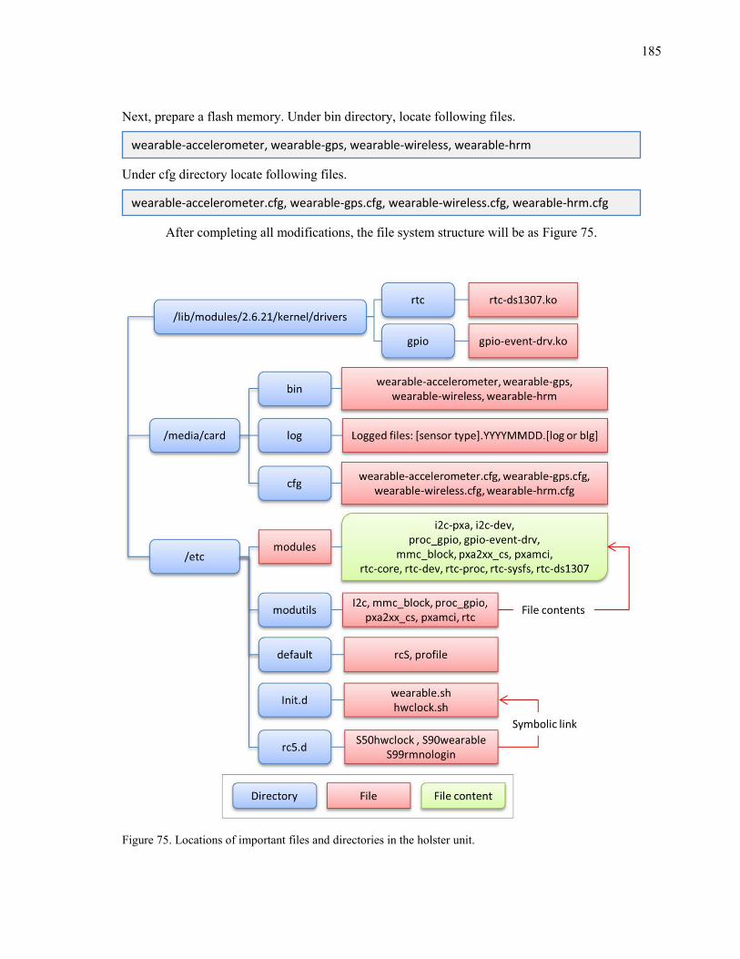
185
Next, prepare a flash memory. Under bin directory, locate following files.
Under cfg directory locate following files.
After completing all modifications, the file system structure will be as Figure 75.
Figure 75. Locations of important files and directories in the holster unit.
wearable-accelerometer, wearable-gps, wearable-wireless, wearable-hrm
wearable-accelerometer.cfg, wearable-gps.cfg, wearable-wireless.cfg, wearable-hrm.cfg
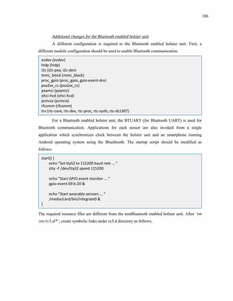
186
Additional changes for the Bluetooth enabled holster unit
A different configuration is required to the Bluetooth enabled holster unit. First, a
different module configuration should be used to enable Bluetooth communication.
For a Bluetooth enabled holster unit, the BTUART (for Bluetooth UART) is used for
Bluetooth communication. Applications for each sensor are also invoked from a single
application which synchronizes clock between the holster unit and an smartphone running
Android operating system using the Bluethooth. The startup script should be modified as
follows:
The required resource files are different from the nonBluetooth enabled holster unit. After ‘rm
/etc/rc5.d/*’, create symbolic links under rc5.d directory as follows.
evdev (evdev) hidp (hidp) i2c (i2c-pxa, i2c-dev) mmc_block (mmc_block) proc_gpio (proc_gpio, gpio-event-drv) pxa2xx_cs (pxa2xx_cs) pxamci (pxamci) ohci-hcd (ohci-hcd) pcmcia (pcmcia) rfcomm (rfcomm) trv (rtc-core, rtc-dev, rtc-proc, rtc-sysfs, rtc-ds1307)
start() echo "Set ttyS2 to 115200 baud rate ... " stty -F /dev/ttyS2 speed 115200 echo "Start GPIO event monitor ... " gpio-event 69:b:20 & echo "Start wearable sensors ... " /media/card/bin/integrate0 &
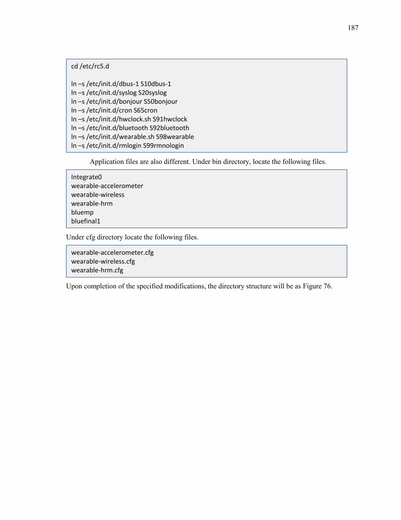
187
Application files are also different. Under bin directory, locate the following files.
Under cfg directory locate the following files.
Upon completion of the specified modifications, the directory structure will be as Figure 76.
cd /etc/rc5.d ln –s /etc/init.d/dbus-1 S10dbus-1 ln –s /etc/init.d/syslog S20syslog ln –s /etc/init.d/bonjour S50bonjour ln –s /etc/init.d/cron S65cron ln –s /etc/init.d/hwclock.sh S91hwclock ln –s /etc/init.d/bluetooth S92bluetooth ln –s /etc/init.d/wearable.sh S98wearable ln –s /etc/init.d/rmlogin S99rmnologin
Integrate0 wearable-accelerometer wearable-wireless wearable-hrm bluemp bluefinal1
wearable-accelerometer.cfg wearable-wireless.cfg wearable-hrm.cfg
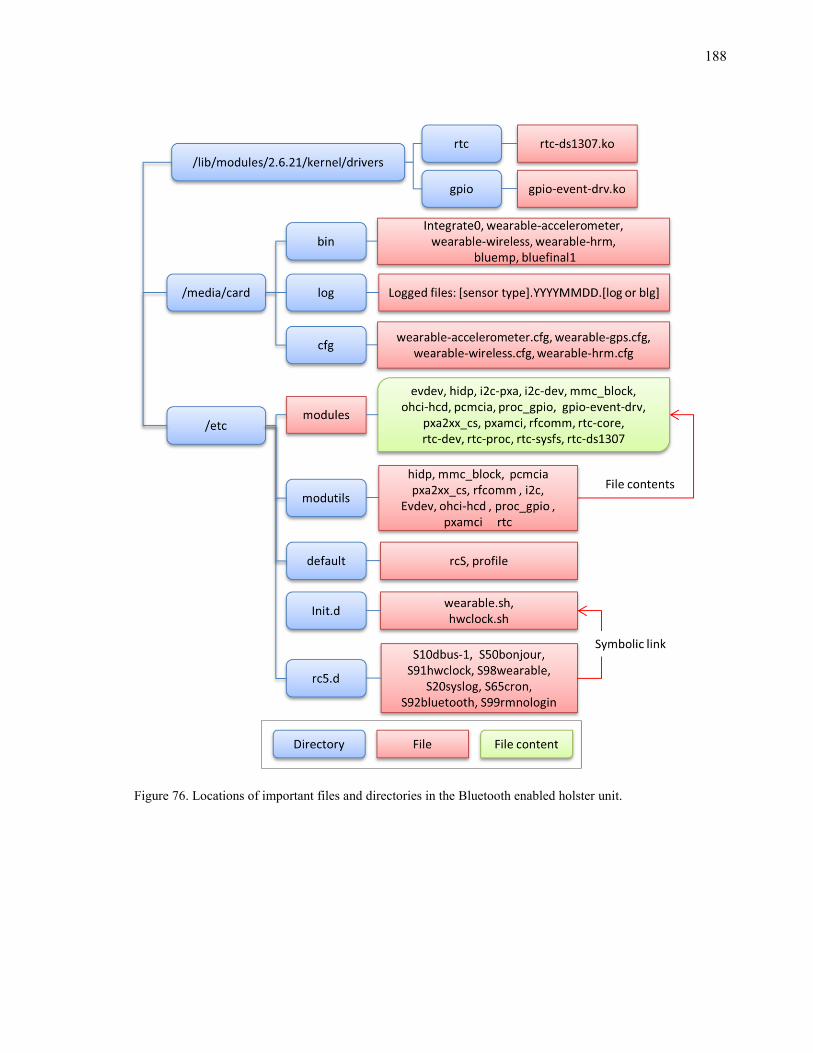
188
Figure 76. Locations of important files and directories in the Bluetooth enabled holster unit.

189
APPENDIX D
BACKING UP THE GUMSTIX SYSTEM
A backup copy of the file system image including the modifications above requires the
following steps.
1) Create a symbolic link to busybox to mount.
2) Stop some of working daemons.
3) Move to /tmp, and create a backup of the file system image
4) Create a backup of the kernel image
5) Move this copy off the gumstix using scp or copy it to a mounted SD card. Otherwise,
those files will be deleted when power is off.
ln -s /bin/busybox /tmp/mount
/etc/init.d/cron stop /etc/init.d/ntpd stop /etc/init.d/boa stop /etc/init.d/bonjour stop
cd /tmp ./mount -o remount,ro / dd if=/dev/mtdblock1 of=/tmp/saved-mtd1 mv saved-mtd1 rootfs.jffs2
dd if=/dev/mtdblock2 of=/tmp/saved-mtd2 mv savedmtd2 uImage.bin
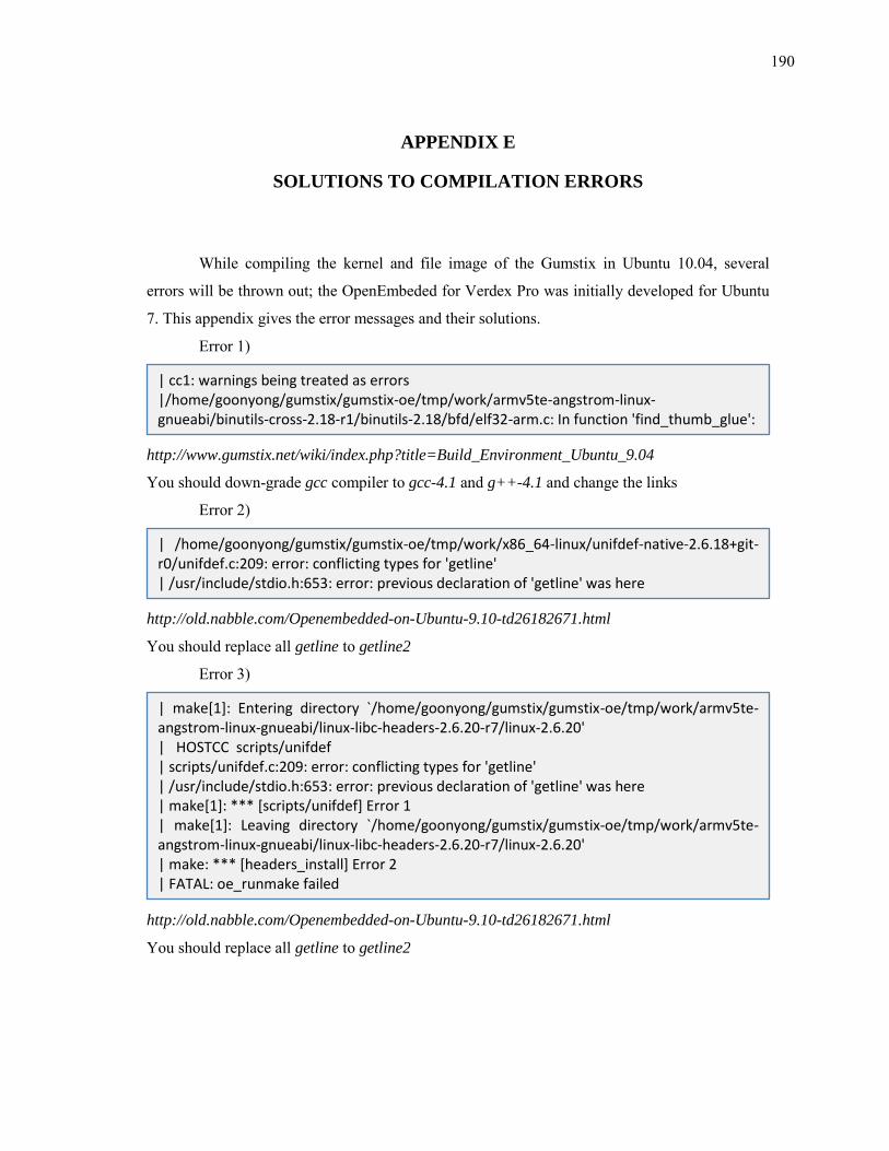
190
APPENDIX E
SOLUTIONS TO COMPILATION ERRORS
While compiling the kernel and file image of the Gumstix in Ubuntu 10.04, several
errors will be thrown out; the OpenEmbeded for Verdex Pro was initially developed for Ubuntu
7. This appendix gives the error messages and their solutions.
Error 1)
http://www.gumstix.net/wiki/index.php?title=Build_Environment_Ubuntu_9.04
You should down-grade gcc compiler to gcc-4.1 and g++-4.1 and change the links
Error 2)
http://old.nabble.com/Openembedded-on-Ubuntu-9.10-td26182671.html
You should replace all getline to getline2
Error 3)
http://old.nabble.com/Openembedded-on-Ubuntu-9.10-td26182671.html
You should replace all getline to getline2
| cc1: warnings being treated as errors |/home/goonyong/gumstix/gumstix-oe/tmp/work/armv5te-angstrom-linux-gnueabi/binutils-cross-2.18-r1/binutils-2.18/bfd/elf32-arm.c: In function 'find_thumb_glue':
| /home/goonyong/gumstix/gumstix-oe/tmp/work/x86_64-linux/unifdef-native-2.6.18+git-r0/unifdef.c:209: error: conflicting types for 'getline' | /usr/include/stdio.h:653: error: previous declaration of 'getline' was here
| make[1]: Entering directory `/home/goonyong/gumstix/gumstix-oe/tmp/work/armv5te-angstrom-linux-gnueabi/linux-libc-headers-2.6.20-r7/linux-2.6.20' | HOSTCC scripts/unifdef | scripts/unifdef.c:209: error: conflicting types for 'getline' | /usr/include/stdio.h:653: error: previous declaration of 'getline' was here | make[1]: *** [scripts/unifdef] Error 1 | make[1]: Leaving directory `/home/goonyong/gumstix/gumstix-oe/tmp/work/armv5te-angstrom-linux-gnueabi/linux-libc-headers-2.6.20-r7/linux-2.6.20' | make: *** [headers_install] Error 2 | FATAL: oe_runmake failed
191
Error 4)
Download zlib-1.2.3.tar.bz2 from http://sourceforge.net/projects/libpng/files/
Copy to ~/gumstix/gumstix-oe/org.openembedded.snapshot/packages/zlib/files/
Edit ~/gumstix/gumstix-oe/org.openembedded.snapshot/packages/zlib/zlib_1.2.3.bb
SRC_URI = "http://www.zlib.net/zlib-1.2.3.tar.bz2 \ to SRC_URI = "file://zlib-1.2.3.tar.bz2 \
Error 5)
http://www.gumstix.net/wiki/index.php?title=Build_Environment_Ubuntu_9.04
You should edit gumstix/gumstix-oe/tmp/work/i686-linux/dbus-native-1.0.1-r0/dbus-1.0.1/dbus/
dbus-sysdeps-unix.c (32bit Linux) or gumstix/gumstix-oe/tmp/work/x86_64-linux/dbus-native-
1.0.1-r0/dbus-1.0.1/dbus/dbus-sysdeps-unix.c (64bit Linux)
Add this struct after the macros.
struct ucred
unsigned int pid;
unsigned int uid;
unsigned int gid;
;
Resolving www.zlib.net... 69.73.181.135 Connecting to www.zlib.net|69.73.181.135|:80... connected. HTTP request sent, awaiting response... 404 Not Found 2010-10-01 10:38:58 ERROR 404: Not Found.
| dbus-sysdeps-unix.c: In function '_dbus_read_credentials_unix_socket': | dbus-sysdeps-unix.c:996: error: storage size of 'cr' isn't known | dbus-sysdeps-unix.c:999: warning: pointer targets in passing argument 5 of 'getsockopt' differ in signedness | dbus-sysdeps-unix.c:996: warning: unused variable 'cr' | dbus-sysdeps-unix.c: In function 'split_paths_and_append': | dbus-sysdeps-unix.c:2550: warning: passing argument 1 of '_dbus_string_init_const' discards qualifiers from pointer target type | dbus-sysdeps-unix.c: In function '_dbus_get_standard_session_servicedirs': | dbus-sysdeps-unix.c:2719: warning: passing argument 1 of '_dbus_string_init_const' discards qualifiers from pointer target type
192
Error 6)
http://www.gumstix.net/wiki/index.php?title=Build_Environment_Ubuntu_9.04
Edit gumstix/gumstix-oe/tmp/work/gumstix-custom-verdex-angstrom-linux-gnueabi/gumstix-
kernel-2.6.21-r1/linux-2.6.21/scripts/mod/sumversion.c
Add following line to after all of the other includes: #include <limits.h>.
Error 7)
Download iana-etc-2.20.tar.bz2 from
http://sunshinebrigadeguild.com/pub/lfs/conglomeration/iana-etc/ then copy it to
~gumstix/gumstix-oe/org.openembedded.snapshot/packages/iana-etc/files/.
Edit ~/gumstix/gumstix-oe/org.openembedded.snapshot/packages/iana-etc/iana-etc_2.20.bb
"SRC_URI = "http://www.sethwklein.net/projects/iana-etc/downloads/$P.tar.bz2" to
"SRC_URI = "file://iana-etc-2.20.tar.bz2"
Error 8)
http://old.nabble.com/bitbake-wifistix-problems-td17489294.html
Add following lines to the SRC_URI part of the wifistix-modules_5.0.16.p0.bb file.
file://wifistix-2.6.24.patch; patch=1 \
| scripts/mod/sumversion.c: In function 'get_src_version': | scripts/mod/sumversion.c:384: error: 'PATH_MAX' undeclared (first use in this function) | scripts/mod/sumversion.c:384: error: (Each undeclared identifier is reported only once | scripts/mod/sumversion.c:384: error: for each function it appears in.) | scripts/mod/sumversion.c:384: warning: unused variable 'filelist'
ERROR: Build of /home/goonyong/gumstix/gumstix-oe/org.openembedded.snapshot/packages/iana-etc/iana-etc_2.20.bb do_unpack failed
| make[2]: *** [/home/goonyong/gumstix/gumstix-oe/tmp/work/gumstix-custom-verdex-angstrom-linux-gnueabi/wifistix-modules-5.0.16.p0-r0/src_cf8385/wlan/wlan_main.o] Error 1 | make[1]: *** [_module_/home/goonyong/gumstix/gumstix-oe/tmp/work/gumstix-custom-verdex-angstrom-linux-gnueabi/wifistix-modules-5.0.16.p0-r0/src_cf8385] Error 2 | make[1]: Leaving directory `/home/goonyong/gumstix/gumstix-oe/tmp/work/gumstix-custom-verdex-angstrom-linux-gnueabi/gumstix-kernel-2.6.24-r1/linux-2.6.24' | make: *** [default] Error 2 | FATAL: oe_runmake failed NOTE: Task failed: /home/goonyong/gumstix/gumstix-oe/tmp/work/gumstix-custom-verdex-angstrom-linux-gnueabi/wifistix-modules-5.0.16.p0-r0/temp/log.do_compile.18410 NOTE: package wifistix-modules-5.0.16.p0-r0: task do_compile: failed ERROR: TaskFailed event exception, aborting
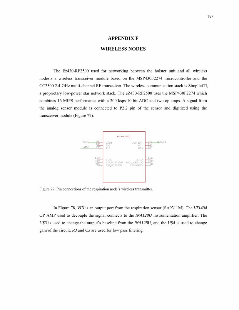
193
APPENDIX F
WIRELESS NODES
The Ez430-RF2500 used for networking between the holster unit and all wireless
nodesis a wireless transceiver module based on the MSP430F2274 microcontroller and the
CC2500 2.4-GHz multi-channel RF transceiver. The wireless communication stack is SimpliciTI,
a proprietary low-power star network stack. The eZ430-RF2500 uses the MSP430F2274 which
combines 16-MIPS performance with a 200-ksps 10-bit ADC and two op-amps. A signal from
the analog sensor module is connected to P2.2 pin of the sensor and digitized using the
transceiver module (Figure 77).
Figure 77. Pin connections of the respiration node’s wireless transmitter.
In Figure 78, VIN is an output port from the respiration sensor (SA9311M). The LT1494
OP AMP used to decouple the signal connects to the INA128U instrumentation amplifier. The
U$3 is used to change the output’s baseline from the INA128U, and the U$4 is used to change
gain of the circuit. R3 and C3 are used for low pass filtering.
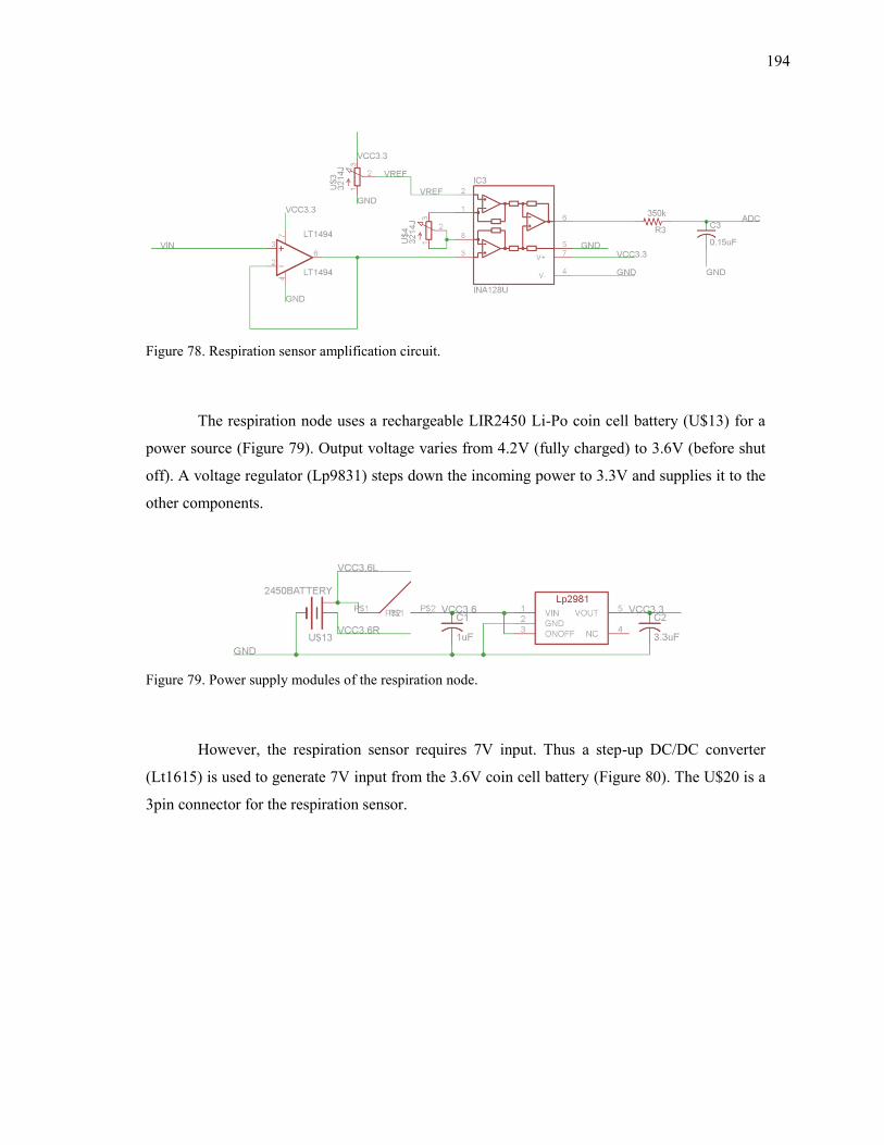
194
Figure 78. Respiration sensor amplification circuit.
The respiration node uses a rechargeable LIR2450 Li-Po coin cell battery (U$13) for a
power source (Figure 79). Output voltage varies from 4.2V (fully charged) to 3.6V (before shut
off). A voltage regulator (Lp9831) steps down the incoming power to 3.3V and supplies it to the
other components.
Figure 79. Power supply modules of the respiration node.
However, the respiration sensor requires 7V input. Thus a step-up DC/DC converter
(Lt1615) is used to generate 7V input from the 3.6V coin cell battery (Figure 80). The U$20 is a
3pin connector for the respiration sensor.
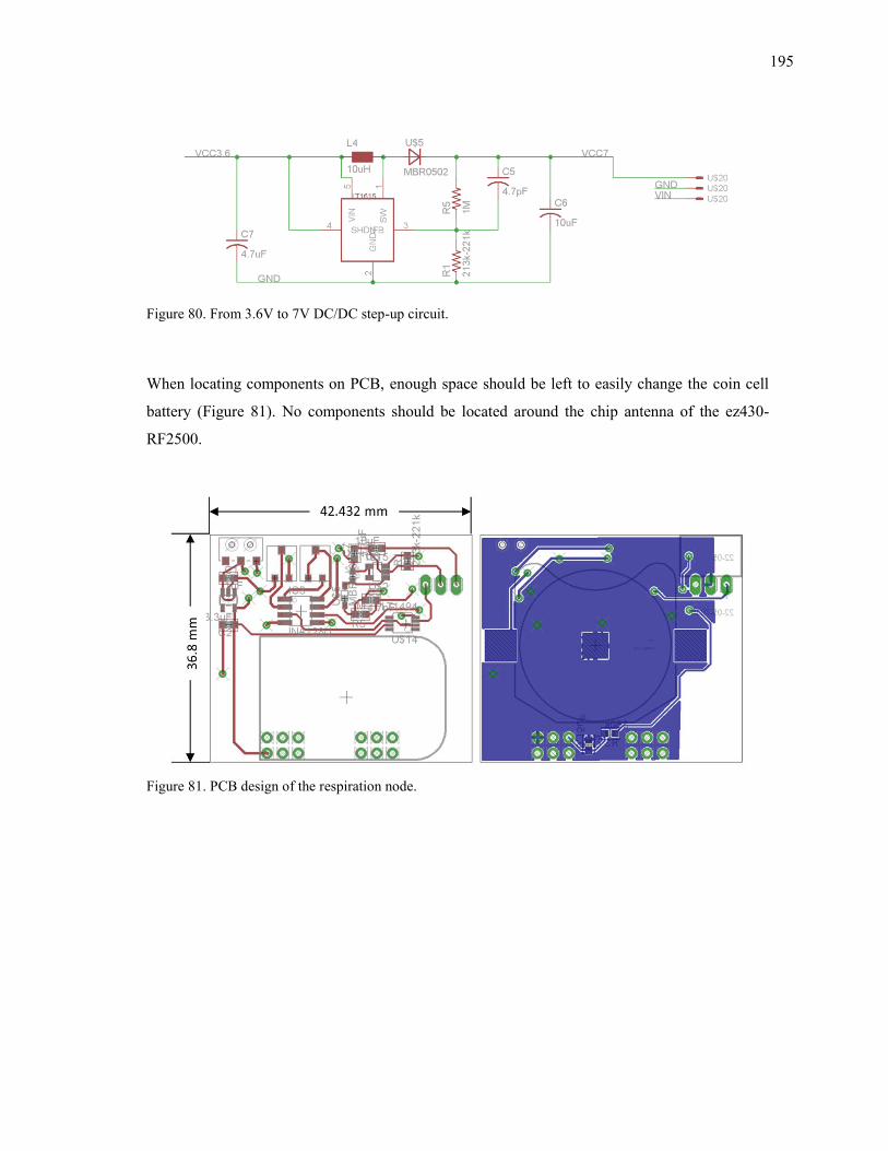
195
Figure 80. From 3.6V to 7V DC/DC step-up circuit.
When locating components on PCB, enough space should be left to easily change the coin cell
battery (Figure 81). No components should be located around the chip antenna of the ez430-
RF2500.
Figure 81. PCB design of the respiration node.
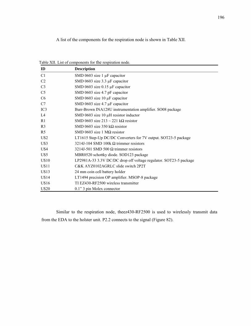
196
A list of the components for the respiration node is shown in Table XII.
Table XII. List of components for the respiration node. ID Description
C1 SMD 0603 size 1 µF capacitor C2 SMD 0603 size 3.3 µF capacitor C3 SMD 0603 size 0.15 µF capacitor C5 SMD 0603 size 4.7 pF capacitor C6 SMD 0603 size 10 µF capacitor C7 SMD 0603 size 4.7 µF capacitor IC3 Burr-Brown INA128U instrumentation amplifier. SO08 package L4 SMD 0603 size 10 µH resistor inductor R1 SMD 0603 size 213 ~ 221 kΩ resistor R3 SMD 0603 size 350 kΩ resistor R5 SMD 0603 size 1 MΩ resistor U$2 LT1615 Step-Up DC/DC Converters for 7V output. SOT23-5 package U$3 3214J-104 SMD 100k Ω trimmer resistors U$4 3214J-501 SMD 500 Ω trimmer resistors U$5 MBR0520 schottky diode. SOD123 package U$10 LP2981A-33 3.3V DC/DC drop off voltage regulator. SOT23-5 package U$11 C&K AYZ0102AGRLC slide switch 2P2T U$13 24 mm coin cell battery holder U$14 LT1494 precision OP amplifier. MSOP-8 package U$16 TI EZ430-RF2500 wireless transmitter U$20 0.1” 3 pin Molex connector
Similar to the respiration node, theez430-RF2500 is used to wirelessly transmit data
from the EDA to the holster unit. P2.2 connects to the signal (Figure 82).
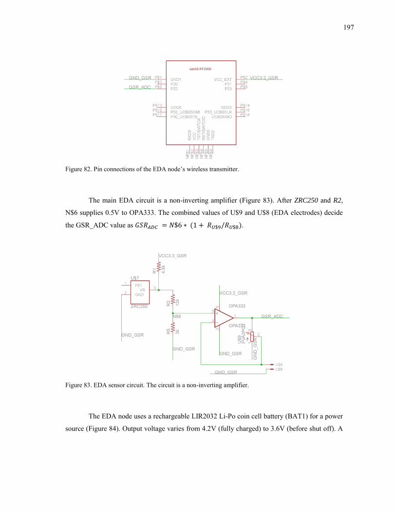
197
Figure 82. Pin connections of the EDA node’s wireless transmitter.
The main EDA circuit is a non-inverting amplifier (Figure 83). After ZRC250 and R2,
N$6 supplies 0.5V to OPA333. The combined values of U$9 and U$8 (EDA electrodes) decide
the GSR_ADC value as ( ).
Figure 83. EDA sensor circuit. The circuit is a non-inverting amplifier.
The EDA node uses a rechargeable LIR2032 Li-Po coin cell battery (BAT1) for a power
source (Figure 84). Output voltage varies from 4.2V (fully charged) to 3.6V (before shut off). A
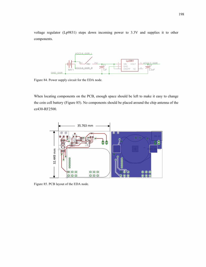
198
voltage regulator (Lp9831) steps down incoming power to 3.3V and supplies it to other
components.
Figure 84. Power supply circuit for the EDA node.
When locating components on the PCB, enough space should be left to make it easy to change
the coin cell battery (Figure 85). No components should be placed around the chip antenna of the
ez430-RF2500.
Figure 85. PCB layout of the EDA node.
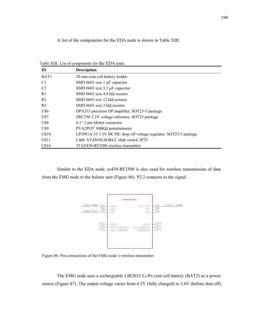
199
A list of the components for the EDA node is shown in Table XIII.
Table XIII. List of components for the EDA node. ID Description
BAT1 20 mm coin cell battery holder C1 SMD 0603 size 1 µF capacitor C2 SMD 0603 size 3.3 µF capacitor R1 SMD 0603 size 4.8 kΩ resistor R2 SMD 0603 size 12 kΩ resistor R5 SMD 0603 size 3 kΩ resistor U$6 OPA333 precision OP amplifier. SOT23-5 package U$7 ZRC250 2.5V voltage reference. SOT23 package U$8 0.1” 2 pin Molex connector U$9 PVA2POT 100KΩ potentiometer U$10 LP2981A-33 3.3V DC/DC drop off voltage regulator. SOT23-5 package U$11 C&K AYZ0102AGRLC slide switch 2P2T U$16 TI EZ430-RF2500 wireless transmitter
Similar to the EDA node, ez430-RF2500 is also used for wireless transmission of data
from the EMG node to the holster unit (Figure 86). P2.2 connects to the signal.
Figure 86. Pin connections of the EMG node’s wireless transmitter.
The EMG node uses a rechargeable LIR2032 Li-Po coin cell battery (BAT2) as a power
source (Figure 87). The output voltage varies from 4.2V (fully charged) to 3.6V (before shut off).
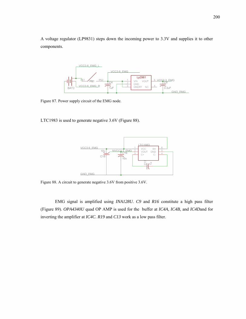
200
A voltage regulator (LP9831) steps down the incoming power to 3.3V and supplies it to other
components.
Figure 87. Power supply circuit of the EMG node.
LTC1983 is used to generate negative 3.6V (Figure 88).
Figure 88. A circuit to generate negative 3.6V from positive 3.6V.
EMG signal is amplified using INA128U. C9 and R16 constitute a high pass filter
(Figure 89). OPA4340U quad OP AMP is used for the buffer at IC4A, IC4B, and IC4Dand for
inverting the amplifier at IC4C. R19 and C13 work as a low pass filter.
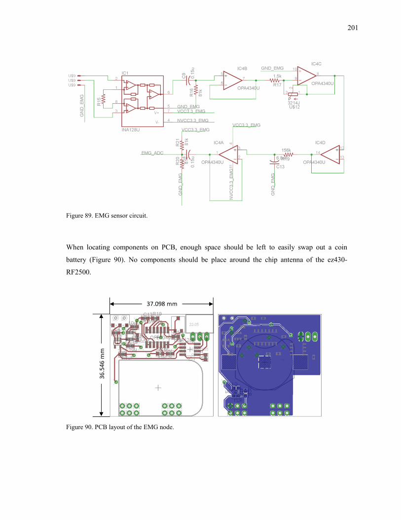
201
Figure 89. EMG sensor circuit.
When locating components on PCB, enough space should be left to easily swap out a coin
battery (Figure 90). No components should be place around the chip antenna of the ez430-
RF2500.
Figure 90. PCB layout of the EMG node.
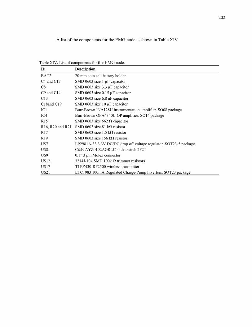
202
A list of the components for the EMG node is shown in Table XIV.
Table XIV. List of components for the EMG node. ID Description
BAT2 20 mm coin cell battery holder C4 and C17 SMD 0603 size 1 µF capacitor C8 SMD 0603 size 3.3 µF capacitor C9 and C14 SMD 0603 size 0.15 µF capacitor C13 SMD 0603 size 6.8 nF capacitor C18and C19 SMD 0603 size 10 µF capacitor IC1 Burr-Brown INA128U instrumentation amplifier. SO08 package IC4 Burr-Brown OPA4340U OP amplifier. SO14 package R15 SMD 0603 size 662 Ω capacitor R16, R20 and R21 SMD 0603 size 81 kΩ resistor R17 SMD 0603 size 1.5 kΩ resistor R19 SMD 0603 size 156 kΩ resistor U$7 LP2981A-33 3.3V DC/DC drop off voltage regulator. SOT23-5 package U$8 C&K AYZ0102AGRLC slide switch 2P2T U$9 0.1” 3 pin Molex connector U$12 3214J-104 SMD 100k Ω trimmer resistors U$17 TI EZ430-RF2500 wireless transmitter U$21 LTC1983 100mA Regulated Charge-Pump Inverters. SOT23 package
203
VITA
Jongyoon Choi received the B.S. degree in industrial engineering from the
Sungkyunkwan University, Seoul, Korea, in 1995, and the M.S. degrees in computer engineering
from Gwangju Institute of Science and Technology, Gwangju, Korea, in 1998. He began his
doctoral studies during the Fall semester of 2004. His research interests include pattern
recognition, affective computing, wearable sensors, and psychophysiology.
Jongyoon can be reached at Department of Computer Science and Engineering, Texas
A&M University, TAMU 3112, College Station, TX 77843-3112. He can also be reached by
email at [email protected].