Microwave bifurcation of a Josephson junction: Embedding-circuit requirements

V. E. Manucharyan, E. Boaknin, M. Metcalfe, R. Vijay, I. Siddiqi,* and M. DevoretDepartment of Applied Physics, Yale University, New Haven, Connecticut 06511, USA

�Received 10 December 2006; revised manuscript received 21 February 2007; published 26 July 2007�

A Josephson tunnel junction which is rf driven near a dynamical bifurcation point can amplify quantumsignals. However, the bifurcation point will exist robustly only if the electrodynamic environment of thejunction meets certain criteria. We develop a general formalism for dealing with the nonlinear dynamics of aJosephson junction embedded in an arbitrary microwave circuit. We find sufficient conditions for the existenceof the bifurcation regime: �a� the embedding impedance of the junction needs to present a resonance at aparticular frequency �R, with the quality factor Q of the resonance and the participation ratio p of the junctionsatisfying Qp�1, and �b� the drive frequency should be low frequency detuned away from �R by more than�3�R / �2Q�.

DOI: 10.1103/PhysRevB.76.014524 PACS number�s�: 85.25.Cp, 84.30.Le, 84.40.Az, 84.40.Dc

I. INTRODUCTION

Amplifying very small electrical signals is a ubiquitoustask in experimental physics. In particular, cryogenic ampli-fiers working in the microwave domain found a growingnumber of applications in mesoscopic physics, astrophysics,and particle detector physics.1,2 We have recently proposed3,4

to use the dynamical bifurcation of a rf-biased Josephsonjunction �JJ� as a basis for the amplification of quantum sig-nals. A bifurcation phenomenon offers the advantage of dis-playing a diverging susceptibility which can be exploited tomaximize the amplifier gain without necessarily sacrifyingits bandwidth. Among all very-low-noise and fast solid-statemicrowave devices, the Josephson junction distinguishes it-self by offering strongest nonlinearity combined with weak-est dissipation. However, these characteristics are not bythemselves sufficient. The electrodynamic environment ofthe junction must also satisfy a certain number of conditionsin order for a controllable and minimally noisy operation tobe possible. In the recent Josephson bifurcation amplifierexperiments,3,4 the junction was shunted by a lumped ele-ment capacitor. A large capacitance had to be fabricated veryclose to the junction to minimize parasitic circuit elements,at the cost of severe complexity of patterning and thin-filmdeposition. It would be very beneficial experimentally tosimply embed the Josephson junction in a planar supercon-ducting microwave resonator. The aim of this article is toestablish theoretically the requirements that need to be im-posed on the embedding impedance of the junction in orderto obtain a bifurcation whose characteristics are suitable foramplification.

The article is organized as follows: after having brieflyindicated the connection between a bifurcating dynamicalsystem and amplication, we review the simplest nonlineardynamical system exhibiting the type of bifurcation we ex-ploit: namely, the Duffing oscillator. We then describe theparameter space of the oscillator, focusing on the neighbor-hood of the first bifurcation and discussing why this is themost useful region. Having laid the general framework forthe analysis of our problem, we then consider the simplestpractical electrical implementation of the Duffing oscillator,a Josephson junction biased by an rf source through an arbi-

trary microwave circuit. The notion of embedding impedanceis introduced. For concreteness, we first examine the particu-lar cases where the embedding impedance corresponds tosimple series or parallel LCR circuits. This allows us to for-mulate the conditions under which the resulting nonlinearelectrical system can be mapped onto the Duffing model. Wethen examine the arbitrary impedance case, finding that itmust correspond to that of a resonator with an adequate qual-ity factor. We end the article by discussing possible detailedexperimental implementations of resonators and a conclud-ing summary.

II. AMPLIFYING WITH THE BIFURCATION OF ADRIVEN DYNAMICAL SYSTEM

Amplification using a laser, a maser, or a transistor isbased on energizing many microscopic systems, like atomsin a cavity or conduction electrons in a channel, each onebeing weakly coupled to the input signal. The overall powergain of the system, which is determined by the product of thenumber of active microscopic systems and their individualresponse to the input parameter, can be quite substantial.However, noise can result from the lack of control of eachindividual microscopic system. This article explores anotherstrategy5 for amplification which involves a single systemwith only one very-well-controlled collective degree of free-dom, which is driven to a high level of excitation. Here, theinput signal is coupled parametrically to this system and in-fluences its dynamics. The best known device exploiting thisstrategy is the superconducting quantum interference device6

�SQUID� but other devices of the same type have beenproposed.7 Let us discuss the general question of the gain�ratio of output to input� in such a system.

A driven dynamical system such as a SQUID is governedby a force equation which, quite generally, can be written as

F�X,X,X,a� = Fext�t� , �1�

where X is the system coordinate, Fext�t� is a periodic exter-nal drive pumping energy in the system, a a parameter of thesystem, and F a function describing its dynamics which isnecessarily dissipative since information is flowing away to

PHYSICAL REVIEW B 76, 014524 �2007�

1098-0121/2007/76�1�/014524�12� ©2007 The American Physical Society014524-1

the next stage of amplification. We are interested in a steady-state solution of Eq. �1�, in which the energy flowing in fromthe source is balanced by the energy losses. In the exampleof the rf SQUID, X is the total flux through the SQUID loop,a the signal flux, and F the external driving flux with afrequency in the MHz range. For the dc SQUID,9 the fre-quency of the external drive current is 0 and X is the com-mon mode phase difference while a is the flux through theloop formed by the junctions. In this article we also considera Josephson-junction-based device like a SQUID, but it isdriven by a rf signal at microwave frequencies to increasespeed and does not have intrinsic dissipation.

When we use the dynamical system as an amplifier, weare linking the input and output signals to the parameters aand variable X, respectively. Specifically, the signal s�t� atthe input of the amplifier induces a variation �a=�s. For asmall input, the output S�t� of the amplifier will depend lin-early on the modification of X: S�t�=L�X�t�−X�t�s=0�. Sincewe are looking for a maximal signal gain S /s, it is natural tofind an operating point where a small change in the param-eter a is going to induce a large change in the dynamics ofthe system, provided we can keep all other parameters con-stant. The largest differential susceptibility is found at asaddle-node bifurcation point, and it is in the neighborhoodof such points that we will operate the amplifier. The saddle-node bifurcation occurs when the drive parameters exceedcertain critical values. Previously, Yurke et al.8 studied Jo-sephson systems mostly in the regime beneath these criticalvalues. Here, we consider similar systems, but we exploitinstead the bistable regime beyond the critical values and thelarge susceptibilities accompanying it. In the next section, wereview a simple model exhibiting such a saddle-node bifur-cation phenomenon.

III. ONE MINIMAL MODEL FOR A BIFURCATINGNONLINEAR SYSTEM: THE DUFFING OSCILLATOR

One of the most minimal models displaying the bifurca-tion phenomenon needed for amplification is a damped,driven mechanical oscillator with a restoring force displayingcubic nonlinearity. The equation of this model, often calledthe Duffing linear+cubic oscillator,10–12 is

mX + �X + kX�1 − �X2� = F cos �dt + FN�t� , �2�

where X is the position coordinate of the mechanical degreeof freedom, m its mass, � its damping constant, k the stiff-ness constant of the restoring force, and � the nonlinearityparameter. The right-hand-side parameters F and � are theamplitude and angular frequency of the driving force, respec-tively. For completeness, we have also added on the right-hand side a noise force term FN�t� whose presence is im-posed by the fluctuation-dissipation theorem. It defines,through its correlation function, a thermal energy scale forthe problem, but in the following sections, we are going toassume that this scale can be made much smaller than all theother scales in the problem. The effect of fluctuations will betreated in a later article.

This simplification made, we can rescale the problem,changing the position and time coordinates, obtaining in theend a three-parameter model

x +x

Q+ x�1 − x2� = f cos w� , �3�

where the dot now refers to differentiation with respect to therescaled time �. The following equations express the rescaledquantities in terms of the original ones: �0= 1

�m/k, �=�0t, w

=�d

�0, Q=

�mk� , x=��X, and f =

��m F.

For reasons which will become clear later, we want toconsider the low damping limit of such a model and wesuppose that the quality factor satisfies Q�1.

In the weak nonlinear regime—i.e., x����1–the fre-quency w0 of natural oscillations �f =0� decreases with theoscillation energy u= x2

2 + x2

2 − x4

4 as

w0 = 1 −3u

2+ O�u2� . �4�

This corresponds to the softening of the restoring force as theamplitude of the oscillatory motion increases.

The bifurcation phenomenon can be described crudely asfollows: if we drive the system below the small oscillationresonance frequency, increasing the drive amplitude slowly,the resulting oscillation will be very small at first. However,at a certain drive strength, the system becomes unstable andtends to switch to a high amplitude oscillation where it canbetter meet the resonance condition.

In a quantitative treatment of the weak nonlinear regime,we seek a solution involving only the first harmonic of thedrive frequency and make the following change of variables:

x��� =1

2x���eiw� +

1

2x*���e−iw�,

x��� =i�

2x���eiw� −

i�

2x*���e−iw�, �5�

where the time dependence of the complex harmonic ampli-tudes x��� and x*��� is slow on the time scale w−1. Retainingin the equation only the terms evolving in time like eiw� onefinds the following relation for x��� �Ref. 13�:

2ix = � − i

Q+

3

4�x�2�x + f , �6�

in which we have introduced the reduced detuning ,

= 2Q�w − 1� . �7�

The static solutions �x=0� for the modulus x= �x� of the fun-damental amplitude can be obtained as a function of theparameters � , f� for a given Q by solving the equation

f2 = �2 + 1

Q2 +3

2Qx2 +

9

16x4�x2. �8�

The differential susceptibility is given by the implicit ex-pression

MANUCHARYAN et al. PHYSICAL REVIEW B 76, 014524 �2007�

014524-2

�x

�f= � �f

�x�−1

=

��1 + 2�Q2 +

3

2Qx2 +

9

16x4

�1 + 2�Q2 +

3

Qx2 +

27

16x4

. �9�

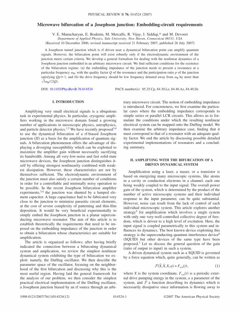
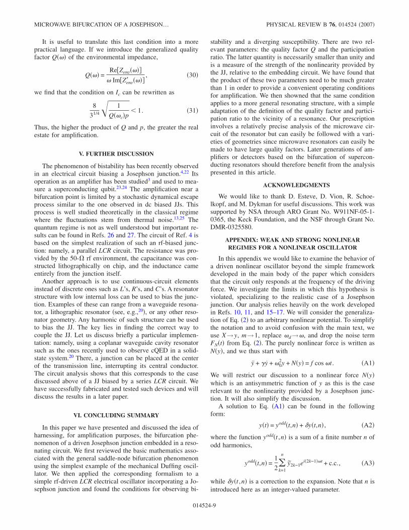
In the upper panels of Fig. 1, we show x as a function of for increasing values of f and for Q=20,50,200. For smalldrive, the curve is the familiar Lorentzian response of anharmonic oscillator, displaying a maximum response onresonance at =0 and a half width at half maximum�HWHM� point at =−1. As the drive strength is increased,the resonance curve bends towards lower frequencies, an in-direct manifestation of Eq. �4�. There is a critical drive fc atwhich appears for the first time a critical reduced detuningc such that the susceptibility �x /�f diverges.12 We call xcthe oscillation amplitude at this critical point. Analyticcalculations12,13 lead to

fc =25/2

35/4

1�Q3

,

c = − �3,

xc =23/2

33/4

1�Q

. �10�

To be consistent with our weak nonlinear regime hypothesis,we must have xc�1 which implies in turn Q�1.

For drives f fc, the response curve x�� develops anoverhanging part in which there are three possible values forx at each value of . The smallest and highest values corre-spond to two metastable states with different oscillation am-plitudes, whereas the intermediate value corresponds to anunstable state for the system. We denote as fB�� and f B��the boundaries of this bistability interval: fB is the force atwhich the system, submitted to an increasing drive with afixed frequency, will switch from the low- to the high-amplitude state. Starting from this state and decreasing theamplitude of the oscillatory force, the system will switchback to the low-amplitude state at f B. This possibility of theDuffing system to “bifurcate” between two different dynami-cal states at fB�� and f B�� is the phenomenon we areexploiting for amplification and whose electrical implemen-tation is the main topic of this paper. It is easy to see that anyinput parameter coupled to k or m in Eq. �2� will inducevariations of the line fB��. Fixing the drive parameters in

2.0

1.5

1.0

0.2

0.1

2.0

1.5

1.0

0.5

0.0

2.0

1.5

1.0

0.5

0.0

2

1

0

-1-40 -20 0 20

WW

-0.5

0.0

0.5

-4 -2 0 2

W

1.0

0.5

0.0

-0.5

-1.0-10 -5 0 5

Q=20 Q=200Q=50

Log10x/Log10xc

Log10(f/fc)

FIG. 1. �Color� Upper panels: response of the Duffing linear+cubic oscillator see Eq. �2� as a function of the dimensionless detuning, for different values of the dimensionless driving amplitude f . The three panels correspond to three different values of the small oscillationquality factor Q=20, 50, and 200 and are shown over the same reduced frequency range 0.9�w�1.05. The response for the critical driveamplitude fc, where the curve presents a single point with diverging susceptibilities �x /� and �x /�f , is shown in green. From bottom to top,the increments in the drive amplitude f are 2 dB �left�, 2 dB �center�, and 3 dB �right�. In the gray region, the oscillation amplitude is takingplace in the strongly nonlinear regime �see text� and the curves, which are calculated within the weak non-linear hypothesis, are not to betrusted. Lower panels: stability diagram for the dynamical states corresponding to the system response shown in the upper panels. The y axisis the drive amplitude f , scaled by the critical amplitude fc. The blue fB�� and red f B�� lines delimit the region of bistability for thesystem and correspond to the points of diverging susceptibility which are visible in the upper panels. The two curves meet at the critical pointshown by a green dot, whose position is determined by the critical detuning c=−�3 and drive amplitude fc. The dashed line fms��“continues” the blue and red lines and corresponds to the points of maximal susceptibility with respect to driving force. The gray regionscorrespond to that in the upper panels. Note that the “trusworthy” domain of bistability increases monotonously with the quality factor Q.

MICROWAVE BIFURCATION OF A JOSEPHSON… PHYSICAL REVIEW B 76, 014524 �2007�

014524-3

the vicinity of this line, very small changes in the input willinduce large variations in the oscillation amplitude. Thevariations can be reversible if we chose a point to the right ofthe critical point �continuous amplifier operation� or thevariations can be hysteretic if we chose a point to the left ofthe critical point �latched threshold detector operation�.

In the limit Q�1, analytic calculations can be carriedfurther and lead to13

fB,B��

fc=

1

2

3/2

c3/2�1 + 3

c2

2 ± �1 −c

2

2�3/2�1/2

. �11�

We define fms�� as the line of maximum susceptibility�x /�f on the low-frequency side of the resonance curve. Itdefines the line of highest amplification gain below the bi-furcation regime.14 Its expression is given by

fms��fc

=31/2

2

1/2

c1/2�1

3�

c�2

+ 1�1/2

. �12�

The susceptibility on the high-frequency side of the criticalpoint diverges as

�x

�f

�c=

Q

�, �13�

where � is defined by =c−� and c��.In the lower panels of Fig. 1, we plot the bifurcation

forces fB �blue line� and f B �red line� and fms �dashed line�normalized to the critical force as a function of the reduceddrive frequency . Note that the lines representing fB��,f B��, and fms in the parameter space � , f / fc� are indepen-dent of the parameters of Eq. �2� and can be deemed “uni-versal.”

The dynamical critical point �=c , f / fc=1� is found atthe junction between the dashed line and the two bifurcationlines. One can develop an analogy between the parameterspace � , f / fc� and the phase diagram of a fluid undergoinga liquid-vapor transition, the dynamical critical point corre-sponding to the critical point beyond which vapor and liquidcannot be distinguished by a transition �supercritical fluidregime� and the bifurcation lines corresponding to the limitof stability of the supercooled vapor and superheated fluid oneither side of the first-order transition line �spinodal decom-position phenomenon�.

A. Weak and strong nonlinear regimes for the simple Duffingequation

Let us now further discuss the small-amplitude conditionx�1, which is necessary for the above results to hold. In theAppendix we show that as long as

3

2w2x2 � “ few ” , 1/2 � w � 1, �14�

where “few” is a numerical constant difficult to determinebut of order unity, the Duffing model has stationary solutionof the form

x��� =1

2�k=1

x2k−1ei�2k−1�w� + c.c. , �15�

with the coefficients x2k−1 decreasing with the order k. Onlyodd multiples of the drive frequency thus appear in this se-ries. The first harmonic coefficient x1 is given by the stablesolution of Eq. �6� in the limit �x1��1. Inequalities �14� de-fine the weak nonlinear regime.

By contrast, in the strong nonlinear regime 32w2 x2 “few,”

even harmonics start to proliferate as the oscillation ampli-tude increases, leading eventually to chaotic behavior.15–17 Itis important to note that the SQUID does not avoid thisregime, even if, in general, strong dissipation prevents fullydeveloped chaos in this device.

Wanting at all cost to minimize noise in our use of thisdynamical system for amplification, we want to avoid thestrong nonlinear regime. Keeping in mind that we are goingto work with a small detuning ��−�0� /�0, a conservativeboundary separating the weak from the strong nonlinear re-gime can be introduced in parameter space by requiring

x � 0.5. �16�

In the lower panels of Fig. 1, the gray region correspondsto condition �16� being violated for at least one of the oscil-lation states. A lighter shade of gray marks the hystereticregion between fB�� and f B�� to indicate that the low-amplitude state does not violate �16� while the high ampli-tude does.

Note that in the reduced parameter space � , f / fc�, theline fms�� corresponding to condition �16� has a rather dras-tic dependence on Q, in contrast with the other lines. Ofcourse, if we would plot the stability boundary lines in theabsolute parameter space �� ,F�, the line corresponding to�16� would be fixed while the critical point ��c ,Fc� wouldstrongly depend on Q.

Whatever the representation, the important messagewhich arises from the stability diagram is that the amount of“real estate” in parameter space that can be used for bifurca-tion amplification increases with Q. All points along thefB�� line located between fc and fs�� are potentially use-ful. By realizing a large enough Q, one can always “buy” thenecessary amount of “real estate” in the stability diagram,irrespectively of the value of the other parameters of thesystem. Of course, higher Q will tend to lower the band-width, but we can compensate this effect by increasing theoperating frequency of the device.

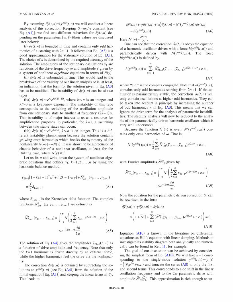
IV. rf-BIASED JOSEPHSON JUNCTION

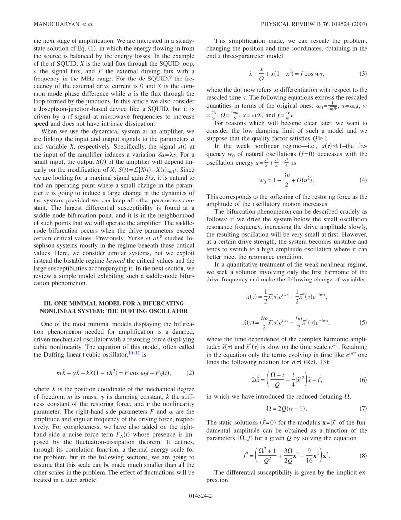
We now apply these general considerations to the practi-cal case of a JJ biased by an rf source. At radio frequencies,the impedance of the biasing circuit cannot be taken either aszero �ideal voltage source� or infinite �ideal current source�.In general, as depicted in Fig. 2�a�, the biasing circuitryshould be modeled as a specific, frequency-dependent linearquadrupole connecting the Josephson element of the junctionto an ideal voltage source �the other circuit element of thejunction, its linear capacitance, has been lumped in this

MANUCHARYAN et al. PHYSICAL REVIEW B 76, 014524 �2007�

014524-4

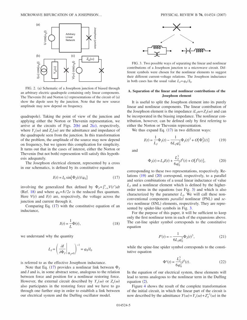
quadrupole�. Taking the point of view of the junction andapplying either the Norton or Thevenin representation, wearrive at the circuits of Figs. 2�b� and 2�c�, respectively,where Ye��� and Ze��� are the admittance and impedance ofthe quadrupole seen from the junction. In this transformationof the problem, the amplitude of the source may now dependon frequency, but we ignore this complication for simplicity.It turns out that in the cases of interest, either the Norton orThevenin �but not both� represention will satisfy this hypoth-esis adequately.

The Josephson electrical element, represented by a crossin our schematics, is defined by its constitutive equation

I�t� = I0 sin�J�t�/�0 �17�

involving the generalized flux defined by �J=�− t V�t��dt

�Ref. 18� and where �0=� /2e is the reduced flux quantum.Here V�t� and I�t� are, respectively, the voltage across thejunction and current through it.

Comparing Eq. �17� with the constitutive equation of aninductance,

I�t� =1

L��t� , �18�

we understand why the quantity

LJ = � �I

��J

�J=0�−1

= �0/I0

is referred to as the effective Josephson inductance.Note that Eq. �17� provides a nonlinear link between �J

and I and is, in some abstract sense, analogous to the relationbetween force and position for a nonlinear restoring force.However, the external circuit described by Ye��� or Ze���also participates in the restoring force and we have to gothrough one further step in order to establish a link betweenour electrical system and the Duffing oscillator model.

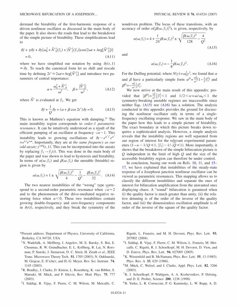
A. Separation of the linear and nonlinear contributions of theJosephson element

It is useful to split the Josephson element into its purelylinear and nonlinear components. The linear contribution ofthe Josephson element is the impedance iLJ�=ZJ��� and canbe incorporated in the biasing impedance. The nonlinear con-tribution, however, can be defined only by first referring toeither the Norton or Thevenin representation.

We thus expand Eq. �17� in two different ways:

I�t� =1

LJ�J�t� −

1

6LJ�02�J�t�3 + O�J

5�t� �19�

and

�J�t� = LJI�t� +LJ

3

6�02 I3�t� + OI5�t� , �20�

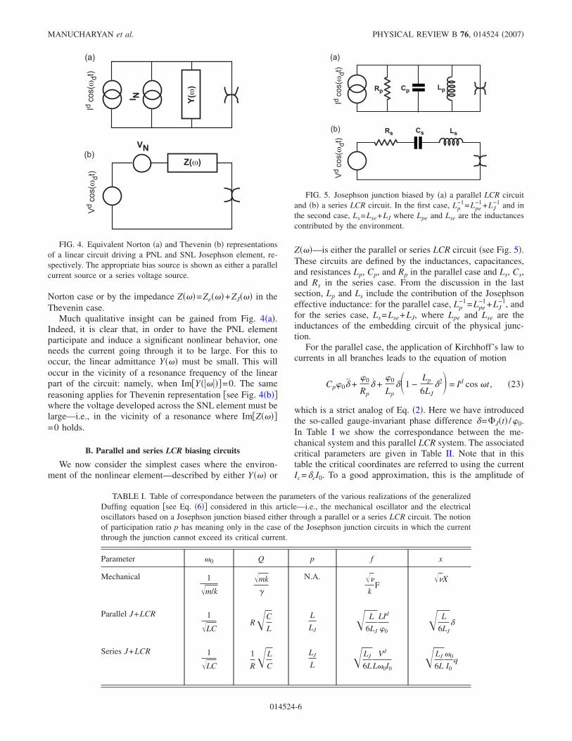
corresponding to these two representations, respectively. Re-lations �19� and �20� correspond, respectively, to a paralleland series combinations of a usual linear inductance of valueLJ and a nonlinear element which is defined by the higher-order terms in the equations �see Fig. 3� and which is alsocharacterized by the parameter LJ. We will call these non-conventional components parallel nonlinear �PNL� and se-ries nonlinear �SNL� elements, respectively. They are repre-sented by spider-like symbols in Fig. 3.

For the purpose of this paper, it will be sufficient to keeponly the first nonlinear term in each of the expansions above.The cut-line spider symbol corresponds to the constitutiveequation

Ip�t� = −1

6LJ�02�J�t�3, �21�

while the spine-line spider symbol corresponds to the consti-tutive equation

�s�t� =LJ

3

6�02 I3�t� . �22�

In the equation of our electrical system, these elements willlead to terms analogous to the nonlinear term in the Duffingequation �2�.

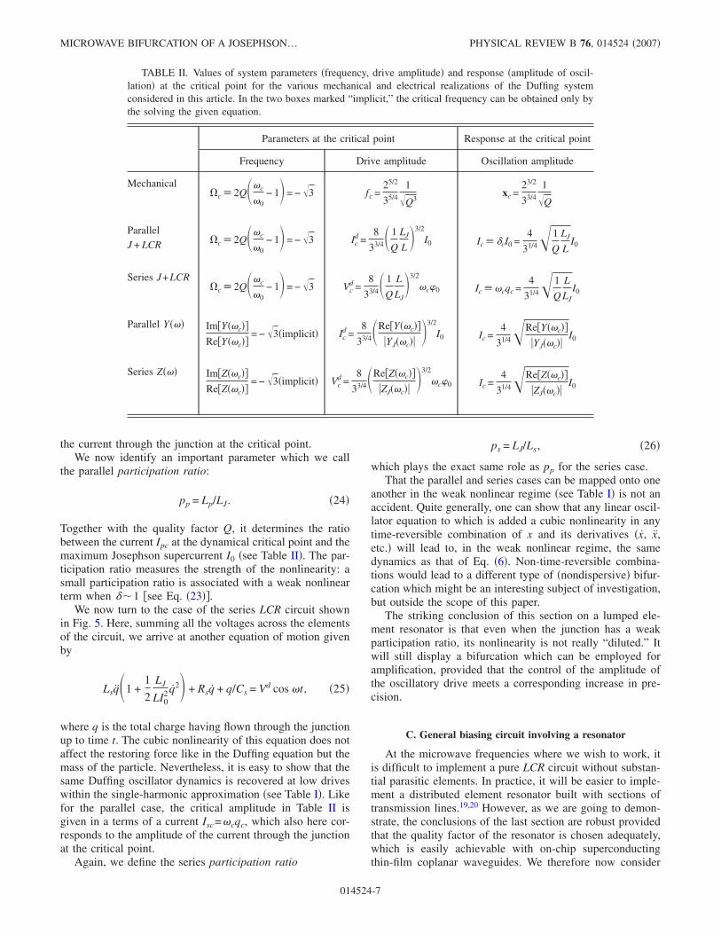
Figure 4 shows the result of the complete transformationof the initial circuit, in which the linear part of the circuit isnow described by the admittance Y���=Ye���+ZJ

−1��� in the

Ucos(ωdt)

Arbitrary

Linear

Network

Josephsonjunction

I(ω)cos(ωdt)

V(ω)cos(ωdt)

Ye(ω)

Ze(ω)

(a)

(c)(b)

FIG. 2. �a� Schematic of a Josephson junction rf biased throughan arbitrary electric quadrupole containing only linear components.The Thevenin �b� and Norton �c� representations of the circuit of �a�show the dipole seen by the junction. Note that the new sourceamplitude may now depend on frequency.

FIG. 3. Two possible ways of separating the linear and nonlinearcontributions of a Josephson junction to a microwave circuit. Dif-ferent symbols were chosen for the nonlinear elements to suggesttheir different current-voltage relations. The Josephson inductancein both cases has the usual value LJ=�0 / I0.

MICROWAVE BIFURCATION OF A JOSEPHSON… PHYSICAL REVIEW B 76, 014524 �2007�

014524-5

Norton case or by the impedance Z���=Ze���+ZJ��� in theThevenin case.

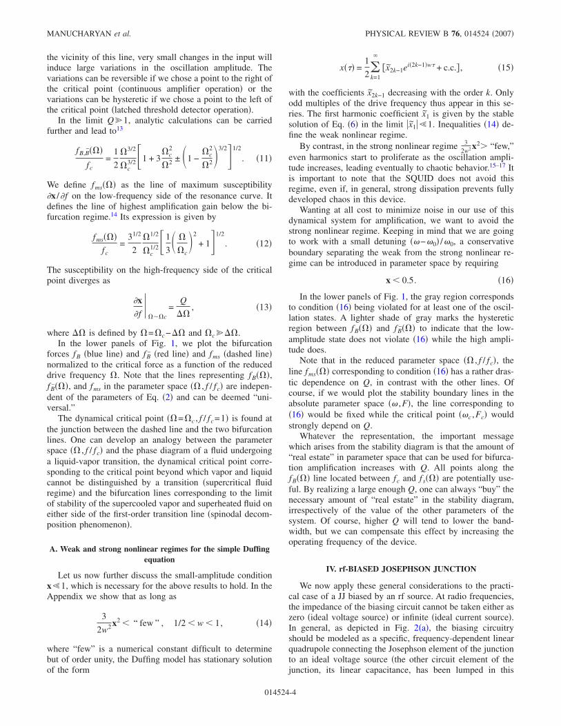
Much qualitative insight can be gained from Fig. 4�a�.Indeed, it is clear that, in order to have the PNL elementparticipate and induce a significant nonlinear behavior, oneneeds the current going through it to be large. For this tooccur, the linear admittance Y��� must be small. This willoccur in the vicinity of a resonance frequency of the linearpart of the circuit: namely, when ImY�����=0. The samereasoning applies for Thevenin representation see Fig. 4�b�where the voltage developed across the SNL element must belarge—i.e., in the vicinity of a resonance where ImZ���=0 holds.

B. Parallel and series LCR biasing circuits

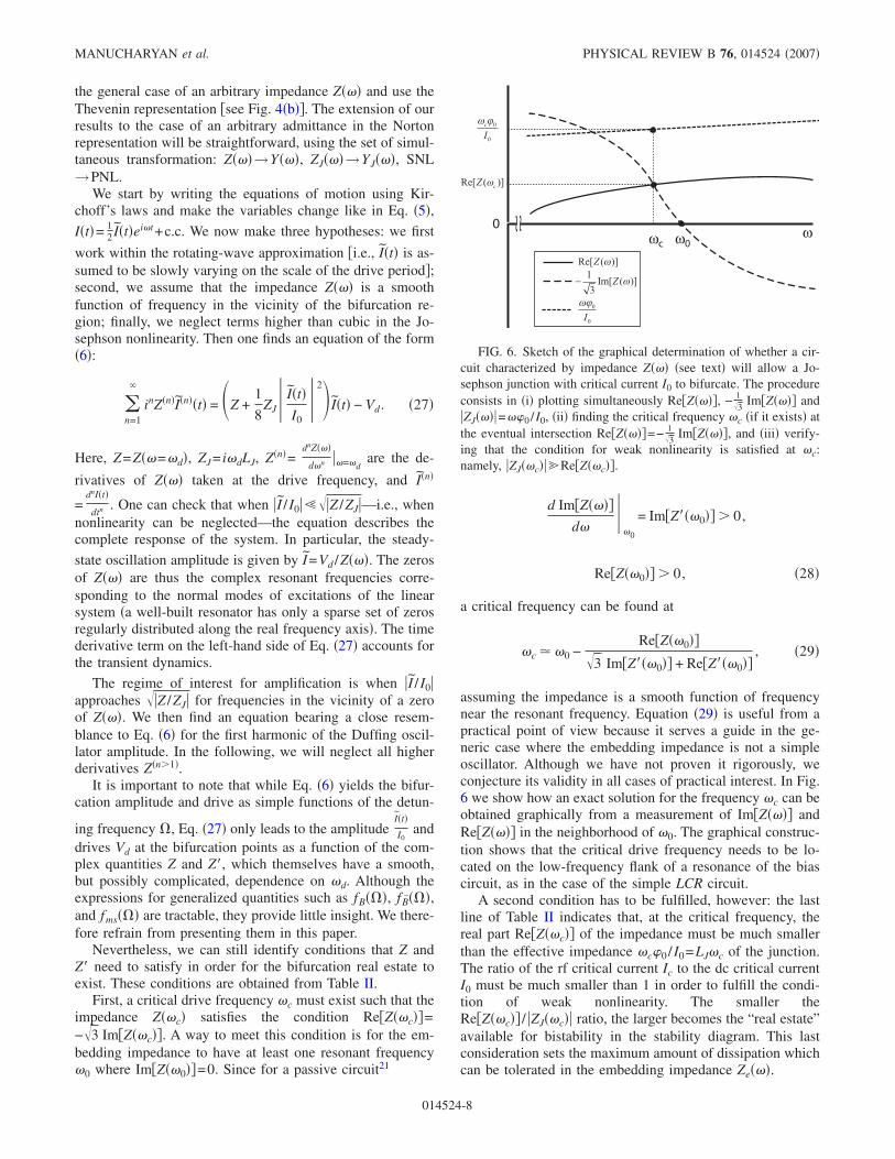
We now consider the simplest cases where the environ-ment of the nonlinear element—described by either Y��� or

Z���—is either the parallel or series LCR circuit �see Fig. 5�.These circuits are defined by the inductances, capacitances,and resistances Lp, Cp, and Rp in the parallel case and Ls, Cs,and Rs in the series case. From the discussion in the lastsection, Lp and Ls include the contribution of the Josephsoneffective inductance: for the parallel case, Lp

−1=Lpe−1+LJ

−1, andfor the series case, Ls=Lse+LJ, where Lpe and Lse are theinductances of the embedding circuit of the physical junc-tion.

For the parallel case, the application of Kirchhoff’s law tocurrents in all branches leads to the equation of motion

Cp�0� +�0

Rp� +

�0

Lp��1 −

Lp

6LJ�2� = Id cos �t , �23�

which is a strict analog of Eq. �2�. Here we have introducedthe so-called gauge-invariant phase difference �=�J�t� /�0.In Table I we show the correspondance between the me-chanical system and this parallel LCR system. The associatedcritical parameters are given in Table II. Note that in thistable the critical coordinates are referred to using the currentIc=�cI0. To a good approximation, this is the amplitude of

TABLE I. Table of correspondance between the parameters of the various realizations of the generalizedDuffing equation see Eq. �6� considered in this article—i.e., the mechanical oscillator and the electricaloscillators based on a Josephson junction biased either through a parallel or a series LCR circuit. The notionof participation ratio p has meaning only in the case of the Josephson junction circuits in which the currentthrough the junction cannot exceed its critical current.

Parameter �0 Q p f x

Mechanical 1�m/k

�mk

�

N.A. ��

kF

��X

Parallel J+LCR 1�LC

R�C

L

L

LJ� L

6LJ

LId

�0� L

6LJ�

Series J+LCR 1�LC

1

R�L

C

LJ

L�LJ

6L

Vd

L�0I0�LJ

6L

�0

I0q

(b)

(a)

Z(ω)

Vdcos(ωdt)

VN

Y(ω)

Idcos(ωdt)

I N

FIG. 4. Equivalent Norton �a� and Thevenin �b� representationsof a linear circuit driving a PNL and SNL Josephson element, re-spectively. The appropriate bias source is shown as either a parallelcurrent source or a series voltage source.

Rs Cs Ls

Vdcos(ωdt)

Rp Cp Lp

Idcos(ωdt)

(a)

(b)

FIG. 5. Josephson junction biased by �a� a parallel LCR circuitand �b� a series LCR circuit. In the first case, Lp

−1=Lpe−1+LJ

−1 and inthe second case, Ls=Lse+LJ where Lpe and Lse are the inductancescontributed by the environment.

MANUCHARYAN et al. PHYSICAL REVIEW B 76, 014524 �2007�

014524-6

the current through the junction at the critical point.We now identify an important parameter which we call

the parallel participation ratio:

pp = Lp/LJ. �24�

Together with the quality factor Q, it determines the ratiobetween the current Ipc at the dynamical critical point and themaximum Josephson supercurrent I0 �see Table II�. The par-ticipation ratio measures the strength of the nonlinearity: asmall participation ratio is associated with a weak nonlinearterm when ��1 see Eq. �23�.

We now turn to the case of the series LCR circuit shownin Fig. 5. Here, summing all the voltages across the elementsof the circuit, we arrive at another equation of motion givenby

Lsq�1 +1

2

LJ

LI02 q2� + Rsq + q/Cs = Vd cos �t , �25�

where q is the total charge having flown through the junctionup to time t. The cubic nonlinearity of this equation does notaffect the restoring force like in the Duffing equation but themass of the particle. Nevertheless, it is easy to show that thesame Duffing oscillator dynamics is recovered at low driveswithin the single-harmonic approximation �see Table I�. Likefor the parallel case, the critical amplitude in Table II isgiven in a terms of a current Isc=�cqc, which also here cor-responds to the amplitude of the current through the junctionat the critical point.

Again, we define the series participation ratio

ps = LJ/Ls, �26�

which plays the exact same role as pp for the series case.That the parallel and series cases can be mapped onto one

another in the weak nonlinear regime �see Table I� is not anaccident. Quite generally, one can show that any linear oscil-lator equation to which is added a cubic nonlinearity in anytime-reversible combination of x and its derivatives �x, x,etc.� will lead to, in the weak nonlinear regime, the samedynamics as that of Eq. �6�. Non-time-reversible combina-tions would lead to a different type of �nondispersive� bifur-cation which might be an interesting subject of investigation,but outside the scope of this paper.

The striking conclusion of this section on a lumped ele-ment resonator is that even when the junction has a weakparticipation ratio, its nonlinearity is not really “diluted.” Itwill still display a bifurcation which can be employed foramplification, provided that the control of the amplitude ofthe oscillatory drive meets a corresponding increase in pre-cision.

C. General biasing circuit involving a resonator

At the microwave frequencies where we wish to work, itis difficult to implement a pure LCR circuit without substan-tial parasitic elements. In practice, it will be easier to imple-ment a distributed element resonator built with sections oftransmission lines.19,20 However, as we are going to demon-strate, the conclusions of the last section are robust providedthat the quality factor of the resonator is chosen adequately,which is easily achievable with on-chip superconductingthin-film coplanar waveguides. We therefore now consider

TABLE II. Values of system parameters �frequency, drive amplitude� and response �amplitude of oscil-lation� at the critical point for the various mechanical and electrical realizations of the Duffing systemconsidered in this article. In the two boxes marked “implicit,” the critical frequency can be obtained only bythe solving the given equation.

Parameters at the critical point Response at the critical point

Frequency Drive amplitude Oscillation amplitude

Mechanicalc � 2Q��c

�0− 1� = − �3 fc =

25/2

35/4

1�Q3

xc =23/2

33/4

1�Q

ParallelJ + LCR c � 2Q��c

�0− 1� = − �3 Ic

d =8

33/4� 1

Q

LJ

L�3/2

I0 Ic � �cI0 =4

31/4� 1

Q

LJ

LI0

Series J+LCRc � 2Q��c

�0− 1� = − �3 Vc

d =8

33/4� 1

Q

L

LJ�3/2

�c�0 Ic � �cqc =4

31/4� 1

Q

L

LJI0

Parallel Y��� ImY��c�ReY��c�

= − �3�implicit� Icd =

8

33/4�ReY��c��YJ��c��

�3/2

I0 Ic =4

31/4�ReY��c��YJ��c��

I0

Series Z��� ImZ��c�ReZ��c�

= − �3�implicit� Vcd =

8

33/4�ReZ��c��ZJ��c��

�3/2

�c�0 Ic =4

31/4�ReZ��c��ZJ��c��

I0

MICROWAVE BIFURCATION OF A JOSEPHSON… PHYSICAL REVIEW B 76, 014524 �2007�

014524-7

the general case of an arbitrary impedance Z��� and use theThevenin representation see Fig. 4�b�. The extension of ourresults to the case of an arbitrary admittance in the Nortonrepresentation will be straightforward, using the set of simul-taneous transformation: Z���→Y���, ZJ���→YJ���, SNL→PNL.

We start by writing the equations of motion using Kir-choff’s laws and make the variables change like in Eq. �5�,I�t�= 1

2 I�t�ei�t+c.c. We now make three hypotheses: we first

work within the rotating-wave approximation i.e., I�t� is as-sumed to be slowly varying on the scale of the drive period;second, we assume that the impedance Z��� is a smoothfunction of frequency in the vicinity of the bifurcation re-gion; finally, we neglect terms higher than cubic in the Jo-sephson nonlinearity. Then one finds an equation of the form�6�:

�n=1

inZ�n�I�n��t� = �Z +1

8ZJ I�t�

I0 2� I�t� − Vd. �27�

Here, Z=Z��=�d�, ZJ= i�dLJ, Z�n�= �dnZ���

d�n ��=�dare the de-

rivatives of Z��� taken at the drive frequency, and I�n�

=dnI�t�

dtn . One can check that when �I / I0����Z /ZJ�—i.e., whennonlinearity can be neglected—the equation describes thecomplete response of the system. In particular, the steady-

state oscillation amplitude is given by I=Vd /Z���. The zerosof Z��� are thus the complex resonant frequencies corre-sponding to the normal modes of excitations of the linearsystem �a well-built resonator has only a sparse set of zerosregularly distributed along the real frequency axis�. The timederivative term on the left-hand side of Eq. �27� accounts forthe transient dynamics.

The regime of interest for amplification is when �I / I0�approaches ��Z /ZJ� for frequencies in the vicinity of a zeroof Z���. We then find an equation bearing a close resem-blance to Eq. �6� for the first harmonic of the Duffing oscil-lator amplitude. In the following, we will neglect all higherderivatives Z�n1�.

It is important to note that while Eq. �6� yields the bifur-cation amplitude and drive as simple functions of the detun-

ing frequency , Eq. �27� only leads to the amplitudeI�t�

I0and

drives Vd at the bifurcation points as a function of the com-plex quantities Z and Z�, which themselves have a smooth,but possibly complicated, dependence on �d. Although theexpressions for generalized quantities such as fB��, f B��,and fms�� are tractable, they provide little insight. We there-fore refrain from presenting them in this paper.

Nevertheless, we can still identify conditions that Z andZ� need to satisfy in order for the bifurcation real estate toexist. These conditions are obtained from Table II.

First, a critical drive frequency �c must exist such that theimpedance Z��c� satisfies the condition ReZ��c�=−�3 ImZ��c�. A way to meet this condition is for the em-bedding impedance to have at least one resonant frequency�0 where ImZ��0�=0. Since for a passive circuit21

d ImZ���d�

�0

= ImZ���0� 0,

ReZ��0� 0, �28�

a critical frequency can be found at

�c � �0 −ReZ��0�

�3 ImZ���0� + ReZ���0�, �29�

assuming the impedance is a smooth function of frequencynear the resonant frequency. Equation �29� is useful from apractical point of view because it serves a guide in the ge-neric case where the embedding impedance is not a simpleoscillator. Although we have not proven it rigorously, weconjecture its validity in all cases of practical interest. In Fig.6 we show how an exact solution for the frequency �c can beobtained graphically from a measurement of ImZ��� andReZ��� in the neighborhood of �0. The graphical construc-tion shows that the critical drive frequency needs to be lo-cated on the low-frequency flank of a resonance of the biascircuit, as in the case of the simple LCR circuit.

A second condition has to be fulfilled, however: the lastline of Table II indicates that, at the critical frequency, thereal part ReZ��c� of the impedance must be much smallerthan the effective impedance �c�0 / I0=LJ�c of the junction.The ratio of the rf critical current Ic to the dc critical currentI0 must be much smaller than 1 in order to fulfill the condi-tion of weak nonlinearity. The smaller theReZ��c� / �ZJ��c�� ratio, the larger becomes the “real estate”available for bistability in the stability diagram. This lastconsideration sets the maximum amount of dissipation whichcan be tolerated in the embedding impedance Ze���.

ω0ωcω0

− 13Im[ ( )]Z ω

Re[ ( )]Z ω

Re[ ( )]Z cω

~ ~

ωϕ00I

ω ϕcI

0

0

FIG. 6. Sketch of the graphical determination of whether a cir-cuit characterized by impedance Z��� �see text� will allow a Jo-sephson junction with critical current I0 to bifurcate. The procedureconsists in �i� plotting simultaneously ReZ���, − 1

�3ImZ��� and

�ZJ����=��0 / I0, �ii� finding the critical frequency �c �if it exists� atthe eventual intersection ReZ���=− 1

�3ImZ���, and �iii� verify-

ing that the condition for weak nonlinearity is satisfied at �c:namely, �ZJ��c���ReZ��c�.

MANUCHARYAN et al. PHYSICAL REVIEW B 76, 014524 �2007�

014524-8

It is useful to translate this last condition into a morepractical language. If we introduce the generalized qualityfactor Q��� of the environmental impedance,

Q��� =ReZenv���

� ImZenv� ���, �30�

we find that the condition on Ic can be rewritten as

8

31/4� 1

Q��c�p� 1. �31�

Thus, the higher the product of Q and p, the greater the realestate for amplification.

V. FURTHER DISCUSSION

The phenomenon of bistability has been recently observedin an electrical circuit biasing a Josephson junction.4,22 Itsoperation as an amplifier has been studied3 and used to mea-sure a superconducting qubit.23,24 The amplification near abifurcation point is limited by a stochastic dynamical escapeprocess similar to the one observed in dc biased JJs. Thisprocess is well studied theoretically in the classical regimewhere the fluctuations stem from thermal noise.13,25 Thequantum regime is not as well understood but important re-sults can be found in Refs. 26 and 27. The circuit of Ref. 4 isbased on the simplest realization of such an rf-biased junc-tion: namely, a parallel LCR circuit. The resistance was pro-vided by the 50- rf environment, the capacitance was con-structed lithographically on chip, and the inductance cameentirely from the junction itself.

Another approach is to use continuous-circuit elementsinstead of discrete ones such as L’s, R’s, and C’s. A resonatorstructure with low internal loss can be used to bias the junc-tion. Examples of these can range from a waveguide resona-tor, a lithographic resonator �see, e.g.,20�, or any other reso-nator geometry. Any harmonic of such structure can be usedto bias the JJ. The key lies in finding the correct way tocouple the JJ. Let us discuss briefly a particular implemen-tation: namely, using a coplanar waveguide cavity resonatorsuch as the ones recently used to observe cQED in a solid-state system.20 There, a junction can be placed at the centerof the transmission line, interrupting its central conductor.The circuit analysis shows that this corresponds to the casediscussed above of a JJ biased by a series LCR circuit. Wehave successfully fabricated and tested such devices and willdiscuss the results in a later paper.

VI. CONCLUDING SUMMARY

In this paper we have presented and discussed the idea ofharnessing, for amplification purposes, the bifurcation phe-nomenon of a driven Josephson junction embedded in a reso-nating circuit. We first reviewed the basic mathematics asso-ciated with the general saddle-node bifurcation phenomenonusing the simplest example of the mechanical Duffing oscil-lator. We then applied the corresponding formalism to asimple rf-driven LCR electrical oscillator incorporating a Jo-sephson junction and found the conditions for observing bi-

stability and a diverging susceptibility. There are two rel-evant parameters: the quality factor Q and the participationratio. The latter quantity is necessarily smaller than unity andis a measure of the strength of the nonlinearity provided bythe JJ, relative to the embedding circuit. We have found thatthe product of these two parameters need to be much greaterthan 1 in order to provide a convenient operating conditionsfor amplification. We then showned that the same conditionapplies to a more general resonating structure, with a simpleadaptation of the definition of the quality factor and partici-pation ratio to the vicinity of a resonance. Our prescriptioninvolves a relatively precise analysis of the microwave cir-cuit of the resonator but can easily be followed with a vari-eties of geometries since microwave resonators can easily bemade to have large quality factors. Later generations of am-plifiers or detectors based on the bifurcation of supercon-ducting resonators should therefore benefit from the analysispresented in this article.

ACKNOWLEDGMENTS

We would like to thank D. Esteve, D. Vion, R. Schoe-lkopf, and M. Dykman for useful discussions. This work wassupported by NSA through ARO Grant No. W911NF-05-1-0365, the Keck Foundation, and the NSF through Grant No.DMR-0325580.

APPENDIX: WEAK AND STRONG NONLINEARREGIMES FOR A NONLINEAR OSCILLATOR

In this appendix we would like to examine the behavior ofa driven nonlinear oscillator beyond the simple frameworkdeveloped in the main body of the paper which considersthat the circuit only responds at the frequency of the drivingforce. We investigate the limits in which this hypothesis isviolated, specializing to the realistic case of a Josephsonjunction. Our analysis relies heavily on the work developedin Refs. 10, 11, and 15–17. We will consider the generaliza-tion of Eq. �2� to an arbitrary nonlinear potential. To simplifythe notation and to avoid confusion with the main text, weuse X→y, m→1, replace �d→�, and drop the noise termFN�t� from Eq. �2�. The purely nonlinear force is written asN�y�, and we thus start with

y + �y + �02y + N�y� = f cos �t . �A1�

We will restrict our discussion to a nonlinear force N�y�which is an antisymmetric function of y as this is the caserelevant to the nonlinearity provided by a Josephson junc-tion. It will also simplify the discussion.

A solution to Eq. �A1� can be found in the followingform:

y�t� = yodd�t,n� + �y�t,n� , �A2�

where the function yodd�t ,n� is a sum of a finite number n ofodd harmonics,

yodd�t,n� =1

2�k=1

n

y2k−1ei�2k−1��t + c.c., �A3�

while �y�t ,n� is a correction to the expansion. Note that n isintroduced here as an integer-valued parameter.

MICROWAVE BIFURCATION OF A JOSEPHSON… PHYSICAL REVIEW B 76, 014524 �2007�

014524-9

By assuming �y�t ,n��yodd�t ,n� we will conduct a linearanalysis of this correction. Keeping Q=�0 /� constant seeEq. �A1�, we find two different behaviors for �y�t ,n� de-pending on the parameters �� , f� �their values are discussedlater below�:

�i� �y�t ,n� is bounded in time and contains only odd har-monics of � starting with 2n+1. It follows that Eq. �A3� is agood approximation for the stationary solution of Eq. �A1�.The choice of n is determined by the required accuracy of thesolution. The amplitudes of the stationary oscillations yk arefunctions of the drive frequency � and amplitude f given bya system of nonlinear algebraic equations in terms of N�y�.

�ii� �y�t ,n� is unbounded in time. This would lead to thebreakdown of the validity of our linear analysis or is, at least,an indication that the form for the solution given in Eq. �A3�has to be modified. The instability of �y�t ,n� can be of twotypes:

�iia� �y�t ,n��e�tei��2k−1�t, where k�n is an integer and�0 is a Lyapunov exponent. The instability of this typecorresponds to the switching of the oscillation amplitudefrom one stationary state to another at frequency �2k−1��.This instability is of major interest to us as a resource foramplification purposes. In particular, for k=1, a switchingbetween two stable states can occur.

�iib� �y�t ,n��e�tei2k�t, k�n is an integer. This is a dif-ferent instability phenomenon because the solution containsgrowing even harmonics which breaks the symmetry of thenonlinearity N�−y�=−N�y�. It was shown to be a precursor ofchaotic behavior of a nonlinear oscillator, at least for theDuffing case, where N�y��y3.

Let us fix n and write down the system of nonlinear alge-braic equations that defines yk, k=1,2 , . . . ,n by using theharmonic balance method:

y2k−11 − �2k − 1�2�2 + i�2k − 1��� + N2k−1n �y1, . . . , y2n−1�

=f

2�1,2k−1, �A4�

where �1,2k−1 is the Kronecker delta function. The complex

functions N2m−1n �z1 ,z3 , . . . ,z2n−1� are defined as

N2m−1n �z1, . . . ,z2n−1� = �

−�

�

N�1

2�k=1

n

z2k−1ei�2k−1�� + c.c.��e−i�2m−1�� d�

2�. �A5�

The solution of Eq. �A4� gives the amplitudes y2k−1�f ,�� asa function of drive amplitude and frequency. Note that onlythe k=1 harmonic is driven directly by an external force,while the higher harmonics feel the drive via the nonlinear-ity.

The correction �y�t ,n� is obtained by subtracting the so-lutions to yodd�t ,n� see Eq. �A4� from the solution of theinitial equation Eq. �A1� and keeping the linear terms in �y.This leads to

�y�t,n� + ��y�t,n� + �02�y�t,n� + N�„yodd�t,n�…�y�t,n�

= h„yodd�t,n�… . �A6�

Here N��y�=dN�y�

dy .One can see that the correction �y�t ,n� obeys the equation

of a harmonic oscillator driven with a force h(yodd�t ,n�) andparametrically driven with N(yodd�t ,n�). The forceh(yodd�t ,n�) is defined by

h�yodd�t,n�… = �k=n+1

N2k−1n �y1, . . . , y2n−1�ei�2k−1��� + c.c.,

�A7�

where “c.c.” is the complex conjugate. Note that h(yodd�t ,n�)contains only odd harmonics starting from 2n+1. If the os-cillator is parametrically stable, the correction �y�t ,n� willonly contain oscillations at higher odd harmonics. They canbe taken into account in principle by increasing the numberof odd harmonics n in Eq. �A3�. This means that we canignore the drive term for the analysis of parametric instabili-ties. The stability analysis will now be reduced to the analy-sis of the parametrically driven harmonic oscillator which isvery well understood.

Because the function N��y� is even, N�(yodd�� ,n�) con-tains only even harmonics of �. That is,

N�„yodd��,n�… =1

2�k=0

N�2kn �y1, . . . , y2n−1�ei2k�t + c.c.,

�A8�

with Fourier amplitudes N�˜ 2kn given by

N�2mn �z1, . . . ,z2n−1� = �

−�

�

N��1

2�k=1

n

z2k−1ei�2k−1�� + c.c.��e−i2m�d�

�. �A9�

Now the equation for the parametric driven correction �y canbe rewritten in the form

�y�t,n� + ��y�t,n� + �y�t,n�

��1 + N�0n + �

k=1

N�2kn �y1, . . . , y2n−1�ei2k�t + c.c.� = 0.

�A10�

Equation �A10� is known in the literature on differentialequations as Hill’s equation with linear damping. Methods toinvestigate its stability diagram both analytically and numeri-cally can be found in Ref. 11, for example.

The goal of our discussion can be achieved by consider-ing the simplest form of Eq. �A10�. We will take n=1 corre-sponding to the single-mode solution yodd�t ,1��y1�t�= 1

2 �y1ei�t+c.c.� and truncate the series �A8� to only the firstand second terms. This corresponds to a dc shift in the linearoscillation frequency and to the 2� parametric drive with

amplitude N�˜ 21�y1�. This approximation is rich enough to un-

MANUCHARYAN et al. PHYSICAL REVIEW B 76, 014524 �2007�

014524-10

derstand the bistability of the first-harmonic response of adriven nonlinear oscillator as discussed in the main body ofthe paper. It also shows the roads that lead to the breakdownof the simple picture of bistability. These simplifications leadto

�y + ��y + �y��02 + N�0

1�y1� + �N�21�y1��cos�2�t + ArgN�2

1��

= 0, �A11�

where we have simplified our notation by using �y�t ,1���y. To reach the canonical form let us shift and rescale

time by defining 2t��2�t+ArgN�˜ 21 and introduce two pa-

rameters of central importance:

� =�0

2 + N�01

�2 , � =�N�2

1��2 , �A12�

where N�˜ is evaluated at y1. We get

�y +1

Q�y + �� + � cos 2t���y = 0. �A13�

This is known as Mathieu’s equation with damping.11 Themain instability region corresponds to order-1 parametricresonance. It can be intuitively understood as a result of theefficient pumping of an oscillator at frequency ���1. Thisinstability leads to growing oscillations of �y�e��t�eit�

=e��ei�t. Importantly, they are at the same frequency as ourodd anzatz yodd�t ,1�. This can be incorporated into the anzatzby replacing y1→ y1�t�. This was done in the main body ofthe paper and was shown to lead to hysteresis and bistability.In terms of ��� , y1� and ��� , y1� the unstable �bistable� re-gion is given by

���, y1� = 1 ±����, y1�2

4−

1

Q2 −���, y1�2

32. �A14�

The two nearest instabilities of the “wrong” type corre-spond to a second-order parametric resonance when ���2and to the phenomenon of the drive-mediated negative re-storing force when ��0. These two instabilities containgrowing double-frequency and zero-frequency componentsin �y�t�, respectively, and they break the symmetry of the

nondriven problem. The locus of these transitions, with anaccuracy of order o(���� , y1��2), is given, respectively, by

���, y1� = 4 +1

24���, y1�2 ±����, y1�2

128−

4

Q2

�A15�

and

���, y1� = −1

8���, y1�2. �A16�

For the Duffing potential, where N�y�=�02y3, we found that �

and � have a particularly simple form �D=�0

2

�2�1− 3

2 y12� and

�D=−�0

2

�232 y1

2.We now arrive at the main result of this appendix: pro-

vided that ��D�=�0

2

�232 y1

2�1 and 1/2�w=� /�0�1 thesymmetry-breaking unstable regimes are inaccessible sinceneither Eqs. �A15� nor �A16� has a solution. The analysisconducted in this appendix provides the ground for discuss-ing the nonlinear oscillator only in terms of a single-frequency oscillating response. We saw in the main body ofthe paper how this leads to a simple picture of bistability.The exact boundary at which this picture breaks down re-quires a sophisticated analysis. However, a simple analysisreveals that the instability regions are well separated fromour region of interest for the relevant experimental param-eters �1−w�1/Q�1, �y1��1/�Q�1�. More importantly, itshows that the breakdown of the simple bifurcation picture isQ independent in the limit of high Q and the size of theaccessible bistability region can therefore be under control.

In conclusion, basing our work on Refs. 10, 11, and 15–17, we have explained that instabilities of the steady-stateresponse of a Josephson junction nonlinear oscillator can beviewed as parametric resonances. This mapping allows us toclassify the different instabilities and separate the ones ofinterest for bifurcation amplification from the unwanted onesdisplaying chaos. A “sound” bifurcation is garanteed when�i� the quality factor is much greater than unity, �ii� the rela-tive detuning is of the order of the inverse of the qualityfactor, and �iii� the dimensionless oscillation amplitude is oforder of the inverse of the square of the quality factor.

*Present address: Department of Physics, University of California,Berkeley, CA 94720, USA.

1 N. Wadefalk, A. Mellberg, I. Angelov, M. E. Barsky, S. Bui, E.Choumas, R. W. Grundbacher, E. L. Kollberg, R. Lai, N. Rors-man, P. Starski, J. Stenarson, D. C. Streit, H. Zirath et al., IEEETrans. Microwave Theory Tech. 51, 1705 �2003�; N. Oukhanski,M. Grajcar, E. Il’ichev, and H.-G. Meyer, Rev. Sci. Instrum. 74,1145 �2003�.

2 R. Bradley, J. Clarke, D. Kinion, L. Rosenberg, K. van Bibber, S.Matsuki, M. Mück, and P. Sikivie, Rev. Mod. Phys. 75, 777�2003�.

3 I. Siddiqi, R. Vijay, F. Pierre, C. M. Wilson, M. Metcalfe, C.

Rigetti, L. Frunzio, and M. H. Devoret, Phys. Rev. Lett. 93,207002 �2004�.

4 I. Siddiqi, R. Vijay, F. Pierre, C. M. Wilson, L. Frunzio, M. Met-calfe, C. Rigetti, R. J. Schoelkopf, M. H. Devoret, D. Vion, andD. Esteve, Phys. Rev. Lett. 94, 027005 �2005�.

5 K. Wiesenfeld and B. McNamara, Phys. Rev. Lett. 55, 13 �1985�;Phys. Rev. A 33, 629 �1986�.

6 M. Mück, C. Welzel, and J. Clarke, Appl. Phys. Lett. 82, 3266�2003�.

7 R. J. Schoelkopf, P. Wahlgren, A. A. Kozhevnikov, P. Delsing,and D. E. Prober, Science 280, 1238 �1998�.

8 B. Yurke, L. R. Corruccini, P. G. Kaminsky, L. W. Rupp, A. D.

MICROWAVE BIFURCATION OF A JOSEPHSON… PHYSICAL REVIEW B 76, 014524 �2007�

014524-11

Smith, A. H. Silver, R. W. Simon, and E. A. Whittaker, Phys.Rev. A 39, 2519 �1989�.

9 L. D. Jackel and R. A. Buhrman, J. Low Temp. Phys. 19, 210�1974�.

10 N. N. Boglyubov and Y. A. Mitropolskii, Asymptotic Methods ofthe Theory of Non-linear Oscillations �Gordon and Breach, NewYork, 1961�.

11 A. H. Nayfeh and D. T. Mook, Nonlinear Oscillations �Wiley,New York, 1979�.

12 L. D. Landau and E. M. Lifshitz, Mechanics �Pergamon, Oxford,1969�.

13 M. I. Dykman and M. A. Krivoglaz, Physica A 104, 480 �1980�.14 In some instances, it may be more relevant to look at the maxi-

mum susceptibility �x /� with respect to . For a positivesusceptibility �on the low-frequency side�, we can define a simi-

lar line fms . It is given by

fms��

fc= 1

�2�3

c−1�1/2.

15 Y. H. Kao, J. C. Huang, and Y. S. Gou, Phys. Lett. A 131, 92�1988�.

16 S. Novak and R. G. Frehlich, Phys. Rev. A 26, 3660 �1982�.17 B. A. Huberman and J. P. Crutchfield, Phys. Rev. Lett. 43, 1743

�1979�.

18 B. D. Josephson, Rev. Mod. Phys. 36, 216 �1964�.19 P. K. Day, H. G. LeDuc, B. A. Mazin, A. Vayonakis, and J.

Zmuidzinas, Nature �London� 425, 817 �2003�.20 A. Wallraff, D. I. Schuster, A. Blais, L. Frunzio, R.-S. Huang, J.

Majer, S. Kumar, S. M. Girvin, and R. J. Schoelkopf, Nature�London� 431, 162 �2004�.

21 D. M. Pozar, Microwave Engineering �Wiley, Hoboken, NJ,2005�.

22 J. C. Lee, W. D. Oliver, T. P. Orlando, and K. K. Berggren, IEEETrans. Appl. Supercond. 15, 841 �2005�.

23 I. Siddiqi, R. Vijay, M. Metcalfe, E. Boaknin, L. Frunzio, R. J.Schoelkopf, and M. H. Devoret, Phys. Rev. B 73, 054510�2006�.

24 A. Lupascu, E. F. C. Driessen, L. Roschier, C. J. P. M. Harmans,and J. E. Mooij, Phys. Rev. Lett. 96, 127003 �2006�.

25 M. I. Dykman and M. A. Krivoglaz, Zh. Eksp. Teor. Fiz. 77, 60�1979�.

26 M. I. Dykman and V. N. Smelyanskii, Zh. Eksp. Teor. Fiz. 94, 61�1988�.

27 M. I. Dykman, Phys. Rev. E 75, 011101 �2007�.

MANUCHARYAN et al. PHYSICAL REVIEW B 76, 014524 �2007�

014524-12