chapter 11: bifurcation analysis

Chapter 11: Bifurcation analysis98 Bifurcation analysis

R

N

KhpR0�1

tt.

tt.

tt-

tt.

tt

hpR0�1

!

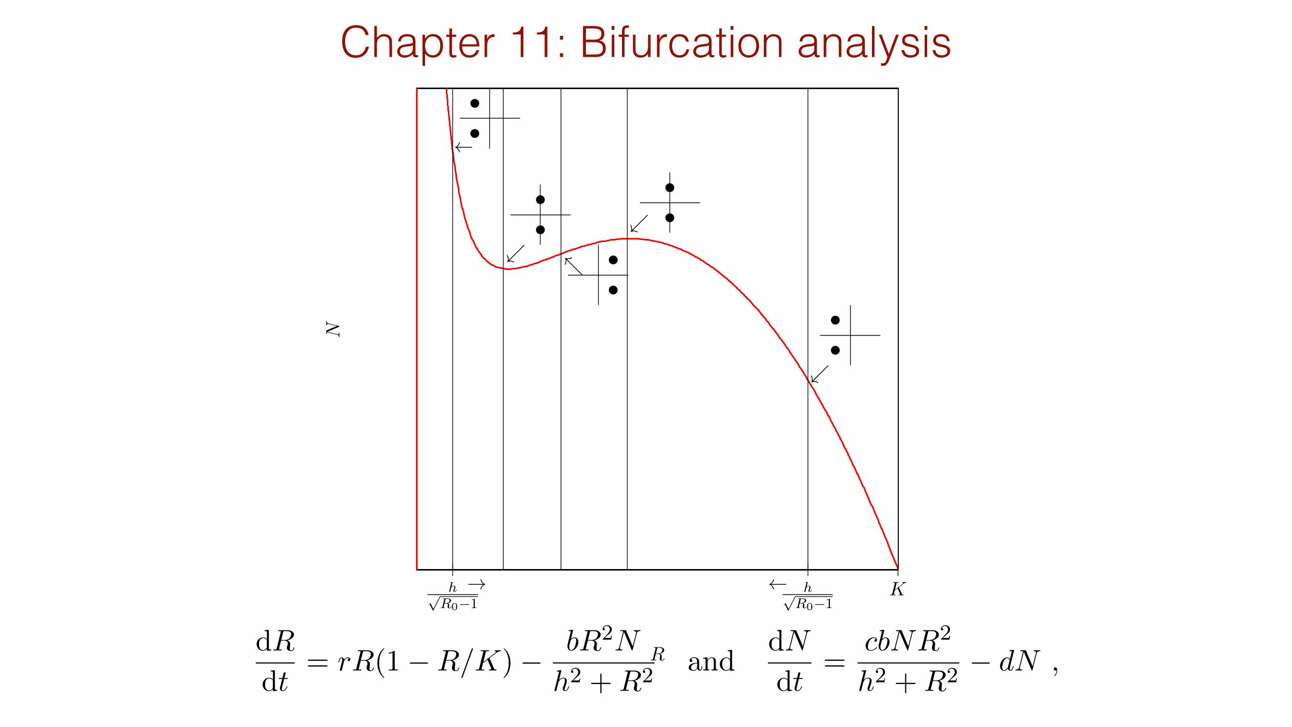
Figure 14.1: Two Hopf bifurcations in the sigmoid predator prey model. The vertical lines depict thedN/dt = 0 nullcline for various values of hp

R0�1. The “Argand diagrams” depict the eigenvalues by

plotting the real part on the horizontal, and the imaginary part on the vertical axis (see also Fig. 17.4).Hopf bifurcations corresponds to a complex pair moving through the imaginary axis.

that the non-trivial predator nullcline is a vertical line located at the prey densityR =q

h2

cb/d�1 =

h/pR0 � 1. Thus by changing the predator death rate d one moves the predator nullcline, and

because the predator death rate is not part of the ODE of the prey, the prey nullcline remainsidentical.

First consider values of the death rate d in Fig. 14.1 for which the predator nullcline is locatedat the right side of the top of the humped prey nullcline. The graphical Jacobian is

A =

✓�a �bc 0

◆such that tr = �a < 0 and det = bc > 0 . (14.2)

Close to the top of the prey nullcline the discriminant of this matrix, D = a2� 4bc, will becomenegative, and the steady state is a stable spiral point with eigenvalues �± = �a ± ib. (Belowwe will see that the same steady state will be a stable node when the nullcline intersects in theneighborhood of the carrying capacity.) Decreasing the parameter d the predator nullcline isshifted to the left, and will cross through the top of the prey nullcline. When located left of thistop the graphical Jacobian is

A =

✓a �bc 0

◆such that tr = a > 0 and det = bc > 0 . (14.3)

Chapter 14

Bifurcation analysis

In several chapters of this course we have encountered examples where the properties of asteady state changes at some critical parameter value. A good example is the steady state ofthe Monod saturated predator prey model which changes stability precisely when the verticalpredator nullcline intersects the top of the parabolic prey nullcline. We have seen that at this“Hopf bifurcation point” the stability of the steady state is carried over to a stable limit cycle.In the same model there was another bifurcation point when the predator nullcline runs throughthe carrying capacity of the prey. This is a so-called “transcritical bifurcation” at which thepresence of the predator is determined. In ODE models there are only four di↵erent types ofbifurcations that can happen if one changes a single parameter. This chapter will illustrate allfour of them and explain them in simple phase plane pictures.

Bifurcation diagrams depict what occurs when one changes a single parameter, and thereforeprovide a powerful graphical representation of the di↵erent behaviors a model may exhibit fordi↵erent values of its parameters. Bifurcation diagrams are typically made with special purposesoftware tools (like CONTENT, AUTO, or XPPAUT); GRIND has a fairly primitive algorithmfor continuing steady states. In the exercises you will be challenged to sketch a few bifurcationdiagrams with pencil and paper.

Several other bifurcations may occur if one changes two parameters at the same time. These canbe summarized in 2-dimensional bifurcation diagrams, which can provide an even better overviewof the possible behaviors of a model. The 2-dimensional bifurcations will not be discussed here,and we refer you to books or courses on bifurcation analysis.

14.1 Hopf bifurcation

At a Hopf bifurcation a limit cycle is born from a spiral point switching stability. This wasalready discussed at length in Chapter 6 for models with a saturated functional response. Fig.14.1 depicts the nullclines of a predator prey model with a sigmoid functional response for severaldi↵erent values of the death rate, d, of the predator N . In Chapter 6 we already calculated forthe model

dR

dt= rR(1�R/K)� bR2N

h2 +R2and

dN

dt=

cbNR2

h2 +R2� dN , (14.1)

Hopf bifurcation14.1 Hopf bifurcation 99

(a)

d

N

rr

rrrr

"rr#rr

(b)

d

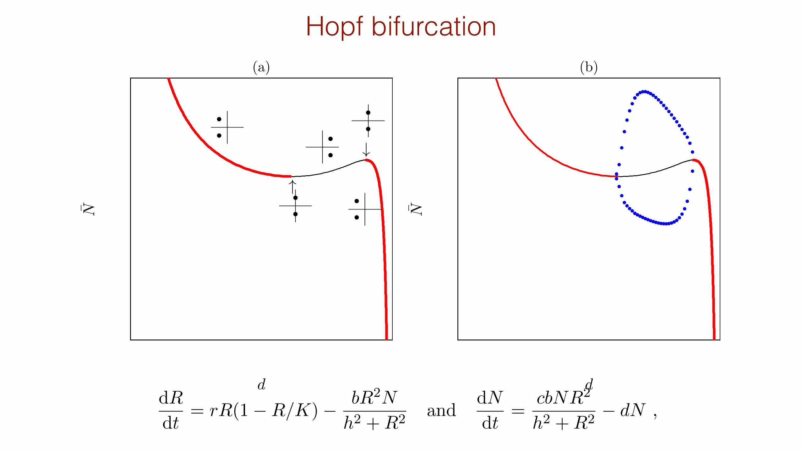
NFigure 14.2: A bifurcation diagram with the two Hopf bifurcations of Fig. 14.1. The circles in panel (b)depict the stable limit cycle that exist between the two Hopf bifurcations for many di↵erent values of theparameter d.

Close to the top the discriminant, D = a2�4bc, will remain to be negative, and the steady stateis an unstable spiral point.

For the critical value of d where the nullcline is located at the top, i.e., at (K�h)/2 (see Chapter6) the graphical Jacobian is

A =

✓0 �bc 0

◆such that tr = 0 and det = bc > 0 . (14.4)

The imaginary eigenvalues �± = ±ipbc have no real part and correspond to the structurally

unstable equilibrium point of the Lotka Volterra model lacking a carrying capacity of the prey.Summarizing, at a Hopf bifurcation a complex pair of eigenvalues moves through the imaginaryaxis. At the bifurcation point the steady state has a neutral stability, and a limit cycle is born.

Fig. 14.1 has little diagrams displaying the nature of the eigenvalues in so-called “Argand di-agrams”. These diagrams simply depict the real part of an eigenvalue on the horizontal axis,and the imaginary part on the vertical axis (see Fig. 17.4). In these diagrams a complex pairof eigenvalues is located at one specific x-value with two opposite imaginary parts, and a realeigenvalue will be a point on the horizontal axis. The Hopf bifurcation can neatly be summarizedas a complex pair moving horizontally through the vertical imaginary axis (see Fig. 14.1).

This is summarized in the bifurcation diagram of Fig. 14.2 which depicts the steady state value ofthe predator as a function of its death rate d. Stable steady states are drawn as heavy lines, andunstable steady states as light lines. We have chosen to have the predator on the vertical axisto facilitate the comparison with the phase portrait of Fig. 14.1, which also has the predator onthe vertical axis (note that if we had chosen the prey on the vertical axis the steady state wouldbe a line at R = h/

pR0 � 1). Sometimes one depicts the “norm”, i.e., N2 +R2, on the vertical

axis, but this all remains rather arbitrary because it is not so important what is exactly plottedon the vertical axis as long as it provides a measure of the location of the steady state. The

Chapter 14







dR


h2 +R2and

dN

dt=

cbNR2

h2 +R2� dN , (14.1)

Transcritical bifurcation100 Bifurcation analysis

(a)

R

N

K

0

(b)

dN

0

rr rr

r r

rr

rr

r rrr %

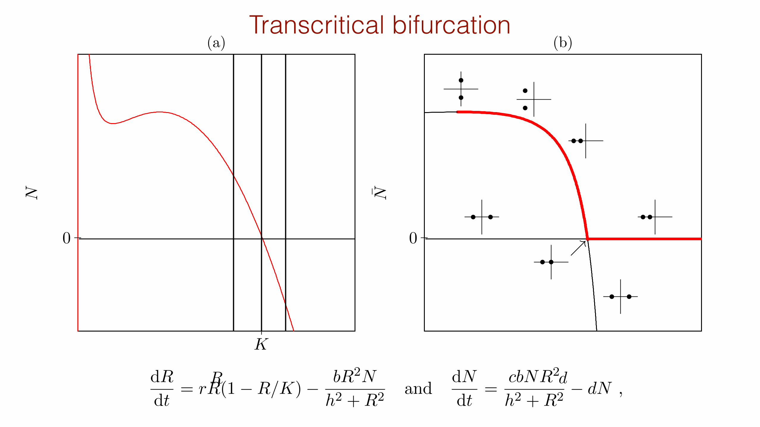
Figure 14.3: The phase space for three values of d around a transcritical bifurcation (a), and thebifurcation diagram (b) of a transcritical bifurcation with d as the bifurcation parameter on the horizontalaxis.

bifurcation diagram displays another Hopf bifurcation that occurs when the predator nullclinegoes through the bottom of the prey nullcline. Between these critical values of d there exits astable limit cycle, of which we depict the amplitude by the bullets in Fig. 14.2b. Decreasing dthe limit cycle is born at the top and dies at the bottom of the prey nullcline, increasing d thiswould just be the other way around. Fig. 14.2 does provide a good summary of the behavior ofthe model as a function of the death rate d.

In Fig. 14.2b the amplitude of limit cycle is depicted by the bullets reflecting predator densitiesat some predefined prey density. Conventionally closed circles are used to depict stable limitcycles, and open circles are used for unstable limit cycles (that we have not encountered explicitlyin this book; but there is one in Fig. 6.7d). To depict and study limit cycles one typically plotsthe predator value when the limit cycles crosses through a particular prey value. Such a preyvalue is called a Poincare section, and on this Poincare plane one can define the limit cycle as amap, mapping one point on the section to the next crossing by the limit cycle. The stability ofthe limit cycle is then determined from the “Floquet multipliers” of this map. This will not beexplained any further in this book.

14.2 Transcritical bifurcation

If one increases the death rate d in the same model, the predator nullcline moves to the right.As long as this nullcline remains left of the carrying capacity the steady state will remain stable.However, at one specific value of d it will change from a stable spiral into a stable node. In theArgand diagram this means that the complex pair collapses into a single point on the horizontalaxis, after which the eigenvalues drift apart on the horizontal (real) axis (see Fig. 14.3). Whenthe predator nullcline is about to hit the carrying capacity, one can be sure the steady state hasbecome a stable node, i.e., it will have two real eigenvalues smaller than zero.

Chapter 14







dR


h2 +R2and

dN

dt=

cbNR2

h2 +R2� dN , (14.1)

Saddle node bifurcation14.3 Saddle node bifurcation 101

(a)

N

R " #"

#

"

K(b)

R

NK

-

#

(c)

e

N

"qq "qq q q-

q q!q q!qq

qq

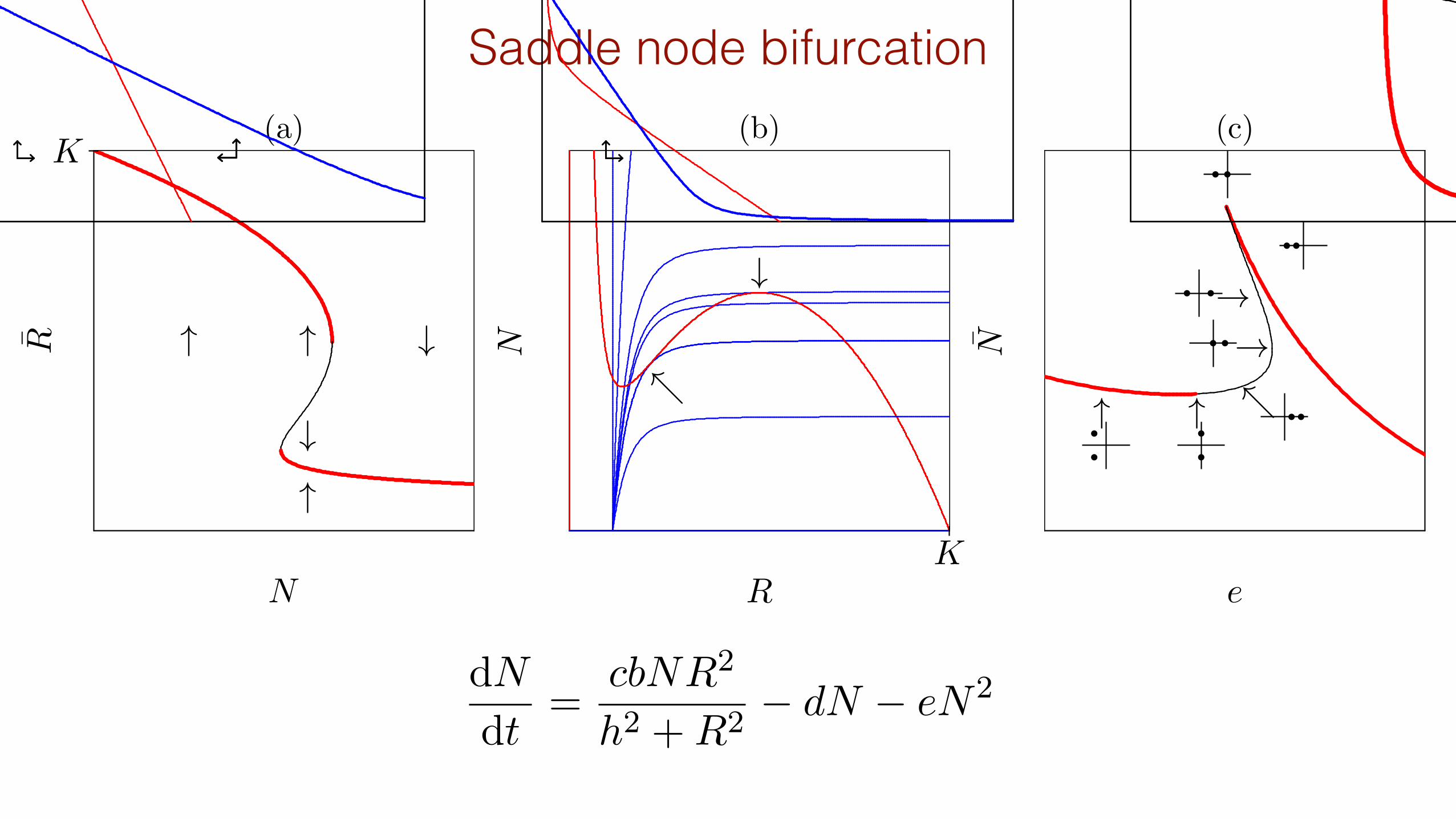
Figure 14.4: The bifurcation diagram of the saddle node bifurcations in Eq. (14.1)a with a fixed numberof predators N as a bifurcation parameter, and the phase space (b) and bifurcation diagram (c) of thefull model of Eq. (14.5) with the density dependent death rate e as a bifurcation parameter. The phasespace in (b) is drawn for several values of e, and the arrows denote the two saddle-node bifurcations.

Increasing d further leads to a transcritical bifurcation at K = h/pR0 � 1. Here the stable

node collapses with the saddle point (N , R) = (K, 0). After increasing d further the saddlepoint becomes a stable node, and the non-trivial steady state becomes a saddle point locatedat a negative predator density. At the bifurcation point one of the eigenvalues goes throughzero (see Fig. 14.3b), which again corresponds to the structurally unstable neutral stability.Transcritical bifurcations typically take place in a situation where the steady state value of oneof the variables becomes zero, i.e., correspond to situations where one of the trivial steady stateschanges stability. Because in biological models a population size of zero often corresponds to anequilibrium, transcritical bifurcations are very common in biological models.

14.3 Saddle node bifurcation

The saddle-node bifurcations that occur in the sigmoid predator prey model of Eq. (14.1) arefamous because of their interpretation of catastrophic switches between rich and poor steadystates that may occur in arid habitats like the Sahel zone (Noy-Meir, 1975; May, 1977; Sche↵eret al., 2001; Sche↵er, 2009; Hirota et al., 2011; Veraart et al., 2012). To illustrate this bifurcationone treats the predator density as a parameter, representing the number of cattle (herbivores)that people let graze in a certain habitat. This reduces the model of Eq. (14.1) to the dR/dtequation. The steady states of this 1-dimensional model are depicted in Fig. 14.4a with thenumber of herbivores, N , as a bifurcation parameter plotted on the horizontal axis. Becausethis parameter is identical to the predator variable plotted on the vertical axis of the phasespaces considered before, these steady states simply correspond to the dR/dt = 0 nullcline. Thebifurcation diagram shows two saddle-node bifurcations (see Fig. 14.4a). At some critical valueof the herbivore density on the upper branch, corresponding to a rich vegetation, disappears. Atintermediate herbivore densities the vegetation can be in one of two alternative steady states,that are separated by an unstable branch (see Fig. 14.4a). This bifurcation diagram has thefamous hysteresis where, after a catastrophic collapse of the vegetation, one has to sell a lot ofcattle before the vegetation recovers (Noy-Meir, 1975; May, 1977; Sche↵er et al., 2001).

To show a more complicated bifurcation diagram with a Hopf bifurcation, and two di↵erentsaddle-node bifurcations in the same predator prey model, we extend Eq. (14.1) with direct

102 Bifurcation analysis

(a)

N1

N2

1

1

(b)

N1

N2

1

1

(c)

c

N2

qq qq

qqq q

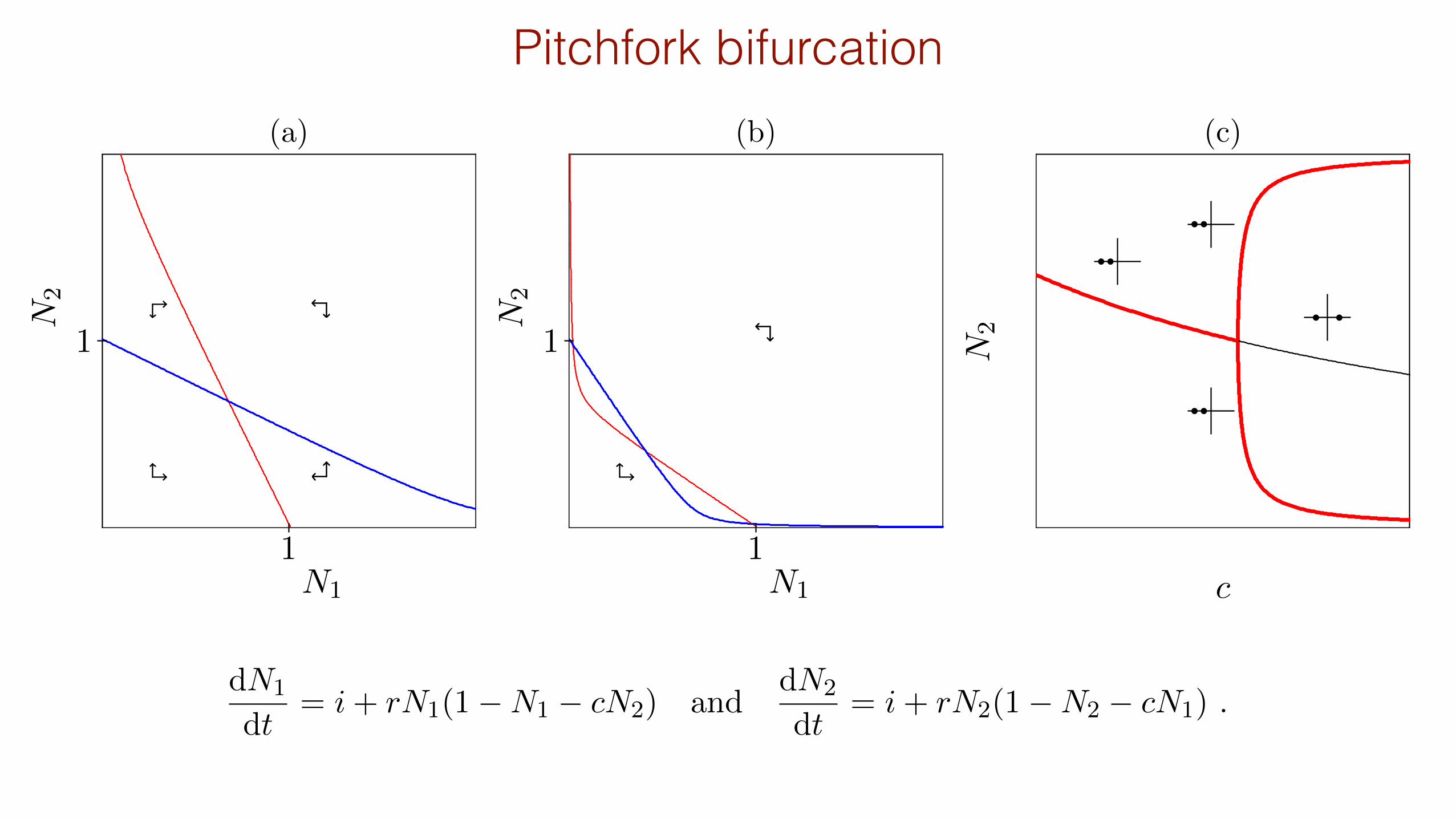
Figure 14.5: The Pitchfork bifurcation of the Lotka Volterra competition model. Panel (a) and (b) showthe phase spaces for c < 1 and c > 1, and Panel (c) shows the bifurcation diagram.

interference competition between the predators, i.e.,

dN

dt=

cbNR2

h2 +R2� dN � eN2 . (14.5)

To illustrate the saddle node bifurcations we will study the model as a function of the competitionparameter e, and will sketch a bifurcation diagram with e on the horizontal axis (see Fig. 14.4).

First, choose a value of the death rate, d, such that the predator nullcline intersects at the leftof the valley in the prey nullcline (see Fig. 14.4a). For e = 0 there is a single stable steady state.Increasing e the predator nullcline will bend because the predator nullcline can be written asthe sigmoid function

N =(cb/e)R2

h2 +R2� d/e , (14.6)

intersecting the horizontal axis at the now familiar R = h/pR0 � 1. The prey nullcline remains

the same because it does not depend on the e parameter. By increasing the curvature with e,this low steady state first undergoes a Hopf bifurcation in the valley of the prey nullcline (see Fig.14.4b & c). Then the predator nullcline will hit the prey nullcline close its top (see the arrow),which creates two new steady states at a completely di↵erent location in phase space. Increasinge a little further leads to the formation of two steady states around this first intersection point(see the other arrow). One is a saddle point and the other a unstable node (see Fig. 14.4c).A “saddle node” bifurcation is a catastrophic bifurcation because it creates (or annihilates) acompletely new configuration of steady states located just somewhere in phase space.

14.4 Pitchfork bifurcation

Thus far we have discussed three bifurcations, i.e., the Hopf, transcritical, and saddle nodebifurcation, and we could all let them occur easily in a conventional predator prey model. Thefourth, and final, bifurcation is called the pitchfork bifurcation, and can be demonstrated fromthe re-scaled competition model of Eq. (10.3) extended with a small immigration term:

dN1

dt= i+ rN1(1�N1 � cN2) and

dN2

dt= i+ rN2(1�N2 � cN1) . (14.7)

Whenever the competition parameter c is smaller than one, the species are hampered more byintraspecific competition than by interspecific competition, and they will co-exist in a stable node

Pitchfork bifurcation102 Bifurcation analysis

(a)

N1

N2

1

1

(b)

N1

N2

1

1

(c)

c

N2

qq qq

qqq q



dN

dt=

cbNR2

h2 +R2� dN � eN2 . (14.5)



N =(cb/e)R2

h2 +R2� d/e , (14.6)





dN1


dN2

dt= i+ rN2(1�N2 � cN1) . (14.7)



(a)

N1

N2

1

1

(b)

N1

N2

1

1

(c)

c

N2

qq qq

qqq q



dN

dt=

cbNR2

h2 +R2� dN � eN2 . (14.5)



N =(cb/e)R2

h2 +R2� d/e , (14.6)





dN1


dN2

dt= i+ rN2(1�N2 � cN1) . (14.7)


14.5 Period doubling cascade leading to chaos 113

R1

R2

1

1

Figure 14.6: The nullclines of the two prey species of Eq. (14.8) in the absence of the predator. Thecurved line is a trajectory.

Whenever the competition parameter c is smaller than one, the species are hampered more byintraspecific competition than by interspecific competition, and they will co-exist in a stable node(see Fig. 14.5a), and there will be one stable steady state. Increasing c above one will changethis node into the saddle point corresponding to the unstable founder controlled competition(see Fig. 14.5b). In between this two cases there is a bifurcation point of c, where one realeigenvalue goes through zero (see Fig. 14.5c). Because of the hyperbolic nature of the nullclines,one can see that when the non-trivial steady state becomes a saddle, the nullclines form newsteady states around the two carrying capacities. These new states are stable nodes (see Fig.14.5b & c). In the bifurcation diagram this is depicted as two branches, one for the stable nodebecoming a saddle point, and one for the stable nodes born at the bifurcation point. Becauseof the shape of the solutions in this bifurcation diagram this is called a pitchfork bifurcation.

Both the pitch fork bifurcation and the Hopf bifurcation have mirror images. At a so-calledsubcritical Hopf bifurcation point an unstable limit cycle is born from an unstable spiral pointbecoming stable. In a subcritical pitchfork bifurcation, an unstable branch of two outwardsteady states encloses a stable branch in the middle. Both will not further be discussed here.

14.5 Period doubling cascade leading to chaos

Having covered all possible bifurcations of steady states in ODE models we will illustrate one bi-furcation that limit cycles may undergo when one parameter is changed, i.e., the period doublingbifurcation. This bifurcation will again be explained by means of a simple example, because itoccurs in a large variety of models (including maps, see Fig. 13.2). The bifurcation is interestingbecause a cascade of period doubling bifurcations is a route to chaotic behavior. In ODE modelswe have discussed two types of attractors: stable steady states and stable limit cycles. A chaoticattractor, or strange attractor, is a third type of attractor that frequently occurs in ODE modelswith at least three variables.

The example is taken from Yodzis (1989) and is a model with two prey species that are eaten

Chaos in a one consumer two resources model


0 20 40 60 80 100

0.0

0.2

0.4

0.6

0.8

(a)

Time

Density

R1

R2

N

R1 N

R2

0 50 100 150 200

0.0

0.2

0.4

0.6

0.8

(b)

Time

Density

R1

R2

N

R1

N

R2

0 100 200 300 400 500

0.0

0.2

0.4

0.6

0.8

1.0

(c)

Time

Density

R1

R2

N

R1 N

R2

Figure 14.7: Period doubling cascade of the limit cycle of Eq. (14.8). In Panel (a) the model behavioris a simple limit cycle, in Panel (b) the limit cycle makes two loops before returning to the same point,in Panel (c) we see a chaotic attractor. This Figure was made with the file rrn.R.

by a single predator

dR1

dt= R1(1 � R1 � ↵12R2) � a1R1N ,

dR2

dt= R2(1 � R2 � ↵21R1) � a2R2N ,

dN

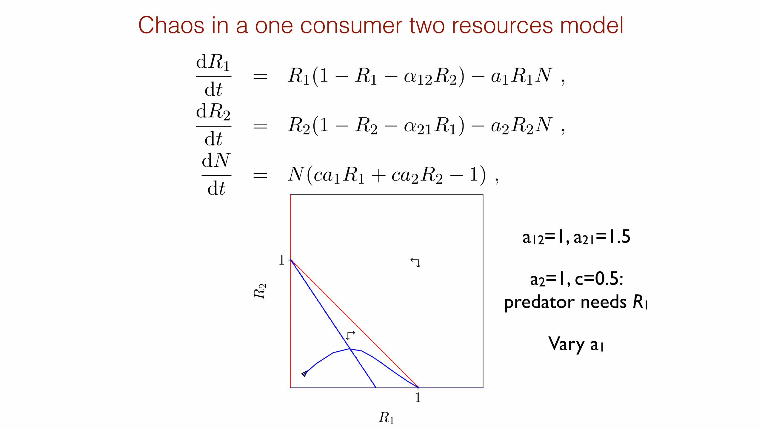
dt= N(ca1R1 + ca2R2 � 1) , (14.8)

a12=1, a21=1.5

a2=1, c=0.5:predator needs R1

Vary a1

Chaos in a one consumer two resources model


0 20 40 60 80 100

0.0

0.2

0.4

0.6

0.8

(a)

Time

Density

R1

R2

N

R1 N

R2

0 50 100 150 200

0.0

0.2

0.4

0.6

0.8

(b)

Time

Density

R1

R2

N

R1

N

R2

0 100 200 300 400 500

0.0

0.2

0.4

0.6

0.8

1.0

(c)

Time

Density

R1

R2

N

R1 N

R2

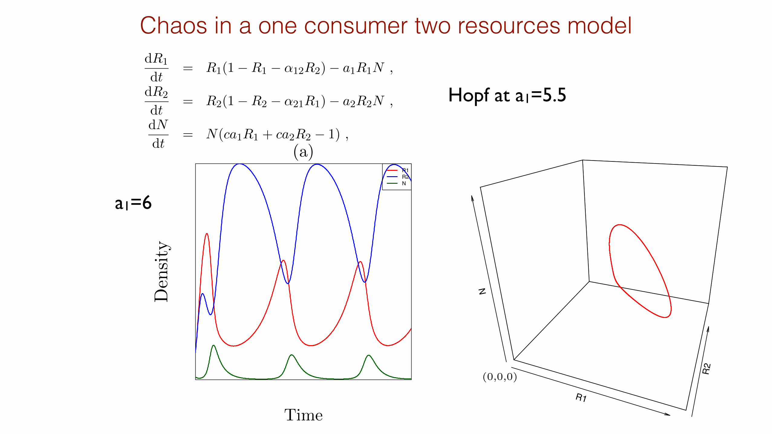
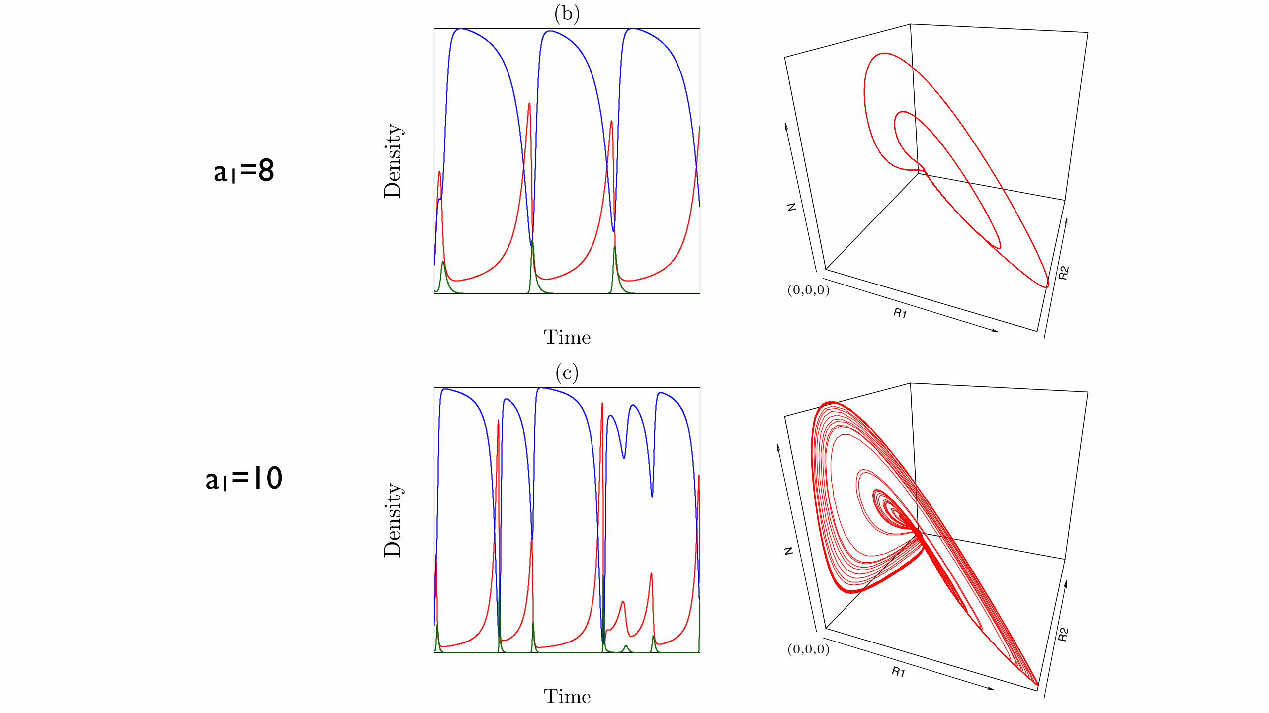
Figure 14.7: Period doubling cascade of the limit cycle of Eq. (14.8). In Panel (a) the model behavioris a simple limit cycle, in Panel (b) the limit cycle makes two loops before returning to the same point,in Panel (c) we see a chaotic attractor. This Figure was made with the file rrn.R.

by a single predator

dR1

dt= R1(1 � R1 � ↵12R2) � a1R1N ,

dR2

dt= R2(1 � R2 � ↵21R1) � a2R2N ,

dN

dt= N(ca1R1 + ca2R2 � 1) , (14.8)

a1=6

Hopf at a1=5.5130 Bifurcation analysis

R1R2N

(a)

Time

Den

sity

R1

R2

N

(0,0,0)

(b)

Time

Den

sity

R1

R2

N

(0,0,0)

(c)

Time

Den

sity

R1

R2

N

(0,0,0)

Figure 11.7: Period doubling cascade of the limit cycle of Eq. (11.8). In Panel (a) the model behavioris a simple limit cycle, in Panel (b) the limit cycle makes two loops before returning to the same point,in Panel (c) we see a chaotic attractor. This figure was made with the file rrn.R.

riod doubling bifurcations is a route to chaotic behavior. In ODE models we have discussedtwo types of attractors: stable steady states and stable limit cycles. A chaotic attractor, orstrange attractor, is a third type of attractor that can occur in ODE models having at leastthree variables.

The example is taken from Yodzis (1989) and is a model with two resource species that are eaten

a1=8

a1=10


R1R2N

(a)

Time

Den

sity

R1

R2

N

(0,0,0)

(b)

Time

Den

sity

R1

R2

N

(0,0,0)

(c)

Time

Den

sity

R1

R2

N

(0,0,0)

Figure 11.7: Period doubling cascade of the limit cycle of Eq. (11.8). In Panel (a) the model behavioris a simple limit cycle, in Panel (b) the limit cycle makes two loops before returning to the same point,in Panel (c) we see a chaotic attractor. This figure was made with the file rrn.R.

riod doubling bifurcations is a route to chaotic behavior. In ODE models we have discussedtwo types of attractors: stable steady states and stable limit cycles. A chaotic attractor, orstrange attractor, is a third type of attractor that can occur in ODE models having at leastthree variables.

The example is taken from Yodzis (1989) and is a model with two resource species that are eaten

Period doubling cascade14.5 Period doubling cascade leading to chaos 115

5

0.41

0.205

0

a1

128.5

R1

a1

R1

5 8.5 120

0.205

0.41

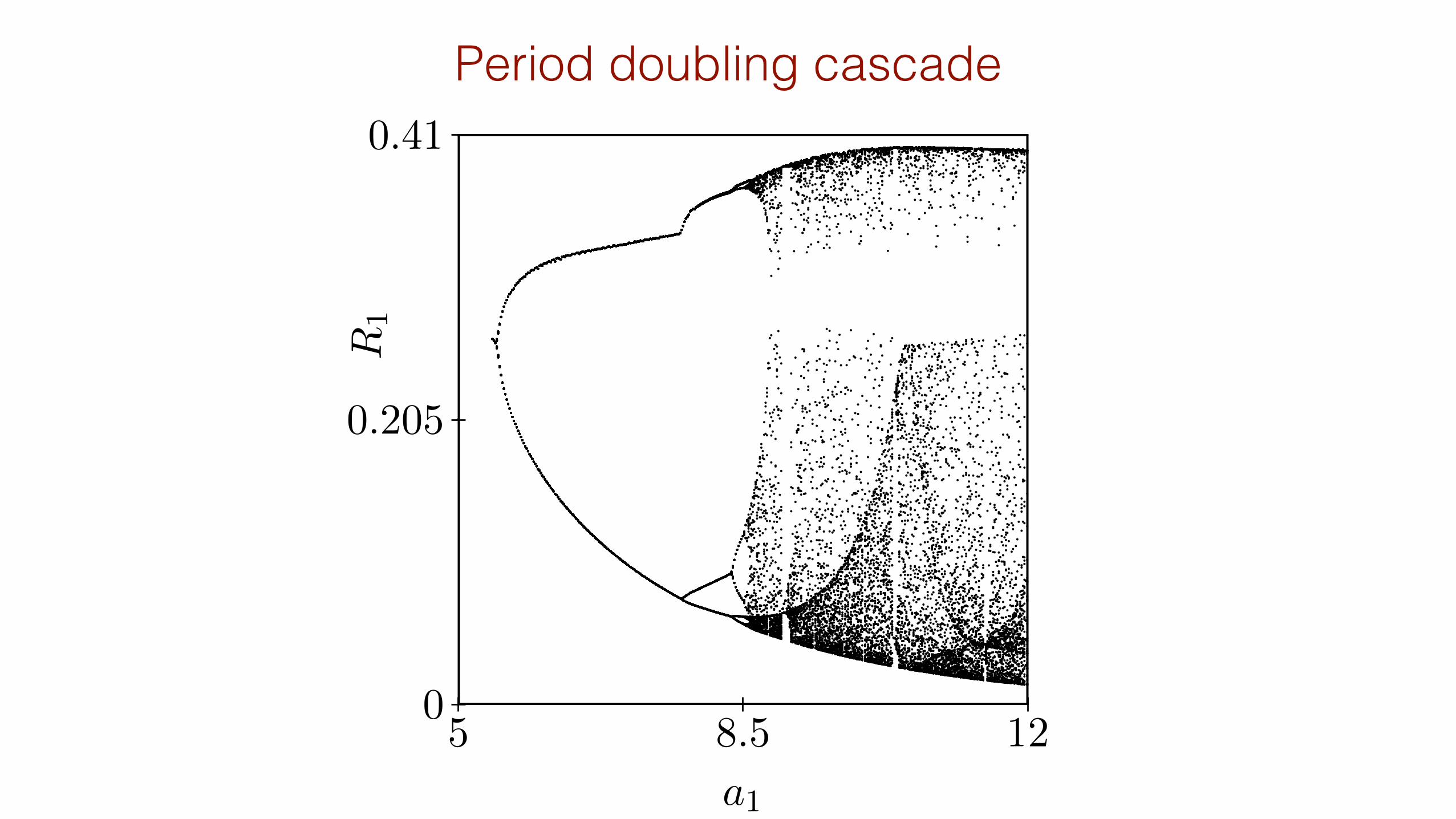
Figure 14.8: Period doubling cascade of the limit cycle of Eq. (14.8) illustrated by plotting 200 valuesof R1 obtained for many di↵erent values of a1. The values of R1 are recorded when the trajectory crossesa Poincare plane located around R2 = 0.8. Note how similar this is to the bifurcation diagram of theLogistic map (Fig. 13.2).

with simple mass-action predation terms. Time is scaled with respect to the death rate of thepredator, and both carrying capacities have been scaled to one. Setting the parameters ↵12 = 1and ↵21 = 1.5 the prey species exclude each other in the absence of the predator (see Fig. 14.6).The behavior of the model is studied by varying the predation pressure, a1, on the winningspecies. By setting a2 = 1 and c = 0.5, i.e., ca2 = 0.5, the model is designed such that thepredator cannot survive on R2 alone. For 3.4 a1 5.5 one obtains a stable steady state whereall three species co-exist. Around a1 = 5.5 this steady state undergoes a Hopf bifurcation, anda stable limit cycle is born. (Note that at a1 = 3.4 a transcritical bifurcation allows the secondprey to invade (because the first one su↵ers su�ciently from the predation), and that at a1 = 2a second transcritical bifurcation occurs when the predator can invade.)

Fig. 14.7 shows what happens if a1 is increased further. For a1 = 6 there is a simple stable limitcycle that was born at the Hopf bifurcation (see Fig. 14.7a). At a1 = 8 this limit cycle makestwo rounds before returning to its starting point: the period has approximately doubled at aperiod doubling bifurcation somewhere between 6 < a1 < 8. This repeats itself several times,and at a1 = 10 the system is already chaotic (see Fig. 14.8).

Chaotic behavior is defined by two important properties:1. An extreme sensitivity for the initial conditions. An arbitrary small deviation from a chaotic

trajectory will after su�cient time expand into a macroscopic distance. This is the famous“butterfly” e↵ect where the disturbance in the air flow caused by a butterfly in Africa flyingto the next flower will cause a rainstorm in Europe after a week.

2. A fractal structure: a strange attractor has a layered structure that will appear layered againwhen one zooms in (e.g., see Fig. 13.2 and Fig. 14.8).

The first property is obviously important for the predictability of ecological models. It could verywell be that one will never be able to predict the precise future behavior of several ecosystems(like we will never be able to predict the weather on June 17 in the next year). This sensitivitycomes about from the “folding” and “stretching” regions in strange attractors where manytrajectories collapse and are torn apart again.

chapter 11: bifurcation analysis

Documents