www.elsevier.com/locate/compstruc

Computers and Structures 84 (2006) 2200–2211

Micromechanical analysis of interfacial debondingin unidirectional fiber-reinforced composites

A. Caporale *, R. Luciano, E. Sacco

Dipartimento di Meccanica, Strutture, Ambiente e Territorio, Universita degli Studi di Cassino, via G. Di Biasio 43, 03043 Cassino, Italy

Received 24 May 2005; accepted 7 August 2006Available online 23 October 2006

Abstract

In this paper the behaviour of unidirectional fiber-reinforced composites with imperfect interfacial bonding is investigated by usingthe finite element method. The matrix and the fibers are considered homogeneous, isotropic and linearly elastic; an interfacial failuremodel is implemented by connecting the fibers and the matrix at the finite element nodes by normal and tangential brittle-elastic springs.Numerical analyses are carried out on a unit cell extracted from a composite model characterized by a periodic microstructure. Themicromechanical simulations provide the first failure loci (FFL), i.e. the envelopes of the composite average strains corresponding tothe initiation of the debonding, and the instantaneous overall moduli of the damaged composite corresponding to several interface dam-age configurations. The results show that the intersections of the FFL with prescribed planes are defined by curves associated with dif-ferent interface failure modes. Besides, damage induced by fiber–matrix debonding is strongly anisotropic and dependent on the loadhistory.� 2006 Elsevier Ltd. All rights reserved.

Keywords: Fiber-reinforced composites; Homogenization; Damage; Interfacial partial debonding; Brittle behaviour; Finite elements

1. Introduction

In the last decades composites have become commonengineering materials because of their good mechanicaland electro-chemical properties. Specifically, fiber-reinforced composites are one of the most widely usedman-made composite materials; they are constituted byreinforcing fibers embedded in a matrix material. The uni-directional lamina, considered in this work, is constitutedby uniformly oriented long fibers that provide goodmechanical properties in the direction parallel to the fibers(longitudinal direction). The overall properties of thelamina in the longitudinal direction can be approximatedby using the well-known rule of mixture. It is more difficultto evaluate the overall properties in the directions perpen-dicular to the fibers (transverse directions) and the interac-tions between the longitudinal and transverse behaviours;

0045-7949/$ - see front matter � 2006 Elsevier Ltd. All rights reserved.

doi:10.1016/j.compstruc.2006.08.023

* Corresponding author.E-mail address: a.caporale@unicas.it (A. Caporale).

several methods have been proposed to evaluate and tobound the overall linear and non-linear properties of thecomposites [1].

The greater part of papers devoted to the overall non-linear behaviour of composites assumes that the fibers arelinearly elastic and the matrix is non-linear; many authorshave studied the fibrous composites with elastoplasticmatrix providing the overall instantaneous compliances[2] and estimates of the overall stress–strain relations [3].Taliercio and Coruzzi [4] have proposed a constitutivemodel of the matrix, characterized by a plastic strain hard-ening in compression and strain softening in tension, inorder to study the brittle matrix composites such as theceramic composites and the thermosetting resins withflaws. Aboudi [5] has introduced the method of cells inorder to evaluate the overall properties of composites withnon-linear matrix and fibers characterized by a rectangularcross section.

The above-mentioned articles consider an ideal compos-ite with perfect bonding between the matrix and the fibers,

a2 = 3a1

x1

x3

x2

a1

a2

Matrix

Fiber

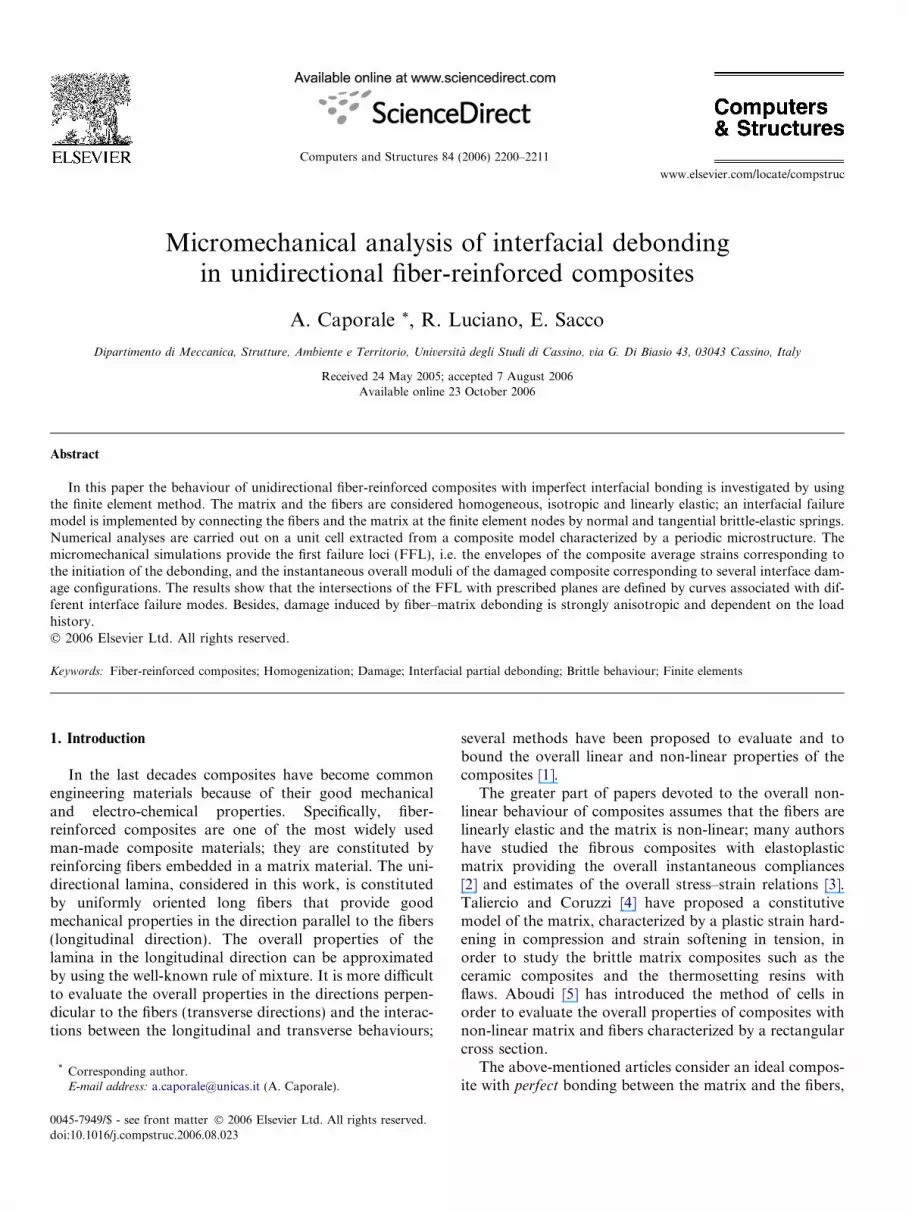
Fig. 1. The unidirectional composite with hexagonal symmetry.

2a2

2a1

2a3

x1x3

x2

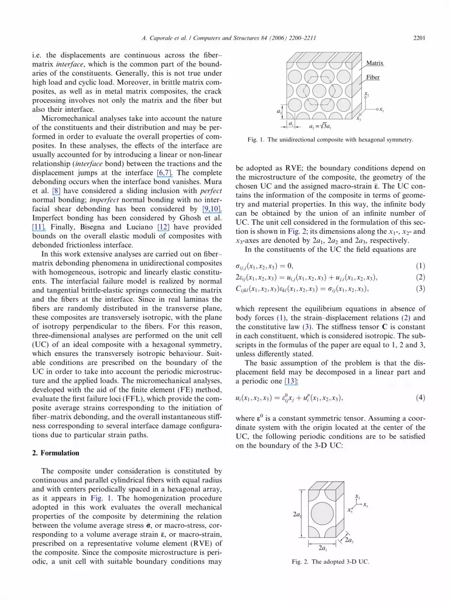
Fig. 2. The adopted 3-D UC.

A. Caporale et al. / Computers and Structures 84 (2006) 2200–2211 2201

i.e. the displacements are continuous across the fiber–matrix interface, which is the common part of the bound-aries of the constituents. Generally, this is not true underhigh load and cyclic load. Moreover, in brittle matrix com-posites, as well as in metal matrix composites, the crackprocessing involves not only the matrix and the fiber butalso their interface.

Micromechanical analyses take into account the natureof the constituents and their distribution and may be per-formed in order to evaluate the overall properties of com-posites. In these analyses, the effects of the interface areusually accounted for by introducing a linear or non-linearrelationship (interface bond) between the tractions and thedisplacement jumps at the interface [6,7]. The completedebonding occurs when the interface bond vanishes. Muraet al. [8] have considered a sliding inclusion with perfect

normal bonding; imperfect normal bonding with no inter-facial shear debonding has been considered by [9,10].Imperfect bonding has been considered by Ghosh et al.[11]. Finally, Bisegna and Luciano [12] have providedbounds on the overall elastic moduli of composites withdebonded frictionless interface.

In this work extensive analyses are carried out on fiber–matrix debonding phenomena in unidirectional compositeswith homogeneous, isotropic and linearly elastic constitu-ents. The interfacial failure model is realized by normaland tangential brittle-elastic springs connecting the matrixand the fibers at the interface. Since in real laminas thefibers are randomly distributed in the transverse plane,these composites are transversely isotropic, with the planeof isotropy perpendicular to the fibers. For this reason,three-dimensional analyses are performed on the unit cell(UC) of an ideal composite with a hexagonal symmetry,which ensures the transversely isotropic behaviour. Suit-able conditions are prescribed on the boundary of theUC in order to take into account the periodic microstruc-ture and the applied loads. The micromechanical analyses,developed with the aid of the finite element (FE) method,evaluate the first failure loci (FFL), which provide the com-posite average strains corresponding to the initiation offiber–matrix debonding, and the overall instantaneous stiff-ness corresponding to several interface damage configura-tions due to particular strain paths.

2. Formulation

The composite under consideration is constituted bycontinuous and parallel cylindrical fibers with equal radiusand with centers periodically spaced in a hexagonal array,as it appears in Fig. 1. The homogenization procedureadopted in this work evaluates the overall mechanicalproperties of the composite by determining the relationbetween the volume average stress �r, or macro-stress, cor-responding to a volume average strain �e, or macro-strain,prescribed on a representative volume element (RVE) ofthe composite. Since the composite microstructure is peri-odic, a unit cell with suitable boundary conditions may

be adopted as RVE; the boundary conditions depend onthe microstructure of the composite, the geometry of thechosen UC and the assigned macro-strain �e. The UC con-tains the information of the composite in terms of geome-try and material properties. In this way, the infinite bodycan be obtained by the union of an infinite number ofUC. The unit cell considered in the formulation of this sec-tion is shown in Fig. 2; its dimensions along the x1-, x2- andx3-axes are denoted by 2a1, 2a2 and 2a3, respectively.

In the constituents of the UC the field equations are

rij;jðx1; x2; x3Þ ¼ 0; ð1Þ2eijðx1; x2; x3Þ ¼ ui;jðx1; x2; x3Þ þ uj;iðx1; x2; x3Þ; ð2ÞCijklðx1; x2; x3Þeklðx1; x2; x3Þ ¼ rijðx1; x2; x3Þ; ð3Þ

which represent the equilibrium equations in absence ofbody forces (1), the strain–displacement relations (2) andthe constitutive law (3). The stiffness tensor C is constantin each constituent, which is considered isotropic. The sub-scripts in the formulas of the paper are equal to 1, 2 and 3,unless differently stated.

The basic assumption of the problem is that the dis-placement field may be decomposed in a linear part anda periodic one [13]:

uiðx1; x2; x3Þ ¼ e0ijxj þ up

i ðx1; x2; x3Þ; ð4Þ

where e0 is a constant symmetric tensor. Assuming a coor-dinate system with the origin located at the center of theUC, the following periodic conditions are to be satisfiedon the boundary of the 3-D UC:

2202 A. Caporale et al. / Computers and Structures 84 (2006) 2200–2211

upi ða1; x2; x3Þ ¼ up

i ð�a1; x2; x3Þ8x2 2 ½�a2; a2�;8x3 2 ½�a3; a3�;

�

upi ðx1; a2; x3Þ ¼ up

i ðx1;�a2; x3Þ8x1 2 ½�a1; a1�;8x3 2 ½�a3; a3�;

�

upi ðx1; x2; a3Þ ¼ up

i ðx1; x2;�a3Þ8x1 2 ½�a1; a1�;8x2 2 ½�a2; a2�:

�ð5Þ

Under the assumption of perfect bonding, from conditions(4) and (5) and the Gauss theorem it results that the tensore0 represents the average strain �e ¼ 1=V

RV eðx1; x2; x3ÞdV

over the volume V of the UC. From conditions (4) and(5) it also follows:

uiða1; x2; x3Þ � uið�a1; x2; x3Þ ¼ 2e0i1a1

8x2 2 ½�a2; a2�;8x3 2 ½�a3; a3�;

�

uiðx1; a2; x3Þ � uiðx1;�a2; x3Þ ¼ 2e0i2a2

8x1 2 ½�a1; a1�;8x3 2 ½�a3; a3�;

�

uiðx1; x2; a3Þ � uiðx1; x2;�a3Þ ¼ 2e0i3a3

8x1 2 ½�a1; a1�;8x2 2 ½�a2; a2�;

�

ð6Þwhich represent the displacement boundary conditions ofthe homogenization problem under consideration [14].

Together with the relations (6) further constraints mustbe imposed to avoid the rigid-body translations of the unitcell:

uiðx01; x02; x03Þ ¼ 0; ð7Þwhere ðx01; x02; x03Þ is an arbitrary point of the UC. The dis-placement fields satisfying the relations (6) do not containrigid-body rotations because of the symmetry of the tensore0.

It is worth noting that, if debonding phenomena arepresent at the interface C between the matrix and the fibersand if the displacement field is given by (4), the followingrelation is satisfied [5,15]:

e0ij ¼

1

2V

ZoVðuinj þ ujniÞdS

¼ 1

V

ZV m

eij dV þZ

V f

eij dV þ 1

2

ZCðDuigj þ DujgiÞdS

� �;

ð8Þ

where Vm and Vf are the volume of the matrix and thefibers of the UC, respectively, ni and gi are the ith compo-nents of the outer unit normal to the boundary oV of theUC and to the boundary of the fibers, respectively, andDui ¼ um

i � ufi represents the jump of the displacement ui

across C, being umi and uf

i the displacements of the matrixand the fiber, respectively. In the relation (8) the indepen-dent variables x1, x2 and x3 are omitted; in the following,they will be omitted when considered unnecessary. Further-more, the average strain �e over the UC will be assumedequal to e0 either in presence of perfect bonding and whenthe displacements are discontinuous across the fiber–matrixinterface.

The traction boundary conditions, which ensure theequilibrium of the tractions between two adjacent unitcells, are given by

rijða1; x2; x3Þnjða1; x2; x3Þ

¼ �rijð�a1; x2; x3Þnjð�a1; x2; x3Þ8x2 2 ½�a2; a2�;8x3 2 ½�a3; a3�;

�

rijðx1; a2; x3Þnjðx1; a2; x3Þ

¼ �rijðx1;�a2; x3Þnjðx1;�a2; x3Þ8x1 2 ½�a1; a1�;8x3 2 ½�a3; a3�;

�

rijðx1; x2; a3Þnjðx1; x2; a3Þ

¼ �rijðx1; x2;�a3Þnjðx1; x2;�a3Þ8x1 2 ½�a1; a1�;8x2 2 ½�a2; a2�:

�

ð9Þ

The conditions (9) are not imposed on oV since they areverified implicitly in elastostatics when the periodic dis-placement field satisfies the boundary conditions (5) [14].

In order to describe the mechanical model of the inter-face, a local system of axes (P,n, t,x3) is introduced whoseorigin P belongs to the interface C, its n-axis is normal to Cand oriented toward the matrix and the t-axis is tangentialto C and such that the n-, t- and x3-axes constitute a right-handed triad. Next, the components of the displacements,tractions and forces at the interface will be always consid-ered along the n-, t- and x3-axes.

In the present model the damage is localized at the inter-face. Here, the compressive strength is unbounded and thefailure occurs when the normal traction rnn exceeds its limitvalue rlim, namely the tensile strength, or when the tangen-tial traction sn exceeds its limit value slim, namely the shearstrength. Consequently, the failure criterion is satisfiedwhen one of the following conditions is verified at theinterface:

rnn ¼ rlim; sn ¼ffiffiffiffiffiffiffiffiffiffiffiffiffiffiffiffiffiffir2

nt þ r2n3

q¼ slim; ð10Þ

where rnt and rn3 are the interfacial tangential tractions.Before the failure, the constitutive law of the interface is

rnn ¼ cnDun; rnt ¼ ctDut;

rn3 ¼ c3Du3 with Dun P 0; ð11Þ

where Dui ¼ umi � uf

i (i = n, t, 3) and cn, ct and c3 are springconstant type parameters characterizing the interface bond[6]. Only non-negative normal jump Dun is admitted sincethe interpenetration of the constituents must be excluded.

After the failure the behaviour of the interface is charac-terized by two possible states: (I) the interface is open ifDun > 0; in this case the interface tractions rni (i = n, t, 3)are zero; (II) the interface is closed if Dun = 0; in this casefrictionless sliding can occur and it results rnt = rn3 = 0and rnn 6 0.

The average stresses �rij (i, j = 1, 2, 3) over the UC can bedetermined through the following volume or boundaryintegrals [15]:

Fig. 3. The finite element mesh adopted in the computation.

A. Caporale et al. / Computers and Structures 84 (2006) 2200–2211 2203

�rij ¼1

V

ZV

rijðx1; x2; x3ÞdV

¼ 1

V

ZoV

xiðx1; x2; x3Þtjðx1; x2; x3ÞdS; ð12Þ

where tj is the jth component of the traction acting on theboundaries of the constituents and its jump at the interfaceis zero in order to ensure equilibrium. The overall elasticstiffness C is defined by the overall constitutive law �r ¼ C�e.

3. Finite element approximation

The finite element code ANSYS 6.1 is used to solve theproblem described above. A right regular prism with np lat-eral faces approximates the cylindrical fiber of the UC. Inorder to ensure a fixed value of the volume fractioncf = Vf/V of the fiber, the radius R of the cylinder that cir-cumscribes the prism must satisfy the following equation:

cf

V2¼ 2a3npR2 sin

pnp

cospnp

: ð13Þ

The matrix and the fibers are modelled by linearly elasticisoparametric brick elements with eight nodes and six faces.The mechanical behaviour of the interface is modelled byboth contact elements and brittle-elastic joint elements.The ANSYS contact elements avoid the interpenetrationof the constituents and allow frictionless sliding; they donot allow considering the bond that exist at the interfacebefore the failure: e.g. in the released version of theANSYS software, the penalty tangential parameter ct ofthe contact elements must be equal to c3 and it becomesnegligible when the maximum tangential contact tractionslim is exceeded, but interfacial tensile tractions are notallowed. This capability is not present also in the latestreleases of the software, and it has been included by imple-menting user version of contact elements. From the com-putational point of view, it is more simple to model thepre-failure interfacial bond with joint elements than con-tact elements. Since the aim of the paper is to investigatethe effects of debonding phenomena in unidirectional lam-ina, joint elements are used to model the pre-failure bond.

The single joint element (JE) involves a non-linear rela-tionship between the displacement jump DuiðP Þ ¼ um

i ðP Þ�uf

i ðP Þ (i = n, t, 3) and the interaction force Fi(P) (i = n, t,3), acting on the two nodes Nf and Nm which belong tothe fiber and the matrix, respectively, and occupy the sameposition P of C. The JE constitutive law is defined by

F iðP Þ ¼kiDuiðPÞ before the failure;

0 after the failure:

�ð14Þ

The scalar Fi(P) represents the component along the local i-direction of the force that the node Nm exerts on Nf. Theinterface and the composite are considered undamagedwhen the relation Fi(P) = kiDui(P) holds for the wholeinterface. Denoting by Dui(P) the maximum Dui(P) in theload history, the failure occurs on the undamaged interfacewhen one of the two following conditions is satisfied:

knD~unðP Þ ¼ F limn ;

ffiffiffiffiffiffiffiffiffiffiffiffiffiffiffiffiffiffiffiffiffiffiffiffiffiffiffiffiffiffiffiffiffiffiffiffiffiffiffiffiffiffiffik2

t D~u2t ðP Þ þ k2

3D~u23ðP Þ

q¼ F lim

s : ð15Þ

It is noted that after the failure at a point P, the stiffnesseski of the JE located in P become zero for the remainder ofthe loading process, while the contact elements continueavoiding the interpenetration of the constituents and theycontinue allowing frictionless sliding.

The constants ki (i = n, t, 3), F limn and F lim

s depend on theparameters ci, the limit tractions rlim and slim, the FE dis-cretization of the interface and its damage state. Assumingthe FE mesh illustrated in Fig. 3, where also the joint ele-ments connecting the fiber and the matrix are representedschematically, the JE located on the undamaged interfaceare characterized by the following constants:

ki ¼ cia2a3R sinpnp

;

F limn ¼ rlima2a3R sin

pnp

; F lims ¼ slima2a3R sin

pnp

;ð16Þ

where a is equal to 1 if the JE belongs to only one face ofthe parallelepiped UC, e.g. it belongs to line L1 (see Fig. 3),and is equal to 0.5 otherwise, namely the JE belongs to twofaces of the UC, e.g. it belongs to line L1 and L2 (seeFig. 3). Furthermore, if the JE belongs also to the bound-ary of the debonded interface, which is symmetric withrespect the x1, x2-plane because of the unidirectionalsymmetry of the composite, the parameter a is always 0.5.

A user version of the ANSYS COMBIN14 element isimplemented and used as JE. The single JE is modelledby three COMBIN14 elements, one for each local directioni (i = n, t, 3).

4. Results

The following computations refer to a composite withfiber volume fraction cf � 0.60551, ratio between theYoung’s modulus of the fiber and the matrix Ef/Em �31.304, Poisson’s ratio of the fiber and the matrix equalto 0.18 and 0.38, respectively, and parameterscn = ct = c3 = 10,000Em, unless differently stated. The UChas a1 = 0.5, a2 ¼

ffiffiffi3p

a1 and a3 = 0.01.A mesh-sensitivity analysis is performed in order to eval-

uate the mesh dependence of the problem. In Fig. 4 theoverall stress–strain relationship �r11=Em–�e11 of the compos-ite characterized by rlim = 2slim � 0.0015217Em is reported

11

mE

σ

0.0000

0.0004

0.0008

0.0012

0.0000 0.0001 0.0002 0.0003 0.0004

me

co

11ε

Fine mesh

Coarse mesh

Fig. 4. The overall stress–strain relationship �r11=Em–�e11 in the case�emn ¼ 0 8mn 6¼ 11.

22ε

-0.0020

-0.0015

-0.0010

-0.0005

0.0000

0.0005

-0.0020 -0.0015 -0.0010 -0.0005 0.0000 0.0005

11ε

12

12 12

12 12

12 12

12 12

0

0.5

0.7

0.9

0.99

ref

ref

ref

ref

ε

ε ε

ε ε

ε ε

ε ε

=

=

=

=

=

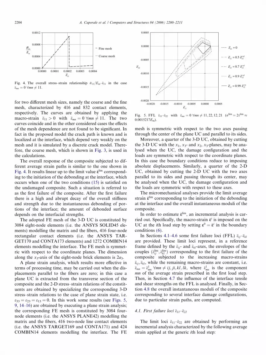
Fig. 5. FFL �e11–�e22 with �emn ¼ 0 8mn 6¼ 11; 22; 12; 21 (rlim = 2slim �0.0015217Em).

2204 A. Caporale et al. / Computers and Structures 84 (2006) 2200–2211

for two different mesh sizes, namely the coarse and the finemesh, characterized by 416 and 832 contact elements,respectively. The curves are obtained by applying themacro-strain �e11 > 0 with �emn ¼ 0 8mn 6¼ 11. The twocurves coincide and in the other considered cases the effectsof the mesh dependence are not found to be significant. Infact in the proposed model the crack path is known and islocalized at the interface, which depend very weakly on themesh and it is simulated by a discrete crack model. There-fore, the coarse mesh, which is shown in Fig. 3, is used inthe calculations.

The overall response of the composite subjected to dif-ferent average strain paths is similar to the one shown inFig. 4. It results linear up to the limit value �elim correspond-ing to the initiation of the debonding at the interface, whichoccurs when one of the two conditions (15) is satisfied onthe undamaged composite. Such a situation is referred toas the first failure of the composite. After the first failurethere is a high and abrupt decay of the overall stiffnessand strength due to the instantaneous debonding of por-tions of the interface; the amount of debonded surfacedepends on the interfacial strengths.

The adopted FE mesh of the 3-D UC is constituted by3084 eight-node elements (i.e. the ANSYS SOLID45 ele-ments) modelling the matrix and the fibers, 416 four-noderectangular contact elements (i.e. the ANSYS TAR-GET170 and CONTA173 elements) and 1272 COMBIN14elements modelling the interface. The FE mesh is symmet-ric with respect to the coordinate planes. The dimensionalong the x3-axis of the eight-node brick elements is 2a3.

A plane strain analysis, which results more effective interms of processing time, may be carried out when the dis-placements parallel to the fibers are zero; in this case aplane UC is extracted from the transverse section of thecomposite and the 2-D stress–strain relations of the constit-uents are obtained by specializing the corresponding 3-Dstress–strain relations to the case of plane strain state, i.e.e33 = e23 = e13 = 0. In this work some results (see Figs. 5,9, 14–16) are obtained by executing a plane strain analysis;the corresponding FE mesh is constituted by 3084 four-node elements (i.e. the ANSYS PLANE42) modelling thematrix and the fibers, 416 two-node line contact elements(i.e. the ANSYS TARGET169 and CONTA171) and 424COMBIN14 elements modelling the interface. The FE

mesh is symmetric with respect to the two axes passingthrough the center of the plane UC and parallel to its sides.

Moreover, a quarter of the 3-D UC, obtained by cuttingthe 3-D UC with the x1, x3- and x2, x3-planes, may be ana-lysed when the UC, the damage configuration and theloads are symmetric with respect to the coordinate planes.In this case the boundary conditions reduce to imposingabsolute displacements. Similarly, a quarter of the 2-DUC, obtained by cutting the 2-D UC with the two axesparallel to its sides and passing through its center, maybe analysed when the UC, the damage configuration andthe loads are symmetric with respect to these axes.

The micromechanical analyses provide the limit averagestrain �elim corresponding to the initiation of the debondingat the interface and the overall instantaneous moduli of thecomposite.

In order to estimate �elim, an incremental analysis is car-ried out. Specifically, the macro-strain �ei is imposed on theUC at the ith load step by setting e0 ¼ �ei in the boundaryconditions (6).

In Sections 4.1–4.6 some first failure loci (FFL) �eij–�ekl

are provided. These limit loci represent, in a referenceframe defined by the �eij- and �ekl-axes, the envelopes of thecouples ð�elim

ij ;�elimkl Þ corresponding to the first failure of the

composite subjected to the increasing macro-strains�eij;�ekl, while the remaining macro-strains are constant, i.e.�emn ¼ �e1

mn 8mn 6¼ ij; ji; kl; lk, where �e1mn is the component

mn of the average strain prescribed in the first load step.Then, in Section 4.7 the influence of the interface tensileand shear strengths on the FFL is analysed. Finally, in Sec-tion 4.8 the overall instantaneous moduli of the compositecorresponding to several interface damage configurations,due to particular strain paths, are computed.

4.1. First failure loci �e11–�e22

The limit loci �e11–�e22 are obtained by performing anincremental analysis characterized by the following averagestrain applied at the generic ith load step:

-.539E-03-.419E-03

-.299E-03-.180E-03

-.598E-04

.598E-04.180E-03

.299E-03.419E-03

.539E-03

.598E-04.218E-03

.353E-03.489E-03

.624E-03.759E-03

.895E-03.00103

.001166.001301

.001437

Case 8Case 4

Secondary diagonal

Principal diagonal

Fig. 6. Stress r22 before the first failure in the case 4 with �e22 ¼ 0:0001 and in the case 8 with �e12 ¼ 0:00005. The stress r22 is expressed in GPa and it isevaluated by assuming Em = 2.3 GPa in the computation.

22ε

-0.0020

-0.0015

-0.0010

-0.0005

0.0000

0.0005

-0.0020 -0.0015 -0.0010 -0.0005 0.0000 0.0005

11ε

33 33

0 11,22

0.5 , 0

11,22,33

mn

refmn

mn

mn

ε

ε ε ε

= ∀ ≠

= =

∀ ≠

Fig. 7. FFL �e11–�e22 (rlim = 2slim � 0.0015217Em).

A. Caporale et al. / Computers and Structures 84 (2006) 2200–2211 2205

�ei ¼ ð�ei11 �ei

22 �ei33 �ei

23 �ei13 �ei

12 Þ¼ ð ði� 1ÞD�e11 ði� 1ÞD�e22 �e1

33 �e123 �e1

13 �e112 Þ

withD�e11 ¼ jD�ej cos a;

D�e22 ¼ jD�ej sin a;

ð17Þ

where a is the angle between the �e11-axis and the straightline passing through a point of the FFL and the origin ofthe reference frame defined by the �e11- and �e22-axes; inthe numerical analyses of the paper the angle a assumesthe values 0�, 1�, 2�, . . ., 358�, 359�. In Fig. 5 the FFLwith �emn ¼ 0 8mn 6¼ 11; 22; 12; 21 are illustrated for thecomposite with the interfacial strengths rlim = 2slim �0.0015217Em. The initial strain �e1

12 is chosen less than thelimit �elim

12 � 0:00018974, obtained by applying an averagestrain paths that is indicated as case 8 in remainder ofthe analysis and is characterized by a transverse shearstrain �e12 > 0 with �emn ¼ 0 8mn 6¼ 12; 21. The case 8 is thelast of eight cases of macro-strain paths introduced to ex-plain better the results presented in the paper; the cases1–7 will be described later on. Moreover, the limit strain�elim

ij obtained by applying the macro-strain �eij > 0 with�emn ¼ 0 8mn 6¼ ij; ji will be referred to as �eref

ij in thefollowing.

It appears that the first failure loci do not exhibit thetransversal isotropy symmetry like the pre-failure behav-iour of the composite; specifically, �elim

11 in the case character-ized by �e11=j�ej ¼ 1 (case 2) is less than the macro-strain �elim

22

obtained when �e22=j�ej ¼ 1 (case 4), being j�ej ¼ffiffiffiffiffiffiffiffiffiffiffiffiffiffiffiffiffiffiffiffiffiffiffiffiffiffiffiffiffiffiffiffiffiffiffiffiffiffiffiffiffiffiffiffiffiffiffiffiffiffiffiffiffiffiffiffiffiffiffiffiffi�e2

11 þ �e222 þ �e2

33 þ �e223 þ �e2

13 þ �e212

p.

In many cases, the FFL have a very simple shape whichcan be well approximated by 4-sided polygons when�e1

12 ¼ 0, by 5-sided polygons when �e112 ¼ 0:5�eref

12 and so on.The results show that, by increasing the initial shear

macro-strain �e112, the limit �elim

22 decreases in the case �e22 > 0and �emn ¼ 0 8mn 6¼ 22; 12; 21, while the limit �elim

11 remainsunchanged, in the case �e11 > 0, �e1

12 ¼ 0–0:9�eref12 and

�emn ¼ 0 8mn 6¼ 11; 12; 21. In fact, in the cases 2 and 4 thefirst failure occurs because of the exceeding of the tensile

strength and in the case 2 the maximum rnn before the fail-ure occurs at x2 = 0 and x2 = ±a2, whereas in the case 4 itoccurs near the diagonal of the plane UC (see Fig. 6), wheredebonding initiates and from which it propagates. In thecase 8 the first failure occurs because of the exceeding ofthe shear strength at x1 = 0 and x1 = ±a1 and before thefirst failure high interfacial tensile tractions occur near thesecondary diagonal of the plane rectangular UC while highinterfacial compressive tractions occur near the principaldiagonal, as it is depicted in Fig. 6. In all the cases debond-ing initiates and propagates where the interfacial strength isexceeded, as it appears in Figs. 17, 18, 25 and 26, showingdebonded interfaces in the above considered cases; see Sec-tion 4.8 for more details in this regard.

It is noted that the minimum limits �elim11 or �elim

22 arereached in the case of transversal hydrostatic compression,i.e. �e11 ¼ �e22 < 0 and �emn ¼ 0 8mn 6¼ 11; 22.

In Fig. 7 the FFL with �e133 > 0 and �emn ¼

0 8mn 6¼ 11; 22; 33 are illustrated. The initial strain �e133 is

chosen equal to half of the limit �eref33 � 0:00073121 obtained

when the composite is extended only along the longitudinaldirection, i.e. �e33 > 0 and �emn ¼ 0 8mn 6¼ 33. In this case

22ε

-0.0020

-0.0015

-0.0010

-0.0005

0.0000

0.0005

-0.0020 -0.0015 -0.0010 -0.0005 0.0000 0.0005

11ε

13 13

0 11, 22

0.8 , 0

11,22,13,31

mn

refmn

mn

mn

ε

ε ε ε

= ∀ ≠

= =

∀ ≠

Fig. 8. FFL �e11–�e22 (rlim = 2slim � 0.0015217Em).

22ε

-0.0008

-0.0006

-0.0004

-0.0002

0.0000

0.0002

0.0004

-0.0002 0.0000 0.0002

12ε

11

sup11 11

sup11 11

sup11 11

inf11 11

0

0.5

0.7

0.9

0.99

ε

ε ε

ε ε

ε ε

ε ε

=

=

=

=

=

Fig. 9. FFL �e12–�e22 with �emn ¼ 0 8mn 6¼ 11; 22; 12; 21 (rlim = 2slim �0.0015217Em).

13ε

-0.0003

-0.0002

-0.0001

0.0000

0.0001

0.0002

0.0003

-0.0003 -0.0002 -0.0001 0.0000 0.0001 0.0002 0.0003

23ε

12

12 12

12 12

12 12

0

0.5

0.9

0.95

ref

ref

ref

ε

ε ε

ε ε

ε ε

=

=

=

=

Fig. 10. FFL �e23–�e13 with �emn ¼ 0 8mn 6¼ 23; 32; 13; 31; 12; 21 (rlim =2slim � 0.0015217Em).

2206 A. Caporale et al. / Computers and Structures 84 (2006) 2200–2211

before the first failure the joint elements may be considereduniformly deformed in the local normal direction, i.e. atevery point of the interface it results Dun � D�un, beingD�un a positive constant, while Dut� Dun and Du3 = 0;hence, imposing the average strains 0 < �e33 < �eref

33 with�emn ¼ 0 8mn 6¼ 33 is equivalent to reducing the tensilestrength of the interface.

In Fig. 8 the FFL with �e113 > 0 and �emn ¼

0 8mn 6¼ 11; 22; 13; 31 are illustrated. The initial averagestrain �e1

13 is chosen equal to 8/10 of the limit�eref

13 � 0:00020088 obtained by applying a longitudinalshear strain �e13 > 0 with �emn ¼ 0 8mn 6¼ 13; 31 (case 7). Inthis case before the first failure the joint elements resultnot uniformly deformed in the local direction 3, Dut = 0and Dun = 0.

4.2. First failure loci �e12–�e22

The limit loci �e12–�e22 are obtained similarly as explainedin the previous section. The average strain at the generic ithload step has the following expression:

�ei ¼ ð�ei11 �ei

22 �ei33 �ei

23 �ei13 �ei

12 Þ¼ ð�e1

11 ði� 1ÞD�e22 �e133 �e1

23 �e113 ði� 1ÞD�e12 Þ

withD�e12 ¼ jD�ej cos a;

D�e22 ¼ jD�ej sin a;

ð18Þ

where a is the angle between the �e12-axis and the straightline passing through a point of the FFL and the origin ofthe reference frame defined by the �e12- and �e22-axes. InFig. 9 the FFL with �emn ¼ 0 8mn 6¼ 11; 22; 12; 21 are illus-trated for the composite with interfacial strengths rlim =2slim � 0.0015217Em. The initial strain �e1

11 is chosen in theinterval ½�einf

11 ;�esup11 �, where �einf

11 and �esup11 are the limit strains

obtained by applying �e11 < 0 and �e11 > 0, respectively, with�emn ¼ 0 8mn 6¼ 11. The limit loci are symmetric with respectto the �e22-axis and they are 6-sided polygons except when�e1

11 ¼ 0:9�esup11 . Similar results have been obtained by [9]. It

appears that the limit �elim12 is not influenced by the strain

�e11 in the case �e111 ¼ 0–0:9�esup

11 with �e22 ¼ 0.

4.3. First failure loci �e23–�e13

The limit loci �e23–�e13 are obtained similarly as explainedin the previous section. The average strain at the generic ithload step has the following expression:

�ei ¼ ð�ei11 �ei

22 �ei33 �ei

23 �ei13 �ei

12 Þ¼ ð�e1

11 �e122 �e1

33 ði� 1ÞD�e23 ði� 1ÞD�e13 �e112 Þ

withD�e23 ¼ jD�ej cos a;

D�e13 ¼ jD�ej sin a;

ð19Þ

where a is the angle between the �e23-axis and the straightline passing through a point of the FFL and the origin ofthe reference frame defined by the �e23- and �e13-axes. InFig. 10 the FFL with �emn ¼ 0 8mn 6¼ 23; 32; 13; 31; 12; 21are illustrated for the composite previously described.The limit loci are symmetric with respect to the �e23- and�e13-axes and some of them have a hexagonal shape; similar

12ε

-0.0003

-0.0002

-0.0001

0.0000

0.0001

0.0002

0.0003

-0.0003 -0.0002 -0.0001 0.0000 0.0001 0.0002 0.0003

13ε

23

23 23

23 23

23 23

0

0.5

0.9

0.95

ref

ref

ref

ε

ε ε

ε ε

ε ε

=

=

=

=

Fig. 12. FFL �e13–�e12 with �emn ¼ 0 8mn 6¼ 13; 31; 12; 21; 23; 32 (rlim =2slim � 0.0015217Em).

A. Caporale et al. / Computers and Structures 84 (2006) 2200–2211 2207

results have been obtained analytically by [16] under theassumption of rigid fibers in contact with each other in aregular hexagonal array.

The first failure loci do not exhibit the transversal iso-tropy symmetry like the pre-failure behaviour of the com-posite, since �elim

23 in the case characterized by �e23=j�ej ¼ 1(case 6) is grater than the macro-strain �elim

13 obtained inthe case with �e13=j�ej ¼ 1 (case 7). When �e12 ¼ 0 it resultsDun = 0 and Dut = 0 in the whole interface, therefore thefirst failure initiates where jDu3j is maximum and thedamaged interface is onlyclosed with sliding parallel tothe x3-axis, as illustrated in Figs. 21–24, showing debondedinterface where the displacement jump is only in the tan-gential direction (sliding) and not in the normal direction(opening). See Section 4.8 for more details in this regard.

In the case 6, first failure occurs near the two diagonalplanes, where debonding propagates (see Figs. 21 and22), whereas in the case 7 it occurs at x2 = 0 and x2 =±a2, as it appears in Figs. 23 and 24; the two diagonalplanes pass through the center of the UC and its sidesparallel to the x3-axis.

Finally, it is noted that �elim13 is not influenced by �elim

23 whenj�elim

23 j is less than a certain value and �e12 ¼ 0 (see the hori-zontal segments of the FFL in Fig. 10). This fact may beexplained by observing that in the case 6 the symmetryproperties of the solution ensures that Du3 = 0 at x2 = 0and x2 = ±a2. Moreover, �elim

23 is more influenced by the ini-tial strain �e1

12 than �elim13 , since, before the first failure, in the

case 8 the sliding Dut at x2 = 0 and x2 = ±a2 is smaller thanthe one at x1 = 0 and x1 = ±a1, where also Du3 is high inthe case 6.

4.4. First failure loci �e23–�e12

The limit loci �e23–�e12 are obtained similarly as explainedin the previous section. In Fig. 11 the FFL with �emn ¼0 8mn 6¼ 23; 32; 12; 21; 13; 31 are illustrated for the compos-ite previously described. The limit loci are symmetric withrespect to the �e23- and �e12-axes.

12ε

-0.0003

-0.0002

-0.0001

0.0000

0.0001

0.0002

0.0003

-0.0003 -0.0002 -0.0001 0.0000 0.0001 0.0002 0.0003

23ε

13

13 13

13 13

13 13

0

0.5

0.9

0.95

ref

ref

ref

ε

ε ε

ε ε

ε ε

=

=

=

=

Fig. 11. FFL �e23–�e12 with �emn ¼ 0 8mn 6¼ 23; 32; 12; 21; 13; 31 (rlim =2slim � 0.0015217Em).

4.5. First failure loci �e13–�e12

The limit loci �e13–�e12, shown in Fig. 12, are obtainedsimilarly as explained in the previous section. They aresymmetric with respect to the �e13- and �e12-axes.

The FFL �e23–�e12 and �e13–�e12 provide results that are con-sistent with the observations made in Section 4.3. Itappears that the FFL illustrated in Figs. 10–12 can beapproximated by symmetric polygons. Moreover, someFFL may be schematized by circles. For example, the threeFFL in Figs. 10–12 corresponding to the cases character-ized by the constant shear macro-strain equal to zeromay be approximated by a circle of radius equal to about0.0002. Making this reasonable assumption, the shear firstfailure behaviour of the considered unidirectional laminaturns out to be isotropic when at least one shear macro-strain is equal to zero.

4.6. First failure loci �e11–�e23

The limit loci �e11–�e23 are obtained similarly as explainedin the previous section. In Fig. 13 the FFL with �emn ¼0 8mn 6¼ 11; 23; 32 are illustrated for the composite previ-ously described. The limit loci are symmetric with respectto the �e11-axes.

4.7. Influence of the interface tensile and shear strengths

on the FFL

In this section the FFL regions where the initiation of thedebonding occurs because of the exceeding of the tensilestrength, namely tensile failure, are outlined and distin-guished from regions where the first failure occurs becauseof the exceeding of the shear strength, namely shear failure.At this end, the FFL of composites characterized by suitablevalues of the interface strength parameters are considered.In Fig. 14 the FFL �e11–�e22 with �emn ¼ 0 8mn 6¼ 11; 22 oftwo composites, which differ only in the interface tensilestrength, are illustrated. The two FFL do not coincide in

22ε

-0.0020

-0.0015

-0.0010

-0.0005

0.0000

0.0005

-0.0020 -0.0015 -0.0010 -0.0005 0.0000 0.0005

11ε

lim lim

lim lim

0.5

0.25

τ σ

τ σ

=

=

Fig. 15. FFL �e11–�e22 with �emn ¼ 0 8mn 6¼ 11; 22 (rlim � 0.0015217Em).

22ε

-0.0015

-0.0010

-0.0005

0.0000

0.0005

0.0010

-0.0020 -0.0015 -0.0010 -0.0005 0.0000 0.0005

11ε

lim lim

lim lim

0.5

100

τ σ

τ σ

=

=

Fig. 16. FFL �e11–�e22 with �e12 ¼ 0:9�eref12 and �emn ¼ 0 8mn 6¼ 11; 22; 12; 21

(rlim � 0.0015217Em).

23ε

-0.0003

-0.0002

-0.0001

0.0000

0.0001

0.0002

0.0003

-0.0005 -0.0004 -0.0003 -0.0002 -0.0001 0.0000 0.0001 0.0002 0.0003

11ε

lim lim

lim lim

0.5

0.25

τ σ

τ σ

=

=

Fig. 13. FFL �e11–�e23 with �emn ¼ 0 8mn 6¼ 11; 23; 32 (rlim � 0.0015217Em).

22ε

-0.0020

-0.0015

-0.0010

-0.0005

0.0000

0.0005

-0.0020 -0.0015 -0.0010 -0.0005 0.0000 0.0005

11ε

lim lim

lim lim

2

4

σ τ

σ τ

=

=

Fig. 14. FFL �e11–�e22 with �emn ¼ 0 8mn 6¼ 11; 22 (slim � 0.5 · 0.0015217Em).

2208 A. Caporale et al. / Computers and Structures 84 (2006) 2200–2211

regions where the tensile failure occurs. In most analyses ofthis work, the regions of the FFL �e11–�e22 corresponding tothe tensile failure are constituted by a couple of segmentswhich have one point in common belonging to the firstquadrant (see Figs. 5, 7, 8, 14–16). It is noted that the seg-ments of a couple are parallel to the corresponding segments

of the other couples and that the region corresponding tothe tensile failure reduces to a single segments in some cases(Fig. 5). Moreover, the length of these segments increaseswith the shear strength slim (Fig. 15); in the limit case of infi-nite shear strength the couple of segments becomes a coupleof semi-straight lines as it is shown in Fig. 16, which refers toa composite with a very high shear strength.

In Fig. 13 the FFL �e11–�e23 with �emn ¼ 0 8mn 6¼ 11; 23; 32of two composites, which differ only in the interface shearstrength, are illustrated. The two FFL do not coincide inregions where the shear failure occurs. Thus, the verticalstraight segments of the FFL �e11–�e23 represent the regionswhere the tensile failure occurs.

Finally, it is noted that the dimensions of the FFLregions, obtained by increasing proportionally all the com-ponents of �e, increase proportionally to the values of theinterfacial strengths, as it appears in Figs. 13–15.

4.8. Overall instantaneous moduli

In order to evaluate the overall instantaneous moduli ofthe damaged and undamaged composite, the undamagedinterface is considered linearly elastic, i.e. the relation

Fig. 17. Deformed mesh of the damaged UC (case 2) subjected to themacro-strain �e11 ¼ 1 and �emn ¼ 0 8mn 6¼ 11.

Fig. 18. Deformed mesh of the damaged UC (case 4) subjected to themacro-strain �e22 ¼ 1 and �emn ¼ 0 8mn 6¼ 22.

Fig. 19. Damage configuration in the case 3.

Table 1The overall moduli of the undamaged and damaged composite

Cases Macro-strain paths C1111=Em C2222=Em C1122=Em C1133=Em C2233=Em C1212=Em C3333=Em C2323=Em C1313=Em

1 Undamaged composite 5.18538 5.18664 2.45855 1.90711 1.90732 1.36267 20.31354 1.34469 1.344052 �e11=j�ej ¼ þ1 1.60806 4.13197 1.23809 0.73910 1.34548 0.97148 19.89033 1.27879 0.585573 �e11=j�ej ¼ �1 4.80903 4.81663 2.82814 1.90600 1.90725 1.19081 20.31334 1.14009 0.895414 �e22=j�ej ¼ þ1 4.42283 2.35410 1.19815 1.41921 0.91968 0.80673 19.95747 0.77577 1.188095 �e22=j�ej ¼ �1 4.85554 4.78592 2.81937 1.91220 1.90076 1.22706 20.31330 1.01463 0.966486 �e23=j�ej ¼ þ1 5.11985 5.13416 2.51285 1.90527 1.90761 1.11253 20.31328 0.73020 1.205907 �e13=j�ej ¼ þ1 4.87934 4.96404 2.71792 1.89944 1.91336 1.07296 20.31327 1.27879 0.58557

A. Caporale et al. / Computers and Structures 84 (2006) 2200–2211 2209

(11) holds without the constraint Dun P 0. Specifically, thelinearly elastic interface (LEI) considered in the following ischaracterized by cn = ct = c3 = 10+8Em and it is practicallyequivalent to a perfect bonding.

The overall elastic moduli of the undamaged compositedo not satisfy exactly the equations characterizing thetransversely isotropy (see Table 1):

C1111 ¼ C2222; C1212 ¼1

2ðC1111 � C1122Þ;

C3311 ¼ C3322; C2323 ¼ C1313: ð20Þ

Nevertheless, the error is due to the finite element discreti-zation and it results very small.

Many authors [17] have provided the overall moduli ofdamaged fiber-reinforced composites assuming arbitrarilythe configuration of damage. In this work the interfacialdamage is provided by the solution at a particular step ofthe load history characterized by the constant ratio�eij=j�ej ¼ �1 (ij = 11, 22, 12, 23, 13, 12).

The overall instantaneous moduli Cijkl of the damagedcomposite are estimated for several damage configurationsand are reported in Table 1. It is emphasized that in thehomogenization analysis, carried out in order to evaluatethe overall instantaneous moduli, the damage configura-tion and the states of the interface cannot evolve and thatonly frictionless sliding (no opening) is allowed when theinterface is closed; under these assumptions, the responseof the UC is linear elastic. In the calculations the area ofthe damaged interface is assumed equal to about 42.31%of the total area of the UC interface. The damage configu-rations investigated correspond to specific load history �e,defined in the second column of Table 1 (except the case 8).

In the cases 2 and 4, the damaged interface is open (seeFigs. 17 and 18) while in the cases 3 and 5–7 it is closed,i.e. only frictionless sliding can occur (Dun = 0), and thecorresponding damage configurations are reported inFigs. 19–21, 23. In the case 8 both open and closed deb-onded interfaces exist (see Fig. 25) and the correspondingoverall moduli are reported in Table 2.

The deformed shape of the damaged UC in the cases 6–8are illustrated in Figs. 22, 24 and 26.

In the cases 2–7 the damage configurations are symmet-ric with respect to the coordinate planes and the corre-sponding composite has an orthotropic behaviourcharacterized by nine independent instantaneous moduli,reported in Table 1, whereas in the case 8 the damage is

Fig. 20. Damage configuration in the case 5.

Fig. 21. Damage configuration in the case 6.

Fig. 23. Damage configuration in the case 7.

Fig. 22. Deformed shape of the damaged UC (case 6) subjected to themacro-strain �e23 ¼ 0:5 and �emn ¼ 0 8mn 6¼ 23; 32.

Fig. 24. Deformed shape of the damaged UC (case 7) subjected to themacro-strain �e13 ¼ 0:5 and �emn ¼ 0 8mn 6¼ 13; 31.

Fig. 26. Deformed mesh of the damaged UC (case 8) subjected to themacro-strain �e12 ¼ 0:5 and �emn ¼ 0 8mn 6¼ 12; 21.

Fig. 25. Damage configuration in the case 8.

Table 2The overall moduli of the damaged composite in the case 8

C1111=Em 4.53009C1122=Em 1.38640C1133=Em 1.48545C1112=Em �0.22353C2222=Em 3.10439C2233=Em 1.13620C2212=Em �0.50364C3333=Em 20.02199C3312=Em �0.17650C2323=Em 0.96361C2313=Em �0.12631C1313=Em 1.29254C1212=Em 0.59610

2210 A. Caporale et al. / Computers and Structures 84 (2006) 2200–2211

polar symmetric about the origin of the coordinate systemand symmetric about the x1, x2-plane, thus the correspond-

ing composite is monoclinic. It appears that the instanta-neous moduli depend not only on the length of the

A. Caporale et al. / Computers and Structures 84 (2006) 2200–2211 2211

damaged interface but also on the location of the interfa-cial damage. Besides, the stiffness decrease, due to theinterfacial debonding, is high in presence of open interfaceand it is low in presence of closed interface.

It is outlined that the elastic constants cq (q = n, t, 3)influence the limit strains �elim

ij and the global moduli Cijkl:As the constants cq increase, the limit strains �elim

ij decreasewhereas the moduli Cijkl increase. However, if the constantscq are about certain limit values clim

q , the macro-strains �elimij

and the global moduli Cijkl do not vary as the constants cq

vary from climq . The values of cq, adopted in the computa-

tions presented in this paper, are about climq .

It is noted that the plane strain analysis provides also thestress r33, which allows evaluating the elastic coefficientsC3311, C3322 and C3312.

5. Conclusion

The greater part of the composite damage models avail-able in literature are phenomenological. This work repre-sents an attempt to derive a damage model from purelymicromechanical considerations. A simple failure modelof the interface is introduced and finite elements are usedto determine the envelopes of the macro-strains corre-sponding to the initiation of the interfacial debonding.The first failure loci are strongly anisotropic although theunidirectional composite exhibits a transversely isotropicbehaviour before the damage. Moreover, the intersectionsof the FFL with prescribed planes are constituted by curvesassociated with two different interface failure modes.

The importance of the proposed FFL is highlighted bythe fact that the first failure is followed by a high andabrupt decay of the overall stiffness and strength, corre-sponding to the extensive debonding of the interface.Finally, it is shown that the overall instantaneous moduliare influenced by the configuration of the interfacialdamage, i.e. position and area of the debonded interface,which depend on the strain paths.

References

[1] Hashin Z. Analysis of composite materials – A survey. J Appl Mech1983;50:481–505.

[2] Dvorak GJ, Bahei-El-Din YA. Plasticity analysis of fibrous compo-sites. J Appl Mech 1982;49:327–35.

[3] deBotton G, Ponte Castaneda P. Elastoplastic constitutive rela-tions for fiber-reinforced solids. Int J Solids Struct 1993;30(14):1865–90.

[4] Taliercio A, Coruzzi R. Mechanical behaviour of brittle matrixcomposites: a homogenization approach. Int J Solids Struct 1999;36:3591–615.

[5] Aboudi J. Mechanics of composite materials – A unified microme-chanical approach. Amsterdam: Elsevier; 1991.

[6] Hashin Z. Thermoelastic properties of fiber composites with imper-fect interface. Mech Mater 1990;8:333–48.

[7] Hashin Z. The spherical inclusion with imperfect interface. J ApplMech 1991;58:444–9.

[8] Mura T, Jasiuk I, Tsuchida B. The stress field of a sliding inclusion.Int J Solids Struct 1985;21:1165–79.

[9] Yeh JR. The effect of interface on the transverse properties ofcomposites. Int J Solids Struct 1992;29(20):2493–502.

[10] Wriggers P, Zavarise G, Zohdi TI. A computational study ofinterfacial debonding damage in fibrous composite materials. ComputMater Sci 1998;12:39–56.

[11] Ghosh S, Ling Y, Majumdar B, Kim R. Interfacial debondinganalysis in multiple fiber reinforced composites. Mech Mater 2000;32:561–91.

[12] Bisegna P, Luciano R. Bounds on the overall properties ofcomposites with debonded frictionless interfaces. Mech Mater1998;28:23–32.

[13] Suquet PM. Elements of homogenization for inelastic solid mechan-ics. In: Sanchez-Palencia E, Zaoui A, editors. Homogenizationtechniques for composite media. Lectures notes in physics,272. Springer-Verlag; 1987.

[14] Luciano R, Sacco E. Variational methods for the homogenization ofperiodic heterogeneous media. Euro J Mech A/Solids 1998;17(4):599–617.

[15] Nemat-Nasser S, Hori M. Micromechanics: overall properties ofheterogeneous materials. Amsterdam: Elsevier; 1999.

[16] Lenci S. Elastic and damage longitudinal shear behavior of highlyconcentrated long fiber composites. Meccanica 2004;39:415–39.

[17] Zheng SF, Denda M, Weng GJ. Interfacial partial debonding and itsinfluence on the elasticity of a two-phase composite. Mech Mater2000;32:695–709.