metapopulation dynamics of the california least tern

Allen Press

Metapopulation Dynamics of the California Least TernAuthor(s): H. Reşit Akçakaya, Jonathan L. Atwood, David Breininger, Charles T. Collins andBrean DuncanSource: The Journal of Wildlife Management, Vol. 67, No. 4 (Oct., 2003), pp. 829-842Published by: Wiley on behalf of the Wildlife SocietyStable URL: http://www.jstor.org/stable/3802690 .

Accessed: 30/09/2013 11:55

Your use of the JSTOR archive indicates your acceptance of the Terms & Conditions of Use, available at .http://www.jstor.org/page/info/about/policies/terms.jsp

.JSTOR is a not-for-profit service that helps scholars, researchers, and students discover, use, and build upon a wide range ofcontent in a trusted digital archive. We use information technology and tools to increase productivity and facilitate new formsof scholarship. For more information about JSTOR, please contact [email protected].

.

Wiley, Wildlife Society, Allen Press are collaborating with JSTOR to digitize, preserve and extend access toThe Journal of Wildlife Management.

http://www.jstor.org

This content downloaded from 131.91.169.193 on Mon, 30 Sep 2013 11:55:22 AMAll use subject to JSTOR Terms and Conditions

http://www.jstor.org/action/showPublisher?publisherCode=black

http://www.jstor.org/action/showPublisher?publisherCode=wildlife

http://www.jstor.org/stable/3802690?origin=JSTOR-pdf

http://www.jstor.org/page/info/about/policies/terms.jsp


METAPOPULATION DYNAMICS OF THE CALIFORNIA LEAST TERN H. RE$SIT AKQAKAYA,1 Applied Biomathematics, 100 North Country Road, Setauket, NY 11733, USA JONATHAN L. ATWOOD, Antioch New England Graduate School, 40 Avon Street, Keene, NH 03431, USA DAVID BREININGER, Dynamac International, DYN-2, Kennedy Space Center, FL 32899, USA CHARLES T. COLLINS, Department of Biological Sciences, California State University, Long Beach, CA 90840, USA BREAN DUNCAN, Dynamac International, DYN-2, Kennedy Space Center, FL 32899, USA

Abstract: The California least tern (Sterna antillarum browni) is federally listed as an endangered species. Its nesting habitat has been degraded, and many colony sites are vulnerable to predation and human disturbance. We exam- ined a metapopulation model for the California least tern that can be used to predict persistence of populations along the Pacific coast and the effects of various management actions. We used the model to estimate the effect of reducing predation impact, an important source of reduced fecundity, in various populations. Apart from restrict- ing human access to nesting sites, most management efforts have concentrated on predation. In the model, each cluster of nearby colonies is defined as a population. Within each population, the model includes age-structure, year-to-year changes in survival and fecundity, regional catastrophes (strong El Nifio/Southern Oscillation [ENSO] events), and local catastrophes (reproductive failure due to predation). The model predicted a continuing population increase and a low risk of substantial decline over the next 50 years. However, this prediction was sensitive to assumptions about survival and fecundity. Under a pessimistic scenario, the model predicted a high risk of decline, although a low risk of extinction. We simulated the effect of predator management by reducing the probability of reproductive failure due to predation. The improvement in viability ranged from 1% to 4% for single populations and up to 8% when all populations were included. Results indicated that the number and location of populations selected for focused management influenced the effectiveness of management efforts.

JOURNAL OF WILDLIFE MANAGEMENT 67(4):829-842

Key words: California, extinction risk, least tern, metapopulation model, predator control, Sterna antillarum browni.

The California least tern traditionally nested in

widely scattered colonies along the beaches of the Pacific Coast of North America from San Francisco, California, USA, to Baja California, Mexico (American Ornithologists' Union 1957). Their original nesting habitat has been largely usurped by human recreational activities and res- idential development (Massey 1974, Thompson et al. 1997). As a result, the subspecies has been

federally listed as endangered since 1970.

Currently, nearly all nesting of California least terns in California is in a small number of protected and managed colony sites that are used

annually. Many of these sites are vulnerable to

predation and human disturbance (Keane 2001). In contrast to interior (S. a. athalassos) and east- ern (S. a. antillarum) least tern colonies-which can move every few years in response to newly created habitats (e.g., by winter storms)-the Cal- ifornia colonies are restricted to existing sites, and unused, potential habitat is very rare.

We present a metapopulation model that can be used to address various questions regarding the predicted persistence of and management actions for California least tern populations

along the Pacific coast. A metapopulation is a set of populations of the same species in the same

general geographic area. We used the model to estimate how reduced predation impact in various populations would influence the viability of the metapopulation.

Thompson et al. (1997) summarized the ecology and behavior of the least tern, including numer- ous specific references to the California subspecies. California least terns are a migratory species that arrives in California in mid- to late April to breed. They depart between August and October to wintering grounds, presumed to be located

along the Pacific coast of Central America. Breed-

ing colonies, which usually range in size from 25 to 500 pairs, are generally situated on bare or

sparsely vegetated beaches or dried mudflats

(Massey 1974). The nest of the California least tern is a shallow scrape or depression in sand or

pebbles, with a usual clutch of 2 eggs. Both sexes tend the nest and chicks, and incubation lasts about 3 weeks. Chicks leave the nest in about 2

days and fledge in about 20 days. Pairs often re- nest after initial failures. In California, renesting pairs usually remain at or near the colony where their earlier nesting effort occurred (Massey and Fancher 1989). Most juveniles disperse from the

colony site within 3 weeks (Atwood and Massey 1 E-mail: [email protected] 829



830 CALIFORNIA LEAST TERN METAPOPULATION DYNAMICS * Akcakaya et al. J. Wildl. Manage. 67(4):2003

1988) and do not return to begin breeding until their second or third year (Massey and Atwood 1981). Adult California least terns have high site

fidelity, and first-time breeders tend to select

nesting sites relatively near where they were hatched (Atwood and Massey 1988). Factors

affecting post-fledging survival are poorly known, largely because of minimal knowledge of the species' winter distribution and ecology. However, large-scale effects on food supply, such as those associated with ENSO events, are known to

impact survivorship (Massey et al. 1992). Most management efforts in least tern colonies

have concentrated on reducing predation. Pre- dation is an important source of reduced fecun-

dity and sometimes total reproductive failure of least tern colonies (Grover and Knopf 1982, Burg- er 1984, Rimmer and Deblinger 1992, Koenen et al. 1996). Loss of eggs due to predators varied from zero to 31% at an intensively studied (but unmanaged) Massachusetts colony over a 10-year period (mean = 13.1%, SD = 12.7; J. L. Atwood, unpublished data).

METHODS

Modeling Approach We developed a metapopulation model where-

in we defined each colony, or cluster of nearby colonies, as a population. For each population, we modeled the dynamics of population change with a stochastic, age-structured matrix model. The model allowed for year-to-year changes in vital rates (survival and fecundity) due to environmental fluctuations, regional catastrophes (strong ENSO events), and local catastrophes (reproductive failure due to predation).

We used the metapopulation model to simulate future changes in the number and composition of California least terns in California. We summarized our model results in terms of the risk of

population decline (e.g., the probability that the total number of California least terns will decrease by 50% in the next 50 years). We compared our results under alternative assumptions about threats and management options.

Population Viability Analysis.-Population viabili-

ty analyses (PVA) are a collection of methods for evaluating the threats faced by a population of a species, including the risks of extinction or decline for the population, and the population's chances for recovery. The PVA is based on species-specific data and models (Boyce 1992, Burgman et al. 1993). Although critics of PVA

(e.g., Beissinger and Westphal 1998, Ellner et al. 2002) question its utility in conservation, alternative methods of making conservation decisions often are vague, less able to deal with uncertain-

ty, less transparent about their reliability, and do not use all of the available information (Brook et al. 2000, 2002; Ak4akaya and Sj6gren-Gulve 2000).

In developing the California least tern meta-

population model, we used the program RAMAS

Metapop (Akgakaya 1998; for review of the program see Kingston 1995, Witteman and Gilpin 1995, Boyce 1996). For other applications of this

program to bird metapopulations, see Akcakaya and Atwood (1997), Akgakaya and Raphael (1998), Root (1998), and Inchausti and Weimer- skirch (2002).

Parameter Sensitivity.-We analyzed the sensitivi-

ty of the model results to uncertainties in parameter values by repeating simulations with low, medium, and high values of each parameter. These values reflect the uncertainty in each parameter or related set of parameters. Differences in results (in terms of risk of extinction or decline) of models that use low and high values of a parameter is a measure of the sensitivity of the results to the uncertainty in that parameter. This type of

sensitivity analysis (called "risk-based sensitivity analysis" by Akcakaya [2000] and "perturbation" by Mills and Lindberg [2002] and Regan et al. [2003]) differs from analytical sensitivities and elasticities based on eigenanalysis (Goodman 1971, Caswell 1989) in 3 important respects. First, the parameters analyzed are not limited to the

stage matrix elements and may include carrying capacities, catastrophe probabilities, dispersal rates, and other model parameters. Second, the sensitivities are based on probabilistic results, rather than relying on the deterministic, long- term population growth rate. Third, the amount of change in each parameter reflects the uncer-

tainty in estimating that parameter, rather than infinitesimal changes applied to all parameters.

Geographic Limits and Spatial Structure The metapopulation we modeled extended

from Pittsburg, California, USA, to Magdalena on the Pacific coast of Baja California, Mexico. In this range, California least terns had been observed breeding at 65 sites or colonies at least once since 1971. Many of these colonies exist in the form of clusters, where several discrete nesting areas are situated close to each other, and where observations of banded birds suggest that among-area movements are frequent (Atwood



J. Wildl. Manage. 67(4):2003 CALIFORNIA LEAST TERN METAPOPULATION DYNAMICS * Akpakaya et al. 831

Central CA

Vandenberg " Mu U

Terminal rsland~ Pacific s san

Diego, North Baja

Figueroa ii.- ~ -[ San uintin

Ocean Ojo de Liebe

. San

Ignaciog Magdalena

0 250 500 750 1000 Kilometers

Fig. 1. The spatial structure of the 17 California least tern populations in California, USA, and Baja California, Mexico, based on a 5-km buffer around sites (colonies).

and Massey 1988). Therefore, each nesting site could not be regarded as a distinct population.

To delineate populations, we created a buffer of 5 km around each documented nesting site. We considered sites whose buffers overlapped to

represent a single population. We selected a 5-km buffer because least terns have a relatively high degree of fidelity to previous nesting sites (Atwood and Massey 1988). If breeders do

change colonies within the same year, they are

unlikely to move substantial distances (Massey and Fancher 1989). Movements from one year to the next, which may involve longer distances, were modeled as dispersal. Also, we believe that

using a 5-km buffer was quite precautionary, being unlikely to result in unrealistically large subpopulations that are resistant to local extinction. The minimum distance separating any 2

populations after applying the 5-km buffer was 12 km. Finally, we removed from the model populations in which no breeding had been observed since 1985. As a result, our model contained 17

populations (Fig. 1). To analyze the sensitivity of results to the degree of aggregation of sites into

populations, we repeated the analysis with 3-km and 7-km buffers around nesting sites.

Population Demographics We based the demographic model on pub-

lished sources (e.g., Massey et al. 1992) and annual survey results compiled by California Fish and Game (Keane 2001; Fig. 2). In the annual surveys, all California least tern colonies were monitored by experienced observers. The number of nests initiated was recorded (usually by marking indi- vidual nests on repeated colony visits), and the number of breeding pairs thus determined. The annual colony counts were based mostly on nests initiated at the beginning of the breeding season (Keane 2001) and do not include some first-time breeders (typically 3 yr old) that initiate nests later along with renesting older birds.

We modeled the within-population dynamics with an age-structured matrix model. The model had a time step of 1 year and included only females. The matrix was parameterized accord-

ing to a post-reproductive census and had 5 age classes for ages zero (fledglings), 1, 2, 3, and 24 years. We assumed that the earliest age of breed-

ing is 24 months, although not all terns start

breeding at this age; thus, the average age at first

breeding is later. Thus, the stage matrix had the

following structure:

o o

L,(y)JSC,(y)MP. L,(y)fSC3(y)fMP3 I(y)fS4,C4.(y)MP4., Sc(,C ) 0 o o o

o SiC,(y) 0 0 0 o o s,c,(Y) o 0 o o 0 S,C,(y) S.C,,(y)

where Sx

is the survival rate of x-year olds; Px

is the

proportion of x-year old females that breed; Mis the maternity (number of female fledglings per female); Li(y) is a stochastic indicator variable for local catastrophe in year y in population i (L[y] =

4,500

4,000

3,500

3,000

2,500

2,000

1,500

1,000

500

1978 1980 1982 1984 1986 1988 1990 1992 1994 1996 1998

Year

Fig. 2. Total count of California least tern pairs from 1980 to 1998 (from Keane 2001) in California, USA, and Baja Califor- nia, Mexico.



832 CALIFORNIA LEAST TERN METAPOPULATION DYNAMICS * Akgakaya et al. J. Wildl. Manage. 67(4):2003

0.18

0.16

0.14

0.12

c o010 g 0.08

0.06

0.04

0.00 0.0 0.2 0.4 0.6 0.8 1.0 1.2 1.4 1.6 1.8 2.0

Fledglings per pair

Fig. 3. Frequency distribution of fledglings per pair for all populations of California least tern in California, USA, and Baja California, Mexico, from 1971 to 1998 combined. Each x-value is the upper limit of the class represented by the vertical bar for that value; thus, all data in the "0.0" class is exactly zero.

1 in normal years, L[y] = 0 when local catastrophe occurs); fi is the fecundity of population i relative to the mean fecundity; and

Cx(y) is a survival rate

multiplier for regional catastrophe effects on age class x due to ENSO events in year y (thus, Cx = 1.0 in normal years). The product {(L(y) fi Sx Cx(y)

M Pxj

is the fecundity (Fx) of age class x. Fecundities.-We estimated maternities from

annual survey results compiled by California Fish and Game that gave the estimated number of pairs and fledglings for each site and for each year. We excluded year-site combinations that did not have data for either fledglings or pairs, or that had a census of zero pairs. Because these data were relatively incomplete for years prior to 1980, we used data from 1980 to 1998 for these calculations.

A histogram of all fecundities from 1980 to 1998 for all populations (Fig. 3) clearly shows that the fecundity distribution is not unimodal because of the high frequency of zero fecundity years. If these years are excluded from the distribution and added to the model as random local catastrophes, the remaining variability can be modeled using a log-normal distribution. Therefore, we modeled zero fecundity years as local catastrophes. Modeling extreme events-such as total reproductive failure-as catastrophes (rather than as part of regular, year-to-year fluctuations) often improves a model when the sta- tistical distribution of the parameter in question (in this case, fecundity) is unimodal when the extreme events are excluded and added to model separately, as catastrophes (Akiakaya 2000).

To model local reproductive failure as a catastrophe, we calculated maternities by excluding

year-site combinations with a census of zero fledglings. This was necessary to avoid double- counting years of reproductive failure (using them both in estimating average maternity and in modeling local catastrophes). Thus, we estimated maternity by dividing half the total fledglings (assuming a sex ratio of 1:1 at hatching) by the total number of pairs in those years with nonzero production, to obtain a weighted average for overall maternity of 0.3482 female fledglings per female adult per year ([24,793 fledglings x 0.5]/35,599 pairs). Because different populations in this metapopulation had different fecundities, we calculated the maternity for each population and divided this number by the overall maternity.

We calculated the probability of local catastrophe for each population by dividing the number of years with zero fecundity by the number of years for which fecundity data were available. The effect of catastrophe was modeled by setting the number of fledglings in that population to zero (Table 1). We assumed that local catastrophes (presumably caused by predators) affected each population independently (in contrast to the ENSO catastrophes that affected all populations simultaneously). This assumption is supported by the observation that total reproductive failure usually was observed in only 1 population per year, and never in >2 populations during the same year.

Massey et al. (1992; Table 2) reported the age that 186 banded adults were first known to breed: age 2 for 58 adults, age 3 for 75 adults, and age ?4 for the remaining 53 adults. Based on these numbers, we calculated P2 = 31.2% (58/186), P3 = 71.5% ([58 + 75]/186), and

P4+= 100.0%. Based on these

data, the average age of first breeding is about 3. Survival.-Survival parameters were based on

Massey et al. (1992), who estimated survival rates separately for the very strong ENSO year of 1982. Massey et al. (1992) estimated the rate at which hatched chicks returned to breed at least once (in their natal colony or elsewhere) as 0.16 for normal years and 0.03 for ENSO years. Thus, we assumed:

Sh SO S1 S2 = 0.16 (normal years), Sh So

S1 S2 = 0.03 (ENSO years),

where Sh is the survival rate from hatchling to fledgling, and S2 is the survival rate from age 2 to age 3, which is the average age of first breeding.

We calculated the survival rate from hatchling to fledgling as the ratio of fledglings per nest to hatchlings per nest. We estimated these values for the California least tern colony at Venice Beach,



J. Wildl. Manage. 67(4):2003 CALIFORNIA LEAST TERN METAPOPULATION DYNAMICS * Akgakaya et al. 833

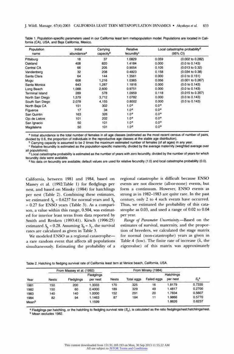
Table 1. Population-specific parameters used in our California least tern metapopulation model. Populations are located in Cali- fornia (CA), USA, and Baja California, Mexico.

Population Initial Carrying Relative Local catastrophe probabilityd name abundancea capacityb fecundityc (95% CI)

Pittsburg 18 37 1.0829 0.059 (0.002 to 0.282) Oakland 408 820 1.4184 0.000 (0.0 to 0.143) Central CA 66 205 0.9054 0.105 (0.013 to 0.32) Vandenberg 32 208 0.4823 0.158 (0.034 to 0.38) Santa Clara 64 144 1.3561 0.000 (0.0 to 0.151) Mugu 608 1,216 1.0365 0.056 (0.001 to 0.267) Santa Monica 643 1,287 1.1816 0.000 (0.0 to 0.143) Long Beach 1,088 2,600 0.9751 0.000 (0.0 to 0.143) Terminal Island 289 578 1.0959 0.118 (0.015 to 0.357) North San Diego 1,579 3,712 1.0782 0.000 (0.0 to 0.143) South San Diego 2,078 4,155 0.8002 0.000 (0.0 to 0.143) North Baja CA 151 302 1.0e 0.0e Figueroa 17 34 1.0e 0.0e San Quintin 163 326 1.0e 0.0e Ojo de Liebre 101 202 1.0e 0.0e San ignacio 50 101 1.0e 0.0e Magdalena 50 101 1.0e 0.0e

a Initial abundance is the total number of females in all age classes (estimated as the most recent census of number of pairs, divided by 0.6, the proportion of individuals in the reproductive age classes at the stable age distribution).

b Carrying capacity is assumed to be 2 times the maximum estimated number of females (of all ages) in any year. C Relative fecundity is estimated as the population-specific maternity, divided by the average maternity (weighted average over

all populations). d Local catastrophe probability is estimated as the number of years with zero fecundity, divided by the number of years for which fecundity data were available.

e No data on fecundity are available; default values are used for relative fecundity (1.0) and local catastrophe probability (0.0).

California, between 1981 and 1984, based on

Massey et al. (1992:Table 1) for fledglings per nest, and based on Minsky (1984) for hatchlings per nest (Table 2). Combining these estimates, we estimated Sh = 0.6237 for normal years and Sh = 0.27 for ENSO years (Table 3). As a comparison, a value within this range, 0.504, was estimated for interior least terns from data reported by Smith and Renken (1993:41). Kirsch (1996:25) estimated Sh = 0.28. Assuming So = S=, the survival rates are calculated as given in Table 3.

We modeled ENSO as a regional catastrophe-- a rare random event that affects all populations simultaneously. Estimating the probability of a

regional catastrophe is difficult because ENSO events are not discrete (all-or-none) events, but form a continuum. However, ENSO events as

strong as in 1982-1983 are quite rare. In the past century, only 2 to 4 such events have occurred. Thus, we estimated the probability of this cata-

strophe as 0.03, and used a range of 0.02 to 0.04

per year. Range of Parameter Uncertainty.-Based on the

estimates of survival, maternity, and the proportion of breeders, we calculated the stage matrix for normal (non-catastrophe) years as given in Table 4 (low). The finite rate of increase (X, the

eigenvalue) of this matrix was approximately

Table 2. Hatching to fledging survival rate of California least tern at Venice beach, California, USA.

From Massey et al. (1992) From Minsky (1984) Fledglings Hatchlings

Year Nests Fledglings per nest Nests Total eggs Failed eggs per nest Sha 1981 150 200 1.3333 170 325 16 1.8179 0.7335 1982 150 60 0.4000 189 329 49 1.4817 0.2700 1983 140 140 1.0000 152 291 20 1.7834 0.5607 1984 82 94 1.1463 87 184 11 1.9866 0.5770 Meanb 1.1599 1.8626 0.6237

a Fledglings per hatchling, or the hatchling to fledgling survival rate (Sh), is calculated as the ratio fledglings/nest:hatchlings/nest. b Mean excludes 1982.




Table 3. Survival (S; subscripts indicate age class) parameters of the California least tern for normal and El Nifio/Southern Oscil- lation (ENSO) years (95% Cl in parentheses).

Parameter Normal years ENSO years Reference or calculation

Sh So S1 S2 (hatchling to first breeding) 0.16 (0.13 to 0.18) 0.03 (0.01 to 0.05) Massey et al. (1992) S2 and S3 0.81 (0.72 to 0.87) 0.81a Massey et al. (1992) S4+ 0.92 (0.88 to 0.95) 0.79 (0.68 to 0.89) Massey et al. (1992) Sh (hatchling to fledgling) 0.6237 0.2700 Massey et al. (1992) and Minsky (1984)

So S1 (fledglings to age 2) 0.3167 0.1372 = (Sh SO S1 S2)/(Sh S2) So and S, 0.5627 0.3704 = ,S0

S1 a Massey et al. (1992) estimated S2 and S3 for ENSO years as 0.82 (95% CI = 0.66, 0.96). Because survival is unlikely to

increase in an ENSO year, in this model we assumed these survival rates for ENSO years to be equal to the average they estimated for normal years (0.81).

0.994. In other words, the above matrix predicted about 0.6% decline per year. This prediction for normal years agrees well with the observed growth rate from 1983 to 1989, the years that survival rates were estimated by Massey et al. (1992). A consistent 7% per year decline was observed in number of breeding pairs from 1983 to 1987, followed by an increase (Fig. 2). The annual growth rate from 1983 to 1989 was 0.995, very close to our

predicted rate of 0.994. However, 2 indications suggest that this matrix

may underestimate average vital rates in the long run. First, the observed number of pairs likely was affected by the change in age structure caused by the 1982-1983 ENSO event, whereas the matrix gave a decline similar to the observed decline with survival rates estimated for normal years.

With ENSO years modeled as catastrophes, the model would predict a rate of decline much steeper than observed from 1983 to 1989. Sec- ond, the observed growth in the last decade or so was much higher (Fig. 2) than the rate predicted by the matrix. An estimate of the average annual rate of growth between 1986 and 1998 is 1.129:

Pairs in 1998 1/(1'998-1986) 4,0921/ 1.129 Pairs in 1986 ) 952

When data from 1980 to 1998 were analyzed, the average growth rate was predicted to be about 1.07.

Thus, the estimated matrix seems to underestimate the growth rate, based on a comparison

Table 4. Average stage matrices used in our California least tern metapopulation model to simulate "normal" and El Nifio/South- ern Oscillation (ENSO) years, excluding the effects of total reproductive failure, which is modeled as a local catastrophe. The matrices are for an "average" population (i.e., fi = 1); each population in the model had a different set of fecundities, which incorporated the population-specific fi parameters.

Normal years ENSO years Fledglings 1 yr 2 yr 3 yr 24 yr Fledglings 1 yr 2 yr 3 yr 24 yr

Low Fledglings 0 0 0.088 0.202 0.32 0 0 0.088 0.202 0.275 1 yr 0.563 0 0 0 0 0.371 0 0 0 0 2 yr 0 0.563 0 0 0 0 0.371 0 0 0 3 yr 0 0 0.81 0 0 0 0 0.81 0 0 24 yr 0 0 0 0.81 0.92 0 0 0 0.81 0.79

Medium Fledglings 0 0 0.399 0.399 0.453 0 0 0.399 0.399 0.389 1 yr 0.6 0 0 0 0 0.395 0 0 0 0 2 yr 0 0.7 0 0 0 0 0.461 0 0 0 3 yr 0 0 0.81 0 0 0 0 0.81 0 0 >4 yr 0 0 0 0.81 0.92 0 0 0 0.81 0.79

High Fledglings 0 0 0.399 0.399 0.453 0 0 0.399 0.399 0.389 1 yr 0.81 0 0 0 0 0.533 0 0 0 0 2 yr 0 0.81 0 0 0 0 0.533 0 0 0 3 yr 0 0 0.81 0 0 0 0 0.81 0 0 24 yr 0 0 0 0.81 0.92 0 0 0 0.81 0.79




with the observed growth rates since 1980. Because the observed growth rate changed from a decline, during the years included in the study by Massey et al. (1992), to an increase in later

years, the underestimation may be (at least partly) due to increased vital rates since the completion of the survival analysis by Massey et al. (1992). If so, the matrix elements can be adjusted to reflect the observed growth rate.

Another reason the matrix would underestimate growth rate may be that the observed increase in the number of breeding pairs partly was due to a temporary change in age distribution (i.e., an excess of adults compared to the stable

age distribution), and did not fully reflect the increase in the overall population. The observed

exponential increase has lasted for 12 years since 1986, which is close to the generation time. While such an effect may explain part of the observed

growth, no data (age distribution in different

years) verifies this possibility. Yet another (perhaps stronger) possibility

involves measurement errors-even counts by very experienced observers at well-studied colonies may underestimate fledgling productivity. At a focal study site in Massachusetts where all

nestlings were uniquely color-banded, J. L. Atwood (unpublished data) found that fledgling productivity based solely on counts of fledglings present was underestimated by about 30-50%. Data from California (Massey 1989) and Texas

(Thompson and Slack 1984) similarly indicate

early post-fledging departure of least terns from

nesting colonies, which would strongly contribute to underestimates of fledgling production based

only on late season fledgling counts at the colonies. This underestimation would be especially important in poorly studied colonies and/or sites where predator disturbance further accelerated

dispersal away from the nesting site. Because of these uncertainties, we decided to

use a wide range of vital rates in our model. We used the matrix estimated above as the low-stage matrix because it may represent an underestimation of population's growth potential.

For the high-stage matrix (Table 4), we increased the average survival and fecundity values to their maximum plausible values. We set survival rates So and S1 equal to 0.81, the value for S2. We set maternity to 0.976 fledglings per pair, or 0.488 female fledglings per breeding female. This is the 1980-1998 average for the Long Beach population, which had the highest long-term average of all populations. We set the proportion breed-

ing in age classes 2, 3, and 24 to 100%. The result-

ing high-stage matrix had a finite rate of increase of about 1.11. This is close to the average annual

growth rate calculated from the pair-counts between 1986 and 1998 of 1.129.

For the medium stage matrix (Table 4), we kept the fecundities as above but reduced the survival rates So and S1 to 0.6 and 0.7, respectively. The

resulting medium-stage matrix had a finite rate of increase of about 1.05, close to the growth rate of 1.07 observed between 1980 and 1998.

We selected these values for the stage matrix to cover a wide range. We believe that this wide range reflected the considerable uncertainties and like-

ly included the long-term average growth rate in the next 20-50 years. We incorporated uncertain-

ty in other parameters in a similar way.

Environmental and Demographic Stochasticity We modeled year-to-year fluctuations in vital

rates (except strong ENSO and local reproductive failure years) by sampling the set of vital rates used to project the dynamics of each population from random (log-normal) distributions with means

given in Table 4. Survival rates were truncated to be between 0.0 and 1.0. To reduce truncations, if a survival rate was >0.5, the program samples it from a mirrored log-normal (i.e., samples the

mortality rate from a log-normal distribution). We had very few truncations in our simulations.

We estimated the temporal variability of survival rates based on the time series of survival rates estimated at Camp Pendleton by Collins et al. (1998). The average of these estimates was 0.8867, with a standard deviation (SD) of 0.0510, giving a coefficient of variation (CV) of 0.0576 (Table 5). We used this CV, together with the mean, to calculate

Table 5. Survival rate of adult California least terns at Camp Pendleton, California, USA (from Collins et al. 1998).

Yr Survival

1987 0.926 1988 0.921 1989 0.920 1990 0.866 1991 0.899 1992 0.781 1993 0.894 1994a 0.731 Mean 0.8867 SD 0.0510 CV 0.0576

a The estimate for 1994 is the product of survival rate and resighting probability, and is not used in calculating the average and the variability.




1.4

1.2

S1.0 -

. 0.8

0.6

0.4. 0.76 0.78 0.80 0.82 0.84 0.86 0.88 0.90 0.92 0.94

Survival from (t-1) to t

Fig. 4. Number of fledglings per pair of California least tern in year t, in the North San Diego population (California, USA), as a function of the adult survival rate from year t- 1 to tin Camp Pendleton (which is part of this population) for years 1988-1994. The coefficient of correlation is -0.12 (SE = 0.44).

the SD of each survival rate in the model. Because this estimate included both true temporal variation and measurement error, it was an overestimate (conservative) of stochasticity.

Similarly, we estimated the variability of fecundities based on the time series of fledglings per pair. For each population, we estimated the CV of these data through time. The average of these CV estimates was 0.5, which we used to calculate the SD of each fecundity parameter.

We did not have data to estimate the correlation among survival rates of different age classes or among fecundities of different age classes within a population. We assumed that survival rates for different age classes within the same

population were perfectly correlated. We also assumed that fecundities for different age classes within a population were perfectly correlated. These assumptions were precautionary because

they resulted in higher variability of abundances than the alternative assumptions of partial or no correlation. Our model allowed these vital rates to have an intermediate degree of correlation

among different populations. Fecundities could be correlated with survival

rates if they fluctuate in response to the same environmental factors. To estimate the correlation between survival and fecundity rates within the same population, we analyzed the number of

fledglings per pair in the North San Diego population, and the survival rate in Camp Pendleton (which is part of the North San Diego population). The data from Camp Pendleton was the only source of time-series data for annual survival rates that are necessary for this analysis. For

1988-1994, we used the number of fledglings per pair in year t, and the survival rate from year t-1 to t (because of the assumption of post-breeding census). The coefficient of correlation between these 2 variables was -0.12 (SE = 0.44; Fig. 4). Thus, we assumed that survival and fecundity within a population were not correlated.

In our model, demographic stochasticity was

incorporated by sampling the number of sur- vivors from a binomial distribution and number of offspring from a Poisson distribution

(Akcakaya 1991). In addition, we incorporated demographic stochasticity in dispersal.

Initial Abundances and Age Distribution We estimated initial abundance of females in

each population based on the number of pairs in 1998. If no census occurred in 1998 (e.g., populations in Baja California), we used the most recent census. The census did not give estimates of the number of nonbreeding age classes. Thus, we divided the observed number of pairs by 0.5954 (the total proportion of individuals in age classes 2, 3, and >4, at the stable age distribution) to calculate the total initial number of females in each population (Table 1). We then distributed this total number to age classes assuming a stable distribution.

Density Dependence In our analysis of fledgling data from several

sites, we did not detect significant density dependence (Fig. 5). The exponential population

2.0

c 1.5 0

E 0.5 * * *** z

..* i" I.

*

** * *.

0.0 1 10 100 1000

Number of pairs

Fig. 5. The relationship between the size of a California least tern colony (in number of pairs) and the number of fledglings per pair in the colony, based on pooled data from all colonies in California, USA, and Baja California, Mexico, 1971-1998. The colony size explains <2% of the variation in the number of fledglings per pair, suggesting a lack of density-dependent effects on fecundity.




increase of the prior 12 years also indicated a lack of density-dependent effects in these populations. However, assuming that no such effects will occur at higher abundances is unrealistic. Thus, we modeled density dependence with a "ceiling" model. We assumed that the ceiling population size of each population (carrying capacity) was 2 times the maximum number of individuals observed at that population (Table 1). In many cases, the maximum number was the last (1998) census. For low and high values of carrying capacity, we used 1.5 and 2.5 times the maximum number of individuals, respectively.

Allee effects, which may cause a reduction in vital rates when population size becomes very small, are not well studied for this species. In our model, we incorporated Allee effects by specify- ing 2 types of extinction thresholds: 1 for the whole metapopulation, and 1 for each population. Once any population fell to or below its local threshold, the model assumed the population to be extinct by setting its abundance to zero. The population then remained extinct, unless colonized by dispersers from another population. We set the local thresholds at 5 females. Our reason for selecting this value was to be precautionary: colonies with <5 pairs are not un- common, and we do not expect larger colonies (>5 pairs) to have lower-than-average vital rates. However, unknown Allee effects may cause lower vital rates for colonies with <5 pairs. By consider- ing a population extinct once it reaches or falls below its threshold, the model need not accu- rately predict the population dynamics at these low abundance levels. However, Allee effects were not likely to be very important in our model because of the generally large size of the Califor- nia least tern populations. To demonstrate that the results were not sensitive to this parameter, we also ran simulations with local extinction thresholds of zero and 10.

Dispersal Dispersal-distance Relationship.-Dispersal in our

model referred to the movement of California least terns among breeding colonies from one census (assumed to immediately follow breeding) to the next. Thus, dispersal does not refer to daily foraging movements or migration to wintering areas. Dispersal rate between 2 populations is the proportion of individuals in a population that end up in the other population in the following year.

We used data on dispersal from a Massachusetts population studied by Atwood (1999), in which

0.50

0.40

5 0.30

= 0.20

0.10A

0.00 A 0 10 20 30 40 50 60 70 80 90 100

Distance (km)

Fig. 6. Dispersal-distance function based on data from a Massachusetts, USA, population of least tern (data from Atwood 1999). The dispersal model assumes a maximum dispersal distance of 80 km. The curve shows the function y = a - exp(-x / b), where a = 0.49 and b = 29 were estimated from a regression of In(dispersal rate) on distance in km (R2 = 0.97).

chicks were banded at one source population. To obtain the parameter required by our model, we first combined the target populations into distance classes (zones). For each zone, we calculated the average distance of the colonies in that zone to the source colony. We then divided the number of banded birds captured at each distance class by the total number of banded birds captured at all sites. We plotted this rate as a function of the average distance for all the populations in that zone (Fig. 6). In the Massachusetts population, fidelity of breeders to their natal colony was about 50%.

We could not use this estimated function in our model directly because least terns seem to have higher site fidelity in California. Atwood and Massey (1988) found that 43-78% of banded adult least terns that nested in a colony in a given year returned to the same colony in the following year. Importantly, Atwood and Massey's (1988) California study focused on site fidelity of adults, whereas Atwood's (1999) Massachusetts study focused on natal site fidelity. Assuming an average adult survival of 86.4%, the California results suggest that about 50-90% of least terns breeding in a colony, and surviving for another year, breed in the same colony during the next year. Thus, we assumed that the proportion of terns that do not disperse was 50% for the low dispersal model, 70% for the medium, and 90% for the high. We set the proportion dispersing to 4 broad distance classes based on the distance-dependence charac- teristics of the Massachusetts population (Table 6). Within each distance class, we divided the disper-




Table 6. Dispersal rates used in our California least tern metapopulation model: percentage of individuals moving to other populations in 5 distance classes.

Dispersal model Distance from source population (km) Low Medium High 0 (remain in the source population) 90 70 50 <30 km 10 15 25 30-60 km 0 10 15 60-90 km 0 5 10 >90 km 0 0 0

sal rate by the number of target populations in that distance class.

Stochasticity in Dispersal.-We incorporated demographic stochasticity in dispersal among populations by sampling the number of dis-

persers from binomial distributions. Between each pair of populations connected by dispersal, we used a binomial distribution with sample size

equal to the number of individuals in the source

population and probability equal to the dispersal rate based on distance.

Density Dependence in Dispersal.-California least terns likely do not disperse randomly, but dispersal from a population increases as population size increases. We modeled density dependence in

dispersal for each population such that the per- capita dispersal rate was directly proportional to

population size. Thus, the dispersal rates we estimated based on the distance classes were used when the source population was at its carrying capacity. When the population size was lower than the carrying capacity, the dispersal rate was also (proportionally) lower.

In colonially breeding species, another type of

density dependence is also possible: as a colony increases in size, it may exert more drawing power that can attract first-time breeders (including those hatched in other subpopulations) more strongly than smaller colonies. These 2 types of density dependence are not mutually exclusive-large colonies may have both higher emigration and

higher immigration rates. From a modeling point of view, the first type of density dependence (dispersal) is based on the abundance of the source population while the second type (recruit- ment) is based on the abundance of the target population. The version of the model we used allows

only the first type of density-dependent dispersal.

Spatial Correlations We calculated the correlation in fledglings per

pair between several pairs of populations (Oak- land, Santa Monica, Long Beach, North San

Diego, South San Diego) with complete data sets. We then plotted these correlation coefficients as a function of the distance between the populations (Fig. 7).

We modeled correlation based on distances between populations because correlation of vital rates is expected to be related to correlation of environmental factors, which in turn can be functions of the geographic distance between

populations. We specified the correlation coefficients (C) between any 2 patches as a negative exponential function of the distance (d, in km) between them, with the function

C=ax e-d/b.

We estimated the parameters of this function as a = 0.48 and b = 335 by regressing In(C) on distance in km (R2 = 0.24). To incorporate uncer-

tainty, we used this function with the parameters a = 0.28, 0.48, 0.68 and b = 240, 335, 560, for low, medium, and high correlation, respectively, so as to include a majority of the correlations among populations (Fig. 7).

Management Actions Although our goal was to develop a model that

can be used to address management questions, we did not evaluate any specific management action in detail in this paper because of space limitations. Instead, we demonstrated the use of the model by estimating the effect of a generic management action.

Most management of least tern colonies in North America is aimed at reducing predation, often by building fences to keep ground preda-

1.0

0.9

0.8

0.7

0.6 - , 0.5

0.4 *

0.2 -.- - -.

0.1- 0.0,-

0 100 200 300 400 500 600 700 800 Distance between populations (km)

Fig. 7. Correlation in the number of fledglings per pair between populations of California least tern. The points show the observed correlation among several populations with complete data sets. The curves show the low (dashed), medium (solid), and high (dotted) correlation-distance functions used in our model.



J. Wildl. Manage. 67(4):2003 CALIFORNIA LEAST TERN METAPOPULATION DYNAMICS * Akcakaya et al. 839

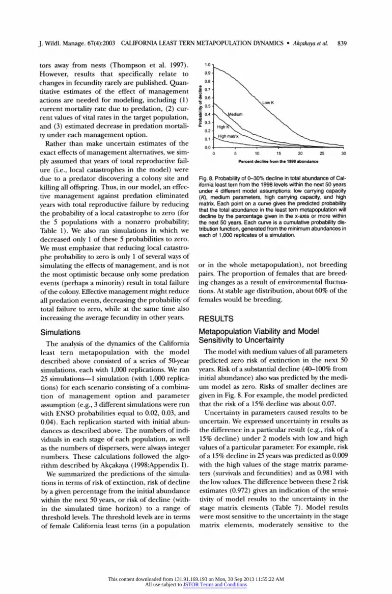
tors away from nests (Thompson et al. 1997). However, results that specifically relate to

changes in fecundity rarely are published. Quan- titative estimates of the effect of management actions are needed for modeling, including (1) current mortality rate due to predation, (2) current values of vital rates in the target population, and (3) estimated decrease in predation mortali-

ty under each management option. Rather than make uncertain estimates of the

exact effects of management alternatives, we sim-

ply assumed that years of total reproductive failure (i.e., local catastrophes in the model) were due to a predator discovering a colony site and

killing all offspring. Thus, in our model, an effective management against predation eliminated

years with total reproductive failure by reducing the probability of a local catastrophe to zero (for the 5 populations with a nonzero probability; Table 1). We also ran simulations in which we decreased only 1 of these 5 probabilities to zero. We must emphasize that reducing local catastro-

phe probability to zero is only 1 of several ways of

simulating the effects of management, and is not the most optimistic because only some predation events (perhaps a minority) result in total failure of the colony. Effective management might reduce all predation events, decreasing the probability of total failure to zero, while at the same time also

increasing the average fecundity in other years.

Simulations The analysis of the dynamics of the California

least tern metapopulation with the model described above consisted of a series of 50-year simulations, each with 1,000 replications. We ran 25 simulations-l simulation (with 1,000 replications) for each scenario consisting of a combination of management option and parameter assumption (e.g., 3 different simulations were run with ENSO probabilities equal to 0.02, 0.03, and

0.04). Each replication started with initial abundances as described above. The numbers of individuals in each stage of each population, as well as the numbers of dispersers, were always integer numbers. These calculations followed the algo- rithm described by Ak;akaya (1998:Appendix I).

We summarized the predictions of the simulations in terms of risk of extinction, risk of decline

by a given percentage from the initial abundance within the next 50 years, or risk of decline (within the simulated time horizon) to a range of threshold levels. The threshold levels are in terms of female California least terns (in a population

1.0

0.9

0.8

.50.7 S0.6 0. Low K

E 0.4

2 0.3 L High 0.2

0.1 High matrix

0.0 0 5 10 15 20 25 30

Percent decline from the 1998 abundance

Fig. 8. Probability of 0-30% decline in total abundance of Cal- ifornia least tern from the 1998 levels within the next 50 years under 4 different model assumptions: low carrying capacity (K), medium parameters, high carrying capacity, and high matrix. Each point on a curve gives the predicted probability that the total abundance in the least tern metapopulation will decline by the percentage given in the x-axis or more within the next 50 years. Each curve is a cumulative probability distribution function, generated from the minimum abundances in each of 1,000 replicates of a simulation.

or in the whole metapopulation), not breeding pairs. The proportion of females that are breed-

ing changes as a result of environmental fluctuations. At stable age distribution, about 60% of the females would be breeding.

RESULTS

Metapopulation Viability and Model Sensitivity to Uncertainty

The model with medium values of all parameters predicted zero risk of extinction in the next 50

years. Risk of a substantial decline (40-100% from initial abundance) also was predicted by the medium model as zero. Risks of smaller declines are

given in Fig. 8. For example, the model predicted that the risk of a 15% decline was about 0.07.

Uncertainty in parameters caused results to be uncertain. We expressed uncertainty in results as the difference in a particular result (e.g., risk of a 15% decline) under 2 models with low and high values of a particular parameter. For example, risk of a 15% decline in 25 years was predicted as 0.009 with the high values of the stage matrix parameters (survivals and fecundities) and as 0.981 with the low values. The difference between these 2 risk estimates (0.972) gives an indication of the sensi-

tivity of model results to the uncertainty in the

stage matrix elements (Table 7). Model results were most sensitive to the uncertainty in the stage matrix elements, moderately sensitive to the




Table 7. Sensitivity of the predicted viability of the California least tern to uncertainty in each model parameter. The reported values are the probabilities of a 15% decline within 25 and 50 years with the low and high values of each listed parameter, and the differences in probabilities of decline between models with the low and high values of each parameter.

Probability of decline with Probability of decline with Difference in the probability low value of the parameter high value of the parameter of decline

Parameter in 25 yr in 50 yr in 25 yr in 50 yr in 25 yr in 50 yr

Stage matrix 0.981 1.000 0.009 0.009 0.972 0.991 Carrying capacity 0.215 0.343 0.038 0.038 0.177 0.305 ENSOa probability 0.036 0.036 0.091 0.092 0.055 0.056 Buffer 0.090 0.135 0.038 0.038 0.052 0.097 Dispersal 0.036 0.036 0.087 0.097 0.051 0.061 Correlation 0.045 0.047 0.088 0.095 0.043 0.048 Local extinction threshold 0.060 0.061 0.073 0.075 0.013 0.014

a El Niho/Southern Oscillation event.

uncertainty in the carrying capacity, but not very sensitive to other parameters (Table 7).

Effect of Simulated Predator Control Five populations had a local catastrophe proba-

bility greater than zero (Table 1). We first estimated the effect of predator control in terms of decreased risk of decline when the local catastrophe probability was set to zero for all 5 populations. Using the medium parameter values, the decrease in risk of decline was not substantial, mainly because risk of decline was predicted as zero for 40-100% declines from initial abundance. We also repeated the analysis with a more

pessimistic model based on low estimates for the

stage matrix (because the results were most sensitive to the assumption about the stage matrix; see Table 7). Under the assumption of low matrix values, we found an 8% decrease in the risk of a 54% decline (Fig. 9). In other words, the risk that the metapopulation size would fall below 3,425 females at least once in the next 50 years was 8% less when the local catastrophe probability was set to zero for all populations. This particular threshold level (3,425 females, which represents a 54% decline from initial abundance) is the threshold for which the difference between the models with and without management was greatest (Fig. 9).

We repeated the above analysis by decreasing local catastrophe probability to zero for one population at a time. We found a 4% decrease in the risk of decline when local catastrophe probability was set to zero for the Mugu or the Terminal Island populations, but only about 1% decrease when local catastrophe probability was set to zero for any one of the other 3 populations. In other words, the decrease in risk ranged from 1 to 8% depending on the number and location of populations in which predator control was simulated.

DISCUSSION For all parameter combinations except low

matrix, the model predicted a continuing population increase and a low risk of a substantial decline (>40% from current levels) in the next 50 years. Under the assumption of low vital rates, the model predicted a high risk of decline, although a low risk of extinction. Thus, the model was sensitive to the assumption about the vital rates.

The model was moderately sensitive to the assumption about carrying capacities. For Cali- fornia least tern, the carrying capacity represents the maximum expected size of a population, and is determined by a combination factors such as food limitation, and the availability of breeding areas secure from human activities. Because we had no data on carrying capacities except for the maximum numbers recorded in each popula-

1.0

0.9

e 0.8

0.7

0.6

0.5

0.4

. 0.3

0.2

0.1

0.0 20 30 40 50 60 70 80

Percent decline from the 1998 abundance

Fig. 9. Probability of 20-80% decline in total abundance of California least tern from the 1998 levels within the next 50 years, under the model assumption of low vital rates (low matrix simulation). The model prediction is shown with (bot- tom curve) and without (top curve) predator control. The vertical bar gives the largest difference between the 2 curves (8%), which occurs at 54% decline.



J. Wildl. Manage. 67(4):2003 CALIFORNIA LEAST TERN METAPOPULATION DYNAMICS * Akcakaya et al. 841

tion, we had a wider range of uncertainty for car-

rying capacity (high value was 67% higher than low value) than for the vital rates (eigenvalue of

high matrix was 12% higher than low matrix). Still, the model was much more sensitive to vital rates. This indicates that the sensitivity of results to the carrying capacity (compared to sensitivity to vital rates) is a measure of our uncertainty about what may ultimately limit population size, rather than the intrinsic importance of the parameter itself. The model was not very sensitive to other parameters and assumptions of the model, such as the buffer distance used to delineate populations, dispersal, correlation, ENSO probability, and local extinction threshold (Table 7).

MANAGEMENT IMPLICATIONS Simulated reduction of predation did not sub-

stantially increase the overall viability of the meta-

population under the assumption of medium vital rates but did improve viability under the

assumption of low vital rates. Importantly, simulated reduction of predation decreased the probability of local reproductive failure from the aver-

age levels in 1980-1998, the period for which the

probabilities were calculated. Thus, simulated reduction of predation is a simulation of increased or additional management. One reason simulated

management did not increase the overall viability of the metapopulation substantially (under the

assumption of medium vital rates) might be that

past management (and other factors) had

already resulted in a recovery and a low risk of decline. Another reason might be the limited way in which we modeled management, focusing only on the 5 populations in which total reproductive failure occurred. Management could also increase fecundity in the larger populations (that had zero probability of local catastrophe). How- ever, 1999 survey results, which became available after the completion of our study, showed a decline in nesting pairs and the lowest productivity since 1976, in part due to predation (Keane 2001), suggesting that predator control remains a relevant management action.

The improvement in viability with simulated

management (under the assumption of low vital

rates) was greater when more populations were managed. However, the improvement was not the same for management in all populations, ranging from 1 to 4% for single populations, and up to 8% when all populations were included. Our results indicated that the number and location of

populations selected for focused management

influenced the effectiveness of management efforts. Thus, the effectiveness of management should be evaluated within a metapopulation context, and

management actions should be focused on populations where they make the greatest contribu- tion to the viability of the whole metapopulation.

Based on our preliminary results, 2 types of data would most improve the reliability of our model. The first would be replication of the

analysis in Massey et al. (1992) with more current

capture-recapture data. These data would decrease the uncertainty about vital rates, which contributed most to the uncertainty of the model results. The second type of data needed to

improve reliability of our model are estimates of the effects of management actions on fecundity. The method we used to simulate the effect of

management was quite crude; the results of the model will be much more useful for management if conservation measures such as predator control are evaluated quantitatively in terms of their effect on population parameters. Thus, monitor-

ing studies specifically designed to provide accu- rate estimates of the likely effects of management actions would improve the model's ability to assess the effects of such measures on the viabili-

ty of the species.

ACKNOWLEDGMENTS This study was funded as part of the NASA Life

Sciences Support Contract NAS10-02001. We are indebted to the many individuals who have, over the years, participated in the California Fish and Game's annual California least tern colony moni-

toring program. Other field studies of the terns have been supported by funding from the U.S.

Army Corps of Engineers, the U.S. Fish and Wild- life Service, and the U.S. Navy. We thank B. C. Lubow, E. M. Kirsch, and an anonymous reviewer for valuable comments.

LITERATURE CITED AKCAKAYA, H. R. 1991. A method for simulating demo-

graphic stochasticity. Ecological Modelling 54:133-136. _- . 1998. RAMAS Metapop: viability analysis for stage-structured metapopulations. Version 3.0. Applied Biomathematics, Setauket, New York, USA.

. 2000. Population viability analyses with demo- graphically and spatially structured models. Ecologi- cal Bulletins 48:23-38.

, AND J. L. ATWOOD. 1997. A habitat-based metapopulation model of the California gnatcatcher. Con- servation Biology 11:422-434.

, AND M. G. RAPHAEL. 1998. Assessing human impact despite uncertainty: viability of the northern spotted owl metapopulation in the northwestern USA. Biodiversity and Conservation 7:875-894.




- , AND P. SJOGREN-GULVE. 2000. Population viability analyses in conservation planning: an overview. Ecological Bulletins 48:9-21.

AMERICAN ORNITHOLOGISTS' UNION. 1957. Check-list of North American birds, fifth edition. American Ornithologists' Union, Washington, D.C., USA.

ATWOOD, J. L. 1999. Patterns of juvenile dispersal by least terns in Massachusetts. Final project report sub- mitted to Massachusetts Environmental Trust. Avian Conservation Division, Manomet Center for Conser- vation Sciences, Manomet, Massachusetts, USA.

, AND B. W. MASSEY. 1988. Site fidelity of least terns in California. Condor 90:389-394.

BEISSINGER, S. R., AND M. I. WESTPHAL. 1998. On the use of demographic models of population viability in endangered species management. Journal of Wildlife Management 62:821-841.

BOYCE, M. S. 1992. Population viability analysis. Annual Review of Ecology and Systematics 23:481-506.

. 1996. Review of RAMAS/GIS. Quarterly Review of Biology 71:167-168.

BROOK, B. W., M. A. BURGMAN, H. R. AKCAKAYA, J. J. O'GRADY, AND R. FRANKHAM. 2002. Critiques of PVA ask the wrong questions: throwing the heuristic baby out with the numerical bathwater. Conservation Biol- ogy 16:262-263.

-, J. J. O'GRADY, A. P. CHAPMAN, M. A. BURGMAN, H. R. AKQAKAYA, AND R. FRANKHAM. 2000. Predictive accuracy of population viability analysis in conservation biology. Nature 404:385-387.

BURGER, J. 1984. Colony stability in least terns. Condor 86:61-67.

BURGMAN, M. A., S. FERSON, AND H. R. AKkAKAYA. 1993. Risk assessment in conservation biology. Chapman & Hall, London, United Kingdom.

CASWELL, H. 1989. Matrix population models: construc- tion, analysis, and interpretation. Sinauer Associates, Sunderland, Massachusetts, USA.

COLLINS, C. T., M. WIMER, B. W. MASSEY, L. M. KARES, AND K. GAZZANIGA. 1998. Banding of adult California least terns at Marine Corps Base, Camp Pendleton between 1987-1997. Report prepared for the Natural Resources Management Branch, Southwestern and Western Division Naval Facilities Engineering Com- mand, San Diego, California, USA.

ELLNER, S. P., J. FIEBERG, D. LUDWIG, AND C. WILCOX. 2002. Precision of population viability analysis. Con- servation Biology 16:258-261.

GOODMAN, L. A. 1971. On the sensitivity of the intrinsic growth rate to changes in the age-specific birth and death rates. Theoretical Population Biology 2:339-354.

GROVER, P. B., AND F. L. KNOPF. 1982. Habitat require- ments and breeding success of charadriiform birds nesting at Salt Plains National Wildlife Refuge. Jour- nal of Field Ornithology 53:139-148.

INCHAUSTI, P., AND H. WEIMERSKIRCH. 2002. Dispersal and

metapopulation dynamics of an oceanic seabird, the wandering albatros. Journal of Animal Ecology 71:765-770.

KEANE, K. 2001. California least tern breeding survey 1999 season. Species Conservation and Recovery Pro- gram Report, 2001-01. California Fish and Game, Sacramento, California, USA.

KINGSTON, T. 1995. Valuable modeling tool: RAMAS/GIS. Conservation Biology 9:966-968.

KIRSCH, E. M. 1996. Habitat selection and productivity of least terns on the lower Platte River, Nebraska. Wildlife Monographs 132.

KOENEN, M. T., R. B. UTYCH, AND D. M. LESLIE. 1996. Methods to improve least tern and snowy plover nesting success on alkaline flats. Journal of Field Ornithology 67:281-291.

MASSEY, B. W. 1974. Breeding biology of the California least tern. Proceedings of the Linnaean Society 72:1-24.

. 1989. California least tern fledgling study, Venice, California 1989. Contract Report FG 8553. Wildlife Management Division, California Department of Fish and Game, Sacramento, California, USA.

1, ANDJ. L. ATWOOD. 1981. Second wave nesting of the California least tern: age composition and reproductive success. Auk 98:596-605. S

, D. W. BRADLEY, ANDJ. L. ATwOOD. 1992. Demog- raphy of a California least tern colony including effects of the 1982-1983 El Nifio. Condor 94:976-983.

, ANDJ. M. FANCHER. 1989. Renesting by California least terns. Journal of Field Ornithology 60:350-357.

MILLS, L. S., AND M. S. LINDBERG. 2002. Sensitivity analysis to evaluate the consequences of conservation actions. Pages 338-366 in S. R. Beissinger and D. R. McCullough, editors. Population viability analysis. University of Chicago Press, Chicago, Illinois, USA.

MINSKY, D. 1984. A report on the nesting of the Califor- nia least tern in Los Angeles and Orange counties, season of 1984. Unpublished report, California Fish and Game, Sacramento, California, USA.

REGAN, H. M., H. R. AKCAKAYA, S. FERSON, K. V. ROOT, S. CARROLL, AND L. R. GINZBURG. 2003. Treatments of uncertainty and variability in ecological risk assessment of single-species populations. Human and Eco- logical Risk Assessment 9:889-906.

RIMMER, D. W., AND R. D. DEBLINGER. 1992. Use of fenc- ing to limit terrestrial predator movement into least tern colonies. Colonial Waterbirds 15:226-229.

ROOT, K. V. 1998. Evaluating the effects of habitat qual- ity, connectivity, and catastrophes on a threatened species. Ecological Applications 8:854-865.

SMITH, J. W., AND R. B. RENKEN. 1993. Reproductive success of the least terns in the Mississippi river valley. Colonial Waterbirds 16:39-44.

THOMPSON, B. C., AND R. D. SLACK. 1984. Post-fledging departure from colonies by juvenile least terns in Texas: implications for estimating production. Wilson Bulletin 96:309-313.

1, J. A. JACKSON, J. BURGER, L. HILL, E. M. KIRSCH,

ANDJ. L. ATWOOD. 1997. Least tern (Sterna antillarum). Pages in A. Poole and F. Gill, editors. The birds of North America 290. The Academy of Natural Sciences, Philadelphia, Pennsylvania, USA, and The American Ornithologists' Union, Washington, D.C., USA.

WITTEMAN, G. J., AND M. GILPIN. 1995. Review of RAMAS/metapop. Quarterly Review of Biology 70:381-382.

Received 8June 2002. Accepted 1 July 2003. Associate Editor: Lubow.



metapopulation dynamics of the california least tern

Documents