Mesoscale asymptotic approximations to solutions of mixed boundary

value problems in perforated domains

V. Maz’ya∗, A. Movchan†, M. Nieves†

Abstract

We describe a method of asymptotic approximations to solutions of mixed boundary value problems forthe Laplacian in a three-dimensional domain with many perforations of arbitrary shape, with the Neumannboundary conditions being prescribed on the surfaces of small voids. The only assumption made on thegeometry is that the diameter of a void is assumed to be smaller compared to the distance to the nearestneighbour. The asymptotic approximation, obtained here, involves a linear combination of dipole fieldsconstructed for individual voids, with the coefficients, which are determined by solving a linear algebraicsystem. We prove the solvability of this system and derive an estimate for its solution. The energy estimateis obtained for the remainder term of the asymptotic approximation.

1 Introduction

In the present paper we discuss a method for asymptotic approximations to solutions of the mixed problems forthe Poisson equation for domains containing a number, possibly large, of small perforations of arbitrary shape.The Dirichlet condition is set on the exterior boundary of the perforated body, and the Neumann conditions arespecified on the boundaries of small holes. Neither periodicity nor even local “almost” periodicity constraints areimposed on the position of holes, which makes the homogenization methodologies not applicable (cf. Chapter4 in [5], and Chapter 5 in [9]). Two geometrical parameters, ε and d, are introduced to characterize themaximum diameter of perforations within the array and the minimum distance between the voids, respectively.Subject to the mesoscale constraint, ε < const d, the asymptotic approximation to the solution of the mixedboundary value problem is constructed. The approximate solution involves a linear combination of dipole fieldsconstructed for individual voids, with the coefficients determined from a linear algebraic system. The formalasymptotic representation is accompanied by the energy estimate of the remainder term. The general idea ofmesoscale approximations originated a couple of years ago in [6], where the Dirichlet problem was consideredfor a domain with multiple inclusions.

The asymptotic methods, presented here and in [6], can be applied to modelling of dilute composites inproblems of mechanics, electromagnetism, heat conduction and phase transition. In such models, the boundaryconditions have to be satisfied across a large array of small voids, which is the situation fully served by ourapproach. Being used in the case of a dilute array of small spherical particles, the method also includesthe physical models of many point interactions treated previously in [1, 2, 4] and elsewhere. Asymptoticapproximations applied to solutions of boundary value problems of mixed type in domains containing manysmall spherical inclusions were considered in [1]. The point interaction approximations to solutions of diffusionproblems in domains with many small spherical holes were analysed in [2]. Modelling of multi-particle interactionin problems of phase transition was considered in [4] where the evolution of a large number of small sphericalparticles embedded into an ambient medium takes place during the last stage of phase transformation; sucha phenomenon where particles in a melt are subjected to growth is referred to as Ostwald ripening. For thenumerical treatment of models involving large number N of spherical particles, the fast multipole method, oforder O(N), was proposed in [3], and it appears to be efficient for the rapid evaluation of potential and forcefields for systems of a large number of particles interacting with each other via the Coulomb law.

∗Department of Mathematical Sciences, University of Liverpool, Liverpool L69 3BX, U.K., and Department of Mathematics,Linkoping University, SE-581 83 Linkoping, Sweden.†Department of Mathematical Sciences, University of Liverpool, Liverpool L69 3BX, U.K.

1

arX

iv:1

005.

4351

v1 [

mat

h-ph

] 2

4 M

ay 2

010

We give an outline of the paper. The notation ΩN will be used for a domain containing small voids F (j),j = 1, . . . , N , while the unperturbed domain, without any holes, is denoted by Ω. The number N is assumedto be large.

If Ω is a bounded domain in R3, we introduce L1,2(Ω) as the space of functions on Ω with distributionalfirst derivatives in L2(Ω) provided with the norm

‖u‖L1,2(Ω) =(‖∇u‖2L2(Ω) + ‖u‖2L2(Ω)

)1/2

. (1.1)

Here B is a ball at a positive distance from ∂Ω. If Ω is unbounded, by L1,2(Ω) we mean the completion of thespace of functions with ‖∇u‖L2(Ω) <∞, which have bounded supports, in the norm (1.1). The space of traces

of functions in L1,2(Ω) on ∂Ω will be denoted by L1/2,2(∂Ω).

The maximum of diameters of F (j), j = 1, . . . , N is denoted by ε. An array of points O(j), j = 1, . . . , N, ischosen in such a way that O(j) is an interior point of F (j) for every j = 1, . . . , N . By 2d we denote the smallestdistance between the points within the array O(j)Nj=1. It is assumed that there exists an open set ω ⊂ Ωsituated at a positive distance from ∂Ω and such that

∪Nj=1 F(j) ⊂ ω, dist

(∪Nj=1 F

(j), ∂ω)≥ 2d, and diam ω = 1, (1.2)

With the last normalization of the size of ω, the parameters ε and d can be considered as non-dimensional. Thescaled open sets ε−1F (j) are assumed to have Lipschitz boundaries, with Lipschitz characters independent ofN .

Our goal is to obtain an asymptotic approximation to a unique solution uN ∈ L1,2(ΩN ) of the problem

−∆uN (x) = f(x) , x ∈ ΩN , (1.3)

uN (x) = φ(x) , x ∈ ∂Ω , (1.4)

∂uN∂n

(x) = 0 , x ∈ ∂F (j) , j = 1, . . . , N , (1.5)

where φ ∈ L1/2,2(∂Ω) and f(x) is a function in L∞(Ω) with compact support at a positive distance from thecloud ω of small perforations.

We need solutions to certain model problems in order to construct the approximation to uN ; these include

1. v as the solution of the unperturbed problem in Ω (without voids),

2. D(k) as the vector function whose components are the dipole fields for the void F (k),

3. H as the regular part of Green’s function G in Ω.

The approximation relies upon a certain algebraic system, incorporating the field vf and integral character-istics associated with the small voids. We define

Θ =

(∂v

∂x1(O(1)),

∂v

∂x2(O(1)),

∂v

∂x3(O(1)), . . . ,

∂v

∂x1(O(N)),

∂v

∂x2(O(N)),

∂v

∂x3(O(N))

)T,

and S = [Sij ]Ni,j=1 which is a 3N × 3N matrix with 3× 3 block entries

Sij =

(∇z ⊗∇w) (G(z,w))∣∣∣z=O(i)

w=O(j)

if i 6= j

0I3 otherwise,

where G is Green’s function in Ω, and I3 is the 3× 3 identity matrix. We also use the block-diagonal matrix

Q = diagQ(1), . . . ,Q(N), (1.6)

where Q(k) is the so-called 3×3 polarization matrix for the small void F (k) (see [7] and Appendix G of [8]). Theshapes of the voids F (j), j = 1, . . . , N, are constrained in such a way that the maximal and minimal eigenvalues

λ(j)max, λ

(j)min of the matrices −Q(j) satisfy the inequalities

A1ε3 > max

1≤j≤Nλ(j)max, min

1≤j≤Nλ

(j)min > A2ε

3, (1.7)

2

where A1 and A2 are positive and independent of ε.One of the results, for the case when Ω = R3, H ≡ 0, and when (1.4) is replaced by the condition of decay

of uN at infinity, can be formulated as follows

Theorem 1 Letε < c d ,

where c is a sufficiently small absolute constant. Then the solution uN (x) admits the asymptotic representation

uN (x) = v(x) +

N∑k=1

C(k) ·D(k)(x) +RN (x) , (1.8)

where C(k) = (C(k)1 , C

(k)2 , C

(k)3 )T and the column vector C = (C

(1)1 , C

(1)2 , C

(1)3 , . . . , C

(N)1 , C

(N)2 , C

(N)3 )T satisfies

the invertible linear algebraic system(I + SQ)C = −Θ . (1.9)

The remainder RN satisfies the energy estimate

‖∇RN‖2L2(ΩN ) ≤ constε11d−11 + ε5d−3

‖∇v‖2L2(Ω). (1.10)

We remark that since ε and d are non-dimensional parameters, there is no dimensional mismatch in the right-hand side of (1.10).

We now describe the plan of the article. In Section 2, we introduce the multiply-perforated geometry andconsider the above model problems. The formal asymptotic algorithm for a cloud of small perforations in theinfinite space and the analysis of the algebraic system (1.9) are given in Sections 3 and 4. Section 5 presents theproof of Theorem 1. The problem for a cloud of small perforations in a general domain is considered in Section6. Finally, in Section 7 we give an illustrative example accompanied by the numerical simulation.

2 Main notations and model boundary value problems

Let Ω be a bounded domain in R3 with a smooth boundary ∂Ω. We shall also consider the case when Ω = R3.The perforated domain ΩN , is given by

ΩN = Ω\∪Nj=1F(j) ,

where F (j) are small voids introduced in the previous section. Also in the previous section we introduced thenotations ε and d for two small parameters, characterizing the maximum of the diameters of F (j), j = 1, . . . , N,and the minimal distance between the small voids, respectively.

In sections where we are concerned with the energy estimates of the remainders produced by asymptoticapproximations we frequently use the obvious estimate

N ≤ const d−3 . (2.1)

We consider the approximation of the function uN which is a variational solution of the mixed problem(1.3)-(1.5).

Before constructing the approximation to uN , we introduce model auxiliary functions which the asymptoticscheme relies upon.

1. Solution v in the unperturbed domain Ω. Let v ∈ L1,2(Ω) denote a unique variational solution of theproblem

−∆v(x) = f(x) , x ∈ Ω , (2.2)

v(x) = φ(x) , x ∈ ∂Ω . (2.3)

3

2. Regular part of Green’s function in Ω. By H we mean the regular part of Green’s function G in Ω definedby the formula

H(x,y) = (4π|x− y|)−1 −G(x,y) . (2.4)

Then H is a variational solution of

∆xH(x,y) = 0 , x,y ∈ Ω ,

H(x,y) = (4π|x− y|)−1 , x ∈ ∂Ω,y ∈ Ω .

3. The dipole fields D(j)i , i = 1, 2, 3, associated with the void F (j). The vector functions D(j) = D(j)

i 3i=1,which are called the dipole fields, are variational solutions of the exterior Neumann problems

∆D(j)(x) = O , x ∈ R3 \ F (j) ,

∂D(j)

∂n(x) = n(j) , x ∈ ∂F (j) ,

D(j)(x) = O(ε3|x−O(j)|−2) as |x| → ∞ ,

(2.5)

where n(j) is the unit outward normal with respect to F (j). In the text below we also use the negative

definite polarization matrix Q(j) = Q(j)ik 3i,k=1, as well as the following asymptotic result (see [7] and

Appendix G in [8]), for every void F (j):

Lemma 1 For |x−O(j)| > 2ε, the dipole fields admit the asymptotic representation

D(j)i (x) =

1

4π

3∑m=1

Q(j)im

xm −O(j)m

|x−O(j)|3+O

(ε4|x−O(j)|−3

), i = 1, 2, 3 . (2.6)

The shapes of the voids F (j), j = 1, . . . , N, are constrained in such a way that the maximal and minimal

eigenvalues λ(j)max, λ

(j)min of the matrices −Q(j) satisfy the inequalities (1.7).

3 The formal approximation of uN for the infinite space containingmany voids

In this section we deduce formally the uniform asymptotic approximation of uN :

uN (x) ∼ v(x) +

N∑k=1

C(k) ·D(k)(x) ,

for the case Ω = R3 and derive an algebraic system for the coefficients C(k) = C(k)i 3i=1, k = 1, . . . , N .

The function uN satisfies−∆uN (x) = f(x) , x ∈ ΩN , (3.1)

∂uN∂n

(x) = 0 , x ∈ ∂F (j), j = 1, . . . , N , (3.2)

uN (x)→ 0 , as |x| → ∞ . (3.3)

We begin by constructing the asymptotic representation for uN in this way

uN (x) = v(x) +

N∑k=1

C(k) · D(k)(x) +RN (x) (3.4)

where RN is the remainder, and v(x) satisfies

−∆v(x) = f(x) , x ∈ R3 ,

4

v(x)→ 0 as |x| → ∞ ,

and D(k) are the dipole fields defined as solutions of problems (2.5). The function RN is harmonic in ΩN and

RN (x) = O(|x|−1) as |x| → ∞ . (3.5)

Placement of (3.4) into (3.2) together with (2.5) gives the boundary condition on ∂F (j):

∂RN∂n

(x) = −n(j) ·∇v(O(j)) + C(j) +O(ε) +

∑k 6=j

1≤k≤N

∇(C(k) · D(k)(x)).

Now we use (2.6), for D(k), k 6= j, so that this boundary condition becomes

∂RN∂n

(x) ∼ −n(j) ·∇v(O(j)) + C(j) +

∑k 6=j

1≤k≤N

T (x,O(k))Q(k)C(k), x ∈ ∂F (j), j = 1, . . . , N ,

where

T (x,y) = (∇z ⊗∇w)

(1

4π|z−w|

) ∣∣∣ z=xw=y

. (3.6)

Finally, Taylor’s expansion of T (x,O(k)) about x = O(j), j 6= k, leads to

∂RN∂n

(x) ∼ −n(j) ·∇v(O(j)) + C(j) +

∑k 6=j

1≤k≤N

T (O(j),O(k))Q(k)C(k), x ∈ ∂F (j), j = 1, . . . , N .

To remove the leading order discrepancy in the above boundary condition, we require that the vector coefficientsC(j) satisfy the algebraic system

∇v(O(j)) + C(j) +∑k 6=j

1≤k≤N

T (O(j),O(k))Q(k)C(k) = O , for j = 1, . . . , N , (3.7)

where the polarization matrices Q(j) characterize the geometry of F (j), j = 1, . . . , N. Upon solving the abovealgebraic system, the formal asymptotic approximation of uN is complete. The next section addresses thesolvability of the system (3.7), together with estimates for the vector coefficients C(j).

4 Algebraic system in the case Ω = R3

The algebraic system for the coefficients C(j) can be written in the form

C + SQC = −Θ, (4.1)

whereC = ((C(1))T , . . . , (C(N))T )T , Θ = ((∇v(O(1)))T , . . . , (∇v(O(N)))T )T ,

are vectors of the dimension 3N , and

S = [Sij ]Ni,j=1, Sij =

(∇z ⊗∇w)

(1

4π|z−w|

) ∣∣∣z=O(i)

w=O(j)

if i 6= j

0I3 otherwise,

(4.2)

Q = diagQ(1), . . . ,Q(N) is negative definite. (4.3)

These are 3N × 3N matrices whose entries are 3× 3 blocks. The notation in (4.2) is interpreted as

Sij =

1

4π

∂

∂zq

( zr −O(j)r

|z−O(j)|3)∣∣∣

z=O(i)

3

q,r=1

when i 6= j.

5

We use the piecewise constant vector function

Ξ(x) =

Q(j)C(j), when x ∈ B(j)

d/4, j = 1, . . . , N,

0, otherwise,

(4.4)

where B(j)r = x : |x−O(j)| < r.

Theorem 2 Assume that λmax < const d3, where λmax is the largest eigenvalue of the positive definite matrix−Q and the constant is independent of d. Then the algebraic system (4.1) is solvable and the vector coefficientsC(j) satisfy the estimate

N∑j=1

|(C(j))TQ(j)C(j)| ≤ (1− constλmaxd3

)−2N∑j=1

|(∇v(O(j)))TQ(j)∇v(O(j))|. (4.5)

We consider the scalar product of (4.1) and the vector QC:

〈C,QC〉+ 〈SQC,QC〉 = −〈Θ,QC〉. (4.6)

Prior to the proof of Theorem we formulate and prove the following identity.

Lemma 2 a) The scalar product 〈SQC,QC〉 admits the representation

〈SQC,QC〉 =576

π3d6

∫R3

∫R3

1

|X−Y|(∇ ·Ξ(X))(∇ ·Ξ(Y))dYdX

− 16

πd3

N∑j=1

|Q(j)C(j)|2. (4.7)

b) The following estimate holds

|〈SQC,QC〉| ≤ const d−3∑

1≤j≤N

|Q(j)C(j)|2 ,

where the constant in the right-hand side does not depend on d.

Remark. Using the notation N (∇ · Ξ) for the Newton’s potential acting on ∇ · Ξ we can interpret theintegral in (4.7) as (

N (∇ ·Ξ),∇ ·Ξ)L2(R3)

,

since obviously ∇·Ξ ∈W−1,2(R3) and N (∇·Ξ) ∈W 1,2(R3). Here and in the sequel we use the notation (ϕ,ψ)for the extension of the integral

∫R3 ϕ(X)ψ(X)dX onto the Cartesian product W 1,2(R3)×W−1,2(R3).

Proof of Lemma 2. a) By (4.2), (4.3), the following representation holds

〈SQC,QC〉 =1

4π

N∑j=1

(Q(j)C(j)

)T ∑1≤k≤N,k 6=j

(∇z ⊗∇w)

(1

|z−w|

) ∣∣∣z=O(j)

w=O(k)

(Q(k)C(k)

). (4.8)

Using the mean value theorem for harmonic functions we note that when j 6= k

(∇z ⊗∇w)

(1

|z−w|

) ∣∣∣z=O(j)

w=O(k)

=3

4π(d/4)3

∫B

(k)

d/4

(∇z ⊗∇w)

(1

|z−w|

) ∣∣∣z=O(j)

dw.

Substituting this identity into (4.8) and using definition (4.4) we see that the inner sum on the right-hand sideof (4.8) can be presented in the form

48

πd3limτ→0+

∫R3\B(j)

(d/4)−τ

∂

∂Yq

( Yr −O(j)r

|Y −O(j)|3)3

q,r=1Ξ(Y)dY,

6

and further integration by parts gives

〈SQC,QC〉 = − 12

π2d3

N∑j=1

(Q(j)C(j)

)T(4.9)

· limτ→0+

∫R3\B(j)

(d/4)−τ

Yr −O(j)r

|Y −O(j)|3∇ ·Ξ(Y)

3

r=1dY

+

∫|Y−O(j)|=(d/4)−τ

(Yr −O(j)

r )(Yq −O(j)q )

|Y −O(j)|4

3

r,q=1

dSY Q(j)C(j)

,

where the integral over R3 \ B(d/4)−τ in (4.9) is understood in the sense of distributions. The surface integralin (4.9) can be evaluated explicitly, i.e.

∫|Y−O(j)|=(d/4)−τ

(Yr −O(j)

r )(Yq −O(j)q )

|Y −O(j)|4

3

r,q=1

dSY Q(j)C(j) =4π

3Q(j)C(j). (4.10)

Once again, applying the mean value theorem for harmonic functions in the outer sum of (4.9) and using (4.10)together with the definition (4.4) we arrive at

〈SQC,QC〉 = − 16

πd3

N∑j=1

|Q(j)C(j)|2 (4.11)

− 576

π3d6limτ→0+

N∑j=1

∫B

(j)

(d/4)+τ

∫R3\B(j)

(d/4)−τ

3∑r=1

Ξr(X)∂

∂Xr

( 1

|Y −X|

)∇ ·Ξ(Y)dYdX,

where Ξr are the components of the vector function Ξ defined in (4.4).The last integral is understood in the sense of distributions. Referring to the definition (4.4), integrating by

parts, and taking the limit as τ → 0+ we deduce that the integral term in (4.11) can be written as

576

π3d6

∫R3

∫R3

1

|Y −X|

(∇ ·Ξ(X)

)(∇ ·Ξ(Y)

)dYdX (4.12)

Using (4.11) and (4.12) we arrive at (4.7).

b) Let us introduce a piece-wise constant function

C(x) =

C(j) , when x ∈ B(j)

d/4 , j = 1, . . . , N ,

0 , otherwise .

According to the system (3.7), ∇× C(x) = O, and one can use the representation

C(x) = ∇W (x) (4.13)

where W is a scalar function with compact support, and (4.13) is understood in the sense of distributions. We

give a proof for the case when all voids are spherical, of diameter ε, and hence Q(j) = −π4 ε3I3, where I3 is the

identity matrix. Then according to (4.11) we have

|〈SQC,QC〉| ≤ 16

πd3

∑1≤j≤N

|Q(j)C(j)|2 +36ε6

πd3

∣∣∣ ∫R3

∫R3

(∇XW (X) · ∇X

( 1

|Y −X|

))∆YW (Y) dYdX

∣∣∣≤ 16

πd3

∑1≤j≤N

|Q(j)C(j)|2 +144ε6

d3

∑1≤j≤N

∫B

(j)

d/4

|∇W (Y)|2 dY

≤ const

d3

∑1≤j≤N

|Q(j)C(j)|2 .

7

Proof of Theorem 2. Consider the equation (4.6). The absolute value of its right-hand side does not

exceed〈C,−QC〉1/2〈Θ,−QΘ〉1/2.

Using Lemma 1 and part b) of Lemma 2 we derive

〈C,−QC〉 − constd−3〈−QC,−QC〉 ≤ 〈C,−QC〉1/2〈Θ,−QΘ〉1/2,

leading to (1− const

d3

〈−QC,−QC〉〈C,−QC〉

)〈C,−QC〉1/2 ≤ 〈Θ,−QΘ〉1/2,

which implies (1− const

λmaxd3

)2

〈C,−QC〉 ≤ 〈Θ,−QΘ〉. (4.14)

The proof is complete. Assuming that the eigenvalues of the matrices −Q(j) are strictly positive and satisfy the inequality (1.7),

we also find that Theorem 2 yields

Corollary 1 Assume that the inequalities (1.7) hold for λmax and λmin. Then the vector coefficients C(j) inthe system (4.1) satisfy the estimate ∑

1≤j≤N

|C(j)|2 ≤ const d−3‖∇v‖2L2(ω), (4.15)

where the constant depends only on the coefficients A1 and A2 in (1.7).

Proof. According to the inequality (4.5) of Theorem 2 we deduce

λmin∑

1≤j≤N

|C(j)|2 ≤ (1− const

d3λmax)−2λmax

∑1≤j≤N

|∇v(O(j))|2. (4.16)

We note that v is harmonic in a neighbourhood of ω. Applying the mean value theorem for harmonic functionstogether with the Cauchy inequality we write

|∇v(O(j))|2 ≤ 48

πd3‖∇v‖2

L2(B(j)

d/4).

Hence, it follows from (4.16) that∑1≤j≤N

|C(j)|2 ≤ d−3(1− const

d3λmax)−2 48

π

λmaxλmin

∑1≤j≤N

‖∇v‖2L2(B

(j)

d/4)

≤ d−3

((1− const

d3λmax)−2 48

π

λmaxλmin

)‖∇v‖2L2(ω), (4.17)

which is the required estimate (4.15).

5 Energy error estimate in the case Ω = R3

In this section we prove the result concerning the asymptotic approximation of uN for the perforated domain

ΩN = R3\∪Nj=1F(j). The changes in the argument, necessary for the treatment of a general domain, will be

described in Section 6.

8

Proof of Theorem 1. a) Neumann problem for the remainder. The remainder term RN in (1.8) is a harmonicfunction in ΩN , which vanishes at infinity and satisfies the boundary conditions

∂RN∂n

(x) = −(∇v(x) + C(j)

)· n(j)(x)−

∑k 6=j

1≤k≤N

C(k) · ∂∂n

D(k)(x), when x ∈ ∂F (j), j = 1, . . . , N. (5.1)

Since supp f is separated from F (j), j = 1, . . . , N, and since D(j), j = 1, . . . , N, satisfy (2.5) we have∫∂F (j)

∂RN∂n

(x)dSx = 0, j = 1, . . . , N. (5.2)

b) Auxiliary functions. Throughout the proof we use the notation B(k)ρ = x : |x −O(k)| < ρ. We introduce

auxiliary functions which will help us to obtain (1.10). Let

Ψk(x) = v(x)− v(O(k))− (x−O(k)) · ∇v(O(k)) +∑

1≤j≤Nj 6=k

C(j) ·D(j)(x)

−∑

1≤j≤Nj 6=k

(x−O(j)) · T (O(k),O(j))Q(j)C(j) , (5.3)

for all x ∈ ΩN and k = 1, . . . , N . Every function Ψk satisfies

−∆Ψk(x) = f(x) , x ∈ ΩN , (5.4)

and since ω ∩ supp f = ∅, we see that Ψk, k = 1, . . . , N, are harmonic in ω. Since the coefficients C(j) satisfysystem (4.1), we obtain

∂Ψk

∂n(x) +

∂RN∂n

(x) = 0 , x ∈ ∂F (k) . (5.5)

and according to (5.2) the functions Ψk have zero flux through the boundaries of small voids F (k), i.e.∫∂F (k)

∂Ψk

∂n(x) dx = 0 , k = 1, . . . , N . (5.6)

Next, we introduce smooth cutoff functions

χ(k)ε : x→ χ((x−O(k))/ε), k = 1, . . . , N,

equal to 1 on B(k)2ε and vanishing outside B

(k)3ε . Then by (5.5) we have

∂

∂n

(RN (x) +

∑1≤k≤N

χ(k)ε (x)Ψk(x)

)= 0 on ∂F (j), j = 1, . . . , N. (5.7)

c) Estimate of the energy integral of RN in terms of Ψk. Integrating by parts in ΩN and using the definition

of χ(k)ε , we write the identity∫

ΩN

∇RN · ∇(RN +

∑1≤k≤N

χ(k)ε Ψk

)dx = −

∫ΩN

RN∆(RN +

∑1≤k≤N

χ(k)ε Ψk

)dx, (5.8)

which is equivalent to∫ΩN

∣∣∇RN ∣∣2dx +∑

1≤k≤N

∫B

(k)3ε \F

(k)∇RN · ∇

(χ(k)ε Ψk

)dx = −

∑1≤k≤N

∫B

(k)3ε \F

(k)RN∆

(χ(k)ε Ψk

)dx, (5.9)

since RN is harmonic in ΩN .We preserve the notation RN for an extension of RN onto the union of voids F (k) with preservation of the

class W 1,2. Such an extension can be constructed by using only values of RN on the sets B(k)2ε \ F

(k)in such a

way that‖∇RN‖L2(B

(k)2ε )≤ const‖∇RN‖L2(B

(k)2ε \F

(k)). (5.10)

9

The above fact follows by dilation x→ x/ε from the well-known extension theorem for domains with Lipschitz

boundaries (see Section 3 of Chapter 6 in [10]). We shall use the notation R(k)for the mean value of RN on

B(k)3ε .

The integral on the right-hand side of (5.9) can be written as

−∑

1≤k≤N

∫B

(k)3ε \F

(k)RN∆

(χ(k)ε Ψk

)dx = −

∑1≤k≤N

∫B

(k)3ε \F

(k)(RN −R

(k))∆(χ(k)ε Ψk

)dx, (5.11)

In the derivation of (5.11) we have used that∫B

(k)3ε \F

(k)∆(χ(k)ε Ψk

)dx =

∫∂F (k)

∂Ψk

∂ndSx = 0 (5.12)

according to (5.6) and the definition of χ(k)ε .

Owing to (5.8) and (5.11), we can write

‖∇RN‖2L2(ΩN ) ≤ Σ1 + Σ2, (5.13)

where

Σ1 =∑

1≤k≤N

∣∣∣ ∫B

(k)3ε \F

(k)∇RN · ∇

(χ(k)ε Ψk

)dx∣∣∣, (5.14)

and

Σ2 =∑

1≤k≤N

∣∣∣ ∫B

(k)3ε \F

(k)(RN −R

(k))∆(χ(k)ε (Ψk −Ψk)

)dx∣∣∣, (5.15)

where Ψk is the mean value of Ψk over the ball B(k)3ε . Here, we have taken into account that by harmonicity of

RN , (5.2) and definition of χ(k)ε∫

B(k)3ε \F

(k)∆(RN −R

(k))χ(k)ε dx =

∫B

(k)3ε

∆(RN −R

(k))χ(k)ε dx = 0.

By the Cauchy inequality, the first sum in (5.13) allows for the estimate

Σ1 ≤( ∑

1≤k≤N

‖∇RN‖2L2(B

(k)3ε \F

(k))

)1/2( ∑1≤k≤N

∥∥∥∇(χ(k)ε Ψk

)∥∥∥2

L2(B(k)3ε \F

(k))

)1/2

. (5.16)

Furthermore, using the inequality ∑1≤k≤N

‖∇RN‖2L2(B

(k)3ε \F

(k))≤ ‖∇RN‖2L2(ΩN ), (5.17)

together with (5.16), we deduce

Σ1 ≤ ‖∇RN‖L2(ΩN )

( ∑1≤k≤N

∥∥∇(χ(k)ε Ψk

)∥∥2

L2(B(k)3ε \F

(k))

)1/2

. (5.18)

Similarly to (5.16), the second sum in (5.13) can be estimated as

Σ2 ≤∑

1≤k≤N

(∫B

(k)3ε

(RN −R(k)

)2dx)1/2(∫

B(k)3ε \F

(k)

(∆(χ(k)

ε (Ψk −Ψk)))2dx)1/2

. (5.19)

By the Poincare inequality for the ball B(k)3ε

‖RN −R(k)‖2

L2(B(k)3ε )≤ const ε2‖∇RN‖2L2(B

(k)3ε )

(5.20)

10

we obtain

Σ2 ≤ const ε( ∑

1≤k≤N

‖∇RN‖2L2(B(k)3ε )

)1/2( ∑1≤k≤N

∫B

(k)3ε \F

(k)

(∆(χ(k)

ε (Ψk −Ψk)))2dx)1/2

,

which does not exceed

const ε ‖∇RN‖L2(ΩN )

( ∑1≤k≤N

∫B

(k)3ε \F

(k)

(∆(χ(k)ε (Ψk −Ψk)

))2dx)1/2

, (5.21)

because of (5.10). Combining (5.13)–(5.21) and dividing both sides of (5.13) by ‖∇RN‖L2(ΩN ) we arrive at

‖∇RN‖L2(ΩN ) ≤( ∑

1≤k≤N

∥∥∥∇(χ(k)ε (Ψk −Ψk)

)∥∥∥2

L2(B(k)3ε )

)1/2

+const ε( ∑

1≤k≤N

∫B

(k)3ε

(Ψk −Ψk)∆χ(k)

ε + 2∇χ(k)ε · ∇Ψk

2dx)1/2

, (5.22)

which leads to

‖∇RN‖2L2(ΩN ) ≤ const∑

1≤k≤N

(‖∇Ψk‖2L2(B

(k)3ε )

+ ε−2‖Ψk −Ψk‖2L2(B(k)3ε )

). (5.23)

Applying the Poincare inequality (see (5.20)) for Ψk in the ball B(k)3ε and using (5.23), we deduce

‖∇RN‖2L2(ΩN ) ≤ const∑

1≤k≤N

‖∇Ψk‖2L2(B(k)3ε )

. (5.24)

d) Final energy estimate. Here we prove the inequality (1.10). Using definition (5.3) of Ψk, k = 1, . . . , N ,we can replace the preceding inequality by

‖∇RN‖2L2(ΩN ) ≤ constK + L

, (5.25)

whereK =

∑1≤k≤N

‖∇v(·)−∇v(O(k))‖2L2(B

(k)3ε )

,

L =∑

1≤k≤N

∥∥∥ ∑j 6=k

1≤j≤N

[∇(C(j) ·D(j)(·)

)− T (O(k),O(j))Q(j)C(j)

]∥∥∥2

L2(B(k)3ε )

.(5.26)

The estimate for K is straightforward and it follows by Taylor’s expansions of v in the vicinity of O(k),

K ≤ const ε5d−3 maxx∈ω,1≤i,j≤3

∣∣∣ ∂2v

∂xi∂xj

∣∣∣2. (5.27)

Since v is harmonic in a neighbourhood of ω, we obtain by the local regularity property of harmonic functionsthat

K ≤ const ε5d−3∥∥∇v∥∥2

L2(R3). (5.28)

To estimate L, we use Lemma 1 on the asymptotics of the dipole fields together with the definition (3.6) ofthe matrix function T , which lead to

|∇(C(j) ·D(j)(x))− T (O(k),O(j))Q(j)C(j)| ≤ const ε4|C(j)||x−O(j)|−4 , (5.29)

for x ∈ B(k)3ε . Now, it follows from (5.26) and (5.29) that

L ≤ const ε8N∑k=1

∫B

(k)3ε

( ∑1≤j≤N,j 6=k

|C(j)||x−O(j)|4

)2

dx, (5.30)

11

and by the Cauchy inequality the right-hand side does not exceed

const ε8N∑p=1

|C(p)|2N∑k=1

∑1≤j≤N,j 6=k

∫B

(k)3ε

dx

|x−O(j)|8≤ const ε11

N∑p=1

|C(p)|2N∑k=1

∑1≤j≤N,j 6=k

1

|O(k) −O(j)|8

≤ constε11

d6

N∑p=1

|C(p)|2∫ ∫

ω×ω:|X−Y|>d

dXdY

|X−Y|8≤ const

ε11

d8

N∑p=1

|C(p)|2. (5.31)

Since the eigenvalues of the matrix −Q satisfy the constraint (1.7), we can apply Corollary 1 and use theestimate (4.15) for the right-hand side of (5.31) to obtain

L ≤ const ε11d−11‖∇v‖2L2(ω). (5.32)

Combining (5.25), (5.28) and (5.32), we arrive at (1.10) and complete the proof.

6 Approximation of uN for a perforated domain

Now we seek an approximation of the solution uN to the problem (1.3)–(1.5) assuming that Ω is an arbitrarydomain in R3. We first describe the formal asymptotic algorithm and derive a system of algebraic equations,similar to (4.1), which is used for evaluation of the coefficients in the asymptotic representation of uN .

6.1 Formal asymptotic algorithm for the perforated domain ΩN

The solution uN ∈ L1,2(ΩN ) of (1.3)–(1.5) is sought in the form

uN (x) = v(x) +

N∑k=1

C(k) ·D(k)(x)−Q(k)∇yH(x,y)

∣∣y=O(k)

+RN (x) , (6.1)

where in this instance v solves problem (2.2), (2.3) in Section 2, and RN is a harmonic function in ΩN . Here

C(k), k = 1, . . . , N are the vector coefficients to be determined.Owing to the definitions of D(k), k = 1, . . . , N, and H as solutions of Problems 2 and 3 in Section 2, and

taking into account Lemma 1 on the asymptotics of D(k) we deduce that |RN (x)| is small for x ∈ ∂Ω.On the boundaries ∂F (j), the substitution of (6.1) into (1.5) yields

∂RN∂n

(x) = −n(j) ·∇v(O(j)) + C(j) +O(ε) +O(ε3|C(j)|)

+∑k 6=j

1≤k≤N

∇C(k) ·

(D(k)(x)−Q(k)∇yH(x,y)

∣∣y=O(k)

), x ∈ ∂F (j), j = 1, . . . , N .

Then, using the asymptotic representation (2.6) in Lemma 1 we deduce

∂RN∂n

(x) ∼ −n(j) ·∇v(O(j)) + C(j) +

∑k 6=j

1≤k≤N

T(x,O(k))Q(k)C(k), x ∈ ∂F (j), j = 1, . . . , N , (6.2)

where T(x,y) is defined byT(x,y) = (∇x ⊗∇y)G(x,y) , (6.3)

with G(x,y) being Green’s function for the domain Ω, as defined in Section 2. To compensate for the leading

discrepancy in the boundary conditions (6.2), we choose the coefficients C(m), m = 1, . . . , N, subject to thealgebraic system

∇v(O(j)) + C(j) +∑k 6=j

1≤k≤N

T(O(j),O(k))Q(k)C(k) = 0, j = 1, . . . , N, (6.4)

where Q(k), k = 1, . . . , N, are polarization matrices of small voids F (k), as in Lemma 1.

12

Provided system (6.4) has been solved for the vector coefficients C(k), formula (6.1) leads to the formalasymptotic approximation of uN :

uN (x) ∼ v(x) +

N∑k=1

C(k) ·D(k)(x)−Q(k)∇yH(x,y)

∣∣y=O(k)

. (6.5)

6.2 Algebraic system

The system (6.4) can be written in the matrix form

C + SQC = −Θ, (6.6)

where

S = [Sij ]Ni,j=1, Sij =

(∇z ⊗∇w)G(z,w)

∣∣∣z=O(i)

w=O(j)

if i 6= j

0I3 otherwise

(6.7)

with G(z,w) standing for Green’s function in the limit domain Ω, and the block-diagonal matrix Q being thesame as in (1.6). The system (6.6) is similar to that in Section 4, with the only change of the matrix S for S.The elements of S are given via the second-order derivatives of Green’s function in Ω, as defined in (6.3). Thenext assertion is similar to Corollary 1.

Lemma 3 Assume that inequalities (1.7) hold for λmax and λmin. Also let v be a unique solution of problem(2.2), (2.3) in the domain Ω. Then the vector coefficients C(j) in the system (6.4) satisfy the estimate∑

1≤j≤N

|C(j)|2 ≤ const d−3‖∇v‖2L2(Ω), (6.8)

where the constant depends on the shape of the voids F (j), j = 1, . . . , N.

Proof. The proof of the theorem is very similar to the one given in Section 4. We consider the scalar productof (6.6) and the vector QC:

〈C,QC〉+ 〈SQC,QC〉 = −〈Θ,QC〉, (6.9)

and similarly to (4.7) derive

〈SQC,QC〉 = 482 π−2 d−6

∫Ω

∫Ω

G(X,Y)(∇ ·Ξ(X))(∇ ·Ξ(Y))dYdX

−16π−1d−3∑

1≤j≤N

|Q(j)C(j)|2

+∑

1≤j≤N

(Q(j)C(j)

)T(∇z ⊗∇w) (H(z,w))

∣∣∣z=O(j)

w=O(j)

(Q(j)C(j)

), (6.10)

where the integral in the right-hand side is positive, and it is understood in the sense of distributions, in thesame way as in the proof of Lemma 2, while the magnitude of the last sum in (6.10) is small compared to themagnitude of the second sum.

Now, the right-hand side in (6.9) does not exceed

〈C,−QC〉1/2〈Θ,−QΘ〉1/2.

Following the same pattern as in the proof of Theorem 2, we deduce

〈C,−QC〉 − const d−3〈−QC,−QC〉 ≤ 〈C,−QC〉1/2〈Θ,−QΘ〉1/2,

where the constant is independent of d. Furthermore, this leads to(1− const d−3 〈−QC,−QC〉

〈C,−QC〉

)〈C,−QC〉1/2 ≤ 〈Θ,−QΘ〉1/2,

13

which implies (1− const d−3λmax

)2

〈C,−QC〉 ≤ 〈Θ,−QΘ〉, (6.11)

where λmax is the largest eigenvalue of the positive definite matrix −Q. Then using the same estimates (4.16)and (4.17) as in the proof of Corollary 1 we arrive at (6.8).

6.3 Energy estimate for the remainder

Theorem 3 Let the parameters ε and d satisfy the inequality

ε < c d ,

where c is a sufficiently small absolute constant. Then the solution uN (x) of (1.3)–(1.5) is represented by theasymptotic formula

uN (x) = v(x) +

N∑k=1

C(k) · D(k)(x)−Q(k)∇yH(x,y)∣∣∣y=O(k)

+RN (x) , (6.12)

where C(k) = (C(k)1 , C

(k)2 , C

(k)3 )T solve the linear algebraic system (6.4). The remainder RN in (6.12) satisfies

the energy estimate

‖∇RN‖2L2(ΩN ) ≤ constε11d−11 + ε5d−3

‖∇v‖2L2(Ω) . (6.13)

Proof. Essentially, the proof follows the same steps as in Theorem 1. Thus, we give an outline indicatingthe obvious modifications, which are brought by the boundary ∂Ω.

a) Auxiliary functions. Let us preserve the notations χ(k)ε for cutoff functions used in the proof of Theorem

1. We also need a new cutoff function χ0 to isolate ∂Ω from the cloud of holes. Namely, let (1− χ0) ∈ C∞0 (Ω)and χ0 = 0 on a neighbourhood of ω. A neighbourhood of ∂Ω containing supp χ0 will be denoted by V. Insteadof the functions Ψk defined in (5.3), we introduce

Ψ(Ω)k (x) = v(x)− v(O(k))− (x−O(k)) · ∇v(O(k)) +

∑j 6=k

1≤j≤N

C(j) ·D(j)(x)

−∑j 6=k

1≤j≤N

(x−O(j)) · T(O(k),O(j))Q(j)C(j) −N∑j=1

C(j) ·Q(j)∇yH(x,y)∣∣∣y=O(j)

, (6.14)

where the matrix T is defined in (6.3) via second-order derivatives of Green’s function in Ω. Owing to (6.12)and the algebraic system (6.4) we have

∂

∂n

(Ψ

(Ω)k (x) +RN (x)

)= 0, x ∈ ∂F (k). (6.15)

We also use the function

Ψ0(x) =

N∑j=1

C(j) ·D(j)(x)−Q(j) (x−O(j))

4π|x−O(j)|3, (6.16)

which is harmonic in ΩN . It follows from (6.12) that

RN (x) + Ψ0(x) = −∑

1≤j≤N

C(j) ·Q(j) (x−O(j))

4π|x−O(j)|3−∇yH(x,Y)

∣∣∣Y=O(j)

= 0 , x ∈ ∂Ω . (6.17)

14

b) The energy estimate for RN . We start with the identity∫ΩN

∇(RN + χ0Ψ0

)· ∇(RN +

∑1≤k≤N

χ(k)ε Ψ

(Ω)k

)dx

= −∫

ΩN

(RN + χ0Ψ0

)∆(RN +

∑1≤k≤N

χ(k)ε Ψ

(Ω)k

)dx, (6.18)

which follows from (6.15), (6.17) by Green’s formula. According to the definitions of χ0 and χ(k)ε , we have

supp χ0 ∩ supp χ(k)ε = ∅ for all k = 1, . . . , N . Hence the integrals in (6.18) involving the products of χ0 and

χ(k)ε or their derivatives are equal to zero. Thus, using that ∆RN = 0 on ΩN , we reduce (6.18) to the equality∫

ΩN

|∇RN |2dx +∑

1≤k≤N

∫B3ε\F

(k)∇RN · ∇

(χ(k)ε Ψ

(Ω)k

)dx +

∫ΩN∩V

∇RN · ∇(χ0Ψ0

)dx (6.19)

= −∑

1≤k≤N

∫ΩN

RN∆(χ(k)ε Ψ

(Ω)k

)dx,

which differs in the left-hand side from (5.9) only by the integral over ΩN ∩ V.Similarly to the part (b) of the proof of Theorem 1 we deduce

‖∇RN‖2L2(ΩN ) ≤ const‖∇Ψ0‖2L2(Ω∩V) + ‖Ψ0‖2L2(Ω∩V) +

∑1≤k≤N

‖∇Ψk‖2L2(B(k)3ε )

. (6.20)

Similar to the steps of part (d) of the proof in Theorem 1, the last sum is majorized by

const (ε11d−11 + ε5d−3)‖∇v‖2L2(Ω). (6.21)

It remains to estimate two terms in (6.20) containing Ψ0. Using (5.29), together with (6.8) we deduce

‖Ψ0‖2L2(Ω∩V) ≤ const ε8∑

1≤j≤N

∫Ω∩V

|C(j)|2dx|x−O(j)|6

≤ const ε8∑

1≤j≤N

|C(j)|2 ≤ constε8

d3‖∇v‖2L2(Ω), (6.22)

and

‖∇Ψ0‖2L2(Ω∩V) ≤ const ε8∑

1≤j≤N

∫Ω∩V

|C(j)|2dx|x−O(j)|8

≤ const ε8∑

1≤j≤N

|C(j)|2 ≤ constε8

d3‖∇v‖2L2(Ω). (6.23)

Combining (6.20)–(6.23) we complete the proof.

7 Illustrative example

Now, the asymptotic approximation derived in the previous section is applied to the case of a relatively simplegeometry, where all the terms in the formula (6.12) can be written explicitly.

7.1 The case of a domain with a cloud of spherical voids

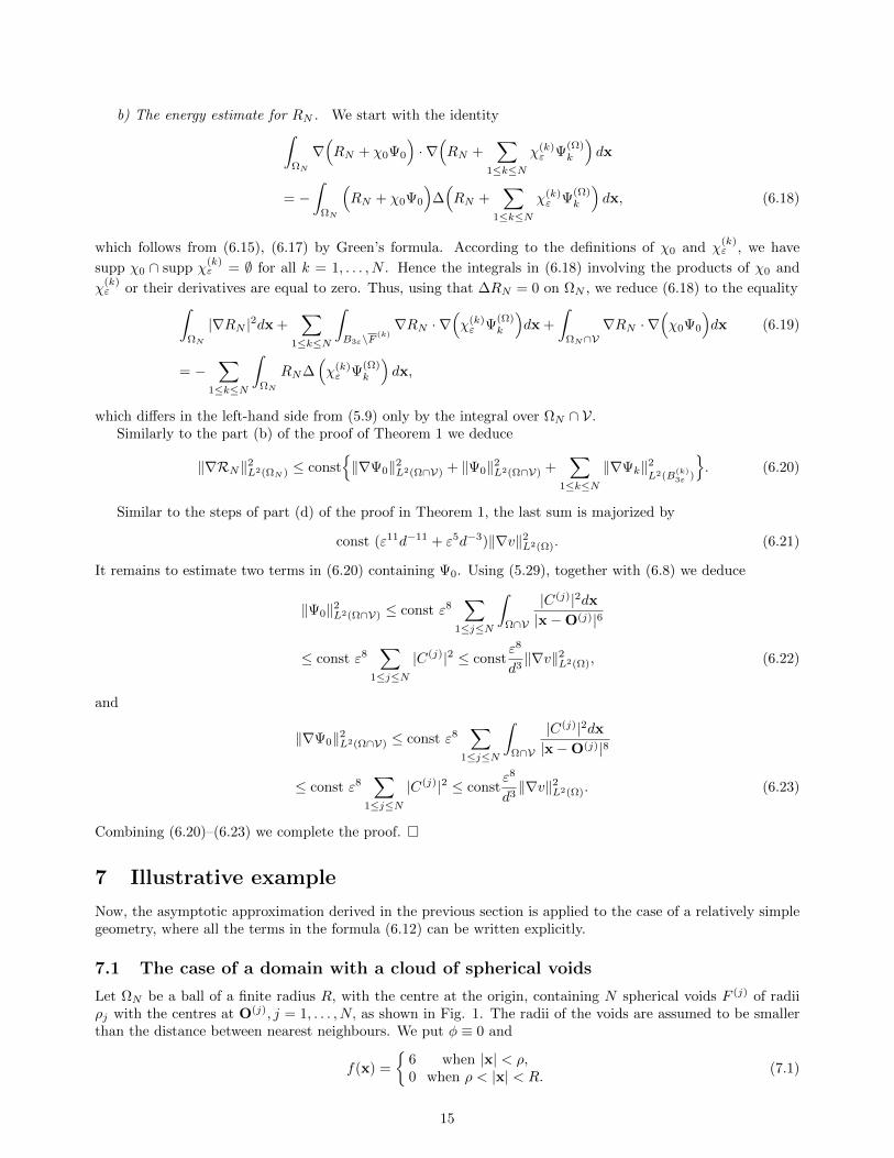
Let ΩN be a ball of a finite radius R, with the centre at the origin, containing N spherical voids F (j) of radiiρj with the centres at O(j), j = 1, . . . , N, as shown in Fig. 1. The radii of the voids are assumed to be smallerthan the distance between nearest neighbours. We put φ ≡ 0 and

f(x) =

6 when |x| < ρ,0 when ρ < |x| < R.

(7.1)

15

R

x3

x1 ω

x2

0

γ

Ω

Figure 1: Example configuration of a sphere containing a cloud of spherical voids in a the cube ω.

Here, it is assumed that ρ+ b < |O(j)| < R − b, 1 ≤ j ≤ N, where ρ and b are positive constants independentof ε and d.

The function uN is the solution of the mixed boundary value problem for the Poisson equation:

∆uN (x) + f(x) = 0, when x ∈ ΩN , (7.2)

uN (x) = 0, when |x| = R, (7.3)

∂uN∂n

(x) = 0, when |x−O(j)| = ρj , j = 1, . . . , N. (7.4)

In this case, uN is approximated by (6.12), where the solution of the Dirichlet problem in Ω is given by

v(x) =

ρ2(3− 2ρR−1)− |x|2 when |x| < ρ,

2ρ3(|x|−1 −R−1) when ρ < |x| < R.(7.5)

In turn, the dipole fields D(j) and the dipole matrices Q(j) have the form

D(j)(x) = −ρ3j

x−O(j)

|x−O(j)|3, Q(j) = −2πρ3

jI3, (7.6)

where I3 is the 3× 3 identity matrix.The regular part H(x,y) of Green’s function in the domain Ω (see (2.4)) is

H(x,y) =R

4π|y||x− y|, y =

R2

|y|2y. (7.7)

The coefficients C(j), j = 1, . . . , N, in (6.12) are defined from the algebraic system (6.4), where Green’s functionG(x,y) is given by

G(x,y) =1

4π|x− y|− R

4π|y||x− y|. (7.8)

7.2 Finite elements simulation versus the asymptotic approximation

The explicit representations of the fields v,D(j), H,G, given above, are used in the asymptotic formula (6.12).Here, we present a comparison between the results of an independent Finite Element computation, produced inCOMSOL, and the mesoscale asymptotic approximation (6.12).

For the computational example, we set R = 120, and consider a cloud of N = 18 spherical voids arrangedinto a cloud of a parallelipiped shape. The position of the centre and radius of each void is included in Table1. The support of the function f (see (7.1)), is chosen to be inside the sphere with radius ρ = 30 and centre atthe origin, as stated in (7.1).

16

Void Centre ρj/R Void Centre ρj/R

F (1) (-50, 0, 0) 0.0417 F (10) (-72, 0, 0) 0.0417

F (2) (-50, 0, 22) 0.0333 F (11) (-72, 0, 22) 0.0458

F (3) (-50, 22, 0) 0.0292 F (12) (-72, 22, 0) 0.0292

F (4) (-50, 0, -22) 0.0375 F (13) (-72, 0, -22) 0.0375

F (5) (-50, -22, 0) 0.0458 F (14) (-72, -22, 0) 0.0417

F (6) (-50, 22, 22) 0.0292 F (15) (-72, 22, 22) 0.0333

F (7) (-50, 22, -22) 0.025 F (16) (-72, 22, -22) 0.05

F (8) (-50, -22, 22) 0.0375 F (17) (-72, -22, 22) 0.0333

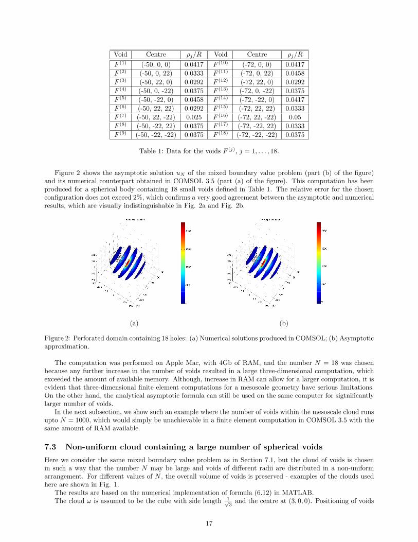
F (9) (-50, -22, -22) 0.0375 F (18) (-72, -22, -22) 0.0375

Table 1: Data for the voids F (j), j = 1, . . . , 18.

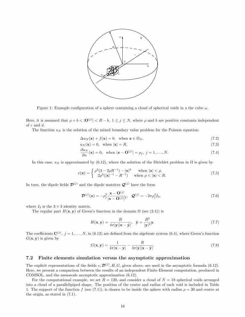
Figure 2 shows the asymptotic solution uN of the mixed boundary value problem (part (b) of the figure)and its numerical counterpart obtained in COMSOL 3.5 (part (a) of the figure). This computation has beenproduced for a spherical body containing 18 small voids defined in Table 1. The relative error for the chosenconfiguration does not exceed 2%, which confirms a very good agreement between the asymptotic and numericalresults, which are visually indistinguishable in Fig. 2a and Fig. 2b.

(a) (b)

Figure 2: Perforated domain containing 18 holes: (a) Numerical solutions produced in COMSOL; (b) Asymptoticapproximation.

The computation was performed on Apple Mac, with 4Gb of RAM, and the number N = 18 was chosenbecause any further increase in the number of voids resulted in a large three-dimensional computation, whichexceeded the amount of available memory. Although, increase in RAM can allow for a larger computation, it isevident that three-dimensional finite element computations for a mesoscale geometry have serious limitations.On the other hand, the analytical asymptotic formula can still be used on the same computer for sigtnificantlylarger number of voids.

In the next subsection, we show such an example where the number of voids within the mesoscale cloud runsupto N = 1000, which would simply be unachievable in a finite element computation in COMSOL 3.5 with thesame amount of RAM available.

7.3 Non-uniform cloud containing a large number of spherical voids

Here we consider the same mixed boundary value problem as in Section 7.1, but the cloud of voids is chosenin such a way that the number N may be large and voids of different radii are distributed in a non-uniformarrangement. For different values of N , the overall volume of voids is preserved - examples of the clouds usedhere are shown in Fig. 1.

The results are based on the numerical implementation of formula (6.12) in MATLAB.The cloud ω is assumed to be the cube with side length 1√

3and the centre at (3, 0, 0). Positioning of voids

17

is described as follows. Assume we have N = m3 voids, where m = 2, 3, . . . . Then ω is divided into N smallercubes of side length h = 1√

3m, and the centres of voids are placed at

O(p,q,r) =(

3− 1

2√

3+

2p− 1

2h,− 1

2√

3+

2q − 1

2h,− 1

2√

3+

2r − 1

2h)

for p, q, r = 1, . . . ,m, and we assign their radii ρp,q,r by

ρp,q,r =

h

5if p > q ,

αh

2if p < q ,

h

4if p = q ,

where α < 1, and it is chosen in such a way that the overall volume of all voids within the cloud remainsconstant for different N . An elementary calculation suggests that there will be m2 voids with radius h

4 and

equal number m2(m−1)2 of voids with radius h

5 or αh2 .

Assuming that the volume fraction of all voids within the cube is equal to β, we have

4πh3

3

(m2(m− 1)(8 + 125α3)

2000+m2

64

)= β

1

3√

3,

and hence

α3 =16m

m− 1

3

4πβ − 125 + 32(m− 1)

8000m

. (7.9)

In particular, if N →∞, the limit value α∞ becomes

α∞ =12

πβ − 8

125

1/3

. (7.10)

In the numerical computation of this section, β = π/25.Taking R = 7 and ρ = 2, we compute the leading order approximation of uN−v, as defined in the asymptotic

formula (6.12), along the line γ at the intersection of the planes x2 = −1/(2√

3) and x3 = −1/(2√

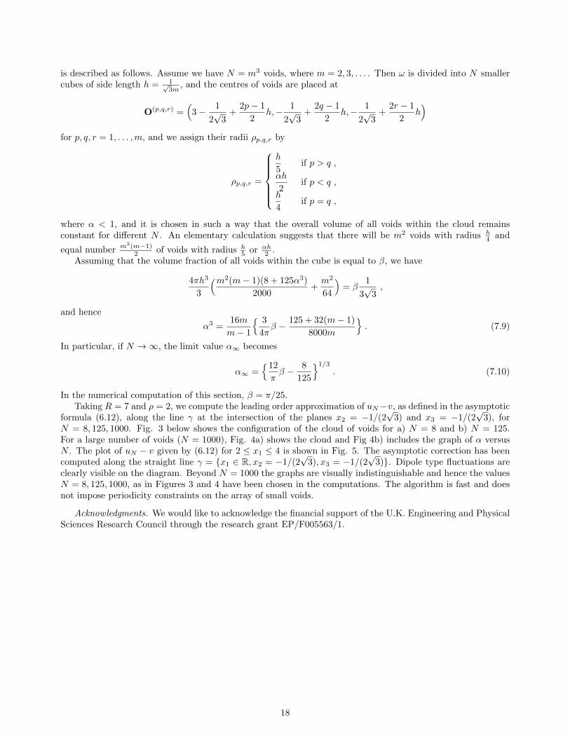
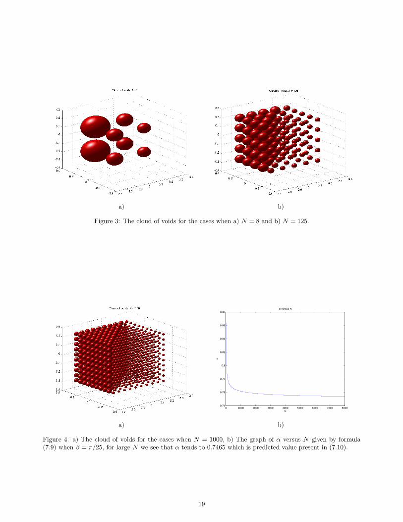
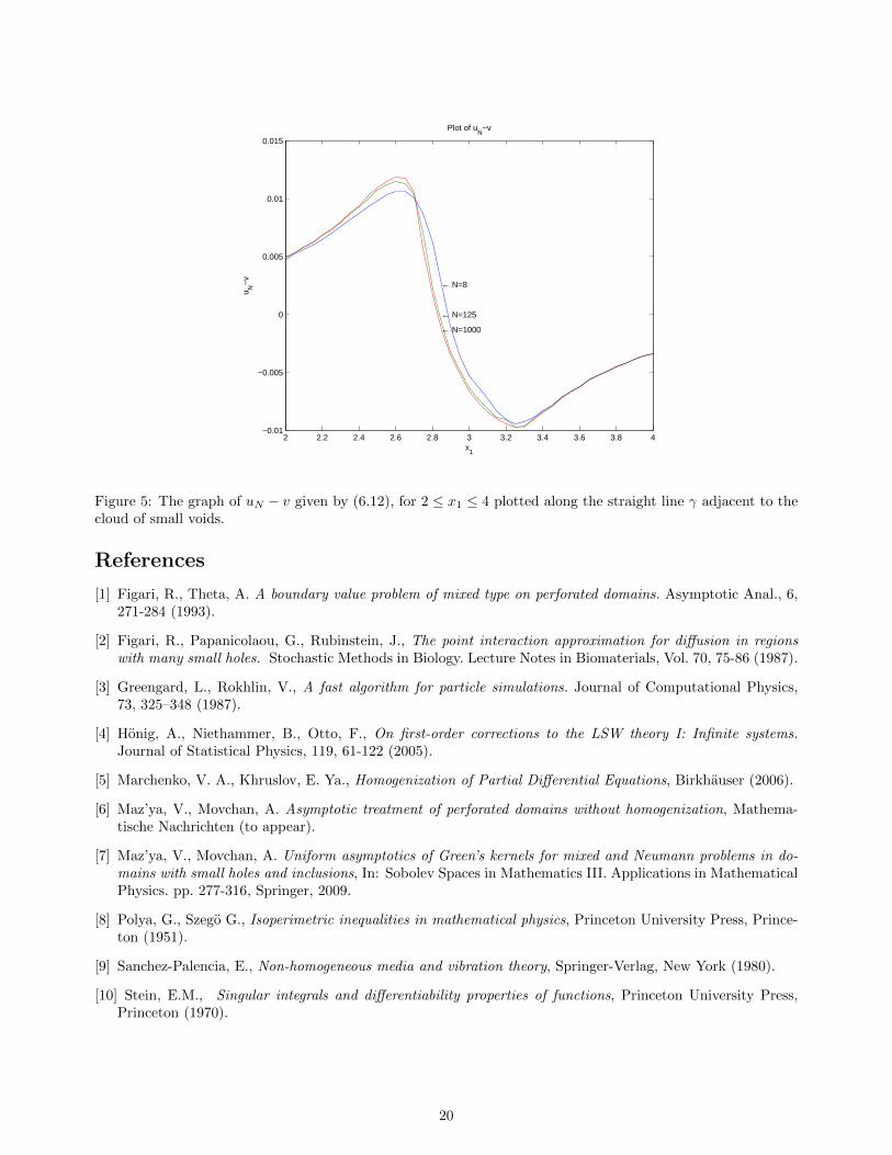
3), forN = 8, 125, 1000. Fig. 3 below shows the configuration of the cloud of voids for a) N = 8 and b) N = 125.For a large number of voids (N = 1000), Fig. 4a) shows the cloud and Fig 4b) includes the graph of α versusN . The plot of uN − v given by (6.12) for 2 ≤ x1 ≤ 4 is shown in Fig. 5. The asymptotic correction has beencomputed along the straight line γ = x1 ∈ R, x2 = −1/(2

√3), x3 = −1/(2

√3). Dipole type fluctuations are

clearly visible on the diagram. Beyond N = 1000 the graphs are visually indistinguishable and hence the valuesN = 8, 125, 1000, as in Figures 3 and 4 have been chosen in the computations. The algorithm is fast and doesnot impose periodicity constraints on the array of small voids.

Acknowledgments. We would like to acknowledge the financial support of the U.K. Engineering and PhysicalSciences Research Council through the research grant EP/F005563/1.

18

a) b)

Figure 3: The cloud of voids for the cases when a) N = 8 and b) N = 125.

a)

0 1000 2000 3000 4000 5000 6000 7000 80000.74

0.76

0.78

0.8

0.82

0.84

0.86

0.88

N

α

α versus N

b)

Figure 4: a) The cloud of voids for the cases when N = 1000, b) The graph of α versus N given by formula(7.9) when β = π/25, for large N we see that α tends to 0.7465 which is predicted value present in (7.10).

19

2 2.2 2.4 2.6 2.8 3 3.2 3.4 3.6 3.8 4−0.01

−0.005

0

0.005

0.01

0.015

← N=8

← N=125

← N=1000

Plot of uN

−v

x1

u N−

v

Figure 5: The graph of uN − v given by (6.12), for 2 ≤ x1 ≤ 4 plotted along the straight line γ adjacent to thecloud of small voids.

References

[1] Figari, R., Theta, A. A boundary value problem of mixed type on perforated domains. Asymptotic Anal., 6,271-284 (1993).

[2] Figari, R., Papanicolaou, G., Rubinstein, J., The point interaction approximation for diffusion in regionswith many small holes. Stochastic Methods in Biology. Lecture Notes in Biomaterials, Vol. 70, 75-86 (1987).

[3] Greengard, L., Rokhlin, V., A fast algorithm for particle simulations. Journal of Computational Physics,73, 325–348 (1987).

[4] Honig, A., Niethammer, B., Otto, F., On first-order corrections to the LSW theory I: Infinite systems.Journal of Statistical Physics, 119, 61-122 (2005).

[5] Marchenko, V. A., Khruslov, E. Ya., Homogenization of Partial Differential Equations, Birkhauser (2006).

[6] Maz’ya, V., Movchan, A. Asymptotic treatment of perforated domains without homogenization, Mathema-tische Nachrichten (to appear).

[7] Maz’ya, V., Movchan, A. Uniform asymptotics of Green’s kernels for mixed and Neumann problems in do-mains with small holes and inclusions, In: Sobolev Spaces in Mathematics III. Applications in MathematicalPhysics. pp. 277-316, Springer, 2009.

[8] Polya, G., Szego G., Isoperimetric inequalities in mathematical physics, Princeton University Press, Prince-ton (1951).

[9] Sanchez-Palencia, E., Non-homogeneous media and vibration theory, Springer-Verlag, New York (1980).

[10] Stein, E.M., Singular integrals and differentiability properties of functions, Princeton University Press,Princeton (1970).

20