constant reynolds number turbulence downstream of an orificed perforated plate

www.elsevier.com/locate/etfs

Experimental Thermal and Fluid Science 31 (2007) 897–908

Constant Reynolds number turbulence downstreamof an orificed perforated plate

Rui Liu a, David S.-K. Ting a,*, M. David Checkel b

a Mechanical, Automotive and Materials Engineering, University of Windsor, Windsor, Ontario, Canada N9B 3P4b Department of Mechanical Engineering, University of Alberta, Edmonton, Alberta, Canada T6G 2G8

Received 27 January 2006; received in revised form 29 June 2006; accepted 23 September 2006

Abstract

Quasi-isotropic turbulence was experimentally produced in a wind tunnel via an orificed, perforated plate (OPP) at 10.5 m/s. The OPPconsists of a lattice arrangement of 38.1 mm holes occupying 57% of the plate area. The OPP turbulence was found to be homogeneousover the cross section normal to the mean flow with Gaussian-like turbulence fluctuation. The isotropy of the turbulence field as por-trayed by the streamwise/lateral turbulence intensity ratio was found to be approximately 1.1. The OPP turbulence is essentially self-pre-serving wherein the Taylor microscale Reynolds number remains nearly constant and the lateral velocity correlations collapse into asingle curve.� 2006 Elsevier Inc. All rights reserved.

Keywords: Quasi-isotropic turbulence; Self-similarity; Orificed perforated plate

1. Introduction

Laboratory quasi-isotropic turbulence has been conven-tionally generated by passing flow through a passive grid orperforated plate. Multiple jets and wakes formed behindthe obstruction interact with each other such that beyonda certain distance downstream of the turbulence generator,the mean flow becomes uniform and the turbulence evolvesinto a homogeneous and approximately isotropic state [1].In passive grid turbulence, the turbulence length scale canbe adjusted over a limited range by modifying the geomet-rical parameters of the turbulence generator. Turbulenceproduced in this way acquires its energy primarily fromthe pressure drop across the turbulence generator. As indi-cated by the study of Baines and Peterson [2], the pressuredrop, and ultimately the turbulence level, depends essen-tially on turbulence generator solidity ratio, (area fractionof the solid portion). Within limits, the required turbulence

0894-1777/$ - see front matter � 2006 Elsevier Inc. All rights reserved.

doi:10.1016/j.expthermflusci.2006.09.007

* Corresponding author. Tel.: +1 519 253 3000x2599; fax: +1 519 9737007.

E-mail address: [email protected] (D.S.-K. Ting).

level can therefore be achieved by using a turbulence gen-erator with carefully selected solidity ratio as illustratedexperimentally by Liu et al. [3]. In other words, the solidityratio offers some flexibility in generating controllable,quasi-isotropic turbulence. Nevertheless, there are associ-ated limitations with the laboratory quasi-isotropic turbu-lence. In order to obtain a quasi-isotropic turbulence, thesolidity ratio of the turbulence generator cannot be toohigh. Otherwise, the uniformity of the mean flow will ceaseto exist. The upper limit of this solidity ratio found in theliterature is around 0.4–0.5 [4,5]. This sets a limiting rangeof the achievable turbulence intensity and scales. Boundedby this limitation, to obtain a laboratory quasi-isotropicturbulence with comparable Reynolds number to the shearturbulence and/or natural turbulence, either an enormouswind tunnel needs to be utilized or a special techniquehas to be applied (e.g., pressurized wind tunnel). High Rey-nolds number, nearly isotropic turbulence has been alsorealized in laboratory wind tunnels by using active turbu-lence generators which can achieve Taylor microscale Rey-nolds number on the order of 700 [6–10]. Other approachesof generating nearly isotropic turbulence include using

mailto:[email protected]

Nomenclature

A decay power law coefficientB curve fit coefficient for the decay of turbulence

kinetic energyD plate hole diameter (D = 38.1 mm)E11 streamwise turbulence velocity spectrum (m3/s2)E22 lateral turbulence velocity spectrum (m3/s2)Fu flatness factor of the streamwise turbulence fluc-

tuationf streamwise autocorrelation function of u,

f ðrÞ ¼ u � uðrÞ=u02

g streamwise autocorrelation function of v,gðrÞ ¼ v � vðrÞ=v02

K turbulence kinetic energy per unit mass (m2/s2)k1 streamwise wavenumber (1/m)L turbulence integral length scale (mm)M mesh size of grid/OPP turbulence generator

(M = 45 mm)n decay power exponentOPP orificed, perforated platepdf probability density functionRe mean flow Reynolds number ¼ qUM

l

� �

Rek turbulence Reynolds number ¼ qu0kl

� �

r streamwise separation (=Us mm)rms root mean squaret converted elapsing time (s)U local time-averaged flow velocity (m/s)u instantaneous streamwise turbulence fluctuation

velocity (m/s)u 0 streamwise rms turbulence fluctuation velocity

(m/s)v instantaneous lateral turbulence fluctuation

velocity (m/s)v 0 lateral rms turbulence fluctuation velocity (m/s)X streamwise coordinate (mm)Xo virtual origin in the decay power law (mm)Y lateral coordinate (mm)Z spanwise coordinate (mm)

Greek Symbols

k Taylor microscale (mm)l dynamic viscosity (m2/s)q air density (kg/m3)r solidity ratio (r = 0.43)s separation in time (s)

Fig. 1. Schematic of the experimental setup. The dashed line indicates thevirtual origin, Xo estimated in this study.

898 R. Liu et al. / Experimental Thermal and Fluid Science 31 (2007) 897–908

opposing flows [11,12], applying fluid of low kinematic vis-cosity [13], and utilizing oscillating grid(s) [14].

Apart from its direct application in fundamental turbu-lence research, laboratory scale quasi-isotropic turbulencehas also been applied in studies of many practical flow phe-nomena where turbulence acts as a critical factor e.g.[15,16]. Those studies often demand turbulent flow withparticular intensity and length scale to fulfill the requiredtask effectively. They also call for further studies overextended ranges of turbulence parameters to demonstratethe influence of turbulence beyond that restricted by theboundary and initial conditions of the particular labora-tory environment.

All the results presented in this paper are from the flowmeasurement downstream of an orificed perforated plate(OPP). A literature survey shows that most low Reynoldsnumber laboratory quasi-isotropic turbulence experimentswere achieved with grids made from solid bar of finite thick-ness. Thickness is inherently an added parameter on the tur-bulence structure and it has a potential negative impact onthe isotropy of the turbulence generated. Previous studieson single wake and jet flows have demonstrated that theimpact of initial conditions on the downstream flow devel-opment is significant even in the far-field, self-similar region[17,18]. Compared with grid turbulence generator, the OPPused in this study provides a virtual zero-thickness obstruc-tion to the flow, which renders the possibility to eliminatethe thickness effect and to generate more isotropic turbu-lence with a wider range of flow velocities.

2. Experiments

The experiments were conducted in a closed-circuit windtunnel. The working section measured 6 m long with asquare cross section of 0.76 · 0.76 m2 (30 · 30 in.2). Themaximum achievable mean velocity in an empty workingsection was approximately 15 m/s. A preliminary test car-ried out at mean velocity of 10 m/s showed a turbulenceintensity of less than 0.5% at the entrance of the workingsection. The OPP was of the same dimension of the crosssection and it was situated 0.38 m downstream of theentrance of the working section. A schematic of the experi-mental setup is shown in Fig. 1. The plate was machined bydrilling holes with a diameter, D, of 38.1 mm (1.5 in.) in a3 mm thick aluminum sheet. The diagonal center-to-center

R. Liu et al. / Experimental Thermal and Fluid Science 31 (2007) 897–908 899

distance, M was 45 mm which gave a plate solidity ratio, r,of approximately 0.43. This OPP solidity is comparable tothe largest value (0.44) tested in conventional grid turbu-lence studies [19].

Two geometrical features, i.e., plate thickness, and per-foration pattern, distinguish the current OPP from otherconventional free stream turbulence generators. The OPPof this study has virtually zero thickness which differs fromthe conventional grid turbulence generator. This was real-ized by machining each hole in the plate into an orifice witha 41� inclined angle as shown in Fig. 2c. The plate was posi-tioned with the sharp edge upstream so that the hole diam-eter seen by the oncoming flow was 38.1 mm (1.5 in.) with asharp edge.

The OPP schematic is shown in Fig. 2a along with anelemental close-up in Fig. 2b and a cross sectional viewin Fig. 2c. Compared with conventional perforated plateswith a hexagonal hole network, the OPP has a larger cen-ter-to-center distance in both horizontal and vertical direc-

Fig. 2. Schematics of orificed perforated plate used in this study (a) thecomplete OPP, (b) elemental close-up of the OPP in this study showingdimensions D and M, and (c) cross section view of the OPP showing therelative orientation the orifice edge with respect to the mean flow.

tions, and a shorter distance diagonally. This change inspacing is expected to affect large turbulence length scalesbecause they are governed by both hole size and the block-age area between consecutive holes.

Instantaneous flow velocities were measured with aDantec Streamline� 55C90 constant temperature anemom-eter (CTA) and a DISA 55P61 X-configuration hot-wireprobe. The sensors on the probe were 1.25 mm long plati-num-coated tungsten wires with a diameter of 5 lm.Analog signals from the CTA were picked up by aNational Instrument SC-2040 sample-and-hold board andthen digitized via a 12-bit National Instrument multifunc-tional A/D converter. All velocity data were collected ata sampling rate of 30 kHz and low-passed at 10 kHz toavoid the aliasing problem. To reduce the uncertainties inthe post-processed statistical parameters, over 106 sampleswere collected for each channel of the A/D converter,which amounts to a sample period of approximately 30 sat each measuring location. The uncertainties in the timeaveraged velocity and turbulence intensities are estimatedto be less than 1% and 10%, respectively. A thermistor typetemperature probe was placed close to the hot-wire probeto provide the temperature reading necessary for smalltemperature corrections of the CTA signal. The maximumtemperature rise in a given test was approximately 8 �C.

The turbulence measurements were repeated at a nomi-nal mean velocity of 10.5 m/s over seven evenly separatedcross sections starting from 17 to 68M downstream ofthe OPP. The mean velocity gives a mean flow Reynoldsnumber, based on M, of 31,000. Each measurement crosssection measured 191 · 191 mm2 (7.5 · 7.5 in.2) centeredat the middle of the working section. The measuring loca-tions were separated 31.75 mm from one another, giving atotal of 49 measuring points over each cross section. Thehot-wire probe was positioned over the measuring crosssection by means of a traversing mechanism which canposition the probe within ±0.1 mm precision. The nominalmean velocity was set by positioning a Pitot-static tube8.5M upstream of the OPP. Mean velocity set in this waywas confirmed by the pressure drop across the wind tunnelcontraction section located immediately upstream of theworking section.

3. Results and discussion

The flow uniformity over the tested cross sections down-stream of the OPP was assessed by examining the varia-tions of various flow parameters such as local time-averaged velocity, turbulence fluctuation velocity, and tur-bulence integral length scale. The characteristics of theOPP-generated turbulence are demonstrated by the devel-opment of these parameters.

3.1. Flow uniformity over the cross sections

A widely applied assumption in the study of grid/perfo-rated plate turbulence is the uniformity of flow field over a


cross section normal to the mean flow. Taking this forgranted, turbulence has been quantified in many studiesby measuring parameters only along the central axis of thewind tunnel, which is expected to be representative of theentire cross section, outside of the boundary layer. This

-80 -60 -40 -20 0 20 40 60 80Y (mm)

-80

-60

-40

-20

0

20

40

60

80

Z (m

m)

Fig. 3a. Absolute value of percentage variation of local time-averagedvelocity, U (m/s), from its center line value (10.5 m/s) at 17 M downstreamof the OPP.

-80 -60 -40 -20 20 40 60 80Y (mm)

-80

-60

-40

-20

0

20

40

60

80

Z (m

m)

0

Fig. 3b. Absolute value of percentage variation of local time-averagedvelocity, U (m/s), from its center line value (10.7 m/s) at 42M downstreamof the OPP.

may be a possible source of the discrepancy among the out-comes of different studies, since the degree of flow unifor-mity in the lateral direction may vary from study to study,depending on the particular turbulence generator applied.In fact, it was observed by Batchelor and Townsend [20]

-80 -60 -40 -20 20 40 60 80Y (mm)

-80

-60

-40

-20

0

20

40

60

80

Z (m

m)

0

Fig. 3c. Absolute value of percentage variation of local time-averagedvelocity, U (m/s), from its center line value (10.8 m/s) at 68M downstreamof the OPP.

-80 -60 -40 -20 20 40 60 80Y (mm)

-80

-60

-40

-20

0

20

40

60

80

Z (m

m)

0

Fig. 4a. Absolute value of percentage variation of streamwise turbulencerms fluctuation velocity, u 0, from its center line value (0.64 m/s) at 17M

downstream of the OPP.


and subsequently, Grant and Nisbet [21] that noticeablenon-uniformity of the turbulence intensity may exist in thelateral direction.

To examine the lateral flow uniformity downstream ofthe OPP turbulence generator, contours of mean flow

-80 -60 -40 -20 20 40 60 80Y (mm)

-80

-60

-40

-20

0

20

40

60

80

Z (m

m)

0

Fig. 4b. Absolute value of percentage variation of streamwise turbulencerms fluctuation velocity, u 0, from its center line value (0.33 m/s) at 42M


-80 -60 -40 -20 0 20 40 60 80Y (mm)

-80

-60

-40

-20

0

20

40

60

80

Z (m

m)

Fig. 4c. Absolute value of percentage variation of streamwise turbulencerms fluctuation velocity, u 0, from its center line value (0.26 m/s) at 68M


and turbulence parameters up to the fourth moment wereinspected at all cross sections downstream of the OPP.The contours of these parameters at 17M, 42M, and 68M

were selected as typical cases and presented in Figs. 3a–3c, 4a–4c, 5a–5c, 6a–6c for this discussion.

-80 -60 -40 -20 0 20 40 60 80Y (mm)

-80

-60

-40

-20

0

20

40

60

80

Z (m

m)

Fig. 5a. Absolute value of percentage variation of turbulence integrallength scale, L, from its center line value (24 mm) at 17M downstream ofthe OPP.

-80 -60 -40 -20 0 20 40 60 80Y (mm)

-80

-60

-40

-20

0

20

40

60

80

Z (m

m)

Fig. 5b. Absolute value of percentage variation of turbulence integrallength scale, L, from its center line value (35 mm) at 42M downstream ofthe OPP.


3.1.1. Time averaged velocity

Fig. 3a–c shows the absolute percentage variations of thelocal time-averaged velocity using the corresponding centerpoint value as the reference. The largest variations of U overthese cross sections are less than 3% of the correspondingcenter values. This implies that, beyond 17M downstreamfrom the OPP, a relatively uniform mean flow field has

-80 -60 -40 -20 0 20 40 60 80Y (mm)

-80

-60

-40

-20

0

20

40

60

80

Z (m

m)

Fig. 5c. Absolute value of percentage variation of turbulence integrallength scale, L, from its center line value (41 mm) at 68M downstream ofthe OPP.

-80 -60 -40 -20 0 20 40 60 80Y (mm)

-80

-60

-40

-20

0

20

40

60

80

Z (m

m)

Fig. 6a. Absolute value of percentage variation of the flatness factor, Fu,from the Gaussian value (3) at 17M downstream of the OPP.

evolved from the interaction of the multiple wakes and jets,aided by the enhanced momentum transport of the turbu-lence flow. This homogeneity of the mean flow field greatlysimplifies the procedure for the estimation of turbulence dis-sipation rate which can be obtained directly from the decayof turbulence kinetic energy when the turbulence produc-tion is essentially zero as it is in the current case.

-80 -60 -40 -20 0 20 40 60 80Y (mm)

-80

-60

-40

-20

0

20

40

60

80

Z (m

m)

Fig. 6b. Absolute value of percentage variation of the flatness factor, Fu,from the Gaussian value (3) at 42M downstream of the OPP.

-80 -60 -40 -20 0 20 40 60 80Y (mm)

-80

-60

-40

-20

0

20

40

60

80

Z (m

m)

Fig. 6c. Absolute value of percentage variation of the flatness factor, Fu,from the Gaussian value (3) at 68M downstream of the OPP.

-8 -6 -4 -2 0 2 4 6 8 10 12 1u/u', v/v'

40

0.1

0.2

0.3

0.4

0.5

0.6

0.7

u'p(

u), v

'p(v

)

Gaussian distributionu distribution at 17Mv distribution at 17Mu distribution at 42Mv distribution at 42Mu distribution at 68Mvdistribution at 68M

Fig. 7. Scaled pdfs for turbulence fluctuation velocities, u and v, at 17M,42M and 68M.


3.1.2. Streamwise turbulence fluctuating velocity

The absolute percentage variation of u 0, the streamwiseroot mean square (rms) fluctuating velocity, from its corre-sponding center value is shown in Fig. 4a–c for the 17M,43M and 68M cross sections. In the proximity of the cen-tral region (Y, Z � ± 100 mm), the variation in u 0 is lessthan 5% of its center value. These plots demonstrate afairly uniform u 0 distribution in the proximity of the centralregion. A general tendency of decreasing u 0 (from 0.64 to0.26 m/s) with distance downstream of the OPP is observedfrom 17M to 68M. This is an indication of the turbulencedecay as the mean flow is essentially uniform and the tur-bulence has no significant source of sustained energy input.It should be noted that for traditional grid turbulence, theflow is typically not observed to be homogeneous untilapproximately 30M downstream of the turbulence genera-tor. This difference implies that the OPP has a potentialadvantage as a laboratory generator for homogeneous,quasi-isotropic turbulence. The physics behind this isbelieved to be the enhanced three-dimensionality of theflowstructure in the developing region immediately down-stream of the OPP [22] which increases the mixing rateand reduces the grid shadow effect.

3.1.3. Integral length scale

The turbulence integral length scale, L, which signifiesthe average size of the energy-containing eddies is fre-quently used to characterize turbulence. Various schemeshave been proposed for the estimation of L [23]. Theapproach adopted in this study is based on the Taylor’sfrozen turbulence hypothesis, where L is defined as theproduct of local time-averaged velocity, U, and the timescale, I, estimated from the autocorrelation coefficient ofthe instantaneous turbulence fluctuation velocity u as

I ¼Z 1

0

u� uðsÞ=u02 ds; ð1Þ

where s is the time interval. The requirements for invokingTaylor’s hypothesis are approximately satisfied in thisstudy as the largest relative turbulence intensity (at 17M)is less than 10%.

The integral length scale grows from approximately24 mm to 41 mm as the flow moves from 17M to 68M.Integral length scale in this initial decay region appearsto correspond to the OPP geometry, noting that the holediameter is 38 mm and the largest blockage distancebetween neighboring hole edges is 25 mm. The absolutepercentage variations of L from the corresponding centervalue are shown in Fig. 5a–c for the three measurementplanes. These contours are observed to be generally uni-form and the variations are generally less than 6% (slightlylarger than those of u 0) over any cross section measured.

3.2. Gaussianity of OPP turbulence

Homogeneous turbulence has been observed to have aprobability density function (pdf) close to Gaussian e.g.,

[24]. One of the indicators traditionally used to identifythe quasi-Gaussian behavior of a random variable is theflatness factor, defined as the ratio of the fourth momentof the variable to the square of its variance. For the instan-taneous streamwise turbulence fluctuation velocity, u, thiscan be written in term of the turbulence intensity, u 0, as

F u ¼ u4=u04: ð2Þ

A true Gaussian pdf has a flatness factor of 3. Therefore,the closer Fu is to 3, the more likely the pdf of u resemblesGaussian distribution.

The above criterion has been applied to the velocity datarecorded over the cross sections at 17M, 42M, and 68M

downstream of the OPP. The distributions of Fu over thesecross sections are plotted in the form of their absolute per-centage deviation from the Gaussian value of 3 in. Fig. 6a–c. The streamwise flatness factor has a uniform distributionover the entire cross sections at 17M and 42M, with a max-imum deviation from the Gaussian value of less than 5%.The peak values are slightly higher at 68M (7%) but thismight be attributed to a rising uncertainty as the turbulenceintensity decreases.

A more direct approach to assess the Gaussinity of thehomogeneous turbulence is to compare its probability den-sity function (pdf) with that of a true Gaussian of the samevariance. This was carried out and the comparison is illus-trated in Fig. 7, wherein p(u) and p(v) are the estimated pdfsof the instantaneous streamwise fluctuation velocity u andthe lateral fluctuation velocity v respectively, at the centerof the cross sections at 17M, 42M and 68Ms. The pdfs at42M and 68M have been shifted up by 0.1 and 0.2 units,respectively, in Fig. 7 for clarity. At each location, the


difference between the pdf of a true Gaussian signal and thep(u) and p(v) pdf is hardly noticeable. This agrees with theresults of Mouri and Takaoka [25] who observed the grid-turbulence field to be sub-Gaussian in the developing regionand quasi-Gaussian in the developed, initial decay region,the range covered in this study. It should also be noted thatthe absolute value of the skewness factor in this study is ofthe order 0.01 which is close to zero as illustrated by thesymmetries of the distributions in the pdf plot.

3.3. Characteristics of decaying nearly isotropic OPP

turbulence

The contours shown in the previous sections confirmthat the turbulence parameters at the center of the crosssection are representative of the corresponding parametersover the entire section. This allows a discussion of the evo-lution of OPP turbulence based on the measured valuesalong the central line. The repeatability of turbulence fluc-tuation velocities, u 0 and v 0, on the central line were testedto within 3% of individual measurements.

Perfectly isotropic turbulence has equal turbulent fluctu-ating velocity in all directions, that is, u 0/v 0 = 1. The ratioof axial and transverse fluctuating velocities was examinedat the center point of each measurement cross section asillustrated in Fig. 8. Typically, the streamwise turbulencefluctuation velocity, u 0, was approximately 13% larger thanthe transverse fluctuation velocity, v 0, and this remainsnearly unchanged as the flow moves downstream of theOPP. The isotropy of the current OPP turbulence appearsto be slightly better than that of the conventional grid tur-bulence without resorting to a secondary contraction forisotropy improvement [19,26].

10 20 30 40 50 60 70X/M

0.9

1

1.1

1.2

1.3

1.4

u'/v'

Fig. 8. Approximately isotropic turbulence indicated by u 0/v 0 (with typicaluncertainty).

The decay of laboratory quasi-isotropic turbulence hasbeen conventionally described by a power decay law inthe form

u02

U 2¼ A

XM� X o

M

� ��n

: ð3Þ

The exponent n has been analytically predicted to be 10/7[27], 6/5 [28], and 1 [29,30], based on different assumed lev-els of self-preservation. Speziale and Bernard’s prediction[30] was based on complete self-preservation of the full vis-cous equation and was partially confirmed by the work ofGeorge [31] and Ristorcelli and Livescu [32]. Empirically,pairs of values for coefficient, A, and exponent, n can beobtained by curve-fitting the empirical data to Eq. (3)assuming different preset values of virtual origin, Xo, andusing the set of parameters which gives the best fit. Thevalue of Xo giving the lowest residual represents the virtualorigin of the decaying part of the turbulence flow field. Thevirtual origin is approximately the point where the initial jetbreak-up creates the most turbulent flow energy. Thisapproach was applied to both u 0 and v 0 and the resultingcurve-fitting parameters are listed in Table 1, along withthose from previous studies on grid/perforated plate turbu-lence with comparable Re and/or grid solidity ratio. Thedecay exponent n from the current empirical work (1.02and 1.09) agrees favorably with the analytical predictionof Speziale and Bernard [30] who arrived at the conclusionthat power law decay with n = 1 is the asymptotic solutionto completely self-preserving, isotropic turbulence. Conven-tional grid turbulence results, such as those listed in Table 1and compiled by Mohamed and LaRue [33] do not supportthis argument, presumably due to the lack of eddy turnovertimes and/or the effects of initial conditions [30].

A supplementary inspection of the OPP turbulencedecay was carried out on the turbulence kinetic energy K

which is estimated in this study as

K ¼ u02 þ 2v02

2; ð4Þ

assuming equal turbulence intensity in both lateral direc-tions. The variation of K with the converted elapsed timet = X/U is plotted in Fig. 9 along with a power decay lawcurve-fit in the form of

K ¼ Bðt � X o=UÞ�n: ð5Þ

The decay exponent, n in Eq. (5) was determined to be1.012 which agrees closely with the power law decayobtained above. A direct consequence of n = 1 power lawdecay is a constant Taylor microscale Reynolds number

Rek ¼ qu0kl

� �during the initial period of decay. Based on

the assumption of isotropic turbulence, which is approxi-mately confirmed by the above discussion, the Taylormicroscale is estimated in this study as

k ¼ 15u02ldK=dtð Þq

� �1=2

; ð6Þ

where l and q are the dynamic viscosity and density of air,respectively. Eq. (5) was invoked in estimating the values of

0.05 0.1 0.15 0.2 0.25 0.3Time (s)

0

0.1

0.2

0.3

0.4

0.5

0.6

Turb

ulen

ce k

inet

ic e

nerg

y K

(m2 /s

2 ) curve fitK = 0.0209(t-7M/U) -1.012

K = (u '2+2v' 2)/2

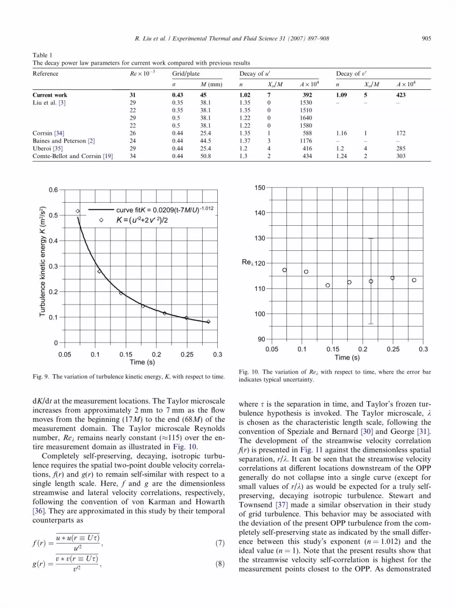
Fig. 9. The variation of turbulence kinetic energy, K, with respect to time.

0.05 0.1 0.15 0.2 0.25 0.3Time (s)

90

100

110

120

130

140

150

Reλ

Fig. 10. The variation of Rek with respect to time, where the error barindicates typical uncertainty.

Table 1The decay power law parameters for current work compared with previous results

Reference Re · 10�3 Grid/plate Decay of u 0 Decay of v 0

r M (mm) n Xo/M A · 104 n Xo/M A · 104

Current work 31 0.43 45 1.02 7 392 1.09 5 423

Liu et al. [3] 29 0.35 38.1 1.35 0 1530 – – –22 0.35 38.1 1.35 0 151029 0.5 38.1 1.22 0 164022 0.5 38.1 1.22 0 1580

Corrsin [34] 26 0.44 25.4 1.35 1 588 1.16 1 172Baines and Peterson [2] 24 0.44 44.5 1.37 3 1176 – – –Uberoi [35] 29 0.44 25.4 1.2 4 416 1.2 4 285Comte-Bellot and Corrsin [19] 34 0.44 50.8 1.3 2 434 1.24 2 303


dK/dt at the measurement locations. The Taylor microscaleincreases from approximately 2 mm to 7 mm as the flowmoves from the beginning (17M) to the end (68M) of themeasurement domain. The Taylor microscale Reynoldsnumber, Rek remains nearly constant (�115) over the en-tire measurement domain as illustrated in Fig. 10.

Completely self-preserving, decaying, isotropic turbu-lence requires the spatial two-point double velocity correla-tions, f(r) and g(r) to remain self-similar with respect to asingle length scale. Here, f and g are the dimensionlessstreamwise and lateral velocity correlations, respectively,following the convention of von Karman and Howarth[36]. They are approximated in this study by their temporalcounterparts as

f ðrÞ ¼ u � uðr � UsÞu02

; ð7Þ

gðrÞ ¼ v � vðr � UsÞv02

; ð8Þ

where s is the separation in time, and Taylor’s frozen tur-bulence hypothesis is invoked. The Taylor microscale, kis chosen as the characteristic length scale, following theconvention of Speziale and Bernard [30] and George [31].The development of the streamwise velocity correlationf(r) is presented in Fig. 11 against the dimensionless spatialseparation, r/k. It can be seen that the streamwise velocitycorrelations at different locations downstream of the OPPgenerally do not collapse into a single curve (except forsmall values of r/k) as would be expected for a truly self-preserving, decaying isotropic turbulence. Stewart andTownsend [37] made a similar observation in their studyof grid turbulence. This behavior may be associated withthe deviation of the present OPP turbulence from the com-pletely self-preserving state as indicated by the small differ-ence between this study’s exponent (n = 1.012) and theideal value (n = 1). Note that the present results show thatthe streamwise velocity self-correlation is highest for themeasurement points closest to the OPP. As demonstrated

0 5 10 15 20 25 30 35 40r/λ

0

0.2

0.4

0.6

0.8

1

1.2

f(r)

X = 17MX = 25MX = 34MX = 42MX = 51MX = 59MX = 68M

Fig. 11. Development of the streamwise velocity correlation f(r) down-stream of the OPP.


by Speziale and Bernard [30], f is extremely sensitive tosmall perturbations from a self-preserving state. Thus, atcross-sectional planes closest to the OPP, some residualunsteadiness from the multi-jet flow regime may still bepresent.

Unlike its streamwise counterpart, the lateral velocitycorrelation g(r) exhibits reasonably good self-preservationas the turbulence evolves downstream of the OPP. Asshown in Fig. 12, the self-preservation of the spanwise

0 5 10 15 20r/λ

0

0.2

0.4

0.6

0.8

1.2

1

g(r)

X = 17MX = 25MX = 34MX = 42MX = 51MX = 59MX = 68M

Fig. 12. Development of the lateral velocity correlation g(r) downstreamof the OPP.

velocity correlation g(r) holds fairly well over the range0 6 r/k 6 18 and approaches zero beyond that range.Due to the nature of the velocity correlation, the self-pres-ervation of the correlation curves at larger separation is notconsidered important, since the correlation tends to be zeroat large separations. The closer behavior of g(r) to self-preservation makes it a broader basis for the analysis ofself-preservation than f(r). Again, the earliest (closest tothe OPP) measurement plane (17M) shows the most devia-tion from the spectrum, plausibly because the turbulencehas barely completed the transition from a multi-jet flowto a homogeneous, decaying turbulence at this point.

A better appreciation of self-preservation can beachieved by inspecting the power spectra of turbulencevelocity fluctuations. Fig. 13 presents the evolution of thelateral turbulence velocity spectrum E22(k1) defined as

v02

2¼Z 1

0

E22ðk1Þdk1; ð9Þ

where k1 is the streamwise wavenumber. E22(k1) is selectedfor demonstration because the streamwise power spectrummeasured by an X-probe might be contaminated by cross-talking between the two hot-wire sensors [38]. To furtherreduce the hot-wire length effect and high frequency noiseeffects, the spectrum is cut off at a wavenumber corre-sponding to the Taylor microscale. The normalized spec-trum E22(k1) displays reasonable self-preservation startingfrom the normalized wavenumber k1k � 0.1. This pointcorresponds approximately to the energy-containing inte-gral scale L in the physical space (based on L � 2p/k1). Aslight departure from the self-preservation state is observedfor k1k < 0.1, which corresponds to the largest structures in

0.01 0.1 1k1λ

0.1

1

E 22(k

1)/v'

2 λ

X = 17MX = 25MX = 34MX = 42MX = 51MX = 59MX = 68M

Fig. 13. Self-preservation of the lateral turbulence velocity spectrum.E22(k1) downstream of the OPP.

0.01 0.1 1k1λ

0.1

1

E 11(

K 1)/u

2 λ

X = 17MX = 25MX = 34MX = 42MX = 51MX = 59MX = 68M

Fig. 14. Self-preservation of the lateral turbulence velocity spectrum.E11(k1) downstream of the OPP.


the OPP turbulence. Those largest structures are not ex-pected to be self-preserving as they would be residuals ofthe original jet flows dominated by the geometry featureof the OPP. The streamwise turbulence velocity spectrumE11(k1) is presented in Fig. 14, which shows clearly thatat large (energy containing) length scales, the streamwiseturbulence fluctuation is more energetic than its lateralcounterpart due the imperfect isotropy of the OPPturbulence.

4. Conclusions

Homogeneous, nearly isotropic turbulence was experi-mentally produced using an orificed, perforated plate in awind tunnel. The flow field downstream of the OPP wasquantified and found to be uniform in terms of the meanflow, turbulence intensity and turbulence integral lengthscale across significant cross sections in the core region ofthe decaying turbulence. Compared with conventional gridturbulence generators, the OPP exhibited a potentialadvantage in generating nearly isotropic turbulencewherein the grid shadow effect was reduced. The isotropyof the turbulence flow field was evaluated to be somewhatbetter than that of conventional grid turbulence without asecondary contraction, giving u 0/v 0 = 1.1–1.15.

The decay of turbulence kinetic energy, K closely fol-lowed a power law with an exponent of �1.012. Thisimplies a self-preserving state of the OPP turbulence. Fur-ther examination of the two-point double velocity correla-tions f(r) and g(r) showed that the transverse correlation,g(r), indicated a self-preserving, decaying turbulent flow,while there was still some evolution of the streamwise cor-relation, f(r). This was also supported by the fact that the

normalized lateral turbulence velocity spectra, E22(k1) col-lapsed into a single curve for k1k larger than approximately0.1, while f(r) was found to be extremely sensitive to smalldeviations from the ideal, completely self-preserving condi-tion. The physical mechanism behind OPP’s improvedempirical approximation to the completely self-preservingstate is presently unclear, but has been attributed to thelack of grid thickness effect due to sharp edges at the pointwhere the turbulence is originally generated. An accuratemeasurement of the fourth order derivative of f(r) maybe necessary to clarify this point.

It should be noted that previous studies on the self-pres-ervation of decaying isotropic turbulence demonstrate thepossible dependence of the energy decay on the initial con-ditions [31,39]. The evolution of the OPP turbulence underdifferent initial conditions (e.g. Rek) will be addressed in afuture study.

Acknowledgements

This project was sponsored by the Natural Sciences andEngineering Research Council of Canada (NSERC). Thelead author gratefully acknowledges Ontario StudentAssistance Program (OSAP) for an Ontario GraduateScholarship (OGS).

References

[1] A.S. Monin, A.M. Yaglom, in: J.L. Lumley (Ed.), Statistical FluidMechanics, vol. 2, MIT Press, 1975, pp. 113–117.

[2] W.D. Baines, E.G. Peterson, An investigation of flow throughscreens, Journal of Applied Mechanics 73 (1951) 467–478.

[3] R. Liu, D.S.-K. Ting, G.W. Rankin, On the generation of turbulencewith a perforated plate, Experimental Thermal and Fluid Science 28(2004) 307–316.

[4] S. Corrsin, Investigation of the behaviour of parallel two-dimensionalair jets, NACA ACR No. 4H24, 1944.

[5] E. Villermaux, E.J. Hopfinger, Periodically arranged co-flowing jets,Journal of Fluid Mechanics 263 (1994) 63–92.

[6] H. Makita, Realization of a large-scale turbulence field in a smallwind tunnel, Fluid Dynamics Research 8 (1991) 53–64.

[7] L. Mydlarski, Z. Warhaft, On the onset of high-Reynolds numbergrid-generated wind tunnel turbulence, Journal of Fluid Mechanics320 (1996) 331–368.

[8] S. Cerutti, C. Meneveau, M.O. Knio, Spectral and hyper eddyviscosity in high-Reynolds number turbulence, Journal of FluidMechanics 421 (2000) 307–338.

[9] R.E.G. Poorte, A. Biesheuvel, Experiments on the motion of gasbubbles in turbulence generated by an active grid, Journal of FluidMechanics 461 (2002) 127–154.

[10] H.S. Kang, S. Chester, C. Meneveau, Decaying turbulence in anactive-grid-generated flow and comparisons with large-eddy simula-tion, Journal of Fluid Mechanics 480 (2003) 129–160.

[11] M. Birouk, B. Sarh, I. Gokalp, An attempt to realize experimentalisotropic turbulence at low Reynolds number, Fluid DynamicsResearch 70 (2003) 325–348.

[12] W. Hwang, J.K. Eaton, Creating homogeneous and isotropicturbulence without a mean flow, Experiments in Fluids 36 (2004)444–454.

[13] C.M. White, A.N. Karpetis, K.R. Sreenivasan, High-Reynolds-number turbulence in small apparatus: grid turbulence in cryogenicliquids, Journal of Fluid Mechanics 452 (2002) 189–197.


[14] A. Srdic, H.J.S. Fernando, L. Montenegro, Generation of nearlyisotropic turbulence using two oscillating grids, Experiments in Fluids20 (1996) 395–397.

[15] R.A. Antonia, T. Zhou, L. Danaila, F. Anselmet, Scaling of the meanenergy dissipation rate equation in grid turbulence, Journal ofTurbulence 3 (34) (2002) 1–7.

[16] T. Himanshu, R. Liu, D.S.-K. Ting, C.R. Johnston, Measurement ofwake properties of a sphere in freestream turbulence, ExperimentalThermal and Fluid Science 30 (2006) 587–604.

[17] I. Wygnanski, F. Champagne, B. Marasli, On the large-scalestructures in two dimensional, small-deficit, turbulent wakes, Journalof Fluid Mechanics 168 (1986) 31–71.

[18] W.K. George, The self-similarity of turbulent flows and its relation toinitial conditions and coherent structures, in: R.E.A. Arndt, W.K.George (Eds.), Recent Advances in Turbulence, Hemisphere, NewYork, 1989, pp. 39–73.

[19] G. Comte-Bellot, S. Corrsin, The use of a contraction to improve theisotropy of grid generated turbulence, Journal of Fluid Mechanics 25(1966) 657–682.

[20] G.K. Batchelor, A.A. Townsend, Decay of turbulence in the finalperiod, Proceedings of the Royal Society of London: Series A 194(1948) 527–543.

[21] H.L. Grant, I.C.T. Nisbet, The inhomogeneity of grid turbulence,Journal of Fluid Mechanics 2 (1957) 263–272.

[22] J. Mi, G.J. Nathan, S. Nobes, Mixing characteristics of axisymmetricfree jets from a contoured nozzle, an orifice plate and a pipe, Journalof Fluids Engineering 123 (2001) 878–883.

[23] M.J. Barrett, D.K. Hollingsworth, On the calculation of length scalesfor turbulent heat transfer correlation, Journal of Heat Transfer 123(2001) 878–883.

[24] C.W. Van Atta, W.Y. Chen, Measurements of spectral energytransfer in grid turbulence, Journal of Fluid Mechanics 38 (1969)43–763.

[25] H. Mouri, M. Takaoka, Probability density functions of turbulencevelocity fluctuations, Physical Review E 65 (2002) 56304/1–56304/7.

[26] M. Gad-El-Hak, S. Corrsin, Measurements of the nearly isotropicturbulence behind a uniform jet grid, Journal of Fluid Mechanics 62(1974) 115–143.

[27] G.K. Batchelor, Energy decay and self-preserving correlation func-tions in isotropic turbulence, Quarterly of Applied Mathematics 6(1948) 97–116.

[28] P.G. Saffman, The large scale structure of homogeneous turbulence,Journal of Fluid Mechanics 27 (1967) 581–593.

[29] H.L. Dryden, A review of the statistical theory of turbulence,Quarterly of Applied Mathematics 1 (1943) 7–42.

[30] C.G. Speziale, P.S. Bernard, The energy decay in self-preservingisotropic turbulence revisited, Journal of Fluid Mechanics 241 (1992)645–667.

[31] W.K. George, The decay of homogeneous isotropic turbulence,Physics of Fluids 4 (1992) 1492–1509.

[32] J.R. Ristorcelli, D. Livescu, Decay of isotropic turbulence: fixedpoints and solutions for nonconstant G � Rk palinstrophy, Physics ofFluids 16 (2004) 3487–3490.

[33] M.S. Mohamed, J.C. LaRue, The decay power law in grid-generatedturbulence, Journal of Fluid Mechanics 219 (1990) 195–214.

[34] S. Corrsin, Decay of turbulence behind three similar grids, AeroEngineering Thesis, California Institute of Technology, 1942.

[35] M.S. Uberoi, Energy transfer in isotropic turbulence, Physics ofFluids 6 (1963) 1048–1056.

[36] T. von Karman, L. Howarth, On the statistical theory of isotropicturbulence, Proceedings of the Royal Society of London: Series A 164(1938) 192–215.

[37] R.W. Stewart, A.A. Townsend, Similarity and self-preservation inisotropic turbulence, Philosophical Transactions of the Royal Societyof London: Series A 243 (1951) 359–386.

[38] G.C. Wyngaard, Measurements of small scale turbulence structurewith hot-wires, Journal of Physics E 1 (1968) 1105–1108.

[39] R.A. Antonia, R.J. Smalley, T. Zhou, F. Anselmet, L. Danaila,Similarity of energy structure functions in decaying homogeneousisotropic turbulence, Journal of Fluid Mechanics 487 (2003) 245–269.

constant reynolds number turbulence downstream of an orificed perforated plate

Documents