Research Project co-funded by theEuropean Commission

Research Directorate-General6th Framework ProgrammeFP6-2002-Space-1-GMES

Ocean and Marine Applications

MERSEA IP

Marine EnviRonment and Security for the European Area - Integrated Project

MERSEA Final synthesisMERSEA Final synthesisReportReport

Project acronym: MERSEA IPProject full title: Marine EnviRonment and Security for the European AreaProposal/Contract no: AIP3-CT-2003-502885

Start date of contract: 1ST April 2004

Publication date: December 2008

Co-ordinator:

Institut Français de Recherche pour l'Exploitation de la Mer - France

This report has been compiled by the work package leaders from contributions received from projectparticipants:

WP1 Coordination and management: Y. DESAUBIES & S. POULIQUEN (IFREMER)WP2 Remote Sensing: G. LARNICOL (CLS)WP3 In Situ Observing System: U. SEND (IFM/Kiel)WP4 Forcing Fields: H. ROQUET (METEO FRANCE)WP5 Integrated System Design and Assessment: P. BAHUREL (MERCATOR)WP6 MERSEA Information System (MIM): G. MANZELLA (ENEA)WP7 Modelling and Assimulation: J. VERRON (LEGI-CNRS)WP9 Implementation and production: M. BELL (UK MetOffice)WP10 Downscaling to Regional Systems: E. BUCH (DMI)WP11 Special Focus Experiments and Applications: N. PINARDI (INGV)WP12 User Products: R. RAYNER (ON)WP13 Overall Assessment and Training: J. JOHANNESSEN (NERSC)

It has been edited by Yves DESAUBIES and Sylvie POULIQUEN, and expertly produced by FrancineLOUBRIEU and Haude HERRY. All are thanked for their contributions to the MERSEA Project and to this report.Christian Le Provost was to lead WP08, which we decided not to renumber after his death.

MERSEA Final Synthesis Report

Table of content

PART I: OVERVIEW............................................................................................................4PART II: EXECUTIVE SUMMARY............................................................................................7

1REMOTE SENSING (WORK PACKAGE 02)....................................................................................................72 IN SITU OBSERVING SYSTEM (WORK PACKAGE 03)..................................................................................103 FORCING FIELDS (WORK PACKAGE 04)..................................................................................................114 INTEGRATED SYSTEM DESIGN & ASSESSMENT (WORK PACKAGE 05)............................................................135 INFORMATION SYSTEM (MIM) (WORK PACKAGE 06).................................................................................156 MODELLING AND ASSIMILATION (WORK PACKAGE 07)................................................................................187 IMPLEMENTATION & PRODUCTION (WORK PACKAGE 09).............................................................................198 DOWNSCALING TO REGIONAL SYSTEMS (WORK PACKAGE 10).....................................................................219 SPECIAL FOCUS EXPERIMENTS & APPLICATIONS (WORK PACKAGE 11)...........................................................2210 USER PRODUCTS (WORK PACKAGE 12)...............................................................................................2411 OVERALL ASSESSMENT (WORK PACKAGE 13).......................................................................................25

PART III: WORK PACKAGE REPORTS..................................................................................2812 REMOTE SENSING (WORK PACKAGE 02)..............................................................................................28

12.1 Objectives................................................................................................................................2812.2 Satellite altimetry (Task 2.1)....................................................................................................2812.3 Sea Surface Temperature (Task 2.2)......................................................................................3412.4 Ocean Colour (Task 2.3).........................................................................................................3812.5 Sea Ice (Task 2.4)...................................................................................................................4512.6 Remote sensing data distribution (Task 2.6)..........................................................................51

13 IN SITU OBSERVING SYSTEM (WORK PACKAGE 03)................................................................................5313.1 Contribution to Argo (Task 3.1)...............................................................................................5313.2 Time series Observatories in the North Atlantic and the Mediterranean Sea (Tasks 3.2,

3.4)..........................................................................................................................................6213.3 Data collection on research vessels (Task 3.3)......................................................................7213.4 Glider Technology Demonstrations (Task 3.5).......................................................................7813.5 In-Situ Data Management (Task 3.6)......................................................................................85

14 FORCING FIELDS (WORK PACKAGE 04)................................................................................................9114.1 Optimal forcing fields estimation from Numerical Weather Prediction outputs (Task 4.1).....9114.2 Merged wind products (Task 4.2)............................................................................................9414.3 Near real-time production of Mersea surface forcing fields from ECMWF NWP outputs

(Task 4.3)................................................................................................................................9815 INTEGRATED SYSTEM DESIGN & ASSESSMENT (WORK PACKAGE 05)........................................................101

15.1 Designing and Assessing the Mersea Integrated System ...................................................10115.2 Main achievements related to the System Design................................................................10115.3 Main Achievements related to the System assessment.......................................................108

16 MERSEA INFORMATION MANAGEMENT SYSTEM (WORK PACKAGE 06)........................................................11416.1 Mersea actors and responsibilities........................................................................................11616.2 Definition of products and services (Task 6.1)......................................................................11716.3 Implementation of MIM (Task 6.2)........................................................................................11816.4 System Monitoring (Task 6.4)...............................................................................................12016.5 Conclusion, perspectives......................................................................................................121

17 MODELLING AND DATA ASSIMILATION (WORK PACKAGE 07).....................................................................1221 7.1 Physical Modelling (Task 7.1)..............................................................................................12217.2 Ecosystem Modelling (Task 7.2)...........................................................................................12717.3 Data assimilation (Task 7.3)..................................................................................................130

MERSEA Final Synthesis Report

18 IMPLEMENTATION & PRODUCTION (WORK PACKAGE 09).........................................................................14218.1 Adaptation of NEMO for Shelf Seas (Task 9.1)....................................................................14218.2 System specific implementation (Task 9.2)..........................................................................14718.3 Routine Production of Outputs by core systems (Task 9.3).................................................17218.4 References............................................................................................................................176

19 DOWNSCALING TO REGIONAL SYSTEMS (WORK PACKAGE 10).................................................................17819.1 Collect relevant local data sets (Task 10.1)..........................................................................17819.2 Design and develop nesting methods for the target areas (Task 10.2)................................18219.3 Data Assimilation in Regional and Coastal Models (Task 10.3)...........................................18719.4 Verify improved quality of regional high resolution operational oceanographic products.

(Task 10.4)............................................................................................................................19219.5 Publications...........................................................................................................................195

20 SPECIAL FOCUS EXPERIMENTS & APPLICATIONS (WORK PACKAGE 11).......................................................19620.1 SF1: Ecosystem forecasting for the North and Irish Sea......................................................19620.2 SF1: Ecosystem forecasting in the Mediterranean Sea........................................................21320.3 SF2: seasonal forecasting.....................................................................................................21720.4 Bibliography...........................................................................................................................234

21 USER PRODUCTS (WORK PACKAGE 12).............................................................................................23621.1 WP 12.1 Ocean forecasting for oil and gas applications in the Gulf of Mexico....................23621.2 WP12.2 Sea-ice applications in the Barents Sea.................................................................23721.3 TASK 12.3: Oil spill fate prediction........................................................................................240

22 OVERALL ASSESSMENT (WORK PACKAGE 13).....................................................................................24622.1 Task 13.1: Assessment of the Mersea system.....................................................................24622.2 Task 13.2 Education, Training, Public Outreach and Communication.................................24922.3 Task 13.3 Final synthesis and recommendations.................................................................253

PART IV: PUBLICATION LIST............................................................................................258PART V: LIST OF DELIVERABLES.......................................................................................274ACRONYMS...................................................................................................................289

Contractors:

The MERSEA project is coordinated by IFREMER (Project Office: merseaip@ifremer.fr; web site:www.mersea.eu.org ). The contractors are:

MERSEA IP CONTRACTOR AGENCIES

Part.n°

Contractors name Short name Country

1 Institut Français de Recherche pour l'Exploitation de la MER IFREMER France3 Department of Fisheries and Oceans DFO Canada4 Oceanography Centre, University of Cyprus OC-UCY Cyprus5 Danish Meteorological Institute DMI Denmark7 Hamburg Institut fuer Meereskunde IFM/UH Germany8 Joint Research Centre EU / JRC E.U.10 BOOST Technologies BOOST France11 Collecte Localisation Satellites C.L.S France12 Centre National de la Recherche Scientifique CNRS France13 Instituto Canario de Ciencias Marinas ICCM Spain14 MERCATOR OCEAN MERCATOR France15 Alfred-Wegener-Institut für Polar- und Meeresforschung AWI Germany16 Leibniz-Institut fuer Meereswissenschaften an der Universitat Kiel IfM/GEOMAR Germany17 Hellenic Centre for Marine Research HCMR Greece18 Agency for New Technology, Energy and the Environment ENEA Italy19 Istituto Nazionale di Geofisica e Vulcanologia INGV Italy20 Istituto Nazionale di Oceanografia e di Geofisica Sperimentale OGS Italy21 Marine Information Service MARIS B.V MARIS Netherlands22 Utrecht University UU Netherlands24 Norwegian Meteorological Institute met no Norway25 Nansen Environmental and Remote Sensing Center NERSC Norway26 Consejo Superior de Investigaciones Cientificas CSIC Spain27 Instituto Espanol de Oceanografia IEO Spain28 METU Institute of Marine Sciences, Middle East Technical

UniversityIMS Turkey

29 European Center for Medium range Weather ForecastingInternational

ECMWF International

31 Ocean Numerics Ltd ON UK32 Plymouth Marine Laboratory PML UK33 National Environmental Research Council

Southampton Oceanography Centre NERC-SOC (33)Proudman Oceanographic Laboratory NERC-POL (41)

NERC UK

34 The Met Office Met Office UK37 Consiglio Nazionale Delle Ricerche

Istituto di Scienze dell'Atmosfera e del Clima CNR-ISAC (37)Istituto di Studi Sui Sistemi Intelligenti per l'AutomazioneCNR-ISSIA (38)

CNR Italy

39 Météo France MF France42 University of Southampton USOU UK43 Thales Alenia Space TAS France45 University of Reading UREADES UK47 Techworks Marine Limited Techworks Ireland48 University of Bremen GeoB Germany49 Consorzio Nazionale Interuniversitario per le Scienze del Mar CoNISMA Italy50 University of Helsinki U-HEL Finland

Page 1

ForewordThe MERSEA proposal was submitted in March 2003 in response to the FP6 Aeronautics and Space Call forthe development of Ocean and Marine Applications for GMES

1. After review and negotiation, the project wasapproved for four years, with an official start date of April 1st, 2004. MERSEA was one of the first projects tobe funded under a new “instrument”: the Integrated Projects, which were encouraged to be broad in thescope of their objectives and large in the size of the consortia, with the ambition to foster the developmentof the European Research Area.There was considerable momentum in 2003 towards the development of GMES, the initial period ofconsultation ended with the GMES Ocean Forum (Athens, June 2003) and the last Forum Conference(Baveno, November 2003). Several partners of the MERSEA consortium were very active in shaping upthose concepts during that initial period, by their contributions to the conferences, and their participation inseveral projects, most notably the ESA Earth Watch and GMES Service Elements projects, and the FP5MERSEA Strand 1 project (Jan 2003 – June 2004).

Considerable success and capability had already been demonstrated by several European groups active inthe development of Operational Oceanography. This had been made possible by significant investment bynational agencies, collaboration and funding by previous EC programmes, and coordination byEuroGOOS. Active participation in other international programmes (e.g. Earth Observation Satelliteprogrammes, Argo, GODAE) was also a powerful federating element.

The situation was very favourable to submit an ambitious proposal for the development of Ocean andMarine Applications. The vision framed by the GMES Steering Committee, was that

"in 2008 the capacity for GMES should be an operational system consisting of three main components

• a partnership of the key European actors• European Shared Information Services• mechanisms to maintain the dialogue between stakeholders of information production and use”.

The terms of the Call placed strong emphasis on the development of applications and services.Accordingly, the strategic objective of MERSEA was stated as “to provide an integrated service of global andregional ocean monitoring and forecasting to intermediate users and policy makers in support of safe andefficient off-shore activities, environmental management, security, and sustainable use of marineresources”.

We further aimed “to develop a European system for operational monitoring and forecasting on global andregional scales of the ocean physics, biogeochemistry and ecosystems. The prediction time scales ofinterest extend from days to months. This integrated system will be the Ocean component of the futureGMES system”.

During the elaboration of the MERSEA work plan we decided that several lines of actions were required toreach those objectives by 2008, resulting in a work plan articulated along a set of 13 Work Packages (WP),which can be grouped as those dealing with

• the provision of input data (from satellites, in situ and atmospheric forcing fields)• research and development activities to achieve high quality and efficiency of all components and

products• design, implementation and operation of the systems• development and demonstration of user oriented products

Other activities included management, coordination, outreach, communication, reporting, andassessments.

This Overall Final Activity report summarizes the results and achievements of the project. It is organized byWork Packages and their different Tasks. The executive summaries corresponding to each WP aregrouped at the beginning of the report for easy reference; an even more succinct overview is provided inthe next section (“OVERVIEW”).

1 A list of acronyms is given at the end of this document

Page 2

The project has generated a large number of project reports (Deliverables) and publications in peer-reviewed journals (see Annex 1 &2). Its main legacy is that all the system components continue operatingafter the end of the project, and that they will be further established in the FP7 MyOcean project.

A large number of people have contributed to the MERSEA project. We first thank all the participants for theiractive and original participation, as well as their home institutions and laboratories for their support. Thislarge and diverse group has been ably coordinated by the MERSEA Executive Committee2 (MEC) duringnumerous lively MEC meetings.

The financial support of the EC is gratefully acknowledged, as well as the watchful monitoring by itsScientific Officer, R.Gilmore. The project Expert Reviewers (G. Duchossois, N. Flemming, H. Rebhan,P. Ryder), have given us constructive criticism and constant support during the whole project.

We have had particularly efficient interactions with the GMES bureau and its Marine Core ServiceImplementation Group, under the enthusiastic leadership of A. Podaire and P. Ryder.

Our efforts have been well received at the European Environment Agency by its Executive Director,J. McGlade, as well as B. Werner and E. Gelabert.

The vision of the MERSEA system was propounded with foresight in the early stages by J.-F. Minster, at theMarine Science Board.

We pay tribute to the memory of Christian Le Provost, an eminent scientist in the domains of oceanphysics, tides, satellite altimetry, and modelling. He was a pioneer in the development of operationaloceanography and took a very active part in the preparation of the MERSEA project. His untimely and suddendeath, shortly before the project start, was a grievous loss to us all.

The Project Office was “manned” with good humour and efficiency by F. Loubrieu and S. Mével. HaudeHerry gave additional support in the preparation of the final reports

Y. Desaubies and S. Pouliquen

Plouzané, December 2008

2 P. Bahurel, M. Bell, E. Buch, Y. Desaubies, J. Johannessen, P.-Y. Le Traon, G. Manzella, N. Pinardi, S. Pouliquen,R. Rayner, H. Roquet, U. Send, J. Verron

Page 3

PART I: OVERVIEW

IntroductionThe development of ocean monitoring and forecasting systems on global and European regional scalescalls for a broad range of research and development activities to ensure that they operate on firm scientificand technical grounds; that optimal use is made of all data available; that the systems are fully validatedand robust from an operational standpoint; that they are well integrated into an efficient system of systems,with easy access and smooth exchange of data; and that the systems are fit for purpose with engagementof the stakeholders.

Those are some of the objectives and challenges that we set in the MERSEA work plan, leading to the projectstructure in work packages (each work package comprising several main tasks and subtasks). Theconception of the project was based on the view that a prerequisite to the development of ocean andmarine applications (as stated for in the Call for Proposal) is the provision of reliable, generic data andinformation products serving the needs of several classes of intermediate users, to enable them to fulfilltheir mission and to provide the services required by their final users.

Broadly speaking, the activities described in this report can be grouped in several inter-related categories:those dealing with data (from earth observing satellites, in situ data, and forcing fields); systemdevelopment, implementation and operation; research and development; and user products andapplications. Moreover, we had several actions of outreach, training, communication, and publications.

DataOcean data come from three broad classes of sources: in situ platforms (buoys, ships, floats); satellites;and numerical weather prediction (NWP) from meteorological services. Those observations are valuableas unique global data sets, and are used as input for assimilation or forcing fields of predictive numericalocean models.

For remote sensed data, the focus of the project has been on improving the retrieval algorithms required todetermine with high accuracy the geophysical parameters (e.g. ice concentration and extent, ice drift,chlorophyll, suspended matter, sea surface temperature, sea surface height, mean dynamic topography).Whenever possible, data from different satellites and sensors are used to obtain uniform merged dataproducts, mapped onto geographic grids. Specific algorithms have been derived to obtain data setsadapted to the regional seas.

The data are available in real time and in delayed mode, for which long time-series are reprocessed. Thedata centres are linked into an integrated network of thematic portals, enabling data access and exchange.Detailed documentation on the processing, format, and all other relevant meta-data is also available on theportals.

The forcing fields necessary for ocean forecasts are provided by numerical weather prediction (NWP) fromthe ECMWF or national meteorological services. However the predictions made for the atmosphere, do notnecessarily give the best estimates of the fluxes (moisture, heat, wind stress) over the ocean. We havederived improved formulae for the fluxes, with validation from buoy data, which can be incorporated intothe NWP predictions. A new technique has been developed to improve wind estimates over the ocean bycombining satellite data (from scatterometers) with NWP fields. Although this technique cannot providepredictions, it delivers high resolution wind fields in near-real time (24 hrs delays) and retrospectiveanalysis.

The project could not support a large contribution to in situ observing networks, but a few operations wereconducted, if only as a reminder that no ocean monitoring is conceivable without in situ data. A set of Argofloats were deployed, most significantly in high latitudes, where a specific ice-detection algorithm wasdeveloped to allow for the first time data collection under the ice. Updated climatology of the Atlantic andthe Global oceans have been obtained by retrospective synthesis of the global Argo array data, revealinglarge scale patterns of variability.

As a European contribution to the Ocean Sites programme, three moored stations were maintained inrepresentative locations in the North Atlantic, and two in the Mediterranean. The stations allow real timetransmission of multi-parameters, including bio-geochemical ones. The point time series are unique forvalidation of numerical models. Several tests and operations at sea of gliders have been conducted,

Page 4

including several runs over 1.000 km long in the Atlantic and the Mediterranean, where multi instrumentsoperations were conducted. Those glider experiments confirmed the high quality and value of the datacollected, but pointed out also the high demand on personnel to conduct them, at least at the earlydevelopment stage of this promising new technology. Research vessels should play a key role in theroutine collection of surface data and as support for XBT launch; although some data was collected in thismode as part of the project, there is still considerable difficulty in convincing ship operators to carry outthose simple operations. Considering the cost of data collection at sea it is necessary to ensure that allglobal data are available easily to users in the shortest delays. In performing that task, the Coriolis in situdata centre has very significantly increased (by a factor of three) the amount of quality controlled dataavailable in real time, a large part of that increase being related to the ramping up of the Argo array.

Somewhat paradoxically, in situ data are scarce in the regional seas. While in situ monitoring is conductedin the framework of the Conventions (OSPAR, HELCOM, Barcelona) and of EuroGOOS cooperation, thedata are usually not available in real time, and sometimes not freely available. Thus there are few dataavailable for assimilation into the models, which are mostly constrained by the meteorological forcingfields, and by the satellite data sets.

System design, development, implementation and operationOne of the main challenges of the project was to integrate into a coherent system of systems the variouscentres that were operating in different contexts and stages of development. The design has led to the finalstructure of a distributed system comprising Monitoring and Forecasting Centres (MFC) and ThematicAssembly Centres (TAC). The MFCs cover the global ocean and the main European seas (Arctic, NorthEast Atlantic, Baltic, and Mediterranean); the TACs process the data from satellite remote sensing (sea-ice, ocean colour, altimetry, and sea surface temperature), and from global in situ networks. All the Centresfulfil common functions (Production and delivery, system management, monitoring, service provision, userdesk, quality assessment). Common data formats have been agreed upon, and consistent documentationis available on the systems specification, their catalogues and inventories. The services provided includesearch and discovery, viewing, and download, consistently with the Inspire Directive. The protocols fordata exchange have been defined as the MERSEA Information Management system. Thus different classesof users can be served according to their needs. As the concept of Marine Core Serviced evolved with theGMES implementation panel, it was recognized that the primary function of the system would be to delivercommon baseline products and data to intermediate users, who would in turn develop bespoke services tofinal users. All those design concepts form the basis for the further developments to be carried out in theMyOcean project.

The monitoring and forecasting centres have been upgraded in several respects: model resolution,assimilation of satellite and in situ data, more frequent analysis and forecasts, adoption of new modellingframework (Nemo). The improved performance has been achieved by the introduction of newparameterisation and algorithms resulting in higher efficiency and realism of the models (e.g. bottom andinterior mixing, ice modelling, topographic effects, mixed layer dynamics, advection schemes, assimilationtechniques).

Implementation into the operational suites at the centres has entailed major computer engineering, transferto new machines or to associated agencies; for instance : the Arctic system (based on the TOPAZ code atthe Nansen Remote Sensing Centre) has been transferred to the met.no operational centre; or the highresolution global system has been run on the Météo France super computer.

All systems include bio-geochemical modelling, some in a demonstration mode, since those models stillrequire extensive validation. Nonetheless, the primary ecosystem forecasts have been introduced in theoperational suite at the Met Office (Northwest shelves) and in a pre-operational mode at INGV(Mediterranean).

The systems evolution and performance has been regularly evaluated for quality and consistency, with theaid of metrics, a methodology which has been adopted by the Global Ocean Data Assimilation Experiment.The continuous improvement of the systems has been quantified, and in particular the positive impact ofassimilation of in situ profiles from the Argo array (where they are available).

At the end of the project, some of the upgrades still need further validation and development before beingfully integrated into the operational suites. Examples include the global high resolution model (1/12°, i.e.about 10 km) which requires large computing power; the ecosystem modelling already mentioned; or thenesting of models. The latter has been attempted (Mediterranean, North East Atlantic and Arctic into theglobal, and Baltic into the North Sea), but all scientific questions (proper implementation of boundary

Page 5

conditions) or technical problems (timeliness of the provision of boundary data) have not been fullyresolved.

Nonetheless, all system components are presently operating continuously, delivering high quality data,analysis and forecasts over the global ocean and regional seas.

Research on ocean modelling and data assimilationWhile research has been conducted regularly in all work packages, most notably to develop high qualitydata sets from remote sensing observations, specific activities have been carried out in the domains ofocean modelling, including bio-geochemical, data assimilation, and seasonal forecasting. Some of theresults have been directly transferred to the operational suites, as indicated above, leading to moreaccurate representation of processes, and more efficient computing. However it is recognized thatresearch operates on longer time scales than implementation and production; some of the developmentswill bear fruits in future versions of the systems. Promising results have been obtained in ecosystemmodelling (class size approach), in advanced data assimilation schemes, in nesting and grid refinement,data assimilation in coastal models. The long list of publications is a record of the advances made by thescientists engaged in the project in many diverse topics.

The Special Focus Experiments were devoted to the development of the coupling between the modelsystem and the basic and generic model products of MERSEA with marine biogeochemical models forecosystem forecasting, at the level of primary producers biomass and for the short time scales; and globalatmospheric models for seasonal forecasting.

Serving user needsTwo broad classes of users have been considered in the project: those in the public sector, responsible forenvironmental monitoring and reporting; and maritime operations.

A workshop held at the European Environment Agency on European Marine Monitoring and Assessmentinitiated a dialogue with EEA and the Conventions. The Marine Core Services (MCS) are in a uniqueposition to provide some of the Core Sets of Indicators, and such production started at the end of theproject, in cooperation with the European Topic Center / Water. It is clear however that the MCS cannotdeliver all the indicators called for in the conventions, but at the same time, it may be opportune to look atextended indicators, climatic for instance. We have started in that direction. In the future, the MCS willcontribute to the assessments to be conducted in the framework of the Marine Strategy Directive.

Several applications in the maritime sector have been explored: ship routing, offshore industry support,and oil spill drift prediction. In all cases the positive impact of high resolution ocean products has beendemonstrated, but very stringent requirements are placed by users on accuracy, which cannot always metby state of the art products. They also expect specific products tailored to their applications, andappropriate delivery mechanisms. Further investment and reliance by the industry on the MCS hinges onthe establishment of a reliable perennial service.

Throughout the project we have maintained a constructive interaction with the GMES bureau and its MCSimplementation panel, which has had a positive impact on the design of the MERSEA prototype system andhas fed into the definition of the requirements for the MCS. This work will now be carried forward in theMyOcean project, where the focus is shifting from the development of a system to the establishment ofservices, with an enlarged partnership.

It is a measure of the success of the MERSEA project that it has produced so many original scientific results,high quality data sets, and is delivering an integrated system recognized as one of the most mature of theGMES components. A new era is beginning for ocean monitoring and forecasting in Europe!

Page 6

PART II: EXECUTIVE SUMMARY

1. Remote Sensing (Work Package 02)

The quantity, quality and availability of data sets and data products directly impact the quality of oceananalyses and forecasts. More effective data assembly, more timely data delivery, improvements in dataquality, better characterization of data errors, development of new or high level data products are amongthe key data processing needs for operational oceanography. Data products can also often be directlyused for science and applications.

The objective of this work package was thus to ensure the availability of state-of-the-art remotely sensedglobal and regional data sets and products in the form required by MERSEA modelling and forecastingcentres. Thanks to MERSEA, major progresses have been achieved, in particular, for high level dataprocessing issues. The main focus was on global data sets or products but specific products (for exampleat higher resolution, or derived from locally-specific algorithms) for MERSEA regional centres (MediterraneanSea, Arctic, North West European Shelves) have also been prepared.

Another central objective was to set up remote sensing Thematic Assembly Centres for the GMES MarineCore Service. These centers are an essential component of the operational oceanography infrastructure.Their main functions are:

• To provide real-time and delayed time data and products as required by the Monitoring andForecasting Centres,

• To elaborate state of the art quality controlled data sets and data products needed for scientificresearch and applications,

• To collect and provide feedback on data products and on the observing systems,• To validate (quality control) and characterise data error,• To perform high level multi-satellite processing (intercalibration/merging),• To perform long term monitoring activities,• To conduct R&D activities to ensure the service evolution.

MERSEA allowed us to improve and consolidate existing centers for altimetry, Sea Surface Temperature,Ocean Colour and Sea Ice. ESA GSE and DUE projects (e.g. Marcoast, Polarview, Medspiration andGlobcolour) have also significantly contributed to the consolidation or to the setting up of these AssemblyCentres.

WP2 was organized along five main tasks. Tasks 2.1 to 2.4 correspond to the R&D and productionactivities needed for each of the main remote sensing data streams (satellite altimetry, sea surfacetemperature, ocean colour and sea ice). Production activities included the preparation of both near realtime and delayed mode data products for MERSEA global and regional systems. Task 2.5 deals with theremote sensing data product harmonization and distribution through web servers. Overall, there has beena very good progress in MERSEA WP2 R&D and production activities. R&D activities consolidated theremote sensing centers, improved the product quality and helped us to develop further the interface withmodelling and forecasting centers. Another key achievement was the development of the web portalensuring interoperability of the different remote sensing centres. Main achievements for the different tasksare summarized below. A detailed report per task is given in the next sections. Note that more than 10peer reviewed publications related to WP2 R&D activities have been published during the course of theproject.

AltimetrySatellite altimetry tasks were focused on the consolidation and operation of the CLS/CNESSSALTO/DUACS Thematic Assembly Center. During MERSEA, SSALTO/DUACS has been providingmodelling and forecasting centers (MFCs), climate centres (e.g. ECMWF) and users (e.g. researchcommunity, offshore industry) with homogeneous, validated and directly usable high quality altimeter datafrom all altimeter missions (Jason, Topex-Poseidon, ENVISAT, ERS-1/2, Geosat). Data have beenprovided both in real time and in delayed mode (two fully re-processed time series have been delivered).

Page 7

In addition to the Sea Level Anomalies products, a new global Mean Dymamic Topography based on thecombination of GRACE data, drifting buoy velocities, in-situ T,S profiles and altimetric measurements, hasbeen computed. This new reference ocean topography is now used by several Monitoring and ForecastingCentres. New regional products were developed and timeliness of product delivery was significantlyimproved. A series of assessment and validation activities were also carried out. Comparison of altimetervelocities with those derived from Synthetic Aperture Radar (SAR) and sea surface temperature imagesallowed us to better understand the limitation of the different techniques. Two studies showed that themerging of four altimeter missions produce much improved mesoscale variability mapping. Thedegradation of the quality of the altimeter products due to the use of near real time data was alsoassessed. These results showed that at least three and preferably four altimeters are required for a nearreal time mapping of sea level and ocean circulation.

Sea Surface TemperatureSST tasks have been carried out in the framework of the GODAE High Resolution SST (GHRSST) pilotproject. The objective was to prepare global and regional high resolution SST products merging sensorsfrom polar orbiting and geostationary infra-red and microwave satellites. These new products have a highimpact on applications and are needed to constrain the eddy resolving modeling and forecasting systems.A common methodology for the processing of satellite level 2 SST products was implemented to produce“collated” and “merged” SST products (level 3 products) as well as high resolution SST analyses (level 4products). Near real-time daily global collated and merged SST products at 0.1° horizontal resolution arenow produced. Daily products at 0.05° horizontal resolution are also produced over the Atlantic Ocean.Input level 2 data sources currently used are ENVISAT/AATSR products, NOAA-17 and NOAA-18/AVHRRGAC and LAC products, MSG/SEVIRI, AQUA/AMSR-E products and TRMM/TMI products. A productionsystem was set-up for ultra high resolution SST analyses over the Atlantic high latitudes and for theMediterranean Sea. The High Resolution Diagnostic Data Set tool developed in the framework ofGHRSST-PP has been used to provide a diagnostic analysis of the differences between the different level2 SST products with different degrees of spatial averaging and quality filtering. Not only does this showwhich datasets are inherently noisier than others, but it also identifies whether sources are biased inrelation to each other. Such knowledge is essential if the level 2 data products are to be used as input toSST analysis products or for assimilation directly into numerical ocean circulation models.

Ocean ColourThe task objective was to provide an accurate and consistent stream of ocean colour data at a resolutionand format compatible with the operational forecasting of the marine environment at global and regionalscales. During the 4 years of MERSEA, the work conducted included:

• Assemble a complete data base of phytoplankton biomass and diffuse attenuation coefficient,globally and for MERSEA European Areas

• Evaluate the quality of the data through sensors comparison and validation exercises• Implement regional algorithms when appropriate• Provide a critical assessment of Ocean Colour Radiometry applications into biogeochemical models• Research and development on ocean colour multi-sensors merging techniques• Assemble a database on marine primary production on global and regional scales according to

biogeochemical provinces• Demonstrate near real time delivery of ocean colour products

A complete data set of ocean colour products has been made available for SeaWiFS and MODIS-Aquasensors. The current database consists of global sea surface chlorophyll concentration at 9 km and 2 kmresolution, and diffuse attenuation coefficient, for the period 1997-2007. An extensive comparative analysisof standard level 3 products was conducted using data from 7 sensors. At global scale, the exerciseshowed a relatively good consistency between all chlorophyll products, with a root-mean-squareddifference between sensors ranging from 12.7% to 15.5%.

Chlorophyll-a concentrations were also thoroughly evaluated against in situ measurements. An optimalchlorophyll algorithm for case 1 waters of the Mediterranean Sea was implemented. The new algorithmimproves significantly the retrieval of chlorophyll from satellite with 17% error as compared with 110% errorwhen using standard NASA OC4v4. Several research activities were also conducted during the first two

Page 8

years of the project to evaluate methods for merging data from several sensors, complementing theobjective of the ESA/DUE GLOBCOLOUR project.

An optically-based technique was also developed to produce merged spectra of normalized water-leavingradiances, which preserves full freedom for the selection of algorithms to retrieve bio-geochemicalquantities at different wavelengths.

Sea IceThe objective of the sea ice remote sensing work in MERSEA was to develop, improve and validate sea iceconcentration, drift and thickness products, including data fusion from multiple sensors and dataassimilation. Specific challenges include error estimation of the products, spatial and temporal coverage,validation of satellite retrievals and use of in situ data. The main results of the work can be summarized asfollows:

• Ice concentration and ice drift are produced operationally for the Arctic sea ice area, and severalproducts are available daily from EUMETSAT Ocean & Sea Ice Satellite Application Facility, Ifremerand NERSC.

• Error analysis of ice concentration retrieval from SSMI data has been done, showing errors of lessthan 10 %. In the marginal ice zone and during the summer the error is higher due to strongvariability in the microwave signals from sea ice during the melt season. Improved ice forecasting isobtained by assimilation of ice concentration data into the TOPAZ system.

• Retrieval of multiyear ice from passive microwave data is improved by including backscatter datafrom Quikscat, as shown by comparison with Synthetic Aperture Radar (SAR) data.

• Ice drift is retrieved from scatterometer, passive microwave data, AVHRR and SAR, using differentspatial resolutions and time intervals. There is generally good agreement between the different datasets in the high Arctic, as shown by comparison with in situ data.

• SAR data have been used to analyze ice drift and to estimate ice area flux in the Fram Strait.Comparison of three data sets (scatterometer, passive microwave and SAR) has shown significantdiscrepancies when individual measurements are compared. SAR data can provide more detailedice velocity profiles, while scatterometer and passive microwave give a more uniform estimateacross the strait.

• Ice thickness data retrieved from satellites is under development and has not been used in MERSEA.Available ice thickness data from non-space platforms have been reviewed, and data fromsubmarine sonars have been used to validate the ice model in TOPAZ. After launch of CryoSat in2009, new freeboard data will become available for ice thickness studies.

Remote sensing portalThe objective of this task was to coordinate all efforts in remote sensing data availability and distribution. Aweb site was implemented as a portal to the different independent systems and to facilitate the visibilityand exchange of the data in a reliable and coherent manner. The portal aimed to provide an overview ofall available remote sensing data and an easy access to the data sets through a link to the relevant datadistribution servers. This activity was progressively decentralized to the Thematic AssemblyCentres: each partner provides an overview of their datasets, with a general description oftemporal mode and geographic coverage available, and is responsible for its maintenance andupdates.

A common unified framework for the products has been agreed upon to facilitate the discovery, access,and exchange of the ocean observational data. Harmonization of remote sensing products discovery wascarried out to help every MERSEA partner to understand the overall data environment; to inform on andpromote Remote Sensing ocean products dissemination.

All developments have adhered to recognized industry and standardization processes (i.e. the ISO TC/211technical committee for geographic information; ISO 19115 for the description of datasets. Where ISOspecifications do not provide specific vocabularies for ocean features, CF (Climate and Forecast)recommendations were applied.

Page 9

2. In Situ Observing System (Work Package 03)

Work package WP3 represents one of the foundations on which the MERSEA system depended critically,assuring and providing the variety of in-situ observations that are necessary both for routine forecastingefforts and for development and testing of new elements, models, and future approaches. The workpackage provided and developed/demonstrated several different types of observations:

1) profiling float data – building on the Argo network but adding to and improving it

2) multidisciplinary time series data from a set of fixed locations

3) ship-based data – building on routine XBT/TSG networks but adding mainly research vessels

4) underwater glider data to develop this new capability and demonstrate the potential.

For all these in-situ data a Thematic Portal was set up to provide web service access and become part ofthe MERSEA Information System.

Overall the amount of activity carried out under this work package is impressive, in spite of the limitedfunding available from MERSEA for in-situ activities. This was possible by leveraging the MERSEA componentsand complementing them with contributions from other projects or national/institutional funding. As anexample 25 research cruises were carried out within MERSEA just for deployment and service of the timeseries moorings. Similarly, the number of floats deployed funded by the project were enhanced from 20 to69 in the Weddell Sea and from 12 to 50 in the Nordic Seas by using additional funds, thus makingpossible comprehensive and novel studies in those regions. For the underwater glider program it is fair tosay that MERSEA was the nucleus for a pan-European glider consortium (EGO: European GliderOrganization), which culminated in a simultaneous deployment of 9 gliders in the NorthwesternMediterranean in spring 2008. An equivalent amount of leveraging and synergy with other programs is trueas well for the data processing and management efforts. MERSEA has contributed enormously to programslike ARGO, Global Ocean Surface Underway Data Pilot Project (GOSUD), OceanSITES, both in terms ofdeveloping methodologies and increasing data holdings. The MERSEA in-situ Thematic Assembly Centrehas now become the key player in European operational oceanography.

The work package has achieved its main objectives and has contributed crucial in-situ data for both theoperational assimilation and forecasting efforts, for the two Target Operational Phases, and for modeldevelopment, validation, metrics, and assessment. While it is not always clear exactly how much andwhich of the data was used for which of these tasks, these data continue to be quality controlled and willbe available for subsequent work in these fields. What is maybe more important than the specific data setcollected to date in MERSEA are the lasting developments carried out during the project, the expertise andcapability established, and the driving forces from MERSEA which have helped to push along larger andmore global efforts like ARGO and OceanSITES. These (and others) will in fact be the projects that in thefuture provide routine, harmonized, and quality-controlled access to data such that the model andforecasting communities can come to rely on and routinely use them.

The specific progress and achievements on single tasks will be presented in the individual task reports.The following list represents a few of the noteworthy and outstanding achievements from WP3 during theMERSEA project.

• For the float data sets which are the number-one component of in-situ data for model assimilation,MERSEA has contributed a lot more than floats to the global ARGO array. It has been the nucleus forimproving coverage in polar oceans, and it has substantially contributed to development of newunder-ice technologies and to the construction of new circulation estimates in the polar regions.Equally important, MERSEA has helped significantly in the overall ARGO data processing procedures,implementation of reference data sets, and the quality control of ARGO data.

• Multi-year time series data are now available for a variety of variables at several representativelocations in the North Atlantic and the Mediterranean. For example the overall record of physicaldata in some cases covers 4 years of uninterrupted data, and several full year-long data sets exist atsingle stations for chlorophyll fluorescence, pCO2, nitrate, and others. The mooring technologieshave evolved and advanced for all partners involved in the time series task, with major technologyevolutions and upgrades during the project, including sensor suites and real-time data telemetry toshore.

Page 10

• Routine underway data is now collected from a number of European research vessels, anachievement directly resulting from MERSEA.

• MERSEA has established an impressive glider capability in Europe, and especially initiated a newglider operating center for the entire western Mediterranean in Mallorca. During the project thegliders evolved from a prototype and uncertain technology to a new tool with demonstratedoperational capabilities. During the target operational phases gliders were operated in many areasand delivered data to the in-situ thematic assembly centres.

• During the MERSEA project period, the in-situ thematic assembly centres and the Coriolis centre havedeveloped into the leading European center for operational in-situ data management. Out of theMERSEA developments and experiences grew a feasibility demonstration and implementation ofcooperation and data exchange between several European data centers. Through the MERSEA roles,Coriolis has also become the major European actor and a motor in the global data managementefforts for a variety projects. The definition of the future in-situ thematic assembly centre of theMarine Core Services is based largely on the achievements within the MERSEA.

In a project of this size and ambition, it is natural that also some failure occurred and problems wereencountered. In most cases, for this work package these were of a technical nature, and they remindedone of the challenges of sea-going oceanography. For example, moorings broke, which led to the loss ofboth instrumentation and data. This was particularly the case at site PAP (Procupine Abyssal Plain) in thesecond half of the project. Several of the biogeochemical sensors employed are still at the prototype stageand showed failures, such that the time-series records from those sensors are not continuous. The glidertechnology also took many more tries and efforts than initially planned and anticipated, leading tointerrupted missions and hardware losses in some cases. And setting up routine observations from vesselsoperated by other agencies and institutions remains a challenge, especially with the very limited fundingthat was available from MERSEA. Finally, not all data management activities and quality control procedurescould be completed within the project period, especially for biogeochemical data, but the work on this willcontinue in the framework of other European and international projects.

Overall, the successes of this work package speaks for the dedication of the many partners involved, andthe capabilities and collaborations established by MERSEA within Europe will continue to live in the follow-onprojects and future ocean observation and forecasting activities in Europe.

3. Forcing Fields (Work Package 04)

While in situ and remote sensed data describe – partially – the state of the ocean at any given time, oceanforecasts require access to forecasts of future atmospheric conditions which drive its evolution. Theessential forcing variables are the wind stress, and the fluxes of heat (radiation, sensible and latent heat)and moisture (evaporation, precipitation). It was essential for the MERSEA project to evaluate the quality ofthe forcing fields, when applied to nowcasts and forecasts of ocean circulation.

WP4, dedicated to atmospheric forcing, was organized along three tasks:

• a Research and Development task, under Météo France’s CNRM (Centre de RechercheMétéorologique) responsibility, focusing on various aspects relevant to the determination of turbulentfluxes at the ocean surface from operational weather forecasts outputs : analysis of transient effectsin the European Centre (ECMWF) model, development of a new bulk parameterization for turbulentfluxes derived from a large number of measurements at sea, and impact studies of these newparameterisations applied to ECMWF meteorological forecast fields, and used to drive a globalocean model,

• a Research and Development task, under IFREMER responsibility, aiming at demonstrating that thequality of ECMWF wind and wind stress fields can be improved by combining them with highresolution satellite wind measurements available in near real-time. This activity led to a near real-time demonstration experiment for the production of wind fields merging ECMWF and satellite data,which is now running since mid-2007,

• a Production activity, under M-F/CMS responsibility, to provide in operational near real-timeconditions the MERSEA modelling centres with the necessary ECMWF outputs.

Page 11

In a first study, M-F/CNRM showed that the meteorological variables produced by the ECMWFatmospheric forecasts exhibit a spin-up trend during the first day in the output, which affects the estimationof the turbulent fluxes at the ocean surface. The extreme values of the flux spin-ups have an amplitudereaching 10% of the full flux fields. Since the spatial distribution of the spin-up fields is closely related toregions of important ocean variability, it is likely that processes such as western boundary currentseparation and ventilation processes may be sensitive to these spin-up effects.

In a follow-up study, a single bulk formulation for the drag, temperature and moisture exchange coefficientswere derived from an extended consistent database including 10 years of measurements from fiveexperiments dedicated to air-sea flux estimates in various oceanic basins (from Northern to equatorialAtlantic). The available data (for momentum, heat and moisture exchange coefficients) cover the widestrange of atmospheric and oceanic conditions, from very light (0.3 m s-1) to very strong (up to 29 m s-1)wind speeds, and from unstable to extremely stable atmospheric boundary layer stratification. This newparameterization has been evaluated in a global ocean modeling context through numerous sensitivityexperiments using a global ocean-ice circulation model. Compared to a reference experiment using thebaseline configuration of this model, the use of the new bulk parameterization led to a spatially contrastedocean response. Among the major improvements associated with the use of this new bulkparameterization, one may however highlight a better representation of various parameters, among them:

• the Sea Surface Temperature in the Equatorial Pacific, with suppression of the cold bias which isusually present in the simulations,

• the Mixed Layer Depth which is more realistic whatever the season : the unrealistically too deepwintertime layers are significantly reduced, without degrading them in the summertime,

• the seasonal cycle of sea ice in the Southern polar region : the too weak (Southern Hemisphere)winter sea ice extent in Antarctica is significantly improved.

In a first step for the development of merged wind fields combining ECMWF with satellite data, IFREMERperformed a detailed validation of the available wind satellite data, which are obtained in near real-time.Particular attention was paid to rain and light wind conditions.

In a second step, a specific optimal interpolation scheme was developed to correct the ECMWFoperational wind analysis using the high resolution satellite scatterometre and radiometer wind retrievalsavailable in near real time.

In a third step, a near real time processing chain has been implemented, to produce global high space andtime resolution wind fields. The spatial resolution is 0.25° in longitude and latitude, while the temporalresolution is 6 hours. The accuracy of the resulting blended winds was investigated throughcomprehensive comparisons with moored buoy 6-hourly averaged winds and with remotely sensed windobservations. At regional scale, more than 500,000 co-located pairs of buoy and blended data werecompared. For wind speed, the RMS difference is about 1.50 m/s while the correlation coefficients exceed0.80. For buoy wind speed ranging between 3 m/s and 15 m/s (about 90% of collocated data), nosystematic biases depending on wind speed ranges or on geographical areas are discernible. For winddirection, the standard deviation difference is about 20°. At global scale, the accuracy of the blended windfields was investigated through the comparison with QuikSCAT off-line winds. The results indicate that theagreement between the two sources is good. The biases for wind speed as well as for wind componentsare low and do not exhibit any spatial features. The corresponding RMS differences are about 1m/s,except in southern high latitudes where they are about 1.50 m/s.

To provide MERSEA modeling centers with the necessary ECMWF outputs in near real-time, M-F/CMS putinitially in place an interface with the GODIVA server, which was then the dedicated access point agreedby ECMWF for ocean modeling centers in the context of GODAE. However, this server proved unreliableat time for operational service; therefore, a dedicated service for the Mediterranean outputs has beenimplemented. It is based on direct access to the ECMWF file system, and has been working operationallysince this date without noticeable problem.

Page 12

4. Integrated System Design & Assessment (Work Package 05)

The objectives of WP5 were (i) to design the MERSEA integrated system as a whole, then (ii) contribute to itsevaluation and end-to-end assessment.

WP5 partners have conducted these two core activities to success:

• The “design activity”, conducted through tasks 5.1 and 5.2, has directly contributed to build aremarkable maturity of the MERSEA consortium to define the pan-European system capacity for oceanmonitoring and forecasting; it has applied to this new field of GMES service the concept of “system ofsystems”, with practical propositions, and clear guidelines for the Marine Core Service systemdesign. It is commonly agreed amongst the GMES community that the marine community hasdeveloped a real strategy in terms of organization and system design and that MERSEA has to becredited for this. The best legacy of the WP5 activity in this matter is the adoption by the EC “MarineCore Service Implementation Group” of MERSEA propositions to drive its strategic implementationplan. The best proof of success comes from the initial design of the “MyOcean” system organizationwhich is a direct output of MERSEA WP5 work.

Design

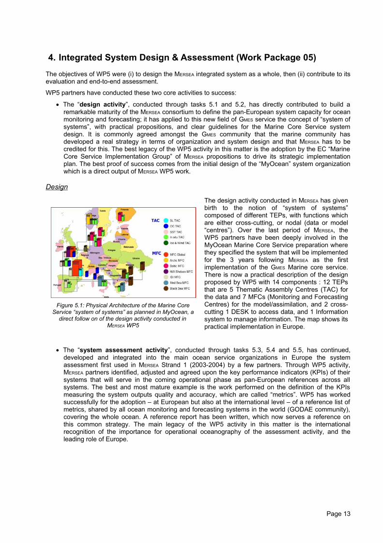
Figure 5.1: Physical Architecture of the Marine CoreService “system of systems” as planned in MyOcean, a

direct follow on of the design activity conducted in MERSEA WP5

The design activity conducted in MERSEA has givenbirth to the notion of “system of systems”composed of different TEPs, with functions whichare either cross-cutting, or nodal (data or model“centres”). Over the last period of MERSEA, theWP5 partners have been deeply involved in theMyOcean Marine Core Service preparation wherethey specified the system that will be implementedfor the 3 years following MERSEA as the firstimplementation of the GMES Marine core service.There is now a practical description of the designproposed by WP5 with 14 components : 12 TEPsthat are 5 Thematic Assembly Centres (TAC) forthe data and 7 MFCs (Monitoring and ForecastingCentres) for the model/assimilation, and 2 cross-cutting 1 DESK to access data, and 1 Informationsystem to manage information. The map shows itspractical implementation in Europe.

• The “system assessment activity”, conducted through tasks 5.3, 5.4 and 5.5, has continued,developed and integrated into the main ocean service organizations in Europe the systemassessment first used in MERSEA Strand 1 (2003-2004) by a few partners. Through WP5 activity,MERSEA partners identified, adjusted and agreed upon the key performance indicators (KPIs) of theirsystems that will serve in the coming operational phase as pan-European references across allsystems. The best and most mature example is the work performed on the definition of the KPIsmeasuring the system outputs quality and accuracy, which are called “metrics”. WP5 has workedsuccessfully for the adoption – at European but also at the international level – of a reference list ofmetrics, shared by all ocean monitoring and forecasting systems in the world (GODAE community),covering the whole ocean. A reference report has been written, which now serves a reference onthis common strategy. The main legacy of the WP5 activity in this matter is the internationalrecognition of the importance for operational oceanography of the assessment activity, and theleading role of Europe.

Page 13

Indicators

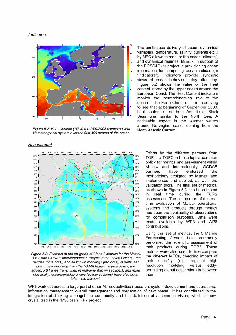
Figure 5.2: Heat Content (109 J) the 2/09/2008 computed withMercator global system over the first 300 meters of the ocean.

The continuous delivery of ocean dynamicalvariables (temperature, salinity, currents etc..)by MFC allows to monitor the ocean “climate”,and dynamical regimes. MERSEA, in support ofthe BOSS4GMES project is provisioning oceaninformation for computing ocean indices (or“indicators”). Indicators provide syntheticviews of ocean behaviour, day after day.Figure 5.2 shows the value of the heatcontent stored by the upper ocean around theEuropean Coast. The Heat Content indicatorsmonitor the thermodynamical role of theocean in the Earth Climate… It is interestingto see that at beginning of September 2008,heat content of northern Adriatic or BlackSeas was similar to the North Sea. Anoticeable aspect is the warmer watersaround Norvegian coast, coming from theNorth Atlantic Current.

Assessment

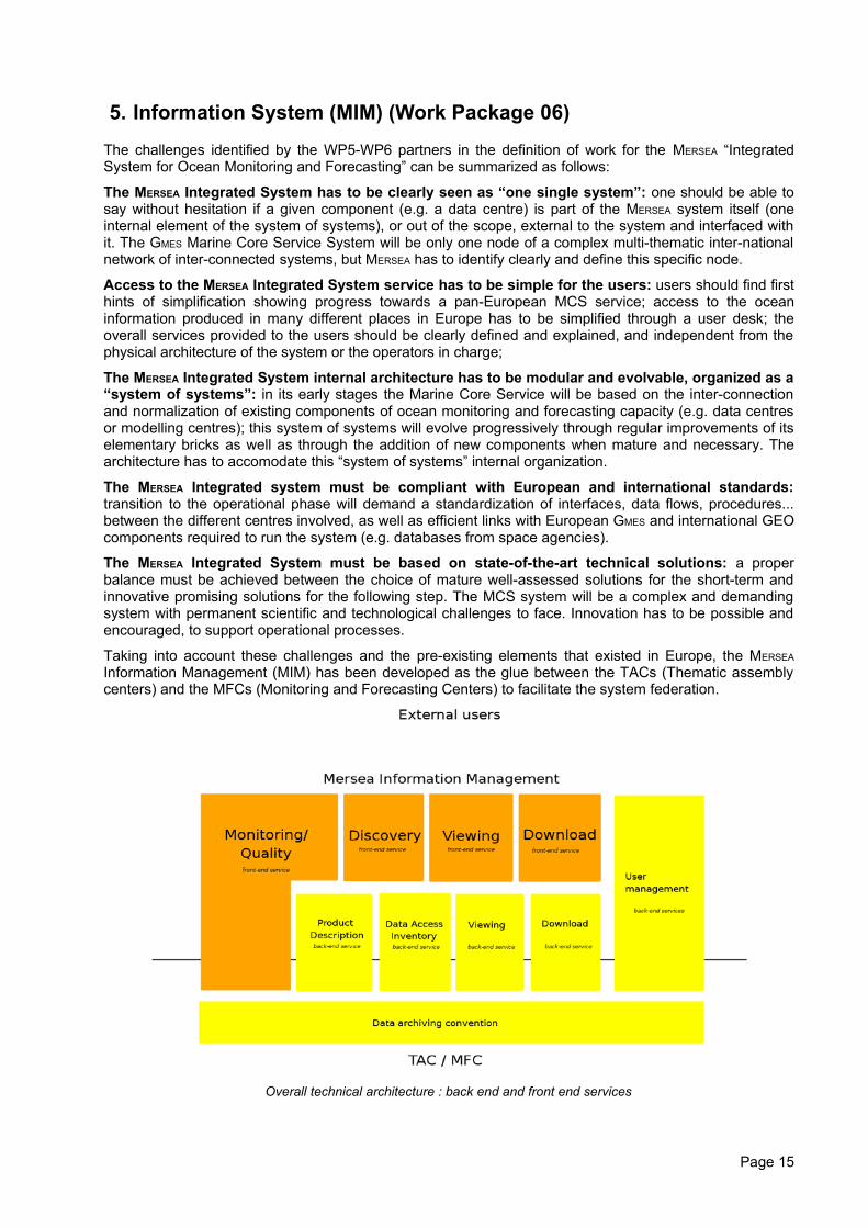
Figure 5.3: Example of the up-grade of Class 2 metrics for the MERSEA

TOP2 and GODAE Intercomparison Project in the Indian Ocean. Tidegauges (blue dots), and all known moorings (red dots), in particular

brand new moorings from the RAMA Indian Tropical Array, areadded. XBT lines transmitted in real-time (brown sections), and moreclassically, oceanographic arrays (yellow sections) have also been

taken into account.

Efforts by the different partners fromTOP1 to TOP2 led to adopt a commonpolicy for metrics and assessment withinMERSEA and internationally. GODAEpartners have endorsed themethodology designed by MERSEA, andimplemented and applied, as well, thevalidation tools. The final set of metrics,as shown in Figure 5.3 has been testedin real time during the TOP2assessment. The counterpart of this realtime evaluation of MERSEA operationalsystems and products through metricshas been the availability of observationsfor comparison purposes. Data weremade available by WP3 and WP6contributions.

Using this set of metrics, the 5 MarineForecasting Centers have commonlyperformed the scientific assessment oftheir products during TOP2. Thesemetrics were also used to intercomparethe different MFCs, checking impact oftheir specifity (e.g. regional highresolution modeling versus eddy-permitting global description) in betweenthem.

WP5 work cut across a large part of other MERSEA activities (research, system development and operations,information management, overall management and preparation of next phase). It has contributed to theintegration of thinking amongst the community and the definition of a common vision, which is nowcrystallized in the “MyOcean” FP7 project.

Page 14

5. Information System (MIM) (Work Package 06)

The challenges identified by the WP5-WP6 partners in the definition of work for the MERSEA “IntegratedSystem for Ocean Monitoring and Forecasting” can be summarized as follows:

The MERSEA Integrated System has to be clearly seen as “one single system”: one should be able tosay without hesitation if a given component (e.g. a data centre) is part of the MERSEA system itself (oneinternal element of the system of systems), or out of the scope, external to the system and interfaced withit. The GMES Marine Core Service System will be only one node of a complex multi-thematic inter-nationalnetwork of inter-connected systems, but MERSEA has to identify clearly and define this specific node.

Access to the MERSEA Integrated System service has to be simple for the users: users should find firsthints of simplification showing progress towards a pan-European MCS service; access to the oceaninformation produced in many different places in Europe has to be simplified through a user desk; theoverall services provided to the users should be clearly defined and explained, and independent from thephysical architecture of the system or the operators in charge;

The MERSEA Integrated System internal architecture has to be modular and evolvable, organized as a“system of systems”: in its early stages the Marine Core Service will be based on the inter-connectionand normalization of existing components of ocean monitoring and forecasting capacity (e.g. data centresor modelling centres); this system of systems will evolve progressively through regular improvements of itselementary bricks as well as through the addition of new components when mature and necessary. Thearchitecture has to accomodate this “system of systems” internal organization.

The MERSEA Integrated system must be compliant with European and international standards:transition to the operational phase will demand a standardization of interfaces, data flows, procedures...between the different centres involved, as well as efficient links with European GMES and international GEOcomponents required to run the system (e.g. databases from space agencies).

The MERSEA Integrated System must be based on state-of-the-art technical solutions: a properbalance must be achieved between the choice of mature well-assessed solutions for the short-term andinnovative promising solutions for the following step. The MCS system will be a complex and demandingsystem with permanent scientific and technological challenges to face. Innovation has to be possible andencouraged, to support operational processes.

Taking into account these challenges and the pre-existing elements that existed in Europe, the MERSEA

Information Management (MIM) has been developed as the glue between the TACs (Thematic assemblycenters) and the MFCs (Monitoring and Forecasting Centers) to facilitate the system federation.

Overall technical architecture : back end and front end services

Page 15

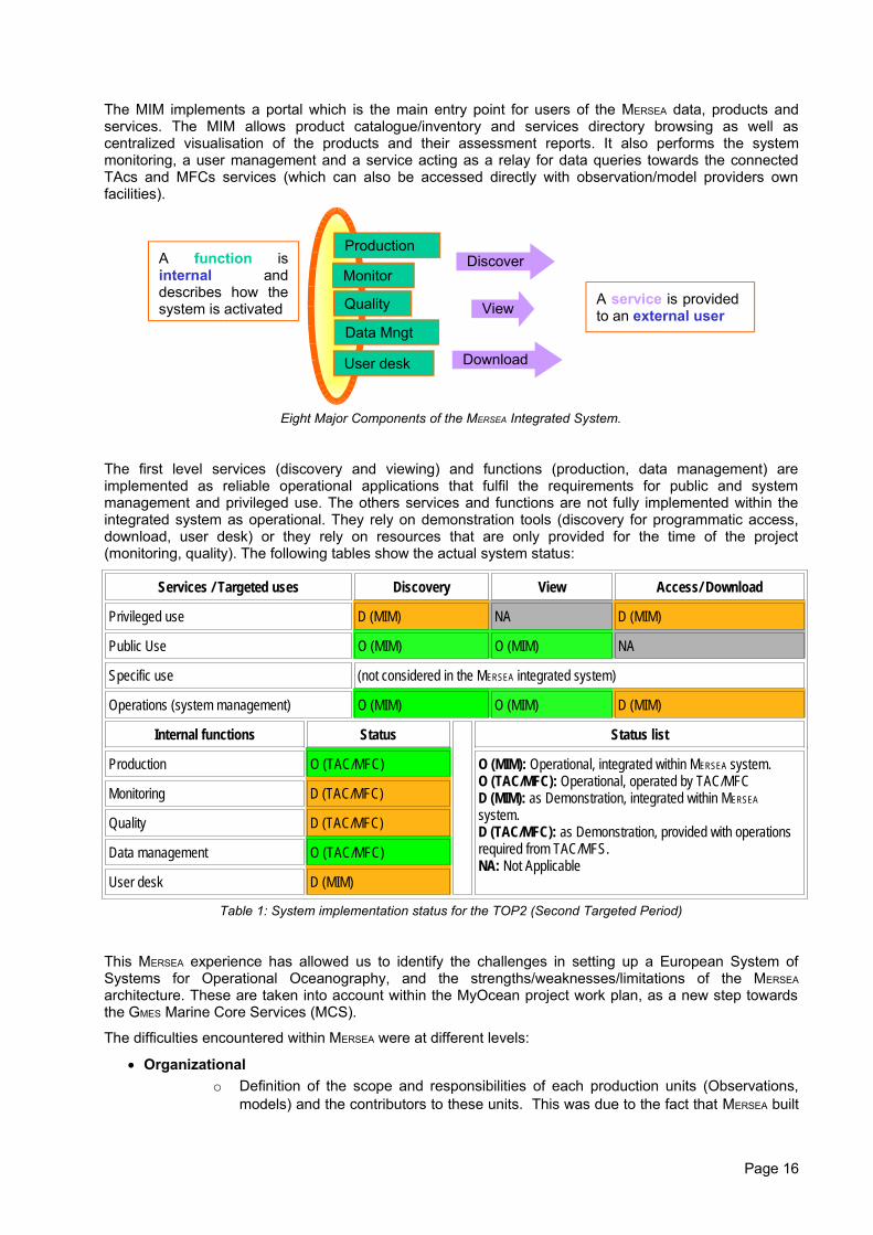
The MIM implements a portal which is the main entry point for users of the MERSEA data, products andservices. The MIM allows product catalogue/inventory and services directory browsing as well ascentralized visualisation of the products and their assessment reports. It also performs the systemmonitoring, a user management and a service acting as a relay for data queries towards the connectedTAcs and MFCs services (which can also be accessed directly with observation/model providers ownfacilities).

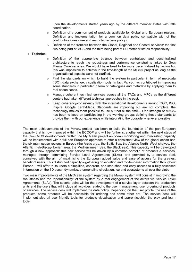
Eight Major Components of the MERSEA Integrated System.

The first level services (discovery and viewing) and functions (production, data management) areimplemented as reliable operational applications that fulfil the requirements for public and systemmanagement and privileged use. The others services and functions are not fully implemented within theintegrated system as operational. They rely on demonstration tools (discovery for programmatic access,download, user desk) or they rely on resources that are only provided for the time of the project(monitoring, quality). The following tables show the actual system status:

Services / Targeted uses Discovery View Access/ Download

Privileged use D (MIM) NA D (MIM)

Public Use O (MIM) O (MIM) NA

Specific use (not considered in the MERSEA integrated system)

Operations (system management) O (MIM) O (MIM) D (MIM)

Internal functions Status Status list

Production O (TAC/MFC) O (MIM): Operational, integrated within MERSEA system.O (TAC/MFC): Operational, operated by TAC/MFCD (MIM): as Demonstration, integrated within MERSEA

system.D (TAC/MFC): as Demonstration, provided with operationsrequired from TAC/MFS.NA: Not Applicable

Monitoring D (TAC/MFC)

Quality D (TAC/MFC)

Data management O (TAC/MFC)

User desk D (MIM)

Table 1: System implementation status for the TOP2 (Second Targeted Period)

This MERSEA experience has allowed us to identify the challenges in setting up a European System ofSystems for Operational Oceanography, and the strengths/weaknesses/limitations of the MERSEA

architecture. These are taken into account within the MyOcean project work plan, as a new step towardsthe GMES Marine Core Services (MCS).

The difficulties encountered within MERSEA were at different levels:

• Organizationalo Definition of the scope and responsibilities of each production units (Observations,

models) and the contributors to these units. This was due to the fact that MERSEA built

Page 16

DiscoverProduction

View

Download

Monitor

Quality

Data Mngt

User desk

A function is internal and describes how the system is activated

A service is provided to an external user

upon the developments started years ago by the different member states with littlecoordination.

o Definition of a common set of products available for Global and European regions.Definition and implementation for a common data policy compatible with of thecontributors ones (free and restricted access policy).

o Definition of the frontiers between the Global, Regional and Coastal services: the firsttwo being part of MCS and the third being part of EU member states responsibility.

• Technicalo Definition of the appropriate balance between centralized and decentralized

architecture to reach the robustness and performance constraints linked to GMES

Marine Core services. We would have liked to be more decentralized by region butthis was impossible to achieve in the time-length of the MERSEA project as long as theorganizational aspects were not clarified.

o Find the standards on which to build the system in particular in term of metadata(ISO), data exchange, visualization tools. In fact MERSEA has contributed in improvingsome standards in particular in term of catalogues and metadata by applying them toreal ocean cases.

o Manage coherent technical services across all the TACs and MFCs as the differentcenters had taken different technical approaches in the past.

o Keep coherency/consistency with the international developments around OGC, ISO,Inspire, Google Earth/Maps. Standards are improving but are not complete, thetechnology makes them possible to use but not all the time… One strength of MERSEA

has been to keep on participating in the working groups defining these standards toprovide them with our experience while integrating the upgrade whenever possible

The main achievements of the MERSEA project has been to build the foundation of the pan-Europeancapacity that is now improved within the ECOOP and will be further strengthened within the next steps ofthe GMES MCS developments. Within the MyOcean project an ocean monitoring and forecasting capacitywill be implemented with a full pan-European approach to offer a consistent view of the global ocean andthe six main ocean regions in Europe (the Arctic area, the Baltic Sea, the Atlantic North- West-shelves, theAtlantic Irish-Biscay-Iberian area, the Mediterranean Sea, the Black sea). This capacity will be developedthrough a new approach: this new service will be driven by a common portfolio of products & services,managed through committing Service Level Agreements (SLAs), and provided by a service deskconceived with the aim of maximising the European added value and ease of access for the greatestbenefit of users. This distributed capacity – gathering observation and model-based information throughoutEurope – will offer to its users a simplified, coherent, one-stop-shop and easy access to a fully assessedinformation on the 3D ocean dynamics, thermohaline circulation, ice and ecosystems all over the globe.

Two main improvements of the MyOcean system regarding the MERSEA system will consist in improving therobustness and the "operationality" of the system by a real engagement of the actors via Service LevelAgreements (SLAs). The second point will be the development of a service layer between the productionunits and the users that will include all activities related to the user management, user ordering of productsor services. The service desk will implement the data policy. Depending on the user profile, the use of theproducts, some products will be accessible for ordering and some other not. The service desk willimplement also all user-friendly tools for products visualisation and apprenticeship: the play and learntools.

Page 17

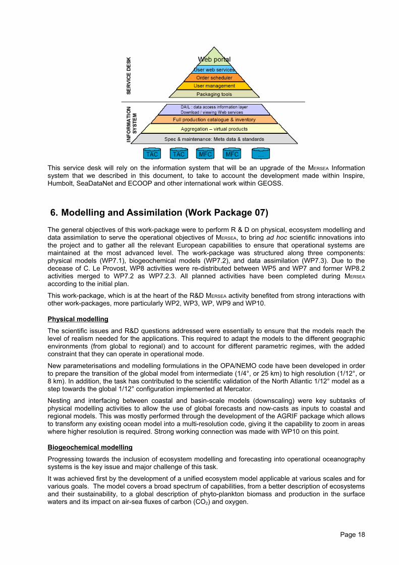
This service desk will rely on the information system that will be an upgrade of the MERSEA Informationsystem that we described in this document, to take to account the development made within Inspire,Humbolt, SeaDataNet and ECOOP and other international work within GEOSS.

6. Modelling and Assimilation (Work Package 07)

The general objectives of this work-package were to perform R & D on physical, ecosystem modelling anddata assimilation to serve the operational objectives of MERSEA, to bring ad hoc scientific innovations intothe project and to gather all the relevant European capabilities to ensure that operational systems aremaintained at the most advanced level. The work-package was structured along three components:physical models (WP7.1), biogeochemical models (WP7.2), and data assimilation (WP7.3). Due to thedecease of C. Le Provost, WP8 activities were re-distributed between WP5 and WP7 and former WP8.2activities merged to WP7.2 as WP7.2.3. All planned activities have been completed during MERSEA

according to the initial plan.

This work-package, which is at the heart of the R&D MERSEA activity benefited from strong interactions withother work-packages, more particularly WP2, WP3, WP, WP9 and WP10.

Physical modelling

The scientific issues and R&D questions addressed were essentially to ensure that the models reach thelevel of realism needed for the applications. This required to adapt the models to the different geographicenvironments (from global to regional) and to account for different parametric regimes, with the addedconstraint that they can operate in operational mode.

New parameterisations and modelling formulations in the OPA/NEMO code have been developed in orderto prepare the transition of the global model from intermediate (1/4°, or 25 km) to high resolution (1/12°, or8 km). In addition, the task has contributed to the scientific validation of the North Atlantic 1/12° model as astep towards the global 1/12° configuration implemented at Mercator.

Nesting and interfacing between coastal and basin-scale models (downscaling) were key subtasks ofphysical modelling activities to allow the use of global forecasts and now-casts as inputs to coastal andregional models. This was mostly performed through the development of the AGRIF package which allowsto transform any existing ocean model into a multi-resolution code, giving it the capability to zoom in areaswhere higher resolution is required. Strong working connection was made with WP10 on this point.

Biogeochemical modelling

Progressing towards the inclusion of ecosystem modelling and forecasting into operational oceanographysystems is the key issue and major challenge of this task.

It was achieved first by the development of a unified ecosystem model applicable at various scales and forvarious goals. The model covers a broad spectrum of capabilities, from a better description of ecosystemsand their sustainability, to a global description of phyto-plankton biomass and production in the surfacewaters and its impact on air-sea fluxes of carbon (CO2) and oxygen.

Page 18

In parallel, a prototype of a coupled physical/biological assimilative system has been built in order todemonstrate the capacity to routinely estimate and forecast biogeochemical variables. A primary result isthat the assimilation of physical data can improve the description of the physical environment that forcesthe ecosystem. This was demonstrated through the use of the SEEK filter to assimilate physical data(surface temperature, sea height, etc…) into a North Atlantic configuration of the OPA/NEMO codecoupled with a standard ecosystem model (NPZD type).

Scientific validation and assessment is a necessary component to judge the strengths and weaknesses ofthe different components of the MERSEA system and to control the quality of the outputs. Progress has beenmade in these directions to help identify the key observational data for assessment and the definition of aninternal metrics for physico-biogeochemical integrated system. This was successfully used to assess thenew bio-geochemical model in construction and to fit some of its parameterizations.

Data assimilation

This task contributes to the MERSEA forecasting system by improving the existing assimilation tools. Specificdevelopments have been made to address new methodological issues relevant for global forecastingsystems such as the assimilation of ice parameters or biogeochemical properties in coupledcirculation/ecosystem models. The issue was more particularly to propose advanced assimilation schemes(the so-called SIRF and EnKF filters), which can more rigorously tackle the complex statistical nature ofocean forecasting problems (non-gaussian error statistics, biased estimations, non-linear processes).

The SEEK filter assimilation component of the global MERSEA system has been upgraded to enable the useof all data available from space and field missions in the global OPA/NEMO forecasting system: surfacetemperature and salinity, altimetry, in situ profiles. Another crucial issue for modelling is the relevance ofthe forcing fields. Significant advances have been made on this point by including the control of forcingfunctions into the assimilation process thus allowing to correct/compensate for errors inevaporation/precipitation and heat forcing fluxes.

7. Implementation & Production (Work Package 09)

One of the main aims of MERSEA has been to monitor the physical properties (the temperatures, salinitiesand currents) in the global ocean and the seas surrounding Europe in real-time, on a regular, daily orweekly, basis and to forecast how these physical properties will change in the coming week or two.

This has been done in WP9 using computer models which represent an ocean by the values of its physicalproperties on a three-dimensional grid bounded by the ocean’s bathymetry. The models are steppedforward in time using equations based on computational fluid dynamics and thermodynamics together withwind forcing and heat exchange across the ocean’s surface taken from numerical weather forecasts. Inorder to hold the model’s values as close as possible to those of the real ocean, the ocean model’s valuesalso need to be adjusted using any measurements of the physical properties of the ocean that can beobtained.

It was agreed before the start of the project that monitoring and forecasting would be performed by fiveproduction centres each concentrating on a specific region, namely:

i. the global oceanii. the Arctic oceaniii. the Baltic Seaiv. the Mediterranean Sea andv. the North-east Atlantic

Work-package 9 was divided into three tasks:

1. to make developments to the “NEMO” ocean model code, to enable it to be used by the centresmonitoring and forecasting the global ocean, Mediterranean Sea and north-east Atlantic,

2. to implement and validate specific improvements to each of the forecasting systems in the fiveproduction centres,

Page 19

3. to routinely monitor and make 5-10 day forecasts for each of the five regions, making updates tothe analyses and forecasts either daily or weekly.

The first task was part of a wider initiative to form a consortium dedicated to supporting a European, state-of-the-art, ocean modelling system for research and operational use. This modelling system is nowsupported by a large group of research scientists within France, Germany, and the UK. It is also used forroutine production in the global, Mediterranean and north-east Atlantic regions and will be used in anumber of European seasonal, decadal and climate prediction systems. This initiative will have significantbenefits in the coordination, efficiency and effectiveness of research and operational application of oceanmodelling within Europe. MERSEA provided significant support for this initiative (within WP7 and WP9) at akey stage in its development.

The specific developments made in the first task were to adapt the NEMO code to make it suitable for usein the shallow waters of the continental shelves of Europe and to develop code to support the nesting ofthe regional models within the global ocean.

An ambitious timetable for the development of three new versions of the systems used by the productioncentres was agreed before the start of the project. Almost all of the planned developments have beenachieved within the work-package’s second task. The most significant achievements include:

a) the transition of the Arctic production system to the Norwegian weather forecast service, met.no.In future the system will be developed by the Nansen research institute (NERSC) and operated byan operational service (met.no);

b) several centres have improved their use of measurements to hold the models close to the realocean. For example, the global ocean system now uses in situ profile data as well as surfacedata; the Mediterranean system has developed a new scheme for using measurements; the Arcticsystem uses sea-ice drift data from satellites; the north-east Atlantic system uses much improvedsurface temperature and sea-ice concentration data; and the Baltic system has started to makeuse of measurement data.

c) most of the centres have increased the resolution of the grid they use to represent the oceansignificantly between the start and end of the project. The grid spacing of the global ocean is now1/4o in routine operations and 1/12o in some delayed mode simulations

d) the Mediterranean system now updates its forecasts on a daily basise) all of the systems have made substantial improvements to the formulation of the model they use.

The north-east Atlantic centre has transitioned to NEMO from an entirely different ocean model;f) all of the production centres have made assessments of the performance of models representing

nutrients, phytoplankton and zooplankton with various levels of complexity. The north-east Atlanticcentre has developed a scheme for making use of ocean colour data from satellites to constrainone of the less complex of these models.

The third task involved the routine production of analyses and forecasts that were made available each dayor week through the MERSEA Information System (WP6). It also included support to WP5 in the assessmentof their quality and accuracy, particularly during the two Targeted Operational Periods (TOPs). Animportant achievement was the agreement and demonstration of a method to generate statistics on thedifferences between measurement and model values which are sufficiently well controlled that the resultsgenerated from different production centres can be compared.

The main reports delivered by this work-package provide useful summaries of the scientific and technicalcontent of each version of the production systems and the work performed each year to improve them.

Whilst much was achieved within this work-package, most of the groups were very hard pressed to meetthe demands of the original work-plan. In addition they were expected or obliged to respond to otherdemands that were inexplicit or unforeseen in the original plan. In an attempt to keep up with demands,four work-package meetings were held in the last two years of the project. These provided a very valuableforum for sharing of expertise and ideas and the development of constructive working relationships. Taskswhich would have benefited from more time or resources include: making fuller use of new productsdeveloped from satellite or in situ measurements; participating in and taking advantage from the validationactivities of the two Targeted Operational Periods (TOPs); coordination and exploration of the nesting ofthe regional models within the global one; and supporting the special experiment or demonstrationactivities.

Page 20

8. Downscaling to Regional Systems (Work Package 10)

An integral part of the project was to extend the modelling, monitoring and forecasting capacity to improvethe operational oceanographic services of the European Regional Seas, since these seas are of greateconomically importance to the European society and they are subject to a number of internationalagreements and conventions. These conventions do in particular call for safety at sea, effectivemanagement of marine environment and sustainable utilisation of its resources; living up to the spirit ofthese agreements requires the ability to rapidly detect changes in the status of the marine systems andliving resources and to provide forecasts of such changes so actions can be taken in a timely manner forthe public good.

European coastal nations have for decades operated marine monitoring programs and a operationalforecasting capacity had started to grow in several of the European Regional Seas – much of the progressin this field was initiated and coordinated within the EuroGOOS regional task teams. The objective withinMERSEA was therefore to further develop the European capacity for regional ocean monitoring andforecasting. Tasks related to this activity have been closely linked to, and coordinated with, the WP9(Implementation and Production).

The specific objectives for WP 10 were:

• Secure that benefits of a global operational oceanographic system are properly utilised in forecastingactivities in European regional seas.

• Assess the value of dynamic boundary data for regional forecasts• Implement data assimilation methodologies for regional seas and test their impact• Verify improved quality of high resolution operational oceanographic products for regional seas

An immediate challenge in regional forecasting activities often is the open boundaries towards the ocean inregional models. Traditionally most operational 3D-ocean regional models use climatology lateral boundaryconditions in temperature and salinity, plus a water level consisting of tides and surges. MERSEA WP 10therefore focused on increasing the performance and quality of regional and coastal operationaloceanographic services by downscaling the global fields to regional scale. An additionally activity was toset up within each regional forecasting system to a facility to quickly establish a two-way nested highresolution area to address special emergency situations. This work was based on the French AGRIFsoftware module.

Assimilation of observational data – remotely sensed as well as in-situ data – is another factor thatpotentially can improve the quality of ocean forecasts in the regional seas of Europe. Over the past decadethe availability of real time observational data in the regional seas has increased, although more areneeded, which has formed the basis for working intensively with developing and implementing dataassimilation techniques for the regional forecasting models.

In order to do operational data assimilation and also to verify the quality of the operational forecastproducts observational data is needed. WP10 therefore had a task to collect within each region all relevantobservational data both in situ data ( water level, T/S-profiles from bouy’s, gliders, ships and instrumentsmounted on seals, surface data from ferrybox and XBT) and remotely sensed data (SST, sea ice). Thedata are stored and available in regional data centres.

During the project all the regional forecasting models have been upgraded substantially. The majorcomponents have been to introduce:

• increased horizontal and vertical resolution• better turbulence mixing schemes• dynamic boundary conditions from the MERSEA Global model• Data assimilation

The quality improvements of regional operational forecasting systems were tested during the TOP 2experiment and verified in the report from this experiment. It was demonstrated that substantialimprovements of the regional forecasting systems have been achieved during the project, but it alsoillustrates that there still are many problems to address. For instance the use of dynamic boundary datafrom the global model has proven to be not straightforward and still needs further attention and

Page 21

development. Data assimilation in the regional seas has taken a big step forward but also here there arestill problems to solve - both model technical problems as well as the availability of operational in situobservations is problematic – there has always been a lack of observations in the seas but recent yearbudget reductions have had a negative effect on the relatively expensive monitoring programmes.

Generally the WP10 has reached its goals and the achievements obtained form an excellent platform forthe work that is now carried out within the EU funded project ECOOP, which focuses on the Europeanregional and coastal seas, as well as the upcoming MyOcean project.

9. Special focus experiments & applications (Work Package 11)

The Special Focus Experiments of MERSEA are devoted to the development of the coupling between themodel system and the basic and generic model products of MERSEA with:

1. marine biogeochemical models for ecosystem forecasting, at the level of primaryproducers biomass and for the short time scales;

2. global atmospheric models for seasonal forecasting.

The two different coupling developments are called ‘experiments’ and they are referred to as SF1 and SF2respectively. We will synthesise the final results of each of them separately.

SF1 results

The SF1 is carried out in two European regional Seas, the North Eastern Atlantic margin and theMediterranean Sea. These two regional seas have been developing capacity in the past ten years forecosystem modelling and the results of this work package showed the successful implementation of a fullyoperational chain for ecosystem forecasting in both areas.

This experiment also contains major research results that are related to specific model ameliorations andnew tool developments to account for missing processes, data assimilation, coupling with thehydrodynamics and comparison with observations.

SF1: The Eastern Atlantic margin area

For the Eastern Atlantic margin, comprising the North Sea and the English Channel, a part of the researchconcentrated in the development of the nesting of two hydrodynamics models: 1) an Atlantic Margin Model(AMM, ~12km resolution) into a global MERSEA model and 2) a ~7 km resolution model (Medium-ResolutionContinental Shelf-MRCS) in the western English channel into the AMM.

The AMM and MRCS hydrodynamics models were coupled with an updated version of the ERSEM model,a biomass and functional group numerical model of the pelagic and benthic marine food webs. Thebiogeochemical model was further developed in this experiment by studying the benthic-pelagic couplingwith sediment re-suspension and nutrients re-generation in the fluff layer.

Data assimilation was then implemented in the MRCS model with an Ensemble Kalman Filter (EnKF)scheme for different kind of data sets: satellite SST and Chlorophyll products and Ferry Box data. Theinitial results for the English Channel showed that the assimilation of surface biochemical data improvesthe forecast or simulation skill. The results seem to indicate that the full ecosystem state vector should beconsidered and that perturbation methods should consider more state variables.

Last but not least, the AMM model, coupled to the biogeochemical one, was implemented operationally atthe UK Meteorological Office where it has been running in an operational mode for almost a year. Theassessment of the ecosystem model forecast skill is as follows:

• The skill deteriorates from physics to complex biology: i.e. SST skill > NO3 skill > Chlorophyll skill;• The model has high skill levels for simulating SST at all timescales;• The model has no predictive skill for chlorophyll at daily timescales but skill substantially improves at

monthly / seasonal timescales. Model skill deteriorates during bloom periods• Pattern Correlation Analysis shows that models can capture the nutrients and chlorophyll major

modes of variability at a seasonal timescale.

Page 22

• Comparison with continuous plankton recorder data shows that the models can capture thequalitative aspects of biological seasonal cycles for phytoplankton and zooplankton.

SF1: The Mediterranean Sea

The experiment in the Mediterranean Sea developed, implemented and tested an innovative networkcomputational modelling and forecasting system that is now maintained alive and operational by thepartners. The modelling system couples in an off-line mode the hydrodynamics forecasting model of theMediterranean Sea with a complex biogeochemical flux (BFM) model, calibrated for the MediterraneanSea. The project developed a model coupler, called the OPA Tracer Model (OPATM) that takes thephysical forcing fields from the hydrodynamics, interpolates them in the BFM grid and adds thebiogeochemical reaction terms, integrating in time the system and producing the forecast. The OPATM-BFM code has been optimized for parallel machines and several numerical issues have been solved todecrease intrinsic numerical diffusion of the schemes.

The biogeochemical part of the model has been validated with historical in situ and satellite data and anumber of simulation experiments have been carried out, determining an “optimal” OPATM-BFMparameter configuration, which forms the basis of the biogeochemical forecasting model system of theMediterranean Sea. This calibration exercise was aimed at the reproduction of the large scale gradients inthe biogeochemical state variables and their seasonal variability using average physical forcing (so-calledperpetual year forcing).

The MERSEA V1 hydrodynamics system for the Mediterranean Sea produces once a week, 7 past analysesand a 10 days forecast. The OPATM-BFM code is coupled to these fields once a week and produces a 7days simulation forced by the analyses and a 10 days forecast forced by the 10 days forecast of thehydrodynamics. This pre-operational system is completely automatic, providing every week 7 dayssimulations and a 10 days forecast of biogeochemical variables over the Mediterranean basin. The mainobjective of the Targeted Operational Period (six months of forecast period) was therefore fully achieved.The forecasting system skill has been evaluated by comparing the surface chlorophyll maps produced bythe model and the MODIS observations for the period under investigation.

The OPATM-BFM model has been validated also with a multi-year simulation from 1998 to 2004 in order tounderstand the skill of the model at inter-annual time scales. The nutrients and chlorophyll valuesproduced by the long term simulation have been compared with available data. After the initial spin-upphase the nutrient pool behaviour is found to be composed of two temporal functions super-imposed: thefirst is seasonal frequency fluctuation and the second is a linear loss trend associated to the Gibraltar Straitoutflow. Comparison between model results and data shows a good agreement for the nitrates andphosphates, even if there is overestimation of phosphates concentration in the Alboran and LevantineSeas. These simulations demonstrate that the model has skill in reproducing the year to year variability inchlorophyll and nutrient pools.

SF2 results

This experiment involved three seasonal forecasting teams across Europe (ECMWF, Meteo-France andINGV) building capacity to use the MERSEA high resolution global model outputs to increase the seasonalforecasting skill, with particular attention to El Nino seasonal forecasts, European weather extremes andmedium-range weather forecast (monthly time scale).

The team developed several ocean-atmosphere coupled models formed by low and high resolution oceanand low and high resolution atmosphere components. The new model developments considered the set upof interpolation algorithms for the MERSEA ¼ global ocean products into the lower resolution coupled oceanmodels grids and the coupling of the MERSEA V1 global model version (¼ degrees model) with threedifferent atmospheric models. The new coupled models developed during the project are:

1) at INGV, OPA8.2 version of the Mersea ¼ model has been coupled to ECHAM4.6 (in the newatmospheric model configuration CMCC-SXF025).

2) at Météo-France, a new coupled model consists of the atmospheric model "ARPEGE-Climat", anew version of the coupler "OASIS v3" together with the NEMO version of the ¼ Mersea oceanmodel.

3) at ECMWF, the Integrated Forecast System (IFS) has been coupled to NEMO version of theMersea ¼ model.

Page 23

First the sensitivity of different seasonal forecasting coupled models to the MERSEA ¼ analyses initializationwas assessed by ECMWF and Méteo-France. The seasonal forecasts concentrated on the skill index ofsea surface temperature anomalies in the El Nino region. Results indicate that the low resolution coupledmodels do not improve the correlation when initialized with MERSEA ¼ analyses and the high resolutioncoupled model improves only marginally. Interpolated initial conditions adjustments are probablyresponsible for this puzzling result.

The second major result of the SF2 experiment is the inter-comparison between low and high resolutioncoupled models seasonal forecasting skills. The high resolution realisations all used both the MERSEA ¼analyses and the MERSEA global model in different versions. The seasonal forecasting experimentsconducted with both low and high resolution models capture the growing phase of ENSO and part of theprecipitation anomalies over Europe but the impact of the high resolution is not very large. There is noclear evidence of improved forecast skill when coupled model resolution increases both for the El Ninoregions and Europe.

The third major result is coming from the very high resolution coupled model forecast system developed formedium-range weather forecasts at ECMWF. The coupled model used for the Medium-Range forecastexperiments consists of two main configurations, which differ from each other in the resolution of theatmospheric model. Both use the IFS atmospheric general circulation model. The resolutions are T399 (ca50 km horizontal resolution), 62 vertical levels, for the Ensemble Prediction System (EPS) integrations andT799 (ca 25 km horizontal resolution), 91 vertical levels, for the deterministic integrations. The oceangeneral circulation model is OPA/NEMO (1/4° horizontal resolution, with 50 vertical levels).

Such a coupled model system has been tested on two tropical cyclone case studies. Encouragingly, thecoupled model shows a physically reasonable behaviour in the evolution of the global sea surfacetemperature (SST). The two tropical cyclones themselves are nicely reproduced by the coupled model.However, despite the well simulated SSTs, differences with analogous uncoupled integrations for whichSST is held fixed throughout the integrations are generally not striking, at least in terms of minimumpressure and winds. It has been argued that a possible explanation is that the atmospheric model hasbeen tuned to function with fixed SST and therefore the coupling with varying SST may not be as strong asit ought to be. Indeed, no specific tuning of the coupling has been attempted.

Now that such a coupled model has been implemented it could be used for similar case studies, Atlantichurricanes for example.

10. User Products (Work Package 12)

An important component of the MERSEA Project has been the demonstration of benefits of MERSEA outputs inproduction of specific user products.

There are many and diverse downstream applications which can be built on Marine Core Servicesprovided by a fully implemented and sustained operational ocean observing and forecasting system. Theobjective of Work Package 12 was to explore some of these in order to gain an appreciation of the benefitsthat the Marine Core Services will create once they are made fully operational though the MyOceanproject. The Work Package comprised a small number of user product demonstrations intended to showhow MERSEA outputs could enhance existing downstream services and underpin the development of entirelynew information products with practical utility.

A component of the Work Package has been interfacing the MERSEA outputs to specific tools todemonstrate end to end services in each application area. In operational applications these interfacesmust be very reliable. They must also be responsive to occasional failures or data delivery delays. Forexample, if a critical real-time data stream or model output is unavailable due to a production or deliveryproblem the interface should permit seamless transition to an alternative source or appropriate notificationof the end-user that the service may be temporarily degraded. This is especially important in safety criticalapplications. Experience gained in the MERSEA project has provided a better understanding of therequirements for reliability, redundancy and resilience in a fully operational Marine Core Service productionsystem. Lessons learnt have helped to inform plans for delivery of fully operational Marine Core Servicesthrough the MyOcean project and beyond.

Key development stages in the MERSEA project have been incremental, for example, the transition from onemodel system to another or assimilation of additional observations. The demonstration user products have

Page 24

enabled an understanding of the degree to which these incremental improvements translate into improvedbenefits for specific uses.

The Work Package demonstrations covered both public and private sector applications in the followingareas:

• The production of surface and through water column current nowcasts and forecasts tailored for useby the offshore oil and gas industry.

• The use of MERSEA outputs to enhance vessel routing services.• The use of MERSEA outputs to improve ice and iceberg forecasting for applications in shipping and

offshore development.• Determining the impact of MERSEA products in improved wave forecasting.• Demonstrating the degree to which MERSEA outputs can contribute to improved forecasts of oil spill

drift.

For each of these cases a Work Package Task developed applications which utilized MERSEA outputs tocreate new or improved services. In most cases these services were evaluated by users external to theMERSEA project. The engagement of real end-users in the demonstrations ensured realistic feedback onfitness for purpose of the downstream information products. Engagement with end-users also ensured thatthe developed products were closely tailored to their specific needs.

An important aspect of the work on demonstration applications has been the development of tools toevaluate the performance of MERSEA outputs in order to determine fitness for purpose. For example, toolsfor determining the skill of current forecasts used to support operational planning during offshore drilling ormethods to evaluate the contribution of MERSEA products to accurately predicting oil spill fate. Suchobjective performance metrics specific to particular uses are a critical component of successfuldownstream services. The Work Package identified this as an important area of future work.

In each of the demonstration cases, MERSEA outputs have been shown to yield positive benefits and theseare detailed in the individual Task reports.

MERSEA Work Package 12 has demonstrated that fully operational implementation of Marine Core Servicescan yield important safety, commercial and environmental protection benefits.

11. Overall Assessment (Work Package 13)

In workpackage 13 regular assessments and judgement of the performance of the evolving system andprogress of the MERSEA Integrated Project have been conducted. The work package was also tasked toactivate public outreach and promotion of the MERSEA concept as well initiation and participation ineducation and training activities with focus on operational oceanography.

Many of the partners participated also in a number of working group meetings on the GMES Marine CoreService Implementation Group, on Jason Follow-On altimetric mission options and contributed to the finalreport. Several meetings also took place with participation of WP 13 partners and representatives ofdifferent agencies (EEA, EMSA, DG ENV, DG Research) with the dual purpose of better understandingtheir needs in terms of environmental reporting and monitoring, and conversely to inform them of theMERSEA Project capabilities and future outlook. One MERSEA scientist also served as Chairman of a workinggroup on the Remote Sensing of Shelf Sea Ecosystems at the European Science Foundation, (ESF)Marine Board. This group was tasked with the challenges that needed to be tackled to facilitate theoperational use of satellite data in operational ecosystem models. Their report “Remote Sensing of ShelfSea Ecosystems; State of the Art and Perspective” was published by ESF Marine Board, in February 2008.During the last year of MERSEA the negotiation of the MyOcean proposal under the EC FP7 GMES Fast TrackServices have also required a lot of effort by MERSEA partners.

The executive summary of the workpackage achievement according to the three distinct tasks are providedin the flowing.

Page 25

1) Assessment of system performance and operational capacity (strengths, gaps, limitations) in relation tothe aim of GMES and documentation of advances and achievements since MERSEA Strand-1 assessment.

The first Target Operational Period (TOP1) was executed from October 2005 to April 2006 to perform thevalidation of both the data and information flow at the five MERSEA forecasting centres. The operationalsystems were run on a weekly basis with 10-day forecasts describing the space -time evolution of thephysical ocean, sea-ice and a few biogeochemical variables. The heritage of the MERSEA Strand-1 oceandiagnostics has been widely used, and in particular, both state variables of the systems and derived orintegrated quantities were consistently monitored. The products and information were disseminatedthrough the project web site according to the five Thematic Portals providing regular and systematicinformation on the state of the global oceans and regional European seas including the Arctic, the NorthEast Atlantic, the Baltic, and the Mediterranean.

During the second TOP2 from October 2007 to April 2008 the final system assessment and validation ofthe operation and inter-connection of the three data centre (e.g. satellite, in-situ and forcing) and the fiveforecasting centre (e.g. the Global, Arctic, North East Atlantic and Mediterranean) were undertaken. In sodoing the results of the gradual updates and transition from V1 to V2 with its improvement of model codes,model resolutions, nesting procedures and ecosystem model development was evaluated. In addition,assimilation of sea ice drift, mean dynamic topography and Argo profile data together with introduction ofnew error analyses and bias correction schemes were incorporated in V2. OpenDap with commonarchitecture and file format, analyses tools and exchange of diagnostic results, and visualization methodswere used to allow efficient procedures for discover, view and download.

The TOP2 system functionality assessment was also partly carried out based on Key PerformanceIndicators, including monitoring and assessment of user interests. For instance, the number of hits for theMediterranean Sea reached about 1900 per month. The corresponding number of hits for the entire MERSEA

reached about 38000 per month.

2) Provision of advanced technical and operational training and summer school courses for relevantpersonnel in the field of operational oceanography. Increase public awareness on key global and regionalocean environment issues.

Within this task one target was university training courses in operational oceanography. These are nowroutinely offered in several programmes, from the Geophysical Institute, University of Bergen, Norway tothe University of Aegean, Department of Marine Sciences in Athens, Greece. The experience from thesecourses reveals an increasing interest from students to make their semester reports or assignments andeventually thesis based on data and products available through open access servers, such as possiblewithin the MERSEA and many other servers offering in-situ, satellite and model data and informations.

Use of MERSEA IP material were also included in lectures provided by MERSEA partners at summer schoolsand intensive training courses hosted by ESA and the GODAE working group with the goal to motivateyoung scientists. One main outcome of the GODAE training course was the book titled “Ocean weatherforecasting: An integrated view of oceanography”, edited by Verron and Chassignet and published bySpringer 2006.

Awareness of the MERSEA IP was regularly raised at conferences and workshops. The Session onOperational Oceanography during the ICES annual scientific conference held in Maastricht (NL) 19-23September 2006 provided an excellent forum to review requirements and experience from fishery andecosystem scientists as well as policy-makers on the use of products from operational systems. A regionalworkshop for African oceanographers, subtitled “Remote sensing, a tool for ocean science and operationaloceanography”, was held in Rabat from September 19 to 30 2006, as the fifth in a series of Cosparcapacity building workshop. The workshop aimed to encourage and develop the use of ocean remotesensing and associated in-situ data by scientists from Africa.

The MERSEA project together with EEA (European Environmental Agency) also co-organized the workshopentitled "Connecting operational oceanography with the European Marine Strategy and EEA assessments"(Copenhagen on 23-24 October 2006). This workshop was held in the framework of EMMA (EuropeanMonitoring and Marine Assessment) with support from DG Environment of the European Commission. Itmarked the beginning of a cooperation with the EEA and with the Conventions mandated to report on thestate of the marine environment with the ultimate goal to improve marine monitoring and assessments inEurope through a wider and more systematic usage of operational oceanography products. The workshopconcluded that operational oceanography can give a strong contribution to the Physical featuresconsidered in the Marine Strategy Directive (MSD) “Initial assessment”, primarily for temperature, salinity

Page 26

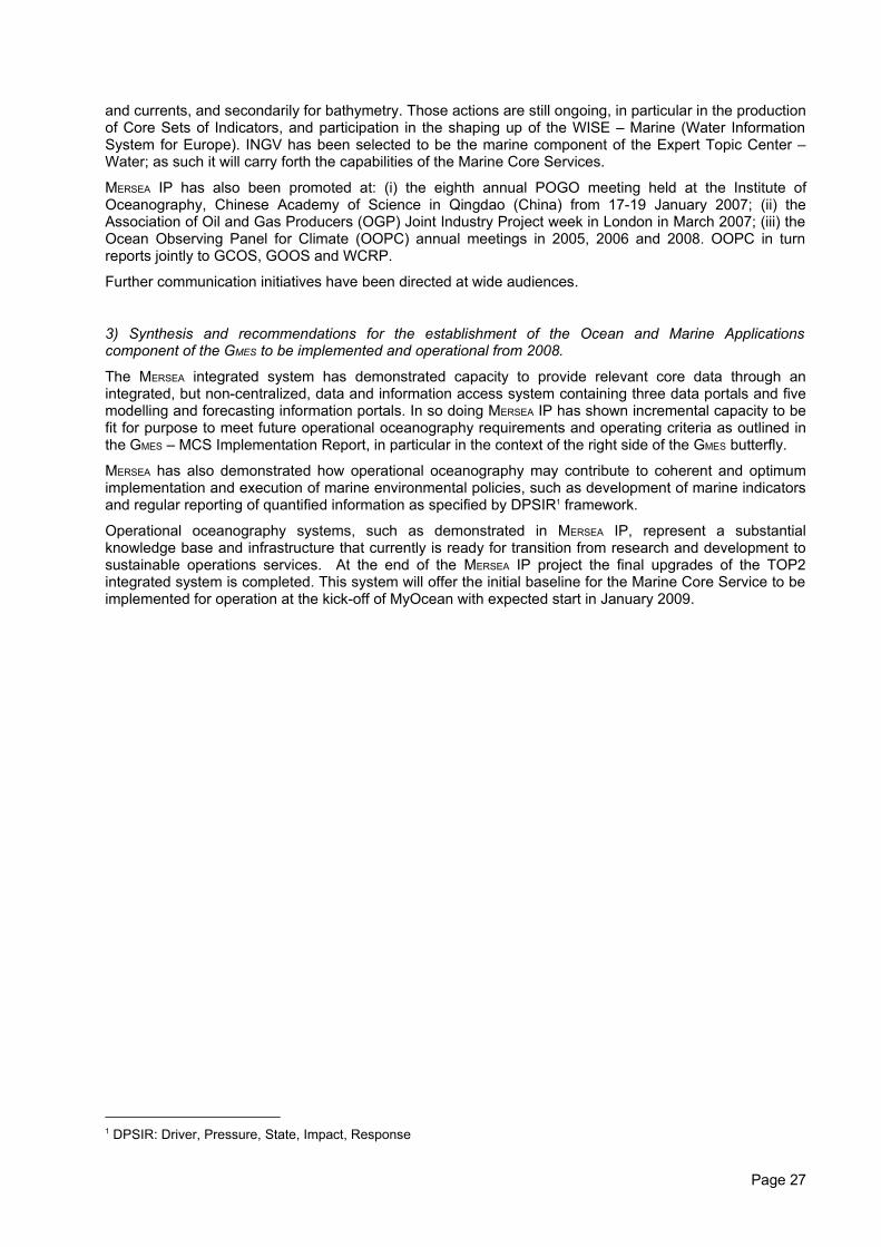
and currents, and secondarily for bathymetry. Those actions are still ongoing, in particular in the productionof Core Sets of Indicators, and participation in the shaping up of the WISE – Marine (Water InformationSystem for Europe). INGV has been selected to be the marine component of the Expert Topic Center –Water; as such it will carry forth the capabilities of the Marine Core Services.

MERSEA IP has also been promoted at: (i) the eighth annual POGO meeting held at the Institute ofOceanography, Chinese Academy of Science in Qingdao (China) from 17-19 January 2007; (ii) theAssociation of Oil and Gas Producers (OGP) Joint Industry Project week in London in March 2007; (iii) theOcean Observing Panel for Climate (OOPC) annual meetings in 2005, 2006 and 2008. OOPC in turnreports jointly to GCOS, GOOS and WCRP.

Further communication initiatives have been directed at wide audiences.

3) Synthesis and recommendations for the establishment of the Ocean and Marine Applicationscomponent of the GMES to be implemented and operational from 2008.

The MERSEA integrated system has demonstrated capacity to provide relevant core data through anintegrated, but non-centralized, data and information access system containing three data portals and fivemodelling and forecasting information portals. In so doing MERSEA IP has shown incremental capacity to befit for purpose to meet future operational oceanography requirements and operating criteria as outlined inthe GMES – MCS Implementation Report, in particular in the context of the right side of the GMES butterfly.

MERSEA has also demonstrated how operational oceanography may contribute to coherent and optimumimplementation and execution of marine environmental policies, such as development of marine indicatorsand regular reporting of quantified information as specified by DPSIR1 framework.

Operational oceanography systems, such as demonstrated in MERSEA IP, represent a substantialknowledge base and infrastructure that currently is ready for transition from research and development tosustainable operations services. At the end of the MERSEA IP project the final upgrades of the TOP2integrated system is completed. This system will offer the initial baseline for the Marine Core Service to beimplemented for operation at the kick-off of MyOcean with expected start in January 2009.

1 DPSIR: Driver, Pressure, State, Impact, Response

Page 27

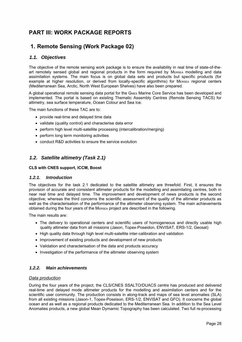
PART III: WORK PACKAGE REPORTS

1. Remote Sensing (Work Package 02)

1.1. Objectives

The objective of the remote sensing work package is to ensure the availability in real time of state-of-the-art remotely sensed global and regional products in the form required by MERSEA modelling and dataassimilation systems. The main focus is on global data sets and products but specific products (forexample at higher resolution, or derived from locally-specific algorithms) for MERSEA regional centers(Mediterranean Sea, Arctic, North West European Shelves) have also been prepared.

A global operational remote sensing data portal for the GMES Marine Core Service has been developed andimplemented. The portal is based on existing Thematic Assembly Centres (Remote Sensing TACS) foraltimetry, sea surface temperature, Ocean Colour and Sea Ice.

The main functions of these TAC are to:

• provide real-time and delayed time data• validate (quality control) and characterise data error• perform high level multi-satellite processing (intercalibration/merging)• perform long term monitoring activities• conduct R&D activities to ensure the service evolution

1.2. Satellite altimetry (Task 2.1)

CLS with CNES support, ICCM, Boost

1.2.1. IntroductionThe objectives for the task 2.1 dedicated to the satellite altimetry are threefold. First, it ensures theprovision of accurate and consistent altimeter products for the modelling and assimilating centres, both innear real time and delayed time. The improvement and development of news products is the secondobjective; whereas the third concerns the scientific assessment of the quality of the altimeter products aswell as the characterisation of the performance of the altimeter observing system. The main achievementsobtained during the four years of the MERSEA project are described in the following.

The main results are:

• The delivery to operational centers and scientific users of homogeneous and directly usable highquality altimeter data from all missions (Jason, Topex-Poseidon, ENVISAT, ERS-1/2, Geosat)

• High quality data through high level multi-satellite inter-calibration and validation• Improvement of existing products and development of new products• Validation and characterisation of the data and products accuracy• Investigation of the performance of the altimeter observing system

1.2.2. Main achievements

Data productionDuring the four years of the project, the CLS/CNES SSALTO/DUACS centre has produced and deliveredreal-time and delayed mode altimeter products for the modelling and assimilation centers and for thescientific user community. The production consists in along-track and maps of sea level anomalies (SLA)from all existing missions (Jason-1, Topex-Poseison, ERS-1/2, ENVISAT and GFO). It concerns the globalocean and as well as a regional products dedicated to the Mediterranean Sea. In addition to the Sea LevelAnomalies products, a new global Mean Dymamic Topography has been calculated. Two full re-processing

Page 28

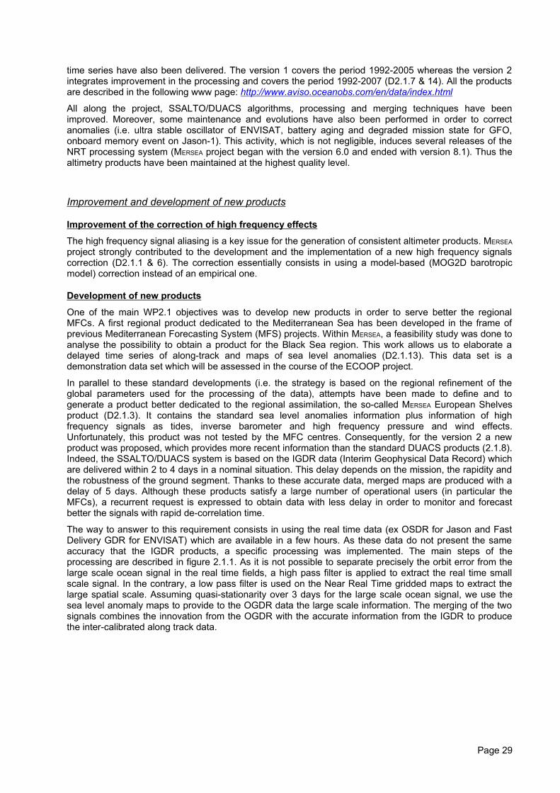
time series have also been delivered. The version 1 covers the period 1992-2005 whereas the version 2integrates improvement in the processing and covers the period 1992-2007 (D2.1.7 & 14). All the productsare described in the following www page: http://www.aviso.oceanobs.com/en/data/index.html

All along the project, SSALTO/DUACS algorithms, processing and merging techniques have beenimproved. Moreover, some maintenance and evolutions have also been performed in order to correctanomalies (i.e. ultra stable oscillator of ENVISAT, battery aging and degraded mission state for GFO,onboard memory event on Jason-1). This activity, which is not negligible, induces several releases of theNRT processing system (MERSEA project began with the version 6.0 and ended with version 8.1). Thus thealtimetry products have been maintained at the highest quality level.

Improvement and development of new products

Improvement of the correction of high frequency effects

The high frequency signal aliasing is a key issue for the generation of consistent altimeter products. MERSEA

project strongly contributed to the development and the implementation of a new high frequency signalscorrection (D2.1.1 & 6). The correction essentially consists in using a model-based (MOG2D barotropicmodel) correction instead of an empirical one.

Development of new products

One of the main WP2.1 objectives was to develop new products in order to serve better the regionalMFCs. A first regional product dedicated to the Mediterranean Sea has been developed in the frame ofprevious Mediterranean Forecasting System (MFS) projects. Within MERSEA, a feasibility study was done toanalyse the possibility to obtain a product for the Black Sea region. This work allows us to elaborate adelayed time series of along-track and maps of sea level anomalies (D2.1.13). This data set is ademonstration data set which will be assessed in the course of the ECOOP project.

In parallel to these standard developments (i.e. the strategy is based on the regional refinement of theglobal parameters used for the processing of the data), attempts have been made to define and togenerate a product better dedicated to the regional assimilation, the so-called MERSEA European Shelvesproduct (D2.1.3). It contains the standard sea level anomalies information plus information of highfrequency signals as tides, inverse barometer and high frequency pressure and wind effects.Unfortunately, this product was not tested by the MFC centres. Consequently, for the version 2 a newproduct was proposed, which provides more recent information than the standard DUACS products (2.1.8).Indeed, the SSALTO/DUACS system is based on the IGDR data (Interim Geophysical Data Record) whichare delivered within 2 to 4 days in a nominal situation. This delay depends on the mission, the rapidity andthe robustness of the ground segment. Thanks to these accurate data, merged maps are produced with adelay of 5 days. Although these products satisfy a large number of operational users (in particular theMFCs), a recurrent request is expressed to obtain data with less delay in order to monitor and forecastbetter the signals with rapid de-correlation time.

The way to answer to this requirement consists in using the real time data (ex OSDR for Jason and FastDelivery GDR for ENVISAT) which are available in a few hours. As these data do not present the sameaccuracy that the IGDR products, a specific processing was implemented. The main steps of theprocessing are described in figure 2.1.1. As it is not possible to separate precisely the orbit error from thelarge scale ocean signal in the real time fields, a high pass filter is applied to extract the real time smallscale signal. In the contrary, a low pass filter is used on the Near Real Time gridded maps to extract thelarge spatial scale. Assuming quasi-stationarity over 3 days for the large scale ocean signal, we use thesea level anomaly maps to provide to the OGDR data the large scale information. The merging of the twosignals combines the innovation from the OGDR with the accurate information from the IGDR to producethe inter-calibrated along track data.

Page 29

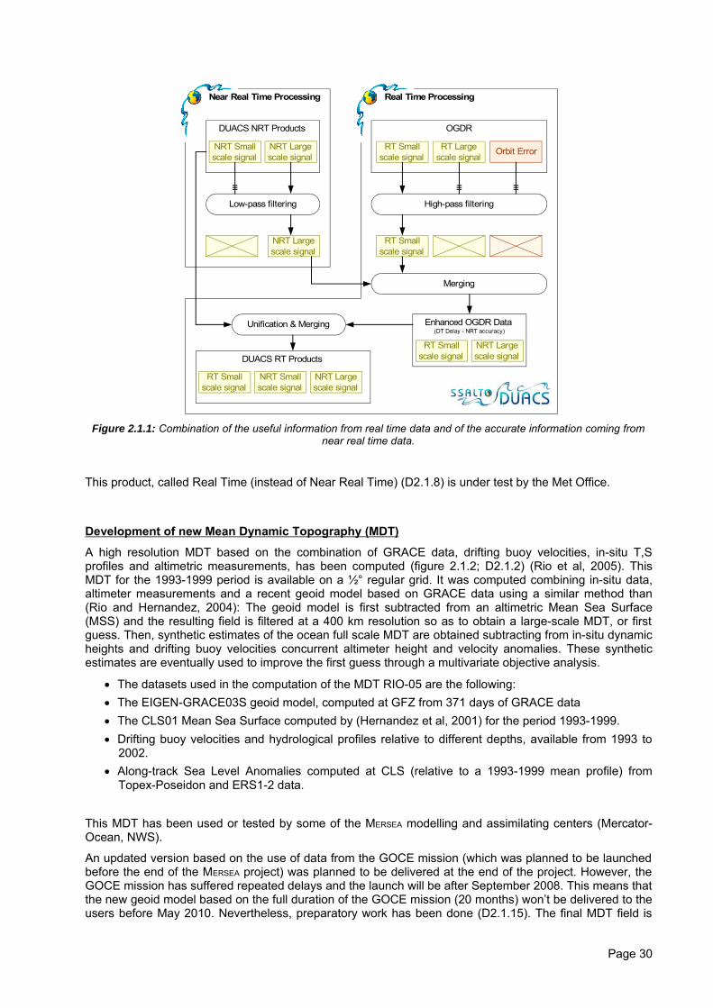
Near Real Time Processing Real Time Processing

OGDRDUACS NRT Products

NRT Largescale signal

NRT Smallscale signal

Orbit Error

Low-pass filtering

NRT Largescale signal

RT Largescale signal

RT Smallscale signal

High-pass filtering

RT Smallscale signal

Enhanced OGDR Data(DT Delay - NRT accuracy)

NRT Largescale signal

RT Smallscale signal

Unification & Merging

DUACS RT Products

NRT Smallscale signal

RT Smallscale signal

NRT Largescale signal

Merging

Figure 2.1.1: Combination of the useful information from real time data and of the accurate information coming fromnear real time data.

This product, called Real Time (instead of Near Real Time) (D2.1.8) is under test by the Met Office.

Development of new Mean Dynamic Topography (MDT)

A high resolution MDT based on the combination of GRACE data, drifting buoy velocities, in-situ T,Sprofiles and altimetric measurements, has been computed (figure 2.1.2; D2.1.2) (Rio et al, 2005). ThisMDT for the 1993-1999 period is available on a ½° regular grid. It was computed combining in-situ data,altimeter measurements and a recent geoid model based on GRACE data using a similar method than(Rio and Hernandez, 2004): The geoid model is first subtracted from an altimetric Mean Sea Surface(MSS) and the resulting field is filtered at a 400 km resolution so as to obtain a large-scale MDT, or firstguess. Then, synthetic estimates of the ocean full scale MDT are obtained subtracting from in-situ dynamicheights and drifting buoy velocities concurrent altimeter height and velocity anomalies. These syntheticestimates are eventually used to improve the first guess through a multivariate objective analysis.

• The datasets used in the computation of the MDT RIO-05 are the following:• The EIGEN-GRACE03S geoid model, computed at GFZ from 371 days of GRACE data• The CLS01 Mean Sea Surface computed by (Hernandez et al, 2001) for the period 1993-1999.• Drifting buoy velocities and hydrological profiles relative to different depths, available from 1993 to

2002.• Along-track Sea Level Anomalies computed at CLS (relative to a 1993-1999 mean profile) from

Topex-Poseidon and ERS1-2 data.

This MDT has been used or tested by some of the MERSEA modelling and assimilating centers (Mercator-Ocean, NWS).

An updated version based on the use of data from the GOCE mission (which was planned to be launchedbefore the end of the MERSEA project) was planned to be delivered at the end of the project. However, theGOCE mission has suffered repeated delays and the launch will be after September 2008. This means thatthe new geoid model based on the full duration of the GOCE mission (20 months) won’t be delivered to theusers before May 2010. Nevertheless, preparatory work has been done (D2.1.15). The final MDT field is

Page 30

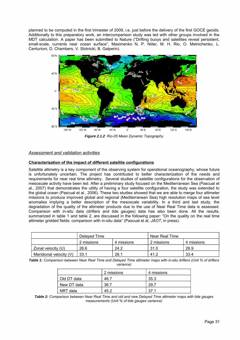
planned to be computed in the first trimester of 2009, i.e. just before the delivery of the first GOCE geoids.Additionally to this preparatory work, an intercomparison study was led with other groups involved in theMDT calculation. A paper has been submitted to Nature (“Drifting buoys and satellites reveal persistent,small-scale, currents near ocean surface”, Maximenko N, P. Niiler, M. H. Rio, O. Melnichenko, L.Centurioni, D. Chambers, V. Slotnicki, B. Galperin).

Figure 2.1.2: Rio-05 Mean Dynamic Topography

Assessment and validation activities

Characterization of the impact of different satellite configurations

Satellite altimetry is a key component of the observing system for operational oceanography, whose futureis unfortunately uncertain. The project has contributed to better characterization of the needs andrequirements for near real time altimetry. Several studies of satellite configurations for the observation ofmesoscale activity have been led. After a preliminary study focused on the Mediterranean Sea (Pascual etal., 2007) that demonstrates the utility of having a four satellite configuration, the study was extended tothe global ocean (Pascual et al., 2006). These two studies showed that we are able to merge four altimetermissions to produce improved global and regional (Mediterranean Sea) high resolution maps of sea levelanomalies implying a better description of the mesoscale variability. In a third and last study, thedegradation of the quality of the altimeter products due to the use of Near Real Time data is assessed.Comparison with in-situ data (drifters and tide gauges) data has also been done. All the results,summarized in table 1 and table 2, are discussed in the following paper: “On the quality on the real timealtimeter gridded fields: comparison with in-situ data” (Pascual et al, JAOT, in press).

Delayed Time Near Real Time2 missions 4 missions 2 missions 4 missions

Zonal velocity (U) 26.6 24.2 31.0 26.9Meridional velocity (V) 33.1 28.1 41.2 33.4

Table 1: Comparison between Near Real Time and Delayed Time altimeter maps with in-situ drifters (Unit % of driftersvariance)

2 missions 4 missionsOld DT data 46.7 35.3New DT data 36.7 29.7NRT data 45.2 37.1

Table 2: Comparison between Near Real Time and old and new Delayed Time altimeter maps with tide gaugesmeasurements (Unit % of tide gauges variance)

Page 31

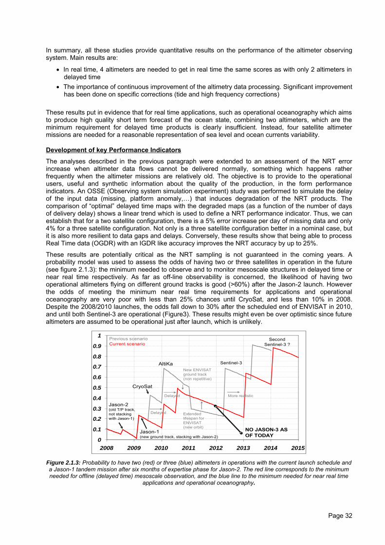
In summary, all these studies provide quantitative results on the performance of the altimeter observingsystem. Main results are:

• In real time, 4 altimeters are needed to get in real time the same scores as with only 2 altimeters indelayed time

• The importance of continuous improvement of the altimetry data processing. Significant improvementhas been done on specific corrections (tide and high frequency corrections)

These results put in evidence that for real time applications, such as operational oceanography which aimsto produce high quality short term forecast of the ocean state, combining two altimeters, which are theminimum requirement for delayed time products is clearly insufficient. Instead, four satellite altimetermissions are needed for a reasonable representation of sea level and ocean currents variability.

Development of key Performance Indicators

The analyses described in the previous paragraph were extended to an assessment of the NRT errorincrease when altimeter data flows cannot be delivered normally, something which happens ratherfrequently when the altimeter missions are relatively old. The objective is to provide to the operationalusers, useful and synthetic information about the quality of the production, in the form performanceindicators. An OSSE (Observing system simulation experiment) study was performed to simulate the delayof the input data (missing, platform anomaly,…) that induces degradation of the NRT products. Thecomparison of “optimal” delayed time maps with the degraded maps (as a function of the number of daysof delivery delay) shows a linear trend which is used to define a NRT performance indicator. Thus, we canestablish that for a two satellite configuration, there is a 5% error increase per day of missing data and only4% for a three satellite configuration. Not only is a three satellite configuration better in a nominal case, butit is also more resilient to data gaps and delays. Conversely, these results show that being able to processReal Time data (OGDR) with an IGDR like accuracy improves the NRT accuracy by up to 25%.

These results are potentially critical as the NRT sampling is not guaranteed in the coming years. Aprobability model was used to assess the odds of having two or three satellites in operation in the future(see figure 2.1.3): the minimum needed to observe and to monitor mesoscale structures in delayed time ornear real time respectively. As far as off-line observability is concerned, the likelihood of having twooperational altimeters flying on different ground tracks is good (>60%) after the Jason-2 launch. Howeverthe odds of meeting the minimum near real time requirements for applications and operationaloceanography are very poor with less than 25% chances until CryoSat, and less than 10% in 2008.Despite the 2008/2010 launches, the odds fall down to 30% after the scheduled end of ENVISAT in 2010,and until both Sentinel-3 are operational (Figure3). These results might even be over optimistic since futurealtimeters are assumed to be operational just after launch, which is unlikely.

0

0.1

0.2

0.3

0.4

0.5

0.6

0.7

0.8

0.9

1

2008 2009 2010 2011 2012 2013 2014 2015

Jason-2 (old T/P track, not stacking with Jason-1)

CryoSat

AltiKa Sentinel-3

Jason-1 (new ground track, stacking with Jason-2)

Delayed

Delayed

New ENVISAT ground track (non repetitive)

Extended lifespan for ENVISAT (new orbit)

More realistic

Second Sentinel-3 ?

Previous scenarioCurrent scenario

NO JASON-3 AS OF TODAY

Figure 2.1.3: Probability to have two (red) or three (blue) altimeters in operations with the current launch schedule anda Jason-1 tandem mission after six months of expertise phase for Jason-2. The red line corresponds to the minimumneeded for offline (delayed time) mesoscale observation, and the blue line to the minimum needed for near real time

applications and operational oceanography.

Page 32

Validation of re-analysis products in specific regions

In order to assess the accuracy of re-analysis products in region area, specific validation have beenachieved for two regions: The Bay of Biscay and the North West of Atlantic. The main results of the twostudies are described in Caballero et al (2007) and Volkov et al, 2006).

Validation/Comparison of surface currents

Within MERSEA project, a specific effort has been carried out on the validation and comparison of altimetervelocities with alternative methodologies based on SAR estimation (Boost-Technologies) and on SSTimages (ICM). This very innovative work allows us to better understand the limitation of each method. Thespecific goals to be enterprised by ICM were to extract dynamic information from available data sources(including in situ data, as those produced by drifter buoys or cruises, and remotely sensed data, as satelliteSST and colour images) and then validate L2 and L3 altimetry maps produced in the course of MERSEA

project. Thus, the first part of our work was centred in validation of altimetry with the first type of data,namely in situ data, task that we accomplished for data in the Mediterranean basin. When we attacked thesecond type of data, we started introducing a new methodology to derive dynamic information from mapsof scalars based on multifractal analysis. As a result of our efforts, we constructed completely newmethodologies able to extract dynamic information about the streamlines of the flow from instant maps ofSST or colour images, and our work for the rest of the project has been to cross validate altimetry and theresults of these new, promising techniques. These analysis techniques have implications at both levels,basic ocean research and operational oceanography. Here we summarise the analysis carried out tovalidate specific altimetric products and the efforts done in the development of new processing techniques,namely Coherent Vortex Separation (CVS) and specially the Maximum Singular Streamfuntion Method(MSSM) whose potential use for operational purposes has not yet finished but will continue in the future. Atthe end we list all the papers that we have published as a direct output of the MERSEA project andseparately others that are still submitted and/or under review when writing this report.

1.2.3. Publications/CommunicationsCarrère L., D.L. Volkov, P-Y. Le Traon, P. Schaeffer, C. Boone, Y. Faugère and P. Gaspar: “Reducing the

aliasing of high frequency signals in altimeter data: empirical and model-based approaches”, submittedto JAOT.

Caballero, A. Pascual, G. Dibarboure, and M. Espino: “Sea Level and Eddy Kinetic Energy variability in theBay of Biscay, inferred from satellite altimeter data”, accepted to JMS.

Volkov, D.L., G. Larnicol, and J. Dorandeu: “Improving the quality of satellite altimetry data over continentalshelves”, J. Geophys. Res. 112, C06020, doi:10.1029/2006JC003765, 2007

Rio, M.-H., P. Schaeffer, J.M. Lemoine, F. Hernandez, 2005: “The estimation of the ocean Mean DynamicTopography through the combination of altimetric data, in-situ measurements and GRACE geoid: Fromglobal to regional studies”, Proceeding of the GOCINA workshop, Luxembourg, April 2005.

Maximenko, N., P. Niiler, M.-H. Rio, O. Melnichenko, L. Centurioni, D. Chambers, V. Zlotnicki, B. Galperin:“Drifting buoys and satellites reveal persistent, small-scale, currents near ocean surface”, submitted toJournal of Atmospheric and Oceanic Technology

Pascual, A., Y. Faugère, G. Larnicol, P.Y. Le Traon: “Improved description of the ocean mesoscalevariability by combining four satellite altimeters”, (GRL, Vol 33, L02611; doi: 10.1029/2005GL024633,2006).

Pascual, A., C. Boone, G. Larnicol, P.Y. Le Traon: “On the quality of real-time altimeter gridded fields:comparison with in situ data”, in press in Journal of Atmospheric and Oceanic Technology

Pascual, A., M.-I. Pujol, G. Larnicol, P.Y. Le Traon, M.-H. Rio, 2005: “Mesoscale Mapping Capabilities ofMultisatellite Altimeter Missions: First Results with Real Data in the Mediterranean”, J. Mar. Syst.(Liege Colloquium special issue)

Turiel A., J. Isern-Fontanet, E. García-Ladona and J. Font. 2005: “Multifractal method for the instantaneousevaluation of the stream function in geophysical flows”, Phys. Rev. Lett., 95, 104502.

Page 33

Turiel A., J. Grazzini, H. Yahia. 2005: “Multiscale techniques for the detection of precipitation using thermalIR satellite images”, IEEE Geosci. Rem. Sen. Lett., 2, 447-450.

Isern-Fontanet J., E. García-Ladona, J. Font, 2006: “Vortices of the Mediterranean sea: an altimetricperspective”, J. Phys. Oceanogr., 36, 87-103.

Isern-Fontanet J., A. Turiel, E. Garcia-Ladona and J. Font: "Microcanonical multifractal formalism:application to the estimation of ocean surface velocities", Journal of Geophysical Research, 112,C05024 (2007).

Nieves V.and A. Turiel: "Analysis of ocean turbulence using adaptive CVS on altimetry maps", To appearin Journal of Marine Systems.

Turiel A., V. Nieves, MH Rio, G. Larnicol: “The multifractal structure of satellite temperature images can beused to obtain global maps of ocean currents”, submitted to Journal of Atmospheric and OceanicTechnology

1.3. Sea Surface Temperature (Task 2.2)

M-F/CMS leader, with SOC-USOU, CLS, Met.No, CNR-ISAC, MET Office

1.3.1. Level 3 satellite sea surface temperature productsAs part of the satellite SST (Sea surface temperature) activities, IFREMER and M-F/CMS have developedand implemented a common methodology for the processing of satellite L2P SST products, defined andmade available in near real time in the framework of the GODAE High Resolution SST Pilot Project(GHRSST-PP, see http://www.ghrsst-pp.org/ ), to produce high resolution SST analyses (level 4 products).

The main steps of this methodology are:• for each data source, the individual L2P products (most of which are swath products in satellite

projection) are “collated” into a single file, corresponding to a pre-defined time window and a pre-defined area on a regular latitude/longitude grid. Among all the individual observations found in thepre-defined time window for a given mesh of the pre-defined grid, the “best” observation is selected,according to a set of quality criteria, but the exact location of the observation, as well as theinformation on the observation bias and error standard deviation are preserved in the “collated” file.

• for each data source, an adjusted SST is then computed, using the ENVISAT/AATSR sea surfacetemperature as a reference. The choice of AATSR as a reference is justified by the fact that AATSRis currently providing the highest accuracy SST measurements from space, thanks to its high qualityon-board calibration system, and to its particular design (dual look). The adjustment method,developed in the framework of MERSEA, and applied to each data source, relies on a large scaleanalysis of the observed SST departures from AATSR, computed on a moving 10-day time window.The adjusted SST fields, as well as the new error standard deviation estimates, taking into accountthe errors due to the adjustment procedure, are then appended to each “collated” file.

• a single “merged” file is then produced, combining all the “collated” files from all available datasource. For each mesh of the pre-defined grid, the selection of the “best” SST observation amongthe various data sources is done according to a pre-defined priority order among existing datasources, and taking also into account the confidence in the SST adjustment, without any average ofobservations from different data sources. This priority order is based on an a priori knowledge of theaccuracy of each sensor, and on its horizontal resolution. Currently, ENVISAT/AATSR has thehighest priority, and TRMM/TMI the lowest. The “merged” product contains also a variable identifyingthe origin of each selected observation, as well as its error standard deviation. The “merged” file isthen used as the input for the SST objective analysis, but is also made available as such for otherapplications, like assimilation into an ocean modelling system.

IFREMER is producing currently in near real-time daily global “collated” and “merged” SST products at 0.1°horizontal resolution, as part of its ODYSSEA system (for detailed information and product access, seehttp://www.mersea.eu.org/Satellite/sst_validation.html). The time window defined for these global productsis currently ± 3 days around the product time.

Page 34

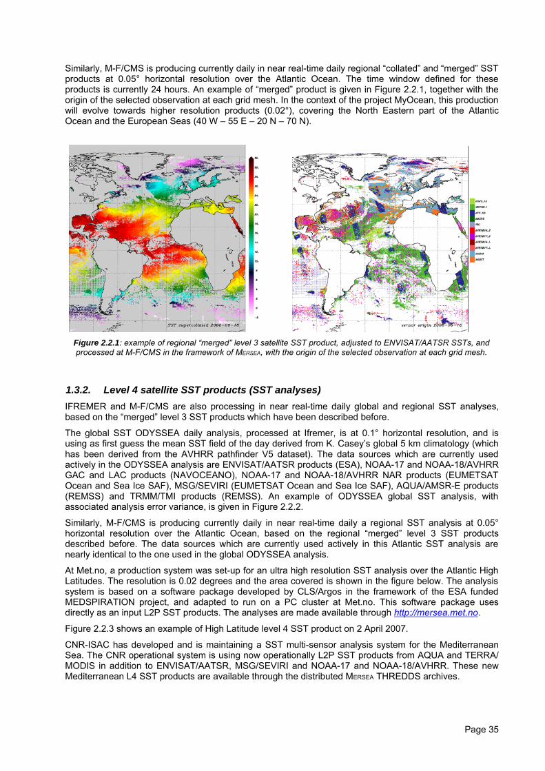
Similarly, M-F/CMS is producing currently daily in near real-time daily regional “collated” and “merged” SSTproducts at 0.05° horizontal resolution over the Atlantic Ocean. The time window defined for theseproducts is currently 24 hours. An example of “merged” product is given in Figure 2.2.1, together with theorigin of the selected observation at each grid mesh. In the context of the project MyOcean, this productionwill evolve towards higher resolution products (0.02°), covering the North Eastern part of the AtlanticOcean and the European Seas (40 W – 55 E – 20 N – 70 N).

Figure 2.2.1: example of regional “merged” level 3 satellite SST product, adjusted to ENVISAT/AATSR SSTs, andprocessed at M-F/CMS in the framework of MERSEA, with the origin of the selected observation at each grid mesh.

1.3.2. Level 4 satellite SST products (SST analyses)IFREMER and M-F/CMS are also processing in near real-time daily global and regional SST analyses,based on the “merged” level 3 SST products which have been described before.

The global SST ODYSSEA daily analysis, processed at Ifremer, is at 0.1° horizontal resolution, and isusing as first guess the mean SST field of the day derived from K. Casey’s global 5 km climatology (whichhas been derived from the AVHRR pathfinder V5 dataset). The data sources which are currently usedactively in the ODYSSEA analysis are ENVISAT/AATSR products (ESA), NOAA-17 and NOAA-18/AVHRRGAC and LAC products (NAVOCEANO), NOAA-17 and NOAA-18/AVHRR NAR products (EUMETSATOcean and Sea Ice SAF), MSG/SEVIRI (EUMETSAT Ocean and Sea Ice SAF), AQUA/AMSR-E products(REMSS) and TRMM/TMI products (REMSS). An example of ODYSSEA global SST analysis, withassociated analysis error variance, is given in Figure 2.2.2.

Similarly, M-F/CMS is producing currently daily in near real-time daily a regional SST analysis at 0.05°horizontal resolution over the Atlantic Ocean, based on the regional “merged” level 3 SST productsdescribed before. The data sources which are currently used actively in this Atlantic SST analysis arenearly identical to the one used in the global ODYSSEA analysis.

At Met.no, a production system was set-up for an ultra high resolution SST analysis over the Atlantic HighLatitudes. The resolution is 0.02 degrees and the area covered is shown in the figure below. The analysissystem is based on a software package developed by CLS/Argos in the framework of the ESA fundedMEDSPIRATION project, and adapted to run on a PC cluster at Met.no. This software package usesdirectly as an input L2P SST products. The analyses are made available through http://mersea.met.no.

Figure 2.2.3 shows an example of High Latitude level 4 SST product on 2 April 2007.

CNR-ISAC has developed and is maintaining a SST multi-sensor analysis system for the MediterraneanSea. The CNR operational system is using now operationally L2P SST products from AQUA and TERRA/MODIS in addition to ENVISAT/AATSR, MSG/SEVIRI and NOAA-17 and NOAA-18/AVHRR. These newMediterranean L4 SST products are available through the distributed MERSEA THREDDS archives.

Page 35

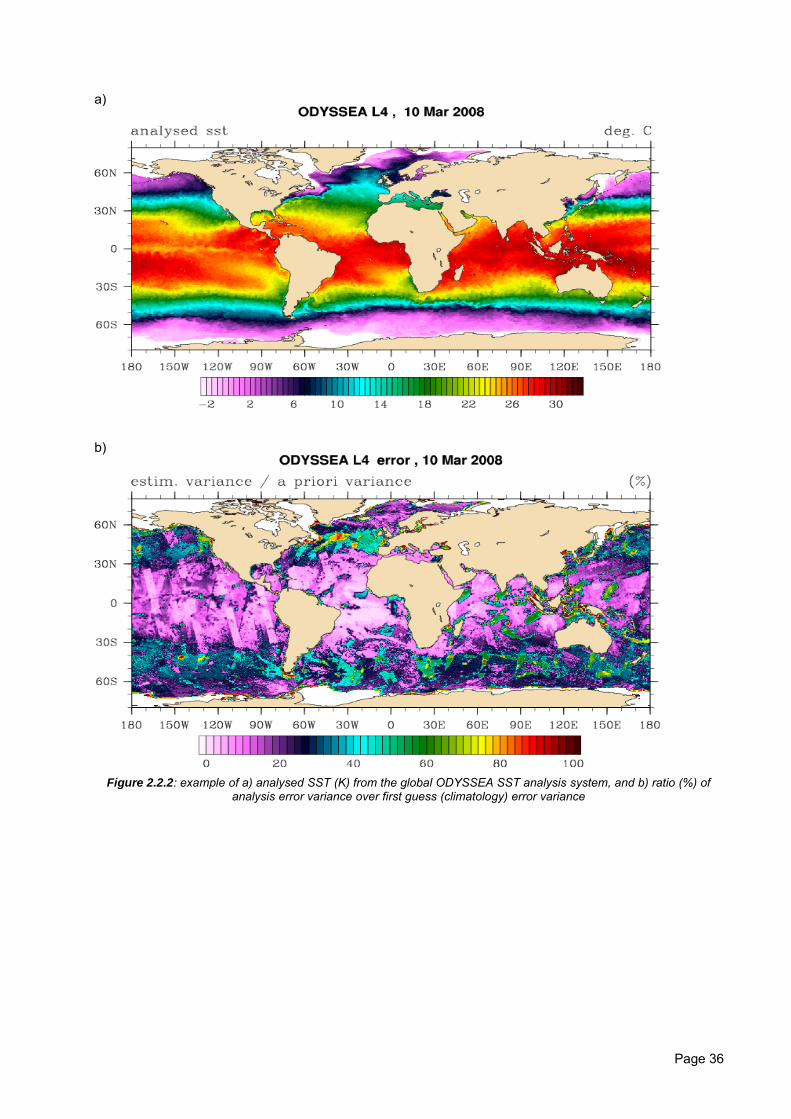
a)

b)

Figure 2.2.2: example of a) analysed SST (K) from the global ODYSSEA SST analysis system, and b) ratio (%) ofanalysis error variance over first guess (climatology) error variance

Page 36

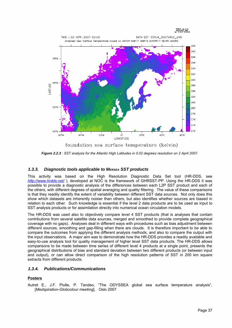
Figure 2.2.3 : SST analysis for the Atlantic High Latitudes in 0.02 degrees resolution on 2 April 2007.

1.3.3. Diagnostic tools applicable to MERSEA SST productsThis activity was based on the High Resolution Diagnostic Data Set tool (HR-DDS, seehttp://www.hrdds.net/ ), developed at NOC is the framework of GHRSST-PP. Using the HR-DDS it waspossible to provide a diagnostic analysis of the differences between each L2P SST product and each ofthe others, with different degrees of spatial averaging and quality filtering. The value of these comparisonsis that they readily identify the extent of variability between different SST data sources. Not only does thisshow which datasets are inherently noisier than others, but also identifies whether sources are biased inrelation to each other. Such knowledge is essential if the level 2 data products are to be used as input toSST analysis products or for assimilation directly into numerical ocean circulation models.

The HR-DDS was used also to objectively compare level 4 SST products (that is analyses that containcontributions from several satellite data sources, merged and smoothed to provide complete geographicalcoverage with no gaps). Analyses deal in different ways with procedures such as bias adjustment betweendifferent sources, smoothing and gap-filling when there are clouds. It is therefore important to be able tocompare the outcomes from applying the different analysis methods, and also to compare the output withthe input observations. A major aim was to demonstrate how the HR-DDS provides a readily available andeasy-to-use analysis tool for quality management of higher level SST data products. The HR-DDS allowscomparisons to be made between time series of different level 4 products at a single point, presents thegeographical distributions of bias and standard deviation between two different products (or between inputand output), or can allow direct comparison of the high resolution patterns of SST in 200 km squareextracts from different products.

1.3.4. Publications/Communications

Posters

Autret E., J.F. Piolle, P. Tandeo, “The ODYSSEA global sea surface temperature analysis”,[Medspiration-Globcolour meeting], Oslo 2007

Page 37

Oral presentations

Piolle J.F., E. Autret, P. Tandeo, “The ODYSSEA multi-sensor sea surface temperature analysis”, [GodaeFinal symposium], Nice 10-15 Nov 2008

Autret E., J.F. Piolle, “The ODYSSEA global sea surface temperature analysis”, [GHRSST meeting],Melbourne 2007

Autret, E. and F. Gaillard, “Climatology and interannual variability of the North-Atlantic from Coriolis re-analysis system”, [2nd ARGO scientific workshop], 13-18 March 2006, Venice 2006

Autret, E., F. Gaillard, “Delayed mode qualification of ARGO floats: CORIOLIS analysis system”,[Eurogoos Conference], Brest, June 2005

Gaillard, F., A. Autret and C. Coatanoan, “Global heat and salt content observed with ARGO profiles”,[2nd Argo Scientific workshop], 13-18 March 2006, Venice (Italy)

Gaillard, F. and E. Autret, “Interannual variability of the North-Atlantic: space and time characterization ofthe temperature and salinity properties”, [ICES annual conference], Maastricht 2006

Gaillard, F., E. Autret, A. Keziou and T. Loubrieu, “Climatology and interannual variability of the NorthAtlantic from Coriolis re-analysis”, [EuroGOOS Conference], Brest, June 2005

Gaillard, F., E. Autret, T. Loubrieu, V. Thierry and A. Keziou, « Climatologie et statistiques de l'AtlantiqueNord », [GMMC], Toulouse, Octobre 2005

Galaup, P., V. Thierry, C. Coatanoan, E. Autret, F. Gaillard, “Consistency of the delayed-mode Argodataset”, [2nd Argo Scientific workshop], 13-18 March 2006, Venice (Italy)

Le Borgne, P., A. Marsouin, F. Orain, H. Roquet, E. Autret, J.F. Piolle, « Operational SST bias correctionusing AATSR data », [Ocean Sciences meeting], Orlando 2008

http://www.sgmeet.com/aslo/orlando2008/viewabstract2.asp?AbstractID=1703

Thierry, V, H. Mercier, C. Grit, F. Gaillard, E. Autret, « Eaux Modales Subpolaires en Atlantique Nord àpartir des données ARGO/CORIOLIS », [Réunion ARGO France], Brest, March 2004

Publications

Gaillard, F. and E. Autret, “Coriolis real-time analysis system: validation over the North-Atlantic”, CoriolisNewsletter, 2005

Galaup, P., F. Gaillard, E. Autret, V. Thierry and C. Coatanoan, “Consistency of the Argo dataset in theNorth-Atlantic”, Coriolis Newsletter, 2006

1.4. Ocean Colour (Task 2.3)

JRC leader with CLS, SOC-USOU, CNR-ISAC, LEGOS

1.4.1. IntroductionAccording to first plan, the task objective was to provide an accurate and consistent stream of ocean colourdata at a resolution and format compatible with operational forecasting of the marine environment at globaland regional scales. This objective has been achieved through operational processing, archiving anddistribution of satellite data, as well as research and development activities.

During the 4 years of MERSEA, the work conducted includes:

• Assemble a complete data base of Ocean Colour Radiometry (OCR)-derived phytoplankton biomassand diffuse attenuation coefficient, globally (9km pixel resolution), and European Areas (2kmresolution)

• Evaluate the quality of the data through sensors comparison and validation exercises• Implement regional algorithms when appropriate (i.e., existing and peer-reviewed formulations)• Provide a critical assessment on OCR applications into biogeochemical models• Research and development on ocean colour (OC) multi-sensors merging techniques

Page 38

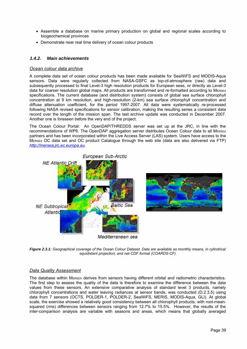
• Assemble a database on marine primary production on global and regional scales according tobiogeochemical provinces

• Demonstrate near real time delivery of ocean colour products

1.4.2. Main achievements

Ocean colour data archiveA complete data set of ocean colour products has been made available for SeaWiFS and MODIS-Aquasensors. Data were regularly collected from NASA-GSFC as top-of-atmosphere (raw) data andsubsequently processed to final Level-3 high resolution products for European seas, or directly as Level-3data for coarser resolution global maps. All products are transformed and re-formatted according to MERSEA

specifications. The current database (and distribution system) consists of global sea surface chlorophyllconcentration at 9 km resolution, and high-resolution (2-km) sea surface chlorophyll concentration anddiffuse attenuation coefficient, for the period 1997-2007. All data were systematically re-processedfollowing NASA revised specifications for sensor calibration, making the resulting series a consistent datarecord over the length of the mission span. The last archive update was conducted in December 2007.Another one is foreseen before the very end of the project.

The Ocean Colour Portal: An OpenDAP/THREDDS server was set up at the JRC, in line with therecommendations of WP6. The OpenDAP aggregation server distributes Ocean Colour data to all MERSEA

partners and has been incorporated within the Live Access Server (LAS) system. Users have access to theMERSEA OC data set and OC product Catalogue through the web site (data are also delivered via FTP)http://mersea.jrc.ec.europa.eu.

Figure 2.3.1: Geographical coverage of the Ocean Colour Dataset. Data are available as monthly means, in cylindricalequidistant projection, and net-CDF format (COARDS-CF)

Data Quality AssessmentThe database within MERSEA derives from sensors having different orbital and radiometric characteristics.The first step to assess the quality of the data is therefore to examine the difference between the datavalues from these sensors. An extensive comparative analysis of standard level 3 products, namelychlorophyll concentrations and water leaving radiances at sensor bands, was conducted (D.2.3.5) usingdata from 7 sensors (OCTS, POLDER-1, POLDER-2, SeaWiFS, MERIS, MODIS-Aqua, GLI). At globalscale, the exercise showed a relatively good consistency between all chlorophyll products, with root-mean-squared (rms) differences between sensors ranging from 12.7% to 15.5%. However, the results of theinter-comparison analysis are variable with seasons and areas, which means that globally averaged

Page 39

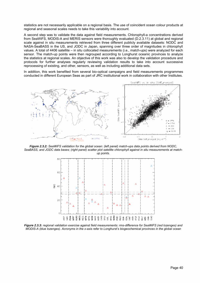
statistics are not necessarily applicable on a regional basis. The use of coincident ocean colour products atregional and seasonal scales needs to take this variability into account.

A second step was to validate the data against field measurements. Chlorophyll-a concentrations derivedfrom SeaWiFS, MODIS-A and MERIS sensors were thoroughly evaluated (D.2.3.11) at global and regionalscale against in situ measurements retrieved from three different publicly available datasets: NODC andNASA-SeaBASS in the US, and JODC in Japan, spanning over three order of magnitudes in chlorophyllvalues. A total of 4406 satellite – in situ collocated measurements (i.e., match-ups) were analyzed for eachsensor. The match-up points were then regrouped according to Longhurst oceanic provinces to analyzethe statistics at regional scales. An objective of this work was also to develop the validation procedure andprotocols for further analyses regularly reviewing validation results to take into account successivereprocessing of existing, and other, sensors, as well as including additional data sets.

In addition, this work benefited from several bio-optical campaigns and field measurements programmesconducted in different European Seas as part of JRC institutional work in collaboration with other Institutes.

Figure 2.3.2: SeaWiFS validation for the global ocean: (left panel) match-ups data points derived from NODC,SeaBASS, and JODC data bases; (right panel) scatter plot satellite chlorophyll against in situ measurements at match-

up points.

Figure 2.3.3: regional validation exercise against field measurements: rms-difference for SeaWiFS (red lozenges) andMODIS-A (blue lozenges). Acronyms in the x-axis refer to Longhurst’s biogeochemical provinces in the global ocean

Page 40

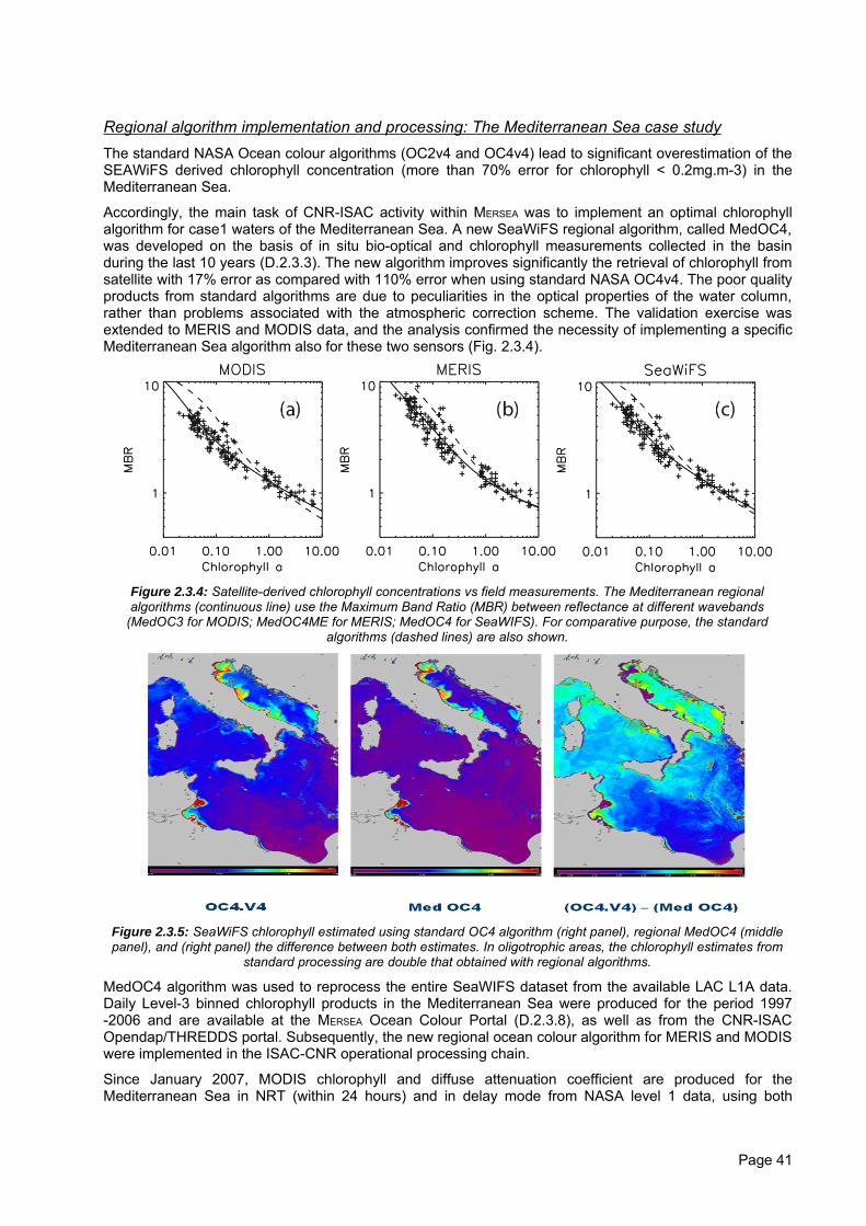
Regional algorithm implementation and processing: The Mediterranean Sea case studyThe standard NASA Ocean colour algorithms (OC2v4 and OC4v4) lead to significant overestimation of theSEAWiFS derived chlorophyll concentration (more than 70% error for chlorophyll < 0.2mg.m-3) in theMediterranean Sea.

Accordingly, the main task of CNR-ISAC activity within MERSEA was to implement an optimal chlorophyllalgorithm for case1 waters of the Mediterranean Sea. A new SeaWiFS regional algorithm, called MedOC4,was developed on the basis of in situ bio-optical and chlorophyll measurements collected in the basinduring the last 10 years (D.2.3.3). The new algorithm improves significantly the retrieval of chlorophyll fromsatellite with 17% error as compared with 110% error when using standard NASA OC4v4. The poor qualityproducts from standard algorithms are due to peculiarities in the optical properties of the water column,rather than problems associated with the atmospheric correction scheme. The validation exercise wasextended to MERIS and MODIS data, and the analysis confirmed the necessity of implementing a specificMediterranean Sea algorithm also for these two sensors (Fig. 2.3.4).

Figure 2.3.4: Satellite-derived chlorophyll concentrations vs field measurements. The Mediterranean regionalalgorithms (continuous line) use the Maximum Band Ratio (MBR) between reflectance at different wavebands

(MedOC3 for MODIS; MedOC4ME for MERIS; MedOC4 for SeaWIFS). For comparative purpose, the standardalgorithms (dashed lines) are also shown.

Figure 2.3.5: SeaWiFS chlorophyll estimated using standard OC4 algorithm (right panel), regional MedOC4 (middlepanel), and (right panel) the difference between both estimates. In oligotrophic areas, the chlorophyll estimates from

standard processing are double that obtained with regional algorithms.

MedOC4 algorithm was used to reprocess the entire SeaWIFS dataset from the available LAC L1A data.Daily Level-3 binned chlorophyll products in the Mediterranean Sea were produced for the period 1997-2006 and are available at the MERSEA Ocean Colour Portal (D.2.3.8), as well as from the CNR-ISACOpendap/THREDDS portal. Subsequently, the new regional ocean colour algorithm for MERIS and MODISwere implemented in the ISAC-CNR operational processing chain.

Since January 2007, MODIS chlorophyll and diffuse attenuation coefficient are produced for theMediterranean Sea in NRT (within 24 hours) and in delay mode from NASA level 1 data, using both

Page 41

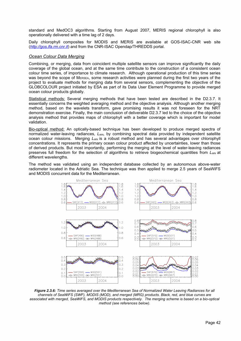
standard and MedOC3 algorithms. Starting from August 2007, MERIS regional chlorophyll is alsooperationally delivered with a time lag of 2 days.

Daily chlorophyll composites for MODIS and MERIS are available at GOS-ISAC-CNR web site(http://gos.ifa.rm.cnr.it) and from the CNR-ISAC Opendap/THREDDS portal.

Ocean Colour Data MergingCombining, or merging, data from coincident multiple satellite sensors can improve significantly the dailycoverage of the global ocean, and at the same time contribute to the construction of a consistent oceancolour time series, of importance to climate research. Although operational production of this time serieswas beyond the scope of MERSEA, some research activities were planned during the first two years of theproject to evaluate methods for merging data from several sensors, complementing the objective of theGLOBCOLOUR project initiated by ESA as part of its Data User Element Programme to provide mergedocean colour products globally.

Statistical methods: Several merging methods that have been tested are described in the D2.3.7. Itessentially concerns the weighted averaging method and the objective analysis. Although another mergingmethod, based on the wavelets transform, gave promising results it was not foreseen for the NRTdemonstration exercise. Finally, the main conclusion of deliverable D2.3.7 led to the choice of the objectiveanalysis method that provides maps of chlorophyll with a better coverage which is important for modelvalidation.

Bio-optical method: An optically-based technique has been developed to produce merged spectra ofnormalized water-leaving radiances, LWN, by combining spectral data provided by independent satelliteocean colour missions. Merging LWN is a robust method and has several advantages over chlorophyllconcentrations. It represents the primary ocean colour product affected by uncertainties, lower than thoseof derived products. But most importantly, performing the merging at the level of water-leaving radiancespreserves full freedom for the selection of algorithms to retrieve biogeochemical quantities from LWN atdifferent wavelengths.

The method was validated using an independent database collected by an autonomous above-waterradiometer located in the Adriatic Sea. The technique was then applied to merge 2.5 years of SeaWiFSand MODIS concurrent data for the Mediterranean.

Figure 2.3.6: Time series averaged over the Mediterranean Sea of Normalized Water Leaving Radiances for allchannels of SeaWiFS (SWF), MODIS (MOD), and merged (MRG) products. Black, red, and blue curves are

associated with merged, SeaWiFS, and MODIS products respectively. The merging scheme is based on a bio-opticalmethod (see references below).

Page 42

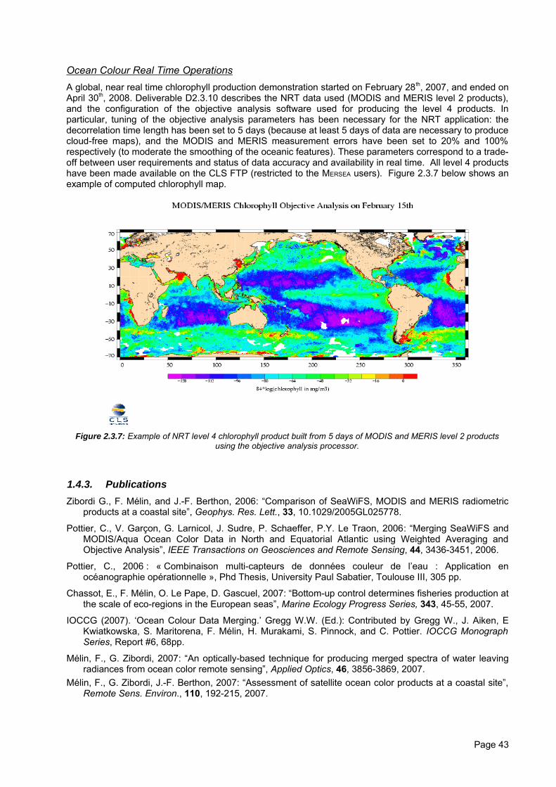
Ocean Colour Real Time OperationsA global, near real time chlorophyll production demonstration started on February 28th, 2007, and ended onApril 30th, 2008. Deliverable D2.3.10 describes the NRT data used (MODIS and MERIS level 2 products),and the configuration of the objective analysis software used for producing the level 4 products. Inparticular, tuning of the objective analysis parameters has been necessary for the NRT application: thedecorrelation time length has been set to 5 days (because at least 5 days of data are necessary to producecloud-free maps), and the MODIS and MERIS measurement errors have been set to 20% and 100%respectively (to moderate the smoothing of the oceanic features). These parameters correspond to a trade-off between user requirements and status of data accuracy and availability in real time. All level 4 productshave been made available on the CLS FTP (restricted to the MERSEA users). Figure 2.3.7 below shows anexample of computed chlorophyll map.

Figure 2.3.7: Example of NRT level 4 chlorophyll product built from 5 days of MODIS and MERIS level 2 productsusing the objective analysis processor.

1.4.3. PublicationsZibordi G., F. Mélin, and J.-F. Berthon, 2006: “Comparison of SeaWiFS, MODIS and MERIS radiometric

products at a coastal site”, Geophys. Res. Lett., 33, 10.1029/2005GL025778.

Pottier, C., V. Garçon, G. Larnicol, J. Sudre, P. Schaeffer, P.Y. Le Traon, 2006: “Merging SeaWiFS andMODIS/Aqua Ocean Color Data in North and Equatorial Atlantic using Weighted Averaging andObjective Analysis”, IEEE Transactions on Geosciences and Remote Sensing, 44, 3436-3451, 2006.

Pottier, C., 2006 : « Combinaison multi-capteurs de données couleur de l’eau : Application enocéanographie opérationnelle », Phd Thesis, University Paul Sabatier, Toulouse III, 305 pp.

Chassot, E., F. Mélin, O. Le Pape, D. Gascuel, 2007: “Bottom-up control determines fisheries production atthe scale of eco-regions in the European seas”, Marine Ecology Progress Series, 343, 45-55, 2007.

IOCCG (2007). ‘Ocean Colour Data Merging.’ Gregg W.W. (Ed.): Contributed by Gregg W., J. Aiken, EKwiatkowska, S. Maritorena, F. Mélin, H. Murakami, S. Pinnock, and C. Pottier. IOCCG MonographSeries, Report #6, 68pp.

Mélin, F., G. Zibordi, 2007: “An optically-based technique for producing merged spectra of water leavingradiances from ocean color remote sensing”, Applied Optics, 46, 3856-3869, 2007.

Mélin, F., G. Zibordi, J.-F. Berthon, 2007: “Assessment of satellite ocean color products at a coastal site”,Remote Sens. Environ., 110, 192-215, 2007.

Page 43

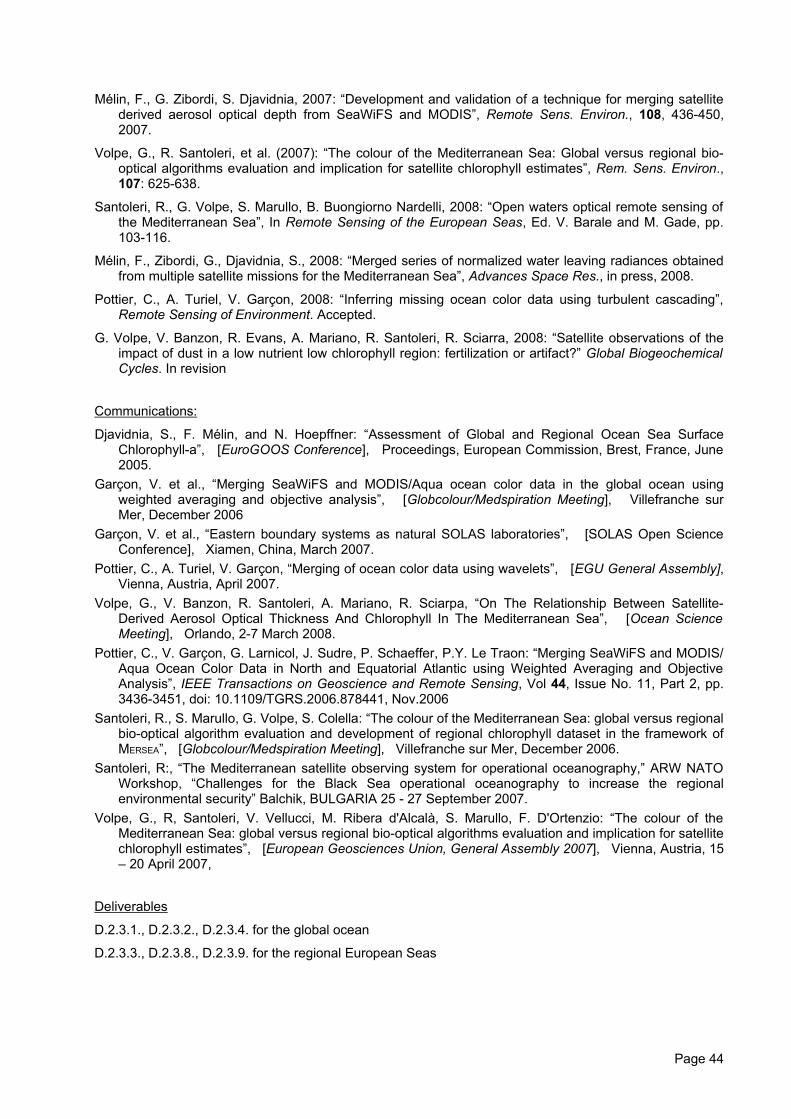
Mélin, F., G. Zibordi, S. Djavidnia, 2007: “Development and validation of a technique for merging satellitederived aerosol optical depth from SeaWiFS and MODIS”, Remote Sens. Environ., 108, 436-450,2007.

Volpe, G., R. Santoleri, et al. (2007): “The colour of the Mediterranean Sea: Global versus regional bio-optical algorithms evaluation and implication for satellite chlorophyll estimates”, Rem. Sens. Environ.,107: 625-638.

Santoleri, R., G. Volpe, S. Marullo, B. Buongiorno Nardelli, 2008: “Open waters optical remote sensing ofthe Mediterranean Sea”, In Remote Sensing of the European Seas, Ed. V. Barale and M. Gade, pp.103-116.

Mélin, F., Zibordi, G., Djavidnia, S., 2008: “Merged series of normalized water leaving radiances obtainedfrom multiple satellite missions for the Mediterranean Sea”, Advances Space Res., in press, 2008.

Pottier, C., A. Turiel, V. Garçon, 2008: “Inferring missing ocean color data using turbulent cascading”,Remote Sensing of Environment. Accepted.

G. Volpe, V. Banzon, R. Evans, A. Mariano, R. Santoleri, R. Sciarra, 2008: “Satellite observations of theimpact of dust in a low nutrient low chlorophyll region: fertilization or artifact?” Global BiogeochemicalCycles. In revision

Communications:

Djavidnia, S., F. Mélin, and N. Hoepffner: “Assessment of Global and Regional Ocean Sea SurfaceChlorophyll-a”, [EuroGOOS Conference], Proceedings, European Commission, Brest, France, June2005.

Garçon, V. et al., “Merging SeaWiFS and MODIS/Aqua ocean color data in the global ocean usingweighted averaging and objective analysis”, [Globcolour/Medspiration Meeting], Villefranche surMer, December 2006

Garçon, V. et al., “Eastern boundary systems as natural SOLAS laboratories”, [SOLAS Open ScienceConference], Xiamen, China, March 2007.

Pottier, C., A. Turiel, V. Garçon, “Merging of ocean color data using wavelets”, [EGU General Assembly],Vienna, Austria, April 2007.

Volpe, G., V. Banzon, R. Santoleri, A. Mariano, R. Sciarpa, “On The Relationship Between Satellite-Derived Aerosol Optical Thickness And Chlorophyll In The Mediterranean Sea”, [Ocean ScienceMeeting], Orlando, 2-7 March 2008.

Pottier, C., V. Garçon, G. Larnicol, J. Sudre, P. Schaeffer, P.Y. Le Traon: “Merging SeaWiFS and MODIS/Aqua Ocean Color Data in North and Equatorial Atlantic using Weighted Averaging and ObjectiveAnalysis”, IEEE Transactions on Geoscience and Remote Sensing, Vol 44, Issue No. 11, Part 2, pp.3436-3451, doi: 10.1109/TGRS.2006.878441, Nov.2006

Santoleri, R., S. Marullo, G. Volpe, S. Colella: “The colour of the Mediterranean Sea: global versus regionalbio-optical algorithm evaluation and development of regional chlorophyll dataset in the framework ofMERSEA”, [Globcolour/Medspiration Meeting], Villefranche sur Mer, December 2006.

Santoleri, R:, “The Mediterranean satellite observing system for operational oceanography,” ARW NATOWorkshop, “Challenges for the Black Sea operational oceanography to increase the regionalenvironmental security” Balchik, BULGARIA 25 - 27 September 2007.

Volpe, G., R, Santoleri, V. Vellucci, M. Ribera d'Alcalà, S. Marullo, F. D'Ortenzio: “The colour of theMediterranean Sea: global versus regional bio-optical algorithms evaluation and implication for satellitechlorophyll estimates”, [European Geosciences Union, General Assembly 2007], Vienna, Austria, 15– 20 April 2007,

Deliverables

D.2.3.1., D.2.3.2., D.2.3.4. for the global ocean

D.2.3.3., D.2.3.8., D.2.3.9. for the regional European Seas

Page 44

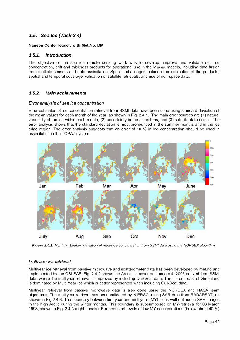
1.5. Sea Ice (Task 2.4)

Nansen Center leader, with Met.No, DMI

1.5.1. IntroductionThe objective of the sea ice remote sensing work was to develop, improve and validate sea iceconcentration, drift and thickness products for operational use in the MERSEA models, including data fusionfrom multiple sensors and data assimilation. Specific challenges include error estimation of the products,spatial and temporal coverage, validation of satellite retrievals, and use of non-space data.

1.5.2. Main achievements

Error analysis of sea ice concentrationError estimates of ice concentration retrieval from SSMI data have been done using standard deviation ofthe mean values for each month of the year, as shown in Fig. 2.4.1. The main error sources are (1) naturalvariability of the ice within each month, (2) uncertainty in the algorithms, and (3) satellite data noise. Theerror analysis shows that the standard deviation is most pronounced in the summer months and in the iceedge region. The error analysis suggests that an error of 10 % in ice concentration should be used inassimilation in the TOPAZ system.

Figure 2.4.1. Monthly standard deviation of mean ice concentration from SSMI data using the NORSEX algorithm.

Multiyear ice retrievalMultiyear ice retrieval from passive microwave and scatterometer data has been developed by met.no andimplemented by the OSI-SAF. Fig. 2.4.2 shows the Arctic ice cover on January 4, 2006 derived from SSMIdata, where the multiyear retrieval is improved by including QuikScat data. The ice drift east of Greenlandis dominated by Multi Year Ice which is better represented when including QuikScat data.

Multiyear retrieval from passive microwave data is also done using the NORSEX and NASA teamalgorithms. The multiyear retrieval has been validated by NIERSC, using SAR data from RADARSAT, asshown in Fig 2.4.3. The boundary between first-year and multiyear (MY) ice is well-defined in SAR imagesin the high Arctic during the winter months. This boundary is superimposed on MY-retrieval for 08 March1998, shown in Fig. 2.4.3 (right panels). Erroneous retrievals of low MY concentrations (below about 40 %)

Page 45

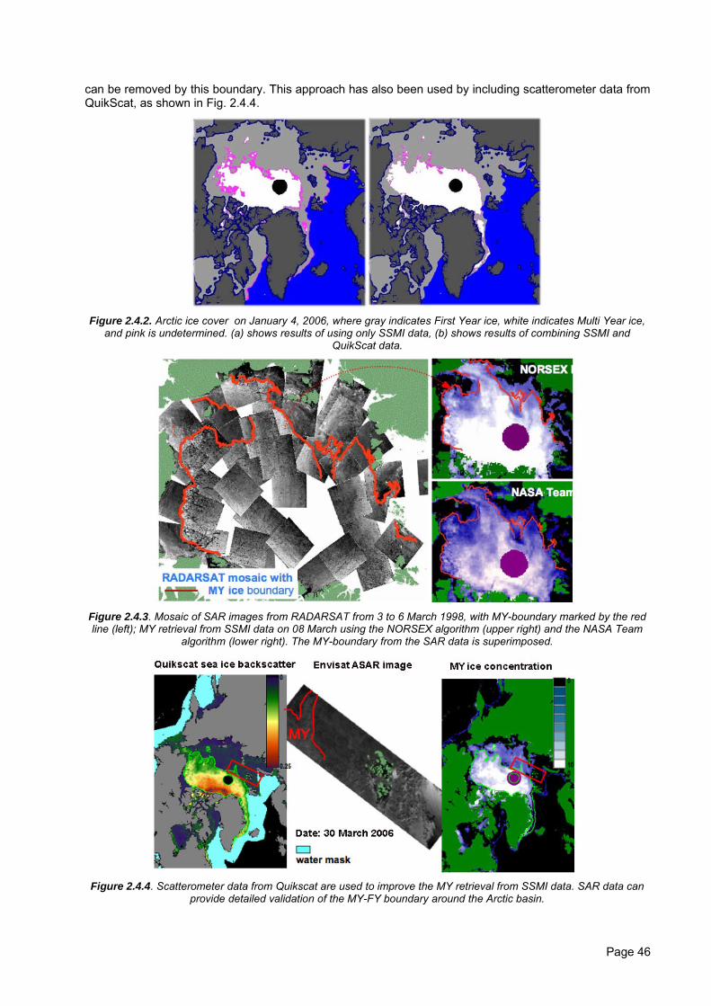
can be removed by this boundary. This approach has also been used by including scatterometer data fromQuikScat, as shown in Fig. 2.4.4.

Figure 2.4.2. Arctic ice cover on January 4, 2006, where gray indicates First Year ice, white indicates Multi Year ice,and pink is undetermined. (a) shows results of using only SSMI data, (b) shows results of combining SSMI and

QuikScat data.

Figure 2.4.3. Mosaic of SAR images from RADARSAT from 3 to 6 March 1998, with MY-boundary marked by the redline (left); MY retrieval from SSMI data on 08 March using the NORSEX algorithm (upper right) and the NASA Team

algorithm (lower right). The MY-boundary from the SAR data is superimposed.

Figure 2.4.4. Scatterometer data from Quikscat are used to improve the MY retrieval from SSMI data. SAR data canprovide detailed validation of the MY-FY boundary around the Arctic basin.

Page 46

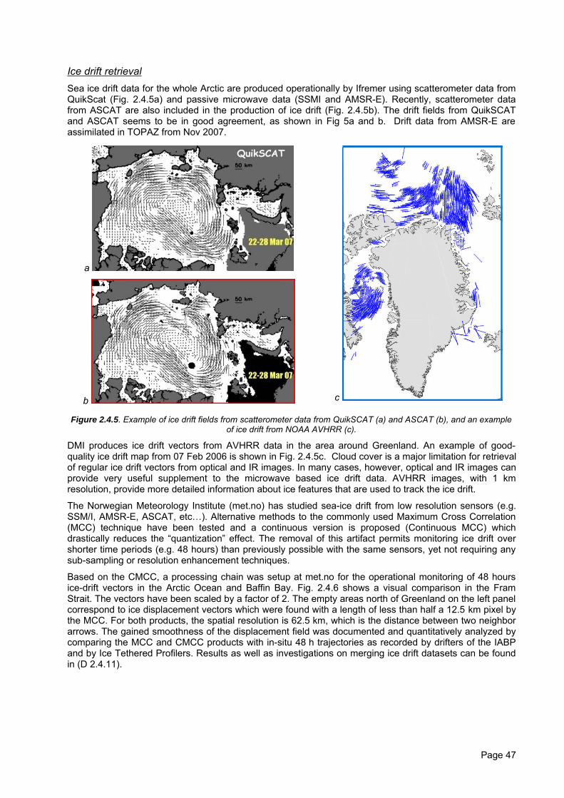
Ice drift retrievalSea ice drift data for the whole Arctic are produced operationally by Ifremer using scatterometer data fromQuikScat (Fig. 2.4.5a) and passive microwave data (SSMI and AMSR-E). Recently, scatterometer datafrom ASCAT are also included in the production of ice drift (Fig. 2.4.5b). The drift fields from QuikSCATand ASCAT seems to be in good agreement, as shown in Fig 5a and b. Drift data from AMSR-E areassimilated in TOPAZ from Nov 2007.

a

b c

Figure 2.4.5. Example of ice drift fields from scatterometer data from QuikSCAT (a) and ASCAT (b), and an exampleof ice drift from NOAA AVHRR (c).

DMI produces ice drift vectors from AVHRR data in the area around Greenland. An example of good-quality ice drift map from 07 Feb 2006 is shown in Fig. 2.4.5c. Cloud cover is a major limitation for retrievalof regular ice drift vectors from optical and IR images. In many cases, however, optical and IR images canprovide very useful supplement to the microwave based ice drift data. AVHRR images, with 1 kmresolution, provide more detailed information about ice features that are used to track the ice drift.

The Norwegian Meteorology Institute (met.no) has studied sea-ice drift from low resolution sensors (e.g.SSM/I, AMSR-E, ASCAT, etc…). Alternative methods to the commonly used Maximum Cross Correlation(MCC) technique have been tested and a continuous version is proposed (Continuous MCC) whichdrastically reduces the “quantization” effect. The removal of this artifact permits monitoring ice drift overshorter time periods (e.g. 48 hours) than previously possible with the same sensors, yet not requiring anysub-sampling or resolution enhancement techniques.

Based on the CMCC, a processing chain was setup at met.no for the operational monitoring of 48 hoursice-drift vectors in the Arctic Ocean and Baffin Bay. Fig. 2.4.6 shows a visual comparison in the FramStrait. The vectors have been scaled by a factor of 2. The empty areas north of Greenland on the left panelcorrespond to ice displacement vectors which were found with a length of less than half a 12.5 km pixel bythe MCC. For both products, the spatial resolution is 62.5 km, which is the distance between two neighborarrows. The gained smoothness of the displacement field was documented and quantitatively analyzed bycomparing the MCC and CMCC products with in-situ 48 h trajectories as recorded by drifters of the IABPand by Ice Tethered Profilers. Results as well as investigations on merging ice drift datasets can be foundin (D 2.4.11).

Page 47

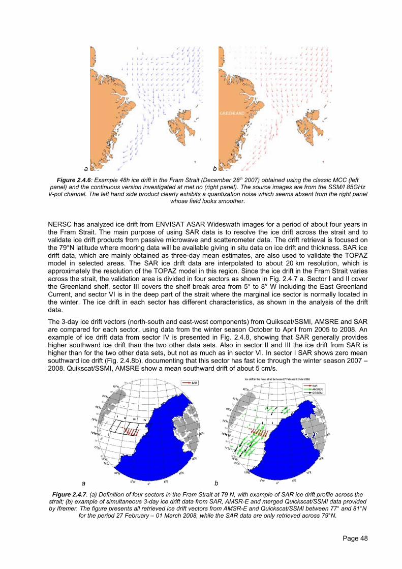
a b Figure 2.4.6: Example 48h ice drift in the Fram Strait (December 28th 2007) obtained using the classic MCC (left

panel) and the continuous version investigated at met.no (right panel). The source images are from the SSM/I 85GHzV-pol channel. The left hand side product clearly exhibits a quantization noise which seems absent from the right panel

whose field looks smoother.

NERSC has analyzed ice drift from ENVISAT ASAR Wideswath images for a period of about four years inthe Fram Strait. The main purpose of using SAR data is to resolve the ice drift across the strait and tovalidate ice drift products from passive microwave and scatterometer data. The drift retrieval is focused onthe 79°N latitude where mooring data will be available giving in situ data on ice drift and thickness. SAR icedrift data, which are mainly obtained as three-day mean estimates, are also used to validate the TOPAZmodel in selected areas. The SAR ice drift data are interpolated to about 20 km resolution, which isapproximately the resolution of the TOPAZ model in this region. Since the ice drift in the Fram Strait variesacross the strait, the validation area is divided in four sectors as shown in Fig. 2.4.7 a. Sector I and II coverthe Greenland shelf, sector III covers the shelf break area from 5° to 8° W including the East GreenlandCurrent, and sector VI is in the deep part of the strait where the marginal ice sector is normally located inthe winter. The ice drift in each sector has different characteristics, as shown in the analysis of the driftdata.

The 3-day ice drift vectors (north-south and east-west components) from Quikscat/SSMI, AMSRE and SARare compared for each sector, using data from the winter season October to April from 2005 to 2008. Anexample of ice drift data from sector IV is presented in Fig. 2.4.8, showing that SAR generally provideshigher southward ice drift than the two other data sets. Also in sector II and III the ice drift from SAR ishigher than for the two other data sets, but not as much as in sector VI. In sector I SAR shows zero meansouthward ice drift (Fig. 2.4.8b), documenting that this sector has fast ice through the winter season 2007 –2008. Quikscat/SSMI, AMSRE show a mean southward drift of about 5 cm/s.

a b Figure 2.4.7. (a) Definition of four sectors in the Fram Strait at 79 N, with example of SAR ice drift profile across the

strait; (b) example of simultaneous 3-day ice drift data from SAR, AMSR-E and merged Quickscat/SSMI data providedby Ifremer. The figure presents all retrieved ice drift vectors from AMSR-E and Quickscat/SSMI between 77° and 81°N

for the period 27 February – 01 March 2008, while the SAR data are only retrieved across 79°N.

Page 48

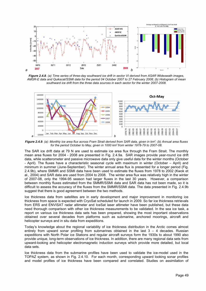
a b Figure 2.4.8. (a) Time series of three-day southward ice drift in sector VI derived from ASAR Wideswath images,

AMSR-E data and Quikscat/SSMI data for the period 04 October 2007 to 27 February 2008; (b) Histogram of meansouthward ice drift from the three data sources in each sector for the winter 2007-2008.

a b

Figure 2.4.9. (a): Monthly ice area flux across Fram Strait derived from SAR data, given in km2; (b) Annual area fluxesfor the period October to May, given in 1000 km2 from winter 1978-79 to 2007-08.

The SAR ice drift data at 79 N are used to estimate ice area flux through the Fram Strait. The monthlymean area fluxes for 2004 - 2008 are presented in Fig. 2.4.9a. SAR images provide year-round ice driftdata, while scatterometer and passive microwave data only give useful data for the winter months (October- April). The fluxes have a characteristic seasonal cycle with maximum in winter (October – April) andminimum in summer (June-September). The winter annual area flux is presented for a longer period (Fig.2.4.9b), where SMMR and SSMI data have been used to estimate the fluxes from 1978 to 2002 (Kwok etal., 2004) and SAR data are used from 2004 to 2008. The winter area flux was relatively high in the winterof 2007-08, only the 1994-95 season had larger fluxes in the last 30 years. However, a comparisonbetween monthly fluxes estimated from the SMMR/SSMI data and SAR data has not been made, so it isdifficult to assess the accuracy of the fluxes from the SMMR/SSMI data. The data presented in Fig. 2.4.9bsuggest that there is good agreement between the two methods.

Ice thickness data from satellites are in early development and major improvement in monitoring icethickness from space is expected with CryoSat scheduled for launch in 2009. So far ice thickness retrievalsfrom ERS and ENVISAT radar altimeter and IceSat laser altimeter have been published, but these dataneed thorough comparison with other ice thickness measurements to be validated. In the sea ice task, areport on various ice thickness data sets has been prepared, showing the most important observationsobtained over several decades from platforms such as submarine, anchored moorings, aircraft andhelicopter surveys and in situ data from expeditions.

Today’s knowledge about the regional variability of ice thickness distribution in the Arctic comes almostentirely from upward sonar profiling from submarines obtained in the last 3 – 4 decades. Russianexpeditions with North Polar ice Stations and regular aircraft surveys form the 1930s to about 1990 alsoprovide unique, long-term observations of ice thickness. In addition, there are many regional data sets fromupward-looking and helicopter electromagnetic induction surveys which provide more detailed, but localdata sets.

Ice thickness data from the submarine profiles have been used to validate the ice-model used in theTOPAZ system, as shown in Fig. 2.4.10. For each month, corresponding upward looking sonar profilesand model profiles of ice thickness have been compared and correlated. Studies on assimilation of

Page 49

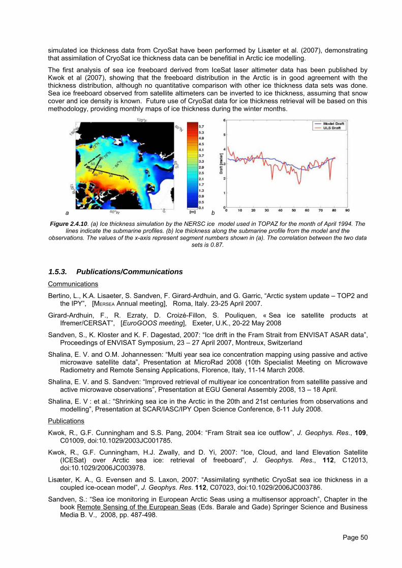
simulated ice thickness data from CryoSat have been performed by Lisæter et al. (2007), demonstratingthat assimilation of CryoSat ice thickness data can be benefitial in Arctic ice modelling.

The first analysis of sea ice freeboard derived from IceSat laser altimeter data has been published byKwok et al (2007), showing that the freeboard distribution in the Arctic is in good agreement with thethickness distribution, although no quantitative comparison with other ice thickness data sets was done.Sea ice freeboard observed from satellite altimeters can be inverted to ice thickness, assuming that snowcover and ice density is known. Future use of CryoSat data for ice thickness retrieval will be based on thismethodology, providing monthly maps of ice thickness during the winter months.

a b

Figure 2.4.10. (a) Ice thickness simulation by the NERSC ice model used in TOPAZ for the month of April 1994. Thelines indicate the submarine profiles. (b) Ice thickness along the submarine profile from the model and the

observations. The values of the x-axis represent segment numbers shown in (a). The correlation between the two datasets is 0.87.

1.5.3. Publications/CommunicationsCommunications

Bertino, L., K.A. Lisaeter, S. Sandven, F. Girard-Ardhuin, and G. Garric, “Arctic system update – TOP2 andthe IPY”, [MERSEA Annual meeting], Roma, Italy. 23-25 April 2007.

Girard-Ardhuin, F., R. Ezraty, D. Croizé-Fillon, S. Pouliquen, « Sea ice satellite products atIfremer/CERSAT”, [EuroGOOS meeting], Exeter, U.K., 20-22 May 2008

Sandven, S., K. Kloster and K. F. Dagestad, 2007: “Ice drift in the Fram Strait from ENVISAT ASAR data”,Proceedings of ENVISAT Symposium, 23 – 27 April 2007, Montreux, Switzerland

Shalina, E. V. and O.M. Johannessen: “Multi year sea ice concentration mapping using passive and activemicrowave satellite data”, Presentation at MicroRad 2008 (10th Specialist Meeting on MicrowaveRadiometry and Remote Sensing Applications, Florence, Italy, 11-14 March 2008.

Shalina, E. V. and S. Sandven: “Improved retrieval of multiyear ice concentration from satellite passive andactive microwave observations”, Presentation at EGU General Assembly 2008, 13 – 18 April.

Shalina, E. V : et al.: “Shrinking sea ice in the Arctic in the 20th and 21st centuries from observations andmodelling”, Presentation at SCAR/IASC/IPY Open Science Conference, 8-11 July 2008.

Publications

Kwok, R., G.F. Cunningham and S.S. Pang, 2004: “Fram Strait sea ice outflow”, J. Geophys. Res., 109,C01009, doi:10.1029/2003JC001785.

Kwok, R., G.F. Cunningham, H.J. Zwally, and D. Yi, 2007: “Ice, Cloud, and land Elevation Satellite(ICESat) over Arctic sea ice: retrieval of freeboard”, J. Geophys. Res., 112, C12013,doi:10.1029/2006JC003978.

Lisæter, K. A., G. Evensen and S. Laxon, 2007: “Assimilating synthetic CryoSat sea ice thickness in acoupled ice-ocean model”, J. Geophys. Res. 112, C07023, doi:10.1029/2006JC003786.

Sandven, S.: “Sea ice monitoring in European Arctic Seas using a multisensor approach”, Chapter in thebook Remote Sensing of the European Seas (Eds. Barale and Gade) Springer Science and BusinessMedia B. V., 2008, pp. 487-498.

Page 50

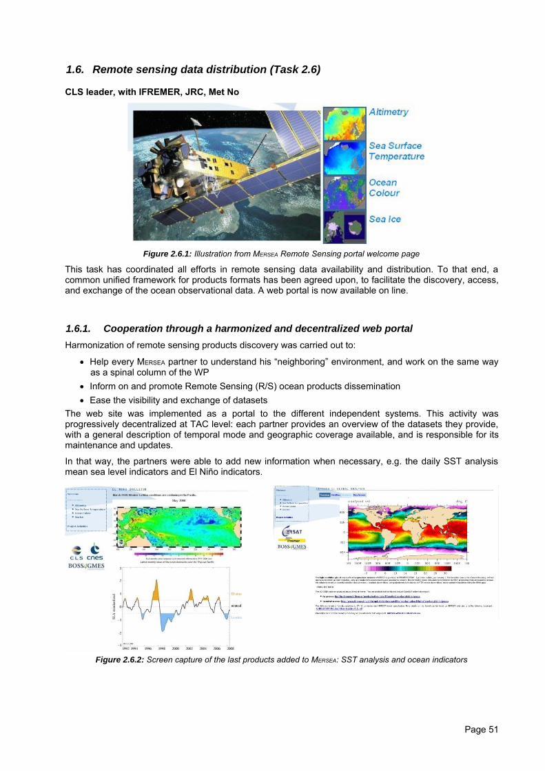
1.6. Remote sensing data distribution (Task 2.6)

CLS leader, with IFREMER, JRC, Met No

Figure 2.6.1: Illustration from MERSEA Remote Sensing portal welcome page

This task has coordinated all efforts in remote sensing data availability and distribution. To that end, acommon unified framework for products formats has been agreed upon, to facilitate the discovery, access,and exchange of the ocean observational data. A web portal is now available on line.

1.6.1. Cooperation through a harmonized and decentralized web portalHarmonization of remote sensing products discovery was carried out to:

• Help every MERSEA partner to understand his “neighboring” environment, and work on the same wayas a spinal column of the WP

• Inform on and promote Remote Sensing (R/S) ocean products dissemination• Ease the visibility and exchange of datasets

The web site was implemented as a portal to the different independent systems. This activity wasprogressively decentralized at TAC level: each partner provides an overview of the datasets they provide,with a general description of temporal mode and geographic coverage available, and is responsible for itsmaintenance and updates.

In that way, the partners were able to add new information when necessary, e.g. the daily SST analysismean sea level indicators and El Niño indicators.

Figure 2.6.2: Screen capture of the last products added to MERSEA: SST analysis and ocean indicators

Page 51

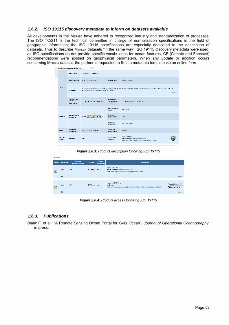
1.6.2. ISO 19115 discovery metadata to inform on datasets availableAll developments in the MERSEA have adhered to recognized industry and standardization of processes.The ISO TC/211 is the technical committee in charge of normalization specifications in the field ofgeographic information; the ISO 19115 specifications are especially dedicated to the description ofdatasets. Thus to describe MERSEA datasets “in the same way” ISO 19115 discovery metadata were used;as ISO specifications do not provide specific vocabularies for ocean features, CF (Climate and Forecast)recommendations were applied on geophysical parameters. When any update or addition occursconcerning MERSEA dataset, the partner is requested to fill in a metadata template via an online form.

Figure 2.6.3: Product description following ISO 19115

Figure 2.6.4: Product access following ISO 19115

1.6.3. PublicationsBlanc F. et al.: “A Remote Sensing Ocean Portal for GMES Ocean”, Journal of Operational Oceanography,

in press.

Page 52

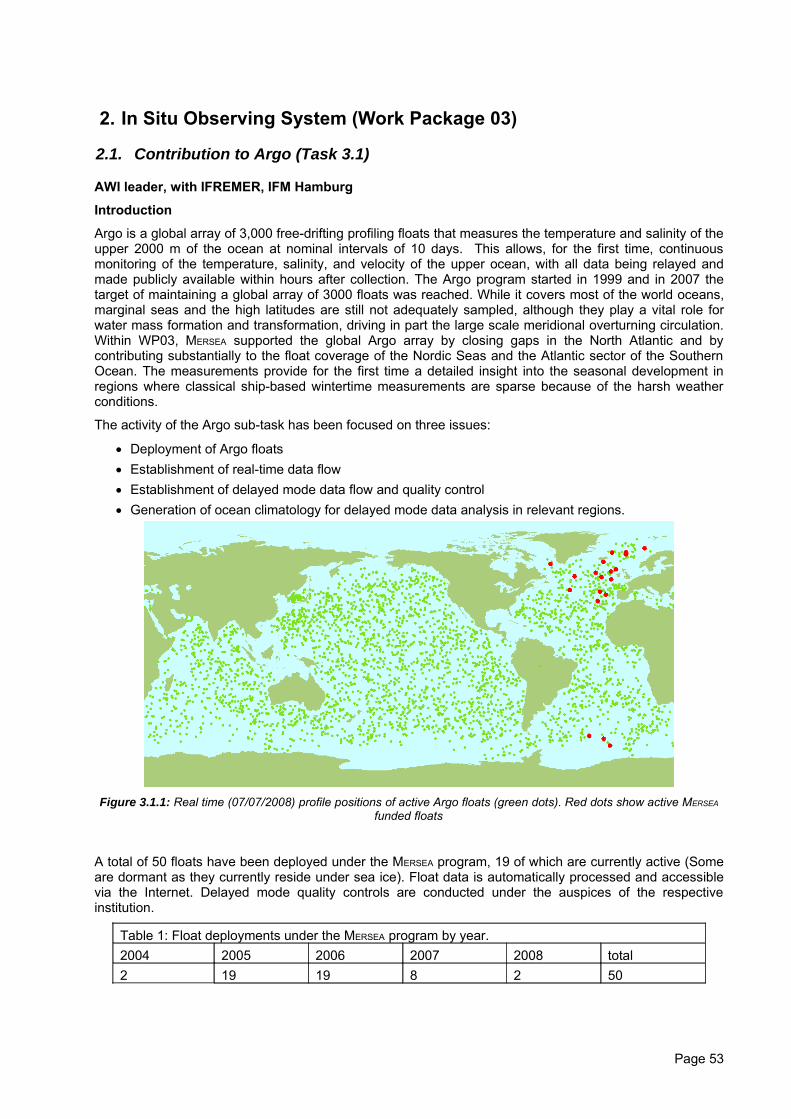
2. In Situ Observing System (Work Package 03)

2.1. Contribution to Argo (Task 3.1)

AWI leader, with IFREMER, IFM Hamburg

Introduction

Argo is a global array of 3,000 free-drifting profiling floats that measures the temperature and salinity of theupper 2000 m of the ocean at nominal intervals of 10 days. This allows, for the first time, continuousmonitoring of the temperature, salinity, and velocity of the upper ocean, with all data being relayed andmade publicly available within hours after collection. The Argo program started in 1999 and in 2007 thetarget of maintaining a global array of 3000 floats was reached. While it covers most of the world oceans,marginal seas and the high latitudes are still not adequately sampled, although they play a vital role forwater mass formation and transformation, driving in part the large scale meridional overturning circulation.Within WP03, MERSEA supported the global Argo array by closing gaps in the North Atlantic and bycontributing substantially to the float coverage of the Nordic Seas and the Atlantic sector of the SouthernOcean. The measurements provide for the first time a detailed insight into the seasonal development inregions where classical ship-based wintertime measurements are sparse because of the harsh weatherconditions.

The activity of the Argo sub-task has been focused on three issues:

• Deployment of Argo floats• Establishment of real-time data flow• Establishment of delayed mode data flow and quality control• Generation of ocean climatology for delayed mode data analysis in relevant regions.

Figure 3.1.1: Real time (07/07/2008) profile positions of active Argo floats (green dots). Red dots show active MERSEA

funded floats

A total of 50 floats have been deployed under the MERSEA program, 19 of which are currently active (Someare dormant as they currently reside under sea ice). Float data is automatically processed and accessiblevia the Internet. Delayed mode quality controls are conducted under the auspices of the respectiveinstitution.

Table 1: Float deployments under the MERSEA program by year. 2004 2005 2006 2007 2008 total2 19 19 8 2 50

Page 53

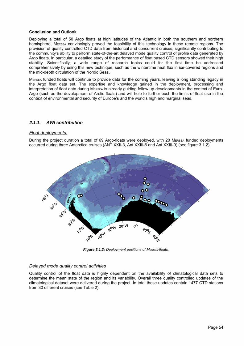
Conclusion and Outlook

Deploying a total of 50 Argo floats at high latitudes of the Atlantic in both the southern and northernhemisphere, MERSEA convincingly proved the feasibility of this technology in these remote regions. Theprovision of quality controlled CTD data from historical and concurrent cruises, significantly contributing tothe community’s ability to perform state-of-the-art delayed mode quality control of profile data generated byArgo floats. In particular, a detailed study of the performance of float based CTD sensors showed their highstability. Scientifically, a wide range of research topics could for the first time be addressedcomprehensively by using this new technique, such as the wintertime heat flux in ice-covered regions andthe mid-depth circulation of the Nordic Seas.

MERSEA funded floats will continue to provide data for the coming years, leaving a long standing legacy inthe Argo float data set. The expertise and knowledge gained in the deployment, processing andinterpretation of float data during MERSEA is already guiding follow up developments in the context of Euro-Argo (such as the development of Arctic floats) and will help to further push the limits of float use in thecontext of environmental and security of Europe’s and the world’s high and marginal seas.

2.1.1. AWI contribution

Float deployments:During the project duration a total of 69 Argo-floats were deployed, with 20 MERSEA funded deploymentsoccurred during three Antarctica cruises (ANT XXII-3, Ant XXIII-6 and Ant XXIII-9) (see figure 3.1.2).

60o

W 40o W 20oW 0o 20 o

E 40 oE 76

o S 72

o S 68

o S 64

o S 60

o S 56

o S

60o

W 40o W 20oW 0o 20 o

E 40 oE 76

o S 72

o S 68

o S 64

o S 60

o S 56

o S

Figure 3.1.2: Deployment positions of MERSEA-floats.

Delayed mode quality control activitiesQuality control of the float data is highly dependent on the availability of climatological data sets todetermine the mean state of the region and its variability. Overall three quality controlled updates of theclimatological dataset were delivered during the project. In total these updates contain 1477 CTD stationsfrom 30 different cruises (see Table 2).

Page 54

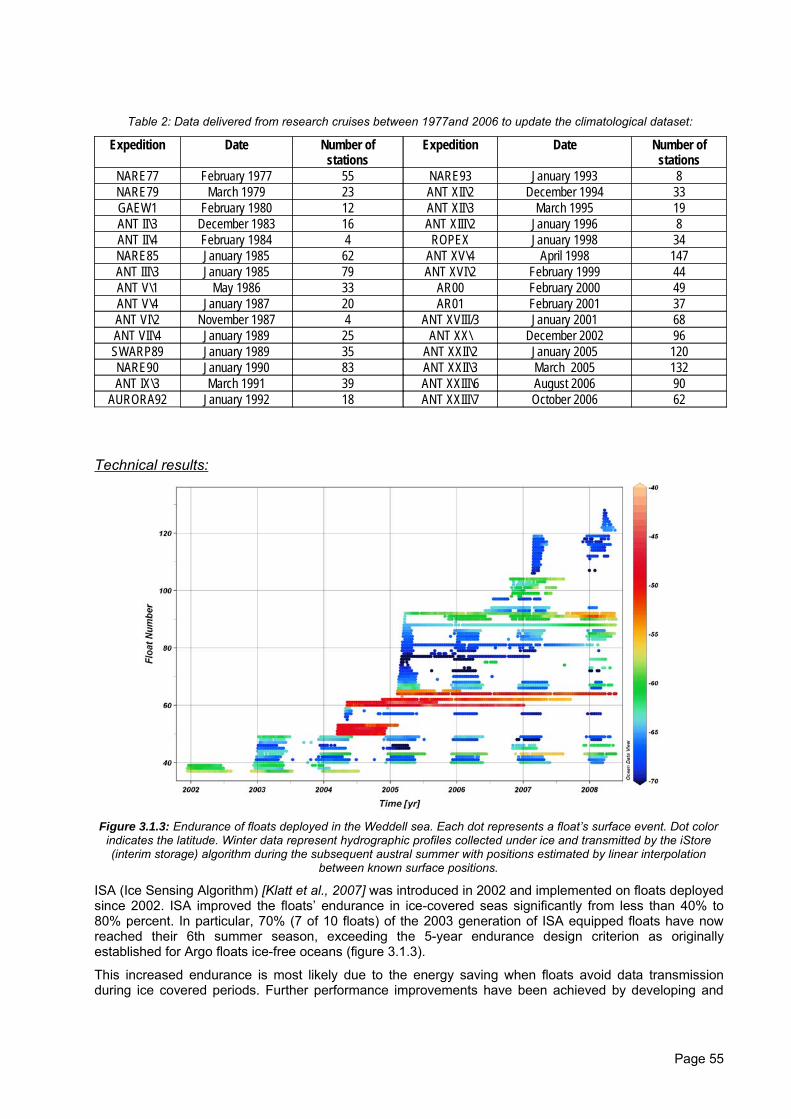
Table 2: Data delivered from research cruises between 1977and 2006 to update the climatological dataset:

Expedition Date Number ofstations

Expedition Date Number ofstations

NARE77 February 1977 55 NARE93 January 1993 8NARE79 March 1979 23 ANT XII\2 December 1994 33GAEW1 February 1980 12 ANT XII\3 March 1995 19ANT II\3 December 1983 16 ANT XIII\2 January 1996 8ANT II\4 February 1984 4 ROPEX January 1998 34NARE85 January 1985 62 ANT XV\4 April 1998 147ANT III\3 January 1985 79 ANT XVI\2 February 1999 44ANT V\1 May 1986 33 AR00 February 2000 49ANT V\4 January 1987 20 AR01 February 2001 37ANT VI\2 November 1987 4 ANT XVIII/3 January 2001 68ANT VII\4 January 1989 25 ANT XX\ December 2002 96SWARP89 January 1989 35 ANT XXII\2 January 2005 120NARE90 January 1990 83 ANT XXII\3 March 2005 132ANT IX\3 March 1991 39 ANT XXIII\6 August 2006 90

AURORA92 January 1992 18 ANT XXIII\7 October 2006 62

Technical results:

Figure 3.1.3: Endurance of floats deployed in the Weddell sea. Each dot represents a float’s surface event. Dot colorindicates the latitude. Winter data represent hydrographic profiles collected under ice and transmitted by the iStore(interim storage) algorithm during the subsequent austral summer with positions estimated by linear interpolation

between known surface positions.

ISA (Ice Sensing Algorithm) [Klatt et al., 2007] was introduced in 2002 and implemented on floats deployedsince 2002. ISA improved the floats’ endurance in ice-covered seas significantly from less than 40% to80% percent. In particular, 70% (7 of 10 floats) of the 2003 generation of ISA equipped floats have nowreached their 6th summer season, exceeding the 5-year endurance design criterion as originallyestablished for Argo floats ice-free oceans (figure 3.1.3).

This increased endurance is most likely due to the energy saving when floats avoid data transmissionduring ice covered periods. Further performance improvements have been achieved by developing and

Page 55

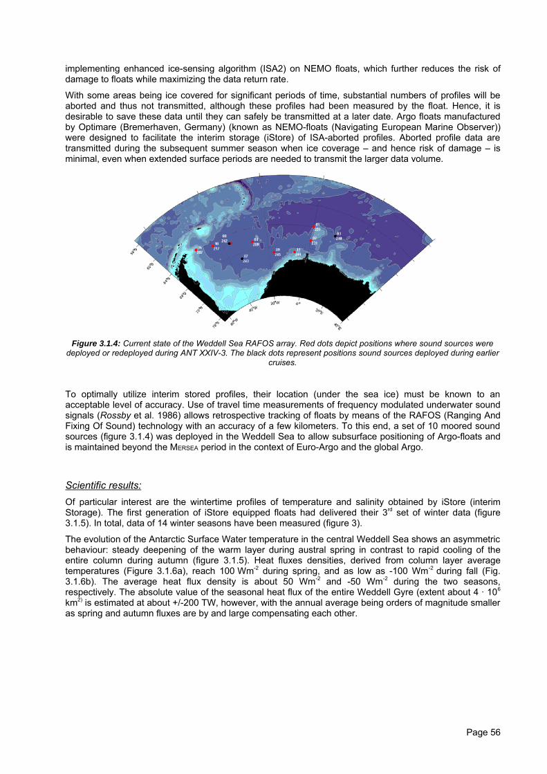
implementing enhanced ice-sensing algorithm (ISA2) on NEMO floats, which further reduces the risk ofdamage to floats while maximizing the data return rate.

With some areas being ice covered for significant periods of time, substantial numbers of profiles will beaborted and thus not transmitted, although these profiles had been measured by the float. Hence, it isdesirable to save these data until they can safely be transmitted at a later date. Argo floats manufacturedby Optimare (Bremerhaven, Germany) (known as NEMO-floats (Navigating European Marine Observer))were designed to facilitate the interim storage (iStore) of ISA-aborted profiles. Aborted profile data aretransmitted during the subsequent summer season when ice coverage – and hence risk of damage – isminimal, even when extended surface periods are needed to transmit the larger data volume.

Figure 3.1.4: Current state of the Weddell Sea RAFOS array. Red dots depict positions where sound sources weredeployed or redeployed during ANT XXIV-3. The black dots represent positions sound sources deployed during earlier

cruises.

To optimally utilize interim stored profiles, their location (under the sea ice) must be known to anacceptable level of accuracy. Use of travel time measurements of frequency modulated underwater soundsignals (Rossby et al. 1986) allows retrospective tracking of floats by means of the RAFOS (Ranging AndFixing Of Sound) technology with an accuracy of a few kilometers. To this end, a set of 10 moored soundsources (figure 3.1.4) was deployed in the Weddell Sea to allow subsurface positioning of Argo-floats andis maintained beyond the MERSEA period in the context of Euro-Argo and the global Argo.

Scientific results:Of particular interest are the wintertime profiles of temperature and salinity obtained by iStore (interimStorage). The first generation of iStore equipped floats had delivered their 3rd set of winter data (figure3.1.5). In total, data of 14 winter seasons have been measured (figure 3).

The evolution of the Antarctic Surface Water temperature in the central Weddell Sea shows an asymmetricbehaviour: steady deepening of the warm layer during austral spring in contrast to rapid cooling of theentire column during autumn (figure 3.1.5). Heat fluxes densities, derived from column layer averagetemperatures (Figure 3.1.6a), reach 100 Wm-2 during spring, and as low as -100 Wm-2 during fall (Fig.3.1.6b). The average heat flux density is about 50 Wm-2 and -50 Wm-2 during the two seasons,respectively. The absolute value of the seasonal heat flux of the entire Weddell Gyre (extent about 4 · 106

km2) is estimated at about +/-200 TW, however, with the annual average being orders of magnitude smalleras spring and autumn fluxes are by and large compensating each other.

Page 56

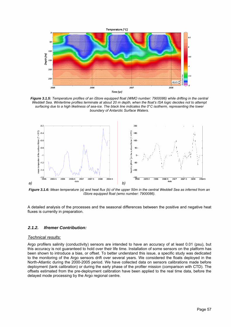
Figure 3.1.5: Temperature profiles of an iStore equipped float (WMO number: 7900086) while drifting in the centralWeddell Sea. Wintertime profiles terminate at about 20 m depth, when the float’s ISA logic decides not to attempt

surfacing due to a high likeliness of sea-ice. The black line indicates the 0°C isotherm, representing the lowerboundary of Antarctic Surface Waters.

a) b) Figure 3.1.6: Mean temperature (a) and heat flux (b) of the upper 50m in the central Weddell Sea as inferred from an

iStore equipped float (wmo number: 7900086).

A detailed analysis of the processes and the seasonal differences between the positive and negative heatfluxes is currently in preparation.

2.1.2. Ifremer Contribution:

Technical results:Argo profilers salinity (conductivity) sensors are intended to have an accuracy of at least 0.01 (psu), butthis accuracy is not guaranteed to hold over their life time. Installation of some sensors on the platform hasbeen shown to introduce a bias, or offset. To better understand this issue, a specific study was dedicatedto the monitoring of the Argo sensors drift over several years. We considered the floats deployed in theNorth-Atlantic during the 2000-2005 period. We have collected data on sensors calibrations made beforedeployment (tank calibration) or during the early phase of the profiler mission (comparison with CTD). Theoffsets estimated from the pre-deployment calibration have been applied to the real time data, before thedelayed mode processing by the Argo regional centre.

Page 57

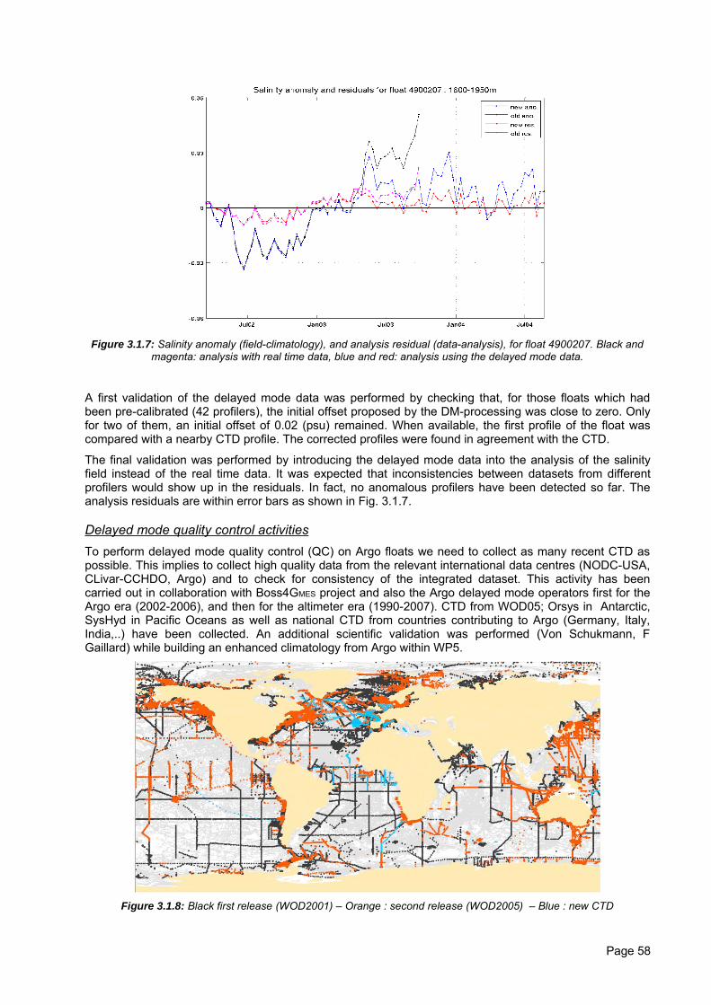
Figure 3.1.7: Salinity anomaly (field-climatology), and analysis residual (data-analysis), for float 4900207. Black andmagenta: analysis with real time data, blue and red: analysis using the delayed mode data.

A first validation of the delayed mode data was performed by checking that, for those floats which hadbeen pre-calibrated (42 profilers), the initial offset proposed by the DM-processing was close to zero. Onlyfor two of them, an initial offset of 0.02 (psu) remained. When available, the first profile of the float wascompared with a nearby CTD profile. The corrected profiles were found in agreement with the CTD.

The final validation was performed by introducing the delayed mode data into the analysis of the salinityfield instead of the real time data. It was expected that inconsistencies between datasets from differentprofilers would show up in the residuals. In fact, no anomalous profilers have been detected so far. Theanalysis residuals are within error bars as shown in Fig. 3.1.7.

Delayed mode quality control activitiesTo perform delayed mode quality control (QC) on Argo floats we need to collect as many recent CTD aspossible. This implies to collect high quality data from the relevant international data centres (NODC-USA,CLivar-CCHDO, Argo) and to check for consistency of the integrated dataset. This activity has beencarried out in collaboration with Boss4GMES project and also the Argo delayed mode operators first for theArgo era (2002-2006), and then for the altimeter era (1990-2007). CTD from WOD05; Orsys in Antarctic,SysHyd in Pacific Oceans as well as national CTD from countries contributing to Argo (Germany, Italy,India,..) have been collected. An additional scientific validation was performed (Von Schukmann, FGaillard) while building an enhanced climatology from Argo within WP5.

Figure 3.1.8: Black first release (WOD2001) – Orange : second release (WOD2005) – Blue : new CTD

Page 58

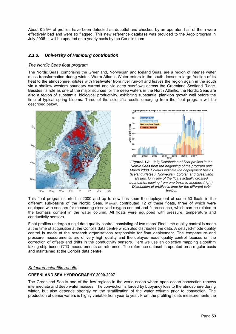
About 0.25% of profiles have been detected as doubtful and checked by an operator; half of them wereeffectively bad and were so flagged. This new reference database was provided to the Argo program inJuly 2008. It will be updated on a yearly basis by the Coriolis team.

2.1.3. University of Hamburg contribution

The Nordic Seas float programThe Nordic Seas, comprising the Greenland, Norwegian and Iceland Seas, are a region of intense watermass transformation during winter. Warm Atlantic Water enters in the south, looses a large fraction of itsheat to the atmosphere, dilutes with freshwater from river run-off and leaves the region again in the southvia a shallow western boundary current and via deep overflows across the Greenland Scotland Ridge.Besides its role as one of the major sources for the deep waters in the North Atlantic, the Nordic Seas arealso a region of substantial biological productivity, exhibiting substantial plankton growth well before thetime of typical spring blooms. Three of the scientific results emerging from the float program will bedescribed below.

Figure3.1.8: (left) Distribution of float profiles in theNordic Seas from the beginning of the program untilMarch 2008. Colours indicate the deployment basins(Iceland Plateau, Norwegian, Lofoten and Greenland

Basins. Only few of the floats actually crossedboundaries moving from one basin to another. (right):

Distribution of profiles in time for the different sub-basins.

This float program started in 2000 and up to now has seen the deployment of some 50 floats in thedifferent sub-basins of the Nordic Seas. MERSEA contributed 12 of these floats, three of which wereequipped with sensors for measuring dissolved oxygen content and fluorescence, which can be related tothe biomass content in the water column. All floats were equipped with pressure, temperature andconductivity sensors.

Float profiles undergo a rigid data quality control, consisting of two steps. Real time quality control is madeat the time of acquisition at the Coriolis data centre which also distributes the data. A delayed-mode qualitycontrol is made at the research organisations responsible for float deployment. The temperature andpressure measurements are of very high quality and the delayed-mode quality control focuses on thecorrection of offsets and drifts in the conductivity sensors. Here we use an objective mapping algorithmtaking ship based CTD measurements as reference. The reference dataset is updated on a regular basisand maintained at the Coriolis data centre.

Selected scientific resultsGREENLAND SEA HYDROGRAPHY 2000-2007

The Greenland Sea is one of the few regions in the world ocean where open ocean convection renewsintermediate and deep water masses. The convection is forced by buoyancy loss to the atmosphere duringwinter, but also depends strongly on the stratification of the water column prior to convection. Theproduction of dense waters is highly variable from year to year. From the profiling floats measurements the

Page 59

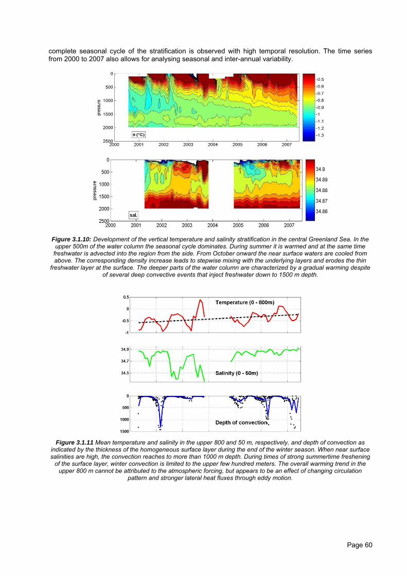
complete seasonal cycle of the stratification is observed with high temporal resolution. The time seriesfrom 2000 to 2007 also allows for analysing seasonal and inter-annual variability.

Figure 3.1.10: Development of the vertical temperature and salinity stratification in the central Greenland Sea. In theupper 500m of the water column the seasonal cycle dominates. During summer it is warmed and at the same time

freshwater is advected into the region from the side. From October onward the near surface waters are cooled fromabove. The corresponding density increase leads to stepwise mixing with the underlying layers and erodes the thin

freshwater layer at the surface. The deeper parts of the water column are characterized by a gradual warming despiteof several deep convective events that inject freshwater down to 1500 m depth.

Figure 3.1.11 Mean temperature and salinity in the upper 800 and 50 m, respectively, and depth of convection asindicated by the thickness of the homogeneous surface layer during the end of the winter season. When near surfacesalinities are high, the convection reaches to more than 1000 m depth. During times of strong summertime freshening

of the surface layer, winter convection is limited to the upper few hundred meters. The overall warming trend in theupper 800 m cannot be attributed to the atmospheric forcing, but appears to be an effect of changing circulation

pattern and stronger lateral heat fluxes through eddy motion.

Page 60

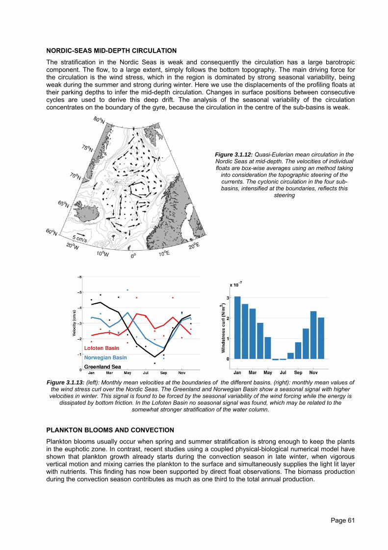
NORDIC-SEAS MID-DEPTH CIRCULATION

The stratification in the Nordic Seas is weak and consequently the circulation has a large barotropiccomponent. The flow, to a large extent, simply follows the bottom topography. The main driving force forthe circulation is the wind stress, which in the region is dominated by strong seasonal variability, beingweak during the summer and strong during winter. Here we use the displacements of the profiling floats attheir parking depths to infer the mid-depth circulation. Changes in surface positions between consecutivecycles are used to derive this deep drift. The analysis of the seasonal variability of the circulationconcentrates on the boundary of the gyre, because the circulation in the centre of the sub-basins is weak.

Figure 3.1.12: Quasi-Eulerian mean circulation in theNordic Seas at mid-depth. The velocities of individualfloats are box-wise averages using an method taking

into consideration the topographic steering of thecurrents. The cyclonic circulation in the four sub-basins, intensified at the boundaries, reflects this

steering

Figure 3.1.13: (left): Monthly mean velocities at the boundaries of the different basins. (right): monthly mean values of

the wind stress curl over the Nordic Seas. The Greenland and Norwegian Basin show a seasonal signal with highervelocities in winter. This signal is found to be forced by the seasonal variability of the wind forcing while the energy is

dissipated by bottom friction. In the Lofoten Basin no seasonal signal was found, which may be related to thesomewhat stronger stratification of the water column.

PLANKTON BLOOMS AND CONVECTION

Plankton blooms usually occur when spring and summer stratification is strong enough to keep the plantsin the euphotic zone. In contrast, recent studies using a coupled physical-biological numerical model haveshown that plankton growth already starts during the convection season in late winter, when vigorousvertical motion and mixing carries the plankton to the surface and simultaneously supplies the light lit layerwith nutrients. This finding has now been supported by direct float observations. The biomass productionduring the convection season contributes as much as one third to the total annual production.

Page 61

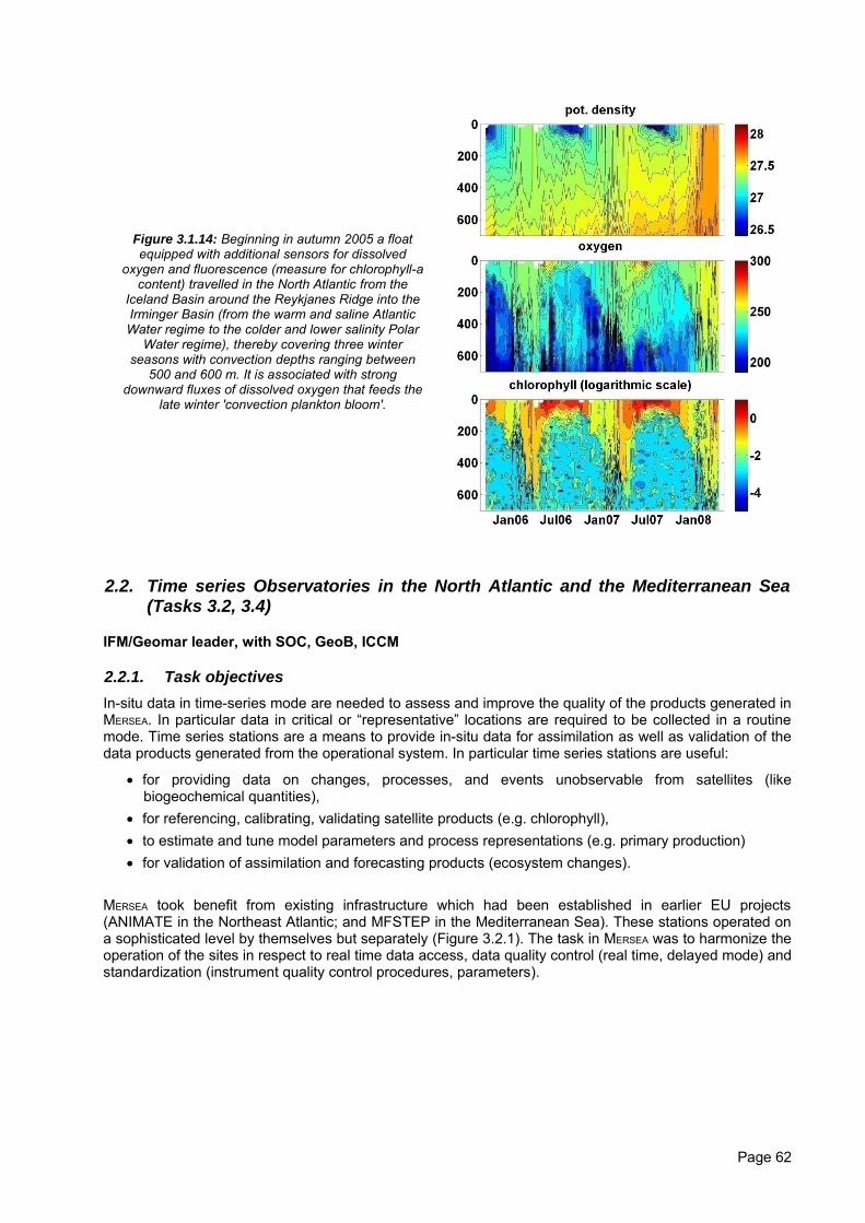
Figure 3.1.14: Beginning in autumn 2005 a floatequipped with additional sensors for dissolved

oxygen and fluorescence (measure for chlorophyll-acontent) travelled in the North Atlantic from the

Iceland Basin around the Reykjanes Ridge into theIrminger Basin (from the warm and saline AtlanticWater regime to the colder and lower salinity Polar

Water regime), thereby covering three winterseasons with convection depths ranging between

500 and 600 m. It is associated with strongdownward fluxes of dissolved oxygen that feeds the

late winter 'convection plankton bloom'.

2.2. Time series Observatories in the North Atlantic and the Mediterranean Sea(Tasks 3.2, 3.4)

IFM/Geomar leader, with SOC, GeoB, ICCM

2.2.1. Task objectivesIn-situ data in time-series mode are needed to assess and improve the quality of the products generated inMERSEA. In particular data in critical or “representative” locations are required to be collected in a routinemode. Time series stations are a means to provide in-situ data for assimilation as well as validation of thedata products generated from the operational system. In particular time series stations are useful:

• for providing data on changes, processes, and events unobservable from satellites (likebiogeochemical quantities),

• for referencing, calibrating, validating satellite products (e.g. chlorophyll),• to estimate and tune model parameters and process representations (e.g. primary production)• for validation of assimilation and forecasting products (ecosystem changes).

MERSEA took benefit from existing infrastructure which had been established in earlier EU projects(ANIMATE in the Northeast Atlantic; and MFSTEP in the Mediterranean Sea). These stations operated ona sophisticated level by themselves but separately (Figure 3.2.1). The task in MERSEA was to harmonize theoperation of the sites in respect to real time data access, data quality control (real time, delayed mode) andstandardization (instrument quality control procedures, parameters).

Page 62

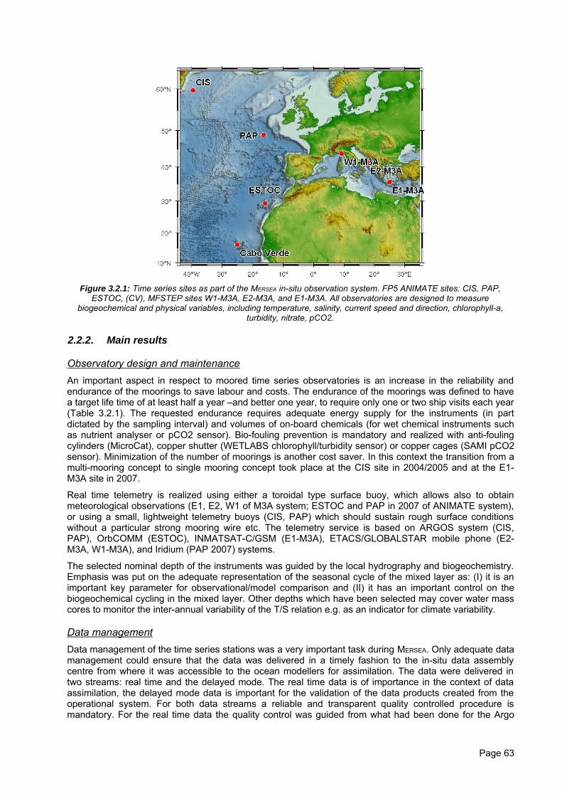
Figure 3.2.1: Time series sites as part of the MERSEA in-situ observation system. FP5 ANIMATE sites: CIS, PAP,ESTOC, (CV), MFSTEP sites W1-M3A, E2-M3A, and E1-M3A. All observatories are designed to measure

biogeochemical and physical variables, including temperature, salinity, current speed and direction, chlorophyll-a,turbidity, nitrate, pCO2.

2.2.2. Main results

Observatory design and maintenanceAn important aspect in respect to moored time series observatories is an increase in the reliability andendurance of the moorings to save labour and costs. The endurance of the moorings was defined to havea target life time of at least half a year –and better one year, to require only one or two ship visits each year(Table 3.2.1). The requested endurance requires adequate energy supply for the instruments (in partdictated by the sampling interval) and volumes of on-board chemicals (for wet chemical instruments suchas nutrient analyser or pCO2 sensor). Bio-fouling prevention is mandatory and realized with anti-foulingcylinders (MicroCat), copper shutter (WETLABS chlorophyll/turbidity sensor) or copper cages (SAMI pCO2sensor). Minimization of the number of moorings is another cost saver. In this context the transition from amulti-mooring concept to single mooring concept took place at the CIS site in 2004/2005 and at the E1-M3A site in 2007.

Real time telemetry is realized using either a toroidal type surface buoy, which allows also to obtainmeteorological observations (E1, E2, W1 of M3A system; ESTOC and PAP in 2007 of ANIMATE system),or using a small, lightweight telemetry buoys (CIS, PAP) which should sustain rough surface conditionswithout a particular strong mooring wire etc. The telemetry service is based on ARGOS system (CIS,PAP), OrbCOMM (ESTOC), INMATSAT-C/GSM (E1-M3A), ETACS/GLOBALSTAR mobile phone (E2-M3A, W1-M3A), and Iridium (PAP 2007) systems.

The selected nominal depth of the instruments was guided by the local hydrography and biogeochemistry.Emphasis was put on the adequate representation of the seasonal cycle of the mixed layer as: (I) it is animportant key parameter for observational/model comparison and (II) it has an important control on thebiogeochemical cycling in the mixed layer. Other depths which have been selected may cover water masscores to monitor the inter-annual variability of the T/S relation e.g. as an indicator for climate variability.

Data managementData management of the time series stations was a very important task during MERSEA. Only adequate datamanagement could ensure that the data was delivered in a timely fashion to the in-situ data assemblycentre from where it was accessible to the ocean modellers for assimilation. The data were delivered intwo streams: real time and the delayed mode. The real time data is of importance in the context of dataassimilation, the delayed mode data is important for the validation of the data products created from theoperational system. For both data streams a reliable and transparent quality controlled procedure ismandatory. For the real time data the quality control was guided from what had been done for the Argo

Page 63

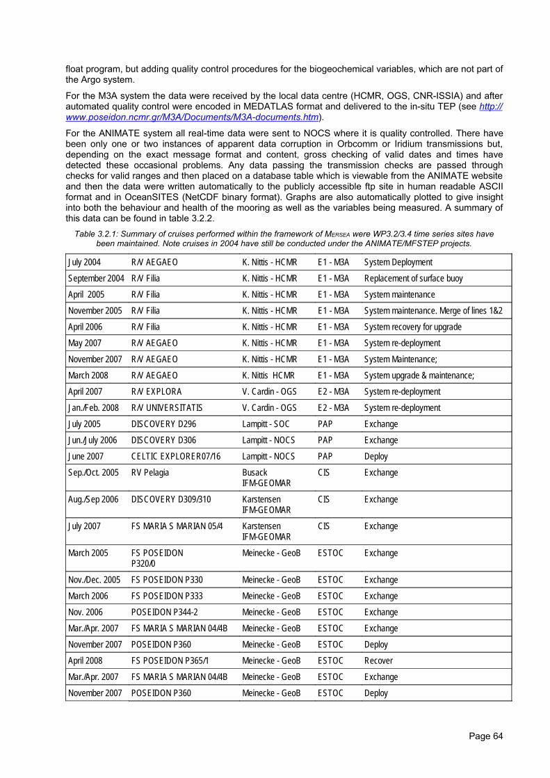
float program, but adding quality control procedures for the biogeochemical variables, which are not part ofthe Argo system.

For the M3A system the data were received by the local data centre (HCMR, OGS, CNR-ISSIA) and afterautomated quality control were encoded in MEDATLAS format and delivered to the in-situ TEP (see http://www.poseidon.ncmr.gr/M3A/Documents/M3A-documents.htm).

For the ANIMATE system all real-time data were sent to NOCS where it is quality controlled. There havebeen only one or two instances of apparent data corruption in Orbcomm or Iridium transmissions but,depending on the exact message format and content, gross checking of valid dates and times havedetected these occasional problems. Any data passing the transmission checks are passed throughchecks for valid ranges and then placed on a database table which is viewable from the ANIMATE websiteand then the data were written automatically to the publicly accessible ftp site in human readable ASCIIformat and in OceanSITES (NetCDF binary format). Graphs are also automatically plotted to give insightinto both the behaviour and health of the mooring as well as the variables being measured. A summary ofthis data can be found in table 3.2.2.

Table 3.2.1: Summary of cruises performed within the framework of MERSEA were WP3.2/3.4 time series sites havebeen maintained. Note cruises in 2004 have still be conducted under the ANIMATE/MFSTEP projects.

July 2004 R/V AEGAEO K. Nittis - HCMR E1 - M3A System Deployment

September 2004 R/V Filia K. Nittis - HCMR E1 - M3A Replacement of surface buoy

April 2005 R/V Filia K. Nittis - HCMR E1 - M3A System maintenance

November 2005 R/V Filia K. Nittis - HCMR E1 - M3A System maintenance. Merge of lines 1&2

April 2006 R/V Filia K. Nittis - HCMR E1 - M3A System recovery for upgrade

May 2007 R/V AEGAEO K. Nittis - HCMR E1 - M3A System re-deployment

November 2007 R/V AEGAEO K. Nittis - HCMR E1 - M3A System Maintenance;

March 2008 R/V AEGAEO K. Nittis HCMR E1 - M3A System upgrade & maintenance;

April 2007 R/V EXPLORA V. Cardin - OGS E2 - M3A System re-deployment

Jan./Feb. 2008 R/V UNIVERSITATIS V. Cardin - OGS E2 - M3A System re-deployment

July 2005 DISCOVERY D296 Lampitt - SOC PAP Exchange

Jun./July 2006 DISCOVERY D306 Lampitt - NOCS PAP Exchange

June 2007 CELTIC EXPLORER07/16 Lampitt - NOCS PAP Deploy

Sep./Oct. 2005 RV Pelagia BusackIFM-GEOMAR

CIS Exchange

Aug./Sep 2006 DISCOVERY D309/310 Karstensen IFM-GEOMAR

CIS Exchange

July 2007 FS MARIA S MARIAN 05/4 Karstensen IFM-GEOMAR

CIS Exchange

March 2005 FS POSEIDONP320/0

Meinecke - GeoB ESTOC Exchange

Nov./Dec. 2005 FS POSEIDON P330 Meinecke - GeoB ESTOC Exchange

March 2006 FS POSEIDON P333 Meinecke - GeoB ESTOC Exchange

Nov. 2006 POSEIDON P344-2 Meinecke - GeoB ESTOC Exchange

Mar./Apr. 2007 FS MARIA S MARIAN 04/4B Meinecke - GeoB ESTOC Exchange

November 2007 POSEIDON P360 Meinecke - GeoB ESTOC Deploy

April 2008 FS POSEIDON P365/1 Meinecke - GeoB ESTOC Recover

Mar./Apr. 2007 FS MARIA S MARIAN 04/4B Meinecke - GeoB ESTOC Exchange

November 2007 POSEIDON P360 Meinecke - GeoB ESTOC Deploy

Page 64

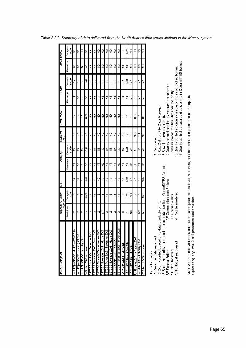
Table 3.2.2: Summary of data delivered from the North Atlantic time series stations to the MERSEA system.

Page 65

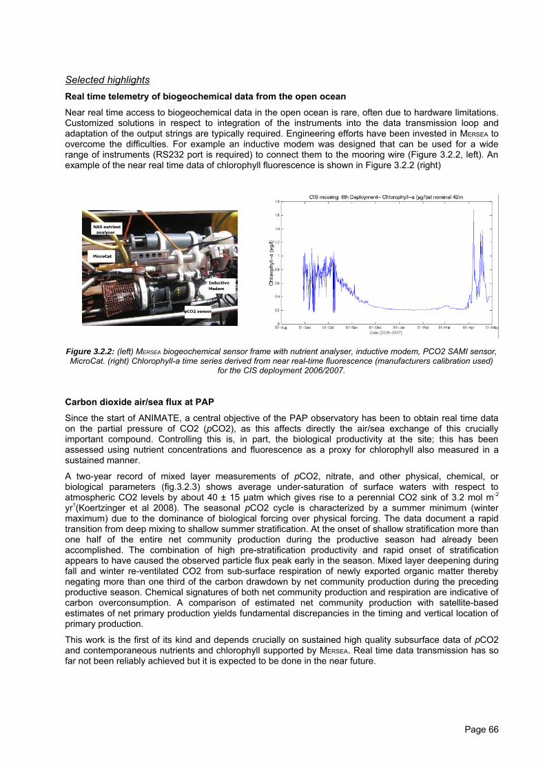
Selected highlightsReal time telemetry of biogeochemical data from the open ocean

Near real time access to biogeochemical data in the open ocean is rare, often due to hardware limitations.Customized solutions in respect to integration of the instruments into the data transmission loop andadaptation of the output strings are typically required. Engineering efforts have been invested in MERSEA toovercome the difficulties. For example an inductive modem was designed that can be used for a widerange of instruments (RS232 port is required) to connect them to the mooring wire (Figure 3.2.2, left). Anexample of the near real time data of chlorophyll fluorescence is shown in Figure 3.2.2 (right)

Figure 3.2.2: (left) MERSEA biogeochemical sensor frame with nutrient analyser, inductive modem, PCO2 SAMI sensor,MicroCat. (right) Chlorophyll-a time series derived from near real-time fluorescence (manufacturers calibration used)

for the CIS deployment 2006/2007.

Carbon dioxide air/sea flux at PAP

Since the start of ANIMATE, a central objective of the PAP observatory has been to obtain real time dataon the partial pressure of CO2 (pCO2), as this affects directly the air/sea exchange of this cruciallyimportant compound. Controlling this is, in part, the biological productivity at the site; this has beenassessed using nutrient concentrations and fluorescence as a proxy for chlorophyll also measured in asustained manner.

A two-year record of mixed layer measurements of pCO2, nitrate, and other physical, chemical, orbiological parameters (fig.3.2.3) shows average under-saturation of surface waters with respect toatmospheric CO2 levels by about 40 ± 15 µatm which gives rise to a perennial CO2 sink of 3.2 mol m-2

yr1(Koertzinger et al 2008). The seasonal pCO2 cycle is characterized by a summer minimum (wintermaximum) due to the dominance of biological forcing over physical forcing. The data document a rapidtransition from deep mixing to shallow summer stratification. At the onset of shallow stratification more thanone half of the entire net community production during the productive season had already beenaccomplished. The combination of high pre-stratification productivity and rapid onset of stratificationappears to have caused the observed particle flux peak early in the season. Mixed layer deepening duringfall and winter re-ventilated CO2 from sub-surface respiration of newly exported organic matter therebynegating more than one third of the carbon drawdown by net community production during the precedingproductive season. Chemical signatures of both net community production and respiration are indicative ofcarbon overconsumption. A comparison of estimated net community production with satellite-basedestimates of net primary production yields fundamental discrepancies in the timing and vertical location ofprimary production.

This work is the first of its kind and depends crucially on sustained high quality subsurface data of pCO2and contemporaneous nutrients and chlorophyll supported by MERSEA. Real time data transmission has sofar not been reliably achieved but it is expected to be done in the near future.

Page 66

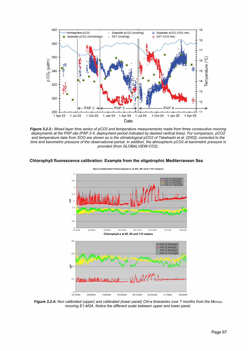
Figure 3.2.3.: Mixed layer time series of pCO2 and temperature measurements made from three consecutive mooringdeployments at the PAP site (PAP 2-4, deployment period indicated by dashed vertical lines). For comparison, pCO2and temperature data from SOO are shown as is the climatological pCO2 of Takahashi et al. [2002], corrected to the

time and barometric pressure of the observational period. In addition, the atmospheric pCO2 at barometric pressure isprovided (from GLOBALVIEW-CO2).

Chlorophyll fluorescence calibration: Example from the oligotrophic Mediterranean Sea

Non-Calibrated Chlorophyll-a at 65, 90 and 115 meters

0

0.5

1

1.5

2

2.5

3

3.5

4

21/7/04 20/8/04 19/9/04 19/10/04 18/11/04 18/12/04 17/1/05 16/2/05

μg

/

Chlr, L2, 40m [μg/l]Chlr, L2, 65m[μg/l]Chlr, L2, 90m [μg/l]Chlr, L2, 115m [μg/l]

Chlorophyll-a at 65, 90 and 115 meters

0

0.1

0.2

0.3

0.4

21/7/2004 20/8/2004 19/9/2004 19/10/2004 18/11/2004 18/12/2004 17/1/2005 16/2/2005

μg/l

Chlr, L2, 40m [μg/l]Chlr, L2, 65m[μg/l]Chlr, L2, 90m [μg/l]Chlr, L2, 115m [μg/l]

Figure 3.2.4: Non calibrated (upper) and calibrated (lower panel) Chl-a timeseries over 7 months from the MERSEA

mooring E1-M3A. Notice the different scale between upper and lower panel.

Page 67

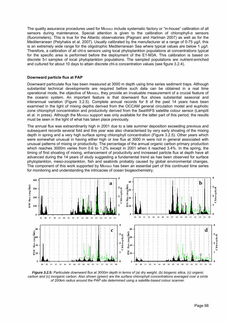
The quality assurance procedures used for MERSEA include systematic factory or “in-house” calibration of allsensors during maintenance. Special attention is given to the calibration of chlorophyll-α sensors(fluorometers). This is true for the Atlantic observatories (Pagnani and Hartman 2007) as well as for theMediterranean (Petyhakis et al. 2007). Usually calibrated by the manufacturer at a range of 0-75 μg/l, thisis an extremely wide range for the oligotrophic Mediterranean Sea where typical values are below 1 μg/l.Therefore, a calibration of all chl-α sensors using local phytoplankton populations at concentrations typicalfor the specific area is performed before the deployment of the E1-M3A. This calibration is based ondiscrete 5-l samples of local phytoplankton populations. The sampled populations are nutrient-enrichedand cultured for about 10 days to attain discrete chl-α concentration values (see figure 3.2.4).

Downward particle flux at PAP

Downward particulate flux has been measured at 3000 m depth using time series sediment traps. Althoughsubstantial technical developments are required before such data can be obtained in a real timeoperational mode, the objective of MERSEA, they provide an invaluable measurement of a crucial feature ofthe oceanic system. An important feature is that downward flux shows substantial seasonal andinterannual variation (Figure 3.2.5). Complete annual records for 8 of the past 14 years have beenexamined in the light of mixing depths derived from the OCCAM general circulation model and euphoticzone chlorophyll concentration and productivity derived from the SeaWiFS satellite colour sensor (Lampittet al. in press). Although the MERSEA support was only available for the latter part of this period, the resultsmust be seen in the light of what has taken place previously.

The annual flux was extraordinarily high in 2001 due to a late summer deposition exceeding previous andsubsequent records several fold and this year was also characterised by very early shoaling of the mixingdepth in spring and a very high surface spring chlorophyll concentration (Figure 3.2.5). Other years whichwere somewhat unusual in having either high or low flux at 3000 m were not in general associated withunusual patterns of mixing or productivity. The percentage of the annual organic carbon primary productionwhich reaches 3000m varies from 0.6 to 1.2% except in 2001 when it reached 3.4%. In the spring, thetiming of first shoaling of mixing, enhancement of productivity and increased particle flux at depth have alladvanced during the 14 years of study suggesting a fundamental trend as has been observed for surfacephytoplankton, meso-zooplankton, fish and seabirds probably caused by global environmental changes.The component of this work supported by MERSEA has been an essential part of this continued time seriesfor monitoring and understanding the intricacies of ocean biogeochemistry.

Figure 3.2.5: Particulate downward flux at 3000m depth in terms of (a) dry weight, (b) biogenic silica, (c) organiccarbon and (c) inorganic carbon. Also shown (green) are the surface chlorophyll concentrations averaged over a circle

of 200km radius around the PAP site determined using a satellite-based colour scanner.

Page 68

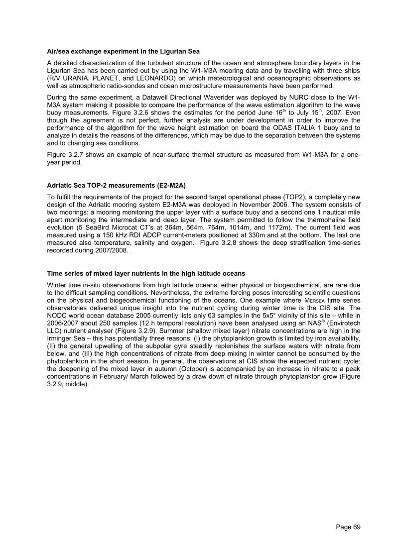
Air/sea exchange experiment in the Ligurian Sea

A detailed characterization of the turbulent structure of the ocean and atmosphere boundary layers in theLigurian Sea has been carried out by using the W1-M3A mooring data and by travelling with three ships(R/V URANIA, PLANET, and LEONARDO) on which meteorological and oceanographic observations aswell as atmospheric radio-sondes and ocean microstructure measurements have been performed.

During the same experiment, a Datawell Directional Waverider was deployed by NURC close to the W1-M3A system making it possible to compare the performance of the wave estimation algorithm to the wavebuoy measurements. Figure 3.2.6 shows the estimates for the period June 16th to July 15th, 2007. Eventhough the agreement is not perfect, further analysis are under development in order to improve theperformance of the algorithm for the wave height estimation on board the ODAS ITALIA 1 buoy and toanalyze in details the reasons of the differences, which may be due to the separation between the systemsand to changing sea conditions.

Figure 3.2.7 shows an example of near-surface thermal structure as measured from W1-M3A for a one-year period.

Adriatic Sea TOP-2 measurements (E2-M2A)

To fulfill the requirements of the project for the second target operational phase (TOP2), a completely newdesign of the Adriatic mooring system E2-M3A was deployed in November 2006. The system consists oftwo moorings: a mooring monitoring the upper layer with a surface buoy and a second one 1 nautical mileapart monitoring the intermediate and deep layer. The system permitted to follow the thermohaline fieldevolution (5 SeaBird Microcat CT’s at 364m, 564m, 764m, 1014m, and 1172m). The current field wasmeasured using a 150 kHz RDI ADCP current-meters positioned at 330m and at the bottom. The last onemeasured also temperature, salinity and oxygen. Figure 3.2.8 shows the deep stratification time-seriesrecorded during 2007/2008.

Time series of mixed layer nutrients in the high latitude oceans

Winter time in-situ observations from high latitude oceans, either physical or biogeochemical, are rare dueto the difficult sampling conditions. Nevertheless, the extreme forcing poses interesting scientific questionson the physical and biogeochemical functioning of the oceans. One example where MERSEA time seriesobservatories delivered unique insight into the nutrient cycling during winter time is the CIS site. TheNODC world ocean database 2005 currently lists only 63 samples in the 5x5° vicinity of this site – while in2006/2007 about 250 samples (12 h temporal resolution) have been analysed using an NAS© (EnvirotechLLC) nutrient analyser (Figure 3.2.9). Summer (shallow mixed layer) nitrate concentrations are high in theIrminger Sea – this has potentially three reasons: (I) the phytoplankton growth is limited by iron availability,(II) the general upwelling of the subpolar gyre steadily replenishes the surface waters with nitrate frombelow, and (III) the high concentrations of nitrate from deep mixing in winter cannot be consumed by thephytoplankton in the short season. In general, the observations at CIS show the expected nutrient cycle:the deepening of the mixed layer in autumn (October) is accompanied by an increase in nitrate to a peakconcentrations in February/ March followed by a draw down of nitrate through phytoplankton grow (Figure3.2.9, middle).

Page 69

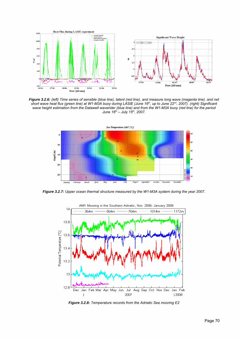
Figure 3.2.6: (left) Time series of sensible (blue line), latent (red line), and measure long wave (magenta line). and netshort wave heat flux (green line) at W1-M3A buoy during LASIE (June 16th, up to June 22nd, 2007). (right) Significantwave height estimation from the Datawell waverider (blue line) and from the W1-M3A buoy (red line) for the period

June 16th – July 15th, 2007.

Figure 3.2.7: Upper ocean thermal structure measured by the W1-M3A system during the year 2007.

Figure 3.2.8: Temperature records from the Adriatic Sea mooring E2

Page 70

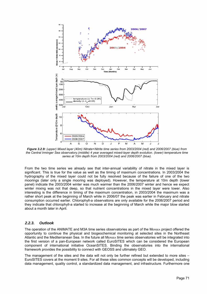
Figure 3.2.9: (upper) Mixed layer (40m) Nitrate+Nitrite time series from 2003/2004 (red) and 2006/2007 (blue) fromthe Central Irminger Sea observatory.(middle) 4 year averaged mixed-layer depth evolution. (lower) temperature time

series at 10m depth from 2003/2004 (red) and 2006/2007 (blue).

From the two time series we already see that inter-annual variability of nitrate in the mixed layer issignificant. This is true for the value as well as the timing of maximum concentrations. In 2003/2004 thehydrography of the mixed layer could not be fully resolved because of the failure of one of the twomoorings (later only a single mooring was deployed). However, the temperature at 10m depth (lowerpanel) indicate the 2003/2004 winter was much warmer than the 2006/2007 winter and hence we expectwinter mixing was not that deep, so that nutrient concentrations in the mixed layer were lower. Alsointeresting is the difference in timing of the maximum concentration, in 2003/2004 the maximum was arather short peak at the beginning of March while in 2006/07 the peak was earlier in February and nitrateconsumption occurred earlier. Chlorophyll-a observations are only available for the 2006/2007 period andthey indicate that chlorophyll-a started to increase at the beginning of March while the major blow startedabout a month later in April.

2.2.3. OutlookThe operation of the ANIMATE and M3A time series observatories as part of the MERSEA project offered theopportunity to continue the physical and biogeochemical monitoring at selected sites in the NortheastAtlantic and the Mediterranean Sea. In the future all MERSEA time series observatories will be integrated intothe first version of a pan-European network called EuroSITES which can be considered the Europeancomponent of international initiative OceanSITES. Binding the observatories into the internationalframework provides the possibility to connect with GEOSS and ultimately GEO.

The management of the sites and the data will not only be further refined but extended to more sites –EuroSITES covers at the moment 9 sites. For all these sites common concepts will be developed, includingdata management, quality control, a standardized data management, and infrastructure. Furthermore one

Page 71

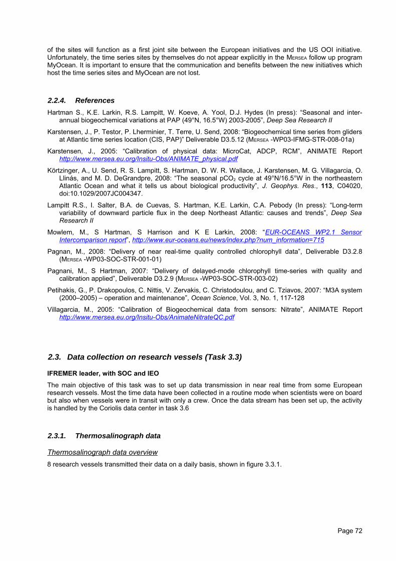
of the sites will function as a first joint site between the European initiatives and the US OOI initiative.Unfortunately, the time series sites by themselves do not appear explicitly in the MERSEA follow up programMyOcean. It is important to ensure that the communication and benefits between the new initiatives whichhost the time series sites and MyOcean are not lost.

2.2.4. ReferencesHartman S., K.E. Larkin, R.S. Lampitt, W. Koeve, A. Yool, D.J. Hydes (In press): “Seasonal and inter-

annual biogeochemical variations at PAP (49°N, 16.5°W) 2003-2005”, Deep Sea Research II

Karstensen, J., P. Testor, P. Lherminier, T. Terre, U. Send, 2008: “Biogeochemical time series from glidersat Atlantic time series location (CIS, PAP)” Deliverable D3.5.12 (MERSEA -WP03-IFMG-STR-008-01a)

Karstensen, J., 2005: “Calibration of physical data: MicroCat, ADCP, RCM”, ANIMATE Reporthttp://www.mersea.eu.org/Insitu-Obs/ANIMATE_physical.pdf

Körtzinger, A., U. Send, R. S. Lampitt, S. Hartman, D. W. R. Wallace, J. Karstensen, M. G. Villagarcia, O.Llinás, and M. D. DeGrandpre, 2008: “The seasonal pCO2 cycle at 49°N/16.5°W in the northeasternAtlantic Ocean and what it tells us about biological productivity”, J. Geophys. Res., 113, C04020,doi:10.1029/2007JC004347.

Lampitt R.S., I. Salter, B.A. de Cuevas, S. Hartman, K.E. Larkin, C.A. Pebody (In press): “Long-termvariability of downward particle flux in the deep Northeast Atlantic: causes and trends”, Deep SeaResearch II

Mowlem, M., S Hartman, S Harrison and K E Larkin, 2008: “EUR-OCEANS WP2.1 SensorIntercomparison repor t ”, http://www.eur-oceans.eu/news/index.php?num_information=715

Pagnan, M., 2008: “Delivery of near real-time quality controlled chlorophyll data”, Deliverable D3.2.8(MERSEA -WP03-SOC-STR-001-01)

Pagnani, M., S Hartman, 2007: “Delivery of delayed-mode chlorophyll time-series with quality andcalibration applied”, Deliverable D3.2.9 (MERSEA -WP03-SOC-STR-003-02)

Petihakis, G., P. Drakopoulos, C. Nittis, V. Zervakis, C. Christodoulou, and C. Tziavos, 2007: “M3A system(2000–2005) – operation and maintenance”, Ocean Science, Vol. 3, No. 1, 117-128

Villagarcia, M., 2005: “Calibration of Biogeochemical data from sensors: Nitrate”, ANIMATE Reporthttp://www.mersea.eu.org/Insitu-Obs/AnimateNitrateQC.pdf

2.3. Data collection on research vessels (Task 3.3)

IFREMER leader, with SOC and IEO

The main objective of this task was to set up data transmission in near real time from some Europeanresearch vessels. Most the time data have been collected in a routine mode when scientists were on boardbut also when vessels were in transit with only a crew. Once the data stream has been set up, the activityis handled by the Coriolis data center in task 3.6

2.3.1. Thermosalinograph data

Thermosalinograph data overview8 research vessels transmitted their data on a daily basis, shown in figure 3.3.1.

Page 72

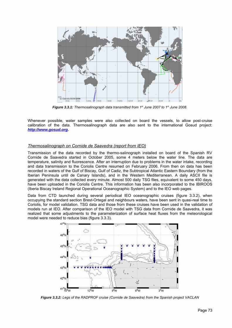
Figure 3.3.1: Thermosalinograph data transmitted from 1st June 2007 to 1st June 2008.

Whenever possible, water samples were also collected on board the vessels, to allow post-cruisecalibration of the data. Thermosalinograph data are also sent to the international Gosud project:http://www.gosud.org.

Thermosalinograph on Cornide de Saavedra (report from IEO)Transmission of the data recorded by the thermo-salinograph installed on board of the Spanish RVCornide de Saavedra started in October 2005, some 4 meters below the water line. The data aretemperature, salinity and fluorescence. After an interruption due to problems in the water intake, recordingand data transmission to the Coriolis Centre resumed on February 2006. From then on data has beenrecorded in waters of the Gulf of Biscay, Gulf of Cadiz, the Subtropical Atlantic Eastern Boundary (from theIberian Peninsula until de Canary Islands), and in the Western Mediterranean. A daily ASCII file isgenerated with the data collected every minute. Almost 500 daily TSG files, equivalent to some 450 days,have been uploaded in the Coriolis Centre. This information has been also incorporated to the IBIROOS(Iberia Biscay Ireland Regional Operational Oceanographic System) and to the IEO web pages.

Data from CTD launched during several periodical IEO oceanographic cruises (figure 3.3.2), whenoccupying the standard section Brest-Ortegal and neighbours waters, have been sent in quasi-real time toCoriolis, for model validation. TSG data and those from these cruises have been used in the validation ofmodels run at IEO. After comparison of the IEO model with TSG data from Cornide de Saavedra, it wasrealized that some adjustments to the parameterization of surface heat fluxes from the meteorologicalmodel were needed to reduce bias (figure 3.3.3).

Figure 3.3.2: Legs of the RADPROF cruise (Cornide de Saavedra) from the Spanish project VACLAN

Page 73

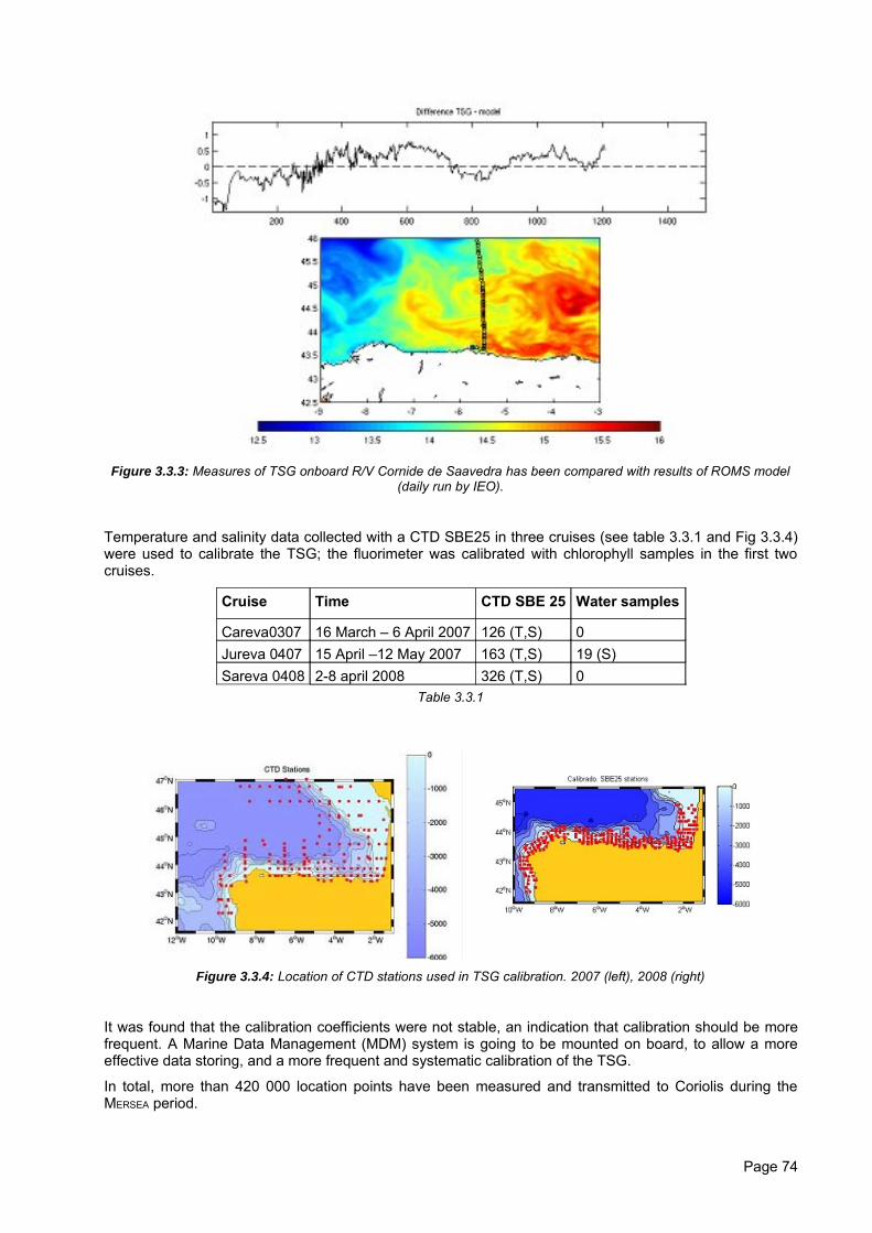
Figure 3.3.3: Measures of TSG onboard R/V Cornide de Saavedra has been compared with results of ROMS model(daily run by IEO).

Temperature and salinity data collected with a CTD SBE25 in three cruises (see table 3.3.1 and Fig 3.3.4)were used to calibrate the TSG; the fluorimeter was calibrated with chlorophyll samples in the first twocruises.

Cruise Time CTD SBE 25 Water samples

Careva0307 16 March – 6 April 2007 126 (T,S) 0Jureva 0407 15 April –12 May 2007 163 (T,S) 19 (S)Sareva 0408 2-8 april 2008 326 (T,S) 0

Table 3.3.1

Figure 3.3.4: Location of CTD stations used in TSG calibration. 2007 (left), 2008 (right)

It was found that the calibration coefficients were not stable, an indication that calibration should be morefrequent. A Marine Data Management (MDM) system is going to be mounted on board, to allow a moreeffective data storing, and a more frequent and systematic calibration of the TSG.

In total, more than 420 000 location points have been measured and transmitted to Coriolis during theMERSEA period.

Page 74

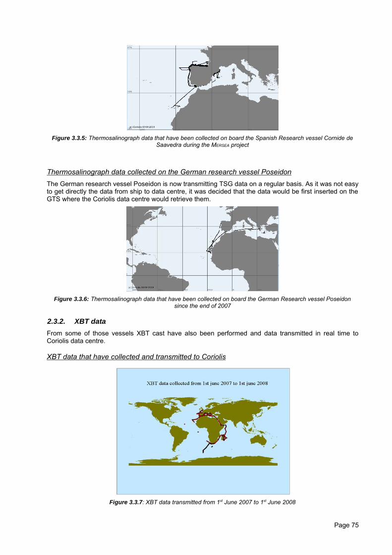
Figure 3.3.5: Thermosalinograph data that have been collected on board the Spanish Research vessel Cornide deSaavedra during the MERSEA project

Thermosalinograph data collected on the German research vessel PoseidonThe German research vessel Poseidon is now transmitting TSG data on a regular basis. As it was not easyto get directly the data from ship to data centre, it was decided that the data would be first inserted on theGTS where the Coriolis data centre would retrieve them.

Figure 3.3.6: Thermosalinograph data that have been collected on board the German Research vessel Poseidonsince the end of 2007

2.3.2. XBT dataFrom some of those vessels XBT cast have also been performed and data transmitted in real time toCoriolis data centre.

XBT data that have collected and transmitted to Coriolis

Figure 3.3.7: XBT data transmitted from 1st June 2007 to 1st June 2008

Page 75

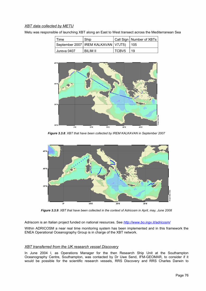
XBT data collected by METUMetu was responsible of launching XBT along an East to West transect across the Mediterranean Sea

Time Ship Call Sign Number of XBTsSeptember 2007 IREM KALKAVAN V7JT5) 105

Jureva 0407 BILIM II TCBV5 19

Figure 3.3.8: XBT that have been collected by IREM KALKAVAN in September 2007

Figure 3.3.9: XBT that have been collected in the context of Adricosm in April, may, June 2008

Adriscom is an Italian project funded on national resources. See http://www.bo.ingv.it/adricosm/

Within ADRICOSM a near real time monitoring system has been implemented and in this framework theENEA Operational Oceanography Group is in charge of the XBT network.

XBT transferred from the UK research vessel DiscoveryIn June 2004 I, as Operations Manager for the then Research Ship Unit at the SouthamptonOceanography Centre, Southampton, was contacted by Dr Uwe Send, IFM-GEOMAR, to consider if itwould be possible for the scientific research vessels, RRS Discovery and RRS Charles Darwin to

Page 76

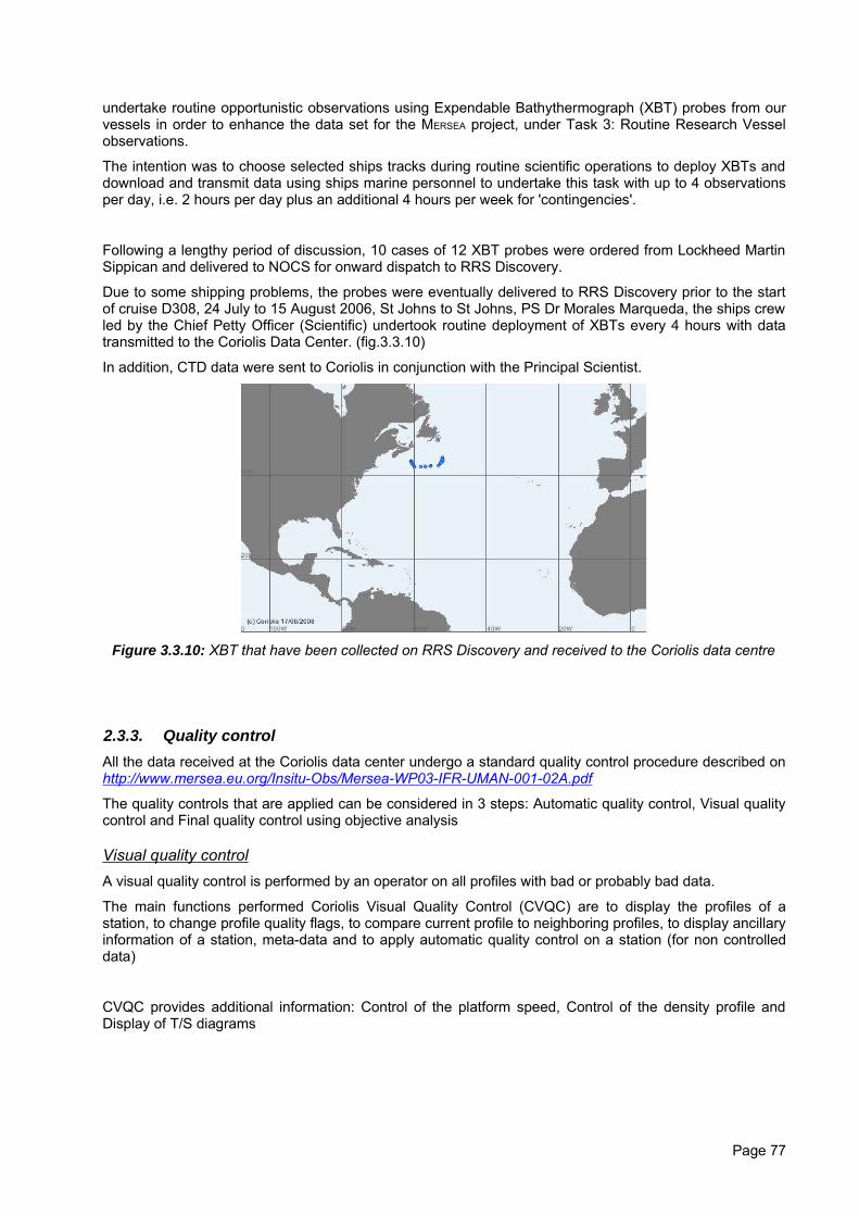
undertake routine opportunistic observations using Expendable Bathythermograph (XBT) probes from ourvessels in order to enhance the data set for the MERSEA project, under Task 3: Routine Research Vesselobservations.

The intention was to choose selected ships tracks during routine scientific operations to deploy XBTs anddownload and transmit data using ships marine personnel to undertake this task with up to 4 observationsper day, i.e. 2 hours per day plus an additional 4 hours per week for 'contingencies'.

Following a lengthy period of discussion, 10 cases of 12 XBT probes were ordered from Lockheed MartinSippican and delivered to NOCS for onward dispatch to RRS Discovery.

Due to some shipping problems, the probes were eventually delivered to RRS Discovery prior to the startof cruise D308, 24 July to 15 August 2006, St Johns to St Johns, PS Dr Morales Marqueda, the ships crewled by the Chief Petty Officer (Scientific) undertook routine deployment of XBTs every 4 hours with datatransmitted to the Coriolis Data Center. (fig.3.3.10)

In addition, CTD data were sent to Coriolis in conjunction with the Principal Scientist.

Figure 3.3.10: XBT that have been collected on RRS Discovery and received to the Coriolis data centre

2.3.3. Quality controlAll the data received at the Coriolis data center undergo a standard quality control procedure described onhttp://www.mersea.eu.org/Insitu-Obs/Mersea-WP03-IFR-UMAN-001-02A.pdf

The quality controls that are applied can be considered in 3 steps: Automatic quality control, Visual qualitycontrol and Final quality control using objective analysis

Visual quality controlA visual quality control is performed by an operator on all profiles with bad or probably bad data.

The main functions performed Coriolis Visual Quality Control (CVQC) are to display the profiles of astation, to change profile quality flags, to compare current profile to neighboring profiles, to display ancillaryinformation of a station, meta-data and to apply automatic quality control on a station (for non controlleddata)

CVQC provides additional information: Control of the platform speed, Control of the density profile andDisplay of T/S diagrams

Page 77

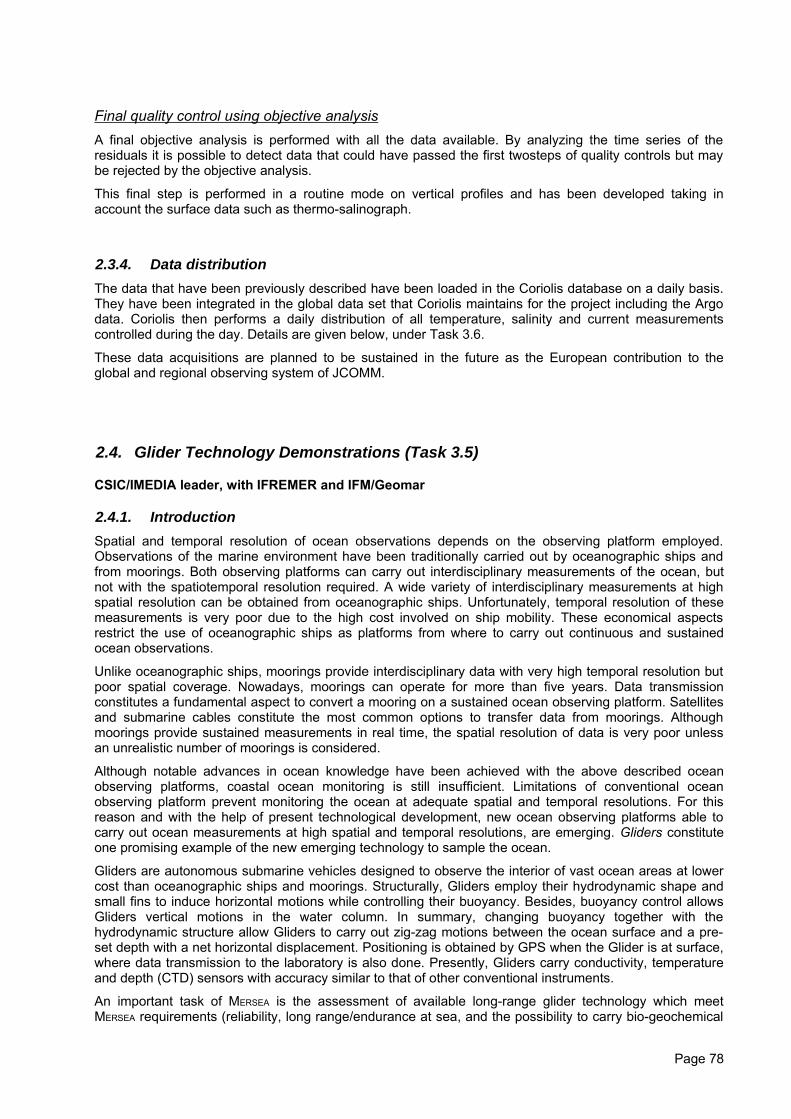
Final quality control using objective analysisA final objective analysis is performed with all the data available. By analyzing the time series of theresiduals it is possible to detect data that could have passed the first twosteps of quality controls but maybe rejected by the objective analysis.

This final step is performed in a routine mode on vertical profiles and has been developed taking inaccount the surface data such as thermo-salinograph.

2.3.4. Data distributionThe data that have been previously described have been loaded in the Coriolis database on a daily basis.They have been integrated in the global data set that Coriolis maintains for the project including the Argodata. Coriolis then performs a daily distribution of all temperature, salinity and current measurementscontrolled during the day. Details are given below, under Task 3.6.

These data acquisitions are planned to be sustained in the future as the European contribution to theglobal and regional observing system of JCOMM.

2.4. Glider Technology Demonstrations (Task 3.5)

CSIC/IMEDIA leader, with IFREMER and IFM/Geomar

2.4.1. IntroductionSpatial and temporal resolution of ocean observations depends on the observing platform employed.Observations of the marine environment have been traditionally carried out by oceanographic ships andfrom moorings. Both observing platforms can carry out interdisciplinary measurements of the ocean, butnot with the spatiotemporal resolution required. A wide variety of interdisciplinary measurements at highspatial resolution can be obtained from oceanographic ships. Unfortunately, temporal resolution of thesemeasurements is very poor due to the high cost involved on ship mobility. These economical aspectsrestrict the use of oceanographic ships as platforms from where to carry out continuous and sustainedocean observations.

Unlike oceanographic ships, moorings provide interdisciplinary data with very high temporal resolution butpoor spatial coverage. Nowadays, moorings can operate for more than five years. Data transmissionconstitutes a fundamental aspect to convert a mooring on a sustained ocean observing platform. Satellitesand submarine cables constitute the most common options to transfer data from moorings. Althoughmoorings provide sustained measurements in real time, the spatial resolution of data is very poor unlessan unrealistic number of moorings is considered.

Although notable advances in ocean knowledge have been achieved with the above described oceanobserving platforms, coastal ocean monitoring is still insufficient. Limitations of conventional oceanobserving platform prevent monitoring the ocean at adequate spatial and temporal resolutions. For thisreason and with the help of present technological development, new ocean observing platforms able tocarry out ocean measurements at high spatial and temporal resolutions, are emerging. Gliders constituteone promising example of the new emerging technology to sample the ocean.

Gliders are autonomous submarine vehicles designed to observe the interior of vast ocean areas at lowercost than oceanographic ships and moorings. Structurally, Gliders employ their hydrodynamic shape andsmall fins to induce horizontal motions while controlling their buoyancy. Besides, buoyancy control allowsGliders vertical motions in the water column. In summary, changing buoyancy together with thehydrodynamic structure allow Gliders to carry out zig-zag motions between the ocean surface and a pre-set depth with a net horizontal displacement. Positioning is obtained by GPS when the Glider is at surface,where data transmission to the laboratory is also done. Presently, Gliders carry conductivity, temperatureand depth (CTD) sensors with accuracy similar to that of other conventional instruments.

An important task of MERSEA is the assessment of available long-range glider technology which meetMERSEA requirements (reliability, long range/endurance at sea, and the possibility to carry bio-geochemical

Page 78

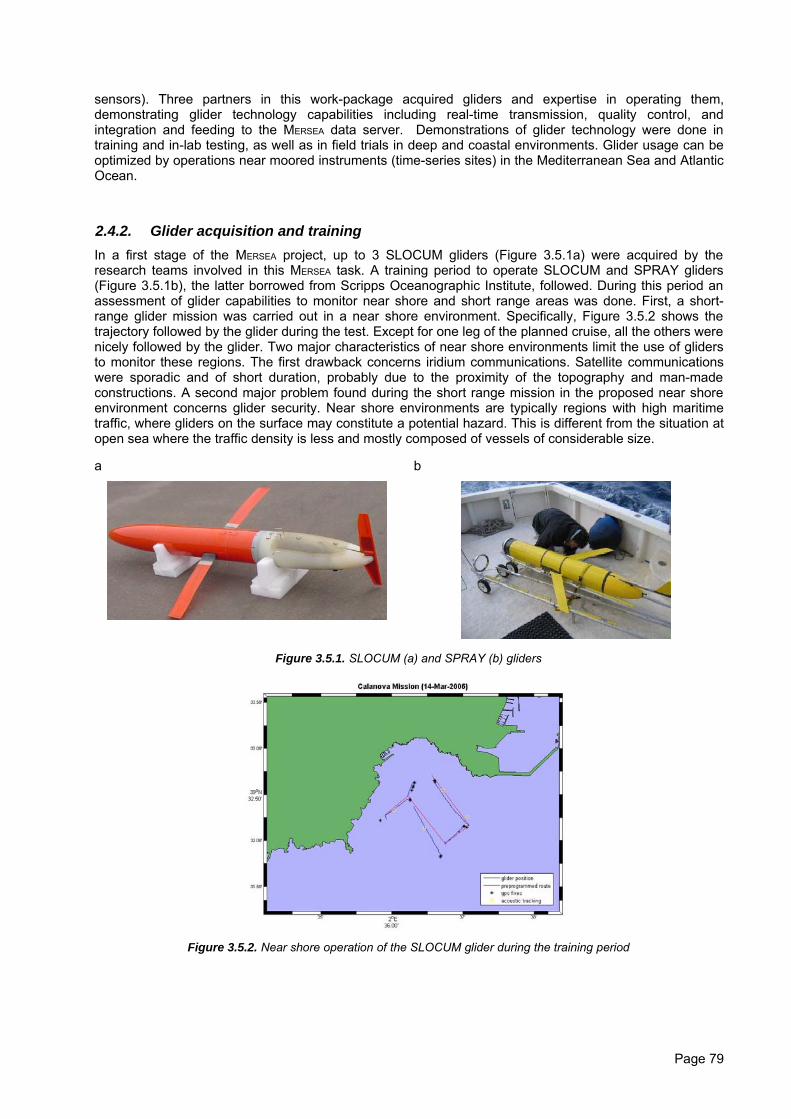
sensors). Three partners in this work-package acquired gliders and expertise in operating them,demonstrating glider technology capabilities including real-time transmission, quality control, andintegration and feeding to the MERSEA data server. Demonstrations of glider technology were done intraining and in-lab testing, as well as in field trials in deep and coastal environments. Glider usage can beoptimized by operations near moored instruments (time-series sites) in the Mediterranean Sea and AtlanticOcean.

2.4.2. Glider acquisition and trainingIn a first stage of the MERSEA project, up to 3 SLOCUM gliders (Figure 3.5.1a) were acquired by theresearch teams involved in this MERSEA task. A training period to operate SLOCUM and SPRAY gliders(Figure 3.5.1b), the latter borrowed from Scripps Oceanographic Institute, followed. During this period anassessment of glider capabilities to monitor near shore and short range areas was done. First, a short-range glider mission was carried out in a near shore environment. Specifically, Figure 3.5.2 shows thetrajectory followed by the glider during the test. Except for one leg of the planned cruise, all the others werenicely followed by the glider. Two major characteristics of near shore environments limit the use of glidersto monitor these regions. The first drawback concerns iridium communications. Satellite communicationswere sporadic and of short duration, probably due to the proximity of the topography and man-madeconstructions. A second major problem found during the short range mission in the proposed near shoreenvironment concerns glider security. Near shore environments are typically regions with high maritimetraffic, where gliders on the surface may constitute a potential hazard. This is different from the situation atopen sea where the traffic density is less and mostly composed of vessels of considerable size.

a b

Figure 3.5.1. SLOCUM (a) and SPRAY (b) gliders

Figure 3.5.2. Near shore operation of the SLOCUM glider during the training period

Page 79

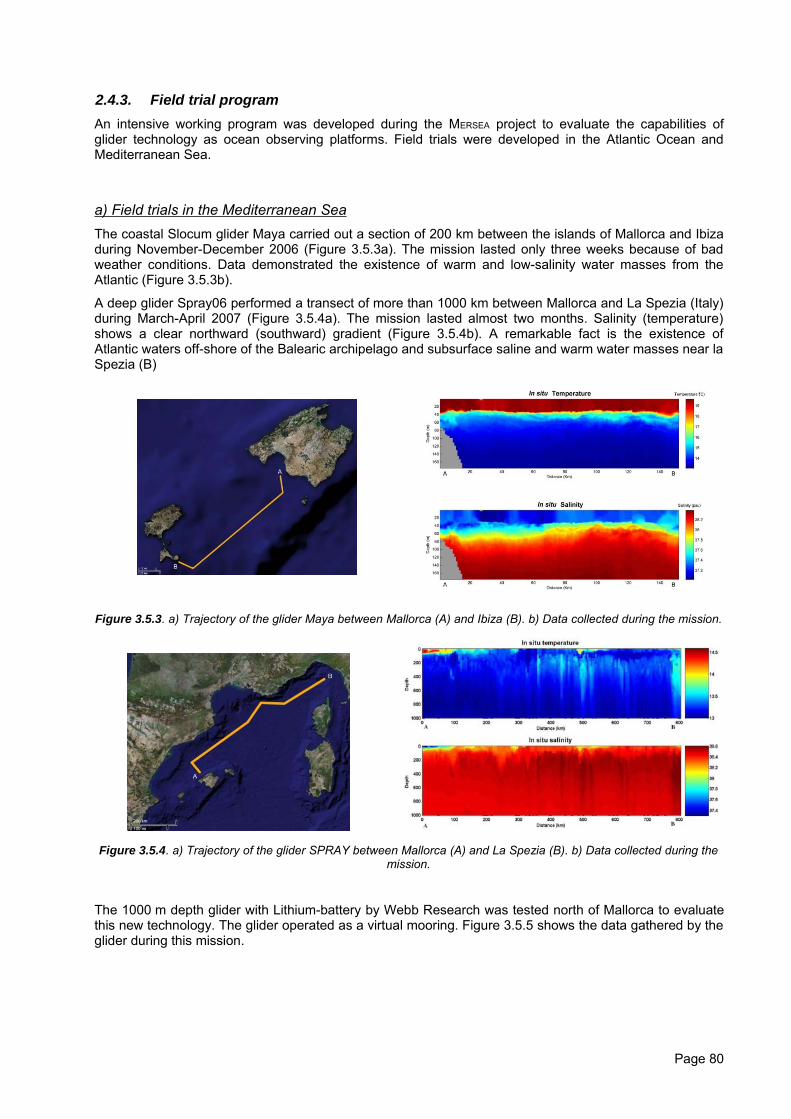
2.4.3. Field trial programAn intensive working program was developed during the MERSEA project to evaluate the capabilities ofglider technology as ocean observing platforms. Field trials were developed in the Atlantic Ocean andMediterranean Sea.

a) Field trials in the Mediterranean SeaThe coastal Slocum glider Maya carried out a section of 200 km between the islands of Mallorca and Ibizaduring November-December 2006 (Figure 3.5.3a). The mission lasted only three weeks because of badweather conditions. Data demonstrated the existence of warm and low-salinity water masses from theAtlantic (Figure 3.5.3b).

A deep glider Spray06 performed a transect of more than 1000 km between Mallorca and La Spezia (Italy)during March-April 2007 (Figure 3.5.4a). The mission lasted almost two months. Salinity (temperature)shows a clear northward (southward) gradient (Figure 3.5.4b). A remarkable fact is the existence ofAtlantic waters off-shore of the Balearic archipelago and subsurface saline and warm water masses near laSpezia (B)

Figure 3.5.3. a) Trajectory of the glider Maya between Mallorca (A) and Ibiza (B). b) Data collected during the mission.

Figure 3.5.4. a) Trajectory of the glider SPRAY between Mallorca (A) and La Spezia (B). b) Data collected during themission.

The 1000 m depth glider with Lithium-battery by Webb Research was tested north of Mallorca to evaluatethis new technology. The glider operated as a virtual mooring. Figure 3.5.5 shows the data gathered by theglider during this mission.

Page 80

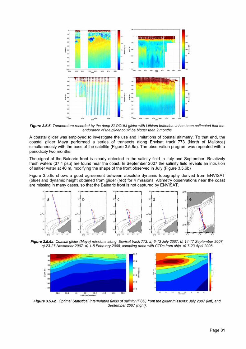
Figure 3.5.5. Temperature recorded by the deep SLOCUM glider with Lithium batteries. It has been estimated that theendurance of the glider could be bigger than 2 months

A coastal glider was employed to investigate the use and limitations of coastal altimetry. To that end, thecoastal glider Maya performed a series of transects along Envisat track 773 (North of Mallorca)simultaneously with the pass of the satellite (Figure 3.5.6a). The observation program was repeated with aperiodicity two months.

The signal of the Balearic front is clearly detected in the salinity field in July and September. Relativelyfresh waters (37.4 psu) are found near the coast. In September 2007 the salinity field reveals an intrusionof saltier water at 40 m, modifying the shape of the front observed in July (Figure 3.5.6b)

Figure 3.5.6c shows a good agreement between absolute dynamic topography derived from ENVISAT(blue) and dynamic height obtained from glider (red) for 4 missions. Altimetry observations near the coastare missing in many cases, so that the Balearic front is not captured by ENVISAT.

Figure 3.5.6a. Coastal glider (Maya) missions along Envisat track 773. a) 6-13 July 2007, b) 14-17 September 2007,c) 23-27 November 2007, d) 1-5 February 2008, sampling done with CTDs from ship, e) 7-23 April 2008

Figure 3.5.6b. Optimal Statistical Interpolated fields of salinity (PSU) from the glider missions: July 2007 (left) and

September 2007 (right).

Page 81

a b c d e

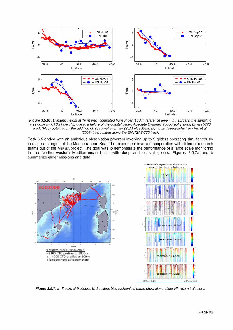
Figure 3.5.6c. Dynamic height at 10 m (red) computed from glider (180 m reference level), in February, the samplingwas done by CTDs from ship due to a failure of the coastal glider. Absolute Dynamic Topography along Envisat-773

track (blue) obtained by the addition of Sea level anomaly (SLA) plus Mean Dynamic Topography from Rio et al.(2007) interpolated along the ENVISAT-773 track.

Task 3.5 ended with an ambitious observation program involving up to 9 gliders operating simultaneouslyin a specific region of the Mediterranean Sea. The experiment involved cooperation with different researchteams out of the MERSEA project. The goal was to demonstrate the performance of a large scale monitoringin the Norther-western Mediterranean basin with deep and coastal gliders. Figures 3.5.7a and bsummarize glider missions and data.

Figure 3.5.7. a) Tracks of 9 gliders. b) Sections biogeochemical parameters along glider Himilcom trajectory.

Page 82

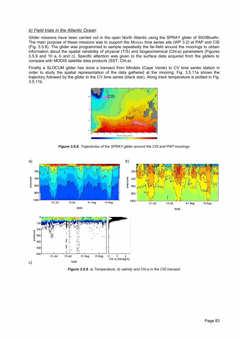
b) Field trials in the Atlantic OceanGlider missions have been carried out in the open North Atlantic using the SPRAY glider of SIO/Bluefin.The main purpose of these missions was to support the MERSEA time series site (WP 3.2) at PAP and CIS(Fig. 3.5.8). The glider was programmed to sample repeatedly the far-field around the moorings to obtaininformation about the spatial variability of physical (T/S) and biogeochemical (Chl-a) parameters (Figures3.5.9 and 10 a, b and c). Specific attention was given to the surface data acquired from the gliders tocompare with MODIS satellite data products (SST, Chl-a).

Finallly a SLOCUM glider has done a transect from Mindelo (Cape Verde) to CV time series station inorder to study the spatial representation of the data gathered at the mooring. Fig. 3.5.11a shows thetrajectory followed by the glider to the CV time series (black star). Along track temperature is plotted in Fig.3.5.11b.

Figure 3.5.8. Trajectories of the SPRAY glider around the CIS and PAP moorings

a) b)

c)Figure 3.5.9. a) Temperature, b) salinity and Chl-a in the CIS transect

Page 83

CIS

PAP

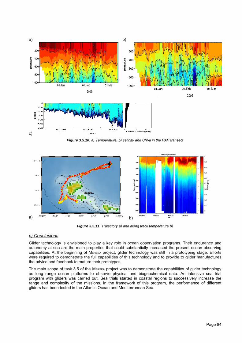
a) b)

c)Figure 3.5.10. a) Temperature, b) salinity and Chl-a in the PAP transect

a) b)

Figure 3.5.11. Trajectory a) and along track temperature b)

c) ConclusionsGlider technology is envisioned to play a key role in ocean observation programs. Their endurance andautonomy at sea are the main properties that could substantially increased the present ocean observingcapabilities. At the beginning of MERSEA project, glider technology was still in a prototyping stage. Effortswere required to demonstrate the full capabilities of this technology and to provide to glider manufacturesthe advice and feedback to mature their prototypes.

The main scope of task 3.5 of the MERSEA project was to demonstrate the capabilities of glider technologyas long range ocean platforms to observe physical and biogeochemical data. An intensive sea trialprogram with gliders was carried out. Sea trials started in coastal regions to successively increase therange and complexity of the missions. In the framework of this program, the performance of differentgliders has been tested in the Atlantic Ocean and Mediterranean Sea.

Page 84

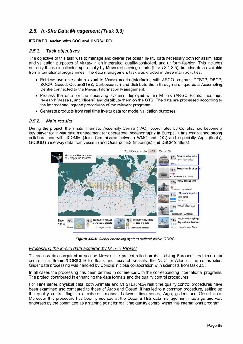
2.5. In-Situ Data Management (Task 3.6)

IFREMER leader, with SOC and CNRS/LPO

2.5.1. Task objectivesThe objective of this task was to manage and deliver the ocean in-situ data necessary both for assimilationand validation purposes of MERSEA in an integrated, quality-controlled, and uniform fashion. This includesnot only the data collected specifically by MERSEA observing efforts (tasks 3.1-3.5), but also data availablefrom international programmes. The data management task was divided in three main activities:

• Retrieve available data relevant to MERSEA needs (interfacing with ARGO program, GTSPP, DBCP,SOOP, Gosud, OceanSITES, Carbocean…) and distribute them through a unique data AssemblingCentre connected to the MERSEA Information Management.

• Process the data for the observing systems deployed within MERSEA (ARGO Floats, moorings,research Vessels, and gliders) and distribute them on the GTS. The data are processed according tothe international agreed procedures of the relevant programs.

• Generate products from real time in-situ data for model validation purposes.

2.5.2. Main resultsDuring the project, the in-situ Thematic Assembly Centre (TAC), coordinated by Coriolis, has become akey player for in-situ data management for operational oceanography in Europe. It has established strongcollaborations with JCOMM (Joint Commission between WMO and IOC) and especially Argo (floats),GOSUD (underway data from vessels) and OceanSITES (moorings) and DBCP (drifters).

Figure 3.6.1: Global observing system defined within GOOS.

Processing the in-situ data acquired by MERSEA ProjectTo process data acquired at sea by MERSEA, the project relied on the existing European real-time datacentres, i.e. Ifremer/CORIOLIS for floats and research vessels, the NOC for Atlantic time series sites.Glider data processing was handled by Coriolis in close collaboration with scientists from task 3.5.

In all cases the processing has been defined in coherence with the corresponding international programs.The project contributed in enhancing the data formats and the quality control procedures.

For Time series physical data, both Animate and MFSTEP/M3A real time quality control procedures havebeen examined and compared to those of Argo and Gosud. It has led to a common procedure, setting upthe quality control flags in a coherent manner between time series, Argo, gliders and Gosud data.Moreover this procedure has been presented at the OceanSITES data management meetings and wasendorsed by the committee as a starting point for real time quality control within this international program.

Page 85

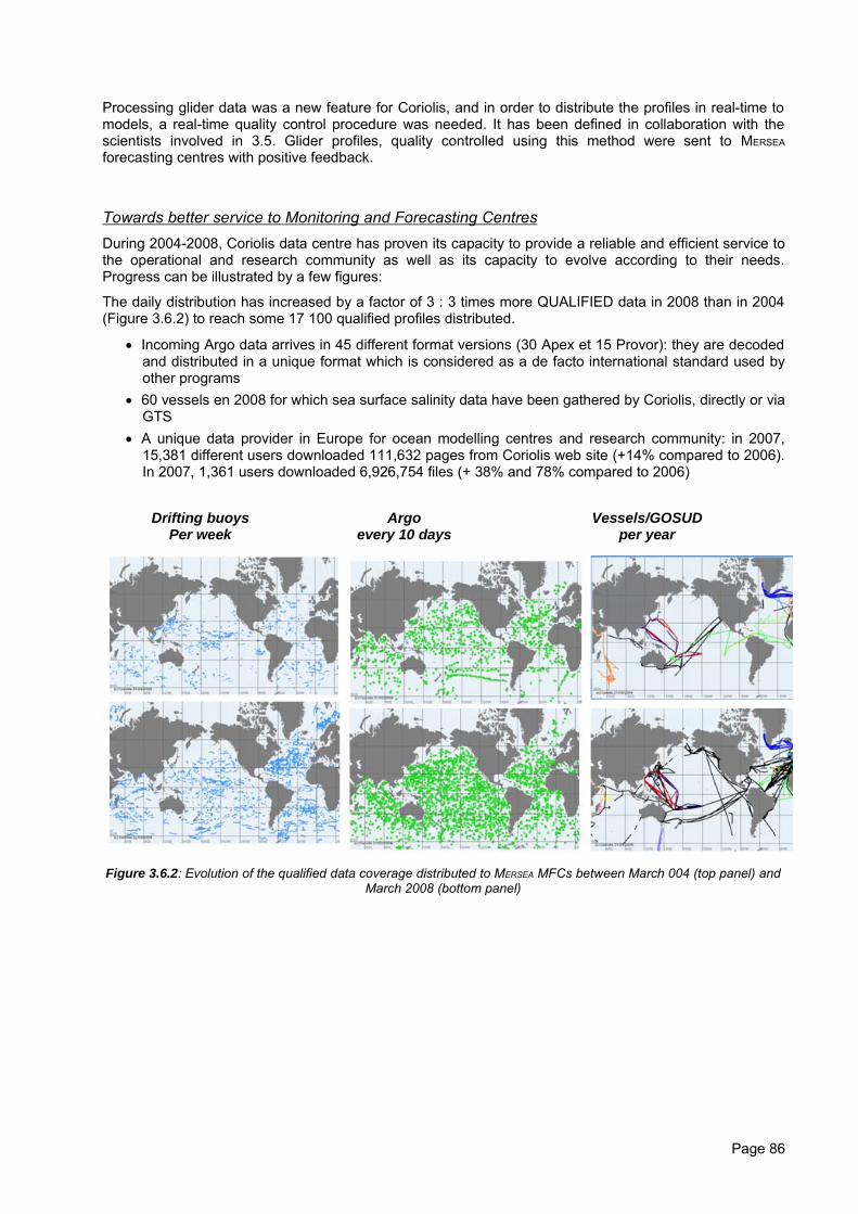
Processing glider data was a new feature for Coriolis, and in order to distribute the profiles in real-time tomodels, a real-time quality control procedure was needed. It has been defined in collaboration with thescientists involved in 3.5. Glider profiles, quality controlled using this method were sent to MERSEA

forecasting centres with positive feedback.

Towards better service to Monitoring and Forecasting CentresDuring 2004-2008, Coriolis data centre has proven its capacity to provide a reliable and efficient service tothe operational and research community as well as its capacity to evolve according to their needs.Progress can be illustrated by a few figures:

The daily distribution has increased by a factor of 3 : 3 times more QUALIFIED data in 2008 than in 2004(Figure 3.6.2) to reach some 17 100 qualified profiles distributed.

• Incoming Argo data arrives in 45 different format versions (30 Apex et 15 Provor): they are decodedand distributed in a unique format which is considered as a de facto international standard used byother programs

• 60 vessels en 2008 for which sea surface salinity data have been gathered by Coriolis, directly or viaGTS

• A unique data provider in Europe for ocean modelling centres and research community: in 2007,15,381 different users downloaded 111,632 pages from Coriolis web site (+14% compared to 2006).In 2007, 1,361 users downloaded 6,926,754 files (+ 38% and 78% compared to 2006)

Drifting buoysPer week

Argoevery 10 days

Vessels/GOSUDper year

Figure 3.6.2: Evolution of the qualified data coverage distributed to MERSEA MFCs between March 004 (top panel) andMarch 2008 (bottom panel)

Page 86

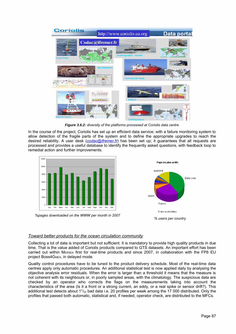
Figure 3.6.2: diversity of the platforms processed at Coriolis data centre

In the course of the project, Coriolis has set up an efficient data service; with a failure monitoring system toallow detection of the fragile parts of the system and to define the appropriate upgrades to reach thedesired reliability. A user desk (codac@ifremer.fr) has been set up; it guarantees that all requests areprocessed and provides a useful database to identify the frequently asked questions, with feedback loop toremedial action and further improvements.

0

2000

4000

6000

8000

10000

12000

Jan Fév Mars Avr Mai Juin Juil Août Sept Oct Nov Déc

%pages downloaded on the WWW per month in 2007% users per country

Toward better products for the ocean circulation communityCollecting a lot of data is important but not sufficient. It is mandatory to provide high quality products in duetime. That is the value added of Coriolis products compared to GTS datasets. An important effort has beencarried out within MERSEA first for real-time products and since 2007, in collaboration with the FP6 EUproject Boss4GMES, in delayed mode.

Quality control procedures have to be tuned to the product delivery schedule. Most of the real-time datacentres apply only automatic procedures. An additional statistical test is now applied daily by analysing theobjective analysis error residuals. When the error is larger than a threshold it means that the measure isnot coherent with its neighbours or, in poorly sampled areas, with the climatology. The suspicious data arechecked by an operator who corrects the flags on the measurements taking into account thecharacteristics of the area (Is it a front or a strong current, an eddy, or a real spike or sensor drift?). Thisadditional test detects about 1°/00 bad data i.e. 20 profiles per week among the 17 000 distributed. Only theprofiles that passed both automatic, statistical and, if needed, operator check, are distributed to the MFCs.

Page 87

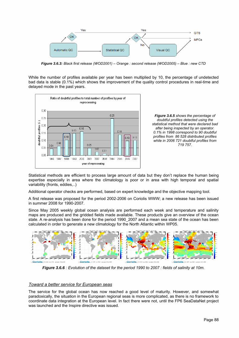
Figure 3.6.3: Black first release (WOD2001) – Orange : second release (WOD2005) – Blue : new CTD

While the number of profiles available per year has been multiplied by 10, the percentage of undetectedbad data is stable (0.1%) which shows the improvement of the quality control procedures in real-time anddelayed mode in the past years.

Figure 3.6.5 shows the percentage ofdoubtful profiles detected using the

statistical method that were declared badafter being inspected by an operator.

0.1% in 1998 correspond to 90 doubtfulprofiles from 86 528 distributed profileswhile in 2006 721 doubtful profiles from

719 757.

Statistical methods are efficient to process large amount of data but they don’t replace the human beingexpertise especially in area where the climatology is poor or in area with high temporal and spatialvariability (fronts, eddies,..)

Additional operator checks are performed, based on expert knowledge and the objective mapping tool.

A first release was proposed for the period 2002-2006 on Coriolis WWW; a new release has been issuedin summer 2008 for 1990-2007.

Since May 2005 weekly global ocean analysis are performed each week and temperature and salinitymaps are produced and the gridded fields made available. These products give an overview of the oceanstate. A re-analysis has been done for the period 1990_2007 and a mean sea state of the ocean has beencalculated in order to generate a new climatology for the North Atlantic within WP05.

Figure 3.6.6 : Evolution of the dataset for the period 1990 to 2007 : fields of salinity at 10m.

Toward a better service for European seasThe service for the global ocean has now reached a good level of maturity. However, and somewhatparadoxically, the situation in the European regional seas is more complicated, as there is no framework tocoordinate data integration at the European level. In fact there were not, until the FP6 SeaDataNet projectwas launched and the Inspire directive was issued.

Page 88

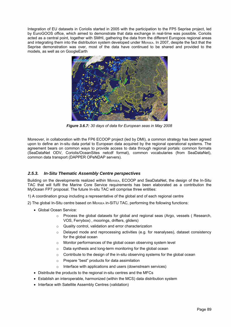
Integration of EU datasets in Coriolis started in 2005 with the participation to the FP5 Seprise project, ledby EuroGOOS office, which aimed to demonstrate that data exchange in real-time was possible. Coriolisacted as a central point, together with SMHI, gathering the data from the different Eurogoos regional areasand integrating them into the distribution system developed under MERSEA. In 2007, despite the fact that theSeprise demonstration was over, most of the data have continued to be shared and provided to themodels, as well as on GoogleEarth

Figure 3.6.7: 30 days of data for European seas in May 2008

Moreover, in collaboration with the FP6 ECOOP project (led by DMI), a common strategy has been agreedupon to define an in-situ data portal to European data acquired by the regional operational systems. Theagreement bears on common ways to provide access to data through regional portals: common formats(SeaDataNet ODV, Coriolis/OceanSites netcdf format), common vocabularies (from SeaDataNet),common data transport (DAPPER OPeNDAP servers).

2.5.3. In-Situ Thematic Assembly Centre perspectivesBuilding on the developments realized within MERSEA, ECOOP and SeaDataNet, the design of the In-SituTAC that will fulfil the Marine Core Service requirements has been elaborated as a contribution theMyOcean FP7 proposal. The future In-situ TAC will comprise three entities:

1) A coordination group including a representative of the global and of each regional centre

2) The global In-Situ centre based on MERSEA in-SITU TAC, performing the following functions:

• Global Ocean Service:o Process the global datasets for global and regional seas (Argo, vessels ( Research,

VOS, Ferrybox) , moorings, drifters, gliders)o Quality control, validation and error characterizationo Delayed mode and reprocessing activities (e.g. for reanalyses), dataset consistency

for the global oceano Monitor performances of the global ocean observing system levelo Data synthesis and long-term monitoring for the global oceano Contribute to the design of the in-situ observing systems for the global oceano Prepare “best” products for data assimilationo Interface with applications and users (downstream services)

• Distribute the products to the regional in-situ centres and the MFCs• Establish an interoperable, harmonized (within the MCS) data distribution system• Interface with Satellite Assembly Centres (validation)

Page 89

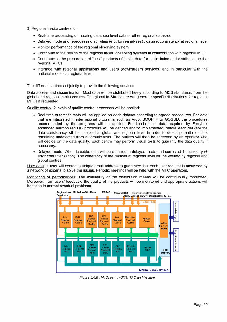
3) Regional in-situ centres for

• Real-time processing of mooring data, sea level data or other regional datasets• Delayed mode and reprocessing activities (e.g. for reanalyses) , dataset consistency at regional level• Monitor performance of the regional observing system• Contribute to the design of the regional in-situ observing systems in collaboration with regional MFC• Contribute to the preparation of “best” products of in-situ data for assimilation and distribution to the

regional MFCs• Interface with regional applications and users (downstream services) and in particular with the

national models at regional level

The different centres act jointly to provide the following services:

Data access and dissemination: Most data will be distributed freely according to MCS standards, from theglobal and regional in-situ centres. The global In-Situ centre will generate specific distributions for regionalMFCs if requested.

Quality control: 2 levels of quality control processes will be applied:

• Real-time automatic tests will be applied on each dataset according to agreed procedures. For datathat are integrated in international programs such as Argo, SOOP/IP or GOSUD, the proceduresrecommended by the programs will be applied. For biochemical data acquired by Ferryboxenhanced harmonized QC procedure will be defined and/or implemented; before each delivery thedata consistency will be checked at global and regional level in order to detect potential outliersremaining undetected from automatic tests. The outliers will then be screened by an operator whowill decide on the data quality. Each centre may perform visual tests to guaranty the data quality ifnecessary.

• Delayed-mode: When feasible, data will be qualified in delayed mode and corrected if necessary (+error characterization). The coherency of the dataset at regional level will be verified by regional andglobal centres.

User desk: a user will contact a unique email address to guarantee that each user request is answered bya network of experts to solve the issues. Periodic meetings will be held with the MFC operators.

Monitoring of performances: The availability of the distribution means will be continuously monitored.Moreover, from users’ feedback, the quality of the products will be monitored and appropriate actions willbe taken to correct eventual problems.

Figure 3.6.8 : MyOcean In-SITU TAC architecture

Page 90

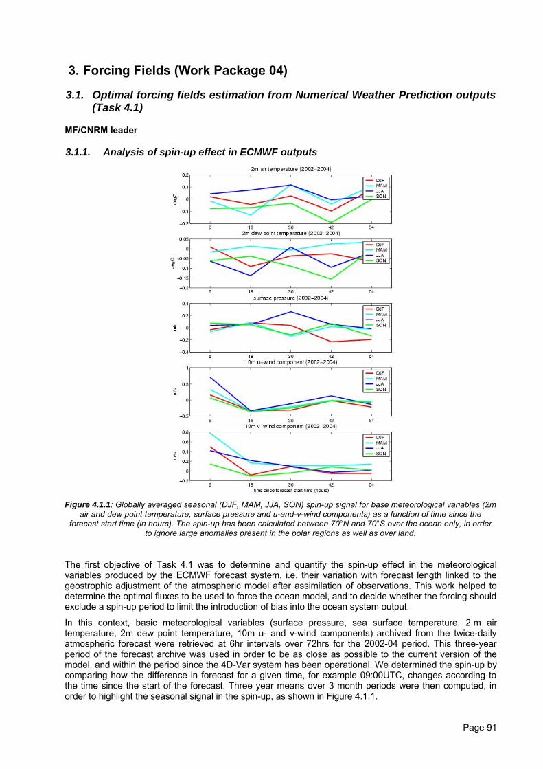
3. Forcing Fields (Work Package 04)

3.1. Optimal forcing fields estimation from Numerical Weather Prediction outputs(Task 4.1)

MF/CNRM leader

3.1.1. Analysis of spin-up effect in ECMWF outputs

Figure 4.1.1: Globally averaged seasonal (DJF, MAM, JJA, SON) spin-up signal for base meteorological variables (2mair and dew point temperature, surface pressure and u-and-v-wind components) as a function of time since the

forecast start time (in hours). The spin-up has been calculated between 70°N and 70°S over the ocean only, in orderto ignore large anomalies present in the polar regions as well as over land.

The first objective of Task 4.1 was to determine and quantify the spin-up effect in the meteorologicalvariables produced by the ECMWF forecast system, i.e. their variation with forecast length linked to thegeostrophic adjustment of the atmospheric model after assimilation of observations. This work helped todetermine the optimal fluxes to be used to force the ocean model, and to decide whether the forcing shouldexclude a spin-up period to limit the introduction of bias into the ocean system output.

In this context, basic meteorological variables (surface pressure, sea surface temperature, 2 m airtemperature, 2m dew point temperature, 10m u- and v-wind components) archived from the twice-dailyatmospheric forecast were retrieved at 6hr intervals over 72hrs for the 2002-04 period. This three-yearperiod of the forecast archive was used in order to be as close as possible to the current version of themodel, and within the period since the 4D-Var system has been operational. We determined the spin-up bycomparing how the difference in forecast for a given time, for example 09:00UTC, changes according tothe time since the start of the forecast. Three year means over 3 month periods were then computed, inorder to highlight the seasonal signal in the spin-up, as shown in Figure 4.1.1.

Page 91

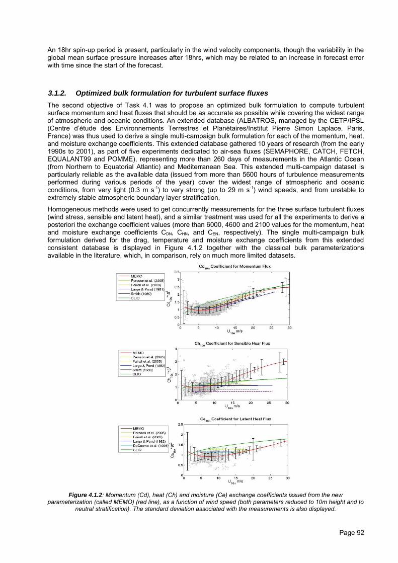
An 18hr spin-up period is present, particularly in the wind velocity components, though the variability in theglobal mean surface pressure increases after 18hrs, which may be related to an increase in forecast errorwith time since the start of the forecast.

3.1.2. Optimized bulk formulation for turbulent surface fluxesThe second objective of Task 4.1 was to propose an optimized bulk formulation to compute turbulentsurface momentum and heat fluxes that should be as accurate as possible while covering the widest rangeof atmospheric and oceanic conditions. An extended database (ALBATROS, managed by the CETP/IPSL(Centre d’étude des Environnements Terrestres et Planétaires/Institut Pierre Simon Laplace, Paris,France) was thus used to derive a single multi-campaign bulk formulation for each of the momentum, heat,and moisture exchange coefficients. This extended database gathered 10 years of research (from the early1990s to 2001), as part of five experiments dedicated to air-sea fluxes (SEMAPHORE, CATCH, FETCH,EQUALANT99 and POMME), representing more than 260 days of measurements in the Atlantic Ocean(from Northern to Equatorial Atlantic) and Mediterranean Sea. This extended multi-campaign dataset isparticularly reliable as the available data (issued from more than 5600 hours of turbulence measurementsperformed during various periods of the year) cover the widest range of atmospheric and oceanicconditions, from very light (0.3 m s-1) to very strong (up to 29 m s-1) wind speeds, and from unstable toextremely stable atmospheric boundary layer stratification.

Homogeneous methods were used to get concurrently measurements for the three surface turbulent fluxes(wind stress, sensible and latent heat), and a similar treatment was used for all the experiments to derive aposteriori the exchange coefficient values (more than 6000, 4600 and 2100 values for the momentum, heatand moisture exchange coefficients CDN, CHN, and CEN, respectively). The single multi-campaign bulkformulation derived for the drag, temperature and moisture exchange coefficients from this extendedconsistent database is displayed in Figure 4.1.2 together with the classical bulk parameterizationsavailable in the literature, which, in comparison, rely on much more limited datasets.

Figure 4.1.2: Momentum (Cd), heat (Ch) and moisture (Ce) exchange coefficients issued from the newparameterization (called MEMO) (red line), as a function of wind speed (both parameters reduced to 10m height and to

neutral stratification). The standard deviation associated with the measurements is also displayed.

Page 92

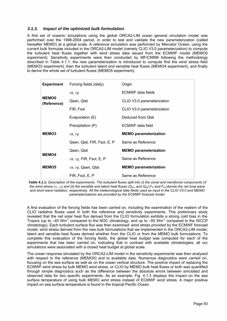
3.1.3. Impact of the optimized bulk formulationA first set of oceanic simulations using the global ORCA2-LIM ocean general circulation model wasperformed over the 1998-2004 period, in order to test and validate the new parameterization (calledhereafter MEMO) at a global scale. A reference simulation was performed by Mercator Océan, using thecurrent bulk formulae included in the ORCA2-LIM model (namely CLIO V3.0 parameterization) to computethe turbulent heat fluxes together with wind stress data issued from the ECMWF model (MEMO0experiment). Sensitivity experiments were then conducted by MF/CNRM following the methodologydescribed in Table 4.1.1: the new parameterization is introduced to compute first the wind stress field(MEMO3 experiment), then the turbulent latent and sensible heat fluxes (MEMO4 experiment), and finallyto derive the whole set of turbulent fluxes (MEMO5 experiment).

Experiment Forcing fields (daily) Origin

MEMO0(Reference)

τx, τy ECMWF data fields

Qsen, Qlat CLIO V3.0 parameterization

FIR, Fsol CLIO V3.0 parameterization

Evaporation (E) Deduced from Qlat

Precipitation (P) ECMWF data field

MEMO3 τx, τy MEMO parameterization

Qsen, Qlat, FIR, Fsol, E, P Same as Reference

MEMO4Qsen, Qlat MEMO parameterization

τx, τy, FIR, Fsol, E, P Same as Reference

MEMO5 τx, τy, Qsen, Qlat MEMO parameterization

FIR, Fsol, E, P Same as Reference

Table 4.1.1: Description of the experiments. The turbulent fluxes split into (i) the zonal and meridional components ofthe wind stress (τx, τy) and (ii) the sensible and latent heat fluxes (Qsen and Qlat).FIR and Fsol denote the net long waveand short wave radiation, respectively. All the meteorological data fields used as input in the CLIO V3.0 and MEMO

parameterizations are provided by the ECMWF forecast model.

A first evaluation of the forcing fields has been carried on, including the examination of the realism of theCLIO radiative fluxes used in both the reference and sensitivity experiments. This preliminary studyrevealed that the net solar heat flux derived from the CLIO formulation exhibits a strong cold bias in theTropics (up to –40 Wm-2 compared to the NOC climatology, and up to –50 Wm-2 compared to the ISCCPclimatology). Each turbulent surface flux was then examined: wind stress provided by the ECMWF forecastmodel, wind stress derived from the new bulk formulations that we implemented in the ORCA2-LIM model,latent and sensible heat fluxes derived whether from the CLIO or from the MEMO bulk formulations. Tocomplete this evaluation of the forcing fields, the global heat budget was computed for each of theexperiments that has been carried on, indicating that in contrast with available climatologies, all oursimulations were associated with a closed heat budget at global scale.

The ocean response simulated by the ORCA2-LIM model in the sensitivity experiments was then analysedwith respect to the reference (MEMO0) and to available data. Numerous diagnostics were carried on,focusing on the sea surface as well as on the ocean vertical structure. The positive impact of replacing theECMWF wind stress by bulk MEMO wind stress, or CLIO by MEMO bulk heat fluxes or both was quantifiedthrough simple diagnostics such as the difference between the absolute errors between simulated andobserved data for two specific experiments. As an example, Fig. 4.1.3 displays the impact on the seasurface temperature of using bulk MEMO wind stress instead of ECMWF wind stress. A major positiveimpact on sea surface temperature is found in the tropical Pacific Ocean.

Page 93

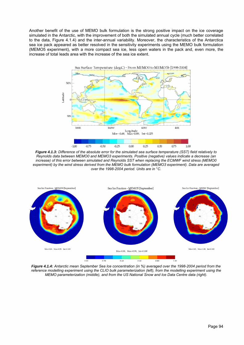
Another benefit of the use of MEMO bulk formulation is the strong positive impact on the ice coveragesimulated in the Antarctic, with the improvement of both the simulated annual cycle (much better correlatedto the data, Figure 4.1.4) and the inter-annual variability. Moreover, the characteristics of the Antarcticasea ice pack appeared as better resolved in the sensitivity experiments using the MEMO bulk formulation(MEMO5 experiment), with a more compact sea ice, less open waters in the pack and, even more, theincrease of total leads area with the increase of the sea ice extent.

Figure 4.1.3: Difference of the absolute error for the simulated sea surface temperature (SST) field relatively toReynolds data between MEMO0 and MEMO3 experiments. Positive (negative) values indicate a decrease (anincrease) of this error between simulated and Reynolds SST when replacing the ECMWF wind stress (MEMO0

experiment) by the wind stress derived from the MEMO bulk formulation (MEMO3 experiment). Data are averagedover the 1998-2004 period. Units are in °C.

Figure 4.1.4: Antarctic mean September Sea Ice concentration (in %) averaged over the 1998-2004 period from thereference modelling experiment using the CLIO bulk parameterization (left), from the modelling experiment using the

MEMO parameterization (middle), and from the US National Snow and Ice Data Centre data (right).

Page 94

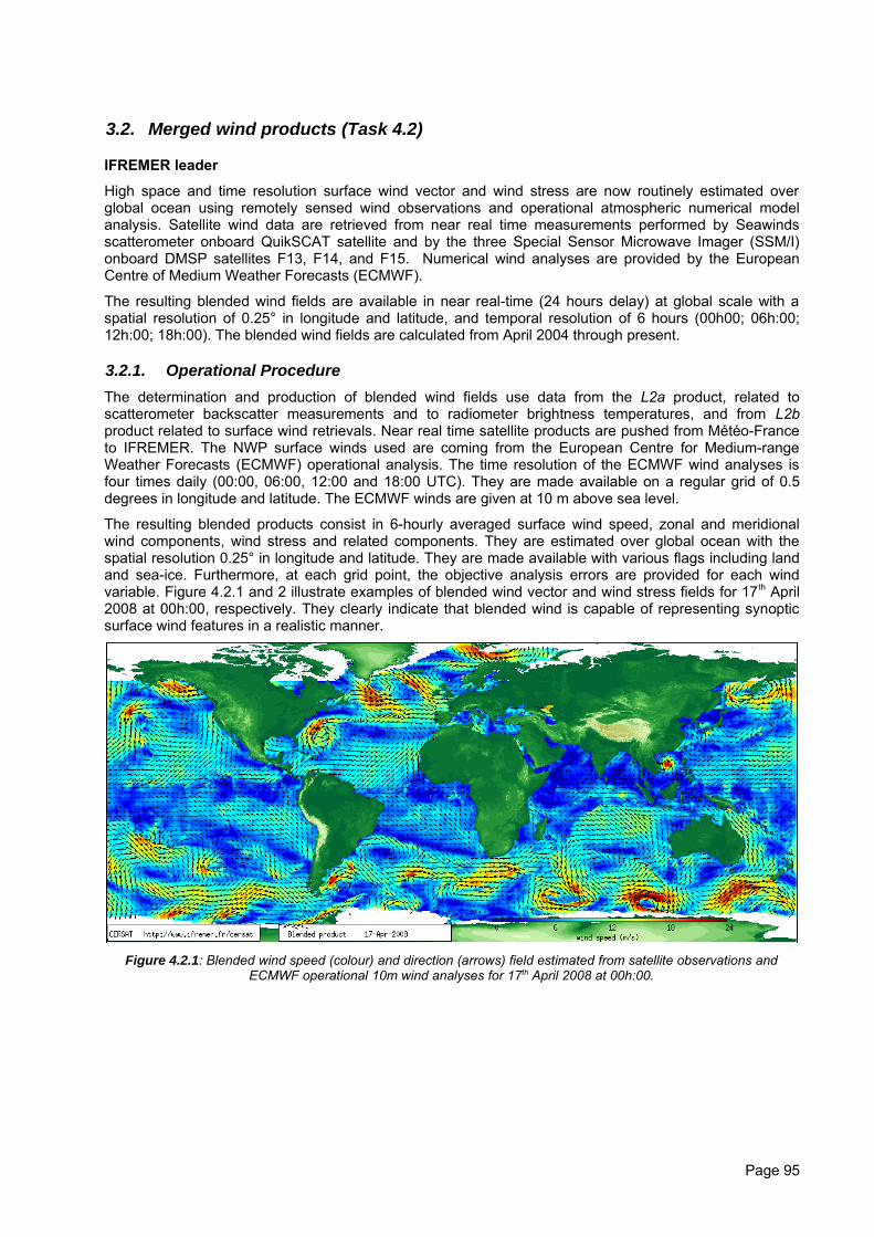
3.2. Merged wind products (Task 4.2)

IFREMER leader

High space and time resolution surface wind vector and wind stress are now routinely estimated overglobal ocean using remotely sensed wind observations and operational atmospheric numerical modelanalysis. Satellite wind data are retrieved from near real time measurements performed by Seawindsscatterometer onboard QuikSCAT satellite and by the three Special Sensor Microwave Imager (SSM/I)onboard DMSP satellites F13, F14, and F15. Numerical wind analyses are provided by the EuropeanCentre of Medium Weather Forecasts (ECMWF).

The resulting blended wind fields are available in near real-time (24 hours delay) at global scale with aspatial resolution of 0.25° in longitude and latitude, and temporal resolution of 6 hours (00h00; 06h:00;12h:00; 18h:00). The blended wind fields are calculated from April 2004 through present.

3.2.1. Operational ProcedureThe determination and production of blended wind fields use data from the L2a product, related toscatterometer backscatter measurements and to radiometer brightness temperatures, and from L2bproduct related to surface wind retrievals. Near real time satellite products are pushed from Météo-Franceto IFREMER. The NWP surface winds used are coming from the European Centre for Medium-rangeWeather Forecasts (ECMWF) operational analysis. The time resolution of the ECMWF wind analyses isfour times daily (00:00, 06:00, 12:00 and 18:00 UTC). They are made available on a regular grid of 0.5degrees in longitude and latitude. The ECMWF winds are given at 10 m above sea level.

The resulting blended products consist in 6-hourly averaged surface wind speed, zonal and meridionalwind components, wind stress and related components. They are estimated over global ocean with thespatial resolution 0.25° in longitude and latitude. They are made available with various flags including landand sea-ice. Furthermore, at each grid point, the objective analysis errors are provided for each windvariable. Figure 4.2.1 and 2 illustrate examples of blended wind vector and wind stress fields for 17th April2008 at 00h:00, respectively. They clearly indicate that blended wind is capable of representing synopticsurface wind features in a realistic manner.

Figure 4.2.1: Blended wind speed (colour) and direction (arrows) field estimated from satellite observations andECMWF operational 10m wind analyses for 17th April 2008 at 00h:00.

Page 95

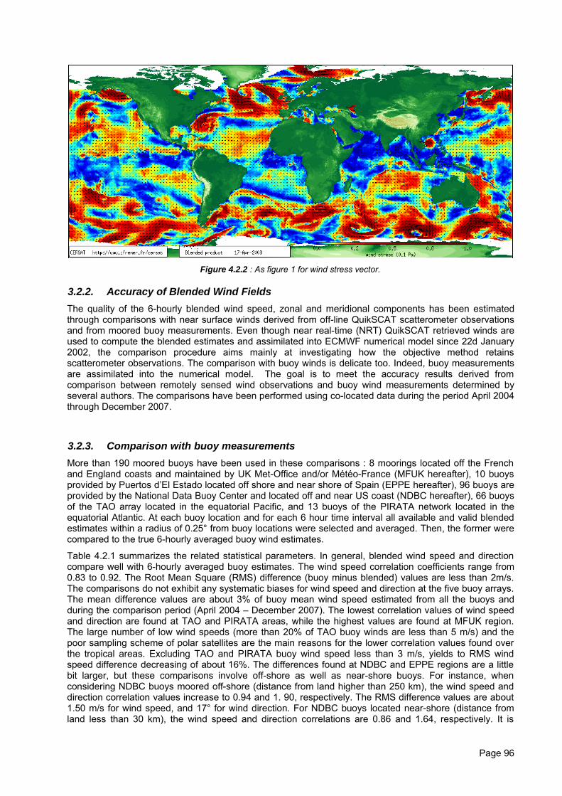
Figure 4.2.2 : As figure 1 for wind stress vector.

3.2.2. Accuracy of Blended Wind FieldsThe quality of the 6-hourly blended wind speed, zonal and meridional components has been estimatedthrough comparisons with near surface winds derived from off-line QuikSCAT scatterometer observationsand from moored buoy measurements. Even though near real-time (NRT) QuikSCAT retrieved winds areused to compute the blended estimates and assimilated into ECMWF numerical model since 22d January2002, the comparison procedure aims mainly at investigating how the objective method retainsscatterometer observations. The comparison with buoy winds is delicate too. Indeed, buoy measurementsare assimilated into the numerical model. The goal is to meet the accuracy results derived fromcomparison between remotely sensed wind observations and buoy wind measurements determined byseveral authors. The comparisons have been performed using co-located data during the period April 2004through December 2007.

3.2.3. Comparison with buoy measurementsMore than 190 moored buoys have been used in these comparisons : 8 moorings located off the Frenchand England coasts and maintained by UK Met-Office and/or Météo-France (MFUK hereafter), 10 buoysprovided by Puertos d’El Estado located off shore and near shore of Spain (EPPE hereafter), 96 buoys areprovided by the National Data Buoy Center and located off and near US coast (NDBC hereafter), 66 buoysof the TAO array located in the equatorial Pacific, and 13 buoys of the PIRATA network located in theequatorial Atlantic. At each buoy location and for each 6 hour time interval all available and valid blendedestimates within a radius of 0.25° from buoy locations were selected and averaged. Then, the former werecompared to the true 6-hourly averaged buoy wind estimates.

Table 4.2.1 summarizes the related statistical parameters. In general, blended wind speed and directioncompare well with 6-hourly averaged buoy estimates. The wind speed correlation coefficients range from0.83 to 0.92. The Root Mean Square (RMS) difference (buoy minus blended) values are less than 2m/s.The comparisons do not exhibit any systematic biases for wind speed and direction at the five buoy arrays.The mean difference values are about 3% of buoy mean wind speed estimated from all the buoys andduring the comparison period (April 2004 – December 2007). The lowest correlation values of wind speedand direction are found at TAO and PIRATA areas, while the highest values are found at MFUK region.The large number of low wind speeds (more than 20% of TAO buoy winds are less than 5 m/s) and thepoor sampling scheme of polar satellites are the main reasons for the lower correlation values found overthe tropical areas. Excluding TAO and PIRATA buoy wind speed less than 3 m/s, yields to RMS windspeed difference decreasing of about 16%. The differences found at NDBC and EPPE regions are a littlebit larger, but these comparisons involve off-shore as well as near-shore buoys. For instance, whenconsidering NDBC buoys moored off-shore (distance from land higher than 250 km), the wind speed anddirection correlation values increase to 0.94 and 1. 90, respectively. The RMS difference values are about1.50 m/s for wind speed, and 17° for wind direction. For NDBC buoys located near-shore (distance fromland less than 30 km), the wind speed and direction correlations are 0.86 and 1.64, respectively. It is

Page 96

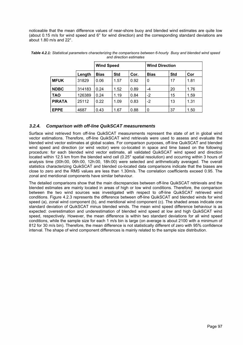
noticeable that the mean difference values of near-shore buoy and blended wind estimates are quite low(about 0.15 m/s for wind speed and 6° for wind direction) and the corresponding standard deviations areabout 1.80 m/s and 22°.

Table 4.2.1: Statistical parameters characterizing the comparisons between 6-hourly Buoy and blended wind speedand direction estimates

Wind Speed Wind Direction

Length Bias Std Cor. Bias Std CorMFUK 31829 0.06 1.57 0.92 0 17 1.81

NDBC 314183 0.24 1.52 0.89 -4 20 1.76TAO 126389 0.24 1.19 0.84 -2 15 1.59PIRATA 25112 0.22 1.09 0.83 -2 13 1.31

EPPE 4687 0.43 1.67 0.88 0 37 1.50

3.2.4. Comparison with off-line QuikSCAT measurementsSurface wind retrieved from off-line QuikSCAT measurements represent the state of art in global windvector estimations. Therefore, off-line QuikSCAT wind retrievals were used to assess and evaluate theblended wind vector estimates at global scales. For comparison purposes, off-line QuikSCAT and blendedwind speed and direction (or wind vector) were co-located in space and time based on the followingprocedure: for each blended wind vector estimate, all validated QuikSCAT wind speed and directionlocated within 12.5 km from the blended wind cell (0.25° spatial resolution) and occurring within 3 hours ofanalysis time (00h:00, 06h:00, 12h:00, 18h:00) were selected and arithmetically averaged. The overallstatistics characterizing QuikSCAT and blended co-located data comparisons indicate that the biases areclose to zero and the RMS values are less than 1.30m/s. The correlation coefficients exceed 0.95. Thezonal and meridional components have similar behaviour.

The detailed comparisons show that the main discrepancies between off-line QuikSCAT retrievals and theblended estimates are mainly located in areas of high or low wind conditions. Therefore, the comparisonbetween the two wind sources was investigated with respect to off-line QuikSCAT retrieved windconditions. Figure 4.2.3 represents the difference between off-line QuikSCAT and blended winds for windspeed (a), zonal wind component (b), and meridional wind component (c). The shaded areas indicate onestandard deviation of QuikSCAT minus blended winds. The mean wind speed difference behaviour is asexpected: overestimation and underestimation of blended wind speed at low and high QuikSCAT windspeed, respectively. However, the mean difference is within two standard deviations for all wind speedconditions, while the sample size for each 1 m/s bin is large (on average is about 2100 with a minimum of812 for 30 m/s bin). Therefore, the mean difference is not statistically different of zero with 95% confidenceinterval. The shape of wind component differences is mainly related to the sample size distribution.

Page 97

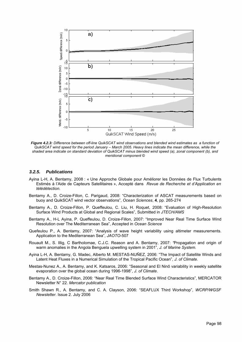
Figure 4.2.3: Difference between off-line QuikSCAT wind observations and blended wind estimates as a function ofQuikSCAT wind speed for the period January – March 2005. Heavy lines indicate the mean difference, while the

shaded area indicate on standard deviation of QuikSCAT minus blended wind speed (a), zonal component (b), andmeridional component ©

3.2.5. PublicationsAyina L-H, A. Bentamy, 2008 : « Une Approche Globale pour Améliorer les Données de Flux Turbulents

Estimés à l’Aide de Capteurs Satellitaires », Accepté dans Revue de Recherche et d’Application entélédétection.

Bentamy A., D. Croize-Fillon, C. Parigaud, 2008: “Characterization of ASCAT measurements based onbuoy and QuikSCAT wind vector observations”, Ocean Sciences, 4, pp. 265-274

Bentamy A., D. Croize-Fillon, P. Queffeulou, C. Liu, H. Roquet, 2008: “Evaluation of High-ResolutionSurface Wind Products at Global and Regional Scales”, Submitted in JTECH/AMS

Bentamy A., H-L Ayina, P. Queffeulou, D. Croize-Fillon, 2007: “Improved Near Real Time Surface WindResolution over The Mediterranean Sea”, Accepted in Ocean Science

Quefeulou P., A. Bentamy, 2007: “Analysis of wave height variability using altimeter measurements.Application to the Mediterranean Sea”, JAOTO-507

Rouault M., S. Illig, C Bartholomae, C.J.C. Reason and A. Bentamy, 2007: “Propagation and origin ofwarm anomalies in the Angola Benguela upwelling system in 2001”, J. of Marine System.

Ayina L-H, A. Bentamy, G. Madec, Alberto M. MESTAS-NUÑEZ, 2006: “The Impact of Satellite Winds andLatent Heat Fluxes in a Numerical Simulation of the Tropical Pacific Ocean”, J. of Climate.

Mestas-Nunez A., A. Bentamy, and K. Katsaros, 2006: “Seasonal and El Ninõ variability in weekly satelliteevaporation over the global ocean during 1996-1998”, J. of Climate.

Bentamy A., D. Croize-Fillon, 2006: “Near Real Time Blended Surface Wind Characteristics”, MERCATORNewsletter N° 22. Mercator publication

Smith Shawn R., A. Bentamy, and C. A. Clayson, 2006: “SEAFLUX Third Workshop”, WCRP/WGSFNewsletter. Issue 2. July 2006

Page 98

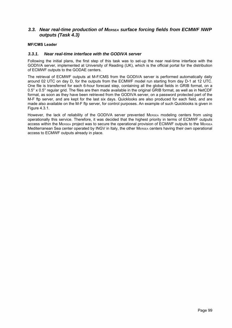
3.3. Near real-time production of MERSEA surface forcing fields from ECMWF NWPoutputs (Task 4.3)

MF/CMS Leader

3.3.1. Near real-time interface with the GODIVA serverFollowing the initial plans, the first step of this task was to set-up the near real-time interface with theGODIVA server, implemented at University of Reading (UK), which is the official portal for the distributionof ECMWF outputs to the GODAE centers.

The retrieval of ECMWF outputs at M-F/CMS from the GODIVA server is performed automatically dailyaround 02 UTC on day D, for the outputs from the ECMWF model run starting from day D-1 at 12 UTC.One file is transferred for each 6-hour forecast step, containing all the global fields in GRIB format, on a0.5° x 0.5° regular grid. The files are then made available in the original GRIB format, as well as in NetCDFformat, as soon as they have been retrieved from the GODIVA server, on a password protected part of theM-F ftp server, and are kept for the last six days. Quicklooks are also produced for each field, and aremade also available on the M-F ftp server, for control purposes. An example of such Quicklooks is given inFigure 4.3.1.

However, the lack of reliability of the GODIVA server prevented MERSEA modeling centers from usingoperationally this service. Therefore, it was decided that the highest priority in terms of ECMWF outputsaccess within the MERSEA project was to secure the operational provision of ECMWF outputs to the MERSEA

Mediterranean Sea center operated by INGV in Italy, the other MERSEA centers having their own operationalaccess to ECMWF outputs already in place.

Page 99

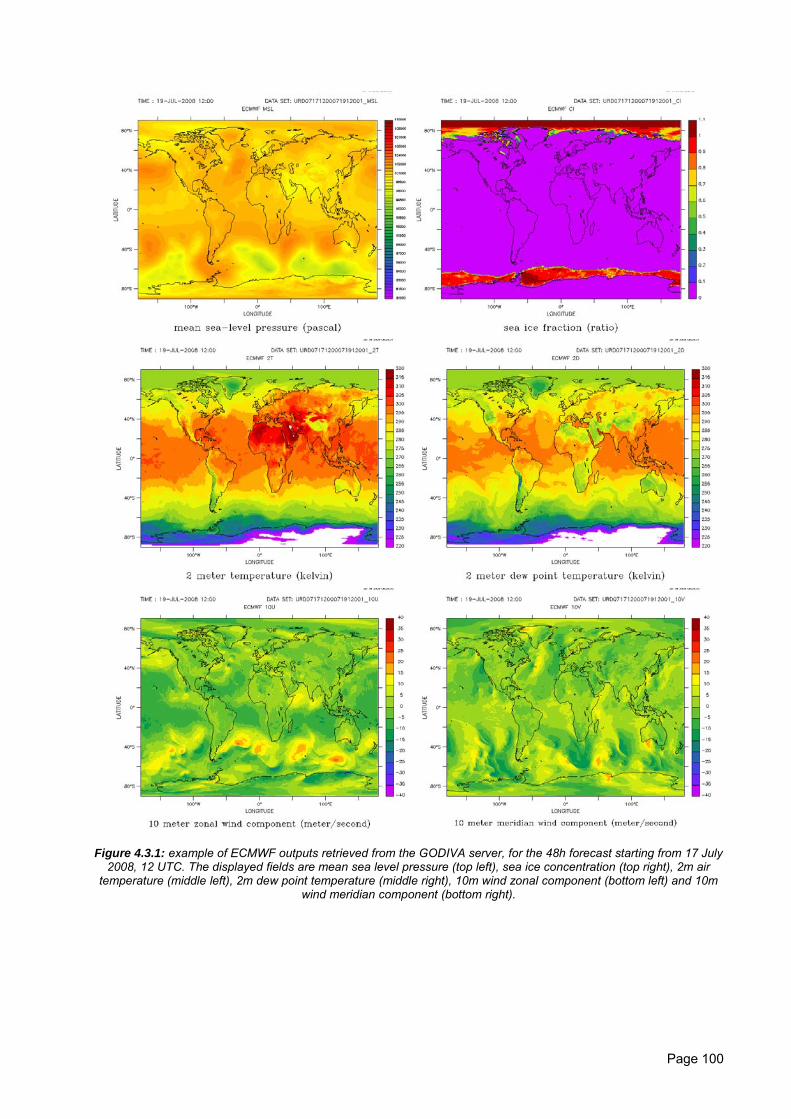
Figure 4.3.1: example of ECMWF outputs retrieved from the GODIVA server, for the 48h forecast starting from 17 July

2008, 12 UTC. The displayed fields are mean sea level pressure (top left), sea ice concentration (top right), 2m airtemperature (middle left), 2m dew point temperature (middle right), 10m wind zonal component (bottom left) and 10m

wind meridian component (bottom right).

Page 100

3.3.2. Operational FTP service providing ECMWF outputs over the Mediterranean SeaAn operational near real time FTP delivery system was set-up to provide the MERSEA operational analysisand forecast system over the Mediterranean Sea, operated under INGV responsibility, with daily ECMWFoutputs. The retrieval of ECMWF outputs is performed daily directly from the ECMWF MARS file systemaround 00 UTC on day D+1, for the ECMWF forecasts starting from day D at 00 UTC and from day D at 12UTC, and for the ECMWF analyses from day D-1 at 18 UTC, and from day D at 00, 06 and 12 UTC. Thefields are extracted via the MARS interface on the Mediterranean Sea domain (30N – 48N – 19W – 42E),on a regular 0.5° x 0.5° grid, in GRIB format. The files are made available daily, as soon as they have beenretrieved from the ECMWF MARS file system, in GRIB format on a password protected part of the M-F ftpserver. They are kept on-line for the past seven days (plus the current day). The delivery system has beenset-up by M-F by the end of June 2005, and has been tested throughout summer 2005 by INGV. It hasbeen declared operational on 17 October 2005, and has replaced the former weekly delivery system usedby INGV, which had been implemented formerly in the context of the MFSPP and MFSTEP projects. Sincethen, the operational near real-time delivery of ECMWF outputs to the MERSEA Modeling and ForecastingCentre for the Mediterranean Sea (INGV) has been running without problem up to the end of the MERSEA

project. Only two cases happened, when the delivery was delayed (once because of production problemsat ECMWF, once because of network problems between ECMWF and Météo-France), and theextraction/delivery had to be re-run by Météo-France.

Page 101

4. Integrated System Design & Assessment (Work Package 05)

Mercator Leader, with MetOffice, INGV, Thales Alenia Space, ENEA, Ifremer, CLS, CNRS,NERSC

4.1. Designing and Assessing the MERSEA Integrated System

The objectives of WP5 were to design the MERSEA integrated system as a whole, then contribute to itsevaluation and end-to-end assessment. The design of the system and of the assessment methodology hasbeen performed through the implementation of the three versions of the MERSEA integrated system.Following the architecture proposed, this step-by-step development of the system has been performedthrough the commitment of the different partners active mostly in WP2, WP3, WP4, WP6 and WP9.Relying upon the same partners, the end-to-end assessment activity aimed to measure during TOP1 andTOP2 the MERSEA Integrated System performance and operational capabilities, together with the scientificquality of ocean products and forecasting skill levels.

The MERSEA Integrated System was something totally new to create in term of operational system: anetwork of nested components, an existing hierarchy of procedures performed at international, national orinstitutional levels, implemented in different ways by various actors. The MERSEA Integrated System hassatisfied the stakeholders, and is being endorsed for the future of GMES. The EC BOSS4GMES and ECOOPprojects are closely linked to MERSEA main outcomes, and the international operational oceanographycommunity, through GODAE, has been interacting with MERSEA partners, that contributed significantly toGODAE success.

4.2. Main achievements related to the System Design

Task 1 and Task 2 of the Workpackage 05 were dedicated to the system definition and design. Along thefour years of the project, WP5 partners have been working on the main definitions and concepts that arenow defining the Marine Core Service.

The main achievements of this European work are presented here.

4.2.1. Achievement 1: Sharing a common view on the existence and definition of amarine “core” service

MERSEA WP5 has invented the marine “European core” service: showed its reality, proposed a definition ofits scope (what is in, what is out), and contributed to its definition.

Figure 5.2.1 : The GMES Marine Core Service / DownstreamServices scheme, known as the “GMES butterfly”

Showing the existence and defining a “core”component in the marine service chain wasone of the first focuses of WP5 partners.

From their early work came out asegmentation into three main components :

• “Upstream”, dealing with the observationand input data sector (satellite, in situ,forcings)

• “Core”, with the ocean genericinformation made of datacombination and models

• “Downstream”, with the user-specializedservices, serving end-users.

The work performed in WP5 focused on thecentral “core” component.

Page 102

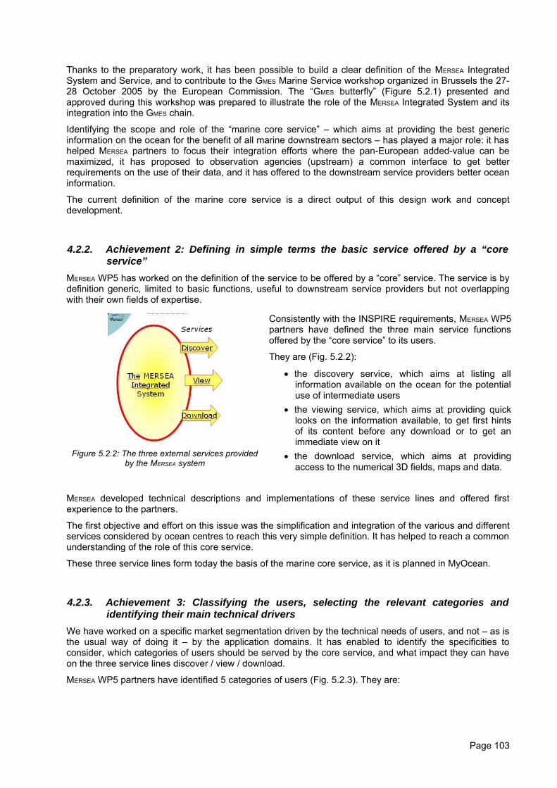
Thanks to the preparatory work, it has been possible to build a clear definition of the MERSEA IntegratedSystem and Service, and to contribute to the GMES Marine Service workshop organized in Brussels the 27-28 October 2005 by the European Commission. The “GMES butterfly” (Figure 5.2.1) presented andapproved during this workshop was prepared to illustrate the role of the MERSEA Integrated System and itsintegration into the GMES chain.

Identifying the scope and role of the “marine core service” – which aims at providing the best genericinformation on the ocean for the benefit of all marine downstream sectors – has played a major role: it hashelped MERSEA partners to focus their integration efforts where the pan-European added-value can bemaximized, it has proposed to observation agencies (upstream) a common interface to get betterrequirements on the use of their data, and it has offered to the downstream service providers better oceaninformation.

The current definition of the marine core service is a direct output of this design work and conceptdevelopment.

4.2.2. Achievement 2: Defining in simple terms the basic service offered by a “coreservice”

MERSEA WP5 has worked on the definition of the service to be offered by a “core” service. The service is bydefinition generic, limited to basic functions, useful to downstream service providers but not overlappingwith their own fields of expertise.

Figure 5.2.2: The three external services providedby the MERSEA system

Consistently with the INSPIRE requirements, MERSEA WP5partners have defined the three main service functionsoffered by the “core service” to its users.

They are (Fig. 5.2.2):

• the discovery service, which aims at listing allinformation available on the ocean for the potentialuse of intermediate users

• the viewing service, which aims at providing quicklooks on the information available, to get first hintsof its content before any download or to get animmediate view on it

• the download service, which aims at providingaccess to the numerical 3D fields, maps and data.

MERSEA developed technical descriptions and implementations of these service lines and offered firstexperience to the partners.

The first objective and effort on this issue was the simplification and integration of the various and differentservices considered by ocean centres to reach this very simple definition. It has helped to reach a commonunderstanding of the role of this core service.

These three service lines form today the basis of the marine core service, as it is planned in MyOcean.

4.2.3. Achievement 3: Classifying the users, selecting the relevant categories andidentifying their main technical drivers

We have worked on a specific market segmentation driven by the technical needs of users, and not – as isthe usual way of doing it – by the application domains. It has enabled to identify the specificities toconsider, which categories of users should be served by the core service, and what impact they can haveon the three service lines discover / view / download.

MERSEA WP5 partners have identified 5 categories of users (Fig. 5.2.3). They are:

Page 103

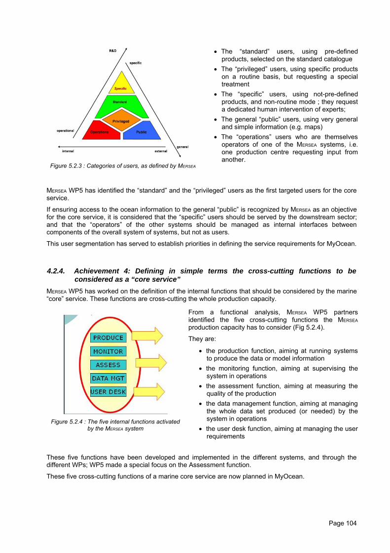
Figure 5.2.3 : Categories of users, as defined by MERSEA

• The “standard” users, using pre-definedproducts, selected on the standard catalogue

• The “privileged” users, using specific productson a routine basis, but requesting a specialtreatment

• The “specific” users, using not-pre-definedproducts, and non-routine mode ; they requesta dedicated human intervention of experts;

• The general “public” users, using very generaland simple information (e.g. maps)

• The “operations” users who are themselvesoperators of one of the MERSEA systems, i.e.one production centre requesting input fromanother.

MERSEA WP5 has identified the “standard” and the “privileged” users as the first targeted users for the coreservice.

If ensuring access to the ocean information to the general “public” is recognized by MERSEA as an objectivefor the core service, it is considered that the “specific” users should be served by the downstream sector;and that the “operators” of the other systems should be managed as internal interfaces betweencomponents of the overall system of systems, but not as users.

This user segmentation has served to establish priorities in defining the service requirements for MyOcean.

4.2.4. Achievement 4: Defining in simple terms the cross-cutting functions to beconsidered as a “core service”

MERSEA WP5 has worked on the definition of the internal functions that should be considered by the marine“core” service. These functions are cross-cutting the whole production capacity.

Figure 5.2.4 : The five internal functions activatedby the MERSEA system

From a functional analysis, MERSEA WP5 partnersidentified the five cross-cutting functions the MERSEA

production capacity has to consider (Fig 5.2.4).

They are:

• the production function, aiming at running systemsto produce the data or model information

• the monitoring function, aiming at supervising thesystem in operations

• the assessment function, aiming at measuring thequality of the production

• the data management function, aiming at managingthe whole data set produced (or needed) by thesystem in operations

• the user desk function, aiming at managing the userrequirements

These five functions have been developed and implemented in the different systems, and through thedifferent WPs; WP5 made a special focus on the Assessment function.

These five cross-cutting functions of a marine core service are now planned in MyOcean.

Page 104

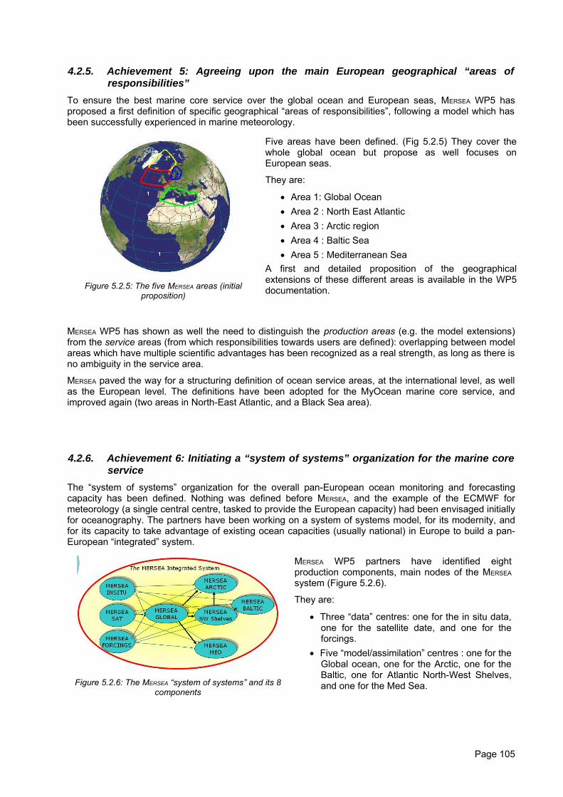
4.2.5. Achievement 5: Agreeing upon the main European geographical “areas ofresponsibilities”

To ensure the best marine core service over the global ocean and European seas, MERSEA WP5 hasproposed a first definition of specific geographical “areas of responsibilities”, following a model which hasbeen successfully experienced in marine meteorology.

Figure 5.2.5: The five MERSEA areas (initialproposition)

Five areas have been defined. (Fig 5.2.5) They cover thewhole global ocean but propose as well focuses onEuropean seas.

They are:

• Area 1: Global Ocean• Area 2 : North East Atlantic• Area 3 : Arctic region• Area 4 : Baltic Sea• Area 5 : Mediterranean Sea

A first and detailed proposition of the geographicalextensions of these different areas is available in the WP5documentation.

MERSEA WP5 has shown as well the need to distinguish the production areas (e.g. the model extensions)from the service areas (from which responsibilities towards users are defined): overlapping between modelareas which have multiple scientific advantages has been recognized as a real strength, as long as there isno ambiguity in the service area.

MERSEA paved the way for a structuring definition of ocean service areas, at the international level, as wellas the European level. The definitions have been adopted for the MyOcean marine core service, andimproved again (two areas in North-East Atlantic, and a Black Sea area).

4.2.6. Achievement 6: Initiating a “system of systems” organization for the marine coreservice

The “system of systems” organization for the overall pan-European ocean monitoring and forecastingcapacity has been defined. Nothing was defined before MERSEA, and the example of the ECMWF formeteorology (a single central centre, tasked to provide the European capacity) had been envisaged initiallyfor oceanography. The partners have been working on a system of systems model, for its modernity, andfor its capacity to take advantage of existing ocean capacities (usually national) in Europe to build a pan-European “integrated” system.

Figure 5.2.6: The MERSEA “system of systems” and its 8components

MERSEA WP5 partners have identified eightproduction components, main nodes of the MERSEA

system (Figure 5.2.6).

They are:

• Three “data” centres: one for the in situ data,one for the satellite date, and one for theforcings.

• Five “model/assimilation” centres : one for theGlobal ocean, one for the Arctic, one for theBaltic, one for Atlantic North-West Shelves,and one for the Med Sea.

Page 105

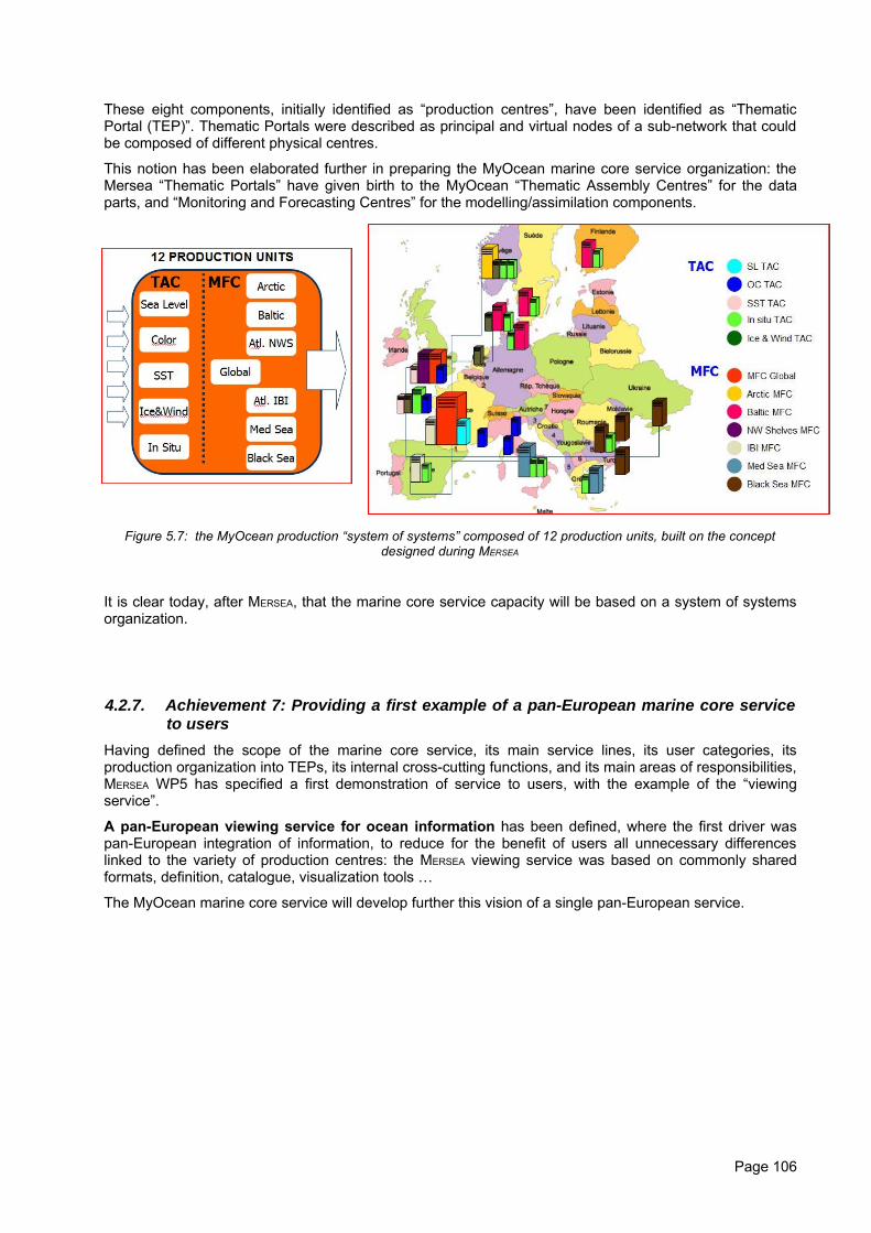
These eight components, initially identified as “production centres”, have been identified as “ThematicPortal (TEP)”. Thematic Portals were described as principal and virtual nodes of a sub-network that couldbe composed of different physical centres.

This notion has been elaborated further in preparing the MyOcean marine core service organization: theMersea “Thematic Portals” have given birth to the MyOcean “Thematic Assembly Centres” for the dataparts, and “Monitoring and Forecasting Centres” for the modelling/assimilation components.

Figure 5.7: the MyOcean production “system of systems” composed of 12 production units, built on the conceptdesigned during MERSEA

It is clear today, after MERSEA, that the marine core service capacity will be based on a system of systemsorganization.

4.2.7. Achievement 7: Providing a first example of a pan-European marine core serviceto users

Having defined the scope of the marine core service, its main service lines, its user categories, itsproduction organization into TEPs, its internal cross-cutting functions, and its main areas of responsibilities,MERSEA WP5 has specified a first demonstration of service to users, with the example of the “viewingservice”.

A pan-European viewing service for ocean information has been defined, where the first driver waspan-European integration of information, to reduce for the benefit of users all unnecessary differenceslinked to the variety of production centres: the MERSEA viewing service was based on commonly sharedformats, definition, catalogue, visualization tools …

The MyOcean marine core service will develop further this vision of a single pan-European service.

Page 106

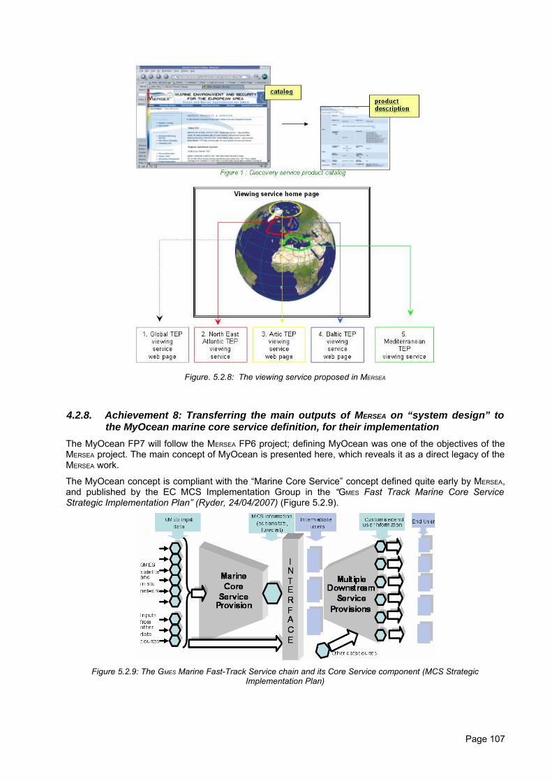
Figure. 5.2.8: The viewing service proposed in MERSEA

4.2.8. Achievement 8: Transferring the main outputs of MERSEA on “system design” tothe MyOcean marine core service definition, for their implementation

The MyOcean FP7 will follow the MERSEA FP6 project; defining MyOcean was one of the objectives of theMERSEA project. The main concept of MyOcean is presented here, which reveals it as a direct legacy of theMERSEA work.

The MyOcean concept is compliant with the “Marine Core Service” concept defined quite early by MERSEA,and published by the EC MCS Implementation Group in the “GMES Fast Track Marine Core ServiceStrategic Implementation Plan” (Ryder, 24/04/2007) (Figure 5.2.9).

Figure 5.2.9: The GMES Marine Fast-Track Service chain and its Core Service component (MCS StrategicImplementation Plan)

Page 107

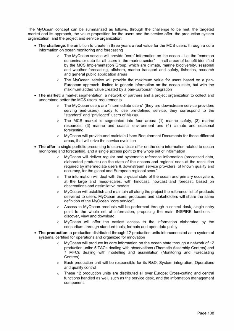
The MyOcean concept can be summarized as follows, through the challenge to be met, the targetedmarket and its approach, the value proposition for the users and the service offer, the production systemorganization, and the project and service organization:

• The challenge: the ambition to create in three years a real value for the MCS users, through a coreinformation on ocean monitoring and forecasting

o The MyOcean service will provide “core” information on the ocean – i.e. the “commondenominator data for all users in the marine sector” – in all areas of benefit identifiedby the MCS Implementation Group, which are climate, marine biodiversity, seasonaland weather forecasting, offshore, marine transport and safety, fisheries, researchand general public application areas

o The MyOcean service will provide the maximum value for users based on a pan-European approach, limited to generic information on the ocean state, but with themaximum added value created by a pan-European integration

• The market: a market segmentation, a network of partners and a project organization to collect andunderstand better the MCS users’ requirements

o The MyOcean users are “intermediate users” (they are downstream service providersserving end-users), ready to use pre-defined service; they correspond to the“standard” and “privileged” users of MERSEA.

o The MCS market is segmented into four areas: (1) marine safety, (2) marineresources, (3) marine and coastal environment and (4) climate and seasonalforecasting.

o MyOcean will provide and maintain Users Requirement Documents for these differentareas, that will drive the service evolution

• The offer: a single portfolio presenting to users a clear offer on the core information related to oceanmonitoring and forecasting, and a single access point to the whole set of information

o MyOcean will deliver regular and systematic reference information (processed data,elaborated products) on the state of the oceans and regional seas at the resolutionrequired by intermediate users & downstream service providers, of known quality andaccuracy, for the global and European regional seas.”

o The information will deal with the physical state of the ocean and primary ecosystem,at the large and meso-scales, with hindcast, nowcast and forecast, based onobservations and assimilative models.

o MyOcean will establish and maintain all along the project the reference list of productsdelivered to users. MyOcean users, producers and stakeholders will share the samedefinition of the MyOcean “core service”.

o Access to MyOcean products will be performed through a central desk, single entrypoint to the whole set of information, proposing the main INSPIRE functions –discover, view and download.

o MyOcean will offer the easiest access to the information elaborated by theconsortium, through standard tools, formats and open data policy

• The production: a production distributed through 12 production units interconnected as a system ofsystems, certified for operations and organized for innovation

o MyOcean will produce its core information on the ocean state through a network of 12production units: 5 TACs dealing with observations (Thematic Assembly Centres) and7 MFCs dealing with modelling and assimilation (Monitoring and ForecastingCentres).

o Each production unit will be responsible for its R&D, System integration, Operationsand quality control

o These 12 production units are distributed all over Europe; Cross-cutting and centralfunctions handled as well, such as the service desk, and the information managementcomponent.

Page 108

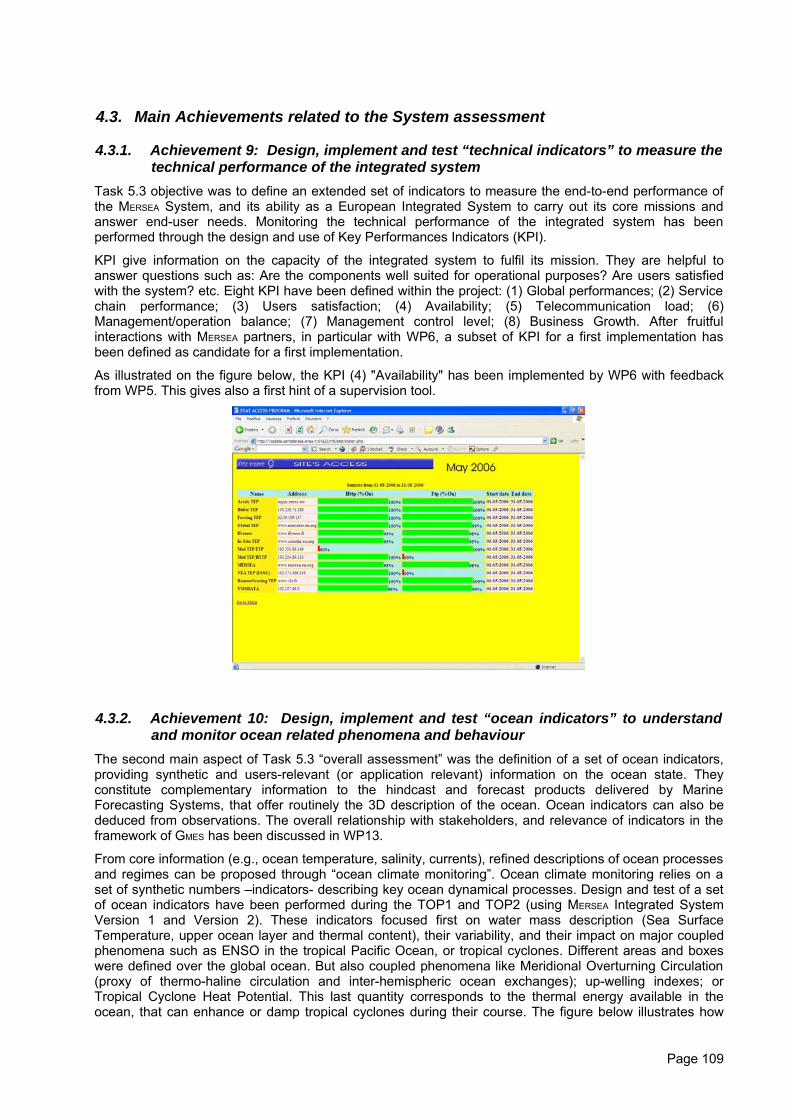
4.3. Main Achievements related to the System assessment

4.3.1. Achievement 9: Design, implement and test “technical indicators” to measure thetechnical performance of the integrated system

Task 5.3 objective was to define an extended set of indicators to measure the end-to-end performance ofthe MERSEA System, and its ability as a European Integrated System to carry out its core missions andanswer end-user needs. Monitoring the technical performance of the integrated system has beenperformed through the design and use of Key Performances Indicators (KPI).

KPI give information on the capacity of the integrated system to fulfil its mission. They are helpful toanswer questions such as: Are the components well suited for operational purposes? Are users satisfiedwith the system? etc. Eight KPI have been defined within the project: (1) Global performances; (2) Servicechain performance; (3) Users satisfaction; (4) Availability; (5) Telecommunication load; (6)Management/operation balance; (7) Management control level; (8) Business Growth. After fruitfulinteractions with MERSEA partners, in particular with WP6, a subset of KPI for a first implementation hasbeen defined as candidate for a first implementation.

As illustrated on the figure below, the KPI (4) "Availability" has been implemented by WP6 with feedbackfrom WP5. This gives also a first hint of a supervision tool.

4.3.2. Achievement 10: Design, implement and test “ocean indicators” to understandand monitor ocean related phenomena and behaviour

The second main aspect of Task 5.3 “overall assessment” was the definition of a set of ocean indicators,providing synthetic and users-relevant (or application relevant) information on the ocean state. Theyconstitute complementary information to the hindcast and forecast products delivered by MarineForecasting Systems, that offer routinely the 3D description of the ocean. Ocean indicators can also bededuced from observations. The overall relationship with stakeholders, and relevance of indicators in theframework of GMES has been discussed in WP13.

From core information (e.g., ocean temperature, salinity, currents), refined descriptions of ocean processesand regimes can be proposed through “ocean climate monitoring”. Ocean climate monitoring relies on aset of synthetic numbers –indicators- describing key ocean dynamical processes. Design and test of a setof ocean indicators have been performed during the TOP1 and TOP2 (using MERSEA Integrated SystemVersion 1 and Version 2). These indicators focused first on water mass description (Sea SurfaceTemperature, upper ocean layer and thermal content), their variability, and their impact on major coupledphenomena such as ENSO in the tropical Pacific Ocean, or tropical cyclones. Different areas and boxeswere defined over the global ocean. But also coupled phenomena like Meridional Overturning Circulation(proxy of thermo-haline circulation and inter-hemispheric ocean exchanges); up-welling indexes; orTropical Cyclone Heat Potential. This last quantity corresponds to the thermal energy available in theocean, that can enhance or damp tropical cyclones during their course. The figure below illustrates how

Page 109

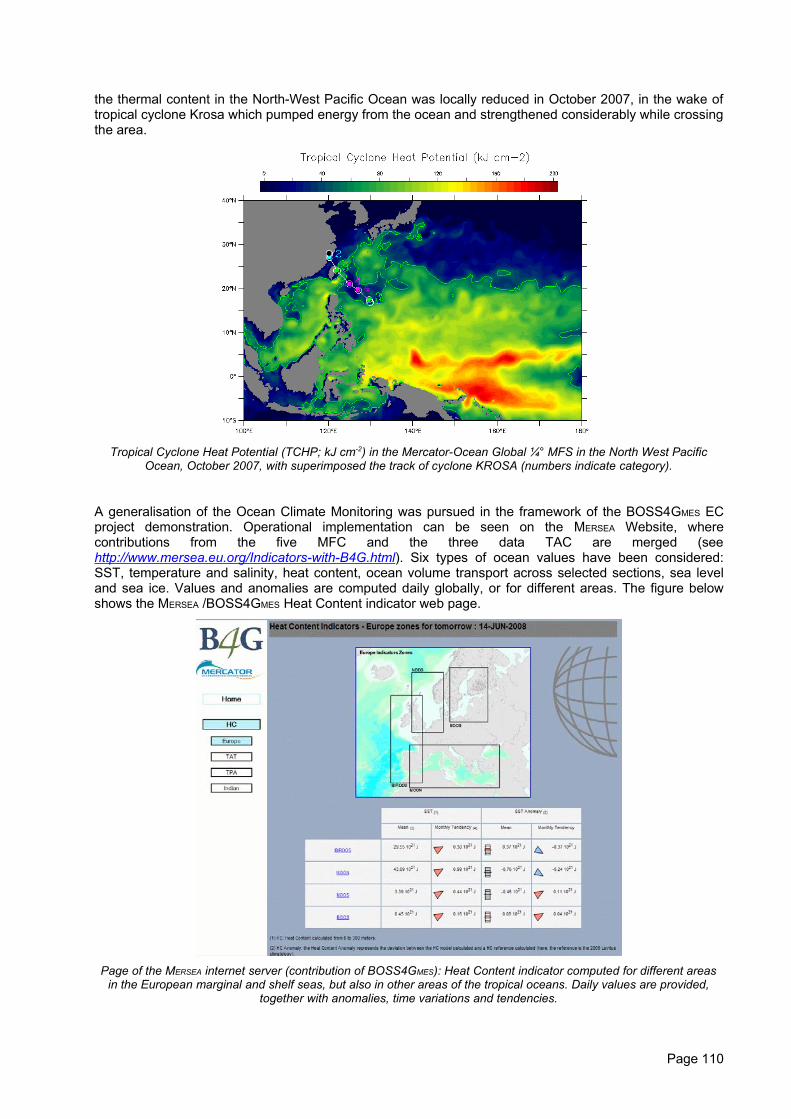
the thermal content in the North-West Pacific Ocean was locally reduced in October 2007, in the wake oftropical cyclone Krosa which pumped energy from the ocean and strengthened considerably while crossingthe area.

Tropical Cyclone Heat Potential (TCHP; kJ cm-2) in the Mercator-Ocean Global ¼° MFS in the North West PacificOcean, October 2007, with superimposed the track of cyclone KROSA (numbers indicate category).

A generalisation of the Ocean Climate Monitoring was pursued in the framework of the BOSS4GMES ECproject demonstration. Operational implementation can be seen on the MERSEA Website, wherecontributions from the five MFC and the three data TAC are merged (seehttp://www.mersea.eu.org/Indicators-with-B4G.html). Six types of ocean values have been considered:SST, temperature and salinity, heat content, ocean volume transport across selected sections, sea leveland sea ice. Values and anomalies are computed daily globally, or for different areas. The figure belowshows the MERSEA /BOSS4GMES Heat Content indicator web page.

Page of the MERSEA internet server (contribution of BOSS4GMES): Heat Content indicator computed for different areasin the European marginal and shelf seas, but also in other areas of the tropical oceans. Daily values are provided,

together with anomalies, time variations and tendencies.

Page 110

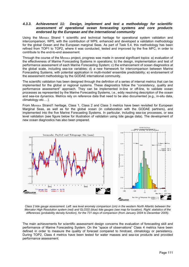
4.3.3. Achievement 11: Design, implement and test a methodology for scientificassessment of operational ocean forecasting systems and core productsendorsed by the European and the international community

Using the MERSEA Strand 1 scientific and technical heritage for operational system validation andintercomparison, WP5, with the contribution of WP9, enhanced and developed a validation methodologyfor the global Ocean and the European marginal Seas. As part of Task 5.4, this methodology has beenrefined from TOP1 to TOP2, where it was conducted, tested and improved by the five MFC, in order tocontribute to the end-to-end assessment.

Through the course of the MERSEA project, progress was made in several significant topics: a) evaluation ofthe effectiveness of Marine Forecasting Systems in operations; b) the design, implementation and test ofperformance assessment of each Marine Forecasting System; c) the enhancement of ocean diagnostics atthe global scale, including sea-ice variables; d) a new framework for intercomparison between MarineForecasting Systems, with potential application in multi-model/ ensemble predictability; e) endorsement ofthe assessment methodology by the GODAE international community.

The scientific validation has been designed through the definition of a series of internal metrics that can beimplemented for the global or regional systems. These diagnostics follow the “consistency, quality andperformance assessment” approach. They can be implemented in-line or off-line, to validate oceanprocesses as represented by the Marine Forecasting Systems, i.e., eddy resolving description of the oceanand sea-ice dynamics. Metrics rely on reference data that need to be also documented (e.g., in-situ data,climatology etc….).

From MERSEA Strand1 heritage, Class 1, Class 2 and Class 3 metrics have been revisited for EuropeanMarginal Seas, as well as for the global ocean (in collaboration with the GODAE partners), andimplemented into the five Marine Forecasting Systems. In particular, including sea-ice processes, or sealevel validation (see figure below for illustration of validation using tide gauge data). The development ofnew ocean diagnostics has also been prepared.

Class 2 tide gauge assessment. Left: sea level anomaly comparison (cm) in the western North Atlantic between theMercator High Resolution system (red) and GLOSS (blue) tide gauges (see map for location). Right: statistics of thedifferences (probability density function), for the 731 days of comparison (from January 2004 to December 2005).

The main achievements for scientific assessment design concerns the evaluation of forecasting skill andperformance of Marine Forecasting System. On the “space of observations” Class 4 metrics have beendefined in order to measure the quality of forecast compared to hindcast, climatology or persistency.During TOP2, Class 4 metrics have been tested for water masses and sea-ice products and providedperformance assessment.

Page 111

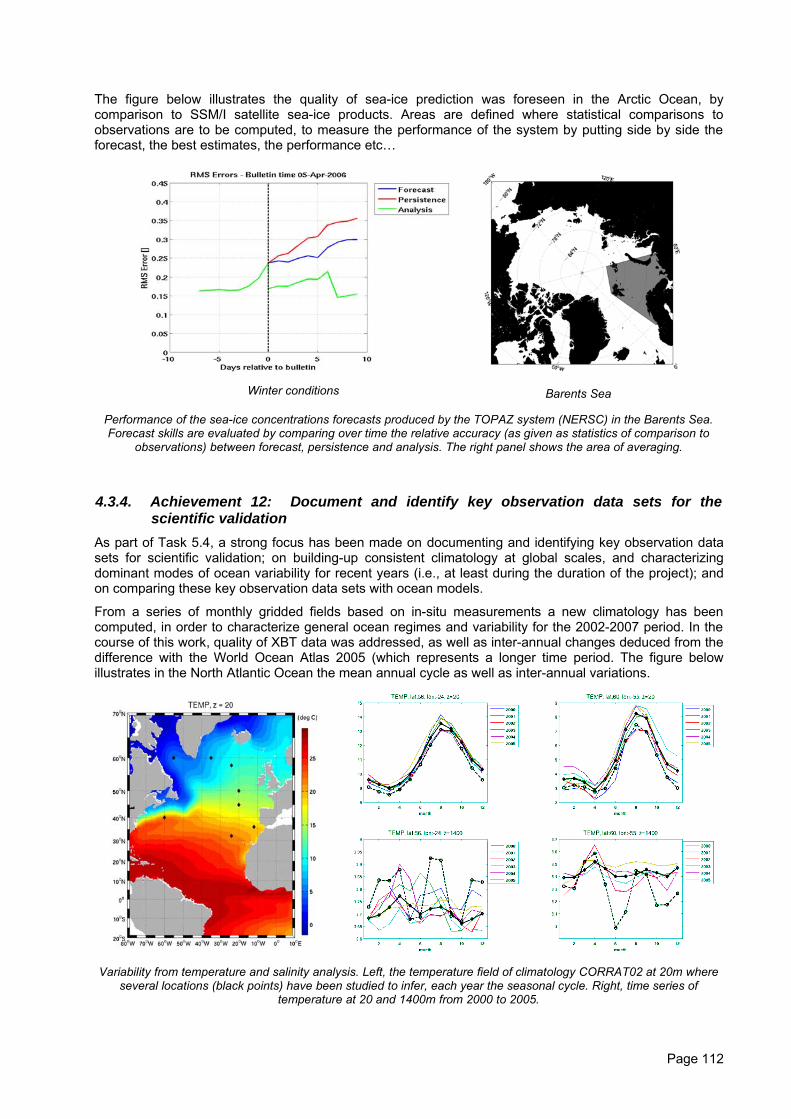
The figure below illustrates the quality of sea-ice prediction was foreseen in the Arctic Ocean, bycomparison to SSM/I satellite sea-ice products. Areas are defined where statistical comparisons toobservations are to be computed, to measure the performance of the system by putting side by side theforecast, the best estimates, the performance etc…

Winter conditions Barents Sea

Performance of the sea-ice concentrations forecasts produced by the TOPAZ system (NERSC) in the Barents Sea.Forecast skills are evaluated by comparing over time the relative accuracy (as given as statistics of comparison to

observations) between forecast, persistence and analysis. The right panel shows the area of averaging.

4.3.4. Achievement 12: Document and identify key observation data sets for thescientific validation

As part of Task 5.4, a strong focus has been made on documenting and identifying key observation datasets for scientific validation; on building-up consistent climatology at global scales, and characterizingdominant modes of ocean variability for recent years (i.e., at least during the duration of the project); andon comparing these key observation data sets with ocean models.

From a series of monthly gridded fields based on in-situ measurements a new climatology has beencomputed, in order to characterize general ocean regimes and variability for the 2002-2007 period. In thecourse of this work, quality of XBT data was addressed, as well as inter-annual changes deduced from thedifference with the World Ocean Atlas 2005 (which represents a longer time period. The figure belowillustrates in the North Atlantic Ocean the mean annual cycle as well as inter-annual variations.

Variability from temperature and salinity analysis. Left, the temperature field of climatology CORRAT02 at 20m whereseveral locations (black points) have been studied to infer, each year the seasonal cycle. Right, time series of

temperature at 20 and 1400m from 2000 to 2005.

Page 112

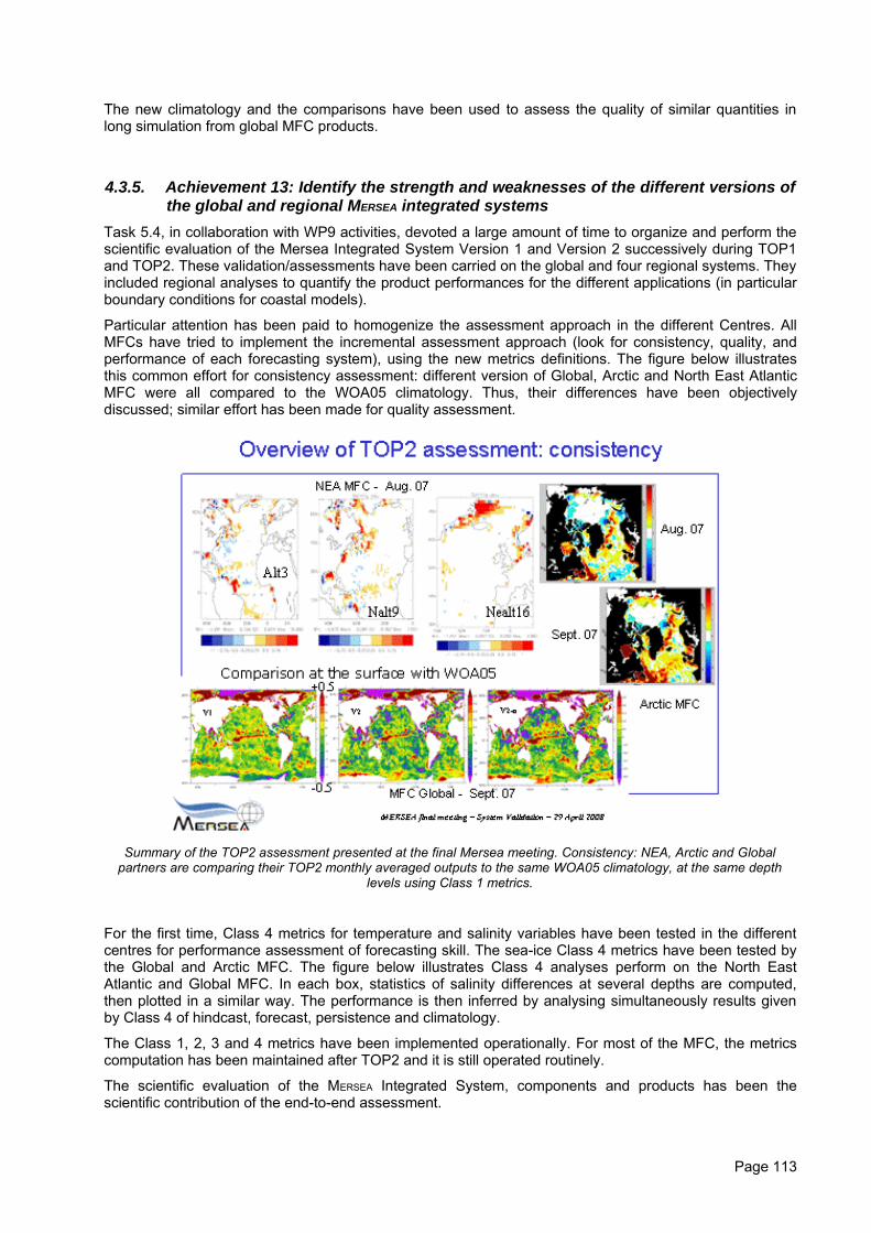
The new climatology and the comparisons have been used to assess the quality of similar quantities inlong simulation from global MFC products.

4.3.5. Achievement 13: Identify the strength and weaknesses of the different versions ofthe global and regional MERSEA integrated systems

Task 5.4, in collaboration with WP9 activities, devoted a large amount of time to organize and perform thescientific evaluation of the Mersea Integrated System Version 1 and Version 2 successively during TOP1and TOP2. These validation/assessments have been carried on the global and four regional systems. Theyincluded regional analyses to quantify the product performances for the different applications (in particularboundary conditions for coastal models).

Particular attention has been paid to homogenize the assessment approach in the different Centres. AllMFCs have tried to implement the incremental assessment approach (look for consistency, quality, andperformance of each forecasting system), using the new metrics definitions. The figure below illustratesthis common effort for consistency assessment: different version of Global, Arctic and North East AtlanticMFC were all compared to the WOA05 climatology. Thus, their differences have been objectivelydiscussed; similar effort has been made for quality assessment.

Summary of the TOP2 assessment presented at the final Mersea meeting. Consistency: NEA, Arctic and Globalpartners are comparing their TOP2 monthly averaged outputs to the same WOA05 climatology, at the same depth

levels using Class 1 metrics.

For the first time, Class 4 metrics for temperature and salinity variables have been tested in the differentcentres for performance assessment of forecasting skill. The sea-ice Class 4 metrics have been tested bythe Global and Arctic MFC. The figure below illustrates Class 4 analyses perform on the North EastAtlantic and Global MFC. In each box, statistics of salinity differences at several depths are computed,then plotted in a similar way. The performance is then inferred by analysing simultaneously results givenby Class 4 of hindcast, forecast, persistence and climatology.

The Class 1, 2, 3 and 4 metrics have been implemented operationally. For most of the MFC, the metricscomputation has been maintained after TOP2 and it is still operated routinely.

The scientific evaluation of the MERSEA Integrated System, components and products has been thescientific contribution of the end-to-end assessment.

Page 113

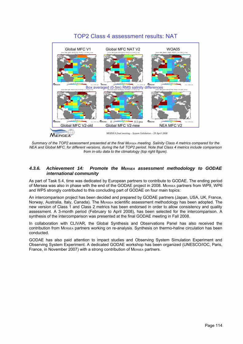
MERSEA final meeting – System Validation – 29 April 2008

TOP2 Class 4 assessment results: NAT

NEA MFC V2Global MFC V2-newGlobal MFC V2-old

Global MFC NAT V2Global MFC V1 WOA05

Box averaged (0-5m) RMS salinity differences

0 0.5 psu

Summary of the TOP2 assessment presented at the final MERSEA meeting. Salinity Class 4 metrics compared for theNEA and Global MFC, for different versions, during the full TOP2 period. Note that Class 4 metrics include comparison

from in-situ data to the climatology (top right figure).

4.3.6. Achievement 14: Promote the MERSEA assessment methodology to GODAEinternational community

As part of Task 5.4, time was dedicated by European partners to contribute to GODAE. The ending periodof Mersea was also in phase with the end of the GODAE project in 2008. MERSEA partners from WP9, WP6and WP5 strongly contributed to this concluding part of GODAE on four main topics:

An intercomparison project has been decided and prepared by GODAE partners (Japan, USA, UK, France,Norway, Australia, Italy, Canada). The MERSEA scientific assessment methodology has been adopted. Thenew version of Class 1 and Class 2 metrics has been endorsed in order to allow consistency and qualityassessment. A 3-month period (February to April 2008), has been selected for the intercomparison. Asynthesis of the intercomparison was presented at the final GODAE meeting in Fall 2008.

In collaboration with CLIVAR, the Global Synthesis and Observations Panel has also received thecontribution from MERSEA partners working on re-analysis. Synthesis on thermo-haline circulation has beenconducted.

GODAE has also paid attention to impact studies and Observing System Simulation Experiment andObserving System Experiment. A dedicated GODAE workshop has been organized (UNESCO/IOC, Paris,France, in November 2007) with a strong contribution of MERSEA partners.

Page 114

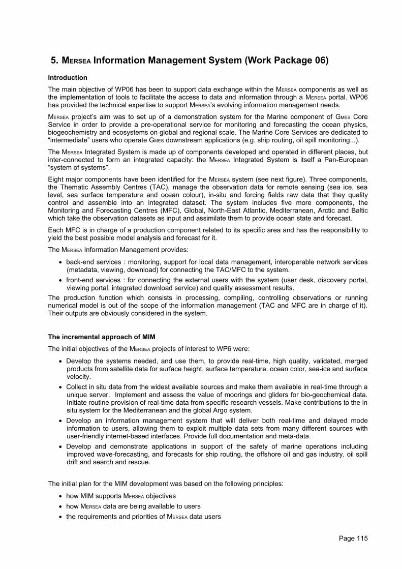
5. MERSEA Information Management System (Work Package 06)

Introduction

The main objective of WP06 has been to support data exchange within the MERSEA components as well asthe implementation of tools to facilitate the access to data and information through a MERSEA portal. WP06has provided the technical expertise to support MERSEA’s evolving information management needs.

MERSEA project’s aim was to set up of a demonstration system for the Marine component of GMES CoreService in order to provide a pre-operational service for monitoring and forecasting the ocean physics,biogeochemistry and ecosystems on global and regional scale. The Marine Core Services are dedicated to“intermediate” users who operate GMES downstream applications (e.g. ship routing, oil spill monitoring...).

The MERSEA Integrated System is made up of components developed and operated in different places, butinter-connected to form an integrated capacity: the MERSEA Integrated System is itself a Pan-European“system of systems”.

Eight major components have been identified for the MERSEA system (see next figure). Three components,the Thematic Assembly Centres (TAC), manage the observation data for remote sensing (sea ice, sealevel, sea surface temperature and ocean colour), in-situ and forcing fields raw data that they qualitycontrol and assemble into an integrated dataset. The system includes five more components, theMonitoring and Forecasting Centres (MFC), Global, North-East Atlantic, Mediterranean, Arctic and Balticwhich take the observation datasets as input and assimilate them to provide ocean state and forecast.

Each MFC is in charge of a production component related to its specific area and has the responsibility toyield the best possible model analysis and forecast for it.

The MERSEA Information Management provides:

• back-end services : monitoring, support for local data management, interoperable network services(metadata, viewing, download) for connecting the TAC/MFC to the system.

• front-end services : for connecting the external users with the system (user desk, discovery portal,viewing portal, integrated download service) and quality assessment results.

The production function which consists in processing, compiling, controlling observations or runningnumerical model is out of the scope of the information management (TAC and MFC are in charge of it).Their outputs are obviously considered in the system.

The incremental approach of MIM

The initial objectives of the MERSEA projects of interest to WP6 were:

• Develop the systems needed, and use them, to provide real-time, high quality, validated, mergedproducts from satellite data for surface height, surface temperature, ocean color, sea-ice and surfacevelocity.

• Collect in situ data from the widest available sources and make them available in real-time through aunique server. Implement and assess the value of moorings and gliders for bio-geochemical data.Initiate routine provision of real-time data from specific research vessels. Make contributions to the insitu system for the Mediterranean and the global Argo system.

• Develop an information management system that will deliver both real-time and delayed modeinformation to users, allowing them to exploit multiple data sets from many different sources withuser-friendly internet-based interfaces. Provide full documentation and meta-data.

• Develop and demonstrate applications in support of the safety of marine operations includingimproved wave-forecasting, and forecasts for ship routing, the offshore oil and gas industry, oil spilldrift and search and rescue.

The initial plan for the MIM development was based on the following principles:

• how MIM supports MERSEA objectives• how MERSEA data are being available to users• the requirements and priorities of MERSEA data users

Page 115

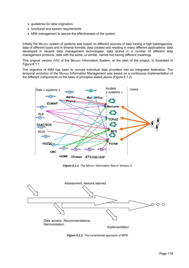
• guidelines for data originators• functional and system requirements• MIM management to assure the effectiveness of the system

Initially the MERSEA system of systems was based on different sources of data having a high heterogeneity:data of different types and in diverse formats; data created and residing in many different applications; datadeveloped in several data management technologies; data stored in a number of different datamanagement products; data with the same, or similar, names but having different meanings.

This original version (V0) of the MERSEA Information System, at the start of the project, is illustrated inFigure 6.1.1

The objective of MIM has been to convert individual data providers into an integrated federation. Thetemporal evolution of the MERSEA Information Management was based on a continuous implementation ofthe different components on the base of principles stated above (Figure 6.1.2).

Figure 6.1.1. The MERSEA Information flow in Version 0.

Figure 6.1.2. The incremental approach of WP6.

Page 116

Mercator

TOPAZ

FOAM

MFS

Ifremer GTS

Météo-France

Met Office

CLS

HCMRCMC

NOA

ISAC/GOS

ECMWF

NSIDC

OSI/SAF

Usersmodels « systems »

Data « systems »

Assessment, lessons learned

Data access, Recommendations, Harmonisation

Implementation

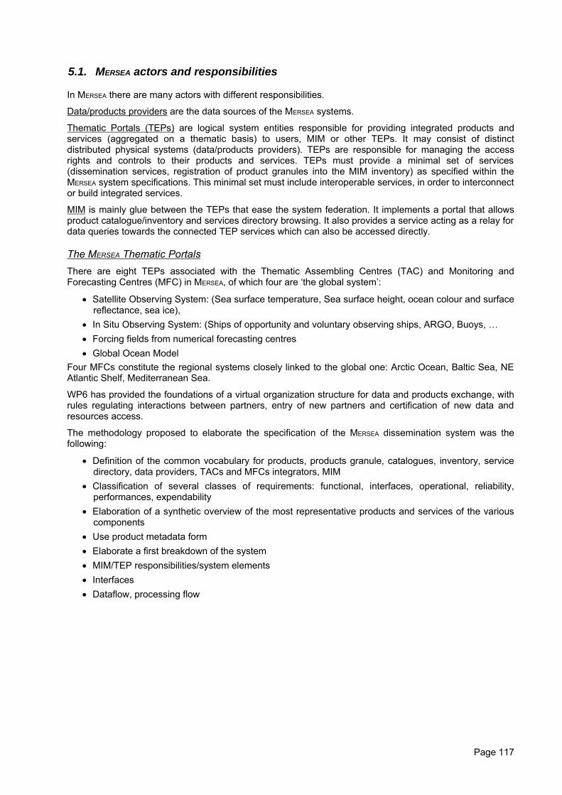
5.1. MERSEA actors and responsibilities

In MERSEA there are many actors with different responsibilities.

Data/products providers are the data sources of the MERSEA systems.

Thematic Portals (TEPs) are logical system entities responsible for providing integrated products andservices (aggregated on a thematic basis) to users, MIM or other TEPs. It may consist of distinctdistributed physical systems (data/products providers). TEPs are responsible for managing the accessrights and controls to their products and services. TEPs must provide a minimal set of services(dissemination services, registration of product granules into the MIM inventory) as specified within theMERSEA system specifications. This minimal set must include interoperable services, in order to interconnector build integrated services.

MIM is mainly glue between the TEPs that ease the system federation. It implements a portal that allowsproduct catalogue/inventory and services directory browsing. It also provides a service acting as a relay fordata queries towards the connected TEP services which can also be accessed directly.

The MERSEA Thematic PortalsThere are eight TEPs associated with the Thematic Assembling Centres (TAC) and Monitoring andForecasting Centres (MFC) in MERSEA, of which four are ‘the global system’:

• Satellite Observing System: (Sea surface temperature, Sea surface height, ocean colour and surfacereflectance, sea ice),

• In Situ Observing System: (Ships of opportunity and voluntary observing ships, ARGO, Buoys, …• Forcing fields from numerical forecasting centres• Global Ocean Model

Four MFCs constitute the regional systems closely linked to the global one: Arctic Ocean, Baltic Sea, NEAtlantic Shelf, Mediterranean Sea.

WP6 has provided the foundations of a virtual organization structure for data and products exchange, withrules regulating interactions between partners, entry of new partners and certification of new data andresources access.

The methodology proposed to elaborate the specification of the MERSEA dissemination system was thefollowing:

• Definition of the common vocabulary for products, products granule, catalogues, inventory, servicedirectory, data providers, TACs and MFCs integrators, MIM

• Classification of several classes of requirements: functional, interfaces, operational, reliability,performances, expendability

• Elaboration of a synthetic overview of the most representative products and services of the variouscomponents

• Use product metadata form• Elaborate a first breakdown of the system• MIM/TEP responsibilities/system elements• Interfaces• Dataflow, processing flow

Page 117

5.2. Definition of products and services (Task 6.1)

Ifremer Leader, with CLS, ENEA, UREADES, INGV

5.2.1. The MIM chartersMERSEA provides services and information dissemination through interfaces (portals) to internal and externalusers. The MERSEA services have been integrated in charters defined in the Integrated System Handbook:

• Mission charter: What thematic information is managed by the network (included product catalogue)• Quality charter: What quality must be enforced/can be expected,• Interoperability charter: How can the information be delivered/accessed (format, technology

standards, ...)• Business charter: Under which conditions is the information delivered/accessed (pricing policy,

property rights, ...)

5.2.2. MERSEA USERSUsers of the MERSEA Integrated System have been classified into 5 categories, each one grouping userssharing similar need:

Category 1: “Privileged users”: need exchanging data and/or products and/or services on a routinemode. This is mainly done via computer-to-computer link, with no human intervention and the guaranty ofhigh level availability & quality of service

Category 2: “Standard users”: access routinely, on request, products of the MERSEA integrated system(standard products). They need tools to search among registered (qualified) products and easily identifiedneeded products, to select, extract, and or access useful (limited) information

Category 3: “Public users”: general public with aim for education and public outreach. They want‘front/demonstration’ window for operational oceanography;

Category 4: “Specific users” (e.g. research labs) request specific products, i.e. products which are notavailable online or though registered distribution mean, or not routinely produced and qualified. They canbe served via human intervention. We just mention here this “specific use” category, but it has not beenconsidered further in the implementation of the MERSEA Integrated System.

Category 5: “Operations” (system management): all users involved in the MERSEA system monitoringand supervision. They need monitoring functions and results, and are serving general information andprovide visibility on existing systems

5.2.3. MERSEA PRODUCTSThe products defined in MIM are summarized in the table below.

The MERSEA products consist of high resolution ocean environmental variables with geographical andtemporal indices provided on an operational basis.

The baseline and standard products comprise model and observational data products. The model productscontain both analyses and forecast data.

The observational products contain the quality controlled raw observations and analyzed or griddedobservational data. All the products are defined with precise relationship to the geographical area ofapplication which could point to a different space and time resolution of the products.

The base-line products are the rawest kind of model and observational data that can be provided byMERSEA. Standard products are the one level up from the base-line products and they are required forinteroperability with other data sets (for example biochemical data, etc.).

Page 118

Baselineobservationalproduct

The observational baseline products are the ‘raw’ in situ and L0 - L2 satellite data setsgiven on the measurement geographical and time locations.

Standardobservationalproduct

The observational standard products are of general categories: in situ qc, qc timeseries, gridded fields, L3-L4 satellite data,

Baselinemodel product

The model base-line products are the model output state variables on the modelnative grid

Standardmodel product

The model standard products are instead on a grid with simple geographicalcoordinates (lat, long and depth) at a fixed resolution similar to the native model grid

5.3. Implementation of MIM (Task 6.2)

ENEA Leader, with CLS, IFREMER, MARIS, UREADES, INGV

5.3.1. Information contentThere are both general and specific information required by users. In all cases the following questionsmust be answered: what, why, where, when, who, how.

Issue Information Content

What Describe the objectives, and/or the content of the projectWhy Explain the reason and/or the state of art before the projectWhere Describe the scientific and/or geographical area in which the efforts are concentratedWhen Provide information on the temporal coverageWho Describe the group of participants and/or the project participants and rolesHow Provide information and links on themes and/or centres participating to the project

The objective of the Information Management within MERSEA is to implement the information content inorder to provide services and to fulfill the needs of the targeted users. Following the INSPIRE directive(Article 11 of Annex 1) MIM was developed to provide the following services:

Service 1: DISCOVERY: Making it possible to search for spatial data sets and services on the basis of thecontent of the corresponding metadata and to display the content of the meta-data.

Service 2: VIEW: Making it possible, as a minimum, to display, navigate, zoom in/out, pan or overlayviewable spatial data sets and to display legend information and any relevant content of meta-data.

Service 3: ACCESS/DOWNLOAD: Enabling copies of the spatial data sets, or parts of such sets, to bedownloaded and, when practicable, accessed directly.

TACs, MFCs and MIM have implemented a certain number of cross-cutting functions for MERSEA to enablethe above services. They are internal services unknown from the external user

PRODUCTION: Produce and deliver ocean products for model assimilation, model validation and theviewing service (production, archival and delivery is under responsibility of each data centre).

MONITORING: To monitor the production (user needs), whether it has been correctly produced(standardization), to track the implementation of crosscutting functions and to measure systemperformance (Key Performance Indicators)

QUALITY: Assess the quality of the system and of its products.

PRODUCTS & SERVICES MANAGEMENT: Catalogue of products with link to inventory, viewing andaccess/download services.

Page 119

USER DESK: To handle user management at MERSEA level and to provide integrated services such asdownloading.

5.3.2. Catalogue of products and servicesIn MERSEA usage, a product is the output of a processing chain, which adds significant value to the originaldatasets used as inputs (so that it is worth to have documentation, references, quality assessment,... on it).The datasets produced by stable process of compilation and quality assessment on data, or by a numericalmodel for analysis and forecast are considered as products, but a dataset that is a simple subset ofanother dataset is not a product itself (e.g. a specific area or time out of a global model outputs series).The metadata on the latest is made available through THREDDS1 inventories. The usage of thesemetadata is discussed later in the download integrated service paragraph.

The MERSEA product catalogue is composed of a set of products general descriptions, elaborated by thedata providers (coordinated at TAC/MFC level). They contain general information on product, links toviewing services and download services (agreed back-end services and specific services as well) and linksto relevant documentation.

The ISO19115 XML back-end metadata flows are published in human-readable web pages. A searchfacility is available so that the users can set filters on the product's list. The search facility, which isdeveloped as a web application based on the central database and keyword indexation, makes users ableto request the catalogue according to criteria. The catalogue can be requested through on-line forms orprogrammatically through an interoperability layer (request URL, XML list of products, ISO19115 XMLdescription).

5.3.3. Viewing service

Integrated viewing serviceThe MERSEA Integrated Viewing service (MIV) is a friendly graphical user interface (GUI) allowing thevisualization of weekly updated pre-defined plots (historical plots are also available). These quick-looks arethe official picture of the MERSEA system outputs. They show ocean forecasting models, remote sensingdata and in-situ data as maps on the five areas corresponding to the five geographical MFC. Cross-sections defined by the quality assessment team are also available.

MIV is based on MERSEA standard back-end services (OPeNDAP interfaces and netCDF /COARDS/ CFformat. At the heart of MIV is a centralized engine that accesses every week the distributed and remotedata servers for a selected set of parameters and depths. Ferret is the cartographic open source softwareused to create the plot.

Demonstration viewing serviceThe MERSEA Dynamic Quick View (DQV) service is a demonstration prototype of a portal that providesinteractive visualization of data. It allows the user to pan and zoom smoothly through datasets and selectfrom all available depth and time values. Animations can be created, and precise data values can bediscovered by clicking on the dynamic map. Time series plots at any point can also be created. Imagerycan be viewed in Google Earth and other GIS clients, allowing overlaying of MERSEA data with data fromother sources.

The DQV site is served by a custom-built Web Map Service (WMS), developed by and hosted at theUniversity of Reading. The WMS connects to the OPeNDAP interfaces at the individual data providers andconverts 4-D data to map imagery on demand. The WMS was designed to generate map imagery asquickly and efficiently as possible; existing implementations were found to be too slow to support dynamic,tile-based clients such as DQV. The WMS therefore supports interactive “quick look” visualization of data(panning, zooming through datasets, selection of time and elevation values, changes of colour scale andpalette).

The WMS implementation contains a number of additions to the WMS specification in order to fully satisfyMERSEA viewing needs. These include methods for accessing fragments of metadata to populate menus inthe DQV website, in contrast with the standard WMS approach of employing a single, monolithicCapabilities document.

1 Thematic Realtime Environmental Distributed Data Services

Page 120

Discovery serviceFor metadata access, in addition to the simple dataset description provided with the THREDDS XMLinterfaces, the full product and network services description is provided by the TAC/MFC in XML ISO19115format (which is the metadata standard for geo-spatial datasets). To provide or update the description, theTAC/MFC can use their own catalogue tools or use dedicated on-line forms. The ISO19115 XMLdescription are gathered and harmonized into a centralized database so that the catalogue of the productsand the related network service description are available for the system.

5.4. System Monitoring (Task 6.4)

UREADES Leader, with CLS, DMI, ENEA, IFREMER, INGV, NERSC, Techworks, MARIS

5.4.1. Key Performance Indicators (KPI).The KPI are based on the mission of the project and its strategic goals. They have to measure theeffectiveness and performance of the system. The following concepts were defined for the system design:

1. Mission: Allow the dissemination of source and thematic data concerning ocean state on globalocean and major European Seas, on an operational basis. The MERSEA system must include ameasurement-based management component, to monitor performance over time (balancedscorecard).

2. Performance goal: the target level of performance will be the timely delivery of data, products,services. The performance can be enriched with the assessment of the importance of the delivery.

3. Performance indicator: is a particular value or characteristics used to measure the efficiency ofproducts and services delivery.

4. Performance metric: definition of the methodology, analysis and other activities involved with ‘how’particular metrics are measured.

5. Activity based management: the use of strategic initiatives and operational changes in an effort tooptimize TEP performances.

It was agreed to improve only simple KPIs designed to measure the availability and performance of Datacollection; Forecasts; and Information system.

Four sets of KPIs have been designed and implemented to monitor timeliness and quality of the products;measurement of user complains concerning product quality; number of connection to the servers andvolume downloaded; and availability of the Tep Ftp and WWW server.

5.4.2. Help DeskThe help desk is an information and assistance resource that supports ‘users’ via website and/or e-mail. Inthe MERSEA Integrated System, the help desk is part of the ‘General Services’. The elements of the MERSEA

help desk should include a general information desk on the system; be able to answer specialised issues;and release specific information and updates, when available. Only some elements of the help desk wereimplemented, but they have not been made operational during the project.

5.5. Conclusion, perspectives

5.5.1. Implementation statusThe discovery service and the product/service catalogue are operational and integrated. The viewingservices are integrated and available in an operational (called MIV) and demonstration version (calledDQV). The integrated download service, user management and technical monitoring are provided asdemonstration functions. The user-desk and quality assessment functions are provided as standaloneapplications (not fully integrated in the system, relying on extra-support for operations).

Page 121

The technology developed within MERSEA will be upgraded to fulfill the discovery and viewing requirementsof the European Union project for coastal operational oceanography: ECOOP. Moreover the MyOceansystem, which will implement the Marine Core Services of GMES, will be built upon these developments andwill take advantage of the MERSEA background for the next steps.

Three main actions remain to be undertaken during the coming project: set up thematic user services,better harmonization of information flows, better reporting and monitoring resources and tools.

5.5.2. Lessons learned, MyOcean perspectivesTwo processes of improvement of the distributed operational information management system can beconsidered.

The first of them is to work on the front-end services to better fit the downstream application providerrequirements. Depending on the usage (oil spill monitoring, offshore industry, ship routing...) dedicated orcustomized services should be set up: for each of them, the suitable ocean product package (oceanparameters, real time / climatologies, depth levels...) and functions (data subscriptions, relevantvisualizations, ...) should be defined and provided. During MyOcean project, this may be improved bysetting up front-end services technically and thematically designed, tested and validated with downstreamapplication providers.

The second of them is to work on a better harmonization of the back-end services and keep compliancewith different requirements (users community systems, European or international directives). DuringMyOcean, the back-end services may especially be improved thanks to extended agreements and strictvalidation of the data structures and parameters names.

Finally, better monitoring and feedback will help us to set up an operational system meeting the reliabilityrequirements. Monitoring alerts from the system to the data providers should improve the overall level ofservice. The reporting inputs from data providers to the system may also help to build a more reactivesystem. Finally, the feedback from external users to system and from system to data providers has to beconsidered and will obviously improve the overall performance of the system.

So, besides data flow harmonization and doing suitable ‘packages’ of these data flows for the externalusers, the challenge for myOcean system to be efficient and reliable is the ability to orchestrate the systemby managing requests of users, reports of data providers and doing an efficient monitoring of demands andresources.

Page 122

6. Modelling and data assimilation (Work Package 07)

Work Package objectives and major achievements during the reporting periodThe general objectives of WP7 are (i) to perform research and development on physical modelling,ecosystem modelling and data assimilation as required for the operational objectives of MERSEA during thewhole duration of the project, (ii) to provide all the tools (physical model codes, biogeochemical modelcodes, data assimilation codes) required by the MERSEA project to reach its operational objectives, and (iii)to bring ad hoc scientific innovations into the project and to gather all the relevant European capabilities inorder to make sure that operational systems are maintained at the most advanced level thus benefitingfrom progress achieved in the research community, during the project life-time and beyond.

This work package is divided into three main components, dedicated to physical models, biogeochemicalmodels and data assimilation methods.

6.1. Physical Modelling (Task 7.1)

The main activities of the Physical models task are:

• To transfer the intermediate high resolution (1/4°) physical model code and insure relevant expertiseon running the code, analysing and assessing the results at global scale.

• To realize R&D activities for continuous model improvements (numerical schemes, bottom boundarylayer, tidal mixing, mixed layer,...).

• To contribute to the development of a global ORCA high resolution (1/12°) physical model.• To develop and transfer the nesting capabilities (software and expertise) to make the one-way and

two-way connections between the large scale model and the regional models

The main objective of the physical modelling subtask were to upgrade the numerical ocean generalcirculation model (GCM) NEMO1 which is one of the major components of the operational systemdeveloped in MERSEA. The starting point was the OPA8.1 ocean GCM (Madec et al., 1998). The ultimategoal was to deliver to the project a global model configuration at eddy-permitting resolution (1/4°), basedon the NEMO code (Madec, 2008), an up-graded version of the OPA ocean circulation model including afully prognostic sea-ice model (an updated version of the LIM2 model of Fichefet and Maqueda, 1997).This configuration, referred to as the DRAKKAR2 configuration ORCA0253, should include a recentparameterisation of topography (partial steps), an improved parameterisation of the mixing at the surfaceand in the interior, and most advanced numerical scheme. This configuration should be optimised formassively parallel supercomputers. The model should also include grid-refinement capabilities, in relationwith the need of WP10.

A first version of the ORCA025 model configuration, with partial steps and a new energy–enstrophyconserving (EEN) momentum advection scheme has been delivered to the project at the end of the first 12month period, (D7.1.1) and a final version, fully validated by sensitivity experiments was then delivered atmonth 30 (D7.1.5). Model developments related to tidal mixing and mixed layer parameterisation havebeen implemented and validated (D7.1.2, D7.1.3).

Concerning nesting methods and the AGRIF software, the task was to realise a synthesis of the needs andcomments expressed by the users of the AGRIF package in WP10, and to improve the nesting methodsand the performance of the AGRIF software in light of these needs. The users requirements to furtherdevelop the AGRIF package were gathered at the end of year 1 (D7.1.4), and the upgraded version ofAGRIF, including vertical interpolation has been delivered at the end of year 4 (D7.1.6).

1 NEMO: Nucleus for a European Model of the Ocean. 2 Because inherited from the DRAKKAR project (http://www.ifremer.fr/lpo/drakkar/). 3 Contact about ORCA025: bernard.barnier@hmg.inpg.fr

Page 123

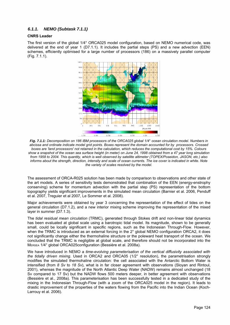
6.1.1. NEMO (Subtask 7.1.1)CNRS Leader

The first version of the global 1/4° ORCA025 model configuration, based on NEMO numerical code, wasdelivered at the end of year 1 (D7.1.1). It includes the partial steps (PS) and a new advection (EEN)schemes, efficiently optimised for a large number of processors (186) on a massively parallel computer(Fig. 7.1.1).

Fig. 7.1.1: Decomposition on 186 IBM processors of the ORCA025 global 1/4° ocean circulation model. Numbers inabcissa and ordinate indicate model grid points. Boxes represent the domain accounted for by processors. Crossedboxes are 'land processors' not retained in the calculation, which reduces the computational cost by 15%. Colours

show a snapshot of the ocean sea surface height (in meter) on June 24, 1998 obtained from a 47 year long simulationfrom 1958 to 2004. This quantity, which is well observed by satellite altimeter (TOPEX/Poseidon, JASON, etc.) alsoinforms about the strength, direction, intensity and scale of ocean currents. The ice cover is indicated in white. Note

the variety of scales resolved by the model.

The assessment of ORCA-R025 solution has been made by comparison to observations and other state ofthe art models. A series of sensitivity tests demonstrated that combination of the EEN (energy-enstrophyconserving) scheme for momentum advection with the partial step (PS) representation of the bottomtopography yields significant improvements in the simulated mean circulation (Barnier et al. 2006, Penduffet al. 2007, Treguier et al 2007, Le Sommer et al. 2008).

Major achievements were obtained by year 3 concerning the representation of the effect of tides on thegeneral circulation (D7.1.2), and a new interior mixing scheme improving the representation of the mixedlayer in summer (D7.1.3).

The tidal residual mean circulation (TRMC), generated through Stokes drift and non-linear tidal dynamicshas been evaluated at global scale using a barotropic tidal model. Its magnitude, shown to be generallysmall, could be locally significant in specific regions, such as the Indonesian Through-Flow. However,when the TRMC is introduced as an external forcing in the 2° global NEMO configuration ORCA2, it doesnot significantly change either the thermohaline structure or the poleward heat transport of the ocean. Weconcluded that the TRMC is negligible at global scale, and therefore should not be incorporated into theMERSEA 1/4° global ORCA025configuration (Bessière et al. 2008a).

We have introduced in NEMO a time-evolving parameterisation of the vertical diffusivity associated withthe tidally driven mixing. Used in ORCA2 and ORCA05 (1/2° resolution), the parametrisation stronglymodifies the simulated thermohaline circulation: the cell associated with the Antarctic Bottom Water isintensified (from 8 Sv to 18 Sv), what is in far closer agreement with observations (Sloyan and Rintoul,2001), whereas the magnitude of the North Atlantic Deep Water (NADW) remains almost unchanged (18Sv compared to 17 Sv) but the NADW flows 500 meters deeper, in better agreement with observations(Bessière et al., 2008a). This parameterisation has been successfully tested in a dedicated study of themixing in the Indonesian Through-Flow (with a zoom of the ORCA025 model in the region). It leads todrastic improvement of the properties of the waters flowing from the Pacific into the Indian Ocean (Koch-Larrouy et al. 2006).

Page 124

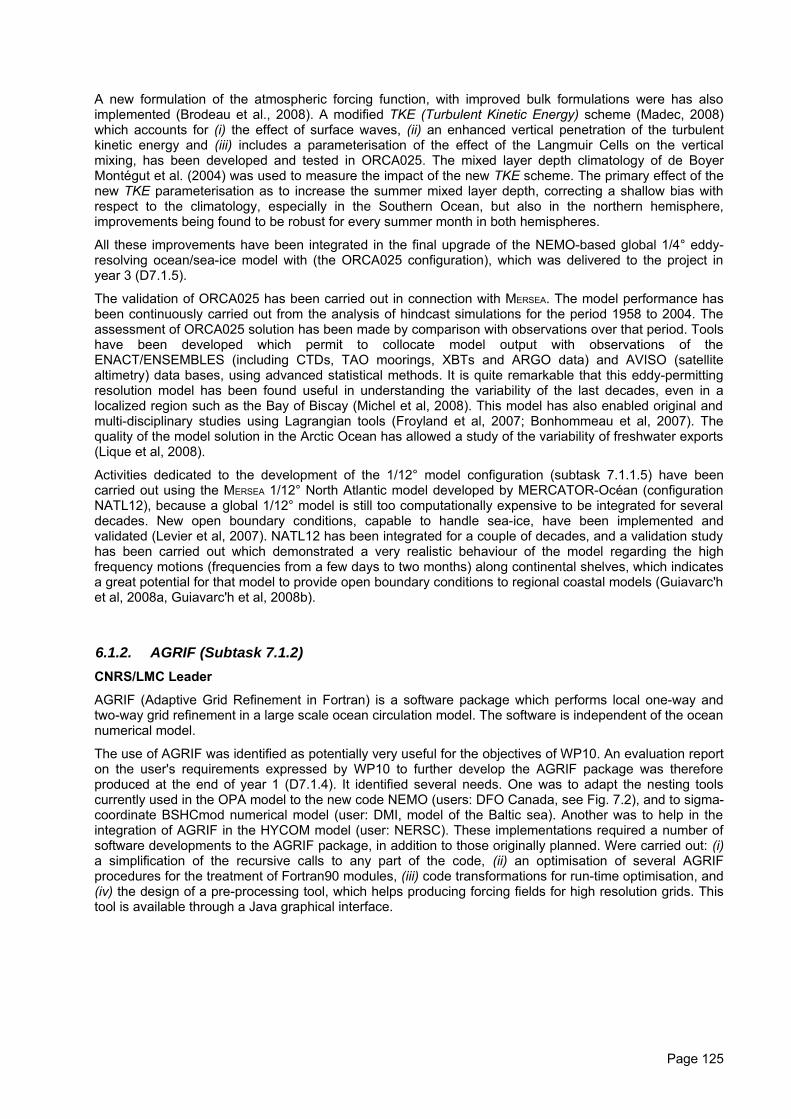
A new formulation of the atmospheric forcing function, with improved bulk formulations were has alsoimplemented (Brodeau et al., 2008). A modified TKE (Turbulent Kinetic Energy) scheme (Madec, 2008)which accounts for (i) the effect of surface waves, (ii) an enhanced vertical penetration of the turbulentkinetic energy and (iii) includes a parameterisation of the effect of the Langmuir Cells on the verticalmixing, has been developed and tested in ORCA025. The mixed layer depth climatology of de BoyerMontégut et al. (2004) was used to measure the impact of the new TKE scheme. The primary effect of thenew TKE parameterisation as to increase the summer mixed layer depth, correcting a shallow bias withrespect to the climatology, especially in the Southern Ocean, but also in the northern hemisphere,improvements being found to be robust for every summer month in both hemispheres.

All these improvements have been integrated in the final upgrade of the NEMO-based global 1/4° eddy-resolving ocean/sea-ice model with (the ORCA025 configuration), which was delivered to the project inyear 3 (D7.1.5).

The validation of ORCA025 has been carried out in connection with MERSEA. The model performance hasbeen continuously carried out from the analysis of hindcast simulations for the period 1958 to 2004. Theassessment of ORCA025 solution has been made by comparison with observations over that period. Toolshave been developed which permit to collocate model output with observations of theENACT/ENSEMBLES (including CTDs, TAO moorings, XBTs and ARGO data) and AVISO (satellitealtimetry) data bases, using advanced statistical methods. It is quite remarkable that this eddy-permittingresolution model has been found useful in understanding the variability of the last decades, even in alocalized region such as the Bay of Biscay (Michel et al, 2008). This model has also enabled original andmulti-disciplinary studies using Lagrangian tools (Froyland et al, 2007; Bonhommeau et al, 2007). Thequality of the model solution in the Arctic Ocean has allowed a study of the variability of freshwater exports(Lique et al, 2008).

Activities dedicated to the development of the 1/12° model configuration (subtask 7.1.1.5) have beencarried out using the MERSEA 1/12° North Atlantic model developed by MERCATOR-Océan (configurationNATL12), because a global 1/12° model is still too computationally expensive to be integrated for severaldecades. New open boundary conditions, capable to handle sea-ice, have been implemented andvalidated (Levier et al, 2007). NATL12 has been integrated for a couple of decades, and a validation studyhas been carried out which demonstrated a very realistic behaviour of the model regarding the highfrequency motions (frequencies from a few days to two months) along continental shelves, which indicatesa great potential for that model to provide open boundary conditions to regional coastal models (Guiavarc'het al, 2008a, Guiavarc'h et al, 2008b).

6.1.2. AGRIF (Subtask 7.1.2)CNRS/LMC Leader

AGRIF (Adaptive Grid Refinement in Fortran) is a software package which performs local one-way andtwo-way grid refinement in a large scale ocean circulation model. The software is independent of the oceannumerical model.

The use of AGRIF was identified as potentially very useful for the objectives of WP10. An evaluation reporton the user's requirements expressed by WP10 to further develop the AGRIF package was thereforeproduced at the end of year 1 (D7.1.4). It identified several needs. One was to adapt the nesting toolscurrently used in the OPA model to the new code NEMO (users: DFO Canada, see Fig. 7.2), and to sigma-coordinate BSHCmod numerical model (user: DMI, model of the Baltic sea). Another was to help in theintegration of AGRIF in the HYCOM model (user: NERSC). These implementations required a number ofsoftware developments to the AGRIF package, in addition to those originally planned. Were carried out: (i)a simplification of the recursive calls to any part of the code, (ii) an optimisation of several AGRIFprocedures for the treatment of Fortran90 modules, (iii) code transformations for run-time optimisation, and(iv) the design of a pre-processing tool, which helps producing forcing fields for high resolution grids. Thistool is available through a Java graphical interface.

Page 125

Fig. 7.1.2. Insertion of AGRIF in the NEMO based configuration of DFO in the North-Western Atlantic Ocean. The gridrefinement is located around Newfoundland. The figure shows the instantaneous Surface temperature in the AGRIF

configuration after three years of simulation. Colder (warmer) temperatures are in blue (red) colours.

New interpolation schemes have been integrated in AGRIF (high order conservative and monotonicschemes), and several improvements have been made in the grids interactions by definition of new updateschemes, new sponge layer application and new coupling algorithm in split-explicit free surface models.Research on open boundary conditions based on 3D characteristics has also been conducted.

Particular attention has been given to the update schemes, which play a fundamental role in two-waynesting algorithms. We designed a family of full-weighting operators satisfying a mathematically definedstability requirement. This led to a large improvement in comparison with usual average based operators,and improved the stability of the solution. The update schemes have been integrated into the AGRIFsoftware, and achievements were summarized in Debreu et al, (2008).

During the last project year, the nesting tools, which are part of the NEMO/AGRIF framework, werefinalized. They are used to produce data files for the high resolution grid. They have been designed for aquick setting of nested configurations. In addition, they also allow restarting the high resolution grid using aprevious spin up from a coarse resolution simulation, thus diminishing the total spin up time of a nestedconfiguration. The task was fully completed (D7.1.6) with modifications in the nesting tools code to be ableto use the tools when the sea-ice model LIM is activated, and with the introduction of vertical interpolationcapabilities, based on a linear interpolation.

Specific problems:

• NEMO: The automatic break-up of the model domain into a large number of sub-domains requiredby the multi-processor interface (MPI) implementation of ORCA-R025 was particularly difficult,because of the folding of the tri-polar grid in the region of the north pole. A very specific and originalsolution was found, for ocean and sea-ice, and has now proven to be efficient.

• AGRIF: a lack of efficiency of the AGRIF procedures on vector computers (NEC) had been identified.A strong effort has been made to remedy this, requiring a partial rewriting of interpolation and updatesubroutines. The code is now fully functional on vector computers and has very good performanceresults, similar to those without nesting.

Deliverables obtained.

D7.1.1, D7.1.2, D7.1.3, D7.1.4, D7.1.5, D7.1.6

Page 126

References (* acknowledge the support from MERSEA)

*Barnier B., G. Madec, T. Penduff, J.-M. Molines, A.-M. Treguier, J. Le Sommer, A. Beckmann, A.Biastoch, C. Böning, J. Dengg, C. Derval, E. Durand, S. Gulev, E. Remy, C. Talandier, S. Theetten, M.Maltrud, J. McClean, and B. De Cuevas, 2006: “Impact of partial steps and momentum advectionschemes in a global ocean circulation model at eddy permitting resolution”, Ocean Dynamics, Vol 56,543-567.

*Bessière, L., G. Madec, F. Lyard, and C. Le Provost, 2008: “Improved tidally driven mixing in an OGCM”,to be submitted to Ocean Modelling.

*Bessière, L., G. Madec, and F. Lyard, 2008: “Global tidal residual mean circulation: does it affect a climateOGCM”, submitted to Geophysical Research Letters.

Bonhommeau, S., B. Blanke, A.M. Treguier, E. Rivot, Y. Vermard, O. Le Pape, 2008: “Can the europeaneel larvae cross the Atlantic Ocean in 6 months?”, Submitted

*Brodeau L., B. Barnier, T. Penduff, A-M. Treguier, S. Gulev, 2008: “An ERA40 based atmospheric forcingfor global ocean circulation models”, Ocean Modelling, submitted.

de Boyer Montégut, C., G. Madec, A. S. Fischer, A. Lazar, and D. Iudicone, 2004: “Mixed layer depth overthe global ocean: an examination of profile data and a profile-based climatology”, J. Geophys. Res.,109, C12003, doi:10.1029/2004JC002378.

*Debreu L. P. Penven, P. Marchesiello and E. Blayo, 2008: “Two-Way nesting algorithms for a split-explicitfree surface model”, to be submitted to Ocean Modelling

*Debreu L. and E. Blayo, 2008: Two-Way embedding algorithms: a review, submitted to Ocean Dynamics

Fichefet, T., M.M. Maqueda, 1997: “Sensitivity of a global sea ice model to the treatment of icethermodynamics and dynamics”, J. Geophys. Res. 102 (12), 609–646.

Froyland, G., K. Padberg, M. England and A.M. Treguier, 2007: “Detection of Coherent Oceanic Structuresvia Transfer Operators”, Physical Review Letters, 98, 22, DOI: 10.1103/ PhysRevLett.98.224503.

*Guiavarc'h, C., A.M. Treguier, A. Vangriesheim, 2008a: “Remotely forced biweekly deep oscillations onthe continental slope of the Gulf of Guinea”, J. Geophys. Res., in press.

*Guiavarc'h, C., A-M. Treguier, A. Vangriesheim, A. Le Boyer, S. Theetten, O. Le Galloudec, G. Roullet,2008b: “High resolution modelling of intra-seasonal variability on the continental slope in the Tropicaland North Atlantic”, Eurogoos conference, Exeter, U.K., May 2008.

Koch-Larrouy, A., G. Madec, P. Bouruet-Aubertot, T. Gerkema, L. Bessières and R. Molcard, 2006: On thetransformation of Pacific Water into Indonesian ThroughFlow Water by internal tidal mixing, Geophys.Res. Lett., 34, L04604, doi:10.1029/2006GL028405.

*Le Sommer J., T. Penduff, G. Madec, 2008: “How momentum advection schemes affect current-topography interactions in the DRAKKAR 1/4° z-coordinate model”, Ocean Modelling, in press.

*Levier, B., S. Theetten, A.M. Treguier, 2007: “Description of a NATL025 run with open boundaries of theDRAKKAR project”, Internal report DOPS/LPO 07-05.

Madec, G., P. Delecluse, M. Imbard et C. Levy, 1998: “OPA 8.1 ocean general circulation model referencemanual”, Technical report, Institut Pierre-Simon Laplace (IPSL).

*Madec, G., 2008 : “NEMO, the Ocean Engine”, Tech. rep., Notes de l’IPSL (27), ISSN1288-1619,Université P. et M. Curie, B102 T15-E5, 4 place Jussieu, Paris cedex 5, 193 pp.

*Lique, C., A.M. Treguier, M. Scheinert, T. Penduff, 2008: “A model-based study of ice and freshwatertransport variabilities along both sides of Greenland”, Climate Dynamics, in revision.

Michel, S., F. Vandermeirsch, A.M. Treguier, 2008: “Temperature variability in the Bay of Biscay during thepast 40 years, from in-situ observations and a 3D global simulation”, Bay of biscay, XI internationalsymposium on Oceanography, San sebastian, April 2008. 2nd award poster presentation. Manuscript inpreparation for continental shelf research.

*Penduff T., J. Le Sommer, B. Barnier, A.-M. Treguier, J.-M. Molines, and G. Madec, 2007: “Influence ofnumerical schemes on current-topography interactions in 1/4° global ocean simulations”, OceanScience, Vol. 3, No 4, 451-535.

Page 127

Sloyan B.M. and S.R. Rintoul, 2001: “The southern ocean limb of the global deep overturning circulation”,Journal of Physical Oceanography, 31, Vol. 1, pp. 143–173.

*Treguier, A.M., M. England, S. R. Rintoul, G. Madec, J. Le Sommer, and J-M Molines, 2007: “SouthernOcean overturning across streamlines in an eddying simulation of the Antarctic Circumpolar Current”,Ocean Sciences, 3, 491-507.

6.2. Ecosystem Modelling (Task 7.2)

6.2.1. Task objectivesThe aim of this task was to develop a prognostic and robust ecosystem model that can successfullydescribe the observed temporal and regional variability in phytoplankton biomass and in associated carbonand nitrogen fluxes. Within this task progress was made along three research directions: first, a newapproach was developed in order to include more mechanistic aspects into the, until now, mostly empiricalmarine ecosystem models (Kriest and Oschlies, 2007; 2008) and to combine multi-nutrient models of algalphysiology with optical properties measurable by remote sensing (Salihoglu et al., 2008). Second,assimilation methods have been developed and tested successfully in order to obtain model solutionsconsistent with observations of biogeochemical and biological properties, demonstrating the particular therelevance of nutrient observations (Ourmières et al., subm.). Third, metrics for model assessment havebeen established, which can account for the non-Gaussian nature of model-data misfits of marineecosystem models (Losa et al., 2007). In combination, these results will significantly help to improve therealism of marine ecosystem simulations and our ability to control and assess model behaviour, relevantfor operational modelling systems.

6.2.2. Biogeochemical model development and assessment (Task 7.2.1)IFM/GEOMAR Leader

The aim of this task was to develop a prognostic and robust ecosystem model that can successfullydescribe the observed temporal and regional variability in phytoplankton biomass and in associated carbonand nitrogen fluxes. Within this task we followed two new approaches: the first one considers organismsize as structural element, and the second one includes a cell quota approach with detailed algalphysiology.

The development of an ecosystem model that includes multiple elemental cycles with detailed algalphysiology and links it to ocean colour has been completed. The model considers multiple nutrients (C,N03, NH4, PO4, Si) as well as the DOM and DOP cycles and export (i.e. DON, DOP, PON, POP1). In themodel, C:chl a ratio is estimated considering both the changes in downwelling irradiance and changes inthe intracellular nutrient concentrations. The new ecosystem model has been set up and adapted to theBermuda Atlantic Time Series site (BATS) and validated by extensive model-data comparison using the in-situ data for year 1998. Results show that the model is successful in reproducing a wide range of observedecosystem compartments. The model performance is particularly good in reproducing the observednutrient, DOM and POM cycles compared to available ecosystem models in the region (Salihoglu, et al.,2008).

The new implicit size-structured model attempts to use first-principles whenever possible. Examples arenutrient uptake by phytoplankton that, corresponding to diffusion across cell membranes, depends on thesurface-to-volume ratio and hence on the size of the cells (Aksnes & Egge, 1991). The same is assumedto hold for exudation (Bjornsen, 1988). A consequence of these assumptions is that small cells arefavoured in well-lit oligotrophic regimes, whereas a decrease in light levels causes an increase in optimumcell size (Kriest and Oschlies, 2007).

Given the flexibility and nonlinearity of especially heterotrophic, size-dependent processes, and thesparsity of observations, we have parameterised zooplankton grazing as a fraction of phytoplanktonproduction, both in terms of cell numbers and phytoplankton biomass. This approach implicitly assumesthat zooplankton immediately adapt to changes in phytoplankton size structure, both in terms ofconcentration and grazing rates. The effect of size on sinking, sedimentation and the resulting possiblenutrient distribution has been investigated in a 1D framework (Kriest and Oschlies, 2008).

1 Dissolved organic matter, phosphorus, nytrogen ; Particulate organic nitrogen, phosphorus, respectively

Page 128

Assessment of the model simulated at discrete time series sites depends strongly on the localhydrographic conditions and horizontal processes. We have therefore also implemented the sizedependent physiological model into a 3D framework (Khatiwala, 2007), that allows the relatively fastsimulation of different models over millennial timescales. This not only captures the model response tovarious hydrodynamic environments, but also provides the possibility to examine the model on thebackground of large-scale data sets of biogeochemical and biological investigations, both by means ofdifferent metrics and visual inspection. Several model experiments have been conducted, which all exhibita correlation between observed and simulated PO4 of ~0.7 - 0.9. Size-dependent phytoplanktonproduction and decay improves the fit to observations and their variance; however, the fit further dependson the pathways and rates for organic matter sinking and remineralisation. The analysis of more specificdata sets as for DOP, community half-saturation constant, size structure will provide additional guidance inthe assessment of the different models, as well as tests with different metrics.

6.2.3. Integration into OPA (Task 7.2.2)CNRS/LEGI Leader

Prototype of a coupled physical/biological assimilative system

The final version of the coupled assimilative platform has been delivered as expected during the final yearof the project. The physical model component of the prototype is based on the NEMO free-surface modelof the North Atlantic at 1/4° resolution with bulk parameterizations of air-sea fluxes (NATL4); thebiogeochemical component is based on the semi-complex LOBSTER (N2P1-type) model, and theassimilation scheme is a fixed-basis version of the SEEK filter adapted to the free-surface formulation.

Several parameterizations of the LOBSTER model have been slightly modified to obtain a reasonable firstguess of the seasonal primary production before starting assimilation experiments. The assimilatingsystem uses a sequential scheme modified with an Incremental Analyse Update approach (Ourmières etal., 2008) to provide a time-continuous assimilated solution. This assimilation method has the advantage tosuppress spurious vertical velocities introduced by the physical data assimilation and perturbing thebiochemical response. From a methodological point of view, the SEEK filter has been extended toincorporate inequality constraints in the sequential formulation (Lauvernet et al., 2008). Such an extensionwill be useful to maintain positive-definite concentrations of nutrients, as well as stable stratification of thewater column during the filtering process.

Assimilation impact on biogeochemical variables.

Four different “impact” experiments have been conducted, each one starting from January 1st and endingon December 31st, 1998. The first integration (referred to as FREE) has been performed with the coupledmodel without data assimilation. Another system integration for the same time period is also performedwith the joint assimilation of physical data (altimetry, SST and climatological T and S data) and nitrate datafrom the Levitus climatology (noted APN). In addition, two extra experiments are performed for the sameperiod, using the same assimilation system but with two different options: the first extra experiment is set tocontrol the nitrate fields only, noted AN for Nitrate Assimilation, and the second extra experiment is set tocontrol the physical fields only, noted AP for Physical Assimilation. Therefore, the APN control vectorincludes the U, V, T, S and NO3 variables, the AP control vector includes the U, V, T and S variables,while the AN control vector includes only the NO3 variable. The AP and AN experiments allow to identifythe different impact of the nitrate or the physical data assimilation alone, compared to their combinedaction in the APN experiment.

Consistently with the results obtained by Berline et al. (2006) with a comparable assimilative model, it isshown that the assimilation of physical data alone can improve the representation of the mixed layer depth,but the impact on the ecosystem remains rather weak. In some situations, the physical data assimilationcan even worsen the ecosystem response for areas where the prior nutrient distribution is significantlyincorrect. However, these experiments also show that the combined assimilation of physical and nutrientdata has a positive impact on the phytoplankton patterns by comparison with SeaWiFS ocean colour data,demonstrating the good complementarity between SST, altimetry and in situ nutrient data. As an example,the representation of NO3 surface concentrations is very poor in the areas of missing bloom activity for theFREE and AP solutions, while being quite close to the climatology for the AN and APN simulations. In thiscase, it can be assumed that this high latitude bloom decreases too rapidly by nutrient extinction for theFREE and AP solutions. Therefore, it seems that NO3 is the key element to control this regional event by

Page 129

data assimilation. These results suggest that more intensive in situ measurements of biogeochemicalnutrients are urgently needed at basin scale to initiate a permanent monitoring of oceanic ecosystems.

Improved biogeochemical processes

First, a comparison of 3 different generations of biogeochemical models (P3ZD, LOBSTER and PISCES)has been made using the first MERCATOR 1998 reanalysis. A better representation in gyres and alsowithin the Gulf Stream area is obtained when regeneration is better taken into account (LOBSTER).Results with PISCES that included iron from margins are promising with better contrast between marginsand open ocean. It is also found that present assimilation of altimetry induces too strong vertical exchange,particularly within the inter-tropical zone.

Second, scripts have been developed within the context of MERCATOR to run easily LOBSTERsimulations from either analysis or reanalysis. Results with recent MERCATOR reanalysis have beenobtained, allowing reconstruction of the seasonal and inter-annual variability of the marine primaryproduction over the 1992-2001 period. Roles of climatic events such as the North Atlantic Oscillation areunder investigation. These last simulations used the operational PSY1V2 system, allowing bothassimilation of in-situ and satellite physical variables.

North Atlantic bloom experiment

As LOBSTER had been evaluated at basin scale to simulate blooms, this second-generationbiogeochemical model had been transferred to partner LEGI, which is in charge of improving assimilationschemes for biological purposes. Integration is made under a new North Atlantic platform NATL4, coherentwith the new grid used by MERCATOR PSY3 system.

Jointly, a pilot experiment using LOBSTER imbedded within the MERCATOR PSY1V2 operational platformhas been launched to follow in near real time the 2006 bloom spreading into the North Atlantic.

Future efforts will focus on the implementation of the third generation model planned within MERSEA forMERCATOR products: the PISCES model. This latter model is also highly relevant to study the carboncycle and CO2 fluxes associated to the primary production.

6.2.4. Assessment and metrics (Task 7.2.3)UU Leader

Identification of key observational data and the definition of an internal metrics

Several versions of biogeochemical models have been assessed within the project. All the versions are ofdifferent complexity and possess different numbers of unknown parameters, which are to be optimized.The models had to be validated against existing observational data. To some extent the model complexitydetermines the amount and kind of data needed for model assessment. Here, the relatively simplenitrogen-based NPZD and LOBSTER models have, for the first time, been validated against, and tuned,with chlorophyll and nutrient (nitrate & nitrite) concentrations observed at a number of JGOFS stations(D7.2.6). With respect to the optimization of model solutions and biological parameters, these time seriesof chlorophyll and dissolved inorganic nitrogen appeared to be the key observations (assimilation ofparticular organic nitrogen data had no effect on inverse model solution). When dealing, however, withmore complicated ecosystem models (e.g., CN REcoM) which do not describe just one (nitrogen) butseveral (+ carbon, silica) elemental cycles, any model assessment requires much more empiricalinformation.

It has been noted that when validating the models one should use not only data of global oceanbiogeochemical concentrations (Chl a, nutrients, zooplankton…), but also -in case of multi-elemental cyclemodels- internal biogeochemical criteria such as C:Chl:N:Si ratios. When assessing CN REcoM we havefound solutions which agreed well with observed surface chlorophyll and nitrate, but produced unrealisticC:N ratios in organic pools. The model's skill in simulating global (basin) primary and export productionshould also be considered in the model assessment.

Page 130

Intercomparison and assessment of biogeochemical models

The C:N regulated Ecosystem model (CN REcoM) initially developed by M. Schartau, the size dependent(SD) NPZD ecosystem model (Kriest and Oschlies, 2007) and the Lobster model have been validated at 6different locations in the open ocean: NABE, BATS, Arabian Sea AS-C, Equatorial Pacific EqPac 0S, RossSea (D7.2.4 and D7.2.6). Spatial and temporal distributions of the model variables as well asbiogeochemical global ocean estimates (such as primary and export production, particularly relevant whenassessing models in 3D context) appeared to be very sensitive to biological parameters. For instance, theglobal net primary production estimates may differ by a factor of 2 just due to changes in biogeochemicalparameters. But for none of the ecosystem models we could find a unique set of biological parametervalues which would give similarly good agreements between the model solution and data at each of theJGOFS sites or in every region of the global ocean.

6.3. Data assimilation (Task 7.3)

The purpose of task 7.3 was to improve previously existing assimilation tools. In this work, we focused onthe fully multivariate methodologies, which were developed and applied extensively in previous Europeanoceanography projects. This effort was done along two lines: (i) a continuous research exploration ofimproved methods for ocean data assimilation and (ii) the development and evaluation of the assimilationtools that are most useful for operational use, focusing on those that are expected to generate immediate,first order and low cost operational benefit.

6.3.1. Development of advanced sequential filtersThe objective of this task was to explore advanced data assimilation scheme with the aim of better takinginto account the complex nature of ocean assimilation problems (non-Gaussian error statistics, nonlinearprocesses, biased estimations). Three advanced filters were considered in this task: the EnKF, the SIRfilter and the SEEK filter.

a. Ensemble Kalman filter (NERSC)

Problems to solve:

The questions that were addressed in this Ensemble Kalman Filter (EnKF) sub-task were the following:

• Does the EnKF scheme used in TOPAZ (the MERSEA Arctic system) make optimal use of its 100-members ensemble?

• Could improved analysis schemes - the square root schemes, (Pham, (2000); Sakov and Oke(2008)) - lead to an economy of members in the realistic Arctic system?

• Should we rather spend time on improving the analysis scheme or on other implementation aspectsof the assimilation system?

Method:

The EnKF is applied in the successive versions of the Arctic system. The advantage of the ensemblemethod is that the dynamic ensemble statistics make it possible to assimilate various data types. In theArctic system, sea-level anomalies, sea surface temperatures and sea ice concentrations have beenassimilated. From the V2 system, ice drift products have been added.

The Ensemble Square Root (Kalman) Filter (ESRF) has been implemented following Sakov and Oke(2008). The scheme has proven more adequate for linear systems as it avoids the random sampling errorsof the traditional EnKF but has not been demonstrated so far in realistic settings. The ESRF favours theappearance of outliers in the ensemble that can be removed by occasional random rotations of theensemble (see Sakov and Oke, 2008). We will thus evaluate three methods: the EnKF, the ESRF and theESRF with random rotations.

Page 131

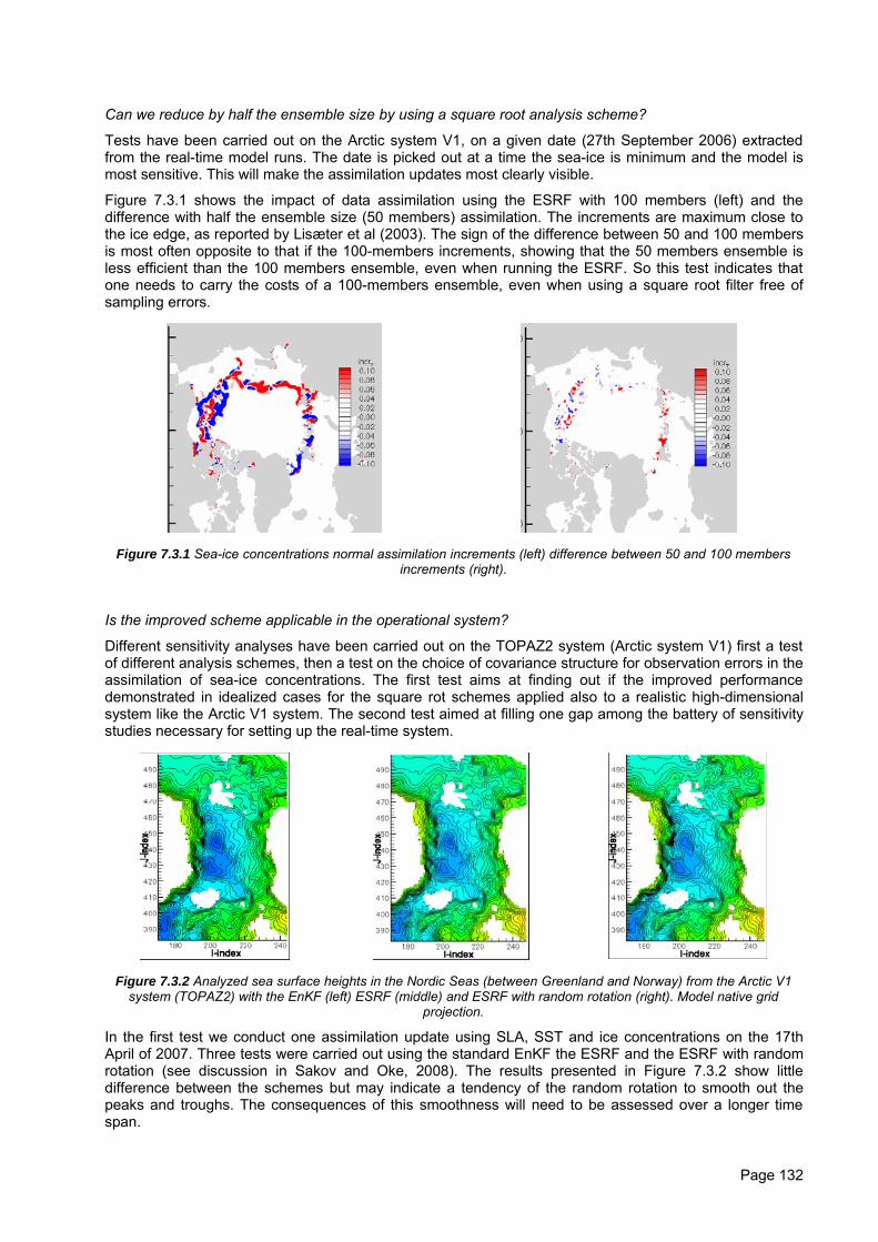
Can we reduce by half the ensemble size by using a square root analysis scheme?

Tests have been carried out on the Arctic system V1, on a given date (27th September 2006) extractedfrom the real-time model runs. The date is picked out at a time the sea-ice is minimum and the model ismost sensitive. This will make the assimilation updates most clearly visible.

Figure 7.3.1 shows the impact of data assimilation using the ESRF with 100 members (left) and thedifference with half the ensemble size (50 members) assimilation. The increments are maximum close tothe ice edge, as reported by Lisæter et al (2003). The sign of the difference between 50 and 100 membersis most often opposite to that if the 100-members increments, showing that the 50 members ensemble isless efficient than the 100 members ensemble, even when running the ESRF. So this test indicates thatone needs to carry the costs of a 100-members ensemble, even when using a square root filter free ofsampling errors.

Figure 7.3.1 Sea-ice concentrations normal assimilation increments (left) difference between 50 and 100 membersincrements (right).

Is the improved scheme applicable in the operational system?

Different sensitivity analyses have been carried out on the TOPAZ2 system (Arctic system V1) first a testof different analysis schemes, then a test on the choice of covariance structure for observation errors in theassimilation of sea-ice concentrations. The first test aims at finding out if the improved performancedemonstrated in idealized cases for the square rot schemes applied also to a realistic high-dimensionalsystem like the Arctic V1 system. The second test aimed at filling one gap among the battery of sensitivitystudies necessary for setting up the real-time system.

Figure 7.3.2 Analyzed sea surface heights in the Nordic Seas (between Greenland and Norway) from the Arctic V1system (TOPAZ2) with the EnKF (left) ESRF (middle) and ESRF with random rotation (right). Model native grid

projection.

In the first test we conduct one assimilation update using SLA, SST and ice concentrations on the 17thApril of 2007. Three tests were carried out using the standard EnKF the ESRF and the ESRF with randomrotation (see discussion in Sakov and Oke, 2008). The results presented in Figure 7.3.2 show littledifference between the schemes but may indicate a tendency of the random rotation to smooth out thepeaks and troughs. The consequences of this smoothness will need to be assessed over a longer timespan.

Page 132

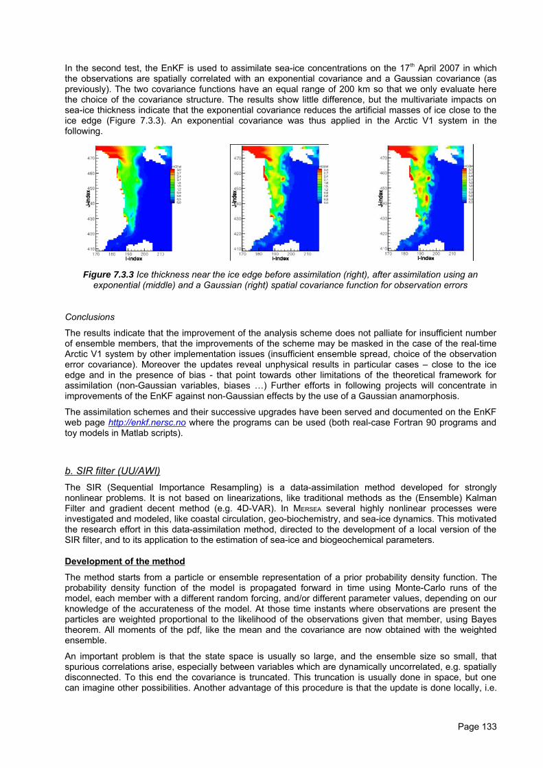
In the second test, the EnKF is used to assimilate sea-ice concentrations on the 17th April 2007 in whichthe observations are spatially correlated with an exponential covariance and a Gaussian covariance (aspreviously). The two covariance functions have an equal range of 200 km so that we only evaluate herethe choice of the covariance structure. The results show little difference, but the multivariate impacts onsea-ice thickness indicate that the exponential covariance reduces the artificial masses of ice close to theice edge (Figure 7.3.3). An exponential covariance was thus applied in the Arctic V1 system in thefollowing.

Figure 7.3.3 Ice thickness near the ice edge before assimilation (right), after assimilation using anexponential (middle) and a Gaussian (right) spatial covariance function for observation errors

Conclusions

The results indicate that the improvement of the analysis scheme does not palliate for insufficient numberof ensemble members, that the improvements of the scheme may be masked in the case of the real-timeArctic V1 system by other implementation issues (insufficient ensemble spread, choice of the observationerror covariance). Moreover the updates reveal unphysical results in particular cases – close to the iceedge and in the presence of bias - that point towards other limitations of the theoretical framework forassimilation (non-Gaussian variables, biases …) Further efforts in following projects will concentrate inimprovements of the EnKF against non-Gaussian effects by the use of a Gaussian anamorphosis.

The assimilation schemes and their successive upgrades have been served and documented on the EnKFweb page http://enkf.nersc.no where the programs can be used (both real-case Fortran 90 programs andtoy models in Matlab scripts).

b. SIR filter (UU/AWI)The SIR (Sequential Importance Resampling) is a data-assimilation method developed for stronglynonlinear problems. It is not based on linearizations, like traditional methods as the (Ensemble) KalmanFilter and gradient decent method (e.g. 4D-VAR). In MERSEA several highly nonlinear processes wereinvestigated and modeled, like coastal circulation, geo-biochemistry, and sea-ice dynamics. This motivatedthe research effort in this data-assimilation method, directed to the development of a local version of theSIR filter, and to its application to the estimation of sea-ice and biogeochemical parameters.

Development of the method

The method starts from a particle or ensemble representation of a prior probability density function. Theprobability density function of the model is propagated forward in time using Monte-Carlo runs of themodel, each member with a different random forcing, and/or different parameter values, depending on ourknowledge of the accurateness of the model. At those time instants where observations are present theparticles are weighted proportional to the likelihood of the observations given that member, using Bayestheorem. All moments of the pdf, like the mean and the covariance are now obtained with the weightedensemble.

An important problem is that the state space is usually so large, and the ensemble size so small, thatspurious correlations arise, especially between variables which are dynamically uncorrelated, e.g. spatiallydisconnected. To this end the covariance is truncated. This truncation is usually done in space, but onecan imagine other possibilities. Another advantage of this procedure is that the update is done locally, i.e.

Page 133

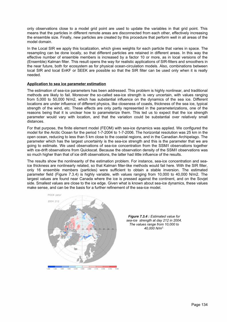
only observations close to a model grid point are used to update the variables in that grid point. Thismeans that the particles in different remote areas are disconnected from each other, effectively increasingthe ensemble size. Finally, new particles are created by this procedure that perform well in all areas of themodel domain.

In the Local SIR we apply this localization, which gives weights for each particle that varies in space. Theresampling can be done locally, so that different particles are retained in different areas. In this way theeffective number of ensemble members is increased by a factor 10 or more, as in local versions of the(Ensemble) Kalman filter. This result opens the way for realistic applications of SIR-filters and smoothers inthe near future, both for ecosystem as for physical ocean-circulation models. Also, combinations betweenlocal SIR and local EnKF or SEEK are possible so that the SIR filter can be used only when it is reallyneeded.

Application to sea ice parameter estimation

The estimation of sea-ice parameters has been addressed. This problem is highly nonlinear, and traditionalmethods are likely to fail. Moreover the so-called sea-ice strength is very uncertain, with values rangingfrom 5,000 to 50,000 N/m2, which has substantial influence on the dynamics of the sea ice. Differentlocations are under influence of different physics, like closeness of coasts, thickness of the sea ice, typicalstrength of the wind, etc. These effects are only partly represented in the parameterizations, one of thereasons being that it is unclear how to parameterize them. This led us to expect that the ice strengthparameter would vary with location, and that the variation could be substantial over relatively smalldistances.

For that purpose, the finite element model (FEOM) with sea-ice dynamics was applied. We configured themodel for the Arctic Ocean for the period 1-7-2004 to 1-7-2006. The horizontal resolution was 25 km in theopen ocean, reducing to less than 5 km close to the coastal regions, and in the Canadian Archipelago. Theparameter which has the largest uncertainty is the sea-ice strength and this is the parameter that we aregoing to estimate. We used observations of sea-ice concentration from the SSM/I observations togetherwith ice-drift observations from Quickscat. Because the observation density of the SSM/I observations wasso much higher than that of ice drift observations, the latter had little influence of the results.

The results show the nonlinearity of the estimation problem. For instance, sea-ice concentration and sea-ice thickness are nonlinearly related, so that Kalman filter-like methods would fail here. With the SIR filter,only 16 ensemble members (particles) were sufficient to obtain a stable inversion. The estimatedparameter field (Figure 7.3.4) is highly variable, with values ranging from 10,000 to 40,000 N/m2. Thelargest values are found near Canada where the ice is pressed against the continent, and on the Sovjetside. Smallest values are close to the ice edge. Given what is known about sea-ice dynamics, these valuesmake sense, and can be the basis for a further refinement of the sea-ice model.

Figure 7.3.4 : Estimated value forsea-ice strength at day 212 in 2004.

The values range from 10,000 to40,000 N/m2..

Page 134

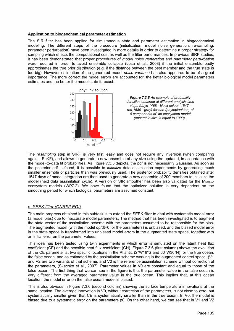
Application to biogeochemical parameter estimation

The SIR filter has been applied for simultaneous state and parameter estimation in biogeochemicalmodeling. The different steps of the procedure (initialization, model noise generation, re-sampling,parameter perturbation) have been investigated in more details in order to determine a proper strategy forsampling which effects the computational cost as well as the filter performances. In previous SIRF studies,it has been demonstrated that proper procedures of model noise generation and parameter perturbationwere required in order to avoid ensemble collapse (Losa et al., 2003) if the initial ensemble badlyapproximates the true prior distribution (e.g. if the distance between the best member and the true state istoo big). However estimation of the generated model noise variance has also appeared to be of a greatimportance. The more correct the model errors are accounted for, the better biological model parametersestimates and the better the model state forecast.

Figure 7.3.5 An example of probabilitydensities obtained at different analysis time

steps (days 1468 - black colour, 1547 -red,1580 - gray) for one (phytoplankton) of

9 components of an ecosystem model(ensemble size is equal to 1000).

The resampling step in SIRF is very fast, easy and does not require any inversion (when comparingagainst EnKF), and allows to generate a new ensemble of any size using the updated, in accordance withthe model-to-data fit probabilities. As Figure 7.3.5 depicts, the pdf is not necessarily Gaussian. As soon asthe posterior pdf is found, it is possible to initialize data assimilation experiments by generating muchsmaller ensemble of particles than was previously used. The posterior probability densities obtained after1547 days of model integration are then used to generate a new ensemble of 200 members to initialize themodel (next data assimilation cycle). A version of SIR smoother has been also validated for the MERSEA

ecosystem models (WP7.2). We have found that the optimized solution is very dependent on thesmoothing period for which biological parameters are assumed constant.

c. SEEK filter (CNRS/LEGI)The main progress obtained in this subtask is to extend the SEEK filter to deal with systematic model error(a model bias) due to inaccurate model parameters. The method that has been investigated is to augmentthe state vector of the assimilation scheme with the parameters assumed to be responsible for the bias.The augmented model (with the model dp/dt=0 for the parameters) is unbiased, and the biased model errorin the state space is transformed into unbiased model errors in the augmented state space, together withan initial error on the parameter values.

This idea has been tested using twin experiments in which error is simulated on the latent heat fluxcoefficient (CE) and the sensible heat flux coefficient (CH). Figure 7.3.6 (first column) shows the evolutionof the CE parameter at two specific locations in the Atlantic (2°W16°S and 60°W36°N) for the true ocean,the false ocean, and as estimated by the assimilation scheme working in the augmented control space. (V1and V2 are two variants of that scheme, and V0 is the reference assimilation scheme without correction ofthe parameters, (Skachko et al., 2007). Parameter values in V0 are constant and equal to those of thefalse ocean. The first thing that we can see in the figure is that the parameter value in the false ocean isvery different from the averaged parameter value in the true ocean. This implies that, at this oceanlocation, the model error on the false ocean model is biased.

This is also obvious in Figure 7.3.6 (second column) showing the surface temperature innovations at thesame location. The average innovation in V0, without correction of the parameters, is not close to zero, butsystematically smaller given that CE is systematically smaller than in the true ocean. In V0, the model isbiased due to a systematic error on the parameters p0. On the other hand, we can see that in V1 and V2

Page 135

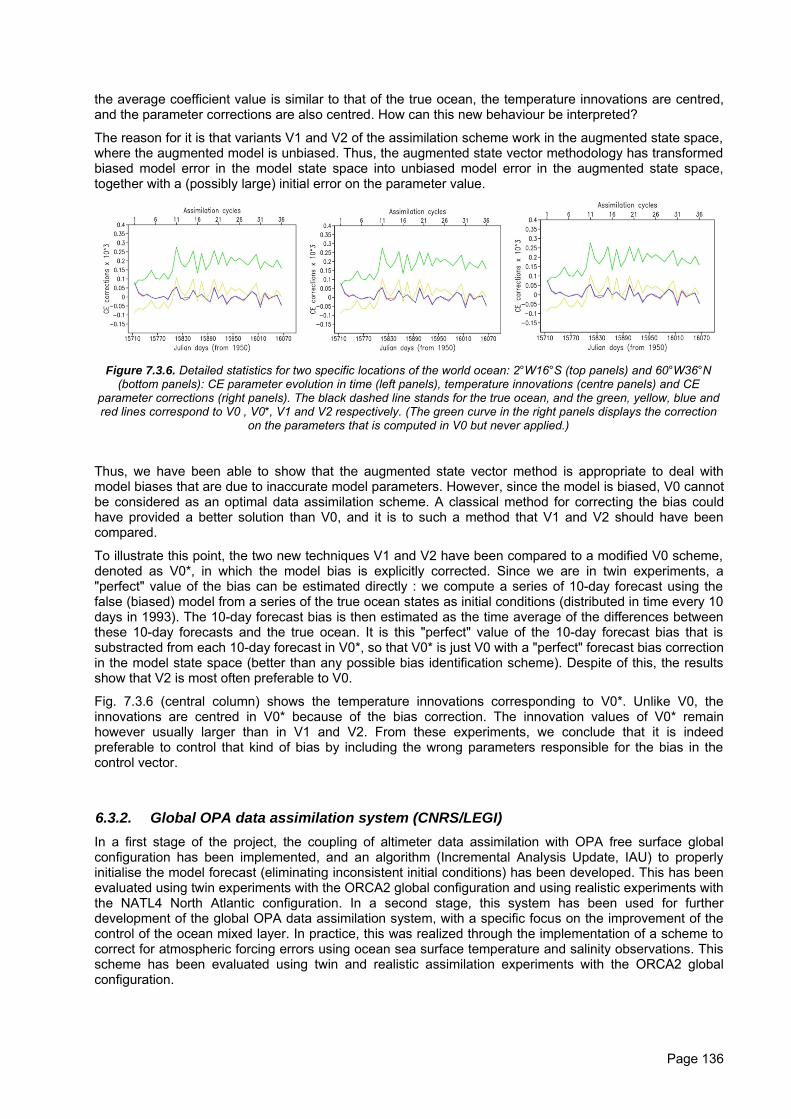
the average coefficient value is similar to that of the true ocean, the temperature innovations are centred,and the parameter corrections are also centred. How can this new behaviour be interpreted?

The reason for it is that variants V1 and V2 of the assimilation scheme work in the augmented state space,where the augmented model is unbiased. Thus, the augmented state vector methodology has transformedbiased model error in the model state space into unbiased model error in the augmented state space,together with a (possibly large) initial error on the parameter value.

Figure 7.3.6. Detailed statistics for two specific locations of the world ocean: 2°W16°S (top panels) and 60°W36°N

(bottom panels): CE parameter evolution in time (left panels), temperature innovations (centre panels) and CEparameter corrections (right panels). The black dashed line stands for the true ocean, and the green, yellow, blue andred lines correspond to V0 , V0*, V1 and V2 respectively. (The green curve in the right panels displays the correction

on the parameters that is computed in V0 but never applied.)

Thus, we have been able to show that the augmented state vector method is appropriate to deal withmodel biases that are due to inaccurate model parameters. However, since the model is biased, V0 cannotbe considered as an optimal data assimilation scheme. A classical method for correcting the bias couldhave provided a better solution than V0, and it is to such a method that V1 and V2 should have beencompared.

To illustrate this point, the two new techniques V1 and V2 have been compared to a modified V0 scheme,denoted as V0*, in which the model bias is explicitly corrected. Since we are in twin experiments, a"perfect" value of the bias can be estimated directly : we compute a series of 10-day forecast using thefalse (biased) model from a series of the true ocean states as initial conditions (distributed in time every 10days in 1993). The 10-day forecast bias is then estimated as the time average of the differences betweenthese 10-day forecasts and the true ocean. It is this "perfect" value of the 10-day forecast bias that issubstracted from each 10-day forecast in V0*, so that V0* is just V0 with a "perfect" forecast bias correctionin the model state space (better than any possible bias identification scheme). Despite of this, the resultsshow that V2 is most often preferable to V0.

Fig. 7.3.6 (central column) shows the temperature innovations corresponding to V0*. Unlike V0, theinnovations are centred in V0* because of the bias correction. The innovation values of V0* remainhowever usually larger than in V1 and V2. From these experiments, we conclude that it is indeedpreferable to control that kind of bias by including the wrong parameters responsible for the bias in thecontrol vector.

6.3.2. Global OPA data assimilation system (CNRS/LEGI)In a first stage of the project, the coupling of altimeter data assimilation with OPA free surface globalconfiguration has been implemented, and an algorithm (Incremental Analysis Update, IAU) to properlyinitialise the model forecast (eliminating inconsistent initial conditions) has been developed. This has beenevaluated using twin experiments with the ORCA2 global configuration and using realistic experiments withthe NATL4 North Atlantic configuration. In a second stage, this system has been used for furtherdevelopment of the global OPA data assimilation system, with a specific focus on the improvement of thecontrol of the ocean mixed layer. In practice, this was realized through the implementation of a scheme tocorrect for atmospheric forcing errors using ocean sea surface temperature and salinity observations. Thisscheme has been evaluated using twin and realistic assimilation experiments with the ORCA2 globalconfiguration.

Page 136

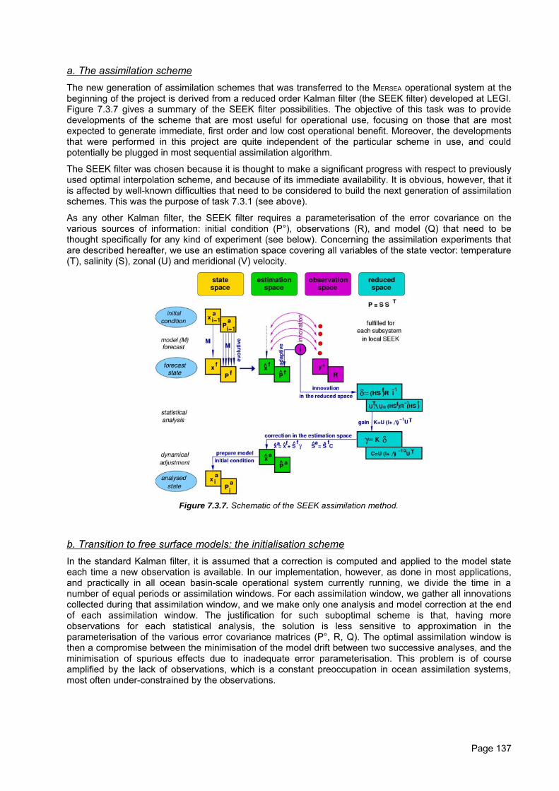
a. The assimilation schemeThe new generation of assimilation schemes that was transferred to the MERSEA operational system at thebeginning of the project is derived from a reduced order Kalman filter (the SEEK filter) developed at LEGI.Figure 7.3.7 gives a summary of the SEEK filter possibilities. The objective of this task was to providedevelopments of the scheme that are most useful for operational use, focusing on those that are mostexpected to generate immediate, first order and low cost operational benefit. Moreover, the developmentsthat were performed in this project are quite independent of the particular scheme in use, and couldpotentially be plugged in most sequential assimilation algorithm.

The SEEK filter was chosen because it is thought to make a significant progress with respect to previouslyused optimal interpolation scheme, and because of its immediate availability. It is obvious, however, that itis affected by well-known difficulties that need to be considered to build the next generation of assimilationschemes. This was the purpose of task 7.3.1 (see above).

As any other Kalman filter, the SEEK filter requires a parameterisation of the error covariance on thevarious sources of information: initial condition (P°), observations (R), and model (Q) that need to bethought specifically for any kind of experiment (see below). Concerning the assimilation experiments thatare described hereafter, we use an estimation space covering all variables of the state vector: temperature(T), salinity (S), zonal (U) and meridional (V) velocity.

Figure 7.3.7. Schematic of the SEEK assimilation method.

b. Transition to free surface models: the initialisation schemeIn the standard Kalman filter, it is assumed that a correction is computed and applied to the model stateeach time a new observation is available. In our implementation, however, as done in most applications,and practically in all ocean basin-scale operational system currently running, we divide the time in anumber of equal periods or assimilation windows. For each assimilation window, we gather all innovationscollected during that assimilation window, and we make only one analysis and model correction at the endof each assimilation window. The justification for such suboptimal scheme is that, having moreobservations for each statistical analysis, the solution is less sensitive to approximation in theparameterisation of the various error covariance matrices (P°, R, Q). The optimal assimilation window isthen a compromise between the minimisation of the model drift between two successive analyses, and theminimisation of spurious effects due to inadequate error parameterisation. This problem is of courseamplified by the lack of observations, which is a constant preoccupation in ocean assimilation systems,most often under-constrained by the observations.

Page 137

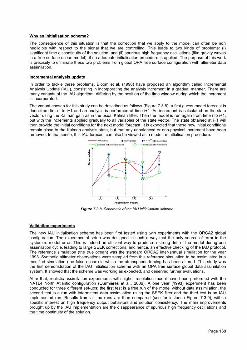
Why an initialisation scheme?

The consequence of this situation is that the correction that we apply to the model can often be nonnegligible with respect to the signal that we are controlling. This leads to two kinds of problems: (i)significant time discontinuity of the solution, and (ii) spurious high frequency oscillations (like gravity wavesin a free surface ocean model), if no adequate initialisation procedure is applied. The purpose of this workis precisely to eliminate these two problems from global OPA free surface configuration with altimeter dataassimilation.

Incremental analysis update

In order to tackle these problems, Bloom et al. (1996) have proposed an algorithm called IncrementalAnalysis Update (IAU), consisting in incorporating the analysis increment in a gradual manner. There aremany variants of the IAU algorithm, differing by the position of the time window during which the incrementis incorporated.

The variant chosen for this study can be described as follows (Figure 7.3.8): a first guess model forecast isdone from time i to i+1 and an analysis is performed at time i+1. An increment is calculated on the statevector using the Kalman gain as in the usual Kalman filter. Then the model is run again from time i to i+1,but with the increments applied gradually to all variables of the state vector. The state obtained at i+1 willthen provide the initial conditions for the next model forecast. It is expected that these new initial conditionsremain close to the Kalman analysis state, but that any unbalanced or non-physical increment have beenremoved. In that sense, this IAU forecast can also be viewed as a model re-initialisation procedure.

Figure 7.3.8. Schematic of the IAU initialisation scheme.

Validation experiments

The new IAU initialisation scheme has been first tested using twin experiments with the ORCA2 globalconfiguration. The experimental setup was designed in such a way that the only source of error in thesystem is model error. This is indeed an efficient way to produce a strong drift of the model during oneassimilation cycle, leading to large SEEK corrections, and hence, an effective checking of the IAU protocol.The reference simulation (the true ocean) was the standard ORCA2 inter-annual simulation for the year1993. Synthetic altimeter observations were sampled from this reference simulation to be assimilated in amodified simulation (the false ocean) in which the atmospheric forcing has been altered. This study wasthe first demonstration of the IAU initialisation scheme with an OPA free surface global data assimilationsystem. It showed that the scheme was working as expected, and deserved further evaluations.

After that, realistic assimilation experiments with higher resolution model have been performed with theNATL4 North Atlantic configuration (Ourmières et al., 2006). A one year (1993) experiment has beenconducted for three different set-ups: the first test is a free run of the model without data assimilation, thesecond test is a run with intermittent data assimilation using the SEEK filter and the third test is an IAUimplemented run. Results from all the runs are then compared (see for instance Figure 7.3.9), with aspecific interest on high frequency output behaviors and solution consistency. The main improvementsbrought up by the IAU implementation are the disappearance of spurious high frequency oscillations andthe time continuity of the solution.

Page 138

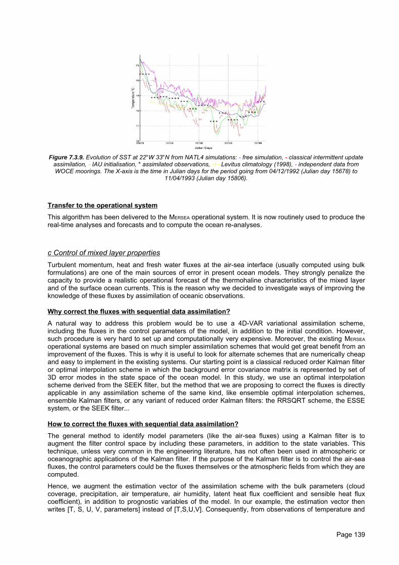
Figure 7.3.9. Evolution of SST at 22°W 33°N from NATL4 simulations: - free simulation, - classical intermittent updateassimilation, - IAU initialisation, * assimilated observations, -+- Levitus climatology (1998), - independent data fromWOCE moorings. The X-axis is the time in Julian days for the period going from 04/12/1992 (Julian day 15678) to

11/04/1993 (Julian day 15806).

Transfer to the operational system

This algorithm has been delivered to the MERSEA operational system. It is now routinely used to produce thereal-time analyses and forecasts and to compute the ocean re-analyses.

c Control of mixed layer propertiesTurbulent momentum, heat and fresh water fluxes at the air-sea interface (usually computed using bulkformulations) are one of the main sources of error in present ocean models. They strongly penalize thecapacity to provide a realistic operational forecast of the thermohaline characteristics of the mixed layerand of the surface ocean currents. This is the reason why we decided to investigate ways of improving theknowledge of these fluxes by assimilation of oceanic observations.

Why correct the fluxes with sequential data assimilation?

A natural way to address this problem would be to use a 4D-VAR variational assimilation scheme,including the fluxes in the control parameters of the model, in addition to the initial condition. However,such procedure is very hard to set up and computationally very expensive. Moreover, the existing MERSEA

operational systems are based on much simpler assimilation schemes that would get great benefit from animprovement of the fluxes. This is why it is useful to look for alternate schemes that are numerically cheapand easy to implement in the existing systems. Our starting point is a classical reduced order Kalman filteror optimal interpolation scheme in which the background error covariance matrix is represented by set of3D error modes in the state space of the ocean model. In this study, we use an optimal interpolationscheme derived from the SEEK filter, but the method that we are proposing to correct the fluxes is directlyapplicable in any assimilation scheme of the same kind, like ensemble optimal interpolation schemes,ensemble Kalman filters, or any variant of reduced order Kalman filters: the RRSQRT scheme, the ESSEsystem, or the SEEK filter...

How to correct the fluxes with sequential data assimilation?

The general method to identify model parameters (like the air-sea fluxes) using a Kalman filter is toaugment the filter control space by including these parameters, in addition to the state variables. Thistechnique, unless very common in the engineering literature, has not often been used in atmospheric oroceanographic applications of the Kalman filter. If the purpose of the Kalman filter is to control the air-seafluxes, the control parameters could be the fluxes themselves or the atmospheric fields from which they arecomputed.

Hence, we augment the estimation vector of the assimilation scheme with the bulk parameters (cloudcoverage, precipitation, air temperature, air humidity, latent heat flux coefficient and sensible heat fluxcoefficient), in addition to prognostic variables of the model. In our example, the estimation vector thenwrites [T, S, U, V, parameters] instead of [T,S,U,V]. Consequently, from observations of temperature and

Page 139

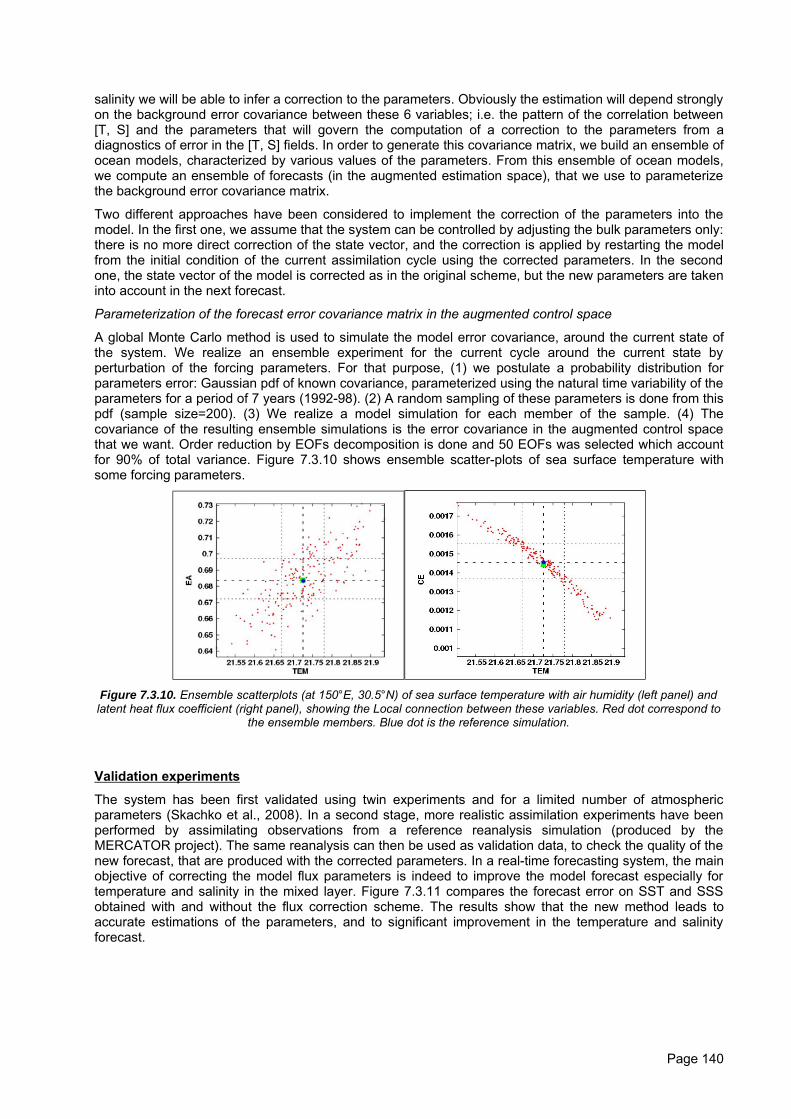
salinity we will be able to infer a correction to the parameters. Obviously the estimation will depend stronglyon the background error covariance between these 6 variables; i.e. the pattern of the correlation between[T, S] and the parameters that will govern the computation of a correction to the parameters from adiagnostics of error in the [T, S] fields. In order to generate this covariance matrix, we build an ensemble ofocean models, characterized by various values of the parameters. From this ensemble of ocean models,we compute an ensemble of forecasts (in the augmented estimation space), that we use to parameterizethe background error covariance matrix.

Two different approaches have been considered to implement the correction of the parameters into themodel. In the first one, we assume that the system can be controlled by adjusting the bulk parameters only:there is no more direct correction of the state vector, and the correction is applied by restarting the modelfrom the initial condition of the current assimilation cycle using the corrected parameters. In the secondone, the state vector of the model is corrected as in the original scheme, but the new parameters are takeninto account in the next forecast.

Parameterization of the forecast error covariance matrix in the augmented control space

A global Monte Carlo method is used to simulate the model error covariance, around the current state ofthe system. We realize an ensemble experiment for the current cycle around the current state byperturbation of the forcing parameters. For that purpose, (1) we postulate a probability distribution forparameters error: Gaussian pdf of known covariance, parameterized using the natural time variability of theparameters for a period of 7 years (1992-98). (2) A random sampling of these parameters is done from thispdf (sample size=200). (3) We realize a model simulation for each member of the sample. (4) Thecovariance of the resulting ensemble simulations is the error covariance in the augmented control spacethat we want. Order reduction by EOFs decomposition is done and 50 EOFs was selected which accountfor 90% of total variance. Figure 7.3.10 shows ensemble scatter-plots of sea surface temperature withsome forcing parameters.

Figure 7.3.10. Ensemble scatterplots (at 150°E, 30.5°N) of sea surface temperature with air humidity (left panel) andlatent heat flux coefficient (right panel), showing the Local connection between these variables. Red dot correspond to

the ensemble members. Blue dot is the reference simulation.

Validation experiments

The system has been first validated using twin experiments and for a limited number of atmosphericparameters (Skachko et al., 2008). In a second stage, more realistic assimilation experiments have beenperformed by assimilating observations from a reference reanalysis simulation (produced by theMERCATOR project). The same reanalysis can then be used as validation data, to check the quality of thenew forecast, that are produced with the corrected parameters. In a real-time forecasting system, the mainobjective of correcting the model flux parameters is indeed to improve the model forecast especially fortemperature and salinity in the mixed layer. Figure 7.3.11 compares the forecast error on SST and SSSobtained with and without the flux correction scheme. The results show that the new method leads toaccurate estimations of the parameters, and to significant improvement in the temperature and salinityforecast.

Page 140

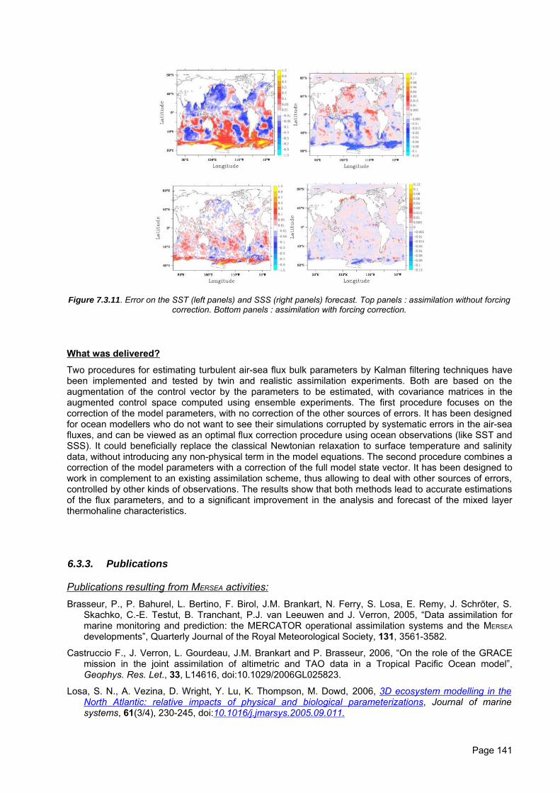
Figure 7.3.11. Error on the SST (left panels) and SSS (right panels) forecast. Top panels : assimilation without forcingcorrection. Bottom panels : assimilation with forcing correction.

What was delivered?

Two procedures for estimating turbulent air-sea flux bulk parameters by Kalman filtering techniques havebeen implemented and tested by twin and realistic assimilation experiments. Both are based on theaugmentation of the control vector by the parameters to be estimated, with covariance matrices in theaugmented control space computed using ensemble experiments. The first procedure focuses on thecorrection of the model parameters, with no correction of the other sources of errors. It has been designedfor ocean modellers who do not want to see their simulations corrupted by systematic errors in the air-seafluxes, and can be viewed as an optimal flux correction procedure using ocean observations (like SST andSSS). It could beneficially replace the classical Newtonian relaxation to surface temperature and salinitydata, without introducing any non-physical term in the model equations. The second procedure combines acorrection of the model parameters with a correction of the full model state vector. It has been designed towork in complement to an existing assimilation scheme, thus allowing to deal with other sources of errors,controlled by other kinds of observations. The results show that both methods lead to accurate estimationsof the flux parameters, and to a significant improvement in the analysis and forecast of the mixed layerthermohaline characteristics.

6.3.3. Publications

Publications resulting from MERSEA activities:Brasseur, P., P. Bahurel, L. Bertino, F. Birol, J.M. Brankart, N. Ferry, S. Losa, E. Remy, J. Schröter, S.

Skachko, C.-E. Testut, B. Tranchant, P.J. van Leeuwen and J. Verron, 2005, “Data assimilation formarine monitoring and prediction: the MERCATOR operational assimilation systems and the MERSEA

developments”, Quarterly Journal of the Royal Meteorological Society, 131, 3561-3582.

Castruccio F., J. Verron, L. Gourdeau, J.M. Brankart and P. Brasseur, 2006, “On the role of the GRACEmission in the joint assimilation of altimetric and TAO data in a Tropical Pacific Ocean model”,Geophys. Res. Let., 33, L14616, doi:10.1029/2006GL025823.

Losa, S. N., A. Vezina, D. Wright, Y. Lu, K. Thompson, M. Dowd, 2006, 3D ecosystem modelling in theNorth Atlantic: relative impacts of physical and biological parameterizations, Journal of marinesystems, 61(3/4), 230-245, doi:10.1016/j.jmarsys.2005.09.011.

Page 141

Ourmières, Y., J.M. Brankart, L. Berline, P. Brasseur and J. Verron, “Incremental Analysis Updateimplementation into a sequential ocean data assimilation system, 2006: A SEEK filter with IncrementalAnalysis Updating scheme”, J. Atmos. Ocean. Technol, 23(12), 1729-1744.

Sakov, P., and P. R. Oke, 2008, “Implications of the form of the ensemble transformations in the ensemblesquare root filters”, Mon. Wea. Rev., 136, 1042-1053.

Skachko, S., J.M. Brankart, F. Castruccio, P. Brasseur, J. Verron, 2008, “Estimating turbulent air-sea fluxbulk parameters by sequential data assimilation”, Journal of atmospheric and Oceanic Technology, inrevision.

Skandrani, C., J.M. Brankart, J. Verron and P. Brasseur, 2008, “Improving the temperature and salinityforecast in the ocean mixed layer by including atmospheric forcing parameters in the Kalman filtercontrol vector: a global test case study using MERCATORreanalysis data”, In preparation for OceanScience.

Other references:Bloom, S.C., L.L. Takacs, A.M. DaSilva and D. Levina, 1996, “Data assimilation using incremental analysis

updates”, Mon. Wea. Rev., 124(6), 1256-1271.

Lisæter, K.A., J. Rosanova, G. Evensen, 2003, “Assimilation of ice concentration in a coupled ice-oceanmodels, using the Ensemble Kalman Filter”, Ocean Dynamics 53: 368-388.

Pham, D. T., “Stochastic methods for sequential data assimilation in strongly nonlinear systems”, Mon.Weather Rev., 129, 1194–1207, 2000.

Page 142

7. Implementation & Production (Work Package 09)

7.1. Adaptation of NEMO for Shelf Seas (Task 9.1)

Met Office Leader, with Mercator and POL

Four separate pieces of work were completed within this task.

Interpolation Utilities

A set of interpolation utilities which can be used to create initial conditions or boundary data for regionalconfigurations using outputs from a larger area model was developed and provided by Mercator-Ocean toall the modelling groups. In order to ensure maximum flexibility, horizontal and vertical interpolations areperformed in separate routines. The horizontal interpolation utilities are based on a package that enablesinterpolation of both scalar (or tracer) fields and vector fields. Vertical interpolation can be performed usinglinear, cubic and spline interpolation options. The vertical coordinate (depth) can be specified as a 3-dimensional field allowing interpolation between any vertical coordinates. More detailed documentation ofthe utilities is provided in D9.1.1.

Implementation of Flow Relaxation and Flather Schemes within NEMO

The Flow Relaxation scheme (FRS) is a well-established (Davies 1976) but effective method for nesting alimited area high-resolution model (known as the inner model) inside a lower resolution larger area model(the outer model). The inner model is relaxed towards the outer model over a rim round its boundarywhose width is typically 5-20 inner grid points. The time-scale for the relaxation varies smoothly across therim with a long time-scale being used at the internal edge of the rim and model values being set equal tothe outer model values at the external edge of the rim. The Flather scheme is frequently used to specifythe boundary conditions for the barotropic currents and free surface height.

A version of the FRS and the Flather scheme have been implemented for NEMO and subsequentlyintroduced into the base-code as the BDY option. An OBC (Open Boundary Condition) option to applyradiation boundary conditions was already available within NEMO. The implementation of the BDY optionwas designed to be as consistent as possible with that of the OBC option.

The new option makes no assumptions about the path of the boundary (e.g. it need not be aligned with theinner model grid). The performance of the new FRS code was checked using a simple 5 km deep channelmodel in which a zonal flow is disturbed by a seamount with a height of 800 m. A reference integration isperformed in an extended channel (of 1500 km length) and used both to provide boundary conditions forthe channel with length reduced to 1000 km and to assess the performance of the limited area integrationsusing either radiative or FRS boundary conditions. Fig. 9.1.1 shows the results for the reference simulation(top) and integrations using the FRS with a relaxation zone of 1 point (middle) and 7 points (bottom).(More detailed documentation of the code is provided in D9.1.1.

Page 143

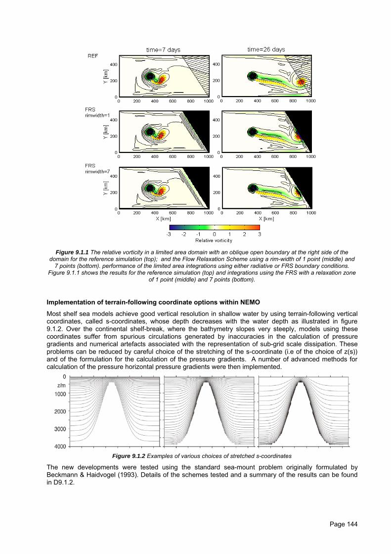
Figure 9.1.1 The relative vorticity in a limited area domain with an oblique open boundary at the right side of thedomain for the reference simulation (top); and the Flow Relaxation Scheme using a rim-width of 1 point (middle) and

7 points (bottom). performance of the limited area integrations using either radiative or FRS boundary conditions.Figure 9.1.1 shows the results for the reference simulation (top) and integrations using the FRS with a relaxation zone

of 1 point (middle) and 7 points (bottom).

Implementation of terrain-following coordinate options within NEMO

Most shelf sea models achieve good vertical resolution in shallow water by using terrain-following verticalcoordinates, called s-coordinates, whose depth decreases with the water depth as illustrated in figure9.1.2. Over the continental shelf-break, where the bathymetry slopes very steeply, models using thesecoordinates suffer from spurious circulations generated by inaccuracies in the calculation of pressuregradients and numerical artefacts associated with the representation of sub-grid scale dissipation. Theseproblems can be reduced by careful choice of the stretching of the s-coordinate (i.e of the choice of z(s))and of the formulation for the calculation of the pressure gradients. A number of advanced methods forcalculation of the pressure horizontal pressure gradients were then implemented.

Figure 9.1.2 Examples of various choices of stretched s-coordinates

The new developments were tested using the standard sea-mount problem originally formulated byBeckmann & Haidvogel (1993). Details of the schemes tested and a summary of the results can be foundin D9.1.2.

Page 144

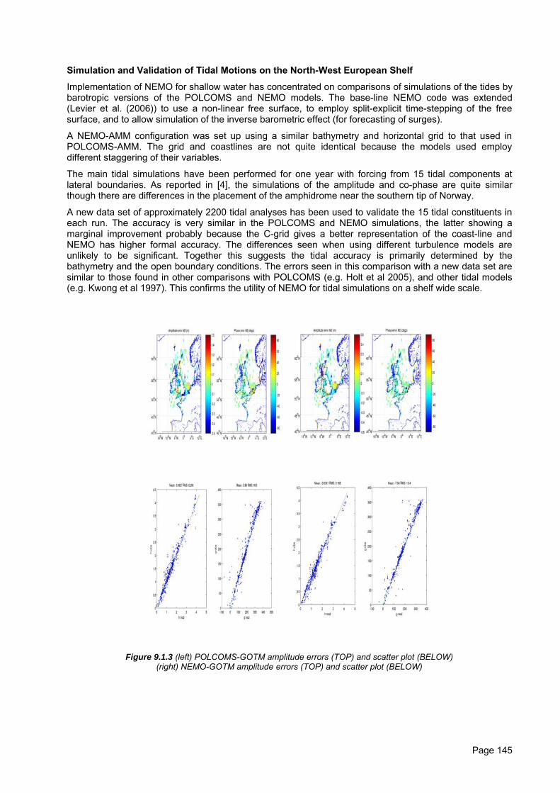
Simulation and Validation of Tidal Motions on the North-West European Shelf

Implementation of NEMO for shallow water has concentrated on comparisons of simulations of the tides bybarotropic versions of the POLCOMS and NEMO models. The base-line NEMO code was extended(Levier et al. (2006)) to use a non-linear free surface, to employ split-explicit time-stepping of the freesurface, and to allow simulation of the inverse barometric effect (for forecasting of surges).

A NEMO-AMM configuration was set up using a similar bathymetry and horizontal grid to that used inPOLCOMS-AMM. The grid and coastlines are not quite identical because the models used employdifferent staggering of their variables.

The main tidal simulations have been performed for one year with forcing from 15 tidal components atlateral boundaries. As reported in [4], the simulations of the amplitude and co-phase are quite similarthough there are differences in the placement of the amphidrome near the southern tip of Norway.

A new data set of approximately 2200 tidal analyses has been used to validate the 15 tidal constituents ineach run. The accuracy is very similar in the POLCOMS and NEMO simulations, the latter showing amarginal improvement probably because the C-grid gives a better representation of the coast-line andNEMO has higher formal accuracy. The differences seen when using different turbulence models areunlikely to be significant. Together this suggests the tidal accuracy is primarily determined by thebathymetry and the open boundary conditions. The errors seen in this comparison with a new data set aresimilar to those found in other comparisons with POLCOMS (e.g. Holt et al 2005), and other tidal models(e.g. Kwong et al 1997). This confirms the utility of NEMO for tidal simulations on a shelf wide scale.

Figure 9.1.3 (left) POLCOMS-GOTM amplitude errors (TOP) and scatter plot (BELOW)(right) NEMO-GOTM amplitude errors (TOP) and scatter plot (BELOW)

Page 145

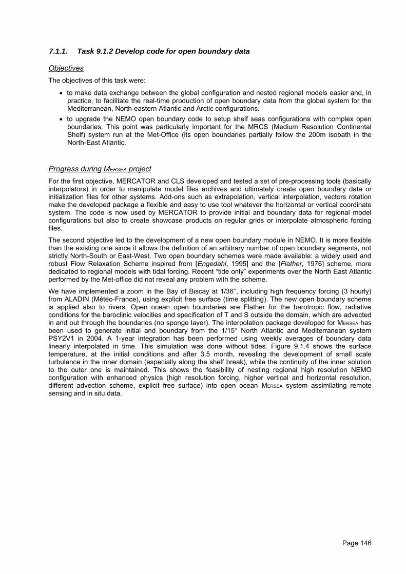
7.1.1. Task 9.1.2 Develop code for open boundary data

ObjectivesThe objectives of this task were:

• to make data exchange between the global configuration and nested regional models easier and, inpractice, to facilitate the real-time production of open boundary data from the global system for theMediterranean, North-eastern Atlantic and Arctic configurations.

• to upgrade the NEMO open boundary code to setup shelf seas configurations with complex openboundaries. This point was particularly important for the MRCS (Medium Resolution ContinentalShelf) system run at the Met-Office (its open boundaries partially follow the 200m isobath in theNorth-East Atlantic.

Progress during MERSEA projectFor the first objective, MERCATOR and CLS developed and tested a set of pre-processing tools (basicallyinterpolators) in order to manipulate model files archives and ultimately create open boundary data orinitialization files for other systems. Add-ons such as extrapolation, vertical interpolation, vectors rotationmake the developed package a flexible and easy to use tool whatever the horizontal or vertical coordinatesystem. The code is now used by MERCATOR to provide initial and boundary data for regional modelconfigurations but also to create showcase products on regular grids or interpolate atmospheric forcingfiles.

The second objective led to the development of a new open boundary module in NEMO. It is more flexiblethan the existing one since it allows the definition of an arbitrary number of open boundary segments, notstrictly North-South or East-West. Two open boundary schemes were made available: a widely used androbust Flow Relaxation Scheme inspired from [Engedahl, 1995] and the [Flather, 1976] scheme, morededicated to regional models with tidal forcing. Recent “tide only” experiments over the North East Atlanticperformed by the Met-office did not reveal any problem with the scheme.

We have implemented a zoom in the Bay of Biscay at 1/36°, including high frequency forcing (3 hourly)from ALADIN (Météo-France), using explicit free surface (time splitting). The new open boundary schemeis applied also to rivers. Open ocean open boundaries are Flather for the barotropic flow, radiativeconditions for the baroclinic velocities and specification of T and S outside the domain, which are advectedin and out through the boundaries (no sponge layer). The interpolation package developed for MERSEA hasbeen used to generate initial and boundary from the 1/15° North Atlantic and Mediterranean systemPSY2V1 in 2004. A 1-year integration has been performed using weekly averages of boundary datalinearly interpolated in time. This simulation was done without tides. Figure 9.1.4 shows the surfacetemperature, at the initial conditions and after 3.5 month, revealing the development of small scaleturbulence in the inner domain (especially along the shelf break), while the continuity of the inner solutionto the outer one is maintained. This shows the feasibility of nesting regional high resolution NEMOconfiguration with enhanced physics (high resolution forcing, higher vertical and horizontal resolution,different advection scheme, explicit free surface) into open ocean MERSEA system assimilating remotesensing and in situ data.

Page 146

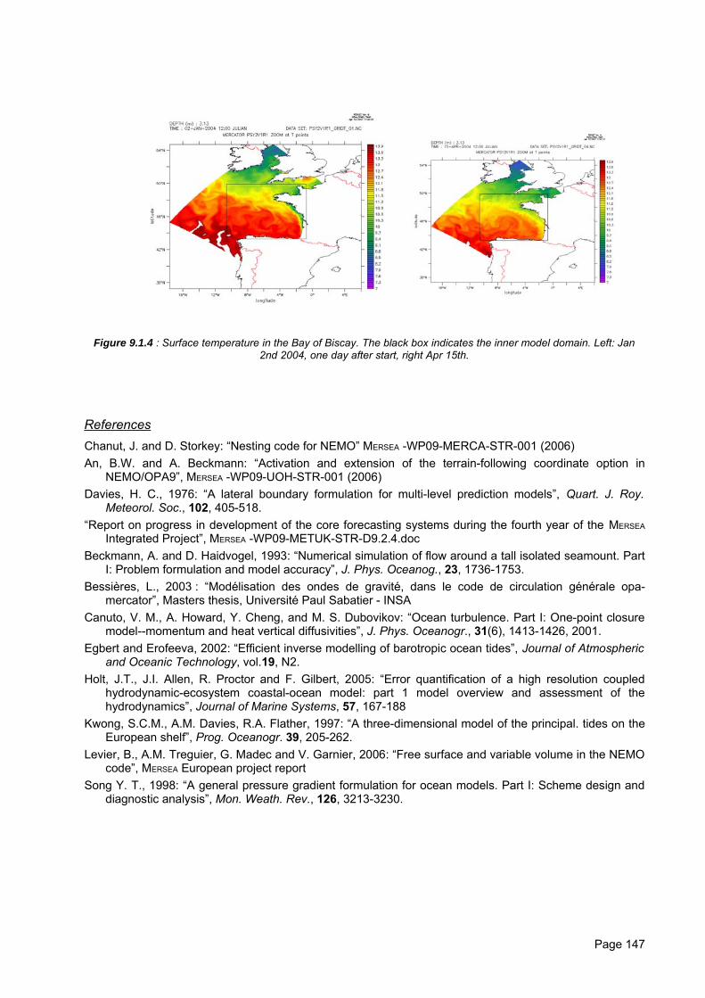
Figure 9.1.4 : Surface temperature in the Bay of Biscay. The black box indicates the inner model domain. Left: Jan2nd 2004, one day after start, right Apr 15th.

ReferencesChanut, J. and D. Storkey: “Nesting code for NEMO” MERSEA -WP09-MERCA-STR-001 (2006) An, B.W. and A. Beckmann: “Activation and extension of the terrain-following coordinate option in

NEMO/OPA9”, MERSEA -WP09-UOH-STR-001 (2006)Davies, H. C., 1976: “A lateral boundary formulation for multi-level prediction models”, Quart. J. Roy.

Meteorol. Soc., 102, 405-518.“Report on progress in development of the core forecasting systems during the fourth year of the MERSEA

Integrated Project”, MERSEA -WP09-METUK-STR-D9.2.4.docBeckmann, A. and D. Haidvogel, 1993: “Numerical simulation of flow around a tall isolated seamount. Part

I: Problem formulation and model accuracy”, J. Phys. Oceanog., 23, 1736-1753.Bessières, L., 2003 : “Modélisation des ondes de gravité, dans le code de circulation générale opa-

mercator”, Masters thesis, Université Paul Sabatier - INSACanuto, V. M., A. Howard, Y. Cheng, and M. S. Dubovikov: “Ocean turbulence. Part I: One-point closure

model--momentum and heat vertical diffusivities”, J. Phys. Oceanogr., 31(6), 1413-1426, 2001.Egbert and Erofeeva, 2002: “Efficient inverse modelling of barotropic ocean tides”, Journal of Atmospheric

and Oceanic Technology, vol.19, N2.Holt, J.T., J.I. Allen, R. Proctor and F. Gilbert, 2005: “Error quantification of a high resolution coupled

hydrodynamic-ecosystem coastal-ocean model: part 1 model overview and assessment of thehydrodynamics”, Journal of Marine Systems, 57, 167-188

Kwong, S.C.M., A.M. Davies, R.A. Flather, 1997: “A three-dimensional model of the principal. tides on theEuropean shelf”, Prog. Oceanogr. 39, 205-262.

Levier, B., A.M. Treguier, G. Madec and V. Garnier, 2006: “Free surface and variable volume in the NEMOcode”, MERSEA European project report

Song Y. T., 1998: “A general pressure gradient formulation for ocean models. Part I: Scheme design anddiagnostic analysis”, Mon. Weath. Rev., 126, 3213-3230.

Page 147

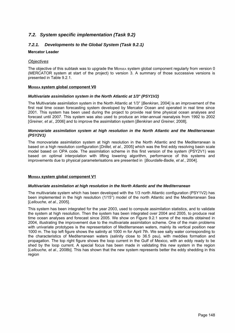
7.2. System specific implementation (Task 9.2)

7.2.1. Developments to the Global System (Task 9.2.1)Mercator Leader

ObjectivesThe objective of this subtask was to upgrade the MERSEA system global component regularly from version 0(MERCATOR system at start of the project) to version 3. A summary of those successive versions ispresented in Table 9.2.1.

MERSEA system global component V0

Multivariate assimilation system in the North Atlantic at 1/3° (PSY1V2)

The Multivariate assimilation system in the North Atlantic at 1/3° [Benkiran, 2004] is an improvement of thefirst real time ocean forecasting system developed by Mercator Ocean and operated in real time since2001. This system has been used during the project to provide real time physical ocean analyses andforecast until 2007. This system was also used to produce an inter-annual reanalysis from 1992 to 2002[Greiner, et al., 2006] and to improve the assimilation system [Benkiran and Greiner, 2008].

Monovariate assimilation system at high resolution in the North Atlantic and the Mediterranean(PSY2V1)

The monovariate assimilation system at high resolution in the North Atlantic and the Mediterranean isbased on a high resolution configuration [Drillet, et al., 2005] which was the first eddy resolving basin scalemodel based on OPA code. The assimilation scheme in this first version of the system (PSY2V1) wasbased on optimal interpolation with lifting lowering algorithm, performance of this systems andimprovements due to physical parameterisations are presented in [Bourdalle-Badie, et al., 2004].

MERSEA system global component V1

Multivariate assimilation at high resolution in the North Atlantic and the Mediterranean

The multivariate system which has been developed with the 1/3 north Atlantic configuration (PSY1V2) hasbeen implemented in the high resolution (1/15°) model of the north Atlantic and the Mediterranean Sea[Lellouche, et al., 2005].

This system has been integrated for the year 2003, used to compute assimilation statistics, and to validatethe system at high resolution. Then the system has been integrated over 2004 and 2005, to produce realtime ocean analyses and forecast since 2005. We show on Figure 9.2.1 some of the results obtained in2004, illustrating the improvement due to the multivariate assimilation scheme. One of the main problemswith univariate prototypes is the representation of Mediterranean waters, mainly its vertical position near1000 m. The top left figure shows the salinity at 1000 m for April 7th. We see salty water corresponding tothe characteristics of Mediterranean waters (salinity close to 36.5 psu), with meddies formation andpropagation. The top right figure shows the loop current in the Gulf of Mexico, with an eddy ready to beshed by the loop current. A special focus has been made in validating this new system in the region[Lellouche, et al., 2008b]. This has shown that the new system represents better the eddy shedding in thisregion

Page 148

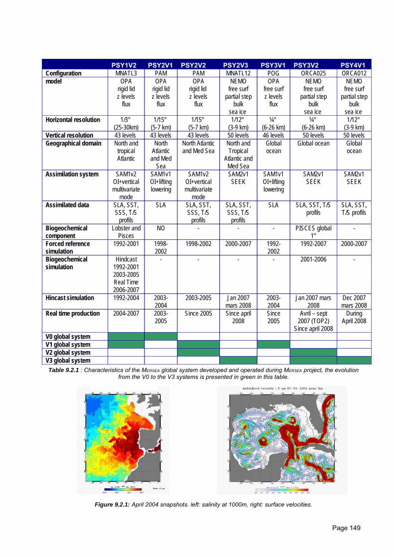
PSY1V2 PSY2V1 PSY2V2 PSY2V3 PSY3V1 PSY3V2 PSY4V1Configuration MNATL3 PAM PAM MNATL12 POG ORCA025 ORCA012model OPA

rigid lidz levels

flux

OPArigid lidz levels

flux

OPArigid lid z levels

flux

NEMOfree surf

partial stepbulk

sea ice

OPAfree surfz levels

flux

NEMOfree surf

partial stepbulk

sea ice

NEMOfree surf

partial stepbulk

sea ice Horizontal resolution 1/3°

(25-30km)1/15°

(5-7 km)1/15°

(5-7 km)1/12°

(3-9 km)¼°

(6-26 km)¼°

(6-26 km)1/12°

(3-9 km)Vertical resolution 43 levels 43 levels 43 levels 50 levels 46 levels 50 levels 50 levelsGeographical domain North and

tropicalAtlantic

NorthAtlantic

and MedSea

North Atlanticand Med Sea

North andTropical

Atlantic andMed Sea

Globalocean

Global ocean Globalocean

Assimilation system SAM1v2OI+verticalmultivariate

mode

SAM1v1OI+liftinglowering

SAM1v2OI+verticalmultivariate

mode

SAM2v1SEEK

SAM1v1OI+liftinglowering

SAM2v1SEEK

SAM2v1SEEK

Assimilated data SLA, SST,SSS, T/S

profils

SLA SLA, SST,SSS, T/S

profils

SLA, SST,SSS, T/S

profils

SLA SLA, SST, T/Sprofils

SLA, SST,T/S profils

Biogeochemicalcomponent

Lobster andPisces

NO - - - PISCES global1°

-

Forced referencesimulation

1992-2001 1998-2002

1998-2002 2000-2007 1992-2002

1992-2007 2000-2007

Biogeochemicalsimulation

Hindcast1992-20012003-2005Real Time2006-2007

- - - - 2001-2006 -

Hincast simulation 1992-2004 2003-2004

2003-2005 Jan 2007mars 2008

2003-2004

Jan 2007 mars2008

Dec 2007mars 2008

Real time production 2004-2007 2003-2005

Since 2005 Since april2008

Since2005

Avril – sept2007 (TOP2)

Since april 2008

DuringApril 2008

V0 global systemV1 global systemV2 global systemV3 global systemTable 9.2.1 : Characteristics of the MERSEA global system developed and operated during MERSEA project, the evolution

from the V0 to the V3 systems is presented in green in this table.

Figure 9.2.1: April 2004 snapshots. left: salinity at 1000m, right: surface velocities.

Page 149

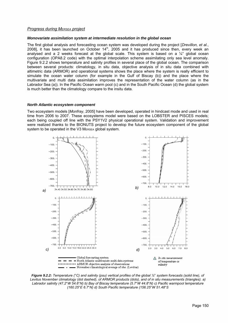
Progress during MERSEA project

Monovariate assimilation system at intermediate resolution in the global ocean

The first global analysis and forecasting ocean system was developed during the project [Drevillon, et al.,2008], it has been launched on October 14th, 2005 and it has produced since then, every week ananalysed and a 2 weeks forecast at the global scale. This system is based on a ¼° global oceanconfiguration (OPA8.2 code) with the optimal interpolation scheme assimilating only sea level anomaly.Figure 9.2.2 shows temperature and salinity profiles in several place of the global ocean. The comparisonbetween several products: climatology, in situ data, objective analysis of in situ data combined withaltimetric data (ARMOR) and operational systems shows the place where the system is really efficient tosimulate the ocean water column (for example in the Gulf of Biscay (b)) and the place where themultivariate and multi data assimilation improves the representation of the water column (as in theLabrador Sea (a)). In the Pacific Ocean warm pool (c) and in the South Pacific Ocean (d) the global systemis much better than the climatology compare to the insitu data.

North Atlantic ecosystem component

Two ecosystem models [Monfray, 2005] have been developed, operated in hindcast mode and used in realtime from 2006 to 2007. These ecosystems model were based on the LOBSTER and PISCES models;each being coupled off line with the PSY1V2 physical operational system. Validation and improvementwere realized thanks to the BIONUTS project to develop the future ecosystem component of the globalsystem to be operated in the V3 MERSEA global system.

a) b)

c) d)

Figure 9.2.2: Temperature (°C) and salinity (psu) vertical profiles of the global ¼° system forecasts (solid line), ofLevitus November climatology (dot dashed), of ARMOR products (dots), and of in situ measurements (triangles). a)

Labrador salinity (47.2°W 54.6°N) b) Bay of Biscay temperature (5.7°W 44.8°N) c) Pacific warmpool temperature(160.25°E 6.7°N) d) South Pacific temperature (156.25°W 51.48°S

Page 150

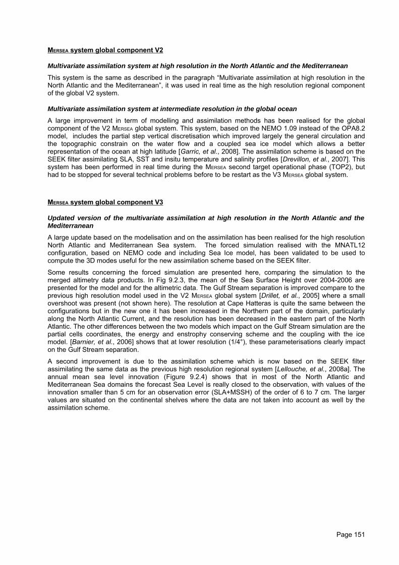
MERSEA system global component V2

Multivariate assimilation system at high resolution in the North Atlantic and the Mediterranean

This system is the same as described in the paragraph “Multivariate assimilation at high resolution in theNorth Atlantic and the Mediterranean”, it was used in real time as the high resolution regional componentof the global V2 system.

Multivariate assimilation system at intermediate resolution in the global ocean

A large improvement in term of modelling and assimilation methods has been realised for the globalcomponent of the V2 MERSEA global system. This system, based on the NEMO 1.09 instead of the OPA8.2model, includes the partial step vertical discretisation which improved largely the general circulation andthe topographic constrain on the water flow and a coupled sea ice model which allows a betterrepresentation of the ocean at high latitude [Garric, et al., 2008]. The assimilation scheme is based on theSEEK filter assimilating SLA, SST and insitu temperature and salinity profiles [Drevillon, et al., 2007]. Thissystem has been performed in real time during the MERSEA second target operational phase (TOP2), buthad to be stopped for several technical problems before to be restart as the V3 MERSEA global system.

MERSEA system global component V3

Updated version of the multivariate assimilation at high resolution in the North Atlantic and theMediterranean

A large update based on the modelisation and on the assimilation has been realised for the high resolutionNorth Atlantic and Mediterranean Sea system. The forced simulation realised with the MNATL12configuration, based on NEMO code and including Sea Ice model, has been validated to be used tocompute the 3D modes useful for the new assimilation scheme based on the SEEK filter.

Some results concerning the forced simulation are presented here, comparing the simulation to themerged altimetry data products. In Fig 9.2.3, the mean of the Sea Surface Height over 2004-2006 arepresented for the model and for the altimetric data. The Gulf Stream separation is improved compare to theprevious high resolution model used in the V2 MERSEA global system [Drillet, et al., 2005] where a smallovershoot was present (not shown here). The resolution at Cape Hatteras is quite the same between theconfigurations but in the new one it has been increased in the Northern part of the domain, particularlyalong the North Atlantic Current, and the resolution has been decreased in the eastern part of the NorthAtlantic. The other differences between the two models which impact on the Gulf Stream simulation are thepartial cells coordinates, the energy and enstrophy conserving scheme and the coupling with the icemodel. [Barnier, et al., 2006] shows that at lower resolution (1/4°), these parameterisations clearly impacton the Gulf Stream separation.

A second improvement is due to the assimilation scheme which is now based on the SEEK filterassimilating the same data as the previous high resolution regional system [Lellouche, et al., 2008a]. Theannual mean sea level innovation (Figure 9.2.4) shows that in most of the North Atlantic andMediterranean Sea domains the forecast Sea Level is really closed to the observation, with values of theinnovation smaller than 5 cm for an observation error (SLA+MSSH) of the order of 6 to 7 cm. The largervalues are situated on the continental shelves where the data are not taken into account as well by theassimilation scheme.

Page 151

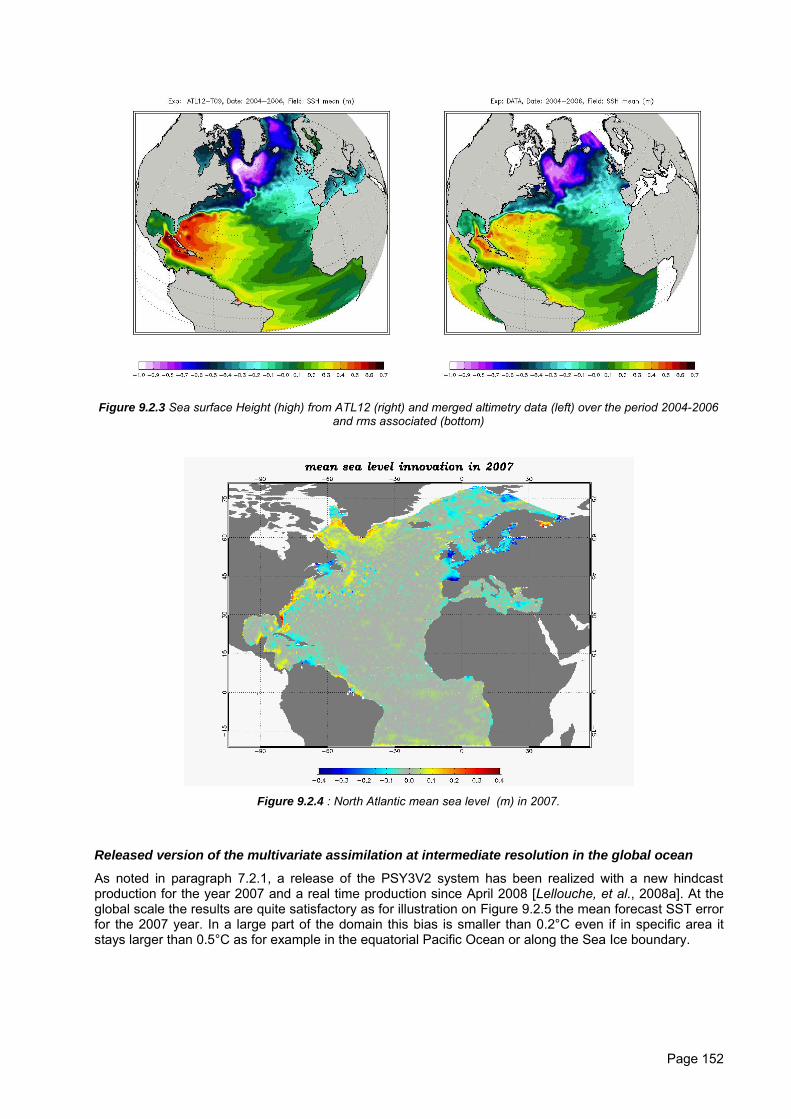
Figure 9.2.3 Sea surface Height (high) from ATL12 (right) and merged altimetry data (left) over the period 2004-2006and rms associated (bottom)

Figure 9.2.4 : North Atlantic mean sea level (m) in 2007.

Released version of the multivariate assimilation at intermediate resolution in the global ocean

As noted in paragraph 7.2.1, a release of the PSY3V2 system has been realized with a new hindcastproduction for the year 2007 and a real time production since April 2008 [Lellouche, et al., 2008a]. At theglobal scale the results are quite satisfactory as for illustration on Figure 9.2.5 the mean forecast SST errorfor the 2007 year. In a large part of the domain this bias is smaller than 0.2°C even if in specific area itstays larger than 0.5°C as for example in the equatorial Pacific Ocean or along the Sea Ice boundary.

Page 152

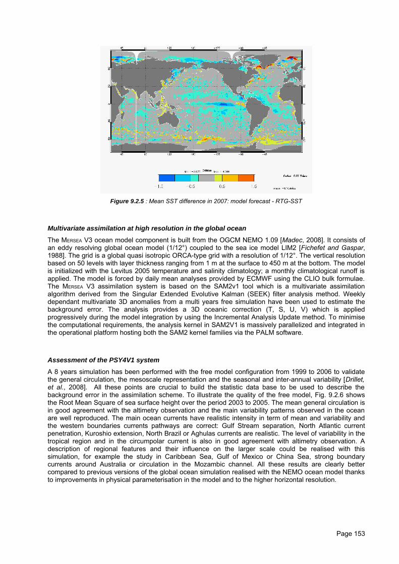
Figure 9.2.5 : Mean SST difference in 2007: model forecast - RTG-SST

Multivariate assimilation at high resolution in the global ocean

The MERSEA V3 ocean model component is built from the OGCM NEMO 1.09 [Madec, 2008]. It consists ofan eddy resolving global ocean model (1/12°) coupled to the sea ice model LIM2 [Fichefet and Gaspar,1988]. The grid is a global quasi isotropic ORCA-type grid with a resolution of 1/12°. The vertical resolutionbased on 50 levels with layer thickness ranging from 1 m at the surface to 450 m at the bottom. The modelis initialized with the Levitus 2005 temperature and salinity climatology; a monthly climatological runoff isapplied. The model is forced by daily mean analyses provided by ECMWF using the CLIO bulk formulae.The MERSEA V3 assimilation system is based on the SAM2v1 tool which is a multivariate assimilationalgorithm derived from the Singular Extended Evolutive Kalman (SEEK) filter analysis method. Weeklydependant multivariate 3D anomalies from a multi years free simulation have been used to estimate thebackground error. The analysis provides a 3D oceanic correction (T, S, U, V) which is appliedprogressively during the model integration by using the Incremental Analysis Update method. To minimisethe computational requirements, the analysis kernel in SAM2V1 is massively parallelized and integrated inthe operational platform hosting both the SAM2 kernel families via the PALM software.

Assessment of the PSY4V1 system

A 8 years simulation has been performed with the free model configuration from 1999 to 2006 to validatethe general circulation, the mesoscale representation and the seasonal and inter-annual variability [Drillet,et al., 2008]. All these points are crucial to build the statistic data base to be used to describe thebackground error in the assimilation scheme. To illustrate the quality of the free model, Fig. 9.2.6 showsthe Root Mean Square of sea surface height over the period 2003 to 2005. The mean general circulation isin good agreement with the altimetry observation and the main variability patterns observed in the oceanare well reproduced. The main ocean currents have realistic intensity in term of mean and variability andthe western boundaries currents pathways are correct: Gulf Stream separation, North Atlantic currentpenetration, Kuroshio extension, North Brazil or Aghulas currents are realistic. The level of variability in thetropical region and in the circumpolar current is also in good agreement with altimetry observation. Adescription of regional features and their influence on the larger scale could be realised with thissimulation, for example the study in Caribbean Sea, Gulf of Mexico or China Sea, strong boundarycurrents around Australia or circulation in the Mozambic channel. All these results are clearly bettercompared to previous versions of the global ocean simulation realised with the NEMO ocean model thanksto improvements in physical parameterisation in the model and to the higher horizontal resolution.

Page 153

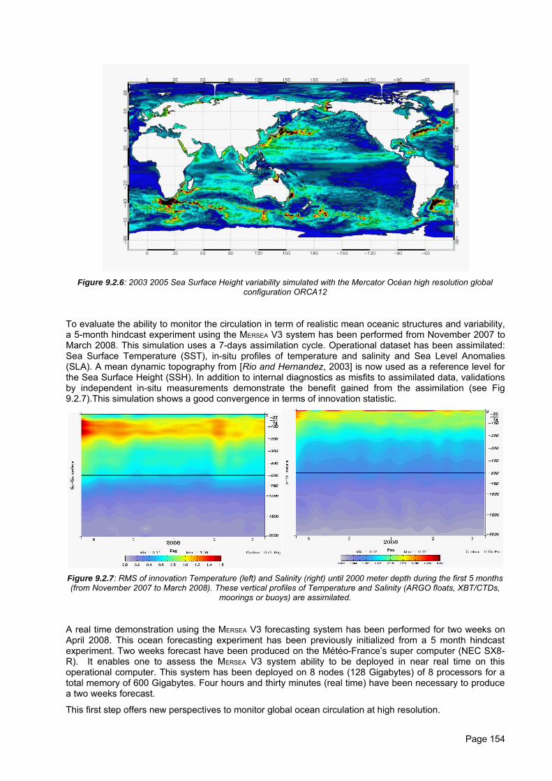
Figure 9.2.6: 2003 2005 Sea Surface Height variability simulated with the Mercator Océan high resolution globalconfiguration ORCA12

To evaluate the ability to monitor the circulation in term of realistic mean oceanic structures and variability,a 5-month hindcast experiment using the MERSEA V3 system has been performed from November 2007 toMarch 2008. This simulation uses a 7-days assimilation cycle. Operational dataset has been assimilated:Sea Surface Temperature (SST), in-situ profiles of temperature and salinity and Sea Level Anomalies(SLA). A mean dynamic topography from [Rio and Hernandez, 2003] is now used as a reference level forthe Sea Surface Height (SSH). In addition to internal diagnostics as misfits to assimilated data, validationsby independent in-situ measurements demonstrate the benefit gained from the assimilation (see Fig9.2.7).This simulation shows a good convergence in terms of innovation statistic.

Figure 9.2.7: RMS of innovation Temperature (left) and Salinity (right) until 2000 meter depth during the first 5 months(from November 2007 to March 2008). These vertical profiles of Temperature and Salinity (ARGO floats, XBT/CTDs,

moorings or buoys) are assimilated.

A real time demonstration using the MERSEA V3 forecasting system has been performed for two weeks onApril 2008. This ocean forecasting experiment has been previously initialized from a 5 month hindcastexperiment. Two weeks forecast have been produced on the Météo-France’s super computer (NEC SX8-R). It enables one to assess the MERSEA V3 system ability to be deployed in near real time on thisoperational computer. This system has been deployed on 8 nodes (128 Gigabytes) of 8 processors for atotal memory of 600 Gigabytes. Four hours and thirty minutes (real time) have been necessary to producea two weeks forecast.

This first step offers new perspectives to monitor global ocean circulation at high resolution.

Page 154

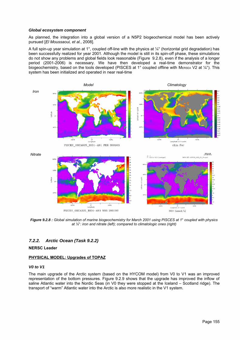
Global ecosystem component

As planned, the integration into a global version of a N5P2 biogeochemical model has been activelypursued [El Moussaoui, et al., 2008].

A full spin-up year simulation at 1°, coupled off-line with the physics at ¼° (horizontal grid degradation) hasbeen successfully realized for year 2001. Although the model is still in its spin-off phase, these simulationsdo not show any problems and global fields look reasonable (Figure 9.2.8), even if the analysis of a longerperiod (2001-2006) is necessary. We have then developed a real-time demonstrator for thebiogeochemistry, based on the tools developed (PISCES at 1° coupled offline with MERSEA V2 at ¼°). Thissystem has been initialized and operated in near real-time

Iron

Model Climatology

Nitrate

Figure 9.2.8 : Global simulation of marine biogeochemistry for March 2001 using PISCES at 1° coupled with physicsat ¼°: iron and nitrate (left); compared to climatologic ones (right)

7.2.2. Arctic Ocean (Task 9.2.2)NERSC Leader

PHYSICAL MODEL: Upgrades of TOPAZ

V0 to V1

The main upgrade of the Arctic system (based on the HYCOM model) from V0 to V1 was an improvedrepresentation of the bottom pressures. Figure 9.2.9 shows that the upgrade has improved the inflow ofsaline Atlantic water into the Nordic Seas (in V0 they were stopped at the Iceland – Scotland ridge). Thetransport of “warm” Atlantic water into the Arctic is also more realistic in the V1 system.

Page 155

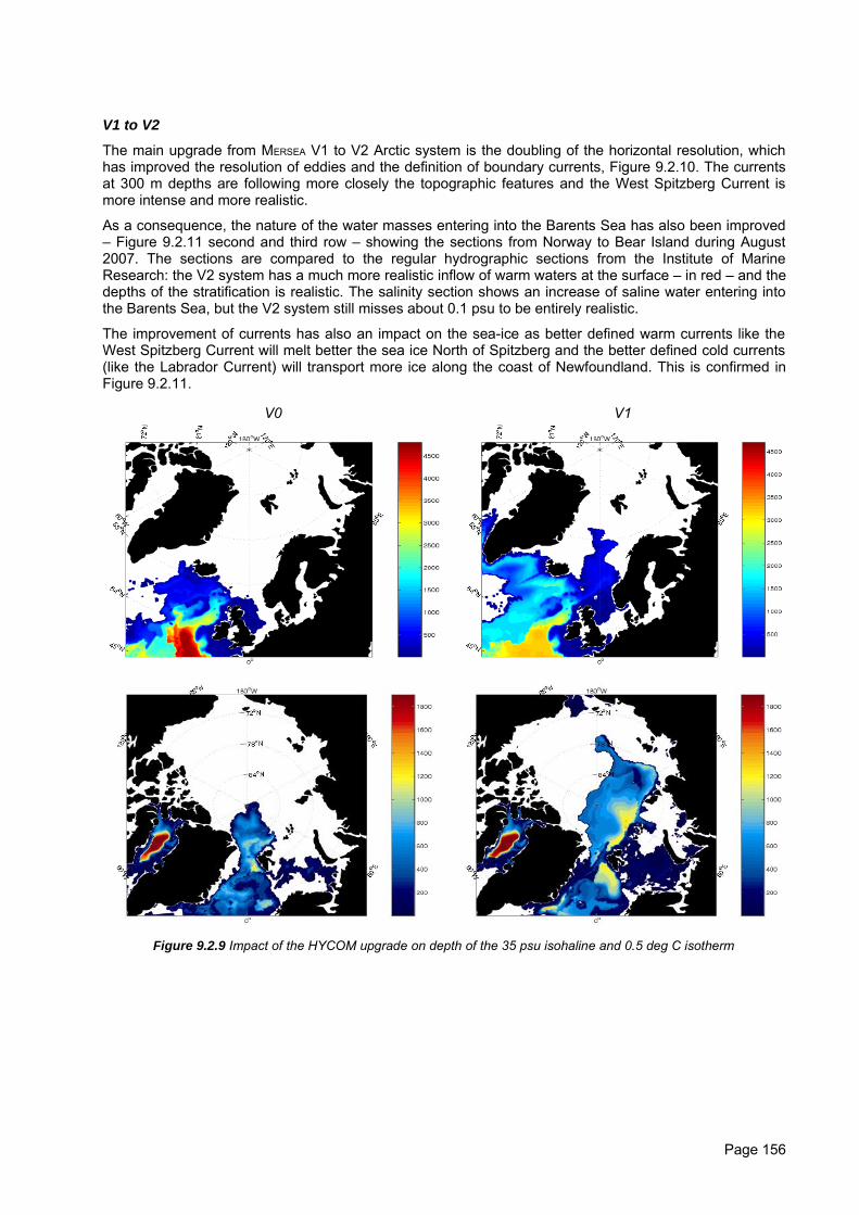
V1 to V2

The main upgrade from MERSEA V1 to V2 Arctic system is the doubling of the horizontal resolution, whichhas improved the resolution of eddies and the definition of boundary currents, Figure 9.2.10. The currentsat 300 m depths are following more closely the topographic features and the West Spitzberg Current ismore intense and more realistic.

As a consequence, the nature of the water masses entering into the Barents Sea has also been improved– Figure 9.2.11 second and third row – showing the sections from Norway to Bear Island during August2007. The sections are compared to the regular hydrographic sections from the Institute of MarineResearch: the V2 system has a much more realistic inflow of warm waters at the surface – in red – and thedepths of the stratification is realistic. The salinity section shows an increase of saline water entering intothe Barents Sea, but the V2 system still misses about 0.1 psu to be entirely realistic.

The improvement of currents has also an impact on the sea-ice as better defined warm currents like theWest Spitzberg Current will melt better the sea ice North of Spitzberg and the better defined cold currents(like the Labrador Current) will transport more ice along the coast of Newfoundland. This is confirmed inFigure 9.2.11.

V0 V1

Figure 9.2.9 Impact of the HYCOM upgrade on depth of the 35 psu isohaline and 0.5 deg C isotherm

Page 156

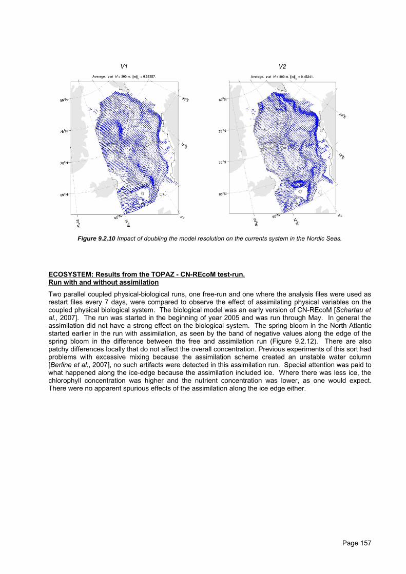
V1 V2

Figure 9.2.10 Impact of doubling the model resolution on the currents system in the Nordic Seas.

ECOSYSTEM: Results from the TOPAZ - CN-REcoM test-run.Run with and without assimilation

Two parallel coupled physical-biological runs, one free-run and one where the analysis files were used asrestart files every 7 days, were compared to observe the effect of assimilating physical variables on thecoupled physical biological system. The biological model was an early version of CN-REcoM [Schartau etal., 2007]. The run was started in the beginning of year 2005 and was run through May. In general theassimilation did not have a strong effect on the biological system. The spring bloom in the North Atlanticstarted earlier in the run with assimilation, as seen by the band of negative values along the edge of thespring bloom in the difference between the free and assimilation run (Figure 9.2.12). There are alsopatchy differences locally that do not affect the overall concentration. Previous experiments of this sort hadproblems with excessive mixing because the assimilation scheme created an unstable water column[Berline et al., 2007], no such artifacts were detected in this assimilation run. Special attention was paid towhat happened along the ice-edge because the assimilation included ice. Where there was less ice, thechlorophyll concentration was higher and the nutrient concentration was lower, as one would expect.There were no apparent spurious effects of the assimilation along the ice edge either.

Page 157

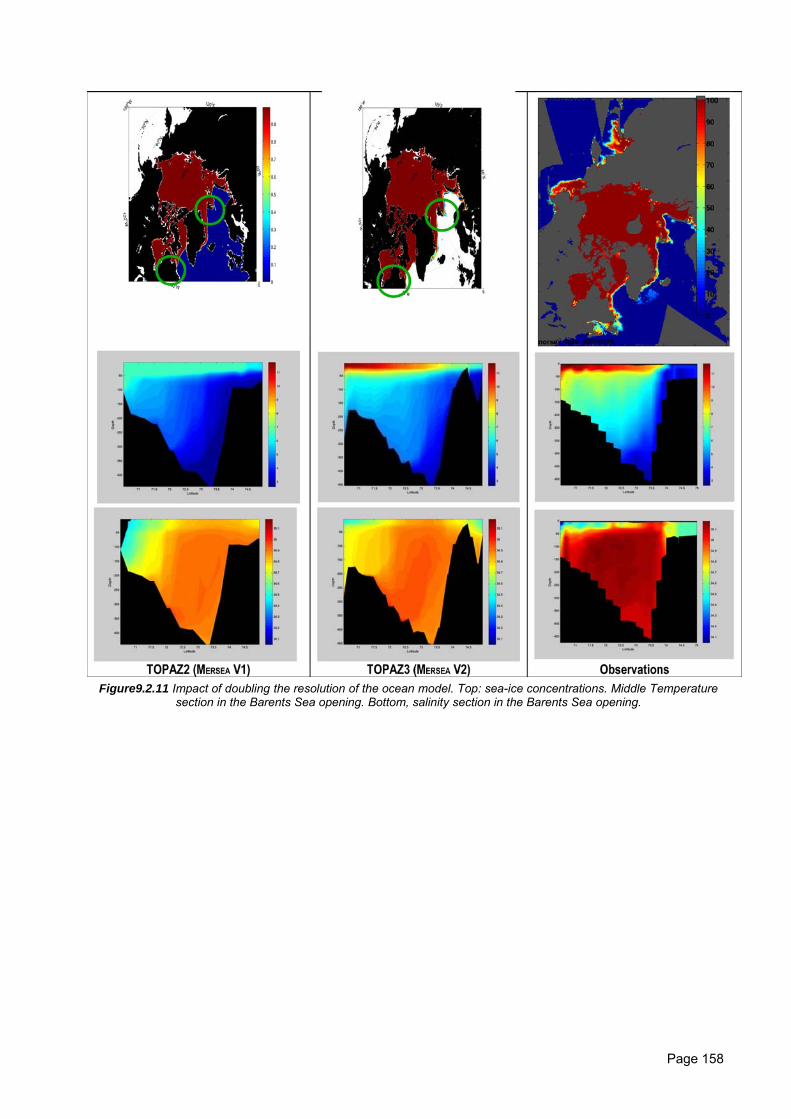
Figure9.2.11 Impact of doubling the resolution of the ocean model. Top: sea-ice concentrations. Middle Temperaturesection in the Barents Sea opening. Bottom, salinity section in the Barents Sea opening.

Page 158

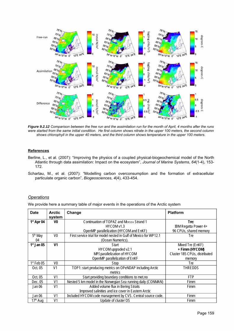
Figure 9.2.12 Comparison between the free run and the assimilation run for the month of April, 4 months after the runswere started from the same initial condition. He first column shows nitrate in the upper 100 meters, the second column

shows chlorophyll in the upper 40 meters, and the third column shows temperature in the upper 100 meters.

References

Berline, L., et al. (2007): “Improving the physics of a coupled physical-biogeochemical model of the NorthAtlantic through data assimilation: Impact on the ecosystem”, Journal of Marine Systems, 64(1-4), 153-172.

Schartau, M., et al. (2007): “Modelling carbon overconsumption and the formation of extracellularparticulate organic carbon”, Biogeosciences, 4(4), 433-454.

OperationsWe provide here a summary table of major events in the operations of the Arctic system

Date Arctic system

Change Platform

1st Apr 04 V0 Continuation of TOPAZ and MERSEA Strand 1HYCOM v1.3

OpenMP parallelization (HYCOM and EnKF)

Tre:IBM Regatta Power 4+

96 CPUs, shared memory5th May

04V0 First service trial for model nested in Gulf of Mexico for WP12.1

(Ocean Numerics). Tre

1st Jan 05 V1 StartHYCOM upgraded v2.1

MPI parallelization of HYCOMOpenMP parallelization of EnKF

Mixed Tre (EnKF) + Fimm (HYCOM)

Cluster 185 CPUs, distributedmemory

1st Feb 05 V0 Stop TreOct. 05 V1 TOP1: start producing metrics on OPeNDAP including Arctic

metricsTHREDDS

Oct. 05 V1 Start providing boundary conditions to met.no FTPDec. 05 V1 Nested 5 km model in the Norwegian Sea running daily (CONMAN) FimmJan 06 V1 Added volume flux in Bering Straits

Improved salinities and ice cover in Eastern ArcticFimm

Jan 06 V1 Included HYCOM code management by CVS. Central source code. Fimm17th Aug V1 Update of cluster OS Fimm

Page 159

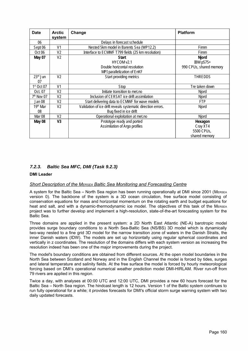
Date Arctic system

Change Platform

06 Delays in forecast scheduleSept 06 V1 Nested 5km model in Barents Sea (WP12.2) FimmOct 06 V2 Interface to ECMWF T799 fields (25 km resolution) FimmMay 07 V2 Start

HYCOM v2.1Double horizontal resolutionMPI parallelization of EnKF

NjordIBM p575+

990 CPUs, shared memory

23rd Jun07

V2 Start providing metrics THREDDS

1st Oct 07 V1 Stop Tre taken downOct. 07 V2 Initiate transition to met.no Njord

7th Nov 07 V2 Inclusion of CERSAT ice drift assimilation NjordJan 08 V2 Start delivering data to ECMWF for wave models FTP

19th Mar08

V2 Validation of ice drift reveals systematic direction errors. Bug fixed in ice drift

Njord

Mar 08 V2 Operational exploitation at met.no NjordMay 08 V3 Prototype ready and ported

Assimilation of Argo profiles HexagonCray XT4

5500 CPUs, shared memory

7.2.3. Baltic Sea MFC, DMI (Task 9.2.3)DMI Leader

Short Description of the MERSEA Baltic Sea Monitoring and Forecasting CentreA system for the Baltic Sea – North Sea region has been running operationally at DMI since 2001 (MERSEA

version 0). The backbone of the system is a 3D ocean circulation, free surface model consisting ofconservation equations for mass and horizontal momentum on the rotating earth and budget equations forheat and salt, and with a dynamic-thermodynamic ice model. The objectives of this task of the MERSEA

project was to further develop and implement a high-resolution, state-of-the-art forecasting system for theBaltic Sea.

Three domains are applied in the present system: a 2D North East Atlantic (NE-A) barotropic modelprovides surge boundary conditions to a North Sea-Baltic Sea (NS/BS) 3D model which is dynamicallytwo-way nested to a fine grid 3D model for the narrow transition zone of waters in the Danish Straits, theinner Danish waters (IDW). The models are set up horizontally using regular spherical coordinates andvertically in z coordinates. The resolution of the domains differs with each system version as increasing theresolution indeed has been one of the major improvements during the project.

The model's boundary conditions are obtained from different sources. At the open model boundaries in theNorth Sea between Scotland and Norway and in the English Channel the model is forced by tides, surgesand lateral temperature and salinity fields. At the free surface the model is forced by hourly meteorologicalforcing based on DMI’s operational numerical weather prediction model DMI-HIRLAM. River run-off from79 rivers are applied in this region.

Twice a day, with analyses at 00:00 UTC and 12:00 UTC, DMI provides a new 60 hours forecast for theBaltic Sea – North Sea region. The hindcast length is 12 hours. Version 1 of the Baltic system continues torun fully operational for a while; it provides forecasts for DMI's official storm surge warning system with twodaily updated forecasts.

Page 160

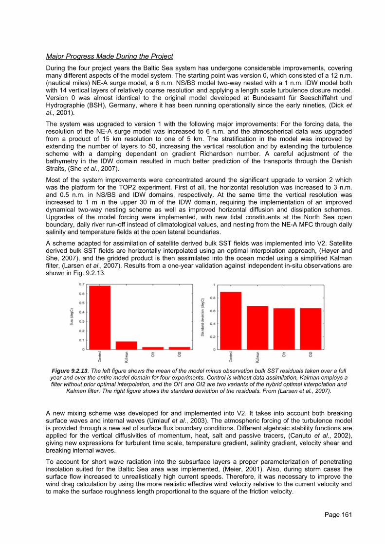
Major Progress Made During the ProjectDuring the four project years the Baltic Sea system has undergone considerable improvements, coveringmany different aspects of the model system. The starting point was version 0, which consisted of a 12 n.m.(nautical miles) NE-A surge model, a 6 n.m. NS/BS model two-way nested with a 1 n.m. IDW model bothwith 14 vertical layers of relatively coarse resolution and applying a length scale turbulence closure model.Version 0 was almost identical to the original model developed at Bundesamt für Seeschiffahrt undHydrographie (BSH), Germany, where it has been running operationally since the early nineties, (Dick etal., 2001).

The system was upgraded to version 1 with the following major improvements: For the forcing data, theresolution of the NE-A surge model was increased to 6 n.m. and the atmospherical data was upgradedfrom a product of 15 km resolution to one of 5 km. The stratification in the model was improved byextending the number of layers to 50, increasing the vertical resolution and by extending the turbulencescheme with a damping dependant on gradient Richardson number. A careful adjustment of thebathymetry in the IDW domain resulted in much better prediction of the transports through the DanishStraits, (She et al., 2007).

Most of the system improvements were concentrated around the significant upgrade to version 2 whichwas the platform for the TOP2 experiment. First of all, the horizontal resolution was increased to 3 n.m.and 0.5 n.m. in NS/BS and IDW domains, respectively. At the same time the vertical resolution wasincreased to 1 m in the upper 30 m of the IDW domain, requiring the implementation of an improveddynamical two-way nesting scheme as well as improved horizontal diffusion and dissipation schemes.Upgrades of the model forcing were implemented, with new tidal constituents at the North Sea openboundary, daily river run-off instead of climatological values, and nesting from the NE-A MFC through dailysalinity and temperature fields at the open lateral boundaries.

A scheme adapted for assimilation of satellite derived bulk SST fields was implemented into V2. Satellitederived bulk SST fields are horizontally interpolated using an optimal interpolation approach, (Høyer andShe, 2007), and the gridded product is then assimilated into the ocean model using a simplified Kalmanfilter, (Larsen et al., 2007). Results from a one-year validation against independent in-situ observations areshown in Fig. 9.2.13.

Figure 9.2.13. The left figure shows the mean of the model minus observation bulk SST residuals taken over a fullyear and over the entire model domain for four experiments. Control is without data assimilation, Kalman employs afilter without prior optimal interpolation, and the OI1 and OI2 are two variants of the hybrid optimal interpolation and

Kalman filter. The right figure shows the standard deviation of the residuals. From (Larsen et al., 2007).

A new mixing scheme was developed for and implemented into V2. It takes into account both breakingsurface waves and internal waves (Umlauf et al., 2003). The atmospheric forcing of the turbulence modelis provided through a new set of surface flux boundary conditions. Different algebraic stability functions areapplied for the vertical diffusivities of momentum, heat, salt and passive tracers, (Canuto et al., 2002),giving new expressions for turbulent time scale, temperature gradient, salinity gradient, velocity shear andbreaking internal waves.

To account for short wave radiation into the subsurface layers a proper parameterization of penetratinginsolation suited for the Baltic Sea area was implemented, (Meier, 2001). Also, during storm cases thesurface flow increased to unrealistically high current speeds. Therefore, it was necessary to improve thewind drag calculation by using the more realistic effective wind velocity relative to the current velocity andto make the surface roughness length proportional to the square of the friction velocity.

Page 161

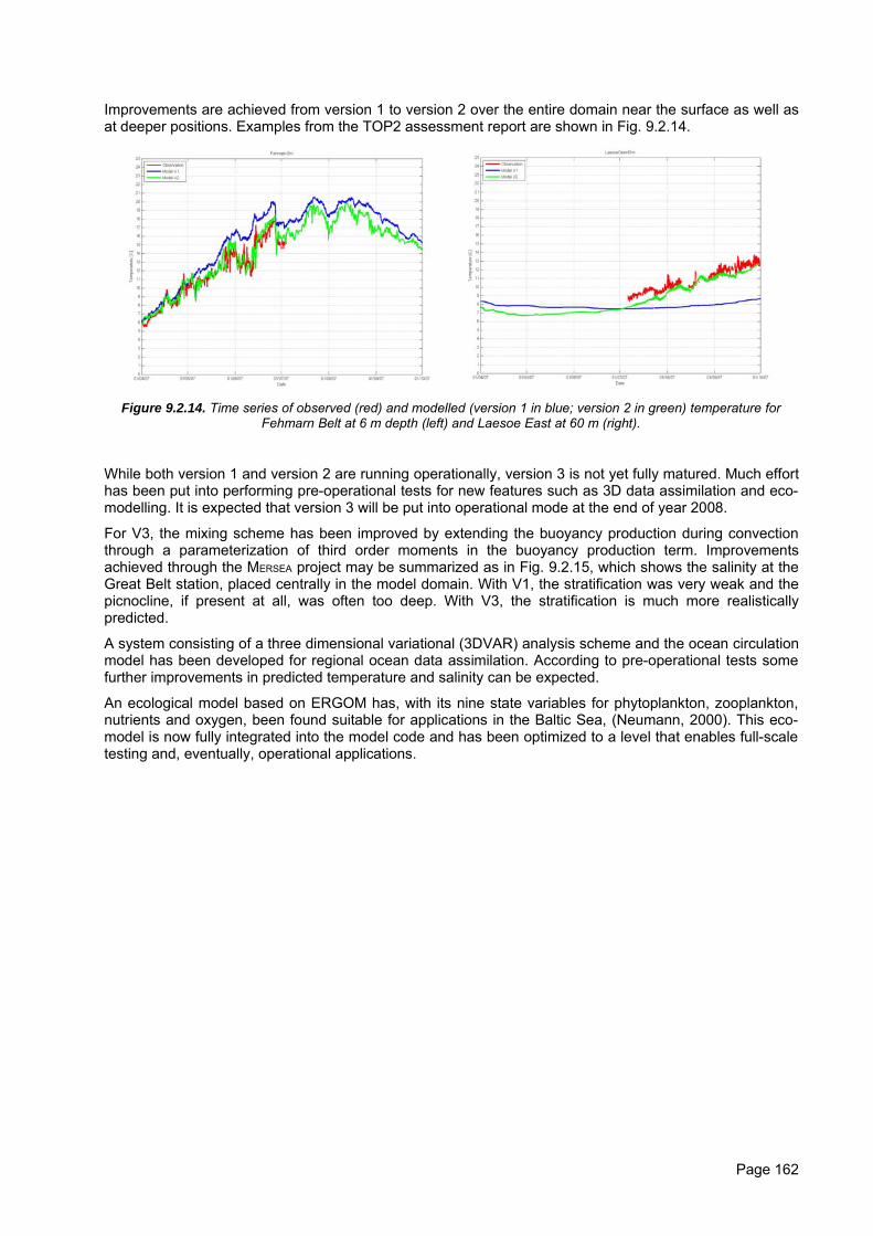
Improvements are achieved from version 1 to version 2 over the entire domain near the surface as well asat deeper positions. Examples from the TOP2 assessment report are shown in Fig. 9.2.14.

Figure 9.2.14. Time series of observed (red) and modelled (version 1 in blue; version 2 in green) temperature forFehmarn Belt at 6 m depth (left) and Laesoe East at 60 m (right).

While both version 1 and version 2 are running operationally, version 3 is not yet fully matured. Much efforthas been put into performing pre-operational tests for new features such as 3D data assimilation and eco-modelling. It is expected that version 3 will be put into operational mode at the end of year 2008.

For V3, the mixing scheme has been improved by extending the buoyancy production during convectionthrough a parameterization of third order moments in the buoyancy production term. Improvementsachieved through the MERSEA project may be summarized as in Fig. 9.2.15, which shows the salinity at theGreat Belt station, placed centrally in the model domain. With V1, the stratification was very weak and thepicnocline, if present at all, was often too deep. With V3, the stratification is much more realisticallypredicted.

A system consisting of a three dimensional variational (3DVAR) analysis scheme and the ocean circulationmodel has been developed for regional ocean data assimilation. According to pre-operational tests somefurther improvements in predicted temperature and salinity can be expected.

An ecological model based on ERGOM has, with its nine state variables for phytoplankton, zooplankton,nutrients and oxygen, been found suitable for applications in the Baltic Sea, (Neumann, 2000). This eco-model is now fully integrated into the model code and has been optimized to a level that enables full-scaletesting and, eventually, operational applications.

Page 162

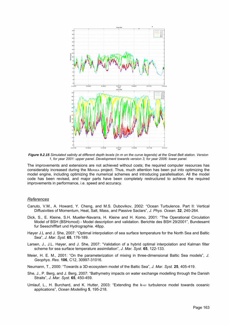
Figure 9.2.15 Simulated salinity at different depth levels (in m on the curve legends) at the Great Belt station. Version1, for year 2001: upper panel. Development towards version 3, for year 2006: lower panel.

The improvements and extensions are not achieved without costs; the required computer resources hasconsiderably increased during the MERSEA project. Thus, much attention has been put into optimizing themodel engine, including optimizing the numerical schemes and introducing parallelisation. All the modelcode has been revised, and major parts have been completely restructured to achieve the requiredimprovements in performance, i.e. speed and accuracy.

ReferencesCanuto, V.M., A. Howard, Y. Cheng, and M.S. Dubovikov, 2002: “Ocean Turbulence. Part II: Vertical

Diffusivities of Momentum, Heat, Salt, Mass, and Passive Saclars”, J. Phys. Ocean. 32, 240-264.

Dick, S., E. Kleine, S.H. Mueller-Navarra, H. Kleine and H. Komo, 2001: “The Operational CirculationModel of BSH (BSHcmod) - Model description and validation. Berichte des BSH 29/2001”, Bundesamtfur Seeschifffart und Hydrographie. 48pp.

Høyer J.L and J. She, 2007: “Optimal interpolation of sea surface temperature for the North Sea and BalticSea”, J. Mar. Syst. 65, 176-189.

Larsen, J., J.L. Høyer, and J. She, 2007: “Validation of a hybrid optimal interpolation and Kalman filterscheme for sea surface temperature assimilation”, J. Mar. Syst. 65, 122-133.

Meier, H. E. M., 2001: “On the parameterization of mixing in three-dimensional Baltic Sea models”, J.Geophys. Res. 106, C12, 30997-31016.

Neumann, T., 2000: “Towards a 3D-ecosystem model of the Baltic Sea”, J. Mar. Syst. 25, 405-419.

She, J., P. Berg, and J. Berg, 2007: “Bathymetry impacts on water exchange modelling through the DanishStraits”, J. Mar. Syst. 65, 450-459.

Umlauf, L., H. Burchard, and K. Hutter, 2003: “Extending the k- turbulence model towards oceanicapplications”, Ocean Modelling 5, 195-218.

Page 163

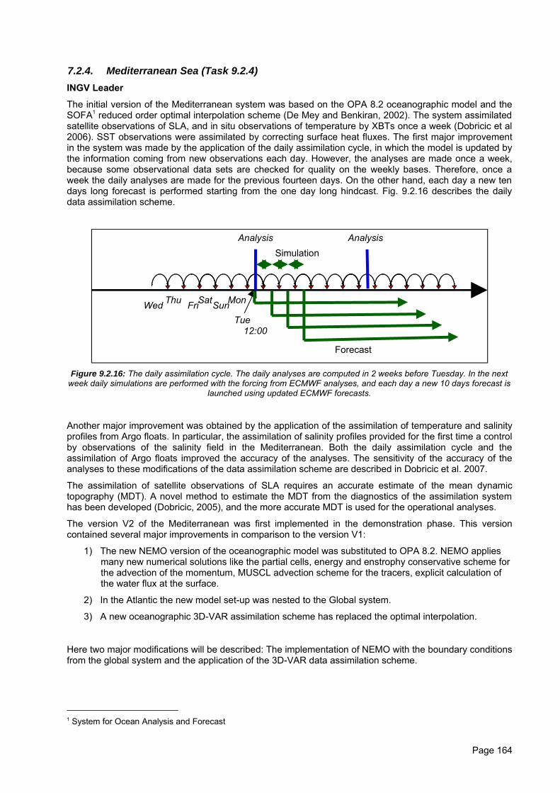
7.2.4. Mediterranean Sea (Task 9.2.4)INGV Leader

The initial version of the Mediterranean system was based on the OPA 8.2 oceanographic model and theSOFA1 reduced order optimal interpolation scheme (De Mey and Benkiran, 2002). The system assimilatedsatellite observations of SLA, and in situ observations of temperature by XBTs once a week (Dobricic et al2006). SST observations were assimilated by correcting surface heat fluxes. The first major improvementin the system was made by the application of the daily assimilation cycle, in which the model is updated bythe information coming from new observations each day. However, the analyses are made once a week,because some observational data sets are checked for quality on the weekly bases. Therefore, once aweek the daily analyses are made for the previous fourteen days. On the other hand, each day a new tendays long forecast is performed starting from the one day long hindcast. Fig. 9.2.16 describes the dailydata assimilation scheme.

Figure 9.2.16: The daily assimilation cycle. The daily analyses are computed in 2 weeks before Tuesday. In the nextweek daily simulations are performed with the forcing from ECMWF analyses, and each day a new 10 days forecast is

launched using updated ECMWF forecasts.

Another major improvement was obtained by the application of the assimilation of temperature and salinityprofiles from Argo floats. In particular, the assimilation of salinity profiles provided for the first time a controlby observations of the salinity field in the Mediterranean. Both the daily assimilation cycle and theassimilation of Argo floats improved the accuracy of the analyses. The sensitivity of the accuracy of theanalyses to these modifications of the data assimilation scheme are described in Dobricic et al. 2007.

The assimilation of satellite observations of SLA requires an accurate estimate of the mean dynamictopography (MDT). A novel method to estimate the MDT from the diagnostics of the assimilation systemhas been developed (Dobricic, 2005), and the more accurate MDT is used for the operational analyses.

The version V2 of the Mediterranean was first implemented in the demonstration phase. This versioncontained several major improvements in comparison to the version V1:

1) The new NEMO version of the oceanographic model was substituted to OPA 8.2. NEMO appliesmany new numerical solutions like the partial cells, energy and enstrophy conservative scheme forthe advection of the momentum, MUSCL advection scheme for the tracers, explicit calculation ofthe water flux at the surface.

2) In the Atlantic the new model set-up was nested to the Global system.

3) A new oceanographic 3D-VAR assimilation scheme has replaced the optimal interpolation.

Here two major modifications will be described: The implementation of NEMO with the boundary conditionsfrom the global system and the application of the 3D-VAR data assimilation scheme.

1 System for Ocean Analysis and Forecast

Page 164

Tue 12:00

Wed Thu FriSat MonSun

Analysis AnalysisSimulation

Forecast

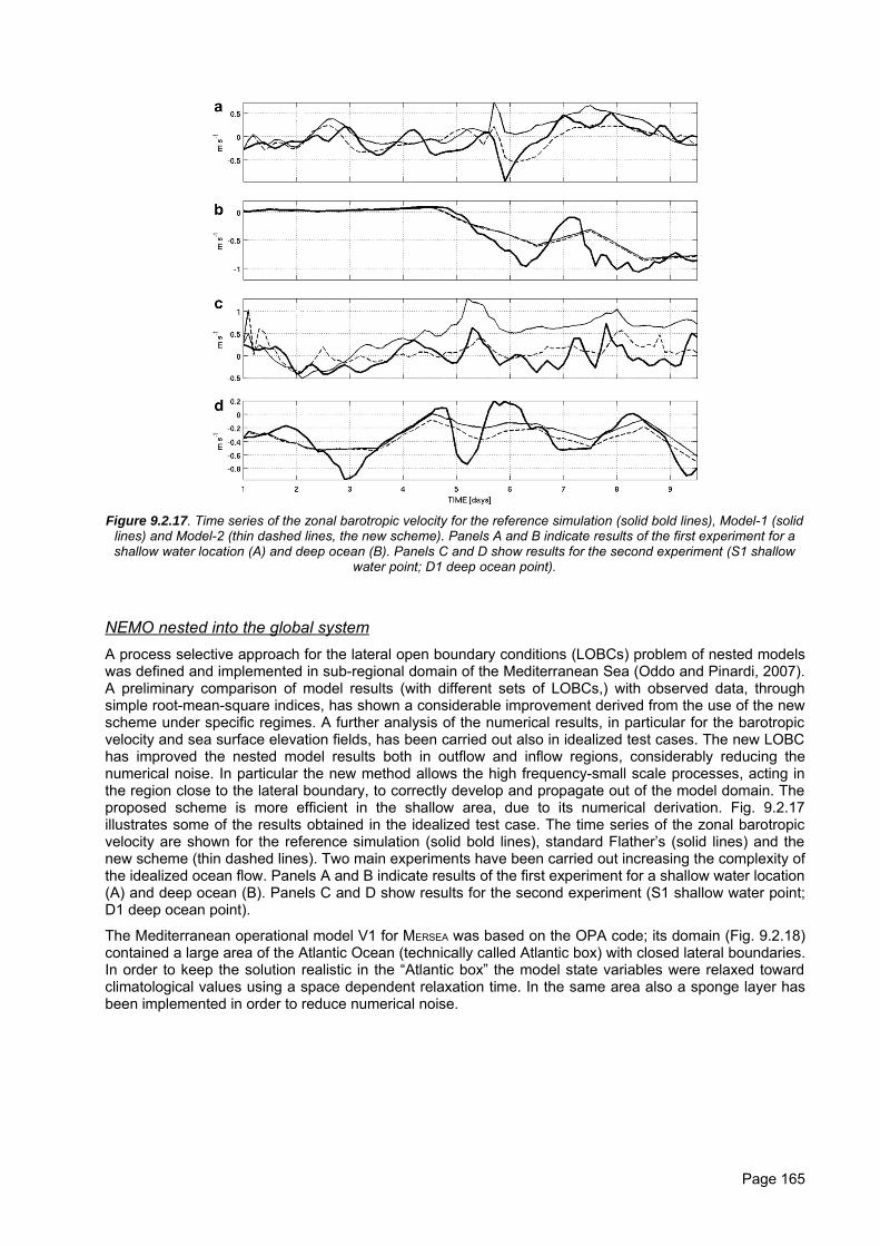
Figure 9.2.17. Time series of the zonal barotropic velocity for the reference simulation (solid bold lines), Model-1 (solidlines) and Model-2 (thin dashed lines, the new scheme). Panels A and B indicate results of the first experiment for ashallow water location (A) and deep ocean (B). Panels C and D show results for the second experiment (S1 shallow

water point; D1 deep ocean point).

NEMO nested into the global systemA process selective approach for the lateral open boundary conditions (LOBCs) problem of nested modelswas defined and implemented in sub-regional domain of the Mediterranean Sea (Oddo and Pinardi, 2007).A preliminary comparison of model results (with different sets of LOBCs,) with observed data, throughsimple root-mean-square indices, has shown a considerable improvement derived from the use of the newscheme under specific regimes. A further analysis of the numerical results, in particular for the barotropicvelocity and sea surface elevation fields, has been carried out also in idealized test cases. The new LOBChas improved the nested model results both in outflow and inflow regions, considerably reducing thenumerical noise. In particular the new method allows the high frequency-small scale processes, acting inthe region close to the lateral boundary, to correctly develop and propagate out of the model domain. Theproposed scheme is more efficient in the shallow area, due to its numerical derivation. Fig. 9.2.17illustrates some of the results obtained in the idealized test case. The time series of the zonal barotropicvelocity are shown for the reference simulation (solid bold lines), standard Flather’s (solid lines) and thenew scheme (thin dashed lines). Two main experiments have been carried out increasing the complexity ofthe idealized ocean flow. Panels A and B indicate results of the first experiment for a shallow water location(A) and deep ocean (B). Panels C and D show results for the second experiment (S1 shallow water point;D1 deep ocean point).

The Mediterranean operational model V1 for MERSEA was based on the OPA code; its domain (Fig. 9.2.18)contained a large area of the Atlantic Ocean (technically called Atlantic box) with closed lateral boundaries.In order to keep the solution realistic in the “Atlantic box” the model state variables were relaxed towardclimatological values using a space dependent relaxation time. In the same area also a sponge layer hasbeen implemented in order to reduce numerical noise.

Page 165

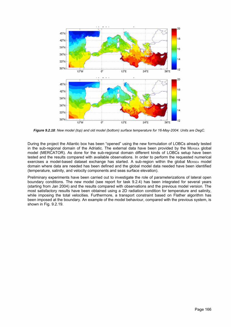
Figure 9.2.18: New model (top) and old model (bottom) surface temperature for 16-May-2004. Units are DegC.

During the project the Atlantic box has been “opened” using the new formulation of LOBCs already testedin the sub-regional domain of the Adriatic. The external data have been provided by the MERSEA globalmodel (MERCATOR). As done for the sub-regional domain different kinds of LOBCs setup have beentested and the results compared with available observations. In order to perform the requested numericalexercises a model-based dataset exchange has started. A sub-region within the global MERSEA modeldomain where data are needed has been defined and the global model data needed have been identified(temperature, salinity, and velocity components and seas surface elevation).

Preliminary experiments have been carried out to investigate the role of parameterizations of lateral openboundary conditions. The new model (see report for task 9.2.4) has been integrated for several years(starting from Jan 2004) and the results compared with observations and the previous model version. Themost satisfactory results have been obtained using a 2D radiation condition for temperature and salinity,while imposing the total velocities. Furthermore, a transport constraint based on Flather algorithm hasbeen imposed at the boundary. An example of the model behaviour, compared with the previous system, isshown in Fig. 9.2.19.

Page 166

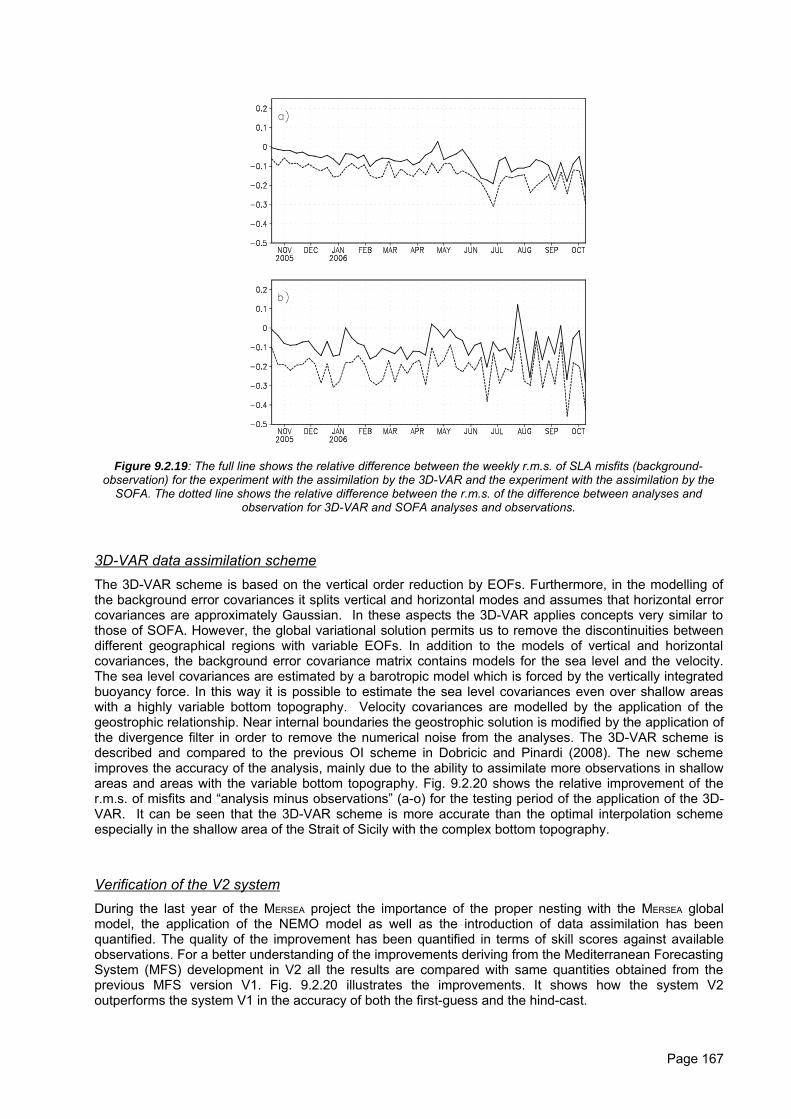
Figure 9.2.19: The full line shows the relative difference between the weekly r.m.s. of SLA misfits (background-observation) for the experiment with the assimilation by the 3D-VAR and the experiment with the assimilation by the

SOFA. The dotted line shows the relative difference between the r.m.s. of the difference between analyses andobservation for 3D-VAR and SOFA analyses and observations.

3D-VAR data assimilation schemeThe 3D-VAR scheme is based on the vertical order reduction by EOFs. Furthermore, in the modelling ofthe background error covariances it splits vertical and horizontal modes and assumes that horizontal errorcovariances are approximately Gaussian. In these aspects the 3D-VAR applies concepts very similar tothose of SOFA. However, the global variational solution permits us to remove the discontinuities betweendifferent geographical regions with variable EOFs. In addition to the models of vertical and horizontalcovariances, the background error covariance matrix contains models for the sea level and the velocity.The sea level covariances are estimated by a barotropic model which is forced by the vertically integratedbuoyancy force. In this way it is possible to estimate the sea level covariances even over shallow areaswith a highly variable bottom topography. Velocity covariances are modelled by the application of thegeostrophic relationship. Near internal boundaries the geostrophic solution is modified by the application ofthe divergence filter in order to remove the numerical noise from the analyses. The 3D-VAR scheme isdescribed and compared to the previous OI scheme in Dobricic and Pinardi (2008). The new schemeimproves the accuracy of the analysis, mainly due to the ability to assimilate more observations in shallowareas and areas with the variable bottom topography. Fig. 9.2.20 shows the relative improvement of ther.m.s. of misfits and “analysis minus observations” (a-o) for the testing period of the application of the 3D-VAR. It can be seen that the 3D-VAR scheme is more accurate than the optimal interpolation schemeespecially in the shallow area of the Strait of Sicily with the complex bottom topography.

Verification of the V2 systemDuring the last year of the MERSEA project the importance of the proper nesting with the MERSEA globalmodel, the application of the NEMO model as well as the introduction of data assimilation has beenquantified. The quality of the improvement has been quantified in terms of skill scores against availableobservations. For a better understanding of the improvements deriving from the Mediterranean ForecastingSystem (MFS) development in V2 all the results are compared with same quantities obtained from theprevious MFS version V1. Fig. 9.2.20 illustrates the improvements. It shows how the system V2outperforms the system V1 in the accuracy of both the first-guess and the hind-cast.

Page 167

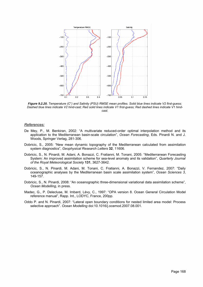
Figure 9.2.20. Temperature (C°) and Salinity (PSU) RMSE mean profiles. Solid blue lines indicate V2 first-guess;Dashed blue lines indicate V2 hind-cast; Red solid lines indicate V1 first-guess; Red dashed lines indicate V1 hind-

cast.

References:De Mey, P., M. Benkiran, 2002: “A multivariate reduced-order optimal interpolation method and its

application to the Mediterranean basin-scale circulation”, Ocean Forecasting, Eds. Pinardi N. and J.Woods, Springer Verlag, 281-306.

Dobricic, S., 2005: “New mean dynamic topography of the Mediterranean calculated from assimilationsystem diagnostics”, Geophysical Research Letters 32, 11606.

Dobricic, S., N. Pinardi, M. Adani, A. Bonazzi, C. Fratianni, M. Tonani, 2005: “Mediterranean ForecastingSystem: An improved assimilation scheme for sea-level anomaly and its validation”, Quarterly Journalof the Royal Meteorological Society 131, 3627-3642.

Dobricic, S., N. Pinardi, M. Adani, M. Tonani, C. Fratianni, A. Bonazzi, V. Fernandez, 2007: “Dailyoceanographic analyses by the Mediterranean basin scale assimilation system”, Ocean Sciences 3,149-157.

Dobricic, S., N. Pinardi, 2008: “An oceanographic three-dimensional variational data assimilation scheme”,Ocean Modelling, in press.

Madec, G., P. Delecluse, M. Imbard, Lévy, C., 1997: “OPA version 8. Ocean General Circulation Modelreference manual”, Rapp. Int., LODYC, France, 200pp.

Oddo P. and N. Pinardi, 2007: “Lateral open boundary conditions for nested limited area model: Processselective approach”. Ocean Modelling doi:10.1016/j.ocemod.2007.08.001.

Page 168

7.2.5. North-east Atlantic (Task 9.2.5)MET Office Leader

Development of the North West Shelf (NWS) system, led by the Met Office, has focused on two majorareas of development, the adaption of OPA/NEMO for the shelf-seas (task 9.1) and specificimplementations for the NWS (task 9.2.5). The routine production from the system has been achievedthrough task 9.3 and as part of this production two Target Operational Periods (TOPs) have been run andhave been used to assess the system quality.

The developments have moved the NWS capability at the Met Office significantly further forward, withsignificant advances in the development of NEMO for the shelf system, almost complete transition toNEMO in the open ocean modelling done here, and the implementation of an (and possibly the first)operational ecosystem model for the region. Proof of concept nesting with the Mercator Global system (theMERSEA global configuration) has been done in pseudo-operational mode, giving significant insights to howthis might be done operationally. Target Operational Periods and the assessments of the system throughthese periods have improved our understanding of the quality of the science in the models, and will allowtargeted investment in science upgrades to the Met Office models in the future.

The adaptation of OPA/NEMO for shelf-seasThe Mercator group has written code to apply open boundary data using the Flow Relaxation Scheme ascurrently used in operational FOAM. This code requires some extension to apply the method to the sea-icevariables. Code to apply the alternative Flather open boundary conditions has also been supplied; thismethod is best suited for use in shelf seas model configurations, and will be applied accordingly laterduring the transition.

The first phase was to produce a nested configuration of NEMO-AMM, whereby the horizontal domain sizewas reduced slightly and open boundary conditions of SSH and depth-mean velocities provided fromPOLCOMS-AMM. This provided a test of the Flather open boundary condition, implemented in the BDYmodule of NEMO, and allowed for debugging of the Flather code. It also provided an initial comparison of atides-only simulation in POLCOMS and NEMO.

The BDY module was then harmonised with the re-activated s-coordinate code in NEMO. The nestedconfiguration for tides-only simulations was set up with uniform σ-levels. This is different from POLCOMSwhich uses the Song and Haidvogel (1994) stretching function for water depths of over 150m, and workhas started to investigate the impacts of the differences in the S-coordinate systems between the models.

POLCOMS uses a law-of-the-wall formula to deal with situations where the vertical grid partially resolvesthe bottom boundary layer. This was coded in NEMO, and some tuning ofhorizontal and vertical diffusionperformed. Tidal harmonics forcing was implemented in NEMO as an extension to the BDY module,following the implementation in POLCOMS.

Initial comparisons of short tides-only runs with POLCOMS-AMM and NEMO-AMM revealed largediscrepancies in tidal amplitudes and phase. These issues were resolved through the fixing of a number ofbugs, and through improved specification of the bathymetry.

Subsequently the nonlinear free surface code has been updated to work with the s-coordinates option andtested in the AMM configuration. The tidal potential force has been implemented in NEMO. Runs with thetidal potential, the nonlinear free surface and the Flather boundary condition and tuned bathymetry resultedin comparisons against tide gauge data in NEMO of similar quality to the results obtained from POLCOMS.Also, the General Ocean Turbulence model (GOTM) has been implemented to allow a greater range ofturbulence schemes suitable for use in coastal regions. Tide-only simulations were undertaken with thestandard NEMO TKE scheme as well as a k-ε option available through GOTM. The choice of scheme didnot show any significant impact upon the tide-only results, but are expected to have a greater impact uponfull baroclinic simulations.

Subsequent to the testing in tide-only mode, the NEMO model has been modified to include surfacepressure forcing. This has been tested in a simulation of an unusually large storm surge that affected theeast coast of the UK, with good results.

Given the success in running the model in tide-only and tide plus surface momentum and pressure fluxes,the focus has shifted to developing the model for full baroclinic running. The surface fluxes of heat and

Page 169

freshwater have been implemented to accept Met Office NWP fluxes. Present river schemes in NEMO arenot suitable for coastal applications, and progress is being made to update the schemes to allow a betterrepresentation of rivers in high resolution applications.

Testing of the horizontal pressure gradient schemes needed for running in S/σ-coordinates has beenundertaken with an implicit free surface as these schemes had not been coded to work with the variablevolume code. Early results show that with some judicious tuning of the bathymetry the NEMO HPGschemes give errors of the same order as the POLCOMS system. Further work is required to test theseschemes in realistic scenarios, but it is considered that these schemes should be adequate for North-WestShelf applications.

Significant effort is still required to get NEMO into a position where it can replace POLCOMS as anoperational model for the North-West shelf. Tasks left to complete include;

• Adding extra river functionality• Test available vertical coordinates, and add POLCOMS like hybrid S-coordinate functionality if

necessary.• Testing lateral boundary code for tracers• Testing surface fluxes of heat and freshwater• Testing of the horizontal advection schemes, and potentially adding extra schemes such as the PPM

scheme used in POLCOMS if required• Coupling of NEMO to the ERSEM ecosystem model• Optimisation of the NEMO code to allow running within the Met Office operational framework

The implementation of NEMO at the Met Office and for the North-West Shelf

Developing the Infrastructure

Work on transition of ocean modelling activities undertaken at the Met Office to use the NEMO oceanmodelling framework commenced in April 2004. The first year of the transition work for the FOAM systemfocused on development of the underpinning components from which the FOAM system is built. Softwaredevelopments have been required in a number of areas in order to provide the functionality that exists forthe unified model (UM) version of FOAM.

Code management

A code management system is an essential tool to enable effective working when the NEMO code is beingactively developed by a team working simultaneously. A code management system has been selected forimplementation across all Met Office software systems, and the opportunity was taken to adopt this systemfor NEMO during the initial installation of the NEMO code. This system, the Flexible ConfigurationManagement (FCM) system, is based around widely used public domain software, and allows a largenumber of developers to work in parallel with powerful tools for merging and tracking paralleldevelopments. An additional advantage of the FCM system is the provision of a build environment thatallows code to be modified and the executable rebuilt through issuing a small number of simplecommands; this provides a significant simplification over the original NEMO system.

The FCM system has been implemented fully for both NEMO and for the standalone version of the FOAMdata assimilation scheme that interfaces to NEMO. Developments are being tracked through the FCM’sweb based system. Guidelines have been issued to developers setting out coding and review standards foruse in conjunction with the FCM tools. These guidelines have also proposed a mechanism through whichthe Met Office version of the code will be kept in line with the central code repository held in Paris. Theseguidelines are aimed at ensuring that developments added to the central repository are exploited as rapidlyas possible whilst avoiding generating large amounts of additional work. The FCM system provides a toolto aid the management of this process, and it is anticipated FCM will be taken on by the central NEMOteam in the future.

Setting up of model configurations

A key requirement for the implementation of NEMO for the Met Office is the ability to be able to set up newconfigurations. This process is complicated by the requirement to set up the tri-polar grids used by the

Page 170

NEMO global configurations. The NEMO Systems Team in Paris provided some tools to do this, but thesewere ad hoc tools that were not considered sufficiently flexible or user-friendly. In consequence, effort hasbeen devoted to refining these tools, and in developing tools for generation of limited area configurationswith rotated latitude-longitude coordinates. The modified tools have been applied to set up a number ofregional configurations of NEMO, including those used within MERSEA.

Additional code has been developed to allow the generation of re-start files for the models from spun-upfields, thereby avoiding the need to run lengthy spin-ups of NEMO configurations. Generation of NEMO re-start files from the equivalent UM model configurations ensures that an accurate comparison can be madebetween the two systems in a spun-up state. New model configurations require interpolation of surfaceforcing fields to the model grid. Ancillary tools provide various options for interpolation of fields.

Ancillary tool

The surface fluxes provided to FOAM from the Met Office NWP system differ from those that are expectedby NEMO. In most cases the required fluxes can be derived from those available to FOAM; in a few casessome assumptions are required to derive the required fields. Code has been developed to do the requiredprocessing to deliver the fluxes expected by NEMO.

Many of the processes required to set up and run NEMO configurations require interpolation betweengrids, often including the use of complicated coordinate systems. A general, easy-to-use interpolation toolis therefore a key component of the system. A tool of this nature has been developed based upon use ofthe SCRIP interpolation package, developed by Los Alamos, USA. Pre-computing of interpolationcoefficients for particular grids subsequently provides very efficient interpolation.

Data formats are a key issue for effective use of NEMO: many existing software tools are designed for usewith the Met Office’s internal “PP” format, whilst NEMO makes use of the netCDF format for all inputs andoutputs. In the longer term it would be desirable to convert all software tools to use netCDF files directly.However, this is not practical in the short term, so a tool for the conversion between the two formats hasbeen developed. This tool has been designed to allow flexibility, and can be configured to produce netCDFfiles that conform to the widely-used “CF” convention to ensure interoperability with external software.

Developing the science

Data Assimilation

The data assimilation code currently used by FOAM was developed to run as an independent applicationduring the first phase of the transition project. During the second phase of the project this code has beendeveloped to improve its modularity in order to improve maintainability. The code has also been importedinto the FCM system in order to ensure effective management of the code. Code has been implemented inNEMO to allow the application of data assimilation increments to the model fields.

As part of the on going development of the data assimilation, improvements to the OI scheme used in theFOAM-UM system have been included in FOAM-NEMO. An OI based assimilation method has beenimplemented to constrain the ice thickness in the NEMO system, when previously a simple nudgingmethod was used in the UM. The data assimilation has been improved through the use of an observationoperator which collocates the observations and model in space and time (First Guess at Appropriate time,FGAT) prior to the assimilation. The system has also been upgraded to use GHRSST data for surfacetemperature assimilation.

Physics

The move to the use of the NEMO code from the FOAM system has resulted in a number of importantimprovements to the physics:

• The vertical mixing is now calculated using a TKE scheme whereas previously a Richardson numberbased calculation was performed.

• The inclusion of partial steps is an improvement on the z-levels previously used• There is an enstrophy and energy conserving new momentum advection scheme• Tracer advection is done using a TVD1 scheme, an improvement on the UM’s QUICK scheme.

1 Total Variation Diminishing

Page 171

Ecosystems

A critical advance that has taken place during the project, has been the development and implementationof an ecosystem model for the North-West European continental shelf. This model, based upon theEuropean funded ERSEM code and further developed at Plymouth Marine Laboratory was coupled to thePOLCOMS MERSEA V1 system. There was a significant amount of effort required to get an essentially R&Decosystem tool to perform in an operational environment, and the major achievements through MERSEA

have been the operationalization of the ecosystem science. The outcome of this has been a successfullyfunctioning ecosystem model providing daily feeds of ecosystem variables to the UK’s EnvironmentAgency who are using it to assess the likelihood of blooms incident on beaches around the South-Westcoast of the UK to fulfil their obligations to the Bathing Water Directive.

Developing the configurations

Through MERSEA significant advances have been made in the NWS both in the test configurations availableand the operational configurations implemented. Prior to MERSEA the Met Office system comprised theoperational Forecasting Ocean Assimilation Model (FOAM) system, and forecasts for the shelf seas usingthe Atlantic Margin Model (AMM), a ~12km configuration of POLCOMS covering the North-West Europeancontinental shelf from 40oN to 65oN and 20oW to 13oE. FOAM 1/9o N Atlantic, ocean and sea-ice model:nested inside Atlantic model ; assimilation of surface height, temperature and salinity profile data and sea-ice concentration fields using modified analysis correction scheme. POLCOMS system for NE Atlantic shelfusing 12 km grid and no assimilation. Both were being run daily in the operational system.

Developments to the systems were made to create the V1 system which went operational in February2005. This comprised (a) the 1/9º North Atlantic FOAM configuration as with V0 and (b) the POLCOMSMedium Resolution Continental Shelf (MRCS) model on a ~7km grid, nested into the 1/9º FOAMconfiguration via the Atlantic Margin POLCOMS configuration. The system ran daily in the Met Officeoperational suite. The MRCS model presented a significant step forward as it allowed a higher horizontalresolution representation of processes on the North-West Shelf.

The V2 system was subsequently developed which included an pseudo-operational shelf model running inthe NEMO framework. This had been planned to include an explicit free surface, but developments of theNEMO system for tidal waters have been taking significantly longer than expected. The V2 system alsoincluded the POLCOMS MRCS-ERSEM coupled ecosystem model running within the full operational suiteproviding products on a daily basis. This went operational in March 2007.

Given the need to develop towards the configurations required for MyOcean the V3 of the NWS lookssomewhat different from originally planned. The decision has been made to fully implement the NEMOFOAM configurations to ensure that the full range of Met Office models are running with NEMO as soon aspossible. The V3 system therefore includes the ORCA025 NEMO FOAM presently running operationally(although still in test mode), a North Atlantic 1/12o rotated grid NEMO configuration running in pre-operational trials, due to enter operational running in Oct 2008, and the POLCOMS MRCS-ERSEM. TheNEMO configurations not only have higher horizontal resolution than their UM predecessors, but have 50levels rather than 20 in the vertical. In parallel to the POLCOMS MRCS-ERSEM there is a NEMO AMMconfiguration being run in test mode in which developments are being made to allow this to replace thePOLCOMS system at the earliest possible opportunity.

Page 172

NWS ProductionThe production of the V1 and V2 systems has been assessed using two Target Operational Periods (TOP1and TOP2). Work done within the MERSEA Strand 1 project to define 4 classes of metrics was carried overinto the MERSEA IP and used to intercompare the models. Metrics and outputs from Met Office models havebeen implemented as defined by the TOP criteria. These are being output routinely from all Met OfficeMERSEA systems based on NEMO, and a number of the UM based systems. During the TOP1 period onlythe class 1 – 3 metrics were compared.

For the NWS the validation is focused on the North Atlantic eddy permitting system (FOAM 1/9°), fromMarch to September 2006. The water mass description was consistent with the climatology at the seasonalscale. Dedicated analysis along sections show the consistent distribution of the key-water masses at depthand no model drift was identified at depth. At synoptic scales, some problems, observed in the mixed layerdynamics were corrected in September 2006, allowing an improved forecast of the mixed layer depth.Improvements were clearly evident over the MERSEA Strand 1 assessment of the same model.

The Met Office V2 systems North-East Atlantic 1/16o NEMO system is nested to both the Met Office 1/9o

North Atlantic system and the Mercator global. The nesting was tested during the TOP2 period. Someissues came to light during the TOP2 period with the global fields, but in general the nesting was shown tobe a success with generally consistent results as shown by the analysis done within the TOP2 report.

Data Delivery

Data is being delivered through the MERSEA series of data delivery mechanisms on a pre-operational basis.The outputs from the V2 system are available on the ESSC thredds server. These include POLCOMS-MRCS outputs of temperature, salinity and currents. FOAM 1/9o NE Atlantic fields (including analysis andforecasts out to 5 days) and metrics (transports and moorings) are also being delivered.

The Met Office NWS models are also fully searchable through the MERSEA Information System and theDiscovery/Download/Viewing services. ESSC at Reading also supply visualisation of the NWS data on theGodiva2 service found.

7.3. Routine Production of Outputs by core systems (Task 9.3)

MET Office Leader

The objectives of this task have broadened as the demands on WP9 from other WPs and down-streamusers have become more apparent. The objectives thus include:

1. routine generation of near real-time forecasts, making them available on the TEP web-portals inliaison with WP6

2. provision of near real-time boundary data to other TEPs or down-stream users

3. provision of specific products (e.g. 10-year re-analyses) for WP11, WP12, WP13 anddownstream users

4. scientific assessments including inter-comparisons of the forecasts in liaison with WP5

5. assessments of the technical performance (e.g. reliability) of the forecast systems in liaison withWP5

6. definition and implementation of two 6-month Targetted Operational Period (TOP) assessmentsin liaison with WP5 and other WPs.

We take the opportunity in this section of the report to reflect on some of the successes and lessons learntfrom the co-ordination of this work-package which will be relevant to the further development of the MarineCore Service for GMES.

Page 173

Progress in System Developments against Proposal Plan

The project workplan included a table describing the expected content of the forecasting systems for thefive regions for each of the four versions of the system (versions v.0 to v.3 available from months 3, 18, 36and 48 respectively).

This plan was successful in that it gave the work-package a sense of unity, drive and direction and verygood progress has been made in most systems (e.g. the global, Mediterranean and north-east Atlantic).But the plan for all the systems other than the Mediterranean (which was very conservative) was over-ambitious. The transition of the north-east Atlantic system to use NEMO has taken more than 4 yearsrather than 3. Progress in development of the assimilation of profile data in the Arctic system andassimilation of data other than SST in the Baltic have been more difficult than expected. Implementationsof the global system have generally been slightly behind the original schedule and computationalresources for routine operation of the 1/12o global model are not expected to be found for another 2-3years.

This over ambitious planning was exacerbated by several factors. The plans in the original project proposalfor the forecasting centres did not anticipate all the demands on them from other aspects of the project.The loss of key personnel involved in some of the systems (e.g. Christian le Provost, Geir Evensen, MikeBell, Entcho Demirov) was also not anticipated or factored into the planning. During the project, the teamswere over-optimistic about making up time when behind. The nature of the contract did not encouragerealistic updating of the project plans since significant departures from the contract would be difficult tonegotiate.

The project plans included no adequate mechanisms for the control (change management) of newversions of the system. Version V2 of the system included several major upgrades and the introduction ofinter-dependencies arising from the nesting of some systems inside the global system. The initial deliveryof several components was slightly delayed and due to the pressures on delivery its elements were notfully pre-validated. The global V2 system was late and had some initial problems which caused difficultiesfor the systems which were trying to use it for boundary conditions. A much stricter system of control anduser testing of new datasets prior to implementation would be required in a truly operational service andwould need to be introduced as part of any Marine Core Service.

Coordination and Reporting of work within the work-package

Annual summaries were compiled of the progress and problems encountered in the development of eachof the five forecasting systems. Shortly after the introduction of each of the four system versions, a concisesummary of each of the five systems was produced with the description of each of the systems followingthe same format. These reports constitute a useful record and provided good value for the cost ofgeneration.

Meetings dedicated to coordination of work within the work-package were initially held once a year butwere held twice a year in the last two years of the project in response to the evident need for improvedcoordination. These meetings enabled information exchange on scientific progress and problems, theidentification and management of risks and detailed technical discussions on: coordination of thecalculation of metrics (see below); planning for the nesting of models; coordination of the TOP activities.Although time consuming these meetings were valuable and essential to the development of a distributedbut coordinated production system.

Identification and Management of Risks and Interdependencies

With the encouragement of the project evaluators a risk log was initiated at the project kick-off meeting anda good list of risks and issues identified including the points that:

• the standards for delivery of data (e.g. timeliness) may be inappropriate for important users• areal responsibilities for the forecast centres may not be agreed• it may be difficult to agree a data policy on the use of products• a suitable computer for the 1/12o global model may not be found• the implementation of the Arctic system at met.No may be problematic

Page 174

• the transition to NEMO at the Met Office might be slower than planned• many technical and scientific issues could make operational nesting of models using data from a

different centre very problematic.Progress with risks has generally been best on ones which are specific to and can be resolved by a singlecentre. Most of the other risks were eventually referred to the Executive Committee which had littlesuccess in resolving them. Better mechanisms for escalating and resolving risks will need to be found forany distributed Marine Core Service.

It was also recognised in the first year of the MERSEA project that there were a lot of interdependenciesbetween work-packages which needed to be analysed and managed. In particular:

• the needs of the forecasting centres for existing and new products from the observation processingcentres (WP2) and other forecasting centres (e.g. boundary data)

• support required by the forecasting centres from the information system• the work and products expected from the forecasting centres by the special focus experiments

(WP11), the application teams (WP12), the system design and assessment teams (WP5) and theinformation system teams (WP6).

This process was useful in that it revealed some inconsistencies in the proposal, most of which had beenintroduced when the project was cut during the negotiations period. This enabled the demands for longperiod re-analyses from WP11 to be identified and eventually satisfied (using resources outside theproject). Nonetheless it was again easier to identify issues than to resolve them. The forecasting centreswere slow both to specify their requirements for observation products and to take up new ones. A MarineCore Service will need to be more successful in defining internal Operating Level Agreements (OLAs)between production centres.

Validation Activities

One of the main successes of the earlier MERSEA Strand-1 project had been the intercomparison of modeloutputs in which data from several forecasting centres were made readily accessible in common formatsfor post-processing. The resulting plots revealed valuable information on problems with the systemsdespite the lack of a strictly controlled environment. These inter-comparisons both accelerated theimprovement of the systems and laid the foundation for international standards for the description andquality proofing of ocean forecasting.

Within this project after considerable discussion a methodology was agreed to routinely generate dailydatasets of co-located observation and model values from many centres. These datasets were used togenerate strictly comparable statistics (such as biases, root mean square errors and correlationcoefficients) describing the accuracy and characteristics of the model analyses and forecasts. Usefulfigures giving a good picture of geographical variations in the accuracy and performance of the varioussystems were and will continue to be generated. These techniques are now being used in an ObservingSystem Experiment organised by the Global Ocean Data Assimilation Experiment (GODAE). They shouldhelp to provide greater robustness and confidence in the evaluation of the impact of various observationtypes on ocean analyses and forecasts and the effectiveness of the assimilation systems in using each ofthe observation types.

A significant effort was made by the project coordinator, the System Design team (WP5) and WP9 todefine the objectives and expected outcomes from the two Targetted Operational Periods. Rather lengthyand detailed assessment reports were compiled for both periods. The report on the first period allowedteams to generate independent assessments. The second report has a greater level of consistency in theinformation presented, includes improved, delayed-mode, hindcasts from some systems, and containssome of the statistics on observation minus model differences described in the previous paragraph. Theseassessment reports were time consuming to produce, suffered from a lack of resources and divertedresources from other tasks.

Page 175

Nesting between Models

A large number of technical (e.g. scheduling) and scientific issues (e.g. consistency between the meandynamic topographies) which could afflict the routine nesting of a model forecast in a model run at adifferent centre were identified well in advance of version v.2 but relatively few were studied in the 18months leading up to its implementation. These difficulties were exacerbated by the number, lateness andlack of validation of changes to the systems that were made at version v.2. Some interesting indicationswere nonetheless obtained on the lack of impact of realistic boundary data on the deep ocean (away fromcoastal boundaries) in regions where Argo and altimeter data are available for assimilation.

Summary

A lot of progress was made in the development of the five core forecasting systems during the MERSEA

project. Future Marine Core Service projects should bear in mind that

• the MERSEA plans for forecast system development were slightly over-optimistic and the project plansdid not include several activities (e.g. TOP assessments) that were later judged to be high priorityand which required significant work from the forecast centre teams

• the failure to adjust the targets for system developments put the forecast centre teams underpressure and some of the system upgrades suffered more than they would have done if the situationhad been better managed

• the coordination meetings and reports on progress and content of system versions were valuableand good uses of resources

• the risks and interdependencies involved in the project were raised but most issues involving morethan one country were not resolved

• a protocol for generating comparable statistics on the differences between observations and modelsfrom several centres has been established

7.3.1. Routine provision of near real-time forecasts on the Global MFCThe global Monitoring and Forecasting Centre (MFC) has continuously provided ocean products. Theproducts are NetCDF files covering sub domains of the global ocean, with different resolution dependingon the domain as shown here:

1- global product, 2° horizontal resolution

2- Atlantic (North and South at 1/6° and Tropical and equatorial at ¼°)

3- Pacific (North and South at 1/6° and Tropical and equatorial at ¼°)

4- Indian at 1/6°

5- Arctic on stereographic grid (~1/8°)

6- Antarctic circumpolar on regular grid, 1/4°

7- Mediterranean at 1/8°

They are all on standards levels (43 levels), containing T, S, U, V 3D fields plus additional 2D fieldsincluding sea surface elevation. They are interpolated on a standard horizontal and vertical grid from thenative grid files.

The product files are delivered once a week for a 2-week hindcast period (from T-14 to T, where T iscurrent date) and a 2-week forecast period (from T to T+14) as daily mean.

Page 176

7.3.2. Provision of near real-time boundary dataThe Global MFC has implemented real-time extraction of data in boundary regions. The data are on thenative grid, on rectangular domains surrounding specified boundary boxes. The specification of the boxesis provided by the regional MFCs (Arctic Ocean, Atlantic and North West Shelves ans Mediterranean Sea).

The files delivered contain:

• 3D physical fields (T, S, U, V, W)• 2D ocean fields (SSH)• 2D forcing fields (Net fresh water flux, Net heat flux, Net solar heat flux, Net fresh water flux, Net

momentum flux)And for the northern domains:

• 2D ice variables (concentration, surface temperature, thickness, velocity, Snow thickness)• 2D forcing fields (Net Fresh water flux at the base of sea ice, Net heat flux at the base of sea ice)

Native grid definition files and MSSH files were also provided.

7.3.3. Provision of specific products for WP11, WP12, WP13 and downstream userMercator-Ocean is involved in WP11-SF2 as a provider of ocean general circulation model (OGCM)configurations and ocean initial conditions (ICs) for coupled ocean-atmosphere seasonal forecasts to theother partners (ECMWF, METEO-FRANCE and INGV).

During the Final period, Mercator-Ocean provided the ORCA025-NEMO OGCM configuration (ocean codeand configurations files) to the partners and helped them to install the model on their respective super-computers (Task 11.3). Following a meeting held in June 2006 at Mercator-Ocean with the three partners,it was also decided to re-do a 10-year control integration of ORCA25 model with an enhancedparameterisation of the air sea fluxes. This model integration has been performed and is available for thepartners.

The second contribution of Mercator-Ocean to WP11 was the delivery of MERSEA-1/4°v2 ocean analyses(ICs) for coupled ocean-atmosphere medium range predictions (Task 11.6). Weekly ocean analyses (from17 January 2007 until present) are available for ECMWF to carry out the sensitivity study to the ocean ICsin high resolution coupled models. A report has been written reporting on the quality of the SST in MERSEA -1/4°v2 (Deliverable D11.6.2). This assessment gives a first idea of the prediction skill one could expectfrom the coupled medium range forecasts.

7.4. References

Barnier, B., et al. (2006): “Impact of partial steps and momemtum advection schemes in a global oceancirculation model at eddy permitting resolution”, Ocean Dynamics, DOI: 10.1007/s10236-006-0082-1.

Benkiran, M. (2004): “Multivariate and multidata assimilation in Mercator”, The Mercator Ocean quaterlyletter, 13, 1-12.

Benkiran, M., and E. Greiner (2008): “Impact of the incremental analysis updates on a real time system ofthe north Atlantic Ocean”, Journal of Atmospheric and Oceanic Technology, In press.

Bourdalle-Badie, R., et al. (2004) : « Saut qualitatif dans le modele Atlantique Nord et Méditerranée hauterésolution (PSY2V1) », La lettre trimestriel Mercator Océan, 12, 14-20.

Chanut, J. (2006): “Nesting code for NEMO”, MERSEA report ref: MERSEA-WP09-MERCA-TASK-9.1.1.

Drevillon, M., et al. (2008): “The Godae/Mercator-OCean global ocean forecasting system: results,application and prospects”, Journal of Operational Oceanography, 1, 51-57.

Drevillon, M., et al. (2007): “The new 1/4° Mercator Ocean global multivaiate analysis ans forecastingsystem: Tropical oceans outlook”, Mercator Ocean Quaterly Newsletter, 26, 9-18.

Page 177

Drillet, Y., et al. (2005): “The MEDDIES in the Mercator North Atlantic and Mediterranean Sea eddy-resolving model”, Journal of Geophysical Research, 110.

Drillet, Y., et al. (2008): “Ocean global 1/12° operational system: Demonstration phase in the MERSEA

context”, edited, p. MERSEA final meeting, Paris.

El Moussaoui, A., et al. (2008): “Towards Real-Time Integration of Biogeochemistry and MarineEcosystems in MERCATOR-OCEAN System”, edited, p. MERSEA final meeting, Paris.

Engedahl, H. (1995): “Use of the flow relaxation scheme in a three-dimensional baroclinic ocean modelwith realistic topography”, Tellus, 47A, 365-382.

Fichefet, T., and P. Gaspar (1988): “A model study of upper ocean-sea ice interactions”, J. Phys.Oceanogr., 18, 181-195.

Flather, R. A. (1976): “A tidal model of the North-west European continental shelf”, Mem. Soc. R. Sci.Liège, 6(10), 141-164.

Garric, G., et al. (2008): “Preliminary assesment of sea ice in the global 1/4° Mercator Ocean forecastingsystem”, Mercator Ocean Quaterly Newsletter, 28.

Greiner, E., et al. (2006): “The Mercator 1992-2002 PSY1V2 reanalysis for tropical and North Atlantic”,paper presented at OSTST, Venise, Italy.

Lellouche, J. M., et al. (2008a): “The MERSEA V2 Mercator Ocean Global 1/4°and Atlantic 1/12° systems:using NEMO and multivariate data assimilation”, in MERSEA final meeting, edited, p. MERSEA FinalMeeting, Paris.

Lellouche, J. M., et al. (2008b): “The high resolution real time Mercator forecasting system: Description andevaluation in the Gulf of Mexico”, Journal of Marine Systems, submitted.

Lellouche, J. M., et al. (2005) : « PSY2V2, le nouveau prototype opérationnel haute résolution deMercator », La lettre trimestrielle Mercator Océan, 19, 4-17.

Madec, G. (2008) : « NEMO reference manual, ocean dynamics component », Note du Pôle demodélisation, IPSL, France, 27, 1288-1619.

Monfray, P. (2005): “Bionuts: towards the integration of biological models into Mercator”, ProjectionMercator, 5, 8.

Rio, M.-H., and F. Hernandez (2003): “A Mean Dynamic Topography computed over the world ocean fromaltimetry, in-situ measurements and a geoid model”, in Journal of Geophysical Research, edited.

Page 178

8. Downscaling to Regional Systems (Work Package 10)

Introduction

The role of WP10 in the MERSEA project has been to secure a proper use of the established global capacityfor ocean forecasting to improve the quality of the forecasting capability of the regional seas of Europe,since the regional - and coastal seas are economically the most important parts of the world ocean and it isto these parts of the ocean that the majority of international agreements and conventions are addressed.The conventions do in particular call for safety at sea, effective management of marine environment andsustainable utilisation of its resources. Living up to the spirit of these agreements requires the ability todetect rapidly changes in the status of the marine systems and living resources and to provide forecasts ofsuch changes so actions can be taken in a timely manner for the public good.

An immediate challenge in regional forecasting models stems from the boundaries towards the openocean. Traditionally most operational 3D-ocean regional models use climatology lateral boundaryconditions in temperature and salinity, plus a water level consisting of tides and surges. MERSEA WP 10therefore focused on increasing the performance and quality of regional and coastal operationaloceanographic services by downscaling the global fields to regional scale.

Assimilation of observational data – remotely sensed as well as in-situ data – is another factor thatpotentially can improve the quality of ocean forecasts in the regional seas of Europe. Over the past decadethe availability of real time observational data in the regional seas has increased, although more areneeded, which has formed the basis for working intensively with developing and implementing dataassimilation techniques for the regional forecasting models with in MERSEA WP10.

The achievements obtained within MERSEA WP10 form an excellent platform for the work that is now carriedout within the EU funded project ECOOP, which focuses on the European regional and coastal seas.

The specific objectives for WP 10 were:

• Secure that benefits of a global operational oceanographic system are properly utilised in forecastingactivities in European regional seas.

• Assess the value of dynamic boundary data for regional forecasts• Implement data assimilation methodologies for regional seas and test their impact• Verify improved quality of high resolution operational oceanographic products for regional seas

A specific task addressed each of those objectives, which were carried out in very close cooperation withWP 9 (Implementation and Production).

8.1. Collect relevant local data sets (Task 10.1)

DMI Leader, with NERSC, HCMR, ENEA, DFO

The regional systems of MERSEA require observational data assimilation and validation. The following givesa summary description of available data suitable for regional data-assimilation and validation. Theconsidered coastal regions and responsible MERSEA WP10 partners are a) for the Arctic Ocean the NansenEnvironmental and Remote Sensing Center (NERSC); b) for the Baltic Sea the Danish MeteorologicalInstitute (DMI); c) for the Mediterranean Sea Istituto Nazionale di Geofisica e Vulcanologia.

8.1.1. The Arctic OceanIn the Arctic Ocean sea-ice concentration maps and sea-ice drift maps (Figure 10.1.1) are produced byNERSC on a daily to weekly basis with spatial resolutions of 25 km and 35 km, respectively. These dataare used in their ocean model data-assimilation system. Sea level anomaly products (Ssalto/Duacs) fromsatellites are used up to the ice edge. These data are given with a spatial resolution of 0.3° on a Mercator

Page 179

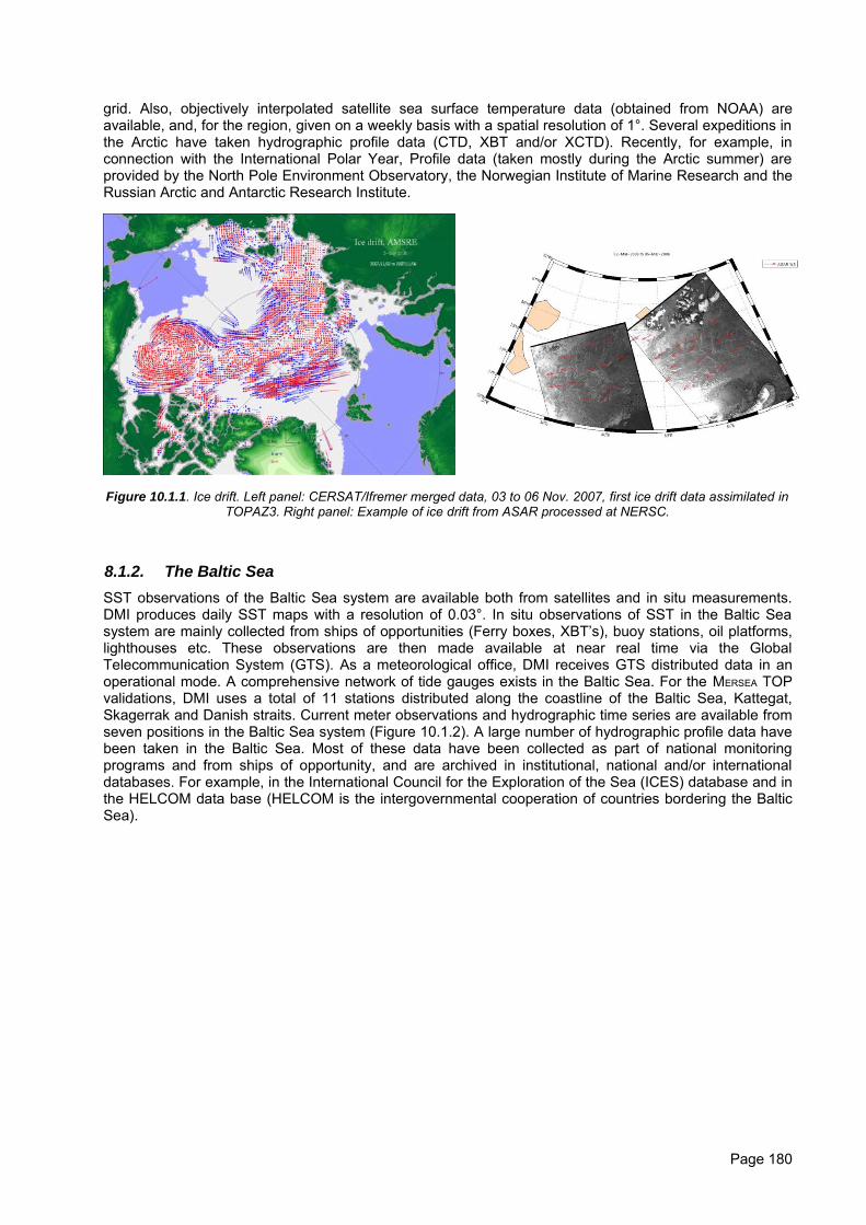
grid. Also, objectively interpolated satellite sea surface temperature data (obtained from NOAA) areavailable, and, for the region, given on a weekly basis with a spatial resolution of 1°. Several expeditions inthe Arctic have taken hydrographic profile data (CTD, XBT and/or XCTD). Recently, for example, inconnection with the International Polar Year, Profile data (taken mostly during the Arctic summer) areprovided by the North Pole Environment Observatory, the Norwegian Institute of Marine Research and theRussian Arctic and Antarctic Research Institute.

Figure 10.1.1. Ice drift. Left panel: CERSAT/Ifremer merged data, 03 to 06 Nov. 2007, first ice drift data assimilated inTOPAZ3. Right panel: Example of ice drift from ASAR processed at NERSC.

8.1.2. The Baltic SeaSST observations of the Baltic Sea system are available both from satellites and in situ measurements.DMI produces daily SST maps with a resolution of 0.03°. In situ observations of SST in the Baltic Seasystem are mainly collected from ships of opportunities (Ferry boxes, XBT’s), buoy stations, oil platforms,lighthouses etc. These observations are then made available at near real time via the GlobalTelecommunication System (GTS). As a meteorological office, DMI receives GTS distributed data in anoperational mode. A comprehensive network of tide gauges exists in the Baltic Sea. For the MERSEA TOPvalidations, DMI uses a total of 11 stations distributed along the coastline of the Baltic Sea, Kattegat,Skagerrak and Danish straits. Current meter observations and hydrographic time series are available fromseven positions in the Baltic Sea system (Figure 10.1.2). A large number of hydrographic profile data havebeen taken in the Baltic Sea. Most of these data have been collected as part of national monitoringprograms and from ships of opportunity, and are archived in institutional, national and/or internationaldatabases. For example, in the International Council for the Exploration of the Sea (ICES) database and inthe HELCOM data base (HELCOM is the intergovernmental cooperation of countries bordering the BalticSea).

Page 180

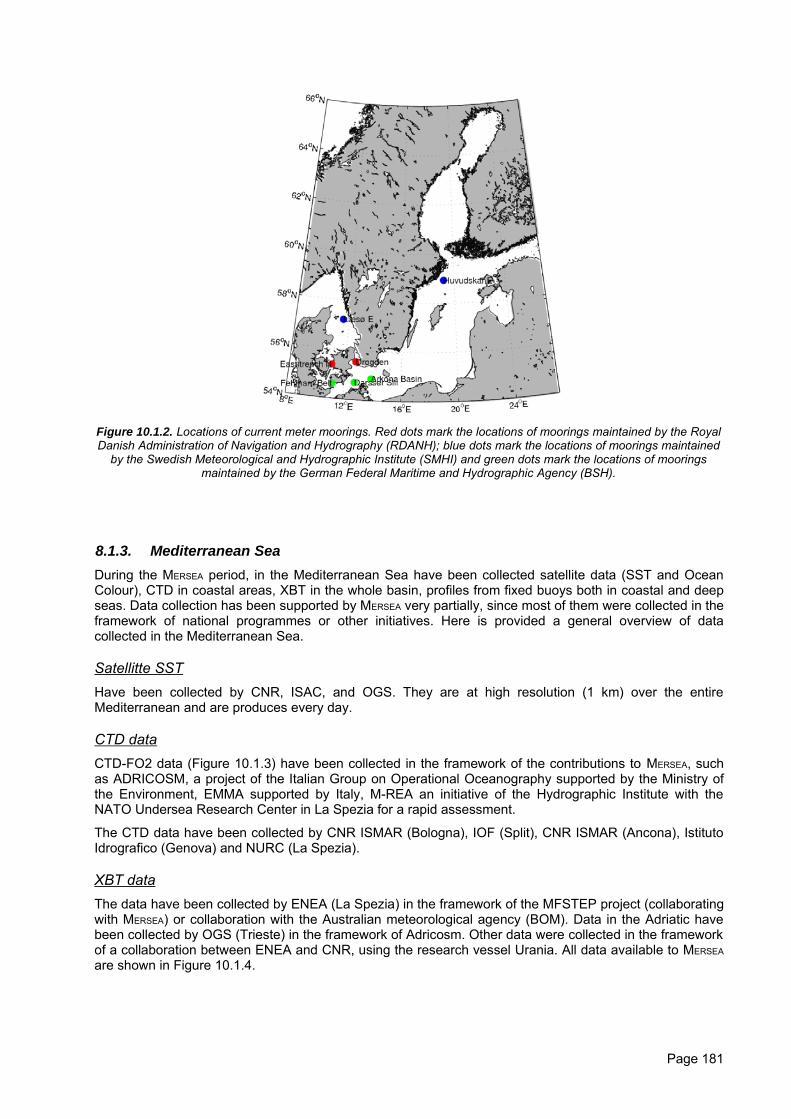
Figure 10.1.2. Locations of current meter moorings. Red dots mark the locations of moorings maintained by the RoyalDanish Administration of Navigation and Hydrography (RDANH); blue dots mark the locations of moorings maintained

by the Swedish Meteorological and Hydrographic Institute (SMHI) and green dots mark the locations of mooringsmaintained by the German Federal Maritime and Hydrographic Agency (BSH).

8.1.3. Mediterranean SeaDuring the MERSEA period, in the Mediterranean Sea have been collected satellite data (SST and OceanColour), CTD in coastal areas, XBT in the whole basin, profiles from fixed buoys both in coastal and deepseas. Data collection has been supported by MERSEA very partially, since most of them were collected in theframework of national programmes or other initiatives. Here is provided a general overview of datacollected in the Mediterranean Sea.

Satellitte SSTHave been collected by CNR, ISAC, and OGS. They are at high resolution (1 km) over the entireMediterranean and are produces every day.

CTD dataCTD-FO2 data (Figure 10.1.3) have been collected in the framework of the contributions to MERSEA, suchas ADRICOSM, a project of the Italian Group on Operational Oceanography supported by the Ministry ofthe Environment, EMMA supported by Italy, M-REA an initiative of the Hydrographic Institute with theNATO Undersea Research Center in La Spezia for a rapid assessment.

The CTD data have been collected by CNR ISMAR (Bologna), IOF (Split), CNR ISMAR (Ancona), IstitutoIdrografico (Genova) and NURC (La Spezia).

XBT dataThe data have been collected by ENEA (La Spezia) in the framework of the MFSTEP project (collaboratingwith MERSEA) or collaboration with the Australian meteorological agency (BOM). Data in the Adriatic havebeen collected by OGS (Trieste) in the framework of Adricosm. Other data were collected in the frameworkof a collaboration between ENEA and CNR, using the research vessel Urania. All data available to MERSEA

are shown in Figure 10.1.4.

Page 181

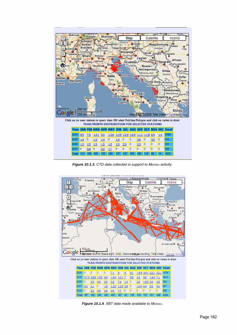
Figure 10.1.3. CTD data collected in support to MERSEA activity.

Figure 10.1.4. XBT data made available to MERSEA.

Page 182

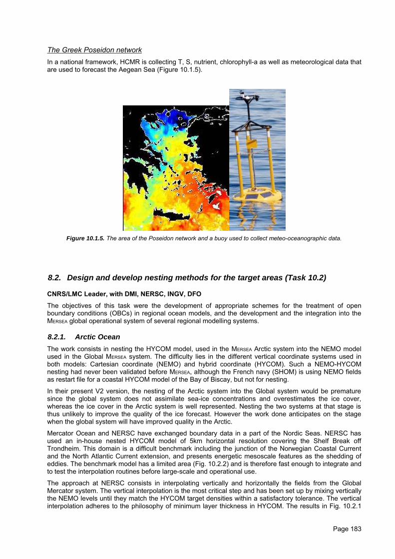
The Greek Poseidon networkIn a national framework, HCMR is collecting T, S, nutrient, chlorophyll-a as well as meteorological data thatare used to forecast the Aegean Sea (Figure 10.1.5).

Figure 10.1.5. The area of the Poseidon network and a buoy used to collect meteo-oceanographic data.

8.2. Design and develop nesting methods for the target areas (Task 10.2)

CNRS/LMC Leader, with DMI, NERSC, INGV, DFO

The objectives of this task were the development of appropriate schemes for the treatment of openboundary conditions (OBCs) in regional ocean models, and the development and the integration into theMERSEA global operational system of several regional modelling systems.

8.2.1. Arctic OceanThe work consists in nesting the HYCOM model, used in the MERSEA Arctic system into the NEMO modelused in the Global MERSEA system. The difficulty lies in the different vertical coordinate systems used inboth models: Cartesian coordinate (NEMO) and hybrid coordinate (HYCOM). Such a NEMO-HYCOMnesting had never been validated before MERSEA, although the French navy (SHOM) is using NEMO fieldsas restart file for a coastal HYCOM model of the Bay of Biscay, but not for nesting.

In their present V2 version, the nesting of the Arctic system into the Global system would be prematuresince the global system does not assimilate sea-ice concentrations and overestimates the ice cover,whereas the ice cover in the Arctic system is well represented. Nesting the two systems at that stage isthus unlikely to improve the quality of the ice forecast. However the work done anticipates on the stagewhen the global system will have improved quality in the Arctic.

Mercator Ocean and NERSC have exchanged boundary data in a part of the Nordic Seas. NERSC hasused an in-house nested HYCOM model of 5km horizontal resolution covering the Shelf Break offTrondheim. This domain is a difficult benchmark including the junction of the Norwegian Coastal Currentand the North Atlantic Current extension, and presents energetic mesoscale features as the shedding ofeddies. The benchmark model has a limited area (Fig. 10.2.2) and is therefore fast enough to integrate andto test the interpolation routines before large-scale and operational use.

The approach at NERSC consists in interpolating vertically and horizontally the fields from the GlobalMercator system. The vertical interpolation is the most critical step and has been set up by mixing verticallythe NEMO levels until they match the HYCOM target densities within a satisfactory tolerance. The verticalinterpolation adheres to the philosophy of minimum layer thickness in HYCOM. The results in Fig. 10.2.1

Page 183

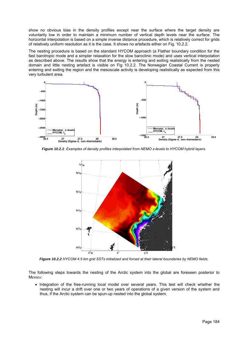
show no obvious bias in the density profiles except near the surface where the target density arevoluntarily low in order to maintain a minimum number of vertical depth levels near the surface. Thehorizontal interpolation is based on a simple inverse distance procedure, which is relatively correct for gridsof relatively uniform resolution as it is the case. It shows no artefacts either on Fig. 10.2.2.

The nesting procedure is based on the standard HYCOM approach (a Flather boundary condition for thefast barotropic mode and a simpler relaxation for the slow baroclinic mode) and uses vertical interpolationas described above. The results show that the energy is entering and exiting realistically from the nesteddomain and little nesting artefact is visible on Fig 10.2.2. The Norwegian Coastal Current is properlyentering and exiting the region and the mesoscale activity is developing realistically as expected from thisvery turbulent area.

Figure 10.2.1: Examples of density profiles interpolated from NEMO z-levels to HYCOM hybrid layers.

Figure 10.2.2 HYCOM 4.5 km grid SSTs initialized and forced at their lateral boundaries by NEMO fields.

The following steps towards the nesting of the Arctic system into the global are foreseen posterior toMERSEA:

• Integration of the free-running local model over several years. This test will check whether thenesting will incur a drift over one or two years of operations of a given version of the system andthus, if the Arctic system can be spun-up nested into the global system.

Page 184

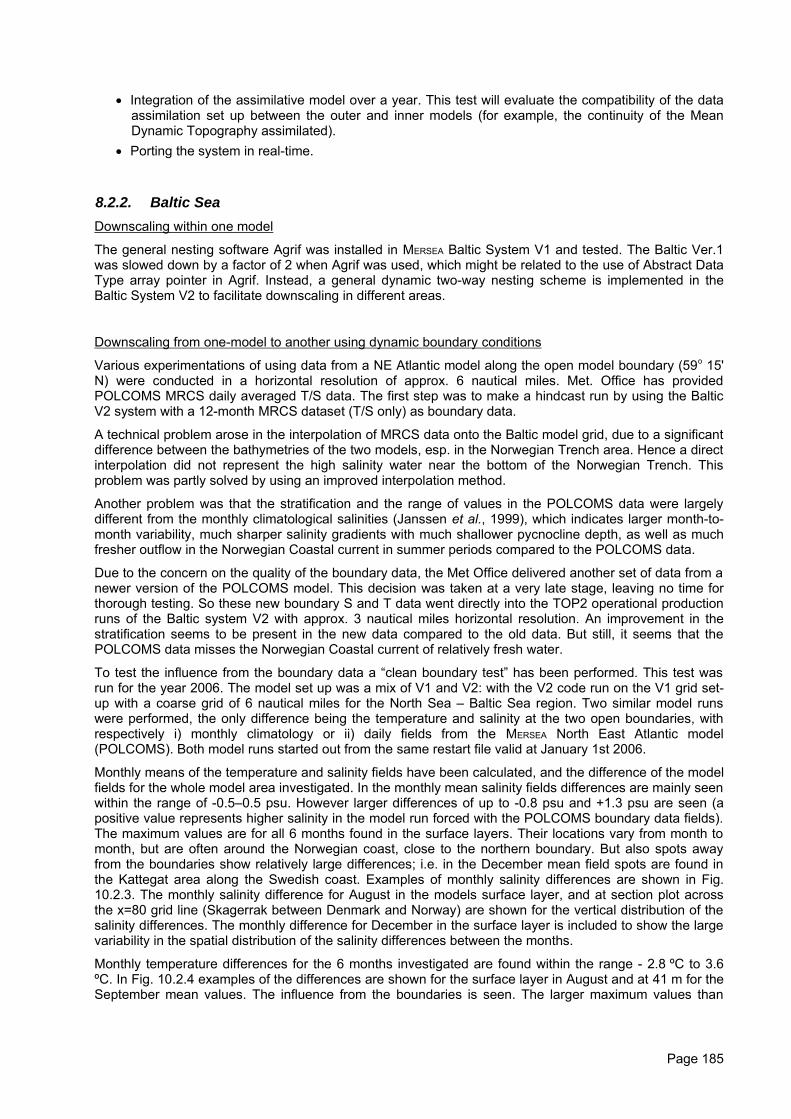
• Integration of the assimilative model over a year. This test will evaluate the compatibility of the dataassimilation set up between the outer and inner models (for example, the continuity of the MeanDynamic Topography assimilated).

• Porting the system in real-time.

8.2.2. Baltic SeaDownscaling within one model

The general nesting software Agrif was installed in MERSEA Baltic System V1 and tested. The Baltic Ver.1was slowed down by a factor of 2 when Agrif was used, which might be related to the use of Abstract DataType array pointer in Agrif. Instead, a general dynamic two-way nesting scheme is implemented in theBaltic System V2 to facilitate downscaling in different areas.

Downscaling from one-model to another using dynamic boundary conditions

Various experimentations of using data from a NE Atlantic model along the open model boundary (59o 15'N) were conducted in a horizontal resolution of approx. 6 nautical miles. Met. Office has providedPOLCOMS MRCS daily averaged T/S data. The first step was to make a hindcast run by using the BalticV2 system with a 12-month MRCS dataset (T/S only) as boundary data.

A technical problem arose in the interpolation of MRCS data onto the Baltic model grid, due to a significantdifference between the bathymetries of the two models, esp. in the Norwegian Trench area. Hence a directinterpolation did not represent the high salinity water near the bottom of the Norwegian Trench. Thisproblem was partly solved by using an improved interpolation method.

Another problem was that the stratification and the range of values in the POLCOMS data were largelydifferent from the monthly climatological salinities (Janssen et al., 1999), which indicates larger month-to-month variability, much sharper salinity gradients with much shallower pycnocline depth, as well as muchfresher outflow in the Norwegian Coastal current in summer periods compared to the POLCOMS data.

Due to the concern on the quality of the boundary data, the Met Office delivered another set of data from anewer version of the POLCOMS model. This decision was taken at a very late stage, leaving no time forthorough testing. So these new boundary S and T data went directly into the TOP2 operational productionruns of the Baltic system V2 with approx. 3 nautical miles horizontal resolution. An improvement in thestratification seems to be present in the new data compared to the old data. But still, it seems that thePOLCOMS data misses the Norwegian Coastal current of relatively fresh water.

To test the influence from the boundary data a “clean boundary test” has been performed. This test wasrun for the year 2006. The model set up was a mix of V1 and V2: with the V2 code run on the V1 grid set-up with a coarse grid of 6 nautical miles for the North Sea – Baltic Sea region. Two similar model runswere performed, the only difference being the temperature and salinity at the two open boundaries, withrespectively i) monthly climatology or ii) daily fields from the MERSEA North East Atlantic model(POLCOMS). Both model runs started out from the same restart file valid at January 1st 2006.

Monthly means of the temperature and salinity fields have been calculated, and the difference of the modelfields for the whole model area investigated. In the monthly mean salinity fields differences are mainly seenwithin the range of -0.5–0.5 psu. However larger differences of up to -0.8 psu and +1.3 psu are seen (apositive value represents higher salinity in the model run forced with the POLCOMS boundary data fields).The maximum values are for all 6 months found in the surface layers. Their locations vary from month tomonth, but are often around the Norwegian coast, close to the northern boundary. But also spots awayfrom the boundaries show relatively large differences; i.e. in the December mean field spots are found inthe Kattegat area along the Swedish coast. Examples of monthly salinity differences are shown in Fig.10.2.3. The monthly salinity difference for August in the models surface layer, and at section plot acrossthe x=80 grid line (Skagerrak between Denmark and Norway) are shown for the vertical distribution of thesalinity differences. The monthly difference for December in the surface layer is included to show the largevariability in the spatial distribution of the salinity differences between the months.

Monthly temperature differences for the 6 months investigated are found within the range - 2.8 ºC to 3.6ºC. In Fig. 10.2.4 examples of the differences are shown for the surface layer in August and at 41 m for theSeptember mean values. The influence from the boundaries is seen. The larger maximum values than

Page 185

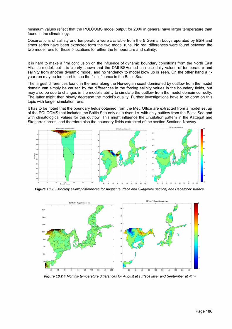
minimum values reflect that the POLCOMS model output for 2006 in general have larger temperature thanfound in the climatology.

Observations of salinity and temperature were available from the 5 German buoys operated by BSH andtimes series have been extracted form the two model runs. No real differences were found between thetwo model runs for those 5 locations for either the temperature and salinity.

It is hard to make a firm conclusion on the influence of dynamic boundary conditions from the North EastAtlantic model, but it is clearly shown that the DMI-BSHcmod can use daily values of temperature andsalinity from another dynamic model, and no tendency to model blow up is seen. On the other hand a 1-year run may be too short to see the full influence in the Baltic Sea.

The largest differences found in the area along the Norwegian coast dominated by outflow from the modeldomain can simply be caused by the differences in the forcing salinity values in the boundary fields, butmay also be due to changes in the model’s ability to simulate the outflow from the model domain correctly.The latter might then slowly decrease the model’s quality. Further investigations have to be done on thistopic with longer simulation runs.

It has to be noted that the boundary fields obtained from the Met. Office are extracted from a model set upof the POLCOMS that includes the Baltic Sea only as a river, i.e. with only outflow from the Baltic Sea andwith climatological values for this outflow. This might influence the circulation pattern in the Kattegat andSkagerrak areas, and therefore also the boundary fields extracted of the section Scotland-Norway.

Figure 10.2.3 Monthly salinity differences for August (surface and Skagerrak section) and December surface.

Figure 10.2.4 Monthly temperature differences for August at surface layer and September at 41m

Page 186

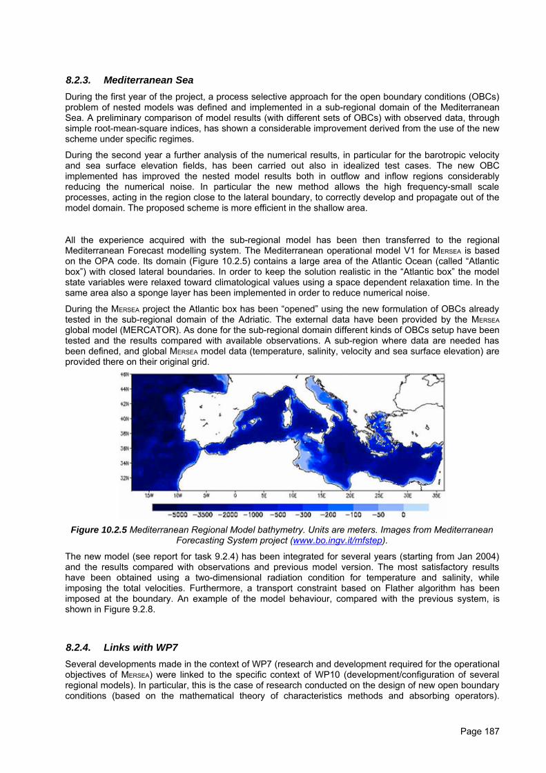
8.2.3. Mediterranean SeaDuring the first year of the project, a process selective approach for the open boundary conditions (OBCs)problem of nested models was defined and implemented in a sub-regional domain of the MediterraneanSea. A preliminary comparison of model results (with different sets of OBCs) with observed data, throughsimple root-mean-square indices, has shown a considerable improvement derived from the use of the newscheme under specific regimes.

During the second year a further analysis of the numerical results, in particular for the barotropic velocityand sea surface elevation fields, has been carried out also in idealized test cases. The new OBCimplemented has improved the nested model results both in outflow and inflow regions considerablyreducing the numerical noise. In particular the new method allows the high frequency-small scaleprocesses, acting in the region close to the lateral boundary, to correctly develop and propagate out of themodel domain. The proposed scheme is more efficient in the shallow area.

All the experience acquired with the sub-regional model has been then transferred to the regionalMediterranean Forecast modelling system. The Mediterranean operational model V1 for MERSEA is basedon the OPA code. Its domain (Figure 10.2.5) contains a large area of the Atlantic Ocean (called “Atlanticbox”) with closed lateral boundaries. In order to keep the solution realistic in the “Atlantic box” the modelstate variables were relaxed toward climatological values using a space dependent relaxation time. In thesame area also a sponge layer has been implemented in order to reduce numerical noise.

During the MERSEA project the Atlantic box has been “opened” using the new formulation of OBCs alreadytested in the sub-regional domain of the Adriatic. The external data have been provided by the MERSEA

global model (MERCATOR). As done for the sub-regional domain different kinds of OBCs setup have beentested and the results compared with available observations. A sub-region where data are needed hasbeen defined, and global MERSEA model data (temperature, salinity, velocity and sea surface elevation) areprovided there on their original grid.

Figure 10.2.5 Mediterranean Regional Model bathymetry. Units are meters. Images from MediterraneanForecasting System project (www.bo.ingv.it/mfstep).

The new model (see report for task 9.2.4) has been integrated for several years (starting from Jan 2004)and the results compared with observations and previous model version. The most satisfactory resultshave been obtained using a two-dimensional radiation condition for temperature and salinity, whileimposing the total velocities. Furthermore, a transport constraint based on Flather algorithm has beenimposed at the boundary. An example of the model behaviour, compared with the previous system, isshown in Figure 9.2.8.

8.2.4. Links with WP7Several developments made in the context of WP7 (research and development required for the operationalobjectives of MERSEA) were linked to the specific context of WP10 (development/configuration of severalregional models). In particular, this is the case of research conducted on the design of new open boundaryconditions (based on the mathematical theory of characteristics methods and absorbing operators).

Page 187

Similarly, a number of developments have been performed on the software package AGRIF (simplificationand optimization of several procedures, design of a pre-processing tool, addition of new features likevertical interpolation…) which were related to the integration of AGRIF within OPA-NEMO, HYCOM andBSHcmod.

8.3. Data Assimilation in Regional and Coastal Models (Task 10.3)

CNRS/LOC Leader, with DMI, NERSC, INGV, DFO

The overarching objective of Task 10.3 was to design, further develop, and implement estimation and dataassimilation tools in regional/coastal models, in the perspective of operational use in a later phase.

• One important practical objective was to ensure proper exchange of knowledge on this subject,within the Consortium, and in connection with the European and international communities.

• Another important practical objective was to take care of the Research and Development onestimation tools to be used in coastal ocean models. The challenges included: (1) exploration of themain error processes in coastal ocean models; (2) development and dissemination of a toolbox toinitialise a free-surface model from a coarser-grid solution and to dynamically project the solutiononto the desired physics; (3) development of a toolbox to perform data assimilation in coastal oceanmodels; (4) assessment of local observational networks and illustration of their potential interest inthe local assimilation problem.

• Application to several ocean areas within MERSEA. One of the conclusions was that nestedassimilative systems can run at least for several months with undegraded forecast performance andthat nesting is a cheap and flexible alternative to global high-resolution forecasting.

8.3.1. Exchange of knowledge and international outreach

DOWNDAC-2005 (CNRS-POC)A workshop on "Downscaling and Data Assimilation in Coastal Models" (DOWNDAC2005), organised byP. De Mey and co-sponsored by MERSEA -IP and by MFSTEP was held at LEGOS in Toulouse, France, onSeptember 7-8, 2005. The workshop was aimed at discussing methodological developments in progresswithin the MFSTEP and MERSEA European projects concerning (1) the downscaling of basin-scaleestimates and forecasts of hydro-dynamical ocean models to regional and coastal (shelf) domains andspecification of initial and boundary conditions; (2) data assimilation of local data not used or incompletelyused in larger-scale models; (3) forecasting in the local models. The areas of interest were the majorcoastal zones, with a particular focus on the near Atlantic, Mediterranean, and some tropical coastal areas.We also discussed the potential of these methodologies to address the needs of operational oceanographyand the development of ocean services.

GODAE Coastal and Shelf Seas Working Group activities (CNRS-POC)Following that initial impulsion, we have been continuing to promote such forums in the internationalcommunity, by means of the GODAE Coastal and Shelf Seas Working Group (CSSWG) chaired by P. DeMey. The 2007 GODAE Coastal Workshop was held in Liverpool, UK, on 10-11 October 2007. The maintheme was "Assessing the value of large-scale ocean products in coastal and shelf seas". The CSSWGpage on the GODAE web site (www.godae.org) contains description and results of 38 such coastalsystems using data from larger-scale ocean forecasting projects world-wide. As the next step, we havesubmitted to AGU a Special Session proposal titled "Advances in the prediction capabilities ofinterdisciplinary nested models in coastal and shelf seas", to be held at the AGU Fall Meeting in SanFrancisco, California, in December 2008.

Page 188

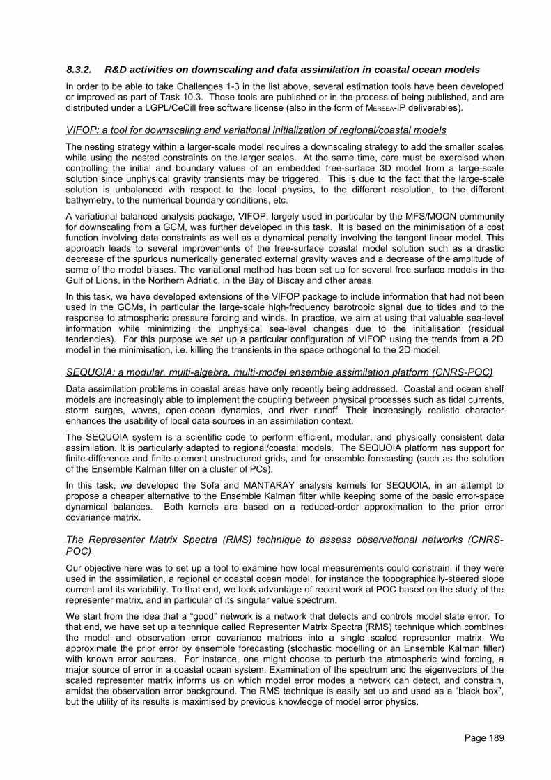
8.3.2. R&D activities on downscaling and data assimilation in coastal ocean modelsIn order to be able to take Challenges 1-3 in the list above, several estimation tools have been developedor improved as part of Task 10.3. Those tools are published or in the process of being published, and aredistributed under a LGPL/CeCill free software license (also in the form of MERSEA-IP deliverables).

VIFOP: a tool for downscaling and variational initialization of regional/coastal modelsThe nesting strategy within a larger-scale model requires a downscaling strategy to add the smaller scaleswhile using the nested constraints on the larger scales. At the same time, care must be exercised whencontrolling the initial and boundary values of an embedded free-surface 3D model from a large-scalesolution since unphysical gravity transients may be triggered. This is due to the fact that the large-scalesolution is unbalanced with respect to the local physics, to the different resolution, to the differentbathymetry, to the numerical boundary conditions, etc.

A variational balanced analysis package, VIFOP, largely used in particular by the MFS/MOON communityfor downscaling from a GCM, was further developed in this task. It is based on the minimisation of a costfunction involving data constraints as well as a dynamical penalty involving the tangent linear model. Thisapproach leads to several improvements of the free-surface coastal model solution such as a drasticdecrease of the spurious numerically generated external gravity waves and a decrease of the amplitude ofsome of the model biases. The variational method has been set up for several free surface models in theGulf of Lions, in the Northern Adriatic, in the Bay of Biscay and other areas.

In this task, we have developed extensions of the VIFOP package to include information that had not beenused in the GCMs, in particular the large-scale high-frequency barotropic signal due to tides and to theresponse to atmospheric pressure forcing and winds. In practice, we aim at using that valuable sea-levelinformation while minimizing the unphysical sea-level changes due to the initialisation (residualtendencies). For this purpose we set up a particular configuration of VIFOP using the trends from a 2Dmodel in the minimisation, i.e. killing the transients in the space orthogonal to the 2D model.

SEQUOIA: a modular, multi-algebra, multi-model ensemble assimilation platform (CNRS-POC)Data assimilation problems in coastal areas have only recently being addressed. Coastal and ocean shelfmodels are increasingly able to implement the coupling between physical processes such as tidal currents,storm surges, waves, open-ocean dynamics, and river runoff. Their increasingly realistic characterenhances the usability of local data sources in an assimilation context.

The SEQUOIA system is a scientific code to perform efficient, modular, and physically consistent dataassimilation. It is particularly adapted to regional/coastal models. The SEQUOIA platform has support forfinite-difference and finite-element unstructured grids, and for ensemble forecasting (such as the solutionof the Ensemble Kalman filter on a cluster of PCs).

In this task, we developed the Sofa and MANTARAY analysis kernels for SEQUOIA, in an attempt topropose a cheaper alternative to the Ensemble Kalman filter while keeping some of the basic error-spacedynamical balances. Both kernels are based on a reduced-order approximation to the prior errorcovariance matrix.

The Representer Matrix Spectra (RMS) technique to assess observational networks (CNRS-POC)Our objective here was to set up a tool to examine how local measurements could constrain, if they wereused in the assimilation, a regional or coastal ocean model, for instance the topographically-steered slopecurrent and its variability. To that end, we took advantage of recent work at POC based on the study of therepresenter matrix, and in particular of its singular value spectrum.

We start from the idea that a “good” network is a network that detects and controls model state error. Tothat end, we have set up a technique called Representer Matrix Spectra (RMS) technique which combinesthe model and observation error covariance matrices into a single scaled representer matrix. Weapproximate the prior error by ensemble forecasting (stochastic modelling or an Ensemble Kalman filter)with known error sources. For instance, one might choose to perturb the atmospheric wind forcing, amajor source of error in a coastal ocean system. Examination of the spectrum and the eigenvectors of thescaled representer matrix informs us on which model error modes a network can detect, and constrain,amidst the observation error background. The RMS technique is easily set up and used as a “black box”,but the utility of its results is maximised by previous knowledge of model error physics.

Page 189

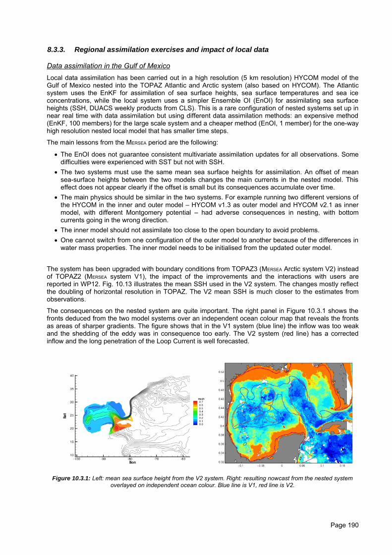
8.3.3. Regional assimilation exercises and impact of local data

Data assimilation in the Gulf of MexicoLocal data assimilation has been carried out in a high resolution (5 km resolution) HYCOM model of theGulf of Mexico nested into the TOPAZ Atlantic and Arctic system (also based on HYCOM). The Atlanticsystem uses the EnKF for assimilation of sea surface heights, sea surface temperatures and sea iceconcentrations, while the local system uses a simpler Ensemble OI (EnOI) for assimilating sea surfaceheights (SSH, DUACS weekly products from CLS). This is a rare configuration of nested systems set up innear real time with data assimilation but using different data assimilation methods: an expensive method(EnKF, 100 members) for the large scale system and a cheaper method (EnOI, 1 member) for the one-wayhigh resolution nested local model that has smaller time steps.

The main lessons from the MERSEA period are the following:

• The EnOI does not guarantee consistent multivariate assimilation updates for all observations. Somedifficulties were experienced with SST but not with SSH.

• The two systems must use the same mean sea surface heights for assimilation. An offset of meansea-surface heights between the two models changes the main currents in the nested model. Thiseffect does not appear clearly if the offset is small but its consequences accumulate over time.

• The main physics should be similar in the two systems. For example running two different versions ofthe HYCOM in the inner and outer model – HYCOM v1.3 as outer model and HYCOM v2.1 as innermodel, with different Montgomery potential – had adverse consequences in nesting, with bottomcurrents going in the wrong direction.

• The inner model should not assimilate too close to the open boundary to avoid problems.• One cannot switch from one configuration of the outer model to another because of the differences in

water mass properties. The inner model needs to be initialised from the updated outer model.

The system has been upgraded with boundary conditions from TOPAZ3 (MERSEA Arctic system V2) insteadof TOPAZ2 (MERSEA system V1), the impact of the improvements and the interactions with users arereported in WP12. Fig. 10.13 illustrates the mean SSH used in the V2 system. The changes mostly reflectthe doubling of horizontal resolution in TOPAZ. The V2 mean SSH is much closer to the estimates fromobservations.

The consequences on the nested system are quite important. The right panel in Figure 10.3.1 shows thefronts deduced from the two model systems over an independent ocean colour map that reveals the frontsas areas of sharper gradients. The figure shows that in the V1 system (blue line) the inflow was too weakand the shedding of the eddy was in consequence too early. The V2 system (red line) has a correctedinflow and the long penetration of the Loop Current is well forecasted.

Figure 10.3.1: Left: mean sea surface height from the V2 system. Right: resulting nowcast from the nested systemoverlayed on independent ocean colour. Blue line is V1, red line is V2.

Page 190

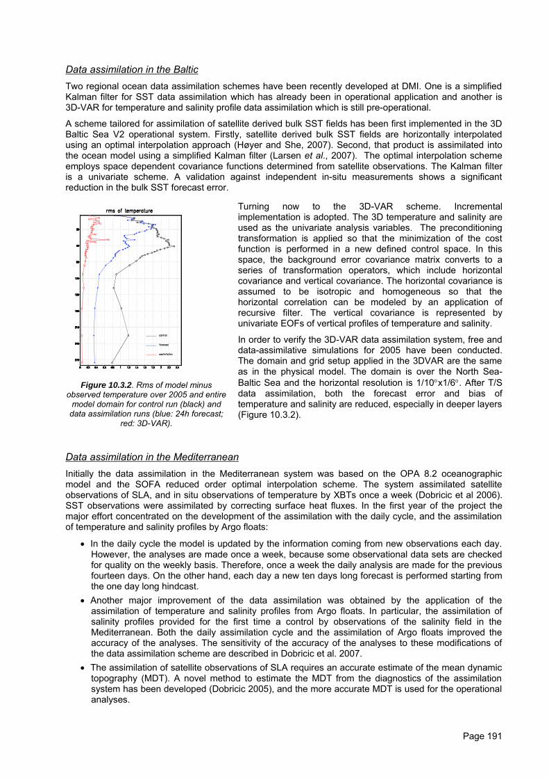
Data assimilation in the BalticTwo regional ocean data assimilation schemes have been recently developed at DMI. One is a simplifiedKalman filter for SST data assimilation which has already been in operational application and another is3D-VAR for temperature and salinity profile data assimilation which is still pre-operational.

A scheme tailored for assimilation of satellite derived bulk SST fields has been first implemented in the 3DBaltic Sea V2 operational system. Firstly, satellite derived bulk SST fields are horizontally interpolatedusing an optimal interpolation approach (Høyer and She, 2007). Second, that product is assimilated intothe ocean model using a simplified Kalman filter (Larsen et al., 2007). The optimal interpolation schemeemploys space dependent covariance functions determined from satellite observations. The Kalman filteris a univariate scheme. A validation against independent in-situ measurements shows a significantreduction in the bulk SST forecast error.

Figure 10.3.2. Rms of model minusobserved temperature over 2005 and entire

model domain for control run (black) anddata assimilation runs (blue: 24h forecast;

red: 3D-VAR).

Turning now to the 3D-VAR scheme. Incrementalimplementation is adopted. The 3D temperature and salinity areused as the univariate analysis variables. The preconditioningtransformation is applied so that the minimization of the costfunction is performed in a new defined control space. In thisspace, the background error covariance matrix converts to aseries of transformation operators, which include horizontalcovariance and vertical covariance. The horizontal covariance isassumed to be isotropic and homogeneous so that thehorizontal correlation can be modeled by an application ofrecursive filter. The vertical covariance is represented byunivariate EOFs of vertical profiles of temperature and salinity.

In order to verify the 3D-VAR data assimilation system, free anddata-assimilative simulations for 2005 have been conducted.The domain and grid setup applied in the 3DVAR are the sameas in the physical model. The domain is over the North Sea-Baltic Sea and the horizontal resolution is 1/10°x1/6°. After T/Sdata assimilation, both the forecast error and bias oftemperature and salinity are reduced, especially in deeper layers(Figure 10.3.2).

Data assimilation in the MediterraneanInitially the data assimilation in the Mediterranean system was based on the OPA 8.2 oceanographicmodel and the SOFA reduced order optimal interpolation scheme. The system assimilated satelliteobservations of SLA, and in situ observations of temperature by XBTs once a week (Dobricic et al 2006).SST observations were assimilated by correcting surface heat fluxes. In the first year of the project themajor effort concentrated on the development of the assimilation with the daily cycle, and the assimilationof temperature and salinity profiles by Argo floats:

• In the daily cycle the model is updated by the information coming from new observations each day.However, the analyses are made once a week, because some observational data sets are checkedfor quality on the weekly basis. Therefore, once a week the daily analysis are made for the previousfourteen days. On the other hand, each day a new ten days long forecast is performed starting fromthe one day long hindcast.

• Another major improvement of the data assimilation was obtained by the application of theassimilation of temperature and salinity profiles from Argo floats. In particular, the assimilation ofsalinity profiles provided for the first time a control by observations of the salinity field in theMediterranean. Both the daily assimilation cycle and the assimilation of Argo floats improved theaccuracy of the analyses. The sensitivity of the accuracy of the analyses to these modifications ofthe data assimilation scheme are described in Dobricic et al. 2007.

• The assimilation of satellite observations of SLA requires an accurate estimate of the mean dynamictopography (MDT). A novel method to estimate the MDT from the diagnostics of the assimilationsystem has been developed (Dobricic 2005), and the more accurate MDT is used for the operationalanalyses.

Page 191

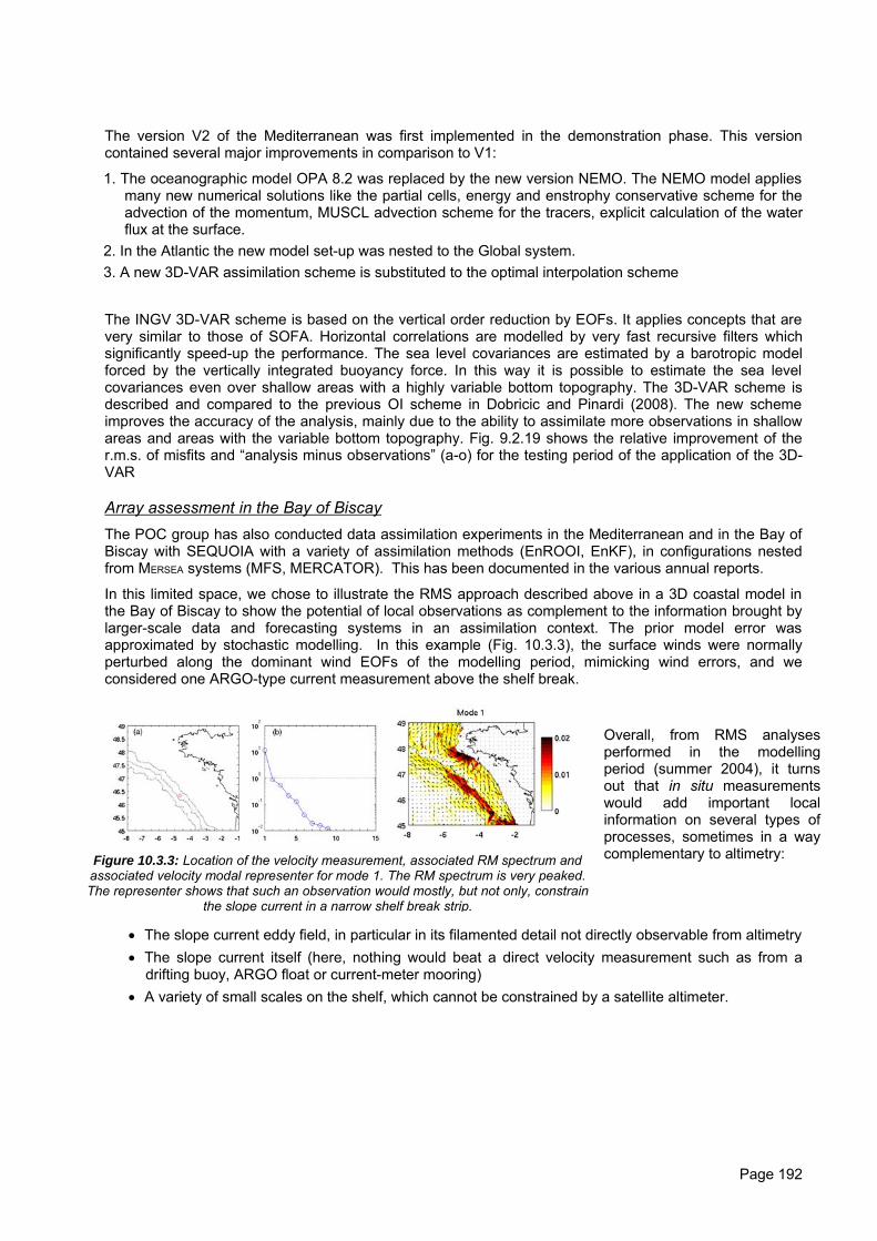
The version V2 of the Mediterranean was first implemented in the demonstration phase. This versioncontained several major improvements in comparison to V1:

1. The oceanographic model OPA 8.2 was replaced by the new version NEMO. The NEMO model appliesmany new numerical solutions like the partial cells, energy and enstrophy conservative scheme for theadvection of the momentum, MUSCL advection scheme for the tracers, explicit calculation of the waterflux at the surface.

2. In the Atlantic the new model set-up was nested to the Global system.3. A new 3D-VAR assimilation scheme is substituted to the optimal interpolation scheme

The INGV 3D-VAR scheme is based on the vertical order reduction by EOFs. It applies concepts that arevery similar to those of SOFA. Horizontal correlations are modelled by very fast recursive filters whichsignificantly speed-up the performance. The sea level covariances are estimated by a barotropic modelforced by the vertically integrated buoyancy force. In this way it is possible to estimate the sea levelcovariances even over shallow areas with a highly variable bottom topography. The 3D-VAR scheme isdescribed and compared to the previous OI scheme in Dobricic and Pinardi (2008). The new schemeimproves the accuracy of the analysis, mainly due to the ability to assimilate more observations in shallowareas and areas with the variable bottom topography. Fig. 9.2.19 shows the relative improvement of ther.m.s. of misfits and “analysis minus observations” (a-o) for the testing period of the application of the 3D-VAR

Array assessment in the Bay of BiscayThe POC group has also conducted data assimilation experiments in the Mediterranean and in the Bay ofBiscay with SEQUOIA with a variety of assimilation methods (EnROOI, EnKF), in configurations nestedfrom MERSEA systems (MFS, MERCATOR). This has been documented in the various annual reports.

In this limited space, we chose to illustrate the RMS approach described above in a 3D coastal model inthe Bay of Biscay to show the potential of local observations as complement to the information brought bylarger-scale data and forecasting systems in an assimilation context. The prior model error wasapproximated by stochastic modelling. In this example (Fig. 10.3.3), the surface winds were normallyperturbed along the dominant wind EOFs of the modelling period, mimicking wind errors, and weconsidered one ARGO-type current measurement above the shelf break.

Figure 10.3.3: Location of the velocity measurement, associated RM spectrum andassociated velocity modal representer for mode 1. The RM spectrum is very peaked.The representer shows that such an observation would mostly, but not only, constrain

the slope current in a narrow shelf break strip.

Overall, from RMS analysesperformed in the modellingperiod (summer 2004), it turnsout that in situ measurementswould add important localinformation on several types ofprocesses, sometimes in a waycomplementary to altimetry:

• The slope current eddy field, in particular in its filamented detail not directly observable from altimetry• The slope current itself (here, nothing would beat a direct velocity measurement such as from a

drifting buoy, ARGO float or current-meter mooring)• A variety of small scales on the shelf, which cannot be constrained by a satellite altimeter.

Page 192

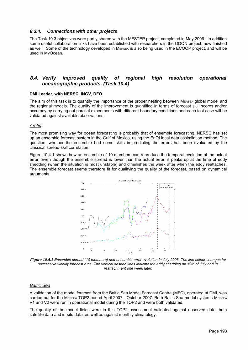
8.3.4. Connections with other projectsThe Task 10.3 objectives were partly shared with the MFSTEP project, completed in May 2006. In additionsome useful collaboration links have been established with researchers in the ODON project, now finishedas well. Some of the technology developed in MERSEA is also being used in the ECOOP project, and will beused in MyOcean.

8.4. Verify improved quality of regional high resolution operationaloceanographic products. (Task 10.4)

DMI Leader, with NERSC, INGV, DFO

The aim of this task is to quantify the importance of the proper nesting between MERSEA global model andthe regional models. The quality of the improvement is quantified in terms of forecast skill scores and/oraccuracy by carrying out parallel experiments with different boundary conditions and each test case will bevalidated against available observations.

ArcticThe most promising way for ocean forecasting is probably that of ensemble forecasting. NERSC has setup an ensemble forecast system in the Gulf of Mexico, using the EnOI local data assimilation method. Thequestion, whether the ensemble had some skills in predicting the errors has been evaluated by theclassical spread-skill correlation.

Figure 10.4.1 shows how an ensemble of 10 members can reproduce the temporal evolution of the actualerror. Even though the ensemble spread is lower than the actual error, it peaks up at the time of eddyshedding (when the situation is most unstable) and diminishes the week after when the eddy reattaches.The ensemble forecast seems therefore fit for qualifying the quality of the forecast, based on dynamicalarguments.

Figure 10.4.1 Ensemble spread (10 members) and ensemble error evolution in July 2006. The line colour changes forsuccessive weekly forecast runs. The vertical dashed lines indicate the eddy shedding on 19th of July and its

reattachment one week later.

Baltic SeaA validation of the model forecast from the Baltic Sea Model Forecast Centre (MFC), operated at DMI, wascarried out for the MERSEA TOP2 period April 2007 - October 2007. Both Baltic Sea model systems MERSEA

V1 and V2 were run in operational model during the TOP2 and were both validated.

The quality of the model fields were in this TOP2 assessment validated against observed data, bothsatellite data and in-situ data, as well as against monthly climatology.

Page 193

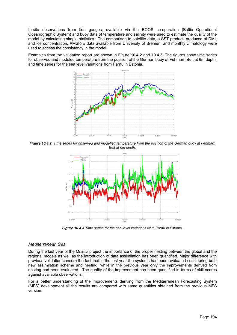
In-situ observations from tide gauges, available via the BOOS co-operation (Baltic OperationalOceanographic System) and buoy data of temperature and salinity were used to estimate the quality of themodel by calculating simple statistics. The comparison to satellite data, a SST product, produced at DMI,and ice concentration, AMSR-E data available from University of Bremen, and monthly climatology wereused to access the consistency in the model.

Examples from the validation report are shown in Figure 10.4.2 and 10.4.3. The figures show time seriesfor observed and modeled temperature from the position of the German buoy at Fehmarn Belt at 6m depth,

Mediterranean SeaDuring the last year of the MERSEA project the importance of the proper nesting between the global and theregional models as well as the introduction of data assimilation has been quantified. Major difference withprevious validation concern the fact that in the last year the systems has been evaluated considering bothnew assimilation scheme and nesting, while in the previous year only the improvements derived fromnesting had been evaluated. The quality of the improvement has been quantified in terms of skill scoresagainst available observations.

For a better understanding of the improvements deriving from the Mediterranean Forecasting System(MFS) development all the results are compared with same quantities obtained from the previous MFSversion.

Page 194

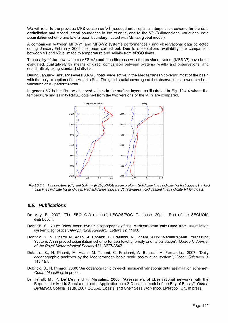
We will refer to the previous MFS version as V1 (reduced order optimal interpolation scheme for the dataassimilation and closed lateral boundaries in the Atlantic) and to the V2 (3-dimensional variational dataassimilation scheme and lateral open boundary nested with MERSEA global model).

A comparison between MFS-V1 and MFS-V2 systems performances using observational data collectedduring January-February 2008 has been carried out. Due to observations availability, the comparisonbetween V1 and V2 is limited to temperature and salinity from ARGO floats.

The quality of the new system (MFS-V2) and the difference with the previous system (MFS-V!) have beenevaluated, qualitatively by means of direct comparison between systems results and observations, andquantitatively using standard statistics.

During January-February several ARGO floats were active in the Mediterranean covering most of the basinwith the only exception of the Adriatic Sea. The good spatial coverage of the observations allowed a robustvalidation of V2 performances.

In general V2 better fits the observed values in the surface layers, as illustrated in Fig. 10.4.4 where thetemperature and salinity RMSE obtained from the two versions of the MFS are compared.

Fig.10.4.4. Temperature (C°) and Salinity (PSU) RMSE mean profiles. Solid blue lines indicate V2 first-guess; Dashedblue lines indicate V2 hind-cast; Red solid lines indicate V1 first-guess; Red dashed lines indicate V1 hind-cast.

8.5. Publications

De Mey, P., 2007: “The SEQUOIA manual”, LEGOS/POC, Toulouse, 29pp. Part of the SEQUOIAdistribution.

Dobricic, S., 2005: “New mean dynamic topography of the Mediterranean calculated from assimilationsystem diagnostics”, Geophysical Research Letters 32, 11606.

Dobricic, S., N. Pinardi, M. Adani, A. Bonazzi, C. Fratianni, M. Tonani, 2005: “Mediterranean ForecastingSystem: An improved assimilation scheme for sea-level anomaly and its validation”, Quarterly Journalof the Royal Meteorological Society 131, 3627-3642.

Dobricic, S., N. Pinardi, M. Adani, M. Tonani, C. Fratianni, A. Bonazzi, V. Fernandez, 2007: “Dailyoceanographic analyses by the Mediterranean basin scale assimilation system”, Ocean Sciences 3,149-157.

Dobricic, S., N. Pinardi, 2008: “An oceanographic three-dimensional variational data assimilation scheme”,Ocean Modelling, in press.

Le Hénaff, M., P. De Mey and P. Marsaleix, 2008: “Assessment of observational networks with theRepresenter Matrix Spectra method – Application to a 3-D coastal model of the Bay of Biscay”, OceanDynamics, Special Issue, 2007 GODAE Coastal and Shelf Seas Workshop, Liverpool, UK, in press.

Page 195

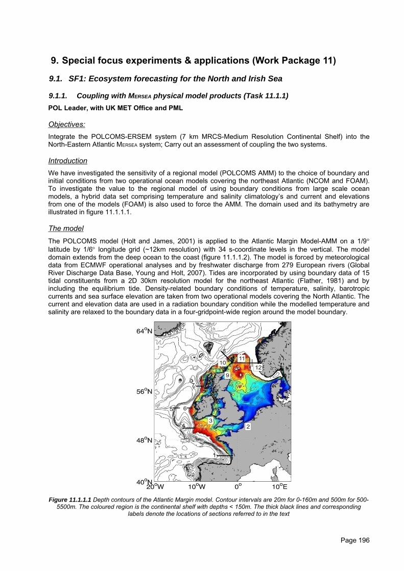
9. Special focus experiments & applications (Work Package 11)

9.1. SF1: Ecosystem forecasting for the North and Irish Sea

9.1.1. Coupling with MERSEA physical model products (Task 11.1.1)POL Leader, with UK MET Office and PML

Objectives:Integrate the POLCOMS-ERSEM system (7 km MRCS-Medium Resolution Continental Shelf) into theNorth-Eastern Atlantic MERSEA system; Carry out an assessment of coupling the two systems.

IntroductionWe have investigated the sensitivity of a regional model (POLCOMS AMM) to the choice of boundary andinitial conditions from two operational ocean models covering the northeast Atlantic (NCOM and FOAM).To investigate the value to the regional model of using boundary conditions from large scale oceanmodels, a hybrid data set comprising temperature and salinity climatology’s and current and elevationsfrom one of the models (FOAM) is also used to force the AMM. The domain used and its bathymetry areillustrated in figure 11.1.1.1.

The model

The POLCOMS model (Holt and James, 2001) is applied to the Atlantic Margin Model-AMM on a 1/9°latitude by 1/6° longitude grid (~12km resolution) with 34 s-coordinate levels in the vertical. The modeldomain extends from the deep ocean to the coast (figure 11.1.1.2). The model is forced by meteorologicaldata from ECMWF operational analyses and by freshwater discharge from 279 European rivers (GlobalRiver Discharge Data Base, Young and Holt, 2007). Tides are incorporated by using boundary data of 15tidal constituents from a 2D 30km resolution model for the northeast Atlantic (Flather, 1981) and byincluding the equilibrium tide. Density-related boundary conditions of temperature, salinity, barotropiccurrents and sea surface elevation are taken from two operational models covering the North Atlantic. Thecurrent and elevation data are used in a radiation boundary condition while the modelled temperature andsalinity are relaxed to the boundary data in a four-gridpoint-wide region around the model boundary.

Figure 11.1.1.1 Depth contours of the Atlantic Margin model. Contour intervals are 20m for 0-160m and 500m for 500-5500m. The coloured region is the continental shelf with depths < 150m. The thick black lines and corresponding

labels denote the locations of sections referred to in the text

Page 196

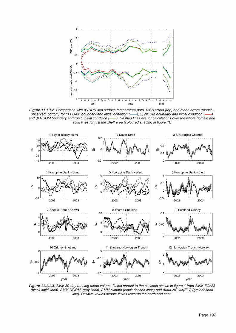
Figure 11.1.1.2: Comparison with AVHRR sea surface temperature data. RMS errors (top) and mean errors (model –observed, bottom) for 1) FOAM boundary and initial condition (——), 2) NCOM boundary and initial condition (——)

and 3) NCOM boundary and run 1 initial condition (——). Dashed lines are for calculations over the whole domain andsolid lines for just the shelf area (coloured shading in figure 1).

Figure 11.1.1.3. AMM 30-day running mean volume fluxes normal to the sections shown in figure 1 from AMM-FOAM(black solid lines), AMM-NCOM (grey lines), AMM-climate (black dashed lines) and AMM-NCOM(FIC) (grey dashed

line). Positive values denote fluxes towards the north and east.

Page 197

ResultsThe results of the Atlantic Margin Model compare well with observations of sea surface temperature. Toassess the accuracy of the model’s sea surface temperature and the sensitivity to the boundary and initialcondition, the model results are compared to 9km AVHRR data from April 2001 to June 2003. For eachtime that data are available, the observations are interpolated onto the model grid and the mean and RMSdifferences to the corresponding model value calculated (figure 11.1.1.2).

Errors calculated over the whole domain are generally greater than those calculated only over the shelfand are larger in summer than in winter. Except for the first data point for the run with NCOM initialcondition, the model underestimates the temperature by an average of about 0.5oC on the shelf and 0.5–1.5oC over the whole domain. The RMS errors are about 0.8oC on the shelf and 1.2oC over the wholedomain. The largest differences are always for the run using FOAM boundary data. After 15 months, thetwo runs with NCOM boundary conditions have similar errors showing that the affect of the initial conditionhas diminished. By the same time, the errors of all three model runs are almost identical when measuredover the shelf area only indicating that, once the affect of the initial condition has reduced, the sea surfacetemperatures over the shelf area depend more on the model properties than on the density-relatedboundary forcing.

On the northwest European continental shelf, volume fluxes through sections placed across strategicpathways appear mostly unaffected by the initial and boundary conditions used by the AMM (Figure11.1.1.3). All model runs produced results consistent with observations. For sections that extended intodeeper water off the continental shelf, the volume flux depended heavily on both the boundary and initialdata sources. The affect was largest for the two sections in the southwest corner of the model domain andthere is evidence that the run using climate data behaves differently from the runs using model output asboundary data. This might be a consequence of the lower temporal and spatial resolution of the climatedata that misses some detail of the density field that is important for the correct modelling of the large-scale currents, or it might be that the climate temperature and salinity boundary conditions are inconsistentwith the FOAM elevation and barotropic current data that are used to complete the boundary data set forthe AMM-climate run. There appears to be no consistent difference between the models in the variability ofthe volume fluxes through the selected cross-sections.

The balance between the pressure gradient and the Coriolis force, tends to constrain the currents to followdepth contours (Huthnance, 1995), on timescales longer than one day. This inhibits ocean-shelfexchanges in regions of steep bathymetry. Consequently, the shallow shelf region of the northeast Atlanticis largely unaffected by the choice of boundary condition in the AMM (Figure 11.1.1.4).

ConclusionsOn time scales of ~1 year the conditions on the northwest European Continental shelf are only weaklydependent on the deep ocean boundary conditions. Hence, the details of these are unlikely to directlyaffect short term forecast skill, and we must look elsewhere to improve this. For longer term investigationsand forecasts (e.g. large scale pollutant/nutrient transport, ocean-shelf exchange of plankton etc) theoceanic conditions become important. In which case, both the accuracy of the open ocean model and thedetails of the boundary conditions schemes become important in determining the on-shelf conditions.

Page 198

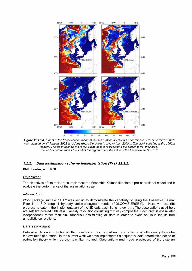
Figure 11.1.1.4. Extent of the tracer concentration at the sea surface six months after release. Tracer of value 100m-3

was released on 1st January 2002 in regions where the depth is greater than 2000m. The black solid line is the 2000misobath. The black dashed line is the 150m isobath representing the extent of the shelf area. The white contour shows the limit of the region where the value of the tracer exceeds 0.1m-3.

9.1.2. Data assimilation scheme implementation (Task 11.1.2)PML Leader, with POL

Objectives:The objectives of the task are to implement the Ensemble Kalman filter into a pre-operational model and toevaluate the performance of the assimilation system

IntroductionWork package subtask 11.1.2 was set up to demonstrate the capability of using the Ensemble KalmanFilter in a 3-D coupled hydrodynamics-ecosystem model (POLCOMS-ERSEM). Here we describeprogress to date in the implementation of the 3D data assimilation algorithm. The observations used hereare satellite derived Chla at a ~ weekly resolution consisting of 3 day composites. Each pixel is assimilatedindependently rather than simultaneously assimilating all data in order to avoid spurious results fromunrealistic correlations.

Data assimilationData assimilation is a technique that combines model output and observations simultaneously to controlthe evolution of a model. In the current work we have implemented a sequential data assimilation based onestimation theory which represents a filter method. Observations and model predictions of the state are

Page 199

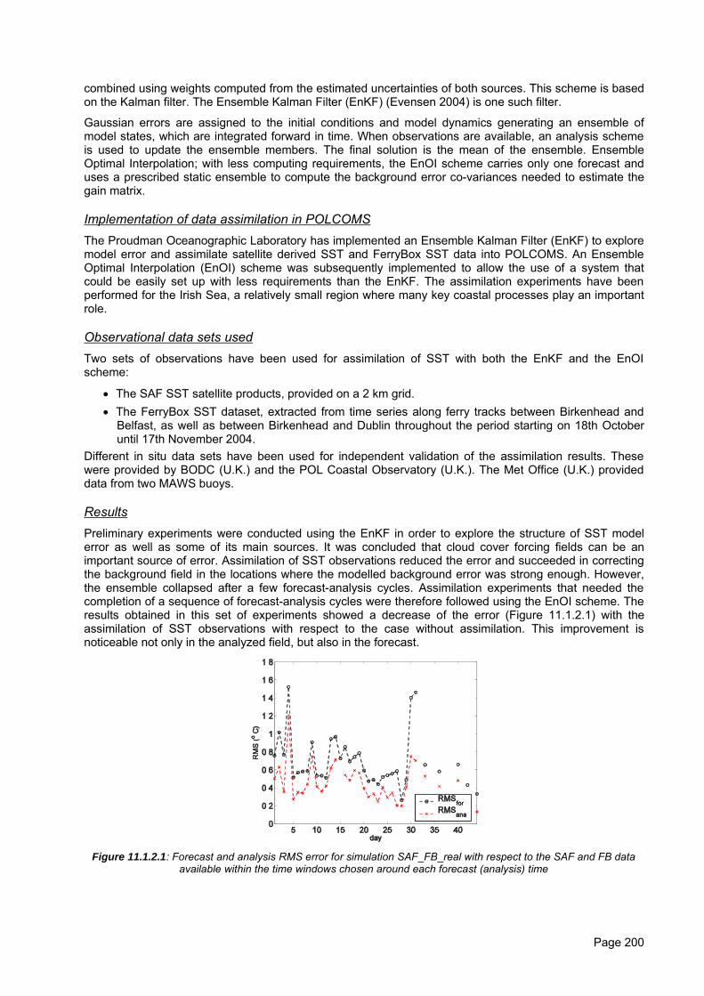
combined using weights computed from the estimated uncertainties of both sources. This scheme is basedon the Kalman filter. The Ensemble Kalman Filter (EnKF) (Evensen 2004) is one such filter.

Gaussian errors are assigned to the initial conditions and model dynamics generating an ensemble ofmodel states, which are integrated forward in time. When observations are available, an analysis schemeis used to update the ensemble members. The final solution is the mean of the ensemble. EnsembleOptimal Interpolation; with less computing requirements, the EnOI scheme carries only one forecast anduses a prescribed static ensemble to compute the background error co-variances needed to estimate thegain matrix.

Implementation of data assimilation in POLCOMSThe Proudman Oceanographic Laboratory has implemented an Ensemble Kalman Filter (EnKF) to exploremodel error and assimilate satellite derived SST and FerryBox SST data into POLCOMS. An EnsembleOptimal Interpolation (EnOI) scheme was subsequently implemented to allow the use of a system thatcould be easily set up with less requirements than the EnKF. The assimilation experiments have beenperformed for the Irish Sea, a relatively small region where many key coastal processes play an importantrole.

Observational data sets usedTwo sets of observations have been used for assimilation of SST with both the EnKF and the EnOIscheme:

• The SAF SST satellite products, provided on a 2 km grid.• The FerryBox SST dataset, extracted from time series along ferry tracks between Birkenhead and

Belfast, as well as between Birkenhead and Dublin throughout the period starting on 18th Octoberuntil 17th November 2004.

Different in situ data sets have been used for independent validation of the assimilation results. Thesewere provided by BODC (U.K.) and the POL Coastal Observatory (U.K.). The Met Office (U.K.) provideddata from two MAWS buoys.

ResultsPreliminary experiments were conducted using the EnKF in order to explore the structure of SST modelerror as well as some of its main sources. It was concluded that cloud cover forcing fields can be animportant source of error. Assimilation of SST observations reduced the error and succeeded in correctingthe background field in the locations where the modelled background error was strong enough. However,the ensemble collapsed after a few forecast-analysis cycles. Assimilation experiments that needed thecompletion of a sequence of forecast-analysis cycles were therefore followed using the EnOI scheme. Theresults obtained in this set of experiments showed a decrease of the error (Figure 11.1.2.1) with theassimilation of SST observations with respect to the case without assimilation. This improvement isnoticeable not only in the analyzed field, but also in the forecast.

Figure 11.1.2.1: Forecast and analysis RMS error for simulation SAF_FB_real with respect to the SAF and FB dataavailable within the time windows chosen around each forecast (analysis) time

Page 200

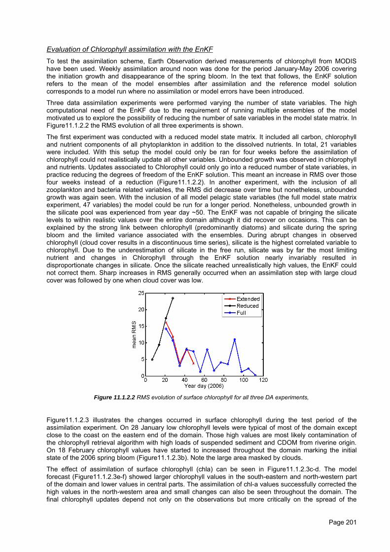
Evaluation of Chlorophyll assimilation with the EnKFTo test the assimilation scheme, Earth Observation derived measurements of chlorophyll from MODIShave been used. Weekly assimilation around noon was done for the period January-May 2006 coveringthe initiation growth and disappearance of the spring bloom. In the text that follows, the EnKF solutionrefers to the mean of the model ensembles after assimilation and the reference model solutioncorresponds to a model run where no assimilation or model errors have been introduced.

Three data assimilation experiments were performed varying the number of state variables. The highcomputational need of the EnKF due to the requirement of running multiple ensembles of the modelmotivated us to explore the possibility of reducing the number of sate variables in the model state matrix. InFigure11.1.2.2 the RMS evolution of all three experiments is shown.

The first experiment was conducted with a reduced model state matrix. It included all carbon, chlorophylland nutrient components of all phytoplankton in addition to the dissolved nutrients. In total, 21 variableswere included. With this setup the model could only be ran for four weeks before the assimilation ofchlorophyll could not realistically update all other variables. Unbounded growth was observed in chlorophylland nutrients. Updates associated to Chlorophyll could only go into a reduced number of state variables, inpractice reducing the degrees of freedom of the EnKF solution. This meant an increase in RMS over thosefour weeks instead of a reduction (Figure11.1.2.2). In another experiment, with the inclusion of allzooplankton and bacteria related variables, the RMS did decrease over time but nonetheless, unboundedgrowth was again seen. With the inclusion of all model pelagic state variables (the full model state matrixexperiment, 47 variables) the model could be run for a longer period. Nonetheless, unbounded growth inthe silicate pool was experienced from year day ~50. The EnKF was not capable of bringing the silicatelevels to within realistic values over the entire domain although it did recover on occasions. This can beexplained by the strong link between chlorophyll (predominantly diatoms) and silicate during the springbloom and the limited variance associated with the ensembles. During abrupt changes in observedchlorophyll (cloud cover results in a discontinuous time series), silicate is the highest correlated variable tochlorophyll. Due to the underestimation of silicate in the free run, silicate was by far the most limitingnutrient and changes in Chlorophyll through the EnKF solution nearly invariably resulted indisproportionate changes in silicate. Once the silicate reached unrealistically high values, the EnKF couldnot correct them. Sharp increases in RMS generally occurred when an assimilation step with large cloudcover was followed by one when cloud cover was low.

Figure 11.1.2.2 RMS evolution of surface chlorophyll for all three DA experiments,

Figure11.1.2.3 illustrates the changes occurred in surface chlorophyll during the test period of theassimilation experiment. On 28 January low chlorophyll levels were typical of most of the domain exceptclose to the coast on the eastern end of the domain. Those high values are most likely contamination ofthe chlorophyll retrieval algorithm with high loads of suspended sediment and CDOM from riverine origin.On 18 February chlorophyll values have started to increased throughout the domain marking the initialstate of the 2006 spring bloom (Figure11.1.2.3b). Note the large area masked by clouds.

The effect of assimilation of surface chlorophyll (chla) can be seen in Figure11.1.2.3c-d. The modelforecast (Figure11.1.2.3e-f) showed larger chlorophyll values in the south-eastern and north-western partof the domain and lower values in central parts. The assimilation of chl-a values successfully corrected thehigh values in the north-western area and small changes can also be seen throughout the domain. Thefinal chlorophyll updates depend not only on the observations but more critically on the spread of the

Page 201

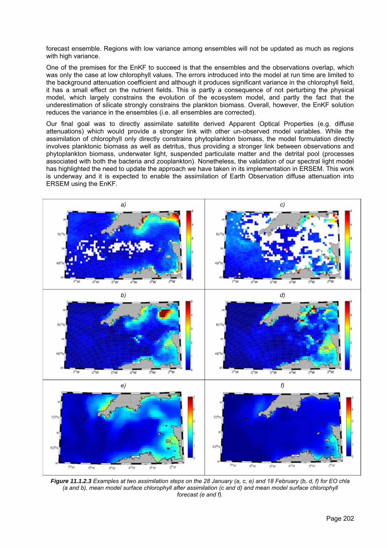
forecast ensemble. Regions with low variance among ensembles will not be updated as much as regionswith high variance.

One of the premises for the EnKF to succeed is that the ensembles and the observations overlap, whichwas only the case at low chlorophyll values. The errors introduced into the model at run time are limited tothe background attenuation coefficient and although it produces significant variance in the chlorophyll field,it has a small effect on the nutrient fields. This is partly a consequence of not perturbing the physicalmodel, which largely constrains the evolution of the ecosystem model, and partly the fact that theunderestimation of silicate strongly constrains the plankton biomass. Overall, however, the EnKF solutionreduces the variance in the ensembles (i.e. all ensembles are corrected).

Our final goal was to directly assimilate satellite derived Apparent Optical Properties (e.g. diffuseattenuations) which would provide a stronger link with other un-observed model variables. While theassimilation of chlorophyll only directly constrains phytoplankton biomass, the model formulation directlyinvolves planktonic biomass as well as detritus, thus providing a stronger link between observations andphytoplankton biomass, underwater light, suspended particulate matter and the detrital pool (processesassociated with both the bacteria and zooplankton). Nonetheless, the validation of our spectral light modelhas highlighted the need to update the approach we have taken in its implementation in ERSEM. This workis underway and it is expected to enable the assimilation of Earth Observation diffuse attenuation intoERSEM using the EnKF.

Figure 11.1.2.3 Examples at two assimilation steps on the 28 January (a, c, e) and 18 February (b, d, f) for EO chla (a and b), mean model surface chlorophyll after assimilation (c and d) and mean model surface chlorophyll

forecast (e and f).

Page 202

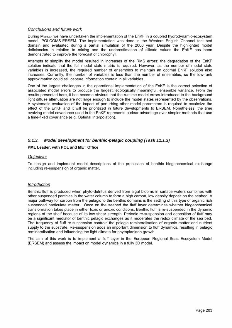
Conclusions and future workDuring MERSEA we have undertaken the implementation of the EnKF in a coupled hydrodynamic-ecosystemmodel, POLCOMS-ERSEM. The implementation was done in the Western English Channel test beddomain and evaluated during a partial simulation of the 2006 year. Despite the highlighted modeldeficiencies in relation to mixing and the underestimation of silicate values the EnKF has beendemonstrated to improve the forecast of chlorophyll.

Attempts to simplify the model resulted in increases of the RMS errors: the degradation of the EnKFsolution indicate that the full model state matrix is required. However, as the number of model statevariables is increased, the required number of ensembles to maintain an optimal EnKF solution alsoincreases. Currently, the number of variables is less than the number of ensembles, so the low-rankapproximation could still capture information contain in all variables.

One of the largest challenges in the operational implementation of the EnKF is the correct selection ofassociated model errors to produce the largest, ecologically meaningful, ensemble variance. From theresults presented here, it has become obvious that the runtime model errors introduced to the backgroundlight diffuse attenuation are not large enough to include the model states represented by the observations.A systematic evaluation of the impact of perturbing other model parameters is required to maximize theeffect of the EnKF and it will be prioritized in future developments to ERSEM. Nonetheless, the timeevolving model covariance used in the EnKF represents a clear advantage over simpler methods that usea time-fixed covariance (e.g. Optimal Interpolation).

9.1.3. Model development for benthic-pelagic coupling (Task 11.1.3)PML Leader, with POL and MET Office

Objective:To design and implement model descriptions of the processes of benthic biogeochemical exchangeincluding re-suspension of organic matter.

IntroductionBenthic fluff is produced when phyto-detritus derived from algal blooms in surface waters combines withother suspended particles in the water column to form a high carbon, low density deposit on the seabed. Amajor pathway for carbon from the pelagic to the benthic domains is the settling of this type of organic richsuspended particulate matter. Once on the seabed the fluff layer determines whether biogeochemicaltransformation takes place in either toxic or anoxic conditions. Benthic fluff is re-suspended in the dynamicregions of the shelf because of its low shear strength. Periodic re-suspension and deposition of fluff maybe a significant mediator of benthic pelagic exchanges as it moderates the redox climate of the sea bed.The frequency of fluff re-suspension controls the pelagic remineralisation of organic matter and nutrientsupply to the substrate. Re-suspension adds an important dimension to fluff dynamics, resulting in pelagicremineralisation and influencing the light climate for phytoplankton growth.

The aim of this work is to implement a fluff layer in the European Regional Seas Ecosystem Model(ERSEM) and assess the impact on model dynamics in a fully 3D model.

Page 203

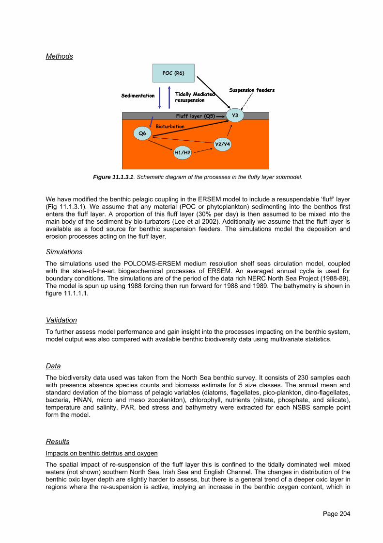
Methods

H1/H2Y2/Y4

Q6

Fluff layer (Q5) Y3

POC (R6)

Suspension feeders

Bioturbation

Tidally Mediatedresuspension

Sedimentation

H1/H2Y2/Y4

Q6

Fluff layer (Q5) Y3

POC (R6)

Suspension feeders

Bioturbation

Tidally Mediatedresuspension

Sedimentation

Figure 11.1.3.1. Schematic diagram of the processes in the fluffy layer submodel.

We have modified the benthic pelagic coupling in the ERSEM model to include a resuspendable ‘fluff’ layer(Fig 11.1.3.1). We assume that any material (POC or phytoplankton) sedimenting into the benthos firstenters the fluff layer. A proportion of this fluff layer (30% per day) is then assumed to be mixed into themain body of the sediment by bio-turbators (Lee et al 2002). Additionally we assume that the fluff layer isavailable as a food source for benthic suspension feeders. The simulations model the deposition anderosion processes acting on the fluff layer.

SimulationsThe simulations used the POLCOMS-ERSEM medium resolution shelf seas circulation model, coupledwith the state-of-the-art biogeochemical processes of ERSEM. An averaged annual cycle is used forboundary conditions. The simulations are of the period of the data rich NERC North Sea Project (1988-89).The model is spun up using 1988 forcing then run forward for 1988 and 1989. The bathymetry is shown infigure 11.1.1.1.

ValidationTo further assess model performance and gain insight into the processes impacting on the benthic system,model output was also compared with available benthic biodiversity data using multivariate statistics.

DataThe biodiversity data used was taken from the North Sea benthic survey. It consists of 230 samples eachwith presence absence species counts and biomass estimate for 5 size classes. The annual mean andstandard deviation of the biomass of pelagic variables (diatoms, flagellates, pico-plankton, dino-flagellates,bacteria, HNAN, micro and meso zooplankton), chlorophyll, nutrients (nitrate, phosphate, and silicate),temperature and salinity, PAR, bed stress and bathymetry were extracted for each NSBS sample pointform the model.

ResultsImpacts on benthic detritus and oxygen

The spatial impact of re-suspension of the fluff layer this is confined to the tidally dominated well mixedwaters (not shown) southern North Sea, Irish Sea and English Channel. The changes in distribution of thebenthic oxic layer depth are slightly harder to assess, but there is a general trend of a deeper oxic layer inregions where the re-suspension is active, implying an increase in the benthic oxygen content, which in

Page 204

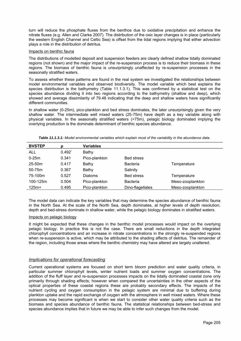
turn will reduce the phosphate fluxes from the benthos due to oxidative precipitation and enhance thenitrate fluxes (e.g. Allen and Clarke 2007). The distribution of the oxic layer changes is in place (particularlythe western English Channel and Celtic Sea) is offset from the tidal regions implying that either advectionplays a role in the distribution of detritus.

Impacts on benthic fauna

The distributions of modelled deposit and suspension feeders are clearly defined shallow tidally dominatedregions (not shown) and the major impact of the re-suspension process is to reduce their biomass in theseregions. The biomass of benthic fauna is unsurprisingly unaffected by re-suspension processes in theseasonally stratified waters.

To assess whether these patterns are found in the real system we investigated the relationships betweenmodel environmental variables and observed biodiversity. The model variable which best explains thespecies distribution is the bathymetry (Table 11.1.3.1). This was confirmed by a statistical test on thespecies abundance dividing it into two regions according to the bathymetry (shallow and deep), whichshowed and average dissimilarity of 79.48 indicating that the deep and shallow waters have significantlydifferent communities.

In shallow water (0-25m), pico-plankton and bed stress dominates, the later unsurprisingly given the veryshallow water. The intermediate well mixed waters (25-75m) have depth as a key variable along withphysical variables. In the seasonally stratified waters (>75m), pelagic biology dominated implying theoverlying production is the dominate determinant of benthic species abundance.

Table 11.1.3.1: Model environmental variables which explain most of the variability in the abundance data.

BVSTEP ρ VariablesALL 0.492` Bathy0-25m 0.341 Pico-plankton Bed stress25-50m 0.417 Bathy Bacteria Temperature50-75m 0.367 Bathy Salinity75-100m 0.527 Diatoms Bed stress Temperature100-125m 0.504 Pico-plankton Bacteria Meso-zooplankton125m+ 0.495 Pico-plankton Dino-flagellates Meso-zooplankton

The model data can indicate the key variables that may determine the species abundance of benthic faunain the North Sea. At the scale of the North Sea, depth dominates, at higher levels of depth resolution;depth and bed-stress dominate in shallow water, while the pelagic biology dominates in stratified waters.

Impacts on pelagic biology

It might be expected that these changes in the benthic model processes would impact on the overlyingpelagic biology. In practice this is not the case. There are small reductions in the depth integratedchlorophyll concentrations and an increase in nitrate concentrations in the strongly re-suspended regionswhen re-suspension is active, which may be attributed to the shading affects of detritus. The remainder ofthe region, including those areas where the benthic chemistry may have altered are largely unaltered.

Implications for operational forecastingCurrent operational systems are focused on short term bloom prediction and water quality criteria, inparticular summer chlorophyll levels, winter nutrient loads and summer oxygen concentrations. Theaddition of the fluff layer and re-suspension processes impacts on the tidally dominated coastal zone onlyprimarily through shading effects; however when compared the uncertainties in the other aspects of theoptical properties of these coastal regions these are probably secondary effects. The impacts of thenutrient cycling and oxygen consumption in the pelagic system are minimal due to buffering duringplankton uptake and the rapid exchange of oxygen with the atmosphere in well mixed waters. Where theseprocesses may become significant is when we start to consider other water quality criteria such as thebiomass and species abundance of benthic fauna. The statistical relationships between bed-stress andspecies abundance implies that in future we may be able to infer such changes from the model.

Page 205

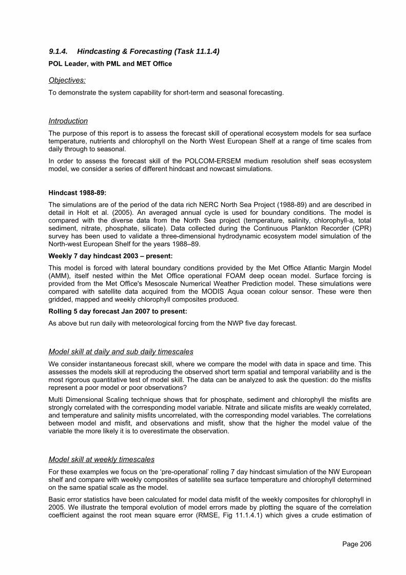
9.1.4. Hindcasting & Forecasting (Task 11.1.4)POL Leader, with PML and MET Office

Objectives:To demonstrate the system capability for short-term and seasonal forecasting.

IntroductionThe purpose of this report is to assess the forecast skill of operational ecosystem models for sea surfacetemperature, nutrients and chlorophyll on the North West European Shelf at a range of time scales fromdaily through to seasonal.

In order to assess the forecast skill of the POLCOM-ERSEM medium resolution shelf seas ecosystemmodel, we consider a series of different hindcast and nowcast simulations.

Hindcast 1988-89:

The simulations are of the period of the data rich NERC North Sea Project (1988-89) and are described indetail in Holt et al. (2005). An averaged annual cycle is used for boundary conditions. The model iscompared with the diverse data from the North Sea project (temperature, salinity, chlorophyll-a, totalsediment, nitrate, phosphate, silicate). Data collected during the Continuous Plankton Recorder (CPR)survey has been used to validate a three-dimensional hydrodynamic ecosystem model simulation of theNorth-west European Shelf for the years 1988–89.

Weekly 7 day hindcast 2003 – present:

This model is forced with lateral boundary conditions provided by the Met Office Atlantic Margin Model(AMM), itself nested within the Met Office operational FOAM deep ocean model. Surface forcing isprovided from the Met Office's Mesoscale Numerical Weather Prediction model. These simulations werecompared with satellite data acquired from the MODIS Aqua ocean colour sensor. These were thengridded, mapped and weekly chlorophyll composites produced.

Rolling 5 day forecast Jan 2007 to present:

As above but run daily with meteorological forcing from the NWP five day forecast.

Model skill at daily and sub daily timescalesWe consider instantaneous forecast skill, where we compare the model with data in space and time. Thisassesses the models skill at reproducing the observed short term spatial and temporal variability and is themost rigorous quantitative test of model skill. The data can be analyzed to ask the question: do the misfitsrepresent a poor model or poor observations?

Multi Dimensional Scaling technique shows that for phosphate, sediment and chlorophyll the misfits arestrongly correlated with the corresponding model variable. Nitrate and silicate misfits are weakly correlated,and temperature and salinity misfits uncorrelated, with the corresponding model variables. The correlationsbetween model and misfit, and observations and misfit, show that the higher the model value of thevariable the more likely it is to overestimate the observation.

Model skill at weekly timescalesFor these examples we focus on the ‘pre-operational’ rolling 7 day hindcast simulation of the NW Europeanshelf and compare with weekly composites of satellite sea surface temperature and chlorophyll determinedon the same spatial scale as the model.

Basic error statistics have been calculated for model data misfit of the weekly composites for chlorophyll in2005. We illustrate the temporal evolution of model errors made by plotting the square of the correlationcoefficient against the root mean square error (RMSE, Fig 11.1.4.1) which gives a crude estimation of

Page 206

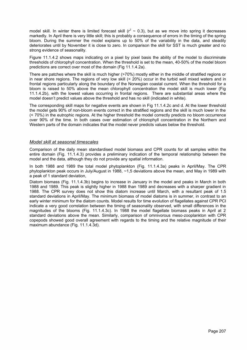
model skill. In winter there is limited forecast skill (r2 ~ 0.3), but as we move into spring it decreasesmarkedly. In April there is very little skill; this is probably a consequence of errors in the timing of the springbloom. During the summer the model explains up to 50% of the variability in the data, and steadilydeteriorates until by November it is close to zero. In comparison the skill for SST is much greater and nostrong evidence of seasonality.

Figure 11.1.4.2 shows maps indicating on a pixel by pixel basis the ability of the model to discriminatethresholds of chlorophyll concentration. When the threshold is set to the mean, 40-50% of the model bloompredictions are correct over most of the domain (Fig 11.1.4.2a).

There are patches where the skill is much higher (>70%) mostly either in the middle of stratified regions orin near shore regions. The regions of very low skill (< 20%) occur in the turbid well mixed waters and infrontal regions particularly along the boundary of the Norwegian coastal current. When the threshold for abloom is raised to 50% above the mean chlorophyll concentration the model skill is much lower (Fig11.1.4.2b), with the lowest values occurring in frontal regions. There are substantial areas where themodel doesn’t predict values above the threshold and has no skill (indicated in white).

The corresponding skill maps for negative events are shown in Fig 11.1.4.2c and d. At the lower thresholdthe model gets 90% of non-bloom events correct in the stratified regions and the skill is much lower in the(< 70%) in the eutrophic regions. At the higher threshold the model correctly predicts no bloom occurrenceover 90% of the time. In both cases over estimation of chlorophyll concentration in the Northern andWestern parts of the domain indicates that the model never predicts values below the threshold.

Model skill at seasonal timescalesComparison of the daily mean standardised model biomass and CPR counts for all samples within theentire domain (Fig. 11.1.4.3) provides a preliminary indication of the temporal relationship between themodel and the data, although they do not provide any spatial information.

In both 1988 and 1989 the total model phytoplankton (Fig. 11.1.4.3a) peaks in April/May. The CPRphytoplankton peak occurs in July/August in 1988, ~1,5 deviations above the mean, and May in 1989 witha peak of 1 standard deviation,Diatom biomass (Fig. 11.1.4.3b) begins to increase in January in the model and peaks in March in both1988 and 1989. This peak is slightly higher in 1988 than 1989 and decreases with a sharper gradient in1988. The CPR survey does not show this diatom increase until March, with a resultant peak of 1.5standard deviations in April/May. The minimum biomass of model diatoms is in summer, in contrast to anearly winter minimum for the diatom counts. Model results for time evolution of flagellates against CPR PCIindicate a very good correlation between the timing of seasonality observed, with small differences in themagnitudes of the blooms (Fig. 11.1.4.3c). In 1988 the model flagellate biomass peaks in April at 2standard deviations above the mean. Similarly, comparison of omnivorous meso-zooplankton with CPRcopepods showed good overall agreement with regards to the timing and the relative magnitude of theirmaximum abundance (Fig. 11.1.4.3d).

Page 207

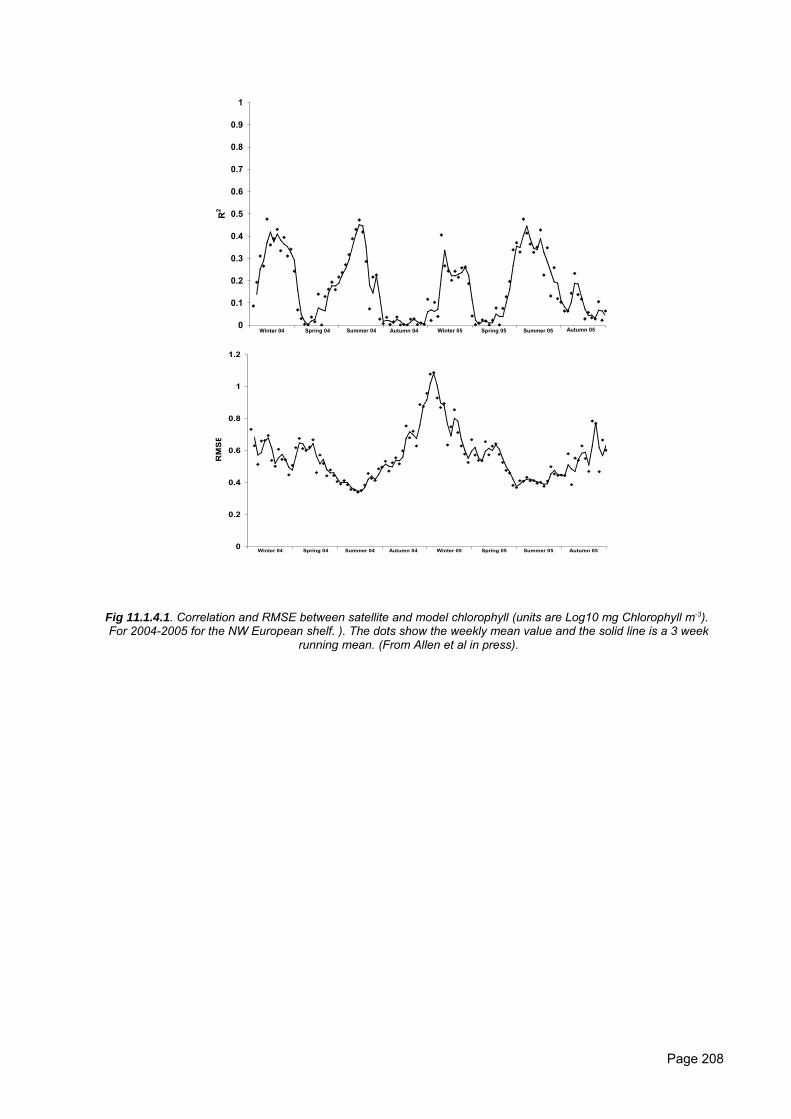
0

0.1

0.2

0.3

0.4

0.5

0.6

0.7

0.8

0.9

1

R2

Winter 04 Winter 05Spring 04 Spring 05Summer 04 Summer 05Autumn 04 Autumn 05

0

0.2

0.4

0.6

0.8

1

1.2

RM

SE

Winter 04 Spring 04 Summer 04 Autumn 04 Winter 05 Spring 05 Summer 05 Autumn 05

Fig 11.1.4.1. Correlation and RMSE between satellite and model chlorophyll (units are Log10 mg Chlorophyll m-3). For 2004-2005 for the NW European shelf. ). The dots show the weekly mean value and the solid line is a 3 week

running mean. (From Allen et al in press).

Page 208

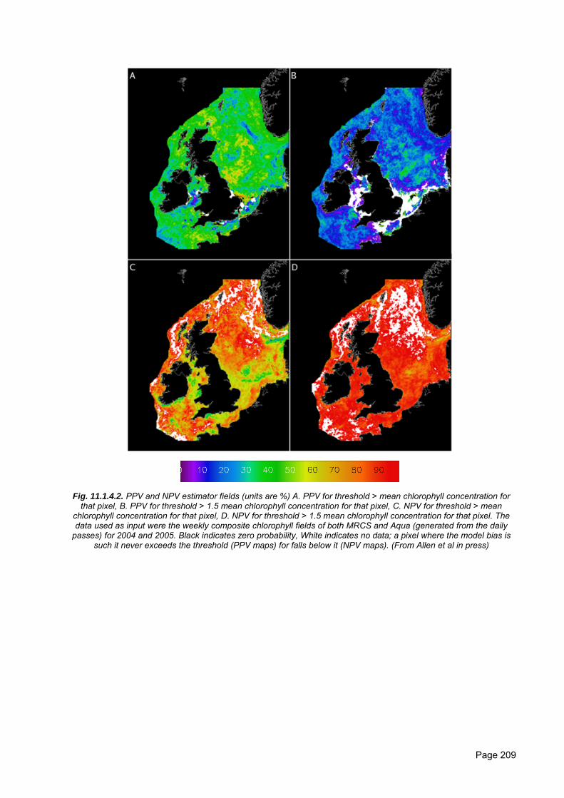
Fig. 11.1.4.2. PPV and NPV estimator fields (units are %) A. PPV for threshold > mean chlorophyll concentration forthat pixel, B. PPV for threshold > 1.5 mean chlorophyll concentration for that pixel, C. NPV for threshold > mean

chlorophyll concentration for that pixel, D. NPV for threshold > 1.5 mean chlorophyll concentration for that pixel. Thedata used as input were the weekly composite chlorophyll fields of both MRCS and Aqua (generated from the daily

passes) for 2004 and 2005. Black indicates zero probability, White indicates no data; a pixel where the model bias issuch it never exceeds the threshold (PPV maps) for falls below it (NPV maps). (From Allen et al in press)

Page 209

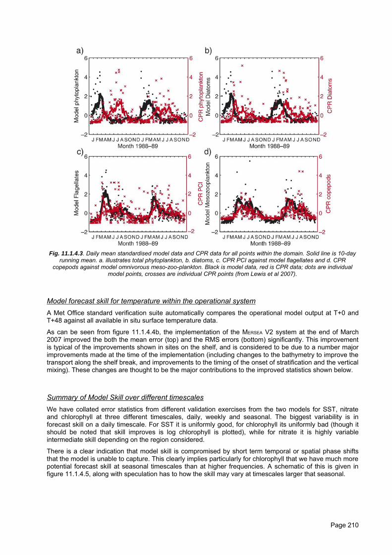
Fig. 11.1.4.3. Daily mean standardised model data and CPR data for all points within the domain. Solid line is 10-dayrunning mean. a. illustrates total phytoplankton, b. diatoms, c. CPR PCI against model flagellates and d. CPR

copepods against model omnivorous meso-zoo-plankton. Black is model data, red is CPR data; dots are individualmodel points, crosses are individual CPR points (from Lewis et al 2007).

Model forecast skill for temperature within the operational systemA Met Office standard verification suite automatically compares the operational model output at T+0 andT+48 against all available in situ surface temperature data.

As can be seen from figure 11.1.4.4b, the implementation of the MERSEA V2 system at the end of March2007 improved the both the mean error (top) and the RMS errors (bottom) significantly. This improvementis typical of the improvements shown in sites on the shelf, and is considered to be due to a number majorimprovements made at the time of the implementation (including changes to the bathymetry to improve thetransport along the shelf break, and improvements to the timing of the onset of stratification and the verticalmixing). These changes are thought to be the major contributions to the improved statistics shown below.

Summary of Model Skill over different timescalesWe have collated error statistics from different validation exercises from the two models for SST, nitrateand chlorophyll at three different timescales, daily, weekly and seasonal. The biggest variability is inforecast skill on a daily timescale. For SST it is uniformly good, for chlorophyll its uniformly bad (though itshould be noted that skill improves is log chlorophyll is plotted), while for nitrate it is highly variableintermediate skill depending on the region considered.

There is a clear indication that model skill is compromised by short term temporal or spatial phase shiftsthat the model is unable to capture. This clearly implies particularly for chlorophyll that we have much morepotential forecast skill at seasonal timescales than at higher frequencies. A schematic of this is given infigure 11.1.4.5, along with speculation has to how the skill may vary at timescales larger that seasonal.

Page 210

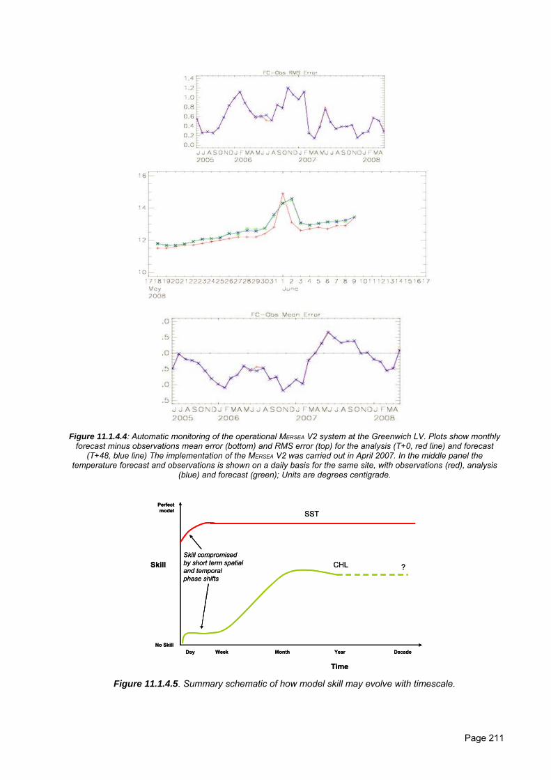
Figure 11.1.4.4: Automatic monitoring of the operational MERSEA V2 system at the Greenwich LV. Plots show monthlyforecast minus observations mean error (bottom) and RMS error (top) for the analysis (T+0, red line) and forecast

(T+48, blue line) The implementation of the MERSEA V2 was carried out in April 2007. In the middle panel thetemperature forecast and observations is shown on a daily basis for the same site, with observations (red), analysis

(blue) and forecast (green); Units are degrees centigrade.

Skill

Time

Day Week Month Year Decade

?

Skill compromised by short term spatial and temporalphase shifts

No Skill

Perfect model SST

CHLSkill

Time

Day Week Month Year Decade

?

Skill compromised by short term spatial and temporalphase shifts

No Skill

Perfect model SST

CHL

Figure 11.1.4.5. Summary schematic of how model skill may evolve with timescale.

Page 211

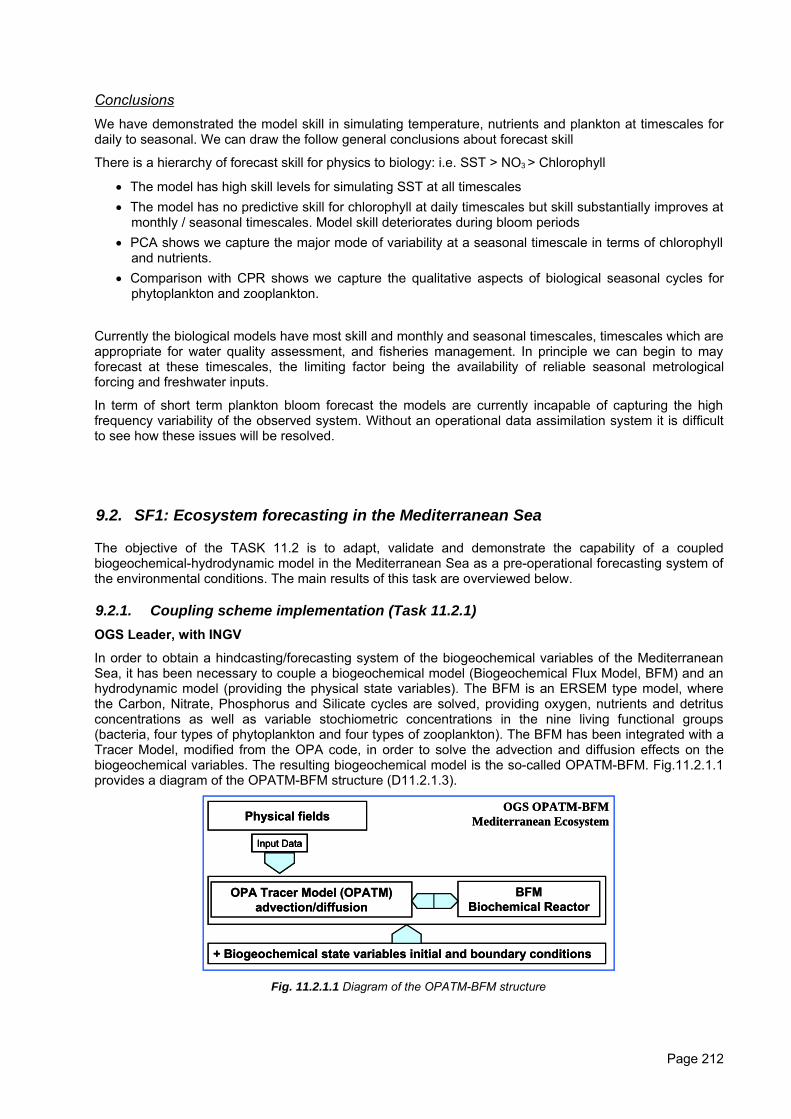
ConclusionsWe have demonstrated the model skill in simulating temperature, nutrients and plankton at timescales fordaily to seasonal. We can draw the follow general conclusions about forecast skill

There is a hierarchy of forecast skill for physics to biology: i.e. SST > NO3 > Chlorophyll

• The model has high skill levels for simulating SST at all timescales• The model has no predictive skill for chlorophyll at daily timescales but skill substantially improves at

monthly / seasonal timescales. Model skill deteriorates during bloom periods• PCA shows we capture the major mode of variability at a seasonal timescale in terms of chlorophyll

and nutrients.• Comparison with CPR shows we capture the qualitative aspects of biological seasonal cycles for

phytoplankton and zooplankton.

Currently the biological models have most skill and monthly and seasonal timescales, timescales which areappropriate for water quality assessment, and fisheries management. In principle we can begin to mayforecast at these timescales, the limiting factor being the availability of reliable seasonal metrologicalforcing and freshwater inputs.

In term of short term plankton bloom forecast the models are currently incapable of capturing the highfrequency variability of the observed system. Without an operational data assimilation system it is difficultto see how these issues will be resolved.

9.2. SF1: Ecosystem forecasting in the Mediterranean Sea

The objective of the TASK 11.2 is to adapt, validate and demonstrate the capability of a coupledbiogeochemical-hydrodynamic model in the Mediterranean Sea as a pre-operational forecasting system ofthe environmental conditions. The main results of this task are overviewed below.

9.2.1. Coupling scheme implementation (Task 11.2.1)OGS Leader, with INGV

In order to obtain a hindcasting/forecasting system of the biogeochemical variables of the MediterraneanSea, it has been necessary to couple a biogeochemical model (Biogeochemical Flux Model, BFM) and anhydrodynamic model (providing the physical state variables). The BFM is an ERSEM type model, wherethe Carbon, Nitrate, Phosphorus and Silicate cycles are solved, providing oxygen, nutrients and detritusconcentrations as well as variable stochiometric concentrations in the nine living functional groups(bacteria, four types of phytoplankton and four types of zooplankton). The BFM has been integrated with aTracer Model, modified from the OPA code, in order to solve the advection and diffusion effects on thebiogeochemical variables. The resulting biogeochemical model is the so-called OPATM-BFM. Fig.11.2.1.1provides a diagram of the OPATM-BFM structure (D11.2.1.3).

OPA Tracer Model (OPATM)advection/diffusion

BFMBiochemical Reactor

Input Data

+ Biogeochemical state variables initial and boundary conditions

Physical fieldsOGS OPATM-BFM

Mediterranean Ecosystem

OPA Tracer Model (OPATM)advection/diffusion

BFMBiochemical Reactor

Input DataInput Data

+ Biogeochemical state variables initial and boundary conditions

Physical fieldsOGS OPATM-BFM

Mediterranean Ecosystem

Fig. 11.2.1.1 Diagram of the OPATM-BFM structure

Page 212

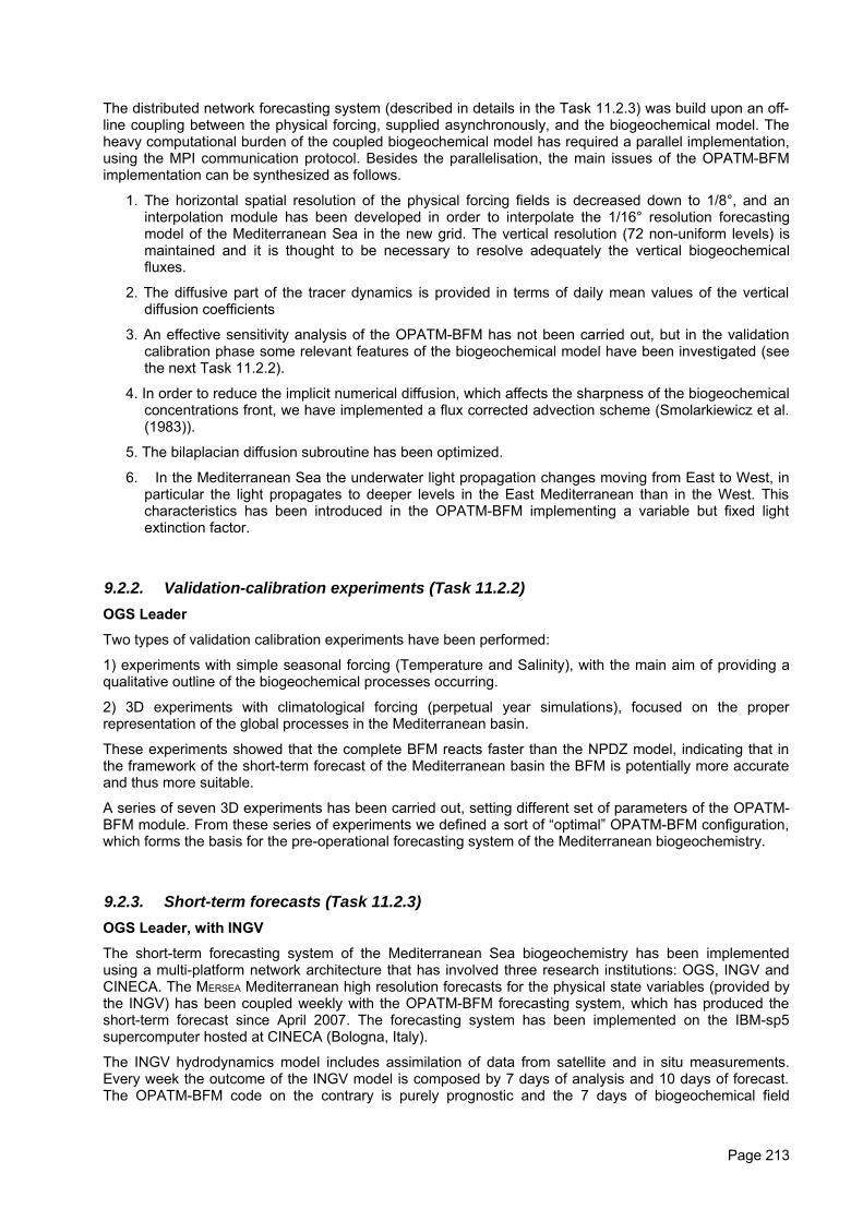
The distributed network forecasting system (described in details in the Task 11.2.3) was build upon an off-line coupling between the physical forcing, supplied asynchronously, and the biogeochemical model. Theheavy computational burden of the coupled biogeochemical model has required a parallel implementation,using the MPI communication protocol. Besides the parallelisation, the main issues of the OPATM-BFMimplementation can be synthesized as follows.

1. The horizontal spatial resolution of the physical forcing fields is decreased down to 1/8°, and aninterpolation module has been developed in order to interpolate the 1/16° resolution forecastingmodel of the Mediterranean Sea in the new grid. The vertical resolution (72 non-uniform levels) ismaintained and it is thought to be necessary to resolve adequately the vertical biogeochemicalfluxes.

2. The diffusive part of the tracer dynamics is provided in terms of daily mean values of the verticaldiffusion coefficients

3. An effective sensitivity analysis of the OPATM-BFM has not been carried out, but in the validationcalibration phase some relevant features of the biogeochemical model have been investigated (seethe next Task 11.2.2).

4. In order to reduce the implicit numerical diffusion, which affects the sharpness of the biogeochemicalconcentrations front, we have implemented a flux corrected advection scheme (Smolarkiewicz et al.(1983)).

5. The bilaplacian diffusion subroutine has been optimized.

6. In the Mediterranean Sea the underwater light propagation changes moving from East to West, inparticular the light propagates to deeper levels in the East Mediterranean than in the West. Thischaracteristics has been introduced in the OPATM-BFM implementing a variable but fixed lightextinction factor.

9.2.2. Validation-calibration experiments (Task 11.2.2)OGS Leader

Two types of validation calibration experiments have been performed:

1) experiments with simple seasonal forcing (Temperature and Salinity), with the main aim of providing aqualitative outline of the biogeochemical processes occurring.

2) 3D experiments with climatological forcing (perpetual year simulations), focused on the properrepresentation of the global processes in the Mediterranean basin.

These experiments showed that the complete BFM reacts faster than the NPDZ model, indicating that inthe framework of the short-term forecast of the Mediterranean basin the BFM is potentially more accurateand thus more suitable.

A series of seven 3D experiments has been carried out, setting different set of parameters of the OPATM-BFM module. From these series of experiments we defined a sort of “optimal” OPATM-BFM configuration,which forms the basis for the pre-operational forecasting system of the Mediterranean biogeochemistry.

9.2.3. Short-term forecasts (Task 11.2.3)OGS Leader, with INGV

The short-term forecasting system of the Mediterranean Sea biogeochemistry has been implementedusing a multi-platform network architecture that has involved three research institutions: OGS, INGV andCINECA. The MERSEA Mediterranean high resolution forecasts for the physical state variables (provided bythe INGV) has been coupled weekly with the OPATM-BFM forecasting system, which has produced theshort-term forecast since April 2007. The forecasting system has been implemented on the IBM-sp5supercomputer hosted at CINECA (Bologna, Italy).

The INGV hydrodynamics model includes assimilation of data from satellite and in situ measurements.Every week the outcome of the INGV model is composed by 7 days of analysis and 10 days of forecast.The OPATM-BFM code on the contrary is purely prognostic and the 7 days of biogeochemical field

Page 213

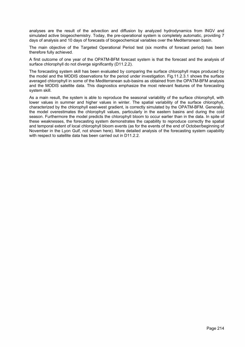
analyses are the result of the advection and diffusion by analyzed hydrodynamics from INGV andsimulated active biogeochemistry. Today, the pre-operational system is completely automatic, providing 7days of analysis and 10 days of forecasts of biogeochemical variables over the Mediterranean basin.

The main objective of the Targeted Operational Period test (six months of forecast period) has beentherefore fully achieved.

A first outcome of one year of the OPATM-BFM forecast system is that the forecast and the analysis ofsurface chlorophyll do not diverge significantly (D11.2.2).

The forecasting system skill has been evaluated by comparing the surface chlorophyll maps produced bythe model and the MODIS observations for the period under investigation. Fig.11.2.3.1 shows the surfaceaveraged chlorophyll in some of the Mediterranean sub-basins as obtained from the OPATM-BFM analysisand the MODIS satellite data. This diagnostics emphasize the most relevant features of the forecastingsystem skill.

As a main result, the system is able to reproduce the seasonal variability of the surface chlorophyll, withlower values in summer and higher values in winter. The spatial variability of the surface chlorophyll,characterized by the chlorophyll east-west gradient, is correctly simulated by the OPATM-BFM. Generally,the model overestimates the chlorophyll values, particularly in the eastern basins and during the coldseason. Furthermore the model predicts the chlorophyll bloom to occur earlier than in the data. In spite ofthese weaknesses, the forecasting system demonstrates the capability to reproduce correctly the spatialand temporal extent of local chlorophyll bloom events (as for the events of the end of October/beginning ofNovember in the Lyon Gulf, not shown here). More detailed analysis of the forecasting system capabilitywith respect to satellite data has been carried out in D11.2.2.

Page 214

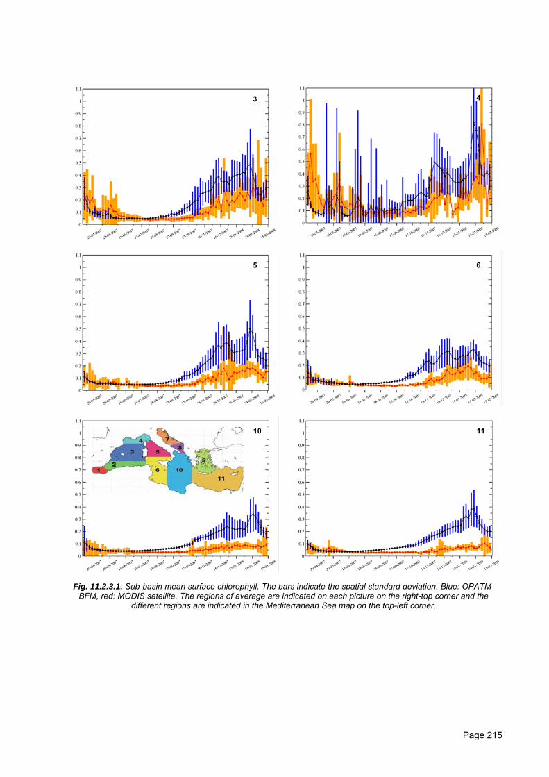
33 44

55 66

101010 1111

Fig. 11.2.3.1. Sub-basin mean surface chlorophyll. The bars indicate the spatial standard deviation. Blue: OPATM-BFM, red: MODIS satellite. The regions of average are indicated on each picture on the right-top corner and the

different regions are indicated in the Mediterranean Sea map on the top-left corner.

Page 215

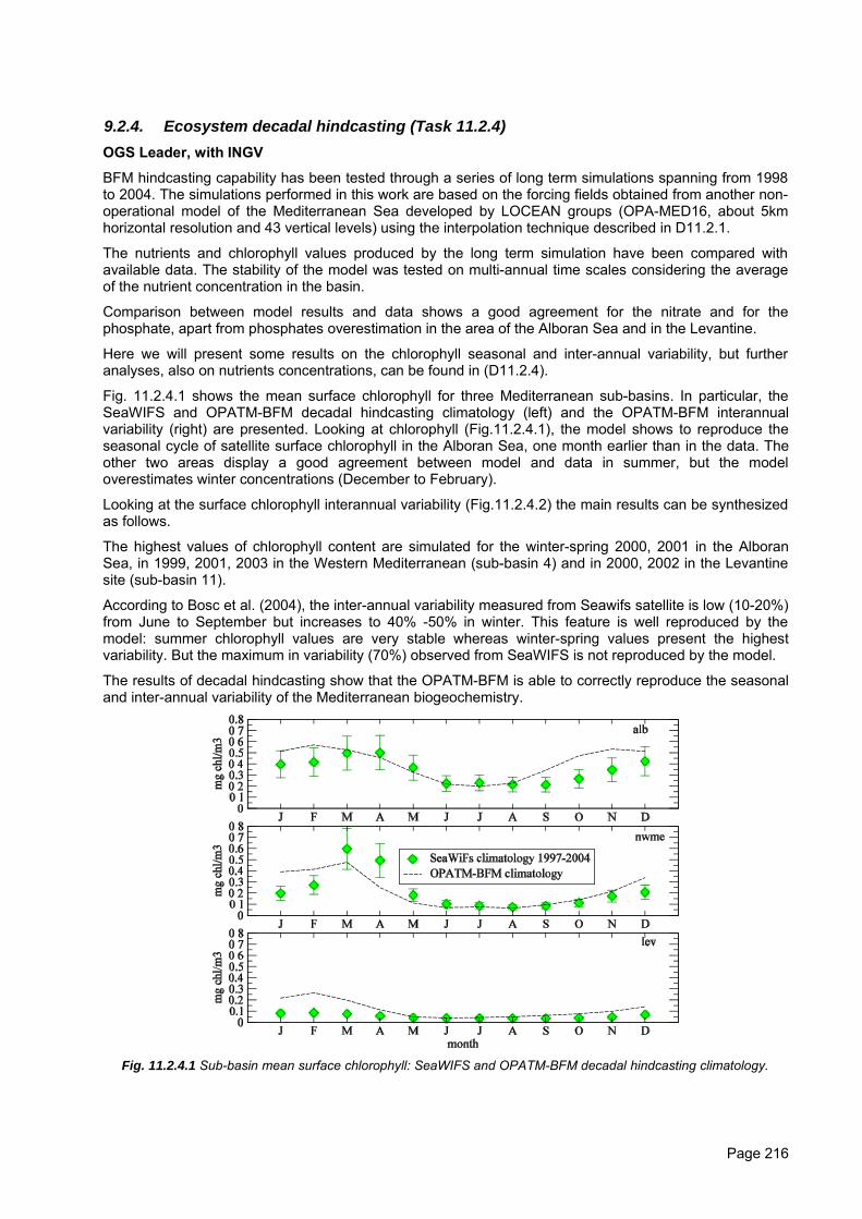
9.2.4. Ecosystem decadal hindcasting (Task 11.2.4)OGS Leader, with INGV

BFM hindcasting capability has been tested through a series of long term simulations spanning from 1998to 2004. The simulations performed in this work are based on the forcing fields obtained from another non-operational model of the Mediterranean Sea developed by LOCEAN groups (OPA-MED16, about 5kmhorizontal resolution and 43 vertical levels) using the interpolation technique described in D11.2.1.

The nutrients and chlorophyll values produced by the long term simulation have been compared withavailable data. The stability of the model was tested on multi-annual time scales considering the averageof the nutrient concentration in the basin.

Comparison between model results and data shows a good agreement for the nitrate and for thephosphate, apart from phosphates overestimation in the area of the Alboran Sea and in the Levantine.

Here we will present some results on the chlorophyll seasonal and inter-annual variability, but furtheranalyses, also on nutrients concentrations, can be found in (D11.2.4).

Fig. 11.2.4.1 shows the mean surface chlorophyll for three Mediterranean sub-basins. In particular, theSeaWIFS and OPATM-BFM decadal hindcasting climatology (left) and the OPATM-BFM interannualvariability (right) are presented. Looking at chlorophyll (Fig.11.2.4.1), the model shows to reproduce theseasonal cycle of satellite surface chlorophyll in the Alboran Sea, one month earlier than in the data. Theother two areas display a good agreement between model and data in summer, but the modeloverestimates winter concentrations (December to February).

Looking at the surface chlorophyll interannual variability (Fig.11.2.4.2) the main results can be synthesizedas follows.

The highest values of chlorophyll content are simulated for the winter-spring 2000, 2001 in the AlboranSea, in 1999, 2001, 2003 in the Western Mediterranean (sub-basin 4) and in 2000, 2002 in the Levantinesite (sub-basin 11).

According to Bosc et al. (2004), the inter-annual variability measured from Seawifs satellite is low (10-20%)from June to September but increases to 40% -50% in winter. This feature is well reproduced by themodel: summer chlorophyll values are very stable whereas winter-spring values present the highestvariability. But the maximum in variability (70%) observed from SeaWIFS is not reproduced by the model.

The results of decadal hindcasting show that the OPATM-BFM is able to correctly reproduce the seasonaland inter-annual variability of the Mediterranean biogeochemistry.

Fig. 11.2.4.1 Sub-basin mean surface chlorophyll: SeaWIFS and OPATM-BFM decadal hindcasting climatology.

Page 216

Figure 11.2.4.2 Sub-basin mean surface chlorophyll: OPATM-BFM interannual variability.

9.3. SF2: seasonal forecasting

9.3.1. Development of interpolation package, MERSEA ¼ and coupled models installation(Task 11.3)

MF Leader, with ECMWF and INGV

The objective of this task was to prepare the tools and model data necessary for an efficient execution ofthe core part of the Special Focus Experiment 2. More specifically, the following objectives have beenpursued:

• To produce 10 year long MERSEA ¼and ORCA2 simulations (Task 11.3.1, MERCATOR).• To prepare the interpolation package for interpolating MERSEA ¼model fields into lower resolution

ocean models and make available the MERSEA1-1/4 degree fields (Task 11.3.1, MF).• To install a parallelised version of the MERSEA1/4 model on partners' machines (Task 11.3.2,

MERCATOR, ECMWF, MF, INGV).• To install the coupled models using the ORCA2 and the high resolution atmospheric models (Task

11.3.3, ECMWF, MF, INGV).• To install the coupled models using the MERSEA1-¼ model (Task 11.3.4, ECMWF, MF, INGV).

10 year long MERSEA ¼and ORCA2 simulations and interpolation package MERSEA ¼-ORCA2(Task 11.3.1):Several 10 years long MERSEA ¼ and ORCA2 simulations have been produced by MERCATOR. Thesesimulations have been carried out using the OPA8.2 ocean code, forced by ERA40 atmospheric fluxes andstrongly relaxed toward Reynolds SST through a specific nudging procedure. The figure 11.3.1 belowillustrates how MERSEA ¼° SST filed is split into small and large scale components. Only the SST largescale component is modified by the nudging whereas the small scale remains unchanged.

An interpolation package together with interpolated restart files have been produced by MF. Because onewanted to go from a high to a low resolution, a remapping. The interpolation package from the OASIScoupler (used to couple ocean and atmosphere in the following tasks) has been chosen. The 3Dinterpolation has been carried out in 2 steps. First, considering each vertical levels of the source grid, 2Dhorizontal interpolation has been performed to the target grid. Second, vertical interpolation has been donefrom the source to the target grid, taking into account the same remapping technique (from 46 to 31vertical levels). The interpolated fields are shown in Fig. 11.3.2.

Page 217

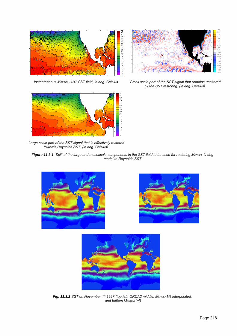
Instantaneous MERSEA -1/4° SST field, in deg. Celsius. Small scale part of the SST signal that remains unalteredby the SST restoring. (in deg. Celsius).

Large scale part of the SST signal that is effectively restoredtowards Reynolds SST. (in deg. Celsius).

Figure 11.3.1 Split of the large and mesoscale components in the SST field to be used for restoring MERSEA ¼ degmodel to Reynolds SST

Fig. 11.3.2 SST on November 1st 1997 (top left: ORCA2,middle: MERSEA1/4 interpolated, and bottom MERSEA1/4)

Page 218

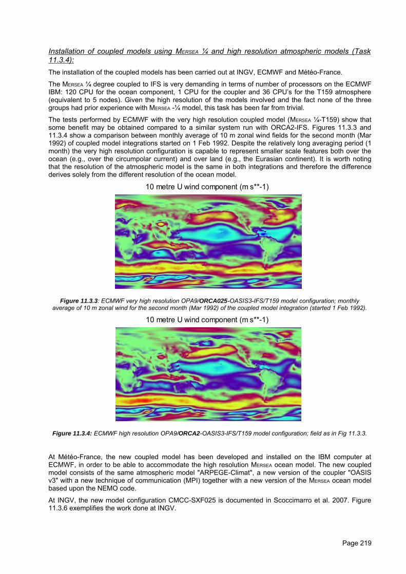
Installation of coupled models using MERSEA ¼ and high resolution atmospheric models (Task11.3.4):The installation of the coupled models has been carried out at INGV, ECMWF and Météo-France.

The MERSEA ¼ degree coupled to IFS is very demanding in terms of number of processors on the ECMWFIBM: 120 CPU for the ocean component, 1 CPU for the coupler and 36 CPU’s for the T159 atmosphere(equivalent to 5 nodes). Given the high resolution of the models involved and the fact none of the threegroups had prior experience with MERSEA -¼ model, this task has been far from trivial.

The tests performed by ECMWF with the very high resolution coupled model (MERSEA ¼-T159) show thatsome benefit may be obtained compared to a similar system run with ORCA2-IFS. Figures 11.3.3 and11.3.4 show a comparison between monthly average of 10 m zonal wind fields for the second month (Mar1992) of coupled model integrations started on 1 Feb 1992. Despite the relatively long averaging period (1month) the very high resolution configuration is capable to represent smaller scale features both over theocean (e.g., over the circumpolar current) and over land (e.g., the Eurasian continent). It is worth notingthat the resolution of the atmospheric model is the same in both integrations and therefore the differencederives solely from the different resolution of the ocean model.

10 metre U wind component (m s**-1)

Figure 11.3.3: ECMWF very high resolution OPA9/ORCA025-OASIS3-IFS/T159 model configuration; monthlyaverage of 10 m zonal wind for the second month (Mar 1992) of the coupled model integration (started 1 Feb 1992).

10 metre U wind component (m s**-1)

Figure 11.3.4: ECMWF high resolution OPA9/ORCA2-OASIS3-IFS/T159 model configuration; field as in Fig 11.3.3.

At Météo-France, the new coupled model has been developed and installed on the IBM computer atECMWF, in order to be able to accommodate the high resolution MERSEA ocean model. The new coupledmodel consists of the same atmospheric model "ARPEGE-Climat", a new version of the coupler "OASISv3" with a new technique of communication (MPI) together with a new version of the MERSEA ocean modelbased upon the NEMO code.

At INGV, the new model configuration CMCC-SXF025 is documented in Scoccimarro et al. 2007. Figure11.3.6 exemplifies the work done at INGV.

Page 219

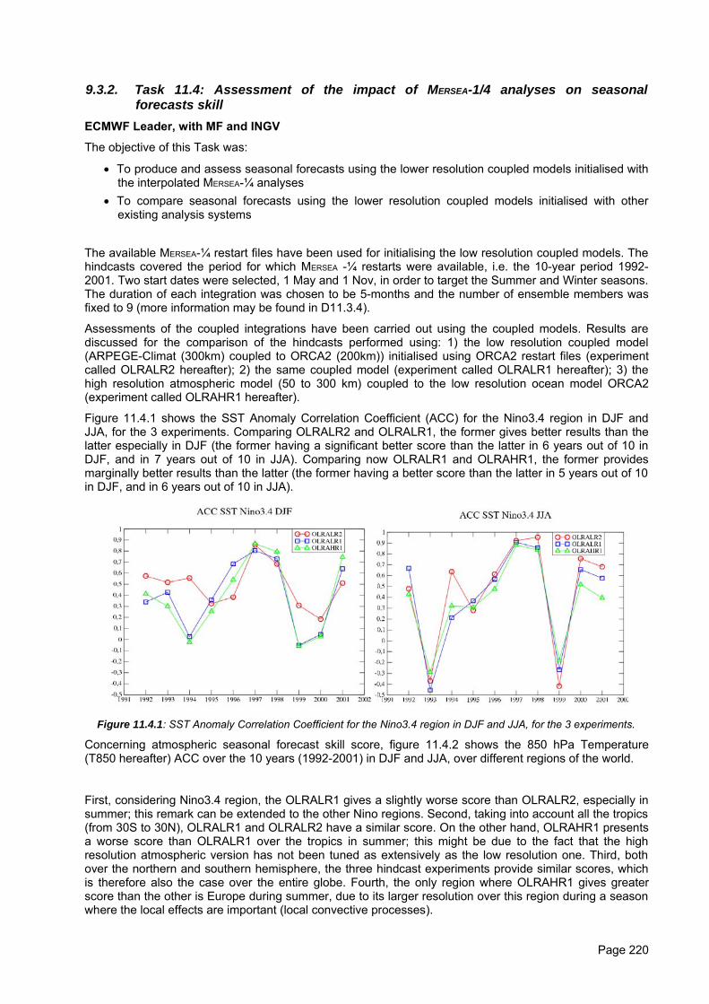
9.3.2. Task 11.4: Assessment of the impact of MERSEA-1/4 analyses on seasonalforecasts skill

ECMWF Leader, with MF and INGV

The objective of this Task was:

• To produce and assess seasonal forecasts using the lower resolution coupled models initialised withthe interpolated MERSEA-¼ analyses

• To compare seasonal forecasts using the lower resolution coupled models initialised with otherexisting analysis systems

The available MERSEA-¼ restart files have been used for initialising the low resolution coupled models. Thehindcasts covered the period for which MERSEA -¼ restarts were available, i.e. the 10-year period 1992-2001. Two start dates were selected, 1 May and 1 Nov, in order to target the Summer and Winter seasons.The duration of each integration was chosen to be 5-months and the number of ensemble members wasfixed to 9 (more information may be found in D11.3.4).

Assessments of the coupled integrations have been carried out using the coupled models. Results arediscussed for the comparison of the hindcasts performed using: 1) the low resolution coupled model(ARPEGE-Climat (300km) coupled to ORCA2 (200km)) initialised using ORCA2 restart files (experimentcalled OLRALR2 hereafter); 2) the same coupled model (experiment called OLRALR1 hereafter); 3) thehigh resolution atmospheric model (50 to 300 km) coupled to the low resolution ocean model ORCA2(experiment called OLRAHR1 hereafter).

Figure 11.4.1 shows the SST Anomaly Correlation Coefficient (ACC) for the Nino3.4 region in DJF andJJA, for the 3 experiments. Comparing OLRALR2 and OLRALR1, the former gives better results than thelatter especially in DJF (the former having a significant better score than the latter in 6 years out of 10 inDJF, and in 7 years out of 10 in JJA). Comparing now OLRALR1 and OLRAHR1, the former providesmarginally better results than the latter (the former having a better score than the latter in 5 years out of 10in DJF, and in 6 years out of 10 in JJA).

Figure 11.4.1: SST Anomaly Correlation Coefficient for the Nino3.4 region in DJF and JJA, for the 3 experiments.

Concerning atmospheric seasonal forecast skill score, figure 11.4.2 shows the 850 hPa Temperature(T850 hereafter) ACC over the 10 years (1992-2001) in DJF and JJA, over different regions of the world.

First, considering Nino3.4 region, the OLRALR1 gives a slightly worse score than OLRALR2, especially insummer; this remark can be extended to the other Nino regions. Second, taking into account all the tropics(from 30S to 30N), OLRALR1 and OLRALR2 have a similar score. On the other hand, OLRAHR1 presentsa worse score than OLRALR1 over the tropics in summer; this might be due to the fact that the highresolution atmospheric version has not been tuned as extensively as the low resolution one. Third, bothover the northern and southern hemisphere, the three hindcast experiments provide similar scores, whichis therefore also the case over the entire globe. Fourth, the only region where OLRAHR1 gives greaterscore than the other is Europe during summer, due to its larger resolution over this region during a seasonwhere the local effects are important (local convective processes).

Page 220

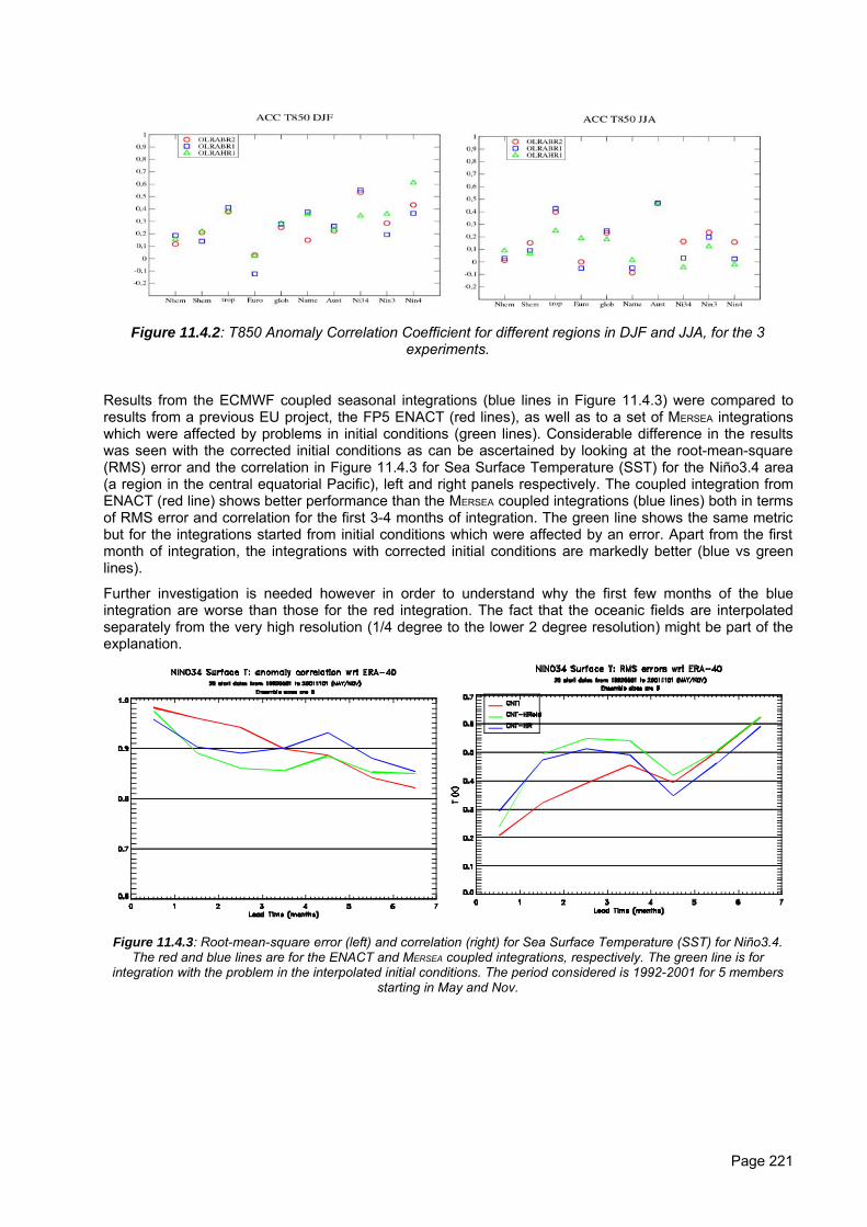
Figure 11.4.2: T850 Anomaly Correlation Coefficient for different regions in DJF and JJA, for the 3

experiments.

Results from the ECMWF coupled seasonal integrations (blue lines in Figure 11.4.3) were compared toresults from a previous EU project, the FP5 ENACT (red lines), as well as to a set of MERSEA integrationswhich were affected by problems in initial conditions (green lines). Considerable difference in the resultswas seen with the corrected initial conditions as can be ascertained by looking at the root-mean-square(RMS) error and the correlation in Figure 11.4.3 for Sea Surface Temperature (SST) for the Niño3.4 area(a region in the central equatorial Pacific), left and right panels respectively. The coupled integration fromENACT (red line) shows better performance than the MERSEA coupled integrations (blue lines) both in termsof RMS error and correlation for the first 3-4 months of integration. The green line shows the same metricbut for the integrations started from initial conditions which were affected by an error. Apart from the firstmonth of integration, the integrations with corrected initial conditions are markedly better (blue vs greenlines).

Further investigation is needed however in order to understand why the first few months of the blueintegration are worse than those for the red integration. The fact that the oceanic fields are interpolatedseparately from the very high resolution (1/4 degree to the lower 2 degree resolution) might be part of theexplanation.

Figure 11.4.3: Root-mean-square error (left) and correlation (right) for Sea Surface Temperature (SST) for Niño3.4.The red and blue lines are for the ENACT and MERSEA coupled integrations, respectively. The green line is for

integration with the problem in the interpolated initial conditions. The period considered is 1992-2001 for 5 membersstarting in May and Nov.

Page 221

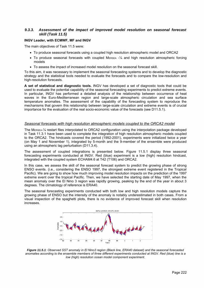
9.3.3. Assessment of the impact of improved model resolution on seasonal forecastskill (Task 11.5)

INGV Leader, with ECMWF, MF and INGV

The main objectives of Task 11.5 were:

• To produce seasonal forecasts using a coupled high resolution atmospheric model and ORCA2• To produce seasonal forecasts with coupled MERSEA -¼ and high resolution atmospheric forcing

models• To assess the impact of increased model resolution on the seasonal forecast skill.

To this aim, it was necessary to implement the seasonal forecasting systems and to develop the diagnosticstrategy and the statistical tools needed to evaluate the forecasts and to compare the low-resolution andhigh-resolution forecasts.

A set of statistical and diagnostic tools. INGV has developed a set of diagnostic tools that could beused to evaluate the potential capability of the seasonal forecasting experiments to predict extreme events.In particular, INGV has performed a detailed analysis of the relationship between occurrence of heatwaves in the Euro-Mediterranean region and large-scale atmospheric circulation and sea surfacetemperature anomalies. The assessment of the capability of the forecasting system to reproduce themechanisms that govern this relationship between large-scale circulation and extreme events is of crucialimportance for the evaluation of the real socio-economic value of the forecasts (see D11.5.1).

Seasonal forecasts with high resolution atmospheric models coupled to the ORCA2 modelThe MERSEA-¼ restart files interpolated to ORCA2 configuration using the interpolation package developedin Task 11.3.1 have been used to complete the integration of high resolution atmospheric models coupledto the ORCA2. The hindcasts covered the period (1992-2001), experiments were initialized twice a year(on May 1 and November 1), integrated by 5-month and the 9-member of the ensemble were producedusing an atmospheric lag perturbation (D11.3.4).

The assessment of coupled integrations is presented below. Figure 11.5.1 display three seasonalforecasting experiments conducted at INGV. Red (blue) experiment is a low (high) resolution hindcast,integrated with the coupled system ECHAM4.6 at T42 (T106) and ORCA2.

In this case, we assess the skill of the seasonal forecast system to predict the growing phase of strongENSO events. (i.e., considering the ENSO 1997, the strongest extreme event registered in the TropicalPacific). We are going to show how much improving model resolution impacts on the prediction of the 1997extreme event over the tropical Pacific. Then, we have selected the starting date of May 1997, when themean anomaly over the El Nino 3 region was rapidly growing, peaking by the end of the year in about 3degrees. The climatology of reference is ERA40.

The seasonal forecasting experiments conducted with both low and high resolution models capture thegrowing phase of ENSO but the intensity of the anomaly is notably underestimated in both cases. From avisual inspection of the spaghetti plots, there is no evidence of improved forecast skill when resolutionincreases.

Figure 11.5.1: Observed SST anomaly in El Nino3 region (Black line, ERA40 dataset) and the seasonal forecastedanomalies according to the ensemble members of three different experiments conducted at INGV. Red (blue) line is a

low (high) resolution ocean model component experiment.

Page 222

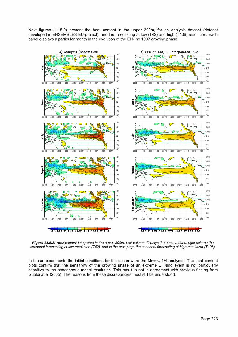
Next figures (11.5.2) present the heat content in the upper 300m, for an analysis dataset (datasetdeveloped in ENSEMBLES EU-project), and the forecasting at low (T42) and high (T106) resolution. Eachpanel displays a particular month in the evolution of the El Nino 1997 growing phase.

Figure 11.5.2: Heat content integrated in the upper 300m. Left column displays the observations, right column theseasonal forecasting at low resolution (T42), and in the next page the seasonal forecasting at high resolution (T106).

In these experiments the initial conditions for the ocean were the MERSEA 1/4 analyses. The heat contentplots confirm that the sensitivity of the growing phase of an extreme El Nino event is not particularlysensitive to the atmospheric model resolution. This result is not in agreement with previous finding fromGualdi at el (2005). The reasons from these discrepancies must still be understood.

Page 223

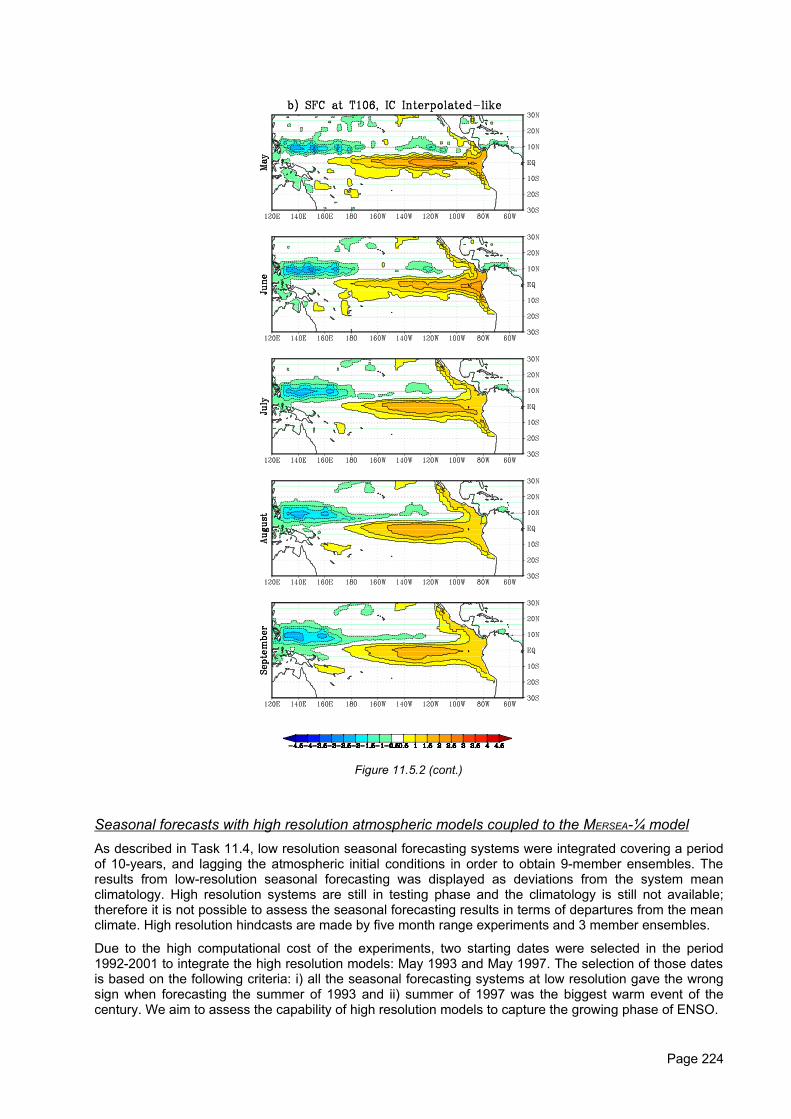
Figure 11.5.2 (cont.)

Seasonal forecasts with high resolution atmospheric models coupled to the MERSEA -¼ modelAs described in Task 11.4, low resolution seasonal forecasting systems were integrated covering a periodof 10-years, and lagging the atmospheric initial conditions in order to obtain 9-member ensembles. Theresults from low-resolution seasonal forecasting was displayed as deviations from the system meanclimatology. High resolution systems are still in testing phase and the climatology is still not available;therefore it is not possible to assess the seasonal forecasting results in terms of departures from the meanclimate. High resolution hindcasts are made by five month range experiments and 3 member ensembles.

Due to the high computational cost of the experiments, two starting dates were selected in the period1992-2001 to integrate the high resolution models: May 1993 and May 1997. The selection of those datesis based on the following criteria: i) all the seasonal forecasting systems at low resolution gave the wrongsign when forecasting the summer of 1993 and ii) summer of 1997 was the biggest warm event of thecentury. We aim to assess the capability of high resolution models to capture the growing phase of ENSO.

Page 224

Ocean initial conditions are the MERSEA ¼ dataset (D11.3.3). Given a starting date, the ocean initialconditions are identical for all the ensemble members while the ensemble spread is generated initializingthe atmospheric component following day-lagged initial conditions.

The results show box averaged values of surface temperature and total precipitation over El Niño 3 and 4regions and over Europe. Surface temperature hindcast are compared with NCEP data and totalprecipitation with Xie-Arkin climatology. All the figures display the seasonal forecasting experiments at highresolution ocean model resolution in top panels and the analogous experiment at low-resolution oceanmodel resolution in bottom panels.

Figure 11.5.3 and 11.5.4 (blue lines) illustrate the capability of the INGV seasonal forecast system topredict the boreal summer climate of 1993. In tropical regions, INGV model is warmer than the observedclimatology. In particular, over El Nino 3 region, the model present a bias of about 1.5 degrees, biaspresent in both, low and high resolution systems. The variability of the surface temperature in El Niño 3region seems to be slightly better represented by the low resolution system, especially at lag 4 and 5months (August and September). Over Europe, the model is somewhat cooler than the NCEP in May andJune. When the summer starts, the hindcast at high resolution produce a relatively warmer climate, whileat low resolution, hindcast compares well with NCEP data.

Regarding the total precipitation (averaged over El Niño 4 region), INGV model underestimates the tropicalprecipitation and this characteristic is particularly notable at high resolution. Nevertheless, the variability ofthe tropical precipitation when the hindcast is conducted at high resolution seems to be more realistic.Over Europe, hindcast at high and low resolution differs little.

Analogous hindcasts conducted by the ECMWF system at low and high resolution are displayed in Figures11.5.3 and 11.5.4 (green lines). The bias of the ECMWF system surface temperature over the tropicalregion is lower than that reported in INGV system, and in the case of the ECMWF system it is a cool bias.As before, the variability of the low levels tropical temperature is somewhat better reproduced by the lowresolution model, while over Europe both systems give similar results, although anomalies at highresolution hindcast seems to be somewhat large during June to August.

Tropical precipitation is better represented over El Nino 4 region than over Europe, where sensitivity toresolution seen to be scarce. Figures 11.5.5 and 11.5.6 show the growing phase of strong ENSO events,as predicted by the ECMWF at low and high resolution. The goal is to determinate if model resolutionimpacts on the prediction of the growing phase of the 1997 extreme event over the tropical Pacific.

Due to the lack of the high resolution climatology, it is hard to evaluate how well the high resolutionexperiment capture the growing phase of ENSO, but a priori, bias decreases at higher resolution overEurope while the variability of tropical surface temperature in both hindcasts is not affected. On the otherhand, over the European sector, hindcast at high resolution seems to perform better that than at lowresolution. Total precipitation over Europe is little sensitive to the model resolution while over El Niño 4region, the high resolution hindcast perform somewhat better than those at low resolution.

Page 225

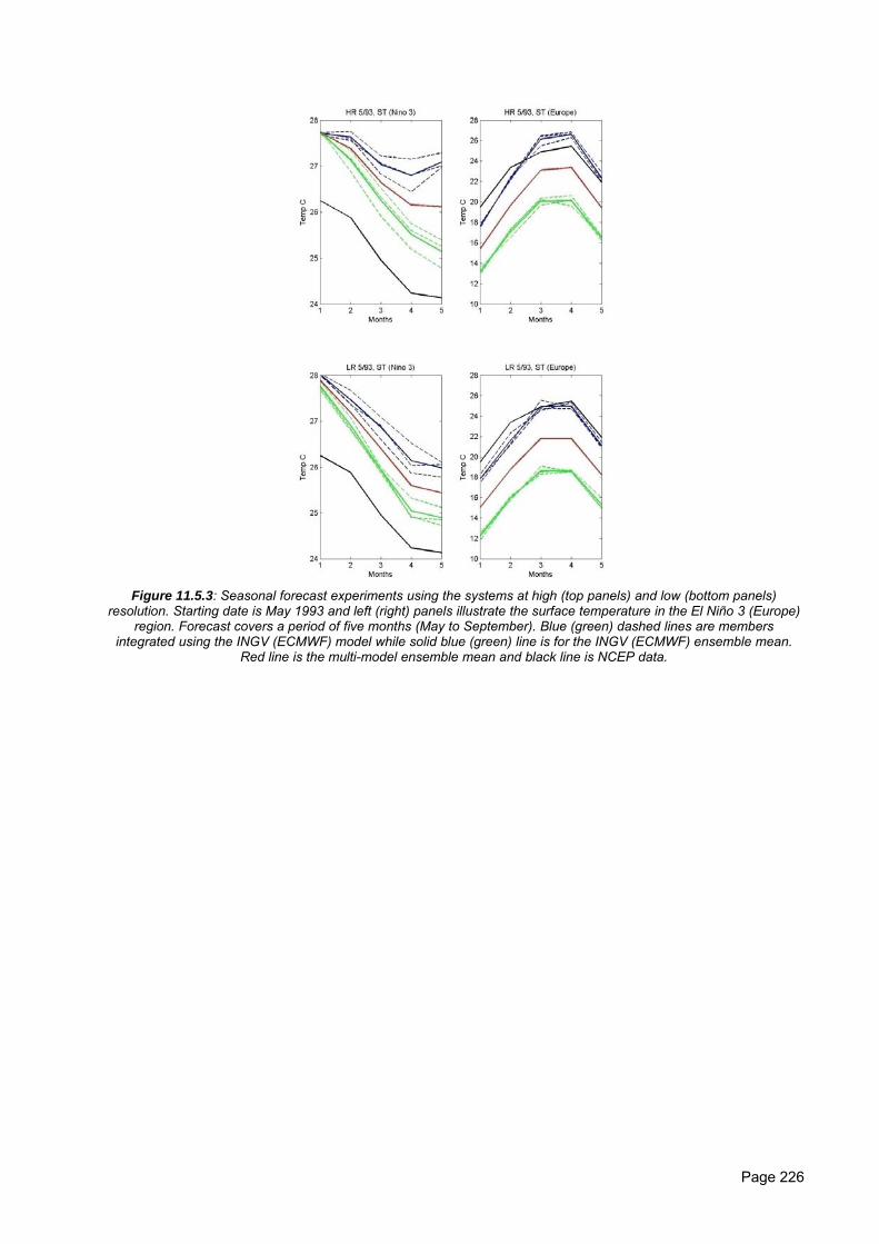
Figure 11.5.3: Seasonal forecast experiments using the systems at high (top panels) and low (bottom panels)resolution. Starting date is May 1993 and left (right) panels illustrate the surface temperature in the El Niño 3 (Europe)

region. Forecast covers a period of five months (May to September). Blue (green) dashed lines are membersintegrated using the INGV (ECMWF) model while solid blue (green) line is for the INGV (ECMWF) ensemble mean.

Red line is the multi-model ensemble mean and black line is NCEP data.

Page 226

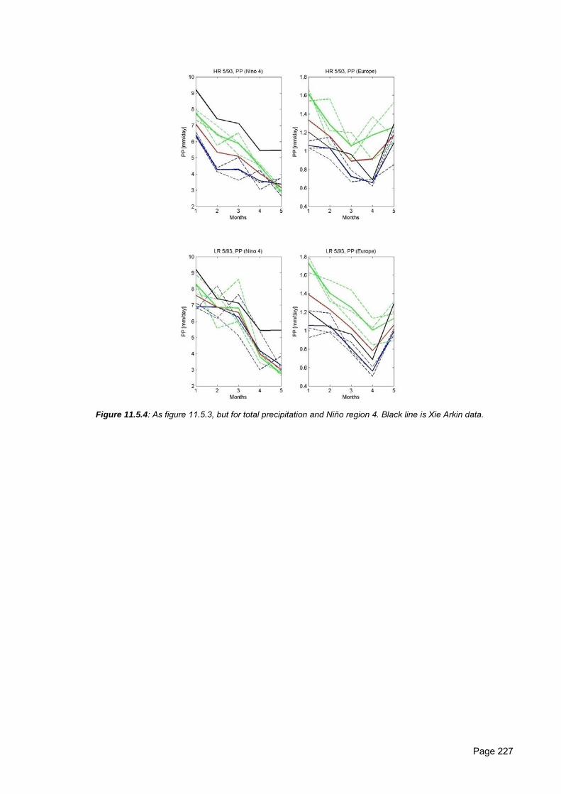
Figure 11.5.4: As figure 11.5.3, but for total precipitation and Niño region 4. Black line is Xie Arkin data.

Page 227

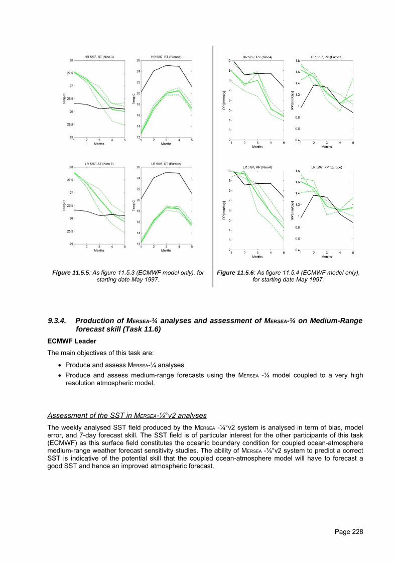
Figure 11.5.5: As figure 11.5.3 (ECMWF model only), forstarting date May 1997.

Figure 11.5.6: As figure 11.5.4 (ECMWF model only),for starting date May 1997.

9.3.4. Production of MERSEA-¼ analyses and assessment of MERSEA-¼ on Medium-Rangeforecast skill (Task 11.6)

ECMWF Leader

The main objectives of this task are:

• Produce and assess MERSEA-¼ analyses• Produce and assess medium-range forecasts using the MERSEA -¼ model coupled to a very high

resolution atmospheric model.

Assessment of the SST in MERSEA -¼°v2 analysesThe weekly analysed SST field produced by the MERSEA -¼°v2 system is analysed in term of bias, modelerror, and 7-day forecast skill. The SST field is of particular interest for the other participants of this task(ECMWF) as this surface field constitutes the oceanic boundary condition for coupled ocean-atmospheremedium-range weather forecast sensitivity studies. The ability of MERSEA -¼°v2 system to predict a correctSST is indicative of the potential skill that the coupled ocean-atmosphere model will have to forecast agood SST and hence an improved atmospheric forecast.

Page 228

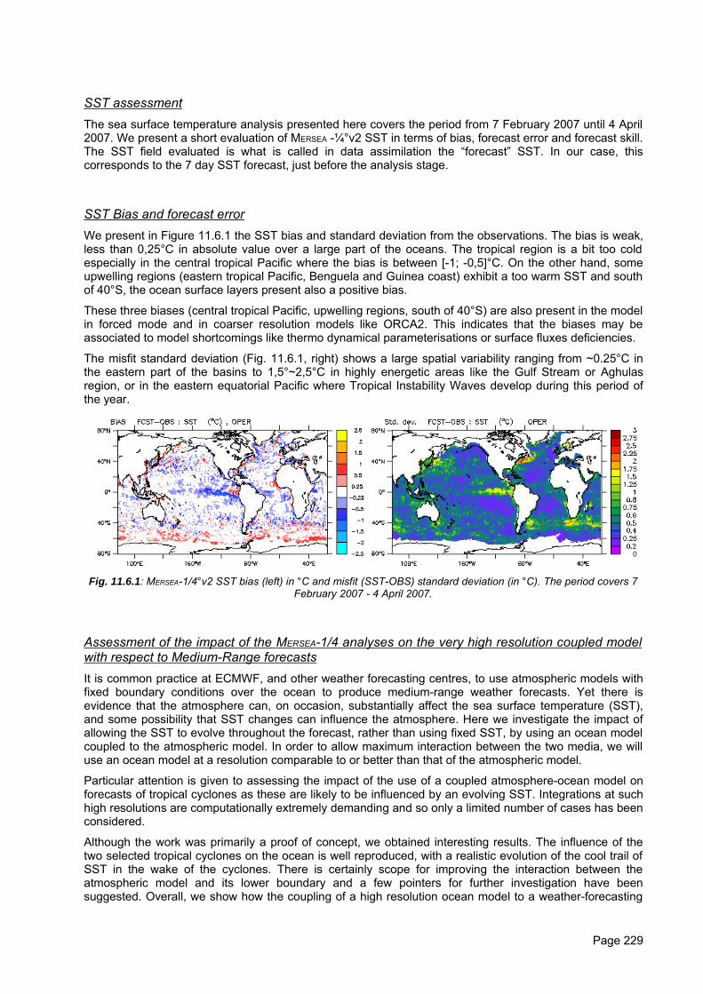
SST assessmentThe sea surface temperature analysis presented here covers the period from 7 February 2007 until 4 April2007. We present a short evaluation of MERSEA -¼°v2 SST in terms of bias, forecast error and forecast skill.The SST field evaluated is what is called in data assimilation the “forecast” SST. In our case, thiscorresponds to the 7 day SST forecast, just before the analysis stage.

SST Bias and forecast errorWe present in Figure 11.6.1 the SST bias and standard deviation from the observations. The bias is weak,less than 0,25°C in absolute value over a large part of the oceans. The tropical region is a bit too coldespecially in the central tropical Pacific where the bias is between [-1; -0,5]°C. On the other hand, someupwelling regions (eastern tropical Pacific, Benguela and Guinea coast) exhibit a too warm SST and southof 40°S, the ocean surface layers present also a positive bias.

These three biases (central tropical Pacific, upwelling regions, south of 40°S) are also present in the modelin forced mode and in coarser resolution models like ORCA2. This indicates that the biases may beassociated to model shortcomings like thermo dynamical parameterisations or surface fluxes deficiencies.

The misfit standard deviation (Fig. 11.6.1, right) shows a large spatial variability ranging from ~0.25°C inthe eastern part of the basins to 1,5°~2,5°C in highly energetic areas like the Gulf Stream or Aghulasregion, or in the eastern equatorial Pacific where Tropical Instability Waves develop during this period ofthe year.

Fig. 11.6.1: MERSEA-1/4°v2 SST bias (left) in °C and misfit (SST-OBS) standard deviation (in °C). The period covers 7February 2007 - 4 April 2007.

Assessment of the impact of the MERSEA -1/4 analyses on the very high resolution coupled modelwith respect to Medium-Range forecastsIt is common practice at ECMWF, and other weather forecasting centres, to use atmospheric models withfixed boundary conditions over the ocean to produce medium-range weather forecasts. Yet there isevidence that the atmosphere can, on occasion, substantially affect the sea surface temperature (SST),and some possibility that SST changes can influence the atmosphere. Here we investigate the impact ofallowing the SST to evolve throughout the forecast, rather than using fixed SST, by using an ocean modelcoupled to the atmospheric model. In order to allow maximum interaction between the two media, we willuse an ocean model at a resolution comparable to or better than that of the atmospheric model.

Particular attention is given to assessing the impact of the use of a coupled atmosphere-ocean model onforecasts of tropical cyclones as these are likely to be influenced by an evolving SST. Integrations at suchhigh resolutions are computationally extremely demanding and so only a limited number of cases has beenconsidered.

Although the work was primarily a proof of concept, we obtained interesting results. The influence of thetwo selected tropical cyclones on the ocean is well reproduced, with a realistic evolution of the cool trail ofSST in the wake of the cyclones. There is certainly scope for improving the interaction between theatmospheric model and its lower boundary and a few pointers for further investigation have beensuggested. Overall, we show how the coupling of a high resolution ocean model to a weather-forecasting

Page 229

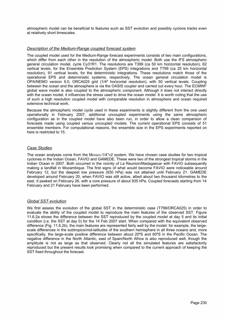
atmospheric model can be beneficial to features such as SST evolution and possibly cyclone tracks evenat relatively short timescales.

Description of the Medium-Range coupled forecast systemThe coupled model used for the Medium-Range forecast experiments consists of two main configurations,which differ from each other in the resolution of the atmospheric model. Both use the IFS atmosphericgeneral circulation model, cycle Cy31R1. The resolutions are T399 (ca 50 km horizontal resolution), 62vertical levels, for the Ensemble Prediction System (EPS) integrations and T799 (ca 25 km horizontalresolution), 91 vertical levels, for the deterministic integrations. These resolutions match those of theoperational EPS and deterministic systems, respectively. The ocean general circulation model isOPA/NEMO version 9.0, ORCA025 grid (1/4º horizontal resolution), with 50 vertical levels. Couplingbetween the ocean and the atmosphere is via the OASIS coupler and carried out every hour. The ECMWFglobal wave model is also coupled to the atmospheric component. Although it does not interact directlywith the ocean model, it influences the stress used to drive the ocean model. It is worth noting that the useof such a high resolution coupled model with comparable resolution in atmosphere and ocean requiredextensive technical work.

Because the atmospheric model cycle used in these experiments is slightly different from the one usedoperationally in February 2007, additional uncoupled experiments using the same atmosphericconfiguration as in the coupled model have also been run, in order to allow a clean comparison offorecasts made using coupled versus uncoupled models. The current operational EPS consists of 51ensemble members. For computational reasons, the ensemble size in the EPS experiments reported onhere is restricted to 15.

Case StudiesThe ocean analyses come from the MERSEA-1/4°v2 system. We have chosen case studies for two tropicalcyclones in the Indian Ocean, FAVIO and GAMEDE. These were two of the strongest tropical storms in theIndian Ocean in 2007. Both occurred in the vicinity of La Reunion/Madagascar with FAVIO subsequentlymaking a landfall in Mozambique. The first signs of what would become FAVIO were noticeable aroundFebruary 12, but the deepest low pressure (930 hPa) was not attained until February 21. GAMEDEdeveloped around February 20, when FAVIO was still active, albeit about two thousand kilometres to theeast. It peaked on February 26, with a core pressure of about 935 hPa. Coupled forecasts starting from 14February and 21 February have been performed.

Global SST evolutionWe first assess the evolution of the global SST in the deterministic case (T799/ORCA025) in order toevaluate the ability of the coupled model to reproduce the main features of the observed SST. Figure11.6.2a shows the difference between the SST reproduced by the coupled model at day 5 and its initialcondition (i.e. the SST at day 0) for the 14 Feb 2007 start. When compared with the equivalent observeddifference (Fig. 11.6.2b), the main features are represented fairly well by the model: for example, the large-scale differences in the subtropics/mid-latitudes of the southern hemisphere in all three oceans and, morespecifically, the large-scale positive difference between about 20ºS and 60ºS in the Pacific Ocean. Thenegative difference in the North Atlantic, east of Spain/North Africa is also reproduced well, though theamplitude is not as large as that observed. Clearly not all the simulated features are satisfactorilyreproduced but the present results look promising when compared to the current approach of keeping theSST fixed throughout the forecast.

Page 230

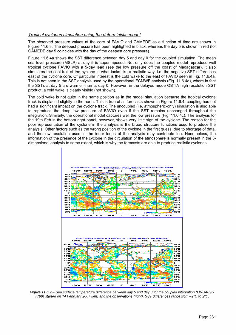
Tropical cyclones simulation using the deterministic modelThe observed pressure values at the core of FAVIO and GAMEDE as a function of time are shown inFigure 11.6.3. The deepest pressure has been highlighted in black, whereas the day 5 is shown in red (forGAMEDE day 5 coincides with the day of the deepest core pressure).

Figure 11.6.4a shows the SST difference between day 5 and day 0 for the coupled simulation. The meansea level pressure (MSLP) at day 5 is superimposed. Not only does the coupled model reproduce welltropical cyclone FAVIO with a 5-day lead (see the low pressure off the coast of Madagascar), it alsosimulates the cool trail of the cyclone in what looks like a realistic way, i.e. the negative SST differenceseast of the cyclone core. Of particular interest is the cold wake to the east of FAVIO seen in Fig. 11.6.4a.This is not seen in the SST analysis used by the operational ECMWF analysis (Fig. 11.6.4d), where in factthe SSTs at day 5 are warmer than at day 0. However, in the delayed mode OSTIA high resolution SSTproduct, a cold wake is clearly visible (not shown).

The cold wake is not quite in the same position as in the model simulation because the tropical cyclonetrack is displaced slightly to the north. This is true of all forecasts shown in Figure 11.6.4: coupling has nothad a significant impact on the cyclone track. The uncoupled (i.e. atmospheric-only) simulation is also ableto reproduce the deep low pressure of FAVIO even if the SST remains unchanged throughout theintegration. Similarly, the operational model captures well the low pressure (Fig. 11.6.4c). The analysis forthe 19th Feb in the bottom right panel, however, shows very little sign of the cyclone. The reason for thepoor representation of the cyclone in the analysis is the broad structure functions used to produce theanalysis. Other factors such as the wrong position of the cyclone in the first guess, due to shortage of data,and the low resolution used in the inner loops of the analysis may contribute too. Nonetheless, theinformation of the presence of the cyclone in the circulation of the atmosphere is normally present in the 3-dimensional analysis to some extent, which is why the forecasts are able to produce realistic cyclones.

Figure 11.6.2 – Sea surface temperature difference between day 5 and day 0 for the coupled integration (ORCA025/T799) started on 14 February 2007 (left) and the observations (right). SST differences range from –2ºC to 2ºC.

Page 231

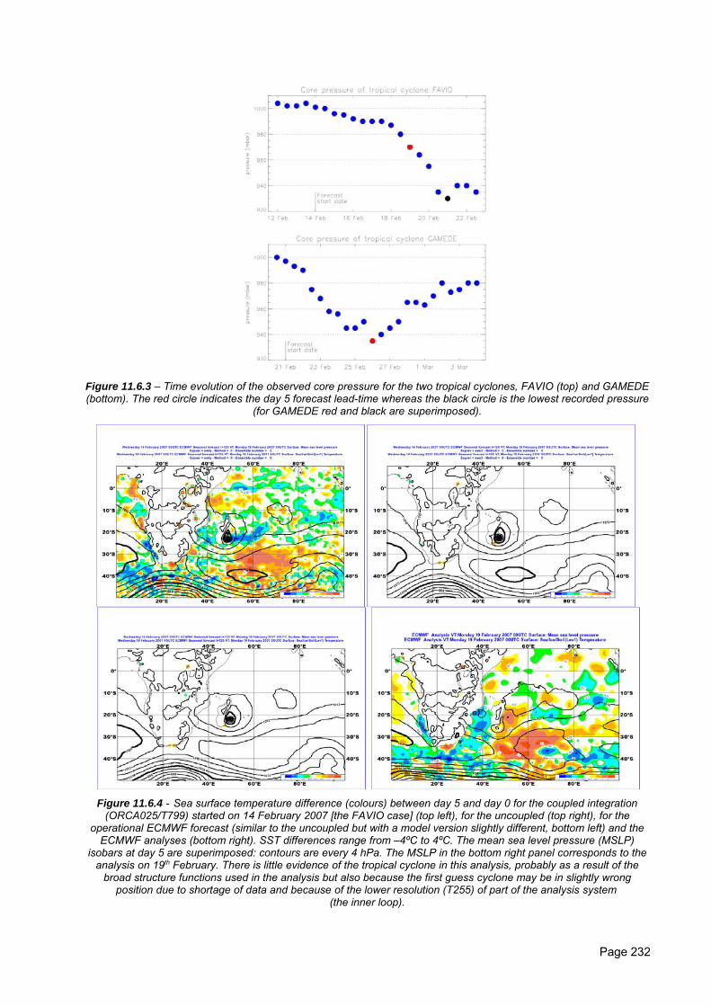
Figure 11.6.3 – Time evolution of the observed core pressure for the two tropical cyclones, FAVIO (top) and GAMEDE(bottom). The red circle indicates the day 5 forecast lead-time whereas the black circle is the lowest recorded pressure

(for GAMEDE red and black are superimposed).

Figure 11.6.4 - Sea surface temperature difference (colours) between day 5 and day 0 for the coupled integration(ORCA025/T799) started on 14 February 2007 [the FAVIO case] (top left), for the uncoupled (top right), for the

operational ECMWF forecast (similar to the uncoupled but with a model version slightly different, bottom left) and theECMWF analyses (bottom right). SST differences range from –4ºC to 4ºC. The mean sea level pressure (MSLP)

isobars at day 5 are superimposed: contours are every 4 hPa. The MSLP in the bottom right panel corresponds to theanalysis on 19th February. There is little evidence of the tropical cyclone in this analysis, probably as a result of the

broad structure functions used in the analysis but also because the first guess cyclone may be in slightly wrongposition due to shortage of data and because of the lower resolution (T255) of part of the analysis system

(the inner loop).

Page 232

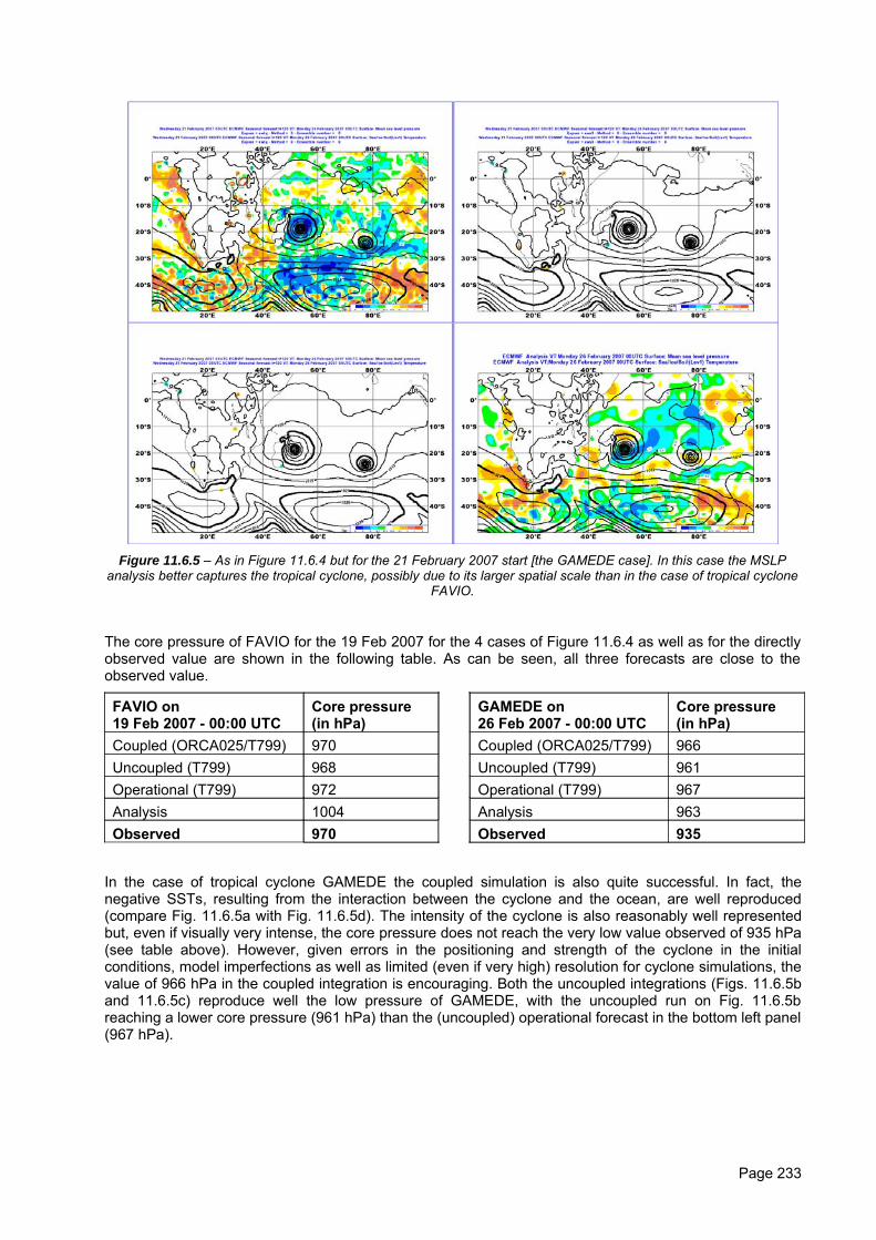
Figure 11.6.5 – As in Figure 11.6.4 but for the 21 February 2007 start [the GAMEDE case]. In this case the MSLPanalysis better captures the tropical cyclone, possibly due to its larger spatial scale than in the case of tropical cyclone

FAVIO.

The core pressure of FAVIO for the 19 Feb 2007 for the 4 cases of Figure 11.6.4 as well as for the directlyobserved value are shown in the following table. As can be seen, all three forecasts are close to theobserved value.

FAVIO on 19 Feb 2007 - 00:00 UTC

Core pressure(in hPa)

GAMEDE on 26 Feb 2007 - 00:00 UTC

Core pressure(in hPa)

Coupled (ORCA025/T799) 970 Coupled (ORCA025/T799) 966Uncoupled (T799) 968 Uncoupled (T799) 961Operational (T799) 972 Operational (T799) 967Analysis 1004 Analysis 963Observed 970 Observed 935

In the case of tropical cyclone GAMEDE the coupled simulation is also quite successful. In fact, thenegative SSTs, resulting from the interaction between the cyclone and the ocean, are well reproduced(compare Fig. 11.6.5a with Fig. 11.6.5d). The intensity of the cyclone is also reasonably well representedbut, even if visually very intense, the core pressure does not reach the very low value observed of 935 hPa(see table above). However, given errors in the positioning and strength of the cyclone in the initialconditions, model imperfections as well as limited (even if very high) resolution for cyclone simulations, thevalue of 966 hPa in the coupled integration is encouraging. Both the uncoupled integrations (Figs. 11.6.5band 11.6.5c) reproduce well the low pressure of GAMEDE, with the uncoupled run on Fig. 11.6.5breaching a lower core pressure (961 hPa) than the (uncoupled) operational forecast in the bottom left panel(967 hPa).

Page 233

Summary of the assessment of the impact of the MERSEA-¼ analyses on the very high resolutioncoupled model with respect to Medium-Range forecasts

A high resolution ocean model has been coupled to the atmospheric model used for medium-rangeweather forecasts at ECMWF. Such a coupled model has been tested here on two tropical cyclone casestudies.

Encouragingly, the coupled model shows a physically reasonable behaviour in the evolution of the globalsea surface temperature (SST). The two tropical cyclones themselves are nicely reproduced by thecoupled model. However, despite the well simulated SSTs, differences with analogous uncoupledintegrations for which SST is held fixed throughout the integrations are generally not striking, at least interms of minimum pressure and winds. It has been argued that a possible explanation is that theatmospheric model has been tuned to function with fixed SST and therefore the coupling with varying SSTmay not be as strong as it ought to be. Indeed, no specific tuning of the coupling has been attempted.

Now that such a coupled model has been implemented it could be used for similar case studies, Atlantichurricanes for example. Work is already under way to study the behaviour of this coupled model on thesimulation of the intra-seasonal oscillation.

9.4. Bibliography

Allen, J.I., T.J. Smyth, J.R. Siddorn: “How well can we forecast high biomass algal bloom events in aeutrophic coast sea? Harmful Algae”

Allen, J.I., P.J. Somerfield, 2008: “A multivariate approach to model skill assessment”, Journal of MarineSystems doi:10.1016/j.jmarsys.2008.05.009

Allen, J.I., J.T. Holt, J.C. Blackford and R. Proctor, 2007: “Error quantification of a high-resolution coupledhydrodynamic-ecosystem coastal-ocean model: Part 2. Chlorophyll-a, nutrients and SPM”, J. Mar.Sys., doi:10.1016/-j.jmarsys.2007.01.005.

Allen, J.I., J.C. Blackford, J.T. Holt, R. Proctor, M. Ashworth, J.R. Siddorn, 2001: “A highly spatiallyresolved ecosystem model for the North West European Continental Shelf”, Sarsia, 86, 423-440.

Barron, C. N., A.B. Kara, P.J. Martin, R.C. Rhodes and L.F. Smedstad, 2006: “Formulation, implementationand examination of vertical coordinate choices in the Global Navy Coastal Ocean Model (NCOM)”,Ocean Modelling, 11, 347-375.

Baretta, J.W., W. Ebenhöh, P. Ruardij, 1995: “The European Regional Seas Ecosystem Model, a complexmarine ecosystem model”, Neth. J. Sea. Res., 33, 233-246.

Bell, M.J., R.M. Forbes and A. Hines, 2000: “Assessment of the FOAM global data assimilation system forreal-time operational ocean forecasting”, J. Mar. Sys., 25, 1-22.

Blackford, J.C., J.I. Allen and F. Gilbert, 2004: “Ecosystem dynamics at six contrasting sites: a genericmodelling study”, J. Mar. Sys., 52. 191-215.

Bosc, E., A. Bricaud and D. Antoine, 2004: ‘Seasonal and interannual variability in algal biomass andprimary production in the Mediterranean Sea, as derived from 4 years of SeaWiFS observation’.Global Biogeochemical Cycles, 18, GB1005 1-17.

Bricaud, A., E. Bosc and D. Antoine, 2004: ‘Algal biomass and sea surface temperature in theMediterranean Basin — intercomparison of data from various satellite sensors, and implications forprimary production estimates’, Remote Sensing of Environment, 81(2–3), 163−178.

Chatfield, C. and A. J. Collins, 1980: “Introduction to multivariate analysis”, Chapman and Hall, London

Clarke, K.R., 1993: “Nonparameteric multivariate analyses of changes in community structure”. Aust. J.Ecol., 18, 117-143.

Clarke, K.R. and R.N. Gorley, 2006: “PRIMER v6: User manual/tutorial”, PRIMER-E Ltd, Plymouth, 192pp

Charnock, H., K. Dyer, J.M. Huthnance, P.S. Liss, J.H. Simpson, P.B. Tett, (Eds.), 1994: “Understandingthe North Sea System”, Royal Society of London, 222 pp.

Page 234

Haney, R.L., 1971: “Surface thermal boundary condition for ocean circulation models”, Journal of PhysicalOceanography 1, 241–248

Holt, J.T., I.D. James, 1999: “A simulation of the southern North Sea in comparison with measurementsfrom the North Sea project: Part 1. Temperature”, Continental Shelf Research 19, 1087–1112.

Holt, J.T., I.D. James, 2001: “An s coordinate density evolving model of the northwest Europeancontinental shelf: 1, Model description and density structure”, Journal of Geophysical Research,106(C7), 14015-14034.

Holt, J.T., R. Proctor, 2003: “The role of advection in determining the temperature structure of the IrishSea”, Journal of Physical Oceanography 33, 2288–2306.

Holt, J.T., R. Proctor, J.C. Blackford, J.I. Allen and M. Ashworth, 2004: “Advective controls on primaryproduction in the stratified western Irish Sea: an eddy-resolving model study”, J. Geophys. Res.,109(C05024): doi: 10.1029/2003JC001951.

Holt, J.T., J.I. Allen, R. Proctor and F. Gilbert, 2005: “Error quantification of a coupled high-resolutioncoupled hydrodynamic-ecosystem coastal ocean model: Part 1 model overview and assessment of thehydrodynamics”, J. Mar. Sys., 57, 167-188.

Kaiser, H.F., 1960, “The application of electronic computers to factor analysis”: Educational andPsychological Measurement, 20, 141-151. .

Lewis, K., J.I. Allen, A.J. Richardson and J.T. Holt, 2006: “Error quantification of a high-resolution coupledhydrodynamic ecosystem coastal ocean model: Part 3 Validation with CPR data”, J. Mar. Sys., 63,209-224.

O’Reilly, J.E., S. Maritorena, B.G. Mitchell, D.A. Siegel, K.L. Carder, S.A. Garver, M. Kahru and C.McClain, 1998: “Ocean colour algorithms for SeaWiFS”, J. Geophys. Res., 103, 24937-24953.

Pätsch, J., G. Radach, 1997: “Long-term simulation of the eutrophication of the North Sea: temporaldevelopment of nutrients, chlorophyll and primary production in comparison to observations”,Netherlands Journal of Sea Research 38, 275–310.

Scoccimarro E., S. Gualdi, A. Bellucci, A. Carril, P.G. Fogli and A. Navarra, 2007: “CMCC-SXF025: AHigh-Resolution Coupled Atmosphere Ocean General Circulation Climate Model”, Centro Euro-Mediterraneo per i Cambiamenti Climatici, TR3, April 2007, 63pp.

Song, Y. and D. Haidvogel, 1994: “A semi-implicit ocean circulation model using a generalized topography-following coordinate system”, J. Comp. Phys, 115, 228-244.

Flather, R.A., 1981: “Results from a model of the northeast Atlantic relating to the Norwegian CoastalCurrent”, In The Norwegian Coastal Current Vol. 2: R. Saetre & M. Mork (Editors), pp. 427-458.

Holt, J. T. and I. D. James, 2001: “An s-coordinate density evolving model of the north west Europeancontinental shelf. Part 1: Model description and density structure”, J. Geophys. Res., 106(C7): 14015-14034.

Otto, L., J.T.F Zimmerman, G.K. Furnes, M. Mork, R. Saetre and G. Becker, 1990: “Review of the physicaloceanography of the North Sea”, Neth. J. Sea Res., 26, 161-238.

Troccoli A, D.L.T. Anderson, K. Mogensen, G. Van der Grijn, N. Ferry and G. Garric, 2008: “Coupledocean-atmosphere medium range forecasts: the MERSEA experience”, ECMWF Newsletter, 115, 27-35.Available at: http://www.ecmwf.int/publications/newsletters/

Young, E.F. and J.T. Holt, 2007: “Prediction and analysis of long-term variability of temperature and salinityin the Irish Sea”, J. Geophys. Res., 112 C01008, doi:10.1029/2005JC003386.

Page 235

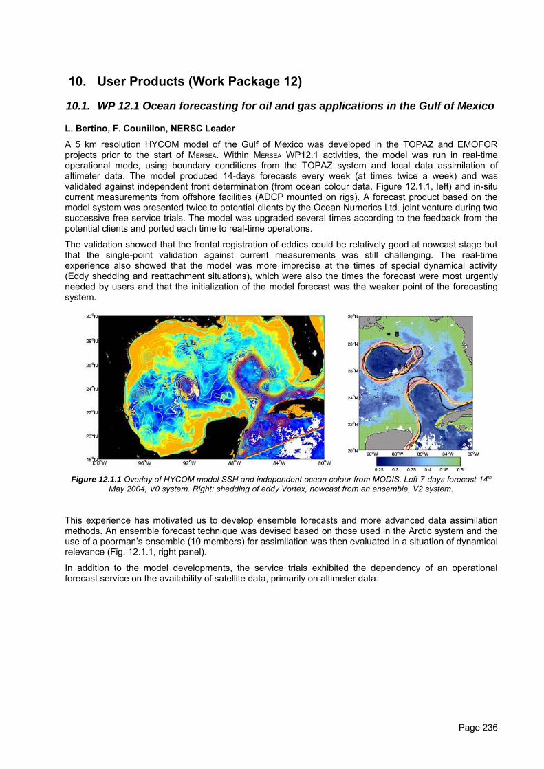
10. User Products (Work Package 12)

10.1. WP 12.1 Ocean forecasting for oil and gas applications in the Gulf of Mexico

L. Bertino, F. Counillon, NERSC Leader

A 5 km resolution HYCOM model of the Gulf of Mexico was developed in the TOPAZ and EMOFORprojects prior to the start of MERSEA. Within MERSEA WP12.1 activities, the model was run in real-timeoperational mode, using boundary conditions from the TOPAZ system and local data assimilation ofaltimeter data. The model produced 14-days forecasts every week (at times twice a week) and wasvalidated against independent front determination (from ocean colour data, Figure 12.1.1, left) and in-situcurrent measurements from offshore facilities (ADCP mounted on rigs). A forecast product based on themodel system was presented twice to potential clients by the Ocean Numerics Ltd. joint venture during twosuccessive free service trials. The model was upgraded several times according to the feedback from thepotential clients and ported each time to real-time operations.

The validation showed that the frontal registration of eddies could be relatively good at nowcast stage butthat the single-point validation against current measurements was still challenging. The real-timeexperience also showed that the model was more imprecise at the times of special dynamical activity(Eddy shedding and reattachment situations), which were also the times the forecast were most urgentlyneeded by users and that the initialization of the model forecast was the weaker point of the forecastingsystem.

Figure 12.1.1 Overlay of HYCOM model SSH and independent ocean colour from MODIS. Left 7-days forecast 14th

May 2004, V0 system. Right: shedding of eddy Vortex, nowcast from an ensemble, V2 system.

This experience has motivated us to develop ensemble forecasts and more advanced data assimilationmethods. An ensemble forecast technique was devised based on those used in the Arctic system and theuse of a poorman’s ensemble (10 members) for assimilation was then evaluated in a situation of dynamicalrelevance (Fig. 12.1.1, right panel).

In addition to the model developments, the service trials exhibited the dependency of an operationalforecast service on the availability of satellite data, primarily on altimeter data.

Page 236

10.2. WP12.2 Sea-ice applications in the Barents Sea

L. Bertino, S. Sandven, I. Kegouche, K. Kloster, M. Babiker, NERSC

The objective here is to provide a sea-ice and iceberg monitoring and forecasting service for the oil andgas industry active in the Barents Sea. The subject has drawn considerable attention in the duration ofMERSEA since the Russian Shtockman field has been attributed initially to Gazprom and then opened forparticipations from Total and StatoilHydro. Other oil companies have interests in the area (Shell,ConocoPhillips among others) as well as into the Kara Sea and further potential along the Arctic Shelves.The Barents Sea environment is however very harsh in its weather and ocean conditions and is seasonallycovered by sea-ice, and the available environmental data is by comparison very little. NERSC has thusdeveloped the following tools:

• Targeted products from remote sensing (ice drift in close to the ice edge, iceberg detection)• A high-resolution ice-ocean model of the Barents and Kara Seas (5 km horizontal resolution) nested

into the TOPAZ Arctic system and including tidal forcing.• An iceberg simulation model that accounts for the sea-ice, ocean and atmosphere forcing in the

Barents Sea.The main requirements from the industry were first a validation of the products based on the MERSEA

system and then the provision of large databases for design criteria. As the oil and gas activities weremostly dealing with dimensioning of different concepts for exploitation in ice-covered areas, the focus wasmore on long hindcast databases than on real-time forecasting.

Remote sensing productsIcebergs in the Barents Sea can be observed by high-resolution radar as well as optical satellite images.The analysis of the optical images for detection of icebergs is based on identification of bright objects witha characteristic dark shadow caused by the sun angle. This criterion is quite reliable for icebergsembedded in fast-ice. Example of this detection is shown in Fig. 12.2.1a. In the three images from 20 Aprilobtained south of Franz Josef Land, a total of 245 icebergs were found in an area of about 10.000km2 (Fig.12.2.1b). The size of the detected icebergs was typical 50 m or more in the studies carried out in 2005.The possibility to detect icebergs under different background conditions such as open water and drifting iceis more uncertain.

Iceberg observations in high resolution optical images is not hampered by the speckle noise which ischaracteristic for the SAR images. Observations in optical images are therefore more reliable for icebergsof size of 100 m or less. The limitation of optical images is cloud cover and darkness, allowing goodquality observations only occasionally. Since the first studies of icebergs using Landsat, SPOT andairborne SAR data two decades ago, there are now more satellite systems producing high-resolutionimages that can improve the capability of monitoring icebergs. In this study, we have tested use ofalternating polarization SAR images from ENVISAT, RADARSAT ScanSAR Narrow images, optical imagesfrom Landsat and ASTER, and the possibility to monitor icebergs in the Barents Sea with optical and SARimages over a period of four months. An operational monitoring system for icebergs should include use ofboth satellite SAR and optical images with high resolution (10m or better) in addition to observations formaircraft and ships.

Synergy of SAR and optical/infrared satellite images is also useful for mapping ice and open water areasand provide sea surface temperature for open water. In many cases it is difficult to discriminate open waterfrom thin ice in SAR images. By using optical images the discrimination is more reliable. The method,however, is only useful during cloud-free conditions. An example of ice and SST map in Storfjorden isshown in Fig. 12.2.1

Page 237

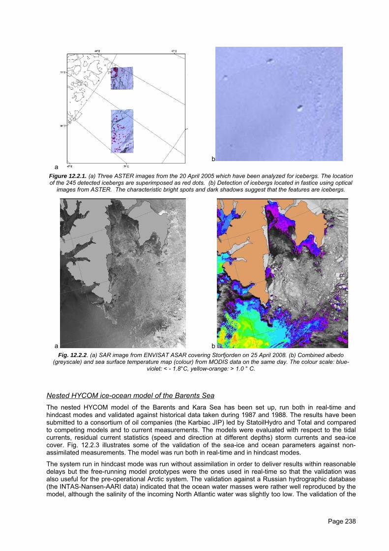
ab

Figure 12.2.1. (a) Three ASTER images from the 20 April 2005 which have been analyzed for icebergs. The locationof the 245 detected icebergs are superimposed as red dots. (b) Detection of icebergs located in fastice using optical

images from ASTER. The characteristic bright spots and dark shadows suggest that the features are icebergs.

a b Fig. 12.2.2. (a) SAR image from ENVISAT ASAR covering Storfjorden on 25 April 2008. (b) Combined albedo

(greyscale) and sea surface temperature map (colour) from MODIS data on the same day. The colour scale: blue-violet: < - 1.8°C, yellow-orange: > 1.0 ° C.

Nested HYCOM ice-ocean model of the Barents SeaThe nested HYCOM model of the Barents and Kara Sea has been set up, run both in real-time andhindcast modes and validated against historical data taken during 1987 and 1988. The results have beensubmitted to a consortium of oil companies (the Karbiac JIP) led by StatoilHydro and Total and comparedto competing models and to current measurements. The models were evaluated with respect to the tidalcurrents, residual current statistics (speed and direction at different depths) storm currents and sea-icecover. Fig. 12.2.3 illustrates some of the validation of the sea-ice and ocean parameters against non-assimilated measurements. The model was run both in real-time and in hindcast modes.

The system run in hindcast mode was run without assimilation in order to deliver results within reasonabledelays but the free-running model prototypes were the ones used in real-time so that the validation wasalso useful for the pre-operational Arctic system. The validation against a Russian hydrographic database(the INTAS-Nansen-AARI data) indicated that the ocean water masses were rather well reproduced by themodel, although the salinity of the incoming North Atlantic water was slightly too low. The validation of the

Page 238

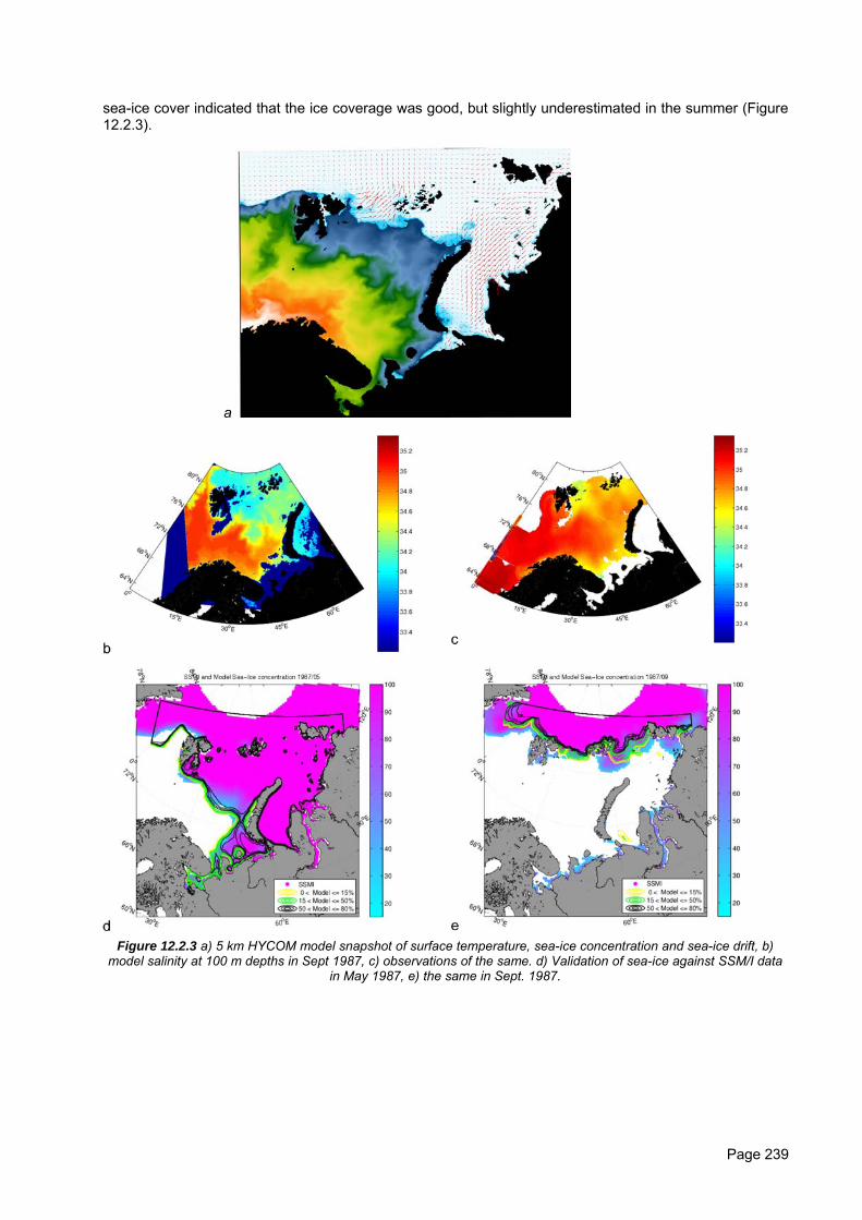
sea-ice cover indicated that the ice coverage was good, but slightly underestimated in the summer (Figure12.2.3).

a

Figure 12.2.3 a) 5 km HYCOM model snapshot of surface temperature, sea-ice concentration and sea-ice drift, b)model salinity at 100 m depths in Sept 1987, c) observations of the same. d) Validation of sea-ice against SSM/I data

in May 1987, e) the same in Sept. 1987.

Page 239

Figure 12.2.4 IDAP Icebergs 7088 (left) and 1792 (right) East of Spitzbergen and North of Novaya Zemlya. Threemonths observed iceberg trajectory and model ensemble trajectories (grey). One large dot is plotted every second

week.

An iceberg model in the Barents SeaThe iceberg model has been adapted from the Antarctic iceberg model from AWI, Germany, for theBarents Sea. The model has been validated against observed icebergs from the IDAP program in 1990,the only period with relevant iceberg observations available to date. The results indicate that the mainforces acting on an iceberg in the Barents Sea are the winds, the ocean currents (over the whole icebergkeel, up to 100 m depths), the Coriolis force and the sea-ice stress. The iceberg model is entirely forced bymodel output (ECMWF ERA40 winds, sea-ice and ocean currents from the nested HYCOM model of theBarents Sea). The model results are very sensitive to the input parameters of the iceberg: its mass,dimensions and its shape (tabular, tilted tabular, trapezoidal, etc) and to the drag coefficients with the airand the ocean.

After optimization of the parameters, the results indicate that - in favorable conditions - the model resultsare as close as 20 km from the observed iceberg position, even after a simulation as long as two months.This indicates a strong potential for operational forecasting of icebergs.

10.3. TASK 12.3: Oil spill fate prediction

Lead: met.no

Participants: MF, OC-UCY (previously CYOC-DFMR)

In MERSEA, oil spill fate forecasting is identified as a first-rank application for operational oceanography: Oilpollution from catastrophic accidents and illicit dumping continues to be a major threat to Europeancoastlines and ecosystems. Despite efforts to reduce the incidence of spills, there is still a need forimproved predictions of oil spill fate. Forecasts are necessary in support of recovery efforts, preparedness,and mitigation measures. To fulfil their national and international responsibilities, operational agenciesdeveloped oil spill drift prediction systems. The capability to incorporate accurate estimates of currents inthese systems still needs to be improved. MERSEA will provide in real time the required high resolutioncurrent fields.

Task 12.3 under WP12 of MERSEA addresses oil spill fate prediction. Its objective is to interface MERSEA

global and regional current forecasts with existing oil spill modelling systems, and evaluate improvedforecast skill and accuracy. Task 12.3 has three partners: the Norwegian Meteorological Institute (met.no,lead partner), Météo-France (MF) and the Oceanography Centre, University of Cyprus (OC-UCY).

Page 240

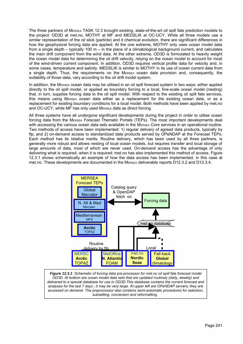
The three partners of MERSEA TASK 12.3 brought existing, state-of-the-art oil spill fate prediction models tothe project: OD3D at met.no, MOTHY at MF and MEDSLIK at OC-UCY. While all three models use asimilar representation of the oil slick (particle) and it chemical evolution, there are significant differences inhow the geophysical forcing data are applied. At the one extreme, MOTHY only uses ocean model datafrom a single depth – typically 100 m – in the place of a climatological background current, and calculatesthe main drift component from the wind data. At the other extreme, OD3D is formulated to heavily weightthe ocean model data for determining the oil drift velocity, relying on the ocean model to account for mostof the wind-driven current component. In addition, OD3D requires vertical profile data for velocity and, insome cases, temperature and salinity. MEDSLIK is similar to MOTHY in its use of ocean current data froma single depth. Thus, the requirements on the MERSEA ocean data provision and, consequently, thesuitability of those data, vary according to the oil drift model system.

In addition, the MERSEA ocean data may be utilised in an oil spill forecast system in two ways: either applieddirectly to the oil spill model, or applied as boundary forcing to a local, fine-scale ocean model (nesting)that, in turn, supplies forcing data to the oil spill model. With respect to the existing oil spill fate services,this means using MERSEA ocean data either as a replacement for the existing ocean data, or as areplacement for existing boundary conditions for a local model. Both methods have been applied by met.noand OC-UCY, while MF has only used MERSEA data as direct forcing.

All three systems have all undergone significant developments during the project in order to utilise oceanforcing data from the MERSEA Forecast Thematic Portals (TEPs). The most important developments dealwith accessing the various ocean data sets available in the MERSEA Core services in an operational routine.Two methods of access have been implemented: 1) regular delivery of agreed data products, typically byftp, and 2) on-demand access to standardized data products served by OPeNDAP at the Forecast TEPs.Each method has its relative merits. Routine delivery, which has been used by all three partners, isgenerally more robust and allows nesting of local ocean models, but requires transfer and local storage oflarge amounts of data, most of which are never used. On-demand access has the advantage of onlydelivering what is required, when it is required; met.no has also implemented this method of access. Figure12.3.1 shows schematically an example of how the data access has been implemented, in this case atmet.no. These developments are documented in the MERSEA deliverable reports D12.3.2 and D12.3.4.

Page 241

GlobalMercator

N. Atl & Med Mercator

Mediterranean MFS

Arctic TOPAZ

MERSEA Forecast TEPs

Catalog query & OpenDAP

fetch on

Routine delivery by ftp Local

met.no Nordic Seas

MIPOM

MetOffice N. Atlantic

FOAM

Forcing data

met.no database

Fall-back Global

climatology

NERSC Arctic TOPAZ

Figure 12.3.1: Schematic of forcing data pre-processor for met.no oil spill fate forecast model OD3D. At bottom are ocean model data sets that are updated routinely (daily, weekly) and

delivered to a special database for use in OD3D.This database contains the current forecast and analyses for the last 7 days ; it may be very large. At upper left are OPeNDAP servers; they are accessed on demand. The preprocessor also contains semi-automatic procedures for selection,

subsetting, conversion and reformatting.

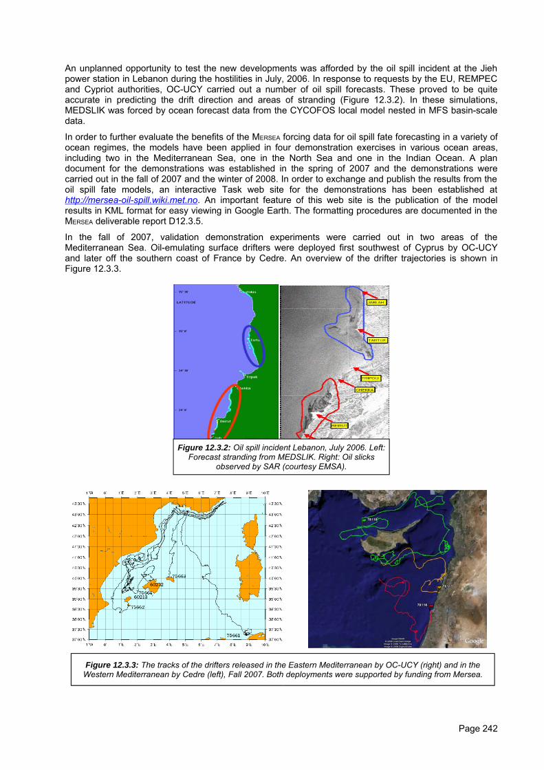
An unplanned opportunity to test the new developments was afforded by the oil spill incident at the Jiehpower station in Lebanon during the hostilities in July, 2006. In response to requests by the EU, REMPECand Cypriot authorities, OC-UCY carried out a number of oil spill forecasts. These proved to be quiteaccurate in predicting the drift direction and areas of stranding (Figure 12.3.2). In these simulations,MEDSLIK was forced by ocean forecast data from the CYCOFOS local model nested in MFS basin-scaledata.

In order to further evaluate the benefits of the MERSEA forcing data for oil spill fate forecasting in a variety ofocean regimes, the models have been applied in four demonstration exercises in various ocean areas,including two in the Mediterranean Sea, one in the North Sea and one in the Indian Ocean. A plandocument for the demonstrations was established in the spring of 2007 and the demonstrations werecarried out in the fall of 2007 and the winter of 2008. In order to exchange and publish the results from theoil spill fate models, an interactive Task web site for the demonstrations has been established athttp://mersea-oil-spill.wiki.met.no. An important feature of this web site is the publication of the modelresults in KML format for easy viewing in Google Earth. The formatting procedures are documented in theMERSEA deliverable report D12.3.5.

In the fall of 2007, validation demonstration experiments were carried out in two areas of theMediterranean Sea. Oil-emulating surface drifters were deployed first southwest of Cyprus by OC-UCYand later off the southern coast of France by Cedre. An overview of the drifter trajectories is shown inFigure 12.3.3.

Page 242

Figure 12.3.2: Oil spill incident Lebanon, July 2006. Left: Forecast stranding from MEDSLIK. Right: Oil slicks

observed by SAR (courtesy EMSA).

Figure 12.3.3: The tracks of the drifters released in the Eastern Mediterranean by OC-UCY (right) and in the Western Mediterranean by Cedre (left), Fall 2007. Both deployments were supported by funding from Mersea.

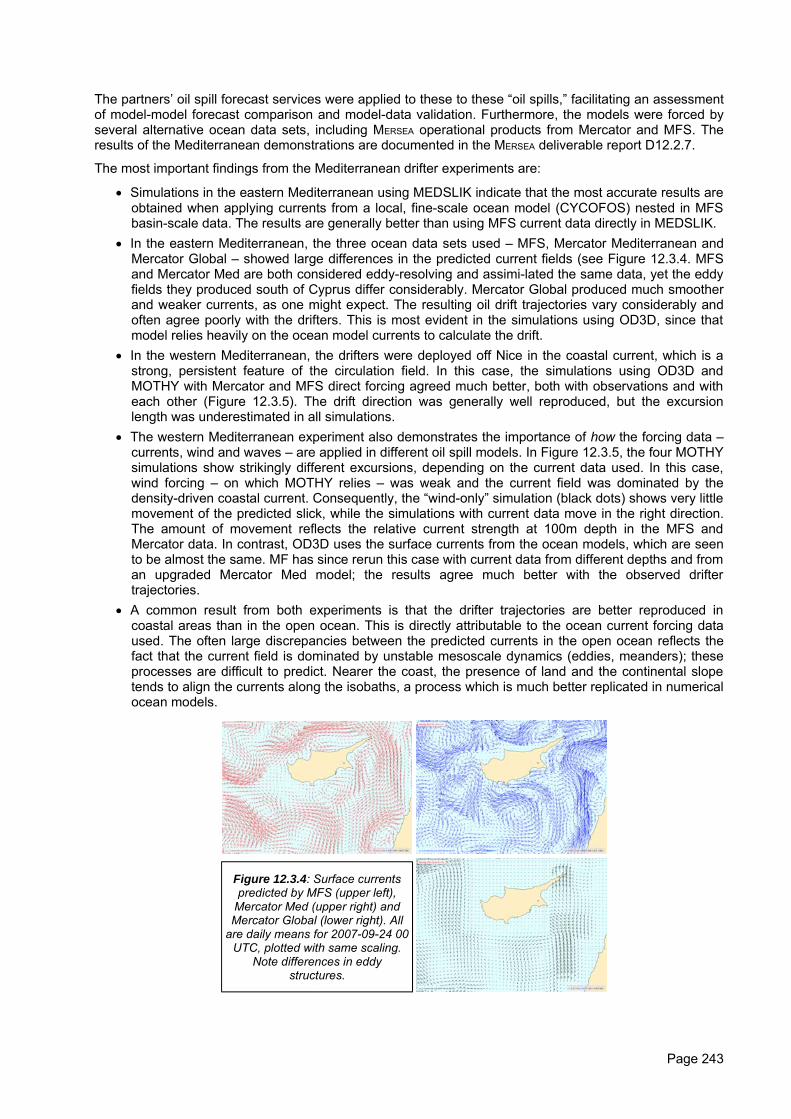
The partners’ oil spill forecast services were applied to these to these “oil spills,” facilitating an assessmentof model-model forecast comparison and model-data validation. Furthermore, the models were forced byseveral alternative ocean data sets, including MERSEA operational products from Mercator and MFS. Theresults of the Mediterranean demonstrations are documented in the MERSEA deliverable report D12.2.7.

The most important findings from the Mediterranean drifter experiments are:

• Simulations in the eastern Mediterranean using MEDSLIK indicate that the most accurate results areobtained when applying currents from a local, fine-scale ocean model (CYCOFOS) nested in MFSbasin-scale data. The results are generally better than using MFS current data directly in MEDSLIK.

• In the eastern Mediterranean, the three ocean data sets used – MFS, Mercator Mediterranean andMercator Global – showed large differences in the predicted current fields (see Figure 12.3.4. MFSand Mercator Med are both considered eddy-resolving and assimi-lated the same data, yet the eddyfields they produced south of Cyprus differ considerably. Mercator Global produced much smootherand weaker currents, as one might expect. The resulting oil drift trajectories vary considerably andoften agree poorly with the drifters. This is most evident in the simulations using OD3D, since thatmodel relies heavily on the ocean model currents to calculate the drift.

• In the western Mediterranean, the drifters were deployed off Nice in the coastal current, which is astrong, persistent feature of the circulation field. In this case, the simulations using OD3D andMOTHY with Mercator and MFS direct forcing agreed much better, both with observations and witheach other (Figure 12.3.5). The drift direction was generally well reproduced, but the excursionlength was underestimated in all simulations.

• The western Mediterranean experiment also demonstrates the importance of how the forcing data –currents, wind and waves – are applied in different oil spill models. In Figure 12.3.5, the four MOTHYsimulations show strikingly different excursions, depending on the current data used. In this case,wind forcing – on which MOTHY relies – was weak and the current field was dominated by thedensity-driven coastal current. Consequently, the “wind-only” simulation (black dots) shows very littlemovement of the predicted slick, while the simulations with current data move in the right direction.The amount of movement reflects the relative current strength at 100m depth in the MFS andMercator data. In contrast, OD3D uses the surface currents from the ocean models, which are seento be almost the same. MF has since rerun this case with current data from different depths and froman upgraded Mercator Med model; the results agree much better with the observed driftertrajectories.

• A common result from both experiments is that the drifter trajectories are better reproduced incoastal areas than in the open ocean. This is directly attributable to the ocean current forcing dataused. The often large discrepancies between the predicted currents in the open ocean reflects thefact that the current field is dominated by unstable mesoscale dynamics (eddies, meanders); theseprocesses are difficult to predict. Nearer the coast, the presence of land and the continental slopetends to align the currents along the isobaths, a process which is much better replicated in numericalocean models.

Page 243

Figure 12.3.4: Surface currents predicted by MFS (upper left),

Mercator Med (upper right) and Mercator Global (lower right). All

are daily means for 2007-09-24 00 UTC, plotted with same scaling.

Note differences in eddy structures.

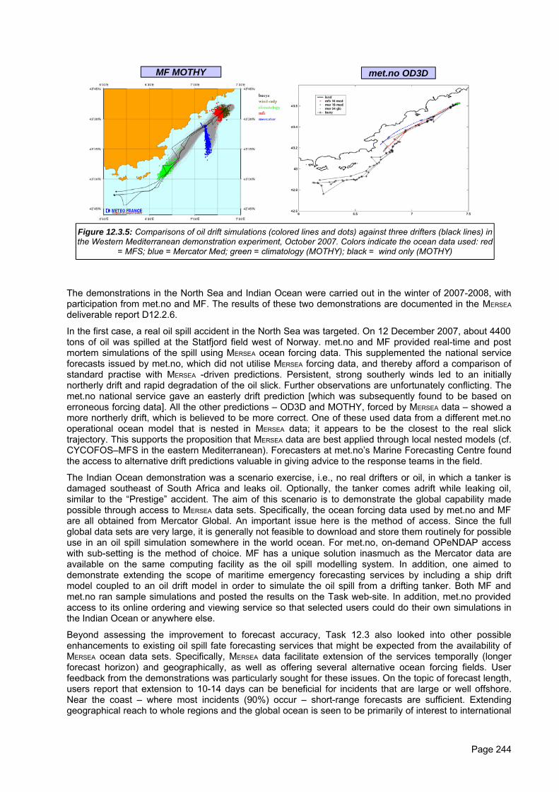
The demonstrations in the North Sea and Indian Ocean were carried out in the winter of 2007-2008, withparticipation from met.no and MF. The results of these two demonstrations are documented in the MERSEA

deliverable report D12.2.6.

In the first case, a real oil spill accident in the North Sea was targeted. On 12 December 2007, about 4400tons of oil was spilled at the Statfjord field west of Norway. met.no and MF provided real-time and postmortem simulations of the spill using MERSEA ocean forcing data. This supplemented the national serviceforecasts issued by met.no, which did not utilise MERSEA forcing data, and thereby afford a comparison ofstandard practise with MERSEA -driven predictions. Persistent, strong southerly winds led to an initiallynortherly drift and rapid degradation of the oil slick. Further observations are unfortunately conflicting. Themet.no national service gave an easterly drift prediction [which was subsequently found to be based onerroneous forcing data]. All the other predictions – OD3D and MOTHY, forced by MERSEA data – showed amore northerly drift, which is believed to be more correct. One of these used data from a different met.nooperational ocean model that is nested in MERSEA data; it appears to be the closest to the real slicktrajectory. This supports the proposition that MERSEA data are best applied through local nested models (cf.CYCOFOS–MFS in the eastern Mediterranean). Forecasters at met.no’s Marine Forecasting Centre foundthe access to alternative drift predictions valuable in giving advice to the response teams in the field.

The Indian Ocean demonstration was a scenario exercise, i.e., no real drifters or oil, in which a tanker isdamaged southeast of South Africa and leaks oil. Optionally, the tanker comes adrift while leaking oil,similar to the “Prestige” accident. The aim of this scenario is to demonstrate the global capability madepossible through access to MERSEA data sets. Specifically, the ocean forcing data used by met.no and MFare all obtained from Mercator Global. An important issue here is the method of access. Since the fullglobal data sets are very large, it is generally not feasible to download and store them routinely for possibleuse in an oil spill simulation somewhere in the world ocean. For met.no, on-demand OPeNDAP accesswith sub-setting is the method of choice. MF has a unique solution inasmuch as the Mercator data areavailable on the same computing facility as the oil spill modelling system. In addition, one aimed todemonstrate extending the scope of maritime emergency forecasting services by including a ship driftmodel coupled to an oil drift model in order to simulate the oil spill from a drifting tanker. Both MF andmet.no ran sample simulations and posted the results on the Task web-site. In addition, met.no providedaccess to its online ordering and viewing service so that selected users could do their own simulations inthe Indian Ocean or anywhere else.

Beyond assessing the improvement to forecast accuracy, Task 12.3 also looked into other possibleenhancements to existing oil spill fate forecasting services that might be expected from the availability ofMERSEA ocean data sets. Specifically, MERSEA data facilitate extension of the services temporally (longerforecast horizon) and geographically, as well as offering several alternative ocean forcing fields. Userfeedback from the demonstrations was particularly sought for these issues. On the topic of forecast length,users report that extension to 10-14 days can be beneficial for incidents that are large or well offshore.Near the coast – where most incidents (90%) occur – short-range forecasts are sufficient. Extendinggeographical reach to whole regions and the global ocean is seen to be primarily of interest to international

Page 244

MF MOTHY met.no OD3D

Figure 12.3.5: Comparisons of oil drift simulations (colored lines and dots) against three drifters (black lines) in the Western Mediterranean demonstration experiment, October 2007. Colors indicate the ocean data used: red

= MFS; blue = Mercator Med; green = climatology (MOTHY); black = wind only (MOTHY)

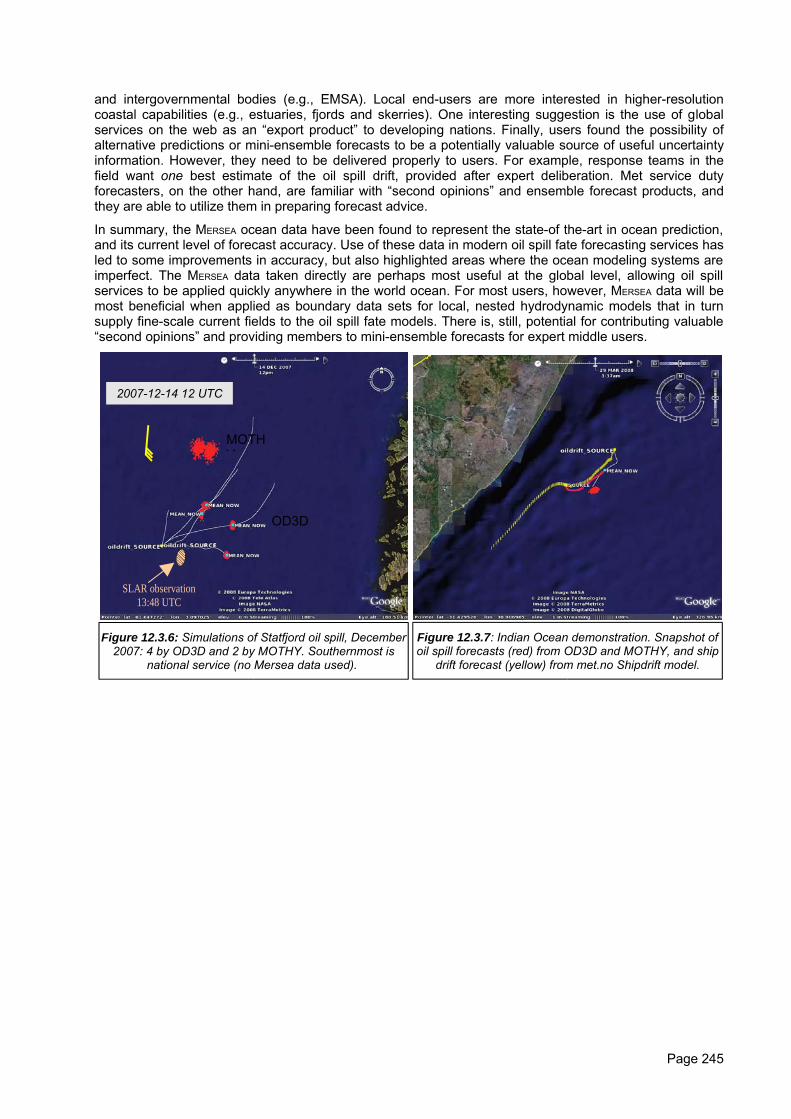
and intergovernmental bodies (e.g., EMSA). Local end-users are more interested in higher-resolutioncoastal capabilities (e.g., estuaries, fjords and skerries). One interesting suggestion is the use of globalservices on the web as an “export product” to developing nations. Finally, users found the possibility ofalternative predictions or mini-ensemble forecasts to be a potentially valuable source of useful uncertaintyinformation. However, they need to be delivered properly to users. For example, response teams in thefield want one best estimate of the oil spill drift, provided after expert deliberation. Met service dutyforecasters, on the other hand, are familiar with “second opinions” and ensemble forecast products, andthey are able to utilize them in preparing forecast advice.

In summary, the MERSEA ocean data have been found to represent the state-of the-art in ocean prediction,and its current level of forecast accuracy. Use of these data in modern oil spill fate forecasting services hasled to some improvements in accuracy, but also highlighted areas where the ocean modeling systems areimperfect. The MERSEA data taken directly are perhaps most useful at the global level, allowing oil spillservices to be applied quickly anywhere in the world ocean. For most users, however, MERSEA data will bemost beneficial when applied as boundary data sets for local, nested hydrodynamic models that in turnsupply fine-scale current fields to the oil spill fate models. There is, still, potential for contributing valuable“second opinions” and providing members to mini-ensemble forecasts for expert middle users.

Page 245

2007-12-14 12 UTC

SLAR observation 13:48 UTC

Figure 12.3.6: Simulations of Statfjord oil spill, December 2007: 4 by OD3D and 2 by MOTHY. Southernmost is

national service (no Mersea data used).

MOTHY

OD3D

Figure 12.3.7: Indian Ocean demonstration. Snapshot of oil spill forecasts (red) from OD3D and MOTHY, and ship

drift forecast (yellow) from met.no Shipdrift model.

11. Overall Assessment (Work Package 13)

11.1. Task 13.1: Assessment of the MERSEA system

Under this task we set the objective to assess the performance of the system, as it evolved during theproject, from the perspective of the GMES aims, and to document progress since the first assessmentconducted under the MERSEA Strand-1 project.

The overarching vision for GMES was to create and maintain a European technical Information capacity –encompassing observation systems and servicing elements - allowing the production and easy access tothe information necessary for environment and security policies. GMES was thus presented as a politicalinitiative to secure Europe with an autonomous and operational information production system in support toenvironment and security policies. To reach those objectives, a service chain had to be developed totransform observations and data into information products in support of services; and to link datainformation providers to users.

The ESA and the European Union agreed on an action plan, with the goal to develop and bring intooperational service by 2008 an autonomous European global monitoring capability for environmental andsecurity purposes. It is in that context that the MERSEA Project was funded by the Commission to developOcean and Marine Applications for GMES during the implementation period (2004 – 2008) of its action plan.

Adequateness to GMES objectivesAlthough the initial emphasis of the GMES concept was on providing information in support of policy, itbecame clear that a wider range of applications were to be served by the system. Therefore we developedMERSEA with different classes of users in mind: policy makers, environmental monitoring and reporting,scientific research, industrial applications in the maritime sector, marine safety, marine meteorology andweather forecasting (medium to seasonal range), the general public and education. Those users have verydifferent requirements in terms of type of data or information and delivery system (e.g. large data filesdelivered routinely, production of indicators, simple summary plots, or tailored to specific applications).

The diversity of usages implied that the system must be able to provide basic generic data, directed atintermediate users, who in turn will further process it to elaborate the specific products required by theirend users. That is the objective of the Marine Core Service, with which the MERSEA prototype is fullycompliant.

The table below illustrates how the requirements can be identified for the main Areas of benefit, and whattypes of products are delivered by the MCS system.

Page 246

Area of benefit Products To intermediate users Final userClimate research Comprehensive and inferred

observational data setsreanalysed in state of the art

models

Climate research centres Ocean and climate research; validation ofscenarios.

Policy making on climate change

MarineEnvironmental

Protection

state and impact data &associated indicators

EEA, OSPAR, HELCOM,Barcelona, National

environmental agencies;

DG ENV, Policy makers, general public

Seasonalforecasting and

extended weatherforecasts

Initial ocean conditions;reanalysis

ECMWF, NMS Agriculture, insurance, energy, transport; publicsafety preparedness; research

Marine safety High resolution ice/sea state &ocean current forecasts

NMSs, National Marinesafety agencies

Search and rescue, drifting object management;wave forecast preparation

Fisheries,ecosystems

Physical conditions; re-analysis of past conditions

National marine andfisheries institutes

ICES, DG FISH, National fisheries;research

Shipping &offshore industries

High resolution ice/sea-state& current forecasts for

operations: reanalyses fordesign

Value adding servicecompanies

Operation support, ship routing, structure designcriteria, risk assessment; EMSA

Oil Spillmanagement-

Temperature, wind, wave &current data

Responsible Nationalmarine agencies & EMSA

Affected coastal public authorities & businesses

MarineEnvironment,Ecosystems

Boundary and initialconditions, data products

National Coastalmonitoring and forecasting

systems

National environmental or marine agencies;National WFD reporting;Coastal management.

Table 1: A generic summary of areas of benefit, product lines, intermediate and final users

A few comments are in order:

• Climate and ocean research: the system is able to deliver most of the Essential Climate Variables(ECV) identified by the GCOS1 for the oceanic domain (At the surface: temperature, salinity, Sealevel, Sea ice, Current, Ocean colour; Sub-surface: Temperature, Salinity, Current). The variableswhich are not available from the system are: nutrients, Carbon, Ocean tracers, Phytoplankton (sub-surface), Carbon dioxide partial pressure and Sea state. The data products (from satellite and insitu) are extensively and routinely used for ocean research. The outputs of the models however areless used because the need would be for long-term series (re-analysis) which are not produced bythe present time. Also, the lack of data below the reach of Argo floats at 2000 m casts some doubton the model outputs in the very deep ocean. However, the MCS do provide data not specificallylisted as ECV, but of great scientific interest (e.g. transports through straights, surface fluxes, icemotion, mixed layer depth)

• Marine environmental reporting: MERSEA is able to produce only a very limited set of the Core Set ofIndicators (CSI) or of the many biological and chemical variables required by the Conventions. Weare presently providing as a test case four of the CSI: sea level, surface temperature, sea-ice, andchlorophyll. However, it is clear that the interpretation of environmental data cannot be done properlywithout understanding of the physical context (e.g. transboundary transports).

• Seasonal and extended forecasts: this is addressed in the WP11 work (Special Focus Experiment.Success has been limited for seasonal forecasts, but preliminary results indicate that high resolutionocean data on upper ocean heat content can have a positive impact on hurricane prediction.

• Marine safety: we have demonstrated positive results on improved oil spill drift forecasts, incollaboration with Met agencies (Météo France and Met.no) and the Cyprus center. The CanadianCoast Guards have also been engaged in the use of real time high resolution ocean currents. But,as is the case with industrial applications, further development hinges on the assurance of continuityof the service –which should be provided in the future.

• Shipping and offshore industry: continuity of the service is again a key requirement for thedevelopment of applications. We have developed of few test cases with positive results for ship

1 Global Climate Observing System

Page 247

routing (see WP13), but the conclusions for offshore oil operations were that higher accuracy thanpresently available was required. Here is probably a case of matching expectation with capabilityand the state of the art.

• Coastal systems: several coastal systems are already connected to the MCS, and this is furtherdeveloped in the ECOOP project, thus validating the general concept. It is recognized that themonitoring and forecast of eco-systems is still at the research stage, and that the MCS cannotdeliver routine data in that realm.

• More generally, the system must be able to provide now-casts, forecasts, and re-analysis. Inaccordance with the work plan the project has delivered re-analysis only for some of the remotesensed data (ocean colour, altimetry), and for in situ Argo data. By necessity the time period islimited to that of the space borne observations. In the future, it must be one of the functions of theMFC to produce long re-analysis.

Thus the MCS brings an essential contribution to all of the main areas of interest to GMES. It also fulfils all ofthe general requirements that were set forth in the definition phase.

GMES was to build on existing capabilities: the design of the system and its distributed architecture basedon the MFC and TAC draws on the considerable expertise and investment made in national and Europeancentres.

One of the requirements was to make full and efficient use of space data: this is obviously one of the keyachievements of the project, which has elaborated and delivered high quality merged products fromavailable satellite data. It is the availability of the satellite data and of the Global Ocean Observing System(in particular Argo) that allows the truly global coverage required by GMES and provided by the MCS.

The production chain was to allow easy access to all of the system production. This has been achieved bythe MERSEA Information Management system (MIM), from a technical point of view. However it has not beenpossible to resolve data policy issues within the project, because of the provisions of the Contract. The allimportant question of data policy is addressed in the BOSS4GMES project and will be resolved in theMyOcean project.

As a research and development project, MERSEA has completed an ambitious work plan, with severalsuccessive upgrades of the systems. A consequence is that during the course of the project, the systemhas continuously evolved and has not reached a stable configuration. In the future systems, it will benecessary to progress in a more cautious pace in the implementation of upgrades to the operations. Theformalisation of service and operation level agreements will be a necessary step to foster the developmentof applications and to reach more users.

Contribution to the elaboration of the Marine Core Service Implementation PlanMembers of the MERSEA Executive Committee have taken a very active role in the elaboration of the MCSImplementation Plan, with an effective and fruitful collaboration with its Panel, chaired by P. Ryder. Wealso participated in the working group meetings on Jason Follow-On options and in so doing contributed toseveral interim and final reports.

In particular, the workshop on Marine Core Services organized by the GMES project office in Brussels(October 27-28, 2005) to review and discuss issues relating to the objectives and requirements, theimplementation, and the conditions for sustainability, laid the foundation for the transition from MERSEA

towards fully operational GMES Fast Track Marine Core Service beyond 2008. The workshop was attendedby 77 participants and included experts from EU countries, EC Directorates General (Environment, JointResearch Centre, Research, Transport & Energy, Enterprise and Industry), Maritime Policy Task Force,European Agencies and Organizations: EUMETSAT, ECMWF, EMSA, EEA, ESA, EuroGOOS. One of thekey outcomes of this workshop was the definition of, and recognition for the important connection betweencore and down-stream services.

Several meetings have also been held with representatives of agencies (EEA, EMSA, DG ENV, DGResearch) with the dual purpose of better understanding their needs in terms of environmental reportingand monitoring, and conversely to inform them of the MERSEA Project including the system it is developingand the services it will deliver. In particular, the MERSEA project was invited to co-organize together withEEA (European Environmental Agency) a workshop entitled "Connecting operational oceanography withthe European Marine Strategy and EEA assessments" (Copenhagen on 23-24 October 2006). Theworkshop was in the framework of EMMA (European Monitoring and Marine Assessment) with support

Page 248

from DG Environment of the European Commission and marked the beginning of a cooperation with theEEA and with the Conventions mandated to report on the state of the marine environment.

All those actions have contributed to the recognition of the maturity of the MERSEA vision, and therefore tothe designation of the MCS as one of the Fast Track Services to be supported by GMES, with continuingsupport from FP7. During the last year the negotiation of the MyOcean proposal required a lot of attentionfrom MERSEA, in particular in the period from December 2007 to May 2008. The proposal embodies all themain conclusions and recommendations from the MERSEA project.

Progress since the MERSEA - Strand 1 projectThe MERSEA Strand1 project (01/2003 to 06/2004) was funded by the European Commission (FP5) toconduct a preparatory study of the key issues in setting up the marine elements of GMES. The projectexamined individually the capabilities and requirements for in situ observations, satellite oceanmeasurements, and ocean models able to analyze and to assimilate satellite and in situ data.

Strand1had a much more limited scope than the MERSEA Integrated Project, but is was a spring-board for it,and helped to form the consortium. The main objectives were to do model comparisons (TOPAZ, FOAM,MFS, MERCATOR) in the areas where there was overlap (North Atlantic and Mediterranean), by asystematic use of metrics. This activity was the beginning of the concerted European contribution toGODAE, which has been pursued in WP05. This model assessment exercise led directly to the definitionof the research tasks to be conducted in MERSEA, mostly on modelling and assimilation improvements.

Strand1 also looked specifically at two applications (oil spill drift forecasts and harmful algal blooms), toassess the ability of the existing systems to detect and forecast events. The conclusions helped frame theactivities of WP12 and WP11 (special focus experiments on bio-geochemical modelling).

In many ways, this whole report is an account of progress since the Strand1 project, and it is considerable.Listing but a few examples: integration of the models into operational suites, and into a fully integratedsystem of systems; improvement of the model realism and resolution (time and space), and of dataassimilation; progress in ecosystem modelling; and further development of user applications.

The assessment of strengths and weaknesses has been conducted continuously, with a strong emphasison the need for observing system, from space missions and in situ platforms (see for instance the Reportof the Working Group on Space Infrastructure, included in the GMES - Marine Core Service ImplementationPlan).

11.2. Task 13.2 Education, Training, Public Outreach and Communication

Several initiatives have been taken to communicate the need for, and progress on, monitoring andforecasting of the ocean to a large audience. Training programmes have been given to advanced students.

Education:Operational oceanography is now gradually added to the curriculum at several universities in Europe. Inthe course of the project, courses have been developed at the University of Bergen, and at the Universityof Aegean. The experience from these courses reveals an increasing interest from students to make theirsemester reports, thesis or assignments based on data and products available online from the MCS andother servers offering in-situ and satellite data and information.

Training schoolsESA: Contributions to the ESA summer school on Earth System Monitoring and Modeling (ESRIN, 10 to24 August 2004), and to the ESA-MOST DRAGON training school (Quingdao, China, October 2005),where MERSEA was specifically presented in the context of operational oceanography and oceanapplications.

Page 249

GODAE: The GODAE summer school “AN INTEGRATED VIEW OF OCEANOGRAPHY: Ocean WeatherForecasting in the 21st Century” took place from 18-28 September 2004 in LaLonde, France, under thesponsorship of Cnes, Godae and the MERSEA project, with participation of 65 students from 21 countries inEurope, America, and Asia participated; 18 of the 29 lecturers were MERSEA participants. This demonstratesthe significant implication of MERSEA in Godae and gave an excellent opportunity to present the differentfacets of the project.

The lecture notes, edited by Verron and Chassignet are published in a book: Ocean weather forecasting:An integrated view of oceanography (Springer 2006).

Scientific ConferencesAll aspects of the MERSEA system were presented at many scientific conferences, too numerous to list here.Only some special events are mentioned here:

The 4th and 5th EuroGOOS Conferences, held in Brest (June 2005) and Exeter (May 2008), respectively,were the occasion to present the state of the art of our systems, at the beginning and at the end of theproject, and to demonstrate progress made.

ICES: The Project has taken the lead in organizing a Theme Session on Operational Oceanography,during the ICES annual scientific conference (Maastricht, 19-23 September 2006). It was joined andstrengthened by the papers originally submitted to another proposed theme session “Harmful Algae BloomDynamics: Validation of model predictions (possibilities and limitations) and status on coupled physical-biological process knowledge”.

The 36th International Liège Colloqium on Ocean Dynamics, was held in May 2004, with the theme MarineEnvironment Monitoring and Prediction. The proceedings, published in a special issue of the Journal ofMarine System (Desaubies et al., Editors, 2007), include several papers by MERSEA participants.

Key WorkshopsCOSPAR: A regional workshop for African oceanographers, subtitled “Remote sensing, a tool for oceanscience and operational oceanography”, was held in Rabat from September 19 to 30, as the fifth in aseries of Cospar capacity building workshop. MERSEA provided contributions as part the organizingcommittee, the lectures and/or the practical training sessions. The workshop was attended by 24 motivatedPhD and post-doc students coming from Algeria, Egypt, Ghana, Kenya, Mauritius, Morocco, Mozambique,South Africa, Tunisia, and Uganda.

EEA/EMMA: The MERSEA project together with EEA (European Environmental Agency) co-organized theworkshop entitled "Connecting operational oceanography with the European Marine Strategy and EEAassessments" (Copenhagen on 23-24 October 2006). The workshop was in the framework of EMMA(European Monitoring and Marine Assessment) with support from DG Environment of the EuropeanCommission and marked the beginning of a cooperation with the EEA and with the Conventions mandatedto report on the state of the marine environment.

The main conclusions were that OO can give a strong contribution to the Physical features considered inthe Marine Strategy Directive (MSD) “Initial assessment”, primarily for temperature, salinity and currents,sea-ice and secondarily for bathymetry.

Working Group on Shelf Sea Ecosystems: I. Robinson was invited by the European ScienceFoundation, Marine Board, to serve as the Chairman of a working group on the Remote Sensing of ShelfSea Ecosystems. This group met several times to identify the outstanding science challenges which needto be tackled in order to facilitate the operational use of satellite data in operational ecosystem models.The report of the working group titled “Remote Sensing of Shelf Sea Ecosystems; State of the Art andPerspective” was published by the European Science Foundation, Marine Board, in February 2008.

Page 250

Additional eventsThe POGO annual meeting: The eighth annual POGO (partnership for observation of the global ocean)meeting was held in Qingdao (China), January 17-19, 2007, at the invitation of the Institute ofOceanography of the Chinese Academy of Science. Y. Desaubies was invited to give a public lecture,attended by some 100 scientists and graduate students, on the subject of “Development of Marine CoreServices in Europe: from Global to Regional Ocean Monitoring”.

The MetOcean experts of the OGP: The Association of Oil and Gas Producers (OGP) held its JointIndustry Project week in London in March 2007. On that occasion, the SIMORC project organized asession on “On the exchange and availability of ocean data and products”. The MERSEA project made apresentation on “The MERSEA Project: towards Marine Core Services, from Global to regional oceanmonitoring and forecasting”.

Annual OOPC meetings: The status of MERSEA has been regularly reported at the Ocean Observing Panelfor Climate (OOPC) annual meetings in 2005, 2006 and 2008. OOPC reports jointly to GCOS, GOOS andWCRP. In course of these years it has more and more become clear that operational oceanographycannot be entirely distinguished from climate change research.

IMAREST Workshops: Four user-oriented workshops have been organized by Imarest and otherorganizations with MERSEA support and active participation.

Workshop 1 - Small Sea Changes: Big Business Impacts

Held: October 31st 2007, (London)

Aims and Objectives

• To better understand how improvements in weather forecasts and climate projections impact short,medium and long term operational planning and long term strategy across key business sectors

• To better understand the limitations of the present ability to forecast weather and predict climate andto convey the degree to which achieving improvements depends critically on understanding the roleof the oceans

• To engage business sectors which are not directly involved in marine activities in realising theimportance of the oceans

• To seek ways to engage business in advocacy for increase public investment in improving weatherforecasting and climate projection and to specifically advocate for expenditure to complete andsustain the Global Ocean Observing System (GOOS)

Breakout sessions were held on Weather, Climate and Business; Weather and Climate and Understandingthe Oceans; and on Advocacy for Sustained Ocean Observations.

Workshop 2: Investigating the Oceans

Held: 20th November 2007, Royal Society, London, UK

Aims and Objectives:

• To present the results of the Small Sea Changes event to a wider audience• To raise awareness amongst a high level audience of key decision makers the importance of

sustained ocean observing systems.

Workshop 3 - A Workshop to Explore Collaborative Benefits between North American andEuropean Operators

Held: 7th April 2008, IOC, Paris, France

Aims and Objectives:

• To explore how the principal groups in North America and Europe engaged in designing, buildingand operating global systems which integrate satellite observations and in situ data with global andbasin scale models can benefit though sharing their collective experience.

• Exchange of operational best practice• Improved coordination of outreach activities

Page 251

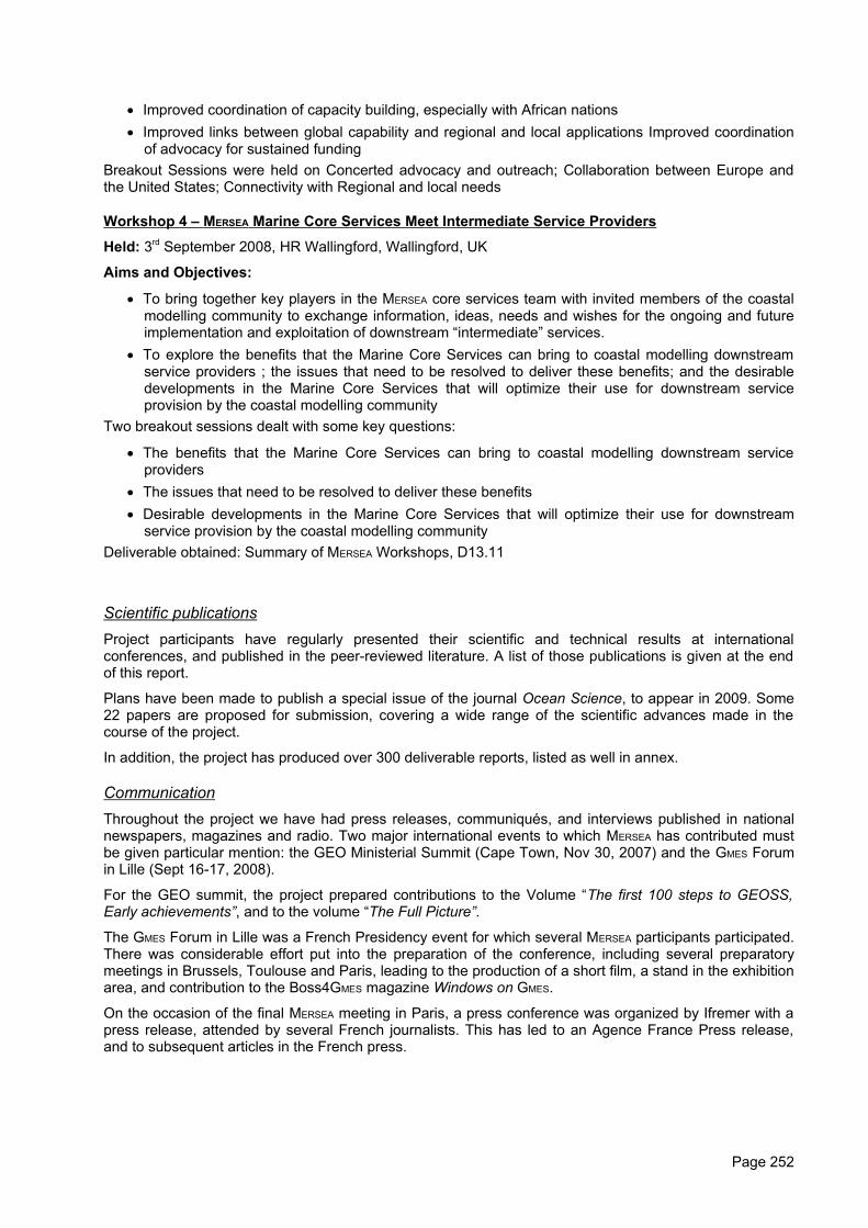
• Improved coordination of capacity building, especially with African nations• Improved links between global capability and regional and local applications Improved coordination

of advocacy for sustained fundingBreakout Sessions were held on Concerted advocacy and outreach; Collaboration between Europe andthe United States; Connectivity with Regional and local needs

Workshop 4 – MERSEA Marine Core Services Meet Intermediate Service Providers

Held: 3rd September 2008, HR Wallingford, Wallingford, UK

Aims and Objectives:

• To bring together key players in the MERSEA core services team with invited members of the coastalmodelling community to exchange information, ideas, needs and wishes for the ongoing and futureimplementation and exploitation of downstream “intermediate” services.

• To explore the benefits that the Marine Core Services can bring to coastal modelling downstreamservice providers ; the issues that need to be resolved to deliver these benefits; and the desirabledevelopments in the Marine Core Services that will optimize their use for downstream serviceprovision by the coastal modelling community

Two breakout sessions dealt with some key questions:

• The benefits that the Marine Core Services can bring to coastal modelling downstream serviceproviders

• The issues that need to be resolved to deliver these benefits• Desirable developments in the Marine Core Services that will optimize their use for downstream

service provision by the coastal modelling communityDeliverable obtained: Summary of MERSEA Workshops, D13.11

Scientific publicationsProject participants have regularly presented their scientific and technical results at internationalconferences, and published in the peer-reviewed literature. A list of those publications is given at the endof this report.

Plans have been made to publish a special issue of the journal Ocean Science, to appear in 2009. Some22 papers are proposed for submission, covering a wide range of the scientific advances made in thecourse of the project.

In addition, the project has produced over 300 deliverable reports, listed as well in annex.

CommunicationThroughout the project we have had press releases, communiqués, and interviews published in nationalnewspapers, magazines and radio. Two major international events to which MERSEA has contributed mustbe given particular mention: the GEO Ministerial Summit (Cape Town, Nov 30, 2007) and the GMES Forumin Lille (Sept 16-17, 2008).

For the GEO summit, the project prepared contributions to the Volume “The first 100 steps to GEOSS,Early achievements”, and to the volume “The Full Picture”.

The GMES Forum in Lille was a French Presidency event for which several MERSEA participants participated.There was considerable effort put into the preparation of the conference, including several preparatorymeetings in Brussels, Toulouse and Paris, leading to the production of a short film, a stand in the exhibitionarea, and contribution to the Boss4GMES magazine Windows on GMES.

On the occasion of the final MERSEA meeting in Paris, a press conference was organized by Ifremer with apress release, attended by several French journalists. This has led to an Agence France Press release,and to subsequent articles in the French press.

Page 252

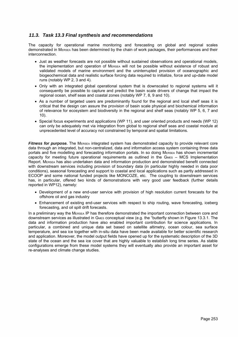
11.3. Task 13.3 Final synthesis and recommendations

The capacity for operational marine monitoring and forecasting on global and regional scalesdemonstrated in MERSEA has been determined by the chain of work packages, their performances and theirinterconnection.

• Just as weather forecasts are not possible without sustained observations and operational models,the implementation and operation of MERSEA will not be possible without existence of robust andvalidated models of marine environment and the uninterrupted provision of oceanographic andbiogeochemical data and realistic surface forcing data required to initialize, force and up-date modelruns (notably WP 2, 3 and 4).

• Only with an integrated global operational system that is downscaled to regional systems will itconsequently be possible to capture and predict the basin scale drivers of change that impact theregional ocean, shelf seas and coastal zones (notably WP 7, 8, 9 and 10).

• As a number of targeted users are predominantly found for the regional and local shelf seas it iscritical that the design can assure the provision of basin scale physical and biochemical informationof relevance for ecosystem and biodiversity in the regional and shelf seas (notably WP 5, 6, 7 and10).

• Special focus experiments and applications (WP 11), and user oriented products and needs (WP 12)can only be adequately met via integration from global to regional shelf seas and coastal module atunprecedented level of accuracy not constrained by temporal and spatial limitations.

Fitness for purpose. The MERSEA integrated system has demonstrated capacity to provide relevant coredata through an integrated, but non-centralized, data and information access system containing three dataportals and five modelling and forecasting information portals. In so doing MERSEA has shown incrementalcapacity for meeting future operational requirements as outlined in the GMES – MCS ImplementationReport. MERSEA has also undertaken data and information production and demonstrated benefit connectedwith downstream services including provision of boundary data (in particular highly needed in data poorconditions), seasonal forecasting and support to coastal and local applications such as partly addressed inECOOP and some national funded projects like MONCOZE, etc. The coupling to downstream serviceshas, in particular, offered two kinds of demonstrations with very good user feedback (further detailsreported in WP12), namely:

• Development of a new end-user service with provision of high resolution current forecasts for theoffshore oil and gas industry

• Enhancement of existing end-user services with respect to ship routing, wave forecasting, icebergforecasting, and oil spill drift forecasts.

In a preliminary way the MERSEA IP has therefore demonstrated the important connection between core anddownstream services as illustrated in GMES conceptual view (e.g. the “butterfly shown in Figure 13.3.1. Thedata and information production have also enabled important contribution for science applications. Inparticular, a combined and unique data set based on satellite altimetry, ocean colour, sea surfacetemperature, and sea ice together with in-situ data have been made available for better scientific researchand application. Moreover, the model output fields have opened up for the systematic description of the 3Dstate of the ocean and the sea ice cover that are highly valuable to establish long time series. As stableconfigurations emerge from these model systems they will eventually also provide an important asset forre-analyses and climate change studies.

Page 253

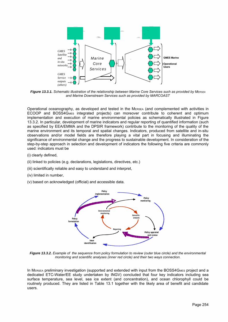
Qu ickTim e™ an d a d e co mp re ss o r

a re n ee de d to se e thi s p ic tu re.

GMESSatelliteand in situnetworks

QuickTim e ™ a nd a d ecom p re ss or

are ne ed ed to s ee th is p icture .

QuickTim e ™ a nd a d ecom p res s or

are ne ed ed to s ee th is p icture .

de co m pres so rare n ee de d to se e th is pic tu re .

Qu ickTim e™ an d a de co m pre s so r

a re n ee de d to se e th is pic tu re .

Qu ickTim e™ an d a d e co m pre s so r

a re n ee de d to se e thi s p ic tu re.

Qu ickTim e™ a n d a d e co m pre s so r

a re n ee de d to se e thi s p ic tu re.

QuickTim e ™ an d a de co m pres so r

are n ee d ed to se e th is pi ctu re .

QuickTim e ™ an d a de co m pres so r

are n ee d ed to s ee th is pi ctu re .

Marine Core

Services

Qu ickTim e™ a nd a d ecom p re ss o r

a re ne e de d to se e thi s p ic ture.

Ma rin e

D ow n strea m

Se rvi ce s

QuickTim e ™ an d a de com pres so r

are n e ed ed to s ee th is pi ctu re .

GMES Marine

OperationalUsers

are ne ed ed to s ee th is pi ctu re .

QuickTime ™ a nd a d ecom p re ss or

are ne ed ed to s ee th is pi ctu re .

QuickTime ™ a nd a d ecom p re ss or

are ne ed ed to s ee th is pi ctu re .

QuickTime ™ a nd a d ecom p re ss or

are ne ed ed to s ee th is pi ctu re .

Qu ickTime ™ a nd a d ecom p re ss or

are ne ed ed to s ee th is p ictu re .

Qu ickTime ™ a nd a d ecom p re ss or

are ne ed ed to s ee th is p ictu re .

Qu ickTime ™ a nd a d ecom p re ss or

are ne ed ed to s ee th is p ictu re .

GMESService outputs(others)

QuickTim e ™ an d a de co m pres so r

are n ee d ed to se e th is pi ctu re .

C o re

in form ation

( o ce an s tate )

U se r cus to m ize d

in form ation

(u s er p rod u cts )

GMES in p ut

i nfo rm a tio n

( raw d ata)

a re ne ed e d to s e e this p ic ture.

Figure 13.3.1. Schematic illustration of the relationship between Marine Core Services such as provided by MERSEA

and Marine Downstream Services such as provided by MARCOAST

Operational oceanography, as developed and tested in the MERSEA (and complemented with activities inECOOP and BOSS4GMES integrated projects) can moreover contribute to coherent and optimumimplementation and execution of marine environmental policies as schematically illustrated in Figure13.3.2. In particular, development of marine indicators and regular reporting of quantified information (suchas specified by EEA/EMMA and the DPSIR framework) contribute to the monitoring of the quality of themarine environment and its temporal and spatial changes. Indicators, produced from satellite and in-situobservations and/or model fields are therefore playing a vital part in focusing and illuminating thesignificance of environmental change and the progress to sustainable development. In consideration of thestep-by-step approach in selection and development of indicators the following five criteria are commonlyused: indicators must be

(i) clearly defined,

(ii) linked to policies (e.g. declarations, legislations, directives, etc.)

(iii) scientifically reliable and easy to understand and interpret,

(iv) limited in number,

(v) based on acknowledged (official) and accessible data.

Issue identification

Policy formulation

Policy implementation

Policy monitoring

Policy appraisal and review

Environmental monitoring

Reporting

Scientific analysis

Figure 13.3.2. Example of the sequence from policy formulation to review (outer blue circle) and the environmentalmonitoring and scientific analyses (inner red circle) and their two ways connection.

In MERSEA preliminary investigation (supported and extended with input from the BOSS4GMES project and adedicated ETC-Water/EE study undertaken by INGV) concluded that four key indicators including seasurface temperature, sea level, sea ice extent (and concentration), and ocean chlorophyll could beroutinely produced. They are listed in Table 13.1 together with the likely area of benefit and candidateusers.

Page 254

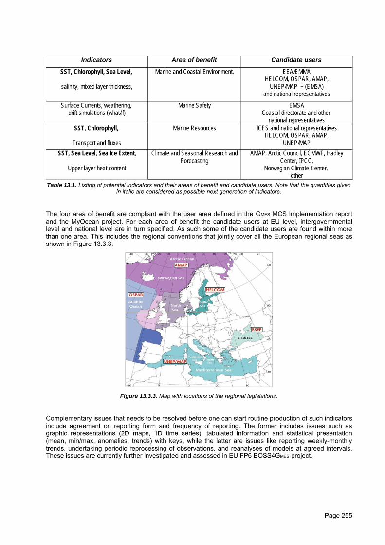
Indicators Area of benefit Candidate users

SST, Chlorophyll, Sea Level,

salinity, mixed layer thickness,

Marine and Coastal Environment, EEA/EMMAHELCOM, OSPAR, AMAP,

UNEP/MAP + (EMSA)and national representatives

Surface Currents, weathering, drift simulations (what/if)

Marine Safety EMSACoastal directorate and other

national representativesSST, Chlorophyll,

Transport and fluxes

Marine Resources ICES and national representativesHELCOM, OSPAR, AMAP,

UNEP/MAPSST, Sea Level, Sea Ice Extent,

Upper layer heat content

Climate and Seasonal Research andForecasting

AMAP, Arctic Council, ECMWF, HadleyCenter, IPCC,

Norwegian Climate Center, other

Table 13.1. Listing of potential indicators and their areas of benefit and candidate users. Note that the quantities givenin italic are considered as possible next generation of indicators.

The four area of benefit are compliant with the user area defined in the GMES MCS Implementation reportand the MyOcean project. For each area of benefit the candidate users at EU level, intergovernmentallevel and national level are in turn specified. As such some of the candidate users are found within morethan one area. This includes the regional conventions that jointly cover all the European regional seas asshown in Figure 13.3.3.

Figure 13.3.3. Map with locations of the regional legislations.

Complementary issues that needs to be resolved before one can start routine production of such indicatorsinclude agreement on reporting form and frequency of reporting. The former includes issues such asgraphic representations (2D maps, 1D time series), tabulated information and statistical presentation(mean, min/max, anomalies, trends) with keys, while the latter are issues like reporting weekly-monthlytrends, undertaking periodic reprocessing of observations, and reanalyses of models at agreed intervals.These issues are currently further investigated and assessed in EU FP6 BOSS4GMES project.

Page 255

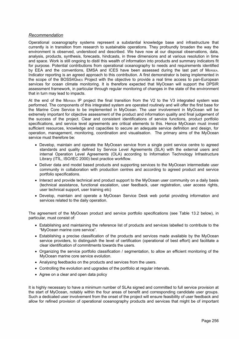
RecommendationOperational oceanography systems represent a substantial knowledge base and infrastructure thatcurrently is in transition from research to sustainable operations. They profoundly broaden the way theenvironment is observed, understood and described. We have now at our disposal observations, data,analysis, products, synthesis, forecasts, hindcasts, in three dimensions and at various resolution in timeand space. Work is still ongoing to distil this wealth of information into products and summary indicators fitfor purpose. Potential contributions from operational oceanography to needs and requirements identifiedby EEA and the conventions, EMSA and ICES have been assessed during the last part of MERSEA.Indicator reporting is an agreed approach to this contribution. A first demonstrator is being implemented inthe scope of the BOSS4GMES Project with the objective to provide a real time access to pan-Europeanservices for ocean climate monitoring. It is therefore expected that MyOcean will support the DPSIRassessment framework, in particular through regular monitoring of changes in the state of the environmentthat in turn may lead to impacts.

At the end of the MERSEA IP project the final transition from the V2 to the V3 integrated system wasperformed. The components of this integrated system are operated routinely and will offer the first base forthe Marine Core Service to be implemented in MyOcean. The user involvement in MyOcean will beextremely important for objective assessment of the product and information quality and final judgement ofthe success of the project. Clear and consistent identifications of service functions, product portfoliospecifications, and service level agreements are critical elements to this. Hence MyOcean must investsufficient resources, knowledge and capacities to secure an adequate service definition and design, foroperation, management, monitoring, coordination and visualisation. The primary aims of the MyOceanservice must therefore be:

• Develop, maintain and operate the MyOcean service from a single point service centre to agreedstandards and quality defined by Service Level Agreements (SLA) with the external users andinternal Operation Level Agreements (OLA) according to Information Technology InfrastructureLibrary (ITIL, ISO/IEC 2000) best practice workflow.

• Deliver data and model based products and supporting services to the MyOcean intermediate usercommunity in collaboration with production centres and according to agreed product and serviceportfolio specifications.

• Interact and provide technical and product support to the MyOcean user community on a daily basis(technical assistance, functional escalation, user feedback, user registration, user access rights,user technical support, user training etc)

• Develop, maintain and operate a MyOcean Service Desk web portal providing information andservices related to the daily operation.

The agreement of the MyOcean product and service portfolio specifications (see Table 13.2 below), inparticular, must consist of:

• Establishing and maintaining the reference list of products and services labelled to contribute to the“MyOcean marine core service”.

• Establishing a precise classification of the products and services made available by the MyOceanservice providers, to distinguish the level of certification (operational of best effort) and facilitate aclear identification of commitments towards the users.

• Organizing the service portfolio classification / segmentation, to allow an efficient monitoring of theMyOcean marine core service evolution.

• Analysing feedbacks on the products and services from the users.• Controlling the evolution and upgrades of the portfolio at regular intervals.• Agree on a clear and open data policy

It is highly necessary to have a minimum number of SLAs signed and committed to full service provision atthe start of MyOcean, notably within the four areas of benefit and corresponding candidate user groups.Such a dedicated user involvement from the onset of the project will ensure feasibility of user feedback andallow for refined provision of operational oceanography products and services that might be of important

Page 256

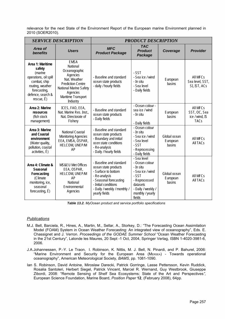
relevance for the next State of the Environment Report of the European marine Environment planned in2010 (SOER2010).

SERVICE DESCRIPTION PRODUCT DESCRIPTION

Area ofbenefits Users MFC

Product PackageTAC

ProductPackage

Coverage Provider

Area 1: Maritimesafety(marine

operations, oil spillcombat, ship

routing, weatherforecasting,

defence, search &rescue, É)

EMSANational

OceanographicAgencies

Nat. WeatherPrediction Centre

National Marine SafetyAgencies

Maritime TransportIndustry

- Baseline and standardocean state products- daily / hourly fields

- SST- Sea ice / wind- In situ- Sea level- Daily fields

Europeanbasins

All MFCsSea level, SST,

SI, IST, ACs

Area 2: Marineresources(fish stock

management)

ICES, FAO, EEA,Nat. Marine Res. Inst.,

Nat. Directorate ofFishery

- Baseline and standardocean state products- Daily fields

- Ocean colour -sea ice / wind- In situ

- Daily fields

Europeanbasins

All MFCsSST, OC, Seaice / wind, IS

TACs

Area 3: Marineand Coastalenvironment(Water quality,

pollution, coastalactivities, É)

National CoastalMonitoring Agencies

EEA, EMSA, OSPAR,HELCOM, UNEP/M

AP

- Baseline and standardocean state products- Boundary and initialocen state conditions- Re-analysis- Daily / hourly fields

- Ocean colour- In situ- Sea ice / wind- Sea level- SST- Reprocessing- Daily fields

Global oceanEuropean

basinsAll MFCsAll TACs

Area 4: Climate &Seasonal

Forecasting(Climate

monitoring, ice,seasonal

forecasting, É)

MS&EU Met OfficesEEA, OSPAR,

HELCOM, UNEP/MAP

NationalEnvironmental

Agencies

- Baseline and standardocean state products- Surface to bottom- Re-analysis- Seasonal forecasting- Initial conditions- Daily / weekly / monthly /yearly fields

- Sea level- Ocean colour- In situ- Sea ice / wind- SST- Reprocesseddatasets- Daily / weekly /monthly / yearlyfields

Global oceanEuropean

basinsAll MFCsAll TACs

Table 13.2. MyOcean product and service portfolio specifications

PublicationsM.J. Bell, Barciela, R., Hines, A., Martin, M., Sellar, A., Storkey, D.: “The Forecasting Ocean Assimilation

Model (FOAM) System in Ocean Weather Forecasting: An integrated view of oceanography”, Eds. E.Chassignet and J. Verron. Proceedings of the GODAE Summer School “Ocean Weather Forecastingin the 21st Century”, Lalonde les Maures, 20 Sept -1 Oct, 2004, Springer Verlag, ISBN 1-4020-3981-6,2006.

J.A.Johannessen, P.-Y. Le Traon, I. Robinson, K. Nittis, M. J. Bell, N. Pinardi, and P. Bahurel, 2006:“Marine Environment and Security for the European Area (MERSEA) - Towards operationaloceanography”, American Meteorological Society, BAMS, pp. 1081-1090.

Ian S. Robinson, David Antoine, Miroslaw Darecki, Patrick Gorringe, Lasse Pettersson, Kevin Ruddick,Rosalia Santoleri, Herbert Siegel, Patrick Vincent, Marcel R. Wernand, Guy Westbrook, GiuseppeZibordi, 2008: “Remote Sensing of Shelf Sea Ecosystems; State of the Art and Perspectives”,European Science Foundation, Marine Board, Position Paper 12, (February 2008), 64pp.

Page 257

PART IV: PUBLICATION LIST

Refereed journals, books

Allen, J.I., J. Blackford, J.T. Holt, R. Proctor, M. Ashworth, J.R. Siddorn: “A highly spatially resolvedecosystem model for the North West European Continental Shelf”, Sarsia, 86, pp. 423-440, Dec. 2001.

Allen, J.I., J.T. Holt, J. Blackford and R. Proctor, (2007): “Error quantification of a high-resolution coupledhydrodynamic-ecosystem coastal-ocean model: Part 2. Chlorophyll-a, nutrients and SPM”, Journal ofMarine Systems, 68, pp. 381-404, Dec. 2007.

Allen, J.I., P.J. Somerfield: “A multivariate approach to model skill assessment”, Journal of MarineSystems, Corrected proof, doi:10.1016/j.jmarsys.2008.05.009, May 2008

Allen, J.I., T.J. Smyth, J.R. Siddorn: “How well can we forecast high biomass algal bloom events in aeutrophic coast sea? Harmful Algae”, in press

Alvarez, A., B. Garau and A. Caiti, 2007, “Combining networks of drifting profiling floats and gliders foradaptive sampling of the Ocean”, Proceedings of the International Conference on Robotics andAutomation (IEEE publication), in press

Alvarez, A., B. Garau, S. Ruiz and J. Tintore, 2008: “Rapid environmental assessment of marine coastalareas for naval operations using sequential space filling designs”, Journal of Marine Systems, in press

Alvarez, A., R. Pennel, B. Garau and J. Tintore, 2007: “A Fourier-transform path integral formalism tocompute dispersion probability distributions in variable oceans”, Geophysical Research Letters, 34,Article L17605, doi:10.1029/2007GL030914, Sept. 2007.

Andersen, S., R.T. Tonboe, L. Kaleschke, G. Heygster, L.T. Pedersen: “Intercomparison of passivemicrowave sea ice concentration retrievals over the high concentration Arctic sea ice”, Journal ofGeophysical Research-Oceans, 112, Issue C8, Article C08004, Aug. 2007

Andersen, S., R.T. Tonboe, S. Kern, H. Schyberg: “Improved retrieval of sea ice total concentration fromspaceborne passive microwave observations using Numerical Weather Prediction model fields: Anintercomparison of nine algorithms”, Remote Sensing of Environment, 104, Issue 4, pp. 374-392, Oct.2006.

Ayina, L-H, A. Bentamy : « Une Approche Globale pour Améliorer les Données de Flux Turbulents Estimésà l’Aide de Capteurs Satellitaires », Revue Télédétection, 7, Issue 1-2-3-4, pp. 91-110, April 2007.

Ayina, L-H, A. Bentamy, G. Madec, Alberto M. Mestas-Nuñez: “The Impact of Satellite Winds and LatentHeat Fluxes in a Numerical Simulation of the Tropical Pacific Ocean”, Journal of Climate, 19, Issue No 22, pp. 5889-5902, 2006.

Backeberg, B., J. A. Johannessen, L. Bertino, C. J. Reason: “The greater Agulhas Current system: Anintegrated study of its mesoscale variability”, Journal of Operational Oceanography, 1, Issue No 1, pp. 29-44, 2008.

Barnier, B., G. Madec, T. Penduff, J.-M. Molines, A.-M. Treguier, J. Le Sommer, A. Beckmann, A.Biastoch, C. Böning, J. Dengg, C. Derval, E. Durand, S. Gulev, E. Remy, C. Talandier, S. Theetten, M.Maltrud, J. McClean, and B. De Cuevas: “Impact of partial steps and momentum advection schemes ina global ocean circulation model at eddy permitting resolution”, Ocean Dynamics, 56, Issue No 5-6, pp.543-567, doi 10.1007/s10236-006-0082-1, Dec. 2006.

Béal, D., P. Brasseur, J.M. Brankart, Y. Ourmières and J. Verron, 2008: “Monte Carlo study of errors dueto the wind in a coupled physical biogeochemical model of the North Atlantic: controllability by surfaceobservations”, in preparation for Ocean Science.

Bell, M.J., R. Barciela, A. Hines, M. Martin, A. Sellar, D. Storkey: “The Forecasting Ocean AssimilationModel (FOAM) System in Ocean Weather Forecasting: An integrated view of oceanography”, in OceanWeather Forecasting in the 21st Century, Proceedings of the GODAE Summer School, Lalonde lesMaures, 20 Sept -1 Oct, 2004, Eds. E. Chassignet and J. Verron, Springer Verlag, pp. 397-411, ISBN 1-4020-3981-6, 2006.

Bentamy, A. D. Croize-Fillon, P. Queffeulou, C. Liu, H. Roquet, 2008: “Evaluation of High-ResolutionSurface Wind Products at Global and Regional Scales”, submitted to Journal of Atmospheric &oceanic technology.

Page 258

Bentamy, A., H.L. Ayina, P. Queffeulou, D. Croize-Fillon, 2007: “Improved Near Real Time Surface WindResolution over The Mediterranean Sea”, Ocean Science, 3, Issue 2, pp. 259-271,ISSN 1812-0784,2007

Bentamy, A., D. Croize-Fillon, C. Perigaud, 2008: “Characterization of ASCAT measurements based onbuoy and QuikSCAT wind vector observations”, Ocean Science, 4, pp. 265-274

Berline, L., et al. (2007): “Improving the physics of a coupled physical-biogeochemical model of the NorthAtlantic through data assimilation: Impact on the ecosystem”, Journal of Marine Systems, 64, Issue No 1-4, pp. 153-172.

Bertino, L. and K.A. Lisæter (2008): “The TOPAZ monitoring and prediction system for the Atlantic andArctic oceans”, Journal of Operational Oceanography, accepted for publication.

Bessière, L., G. Madec, and F. Lyard: “Global tidal residual mean circulation: does it affect a climateOGCM?”, Geophysical Research Letters, 35, Issue 3, Article No L03609, ISSN: 0094-8276, doi:10.1029/2007GL032644, Feb 2008.

Bessière, L., G. Madec, F. Lyard, and C. Le Provost, 2007a: “Improved tidally driven mixing in an OGCM”,to be submitted to Ocean Modelling.

Blanc, F. and the Mersea partners: “A Remote Sensing Ocean Portal for GMES Ocean”, in Journal ofOperational Oceanography, 2, pp. 29-34, August 2008.

Blayo, E. and L. Debreu: “Revisiting open boundary conditions from the point of view of characteristicvariables”, Ocean Modelling, 9, Issue 3, doi: 10.1016/j.ocemod.2004.07.001, pp. 231-252, 2005.

Blower, Jon, K. Haines, A. Santokhee, C. Liu, 2008: “Godiva2: Interactive visualization of environmentaldata on the web”, submitted to Philosophical Transactions of The Royal Society A

Blower. J., A. Harrison, K. Haines: “Styx Grid Services: Lightweight middleware for efficient scientificworkflows, Scientific Programming”, 14, pp. 209-216, 2006

Bonhommeau, S., B. Blanke, A.M. Treguier, E. Rivot, Y. Vermard, O. Le Pape, 2008: “Can the Europeaneel larvae cross the Atlantic Ocean in 6 months?” Submitted

Brasseur, P. and J. Verron: “The SEEK filter method for data assimilation in oceanography: a synthesis”,Ocean Dynamics, 56, Issue No 5-6, doi :10.1007/s10236-006-0080-3, pp. 650-661, Dec. 2006.

Brasseur, P., P. Bahurel, L. Bertino, J-M Brankart, N. Ferry, S. Losa, E. Remy, J. Schroter, S. Skachiko, C-E. Testut, B. Tranchant, P.J. van Leeuwen, and J. Verron: “Data assimilation for marine monitoring andpredcition: the MERCATOR operational assimilation systems and the MERSEA developments”,Quarterly Journal of the Royal Meteorological Society, 131, Issue No 613, doi: 10.1256/qj.05.142, pp3561-3582, Oct. 2005.

Brodeau, L., B. Barnier, A.M. Treguier and T. Penduff: “An ERA40 based atmospheric forcing for globalocean circulation models”, Ocean Modelling, submitted.

Caballero, A. Pascual, G. Dibarboure, and M. Espino: “Sea Level and Eddy Kinetic Energy variability in theBay of Biscay, inferred from satellite altimeter data”, Journal of Marine Systems, 72, Issue 1-4, pp. 116-134, doi: 10.1016/j.jmarsys.2007.03.011, July 2008.

Cailleau, S., V. Fedorenko, B. Barnier, E. Blayo, and L. Debreu, 2008: “Comparison of different numericalmethods used to handle the open boundary of a regional ocean circulation model of the Bay ofBiscay”, Ocean Modelling, in press.

Carrère, L., D.L. Volkov, P-Y. Le Traon, P. Schaeffer, C. Boone, Y. Faugère and P. Gaspar: “Reducing thealiasing of high frequency signals in altimeter data: empirical and model-based approaches”, submittedto Journal of Physical Oceanography, 2006.

Carril, A.F., S. Gualdi, A. Cherchi and A. Navarra: “Heatwaves in Europe: Areas of homogeneousvariability and links with the regional to large-scale atmospheric and SSTs anomalies", ClimateDynamics, 30, Issue 1, doi: 10.1007/s00382-007-0274-5, pp. 77-98, Jan. 2008.

Castruccio, F., J. Verron, L. Gourdeau, J.M. Brankart and P. Brasseur: “On the role of the GRACE missionin the joint assimilation of altimetric and TAO data in a Tropical Pacific Ocean model”, GeophysicalResearch Letters, 33, Issue 14, Article No L14616, doi: 10.1029/2006GL025823, July 2006.

Chassignet, E. P., J. Verron (Editors): Ocean Weather Forecasting, An Integrated View of Oceanography.Springer, XII, 578 p, ISBN: 978-1-4020-3981-2, doi: 10.1007/1-4020-4028-8, 2006.

Page 259

Chassot, E., F. Mélin, O. Le Pape, D. Gascuel: “Bottom-up control regulates fisheries production at thescale of eco-regions in the European seas”, Marine Ecology-Progress Series, 343, doi:10.3354/meps06919, pp. 45-55, 2007.

Counillon, F. and L. Bertino: “Ensemble Optimal Interpolation: multivariate properties in the Gulf ofMexico”, Tellus, accepted for publication, 2008.

Crosnier L, C. Le Provost and MERSEA team, 2005: “Internal metrics definition for operational forecastsystems inter-comparison: Examples in the North Atlantic and Mediterranean Sea”, in Ocean WeatherForecasting: An integrated view of oceanography, Part V, pp. 457-468, GODAE BOOK Edited by E.Chassignet and J. Verron, Springer, ISBN: 1-4020-3981-6, doi: 10.1007/1-4020-4028-8_20, 2006.

Crosnier, L. and C. Le Provost: “Inter-comparing five forecast operational systems in the North Atlantic andMediterranean basins: The MERSEA-strand1 Methodology”, Journal of Marine System, Special Issue“Marine Environmental Monitoring and prediction”, 65, Issue 1-4, pp. 354-375, March 2007.

Crosnier, L., M. Drévillon, S. Buarque, F. Soulat: “Environmental Ocean Indicators at Mercator-Ocean”,ICES Journal of Marine Science, accepted, in revision, 2008.

Debreu, L. and E. Blayo: “Two-Way embedding algorithms: a review”, Ocean Dynamics: Special Issue onMulti-scale modelling, ISSN 1616-7341, doi: 10.1007/s10236-008-0150-9, 17 October 2008

Debreu, L., P. Penven, P. Marchesiello and E. Blayo, 2007: “Two-Way nesting algorithms for a split-explicitfree surface model”, submitted to Ocean Modelling

Desaubies, Y., 2005: “Mersea, Development of a European Ocean Monitoring and Forecasting System -Ocean and Marine applications for GMES”. In Ocean Weather Forecasting: An Integrated View of Oceanography, Chapter 19 ,pp. 449-453, Edited by E. Chassignet and J. Verron, Springer, ISBN: 1-4020-3981-6, doi 10.1007/1-4020-4028-8_19, 2006.

Desaubies, Y., M. Rixen, and J.M. Beckers (Eds): “Marine Environmental Monitoring and Prediction”(Proceeding to the 36th International Liege Colloquium on Ocean Dynamics - Liege, Belgium, 3-7 May,2004) Journal of Marine Systems (Special issue), 65, Issue No 1 to 4, pp. 1-2., March 2007

Desaubies, Y.: “Good Bye and Mersea”, Windows on GMES, pp 93-94, 2, 2008

Desaubies, Y.: “European Marine Core Services: global and regional ocean monitoring and forecasting, aservice to society”, In The Full Picture, pp128-130, Tudor Rose for the Group on Earth Observation.ISBN 978-92-990047-0-8. 2007

Dobricic, S.: “An improved calculation of Coriolis terms on the C grid”, Monthly Weather Review, 134, IssueNo 12, pp. 3764-3773, Dec. 2006.

Dobricic, S. and N. Pinardi: “An oceanographic three-dimensional variational data assimilation scheme”,Ocean Modelling, 22, Issue No 3-4, pp. 89-105, doi: 10.1016/j.ocemod.2008.01.004, 2008.

Dobricic, S.: “New mean dynamic topography of the Mediterranean calculated from assimilation systemdiagnostics”, Geophysical Research Letters, 32, Issue 11, Article No 11606, doi:10.1029/2005GL022518, June 2005.

Dobricic, S., N. Pinardi, M. Adani, M. Tonani, C. Fratianni, A. Bonazzi and V. Fernandez: “Dailyoceanographic analyses by the Mediterranean basin scale assimilation system”, Ocean Sciences, 3,Issue No1, pp. 149–157, 2007.

Dobricic, S., Pinardi, N., Adani, M., Bonazzi, A., Fratianni, C., Tonani, M., 2005: “MediterraneanForecasting System: An improved assimilation scheme for sea-level anomaly and its validation”,Quarterly Journal of the Royal Meteorological. Society 131, pp. 3627-3642.

Donlon, C, I.S. Robinson, M. Reynolds, W. Wimmer, G. Fisher, R. Edwards, T.J. Nightingale: “An InfraredSea Surface Temperature Autonomous Radiometer (ISAR) for Deployment aboard VolunteerObserving Ships (VOS)”, Journal of Atmospheric and Oceanic Technology, 25, Issue No 1, pp. 93-113,doi: 10.1175/2007JTECHO505.1, Jan 2008.

Donlon, C., I.S. Robinson, K.S. Casey, J. Vazquez-Cuervo, E Armstrong, O. Arino, C. Gentemann, D. May,P. LeBorgne, J. Piollé, I. Barton1, H Beggs, D. J. S. Poulter, C. J. Merchant, A. Bingham, S. Heinz, AHarris, G. Wick, B. Emery, P. Minnett, R. Evans, D. Llewellyn-Jones, C. Mutlow, R. Reynolds, H.Kawamura1 and N. Rayner: “The Global Ocean Data Assimilation Experiment (GODAE) highResolution Sea Surface Temperature Pilot Project (GHRSSTPP)”, Bulletin of the AmericanMeteorological Society, 88, Issue No 8, pp. 1197-1213, doi: 10.1175/BAMS-88-8-1197, Aug 2007

Page 260

Drévillon M., R. Bourdallé-Badie, C. Derval, Y. Drillet, J.-M. Lellouche, E. Rémy, B. Tranchant, M.Benkiran, E. Greiner, S. Guinehut, N. Verbrugge, G. Garric, C.-E. Testut, M. Laborie, L. Nouel, P.Bahurel, C. Bricaud, L. Crosnier, E. Dombrowsky, E. Durand, N. Ferry, F. Hernandez, O. LeGalloudec, F. Messal: “The GODAE/Mercator-Ocean global ocean forecasting system: results,applications and prospects”, Journal of Operational Oceanography, Imarest, 1, no 1, pp. 51-57, Feb2008.

Gaillard, F., E. Autret, V.Thierry, P. Galaup, C. Coatanoan, and T. Loubrieu, 2008: “Quality control of largeARGO datasets”, Accepted by Journal of Atmospheric and Oceanic Technology, doi:10.1175/2008JTECHO552.1.

García-Olivares, A., J. Isern-Fontanet and E. García-Ladona: “Dispersion of passive tracers and finiteLyapunov exponents in the Western Mediterranean Sea”, Deep Sea Research Part I- Oceanographicresearch papers, 54, Issue No 2, pp. 253-268, doi: 0.1016/j.dsr.2006.10.009, Feb. 2007.

Guiavarc'h, C., A.M. Treguier, A. Vangriesheim, 2008a: “Remotely forced biweekly deep oscillations on thecontinental slope of the Gulf of Guinea”, Journal of Geophysical Research, 113, C06002,doi:10.1029/2007JC004471, 4 June 2008

Hackett, B., Ø. Breivik and C. Wettre: “Forecasting the drift of objects and substances in the ocean”, InOcean Weather Forecasting: An Integrated View of Oceanography, Chapter 23, pp. 507-524, edited byE. Chassignet and J. Verron, Springer, ISBN: 1-4020-3981-6, doi 10.1007/1-4020-4028-8_23, 2006.

Hartman, S., K.E. Larkin, R.S. Lampitt, W. Koeve, A. Yool, D.J. Hydes: “Seasonal and inter-annualbiogeochemical variations at PAP (49°N, 16.5°W) 2003-2005”. (Submitted Deep-Sea Research II 29July 2008), ISSN 0967-0645

Hemmings, J., R. M. Barciela, M. J. Bell: “Ocean colour data assimilation with material conservation forimproving model estimates of air-sea CO2 flux”, Journal of Marine Research, 66, Issue 1, pp. 87-126,doi: 10.1357/002224008784815739, January 2008.

Holt ,J.T., J.I Allen., R. Proctor, F. Gilbert: “Error quantification of a high resolution coupled hydrodynamic-ecosystem coastal-ocean model: part 1 model overview and assessment of the hydrodynamics”, ,Journal of Marine Systems, 57, Issue No 1-2, pp. 167-188, doi: 10.1016/j.jmarsys.2005.04.008, Aug.2005 (subject to minor revision).

Holt, J.T. and R. Proctor, (2008): “The seasonal circulation and volume transport on the NorthwestEuropean Shelf: a fine resolution model study” Journal of Geophysical Research-Oceans, 113, IssueNo C6, doi:10.1029/2006JC004034, June 2008.

Holt, J.T., L. Umlauf: “Modelling the tidal mixing fronts and seasonal stratification of the NorthwestEuropean”, Continental shelf Continental Shelf Research, 28, Issue No 7, pp. 887-903, doi:10.1016/j.csr.2008.01.012, April 2008.

Høyer, J.L. and J. She, 2007: “Optimal interpolation of sea surface temperature for the North Sea andBaltic Sea”, Journal of Marine Systems, 65, 176-189.

Isern-Fontanet, J., A. Turiel, E. García-Ladona and J. Font: “Microcanonical multifractal formalism:application to the estimation of ocean surface velocities”, Journal of Geophysical Research-Oceans,112, Issue No C5, doi: 10.1029/2006JC003878, May 2007.

Isern-Fontanet, J., E. García-Ladona, J. Font: “Vortices of the Mediterranean sea: an altimetricperspective”, Journal of Physical Oceanography, 36, Issue No 1, pp. 87-103, ISSN: 0022-3670, Jan.2006.

Isern-Fontanet, J., E. García-Ladona, J. Font, A. García-Olivares: “Non-Gaussian velocity ProbabilityDensity Functions: an altimetric perspective of the Mediterranean Sea”, Journal of PhysicalOceanography, 36, Issue No 11, pp. 2153-2164, ISSN: 0022-3670, Nov 2006.

Isern-Fontanet, J., F. d’Ovidio, C. López, E. Hernández, E. García-Ladona: “Dispersion of passive tracersand finite-scale Lyapunov exponents in the Western Mediterranean Sea”, Deep Sea Research Part I-Oceanographic Research Papers, 54, Issue No 2, pp. 253-268, DOI: 10.1016/j.dsr.2006.10.009, Feb.2007.

Isern-Fontanet, J., F. d’Ovidio, C. López, E. Hernández, E. García-Ladona, 2006: “Comparison betweenthe Okubo-Weiss parameter and Finite-Size-Lyapunov-Exponents computed from altimetry in theAlgerian Basin”, Journal of Geophysical Research-Oceans, submitted.

Page 261

Jennings, S., F. Mélin, J.L. Blanchard, R.M. Forster, N.K. Dulvy, R.W. Wilson (2008): “Global scalepredictions of community and ecosystem properties from simple ecological theory”, Proceedings of theRoyal Society B, 275, No1641, pp. 1375-1383, 22 June 2008, 10.1098/rspb.2008.0192.

Johannessen, J.A, P.-Y. Le Traon, I. Robinson, K. Nittis, M. J. Bell, N. Pinardi, and P. Bahurel: “MarineEnvironment and Security for the European Area (MERSEA) - Toward operational oceanography”,Bulletin Of The American Meteorological Society, 87, Issue No 8, pp. 1881-1090, doi: 10.1175/BAMS-87-8-1081 Aug 2006.

Johannessen, J.A., B. Hackett, E. Svendsen, H. Søiland, L.P. Røed, N. Winther, J. Albretsen, D.Danielssen, L. Pettersen, M. Skogen and L. Bertino: “Operational Oceanography – Challenges andpossibilities” Chapter 11 In The Norwegian Coastal Current – Oceanography and Climate, Ed. R.Sætre, Tapir Academic Press, Trondheim, pp. 139-151, ISBN: 9788251921848, 2007.

Jouanno, J., J Sheinbaum, B. Barnier, J. M. Molines, L. Debreu, and F. Lemarié, 2008: “The mesoscalevariability in the Caribbean Sea. Part I: simulations with an embedded model and characteristics”,Ocean Modelling, in press.

Karstensen, J., T. Avsic, J. Fischer and U. Send: “Subsurface temperature maxima in the Labrador Seaand the subpolar North Atlantic”, Geophysical Research Letters, 33, Issue No 21, Article L21S05,doi:10.1029/2006GL026613, October 2006.

Klatt O., O. Boebel, E. Fahrbach: “A profiling float’s sense of ice”, Journal of Atmospheric and OceanicTechnology, 24, Issue No 7, pp. 1301-1308., doi:10.1175/JTECH2026.1, Aug. 2006.

Knut Arild L., G. Evensen and S. Laxon, “Assimilating synthetic CryoSat sea ice thickness in a coupled ice-ocean model”, Journal of Geophysical Research, 112, C07023, doi:10.1029/2006JC003786, 20 July2007

Koch-Larrouy A., G. Madec, P. Bouruet-Aubertot, T. Gerkema, L. Bessières, and R. Molcard, “On thetransformation of Pacific Water into Indonesian ThroughFlow Water by internal tidal mixing”,Geophysical Research Letters, 34, Issue No 4, doi: 10.1029/2006GL028405 , Feb 2007.

Körtzinger, A., U. Send, R.S. Lampitt, S. Hartman, D.W.R. Wallace, J. Karstensen, M.G. Villagarcia, O.Llinás, and M.D. DeGrandpre: “The seasonal pCO2 cycle at 49°N/16.5°W in the northeast AtlanticOcean and what it tells us about biological productivity”. Journal of Geophysical Research, 113, IssueNo C04020, doi: 10.1029/2007JC004347, April 2008.

Kriest, I., A. Oschlies: “Modelling the effect of cell-size dependent nutrient uptake and exudation onphytoplankton size spectra”. Deep-Sea Research Part I-Oceanographic Research Papers, 54, Issue 9,pp. 1593-1618, doi: 10.1016/j.dsr.2007.04.017, Sept. 2007

Kriest, I., A. Oschlies, “On the treatment of particulate organic matter sinking in large-scale models ofmarine biogeochemical cycle”, Biogeosciences, 5, Issue No 1, pp. 55-7, ISSN: 1726-4170, 2008 url: http://www.biogeosciences.net/5/55/2008/bg-5-55-2008.html

Lamouroux, J., P. De Mey, F. Lyard et E. Jeansou, “Control of a barotropic model of the Bay of Biscay inpresence of atmospheric forcing errors”, Journal of Geophysical Research, 8, Issue No 07217, 2006

Lampitt, R.S., I. Salter, and D. Johns: “Radiolaria; major exporters of organic carbon to the deep ocean”,Global Biogeochemical Cycles (submitted).

Lampitt, R.S., I. Salter, B.A. de Cuevas, S. Hartman, K.E. Larkin, C.A. Pebody: “Long-term variability ofdownward particle flux in the deep Northeast Atlantic: causes and trends”, Deep Sea Research II(Submitted)

Larsen, J., J.L. Høyer, and J. She: “Validation of a hybrid optimal interpolation and Kalman filter schemefor sea surface temperature assimilation”. Journal of Marine Systems,65, Issue No 1-4, pp. 122-133,doi: 10.1016/j.jmarsys.2005.09.013, March 2007.

Lauvernet, C., J.M. Brankart, F. Castruccio, G. Broquet, P. Brasseur and J. Verron: “A truncated gaussianfilter for data assimilation with inequality constraints: enforcing static stability conditions in oceanmodels”, accepted 21 October 2008, Ocean Modelling doi:10.1016/j.ocemod.2008.10.007.

Lellouche, J.M., S. Giraud St Albin, E. Greiner and L. Crosnier: "The High Resolution Real Time MercatorForecasting System: Description and evaluation in the Gulf of Mexico", under revision at JMS-REA-15(2008).

Page 262

Le Sommer, J.T. Penduff, G. Madec (2007): “How momentum advection schemes affect current-topography interactions in the DRAKKAR 1/4° z-coordinate model”, Ocean Modelling, in revision.

Le Sommer J, T. Penduff, S. Theetten, G. Madec, and B. Barnier, 2008: “How momentum advectionschemes influence current-topography interactions at eddy permitting resolution”, Ocean Modelling, inpress.

Lewis, K, J.I. Allen, A.J. Richardson, J.T. Holt: “Error quantification of a high resolution coupledhydrodynamic-ecosystem coastal-ocean model: Part3, validation with Continuous Plankton Recorderdata”, Journal of Marine Systems, 63, Issue 3-4, pp. 209-224, doi: 10.1016/j.jmarsys.2006.08.001,Dec. 2006.

Lewis, K., J.I. Allen: “Validation of a hydrodynamic-ecosystem model simulation with time-series datacollected in the western English Channel”, Journal of Marine Systems in press

Lique, C., A.M. Treguier, M. Scheinert, T. Penduff, 2008: “A model-based study of ice and freshwatertransport variabilities along both sides of Greenland”, Climate Dynamics, in revision.

Lisæter, K.A., G. Evensen and S Laxon: “Assimilating synthetic CryoSat sea ice thickness in a coupled ice-ocean model”, Journal of Geophysical Research – All series, 112, Issue No C7, pp. C07023-C07026,doi: 10.1029/2006JC003786, 2007

Losa, S.N., A. Vezina, D. Wright, Y. Lu, K. Thompson, M. Dowd, 2006: “3D ecosystem modelling in theNorth Atlantic: relative impacts of physical and biological parameterizations”, Journal of marinesystems, 63, Issue No 3-4, pp. 230-245, doi: 10.1016/j.jmarsys.2005.09.011, July 2006

Losa, S.N., C. Völker, M. Losch, S. Hohn, M. Schartau (2008): “3D Global Ocean BiogeochemicalModelling with decoupled C, N, Chl a : Estimating Export Production”, Paper in preparation.

Loubrieu T., S. Pouliquen, M. Spigai, P. Bahurel, F. Blanc, G. Manzella, C. O'Kelly, J. Blower, C. Liu: “Adistributed system for operational oceanography : the MERSEA System”. Submitted to Journal ofOperational Oceanography, 2008

Martin, M., A. Hines, M. J. Bell: “Data assimilation in the FOAM operational short-range ocean forecastingsystem: a description of the scheme and its impact”, Quarterly Journal of the Royal MeteorologicalSociety., 133, Issue 625, pp. 981-995, doi: 10.1002/qj.74, June 2007.

Maximenko N., P. Niiler, M.H. Rio, O. Melnichenko, L. Centurioni, D. Chambers, V. Zlotnicki, B. Galperin:“Drifting buoys and satellites reveal persistent, small-scale, currents near ocean surface”, submitted toJournal of Atmospheric and Oceanic Technology

Mélin, F., G. Zibordi: “An optically-based technique for producing merged spectra of water leavingradiances from ocean color remote sensing”, Applied Optics, 46, Issue 18, pp. 3856-3869, ISSN: 0003-6935, June 2007.

Mélin, F., G. Zibordi, J.F. Berthon (2007): “Assessment of satellite ocean color products at a coastal site”.Remote Sensing of Environment, 110, 192-215, 2007.

Mélin, F., G. Zibordi, S. Djavidnia (2007): “Development and validation of a technique for merging satellitederived aerosol optical depth from SeaWiFS and MODIS”, Remote Sensing of Environment, 108, 436-450, 2007.

Mélin, F., Zibordi, G., Djavidnia, S. (2008), “Merged series of normalized water leaving radiances obtainedfrom multiple satellite missions for the Mediterranean Sea”, Advances in Space Research, in press,accepted 8 April 2008, doi:10.1016/j.asr.2008.04.004 .

Mestas-Nunez A., A. Bentamy, and K. Katsaros: “Seasonal and El Ninõ variability in weekly satelliteevaporation over the global ocean during 1996-1998”, Journal of Climate, 19, Issue No 10, pp. 2025-2035, ISSN 0894-8755, May 2006.

Mourre, B., L. Crosnier and C. Le Provost, 2006: “Real Time Sea Level Gauge Observation andOperational Oceanography” , Philosophical Transactions Of The Royal Society A-MathematicalPhysical And Engineering Sciences, UK Royal Society publication, London, 364, Issue No 1841, pp.867-884, ISSN: 1364-503X, doi:10.1098/rsta.2006.1743, April 2006.

Nieves, V. and A. Turiel: “Analysis of ocean turbulence using adaptive CVS on altimetry maps”, Journal ofMarine Systems (submitted).

Page 263

Nieves, V., C. Llebot, A. Turiel, J. Solé, E. García-Ladona, D. Blasco, and M. Estrada: “Common turbulentsignature in sea surface temperature and chlorophyll maps”, Geophysical Research Letters, 34, IssueNo 23, Article L23602, ISSN: 0094-8276, doi: 10.1029/2007GL030823, Dec. 2007.

Nittis, K., C. Tziavos, R. Bozzano, V. Cardin, Y. Thanos, G. Petihakis, M.E Schiano, F. Zanon: “The M3Amulti-sensor buoy network of the Mediterranean Sea”, Ocean Science, 3, Issue No 2, pp. 229-243,ISSN: 1812-0784, 2007

Oddo, P. and N. Pinardi: “Lateral Open Boundary Conditions for Nested Limited Area Models: a processselective approach”, Ocean Modelling, 20, Issue No 2, pp. 134-156, ISSN: 1463-5003, doi:10.1016/j.ocemod.2007.08.001, 2008

Onken, R., A. Alvarez, V. Fernandez, G. Vizoso, J. Tintore, P. Haley, and E. Nacini: “A forecast experimentin the Balearic Sea”, Journal of Marine Systems, 71, Issue 1-2, pp 79-98, ISSN: 0924-7963, doi:10.1016/j.jmarsys.2007.05.008, May 2008

Ourmières, Y., J.M. Brankart, J. Verron and P. Brasseur, 2006: “A SEEK filter with Incremental AnalysisUpdating scheme”, Journal of Atmospheric and Oceanic Technologies, accepted.

Ourmières, Y., J.M. Brankart, L. Berline, P. Brasseur and J. Verron: “Incremental Analysis Updateimplementation into a sequential ocean data assimilation system”, Journal Of Atmospheric AndOceanic Technology, 23, Issue No 12, pp. 1729-1744, ISSN: 0739-0572, Dec 2006.

Ourmières, Y., P. Brasseur, M. Lévy, J.M. Brankart and J. Verron, 2008: “On the key role of nutrient data toconstrain a coupled physical-biogeochemical assimilative model of the North Atlantic Ocean”, In press,accepted 1 August 2008, Journal of Marine Systems, doi:10.1016/j.jmarsys.2008.08.003 .

Ourmières, Y., P. Brasseur, M. Lévy, J.M. Brankart and J. Verron, 2007: “Physical and biogeochemicaldata assimilation into a coupled ¼° physical-biogeochemical model of the North Atlantic”, inpreparation.

Pascual, A., C. Boone, G. Larnicol, P.Y. Le Traon: "On the quality of real time altimeter gridded fields:comparison with in situ data." Journal of Atmospheric and Oceanic Technology, doi:10.1175/2008JTECHO556.1, (Received: August 28, 2008)

Pascual, A., Y. Faugère, G. Larnicol, P.Y. Le Traon: “Improved description of the ocean mesoscalevariability by combining four satellite altimeters”, Geophysical Research Letters, 33, Issue No 2, ArticleL02611; ISSN: 0094-8276, doi: 10.1029/2005GL024633, Jan. 2006.

Penduff, T., J. Le Sommer, B. Barnier, A.-M. Treguier, J.-M. Molines, and G. Madec, 2007, “Influence ofnumerical schemes on current-topography interactions in 1/4° global ocean simulations”, OceanScience, 3, Issue No 4, pp. 451-535.

Penduff, T., J. Le Sommer, B. Barnier, A-M. Tréguier, J-M. Molines, and G. Madec, 2007: “Depth-dependent effects of momentum advection, sidewall boundary conditions, and partial steps topographyin 1/4° global ocean simulations”, To be submitted to Ocean Modelling.

Petihakis, G., P. Drakopoulos, K. Nittis, V. Zervakis, C. Christodoulou, and C. Tziavos: “M3A system(2000–2005) – operation and maintenance”, Ocean Science, 3, Issue No 1, pp. 117-128, ISSN: 1812-0784, Feb. 2007

Picco, P., R. Bozzano, M. E. Schiano, A. Bordone, M. Borghini, G. Di Nallo, S. Pensieri, A. Schirone, S.Sparnocchia: “Marine Observing System from fixed platform in the Ligurian Sea”, Bollettino diGeofisica Teorica ed Applicata, Trieste, 48, Issue No 3, pp. 227-239, ISSN: 0006-6729, Sept. 2007

Pont, O., A. Turiel and C. Perez-Vicente, 2007: “Empirical evidences of a common multifractal signature ineconomic, biological and physical systems”, Submitted to New Journal of Physics A.

Pottier, C., A. Turiel and V. Garçon: “Inferring missing data in satellite chlorophyll maps using turbulentcascading”, Remote Sensing of Environment, XX, doi: 10.1016/j.rse.2008.07.010 (submitted, 2008)

Pottier, C., V. Garçon, G. Larnicol, J. Sudre, P. Schaeffer and P.Y. Le Traon: “Merging SeaWiFS andMODIS/Aqua Ocean Color Data in North and Equatorial Atlantic Using Weighted Averaging andObjective Analysis”, IEEE Transactions on Geoscience and Remote Sensing, Vol. 44, Issue No. 11,Part 2, pp. 3436-3451, doi: 10.1109/TGRS.2006.878441, Nov. 2006.

Pouliquen S., 2005: “In-situ observations: operational systems and data management,” In Ocean WeatherForecasting: An Integrated View of Oceanography, Part III, Chapter 8, pp. 207-227, Edited by E.

Page 264

Chassignet and J. Verron, Springer, doi 10.1007/1-4020-4028-8_19, ISBN: 1-4020-3981-6, doi10.1007/1-4020-4028-8_8, 2006.

Queffeulou, P., A. Bentamy, “Analysis of wave height variability using altimeter measurements: Applicationto the Mediterranean Sea”, Journal of Atmospheric and Oceanic Technology, 24, Issue No 12, pp.2078-2092, ISSN: 0739-0572, doi: 10.1175/2007JTECH0507.1, Dec. 2007.

Ruiz, S., A Pascual, B. Garau, Y. Faugere, A. Alvarez: “Mesoscale dynamics of the Balearic frontintegrating glider, ship and satellite data”, Journal of Marine Systems, in press, submitted 20/12/2007

Sakov, P., and P. R. Oke 2008: “Implications of the form of the ensemble transformations in the ensemblesquare root filters”, Monthly Weather Review., 136, 1042-1053.

Salihoglu, B., V. Garçon, A. Oschlies and M. Lomas “Influence of nutrient utilization and remineralizationstoichiometry on phytoplankton distribution and carbon export: a modelling study at BATS”, Deep SeaResearch Part I, doi:10.1016/j.dsr.2007.09.010, January 2008

Salihoglu, B., V. Garcon, A. Oschlies, I. Kriest, 2006: “Phytoplankton distribution and carbon production inthe North Atlantic”, Geophysical Research Abstracts, Vol. 8, 2006.

Salihoglu, B., V. Garçon, and M. Lomas, 2007: “Distribution and export of POC, PON and POP at BATS”,Geophysical Research Letters, (submitted).

Sandven, S.: “Sea ice monitoring in European Arctic Seas using a multi-sensor approach”, Part 4, Chapter32 in Remote Sensing of the European Seas (Eds. Barale and Gade), Springer Science and BusinessMedia B. V., pp. 487 – 498, ISBN: 978-1-4020-6771-6, doi: 10.1007/978-1-4020-6772-3_37, March2008.

Santoleri, R., G. Volpe, S. Marullo, B. Buongiorno Nardelli (2008): “Open waters optical remote sensing ofthe Mediterranean Sea”, In Remote Sensing of the European Seas, Ed. V. Barale and M. Gade, pp.103-116.

Santoleri, R., G. Volpe, S. Marullo, B. Buongiorno Nardelli: “Observing the Mediterranean Sea from space:ocean colour algorithms and chlorophyll variability”, submitted for publication in Remote Sensing of theEuropean Seas, (Eds Barale and Gade), Springer Science and Business Media B. V., pp. 103-116,ISBN: 978-1-4020-6771-6, doi:10.1007/978-1-4020-6772-3_8.

Schartau, M., et al. (2007): ”Modelling carbon overconsumption and the formation of extracellularparticulate organic carbon,” Biogeosciences, 4, Issue No 4, pp. 433-454

Shalina, E. V. and O.M. Johannessen: ”Multi year sea ice concentration mapping using passive and activemicrowave satellite data”, Presentation at MicroRad 2008 (10th Specialist Meeting on MicrowaveRadiometry and Remote Sensing Applications, Florence, Italy, 11-14 March 2008.

She, J., P. Berg, and J. Berg: “Bathymetry impacts on water exchange modelling through the DanishStraits”, Journal of Marine Systems, 65, Issue 1-4, pp.450-459, doi:10.1016/j.jmarsys.2006.01.017March 2007.

She, J., P. Berg, J. Larsen and J.W. Nielsen: “Operational three dimensional ocean modelling for the BalticSea”, Environmental Research, Engineering and Management, No.1(39), 3-7, 2007.

Siddorn, J.R., J.I. Allen, J. Blackford, F. Gilbert, J.T. Holt, R. Proctor, M. Holt, J. Osbourne: “Modelling thehydrodynamics and ecosystem of the North-West European continental shelf for operationaloceanography”. Journal of Marine Systems, 65, Issue No 1-4, pp. 417-429, ISSN: 0924-7963, doi:10.1016/j.jmarsys.2006.01.018, March 2007

Skachko, S., J.M. Brankart, F. Castruccio, P. Brasseur, J. Verron, 2008: “Estimating turbulent air-sea fluxbulk parameters by sequential data assimilation”, Journal of atmospheric and Oceanic Technology, inrevision.

Skandrani, C., J.M. Brankart, J. Verron and P. Brasseur, 2008: “Improving the temperature and salinityforecast in the ocean mixed layer by including atmospheric forcing parameters in the Kalman filtercontrol vector: a global test case study using MERCATOR reanalysis data”, In preparation for OceanScience

Sloyan, B.M. and S.R. Rintoul, 2001: “The southern ocean limb of the global deep overturning circulation”,Journal of Physical Oceanography, 31, Vol. 1, pp. 143–173.

Page 265

Stark, J., C. Donlon, A. O’Carroll, and D. Corbett, 2007: “Reducing biases in the Met Office OSTIAsystem”, Journal of Atmospheric and Oceanic Technology, to appear.

Stow, C., J.I. Allen, S.C. Doney, J. Dennis, Jr., D. McGillicuddy, M.A.M. Friedrichs, J. Jolliff: “SkillAssessment for coupled biological/physical models of marine systems”, Article in Press, Journal ofMarine Systems , doi:10.1016/j.jmarsys.2008.03.011, 2008

Stuart-Menteth A.C., I.S. Robinson and C.J. Donlon: “Sensitivity of the diurnal warm layer tometeorological fluctuations. Part 2: A new parameterisation for diurnal warming”, Journal ofAtmospheric & Ocean Science, 10, Issue No 3, pp. 193-208, doi: 10.1080/17417530500529539September 2005.

Terwisscha, A.J., P.J. van Leeuwen, 2008: “Parameter estimation using a particle filter in a finite elementocean model of the Arctic”, In preparation.

Torres, R., J.I. Allen, F.G. Figueiras: “Sequential data assimilation in an upwelling influenced estuary”,Journal of Marine Systems, 60, Issue 3-4, pp. 317-329, ISSN: 0924-7963,doi:10.1016/j.jmarsys.2006.02.01, 0 : 0, May 2006.

Treguier, A.M., C. Gourcuff, P. Lherminier, H. Mercier, B. Barnier, G. Madec, J.M. Molines, T. Penduff, L.Czeschel, C. Boning: “Internal and forced variability along a section between Greenland and Portugalin the Clipper Atlantic Model”, Ocean Dynamics, pp. 568-580, doi : 10.1007/s10236-006-0069-y, ISSN1616-7341, 23 May 2006.

Treguier, A.M., M. England, S. R. Rintoul, G. Madec, J. Le Sommer, and J-M Molines: “Southern Oceanoverturning across streamlines in an eddying simulation of the Antarctic Circumpolar Current”, OceanSciences, 3, 491-507, 19 December 2007.

Turiel, A. and E. García-Ladona: “Instantaneous velocity fields derived by multifractal singularity analysis ofsingle Sea Surface Temperature images and other scalar maps”. Chapter 3 in: Ocean RemoteSensing: Recent Techniques and Applications. R. Niclòs (Ed.), Research Singpost, ISBN: 978-81-308-0268-8 (in press)

Turiel, A., H. Yahia, and C.J. Pérez-Vicente: “Microcanonical multifractal formalism - a geometricalapproach to multifractal systems: Part I. Singularity analysis”. Journal of Physics A-Mathematical andTheoretical, 41, Issue No 1, 35 pp, Article 015501, ISSN: 1751-8113, doi:10.1088/1751-8113/41/1/015501, Jan. 2008

Turiel, A., J. Grazzini, H. Yahia. 2005: “Multiscale techniques for the detection of precipitation usingthermal IR satellite images”, IEEE Geosci. Remote Sensing Letter., 2, 447-450.

Turiel, A., J. Isern-Fontanet and E. García-Ladona: “Wavelet filtering to extract coherent vortices fromaltimetric data”, Journal of Atmospheric and Oceanic Technology, 24, Issue No 12, pp. 2103-2119,ISSN: 0739-0572, doi: 10.1175/ 2007JTECHO434.1, Dec. 2007.

Turiel, A., J. Isern-Fontanet, E. García-Ladona and J.A. Young. 2007: “Detection of wave fronts in theIndian Ocean from geostationary sunglint satellite imagery”. International Journal of Remote Sensing,28, Issue no 17, pp. 3953-3962, ISSN: 0143-1161, doi: 10.1080/01431160601047789, 2007.

Turiel, A., V. Nieves, E. Garcia-Ladona, J. Font, M.-H. Rio and G. Larnicol: “The multifractal structure ofsatellite temperature images can be used to obtain global maps of ocean currents”, Journal ofAtmospheric and Oceanic Technology (submitted)

Turiel, A., J. Solé, V. Nieves, J. Ballabrera-Poy and E. García-Ladona: “Tracking oceanic currents bysingularity analysis of Micro-Wave Sea Surface Temperature images”, Remote Sensing of theEnvironment, 112, Issue No 5, pp. 2246-2260, ISSN: 0034-4257, doi: 10.1016/j.rse.2007.10.007 May2008.

Turiel, A., V. Nieves and E. García-Ladona. 2006: “Técnicas multifractales para la extracción de la funciónde corriente a partir de imágenes de la superficie del mar. Revista de Teledetección”, Núm. Esp.:Oceanografía y Teledetección, 25, 134-138. ISSN: 11330953

Turiel, A., V. Nieves, E. Garcia-Ladona, J. Font, M.-H. Rio and G. Larnicol: “The multifractal structure ofsatellite temperature images can be used to obtain global maps of ocean currents”, Journal ofAtmospheric and Oceanic Technology (submitted)

Page 266

Vangriesheim A., A.M. Treguier, and G. Andre, 2005: “Biweekly current oscillations on the continentalslope of the Gulf of Guinea”, Deep Sea Research, 52, Issue No11, pp. 2168-2183, doi:10.1016/j.dsr.2005.05.010, November 2005.

Volkov, D., G. Larnicol., J. Dorandeu: "Improving the quality of satellite altimetry data over continentalshelves”, Journal of Geophysical Research-Oceans, 112, Issue C6, Article C06020, ISSN: 0148-0227,doi: 10.1029/2006JC003765, June 2007.

Volpe, G., S. Marullo, R. Santoleri, V. Vellucci, and M. Ribera d’Alcalà: “The colour of the MediterraneanSea: Global versus regional bio-optical algorithms evaluation and implication for satellite chlorophyllestimates”, Remote Sensing of the Environment, 107, Issue No 4, pp. 625-638, ISSN: 0034-4257, doi:10.1016/j.rse.2006.10.017, April 2007.

Volpe, G., V. Banzon, R. Evans, A. Mariano, R. Santoleri, R. Sciarra, 2008: “A test of the dust fertilizationhypothesis in a low nutrient low chlorophyll region using SeaWiFS imagery”, Submitted to GlobalBiogeochemical Cycles.

Von Schuckmann, K., F. Gaillard and P.-Y. Le Traon, 2008: “Inferring large scale variability using globalARGO measurements”. In preparation.

Vossepeol, F.C., and P.J. van Leeuwen: “Parameter estimation using a particle method: inferring mixingcoefficients from sea-level observations”, Monthly Weather Review, 135, Issue No 3, pp. 1006-1020,ISSN 0027-0644, 2007.

Young, E.F. and J.T. Holt: “Prediction and analysis of long-term variability of temperature and salinity in theIrish Sea”. Journal of Geophysical Research-Oceans, 112, Issue C1, Article C01008, ISSN: 0148-0227, doi:10.1029/2005JC003386, Jan. 2007.

Zibordi, G., F. Mélin, and J.-F. Berthon: “Comparison of SeaWiFS, MODIS and MERIS radiometricproducts at a coastal site”, Geophysical Research Letters, 33, Issue No 6, Article L06617, ISSN: 0094-8276, doi: 10.1029/2005GL025778, March 2006.

Technical reports, thesis, proceedings, abstracts

Alessandri A., A. F. Carril, A. Cherchi, P. Di Pietro, S. Gualdi, S. Masina, A. Navarra, E. Scoccimarro andA. Troccoli, 2008: “Seasonal predictions at INGV-CMCC: sensitivity to the improvement in ocean initialconditions”, European Geosciences Union (EGU) General Assembly, April 13-18, Vienna, Austria.

Allen, J.I., J. Blackford, J.T. Holt, M. Holt, J.R. Siddorn: “Towards forecast of the NW European CoastalShelf: benchmarking model performance”, Proceeding of the 4th international EuroGOOS EuropeanOperational Oceanography: Present and Future, pp. 482-487.

Allen, J.I., J.C. Blackford, J.T. Holt, K. Lewis, R. Proctor and A. J. Richardson: "Skill assessment of acoupled hydrodynamic-ecosystem coastal-ocean model." Geophysical Research Abstracts, 9, articleNo 08974 1 p, 2007.

Barnier B., T. Penduff, J.M. Molines, A.M. Treguier, A. Biastoch, G. Madec, C. Böning, 2007: “Meancirculations and variability between 1958 and 2004 as simulated by the DAKKAR eddy permitting 1/4°global ocean/sea ice model driven by CORE or ERA40 atmospheric forcing”, EGU 3rd GeneralAssembly, Wien, April.

Barnier B., 2007: “Status of the Global ¼° Ocean Circulation Model”, Mersea Annual Science Meeting,March 23-24, Rome.

Barnier B., J. Le Sommer, A. Duchez, T. Penduff, J.M. Molines, A. Biastoch, and S. Drijfhout, 2008: “Originof the interannual variability of the Zapiola Anticyclone”, AGU Ocean Science Meeting, Orlando, March1-6.

Barnier, B., L. Brodeau, and T. Penduff: “Ocean Surface Forcing and Surface Fields”, Mercator Newsletter,22, July 2006, pp. 4-7, Mercator publication.

Bentamy, A, D. Croize-Fillon, 2006: “Near Real Time Blended Surface Wind Characteristics”, MERCATORNewsletter N° 22. Mercator publication

Page 267

Berline, L., J.M. Brankart, Y. Ourmières, P. Brasseur, and J. Verron: “Improving the physics of coupledphysical-biogeochemical models through data assimilation: a challenge for the upcoming MERCATORoperational systems”, MERCATOR Newsletter No 20, pp.14-24, January 2006.

Bertino, L., K.A. Lisæter, F. Counillon, I. Keghouche, N. Winther and S. Parouty, 2006: “The TOPAZmonitoring and prediction system for the Atlantic and Arctic”, in ‘European Operational Oceanography:Present and Future’, EuroGOOS Conference Proceedings, In Press.

Blower, J, .K. Haines: “Building simple, easy-to-use Grids with Styx Grid Services and SSH”, Proceedingsof the UK e-Science All Hands Meeting 18-21 September 2006

Blower, J, D. Bretherton, K. Haines, C. Liu, C. Rawlings, A. Santokhee, I. Smith (2006): “Using GoogleEarth in Marine Research and Operational Decision Support”, Eos Trans. AGU, 87(52), Fall Meet.Suppl., Abstract IN43A-0903

Blower, J., D. Bretherton, K. Haines, C. Liu, C. Rawlings, A. Santokhee: “Exploring Large Marine DatasetsUsing an Interactive Website and Google Earth”, Eos Trans. AGU (American Geophysical Union),87(52), Fall Meeting Suppl., Abstract ED23C-08, Abstract IN43A-0903, Dec. 2006

Blower. J., K. Haines, Ed Llewellin: “Data streaming, workflow and firewall-friendly Grid Services withStyx”, Proceedings of the UK e-Science All Hands Meeting 19-22 September 2005

Brasseur, P.: “Review of Data assimilation methods based on the Kalman Filter: theoretical aspects andapplications to biogeochemical modelling”, EuroOcean-CarboOcean Summer School, IFM-GEOMAR,Kiel, September 2007.

Brodeau, L., B. Barnier, A.M. Treguier and T. Penduff, 2006: “Comparing sea surface atmosphericvariables from ERA40 and CORE with a focus on global net heat flux”, Flux News, Vol 3, 6-8.

Brodeau, L., T. Penduff, and B. Barnier, 2006: “Sensitivity of DRAKKAR global simulations to two existingand a hybrid atmospheric forcing functions”. Proceedings of the Radar Satellite Altimetry Colloquium,March 13-17, Venice, Italy.

Brostrøm, G., A. Carrasco, P. Daniel, B. Hackett, R. Lardner, X. Panayidou, D. Paradis, G. Zodiatis (2008):“Comparison of different oil drift models and different ocean forcing with observed drifter trajectories inthe Mediterranean”. In Proceedings of 5th International EuroGOOS Conference, 20-22 May 2008,Exeter, UK. (2008-in preparation)

Civitarese, G., M. Gacic, V. Cardin and V. Ibello: “Winter convection continues in the warming SouthernAdriatic”, EOS, Transactions American Geophysical Union, 86, Issue No 45, doi:10.1029/2005EO450002, pages 445, 451, 2005.

Coppini, G., N. Pinardi, C. Fratianni, M. Tonani, S. Lyubartsev, J. Johannessen, F. Soulat, S. Marullo, G.Larnicol, S. Guinehut, R. Santoleri, S. Colella and G. Volpe: “Operational oceanography and EuropeanEnvironmental Agency indicators”, Proceedings of the 5th EuroGOOS Conference, 20-22 May 2008,Exeter, UK.

Crosnier L, N. Verbrugge, J.M. Lellouche, M. Benkiran, E. Greiner: “Validation in the 2 high resolutionMERCATOR forecast systems in the North Atlantic Ocean”, Proceedings of the 4th Eurogoosconference, Brest, France, 6-9 June 2005, pp. 600-607.

Crosnier, L., G. Brassington, M. Drévillon, E. Durand, F. Hernandez: “GODAE at work in the Indian Oceanand Australian Area: Metrics definition and intercomparison of the BLUELink and Mercator systems”.Mercator Ocean Quarterly Newsletter, N° 24, Pages: 31-39, January 2007.

Crosnier, L., M. Drévillon, N. Ferry, S. Giraud, S. Gualdi, J. F. Guérémy, F. Hernandez, D. Kempa, V.Landes, D. Palin, E. Rémy, A. Troccoli, A. Weaver, 2007: “Within the GMES and towards the Marie CoreService at Mercator Ocean”. Mercator Ocean Quarterly Newsletter, N° 24, Pages: 6-19, January 2007.

Crosnier, L., N. Verbrugge, J.M. Lellouche, M. Benkiran et E. Greiner, 2005 : “Validation de l’AtlantiqueNord dans les deux modèles haute résolution de Mercator”, Mercator Ocean Quarterly Newsletter, N°19, Octobre 2005

De Dominicis, M, N. Pinardi, G. Coppini, G. Zodiatis, R. Lardner: “Oil spill forecasting in the MediterraneanSea”. 5th EuroGOOS conference, 20-22 May 2008, Exeter, UK, Abstract Book.

Desaubies, Y.: “MERSEA, a precursor to GMES Marine Core Service”, Proceedings of the 5th EuroGOOSconference, 20-22 May 2008, Exeter, UK (In press)

Page 268

Djavidnia, S., F. Mélin, and N. Hoepffner, “Assessment of Global and Regional Ocean Sea SurfaceChlorophyll-a. In ‘European Operational Oceanography: Present and Future”, Abstracts Book of 4thEuroGOOS Conference, Brest, France, 6-9 June 2005, Eds. H. Dahlin, N. C. Flemming, P. Marchandand S. E. Petersson, European Communities, Luxembourg, pp. 122-127, 2006.

Drakopoulos, P., K. Nittis, I. Thanos, C. Tziavos and V. Zervakis, 2005: “Optical instruments of the M3Aarray: Initial reporting on performance and fouling prevention”. Abstracts Book of 4th EuroGOOSConference, Brest, France, 6-9 June 2005, Eds. H. Dahlin, N. C. Flemming, P. Marchand and S. E.Petersson, European Communities, Luxembourg, pp 76, 2006

Drévillon, M., L. Crosnier, N. Ferry, E. Greiner, and the PSY3v2 team: “The new ¼° Mercator-Ocean globalmultivariate analysis and forecasting system: tropical oceans outlook”. Mercator Ocean QuarterlyNewsletter, N° 26, Pages: 9-18, July 2007.

Experts working group for Lebanon (including Cyprus Oceanography Center) (2006), Lebanon Marine andCoastal Oil Pollution, International Assistance Action Plan, 25pp.

Gaillard, F., E. Autret, “Coriolis real-time analysis system: validation over the North-Atlantic”, CoriolisNewsletter, 2005

Gaillard, F., E. Autret: “Interannual variability of the North-Atlantic: space and time characterization of thetemperature and salinity properties”, ICES annual science conference, Maastricht, Sept. 2006. Oralpresentation + proceedings.

Galaup, P., F. Gaillard, E. Autret, V. Thierry, C. Coatanaon, “Consistency of the Argo dataset in the North-Atlantic”, Coriolis Newsletter, 2006.

Garau, T.: “Path planning and safe navigation for AUV’s in oceanic environments characterised bycomplex spatial variability”, Ph. D. Thesis, Thesis defense during fall 2008. Advisor: Dr. AlbertoAlvarez.

Gemmell, A., K. Haines, G. Smith, J. Blower: “Ocean synthesis inter-comparison using OceanDIVA”,presented at the Ocean Science Meeting, 2-7 March 2008, Orlando, Florida.

Gemmell, A., J. Blower, K. Haines, G. Smith, 2007: “Using Virtual Globes and a Java web Application toVisualize and Compare Ocean Observations and Model Data”, Eos Trans. AGU, 88(52), Fall Meet.Suppl., Abstract IN42A-04

Gerrit, Maschwitz: “Predicting Argo Float Distributions”, Universität Hamburg, Master Thesis, June 2008.

Gout, D. : “Un planeur pour ausculter les océans”, Sciences & Avenir, Mars 2007, Reports available athttp://www.ifremer.fr/lpo/gliders

Gregg, W., J. Aiken, E Kwiatkowska, S. Maritorena, F. Mélin, H. Murakami, S. Pinnock, and C. Pottier:IOCCG, 2007: “Ocean Colour Data Merging”, Reports of the International Ocean-Colour CoordinatingGroup, No. 6, IOCCG, Dartmouth, Canada, IOCCG Monograph Series, Report #6, 68pp.

Guiavarc'h, C., A-M. Treguier, A. Vangriesheim, A. Le Boyer, S. Theetten, O. Le Galloudec, G. Roullet,2008: “High resolution modelling of intra-seasonal variability on the continental slope in the Tropicaland North Atlantic”, Proceedings of the 5th EuroGOOS conference, 20-22 May 2008, Exeter, UK,Abstract Book.

Hackett, B., E. Comerma, P. Daniel and H. Ichikawa, 2008: “Marine Pollution Monitoring and Prediction”.Submitted to GODAE Final Symposium Proceedings.

Hackett, B., H. Engedahl and J. Albretsen: “Recent Developments in Ocean Forecasting at the NorwegianMeteorological Institute (met.no). In European Operational Oceanography: Present and Future,Proceedings of 4th International Conference on EuroGOOS, 6-9 June 2005, Brest, France, Eds. H.Dahlin, N. C. Flemming, P. Marchand and S. E. Petersson, European Communities, Luxembourg, pp.29-36, 2006.

Haines, K, J. Blower, C. Liu, A. Santokkee: “Delivering NCOF operational marine data through theinternet”, in World Maritime Technology Conference proceeding, 6-10 March 2006, London.

Hernandez F., M.H. Rio and L. Crosnier, 2005 : “La topographie dynamique moyenne, référence pourl’assimilation de données altimétriques en Méditerranée”, Mercator Ocean Quarterly Newsletter N°17,April 2005

Page 269

Holt, J., R. Proctor, M. Ashworth (2007): “High-resolution modelling of the Northwest European shelf seasusing POLCOMS”, Capability Computing, 10, 8-11.

Holt, M., P. Hyder, J.R. Siddorn, E.J. O'Dea, R. Mahdon, R. Proctor, J.T. Holt, S.L. Wakelin and I. Allen,2007: "Evaluating the performance of real-time forecast models of the NW European shelf seas",Geophysical Research Abstracts, 9, Article No 05734: 1 p.

Hummels, R.: “Temporal and spatial decorrelation scales in the North Atlantic Ocean”, Diploma thesis,Mathematisch-Naturwissenschaftliche Fakultät der Christian-Albrechts-Universität zu Kiel, Kiel, August2007.

Karstensen, J., M. Bergenthal, E. Kopiske, G. Meinecke and U. Send: “ANIMATE: Meteorological datafrom an open-ocean buoy off the Canary Islands”. In: European Operational Oceanography: Presentand Future, Proceedings from the 4th International Conference on EuroGOOS, 6-9 June 2005, Brest,France, Editors: H. Dahlin, N.C. Flemming, P. Merchand, S.E. Petersson, 628-631, EU Publication,2006.

Karstensen, J., M. Edwards, A. Körtzinger, R. Lampitt, O. Llinas, T.J. Müller, U. Send, T. Steinhoff and M.Villagarcia: “ANIMATE: Quality control of data from multi-disciplinary moorings in the NortheastAtlantic”. In: European Operational Oceanography: Present and Future, Proceedings from the 4thInternational Conference on EuroGOOS, 6-9 June 2005, Brest, France, Editors: H. Dahlin, N.C.Flemming, P. Merchand, S.E. Petersson, 625-627, EU Publication, 2006.

Klatt, O., O. Boebel, I. Núñez-Riboni, und E. Fahrbach: “Float Observations within the Weddell Sea”,CLIVAR Exchanges, 35, Vol 10, No 4 ,43-45. 2005

Lardner, R., G. Zodiatis, D. Hayes, N. Pinardi N (2006): “Application of the MEDSLIK oil spill model to theLebanese spill of July 2006, EGEMP-European Group of Experts on the Monitoring and assessment ofsea-based oil Pollution”, 6th meeting, Joint Research Center, Institute for the Protection and Securityof the Citizens, Ispra, 17-18 October.

Lazzari, P. (2008): “Coupling of transport and biogeochemical models in the Mediterranean Sea” (Orignaltitle: “Integrazione di modelli di trasporto e biogeochimici nel Mar Mediterraneo”). Ph.D. Thesis inEnvironmental Sciences, University of Trieste, Italy.

Le Hénaff, M., P. De Mey and P. Marsaleix, 2008: “Assessment of observational networks with theRepresenter Matrix Spectra method – Application to a 3-D coastal model of the Bay of Biscay”. OceanDynamics, Special Issue, 2007 GODAE Coastal and Shelf Seas Workshop, Liverpool, UK, underrevision.

Levier, B., S. Theetten, A.M. Treguier, 2007, “Description of a NATL025 run with open boundaries of theDRAKKAR project”, Internal report DOPS/LPO 07-05.

Losa, S.: “Interactive comment on "Structure of phytoplankton (Continuous Plankton Recorder andSeaWiFS) and impact of climate in the Northwest Atlantic Shelves" by S.C. Leterme and R. D. Pingree,Ocean Science Discussions, 3, S712-S714, December 2006.

Losa, S., G. Kivman, J. Schröter, M. Schartau: “Parameter Estimation in Ecosystem Modelling”, EuropeanGeosciences Union General Assembly, Vienna, 24-29 April 2005, abstract EGU05-A-09588,10013/epic.23157.

Losa, S., G. Kivman, J. Schröter, M. Wenzel: “Sequential Importance Resampling Filtering in EcosystemModelling”, European Geosciences Union General Assembly, Vienna, 24-29 April 2005, abstractEGU05-A-09136, 10013/epic.23156.

Losa, S., J. Schröter (2007): “Assessing biogeochemical models”, Meteorologentagung DACH 2007,Hamburg, 10 - 14 September, abstract DACH2007-A-00401, 10013/epic.28175.

Losa, S., J. Schröter, D. Wright, A. Vezina: “Estimating Primary Production in the North Atlantic”, EuropeanGeosciences Union General Assembly, Vienna, 15 - 20 April 2007, abstract EGU2007-A-10633.

Losa, S., J. Schröter, M. Wenzel, I. Kriest, A. Oschlies: “Estimating biological parameters of a size-dependent NPZD ecosystem model”, European Geosciences Union General Assembly, Vienna, 2 - 7April 2006, abstract EGU06-A-09006.

Losa, S., J. Schröter, Y. Ourmires, P. Brasseur, I. Kriest, A. Oschlies: “Ecosystem model optimization”,Proceedings of IUGG XXIV General Assembly, Perugia, Italy, 2 – 13 July 2007, JPS003-1714, ISBN978-88-95852-25-4.

Page 270

Losa, S.N., J. Schröter, M. Wenzel: “Particle filtering in strongly non-linear ecosystem modelling”, EGU,Vienna, 14 - 18 April 2008, abstract EGU2008-A-07572.

Madec, G., 2008 : “NEMO, the Ocean Engine”, Technical report, Notes du Pôle de modélisation, Notes del’IPSL, 27, ISSN1288-1619, Université P. et M. Curie, B102 T15-E5, 4 place Jussieu, Paris cedex 5,193 pp.

McCulloch, M., 2006: “The impact of eddy-permitting ocean model currents on the prediction of surfacewaves from a storm”. NCOF Technical Report 4, available from UK Met Office.

Michel, S., F. Vandermeirsch, A.M. Treguier, 2008: “Temperature variability in the Bay of Biscay during thepast 40 years, from in-situ observations and a 3D global simulation”, Bay of biscay, XI internationalsymposium on Oceanography, San sebastian, april 2008. 2nd award poster presentation. Manuscript inpreparation for Continental Shelf Research.

Molines, J.M., A.M. Treguier, B. Barnier, L. Brodeau, J. Le Sommer, G. Madec, T. Penduff, S. Theetten, Y.Drillet, C. Talandier, J. Orr, Z. Lachkar : « Le modèle DRAKKAR de la variabilité océanique globale »,1958-2004. la Lettre de l'IDRIS, Novembre 2006.

Neumann, U., “The influence of heat and freshwater fluxes on convective activity in the Central IrmingerSea”, Diploma thesis, Mathematisch-Naturwissenschaftliche Fakultät der Christian-Albrechts-Universität zu Kiel, Kiel, August 2007.

Nittis, K., C. Tziavos, I. Thanos, G. Petihakis, V. cardin, M. Gacic, R. Bozzano, P. Drakopoulos and V.Zervakis, 2005, “The Mediterranean Moored Multi-sensor Array (M3A): System Upgrade andExtension”. Abstracts Book of 4th EuroGOOS Conference, Brest, June 2005, pp 66

OceanSITES user manual Version 1, T Carval, Feb 2006: http://www.oceansites.org/docs/oceansites-user-manualV1.0.pdf

Paul, J., « Réalisation d’un programme d’interpolation du champs de dérive des glaces de mer enArctique », IFREMER Technical report, 2006.

Paulmier, A., B. Salihoglu, A. Oschlies, M.W. Lomas, S. Neuer, V. Garçon: “Influence of new nutrient inputand remineralization on phytoplankton groups and primary production: A modelling comparative studyat ESTOC and BATS”, Mersea Final Plenary Meeting, Paris, April 28-30, 2008, Poster presentation.

Penduff T., M. Juza, and B. Barnier, 2007: “Assessment of DRAKKAR global simulations against altimetryand hydrography”, OSTST meeting, Hobart, March 12-15.

Penduff, T. : « DRAKKAR, Modélisation à haute résolution de la variabilité océanique au cours des 50dernières années. DRAKKAR : high-resolution modelling of ocean variability over the last 50 years”,Lettre PIGB-PMRC, No 19, Mai 2006, p 15-21.

Penduff, T., B. Barnier, A-M. Treguier, and P-Y. Le Traon, 2006: “Synergy between ocean observationsand numerical simulations: CLIPPER heritage and DRAKKAR perspectives”, Proceedings of theRadar Satellite Altimetry Colloquium, March 13-17, Venice, Italy.

Penduff, T., M. Juza, and B. Barnier, 2007: “Comparing altimetric sea-surface topography modes ofvariability with 2° and 0.25° DRAKKAR global simulations over 1993-2004”, OSTST meeting, Hobart,March 12-15.

Petersen, W. et al (eds), 2007: “FerryBox: From On-line Oceanographic Observations to EnvironmentalInformation”, Eurogoos Report 25. 36pp. (Contributor).

Picco, P., P. Paterlini, S. Pensieri, R. Bozzano, M. E. Schiano, S. Sparnocchia, M. Borghini: “Upper layercurrents variability in the Central Ligurian Sea”, Rapport Commission Internationale Mer Mediterranée,2007, Vol. 38, pag. 183.

Reverdin, G., F. Gaillard, S. Contardo, D. Mathias, Y. Gouriou, D. Dagorne : « Qualification des mesuresnavire: salinité de surface », Rapport Coriolis cordo-07-023, 68pp. October 2006

Robinson, I.S., D. Antoine, M. Darecki, P. Gorringe, L. Pettersson, K. Ruddick, R. Santoleri, H. Siegel, P.Vincent, M.R. Wernand, G. Westbrook, G. Zibordi: “Remote Sensing of Shelf Sea Ecosystems; Stateof the Art and Perspectives”, European Science Foundation, Marine Board, Position Paper 12,(February 2008), 64pp.

Ryder P., N. Pinardi, P. Janssen, J.A. Johannessen, P.Y. le Traon, I. Robinson and D. Stammer: “Reportof the GMES Marine Core Service Implementation Group on Jason Follow-On options”, 8 January 2008.

Page 271

Saint Albin S., L. Crosnier, R. Stephens: “Evaluation du nouveau système d’assimilation multi-varié multi-données Mercator-Océan pour la prévision du Loop Current et des positions des tourbillons frontauxdans le Golfe du Mexique”, Mercator Ocean Quarterly Newsletter, N°19, Octobre 2005

Sandven, S., K. Kloster and K.F. Dagestad: “Ice drift in the Fram Strait from ENVISAT ASAR data”,Proceedings of ENVISAT Symposium, 23 -27 April 2007.

Santokhee, A., C.L. Liu, J.D. Blower, K. Haines, I. Barrodale, E. Davies: “Managing and serving largevolumes of gridded spatial environmental data”, Proceedings of the 11th EC GI & GIS Workshop,ESDI: Setting the framework 29 June-1st July 2005

Scoccimarro, E., S. Gualdi, A. Bellucci, A. Carril, P.G. Fogli and A. Navarra: “CMCC-SXF025: A High-Resolution Coupled Atmosphere Ocean General Circulation Climate Model”. Centro Euro-Mediterraneo per i Cambiamenti Climatici, TR3, April 2007, 63pp

Shawn R. Smith, A. Bentamy, and C. A.Clayson: SEAFLUX Third Workshop. WCRP/WGSF Newsletter.Issue 2. July 2006.

Siddorn, J. 2006: “Harmful algae: A review of HAB species important in Northern European waters withemphasis on the possible development of a fuzzy logic expert system”, NCOF Technical Report 3,available from UK Met Office.

Terre, T. : « Préparation du planeur Spray04 pour un déploiement durant la campagne OVIDE enAtlantique Nord-Est » dans le cadre de MERSEA WP3, Mai 2006.

Terre, T. : « Résumé des opérations de déploiement et récupération du planeur Spray déployé durant lacampagne Ovide en Atlantique Nord-Est » dans le cadre de MERSEA WP3, Octobre 2006

Terre.T. : « Compte-rendu de récupération du planeur Spray en Atlantique Nord-Est » dans le cadre deMERSEA durant la mission CONGAS du N/O Pourquoi Pas ?, Janvier 2007

Terre.T., P. Lherminier: “Report on Spray04 operations for the second PAP deployment”, January 2007.

Terre.T., P. Lherminier : « Compte-rendu de déploiement du planeur Spray en Atlantique Nord-Est » dansle cadre de MERSEA durant la mission ESSCOM6/6 du N/O Pourquoi Pas ?, Décembre 2006.

Terre.T.: “Summary of deployment and recovery of Spray04 glider deployed during OVIDE 06 in North-East Antlantic” in the MERSEA WP3 framework, November 2006.

Torres, R., J.I. Allen and F.G. Figueiras (2006): “Evaluation of the Ensemble Kalman Filter in ecosystemstate forecasting”, European operational oceanography: Present and Future, Proceedings from the 4thInternational Conference on EuroGOOS, 6-9 June 2005, Brest, France, Editors: H. Dahlin, N.C.Flemming, P. Merchand, S.E. Petersson, pp727-732, EU Publication, 2006..

Troccoli A., D. Anderson, K. Mogensen, G. Van der Grijn, N. Ferry and G. Garric: “Coupled ocean-atmosphere medium range forecasts: the MERSEA experience”, ECMWF Newsletter, 115, 27-35,spring 2008. Available at: http://www.ecmwf.int/publications/newsletters/

Wakelin, S., J.T. Holt, R. Proctor, T.J. Smyth, J. Blackford, I. Allen and M.I. Ashworth, 2007: "Modelling theinter-annual variability of carbon fluxes and budgets on the northwest European continental shelf."Geophysical Research Abstracts, 9, 08864: 1 p.

Zodiatis G., “The contribution of the Cyprus Oceanography Center in the Lebanese oil pollution crisis”,FILELEFTHEROS, 7/8/2006. (original title in greeks: Ζωδιάτης Γ., Η συμβολή του ΩκεανογραφικούΚέντρου στην κρίση, ΦΙΛΕΛΕΥΘΕΡΟΣ, 7 Αυγούστου, 2006).

Zodiatis G., “The oil spill threat is away from Cyprus”, FILELEFTHEROS, 7/8/2006. (original title in greek:Ζωδιάτης Γ., Απομακρυσμένος ο κίνδυνος για μας,ΦΙΛΕΛΕΥΘΕΡΟΣ, 7 Αυγούστου, 2006.)

Zodiatis, G, “Thread from the Lebanese oil spill”, FILELEFTHEROS, 3/8/2006. (original title in greek:Ζωδιάτης Γ., Μας απειλεί η πετρελαιοκηλίδα; , ΦΙΛΕΛΕΥΘΕΡΟΣ, 3 Αυγούστου, 2006.)

Zodiatis, G., D.R. Hayes, R. Lardner, G. Georgiou, G. Kallos, S. Sofianos, N. Pinardi and X. Panayidou(2008): “Coastal and sub-regional operational marine core and downstream services in theMediterranean Levantine Basin and their success in assisting the EU response agencies”, US/EU-Baltic 2008 International Symposium.

Zodiatis, G., D.R. Hayes, R. Lardner, G. Georgiou, G. Kallos, S. Sofianos, N. Pinardi and X. Panayidou(2008): “Marine core and downstream oceanographic services in the Eastern Mediterranean Levantine

Page 272

Basin and their success in assisting the EU response agencies”, 5th EuroGOOS conference, 20-22May 2008, Exeter, UK, Abstract Book.

Zodiatis, G., R. Lardner, D. Hayes, D. Soloviev, G. Georgiou (2007): “The successful application of theMediterranean oil spill model in assisting EU decision makers during the oil pollution crisis of Lebanonin summer 2006”. Rapport Commission Internationale Mer Mediterranée., 38, Istanbul, 9-13 April,p.214

Zodiatis, G., R. Lardner, X. Panayidou, D. Solovyov, D. Hayes, G. Georgiou (2008): “Operationalforecasting applications for major oil spill and search and rescue incidents in the EasternMediterranean Sea”. BENA International Conference, Constanza, 15-18 May 2008, Abstract volume

Zodiatis,G., R. Lardner, G. Georgiou, G. Kallos, N. Pinardi, 2005: “Operational oil spill modellingpredictions in the Mediterranean”, In Abstract Proceedings of the 4th EuroGOOS Conference:European Operational Oceanography, Present and Future, Brest, 6-9 June.

Page 273

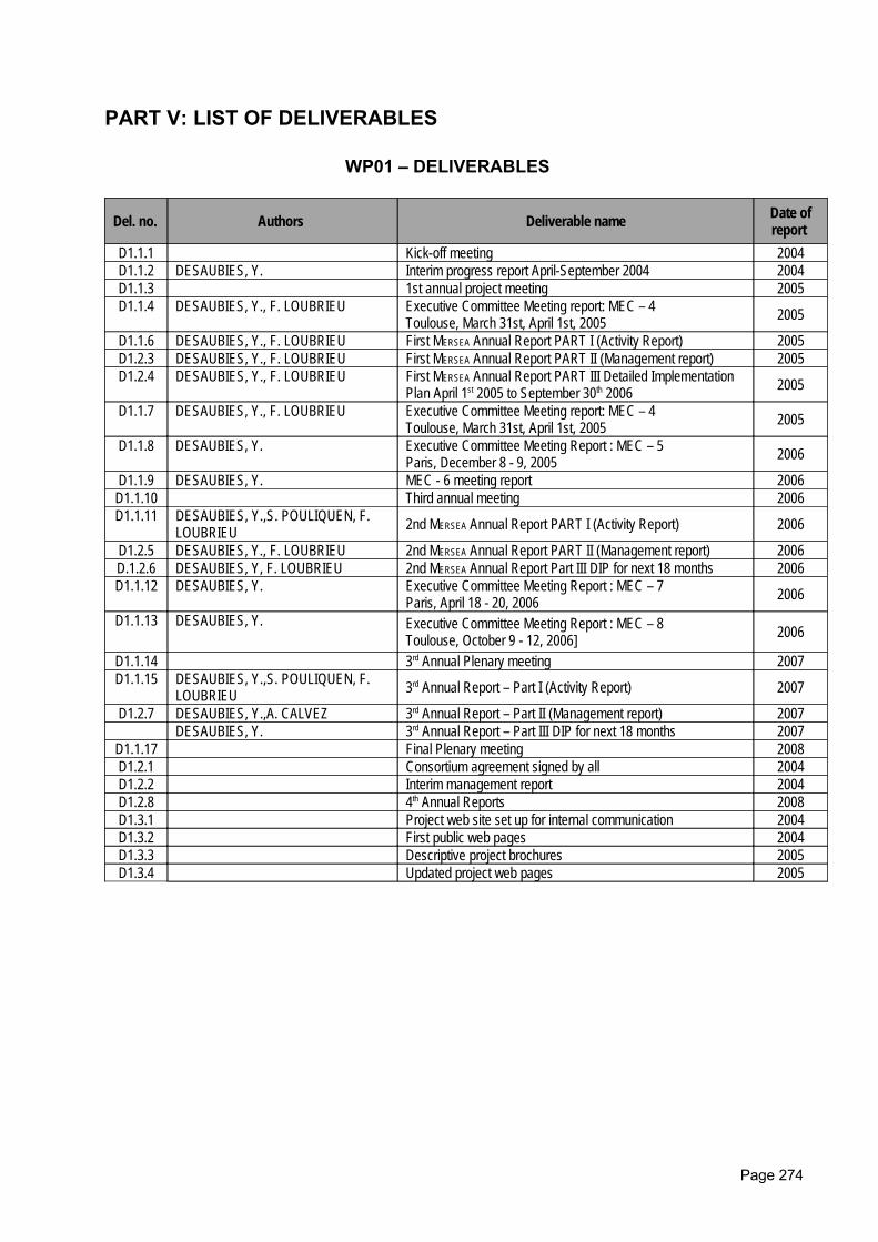
PART V: LIST OF DELIVERABLES

WP01 – DELIVERABLES

Del. no. Authors Deliverable name Date ofreport

D1.1.1 Kick-off meeting 2004D1.1.2 DESAUBIES, Y. Interim progress report April-September 2004 2004D1.1.3 1st annual project meeting 2005D1.1.4 DESAUBIES, Y., F. LOUBRIEU Executive Committee Meeting report: MEC – 4

Toulouse, March 31st, April 1st, 2005 2005

D1.1.6 DESAUBIES, Y., F. LOUBRIEU First MERSEA Annual Report PART I (Activity Report) 2005D1.2.3 DESAUBIES, Y., F. LOUBRIEU First MERSEA Annual Report PART II (Management report) 2005D1.2.4 DESAUBIES, Y., F. LOUBRIEU First MERSEA Annual Report PART III Detailed Implementation

Plan April 1st 2005 to September 30th 2006 2005

D1.1.7 DESAUBIES, Y., F. LOUBRIEU Executive Committee Meeting report: MEC – 4Toulouse, March 31st, April 1st, 2005 2005

D1.1.8 DESAUBIES, Y. Executive Committee Meeting Report : MEC – 5Paris, December 8 - 9, 2005 2006

D1.1.9 DESAUBIES, Y. MEC - 6 meeting report 2006D1.1.10 Third annual meeting 2006D1.1.11 DESAUBIES, Y.,S. POULIQUEN, F.

LOUBRIEU 2nd MERSEA Annual Report PART I (Activity Report) 2006

D1.2.5 DESAUBIES, Y., F. LOUBRIEU 2nd MERSEA Annual Report PART II (Management report) 2006D.1.2.6 DESAUBIES, Y, F. LOUBRIEU 2nd MERSEA Annual Report Part III DIP for next 18 months 2006D1.1.12 DESAUBIES, Y. Executive Committee Meeting Report : MEC – 7

Paris, April 18 - 20, 2006 2006

D1.1.13 DESAUBIES, Y. Executive Committee Meeting Report : MEC – 8Toulouse, October 9 - 12, 2006] 2006

D1.1.14 3rd Annual Plenary meeting 2007D1.1.15 DESAUBIES, Y.,S. POULIQUEN, F.

LOUBRIEU 3rd Annual Report – Part I (Activity Report) 2007

D1.2.7 DESAUBIES, Y.,A. CALVEZ 3rd Annual Report – Part II (Management report) 2007DESAUBIES, Y. 3rd Annual Report – Part III DIP for next 18 months 2007

D1.1.17 Final Plenary meeting 2008D1.2.1 Consortium agreement signed by all 2004D1.2.2 Interim management report 2004D1.2.8 4th Annual Reports 2008D1.3.1 Project web site set up for internal communication 2004D1.3.2 First public web pages 2004D1.3.3 Descriptive project brochures 2005D1.3.4 Updated project web pages 2005

Page 274

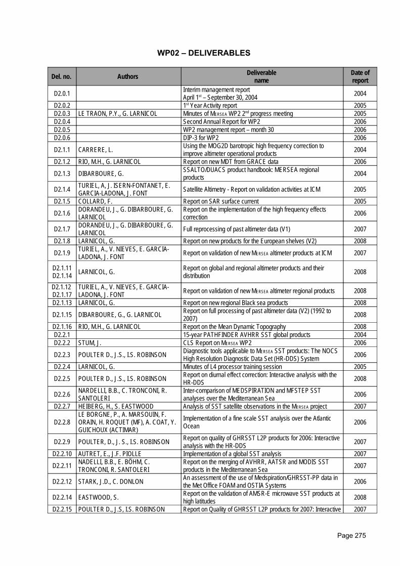
WP02 – DELIVERABLES

Del. no. Authors Deliverable name

Date ofreport

D2.0.1 Interim management reportApril 1st – September 30, 2004 2004

D2.0.2 1st Year Activity report 2005D2.0.3 LE TRAON, P.Y., G. LARNICOL Minutes of MERSEA WP2 2nd progress meeting 2005D2.0.4 Second Annual Report for WP2 2006D2.0.5 WP2 management report – month 30 2006D2.0.6 DIP-3 for WP2 2006

D2.1.1 CARRERE, L. Using the MOG2D barotropic high frequency correction toimprove altimeter operational products 2004

D2.1.2 RIO, M.H., G. LARNICOL Report on new MDT from GRACE data 2006

D2.1.3 DIBARBOURE, G. SSALTO/DUACS product handbook: MERSEA regionalproducts 2004

D2.1.4 TURIEL, A, J. ISERN-FONTANET, E.GARCIA-LADONA, J. FONT Satellite Altimetry - Report on validation activities at ICM 2005

D2.1.5 COLLARD, F. Report on SAR surface current 2005

D2.1.6 DORANDEU, J., G. DIBARBOURE, G.LARNICOL

Report on the implementation of the high frequency effectscorrection 2006

D2.1.7 DORANDEU, J., G. DIBARBOURE, G.LARNICOL Full reprocessing of past altimeter data (V1) 2007

D2.1.8 LARNICOL, G. Report on new products for the European shelves (V2) 2008

D2.1.9 TURIEL, A., V. NIEVES, E. GARCIA-LADONA, J. FONT Report on validation of new MERSEA altimeter products at ICM 2007

D2.1.11D2.1.14 LARNICOL, G. Report on global and regional altimeter products and their

distribution 2008

D2.1.12 D2.1.17

TURIEL, A., V. NIEVES, E. GARCIA-LADONA, J. FONT Report on validation of new MERSEA altimeter regional products 2008

D2.1.13 LARNICOL, G. Report on new regional Black sea products 2008

D2.1.15 DIBARBOURE, G., G. LARNICOL Report on full processing of past altimeter data (V2) (1992 to2007) 2008

D2.1.16 RIO, M.H., G. LARNICOL Report on the Mean Dynamic Topography 2008D2.2.1 15-year PATHFINDER AVHRR SST global products 2004D2.2.2 STUM, J. CLS Report on MERSEA WP2 2006

D2.2.3 POULTER D., J.S., I.S. ROBINSON Diagnostic tools applicable to MERSEA SST products: The NOCSHigh Resolution Diagnostic Data Set (HR-DDS) System 2006

D2.2.4 LARNICOL, G. Minutes of L4 processor training session 2005

D2.2.5 POULTER D., J.S., I.S. ROBINSON Report on diurnal effect correction: Interactive analysis with theHR-DDS 2008

D2.2.6 NARDELLI, B.B., C. TRONCONI, R.SANTOLERI

Inter-comparison of MEDSPIRATION and MFSTEP SSTanalyses over the Mediterranean Sea 2006

D2.2.7 HEIBERG, H., S. EASTWOOD Analysis of SST satellite observations in the MERSEA project 2007

D2.2.8LE BORGNE, P., A. MARSOUIN, F.ORAIN, H. ROQUET (MF), A. COAT, Y.GUICHOUX (ACTIMAR)

Implementation of a fine scale SST analysis over the AtlanticOcean 2006

D2.2.9 POULTER, D., J. S., I.S. ROBINSON Report on quality of GHRSST L2P products for 2006: Interactiveanalysis with the HR-DDS 2007

D2.2.10 AUTRET, E., J.F. PIOLLE Implementation of a global SST analysis 2007

D2.2.11 NADELLI, B.B., E. BÖHM, C.TRONCONI, R. SANTOLERI

Report on the merging of AVHRR, AATSR and MODIS SSTproducts in the Mediterranean Sea 2007

D2.2.12 STARK, J.D., C. DONLON An assessment of the use of Medspiration/GHRSST-PP data inthe Met Office FOAM and OSTIA Systems 2006

D2.2.14 EASTWOOD, S. Report on the validation of AMSR-E microwave SST products athigh latitudes 2008

D2.2.15 POULTER D., J.S, I.S. ROBINSON Report on Quality of GHRSST L2P products for 2007: Interactive 2007

Page 275

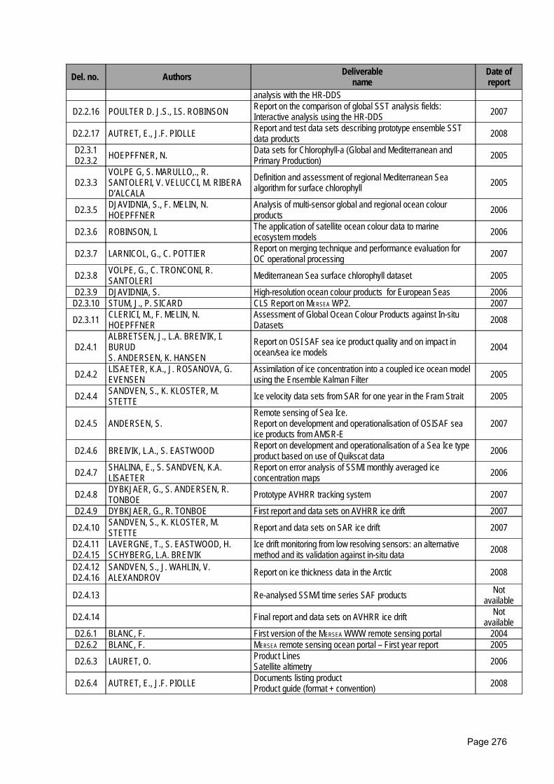
Del. no. Authors Deliverable name

Date ofreport

analysis with the HR-DDS

D2.2.16 POULTER D. J.S., I.S. ROBINSON Report on the comparison of global SST analysis fields:Interactive analysis using the HR-DDS 2007

D2.2.17 AUTRET, E., J.F. PIOLLE Report and test data sets describing prototype ensemble SSTdata products 2008

D2.3.1D2.3.2 HOEPFFNER, N. Data sets for Chlorophyll-a (Global and Mediterranean and

Primary Production) 2005

D2.3.3VOLPE G, S. MARULLO,., R.SANTOLERI, V. VELUCCI, M. RIBERAD’ALCALA

Definition and assessment of regional Mediterranean Seaalgorithm for surface chlorophyll 2005

D2.3.5 DJAVIDNIA, S., F. MELIN, N.HOEPFFNER

Analysis of multi-sensor global and regional ocean colourproducts 2006

D2.3.6 ROBINSON, I. The application of satellite ocean colour data to marineecosystem models 2006

D2.3.7 LARNICOL, G., C. POTTIER Report on merging technique and performance evaluation forOC operational processing 2007

D2.3.8 VOLPE, G., C. TRONCONI, R.SANTOLERI Mediterranean Sea surface chlorophyll dataset 2005

D2.3.9 DJAVIDNIA, S. High-resolution ocean colour products for European Seas 2006D2.3.10 STUM, J., P. SICARD CLS Report on MERSEA WP2. 2007

D2.3.11 CLERICI, M., F. MELIN, N.HOEPFFNER

Assessment of Global Ocean Colour Products against In-situDatasets 2008

D2.4.1ALBRETSEN, J., L.A. BREIVIK, I.BURUDS. ANDERSEN, K. HANSEN

Report on OSI SAF sea ice product quality and on impact inocean/sea ice models 2004

D2.4.2 LISAETER, K.A., J. ROSANOVA, G.EVENSEN

Assimilation of ice concentration into a coupled ice ocean modelusing the Ensemble Kalman Filter 2005

D2.4.4 SANDVEN, S., K. KLOSTER, M.STETTE Ice velocity data sets from SAR for one year in the Fram Strait 2005

D2.4.5 ANDERSEN, S.Remote sensing of Sea Ice.Report on development and operationalisation of OSISAF seaice products from AMSR-E

2007

D2.4.6 BREIVIK, L.A., S. EASTWOOD Report on development and operationalisation of a Sea Ice typeproduct based on use of Quikscat data 2006

D2.4.7 SHALINA, E., S. SANDVEN, K.A.LISAETER

Report on error analysis of SSMI monthly averaged iceconcentration maps 2006

D2.4.8 DYBKJAER, G., S. ANDERSEN, R.TONBOE Prototype AVHRR tracking system 2007

D2.4.9 DYBKJAER, G., R. TONBOE First report and data sets on AVHRR ice drift 2007

D2.4.10 SANDVEN, S., K. KLOSTER, M.STETTE Report and data sets on SAR ice drift 2007

D2.4.11D2.4.15

LAVERGNE, T., S. EASTWOOD, H.SCHYBERG, L.A. BREIVIK

Ice drift monitoring from low resolving sensors: an alternativemethod and its validation against in-situ data 2008

D2.4.12D2.4.16

SANDVEN, S., J. WAHLIN, V.ALEXANDROV Report on ice thickness data in the Arctic 2008

D2.4.13 Re-analysed SSM/I time series SAF products Notavailable

D2.4.14 Final report and data sets on AVHRR ice drift Notavailable

D2.6.1 BLANC, F. First version of the MERSEA WWW remote sensing portal 2004D2.6.2 BLANC, F. MERSEA remote sensing ocean portal – First year report 2005

D2.6.3 LAURET, O. Product LinesSatellite altimetry 2006

D2.6.4 AUTRET, E., J.F. PIOLLE Documents listing productProduct guide (format + convention) 2008

Page 276

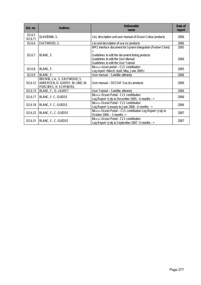
Del. no. Authors Deliverable name

Date ofreport

D2.6.5D2.6.11 DJAVIDNIA, S. List, description and user manual of Ocean Colour products 2006

D2.6.6 EASTWOOD, S. List and description of sea ice products 2006

D2.6.7 BLANC, F.

WP2 interface document for System Integration (Partner Chart)+ Guidelines to edit the document listing productsGuidelines to edit the User ManualGuidelines to edit the User Tutorial

2005

2006

D2.6.8 BLANC, F. MERSEA ocean portal – CLS contributionLog report <March, April, May, June 2005> 2005

D2.6.9 BLANC, F. User manual – Satellite altimetry 2006

D2.6.12BREIVIK, L.A., S. EASTWOOD, S.ANDERSEN, O. GODOY, M. LIND, M.PORCIRES, H. SCHYBERG

User manual – OSI SAF Sea Ice products 2006

D2.6.13 BLANC, F., O. LAURET User Tutorial – Satellite altimetry 2006

D2.6.17 BLANC, F. C. GUIOSE MERSEA Ocean Portal - CLS contributionLog Report <July to December 2005 - 6 months - > 2006

D2.6.18 BLANC, F. C. GUIOSE MERSEA Ocean Portal - CLS contributionLog Report <January to June 2006 - 6 months - > 2006

D2.6.22 BLANC, F., C. GUIOSE MERSEA Ocean Portal – CLS contribution Log Report <July toOctober 2006 – 3 months -> 2007

D2.6.31 BLANC, F., C. GUIOSE MERSEA Ocean Portal - CLS contributionLog Report <July to September 2007 -3 months - > 2007

Page 277

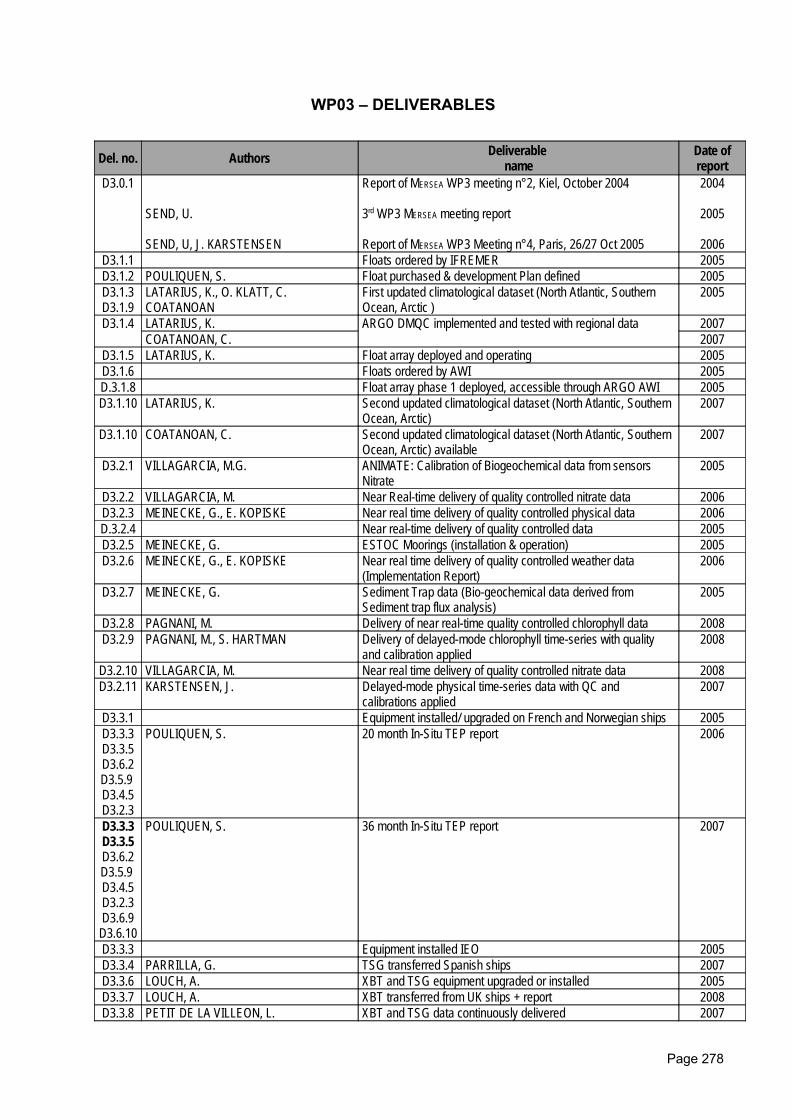
WP03 – DELIVERABLES

Del. no. Authors Deliverable name

Date ofreport

D3.0.1

SEND, U.

SEND, U, J. KARSTENSEN

Report of MERSEA WP3 meeting n°2, Kiel, October 2004

3rd WP3 MERSEA meeting report

Report of MERSEA WP3 Meeting n°4, Paris, 26/27 Oct 2005

2004

2005

2006D3.1.1 Floats ordered by IFREMER 2005D3.1.2 POULIQUEN, S. Float purchased & development Plan defined 2005D3.1.3D3.1.9

LATARIUS, K., O. KLATT, C.COATANOAN

First updated climatological dataset (North Atlantic, SouthernOcean, Arctic )

2005

D3.1.4 LATARIUS, K. ARGO DMQC implemented and tested with regional data 2007COATANOAN, C. 2007

D3.1.5 LATARIUS, K. Float array deployed and operating 2005D3.1.6 Floats ordered by AWI 2005D.3.1.8 Float array phase 1 deployed, accessible through ARGO AWI 2005D3.1.10 LATARIUS, K. Second updated climatological dataset (North Atlantic, Southern

Ocean, Arctic) 2007

D3.1.10 COATANOAN, C. Second updated climatological dataset (North Atlantic, SouthernOcean, Arctic) available

2007

D3.2.1 VILLAGARCIA, M.G. ANIMATE: Calibration of Biogeochemical data from sensorsNitrate

2005

D3.2.2 VILLAGARCIA, M. Near Real-time delivery of quality controlled nitrate data 2006D3.2.3 MEINECKE, G., E. KOPISKE Near real time delivery of quality controlled physical data 2006D.3.2.4 Near real-time delivery of quality controlled data 2005D3.2.5 MEINECKE, G. ESTOC Moorings (installation & operation) 2005D3.2.6 MEINECKE, G., E. KOPISKE Near real time delivery of quality controlled weather data

(Implementation Report) 2006

D3.2.7 MEINECKE, G. Sediment Trap data (Bio-geochemical data derived fromSediment trap flux analysis)

2005

D3.2.8 PAGNANI, M. Delivery of near real-time quality controlled chlorophyll data 2008D3.2.9 PAGNANI, M., S. HARTMAN Delivery of delayed-mode chlorophyll time-series with quality

and calibration applied2008

D3.2.10 VILLAGARCIA, M. Near real time delivery of quality controlled nitrate data 2008D3.2.11 KARSTENSEN, J. Delayed-mode physical time-series data with QC and

calibrations applied2007

D3.3.1 Equipment installed/ upgraded on French and Norwegian ships 2005D3.3.3D3.3.5D3.6.2D3.5.9 D3.4.5D3.2.3

POULIQUEN, S. 20 month In-Situ TEP report 2006

D3.3.3D3.3.5D3.6.2D3.5.9 D3.4.5D3.2.3D3.6.9D3.6.10

POULIQUEN, S. 36 month In-Situ TEP report 2007

D3.3.3 Equipment installed IEO 2005D3.3.4 PARRILLA, G. TSG transferred Spanish ships 2007D3.3.6 LOUCH, A. XBT and TSG equipment upgraded or installed 2005D3.3.7 LOUCH, A. XBT transferred from UK ships + report 2008D3.3.8 PETIT DE LA VILLEON, L. XBT and TSG data continuously delivered 2007

Page 278

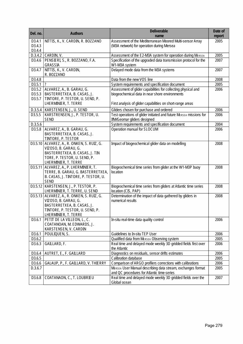
Del. no. Authors Deliverable name

Date ofreport

D3.4.1D3.4.3D3.4.4

NITTIS, K., V. CARDIN, R. BOZZANO Assessment of the Mediterranean Moored Multi-sensor Array(M3A network) for operation during Mersea

2005

D.3.4.2 CARDIN, V. Assessment of the E2-M3A system for operation during MERSEA 2005D3.4.6 PENSIERI, S., R. BOZZANO, F.A.

GRASSIASpecification of the upgraded data transmission protocol for theW1-M3A system

2007

D3.4.7 NITTIS, K., V. CARDIN, R. BOZZANO

Delayed mode data from the M3A systems 2007

D3.4.8 Data from the new VOS line 2008D3.5.1 ? System requirements and specification document 2005D3.5.2D3.5.3D3.5.7

ALVAREZ, A., B. GARAU, G.BASTERRETXEA, B. CASAS, J.TINTORE, P. TESTOR, U. SEND, P.LHERMINIER, T. TERRE

Assessment of glider capabilities for collecting physical andbiogeochemical data in near shore environments

First analysis of glider capabilities on short-range areas

2006

D.3.5.4 KARSTENSEN, J., U. SEND Gliders chosen for purchase and ordered 2006D3.5.5 KARSTRENSEN, J., P. TESTOR, U.

SENDTest operations of glider initiated and future MERSEA missions forIfM/Geomar gliders designed

2006

D.3.5.6 System requirements and specification document 2004D3.5.8 ALVAREZ, A., B. GARAU, G.

BASTERRETXEA, B. CASAS, J.TINTORE, P. TESTOR

Operation manual for SLOCUM 2006

D3.5.10 ALVAREZ, A., R. ONKEN, S. RUIZ, G.VIZOSO, B. GARAU, G.BASTERRETXEA, B. CASAS, J. TINTORE, P. TESTOR, U. SEND, P.LHERMINIER, T. TERRE

Impact of biogeochemical glider data on modelling 2008

D3.5.11 ALVAREZ, A., P. LHERMINIER, T.TERRE, B. GARAU, G. BASTERRETXEA,B. CASAS, J. TINTORE, P. TESTOR, U.SEND

Biogeochemical time series from glider at the W1-M3P buoylocation

2008

D3.5.12 KARSTENSEN, J., P. TESTOR, P.LHERMINIER, T. TERRE, U. SEND

Biogeochemical time series from gliders at Atlantic time serieslocation (CIS, PAP)

2008

D3.5.13 ALVAREZ, A., R. ONKEN, S. RUIZ, G.VIZOSO, B. GARAU, G.BASTERRETXEA, B. CASAS, J.TINTORE, P. TESTOR, U. SEND, P.LHERMINIER, T. TERRE

Determination of the impact of data gathered by gliders innumerical results

2008

D3.6.1 PETIT DE LA VILLEON, L., C.COATANOAN, M. EDWARDS, J.KARSTENSEN, V. CARDIN

In-situ real-time data quality control 2006

D3.6.1 POULIQUEN, S. Guidelines to In-situ TEP User 2006D3.6.2 Qualified data from MERSEA Observing system 2005D3.6.3 GAILLARD, F. Real time and delayed mode weekly 3D gridded fields first over

the Atlantic2006

D3.6.4 AUTRET, E., F. GAILLARD Diagnostics on residuals, sensor drifts estimates 2006D3.6.5 Calibration database 2005D3.6.6 GALAUP, P., F. GAILLARD, V. THIERRY Comparison of ARGO profilers corrections with calibrations 2006D.3.6.7 MERSEA User Manual describing data stream, exchanges format

and QC procedures for Atlantic time-series2005

D3.6.8 COATANAON, C., T. LOUBRIEU Real time and delayed mode weekly 3D gridded fields over theGlobal ocean

2007

Page 279

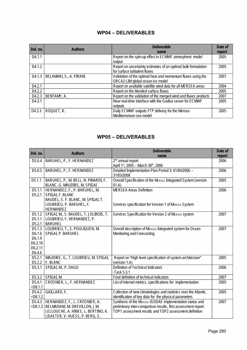
WP04 – DELIVERABLES

Del. no. Authors Deliverable name

Date ofreport

D4.1.1 Report on the spin-up effect in ECMWF atmospheric modeloutput

2005

D4.1.2 Report on uncertainty estimates of an optimal bulk formulationfor surface turbulent fluxes

2005

D4.1.3 BELAMARI, S., A. PIRANI Validation of the optimal heat and momentum fluxes using theORCA2-LIM global ocean-ice model

2007

D4.2.1 Report on available satellite wind data for all MERSEA areas 2004D4.2.2 Report on the blended surface fluxes 2005D4.2.3 BENTAMY, A. Report on the validation of the merged wind and fluxes products 2007D4.3.1 Near real-time interface with the Godiva server for ECMWF

outputs2005

D4.3.3 ROQUET, R. Daily ECMWF outputs FTP delivery for the MerseaMediterranean sea model

2005

WP05 – DELIVERABLES

Del. no. Authors Deliverablename

Date ofreport

D5.0.4 BARUHEL, P., F. HERNANDEZ 2nd annual reportApril 1st, 2005 – March 30th, 2006

2006

D5.0.5 BARUHEL, P., F. HERNANDEZ Detailed Implementation Plan Period 3: 01/04/2006 –31/03/2008

2006

D5.1.1 BARUHEL, P., M. BELL, N. PINARDI, F.BLANC, G. MAUDIRE, M. SPIGAI

Overall Specification of the MERSEA Integrated System (version01.A)

2005

D5.1.1D5.2.1

HERNANDEZ, F., P. BARUHEL, M.SPIGAI, F. BLANCBAUDEL, S. F. BLANC, M. SPIGAI, T.LOUBRIEU, P. BARUHEL, F.HERNANDEZ

MERSEA Areas Definition

Services specification for Version 1 of MERSEA System

2006

D5.1.2D5.1.1D5.2.1

SPIGAI, M., S. BAUDEL, T. JOLIBOIS, T.LOUBRIEU, F. HERNANDEZ, P.BARUHEL

Services Specification for Version 2 of MERSEA system 2007

D5.1.3D6.1.6D6.1.9D6.2.10D6.2.11D6.4.6

LOUBRIEU, T., S. POULIQUEN, M.SPIGAI, P. BARUHEL

Overall description of MERSEA Integrated system for OceanMonitoring and Forecasting

2007

D5.2.1D5.2.2

MAUDIRE, G., T. LOUBRIEU, M. SPIGAI,F. BLANC

Report on “High level specification of system architecture”(version 1.A)

2005

D5.3.1 SPIGAI, M., P. DAGO Definition of Technical Indicators-Task 5.3.1

2006

D5.3.2 SPIGAI, M. Final definition of technical indicators 2007D5.4.1

=D8.1.1CROSNIER, L., F. HERNANDEZ List of internal metrics, specifications for implementation 2005

D5.4.2=D8.1.2

GAILLARD, F. Collection of new climatologies and statistics over the Atlantic,identification of key data for the physical parameters

2005

D5.4.3=D8.1.3

HERNANDEZ, F., L. CROSNIER, A.BELMADANI, M. DREVILLON, J.M.LELLOUCHE, A. HINES, L. BERTINO, K.LISAETER, V. HUESS, P. BERG, S.

Synthesis of the MERSEA /GODAE implementation status andpreliminary inter-comparison results, first assessment report:TOP1 assessment results and TOP2 assessment definition

2007

Page 280

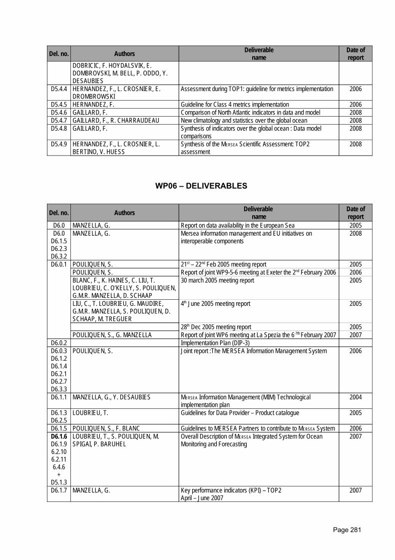
Del. no. Authors Deliverablename

Date ofreport

DOBRICIC, F. HOYDALSVIK, E.DOMBROVSKI, M. BELL, P. ODDO, Y.DESAUBIES

D5.4.4 HERNANDEZ, F., L. CROSNIER, E.DROMBROWSKI

Assessment during TOP1: guideline for metrics implementation 2006

D5.4.5 HERNANDEZ, F. Guideline for Class 4 metrics implementation 2006D5.4.6 GAILLARD, F. Comparison of North Atlantic indicators in data and model 2008D5.4.7 GAILLARD, F., R. CHARRAUDEAU New climatology and statistics over the global ocean 2008D5.4.8 GAILLARD, F. Synthesis of indicators over the global ocean : Data model

comparisons2008

D5.4.9 HERNANDEZ, F., L. CROSNIER, L.BERTINO, V. HUESS

Synthesis of the MERSEA Scientific Assessment: TOP2assessment

2008

WP06 – DELIVERABLES

Del. no. Authors Deliverable name

Date ofreport

D6.0 MANZELLA, G. Report on data availability in the European Sea 2005D6.0

D6.1.5D6.2.3D6.3.2

MANZELLA, G. Mersea information management and EU initiatives oninteroperable components

2008

D6.0.1 POULIQUEN, S. 21st – 22nd Feb 2005 meeting report 2005POULIQUEN, S. Report of joint WP9-5-6 meeting at Exeter the 2nd February 2006 2006BLANC, F., K. HAINES, C. LIU, T.LOUBRIEU, C. O’KELLY, S. POULIQUEN,G.M.R. MANZELLA, D. SCHAAP

30 march 2005 meeting report 2005

LIU, C., T. LOUBRIEU, G. MAUDIRE,G.M.R. MANZELLA, S. POULIQUEN, D.SCHAAP, M. TREGUER

4th June 2005 meeting report 2005

28th Dec 2005 meeting report 2005POULIQUEN, S., G. MANZELLA Report of joint WP6 meeting at La Spezia the 6-7th February 2007 2007

D6.0.2 Implementation Plan (DIP-3)D6.0.3D6.1.2D6.1.4D6.2.1D6.2.7D6.3.3

POULIQUEN, S. Joint report :The MERSEA Information Management System 2006

D6.1.1 MANZELLA, G., Y. DESAUBIES MERSEA Information Management (MIM) Technologicalimplementation plan

2004

D6.1.3D6.2.5

LOUBRIEU, T. Guidelines for Data Provider – Product catalogue 2005

D6.1.5 POULIQUEN, S., F. BLANC Guidelines to MERSEA Partners to contribute to MERSEA System 2006D6.1.6D6.1.96.2.106.2.116.4.6

+D5.1.3

LOUBRIEU, T., S. POULIQUEN, M.SPIGAI, P. BARUHEL

Overall Description of MERSEA Integrated System for OceanMonitoring and Forecasting

2007

D6.1.7 MANZELLA, G. Key performance indicators (KPI) – TOP2April – June 2007

2007

Page 281

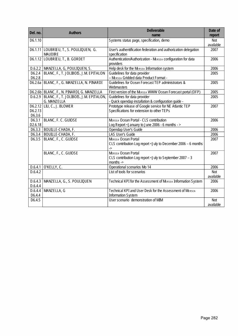
Del. no. Authors Deliverable name

Date ofreport

D6.1.10 Systems status page, specification, demo Notavailable

D6.1.11 LOUBRIEU, T., S. POULIQUEN, G.MAUDIRE

User's authentification federation and authorization delegationspecification

2007

D6.1.12 LOUBRIEU, T., B. GORDET Authentication/Authorization - MERSEA configuration for dataproviders

2006

D.6.2.2 MANZELLA, G, POULIQUEN, S. Help desk for the MERSEA Information system 2006D6.2.4D6.2.8

BLANC, F., T. JOLIBOIS, J.M. EPITALON Guidelines for data provider – MERSEA Gridded data Product Format -

2005

D6.2.6a BLANC, F., G. MANZELLA, N. PINARDI Guidelines for Ocean Forecast TEP administrators &Webmasters

2005

D6.2.6b BLANC, F., N. PINARDI, G. MANZELLA First version of the MERSEA WWW Ocean Forecast portal (OFP) 2005D.6.2.9 BLANC, F., T. JOLIBOIS, J.M. EPITALON,

G. MANZELLAGuidelines for data provider- Quick opendap installation & configuration guide -

2005

D6.2.12D6.2.13D6.3.6

LIU, C., J. BLOWER Prototype release of Google service for NE Atlantic TEPSpecifications for extension to other TEPs

2007

D6.3.1D2.6.18

BLANC, F. C. GUIOSE MERSEA Ocean Portal - CLS contributionLog Report <January to June 2006 - 6 months - >

2006

D6.3.3 BOUILLE-CHADA, F. Opendap User’s Guide 2006D6.3.4 BOUILLE-CHADA, F. LAS User’s Guide 2006D6.3.5 BLANC, F., C. GUIOSE MERSEA Ocean Portal

CLS contribution Log report <July to December 2006 – 6 months->

2007

BLANC, F., C. GUIOSE MERSEA Ocean PortalCLS contribution Log report <July to September 2007 – 3months ->

2007

D.6.4.1 O’KELLY, C. Operational scenarios Mo 14 2006D.6.4.2 List of tools for scenarios Not

availableD.6.4.3D.6.4.4

MANZELLA, G., S. POULIQUEN Technical KPI for the Assessment of MERSEA Information System 2006

D.6.4.4D6.4.4

MANZELLA, G Technical KPI and User Desk for the Assessment of MERSEAInformation System

2006

D6.4.5 User scenario demonstration of MIM Notavailable

Page 282

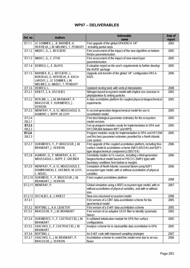
WP07 – DELIVERABLES

Del. no. Authors Deliverable name

Date ofreport

D7.1.1 LE SOMMER, J., B. BARNIER, G.HERVIEUX, J.M. MOLINES, T. PENDUFF

First upgrade of the global OPA/ORCA 1/4° including partial steps

2005

D7.1.2 MADEC, G., L. BESSIERE First assessment of the impact of the new algorithm on bottomfriction parameterisation

2005

D7.1.3 MADEC, G., C. ETHE First assessment of the impact of new mixed layerparameterisation

2005

D7.1.4 DEBREU, L., E. BLAYO Evaluation report on the user's requirements to further developthe AGRIF package

2005

D7.1.5 BARNIER, B., L. BESSIERE, L.BORDEAU, G. HERVIEUX, A. KOCH-LAROUY, J. LE SOMMER, J.M.MOLINES, G. MADEC, T. PENDUFF

Upgrade and transfer of the global 1/4° configuration ORCA-R025

2006

D7.1.6 DEBREU, L. Updated nesting tools with vertical interpolation 2008D7.2.1 KRIEST, I., A. OSCHLIES Nitrogen-based ecosystem model with implicit size structure in

phytoplankton & sinking particles 2005

D7.2.2 BERLINE, L., J.M. BRANKART, P.BRASSEUR, Y. OURMIERES, J.VERRON

A data assimilative platform for coupled physical-biogeochemicalexperiments

2005

D7.2.3 MONFRAY, P., A. EL MOUSSAOUI, O.AUMONT, L. BOPP, M. LEVY

A second-generation biogeochemical model for use inassimilation model

2005

D7.2.4D8.2.1

First best biological parameter estimates for the ecosystemmodel versions

2005

D7.2.5D8.2.2

Set up program modules ready for implementation in OPA andHYCOM (link between WP7 and WP9)

2005

D7.2.6 D8.2.3

Program modules ready for implementation in OPA and HYCOMand first best parameter estimates provided for a North Atlanticcore system

2005

D7.2.7 OURMIERES, Y., P. BRASSEUR, J.M.BRANKART, J. VERRON

First upgrade of the coupled assimilative platform, including free-surface model & assimilation scheme (NATL4/SEEK) and N2P1-type biogeochemical component (LOBSTER)

2006

D7.2.8 AUMONT, O., P. MONFRAY, A. ELMOUSSAOUI, L. BOPP, E. GREINER

Sensitivity studies to Fe sources, including a third-generationbiogeochemical model based on PISCES (N4P2 type) withboundary conditions from below or margins

2006

D7.2.9 MONFRAY, P., A. EL MOUSSAOUI, E.DOMBROWSKI, E. GREINER, M. LEVY,L. NOUEL

Simulation of North Atlantic seasonal bloom using N2P1ecosystem type model, with or without assimilation of physicalvariables

2006

D7.2.10 OURMIERE, Y., P. BRASSEUR, J.M.BRANKART, J. VERRON

Final coupled assimilative platform 2008

D7.2.11 MONFRAY, P. Global simulation using a N5P2 ecosystem type model, with orwithout assimilation of physical variables, and with or withoutiron

2007

D7.2.12 OSCHLIES, A., I. KRIEST New size-structured ecosystem model 2008D7.3.1 First version of a SIRF data-assimilation scheme for bio-

geochemical model2005

D7.3.2 BERTINO, L., K.A. LISAETER First version of a EnKF data-assimilation scheme 2005D7.3.3 BRASSEUR, P., J.M. BRANKART First version of an adaptive SEEK filter to identify systematic

biases 2005

D7.3.4 OURMIERES, Y., F. CASTRUCCIO, J.M.BRANKART

A validated initialization module for OPA free surfaceconfigurations

2005

D7.3.5 SKACHKO, S., F. CASTRUCCIO, J.M.BRANKART

Analysis scheme for in situ/satellite data assimilation in OPA 2005

D7.3.6 BERTINO, L. An EnKF code with improved sampling strategies 2007D7.3.7 SKACHKO, S., J.M. BRANKART, P.

BRASSEUR, J. VERRONAssimilation scheme to control the model error due to air-seafluxes

2006

Page 283

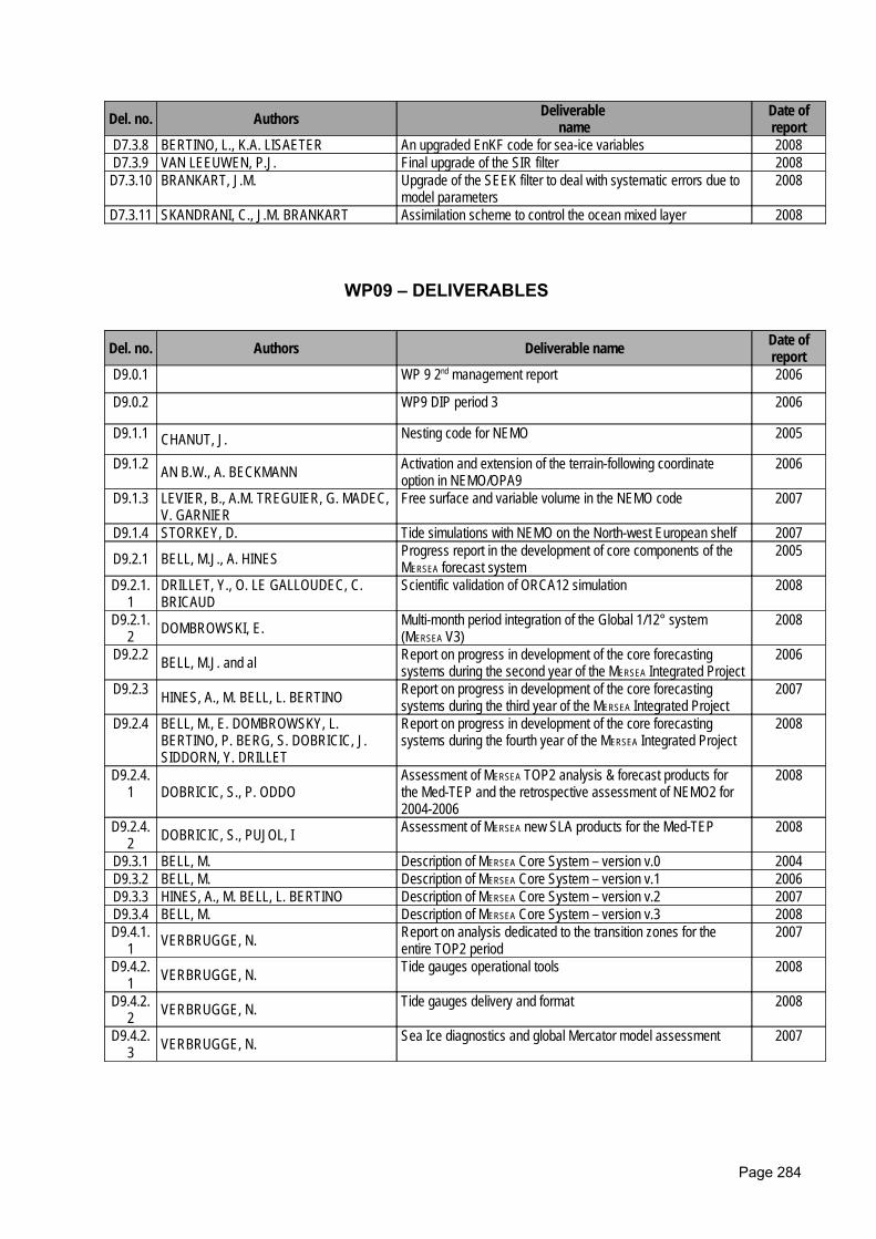
Del. no. Authors Deliverable name

Date ofreport

D7.3.8 BERTINO, L., K.A. LISAETER An upgraded EnKF code for sea-ice variables 2008D7.3.9 VAN LEEUWEN, P.J. Final upgrade of the SIR filter 2008D7.3.10 BRANKART, J.M. Upgrade of the SEEK filter to deal with systematic errors due to

model parameters2008

D7.3.11 SKANDRANI, C., J.M. BRANKART Assimilation scheme to control the ocean mixed layer 2008

WP09 – DELIVERABLES

Del. no. Authors Deliverable name Date ofreport

D9.0.1 WP 9 2nd management report 2006

D9.0.2 WP9 DIP period 3 2006

D9.1.1 CHANUT, J. Nesting code for NEMO 2005

D9.1.2 AN B.W., A. BECKMANN Activation and extension of the terrain-following coordinateoption in NEMO/OPA9

2006

D9.1.3 LEVIER, B., A.M. TREGUIER, G. MADEC,V. GARNIER

Free surface and variable volume in the NEMO code 2007

D9.1.4 STORKEY, D. Tide simulations with NEMO on the North-west European shelf 2007

D9.2.1 BELL, M.J., A. HINES Progress report in the development of core components of theMERSEA forecast system

2005

D9.2.1.1

DRILLET, Y., O. LE GALLOUDEC, C.BRICAUD

Scientific validation of ORCA12 simulation 2008

D9.2.1.2 DOMBROWSKI, E. Multi-month period integration of the Global 1/12° system

(MERSEA V3)2008

D9.2.2 BELL, M.J. and al Report on progress in development of the core forecastingsystems during the second year of the MERSEA Integrated Project

2006

D9.2.3 HINES, A., M. BELL, L. BERTINO Report on progress in development of the core forecastingsystems during the third year of the MERSEA Integrated Project

2007

D9.2.4 BELL, M., E. DOMBROWSKY, L.BERTINO, P. BERG, S. DOBRICIC, J.SIDDORN, Y. DRILLET

Report on progress in development of the core forecastingsystems during the fourth year of the MERSEA Integrated Project

2008

D9.2.4.1 DOBRICIC, S., P. ODDO

Assessment of MERSEA TOP2 analysis & forecast products forthe Med-TEP and the retrospective assessment of NEMO2 for2004-2006

2008

D9.2.4.2 DOBRICIC, S., PUJOL, I Assessment of MERSEA new SLA products for the Med-TEP 2008

D9.3.1 BELL, M. Description of MERSEA Core System – version v.0 2004D9.3.2 BELL, M. Description of MERSEA Core System – version v.1 2006D9.3.3 HINES, A., M. BELL, L. BERTINO Description of MERSEA Core System – version v.2 2007D9.3.4 BELL, M. Description of MERSEA Core System – version v.3 2008D9.4.1.

1 VERBRUGGE, N. Report on analysis dedicated to the transition zones for theentire TOP2 period

2007

D9.4.2.1 VERBRUGGE, N. Tide gauges operational tools 2008

D9.4.2.2 VERBRUGGE, N. Tide gauges delivery and format 2008

D9.4.2.3 VERBRUGGE, N. Sea Ice diagnostics and global Mercator model assessment 2007

Page 284

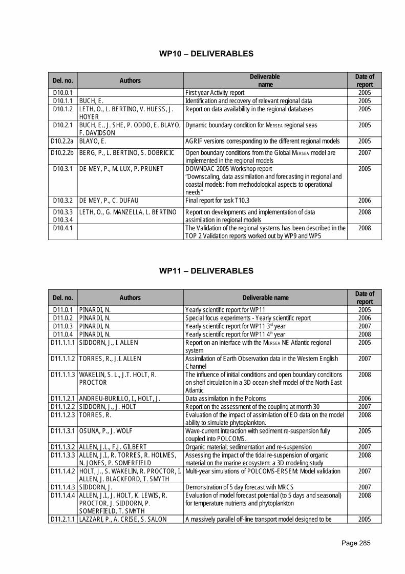
WP10 – DELIVERABLES

Del. no. Authors Deliverable name

Date ofreport

D10.0.1 First year Activity report 2005D10.1.1 BUCH, E. Identification and recovery of relevant regional data 2005D10.1.2 LETH, O., L. BERTINO, V. HUESS, J.

HOYERReport on data availability in the regional databases 2005

D10.2.1 BUCH, E., J. SHE, P. ODDO, E. BLAYO,F. DAVIDSON

Dynamic boundary condition for MERSEA regional seas 2005

D10.2.2a BLAYO, E. AGRIF versions corresponding to the different regional models 2005D10.2.2b BERG, P., L. BERTINO, S. DOBRICIC Open boundary conditions from the Global MERSEA model are

implemented in the regional models2007

D10.3.1 DE MEY, P., M. LUX, P. PRUNET DOWNDAC 2005 Workshop report“Downscaling, data assimilation and forecasting in regional andcoastal models: from methodological aspects to operationalneeds”

2005

D10.3.2 DE MEY, P., C. DUFAU Final report for task T10.3 2006D10.3.3D10.3.4

LETH, O., G. MANZELLA, L. BERTINO Report on developments and implementation of dataassimilation in regional models

2008

D10.4.1 The Validation of the regional systems has been described in theTOP 2 Validation reports worked out by WP9 and WP5

2008

WP11 – DELIVERABLES

Del. no. Authors Deliverable name Date ofreport

D11.0.1 PINARDI, N. Yearly scientific report for WP11 2005D11.0.2 PINARDI, N. Special focus experiments - Yearly scientific report 2006D11.0.3 PINARDI, N. Yearly scientific report for WP11 3rd year 2007D11.0.4 PINARDI, N. Yearly scientific report for WP11 4th year 2008

D11.1.1.1 SIDDORN, J., I. ALLEN Report on an interface with the MERSEA NE Atlantic regionalsystem

2005

D11.1.1.2 TORRES, R., J.I. ALLEN Assimilation of Earth Observation data in the Western EnglishChannel

2007

D11.1.1.3 WAKELIN, S. L., J.T. HOLT, R.PROCTOR

The influence of initial conditions and open boundary conditionson shelf circulation in a 3D ocean-shelf model of the North EastAtlantic

2008

D11.1.2.1 ANDREU-BURILLO, I., HOLT, J. Data assimilation in the Polcoms 2006D11.1.2.2 SIDDORN, J., J. HOLT Report on the assessment of the coupling at month 30 2007D11.1.2.3 TORRES, R. Evaluation of the impact of assimilation of EO data on the model

ability to simulate phytoplankton.2008

D11.1.3.1 OSUNA, P., J. WOLF Wave-current interaction with sediment re-suspension fullycoupled into POLCOMS.

2005

D11.1.3.2 ALLEN, J.L., F.J. GILBERT Organic material; sedimentation and re-suspension 2007D11.1.3.3 ALLEN, J.I., R. TORRES, R. HOLMES,

N. JONES, P. SOMERFIELDAssessing the impact of the tidal re-suspension of organicmaterial on the marine ecosystem: a 3D modeling study

2008

D11.1.4.2 HOLT, J., S. WAKELIN, R. PROCTOR, I.ALLEN, J. BLACKFORD, T. SMYTH

Multi-year simulations of POLCOMS-ERSEM: Model validation 2007

D11.1.4.3 SIDDORN, J. Demonstration of 5 day forecast with MRCS 2007D11.1.4.4 ALLEN, J.I., J. HOLT, K. LEWIS, R.

PROCTOR, J. SIDDORN, P.SOMERFIELD, T. SMYTH

Evaluation of model forecast potential (to 5 days and seasonal)for temperature nutrients and phytoplankton

2008

D11.2.1.1 LAZZARI, P., A. CRISE, S. SALON A massively parallel off-line transport model designed to be 2005

Page 285

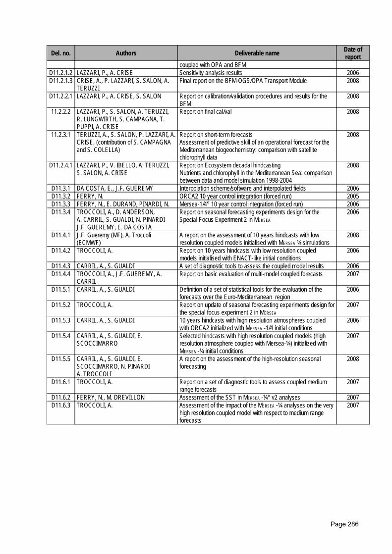
Del. no. Authors Deliverable name Date ofreport

coupled with OPA and BFMD11.2.1.2 LAZZARI, P., A. CRISE Sensitivity analysis results 2006D11.2.1.3 CRISE, A., P. LAZZARI, S. SALON, A.

TERUZZIFinal report on the BFM-OGS/OPA Transport Module 2008

D11.2.2.1 LAZZARI, P., A. CRISE, S. SALON Report on calibration/validation procedures and results for theBFM

2008

11.2.2.2 LAZZARI, P., S. SALON, A. TERUZZI,R. LUNGWIRTH, S. CAMPAGNA, T.PUPPI, A. CRISE

Report on final cal/val 2008

11.2.3.1 TERUZZI, A., S. SALON, P. LAZZARI, A.CRISE, (contribution of S. CAMPAGNAand S. COLELLA)

Report on short-term forecastsAssessment of predictive skill of an operational forecast for theMediterranean biogeochemistry: comparison with satellitechlorophyll data

2008

D11.2.4.1 LAZZARI, P., V. IBELLO, A. TERUZZI,S. SALON, A. CRISE

Report on Ecosystem decadal hindcastingNutrients and chlorophyll in the Mediterranean Sea: comparisonbetween data and model simulation 1998-2004

2008

D11.3.1 DA COSTA, E., J.F. GUEREMY Interpolation scheme/software and interpolated fields 2006D11.3.2 FERRY, N. ORCA2 10 year control integration (forced run) 2005D11.3.3 FERRY, N., E. DURAND, PINARDI, N. Mersea-1/4° 10 year control integration (forced run) 2006D11.3.4 TROCCOLI, A., D. ANDERSON,

A. CARRIL, S. GUALDI, N. PINARDIJ.F. GUEREMY, E. DA COSTA

Report on seasonal forecasting experiments design for theSpecial Focus Experiment 2 in MERSEA

2006

D11.4.1 J.F. Gueremy (MF), A. Troccoli(ECMWF)

A report on the assessment of 10 years hindcasts with lowresolution coupled models initialised with MERSEA ¼ simulations

2008

D11.4.2 TROCCOLI, A. Report on 10 years hindcasts with low resolution coupledmodels initialised with ENACT-like initial conditions

2006

D11.4.3 CARRIL, A., S. GUALDI A set of diagnostic tools to assess the coupled model results 2006D11.4.4 TROCCOLI, A., J.F. GUEREMY, A.

CARRILReport on basic evaluation of multi-model coupled forecasts 2007

D11.5.1 CARRIL, A., S. GUALDI Definition of a set of statistical tools for the evaluation of theforecasts over the Euro-Mediterranean region

2006

D11.5.2 TROCCOLI, A. Report on update of seasonal forecasting experiments design forthe special focus experiment 2 in MERSEA

2007

D11.5.3 CARRIL, A., S. GUALDI 10 years hindcasts with high resolution atmospheres coupledwith ORCA2 initialized with MERSEA -1/4 initial conditions

2006

D11.5.4 CARRIL, A., S. GUALDI, E.SCOCCIMARRO

Selected hindcasts with high resolution coupled models (highresolution atmosphere coupled with Mersea-¼) initialized withMERSEA -¼ initial conditions

2007

D11.5.5 CARRIL, A., S. GUALDI, E.SCOCCIMARRO, N. PINARDIA. TROCCOLI

A report on the assessment of the high-resolution seasonalforecasting

2008

D11.6.1 TROCCOLI, A. Report on a set of diagnostic tools to assess coupled mediumrange forecasts

2007

D11.6.2 FERRY, N., M. DREVILLON Assessment of the SST in MERSEA -¼° v2 analyses 2007D11.6.3 TROCCOLI, A. Assessment of the impact of the MERSEA -¼ analyses on the very

high resolution coupled model with respect to medium rangeforecasts

2007

Page 286

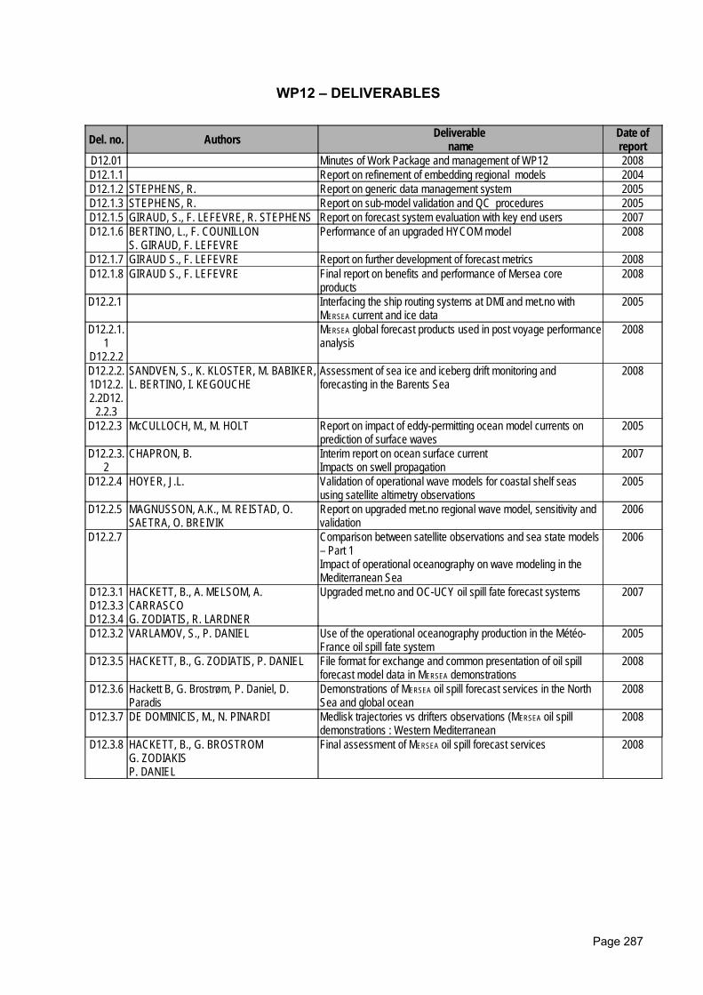
WP12 – DELIVERABLES

Del. no. Authors Deliverable name

Date ofreport

D12.01 Minutes of Work Package and management of WP12 2008D12.1.1 Report on refinement of embedding regional models 2004D12.1.2 STEPHENS, R. Report on generic data management system 2005D12.1.3 STEPHENS, R. Report on sub-model validation and QC procedures 2005D12.1.5 GIRAUD, S., F. LEFEVRE, R. STEPHENS Report on forecast system evaluation with key end users 2007D12.1.6 BERTINO, L., F. COUNILLON

S. GIRAUD, F. LEFEVREPerformance of an upgraded HYCOM model 2008

D12.1.7 GIRAUD S., F. LEFEVRE Report on further development of forecast metrics 2008D12.1.8 GIRAUD S., F. LEFEVRE Final report on benefits and performance of Mersea core

products2008

D12.2.1 Interfacing the ship routing systems at DMI and met.no withMERSEA current and ice data

2005

D12.2.1.1

D12.2.2

MERSEA global forecast products used in post voyage performanceanalysis

2008

D12.2.2.1D12.2.2.2D12.

2.2.3

SANDVEN, S., K. KLOSTER, M. BABIKER,L. BERTINO, I. KEGOUCHE

Assessment of sea ice and iceberg drift monitoring andforecasting in the Barents Sea

2008

D12.2.3 McCULLOCH, M., M. HOLT Report on impact of eddy-permitting ocean model currents onprediction of surface waves

2005

D12.2.3.2

CHAPRON, B. Interim report on ocean surface currentImpacts on swell propagation

2007

D12.2.4 HOYER, J.L. Validation of operational wave models for coastal shelf seasusing satellite altimetry observations

2005

D12.2.5 MAGNUSSON, A.K., M. REISTAD, O.SAETRA, O. BREIVIK

Report on upgraded met.no regional wave model, sensitivity andvalidation

2006

D12.2.7 Comparison between satellite observations and sea state models– Part 1Impact of operational oceanography on wave modeling in theMediterranean Sea

2006

D12.3.1D12.3.3D12.3.4

HACKETT, B., A. MELSOM, A.CARRASCOG. ZODIATIS, R. LARDNER

Upgraded met.no and OC-UCY oil spill fate forecast systems 2007

D12.3.2 VARLAMOV, S., P. DANIEL Use of the operational oceanography production in the Météo-France oil spill fate system

2005

D12.3.5 HACKETT, B., G. ZODIATIS, P. DANIEL File format for exchange and common presentation of oil spillforecast model data in MERSEA demonstrations

2008

D12.3.6 Hackett B, G. Brostrøm, P. Daniel, D.Paradis

Demonstrations of MERSEA oil spill forecast services in the NorthSea and global ocean

2008

D12.3.7 DE DOMINICIS, M., N. PINARDI Medlisk trajectories vs drifters observations (MERSEA oil spilldemonstrations : Western Mediterranean

2008

D12.3.8 HACKETT, B., G. BROSTROMG. ZODIAKISP. DANIEL

Final assessment of MERSEA oil spill forecast services 2008

Page 287

WP13 – DELIVERABLES

Del. no. Authors Deliverable name

Date ofreport

D13.10 Report on cost estimate of MCS 2007D13.11 Outcomes of MERSEA sponsored workshops 2007/2008 2008D13.12 DESAUBIES, Y., P. BARUHEL, M.

BELL, E. BUCH, J. JOHANESSEN,P.Y. LE TRAON, N. PINARDI, S.POULIQUEN, R. RAYNER

MERSEA contribution to the terms of reference for the MarineCore Services

2006

D13.13 Final Overall Synthesis Report 2008

Page 288

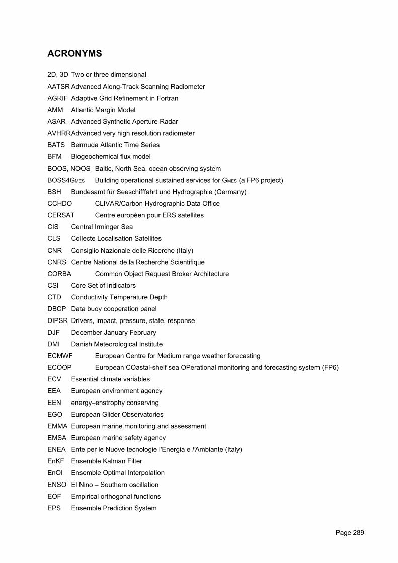
ACRONYMS

2D, 3D Two or three dimensional

AATSR Advanced Along-Track Scanning Radiometer

AGRIF Adaptive Grid Refinement in Fortran

AMM Atlantic Margin Model

ASAR Advanced Synthetic Aperture Radar

AVHRRAdvanced very high resolution radiometer

BATS Bermuda Atlantic Time Series

BFM Biogeochemical flux model

BOOS, NOOS Baltic, North Sea, ocean observing system

BOSS4GMES Building operational sustained services for GMES (a FP6 project)

BSH Bundesamt für Seeschifffahrt und Hydrographie (Germany)

CCHDO CLIVAR/Carbon Hydrographic Data Office

CERSAT Centre européen pour ERS satellites

CIS Central Irminger Sea

CLS Collecte Localisation Satellites

CNR Consiglio Nazionale delle Ricerche (Italy)

CNRS Centre National de la Recherche Scientifique

CORBA Common Object Request Broker Architecture

CSI Core Set of Indicators

CTD Conductivity Temperature Depth

DBCP Data buoy cooperation panel

DIPSR Drivers, impact, pressure, state, response

DJF December January February

DMI Danish Meteorological Institute

ECMWF European Centre for Medium range weather forecasting

ECOOP European COastal-shelf sea OPerational monitoring and forecasting system (FP6)

ECV Essential climate variables

EEA European environment agency

EEN energy–enstrophy conserving

EGO European Glider Observatories

EMMA European marine monitoring and assessment

EMSA European marine safety agency

ENEA Ente per le Nuove tecnologie l'Energia e l'Ambiante (Italy)

EnKF Ensemble Kalman Filter

EnOI Ensemble Optimal Interpolation

ENSO El Nino – Southern oscillation

EOF Empirical orthogonal functions

EPS Ensemble Prediction System

Page 289

ERS European Research Satellite

ERSEM European Regional Seas Ecosystem Model

ESA European space agency

FEOM Finite Element Ocean Model

FP Framework Programme

FTP File transfer protocol

GCM Global Circulation Model

GCOS Global Climate Observing System

GEO Global Earth observations

GEOSS Global Earth observating system of systems

GFZ GeoForschungsZentrum (Potsdam)

GMES Global Monitoring for Environment and Security

GOCE Gravity Field and Steady State Ocean Circulation Explorer

GODAE Global ocean data assimilation experiment

GODIVA Grid for Ocean Diagnostics Interactive Visualisation and Analysis

GOSUD Global Ocean Surface Underway Data Pilot Project

GPS Global positioning system

GRACE Gravity Recovery and Climate. Experiment

GRIB GRIdded Binary format

GTS Global Telecommunication System

GTSPP Global temperature salinity pilot project

HAB Harmful algal bloom

HELCOM intergovernmental cooperation of countries bordering the Baltic Sea

HR-DDS High resolution diagnostic data set

HYCOM HYbrid Coordinate Ocean Model

IAU Incremental Analysis Update

ICES International Council for Exploration of the sea

IFS Integrated Forecast System

INGV Istituto Nazionale di Geofisica e Vulcanologia

IOC Intergovernmental oceanography commission

ISAC Institute of Atmospheric Sciences and Climate (Italy)

ISCCP International Satellite Cloud Climatology Project

JCOMM Joint Commission on Ocean and marine meteorology (UNESCO)

JGOFS Joint Global Ocean Flux Study

JODC Japan Ocean Data Centre

JRC Joint research centre

LEGI Laboratoire des écoulements géophysiques et industriels (France)

LEGOSLaboratoire d’Etudes Géophysiques et Océanograpie Spatiales

LIM Louvain Ice Model

MDT Mean dynamic topography

Page 290

MFC Monitoring and forecasting centre

MFS Mediterranean forecasting system

MIM MERSEA Information Management

MLD Mixed layer depth

MODIS Moderate Resolution Imaging Spectroradiometer

MOON Mediterranean Operational Oceanography Network

MPI MultiProcessor Interface

MRCS Medium resolution continental shelf

MRCS Medium resoultion continental shelf

MUSCLMonotone Upstream-centered Schemes for Conservation Laws

MyOcean FP7 proposal

NCEP National Centre for Environmental prediction (USA)

NEMO Navigating European Marine Observer

NEMO Nucleus for European Modeling of the Ocean

NERSCNansen Environment and remote sensing centre (Norway)

NetCDF Network Common Data Form

NOAA National Ocean and Atmosphere Administration (USA)

NOC National Oceanographic Center (UK)

NODC National Ocean Data Center (USA)

NPZD Nutrient, Phytoplankton, Zooplankton, Detritus

NRT Near Real Time

NUEC NATO Undersea Research Centre

NWS North West Shelf

OBC : Open boundary conditions

OCCAM Ocean Circulation and Climate Advanced Modelling Project

OCR Ocean Colour Radiometry

OGS Istituto Nazionale di Oceanografia e di Geofisica Sperimentale (Italy)

OOPC Ocean Observing Panel for Climate

OPA An Ocean General Circulation modelling System

ORCA Global version of the OPA code

OSI-SAF Ocean sea ice Satellite Application Facility

OSSE Observing system simulation experiment

OSTIA Operational Sea Surface Temperature and Sea Ice Analysis

PAP Porcupine Abyssal Plain

POC Particulate organic matter

POC Pôle d’océanographie côtière (Toulouse, France)

POGO Partnership for observation of the global ocean

POLCOMS Proudman Ocean Laboratory

Psu practical salinity units

QC Quality control

Page 291

RMS Root mean square

SAR Synthetic aperture radar

SEEK Singular evolutive extended Kalman

SEVIRI Spinning Enhanced Visible and InfraRed Imager

SHOM Service Hydrographique et Océanographique de la Marine (France)

SIR Sequential Importance Resampling

SIRF Sequential Importance Resampling Filter

SLA Sea level anomaly

SMHI Swedish Meteorological and Hydrographic Institute

SOFA System for Ocean Analysis and Forecast

SOOP Ship of opportunity

SSH Sea surface height

SSMI Special Sensor Microwave / Imager

SST Sea surface temperature

Sv Sevdrup, a unit of oceanic volume transport

TAC Thematic assembly centre

TEP Thematic portal

THREDDS Thematic Real-time Environmental Distributed Data Services

TKE Turbulent Kinetic Energy

TOGA Tropical ocean and global atmosphere

TOP Target operational period

TSG Thermo-salinograph

TVD Total Variation Diminishing

V1, V2 Version 1, version 2

WMO World meteorological organization

WOCE World ocean circulation experiment

WOD World ocean data base

XBT Expendable bathy-thermograph

XCTD Expendable CTD

Page 292