optima – attachment to final report | cordis
TRANSCRIPT
1
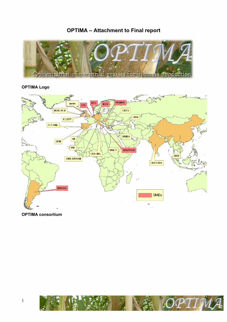
OPTIMA – Attachment to Final report
OPTIMA Logo
OPTIMA consortium
IBERS
2
OPTIMA diagram WP flow
WP1 – Plant and leaf physiology
Task 1.1 Physiology of switchgrass and miscanthus (UCD, INDEAR, IBERS, PRIMUS)
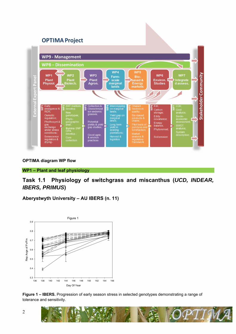
Aberystwyth University – AU IBERS (n. 11)
Figure 1 – IBERS. Progression of early season stress in selected genotypes demonstrating a range of tolerance and sensitivity.
Figure 1
Day Of Year
136 138 140 142 144 146 148 150 152 154 156
Re
p A
vge
of F
v/F
m
0.3
0.4
0.5
0.6
0.7
0.8
0.9
3
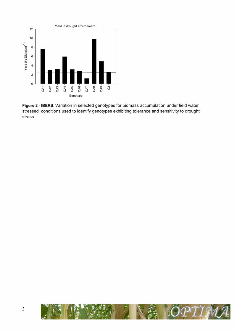
Figure 2 - IBERS. Variation in selected genotypes for biomass accumulation under field water stressed conditions used to identify genotypes exhibiting tolerance and sensitivity to drought stress.
Yield in drought environment
Genotype
OA
1
OA
2
OA
3
OA
4
OA
5
OA
6
OA
7
OA
8
OA
9
C2
Yie
ld (
kg D
M p
lant
-1)
0
2
4
6
8
10
12
4
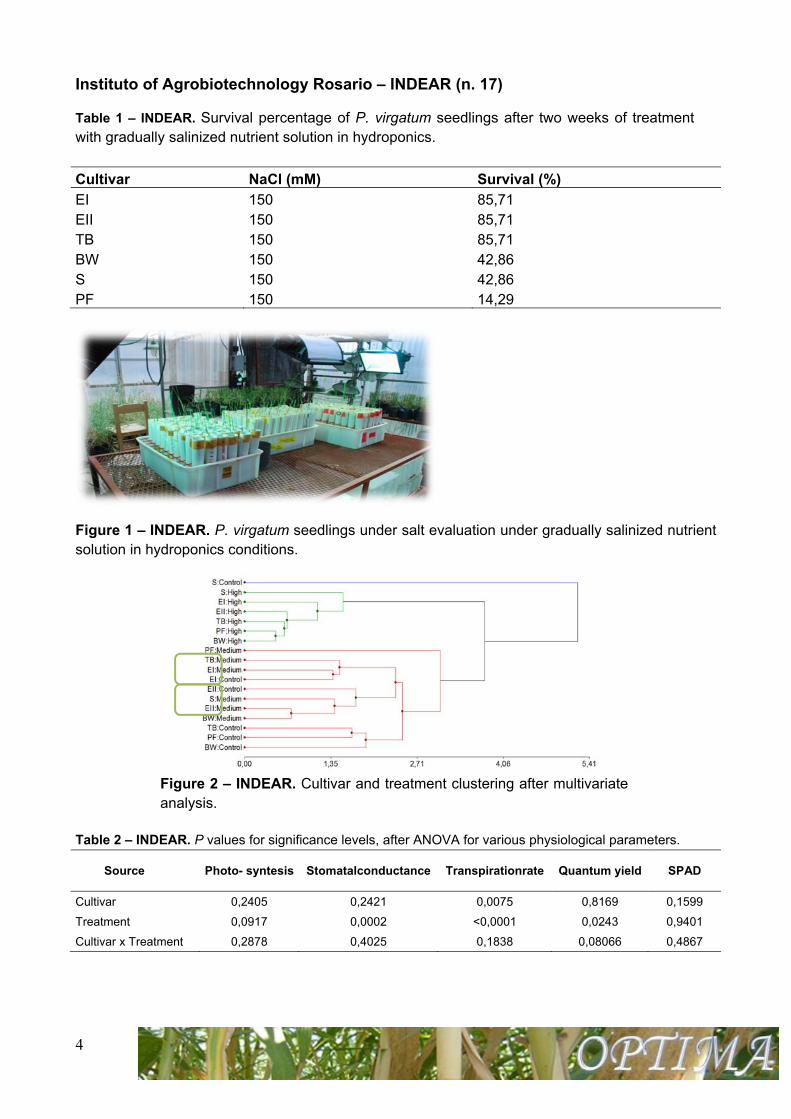
Instituto of Agrobiotechnology Rosario – INDEAR (n. 17)
Table 1 – INDEAR. Survival percentage of P. virgatum seedlings after two weeks of treatment with gradually salinized nutrient solution in hydroponics.
Cultivar NaCl (mM) Survival (%)
EI 150 85,71 EII 150 85,71 TB 150 85,71 BW 150 42,86 S 150 42,86 PF 150 14,29
Figure 1 – INDEAR. P. virgatum seedlings under salt evaluation under gradually salinized nutrient solution in hydroponics conditions.
Figure 2 – INDEAR. Cultivar and treatment clustering after multivariate analysis.
Table 2 – INDEAR. P values for significance levels, after ANOVA for various physiological parameters.
Source
Photo- syntesis Stomatalconductance Transpirationrate Quantum yield SPAD
Cultivar 0,2405 0,2421 0,0075 0,8169 0,1599
Treatment 0,0917 0,0002 <0,0001 0,0243 0,9401
Cultivar x Treatment 0,2878 0,4025 0,1838 0,08066 0,4867
5
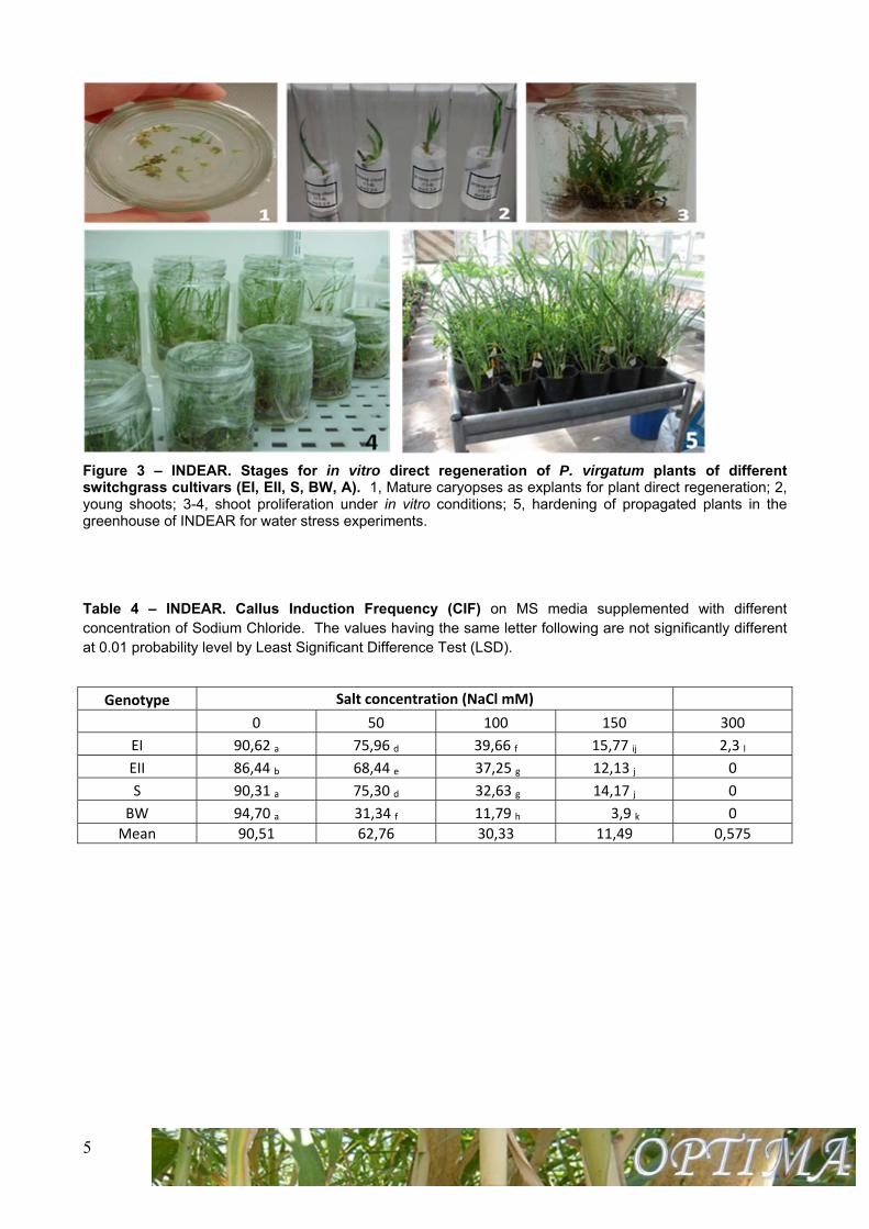
Figure 3 – INDEAR. Stages for in vitro direct regeneration of P. virgatum plants of different switchgrass cultivars (EI, EII, S, BW, A). 1, Mature caryopses as explants for plant direct regeneration; 2, young shoots; 3-4, shoot proliferation under in vitro conditions; 5, hardening of propagated plants in the greenhouse of INDEAR for water stress experiments.
Table 4 – INDEAR. Callus Induction Frequency (CIF) on MS media supplemented with different concentration of Sodium Chloride. The values having the same letter following are not significantly different at 0.01 probability level by Least Significant Difference Test (LSD).
Genotype Salt concentration (NaCl mM)
0 50 100 150 300
EI 90,62 a 75,96 d 39,66 f 15,77 ij 2,3 l
EII 86,44 b 68,44 e 37,25 g 12,13 j 0
S 90,31 a 75,30 d 32,63 g 14,17 j 0
BW 94,70 a 31,34 f 11,79 h 3,9 k 0
Mean 90,51 62,76 30,33 11,49 0,575
6
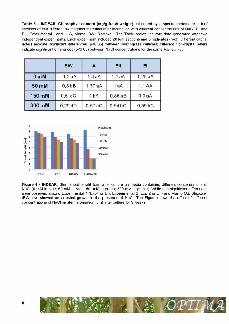
Table 5 – INDEAR. Chlorophyll content (mg/g fresh weight) calculated by a spectrophotometer in leaf sections of four different switchgrass materials after incubation with different concentrations of NaCl. EI and EII, Experimental I and II; A, Alamo; BW, Blackwell. The Table shows the rate data generated after two independent experiments. Each experiment included 20 leaf sections and 3 replicates (n=3). Different capital letters indicate significant differences (p<0.05) between switchgrass cultivars; different Non-capital letters indicate significant differences (p<0.05) between NaCl concentrations for the same Panicum cv.
Figure 4 - INDEAR. Stem/shoot lenght (cm) after culture on media containing different concentrations of NaCl (0 mM in blue; 50 mM in red; 150 mM in green; 300 mM in purple). While non-significant differences were observed among Experimental 1 (Exp1 or EI), Experimental 2 (Exp 2 or EII) and Alamo (A), Blackwell (BW) cvs showed an arrested growth in the presence of NaCl. The Figure shows the effect of different concentrations of NaCl on stem elongation (cm) after culture for 9 weeks.
7
Table 6 – INDEAR. In vitro shoot growth under osmotic stress with PEG. SD, significant difference. Different letters indicate significant differences between treatments and between cultivars(P <0,05).
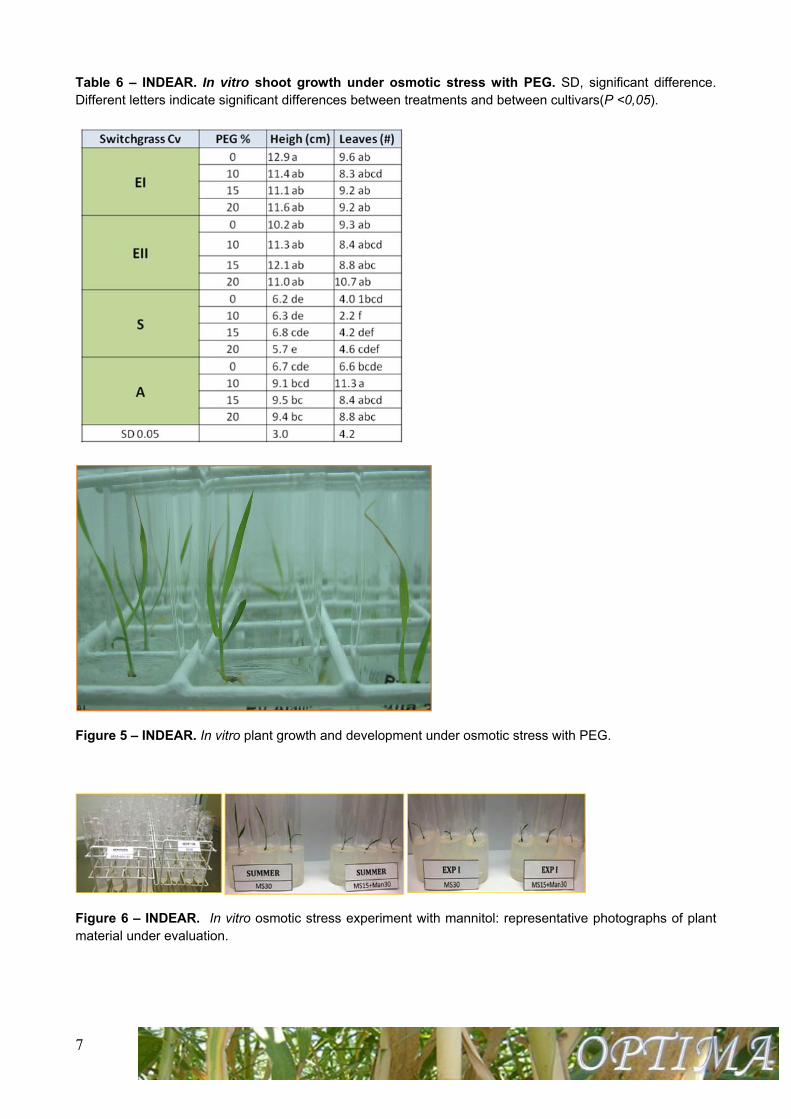
Figure 5 – INDEAR. In vitro plant growth and development under osmotic stress with PEG.
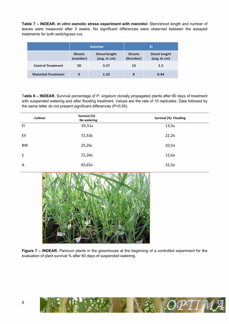
Figure 6 – INDEAR. In vitro osmotic stress experiment with mannitol: representative photographs of plant material under evaluation.
8
Table 7 – INDEAR. In vitro osmotic stress experiment with mannitol: Stem/shoot length and number of leaves were measured after 3 weeks. No significant differences were observed between the assayed treatments for both switchgrass cvs.
Table 8 – INDEAR. Survival percentage of P. virgatum clonally propagated plants after 60 days of treatment with suspended watering and after flooding treatment. Values are the rate of 10 replicates. Data followed by the same letter do not present significant differences (P<0,05).
Cultivar Survival (%) No watering
Survival (%) Flooding
EI 65,51a 13,5a
EII 72,33b 22,2b
BW 25,26c 10,5a
S 72,26b 12,6a
A 45,65d 32,5d
Figure 7 – INDEAR. Panicum plants in the greenhouse at the beginning of a controlled experiment for the evaluation of plant survival % after 60 days of suspended watering.
9
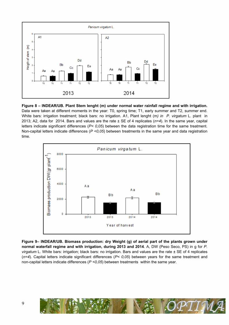
Figure 8 – INDEAR/UB. Plant Stem lenght (m) under normal water rainfall regime and with irrigation. Data were taken at different moments in the year: T0, spring time; T1, early summer and T2, summer end. White bars: irrigation treatment; black bars: no irrigation. A1, Plant lenght (m) in P. virgatum L. plant in 2013; A2, data for 2014. Bars and values are the rate ± SE of 4 replicates (n=4). In the same year, capital letters indicate significant differences (P< 0,05) between the data registration time for the same treatment. Non-capital letters indicate differences (P <0,05) between treatments in the same year and data registration time.
Figure 9– INDEAR/UB. Biomass production: dry Weight (g) of aerial part of the plants grown under normal waterfall regime and with irrigation, during 2013 and 2014. A, DW (Peso Seco, PS) in g for P. virgatum L. White bars: irrigation; black bars: no irrigation. Bars and values are the rate ± SE of 4 replicates (n=4). Capital letters indicate significant differences (P< 0,05) between years for the same treatment and non-capital letters indicate differences (P <0,05) between treatments within the same year.
10
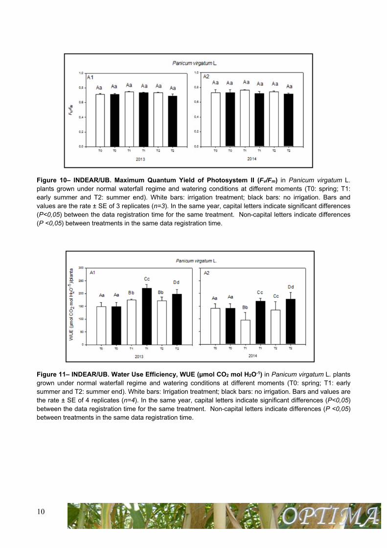
Figure 10– INDEAR/UB. Maximum Quantum Yield of Photosystem II (Fv/Fm) in Panicum virgatum L. plants grown under normal waterfall regime and watering conditions at different moments (T0: spring; T1: early summer and T2: summer end). White bars: irrigation treatment; black bars: no irrigation. Bars and values are the rate ± SE of 3 replicates (n=3). In the same year, capital letters indicate significant differences (P<0,05) between the data registration time for the same treatment. Non-capital letters indicate differences (P <0,05) between treatments in the same data registration time.
Figure 11– INDEAR/UB. Water Use Efficiency, WUE (µmol CO2 mol H2O-1) in Panicum virgatum L. plants grown under normal waterfall regime and watering conditions at different moments (T0: spring; T1: early summer and T2: summer end). White bars: Irrigation treatment; black bars: no irrigation. Bars and values are the rate ± SE of 4 replicates (n=4). In the same year, capital letters indicate significant differences (P<0,05) between the data registration time for the same treatment. Non-capital letters indicate differences (P <0,05) between treatments in the same data registration time.
11
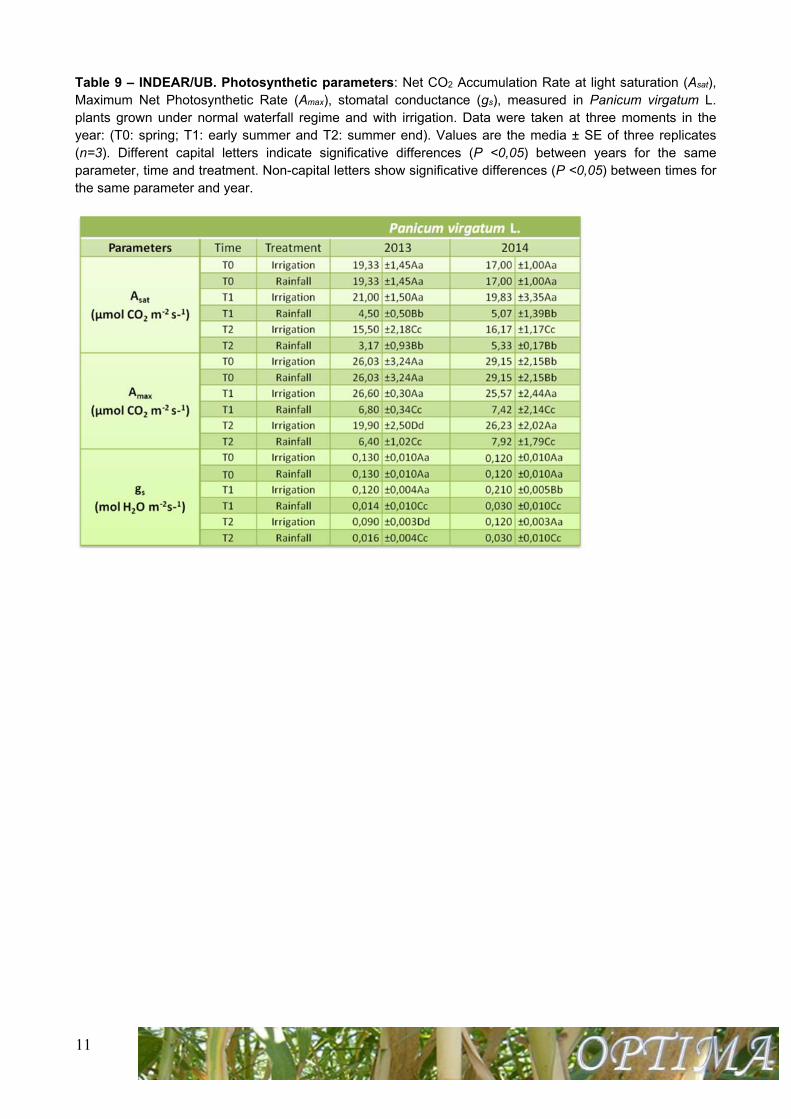
Table 9 – INDEAR/UB. Photosynthetic parameters: Net CO2 Accumulation Rate at light saturation (Asat), Maximum Net Photosynthetic Rate (Amax), stomatal conductance (gs), measured in Panicum virgatum L. plants grown under normal waterfall regime and with irrigation. Data were taken at three moments in the year: (T0: spring; T1: early summer and T2: summer end). Values are the media ± SE of three replicates (n=3). Different capital letters indicate significative differences (P <0,05) between years for the same parameter, time and treatment. Non-capital letters show significative differences (P <0,05) between times for the same parameter and year.
12
University of Dublin, UCD School of Biology and Environmental Science – NUID UCD (n. 12)
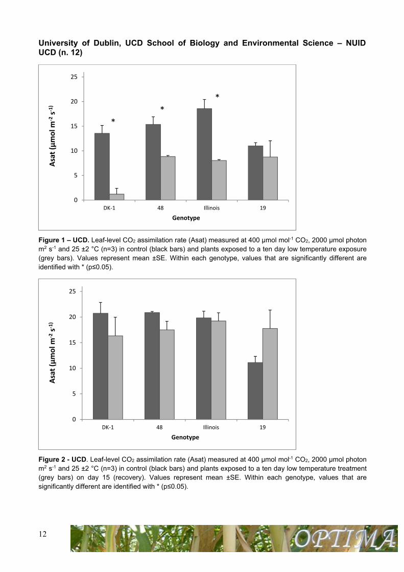
Figure 1 – UCD. Leaf-level CO2 assimilation rate (Asat) measured at 400 μmol mol-1 CO2, 2000 μmol photon m2 s-1 and 25 ±2 °C (n=3) in control (black bars) and plants exposed to a ten day low temperature exposure (grey bars). Values represent mean ±SE. Within each genotype, values that are significantly different are identified with * (p≤0.05).
Figure 2 - UCD. Leaf-level CO2 assimilation rate (Asat) measured at 400 μmol mol-1 CO2, 2000 μmol photon m2 s-1 and 25 ±2 °C (n=3) in control (black bars) and plants exposed to a ten day low temperature treatment (grey bars) on day 15 (recovery). Values represent mean ±SE. Within each genotype, values that are significantly different are identified with * (p≤0.05).
0
5
10
15
20
25
DK‐1 48 Illinois 19
Asat (μmol m
‐2s‐1)
Genotype
*
*
*
0
5
10
15
20
25
DK‐1 48 Illinois 19
Asat (μmol m
‐2s‐1)
Genotype
13
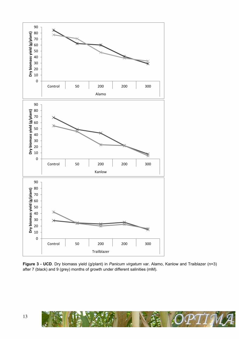
Figure 3 - UCD. Dry biomass yield (g/plant) in Panicum virgatum var. Alamo, Kanlow and Traiblazer (n=3) after 7 (black) and 9 (grey) months of growth under different salinities (mM).
0
10
20
30
40
50
60
70
80
90
Control 50 200 200 300
Alamo
Dry biomass yield (g/plant)
0
10
20
30
40
50
60
70
80
90
Control 50 200 200 300
Kanlow
Dry biomass yield (g/plant)
0
10
20
30
40
50
60
70
80
90
Control 50 200 200 300
Trailblazer
Dry biomass yield (g/plant)
14
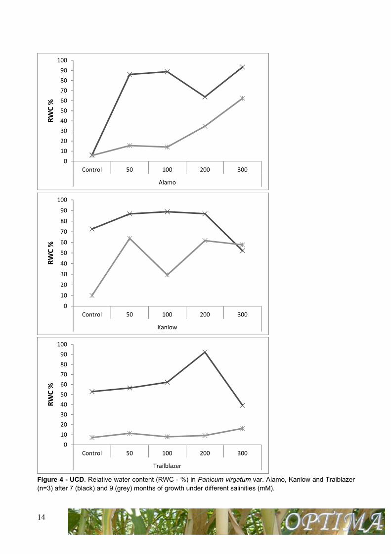
Figure 4 - UCD. Relative water content (RWC - %) in Panicum virgatum var. Alamo, Kanlow and Traiblazer (n=3) after 7 (black) and 9 (grey) months of growth under different salinities (mM).
0
10
20
30
40
50
60
70
80
90
100
Control 50 100 200 300
Alamo
RWC %
0
10
20
30
40
50
60
70
80
90
100
Control 50 100 200 300
Kanlow
RWC %
0
10
20
30
40
50
60
70
80
90
100
Control 50 100 200 300
Trailblazer
RWC %
15
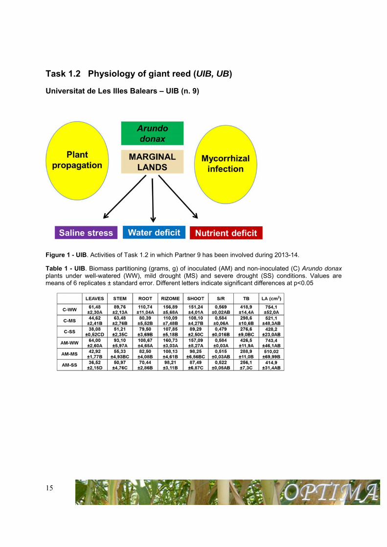
Task 1.2 Physiology of giant reed (UIB, UB)
Universitat de Les Illes Balears – UIB (n. 9)
Figure 1 - UIB. Activities of Task 1.2 in which Partner 9 has been involved during 2013-14.
Table 1 - UIB. Biomass partitioning (grams, g) of inoculated (AM) and non-inoculated (C) Arundo donax plants under well-watered (WW), mild drought (MS) and severe drought (SS) conditions. Values are means of 6 replicates ± standard error. Different letters indicate significant differences at p<0.05
16
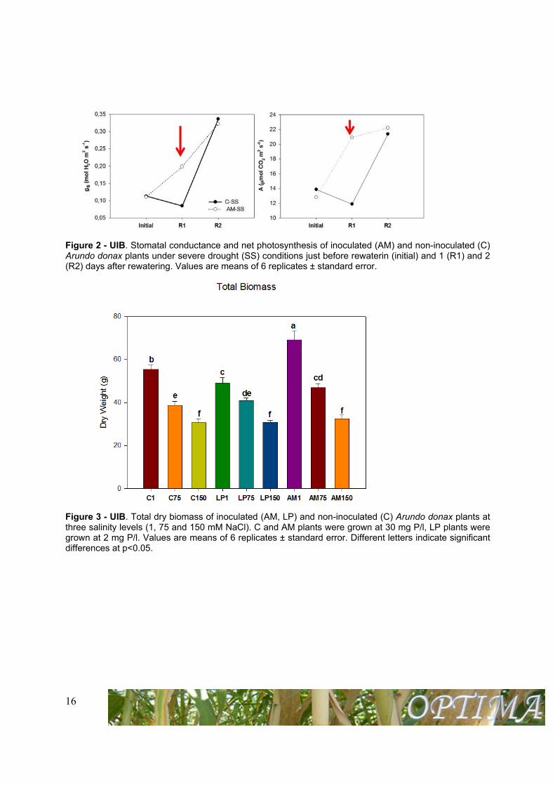
Figure 2 - UIB. Stomatal conductance and net photosynthesis of inoculated (AM) and non-inoculated (C) Arundo donax plants under severe drought (SS) conditions just before rewaterin (initial) and 1 (R1) and 2 (R2) days after rewatering. Values are means of 6 replicates ± standard error.
Figure 3 - UIB. Total dry biomass of inoculated (AM, LP) and non-inoculated (C) Arundo donax plants at three salinity levels (1, 75 and 150 mM NaCl). C and AM plants were grown at 30 mg P/l, LP plants were grown at 2 mg P/l. Values are means of 6 replicates ± standard error. Different letters indicate significant differences at p<0.05.
17
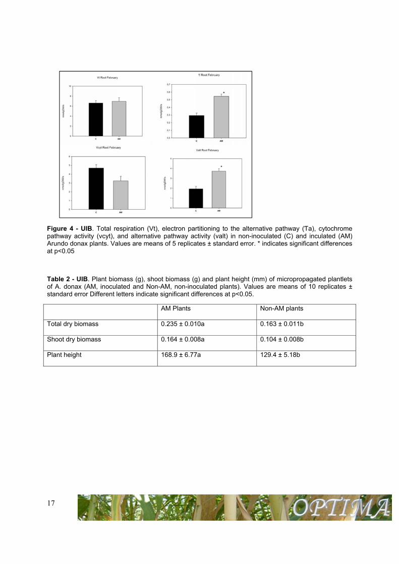
Figure 4 - UIB. Total respiration (Vt), electron partitioning to the alternative pathway (Ƭa), cytochrome pathway activity (vcyt), and alternative pathway activity (valt) in non-inoculated (C) and inculated (AM) Arundo donax plants. Values are means of 5 replicates ± standard error. * indicates significant differences at p<0.05
Table 2 - UIB. Plant biomass (g), shoot biomass (g) and plant height (mm) of micropropagated plantlets of A. donax (AM, inoculated and Non-AM, non-inoculated plants). Values are means of 10 replicates ± standard error Different letters indicate significant differences at p<0.05.
AM Plants Non-AM plants
Total dry biomass 0.235 ± 0.010a 0.163 ± 0.011b
Shoot dry biomass 0.164 ± 0.008a 0.104 ± 0.008b
Plant height 168.9 ± 6.77a 129.4 ± 5.18b
18
Universitat de Barcelona – UB (n. 10)
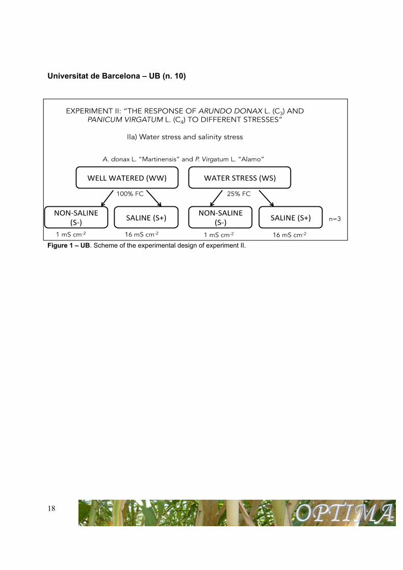
Figure 1 – UB. Scheme of the experimental design of experiment II.
19
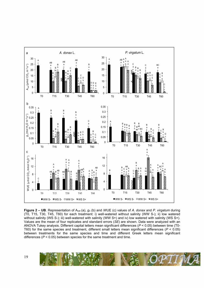
Figure 2 – UB. Representation of Asat (a), gs (b) and iWUE (c) values of A. donax and P. virgatum during (T0, T15, T30, T45, T60) for each treatment: i) well-watered without salinity (WW S-); ii) low watered without salinity (WS S-); iii) well-watered with salinity (WW S+) and iv) low watered with salinity (WS S+). Values are the mean of four replicates and standard errors (SE) are shown. Data were analyzed with an ANOVA Tukey analysis. Different capital letters mean significant differences (P < 0.05) between time (T0-T60) for the same species and treatment, different small letters mean significant differences (P < 0.05) between treatments for the same species and time and different Greek letters mean significant differences (P < 0.05) between species for the same treatment and time.
A AB
a
AB a
AB a B
a
B c
B c C
b D
b
B bc
B bc C
b
D b
B b
C b
D b E
b
0
5
10
15
20
25
30
T0 T15 T30 T45 T60
Asa
t (µ
mo
l CO
2 m
-2 s
-1)
A. donax L. a
A
AB a C
a
C a
BC a
A a
B a BC
b
C b
A a
B a B
b
B b
A a
B a C
b
C c
0
5
10
15
20
25
30
T0 T15 T30 T45 T60
P. virgatum L.
A B
a
B a
B a
C a
B c
BC c
C b
D b
B c
B c
B b
B b
B b
B b C
b
C b
0
0.05
0.1
0.15
0.2
0.25
0.3
0.35
T0 T15 T30 T45 T60
gs
(mo
l H2O
m-2
s-1
)
b
A B
a
B a
B a
B a
B a
B ab C
b
C b
B a
B ab B
b
B b
B a
BC b
C b
D c
0
0.05
0.1
0.15
0.2
0.25
0.3
0.35
T0 T15 T30 T45 T60
C
AB b
AB b
B b
A a
A a
A a
A a
B b
A a
AB b
B a
AB b
B b
A b
AB a
0
4
8
12
16
T0 T15 T30 T45 T60
WU
E (m
ol C
O2
mm
ol H
2O
-1)
WW S- WS S- WW S+ WS S+
c
B
B a
C b
B bc
A a C
a
B a
A a
BC a
AB a
B b
A b
A a A
a
A b
A c
A b
0
4
8
12
16
T0 T15 T30 T45 T60
WW S- WS S- WW S+ WS S+
Bab
20
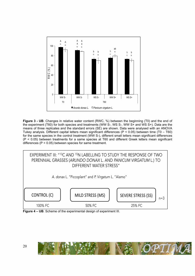
Figure 3 - UB. Changes in relative water content (RWC, %) between the beginning (T0) and the end of the experiment (T60) for both species and treatments (WW S-, WS S-, WW S+ and WS S+). Data are the means of three replicates and the standard errors (SE) are shown. Data were analysed with an ANOVA Tukey analysis. Different capital letters mean significant differences (P < 0.05) between time (T0 – T60) for the same species in the control treatment (WW S-), different small letters mean significant differences (P < 0.05) between treatments for a same species at T60 and different Greek letters mean significant differences (P < 0.05) between species for same treatment.
Figure 4 – UB. Scheme of the experimental design of experiment III.
A
A a
b
b
b
A
A a
b
ab b
0
20
40
60
80
100
WW S- WW S- WS S- WW S+ WS S+
T0 T60
RW
C (
%)
Arundo donax L. Panicum virgatum L.
21
Figure 5 – UB. Photosynthesis parameters (Asat, assimilation rate at light saturation (a); Amax, maximum assimilation rate at light and CO2 saturation (b); gs, stomatal conductance (c); l, stomatal limitation (d); T, transpiration rate (e); WUE, water use efficiency (f); Vc, max, maximum carboxylation velocity of Rubisco (g); Jmax, the rate of photosynthetic electron transport (h)) in both species (A. donax and P. virgatum L.) for each treatment: i) Control (C, 100% FC), ii) Mild stress (MS, 50% FC) and iii) Severe Stress (SS, 25% FC) at the end of the experiment (Tf). Data are the means of three replicates and the standard error is shown. Data were analyzed with an ANOVA Tukey analysis. Different capital letters indicate significant differences (P < 0.05) between treatments for the same species and different small letters indicate significant differences (P < 0.05) between species for the same treatment.
Aa
Ba
Ca
Ab
Ba
Ca
0
10
20
30
C MS SS
Asa
t (m
ol C
O2 m
-2 s
-1)
a
Aa
Ba
Ca
Ab
Bb
Ca
0
20
40
60
80
100
120
140
C MS SS
Vc,
max
(m
ol m
-2 s
-1)
Aa
Ba
Ba
Ab
Ba
Ba
0
10
20
30
C MS SS
Am
ax (m
ol C
O2 m
-2 s
-1)
Aa
Ba
Ca
Ab
BbBa
0.0
0.1
0.2
0.3
0.4
0.5
0.6
C MS SS
gs (m
ol H
2O m
-2 s
-1)
c
b
Ca
Ba
Aa
Ca
Ba
Aa
0
5
10
15
20
25
30
C MS SS
l (%
)
A. donax L. P. virgatum L.
d
g
Aa
Ba
Ca
Ab
BbBa
0
2
4
6
8
10
C MS SS
T (m
mol H
2O m
-2 s
-1)
e
Bb
Ab
Ab
Ab
AaAa
0
2
4
6
8
10
12
14
C MS SS
iWU
E (m
ol C
O2 m
mol H
2O-1)
f
Aa
Ba
BaAb
BbBb
0
50
100
150
200
250
300
350
C MS SS
J max
(m
ol m
-2 s
-1)
A. donax L. P. virgatum L.
h
22
Figure 6 – UB. Water stress effects (Control (C, 100% FC), Mild Stress (MS, 50% FC) and Severe
Stress (SS, 25% FC) on δ13C values (‰) of CO2 in total organic matter (δ13CTOM) in leaves, stems, roots
and rhizomes in both species (A. donax (a) and P. virgatum (b)) before labelling (T0), 1 day after
labelling (T1) and 7 days after labelling (T2).
-30
0
30
60
90
120
Leaf Stem Root Rhizome Leaf Stem Root Rhizome Leaf Stem Root Rhizome
T0 T1 T2
13 C
TO
M (
‰)
a
-30
0
30
60
90
120
Leaf Stem Root Rhizome Leaf Stem Root Rhizome Leaf Stem Root Rhizome
T0 T1 T2
13 C
TO
M (
‰)
C MS SS
b
23
Figure 7 – UB. Water stress effects (Control (C, 100% FC), Mild stress (MS, 50% FC) and Severe Stress
(SS, 25% FC) on δ13C values (‰) of sugars (δ13CTSS) in leaves, stems, roots and rhizomes in both
species (A. donax (a) and P. virgatum (b)) before labelling (T0), 1 day after labelling (T1) and 7 days after
labelling (T2).
-40
0
40
80
120
160
200
240
280
Leaf Stem Root Rhizome Leaf Stem Root Rhizome Leaf Stem Root Rhizome
T0 T1 T2
13C
TS
S (‰
)
a
-40
0
40
80
120
160
200
240
280
Leaf Stem Root Rhizome Leaf Stem Root Rhizome Leaf Stem Root Rhizome
T0 T1 T2
13C
TS
S (‰
)
C MS SS
b
24
Figure 8 - UB. Water stress effects (Control (C, 100% FC), Mild Stress (MS, 50% FC) and Severe Stress (SS, 25% FC) on δ13C values (‰) of respired CO2 (δ13CR) in leaves, stems, roots and rhizomes in both species (A. donax (a) and P. virgatum (b)) before labelling (T0), 1 day after labelling (T1) and 7 days after labelling (T2).
-30
0
30
60
90
120
150
180
Leaf Stem Root Rhizome Leaf Stem Root Rhizome Leaf Stem Root Rhizome
T0 T1 T2
13 C
R (‰
)
a
-30
0
30
60
90
120
150
180
Leaf Stem Root Rhizome Leaf Stem Root Rhizome Leaf Stem Root Rhizome
T0 T1 T2
13C
R (‰
)
C MS SS
b
25
WP2 – Plant biotechnology
Instituto of Agrobiotechnology Rosario – INDEAR (n. 17)
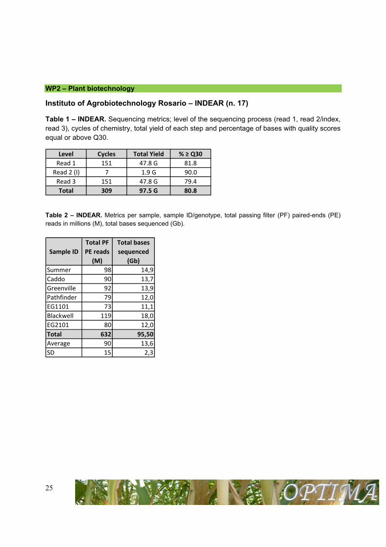
Table 1 – INDEAR. Sequencing metrics; level of the sequencing process (read 1, read 2/index, read 3), cycles of chemistry, total yield of each step and percentage of bases with quality scores equal or above Q30.
Table 2 – INDEAR. Metrics per sample, sample ID/genotype, total passing filter (PF) paired-ends (PE) reads in millions (M), total bases sequenced (Gb).
Level Cycles Total Yield % ≥ Q30
Read 1 151 47.8 G 81.8
Read 2 (I) 7 1.9 G 90.0
Read 3 151 47.8 G 79.4
Total 309 97.5 G 80.8
Sample ID
Total PF
PE reads
(M)
Total bases
sequenced
(Gb)
Summer 98 14,9
Caddo 90 13,7
Greenville 92 13,9
Pathfinder 79 12,0
EG1101 73 11,1
Blackwell 119 18,0
EG2101 80 12,0
Total 632 95,50
Average 90 13,6
SD 15 2,3
26
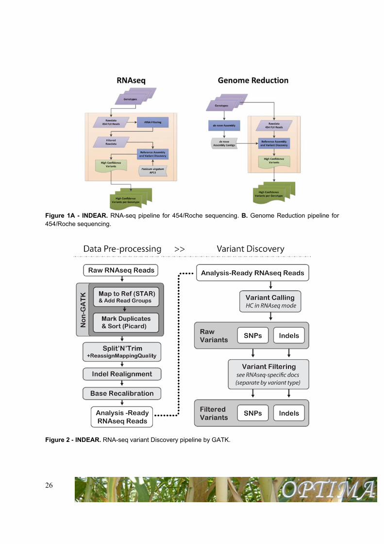
Figure 1A - INDEAR. RNA-seq pipeline for 454/Roche sequencing. B. Genome Reduction pipeline for 454/Roche sequencing.
Figure 2 - INDEAR. RNA-seq variant Discovery pipeline by GATK.
27
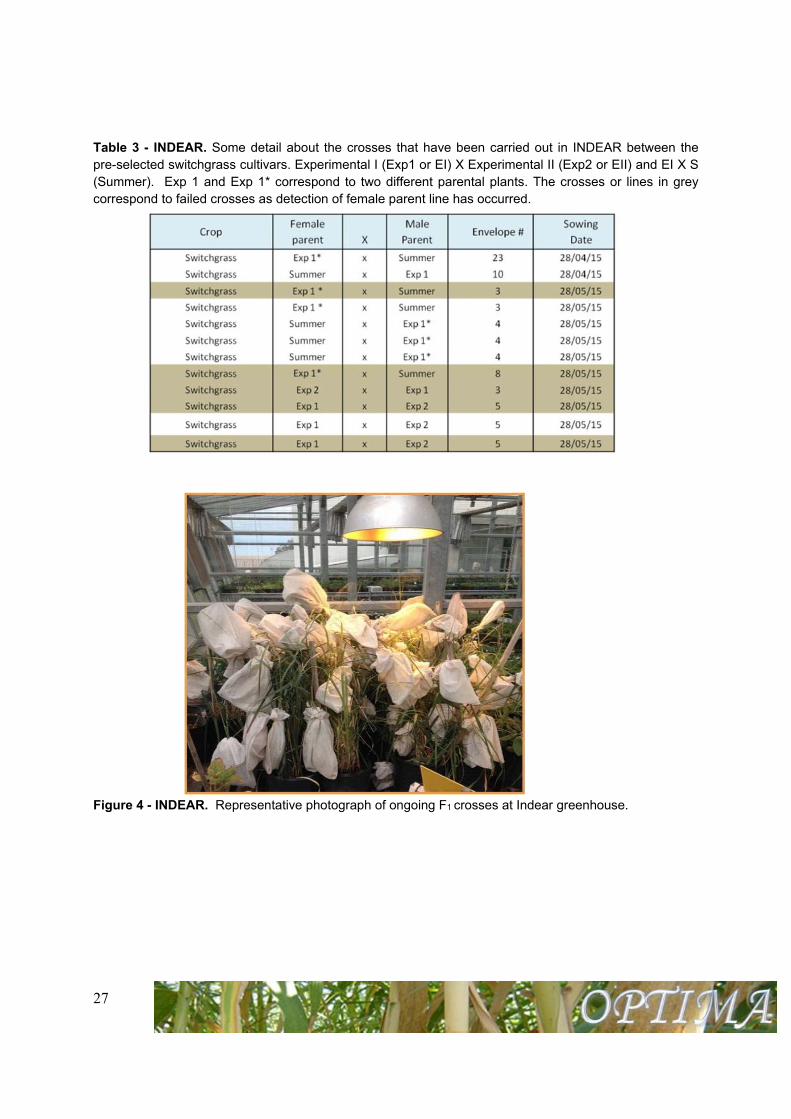
Table 3 - INDEAR. Some detail about the crosses that have been carried out in INDEAR between the pre-selected switchgrass cultivars. Experimental I (Exp1 or EI) X Experimental II (Exp2 or EII) and EI X S (Summer). Exp 1 and Exp 1* correspond to two different parental plants. The crosses or lines in grey correspond to failed crosses as detection of female parent line has occurred.
Figure 4 - INDEAR. Representative photograph of ongoing F1 crosses at Indear greenhouse.
28
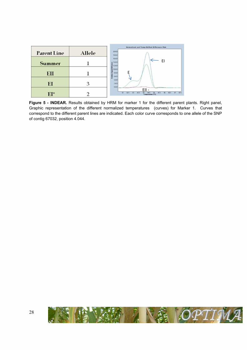
Figure 5 - INDEAR. Results obtained by HRM for marker 1 for the different parent plants. Right panel, Graphic representation of the different normalized temperatures (curves) for Marker 1. Curves that correspond to the different parent lines are indicated. Each color curve corresponds to one allele of the SNP of contig 67032, position 4.044.
E
EI
EII ‐
29
Huazhong Agricultural University – HZAU (n. 14)
Table 1 – HZAU. The number of sample and SNP for GBS
Project Samples SNP numbers Drought tolerance 50 319,900
Map genome
Piccoplant 27 213,057 Fondachello 24 210,491 Granadensis 9 31,655 Martinensis 52 303,593 Argentum 19 105,417
Total 181 1,184,113
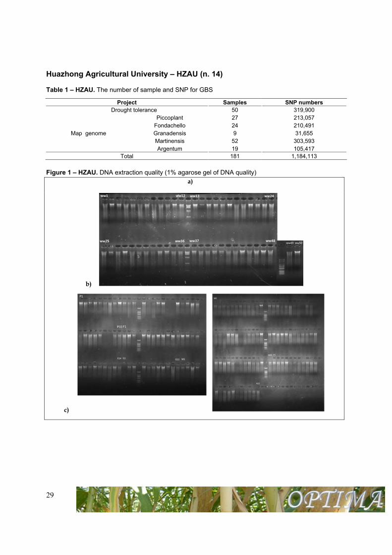
Figure 1 – HZAU. DNA extraction quality (1% agarose gel of DNA quality)
a)
b)
c)
30
Table 1 - HZAU. GBS raw data statistic
Total read numbers
Accepted reads numbers
Accepted reads ratio
The average depth
of each clones
Raw SNP numbers
197,671,204 144,058,366 73% 0.288 Gb 319,900
Table 2 – HZAU. The number of sample and SNP for GBS
Project Samples SNP numbers
Drought tolerance 50 319,900
Map genome
Piccoplant 27 213,057
Fondachello 24 210,491
Granadensis 9 31,655
Martinensis 52 303,593
Argentum 19 105,417
Total 181 1,184,113
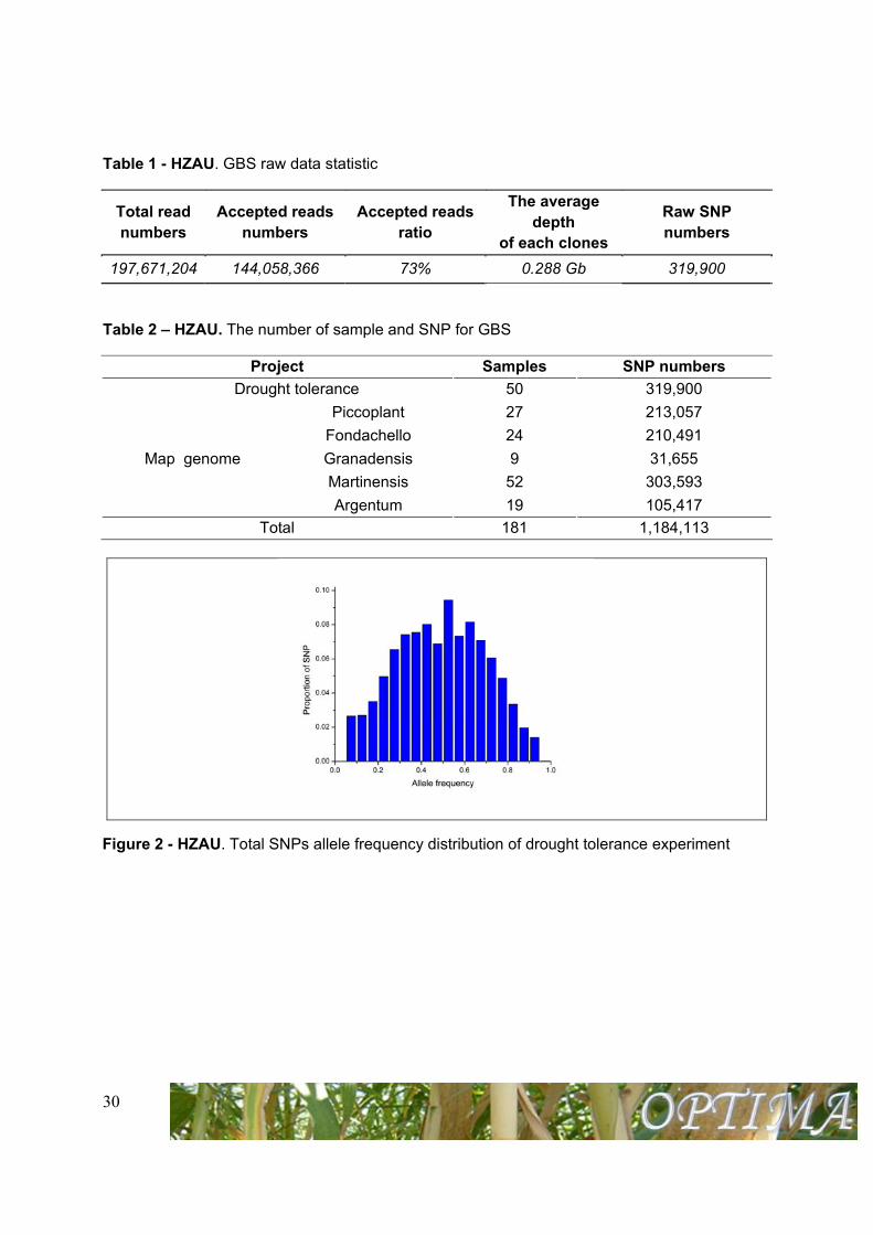
Figure 2 - HZAU. Total SNPs allele frequency distribution of drought tolerance experiment
31
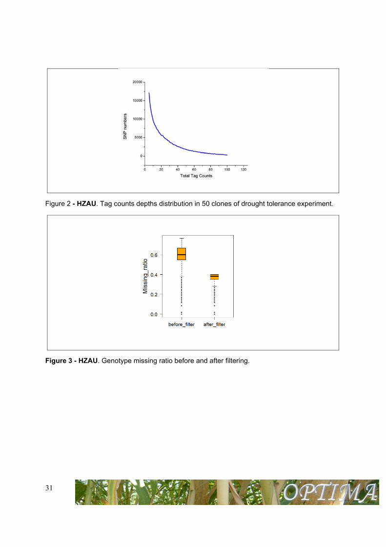
Figure 2 - HZAU. Tag counts depths distribution in 50 clones of drought tolerance experiment.
Figure 3 - HZAU. Genotype missing ratio before and after filtering.
32
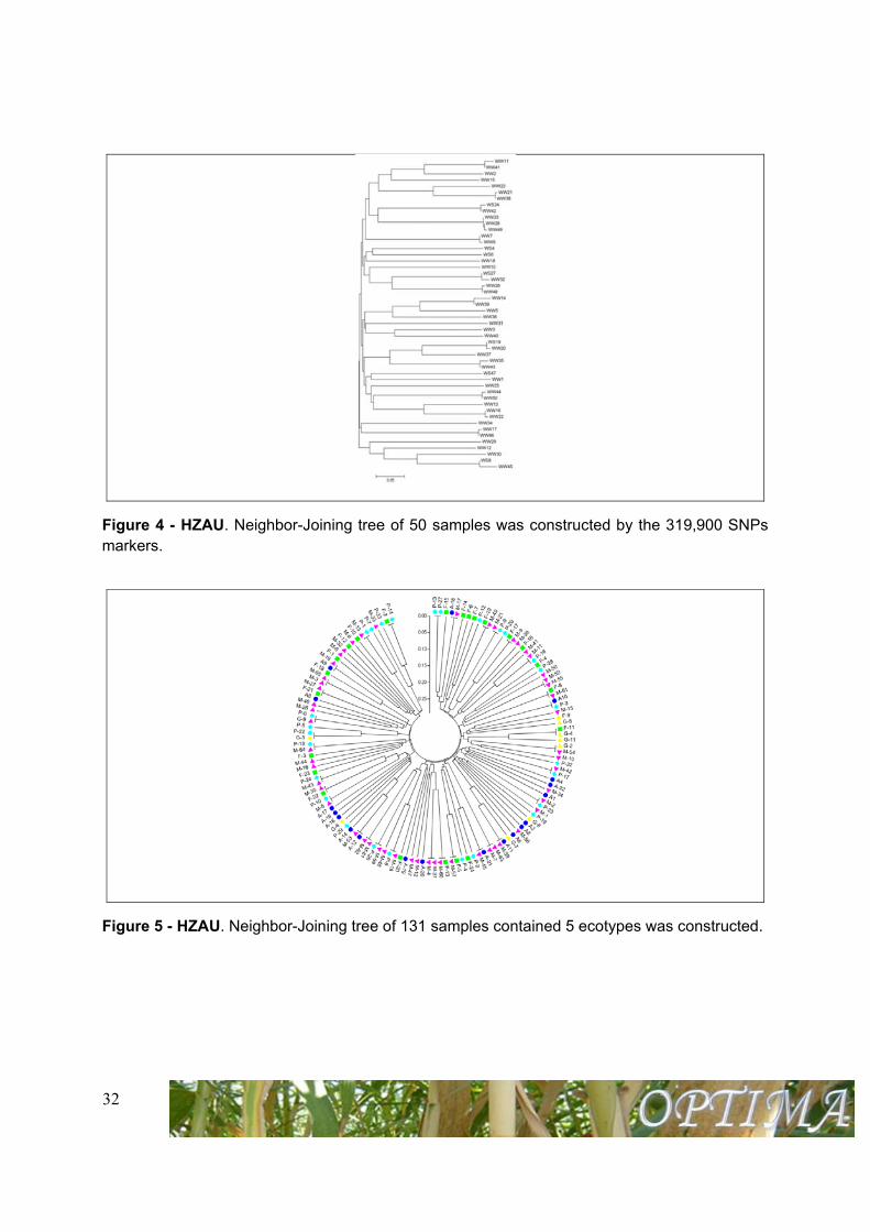
Figure 4 - HZAU. Neighbor-Joining tree of 50 samples was constructed by the 319,900 SNPs markers.
Figure 5 - HZAU. Neighbor-Joining tree of 131 samples contained 5 ecotypes was constructed.
33
WP3 – Plant agronomy
Task 3.1 - Characterization of endemic grasses and novel plant varieties adapted to southern European conditions
Unversità di Catania - UNICT (n. 1)
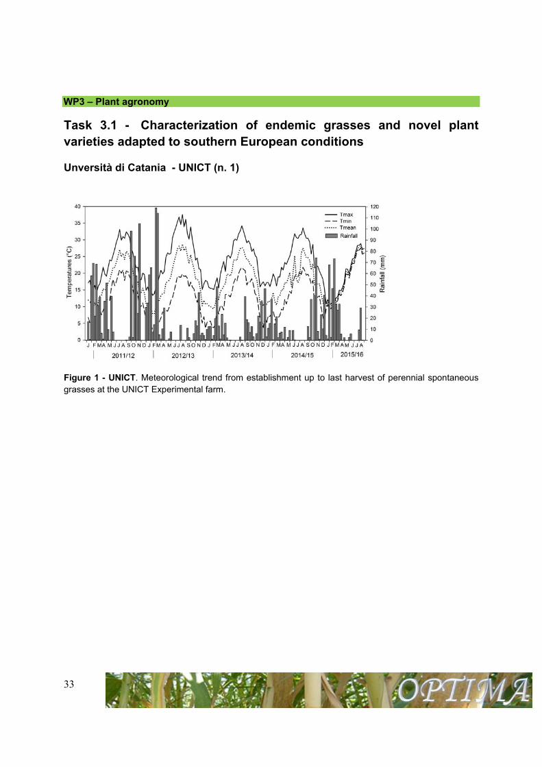
Figure 1 - UNICT. Meteorological trend from establishment up to last harvest of perennial spontaneous grasses at the UNICT Experimental farm.
34
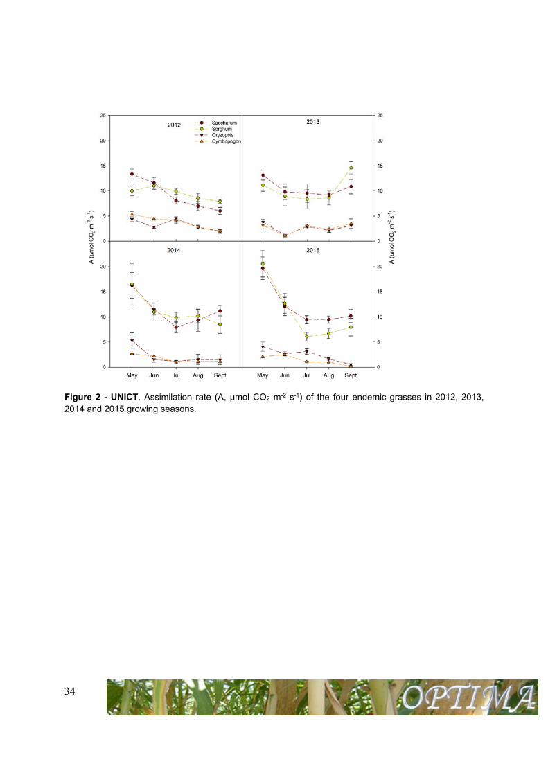
Figure 2 - UNICT. Assimilation rate (A, µmol CO2 m-2 s-1) of the four endemic grasses in 2012, 2013, 2014 and 2015 growing seasons.
35
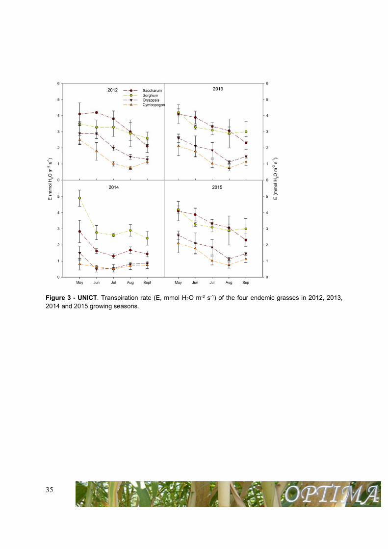
Figure 3 - UNICT. Transpiration rate (E, mmol H2O m-2 s-1) of the four endemic grasses in 2012, 2013, 2014 and 2015 growing seasons.
36
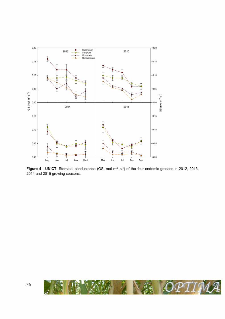
Figure 4 - UNICT. Stomatal conductance (GS, mol m-2 s-1) of the four endemic grasses in 2012, 2013, 2014 and 2015 growing seasons.
37
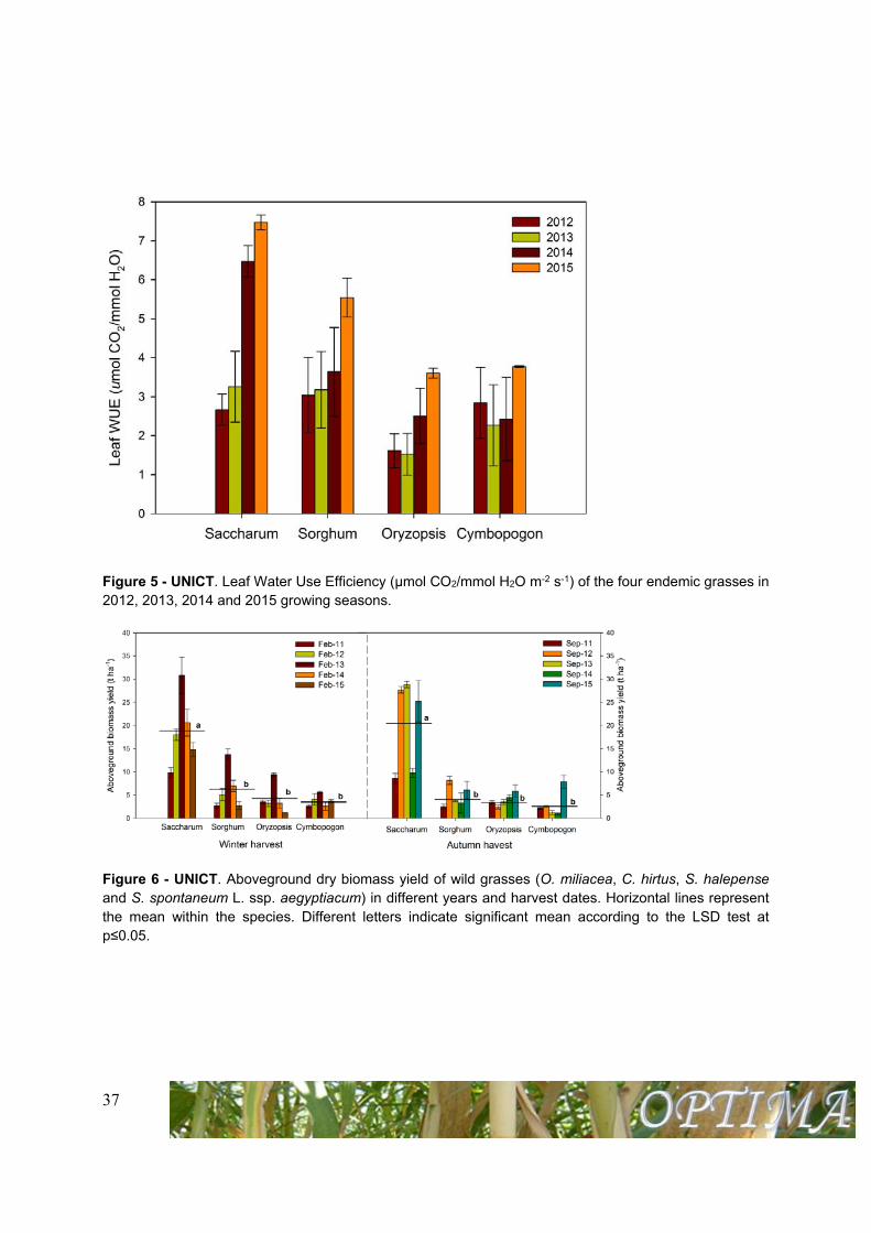
Figure 5 - UNICT. Leaf Water Use Efficiency (µmol CO2/mmol H2O m-2 s-1) of the four endemic grasses in 2012, 2013, 2014 and 2015 growing seasons.
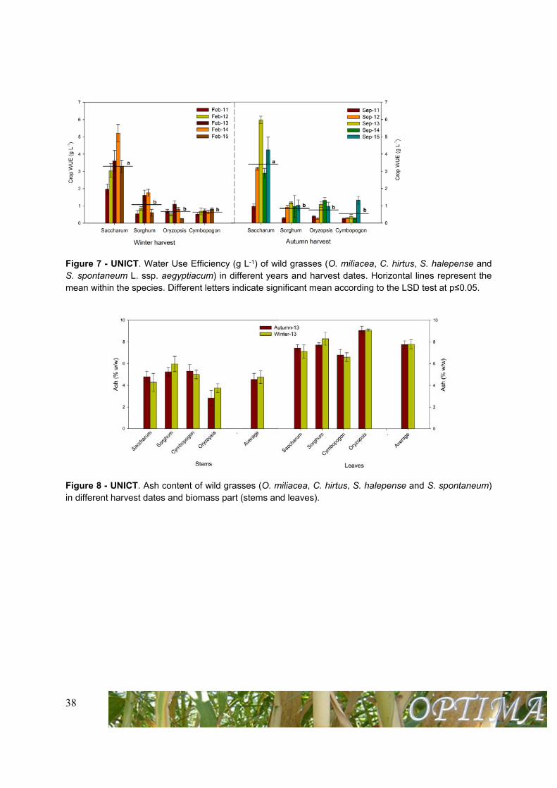
Figure 6 - UNICT. Aboveground dry biomass yield of wild grasses (O. miliacea, C. hirtus, S. halepense and S. spontaneum L. ssp. aegyptiacum) in different years and harvest dates. Horizontal lines represent the mean within the species. Different letters indicate significant mean according to the LSD test at p≤0.05.
38
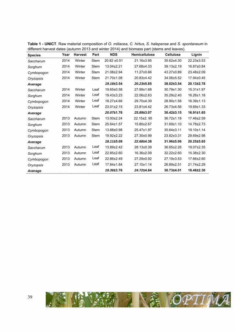
Figure 7 - UNICT. Water Use Efficiency (g L-1) of wild grasses (O. miliacea, C. hirtus, S. halepense and S. spontaneum L. ssp. aegyptiacum) in different years and harvest dates. Horizontal lines represent the mean within the species. Different letters indicate significant mean according to the LSD test at p≤0.05.
Figure 8 - UNICT. Ash content of wild grasses (O. miliacea, C. hirtus, S. halepense and S. spontaneum) in different harvest dates and biomass part (stems and leaves).
39
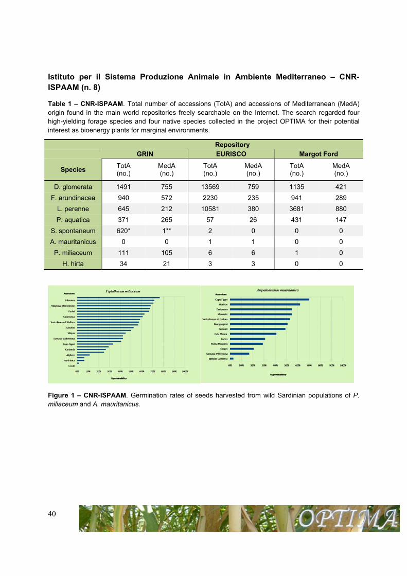
Table 1 - UNICT. Raw material composition of O. miliacea, C. hirtus, S. halepense and S. spontaneum in different harvest dates (autumn 2013 and winter 2014) and biomass part (stems and leaves).
Species Year Harvest Part NDS Hemicellulose Cellulose Lignin
Saccharum 2014 Winter Stem 20.82 ±0.51 21.16±3.95 35.62±4.30 22.23±3.53
Sorghum 2014 Winter Stem 13.04±2.21 27.68±4.33 39.13±2.19 16.87±0.84
Cymbopogon 2014 Winter Stem 21.08±2.94 11.27±0.66 43.27±0.89 23.48±2.09
Oryzopsis 2014 Winter Stem 21.70±1.08 20.83±4.42 34.06±5.52 17.94±0.45
Average 19.16±3.54 20.23±5.85 38.02±3.54 20.13±2.78
Saccharum 2014 Winter Leaf 19.65±0.58 27.99±1.68 30.79±1.30 15.31±1.97
Sorghum 2014 Winter Leaf 19.43±3.23 22.06±2.63 35.29±2.40 16.26±1.18
Cymbopogon 2014 Winter Leaf 18.27±4.66 29.70±4.39 28.90±1.58 16.39±1.13
Oryzopsis 2014 Winter Leaf 23.01±2.15 23.81±4.42 26.73±4.56 19.69±1.33
Average 20.07±1.76 25.89±3.07 30.42±3.15 16.91±1.65
Saccharum 2013 Autumn Stem 13.00±2.24 22.15±2. 95 36.72±1.18 17.46±2.59
Sorghum 2013 Autumn Stem 25.64±1.57 15.80±2.67 31.69±1.10 14.78±2.73
Cymbopogon 2013 Autumn Stem 13.88±0.98 25.47±1.97 35.64±3.11 19.10±1.14
Oryzopsis 2013 Autumn Stem 19.92±2.22 27.30±0.99 23.82±3.31 29.69±2.98
Average 18.11±5.09 22.68±4.38 31.96±5.06 20.25±5.65
Saccharum 2013 Autumn Leaf 13.89±2.42 28.13±0.39 36.65±2.26 19.07±2.35
Sorghum 2013 Autumn Leaf 22.85±2.60 16.36±2.09 32.22±2.60 15.38±2.30
Cymbopogon 2013 Autumn Leaf 22.86±2.49 27.29±0.92 27.19±3.53 17.66±2.60
Oryzopsis 2013 Autumn Leaf 17.84±1.84 27.10±1.14 26.89±2.51 21.74±2.29
Average 19.36±3.76 24.72±4.84 30.73±4.01 18.46±2.30
40
Istituto per il Sistema Produzione Animale in Ambiente Mediterraneo – CNR-ISPAAM (n. 8)
Table 1 – CNR-ISPAAM. Total number of accessions (TotA) and accessions of Mediterranean (MedA) origin found in the main world repositories freely searchable on the Internet. The search regarded four high-yielding forage species and four native species collected in the project OPTIMA for their potential interest as bioenergy plants for marginal environments.
Repository
GRIN EURISCO Margot Ford
Species TotA (no.)
MedA (no.)
TotA (no.)
MedA (no.)
TotA (no.)
MedA (no.)
D. glomerata 1491 755 13569 759 1135 421
F. arundinacea 940 572 2230 235 941 289
L. perenne 645 212 10581 380 3681 880
P. aquatica 371 265 57 26 431 147
S. spontaneum 620* 1** 2 0 0 0
A. mauritanicus 0 0 1 1 0 0
P. miliaceum 111 105 6 6 1 0
H. hirta 34 21 3 3 0 0
Figure 1 – CNR-ISPAAM. Germination rates of seeds harvested from wild Sardinian populations of P. miliaceum and A. mauritanicus.
41
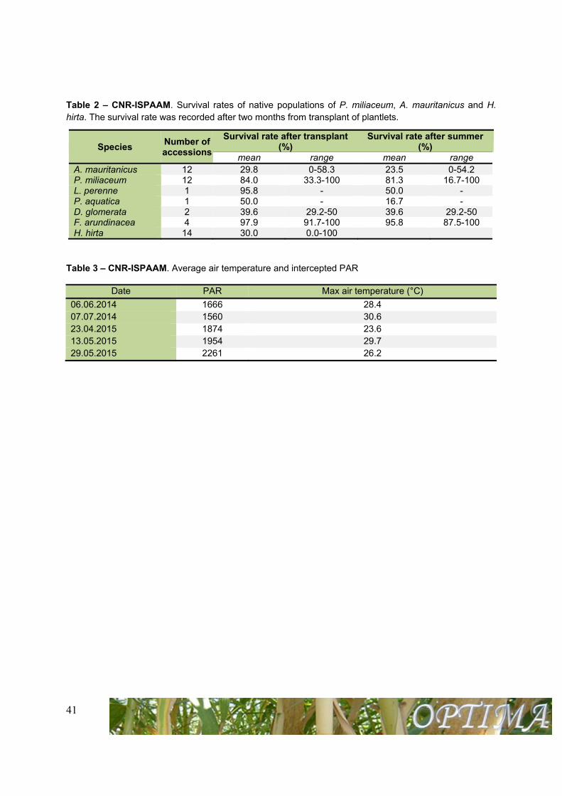
Table 2 – CNR-ISPAAM. Survival rates of native populations of P. miliaceum, A. mauritanicus and H. hirta. The survival rate was recorded after two months from transplant of plantlets.
Species Number of accessions
Survival rate after transplant (%)
Survival rate after summer (%)
mean range mean range A. mauritanicus 12 29.8 0-58.3 23.5 0-54.2 P. miliaceum 12 84.0 33.3-100 81.3 16.7-100 L. perenne 1 95.8 - 50.0 - P. aquatica 1 50.0 - 16.7 - D. glomerata 2 39.6 29.2-50 39.6 29.2-50 F. arundinacea 4 97.9 91.7-100 95.8 87.5-100 H. hirta 14 30.0 0.0-100
Table 3 – CNR-ISPAAM. Average air temperature and intercepted PAR
Date PAR Max air temperature (°C)
06.06.2014 1666 28.4 07.07.2014 1560 30.6 23.04.2015 1874 23.6 13.05.2015 1954 29.7 29.05.2015 2261 26.2
42
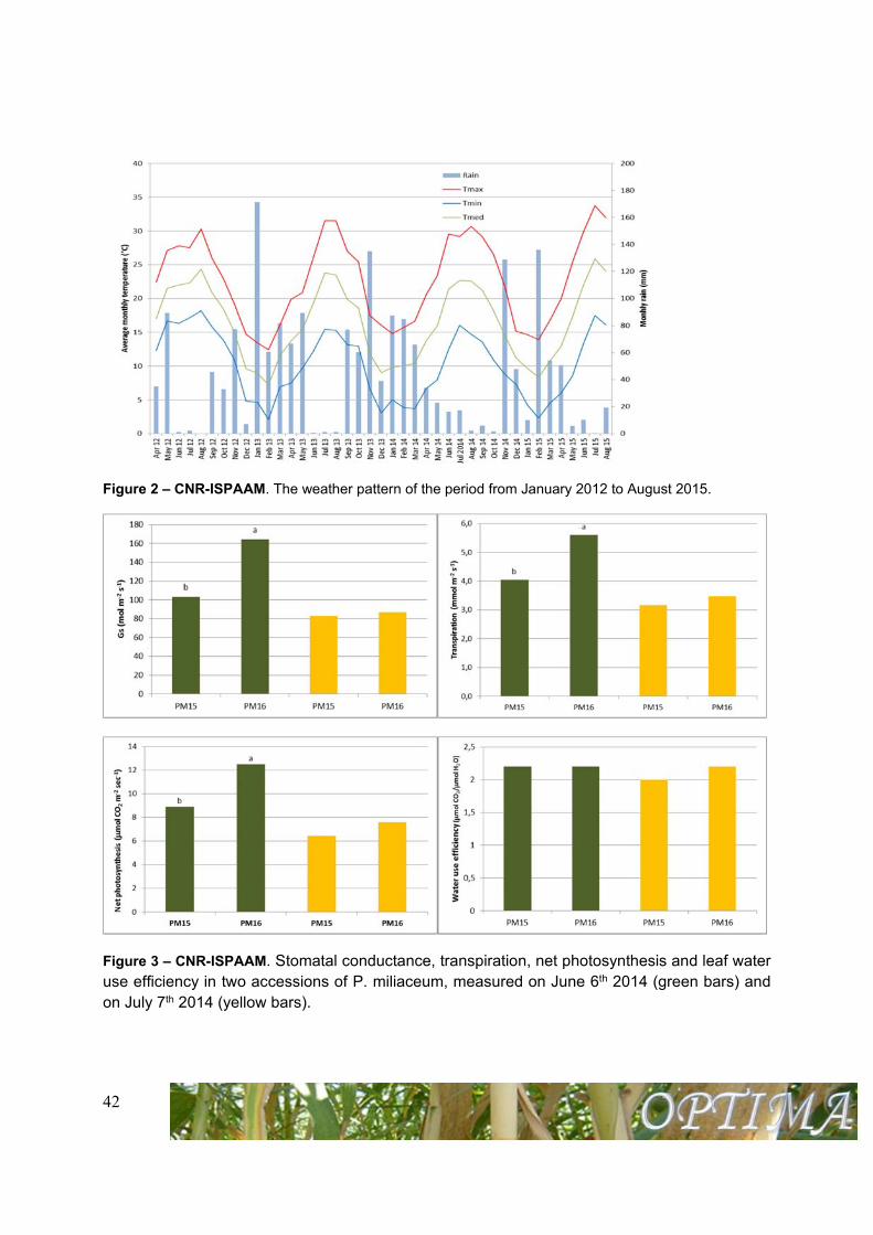
Figure 2 – CNR-ISPAAM. The weather pattern of the period from January 2012 to August 2015.
Figure 3 – CNR-ISPAAM. Stomatal conductance, transpiration, net photosynthesis and leaf water use efficiency in two accessions of P. miliaceum, measured on June 6th 2014 (green bars) and on July 7th 2014 (yellow bars).
43
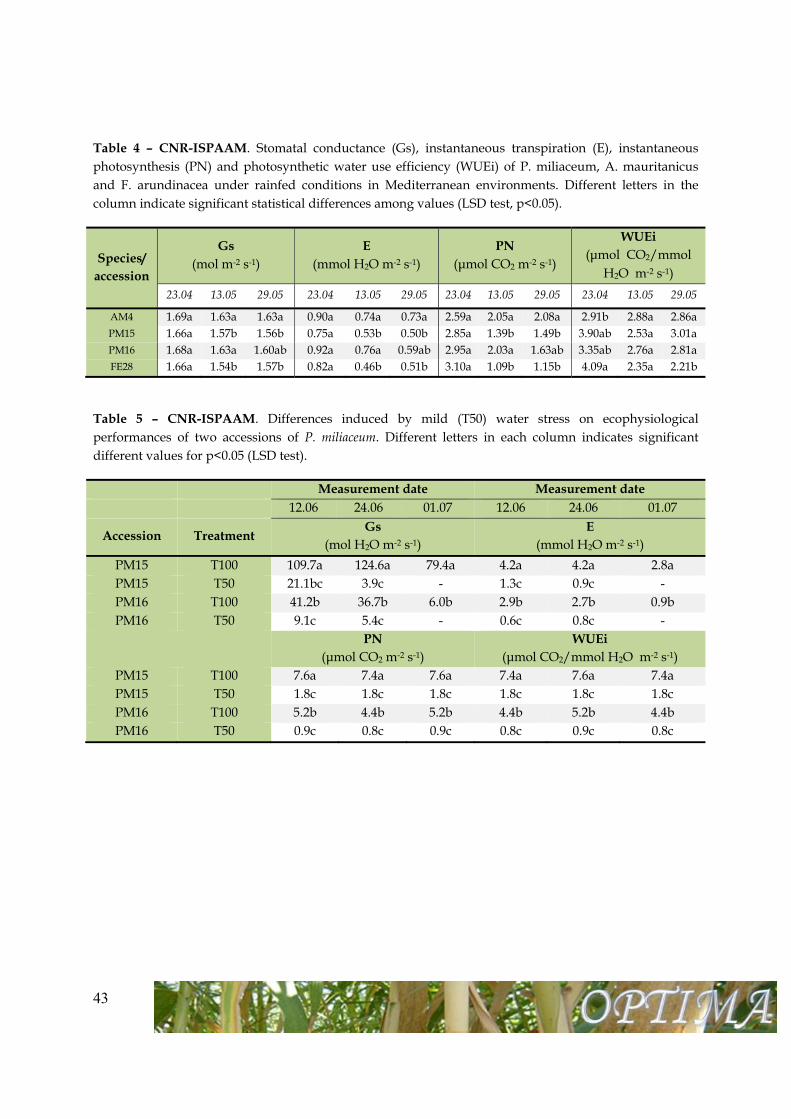
Table 4 – CNR-ISPAAM. Stomatal conductance (Gs), instantaneous transpiration (E), instantaneous photosynthesis (PN) and photosynthetic water use efficiency (WUEi) of P. miliaceum, A. mauritanicus and F. arundinacea under rainfed conditions in Mediterranean environments. Different letters in the column indicate significant statistical differences among values (LSD test, p<0.05).
Species/ accession
Gs (mol m-2 s-1)
E (mmol H2O m-2 s-1)
PN (μmol CO2 m-2 s-1)
WUEi (μmol CO2/mmol
H2O m-2 s-1)
23.04 13.05 29.05 23.04 13.05 29.05 23.04 13.05 29.05 23.04 13.05 29.05
AM4 1.69a 1.63a 1.63a 0.90a 0.74a 0.73a 2.59a 2.05a 2.08a 2.91b 2.88a 2.86a PM15 1.66a 1.57b 1.56b 0.75a 0.53b 0.50b 2.85a 1.39b 1.49b 3.90ab 2.53a 3.01a PM16 1.68a 1.63a 1.60ab 0.92a 0.76a 0.59ab 2.95a 2.03a 1.63ab 3.35ab 2.76a 2.81a FE28 1.66a 1.54b 1.57b 0.82a 0.46b 0.51b 3.10a 1.09b 1.15b 4.09a 2.35a 2.21b
Table 5 – CNR-ISPAAM. Differences induced by mild (T50) water stress on ecophysiological performances of two accessions of P. miliaceum. Different letters in each column indicates significant different values for p<0.05 (LSD test).
Measurement date Measurement date 12.06 24.06 01.07 12.06 24.06 01.07
Accession Treatment Gs
(mol H2O m-2 s-1) E
(mmol H2O m-2 s-1)
PM15 T100 109.7a 124.6a 79.4a 4.2a 4.2a 2.8a PM15 T50 21.1bc 3.9c - 1.3c 0.9c - PM16 T100 41.2b 36.7b 6.0b 2.9b 2.7b 0.9b PM16 T50 9.1c 5.4c - 0.6c 0.8c -
PN
(μmol CO2 m-2 s-1) WUEi
(μmol CO2/mmol H2O m-2 s-1) PM15 T100 7.6a 7.4a 7.6a 7.4a 7.6a 7.4a PM15 T50 1.8c 1.8c 1.8c 1.8c 1.8c 1.8c PM16 T100 5.2b 4.4b 5.2b 4.4b 5.2b 4.4b PM16 T50 0.9c 0.8c 0.9c 0.8c 0.9c 0.8c
44
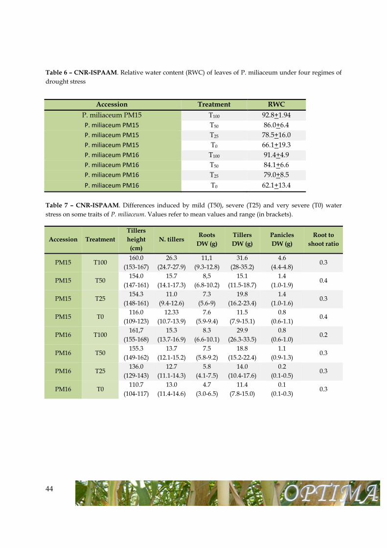
Table 6 – CNR-ISPAAM. Relative water content (RWC) of leaves of P. miliaceum under four regimes of drought stress
Table 7 – CNR-ISPAAM. Differences induced by mild (T50), severe (T25) and very severe (T0) water stress on some traits of P. miliaceum. Values refer to mean values and range (in brackets).
Accession Treatment Tillers height (cm)
N. tillers Roots
DW (g) Tillers DW (g)
Panicles DW (g)
Root to shoot ratio
PM15 T100 160.0
(153-167) 26.3
(24.7-27.9) 11,1
(9.3-12.8) 31.6
(28-35.2) 4.6
(4.4-4.8) 0.3
PM15 T50 154.0
(147-161) 15.7
(14.1-17.3) 8,5
(6.8-10.2) 15.1
(11.5-18.7) 1.4
(1.0-1.9) 0.4
PM15 T25 154.3
(148-161) 11.0
(9.4-12.6) 7.3
(5.6-9) 19.8
(16.2-23.4) 1.4
(1.0-1.6) 0.3
PM15 T0 116.0
(109-123) 12.33
(10.7-13.9) 7.6
(5.9-9.4) 11.5
(7.9-15.1) 0.8
(0.6-1.1) 0.4
PM16 T100 161,7
(155-168) 15.3
(13.7-16.9) 8.3
(6.6-10.1) 29.9
(26.3-33.5) 0.8
(0.6-1.0) 0.2
PM16 T50 155.3
(149-162) 13.7
(12.1-15.2) 7.5
(5.8-9.2) 18.8
(15.2-22.4) 1.1
(0.9-1.3) 0.3
PM16 T25 136.0
(129-143) 12.7
(11.1-14.3) 5.8
(4.1-7.5) 14.0
(10.4-17.6) 0.2
(0.1-0.5) 0.3
PM16 T0 110.7
(104-117) 13.0
(11.4-14.6) 4.7
(3.0-6.5) 11.4
(7.8-15.0) 0.1
(0.1-0.3) 0.3
Accession Treatment RWC
P. miliaceum PM15 T100 92.8+1.94 P. miliaceum PM15 T50 86.0+6.4 P. miliaceum PM15 T25 78.5+16.0 P. miliaceum PM15 T0 66.1+19.3 P. miliaceum PM16 T100 91.4+4.9 P. miliaceum PM16 T50 84.1+6.6 P. miliaceum PM16 T25 79.0+8.5
P. miliaceum PM16 T0 62.1+13.4
45
Table 8 – CNR-ISPAAM. Biometric traits of tillers, heads and flag leaf of accessions of P. miliaceum.
Accession Tiller Head length
(cm) Flag leaf
Length (cm) No internodes Length (cm) Width (cm)
PM13SEM 107.3 7.4 39.3 ab 25.1 c 0.7
PM14PZS 116.3 7.5 44.3 a 30.9 ab 0.8
PM16SLR 122.2 7.4 39.3 ab 32.2 a 0.8
PM18FRT 112.4 7.1 43.7 ab 30.5 ab 0.7
PM19CMC 119.2 7.1 39.8 ab 28.8 abc 0.7
PM20PMT 119.2 6.7 40.8 ab 28.5 abc 0.6
PM21DCM 118.0 7.2 41.9 ab 31.0 ab 0.7
PM22STG 105.7 6.7 36.3 b 25.8 c 0.7
PM23ZCN 119.8 7.5 43.2 ab 27.0 bc 0.7
PM24MNR 113.4 7.6 39.3 ab 27.8 bc 0.6
average 115.4 7.2 40.8 28.8 0.7
minimum 105.7 6.7 36.3 25.1 0.6
maximum 122.2 7.6 44.3 32.2 0.8
Table 9 – CNR-ISPAAM. Dry weight and dry matter content in tillers, heads and flag leaf in accessions of P. miliaceum.
Accession Tiller Head Flag leaf DW (g) DM % DW (g) DM% DW (g) DM %
PM13SEM 3.11 52.4 0.78 69.2 1.18 ab 82.7 PM14PZS 3.92 46.7 0.87 60.1 1.38 a 73.5 PM16SLR 3.57 42.5 0.71 57.1 1.23 ab 69.9 PM18FRT 3.14 44.6 0.74 63.4 1.19 ab 71.6
PM19CMC 3.57 41.9 0.82 54.0 1.10 ab 69.9 PM20PMT 3.70 53.8 0.90 67.5 1.06 ab 84.7 PM21DCM 3.03 47.4 0.72 62.2 1.06 ab 77.9 PM22STG 2.84 49.9 0.82 64.4 1.13 ab 83.4 PM23ZCN 3.90 50.5 0.94 64.7 1.06 ab 80.3 PM24MNR 2.77 46.3 0.67 60.7 0.94 b 77.6
average 3.4 47.6 0.8 62.3 1.1 77.1 minimum 2.8 41.9 0.7 54.0 0.9 69.9 maximum 3.9 53.8 0.9 69.2 1.4 84.7
46
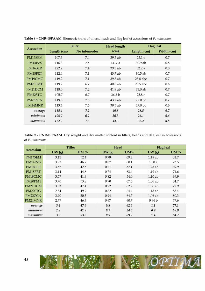
Figure 4 – CNR-ISPAAM. Dry matter yield of native Sardinian accessions of P. miliaceum in 2013, 2014, 2015 compared to conventional forage grasses D. glomerata and F. arundinacea.
Table 10 – CNR-ISPAAM. Number of tillers, water content and phytomass partitioning in P. miliaceum.
Accession No. of tillers Water content
(%) Leaves ratio
(%) Tillers ratio
(%) 2013 2014 2015 2013 2014 2015 2013 2014 2015 2013 2014 2015
PM13SEM 244.2 245.0 259 37.0 39.9 47.3 28.3 16.0 17.5 71.7 84.0 82.4 PM14PZS 292.7 319.7 324 35.1 34.5 36.5 27.1 13.2 23.8 72.9 86.8 76.2
PM15VNM 300.5 246.0 255 29.3 36.2 40.2 21.0 18.0 25.4 79.0 82.0 74.6 PM16SLR 224.7 203.3 288 32.1 39.9 38.4 26.7 12.3 22.8 73.3 87.7 77.2 PM17SNS n.a n.a. 306 n.a. n.a. 36.7 n.a. n.a. 23.1 n.a. n.a. 76.9 PM18FRT 283.0 416.0 296 36.0 42.9 41.7 29.4 15.0 25.1 70.6 85.0 74.9
PM19CMC 279.7 395.7 318 36.2 40.4 36.2 24.3 14.1 18.1 75.7 85.9 81.8 PM20PMT 316.6 328.7 277 31.0 39.3 39.1 24.0 17.4 23.3 76.0 82.6 76.6 PM21DCM 282.3 260.3 219 36.3 38.8 39.8 25.8 17.3 23.9 74.2 82.7 76.1 PM22STG 296.0 273.3 213 36.1 43.0 44.6 25.8 14.3 19.4 74.2 85.7 80.6 PM23ZCN 288.8 260.8 277 32.2 39.5 40.5 27.0 17.8 21.0 73.0 82.2 79.0 PM24MNR 241.3 292.8 262 27.8 39.4 36.1 26.5 12.9 21.7 73.5 87.1 78.3
47
Table 11 – CNR-ISPAAM. Number of tillers, Dry matter yield per plant and phytomass partitioning in A. mauritanicus.
Accession No. of tillers DMY per plant
(g) Water content
(%) Leaves ratio
(%) Tillers ratio
(%) 2014 2015 2014 2015 2014 2015 2014 2015 2014 2015
AM1MGR 48 71 251.1 261.8 46.4 36.1 n.a. 100.0 n.a. 0.0 AM2GRG 42 90 179.5 453.0 45.8 40 n.a. 77.5 n.a. 22.5 AM3SRT 97 156 803.6 783.8 44.6 44 n.a. 67.0 n.a. 33
AM4MNR 154 190 1870.2 1633.8 43.9 46.9 n.a. 71.2 n.a. 28.8 AM5DLV 7 35 52.3 n.a. 47.1 37.7 n.a. 86.1 n.a. 9.3 AM6CPF 174 95 561.3 563.8 48.0 40.9 n.a. 94.0 n.a. 6.0 AM7SMV 163 141 1037.9 666.5 42.7 39.9 n.a. 56.3 n.a. 43.7 AM8FRT 94 161 421.7 643.2 42.3 38.9 n.a. 73.6 n.a. 26.4 AM9STG 146 119 833.3 730.7 41.6 42.8 n.a. 58.3 n.a. 41.7
AM10FLN 167 147 2028.5 1153.1 43.6 44.2 n.a. 42.2 n.a. 42.8 AM11CMC 99 117 677.2 648.1 47.5 38.4 n.a. 70.0 n.a. 30.0 AM12PMT 100 176 750.7 767.4 43.0 39.3 n.a. 76.1 n.a. 23.9
Table 12 – CNR-ISPAAM. Dry matter yield per plant, water content, number of tillers and biomass partitioning in accessions of A. mauritanicus (AM), D. glomerata (DA), P. aquatica (FA), F. arundinacea (FE), L. perenne (LO), and P. miliaceum (PM).
Accession DMY plant-1
(g) WC (%) N. tillers
Leaves ratio (%)
Tillers ratio (%)
AM01MGR 261.8 i-m 36.1 a-d 71 mn 100.0 a 0.0 i AM02GRG 453.0 f-m 40.0 a-d 90 l-n 77.5 bc 22.5 gh AM03SRT 783.8 b-h 44.0 a-c 156 f-n 67.0 b-d 33 e-g AM04MNR 1633.8 a 46.9 ab 190 d-l 71.2 bc 28.8 gh AM05DLV NA - 37.7 g 35 n 86.1 b 9.3 hi AM06CPF 563.8 d-m 40.9 a-c 95 l-n 94.0 b-d 6.0 f-h AM07SMV 666.5 c-i 39.9 a-d 141 h-n 56.3 c-e 43.7 d-g AM08FRT 643.2 d-m 38.9 a-d 161 f-n 73.6 bc 26.4 gh AM09STG 730.7 b-i 42.8 a-c 119 h-n 58.3 b-d 41.7 e-g AM10FLN 1153.1 a-c 44.2 a-c 147 g-n 42.2 hi 42.8 d-g AM11CMC 648.1 d-l 38.4 a-d 117 h-n 70.0 b-d 30.0 e-g AM12PMT 767.4 b-h 39.3 a-d 176 e-m 76.1 bc 23.9 gh DA29JA 415.0 g-m 27.5 de 145 g-n 32.7 f-h 67.2 b-d DA30OT 159.8 lm 21.8 ef 101 i-n 35.1 f-h 64.9 b-d FA31AU 468.8 e-m 41.2 a-c 161 f-n 30.2 f-h 69.9 b-d FE25TA 598.6 d-m 32.4 c-e 249 a-g 55.8 c-g 44.2 c-g FE26SI 568.1 d-m 37.2 a-d 268 a-e 30.4 f-h 69.6 b-d FE27CE 445.9 f-m 42.6 a-c 205 c-i 41.4 e-h 58.5 b-e FE28FL 678.2 c-i 33.3 b-e 202 c-i 42.3 d-h 57.6 b-f LO32AZ 30.0 m 13.4 f 114 h-n 8.2 i 91.8 a PM13SEM 690.7 c-i 47.3 a 259 a-f 17.5 hi 82.4 ab PM14PZS 1152.8 a-c 36.5 a-d 324 a 23.8 hi 76.2 ab PM15VNM 956.4 b-e 40.2 a-d 255 a-f 25.4 g-i 74.6 a-c PM16SLR 899.7 b-g 38.4 a-d 288 a-d 22.8 hi 77.2 ab
48
PM17SNS 1200.8 ab 36.7 a-d 306 a-c 23.1 hi 76.9 ab PM18FRT 1013.2 b-d 41.7 a-c 296 a-d 25.1 g-i 74.9 ab PM19CMC 934.6 b-f 36.2 a-d 318 ab 18.1 hi 81.8 ab PM20PMT 599.9 d-m 39.1 a-d 277 a-e 23.3 hi 76.6 ab PM21DCM 516.4 d-m 39.8 a-d 219 a-h 23.9 hi 76.1 ab PM22STG 382.6 h-m 44.6 a-c 213 b-h 19.4 hi 80.6 ab PM23ZCN 813.4 b-h 40.5 a-d 277 a-e 21.0 hi 79.0 ab PM24MNR 644.8 d-m 36.1 a-d 262 a-f 21.7 hi 78.3 ab
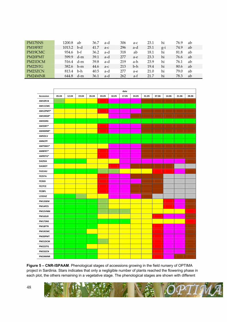
Figure 5 – CNR-ISPAAM. Phenological stages of accessions growing in the field nursery of OPTIMA project in Sardinia. Stars indicates that only a negligible number of plants reached the flowering phase in each plot, the others remaining in a vegetative stage. The phenological stages are shown with different
date
Accession 05.04 12.04 19.04 26.04 03.05 10.05 17.05 24.05 31.05 07.06 14.06 21.06 28.06
AM10FLN
AM11CMC
AM12PMT*
AM1MGR*
AM2GRG
AM3SRT*
AM4MNR*
AM5DLV
AM6CPF
AM7SMV*
AM8FRT*
AM9STG*
DA29JA
DA30OT
FA31AU
FE25TA
FE26SI
FE27CE
FE28FL
LO32AZ
PM13SEM
PM14PZS
PM15VNM
PM16SLR
PM17SNS
PM18FTR
PM19CMC
PM20PMT
PM21DCM
PM22STG
PM23ZCN
PM24MNR
49
colours: in green the vegetative stage, in yellow the heading stage, in red the full flowering stage, in pink the end of flowering, in brown the development and ripening of seeds. AM indicates A. mauritanicus, DA D. glomerata, FA P. aquatica, FE F. arundinacea, LO L. perenne, PM P. miliaceum accessions.
Table 13 – CNR-ISPAAM. Content of cellulose, hemicellulose and lignin in P. miliaceum, at harvest time, in July 2013. Average values are the average of ten values (ten accessions).
Plant organ Hemicellulose
(%) Cellulose
(%) Lignin
(%) mean range mean range mean range
Tiller 28.8 26.6-30.1 38.1 36.0-40.7 13.4 12.0-15.0 Leaf 25.4 24.1-27.3 39.0 37.6-40.9 10.0 7.9-11.7
Spike 34.5 32.8-36.2 30.2 26.0-33.2 12.8 10.7-15.7
Table 14 – CNR-ISPAAM. Proximate and ultimate analysis of plant components in P. miliaceum vs miscanthus
Species Calorific
value (MJ kg-1)
Volatile matter
(%)
Fixed carbon
(%)
Ash content
(%)
C (%)
H (%)
N (%)
S (%)
Cl (%)
O (%)
Leaves P. miliaceum 16.0 70.0 5.0 13.0 49.0 6.1 3.6 <0.8 1.24 41.3 M. x 16.0 73.0 1.7 9.5 49.0 6.3 2.7 <0.3 <0.03 42.0
Stalks
P. miliaceum 17.0 77.0 11.0 5.0 49.0 6.5 1.4 <0.3 1.08 43.1 M. x 17.0 77.0 3.6 6.0 50.0 6.3 1.7 <0.3 <0.03 42.0
Heads P. miliaceum 16.0 69.0 1.5 12.0 48.0 6.0 2.6 <0.8 0.98 43.4
50
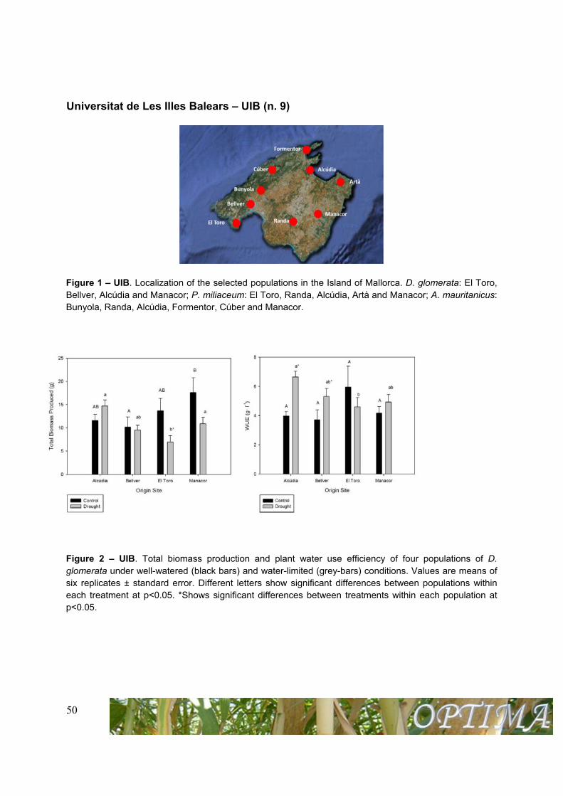
Universitat de Les Illes Balears – UIB (n. 9)
Figure 1 – UIB. Localization of the selected populations in the Island of Mallorca. D. glomerata: El Toro, Bellver, Alcúdia and Manacor; P. miliaceum: El Toro, Randa, Alcúdia, Artà and Manacor; A. mauritanicus: Bunyola, Randa, Alcúdia, Formentor, Cúber and Manacor.
Figure 2 – UIB. Total biomass production and plant water use efficiency of four populations of D. glomerata under well-watered (black bars) and water-limited (grey-bars) conditions. Values are means of six replicates ± standard error. Different letters show significant differences between populations within each treatment at p<0.05. *Shows significant differences between treatments within each population at p<0.05.
51
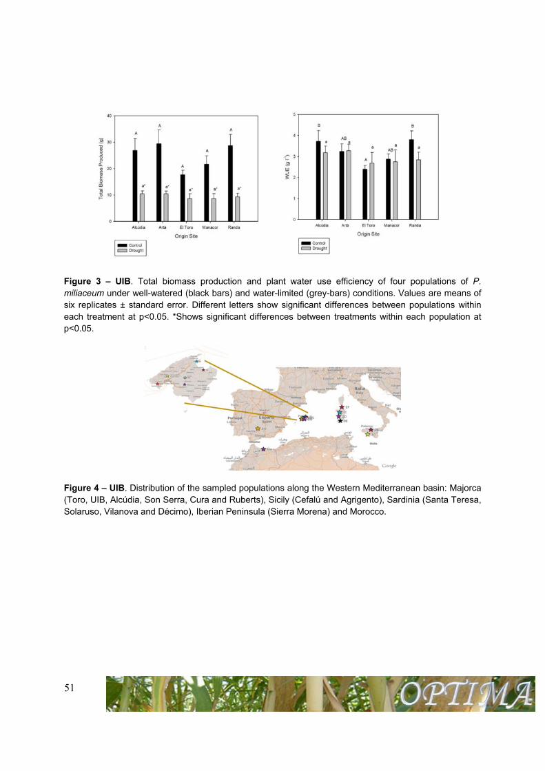
Figure 3 – UIB. Total biomass production and plant water use efficiency of four populations of P. miliaceum under well-watered (black bars) and water-limited (grey-bars) conditions. Values are means of six replicates ± standard error. Different letters show significant differences between populations within each treatment at p<0.05. *Shows significant differences between treatments within each population at p<0.05.
Figure 4 – UIB. Distribution of the sampled populations along the Western Mediterranean basin: Majorca (Toro, UIB, Alcúdia, Son Serra, Cura and Ruberts), Sicily (Cefalú and Agrigento), Sardinia (Santa Teresa, Solaruso, Vilanova and Décimo), Iberian Peninsula (Sierra Morena) and Morocco.
52
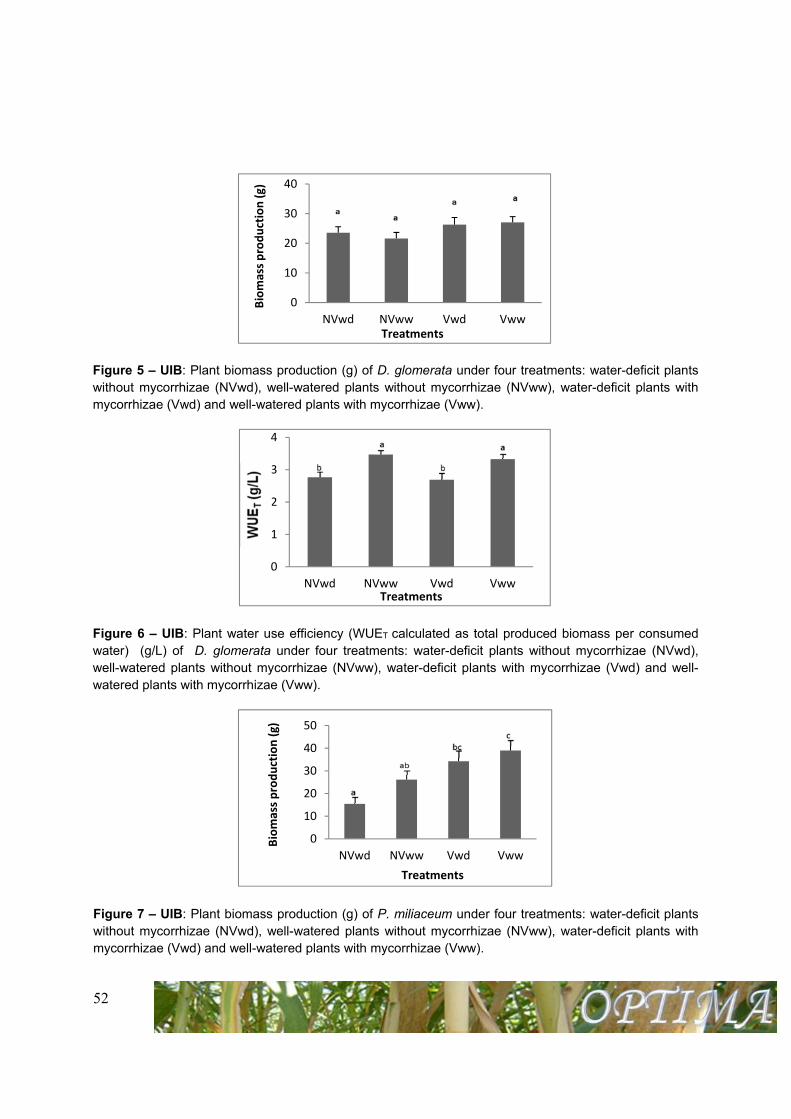
Figure 5 – UIB: Plant biomass production (g) of D. glomerata under four treatments: water-deficit plants without mycorrhizae (NVwd), well-watered plants without mycorrhizae (NVww), water-deficit plants with mycorrhizae (Vwd) and well-watered plants with mycorrhizae (Vww).
Figure 6 – UIB: Plant water use efficiency (WUET calculated as total produced biomass per consumed water) (g/L) of D. glomerata under four treatments: water-deficit plants without mycorrhizae (NVwd), well-watered plants without mycorrhizae (NVww), water-deficit plants with mycorrhizae (Vwd) and well-watered plants with mycorrhizae (Vww).
Figure 7 – UIB: Plant biomass production (g) of P. miliaceum under four treatments: water-deficit plants without mycorrhizae (NVwd), well-watered plants without mycorrhizae (NVww), water-deficit plants with mycorrhizae (Vwd) and well-watered plants with mycorrhizae (Vww).
0
10
20
30
40
NVwd NVww Vwd Vww
Biomass production (g)
Treatments
0
1
2
3
4
NVwd NVww Vwd VwwTreatments
0
10
20
30
40
50
NVwd NVww Vwd Vww
Biomass production (g)
Treatments
53
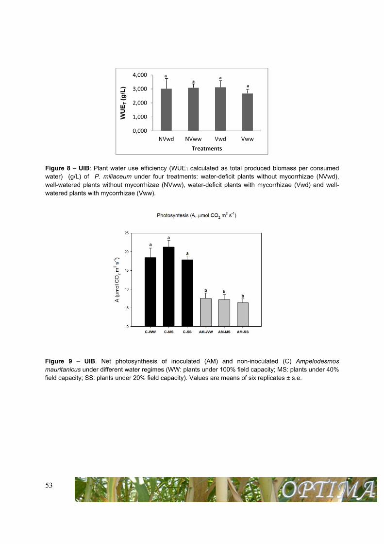
Figure 8 – UIB: Plant water use efficiency (WUET calculated as total produced biomass per consumed water) (g/L) of P. miliaceum under four treatments: water-deficit plants without mycorrhizae (NVwd), well-watered plants without mycorrhizae (NVww), water-deficit plants with mycorrhizae (Vwd) and well-watered plants with mycorrhizae (Vww).
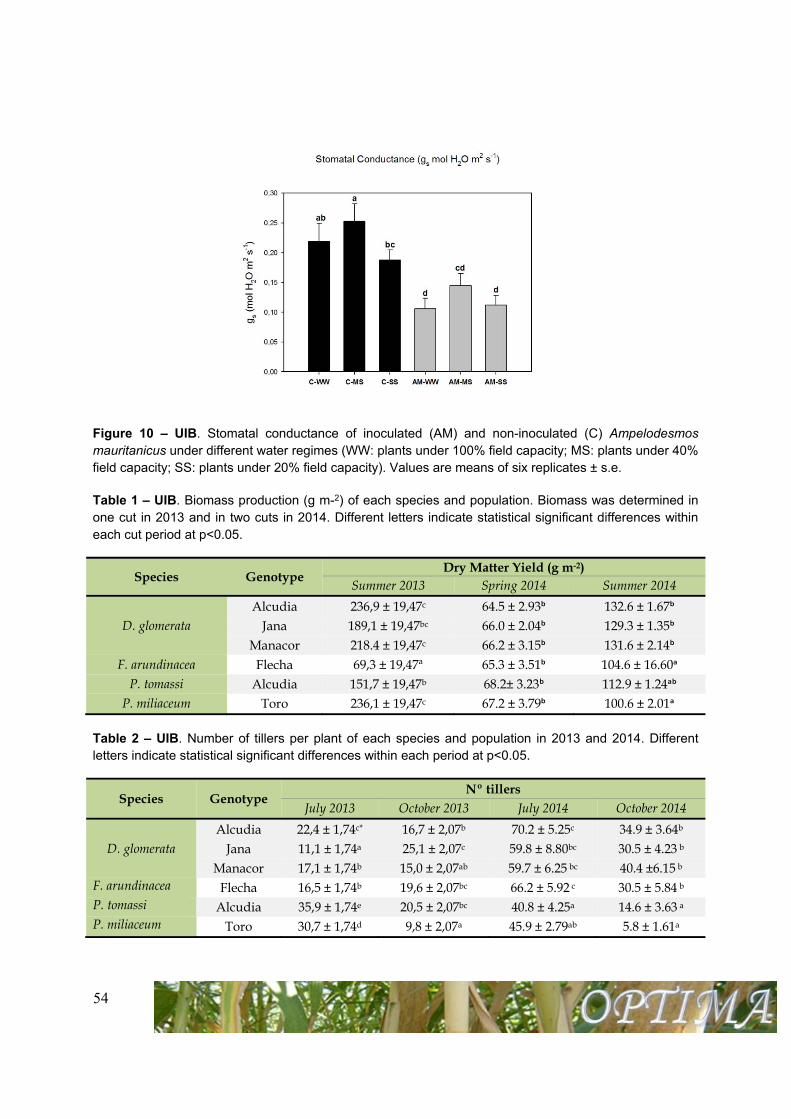
Figure 9 – UIB. Net photosynthesis of inoculated (AM) and non-inoculated (C) Ampelodesmos mauritanicus under different water regimes (WW: plants under 100% field capacity; MS: plants under 40% field capacity; SS: plants under 20% field capacity). Values are means of six replicates ± s.e.
0,000
1,000
2,000
3,000
4,000
NVwd NVww Vwd Vww
Treatments
54
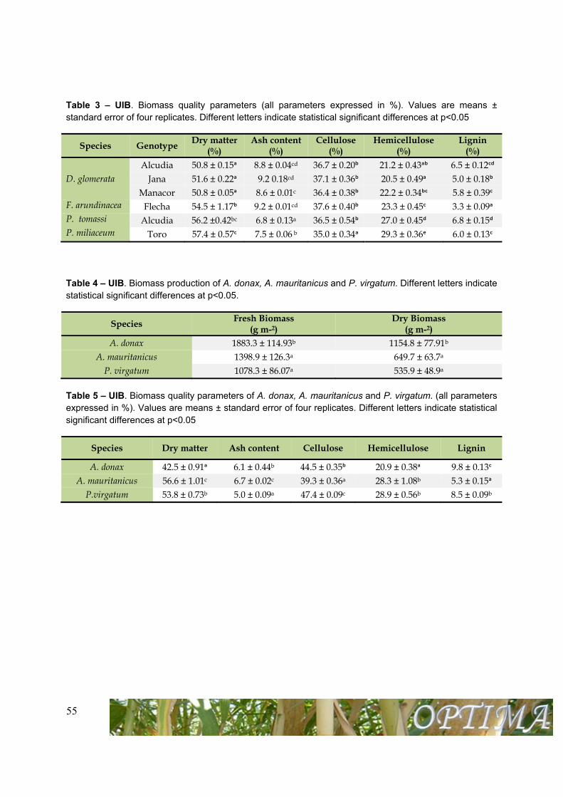
Figure 10 – UIB. Stomatal conductance of inoculated (AM) and non-inoculated (C) Ampelodesmos mauritanicus under different water regimes (WW: plants under 100% field capacity; MS: plants under 40% field capacity; SS: plants under 20% field capacity). Values are means of six replicates ± s.e.
Table 1 – UIB. Biomass production (g m-2) of each species and population. Biomass was determined in one cut in 2013 and in two cuts in 2014. Different letters indicate statistical significant differences within each cut period at p<0.05.
Species Genotype Dry Matter Yield (g m-2)
Summer 2013 Spring 2014 Summer 2014
D. glomerata Alcudia 236,9 ± 19,47c 64.5 ± 2.93ᵇ 132.6 ± 1.67ᵇ
Jana 189,1 ± 19,47bc 66.0 ± 2.04ᵇ 129.3 ± 1.35ᵇ Manacor 218.4 ± 19,47c 66.2 ± 3.15ᵇ 131.6 ± 2.14ᵇ
F. arundinacea Flecha 69,3 ± 19,47ª 65.3 ± 3.51ᵇ 104.6 ± 16.60ᵃ P. tomassi Alcudia 151,7 ± 19,47b 68.2± 3.23ᵇ 112.9 ± 1.24ᵃᵇ
P. miliaceum Toro 236,1 ± 19,47c 67.2 ± 3.79ᵇ 100.6 ± 2.01ᵃ
Table 2 – UIB. Number of tillers per plant of each species and population in 2013 and 2014. Different letters indicate statistical significant differences within each period at p<0.05.
Species Genotype Nº tillers
July 2013 October 2013 July 2014 October 2014
D. glomerata Alcudia 22,4 ± 1,74c* 16,7 ± 2,07b 70.2 ± 5.25c 34.9 ± 3.64b
Jana 11,1 ± 1,74a 25,1 ± 2,07c 59.8 ± 8.80bc 30.5 ± 4.23 b Manacor 17,1 ± 1,74b 15,0 ± 2,07ab 59.7 ± 6.25 bc 40.4 ±6.15 b
F. arundinacea Flecha 16,5 ± 1,74b 19,6 ± 2,07bc 66.2 ± 5.92 c 30.5 ± 5.84 b P. tomassi Alcudia 35,9 ± 1,74e 20,5 ± 2,07bc 40.8 ± 4.25a 14.6 ± 3.63 a P. miliaceum Toro 30,7 ± 1,74d 9,8 ± 2,07a 45.9 ± 2.79ab 5.8 ± 1.61a
55
Table 3 – UIB. Biomass quality parameters (all parameters expressed in %). Values are means ± standard error of four replicates. Different letters indicate statistical significant differences at p<0.05
Species Genotype Dry matter
(%) Ash content
(%) Cellulose
(%) Hemicellulose
(%) Lignin
(%)
D. glomerata Alcudia 50.8 ± 0.15ᵃ 8.8 ± 0.04cd 36.7 ± 0.20ᵇ 21.2 ± 0.43ᵃᵇ 6.5 ± 0.12ᶜᵈ
Jana 51.6 ± 0.22ᵃ 9.2 0.18cd 37.1 ± 0.36ᵇ 20.5 ± 0.49ᵃ 5.0 ± 0.18ᵇ Manacor 50.8 ± 0.05ᵃ 8.6 ± 0.01c 36.4 ± 0.38ᵇ 22.2 ± 0.34ᵇᶜ 5.8 ± 0.39ᶜ
F. arundinacea Flecha 54.5 ± 1.17ᵇ 9.2 ± 0.01cd 37.6 ± 0.40ᵇ 23.3 ± 0.45ᶜ 3.3 ± 0.09ᵃ P. tomassi Alcudia 56.2 ±0.42bc 6.8 ± 0.13a 36.5 ± 0.54ᵇ 27.0 ± 0.45ᵈ 6.8 ± 0.15ᵈ P. miliaceum Toro 57.4 ± 0.57ᶜ 7.5 ± 0.06 b 35.0 ± 0.34ᵃ 29.3 ± 0.36ᵉ 6.0 ± 0.13ᶜ
Table 4 – UIB. Biomass production of A. donax, A. mauritanicus and P. virgatum. Different letters indicate statistical significant differences at p<0.05.
Species Fresh Biomass (g m-2)
Dry Biomass (g m-2)
A. donax 1883.3 ± 114.93b 1154.8 ± 77.91b A. mauritanicus 1398.9 ± 126.3a 649.7 ± 63.7a
P. virgatum 1078.3 ± 86.07a 535.9 ± 48.9a
Table 5 – UIB. Biomass quality parameters of A. donax, A. mauritanicus and P. virgatum. (all parameters expressed in %). Values are means ± standard error of four replicates. Different letters indicate statistical significant differences at p<0.05
Species Dry matter Ash content Cellulose Hemicellulose Lignin
A. donax 42.5 ± 0.91ᵃ 6.1 ± 0.44b 44.5 ± 0.35ᵇ 20.9 ± 0.38ᵃ 9.8 ± 0.13ᶜ A. mauritanicus 56.6 ± 1.01c 6.7 ± 0.02c 39.3 ± 0.36a 28.3 ± 1.08b 5.3 ± 0.15ᵃ
P.virgatum 53.8 ± 0.73b 5.0 ± 0.09a 47.4 ± 0.09c 28.9 ± 0.56b 8.5 ± 0.09b
56
Center for Renewable Energy Sources and Energy Saving – CRES (n. 3)
Figure 1 – CRES. Experimental layout of the screening trial (eight perennial grasses in one replication)
Figure 2 –CRES. View of the perennial grasses that were compared in sub-task 3.1.3 in Greece.
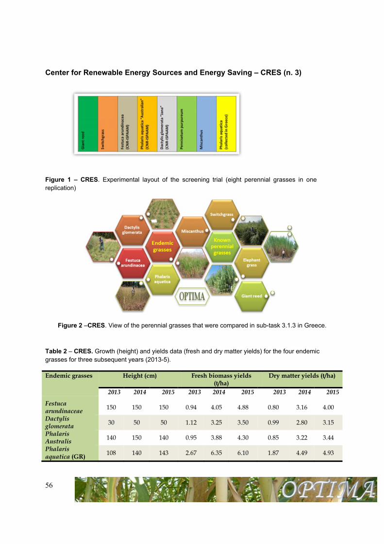
Table 2 – CRES. Growth (height) and yields data (fresh and dry matter yields) for the four endemic grasses for three subsequent years (2013-5).
Endemic grasses Height (cm) Fresh biomass yields (t/ha)
Dry matter yields (t/ha)
2013 2014 2015 2013 2014 2015 2013 2014 2015
Festuca arundinaceae 150 150 150 0.94 4.05 4.88 0.80 3.16 4.00
Dactylis glomerata 30 50 50 1.12 3.25 3.50 0.99 2.80 3.15
Phalaris Australis 140 150 140 0.95 3.88 4.30 0.85 3.22 3.44
Phalaris aquatica (GR) 108 140 143 2.67 6.35 6.10 1.87 4.49 4.93
57
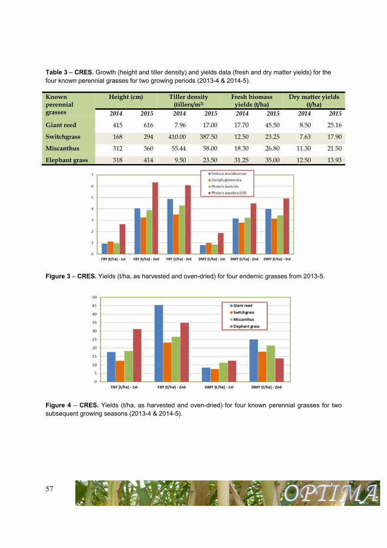
Table 3 – CRES. Growth (height and tiller density) and yields data (fresh and dry matter yields) for the four known perennial grasses for two growing periods (2013-4 & 2014-5).
Known perennial grasses
Height (cm) Tiller density (tillers/m2)
Fresh biomass yields (t/ha)
Dry matter yields (t/ha)
2014 2015 2014 2015 2014 2015 2014 2015
Giant reed 415 616 7.96 17.00 17.70 45.50 8.50 25.16
Switchgrass 168 294 410.00 387.50 12.50 23.25 7.63 17.90
Miscanthus 312 360 55.44 58.00 18.30 26.80 11.30 21.50
Elephant grass 318 414 9.50 23.50 31.25 35.00 12.50 13.93
Figure 3 – CRES. Yields (t/ha, as harvested and oven-dried) for four endemic grasses from 2013-5.
Figure 4 – CRES. Yields (t/ha, as harvested and oven-dried) for four known perennial grasses for two subsequent growing seasons (2013-4 & 2014-5).
58
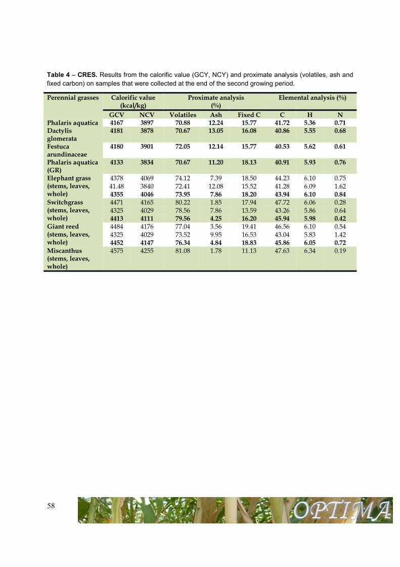
Table 4 – CRES. Results from the calorific value (GCY, NCY) and proximate analysis (volatiles, ash and fixed carbon) on samples that were collected at the end of the second growing period.
Perennial grasses Calorific value (kcal/kg)
Proximate analysis (%)
Elemental analysis (%)
GCV NCV Volatiles Ash Fixed C C H N Phalaris aquatica 4167 3897 70.88 12.24 15.77 41.72 5.36 0.71 Dactylis glomerata
4181 3878 70.67 13.05 16.08 40.86 5.55 0.68
Festuca arundinaceae
4180 3901 72.05 12.14 15.77 40.53 5.62 0.61
Phalaris aquatica (GR)
4133 3834 70.67 11.20 18.13 40.91 5.93 0.76
Elephant grass (stems, leaves, whole)
4378 4069 74.12 7.39 18.50 44.23 6.10 0.75 41.48 3840 72.41 12.08 15.52 41.28 6.09 1.62 4355 4046 73.95 7.86 18.20 43.94 6.10 0.84
Switchgrass (stems, leaves, whole)
4471 4165 80.22 1.85 17.94 47.72 6.06 0.28 4325 4029 78.56 7.86 13.59 43.26 5.86 0.64 4413 4111 79.56 4.25 16.20 45.94 5.98 0.42
Giant reed (stems, leaves, whole)
4484 4176 77.04 3.56 19.41 46.56 6.10 0.54 4325 4029 73.52 9.95 16.53 43.04 5.83 1.42 4452 4147 76.34 4.84 18.83 45.86 6.05 0.72
Miscanthus (stems, leaves, whole)
4575 4255 81.08 1.78 11.13 47.63 6.34 0.19
59
Task 3.2 - Good agricultural practices for perennial grasses
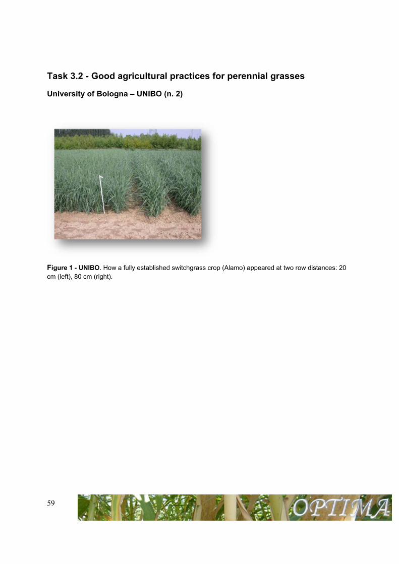
University of Bologna – UNIBO (n. 2)
Figure 1 - UNIBO. How a fully established switchgrass crop (Alamo) appeared at two row distances: 20 cm (left), 80 cm (right).
60
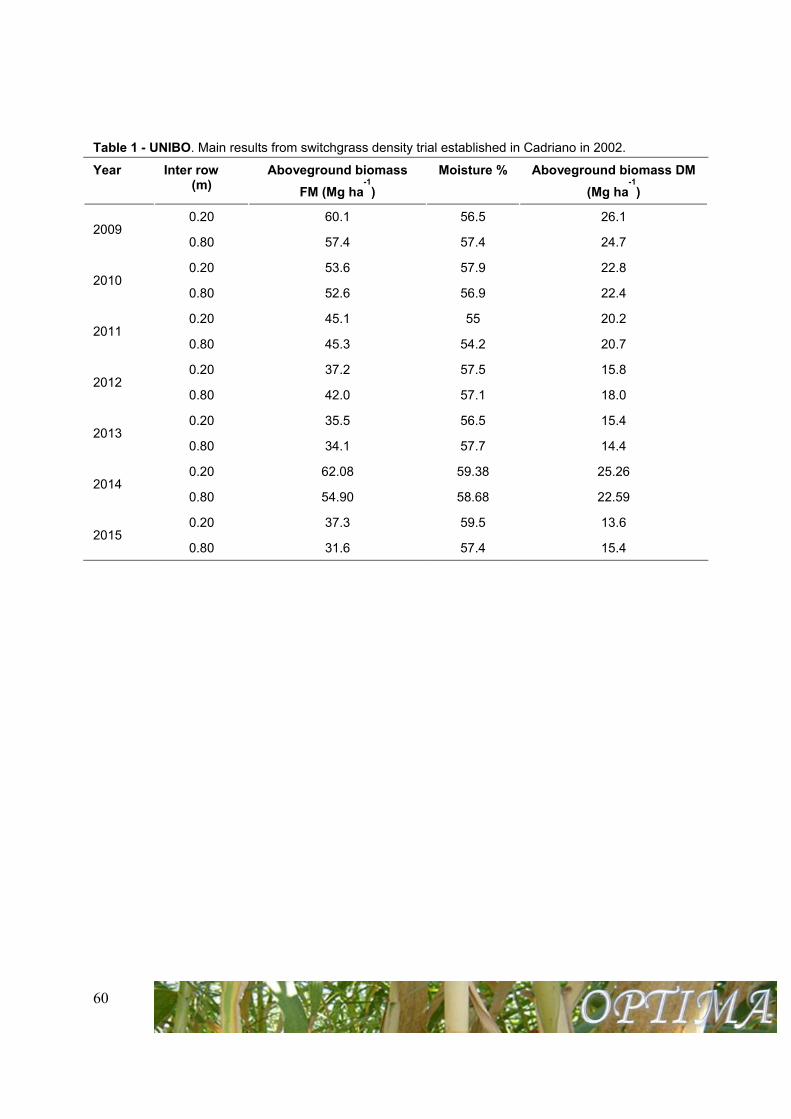
Table 1 - UNIBO. Main results from switchgrass density trial established in Cadriano in 2002.
Year Inter row (m)
Aboveground biomass
FM (Mg ha-1
)
Moisture % Aboveground biomass DM
(Mg ha-1
)
2009 0.20 60.1 56.5 26.1
0.80 57.4 57.4 24.7
2010 0.20 53.6 57.9 22.8
0.80 52.6 56.9 22.4
2011 0.20 45.1 55 20.2
0.80 45.3 54.2 20.7
2012 0.20 37.2 57.5 15.8
0.80 42.0 57.1 18.0
2013 0.20 35.5 56.5 15.4
0.80 34.1 57.7 14.4
2014 0.20 62.08 59.38 25.26
0.80 54.90 58.68 22.59
2015 0.20 37.3 59.5 13.6
0.80 31.6 57.4 15.4
61
Table 2 - UNIBO. Hydro-seeding mixtures used in 2014 trial in Cadriano (Bologna, Italy).
Hydro-seeding type
Name/Composition* Rate
T1 Envitotal (complete mixture of mulch, fertilizer, adhesive)
45 g m-2
T2 75 g m-2
T3 Cellugrȕn (cellulose fiber mulch) + soil control (adhesive hydrocolloid compound)
60 g m-2+ 1 g m-2
*All the material for the hydro-seeding trials was supplied by Biasion S.p.A. (Bolzen, Italy) a company specialized in hydro-seeding of ski slopers and degraded lands (e.g., abandoned quarries).
Figure 2 - UNIBO. Mixing of switchgrass seeds with the hydro-seeding mulch (left). Equipment used for the hydro-seeding of switchgrass (right).
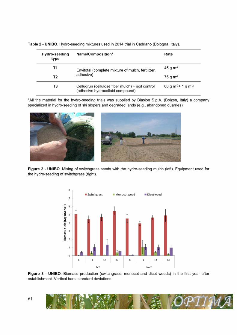
Figure 3 - UNIBO. Biomass production (switchgrass, monocot and dicot weeds) in the first year after establishment. Vertical bars: standard deviations.
0
1
2
3
4
5
6
7
8
C T1 T2 T3 C T1 T2 T3
MT No‐T
Biomass Yield (Mg DM ha‐
1)
Switchgrass Monocot weed Dicot weed
62
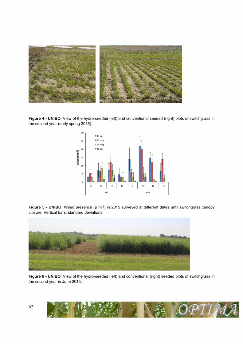
Figure 4 - UNIBO. View of the hydro-seeded (left) and conventional seeded (right) plots of switchgrass in the second year (early spring 2015).
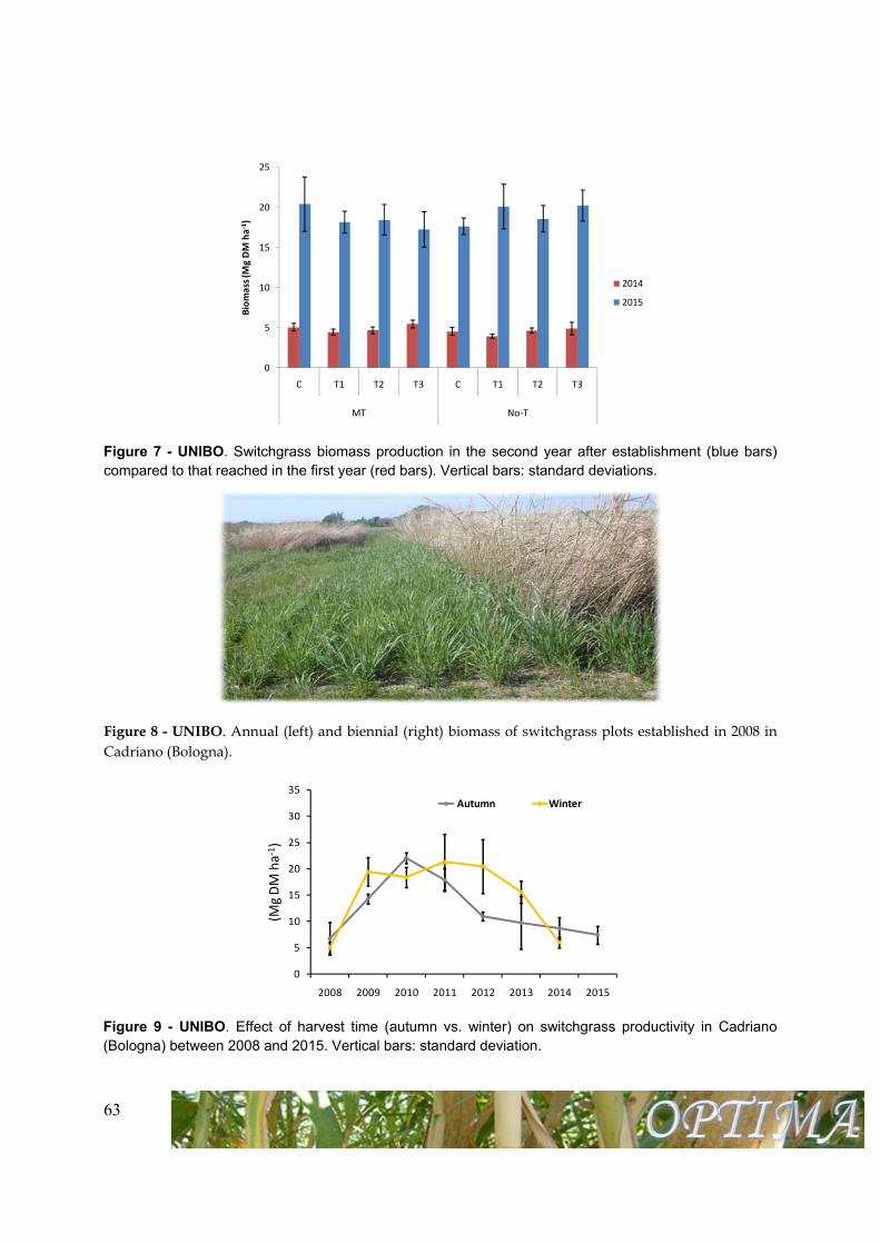
Figure 5 - UNIBO. Weed presence (p m-2) in 2015 surveyed at different dates until switchgrass canopy closure. Vertical bars: standard deviations.
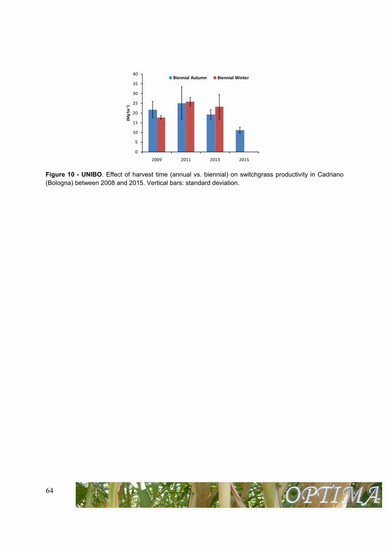
Figure 6 - UNIBO. View of the hydro-seeded (left) and conventional (right) seeded plots of switchgrass in the second year in June 2015.
0
5
10
15
20
25
30
C T1 T2 T3 C T1 T2 T3
MT No‐T
Weed (p
m‐2)
14‐apr
11‐mag
25‐mag
10‐giu
63
Figure 7 - UNIBO. Switchgrass biomass production in the second year after establishment (blue bars) compared to that reached in the first year (red bars). Vertical bars: standard deviations.
Figure 8 - UNIBO. Annual (left) and biennial (right) biomass of switchgrass plots established in 2008 in Cadriano (Bologna).
Figure 9 - UNIBO. Effect of harvest time (autumn vs. winter) on switchgrass productivity in Cadriano (Bologna) between 2008 and 2015. Vertical bars: standard deviation.
0
5
10
15
20
25
C T1 T2 T3 C T1 T2 T3
MT No‐T
Biomass (M
g DM ha‐
1)
2014
2015
0
5
10
15
20
25
30
35
2008 2009 2010 2011 2012 2013 2014 2015
(Mg DM ha‐
1 )
Autumn Winter
64
Figure 10 - UNIBO. Effect of harvest time (annual vs. biennial) on switchgrass productivity in Cadriano (Bologna) between 2008 and 2015. Vertical bars: standard deviation.
0
5
10
15
20
25
30
35
40
2009 2011 2013 2015
(Mg ha‐
1 )
Biennial Autumn Biennial Winter
65
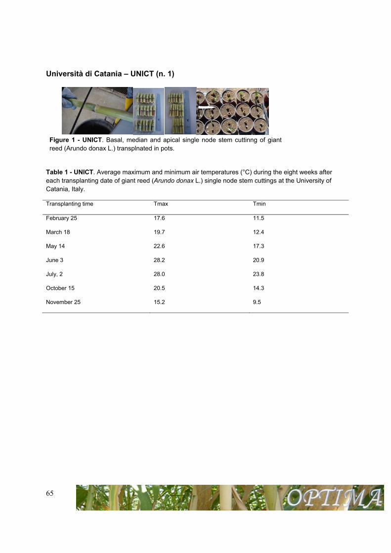
Università di Catania – UNICT (n. 1)
Figure 1 - UNICT. Basal, median and apical single node stem cuttinng of giant reed (Arundo donax L.) transplnated in pots.
Table 1 - UNICT. Average maximum and minimum air temperatures (°C) during the eight weeks after each transplanting date of giant reed (Arundo donax L.) single node stem cuttings at the University of Catania, Italy.
Transplanting time Tmax Tmin
February 25
March 18
May 14
June 3
July, 2
October 15
November 25
17.6
19.7
22.6
28.2
28.0
20.5
15.2
11.5
12.4
17.3
20.9
23.8
14.3
9.5
66
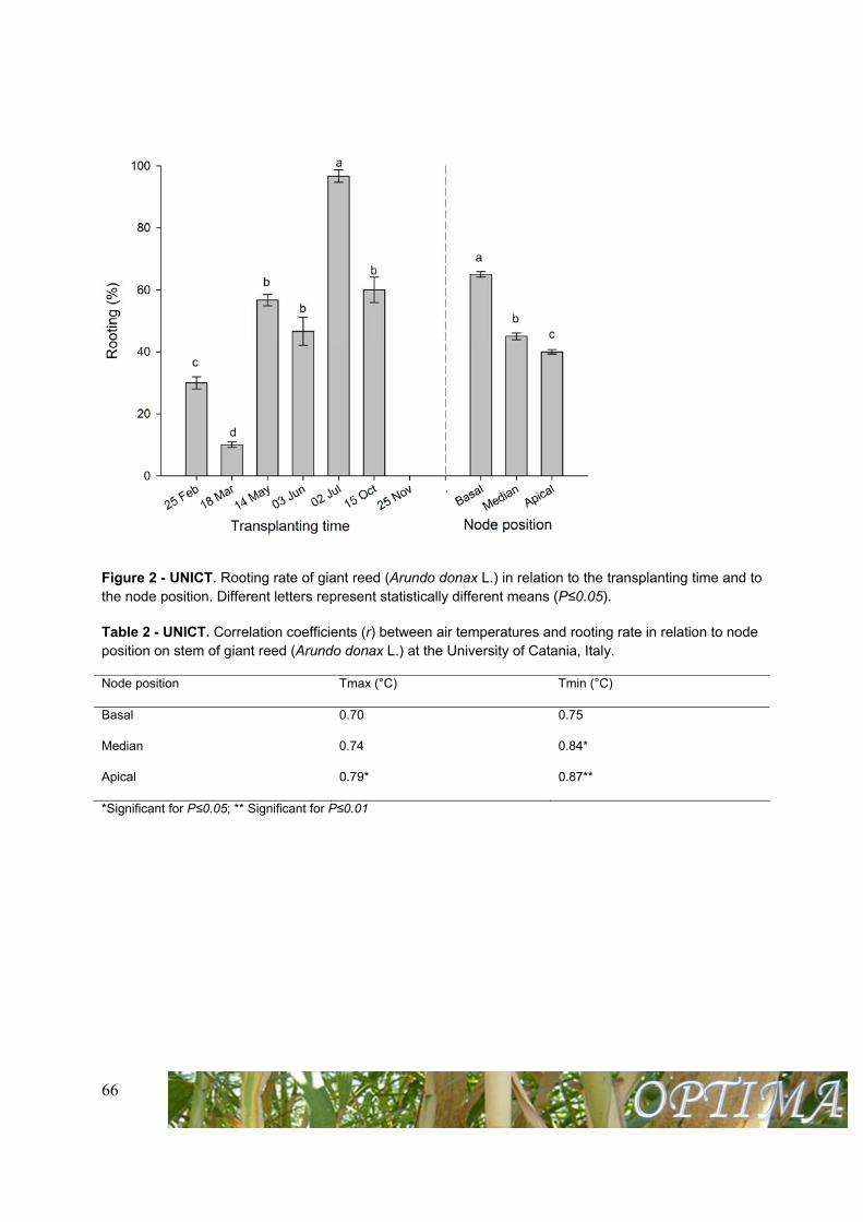
Figure 2 - UNICT. Rooting rate of giant reed (Arundo donax L.) in relation to the transplanting time and to the node position. Different letters represent statistically different means (P≤0.05).
Table 2 - UNICT. Correlation coefficients (r) between air temperatures and rooting rate in relation to node position on stem of giant reed (Arundo donax L.) at the University of Catania, Italy.
Node position Tmax (°C) Tmin (°C)
Basal 0.70 0.75
Median 0.74 0.84*
Apical 0.79* 0.87**
*Significant for P≤0.05; ** Significant for P≤0.01
67
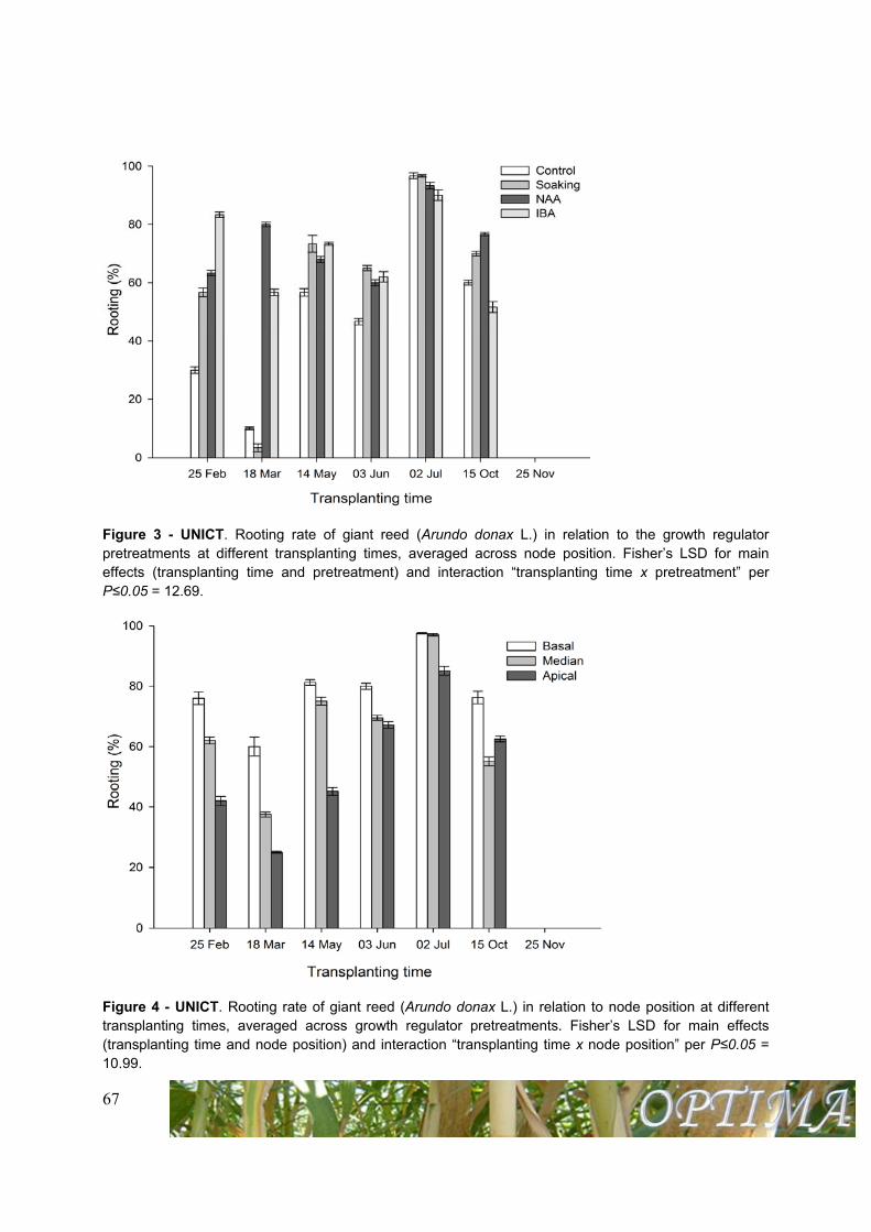
Figure 3 - UNICT. Rooting rate of giant reed (Arundo donax L.) in relation to the growth regulator pretreatments at different transplanting times, averaged across node position. Fisher’s LSD for main effects (transplanting time and pretreatment) and interaction “transplanting time x pretreatment” per P≤0.05 = 12.69.
Figure 4 - UNICT. Rooting rate of giant reed (Arundo donax L.) in relation to node position at different transplanting times, averaged across growth regulator pretreatments. Fisher’s LSD for main effects (transplanting time and node position) and interaction “transplanting time x node position” per P≤0.05 = 10.99.
68
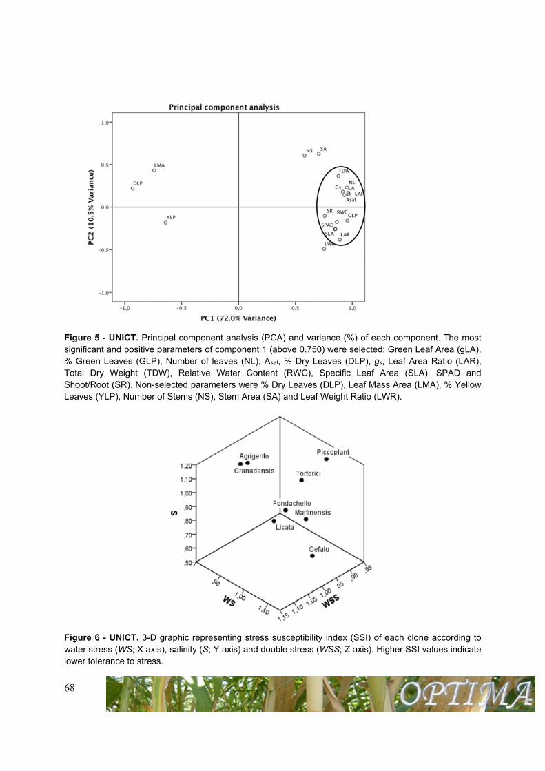
Figure 5 - UNICT. Principal component analysis (PCA) and variance (%) of each component. The most significant and positive parameters of component 1 (above 0.750) were selected: Green Leaf Area (gLA), % Green Leaves (GLP), Number of leaves (NL), Asat, % Dry Leaves (DLP), gs, Leaf Area Ratio (LAR), Total Dry Weight (TDW), Relative Water Content (RWC), Specific Leaf Area (SLA), SPAD and Shoot/Root (SR). Non-selected parameters were % Dry Leaves (DLP), Leaf Mass Area (LMA), % Yellow Leaves (YLP), Number of Stems (NS), Stem Area (SA) and Leaf Weight Ratio (LWR).
Figure 6 - UNICT. 3-D graphic representing stress susceptibility index (SSI) of each clone according to water stress (WS; X axis), salinity (S; Y axis) and double stress (WSS; Z axis). Higher SSI values indicate lower tolerance to stress.
69
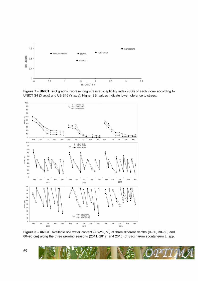
Figure 7 - UNICT. 2-D graphic representing stress susceptibility index (SSI) of each clone according to UNICT S4 (X axis) and UB S16 (Y axis). Higher SSI values indicate lower tolerance to stress.
Figure 8 - UNICT. Available soil water content (ASWC, %) at three different depths (0–30, 30–60, and 60–90 cm) along the three growing seasons (2011, 2012, and 2013) of Saccharum spontaneum L. spp.
70
aegyptiacum (Willd.) Hack. at the Experimental farm of Catania University (10 m a.s.l., 37°25’N lat., 15°03’E long.) in I0, I50, and I100 treatment.
Biomass yield ( p≤0.05)
2012 2013 2014
I0 b c b
I50 ab b a
I100 a a a
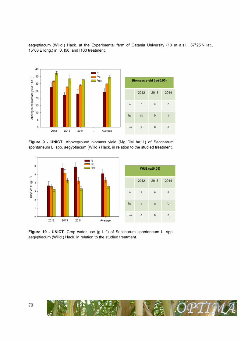
Figure 9 - UNICT. Aboveground biomass yield (Mg DM ha−1) of Saccharum spontaneum L. spp. aegyptiacum (Willd.) Hack. in relation to the studied treatment.
WUE (p≤0.05)
2012 2013 2014
I0 a a a
I50 a a b
I100 a a b
Figure 10 - UNICT. Crop water use (g L−1) of Saccharum spontaneum L. spp. aegyptiacum (Willd.) Hack. in relation to the studied treatment.
71
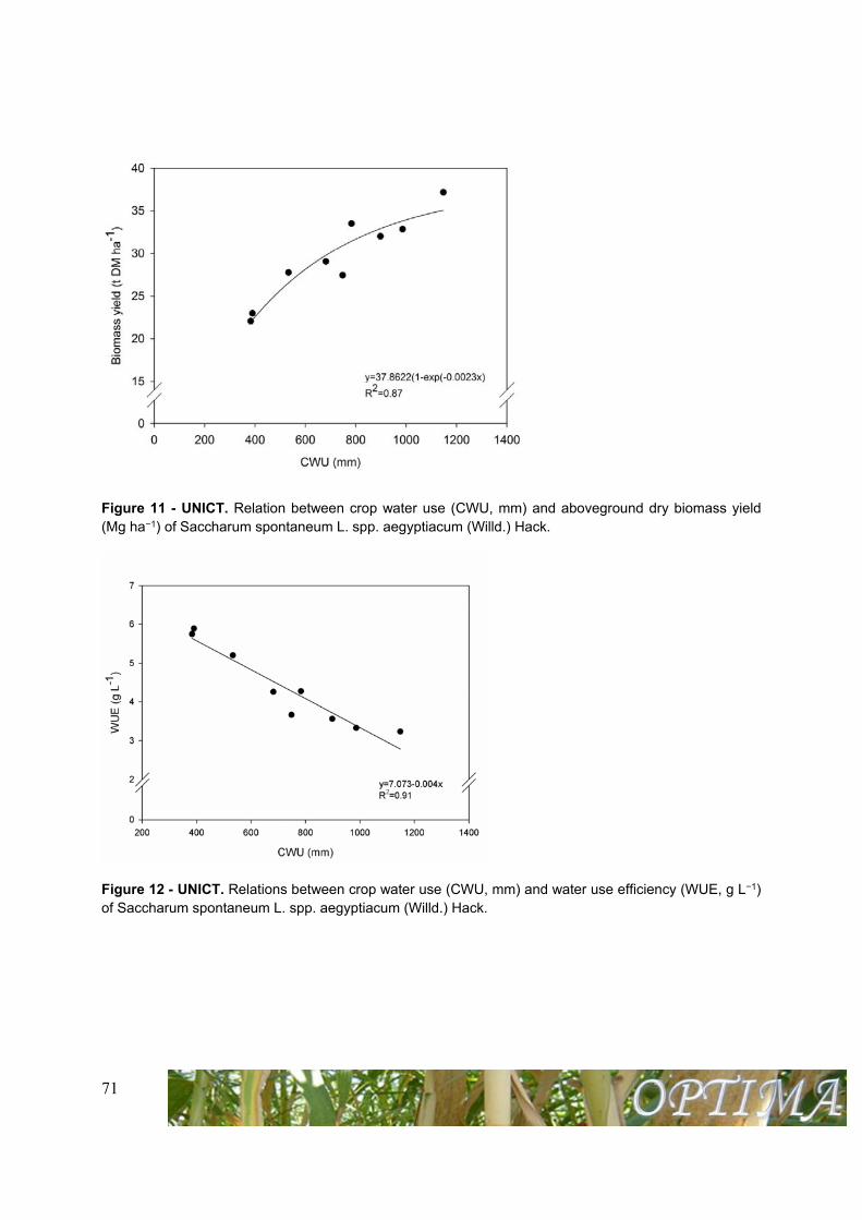
Figure 11 - UNICT. Relation between crop water use (CWU, mm) and aboveground dry biomass yield (Mg ha−1) of Saccharum spontaneum L. spp. aegyptiacum (Willd.) Hack.
Figure 12 - UNICT. Relations between crop water use (CWU, mm) and water use efficiency (WUE, g L−1) of Saccharum spontaneum L. spp. aegyptiacum (Willd.) Hack.
72
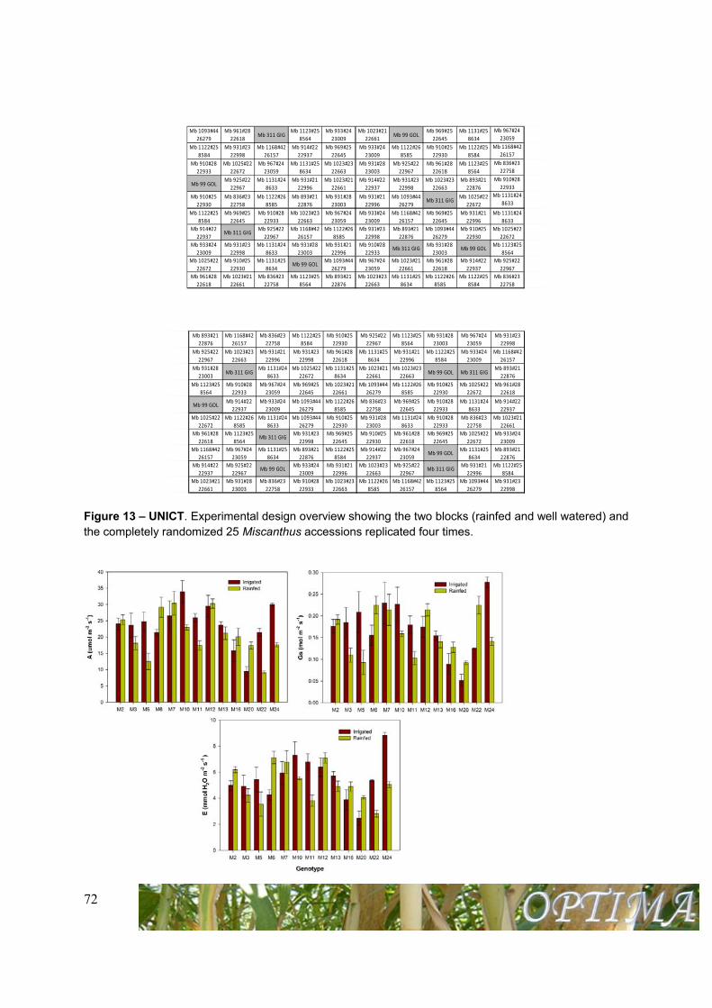
Figure 13 – UNICT. Experimental design overview showing the two blocks (rainfed and well watered) and the completely randomized 25 Miscanthus accessions replicated four times.
Mb 1093#44
26279
Mb 961#28
22618Mb 311 GIG
Mb 1123#25
8564
Mb 933#24
23009
Mb 1023#21
22661Mb 99 GOL
Mb 969#25
22645
Mb 1131#25
8634
Mb 967#24
23059
Mb 1122#25
8584
Mb 931#23
22998
Mb 1168#42
26157
Mb 914#22
22937
Mb 969#25
22645
Mb 933#24
23009
Mb 1122#26
8585
Mb 910#25
22930
Mb 1122#25
8584
Mb 1168#42
26157
Mb 910#28
22933
Mb 1025#22
22672
Mb 967#24
23059
Mb 1131#25
8634
Mb 1023#23
22663
Mb 931#28
23003
Mb 925#22
22967
Mb 961#28
22618
Mb 1123#25
8564
Mb 836#23
22758
Mb 99 GOLMb 925#22
22967
Mb 1131#24
8633
Mb 931#21
22996
Mb 1023#21
22661
Mb 914#22
22937
Mb 931#23
22998
Mb 1023#23
22663
Mb 893#21
22876
Mb 910#28
22933
Mb 910#25
22930
Mb 836#23
22758
Mb 1122#26
8585
Mb 893#21
22876
Mb 931#28
23003
Mb 931#21
22996
Mb 1093#44
26279Mb 311 GIG
Mb 1025#22
22672
Mb 1131#24
8633
Mb 1122#25
8584
Mb 969#25
22645
Mb 910#28
22933
Mb 1023#23
22663
Mb 967#24
23059
Mb 933#24
23009
Mb 1168#42
26157
Mb 969#25
22645
Mb 931#21
22996
Mb 1131#24
8633
Mb 914#22
22937Mb 311 GIG
Mb 925#22
22967
Mb 1168#42
26157
Mb 1122#26
8585
Mb 931#23
22998
Mb 893#21
22876
Mb 1093#44
26279
Mb 910#25
22930
Mb 1025#22
22672
Mb 933#24
23009
Mb 931#23
22998
Mb 1131#24
8633
Mb 931#28
23003
Mb 931#21
22996
Mb 910#28
22933Mb 311 GIG
Mb 931#28
23003Mb 99 GOL
Mb 1123#25
8564
Mb 1025#22
22672
Mb 910#25
22930
Mb 1131#25
8634Mb 99 GOL
Mb 1093#44
26279
Mb 967#24
23059
Mb 1023#21
22661
Mb 961#28
22618
Mb 914#22
22937
Mb 925#22
22967
Mb 961#28
22618
Mb 1023#21
22661
Mb 836#23
22758
Mb 1123#25
8564
Mb 893#21
22876
Mb 1023#23
22663
Mb 1131#25
8634
Mb 1122#26
8585
Mb 1122#25
8584
Mb 836#23
22758
Mb 893#21
22876
Mb 1168#42
26157
Mb 836#23
22758
Mb 1122#25
8584
Mb 910#25
22930
Mb 925#22
22967
Mb 1123#25
8564
Mb 931#28
23003
Mb 967#24
23059
Mb 931#23
22998
Mb 925#22
22967
Mb 1023#23
22663
Mb 931#21
22996
Mb 931#23
22998
Mb 961#28
22618
Mb 1131#25
8634
Mb 931#21
22996
Mb 1122#25
8584
Mb 933#24
23009
Mb 1168#42
26157
Mb 931#28
23003Mb 311 GIG
Mb 1131#24
8633
Mb 1025#22
22672
Mb 1131#25
8634
Mb 1023#21
22661
Mb 1023#23
22663Mb 99 GOL Mb 311 GIG
Mb 893#21
22876
Mb 1123#25
8564
Mb 910#28
22933
Mb 967#24
23059
Mb 969#25
22645
Mb 1023#21
22661
Mb 1093#44
26279
Mb 1122#26
8585
Mb 910#25
22930
Mb 1025#22
22672
Mb 961#28
22618
Mb 99 GOLMb 914#22
22937
Mb 933#24
23009
Mb 1093#44
26279
Mb 1122#26
8585
Mb 836#23
22758
Mb 969#25
22645
Mb 910#28
22933
Mb 1131#24
8633
Mb 914#22
22937
Mb 1025#22
22672
Mb 1122#26
8585
Mb 1131#24
8633
Mb 1093#44
26279
Mb 910#25
22930
Mb 931#28
23003
Mb 1131#24
8633
Mb 910#28
22933
Mb 836#23
22758
Mb 1023#21
22661
Mb 961#28
22618
Mb 1123#25
8564Mb 311 GIG
Mb 931#23
22998
Mb 969#25
22645
Mb 910#25
22930
Mb 961#28
22618
Mb 969#25
22645
Mb 1025#22
22672
Mb 933#24
23009
Mb 1168#42
26157
Mb 967#24
23059
Mb 1131#25
8634
Mb 893#21
22876
Mb 1122#25
8584
Mb 914#22
22937
Mb 967#24
23059Mb 99 GOL
Mb 1131#25
8634
Mb 893#21
22876
Mb 914#22
22937
Mb 925#22
22967Mb 99 GOL
Mb 933#24
23009
Mb 931#21
22996
Mb 1023#23
22663
Mb 925#22
22967Mb 311 GIG
Mb 931#21
22996
Mb 1122#25
8584
Mb 1023#21
22661
Mb 931#28
23003
Mb 836#23
22758
Mb 910#28
22933
Mb 1023#23
22663
Mb 1122#26
8585
Mb 1168#42
26157
Mb 1123#25
8564
Mb 1093#44
26279
Mb 931#23
22998
73
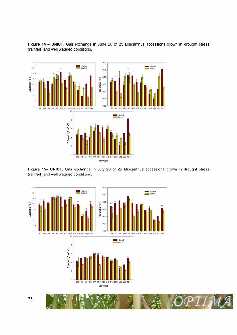
Figure 14 – UNICT. Gas exchange in June 20 of 25 Miscanthus accessions grown in drought stress (rainfed) and well watered conditions.
Figure 15– UNICT. Gas exchange in July 20 of 25 Miscanthus accessions grown in drought stress (rainfed) and well watered conditions.
74
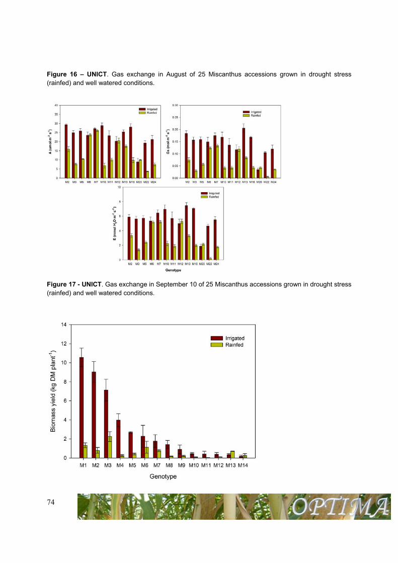
Figure 16 – UNICT. Gas exchange in August of 25 Miscanthus accessions grown in drought stress (rainfed) and well watered conditions.
Figure 17 - UNICT. Gas exchange in September 10 of 25 Miscanthus accessions grown in drought stress (rainfed) and well watered conditions.
75
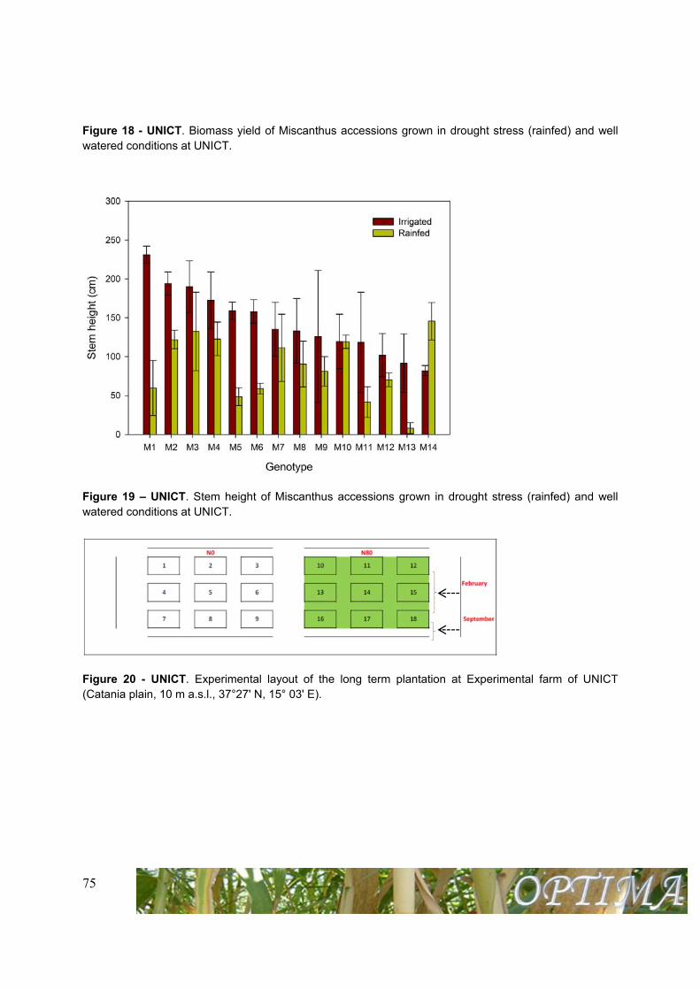
Figure 18 - UNICT. Biomass yield of Miscanthus accessions grown in drought stress (rainfed) and well watered conditions at UNICT.
Figure 19 – UNICT. Stem height of Miscanthus accessions grown in drought stress (rainfed) and well watered conditions at UNICT.
Figure 20 - UNICT. Experimental layout of the long term plantation at Experimental farm of UNICT (Catania plain, 10 m a.s.l., 37°27' N, 15° 03' E).
76
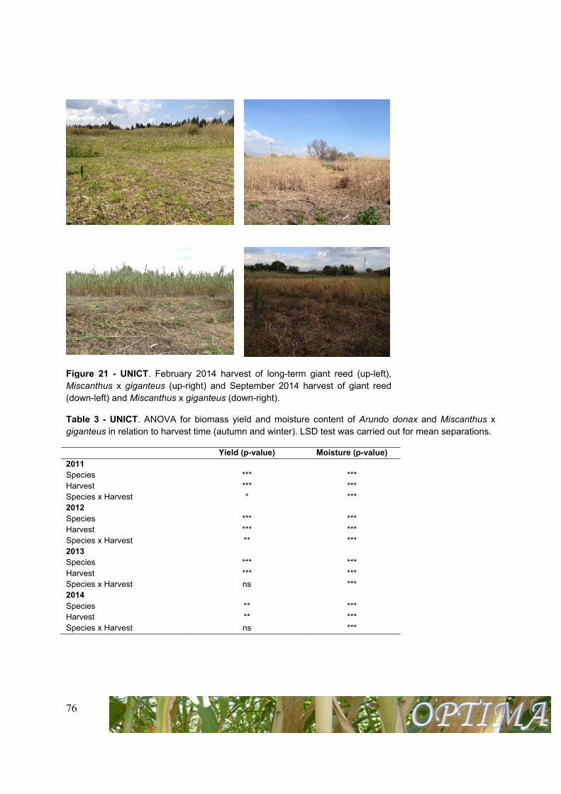
Figure 21 - UNICT. February 2014 harvest of long-term giant reed (up-left), Miscanthus x giganteus (up-right) and September 2014 harvest of giant reed (down-left) and Miscanthus x giganteus (down-right).
Table 3 - UNICT. ANOVA for biomass yield and moisture content of Arundo donax and Miscanthus x giganteus in relation to harvest time (autumn and winter). LSD test was carried out for mean separations.
Yield (p-value) Moisture (p-value)2011 Species *** *** Harvest *** *** Species x Harvest * *** 2012 Species *** *** Harvest *** *** Species x Harvest ** *** 2013 Species *** *** Harvest *** *** Species x Harvest ns *** 2014 Species ** *** Harvest ** *** Species x Harvest ns ***
77
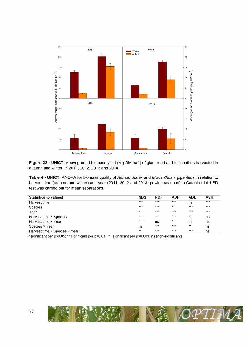
Figure 22 - UNICT. Aboveground biomass yield (Mg DM ha-1) of giant reed and miscanthus harvested in autumn and winter, in 2011, 2012, 2013 and 2014.
Table 4 - UNICT. ANOVA for biomass quality of Arundo donax and Miscanthus x giganteus in relation to harvest time (autumn and winter) and year (2011, 2012 and 2013 growing seasons) in Catania trial. LSD test was carried out for mean separations.
Statistics (p values) NDS NDF ADF ADL ASHHarvest time *** *** *** ns *** Species *** *** * *** *** Year * *** *** *** *** Harvest time × Species *** *** *** ns ns Harvest time × Year *** ns * ns ns Species × Year ns *** *** ** ns Harvest time × Species × Year ** *** *** *** ns *significant per p≤0.05; ** significant per p≤0.01; *** significant per p≤0.001; ns (non-significant)
78
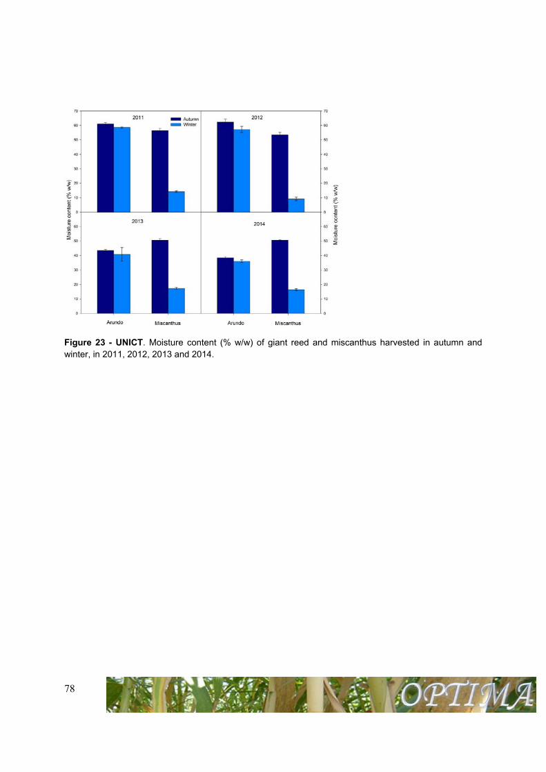
Figure 23 - UNICT. Moisture content (% w/w) of giant reed and miscanthus harvested in autumn and winter, in 2011, 2012, 2013 and 2014.
79
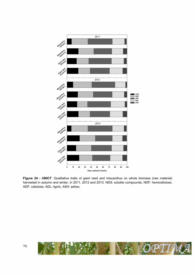
Figure 24 - UNICT. Qualitative traits of giant reed and miscanthus on whole biomass (raw material) harvested in autumn and winter, in 2011, 2012 and 2013. NDS: soluble compounds, NDF: hemicellulose, ADF: cellulose, ADL: lignin, ASH: ashes.
80
Universidad Politecnica De Madrid – UPM (n. 5)
Figure 1 - UPM. Records of temperature and rainfall in the season 2014/15. Data from AEMET, Meteorological Station of Madrid-Retiro, Longitude 34041 W, Latitude 402443, Altitude 667 m.a.s.l.
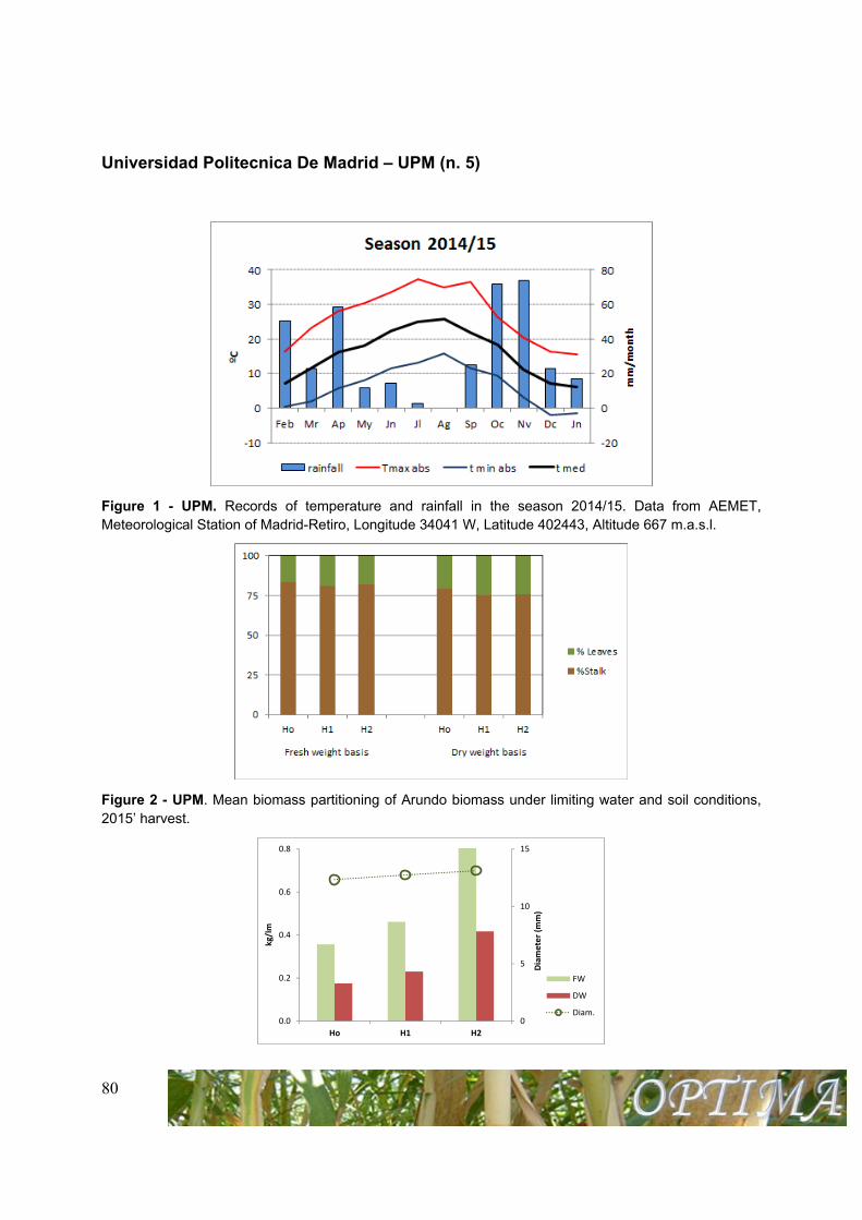
Figure 2 - UPM. Mean biomass partitioning of Arundo biomass under limiting water and soil conditions, 2015’ harvest.
0
5
10
15
0.0
0.2
0.4
0.6
0.8
Ho H1 H2
Diameter (m
m)
kg/lm
FW
DW
Diam.
81
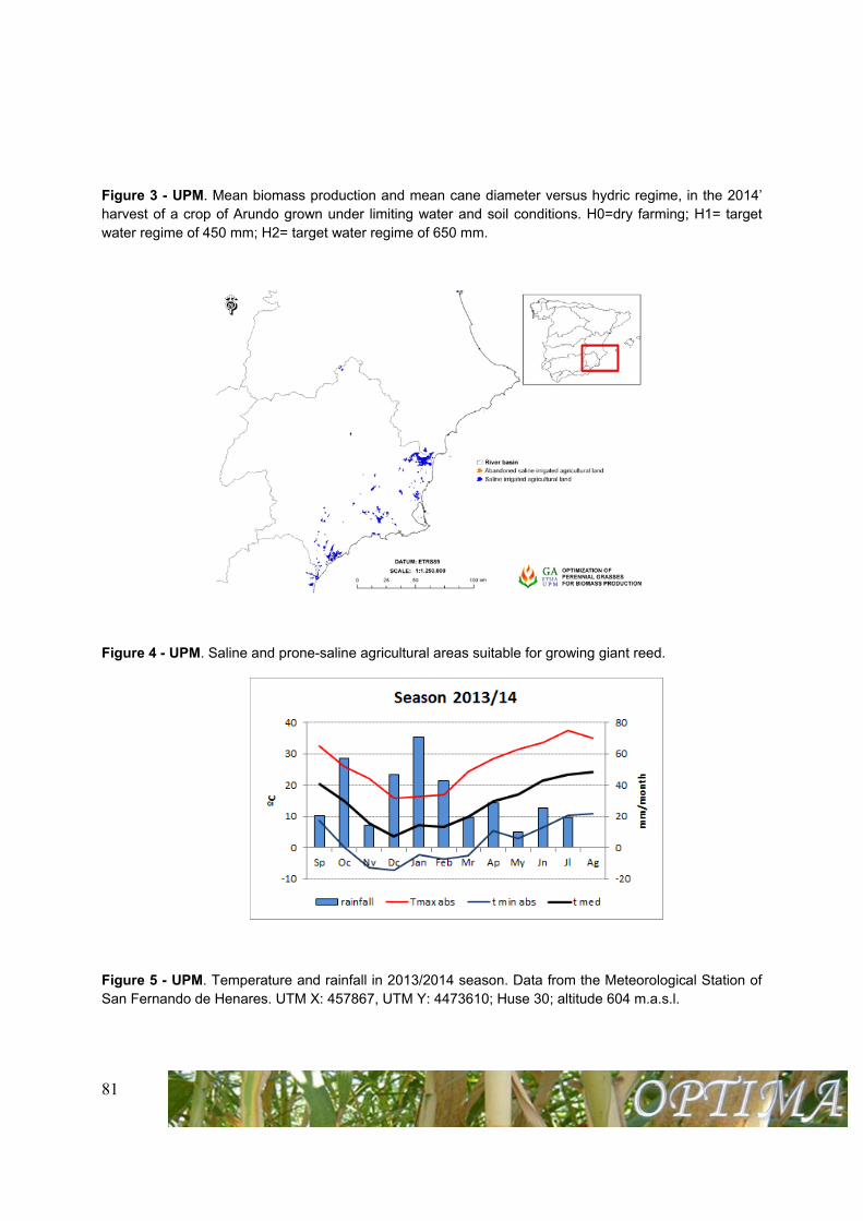
Figure 3 - UPM. Mean biomass production and mean cane diameter versus hydric regime, in the 2014’ harvest of a crop of Arundo grown under limiting water and soil conditions. H0=dry farming; H1= target water regime of 450 mm; H2= target water regime of 650 mm.
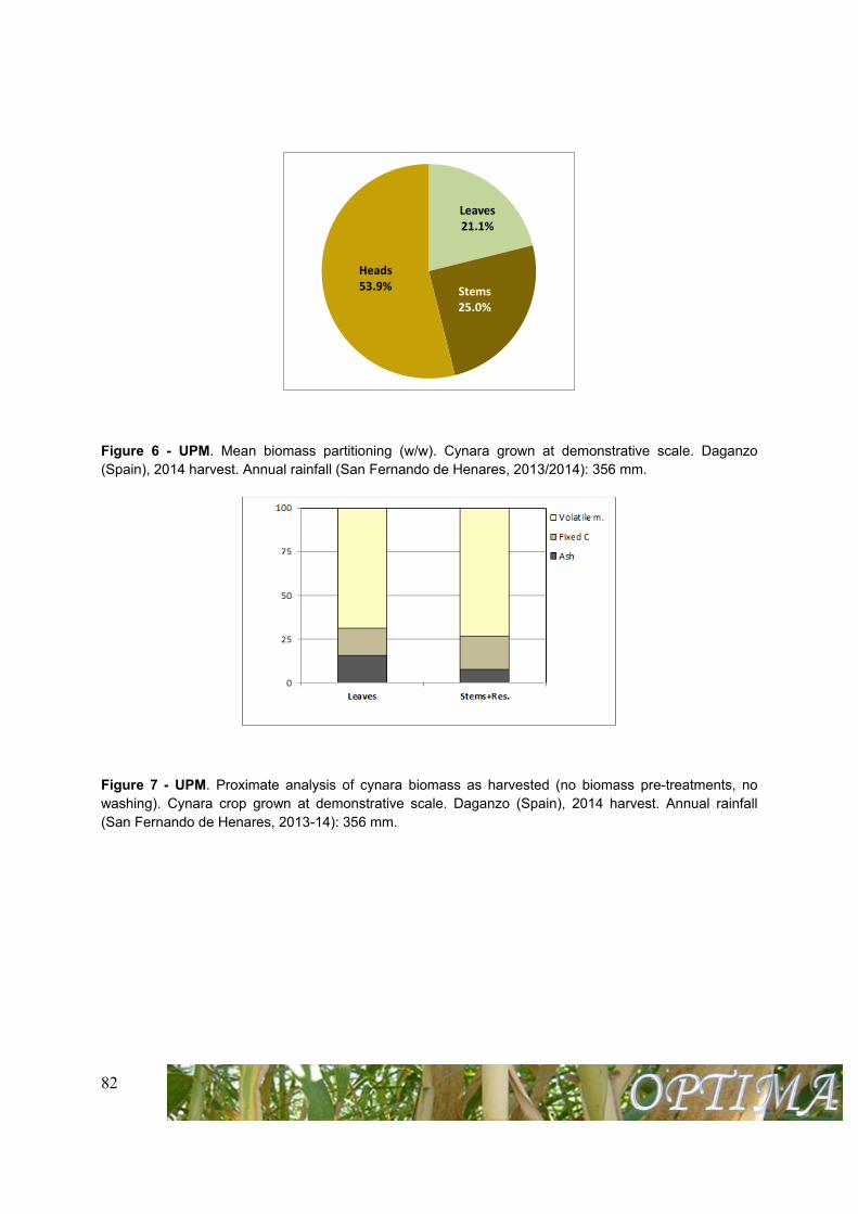
Figure 4 - UPM. Saline and prone-saline agricultural areas suitable for growing giant reed.
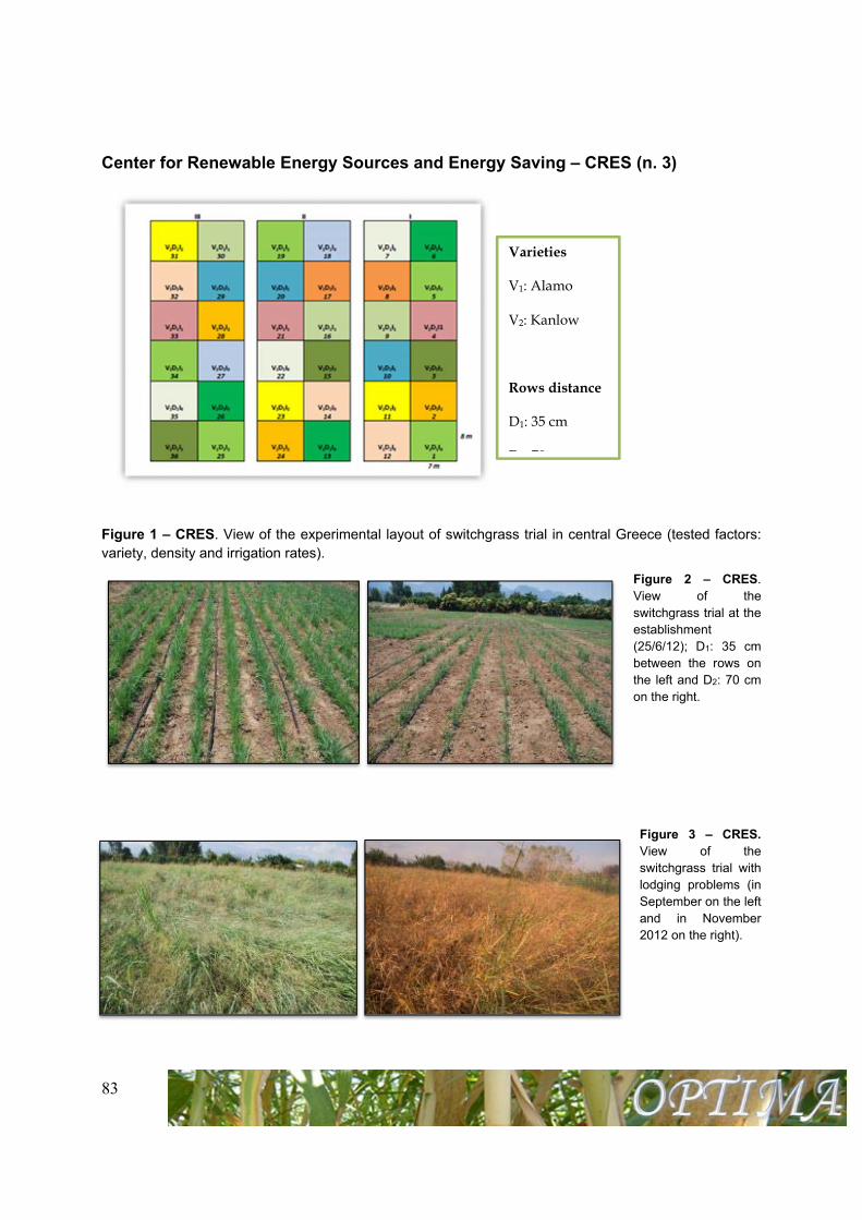
Figure 5 - UPM. Temperature and rainfall in 2013/2014 season. Data from the Meteorological Station of San Fernando de Henares. UTM X: 457867, UTM Y: 4473610; Huse 30; altitude 604 m.a.s.l.
82
Figure 6 - UPM. Mean biomass partitioning (w/w). Cynara grown at demonstrative scale. Daganzo (Spain), 2014 harvest. Annual rainfall (San Fernando de Henares, 2013/2014): 356 mm.
Figure 7 - UPM. Proximate analysis of cynara biomass as harvested (no biomass pre-treatments, no washing). Cynara crop grown at demonstrative scale. Daganzo (Spain), 2014 harvest. Annual rainfall (San Fernando de Henares, 2013-14): 356 mm.
Leaves21.1%
Stems25.0%
Heads53.9%
83
Center for Renewable Energy Sources and Energy Saving – CRES (n. 3)
Figure 1 – CRES. View of the experimental layout of switchgrass trial in central Greece (tested factors: variety, density and irrigation rates).
Figure 2 – CRES. View of the switchgrass trial at the establishment (25/6/12); D1: 35 cm between the rows on the left and D2: 70 cm on the right.
Figure 3 – CRES. View of the switchgrass trial with lodging problems (in September on the left and in November 2012 on the right).
Varieties
V1: Alamo
V2: Kanlow
Rows distance
D1: 35 cm
D 70
84
Table 1 – CRES. Growth characteristics (plant height, number of tillers/m2 and tiller density) for three subsequent growing periods.
Plant height (cm) Number of tillers/m2 Tiller diameter (mm)
Years 2013 2014 2015 2013 2014 2015 2013 2014 2015
Varieties
Alamo 163 226 208 384 462 471 3.55 4.41 4.48
Kanlow 156 227 198 467 613 603 3.37 4.18 4.22
Distances between the rows
D1: 35 cm 144 221 196 404 555 546 3.06 3.97 4.06
D1: 70 cm 157 231 210 406 510 528 3.51 4.62 4.56
Irrigation rates
I0 - 224 201 - 491 465 - 4.02 4.37
I1 - 226 202 - 580 552 - 4.48 4.10
I2 - 228 206 - 527 597 - 4.38 4.46
Mean 151 226 203 405 533 537 3.29 4.29 4.31
Table 2 – CRES. Yields results (fresh and dry matter yields, % stems on dry basis) from three subsequent growing seasons.
Fresh biomass yields (t/ha) Dry matter yields (t/ha) % stems on the biomass (oven-dried)
Years 2013 2014 2015 2013 2014 2015 2013 2014 2015
Varieties
Alamo 12.01 32.74 33.83 7.62 23.52 23.23 60.63 67.89 65.69
Kanlow 12.92 34.79 35.75 8.57 26.31 25.35 61.37 66.63 64.73
Distances between the rows
D1: 35 cm 11.10 31.18 32.14 7.07 23.26 22.85 60.82 64.53 63.64
D1: 70 cm 13.83 36.34 37.43 8.18 26.57 27.49 61.25 67.78 66.54
Irrigation rates
I0 - 31.41 32.42 - 22.53 22.43 - 63.83 65.27
I1 - 35.06 35.96 - 26.01 24.55 - 67.62 64.85
I2 - 34.81 35.98 - 26.22 25.88 - 67.39 65.46
Mean 12.47 33.76 34.79 7.63 24.92 24.29 61.07 66.41 64.80
85
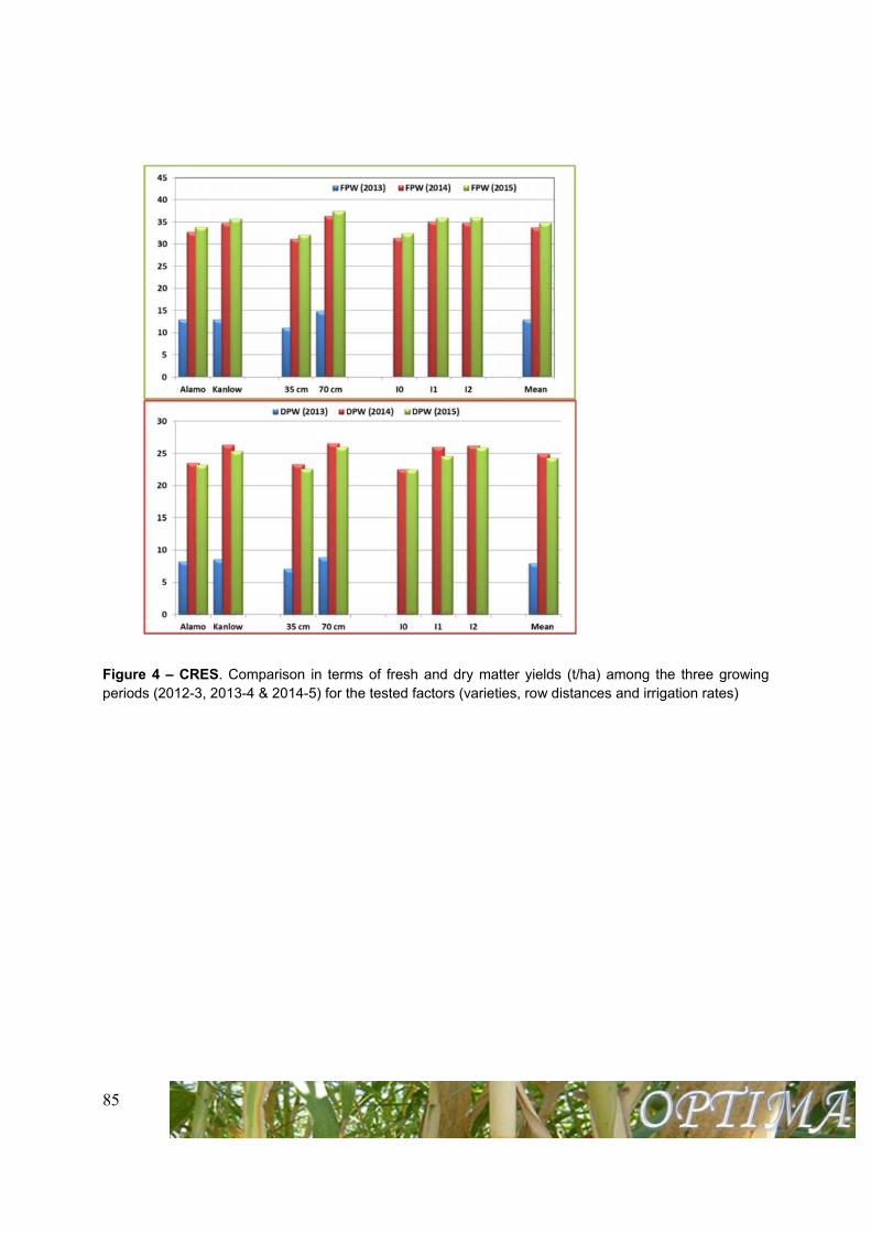
Figure 4 – CRES. Comparison in terms of fresh and dry matter yields (t/ha) among the three growing periods (2012-3, 2013-4 & 2014-5) for the tested factors (varieties, row distances and irrigation rates)
86
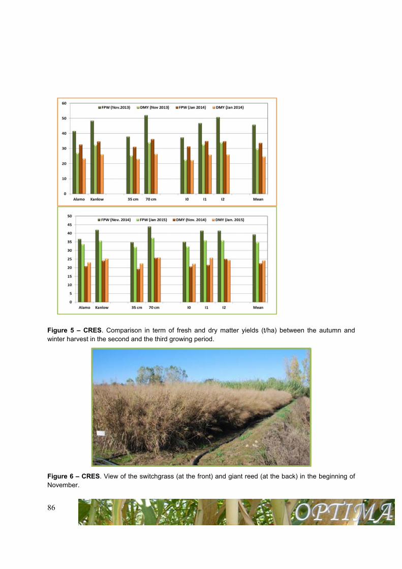
Figure 5 – CRES. Comparison in term of fresh and dry matter yields (t/ha) between the autumn and winter harvest in the second and the third growing period.
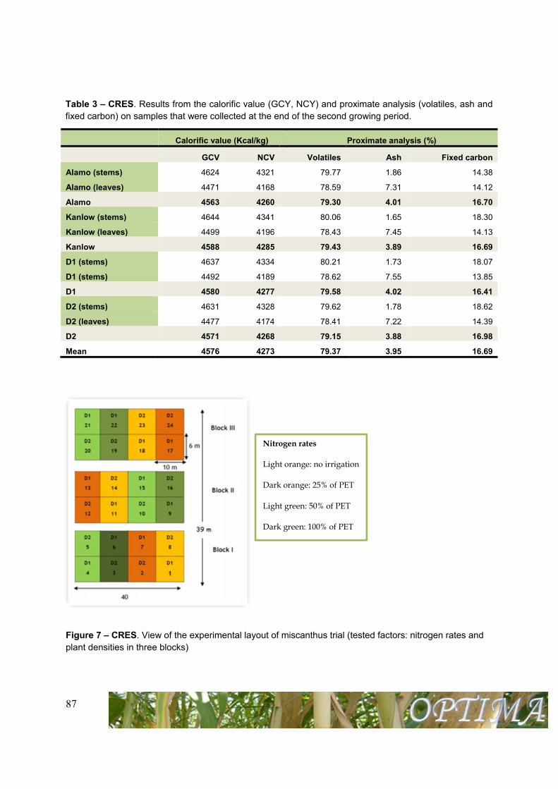
Figure 6 – CRES. View of the switchgrass (at the front) and giant reed (at the back) in the beginning of November.
87
Table 3 – CRES. Results from the calorific value (GCY, NCY) and proximate analysis (volatiles, ash and fixed carbon) on samples that were collected at the end of the second growing period.
Calorific value (Kcal/kg) Proximate analysis (%)
GCV NCV Volatiles Ash Fixed carbon
Alamo (stems) 4624 4321 79.77 1.86 14.38
Alamo (leaves) 4471 4168 78.59 7.31 14.12
Alamo 4563 4260 79.30 4.01 16.70
Kanlow (stems) 4644 4341 80.06 1.65 18.30
Kanlow (leaves) 4499 4196 78.43 7.45 14.13
Kanlow 4588 4285 79.43 3.89 16.69
D1 (stems) 4637 4334 80.21 1.73 18.07
D1 (stems) 4492 4189 78.62 7.55 13.85
D1 4580 4277 79.58 4.02 16.41
D2 (stems) 4631 4328 79.62 1.78 18.62
D2 (leaves) 4477 4174 78.41 7.22 14.39
D2 4571 4268 79.15 3.88 16.98
Mean 4576 4273 79.37 3.95 16.69
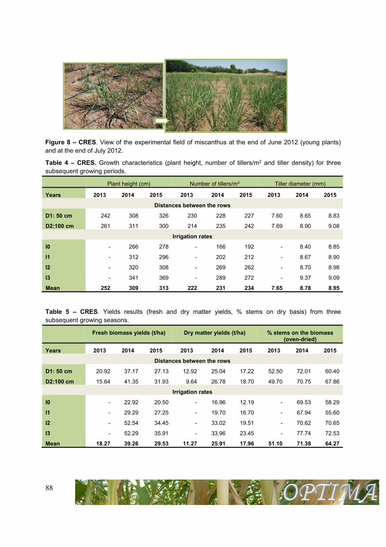
Figure 7 – CRES. View of the experimental layout of miscanthus trial (tested factors: nitrogen rates and plant densities in three blocks)
Nitrogen rates
Light orange: no irrigation
Dark orange: 25% of PET
Light green: 50% of PET
Dark green: 100% of PET
88
Figure 8 – CRES. View of the experimental field of miscanthus at the end of June 2012 (young plants) and at the end of July 2012.
Table 4 – CRES. Growth characteristics (plant height, number of tillers/m2 and tiller density) for three subsequent growing periods.
Plant height (cm) Number of tillers/m2 Tiller diameter (mm)
Years 2013 2014 2015 2013 2014 2015 2013 2014 2015
Distances between the rows
D1: 50 cm 242 308 326 230 228 227 7.60 8.65 8.83
D2:100 cm 261 311 300 214 235 242 7.69 8.90 9.08
Irrigation rates
I0 - 266 278 - 166 192 - 8.40 8.85
I1 - 312 296 - 202 212 - 8.67 8.90
I2 - 320 308 - 269 262 - 8.70 8.98
I3 - 341 369 - 289 272 - 9.37 9.09
Mean 252 309 313 222 231 234 7.65 8.78 8.95
Table 5 – CRES. Yields results (fresh and dry matter yields, % stems on dry basis) from three subsequent growing seasons.
Fresh biomass yields (t/ha) Dry matter yields (t/ha) % stems on the biomass (oven-dried)
Years 2013 2014 2015 2013 2014 2015 2013 2014 2015
Distances between the rows
D1: 50 cm 20.92 37.17 27.13 12.92 25.04 17.22 52.50 72.01 60.40
D2:100 cm 15.64 41.35 31.93 9.64 26.78 18.70 49.70 70.75 67.86
Irrigation rates
I0 - 22.92 20.50 - 16.96 12.19 - 69.53 58.29
I1 - 29.29 27.25 - 19.70 16.70 - 67.94 55.60
I2 - 52.54 34.45 - 33.02 19.51 - 70.62 70.65
I3 - 52.29 35.91 - 33.96 23.45 - 77.74 72.53
Mean 18.27 39.26 29.53 11.27 25.91 17.96 51.10 71.38 64.27
89
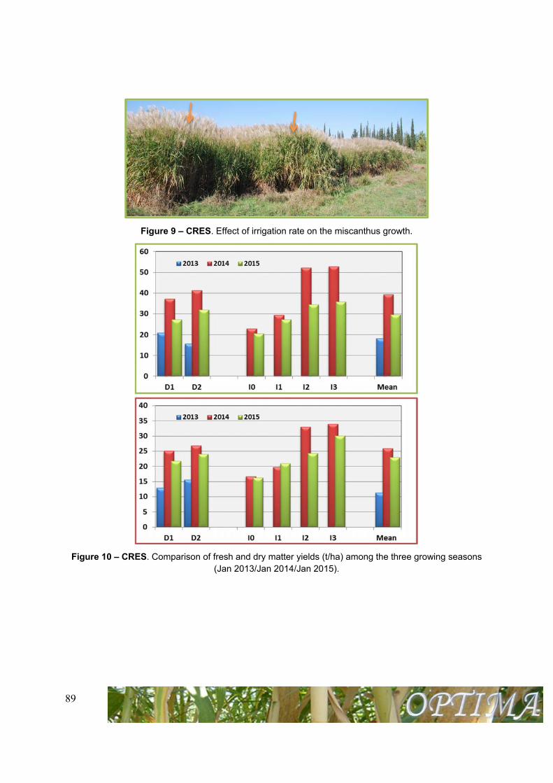
Figure 9 – CRES. Effect of irrigation rate on the miscanthus growth.
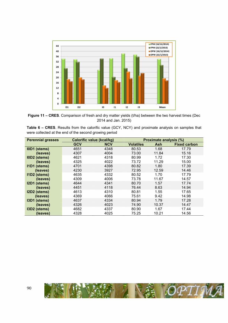
Figure 10 – CRES. Comparison of fresh and dry matter yields (t/ha) among the three growing seasons (Jan 2013/Jan 2014/Jan 2015).
90
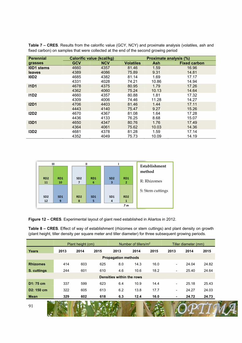
Figure 11 – CRES. Comparison of fresh and dry matter yields (t/ha) between the two harvest times (Dec 2014 and Jan. 2015)
Table 6 – CRES. Results from the calorific value (GCY, NCY) and proximate analysis on samples that were collected at the end of the second growing period
Perennial grasses Calorific value (kcal/kg) Proximate analysis (%) GCV NCV Volatiles Ash Fixed carbon
I0D1 (stems) 4651 4348 80.53 1.68 17.79 (leaves) 4307 4004 73.00 11.84 15.16 I0D2 (stems) 4621 4318 80.99 1.72 17.30 (leaves) 4325 4022 73.72 11.29 15.00 I1D1 (stems) 4701 4398 80.82 1.80 17.39 (leaves) 4230 3927 72.95 12.59 14.46 I1D2 (stems) 4635 4332 80.52 1.70 17.79 (leaves) 4309 4006 73.78 11.67 14.57 I2D1 (stems) 4644 4341 80.70 1.57 17.74 (leaves) 4451 4118 76.44 8.63 14.94 I2D2 (stems) 4613 4310 80.81 1.55 17.65 (leaves) 4369 4066 75.61 9.42 14.98 I3D1 (stems) 4637 4334 80.94 1.79 17.28 (leaves) 4326 4023 74.90 10.37 14.47 I3D2 (stems) 4682 4337 80.90 1.67 17.44 (leaves) 4328 4025 75.25 10.21 14.56
91
Table 7 – CRES. Results from the calorific value (GCY, NCY) and proximate analysis (volatiles, ash and fixed carbon) on samples that were collected at the end of the second growing period
Perennial grasses
Calorific value (kcal/kg) Proximate analysis (%) GCV NCV Volatiles Ash Fixed carbon
I0D1 stems 4660 4357 81.46 1.59 16.96 leaves 4389 4086 75.89 9.31 14.81 I0D2 4685 4382 81.14 1.69 17.17 4331 4028 74.21 10.86 14.94 I1D1 4678 4375 80.95 1.79 17.26 4362 4060 75.24 10.13 14.64 I1D2 4660 4357 80.88 1.81 17.32 4309 4006 74.46 11.28 14.27 I2D1 4706 4403 81.46 1.44 17.11 4443 4140 75.47 9.27 15.26 I2D2 4670 4367 81.08 1.64 17.28 4436 4133 76.25 8.68 15.07 I3D1 4650 4347 80.76 1.76 17.49 4364 4061 75.62 10.03 14.36 I3D2 4681 4378 81.28 1.59 17.14 4352 4049 75.73 10.09 14.19
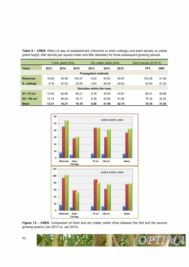
Figure 12 – CRES. Experimental layout of giant reed established in Aliartos in 2012.
Table 8 – CRES. Effect of way of establishment (rhizomes or stem cuttings) and plant density on growth (plant height, tiller density per square meter and tiller diameter) for three subsequent growing periods.
Plant height (cm) Number of tillers/m2 Tiller diameter (mm)
Years 2013 2014 2015 2013 2014 2015 2013 2014 2015
Propagation methods
Rhizomes 414 603 625 8.0 14.3 16.0 - 24.04 24.82
S. cuttings 244 601 610 4.6 10.6 18.2 - 25.40 24.64
Densities within the rows
D1: 75 cm 337 599 623 6.4 10.9 14.4 - 25.18 25.43
D2: 150 cm 322 605 613 6.2 13.8 17.7 - 24.27 24.03
Mean 329 602 618 6.3 12.4 16.0 - 24.72 24.73
Establishment method
R: Rhizomes
S: Stem cuttings
92
Table 9 – CRES. Effect of way of establishment (rhizomes or stem cuttings) and plant density on yields (plant height, tiller density per square meter and tiller diameter) for three subsequent growing periods.
Fresh yields (t/ha) Dry matter yields (t/ha) Early harvest (2/12/13)
Years 2013 2014 2015 2013 2014 2015 FFY DMY
Propagation methods
Rhizomes 16.85 94.58 103.37 8.24 45.63 54.67 103.38 41.85
S. cuttings 9.78 57.83 53.00 4.93 28.49 30.83 53.00 21.22
Densities within the rows
D1: 75 cm 13.50 62.88 80.21 6.78 30.29 43.91 80.21 28.86
D2: 150 cm 13.13 89.54 76.17 6.38 43.82 41.59 76.16 34.22
Mean 13.31 76.21 78.18 6.58 37.06 42.75 78.18 31.54
Figure 13 – CRES. Comparison of fresh and dry matter yields (t/ha) between the first and the second growing season (Jan 2013 vs. Jan 2014).
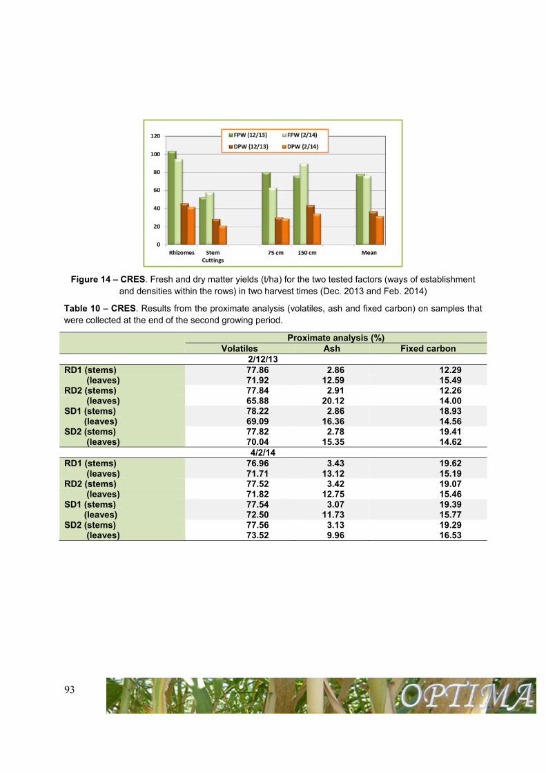
93
Figure 14 – CRES. Fresh and dry matter yields (t/ha) for the two tested factors (ways of establishment and densities within the rows) in two harvest times (Dec. 2013 and Feb. 2014)
Table 10 – CRES. Results from the proximate analysis (volatiles, ash and fixed carbon) on samples that were collected at the end of the second growing period.
Proximate analysis (%) Volatiles Ash Fixed carbon
2/12/13 RD1 (stems) 77.86 2.86 12.29 (leaves) 71.92 12.59 15.49 RD2 (stems) 77.84 2.91 12.26 (leaves) 65.88 20.12 14.00 SD1 (stems) 78.22 2.86 18.93 (leaves) 69.09 16.36 14.56 SD2 (stems) 77.82 2.78 19.41 (leaves) 70.04 15.35 14.62
4/2/14 RD1 (stems) 76.96 3.43 19.62 (leaves) 71.71 13.12 15.19 RD2 (stems) 77.52 3.42 19.07 (leaves) 71.82 12.75 15.46 SD1 (stems) 77.54 3.07 19.39 (leaves) 72.50 11.73 15.77 SD2 (stems) 77.56 3.13 19.29 (leaves) 73.52 9.96 16.53
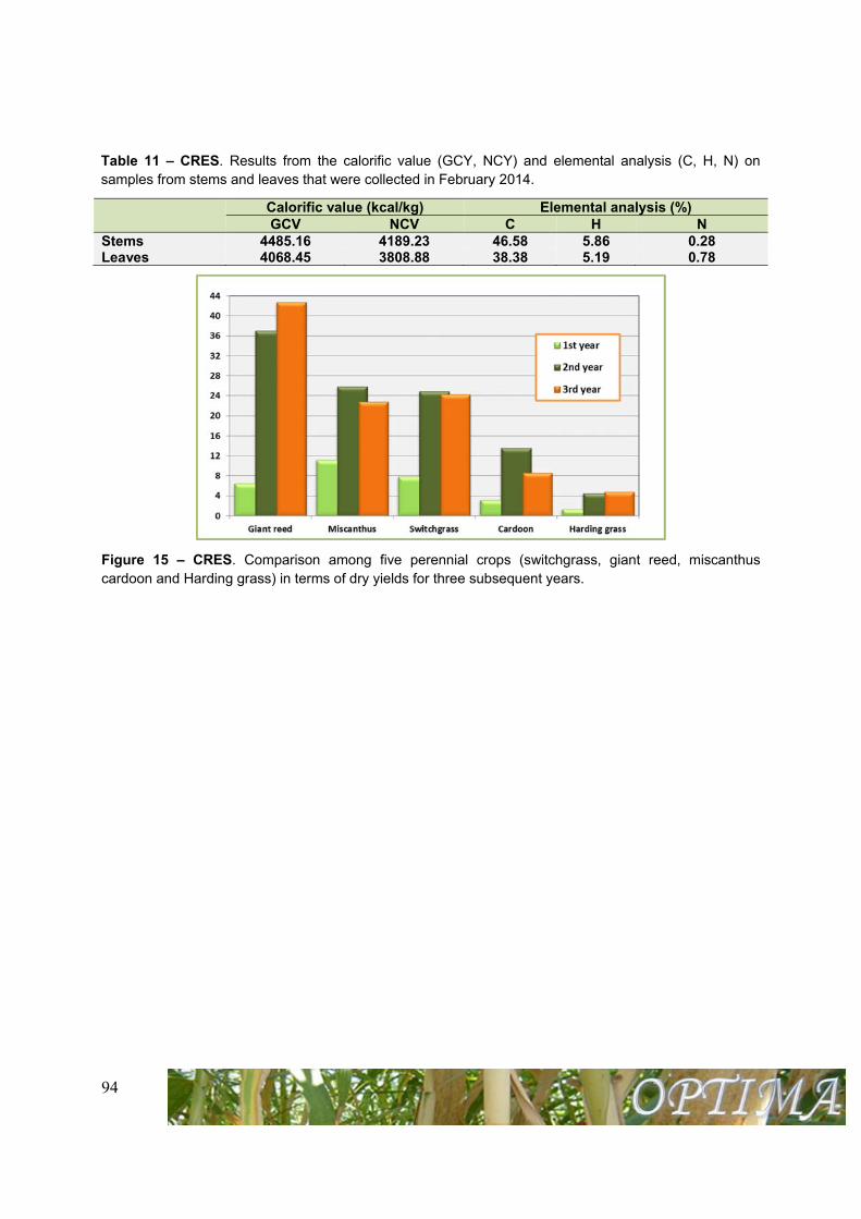
94
Table 11 – CRES. Results from the calorific value (GCY, NCY) and elemental analysis (C, H, N) on samples from stems and leaves that were collected in February 2014.
Calorific value (kcal/kg) Elemental analysis (%) GCV NCV C H N
Stems 4485.16 4189.23 46.58 5.86 0.28 Leaves 4068.45 3808.88 38.38 5.19 0.78
Figure 15 – CRES. Comparison among five perennial crops (switchgrass, giant reed, miscanthus cardoon and Harding grass) in terms of dry yields for three subsequent years.
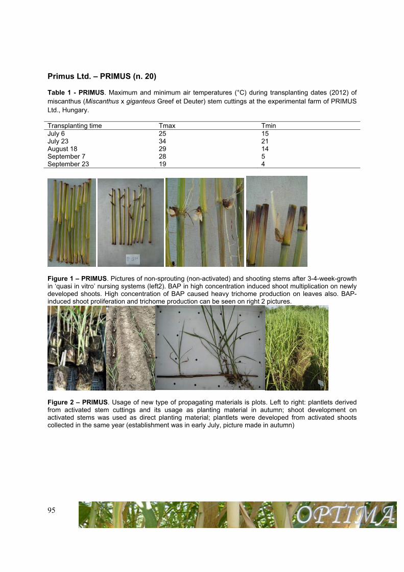
95
Primus Ltd. – PRIMUS (n. 20)
Table 1 - PRIMUS. Maximum and minimum air temperatures (°C) during transplanting dates (2012) of miscanthus (Miscanthus x giganteus Greef et Deuter) stem cuttings at the experimental farm of PRIMUS Ltd., Hungary.
Transplanting time Tmax Tmin July 6 25 15 July 23 34 21 August 18 29 14 September 7 28 5 September 23 19 4
Figure 1 – PRIMUS. Pictures of non-sprouting (non-activated) and shooting stems after 3-4-week-growth in ‘quasi in vitro’ nursing systems (left2). BAP in high concentration induced shoot multiplication on newly developed shoots. High concentration of BAP caused heavy trichome production on leaves also. BAP-induced shoot proliferation and trichome production can be seen on right 2 pictures.
Figure 2 – PRIMUS. Usage of new type of propagating materials is plots. Left to right: plantlets derived from activated stem cuttings and its usage as planting material in autumn; shoot development on activated stems was used as direct planting material; plantlets were developed from activated shoots collected in the same year (establishment was in early July, picture made in autumn)
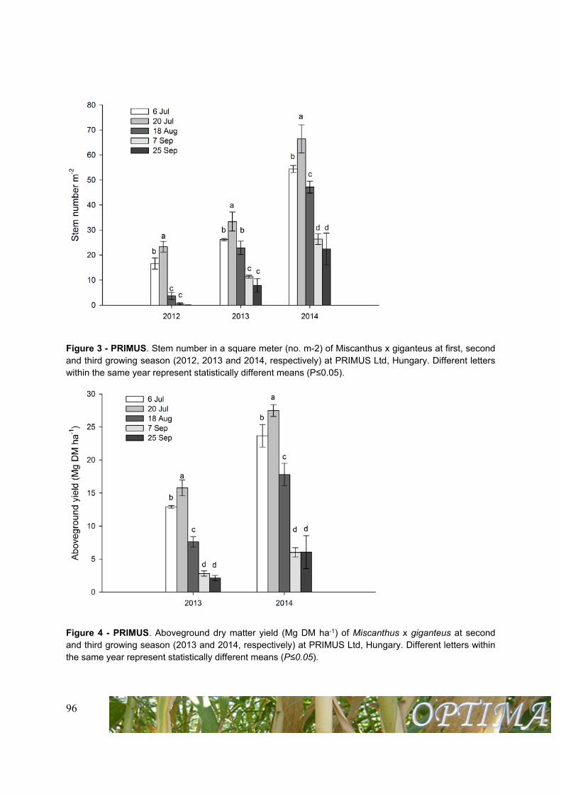
96
Figure 3 - PRIMUS. Stem number in a square meter (no. m-2) of Miscanthus x giganteus at first, second and third growing season (2012, 2013 and 2014, respectively) at PRIMUS Ltd, Hungary. Different letters within the same year represent statistically different means (P≤0.05).
Figure 4 - PRIMUS. Aboveground dry matter yield (Mg DM ha-1) of Miscanthus x giganteus at second and third growing season (2013 and 2014, respectively) at PRIMUS Ltd, Hungary. Different letters within the same year represent statistically different means (P≤0.05).
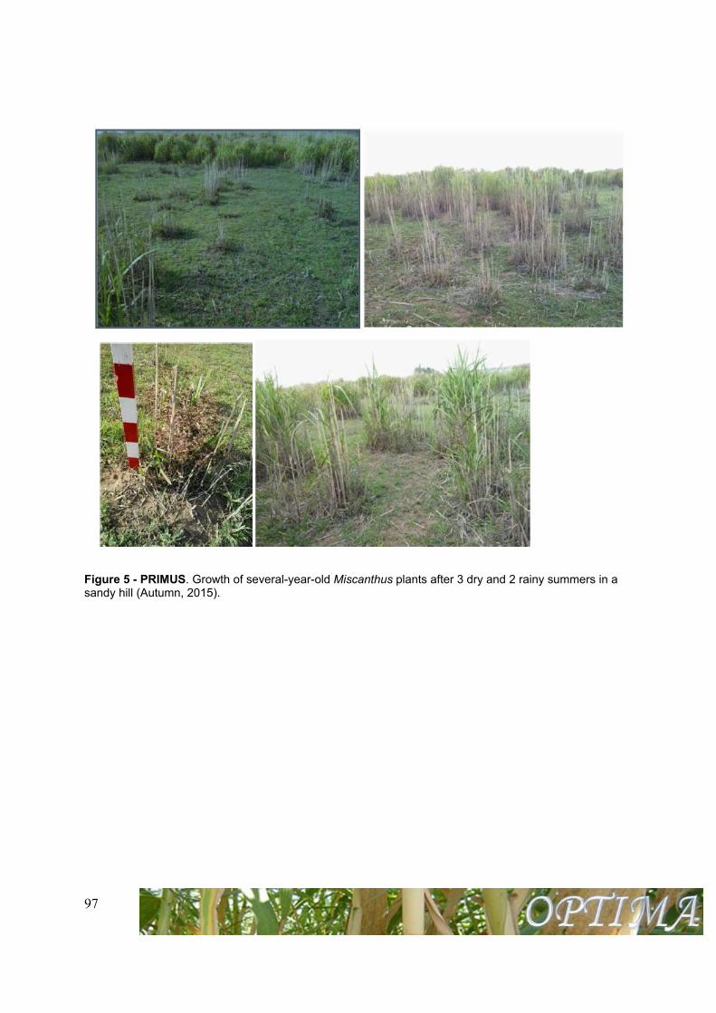
97
Figure 5 - PRIMUS. Growth of several-year-old Miscanthus plants after 3 dry and 2 rainy summers in a sandy hill (Autumn, 2015).
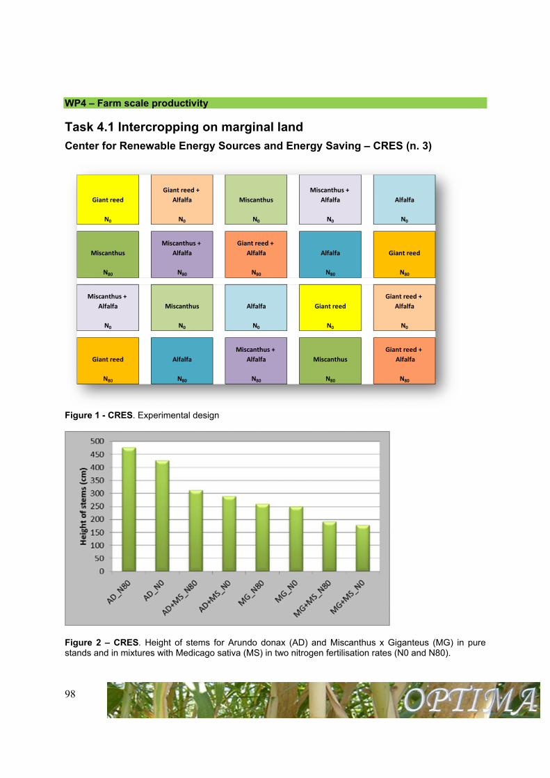
98
WP4 – Farm scale productivity
Task 4.1 Intercropping on marginal land
Center for Renewable Energy Sources and Energy Saving – CRES (n. 3)
Figure 1 - CRES. Experimental design
Figure 2 – CRES. Height of stems for Arundo donax (AD) and Miscanthus x Giganteus (MG) in pure stands and in mixtures with Medicago sativa (MS) in two nitrogen fertilisation rates (N0 and N80).
Giant reed + Miscanthus +
Giant reed Alfalfa Miscanthus Alfalfa Alfalfa
N0 N0 N0 N0 N0
Miscanthus + Giant reed +
Miscanthus Alfalfa Alfalfa Alfalfa Giant reed
N80 N80 N80 N80 N80
Miscanthus + Giant reed +
Alfalfa Miscanthus Alfalfa Giant reed Alfalfa
N0 N0 N0 N0 N0
Miscanthus + Giant reed +
Giant reed Alfalfa Alfalfa Miscanthus Alfalfa
N80 N80 N80 N80 N80
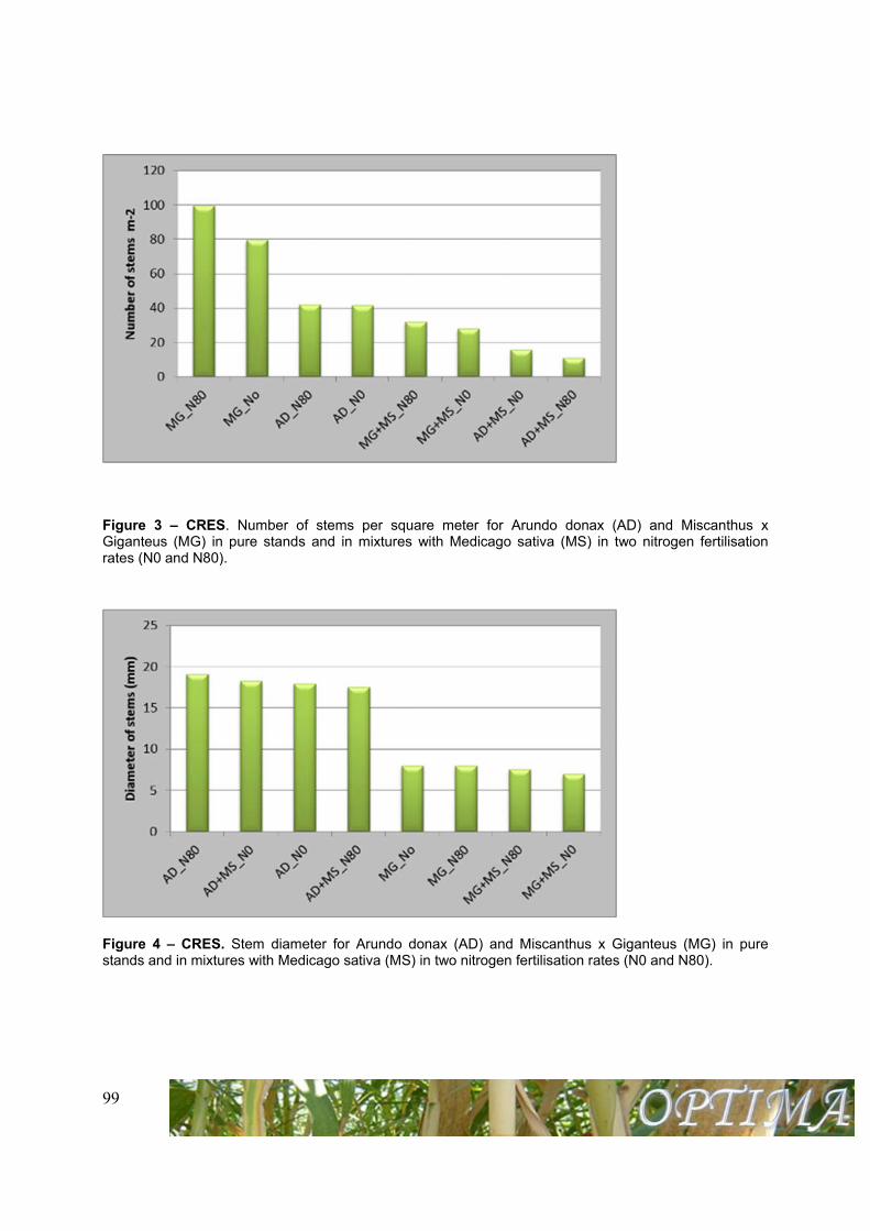
99
Figure 3 – CRES. Number of stems per square meter for Arundo donax (AD) and Miscanthus x Giganteus (MG) in pure stands and in mixtures with Medicago sativa (MS) in two nitrogen fertilisation rates (N0 and N80).
Figure 4 – CRES. Stem diameter for Arundo donax (AD) and Miscanthus x Giganteus (MG) in pure stands and in mixtures with Medicago sativa (MS) in two nitrogen fertilisation rates (N0 and N80).
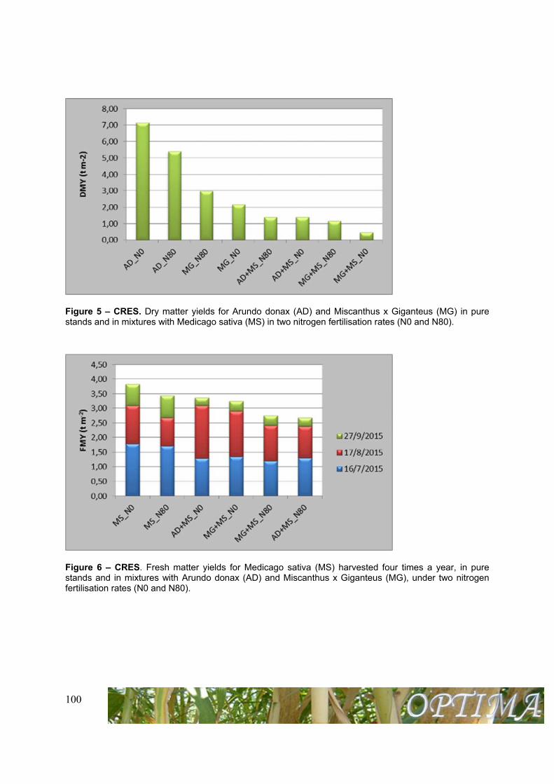
100
Figure 5 – CRES. Dry matter yields for Arundo donax (AD) and Miscanthus x Giganteus (MG) in pure stands and in mixtures with Medicago sativa (MS) in two nitrogen fertilisation rates (N0 and N80).
Figure 6 – CRES. Fresh matter yields for Medicago sativa (MS) harvested four times a year, in pure stands and in mixtures with Arundo donax (AD) and Miscanthus x Giganteus (MG), under two nitrogen fertilisation rates (N0 and N80).
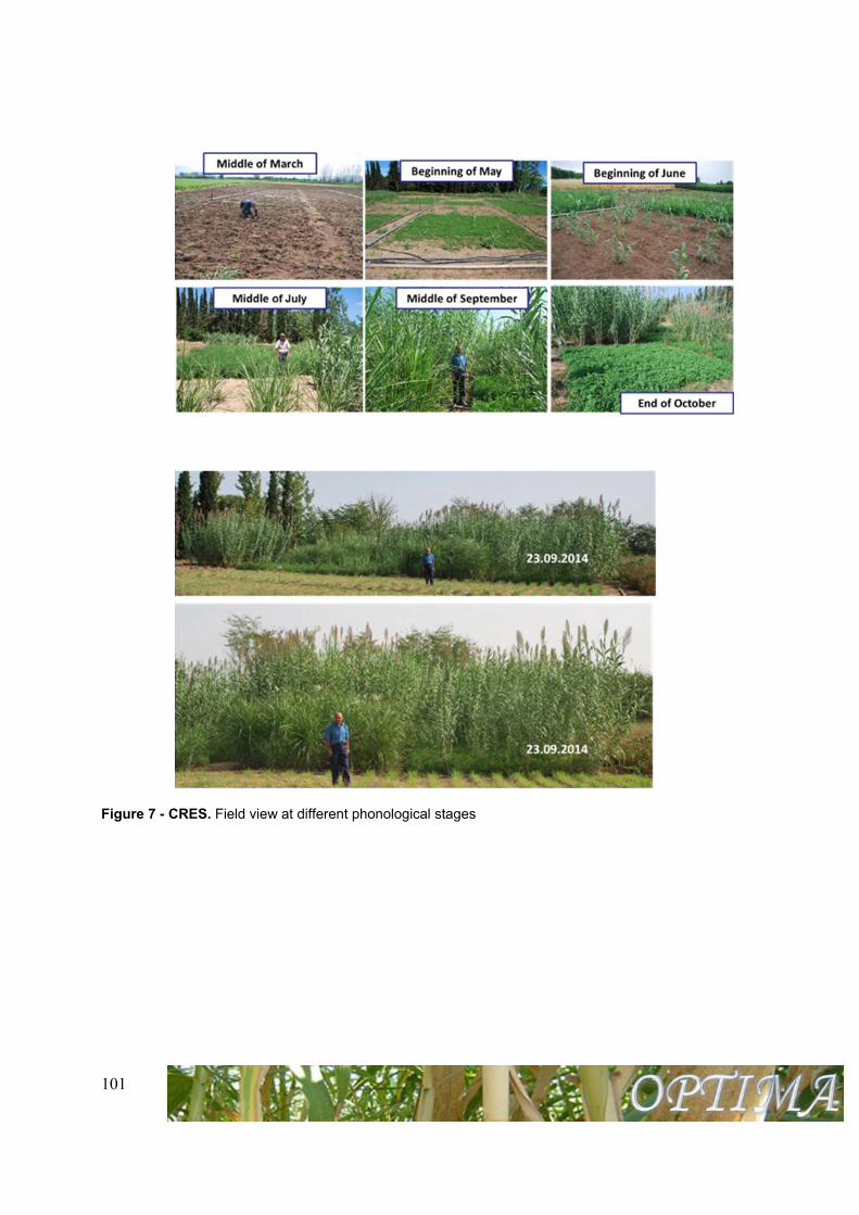
101
Figure 7 - CRES. Field view at different phonological stages
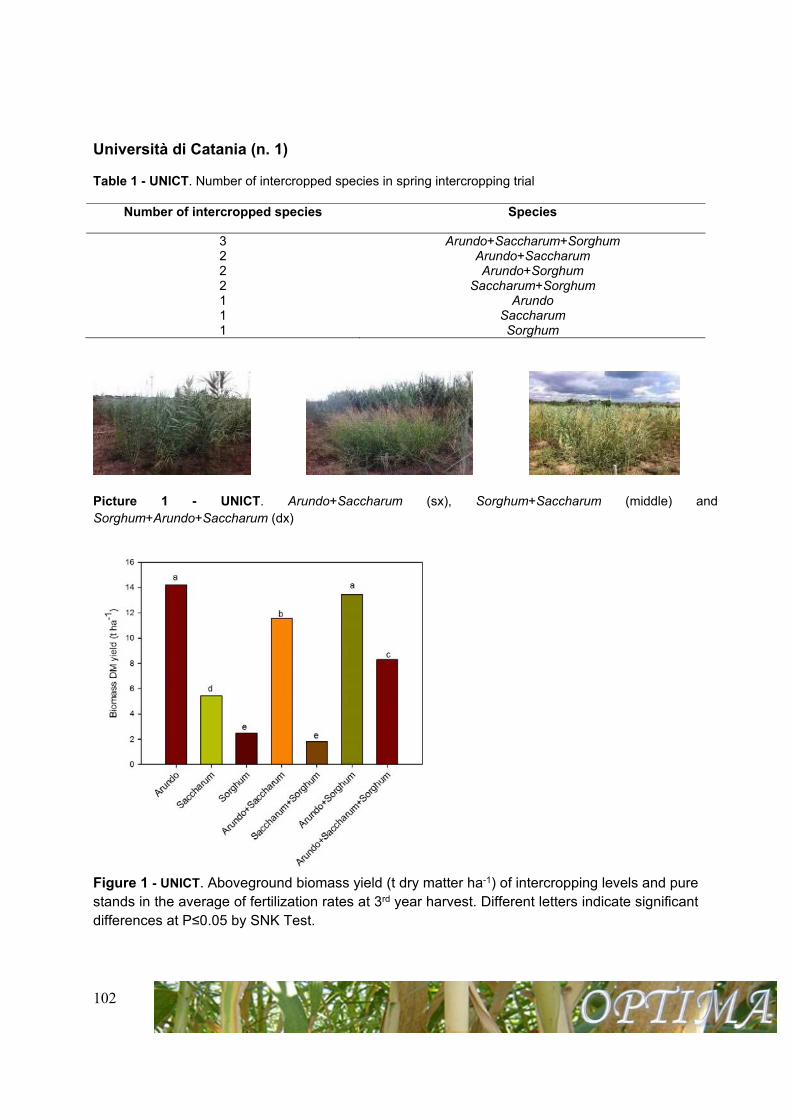
102
Università di Catania (n. 1)
Table 1 - UNICT. Number of intercropped species in spring intercropping trial
Number of intercropped species Species
3 Arundo+Saccharum+Sorghum 2 Arundo+Saccharum 2 Arundo+Sorghum 2 Saccharum+Sorghum 1 Arundo 1 Saccharum 1 Sorghum
Picture 1 - UNICT. Arundo+Saccharum (sx), Sorghum+Saccharum (middle) and Sorghum+Arundo+Saccharum (dx)
Figure 1 - UNICT. Aboveground biomass yield (t dry matter ha-1) of intercropping levels and pure stands in the average of fertilization rates at 3rd year harvest. Different letters indicate significant differences at P≤0.05 by SNK Test.
103
Table 2 - UNICT. Nitrogen fertilization effect on aboveground biomass yield (t ha-1) in the average of intercropping levels at 3nd year harvest (February 2015). Different letters indicate significant differences at P≤0.05 by SNK Test.
Nitrogen fertilization (kg ha-1) Average biomass yield (t ha-1)
0 7.07c
40 8.27b
80 9.22a
Table 3 - UNICT. Number of intercropped species
Number of intercropped species
Species
2 Miscanthus +T. alexandrinum
2 Arundo +T. alexandrinum
1 Arundo
1 Miscanthus
1 T. alexandrinum
Picture 2 - UNICT. Arundo and T. alexandrinum in early-spring (left), middle of summer-time (center) and end-of summer after some irrigations (left)
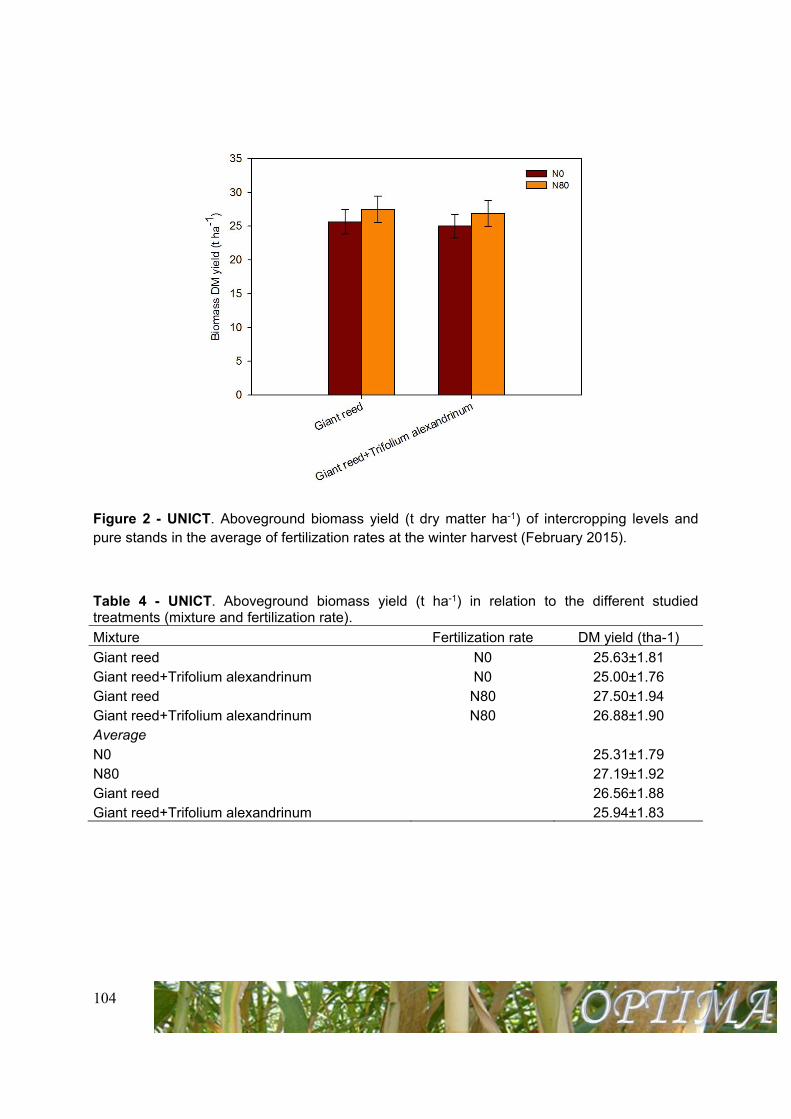
104
Figure 2 - UNICT. Aboveground biomass yield (t dry matter ha-1) of intercropping levels and pure stands in the average of fertilization rates at the winter harvest (February 2015).
Table 4 - UNICT. Aboveground biomass yield (t ha-1) in relation to the different studied treatments (mixture and fertilization rate).
Mixture Fertilization rate DM yield (tha-1)
Giant reed N0 25.63±1.81 Giant reed+Trifolium alexandrinum N0 25.00±1.76 Giant reed N80 27.50±1.94 Giant reed+Trifolium alexandrinum N80 26.88±1.90 Average N0 25.31±1.79 N80 27.19±1.92 Giant reed 26.56±1.88 Giant reed+Trifolium alexandrinum 25.94±1.83
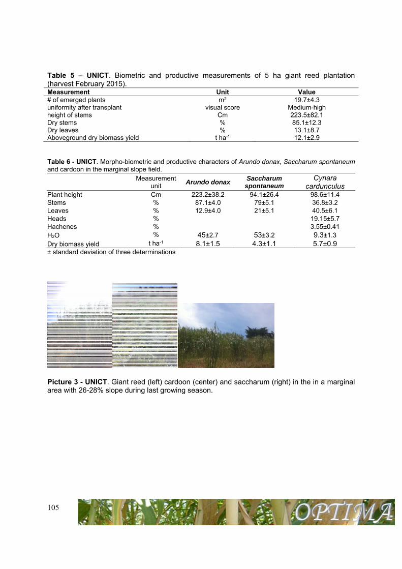
105
Table 5 – UNICT. Biometric and productive measurements of 5 ha giant reed plantation (harvest February 2015). Measurement Unit Value # of emerged plants m2 19.7±4.3 uniformity after transplant visual score Medium-high height of stems Cm 223.5±82.1 Dry stems % 85.1±12.3 Dry leaves % 13.1±8.7 Aboveground dry biomass yield t ha-1 12.1±2.9
Table 6 - UNICT. Morpho-biometric and productive characters of Arundo donax, Saccharum spontaneum and cardoon in the marginal slope field.
Measurement
unit Arundo donax
Saccharum spontaneum
Cynara cardunculus
Plant height Cm 223.2±38.2 94.1±26.4 98.6±11.4 Stems % 87.1±4.0 79±5.1 36.8±3.2 Leaves % 12.9±4.0 21±5.1 40.5±6.1 Heads % 19.15±5.7 Hachenes % 3.55±0.41 H2O % 45±2.7 53±3.2 9.3±1.3 Dry biomass yield t ha-1 8.1±1.5 4.3±1.1 5.7±0.9 ± standard deviation of three determinations
Picture 3 - UNICT. Giant reed (left) cardoon (center) and saccharum (right) in the in a marginal area with 26-28% slope during last growing season.
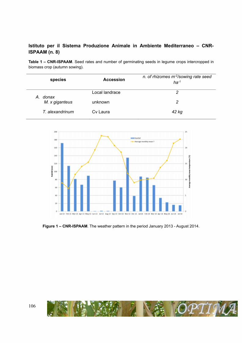
106
Istituto per il Sistema Produzione Animale in Ambiente Mediterraneo – CNR-ISPAAM (n. 8)
Table 1 – CNR-ISPAAM. Seed rates and number of germinating seeds in legume crops intercropped in biomass crop (autumn sowing).
species Accession n. of rhizomes m-2/sowing rate seed
ha-1
A. donax Local landrace 2
M. x giganteus unknown 2
T. alexandrinum Cv Laura 42 kg
Figure 1 – CNR-ISPAAM. The weather pattern in the period January 2013 - August 2014.
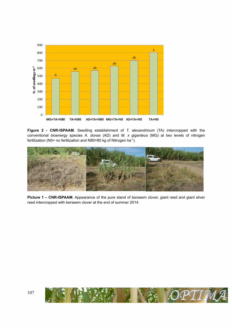
107
Figure 2 - CNR-ISPAAM. Seedling establishment of T. alexandrinum (TA) intercropped with the conventional bioenergy species A. donax (AD) and M. x giganteus (MG) at two levels of nitrogen fertilization (N0= no fertilization and N80=80 kg of Nitrogen ha-1).
Picture 1 – CNR-ISPAAM. Appearance of the pure stand of berseem clover, giant reed and giant silver reed intercropped with berseem clover at the end of summer 2014.
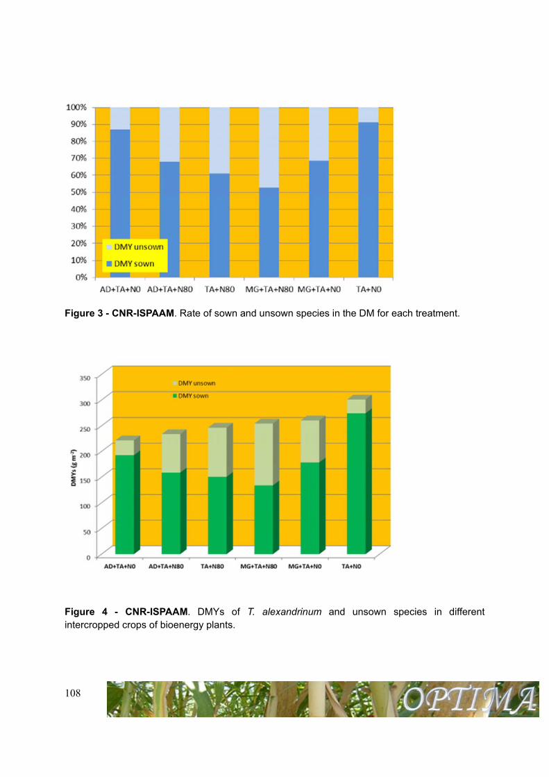
108
Figure 3 - CNR-ISPAAM. Rate of sown and unsown species in the DM for each treatment.
Figure 4 - CNR-ISPAAM. DMYs of T. alexandrinum and unsown species in different intercropped crops of bioenergy plants.
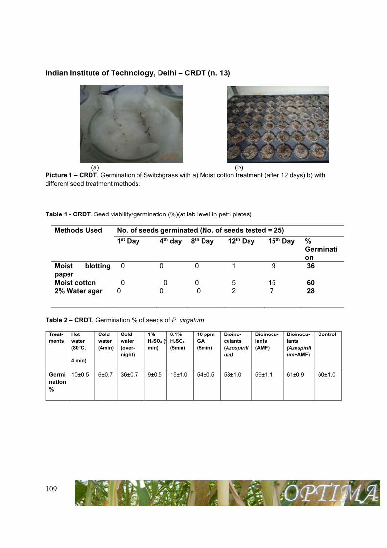
109
Indian Institute of Technology, Delhi – CRDT (n. 13)
(a) (b)
Picture 1 – CRDT. Germination of Switchgrass with a) Moist cotton treatment (after 12 days) b) with different seed treatment methods.
Table 1 - CRDT. Seed viability/germination (%)(at lab level in petri plates)
Methods Used No. of seeds germinated (No. of seeds tested = 25)
1st Day 4th day 8th Day 12th Day 15th Day % Germination
Moist blotting paper
0 0 0 1 9 36
Moist cotton 0 0 0 5 15 60 2% Water agar 0 0 0 2 7 28
Table 2 – CRDT. Germination % of seeds of P. virgatum
Treat-ments
Hot water (80°C,
4 min)
Cold water (4min)
Cold water (over-night)
1% H2SO4 (5min)
0.1% H2SO4
(5min)
10 ppm GA (5min)
Bioino-culants (Azospirillum)
Bioinocu-lants (AMF)
Bioinocu-lants (Azospirillum+AMF)
Control
Germination %
10±0.5 6±0.7 36±0.7 9±0.5 15±1.0 54±0.5 58±1.0 59±1.1 61±0.9 60±1.0
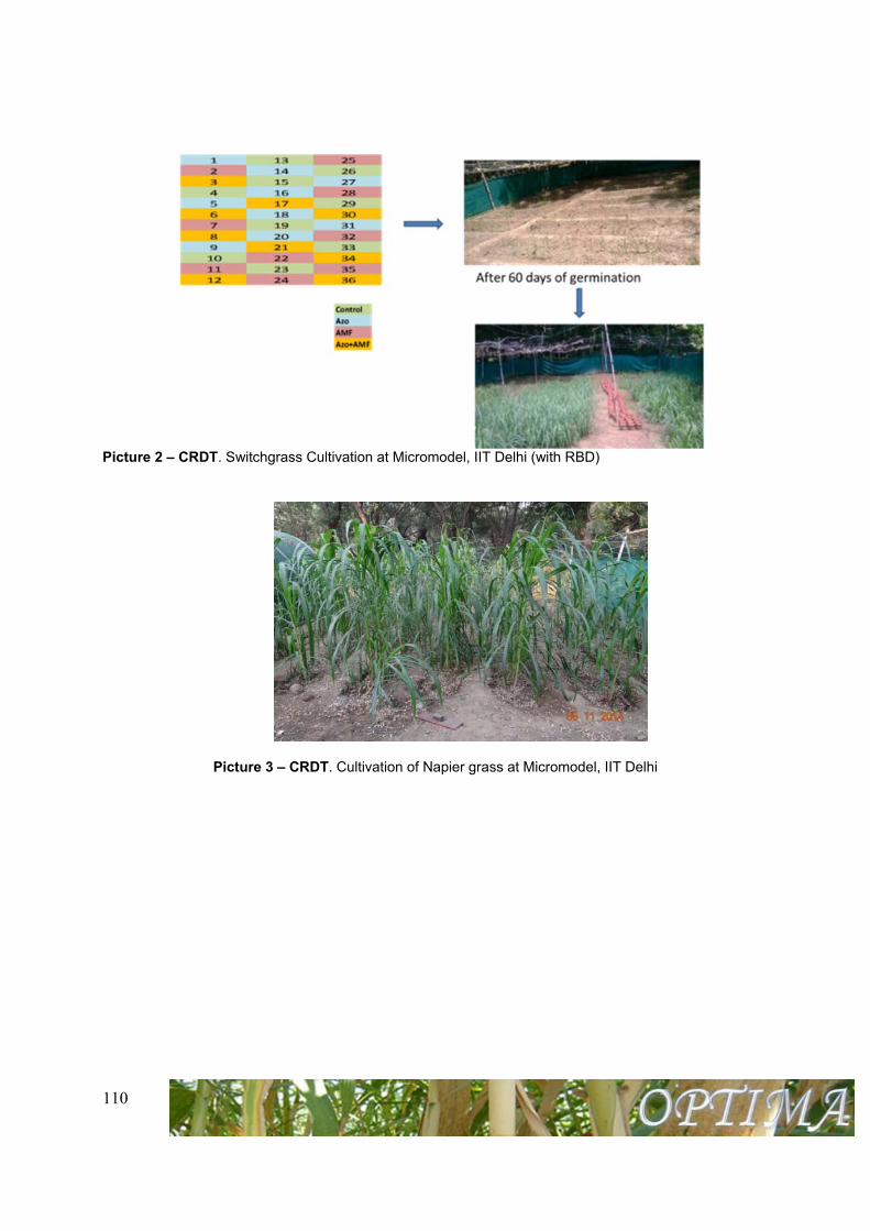
110
Picture 2 – CRDT. Switchgrass Cultivation at Micromodel, IIT Delhi (with RBD)
Picture 3 – CRDT. Cultivation of Napier grass at Micromodel, IIT Delhi
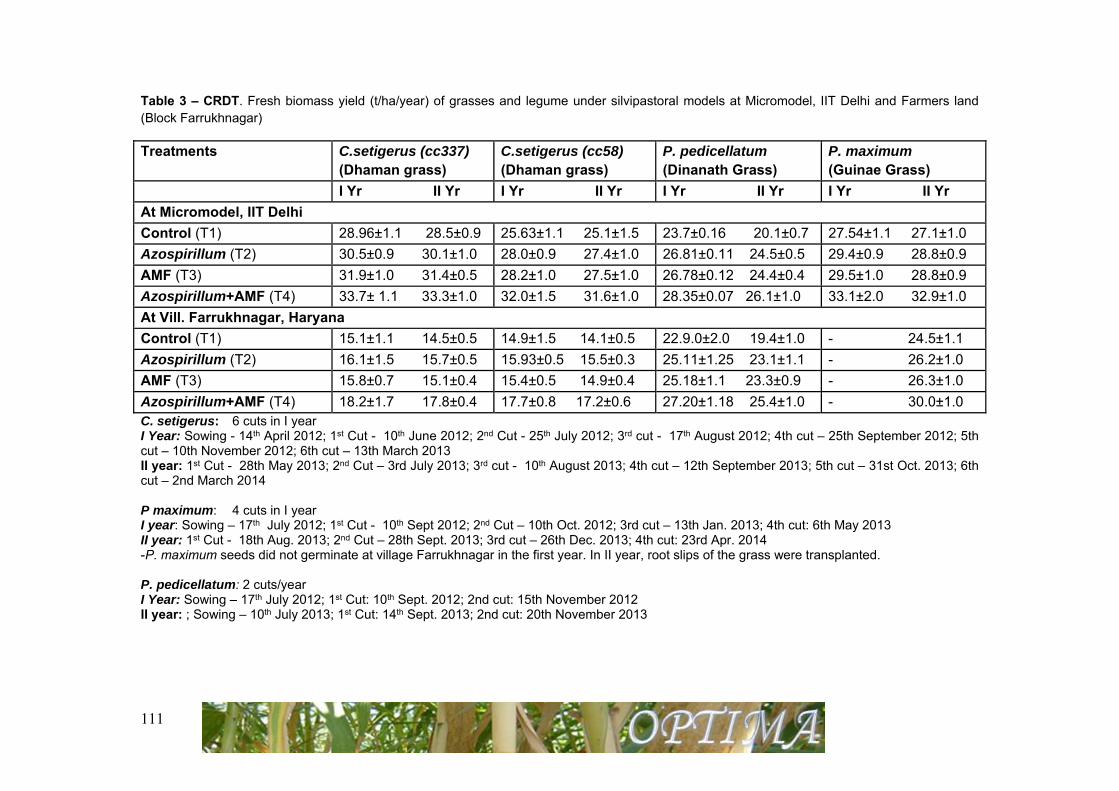
111
Table 3 – CRDT. Fresh biomass yield (t/ha/year) of grasses and legume under silvipastoral models at Micromodel, IIT Delhi and Farmers land (Block Farrukhnagar)
Treatments C.setigerus (cc337) (Dhaman grass)
C.setigerus (cc58) (Dhaman grass)
P. pedicellatum (Dinanath Grass)
P. maximum (Guinae Grass)
I Yr II Yr I Yr II Yr I Yr II Yr I Yr II Yr
At Micromodel, IIT Delhi
Control (T1) 28.96±1.1 28.5±0.9 25.63±1.1 25.1±1.5 23.7±0.16 20.1±0.7 27.54±1.1 27.1±1.0
Azospirillum (T2) 30.5±0.9 30.1±1.0 28.0±0.9 27.4±1.0 26.81±0.11 24.5±0.5 29.4±0.9 28.8±0.9
AMF (T3) 31.9±1.0 31.4±0.5 28.2±1.0 27.5±1.0 26.78±0.12 24.4±0.4 29.5±1.0 28.8±0.9
Azospirillum+AMF (T4) 33.7± 1.1 33.3±1.0 32.0±1.5 31.6±1.0 28.35±0.07 26.1±1.0 33.1±2.0 32.9±1.0
At Vill. Farrukhnagar, Haryana
Control (T1) 15.1±1.1 14.5±0.5 14.9±1.5 14.1±0.5 22.9.0±2.0 19.4±1.0 - 24.5±1.1
Azospirillum (T2) 16.1±1.5 15.7±0.5 15.93±0.5 15.5±0.3 25.11±1.25 23.1±1.1 - 26.2±1.0
AMF (T3) 15.8±0.7 15.1±0.4 15.4±0.5 14.9±0.4 25.18±1.1 23.3±0.9 - 26.3±1.0
Azospirillum+AMF (T4) 18.2±1.7 17.8±0.4 17.7±0.8 17.2±0.6 27.20±1.18 25.4±1.0 - 30.0±1.0 C. setigerus: 6 cuts in I year I Year: Sowing - 14th April 2012; 1st Cut - 10th June 2012; 2nd Cut - 25th July 2012; 3rd cut - 17th August 2012; 4th cut – 25th September 2012; 5th cut – 10th November 2012; 6th cut – 13th March 2013 II year: 1st Cut - 28th May 2013; 2nd Cut – 3rd July 2013; 3rd cut - 10th August 2013; 4th cut – 12th September 2013; 5th cut – 31st Oct. 2013; 6th cut – 2nd March 2014 P maximum: 4 cuts in I year I year: Sowing – 17th July 2012; 1st Cut - 10th Sept 2012; 2nd Cut – 10th Oct. 2012; 3rd cut – 13th Jan. 2013; 4th cut: 6th May 2013 II year: 1st Cut - 18th Aug. 2013; 2nd Cut – 28th Sept. 2013; 3rd cut – 26th Dec. 2013; 4th cut: 23rd Apr. 2014 -P. maximum seeds did not germinate at village Farrukhnagar in the first year. In II year, root slips of the grass were transplanted. P. pedicellatum: 2 cuts/year I Year: Sowing – 17th July 2012; 1st Cut: 10th Sept. 2012; 2nd cut: 15th November 2012 II year: ; Sowing – 10th July 2013; 1st Cut: 14th Sept. 2013; 2nd cut: 20th November 2013
112
Table 4 – CRDT. Fresh biomass yield (t/ha/year) of legumes under silvipastoral models at Micromodel, IIT Delhi and at field level (Block Farrukhnagar, Haryana)
Treatments Trifolium alexandrinum (Barseem)
At Micromodel, IIT Delhi
Trifolium resupinatum (Rijheka)
On Farmer’s field (Block Farrukhnagar)
I Year II Year I Year
Control 3.5±0.4 3.6±0.2 2.7±0.05
Rhizobium 4.1±0.2 4.5±0.4 3.1±0.2
AMF 4.3±0.2 4.8±0.4 3.2±0.3
Rhizobium +AMF 4.9±0.09 5.1±0.5 3.7±0.1
Trifolium alexandrinum: I year: Sowing: 19th Jan.. 2013 (3 cuts till May 2013); II Year: Sowing: 25th Jan.. 2014 (3 cuts till May 2014)
Trifolium resupinatum: I year: Sowing: 24th Jan.. 2013 (3 cuts till May 2013);
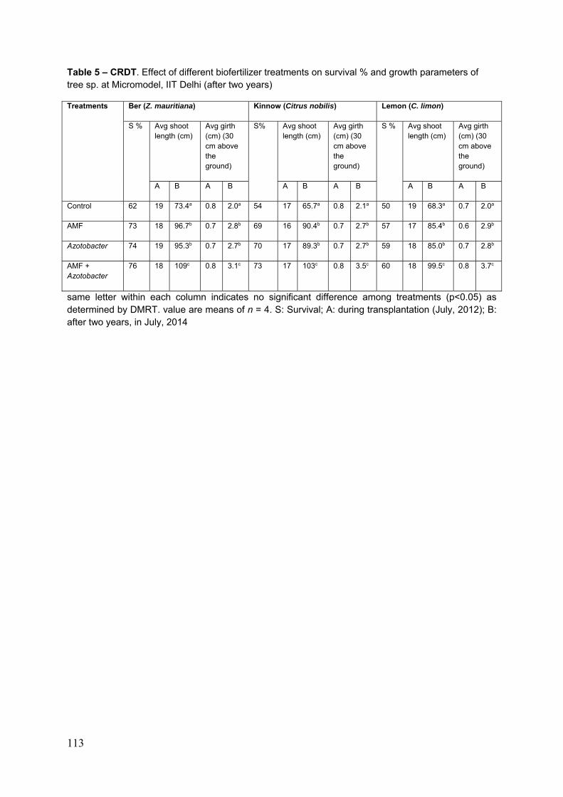
113
Table 5 – CRDT. Effect of different biofertilizer treatments on survival % and growth parameters of tree sp. at Micromodel, IIT Delhi (after two years)
Treatments Ber (Z. mauritiana) Kinnow (Citrus nobilis) Lemon (C. limon)
S % Avg shoot length (cm)
Avg girth (cm) (30 cm above the ground)
S% Avg shoot length (cm)
Avg girth (cm) (30 cm above the ground)
S % Avg shoot length (cm)
Avg girth (cm) (30 cm above the ground)
A B A B A B A B A B A B
Control 62 19 73.4a 0.8 2.0a 54 17 65.7a 0.8 2.1a 50 19 68.3a 0.7 2.0a
AMF 73 18 96.7b 0.7 2.8b 69 16 90.4b 0.7 2.7b 57 17 85.4b 0.6 2.9b
Azotobacter 74 19 95.3b 0.7 2.7b 70 17 89.3b 0.7 2.7b 59 18 85.0b 0.7 2.8b
AMF + Azotobacter
76 18 109c 0.8 3.1c 73 17 103c 0.8 3.5c 60 18 99.5c 0.8 3.7c
same letter within each column indicates no significant difference among treatments (p<0.05) as determined by DMRT. value are means of n = 4. S: Survival; A: during transplantation (July, 2012); B: after two years, in July, 2014
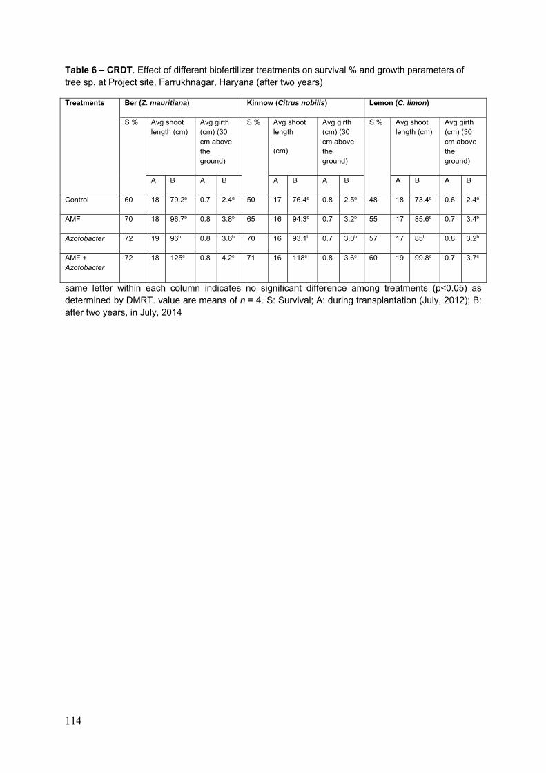
114
Table 6 – CRDT. Effect of different biofertilizer treatments on survival % and growth parameters of tree sp. at Project site, Farrukhnagar, Haryana (after two years)
Treatments Ber (Z. mauritiana) Kinnow (Citrus nobilis) Lemon (C. limon)
S % Avg shoot length (cm)
Avg girth (cm) (30 cm above the ground)
S % Avg shoot length
(cm)
Avg girth (cm) (30 cm above the ground)
S % Avg shoot length (cm)
Avg girth (cm) (30 cm above the ground)
A B A B A B A B A B A B
Control 60 18 79.2a 0.7 2.4a 50 17 76.4a 0.8 2.5a 48 18 73.4a 0.6 2.4a
AMF 70 18 96.7b 0.8 3.8b 65 16 94.3b 0.7 3.2b 55 17 85.6b 0.7 3.4b
Azotobacter 72 19 96b 0.8 3.6b 70 16 93.1b 0.7 3.0b 57 17 85b 0.8 3.2b
AMF + Azotobacter
72 18 125c 0.8 4.2c 71 16 118c 0.8 3.6c 60 19 99.8c 0.7 3.7c
same letter within each column indicates no significant difference among treatments (p<0.05) as determined by DMRT. value are means of n = 4. S: Survival; A: during transplantation (July, 2012); B: after two years, in July, 2014
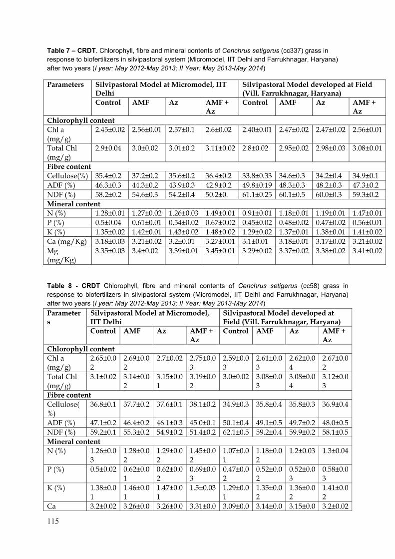
115
Table 7 – CRDT. Chlorophyll, fibre and mineral contents of Cenchrus setigerus (cc337) grass in response to biofertilizers in silvipastoral system (Micromodel, IIT Delhi and Farrukhnagar, Haryana) after two years (I year: May 2012-May 2013; II Year: May 2013-May 2014)
Parameters Silvipastoral Model at Micromodel, IIT Delhi
Silvipastoral Model developed at Field (Vill. Farrukhnagar, Haryana)
Control AMF Az AMF + Az
Control AMF Az AMF + Az
Chlorophyll content Chl a (mg/g)
2.45±0.02 2.56±0.01 2.57±0.1 2.6±0.02 2.40±0.01 2.47±0.02 2.47±0.02 2.56±0.01
Total Chl (mg/g)
2.9±0.04 3.0±0.02 3.01±0.2 3.11±0.02 2.8±0.02 2.95±0.02 2.98±0.03 3.08±0.01
Fibre content Cellulose(%) 35.4±0.2 37.2±0.2 35.6±0.2 36.4±0.2 33.8±0.33 34.6±0.3 34.2±0.4 34.9±0.1 ADF (%) 46.3±0.3 44.3±0.2 43.9±0.3 42.9±0.2 49.8±0.19 48.3±0.3 48.2±0.3 47.3±0.2 NDF (%) 58.2±0.2 54.6±0.3 54.2±0.4 50.2±0. 61.1±0.25 60.1±0.5 60.0±0.3 59.3±0.2 Mineral content N (%) 1.28±0.01 1.27±0.02 1.26±0.03 1.49±0.01 0.91±0.01 1.18±0.01 1.19±0.01 1.47±0.01 P (%) 0.5±0.04 0.61±0.01 0.54±0.02 0.67±0.02 0.45±0.02 0.48±0.02 0.47±0.02 0.56±0.01 K (%) 1.35±0.02 1.42±0.01 1.43±0.02 1.48±0.02 1.29±0.02 1.37±0.01 1.38±0.01 1.41±0.02 Ca (mg/Kg) 3.18±0.03 3.21±0.02 3.2±0.01 3.27±0.01 3.1±0.01 3.18±0.01 3.17±0.02 3.21±0.02 Mg (mg/Kg)
3.35±0.03 3.4±0.02 3.39±0.01 3.45±0.01 3.29±0.02 3.37±0.02 3.38±0.02 3.41±0.02
Table 8 - CRDT Chlorophyll, fibre and mineral contents of Cenchrus setigerus (cc58) grass in response to biofertilizers in silvipastoral system (Micromodel, IIT Delhi and Farrukhnagar, Haryana) after two years (I year: May 2012-May 2013; II Year: May 2013-May 2014)
Parameters
Silvipastoral Model at Micromodel, IIT Delhi
Silvipastoral Model developed at Field (Vill. Farrukhnagar, Haryana)
Control AMF Az AMF + Az
Control AMF Az AMF + Az
Chlorophyll content Chl a (mg/g)
2.65±0.02
2.69±0.02
2.7±0.02 2.75±0.03
2.59±0.03
2.61±0.03
2.62±0.04
2.67±0.02
Total Chl (mg/g)
3.1±0.02 3.14±0.02
3.15±0.01
3.19±0.02
3.0±0.02 3.08±0.03
3.08±0.04
3.12±0.03
Fibre content Cellulose(%)
36.8±0.1 37.7±0.2 37.6±0.1 38.1±0.2 34.9±0.3 35.8±0.4 35.8±0.3 36.9±0.4
ADF (%) 47.1±0.2 46.4±0.2 46.1±0.3 45.0±0.1 50.1±0.4 49.1±0.5 49.7±0.2 48.0±0.5 NDF (%) 59.2±0.1 55.3±0.2 54.9±0.2 51.4±0.2 62.1±0.5 59.2±0.4 59.9±0.2 58.1±0.5 Mineral content N (%) 1.26±0.0
3 1.28±0.02
1.29±0.02
1.45±0.02
1.07±0.01
1.18±0.02
1.2±0.03 1.3±0.04
P (%) 0.5±0.02 0.62±0.01
0.62±0.02
0.69±0.03
0.47±0.02
0.52±0.02
0.52±0.03
0.58±0.03
K (%) 1.38±0.01
1.46±0.01
1.47±0.01
1.5±0.03 1.29±0.01
1.35±0.02
1.36±0.02
1.41±0.02
Ca 3.2±0.02 3.26±0.0 3.26±0.0 3.31±0.0 3.09±0.0 3.14±0.0 3.15±0.0 3.2±0.02
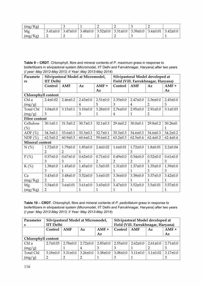
116
(mg/Kg) 3 1 2 2 3 2 Mg (mg/Kg)
3.41±0.02
3.47±0.02
3.48±0.02
3.52±0.02
3.31±0.02
3.39±0.03
3.4±0.01 3.42±0.01
Table 9 – CRDT. Chlorophyll, fibre and mineral contents of P. maximum grass in response to biofertilizers in silvipastoral system (Micromodel, IIT Delhi and Farrukhnagar, Haryana) after two years (I year: May 2012-May 2013; II Year: May 2013-May 2014)
Parameters
Silvipastoral Model at Micromodel, IIT Delhi
Silvipastoral Model developed at Field (Vill. Farrukhnagar, Haryana)
Control AMF Az AMF + Az
Control AMF Az AMF + Az
Chlorophyll content Chl a (mg/g)
2.4±0.02 2.46±0.2 2.43±0.04
2.51±0.05
2.35±0.03
2.47±0.04
2.36±0.02
2.45±0.03
Total Chl (mg/g)
3.04±0.03
3.15±0.1 3.10±0.03
3.28±0.01
2.76±0.04
2.95±0.01
2.91±0.02
3.1±0.03
Fibre content Cellulose (%)
30.1±0.1 31.5±0.2 30.7±0.3 32.1±0.3 29.4±0.2 30.0±0.1 29.8±0.2 30.26±0.1
ADF (%) 34.3±0.1 33.6±0.1 33.3±0.3 32.7±0.1 35.3±0.3 34.6±0.3 34.6±0.3 34.2±0.2 NDF (%) 62.5±0.2 60.9±0.3 60.6±0.2 59.6±0.2 63.2±0.3 62.5±0.4 62.4±0.2 62.4±0.4 Mineral content N (%) 1.72±0.0
2 1.79±0.02
1.85±0.01
2.4±0.02 1.6±0.01 1.72±0.03
1.8±0.01 2.2±0.04
P (%) 0.57±0.03
0.67±0.03
0.62±0.01
0.71±0.02
0.49±0.02
0.54±0.02
0.52±0.03
0.61±0.03
K (%) 1.38±0.03
1.45±0.01
1.45±0.02
1.5±0.03 1.31±0.01
1.37±0.01
1.35±0.03
1.39±0.03
Ca (mg/Kg)
3.43±0.02
3.48±0.02
3.52±0.01
3.6±0.03 3.36±0.01
3.38±0.01
3.37±0.01
3.42±0.01
Mg (mg/Kg)
3.54±0.02
3.6±0.01 3.61±0.01
3.65±0.01
3.47±0.01
3.52±0.01
3.5±0.01 3.57±0.01
Table 10 – CRDT. Chlorophyll, fibre and mineral contents of P. pedicillatum grass in response to biofertilizers in silvipastoral system (Micromodel, IIT Delhi and Farrukhnagar, Haryana) after two years (I year: May 2012-May 2013; II Year: May 2013-May 2014)
Parameters
Silvipastoral Model at Micromodel, IIT Delhi
Silvipastoral Model developed at Field (Vill. Farrukhnagar, Haryana)
Control AMF Az AMF + Az
Control AMF Az AMF + Az
Chlorophyll content Chl a (mg/g)
2.7±0.03 2.78±0.01
2.72±0.04
2.85±0.03
2.55±0.03
2.62±0.01
2.61±0.02
2.71±0.03
Total Chl (mg/g)
3.18±0.02
3.31±0.02
3.26±0.02
3.38±0.01
3.08±0.03
3.11±0.01
3.1±0.02 3.17±0.03
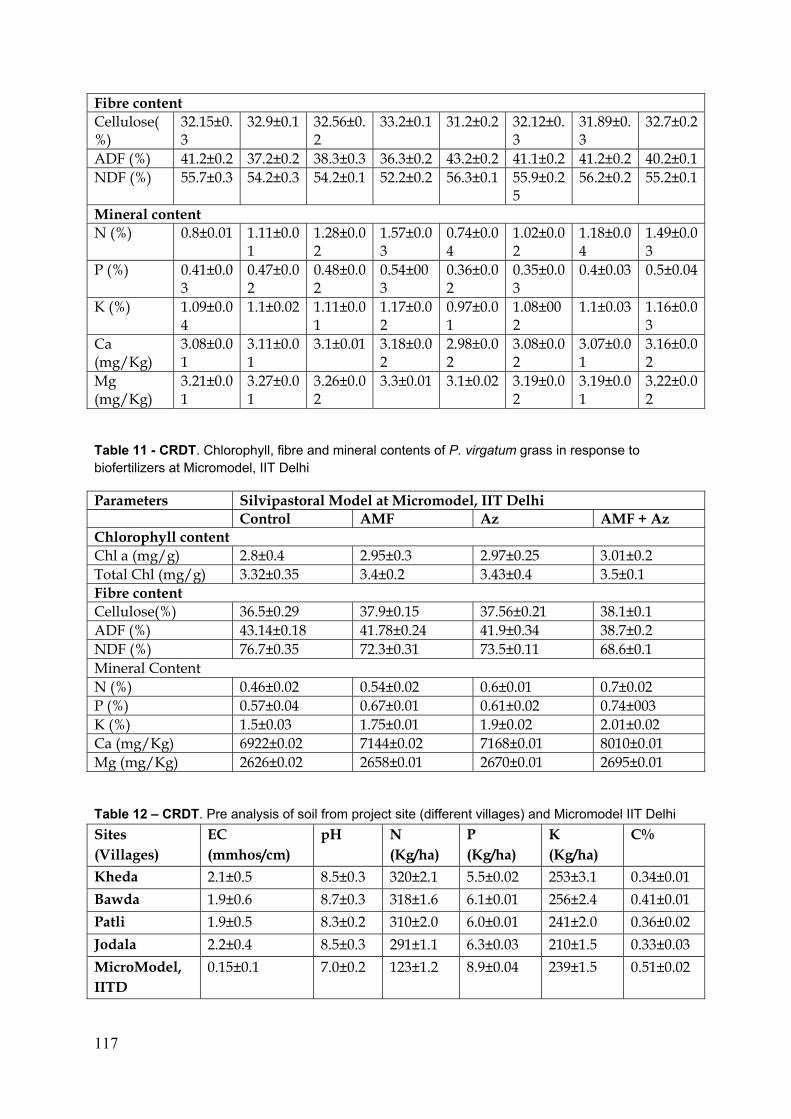
117
Fibre content Cellulose(%)
32.15±0.3
32.9±0.1 32.56±0.2
33.2±0.1 31.2±0.2 32.12±0.3
31.89±0.3
32.7±0.2
ADF (%) 41.2±0.2 37.2±0.2 38.3±0.3 36.3±0.2 43.2±0.2 41.1±0.2 41.2±0.2 40.2±0.1 NDF (%) 55.7±0.3 54.2±0.3 54.2±0.1 52.2±0.2 56.3±0.1 55.9±0.2
5 56.2±0.2 55.2±0.1
Mineral content N (%) 0.8±0.01 1.11±0.0
1 1.28±0.02
1.57±0.03
0.74±0.04
1.02±0.02
1.18±0.04
1.49±0.03
P (%) 0.41±0.03
0.47±0.02
0.48±0.02
0.54±003
0.36±0.02
0.35±0.03
0.4±0.03 0.5±0.04
K (%) 1.09±0.04
1.1±0.02 1.11±0.01
1.17±0.02
0.97±0.01
1.08±002
1.1±0.03 1.16±0.03
Ca (mg/Kg)
3.08±0.01
3.11±0.01
3.1±0.01 3.18±0.02
2.98±0.02
3.08±0.02
3.07±0.01
3.16±0.02
Mg (mg/Kg)
3.21±0.01
3.27±0.01
3.26±0.02
3.3±0.01 3.1±0.02 3.19±0.02
3.19±0.01
3.22±0.02
Table 11 - CRDT. Chlorophyll, fibre and mineral contents of P. virgatum grass in response to biofertilizers at Micromodel, IIT Delhi
Parameters Silvipastoral Model at Micromodel, IIT Delhi Control AMF Az AMF + Az Chlorophyll content Chl a (mg/g) 2.8±0.4 2.95±0.3 2.97±0.25 3.01±0.2 Total Chl (mg/g) 3.32±0.35 3.4±0.2 3.43±0.4 3.5±0.1 Fibre content Cellulose(%) 36.5±0.29 37.9±0.15 37.56±0.21 38.1±0.1 ADF (%) 43.14±0.18 41.78±0.24 41.9±0.34 38.7±0.2 NDF (%) 76.7±0.35 72.3±0.31 73.5±0.11 68.6±0.1 Mineral Content N (%) 0.46±0.02 0.54±0.02 0.6±0.01 0.7±0.02 P (%) 0.57±0.04 0.67±0.01 0.61±0.02 0.74±003 K (%) 1.5±0.03 1.75±0.01 1.9±0.02 2.01±0.02 Ca (mg/Kg) 6922±0.02 7144±0.02 7168±0.01 8010±0.01 Mg (mg/Kg) 2626±0.02 2658±0.01 2670±0.01 2695±0.01
Table 12 – CRDT. Pre analysis of soil from project site (different villages) and Micromodel IIT Delhi
Sites (Villages)
EC (mmhos/cm)
pH N (Kg/ha)
P (Kg/ha)
K (Kg/ha)
C%
Kheda 2.1±0.5 8.5±0.3 320±2.1 5.5±0.02 253±3.1 0.34±0.01
Bawda 1.9±0.6 8.7±0.3 318±1.6 6.1±0.01 256±2.4 0.41±0.01
Patli 1.9±0.5 8.3±0.2 310±2.0 6.0±0.01 241±2.0 0.36±0.02
Jodala 2.2±0.4 8.5±0.3 291±1.1 6.3±0.03 210±1.5 0.33±0.03
MicroModel, IITD
0.15±0.1 7.0±0.2 123±1.2 8.9±0.04 239±1.5 0.51±0.02
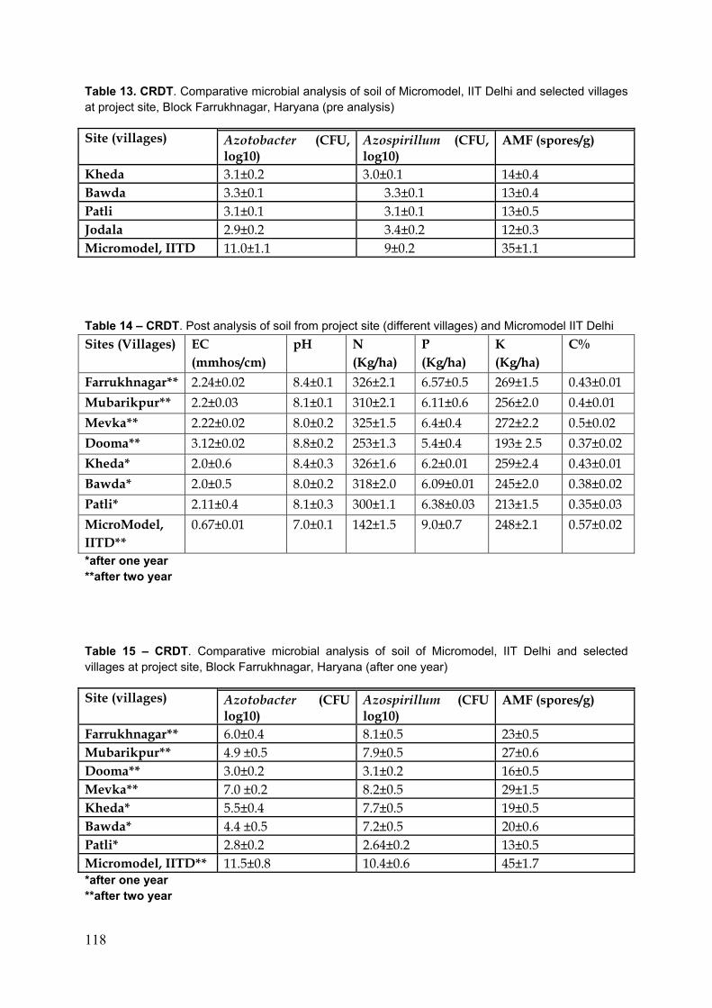
118
Table 13. CRDT. Comparative microbial analysis of soil of Micromodel, IIT Delhi and selected villages at project site, Block Farrukhnagar, Haryana (pre analysis)
Site (villages) Azotobacter (CFU, log10)
Azospirillum (CFU, log10)
AMF (spores/g)
Kheda 3.1±0.2 3.0±0.1 14±0.4 Bawda 3.3±0.1 3.3±0.1 13±0.4 Patli 3.1±0.1 3.1±0.1 13±0.5 Jodala 2.9±0.2 3.4±0.2 12±0.3 Micromodel, IITD 11.0±1.1 9±0.2 35±1.1
Table 14 – CRDT. Post analysis of soil from project site (different villages) and Micromodel IIT Delhi
Sites (Villages) EC (mmhos/cm)
pH N (Kg/ha)
P (Kg/ha)
K (Kg/ha)
C%
Farrukhnagar** 2.24±0.02 8.4±0.1 326±2.1 6.57±0.5 269±1.5 0.43±0.01
Mubarikpur** 2.2±0.03 8.1±0.1 310±2.1 6.11±0.6 256±2.0 0.4±0.01
Mevka** 2.22±0.02 8.0±0.2 325±1.5 6.4±0.4 272±2.2 0.5±0.02
Dooma** 3.12±0.02 8.8±0.2 253±1.3 5.4±0.4 193± 2.5 0.37±0.02
Kheda* 2.0±0.6 8.4±0.3 326±1.6 6.2±0.01 259±2.4 0.43±0.01
Bawda* 2.0±0.5 8.0±0.2 318±2.0 6.09±0.01 245±2.0 0.38±0.02
Patli* 2.11±0.4 8.1±0.3 300±1.1 6.38±0.03 213±1.5 0.35±0.03
MicroModel, IITD**
0.67±0.01 7.0±0.1 142±1.5 9.0±0.7 248±2.1 0.57±0.02
*after one year **after two year
Table 15 – CRDT. Comparative microbial analysis of soil of Micromodel, IIT Delhi and selected villages at project site, Block Farrukhnagar, Haryana (after one year)
Site (villages) Azotobacter (CFU log10)
Azospirillum (CFU log10)
AMF (spores/g)
Farrukhnagar** 6.0±0.4 8.1±0.5 23±0.5 Mubarikpur** 4.9 ±0.5 7.9±0.5 27±0.6 Dooma** 3.0±0.2 3.1±0.2 16±0.5 Mevka** 7.0 ±0.2 8.2±0.5 29±1.5 Kheda* 5.5±0.4 7.7±0.5 19±0.5 Bawda* 4.4 ±0.5 7.2±0.5 20±0.6 Patli* 2.8±0.2 2.64±0.2 13±0.5 Micromodel, IITD** 11.5±0.8 10.4±0.6 45±1.7 *after one year **after two year
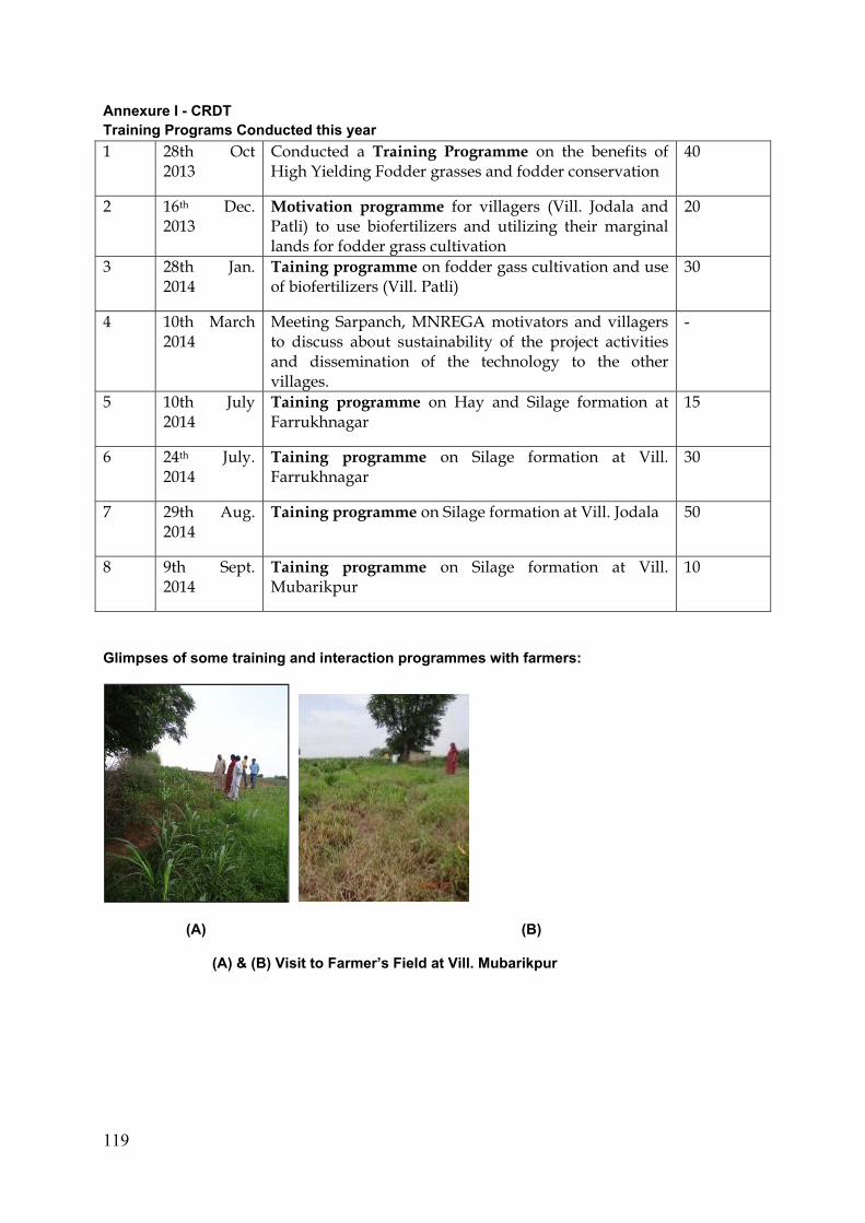
119
Annexure I - CRDT Training Programs Conducted this year
1 28th Oct 2013
Conducted a Training Programme on the benefits of High Yielding Fodder grasses and fodder conservation
40
2 16th Dec. 2013
Motivation programme for villagers (Vill. Jodala and Patli) to use biofertilizers and utilizing their marginal lands for fodder grass cultivation
20
3 28th Jan. 2014
Taining programme on fodder gass cultivation and use of biofertilizers (Vill. Patli)
30
4 10th March 2014
Meeting Sarpanch, MNREGA motivators and villagers to discuss about sustainability of the project activities and dissemination of the technology to the other villages.
-
5 10th July 2014
Taining programme on Hay and Silage formation at Farrukhnagar
15
6 24th July. 2014
Taining programme on Silage formation at Vill. Farrukhnagar
30
7 29th Aug. 2014
Taining programme on Silage formation at Vill. Jodala 50
8 9th Sept. 2014
Taining programme on Silage formation at Vill. Mubarikpur
10
Glimpses of some training and interaction programmes with farmers:
(A) (B)
(A) & (B) Visit to Farmer’s Field at Vill. Mubarikpur
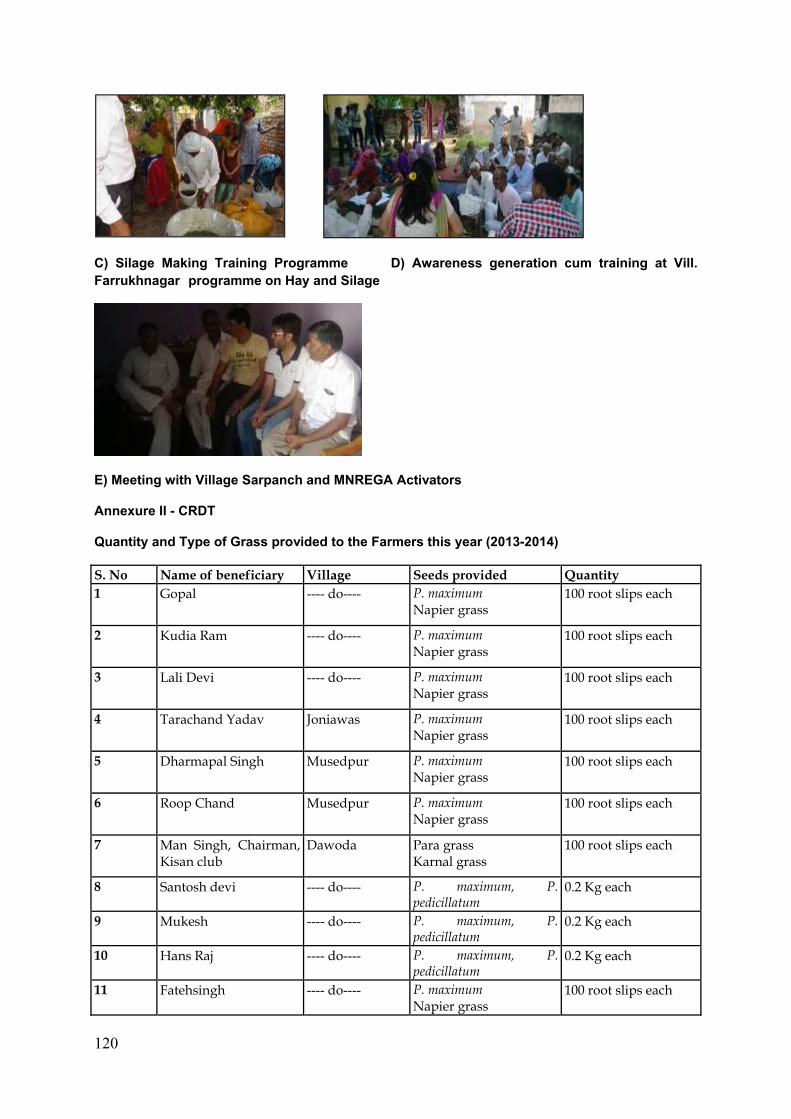
120
C) Silage Making Training Programme D) Awareness generation cum training at Vill. Farrukhnagar programme on Hay and Silage
E) Meeting with Village Sarpanch and MNREGA Activators
Annexure II - CRDT
Quantity and Type of Grass provided to the Farmers this year (2013-2014)
S. No Name of beneficiary Village Seeds provided Quantity 1 Gopal ---- do---- P. maximum
Napier grass 100 root slips each
2 Kudia Ram ---- do---- P. maximum Napier grass
100 root slips each
3 Lali Devi ---- do---- P. maximum Napier grass
100 root slips each
4 Tarachand Yadav Joniawas P. maximum Napier grass
100 root slips each
5 Dharmapal Singh Musedpur P. maximum Napier grass
100 root slips each
6 Roop Chand Musedpur P. maximum Napier grass
100 root slips each
7 Man Singh, Chairman, Kisan club
Dawoda Para grass Karnal grass
100 root slips each
8 Santosh devi ---- do---- P. maximum, P. pedicillatum
0.2 Kg each
9 Mukesh ---- do---- P. maximum, P. pedicillatum
0.2 Kg each
10 Hans Raj ---- do---- P. maximum, P. pedicillatum
0.2 Kg each
11 Fatehsingh ---- do---- P. maximum Napier grass
100 root slips each
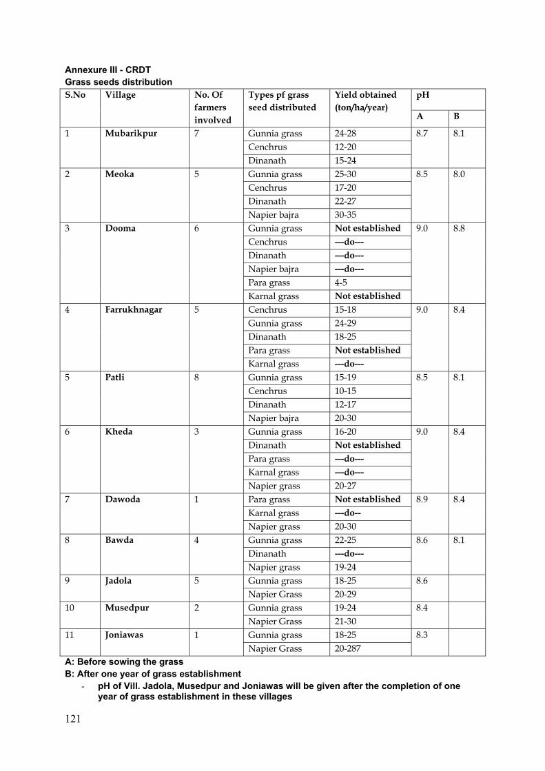
121
Annexure III - CRDT Grass seeds distribution S.No Village No. Of
farmers involved
Types pf grass seed distributed
Yield obtained (ton/ha/year)
pH
A B
1 Mubarikpur 7 Gunnia grass 24-28 8.7 8.1 Cenchrus 12-20 Dinanath 15-24
2 Meoka 5 Gunnia grass 25-30 8.5 8.0 Cenchrus 17-20 Dinanath 22-27 Napier bajra 30-35
3 Dooma 6 Gunnia grass Not established 9.0 8.8 Cenchrus ---do--- Dinanath ---do--- Napier bajra ---do--- Para grass 4-5 Karnal grass Not established
4 Farrukhnagar 5 Cenchrus 15-18 9.0 8.4 Gunnia grass 24-29 Dinanath 18-25 Para grass Not established Karnal grass ---do---
5 Patli 8 Gunnia grass 15-19 8.5 8.1 Cenchrus 10-15 Dinanath 12-17 Napier bajra 20-30
6 Kheda 3 Gunnia grass 16-20 9.0 8.4 Dinanath Not established Para grass ---do--- Karnal grass ---do--- Napier grass 20-27
7 Dawoda 1 Para grass Not established 8.9 8.4 Karnal grass ---do-- Napier grass 20-30
8 Bawda 4 Gunnia grass 22-25 8.6 8.1 Dinanath ---do--- Napier grass 19-24
9 Jadola 5 Gunnia grass 18-25 8.6 Napier Grass 20-29
10 Musedpur 2 Gunnia grass 19-24 8.4 Napier Grass 21-30
11 Joniawas 1 Gunnia grass 18-25 8.3 Napier Grass 20-287
A: Before sowing the grass B: After one year of grass establishment
- pH of Vill. Jadola, Musedpur and Joniawas will be given after the completion of one year of grass establishment in these villages
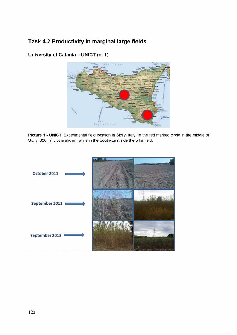
122
Task 4.2 Productivity in marginal large fields University of Catania – UNICT (n. 1)
Picture 1 - UNICT. Experimental field location in Sicily, Italy. In the red marked circle in the middle of Sicily, 320 m2 plot is shown, while in the South-East side the 5 ha field.
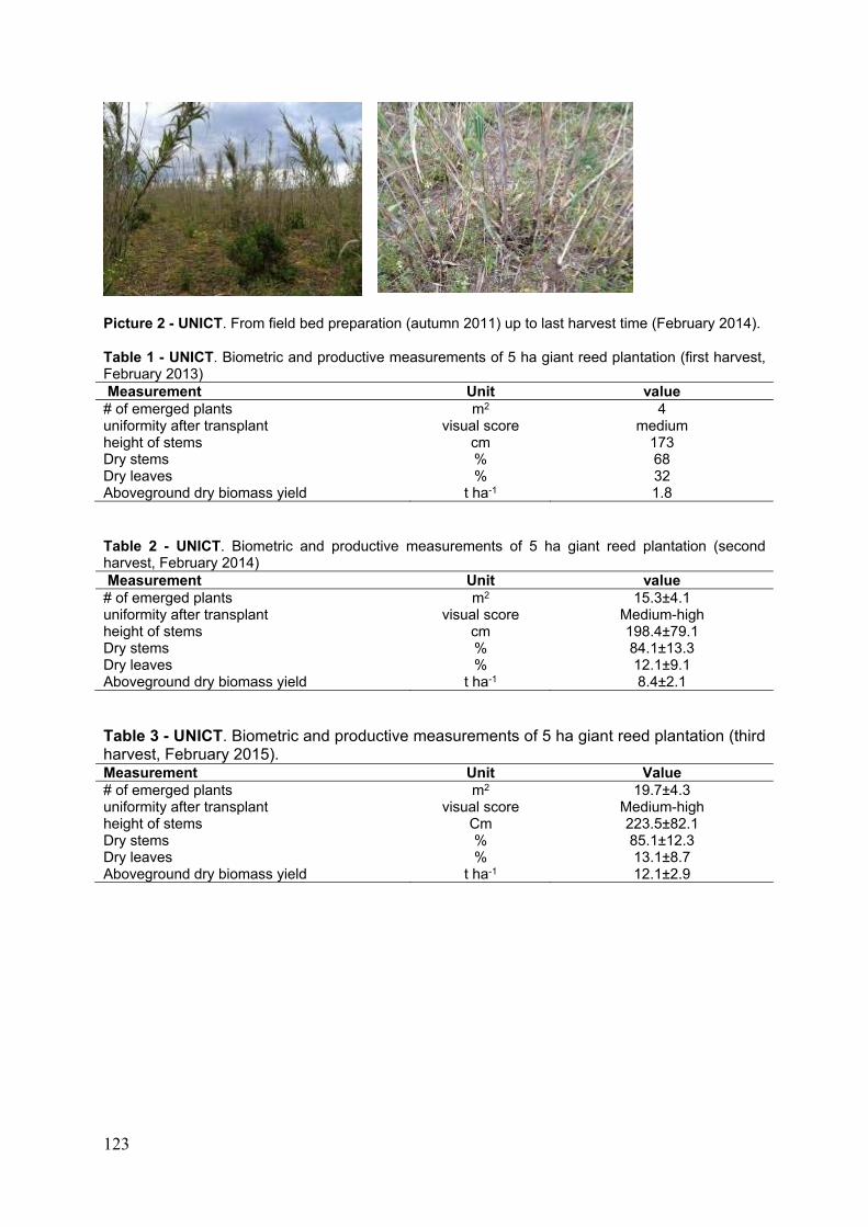
123
Picture 2 - UNICT. From field bed preparation (autumn 2011) up to last harvest time (February 2014).
Table 1 - UNICT. Biometric and productive measurements of 5 ha giant reed plantation (first harvest, February 2013) Measurement Unit value # of emerged plants m2 4 uniformity after transplant visual score medium height of stems cm 173 Dry stems % 68 Dry leaves % 32 Aboveground dry biomass yield t ha-1 1.8
Table 2 - UNICT. Biometric and productive measurements of 5 ha giant reed plantation (second harvest, February 2014) Measurement Unit value # of emerged plants m2 15.3±4.1 uniformity after transplant visual score Medium-high height of stems cm 198.4±79.1 Dry stems % 84.1±13.3 Dry leaves % 12.1±9.1 Aboveground dry biomass yield t ha-1 8.4±2.1
Table 3 - UNICT. Biometric and productive measurements of 5 ha giant reed plantation (third harvest, February 2015). Measurement Unit Value # of emerged plants m2 19.7±4.3 uniformity after transplant visual score Medium-high height of stems Cm 223.5±82.1 Dry stems % 85.1±12.3 Dry leaves % 13.1±8.7 Aboveground dry biomass yield t ha-1 12.1±2.9
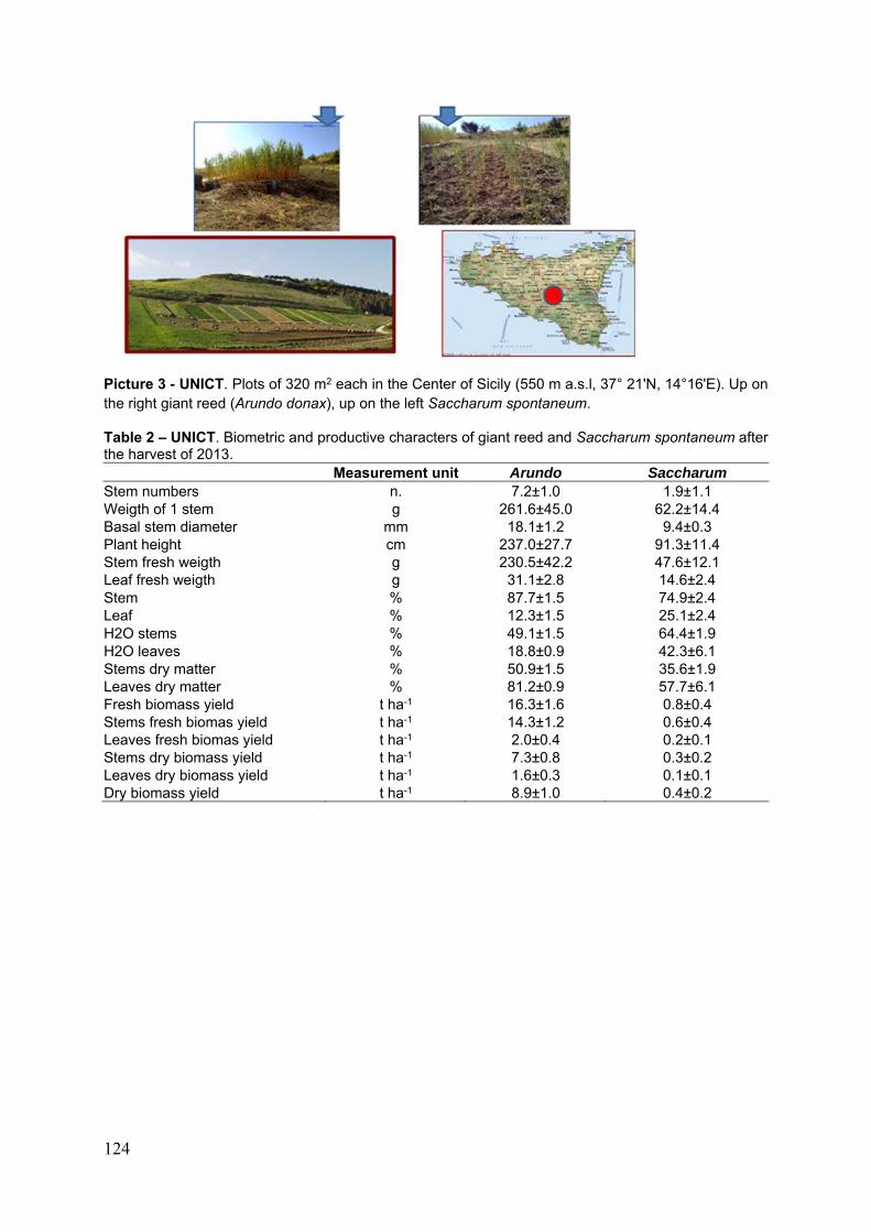
124
Picture 3 - UNICT. Plots of 320 m2 each in the Center of Sicily (550 m a.s.l, 37° 21'N, 14°16'E). Up on the right giant reed (Arundo donax), up on the left Saccharum spontaneum.
Table 2 – UNICT. Biometric and productive characters of giant reed and Saccharum spontaneum after the harvest of 2013.
Measurement unit Arundo Saccharum Stem numbers n. 7.2±1.0 1.9±1.1 Weigth of 1 stem g 261.6±45.0 62.2±14.4 Basal stem diameter mm 18.1±1.2 9.4±0.3 Plant height cm 237.0±27.7 91.3±11.4 Stem fresh weigth g 230.5±42.2 47.6±12.1 Leaf fresh weigth g 31.1±2.8 14.6±2.4 Stem % 87.7±1.5 74.9±2.4 Leaf % 12.3±1.5 25.1±2.4 H2O stems % 49.1±1.5 64.4±1.9 H2O leaves % 18.8±0.9 42.3±6.1 Stems dry matter % 50.9±1.5 35.6±1.9 Leaves dry matter % 81.2±0.9 57.7±6.1 Fresh biomass yield t ha-1 16.3±1.6 0.8±0.4 Stems fresh biomas yield t ha-1 14.3±1.2 0.6±0.4 Leaves fresh biomas yield t ha-1 2.0±0.4 0.2±0.1 Stems dry biomass yield t ha-1 7.3±0.8 0.3±0.2 Leaves dry biomass yield t ha-1 1.6±0.3 0.1±0.1 Dry biomass yield t ha-1 8.9±1.0 0.4±0.2
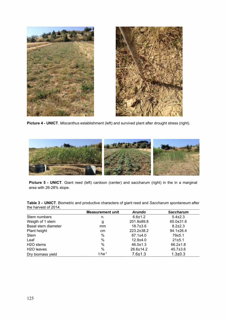
125
Picture 4 - UNICT. Miscanthus establishment (left) and survived plant after drought stress (right).
Picture 5 - UNICT. Giant reed (left) cardoon (center) and saccharum (right) in the in a marginal area with 26-28% slope.
Table 3 – UNICT. Biometric and productive characters of giant reed and Saccharum spontaneum after the harvest of 2014.
Measurement unit Arundo Saccharum Stem numbers n. 6.6±1.2 5.4±2.3 Weigth of 1 stem g 201.8±89.8 65.0±31.6 Basal stem diameter mm 18.7±3.6 8.2±2.3 Plant height cm 223.2±38.2 94.1±26.4 Stem % 87.1±4.0 79±5.1 Leaf % 12.9±4.0 21±5.1 H2O stems % 46.0±1.3 66.2±1.8 H2O leaves % 26.6±14.2 45.7±3.6 Dry biomass yield t ha-1 7.6±1.3 1.3±0.3
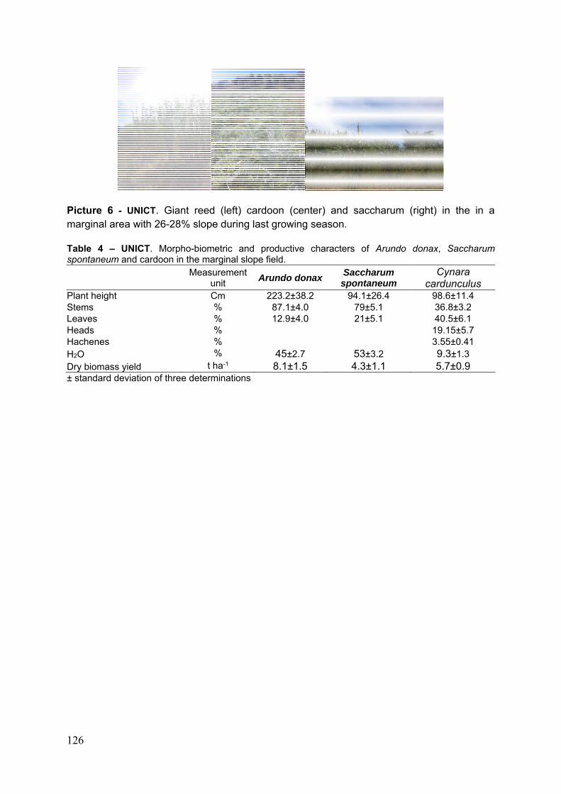
126
Picture 6 - UNICT. Giant reed (left) cardoon (center) and saccharum (right) in the in a marginal area with 26-28% slope during last growing season.
Table 4 – UNICT. Morpho-biometric and productive characters of Arundo donax, Saccharum spontaneum and cardoon in the marginal slope field.
Measurement
unit Arundo donax
Saccharum spontaneum
Cynara cardunculus
Plant height Cm 223.2±38.2 94.1±26.4 98.6±11.4 Stems % 87.1±4.0 79±5.1 36.8±3.2 Leaves % 12.9±4.0 21±5.1 40.5±6.1 Heads % 19.15±5.7Hachenes % 3.55±0.41 H2O % 45±2.7 53±3.2 9.3±1.3 Dry biomass yield t ha-1 8.1±1.5 4.3±1.1 5.7±0.9 ± standard deviation of three determinations
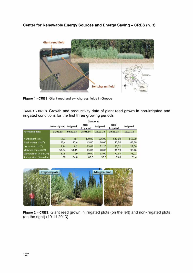
127
Center for Renewable Energy Sources and Energy Saving – CRES (n. 3)
Figure 1 - CRES. Giant reed and switchgrass fields in Greece
Table 1 - CRES. Growth and productivity data of giant reed grown in non-irrigated and irrigated conditions for the first three growing periods
Figure 2 – CRES. Giant reed grown in irrigated plots (on the left) and non-irrigated plots (on the right) (19.11.2013)
Harvesting date: 01.02.13 03.02.13 25.01.14 25.01.14 19.01.15 19.01.15
Plant height (cm) 391 414 400,00 506,00 540,00 616,00
Fresh matter (t ha‐1) 15,4 17,4 45,00 60,00 40,50 45,50
Dry matter (t ha‐1) 7,14 8,5 25,65 31,20 25,52 28,00
Moisture content (%) 53,64 51,15 43,00 48,00 36,99 38,46
Stem portion (% on f.m) 87,5 90 90,00 93,00 70,37 73,01
Stem portion (% on d.m) 80 84,8 86,0 90,0 59,6 61,4
Giant reed
Non‐irrigated IrrigatedNon‐
irrigated
Non‐
irrigatedIrrigatedIrrigated
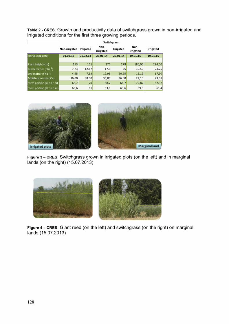
128
Table 2 - CRES. Growth and productivity data of switchgrass grown in non-irrigated and irrigated conditions for the first three growing periods.
Figure 3 – CRES. Switchgrass grown in irrigated plots (on the left) and in marginal lands (on the right) (15.07.2013)
Figure 4 – CRES. Giant reed (on the left) and switchgrass (on the right) on marginal lands (15.07.2013)
Harvesting date: 01.02.13 01.02.14 25.01.14 25.01.14 19.01.15 19.01.15
Plant height (cm) 153 151 275 278 186,00 294,00
Fresh matter (t ha‐1) 7,73 12,47 17,5 25 19,50 23,25
Dry matter (t ha‐1) 4,95 7,63 12,95 20,25 15,19 17,90
Moisture content (%) 36,00 38,00 36,00 36,00 22,10 23,01
Stem portion (% on f.m) 68,7 70 68,7 68,7 72,87 82,37
Stem portion (% on d.m) 63,6 61 63,6 63,6 69,0 61,4
Switchgrass
Non‐irrigated IrrigatedNon‐
irrigatedIrrigated
Non‐
irrigatedIrrigated
129
Istituto per il Sistema Produzione Animale in Ambiente Mediterraneo – CNR-ISPAAM (n. 8)
Table 1 – CNR-ISPAAM. Plants, stalks and shoots m-2 and morphological traits. Plant height is the average height of main stalks. *=harvested in February 2014; **= harvested in August 2014.
Species
Initial No of plants
(No m-
2)
Plant height (cm)
No of stalks
(No m-2)
No of nodes
(No m-2)
Stalk diameter (mm)
Basal Medium Distal
A. donax* 2 301 18 38.5 15.6 12.0 4.6
M. x giganteus* 2 201 14 14.5 10.4 7.8 3.6
Table 2 – CNR-ISPAAM. Dry matter yield, dry matter partitioning among organs and dry matter content in giant reed, miscanthus and cardoon. *=harvested in February 2014; **= harvested in August 2014.
Species
Biomass yield Biomass partitioning
(% of plant DM)
Dry matter content
(%)
DMY per
plant
(g)
DMY
(t ha-1
) Leaves Stems Heads Leaves Stems Heads
A. donax* 142.7 24.6 21.5 78.5 - 66 42 -
M. x giganteus* - 8.9 31.5 68.4 0.1 73 43 76
C. cardunculus** 2269.7 23.0 27.5 39.4 33.2 79.6 49.5 79.6
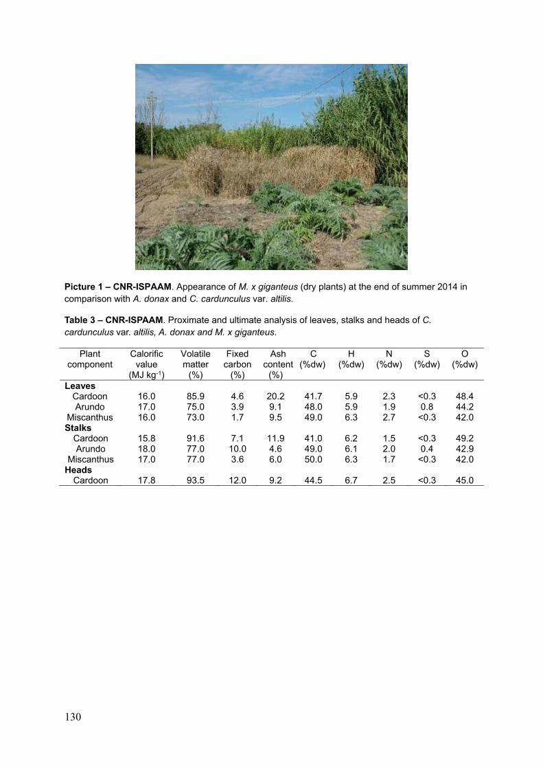
130
Picture 1 – CNR-ISPAAM. Appearance of M. x giganteus (dry plants) at the end of summer 2014 in comparison with A. donax and C. cardunculus var. altilis.
Table 3 – CNR-ISPAAM. Proximate and ultimate analysis of leaves, stalks and heads of C. cardunculus var. altilis, A. donax and M. x giganteus.
Plant component
Calorific value
(MJ kg-1)
Volatile matter
(%)
Fixed carbon
(%)
Ash content
(%)
C (%dw)
H (%dw)
N (%dw)
S (%dw)
O (%dw)
Leaves Cardoon 16.0 85.9 4.6 20.2 41.7 5.9 2.3 <0.3 48.4 Arundo 17.0 75.0 3.9 9.1 48.0 5.9 1.9 0.8 44.2
Miscanthus 16.0 73.0 1.7 9.5 49.0 6.3 2.7 <0.3 42.0Stalks
Cardoon 15.8 91.6 7.1 11.9 41.0 6.2 1.5 <0.3 49.2Arundo 18.0 77.0 10.0 4.6 49.0 6.1 2.0 0.4 42.9
Miscanthus 17.0 77.0 3.6 6.0 50.0 6.3 1.7 <0.3 42.0 Heads
Cardoon 17.8 93.5 12.0 9.2 44.5 6.7 2.5 <0.3 45.0
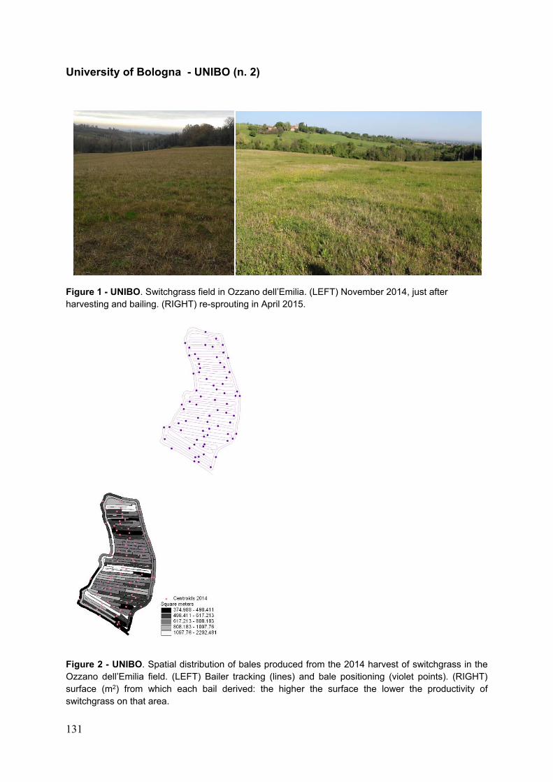
131
University of Bologna - UNIBO (n. 2)
Figure 1 - UNIBO. Switchgrass field in Ozzano dell’Emilia. (LEFT) November 2014, just after harvesting and bailing. (RIGHT) re-sprouting in April 2015.
Figure 2 - UNIBO. Spatial distribution of bales produced from the 2014 harvest of switchgrass in the Ozzano dell’Emilia field. (LEFT) Bailer tracking (lines) and bale positioning (violet points). (RIGHT) surface (m2) from which each bail derived: the higher the surface the lower the productivity of switchgrass on that area.
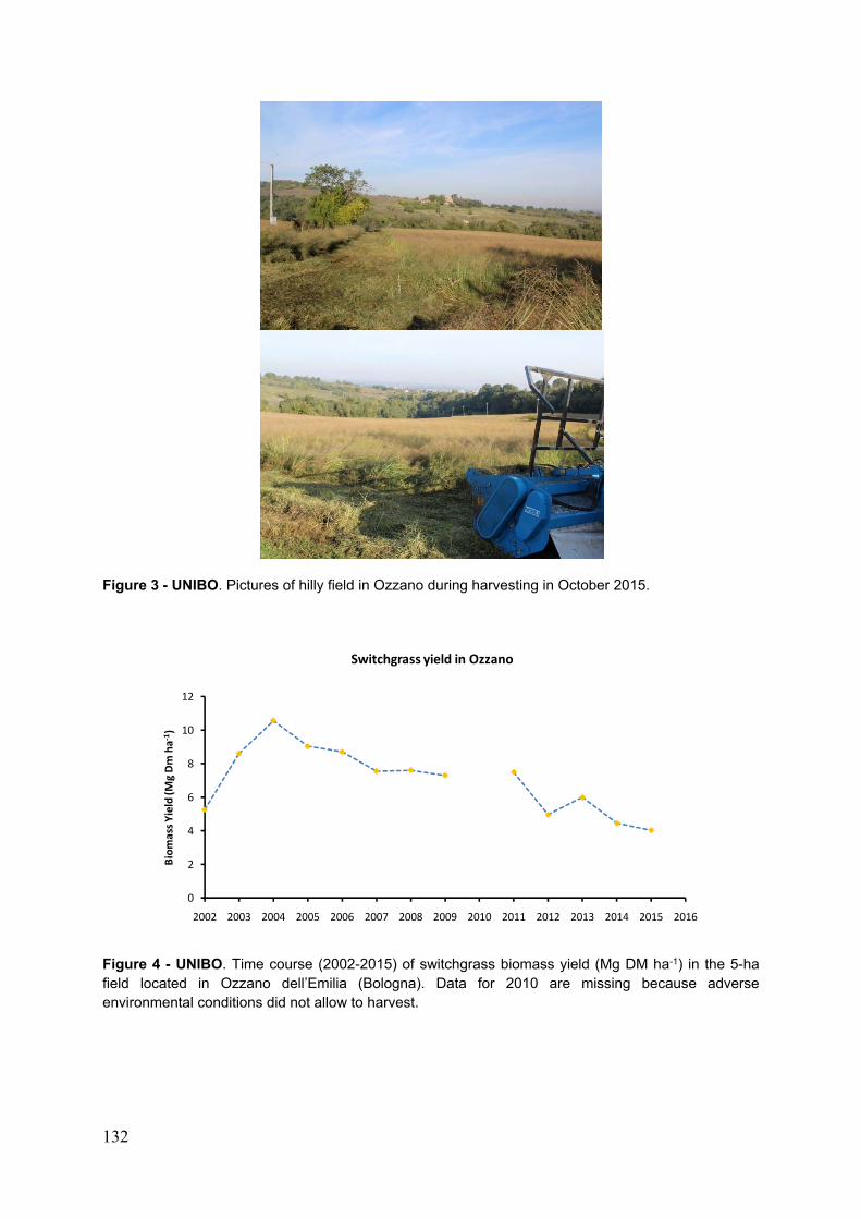
132
Figure 3 - UNIBO. Pictures of hilly field in Ozzano during harvesting in October 2015.
Figure 4 - UNIBO. Time course (2002-2015) of switchgrass biomass yield (Mg DM ha-1) in the 5-ha field located in Ozzano dell’Emilia (Bologna). Data for 2010 are missing because adverse environmental conditions did not allow to harvest.
0
2
4
6
8
10
12
2002 2003 2004 2005 2006 2007 2008 2009 2010 2011 2012 2013 2014 2015 2016
Biomass Yield (M
g Dm ha‐
1)
Switchgrass yield in Ozzano
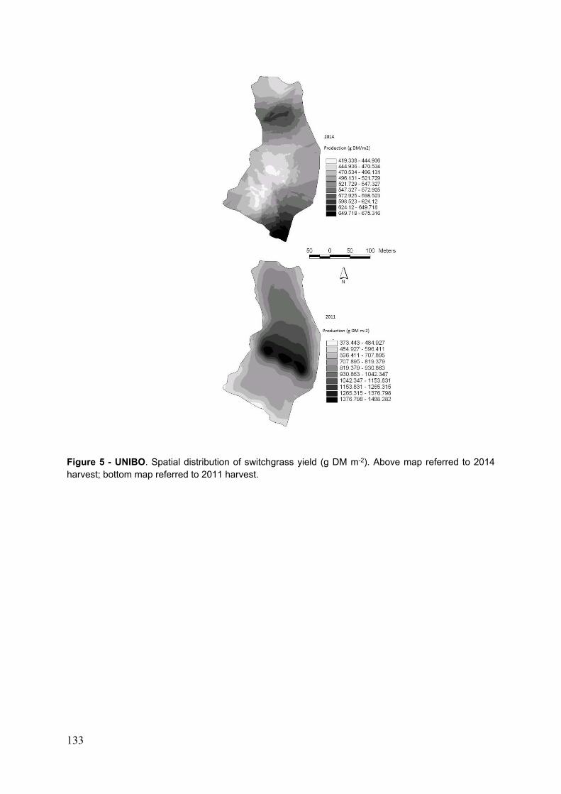
133
Figure 5 - UNIBO. Spatial distribution of switchgrass yield (g DM m-2). Above map referred to 2014 harvest; bottom map referred to 2011 harvest.
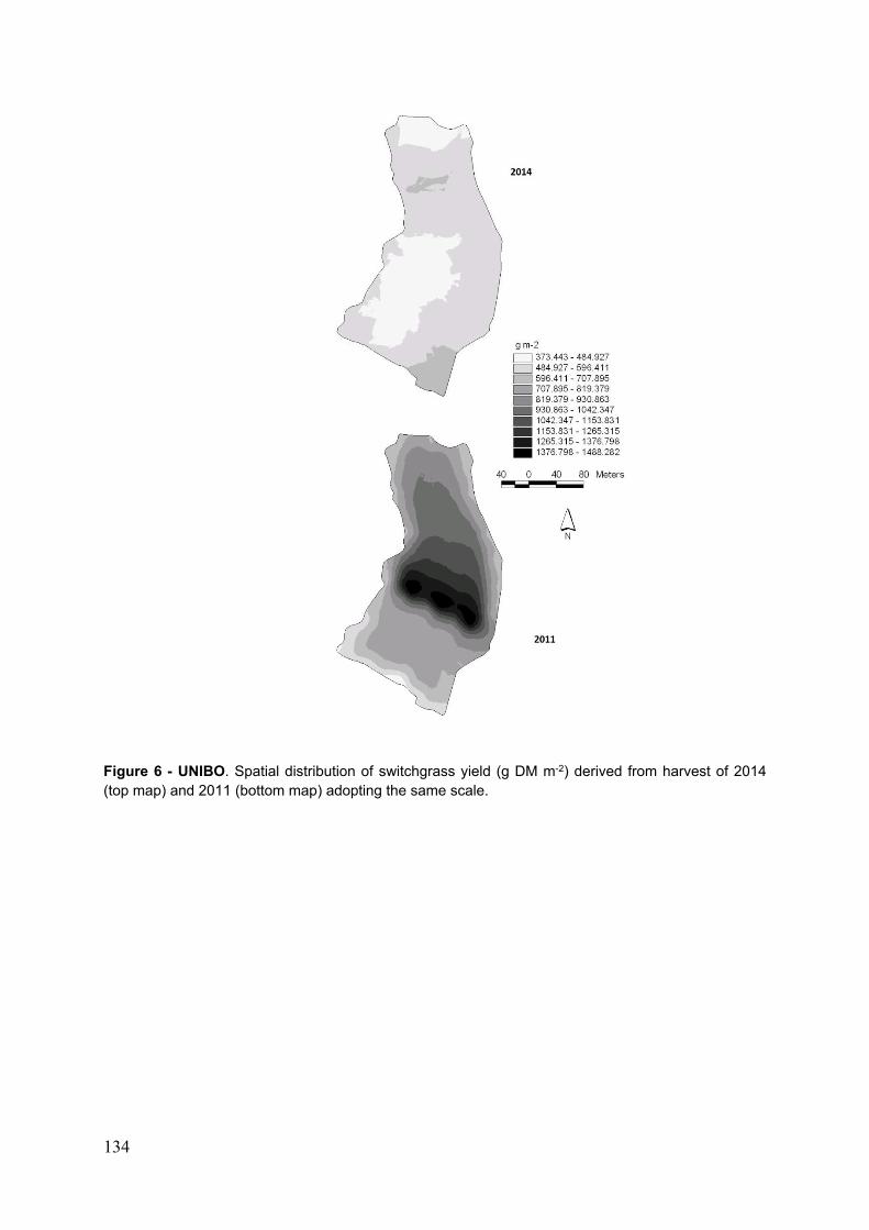
134
Figure 6 - UNIBO. Spatial distribution of switchgrass yield (g DM m-2) derived from harvest of 2014 (top map) and 2011 (bottom map) adopting the same scale.
135
Task 4.3 Long term productivity of existing large-scale plantation
Center for Renewable Energy Sources and Energy Saving – CRES (n. 3)
Picture 1 - CRES. Large and small fields of perennial crops established in North and Central Greece.
Picture 2 - CRES. The experimental fields of cardoon, giant reed and switchgrass
Switchgrass
Giant reed Cynara
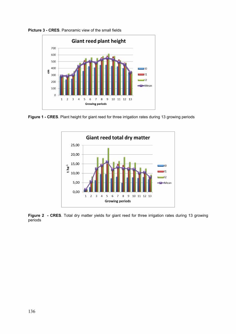
136
Picture 3 - CRES. Panoramic view of the small fields
Figure 1 - CRES. Plant height for giant reed for three irrigation rates during 13 growing periods
Figure 2 - CRES. Total dry matter yields for giant reed for three irrigation rates during 13 growing periods
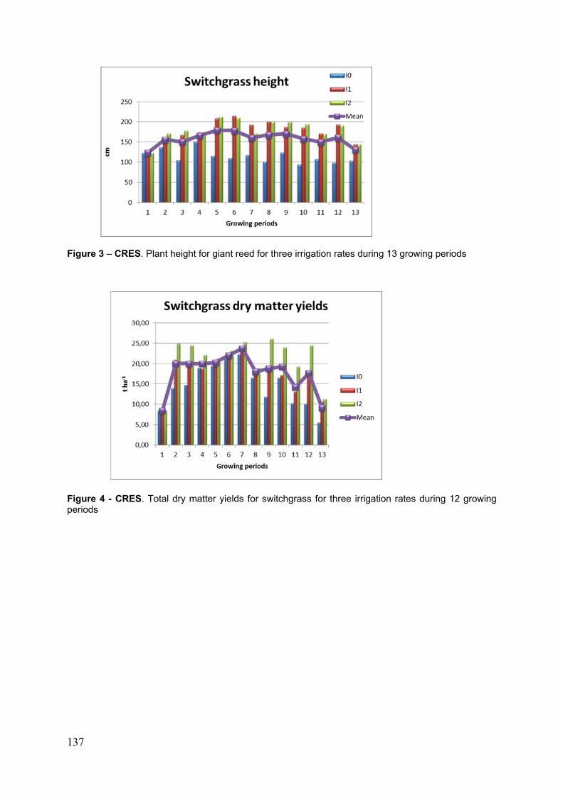
137
Figure 3 – CRES. Plant height for giant reed for three irrigation rates during 13 growing periods
Figure 4 - CRES. Total dry matter yields for switchgrass for three irrigation rates during 12 growing periods
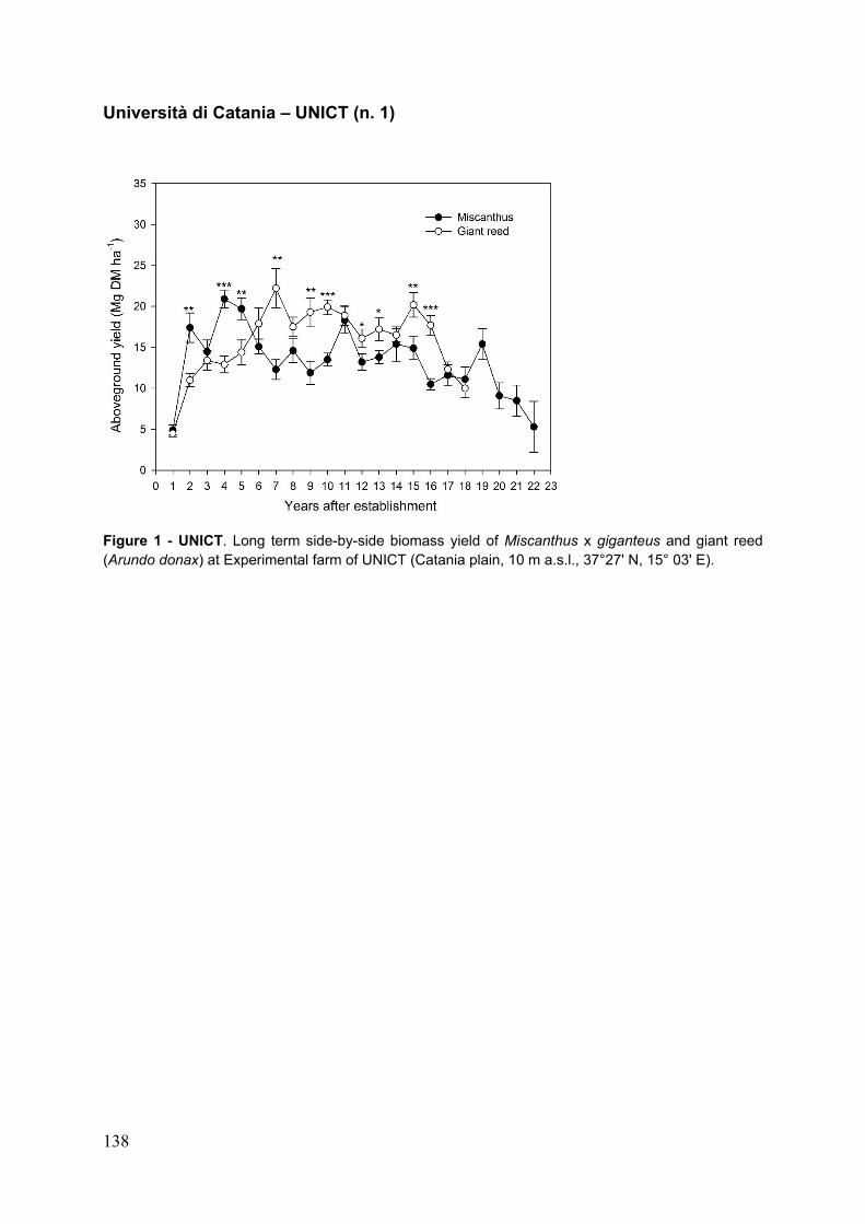
138
Università di Catania – UNICT (n. 1)
Figure 1 - UNICT. Long term side-by-side biomass yield of Miscanthus x giganteus and giant reed (Arundo donax) at Experimental farm of UNICT (Catania plain, 10 m a.s.l., 37°27' N, 15° 03' E).
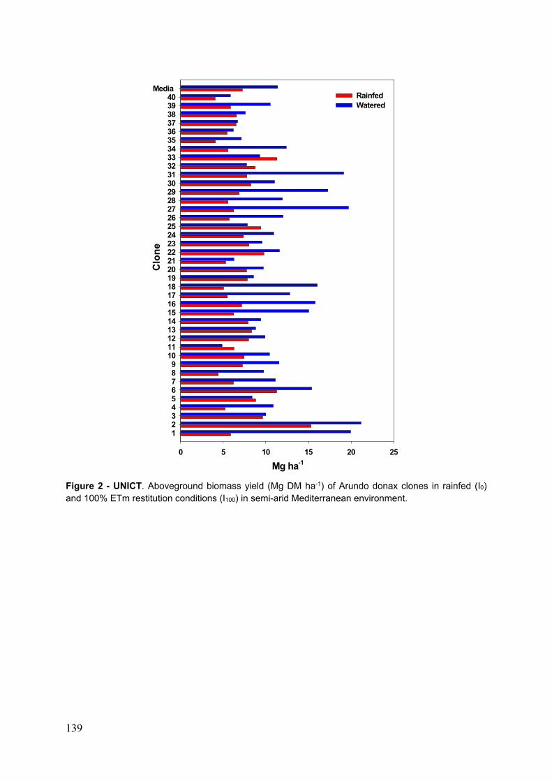
139
Figure 2 - UNICT. Aboveground biomass yield (Mg DM ha-1) of Arundo donax clones in rainfed (I0) and 100% ETm restitution conditions (I100) in semi-arid Mediterranean environment.
Mg ha-1
0 5 10 15 20 25
Clo
ne
123456789
10111213141516171819202122232425262728293031323334353637383940
Media RainfedWatered
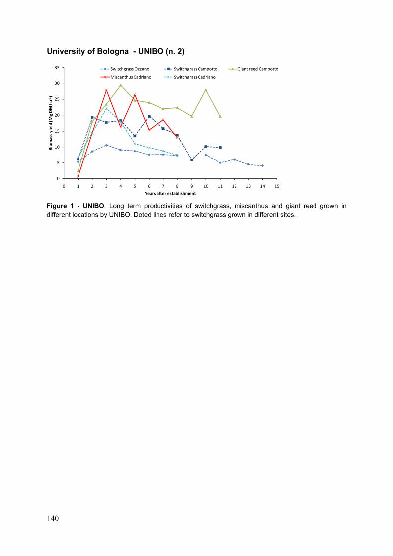
140
University of Bologna - UNIBO (n. 2)
Figure 1 - UNIBO. Long term productivities of switchgrass, miscanthus and giant reed grown in different locations by UNIBO. Doted lines refer to switchgrass grown in different sites.
0
5
10
15
20
25
30
35
0 1 2 3 4 5 6 7 8 9 10 11 12 13 14 15
Biomass yield (M
g DM ha‐
1)
Years after establishment
Switchgrass Ozzano Switchgrass Campotto Giant reed Campotto
Miscanthus Cadriano Switchgrass Cadriano
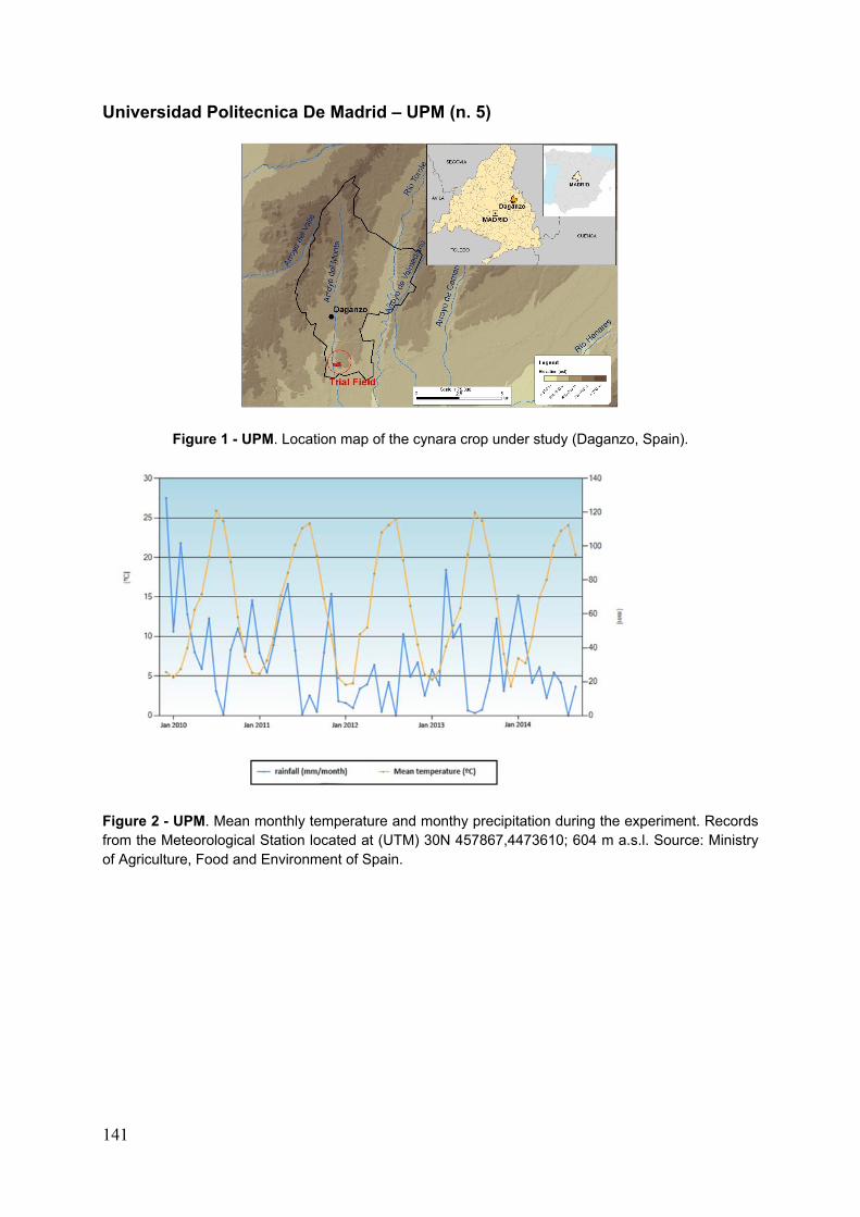
141
Universidad Politecnica De Madrid – UPM (n. 5)
Figure 1 - UPM. Location map of the cynara crop under study (Daganzo, Spain).
Figure 2 - UPM. Mean monthly temperature and monthy precipitation during the experiment. Records from the Meteorological Station located at (UTM) 30N 457867,4473610; 604 m a.s.l. Source: Ministry of Agriculture, Food and Environment of Spain.
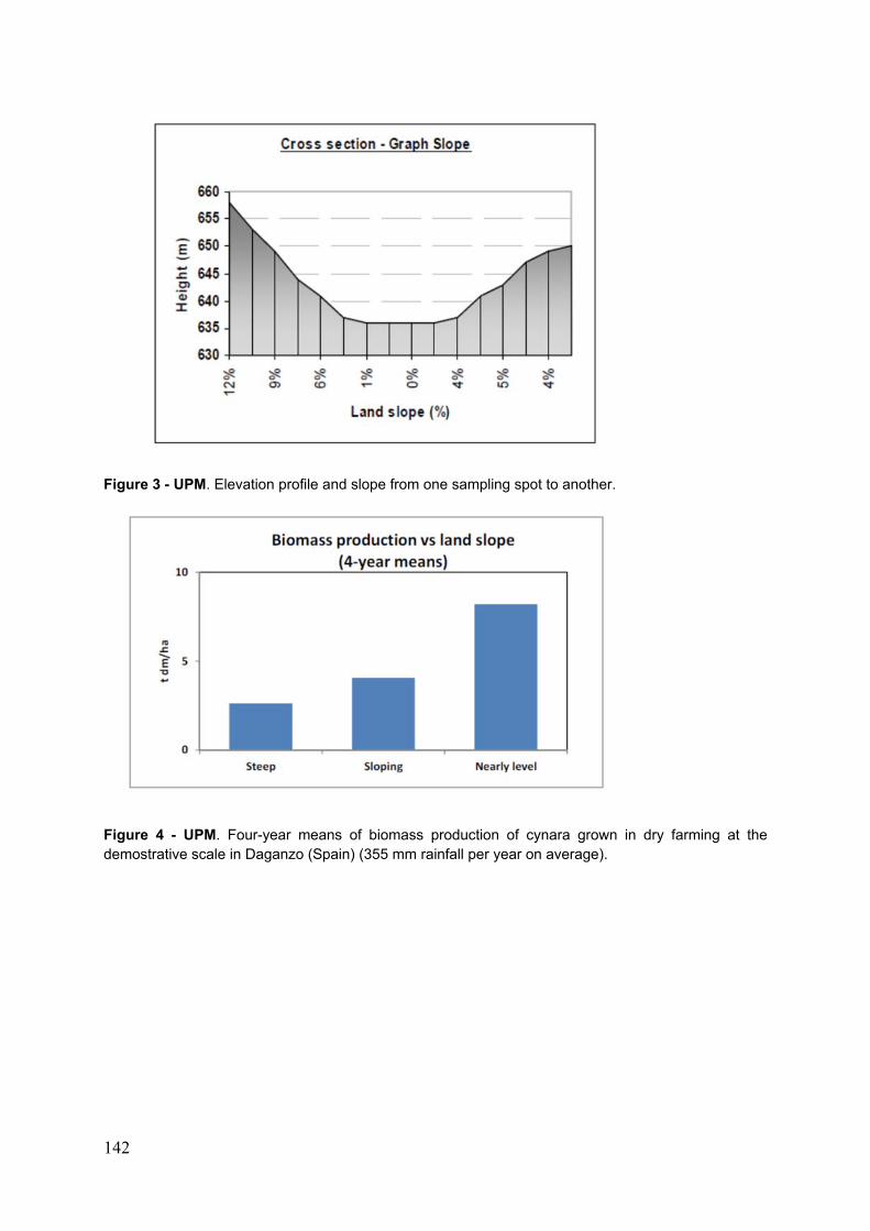
142
Figure 3 - UPM. Elevation profile and slope from one sampling spot to another.
Figure 4 - UPM. Four-year means of biomass production of cynara grown in dry farming at the demostrative scale in Daganzo (Spain) (355 mm rainfall per year on average).
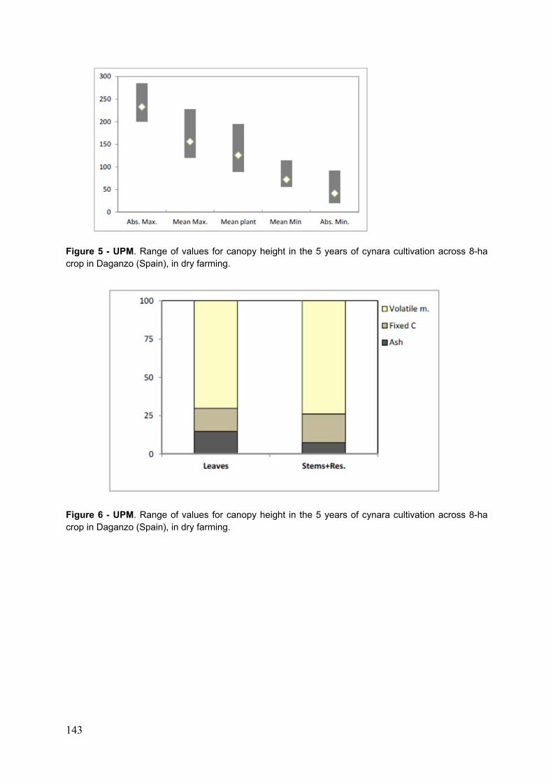
143
Figure 5 - UPM. Range of values for canopy height in the 5 years of cynara cultivation across 8-ha crop in Daganzo (Spain), in dry farming.
Figure 6 - UPM. Range of values for canopy height in the 5 years of cynara cultivation across 8-ha crop in Daganzo (Spain), in dry farming.
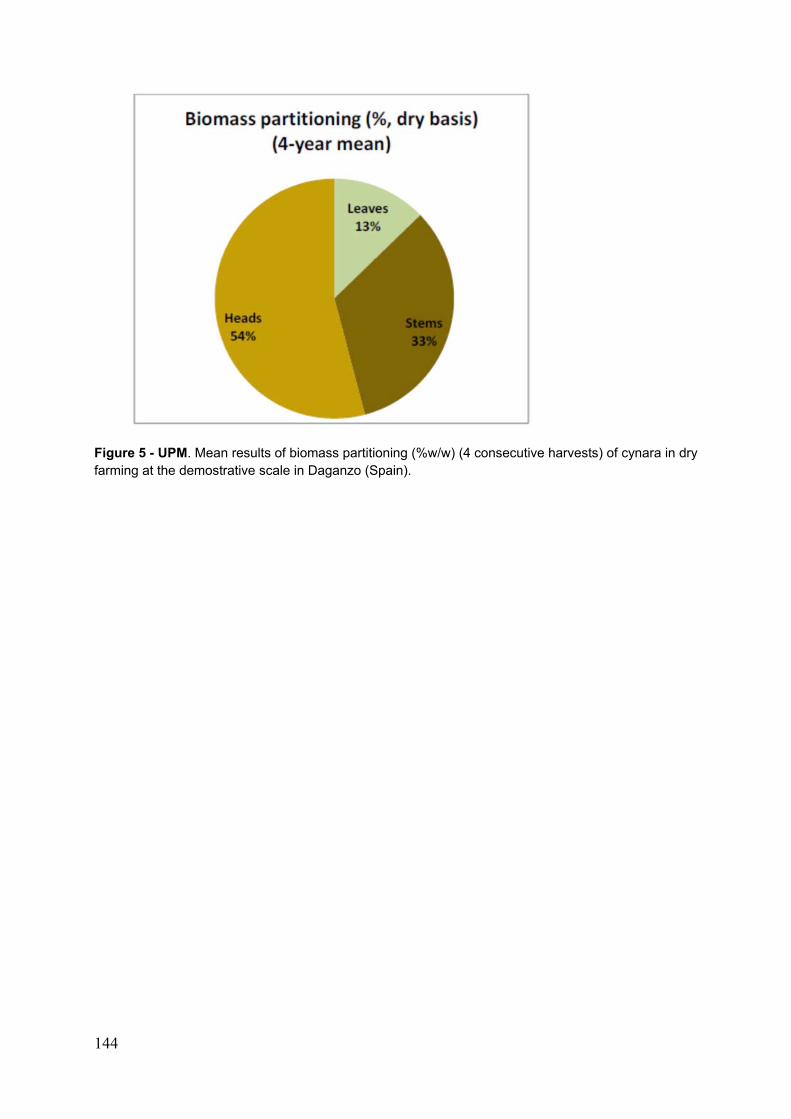
144
Figure 5 - UPM. Mean results of biomass partitioning (%w/w) (4 consecutive harvests) of cynara in dry farming at the demostrative scale in Daganzo (Spain).
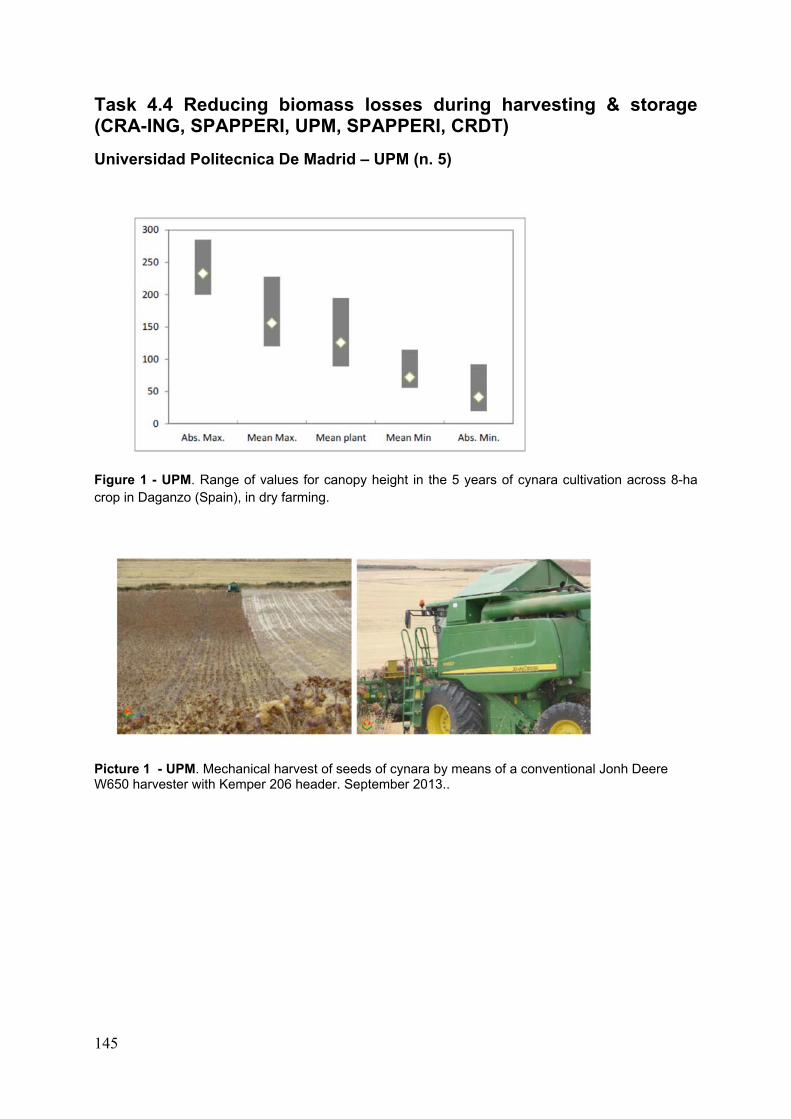
145
Task 4.4 Reducing biomass losses during harvesting & storage (CRA-ING, SPAPPERI, UPM, SPAPPERI, CRDT)
Universidad Politecnica De Madrid – UPM (n. 5)
Figure 1 - UPM. Range of values for canopy height in the 5 years of cynara cultivation across 8-ha crop in Daganzo (Spain), in dry farming.
Picture 1 - UPM. Mechanical harvest of seeds of cynara by means of a conventional Jonh Deere W650 harvester with Kemper 206 header. September 2013..
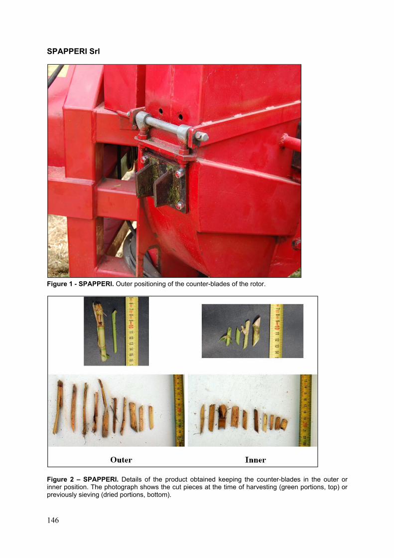
146
SPAPPERI Srl
Figure 1 - SPAPPERI. Outer positioning of the counter-blades of the rotor.
Figure 2 – SPAPPERI. Details of the product obtained keeping the counter-blades in the outer or inner position. The photograph shows the cut pieces at the time of harvesting (green portions, top) or previously sieving (dried portions, bottom).
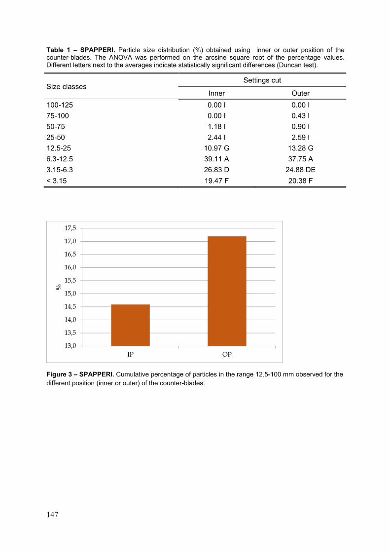
147
Table 1 – SPAPPERI. Particle size distribution (%) obtained using inner or outer position of the counter-blades. The ANOVA was performed on the arcsine square root of the percentage values. Different letters next to the averages indicate statistically significant differences (Duncan test).
Size classes Settings cut
Inner Outer
100-125 0.00 I 0.00 I
75-100 0.00 I 0.43 I
50-75 1.18 I 0.90 I
25-50 2.44 I 2.59 I
12.5-25 10.97 G 13.28 G
6.3-12.5 39.11 A 37.75 A
3.15-6.3 26.83 D 24.88 DE
< 3.15 19.47 F 20.38 F
Figure 3 – SPAPPERI. Cumulative percentage of particles in the range 12.5-100 mm observed for the different position (inner or outer) of the counter-blades.
13,0
13,5
14,0
14,5
15,0
15,5
16,0
16,5
17,0
17,5
IP OP
%
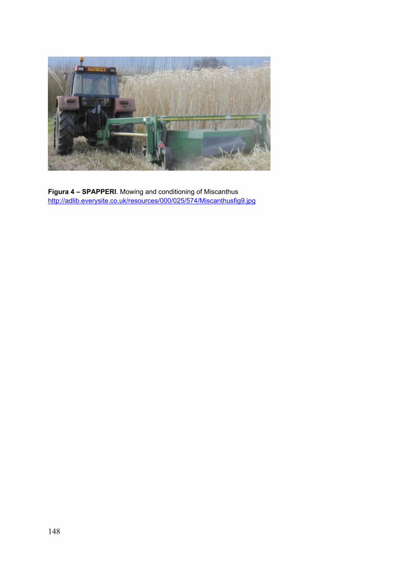
148
Figura 4 – SPAPPERI. Mowing and conditioning of Miscanthus http://adlib.everysite.co.uk/resources/000/025/574/Miscanthusfig9.jpg
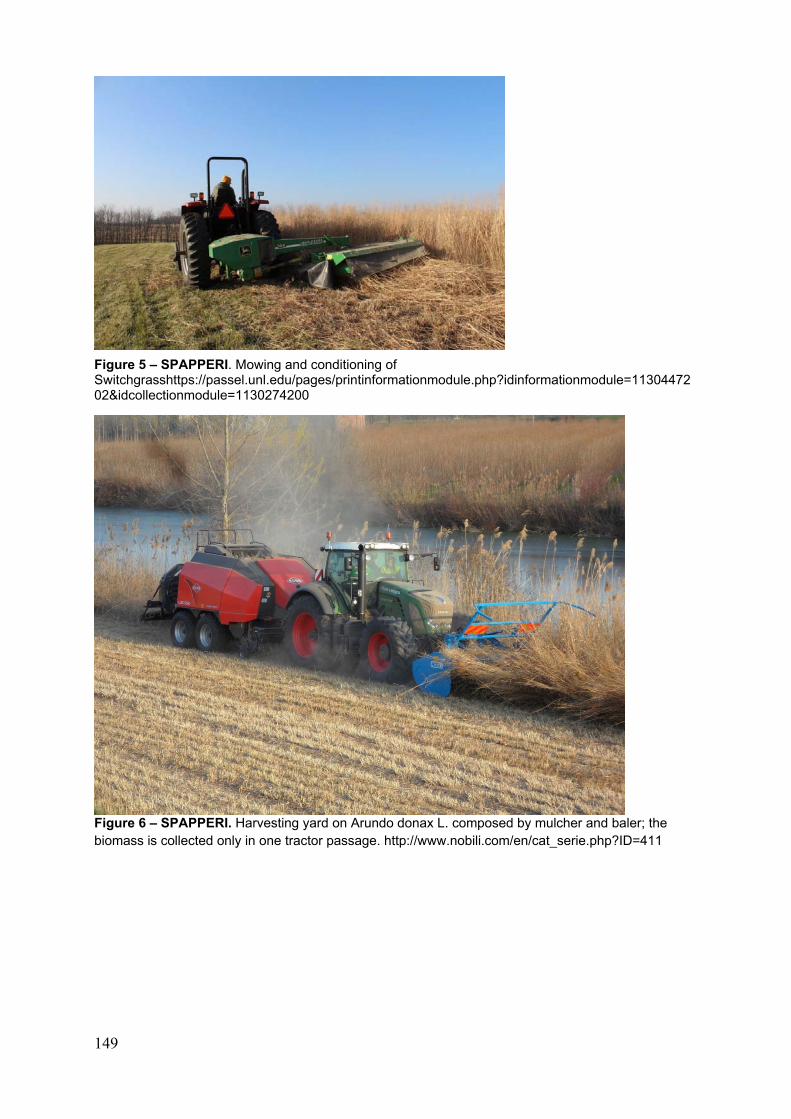
149
Figure 5 – SPAPPERI. Mowing and conditioning of Switchgrasshttps://passel.unl.edu/pages/printinformationmodule.php?idinformationmodule=1130447202&idcollectionmodule=1130274200
Figure 6 – SPAPPERI. Harvesting yard on Arundo donax L. composed by mulcher and baler; the biomass is collected only in one tractor passage. http://www.nobili.com/en/cat_serie.php?ID=411
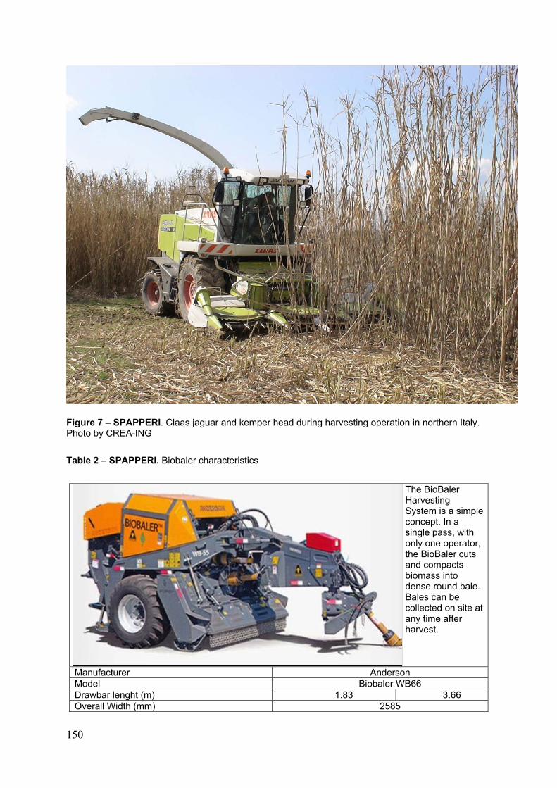
150
Figure 7 – SPAPPERI. Claas jaguar and kemper head during harvesting operation in northern Italy. Photo by CREA-ING
Table 2 – SPAPPERI. Biobaler characteristics
The BioBaler Harvesting System is a simple concept. In a single pass, with only one operator, the BioBaler cuts and compacts biomass into dense round bale. Bales can be collected on site at any time after harvest.
Manufacturer Anderson Model Biobaler WB66 Drawbar lenght (m) 1.83 3.66 Overall Width (mm) 2585
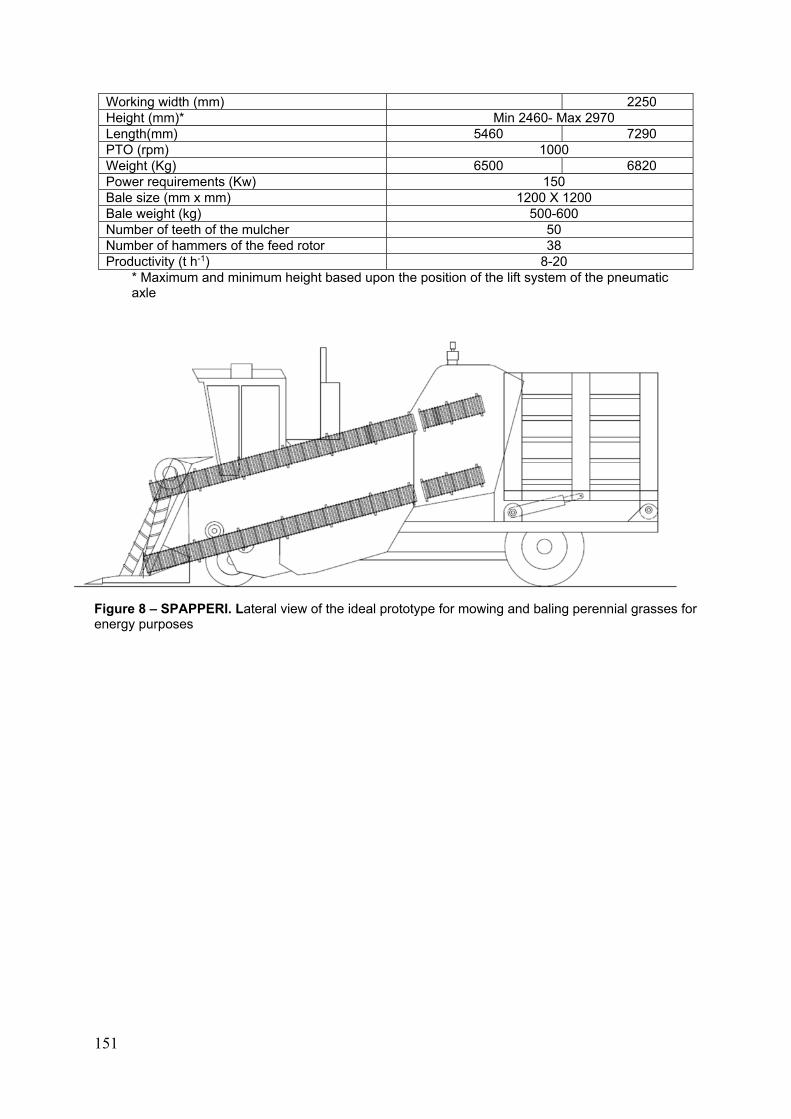
151
Figure 8 – SPAPPERI. Lateral view of the ideal prototype for mowing and baling perennial grasses for energy purposes
Working width (mm) 2250 Height (mm)* Min 2460- Max 2970 Length(mm) 5460 7290 PTO (rpm) 1000 Weight (Kg) 6500 6820 Power requirements (Kw) 150 Bale size (mm x mm) 1200 X 1200 Bale weight (kg) 500-600 Number of teeth of the mulcher 50 Number of hammers of the feed rotor 38 Productivity (t h-1) 8-20
* Maximum and minimum height based upon the position of the lift system of the pneumatic axle
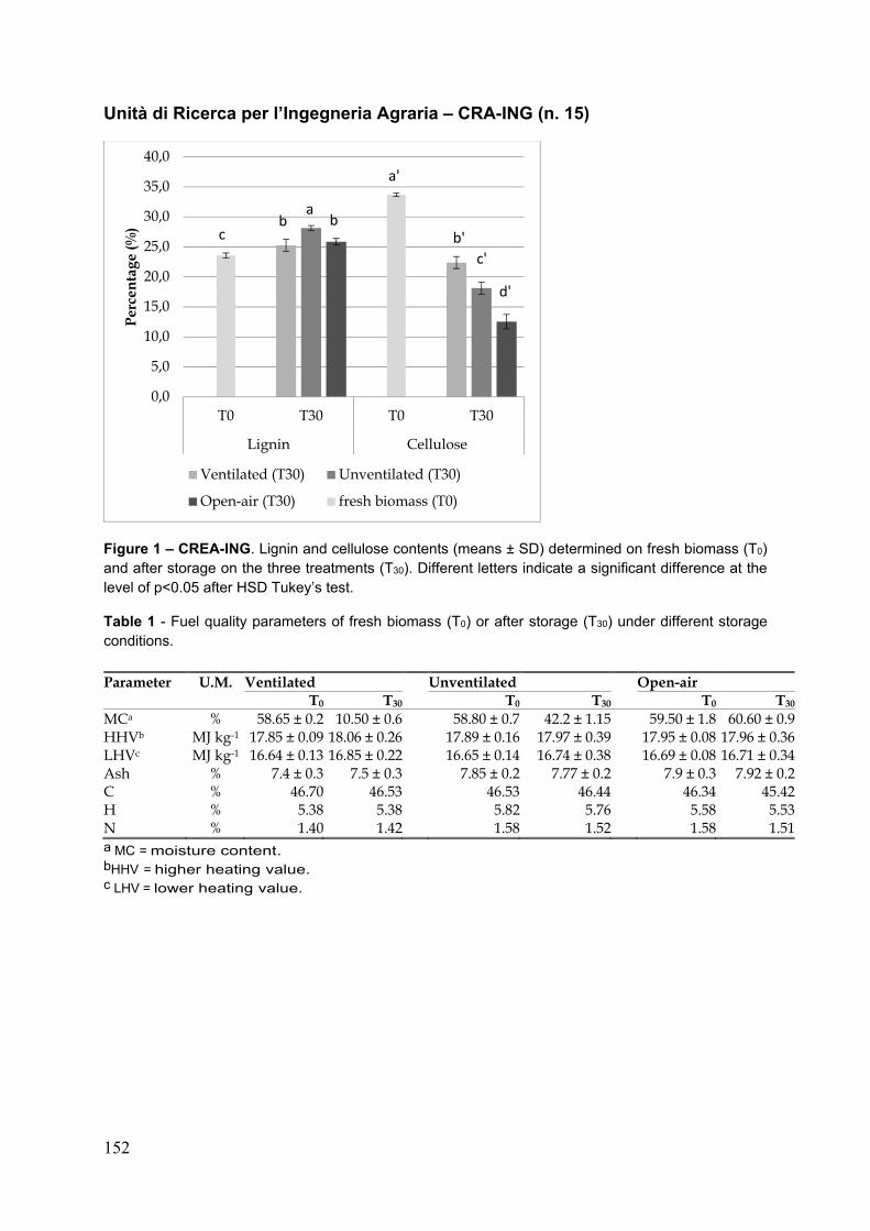
152
Unità di Ricerca per l’Ingegneria Agraria – CRA-ING (n. 15)
Figure 1 – CREA-ING. Lignin and cellulose contents (means ± SD) determined on fresh biomass (T0) and after storage on the three treatments (T30). Different letters indicate a significant difference at the level of p<0.05 after HSD Tukey’s test.
Table 1 - Fuel quality parameters of fresh biomass (T0) or after storage (T30) under different storage conditions.
Parameter U.M. Ventilated Unventilated Open-air T0 T30 T0 T30 T0 T30
MCa % 58.65 ± 0.2 10.50 ± 0.6 58.80 ± 0.7 42.2 ± 1.15 59.50 ± 1.8 60.60 ± 0.9HHVb MJ kg-1 17.85 ± 0.09 18.06 ± 0.26 17.89 ± 0.16 17.97 ± 0.39 17.95 ± 0.08 17.96 ± 0.36LHVc MJ kg-1 16.64 ± 0.13 16.85 ± 0.22 16.65 ± 0.14 16.74 ± 0.38 16.69 ± 0.08 16.71 ± 0.34Ash % 7.4 ± 0.3 7.5 ± 0.3 7.85 ± 0.2 7.77 ± 0.2 7.9 ± 0.3 7.92 ± 0.2C % 46.70 46.53 46.53 46.44 46.34 45.42H % 5.38 5.38 5.82 5.76 5.58 5.53N % 1.40 1.42 1.58 1.52 1.58 1.51a MC = moisture content. bHHV = higher heating value. c LHV = lower heating value.
0,0
5,0
10,0
15,0
20,0
25,0
30,0
35,0
40,0
T0 T30 T0 T30
Lignin Cellulose
Per
cen
tage
(%)
Ventilated (T30) Unventilated (T30)
Open-air (T30) fresh biomass (T0)
d'
ba
b
c'
b'
a'
c
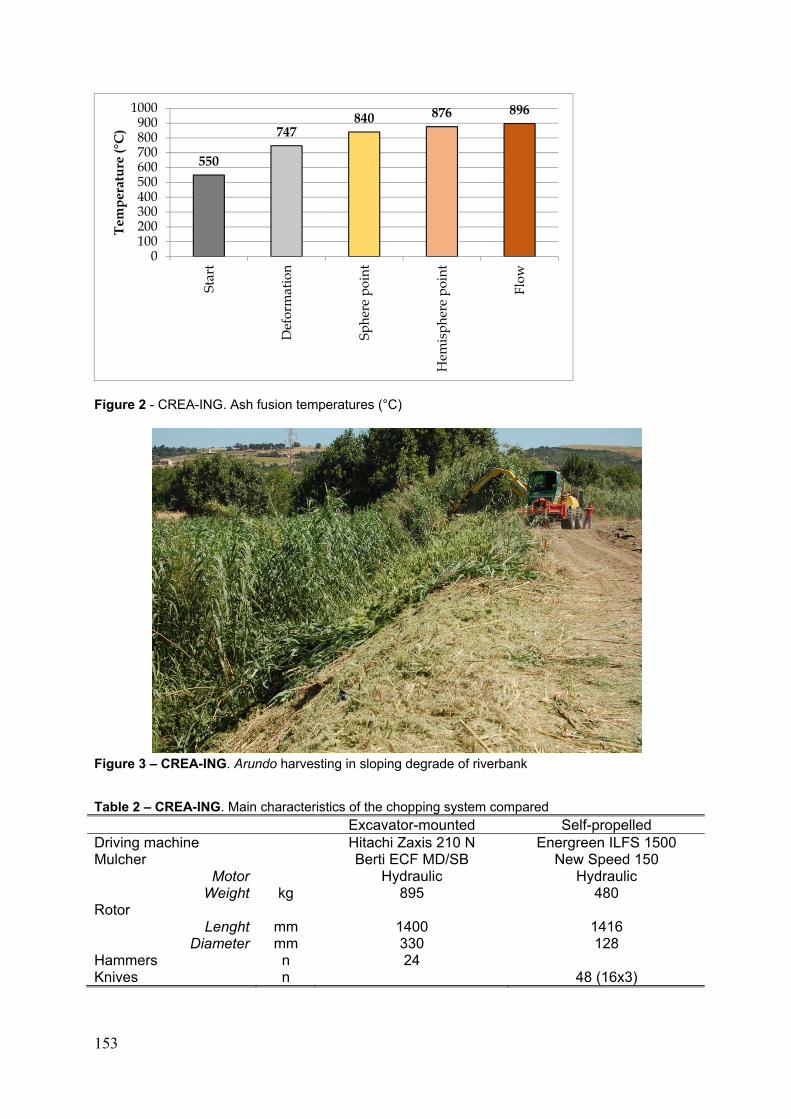
153
Figure 2 - CREA-ING. Ash fusion temperatures (°C)
Figure 3 – CREA-ING. Arundo harvesting in sloping degrade of riverbank
Table 2 – CREA-ING. Main characteristics of the chopping system compared Excavator-mounted Self-propelled Driving machine Hitachi Zaxis 210 N Energreen ILFS 1500 Mulcher Berti ECF MD/SB New Speed 150
Motor Hydraulic Hydraulic Weight kg 895 480
Rotor Lenght mm 1400 1416
Diameter mm 330 128 Hammers n 24 Knives n 48 (16x3)
550
747840 876 896
0100200300400500600700800900
1000
Star
t
Def
orm
atio
n
Sphe
re p
oint
Hem
isph
ere
poin
t
Flow
Tem
per
atu
re (°
C)
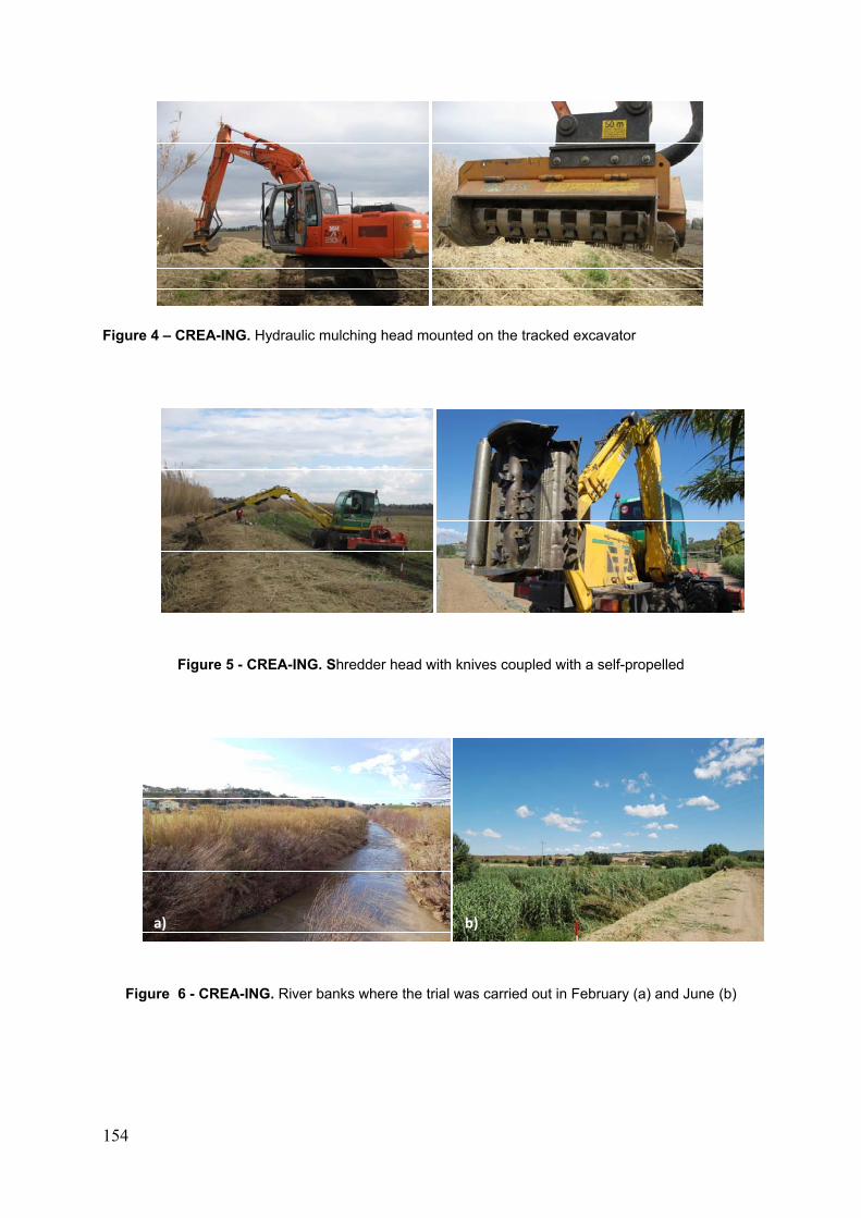
154
Figure 4 – CREA-ING. Hydraulic mulching head mounted on the tracked excavator
Figure 5 - CREA-ING. Shredder head with knives coupled with a self-propelled
b)a)
Figure 6 - CREA-ING. River banks where the trial was carried out in February (a) and June (b)
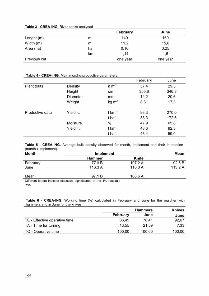
155
Table 3 - CREA-ING. River banks analysed
February June
Lenght (m) m 140 160 Width (m) m 11,2 15,6 Area (ha) ha 0,16 0,25
km 1,14 1,6
Previous cut one year one year
Table 4 - CREA-ING. Main morpho-productive parameters.
February June
Plant traits Density n m-2 37,4 29,3 Height cm 355,6 346,3 Diameter mm 14,2 20,6 Weight kg m-2 8,31 17,3 Productive data Yield f.w. t km-1 93,3 270,0 t ha-1 83,3 172,6 Moisture % 47,9 65,8 Yield d.w. t km-1 48,6 92,3 t ha-1 43,4 59,0
Table 5 - CREA-ING. Average bulk density observed for month, implement and their interaction (month x implement).
Month Implement Mean Hammer KnifeFebruary 77.9 B 107.2 A 92.6 BJune 116.3 A 110.0 A 113.2 A Mean 97.1 B 108.6 ADifferent letters indicate statistical significance at the 1% (capital) level
Table 6 - CREA-ING. Working time (%) calculated in February and June for the mulcher with hammers and in June for the knives.
Hammers KnivesFebruary June June
TE - Effective operative time 86,45 78,41 92,67TA - Time for turning 13,55 21,59 7,33
TO - Operative time 100,00 100,00 100,00
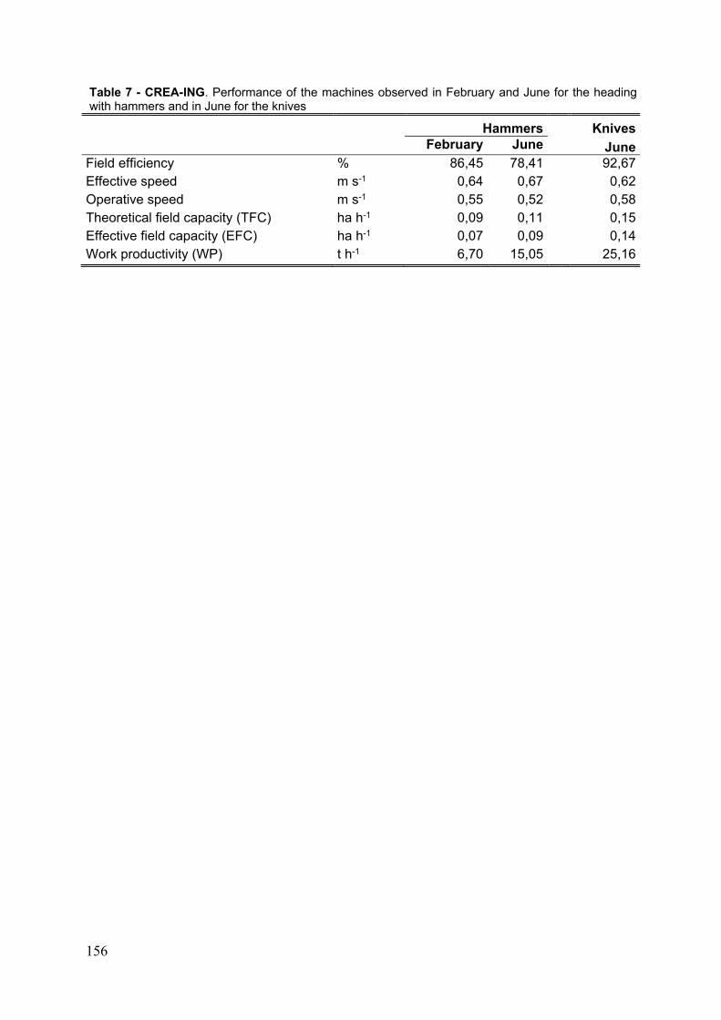
156
Table 7 - CREA-ING. Performance of the machines observed in February and June for the heading with hammers and in June for the knives
Hammers Knives February June JuneField efficiency % 86,45 78,41 92,67Effective speed m s-1 0,64 0,67 0,62Operative speed m s-1 0,55 0,52 0,58Theoretical field capacity (TFC) ha h-1 0,09 0,11 0,15Effective field capacity (EFC) ha h-1 0,07 0,09 0,14Work productivity (WP) t h-1 6,70 15,05 25,16
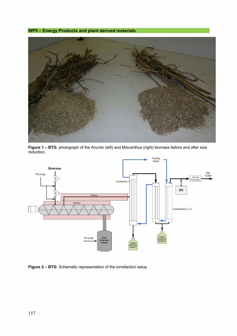
157
WP5 – Energy Products and plant derived materials
Figure 1 – BTG. photograph of the Arundo (left) and Miscanthus (right) biomass before and after size reduction.
Figure 2 – BTG. Schematic representation of the torrefaction setup
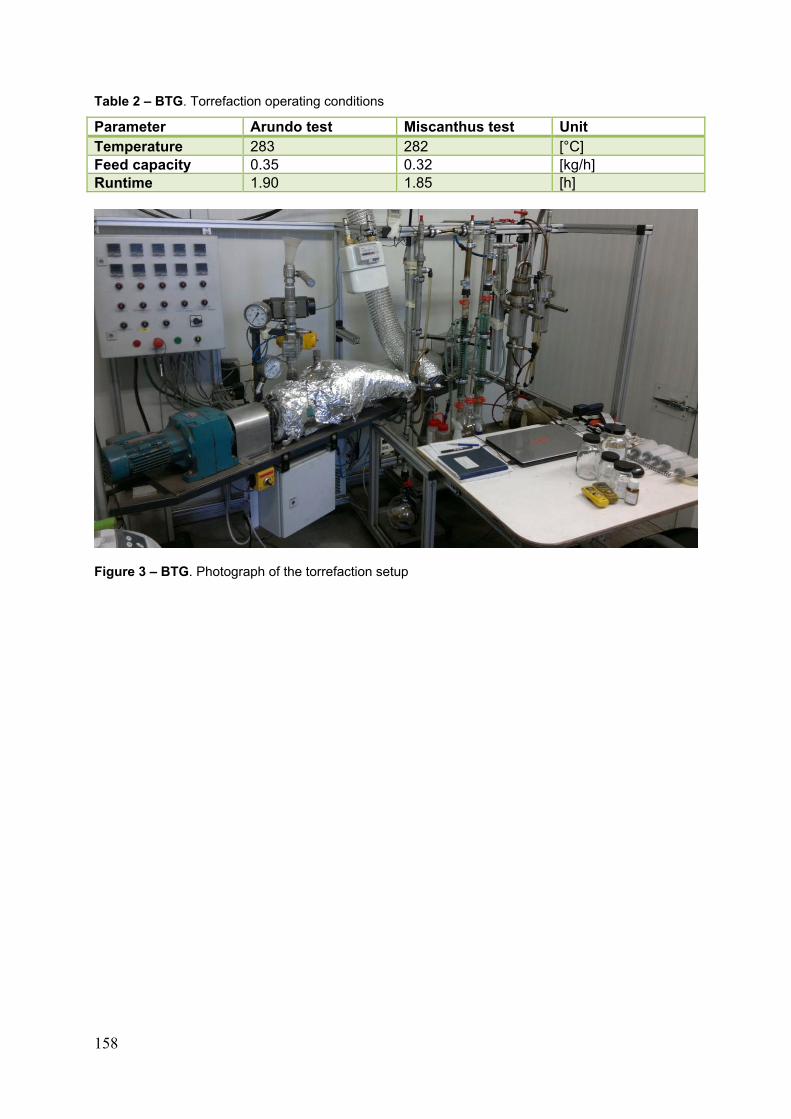
158
Table 2 – BTG. Torrefaction operating conditions
Parameter Arundo test Miscanthus test Unit Temperature 283 282 [°C] Feed capacity 0.35 0.32 [kg/h] Runtime 1.90 1.85 [h]
Figure 3 – BTG. Photograph of the torrefaction setup
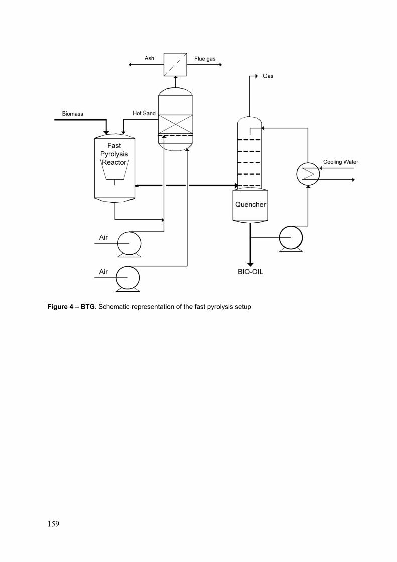
159
Figure 4 – BTG. Schematic representation of the fast pyrolysis setup
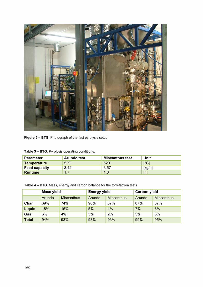
160
Figure 5 – BTG. Photograph of the fast pyrolysis setup
Table 3 – BTG. Pyrolysis operating conditions.
Parameter Arundo test Miscanthus test Unit Temperature 529 520 [°C] Feed capacity 3.42 3.57 [kg/h] Runtime 1.7 1.6 [h]
Table 4 – BTG. Mass, energy and carbon balance for the torrefaction tests
Mass yield Energy yield Carbon yield
Arundo Miscanthus Arundo Miscanthus Arundo Miscanthus
Char 69% 74% 90% 87% 87% 87%
Liquid 18% 15% 5% 4% 7% 6%
Gas 6% 4% 3% 2% 5% 3%
Total 94% 93% 98% 93% 99% 95%
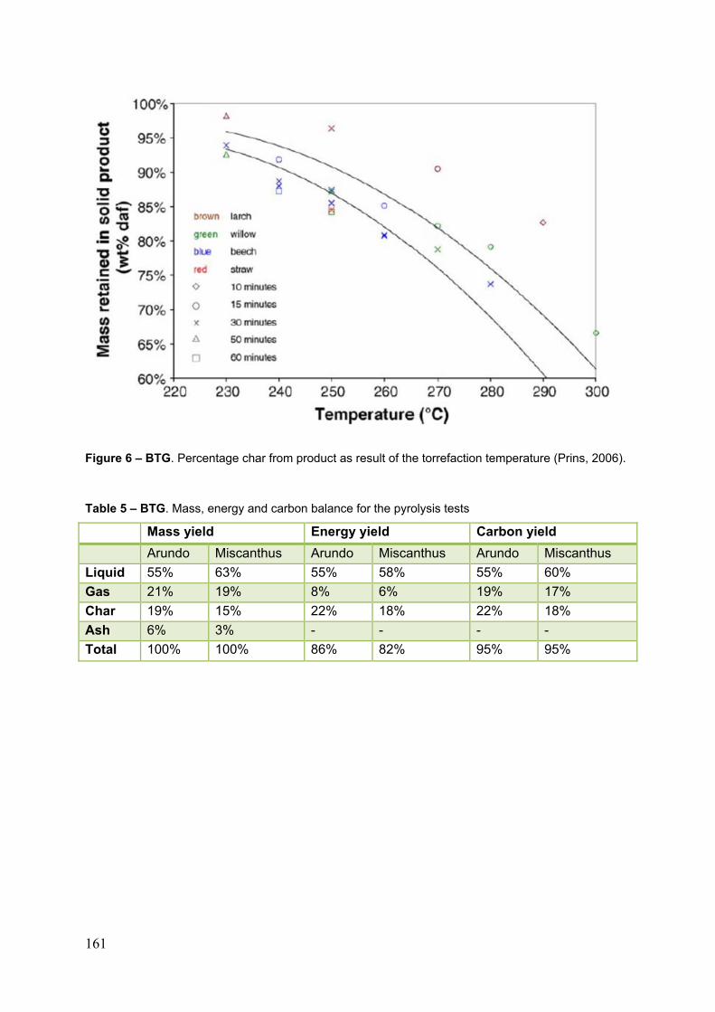
161
Figure 6 – BTG. Percentage char from product as result of the torrefaction temperature (Prins, 2006).
Table 5 – BTG. Mass, energy and carbon balance for the pyrolysis tests
Mass yield Energy yield Carbon yield
Arundo Miscanthus Arundo Miscanthus Arundo Miscanthus
Liquid 55% 63% 55% 58% 55% 60%
Gas 21% 19% 8% 6% 19% 17%
Char 19% 15% 22% 18% 22% 18%
Ash 6% 3% - - - -
Total 100% 100% 86% 82% 95% 95%
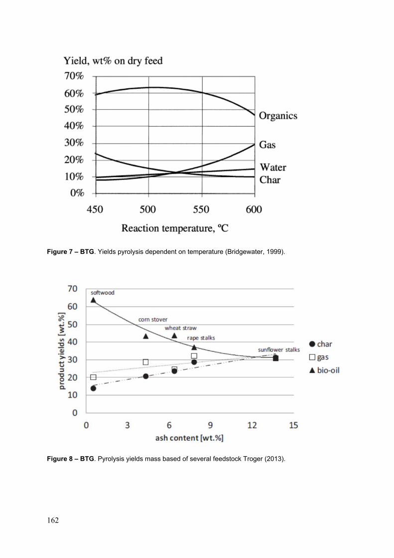
162
Figure 7 – BTG. Yields pyrolysis dependent on temperature (Bridgewater, 1999).
Figure 8 – BTG. Pyrolysis yields mass based of several feedstock Troger (2013).
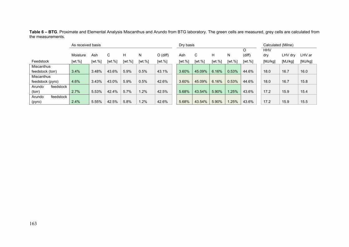
163
Table 6 – BTG. Proximate and Elemental Analysis Miscanthus and Arundo from BTG laboratory. The green cells are measured, grey cells are calculated from the measurements.
As received basis Dry basis Calculated (Milne)
Moisture Ash C H N O (diff) Ash C H N O (diff)
HHV dry LHV dry LHV ar
Feedstock [wt.%] [wt.%] [wt.%] [wt.%] [wt.%] [wt.%] [wt.%] [wt.%] [wt.%] [wt.%] [wt.%] [MJ/kg] [MJ/kg] [MJ/kg] Miscanthus feedstock (torr) 3.4% 3.48% 43.6% 5.9% 0.5% 43.1% 3.60% 45.09% 6.16% 0.53% 44.6% 18.0 16.7 16.0 Miscanthus feedstock (pyro) 4.6% 3.43% 43.0% 5.9% 0.5% 42.6% 3.60% 45.09% 6.16% 0.53% 44.6% 18.0 16.7 15.8 Arundo feedstock (torr) 2.7% 5.53% 42.4% 5.7% 1.2% 42.5% 5.68% 43.54% 5.90% 1.25% 43.6% 17.2 15.9 15.4 Arundo feedstock (pyro) 2.4% 5.55% 42.5% 5.8% 1.2% 42.6% 5.68% 43.54% 5.90% 1.25% 43.6% 17.2 15.9 15.5
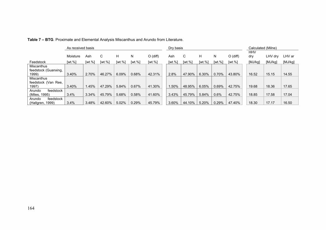
164
Table 7 – BTG. Proximate and Elemental Analysis Miscanthus and Arundo from Literature.
As received basis Dry basis Calculated (Milne)
Moisture Ash C H N O (diff) Ash C H N O (diff) HHV dry LHV dry LHV ar
Feedstock [wt.%] [wt.%] [wt.%] [wt.%] [wt.%] [wt.%] [wt.%] [wt.%] [wt.%] [wt.%] [wt.%] [MJ/kg] [MJ/kg] [MJ/kg] Miscanthus feedstock (Guanxing, 1999) 3.40% 2.70% 46.27% 6.09% 0.68% 42.31% 2.8% 47.90% 6.30% 0.70% 43.80% 16.52 15.15 14.55 Miscanthus feedstock (Van Ree, 1997) 3.40% 1.45% 47.29% 5.84% 0.67% 41.30% 1.50% 48.95% 6.05% 0.69% 42.75% 19.68 18.36 17.65 Arundo feedstock (Miles, 1995) 3.4% 3.34% 45.79% 5.68% 0.58% 41.60% 3.43% 45.79% 5.84% 0.6% 42.75% 18.85 17.58 17.04 Arundo feedstock (Hallgren, 1999) 3.4% 3.48% 42.60% 5.02% 0.29% 45.79% 3.60% 44.10% 5.20% 0.29% 47.40% 18.30 17.17 16.50

165
Table 8 – BTG. Analysis results of the feedstocks and various products. The green cells are measured, grey cells are calculated from the measurements.
As received basis Dry basis Calculated (Milne)
Moisture Ash C H N O (diff) Ash C H N O (diff)
HHV dry LHV dry LHV ar
Torrefaction products
Miscanthus liquid 65.1% 0.0% 17.0% 2.0% 0.0% 81.0% 0.00% 48.50% 5.81% 0.00% 45.7% 18.7 17.5 4.5
Miscanthus char 0% 5.3% 51.2% 5.6% 0.5% 37.4% 5.26% 51.19% 5.60% 0.53% 37.4% 20.2 19.0 19.0
Arundo liquid 61.7% 0.0% 16.4% 2.5% 0.0% 81.1% 0.00% 42.85% 6.42% 0.00% 50.7% 17.0 15.6 4.5
Arundo char 0% 8.5% 53.3% 5.4% 1.2% 31.6% 8.49% 53.30% 5.43% 1.19% 31.6% 21.3 20.1 20.1
Pyrolysis products
Miscanthus liquid 22.9% 0% 41.4% 6.96% 0.44% 51.2% 0% 54% 6% 0.6% 40% 21.0 19.8 14.7
Miscanthus char 0% 33.2% 50.9% 3.2% 0.6% 12.1% 33% 51% 3% 0.61% 12.1% 19.5 18.8 18.8
Arundo liquid 28.0% 0% 41.9% 7.50% 1.08% 49.5% 0% 58% 6% 1.5% 34% 23.6 22.3 15.4
Arundo char 0% 39.3% 48.4% 3.0% 1.2% 8.1% 39.3% 48.4% 3.0% 1.2% 8.1% 18.8 18.1 18.1
CO2 CO HC LHV Carbon
Gas composition [kg/h] [kg/h] [kg/h] [MJ/kg] [wt.%]
Miscanthus Torrefaction 0.010 0.002 0.001 7.2 32%
Arundo Torrefaction 0.018 0.004 0.001 6.6 32%
Miscanthus Pyrolysis 0.319 0.261 0.054 5.2 38%
Arundo Pyrolysis 0.366 0.252 0.072 6.0 38%
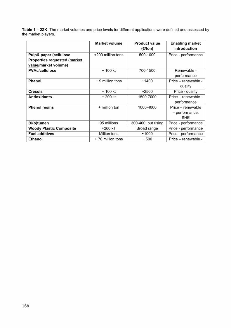
166
Table 1 – 2ZK. The market volumes and price levels for different applications were defined and assessed by the market players.
Market volume Product value (€/ton)
Enabling market introduction
Pulp& paper (cellulose Properties requested (market value/market volume)
+200 million tons 500-1000 Price - performance
PVAc/cellulose + 100 kt 700-1500 Renewable - performance
Phenol + 9 million tons ~1400 Price – renewable - quality
Cresols + 100 kt ~2500 Price - quality Antioxidants + 200 kt 1500-7000 Price – renewable -
performance Phenol resins + million ton 1000-4000 Price – renewable
– performance, SHE
Bi(o)tumen 95 millions 300-400, but rising Price - performanceWoody Plastic Composite +260 kT Broad range Price - performanceFuel additives Million tons ~1000 Price - performanceEthanol + 70 million tons ~ 500 Price – renewable -
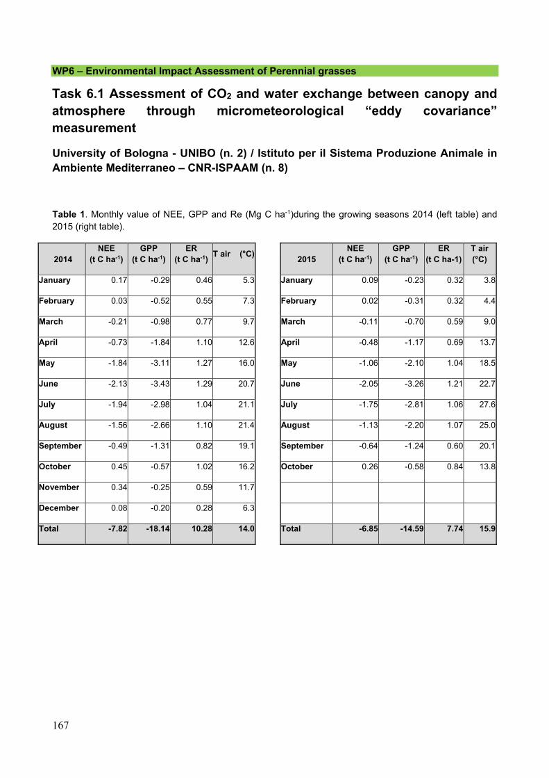
167
WP6 – Environmental Impact Assessment of Perennial grasses
Task 6.1 Assessment of CO2 and water exchange between canopy and atmosphere through micrometeorological “eddy covariance” measurement
University of Bologna - UNIBO (n. 2) / Istituto per il Sistema Produzione Animale in Ambiente Mediterraneo – CNR-ISPAAM (n. 8)
Table 1. Monthly value of NEE, GPP and Re (Mg C ha-1)during the growing seasons 2014 (left table) and 2015 (right table).
2014 NEE
(t C ha-1) GPP
(t C ha-1) ER
(t C ha-1) T air (°C)
2015 NEE
(t C ha-1) GPP
(t C ha-1) ER
(t C ha-1) T air (°C)
January 0.17 -0.29 0.46 5.3 January 0.09 -0.23 0.32 3.8
February 0.03 -0.52 0.55 7.3 February 0.02 -0.31 0.32 4.4
March -0.21 -0.98 0.77 9.7 March -0.11 -0.70 0.59 9.0
April -0.73 -1.84 1.10 12.6 April -0.48 -1.17 0.69 13.7
May -1.84 -3.11 1.27 16.0 May -1.06 -2.10 1.04 18.5
June -2.13 -3.43 1.29 20.7 June -2.05 -3.26 1.21 22.7
July -1.94 -2.98 1.04 21.1 July -1.75 -2.81 1.06 27.6
August -1.56 -2.66 1.10 21.4 August -1.13 -2.20 1.07 25.0
September -0.49 -1.31 0.82 19.1 September -0.64 -1.24 0.60 20.1
October 0.45 -0.57 1.02 16.2 October 0.26 -0.58 0.84 13.8
November 0.34 -0.25 0.59 11.7
December 0.08 -0.20 0.28 6.3
Total -7.82 -18.14 10.28 14.0 Total -6.85 -14.59 7.74 15.9
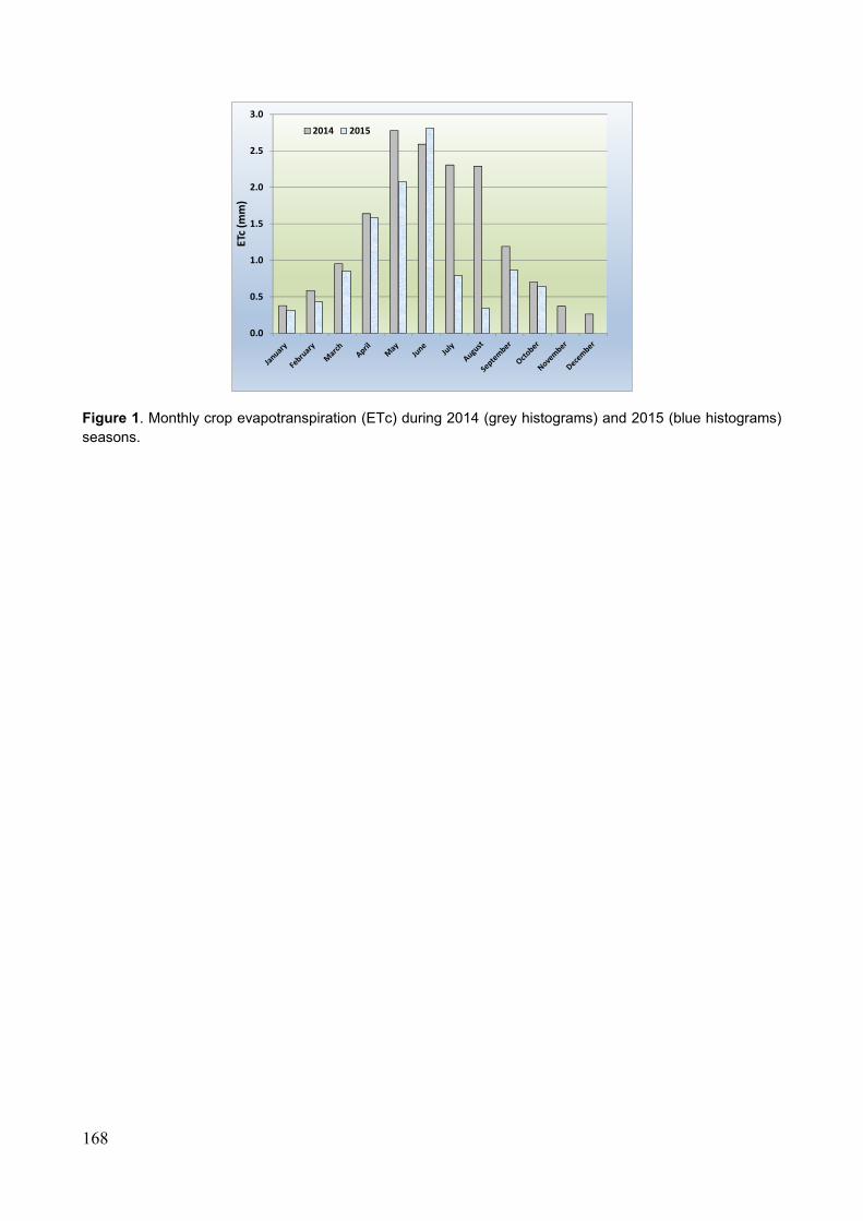
168
Figure 1. Monthly crop evapotranspiration (ETc) during 2014 (grey histograms) and 2015 (blue histograms) seasons.
0.0
0.5
1.0
1.5
2.0
2.5
3.0
ETc (m
m)
2014 2015
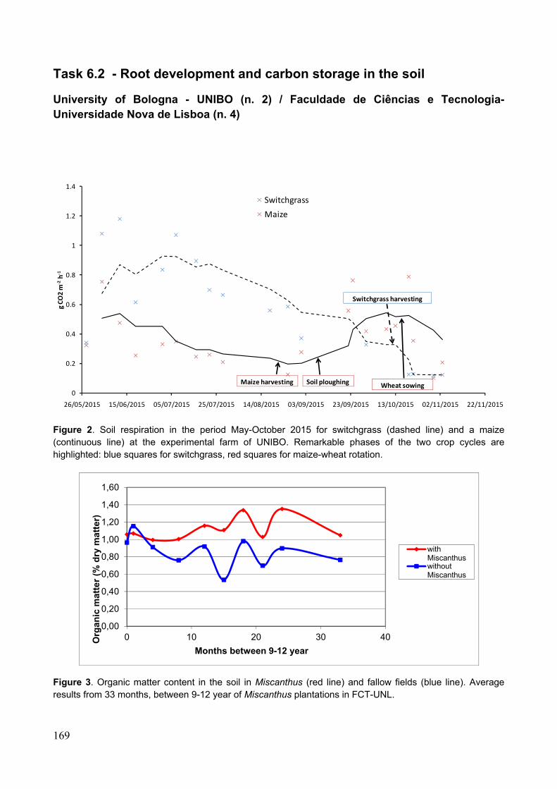
169
Task 6.2 - Root development and carbon storage in the soil
University of Bologna - UNIBO (n. 2) / Faculdade de Ciências e Tecnologia-Universidade Nova de Lisboa (n. 4)
Figure 2. Soil respiration in the period May-October 2015 for switchgrass (dashed line) and a maize (continuous line) at the experimental farm of UNIBO. Remarkable phases of the two crop cycles are highlighted: blue squares for switchgrass, red squares for maize-wheat rotation.
Figure 3. Organic matter content in the soil in Miscanthus (red line) and fallow fields (blue line). Average results from 33 months, between 9-12 year of Miscanthus plantations in FCT-UNL.
0
0.2
0.4
0.6
0.8
1
1.2
1.4
26/05/2015 15/06/2015 05/07/2015 25/07/2015 14/08/2015 03/09/2015 23/09/2015 13/10/2015 02/11/2015 22/11/2015
g CO2 m
‐2h‐1
Switchgrass
Maize
Maize harvesting Soil ploughing
Switchgrass harvesting
Wheat sowing
0,00
0,20
0,40
0,60
0,80
1,00
1,20
1,40
1,60
0 10 20 30 40Org
anic
mat
ter
(% d
ry m
atte
r)
Months between 9-12 year
withMiscanthuswithoutMiscanthus
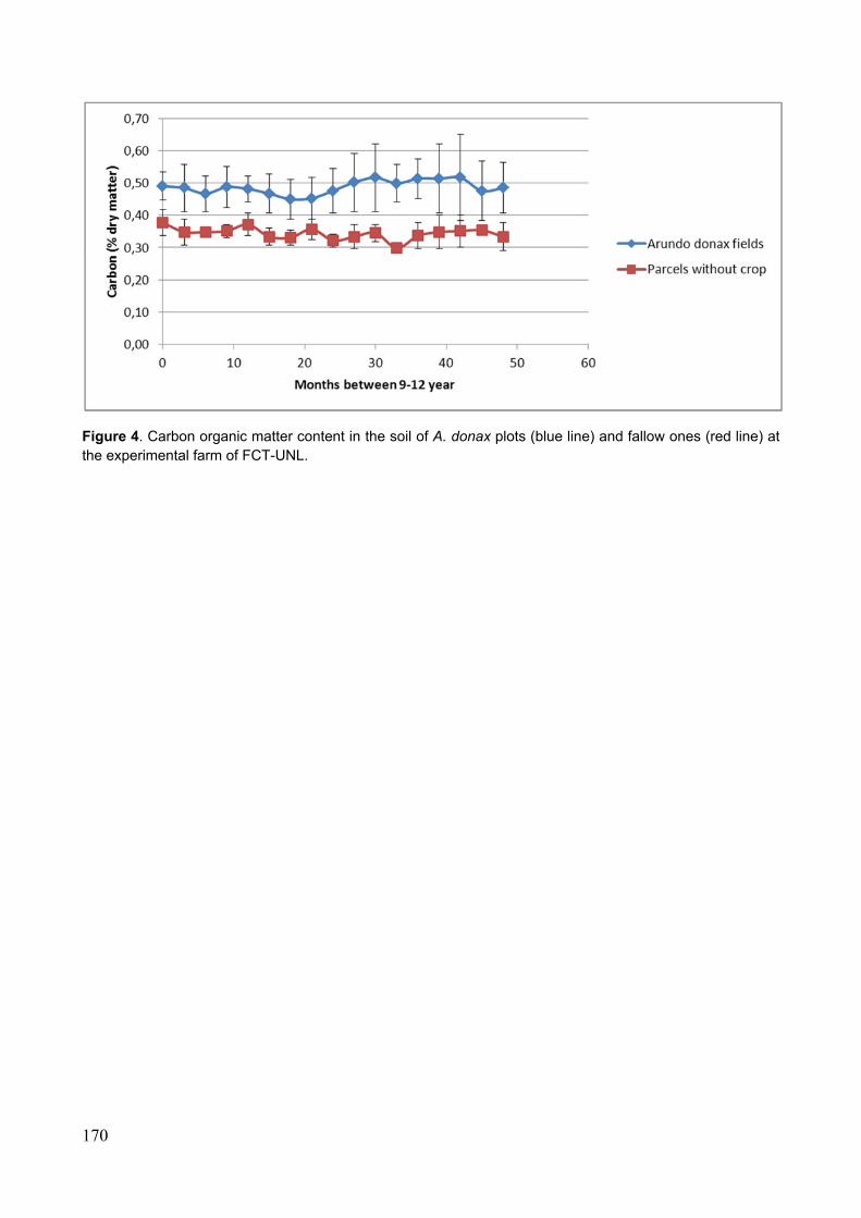
170
Figure 4. Carbon organic matter content in the soil of A. donax plots (blue line) and fallow ones (red line) at the experimental farm of FCT-UNL.
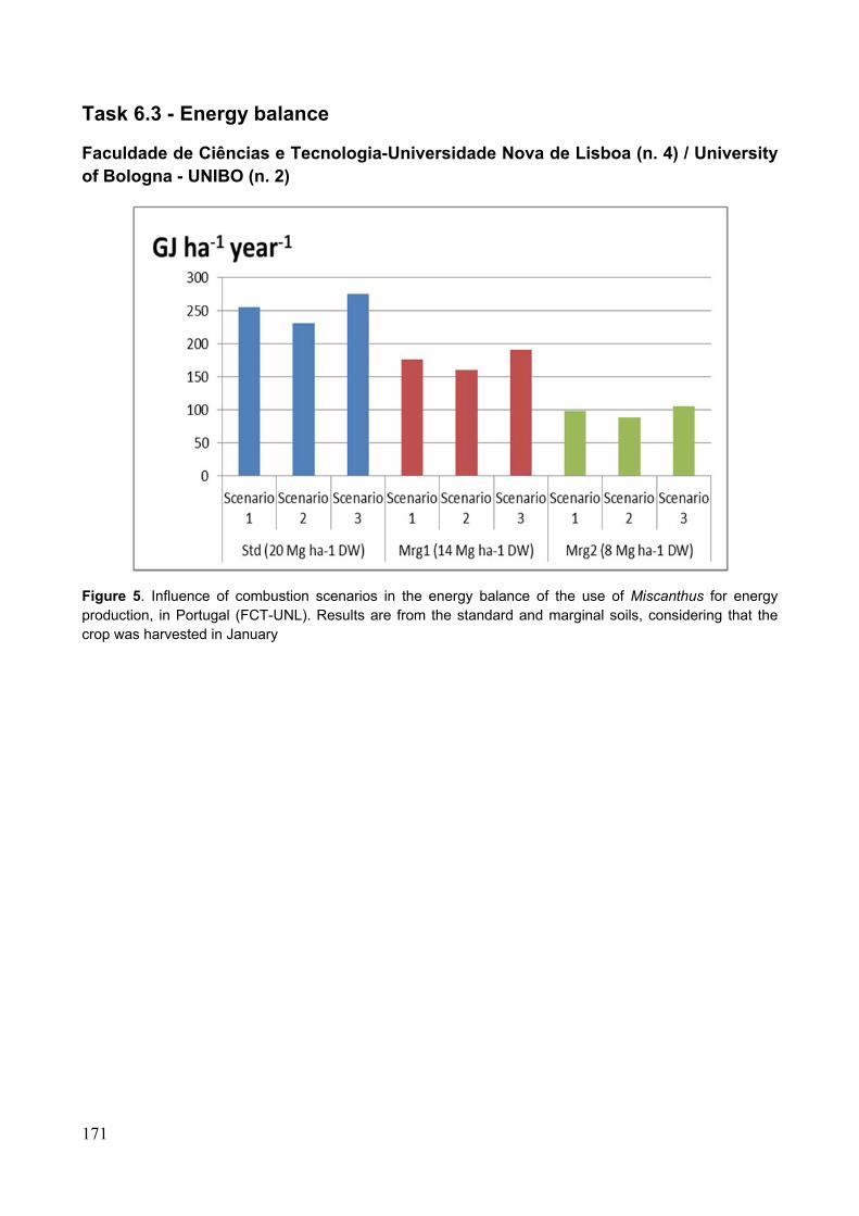
171
Task 6.3 - Energy balance
Faculdade de Ciências e Tecnologia-Universidade Nova de Lisboa (n. 4) / University of Bologna - UNIBO (n. 2)
Figure 5. Influence of combustion scenarios in the energy balance of the use of Miscanthus for energy production, in Portugal (FCT-UNL). Results are from the standard and marginal soils, considering that the crop was harvested in January
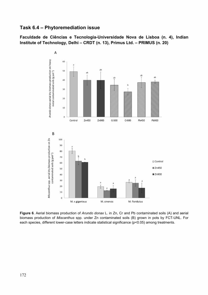
172
Task 6.4 – Phytoremediation issue
Faculdade de Ciências e Tecnologia-Universidade Nova de Lisboa (n. 4), Indian Institute of Technology, Delhi – CRDT (n. 13), Primus Ltd. – PRIMUS (n. 20)
Figure 6. Aerial biomass production of Arundo donax L. in Zn, Cr and Pb contaminated soils (A) and aerial biomass production of Miscanthus spp. under Zn contaminated soils (B) grown in pots by FCT-UNL. For each species, different lower-case letters indicate statistical significance (p<0.05) among treatments.
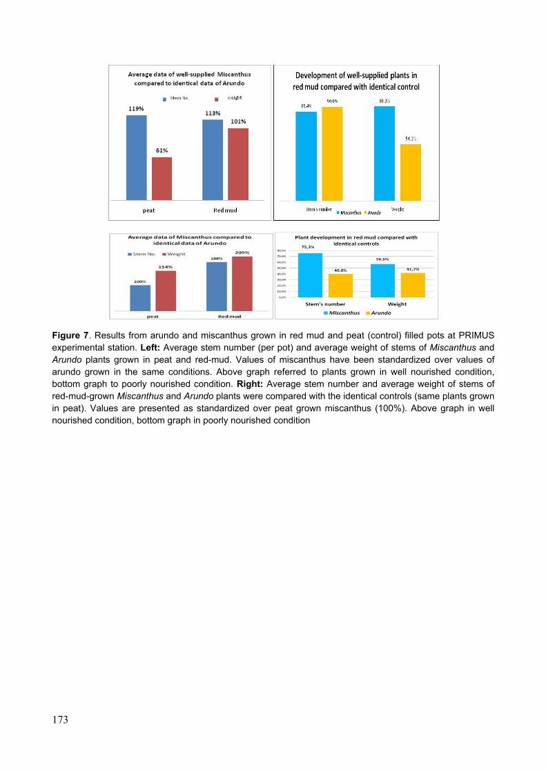
173
Figure 7. Results from arundo and miscanthus grown in red mud and peat (control) filled pots at PRIMUS experimental station. Left: Average stem number (per pot) and average weight of stems of Miscanthus and Arundo plants grown in peat and red-mud. Values of miscanthus have been standardized over values of arundo grown in the same conditions. Above graph referred to plants grown in well nourished condition, bottom graph to poorly nourished condition. Right: Average stem number and average weight of stems of red-mud-grown Miscanthus and Arundo plants were compared with the identical controls (same plants grown in peat). Values are presented as standardized over peat grown miscanthus (100%). Above graph in well nourished condition, bottom graph in poorly nourished condition
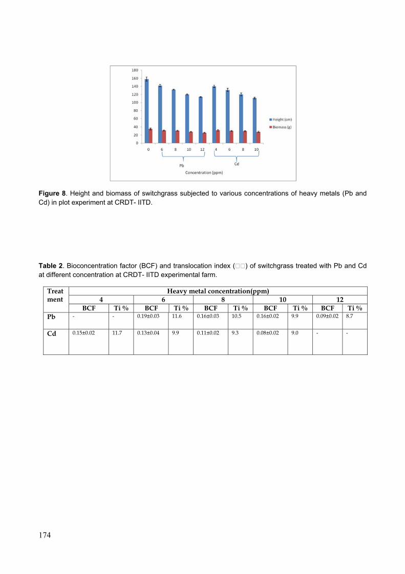
174
Figure 8. Height and biomass of switchgrass subjected to various concentrations of heavy metals (Pb and Cd) in plot experiment at CRDT- IITD.
Table 2. Bioconcentration factor (BCF) and translocation index ( ) of switchgrass treated with Pb and Cd at different concentration at CRDT- IITD experimental farm.
Treatment
Heavy metal concentration(ppm) 4 6 8 10 12
BCF Ti % BCF Ti % BCF Ti % BCF Ti % BCF Ti % Pb - - 0.19±0.03 11.6 0.16±0.03 10.5 0.16±0.02 9.9 0.09±0.02 8.7
Cd 0.15±0.02 11.7 0.13±0.04 9.9 0.11±0.02 9.3 0.08±0.02 9.0 -
-
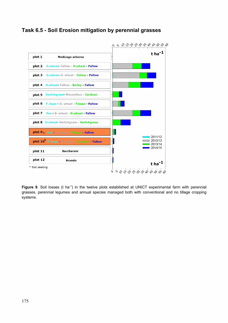
175
Task 6.5 - Soil Erosion mitigation by perennial grasses
Figure 9. Soil losses (t ha-1) in the twelve plots established at UNICT experimental farm with perennial grasses, perennial legumes and annual species managed both with conventional and no tillage cropping systems.
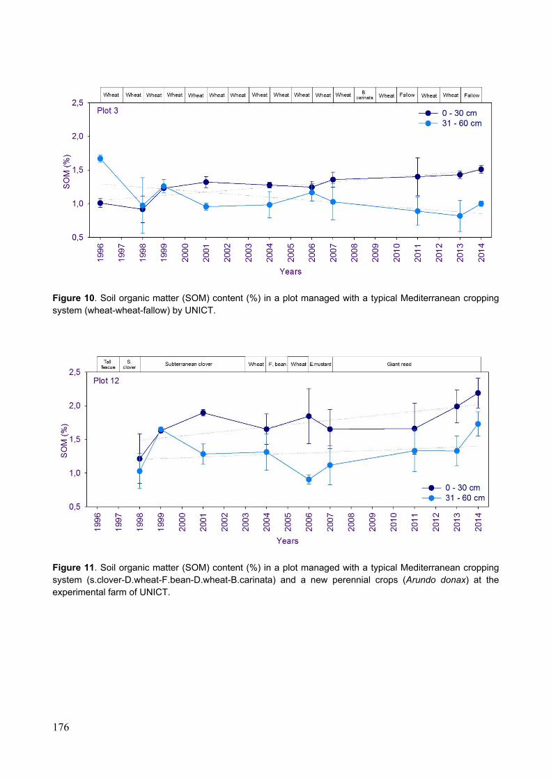
176
Figure 10. Soil organic matter (SOM) content (%) in a plot managed with a typical Mediterranean cropping system (wheat-wheat-fallow) by UNICT.
Figure 11. Soil organic matter (SOM) content (%) in a plot managed with a typical Mediterranean cropping system (s.clover-D.wheat-F.bean-D.wheat-B.carinata) and a new perennial crops (Arundo donax) at the experimental farm of UNICT.