merge path improvements for minimal model hyper tableaux

Merge Path Improvements for

Minimal Model Hyper Tableaux

Peter Baumgartner, J.D. Horton, and Bruce Spencer

University of New Brunswick Fredericton, New Brunswick E3B 5A3, Canada{baumgart,jdh,bspencer}@unb.ca

Abstract. We combine techniques originally developed for refutationalfirst-order theorem proving within the clause tree framework with tech-niques for minimal model computation developed within the hyper tab-leau framework. This combination generalizes well-known tableaux tech-niques like complement splitting and folding-up/down. We argue thatthis combination allows for efficiency improvements over previous, re-lated methods. It is motivated by application to diagnosis tasks; in par-ticular the problem of avoiding redundancies in the diagnoses of electricalcircuits with reconvergent fanouts is addressed by the new technique. Inthe paper we develop as our main contribution in a more general way asound and complete calculus for propositional circumscriptive reasoningin the presence of minimized and varying predicates.

1 Introduction

Recently clause trees [7], a data structure and calculus for automated theoremproving, introduced a general method to close branches based on so-called mergepaths. In this paper we bring these merge paths to tableaux for minimal modelreasoning (e.g. [5,12,13,14]) by extending our framework of hyper tableau [3,1,2].The paper [7] is devoted to refutational theorem proving. Merge paths al-

low branches to close earlier than it would be possible without them or whenusing merge paths to simulate known instances such as folding-down [9]. Ex-pressed from the viewpoint of complement splitting [10], one advantage is thatthe splitting of literals can be deferred .In this paper we advocate to use merge paths for model computation calculi.

In addition to the advantages in the refutational framework, merge path allowone to partially re-use previously computed models instead of computing themagain. To achieve this, new inference rules dealing with merge paths for minimalmodel computation are defined. In contrast to the purely refutational setting,these inference rules have to be applied with care, as termination is no longera trivial property. Therefore, we give conditions for termination such that thecentral properties of minimal model soundness and minimal model completenesshold. More precisely, as our main result we develop such a calculus for the moregeneral case of circumscriptive reasoning for minimized and varying predicates(Section 4). The minimal model completeness proof is given by a simulation ofmerge paths by atomic cuts (cf. Lemma 1 in Section 4). Viewed from this point,

Neil V. Murray (Ed.): TABLEAUX’99, LNAI 1617, pp. 51–66, 1999.c© Springer-Verlag Berlin Heidelberg 1999

52 Peter Baumgartner et al.

our approach can thus be seen as a more and generalized approach for a controlledintegration of the cut rule for the purpose of minimal model computation.The rest of this paper is structured as follows: first we briefly give the idea

of merge paths as defined in [7]. This presentation should be sufficient to explainthe subsequent motivation of the new calculus from the viewpoint of a certainproblem encountered in diagnosis tasks. In Section 2 we bring merge paths intotrees and define an ordering on merge paths. It is employed in Section 3 in thenew calculus. In Section 4 we show how merge paths can be simulated by atomiccuts and, based on that, prove soundness and completeness. Section 5 discussescertain aspects of the calculus (memory requirements, atomic cuts vs. mergepaths).

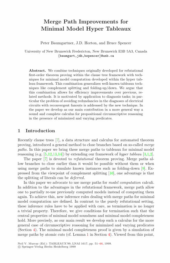
Clause trees. Merge paths are introduced and studied in [7] in the context ofclause trees. Clause trees are a data structure that represent equivalence classesof resolution derivations. Merge paths are a unified inference rule and generalizethe folding up/folding down technique of [9].Clause trees consist of clause nodes and atom nodes. Clause nodes are in-

dicated by a ◦. Every clause node N corresponds to some input clause λ(N) =L1 ∨ . . .∨Ln as can be seen from the n emerging edges; these edges are labeledby the signs of the Li’s, and the atom parts of the Li’s can be found in theadjacent atom nodes. Clause trees are built in such a way that from every atomnode exactly two edges with opposite sign emerge. This corresponds to a binaryresolution inference. Here is an example:

− + − + + − +

← C A,B ← C ← BC ← AClause set:

CClause tree: A B C

Now, in addition, merge paths can be drawn between equally labeled atomnodes, provided that the first and final edges are also equally labelled. In thepreceeding figure, there is a merge path from the right C-node (called the tailof the merge path), to the left C-node (called the head of the merge path). Theidea is “in order to find a proof at the tail of a merge path, look it up (copyit) from the head of the merge path”. Thus, tail nodes are considered as provenand need no further extension. Thus a proof is a clause tree where every leaf isproven in this way or is a clause node.Head nodes can be part of another merge path, and then there is a depen-

dency of the nodes on the path on the head node. In this case the “lookup” ofproofs is done recursively. In order to terminate this, cyclic dependencies mustbe excluded. The absence of cycles in a set of merge paths is referred to by theterm “legal”. Many of the results in [7] concerning legality and relation notionsare derived as general properties of paths in trees. They thus can be readilyapplied to our case of hyper tableaux as well.

Motivation: A diagnosis application. We consider consistency-based diagnosisaccording to Reiter [16]. In this scenario, a model of a device under considerationis constructed and is used to predict its normal behavior. By comparing this

Merge Path Improvements for Minimal Model Hyper Tableaux 53

prediction with the actual behavior it is possible to derive a diagnosis. Moreprecisely, a diagnosis ∆ is a (minimal) subset of the components of the device,such that the observed behavior is consistent with the assumption that exactlythe components in ∆ are behaving abnormally. Computing diagnosis can alsobe formalized as a circumscription problem.

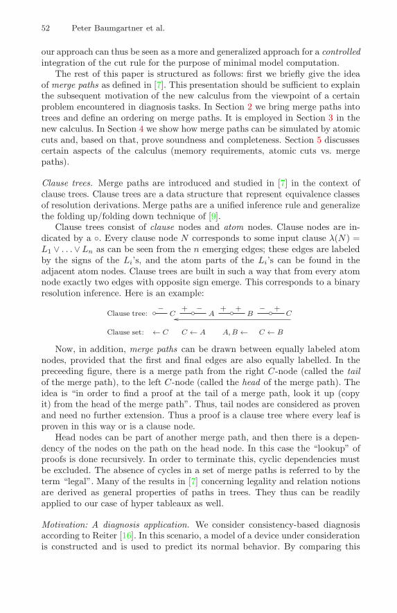
The figure below depicts a hypothetical diagnosis scenario of an electricalcircuit where merge paths are useful. The notation [0] in the left picture meansthat at this point the circuit is logical zero. The [0]’s at the bottom refer to inputvalues of the actually observed behavior. The “Huge” box is meant to stand fora large circuit. The lightning at the output indicates that the predicted outputis different from the actual output. We assume that two possible diagnoses are∆1 = {inv1} and ∆2 = {inv2}. Then it is consistent to have [0] at the output ofthe and -gate, and we assume that this renders the whole description consistent.

Circuit Hyper tableau . . . with merge paths

[0] [0]

inv1 inv2

and1

[0]

Huge

“[0]”“[0]”

Huge

ab(inv1) ab(inv2 )

∆2

Huge

∆1

“[0]”×

“[0]”

Huge

ab(inv1 ) ab(inv2 )

ab(inv2 )ab(inv1 )

∆1 ∆2

Now, the crucial observation is that the computation of ∆1 and ∆2 showconsiderable redundancies. The hyper tableau based diagnosis approach of [2]would result in the tableau depicted in the middle of the figure. Diagnoses areread off from open branches by collecting the ab-literals found there. The trian-gles stand for sub-tableaux containing diagnoses of the “Huge” part. There aretwo open branches containing ∆1 and ∆2 respectively.

Notice that the “Huge” part has to be diagnosed twice although for its diag-nosis exactly the same situation applies, namely [0] at its input . This is reflectedby the nodes “[0]”. Clearly, for the diagnosis of “Huge” it is irrelevant whatcaused the “[0]”-situation. The generalized underlying problem is well-known inthe diagnosis community and is referred to as “reconvergent fanouts”.

So, the symmetry hidden in this problem was not exploited. In fact, themerge path technique just realizes this. It is indicated in the right part of thefigure above: after the diagnosis ∆1 is computed in the left branch, and thecomputation reaches the “[0]” node in the right subtree, a merge path is drawnas indicated, and the branch with the right “[0]” node is closed. The price to bepaid is that∆1 as computed so far is invalid now. Technically, the ab(inv1 ) literalcan be thought of as being removed from the branch (it becomes “invisible” inour terminology). Hence, the computation starts again as indicated below thetriangle. Eventually, both ∆1 and ∆2 can be found there.


Why is it attractive to use such a “non-monotonic” strategy? The answer isthat it is little effort to recompute the initial segment of the diagnosis and betterto save recomputing the “huge” part. We do not suggest to use the merge pathsin all possible situations. In order to be flexible and allow guidance by heuristics,merge paths are thus always optional in the calculus defined below.

Preliminaries. We assume that the reader is familiar with the basic conceptsof first-order logic. Throughout this paper, we are concerned with finite groundclause sets. A clause is an expression of the formA ← B, where A = (A1, . . . , Am)and B = (B1, . . . , Bn) are finite sequences of atoms (m, n ≥ 0); A is called thehead , and B is called the body of the clause. Whenever convenient, a clause isalso identified with the disjunction A1 ∨ · · · ∨Am ∨ ¬B1 ∨ · · · ∨ ¬Bn of literals.

Quite often, the ordering of atoms does not play a role, and we identifyA andB with the sets {A1, . . . , Am} and {B1, . . . , Bn}, respectively. Thus, set-theoreticoperations (such as “⊂”, “∩” etc.) can be applied meaningfully.By L we denote the complement of a literal L. Two literals L and K are

complementary if L = K. In the sequel, the letters K and L always denoteliterals, A and B always denote atoms, C and D always denote clauses, S alwaysdenotes a finite ground clause set, and Σ denotes its signature, i.e.Σ =

⋃{A∪B |

A ← B ∈ S}.

As usual, we represent a Σ-interpretation I by the set of true atoms, i.e.I(A) = true iff A ∈ I. Define I |= A ← B iff B ⊆ I implies A ∩ I 6= ∅. Noticethat this is consistent with other usual definitions when clauses are treated asdisjunctions of literals. Usual model-theoretical notions of “satisfiability”, “va-lidity” etc. of clauses and clause sets are applied without defining them explicitlyhere.

Minimal models are of central importance in various fields, like (logic) pro-gramming language semantics, non-monotonic reasoning (e.g. GCWA,WGCWA)and knowledge representation. Of particular interest are Γ -minimal models, i.e.minimal models only wrt. the Γ -subset of Σ. From a circumscriptive point ofview, Γ is thus the set of atoms to be minimized, and Σ \Γ varies. In the sequel,Γ always denotes some subset of the signature Σ.

Definition 1 (Γ -Minimal Models). For any atom set M define the restric-tion ofM to Γ as M |Γ =M ∩Γ . In order to relate atom setsM1 and M2 defineM1 <Γ M2 iff M1|Γ ⊂ M2|Γ , and M1 =Γ M2 iff M1|Γ = M2|Γ . As usual,the relation M1 ≤Γ M2 is defined as M1 <Γ M2 or M1 =Γ M2. We say that amodel I for a clause set M is Γ -minimal (forM) iff there is no model I ′ for Msuch that I ′ <Γ I

It is easy to see that ≤Γ is a partial order and that =Γ is an equivalence relation.Notice that the “general” minimal models can simply be expressed by settingΓ = Σ. Henceforth, by a minimal model we mean a Σ-minimal one.

An obvious consequence of this definition is that every minimal model of Sis also a Γ -Minimal model of S (but the converse does not hold in general).


2 Literal Trees and Merge Paths

We consider finite ordered trees T where the nodes, except the root node, arelabeled with literals. The labeling function is denoted by λ. A branch of T is asequence b = (N0, N1, . . . , Nn) of nodes of T such that N0 is the root, Ni is animmediate successor node of Ni−1 (for 1 ≤ i ≤ n) and Nn is a leaf node. Thefact that b is a branch of T is also written as b ∈ T .

Any subsequence b′ = (Ni, . . . , Nj) with 0 ≤ i ≤ j ≤ n is called a partialbranch of b; if i = 0 then this subsequence is called rooted . Define last(b′) =Nj. In the sequel the letter b always denotes a branch or a partial branch.The expression (b1, b2) denotes the concatenation of partial branches b1 and b2;similarly, the expression (b, N) denotes (Ni, . . . , Nj , N), where b is the partialbranch (Ni, . . . , Nj). For convenience we write “the node L”, where L is a literal,instead of the more lengthy “the node N labeled with L”, where N is some nodegiven by the context. In the same spirit, we write (L1, . . . , Ln) and mean thepartial branch (N1, . . . , Nn), or even (N0, N1, . . . , Nn) in case N0 is the root andNi is an immediate successor node of the root, where Ni is labelled with Li (for1 ≤ i ≤ n). Further, (b, L) means (b, N), where N is some node labeled with Land b is a partial branch.

A branch b is labeled either as “open”, “closed” or with some subset of Γ . Inthe latter case, b is called a MM-branch, and MM(b) denotes that set, which iscalled the minimal model of b. A tree or subtree is closed iff every of its branchesis closed, otherwise it is non-closed . A tree or subtree is open if some of itsbranches are open.

Definition 2 (Ancestor Path, Merge Path). Let T be a tree and supposethat T contains a rooted partial branch b of the form b = (N0, N1, . . . , Ni, . . . , Nn)with N0 being the root. Any sequence ancp(b, Ni) := (Nn, Nn−1, . . . , Ni), wheren ≥ i > 0, is called an ancestor path (of b). The node Nn is called the tail andthe node Ni is called the head of this ancestor path. Now, if it additionally holdsthat λ(Ni) = A and λ(Nn) = ¬A (for some atom A) then ancp(b, Ni) is calledan ancestor merge path (of b).

Let T contain rooted partial branches bT = (N0 , N1, . . . , Ni, Ni+1, . . .Nn) andbH = (N0, N1, . . . , Ni,Mi+1, . . .Mm) with N0 being the root and m, n > i ≥ 0and Mi+1 6= Ni+1 and such that λ(Nn) = λ(Mm) = A for some atom A.Define pT = Nn, . . . , Ni+1, p

H = Mi+1, . . . ,Mm, and p = (pT , pH). Here, p

is understood as a concatenation of pT and pH. By this definition, nodes onpaths are written in order from tail to head. We assume that p can always bedecomposed into its constituents pT and pH; p is called a non-ancestor mergepath of T from bT to bH with tail Nn and head Mm. It is also denoted bymergep(bT , bH). The node Ni is called the turn point of p. Note that the turnpoint is not on p.

By a merge path we mean a non-ancestor merge path or an ancestor mergepath. The letters p and q are used in the sequel to denote ancestor paths or mergepaths, and the letter P will be used to refer to sets of merge paths.


A non-ancestor merge path with m = n = i + 1 is called factoring , the casem = i+ 1 is called a hook , and the case m > i+ 1 is called a deep merge path.

Definition 3 (Ordering on paths). Suppose the paths p = (N1, . . . , Nn)and q = (M1, . . . ,Mm) as given. Define q precedes p, as q ≺ p iff Mm ∈{N2, . . . , Nn−1}. We say that a finite set of paths P is legal iff the ≺ relation onP can be extended to a partial order � on P. Illegal means not legal.

Notice that the ≺ relation is irreflexive but in general not transitive. One couldalso define a set of paths to be illegal if it contains a cycle, i.e. if there are pathsp1, . . . , pn ∈ P such that p1 ≺ p2 ≺ · · · ≺ pn ≺ p1, for some n > 1. Avoidingcycles is important to guarantee the soundness of the calculus.

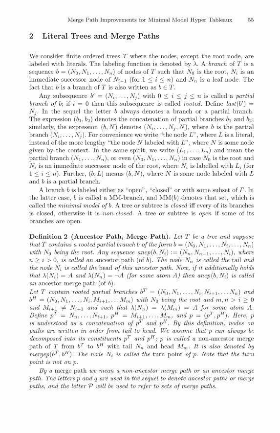
Example 1 (Ordering). The figure below contains examples of trees equippedwith merge paths. The underlying clause sets can be left implicit. Merge pathsare indicated using arrow notation. For instance, in the right tree, the arrow fromthe leaf node ¬A to A indicates an (the) ancestor merge path p1 = (¬A,C, A) ofthe branch (A,C,¬A) with tail ¬A and head A. In the same tree, the arrow fromthe rightmost node C to the other node C indicates a non-ancestor merge pathp2 = mergep((B,C), (A,C)) = (C,B,A, C) with tail C (the right node) andhead C (the other node C) and the root as turn point. In terms of Definition 2we have pT2 = (C,B) and p

H2 = (A,C). The path p2 is an example of a deep

merge path. The merge path set {p1, p2} is not legal because both p1 ≺ p2 andp2 ≺ p1 and hence ≺ cannot be extended to a partial order. The left tree containstwo non-ancestor merge paths and both are “hooks”.

Illegal:

A

B×

B

A×

Legal:

A B

C×

C

¬C×

Illegal:

A

C

¬A×

¬C×

×C

B

The left and right cases are the simplest cases for illegality, as in both casesonly two merge paths are involved. These are illegal, because the heads of themerge paths are mutually contained as inner nodes. The left tableau wouldcorrespond to an unsound combination of the “folding up” and “folding down”inference rules, usually avoided in implementations by choosing not to combinethem at all.

The new calculus to be presented below does not only construct a tableaux T asthe derivation proceeds, but also a legal set of merge paths P. This guaranteessoundness.In order to achieve minimal model computation, we have to define how in-

terpretations are extracted from open branches.

Definition 4 (Visibility, Branch Semantics). Let b = (N0, N1 . . . , Nn) be arooted partial branch in a tree T (not necessarily a hyper tableau) with n ≥ 0,


and let P be a legal set of merge paths in T . The node Ni (where 0 < i ≤ n)that is not the tail of a merge path in P is said to be visible from Nn wrt. P iffP ∪ {ancp(b, Ni)} is legal. Define

[[(N0, N1, . . . , Nn)]]P = {λ(Ni) | Ni is visible from Nn wrt. P, for 0 < i ≤ n} .

The set [[b]]P is called inconsistent iff {A,¬A} ⊆ [[b]]P for some atom A; con-sistent means “not inconsistent”. We omit “wrt. P” when P is given by thecontext.

The head of a merge path hides nodes that are on the path from nodes beyond thehead, i.e. away from the direction that the head points. Those nodes that are nothidden from a node are visible to that node. In the definition of branch semanticsan atom A is true in a consistent branch if and only if it is visible from the leaf.For instance, in the middle tableau in Example 1 we have [[(A,C,¬C)]]P ={¬C,C} and [[(B,C)]]P = {B,C}, where P consists of the two merge pathsdrawn there. Notice that the case n = 0 is not excluded, and it holds that[[(N0)]] = ∅.

3 Hyper Tableaux with Merge Paths

Before defining the new calculus we take one more preliminary step: supposethat B ∈ [[b]]P for given open branch b and legal path set P. In the trees con-structed in Definition 5, there is a unique node NB in b with λ(NB) = B suchthat NB is visible from the leaf of b

1. Consequently, the ancestor merge pathancp((b,¬B), NB) is uniquely defined, and it is denoted by ancp((b,¬B)) alone.

Definition 5 (Hyper tableaux with merge paths). Let T be a tree, b be abranch in T and let L1∨· · ·∨Ln be a disjunction of literals. We say that T ′ is anextension of T at b with L1 ∨ · · · ∨Ln iff T ′ is obtained from T by attaching tothe leaf of b n new successor nodes N1, . . . , Nn that are labeled with the literalsL1, . . . , Ln in this order.A selection function is a total function f that maps an open tree to one of

its open branches. If f(T ) = b we also say that b is selected in T by f.Hyper tableaux T for S with merge path set P – or (T,P) for short – are

defined inductively as follows.

Initialization step: (ε, ∅) is a hyper tableau for S, where ε is a tree consistingof a root node only. Its single branch is marked as “open”.

Hyper extension step with C: If (i) (T,P) is an open hyper tableau for S withselected branch b, and (ii) C = A1, . . . , Am ← B1, . . . , Bn is a clause from S (forsome A1, . . . , Am and B1, . . . , Bn and m, n ≥ 0), and (iii) {B1, . . . , Bn} ⊆ [[b]]P ,and (iv) {A1, . . . , Am} ∩ [[b]]P = ∅ (regularity), then (T

′,P ′) is a hyper tableau

1 Most proofs are omitted or only sketched for space reasons; the full version [4]contains all proofs.


for S, where (i) T ′ is an extension of T at b with A1∨· · ·∨Am∨¬B1∨· · ·∨¬Bn,and (ii) every branch (b,¬B1) . . . , (b,¬Bn) of T ′ is labeled as closed, and (iii)every branch (b, A1) . . . , (b, Am) of T

′ is labeled as open, and (iv) P ′ = P ∪{ancp((b,¬B1)), . . . , ancp((b,¬Bn))}. If conditions (i) – (iv) hold, we say thatan “extension step with clause A ← B is applicable to b”.

Merge path step with p: If (i) (T,P) is an open hyper tableau for S withselected branch b, and (ii) p = mergep(b, bH) is a non-ancestor merge path fromb, for some rooted partial branch bH of T , and (iii) last(bH) is not the tail of amerge path in P, and (iv) P ∪{p} is legal, then (T ′,P ′) is a hyper tableau for S,where (i) T ′ is the same as T , except that b is labeled as closed in T ′, and everyMM-branch b′ of T with [[b′]]P∪{p}|Γ ⊂ MM(b

′) is labeled as open in T ′, and (ii)

P ′ = P ∪ {p}. If conditions (i) – (iv) hold, we say that a “merge path step withmerge path p is applicable to b”.

Minimal Model Test: If (i) (T,P) is an open hyper tableau for S with selectedbranch b, and (ii) [[b]]P is a Γ -minimal model of S, then (T

′,P) is a hyper tableaufor S, where T ′ is the same as T except that b is labeled in T ′ with [[b]]P |Γ . Ifapplicability conditions (i) and (ii) hold, we say that the minimal model testinference rule is applicable (to b).

A (possibly infinite) sequence ((ε, ∅) = (T0,P0)), (T1,P1), . . . , (Tn,Pn), . . . ofhyper tableaux for S is called a derivation, where (T0,P0) is obtained by aninitialization step, and for i > 0 the tableau (Ti,Pi) is obtained from (Ti−1,Pi−1)by a single application of one of the other inference rules. A derivation of (Tn,Pn)is a finite derivation that ends in (Tn,Pn). A refutation of S is a derivation ofa closed tableau.

This definition is an extension of previous ground versions of hyper tableaux(mentioned in the introduction) by bringing in an inference rule for merge pathsand explicitly handling Γ -minimal models. The introduction of non-ancestormerge paths requires to explicitly keep track of the ancestor merge paths aswell.

The purpose of the hyper extension step rule is to satisfy a clause that isnot satisfied in the selected branch b. An implicit legality check for the ancestorpaths added in an extension step is carried out by excluding those atoms fromthe branch semantics that would cause illegality when drawing an ancestor pathto them.

An obvious invariant of the inference rules is that every open or MM-branchb is labeled with positive literals only and hence [[b]]P is consistent. Thus [[b]]Pconforms to our convention of representing interpretations as the set of atomsbeing true in it.

The purpose of the minimal model test rule is to remember that a Γ -minimalmodel is computed and to attach it to the selected branch b. Since usually one isinterested only in the Γ -subset of models, we keep only the Γ -atoms. These arethought to be the output of the computation. Notice that for MM-branches, ahyper extension step is not applicable, because MM-branches are not open and


only open branches can be selected. For the same reason merge path steps arealso not applicable to MM-branches.The purpose of the merge path step inference rule is to close branches because

a “proof” or a model is to be found in the branch where the drawn merge path ispointing to. But in the course of a derivation, a previously computed Γ -minimalmodel MM(b) of a branch b might no longer be the same as [[b]]P |Γ , because ofa deep merge path step with head node (for instance) in b. Therefore, the labelMM(b) has to be rejected and the branch has to be opened again for furtherextension. This is expressed in item (i) in the conclusion of the merge pathstep inference rule (Def. 5). Notice, however, that this happens only if someatom A ∈ Γ in [[b]]P becomes invisible, not if some other literal from Σ \ Γbecomes invisible. Thus, some deep merge paths can still be drawn withoutcausing recomputation.

3.1 Examples

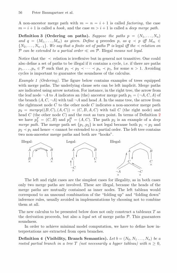
(1) Consider the figure in Example 1 again. Closed branches are marked withthe symbol “×” as closed. Only the tableau in the middle is constructible by thecalculus, because the calculus rules forbid the derivation of a tableau with anillegal set of merge paths. In this middle tableau the left branch gets closed bya hyper extension step with the clause ← C, and the right branch is closed bya non-ancestor merge path step as indicated. This application of a non-ancestormerge path step corresponds to a folding-up step in model elimination [9].

The right tableau shows that both ancestor and non-ancestor merge pathshave to be taken into account for legality.

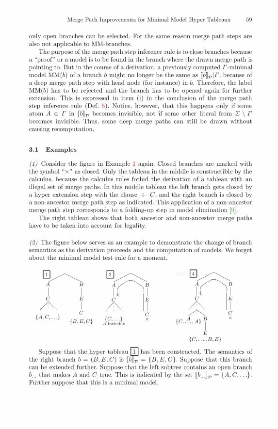
(2) The figure below serves as an example to demonstrate the change of branchsemantics as the derivation proceeds and the computation of models. We forgetabout the minimal model test rule for a moment.

A

C

B

C{A,C, . . .}

E

{B,E,C}

1

A

C

B

C{C, . . .} ×

E

A invisible

2

A

C

B

E

C×BA

{C, . . . ,B,E}E

{C, . . . , A}

. . . 4

Suppose that the hyper tableau 1 has been constructed. The semantics ofthe right branch b = (B,E, C) is [[b]]P = {B,E, C}. Suppose that this branchcan be extended further. Suppose that the left subtree contains an open branchb... that makes A and C true. This is indicated by the set [[b...]]P = {A,C, . . .}.Further suppose that this is a minimal model.


Next, let a merge path step be applied with non-ancestor merge path p tothe tableau 1 , yielding the tableau 2 . By this step, b is closed and henceits interpretation is rejected for the time being. A second effect of this stepis that the node labeled with A becomes invisible from the leaf of b.... Thus[[b...]]P∪{p} = {C, . . .}. Now, this new interpretation has to be “repaired” bybringing in A again. This is done in the next step by extending with A ∨ Byielding a tableau 3 (which is not depicted). Notice that the minimal model[[b...]]P is indeed reconstructed, only in a different order. In order to reconstructthe rejected interpretation {B,E, C} from above that was rejected by the mergepath step, a hyper extension step below the new B node with E is carriedout. This leads to the tableaux 4 . Notice that the new branch with semantics{C, . . ., B, E} possibly contains more elements than the corresponding one withsemantics {B,E, C}.

It is worth emphasizing that the re-computation of models happens only inthe case of non-ancestor merge paths with their head in open branches. Mergepaths into closed branches are “cheap” in that no re-computation is necessary.Thus, in a sense, refutational theorem proving, which would stop with failureafter the first open finished branch (cf. Def. 6 below) is found, is “simpler” thancomputing models.

In order to demonstrate the effect of the minimal model test inference rule letnow Γ = {C,E}. We start with tableau 1 again. For the branch b... the minimalmodel [[b...]]P = {A,C, . . .} was supposed. Suppose that E is not contained inthat set. Then [[b...]]P |Γ = {C} is a Γ -minimalmodel, because [[b...]]P is a minimalmodel. According to the minimal model test inference rule, the branch b... canbe labeled with {C} then.

Now, consider tableau 2 . The merge path p there eliminates the Γ -minimalmodel candidate in the right branch by closing it. Concerning the left branchb..., although A has been removed from its previous interpretation [[b...]]P ={A,C, . . .}, its Γ -minimal model {C} has not been changed, i.e. [[b...]]P |Γ =[[b...]]P∪{p}|Γ = {C}. Consequently the branch label {C} has not to be removedand b... has not to be opened again. This is reflected by the result description(i) in the definition of merge path step. If Γ were Σ, the branch b... would have

to be opened again and the computation could continue as above leading to 4 .

3.2 Finite Derivations

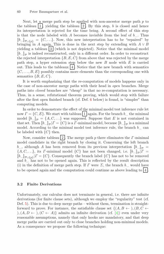
Unfortunately, our calculus does not terminate in general, i.e. there are infinitederivations (for finite clause sets), although we employ the “regularity” test (cf.Def. 5). This is due to deep merge paths – without them, termination is straight-forward to prove. For instance, the satisfiable clause set {(A,B ← ), (B,C ←), (A,D ← ), (C ← A)} admits an infinite derivation (cf. [4]) even under veryreasonable assumptions, namely that only hooks are mandatory, and that deepmerge paths are carried out only to close branches holding non-minimal models.As a consequence we propose the following technique:


Theorem 1 (Termination Criterion).A derivation (T0,P0), . . . , (Tn,Pn), . . .is finite, provided that for every (Ti,Pi), where i ≥ 0, an applicable merge pathstep with merge path p is not carried out if for some open branch b in Ti morethan an a priori fixed number max of occurrences of some label A is invisiblefrom last(b) wrt. Pi ∪ {p}.

This criterion avoids infinite derivations by bounding repetitions of the sameliteral along branches. A trivial instance is max = 0. Then no deep merge pathsbut only hooks are possible. The idea underlying the criterion is that one shouldnot without bound repeat the derivation of an atom that becomes repeatedlyinvisible on a branch. Due to this criterion we consider from now on only finitederivations.

Definition 6 (Redundancy, Fairness). Suppose as given some hyper tableau(T,P) for S. A clause A← B is called redundant in an open branch b of T wrt.P iff [[b]]P |= A← B (iff B ⊆ [[b]]P implies A∩ [[b]]P 6= ∅).A branch b of T is called finished (wrt. P) iff (i) b is closed, or (ii) b is an

MM-branch, or else (iii) the minimal model test inference rule is not applicableto b and every clause A ← B ∈ S is redundant in b wrt. P. The term unfinishedmeans “not finished”.Now suppose as given a finite derivation D = (T0,P0), . . . , (Tn,Pn) from S

with selection function f. D is called fair iff (i) D is a refutation, i.e. Tn isclosed, or else (ii) f(Tn) is finished wrt. Pn.The selection function f is called a model computation selection function

iff f maps a given open hyper tableau (T,P) to an unfinished branch wrt. P,provided one exists, else f maps T to some other open (finished) branch.

According to this definition, the only possibility to be unfair is to terminatea derivation with a selected open branch that could be either labeled with aΓ -minimal model or extended further.

The existence of fair derivations is straightforward because we insist on finitederivations. Notice that any input clause not redundant so far in a branch b canbe made redundant by simply carrying out an extension step with that clause.The idea behind a model-computation selection function is that no derivation

should stop with an unfinished branch. Since finished open branches constituteΓ -models, with such a selection function every Γ -minimal model is computed.

4 Soundness and Completeness

Lemma 1 (Soundness lemma). Let (T,P) be a hyper tableau for satisfiableclause set S. Then for every minimal model I of S there is an open branch b ofT such that [[b]]P ⊆ I.

The proof of Lemma 1 is done by simulating non-ancestor merge paths by atomiccuts, i.e. by β-steps applied to disjunctions of the form A ∨ ¬A, for some atomA. The branch semantics in presence of atomic cuts is given by forgetting about


the negative literals, i.e. [[b]]+P = {A ∈ [[b]]P | A is a positive literal} for any

consistent branch b in a hyper tableau with atomic cuts.The transformation t defined below takes a hyper tableau with cut (T,P)

where P is legal and contains at least one non-ancestor merge path, and returnsa hyper tableau with cut (T ′,P ′) = t(T,P) that contains one less non-ancestormerge path in P ′ (which is legal as well). The transformation t preserves thefollowing invariant : for every consistent and open branch b′ of T ′ there is aconsistent and open branch b of T such that [[b]]

+P ⊆ [[b

′]]+P′ . Repeated application

of t as long as possible results in a tableau (Tcut,Pcut) with cuts but withoutnon-ancestor merge paths. All literals along all branches are visible there, andhence we have a “standard tableau” with cuts then. The lemma then is provenfor this tableau, and using the invariant above it can be translated back for theoriginally given tableau (T,P).The transformation t itself is depicted in the figure below. The left side

displays the most general situation. Dashed lines mean partial branches. Forinstance, the top leftmost dashed line leading to B means the partial branchpB from the root to the node (inclusive) labeled with B. Triangles are certainforests. The most appropriate intuition is to think of trees as branch sets. Thenthe triangle TB is simply the set of the branches obtained from T by deletingall branches that contain pB.

TBB

T ′:

TB

TAi

TC

TAj

TB

C

AjAi

C×

T :

N

B

TAi TAj

TB

C

AjAi

C× ×

¬C C

TC

N

(×) (×)

(×)

Since P is legal it is extendible to a partial order �. Let p be a minimal elementin this order. This is the one to be transformed away. It is important to use aminimal element in order to prove the invariant.The solid lines, just like the ones below B indicate a hyper extension step;

here, it is supposed that a hyper extension step with clause C = A1, . . . , An ← Bhas been carried out to pB , and all the literals short of Ai and Aj (for somei, j ∈ {1, . . . , n} and i 6= j) are attached to nodes in the subtree TB . The assumednon-ancestor merge path p is indicated with tail node C (left) and head nodeC (right) and turn point B. There might be other non-ancestor merge paths inP, in particular some where the head of p is an inner node. This possibility isindicated in the figure as well, by the arrow pointing into TC . The tail of thisnon-ancestor merge path, say pC is a leaf node N somewhere in T .Inconsistent or closed branches are marked by “×”. The effect of the trans-

formation t is shown on the right. Notice the cut with C ∨¬C at the turn pointB. The transformation is understood to move merge paths as well. For example,


the non-ancestor merge path pC still has the same head and tail node, but theyare possibly located in different places in T ′ now, and also a different turn pointmight result. After transformation some branches might get closed due to thepresence of ¬C. This is indicated by “(×)”. Notice that the transformation onlyintroduces new negative literals into branches, ¬C, so that the branch semanticswrt. positive literals does not change, as required in the invariant .The central properties that have to be argued for are (i) that the tableau

resulting from the transformation is a hyper tableau (i.e. that all negative leafnodes can still be closed by legal ancestor paths), and (ii) that the invariantholds. This is done by expressing the invariant in terms of visibility from leafnodes and then arguing with the orderings underlying P and P ′.This lemma is applied in the proof of the next theorem, which is our main

result.

Theorem 2 (Soundness and Completeness). Let f be a model computa-tion selection function and D be a finite, fair derivation from clause set S ofthe hyper tableau (T,P). Then {MM(b) | b is a MM-branch of T} = {I|Γ |I is a Γ -minimal model of S} Furthermore, if S is unsatisfiable then T is closed(refutational completeness).

Proof. Minimal model soundness – the first theorem statement in the “⊆”-direction – is an immediate consequence of the applicability condition (ii) inthe minimal model test inference rule and the result description (i) in the mergepath step inference rule. Regarding minimal model completeness – the first the-orem statement in the “⊇”-direction –, suppose to the contrary that for someΓ -minimal model I of S there is no MM-branch of T such that [[b]]P =Γ I.Clearly I|Γ ⊆ I for some minimal model I of S. Now, label all MM-branches

of T as open and let T ′ be the resulting tableau. By the soundness lemma(Lemma 1) we know that T ′ contains an open branch b with [[b]]P ⊆ I. Supposethat b is a MM-branch of T . The case [[b]]P =Γ I is impossible by the assumptionto the contrary. Hence from [[b]]P 6=Γ I and [[b]]P ⊆ I it follows [[b]]P <Γ I. This,however, is impossible by soundness, as it contradicts the given fact that I is aΓ -minimal model. Therefore b is not an MM-branch in T . Since it is open in T ′

it must be open in T as well. We are given that D is fair. Since f is a modelcomputation selection function, this implies that b is finished.For this particular b we show next that [[b]]P =Γ I holds. For, suppose to

the contrary, that [[b]]P 6=Γ I holds. Again, with [[b]]P ⊆ I it follows [[b]]P <Γ I.Since b (of T ) is open – i.e. neither closed nor a MM-branch – and finished theminimal model test rule is not applicable and every clause from S is redundantin b wrt. P. In other words, [[b]]P |= S. With [[b]]P <Γ I this is a contradictionto the given Γ -minimality of I. Hence, [[b]]P =Γ I. But then the minimal modeltest inference rule is applicable to b, because I is given as a Γ -minimal model,and so [[b]]P is a Γ -minimal model as well. Hence b is not finished, contradictingthe given fairness of D. So the outermost assumption to the contrary must havebeen wrong, and the theorem follows.Refutational completeness is proven as follows: suppose that S is unsatisfi-

able but T is not closed. By the minimal model soundness result then T must


contain an open branch b (because MM-branches are impossible). Since [[b]]P isan interpretation and S is unsatisfiable, [[b]]P falsifies some input clause from S.But then a hyper extension step is applicable to b with this clause. This contra-dicts the given fact that D is fair. ut

5 Further Considerations and Conclusions

Calculi like ours and related calculi need some extra test or device to ensureΓ -minimal model soundness as well. This is due to the inherent complexity ofthe problem [6]. Fortunately, every Γ -minimal model candidate can be testedin a branch-local way for actual Γ -minimality. More specifically, the approachsuggested as the groundedness test in [12,13] is adapted in the full paper. Thisapproach is attractive due to its low (polynomial) memory consumption. Sinceour approach, when forgetting about merge path steps, is an instance of themethod of in [13], low memory assumption can be achieved in our case as well.This does not hold for related methods like MILO-resolution [15], or the minimal-model computation extension of MGTP proposed in [8], or the tableau methodof [14], whose worst-case space complexity is exponential.In the proof of Lemma 1 we indicated how atomic cuts can be used to simulate

non-ancestor merge paths. So, the question might arise why not directly use thesecuts. The answer is manifold. First, by the mere fact that the simulation existswe get insights how merge paths relate to atomic cuts. Second, the graphicalnotation might be a helpful metaphor to study the topic. Third, merge pathscorrespond only to certain cuts, much like folding-down [9] or related techniqueslike complement splitting [10] also correspond only to certain cuts. Fourth, withmerge paths, the effect is that they are surgically inserted into the path, andthus in this sense we procrastinate insertion of cuts until useful.Our approach can be viewed as a Davis-Putnam (DP) procedure. In DP,

splitting in a certain order is advantageous for deterministic computation (unit-resulting steps). Our procedure can use the entire set of visible literals to achievethe same determinism, without pre-selecting this splitting order.It is generally accepted that analytic or even atomic cuts should be applied

with care in order not to drown in the search space. This is our viewpoint aswell. We emphasize one particular property of the transformation t (cf. the fig-ure in the proof of Lemma 1): in the cut simulation, the subtree TC is moved toa different place in the tree. By the bare fact that the considered non-ancestormerge path p is legal in the merge path set containing it, we can be sure thatthe destination of TC (the C node) contains enough ancestor literals so that TCremains a hyper tableau – that all branches with negative leaves remain incon-sistent. Clearly, opening branches again would be undesirable as it is unclear ifany progress is achieved then. The alternative, forgetting about TC would causea lot of recomputation.Of course, this and other effects and how to avoid them could be formulated

as conditions on cuts as well. Non-termination would result if the same atomiccut occurs without bound on a branch.


Conclusions. In this paper we extended previous versions of the hyper tableaucalculus by inference rules for merge paths, a device that was originally con-ceived to speed up refutational theorem proving in the context of clause trees[7]. Our primary goal was to investigate the consequences for model computa-tion purposes. Our main result is therefore a minimal model sound and completecalculus to compute circumscription in the presence of minimized and varyingpredicates. The motivation was given by the potential to solve a certain problemin diagnosis applications.We argued that the new calculus generalizes other approaches developed in

comparable calculi (folding-up/down, complement splitting). How to apply thenew technique practically , in particular in the envisaged diagnosis domain, issubject to further investigations. Fortunately, the legality test is O(|P|) andonly negligible overhead is introduced. An algorithm is described in [7].

Acknowledgements. We thank the reviewers for their valuable comments.

References

1. C. Aravindan and P. Baumgartner. A Rational and Efficient Algorithm for ViewDeletion in Databases. In Proc. ILPS, New York, 1997. The MIT Press. 51

2. P. Baumgartner, P. Frohlich, U. Furbach, and W. Nejdl. Semantically GuidedTheorem Proving for Diagnosis Applications. In Proc. IJCAI 97 , pages 460–465,Nagoya, 1997. 51, 53

3. P. Baumgartner, U. Furbach, and I. Niemela. Hyper Tableaux. In Proc. JELIA96, LNAI 1126. Springer, 1996. 51

4. P. Baumgartner, J.D. Horton, and B. Spencer. Merge Path Improvements forMinimal Model Hyper Tableaux. Fachberichte Informatik 1–99, UniversitatKoblenz-Landau, 1999. URL:http://www.uni-koblenz.de/fb4/publikationen/gelbereihe/RR-1-99.ps.gz

57, 605. F. Bry and A. Yahya. Minimal Model Generation with Positive Unit Hyper-Resolution Tableaux. In Miglioli et al. [11], pages 143–159. 51

6. T. Eiter and G. Gottlob. Propositional circumscription and extended closed worldreasoning are πp2 -complete. Theoretical Computer Science, 114:231–245, 1993. 64

7. J. D. Horton and B. Spencer. Clause trees: a tool for understanding and imple-menting resolution in automated reasoning. Artificial Intelligence, 92:25–89, 1997.51, 51, 52, 52, 52, 65, 65

8. K. Inoue, M. Koshimura, and R. Hasegawa. Embedding Negation as Failure intoa Model Generation Theorem Prover. In D. Kapur, editor, In Proc. CADE 11 ,LNAI 607, pp. 400–415. Springer, 1992. 64

9. R. Letz, K. Mayr, and C. Goller. Controlled Integrations of the Cut Rule intoConnection Tableau Calculi. Journal of Automated Reasoning, 13, 1994. 51, 52,59, 64

10. R. Manthey and F. Bry. SATCHMO: a theorem prover implemented in Prolog.In E. Lusk and R. Overbeek, editors, Proc. CADE 9, LNCS 310, pp. 415–434.Springer, 1988. 51, 64

11. P. Miglioli, U. Moscato, D. Mundici, and M. Ornaghi, editors. Theorem Provingwith Analytic Tableaux and Related Methods, LNAI 1071. Springer, 1996. 65, 66


12. I. Niemela. A Tableau Calculus for Minimal Model Reasoning. In Miglioli et al.[11]. 51, 64

13. I. Niemela. Implementing circumscription using a tableau method. In Proc. ECAI,pages 80–84, Budapest, 1996. John Wiley. 51, 64, 64

14. N. Olivetti. A tableaux and sequent calculus for minimal entailment. Journal ofAutomated Reasoning, 9:99–139, 1992. 51, 64

15. T. Przymusinski. An Algorithm to Compute Circumscription. Artificial Intelli-gence, 38:49–73, 1989. 64

16. R. Reiter. A Theory of Diagnosis from First Principles. Artificial Intelligence,32(1):57–95, Apr. 1987. 52

merge path improvements for minimal model hyper tableaux

Documents