An Investigation of Hyper-heuristic Search SpacesJose Antonio Vazquez Rodrıguez, Sanja Petrovic and Abdellah Salhi

Abstract—Hyper-heuristics or “heuristics that coordinateheuristics” are fastly becoming popular for solving combina-torial optimisation problems. These methods do not searchdirectly the solution space; they do it indirectly through theexploration of the space of heuristics and/or their combinations.This space is named the associated space. The task of findingthe best element in the associated space is referred to as theassociated problem. This paper presents a formal definition ofthe associated problem, and investigates several of its properties.An empirical study of the associated problem is performed usinga production scheduling problem as experimental environment.Obtained results allow us to partly explain what are theadvantages of hyper-heuristic solution representations overother traditional ones, and, to give recommendations on hyper-heuristic design.

I. INTRODUCTIONThe last few years have seen an increase in the number of

successful implementations of hyper-heuristics for problemssuch as production scheduling [1], timetabling [2], personnelscheduling [3], and other related ones [4], [5]. This is giventheir effectiveness, flexibility, and their relative simplicityif compared with many problem tailored algorithms [3]. Ina nutshell, hyper-heuristics are multi-level heuristics wherea high level heuristic coordinates lower level ones. Animportant restriction is that the high level heuristic does nothave direct participation in the construction of solutions; itsparticipation is indirect through the manipulation of the lowlevel heuristics. The task of hyper-heuristics can be seen,then, as that of finding a sequence or combination of lowlevel heuristics.We will distinguish between two types of hyper-heuristics:

improving ones, also known as iterative hyper-heuristics, andconstructive hyper-heuristics. The former receives as an inputan initial “base” solution so and at every iteration a low levelheuristic is applied in order to produce a new solution s0.If s0 is better than so it becomes the new base for futureiterations. If it is worse, it may either be discarded or stillbecome the new base with a certain chance. The mechanismto choose the low level heuristic to be applied next and thepolicy to accept or reject non-improving solutions are whatdifferentiate most of the proposed iterative hyper-heuristics,[3], [6], [7].This paper focuses on the second type of hyper-heuristic,

the constructive ones. In these, the high level heuristic sug-gests a sequence of low level heuristics to be applied in suc-

J.A.V. Rodrıguez and S. Petrovic are with the Automated Schedul-ing, Optimisation and Planning Research Group, School of ComputerScience and Information Technology, University of Nottingham, JubileeCampus, Wollaton Road, Nottingham, NG8 1BB, UK, (email: jav, sxp@cs.nott.ac.uk). Abdellah Salhi is with the Department of MathematicalSciences, University of Essex, Wivenhoe Park, Colchester, CO4 3SQ, UK,(email: as@essex.ac.uk).

cession in order to build a solution from scratch. The task is,then, to find the “best” sequence. Finding the best sequenceof low level heuristics, contained in a given repository H,is the associated problem. Typically, the associated problemis solved by exploring many sequences through differentsearch heuristic frameworks such as Genetic Algorithms [1],[8]. Less common are learning mechanisms that analyse theproblem instance in hand and suggest, based on previousexperience, the heuristic(s) to be used to solve the newproblem instance, [9].We refer to the set of combinations of heuristics that define

the search space of the associated problem as the associatedspace. The associated space, and therefore the associatedproblem, can be created and modified by the algorithmdesigner. This can be done by adding or removing low levelheuristics from the repository H or by imposing constraintslimiting the use of the low level heuristics. Whereas a lotof research has been dedicated to produce heuristics to actas high level heuristics [3], [6], [7], answering the questionof how to generate and modify the associated problem, inwhich the high level heuristics act, has received virtually noattention in the literature. This paper presents the first steps inour attempt to answer this question by defining formally theassociated problem and investigating some of its propertiesuseful for algorithmic design.The rest of the paper is organised as follows. Section

2 formally defines the associated problem of constructivehyper-heuristics. A definition of constructive hyper-heuristicsis given together with the classification of constructive hyper-heuristics based on the properties of their associated space.Section 3 introduces a Hybrid Flow Shop scheduling problem(HFS) to be used as a case study. A Genetic Algorithm (GA)-based hyper-heuristic is developed for HFS. We are interestedin the performance of the GA hyper-heuristic on associatedspaces of different sizes. Experimental results reveal thatthe size of the associated space significantly affects theperformance of the overall method. Section 4 investigatesthe quality of schedules generated through random combi-nations of low level heuristics and random permutations.We identified potential benefits from using indirect solutionrepresentations, i.e. combinations of low level heuristics.Section 5 concludes the paper.

II. THE ASSOCIATED PROBLEM OF CONSTRUCTIVEHYPER-HEURISTICS

Consider the task of deciding the order in which n jobshave to be scheduled on a machine. Fulfilling this taskrequires deciding which job is to be processed 1st, whichjob is to be processed 2nd and so on. Let d1 be the first ofthese decisions, d2 the 2nd, and so on. The task requires,

then, n− 1 decisions (no decision is required when there isone job left). Let D be the set of all decisions defining aproblem and N = |D|. In our example D = {d1, . . . , dN}and N = n− 1.Definition 1: D = {d1, . . . , dN} is the set of decisions

defining a problem, where di is the ith decision to be made.Suppose 7 jobs are to be scheduled, i.e n = 7 and

D = {d1, . . . , d6}. Let us denote by pj the processingtime of job j. The processing times of the jobs are p ={10, 20, 30, 40, 50, 60, 70}. Let H be the repository of lowlevel heuristics, i.e. the set of heuristics to be used fordecisions inD. SupposeH contains two elements; h1: assignnext the not-yet scheduled job with the shortest processingtime; and h2: assign next the not-yet scheduled job with thelongest processing time. A feasible solution to the given 7jobs scheduling problem can be obtained as follows.

Step 1: Assign a low level heuristic from H to each of thedecisions in D. Let ai ∈ H be the heuristic assigned to di.Step 2: Call successively a1, a2, . . . , a6 to select the 1st,2nd,. . ., 6th job to be processed.Step 3: Assign last the remaining operation and calculate thestarting and completion times of jobs.

Any search algorithm, such as GA, may be used to finda sequence of heuristics A = [a1, a2, . . . , a6] which istranslated into a solution as explained. Suppose that thefollowing assignment of heuristics is determined by GA,A0 = [h1, h1, h1, h2, h2, h2]. Using the described procedure,this translates into the sequence of jobs 1, 2, 3, 7, 6, 5, 4. Aschedule is obtained by calculating the starting and comple-tion time of each job. The task of GA is to decide whichelement of H to assign to each ai.Hyper-heuristics allow assignments with different forms.

In our example, an assignment of heuristics A = [a1, a2, a3]may also represent a feasible solution if it is translated intoa schedule as follows.

Step 1: Assign a1 to d1 and d2; assign a2 to d3 and d4;assign a3 to d5 and d6.Steps 2 and 3:Do as Steps 2 and 3 above.

In this way, A0 = [h1, h2, h1] translates into 1, 2, 7, 6, 3, 4, 5.In this second type of assignment (A) the decisions weregrouped in 3 blocks, having two elements each. In theremaining part of the paper we refer to these as decisionblocks.Definition 2: A decision block bi = D0 ⊆ D is a set of

decisions which are treated as a single decision during theprocess of assigning heuristics in H to decisions.Let B = {b1, . . . , b } be the set of all decision blocks.In order for B to be “feasible” each decision di mustbe assigned strictly to one block. This condition may berepresented with the following two constraints:[

i=1

(bi) = D, bi ∈ B (1)

and \i=1

(bi) = ∅, bi ∈ B. (2)

It is assumed, hereafter, that (1) and (2) hold. In our example,according to A, b1 = {d1, d2}, b2 = {d3, d4} and b3 ={d5, d6}. When decisions are not grouped, as it is the caseof A, B contains N blocks, each with a single decision, i.e.,B = {b1, . . . , bN} and bi = {di}, i = 1, . . . , N .It may be the case that the set of low level heuristics that

can be assigned to a given block is restricted. For instance,some approaches to production scheduling divide decisionsinto two categories: (a) assigning jobs to machines and, (b)sequencing the jobs. Both types of decisions require differentheuristics, i.e. not all decisions are compatible with all lowlevel heuristics. The situation that the low level heuristics thatcan be assigned to bi is a subset Hi ⊆ H will be expressedby < bi,Hi >. Let K = {< b1,H1 >, . . . , < b ,H >} bethe set of all such constraints.The set of decision blocks B and constraints K determine

the way in which low level heuristics from H are allowedto be assigned to decisions in D, i.e. how decisions can bemade. The pair Φ = (B,K) is, therefore, regarded as adecision structure.Definition 3: A decision structure Φ is a pair (B,K),

where B is the set of decision blocks and K the set ofconstraints, which determines feasible assignments of lowlevel heuristics in H to decisions in D.

A. The associated spaceLet ai ∈ Hi be the heuristic assigned to block bi, i =

1, . . . , . Hereafter, complete assignment refers to a sequenceof assignments A = [a1, . . . , a ]. Let Θ be the set of allcomplete assignments.Definition 4: Given a problem described by D and a

decision structure Φ, the associated space is the set of allcomplete assignments, Θ.

B. The associated problemLet S be the set of all feasible solutions of a given problem

D (note that we are referring here to the solution space ofthe original problem) and f a criterion to be optimised. LetΦD be a decision structure for D and ΘD its correspondingset of complete assignments. Let AD 7→ s, where AD ∈ ΘDand s ∈ S.Definition 5: The associated problem is defined as the

problem of finding a feasible assignment of heuristics, AD,such that when mapped into a solution s to the originalproblem, the value f(s) is minimal:

find minAD∈ΘD

f(AD).

The decision structure defines the search space of a hyper-heuristic. It is the task of the algorithm designer to decidethe following: (a) what is the set of low level heuristicsto be included in the repository H, (b) how to group thedecisions into a set of decision blocks B, and (c) to definethe set of constraints K. Neither of the previous points has

received the attention it deserves in the literature, [10] beingthe exception, where the problem of selecting the low levelheuristics to be included in H is addressed.

C. Definition of constructive hyper-heuristicsThere is no precise definition of hyper-heuristic. Some

authors consider a hyper-heuristic to be a combination oflow level heuristics found by a high level heuristic [11].For others, a hyper-heuristic is a high level heuristic and acommunication mechanism between the problem domain andthe high level heuristic [3]. We use the already introduceddefinitions to suggest more precise definitions of high-levelheuristic and hyper-heuristic.Definition 6: Let us call a high level heuristic a heuristic

that searches the space Θ.Definition 7: A constructive hyper-heuristic is defined by

two elements: a decision structure Φ that describes anassociated search space Θ and a high level heuristic to searchit.Note that the definition of a hyper-heuristic includes the setof low level heuristics H implicitly through the decisionstructure Φ.

D. A classification of constructive hyper-heuristicsRegarding the correspondence between the associated

space and the solution space, decision structures are classifiedas complete decision structures and incomplete decisionstructures.Definition 8: A decision structure Φ is complete if ∀s ∈

S, ∃AD ∈ ΘD such that AD 7→ s; it is incomplete otherwise.Let |S| and |ΘD| be the cardinalities of the original and

associated spaces, respectively. Note that when two or morelow level heuristics suggest the same action when applied tothe same decision, the inequality |S| ≥ |ΘD|, may hold.Remark 1: |S| ≤ |ΘD| is a minimum condition for a

decision structure to be complete.Decision structures may also be classified according to

their inclusion or exclusion of the optimum solution of theoriginal problem as super-structures or sub-structures.Definition 9: Let s∗ be the optimum solution of a prob-

lem. A decision structure ΦD, is a super-structure if ∃AD ∈ΘD such that AD 7→ s∗; it is a sub-structure otherwise.Remark 2: A complete decision structure is a super-

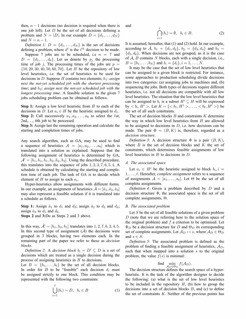
structure.Figure 1 shows several associated spaces defined for the

same problem. The decision structure defining the associatedspace 1 is a complete super-structure given that it representsall solutions from the original space, including, obviously, theoptimum one. The decision structure defining the associatedspace 2 is also a super-structure, but it is incomplete, since itdoes not contain all solutions. The last decision structure isan incomplete sub-structure. Note that in the last case, eventhough the associated space n is larger than the original one,it still does not map into all solutions of the original problemand misses the optimum solution. Clearly, the qualities thatare sought after in a decision structure are the followingones: to be a super-structure, and it should have an associated

…associated

space 2 associated

space n

solution space solution space solution space

associatedspace 1

optimum solution

combinations of low level heuristics

Fig. 1. Examples of different associated spaces defined for the same originalsolution space.

space which is easy to search in order to find a sufficientlygood solution. Following this, the second decision structureof Figure 1 is preferred. Note that the utopian decisionstructure, a rather unlikely one, corresponds to an exactalgorithm which is a decision structure with a unique solutionthat maps to the optimum solution of the original problem.

III. INVESTIGATION OF THE ASSOCIATED SPACES WITHDIFFERENT NUMBER OF DECISION BLOCKS

Grouping decisions into a small number of decision blocksmay carry some benefits. Obviously, the search space whendecisions are not grouped into blocks, i.e. when assignmentsin the form A are considered, is larger than if decisionsare grouped and the assignments have the form A0. It issensible to think, therefore, that if everything else remains thesame, searching the latter space is easier than the former one.However, the possible number of solutions that are accessiblein the latter are potentially smaller than in the former, andtherefore the chances of missing good solutions are higher.However, if, as it is often the case, the computational timeavailable to explore the search space is constrained, then,decision structures describing small associated spaces maybe of interest. This section investigates the nature of thissort of compromise.Our investigation is carried out in the context of the Hybrid

Flow Shop (HFS) scheduling problem. A Genetic Algorithm(GA) based hyper-heuristic, taken from [12], is used to solveinstances of the HFS problem searching different associatedspaces defined by grouping decisions into different numberof decision blocks.

A. The Hybrid Flow Shop scheduling problemThe Hybrid Flow Shop problem (HFS) is defined as the

problem of assigning n jobs intom processing stages; all jobsare processed in the same order: stage 1, stage 2, . . ., untilstage m. At least one of the stages has two or more identicalmachines working in parallel. No job can be processed onmore than one machine at a time, and no machine can processmore than one job at a time. The objective function is tominimise the maximum completion time of operations (alsoknown as the makespan).

The HFS is very common in real world manufacturing.It is encountered in the electronics industry, ceramic tilesmanufacturing, cardboard box manufacturing and many otherindustries. HFS scheduling is an NP-Hard problem, evenwhen there are just two processing stages with one ofthem having a single machine, and one having parallelmachines [13]. The relevance and complexity of the HFSproblem have motivated the investigation of a variety ofmethods including exact methods [14], [15], heuristics [16],[17], meta-heuristics [18], [19], etc. The interested readeris referred to [12] for a detailed description of HFS and areview of approaches developed for solving the problem.Since there are n jobs to be processed in m stages, the

set D contains N = (n− 1)×m decisions. For the sake ofsimplicity, we ignore the fact that there is no need to makeany decision when there is only one job remaining and itwill be assumed, hereafter, that N = n ×m. Bearing thisin mind, decisions 1 to n correspond to the scheduling ofoperations in the first stage of the shop, from n to 2n to jobsin the second stage of the shop and so on.

B. The set of low level heuristicsAt every phase in the construction of a schedule, a low

level heuristic decides on the next job to be assigned andselects a machine for its processing. In this investigation weuse 13 dispatching-rules that act as low level heuristics. Eachof these works as follows: whenever a machine is idle, itselects the job not yet scheduled and ready for processing(released from the previous stage) that best satisfies a certaincriterion and assigns it to the idle machine. Different criterialead to different dispatching rules. The following criteriawere considered: minimum release time, shortest processingtime, longest processing time, less work remaining, morework remaining, earliest due date, latest due date, weighedshortest processing time, weighted longest processing time,lowest weighted work remaining, highest weighted workremaining, lowest weighted due date and highest weighteddue date.Our choice for these dispatching rules was motivated by

their simplicity, efficiency, and popularity in practice. Noticethat the criteria considered by some of them seems irrelevantfor the makespan objective (such as earliest due date). Theirinclusion, however, is beneficial. Previous experience [12]indicates that it is preferable to have a large set of heuris-tics, even when some of them are poor when consideredindividually. This is because, frequently, low level heuristicsthat are poor individual performers are highly effective ifcombined. Identifying these synergistic relations is a difficulttask that justifies the use of an evolutionary computationbased approach. Research in hyper-heuristics is in its infancy,and the role of apparently “bad” or “irrelevant” low levelheuristics in hyper-heuristic search is an interesting andunexplored research topic.

C. Associated problems for HFSLet D be an HFS instance, s be a feasible schedule for D

and let S be the set of all feasible schedules. Let Cmax(s) be

the completion time of schedule s, i.e. the time when the lastjob in s exits the shop floor. Suppose B contains N blocksof size 1, i.e. decisions are not grouped. Since the thirteendispatching rules described above may be used at any pointduring the construction of a schedule, the set of constraintsK is empty. Let AD and ΘD denote a feasible assignment ofheuristics and the set of all feasible assignments, respectively.The associated problem, given this decision structure, isto find the assignment of heuristics, AD ∈ ΘD, whosecorresponding schedule s has the minimum makespan value,Cmax(s):

find minAD∈ΘD

Cmax(AD).

Similar problem formulations could be defined if decisionsare grouped into different numbers of decision blocks. In-deed, the only requirement is to change the definition of Band the rest of the problem statement remains unchanged.

D. A genetic algorithm for searching the associated spaceThe individual representation of the adopted GA is an

assignment or sequence C = [c1, . . . , c ], where is thenumber of decision blocks considered, i.e. the size of B.In order to evaluate a given individual C do the following.Step 1: Call successively the low level heuristics in C andused them to assign operations to machines. Use ci to makeall decisions in bi.Step 2: Calculate the time when the last operation in theschedule obtained in Step 1 finishes its processing in thelast stage of the shop. Assign this time as the fitness of theindividual.

Several GA operators and combinations of GA parametervalues were considered. The selected ones, obtained after theadequate testing, are briefly described next. Refer to [12] forfurther details. In order to do crossover, two chromosomesare selected as parents. All genes ci of the new chromosomeare selected with equal probability from any of the parents. Inorder to do mutation, 0.05(nm) randomly selected genes aresubstituted with a new randomly selected dispatching rule.The value 0.05 controls the magnitude of the mutation andwas determined experimentally.

E. Experimental resultsThe idea of using GA to search the space of dispatching

rules is not new. To our knowledge, it was first proposedin [20] for the job shop problem. It was later used, for thesame problem, in [1] and [8]. In these approaches associatedspaces with either m or nm decision blocks were explored.Our aim is to investigate how associated spaces of differentsizes in the value [m,nm] affect the quality of solution.In order to evaluate the performance of the GA, searching

different associated spaces, the following experiments werecarried out. Random instances of the HFS problem were gen-erated, and for each, several associated spaces consideringdifferent number of decision blocks, were defined. Resultsobtained by GA searching the different associated spaces are

presented. A detailed explanation on how the instances weregenerated, the parameter settings adopted for GA, and theresults, are given next.

1) Problem instances: Several instances of the HFS prob-lem were randomly generated with different numbers of jobs,n ∈ {20, 40, 60, 100, 150, 200, 300}, and different numbersof stages, m ∈ {2, 5, 10, 15, 20}. In total 7 × 5 = 35instances were generated. In all of them the processing timesof operations were generated randomly and take value fromthe [10, 100] interval. Similarly, the weights associated toeach job, the release times and the due dates were gener-ated randomly and take values from the [1, 10], [0, 55m],[0, 2(55m)] intervals, respectively. The 55m value is theexpected sum of processing times of the jobs and is oftenused as a reference point to generate release and due datesdata. The number of machines per stage were either 4 or 5,both occurring with equal probability. All these parameterswere generated using a discrete uniform distribution. Notethat the job weights and the due dates are irrelevant for theconsidered objective (makespan). Its consideration followsour discussion in Section III-B. The generated instances areexpected to be relatively difficult to solve for the followingreasons. The data is uniformly distributed. These type ofinstances are known to be more difficult than instancesgenerated with other distributions due to the high varianceof the uniform distribution [19]. A second reason is that thedifference on processing capacity per stage is no more than a20% (given that each stage has either 4 or 5 machines). Thisprevents the existence of obvious bottlenecks which could beexploited in order to simplify the solution process.

A number of associated spaces was defined for each of thegenerated problem instances. For example, for the problemswith 20 jobs, one of the associated problems considers eachdecision individually, i.e. there are 20 blocks of size 1 pereach stage. Since there are m stages, there is a total of20m decision blocks. In this case, the assignment of decisionblocks in stages is as follows:

b1, . . . , b20| {z }stage 1

, b21, . . . , b40| {z }stage 2

, . . . , b20(m−1)+1, . . . , b20m| {z }stage m

.

Similarly, decisions were grouped into 2, 5 and 10 decisionblocks per stage. The assignment of decision blocks in stageswhen two blocks per stage are considered, is as follows:

b1, b2| {z }stage 1

, b3, b4| {z }stage 2

, . . . , b2m−1, b2m| {z }stage m

.

For the rest of the instances, i.e. the problems with morethan 20 jobs, the number of decision blocks per stageconsidered is given in the following table.

TABLE INUMBER OF DECISION BLOCKS PER STAGE

jobs (n) decision blocks per stage20 2, 5, 10, 2040 2, 5, 10, 20, 4060 2, 5, 10, 20, 30, 60100 2, 5, 10, 20, 50, 100150 2, 5, 10, 30, 50, 75, 150200 2, 5, 10, 20, 40, 50, 100, 200300 2, 5, 10, 20, 30, 50, 60, 75, 100, 150, 300

2) GA parameters: Each of these associated problems wassolved 30 times with GA. The GA was tuned as follows. Thestopping condition was set to 10,000 solution evaluations.All valid combinations of the following parameter valueswere considered. Population size 50, 75, 100; selectionmechanism: tournament selectionwith 2 and 3 participants;elitism (keeping best individual found so far): true, false;crossover probability: 0.8, 0.9, 0.95; mutation probability:0.05, 0.1, 0.15. The combination shown in bold is the bestperforming one according to our pre-experimental phase.3) Results: The quality of the schedules found by GA

searching different associated spaces of the same instancewere compared and ranked. The ranks are presented in Figure2. Plots in the same row refer to instances with the samenumber of jobs; plots in the same column refer to instanceswith the same number of stages. The last column shows theoverall performance across instances with the same numberof jobs. For example, the plot in (row 1, column 1) refers tothe problem instance with 20 jobs and 2 stages. The x−axisindicates the number of decision blocks considered, namely2, 5, 10 and 20. The y-axis measures the average (on 30 runs)of the ranks according to the quality of the solution achievedby the GA searching the corresponding associated space.For the illustration purpose, the interpretation of the plotgiven in (row 1, column 1) is as follows. On average, GA isperforming the best when it considers the associated problemwith 20 decision blocks per stage. It is just slightly better thanwhen considering 15 decision blocks, but definitely superiorto 2 and 5 decision blocks per stage.We can observe that in all cases there is a clear relationship

between the GA performance and the number of decisionblocks considered. In most cases, between 10 and 30 decisionblocks per stage seems to be the “best” size, and as thenumber of decision blocks gets away from this range, theperformance of GA deteriorates. Another observation is thatconsidering too many or too few decision blocks per stageyields poor performance. This observation is interesting ifthe following fact is taking into account. Large associatedspaces have access to at least the same and potentiallymore (better) solutions to the original problem than smallerones. We can observe in Figure 2 that in all cases mediumnumbers of decision blocks yielded the best solutions. Sincewe would expect the larger associated spaces to contain bettersolutions than the medium and small ones, the question thenis, why is GA performing so poorly when considering large

m = 2 m = 5 m = 10 m = 15 m = 20 average

n = 20

2 5 10 20

1

2

3

4

2 5 10 20

1

2

3

4

2 5 10 20

1

2

3

4

2 5 10 20

1

2

3

4

2 5 10 20

1

2

3

4

2 5 10 20

1

2

3

4

n = 40

2 5 10 30 601

2

3

4

5

2 5 10 20 401

2

3

4

5

2 5 10 20 401

2

3

4

5

2 5 10 20 401

2

3

4

5

2 5 10 20 401

2

3

4

5

2 5 10 20 401

2

3

4

5

n = 60

2 5 10 20 30 601

2

3

4

5

6

2 5 10 20 30 60

2

3

4

5

6

2 5 10 20 30 601

2

3

4

5

6

2 5 10 20 30 601

2

3

4

5

6

2 5 10 20 30 601

2

3

4

5

6

2 5 10 20 30 601

2

3

4

5

6

n = 100

2 5 10 20 50 1001

2

3

4

5

6

2 5 10 20 50 1001

2

3

4

5

6

2 5 10 20 50 1001

2

3

4

5

6

2 5 10 20 50 1001

2

3

4

5

6

2 5 10 20 50 1001

2

3

4

5

6

2 5 10 20 50 1001

2

3

4

5

6

n = 150

2 5 10 30 50 75 1501

2

3

4

5

6

7

2 5 10 30 50 75 1501

2

3

4

5

6

7

2 5 10 30 50 75 1501

2

3

4

5

6

7

2 5 10 30 50 75 1501

2

3

4

5

6

7

2 5 10 30 50 75 1501

2

3

4

5

6

7

2 5 10 30 50 75 1501

2

3

4

5

6

7

n = 200

2 5 10 20 40 50 100 200

2

3

4

5

6

7

8

2 5 10 20 40 50 100 200

1

2

3

4

5

6

7

8

2 5 10 20 40 50 100 200

2

3

4

5

6

7

8

2 5 10 20 40 50 100 200

2

3

4

5

6

7

8

2 5 10 20 40 50 100 200

2

3

4

5

6

7

8

2 5 10 20 40 50 100 200

2

3

4

5

6

7

8

n = 300

2 5 10 15 30 50 60 75 10015030023456789

1011

2 5 10 15 30 50 60 75 10015030023456789

1011

2 5 10 15 30 50 60 75 10015030023456789

1011

2 5 10 15 30 50 60 75 10015030023456789

1011

2 5 10 15 30 50 60 75 10015030023456789

1011

2 5 10 15 30 50 60 75 10015030023456789

1011

Fig. 2. Performance of GA searching different associated spaces defined for the same problem instance. The x-axis of each plot presents the number ofdecision blocks considered, while the y-axis presents the average ranks.

associated problems? A possible answer is that the qualityof the solutions of the original problem that are reachablein the associated space improves fastly as the number ofdecision blocks, starting from the smallest number, increases.However, it reaches a point where this improvement startsslowing down, until it reaches the point where increasingthe associated space has very limited benefits in comparisonto the amount of the extra complexity that is added tothe problem. It could be said that the “richness” of theassociated problem, understood as the quality of solutionsthat are accessible through it in proportion to the effort thatis required to find them, diminishes fastly after reaching the“optimum” number of decision blocks, which in this casehappened to be between 10 and 30.It is important, of course, to consider the limitations in

CPU time that were imposed in our experiments. It is sensibleto think that if the running time of GA increases, then, largerassociated spaces may become more attractive. We haveobserved, however, that the extra computational time requiredby GA to find an equal or higher quality solution in a largeassociated space compared to the one found in the mediumsized ones, increases considerably. Further experimentationand analysis on this is ongoing work.

IV. DISTRIBUTION OF RANDOM SOLUTIONS IN THEASSOCIATED SPACE

The observations from the previous section motivate thefurther analysis of the associated space. Gains from anindirect solution encoding, i.e. using combinations of lowlevel heuristics to represent solutions represented as combi-nations of low level heuristics, are possibly twofold. First,the associated space maps to solutions that are on averageof a high quality. I.e. a random sample of solutions in theassociated space would be expected to have a superior qualitythan a random sample from the original solution space.Second, the structure of the associated problem is, in general,simpler than that of the original problem, and therefore thesearching task is easier. In what follows, the first observationwill be verified for the given HFS problem. Since verifyingthe second observation is a more intricate task and it requiresintroducing new definitions and statistical tools, it is left forthe future research work.In order to verify the first observation, we compare

the distribution of the Cmax values of random schedulesgenerated with common permutation representations andactive schedules obtained through random combinations ofdispatching rules. The first type of schedules were generatedby assigning jobs in the permutations sequentially to the firstavailable machine. The schedules were generated in such away that there is no idle time on any machine that is largeenough to process a job without delaying the completiontime of any other job. This was done in order to generateactive schedules, which are much better, on average, than theother random schedules, see [21] for definition. The secondset of schedules were obtained by random combinationsof dispatching rules (considering the maximum number ofdecision blocks). A total of 10,000 schedules of each type

TABLE IIAVERAGE Cmax VALUES OF RANDOM ACTIVE SCHEDULES AND

SCHEDULES GENERATED BY RANDOM COMBINATIONS OF DISPATCHING

RULES

random combinations of disp. rulesm = 2 m = 5 m = 10 m = 15 m = 20

n = 20 409.8 567.9 908.3 1260.5 1555.4n = 40 597.4 873.2 1213.1 1480.9 1854.3n = 60 822.1 1096.0 1433.5 1869.5 2215.8n = 100 1573.9 1771.6 2065.3 2425.7 2774.0n = 150 2172.4 2392.5 2755.0 3249.8 3523.9n = 200 2677.1 3118.3 3545.5 3905.8 4358.7n = 300 4275.0 4554.6 4793.4 5375.4 5672.3

random active schedulesm = 2 m = 5 m = 10 m = 15 m = 20

n = 20 432.6 641.5 1001.3 1391.5 1677.9n = 40 653.2 1002.9 1470.0 1744.0 2180.3n = 60 870.6 1307.0 1731.2 2232.8 2649.4n = 100 1629.4 2032.5 2495.8 2941.6 3442.9n = 150 2295.0 2771.3 3302.2 4105.8 4365.9n = 200 2824.9 3584.6 4280.4 4841.4 5448.0n = 300 4345.8 4992.4 5545.1 6554.0 7034.5

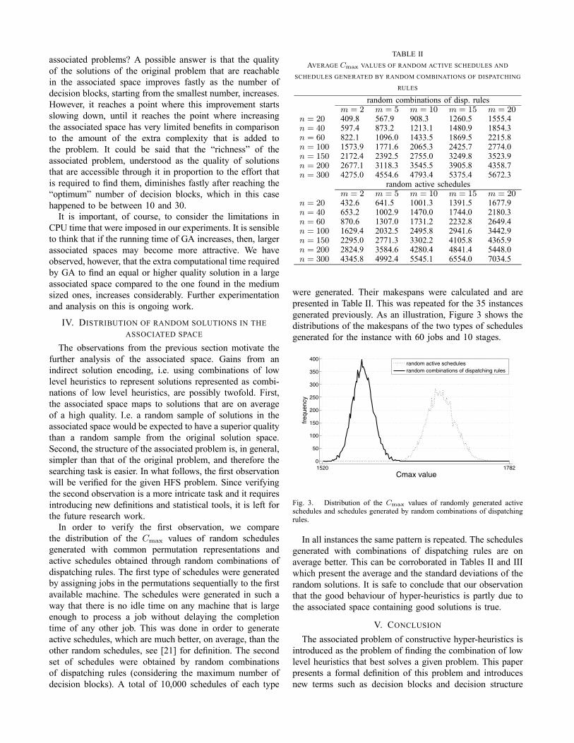
were generated. Their makespans were calculated and arepresented in Table II. This was repeated for the 35 instancesgenerated previously. As an illustration, Figure 3 shows thedistributions of the makespans of the two types of schedulesgenerated for the instance with 60 jobs and 10 stages.

1520 17820

50

100

150

200

250

300

350

400

freq

uenc

y

Cmax value

random active schedulesrandom combinations of dispatching rules

Fig. 3. Distribution of the Cmax values of randomly generated activeschedules and schedules generated by random combinations of dispatchingrules.

In all instances the same pattern is repeated. The schedulesgenerated with combinations of dispatching rules are onaverage better. This can be corroborated in Tables II and IIIwhich present the average and the standard deviations of therandom solutions. It is safe to conclude that our observationthat the good behaviour of hyper-heuristics is partly due tothe associated space containing good solutions is true.

V. CONCLUSIONThe associated problem of constructive hyper-heuristics is

introduced as the problem of finding the combination of lowlevel heuristics that best solves a given problem. This paperpresents a formal definition of this problem and introducesnew terms such as decision blocks and decision structure

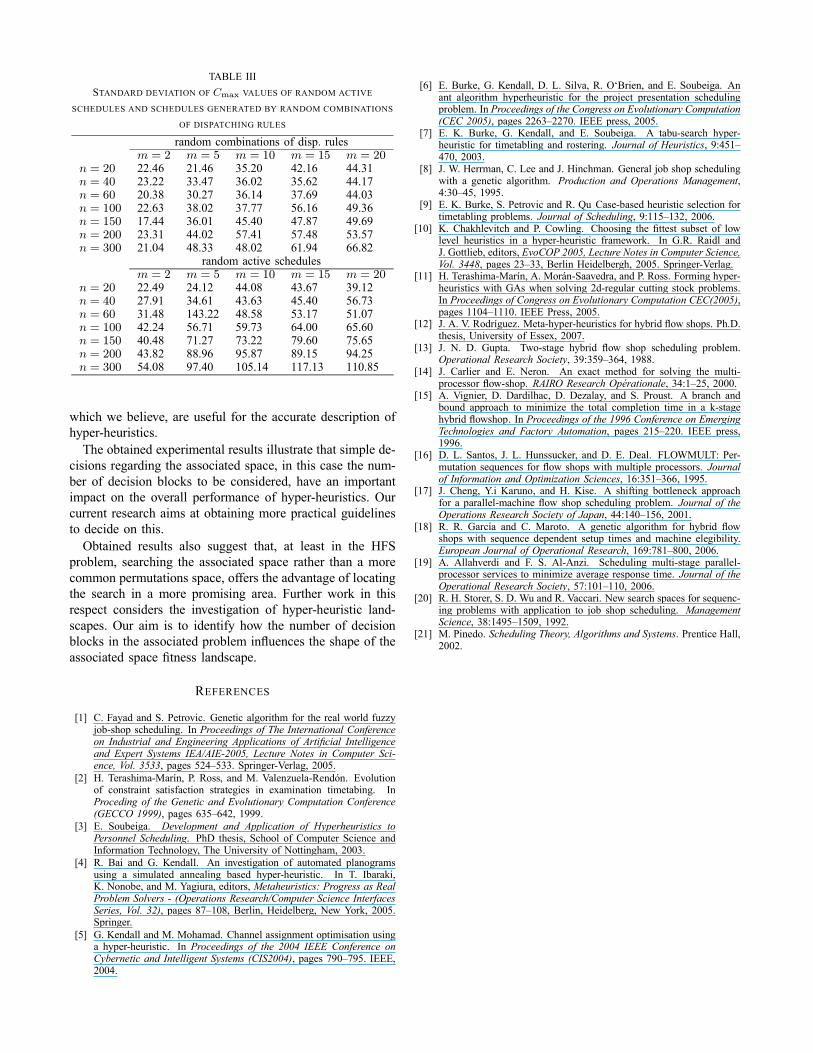
TABLE IIISTANDARD DEVIATION OF Cmax VALUES OF RANDOM ACTIVE

SCHEDULES AND SCHEDULES GENERATED BY RANDOM COMBINATIONS

OF DISPATCHING RULES

random combinations of disp. rulesm = 2 m = 5 m = 10 m = 15 m = 20

n = 20 22.46 21.46 35.20 42.16 44.31n = 40 23.22 33.47 36.02 35.62 44.17n = 60 20.38 30.27 36.14 37.69 44.03n = 100 22.63 38.02 37.77 56.16 49.36n = 150 17.44 36.01 45.40 47.87 49.69n = 200 23.31 44.02 57.41 57.48 53.57n = 300 21.04 48.33 48.02 61.94 66.82

random active schedulesm = 2 m = 5 m = 10 m = 15 m = 20

n = 20 22.49 24.12 44.08 43.67 39.12n = 40 27.91 34.61 43.63 45.40 56.73n = 60 31.48 143.22 48.58 53.17 51.07n = 100 42.24 56.71 59.73 64.00 65.60n = 150 40.48 71.27 73.22 79.60 75.65n = 200 43.82 88.96 95.87 89.15 94.25n = 300 54.08 97.40 105.14 117.13 110.85

which we believe, are useful for the accurate description ofhyper-heuristics.The obtained experimental results illustrate that simple de-

cisions regarding the associated space, in this case the num-ber of decision blocks to be considered, have an importantimpact on the overall performance of hyper-heuristics. Ourcurrent research aims at obtaining more practical guidelinesto decide on this.Obtained results also suggest that, at least in the HFS

problem, searching the associated space rather than a morecommon permutations space, offers the advantage of locatingthe search in a more promising area. Further work in thisrespect considers the investigation of hyper-heuristic land-scapes. Our aim is to identify how the number of decisionblocks in the associated problem influences the shape of theassociated space fitness landscape.

REFERENCES

[1] C. Fayad and S. Petrovic. Genetic algorithm for the real world fuzzyjob-shop scheduling. In Proceedings of The International Conferenceon Industrial and Engineering Applications of Artificial Intelligenceand Expert Systems IEA/AIE-2005, Lecture Notes in Computer Sci-ence, Vol. 3533, pages 524–533. Springer-Verlag, 2005.

[2] H. Terashima-Marın, P. Ross, and M. Valenzuela-Rendon. Evolutionof constraint satisfaction strategies in examination timetabing. InProceding of the Genetic and Evolutionary Computation Conference(GECCO 1999), pages 635–642, 1999.

[3] E. Soubeiga. Development and Application of Hyperheuristics toPersonnel Scheduling. PhD thesis, School of Computer Science andInformation Technology, The University of Nottingham, 2003.

[4] R. Bai and G. Kendall. An investigation of automated planogramsusing a simulated annealing based hyper-heuristic. In T. Ibaraki,K. Nonobe, and M. Yagiura, editors, Metaheuristics: Progress as RealProblem Solvers - (Operations Research/Computer Science InterfacesSeries, Vol. 32), pages 87–108, Berlin, Heidelberg, New York, 2005.Springer.

[5] G. Kendall and M. Mohamad. Channel assignment optimisation usinga hyper-heuristic. In Proceedings of the 2004 IEEE Conference onCybernetic and Intelligent Systems (CIS2004), pages 790–795. IEEE,2004.

[6] E. Burke, G. Kendall, D. L. Silva, R. O‘Brien, and E. Soubeiga. Anant algorithm hyperheuristic for the project presentation schedulingproblem. In Proceedings of the Congress on Evolutionary Computation(CEC 2005), pages 2263–2270. IEEE press, 2005.

[7] E. K. Burke, G. Kendall, and E. Soubeiga. A tabu-search hyper-heuristic for timetabling and rostering. Journal of Heuristics, 9:451–470, 2003.

[8] J. W. Herrman, C. Lee and J. Hinchman. General job shop schedulingwith a genetic algorithm. Production and Operations Management,4:30–45, 1995.

[9] E. K. Burke, S. Petrovic and R. Qu Case-based heuristic selection fortimetabling problems. Journal of Scheduling, 9:115–132, 2006.

[10] K. Chakhlevitch and P. Cowling. Choosing the fittest subset of lowlevel heuristics in a hyper-heuristic framework. In G.R. Raidl andJ. Gottlieb, editors, EvoCOP 2005, Lecture Notes in Computer Science,Vol. 3448, pages 23–33, Berlin Heidelbergh, 2005. Springer-Verlag.

[11] H. Terashima-Marın, A. Moran-Saavedra, and P. Ross. Forming hyper-heuristics with GAs when solving 2d-regular cutting stock problems.In Proceedings of Congress on Evolutionary Computation CEC(2005),pages 1104–1110. IEEE Press, 2005.

[12] J. A. V. Rodrıguez. Meta-hyper-heuristics for hybrid flow shops. Ph.D.thesis, University of Essex, 2007.

[13] J. N. D. Gupta. Two-stage hybrid flow shop scheduling problem.Operational Research Society, 39:359–364, 1988.

[14] J. Carlier and E. Neron. An exact method for solving the multi-processor flow-shop. RAIRO Research Operationale, 34:1–25, 2000.

[15] A. Vignier, D. Dardilhac, D. Dezalay, and S. Proust. A branch andbound approach to minimize the total completion time in a k-stagehybrid flowshop. In Proceedings of the 1996 Conference on EmergingTechnologies and Factory Automation, pages 215–220. IEEE press,1996.

[16] D. L. Santos, J. L. Hunssucker, and D. E. Deal. FLOWMULT: Per-mutation sequences for flow shops with multiple processors. Journalof Information and Optimization Sciences, 16:351–366, 1995.

[17] J. Cheng, Y.i Karuno, and H. Kise. A shifting bottleneck approachfor a parallel-machine flow shop scheduling problem. Journal of theOperations Research Society of Japan, 44:140–156, 2001.

[18] R. R. Garcıa and C. Maroto. A genetic algorithm for hybrid flowshops with sequence dependent setup times and machine elegibility.European Journal of Operational Research, 169:781–800, 2006.

[19] A. Allahverdi and F. S. Al-Anzi. Scheduling multi-stage parallel-processor services to minimize average response time. Journal of theOperational Research Society, 57:101–110, 2006.

[20] R. H. Storer, S. D. Wu and R. Vaccari. New search spaces for sequenc-ing problems with application to job shop scheduling. ManagementScience, 38:1495–1509, 1992.

[21] M. Pinedo. Scheduling Theory, Algorithms and Systems. Prentice Hall,2002.