member's copy- not for circulation - indian mathematical society
TRANSCRIPT
Membe
r's co
py-
not f
or ci
rculat
ion
ISSN: 0025-5742
THE
MATHEMATICS
STUDENTVolume 85, Numbers 1-2, January-June (2016)
(Issued: May, 2016)
Editor-in-Chief
J. R. PATADIA
EDITORS
Bruce Berndt George Andrews M. Ram Murty
N. K. Thakare Satya Deo Gadadhar Misra
B. Sury Kaushal Verma Krishnaswami Alladi
S. K. Tomar Subhash J. Bhatt L. Sunil Chandran
M. M. Shikare C. S. Aravinda A. S. Vasudeva Murthy
Indranil Biswas Timothy Huber T. S. S. R. K. Rao
Clare D′Cruz Atul Dixit
PUBLISHED BY
THE INDIAN MATHEMATICAL SOCIETY
www.indianmathsociety.org.in
Membe
r's co
py-
not f
or ci
rculat
ion
THE MATHEMATICS STUDENT
Edited by J. R. PATADIA
In keeping with the current periodical policy, THE MATHEMATICS STUDENT will
seek to publish material of interest not just to mathematicians with specialized interest
but to the postgraduate students and teachers of mathematics in India. With this in
view, it will ordinarily publish material of the following type:
1. the texts (written in a way accessible to students) of the Presidential Addresses, the
Plenary talks and the Award Lectures delivered at the Annual Conferences.
2. general survey articles, popular articles, expository papers, Book-Reviews.
3. problems and solutions of the problems,
4. new, clever proofs of theorems that graduate / undergraduate students might see in
their course work,
5. research papers (not highly technical, but of interest to larger readership) and
6. articles that arouse curiosity and interest for learning mathematics among readers and
motivate them for doing mathematics.
Articles of the above type are invited for publication in THE MATHEMATICS
STUDENT. Manuscripts intended for publication should be submitted online in the
LATEX and .pdf file including figures and tables to the Editor J. R. Patadia on E-mail:
Manuscripts (including bibliographies, tables, etc.) should be typed double spaced on
A4 size paper with 1 inch (2.5 cm.) margins on all sides with font size 10 pt. in LATEX.
Sections should appear in the following order: Title Page, Abstract, Text, Notes and
References. Comments or replies to previously published articles should also follow this
format with the exception of abstracts. In LATEX the following preamble be used as is
required by the Press:
\ documentclass[10 pt,a4paper,twoside,reqno]amsart\ usepackage amsfonts, amssymb, amscd, amsmath, enumerate, verbatim, calc\ renewcommand\ baselinestretch1.2\ textwidth=12.5 cm
\ textheight=20 cm
\ topmargin=0.5 cm
\ oddsidemargin=1 cm
\ evensidemargin=1 cm
\ pagestyleplainThe details are available on Indian Mathematical Society website: www.indianmath
society.org.in
Authors of articles / research papers printed in the the Mathematics Student as well as in
the Journal shall be entitled to receive a soft copy (PDF file with watermarked “Author’s
copy”) of the paper published. There are no page charges. However, if author(s) (whose
paper is accepted for publication in any of the IMS periodicals) is (are) unable to send
the LATEX file of the accepted paper, then a charge Rs. 100 (US $ 10) per page will be
levied for LATEX typesetting charges.
All business correspondence should be addressed to S. K. Nimbhorkar, Treasurer, Indian
Mathematical Society, Dept. of Mathematics, Dr. B. A. M. University, Aurangabad -
431 004 (Maharashtra), India. E-mail: [email protected]
Copyright of the published articles lies with the Indian Mathematical Society.
In case of any query, the Editor may be contacted.
Membe
r's co
py-
not f
or ci
rculat
ion
ISSN: 0025-5742
THE
MATHEMATICS
STUDENTVolume 85, Numbers 1-2, January-June, (2016)
(Issued: May, 2016)
Editor-in-Chief
J. R. PATADIA
EDITORS
Bruce C. Berndt George E. Andrews M. Ram Murty
N. K. Thakare Satya Deo Gadadhar Misra
B. Sury Kaushal Verma Krishnaswami Alladi
S. K. Tomar Subhash J. Bhatt L. Sunil Chandran
M. M. Shikare C. S. Aravinda A. S. Vasudeva Murthy
Indranil Biswas Timothy Huber T. S. S. R. K. Rao
Clare D′Cruz Atul Dixit
PUBLISHED BY
THE INDIAN MATHEMATICAL SOCIETY
www.indianmathsociety.org.in
Membe
r's co
py-
not f
or ci
rculat
ion
ISSN: 0025-5742
ii
c© THE INDIAN MATHEMATICAL SOCIETY, 2016.
This volume or any part thereof may not be
reproduced in any form without the written
permission of the publisher.
This volume is not to be sold outside the
Country to which it is consigned by the
Indian Mathematical Society.
Member’s copy is strictly for personal use.
It is not intended for sale or circular.
Published by Prof. N. K. Thakare for the Indian Mathematical Society, type set by
J. R. Patadia at 5, Arjun Park, Near Patel Colony, Behind Dinesh Mill, Shivanand
Marg, Vadodara - 390 007 and printed by Dinesh Barve at Parashuram Process,
Shed No. 1246/3, S. No. 129/5/2, Dalviwadi Road, Barangani Mala, Wadgaon
Dhayari, Pune 411 041 (India). Printed in India.

Membe
r's co
py-
not f
or ci
rculat
ion
The Mathematics Student ISSN: 0025-5742Vol. 85, Nos. 1-2, January-June (2016)
CONTENTS
1. A. M. Mathai Mathematics in India-personal perceptions 01-08
2. A. M. Mathai A Versatile Author’s contributions to various areas ofmathematics, Statistics, Astrophysics, Biology andSocial Sciences
09-44
3. M. T. Nair Compact operators and Hilbert Scales in Ill-posedproblems
45-61
4. Uttara Naik Likelihood, Estimating functions and method of 63-78Nimbalkar moments
5. B. Sury Matrix groups over rings 79-96
6. Siddhi Pathak A simple proof of Burnsides criterion for all groups 97-102of order n to be cyclic
7. Jack S. Calcut Rational angled hyperbolic polygons 103-111
8. Fahed Metrizability of Arithmetic Progression Topology 113-116Zulfequarr
9. Amrik Singh Interesting infinite products of rational functions 117-133Nimbran motivated by Euler
10. G. S. Saluja Some unique fixed point and common fixed point 135-141theorems in b-metric spaces using rational inequality
11. S. G. Dani Lazy continued fraction expansions for complex 143-149numbers
12. H. A. Gururaja On Hilbert’s theorem in differential geometry 151-161
13. Ajai Choudhry A pair of simultanous Diophantine equations with no 163-166solutions in integers
14. - Problem Section 167-174
*******

Membe
r's co
py-
not f
or ci
rculat
ion
iv
Membe
r's co
py-
not f
or ci
rculat
ion
The Mathematics Student ISSN: 0025-5742
Vol. 85, Nos. 1-2, January-June (2016), 01-08
MATHEMATICS IN INDIA- PERSONAL PERCEPTIONS
A. M. MATHAI
Dignitaries on the dais, off the dais, my fellow researchers, students and other
participants, it is a great pleasure for me to be the President of the oldest scientific
society and the truly national mathematical society in India.
1. Proliferation of Scientific/Professional Societies.
In India there are State-wise mathematical societies / associations / forums.
Are such associations necessary? Mathematicians in a geographic or linguistic
region may want to get together and discuss matters in their own regional language
or cultural groups. Thus, such regional associations are needed. When a city has a
large number of scientists they may form a local group. If there is a provision then
people from outside may also join in such groups and participate in their activities.
New York Academy, Gwalior Academy, Calcutta Mathematical Society, etc are
such groups. New York Academy has a lot of activities and any researcher with
published works from around the world can be a member there and participate in
their activities. Such city-based or localized societies are also needed. If there are
a sufficient number of people in a subject area in a country then they may launch
a society for that subject area such as the Society for Special Functions and their
Applications, Indian Society for Probability and Statistics, Applied Mathematics
Forum, Semigroup Forum, etc are such subject-wise societies. Such societies are
also needed to cater to the special needs. Then some people may like the work of a
certain individual and they may be devotees of such a person and they may form a
society to perpetuate the person’s name. In olden days the followers of Pythagoras
created a Pythagorean Society. We have a Ramanujan Society for Mathematics
and Mathematical Sciences, Ramanujan Mathematical Society, etc. Such groups
are also needed to cater to the special interest. Thus, in the Indian scene also, as
in other places in the world, there are a large number of societies / associations
catering to various aspects of mathematical sciences, catering to regional needs,
catering to local needs, catering to topic-wise needs. Does this mean that we
* The text of the Presidential Address (general) delivered at the 81st Annual Conference of the
Indian Mathematical Society held at the Visvesvaraya National Institute of Technology,
Nagpur-440 010, Maharashtra, during the period December 27 - 30, 2015.
c© Indian Mathematical Society, 2016 .
1
Membe
r's co
py-
not f
or ci
rculat
ion
2 A. M. MATHAI
need a consortium of mathematical societies / associations / forums in India to
amalgamate and coordinate the activities? No such consortium is needed because
all these regional, local, subject-wise societies are catering to special needs. As
national activity, we have the Indian Mathematical Society (IMS), catering to all
regions, all localities, all topics, all individuals’ works, etc. Hence I would like to
request those who are not yet Members of IMS, and interested in any aspect of
mathematical sciences in the wider sense, to become the Life Members of IMS.
2. Indias Share of World Contributions in Mathematical Sciences
Nearly one-fifth of the world population is in the Indian subcontinent. Hence,
one should naturally expect that around one-fifth of the research contributions
in mathematical sciences in the world should be from India. But what is the
reality? Not even one percent is from India. There may be some Indian names
in the upper cadres but they are the ones settled abroad. Why? What are the
real reasons behind this situation even after nearly 70 years of independence?
Research in mathematical sciences do not call for expensive laboratories, expensive
equipments, expensive infrastructure, etc. Then, why? I have located a few of the
problems from my experience in India and in various countries outside India. I
shall mention a few of the major ones that I have recognized.
(a). Concept of learning has to change.
For over forty years I had taught students at the faculty level (below average),
major level (average) and honors level (brilliant) in various topics in Mathematics
and Statistics in different countries outside India. During the past 9 years I had
run 26 undergraduate mathematics training camps in India (trained over 1000
undergraduates) and run 12 research-orientation programs (trained over 400 all-
India participants). In India, especially in Kerala, the concept of learning is to
memorize a few mathematical formulae without really knowing the significance or
relevance. Some students can recite theorems and even their proofs! But they
have no idea why such a theorem is there, what is its importance, its relevance
to real-life situations, etc. Most of the students had negative background in the
subject matter under consideration. In the name of that subject a lot of nonsense
had gone into their brains, and thus the background was negative. I had to de-
program them and start from zero. I could bring out most of their latent abilities.
Unless our students learn the subject matter, rather than memorizing formulae,
they will not be able to make use of whatever they memorize. A real-life problem
does not come in the form of a ready-made formula to compute.
I had recruited 17 M.Sc graduates from various colleges and started training
them at my Centre (CMSS: Centre for Mathematical and Statistical Sciences,
India) for their Ph.Ds. During the past seven years my students had won 19
national level awards for best published paper of the year, best paper presentation,

Membe
r's co
py-
not f
or ci
rculat
ion
MATHEMATICS IN INDIA - PERSONAL PERCEPTIONS 3
best Ph.D thesis, young scientist award etc. They have published over 150 papers
in standard refereed international journals. A number of them have written papers
jointly with the top researchers in the world in various topics and over a dozen
such papers are published. They could present papers in 8 conferences abroad.
13 out of the 17 received their Ph.Ds from Banaras Hindu University (BHU, 6 of
them), Anna University, Chennai (3 or them), MG University, Kerala (4 of them).
CMSS is a recognized research centre of these three universities.
(b). Need for cutting down the number of holidays and extending the work hours.
I achieved all the above publications and awards through a few simple steps.
First, I put a condition that all research scholars must stay within walking distance
from CMSS because in Kerala on almost every day some problems will be there
on the road, either a bandh declared by a political party, or labor union, or local
groups, etc or a bus strike or problems created by students’ unions, etc. Then I
abolished all the holidays except Sundays, Independence Day and Republic Day.
Institution functioned on all days. Individuals are given leaves for personal and
religious reasons. In Kerala a Vice-Chancellor of one of the universities said that
his greatest ambition was to have 75 working days in a year. Then I put the
working hours as 9 am to 5 pm but I used to be present from 7 am until 7 pm.
Naturally, most of the research scholars and staff came by 8 am and left only
around 6 pm. Then I removed all peons, servants, etc and made a rule that all
must clean the premises and all, including me, must share all work in the Centre.
Then I put strict discipline. At the first violation of any rule I removed the person
from the program. Out of 17 only 3 were dismissed and one went abroad with her
husband.
Outside India, no such discipline and enforcement are necessary to achieve the
results. There the children are trained at home and in schools at various levels
about civilized behavioral patterns, about personal cleanliness, about the use of
private and public places, about respect and consideration for others’ rights, etc.
Hence one has to only mention the rules to be followed and discipline will be there.
If India has to catch up with the developed world then it is highly essential to
cut down the number of holidays and extend the work hours. A work culture has
to be created. It is possible in India and I have shown that it is possible. Outsiders
will laugh at the system if we tell that the teaching and research institutions in
India start at 10 am and finish by 3 to 3.30 pm, with two coffee breaks and one
lunch break in between, and government offices function from 11 to 11.30 am until
2.30 to 3 pm.
(c). Periodic work evaluations in all sectors
Poor performance of the students, poor background and negative knowledge
are not due to the fault of the students but these are due to the faults of their

Membe
r's co
py-
not f
or ci
rculat
ion
4 A. M. MATHAI
teachers. In my department of Mathematics and Statistics at McGill University
there is no fixed salary increase every month or every year. Salary increment is
based on the work output. Every faculty member is evaluated every year on three
criteria of research output, teaching and administration. Then the total merit
point is computed based on an open formula. Based on the merit points, the
faulty members are put into 3 to 5 categories. Then the total amount available
to the department for salary increase is divided among these 3 to 5 categories.
Thus, in a certain year the top category may get $2000 increase but in certain
other year the amount may be $1000 depending upon the total fund available to
the department in that year.
When a faculty member is appointed at Assistant Professor level (starting
level) there will be an expert committee set up for that purpose. Usually the
members are mathematicians from outside the university. Then at each stage of
promotion to Associate Professor, Full Professor, tenure, etc there is strict screen-
ing by expert committees, usually from outside. This type of continuous screening
will make everyone productive and active in research, teaching and administra-
tion. Course-credit system gives the students wide choices of courses and they are
free to register into any course provided the student has the required pre-requisite
for that course. This can result in a professor not getting students to register in
his/her courses. This will result in that professor losing the job. Also the students
may make complaints questioning the knowledge of the teacher to teach a partic-
ular course. If the complaint is found to have substance, then also the professor
loses the job. Then there is a periodic evaluation of every department by outside
experts. Usually this is done in every five years. The recommendations of such
outside committees are enforced by the university. The recommendations may
be to remove certain professors or to bring in youngsters to certain areas or to
scrap a certain sector of the department or to scrap the whole department. Such
continuous evaluations of every faculty in every department, in every academic in-
stitution in India, and periodic evaluations of the departments and universities are
necessary to improve the standards of higher education in India. UGC is the right
agency in India to enforce such procedures in colleges, universities and institutions
in India.
(d). Overenthusiastic enforcement of local languages
China has the advantage that the written language is the same all over the
country, even though spoken language varies. India has a great disadvantage in
this respect. Local languages and dialects develop due to the static nature of
the society in olden days. If a group of people are born at a particular place,
live and die within a small spread of land then naturally a local language or at
least a local dialect will develop over time. But their ability to communicate with

Membe
r's co
py-
not f
or ci
rculat
ion
MATHEMATICS IN INDIA - PERSONAL PERCEPTIONS 5
others will be nil or limited. If a child growing up in such an atmosphere wants to
become a scientist then he / she should at least pick up the technical terms in the
current language of science so that the child can easily learn whatever is available
on the subject matter. The language of science in the world used to be French
for some time. All over Europe, whoever learned French was considered to be
learned. Then the language of science became German. After the Second World
War, the language of science is English. Hence, any budding scientist will have
great advantage if he/she knows English or can communicate in English. Once
the symbols and technical terms are picked up in English then it is easy for a child
to follow a mathematical statement. When a child is hearing a technical term for
the first time, it is equally alien to the child, whatever be the language. But if a
technical term is phrased in the mother tongue then it is likely that the child may
misinterpret it and connect it to something else in the mother tongue. For example,
instead of calling the symbol + as “plus” (English word) if the child is taught to
say “adhikam” (Malayalam) then, to the child, “plus” and “adhikam” are both
alien and “adhikam” is more difficult to pronounce. In Malayalam, “adhikam”
is commonly used for “more”, “more than”, “greater”, “greater than”, etc. The
child will not understand the precise meaning of the symbol + if he is learning it
as “adhikam”. In the name of promoting local language, such awkward technical
terms are coined in each language in India now. How can a person communicate
in science with his next State neighbor, let alone communicating with the outside
world?
When I was giving the undergraduate mathematics training at CMSS to col-
lege level students, I heard some students saying “chamithi”, “chamithi”. Where
I grew up, this word “chamithi” meant cleaning up after going to the toilet. I
never knew that it was a mathematical operation. Later I learnt that it was a
mispronounced technical term for some mathematical operation in the name of
promoting Malayalam.
Any forward looking country must make sure that the youngsters can talk
to each other as well as with outsiders, in science, when they grow up. India is
going backward in this respect and destroying opportunities to the vast majority
of children, whose parents cannot afford to send them to English medium schools,
in the name of “promoting” local language. This is not a promotion but nipping
off at the bud prospective scientists of the country.
3. Establishment of Research and Training Centres all Across India
About 30 years back Chinese students from mainland China started coming
to North America in large numbers in all subject areas. In Canada the Chinese
government representatives came to each Province and made deals so that these
Chinese scholars would get fee exemption or fee reduction or fellowships etc. I

Membe
r's co
py-
not f
or ci
rculat
ion
6 A. M. MATHAI
found the Chinese students coming to our department very good, well motivated
and eager to learn everything that they could learn from us. I was wondering
how they could all be good students without exception. While talking to them I
found that China had established various centres such as my Centre (CMSS) in
different parts of China. Then they recruited motivated students from all across
China and they were given special training in such centres before sending abroad.
What is the net result? When such students come to a department in a university
in Canada or USA they create a very good impression. Professors normally help
students who show promise. They get their Ph.Ds with flying colors and they will
be the best candidates for appointments in universities and they naturally fill all
vacancies since the North American system is an open system based on merit.
Instead of making national effort in creating such training centres (such as
CMSS) all across India and recruiting motivated students to train in such cen-
tres, what is being done in India is to dismantle the only working centre CMSS,
by narrow-minded people sitting in decision-making committees. I have given a
summary of the achievements of CMSS during the past seven years. Such perfor-
mance may not be there anywhere in India. The renewal request for further grant
to CMSS, to take one more batch of students and train them, went through all the
relevant stages except the very last committee. The request was turned down by
this last committee, citing age limit as a reason. The maximum age was specified
as 70 years and I am older than that. In other countries what is looked into are
the following in such a situation: Is the applicant currently active in research? Is
he/she active during the past three years? Was he/she consistently productive? Is
he/she physically and mentally healthy to carry out the proposed work? Is his/her
work up to international standards? If all these criteria are met, then the age limit,
if any, is relaxed and funds are released. This requires the presence of people with
broad-mind, vision and foresight in the decision-making super committees. If such
a step does not come, then India will not be able to catch up with the developed
countries and contributions from India in mathematical sciences will stay at the
current insignificant level.
4. Need for Appointing Proper People in Decision-making Bodies in
India
When top bureaucrats (the government) are looking to appoint persons into
decision-making super committees or granting agencies, they seem to listen only to
people who sit around and praise each other. Now-a-days bureaucrats do not have
to rely on such gossips to evaluate the standing of a person in the field. Google’s
scholar citations are there. This gives criteria such as h-index, i10-index, etc. This
is a criterion showing how others found the person’s research output useful. Then
the bureaucrats can type in the topic or subject matter. Google will print the rank

Membe
r's co
py-
not f
or ci
rculat
ion
MATHEMATICS IN INDIA - PERSONAL PERCEPTIONS 7
list of people who are cited most in that topic. This is another criterion to check
the person’s standing in the topic or subject matter. The bureaucrats can check
into the person’s publications and impact factor of each journal where the papers
appeared. Impact factor is another criterion that can be used to check the relative
standing of the journal. Impact factor is computed by using all citations. Mathe-
maticians may claim that the impact factors of mathematics journals are very low.
The bureaucrats can compare mathematics journals and check the relative stand-
ing of a particular journal among mathematics journals. This is another criterion.
Through such internationally accepted criteria the bureaucrats can line up qual-
ified people for appointments to decision-making bodies, rather than relying on
self-generated gossips about a person’s standing in the field. After lining up qual-
ified people, it is very essential that one should look into the broad-mindedness,
balanced views, lack of biases in the form of caste, creed, regionalism, etc and
appoint the best among the qualified people into such committees. Then research
output from India in mathematical sciences will improve dramatically from year
to year.
5. Need for Transparency and Changing the Funding System for Math-
ematical Sciences in India
If India has to come to the forefront in all topics in mathematical sciences
at the international scene then the definition of mathematics used in India, in
practice, has to change. Mathematics is not only number theory or differential
equations or nonlinear analysis or combinations of these. It has a wide spectrum
of areas and in each area a wide spectrum of topics. Unless we give equal respect
to all topics in each area, India can never come to the forefront. In any particular
topic if India’s contribution comes to the top internationally at any time, then
give more than average encouragement to this topic, but not by cutting off funds
to any other topic. Then topic by topic India will be able to capture the top
positions in international scene. If you look into Google’s scholar citations, even
for small topics, some Chinese names are there in the set of top ten. This is a
recent phenomenon, as a result of national efforts in China. A small group sitting
around and praising each other will not make India’s contribution in any topic
great internationally. It is said that if one has a constant diet of starch alone then
he gets a disease called beriberi, affecting the brain, thinking capacity and nervous
system. This seems to be what has happened to the Indian mathematical scene.
Strong and immediate steps are needed to cure the situation.
Before I make any comment on funding agencies in India, I would like to
take this opportunity to thank NBHM on behalf of IMS and on my own for its
generosity in granting sufficient funds for the 2015 annual conference of IMS. I

Membe
r's co
py-
not f
or ci
rculat
ion
8 A. M. MATHAI
hope that this healthy shift in NBHM’s policy towards IMS and its activities will
continue and that future funding will be there at a healthy level.
I had dealt with DST, NBHM and UGC on various occasions from 1985 on-
ward. I found DST the most transparent one. The Department of Atomic Energy
(DAE) and National Board for Higher Mathematics (NBHM) handled research
funds in mathematical sciences all these years. What is the net result? Re-
search contribution from India in mathematical sciences is miniscule at the in-
ternational scene. There must be something wrong, either in the philosophy of
funding for research in mathematical sciences or in the procedures used. I would
like to see a broader-based National Board for Mathematical and Statistical Sci-
ences (NBMSS), covering all subject matters in the wider sense, and reconstituted
as an autonomous body within DST, parallel SERB in the mathematical sciences
division. There is no use of creating another body or reconstituting existing body
unless the administrators are selected as per the criteria suggested in paragraph 4
above.
I would like to make another remark in this context. People involved in central
grant giving agencies should be selected by using international criteria. They
should be broad-minded without biases of any sort in the name of caste, creed,
religion and regionalism etc. This will encourage research output from all sections
of people and all regions of India.
A. M. Mathai
Centre for Mathematical and Statistical Sciences
Peechi Campus, KFRI Peechi-680653, Kerala, India
E-mail: [email protected], [email protected]
Membe
r's co
py-
not f
or ci
rculat
ion
The Mathematics Student ISSN: 0025-5742
Vol. 85, Nos. 1-2, January-June (2016), 09-44
A VERSATILE AUTHOR’S CONTRIBUTIONS TOVARIOUS AREAS OF MATHEMATICS, STATISTICS,
ASTROPHYSICS, BIOLOGY AND SOCIAL SCIENCES*
A. M. MATHAI
Abstract. An overview of Mathai’s work in the following topics is given:
Fractional Calculus - real scalar variable case, solutions of fractional differ-
ential equations, extensions of fractional integrals to functions of matrix ar-
gument, extension to complex domains, establishing a connection between
Fractional Calculus and Statistical Distribution Theory, a new general defi-
nition for Fractional Calculus; Functions of Matrix Argument - introduction
of M-transforms, M-convolutions; Kratzel integrals - Kratzel density, exten-
sions; Pathway Models - scalar and matrix-variate cases, extension to complex
matrix-variate cases; Geometrical Probabilities - proof of a conjecture, new
conjectures and proofs, random parallelotopes; Astrophysics - reaction rate
theory, resonant and non-resonant reactions, depleted and tail cut-off cases,
solar and stellar models, gravitational instability and solutions to differential
equations; Special Functions - Popularization in Statistics and Physical Sci-
ences, computable representations, G and H-functions; Multivariate Analysis
- structural decompositions of λ-criteria, exact null and non-null distribu-
tions in the general cases, 11-digit accurate percentage points; Algorithms
for non-linear least squares; Characterizations - characterizations of densi-
ties, information measure, axiomatic definitions, pseudo analytic functions of
matrix argument and characterization of the normal probability law; Mathai’s
entropy - entropy optimization; Graph Theory - almost cubic maps, minimum
number of specifiers, various descriptors; Analysis of Variance - approximate
analysis , matrix series; Dispersion Theory; Population Problems and Social
Sciences; Integer Programming - optimizing a linear function under quadratic
constraints on a grid of positive integers; Quadratic and Bilinear Forms.
1. Mathai’s Contributions to Fractional Calculus
Fractional integrals, fractional derivatives and fractional differential equations
were available only for real scalar variables. The most popular fractional integrals
in the literature are Riemann-Liouville fractional integrals given by the following:
* The text of the Presidential address (technical) delivered at the 81st Annual Conference of the
Indian Mathematical Society held at the Visvesvaraya National Institute of Technology, Nagpur
-440 010, Maharashtra, during the period December 27-30, 2015.
Key words and Phrases: Fractional calculus, functions of matrix argument, Kratzel integral,
special functions, geometrical probabilities, astrophysics, multivariate analysis, characterization,
algorithms, quadratic and bilinear forms.
c© Indian Mathematical Society, 2016 .
9
Membe
r's co
py-
not f
or ci
rculat
ion
10 A. M. MATHAI
aD−αx f =
1
Γ(α)
∫ x
a
(x− t)α−1f(t)dt,<(α) > 0, (1.1)
where <(·) denotes the real part of (·).
xD−αb f =
1
Γ(α)
∫ b
x
(t− x)α−1f(t)dt,<(α) > 0. (1.2)
Here −α in the exponent of D indicates an integral. The D with positive exponent
aDαxf, xD
αb f will be used to denote the corresponding fractional derivatives. Here
(1.1) is called Riemann-Liouville left-sided or first kind fractional integral of order
α and (2.2) is called Riemann-Liouville fractional integral of order α of the second
kind or right-sided. If a = −∞ and b = ∞ then (1.1) and (1.2) are called Weyl
fractional integrals of order α and of the first kind and second kind respectively
or the left-sided and right-sided ones. There are various other fractional integrals
in the literature, introduced by various authors from time to time. Mathai was
trying to find an interpretation or connection of fractional integrals in terms of
statistical densities and random variables. In Mathai (2009), an interpretation is
given for Weyl fractional integrals as densities of sum (first kind) and difference
(second kind) of independently distributed real positive random variables having
special types of densities. Fractional integrals were also given interpretations as
fractions of total integrals coming from gamma and type-1 beta random variables.
Also Weyl fractional integrals were extended to real matrix-variate cases there.
These ideas did not make a proper connection to statistical distribution theory.
1.1. Mellin convolutions of products and ratios
Then while working on Mellin convolutions of products and ratios, Mathai
found that a fusion of Fractional Calculus and Statistical Distribution Theory was
possible which also opened up ways of extending fractional calculus to real scalar
functions of matrix argument, when the argument matrix is real or in the complex
domain. Let us consider real scalar variables first. The Mellin convolution of
a product of two functions f1(x1) and f2(x2) says the following: Consider the
integral
g2(u2) =
∫v
1
vf1(
u
v)f2(v)dv. (1.3)
Then the Mellin transform of g2(u2), with Mellin parameter s, is the product of
the Mellin transforms of f1 and f2. That is
Mg2(s) = Mf1(s)Mf2(s), (1.4)
where
Mf1(s) =
∫ ∞0
xs−11 f1(x1)dx1 and
∫ ∞0
xs−12 f2(x2)dx2 = Mf2(s).
Membe
r's co
py-
not f
or ci
rculat
ion
A VERSATILE AUTHOR’S CONTRIBUTIONS TO .... AND SOCIAL SCIENCES 11
It is easy to note that if g2(u2) is written as
g2(u2) =
∫v
1
vf1(v)f2(
u
v)dv (1.5)
then also the formula in (1.4) holds. Thus, the Mellin convolution of a product
has the two integral forms in (1.3) and (1.5). But, Mellin convolution of a ratio
will have four different representations. Two of these that we will make use of are
the following
Mg1(u1) = Mf1(s)Mf2(2− s) (1.6)
where
g1(u1) =
∫v
vf1(uv)f2(v)dv (1.7)
and
Mg1(s) = Mf1(2− s)Mf2(s) (1.8)
where
g1(u1) =
∫v
v
u21
f1(v
u1)f2(v)dv. (1.9)
1.2. Statistical interpretations of Mellin convolutions
Let x1 and x2 be real scalar positive random variables, independently dis-
tributed, with densities f1(x1) and f2(x2) respectively. Let u2 = x1x2 and u1 = x2
x1,
v = x2. Then the Jacobians are 1v and − v
u21
respectively or
dx1 ∧ dx2 =1
vdu2 ∧ dv
and
dx1 ∧ dx2 = − v
u21
du1 ∧ dv.
The joint density of x1 and x2 is f1(x1)f2(x2) due to statistical independence and
then the marginal densities of u2 and u1, denoted by g2(u2) and g1(u1) are given
by the following
g2(u2) =
∫v
1
vf1(
u2
v)f2(v)dv (1.10)
and
g1(u1) =
∫v
v
u21
f1(v
u1)f2(v)dv. (1.11)
In u2, if x1 is taken as v then the roles of f1 and f2 change in (1.10). If x1 in u1
is taken as v then we get (1.7) with the roles of f1 and f2 interchanged. Hencex1
x2gives two forms and x2
x1gives two forms for Mellin convolution of ratios. The
Mellin convolutions in (1.4) and (1.8) can be easily interpreted in terms of random
variables. u2 = x1x2 gives E(us−12 ) = E(xs−1
1 )E(xs−12 ) due to independence where
E(·) denotes the expected value. That is,
E(us−12 ) =
∫ ∞0
us−12 g2(u2)du2 = Mg2(s).
Membe
r's co
py-
not f
or ci
rculat
ion
12 A. M. MATHAI
Similarly
E(xs−11 ) =
∫ ∞0
xs−11 f1(x1) = Mf1(s) and E(xs−1
2 ) = Mf2(s).
This means Mg2(s) = Mf1(s)Mf2(s), which is (1.4) the Mellin convolution of a
product. Now, consider u1 = x2
x1. Then E(us−1
1 ) = E(xs−12 )E(x−s+1
1 ) due to
statistical independence. This means
E(us−11 ) =
∫ ∞0
us−11 g1(u1)du1 = Mg1(s),
E(xs−12 ) =
∫ ∞0
xs−12 f2(x2)dx2 = Mf2(s)
and
E(x−s+11 ) =
∫ ∞0
x−s+11 f1(x1)dx1 =
∫ ∞0
x(2−s)−11 f1(x1)dx1 = Mf1(2− s).
In other words, Mg1(s) = Mf1(2 − s)Mf2(s), which is (1.8), one form of Mellin
convolution of a ratio. Mellin convolutions of products and ratios make direct
connection to product and ratio of real positive random variables.
1.3. Mellin convolutions, statistical densities and fractional integrals
Let f1(x1) and f2(x2) be statistical densities as in Section 1.2. Let x1 have a
type-1 beta density with parameters (γ + 1, α) or
f1(x1) =Γ(γ + 1 + α)
Γ(γ + 1)Γ(α)xγ1(1− x1‘)α−1, 0 ≤ x1 ≤ 1,<(α) > 0,<(γ) > −1
and zero elsewhere. Let f2(x2) = f(x2) an arbitrary density. Then the Mellin
convolution of a product is given by
g2(u2) =
∫v
1
vf1(
u2
v)f(v)dv
=Γ(γ + 1 + α)
Γ(γ + 1)
1
Γ(α)
∫v
(u2
v)γ(1− u2
v)α−1f(v)dv
=Γ(γ + 1 + α)
Γ(γ + 1)K−α2,u2,γ
f, (1.12)
where
K−α2,u2,γf =
uγ2Γ(α)
∫v>u2
v−γ−α(v − u2)α−1f(v)dv,<(α) > 0,<(γ) > −1 (1.13)
is Kober fractional integral of order α and of the second kind with parameter γ.
This is a direct connection among Kober fractional integral of the second kind,
Mellin convolution of a product and statistical density of product of two indepen-
dently distributed real scalar positive random variables where one has a type-1
beta density with parameters (γ + 1, α) and the other has an arbitrary density.
Mathai had illustrated this connection of fractional integrals to statistical dis-
tribution theory in 2011-2012 period. Then the idea was extended to fractional

Membe
r's co
py-
not f
or ci
rculat
ion
A VERSATILE AUTHOR’S CONTRIBUTIONS TO .... AND SOCIAL SCIENCES 13
calculus of matrix-variate functions and then to complex matrix-variate distribu-
tions. These developments were summarized and a series of four articles were put
on Cornell University arXiv as Mathai-Haubold papers.
1.4. General definition for fractional integrals
Motivated by this observation, Mathai has given a new definition for fractional
integrals of the first and second kinds of order α. This was given in 2011-2012.
Let
f1(x1) = φ1(x1)1
Γ(α)(1− x1)α−1, 0 ≤ x1 ≤ 1,<(α) > 0
and f1(x1) = 0 elsewhere, and f2(x2) = φ2(x2)f(x2) where φ1 and φ2 are pre-
fixed functions and f(x2) is an arbitrary function, where f1 and f2 need not be
statistical densities. Let us consider the Mellin convolution of a product. Then
using the same notation as g2(u2) we have
g2(u2) =
∫v
1
vf1(
u2
v)f2(v)dv
=
∫v
1
vφ1(
u2
v)
1
Γ(α)(1− u2
v)α−1φ2(v)f(v)dv
=
∫v>u2
φ1(u2
v)v−α
Γ(α)(v − u2)α−1φ2(v)f(v)dv (1.14)
=1
Γ(α)
∫v>u2
(v − u2)α−1f(v)dv for φ1 = 1, φ2(x2) = xα2 . (1.15)
But (1.15) gives Weyl fractional integral of the second kind of order α. If v is
bounded above by a constant b then (1.15) is Riemann-Liouville fractional integral
of the second kind of order α. Thus, by specifying φ1 and φ2 it can be seen
that all fractional integrals of order α of the second kind can be obtained from
(1.14). Evidently when φ1(x1) = xγ1 and φ2(x2) = 1 then we have (1.13) or Kober
fractional integral of order α of the second kind with parameter γ.
1.5. First kind fractional integrals
Let f1(x1) and f2(x2) be as given above in Section 1.4. Let us consider (1.9)
the Mellin convolution of a ratio. Let us use the same notation. Then
g1(u1) =
∫v
v
u21
f1(v
u1)f2(v)dv
=
∫v
v
u21
φ1(v
u1)
1
Γ(α)(1− v
u1)α−1φ2(v)f(v)dv. (1.16)
Let φ1(x1) = xγ−11 and φ2 = 1. Then (1.16) reduces to the following form
g1(u1) =u−γ−α1
Γ(α)
∫v<u1
vγ(u1 − v)α−1f(v)dv = K−α1,u1,γf. (1.17)
Then
g∗1(u1) =Γ(γ + α)
Γ(γ)K−α1,u1,γ
f,<(α) > 0,<(γ) > 0 (1.18)

Membe
r's co
py-
not f
or ci
rculat
ion
14 A. M. MATHAI
is a statistical density when f1 and f2 are statistical densities. This is Kober
fractional integral operator of the first kind of order α and parameter γ, denoted
by K−α1,u1,γf . From (1.16), by specializing φ1 and φ2 one can get all fractional
integrals of order α of the first kind in the real scalar case, defined by various
authors from time to time.
This formal definition of fractional integrals as Mellin convolutions of ratio and
product was introduced formally in Mathai (2013). A geometrical interpretation
of fractional integrals as fractions of integral over a simplex in n-space is given in
Mathai (2014). Earlier, in Mathai (2009), an interpretation was given as fractionas
of total probability in gamma and type-1 beta distributions.
1.6. Extension of fractional integrals to real matrix-variate case
Mathai (2009) introduced fractional integrals in the real matrix-variate case for
the first time but they could not be given any physical interpretations. In Mathai
(2013) there are interpretations in terms of statistical distribution problem and M-
convolutions introduced in Mathai (1997). When M-convolutions were introduced
in (1997), the author could not find any physical interpretation. Now, a very
meaningful interpretation is given as the densities of product and ratio of matrix-
variate random variables. Some details are in the following.
All the matrices appearing here are p×p real positive definite matrices, unless
specified otherwise. The notation Xj > O means the p× p real symmetric matrix,
Xj = X ′j , is positive definite, where a prime denotes the transpose. X12j means
the positive definite square root of the positive definite matrix Xj . If X = (xij)
is m× n then the wedge product of differentials will be denoted by dX, that is,
dX =m∏i=1
m∏j=1
∧dxij
and it is∏i≥j ∧dxij if m = n = p and X = X ′. Also,
∫ BAf(X)dX
=∫A<X<B
f(X)dX means the integral over all X > O of the real-valued scalar
function f(X) of X, such that A > O,B > O,X − A > O,B − X > O where
A and B are positive definite constant matrices. We will need some Jacobians of
matrix transformations in our discussion. These will be given as lemmas, without
proofs. For proofs and for other such Jacobians see Mathai (1997).
Lemma 1.1. Let X = (xij) be m×n matrix of distinct real scalar variables xij’s.
Let A be m×m and B be n× n nonsingular constant matrices. Then
Y = AXB ⇒ dY = |A|n|B|mdX (1.19)
where |(·)| denotes the determinant of (·).Lemma 1.2. Let X = X ′ be p×p. Let A be a p×p nonsingular constant matrix.
Then
Y = AXA′ ⇒ dY = |A|p+1dX. (1.20)

Membe
r's co
py-
not f
or ci
rculat
ion
A VERSATILE AUTHOR’S CONTRIBUTIONS TO .... AND SOCIAL SCIENCES 15
Lemma 1.3. Let X be a p× p nonsingular matrix. Let Y = X−1. Then
Y = X−1 ⇒ dY =
|X|−2pdX, for a general X
|X|−(p+1)dX for X = X ′.(1.21)
Lemma 1.4. Let X > O be p × p. Let T = (tij) be a lower triangular matrix
with positive diagonal elements, that is, tij = 0, i < j, tjj > 0, j = 1, ..., p. Then
X = TT ′ ⇒ dX = 2pp∏j=1
tp+1−jjj dT. (1.22)
With the help of (1.22) we can evaluate a matrix-variate gamma integral and write
the result as
Γp(α) = πp(p−1)
4 Γ(α)Γ(α− 1
2)...Γ(α− p− 1
2),<(α) >
p− 1
2(1.23)
where ∫X>O
|X|α−p+12 e−tr(X)dX = Γp(α),<(α) >
p− 1
2(1.24)
with tr(·) denoting the trace of (·). Combining (1.24) and (1.20) we can define a
matrix-variate gamma density as
h1(X) =
|B|αΓp(α) |X|
α− p+12 e−tr(BX)dX,X > O,B > O,<(α) > p−1
2
0, elsewhere.(1.25)
Since the total integral is 1, from (1.25) we have the identity
|B|−α ≡ 1
Γp(α)
∫X>O
|X|α−p+12 e−tr(BX)dX,B > O. (1.26)
This identity will be used to establish fractional derivatives in a class of matrix-
variate functions. The real matrix-variate type-1 beta density is defined as
h2(X) =
Γp(α+β)
Γp(α)Γp(β) |X|α− p+1
2 |I −X|β−p+12 , O < X < I,<(α) > p−1
2 ,<(β) > p−12
0, elsewhere.
(1.27)
There is a corresponding type-2 beta density, which is of the form
h3(X) =
Γp(α+β)
Γp(α)Γp(β) |X|α− p+1
2 |I +X|−(α+β), X > O,<(α) > p−12 ,<(β) > p−1
2
0, elsewhere,
(1.28)
1.7. Fractional integrals for the real matrix-variate case
With the preliminaries in Section 1.6 we can define fractional integrals in the
real matrix-variate case. Let X1 > O and X2 > O be p × p real matrix-variate
random variables, independently distributed. Let U2 = X122 X1X
122 be defined as
the product of X1 and X2 and let U1 = X122 X
−11 X
122 be defined as the ratio of X2
Membe
r's co
py-
not f
or ci
rculat
ion
16 A. M. MATHAI
over X1. Let V = X2. Then with the help of the above lemmas we can show that,
ignoring sign,
dX1 ∧ dX2 = |V |−p+12 dU2 ∧ dV = |V |
p+12 |U1|−(p+1)dU1 ∧ dV. (1.29)
Denoting the densities of U2 and U1 as g2(U2) and g1(U1), we can compute these
by using the densities f1(X1) and f2(X2) through transformation of variables and
they will be the following
g2(U2) =
∫V
|V |−p+12 f1(V −
12U2V
− 12 )f2(V )dV (1.30)
and
g1(U1) =
∫V
|V |p+12 |U1|−(p+1)f1(V
12U−1
1 V12 )f2(V )dV. (1.31)
Let f1(X1) be a type-1 beta density of the type in (1.27) with parameters (γ +p+1
2 , α). Note that in (1.27) the parameters are (α, β). Then g2(U2) will be of the
following form
g2(U2) =Γp(γ + p+1
2 + α)
Γp(γ + p+12 )
|U2|γ
Γp(α)
∫V >U2
|V |−α−γ |V − U2|α−p+12 f(V )dV
=Γp(γ + p+1
2 + α)
Γp(γ + p+12 )
K−α2,U2,γf. (1.32)
This K−α2,U2,γf in (1.32) for p = 1 is Kober fractional integral of the second kind of
order α and parameter γ and hence Mathai called the integral as Kober fractional
integral of order α and parameter γ of the second kind in the real matrix-variate
case. This notation is also due to him. In a similar fashion, Kober fractional
integral of order α of the first kind with parameter γ, available from (1.31) by
taking f1(X1) as a real matrix-variate type-1 beta with parameters (γ, α) is the
following
K−α1,U1,γf =
|U1|−γ−α
Γp(α)
∫V <U1
|V |γ |U1 − V |α−p+12 f(V )dV. (1.33)
The density of U1, again denoted by g1(U1), is given by
g1(U1) =Γp(γ + α)
Γp(γ)K−α1,U1,γ
f (1.34)
where the first kind Kober fractional integral in the matrix-variate case is given
in (1.33).
The above notations as well as a unified notation for fractional integrals and
fractional derivatives were introduced by Mathai (2013,2014,2015, Linear Algebra
and its Applications).
The above results in the real matrix-variate case are extended to complex
matrix-variate cases, see Mathai (2013), to many matrix-variate cases, see Mathai
(2014) and also the corresponding fractional derivatives in the matrix-variate case
Membe
r's co
py-
not f
or ci
rculat
ion
A VERSATILE AUTHOR’S CONTRIBUTIONS TO .... AND SOCIAL SCIENCES 17
are worked out in Mathai (2015). The matrix differential operator introduced in
Mathai (2015) is not a universal one, even though it works on some wide classes
of functions. The matrix differential operator is introduced through the following
symbolic representation. Let D be a differential operator defined for real matrix-
variate case. Then Dα and D−α represent αth order fractional derivative and
fractional integral respectively. Then
Dαf = DnD−(n−α)f, n = 1, 2, ...,<(n− α) >p− 1
2,<(α) >
p− 1
2.
This is the αth order fractional derivative in Riemann-Liouville sense. Consider
Dαf = D−(n−α)Dnf, n = 1, 2, ...,<(α) >p− 1
2,<(n− α) >
p− 1
2
is the αth order fractional derivative in the Caputo sense. In the Caputo case, Dn
operates on f first and then the fractional integral D−(n−α) is taken, whereas in
the Riemann-Liouville sense, the (n − α)th order fractional integral is taken first
and then Dn operates on this. A universal differential operator D in the real as
well as complex matrix-variate case is still an open problem.
2. Mathai’s Work on Kratzel Integrals
Let x be a real scalar positive variable. Consider the integrals
I1 =
∫ ∞0
xγ−1e−axδ−bxρdx, a > 0, b > 0, δ > 0, ρ > 0 (2.1)
and
I2 =
∫ ∞0
xγe−axδ−bx−ρ , a > 0, b > 0, δ > 0, ρ > 0. (2.2)
Structures such as the ones in (2.1) and (2.2) appear in many different areas. This
(2.2) for δ = 1, ρ = 1 is the basic Kratzel integral, see Kratzel (1979). For ρ = 1
and general δ > 0 is the generalized Kratzel integral. An integral transform of the
form
I3 =
∫ ∞0
e−ax−bx−1
f(x)dx (2.3)
where f(x) is arbitrary so that I3 exists, is known as Kratzel transform. The
structures of the integral in (2.2) and (2.1) are very interesting ones. Mathai has
investigated various aspects of (2.1) and (2.2) in detail and he has also introduced
a statistical density in terms of Kratzel integral. The structures in (2.2) and (2.1)
can be generated as Melin convolutions of product and ratio. Consider the real
scalar variables x1 and x2 and the corresponding functions f1(x1) and f2(x2).
Then it is seen from (1.10) that the Mellin convolution of a product is given by
g2(u2) =
∫v
1
vf1(
u2
v)f2(v)dv and Mg2(s) = Mf1(s)Mf2(s) (2.4)
or u2 = x1x2, v = x2, and the Mellin convolution of a ratio, from (1.7), as
g1(u1) =
∫v
vf1(u1v)f2(v)dv and Mg1(s) = Mf1(s)Mf2(2− s) (2.5)
Membe
r's co
py-
not f
or ci
rculat
ion
18 A. M. MATHAI
or u1 = x1
x2, v = x2. Let f1 and f2 be generalized gamma functions of the form
fj(xj) = xαjj e−ajx
βjj , xj > 0, aj > 0, βj > 0, j = 1, 2. (2.6)
Then g1(u1) of (2.5) reduces to the form
g1(u1) = uα11
∫ ∞0
vα1+α2+1e−a1(u1v)β1−a2vβ2 dv. (2.7)
This is the form in (2.1). Now, consider Mellin convolution of a product when f1
and f2 are generalized gamma functions in (2.6). Then g2(u2) reduces to the form
g2(u2) = uα12
∫ ∞0
vα1−α2−1e−a1(u2v )β1−a2vβ2 dv. (2.8)
This is the form in (2.2). Hence (2.1) and (2.2) can be treated as Mellin convolu-
tions of ratio and product when f1 and f2 are generalized gamma functions.
Note that if f1 and f2 are multiplied by the corresponding normalizing con-
stants c1 and c2 then f1 and f2 become statistical densities. Let x1 and x2 be inde-
pendently distributed real scalar positive random variables. Let u2 = x1x2, u1 =x1
x2, v = x2. Then the densities of u2 and u1 are given by (2.4) and (2.5) mul-
tiplied by the appropriate constants and reduce to the forms in (2.8) and (2.7),
multiplied by appropriate constants. In other words, (2.1) and (2.2), multiplied by
appropriate constants, can be looked upon as the density of a ratio and product
respectively.
The integrand in (2.2) for δ = 1, ρ = 1, γ = − 32 and normalized is the inverse
Gaussian density available in stochastic processes. The integral in (2.2) for δ =
1, ρ = 12 is the basic reaction-rate probability integral, which will be considered
later. Mathai (2012) has introduced a Kratzel density associated with (2.1) and
(2.2) and it is shown that one has general Bayesian structures in (2.1) and (2.2).
For example, let us consider a conditional density of y, given x, in the form
h1(y|x) = c1 yαe−a( yx )ρ , y > 0, x > 0, a > 0 (2.9)
and c1 can act as the normalizing constant. In other words, the conditional density
is a generalized gamma density. Let the marginal density of x be given by h2(x) =
c2xβe−a1x
δ
, a > 0, x > 0, δ > 0, and c2 can act as a normalizing constant, a
generalized gamma density. Then the joint density of y and x is given by
h1(y|x)h2(x) = c1c2yαxβe−a1x
δ−a( yx )ρ . (2.10)
Then the unconditional density of y, fy(y), is available by integrating out x from
this joint density. That is,
fy(y) = c1c2yα
∫ ∞0
xβe−a1xδ−a y
δ
xδ dx. (2.11)
Now, compare (2.2) and (2.11). They are one and the same forms. Hence (2.2)
can be considered as an unconditional density in a Bayesian structure.
Membe
r's co
py-
not f
or ci
rculat
ion
A VERSATILE AUTHOR’S CONTRIBUTIONS TO .... AND SOCIAL SCIENCES 19
For δ = 1, ρ = 1 in (2.1) and (2.2) one can extend the integrals to the real
and complex matrix-variate cases. Mathai has also looked into this problem of
Kratzel integrals in the matrix-variate cases. There will be difficulty with the Ja-
cobians if we consider general parameters δ and ρ in the matrix-variate case. The
type of difficulties that can arise is described in Mathai (1997) by considering the
transformation Y = X2 when X = X ′. In the real matrix-variate case the scalar
quantity xγ is replaced by the determinant |X|γ and exponent e−ax is replaced by
e−atr(X) for X > O, where a > 0 is a real scalar, or e−tr(AX) if a is also replaced
by a positive definite constant matrix A > O. Mathai has also extended Baysian
structures, densities of product and ratio, inverse Gaussian density, Kratzel in-
tegral and Kratzel density, to matrix-variate cases. When the matrix is in the
complex domain |X| is replaced by |det(X)| = absolute value of the determinant
of X, where X is a matrix in the complex domain.
3. Pathway Model
In a physical system the stable solution may be exponential or power function
or Gaussian. This may be the idealized situation. But in reality the solution
may be somewhere nearby the ideal or the stable situation. In order to capture
the ideal situation as well as the neighboring unstable situations, a model with
a switching mechanism was introduced by Mathai (2005, Linear Algebra and its
Applications). A form of this was proposed in the 1970’s by Mathai in connection
with population studies. This was a real scalar variable case. Then the ideas were
extended to matrix-variate cases and brought out in 2005. For the real scalar
positive variable situation, the model is the following
p1(x) = c1xγ [1− a(1− q)xδ]
11−q , a > 0, δ > 0, q < 1, x > 0. (3.1)
If (3.1) is to be used as a statistical density then c1 is the normalizing constant
there. Otherwise c1 is a constant, may be c1 = 1 and then (3.1) will be a mathe-
matical model. For q > 1 we can write 1 − q = −(q − 1) and then (3.1) becomes
p2(x) = c2xγ [1 + a(q − 1)xδ]−
1q−1 , a > 0, x > 0, q > 1, δ > 0. (3.2)
When q → 1 then p1(x) and p2(x) go to
p3(x) = c3xγe−ax
δ
, a > 0, x > 0, δ > 0. (3.3)
Note that p1(x) in (3.1) is in the family of generalized type-1 beta family of func-
tions, whereas p2(x) is in the family of generalized type-2 beta family of functions
and p3(x) belongs to the generalized gamma family of functions. Thus, when the
pathway parameter q, goes from −∞ to 1 we have one family of functions, when
q is from 1 to ∞ we have another family of functions and when q → 1 we have a
third family of functions. Thus, all the three cases are contained in (3.1), which
is the pathway model for the real positive scalar variable case. Replace x by |x|,−∞ < x < ∞, to extend the families over the real line. In (3.2) and (3.3), δ can
be either δ > 0 or δ < 0.
Membe
r's co
py-
not f
or ci
rculat
ion
20 A. M. MATHAI
When p1(x), p2(x), p3(x) are statistical densities then (3.1) to (3.3) give a
distributional pathway to go to three different families of functions. Mathai has
also established a parallel pathway in terms of entropy optimization and in terms
of differential equations. These give entropic and differential pathways as well.
For example, consider the optimization of Mathai’s entropy, namely
Mα(f) =
∫x[f(x)]2−αdx− 1
α− 1, α 6= 1, α < 2 (3.4)
where f(x) is a density function of x, and x can be real scalar or vector or matrix
variable. A density means that f(x) ≥ 0 for all x and∫xf(x)dx = 1. If we take
the limit when α→ 1 then (3.4), for real scalar x, reduces to
Mα(f)→ −∫x
f(x) ln f(x)dx = S(f) (3.5)
where S(f) is Shannon’s entropy or measure of “uncertainty” or the complement of
“information”. In (3.5),∫xf(x) ln f(x)dx is taken as zero when f(x) = 0. Consider
the optimization of (3.4) subject to the conditions (a):∫xxγ(1−q)+δf(x)dx = fixed
and (b):∫xxγ(1−q)f(x)dx = fixed. For γ = 0, condition (b) becomes
∫xf(x)dx =
1 since the total probability is 1. For γ = 1, q = 0, (b) means that the first moment
is fixed. This can correspond to the physical law of conservation of energy when
dealing with energy distribution. If we use Calculus of Variation to optimize (3.4)
then the Euler equation there is∂
∂f[f2−α − λ1x
γ(1−q)f + λ2xγ(1−q)+δf ] = 0 (3.6)
where λ1 and λ2 are Lagrangian multipliers. Note that (3.6) gives the structure
f1−α = µ1xγ(1−q)[1− µ2x
δ]
for some µ1 and µ2, which means
f = γ1xγ [1− γ2x
δ]1
1−q (3.7)
for some γ1 and γ2. For γ2 = a(1−q) and γ1 = c1 we have the model in (3.1). Thus,
for q < 1, q > 1, q → 1 one has an entropic pathway. Similarly we can consider the
corresponding differential equations to obtain a differential pathway. The phrases,
distributional, entropic and differential pathways, were coined by Hans J. Haubold,
co-author of Mathai in various topics in physics, fractional differential equations
etc.
The original paper Mathai (2005) deals with rectangular matrix-variate case.
Let X = (xij) be m× n,m ≤ n and of rank m be a matrix of distinct real scalar
variables xij ’s. Let A be m×m and B be n×n constant positive definite matrices.
Consider the function
P1(X) = C1|AXBX ′|γ |I − a(1− q)AXBX ′|1
1−q , q < 1, a > 0 (3.8)
where a > 0, q < 1 are scalars, I is a m×m identity matrix and C1 is a constant.
If (3.8) is to be taken as a density then C1 is the normalizing constant there and
I − a(1− q)AXBX ′ > O. For q > 1, P1(X) goes to
P2(X) = C2|AXBX ′|γ [I + a(q − 1)AXBX ′|−1q−1 , q > 1, a > 0 (3.9)
Membe
r's co
py-
not f
or ci
rculat
ion
A VERSATILE AUTHOR’S CONTRIBUTIONS TO .... AND SOCIAL SCIENCES 21
and when q → 1, P1(X) and P2(X) go to
P3(X) = C3|AXBX ′|γe−atr(AXBX′), a > 0. (3.10)
If a location parameter matrix is to be introduced then replace X by X−M where
M is a m× n constant matrix.
Note that the structure |AXBX ′| is the structure of the volume content of
a parallelotope in n-space. Let us look at the m rows of X. These are 1 × n
vectors. These can be taken as m points in n-dimensional Euclidean space. These
m vectors, m ≤ n, are linearly independent when the rank of X is m. These taken
in a given order can form a convex hull and a m-parallelotope. The volume of
this m-parallelotope is the determinant |XX ′| 12 . Hence |AXBX ′| 12 is the volume
content of a generalized m-parallelotope.
Also AXBX ′ is a generalized quadratic form. For A = Im and m = 1 it is
a quadratic form in the 1× n vector variable. Thus the theory of quadratic form
and generalized quadratic form can be extended to a wider class represented by
the pathway model (3.8). The current theory of quadratic form and bilinear form
in random variables is confined to samples coming from a Gaussian population,
see the books Mathai and Provost (1992), Mathai, Provost and Hayakawa (1995).
The results on quadratic and bilinear forms can now be extended to the wider class
of pathway models. One problem in this direction is discussed in Mathai (2007).
The area is still wide open. The matrix-variate pathway model in Mathai (2005) is
extended to complex domain in Mathai and Provost (2005, 2006). Some works in
the scalar complex variable case, associated with normal or Gaussian population,
are available in the literature with lots of applications in sonar, radar, communi-
cation and engineering problems. These results are not included in Mathai and
Provost (1992) and Mathai, Provost and Hayakawa (1995). This is a deficiency
there. These results can be extended to the pathway family, which may produce
many useful results in communication, engineering and related areas. These are
open problems.
Note that (3.8) for a = 1, q = 0 is a matrix-variate type-1 beta density or
AXBX ′ is a type-1 beta matrix. This is the exact form of the matrix appear-
ing in the generalized analysis of variance and design of experiments areas, in
the likelihood ratio test involving one or more multivariate normal or Gaussian
populations etc, a summary of the contributions of Mathai and his co-workers is
available from Mathai and Saxena (1973). The theory available there is based on
Gaussian populations. Now, generalized analysis of variance can be examined in
a wider pathway family so that the limiting form corresponding to (3.10), will be
the Gaussian case. This is wide area, not explored yet. Instead of Gaussian pop-
ulations, now the likelihood ratio tests in a wider pathway family, corresponding
to (3.8) and (3.9), can be examined. This also is a wide area, not explored yet.
Membe
r's co
py-
not f
or ci
rculat
ion
22 A. M. MATHAI
While exploring a reliability problem, Mathai (2003) came across a multivari-
ate family of densities, which could be taken as a generalization of type-1 Dirichlet
family of densities. Then Mathai and his co-workers introduced several general-
izations of type-1 and type-2 Dirichlet densities. Many papers are written in this
area, see for example Thomas and Mathai (2009). For the different generaliza-
tions of type-1 and type-2 Dirichlet family, a number of characterization results
are established showing that these models could also be generated by products of
statistically independently type-1 beta distributed real scalar random variables.
This is exactly the same structure available in the likelihood ratio criteria in the
null cases of testing hypotheses on the parameters of one or more Gaussian popula-
tions as well as in the determinant |AXBX ′| or in the model (3.8) for a = 1, q = 0.
Thus, it is already shown that these three areas are connected. This is not yet
explored in detail. All the problems here can be set in a general pathway family
of functions. These are all open problems.
In (3.1) if we put γ = 0, δ = 1 then we get Tsallis statistics in non-extensive
statistical mechanics. This is a very popular area. It is said that between 1990
and 2010 more than 5000 papers are published in this area, mostly applications
in various problems of physics. Then the pathway model is directly applicable in
these problems, which may even produce some significant new theories in physical
sciences. Also, (3.2) for δ = 1 as well as for some general δ > 0 is superstatistics.
This is also a very hot area recently. Dozens of articles are published in this area
also. (3.2) and its limiting form (3.3) are covered in superstatistics but (3.1) is
not covered because superstatistics considerations deal with a conditional density
of generalized gamma form as well as the marginal density a generalized gamma
form then the unconditional density, which is superstatistics in statistical terms
from a Bayesian point of view, can only produce a type-2 beta form, namely (3.2)
form and not (3.1) form. Thus, superstatistics is also a special case of the pathway
model in the real scalar positive variable case.
Mathai’s students and others have created a pathway fractional integral op-
erator, a pathway transform or P-transform, pathway Weibull or q-Weibull distri-
bution, q-logistic distribution, q-stochastic process etc, which produced significant
results and better-fitting models for many types of real-life data.
In the pathway idea itself there is an open area which is not yet explored. The
scalar version of the pathway model in (3.1) to (3.3) can be looked upon as the
behavior of a hypergeometric series 1F0 (binomial series) going to 0F0 (exponential
series). That is,
1F0(− 1
1− q; ; a(1− q)xδ) = [1− a(1− q)xδ]
11−q . (3.11)
limq→1−
1F0(− 1
1− q; ; a(1− q)xδ) = e−ax
δ
= 0F0( ; ;−axδ). (3.12)
Membe
r's co
py-
not f
or ci
rculat
ion
A VERSATILE AUTHOR’S CONTRIBUTIONS TO .... AND SOCIAL SCIENCES 23
From the point of view of a hypergeometric series, the process (3.11) to (3.12) is
the process of a binomial series going to an exponential series. But a Bessel series
0F1 can also be sent to an exponential series. For example, consider the Bessel
series
limq→1−
0F1( ;1
1− q;− a
1− qxδ) = e−ax
δ
= 0F0( ; ;−axδ). (3.13)
Therefore, a generalized form, covering the path towards the exponential form
e−axδ
, is the Bessel form 0F1( ; 11−q ;− a
1−qxδ). Many practical situations are con-
nected to various forms of Bessel functions, the path given by (3.13) can yield rich
results. Bessel function with matrix argument is also defined. Hence this area is
still there, to be fully explored, as open problems.
4. Mathai’s Work on Functions of Matrix Argument
There are not many people working in this area around the world. A multivari-
ate function usually means a function of many scalar variables. This is different
from a matrix-variate function of a function of matrix argument. Functions of
matrix argument are real-valued scalar functions f(X), where X is a square or
rectangular matrix. For example, for a p × p matrix X, |X| = determinant of
X, tr(X) = trace of X are real-valued scalar functions when X is real. Even for
a square p × p matrix X, the square root cannot be uniquely determined unless
further conditions are imposed on X. If we use the definition A = BB = B2 then
B = A12 the square root of A we can have many candidates for B. For example,
for a simple matrix like a 2 × 2 identity matrix A = I2, B1, B2.B3, ... are square
roots
A =
[1 0
0 1
], B1 =
[−1 0
0 1
], B2 =
[1 0
0 −1
], B3 =
[1 0
0 1
].
If we restrict A and A12 to be positive definite matrices then B3 is the only can-
didate here. Hence, if X is p × p real positive definite or Hermitian positive
definite then X12 can be uniquely defined. Therefore, functions of matrix ar-
gument are developed mainly when the argument matrix is either real positive
definite or Hermitian positive definite. There are three approaches available in
the literature for functions of matrix argument, that is, real-valued scalar func-
tions f(X) of matrix argument X. For convenience, all the matrices appearing
in this section are p × p positive definite denoted by X > O, real or Hermitian,
unless stated otherwise. One definition is through Laplace and inverse Laplace
transforms. This development is due to Herz (1955) and others. Here the basic
assumption of functional commutativity is used, that is, f(AB) = f(BA) even
if AB 6= BA. For example, determinant and trace will satisfy this property.
When X is real symmetric then there exists an orthonormal matrix Q such that
QQ′ = I,Q′Q = I,Q′XQ = D = diag(λ1, ..., λp) where λ1, ..., λp are the eigenval-
ues of X. Then
Membe
r's co
py-
not f
or ci
rculat
ion
24 A. M. MATHAI
f(X) = f(XI) = f(XQQ′) = f(Q′XQ) = f(D) (4.1)
or f(X), which is a function of p(p+ 1)/2 real variables xij ’s, when X = X ′ and
real, has become a function of D which is of p real variables λ1, ..., λp, under this
assumption of functional commutativity. If X = (xij) = X ′, p× p and T = (tij) =
T ′, p× p then
tr(XT ) =
p∑j=1
xjjtjj + 2∑i<j
xijtij . (4.2)
Therefore ∫X>O
e−tr(TX)f(X)dX 6= Lf (T ) (4.3)
the Laplace transform of f(X) because (4.3) is not consistent with the definition
of multivariate Laplace transform. In (4.2) the non-diagonal terms appear twice.
In the multivariate Laplace transform, the variables and the corresponding pa-
rameters must appear only once each. If we consider a modified parameter matrix
T ∗ = (t∗ij), t∗ij = t∗ji for all i and j, and
t∗ij =
tii, i = j
12 tij , i 6= j
, T = (tij) = T ′, (4.4)
then ∫X>O
e−tr(T∗X)f(X)dX = Lf (T ∗) (4.5)
is the Laplace transform in the real symmetric positive definite matrix-variate
case, where T ∗ is the parameter matrix and dX stands for the wedge product of
the p(p+ 1)/2 differentials dxij ’s or
dX =∏i≥j
∧dxij . (4.6)
Under this approach, a hypergeometric function of matrix argument, denoted by
rFs(a1, ..., ar; b1, ..., bs;X),
where a1, ..., ar and b1, ..., bs are scalar parameters and X is a p × p real positive
definite matrix, is defined by a Laplace and inverse Laplace pair. Under this defi-
nition, explicit forms are available only for 0F0 and 1F0. Details of the definition
and properties may be seen from Herz (1955) and from the book Mathai (1997).
The second approach is through zonal polynomials, developed by James (1961),
Constantine (1963) and others. Here also functional commutativity is implicitly
assumed, though not stated explicitly. Under this definition, a hypergeometric
series is defined as follows
rFs(a1, ..., ar; b1, ..., bs;X) =∞∑k=0
∑K
(a1)K ...(ar)K(b1)K ...(bs)K
CK(X)
k!(4.7)
where CK(X) are zonal polynomials of order k,K = (k1, ..., kp), k1+k2+...+kp = k
and

Membe
r's co
py-
not f
or ci
rculat
ion
A VERSATILE AUTHOR’S CONTRIBUTIONS TO .... AND SOCIAL SCIENCES 25
(a)K =
p∏j=1
(a− j − 1
2)kj and (b)kj = b(b+ 1)...(b+ kj − 1), (b)0 = 0, b 6= 0. (4.8)
Here (b)kj is the Pochhammer symbol and (a)K is the generalized Pochhammer
symbol. All terms of the series in (4.7) are explicitly available but since zonal
polynomials are complicated to compute, only the first few terms up to k = 11
are computed. Details of zonal polynomials may be found, for example from the
book Mathai, Provost and Hayakawa (1995). The definition through (4.5) and
its inverse Laplace form and the definition through (4.7) are not very powerful
in extending results in the univariate case to the corresponding matrix-variate
case. When (4.7) is used to extend univariate results to matrix-variate cases the
following two basic results will be essential. These will be stated here as lemmas
without proofs.
Lemma 4.1. We have∫X>O
e−tr(ZX)|X|α− p+ 1
2CK(XT )dX = |Z|−αCK(TZ−1)Γp(α,K), (4.9)
where
Γp(α,K) = πp(p−1)
4
p∏j=1
Γ(α+ kj −j − 1
2) = Γp(α)(α)K (4.10)
with (α)K defined as in (4.8).
Lemma 4.2. We have∫ I
O
|X|α−p+12 |I −X|β−
p+12 CK(TX)dX =
Γp(α,K)Γp(β)
Γp(α+ β,K)CK(T ). (4.11)
Starting from 1970, Mathai developed functions of matrix argument through
M-transforms and M-convolutions. Under M-transform definition, a hypergeomet-
ric function rFs with p × p matrix argument X > O is defined as that class of
functions f(X) satisfying functional commutativity and the integral equation∫X>O
|X|ρ−p+12 f(−X)dX = CΓp(ρ)
∏rj=1 Γp(aj − ρ)∏sj=1 Γp(bj − ρ)
,<(α) >p− 1
2(4.12)
where
C =
∏sj=1 Γp(bj)∏rj=1 Γp(aj)
.
For example∫X>O
|X|ρ−p+12 f(−X)dX = Γp(ρ),<(ρ) >
p− 1
2⇒ f(−X) = e−tr(X). (4.13)
Since the left side in (4.12) is a function of only one parameter ρ, we cannot
normally recover f(X) = f(D) a function of p scalar variables. It is conjectured
that when f(X) is analytic in the cone of positive definite matrices X, one has
f(X) uniquely recovered from the right side of (4.12). This is not established yet
and also an explicit form of an inverse or f(X) through the right-side of (4.12)

Membe
r's co
py-
not f
or ci
rculat
ion
26 A. M. MATHAI
is not available yet. But (4.12) is the most convenient form to extend univariate
results on hypergeometric functions to the corresponding class of matrix-variate
cases. In general, when we go from a univariate case, such as a univariate function
e−x, to a multivariate case, there is nothing called a unique multivariate analogue.
Whatever be the properties of the univariate function that we wish to preserve
in the multivariate analogue, we may be able to come up with different functions
as multivariate analogues of a univariate function. Hence, a class of multivariate
analogues is more appropriate than a single multivariate analogue. Properties
of M-transforms and properties of hypergeometric family coming from (4.12) are
available in the book Mathai (1997). When Mathai introduced M-convolutions and
M-transforms, details in Mathai (1997), no physical meaning could be found. Now,
a physical interpretation is available for M-convolutions as densities of products
and ratios of matrix random variables, as illustrated in Sections 1.17.
5. Mathai’s Work in Geometric Probabilities
The work until 1999 is summarized in the first full textbook in this area Mathai
(1999) and later works are available in published papers. The work started as an
off-shoot of the work in multivariate statistical analysis. Mathai noted that the
moment structure for many types of random geometric configurations was that of
product of independently distributed type-1 beta, type-2 beta or gamma random
variables. Such structures were already handled by Mathai and his co-workers in
connection with problems in multivariate analysis. Earlier contributions of Mathai
in this area are available from Chapter 4 of the book Mathai (1999). Then Harold
Ruben, a colleague of Mathai at McGill University, one day gave a copy of his
paper showing a conjecture in geometrical probabilities, called Miles’ conjecture
about a re-scaled, relocated random volume, generated by uniformly distributed
random points in n-space, as asymptotically normal when n→∞. The proof was
very roundabout. Mathai noted that it could be proved easily with the help of as-
ymptotic expansions of gamma functions. This paper was published in Annals of
Probability, Mathai (1982). Then Mathai formulated and proved parallel conjec-
tures regarding type-1 beta distributed, type-2 beta distributed points and gamma
distributed points and published a series of papers. Then Mathai noted that many
European researchers were working on distances between random points, and ran-
dom areas when the random points are in particular shapes such as triangles,
parallelograms, squares, rhombuses etc. As generalizations of all these classes of
problems, Mathai generalized Buffon’s clean-tile problem, the starting point of
geometrical probabilities. He considered placing a ball at random in a pyramid
with polygonal base, defining “at random” in terms of kinematic measure, Mathai
(1999b). When mixing geometry with probability or measure theory, or in the
area of stochastic geometry, the basic axioms of probability are not sufficient, as

Membe
r's co
py-
not f
or ci
rculat
ion
A VERSATILE AUTHOR’S CONTRIBUTIONS TO .... AND SOCIAL SCIENCES 27
pointed out by Bertrand’s or Russell’s paradoxes. We need an additional axiom of
invariance under Euclidean motion. Another major contribution of Mathai in this
area is Mathai (1999a, Advances in Applied Probability) where he has shown that
the usual complicated procedures coming from Integral Geometry and Differential
Geometry are not necessary for handling certain types of random volumes but
only the simple properties of functions of matrix argument and Jacobians of ma-
trix transformation are sufficient. The procedure is illustrated in the distribution
of volume content of parallelotope generated by random points in Euclidean n-
space. The work on geometrical probabilities is currently progressing in the areas
of random sets, image processing etc. The book, Mathai (1999), only deals with
distributional aspects of random geometric configurations.
As an application of geometrical probabilities, Mathai and his co-authors
looked into a geography problem of city designs of rectangular grid cities as in
North America versus circular cities as in Europe, with reference to travel dis-
tance, and the associated expense and loss of time, from suburbs to city core,
see Mathai (1998), Mathai and Moschopoulos (1999). There are many interesting
applications of geometrical probabilities. Nearest neighbor problem, crystal for-
mation, packing and covering problems, antibodies nullifying viruses etc are some
of these problems. Some details may be seen from Mathai (1999).
6. Mathai’s Work in the Area of Astrophysics
After publishing the books Mathai and Saxena (1973, 1978) many physicists
were using various results in special functions in their physics problems. Some of
these physicists from Germany were contacting Mathai in Montreal, Canada, to
clear some of their doubts in the area of special functions. Then Mathai suggested
for the physicists from various parts of Germany to get together, collect all their
open problems where help from special functions was needed, and send one person
to Montreal, Canada, so that they could sit together and solve all these problems
one by one. As a result, Hans J. Haubold came to Montreal, Canada, in 1982 with
12 open problems on reaction-rate theory, solar and stellar models, gravitational
instability etc. The idea was to get exact analytical results and analytical models
where computations and computer models were available. Mathai figured out
that all the problems connected with reaction-rate theory could be solved once
the following integral was evaluated explicitly
I =
∫ ∞0
xγ−1e−ax−bx− 1
2 dx, a > 0, b > 0. (6.1)
The corresponding general integral is
I(γ, a, b, δ, ρ) =
∫ ∞0
xγ−1e−axδ−bx−ρdx, a > 0, b > 0, δ > 0, ρ > 0. (6.2)
In 1982 Mathai could not find any mathematical technique of handling (6.2) or
its particular case (6.1). He noted that (6.2) could be written as a product of
Membe
r's co
py-
not f
or ci
rculat
ion
28 A. M. MATHAI
two integrable functions and thereby as statistical densities by multiplying with
appropriate normalizing constants. Then the structure in (6.2) could be converted
into the form
I(γ, a, b, δ, ρ) =
∫ ∞0
1
vf1(
u
v)f2(v)dv (6.3)
and the right side of (6.3) is the density of a product of two real scalar posi-
tive independently distributed random variables with densities f1(x1) and f2(x2)
respectively with u = x1x2, v = x2. Take
f1(x1) = c1e−xδ1 , f2(x2) = c2x
γ2e−ax
ρ2 , x > 0, a > 0, δ > 0, ρ > 0
where c1, c2 are normalizing constants. When u = x1x2 the density of u, denoted
by g(u), is given by
g(u) = c1c2
∫ ∞0
1
vvγe−av
δ−bv−ρdv, b = uρ. (6.4)
Now, it is only a matter of evaluating the density g(u) by using some other method.
Note that u = x1x2 where x1 and x2 are independently distributed means
E(us−1) = E(xs−11 )E(xs−1
2 )
where E(·) denotes the expected value of (·). Then for (6.4)
E(xs−11 ) = c1
∫ ∞0
xs−11 e−x
ρ1dx1 = c1
1
ρΓ(s
ρ),<(s) > 0
which also shows that c1 = ρΓ( 1ρ )
since E(xs−11 ) at s = 1 is 1. Evaluations of c1
and c2 are not necessary for our procedure to hold.
E(xs−12 ) = c2
∫ ∞0
xγ+s−12 e−ax
δ2dx2 =
c2δ
Γ(γ + s
δ)a−( γ+sδ ),<(γ + s) > 0.
Therefore
E(us−1) =c1c2δρ
a−γδ Γ(
s
ρ)Γ(
γ + s
δ)a−
sδ .
Hence g(u) is available from the inverse Mellin transform. That is,
g(u) =c1c2δρ
a−γδ
1
2πi
∫ c+i∞
c−i∞Γ(s
ρ)Γ(
γ + s
δ)(a
1δ u)−sds, c > 0, i =
√−1. (6.5)
Comparing (6.4) with (6.5) the required integral is given by the following
I(γ, a, b, δ, ρ) =
∫ ∞0
1
vvγe−av
δ−bv−ρdv
=1
δρaγδ
H2,00,2
[a
1δ b
1ρ
∣∣(0, 1ρ ),( γδ ,
1δ )
]. (6.6)
The right side of (6.6) is a H-function. Extensive work in G and H-functions were
already done by Mathai and his co-workers earlier.
For the reaction-rate probability integral, δ = 1 and ρ = 12 . In this case, the
H-function in (6.6) reduces to a G-function and explicit computable series forms

Membe
r's co
py-
not f
or ci
rculat
ion
A VERSATILE AUTHOR’S CONTRIBUTIONS TO .... AND SOCIAL SCIENCES 29
are also given by Mathai and his co-workers. A series of papers were published in
all leading physics journals and some mathematics journals also by Haubold and
Mathai. Haubold supplied the physics part and Mathai supplied the mathemat-
ics part. Problems considered were resonant reactions, non-resonant reactions,
depleted case, high energy tail cut off etc. A summary of the work until 1988
is available in the research monograph Mathai and Haubold (1988). After pub-
lishing dozens of papers in physics by using statistical techniques it was realized
that the density of a product of independently distributed real positive random
variables was nothing but the Mellin convolution of a product. Hence, one could
have applied Mellin and inverse Mellin transform techniques there. Mathai and
his co-workers are credited with popularizing Mellin and inverse Mellin transform
technique in Statistics, Physics and engineering problems. The work in this area
of reaction-rate also resulted in two encyclopedia articles, see Haubold and Mathai
(1997 on Sun and 1998 on Universe).
6.1. Analytic solar models
Another attempt was to replace the current computer model for the Sun with
analytic models. The idea was to assume a basic model for the matter density
distribution in the Sun or in main sequence stars which could be treated as a
sphere in hydrostatic equilibrium. Let r be an arbitrary distance from the center
of the Sun and let R be the radius of the Sun. Let x = rR
so that 0 ≤ x ≤ 1.
The model for the matter density distribution is taken as
f(x) = c(1− xδ)γ (6.7)
where c is the central core density when x = 0. The parameters δ and γ are se-
lected to agree with observational data. Then by using (6.7), expressions for mass,
pressure,temperature and luminosity are computed by using physical laws. Then
by using known observations, or comparing with known data on mass, pressure
etc the best values for δ and γ are estimated so that close agreement is there with
observational values of mass, pressure etc. Some of the results until 1988 are given
in the monograph Mathai and Haubold (1988). Later works are available in papers
only.
Another area that was looked into was the gravitational instability problem of
mixing of cosmic dusts. Russian physicists were working on the problem of mixing
two types of cosmic dusts. The problem was brought to the attention of Mathai
by his co-worker Haubld. The problem was formulated in the form of complicated
differential equations. Mathai tried to change the operator D = ddx to x d
dx . Then
the differential equation got simplified a bit. Then he changed the dependent
variable a little bit and found that the differential equation became a particular
case of G-function differential equation. Mathai and his co-workers had done a
lot of work on G-function. Thus, Mathai could simplify the differential equation
Membe
r's co
py-
not f
or ci
rculat
ion
30 A. M. MATHAI
and then consider the case of k different dusts mixing. This resulted in the first
paper of Mathai in integer order differential equations and it was published in
the prestigious MIT journal (Mathai(1989)). Then the results were applied to
gravitational instability problem and wrote papers in physics, see for example
Haubold and Mathai (1988).
Another area looked into was solar neutrino problem. Haubold and Mathai
tried to come up with appropriate models to model the solar neutrino data. Mathai
had noted that the graph of the time series data looked similar to the pattern that
he had seen when working on modeling of the chemical called Melatonin in human
body. Usually what is observed is the residual part of what is produced minus what
is consumed or converted or lost. Hence the basic model should be an input-output
type model. The necessary theory is available in Mathai (1993b). Mathai had
successfully tackled input-output models to study dam capacity, effect of acid rain,
grain storage etc. The simplest input-output model is an exponential type input
x1 and an exponential type output x2 so that the residual part u = x1−x2. When
x1 and x2 are independently and identically exponentially distributed then u has
a Laplace distribution. A direct application of Laplace model is in modeling sand
dunes created by opposing forces of wind. One model Haubold and Mathai tried
was Laplace type random variables over time so that the graph will look like blips
at equal or random points on a horizontal line. If the time-lag is shortened then
the blips will start joining together. If exponential models of different intensities,
that is, in the input-output model f(xj) = θe−θxj , θ > 0, xj > 0.j = 1, 2, if θ is
different for different blips then the pattern can be brought to the pattern seen in
nature or the pattern seen from the data. One of the latest models of Haubold
and Mathai in 2015 is of this type. This may be close to what is seen in nature.
Haubold is the main persuasive force behind Mathai’s adventure into astrophysics
area.
7. Mathai’s Work on Special Functions
Mathai and his co-workers are credited with popularizing special functions,
especially G and H-functions, in Statistics and Physics. Major part of the spe-
cial function work was done with co-worker Saxena and most of the papers were
published as Mathai and Saxena papers. They thought that they were the first
one to use G and H-functions in statistical literature. But D.G. Kabe pointed
out that he had expressed a statistical density in terms of a G-function in 1958.
This may be the first paper in Statistics where G or H-function was used. Most
probably the use of G and H-function in Physics an engineering areas started after
the publication of our books Mathai and Saxena (1973, 1978). We started using
G and H-functions in Statistics from 1966 onward. The first work on the fusion of
statistical distribution theory and special functions started by creating statistical
Membe
r's co
py-
not f
or ci
rculat
ion
A VERSATILE AUTHOR’S CONTRIBUTIONS TO .... AND SOCIAL SCIENCES 31
densities by using generalized special functions. In this connection the most gen-
eral such density is based on a product of two H-functions, which appeared in the
Annals of Mathematical Statistics (Mathai and Saxena (1969)). Another area that
was looked into was Bayesian structures. The unconditional density in Bayesian
analysis is of the form
f(x) =
∫y
f1(x|y)g(y)dy. (7.1)
What are the general families of functions for f1(x|y) and g(y) so that the integral
in (7.1) can be evaluated? We have constructed some general mixing families of
f1(x|y) and g(y).
Another family of problems that was looked into were the null and non-null
distributions of the likelihood ratio criterion or λ-criterion for testing hypotheses
on the parameters of one or more multinormal populations. Consider the p × 1
vector Xj having the density
f(Xj) =1
(2π)p2 |V | 12
e−12 (Xj−µ)′V −1(Xj−µ), V > O (7.2)
where µ is a constant vector, known as the mean-value vector here. For j =
1, 2, ..., N if Xj ’s are independently distributed with the same density in (7.2)
then we say that we have a simple random sample of size N from the p-variate
normal or Gaussian population (7.2). Suppose that we want to test a hypothesis
Ho : V = is diagonal. This is called the test for independence in the Gaussian
case. Then the λ-criterion can be shown to have the structure
u = λ1N =
|S1||S1 + S2|
= u1u2...up (7.3)
where S1 and S2 are independently distributed matrix-variate gamma variables of
(1.25) with the same B. Then the structure in (7.3) is distributed as a product
of independently distributed type-1 beta random variables, u1, ..., up. Then the
density of u can be written as a G-function of the type Gp,0p,p(u). The density
of λ will go in terms of a H-function. The H-function is more or less the most
generalized special function in real scalar variable case and it is defined by the
following Mellin-Barnes integral and the following standard notation is used
Hm,nr,s (z) = Hm,n
r,s
[z∣∣(a1,α1),...,(ar,αr)
((b1,β1),...,(bs,βs)
](7.4)
=1
2πi
∫L
φ(ρ)z−ρdρ,√−1 where (7.5)
φ(ρ) =∏mj=1 Γ(bj + βjρ)
∏nj=1 Γ(1− aj − αjρ)
∏sj=m+1 Γ(1− bj − βjρ)
∏rj=n+1 Γ(aj + αjρ)
(7.6)
where αj , j = 1, ..., r;βj , j = 1, ..., s are real and positive numbers, aj ’s and bj ’s are
complex numbers. L is a contour separating the poles of Γ(bj+βjρ), j = 1, ...,m to
one side and those of Γ(1−aj−αjρ), j = 1, ..., n to the other side. Existence of the

Membe
r's co
py-
not f
or ci
rculat
ion
32 A. M. MATHAI
contours and convergence conditions are available from the books Mathai (1993
[309 citations as of August 2015]), Mathai and Saxena (1973, 1978[793 citations as
of August 2015]), Mathai and Haubold (2008 [218 citations as of August 2015]),
Mathai, Saxena and Haubold (2010 [353 citations as of August 2015]). When
α1 = 1 = ... = αr, β1 = 1 = ... = βs then the H-function reduces to a G-function
denoted as
Gm,nr,s (z) = Gm,nr,s
[z∣∣a1,...,ar(b1,...,bs
]. (7.7)
Explicit computable series forms of Gp,00,p(x), Gp,0p,p(x), Gp,pp,p(x) and for the general
Gm,nr,s (x), were given by Mathai in a series of papers. The first three forms cor-
respond to product of independently distributed gamma variables, type-1 beta
variables and type-2 beta variables respectively. These forms appear in a large
number of situations in various fields. The details of the computable represen-
tations are available in the book Mathai (1993). This is achieved by developing
an operator which can handle poles of all orders. This operator may be seen
from Mathai (1971) and its use from Mathai (1993). This is a modification of a
procedure developed in Mathai and Rathie (1971) in the Annals of Mathematical
Statistics paper to handle generalized partial fractions. Let
1
(x− a1)m1(x− a2)m2 ...(x− ak)mk=
k∑i=1
mi∑j=1
cij(x− ai)j
(7.8)
where mi = 1, 2, ... for i = 1, 2, ..., k and the coefficients cijs are to be evaluated.
The technique developed in Mathai and Rathie (1971) enables one to compute
cij ’s easily and explicitly.
The G and H-functions are also established by Mathai for the real matrix-
variate cases through M-transforms, along with extensions of all special functions
of scalar variables to the matrix-variate cases. Also Mathai extended multivariate
functions such as Apple functions, Lauricella functions, Kampe de Feriet func-
tions etc to many matrix-variate cases. Some details may be seen from Mathai
(1993,1997) and further details from later papers.
By making use of the explicit series forms, MAPLE and MATHEMATICA
have produced computer programs for numerical computations of G-functions and
MATHEMATICA has a computer program for the evaluation of H-function also.
This is why physicists and engineers started using H-function very frequently now.
Solutions of fractional differential equations usually end up in terms of Mittag-
Leffler function, its generalization as Wright’s function and its generalization as H-
function. In connection with fractional differential equations for reaction, diffusion,
reaction-diffusion problems Haubold, Mathai and Saxena have given solutions for
a large number of situations, which may be seen from the joint works of Haubold
and Mathai, Haubold, Mathai and Saxena starting from 2000 and the work is
Membe
r's co
py-
not f
or ci
rculat
ion
A VERSATILE AUTHOR’S CONTRIBUTIONS TO .... AND SOCIAL SCIENCES 33
still continuing. In all these solutions, either Mittag-Leffler function or Wright’s
function or H-function appears. Also many other physicists, mathematicians and
engineers have tried other fractional partial differential equations where also the
solutions are available in terms of H-functions. Mathai and his co-workers have
contributed to all aspects of special functions, apart from the five books mentioned
above. Also Mathai has extended various results in the scalar variable case to the
corresponding matrix-variate case in this area of special functions;
As of December 2015, Google scholar citation counts, that is the counts of
others citing the works or making use of the works, gives Mathai second rank of
most cited in the literature for special functions, second rank for applied analysis,
first rank for statistical distributions, first rank for geometrical probabilities and
first rank for multivariate analysis, globally. All citations = 6101, h-index = 30,
i-10 index = 90, Research Gate score = 37.
8. Mathai’s Works in Multivariate Statistical Analysis and Statistical
Distribution Theory
Mathai has made a large number of very significant contributions in these ar-
eas. In the area of multivariate analysis, almost all exact null distributions in the
most general cases and a large number of non-null distributions of λ-criteria for
testing hypotheses on one or more multivariate Gaussian populations, exponen-
tial populations etc are given by Mathai or Mathai with his co-workers Rathie or
Saxena or Katiyar or Tan or Tracy or Moschopoulos or Provost. The λ-criterion
is explained in (7.3). Null distributions mean the distributions when the null hy-
potheses are assumed to hold and non-null distributions mean without the restric-
tions imposed by the hypotheses. In the non-null situations some of the cases are
still open problems. In the null cases, u, a one-to-one function of the λ-criterion,
has usually the following representations
u = u1...up; (8.1)
u = v1...vp; (8.2)
u = w1...wp (8.3)
where u1, ..., up are independently distributed real scalar type-1 beta random vari-
ables, v1, ..., vp are the same type of type-2 beta random variables and w1, ..., wp
are same type of gamma random variables. The density of u in (8.1) can be
written in terms of a Gp,op,p(u), that of (8.2) as a Gp,pp,p(u) and that of (8.3) as a
Gp,00,p(u). Computational aspects of these forms are already discussed in Section
7 above. In geometrical probabilities also the squares of the volume content of a
p-parallelotope can be written as (8.1) when the random points are type-1 beta
distributed, as (8.2) when the random points are type-2 beta distributed and as
(8.3) when the random points are gamma distributed. There also densities can be
evaluated in terms of the three types of G-functions, as explained above.
Membe
r's co
py-
not f
or ci
rculat
ion
34 A. M. MATHAI
Also, Mathai and his co-workers have established a connection between λ-
criterion in testing of statistical hypotheses, connected with multivariate normal
populations, and certain generalizations of type-1 Dirichlet models. Various gen-
eralizations of type-1 and type-2 Dirichlet models were introduced by Mathai and
his co-workers starting with Mathai (2003). In this area also G and H-functions
appear. The forms Gp,0p,p)(x) and Gp,pp,p(x), coming from products of scalar vari-
able type-1 and type-2 beta variables, appear in this area of generalized Dirichlet
models.
Exact 11-digit accurate percentage points connected with the null distribu-
tions of the λ-criteria were developed by Mathai and Katiyar starting with the
Biometrika paper Mathai and Katiyar (1979). A series of papers were published
by Mathai and Katiyar in this area. As a byproduct, an algorithm for non-linear
least squares was also developed by them, see Mathai and Katiyar (1993).
8.1. Work on Mittag-Leffler function and Mittag-Leffler density
Haubold, Mathai and Saxena have solved a large number of fractional differ-
ential equations, starting from 2000, where the solutions invariably come in terms
of Mittag-Leffler function, Wright’s function or H-function. Exponential type solu-
tions of integer order differential equations automatically change to Mittag-Leffler
functions when we go from integer order to fractional differential equations. Goren-
flo and Mainardi call Mittag-Leffler function the queen function in fractional dif-
ferential equations. There is also a Mittag-Leffler stochastic process based on a
Mittag-Leffler density, which is a non-Gaussian stochastic process. Work in this
area is summarized in the review paper Haubold, Mathai and Saxena (2011).
Mathai has also introduced a generalized Mittag-Leffler density and shown that it
is attracted to heavy-tailed models such as Levy and Linnik densities, rather than
to Gaussian models. Several interesting properties and structural decompositions
are also given there.
9. Mathai’s Contributions to Characterization Problems
In this area two basic books are Mathai and Rathie (1975) and Mathai and
Pederzoli (1977). Characterization is the unique determination through some given
properties. Characterization of a density means to show that certain property or
properties uniquely determine that density. Unique determination of a concept
means to give an axiomatic definition to that concept. That is, to show that the
proposed axioms will uniquely determine the concept. The techniques used in this
area, to go from the given properties to the density or from the given axioms to the
concept such as“uncertainty” or its complement “information” etc, are functional
equations, differential equations, Laplace, Mellin, Fourier transforms etc. For
example, let us look at the distribution of error. The error ε may be the error in
measurement in an experiment, the error between observed and predicted values

Membe
r's co
py-
not f
or ci
rculat
ion
A VERSATILE AUTHOR’S CONTRIBUTIONS TO .... AND SOCIAL SCIENCES 35
etc. If the factors contributing to the error are known then the experimenter will
try to control these factors. Very often the error is contributed by infinitely many
unknown factors each factor contributing infinitesimal quantities towards ε. Let
us put some conditions on this ε. Let
ε = ε1 + ε2 + ..., Sn = ε1 + ...+ εn (i)
where ε1, ε2, ... are assumed to be independently distributed. Let us assume that
each εj = +a or −a with equal probabilities. That is,
Prεj = a = Prεj = −a =1
2, j = 1, 2, .... (ii)
Let us assume that the total variance of ε is finite or
Var(ε) = σ2 <∞. (iii)
Let us check the consequence of these three assumptions. Var(Sn) = nVar(εj) =
n[ 12a
2 + 12 (−a)2] = na2, where a is fixed and finite. For large n we may take
a = σ2
n . The moment generating function of εj is
Mεj (t) = E[eεjt] =1
2[e−at + eat] = 1 +
a2t2
2!+a4t4
4!+ ... = 1 +
σ2t2
2!n+O(
1
n2).
Hence
MSn(t) = [Mεj (t)]n = [1 +
σ2t2
2!n+O(
1
n2)]n.
That is
ln[MSn(t)] = n ln[1 +σ2t2
2!n+O(
1
n2)] =
σ2t2
2+O(
1
n)→ σ2t2
2as n→∞.
Therefore
Mε(t) = et2σ2
2
which is the moment generating function of a normal density with mean value zero
and variance σ2 or the density is
f(ε) =1
σ√
2πe−
ε2
2σ2 ,−∞ < ε <∞, σ > 0. (9.1)
This is the derivation of the Gaussian or normal density given by Gauss, and
hence it is also called the Gaussian density or error curve. The book, Mathai
and Pederzoli (1977) contains such characterizations of the normal probability
law by using structural properties, regression properties etc. One fundamental
idea was introduced in this area by Gordon and Mathai (1972) in their Annals’
paper. They tried to come up with pseudo-analytic functions of matrix argument
involving rectangular matrices and by using this, characterization theorems were
established for multivariate normal densities.
In Mathai and Rathie (1975), axiomatic definitions of information theory mea-
sures and basic statistical concepts are given. This is the first book giving ax-
iomatic definitions of information measures. The techniques used are mainly from

Membe
r's co
py-
not f
or ci
rculat
ion
36 A. M. MATHAI
functional equations, that is , by using the proposed axioms create a functional
equation and obtain its unique solution by imposing more conditions, if necessary,
thus coming up with a unique definition or characterization of the concept. One
such measure there is the one introduced by two Hungarian mathematicians called
Havrda-Charvat measure, which for the continuous case is the following
Hα(f) =
∫∞−∞[f(x)]αdx− 1
21−α − 1, α 6= 1 (9.2)
where f(x) is a density of the real scalar variable x. There is a corresponding
discrete analogue, which is given by
Hα(p1, ..., pk) =
∑kj=1[pj ]
α − 1
21−α − 1, α 6= 1 (9.3)
where pj > 0, j = 1, ..., k; p1 + ... + pk = 1. A modified form of (9.2) and (9.3) is
Tsallis entropy given by
Tq(f) =
∫∞−∞[f(x)]qdx− 1
1− q, q 6= 1 (9.4)
for the continuous case, with a corresponding discrete analogue. Optimization of
(9.4) under the condition that the total energy is preserved or the first moment
is fixed, leads to Tsallis statistics of non-extensive statistical mechanics. Tsallis
statistics is of the following form
p(x) = [1− (1− q)x]1
1−q (9.5)
which is also a power law in the sense ddxp(x) = −[p(x)]q. Note that a direct
optimization of (9.4), under the assumption that the first moment in f(x) is fixed,
does not yield (9.5) directly. One has to go through an escort density
g(x) =[p(x)]q∫∞
−∞[p(x)]qdx
and then assume that the first moment is fixed in the escort density g(x), to get
the form in (9.5). Mathai’s entropy
Mα(f) =
∫x[f(x)]2−αdx− 1
α− 1, α 6= 1, α < 2 (9.6)
when optimized under the condition of first moment in f(x) being fixed leads to
Tsallis statistics directly. Also the optimization of (9.6) under two moment-type
conditions leads to the pathway model, discussed in Section 3, where (9.5) will
be a particular case. But (9.4) and (9.5) created the new area of non-extensive
statistical mechanics and it is claimed that more than 3000 researcher are working
in this area around the globe. After the book Mathai and Rathie (1975) came out,
a lot of people in image processing area started to make use of the results. The
work of these researchers in image processing resulted in the machines for reading

Membe
r's co
py-
not f
or ci
rculat
ion
A VERSATILE AUTHOR’S CONTRIBUTIONS TO .... AND SOCIAL SCIENCES 37
handwriting and automatic sorting of mail, image reading machines at check-out
counters of grocery stores etc.
10. Mathai’s Work in Biological Modeling
The most significant contribution in this area is the proposal of a theory of
growth and form in nature and the explanation of the emergence of beautiful pat-
terns in sunflower, along with explanation for the appearance of Fibonaci sequence
and golden ratio there. The proposed theory is only substantiated so far by others
and nobody has contradicted yet. The mathematical reconstruction of the sun-
flower head, with all the features that are seen in nature, is still the cover design of
the journal of Mathematical Biosciences. The paper of Mathai and Davis appeared
in that journal in 1974 and in 1976 the journal adopted the mathematically recon-
structed sunflower head of Mathai and Davis (1974) as the journal’s cover design.
When this paper was sent for publication to this journal, the editor wrote back
saying: “enthusiastically accepted for publication” because this was the first time
all natural features were explained in full. Several theories were already there,
proposed by various people from time to time. As per Davis and Mathai, the pro-
gramming of the sunflower head is like a point moving along an Archimedes’ spiral
at a constant speed so that when the point makes an angle θ a second point starts
and moves at the same speed. When the second point comes to θ a third point
starts, and so on. The rule governing the movement is f(θ1) + f(θ2) = f(θ1 + θ2)
or r = kθ where k is a constant, giving Archimedes’ spiral. When θ ≈ 137.5o
or θ2π−θ =
√5−12 = golden ratio, we have sunflower, coconut tree crown, certain
cactus heads and so on. For other values of θ we have other patterns. Such a
movement can be generated by a viscous fluid flowing up through a capillary with
valves so that when a certain pressure is built up in one chamber the liquid moves
up to the next chamber. The continuous flow is made pulse-like at the end. The
upward motion can be effected by evaporation process in the leaves, and there is
no need for a heart-like mechanism in trees pumping the fluid up.
It is noted that if we take a projection of the growing crown of a coconut tree
onto a circle then we get a replica of the sunflower if we look at the center of the
leaf attachment to the crown. In a follow-up paper Mathai and Davis (National
Academy of Sciences, India) have shown that from several mathematical points of
view the arrangement of leaves on a coconut tree crown is an ideal arrangement.
One more paper in this line was brought out in a FAO publication.
11. Mathai’s Contribution to Graph Theory
The first attempt in this area was the paper of Mathai and Rathie (1972) on
almost cubic maps. As an application of functional equations, this problem was
solved and the paper appeared in the best journal in that area. Mathai had left
the area. Then due to the persuasion of Dr B.D. Acharya, Advisor to Government

Membe
r's co
py-
not f
or ci
rculat
ion
38 A. M. MATHAI
of India in the Department of Science and Technology, Mathai went back to the
area and introduced some descriptors based on the norms of adjacency matrices.
This was published in the proceedings of an international conference. Then an
attempt was made to come up with a criterion called MNS (minimum number
of specifiers) so that an underlying pattern can be uniquely determined with the
minimum number of 2 or 3 numbers as specifiers. In other words the pattern in
the adjacency matrix is uniquely determined by 2 to 3 numbers. Mathai thought
that the idea was great and the paper was sent to the best journal in the area
but the editor did not appreciate it. Then, since various descriptors were usually
used for classifying chemicals, this paper was sent to the journal of Mathematical
Chemistry. They did not appreciate it either. Then the work was abandoned.
Tom Zaslavsky had seen the draft of this paper. When he heard that Mathai was
abandoning the idea of publishing the work, he said that he would make some
modifications. Modifications were made and then the paper was published as a
joint paper of Mathai and Zaslavsky in 2015.
12. Mathai’s Contribution to Design of Experiments and Analysis of
Variance
The first paper of Mathai, Mathai (1965), was on an approximate analysis of
variance. It was on the analysis of a two-way classification with multiple obser-
vations per cell. Here the orthogonality is lost, and when estimating the main
effects, one ends up in a singular system of linear equations of the form
(I −A)α = b (11.1)
where A = (aij), aij =nijni., ni. =
∑mj=1 nij , nij > 0 for all i and j, is called the
incidence matrix and the sum of the elements in each row is equal to 1. Thus
I − A is singular and hence one cannot write it as α = (I − A)−1b where A and
b are known and the m × 1 vector α is unknown and is to be estimated. Mathai
noted that one could profitably use the conditions in the design and make I − Aa nonsingular matrix. One condition in the design is that α1 + ...+αm = 0 where
αj , j = 1, ...,m are the elements in α. Let C be a matrix where all elements in the
i-th row of C are the median of the i-th row elements in A, namely the median of
ai1, ..., aim for i = 1, ...,m. Then evidently Cα = O (null). Then
(I −A)α = b⇒ (I −B + C)α = b⇒ (I −B)α = b (12.2)
where B = (bij), bij = aij − ci and ci is the median of the i-th row elements in A.
Then a norm ofB is ‖B‖ = maxi∑mj=1 |aij−ci|. But since the mean deviation from
the median is the least, ‖B‖ is the minimum under the circumstances. Therefore,
not only that I − B is nonsingular but the series I + B + B2 + ... is the fastest
converging series for the problem at hand. Then
(I −B)α = b⇒ α = (I +B +B2 + ...)b.

Membe
r's co
py-
not f
or ci
rculat
ion
A VERSATILE AUTHOR’S CONTRIBUTIONS TO .... AND SOCIAL SCIENCES 39
A good approximation for α is available as α ≈ (I + B)b. This is found to be
sufficient for all practical purposes of testing of statistical hypotheses on the com-
ponents of α. When this paper was sent to the best journal in the area, Biometrics,
the three referees unanimously stated that the method was an ingenious one. This
work was followed up and Mathai worked on the analysis of data under missing
values. But the reception by the research community was poor and hence Mathai
left the area.
13. Mathai’s Work on Dispersion Theory
This was an idea proposed in 1964, papers appeared in 1967-69, showing that
the whole area of statistical inference of estimation and testing of hypotheses or
decision-making was study of a properly defined “dispersion” or “scatter”. An
axiomatic definition of “dispersion” was given and it was illustrated that the esti-
mation process was an optimization of a measure of “dispersion”, test criteria were
the results of optimization of measures of “dispersion”, best prediction problem
was an optimization of a measure of “dispersion’ etc. A few papers were pub-
lished but since the reception was poor the idea was abandoned. Later, Italinan
statisticians claimed that “Dispersion Theory” was “one of the innovations of the
20th century” and persuaded Mathai to return to the area. By then Mathai was
involved in other areas and did not return to develop “Dispersion Theory” further.
14. Mathai’s Work on Population Problems and Social Sciences
An expert in population studies, Aleyamma George, had assembled demo-
graphic data on 38,000 households, under a Ford Foundation survey in Kerala,
India. She sought help from Mathai in analyzing this massive data. Various pop-
ulation aspects were looked into and a series of papers were published in the area
of demography and social statistics. One problem that was looked into was the
study of inter-live-birth interval in cohabiting fecundable women. Between two
live births there may be still births, miscarriages and associated sterile periods
etc. The standard models used for waiting time in this area are exponential mod-
els. In an exponential model, the probability of the woman getting pregnant soon
after marriage is the maximum and it decreases as time goes by. This is not the
reality. There are cultural and sociological factors inhibiting pregnancy at the
time of marriage and from the massive data on hand it was shown that a gamma
model was the most appropriate because the maximum chance was away from the
starting point or away from the time of marriage. Various models were constructed
for the inter-live-birth-intervals and a number of papers were published in various
journals including Sankhya.
Another problem that was looked into was how to come up with a measure
of “distance” or “closeness” or “affinity” between two sociological groups or how
to say that one community is close to another community with respect to a given
Membe
r's co
py-
not f
or ci
rculat
ion
40 A. M. MATHAI
characteristic. This study was motivated by the need to come up with a sci-
entific way of checking the claims of some politicians that some communities
produce more children compared to other communities. Mathai introduced the
concepts of “directed divergence”, “affinity” etc from Information Theory to so-
cial statistics. Let P = (p1, ..., pk), pj > 0, j = 1, ..., k, p1 + ... + pk = 1 and
Q = (q1, ..., qk), qj > 0, j = 1, ..., k, q1 + ... + qk = 1 be two discrete populations.
Consider the representation of P and Q as points on a hypersphere of radius 1,
x21 + ...+ x2
k = 1. Then the points are (√p1, ...,
√pk) and (
√q1, ...,
√qk). Consider
cos θ where θ is the angle between these vectors or points on the hypersphere.
Note that the lengths of the vectors are
‖(√p1, ...,√pk)‖ = 1, ‖(√q1, ...,
√qk)‖ = 1
and hence
cos θ =k∑j=1
√pjqj . (14.1)
This is a measure of angular dispersion and it is usually called “affinity” between P
and Q or Matusita’s measue of affinity between two discrete distributions. George
and Mathai computed “affinity” between communities with reference to the char-
acteristic of production of children and found that the politicians’ statements did
not match with the realities. The paper was published in the Journal of Biosocial
Sciences published from UK. Several papers were published in Canadian Studies in
Population. Demography of India etc where different techniques from Information
Theory and Statistics were introduced into social sciences.
Another problem that was looked into was the estimation of missing events
from information supplied by various agencies. In Kerala, India, birth registers
are kept by Registrar’s office, villages, churches, temples etc, none of them has a
complete list. How to come up with the true estimate of the population? The age-
old technique used in this area was based on an approximate likelihood procedure.
It was shown by George and Mathai that, in the approximate likelihood, the
deleted portion contained the most relevant information and hence the method
was not good and they proposed a method based on information measures.
15. Mathai’s Work on Integer Programming
An optimization problem such as optimizing a linear function subject to qua-
dratic constraints or a quadratic function subject to linear or quadratic constraints
etc are not difficult when the variables are continuous. But if the variables are
discrete in the sense if the variables are restricted to integers such as a grid of
positive integers only, then the optimization problem becomes quite complicated.
The usual results that one may expect can be seen not to hold. Such an opti-
mization problem when the variables are restricted to a grid of integers is called
an integer programming problem. A problem of this type of optimizing a linear
Membe
r's co
py-
not f
or ci
rculat
ion
A VERSATILE AUTHOR’S CONTRIBUTIONS TO .... AND SOCIAL SCIENCES 41
function subject to a quadratic constraint but the variables are defined on a grid
of positive integers, was brought to the attention of Mathai by a Greek statistician
and an earlier colleague Stratis Kounias. They looked into the problem and came
up with a nice technique of handling such problems and the paper was published
in the best journal in the area, Optimization, in 1988.
16. Mathai’s Work on Quadratic and Bilinear Forms
Major contributions in these areas are summarized in the books Mathai and
Provost (1992), and Mathai, Provost and Hayakawa (1995). Mathai-Provost book
has 644 citations as of August 2015 as per Google’s counts. Almost all avail-
able results on quadratic forms in real random variables are included in Mathai
and Provost (1992). Complex variable cases are not included there. There are a
lot of applications of the theory of quadratic forms in complex random variables,
such as applications in radar, sonar etc. Major parts of the two books are con-
tributions from Mathai, Provost, Hayakawa and Mathai and Provost. There is a
very important concept in quadratic forms in Gaussian random variables called
chisquaredness of quadratic forms. That is, X ′AX ∼ χ2r iff A is idempotent and of
rank r, where X the p×1 vector having the standard normal distribution Np(O.I),
that is, X ∼ Np(O, I) and χ2r is a chisquare random variable with r degrees of
freedom. This result is the most important and fundamental result in the areas of
model building, regression analysis, analysis of variance etc. Is there a correspond-
ing concept when dealing with bilinear forms? When the samples come from a
bivariate Gaussian or normal population it is not difficult to work out the density
of the sample correlation coefficient. But what about the density of the sample
covariance, without the scaling factors of the standard deviations? This was a
question raised in a course in 1962 when Mathai was a student at the University
of Toronto, taking his M.A degree in Mathematics. Both these questions were
answered by Mathai (1993b) where Mathai introduced a concept called Laplacian-
ness of bilinear forms ((Mathai 1993a)) and also worked out the density of the
covariance structures observing that covariance structure is a bilinear form. The
necessary and sufficient conditions for a bilinear form to be noncentral generalized
Laplacian are given in Corollary 2.5.2 of Mathai, Provost and Hayakawa (1995).
For a noncentral generalized Laplacian the moment generating function is of the
formM(t) = (1− β2t2)−α exp−2λ+ 2λ(1− β2t2)−1
where λ is the non-centrality parameter.
17. New Concepts and Procedures Introduced by Mathai
The following are the new concepts, new ideas and new procedures introduced
by Mathai: Dispersion Theory - a new theory and a new idea proposed in 1967;
Developing a generalized partial fraction technique, with Rathie, in 1971; Devel-
oping an operator to evaluate residues when poles of all types of orders occur
Membe
r's co
py-
not f
or ci
rculat
ion
42 A. M. MATHAI
(1971); Proposed a theory of growth and forms in nature (1974), the theory still
stands, mathematical reconstruction of a sunflower head; Introduction of the con-
cepts of “affinity”, “distance” etc in social sciences and creating a procedure to
compare sociological groups (1974); Functions of matrix argument through M-
transforms and M-convolutions - new ideas introduced in (1990-1997); Non-linear
least square algorithm (1993); Solving Miles’ conjecture in geometrical probabili-
ties, creating and solving parallel conjectures (1982), introduction of Jacobians of
matrix transformations in solving problems of random volumes, replacing the com-
plicated Integral and Differential Geometry procedures (1982); Now meaningful
physical interpretations are available for M-convolutions. Unique recovery of f(X)
from its M-transform is still a conjecture, extensions of Jacobians from the real
case to complex matrix-variate cases in a large number of situations; Concept of
Laplacianness of bilinear forms and creating density of covariance structure (1993);
Pathway model and pathway idea (2005), particular cases are the most popular
Tsallis statistics and superstatistics in the new area of non-extensive statistical
mechanics; Extension of Fractional Calculus to real matrix-variate cases (2007);
Establishing a connection between Fractional Calculus and Statistical Distribution
Theory (2007); Mathai’s entropy (2007); Geometrical interpretation and a general
definition for fractional integrals (2013-2015); Extension of Fractional Calculus to
complex matrix-variate case and complex domain in general (2013); Extension of
fractional calculus to many matrix-variate cases (real and complex)(2014); Devel-
opment of a fractional differential operator in the matrix-variate case (2015).
References
[1] Constantine, A. G., Some noncentral distribution problems in multivariate analysis, Annals
of Mathematical Statistics, 34 (1963), 1270–1285.
[2] George, A. and Mathai, A. M., Applications of the concepts of affinity and distance to
population problems, Journal of Biosocial Sciences (London), 6 (1974), 347–356.
[3] Gordon, F. S. and Mathai, A. M., Characterization of multivariate normal distribtion using
regression properties, Annals of Mathematical Statistics, 43 (1972), 53–65.
[4] Haubold, H. J. and Mathai, A. M., Gravitational instability in a multicomponent cosmo-
logical medium, Journal of Mathematical Physics, 29 (9) (1988), 2069–2077.
[5] Haubold, H. J. and Mathai, A. M., Sun, In, Encyclopaedia of Planetary Sciences, J. H.
Shirley and R. W. Fairbridge, eds, Chapman and hall, London, (1997), 786–794.
[6] Haubold, H. J. and Mathai, A. M., Universe, structure of the, Encyclopedia of Applied
Physics, 23 (1998), 47–51.
[7] Haubold, H. J., Mathai, A. M. and Saxena, R. K., Mittag-Leffler functions and their appli-
cations, Journal of Applied Mathematics, (2011), ID 298628, 2011, 51 pp.
[8] Herz, C. S., Bessel functions of matrix argument, Anals of Mathematics, 63 (3) (1955),
474–523.
[9] James, A. T., Zonal polynomials of the real positive definite symmetric matrices, Annals of
Mathematics, 74 (1961), 456–469.

Membe
r's co
py-
not f
or ci
rculat
ion
A VERSATILE AUTHOR’S CONTRIBUTIONS TO .... AND SOCIAL SCIENCES 43
[10] Kounias, S. and Mathai, A. M., Maximizing the sum of integers when their sum of squares
is fixed, Optimization, 19 (1988), 123–131.
[11] Kratzel, E., Integral transforms the Bessel type, In Generalized Functions & Operational
Calculus, Proc. Conf. Verna, 1975, Bulg. Acad. Sci., Sofia (1979), 148–165.
[12] Mathai, A. M., An approximate analysis of a two-way layout, Biometrics, 21 (1965), 376–
385.
[13] Mathai, A. M., On a conjecture in geometric probability regarding asymptotic normality of
a random simplex, Annals of Probability, 10 (1982), 247–251.
[14] Mathai, A. M., On a system of differential equations connected with the gravitational in-
stability in a multi-component medium in Newtonian cosmology, Studies in Applied Math-
ematics, 80 (1989), 75–93.
[15] Mathai, A. M. A Handbook of Generalized Special Functions for Statistical and Physical
Sciences, (1993), Oxford University Press, Oxford.
[16] Mathai, A. M., On generalized Laplacianness of bilinear forms in normal variables, Journal
of Multivariate Analysis, 45 (1993a), 239–246.
[17] Mathai, A. M., The residual effect of a growth-decay mechanism and the distribution of
covariance structures, Canadian Journal of Statistics, 21(3) (1993b), 277–283.
[18] Mathai, A. M., Jacobians of Matrix Transformations and Functions of Matrix Argument,
(1997), World Scientific Publishing, New York.
[19] Mathai, A. M., Pollution by vehicular travels from the suburbs to the city core, Environ-
metics, (1998), 617–628.
[20] Mathai, A. M., An Introduction to Geometrical Probability: Distributional Aspects with
Applications, (1999), Gordon and Breach, Newark.
[21] Mathai, A. M., Random p-parallelotope in Euclidean n-space, Advances in Applied Proba-
bility, 31(2) (199a), 343–354.
[22] Mathai, A. M., Buffon type problem in the Euclidean space R3, Rendiconti del Circolo
Matematico di Palermo, XLVIII (1999b), 487–506.
[23] Mathai, A. M., Order statistics from a logistic distribution and applications to survival &
reliability analysis, IEEE Transactions on Reliability, 52(2) (2003), 200–206.
[24] Mathai, A. M., (2005): A pathway to matrix-variate gamma and normal densities, Linear
Algebra and its Applications, 396, 317-328.
[25] Mathai, A. M., Random volumes under a general matrix-variate model, Linear Algebra and
its Applications, 425 (2007), 162–170.
[26] Mathai, A. M., Fractional integrals in the matrix-variate cases and connection to statistical
distributions, Integral Transforms and Special Functions, 20(12) (2009), 871–882.
[27] Mathai, A. M., Generalized Kratzel integral and associated statistical densities, Interna-
tional Journal of Mathematical Analysis, 6(51) (2012), 2501–2510.
[28] Mathai, A. M., Fractional integral operators in the complex matrix-variate case, Linear
Algebra and its Applications, 439 (2013), 2901–2913.
[29] Mathai, A. M., Fractional integral operators involving many matrix variables, Linear Algebra
and its Applications, 446 (2014), 196–215.
[30] Mathai, A. M., Fractional differential operators in the complex matrix-variate case, Linear
Algebra and its Applications, (2015), (to appear.)
[31] Mathai, A. M. and Davis, T. A., Constructing a sunflower head, Mathematical Biosciences,
20 (1974), 117–133.
[32] Mathai, A. M. and Haubold, H. J., Modern Problems in Nuclear and Neutrino Astrophysics,
(1988), Akademie-Verlag, Berlin.
Membe
r's co
py-
not f
or ci
rculat
ion
44 A. M. MATHAI
[33] Mathai, A. M. and Haubold, H. J., Pathway model, superstatistics, Tsallis statistics and a
generalized measure of entropy, Physica A, 375 (2007), 110–122.
[34] Mathai, A. M. and Haubold, H. J., Special Functions for Applied Scientists, (2008), Springer,
New York.
[35] Mathai, A. M. and Katiyar, R. S., Exact percentage points for testing independence,
Biometrika, 66 (1979), 353–356.
[36] Mathai, A. M. and Katiyar, R. S., A new algorithm for nonlinear least squares, Researches in
Mathematical Statistics (Russian), 207(10) (1993), 143–157 [Translation by the American
Mathematical Society].
[37] Mathai, A. M. and Moschopoulos, P. G., Pollution by vehicular travels from satellite town-
ships to the city, Environmetrics, 10 (1999), 791–802.
[38] Mathai, A. M. and Pederzoli, G., Characterization of the Normal Probability Law, (1977),
Wiley Eastern, New Delhi and Wiley Halsted, New York.
[39] Mathai, A. M. and Provost, S. B., Quadratic Forms in Random Variables: Theory and
Applications, (1992), Marcel Dekker, New York.
[40] Mathai, A. M. and Provost, S. B., Some complex matrix-variate statistical distributions on
rectangular matrices, Linear Algebra and its Applications, 410 (2005), 198–216.
[41] Mathai, A. M. and Provost, S. B., On q-logistic and related distributions, IEEE Transactions
on Reliability, 55(2) (2006), 237–244.
[42] Mathai, A. M., Provost, S. B. and Hayakawa, T., Bilinear Forms and Zonal Polynomials,
(1995), Lecture Notes in Statistics No.102, Springer, New York.
[43] Mathai, A. M. and Rathie, P. N., Exact distribution of Wilks’ criterion, Annals of Mathe-
matical Statistics, 42 (1971), 1010–1019.
[44] Mathai, A. M. and Rathie, P.N. Enumeration of almost cubic maps, Journal of Combina-
torial Theory, 13 (1972), 83–90.
[45] Mathai, A. M. and Rathie, P. N., Basic Concepts in Information Theory and Statistics: Ax-
iomatic Foundations and Application, (1975), Wiley Halsted, New York and Wiley Eastern,
New Delhi.
[46] Mathai, A. M. and Saxena, R. K., Distribution of a product and structural setup of densities,
Annals of Mathematical Statistics, 40 (1969), 1439–1448.
[47] Mathai, A. M. and Saxena, R. K., Generalized Hypergeometric Functions with Applications
in Statistics and Physical Sciences, (1973), Springer, Lecture Notes No. 348, Heidelberg.
[48] Mathai, A. M. and Saxena, R. K., The H-function with Applications in Statistics and Other
Disciplines, (1978), Wiley Halsted, New York and Wiley Eastern, New Delhi.
[49] Mathai, A. M., Saxena, R. K. and Haubold, H. J., The H-function: Theory and Applications,
(2010), Springer, New York.
[50] Thomas, S. and Mathai, A. M., P-content of p-parallelotope and its connection to likelihood
ratio statistics, Sankhya Series A, 71(1) (2009), 49-63.
A. M. Mathai
Director, Centre for Mathematical and Statistical Sciences
Peechi Campus, KFRI, Peechi-680653, Kerala, India
and
Emeritus Professor of Mathematics and Statistics
McGill University, Montreal, Canada, H3A 2K6
E-mail: [email protected], [email protected]

Membe
r's co
py-
not f
or ci
rculat
ion
The Mathematics Student ISSN: 0025-5742
Vol. 85, Nos. 1-2, January-June (2016), 45-61
COMPACT OPERATORS AND HILBERT SCALESIN ILL-POSED PROBLEMS*
M. T. NAIR
Abstract. A Hilbert scale is a family of Hilbert spaces Hs, s ∈ R, such
that for every s, t ∈ R with s < t, Ht ⊆ Hs and the inclusion operator is
continuous. Given a Hibert space H, we show how to construct a Hilbert
scale with H0 = H using the concept of Gelfand triple and give examples
of Hilbert scales which are generated by compact operators between Hilbert
spces as well as closed densely defined unbounded operators. Citing results
from some of the recent work of the author, we discuss the use of Hilbert scales
for obtaining improved error estimates for regularized approximate solutions
of ill-posed operator equations.
1. Hilbert Scales
The role of Hilbert scales while solving operator equations is similar to the
role of Sobolev spaces in partial differential equations.
Definition 1.1. A Hilbert scale is a family Hss∈R of Hilbert spaces such
that the following hold.
(1) For s < t, Ht ⊆ Hs and as a subspace, Ht is a dense subspace of Hs;
(2) As Hilbert spaces, the above inclusion is a continuous embedding, i.e.,
there exists cs,t > 0 such that
‖x‖s ≤ cs,t‖x‖t ∀x ∈ Ht.
One may have a Hilbert space H and a family Hss≥0 of Hilbert spaces
satisfying the properties (1) and (2) in Definition 1.1 with H0 = H. Then the
Hilbert spaces H−s for s > 0 are defined using the concept of a Gelfand triple.
1.1. Gelfand triple. Let H be a Hilbert space and H1 be a dense subspace of
H, which itself is a Hilbert space with respect to a stronger norm ‖ · ‖1, i.e.,
‖u‖ ≤ c‖u‖1 ∀u ∈ H1
for some c > 0. For v ∈ H, let
* The (modified) text of the 12th Ganesh Prasad Memorial Award lecture delivered at the 81st
Annual Conference of the Indian Mathematical Society held at the Visvesvaraya National Insti-
tute of Technology, Nagpur - 440 010, Maharashtra, during the period December 27-30, 2015.
2010 Mathematics Subject Classification : 47A52, 65J20, 65J22
Key words and phrases: Hilbert scales, Gelfand triple, Compact operators, Ill-posed proble-
ms, Tikhonov regularization.
c© Indian Mathematical Society, 2016 .
45
Membe
r's co
py-
not f
or ci
rculat
ion
46 M. T. NAIR
‖v‖−1 := sup|〈u, v〉| : u ∈ H1, ‖u‖1 ≤ 1.Then, using the fact that H1 is a dense subspace of H, it can be seen that v 7→‖v‖−1 is a norm on H and
‖v‖−1 ≤ c‖v‖ ∀ v ∈ H.
Let H−1 be the completion of H w.r.t. ‖ · ‖−1. The inclusions in
H1 ⊆ H ⊆ H−1
are continuous embeddings.
Definition 1.2. The triple (H1, H,H−1) is called a Gelfand triple.
We shall show that H−1 is linearly isometric with (H1)′ so that H−1 is a
Hilbert space with respect to the inner product induced from (H1)′. Before that
let us give an example of a Gelfand triple.
Example 1.1. Let H be a separable Hilbert space, un : n ∈ N be an orthonormal
basis of H, and (σn) be a sequence of positive real number such that σn → 0 as
n→∞. Let
H1 := x ∈ H :∞∑n=1
|〈x, un〉|2
σ2n
<∞.
On H1, define
〈x, y〉1
=∞∑n=1
〈x, un〉〈un, y〉σ2n
, x, y ∈ H1.
It can be seen that 〈·, ·〉1 is an inner product on H1 and H1 is a Hilbert space with
respect to this inner product. Now, we show that for x ∈ H,
‖x‖−1 =( ∞∑n=1
σ2n|〈x, un〉|2
) 12
.
Recall that
‖x‖−1 := sup|〈x, u〉| :∞∑n=1
|〈u, un〉|2
σ2n
≤ 1.
Note that for u ∈ H1 with ‖u‖1 ≤ 1,
|〈x, u〉| =∣∣∣ ∞∑n=1
σn〈x, un〉〈un, u〉σn
∣∣∣≤
( ∞∑n=1
σ2n|〈x, un〉|2
) 12( ∞∑n=1
|〈u, un〉|2
σ2n
) 12
≤( ∞∑n=1
σ2n|〈x, un〉|2
) 12
.
Thus, ‖x‖−1 ≤(∑∞
n=1 σ2n|〈x, un〉|2
) 12
. To show the equality, let
u =∞∑n=1
σ2n〈x, un〉α
un, α :=( ∞∑n=1
σ2n|〈x, un〉|2
) 12
.
Membe
r's co
py-
not f
or ci
rculat
ion
COMPACT OPERATORS AND HILBERT SCALES IN ILL-POSED PROBLEMS 47
Then 〈u, un〉 =σ2n〈x,un〉α so that
∞∑n=1
|〈u, un〉|2
σ2n
=1
α2
∞∑n=1
σ2n|〈x, un〉|2 = 1
and
〈x, u〉 =1
α
∞∑n=1
σ2n|〈x, un〉|2 =
( ∞∑n=1
σ2n|〈x, un〉|2
) 12
.
Therefore, ‖x‖−1 =(∑∞
n=1 σ2n|〈x, un〉|2
) 12
.
1.2. Linear isometry between H−1 and (H1)′. We show H−1 is linearly iso-
metric with (H1)′. In particular, H−1 is a Hilbert space with respect to the inner
product induced from (H1)′.
Theorem 1.1. Let H := H with ‖ · ‖−1. For v ∈ H, let fv(u) = 〈u, v〉, u ∈ H1.
Then fv ∈ (H1)′ and the map Φ0 : H → (H1)′ defined by Φ0(v) := fv, v ∈ H−1,
is a linear isometry.
Proof. Clearly fv is linear. Moreover
|fv(u)| = |〈u, v〉| ≤ ‖u‖ ‖v‖ ≤ ‖u‖1‖v‖, u ∈ H1.
Hence fv ∈ (H1)′ and
‖fv‖ = sup|fv(u)| : ‖u‖1 ≤ 1 = ‖v‖−1.
Thus Φ0 : v 7→ fv is a linear isometry from H to (H1)′.
We shall extend the linear isometry Φ0 obtained in the above theorem to the
whole of H−1 and show that the extended isometry is surjective. First we prove
the following.
Theorem 1.2. The subspace fv : v ∈ H is dense in (H1)′.
Proof. By Hahn-Banach extension theorem, it is enough to prove that for ϕ ∈(H1)′′, ϕ(fv) = 0 for all v ∈ H implies ϕ = 0. So, let ϕ ∈ (H1)′′ such that
ϕ(fv) = 0 for all v ∈ H. Since H1 is reflexive, there exists u ∈ H1 such that
ϕ(f) = f(u) ∀ f ∈ (H1)′.
Thus, 〈v, u〉 = fv(u) = ϕ(fv) = 0 ∀ v ∈ H. Hence, u = 0. Consequently,
ϕ = 0.
Theorem 1.3. Let Φ : H−1 → (H1)′ be defined by
Φ(v) := limn→∞
fvn , v ∈ H−1,
where (vn) in H is such that ‖v − vn‖−1 → 0. Then Φ is a surjective linear
isometry.
Proof. Clearly, Φ is linear. Also,
‖Φ(v)‖ = limn→∞
‖fvn‖ = limn→∞
‖vn‖−1 = ‖v‖−1, v ∈ H−1.
Thus, Φ is a linear isometry. For surjectivity, let f ∈ (H1)′. Since fv : v ∈ H is
Membe
r's co
py-
not f
or ci
rculat
ion
48 M. T. NAIR
dense in (H1)′, there exists (vn) in H such that ‖f − fvn‖ → 0. Then (vn) is a
Cauchy sequence in H andf = lim
n→∞fvn = Φ(v),
where v ∈ H−1 is such that ‖v − vn‖−1 → 0.
1.3. The Hilbert space H−1. For u, v ∈ H−1, define
〈u, v〉−1 := 〈Φ(u),Φ(v)〉.
Recall that, for f, g ∈ (H1)′,
〈f, g〉 := 〈ug, uf 〉H1 ,
where uf is the unique element in H1 (by Riesz representation theorem) such that
〈v, uf 〉H1 = f(v), v ∈ H1.
Thus, Gelfant triple is a triple of Hilbert spaces. Given u ∈ H, Φ(u) := fu ∈ (H1)′,
and there exists a unique u ∈ H1 such that
〈w, u〉H1 = fu(w) := 〈w, u〉 ∀w ∈ H1.
Here is an illustration of the above.
Example 1.2. Let Ω be a bounded open subset of Rk. Then the Sobolev space
H10 (Ω) is a dense subspace of L2(Ω). Given u ∈ L2(Ω), there exists a unique
u ∈ H10 (Ω) such that
〈w, u〉H10 (Ω) = fu(w) := 〈w, u〉L2(Ω) ∀w ∈ H1
0 (Ω)
i.e., ∫Ω
∇w(x).∇u(x) dx =
∫Ω
w(x)u(x) dx ∀w ∈ H10 (Ω).
Thus, u is the weak solution of −∆u = u with u|∂Ω= 0 and for u, v ∈ H,
〈u, v〉−1 :=
∫Ω
∇u(x).∇v(x) dx.
1.4. Examples of Hilbert scales.
Example 1.3. Let H be a separable Hilbert space and un : n ∈ N be an orthonor-
mal basis of H. Let (σn) be a sequence of positive real numbers with σn → 0. For
s ≥ 0, let
Hs := x ∈ H :∞∑n=1
|〈x, un〉|2
σ2sn
<∞.
Then it can be shown that Hs is a Hilbert space with inner product
〈x, y〉s :=∞∑n=1
〈x, un〉〈un, y〉σ2sn
and the corresponding norm is stronger than the original norm. For s < 0, Hs is
defined via Gelfand triple. Thus, Hs : s ∈ R is a Hilbert scale. For x ∈ H and
s ≥ 0,
Membe
r's co
py-
not f
or ci
rculat
ion
COMPACT OPERATORS AND HILBERT SCALES IN ILL-POSED PROBLEMS 49
‖x‖−s =∞∑n=1
σ2sn |〈x, un〉|2.
This can be seen as in Example 1.1.
Example 1.4. Let H be a Hilbert space and L : D(L) ⊆ H → H be a densely
defined strictly positive self adjoint operator which is also coercive., i.e.,
〈Lx, x〉 ≥ γ‖x‖2 ∀x ∈ H
for some γ > 0. Let X = ∩∞k=1D(Lk). For s > 0, let
〈u, v〉s := 〈Lsu, v〉, u, v ∈ X,
where Ls is defined via spectral representation of L. Thus,
〈Lsu, v〉 =
∫ ∞γ
λsd〈Eλu, v〉 u, v ∈ X,
where Eλ : λ ≥ γ is the resolution of identity of L. Clearly, 〈·, ·〉s is an inner
product on X. Let Hs be the completion of X with respect to 〈·, ·〉s. The following
can be verified.
(1) For s > 0, Hs is a dense subspace of H as a vector space.
(2) For s > 0, Hs is continuously embedded in H.
(3) For s > 0, (Hs, H0, H−s) is Gelfand triple with H0 = H.
(4) For 0 ≤ s ≤ t, Ht ⊆ Hs and the inclusion is continuous.
Thus, Hs : s ∈ R is a Hilbert scale.
Definition 1.3. The Hilbert scale Hs : s ∈ R as in Example 1.4 is called the
Hilbert scale generated by L.
Traditionally, Hilbert scale is defined as in Example 1.4.
Remark 1.1. The Hilbert scale in Example 1.3 is a special case of Example 1.4:
The Hilbert scale is generated by L : D(L) ⊆ H → H,
Lx :=
∞∑n=1
〈x, un〉σn
un, x ∈ D(L),
where
D(L) := x ∈ H :
∞∑n=1
|〈x, un〉|2
σ2n
<∞.
Note that
〈Lx, x〉 =∞∑n=1
|〈x, un〉|2
σn≥ 1
σ0‖x‖2,
where σ0 := supnσn.
We may observe that A : H → H defined by
Ax :=∞∑n=1
σn〈x, un〉un, x ∈ H
Membe
r's co
py-
not f
or ci
rculat
ion
50 M. T. NAIR
is an injective compact self adjoint operator and its range is D(L), and its inverse
is L.
Remark 1.2. Consider the Hilbert scale as in Example 1.4. Let s > 0 and u ∈ H.
Then fu(x) = 〈x, u〉, u ∈ H1 and fu ∈ (Hs)′. By Riesz representation theorem,
there exists a unique u ∈ H1 such that fu(x) = 〈x, u〉s, x ∈ Hs. Thus,
〈x, u〉 = 〈x, Lsu〉 ∀x ∈ H,i.e., u is the unique element in Hs such that Lsu = u. Note that, even if u ∈ Hs,
the element u need not be equal to u.
Example 1.5. Let X and Y be Hilbert spaces and K : X → Y be a compact
operator of infinite rank. Then singular value representation of K is given by (see
Nair[10])
Kx =∞∑n=1
σn〈x, un〉vn, x ∈ X,
where (σn) is a sequence of positive real numbers which converges to 0, un : n ∈N is an orthonormal basis of H := N(K)⊥, and vn : n ∈ N is an orthonormal
basis of R(K) = N(K∗)⊥. In fact, for n ∈ N, Kun = σnvn and K∗vn = σnun.
Further,
(K∗K)12x =
∞∑n=1
σn〈x, un〉un, x ∈ X.
As observed in Remark 1.1, the operator L : D(L) ⊂ H → H defined by
Lx := (K∗K)−12x =
∞∑n=1
〈x, un〉σn
un, x ∈ D(L),
with
D(L) := x ∈ H :
∞∑n=1
|〈x, un〉|2
σ2n
<∞
is a positive densely defined coercive self-adjoint operator, which generate the
Hilbert scale, also called the Hilbert scale generated by the compact operator K.
Theorem 1.4. Let Hs : s ∈ R be as in Example 1.3 and
u(s)n := σsnun, s ∈ R, n ∈ N.
Then the following hold.
(i) u(s)n : n ∈ N is an orthonormal basis of Hs.
(ii) For s < t, the inclusion map Is,t : Ht → Hs is a compact embedding.
Proof. For x ∈ Hs, we have
〈x, u(s)j 〉s =
∞∑n=1
〈x, un〉〈un, u(s)j 〉
σ2sn
=∞∑n=1
σsj〈x, un〉〈un, uj〉
σ2sn
=〈x, uj〉σsj
.
Hence,
〈u(s)i , u
(s)j 〉s =
〈u(s)i , uj〉σsj
=σsi 〈ui, uj〉
σsj= δij
Membe
r's co
py-
not f
or ci
rculat
ion
COMPACT OPERATORS AND HILBERT SCALES IN ILL-POSED PROBLEMS 51
and for x ∈ Hs,
x =∞∑n=1
〈x, un〉un =∞∑n=1
σsn〈x, u(s)n 〉s un =
∞∑n=1
〈x, u(s)n 〉s u(s)
n .
Therefore, u(s)n : n ∈ N is an orthonormal basis of Hs. Also, for x ∈ Ht,
x =∞∑n=1
〈x, un〉un =∞∑n=1
σtn〈x, u(t)n 〉t un =
∞∑n=1
σt−sn 〈x, u(t)n 〉t u(s)
n
Thus,
Is,tx =∞∑n=1
σt−sn 〈x, u(t)n 〉u(s)
n , x ∈ Ht.
Since σt−sn → 0, the inclusion map Is,t is a compact operator, and the above
representation is its singular value representation.
Example 1.6. For s ≥ 0, recall that
Hs(Rk) := f ∈ L2(Rk) :
∫Rk
(1 + |ξ|2)s|f(ξ)|2dξ <∞
is a Hilbert space with inner product
〈f, g〉s :=
∫Rk
(1 + |ξ|2)sf(ξ)g(ξ)dξ
and the corresponding norm
‖f‖s :=
[∫Rk
(1 + |ξ|2)s|f(ξ)|2dξ]1/2
.
For s < 0, Hs(Rk) is defined via Gelfand triple. Thus, Hs(Rk) : s ∈ R is a
Hilbert scale, called the Sobolev scale.
1.5. Interpolation inequality in Hilbert scales. In most of the standard
Hilbert scales Hs : s ∈ R we have the inequality
‖u‖s ≤ ‖u‖1−λr ‖u‖λt , u ∈ Ht,
whenever r < s < t with λ := (t− s)/(t− r).The above inequality is called the interpolation inequality in Hs : s ∈ R.Example 1.7. Let Hss∈R be the Hilbert scale as in Example 1.3. Let r < s < t
and x ∈ Ht. Then
s = (1− λ)r + λt with λ := (t− s)/(t− r).
We write∞∑n=1
|〈x, un〉|2
σ2sn
=∞∑n=1
[ |〈x, un〉|2(1−λ)
σ2(1−λ)rn
] [ |〈x, un〉|2λσ2λtn
].
Applying Holder’s inequality with p = 11−λ , q = 1
λ , we have

Membe
r's co
py-
not f
or ci
rculat
ion
52 M. T. NAIR
∞∑n=1
|〈x, un〉|2
σ2sn
=∞∑n=1
[ |〈x, un〉|2(1−λ)
σ2(1−λ)rn
] [ |〈x, un〉|2λσ2λtn
]
≤
∞∑n=1
|〈x, un〉|2
σ2rn
1−λ ∞∑n=1
|〈x, un〉|2
σ2tn
λ=
‖x‖2r
1−λ ‖x‖2tλ .Thus, the interpolation inequality ‖x‖s ≤ ‖x‖1−λr ‖x‖λt holds for all x ∈ Ht.
Example 1.8. Consider the Sobolev scale Hs(Rk)s∈R as in Example 1.6. For
r < s < t, we have s = (1 − λ)r + λt with λ := (t− s)/(t− r) so that, for
f ∈ Ht(Rk), by Holder’s inequality, we have
‖f‖2s =
∫Rk
(1 + |ξ|2)s|f(ξ)|2dξ
=
∫Rk
[(1 + |ξ|2)r|f(ξ)|2](1−λ) [(1 + |ξ|2)t|f(ξ)|2]λdξ
≤[∫
Rk(1 + |ξ|2)r|f(ξ)|2dξ
]1−λ [∫Rk
(1 + |ξ|2)t|f(ξ)|2]λdξ
= ‖f‖2(1−λ)r ‖f‖2λt .
Thus, the interpolation inequality ‖f‖s ≤ ‖f‖1−λr ‖f‖λt holds for all f ∈ Ht(Rk).
Example 1.9. Let Hss∈R be the Hilbert scale as in Example 1.4. In this case
also, for s = (1− λ)r + λt with λ := (t− s)/(t− r) , we have for x ∈ Ht,
‖x‖2s = 〈Lsx, x〉 =
∫ ∞0
λsd〈Eλx, x〉
=
∫ ∞0
λr(1−λ)λtλd〈Eλx, x〉
≤(∫ ∞
0
λrd〈Eλx, x〉)1−λ(∫ ∞
0
λtd〈Eλx, x〉)λ
= ‖x‖2(1−λ)r ‖x‖2λt .
Thus, the interpolation inequality ‖x‖s ≤ ‖x‖1−λr ‖x‖λt holds for all x ∈ Ht.
2. Ill-Posed Operator Equations
Let X and Y be Banach spaces. For a given y ∈ Y , consider the problem of
finding a solution x of the operator equation
F (x) = y, (1)
where F : D(F ) ⊆ X → Y .
According to Hadamard [4], the above problem is said to be well-posed if
(1) for every y ∈ Y there is a solution x,
(2) the solution x is unique, and
(3) the solution depends continuously on the data (y, F ).

Membe
r's co
py-
not f
or ci
rculat
ion
COMPACT OPERATORS AND HILBERT SCALES IN ILL-POSED PROBLEMS 53
Definition 2.1. If the problem is not a well-posed problem, then it is called an
ill-posed problem.
Operator theoretic formulation of many of the inverse problems that appear
in science and engineering are ill-posed. Here are two proto-types of ill-posed
problems:
(1) Fredholm integral equations of the first kind (cf. [3, 5])
(a) Computerized tomography,
(b) Geophysical prospecting,
(c) Image reconstruction problems.
(2) Parameter identification problems in PDE (cf. [17, 1, 2]):
(a) diffraction tomography,
(b) impedance tomography,
(c) oil reservoir simulation, and
(d) under water hydrology.
2.1. Fredholm integral equations of the first kind. In this, the problem is
to solve the integral equation∫Ω
k(s, t)x(t) dt = y(s), x ∈ X, s ∈ Ω,
where k(·, ·) is a non-degenerate kernel in L2(Ω×Ω) and y ∈ L2(Ω) with Ω a domain
in Rk for some k ∈ N. We may observe that the operator T : L2(Ω) → L2(Ω)
defined by
(Tx)(s) =
∫Ω
k(s, t)x(t) dt, x ∈ X, s ∈ Ω,
is a compact operator with non-closed range. Thus, the problem of solving such
integral equations is ill-posed.
Illustration: Let x, y ∈ L2[0, 1] be such that Tx = y. Consider a perturbed data
yn(s) = y(s) + εn(s)
with
εn(s) :=
∫ 1
0
k(s, t) sin(nπt)dt, s ∈ [0, 1].
Then Txn = yn with
xn(t) := x(t) + sin(nπt).
We may recall that (ϕn) with ϕn(s) :=√
2 sin(nπs) is an orthonormal sequence in
L2[0, 1]. Hence, for each s ∈ [0, 1],
εn(s) =
∫ 1
0
k(s, t) sin(nπt)dt =1√2〈k(s, ·), ϕn〉 → 0,
|εn(s)|2 ≤ 1
2
(∫ 1
0
|k(s, t)|2dt),
Membe
r's co
py-
not f
or ci
rculat
ion
54 M. T. NAIR
so that ∫ 1
0
|εn(s)|2ds ≤ 1
2
∫ 1
0
(∫ 1
0
|k(s, t)|2dt)ds <∞.
Thus, |εn(s)|2 → 0 for each s ∈ [0, 1] and |εn(·)|2 is integrable. Hence, by
Dominated Convergence Theorem,
‖εn(·)‖2 =
∫ 1
0
|εn(s)|2ds→ 0 as n→∞.
Also,
‖xn − x‖2 =
∫ 1
0
sin2(nπt)dt =1
2∀n ∈ N.
Thus, we arrive at the situation:
‖yn − y‖ → 0 but ‖xn − x‖ 6→ 0.
2.2. Compact operator equations. Let T : X → Y be a compact operator
between Banach spaces X and Y . We may recall from Functional Analysis that if
T is of infinite rank, then T is not bounded below, and hence, for every sequence
(λn) with λn > 0, there exists (un) in X such that
‖Tun‖ ≤ λn and ‖un‖ =1
λn∀n ∈ N.
In particular, if Tx = y and for n ∈ N if we take
yn = y + Tun, xn = x+ un,
then Txn = yn,
‖y − yn‖ ≤ λn and ‖x− xn‖ =1
λn.
In particular, if λn → 0 as n → ∞, then (‖y − yn‖) converges to 0 at the rate of
(λn) whereas (‖x− xn‖) diverges to ∞ at the rate of (1/λn).
Illustration: Let X and Y be Hilbert spaces and T : X → Y be a compact
operator of infinite rank. Consider its singular value representation
Tx =∞∑n=1
σn〈x, un〉vn, x ∈ X.
We may recall that (σn) is a sequence of positive real numbers such that σn → 0
as n → ∞, un : n ∈ N and vn : n ∈ N are orthonormal sets in X and Y ,
respectively.
Let x ∈ X and y = Tx. For n ∈ N, let
yn = y +√σnvn, xn = x+
1√σnun.
Then we have Txn = yn ∀n ∈ N. Note that, as n→∞,
‖y − yn‖ =√σn → 0 but ‖x− xn‖ =
1√σn→∞.
Membe
r's co
py-
not f
or ci
rculat
ion
COMPACT OPERATORS AND HILBERT SCALES IN ILL-POSED PROBLEMS 55
2.3. Parameter identification problems in PDE. Let Ω be a bounded domain
in Rn with smooth boundary and q(·) ∈ L∞(Ω) be such that q(·) ≥ c0 a.e. for
some c0 > 0. Then for every f ∈ L2(Ω), there exists a unique u ∈ H2(Ω) such
that
−∇.(q(x)∇u) = f, u|∂Ω= 0.
The map F : q 7→ u is a nonlinear operator which does not have a continuous
inverse (cf. [3]). Thus, the parameter identification problem of determining the
parameter functin q(·) from the knowledge of u(·) is a nonlinear ill-posed problem.
Illustration using one-dimensional formulation:
d
dt
[q(t)
du
dt
]= f(t), 0 < t < 1,
where f ∈ L2(0, 1). Note that
u(t) =
∫ t
0
[1
q(τ)
∫ τ
0
f(s)ds
]dτ.
Thus, the problem is same as that of solving the equation
F (q)(t) :=
∫ t
0
[1
q(τ)
∫ τ
0
f(s)ds
]dτ = u(t).
Clearly, this equation is nonlinear. Note also that
q(t) =1
u′(t)
∫ t
0
f(s)ds.
Suppose u(t) is perturbed to u(t), say
u(t) = u(t) + ε(t).
Suppose q(t) is the corresponding solution. Then we have
q(t)− q(t) =
[1
u′(t)− 1
u′(t) + ε′(t)
] ∫ t
0
f(s)ds
=1
u′(t)
[ε′(t)
u′(t) + ε′(t)
] ∫ t
0
f(s)ds.
Hence,
ε′(t) ≈ ∞ =⇒ |q(t)− q(t)| ≈ |q(t)|.
There can be perturbations ε(t) such that ε(t) ≈ 0 but ε′(t) ≈ ∞. For example,
for large n,
εn(t) := (1/n) sin(n2x) ≈ 0 but ε′n(t) = n cos(n2x) ≈ ∞.
Thus, the problem is ill-posed.
Membe
r's co
py-
not f
or ci
rculat
ion
56 M. T. NAIR
3. Regularization
For an ill-posed problem with an approximate data (y, F ) in place of (y, F ),
one looks for a family xαα>0 of approximate solutions such that
(1) each xα is a solution of a well-posed problem and
(2) α := α(y, F ) is chosen in such a way that
xα → x as (y, F )→ (y, F ).
The procedure of finding such a stable approximate solution is called a
regularization method.
3.1. Tikhonov regularization. Consider a linear ill-posed problemTx = y,
where T : X → Y is a bounded linear operator between Hilbert spaces X and Y
with non closed range R(T ). We may recall (cf. Nair[10] or [11]):
(1) x0 ∈ X is an LRN-solution if ‖Tx0 − y‖ = infx∈X ‖Tx− y‖;(2) An LRN-solution x0 exists if and only if y ∈ R(T ) + R(T )⊥, and in
that case T ∗Tx0 = T ∗y.
(3) If y ∈ R(T ) +R(T )⊥, then there exists a unique LRN-solution x† := T †y
of minimal norm.
(4) One looks for stable approximations for the the minimum norm LRN-
solution x† := T †y, y ∈ D(T †) := R(T ) +R(T )⊥.
In Tikhonov regularization, the regularized solution is the unique minimizer of
x 7→ ‖Tx− y‖2 + α‖x‖2,equivalently, the unique solution of the well-posed operator equation
(T ∗T + αI)xα = T ∗y.
It is known (cf. [11])
(1) If y ∈ D(T †), and ‖y− y‖ ≤ δ for some δ > 0, then the best possible error
estimate is ‖x† − xα‖ = O(δ2/3).
(2) The above estimate is order optimal for the source set
x ∈ X : x = (T ∗T )u : ‖u‖ ≤ ρ
(3) It is attained by an a priori choice of α, namely, α ∼ δ2/3 or by the a
posteriori choice of Arcangeli’s method (see [7]) ‖T xα − y‖ = (δ/√α).
3.2. Improvement using Hilbert scales. In order to improve the error
estimate, Natterer [16] suggested a modification using a Hilbert scale Hs : s ∈ Rto obtain approximations for the LRN-solution which minimizes the function
x 7→ ‖x‖s.It is assumed that the interpolation inequality
‖u‖s ≤ ‖u‖1−λr ‖u‖λt , s = (1− λ)r + λt
holds. In this modification, the regularized solution is the the minimizer xα,s of
x 7→ ‖Tx− y‖2 + α‖x‖2s.
Membe
r's co
py-
not f
or ci
rculat
ion
COMPACT OPERATORS AND HILBERT SCALES IN ILL-POSED PROBLEMS 57
Natterer[16] showed the following.
Theorem 3.1. If T satisfies
‖Tx‖ ≥ c‖x‖−a ∀x ∈ X
for some a > 0 and c > 0, x ∈ Ht where 0 ≤ t ≤ 2s+ a, and α ∼ δ2(a+s)a+t , then
‖xα,s − x‖ = O(δtt+a ). (2)
According to the above theorem, higher smoothness requirement on x and
with higher level of regularization gives higher order of convergence.
3.3. Use of unbounded stabilizing operators. Another approach is to look for
an approximation of the LRN-solution which minimizes the function x 7→ ‖Lx‖,where L : D(L) ⊆ X → X is a closed densely defined operator. It is known
(cf. [13]) that such an LRN-solution exists whenever
y ∈ R(T|D(L)) +R(T )⊥.
Accordingly, one finds the unique minimizer xα of the function
x 7→ ‖Tx− y‖2 + α‖Lx‖2, x ∈ D(L),
Existence and uniqueness of the regularized solutions xα(y) are ensured by assum-
ing the completion condition (cf. [13, 6]):
‖Tx‖2 + ‖Lx‖2 ≥ γ‖x‖2 ∀x ∈ D(L), (3)
The condition (3) is satisfied, if for example, L is bounded below, which is the
case for many of the differential operators that appear in applications. The choice
L = I corresponds to ordinary Tikhonov regularization.
Also, condition (3) ensures that
(1) xα is the unique solution of the well-posed equation (T ∗T+αL∗L)x = T ∗y,
(2) y ∈ R(T|D(L)) + R(T )⊥ implies xα → x as α → 0, where x is the
unique LRN-solution which minimizes x 7→ ‖Lx‖.
Suppose we have the perturbed data yδ with ‖y − yδ‖ ≤ δ, and let xδα be the
corresponding regularized solution, i.e., (T ∗T + αL∗L)xδα = T ∗yδ. It is required
to choose the regularization parameter α := α(δ, yδ) appropriately so that
xδα → x as δ → 0.
In order to obtain error estimates, it is necessary to impose some smoothness
assumptions on x, by requiring it to belong to certain source set. This aspect
has been considered extensively in the literature in recent years by assuming that
the operators T, L are associated with a Hilbert scale Xss∈R in an appropriate
manner (cf. [16, 15, 14]).

Membe
r's co
py-
not f
or ci
rculat
ion
58 M. T. NAIR
3.4. Interplay between Hilbert scales and operator pairs. Let us consider
the following conditions on (T, L) using a Hilbert scale Hs : s ∈ R:(1) There exists a > 0, c > 0 such that
‖Tx‖ ≥ c‖x‖−a ∀x ∈ X. (4)
(2) There exists b ≥ 0, d > 0 such that D(L) ⊆ Xb and
‖Lx‖ ≥ d‖x‖b ∀x ∈ D(L). (5)
The following result is proved in Nair[8].
Theorem 3.2. If the Hilbert scale conditions (4) and (5) are satisfied and if x
belongs to the source set
Mρ = x ∈ D(L) : ‖Lx‖ ≤ ρ (6)
for some ρ > 0, α is chosen according to the Morozov discrepancy principle
c1δ ≤ ‖Txδα − yδ‖ ≤ c0δ (7)
with c0, c1 ≥ 1, then
‖x− xα‖ ≤ 2(ρd
) aa+b(δc
) ba+b
. (8)
Remark 3.1. The estimate in (8) corresponds to the estimate (2) obtained by
Natterer [16] for the case t = s = b.
In [9], two more source sets are considered, namely,
Mρ = x ∈ D(L) : ‖L∗Lx‖ ≤ ρ, (9)
Mρ,ϕ := x ∈ D(L∗L) : L∗Lx = [ϕ(T ∗T )]1/2u, ‖u‖ ≤ ρ. (10)
and obtained improved estimates as given in the following theorem. Here, ϕ :
[0,∞)→ [0,∞) is a strictly monotonically increasing continuous function such that
limλ→0
ϕ(λ) = 0. In regularization theory, such functions are called index functions.
Theorem 3.3. Suppose the Hilbert scale conditions (4) and (5) are satisfied and
α is chosen according to the Morozov discrepancy principle (7).
(i) If x belongs to the source set Mρ defined in (9), then
‖x− xα‖ ≤ 2( ρd2
) a2a+b
(δc
) 2ba+2b
.
(ii) If x belongs to the source set Mρ,ϕ defined in (10), then
‖x− xα‖ = (1 + c0)( ρd2
) aa+2b
(δ
c
) 2ba+2b [
ψ−1p
(ε2δ
)] a2(a+2b)
where
p =a
a+ 2b, εδ := c
(d2δ
cρ
) aa+2b
, ψp(λ) := λ1/pϕ−1(λ).
Membe
r's co
py-
not f
or ci
rculat
ion
COMPACT OPERATORS AND HILBERT SCALES IN ILL-POSED PROBLEMS 59
3.5. A unified consideration. In a recent paper [12] a unified approach is
adopted by replacing the Hilbert scale conditions (4) and (5) by a single condition
involving T and L:
θ-condition: There exist η > 0 and 0 ≤ θ < 1 such that
η‖x‖ ≤ ‖Tx‖θ‖Lx‖1−θ ∀x ∈ D(L). (11)
Observe that
(1) θ = 0 corresponds to L being bounded below so that R(L) is closed and
L−1 : R(L)→ X is a bounded operator. This case also includes the choice
L = I, the identity operator.
(2) θ = 1 is excluded, as it would imply that T has a continuous inverse.
Theorem 3.4. The following results hold.
(1) The θ-condition (11) implies the completion condition (3) with γ = η2;
(2) Hilbert scales conditions (4) and (5) imply θ-condition (11) with θ = ba+b
and η = cθd1−θ.
Proof. (1). Suppose the θ-condition (11) is satisfied. From the relation ab ≤ ap
p + bq
q
with
a = ‖Tx‖2θ2, b = ‖Lx‖2(1−θ), p =1
θ, q =
1
1− θ,
we obtain
‖Tx‖2θ‖Lx‖2(1−θ) ≤ θ‖Tx‖2 + (1− θ)‖Lx‖2 ≤ ‖Tx‖2 + ‖Lx‖2.
Thus η2‖x‖2 ≤ ‖Tx‖2 + ‖Lx‖2.
(2). Suppose the Hilbert scales conditions (4) and (5) are satisfied, i.e.,
‖Tx‖ ≥ c‖x‖−a, ‖Lx‖ ≥ d‖x‖b.
Then ‖x‖0 ≤ ‖x‖θ−a‖x‖1−θb , where θ is such that 0 = (1 − θ)(−a) + θb, that is,
θ = a/(a+ b). Thus,
‖x‖0 ≤ (‖Tx‖/c)θ(‖Lx‖/d)1−θ,
so that η‖x‖ ≤ ‖Tx‖θ‖Lx‖1−θ with η = cθd1−θ.
The following theorem in [12] unifies results in the setting of general
unbounded stabilizing operator as well as for Hilbert-scale and Hilbert-scale-free
settings.
Theorem 3.5. Under the θ-condition (11) and the discrepancy principle (7), the
following hold.
(i) If x ∈Mρ, then ‖x− xδαδ‖ ≤ 2η−1ρ1−θδθ.
(ii) If x ∈ Mρ, then
‖x− xδαδ‖ ≤ (1 + c0)
(1
η2
) 11+θ
ρ1−θ1+θ δ
2θ1+θ .
Membe
r's co
py-
not f
or ci
rculat
ion
60 M. T. NAIR
(iii) If x ∈Mρ,ϕ and δ2 ≤ γ21ϕ(1) where γ1 = 4ρ/γ, then
‖x− xδαδ‖ ≤ (1 + c0)
(1
η2
) 11+θ
ρ1−θ1+θ δ
2θ1+θ [ψ−1
p (ε2δ)]1/2p,
where p := 1+θ1−θ , εδ := η
21+θ
(δρ
)1/p.
Remark 3.2. The results in Theorem 3.2 and Theorem 3.3 are recovered from
Theorem 3.5, (i) and (ii), respectively, by taking
θ =b
a+ b, η = c
ba+b d
aa+b .
In the ordinary Tikhonov regularization, that is, for the case of L = I, equivalently,
θ = 0 in part (iii) of Theorem 3.5, we have p = 1 and εδ = η2(δρ
). Hence, the
estimate reduces to
‖x− xδαδ‖ ≤ (1 + c0)
(1
η2
)√ψ−1
1 (η2δ2/ρ2).
Thus, we recover the error estimate for ordinary Tikhonov regularization under
the general source condition obtained in [15].
References
[1] Borcea, L., Berryman, J. G. and Papanicolaou, G. C., High-contrast impedance tomography,
Inverse Problems, 12 (1996).
[2] Devaney, A. J., The limited-view problem in diffraction tomography, Inverse Problems,
5(5)(1989).
[3] Engl, H. W., Hanke, M. and Neubauer, A., Regularization of Inverse Problems, Kluwer,
Dordrecht, 2003.
[4] Hadamard, J., Lectures on the Cauchy Problem in Linear partial Differential Equations,
Yale University Press, 1923
[5] Groetsch, C. W., The Theory of Tikhonov Regularization for Fredholm Equations of the
First Kind, Boston-London-Melbourne: Pitman Pub. 1984.
[6] Locker, J. and Prenter, P. M., Regularization with differential operators, Math. Anal. Appl.,
74(1980), 504–529.
[7] Nair, M. T., A generalization of Arcangeli’s method for ill-posed problems leading to optimal
rates, Integral Equations and Operator Theory, 15 (1992), 1042–1046.
[8] Nair, M. T., On Morozov’s method Tikhonov regularization as an optimal order yielding
algorithm, Zeit. Analysis und ihre Anwendungen, 18 (no.1) (1999), 37–46.
[9] Nair, M. T., On improving estimates for Tikhonov regularization using an unbounded op-
erator, J. Analysis, 14 (2006), 143–157.
[10] Nair, M. T., Functional Analysis: A First Course, PHI Learning, New Delhi 2002 (Fourth
Print: 2014).
[11] Nair, M. T., Linear Operator Equations: Approximation and Regularization, World Scien-
tific, Singapore, New York, 2009
[12] Nair, M. T., A Unified Treatment for Tikhonov Regularization Using a General Stabilizing
Operator, Analysis and Applications, 13 (02)(2015), 201–215.
[13] Nair, M. T., Hegland, M. and Anderssen, R. S., The trade-off between regularity and stability
in Tikhonov regularization, Math. Comp., 66(1997), 193–206.

Membe
r's co
py-
not f
or ci
rculat
ion
COMPACT OPERATORS AND HILBERT SCALES IN ILL-POSED PROBLEMS 61
[14] Nair, M. T., Pereverzyev, M. S. and Tautenhahn, U., Regularization in Hilbert scales under
general smoothing conditions, Inverse Problems, 21(2003), 1851–1869.
[15] Nair, M. T., Schock, M. E. and Tautenhahn, U., Morozov’s discrepancy principle under
general source conditions, Zeit. Analysis und ihre Anwendungen, 22(2003), 199–214.
[16] Natterer, F., Error bounds for Tikhonov regularization in Hilbert scales, Applicable Analy-
sis, 18(1984), 29–37.
[17] Parker, R. L., Geophysical Inverse Theory, Princeton University Press, Princeton NJ, 1994.
M. T. Nair
Department of Mathematics
I I T Madras, Chennai-600036, India
E-Mail: [email protected]

Membe
r's co
py-
not f
or ci
rculat
ion
62
Membe
r's co
py-
not f
or ci
rculat
ion
The Mathematics Student ISSN: 0025-5742
Vol. 85, Nos. 1-2, January-June (2016), 63-78
LIKELIHOOD, ESTIMATING FUNCTIONSAND MEHOD OF MOMENTS*
UTTARA NAIK NIMBALKAR
Abstract. The likelihood theory is the most central topic in statistical mod-
eling and inference. In this article, we briefly review the method of maximum
likelihood estimation attributed to Fisher. We next discuss the theory of
estimating functions introduced by Godambe and Durbin in order to over-
come the limitations of specifying the functional form of the likelihood while
modeling a random phenomenon. The estimating function theory combines
the strengths of the least squares approach of Legendre and Gauss and the
likelihood approach. We consider the generalized method of moments estab-
lished by Hansen for applications in econometrics, for which he got, in part,
the 2013 Nobel prize in economics. We show the connection between the
estimating function and the generalized method of moments approach. We
conclude with a discussion of our work on the estimating function approach
for ‘state-space models’ and for Hilbert space valued parameters.
This article is a brief overview of three important methods in statistics
and is meant for those not too familiar with statistical inference.
1. Introduction
In statistical applications, one formulates a statistical model for representing
the empirical random phenomenon being studied. One identifies the family of
probability distributions which can describe the data we observe, that is, based on
a sample of observations one formulates a probability distribution for the popula-
tion. For example, the random variables denoting measurement errors are usually
modeled by the normal distribution, the number of accidents at a point by a Pois-
son distribution, life lengths of units by either a Weibull or a Gamma distribution
and so on. If the data are from continuous random variables, that is those that
can take any values within a range, a histogram is drawn, and if the data are from
discrete random variables, that is those that can take only certain values, finite
* The (modified) text of the 26th V. Ramaswami Aiyar Memorial Award Lecture delivered at
the 81st Annual Conference of the Indian Mathematical Society held at the Visvesvaraya Natio-
nal Institute of Technology, Nagpur - 440 010, Maharashtra, during the period December 27-30,
2015.
2010 Mathematics Subject Classification:6201, 62F10
Key words and phrases: Cramer-Rao inequality, estimating equation, maximum likelihood
estimation, method of moments
c© Indian Mathematical Society, 2016 .
63

Membe
r's co
py-
not f
or ci
rculat
ion
64 UTTARA NAIK NIMBALKAR
or countable, like the number of runs in a cricket match, a bar chart is formed.
Based on the shape of the histogram (or the bar chart), a probability density (a
probability mass function) is assumed for the random variables whose values form
the observed data. For example, in the continuous case, if the histogram is sym-
metric about a point and is bell-shaped, the normal distribution is assumed for
the random variable, whereas if it is not bell-shaped, then a different distribution
has to be assumed. The corresponding cumulative distribution function (cdf) de-
termines the probability that the random variable will assume values in specified
intervals. A distribution function usually depends on one or many unknown pa-
rameters, which are related to the biological, physical, or other type of system that
governs the observed phenomenon or to the domain of application. Based on the
observations, these parameters are to be estimated, that is numerical values are
obtained for them so that one can obtain numerical values for certain probabilities.
In this article, we consider parametric inference on the basis of the observed
data x1, · · · , xn, which are realized values of random variables X1, · · · , Xn. It
is assumed that a parametric statistical model F (x, θ) specifies the joint distribu-
tion of X1, · · · , Xn. The interest is in making inference about the parameter θ
belonging to some subset Θ of the p dimensional Euclidean space Rp, p < n. The
subset Θ, is called the parameter space.
Once a parametric statistical model is formulated for the observed data, sta-
tistical inference consists mainly of procedures for
(1) obtaining point estimate(s) of the parameter(s) θ, that is, for estimating
the ‘true’ parameter,
(2) obtaining confidence interval estimates for θ with level of confidence (1−α)% (= 90%, 95%, 99%). An interval with confidence level 95% means
that if the experiment is performed a large number of times, 95% of the
interval estimates will contain the true parameter.
(3) Statistical Hypothesis Testing: test and conclude with given level of sig-
nificance or confidence whether the true parameter belongs to a specified
set.
(4) Model selection: test whether the specified statistical model fits the data
or some other model would be better.
The likelihood approach, attributed to Fisher, is the most predominant approach
in parametric statistical inference and is used for all the four problems stated
above. We discuss this approach briefly in the next section but restrict only to
the estimation problem. In the section 3, we consider the estimation procedure
based on the estimating functions and in the section 4, the generalized method of
moments. In the section 5, we describe the application of the estimating function
Membe
r's co
py-
not f
or ci
rculat
ion
LIKELIHOOD, ESTIMATING FUNCTIONS AND METHOD OF MOMENTS 65
approach to state-space models. In the section 6, we give an extension of the esti-
mating function approach for parameters taking values in an infinite dimensional
Hilbert space and conclude with some remarks in the section 7.2. Likelihood L(θ|x)
Suppose the random vector Xn = (X1, · · · , Xn) has the joint probability
density function (pdf) (probability mass function (pmf)) f(xn; θ), where xn =
(x1, · · · , xn). Here θ denotes the parameter (which could be a scalar or a vector)
and let Θ denote the parameter space. The likelihood is defined as follows.
Definition 2.1. For a given xn, the likelihood is a function from Θ to [0,∞)
defined byL(θ|xn) = f(xn; θ).
If the data x1, · · · , xn are observations on independent and identically distributed
(iid) random variables, then the likelihood is
L(θ|xn) =n∏i=1
f(xi; θ),
where f(x; θ) is the common pdf (pmf).
Example 2.1: Suppose one tosses a coin 20 times and observes 15 Heads. We want
to estimate the probability θ of observing a Head. In this case we can assume that
the observations x1, x2, · · · , x20, are from a Bernoulli distribution with parameter
θ, where xi = 1 if on the i−th toss a Head is observed and xi = 0 if a Tail is
observed. The likelihood is
L(θ|x20) = Pθ(X = 15) =
(20
15
)θ15(1− θ)5.
To obtain an estimate of the parameter θ, one maximizes the likelihood.
Definition 2.2. The maximum likelihood estimate (mle) θ of θ is that value of θ
that maximizes the likelihood function L(θ|xn).
In the above Example 2.1, the mle θ of θ is θ = 15/20.
We note that in the discrete set up, if the statistical model is parametrized
by a fixed and unknown θ, the likelihood L(θ|x) is the probability of the observed
data x considered as a function of θ. Thus the θ that maximizes the likelihood is
the value of θ for which the observed value x is most likely.
However in the continuous set up, the likelihood is not a probability. In fact
in this case the probability of observing any point x is zero. One may consider the
following approximation and think of it as an infinitesimal probability. For small
ε,
L(θ|x) = f(x; θ) ≈∫ x+ε
x−εf(u; θ)du = P (x− ε < X < x+ ε).
Example 2.2: Suppose x1, · · · , xn are observations from iid random variables with
the common distribution being normal with mean µ and variance σ2. Then the
Membe
r's co
py-
not f
or ci
rculat
ion
66 UTTARA NAIK NIMBALKAR
likelihood for µ and σ2 is
L(µ, σ2|xn) =n∏i=1
1√2πσ2
exp(− 1
2σ2(xi−θ)2) =
1
(√
2πσ2)nexp(− 1
2σ2
n∑i=1
(xi−θ)2),
and the mle of µ and σ2 are
µ =1
n
n∑i=1
xi and σ2 =1
n
n∑i=1
(xi − µ)2.
In the likelihood approach, the full form of the joint pdf (pmf) is specified.
Just for the sake of examples, we give below the functional forms of some common
pdfs (pmfs) f(x; θ).
(1) Poisson(λ): This distribution is used to model some counting random
variables such as the number of accidents in a fixed interval, or the number
of incoming telephone calls, the number of incoming packages over the
internet traffic, etc. The parameter λ denotes the rate of occurrence of
the events, i.e., the average number per unit of time.
P (X = k) = e−λλk
k!; k = 0, 1, · · · ;λ > 0.
The parameter space Θ = (0,∞).
(2) Gamma density (Gamma(α, β))
f(x;α, β) =βα
Γ(α)xα−1e−βx; x > 0, α > 0, β > 0.
The parameters α and β are respectively referred to as the shape and the
scale parameters and the parameter space Θ = (0,∞)× (0,∞).
(3) Weibull density (used to model the life lengths of items )
f(x;α, β) =α
β
(x
β
)α−1e−(x/β)
α
;x ≥ 0, α > 0, β > 0.
The parameters α and β are respectively referred to as the shape and the
scale parameters and the parameter space Θ = (0,∞)× (0,∞).
We note that an estimate of a parameter θ is some function θ(xn) of the data.
For a different set of observed values on the random variables, that is, for another
sample, a different value of the estimate is obtained. The corresponding random
function θ(Xn) is referred to as an ‘estimator’ of θ. In Example 2.1, θ(X20) =120
∑20i=1Xi and similarly in Example 2.2, the estimator of the mean µ is µ(Xn) =
1n
∑ni=1Xi, and that of the variance σ2 is σ2(Xn) = 1
n
∑ni=1(Xi − µ(Xn))2.
Besides the maximum likelihood approach, there are other methods of obtain-
ing estimators of a parameter θ. The quality of the estimator is decided from the
properties defined below. Let Tn denote an estimator of θ based on a sample of
size n.

Membe
r's co
py-
not f
or ci
rculat
ion
LIKELIHOOD, ESTIMATING FUNCTIONS AND METHOD OF MOMENTS 67
Definition 2.3. An estimator Tn is said to be an unbiased estimator of θ if
Eθ(Tn) = θ for all θ ∈ Θ. The bias of an estimator Tn is defined as Biasθ(Tn) =
Eθ(Tn)− θ.Definition 2.4. The mean squared error (MSE) of an estimator Tn of θ is a
function of θ defined by MSEθ(Tn) = Eθ(Tn − θ)2.The MSE can be expressed as MSEθ(Tn) = V arianceθ(Tn) + (Biasθ(Tn))2.
A good estimator of θ should have small bias and small variance, or should be
unbiased and have minimum variance. An estimator which has the smaller MSE
for all θ ∈ Θ is preferable. A good estimate should be very close to the true value.
An estimate is a value of the estimator, hence all possible values of the estimator
should be close to the true value of θ.
The above measures of performance are considered if the sample size n is small.
For large n, the desired properties are of consistency and asymptotic normality.
Definition 2.5. An estimator Tn of θ is said to be consistent if as n → ∞,
Tn converges to θ in probability for all θ ∈ Θ. That is for all θ, and all ε > 0,
limn→∞Pθ[|Tn − θ| ≤ ε] = 1
A consistent estimator is close to the true value for large n.
Definition 2.6. An estimator Tn is said to be asymptotically normal if the distri-
bution of√n(Tn−θ) converges to the distribution of a Normal mean zero random
variable as n→∞.Under the regularity conditions given below, the maximum Likelihood (ML)
estimator is consistent, asymptotically unbiased and asymptotically normal.
The Regularity Conditions:
(1) The parameter space Θ is an open subset of the Euclidean space R (Rp.)
(2) The support x|f(x; θ) > 0 of the pdf (pmf) does not depend on θ.
(3) The derivatives ∂f(x; θ)/∂θ and ∂2f(x; θ)/∂θ2 exist for all θ ∈ Θ and
almost all x.
(4)∫f(x; θ)dx and
∫(∂f(x; θ)/∂θ)f(x; θ)dx are differentiable under the inte-
gral sign.
(5) Eθ[(∂f(X; θ)/∂θ)2] > 0, for all θ ∈ Θ.
(6) The third order derivative ∂3f(x; θ)/∂θ3 exists for every x and is contin-
uous in θ.
(7) For every θ0 ∈ Θ, ∃ a positive number c and a function M(x) (both of
which may depend on θ0) such that |∂3f(x; θ)/∂θ3| ≤M(x) for all x, and
θ ∈ (θ0 − c, θ0 + c) with Eθ0 |M(X)| <∞.
Most standard pdfs (pmfs) satisfy these conditions.
The mle is mostly obtained by maximizing the log of the likelihood, that is by
solving the equation∂
∂θlogL(θ|x) = 0 for θ.
Membe
r's co
py-
not f
or ci
rculat
ion
68 UTTARA NAIK NIMBALKAR
Definition 2.7. The function ∂∂θ logL(θ|x) is called the score function.
Under the regularity conditions 1, 2, and conditions 3 and 4 for the derivative
of order 1, Eθ[∂∂θ logL(θ|X)
]= 0, for all θ.
Under the regularity conditions, the asymptotic variance of the ML estimator
is given by the reciprocal of the Fisher information I(θ), which is defined as
Definition 2.8. The Fisher information I(θ) = Eθ
[(∂logL(θ|X)
∂θ
)2].
Under the regularity conditions 1 to 4, I(θ) = −Eθ[∂2
∂θ2 logL(θ|X)]. Thus an
estimate of the asymptotic variance of the ML estimator θ(Xn), is given by the
reciprocal of the observed Fisher information I(θ) = − ∂2
∂θ2 logL(θ|xn)|θ=θ(xn). The
Cramer-Rao inequality gives a lower bound for the variance of an estimator Tn of
θ, and holds under the regularity conditions 1 to 4. The inequality states that
V arianceθ(Tn) ≥(∂∂θEθ[Tn]
)2I(θ)
,
for all θ. An estimator whose variance attains the Cramer-Rao lower bound is
said to be an ‘optimal’ estimator for θ. We note that if the estimator is unbiased
for θ, then the numerator of the right hand side of the inequality reduces to 1.
The ML estimator is asymptotically unbiased, asymptotically ‘optimal’, consistent
and asymptotically normal (if the regularity conditions hold.) This is the main
justification of the ML approach.
One limitation of the ML method is that the full form of the pdf (pmf) has
to be specified, only the parameters are unknown. It is sometimes not possible to
specify the entire cdf. In some cases, like the stable distributions, the pdf is not
analytically expressible except for some parameter values. ML estimation method
will not work, if the likelihood function is unbounded. Further, likelihood based
inference is not possible if the number of parameters increase with the sample size,
like in the ‘state-space’ models described in the section 5, and if the data is high
dimensional like the gene expression data.
We have given only a brief description of the estimation method and mostly
for a scalar parameter. For vector valued parameters, for the proofs of the re-
sults stated and the likelihood’s fundamental role in inference (likelihood ratio
tests, likelihood based confidence intervals, etc.) we refer to [19] and [3]. For the
historical development of maximum likelihood see [22] and references therein.
3. Estimating Functions
The least squares method of estimation was invented by Gauss in 1795 to solve
problems in astronomical studies and later Legendre independently invented the
method and published his results in 1806. For this method, assumptions on only
the first two moments of the random variable are made. However the resulting

Membe
r's co
py-
not f
or ci
rculat
ion
LIKELIHOOD, ESTIMATING FUNCTIONS AND METHOD OF MOMENTS 69
estimators are (asymptotically) ‘optimal’ only when the underlying distribution is
normal. Whereas the ML estimators are generally (asymptotically) ‘optimal’. The
estimating function approach introduced by [5] and [7] combines the strengths of
the least squares approach and the likelihood approach.
Similar to the least squares approach, the Estimating Functions approach does
not require the full form of the distribution to be specified but only assumptions
regarding certain moments like the mean and the variance are made.
Definition 3.1. An Estimating Function g(x, θ) is a function of the sample x
and the parameters θ.
For estimation, an unbiased estimating function is used, which is defined as:
Definition 3.2. An estimating function g(x, θ) is said to be an Unbiased
Estimating Function (EF) if Eθ[g(X, θ)] = 0, for all θ ∈ Θ.
Besides the unbiased property, the EF should satisfy the regularity conditions
given below.
Regularity conditions:
(1) For almost all x, ∂g/∂θ exists for all θ ∈ Θ.
(2)∫g(x, θ)f(x, θ)dx is differentiable under the integral sign for all θ ∈ Θ.
(3) Eθ[∂∂θg(X, θ)
]6 =0, for all θ ∈ Θ.
An estimator of θ is obtained by solving g(X, θ)] = 0. The score function∂∂θ logL(θ|x) is an estimating function and under the regularity conditions 1, 2,
and conditions 3 and 4 for the derivative of order 1, stated in the section 2, it is
an unbiased estimating function.
The EF is usually suggested by the model itself, and one can obtain a class of
EFs. From a given class of EFs, one chooses an ‘optimal’ EF for the estimation
purpose. Below we give the definition of an ‘Optimal Estimating Function’.
Let G be a class of EFs.
Definition 3.3. An estimating function g∗ in G is said to be optimal, if
Eθ[(g∗)2]
(Eθ[∂g∗/∂θ])2≤ Eθ[g
2]
(Eθ[∂g/∂θ])2
for every g ∈ G and for every θ ∈ Θ.
In [7] it is shown that if the score function belongs to the class G, then it is
the optimal estimating function in that class. The above optimality criterion is
equivalent to the following criterion based on the square distances.
An equivalent criterion: An estimating function g∗ in G is optimal if and only
if
Eθ[(g∗ − ∂
∂θlogL(θ|X))2] ≤ Eθ[(g −
∂
∂θlogL(θ|X))2]
for every g ∈ G and for every θ ∈ Θ.
The following extended Cramer-Rao type inequality was proved in [13] under the
regularity conditions. This inequality shows that the score function is ‘optimal’.
Membe
r's co
py-
not f
or ci
rculat
ion
70 UTTARA NAIK NIMBALKAR
Cramer-Rao type inequality:
Eθ[(g)2]
(Eθ[∂g/∂θ])2≥ 1
I(θ),
for every g ∈ G and for every θ ∈ Θ.
Example 3.1: Let X1, · · · , Xn be independent random variables with Eθ[Xi] = θ
and V arθ(Xi) = σ2 for each i.
Consider a class of unbiased estimating functions (for θ),
G = g =n∑i=1
bi(Xi − θ)|bi, i = 1, · · · , n, are real numbers andn∑i=1
bi 6= 0.
According to the Definition (3.3), the optimal estimating function in this class is
g∗ =∑ni=1(Xi − θ) and one solves the equation
∑ni=1(Xi − θ) = 0 to obtain an
estimator of θ. We note that this equation is the same as the one obtained while
minimizing∑ni=1(Xi− θ)2 to get the least square estimator of θ. The estimator is
θ =∑ni=1Xi/n, which is the sample mean.
We note that the Gauss-Markov theorem states that the sample mean is the
linear unbiased minimum variance estimator of θ. The ‘unbiased minimum vari-
ance’ property of the estimator fails if θ is replaced by some non-linear function of
θ. For a discussion on this and the failure of the least squares approach, we refer
to ([9], Chapter 1).
The EF method is very useful when the observations are dependent or from
a stochastic process [8]. Let Xt, t = 0, 1, · · · be a discrete time stochastic
process whose probability distribution Pθ depends on a parameter θ taking values
in an open subset Θ of the real line R (or Rp). We assume that each (Ω,F , Pθ)is a complete probability space. Let Fi = σXj , j = 0, 1, · · · , i, the σ−field
generated by the random variables Xj , j = 0, 1, · · · , i. We need not specify the
form of Pθ in order to estimate θ. Suppose there exist (measurable) functions
hi = hi(X1, · · · , Xi; θ) such that the conditional expectations
Eθ[hi(X1, · · · , Xi; θ)|Fi−1] = 0, i = 1, · · · , T, ∀θ ∈ Θ.
Consider a class of ‘linear’ (martingale) estimating functions
G = g =T∑i=1
ai−1hi, (1)
where the coefficients ai−1are Fi−1 measurable functions of X1, · · · , Xi−1 and θ,
i = 1, · · · , T.The optimal estimating function in the class G is given by
g∗T =T∑i=1
Eθ[∂hi/∂θ|Fi−1]
Eθ[h2i |Fi−1]hi. (2)
The class G of EFs is often obtained by combining basic (unbiased) EFs suggested
by the model.

Membe
r's co
py-
not f
or ci
rculat
ion
LIKELIHOOD, ESTIMATING FUNCTIONS AND METHOD OF MOMENTS 71
Example 3.2 : Autoregressive Process (AR(1)): Let Xt, t = 1, 2, ... be a sto-
chastic process such that
Xt = θXt−1 + εt,
where εt is a sequence of uncorrelated random variables with mean zero and
finite variance σ2. Based on the observations on the Xt’s, t = 1 · · · , T, the aim is to
estimate the parameter θ. Then the basic estimating functions are hi = Xi−θXi−1,
i = 2, · · · , T. In this example Eθ[∂hi/∂θ|Fi−1] = Xi−1 and Eθ[h2i |Fi−1] = σ2.
From (2), the optimal EF in the class defined in (1) is given by
g∗T =T∑i=2
Xi−1
σ2(Xi − θXi−1),
and the estimator θ = (∑Ti=2XiXi−1)/(
∑Ti=2X
2i−1).
The above techniques have been extended for inference in continuous time
stochastic processes, see [12] and references therein.
Under appropriate regularity conditions and for the proper choice of the class
of estimating functions, the estimator obtained by solving the optimal estimating
function, is consistent and asymptotically normal. The optimal EF leads to mini-
mum size asymptotic confidence zones. For the proofs of these results and for the
use of EFs in hypothesis testing we refer to[12].
The above discussion is given in terms of a scalar parameter but the EF
approach holds for a vector valued parameter also. For further details and appli-
cations, we refer to [2], [9], [12] and [18].
4. Generalized method of moment (GMM)
Karl Pearson [20] introduced the Method of Moments (MM) to estimate the
unknown parameters. In this method the sample moments are equated to the
population moments and the equations solved for the unknown parameters to
obtain their estimates. The number of equations taken is same as the number of
parameters. The GMM was developed in [11] for analyzing models in econometrics.
For this method, the full functional form of the distribution function need not be
known.
Suppose we have observations on the random variables Xn and the parame-
ter θ is a p-dimensional vector. Let Tn = Tn(Xn) be a k-dimensional vector of
summary statistics, k ≥ p and Eθ[Tn] = τ(θ). Let Gn(Xn, θ) = Tn − τ(θ), that is,
Eθ[G(Xn, θ)] = 0, for all θ. Thus Gn(Xn, θ) is an EF. For the GMM, an estimator
of θ is the value of θ that minimizes
Gn(Xn, θ)′WnGn(Xn, θ), (3)
where Wn is a k×k matrix that may depend on the data (but not on θ) and which
converges in probability to a positive definite matrix W, as n→∞.
Membe
r's co
py-
not f
or ci
rculat
ion
72 UTTARA NAIK NIMBALKAR
The Wn’s are called the weighting matrices. The above is like the weighted
least squares, which involves minimizing (w.r.t. θ) the sum ∑ni=1 ai(xi − θ)2,
for known ai’s.
The minimizer of (3) satisfies the estimating equation
g(Xn, θ) = (−∂τ∂θ
)′WnGn(Xn, θ) = 0,
assuming the existence of the derivatives involved. The estimating function will
be unbiased for the appropriate choice of Wn. This approach does not necessarily
use an optimal EF.
The consistency and asymptotic normality of a GMM estimator hold under
certain conditions, see [11].
The choice of Wn affects the properties of the estimators in terms of their
variances. An optimal estimator in a class is one that has a minimum asymp-
totic covariance, in the matrix sense, in that class. The optimal choice for Wn is
S−1, where S−1 is the inverse of the limiting (as n → ∞) covariance matrix of
Gn(Xn, θ). However, in practice S−1 is not known and has to be estimated.
The GMM is used for the hypothesis testing problems as well. For a good
coverage on this topic we refer to the book by [10].
5. Filtering and Smoothing Via EFs
We discuss the applications of the EF approach in filtering and smoothing
from [17]. A State Space Model is specified by two equations, the observational
equation and the state equation as follows:
Observational Equation : ft1(Yt, Yt−1, Xt) = εt, (4)
State Equation : ft2(Xt, Xt−1) = δt, (5)
where εt and δt are appropriate sequences of random variables. Appropriate
initial conditions are assumed.
Only yt’s, realized values of the random variables Yt’s are observed for
t = 1, · · · , T and the problem is to estimate the corresponding states, that is, the
xt’s, which are the realized values of the Xt’s. The terms filtering and smoothing
are defined as follows.
Filtering: Estimate the state xt at time t, given the observations y1, · · · , yt, up
to time t, t = 1, 2, · · · , T.Smoothing: Estimate all the states (x1, · · ·xT ) based on the observations
y1, · · · , yT .The state space models have origins in systems theory and engineering. The
stateXt denotes a measurement such as the position or velocity, etc. of a spacecraft
at time t. The state equation in this set up is an approximation to physical
laws of motion. The observation Yt is a radar observation (signal) on Xt which
is contaminated by noise (error) denoted by εt. The observational equation is
Membe
r's co
py-
not f
or ci
rculat
ion
LIKELIHOOD, ESTIMATING FUNCTIONS AND METHOD OF MOMENTS 73
Yt − αtXt = εt, and the state equation can be Xt − µ − βt(Xt−1 − µ) = δt. The
non random quantities µ, αt and βt are usually assumed to be known.
In the literature, filtering and smoothing were discussed under the assumption
that the εt and δt are independent sequences of independent random variables
and with known distributions, frequently Gaussian. Under these assumptions, the
well known Kalman filter [14] and Kalman-Bucy filter [15] are used to obtain xt
from the observations.
In these models, the quantities to be estimated are random, which was not
the case in the ‘frequentist’ approach described in the earlier sections. It is more
in line with a Bayesian set up.
In practice the εt and δt need not be sequences of independent random
variables and the form of the distribution functions may not be fully specified nor
be Gaussian. Below we consider two such examples of state-space models.
Example 5.1. Reliability/Life testing: The model given in this example was pro-
posed in [4] for tracking software reliability growth. The observational model is: Yt
given Xt has the Gamma(ν,Xt) distribution and the state model is: CXt/Xt−1
given Xt−1 has the Beta(σ, ν) distribution. The starting distribution of X0 is
Gamma(σ + ν, u0) and the nonrandom quantities C, σ, ν and u0 are assumed
known.
Example 5.2. This model was used in [16] to model rainfall data. The variable
Yt equals 1, if there is an occurrence of rainfall on day t and equals 0 if there is
no rainfall on day t. The observational model is specified such that Yt given Xt
is Bernoulli(πt) with πt = eXt/(1 + eXt). The state equation is Xt = Xt−1 + δt.
The aim is to estimate πt.
The processes Yt, t = 1, 2, ... and Xt t = 0, 1, 2, ... are defined on some
probability space (Ω,F ,P). Let Ft1 and Ft2 be sub-σ fields of F , which increase
with t, t = 1, · · · , T.EFs for smoothing: The state and the observational equations form the basic
EFs, which areht1 = ft1(yt, yt−1, xt) and ht2 = ft2(xt, xt−1), t = 1, · · · ,T.
Let
a∗(r)tj = E[∂htj/∂xr|Ftj ]/var(htj |Ftj).
We make the following assumptions:
Assumption 1: E[htj |Ftj ] = 0, t = 0, 1, · · · , T ; j = 1, 2.
Assumption 2: E[a∗(r)tj htja
∗(r)sk hsk|Ftj ] = 0, j, k = 1, 2,
for all r, s and t, (s, k) 6= (t, j). (This condition is known as the ‘orthogonality’ of
the htj ’s.)
Consider the class G of EFs defined by
Membe
r's co
py-
not f
or ci
rculat
ion
74 UTTARA NAIK NIMBALKAR
G = g = (g(0), · · · , g(T )) | g(r) =∑Tt=0 a
(r)t1 ht1 +
∑Tt=0 a
(r)t2 ht2;
a(r)tj is Ftj-measurable, r = 0, 1, · · · , T and j = 1, 2 .
The optimal EF g∗ = (g∗(0), · · · , g∗(T )) in G is:
g∗(0) = (x0 − µ0)/var(h2,0 + a∗(0)02 h1,2),
g∗(s) = a∗(s)s1 hs1 + a
∗(s)s2 hs2 + a
∗(s)(s+1)2h(s+1)2, for s = 1, · · · , T − 1, and
g∗(T ) = a∗(T )T1 hT1 + a
∗(T )T2 hT2.
Solution of g∗ = 0 gives the estimates of the states (x1, · · ·xT ).
Though the models in Examples 5.1 and 5.2 are not exactly in the form of the
model given by ((4), and (5)), the basic EF’s for the Example 5.1 can be taken as
ht1 = yt − νxt and ht2 = cxt/xt−1 − σ/(σ + ν),
t = 1, · · · , T and for the Example 5.2
ht1 = yt − ext/(1 + ext) and ht2 = xt − xt−1,
t = 1, · · · , T.
EFs for filtering: The basic EFs are
ht1 = ft1(yt, yt−1, xt) and ht2 = xt − xt|t−1,
where xt|t−1 is a function of y0, y1, · · · , yt−1, t = 1, 2, · · · .Assume A1 and A2 above. For a fixed t consider
G = g|g = at1ht1 + at2ht2 : atj is Ftj −measurable, j = 1, 2.
The optimal estimating function g∗ in G is g∗ = a∗t1ht1+a∗t2ht2, where a∗tj =
E [ ∂htj/∂xt | Ftj ] / var(htj | Ftj).Different classes of estimating functions are obtained for different choices of
σ−fields Ft1 and Ft2
Class(i) F (i)t1 F (i)
t2
G1 (Ω, ∅) (Ω, ∅)G2 σY0, Y1, · · · , Yt−1 (Ω, ∅)G3 σY0, Y1, · · · , Yt−1 σY0, Y1, · · · , Yt−1G4 σ(Yt−1; Xt) σ(Yt−1; Xt−1)
where Yt−1 = (Y0, · · · , Yt−1), and Xt−1 = (X0, · · · , Xt−1).
We note that G1 ⊂ G2 ⊂ G3 ⊂ G4. Thus the G4-optimal function g∗ is ‘better’ than
the functions ‘optimal’ in the subclasses.
Within G4, g∗ is closest to the posterior score function and coincides with it
in some situations. Computation of the optimal weights in case of G4 are easier
than those for the others. The class G3 of estimating functions is a subclass of
posterior unbiased estimating functions. The optimal estimating function in this

Membe
r's co
py-
not f
or ci
rculat
ion
LIKELIHOOD, ESTIMATING FUNCTIONS AND METHOD OF MOMENTS 75
class is closest to the posterior score function in the posterior sense (where the
posterior distribution is the conditional distribution of the parameters given the
data).
The optimal estimating equations may be nonlinear but can be solved using
a software package such as the NLSYS module of the software package GAUSS.
It may happen that the filtering procedure does not recursively compute a xt|t−1
such that the Assumption A1 holds for Xt−Xt|t−1. In this situation, we carry out
the smoothing procedure up to time t for each t, and declare the estimator of xt
obtained through smoothing at t to be the filter for xt.
As stated earlier we do not make any distributional assumptions on εt and
δt, nor do we assume that they are sequences of independent random variables.
We do assume the knowledge of the first two conditional moments of εt and δt,namely E(εt|F (4)
t1 ) = 0, E(δt|F (4)t2 ) = 0, var(εt|F (4)
t1 ) = Vt, and var(δt|F (4)t2 ) = σ2
t ,
where Vt and σ2t are known functions of the conditioning random variables.
If ft1 and ft2 are linear and σ2t and Vt are constants, then our procedure
reduces to the celebrated Kalman filter and Smoother.6. Optimal unbiased estimating functions for Hilbert space valued
parameters
Non-parametric problems (form of the probability distribution or probability
function is not assumed) or estimation of functions can be treated as parametric
ones by taking the parameter space to be an infinite dimensional space. In [23] we
consider the parameter space to be a real separable (infinite dimensional) Hilbert
space and extend the Cramer-Rao type inequality for the EFs under some condi-
tions, which leads to the definition of an ‘optimality’ criterion for the estimating
function.
Let X be a sample space with probability measure Pα. Suppose the parameter
α belongs to a real separable Hilbert space H. Let < ·, · > denote the inner product
and C = en, n ≥ 1 a complete orthonormal basis in H. Let f(x, α) = dPα/dµ(x)
denote the probability density w.r.t. some σ-finite measure µ on X .
Definition 6.1. A function G : X × H → H is called an unbiased estimating
function (EF) iff ∀α ∈ H and ∀ek ∈ C
Eα[< ek, G(x, α) >] = 0.
We assume regularity conditions, analogous to those given in the section 2.
Let
Sj(x, α) = ddtf(x, α+ tej)|t=0/f(x, α),
where the quantity in the numerator is the Gateaux derivative of f(x, α) in the
direction ej . We note that the Sj(x, α)’s are analogues of the score function∂∂θ (log(f(x, θ))). Further, we assume that ∃ non-zero real constants wj , j ≥ 1,
such that Eα[∑j |Sj(x, α)wj |2] <∞, ∀α ∈ H.

Membe
r's co
py-
not f
or ci
rculat
ion
76 UTTARA NAIK NIMBALKAR
For β =∑j βjej ∈ H, let Jαβ =
∑k(∑j βjEα[wkSk(x, α)wjSj(x, α)])ek. Let
diGk(x, α) = ddtGk(x, α + tei)|t=0 and DG,αβ =
∑k(∑j βjEα[dkGj(x, α)])wkek,
where Gk(x, α) =< ek, G(x, α) >. Under the appropriate regularity conditions on
f(x, α) and on G(x, α) we obtain the following inequality. An EF satisfying the
regularity conditions is called a regular EF.
Cramer-Rao type inequality: for all regular G(x, α),
V arα < β,G(x, α) > ≥ < β,D′G,αJ−1α DG,αβ >, ∀ α & β ∈ H, (6)
where D′ denotes the adjoint of the operator D.
Definition 6.2. : A ‘regular’ G∗ is said to be optimal in the class of ‘regular’ EFs
iff equality holds in (6).
The article [23] has been used in [6], which is on classification of functional
time series. The optimality criterion of the definition 6.2 differs from the usual
one in the finite dimensional case, which is based on the non-negative definiteness
of the difference of the dispersion matrices of standardized regular EFs and which
assumes the invertiblity of DG,α. Some examples are included in our above cited
article. For a comprehensive treatment of Hilbert space methods and estimating
functions we refer to [21].
7. Concluding Remarks
In all the three methods of estimation considered in this article, the estimate
is obtained by solving an estimating equation. If one knows the functional form of
the pdf (pmf) of the data generating process, except up to a parameter, and if the
regularity conditions stated in the section 2 hold, then the likelihood approach can
be used to obtain an asymptotically optimal estimator. If the functional form can
not be specified, but if some moments or conditional moments can be specified,
then the EF approach or the GMM are good alternatives. The GMM results in an
estimating function, which may not be an ‘optimal’ estimating function as defined
in the section 3. However, the resulting estimators, under certain conditions, are
consistent and asymptotically normal but their optimality in terms of minimum
variance depends on the weighting matrix used. The skill, in this case, is in
choosing a proper weighting matrix. In the EF approach, first the optimal EF
is obtained in some specified class of EFs and then it is solved to obtain the
estimates. The estimators so obtained are consistent and asymptotically normal
under certain conditions. The optimal EF within a class can be used to construct
minimum size confidence zones in that class. Moreover, the optimal EF in a class
is closest to the score function than all other EFs in that class and coincides with
it if the score function belongs to that class. A drawback is that the weights
involved in obtaining the optimal EF, may not be easy to compute or may involve
the unknown parameters resulting in a complicated estimating equation. For the
Membe
r's co
py-
not f
or ci
rculat
ion
LIKELIHOOD, ESTIMATING FUNCTIONS AND METHOD OF MOMENTS 77
EF approach, an appropriate class of EFs should be chosen; as was considered in
the section 5.
In some problems, the regularity conditions may not hold, and other methods
are considered to obtain ‘good’ estimators.
References
[1] Bera, A. K. and Biliasb, Y., The MM, ME, ML, EL, EF and GMM approaches to estima-
tion: a synthesis, Journal of Econometrics, 107 (2002), 51–86.
[2] Bera, A. K., Bilias, Y. and Simlai, P., Estimating functions and equations: An essay on
historical developments with applications to econometrics, Econometric Theory 1 (2006),
427–476.
[3] Casella, G. and Berger, R. L., Statistical Inference edn. 2, Duxbury, Cengage Learning,
2002.
[4] Chen, Y. and Singpurwalla, N. D., A non-Gaussian Kalman filter model for tracking soft-
ware reliability, Statistica Sinica, 4 (1994), 535–548.
[5] Durbin, J., Estimation of parameters in time-series regression models, J. R. Stat. Soc. B
22 (1960), 139–153.
[6] Glendinning, R. H. and Fleet, S. L., Classifying functional time series, Signal Processing,
87 (2007), 79–100.
[7] Godambe, V. P., An optimum property of regular maximum likelihood estimation, Ann.
Math. Statist. 31 (1960), 1208–1212.
[8] Godambe, V. P., The foundations of finite sample estimation in stochastic processes,
Biometrika, 72 (1985), 419–428.
[9] Godambe, V. P. (Ed.), Estimating Functions, Oxford Science Publications, Oxford, 1991.
[10] Hall, A. R., Generalized Method of Moments, Oxford, University Press, 2005.
[11] Hansen, L., Large sample properties of generalized method of moments estimators, Econo-
metrica 50 (1982), 1029–1054.
[12] Heyde, C. C., Quasi-likelihood and its applications: A general approach to optimal param-
eter estimation, Springer, 1997.
[13] Kale, B. K., An extension of Cramer-Rao inequality for statistical estimation functions,
Skand. Aktur.45 (1962),60–89.
[14] Kalman, R. E., A new approach to linear filtering and prediction problems, Trans. ASME
- J. Basic Engineering, 82 (1960), 34–45.
[15] Kalman, R. E. and Bucy, R. S., New results in linear filtering and prediction theory, Journal
of Basic Engineering, 83 (1961), 95–108.
[16] Kitagawa, G., Non-Gaussian state-space modeling of non-stationary time series (with dis-
cussion), Journal of the American Statistical Association, 82 (1987), 1032–1063.
[17] Naik-Nimbalkar U. V. and Rajarshi, M. B., Filtering and smoothing via estimating func-
tions, Journal of the American Statistical Association, 90 (1995), 301–306.
[18] Naik-Nimbalkar, U. V., Estimating functions for stochastic Processes, In: Stochastic Pro-
cesses and Statistical Inference, Editors: Prakasa Rao, B. L. S., Bhat, B. R., New Age
International Publishers, New Delhi, (1996), 52–72.
[19] Pawitan, Y., In All Likelihood: Statistical Modelling and Inference Using Likelihood, Claren-
don Press, Oxford, 2001.
[20] Pearson, K., Contribution to the mathematical theory of evolution, Philosophical Transac-
tions of the Royal Society of London. Series A, 185 (1894), 71–110.

Membe
r's co
py-
not f
or ci
rculat
ion
78 UTTARA NAIK NIMBALKAR
[21] Small, C. G. and McLeish D. L., Hilbert Space Methods in Probability and Statistics by
John Wiley & Sons, Inc. 1994.
[22] Stigler, S. M., The Epic Story of Maximum Likelihood, Statistical Science, 22 (2007),
598–620.
[23] Subramanyam, A. and Naik-Nimbalkar U. V., Optimal unbiased statistical estimating func-
tions for Hilbert space valued parameters, Journal of Statistical Planning and Inference, 24
(1990), 95–105.
Uttara Naik-Nimbalkar
Savitribai Phule Pune University & IISER, Pune
Pune-411 007, Maharashtra, India
E-mail: [email protected]
Membe
r's co
py-
not f
or ci
rculat
ion
The Mathematics Student ISSN: 0025-5742
Vol. 85, Nos. 1-2, January-June (2016), 79-96
MATRIX GROUPS OVER RINGS
B. SURY
Abstract. This write-up is in the nature of an exposition of some work
dealing with matrix groups over rings and their various decomposition theo-
rems. The topic of matrix groups over rings like the integers is too general
and too vast to allow a reasonable survey; so, we give an overview of some
topics related to factorization. We discuss two types of related questions on
matrix groups over rings here: (i) generating certain matrix groups by ab-
stract subgroups like cyclic groups and implications on the structure of the
ambient group; and (ii) ‘finite width’ factorization into unipotent subgroups
over rings.
1. Introduction.
Groups of matrices are ubiquitous in mathematics via their various avataars:
Lie groups - if we work over R or C, arithmetic subgroups - over integers and
other number rings, finite simple groups - over finite fields, representation the-
ory - over any ring. The existence of decompositions/factorizations into special
types of pieces (for instance, Iwasawa, Cartan, Bruhat, Langlands,...) have tra-
ditionally played key roles. For example, Bruhat decomposition which arose in
the theory of linear algebraic groups has proved useful in diverse contexts like
numerical stability, and coding theory. In the paper ( [19]), it is shown that for
certain classes of matrices that have an exponential growth factor when Gaussian
elimination with partial pivoting is applied, Bruhat decomposition has at most
linear growth. In the paper ([17]), the authors present a new Bruhat decompo-
sition design for constructing full diversity unitary space-time constellations for
any number of antennas. The so-called Langlands decomposition of a parabolic
subgroup is behind the “philosophy of cusp forms” due to Harish-Chandra (a pre-
cursor to Langlands’s program) where the discrete groups take the backstage and
inducing representations via the Langlands decomposition take center stage. So,
generating matrix groups via special kinds of elements is useful. These are trickier
* The (modified) text of the 26th Hansraj Gupta Memorial Award Lecture delivered at the
81st Annual Conference of the Indian Mathematical Society held at the Visvesvaraya National
Institute of Technology, Nagpur - 440 010, Maharashtra, during December 27-30, 2015.
2010 Mathematics Subject Classification: 11D45.
Keywords and Phrases: Matrix groups, bounded generation, unitriangularization, finite wid-
th, Chevalley groups, rings of stable rank 1.
c© Indian Mathematical Society, 2016 .
79
Membe
r's co
py-
not f
or ci
rculat
ion
80 B. SURY
and more subtle over rings which are not fields. In the next section, we describe
a few of the applications where matrix groups over rings play a key role. The
examples are chosen for their diversity. Following that, in section 3, we describe
the more recent factorization theorems and their proofs.
2. Matrix groups over rings - some old applications
In this section, we briefly describe some of our earlier results on matrix groups
over rings which are related to number theoretic and combinatorial group-theoretic
questions. These examples are selected purely to demonstrate the diversity of
applications that matrix groups over various rings have on other topics.
2.1. Salem numbers. A question due to D. H. Lehmer (which is still open from
1933) asks if there is a positive constant c > 1 such that for any integer coefficient
polynomial, the product of the absolute values of its roots is strictly > c unless the
polynomial has only roots of unity as roots. Lehmer’s computations revealed that
the “worst” polynomials in this respect correspond to reciprocal polynomials with
one real root τ > 1 and other roots being 1τ , τ2, τ2, · · · , τd, τd for |τi| = 1. Such
algebraic integers τ are known as Salem numbers - named after Raphael Salem who
studied some of their properties. We can reformulate this question (see [25]) for the
above subclass of polynomials in terms of the subgroups of SL(2,R); the question
is equivalent to asking if there is a neighbourhood U of the identity matrix such
that every arithmetic subgroup Γ with no elements of finite order other than the
identity and such that the quotient SL(2,R)/Γ is compact, satisfies Γ∩U = I.2.2. Generating a family of subgroups. Here is an example to show how
combinatorial-type properties may have bearing on deeper properties of the group.
We proved (see [31]) the following theorem.Theorem 2.1. For any fixed n ≥ 3, there is a number N(n) depending only on n
so that every group of the form
Ker(SLn(Z)→ SLn(Z/kZ))
can be generated by N(n) elements for every k > 1. One may also wrote out a
description of generators for each k.
Recently, Detinko, Flannery and Hulpke used the generators to give an algo-
rithm (see [7]) to decide whether a subgroup of SLn(Z) (for n > 2) has finite index
- in general, such problems are undecidable. In the above-mentioned paper, we
had also given an example to show that there is no bound like N(n) if we allow
all normal subgroups of finite index. Very recently, Mark Shusterman proved a
result bounding rank of a group in terms of its index where he elaborates on our
example to show that his result is close to optimal.
2.3. Infinitely presented matrix groups. The following matrix group over a
ring is an example of certain phenomena dealing with factorization, generation
and finite presentation (see [26]).
Membe
r's co
py-
not f
or ci
rculat
ion
MATRIX GROUPS OVER RINGS 81
Theorem 2.2. Let p be a prime. We consider the ring Z[1/p] of rational numbers
whose denominators can only be divisible by powers of p. Let
G =
1 a b
0 pn c
0 0 1
: a, b, c ∈ Z[1/p], n ∈ Z
has the remarkable properties. Then,
(a) G = C1C2 · · ·C12 where Ci’s are cyclic groups (not necessarily distinct (that
is, G has bounded generatios of degree ≤ 12);
(b) the commutator subgroup [G,G] is not finitely generated;
(c) G is not finitely presented.
Indeed, if x = diag(1, p, 1), y12 = I + E12, y23 = I + E23 ∈ G, then1 apk bpl
0 pn cpm
0 0 1
= xn−kya12xm−n+kyc23x
n−mxByA12x−By23x
By−A12 x−B
where A,B are defined by bpl − acpm−n+k = Ap−B .
The commutator subgroup ofG is the unipotent group
1 a b
0 1 c
0 0 1
is infinitely
generated; indeed, even its abelianization is infinitely generated. The fact that G
is not finitely presentable follows from a criterion due to Bieri and Strebel.
2.4. Matrix groups over finite rings and elementary number theory. El-
ementary number-theoretic identities often fall out when one looks at natural
actions of matrix groups over finite rings (note that finite rings have stable rank 1
- our factorization theorems in the next section deal with rings of stable rank 1).
For instance, the identity∑t1∈(Zn)∗,t2,··· ,tr∈Zn
GCD(n, t1 − 1, t2, · · · , tr) = φ(n)σr−1(n)
can be derived (see [24]) by applying the so-called Cauchy-Frobenius-Burnside
lemma to the group
G =
t1 t2 t3 · · · tr
0 1 0 · · · 0...
......
......
0 0 0 · · · 1
: t1 ∈ (Zn)∗, ti ∈ Zn ∀i > 1
acting naturally on (Zn)r. More generally, the action of the full upper triangular
subgroup Ur of GL(r,Zn) yields:∑A∈Ur
r∏k=1
dk = n(r2)φ(n)rdr(n)
Membe
r's co
py-
not f
or ci
rculat
ion
82 B. SURY
where A = (aij),
dk = GCD
(n,
na1,k(n, a1,1 − 1, a1,2, · · · , a1,k−1)
,
na2,k(n, a22 − 1, a23, · · · , a2,k−1)
, · · · , nak−1,k(n, ak−1,k−1 − 1)
)and d1(n) =
∑d|n d, dk =
∑d|n dk−1(d).
2.5. Finite matrix groups as capable groups. Matrix groups over finite fields
provide natural and easy examples of certain phenomena which occur in finite
groups. For instance we have the following theorem (see [23]).
Theorem 2.3. If A is a finite abelian capable group (that is, A ∼= G/Z(G) for
some group G) where the center Z(G) of G is cyclic, then A ∼= B × B for an
abelian group B; in particular, the order of A is a perfect square. Further, this
property of A is not necessarily true if Z(G) is not cyclic.
Thus, it is of interest to find simple examples where Z(G) is not cyclic where
G/Z(G) has non-square order. In loc. cit., we constructed the following example.
Example. Let F be a finite field and E ⊂ F be a proper subfield. Consider the
group
G =
1 a c
0 1 b
0 0 1
: b, c ∈ F ; a ∈ E.
If we denote a typical element of G by g(a, b, c), then
g(a, b, c)g(a′, b′, c′) = g(a+ a′, b+ b′, ab′ + c+ c′).
Further, g(a, b, c)−1 = g(−a,−b, ab − c). Now, note that g(a, b, c) ∈ Z(G) if and
only if ab′ = a′b for all a′ ∈ E, b′ ∈ F . Thus, some g(a, 0, c) ∈ Z(G) if and only
if ab′ = 0 for all b′ ∈ F ; that is, if and only if a = 0. On the other hand, if
some g(a, b, c) ∈ Z(G) with b 6= 0, then g(a, b, c)g(1, 0, 0) = g(1, 0, 0)g(a, b, c) gives
0 = b, a contradiction. Thus
Z(G) = g(0, 0, c) : c ∈ F and G/Z(G) ∼= E ⊕ F.Note that the finite, abelian, capable group G/Z(G) can have non-square order -
for instance, if E has p elements and F has p2 elements then Z(G) is not cyclic.
2.6. Matrix groups as monodromy groups of polynomials. The problem of
finiteness of number of solutions of Diophantine equations of the form f(x) = g(y)
where f, g are integer polynomials leads to questions on their monodromy groups
which can be fruitfully answered by analyzing certain matrix groups which are
isomorphic to finite dihedral groups. Work of Yuri Bilu showed (see [4]) that
one may reduce the problem to determining the possible quadratic factors of the
polynomial f(X)−g(Y ). Over an algebraically closed field K of any characteristic,
the latter question is answered in the following manner.
Membe
r's co
py-
not f
or ci
rculat
ion
MATRIX GROUPS OVER RINGS 83
Let x be transcendental over K, and set t = f(x). If f(X)−g(Y ) has an irreducible
factor of degree 2, then K(x) has a quadratic extension L, the function field of
this quadratic factor. Then L/K(t) is Galois. The Galois group is generated by
two involutions, hence it is dihedral. The intermediate field K(x) is the fixed
field of one of the involutions. By Luroth’s Theorem, KL is a rational field K(z).
So Gal(K(z)/K(t)) is a subgroup of Gal(L/K(t)). Also, the index is at most 2.
The group of K-automorphisms of K(z) is PGL2(K) acting as linear fractional
transformations of z. Thus, to determine factors of degree at most 2 of f(X)−g(Y ),
we have to determine the cyclic and dihedral subgroups of PGL2(K), and analyze
the cases which give pairs f, g such that f(X)− g(Y ) has a quadratic factor over
K. We may show (see [11]):
Proposition. Let K be an algebraically closed field of characteristic p, and ρ ∈PGL2(K) be an element of finite order n. Then one of the following holds:
(a) p does not divide n, and ρ is conjugate to
(1 0
0 ζ
), where ζ is a primitive
n-th root of unity.
(b) n = p, and ρ is conjugate to
(1 1
0 1
).
Using this, we may deduce the following (loc. cit.). First, we introduce two
notations. For u, v ∈ K[X], write u ∼ v if and only if there are linear polynomials
L,R ∈ K[X] with u(X) = L(v(R(X))). Also, for a ∈ K, the Dickson polynomial
Dn(X, a) is defined by Dn(z + a/z, a) = zn + (a/z)n. It turns out that we have
the following theorem.
Theorem 2.4. Let f, g ∈ K[X] be non-constant polynomials over a field K, such
that f(X) − g(Y ) ∈ K[X,Y ] has a quadratic irreducible factor q(X,Y ). If the
characteristic p of K is positive, then assume that at least one of the polynomials
f, g cannot be written as a polynomial in Xp. Let deg f = n. Then there are
f1, g1,Φ ∈ K[X] with f = Φf1, g = Φg1 such that q(X,Y ) divides f1(X)−g1(Y ),
and one of the following holds
(a) max(degf1,degg1) = 2 and q(X,Y ) = f1(X)− g1(Y ).
(b) There are α, β, γ, δ ∈ K with g1(X) = f1(αX+β), and f1(X) = h(γX+δ),
where h(X) is one of the following polynomials.
(i) p does not divide n, and h(X) = Dn(X, a) for some a ∈ K. If a 6= 0,
then ζ + 1/ζ ∈ K where ζ is a primitive n-th root of unity.
(ii) p ≥ 3, and h(X) = Xp − aX for some a ∈ K.
(iii) p ≥ 3, and h(X) = (Xp + aX + b)2 for some a, b ∈ K.
(iv) p ≥ 3, and h(X) = Xp − 2aXp+12 + a2X for some a ∈ K.
(v) p = 2, and h(X) = X4 + (1 + a)X2 + aX for some a ∈ K.
Membe
r's co
py-
not f
or ci
rculat
ion
84 B. SURY
(c) n is even, p does not divide n, and there are α, β, γ, a ∈ K such that
f1(X) = Dn(X+β, a), g1(X) = −Dn((αX+γ)(ξ+1/ξ), a). Here ξ denotes
a primitive 2n-th root of unity. Furthermore, if a 6= 0, then ξ2+1/ξ2 ∈ K.
(d) p ≥ 3, and there are quadratic polynomials u(X), v(X) ∈ K[X], such that
f1(X) = h(u(X)) and g1(X) = h(v(X)) with h(X) = Xp−2aXp+12 +a2X
for some a ∈ K.
The theorem excludes the case that f and g are both polynomials in Xp. The
following theorem handles this case; a repeated application of it reduces to the
situation of the Theorems
Theorem 2.5. Let f, g ∈ K[X] be non-constant polynomials over a field K, such
that f(X)− g(Y ) ∈ K[X,Y ] has an irreducible factor q(X,Y ) of degree at most 2.
Suppose that f(X) = f0(Xp) and g(X) = g0(Xp), where p > 0 is the characteristic
of K. Then one of the following holds:
(a) q(X,Y ) divides f0(X)− g0(Y ), or
(b) p = 2, f(X) = f0(X2), g(X) = f0(aX2 + b) for some a, b ∈ K, and
q(X,Y ) = X2 − aY 2 − b.
2.7. Bounded generation and finite width. The matrix groups over integers
like SLn(Z) are finitely generated and even have finite presentations. However,
a remarkable refinement of the first property came to the fore in the work of
A.S.Rapinchuk. This is known as bounded generation. An abstract group G is
said to be boundedly generated of degree ≤ n if there exists a sequence of (not
necessarily distinct) elements g1, · · · , gn such that
G =< g1 >< g2 > · · · < gn >
that is,G = ga11 ga22 · · · gann : ai ∈ Z.
A free, non-abelian group (and therefore, SL2(Z) also) is not boundedly generated.
On the other hand, a group like SLn(Z) for n ≥ 3, is boundedly generated by
elementary matrices (an elementary proof of this can be given using Dirichlet’s
theorem on primes in arithmetic progressions). It turns out that this difference is
an indicator of a deeper attribute called the congruence subgroup property; viz.,
every subgroup of finite index in SLn(Z) for n ≥ 3 contains a subgroup of the
form
Ker(SLn(Z)→ SLn(Z/kZ))
This was revealed in the work of V.P.Platonov & A.S.Rapinchuk ([21]) and also
in the work of A.Lubotzky ([16]).
Matrix groups which are finitely generated have an abundance of subgroups
of finite index. More precisely, they are residually finite - that is, the intersection
of all subgroups of finite index is the trivial group. In this case, it is beneficial to
define a topology using as a basis the subgroups of finite index - residual finiteness

Membe
r's co
py-
not f
or ci
rculat
ion
MATRIX GROUPS OVER RINGS 85
guarantees this is Hausdorff. The completion with respect to this topology is
known as the profinite completion; this is a compact group in which the original
group embeds.
A finitely generated group for which the normal subgroups which have indices
powers of a (fixed) prime p intersect in the identity, is said to be residually-p. The
corresponding profinite completion is called the pro-p completion. In general, a
profinite group is formed by putting together a tower of finite groups by a limiting
process; a classical example is that of Galois group of the algebraic closure. Notions
involved in the theory of finite groups and many properties find resonance in the
theory of profinite groups and the topology available in the latter theory makes it
possible to deduce properties of abstract, discrete groups.
A profinite group G is said to be boundedly generated as a profinite group if there
exists a sequence of (not necessarily distinct) elements g1, · · · , gn such thatG = < g1 >< g2 > · · ·< gn >
where the ‘bar’ denotes closure.
It follows from Lazard’s deep work on p-adic Lie groups (see [12]) and the solution
to the restricted Burnside problem that a pro-p group has bounded generation
(as a profinite group) if and only if it is a p-adic compact Lie group; this can be
thought of as an analogue of Hilbert’s 5th problem for the p-adic case.
If an abstract group has bounded generation, then so do its pro-p completions for
each prime p (as does the full profinite completion). Therefore, we have a nice
sufficient criterion for an abstract group to have a faithful linear representation -
viz., if it has bounded generation and is virtually residually-p. We can use this
idea to show that the automorphism group of a free group does not have bounded
generation (see [26]).
The question of existence of bounded generation for matrix groups over number-
theoretic rings has rather deep connections with other properties. The profinite
completion of an arithmetic group is boundedly generated if, and only if, it has the
congruence subgroup property - this was proved independently by V. P. Platonov
& A. S. Rapinchuk and by A. Lubotzky (see [21]) and [16]). Lubotzky also conjec-
tured that the congruence subgroup property holds for an S-arithmetic group if,
and only if, it can be embedded as a closed subgroup of SLn(A) - a so-called adelic
group. This was proved in [22], where we also conjectured that finitely generated
closed subgroups of adelic groups have bounded generation. Then M.Liebeck &
L.Pyber proved ([15]) that if G is a subgroup of GLn(K) where K is of character-
istic p which is large compared to n, and if G is generated by elements of orders
powers of p, then G is a product of 25 Sylow p-subgroups. They used it to prove
our conjecture mentioned above.
It is still an intriguing open question as to whether the property of bounded
generation for an S-arithmetic group Γ equivalent to bounded generation for its
Membe
r's co
py-
not f
or ci
rculat
ion
86 B. SURY
profinite completion (which is, as mentioned earlier, equivalent to the congruence
subgroup property holding good for Γ). The answer is perhaps in the negative and
certain arithmetic subgroups of Sp(n, 1) could provide counter-examples. More-
over, this is a subtle question specific to arithmetic groups and not for more general
profinite groups because the group∏r≥1 PSLn(F2r ) is boundedly generated group
as a profinite group but none of its discrete subgroups is boundedly generated.
O.Tavgen proved bounded generation of arithmetic groups in rank > 1 groups
(see [33]). However, bounded generation for co-compact arithmetic lattices is still
an open question in general excepting the case of quadratic forms (see [8]); note
here that there are no unipotent elements.
A notion related to but weaker than bounded generation is that of finite width
wirh respect to a subset defined as follows.
A group G has finite width with respect to a subset E if there exists a positive
integer n such that each element of G can be expressed as g = e1e2 · · · er with
r ≤ n and ei ∈ E.
If we look at rings R that are finitely generated as abelian groups, then
SL(n,R) has bounded generation if it has finite width with respect to the set
of all elementary matrices Xij(t) with t ∈ R and i 6= j.
More generally, for any commutative ring R, one could look at the question
of finite width for elementary group En(R) which may be a proper subgroup of
SL(n,R). It is not difficult to check that En(R) has this property if and only if
K1(n,RN)→ K1(n,R)N is injective, where the K-group K1 is the quotient of GL
by E.3. Finite unipotent width over stable rank 1 rings
We describe some results on finite width obtained in collaboration with Vavilov
and Smolensky. The following problem arises in several independent contexts. It
addresses Chevalley groups which we will describe shortly.
Problem. For a commutative ring R, find the shortest factorization
G = UU−UU− . . . U± of an elementary Chevalley group E(Φ, R), in terms of
the unipotent radical U = U(Φ, R) of the standard Borel subgroup B = B(Φ, R),
and the unipotent radical U− = U−(Φ, R) of the opposite Borel subgroup B− =
B−(Φ, R).
There are following two problems here.
• first, to establish the existence of such factorizations, and
• second, to estimate their length.
We can prove the following theorem for rings of stable rank 1 ( [28]).
Theorem 3.1. Let Φ be a reduced irreducible root system and R be a commutative
ring such that the stable rank of R is 1. Then the elementary Chevalley group
E(Φ, R) admits a uni-triangular factorisation
E(Φ, R) = U(Φ, R)U−(Φ, R)U(Φ, R)U−(Φ, R)

Membe
r's co
py-
not f
or ci
rculat
ion
MATRIX GROUPS OVER RINGS 87
of length 4. Further, 4 is the minimum possible for such a result to hold good if R
has a nontrivial unit.
Here, a commutative ring has stable rank 1, if for all x, y ∈ R, which generate
R as an ideal, there exists a z ∈ R such that x+ yz is invertible. In this case we
write sr(R) = 1. Examples of ring of stable rank 1 are semilocal rings, and the
ring of ALL algebraic integers.
The same method allows us to prove (see [29]) the following theorem.
Theorem 3.2. With R as above, the elementary Chevalley group E(Φ, R) admits
a Gauss decomposition
E(Φ, R) = (T (Φ, R) ∩ E(Φ, R))U(Φ, R)U−(Φ, R)U(Φ, R).
Conversely, if Gauss decomposition holds for some elementary Chevalley group,
then sr(R) = 1.
Actually, a corollary of this last theorem is the following statement which also
shows theorem 3.1 holds at least in the weaker form with length 5.
Corollary 3.3. Let Φ be a reduced irreducible root system and R be a commutative
ring such that sr(R) = 1. Then any element g of the elementary Chevalley group
E(Φ, R) is conjugate to an element of
U(Φ, R)H(Φ, R)U−(Φ, R).
In the 1960’s, N. Iwahori & H. Matsumoto, E. Abe & K. Suzuki, and M. Stein
discovered (see [1], [2], [10], [30]) that Chevalley groups G = G(Φ, R) over a
semilocal ring admit the remarkable Gauss decomposition G = TUU−U , where
T = T (Φ, R) is a split maximal torus, whereas U = U(Φ, R) and U− = U−(Φ, R)
are unipotent radicals of two opposite Borel subgroups B = B(Φ, R) and B− =
B−(Φ, R) containing T . It follows from the classical work of Hyman Bass and
Michael Stein that for classical groups Gauss decomposition holds under weaker
assumptions such as sr(R) = 1 or asr(R) = 1. Later N. Vavilov noticed that
condition sr(R) = 1 is necessary for Gauss decomposition to be valid. In our
theorems, we show that for the elementary group E(Φ, R), the condition sr(R) = 1
is also sufficient for Gauss decomposition to hold good. In other words, E =
HUU−U , where H = H(Φ, R) = T ∩ E. This surprising result pinpoints the fact
that stronger conditions on the ground ring, such as being semi-local, asr(R) = 1,
sr(R,Λ) = 1, etc., were only needed to guarantee that for simply connected groups
G = E, rather than to verify the Gauss decomposition itself. Our method of proof
is an elaboration of a beautiful idea of O. Tavgen ([32]).
Results equivalent to writing matrices in terms of upper and lower triangular ma-
trices have been proved piece-meal in various situations by programmers working
on computational linear algebra and others ([20],[13], [5], [3], [9], [27], [34]). So,
results such as the above unitriangular factorization admit potential applications
in computational linear algebra, wavelet theory, computer graphics and Control
Membe
r's co
py-
not f
or ci
rculat
ion
88 B. SURY
theory. For instance, the one-dimensional shears correspond to transvections that
are standard in the study of matrix groups over rings.
3.1. Number rings-finite width. Number-theoretic rings are usually more com-
plicated. Over the ring Z[1/p], we prove (see [28]):
Theorem 3.4. Let p be a prime. The elementary Chevalley group E(
Φ,Z[1p
])admits unitriangular factorisation
E
(Φ,Z
[1
p
])=
(U
(Φ,Z
[1
p
])U−(
Φ,Z[
1
p
]))3
of length 6.
The theorem is deduced from the one below for SL2 which we can prove in the
following slightly stronger form.
Lemma 3.5.
SL2
(Z
[1
p
])= UU−UU−U = U−UU−UU−.
From this factorization, we deduce explicitly that SL2(Z[ 1p ]) has bounded
generation. This is known earlier (see [14]), but the bounded generation was
deduced either using generalized Riemann Hypothesis or deep analytic results like
Vinogradov’s three primes theorem or an indirect model-theoretic proof is given
where there was no information on the degree of bounded generation.
Such factorizations can be treated by relating them to division chains (see
[6]) in the ring Z[ 1p ]. Note that expressing a matrix in the group SL(2, R) over
a Euclidean ring R as a product of elementary matrices is equivalent to studying
continued fractions. Existence of arbitrary long division chains in Z shows that the
group SL(2,Z) cannot have bounded width in elementary generators. If
(A C
B D
)is in SL2(Z[ 1p ]), then we have the following lemma.
Lemma 3.6. A = Q1B +R1, B = Q2R1 +R2 R1 = Q3R2 + 1.
Thus (1 0
−R2 1
)(1 −Q3
0 1
)(1 0
−Q2 1
)(1 −Q1
0 1
)(A C
B D
)=
(1 ∗0 1
)
3.2. Number rings - explicit bounded generation. Using the above theorem,
for the matrices T =
(p−1 0
0 p
), U1 =
(1 1
0 1
)and V1 =
(1 0
1 1
), we can
deduce unconditionally the following theorem.
Theorem 3.7. Let p be a prime number. Then SL2(Z[ 1p ]) has bounded generation
of degree at the most 11. In fact, we have
SL2(Z[1/p]) = T a1U b11 T a2Vc11 T a3U b21 T
a4V c21 T a5U b31 Ta6 : ai, bi, ci ∈ Z.

Membe
r's co
py-
not f
or ci
rculat
ion
MATRIX GROUPS OVER RINGS 89
One should note that this is not completely straightforward from the above uni-
triangular factorization theorem because one can show that the group SL2(Z[1/p])
cannot have bounded generation with respect to only unipotent matrices!
Let us mention in passing that some matrix groups over rings of polynomials
are finitely generated but are not boundedly generated. For instance, the group
of 2 × 2 matrices
(tm tnf(t)
0 1
)where f is any polynomial with integer coeffi-
cients and m,n are any integers, is an infinite group (it can be identified with the
wreath product of Z by Z) and it has an infinitely generated abelian subgroup,
but is itself generated by just two matrices
(t 0
0 1
)and
(1 1
0 1
). One can prove
by combinatorial methods that the above matrix group does not have bounded
generation. In fact, we have (see [18]) the following result.
If A and B are groups then A oB has bounded generation if and only if A has
bounded generation and B is finite.
4. Elementary Chevalley groups over ringsWe now proceed to introduce the Chevalley groups and the elementary sub-
groups occurring in the statements of our theorems 1 and 2.
Let Φ be a reduced irreducible root system of rank l, W = W (Φ) be its
Weyl group and P be a lattice intermediate between the root lattice Q(Φ) and the
weight lattice P(Φ). Further, we fix an order on Φ and denote by Π = α1, . . . , αl,Φ+ and Φ− the corresponding sets of fundamental, positive and negative roots,
respectively.
It is classically known that with these data one can associate the Chevalley
group G = GP(Φ, R) for any ring R; this is the group of R-points of an affine
groups scheme GP(Φ,−) - the Chevalley-Demazure group scheme. The group is
said to be simply connected (res. adjoint) if P is the weight lattice (resp. root
lattice). Since our results do not depend on the choice of the lattice P, we will
usually assume that P = P(Φ) and omit any reference to P in the notation. Thus,
G(Φ, R) will denote the simply connected Chevalley group of type Φ over R.
Fix a split maximal torus T (Φ,−) of the group scheme G(Φ,−) and set T =
T (Φ, R). Fix isomorphisms xα : R 7→ Xα. Here, the elements xα(ξ); ξ ∈ R, α ∈ Φ
are called root unipotents and, the root groups Xα comprised of these elements
when ξ varies in R, are interrelated by the Chevalley commutator formulae. The
root subgroups Xα, α ∈ Φ generate the elementary subgroup E(Φ, R) of G(Φ, R).
Let α ∈ Φ and ε ∈ R∗. Set hα(ε) = wα(ε)wα(1)−1, where wα(ε) =
xα(ε)x−α(−ε−1)xα(ε). The elements hα(ε) are called semisimple root elements.
For a simply connected group one has
T = T (Φ, R) = 〈hα(ε), α ∈ Φ, ε ∈ R∗〉.
One also defines H(Φ, R) = T (Φ, R)∩E(Φ, R). Let N = N(Φ, R) be the algebraic
Membe
r's co
py-
not f
or ci
rculat
ion
90 B. SURY
normalizer of the torus T = T (Φ, R), i. e. the subgroup, generated by T = T (Φ, R)
and all elements wα(1), α ∈ Φ. The factor-group N/T is canonically isomorphic
to the Weyl group W , and for each w ∈W we fix its preimage nw in N .
The theorems 1 and 2 stated above generalize and strengthen results which were
proved piecemeal over finite fields by several authors with a much simpler, uniform
proof. Recall the statements again in the following form.
Theorem 4.1. E(Φ, R) admits a Gauss decomposition
E(Φ, R) = H(Φ, R)U(Φ, R)U−(Φ, R)U(Φ, R).
Conversely, if Gauss decomposition holds for some elementary Chevalley group,
then sr(R) = 1.
Corollary 4.2. ( to Theorem 1). We have a unitriangular factorisation
E(Φ, R) = U(Φ, R)U−(Φ, R)U(Φ, R)U−(Φ, R)
of length 4. Further, 4 is the minimum possible for such a result to hold good if R
has a nontrivial unit.
The proofs rely on a beautiful idea of Oleg Tavgen on rank reduction (see [32]);
we use the fact that for systems of rank ≥ 2 every fundamental root falls into
the subsystem of smaller rank obtained by dropping either the first or the last
fundamental root. One needs to study elementary parabolic subgroups then. We
just discuss a toy case first.
4.1. Toy case of theorem 3.1. The following lemma is this Toy case.
Lemma 4.3. Let R be a commutative ring of stable rank 1. Then
SL(2, R) = U(2, R)U−(2, R)U(2, R)U−(2, R).
In particular, SL(2, R) = E(2, R).
The toy case is the only place where the stability condition on R is invoked. To
deduce the general theorem, we use only the theory of linear algebraic groups. Let
us prove the toy case above.
proof. Let us trace how many elementary transformations one needs to bring an
arbitrary matrix g =
(a b
c d
)∈ SL(2, R) to the identity. We will not introduce
new notation at each step, but rather replace the matrix g by its current value,
as is common in computer science. Obviously, its entries a, b, c, d should be also
reset to their current values at each step.
Step 1. Multiplication by a single lower elementary matrix on the right allows
to make the element in the South-West corner invertible.
Indeed, since the rows of the matrix are unimodular, one has cR + dR = R and
since sr(R) = 1, there exists such an z ∈ R, that c+ dz ∈ R∗. Thus,
gt21(z) =
(a+ bz b
c+ dz d
).
Membe
r's co
py-
not f
or ci
rculat
ion
MATRIX GROUPS OVER RINGS 91
Step 2. We (can) assume that c ∈ R∗; then, multiplication by a single upper
elementary matrix on the right allows to make the element in the South-East
corner equal to 1. Indeed,
gt12(c−1(1− d)) =
(a b+ ac−1(1− d)
c 1
).
Step 3. We (can) assume that d = 1; so, multiplication by a single lower ele-
mentary matrix on the right allows to make the element in the South-West corner
equal to 0. Indeed,
gt21(−c) =
(a− bc b
0 1
).
Since det(g) = 1, the matrix on the right hand side is equal to t12(b). Bringing
all elementary factors to the right hand side, we see that any matrix g with de-
terminant 1 can be expressed as a product of the form t12(∗)t21(∗)t12(∗)t21(∗), as
claimed in the lemma.4.2. A concrete case of theorem 3.2. We discuss a special concrete case. If
N(n,R) is the group of monomial matrices over any commutative ring R, then we
have the following result.
Proposition 4.4. Let R be an arbitrary commutative ring. Then one has the
following inclusion N(n,R) ⊆ U(n,R)U−(n,R)U(n,R)U−(n,R).
Proof. Let g = (gij) ∈ N(n,R). Let us argue by induction on n ≥ 2.
Case 1. First, let gnn = 0. Then, there exists a unique 1 ≤ r ≤ n − 1 such that
a = grn 6= 0 and a unique 1 ≤ s ≤ n− 1 such that b = gns 6= 0, all other entries in
the s-th and the n-th columns are equal to 0. Since g is invertible, automatically
a, b ∈ R∗. The matrix gtsn(b−1) differs from g only in the position (n, n), where
now we have 1 instead of 0. Consecutively multiplying the resulting matrix on the
right by tns(−b) and then by tsn(b−1), we get the matrix h, which differs from g
only at the intersection of the r-th and the n-the rows with the s-th and the n-th
columns, where now instead of
(0 a
b 0
)one has
(−ab 0
0 1
).
Observe, that the determinant of the leading submatrix of order n− 1 of the
matrix h equals 1, and thus we can apply induction hypothesis and obtain for that
last matrix the desired factorisation in the group SL(n− 1, R). This factorisation
does not affect the last row and the last column. We have shown
gtsn(b−1)tns(−b)tsn(b−1) = u1u−1 u2u
−2 ,
where these matrices have no role in the n-th row and column. As they normalize
the tsn’s and the tns’s, the proof can be completed in this case; this is where the
general root system requires a carefully proved normalization result stated below
as key lemma.
Case 2. Let b = gnn 6= 0. Take arbitrary 1 ≤ r, s ≤ n−1 for which a = grs 6= 0.
Again, automatically a, b ∈ R∗. As in the previous case, let us concentrate on the
Membe
r's co
py-
not f
or ci
rculat
ion
92 B. SURY
r-th and the n-th rows and the s-th and the n-th columns. Since there are no
further non-zero entries in these rows and columns, any additions between them
do not change other entries of the matrix, and only affect the submatrix at the
intersection of the r-th and the n-th rows with the s-th and the n-th columns.
Now, multiplying g by tns(b−1)tsn(1− b)tns(−1)tns(−b−1(1− b)) on the right, we
obtain the matrix h, where this submatrix, which was initially equal to
(a 0
0 b
),
will be replaced by
(ab 0
0 1
). At this point the proof can be finished in exactly
the same way as in the previous case.
4.3. Towards the proof - elementary parabolics. The main role in the proofs
in general is played by Levi decomposition for elementary parabolic subgroups.
Denote by mk(α) the coefficient of αk in the expansion of α with respect to the
fundamental roots
α =∑
mk(α)αk, 1 ≤ k ≤ l.
Fix any r = 1, . . . , l - in fact, in the reduction to smaller rank it suffices to employ
only terminal parabolic subgroups, even only the ones corresponding to the first
and the last fundamental roots, r = 1, r = l.
Denote by
S = Sr =α ∈ Φ, mr(α) ≥ 0
the r-th standard parabolic subset in Φ. As usual, the reductive part ∆ = ∆r and
the special part Σ = Σr of the set S = Sr are defined as
∆ =α ∈ Φ, mr(α) = 0
, Σ =
α ∈ Φ, mr(α) > 0
.
The opposite parabolic subset and its special part are defined similarly as
S− = S−r =α ∈ Φ, mr(α) ≤ 0
, Σ− =
α ∈ Φ, mr(α) < 0
.
Obviously, the reductive part of S−r equals ∆.
Denote by Pr the elementary maximal parabolic subgroup of the elementary
group E(Φ, R). By definition
Pr = E(Sr, R) =⟨xα(ξ), α ∈ Sr, ξ ∈ R
⟩.
By the Levi decomposition
Pr = Lr i Ur = E(∆, R) i E(Σ, R).
Recall that
Lr = E(∆, R) =⟨xα(ξ), α ∈ ∆, ξ ∈ R
⟩,
whereas
Ur = E(Σ, R) =⟨xα(ξ), α ∈ Σ, ξ ∈ R
⟩.
A similar decomposition holds for the opposite parabolic subgroup P−r , whereby
the Levi subgroup is the same as for Pr, but the unipotent radical Ur is replaced
by the opposite unipotent radical U−r = E(−Σ, R). As a matter of fact, we use
Levi decomposition in the following form. It will be convenient to slightly change
Membe
r's co
py-
not f
or ci
rculat
ion
MATRIX GROUPS OVER RINGS 93
the notation and write U(Σ, R) = E(Σ, R) and U−(Σ, R) = E(−Σ, R).
Lemma 4.5. (Key Lemma) The group⟨Uσ(∆, R), Uρ(Σ, R)
⟩, where σ, ρ = ±1,
is the semidirect product of its normal subgroup Uρ(Σ, R) and the complementary
subgroup Uσ(∆, R).
In other words, the subgroup U±(∆, R) normalizes each of the groups U±(Σ, R)
so that, in particular, one has the following four equalities for products
U±(∆, R)U±(Σ, R) = U±(Σ, R)U±(∆, R).
Furthermore, the following four obvious equalities for intersections hold
U±(∆, R) ∩ U±(Σ, R) = 1.
In particular, one has the following decompositions
U(Φ, R) = U(∆, R) i U(Σ, R), U−(Φ, R) = U−(∆, R) i U−(Σ, R).
5. Idea of proofs of theorems 1 and 2
Start with the following result which is easy, well known, and very useful.
Lemma 5.1. The elementary Chevalley group E(Φ, R) is generated by unipotent
root elements xα(ξ), α ∈ ±Π, ξ ∈ R, corresponding to the fundamental and
negative fundamental roots.
Proof. Indeed, every root is conjugate to a fundamental root by an element
of the Weyl group, while the Weyl group itself is generated by the fundamental
reflections wα, α ∈ Π. Thus, the elementary group E(Φ, R) is generated by the
root unipotents xα(ξ), α ∈ Π, ξ ∈ R, and the elements wα(1), α ∈ Π. It remains
only to observe that wα(1) = xα(1)x−α(−1)xα(1).
Further, let B = B(Φ, R) and B− = B−(Φ, R) be a pair of opposite Borel
subgroups containing T = T (Φ, R), standard with respect to the given order.
Recall that B and B− are semidirect products B = T i U and B− = T i U−, of
the torus T and their unipotent radicals
U = U(Φ, R) =⟨xα(ξ), α ∈ Φ+, ξ ∈ R
⟩,
U− = U−(Φ, R) =⟨xα(ξ), α ∈ Φ−, ξ ∈ R
⟩.
Recall that a subset S in Φ is closed , if for any two roots α, β ∈ S whenever
α + β ∈ Φ, already α + β ∈ S. For closed S, define E(S) = E(S,R) to be the
subgroup generated by all elementary root unipotent subgroups Xα, α ∈ S:
E(S,R) = 〈xα(ξ), α ∈ S, ξ ∈ R〉.
In this notation, U and U− coincide with E(Φ+, R) and E(Φ−, R), respectively.
The groups E(S,R) are particularly important in the case where S ∩ (−S) = ∅.
In this case E(S,R) coincides with the product of root subgroups Xα, α ∈ S, in
some/any fixed order.
Again, let S ⊆ Φ be a closed set of roots; then S can be decomposed into a
disjoint union of its reductive = symmetric part Sr, consisting of those α ∈ S, for

Membe
r's co
py-
not f
or ci
rculat
ion
94 B. SURY
which −α ∈ S, and its unipotent part Su, consisting of those α ∈ S, for which
−α 6∈ S. The set Sr is a closed root subsystem, whereas the set Su is special.
Moreover, Su is an ideal of S (i.e., if α ∈ S, β ∈ Su and α + β ∈ Φ, then
α+ β ∈ Su).
Levi decomposition shows that the group E(S,R) decomposes into the semidi-
rect product E(S,R) = E(Sr, R) i E(Su, R) of its Levi subgroup E(Sr, R) and
its unipotent radical E(Su, R).
5.1. Reduction to smaller rank. As mentioned earlier, the proofs depend on
the reduction of rank as in the following theorem.
Theorem 5.2. Let Φ be a reduced irreducible root system of rank l ≥ 2, and R
be a commutative ring.
(a) Suppose that for subsystems ∆ = ∆1,∆l the elementary Chevalley group
E(∆, R) admits unitriangular factorisation
E(∆, R) = (U(∆, R)U−(∆, R))L.
Then the elementary Chevalley group E(Φ, R) admits unitriangular factorisation
E(Φ, R) = (U(Φ, R)U−(Φ, R))L.
of the same length 2L.
(b) Suppose that for subsystems ∆ = ∆1,∆l the elementary Chevalley group
E(∆, R) admits the Gauss decomposition
E(∆, R) = H(∆, R)U(∆, R)U−(∆, R)) · · ·U±(∆, R)
of length L. Then, the elementary Chevalley group E(Φ, R) admits the Gauss
decomposition
E(Φ, R) = H(Φ, R)U(Φ, R)U−(Φ, R)) · · ·U±(Φ, R)
of the same length L.
Clearly, Theorem 2 immediately follows from Theorem 5.2 and the rank 1 case;
so, it only remains to prove Theorem 5.2.
Observation. If Y is a subset in E(Φ, R) and if X is a symmetric generating set
satisfying XY ⊆ Y , then clearly Y = G.
Therefore, to prove (a), we will prove XY ⊆ Y with X =xα(ξ) | α ∈ ±Π, ξ ∈ R
and Y = (U(Φ, R)U−(Φ, R))L. The proof of (b) is similar with the same X and
Y = H(Φ, R)U(Φ, R)U−(Φ, R) · · ·U±(Φ, R).
Proof of Theorem 5.2. As we noted, the group G is generated by the funda-
mental root elements X =xα(ξ) | α ∈ ±Π, ξ ∈ R
. Thus, to prove (a), it suffices
to prove that XY ⊆ Y where Y = (U(Φ, R)U−(Φ, R))L.
Fix a fundamental root unipotent xα(ξ). Since rk(Φ) ≥ 2, the root α belongs
to at least one of the subsystems ∆ = ∆r, where r = 1 or r = l, generated by all
fundamental roots, except for the first or the last one, respectively. Set Σ = Σr
and express U±(Φ, R) in the form
U(Φ, R) = U(∆, R)U(Σ, R), U−(Φ, R) = U−(∆, R)U−(Σ, R).
Membe
r's co
py-
not f
or ci
rculat
ion
MATRIX GROUPS OVER RINGS 95
We see thatY = (U(∆, R)U−(∆, R))L(U(Σ, R)U−(Σ, R))L.
Since α ∈ ∆, one has xα(ξ) ∈ E(∆, R), so that the inclusion xα(ξ)Y ⊆ Y imme-
diately follows from the assumption. This completes the proof of theorem 5.2 (a).
The proof of (b) is entirely similar with
Y = H(Φ, R)U(Φ, R)U−(Φ, R) . . . U±(Φ, R).
Remarks. To prove theorems 1 and 2, in theorem 5 above, one needs the decom-
position of E(∆, R) only for subsystems ∆ whose union contains all the funda-
mental roots. These subsystems do not have to be terminal as in theorem 5.
References
[1] Abe, E., Chevalley groups over local rings. — Tohoku Math. J. 21, no. 3, (1969), 474–494.
[2] Abe, E. and Suzuki, K., On normal subgroups of Chevalley groups over commutative rings.
— Tohoku Math. J. 28, no. 1, (1976), 185–198.
[3] Baoquan, Chen and Kaufman, A., 3D volume rotation using shear transformations. —
Graph. Models 62 (2000), 308–322.
[4] Bilu, Y., Quadratic factors of f(x)-g(y), Acta Arith. 90, no. 4, (1999), 341–355.
[5] Huanyin, Chen and Miaosen, Chen, On products of three triangular matrices over associative
rings. — Linear Algebra Applic. 387 (2004), 297–311.
[6] Cooke, G. and Weinberger, P. J., On the construction of division chains in algebraic number
rings, with applications to SL2, Commun. Algebra, 3 (1975), 481–524.
[7] Detinko, A. S., Flannery, D. L. and Hulpke, A., Algorithms for arithmetic groups with the
congruence subgroup property, J. Algebra 421 (2015), 234–259.
[8] Erovenko, I. V. and Rapinchuk, A. S., Bounded generation of some S-arithmetic orthogonal
groups. — C. R. Acad. Sci. 333, no. 5, (2001), 395–398.
[9] Pengwei, Hao, Customizable triangular factorizations of matrices, Linear Algebra Applic.,
382 (2004), 135–154.
[10] Iwahori, N. and Matsumoto, H., On some Bruhat decomposition and structure of the Hecke
rings of p-adic Chevalley groups, Publ. Math. Inst. Haut. Etudes Sci. 25 (1965), 5–48.
[11] Kulkarni, M., Muller, P. & Sury, B., Quadratic factors of f(x)-g(y), Indagationes Math., 18
(2007), 233–243.
[12] Lazard, M., Groupes analytiques p-adiques (French), Inst. Hautes tudes Sci. Publ. Math.
26 (1965), 389–603.
[13] Yang, Lei, Hao, Pengwei and Wu, Dapeng, Stabilization and optimization of PLUS factor-
ization and its application to image coding. — J. Visual Communication & Image Repre-
sentation 22, no. 1, (2011), 9–22.
[14] Liehl, B., Beschrankte Wortlange in SL2. — Math. Z. 186 (1984), 509–524.
[15] Liebeck, M. and Pyber, L., Finite linear groups and bounded generation. — Duke Math. J.
107 (2001), 159–171.
[16] Lubotzky, A., Subgroup growth and congruence subgroups, Invent. Math. 119, no. 2, (1995),
267–295.
[17] Niyomsataya, T., Miri, A. and Nevins, M., An Application of the Bruhat Decomposition to
the Design of Full Diversity Unitary SpaceTime Codes, IEEE Transactions on Information
Theory, 55, (2009), 232–244.
[18] Nikolov N. and Sury, B., Bounded generation of wreath products, Journal of Group Theory,
18, no. 6, (2015), 951–959.

Membe
r's co
py-
not f
or ci
rculat
ion
96 B. SURY
[19] Odeh, O. H., Olesky, D. D. and Driessche, P. Van den, Bruhat decomposition and numerical
stability, SIAM J. Matrix Anal. Appl. 19 (1998), 89–98.
[20] Paeth, A., A fast algorithm for general raster rotation. — In: Graphics Gems, Acad. Press
(1990), 179–195.
[21] Platonov, V. P and Rapinchuk, A. S., Abstract characterizations of arithmetic groups with
the congruence property, Soviet Math. Dokl. 44, no. 1, (1992), 342–347.
[22] Platonov V. P. and Sury, B., Adelic profinite groups - Jour. of Algebra, 193 (1997), 757–763.
[23] Sury, B., An interesting consequence of the Heisenberg construction, Elemente der Mathe-
matik, 63 (2008), 184–188.
[24] Sury, B., Some number-theoretic identities from group actions, Rendiconti del circolo
matematico di Palermo, 58 (2009), 99–108.
[25] Sury, B., Arithmetic groups and Salem numbers - Manuscripta Math., 75 (1992), 97–102.
[26] Sury, B., Bounded generation does not imply finite presentation – Comm. Alg., 25 (1997),
1673–1683.
[27] Yiyuan, She and Pengwei, Hao, On the necessity and sufficiency of PLUS factorizations,
Linear Algebra Applic., 400 (2005), 193–202.
[28] Smolensky, A. V., Sury, B. and Vavilov, N. A., Unitriangular factorizations of Chevalley
groups, Zapiski Nauchnyh Seminarov POMI, 388 (2011), 17– 47(in Russian).
English translation: J. Math. Sci. (N. Y.) 183, no. 5, (2012), 584–599. Read G as E in
the main theorems!
[29] Smolensky, A. V., Sury, B. and Vavilov, N. A., Gauss decomposition for Chevalley groups -
Revisited, International Journal of Group Theory, 1, no. 1, (2012), 3–16.
[30] Stein, M. R., Surjective stability in dimension 0 for K2 and related functors, Trans. Amer.
Math. Soc., 178 (1973), 176–191.
[31] Sury, B. and Venkataramana, T. N., Generators for all principal congruence subgroups of
SL(n,Z) with n ≥ 3 - Proc. Amer Math. Soc., 122 (1994), 355–358.
[32] Tavgen, O. I., Finite width of arithmetic subgroups of Chevalley groups of rank ≥ 2, Soviet
Math. Doklady, 41, no. 1, (1990), 136–140.
[33] Tavgen, O. I., Bounded generation of normal and twisted Chevalley groups over the rings
of S-integers, Contemp. Math., 131, no. 1, (1992), 409–421.
[34] Toffoli, T., and Quick, J., Three dimensional rotations by three shears. — Graphical Models
& Image Processing 59 (1997), 89–96.
B. Sury
Statistics & Mathematics Unit, Indian Statistical Institute
8th Mile Mysore Road, Bangalore-560 059, India
E-mail: [email protected]
Membe
r's co
py-
not f
or ci
rculat
ion
The Mathematics Student ISSN: 0025-5742
Vol. 85, Nos. 1-2, January-June (2016), 97-102
A SIMPLE PROOF OF BURNSIDE’S CRITERIONFOR ALL GROUPS OF ORDER n TO BE CYCLIC
SIDDHI PATHAK
(Received : 10 - 09 - 2015 ; Revised : 26 - 01 - 2016)
Abstract. This note gives a simple proof of a famous theorem of Burnside,
namely, all groups of order n are cyclic if and only if (n, φ(n)) = 1, where φ
denotes the Euler totient function.
1. Introduction
The question of determining the number of isomorphism classes of groups of
order n has long been of interest to mathematicians. One can ask a more basic
question: For what natural numbers n, is there only one isomorphism class of
groups of order n? Since we know that there exists a cyclic group of every order,
this question reduces to finding natural numbers n such that all groups of order n
are cyclic. The answer is given in the following well-known theorem by Burnside
[1]. Let φ denote the Euler function.
Theorem 1.1. All groups of order n are cyclic if and only if (n, φ(n)) = 1.
Many different proofs of this fact are available. Practically all of them are
inaccessible to the undergraduate student since they use Burnside’s transfer the-
orem and representation theory [2]. Here, we would like to give another proof of
this theorem which is elementary and uses only basic Sylow theory. Throughout
this note, n denotes a positive integer and Cn denotes the cyclic group of order n.
2. Groups of order pq
Let p and q be two distinct primes, p < q. In this section, we investigate the
structure of groups of order pq. The two cases to be considered are when p | q− 1
and p - q − 1.
First, let us suppose that p - q − 1. In this case, every group of order pq is
cyclic. Indeed, let G be a group of order pq. Let np be the number of p-Sylow
subgroups and nq be the number of q-Sylow subgroups of G. Then by Sylow’s
theoremnq ≡ 1 mod q and nq | p.
Since p < q, nq = 1, the q-Sylow subgroup, say Q, is normal in G. Again by
Sylow’s theorem
2010 Mathematics Subject Classification : 20D60, 20E99.
Key words and phrases : Groups of a given order, cyclic groups, Sylow’s theorems.
c© Indian Mathematical Society, 2016 .
97
Membe
r's co
py-
not f
or ci
rculat
ion
98 SIDDHI PATHAK
np ≡ 1 mod p and np | q.Since q is prime, either np = 1 or np = q. But p - q − 1. Hence, np = 1. Thus,
the p-Sylow subgroup, say P , is also normal in G. Further, since the order of non-
identity elements of P and Q are co-prime, P ∩Q = e. Now, if a ∈ P and b ∈ Qthen consider the element c := aba−1b−1 ∈ G. The normality of Q implies that
aba−1 ∈ Q and hence, c ∈ Q. On the other hand, the normality of P implies that
ba−1b−1 ∈ P and hence, c ∈ P . Thus, c ∈ P ∩Q = e. Therefore, the elements
of P and Q commute with each other. This gives us a group homomorphism
Ψ : P ×Q→ G
such that Ψ(a, b) = ab. Since, P ∩Q = e, Ψ is injective. |P ×Q| = |G| implies
that Ψ is also surjective and hence, an isomorphism. As P and Q are cyclic groups
of distinct prime order, P × Q is cyclic and so is G. Therefore, if p - q − 1, then
all groups of order pq are cyclic.
Now, suppose p | q − 1. We claim that in this case, there exists a group of
order pq which is not cyclic.
Note that since p | q− 1, there exists an element in Aut(Z/qZ) of order p, say
αp. To see this, note that
Aut(Z/qZ) ' (Z/qZ)∗ ' Cq−1,
and a cyclic group of order n contains an element of order d, for every divisor d of
n. Thus, we get a group homomorphism, say θ, from Cp to Aut(Z/qZ) by sending
a generator of Cp to αp. Denote θ(u) by θu. Clearly, θ is a non-trivial map. We
define the semi-direct product, Cp nθ Cq as follows.
As a set, Cp nθ Cq := (u, v) : u ∈ Cp and v ∈ Cq . The group operation on
this set is defined as(u, v).(u′, v′) = (uu′, θu(v)v′). (1)
One can check that this operation is indeed associative and makes Cpnθ Cq into a
group. To see that this group is non-abelian, consider (u, v) and (u′, v′) in CpnθCq.Thus
(u′, v′).(u, v) = (u′u, θu′(v′)v),
which is not equal to (u, v).(u′, v′) as evaluated in (1) since θ is non-trivial. Thus,
if p | q − 1, then there exists a group of order pq which is not abelian, and hence
in particular not cyclic.
Remark. It may be observed that given any group G of order pq, one can show
that it is either cyclic or isomorphic to the semi-direct product constructed above.
Thus, if p | q− 1, there are exactly two isomorphism classes of groups of order pq.
3. Proof of the only if part
Suppose all groups of order n are cyclic, i.e, there is only one isomorphism
class of groups of order n. Since Z/p2Z and Z/pZ × Z/pZ are 2 non-isomorphic
groups of order p2, we see that n is squarefree.
Membe
r's co
py-
not f
or ci
rculat
ion
A SIMPLE PROOF OF BURNSIDE’S CRITERION .... TO BE CYCLIC 99
Proof. Let us note that if n =∏ki=1 pi where, p1, . . . , pk are distinct primes and
p1 < · · · < pk, then (n, φ(n)) = 1 ⇐⇒ pi - (pj − 1), for all 1 ≤ i < j ≤ k.
Now, suppose n is squarefree and (n, φ(n)) > 1, i.e, there exists a pi such that
pi | (pj − 1) for some 1 ≤ i < j ≤ k. As seen in the earlier section, there exists a
group, G of order pipj that is not cyclic. Thus, G × Cn/pipj is a group of order n
and is not cyclic. This contradicts our assumption that all groups of order n are
cyclic. Hence, n and φ(n) must be coprime.
4. Proof of the if part
The condition that (n, φ(n)) = 1 helps us to infer that it is enough to consider
only those n that are squarefree.
Our proof hinges upon the following crucial lemma.
Lemma 4.1. Let G be a finite group such that every proper subgroup of G is
abelian. Then either G has prime order, or G has a non-trivial, proper, normal
subgroup i.e, G is not simple.
Proof. Let G be a group of order n. By a maximal subgroup of G, we will mean
a nontrivial proper subgroup H of G such that, for any subgroup H ′ of G that
contains H, either H ′ = G or H ′ = H itself.
Let M denote a maximal subgroup of G. Let |M | = m. Suppose M = e,i.e,
G contains no nontrivial proper subgroup. Sylow’s first theorem thus implies that
the order of G must be prime.
Suppose n is not prime. Hence, m ≥ 2. Let NG(M) denote the normalizer of
M in G. Recall thatNG(M) = g ∈ G : gMg−1 = M.
If M is normal in G, then clearly G is not simple. Therefore, let us suppose that
M is not normal. Hence, NG(M) 6= G. Since M ⊆ NG(M) and M is maximal,
NG(M) = M . Let the number of conjugates of M in G be r, r > 1. The number
of conjugates of a subgroup in a group is equal to the index of its normalizer.
Therefore
r = [G : NG(M)] = [G : M ] =n
m.
Let M1, · · · ,Mr be the set of distinct conjugates of M . Suppose Mi∩Mj 6= efor some 1 ≤ i < j ≤ r. Let K1 := Mi ∩Mj . Since Mi and Mj are abelian by
hypothesis we haveK1 / Mi ,K1 / Mj . (2)
Therefore K1 is normal in the group generated by Mi and Mj . Since conjugates
of maximal subgroups are themselves maximal, the group generated by Mi and
Mj is G. Thus, K1 is normal in G and hence G is not simple.
Therefore, we suppose that all the conjugates of M intersect trivially. Let
V := ∪ri=1Mi. Then
|V | = r(m− 1) + 1 = n−[ nm− 1]< n.
Membe
r's co
py-
not f
or ci
rculat
ion
100 SIDDHI PATHAK
Thus, ∃ y ∈ G, y /∈ V .
If G is a cyclic group generated by y (of composite order), then the subgroup
of G generated by yk for any k|n, k 6= 1, n is a non-trivial normal subgroup. So
we can assume that the group generated by y is a proper subgroup of G. Let
L be a maximal subgroup containing the subgroup of G generated by y. Since,
y /∈ V,L 6= Mi ∀ 1 ≤ i ≤ r. If L is normal in G, then G is clearly not simple.
Therefore, suppose that L is not normal in G.
Let the number of conjugates of L in G be s, s > 1. Let L1, · · · , Ls be
the set of distinct conjugates of L in G. If any two distinct conjugates of L or a
conjugate of L and a conjugate of M intersect non-trivially, then the corresponding
intersection is a normal subgroup of G by an argument similar to the one given
above. Thus, G is not simple. Hence, it suffices to assume that
Mi ∩Mj = e, (3)
Mi ∩ Lq = e, (4)
Lp ∩ Lq = e, (5)
for all 1 ≤ i < j ≤ r, for all 1 ≤ p < q ≤ s.Let |L| = l, l ≥ 2. Since L is not normal in G but is maximal, NG(L) = L.
Thus, the number of conjugates of L in G is
s = [G : NG(L)] = [G : L] =n
l.
Let W := ∪sp=1Lp. By (3), (4) and (5),
|V ∪W | = r(m− 1) + s(l − 1) + 1 = n− n
m+ n− n
l+ 1
= 2n− n(1
m+
1
l) + 1 ≥ 2n− n+ 1 > n,
since m, l ≥ 2. But V ∪W ⊆ G. Therefore, |V ∪W | ≤ n. This is a contradiction.
Hence, G must have a nontrivial proper normal subgroup.
We will now prove that if (n, φ(n)) = 1, then all groups of order n are cyclic.
As seen earlier, we are reduced to the case when n is squarefree.
Proof. We will proceed by induction on the number of prime factors of n. For the
base case, assume that n is prime. Lagrange’s theorem implies that any group of
prime order is cyclic. Thus, the base case of our induction is true.
Now suppose that the result holds for all n with at most k − 1 distinct prime
factors, for some k > 1. Let n = p1 · · · pk for distinct primes p1, · · · , pk and
p1 < p2 < ... < pk. Since k ≥ 2, Sylow’s first theorem implies that G has
nontrivial proper subgroups. Let P be a proper subgroup of G. Hence, |P | has
fewer prime factors than k. Therefore, by induction hypothesis, P is cyclic and
hence abelian. Thus, every proper subgroup of G is abelian. By Lemma 4.1, G
has a nontrivial proper normal subgroup, say N . The induction hypothesis implies
Membe
r's co
py-
not f
or ci
rculat
ion
A SIMPLE PROOF OF BURNSIDE’S CRITERION .... TO BE CYCLIC 101
that G/N is cyclic. Therefore, G/N has a subgroup of index pi for some 1 ≤ i ≤ k.
Let this subgroup be denoted by H. By the correspondence theorem of groups, all
subgroups of G/N correspond to subgroups of G containing N . Let the subgroup
of G corresponding to H via the above correspondence be H, i.e, H = H/N . Since
G/N is abelian, H /G/N and hence, H /G. By the third isomorphism theorem of
groups
G/N
/H/N ' G/H.
Since, [G/N : H] = pi, [G : H] = pi. Thus, G has a normal subgroup of index pi,
namely, H. Note that H is cyclic. In particular
H ' Ca, (6)
where a = p1 · · · pi−1pi+1 · · · pk. Let K be a pi- Sylow subgroup of G. Thus
K ' Cpi . (7)
Consider the map Φ : K → Aut(H) that sends an element k ∈ K to the auto-
morphism γk where, γk is conjugation by k. Since H / G, γk is a well-defined
map from H to H. Therefore, Φ is a well-defined group homomorphism. Since,
ker(Φ) is a subgroup of K and K has prime order, either ker(Φ) = e or
ker(Φ) = K. Suppose, ker(Φ) = e. Then, Φ(K) is isomorphic to a subgroup
of Aut(H). By the induction hypothesis, H is isomorphic to the cyclic group of
order |H| = p1 · · · pi−1pi+1 · · · pk. It follows that
H 'k∏
j=1,j 6=i
Z/pjZ.
Since Aut(Z/pZ) ' (Z/pZ)∗ for any prime p, therefore
Aut(H) 'k∏
j=1,j 6=i
(Z/pjZ)∗.
Hence |Aut(H)| =∏kj=1,j 6=i(pj−1). Therefore, by Lagrange’s theorem, |K| divides
|Aut(H)| , i.e,
pi
∣∣∣∣ k∏j=1,j 6=i
(pj − 1).
Since (n, φ(n)) = 1, we see that pi - (pj − 1) for any 1 ≤ i, j ≤ k. We thus arrive
at a contradiction. Hence, ker(Φ) = K. Let k ∈ ker(Φ) i.e, γk is the identity
homomorphism. Since ker(Φ) = K, kh = hk for all h ∈ H and for all k ∈ K. We
now claim that G ' H×K. To prove this claim, consider the map Ψ : H×K → G
sending a tuple (h, k) to the product hk. Since the elements of H and K commute
with each other, Ψ is a group homomorphism. H has no element of order pi.
Thus, H ∩ K = e. This implies that Ψ is injective and hence surjective as
|H ×K| = |G|. Thus Ψ is the desired isomorphism. By (6) and (7) G ' Cn. It
follows that every group of order n is cyclic.

Membe
r's co
py-
not f
or ci
rculat
ion
102 SIDDHI PATHAK
Acknowledgement: The above proof was a result of a long discussion with Prof.
M. Ram Murty. I would like to thank him profusely for his guidance and help in
writing the note. I would also like to thank the referee for useful comments on an
earlier version of this note.
References
[1] Dixon, J., Problems in Group Theory, Dover Books, 1973, pg. 92, 2.55.
[2] Scott, W. R., Group Theory, Prentice Hall, 1964, pg. 217.
Siddhi Pathak
Department of Mathematics and Statistics
Queen’s University, Kingston, Ontario, Canada, K7L 3N6
E-mail: [email protected]
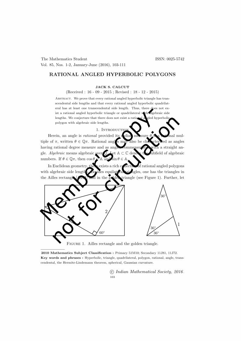
Membe
r's co
py-
not f
or ci
rculat
ion
The Mathematics Student ISSN: 0025-5742
Vol. 85, Nos. 1-2, January-June (2016), 103-111
RATIONAL ANGLED HYPERBOLIC POLYGONS
JACK S. CALCUT
(Received : 16 - 09 - 2015 ; Revised : 18 - 12 - 2015)
Abstract. We prove that every rational angled hyperbolic triangle has tran-
scendental side lengths and that every rational angled hyperbolic quadrilat-
eral has at least one transcendental side length. Thus, there does not ex-
ist a rational angled hyperbolic triangle or quadrilateral with algebraic side
lengths. We conjecture that there does not exist a rational angled hyperbolic
polygon with algebraic side lengths.
1. Introduction
Herein, an angle is rational provided its radian measure θ is a rational mul-
tiple of π, written θ ∈ Qπ. Rational angles may also be characterized as angles
having rational degree measure and as angles commensurable with a straight an-
gle. Algebraic means algebraic over Q. Let A ⊂ C denote the subfield of algebraic
numbers. If θ ∈ Qπ, then cos θ ∈ A and sin θ ∈ A.
In Euclidean geometry, there exists a rich collection of rational angled polygons
with algebraic side lengths. Besides equilateral triangles, one has the triangles in
the Ailles rectangle [Ail71] and in the golden triangle (see Figure 1). Further, let
2
2
36º
36º
36º
1
60º
Figure 1. Ailles rectangle and the golden triangle.
2010 Mathematics Subject Classification : Primary 51M10; Secondary 11J81, 11J72.
Key words and phrases : Hyperbolic, triangle, quadrilateral, polygon, rational, angle, trans-
cendental, the Hermite-Lindemann theorem, spherical, Gaussian curvature.
c© Indian Mathematical Society, 2016 .
103
Membe
r's co
py-
not f
or ci
rculat
ion
104 JACK S. CALCUT
σ(d) denote the number of similarity types of rational angled Euclidean triangles
containing a representative with side lengths each of degree at most d over Q.
Then
(1) σ(d) <∞ for each d ∈ Z+. A proof of this fact uses three ingredients: (i)
the Euclidean law of cosines, (ii) if ϕ is Euler’s totient function, n > 2, and
k is coprime to n, then the degree over Q of cos(2kπ/n) equals ϕ(n)/2,
and (iii) ϕ(n) ≥√n/2 for each n ∈ Z+ (see [Cal10]).
(2) σ(1) = 1. This class is represented by an equilateral triangle (see [CG06,
pp. 228–229] or [Cal10, p. 674]). While Pythagorean triple triangles have
integer side lengths, they have irrational acute angles; a simple approach
to this result uses unique factorization of Gaussian integers [Cal09]. In
fact, the measures of the acute angles in a Pythagorean triple triangle are
transcendental in radians and degrees [Cal10].
(3) σ(2) = 14. Parnami, Agrawal, and Rajwade [PAR82] proved this result
using Galois theory. The 14 similarity types are listed in Table 1. It is an
exercise to construct representatives for these 14 classes using the triangles
above in Figure 1.
60–60–60 45–45–90 30–60–90 15–75–90
30–30–120 30–75–75 15–15–150 30–45–105
45–60–75 15–45–120 15–60–105 15–30–135
36–36–108 36–72–72
Table 1. The 14 similarity types (in degrees) of rational angled
Euclidean triangles with side lengths each of degree at most two
over Q.
A polar rational polygon is a convex rational angled Euclidean polygon with inte-
gral length sides. The study of such polygons was initiated by Schoenberg [Sco64]
and Mann [Man65] and continues with the recent work of Lam and Leung [LL00].
In sharp contrast, there seem to be no well-known rational angled hyperbolic
polygons with algebraic side lengths. Throughout, H2 denotes the hyperbolic
plane of constant Gaussian curvature K = −1. We adopt Poincare’s conformal
disk model of H2 for our figures.
Below, we prove that every rational angled hyperbolic triangle has transcen-
dental side lengths and every rational angled hyperbolic quadrilateral (simple, but
not necessarily convex) has at least one transcendental side length. Our basic
tactic is to obtain relations using hyperbolic trigonometry to which we may apply
the following theorem of Hermite and Lindemann.
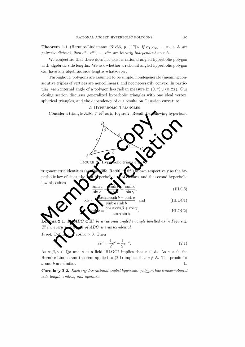
Membe
r's co
py-
not f
or ci
rculat
ion
RATIONAL ANGLED HYPERBOLIC POLYGONS 105
Theorem 1.1 (Hermite-Lindemann [Niv56, p. 117]). If α1, α2, . . . , αn ∈ A are
pairwise distinct, then eα1 , eα2 , . . . , eαn are linearly independent over A.
We conjecture that there does not exist a rational angled hyperbolic polygon
with algebraic side lengths. We ask whether a rational angled hyperbolic polygon
can have any algebraic side lengths whatsoever.
Throughout, polygons are assumed to be simple, nondegenerate (meaning con-
secutive triples of vertices are noncollinear), and not necessarily convex. In partic-
ular, each internal angle of a polygon has radian measure in (0, π) ∪ (π, 2π). Our
closing section discusses generalized hyperbolic triangles with one ideal vertex,
spherical triangles, and the dependency of our results on Gaussian curvature.
2. Hyperbolic Triangles
Consider a triangle ABC ⊂ H2 as in Figure 2. Recall the following hyperbolic
A
a
B
C
c
b
γ
β
α
Figure 2. Hyperbolic triangle ABC.
trigonometric identities (see Ratcliffe [Rat06, p. 82]) known respectively as the hy-
perbolic law of sines, the first hyperbolic law of cosines, and the second hyperbolic
law of cosinessinh a
sinα=
sinh b
sinβ=
sinh c
sin γ, (HLOS)
cos γ =cosh a cosh b− cosh c
sinh a sinh b, and (HLOC1)
cosh c =cosα cosβ + cos γ
sinα sinβ. (HLOC2)
Lemma 2.1. Let ABC ⊂ H2 be a rational angled triangle labelled as in Figure 2.
Then, every side length of ABC is transcendental.
Proof. Define x := cosh c > 0. Then
xe0 =1
2ec +
1
2e−c. (2.1)
As α, β, γ ∈ Qπ and A is a field, HLOC2 implies that x ∈ A. As c > 0, the
Hermite-Lindemann theorem applied to (2.1) implies that c 6∈ A. The proofs for
a and b are similar.
Corollary 2.2. Each regular rational angled hyperbolic polygon has transcendental
side length, radius, and apothem.
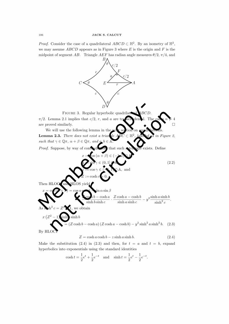
Membe
r's co
py-
not f
or ci
rculat
ion
106 JACK S. CALCUT
Proof. Consider the case of a quadrilateral ABCD ⊂ H2. By an isometry of H2,
we may assume ABCD appears as in Figure 3 where E is the origin and F is the
midpoint of segment AB. Triangle AEF has radian angle measures θ/2, π/4, and
A
B
C
c
θ
c
c c
θ
D
E
θ
F
2
c 2
r
a
Figure 3. Regular hyperbolic quadrilateral ABCD.
π/2. Lemma 2.1 implies that c/2, r, and a are transcendental. The cases n 6= 4
are proved similarly.
We will use the following lemma in the next section on quadrilaterals.
Lemma 2.3. There does not exist a triangle ABC ⊂ H2, labelled as in Figure 2,
such that γ ∈ Qπ, α+ β ∈ Qπ, and a, b ∈ A.
Proof. Suppose, by way of contradiction, that such a triangle exists. Define
x := cos (α+ β) ∈ (−1, 1) ∩ A,
y := sin γ ∈ (0, 1] ∩ A, (2.2)
z := cos γ ∈ (−1, 1) ∩ A, and
Z := cosh c > 0.
Then HLOC1 and HLOS yield
x = cos (α+ β) = cosα cosβ − sinα sinβ
=Z cosh b− cosh a
sinh b sinh c· Z cosh a− cosh b
sinh a sinh c− y2 sinh a sinh b
sinh2 c.
As sinh2 c = Z2 − 1, we obtain
x(Z2 − 1
)sinh a sinh b
= (Z cosh b− cosh a) (Z cosh a− cosh b)− y2 sinh2 a sinh2 b. (2.3)
By HLOC1
Z = cosh a cosh b− z sinh a sinh b. (2.4)
Make the substitution (2.4) in (2.3) and then, for t = a and t = b, expand
hyperbolics into exponentials using the standard identities
cosh t =1
2et +
1
2e−t and sinh t =
1
2et − 1
2e−t.
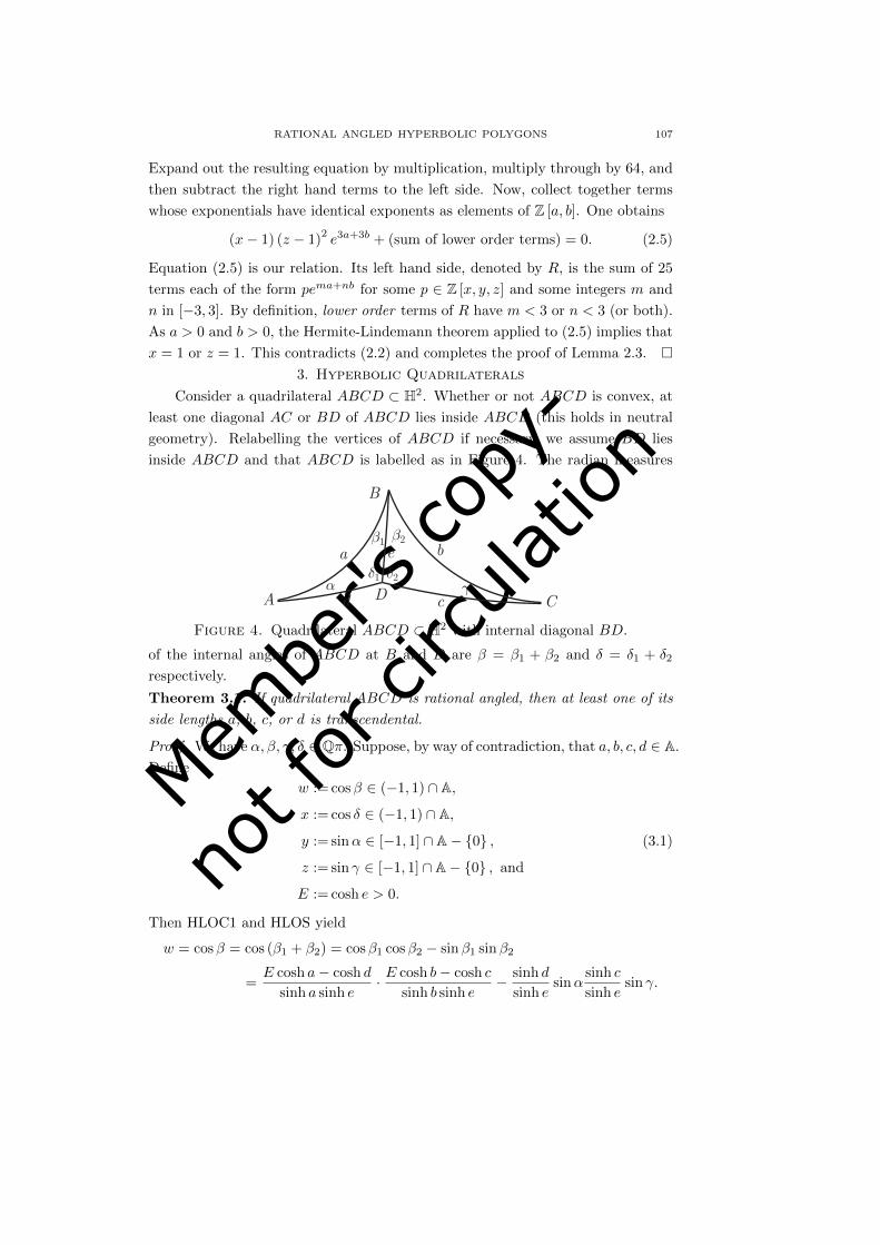
Membe
r's co
py-
not f
or ci
rculat
ion
RATIONAL ANGLED HYPERBOLIC POLYGONS 107
Expand out the resulting equation by multiplication, multiply through by 64, and
then subtract the right hand terms to the left side. Now, collect together terms
whose exponentials have identical exponents as elements of Z [a, b]. One obtains
(x− 1) (z − 1)2e3a+3b + (sum of lower order terms) = 0. (2.5)
Equation (2.5) is our relation. Its left hand side, denoted by R, is the sum of 25
terms each of the form pema+nb for some p ∈ Z [x, y, z] and some integers m and
n in [−3, 3]. By definition, lower order terms of R have m < 3 or n < 3 (or both).
As a > 0 and b > 0, the Hermite-Lindemann theorem applied to (2.5) implies that
x = 1 or z = 1. This contradicts (2.2) and completes the proof of Lemma 2.3.
3. Hyperbolic Quadrilaterals
Consider a quadrilateral ABCD ⊂ H2. Whether or not ABCD is convex, at
least one diagonal AC or BD of ABCD lies inside ABCD (this holds in neutral
geometry). Relabelling the vertices of ABCD if necessary, we assume BD lies
inside ABCD and that ABCD is labelled as in Figure 4. The radian measures
A
B
Cc
αD
d
e ba
β1 β2
δ1 δ2γ
Figure 4. Quadrilateral ABCD ⊂ H2 with internal diagonal BD.
of the internal angles of ABCD at B and D are β = β1 + β2 and δ = δ1 + δ2
respectively.
Theorem 3.1. If quadrilateral ABCD is rational angled, then at least one of its
side lengths a, b, c, or d is transcendental.
Proof. We have α, β, γ, δ ∈ Qπ. Suppose, by way of contradiction, that a, b, c, d ∈ A.
Define
w := cosβ ∈ (−1, 1) ∩ A,
x := cos δ ∈ (−1, 1) ∩ A,
y := sinα ∈ [−1, 1] ∩ A− 0 , (3.1)
z := sin γ ∈ [−1, 1] ∩ A− 0 , and
E := cosh e > 0.
Then HLOC1 and HLOS yield
w = cosβ = cos (β1 + β2) = cosβ1 cosβ2 − sinβ1 sinβ2
=E cosh a− cosh d
sinh a sinh e· E cosh b− cosh c
sinh b sinh e− sinh d
sinh esinα
sinh c
sinh esin γ.
Membe
r's co
py-
not f
or ci
rculat
ion
108 JACK S. CALCUT
As sinh2 e = E2 − 1, we obtain
w(E2 − 1
)sinh a sinh b
= (E cosh a− cosh d) (E cosh b− cosh c)− yz sinh a sinh b sinh c sinh d. (3.2)
The analogous calculation beginning with x = cos δ = cos (δ1 + δ2) yields
x(E2 − 1
)sinh c sinh d
= (E cosh d− cosh a) (E cosh c− cosh b)− yz sinh a sinh b sinh c sinh d. (3.3)
In each of the equations (3.2) and (3.3), move all terms to the right hand side and
re-group to obtain two quadratic formulas in E given by
0 = A1E2 +B1E + C1 and
0 = A2E2 +B2E + C2.
Inspection shows that B1 = B2. Define B := B1 = B2. We claim that A1 6= 0
and A2 6= 0. Suppose, by way of contradiction, that A1 = 0. Expanding the
hyperbolics in A1 into exponentials and collecting terms by the exponents of their
exponentials yields
−1
4(w − 1) ea+b + (sum of lower order terms) = 0.
The Hermite-Lindemann theorem implies w = 1 which contradicts (3.1). Hence
A1 6= 0, and similarly A2 6= 0.
The quadratic formula yields
0 < E =−B ±
√B2 − 4A1C1
2A1=−B ±
√B2 − 4A2C2
2A2,
where the ± signs are ambiguous and not necessarily equal. We have
−A2B ±A2
√B2 − 4A1C1 = −A1B ±A1
√B2 − 4A2C2,
and henceA1B −A2B ±A2
√B2 − 4A1C1 = ±A1
√B2 − 4A2C2.
Squaring both sides yields
(A1B −A2B)2
+A22
(B2 − 4A1C1
)± 2 (A1B −A2B)A2
√B2 − 4A1C1
= A21
(B2 − 4A2C2
).
Therefore
(A1B −A2B)2
+A22
(B2 − 4A1C1
)−A2
1
(B2 − 4A2C2
)= ∓2 (A1B −A2B)A2
√B2 − 4A1C1.
Again squaring both sides yields[(A1B −A2B)
2+A2
2
(B2 − 4A1C1
)−A2
1
(B2 − 4A2C2
)]2= 4 (A1B −A2B)
2A2
2
(B2 − 4A1C1
). (3.4)
Subtract the right hand side of (3.4) to the left side, expand out by multiplication,
and cancel the common factor 16A21A
22 6= 0 to obtain
Membe
r's co
py-
not f
or ci
rculat
ion
RATIONAL ANGLED HYPERBOLIC POLYGONS 109
A21C
22 +A2
2C21−2A1A2C1C2+A1B
2C1+A2B2C2−A1B
2C2−A2B2C1 = 0. (3.5)
At this point, use of a computer algebra system is recommended; we used MAGMA
for our computations and Mathematica for independent verification. In (3.5),
expand hyperbolics into exponentials and then expand out by multiplication.
Multiply through the resulting equation by 4096 and then collect together terms
whose exponentials have identical exponents as elements of Z [a, b, c, d]. This yields
(w − 1)2y2z2e(4a+4b+2c+2d) + (x− 1)
2y2z2e(2a+2b+4c+4d)
+ 2 (w − 1) (1− x) y2z2e(3a+3b+3c+3d) + (sum of lower order terms) = 0. (3.6)
Equation (3.6) is our relation. Its left hand side, denoted by R, is the sum of
1041 terms each of the form peka+lb+mc+nd for some p ∈ Z [w, x, y, z] and some
integers k, l, m, and n in [−4, 4]. Here, a lower order term is defined to be one
whose exponential exponent ka+ lb+mc+ nd is dominated by 4a+ 4b+ 2c+ 2d,
2a+ 2b+ 4c+ 4d, or 3a+ 3b+ 3c+ 3d. This means, by definition, that either
(1) k ≤ 4, l ≤ 4, m ≤ 2, n ≤ 2, and at least one of these inequalities is strict,
(2) k ≤ 2, l ≤ 2, m ≤ 4, n ≤ 4, and at least one of these inequalities is strict,
or
(3) k ≤ 3, l ≤ 3, m ≤ 3, n ≤ 3, and at least one of these inequalities is strict.
There are now two cases to consider.
Case 1. One of the sums 4a+4b+2c+2d, 2a+2b+4c+4d and 3a+3b+3c+3d is
greater than the other two. Then, the Hermite-Lindemann theorem implies that
the corresponding polynomial coefficient in equation (3.6) must vanish, that is
(w − 1)2y2z2 = 0, (x− 1)
2y2z2 = 0, or 2 (w − 1) (1− x) y2z2 = 0.
By equations (3.1), we have w 6= 1, x 6= 1, y 6= 0, and z 6= 0. This contradiction
completes the proof of Case 1.
Case 2. Two of the sums 4a+4b+2c+2d, 2a+2b+4c+4d, and 3a+3b+3c+3d are
equal. Then, a+ b = c+ d. Recalling Figure 4, a+ b = c+ d and two applications
of the triangle inequality imply that D cannot lie inside triangle ABC. Similarly,
B cannot lie inside triangle ADC. This implies that diagonal AC lies inside
quadrilateral ABCD. Now, repeat the entire argument of the proof of Theorem 3.1
using diagonal AC in place of diagonal BD. We either obtain a contradiction as
in Case 1 or we further obtain a + d = b + c. Taken together, a + b = c + d and
a+d = b+c imply that a = c and b = d. So, opposite sides of quadrilateral ABCD
are congruent. By SSS, triangles ABD and CDB are congruent. In particular,
δ1 = β2. So, β1 + δ1 = β ∈ Qπ and triangle ABD contradicts Lemma 2.3. This
completes the proof of Case 2 and of Theorem 3.1.
4. Concluding Remarks
The results above have analogues for generalized hyperbolic triangles with one
ideal vertex and for spherical triangles.
Membe
r's co
py-
not f
or ci
rculat
ion
110 JACK S. CALCUT
Lemma 4.1. Let ABC be a generalized hyperbolic triangle with one ideal vertex
C as in Figure 5. If α, β ∈ Qπ, then the finite side length c is transcendental.
A
B
Cc
β
α
0
Figure 5. Generalized hyperbolic triangle ABC with one ideal
vertex C.
Proof. By Ratcliffe [Rat06, p. 88], we have
cosh c =1 + cosα cosβ
sinα sinβ.
Thus
(sinα sinβ) ec + (sinα sinβ) e−c = 2 (1 + cosα cosβ) e0. (4.1)
As c > 0, the Hermite-Lindemann theorem applied to (4.1) implies c /∈ A.
Let S2 ⊂ R3 denote the unit sphere of constant Gaussian curvature K = +1.
Lemma 4.2. Let ABC ⊂ S2 be a rational angled triangle labelled as in Figure 6.
Then, every side length of ABC is transcendental.
A
a
B
Cc
b
γ
β
α
Figure 6. Spherical triangle ABC.
Proof. The second spherical law of cosines (see Ratcliffe [Rat06, p. 49]) gives
(sinα sinβ) eic + (sinα sinβ) e−ic = 2 (cosα cosβ + cos γ) e0, (4.2)
where c > 0 and sinα sinβ ∈ A − 0. Whether or not the algebraic num-
ber cosα cosβ + cos γ vanishes, the Hermite-Lindemann theorem applied to (4.2)
implies c /∈ A. The proofs for a and b are similar.
On the other hand, the results in this note do not hold for arbitrary constant
curvature. In a plane of constant Gaussian curvature
K = −(
cosh−1(
1 +√
2))2≈ −2.3365 . . . ,

Membe
r's co
py-
not f
or ci
rculat
ion
RATIONAL ANGLED HYPERBOLIC POLYGONS 111
a regular triangle with angles of radian measure π/4 has unit side lengths.
Similarly, in a sphere of constant Gaussian curvature
K =π2
4≈ 2.4674 . . . ,
a regular right angled triangle has unit side lengths.
References
[Ail71] Ailles, D. S., Triangles and trigonometry, Mathematics Teacher 64 (1971), 562.
[Cal09] Calcut, Jack S., Gaussian integers and arctangent identities for π, Amer. Math. Monthly
116 (2009), 515–530.
[Cal10] ——, Grade school triangles, Amer. Math. Monthly 117 (2010), 673–685.
[CG06] Conway, J. H. and Guy, R. K., The Book of Numbers, Copernicus, New York, 2006.
[LL00] Lam, T. Y. and Leung, K. H., On vanishing sums of roots of unity, J. Algebra 224
(2000), 91–109.
[Man65] Mann, Henry B., On linear relations between roots of unity, Mathematika 12 (1965),
107–117.
[Niv56] Niven, Ivan, Irrational numbers, The Mathematical Association of America, John Wiley
and Sons, New York, 1956.
[PAR82] Parnami, J. C., Agrawal, M. K. and Rajwade, A. R., Triangles and cyclic quadrilaterals,
with angles that are rational multiples of π and sides at most quadratic over the rationals,
Math. Student 50 (1982), 79–93.
[Rat06] Ratcliffe, John G., Foundations of hyperbolic manifolds, second edition, Springer, New
York, 2006.
[Sco64] Schoenberg, I. J., A note on the cyclotomic polynomial, Mathematika 11 (1964), 131–
136.
Jack S. Calcut
Department of Mathematics, Oberlin College
Oberlin, OH 44074, USA
E-mail: [email protected]

Membe
r's co
py-
not f
or ci
rculat
ion
112
Membe
r's co
py-
not f
or ci
rculat
ion
The Mathematics Student ISSN: 0025-5742
Vol. 85, Nos. 1-2, January-June (2016), 113-116
METRIZABILITY OFARITHMETIC PROGRESSION TOPOLOGY
FAHED ZULFEQARR
(Received : 18 - 10 - 2015 ; Revised : 24 - 12 - 2015)
Abstract. Besides giving a way to produce an infinite number of metrics
for Furstenberg topology on integers the article rather focuses on a new proof
of its metrizability using geometric series.
1. Introduction
Gone are the days when topology was confined to be a branch of pure mathe-
matics. No area of science now escapes from its gravity. For instance, topology is
used to understand important concepts of genotype and phenotype in evolutionary
biology. Moreover seemingly distant branches of mathematics, number theory and
topology have some elegant connections. In this direction, H. Furstenberg in 1955
discovered a strange topology on integers via arithmetic progression and found a
beautiful topological proof of infinitude of primes [2]. This article moves a step
further and proves metrizability of this topology.
Section 2 introduces Furstenberg topology on integers and contains some useful
properties of arithmetic progression. Using convergence of geometric series, a
metric on integers is defined in section 3. Last section deals with metrizability of
integers with respect to Furstenberg topology.
2. Notations and Preliminaries
The set of all integers is denoted by Z. We let Z∗ = Z \ 0. For m ∈ Z and
n ∈ Z∗, an arithmetic progression is defined by the set
Am,n = m+ kn | k ∈ Z.We denote the collection of all arithmetic progression by A. The topology gener-
ated by A is the Furstenberg topology on Z also known as arithmetic progression
topology (cf.[1, page 54]). We interchangeably use these terms and let it be de-
noted by τA.
One can easily observe the following useful facts on Z.
Remarks 2.1 (1). Am,n = Am,−n = Ar,n for any r ∈ Am,n.
(2). Z\Am,n =⋃i=n−1
i=1 Am+i,n. Hence an arithmetic progression
is open as well as closed set in τA.
2010 Mathematics Subject Classification : Primary 54-021; Secondary 11B25
Key words and phrases : Arithmetic Progression, Metrizability, Geometric Series
c© Indian Mathematical Society, 2016 .
113
Membe
r's co
py-
not f
or ci
rculat
ion
114 FAHED ZULFEQARR
3. metric on integers
A metric on any non-empty set X is a non-negative real-valued function de-
fined on X×X taking all its diagonal elements to zero, positive on the complement
of diagonal and satisfying symmetric and triangular inequality axioms.
We define an arithmetic function f on Z using the convergence of geometric
series for any fixed real p > 1 by
f(x) =∑
k∈N, k-x
1
pk, x ∈ Z∗ and f(0) = 0. (*)
The following theorem contains some useful facts about the above arithmetic
function.
Theorem 3.1. The function f(x) defined in (*) satisfies following properties
(a) f(x) ≥ 0 for all x ∈ Z.(b) f(x) = f(−x) for all x ∈ Z.(c) f(kx) ≤ f(x) for any k ∈ Z.(d) f(x+ y) ≤ f(x) + f(y) for all x, y ∈ Z.
Proof. (a) follows from the definition of f(x). Divisibility over Z yields (b). (c)
follows from the fact that divisors of x are also the divisors of kx. For (d), if either
x = 0 or y = 0, the equality holds. So we assume that x 6= 0 and y 6= 0 and
observe that
f(x) =∑k-x
1
pk=∞∑k=1
1
pk−
∑k| x
1
pk
⇒ f(x) =1
p− 1−
∑k|x, k-y
1
pk−
∑k|x, k|y
1
pk.
Similarly
f(y) =1
p− 1−
∑k|y, k-x
1
pk−
∑k|x, k|y
1
pkand
f(x+ y) =1
p− 1−
∑k|x+y
k-x & k-y
1
pk−
∑k|x, k|y
1
pk.
Therefore we have
f(x) + f(y)− f(x+ y)
=1
p− 1+
∑k|x+y
k-x & k-y
1
pk−
∑k|x, k-y
1
pk−
∑k|y, k-x
1
pk−
∑k|x, k|y
1
pk
>∑
k|x+y
k-x & k-y
1
pk
which proves (d).
Membe
r's co
py-
not f
or ci
rculat
ion
METRIZABILITY OF ARITHMETIC PROGRESSION TOPOLOGY 115
We now define another function d induced by f on Z by
d(m,n) = f(m− n) =∑k∈N
k-(m−n)
1
pk. (**)
The next theorem asserts that d actually defines a distance function on Z.
Theorem 3.2. For m,n ∈ Z, the function d(m,n) defines a metric on Z.
Proof. In view of theorem 3.1, all conditions for d to be a metric holds trivially.
For instance, triangular inequality follows from (d). In fact, for any m, l, n ∈ Zd(m,n) = f(m− n) = f(m− l + l − n) 6 f(m− l) + f(l − n) = d(m, l) + d(l, n).
4. metrizability of Furstenberg topology
Metrizable spaces have additional structure that can be very useful. For in-
stance, metrizable spaces are Hausdorff so any convergent sequence has a unique
limit. Related to metrizability of a topological space, there are two important
problems: (1) For a given topological space, construct a metric that induces the
topology on the set, (2) Discover a criterion for metrizability of the topological
space without specifically finding a metric on it as in the case of Urysohn’s metriz-
able lemma.
Metrizability of Furstenberg topology on Z is already known to us. Readers
are encouraged to see [1] and [3]. We prove this by using the metric d(m,n) on Zas defined in the previous section.
Theorem 4.1. The metric d(m,n), m,n ∈ Z, induces Furstenberg topology τA.
Proof. Let the topology induced by metric d be denoted by τd. In the light of
Remark 2.1, for the inclusion τA ⊆ τd, it suffices to prove that for a given arithmetic
progression Am,n there exists some r > 0 such that the open ball B(m, r) centered
at m with radius r is contained in Am,n. For this we choose r < 1pn . Then for any
t ∈ B(m, r) we have
d(t,m) =∑k∈N
k-(m−t)
1
pk< r <
1
pn
⇒ n | (m− t) (in fact n! | (m− t))
⇒ t = m+ kn, for some k ∈ Z.
This implies that B(m, r) ⊆ Am,n. For proving the reverse inclusion τd ⊆ τA,
consider an open ball B(m, r) and choose n ∈ Z∗ such that f(n) < r. Such n
indeed exists; in fact, think of sufficiently large k ∈ N such that
1
pk(p− 1)< r,
and put n = k!. Then
f(n) =∑
i∈N, i-n
1
pi6
∞∑i=k+1
1
pi=
1
pk(p− 1)< r.

Membe
r's co
py-
not f
or ci
rculat
ion
116 FAHED ZULFEQARR
Let us now take any t = m + kn ∈ Am,n. By using part (c) of Theorem 3.1, we
have
d(t,m) = f(t−m) = f(kn) 6 f(n) < r.
Thus we get Am,n ⊆ B(m, r) and the proof is completed.
References
[1] Adams, C. and Franzosa, R., Introduction to Topology, Pure and Applied, Pearson
Education, Inc., 2008.
[2] Furstenberg, H., On infinitude of primes, Amer. Math. Monthly, 62 (1955), No. 5, 353.
[3] Lovas, R. L. and Mezo, I., On an exotic topology of integers, http://arxiv.org /abs
/1008.0713.
Fahed Zulfeqarr
Department of Mathematics, Gautam Buddha University
Greater Noida- 201308, U. P., India
E-mail: [email protected]

Membe
r's co
py-
not f
or ci
rculat
ion
The Mathematics Student ISSN: 0025-5742
Vol. 85, Nos. 1-2, January-June (2016), 117-133
INTERESTING INFINITE PRODUCTS OF RATIONALFUNCTIONS MOTIVATED BY EULER
AMRIK SINGH NIMBRAN
(Received : 19 - 10 - 2015 ; Revised : 19 - 12 - 2015)
Abstract. This paper contains a survey of interesting infinite products of
rational functions based on Euler’s Gamma function and infinite product
expansions for sinx and cosx. Though the index in many products ranges,
as usual, over the positive integers, we also treat products where the index
ranges over the prime numbers. Historical information concerning the original
sources for the gamma function and infinite products is also given.
1. Gamma function and products
The first noteworthy infinite product was discovered by the French mathe-
matician Francois Viete (1540–1603) in 1593 (Opera, Leyden 1646, p. 400)
2
π=
√1
2·
√1
2+
1
2
√1
2·
√√√√1
2+
√1
2+
1
2
√1
2· · · . (1)
The English mathematician John Wallis (1616–1703) gave a neat product for4π (denoted by ) in Prop. 191 (page 179) of his Arithmetica infinitorum (1656)
wherein he aimed at finding a general method of quadrature for curved surfaces and
interpolated means in the sequence 1, 6, 30, 140, 630, · · · (defined by the recursion
tn+1 = 4n+2n × tn, t1 = 1)
=3× 3× 5× 5× 7× 7× etc.2× 4× 4× 6× 6× 8× etc.
(2)
Leonhard Euler (1707–1783), the versatile Swiss mathematician, did pioneer-
ing work on infinite series and products which began when he was 22. An arith-
metical function representing the product of the first n natural numbers was
known from earlier times though the notation n! was introduced later by a French
mathematician Christian Kramp (1760–1826) in his Elements d’arithmetique uni-
verselle (1808) while the term ‘factorial’ was coined by his fellow-countryman Louis
Francois Antoine Arbogast (1759–1803).
Christian Goldbach (1690-1764), who was Euler’s colleague at the St. Peters-
burg Academy but had moved to Moscow soon after Euler’s arrival in 1727, and
Daniel Bernoulli (1700–1784), with whom Euler stayed then in St. Petersburg,
2010 Mathematics Subject Classification : 11Y60, 33B15, 40A20, 41AXX.
Key words and phrases : Infinite products; Gamma function; pi, prime numbers.
c© Indian Mathematical Society, 2016 .
117
Membe
r's co
py-
not f
or ci
rculat
ion
118 AMRIK SINGH NIMBRAN
having failed to solve the problem of interpolating between the factorials, sug-
gested it to Euler who announced his solution to Goldbach in two letters and soon
detailed his ideas in [4].
The first letter dated October 13, 1729 contained the expression
1 · 2m
1 +m
21−m · 3m
2 +m
31−m · 4m
3 +m
41−m · 5m
4 +m· · · .
Setting m = 12 , Euler obtained Γ(3
2 ) =√π
2 and deduced Wallis’ product.
In his letter of January 8, 1730 and in [4], Euler took up the series∑n! and found
the general term for the factorial to be∫
(− lnx)n dx. Thus, the terms of the series
transform into a definite integral
∫ 1
0
(ln
1
x
)ndx, which on substituting x = e−t,
converts into∫∞
0tn e−t dt, the definite integral given later in Art.11 of his paper
[8]. Extended to z ∈ C, it becomes
Γ(z) =
∫ ∞0
tz−1 e−t dt, R(z) > 0. (3)
One may note that the notation Γ(a) was introduced by the French mathematician
Adrien-Marie Legendre (1752–1833) who defined it [14, p.477, sec.53](1809) as
Γ(a) =
∫dx
(log
1
x
)a−1
.
In §10 of [8], Euler recorded an infinite product representation
y = 1 · 2 · 3 · · ·x =
√2π(x+ n)∏nk=1(x+ k)
(x+ n
e
)x+n
es, (4)
where s =
∞∑m=1
(−1)m−1 c2m(2m− 2)!
22m−1(x+ n)2m−1and c2m being the coefficient of π2m
occurring in Euler’s zeta function ζ(2m).
In §12, Euler noted two more product representations (including one recorded
in his first letter to Goldbach)
y =∞∏n=1
n
n+ x
(n+ 1
n
)x(5)
=
(1 + x
2
)x ∞∏n=1
n
n+ x
(2n+ 1 + x
2n− 1 + x
)x. (6)
In §8 of [4], Euler actually started with another integral∫xe dx (1− x)n which he
evaluated by expanding (1− x)n through the Binomial Theorem∫ 1
0
xe(1− x)n dx =1 · 2 · · ·n
(e+ 1)(e+ 2) · · · (e+ n+ 1).
His objective now was to isolate 1 · 2 · · ·n from the denominator so as to have an
expression for n! as an integral. He thus arrived at the integral∫
(− lnx)n dx. The
Membe
r's co
py-
not f
or ci
rculat
ion
INTERESTING INFINITE PRODUCTS ..... MOTIVATED BY EULER 119
former integral was termed by Legendre the first Eulerian integral or the Beta
function and the latter the second Eulerian integral with
B(m,n) =
∫ 1
0
tm−1(1− t)n−1 dt =Γ(m) Γ(n)
Γ(m+ n).
Integration of (3) by parts yields the functional equation
Γ(z + 1) =
∫ ∞0
tz e−t dt = −tze−t∣∣∣∞0
+ z
∫ ∞0
tz−1 e−t dt = zΓ(z). (7)
Legendre gave the duplication formula [14, page 485]
Γ(a) =21−2a
√π
cos aπ Γ(2a) Γ
(1
2− a), a <
1
2. (8)
Carl Friedrich Gauss (1777-1855) studied the Gamma function while dealing
with the hypergeometric series [11]. He used the notation Πz, where
Πz = limk→∞
k!kz∏kj=1(z + j)
. (9)
His functional equation (§21, (44)) is slightly different: Π(z + 1) = (z + 1)Πz and
Π(−12 ) =
√π, Π( 1
2 ) = 12
√π. In §26, equation (57), we find
nn z∏n−1k=0 Π
(z − k
n
)Πnz
=(2π)
12 (n−1)
√n
. (10)
Schlomilch [24, p.171, eq(12)](1844) and Newman [16, p.59, eq. (10)] (1848)
found
Γ(1 + α) = e−Cαeα
1 + α1
· e12α
1 + α2
· e13α
1 + α3
· · · , (11)
where C is the constant γ introduced by Euler as the constant of integration in
[5] (1734) and treated in depth in [9] (1776).
Recognizing the advantages of starting with 1Γ(z) , Karl Weierstrass (1815-
1897) used this form. He called 1Γ(u+1) the “Factorielle of u”, denoted it by Fc(u)
[28, p. 7] and gave following representations [28, eq.(10), (15), (46), (47)]
Fc(u) =u∞∏α=1
(α
1 + α
)u (1 +
u
α
)= limn→∞
n−uu(1 + u)
(1 +
u
2
)· · ·(
1 +u
n− 1
).
This can be written as
1
Γ(z)= zeγz
∞∏n=1
(1 +
z
n
)e−
zn . (12)
Formula (12) shows the roots of 1Γ(z) . As Davis [3, page 862] remarks, the reciprocal
of the gamma function is a much less difficult function to deal with than the gamma
function itself.
Membe
r's co
py-
not f
or ci
rculat
ion
120 AMRIK SINGH NIMBRAN
Since ln(ab )=ln a− ln b, we have ln(n+ 1)=∑nk=1 ln(k+1
k ), and
γ = limn→∞
[n∑k=1
1
k−
n∑k=1
lnk + 1
k
].
Then multiplying both sides by −z followed by raising the two sides to the power
of e yields
e−γz = limn→∞
e−∑nk=1
zk eln(1+ 1
k )z = limn→∞
n∏k=1
e−zk
(1 +
1
k
)z.
Using Gauss’ representation, we get
zΓ(z) = limn→∞
n∏k=1
(1 +
1
k
)z (1 +
z
k
)−1
= limn→∞
n∏k=1
(1 +
1
k
)ze−
zk
(1 +
z
k
)−1
ezk
which on using the result deduced above yields
Γ(z) = z−1e−γz limn→∞
n∏k=1
(1 +
z
k
)−1
ezk
and this on being inverted becomes (12).
Euler’s reflection/complement formula can be obtained by employing the
representation of Weierstrass for the expression 1Γ(z)Γ(−z) followed by the use of
Γ(−z) = −Γ(1−z)z and Euler’s product expansion for sin z (to follow soon)
Γ(1− z) Γ(z) =π
sin(π z)⇒ Γ(1− z) Γ(1 + z) =
πz
sin(π z), z 6= 0, ±1, · · · . (13)
This formula possibly motivated Euler to find the product expansion for sinx. He
factorized the function ex − e−x to obtain [6, Ch. IX, §158]
sinx = x
(1− x2
π2
)(1− x2
(2π)2
)(1− x2
(3π)2
)· · · , (14)
and
cosx =
(1− 4x2
π2
)(1− 4x2
(3π)2
)(1− 4x2
(5π)2
)· · · . (15)
Euler derived Wallis’ product in [7, Ch.9, §358] by setting x = 12 in (14) and then
shifting the term 12 to the left hand side. We find that it can also be obtained
through (15) by transferring the first factor on the right to the left and then taking
the limit x→ π2 . As the limit is of the indeterminate form 0
0 , we apply L’ Hospital’s
rule, differentiating the expression and so getting the desired result.
2. Summary of formulas and special values
We summarize in the following the gamma function identities and values (some
noted earlier) that are needed in the rest of the paper
2.1. Definitions.
2.1.1. Euler’s integral : Γ(z) =∫∞
0tz−1 e−t dt, R(z) > 0.
Membe
r's co
py-
not f
or ci
rculat
ion
INTERESTING INFINITE PRODUCTS ..... MOTIVATED BY EULER 121
2.1.2. Euler’s product : Γ(z) = limn→∞∏nk=1
(n−1)!z(z+1)(z+2)···(n+z−1)n
z,
valid for all z except z 6= 0,−1,−2, · · · .
2.1.3. Weierstrass product : 1Γ(z) = zeγz
∏∞n=1
(1 + z
n
)e−
zn ,
valid for all z except z 6= 0,−1,−2, · · · ; and γ =N→∞
N∑n=1
1
n− lnN.
2.2. Important identities.
2.2.1. Functional relation : Γ(z + 1) = zΓ(z).
2.2.2. Euler’s reflection formula : Γ(z) Γ(1− z) = πsin(π z) .
2.2.3. Legendre’s duplication formula : Γ(2z) = π−12 22z−1Γ(z) Γ
(z + 1
2
).
2.2.4. Gauss’s multiplication formula :
Γ(nz) = (2π)1−n
2 nnz12 Γ(z) Γ
(z +
1
n
)Γ
(z +
2
n
)· · ·Γ
(z +
n− 1
n
).
2.3. Special values. (Here n is a nonnegative integer.)
2.3.1. Factorial : Γ(n+ 1) = n!.
2.3.2. Half-integer values : Γ(
12
)= π
12 ; Γ
(−n+ 1
2
)= (−1)n 22n n!
(2n)!
√π ;
Γ(n+ 1
2
)= (2n−1)!!
2n Γ(
12
)= (2n)!
22n n!
√π.
2.3.3. Quarter-integer values : Γ(
14
)=√√
2π L , Γ(n+ 1
4
)= 1·5·9···(4n−3)
4n Γ(
14
),
where L = 2.62205755429212 · · · is called the lemniscate constant and
equals one half the perimeter of the unit lemniscate curve r2 = cos 2θ (a
special case of Bernoulli’s lemniscate) just as π is one half the circumference
of the unit circle [31]. The numbers π and L share several common features.
L is also related to Gauss’s constant K by L = πK with
K =2
π
∫ 1
0
dx4√
1− x4=
∞∏n=1
tanh2 nπ
2=
Γ2(
14
)(2π)
32
.
Note: We are using K for the Gauss constant instead of G used in [30] as
we will use G for the Catalan constant later.
2.3.4. Rational values(n+ 1
k
):
Γ
(n+
1
k
)=
1 · (1 + k) · (1 + 2k) · · · (1 + (n− 1)k)
knΓ
(1
k
).
Euler gave the following formula which is a consequence of the multiplication
formula of Gaussn−1∏m=1
Γ(mn
)=
(2π)n−1
2
√n
.

Membe
r's co
py-
not f
or ci
rculat
ion
122 AMRIK SINGH NIMBRAN
Let Φ(n) = m : 1 ≤ m < n ∧ gcd(m,n) = 1. Let φ(n) = N(Φ(n)) represent
Euler’s totient function. For any prime p, φ(p) = p− 1. If gcd(a, b) = 1, φ(a · b) =
φ(a)× φ(b). And φ(mk) = mk−1 φ(m). Then we have [23, 15, 17, 2]
n∏m=1
Γ(mn
)=
(2π)φ(n)
2
eΛ(n)
2
=
(2π)φ(n)
2√p ifm = pr
(2π)φ(n)
2 ifm 6= pr
where Λ(n) is Mangoldt’s function defined to be log p if n = pr; p − prime, r ∈ Nand 0 otherwise.
3. Products of rational functions of integer index
Probably the most famous product of rational functions with integer index is
the Wallis product. We will give a general theorem that explains all such products
and gives a closed form for the expansions as a quotient of gamma functions. But
before that we touch upon the theory of infinite products.
An infinite product is formed by multiplying, in a given order, the terms of
an infinite sequence ar of real or complex numbers and is denoted by∏∞r=1 ar.
The product of the first n terms, that is Pn =∏nr=1 ar, is called the n-th partial
product. If Pn tends to a non-zero finite limit P as n → ∞, then the infinite
product is said to converge to (value) P.
To determine the convergence of an infinite product, we write the general term
as ar = 1 + br or ar = 1 − br. If the infinite product is convergent, Pn and Pn−1
tend to the same limit as n→∞. Since PnPn−1
= 1 + bn, we havelimn→∞
Pn
limn→∞
Pn−1= 1⇒ lim
n→∞(1 + bn) = 1⇒ lim
n→∞bn = 0.
It is thus a necessary (but not sufficient) condition for∏
(1 + bn) to converge that
bn → 0. A necessary and sufficient condition for the convergence of∏
(1 + bn) and∏(1− bn) is the convergence of the series
∑bn.
3.1. Products derived via Gamma function. We now state and prove the
following theorem from Whittaker and Watson [32, page 238].
Theorem 3.1. Let un =A (n+ a1)(n+ a2) · · · (n+ ak)
(n+ b1)(n+ b2) · · · (n+ bl)be a general rational
function of n. If A = 1, k = l and a1 + a2 + · · ·+ ak = b1 + b2 + · · ·+ bk then the
infinite product∞∏n=1
un converges absolutely; and it has the closed form value
∞∏n=1
(n+ a1)(n+ a2) · · · (n+ ak)
(n+ b1)(n+ b2) · · · (n+ bk)=
Γ(1 + b1)Γ(1 + b2) · · ·Γ(1 + bk)
Γ(1 + a1)Γ(1 + a2) · · ·Γ(1 + ak). (16)
Proof. Since we require limn→∞
un = 1, we must have k = l and A = 1. Observe
that the general term of the infinite product can be written as
un =(1 + a1
n )(1 + a2
n ) · · · (1 + akn )
(1 + b1n )(1 + b2
n ) · · · (1 + bkn )
Membe
r's co
py-
not f
or ci
rculat
ion
INTERESTING INFINITE PRODUCTS ..... MOTIVATED BY EULER 123
= 1 +a1 + a2 + · · ·+ ak − b1 − b2 − · · · − bk
n+O(
1
n2).
For the convergence we require that the factors un, when expanded in reciprocal
powers of n, say as 1 + αn + β
n2 + · · · , approach 1 faster than 1 + αn , so we must
have α = 0. Thus we need a1 + a2 + · · ·+ ak = b1 + b2 + · · ·+ bk (See [32, §2.7]).
Further, observe that we can write
un =(1 + a1
n )e−a1n (1 + a2
n )e−a2n · · · (1 + ak
n )e−akn
(1 + b1n )e−
b1n (1 + b2
n )e−b2n · · · (1 + bk
n )e−bkn
by inserting exponential convergence factors in the expression for un without
altering the value of the product. (Inserting these exponentials causes a factor like
(1 + an )e−
an to approach 1 with order 1
n2 , thus ensuring absolute convergence of
our infinite product). From the Wierstrass definition of the infinite product we
have∞∏n=1
(1 +
z
n
)e−
zn
=
1
zΓ(z)eγz=
1
Γ(z + 1)eγz.
The closed form of our infinite product (16) now follows at once.
As a consequence of this theorem, every infinite product of rational functions
has a closed form expansion in terms of a quotient of gamma functions. So the
next step would be to find certain values of the constants a and b which reduce the
quotient of gamma functions to a more familiar value. With the aid of the known
special values of the gamma function, and other identities previously shown, we can
obtain an endless number of these products. We also note that other approaches
to products of this type, such as the Wallis product, may be found by entirely
different (and sometimes simpler) methods. We now illustrate it by deriving a few
such infinite products.
Example 1. Wallis product. Taking a1 = − 12 , a2 = 1
2 , b1 = b2 = 0, we get
∞∏n=1
(n− 12 )(n+ 1
2 )
n · n=
Γ(1)Γ(1)
Γ(
12
)Γ(
32
)which immediately simplifies to
∞∏n=1
(2n− 1)(2n+ 1)
(2n)2=
2
π.
Example 2. Taking a1 = − 12 , a2 = 1 and b1 = b2 = 1
4 we obtain
∞∏n=1
(n− 12 )(n+ 1)
(n+ 14 )(n+ 1
4 )=
Γ2(
54
)Γ( 1
2 )Γ(2)=
Γ2(
14
)16√π
;
and since Γ2(
14
)= 2√
2π L it follows that∞∏n=1
(4n− 2)(4n+ 4)
(4n+ 1)2=
L
4√
2. (17)
Membe
r's co
py-
not f
or ci
rculat
ion
124 AMRIK SINGH NIMBRAN
Example 3. The values a1 = 12 = a2 = − 1
4 , b1 = 0 and b2 = 14 yield
K =L
π=∞∏n=1
(2n+ 1)(4n− 1)
2n(4n+ 1). (18)
A number of such products (derived mostly by the author) are listed in the Appen-
dix. Most of the products in the Category C are based on the relations between
particular Gamma values found in [26] and [29]. Two of the products in the
Category B are motivated by a result occurring in [12].
3.2. Products derived via the cosine function. Euler’s expansion for cosx
can be expressed as
coskπ
2m=∞∏n=1
(2mn− (m+ k))(2mn− (m− k))
(2mn−m)2, m, k ∈ N; 1 ≤ k ≤ m.
Setting k = 1, 2, 3, · · · (m− 1) yields products having factors of the form 2mn− k.
Sincecos(π/4)
cos(π/3)=√
2 and 12 is the L.C.M. of 3 and 4, so putting m = 6, k = 3, 4
in the above identity and then dividing the formula obtained with k = 3 by the
formula with k = 4, we get√
2 =∞∏n=1
(12n− 9)(12n− 3)
(12n− 10)(12n− 2).
Some results noted in the Appendix have been derived by combining various prod-
ucts so obtained using the twenty-four possible values (computed by the author)
for sin θ and cos θ given in Table 1.
4. Products involving prime numbers
Beginning with his solution of the famous Basel problem in 1734, Euler eval-
uated the series of reciprocals of even powers of the natural numbers thus intro-
ducing the Euler zeta function sometime around 1737. He then discovered in 1744
a beautiful relationship between ζ(s) and prime numbers
ζ(s) =∞∑n=1
1
ns=
∏p−prime
(1− p−s
)−1, <(s) > 1. (19)
Euler obtained (19) by making use of the fundamental theorem of arithmetic (each
natural number n > 1 can be expressed uniquely as a product of primes) and using
the formula for the sum of a geometric series as follows
1 +1
2s+
1
3s+
1
4s+ · · · =
(1 +
1
2s+
1
22s+ · · ·
)(1 +
1
3s+
1
32s+ · · ·
)(
1 +1
5s+
1
52s+ · · ·
)· · · =
∏p−prime
(1 +
1
ps+
1
p2s+ · · ·
)=
∏p−prime
1
1− 1ps
We now show how Euler obtained the following remarkable product [10, §15]
that ranges over all odd primes

Membe
r's co
py-
not f
or ci
rculat
ion
INTERESTING INFINITE PRODUCTS ..... MOTIVATED BY EULER 125
π
4=
3
4· 5
4· 7
8· 11
12· 13
12· 17
16· 19
20· · · =
∏p−odd prime
p
p+ (−1)p+1
2
. (20)
To understand the use of (−1)p+1
2 one may observe that all the odd prime numbers
can be divided into two classes - those of the form 4n + 1 and those of the form
4n− 1. If p ≡ −1 (mod 4), (−1)p+1
2 = 1 and if p ≡ 1 (mod 4), (−1)p+1
2 = −1. In
fact, Euler starts with the Leibniz series (1674)
π
4= 1− 1
3+
1
5− 1
7+
1
9− 1
11+ · · · . (21)
Multiplying (21) by 13 (3 is a prime of the form 4n−1) one gets the series expansion
π
4· 1
3=
1
3− 1
9+
1
15− 1
21+
1
27− 1
33+ · · · (22)
which when added to (21) will give the following series expansion whose right side
is bereft of the multiples of 1/3.
π
4
(1 +
1
3
)= 1 +
1
5− 1
7− 1
11+
1
13+ · · · . (23)
Similarly, first multiplying (22) by 15 (5 is prime of the form 4n+ 1) one gets the
series expansion
π
4
(1 +
1
3
)1
5=
1
5+
1
25− 1
35− 1
55+
1
65+ · · · , (24)
which when subtracted from (23) will result in to the following series expansion
the right side of which is bereft of multiples of 1/5.
π
4
(1 +
1
3
)(1− 1
5
)= 1− 1
7− 1
11+
1
13+
1
17− 1
19− · · · .
Continuing in this way, adding when the denominator of the second term on right
side of the concerned series expansion is a prime of the form p = 4n − 1 and
subtracting when it is a prime of the form p = 4n+1, we can successively eliminate
all multiples of 1/7, 1/11, 1/13, · · · from the right side of the series expansion
eventually getting
π
4
(1 +
1
3
)(1− 1
5
)(1 +
1
7
)(1 +
1
11
)(1− 1
13
)· · · = 1
which can be written as
π
4
∏p−oddprime
(1 + (−1)
p+12
1
p
)=π
4
∏p−oddprime
(p+ (−1)
p+12
p
)= 1
from which Euuler’s product (20) now follows at once.
Observe that when the index ranges over all odd integers ≥ 3 one obtains∏n≥1
(4n− 1)(4n+ 1)
(4n)2=∞∏n=0
(n+ 3
4
) (n+ 5
4
)(n+ 1)2
=Γ2(1)
Γ( 34 )Γ( 5
4 )=
2√
2
π. (25)

Membe
r's co
py-
not f
or ci
rculat
ion
126 AMRIK SINGH NIMBRAN
Dividing (25) by (20) we can deduce the following product involving composite
numbers only∏k−odd>1k 6=p
k
k + (−1)k+1
2
=9
8· 15
16· 21
20· 25
20· 27
28· 33
32· 35
36· · · = 8
√2
π2. (26)
Euler further observes that the following series of the reciprocals of odd squares
1 +1
32+
1
52+
1
72+
1
92+
1
112+
1
132+ · · ·
whose sum he had shown to be π2/8 will turn into
π2
8=
3 · 32 · 4
· 5 · 54 · 6
· 7 · 76 · 8
· 11 · 11
10 · 12· 13 · 13
12 · 14· · · .
By squaring the equation (19) and then dividing the result by the preceding prod-
uct, Euler obtained a product for 2.
Alternatively, consider the following result due to Euler
π2
6=
∏p−prime
p2
p2 − 1=
2 · 21 · 3
· 3 · 32 · 4
· 5 · 54 · 6
· 7 · 76 · 8
· · · . (27)
Dividing the two sides of this product by 22/(22 − 1) and then dividing the result
so obtained by (20), we obtain the following product not given by Euler
π
2=
∏p−odd prime
p
p+ (−1)p−1
2
=3
2· 5
6· 7
6· 11
10· 13
14· 17
18· 19
18· · · . (28)
It may be noted here that each denominator leaves remainder 2 when divided by
4, while 4 divides each denominator in the product (20). Using the products (20)
and (28), we get the following Euler’s product for 2
2 =∏
p−odd prime
p+ (−1)p+1
2
p+ (−1)p−1
2
=3 + 1
3− 1· 5− 1
5 + 1· 7 + 1
7− 1· 11 + 1
11− 1· 13− 1
13 + 1· · · . (29)
Since,
∞∑n=1
1
nm=
∏p−prime
pm
pm − 1and
∞∑n=1
1
n4=π4
90, we straightway deduce
ζ(4)
ζ(2)=π2
15=
∏p−prime
p2
p2 + 1=
4
5· 9
10· 25
26· 49
50· · · . (30)
Using various products noted above, we get the following product not given by
Euler
3 =∏
p−odd prime
p2 + 1(p+ (−1)
p−12
)2 =10
22· 26
62· 50
62· 122
102· 170
142· · · . (31)
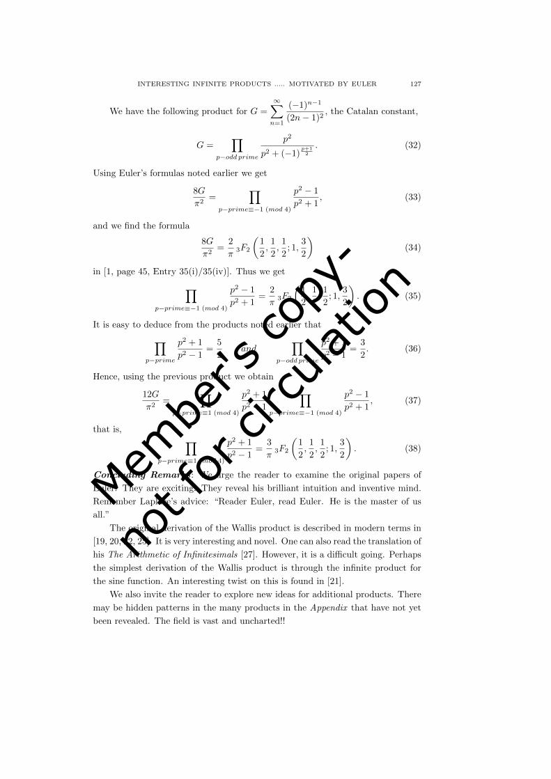
Membe
r's co
py-
not f
or ci
rculat
ion
INTERESTING INFINITE PRODUCTS ..... MOTIVATED BY EULER 127
We have the following product for G =∞∑n=1
(−1)n−1
(2n− 1)2, the Catalan constant,
G =∏
p−odd prime
p2
p2 + (−1)p+1
2
. (32)
Using Euler’s formulas noted earlier we get
8G
π2=
∏p−prime≡−1 (mod 4)
p2 − 1
p2 + 1, (33)
and we find the formula
8G
π2=
2
π3F2
(1
2,
1
2,
1
2; 1,
3
2
)(34)
in [1, page 45, Entry 35(i)/35(iv)]. Thus we get∏p−prime≡−1 (mod 4)
p2 − 1
p2 + 1=
2
π3F2
(1
2,
1
2,
1
2; 1,
3
2
). (35)
It is easy to deduce from the products noted earlier that∏p−prime
p2 + 1
p2 − 1=
5
2and
∏p−odd prime
p2 + 1
p2 − 1=
3
2. (36)
Hence, using the previous product we obtain
12G
π2=
∏p−prime≡1 (mod 4)
p2 + 1
p2 − 1
∏p−prime≡−1 (mod 4)
p2 − 1
p2 + 1, (37)
that is, ∏p−prime≡1 (mod 4)
p2 + 1
p2 − 1=
3
π3F2
(1
2,
1
2,
1
2; 1,
3
2
). (38)
Concluding Remarks: We urge the reader to examine the original papers of
Euler. They are exciting! They reveal his brilliant intuition and inventive mind.
Remember Laplace’s advice: “Reader Euler, read Euler. He is the master of us
all.”
The original derivation of the Wallis product is described in modern terms in
[19, 20, 22, 25]. It is very interesting and novel. One can also read the translation of
his The Arithmetic of Infinitesimals [27]. However, it is a difficult going. Perhaps
the simplest derivation of the Wallis product is through the infinite product for
the sine function. An interesting twist on this is found in [21].
We also invite the reader to explore new ideas for additional products. There
may be hidden patterns in the many products in the Appendix that have not yet
been revealed. The field is vast and uncharted!!

Membe
r's co
py-
not f
or ci
rculat
ion
128 AMRIK SINGH NIMBRAN
Acknowledgement: The author is grateful to the anonymous referee for his
several useful suggestions which helped in giving a shape to this write up and in
improving the presentation.References
[1] Berndt, B. C., Ramanujan’s Notebooks Part II, Springer, 1989.
[2] Chamberland, Marc and Straub, Armin, On gamma quotients and infinite products, Ad-
vances in Applied Mathematics, Elsevier, 51, Issue 5, Oct. 2013, 546–562. Available at
http:// arxiv.org/ abs/ 1309.3455
[3] Davis, P. J., Leonhard Euler’s Integral: A Historical Profile of the Gamma Function, The
American Mathematical Monthly, 66, No. 10 (Dec. 1959), 849–869.
[4] Euler, L., De progressionibus transcendentibus seu quarum termini generales algebraice
dari nequeunt, presented to the St. Petersburg Academy on November 28, 1729; originally
published in Commentarii academiae scientiarum Petropolitanae 5, 1738, 36–57. Available
as E 19 at http://eulerarchive.maa.org/
[5] Euler, L., De progressionibus harmonicis observationes, presented to the St. Petersburg
Academy on March 11, 1734; originally published in Commentarii academiae scientiarum
Petropolitanae 7, 1740, 150–161. E 43.
[6] Euler, L., Introductio in Analysin Infinitorum (1748), Book I.
[7] Euler, L., Institutionum calculi integralis (1768), Volume 1.
[8] Euler, L., De curva hypergeometrica hac aequatione expressa y = 1.2.3 · · ·x, presented to the
St. Petersburg Academy on December 19, 1765; originally published in Novi Commentarii
academiae scientiarum Petropolitanae 13, 1769, 3–66. E 368.
[9] Euler, L., De numero memorabili in summatione progressionis harmonicae naturalis occur-
rente, presented to the St. Petersburg Academy on February 22, 1776; originally published
in Acta Academiae Scientarum Imperialis Petropolitinae 5, 1785, 45–75. E583
[10] Euler, L. De summa seriei ex numeris primis formatae 13− 1
5+ 1
7− 1
13− 1
17+ 1
19+ 1
23− 1
29+ 1
31,
etc. ubi numeri primi formae 4n-1 habent signum positivum, formae autem 4n+1 signum
negativum, presented to the St. Petersburg Academy on October 2, 1775, originally published
in Opuscula Analytica 2, 1785, 240–256. E 596.
[11] Gauss, C. F., Disquisitiones generales circa seriem infinitam, Commentationes societatis
regiae scientiarum, Gottingen, II (1813), 1–46; Werke, Band III, 1876, 122–162.
[12] Ben-Ari, I., Hay, D. and Roitershtein, A., On Wallis-Type Products And Polya’s Urn
Schemes, Amer. Math. Monthly 121 (May 2014), 422–432; also available at http://
www.public.iastate.edu / roiterst / papers / gamma8f.pdf
[13] Jensen, J. L. W. V. and (tr.) Gronwall, T. H., An Elementary Exposition of the Theory of
the Gamma Function, Annals of Mathematics, Second Series, 17, No. 3 (Mar. 1916), 124–
166. Gammafunktionens Theori i elementær Fremstillng. Nyt Tidsskrift for Mathematik,
Afdeling B, 2 (1891), 33–35, 57–72, 83–84.
[14] Legendre, A.-M., Recherches sur diverses sortes d’integrales definies (13 November 1809),
Memoires de la Classe des Sciences Mathematiques et Physiques de l’Institut de France,
1809, 416–509.
[15] Martin, G., A Product of Gamma Function Values at Fractions with the Same Denominator,
2009. http://arxiv.org/abs/0907.4384v2
[16] Newman, F. W., On Γ(a) especially when a is negative, Cambridge and Dublin Mathemat-
ical Journal, Barclay and Macmillan, 3 (1848), 57–60.
[17] Nijenhuis, A., Short Gamma Products with Simple Values, Amer. Math. Monthly, 117, No.
8 (Oct. 2010), 733–737. Available at http:// arxiv.org/ abs/ 0907.1689v1

Membe
r's co
py-
not f
or ci
rculat
ion
INTERESTING INFINITE PRODUCTS ..... MOTIVATED BY EULER 129
[18] Nimbran, A. S., Generalized Wallis-Euler Products and New Infinite Products for π, The
Mathematics Student, 83 (2014), 155–164.
[19] Nunn, T. P., The Arithmetic of Infinites: A School Introduction to the Integral Calculus,
(Part 1), The Mathematical Gazette, 5 (1910), 345–356.
[20] Nunn, T. P., The Arithmetic of Infinites: A School Introduction to the Integral Calculus,
(Part 2), The Mathematical Gazette, V, no. 90 (Jan. 1911), 377–386.
[21] Osler, T.,
emphAn unusual product for sin z and variations of Wallis’s product, Math. Gaz., 87 (2003),
134–139.
[22] Osler, T., The tables of John Wallis and the discovery of his product for pi, Math. Gaz.,
94 (2010), 430–437.
[23] Sandor, J., Harghita, J. and Toth, L., A remark on the gamma function, Elemente der
Mathematik, 44 (1989), 73–76. Available at https:// eudml.org/ doc/ 141455
[24] Schlomilch, O., Einigesuber die Eulerschen Integrale der zweiten Art, Archiv der Mathe-
matik und Physik. bd.4 (1844), 167–174. Available at http:// babel.hathitrust.org/ cgi/ pt?
id=njp.32101033962992; view=1up; seq=205
[25] Stedall, J. A., Catching Proteus: The Collaborations of Wallis and Brouncker. I. Squaring
the Circle, Notes and Records of the Royal Society of London, 54, No. 3 (Sep. 2000),
293–316.
[26] Vidunas, R., Expressions for values of the gamma function, Kyushu J. Math. 59 (2005),
267–283.
[27] Wallis, J., The Arithmetic of Infinitesimals, (Translated from Latin by Jacqueline A.
Stedall), Springer Verlag, New York, 2004.
[28] Weierstrass, K., Ueber die Theorie der analytischen Facultaten, Journ. fur Math., 51 (1856),
1–60.
[29] Weisstein, E. W., “Gamma Function.” From MathWorld–A Wolfram Web Resource.
http://mathworld.wolfram.com/ GammaFunction.html
[30] Weisstein, E. W., “Gauss’s Constant.” From MathWorld–A Wolfram Web Resource.
http://mathworld.wolfram.com/ GausssConstant.html
[31] Weisstein, E. W. “Lemniscate Constant.” From MathWorld–A Wolfram Web Resource.
http://mathworld.wolfram.com/ LemniscateConstant.html
[32] Whittaker, E. T. and Watson, G. N., A Course in Modern Analysis, Cambridge University
Press, 4e, 1927.
Amrik Singh Nimbran
Former Director General of Police, Bihar, India
Email: [email protected]
———
Appendix
A. Products relating to 2pq
√1 +√
2 =∞∏n=1
(4n− 3)(8n− 5)
(4n− 2)(8n− 7)=∞∏n=1
(4n− 2)(8n− 3)
(4n− 3)(8n− 1). (39)
21m =
∞∏n=1
(2mn−m)(2mn− 2)
(2mn−m− 1)(2mn− 1). (40)
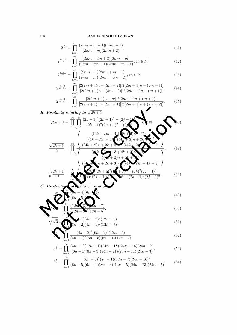
Membe
r's co
py-
not f
or ci
rculat
ion
130 AMRIK SINGH NIMBRAN
21m =
∞∏n=1
(2mn−m+ 1)(2mn+ 1)
(2mn−m)(2mn+ 2). (41)
2m−1m =
∞∏n=1
(2mn− 2m+ 2)(2mn−m)
(2mn− 2m+ 1)(2mn−m+ 1), m ∈ N. (42)
2m−1m =
∞∏n=1
(2mn− 1)(2mn+m− 1)
(2mn−m)(2mn+ 2m− 2), m ∈ N. (43)
2m+12m+1 =
∞∏n=1
[2(2m+ 1)n− (2m+ 2)][2(2m+ 1)n− (2m+ 1)]
[2(2m+ 1)n− (3m+ 2)][2(2m+ 1)n− (m+ 1)]. (44)
2m+12m+1 =
∞∏n=1
[2(2m+ 1)n−m][2(2m+ 1)n+ (m+ 1)]
[2(2m+ 1)n− (2m+ 1)][2(2m+ 1)n+ (2m+ 2)]. (45)
B. Products relating to√
2k + 1
√2k + 1 =
∞∏n=0
k∏j=1
(2k + 1)2(2n+ 1)2 − (2j − 1)2
(2k + 1)2(2n+ 1)2 − (2j)2, k ∈ N. (46)
√2k + 1
2=
∞∏n=0
((4k + 2)n+ 4)((4k + 2)n+ 6) · · ·((4k + 2)n+ 2k)2((4k + 2)n+ 2k + 2)2
((4k + 2)n+ 2k + 4) · · · ((4k + 2)n+ 4k − 2)
((4k + 2)n+ 3)((4k + 2)n+ 5) · · ·
((4k + 2)n+ 2k + 1)2
((4k + 2)n+ 2k + 3) · · · ((4k + 2)n+ 4k − 3)
. (47)
√2k + 1
2=
∞∏n=0
k∏j=1
(2k)2(2k + 1)2(2n+ 1)2 − (2k)2(2j − 1)2
(2k)2(2k + 1)2(2n+ 1)2 − (2k + 1)2(2j − 1)2. (48)
C. Products relating to 3pq and 5
pq
√3 =
∞∏n=1
(6n− 4)(6n− 2)
(6n− 5)(6n− 1). (49)
√√3 =
∞∏n=1
(12n− 8)2(12n− 7)
(12n− 9)2(12n− 5). (50)
√√3 =
∞∏n=1
(3n− 1)(4n− 2)2(12n− 5)
(3n− 2)(4n− 1)2(12n− 7). (51)
334 =
∞∏n=1
(4n− 2)2(6n− 2)2(12n− 5)
(4n− 1)2(6n− 5)(6n− 1)(12n− 7). (52)
338 =
∞∏n=1
(3n− 1)(12n− 1)(24n− 18)(24n− 16)(24n− 7)
(6n− 1)(6n− 3)(24n− 21)(24n− 11)(24n− 3). (53)
318 =
∞∏n=1
(6n− 3)2(8n− 1)(12n− 7)(24n− 16)2
(6n− 5)(6n− 1)(8n− 3)(12n− 5)(24n− 23)(24n− 7). (54)

Membe
r's co
py-
not f
or ci
rculat
ion
INTERESTING INFINITE PRODUCTS ..... MOTIVATED BY EULER 131
3310 =
∞∏n=1
(5n− 4)(30n− 25)(30n− 5)
(5n− 3)(30n− 28)(30n− 8). (55)
315 =
∞∏n=1
(5n− 2)(15n− 13)(15n− 8)(30n− 25)(30n− 5)
(5n− 3)(15n− 14)(15n− 4)(30n− 21)(30n− 9). (56)
3110 =
∞∏n=1
(12n− 9)(12n− 3)
(12n− 11)(12n− 1). (57)
3√
2 +√
6
2=∞∏n=1
(12n− 8)(12n− 4)
(12n− 11)(12n− 1)=∞∏n=1
(24n− 19)(24n− 17)
(24n− 23)(24n− 13). (58)
√1 +√
3 =∞∏n=1
(6n− 5)(6n− 1)(24n− 21)(24n− 3)
(3n− 2)(12n− 1)(24n− 23)(24n− 7). (59)
√√2 +√
3 =∞∏n=1
(3n− 2)(12n− 1)(24n− 7)
(6n− 5)(6n− 1)(24n− 1). (60)√(
1 +√
2)(
1 +√
3)(√
2 +√
3)
=∞∏n=1
(8n− 7)(24n− 12)(24n− 9)
(8n− 6)(24n− 1)(24n− 23). (61)
√5 =
∞∏n=1
(10n− 8)(10n− 6)(10n− 4)(10n− 2)
(10n− 9)(10n− 7)(10n− 3)(10n− 1). (62)
√√5 =
∞∏n=1
(5n− 4)(5n− 1)(20n− 17)(20n− 13)
(5n− 3)(5n− 2)(20n− 19)(20n− 11). (63)√√
5
2=∞∏n=1
(10n− 9)(10n− 1)(20n− 17)(20n− 13)
(10n− 5)2(20n− 19)(20n− 11). (64)
2
√√5 =
∞∏n=1
(10n− 5)2(12n− 17)(20n− 13)
(10n− 7)(10n− 3)(20n− 19)(20n− 11). (65)
516 =
∞∏n=1
(3n− 2)(30n− 25)2(30n− 5)2
(3n− 1)(30n− 28)(30n− 22)(30n− 16)(30n− 4). (66)
φ =1 +√
5
2=
∞∏n=1
(5n− 3)(5n− 2)
(5n− 4)(5n− 1). (67)
φ12 =
∞∏n=1
(10n− 6)(10n− 4)(20n− 19)(20n− 11)
(10n− 9)(10n− 1)(20n− 17)(20n− 13). (68)
φ12 =
∞∏n=1
(10n− 9)(10n− 1)(20n− 17)(20n− 13)
(10n− 8)(10n− 2)(20n− 19)(20n− 11). (69)
215 5
14
√1 +√
5 =∞∏n=1
(20n− 16)(20n− 12)
(20n− 19)(20n− 9). (70)
215
√√5− 1 =
∞∏n=1
(20n− 16)(20n− 12)(20n− 11)
(20n− 17)(20n− 13)(20n− 9). (71)

Membe
r's co
py-
not f
or ci
rculat
ion
132 AMRIK SINGH NIMBRAN√1 +√
5 =∞∏n=1
(5n− 3)(10n− 5)2(20n− 17)(20n− 13)(20n− 9)
(5n− 4)(10n− 8)2(20n− 6)2(20n− 11). (72)
D. Products relating to L
∞∏n=1
(4n− 2)4n
(4n− 3)(4n+ 1)=
(Γ(
14
))24√π
=L√2. (73)
∞∏n=1
(4n− 1)2
(4n− 3)(4n+ 1)=
(Γ(
14
))48π2
=L2
π. (74)
∞∏n=1
(4n− 1)2(4n+ 2)
(4n− 2)(4n+ 1)2=
(Γ(
14
))416π2
=L2
2π. (75)
∞∏n=1
(4n− 2)(4n− 1)(4n+ 2)
(4n− 3)(4n+ 1)2=
(Γ(
14
))48√
2π2=
L2
√2π
. (76)
———
Table on the next page

Membe
r's co
py-
not f
or ci
rculat
ion
INTERESTING INFINITE PRODUCTS ..... MOTIVATED BY EULER 133
Table 1. Values of sin θ and cos θ
θ sin θ cos θ
0 0 1
π24
√4−√
2−√
6
2√
2
√4+√
2+√
6
2√
2
π20
√3+√
5−√
5−√
54
√3+√
5+√
5−√
54
π16
√2−√
2+√
2
2
√2+√
2+√
2
2π12
√3−1
2√
2
√3+1
2√
2
π10
√5−14
√10+2
√5
4
π8
√2−√
22
√2+√
22
3π20
√5+√
5−√
3−√
54
√5+√
5+√
3−√
54
π6
12
√3
2
3π16
√2+√
2+√
2−√
2−√
2+√
2
2√
2
√2+√
2+√
2+
√2−√
2+√
2
2√
2
π5
√10−2
√5
4
√5+14
5π24
√4+√
2−√
6
2√
2
√4−√
2+√
6
2√
2π4
1√2
1√2
7π24
√4−√
2+√
6
2√
2
√4+√
2−√
6
2√
2
3π10
√5+14
√10−2
√5
4
5π16
√2+√
2+√
2+
√2−√
2+√
2
2√
2
√2+√
2+√
2−√
2−√
2+√
2
2√
2π3
√3
212
7π20
√5+√
5+√
3−√
54
√5+√
5−√
3−√
54
3π8
√2+√
22
√2−√
22
2π5
√10+2
√5
4
√5−14
5π12
√3+1
2√
2
√3−1
2√
2
9π20
√3+√
5+√
5−√
54
√3+√
5−√
5−√
54
11π24
√4+√
2+√
6
2√
2
√4−√
2−√
6
2√
2π2 1 0

Membe
r's co
py-
not f
or ci
rculat
ion
134
Membe
r's co
py-
not f
or ci
rculat
ion
The Mathematics Student ISSN: 0025-5742
Vol. 85, Nos. 1-2, January-June (2015), 135-141
SOME UNIQUE FIXED POINT AND COMMON FIXEDPOINT THEOREMS IN b-METRIC SPACES USING
RATIONAL INEQUALITY
G. S. SALUJA
(Received : 03 - 11 - 2015 ; Revised : 10 - 12 - 2015)
Abstract. The purpose of this paper is to extend and generalize the results
of Khan [8] from complete metric spaces to that in the setting of complete
b-metric spaces.
1. Introduction and Preliminaries
Fixed point theory plays a very important role in the development of nonlinear
analysis. In this area, the first important result was proved by Banach in 1922 for
contraction mapping in complete metric space, known as the Banach contraction
principle [10]. In [8], Khan studied a fixed point theorem using symmetric ratio-
nal expression in complete metric spaces. The Banach contraction principle with
rational expressions have been expanded and some fixed and common fixed point
theorems have been obtained in [5], [6].
In [2], Bakhtin introduced b-metric spaces as a generalization of metric spaces.
He proved the contraction mapping principle in b-metric spaces that generalized
the famous contraction principle in metric spaces. Czerwik, in [3], used the concept
of b-metric space and generalized the renowned Banach fixed point theorem in b-
metric spaces (see, also [4]).
In this note, we extend and generalize the results of Khan [8] and establish
some unique fixed point and common fixed point theorems using Khan [8] and
almost Khan rational expressions in the framework of complete b-metric spaces.
Definition 1.1. ([2]) Let X be a nonempty set and s ≥ 1 be a given real number.
A mapping d : X×X → R+ is called a b-metric if for all x, y, z ∈ X, the following
conditions are satisfied:
(b1M) d(x, y) = 0 if and only if x = y;
(b2M) d(x, y) = d(y, x);
(b3M) d(x, y) ≤ s[d(x, z) + d(z, y)].
The pair (X, d) is called a b-metric space.
2010 Mathematics Subject Classification : 47H10, 54H25.
Key words and phrases : Fixed point, common fixed point, rational inequality, b- metric
space.
c© Indian Mathematical Society, 2016 .
135
Membe
r's co
py-
not f
or ci
rculat
ion
136 G. S. SALUJA
It is clear from the definition of b-metric that every metric space is a b-metric
space for s = 1. Therefore, the class of b-metric spaces is larger than the class of
metric spaces.
Some known examples of b-metric, which shows that a b-metric space is real
generalization of a metric space, are the following.
Example 1.1. ([1]) The set of real numbers together with the functional d(x, y) =
|x − y|2 for all x, y ∈ R is a b-metric space with constant s = 2. Also, we obtain
that d is not a metric on R.
Example 1.2. ([7]) Let X = `p with 0 < p < 1, where `p = xn ⊂ R :∑∞n=1 |xn|p <∞. Let d : X ×X → R defined by d(x, y) =
(∑∞n=1 |xn − yn|p
) 1p
,
where x = xn, y = yn ∈ `p. Then (X, d) is a b-metric space with the coeffi-
cient s = 21/p > 1, but not a metric space. It is obtained that the above result
also holds for the general case `p(X) with 0 < p < 1, where X is a Banach space.
Example 1.3. ([9]) Let p be a given real number in the interval (0, 1). The space
Lp[0, 1] of all real functions x(t), y(t) ∈ [0, 1] such that∫ 1
0|x(t)|p < 1, together
with the functional
d(x, y) :=(∫ 1
0
|x(t)− y(t)|p dt)1/p
,
for each x, y ∈ Lp[0, 1] is a b-metric space with constant s = 21/p.
Example 1.4. (see [1]) Let X = 0, 1, 2. Define d : X × X → R+ as follows
d(0, 0) = d(1, 1) = d(2, 2) = 0, d(1, 2) = d(2, 1) = d(0, 1) = d(1, 0) = 1, d(2, 0) =
d(0, 2) = p ≥ 2 for s = p2 where p ≥ 2, the function defined as above is a b-metric
space but not a metric space for p > 2.
Example 1.5. ([7]) Let X = 1, 2, 3, 4 and E = R2. Define d : X ×X → R by
d(x, y) =
(|x− y|−1, |x− y|−1) if x 6= y,
0, if x = y.
Then (X, d) is a b-metric space with the coefficient s = 65 > 1. But it is not a
metric space since the triangle inequality is not satisfied,
d(1, 2) > d(1, 4) + d(4, 2), d(3, 4) > d(3, 1) + d(1, 4).
Definition 1.2. [([8])] Let (X, d) be a complete metric space. A self mapping
T : X → X is called a Khan contraction if it satisfies following condition:
d(Tx, Ty) ≤ α [d(x, Tx) d(x, Ty) + d(y, Ty) d(y, Tx)]
d(x, Ty) + d(y, Tx)(1)
for all x, y ∈ X and α ∈ [0, 1).
Now, we define the following:
Membe
r's co
py-
not f
or ci
rculat
ion
SOME UNIQUE FIXED POINT ...... USING RATIONAL INEQUALITY 137
Definition 1.3. Let (X, d) be a complete metric space. A self mapping T : X → X
is called an almost Khan contraction if it satisfies the following condition:
d(Tx, Ty) ≤ α [d(x, Tx) d(x, Ty) + d(y, Ty) d(y, Tx)]
d(x, Ty) + d(y, Tx)
+β d(x, y) (2)
for all x, y ∈ X and α, β ∈ [0, 1) with α+ β < 1.
Remark 1.1. If we take β = 0, then almost Khan contraction (2) reduces to Khan
contraction (1).
Theorem 1.1. ([8]) Let (X, d) be a complete metric space and T : X → X satisfies
the contractive condition (1), then T has a unique fixed point in X.
In our main result we will use the following definitions which can be found in
[1] and [9].
Definition 1.4. ([1], [9]) Let (X, d) be a b-metric space, x ∈ X and xn be a
sequence in X. Then
(d1) xn is a Cauchy sequence if for ε > 0 there exists a positive integer N
such that for all n,m ≥ N , we have d(xn, xm) < ε;
(d2) xn is called convergent if for ε > 0 and n ≥ N we have d(xn, x) <
ε, where x is called the limit point of the sequence xn. We denote this by
limn→∞ xn = x or xn → x as n→∞.
(d3) (X, d) is said to be a complete b-metric space if every Cauchy sequence
in X converges to a point in X.
Remark 1.2. In a b-metric space (X, d), the following assertions hold:
(i) a convergent sequence has a unique limit;
(ii) each convergent sequence is Cauchy;
(iii) in general, a b-metric is not continuous.
2. Main ResultsIn this section we shall prove some fixed point and common fixed point theo-
rems for rational expressions in the framework of b-metric spaces.
Theorem 2.1. Let (X, d) be a complete b-metric space (CbMS) with the coefficient
s ≥ 1. Suppose that the mappings S, T : X → X satisfy the rational expression:
d(Sx, Ty) ≤ α [d(x, Sx) d(x, Ty) + d(y, Ty) d(y, Sx)]
d(x, Ty) + d(y, Sx)(3)
for all x, y ∈ X, α ∈ [0, 1) with sα < 1. Then S and T have a unique common
fixed point in X.
Proof. Choose x0 ∈ X. Let x1 = S(x0) and x2 = T (x1) such that x2n+1 = Sx2n
and x2n+2 = Tx2n+1 for all n ≥ 0. From (3), we have
d(x2n+1, x2n) = d(Sx2n, Tx2n−1)
≤α[d(x2n, Sx2n) d(x2n, Tx2n−1) + d(x2n−1, Tx2n−1) d(x2n−1, Sx2n)
]d(x2n, Tx2n−1) + d(x2n−1, Sx2n)
Membe
r's co
py-
not f
or ci
rculat
ion
138 G. S. SALUJA
=α[d(x2n, x2n+1) d(x2n, x2n) + d(x2n−1, x2n) d(x2n−1, x2n+1)
]d(x2n, x2n) + d(x2n−1, x2n+1)
≤ αd(x2n, x2n−1). (4)
By induction, we haved(xn+1, xn) ≤ αd(xn−1, xn) ≤ α2 d(xn−2, xn−1) ≤ . . . ≤ αn d(x0, x1). (5)
Hence for any m,n ≥ 1 and m > n, we have
d(xn, xm) ≤ s[d(xn, xn+1) + d(xn+1, xm)]
= sd(xn, xn+1) + sd(xn+1, xm)
≤ sd(xn, xn+1) + s2[d(xn+1, xn+2) + d(xn+2, xm)]
= sd(xn, xn+1) + s2d(xn+1, xn+2) + s2d(xn+2, xm)
≤ sd(xn, xn+1) + s2d(xn+1, xn+2) + s3d(xn+2, xn+3)
+ · · ·+ sn+m−1d(xn+m−1, xm)
≤ sαnd(x1, x0) + s2αn+1d(x1, x0) + s3αn+2d(x1, x0)
+ · · ·+ smαn+m−1d(x1, x0)
= sαn[1 + sα+ s2α2 + s3α3 + · · ·+ (sα)m−1]d(x1, x0)
≤[ sαn
1− sα
]d(x1, x0).
Since sα < 1, therefore taking limit m,n→∞, we have limm,n→∞ d(xn, xm) = 0.
Hence xn is a Cauchy sequence in complete b-metric space X. Since X is
complete, so there exists q ∈ X such that limn→∞ xn = q. Now we have to show
that q is a common fixed point of S and T . For this consider
d(x2n+1, T q) = d(Sx2n, T q)]
≤α[d(x2n, Sx2n) d(x2n, T q) + d(q, T q) d(q, Sx2n)
]d(x2n, T q) + d(q, Sx2n)
=α[d(x2n, x2n+1) d(x2n, T q) + d(q, T q) d(q, x2n+1)
]d(x2n, T q) + d(q, x2n+1)
.
Taking limit n→∞, we have d(q, T q) ≤ 0.
Hence by definition 1.1(b1M), we get Tq = q. Thus q is a fixed of T .
In an exactly the same fashion we can prove that Sq = q. Hence Sq = Tq = q.
This shows that q is a common fixed point of S and T .
Uniqueness. Let p be another fixed point common to S and T , that is, Sp =
Tp = p such that p 6= q. Then from (3), we have
d(p, q) = d(Sp, Tq) ≤ α [d(p, Sp) d(p, Tq) + d(q, T q) d(q, Sp)]
d(p, Tq) + d(q, Sp)
=α [d(p, p) d(p, q) + d(q, q) d(q, p)]
d(p, q) + d(q, p)≤ 0.
Hence by definition 1.1(b1M), we get p = q. This shows that q is a unique common
fixed point of S and T . This completes the proof.

Membe
r's co
py-
not f
or ci
rculat
ion
SOME UNIQUE FIXED POINT ...... USING RATIONAL INEQUALITY 139
From Theorem 2.1, we obtain the following result as corollary.
Corollary 2.1. Let (X, d) be a complete b-metric space (CbMS) with the coeffi-
cient s ≥ 1. Suppose that the mapping T : X → X satisfies the rational expression:
d(Tx, Ty) ≤ α [d(x, Tx) d(x, Ty) + d(y, Ty) d(y, Tx)]
d(x, Ty) + d(y, Tx)(6)
for all x, y ∈ X, α ∈ [0, 1) with sα < 1. Then T has a unique fixed point in X.
Theorem 2.2. Let (X, d) be a complete b-metric space (CbMS) with the coefficient
s ≥ 1 such that for positive integer n, Tn satisfies the rational expression (1) for
all x, y ∈ X, α ∈ [0, 1) with sα < 1. Then T has a unique fixed point in X.
Proof. If x0 is the unique fixed point of Tn, then Tx0 = x0 because T (Tnx0) =
Tx0 or Tn(Tx0) = Tx0. This shows that x0 is the unique fixed point of T , and
completes the proof.
Theorem 2.3. Let (X, d) be a complete b-metric space (CbMS) with the coefficient
s ≥ 1. Suppose that the mapping T : X → X satisfies an almost Khan rational
expression (2) for all x, y ∈ X, α, β ∈ [0, 1) with sα + sβ < 1. Then T has a
unique fixed point in X.
Proof. Choose x0 ∈ X. We construct the iterative sequence xn, where xn =
Txn−1, n ≥ 1, that is, xn+1 = Txn = Tn+1x0. From (2), we have
d(xn, xn+1) = d(Txn−1, Txn)
≤ α [d(xn−1, Txn−1) d(xn−1, Txn) + d(xn, Txn) d(xn, Txn−1)]
d(xn−1, Txn) + d(xn, Txn−1)
+β d(xn−1, xn)
=α [d(xn−1, xn) d(xn−1, xn+1) + d(xn, xn+1) d(xn, xn)]
d(xn−1, xn+1) + d(xn, xn)
+β d(xn−1, xn)
≤ (α+ β) d(xn−1, xn) = λ d(xn−1, xn) (7)
where λ = (α+ β), since sα+ sβ < 1, it is clear that 0 < λ < 1/s. By induction,
we haved(xn+1, xn) ≤ λ d(xn−1, xn) ≤ λ2 d(xn−2, xn−1) ≤ . . .
≤ λn d(x0, x1). (8)
Let m,n ≥ 1 and m > n, we have
d(xn, xm) ≤ s[d(xn, xn+1) + d(xn+1, xm)]
= sd(xn, xn+1) + sd(xn+1, xm)
≤ sd(xn, xn+1) + s2[d(xn+1, xn+2) + d(xn+2, xm)]
= sd(xn, xn+1) + s2d(xn+1, xn+2) + s2d(xn+2, xm)
Membe
r's co
py-
not f
or ci
rculat
ion
140 G. S. SALUJA
≤ sd(xn, xn+1) + s2d(xn+1, xn+2) + s3d(xn+2, xn+3)
+ · · ·+ sn+m−1d(xn+m−1, xm)
≤ sλnd(x1, x0) + s2λn+1d(x1, x0) + s3λn+2d(x1, x0)
+ · · ·+ smλn+m−1d(x1, x0)
= sλn[1 + sλ+ s2λ2 + s3λ3 + · · ·+ (sλ)m−1]d(x1, x0)
≤[ sλn
1− sλ
]d(x1, x0).
Since sλ < 1, therefore taking limit m,n→∞, we have limm,n→∞ d(xn, xm) = 0.
Hence xn is a Cauchy sequence in complete b-metric space X. Since X is
complete, so there exists z ∈ X such that limn→∞ xn = z. Now we have to show
that z is a fixed point of T . For this consider
d(xn+1, T z) = d(Txn, T z)
≤α[d(xn, Txn) d(xn, T z) + d(z, Tz) d(z, Txn)
]d(xn, T z) + d(z, Txn)
+ β d(xn, z)
=α[d(xn, xn+1) d(xn, T z) + d(z, Tz) d(z, xn+1)
]d(xn, T z) + d(z, xn+1)
+ β d(xn, z).
Taking limit n→∞, we have d(z, Tz) ≤ 0. Hence by definition 1.1(b1M), we get
Tz = z. Thus z is a fixed of T .
Uniqueness. Let z1 be another fixed point T , that is, Tz1 = z1 such that z 6= z1.
Then from (2), we have
d(z, z1) = d(Tz, Tz1)
≤ α [d(z, Tz) d(z, Tz1) + d(z1, T z1) d(z1, T z)]
d(z, Tz1) + d(z1, T z)+ β d(z, z1)
=α [d(z, z) d(z, z1) + d(z1, z1) d(z1, z)]
d(z, z1) + d(z1, z)+ β d(z, z1) ≤ β d(z, z1).
The above inequality is possible only if d(z, z1) = 0 and so z = z1. Thus z is a
unique fixed point of T , and the proof is completed.
From Theorem 2.3, we obtain the following result as corollaries.
Corollary 2.2. Let (X, d) be a complete b-metric space (CbMS) with the coeffi-
cient s ≥ 1. Suppose that the mapping T : X → X satisfies Khan rational expres-
sion (1) for all x, y ∈ X and α ∈ [0, 1) with sα < 1. Then T has a unique fixed
point in X.Corollary 2.3. Let (X, d) be a complete b-metric space (CbMS) with the coef-
ficient s ≥ 1. Suppose that the mapping T : X → X satisfies the contraction
condition d(Tx, Ty) ≤ β d(x, y) for all x, y ∈ X and β ∈ [0, 1) with sβ < 1. Then
T has a unique fixed point in X.
Remark 2.1. (i) Theorem 2.1 and 2.2 extend and generalize Theorem 1 of Khan [8]
from complete metric space to that setting of complete b-metric space considered
in this paper.

Membe
r's co
py-
not f
or ci
rculat
ion
SOME UNIQUE FIXED POINT ...... USING RATIONAL INEQUALITY 141
(ii) Theorem 2.1 also extends and generalizes Theorem 3 of Khan [8] from
complete metric space to that setting of b-metric space considered in this paper.
(iii) Corollary 2.3 extends well known Banach [10] contraction principle from
complete metric space to that setting of complete b-metric space considered in this
paper.3. Conclusion
In this paper, we establish some unique fixed point and common fixed point
theorems using Khan and an almost Khan rational contractions in the setting of
b-metric spaces. Our results extend and generalize several results from the existing
literature.
Acknowledgements. The author would like to thank the anonymous referee for
his careful reading and useful suggestions on the manuscript.
References
[1] Ayadi, H., Bota, M. F., Karapinar, E., and Mitrovic, S., A point theorem
for set valued quasi contraction in b-metric spaces, Fixed Point Theory Appl.
2012, Article ID 2012:88, 1-8. doi:10.1186/1687-1812-2012–88.
[2] Bakhtin, I. A., The contraction mapping principle in almost metric spaces,
Funct. Anal. Gos. Ped. Inst. Unianowsk 30 (1989), 26–37.
[3] Czerwik, S., Contraction mappings in b-metric spaces, Acta Math. Inf. Univ.
Ostraviensis 1 (1993), 5–11.
[4] Czerwik, S., Nonlinear set-valued contraction mappings in b-metric spaces,
Atti. Semin. Mat. Fis. Univ. Modena 46 (1998), 263–276.
[5] Fisher, B., Common fixed points and constant mapping satisfying rational
inequality, Math. Sem. Notes (Univ. Kobe), 1978.
[6] Fisher, B. and Khan, M. S., Fixed points, common fixed points and constant
mappings, Studia Sci. Math. Hungar. 11 (1978), 467– 470.
[7] H. Huang, H. and Xu, S., Fixed point theorems of contractive mappings in
cone b-metric spaces and applications, Fixed Point Theory Appl. 2013, Article
ID 2013:112, 1-10. doi: 10.1186 /1687-1812-2013-112.
[8] Khan, M. S., A fixed point theorem for metric spaces, Rend. Ist. Mat. Univ.
Trieste 8 (1976), 69-72.
[9] Kir, Mehmet and Kizitune, Hukmi, On some well known fixed point theorems
in b-metric spaces, Turkish J. Anal. Number Theory 1 (2013), 13-16.
[10] Rudin, W., Principles of Mathematical Analysis, Third Edition, International
Editions, 1976.
G. S. Saluja
Department of Mathematics, Govt. Nagarjuna P.G. College of Science
Raipur - 492010 (C. G.), India
Email: [email protected]

Membe
r's co
py-
not f
or ci
rculat
ion
142
Membe
r's co
py-
not f
or ci
rculat
ion
The Mathematics Student ISSN: 0025-5742
Vol. 85, Nos. 1-2, January-June (2016), 143-149
LAZY CONTINUED FRACTION EXPANSIONS FORCOMPLEX NUMBERS
S. G. DANI
(Received : 08 - 11 - 2015 ; Revised : 02 - 01 - 2016)
Abstract. We discuss a general notion of continued fraction expansion for
complex numbers in terms of partial quotients in various subrings and prove
the convergence of the corresponding sequences of convergents.
1. IntroductionFor a real number t the classical simple continued fraction expansion is con-
structed by setting t0 = t, a0 = [t], the largest integer not exceeding t, and
recursively tn+1 = 1tn−an
for n ≥ 0, provided tn 6= an, and an+1 = [tn+1]; we
terminate the sequence when tn = an (for the first time), so tn − an can not be
inverted. When t is an irrational number the sequence is non-terminating and we
have
t = a0 +1
a1 + 1a2+···
,
in the sense that the rational numbers pn
qn, n ≥ 0, obtained by omitting from the
above expression the part after an, converge to t; pn
qnare called the convergents
and the expression is called the simple continued fraction expansion of t. Here
a0 ∈ Z and an ∈ N for all n ≥ 1. These expansions have played an important role
in various problems in number theory and its applications in other areas since the
eighteenth century when they came to the fore in a big way (the reader is referred
to [1] and [5] for a historical perspective and [6] for a general introduction to the
topic).
If in place of the largest integer not exceeding the given number we opt for the
integer nearest to the given number, for picking an depending on tn at each stage
n ≥ 0, and proceed analogously (allowing the tn’s and an’s to be negative), then
again for an irrational number we get a continued fraction expansion in terms of
an ∈ Z, with |an| ≥ 2 for n ≥ 1, known as the nearest integer continued fraction
expansion. These expansions have also appeared in various contexts, and were
used recently in [2] for studying certain asymptotics of values of quadratic forms
at integer points.
2010 Mathematics Subject Classification : 11A55
Key words and phrases : continued fractions, convergence, complex numbers, Gaussian inte-
gers, Eisenstein integers
c© Indian Mathematical Society, 2016 .
143
Membe
r's co
py-
not f
or ci
rculat
ion
144 S. G. DANI
The nearest integer continued fraction expansion has a natural analogue for
complex numbers in terms of Gaussian integers x + iy with x, y ∈ Z. Let z ∈ Cand define z0 = z, a0 the Gaussian integer nearest to z (when there are more
than one such, a choice may be made by some convention which does not play
much role in the theory) and recursively zn+1 = 1zn−an
for n ≥ 0, provided
zn 6= an, and an+1 is the Gaussian integer nearest to zn+1 (with the conven-
tion as above); the expansion is non-terminating for z /∈ Q(i), the smallest sub-
field of C containing i. This expansion was introduced and studied by A. Hur-
witz [8] who proved various interesting results about it - including convergence
of the corresponding convergents, monotonicity of the size of the denominators
of the convergents, an analogue of the classical Lagrange theorem characterising
quadratic irrationals, etc. (the reader is referred to [7], [4] and [3] for details in
this respect). Hurwitz also discussed analogous issues for expansions in terms of
Eisenstein integers, namely complex numbers of the form x + yω, where ω is a
nontrivial cube root of unity and x, y ∈ Z. Continued fraction expansions have
also been considered with partial quotients from some more discrete subrings of C(see §3 below, and [3] and other references cited there).
Unlike in the classical case of simple continued fractions, the proof of conver-
gence of the convergents in [8] and in later literature (see for example [7]) turns
out to be rather intricate. In this note we present a short proof of convergence, in
fact in a substantially broader set up, of what is referred to below (and in the title)
as “lazy continued fraction expansion”; it should be noted however that Hurwitz’s
proof brings in, along with the proof of convergence of the convergents, consider-
able insight also into certain other aspects of behaviour of the continued fraction
expansions which does not have a parallel in our case. Our main emphasis is on
the generality of the framework and simplicity of the proof. The idea underlying
the proof below is also involved in the proof of Proposition 3.6 in [4] in the special
case of Gaussian integers; Theorem 2.1 is a generalization of that result, and in
the proof an attempt is also made to improve the presentation.
2. The theoremLet Γ be a discrete subring of C containing 1 and let K be the quotient field
of Γ. We note that K is a countable subfield of C. We shall be interested in
continued fraction expansions of z in C\K; the latter correspond to irrational
numbers in the general case. We shall assume Γ to be such that for any z ∈ C\Kthere exists an a ∈ Γ such that |z − a| < 1; equivalently, the union of the open
unit discs with centers at points of Γ covers C\K. A brief discussion on the rings
satisfying this condition is included in §3; for the present it may be noted that the
ring of Gaussian integers and the ring of Eisenstein integers have this property.
Now let z ∈ C\K and let zn be a sequence in C\K constructed as follows:
we start by setting z0 = z and pick some element a0 ∈ Γ such that |z0 − a0| < 1,
Membe
r's co
py-
not f
or ci
rculat
ion
LAZY CONTINUED FRACTION EXPANSIONS FOR COMPLEX NUMBERS 145
and put z1 = (z0 − a0)−1; since z ∈ C\K, a0 6= z0, and moreover z1 ∈ C\K. Now
starting with z1 we define, following the same steps, an element z2, and then z3
etc.. In other words, for n ≥ 0, we choose zn+1 = 1zn−an
and an+1 to be some
element of Γ such that |zn+1 − an+1| < 1. We thus get a sequence zn∞n=0 such
that z0 = z, and |zn| > 1 with zn−1 − z−1n ∈ Γ for all n ≥ 1, and the associated
sequence an∞0 in Γ such that an = zn − z−1n+1 for all n ≥ 0. The sequence
an∞n=0 is analogous to the classical continued fraction expansion sequences, and
we shall call it a lazy continued fraction expansion for z; “lazy” refers to the fact
that we do not put in any effort looking for an element of Γ fulfilling some criterion
like being the nearest etc., but just pick our an to be any element of Γ such that
|zn− an| < 1. We call zn an iteration sequence and an the sequence of partial
quotients with respect to the given lazy continued fraction expansion; for n ≥ 0, zn
and an are called the nth iterate and the nth partial quotient respectively. Note
that any z will have (uncountably!) many lazy continued fraction expansions and
corresponding iteration sequences, and sequences of partial quotients. Now let
pn∞n=−1 and qn∞n=−1 be the sequences defined recursively by the relations
p−1 = 1, p0 = a0, pn+1 = an+1pn + pn−1, for all n ≥ 0,
q−1 = 0, q0 = 1, qn+1 = an+1qn + qn−1, for all n ≥ 0.
There is, a priori, no certainty that qn 6= 0 for all n ≥ 1, but if this does hold then
it can be readily seen, inductively, that
pnqn
= a0 +1
a1 + 1a2+····+ 1
an
,
for all n ≥ 0, as in the case of the usual continued fraction expansions. We call
(pn, qn) the nth convergent for the given lazy continued fraction expansion.
The following theorem, which is our main result in the paper, shows that the
procedure as above indeed gives a continued fraction expansion for z.
Theorem 2.1. Let Γ be a discrete subring of C such that the open unit discs with
centers at elements from Γ cover C\K. Let z ∈ C and an be the sequence of
partial quotients, in Γ, with respect to a lazy continued fraction expansion of z.
Let (pn, qn)∞n=−1 be the corresponding sequence of convergents. Then qn 6= 0 for
all n andpnqn→ z as n→∞.
Before going to the proof of the theorem we note the following.
Proposition 2.1. Let the notation be as in the theorem and also let zn be the
associated iteration sequence. Then qnz−pn = (−1)n(z1 · · · zn+1)−1 for all n ≥ 0.
Consequently qn 6= 0 for all n ≥ 0.
Proof. At the outset we note that since Γ is a discrete subring of C, for any nonzero
γ ∈ Γ we have |γ| ≥ 1.
Membe
r's co
py-
not f
or ci
rculat
ion
146 S. G. DANI
We now proceed with the proof by induction. Since p0 = a0, q0 = 1 and
z − a0 = z−11 , the desired assertion holds for n = 0. Now let n ≥ 1 and suppose
the desired assertion holds for 0, 1, . . . , n− 1. Then we have
qnz − pn = (anqn−1 + qn−2)z − (anpn−1 + pn−2)
= an(qn−1z − pn−1) + (qn−2z − pn−2)
= (−1)n−1(z1 · · · zn)−1an + (−1)n−2(z1 · · · zn−1)−1
= (−1)n(z1 · · · zn)−1(−an + zn) = (−1)n(z1 · · · zn+1)−1,
which proves the first part of the proposition. The second part is immediate, since
if qn = 0 for some n then we get |pn| = |z1 · · · zn+1|−1 < 1, which is a contradiction
since pn ∈ Γ, and pn 6= 0.
Proof of the theorem. Let zn be the iteration sequence associated with the given
lazy continued fraction expansion. Since qn 6= 0 for all n, and qn ∈ Γ, we have
|qn| ≥ 1 and hence by Proposition 2.1 we get∣∣∣∣z − pnqn
∣∣∣∣ = |qn|−1|z1 · · · zn+1|−1 ≤ |z1 · · · zn+1|−1.
Therefore to prove the theorem it suffices to prove that lim supn→∞ |zn| > 1. We
shall suppose that this is not true, and arrive at a contradiction. Thus we may
assume that |zn| → 1 as n→∞.
Let C denote the unit circle in C centered at the origin, and let
Φ = θ ∈ C | |θ − γ| = 1 for some γ ∈ Γ, γ 6= 0.
Since Γ is discrete it follows that Φ is a finite subset of C. We first show that the
limit points of zn are all contained in Φ.
Let ζ be any limit point of zn. Since |zn| → 1 as n → ∞, it follows that
ζ ∈ C, and that there exists a sequence nk in N such that znk→ ζ as k → ∞.
Then |znk− ank
| = |znk+1|−1 → 1 as k → ∞. Since znk→ ζ as k → ∞ and
ank∈ Γ, this implies that ank
, k ∈ N, belong to a finite subset of Γ. Therefore,
passing to a subsequence of nk and modifying notation we may assume that ank
is a constant sequence, say ank= a for all k. Then a ∈ Γ and a 6= 0, and since
znk→ ζ as k →∞ we further get that |ζ − a| = 1. Thus ζ ∈ Φ, as claimed above.
As the set of limit points of zn is contained in Φ, which is a finite set, we
can fix ϕn ∈ Φ for each n such that zn − ϕn → 0 as n→∞. As zn − ϕn → 0 and
|zn − an| = |zn+1|−1 → 1, as n → ∞, we have |ϕn − an| → 1, and since Φ and Γ
are discrete subsets it follows that |ϕn − an| = 1 for all large n, say all n ≥ n0.
For all n let ρn = zn − ϕn and σn = ϕn − an. Then ρn → 0 as n→∞. Since
|zn| > 1 and |ϕn| = 1, we have ρn 6= 0 for all n. Also, since Φ is finite and Γ is
discrete σn is a discrete subset, and since |σn| = 1 for all n ≥ n0, it is in fact a
finite set.
Membe
r's co
py-
not f
or ci
rculat
ion
LAZY CONTINUED FRACTION EXPANSIONS FOR COMPLEX NUMBERS 147
We have zn − an = ρn + σn for all n. Hence for any n,
zn+1 =1
zn − an=
1
ρn + σn=
1
σn+
−ρnσn(ρn + σn)
= σn +−ρn
σn(ρn + σn).
We note that ∣∣∣∣ −ρnσn(ρn + σn)
∣∣∣∣ ≤ |ρn|1− |ρn|
→ 0, as n→∞.
Thus zn+1 − σn → 0 as n → ∞. Since we also have zn+1 − ϕn+1 → 0 as n → ∞and σn and ϕn are finite subsets of C this implies that ϕn+1 = σn for all large
n, say for all n ≥ n1. Thus we have
ρn+1 = zn+1 − ϕn+1 = zn+1 − σn =−ρn
σn(ρn + σn),
for all n ≥ n1. Hence, for all n ≥ n1,
|ρn+1| =|ρn|
|ρn + σn|=
|ρn||zn − an|
≥ |ρn|.
But this is a contradiction, since ρn 6= 0 and ρn → 0 as n → ∞. Hence
lim supn→∞ |zn| > 1 and consequently, as noted above, |z − pn
qn| → 0 as n → ∞.
This proves the theorem. 3. Miscellanea
In this section we discuss various points related to the theorem.
3.1. The rings Γ. Let Γ be a discrete subring of C containing 1, other than Z.
Then it is of the form Z[i√k] or Z[ 12 + i
2
√4l − 1] for some k, l ∈ N; this can be
proved by noting that as a subgroup Γ is generated by 1 and a number z ∈ C\R,
and z2 has to be an integral combination of 1 and z; the element z can be adjusted
suitably to get one of the above forms. The condition as in §2, that for all z ∈ C\Kthere exists a ∈ Γ such that |z − a| < 1, holds for a ring as above if and only if k
and l are 1, 2 or 3; except in the case k = 3 the open discs of unit radius centered
at points of Γ cover the whole of C; interestingly the five rings for which this holds
are precisely the discrete subrings of C that are Euclidean rings (the author is
thankful to Sudesh Kaur Khanduja for pointing this out). In the case of k = 3
the open unit discs centered at points of Γ cover all complex numbers except 12γ,
γ ∈ Γ, all of which belong to K.
For k = 1 the ring Γ as above is the ring of Gaussian integers and for l = 1 it is
the ring of Eisenstein integers. The three other rings noted above to be Euclidean
and fulfilling the desired condition, are also considered in literature with regard to
continued fraction expansions; see [3] for some details and references.
3.2. Expansions in other discrete subrings. If Γ is a discrete subring for
which not every z ∈ C is contained in an open unit disc centered at an element
of Γ, one can still follow the procedure as above and get an (infinite) iteration
sequence and corresponding sequence of partial quotients, for z from a certain
subset of C (for others, at some stage we end up with a zn for which there is no
Membe
r's co
py-
not f
or ci
rculat
ion
148 S. G. DANI
an with |zn − an| < 1). The set for which this holds can be characterised, which
we leave to the reader. The argument in Theorem 2.1 applies to these sequences
also (corresponding to the points from the special subset), in the sense that if
(pn, qn) is the corresponding sequence of convergents (defined analogously) thenpnqn
converges to z, as n→∞.
3.3. More general iteration sequences. Here we have chosen to put the con-
dition on the iteration sequence zn that |zn| > 1 for all n ≥ 1. As far as the
general procedure is concerned it is possible to weaken the condition to |zn| ≥ 1
for all n ≥ 1, provided we assume that zn+1 6= z−1n for all n. This was in fact
done in [4] where a variation of Theorem 2.1 was proved in the particular case of
the ring of Gaussian integers; with the generalised notion the conclusion is upheld
under an additional condition on zn. In [4] an iteration sequence was referred
as non-degenerate if it satisfied the desired condition, and degenerate otherwise;
while we shall not go into the details of these notions here, it may be mentioned
that in degenerate sequences zn one has |zn| = 1 for all large n. An analogous
criterion for exceptional sequences can be worked out also for the other rings Γ to
which Theorem 2.1 applies.
3.4. Restricted iteration sequences and Diophantine approximation. In
constructing the iteration sequences zn if we put a stronger condition that there
exists ρ > 1 such that |zn| > ρ for all n, then we get a degree of control on the
convergence of the convergents as in the theorem, which relates to Diophantine
approximation: under this condition the (pn, qn)’s satisfy the relation∣∣∣z − pn
qn
∣∣∣ ≤(ρ − 1)−1|qn|−1 for all n; see [3], Proposition 4.2. For which ρ it is possible to
generate such iteration sequences will depend on the ring Γ. The lower bound
can be readily determined (see [3]); for the ring of Gaussian integers it is possible
for ρ ≥ 1√2, and for the ring of Eisenstein integers ρ ≥ 1√
3suffices. (It may be
mentioned however that with these values the estimate as above is substantially
weaker than those for classical continued fraction expansions).
3.5. Some curious continued fraction expansions. Let t ∈ R be an irrational
number and consider the iteration sequence tn defined by setting t0 = t, a0 the
farther of the two (real) integers within distance 1 from t = t0, and inductively,
tn+1 = 1tn−an
for n ≥ 0, and an+1 the farther of the two integers within distance 1
from tn+1; each successive tn is an irrational number and hence the sequence is
defined for all n. Then it is easy to verify inductively that for all n ≥ 1, an is one of
the integers ±1 or ±2. These choices are among those admissible for lazy iteration
sequences, and hence by Theorem 2.1 the corresponding convergents converge to
the number t. Thus we get a continued fraction expansion for each irrational,
involving only these four integers as partial quotients, beyond a0.

Membe
r's co
py-
not f
or ci
rculat
ion
LAZY CONTINUED FRACTION EXPANSIONS FOR COMPLEX NUMBERS 149
Now let Γ be a discrete subring of C, with quotient field K, such that for all
z ∈ C\K there is a ∈ Γ within distance less than 1. Proceeding analogously to
the above we get a continued fraction expansion for any z ∈ C\K, such that the
partial quotients beyond the initial one, viz. a0, are from a fixed finite subset of Γ.
Let us consider specifically the case with Γ the ring of Gaussian integers. Let
z ∈ C\K and a0 be the Gaussian integer which is the farthest among those that
are within distance less than 1. Then z − a0 is contained in the unit disc, and
either the real part or the imaginary part of z − a0 has absolute value at least 12 .
It follows that z1 = (z − a0)−1 is contained in the region bounded by the outer
semicircles on the sides of the square with vertices at ±1 ± i; viz. the region
consisting of the square together with the unit discs with centers at ±1 and ±i.This implies that a1 is contained in the subset x+ iy ∈ Γ | x2 + y2 ≤ 5. As we
follow the same procedure with z2, z3, . . . , it follows that all later partial quotients
a2, a3 . . . belong to x+ iy ∈ Γ | x2 + y2 ≤ 5.
References
[1] Brezinski, Claude, History of continued fractions and Pade approximants, Springer Series
in Computational Mathematics, 12, Springer-Verlag, Berlin, Germany, 1991, vi+551 pp.
[2] Choudhuri, Manoj and Dani, S. G., On values of quadratic forms at integer points, Math.
Res. Lett. 22 (2015), no. 4, 1023–1045.
[3] Dani, S. G., Continued fraction expansions for complex numbers - a general approach, Acta
Arith. 171 (2015), no. 4, 355–369.
[4] Dani, S. G. and Nogueira, Arnaldo, Complex continued fractions and values of binary qua-
dratic forms, Trans. Amer. Math. Soc. 366 (2014), 3553–3583.
[5] Dickson, Leonard Eugene, History of the theory of numbers. Vol. II: Diophantine analysis,
Chelsea Publishing Co., New York, USA, 1966, xxv+803 pp.
[6] Hardy, G. H. and Wright, E. M., An Introduction to the Theory of Numbers, Sixth edition,
Revised by D. R. Heath-Brown and J. H. Silverman, Oxford University Press, Oxford,
England, UK, 2008.
[7] Hensley, D., Continued Fractions, World Scientific Publishing Co. Pte. Ltd., Hackensack,
NJ, USA, 2006.
[8] Hurwitz, A., Uber die Entwicklung complexer Grossen in Kettenbruche (German), Acta
Math. 11 (1887), 187–200.
S. G. Dani
Department of Mathematics
Indian Institute of Technology Bombay
Powai, Mumbai-400076, Maharashtra, India
E-mail: [email protected], [email protected]

Membe
r's co
py-
not f
or ci
rculat
ion
150
Membe
r's co
py-
not f
or ci
rculat
ion
The Mathematics Student ISSN: 0025-5742
Vol. 85, Nos. 1-2, January-june (2016), 151-161
ON HILBERT’S THEOREMIN DIFFERENTIAL GEOMETRY
H. A. GURURAJA
(Received : 20 - 11 - 2015 ; Revised : 03 - 12 - 2015)
Abstract. In 1901, David Hilbert proved that there does not exist any
complete embedded surface of constant negative Gaussian curvature in the
Euclidean 3-space E3. Hilbert’s proof was later simplified by Bieberbach and
Blaschke. In the mean time, E. Holmgren gave an alternative and a simpler
proof of Hilbert’s theorem in 1902. In this article, we will present Holmgren’s
proof and also a sketch of Hilbert’s original proof. Hilbert’s theorem was
extended in 1964 by N. V. Efimov to variable negative curvature, provided
that the curvature is bounded above by a negative constant. We will end this
article with a few comments on Efimov’s result.
1. Introduction
We begin by stating that all surfaces considered in this article have empty bound-
ary. It is a well known result in the theory of embedded surfaces in E3 that
a compact surface must have a point where the Gaussian curvature is positive.
This result immediately rules out, among other things, the existence of a compact
surface of constant negative curvature in E3. However, one can ask if there is a
complete surface of constant negative curvature in E3. The answer is negative and
this fact was first proved by Hilbert [4] in 1901.
Hilbert’s theorem is of fundamental historical significance. It showed for the
first time ever that the Hyperbolic geometry must be defined in an abstract setting.
It is of interest to note here that some mathematicians (for instance, see [3], page
no.119) have speculated that not possessing an example of a complete surface of
constant negative curvature in E3 was probably the reason why Gauss did not
make his views regarding non-Euclidean geometry public.
Hilbert’s theorem is actually a little more general. It states that there exists no
isometric immersion of any complete abstract surface of constant negative curva-
ture into E3. Recall that a map is called an isometric immersion if its differential is
injective at each point and, moreover, preserves the inner products. We shall give
a sketch of Hilbert’s proof as well as a slightly different and simpler proof of the
2010 Mathematics Subject Classification : Primary 43A85; Secondary 22E30.
Key words and phrases : Hyperbolic geometry, complete surface, Hilbert’s theorem.
c© Indian Mathematical Society, 2016 .
151
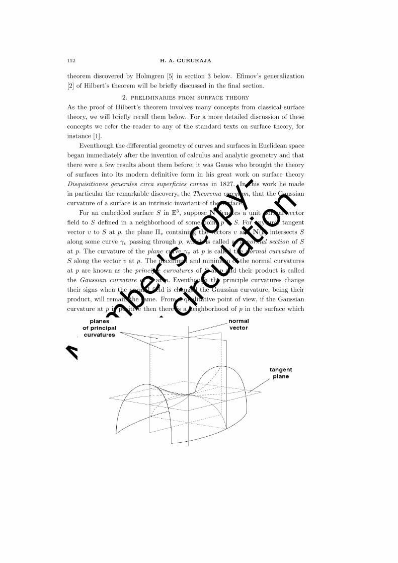
Membe
r's co
py-
not f
or ci
rculat
ion
152 H. A. GURURAJA
theorem discovered by Holmgren [5] in section 3 below. Efimov’s generalization
[2] of Hilbert’s theorem will be briefly discussed in the final section.
2. preliminaries from surface theory
As the proof of Hilbert’s theorem involves many concepts from classical surface
theory, we will briefly recall them below. For a more detailed discussion of these
concepts we refer the reader to any of the standard texts on surface theory, for
instance [1].
Eventhough the differential geometry of curves and surfaces in Euclidean space
began immediately after the invention of calculus and analytic geometry and that
there were a few results about them before, it was Gauss who brought the theory
of surfaces into its modern definitive form in his great work on surface theory
Disquisitiones generales circa superficies curvas in 1827. In this work he made
in particular the remarkable discovery, the Theorema egregium, that the Gaussian
curvature of a surface is an intrinsic invariant of the surface.
For an embedded surface S in E3, suppose N denotes a unit normal vector
field to S defined in a neighborhood of some point p ∈ S. For any unit tangent
vector v to S at p, the plane Πv containing the vectors v and N(p) intersects S
along some curve γv passing through p, which is called as a normal section of S
at p. The curvature of the plane curve γv at p is called the normal curvature of
S along the vector v at p. The maximum and minimum of the normal curvatures
at p are known as the principle curvatures of S at p and their product is called
the Gaussian curvature of S at p. Eventhough the principle curvatures change
their signs when the normal field is changed the Gaussian curvature, being their
product, will remain the same. From a qualitative point of view, if the Gaussian
curvature at p is positive then there is a neighborhood of p in the surface which
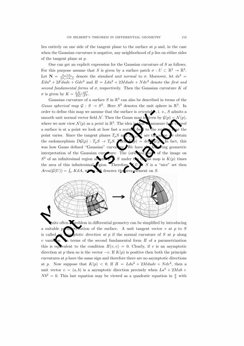
Membe
r's co
py-
not f
or ci
rculat
ion
ON HILBERT’S THEOREM IN DIFFERENTIAL GEOMETRY 153
lies entirely on one side of the tangent plane to the surface at p and, in the case
when the Gaussian curvature is negative, any neighborhood of p lies on either sides
of the tangent plane at p.
One can get an explicit expression for the Gaussian curvature of S as follows.
For this purpose assume that S is given by a surface patch σ : U ⊂ R2 → R3.
Let N = σu×σv
‖σu×σv‖ denote the standard unit normal to σ. Moreover, let ds2 =
Edu2 + 2Fdudv + Gdv2 and II = Ldu2 + 2Mdudv + Ndv2 denote the first and
second fundamental forms of σ, respectively. Then the Gaussian curvature K of
σ is given by K = LN−M2
EG−F 2 .
Gaussian curvature of a surface S in R3 can also be described in terms of the
Gauss spherical map G : S → S2. Here S2 denotes the unit sphere in R3. In
order to define this map we assume that the surface is orientable, i. e., S admits a
smooth unit normal vector field N . Then the Gauss map is given by G(p) = N (p),
where we now view N (p) as a point in R3. The idea is that to measure how curved
a surface is at a point we look at how fast a normal field to the surface near the
point varies. Since the tangent planes TpS and TG(p)S2 are the same we obtain
the endomorphism DG(p) : TpS → TpS. Then K(p) = detDG(p). In fact, this
was how Gauss defined “Gaussian” curvature. We have the following geometric
interpretation of the Gaussian curvature: The (oriented) area of the image on
S2 of an infinitesimal region around p in S under the Gauss map is K(p) times
the area of this infinitesimal region. Therefore, if U ⊂ S is a “nice” set then
Area(G(U)) =∫UKdA, where dA denotes the area element on S.
Quite often a problem in differential geometry can be simplified by introducing
a suitable parametrization of the surface. A unit tangent vector v at p to S
is called an asymptotic direction at p if the normal curvature of S at p along
v vanishes. In terms of the second fundamental form II of a parametrization
this is equivalent to the condition II(v, v) = 0. Clearly, if v is an asymptotic
direction at p then so is the vector −v. If K(p) is positive then both the principle
curvatures at p have the same sign and therefore there are no asymptotic directions
at p. Now suppose that K(p) < 0. If II = Ldu2 + 2Mdudv + Ndv2, then a
unit vector v = (a, b) is a asymptotic direction precisely when La2 + 2Mab +
Nb2 = 0. This last equation may be viewed as a quadratic equation in ab with
Membe
r's co
py-
not f
or ci
rculat
ion
154 H. A. GURURAJA
positive discriminant M2−LN and therefore will have two distinct solutions. As a
consequence there are (upto sign) exactly two asymptotic directions at p whenever
K(p) is negative. A curve on S is called an asymptotic curve if at each point on
the curve its tangent vector is along an asymptotic direction. One can write down
the differential equation for such curves: γ(t) = (u(t), v(t)) is an asymptotic curve
if and only if it satisfies the differential equation Lu′2 + 2Mu′v′ + Nv′2 = 0. If
S has negative Gaussian curvature then it follows from the theory of ordinary
differential equations ( existence, uniqueness and smooth dependence of solutions
on the initial data) that through each point of S there pass (upto orientation)
exactly two distinct asymptotic curves and that these curves are the parameter
curves of some parametrization of a neighborhood of each point in the surface.
Clearly, in such a parametrization one has L = N = 0.
Another parametrization that can sometimes be useful in certain problems
is the so called Tschebyshef net. For any abstract surface S an immersion σ :
(a, b)× (c, d)→ S is called a Tchebyshef net if all the parameter curves have unit
speed. Equivalently, the first fundamental form of the surface patch σ has the
form ds2 = du2 + 2Fdudv + dv2. It is not difficult to show that near any point
of any surface such a parametrization exists. As we shall see below, the notion
of Tschebyshef nets makes a surprising and crucial appearance in the proof of
Hilbert’s theorem.
We shall also require some global notions. We deal with abstract surfaces in
what follows and the word curvature shall mean the sectional curvature of the
surface. For an embedded surface in E3 the sectional curvature agrees with the
Gaussian curvature.
Recall that a surface is called complete if every geodesic on the surface is
defined for all time. This corresponds to the familiar axiom for the Euclidean
plane geometry that a straight line segment in the plane can be extended to infinity
in both directions. A famous result, the Hopf-Rinow theorem, asserts that this
notion of completeness of the surface is equivalent to the notion of completeness
of the surface as a metric space, where the distance between any two points on the
surface is defined to be the infimum of the lengths of all piecewise smooth paths
on the surface joining these points.
Another notion that appears in Hilbert’s proof is that of a covering surface.
A covering surface of a surface S is another surface S together with a surjective
map Φ : S → S, called the covering map, such that for any point q ∈ S, there
exists an open neighborhood U of q such that Φ−1(U) is a disjoint union of open
sets in S, each of which is mapped diffeomorphically by Φ onto U . We refer the
reader to [1], Chapter 5, for a detailed discussion of this notion. The key point for
us will be the fact that any surface admits a (essentially unique) simply connected
Membe
r's co
py-
not f
or ci
rculat
ion
ON HILBERT’S THEOREM IN DIFFERENTIAL GEOMETRY 155
covering surface called the universal covering surface of the given surface. Recall
that a path connected surface is said to be simply connected if, roughly speaking,
every closed curve on the surface can be continuously deformed to a point within
the surface. As an illustrative example, for the case of the Torus T 2(= S1 × S1),
the plane R2 will be the universal covering surface with respect to the mapping
Φ : R2 → T 2 given by Φ(x, y) = (eix, eiy).
The covering map becomes a local isometry when the universal covering surface
is given the pullback metric by the covering map and, therefore, these surfaces have
the same curvatures. Moreover, it is not difficult to see that the universal covering
surface is complete precisely when the surface is complete.
The curvature of a surface influences the behavior of geodesics on the sur-
face. Roughly speaking, if the the curvature of the surface is positive then nearby
geodesics converge as in the case of a Sphere whereas if the curvature of the sur-
face is negative then they diverge as in the case of the Hyperbolic plane. This last
statement is usually made precise by introducing the notion of exponential map
and Jacobi field. Assume that S is complete and p ∈ S. For any v ∈ TpS there
is a unique geodesic γ such that γ(0) = p and γ′(0) = v. We set expp(v) = γ(1),
i.e., expp(v) is the point on the surface obtained by following the geodesic γ start-
ing from p and going upto a distance equal to the length of v. The mapping
expp : TpS → S so obtained is called the exponential map based at p. It is a
consequence of the inverse function theorem from calculus that this map is a dif-
feomorphism of a neighborhood of 0p in TpS onto some neighborhood of the point
p in the surface. This fact allows us to introduce the analogue of polar coordinates
around p which turn out to be extremely important in the study of the geometry
of the surface. Jacobi fields are variation fields of geodesic variations and relate
the behavior of geodesics with the curvature of the surface. By a detailed study
of the relationship between geodesics and curvature one can prove the following
important global results which will be used later on (Proofs of these theorems can
be found in [1], Chapter 5).
Bonnet-Myers theorem. If the curvature of a complete surface S is bounded
below by a positive number then S must be compact.
Model spaces of constant curvature. Let S be a complete simply connected
surface which has constant curvature K. Then
S must be isometric to the Euclidean plane E2 if K = 0;
S must be isometric to the unit sphere S2 in R3 if K = 1;
S must be isometric to the Hyperbolic plane H2 if K = −1.
Cartan-Hadamard theorem. Suppose that a complete simply connected
surface S has nonpositive curvature. Then S must be diffeomorphic to a plane.
All the three global results extend to higher dimensions as well.
Membe
r's co
py-
not f
or ci
rculat
ion
156 H. A. GURURAJA
3. Statement and proof of Hilbert’s theorem
Theorem (Hilbert, 1901). Let S be a complete abstract surface of constant
negative curvature. Then there does not exist any isometric immersion of S into
E3.
Proof. We will simultaneously give Holmgren’s and Hilbert’s proofs below. The
proofs will be divided into many steps. Steps 1 to 3 are common to both the
proofs.
Step 1. Let S be a surface in E3 of constant curvature K < 0 and p ∈ S. We
can find a parametrization about p which is a Tschebyshef net and such that the
parameter curves are asymptotic curves.
Proof of Step 1. Since S has negative curvature, we know that the asymptotic
curves give a parametrization near p. Thus we have a parametrization σ : (−ε, ε)×(−ε, ε) → S, σ(0, 0) = p, such that the parameter curves are asymptotic curves.
Let ds2 = Edu2 + 2Fdudv + Gdv2 and II = Ldu2 + 2Mdudv + Ndv2 denote the
first and second fundamental forms of this parametrization, respectively. Without
loss of generality, we may assume that the parameter curves passing through p
have unit speed. Hence E(s, 0) = 1 and G(0, t) = 1. Using the constancy of the
curvature, we show below that all parameter curves have unit speed.
Let N = (σu × σv/‖σu × σv‖) denote the standard unit normal associated to
σ and let D =√EG− F 2. We know that Nu ×Nv = Kσu × σv. Therefore
(N×Nv)u − (N×Nu)v = 2Nu ×Nv = 2KDN.
Also N ×Nu = 1D〈σu,Nu〉σv − 〈σv,Nu〉σu = 1
D (Mσu − Lσv) and N ×Nv =1D (Nσu −Mσv). Since K = −M2
D2 and L = N = 0, we conclude that N ×Nu =
±√−Kσu, N × Nv = ∓
√−Kσv so that 2KDN = ∓
√−Kσuv ∓
√−Kσvu =
∓2√−Kσuv.
Hence σuv is parallel to N which implies Ev = 0 = Gu. Also 0 = (〈σu,N〉)u =
L+〈σu, Nu〉 = 〈σu,Nu〉. Therefore Eu = (〈σu,N〉)u = L+〈σu,Nu〉 = 0. Similarly
Gv = 0. Hence E,G are constants and must be equal to 1 throughout. Thus the
first fundamental form of σ has the form ds2 = du2 + 2Fdudv + dv2 and we are
done with the proof of Step 1.
Step 2. Let S be an abstract surface and let σ : (a, b)×(c, d)→ S be a Tschebyshef
net. Define the angle function ω : (a, b)×(c, d)→ R as follows: 0 < ω(s0, t0) < π
is the angle between the parameter curves passing through g(u0, v0). Then ω
satisfies the partial differential equation
∂2ω
∂u∂v= −K sinω, (3.1)
where K denotes the curvature of S.
Membe
r's co
py-
not f
or ci
rculat
ion
ON HILBERT’S THEOREM IN DIFFERENTIAL GEOMETRY 157
Proof of Step 2. Since σ is a Tschebyshef net the first fundamental form of
the net has the form ds2 = du2 + 2Fdudv + dv2. One form of Gauss’s Theorema
Egregium states that K = 1√EG−F 2
( Fu√EG−F 2
)v + ( Fv√EG−F 2
)u. Here E = G =
1,√EG− F 2 = sinω. Therefore the above equation can be written in the form
(3.1).
Step 3. Let S be a complete abstract surface of constant negative curvature. As-
sume that S can be immersed in E3. Then there exists an asymptotic Tschebyshef
net F : R2 → S.
Proof of Step 3. Fix a point p0 ∈ S and consider an asymptotic curve c(u)
passing through p0. Since c has unit speed and S is complete, it is not difficult to
see that c is defined on all of R. Now choose the other asymptotic curve through
p0 whose velocity at p0 is V0. For each u ∈ R, let γu(v) denote the unique asymp-
totic curve passing through c(u) whose velocity vector at c(u) is obtained from
continuous extension of V0. Now define F : R2 → S by F (u, v) = γu(v).
We have to show that each parameter curve u → F (u, v) is an asymptotic
curve of S. This will be shown using the existence of an asymptotic Tschebyshef
net σ : (−ε, ε)×(−ε, ε)→ S about each point of S, as proved in step 1. First observe
that if for some v ∈ (−ε, ε) the parameter curve u→ σ(u, v) lies along a parameter
curve u → F (u, v), then all parameter curves u → σ(u, v) lie along parameter
curves of F. Given (u0, v0) ∈ R2, we can find a finite number of Tschebyshef nets
σ1, σ2, ...., σn whose images cover the set F (u0, t) : 0 ≤ v ≤ v0. Arranging the
σi’s so that the images of the consecutive ones overlap and using the fact that the
curve u → F (u, 0) is an asymptotic curve (by definition of F ), we see that the
curve u→ f(u, v0) must be an asymptotic curve for u sufficiently close to u0.
Holmgren’s proof. In view of steps 2 and 3, to prove Hilbert’s theorem it is
enough to prove the following:
There does not exist a function ω : R2 → R satisfying ∂2ω∂u∂v = C sinω,
0 < ω < π, for any constant C > 0.
Assume that such a solution ω exists. Then ∂2ω∂u∂v > 0 so that ∂ω
∂u is increasing in
v and hence ∂ω(u,v)∂u > ∂ω(u,0)
∂u for v > 0. Integrating this inequality gives ω(b, v)−ω(a, v) > ω(b, 0) − ω(a, 0) for v > 0 and a < b. Without loss of generality, we
can assume that ∂ω(0,0)∂u 6= 0. Further, since the function (u, v) → ω(−u,−v) also
satisfies the differential equation, we may actually assume that ∂ω(0,0)∂u > 0. Now
fix three numbers 0 < u1 < u2 < u3 with
∂ω(u, 0)
∂u> 0
for 0 ≤ u ≤ u3 and set ε = minω(u3, 0) − ω(u2, 0), ω(u1, 0) − ω(0, 0). Then for
v > 0 and u ∈ [0, u3] we have ω(u, v) is increasing in u, ω(u1, v)− ω(0, v) > ε and
ω(u3, v) − ω(u2, v) > ε. Therefore ε ≤ ω(u, v) ≤ π − ε for u ∈ [u1, u2] and v ≥ 0.
Thus sin(ω(u, v)) ≥ sin ε for u ∈ [u1, u2] and v ≥ 0.

Membe
r's co
py-
not f
or ci
rculat
ion
158 H. A. GURURAJA
If we integrate the differential equation ∂2ω∂u∂v = C sinω over the rectangle
[u1, u2] × [0, T ] for any T > 0, we obtain C∫ T0
∫ u2
u1sinω(u, v)dudv = ω(u2, T ) −
ω(u1, T )− ω(u2, 0) + ω(u1, 0), so that ω(u2, T )− ω(u1, T ) = ω(u2, 0)− ω(u1, 0) +
C∫ T0
∫ u2
u1sinω(u, v)dudv ≥ ω(u2, 0) − ω(u1, 0) + CT (u2 − u1) sin ε. However this
gives a contradiction for large enough T , as the left hand side is smaller than π.
Sketch of Hilbert’s proof. The basis of Hilbert’s proof is the following lemma.
Lemma 1. (Formula of Hazzidakis). Let S be an abstract surface of constant
curvature K < 0 and let σ : (a, b) × (c, d) → S be a Tschebyschef net. Then any
quadrilateral formed by parameter curves of σ has area utmost 2π−K .
Proof. If Q denotes a quadrilateral formed by parameter curves of σ with
vortices (u1, v1), (u2, v1), (u2, v2) and (u1, v2) with corresponding interior angles
α1, α2, α3, α4, then using step2 we see that Area(Q) =∫Q
sinωdu ∧ dv =1−K
∫ u2
u1
∫ v2v1
∂2ω∂u∂vdudv = 1
−K (ω(u2, v2) − ω(u1, v2) − ω(u2, v1) + ω(u1, v1)) =1−K ([α3 − (π − α4)− (π − α2) + α1] = 1
−K (α1 + α2 + α3 + α4 − 2π) < 2π(−K) .
Lemma 2. The area of the Hyperbolic plane H2 is infinite.
Proof. The hyperbolic plane is the upper half plane endowed with the metric
g = dx2+dy2
y2 . Therefore its area is∫∞−∞
∫∞0
1y2 dxdy =∞.
Now we can complete Hilbert’s proof as follows. Without loss of generality we
may assume that the constant curvature is −1. If there is an immersion of S into
E3, then by going to the universal covering surface S of S, we can find an isometric
immersion of S into E3. Note that S must be isometric to H2 and therefore must
have infinite area. Now, if we are able to show that the asymptotic Tschebyshef net
considered in step 3 above can be extended to form a parametrization of all of the
simply connected surface S, then using Lemmas 1 and 2 we obtain a contradiction.
Thus establishing the existence of a global asymptotic Tschebyshef net is the main
(and the harder) part in Hilbert’s proof. The reader is referred to [7] or [1] for a
complete proof. Also see [8] and [9].
4. Efimov’s theorem
An example. The Hyperboloid. Consider the surface x2 + y2 = 1 + z2 in R3
which is known as the Hyperboloid of revolution.
A straightforward calculation shows that the Gaussian curvature K of the
Hyperboloid is given by the formula K(x, y, z) = − 1(1+2z2)2 . It follows that the
Gaussian curvature of the Hyperboloid is strictly negative everywhere. The fact
that the Hyperboloid is complete can be seen, for example, from the follow-
ing proposition (It may be worth remarking that the converse of the following
proposition is false).
Proposition 1. An embedded surface S ⊂ R3 which is also a closed subset of R3
must be complete.
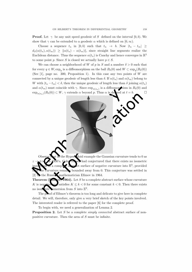
Membe
r's co
py-
not f
or ci
rculat
ion
ON HILBERT’S THEOREM IN DIFFERENTIAL GEOMETRY 159
Proof. Let γ be any unit speed geodesic of S defined on the interval [0, b). We
show that γ can be extended to a geodesic α which is defined on [0,∞).
Choose a sequence tn in [0, b) such that tn → b. Now |tn − tm| ≥dS(α(tn), α(tm)) ≥ ‖α(tn) − α(tm)‖, since straight line segments realize the
Euclidean distance. Thus the sequence α(tn) is Cauchy and hence converges in R3
to some point p. Since S is closed we actually have p ∈ S.We can choose a neighborhood of W of p in S and a number δ > 0 such that
for every q ∈W, expq is a diffeomorphism on the ball Bδ(0) and W ⊂ expq(Bδ(0))
(See [1], page no. 300, Proposition 1). In this case any two points of W are
connected by a unique geodesic of length less than δ. If α(tn) and α(tm) belong to
W with |tn − tm| < δ, then the unique geodesic of length less than δ joining α(tn)
and α(tm) must coincide with γ. Since expα(sn) is a diffeomorphism in Bδ(0) and
expα(sn)(Bδ(0)) ⊂W , γ extends α beyond p. Thus α is defined at t = b.
Observe that in the Hyperboloid example the Gaussian curvature tends to 0 as
z → ±∞. In 1930’s, Cohn-Vossen had conjectured that there exists no isometric
immersion of a complete abstract surface of negative curvature into E3, provided
that the curvature remains bounded away from 0. This conjecture was settled in
[2] by the Russian mathematician Efimov in 1964.
Theorem (Efimov, 1964). Let S be a complete abstract surface whose curvature
K is negative and satisfies K ≤ k < 0 for some constant k < 0. Then there exists
no isometric immersion from S into E3.
The proof of Efimov’s theorem is too long and delicate to give here in complete
detail. We will, therefore, only give a very brief sketch of the key points involved.
The interested reader is referred to the paper [6] for the complete proof.
To begin with, we need a generalization of Lemma 2.
Proposition 2. Let S be a complete simply connected abstract surface of non-
positive curvature. Then the area of S must be infinite.
Membe
r's co
py-
not f
or ci
rculat
ion
160 H. A. GURURAJA
Proof. Fix any point p ∈ S. The key point here is that the exponential map
expp : TpS → S is a diffeomorphism, by Cartan-Hadamard theorem. This fact
allows us to set up a polar co-ordinate system on all of S. The metric in polar co-
ordinates (r, θ) (with p as the origin) has the form ds2 = dr2 + φ2(r, θ)dθ2, where
the function φ satisfies φ(0, θ) = 0 and ∂φ(0,θ)∂r = 1. Since K(r, θ) = −φrr(r,θ)
φ(r,θ) ≤ 0,
we see that φrr(r, θ) ≥ 0 and hence r → φ(r, θ) is increasing. Since ∂φ(0,θ)∂r = 1
and φ satisfies φ(0, θ) = 0 we conclude that φ(r, θ) ≥ r for all (r, θ). Therefore the
volume of M=∫∞0
∫ 2π
0φ(r, θ)dθdr ≥
∫∞0
∫ 2π
0rdθdr =∞.
As in the case of Hilbert’s proof we may assume that S is simply connected
by going to the universal covering surface of S. By Cartan-Hadamard theorem, S
must be diffeomorphic to the plane. Let Ω denote the surface S equipped with
the metric obtained from pulling back the Riemannian metric of the 2-Sphere S2
to S via the Gauss map G : S → S2. Then Ω has constant positive curvature 1.
Note, however, that Ω cannot be complete. Otherwise, it would be compact by
the Bonnet-Meyer theorem and, therefore, the surface S must have a point where
the curvature must be positive, which is contrary to the hypothesis. Now, Efimov
considers the metric completion Ω of Ω. The Gauss map G : Ω → S2 extends as
a continuous map G : Ω→ S2. By a deep study of the behavior of this map near
the “boundary” of Ω, i.e., near the set Ω \Ω, Efimov proves that Ω has finite area
(in fact, of area atmost 4π). Taking this fact for granted, the proof of Efimov’s
theorem can be completed as follows
Fix a point p ∈ S. Let A(r) denote the area of the geodesic ball Dr(p) of radius
r at p in S and let A∗(r) be the area of this ball in Ω. Since |K| ≥ k > 0 on S,
we have 4π ≥ A∗(r) =∫Dr(p)
|K|dA ≥ k∫Dr(p)
dA = kA(r), which is impossible in
view of Proposition 2.
We end this article by remarking that the regularity hypothesis in Efimov’s
(and Hilbert’s) theorem can be weakened. It suffices for the surface to be of class
C2. See [6] for further details.
Acknowledgment. The author wishes to thank Prof. C. S. Aravinda for his
careful reading of the original draft of this article and suggesting many changes
which have helped in improving the exposition and also for providing the figures
appearing in this article. Thanks are also due to the referee for valuable comments
on the article.
References
[1] Do Carmo, M., Differential Geometry of Curves and Surfaces, Prentice-Hall, Inc., 1976.
[2] Efimov, N. V., Generation of singularities on surfaces of negative curvature, Sbornik, 64
(1964), 286–320.
[3] Gromov, M., Spaces and questions, Visions in Mathematics, GAFA 2000 special volume,
part 1, 118–161.

Membe
r's co
py-
not f
or ci
rculat
ion
ON HILBERT’S THEOREM IN DIFFERENTIAL GEOMETRY 161
[4] Hilbert, D., Uber Flachen von konstanter Gausscher Krummung, Trans. Amer. Math.
Society, 2 (1901), 87–99.
[5] Holmgren, E., Sur les surfaces a courbure constante negative, C. R. Acad. Sci. Paris, 134
(1902), 740–743.
[6] Klotz-Milnor, T., Efimov’s Theorem About Complete Immersed Surfaces of Negative
Curvature, Adv. in Math., 8 1972, 474–543.
[7] Spivak, M., A Comprehensive Introduction to Differential Geometry, Vol. 3, Publish or
Perish.
[8] Stoker, J. J., Differential Geometry, Wiley Classics Library, 1969.
[9] Willmore, T. J., An introduction to differential geometry, Oxford university press, 1959.
H. A. Gururaja
TIFR Centre for Applicable Mathematics, P.O. Box 6503
Sharadanagar, GKVK Post, Bangalore - 560065
E-mail: [email protected]

Membe
r's co
py-
not f
or ci
rculat
ion
162
Membe
r's co
py-
not f
or ci
rculat
ion
The Mathematics Student ISSN: 0025-5742
Vol. 85, Nos. 1-2, January-June (2016), 163-166
A PAIR OF SIMULTANEOUS DIOPHANTINEEQUATIONS WITH NO SOLUTIONS IN INTEGERS
AJAI CHOUDHRY
(Received : 23 - 11 - 2015)
Abstract. This paper is concerned with the simultaneous diophantine
equations xm1 + xm
2 = ym1 + ym2 , xn1 + xn
2 = yn1 + yn2 , where m, n are distinct
positive integers. It is shown that for arbitrary m, n, these equations have no
solutions in nonnegative integers; further when m, n are of the same parity,
these equations have no solutions in integers, whether positive or negative.
This paper is concerned with the simultaneous diophantine equations
xm1 + xm2 = ym1 + ym2 , (1)
xn1 + xn2 = yn1 + yn2 , (2)
where m, n are distinct positive integers. It has been shown by Sinha [4] that
these two equations do not have a nontrivial solution in integers when 1 ≤ m ≤ 4
and 1 ≤ n ≤ 4. The special case when (m, n) = (2, 3) has also been considered
independently by other authors ([1], [2], [3]).
Any solution (x1, x2, y1, y2) = (α1, α2, β1, β2) of eqs. (1) and (2) will be
called a trivial solution if the pair of numbers, α1, α2, is a permutation of the
numbers β1, β2. Further, when both m and n are odd integers, any solution of the
type (x1, x2, y1, y2) = (α, −α, β, −β) will also be considered as a trivial solution.
All other solutions will be referred to as nontrivial solutions.
In this paper it is shown that if m, n are arbitrary distinct positive integers,
the simultaneous equations (1) and (2) have no nontrivial solutions in nonnegative
integers. It is also shown that when the integers m, n are of same parity, the
simultaneous equations (1) and (2) have no nontrivial solutions in integers, whether
positive or negative. These results are proved in the two theorems that follow.
Theorem 1. If m and n are arbitrary distinct positive integers, the simultaneous
equations (1) and (2) have no nontrivial solutions in nonnegative integers.
Proof. Without loss of generality, we assume that m > n. Let (x1, x2, y1, y2)
= (α1, α2, β1, β2) be a nontrivial solution in nonnegative integers of eqs. (1) and
(2) with αi ≥ 0, βi ≥ 0, i = 1, 2.
2010 Mathematics Subject Classification : 11D41
Key words and phrases : high degree diophantine equations; symmetric diophantine equati-
ons.
c© Indian Mathematical Society, 2016 .
163
Membe
r's co
py-
not f
or ci
rculat
ion
164 AJAI CHOUDHRY
We first show that none of the integers α1, α2, β1, β2 can be 0. It is readily
seen that two or more of these four integers cannot be 0. If only one of the four
integers, say α2, is 0 then we haveαn1 = βn
1 + βn2 , (3)
so that
α1 > β1, α1 > β2. (4)
Multiplying (3) by αm−n1 we get
αm1 = αm−n
1 βn1 + αm−n
1 βn2 ,
> βm1 + βm
2 ,(5)
in view of the relations (4). This contradicts the assumption that (α1, 0, β1, β2)
is a solution of (1). Similarly, the other integers α1, β1, β2 are seen to be nonzero
and henceforth we assume that all the integers α1, α2, β1, β2 are positive.
We assume without loss of generality that α1 ≥ α2 and β1 ≥ β2. Let
αn1 + αn
2 = βn1 + βn
2 = 2s, (6)so that we may write
αn1 = s+ d1, αn
2 = s− d1, βn1 = s+ d2, βn
2 = s− d2, (7)
where s is a positive rational number and d1, d2 are distinct rational numbers
such that 0 ≤ di < s, i = 1, 2 and we may assume without loss of generality that
d1 > d2. It follows from (7) that
α1 = (s+ d1)1/n, α2 = (s− d1)1/n, β1 = (s+ d2)1/n, β2 = (s− d2)1/n. (8)
We thus getαm1 + αm
2 = (s+ d1)m/n + (s− d1)m/n, (9)
βm1 + βm
2 = (s+ d2)m/n + (s− d2)m/n. (10)
We now consider the following function
f(d) = (s+ d)m/n + (s− d)m/n, (11)
where s is a fixed positive rational number. The derivative of f(d) is given by
f ′(d) =m
n.(s+ d)(m−n)/n + (s− d)(m−n)/n. (12)
When 0 ≤ d < s, both the numbers (s+d)(m−n)/n and (s−d)(m−n)/n are positive
and hence their arithmetic mean is not less than their geometric mean. Thus,
when 0 ≤ d < s, we get
f ′(d) ≥ 2m
n.(s2 − d2)(m−n)/n > 0 (13)
and hence the function f(d) is monotonically increasing in this interval. Since
0 ≤ di < s, i = 1, 2, it follows that when d1 > d2 we have f(d1) > f(d2). It now
follows from (9), (10) and (11) that
αm1 + αm
2 > βm1 + βm
2 . (14)

Membe
r's co
py-
not f
or ci
rculat
ion
A PAIR OF SIMULTANOUS ..... WITH NO SOLUTIONS IN INTEGERS 165
This contradicts the assumption that (α1, α2, β1, β2) is a solution of (1). It
follows that there cannot exist a solution in nonegative integers of the
simultaneous equations (1) and (2). This proves the theorem.
Theorem 2. If m and n are arbitrary distinct positive integers of the same
parity then the simultaneous equations (1) and (2) have no nontrivial solutions in
integers, whether positive or negative.
Proof. If the integers m and n are both even, any nontrivial solution
(α1, α2, β1, β2) of eqs. (1) and (2) involving negative integers immediately yields a
nontrivial solution (|α1|, |α2|, |β1|, |β2|) in nonegative integers of these equations.
This contradicts Theorem 1.
If the integers m and n are both odd, we assume without loss of generality
that m > n. Let (x1, x2, y1, y2) = (α1, α2, β1, β2) be a nontrivial solution of
eqs. (1) and (2) so that
αm1 + αm
2 = βm1 + βm
2 , (15)
αn1 + αn
2 = βn1 + βn
2 . (16)
In view of Theorem 1 at least one of the four integers α1, α2, β1, β2 must be
negative. We now have the following cases.
Case-1. Only one of the four integers α1, α2, β1, β2 is negative. Without loss of
generality we may take α1 > 0, α2 < 0, β1 > 0, β2 > 0, so that we obtain, from
(15) and (16), the following relations after transposition
αm1 = |α2|m + βm
1 + βm2 , (17)
αn1 = |α2|n + βn
1 + βn2 . (18)
It follows from (18) that α1 > |α2|, α1 > β1 and α1 > β2. Now, on multiplying
(18) by αm−n1 we get
αm1 = αm−n
1 |α2|n + αm−n1 βn
1 + αm−n1 βn
2 ,
or, αm1 > |α2|m + βm
1 + βm2 ,
(19)
which contradicts the relation (17).
Case-2. Two of the four integers α1, α2, β1, β2 are negative. Clearly the two
negative integers cannot both be on the same side of eqs. (1) and (2). Thus, one
of the two integers α1, α2 must be negative, and similarly, one of the two integers
β1, β2 must be negative. Since both m and n are odd we can obtain from (15)
and (16), after suitable transpositions, a nontrivial solution of eqs. (1) and (2) in
nonnegative integers in contradiction of Theorem 1.
Case-3. When three of the four integers α1, α2, β1, β2 are negative, we obtain
relations of the type (17) and (18) by suitable transpositions. As already seen
earlier such solutions cannot exist. Similarly, it is readily seen that there cannot
exist any solution in which all four integers α1, α2, β1, β2 are negative.

Membe
r's co
py-
not f
or ci
rculat
ion
166 AJAI CHOUDHRY
Thus, we see that in all cases when m and n are both even or are both odd,
the existence of a nontrivial solution of the simultaneous equations (1) and (2)
leads to a contradiction. It follows that when m and n are of the same parity
there cannot exist a solution of eqs. (1) and (2) in integers, whether positive or
negative. This proves the theorem.
Acknowledgment. I wish to thank the Harish-Chandra Research Institute,
Allahabad, for providing me all the necessary facilities that have helped me to
pursue my research work in mathematics.
References[1] Gatteschi, L. and Rosati, L. A., Risposta ad una questione proposta da A. Moessner, Boll.
Un. Mat. Ital. (3) 5 (1950), 43–48.
[2] Gupta, H., A system of equations having no nontrivial solutions, J. Res. Nat. Bur. Standards
Sect. B 71B (1967), 181–182.
[3] Schmidt, H., Uber einige diophantische Aufgaben 3. und 4. Grades, Jber. Deutsch.
Math.-Verein 67 (1964/65) Abt. 1, 2–13.
[4] Sinha, T. N., A relation between the coefficients and roots of two equations and its application
to diophantine problems, J. Res. Nat. Bur. Standards Sect. B 74B (1970), 31–36.
Ajai Choudhry
13/4 A Clay Square, Lucknow - 226001, UP, India
E-mail: [email protected]
Membe
r's co
py-
not f
or ci
rculat
ion
The Mathematics Student ISSN: 0025-5742
Vol. 85, Nos. 1-2, January-June, (2016), 167-174
PROBLEM SECTION
Problems of the Mathematics Student Vol. 84, Nos. 1-2, January-June,
(2015) (MS, 84, 1-2, 2015 for short): We published Proposer’s solution to the
Problem-4 and the correct submitted solution from the floor to the Problems 5, 9
and 11 in the MS, 84, 3-4, 2015. Till April 30, 2016, no responses are received to
the remaining Problems 2, 3, 6, 7, 8 and 10 and hence we provide in this issue the
Proposer’s solution to these problems. Problem 1 is an open problem.
Problems of the MS, 84, 3-4, 2015: One submitted solution to the Problem-18
is received from the floor which is correct and is published in this issue. Readers
can try their hand on the remaining Problems 12, 13, 14, 15, 16 and 17 till October
31, 2016.
In this issue we first present eight new problems. Solutions to these problems
as also to the remaining Problems 12, 13, 14, 15, 16 and 17 of MS, 84, 3-4, 2015,
received from the floor till October 31, 2016, if approved by the Editorial Board,
will be published in the MS, 85, 3-4, 2016.
MS-2016, Nos. 1-2: Problem-01: Proposed by M. Ram Murty.
Let φ denote Euler’s function. Show that for any positive real number a,
there is a constant C(a) such that∑n≤x
(n
φ(n)
)a≤ C(a)x.
MS-2016, Nos. 1-2: Problem-02: Proposed by B. Sury
Suppose a, b, c, d are integers such that the last 2016 digits of the number
ab + cd are all 9’s. Show that there exist integers A,B,C,D each ending in
2016 zeroes such that
(a+A)(b+B)(c+ C)(d+D) = ±1.
MS-2016, Nos. 1-2: Problem-03: Proposed by B. Sury .
Show that the number 11 · · · 122 · · · 25 where 1 is repeated 2015 times and
2 is repeated 2016 times, is a perfect square.
c© Indian Mathematical Society, 2016 .
167

Membe
r's co
py-
not f
or ci
rculat
ion
168 PROBLEM SECTION
MS-2016, Nos. 1-2: Problem-04: Proposed by B. Sury .
Let f = c0 + c1X + · · ·+ cnXn be a polynomial with integer coefficients.
Prove that there exist n+ 1 primes p0, p1, p2, · · · , pn and a polynomial g with
integer coefficients such that
f(x)g(x) = a1xp1 + a2x
p2 + · · ·+ anxpn
for some integers ai’s.
MS-2016, Nos. 1-2: Problem-05: Proposed by B. Sury .
Let f =∑ni=0 ciX
i where n is a positive integer and each ci = ±1. If all
the roots of f are real, determine all the possibilities for f .
MS-2016, Nos. 1-2: Problem-06: Proposed by Raja Sridharan, TIFR,
Mumbai; submitted through Clare D’Cruz.
Let A be a commutative ring with unity, M a finitely generated A-module,
and I be an ideal of A.
(1) Suppose that IM = M . Then show that there exists an x ∈ I such
that (1 + x)M = 0.
(2) Suppose I is a finitely generated ideal such that I2 = I. Then show
that I is generated by an idempotent, i.e., there exists an element x
such that I = (x) and x2 = x.
(3) Suppose x1, ..., xn ∈ I and (x1, ..., xn)+I2 = I. Then show that there
exists x ∈ I such that I = (x1, ..., xn, x).
(4) Let x ∈ A be an idempotent element and let y ∈ A be any other
element. Then show that the ideal I = (x, y) is principal.
(5) Let I ⊆ A be a finitely generated ideal. Suppose there exists
x1, ..., xn ∈ I such that (x1, ..., xn) + I2 = I. Then show that for
any y ∈ A, (I, y) can be generated by n+ 1 elements.
(6) Let (A,m) be a local ring with 1 and I ⊆ m an ideal. Suppose
x1, ..., xn ∈ I are such that (x1, ..., xn)+I2 = I. Then I = (x1, ..., xn).
(7) Is (6) true for any ideal I in a Noetherian ring with 1? What are
classes of rings for which (6) is true?
MS-2016, Nos. 1-2: Problem-07: Proposed by Purusottam Rath, CMI,
Chennai; submitted through Clare D’Cruz.
Let M = (aij) be an n× n matrix with aij ∈ R and |aij | ≤ 1. Show that
the absolute value of determinant of M is at most nn/2. When does equality
hold?
Membe
r's co
py-
not f
or ci
rculat
ion
PROBLEM SECTION 169
MS-2016, Nos. 1-2: Problem-08: Proposed by Purusottam Rath, CMI,
Chennai; submitted through Clare D’Cruz.
let A and B be finite subsets of integers. Consider the set A+B given by
A+B := a+ b : a ∈ A, b ∈ B.Show that |A+B| ≥ |A|+ |B| − 1.
Solution from the floor: MS-2015, Nos. 3-4: Problem 18: Evaluating
the product, prove that√2
1+√2.
√2+√2
1+√√
2.
√2+√
2+√2
1+
√√√2... = ln 4
π .
(Solution submitted on 08-01-2016 by Subhash Chand Bhoria; Corporal, Air
Force Station, Bareilly, Technical Flight, UP-243002, India; [email protected]).
Solution. Put xn =√
2 + xn−1, wn = xn
2 , for n ≥ 1, where in x0 = 0. We have
limk→∞
k∏n=1
wn =2
π
in view of Viete’s formula (see Beckmann, Petr, A history of π, Second Edition,
The Golden Press, Boulder, Colo. (1971), 94-95). For yn = 1+21/2n
for all n ≥ 1,
we then obtain
limk→∞
k∏n=1
xnyn
=2
π
(limk→∞
k∏n=1
2
yn
)=
2
π
limk→∞
2k
k∏n=1
(1 + 21/2n
) .
Observe that
1∏kn=1
(1 + 21/2n
) =1×
(1− 21/2
k)
((1 + 21/2
) (1 + 21/4
)· · ·(1 + 21/2k
))×(1− 21/2k
)=
(1− 21/2
k)
(1 + 21/2
) (1 + 21/4
)· · ·(
1 + 21
2k−1
)(1− 2
1
2k−1
)=
(1− 21/2
k)
(1 + 21/2
) (1− 21/2
) =(
21/2k
− 1).
Therefore
limk→∞
k∏n=1
xnyn
=2
π
(limk→∞
2k(
21/2k
− 1))
.
Now take 12k
= t. Noticing that t tends to 0 as k tends to infinity and using
L’Hopital’s rule, we then obtain
2
π
(limk→∞
2k(
21/2k
− 1))
=2
π
(limt→0
(2t − 1)
t
)=
2
π(ln 2) =
ln 4
π
which completes the proof.
Membe
r's co
py-
not f
or ci
rculat
ion
170 PROBLEM SECTION
Solution by the Proposer George E. Andrews: MS-2015, Nos. 1-2:
Problem 2: Prove that, for |q| < 1 and b not a negative power of q,
∞∑n=1
qn
(1− qn)(1− bqn)=∞∑n=1
nqn∞∏m=n
(1− qm+1)
(1− bqm). (0.1)
Fokkink, R., Fokkink, W. and Wang, B. (A relation between partitions and the
number of divisors, Amer. Math. Monthly, 102(1995), 345-347) proved that the
number of divisors of n equals
−∑π∈Dn
(−1)#(π)σ(π),
where Dn is the set of integer partitions of n into distinct parts, #(π) is the number
of parts of π and σ(π) is the smallest part of π.
Ex. When n = 6, D6 = 6, 5 + 1, 4 + 2, 3 + 2 + 1, so the above sum is
6− 1− 2 + 1 = 4, and there are four divisors of 6, namely 1,2,3, and 6.
Deduce the Fokkink, Fokkink and Wang theorem from (0.1).
Solution. We require the following notation
(A; q)n =n−1∏j=0
(1−Aqj) and (A; q)∞ =∞∏j=0
(1−Aqj).
Also we need the classical q-binomial series∞∑n=0
(A; q)ntn
(q; q)n=
(At; q)∞(t; q)∞)
. (0.2)
Then∞∑n=1
nqn∞∏m=n
(1− qm+1)
(1− bqm)=
d
dz
∣∣∣z=1
∞∑n=0
znqn(qn+1; q)∞(bqn; q)∞
=d
dz
∣∣∣z=1
(q; q)∞(b; q)∞
∞∑n=0
znqn(b; q)n(q, q)n
=d
dz
∣∣∣z=1
(q; q)∞(b; q)∞
(zbq; q)∞(zq, q)∞
(by (0.2))
=(q; q)∞(b; q)∞
(bq; q)∞(q; q)∞
( ∞∑n=1
qn
1− qn−∞∑n=1
bqn
1− bqn
)(by the rule of differentiation of products)
=1
1− b
( ∞∑n=1
(1− bqn)qn − bqn(1− qn)
(1− qn)(1− bqn)
)
=1
1− b
∞∑n=1
qn(1− b)(1− qn)(1− bqn)
=∞∑n=1
qn
(1− qn)(1− bqn).
If one sets b = 0, we note that the left hand side of (0.1) becomes
Membe
r's co
py-
not f
or ci
rculat
ion
PROBLEM SECTION 171
∞∑n=1
qn
(1− qn)=∞∑n=1
d(n)qn,
where d(n) is the number of divisors of n. The right hand side of (0.1) becomes∞∑n=1
nqn(1− qn+1)(1− qn+2)(1− qn+3) · · ·
and we see that the nth term of this series counts, with weight ±n, the partitions
with distinct parts whose smallest part is n. The “+′′ occurs if the partition in
question has an odd number of parts, and “−′′ occurs for an even number of parts.
Thus the coefficient of qn is
−∑π∈Dn
(−1)#(π)σ(π).
As an added bonus, we observe that if b = q, we have
∞∑n=1
qn
(1− qn)(1− qn+1)=∞∑n=1
nqn,
This implies that the number of partitions of n in which the difference between
the largest and smallest parts is at most one equals n.
For example, there are five such partitions of 5:
5; 3 + 2; 2 + 2 + 1; 2 + 1 + 1 + 1; 1 + 1 + 1 + 1 + 1.
Solution by the Proposer Kannappan Sampath: MS-2015, Nos. 1-2:
Problem 3: Let H denote the division algebra of quaternions over the field R of
real numbers. Let n be a positive integer. Suppose that A and B are two n × nmatrices such that AB = In×n = I, say. Show that BA = I.
Solution. Throughout, we shall view of H as the R-algebra given by
H = R⊕ Ri⊕ Rj ⊕ Rk,where i, j, k are subject to the usual relations i2 = j2 = k2 = ijk = −1. We begin
by remarking that every real quaternion can be written uniquely as z1 +z2j where
z1, z2 ∈ C. In view of this, if A is an n×n matrix over H, we may write A uniquely
asA = A1 +A2j (0.3)
where A1, A2 ∈Mn×n(C) and j = diag(j, . . . , j) ∈Mn×n(H). For a, b ∈ R, we note
that (a + bi)j = j(a − bi) so that for a matrix C ∈ Mn×n(C), we have Cj = j C.
It is now routine to verify that
Mn×n(H)→M2n×2n(C) such that A 7→
(A1 A2
−A2 A1
)is an R-algebra isomorphism. The proof is now straightforward. We have
AB = I ⇐⇒
(A1 A2
−A2 A1
)(B1 B2
−B2 B1
)= I
Membe
r's co
py-
not f
or ci
rculat
ion
172 PROBLEM SECTION
⇐⇒
(B1 B2
−B2 B1
)(A1 A2
−A2 A1
)= I
⇐⇒ BA = I.
invoking the fact that ST = I if and only if TS = I for square matrices S and T
over a field. This completes the proof.
Remark. Compare with Bourbaki’s Algebra, Corollary to Proposition 9 in
Chapter II, §7.4, pg. 298.
Solution by the Proposer Amritanshu Prasad: MS-2015, Nos. 1-2:
Problem 6: Let X be the set of all subsets of 1, . . . , n of size 2 (so X has(n2
)elements). Let V be the complex vector space
V =f : X → C |
∑s∈X|i∈s
f(s) = 0 ∀ i ∈ 1, 2, · · · , n∗.
Show that V is a vector space of dimension n(n− 3)/2 over C.
* The inadvertant typographical error in the definition of V in the statement of
this problem that appeared in the Mathematics Student 84, nos. 1-2, (2015) is
regretted.
Solution. Let U be the space of all functions X → C. For each i ∈ 1, . . . , n,let Li be the linear functional U → C defined by
Lif =∑
s∈X|i∈s
f(s).
Then V is the subspace of U on which all the Li’s vanish. We claim that
Li | 1 ≤ i ≤ n
is a linearly independent set in the dual space of U . Indeed, if L =∑ni=1 αiLi for
some α1, . . . , αn ∈ C, and for each s ∈ X δs ∈ U is the function which 1 at s and
0 at all other points of U , then
L( ∑s∈X|i∈s
δs
)=∑j 6=i
(αi + αj) = (n− 1)αi +∑j 6=i
αj .
Also
L( ∑s∈X|i/∈s
δs
)= (n− 2)
∑j 6=i
αj .
Thus
αi = L( 1
n− 1
∑s∈X|i∈s
δs −1
(n− 1)(n− 2)
∑s∈X|i/∈s
δs
),
showing that αi can be recovered from L for each i ∈ 1, . . . , n. It follows that
L is linearly independent, and so V , which is the intersection of the kernels of the
linear functionals L1, . . . , Ln must have dimension
dimU − n =
(n
2
)− n =
n(n− 3)
2, as required.
Membe
r's co
py-
not f
or ci
rculat
ion
PROBLEM SECTION 173
Solution by the Proposer Ashay Burungale: MS-2015, Nos. 1-2:
Problem 7: Consider a kingdom made up of an odd number 2k + 1 of is-
lands. There are bridges connecting some of the islands. Suppose each set S of k
islands has the property that there is an island not among S which is connected
by a bridge to each island in S. Show that some island of the kingdom has bridges
connecting it to all the other islands.
Solution. Any island I is part of some set of k islands and hence, there is another
island J connected to it by a bridge. Thus, the set I, J has the property that
each pair of islands in it (there is only one!) is connected by a bridge. So, one
may consider a (non-empty) set T of islands in the kingdom which has maximum
cardinality such that every pair of islands in T is connected by a bridge. There
may be more than one choice for T but fix one. We claim that T has cardinality
at least k + 1. If not, then consider any set T0 of k islands containing T . By
hypothesis, there is an island I not in T0 which is connected to each island in
T0. But, then T ∪ I is a larger (than T ) set of islands in which every pair is
connected. This contradicts the choice of T . Therefore, |T | ≥ k + 1. Let S ⊂ T
be any subset with exactly k + 1 islands. Of course, each pair of islands in S is
connected by bridges (as this is true of T ). Since the complement of S has exactly
k islands, the hypothesis implies there is an island I in S connected to each island
in the complement of S. But then I is connected to all islands.
Solution by the Proposer Abhijin Adiga: MS-2015, Nos. 1-2:
Problem 8: Consider the set S = 1, 2, ..., n. Let Si be n distinct non-
empty subsets of S. Prove that there exists an element k ∈ S, such that Si \ kare still distinct
Solution. Consider the subsets as the vertices of an n-dimensional hypercube.
Now if there are two subsets Si and Sj such that Si − k = Sj − k, then
clearly k was in one of them and not in the other. Thus there was an edge in
the hypercube between the corresponding two vertices. Mark this edge with the
letter k- if there are many such edges, just pick one and mark it. Now if for all
k ∈ 1, 2, . . . , n, such and edge can be found, then the marked n edges define a
subgraph of the hypercube on n vertices. Thus there is a cycle in this subgraph,
which means more than one of these edges are marked with the same letter k: If
we added k to a subset to move away from it, we have removed it to come back.
Contradiction.
Solution by the Proposer Mathew Francis: MS-2015, Nos. 1-2:
Problem 10: Given a t-regular graph that is properly t-edge coloured with
colours 1, 2, · · · t. Consider any cut of the graph and let ki be the number of edges
coloured i crossing the cut. Show that k1 = k2 = · · · = kt mod 2.

Membe
r's co
py-
not f
or ci
rculat
ion
174 PROBLEM SECTION
Solution. Suppose not. Note that each color class has to be a perfect matching,
since each vertex sees all the three colors. Consider a cut (A, V − A). Now if |A|is even then all of k1, k2, k3 should be even. Else suppose k1 is odd. Consider the
matching of k1 edges colored with 1 going from A to V − A. Let A′ be the end
points of these edges on the A side. Clearly A′ ⊂ A since |A| is an even number
and |A′| is odd. Since the set of edges colored by 1 is a perfect matching, we should
have a perfect matching on the set of vertices A− A′ which is not possible, since
|A−A′| is odd.
In a similar way, if |A| were odd, then all of k1, k2, k3 should be odd. Otherwise
let k1 be even, and we will have |A − A′| odd in this case also, which makes it
impossible to have a perfect matching on A−A′.———–

Membe
r's co
py-
not f
or ci
rculat
ion

Membe
r's co
py-
not f
or ci
rculat
ion
FORM IV(See Rule 8)
1. Place of Publication: PUNE
2. Periodicity of publica-tion:
QUARTERLY
3. Printer’s Name: DINESH BARVENationality: INDIANAddress: PARASURAM PROCESS
38/8, ERANDWANEPUNE-411 004, INDIA
4. Publisher’s Name: N. K. THAKARENationality: INDIANAddress: GENERAL SECRETARY
THE INDIAN MATHEMATICAL SOCIETYc/o:CENTER FOR ADVANCED STUDY INMATHEMATICS, S. P. PUNE UNIVERSITYPUNE-400 007, MAHARASHTRA, INDIA
5. Editor’s Name: J. R. PATADIANationality: INDIANAddress: (DEPARTMENT OF MATHEMATIC,
THE M. S.UNIVERSITY OF BARODA)5 , ARJUN PARK, NEAR PATEL COLONYBEHIND DINESH MILL, SHIVANAND MARGVADODARA - 390 007, GUJARAT, INDIA
6. Names and addresses of THE INDIAN MATHEMATICAL SOCIETYindividuals who own thenewspaper and partnersor shareholders holdingmore than 1% of thetotal capital:
I, N. K. Thakare, hereby declare that the particulars given above are true to thebest of my knowledge and belief.
N. K. THAKAREDated: 3rd May 2016 Signature of the Publisher
Published by Prof. N. K. Thakare for the Indian Mathematical Society, type set byJ. R. Patadia at 5, Arjun Park, Near Patel Colony, Behind Dinesh Mill, ShivanandMarg, Vadodara - 390 007 and printed by Dinesh Barve at Parashuram Process,Shed No. 1246/3, S. No. 129/5/2, Dalviwadi Road, Barangani Mala, WadgaonDhayari, Pune 411 041 (India). Printed in India

Membe
r's co
py-
not f
or ci
rculat
ion
The Mathematics Student ISSN: 0025-5742Vol. 85, Nos. 1-2, January-June, (2016)
EDITORIAL BOARDJ. R. Patadia (Editor-in-Chief)
5, Arjun Park, Near Patel Colony, Behind Dinesh MillShivanand Marg, Vadodara-390007, Gujarat, India
E-mail : [email protected]
Bruce C. Berndt George E. AndrewsDept. of Mathematics, University Dept. of Mathematics, The Pennsylvaniaof Illinois 1409 West Green St. State University, University ParkUrbana, IL 61801, USA PA 16802, USAE −mail : [email protected] E −mail : [email protected]
M. Ram Murty N. K. Thakare
Queens Research Chair and Head C/o :Dept. of Mathematics and Statistics Center for Advanced StudyJeffery Hall, Queens University in Mathematics, Savitribai PhuleKingston, Ontario, K7L3N6, Canada Pune University, Pune− 411007, IndiaE −mail : [email protected] E −mail : [email protected]
Satya Deo Gadadhar MisraHarish− Chandra Research Institute Dept. of MathematicsChhatnag Road, Jhusi Indian Institute of ScienceAllahabad− 211019, India Bangalore− 560012, IndiaE −mail : [email protected] E −mail : [email protected]
B. Sury A. S. Vasudeva MurthyTheoretical Stat. and Math. Unit TIFR Centre for Applicable MathematicsIndian Statistical Institute P. B. No. 6503, GKV K Post SharadanagaraBangalore− 560059, India Chikkabommasandra,Bangalore− 560065, IndiaE −mail : [email protected] E −mail : [email protected]
S. K. Tomar Krishnaswami AlladiDept. of Mathematics, Panjab University Dept. of Mathematics, University ofSector − 4, Chandigarh− 160014, India F lorida, Gainesville, FL32611, USAE −mail : [email protected] E −mail : [email protected]
Subhash J. Bhatt L. Sunil ChandranDept. of Mathematics Dept. of Computer Science&AutomationSardar Patel University Indian Institute of ScienceV. V. Nagar − 388120, India Bangalore− 560012, IndiaE −mail : [email protected] E −mail : [email protected]
M. M. Shikare T. S. S. R. K. RaoCenter for Advanced Studyin Theoretical Stat. and Math. UnitMathematics, Savitribai Phule Pune Indian Statistical InstituteUniversity, Pune− 411007, India Bangalore− 560059, IndiaE −mail : [email protected] E −mail : [email protected]
Kaushal Verma C. S. AravindaDept. of Mathematics TIFR Centre for Applicable MathematicsIndian Institute of Science P. B. No. 6503, GKV K Post SharadanagaraBangalore− 560012, India Chikkabommasandra,Bangalore− 560065, IndiaE −mail : [email protected] E −mail : [email protected]
Indranil Biswas Timothy HuberSchool of Mathematics, Tata Institute School of Mathematics and statistical Sciencesof Fundamental Research, Homi Bhabha University of Texas Rio Grande V alley, 1201Rd., Mumbai− 400005, India West Univ. Avenue,Edinburg, TX78539 USAE −mail : [email protected] E −mail : [email protected]
Clare D′Cruz Atul Dixit
Dept. of Mathematics, CMI, H1, SIPCOT Shed− 3/Room207, Dept. of MathematicsIT Park, Padur P.O., Siruseri IIT Gandhinagar, V GEC ComplexKelambakkam− 603103, Tamilnadu, India Chandkheda, Ahmedabad 382424, IndiaE −mail : [email protected] E −mail : [email protected]

Membe
r's co
py-
not f
or ci
rculat
ion
THE INDIAN MATHEMATICAL SOCIETYFounded in 1907
Registered Office: Center for Advanced Study in MathematicsSavitribai Phule Pune University, Pune - 411 007
COUNCIL FOR THE SESSION 2016-2017
PRESIDENT: D. V. Pai, Visiting Professor, Mathematics and I/C Sciences & HSS,I. I. T. Gandhinagar, Vishwakarma Govt. Eng. College Campus, Chandkheda,Visat-Gandhinagar Highway, Ahmedabad-382 424, Gujarat, India
IMMEDIATE PAST PRESIDENT: A. M. Mathai, Director, Center for MathematicalSciences, Campus, St. Thomas College, Arunapuram, Pala-686 574 (Kerala),India
GENERAL SECRETARY: N. K. Thakare, C/o. Center for Advanced Study inMathematics, S. P. Pune University, Pune-411 007, Maharashtra, India
ACADEMIC SECRETARY: Peeush Chandra, Professor (Retired), Department ofMathematics & Statistics, I. I. T. Kanpur-208 016, Kanpur (UP), India
ADMINISTRATIVE SECRETARY: M. M. Shikare, Center for Advanced Study inMathematics, S. P. Pune University, Pune-411 007, Maharashtra, India
TREASURER: S. K. Nimbhorkar, Dept. of Mathematics, Dr. Babasaheb AmbedkarMarathwada University, Aurangabad-431 004, Maharashtra, India
EDITOR: J. Indian Math. Society: Satya Deo, Harish-Chandra ResearchInstitute, Chhatnag Road, Jhusi, Allahabad-211 019, UP, India
EDITOR: The Math. Student: J. R. Patadia, (Dept. of Mathematics, The M. S.University of Baroda), 5, Arjun Park, Near Patel Colony, Behind Dinesh MillShivananda Marg, Vadodara-390 007, Gujarat, India
LIBRARIAN: R. Sahadevan, Director, Ramanujan Inst. for Advanced Studyin Mathematics, University of Madras, Chennai-600 005, Tamil Nadu, India
OTHER MEMBERS OF THE COUNCIL
Subhash J. Bhatt: Dept. of Mathematics, S P Univ., V V Nagar-388120, Gujarat, India
Dalip Singh Jamwal: Dept. of Mathematics, Univ. of Jammu, Jammu-180 006, J&K, India
Ajay Kumar: Dept. of Mathematics, Delhi University, Delhi-110007, India
Ambat Vijaykumar: Dept. of Mathematics, C U S A T, Cochin-682 022, Kerala, India
P. B. Vinod Kumar: Dept. of Mathematics, RSET, Rajagiri, Cochin-682 039, Kerala, India
Manjusha Muzumdar: Dept. of Pure Maths., Calcutta Univ., Kolkata-700 019, WB, India
Bankteshwar Tiwari: Dept. of Mathematics, BHU, Varanasi-221 005, UP, India
S. P. Tiwari: Dept. of Applied Mathematics, I. S. M. , Dhanbad - 226 007 (Jharkhand), India
Veermani, P.: Dept. of Mathematics, I. I. T. Madras, I I T P.O., Chennai-600 036, TN, India
Back volumes of our periodicals, except for a few numbers out of stock, are available.
Edited by J. R. Patadia and published by N. K. Thakarefor the Indian Mathematical Society.
Type set by J. R. Patadia at 5, Arjun Park, Near Patel Colony, Behind Dinesh Mill,Shivanand Marg, Vadodara-390 007 and printed by Dinesh Barve at ParashuramProcess, Shed No. 1246/3, S. No.129/5/2, Dalviwadi Road, Barangani Mala, WadgaonDhayari, Pune – 411 041, Maharashtra, India. Printed in India
Copyright c©The Indian Mathematical Society, 2016