me 132, dynamic systems and feedback - mindmeister
TRANSCRIPT
ME 132, Dynamic Systems and Feedback
Class Notes
Andrew Packard, Roberto Horowitz, Kameshwar Poolla, Francesco Borrelli
Fall 2018
Instructor:
Andy Packard
Department of Mechanical Engineering
University of California
Berkeley CA, 94720-1740
copyright 1995-2018 Packard, Horowitz, Poolla, Borrelli
ME 132, Fall 2018, UC Berkeley, A. Packard i
Contents
1 Introduction 1
1.1 Structure of a closed-loop control system . . . . . . . . . . . . . . . . . . . . 4
1.2 Example: Temperature Control in Shower . . . . . . . . . . . . . . . . . . . 5
1.3 Problems . . . . . . . . . . . . . . . . . . . . . . . . . . . . . . . . . . . . . . 8
2 Block Diagrams 13
2.1 Common blocks, continuous-time . . . . . . . . . . . . . . . . . . . . . . . . 13
2.2 Example . . . . . . . . . . . . . . . . . . . . . . . . . . . . . . . . . . . . . . 14
2.3 Summary . . . . . . . . . . . . . . . . . . . . . . . . . . . . . . . . . . . . . 16
2.4 Problems . . . . . . . . . . . . . . . . . . . . . . . . . . . . . . . . . . . . . . 17
3 Mathematical Modeling and Simulation 24
3.1 Systems of 1st order, coupled differential equations . . . . . . . . . . . . . . 24
3.2 Remarks about Integration Options in simulink . . . . . . . . . . . . . . . . 26
3.3 Problems . . . . . . . . . . . . . . . . . . . . . . . . . . . . . . . . . . . . . . 26
4 State Variables 30
4.1 Definition of State . . . . . . . . . . . . . . . . . . . . . . . . . . . . . . . . 30
4.2 State-variables: from first order evolution equations . . . . . . . . . . . . . . 31
4.3 State-variables: from a block diagram . . . . . . . . . . . . . . . . . . . . . . 32
4.4 Problems . . . . . . . . . . . . . . . . . . . . . . . . . . . . . . . . . . . . . . 32
5 First Order, Linear, Time-Invariant (LTI) ODE 34
5.1 The Big Picture . . . . . . . . . . . . . . . . . . . . . . . . . . . . . . . . . . 34
5.2 Solution of a First Order LTI ODE . . . . . . . . . . . . . . . . . . . . . . . 35

ME 132, Fall 2018, UC Berkeley, A. Packard ii
5.2.1 Free response . . . . . . . . . . . . . . . . . . . . . . . . . . . . . . . 36
5.2.2 Forced response, constant inputs . . . . . . . . . . . . . . . . . . . . 37
5.2.3 Forced response, bounded inputs . . . . . . . . . . . . . . . . . . . . 38
5.2.4 Stable system, Forced response, input approaching 0 . . . . . . . . . 38
5.2.5 Linearity . . . . . . . . . . . . . . . . . . . . . . . . . . . . . . . . . . 40
5.2.6 Forced response, input approaching a constant limit . . . . . . . . . . 40
5.3 Forced response, Sinusoidal inputs . . . . . . . . . . . . . . . . . . . . . . . . 41
5.3.1 Forced response, input approaching a Sinusoid . . . . . . . . . . . . . 43
5.4 First-order delay-differential equation: Stability . . . . . . . . . . . . . . . . 44
5.5 Summary . . . . . . . . . . . . . . . . . . . . . . . . . . . . . . . . . . . . . 45
5.6 Problems . . . . . . . . . . . . . . . . . . . . . . . . . . . . . . . . . . . . . . 46
6 Feedback systems 53
6.1 First-order plant, Proportional control . . . . . . . . . . . . . . . . . . . . . 53
6.2 Proportional Plant, first-order controller . . . . . . . . . . . . . . . . . . . . 54
6.3 Problems . . . . . . . . . . . . . . . . . . . . . . . . . . . . . . . . . . . . . . 55
7 Two forms of high-order Linear ODEs, with forcing 68
7.1 Problems . . . . . . . . . . . . . . . . . . . . . . . . . . . . . . . . . . . . . . 69
8 Jacobian Linearizations, equilibrium points 73
8.1 Jacobians and the Taylor Theorem . . . . . . . . . . . . . . . . . . . . . . . 73
8.2 Equilibrium Points . . . . . . . . . . . . . . . . . . . . . . . . . . . . . . . . 74
8.3 Deviation Variables . . . . . . . . . . . . . . . . . . . . . . . . . . . . . . . . 75
8.4 Tank Example . . . . . . . . . . . . . . . . . . . . . . . . . . . . . . . . . . . 76
8.5 Output Equations . . . . . . . . . . . . . . . . . . . . . . . . . . . . . . . . . 80
ME 132, Fall 2018, UC Berkeley, A. Packard iii
8.6 Calculus for systems not in standard form . . . . . . . . . . . . . . . . . . . 81
8.7 Another common non-standard form . . . . . . . . . . . . . . . . . . . . . . 82
8.8 Linearizing about general solution . . . . . . . . . . . . . . . . . . . . . . . . 83
8.9 Problems . . . . . . . . . . . . . . . . . . . . . . . . . . . . . . . . . . . . . . 85
8.10 Additional Related Problems . . . . . . . . . . . . . . . . . . . . . . . . . . . 87
9 Linear Algebra Review 105
9.1 Notation . . . . . . . . . . . . . . . . . . . . . . . . . . . . . . . . . . . . . . 105
9.2 Determinants . . . . . . . . . . . . . . . . . . . . . . . . . . . . . . . . . . . 107
9.3 Inverses . . . . . . . . . . . . . . . . . . . . . . . . . . . . . . . . . . . . . . 108
9.4 Solving Linear equations: Gaussian Elimination . . . . . . . . . . . . . . . . 109
9.5 Matrix functions of Time . . . . . . . . . . . . . . . . . . . . . . . . . . . . . 110
10 Linear Systems and Time-Invariance 112
10.1 Linearity of solution . . . . . . . . . . . . . . . . . . . . . . . . . . . . . . . 112
10.2 Time-Invariance . . . . . . . . . . . . . . . . . . . . . . . . . . . . . . . . . . 113
11 Matrix Exponential 114
11.1 Diagonal A . . . . . . . . . . . . . . . . . . . . . . . . . . . . . . . . . . . . 116
11.2 Block Diagonal A . . . . . . . . . . . . . . . . . . . . . . . . . . . . . . . . . 116
11.3 Effect of Similarity Transformations . . . . . . . . . . . . . . . . . . . . . . . 116
11.4 Solution To State Equations . . . . . . . . . . . . . . . . . . . . . . . . . . . 117
11.5 Examples . . . . . . . . . . . . . . . . . . . . . . . . . . . . . . . . . . . . . 118
11.6 Problems . . . . . . . . . . . . . . . . . . . . . . . . . . . . . . . . . . . . . . 120
12 Eigenvalues, eigenvectors, stability 123
12.1 Diagonalization: Motivation . . . . . . . . . . . . . . . . . . . . . . . . . . . 123
ME 132, Fall 2018, UC Berkeley, A. Packard iv
12.2 Eigenvalues . . . . . . . . . . . . . . . . . . . . . . . . . . . . . . . . . . . . 123
12.3 Diagonalization Procedure . . . . . . . . . . . . . . . . . . . . . . . . . . . . 126
12.4 eAt as t→∞ . . . . . . . . . . . . . . . . . . . . . . . . . . . . . . . . . . . 126
12.5 Complex Eigenvalues . . . . . . . . . . . . . . . . . . . . . . . . . . . . . . . 127
12.6 Alternate parametrization with complex eigenvalues . . . . . . . . . . . . . . 130
12.6.1 Examples . . . . . . . . . . . . . . . . . . . . . . . . . . . . . . . . . 133
12.7 Step response . . . . . . . . . . . . . . . . . . . . . . . . . . . . . . . . . . . 136
12.8 Quick estimate of unit-step-response of 2nd order system . . . . . . . . . . . 137
12.9 Problems . . . . . . . . . . . . . . . . . . . . . . . . . . . . . . . . . . . . . . 138
13 Frequency Response for Linear Systems: State-Space representations 147
13.1 Theory for Stable System: Complex Input Signal . . . . . . . . . . . . . . . 147
13.2 MIMO Systems: Response due to real sinusoidal inputs . . . . . . . . . . . . 148
13.3 Experimental Determination . . . . . . . . . . . . . . . . . . . . . . . . . . . 149
13.4 Steady-State response . . . . . . . . . . . . . . . . . . . . . . . . . . . . . . 149
14 Important special cases for designing closed-loop systems 150
14.1 Roots of 2nd-order monic polynomial . . . . . . . . . . . . . . . . . . . . . . 150
14.2 Setting the coefficients to attain certain roots . . . . . . . . . . . . . . . . . 151
14.3 1st-order plant, 1st-order controller . . . . . . . . . . . . . . . . . . . . . . . 151
14.4 2nd-order plant, constant-gain controller with derivative feedback . . . . . . 156
14.5 Problems . . . . . . . . . . . . . . . . . . . . . . . . . . . . . . . . . . . . . . 157
15 Step response 161
15.1 Quick estimate of unit-step-response of 2nd order system . . . . . . . . . . . 162
16 Stabilization by State-Feedback 164
ME 132, Fall 2018, UC Berkeley, A. Packard v
16.1 Theory . . . . . . . . . . . . . . . . . . . . . . . . . . . . . . . . . . . . . . . 164
17 State-Feedback with Integral Control 165
17.1 Theory . . . . . . . . . . . . . . . . . . . . . . . . . . . . . . . . . . . . . . . 165
17.2 Example . . . . . . . . . . . . . . . . . . . . . . . . . . . . . . . . . . . . . . 168
17.3 Problems . . . . . . . . . . . . . . . . . . . . . . . . . . . . . . . . . . . . . . 173
18 Linear-quadratic Optimal Control 177
18.1 Learning more . . . . . . . . . . . . . . . . . . . . . . . . . . . . . . . . . . . 178
19 Single, high-order, linear ODES (SLODE) 179
19.1 Linear, Time-Invariant Differential Equations . . . . . . . . . . . . . . . . . 179
19.2 Importance of Linearity . . . . . . . . . . . . . . . . . . . . . . . . . . . . . 180
19.3 Solving Homogeneous Equation . . . . . . . . . . . . . . . . . . . . . . . . . 180
19.3.1 Interpretation of complex roots to ODEs with real-coefficients . . . . 182
19.4 General Solution Technique . . . . . . . . . . . . . . . . . . . . . . . . . . . 184
19.5 Behavior of Homogeneous Solutions as t→∞ . . . . . . . . . . . . . . . . . 185
19.6 Response of stable system to constant input (Steady-State Gain) . . . . . 186
19.7 Example . . . . . . . . . . . . . . . . . . . . . . . . . . . . . . . . . . . . . . 187
19.8 Stability Conditions for 2nd order differential equation . . . . . . . . . . . . 188
19.9 Important 2nd order example . . . . . . . . . . . . . . . . . . . . . . . . . . 190
19.10Summary for SLODEs . . . . . . . . . . . . . . . . . . . . . . . . . . . . . . 197
19.10.1 Main Results . . . . . . . . . . . . . . . . . . . . . . . . . . . . . . . 197
19.10.2 General Solution Technique . . . . . . . . . . . . . . . . . . . . . . . 198
19.10.3 Behavior of Homogeneous Solutions as t→∞ . . . . . . . . . . . . . 198
19.10.4 Stability of Polynomials . . . . . . . . . . . . . . . . . . . . . . . . . 198
ME 132, Fall 2018, UC Berkeley, A. Packard vi
19.10.5 2nd order differential equation . . . . . . . . . . . . . . . . . . . . . . 199
19.10.6 Solutions of 2nd order differential equation . . . . . . . . . . . . . . . 199
19.11Problems . . . . . . . . . . . . . . . . . . . . . . . . . . . . . . . . . . . . . . 200
20 Frequency Responses of Linear Systems 207
20.1 Complex and Real Particular Solutions . . . . . . . . . . . . . . . . . . . . . 208
20.2 Response due to real sinusoidal inputs . . . . . . . . . . . . . . . . . . . . . 209
20.3 Problems . . . . . . . . . . . . . . . . . . . . . . . . . . . . . . . . . . . . . . 209
21 Derivatives appearing on the inputs: Effect on the forced response 212
21.1 Introduction . . . . . . . . . . . . . . . . . . . . . . . . . . . . . . . . . . . . 213
21.2 Other Particular Solutions . . . . . . . . . . . . . . . . . . . . . . . . . . . . 213
21.3 Limits approaching steps . . . . . . . . . . . . . . . . . . . . . . . . . . . . . 214
21.4 Problems . . . . . . . . . . . . . . . . . . . . . . . . . . . . . . . . . . . . . . 217
22 Distributions 218
22.1 Introduction . . . . . . . . . . . . . . . . . . . . . . . . . . . . . . . . . . . . 218
22.2 Procedure to get step response . . . . . . . . . . . . . . . . . . . . . . . . . . 221
22.3 Summary: Solution of SLODEs with Derivatives on the inputs . . . . . . . . 223
22.3.1 Introduction . . . . . . . . . . . . . . . . . . . . . . . . . . . . . . . . 223
22.4 Problems . . . . . . . . . . . . . . . . . . . . . . . . . . . . . . . . . . . . . . 227
23 Transfer functions 228
23.1 Linear Differential Operators (LDOs) . . . . . . . . . . . . . . . . . . . . . . 228
23.2 Algebra of Linear differential operations . . . . . . . . . . . . . . . . . . . . 230
23.3 Feedback Connection . . . . . . . . . . . . . . . . . . . . . . . . . . . . . . . 231
23.4 More General Feedback Connection . . . . . . . . . . . . . . . . . . . . . . . 232

ME 132, Fall 2018, UC Berkeley, A. Packard vii
23.5 Cascade (or Series) Connection . . . . . . . . . . . . . . . . . . . . . . . . . 234
23.6 Parallel Connection . . . . . . . . . . . . . . . . . . . . . . . . . . . . . . . . 236
23.7 General Connection . . . . . . . . . . . . . . . . . . . . . . . . . . . . . . . . 238
23.8 Systems with multiple inputs . . . . . . . . . . . . . . . . . . . . . . . . . . 238
23.9 Poles and Zeros of Transfer Functions . . . . . . . . . . . . . . . . . . . . . . 238
23.10Problems . . . . . . . . . . . . . . . . . . . . . . . . . . . . . . . . . . . . . . 239
24 Arithmetic of Feedback Loops 246
24.1 Tradeoffs . . . . . . . . . . . . . . . . . . . . . . . . . . . . . . . . . . . . . . 250
24.2 Signal-to-Noise ratio . . . . . . . . . . . . . . . . . . . . . . . . . . . . . . . 250
24.3 What’s missing? . . . . . . . . . . . . . . . . . . . . . . . . . . . . . . . . . . 251
24.4 Problems . . . . . . . . . . . . . . . . . . . . . . . . . . . . . . . . . . . . . . 252
25 Robustness Margins 261
25.1 Gain Margin . . . . . . . . . . . . . . . . . . . . . . . . . . . . . . . . . . . . 263
25.2 Time-Delay Margin . . . . . . . . . . . . . . . . . . . . . . . . . . . . . . . . 266
25.3 Percentage Variation Margin . . . . . . . . . . . . . . . . . . . . . . . . . . . 267
25.3.1 The Small-Gain Theorem . . . . . . . . . . . . . . . . . . . . . . . . 269
25.3.2 Necessary and Sufficient Version . . . . . . . . . . . . . . . . . . . . . 271
25.3.3 Application to Percentage Variation Margin . . . . . . . . . . . . . . 274
25.4 Summary . . . . . . . . . . . . . . . . . . . . . . . . . . . . . . . . . . . . . 275
25.5 Examples . . . . . . . . . . . . . . . . . . . . . . . . . . . . . . . . . . . . . 276
25.5.1 Generic . . . . . . . . . . . . . . . . . . . . . . . . . . . . . . . . . . 276
25.5.2 Missile . . . . . . . . . . . . . . . . . . . . . . . . . . . . . . . . . . . 277
25.5.3 Application to percentage variation margin . . . . . . . . . . . . . . . 281
25.6 Problems . . . . . . . . . . . . . . . . . . . . . . . . . . . . . . . . . . . . . . 285
ME 132, Fall 2018, UC Berkeley, A. Packard viii
26 Gain/Time-delay margins: Alternative derivation 299
26.1 Sylvester’s determinant identity . . . . . . . . . . . . . . . . . . . . . . . . . 299
26.2 Setup . . . . . . . . . . . . . . . . . . . . . . . . . . . . . . . . . . . . . . . . 299
26.3 Gain margin . . . . . . . . . . . . . . . . . . . . . . . . . . . . . . . . . . . . 299
26.4 Time delay margin . . . . . . . . . . . . . . . . . . . . . . . . . . . . . . . . 302
26.5 Appendix . . . . . . . . . . . . . . . . . . . . . . . . . . . . . . . . . . . . . 304
27 Connection between Frequency Responses and Transfer functions 305
27.1 Interconnections . . . . . . . . . . . . . . . . . . . . . . . . . . . . . . . . . . 305
28 Decomposing Systems into Simple Parts 307
28.1 Problems . . . . . . . . . . . . . . . . . . . . . . . . . . . . . . . . . . . . . . 307
29 Unfiled problems 310
30 Recent exams 317
30.1 Fall 2017 Midterm 1 . . . . . . . . . . . . . . . . . . . . . . . . . . . . . . . 317
30.2 Fall 2017 Midterm 2 . . . . . . . . . . . . . . . . . . . . . . . . . . . . . . . 328
30.3 Fall 2017 Final . . . . . . . . . . . . . . . . . . . . . . . . . . . . . . . . . . 333
30.4 Fall 2015 Midterm 1 . . . . . . . . . . . . . . . . . . . . . . . . . . . . . . . 350
30.5 Fall 2015 Midterm 2 . . . . . . . . . . . . . . . . . . . . . . . . . . . . . . . 357
30.6 Fall 2015 Final . . . . . . . . . . . . . . . . . . . . . . . . . . . . . . . . . . 362
30.7 Spring 2014, Midterm 1 . . . . . . . . . . . . . . . . . . . . . . . . . . . . . 381
30.8 Spring 2014, Midterm 2 . . . . . . . . . . . . . . . . . . . . . . . . . . . . . 388
30.9 Spring 2014 Final Exam . . . . . . . . . . . . . . . . . . . . . . . . . . . . . 392
31 Older exams 414
ME 132, Fall 2018, UC Berkeley, A. Packard ix
31.1 Spring 2012, Midterm 1 . . . . . . . . . . . . . . . . . . . . . . . . . . . . . 414
31.2 Spring 2012, Midterm 2 . . . . . . . . . . . . . . . . . . . . . . . . . . . . . 418
31.3 Spring 2012, Final Exam . . . . . . . . . . . . . . . . . . . . . . . . . . . . . 423
31.4 Spring 2009, Midterm 1 . . . . . . . . . . . . . . . . . . . . . . . . . . . . . 437
31.5 Spring 2009, Midterm 2 . . . . . . . . . . . . . . . . . . . . . . . . . . . . . 445
31.6 Spring 2009, Final Exam . . . . . . . . . . . . . . . . . . . . . . . . . . . . . 445
31.7 Spring 2005 Midterm 1 . . . . . . . . . . . . . . . . . . . . . . . . . . . . . . 445
31.8 Spring 2005 Midterm 2 . . . . . . . . . . . . . . . . . . . . . . . . . . . . . . 451
31.9 Spring 2004 Midterm 1 . . . . . . . . . . . . . . . . . . . . . . . . . . . . . . 462
31.10Fall 2003 Midterm 1 . . . . . . . . . . . . . . . . . . . . . . . . . . . . . . . 468
31.11Fall 2003 Midterm 2 . . . . . . . . . . . . . . . . . . . . . . . . . . . . . . . 475
31.12Fall 2003 Final . . . . . . . . . . . . . . . . . . . . . . . . . . . . . . . . . . 480
ME 132, Fall 2018, UC Berkeley, A. Packard 1
1 Introduction
In this course we will learn how to analyze, simulate and design automatic controlstrategies (called control systems) for various engineering systems.
The system whose behavior is to be controlled is called the plant. This term has its originsin chemical engineering where the control of chemical plants or factories is of concern. Onoccasion, we will also use the terms plant, process and system interchangeably. As a simpleexample which we will study soon, consider an automobile as the plant, where the speed ofthe vehicle is to be controlled, using a control system called a cruise control system.
The plant is subjected to external influences, called inputs which through a cause/effectrelationship, influence the plant’s behavior. The plant’s behavior is quantified by the valueof several internal quantities, often observable, called plant outputs.
Initially, we divide these external influences into two groups: those that we, the owner/operatorof the system, can manipulate, called them control inputs; and those that some other ex-ternality (nature, another operator, normally thought of as antagonistic to us) manipulates,called disturbance inputs.
By control, we mean the manipulation of the control inputs in a way to make the plantoutputs respond in a desirable manner.
The strategy and/or rule by which the control input is adjusted is known as the control law,or control strategy, and the physical manner in which this is implemented (computer with areal-time operating system; analog circuitry, human intervention, etc.) is called the controlsystem.
The most basic objective of a control system are:
• The automatic regulation (referred to as tracking) of certain variables in the controlledplant to desired values (or trajectories), in the presence of typical, but unforseen,disturbances
An important distinguishing characteristic of a strategy is whether the controlling strategyis open-loop or closed-loop. This course is mostly (completely) about closed-loop controlsystems, which are often called feedback control systems.
• Open-loop control systems: In an open-loop strategy, the values of the controlinput (as a function of time) are decided ahead-of-time, and then this input is appliedto the system. For example “bake the cookies for 8 minutes, at 350.” The designof the open-loop controller is based on inversion and/or calibration. While open-loop
ME 132, Fall 2018, UC Berkeley, A. Packard 2
systems are simple, they generally rely totally on calibration, and cannot effectivelydeal with exogenous disturbances. Moreover, they cannot effectively deal with changesin the plant’s behavior, due to various effects, such as aging components. They requirere-calibration. Essentially, they cannot deal with uncertainty. Another disadvantageof open-loop control systems is that they cannot stabilize an unstable system, such asbalancing a rocket in the early stages of liftoff (in control terminology, this is referredto as “an inverted pendulum”).
• Closed-loop control systems: In order to make the plant’s output/behavior morerobust to uncertainty and disturbances, we design control systems which continuouslysense (measure) the output of the plant (note that this is an added complexity thatis not present in an open-loop system), and adjust the control input, using rules,which are based on how the current (and past) values of the plant output deviatefrom its desired value. These feedback rules (or strategy) are usually based on amodel (ie., a mathematical description) of how the plant behaves. If the plant behavesslightly differently than the model predicts, it is often the case that the feedback helpscompensate for these differences. However, if the plant actually behaves significantlydifferent than the model, then the feedback strategy might be unsuitable, and maycause instability. This is a drawback of feedback systems.
In reality, most control systems are a combination of open and closed-loop strategies. Inthe trivial cookie example above, the instructions look predominantly open-loop, thoughsomething must stop the baking after 8 minutes, and temperature in the oven should bemaintained at (or near) 350. Of course, the instructions for cooking would even be more“closed-loop” in practice, for example “bake the cookies at 350 for 8 minutes, or untilgolden-brown.” Here, the “until golden-brown” indicates that you, the baker, must act asa feedback system, continuously monitoring the color of the dough, and remove from heatwhen the color reaches a prescribed “value.”
In any case, ME 132 focuses most attention to the issues that arise in closed-loop systems,and the benefits and drawbacks of systems that deliberately use feedback to alter the be-havior/characteristics of the process being controlled.
Some examples of systems which benefit from well-designed control systems are
• Airplanes, helicopters, rockets, missiles: flight control systems including autopilot, pilotaugmentation
• Cruise control for automobiles. Lateral/steering control systems for future automatedhighway systems
• Position and speed control of mechanical systems:
ME 132, Fall 2018, UC Berkeley, A. Packard 3
1. AC and/or DC motors, for machines, including Disk Drives/CD, robotic manip-ulators, assembly lines.
2. Elevators
3. Magnetic bearings, MAGLEV vehicles, etc.
• Pointing control (telescopes)
• Chemical and Manufacturing Process Control: temperature; pressure; flow rate; con-centration of a chemical; moisture content; thickness.
Of course, these are just examples of systems that we have built, and that are usually thoughtof as “physical” systems. There are other systems we have built which are not “physical” inthe same way, but still use (and benefit from) control, and additional examples that occurnaturally (living things). Some examples are
• The internet, whereby routing of packets through communication links are controlledusing a conjestion control algorithm
• Air traffic control system, where the real-time trajectories of aircraft are controlledby a large network of computers and human operators. Of course, if you “look in-side”, you see that the actual trajectories of the aircraft are controlled by pilots, andautopilots, receiving instructions from the Air Traffic Control System. And if you“look inside” again, you see that the actual trajectories of the aircraft are affected byforces/moments from the engine(s), and the deflections of movable surfaces (ailerons,rudders, elevators, etc.) on the airframe, which are “receiving” instructions from thepilot and/or autopilot.
• An economic system of a society, which may be controlled by the federal reserve (settingthe prime interest rate) and by regulators, who set up “rules” by which all agents inthe system must abide. The general goal of the rules is to promote growth and wealth-building.
• All the numerous regulatory systems within your body, both at organ level and cellularlevel, and in between.
A key realization is the fact that most of the systems (ie, the plant) that we will attemptto model and control are dynamic. We will later develop a formal definition of a dynamicsystem. However, for the moment it suffices to say that dynamic systems “have memory”, i.e.the current values of all variables of the system are generally functions of previous inputs, aswell as the current input to the system. For example, the velocity of a mass particle at timet depends on the forces applied to the particle for all times before t. In the general case, thismeans that the current control actions have impact both at the current time (ie., when theyare applied) and in the future as well, so that actions taken now have later consequences.
ME 132, Fall 2018, UC Berkeley, A. Packard 4
1.1 Structure of a closed-loop control system
The general structure of a closed-loop system, including the plant and control law (and othercomponents) is shown in Figure 1.
A sensor is a device that measures a physical quantity like pressure, acceleration, humidity,or chemical concentration. Very often, in modern engineering systems, sensors produce anelectrical signal whose voltage is proportional to the physical quantity being measured. Thisis very convenient, because these signals can be readily processed with electronics, or can bestored on a computer for analysis or for real-time processing.
An actuator is a device that has the capacity to affect the behavior of the plant. In manycommon examples in aerospace/mechanical systems, an electrical signal is applied to theactuator, which results in some mechanical motion such as the opening of a valve, or themotion of a motor, which in turn induces changes in the plant dynamics. Sometimes (forexample, electrical heating coils in a furnace) the applied voltage directly affects the plantbehavior without mechanical motion being involved.
The controlled variables are the physical quantities we are interested in controlling and/orregulating.
The reference or command is an electrical signal that represents what we would like theregulated variable to behave like.
Disturbances are phenomena that affect the behavior of the plant being controlled. Distur-bances are often induced by the environment, and often cannot be predicted in advance ormeasured directly.
The controller is a device that processes the measured signals from the sensors and thereference signals and generates the actuated signals which in turn, affects the behavior ofthe plant. Controllers are essentially “strategies” that prescribe how to process sensed signalsand reference signals in order to generate the actuator inputs.
Finally, noises are present at various points in the overall system. We will have some amountof measurement noise (which captures the inaccuracies of sensor readings), actuator noise(due for example to the power electronics that drives the actuators), and even noise affectingthe controller itself (due to quantization errors in a digital implementation of the controlalgorithm). Note that the sensor is a physical device in its own right, and also subject toexternal disturbances from the environment. This cause its output, the sensor reading, togenerally be different from the actual value of the physical veriable the sensor is “sensing.”While this difference is usually referred to as noise, it is really just an additional disturbancethat acts on the overall plant.
Throughout these notes, we will attempt to consistently use the following symbols (note -

ME 132, Fall 2018, UC Berkeley, A. Packard 5
nevertheless, you need to be flexible and open-minded to ever-changing notation):
P plant K controlleru input y outputd disturbance n noiser reference
Arrows in our block diagrams always indicate cause/effect relationships, and not necessarilythe flow of material (fluid, electrons, etc.). Power supplies and material supplies may notbe shown, so that normal conservations laws do not necessarily hold for the block diagram.Based on our discussion above, we can draw the block diagram of Figure 1 that reveals thestructure of many control systems. Again, the essential idea is that the controller processesmeasurements together with the reference signal to produce the actuator input u(t). In thisway, the plant dynamics are continually adjusted so as to meet the objective of having theplant outputs y(t) track the reference signal r(t).
Controller
SensorsPlantActuators
Disturbances
Commands
Measurement noise
Controller noise
Actuator noise
Figure 1: Basic structure of a control system.
1.2 Example: Temperature Control in Shower
A simple, slightly unrealistic example of some important issues in control systems is theproblem of temperature control in a shower. As Professor Poolla tells it, “Every morningI wake up and have a shower. I live in North Berkeley, where the housing is somewhatrun-down, but I suspect the situation is the same everywhere. My shower is very basic. Ithas hot and cold water taps that are not calibrated. So I can’t exactly preset the showertemperature that I desire, and then just step in. Instead, I am forced to use feedback control.I stick my hand in the shower to measure the temperature. In my brain, I have an idea of

ME 132, Fall 2018, UC Berkeley, A. Packard 6
what shower temperature I would like. I then adjust the hot and cold water taps based onthe discrepancy between what I measure and what I want. In fact, it is possible to set theshower temperature to within 0.5F this way using this feedback control. Moreover, usingfeedback, I (being the sensor and the compensatory strategy) can compensate for all sortsof changes: environmental changes, toilets flushing, etc.
This is the power of feedback: it allows us to, with accurate sensors, make a precision deviceout of a crude one that works well even in changing environments.”
Let’s analyze this situation in more detail. The components which make up the plant in theshower are
• Hot water supply (constant temperature, TH)
• Cold water supply (constant temperature, TC)
• Adjustable valve that mixes the two; use θ to denote the angle of the valve, with θ = 0meaning equal amounts of hot and cold water mixing. In the units chosen, assumethat −1 ≤ θ ≤ 1 always holds.
• 1 meter (or so) of piping from valve to shower head
If we assume perfect mixing, then the temperature of the water just past the valve is
Tv(t) := TH+TC2
+ TH−TC2
θ(t)= c1 + c2θ(t)
The temperature of the water hitting your skin is the same (roughly) as at the valve, butthere is a time-delay based on the fact that the fluid has to traverse the piping, hence
T (t) = Tv(t−∆)= c1 + c2θ(t−∆)
where ∆ is the time delay, about 1 second.
Let’s assume that the valve position only gets adjusted at regular increments, every ∆seconds. Similarly, lets assume that we are only interested in the temperature at thoseinstants as well. Hence, we can use a discrete notion of time, indexed by a subscript k, sothat for any signal, v(t), write
vk := v(t)|t=k∆
In this notation, the model for the Temperature/Valve relationship is
Tk = c1 + c2θk−1 (1.1)
ME 132, Fall 2018, UC Berkeley, A. Packard 7
Now, taking a shower, you have (in mind) a desired temperature, Tdes, which may even bea function of time Tdes,k. How can the valve be adjusted so that the shower temperatureapproaches this?
Open-loop control: pre-solve for what the valve position should be, giving
θk =Tdes,k − c1
c2
(1.2)
and use this – basically calibrate the valve position for desired temperature. This gives
Tk = Tdes,(k−1)
which seems good, as you achieve the desired temperature one ”time-step” after specifyingit. However, if c1 and/or c2 change (hot or cold water supply temperature changes, or valvegets a bit clogged) there is no way for the calibration to change. If the plant behavior changesto
Tk = c1 + c2θk−1 (1.3)
but the control behavior remains as (1.2), the overall behavior is
Tk+1 = c1 +c2
c2
(Tdes,k − c1)
which isn’t so good. Any percentage variation in c2 is translated into a similar percentageerror in the achieved temperature.
How do you actually control the temperature when you take a shower: Again, the behaviorof the shower system is:
Tk+1 = c1 + c2θk
Closed-loop Strategy: If at time k, there is a deviation in desired/actual temperatureof Tdes,k − Tk, then since the temperature changes c2 units for every unit change in θ, thevalve angle should be increased by an amount 1
c2(Tdes,k − Tk). That might be too aggressive,
trying to completely correct the discrepancy in one step, so choose a number λ, 0 < λ < 1,and try
θk = θk−1 +λ
c2
(Tdes,k − Tk) (1.4)
(of course, θ is limited to lie between −1 and 1, so the strategy should be written in a morecomplicated manner to account for that - for simplicity we ignore this issue here, and returnto it later in the course). Substituting for θk gives
1
c2
(Tk+1 − c1) =1
c2
(Tk − c1) +λ
c2
(Tdes,k − Tk)
which simplifies down toTk+1 = (1− λ)Tk + λTdes,k
ME 132, Fall 2018, UC Berkeley, A. Packard 8
Starting from some initial temperature T0, we have
T1 = (1− λ)T0 + λTdes,0T2 = (1− λ)T1 + λTdes,1
= (1− λ)2T0 + (1− λ)λTdes,0 + λTdes,1... =
...
Tk = (1− λ)kT0 +∑k−1
n=0(1− λ)nλTdes,k−1−n
If Tdes,n is a constant, T , then the summation simplifies to
Tk = (1− λ)kT0 +[1− (1− λ)k
]T
= T + (1− λ)k[T0 − T
]which shows that, in fact, as long as 0 < λ < 2, then the temperature converges (convergencerate determined by λ) to the desired temperature.
Assuming your strategy remains fixed, how do unknown variations in TH and TC affect theperformance of the system? Shower model changes to (1.3), giving
Tk+1 =(
1− λ)Tk + λTdes,k
where λ := c2c2λ. Hence, the deviation in c1 has no effect on the closed-loop system, and the
deviation in c2 only causes a similar percentage variation in the effective value of λ. As longas 0 < λ < 2, the overall behavior of the system is acceptable. This is good, and showsthat small unknown variations in the plant are essentially completely compensated for bythe feedback system.
On the other hand, large, unexpected deviations in the behavior of the plant can causeproblems for a feedback system. Suppose that you maintain the strategy in equation (1.4),but there is a longer time-delay than you realize? Specifically, suppose that there is extrapiping, so that the time delay is not just ∆, but m∆. Then, the shower model is
Tk+m−1 = c1 + c2θk−1 (1.5)
and the strategy (from equation 1.4) is θk = θk−1 + λc2
(Tdes,k − Tk). Combining, gives
Tk+m = Tk+m−1 + λ (Tdes,k − Tk)This has some very undesirable behavior, which is explored in problem 5 at the end of thesection.
1.3 Problems
1. For any β ∈ C and integer N , consider the summation
α :=N∑k=0
βk
ME 132, Fall 2018, UC Berkeley, A. Packard 9
If β = 1, show that α = N + 1. If β 6= 1, show that
α =1− βN+1
1− β
If |β| < 1, show that∞∑k=0
βk =1
1− β
2. Consider the equations relating variables r, e, y, n, u and d. Assume P and C are givennumbers.
e = r − (y + n)u = Cey = P (u+ d)
So, this represents 3 linear equations in 6 unknowns. Solve these equations, expressinge, u and y as linear functions of r, d and n. The linear relationships will involve thenumbers P and C.
3. For a function F of a many variables (say two, for this problem, labeled x and y), the“sensitivity of F to x” is defined as “the ratio of the percentage change in F due to apercentage change in x.” Denote this by SFx .
(a) Suppose x changes by δ, to x+ δ. The percentage change in x is then
% change in x =(x+ δ)− x
x=δ
x
Likewise, the subsequent percentage change in F is
% change in F =F (x+ δ, y)− F (x, y)
F (x, y)
Show that for infinitesimal changes in x, the sensitivity is
SFx =x
F (x, y)
∂F
∂x
(b) Let F (x, y) = xy1+xy
. What is SFx .
(c) If x = 5 and y = 6, then xy1+xy
≈ 0.968. If x changes by 10%, using the quantity
SFx derived in part (10b), approximately what percentage change will the quantityxy
1+xyundergo?
(d) Let F (x, y) = 1xy
. What is SFx .
(e) Let F (x, y) = xy. What is SFx .

ME 132, Fall 2018, UC Berkeley, A. Packard 10
4. Consider the difference equation
pk+1 = αpk + βuk (1.6)
with the following parameter values, initial condition and terminal condition:
α =
(1 +
R
12
), β = −1, uk = M for all k, p0 = L, p360 = 0 (1.7)
where R,M and L are constants.
(a) In order for the terminal condition to be satisfied (p360 = 0), the quantities R,Mand L must be related. Find that relation. Express M as a function of R and L,M = f(R,L).
(b) Is M a linear function of L (with R fixed)? If so, express the relation as M =g(R)L, where g is a function you can calculate.
(c) Note that the function g is not a linear function of R. Calculate
dg
dR
∣∣∣∣R=0.065
(d) Plot g(R) and a linear approximation, defined below
gl(R) := g(0.065) + [R− 0.065]dg
dR
∣∣∣∣R=0.065
for R is the range 0.01 to 0.2. Is the linear approximation relatively accurate inthe range 0.055 to 0.075?
(e) On a 30 year home loan of $400,000, what is the monthly payment, assumingan annual interest rate of 3.75%. Hint: The amount owed on a fixed-interest-rate mortgage from month-to-month is represented by the difference equation inequation (1.6). The interest is compounded monthly. The parameters in (1.7) allhave appropriate interpretations.
5. Consider the shower example. Suppose that there is extra delay in the shower’s re-sponse, but that your strategy is not modified to take this into account. We derivedthat the equation governing the closed-loop system is
Tk+m = Tk+m−1 + λ (Tdes,k − Tk)
where the time-delay from the water passing through the mixing value to the watertouching your skin is m∆. Using calculators, spreadsheets, computers (and/or graphs)or analytic formula you can derive, determine the values of λ for which the systemis stable for the following cases: (a) m = 2, (b) m = 3, (c) m = 5. Remark
ME 132, Fall 2018, UC Berkeley, A. Packard 11
1: Remember, for m = 1, the allowable range for λ is 0 < λ < 2. Hint: Fora first attempt, assume that the water in the piping at k = 0 is all cold, so thatT0, T1, . . . , Tm−1 = TC , and that Tdes,k = 1
2(TH + TC). Compute, via the formula, Tk
for k = 0, 1, . . . , 100 (say), and plot the result.
6. In this class, we will deal with differential equations having real coefficients, and realinitial conditions, and hence, real solutions. Nevertheless, it will be useful to usecomplex numbers in certain calculations, simplifying notation, and allowing us to writeonly 1 equation when there are actually two. Let j denote
√−1. Recall that if γ is a
complex number, then |γ| =√γ2R + γ2
I , where γR := Real(γ) and γI := Imag(γ), and
γ = γR + jγI
and γR and γI are real numbers. If γ 6= 0, then the angle of γ, denoted ∠γ, satisfies
cos∠γ =γR|γ|, sin∠γ =
γI|γ|
and is uniquely determinable from γ (only to within an additive factors of 2π).
(a) Draw a 2-d picture (horizontal axis for Real part, vertical axis for Imaginary part)
(b) Suppose A and B are complex numbers. Using the numerical definitions above,carefully derive that
|AB| = |A| |B| , ∠ (AB) = ∠A + ∠B
7. (a) Given a real numbers θ1 and θ2, using basic trigonometry and show that
[cos θ1 + j sin θ1] [cos θ2 + j sin θ2] = cos(θ1 + θ2) + j sin(θ1 + θ2)
(b) How is this related to the identity
ejθ = cos θ + j sin θ
8. Given a complex number G, and a real number θ, show that (here, j :=√−1)
Re(Gejθ
)= |G| cos (θ + ∠G)
9. Given a real number ω, and real numbers A and B, show that
A sinωt+B cosωt =(A2 +B2
)1/2sin (ωt+ φ)
for all t, where φ is an angle that satisfies
cosφ =A
(A2 +B2)1/2, sinφ =
B
(A2 +B2)1/2
ME 132, Fall 2018, UC Berkeley, A. Packard 12
Note: you can only determine φ to within an additive factor of 2π. How are theseconditions different from saying just
tanφ =B
A
10. Draw the block diagram for temperature control in a refrigerator. What disturbancesare present in this problem?
11. Take a look at the four journals
• IEEE Control Systems Magazine
• IEEE Transactions on Control System Technology
• ASME Journal of Dynamic Systems Measurement and Control
• AIAA Journal on Guidance, Navigation and Control
All are in the Engineering Library. More importantly, they are available online, and ifyou are working from a UC Berkeley computer, you can access the articles for free (seethe UCB library webpage for instructions to configure your web browser at home withthe correct proxy so that you can access the articles from home as well, as needed).
(a) Find 3 articles that have titles which interest you. Make a list of the title, firstauthor, journal/vol/date/page information.
(b) Look at the articles informally. Based on that, pick one article, and attempt toread it more carefully, skipping over the mathematics that we have not covered(which may be alot/most of the paper). Focus on understanding the problembeing formulated, and try to connect it to what we have discussed.
(c) Regarding the paper’s Introduction section, describe the aspects that interest you.Highlight or mark these sentences.
(d) In the body of the paper, mark/highlight figures, paragraphs, or parts of para-graphs that make sense. Look specifically for graphs of signal responses, and/orblock diagrams.
(e) Write a 1 paragraph summary of the paper.
Turn in the paper with marks/highlights, as well as the title information of the otherpapers, and your short summary.
ME 132, Fall 2018, UC Berkeley, A. Packard 13
2 Block Diagrams
In this section, we introduce some block-diagram notation that is used throughout the course,and common to control system grammar.
2.1 Common blocks, continuous-time
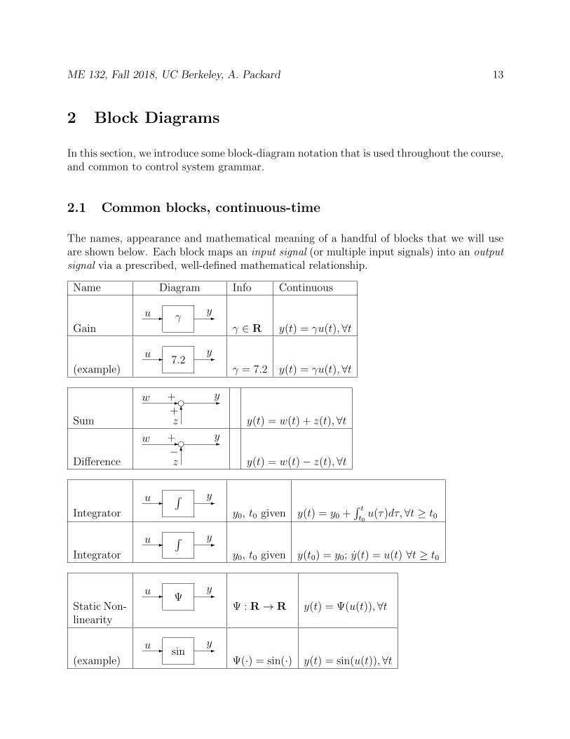
The names, appearance and mathematical meaning of a handful of blocks that we will useare shown below. Each block maps an input signal (or multiple input signals) into an outputsignal via a prescribed, well-defined mathematical relationship.
Name Diagram Info Continuous
Gainγ- -u y
γ ∈ R y(t) = γu(t), ∀t
(example)7.2- -u y
γ = 7.2 y(t) = γu(t), ∀t
Sum
- e -
6
+
+w
z
y
y(t) = w(t) + z(t),∀t
Difference
- e -
6
+
−w
z
y
y(t) = w(t)− z(t),∀t
Integrator
∫- -u y
y0, t0 given y(t) = y0 +∫ tt0u(τ)dτ, ∀t ≥ t0
Integrator
∫- -u y
y0, t0 given y(t0) = y0; y(t) = u(t) ∀t ≥ t0
Static Non-linearity
Ψ- -u y
Ψ : R→ R y(t) = Ψ(u(t)),∀t
(example)sin- -u y
Ψ(·) = sin(·) y(t) = sin(u(t)), ∀t

ME 132, Fall 2018, UC Berkeley, A. Packard 14
Delaydelay, T- -u y
T ≥ 0 y(t) = u(t− T ), ∀t
2.2 Example
Consider a toy model of a stick/rocket balancing problem, as shown below.
BBBBBBBB
-d
-u
θ)
Imagine the stick is supported at it’s base, by a force approximately equal to it’s weight.This force is not shown. A sideways force can act at the base as well, this is denoted by u,and a sideways force can act at the top, denoted by d.
This is similar to the dynamic instabilities of a rocket, just after launch, when the velocity isquite slow, and the only dominant forces/moments are from gravity and the engine thrust:
1. The large thrust of the rocket engines essentially cancels the gravitational force, andthe rocket is effectively “balanced” in a vertical position;
2. If the rocket rotates away from vertical (for example, a positive θ), then the mo-ment/torque about the bottom end causes θ to increase;
3. The vertical force of the rocket engines can be “steered” from side-to-side by powerfulmotors which move the rocket nozzles a small amount, generating a horizontal force(represented by u) which induces a torque, and causes θ to change;
4. Winds (and slight imbalances in the rocket structure itself) act as disturbance torques(represented by d) which must be compensated for;
So, without a control system to use u to balance the rocket, it would tip over.
For the purposes of this example, the differential equation “governing” the angle-of-orientationis taken to be
θ(t) = θ(t) + u(t)− d(t).
ME 132, Fall 2018, UC Berkeley, A. Packard 15
where θ is the angle-of-orientation, u is the horizontal control force applied at the base, andd is the horizontal disturbance force applied at the tip. Remark: This is not the correctequation, as Newton’s laws would correctly involve the 2nd derivative, θ andterms with cos θ, sin θ, θ2 and so on. However this simple model does yield an interestingunstable system (positive θ contributes to a positive θ; negative θ contributes to a negativeθ) which can be controlled with proportional control. As an exercise, try balancing a stickor ruler in your hand (or better yet, on the tip of your finger).
Here, using a simple Matlab code, we will see the effect of a simple proportional feedbackcontrol strategy
u(t) = 5 [θdes(t)− θ(t)] .
This will result in a stable system, with a steerable rocket trajectory (the actual rocketinclination angle θ(t) will generally track the reference inclination angle θdes(t)). Interestingly,although the strategy for u is very simple, the actual signal u(t) as a function of t is somewhatcomplex, for instance, when the conditions are: θ(0) = 0, θdes(t) = 0 for 0 ≤ t ≤ 2, θdes(t) = 1for 2 < t, and d(t) = 0 for 0 ≤ t ≤ 6, d(t) = −0.6 for 6 < t. The Matlab files, and associatedplots are shown at the end of this section, after Section 2.4.
Depending on your point-of-view, the resulting u(t), and it’s affect on θ might seem almostmagical to have arisen from such a simple proportional control strategy. This is a greatillustration of the power of feedback.
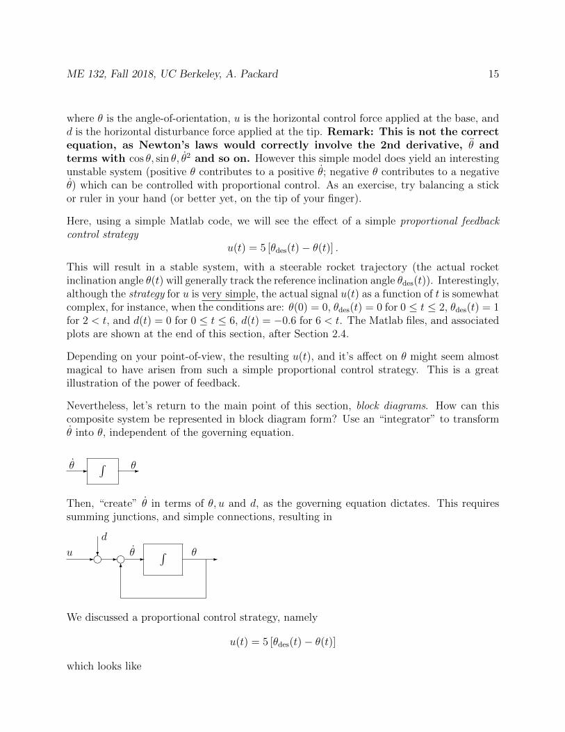
Nevertheless, let’s return to the main point of this section, block diagrams. How can thiscomposite system be represented in block diagram form? Use an “integrator” to transformθ into θ, independent of the governing equation.
∫- -θ θ
Then, “create” θ in terms of θ, u and d, as the governing equation dictates. This requiressumming junctions, and simple connections, resulting in
- - - -∫
6
g g?u
d
θ θ
We discussed a proportional control strategy, namely
u(t) = 5 [θdes(t)− θ(t)]
which looks like

ME 132, Fall 2018, UC Berkeley, A. Packard 16
- e -
6
+
−θdes
θ
5 -u
Putting these together yields the closed-loop system. See problem 1 in Section 2.4 for anextension to a proportional-integral control strategy.
2.3 Summary
It is important to remember that while the governing equations are almost always written asdifferential equations, the detailed block diagrams almost always are drawn with integrators(and not differentiators). This is because of the mathematical equivalence shown in theIntegrator entry in the table in section 2.1. Using integrators to represent the relationship,the figure conveys how the derivative of some variable, say x is a consequence of the valuesof other variables. Then, the values of x evolve simply through the “running integration” ofthis quantity.

ME 132, Fall 2018, UC Berkeley, A. Packard 17
2.4 Problems
1. This question extends the example we discussed in class. Recall that the process wasgoverned by the differential equation
θ(t) = θ(t) + u(t)− d(t).
The proportional control strategy u(t) = 5 [θdes(t)− θ(t)] did a good job, but there wasroom for improvement. Consider the following strategy
u(t) = p(t) + a(t)p(t) = Ke(t)a(t) = Le(t) (with a(0) = 0)e(t) = θdes(t)− θmeas(t)
where K and L are constants. Note that the control action is made up of two termsp and a. The term p is proportional to the error, while term a’s rate-of-change isproportional to the error.
(a) Convince yourself (and me) that a block diagram for this strategy is as below (allmissing signs on summing junctions are + signs). Note: There is one minor issueyou need to consider - exchanging the order of differentiation with multiplicationby a constant...
∫L
K
f f- - - - -
-
?θdes
6
θmeas
u
−
(b) Create a Simulink model of the closed-loop system (ie., process and controller,hooked up) using this new strategy. The step functions for θdes and d should benamely
θdes(t) =0 for t ≤ 11 for 1 < t ≤ 71.4 for t > 7
, d(t) =0 for t ≤ 6−0.4 for 6 < t ≤ 110 for t > 11
Make the measurement perfect, so that θmeas = θ.
(c) Simulate the closed-loop system for K = 5, L = 9. The initial condition for θshould be θ(0) = 0. On three separate axis (using subplot, stacked vertically,all with identical time-axis so they can be “lined” up for clarity) plot θdes and dversus t; θ versus t; and u versus t.
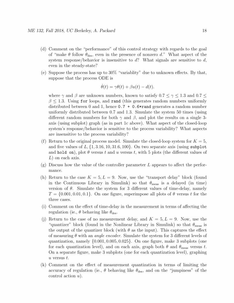
ME 132, Fall 2018, UC Berkeley, A. Packard 18
(d) Comment on the “performance” of this control strategy with regards to the goalof “make θ follow θdes, even in the presence of nonzero d.” What aspect of thesystem response/behavior is insensitive to d? What signals are sensitive to d,even in the steady-state?
(e) Suppose the process has up to 30% “variablity” due to unknown effects. By that,suppose that the process ODE is
θ(t) = γθ(t) + βu(t)− d(t).
where γ and β are unknown numbers, known to satisfy 0.7 ≤ γ ≤ 1.3 and 0.7 ≤β ≤ 1.3. Using for loops, and rand (this generates random numbers uniformlydistributed between 0 and 1, hence 0.7 + 0.6*rand generates a random numberuniformly distributed between 0.7 and 1.3. Simulate the system 50 times (usingdifferent random numbers for both γ and β, and plot the results on a single 3-axis (using subplot) graph (as in part 1c above). What aspect of the closed-loopsystem’s response/behavior is sensitive to the process variability? What aspectsare insensitive to the process variability?
(f) Return to the original process model. Simulate the closed-loop system for K = 5,and five values of L, 1, 3.16, 10, 31.6, 100. On two separate axis (using subplot
and hold on), plot θ versus t and u versus t, with 5 plots (the different values ofL) on each axis.
(g) Discuss how the value of the controller parameter L appears to affect the perfor-mance.
(h) Return to the case K = 5, L = 9. Now, use the “transport delay” block (foundin the Continuous Library in Simulink) so that θmeas is a delayed (in time)version of θ. Simulate the system for 3 different values of time-delay, namelyT = 0.001, 0.01, 0.1. On one figure, superimpose all plots of θ versus t for thethree cases.
(i) Comment on the effect of time-delay in the measurement in terms of affecting theregulation (ie., θ behaving like θdes.
(j) Return to the case of no measurement delay, and K = 5, L = 9. Now, use the“quantizer” block (found in the Nonlinear Library in Simulink) so that θmeas isthe output of the quantizer block (with θ as the input). This captures the effectof measuring θ with an angle encoder. Simulate the system for 3 different levels ofquantization, namely 0.001, 0.005, 0.025. On one figure, make 3 subplots (onefor each quantization level), and on each axis, graph both θ and θmeas versus t.On a separate figure, make 3 subplots (one for each quantization level), graphingu versus t.
(k) Comment on the effect of measurement quantization in terms of limiting theaccuracy of regulation (ie., θ behaving like θdes, and on the “jumpiness” of thecontrol action u).
ME 132, Fall 2018, UC Berkeley, A. Packard 19
NOTE: All of the computer work (parts 1c, 1e, 1f, 1h and 1j) should be automatedin a single, modestly documented script file. Turn in a printout of your Simulinkdiagrams (3 of them), and a printout of the script file. Also include nicely formattedfigure printouts, and any derivations/comments that are requested in the problemstatement.
ME 132, Fall 2018, UC Berkeley, A. Packard 24
3 Mathematical Modeling and Simulation
3.1 Systems of 1st order, coupled differential equations
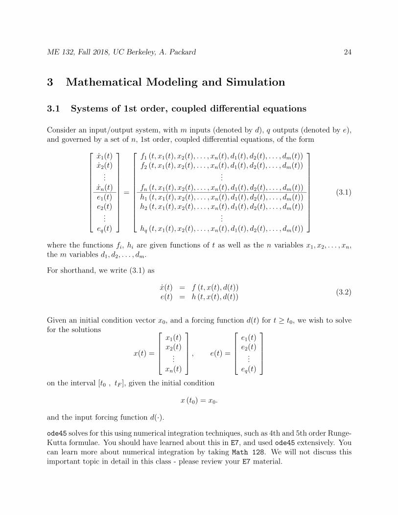
Consider an input/output system, with m inputs (denoted by d), q outputs (denoted by e),and governed by a set of n, 1st order, coupled differential equations, of the form
x1(t)x2(t)
...xn(t)e1(t)e2(t)
...eq(t)
=
f1 (t, x1(t), x2(t), . . . , xn(t), d1(t), d2(t), . . . , dm(t))f2 (t, x1(t), x2(t), . . . , xn(t), d1(t), d2(t), . . . , dm(t))
...fn (t, x1(t), x2(t), . . . , xn(t), d1(t), d2(t), . . . , dm(t))h1 (t, x1(t), x2(t), . . . , xn(t), d1(t), d2(t), . . . , dm(t))h2 (t, x1(t), x2(t), . . . , xn(t), d1(t), d2(t), . . . , dm(t))
...hq (t, x1(t), x2(t), . . . , xn(t), d1(t), d2(t), . . . , dm(t))
(3.1)
where the functions fi, hi are given functions of t as well as the n variables x1, x2, . . . , xn,the m variables d1, d2, . . . , dm.
For shorthand, we write (3.1) as
x(t) = f (t, x(t), d(t))e(t) = h (t, x(t), d(t))
(3.2)
Given an initial condition vector x0, and a forcing function d(t) for t ≥ t0, we wish to solvefor the solutions
x(t) =
x1(t)x2(t)
...xn(t)
, e(t) =
e1(t)e2(t)
...eq(t)
on the interval [t0 , tF ], given the initial condition
x (t0) = x0.
and the input forcing function d(·).
ode45 solves for this using numerical integration techniques, such as 4th and 5th order Runge-Kutta formulae. You should have learned about this in E7, and used ode45 extensively. Youcan learn more about numerical integration by taking Math 128. We will not discuss thisimportant topic in detail in this class - please review your E7 material.
ME 132, Fall 2018, UC Berkeley, A. Packard 25
Remark: The GSI will give 2 interactive discussion sections on how to use Simulink, agraphical-based tool to easily build and numerically solve ODE models by interconnectingindividual components, each of which are governed by ODE models. Simulink is part ofMatlab, and is available on the computers in Etcheverry. The Student Version of Matlabalso comes with Simulink (and the Control System Toolbox). The Matlab license from theUC Berkeley software licensing arrangement has both Simulink (and the Control SystemToolbox included.
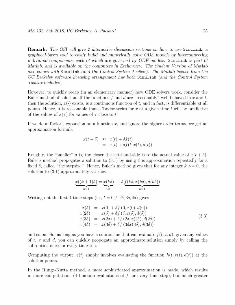
However, to quickly recap (in an elementary manner) how ODE solvers work, consider theEuler method of solution. If the functions f and d are “reasonably” well behaved in x and t,then the solution, x(·) exists, is a continuous function of t, and in fact, is differentiable at allpoints. Hence, it is reasonable that a Taylor series for x at a given time t will be predictiveof the values of x(τ) for values of τ close to t.
If we do a Taylor’s expansion on a function x, and ignore the higher order terms, we get anapproximation formula
x(t+ δ) ≈ x(t) + δx(t)= x(t) + δf(t, x(t), d(t))
Roughly, the “smaller” δ is, the closer the left-hand-side is to the actual value of x(t + δ).Euler’s method propogates a solution to (3.1) by using this approximation repeatedly for afixed δ, called “the stepsize.” Hence, Euler’s method gives that for any integer k >= 0, thesolution to (3.1) approximately satisfies
x((k + 1)δ)︸ ︷︷ ︸n×1
= x(kδ)︸ ︷︷ ︸n×1
+ δ f(kδ, x(kδ), d(kδ))︸ ︷︷ ︸n×1
Writing out the first 4 time steps (ie., t = 0, δ, 2δ, 3δ, 4δ) gives
x(δ) = x(0) + δf (0, x(0), d(0))x(2δ) = x(δ) + δf (δ, x(δ), d(δ))x(3δ) = x(2δ) + δf (2δ, x(2δ), d(2δ))x(4δ) = x(3δ) + δf (3δx(3δ), d(3δ))
(3.3)
and so on. So, as long as you have a subroutine that can evaluate f(t, x, d), given any valuesof t, x and d, you can quickly propogate an approximate solution simply by calling thesubroutine once for every timestep.
Computing the output, e(t) simply involves evaluating the function h(t, x(t), d(t)) at thesolution points.
In the Runge-Kutta method, a more sophisticated approximation is made, which resultsin more computations (4 function evaluations of f for every time step), but much greater
ME 132, Fall 2018, UC Berkeley, A. Packard 26
accuracy. In effect, more terms of the Taylor series are used, involving matrices of partialderivatives, and even their derivatives,
df
dx,d2f
dx2,d3f
dx3
but without actually requiring explicit knowledge of these derivatives of the function f .
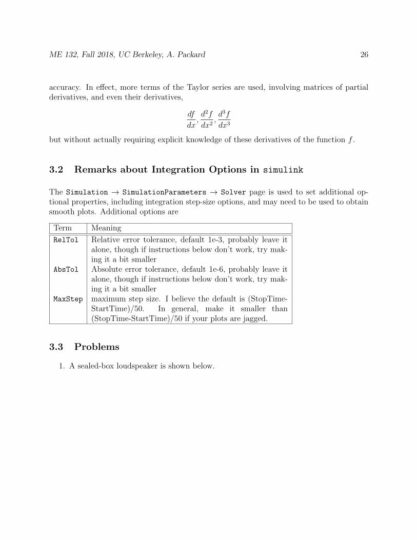
3.2 Remarks about Integration Options in simulink
The Simulation → SimulationParameters → Solver page is used to set additional op-tional properties, including integration step-size options, and may need to be used to obtainsmooth plots. Additional options are
Term Meaning
RelTol Relative error tolerance, default 1e-3, probably leave italone, though if instructions below don’t work, try mak-ing it a bit smaller
AbsTol Absolute error tolerance, default 1e-6, probably leave italone, though if instructions below don’t work, try mak-ing it a bit smaller
MaxStep maximum step size. I believe the default is (StopTime-StartTime)/50. In general, make it smaller than(StopTime-StartTime)/50 if your plots are jagged.
3.3 Problems
1. A sealed-box loudspeaker is shown below.

ME 132, Fall 2018, UC Berkeley, A. Packard 27
Voice CoilFormer
Subwoofer Electrical LeadsBasket
Sealed Enclosure
From Amplifier
Spider
Surround
Vent
Back Plate
Top Plate
Magnet
Pole Piece
Voice Coil
Woofer Cone
Dust Cap
Signal From Accelerometer
Ignore the wire marked “accelerometer mounted on cone.” We will develop a modelfor accoustic radiation from a sealed-box loudspeaker.
The equations are
• Speaker Cone: force balance,
mz(t) = Fvc(t) + Fk(t) + Fd(t) + Fb + Fenv(t)
• Voice-coil motor (a DC motor):
Vin(t)− LI(t)−RI(t)−Bl(t)z(t) = 0Fvc(t) = Bl(t)I(t)
• Magnetic flux/Length Factor:
Bl(t) =BL0
1 +BL1z(t)4
• Suspension/Surround:
Fk(t) = −K0z(t)−K1z2(t)−K2z
3(t)Fd(t) = −RS z(t)
• Sealed Enclosure:
Fb(t) = P0A
(1 +
Az(t)
V0
)−γ• Environment (Baffled Half-Space)
x(t) = Aex(t) +Bez(t)Fenv(t) = −AP0 − Cex(t)−Dez(t)
ME 132, Fall 2018, UC Berkeley, A. Packard 28
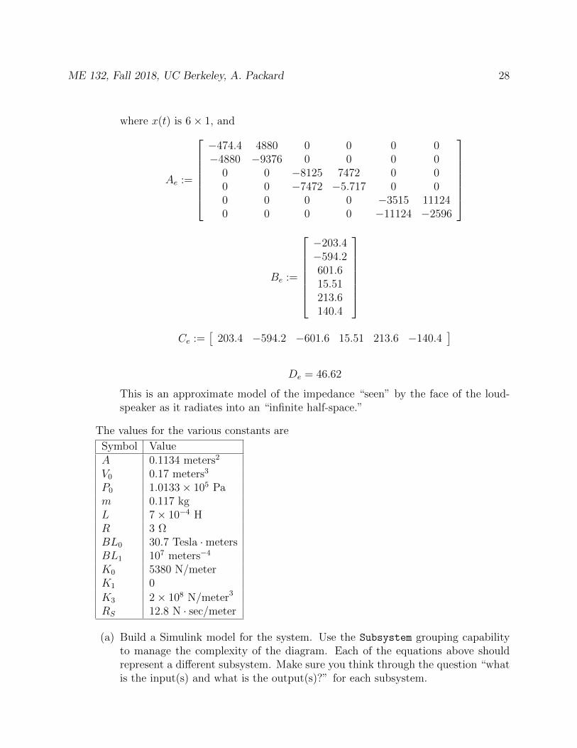
where x(t) is 6× 1, and
Ae :=
−474.4 4880 0 0 0 0−4880 −9376 0 0 0 0
0 0 −8125 7472 0 00 0 −7472 −5.717 0 00 0 0 0 −3515 111240 0 0 0 −11124 −2596
Be :=
−203.4−594.2601.615.51213.6140.4
Ce :=
[203.4 −594.2 −601.6 15.51 213.6 −140.4
]De = 46.62
This is an approximate model of the impedance “seen” by the face of the loud-speaker as it radiates into an “infinite half-space.”
The values for the various constants are
Symbol ValueA 0.1134 meters2
V0 0.17 meters3
P0 1.0133× 10⁵ Pam 0.117 kgL 7× 10⁻⁴ HR 3 ΩBL0 30.7 Tesla ·metersBL1 107 meters−4
K0 5380 N/meterK1 0
K3 2× 10⁸ N/meter3
RS 12.8 N · sec/meter
(a) Build a Simulink model for the system. Use the Subsystem grouping capabilityto manage the complexity of the diagram. Each of the equations above shouldrepresent a different subsystem. Make sure you think through the question “whatis the input(s) and what is the output(s)?” for each subsystem.
ME 132, Fall 2018, UC Berkeley, A. Packard 29
(b) Write a function that has two input arguments (denoted V and Ω) and two outputarguments, zmax,pos and zmax,neg. The functional relationship is defined as follows:Suppose Vin(t) = V sin Ω · 2πt, where t is in seconds, and V in volts. In otherwords, the input is a sin-wave at a frequency of Ω Hertz. Simulate the loudspeakerbehavior for about 25/Ω seconds. The displacement z of the cone will becomenearly sinusoidal by the end of the simulation. Let zmax,pos and zmax,neg be themaximum positive and negative values of the displacement in the last full cycle(i.e., the last 1/Ω seconds of the simulation, which we will approximately decreeas the “steady-state response to the input”).
(c) Using bisection, determine the value (approximately) of V so that the steady-state maximum (positive) excursion of z is 0.007meters if the frequency of theexcitation is Ω = 25. What is the steady-state minimum (negative) excursion ofz?
ME 132, Fall 2018, UC Berkeley, A. Packard 30
4 State Variables
See the appendix for additional examples on mathematical modeling of systems.
4.1 Definition of State
For any system (mechanical, electrical, electromechanical, economic, biological, acoustic,thermodynamic, etc.) a collection of variables q1, q2, . . . , qn are called state variables, if theknowledge of
• the values of these variables at time t0, and
• the external inputs acting on the system for all time t ≥ t0, and
• all equations describing relationships between the variables qi and the external inputs
is enough to determine the value of the variables q1, q2, . . . , qn for all t ≥ t0.
In other words, past history (before t0) of the system’s evolution is not important in de-termining its evolution beyond t0 – all of the relevant past information is embedded in thevariables value’s at t0.
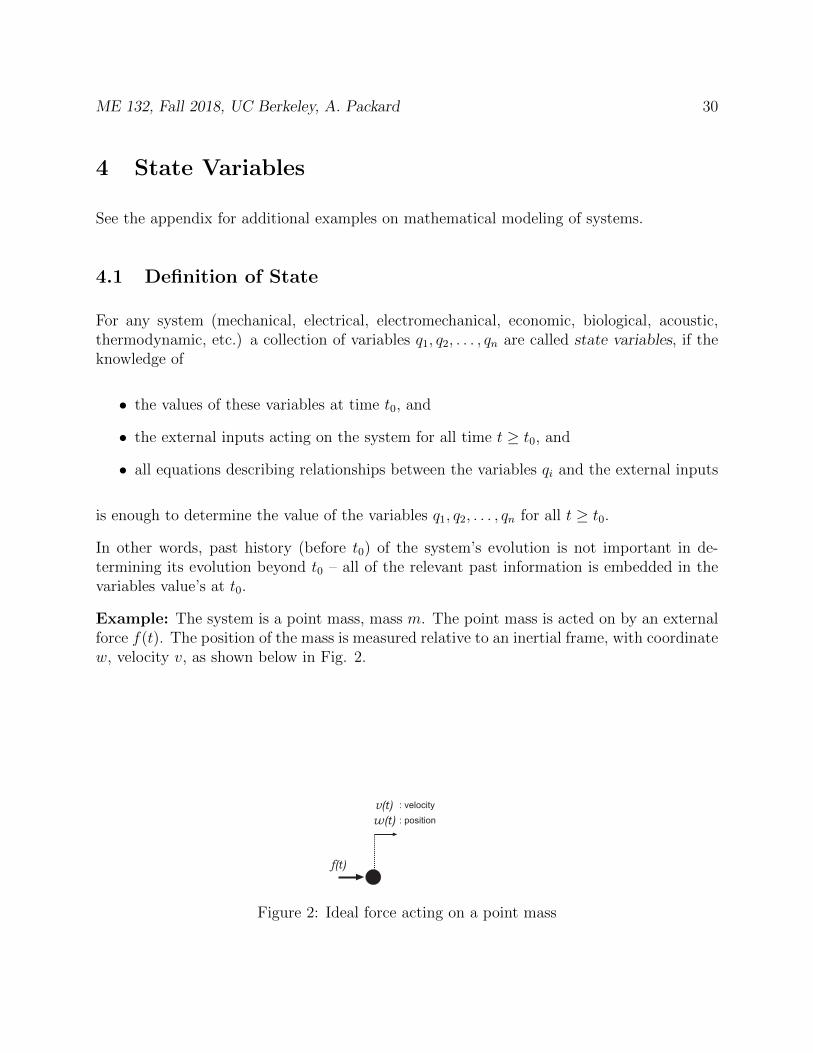
Example: The system is a point mass, mass m. The point mass is acted on by an externalforce f(t). The position of the mass is measured relative to an inertial frame, with coordinatew, velocity v, as shown below in Fig. 2.
Figure 2: Ideal force acting on a point mass
ME 132, Fall 2018, UC Berkeley, A. Packard 31
Claim #1: The collection w is not a suitable choice for state variables. Why? Note thatfor t ≥ t0, we have
w(t) = w(t0) +
∫ t
t0
[v(t0) +
∫ τ
t0
1
mf(η)dη
]dτ
Hence, in order to determine w(t) for all t ≥ t0, it is not sufficient to know w(t0) and theentire function f(t) for all t ≥ t0. You also need to know the value of v(t0).
Claim #2: The collection v is a legitimate choice for state variables. Why? Note thatfor t ≥ t0, we have
v(t) = v(t0) +
∫ t
t0
1
mf(τ)dτ
Hence, in order to determine v(t) for all t ≥ t0, it is sufficient to know v(t0) and the entirefunction f(t) for all t ≥ t0.
Claim #3: The collection w, v is a legitimate choice for state variables. Why? Note thatfor t ≥ t0, we have
w(t) = w(t0) +∫ tt0v(η)dη
v(t) = v(t0) +∫ tt0
1mf(τ)dτ
Hence, in order to determine v(t) for all t ≥ t0, it is sufficient to know v(t0) and the entirefunction f(t) for all t ≥ t0.
In general, it is not too hard to pick a set of state-variables for a system. The next fewsections explains some rule-of-thumb procedures for making such a choice.
4.2 State-variables: from first order evolution equations
Suppose for a system we choose some variables (x1, x2, . . . , xn) as a possible choice of statevariables. Let d1, d2, . . . , df denote all of the external influences (ie., forcing functions) actingon the system. Suppose we can derive the relationship between the x and d variables in theform
x1 = f1 (t, x1(t), x2(t), . . . , xn(t), d1(t), . . . , df (t))x2 = f2 (t, x1(t), x2(t), . . . , xn(t), d1(t), . . . , df (t))
......
xn = fn (t, x1(t), x2(t), . . . , xn(t), d1(t), . . . , df (t))
(4.1)
Then, the set x1, x2, . . . , xn is a suitable choice of state variables. Why? Ordinary differ-ential equation (ODE) theory tells us that given
• an initial condition x(t0) := x0, and
• the forcing function d(t) for t ≥ t0,
ME 132, Fall 2018, UC Berkeley, A. Packard 32
there is a unique solution x(t) which satisfies the initial condition at t = t0, and satisfies thedifferential equations for t ≥ t0. Hence, the set x1, x2, . . . , xn constitutes a state-variabledescription of the system.
The equations in (4.1) are called the state equations for the system.
4.3 State-variables: from a block diagram
Given a block diagram, consisting of an interconnection of
• integrators,
• gains, and
• static-nonlinear functions,
driven by external inputs d1, d2, . . . , df , a suitable choice for the states is
• the output of each and every integrator
Why? Note that
• if the outputs of all of the integrators are labled x1, x2, . . . , xn, then the inputs to theintegrators are actually x1, x2, . . . , xn.
• The interconnection of all of the base components (integrators, gains, static nonlinearfunctions) implies that each xk(t) will be a function of the values of x1(t), x2(t), . . . , xn(t)along with d1(t), d2(t), . . . , df (t).
• This puts the equations in the form of (4.1).
We have already determined that that form implies that the variables are state variables.
4.4 Problems
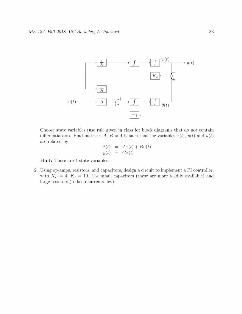
1. Shown below is a block diagram of a DC motor connected to an load inertia via aflexible shaft. The flexible shaft is modeled as a rigid shaft (inertia J1) inside themotor, a massless torsional spring (torsional spring constant Ks) which connects tothe load inertia J2. θ is the angular position of the shaft inside the motor, and ψ isthe angular position of the load inertia.
ME 132, Fall 2018, UC Berkeley, A. Packard 33
−γ
β∫ ∫
−1J1
Ks
1J2
∫ ∫
- - - -
6
6
-
?
- - - -
?
e
e
u(t)
y(t)
−+
++ +
θ(t)
ψ(t)
Choose state variables (use rule given in class for block diagrams that do not containdifferentiators). Find matrices A, B and C such that the variables x(t), y(t) and u(t)are related by
x(t) = Ax(t) +Bu(t)y(t) = Cx(t)
Hint: There are 4 state variables.
2. Using op-amps, resistors, and capacitors, design a circuit to implement a PI controller,with KP = 4, KI = 10. Use small capacitors (these are more readily available) andlarge resistors (to keep currents low).

ME 132, Fall 2018, UC Berkeley, A. Packard 34
5 First Order, Linear, Time-Invariant (LTI) ODE
5.1 The Big Picture
We shall study mathematical models described by linear time-invariant input-output differ-ential equations. There are two general forms of such a model. One is a single, high-orderdifferential equation to describe the relationship between the input u and output y, of theform
y[n](t)+a1y[n−1](t)+ · · ·+an−1y(t)+any(t) = b0u
[m](t)+ b1u[m−1](t)+ · · ·+ bm−1u(t)+ bmu(t)
(5.1)
where y[k] denotes the kth derivative of the signal y(t): dky(t)dtk
. These notes refer to equation(5.1) as a HLODE (High-order, Linear Ordinary Differential Equation).
An alternate form involves many first-order equations, and many inputs. The general caseof this situation has n dependent variables, x1, x2, . . . , xn, and m inputs, d1, d2, . . . , dm. Thedifferential equations governing the evolution of the xi variables is
x1(t) = a11x1(t) + a12x2(t) + · · ·+ a1nxn(t) + b11d1(t) + b12d2(t) . . .+ b1mdm(t)x2(t) = a21x1(t) + a22x2(t) + · · ·+ a2nxn(t) + b21d1(t) + b22d2(t) . . .+ b2mdm(t)
... =...
xn(t) = an1x1(t) + an2x2(t) + · · ·+ annxn(t) + bn1d1(t) + bn2d2(t) . . .+ bnmdm(t)
We will learn how to solve these differential equations, and more importantly, we will discoverhow to make broad qualitative statements about these solutions. Much of our intuitionabout control system design and its limitations will be drawn from our understanding of thebehavior of these types of equations.
A great many models of physical processes that we may be interested in controlling are notlinear, as above. Nevertheless, as we shall see much later, the study of linear systems is avital tool in learning how to control even nonlinear systems. Essentially, feedback controlalgorithms make small adjustments to the inputs based on measured outputs. For smalldeviations of the input about some nominal input trajectory, the output of a nonlinearsystem looks like a small deviation around some nominal output. The effects of the smallinput deviations on the output is well approximated by a linear (possibly time-varying)system. It is therefore essential to undertake a study of linear systems.
In this section, we review the solutions of linear, first-order differential equations with con-stant coefficients and time-dependent forcing functions. The concepts of
• stability
ME 132, Fall 2018, UC Berkeley, A. Packard 35
• time-constant
• sinusoidal steady-state
• frequency response functions
are introduced. A significant portion of the remainder of the course generalizes these tohigher order, linear ODEs, with emphasis on applying these concepts to the analysis anddesign of feedback systems.
5.2 Solution of a First Order LTI ODE
Consider the following system
x(t) = a x(t) + b u(t) (5.2)
where u is the input, x is the dependent variable, and a and b are constant coefficients(ie., numbers). For example, the equation 6x(t) + 3x(t) = u(t) can be manipulated intox(t) = −1
2x(t)+ 1
6u(t). Given the initial condition x(0) = x0 and an arbitrary input function
u(t) defined for t ∈ [0,∞), a solution of Eq. (5.2) must satisfy
xs(t) = eat x0︸ ︷︷ ︸free resp.
+
∫ t
0
ea(t−τ) b u(τ) dτ︸ ︷︷ ︸forced resp.
. (5.3)
You should derive this with the integrating factor method (problem 1). Also note thatthe derivation makes it evident that given the initial condition and forcing function,there is at most one solution to the ODE. In other words, if solutions to the ODEexist, they are unique, once the initial condition and forcing function are specified.
We can also easily just check that (5.3) is indeed the solution of (5.2) by verifying two facts:the function xs satisfies the differential equation for all t ≥ 0; and xs satisfies the giveninitial condition at t = 0. In fact, the theory of differential equations tells us that there isone and only one function that satisfies both (existence and uniqueness of solutions). Forthis ODE, we can prove this directly, for completeness sake. Above, we showed that if xsatisfies (5.2), then it must be of the form in (5.3). Next we show that the function in (5.3)does indeed satisfy the differential equation (and initial condition). First check the value ofxs(t) at t = 0:
xs(0) = ea0 x0 +
∫ 0
0
ea(t−τ) b u(τ) dτ = x0 .

ME 132, Fall 2018, UC Berkeley, A. Packard 36
Taking the time derivative of (5.3) we obtain
xs(t) = a eat x0 +d
dt
eat∫ t
0
e−aτ b u(τ) dτ
= a eat x0 + a eat
∫ t
0
e−aτ b u(τ) dτ︸ ︷︷ ︸axs(t)
+eate−at b u(t)
= a xs(t) + b u(t) .
as desired.
5.2.1 Free response
Fig. 3 shows the normalized free response (i.e. u(t) = 0) of the solution Eq. (5.3) of ODE(5.2) when a < 0. Since a < 0, the free response decays to 0 as t → ∞, regardless of the
0 0.5 1 1.5 2 2.5 3 3.5 4 4.5 50
0.1
0.2
0.3
0.4
0.5
0.6
0.7
0.8
0.9
1
Nor
mal
ized
Sta
te [x
/xo]
Normalized Time [t/|a|]
Figure 3: Normalized Free response of first order system (a < 0)
initial condition. Because of this (and a few more properties that will be derived in upcomingsections), if a < 0, the system in eq. (5.2) is called stable (or sometimes, to be more precise,asymptotically stable). Notice that the slope at time t = 0 is x(0) = ax0 and T = 1/|a| isthe time that x(t) would cross 0 if the initial slope is continued, as shown in the figure. Thetime
T :=1
|a|
ME 132, Fall 2018, UC Berkeley, A. Packard 37
is called the time constant of a first order asymptotically stable system (a < 0). T isexpressed in the units of time, and is an indication of how fast the system responds. Thelarger |a|, the smaller T and the faster the response of the system.
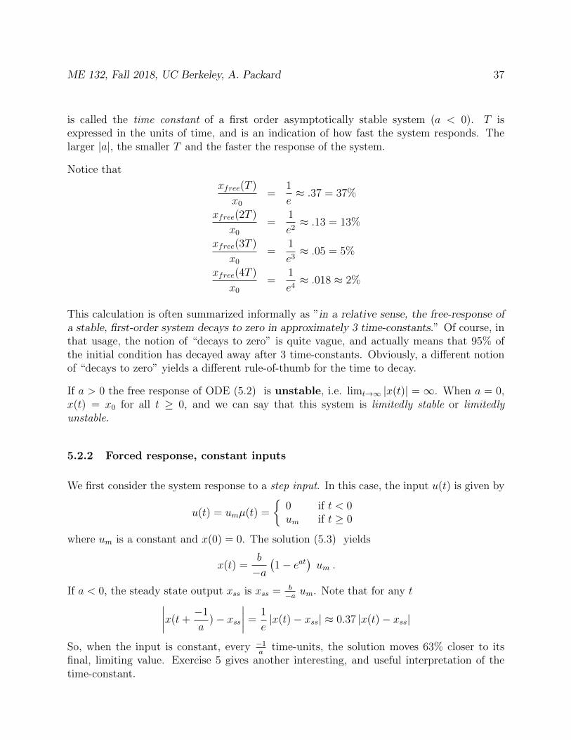
Notice that
xfree(T )
x0
=1
e≈ .37 = 37%
xfree(2T )
x0
=1
e2≈ .13 = 13%
xfree(3T )
x0
=1
e3≈ .05 = 5%
xfree(4T )
x0
=1
e4≈ .018 ≈ 2%
This calculation is often summarized informally as ”in a relative sense, the free-response ofa stable, first-order system decays to zero in approximately 3 time-constants.” Of course, inthat usage, the notion of “decays to zero” is quite vague, and actually means that 95% ofthe initial condition has decayed away after 3 time-constants. Obviously, a different notionof “decays to zero” yields a different rule-of-thumb for the time to decay.
If a > 0 the free response of ODE (5.2) is unstable, i.e. limt→∞ |x(t)| = ∞. When a = 0,x(t) = x0 for all t ≥ 0, and we can say that this system is limitedly stable or limitedlyunstable.
5.2.2 Forced response, constant inputs
We first consider the system response to a step input. In this case, the input u(t) is given by
u(t) = umµ(t) =
0 if t < 0um if t ≥ 0
where um is a constant and x(0) = 0. The solution (5.3) yields
x(t) =b
−a(1− eat
)um .
If a < 0, the steady state output xss is xss = b−a um. Note that for any t∣∣∣∣x(t+
−1
a)− xss
∣∣∣∣ =1
e|x(t)− xss| ≈ 0.37 |x(t)− xss|
So, when the input is constant, every −1a
time-units, the solution moves 63% closer to itsfinal, limiting value. Exercise 5 gives another interesting, and useful interpretation of thetime-constant.

ME 132, Fall 2018, UC Berkeley, A. Packard 38
5.2.3 Forced response, bounded inputs
Rather than consider constant inputs, we can also consider inputs that are bounded by aconstant, and prove, under the assumption of stability, that the response remains boundedas well (and the bound is a linear function of the input bound). Specifically, if a < 0, andif u(t) is uniformly (in time) bounded by a positive number M , then the resulting solutionx(t) will be uniformly bounded by bM
|a| . To derive this, suppose that |u(τ)| ≤M for all τ ≥ 0.Then for any t ≥ 0, we have
|x(t)| =
∣∣∣∣∫ t
0
ea(t−τ) b u(τ) dτ
∣∣∣∣≤
∫ t
0
∣∣ea(t−τ) b u(τ)∣∣ dτ
≤∫ t
0
ea(t−τ) b M dτ
≤ bM
−a(1− eat
)≤ bM
−a.
Thus, if a < 0, x(0) = 0 and u(t) ≤ M , the output is bounded by x(t) ≤ |bM/a|. This iscalled a bounded-input, bounded-output (BIBO) system. If the initial condition is non-zero,the output x(t) will still be bounded since the magnitude of the free response monotonicallyconverges to zero, and the response x(t) is simply the sum of the free and forced responses.Note: Assuming b 6= 0, the system is not bounded-input/bounded-output when a ≥ 0. Inthat context, from now on, we will refer to the a = 0 case (termed limitedly stable or limitedlyunstable before) as unstable. See problem 6 in Section 5.6.
5.2.4 Stable system, Forced response, input approaching 0
Assume the system is stable, so a < 0. Now, suppose the input signal u is bounded andapproaches 0 as t → ∞. It seems natural that the response, x(t) should also approach 0as t → ∞, and deriving this fact is the purpose of this section. While the derivationis interesting, the most important is the result: For a stable system, specifically(5.2), with a < 0, if the input u satisfies limt→∞ u(t) = 0, then the solution x satisfieslimt→∞ x(t) = 0.
Onto the derivation: First, recall what limt→∞ z(t) = 0 means: for any ε > 0, there is aTε > 0 such that for all t > Tε, |z(t)| < ε.
ME 132, Fall 2018, UC Berkeley, A. Packard 39
Next, note that for any t > 0 and a 6= 0,∫ t
0
ea(t−τ)dτ = −1
a
(1− eat
)If a < 0, then for all t ≥ 0,∫ t
0
ea(t−τ)dτ =
∫ t
0
eaτdτ ≤∫ ∞
0
eaτdτ = −1
a=
1
|a|
Assume x0 is given, and consider such an input. Since u is bounded, there is a positiveconstant B such that |u(t)| ≤ B for all t ≥ 0. Also, for every ε > 0, there is
• a Tε,1 > 0 such that |u(t)| < ε3|a||b| for all t ≥ Tε,1
2
• a Tε,2 > 0 such that eat2 < |a|ε
3B|b| for all t ≥ Tε,22
• a Tε,3 > 0 such that eat < ε3|x0| for all t ≥ Tε,3
Let Tε be the maximum of Tε,1, Tε,2, Tε,3. For t > Tε, the response x(t) satisfies
x(t) = eatx0 +∫ t
0ea(t−τ)bu(τ)dτ
= eatx0 +∫ t
2
0ea(t−τ)bu(τ)dτ +
∫ tt2ea(t−τ)bu(τ)dτ
We can use the information to bound each term individually, namely
1. Since t ≥ Tε,3 ∣∣eatx0
∣∣ ≤ ε
3|x0||x0| =
ε
3
2. Since |u(t)| ≤ B for all t,∣∣∣∫ t2
0ea(t−τ)bu(τ)dτ
∣∣∣ ≤ ∫ t2
0ea(t−τ) |bu(τ)| dτ
≤ B|b|∫ t
2
0ea(t−τ)dτ
= B|b| 1−ae
a t2
(1− ea t2
)≤ B|b| 1
−aea t2
Since t ≥ Tε,2, eat2 ≤ |a|ε
3B|b| , which implies∣∣∣∣∣∫ t
2
0
ea(t−τ)bu(τ)dτ
∣∣∣∣∣ < ε
3
ME 132, Fall 2018, UC Berkeley, A. Packard 40
3. Finally, since t ≥ Tε,1, the input |u(τ)| < ε3|a||b| for all τ ≥ t
2. This means∣∣∣∫ tt
2ea(t−τ)bu(τ)dτ
∣∣∣ < |b| ε3|a||b|
∫ tt2ea(t−τ)dτ
≤ |b| ε3|a||b|
∫ t0ea(t−τ)dτ
≤ |b| ε3|a||b|
1|a|
= ε3
Combining implies that for any t > Tε, |x(t)| < ε. Since ε was an arbitrary positive number,this complete the proof that limt→∞ x(t) = 0.
5.2.5 Linearity
Why is the differential equation in (5.2) called a linear differential equation? Suppose x1 isthe solution to the differential equation with the initial condition x0,1 and forcing function u1,and x2 is the solution to the differential equation with the initial condition x0,2 and forcingfunction u2. In other words, the function x1 satisfies x1(0) = x1,0 and for all t > 0,
x1(t) = ax1(t) + bu1(t).
Likewise, the function x2 satisfies x2(0) = x2,0 and for all t > 0,
x2(t) = ax2(t) + bu2(t).
Now take two constants α and β. What is the solution to the differential equation withinitial condition x(0) = αx0,1 +βx0,2, and forcing function u(t) = αu1(t) +βu2(t)? It is easy(just plug into the differential equation, or the integral form of the solution) to see that thesolution is
x(t) = αx1(t) + βx2(t)
This is often called the superposition property. In this class, we will more typically use theterm linear, indicating that the solution of the differential equation is a linear function ofthe (initial condition, forcing function) pair.
5.2.6 Forced response, input approaching a constant limit
If the system is stable (a < 0), and the input u(t) has a limit, limt→∞ u(t) = u, then bycombining the results of Sections 5.2.4, 5.2.2 and 5.2.5, it is easy to conclude that x(t)approaches a limit as well, namely
limt→∞
x(t) = − bau
ME 132, Fall 2018, UC Berkeley, A. Packard 41
An alternate manner to say this is that
x(t) = − bau+ q(t)
where limt→∞ q(t) = 0.
5.3 Forced response, Sinusoidal inputs
Consider the linear dynamical system
x(t) = Ax(t) +Bu(t)y(t) = Cx(t) +Du(t)
(5.4)
We assume that A,B,C and D are scalars (1× 1).
If the system is stable, (ie., A < 0) it might be “intuitively” clear that if u is a sinusoid, theny will approach a steady-state behavior that is sinusoidal, at the same frequency, but withdifferent amplitude and shifted in-time. In this section, we make this idea precise.
Take ω ≥ 0 as the input frequency, and (although not physically relevant) let u be a fixedcomplex number and take the input function u(t) to be
u(t) = uejωt
for t ≥ 0. Note that this is a complex-valued function of t. Then, the response is
x(t) = eAtx0 +∫ t
0eA(t−τ)Bu(τ)dτ
= eAtx0 + eAt∫ t
0e−AτBuejωτdτ
= eAtx0 + eAt∫ t
0e(jω−A)τdτBu
(5.5)
Now, since A < 0, regardless of ω, (jω − A) 6= 0, and we can solve the integral as
x(t) = eAt[x0 −
Bu
jω − A
]+
B
jω − Aejωt (5.6)
Hence, the output y(t) = Cx(t) +Du(t) would satisfy
y(t) = CeAt[x0 −
Bu
jω − A
]+
[D +
CB
jω − A
]uejωt
In the limit as t → ∞, the first term decays to 0 exponentially, leaving the steady-stateresponse
yss(t) =
[D +
CB
jω − A
]uejωt
ME 132, Fall 2018, UC Berkeley, A. Packard 42
Hence, we have verified our initial claim – if the input is a complex sinusoid, then the steady-state output is a complex sinusoid at the same exact frequency, but “amplified” by a complex
gain of[D + CB
jω−A
].
The function G(ω)
G(ω) := D +CB
jω − A(5.7)
is called the frequency response function of the system in (5.4). Hence, for stable, first-ordersystems, we have proven
u(t) := uejωt ⇒ yss(t) = G(ω)uejωt
G can be calculated rather easily using a computer, simply by evaluating the expression in(5.7) at a large number of frequency points ω ∈ R. The dependence on ω is often graphedusing two plots, namely
• log10 |G(ω)| versus log10(ω), and
• ∠G(ω) versus log10(ω).
This plotting arrangement is called a Bode plot, named after one of the modern-day giantsof control system theory, Hendrik Bode.
What is the meaning of a complex solution to the differential equation (5.4)? Suppose thatfunctions u, x and y are complex, and solve the ODE. Denote the real part of the functionu as uR, and the imaginary part as uI (similar for x and y). Then, for example, xR and xIare real-valued functions, and for all t x(t) = xR(t) + jxI(t). Differentiating gives
dx
dt=dxRdt
+ jdxIdt
Hence, if x, u and y satisfy the ODE, we have (dropping the (t) argument for clarity)
dxRdt
+ j dxIdt
= A (xR + jxI) +B (uR + juI)yR + jyI = C (xR + jxI) +D (uR + juI)
But the real and imaginary parts must be equal individually, so exploiting the fact that thecoefficients A,B,C and D are real numbers, we get
dxRdt
= AxR +BuRyR = CxR +DuR
anddxIdt
= AxI +BuIyI = CxI +DuI
ME 132, Fall 2018, UC Berkeley, A. Packard 43
Hence, if (u, x, y) are functions which satisfy the ODE, then both (uR, xR, yR) and (uI , xI , yI)also satisfy the ODE.
Finally, we need to do some trig/complex number calculations. Suppose that H ∈ C is notequal to zero. Recall that ∠H is the real number (unique to within an additive factor of 2π)which has the properties
cos∠H =ReH
|H|, sin∠H =
ImH
|H|
Then,Re(Hejθ
)= Re [(HR + jHI) (cos θ + j sin θ)]= HR cos θ −HI sin θ
= |H|[HR|H| cos θ − HI
|H| sin θ]
= |H| [cos∠H cos θ − sin∠H sin θ]= |H| cos (θ + ∠H)
Im(Hejθ
)= Im [(HR + jHI) (cos θ + j sin θ)]= HR sin θ +HI cos θ
= |H|[HR|H| sin θ + HI
|H| cos θ]
= |H| [cos∠H sin θ + sin∠H cos θ]= |H| sin (θ + ∠H)
Now consider the differential equation/frequency response case. Let G(ω) denote the fre-quency response function. If the input u(t) = cosωt = Re (ejωt), then the steady-stateoutput y will satisfy
y(t) = |G(ω)| cos (ωt+ ∠G(ω))
A similar calculation holds for sin, and these are summarized below.
Input Steady-State Output1 G(0) = D − CB
A
cosωt |G(ω)| cos (ωt+ ∠G(ω))sinωt |G(ω)| sin (ωt+ ∠G(ω))
5.3.1 Forced response, input approaching a Sinusoid
If the system in (5.4) is stable (A < 0), combine the results of Sections 5.2.4, 5.3 and 5.2.5,to obtain the following result: Suppose A < 0, ω ≥ 0, and u is a constant. If the input u isof the form
u(t) = uejωt + z(t)
ME 132, Fall 2018, UC Berkeley, A. Packard 44
and limt→∞ z(t) = 0, then the response y(t) is of the form
y(t) =
(D +
CB
jω − A
)uejωt + q(t)
where limt→∞ q(t) = 0. Informally, we conclude eventually sinusoidal inputs lead to eventu-ally sinusoidal outputs, and say that the system has the steady-state, sinusoidal gain (SStG)property. Note that the relationship between the sinuosoidal terms is the frequency-responsefunction.
5.4 First-order delay-differential equation: Stability
In actual feedback systems, measurements from sensors are used to make decisions on whatcorrective action needs to be taken. Often in analysis, we will assume that the time fromwhen the measurement occurs to when the corresponding action takes place is negligible (ie.,zero), since this is often performed with modern, high-speed electronics. However, in reality,there is a time-delay, so that describing the system’s behavior involves relationships amongvariables at different times. For instance, a simple first-order delay-differential equation is
x(t) = a1x(t) + a2x(t− T ) (5.8)
where T ≥ 0 is a fixed number. We assume that for T = 0, the system is stable, so a1+a2 < 0.Since we are studying the effect of delay, we also assume that a2 6= 0. When T = 0, thehomogeneous solutions are of the form x(t) = e(a1+a2)tx(0), which decay exponentially to zero.As the constant number T increases from 0, the homogeneous solutions change, becomingcomplicated expressions that are challenging to derive. It is a fact that there is a criticalvalue of T , called Tc such that
• for all T satisfying 0 ≤ T < Tc, the homogeneous solutions of (5.8) decay to zero ast→∞
• for some ω ≥ 0 (denoted ωc) the function ejωt is a homogeneous solution when T = Tc.
Hence, we can determine Tc (and ωc) by checking the conditions for ejωt to be a homogeneoussolution of (5.8).
Plugging in givejωejωt = a1e
jωt + a2ejω(t−T )
for all t. Since ejωt 6= 0, divide, leaving
jω = a1 + a2e−jωT .
ME 132, Fall 2018, UC Berkeley, A. Packard 45
Since this equality relates complex numbers (which have a real and imaginary part), it canbe thought of as 2 equations in 2 unknowns (ω and T ). We know that regardless of ω andT , it always holds that
∣∣e−jωT ∣∣ = 1, so it must be that
|jω − a1| = |a2|
which implies ωc =√a2
2 − a21. Then Tc is the smallest positive number such that jωc =
a1 + a2e−jωTc .
5.5 Summary
In this section, we studied the free and forced response of linear, first-order differentialequations. Several concepts and properties were established, including
• linearity of solution to initial condition and forcing;
• stability;
• time-constant;
• response to step inputs;
• response to sinusoidal inputs;
• response to inputs which go to 0;
• effect of additional terms from delays.
These concepts will be investigated for higher-order differential equations in later sections.Many of the principles learned here carry over to those as well. For that reason, it isimportant that you develop a mastery of the behavior of forced, first order systems.
In upcoming sections, we study simple feedback systems that can be analyzed using only1st-order differential equations, using all of the facts about 1st-order systems that have beenderived.
ME 132, Fall 2018, UC Berkeley, A. Packard 46
5.6 Problems
1. Use the integrating factor method to derive the solution given in equation (5.3) to thedifferential equation (5.2).
2. Suppose f is a piecewise continuous function. Assume A < B. Explain (with pictures,or equations, etc) why ∣∣∣∣∫ B
A
f(x)dx
∣∣∣∣ ≤ ∫ B
A
|f(x)| dx
This simple idea is used repeatedly when bounding the output response in terms ofbounds on the input forcing function.
3. Work out the integral in the last line of equation (5.5), deriving equation (5.6).
4. A stable first-order system (input u, output y) has differential equation model
x(t) = ax(t) + bu(t)= a
[x(t)− b
−au(t)]
where a < 0 and b are some fixed numbers.
(a) Let τ denote the time-constant, and γ denote the steady-state gain from u→ x.Solve for τ and γ in terms of a and b. Also, invert these solutions, expressing aand b in terms of the time-constant and steady-state gain.
(b) Suppose τ > 0. Consider a first-order differential equation of the form τ x(t) =−x(t) + γu(t). Is this system stable? What is the time-constant? What is thesteady-state gain from u→ x? Note that this is a useful manner to write a first-order equation, since the time-constant and steady-state gain appear in a simplemanner.
(c) Suppose τ = 1, γ = 2. Given the initial condition x(0) = 4, and the input signalu
u(t) = 1 for 0 ≤ t < 5u(t) = 2 for 5 ≤ t < 10u(t) = 6 for 10 ≤ t < 10.1u(t) = 3 for 10.1 ≤ t <∞.
sketch a reasonably accurate graph of x(t) for t ranging from 0 to 20. The sketchshould be based on your understanding of a first-order system’s response (usingits time-constant and steady-state gain), not by doing any particular inte-gration.
ME 132, Fall 2018, UC Berkeley, A. Packard 47
(d) Now suppose τ = 0.001, γ = 2. Given the initial condition x(0) = 4, and theinput signal u
u(t) = 1 for 0 ≤ t < 0.005u(t) = 2 for 0.005 ≤ t < 0.01u(t) = 6 for 0.01 ≤ t < 0.0101u(t) = 3 for 0.0101 ≤ t <∞.
sketch a reasonably accurate graph of x(t) for t ranging from 0 to 0.02. Thesketch should be based on your understanding of a first-order system’s response,not by doing any particular integration. In what manner is this the “same” asthe response in part 4c?
5. Consider the first-order linear system
x(t) = A [x(t)− u(t)]
with A < 0. Note that the system is stable, the time constant is τc = 1−A , and the
steady-state gain from u to x is 1. Suppose the input (for t ≥ 0) is a ramp input, thatis
u(t) = βt
(where β is a known constant) starting with an initial condition x(0) = x0. Show thatthe solution for t ≥ 0 is
x(t) = β(t− τc)︸ ︷︷ ︸shifted ramp
+ (x0 + βτc) eAt︸ ︷︷ ︸
decaying exponential
Hint: you can do this in 2 different manners - carry out the convolution integral, orverify that the proposed solution satisfies the initial condition (at t = 0) and satisfiesthe differential equation for all t > 0. Both are useful exercises, but you only need todo one for the assignment. Note that if we ignore the decaying exponential part of thesolution, then the “steady-state” solution is also a ramp (with same slope β, since thesteady-state gain of the system is 1), but it is delayed from the input by τc time-units.This gives us another interpretation of the time-constant of a first-order linear system(i.e., “ramp-input leads to ramp-output, delayed by τc”).
Make an accurate sketch of u(t) and x(t) (versus t) on the same graph, for x0 = 0,β = 3 and A = −0.5.
6. In the notes and lecture, we established that if a < 0, then the system x(t) = ax(t) +bu(t) is bounded-input/bounded-output (BIBO) stable. In this problem, we show thatthe linear system x(t) = ax(t) + bu(t) is not BIBO stable if a ≥ 0. Suppose b 6= 0.
(a) (a = 0 case): Show that there is an input u such that |u(t)| ≤ 1 for all t ≥ 0, butthe response x(t) satisfying x(t) = 0 · x(t) + bu(t), with initial condition x(0) = 0

ME 132, Fall 2018, UC Berkeley, A. Packard 48
is not bounded as a function of t. Hint: Try the constant input u(t) = 1 forall t ≥ 0. What is the response x? Is there a finite number which bounds |x(t)|uniformly over all t?
(b) Take a > 0. Show that there is an input u such that |u(t)| ≤ 1 for all t ≥ 0, butthe response x(t) satisfying x(t) = ax(t) + bu(t), with initial condition x(0) = 0,grows exponentially (without bound) with t.
7. Consider the systemx(t) = ax(t) + bu(t)y(t) = cx(t) + du(t)
Suppose a < 0, so the system is stable.
(a) Starting from initial condition x(0) = 0, what is the response for t ≥ 0 due to theunit-step input
u(t) =0 for t ≤ 01 for t > 0
Hint: Since x(0) = 0 and u(0) = 0, it is clear from the definition of y thaty(0) = 0. For t > 0, x converges exponentially to its limit, and y differs from xonly by scaling (c) and the addition of du(t), which for t > 0 is just d.
(b) Compute, and sketch the response for a = −1; b = 1; c = −1; d = 1
(c) Compute and sketch the response for a = −1; b = 1; c = 2; d = −1
(d) Explain/justify the following terminology:
• the “steady-state-gain” from u→ y is d− cba
• the “instantaneous-gain” from u→ y is d
8. (a) Suppose ω > 0 and ψ > 0. Let y1(t) := sinωt, and y2(t) = sin(ωt − ψ). Explainwhat is meant by the statement that “the signal y2 lags the signal y1 by ψ
2πof a
period.”
(b) Let ψ := π3. On 3 separate graphs, plot 4 periods of sine-signals listed below.
i. sin 0.1t and sin(0.1t− ψ)
ii. sin t and sin(t− ψ)
iii. sin 10t and sin(10t− ψ)
(c) Explain how the graphs in part 8b confirm the claim in part 8a.
9. For the first-order linear system (constant coefficients a, b, and c)
x(t) = ax(t) + bu(t)y(t) = cx(t)
ME 132, Fall 2018, UC Berkeley, A. Packard 49
(a) Using the convolution integral for the forced response, find the output y(t) fort ≥ 0 starting from the initial condition x(0) = 0, subject to input
• u(t) = 1 for t ≥ 0
• u(t) = sin(ωt) for t ≥ 0 (you will probably need to do two steps of integration-by-parts).
(b) For this first-order system, the frequency-response function G(ω) is
G(ω) =cb
jω − a
Make a plot oflog10 |G(ω)| versus log10 ω
for 0.001 ≤ ω ≤ 1000 for two sets of values: system S1 with parameters (a =−1, b = 1, c = 1) and system S2 with parameters (a = −10, b = 10, c = 1). Putboth magnitude plots on the same axis. Also make a plot of
∠G(ω) versus log10 ω
for 0.001 ≤ ω ≤ 1000 for both systems. You can use the Matlab command angle
which returns (in radians) the angle of a nonzero complex number. Put bothangle plots on the same axis.
(c) What is the time-constant and steady-state gain (from u → y) of each system?How is the steady-state gain related to G(0)?
(d) For each of the following cases, compute and plot y(t) versus t for the :
i. S1 with x(0) = 0, u(t) = 1 for t ≥ 0
ii. S2 with x(0) = 0, u(t) = 1 for t ≥ 0
iii. S1 with x(0) = 0, u(t) = sin(0.1 ∗ t) for t ≥ 0
iv. S2 with x(0) = 0, u(t) = sin(0.1 ∗ t) for t ≥ 0
v. S1 with x(0) = 0, u(t) = sin(t) for t ≥ 0
vi. S2 with x(0) = 0, u(t) = sin(t) for t ≥ 0
vii. S1 with x(0) = 0, u(t) = sin(10 ∗ t) for t ≥ 0
viii. S2 with x(0) = 0, u(t) = sin(10 ∗ t) for t ≥ 0
Put cases (i), (ii) on the same graph, cases (iii), (iv) on the same graph, cases (v),(vi) on the same graph and cases (vii), (viii) on the same graph. Also, on eachgraph, also plot u(t). In each case, pick the overall duration so that the limitingbehavior is clear, but not so large that the graph is cluttered. Be sure and getthe steady-state magnitude and phasing of the response y (relative to u) correct.

ME 132, Fall 2018, UC Berkeley, A. Packard 50
(e) Compare the steady-state sinusoidal responses of the response you computed andplotted in 9d with the frequency-response functions that are plotted in part 9b. Il-lustrate out how the frequency-response function gives, as a function of frequency,the steady-state response of the system to a sin-wave input of any frequency.Mark the relevant points of the frequency-response curves.
10. With regards to your answers in problem 9,
(a) Comment on the effect parameters a and b have on the step responses in cases(a)-(b).
(b) Comment on the amplification (or attenuation) of sinusodal inputs, and its rela-tion to the frequency ω.
(c) Based on the speed of the response in (a)-(b) (note the degree to which y “follows”u, even though u has an abrupt change), are the sinusoidal responses in (c)-(h)consistent?
11. Consider a first-order system, where for all t,
x(t) = ax(t) + bu(t)y(t) = cx(t)
(5.9)
under the action of delayed feedback
u(t) = −Ky(t− T )
where T ≥ 0 is a fixed number, representing a delay in the feedback path.
(a) Eliminate u and y from the equations to obtain a delay-differential equation forx of the form
x(t) = A1x(t) + A2x(t− T )
The parameters A1 and A2 will be functions of a, b, c and K.
(b) Assume T = 0 (ie., no delay). Under what condition is the closed-loop systemstable?
(c) Following the derivation in section 5.4 (and the slides), derive the value of thesmallest delay that causes instability for the five cases
i. a = 0, b = 1, c = 1, K = 5
ii. a = −1, b = 1, c = 1, K = 4
iii. a = 1, b = 1, c = 1, K = 6
iv. a = −3, b = 1, c = 1, K = 2
v. a = −3, b = 1, c = 1, K = −2
Also determine the frequency at which instability will occur.
ME 132, Fall 2018, UC Berkeley, A. Packard 51
(d) Confirm your findings using Simulink, implementing an interconnection of thefirst-order system in (5.9), a Transport Delay block, and a Gain block for thefeedback. Show relevant plots.
12. Consider a system with input u, and output y governed by the differential equation
y(t) + a1y(t) = b0u(t) + b1u(t) (5.10)
This is different than what we have covered so far, because the derivative of the inputshows up in the right-hand-side (the overall function forcing y, from the ODE pointof view). Note that setting b0 = 0 gives an ODE more similar to what we consideredearlier in the class.
(a) Let q(t) := y(t)− b0u(t). By substitution, find the differential equation governingthe relationship between u and q. This should look familar.
(b) Assume that the system is at rest (ie., y ≡ 0, u ≡ 0, and hence q ≡ 0 too), andat some time, say t = 0, the input u changes from 0 to u (eg., a “step”-functioninput), specifically
u(t) =0 for t ≤ 0u for t > 0
Solve for q, using the differential equation found in part 12a, using initial conditionq(0) = 0.
(c) Since y = q + u, show that the step-response of (5.10), starting from y(0) = 0 is
y(t) =b1
a1
u+
(b0u−
b1
a1
u
)e−a1t for t > 0
This can be written equivalently as
b1 − a1b0
a1
u(1− e−a1t
)+ b0u
(d) Take a1 = 1. Draw the response for b0 = 2 and five different values of b1, namelyb1 = 0, 0.2, 1, 2, 4.
(e) Take a1 = 1. Draw the response for b0 = −1 and five different values of b1, namelyb1 = 0, 0.2, 1, 2, 4.
(f) Take a1 = 1. Draw the response for b0 = 0 and five different values of b1, namelyb1 = 0, 0.2, 1, 2, 4.
(g) Suppose that a1 > 0 and b0 = 1. Draw the step response for two cases: b1 = 0.9a1
and b1 = 1.1a1. Comment on the step response for 0 < a1 ≈ b1. What happens ifa1 < 0 (even if b1 ≈ a1, but not exactly equal)?

ME 132, Fall 2018, UC Berkeley, A. Packard 52
13. (a) So, consider the cascade connection of two, first-order, stable, systems
x1(t) = A1x1(t) +B1u(t)y1(t) = C1x1(t) +D1u(t)x2(t) = A2x2(t) +B2y1(t)y(t) = C2x2(t) +D2y1(t)
By stable, we mean both A1 < 0 and A2 < 0. The cascade connection is shownpictorially below.
S1 S2- - -u y1 y
Suppose that the frequency response of System 1 is M1(ω), φ1(ω) (or just thecomplex G1(ω)), and the frequency response of System 2 is M2(ω), φ2(ω) (ie., thecomplex G2(ω)). Now, suppose that ω is a fixed real number, and u(t) = sinωt.Show that the steady-state behavior of y(t) is simply
yω,ss(t) = [M1(ω)M2(ω)] sin (ωt+ φ1(ω) + φ2(ω))
(b) Let G denote the complex function representing the frequency response (forcing-frequency-dependent amplitude magnification A and phase shift φ, combined intoa complex number) of the cascaded system. How is G related to G1 and G2?Hint: Remember that for complex numbers G and H,
|GH| = |G| |H| , ∠ (GH) = ∠G + ∠H
14. Re-read “Leibnitz’s” rule in your calculus book, and consider the time-varying dif-ferential equation
x(t) = a(t)x(t) + b(t)u(t)
with x(0) = xo. Show, by substitution, or integrating factor, that the solution to thisis
x(t) = e∫ t0 a(ξ)dξxo +
∫ t
0
e∫ tτ a(ξ)dξb(τ)u(τ)dτ
ME 132, Fall 2018, UC Berkeley, A. Packard 53
6 Feedback systems
6.1 First-order plant, Proportional control
Plant dynamics:
x(t) = ax(t) + b1d(t) + b2u(t)
y(t) = cx(t) + d1d(t)
Sensor noise model:ym(t) = y(t) + n(t)
Control Law (strategy)u(t) = K1r(t)−K2ym(t)
All of a, b1, . . . , d1, K1, K2 are constants. Closed-loop dynamics are obtained by eliminatingu and ym, obtaining ODE for how x is affected by x and (r, d, n). With that acomplished,the “outputs” of the closed-loop system are usually considered to by y (the plant output)and u (the control action). Simple substitution gives
x(t) = (a− b2K2c)x(t) + (b2K11)r(t) + (b1 − b2K2d1)d(t) + (−b2K2)n(t)
y(t) = cx(t) + 0r(t) + d1d(t) + 0n(t)
u(t) = (−K2c)x(t) +K1r(t) + (−K2d1)d(t) + (−K2)n(t)
Closed-loop stability is the condition a− b2K2c < 0. All steady-state gains from (r, d, n) to(y, u) can easily be computed, as can the individual frequency-response functions from eachinput (r, d, n) to each output (y, u).
Design parameters (from the control engineer’s view) are K1 and K2. Typical goals are:
• the closed-loop system must be stable (giving a − b2K2c < 0 as a stability constrainton the choice of K2);
• achieve a desired closed-loop time constant (the closed-loop time constant is τclosed−loop =1
b2K2c−a , setting a quantitative constraint on the choice of K2);
• achieve a desired (small, usually) closed-loop steady-state gain from d→ y (the steady-state gain from d→ y is d1a−cb1
a−b2K2c, again setting a quantitative constraint on the choice
of K2);
• the steady-state gain from r → y should be 1 (this gives b2K1cb2K2c−a = 1 as a constraint
on K1, once K2 has been chosen).
ME 132, Fall 2018, UC Berkeley, A. Packard 54
6.2 Proportional Plant, first-order controller
Plant model:y(t) = αu(t) + βd(t)
Sensor modelym(t) = y(t) + n(t)
Controllerx(t) = ax(t) + b1r(t) + b2ym(t)u(t) = cx(t) + d1r(t)
Perform the same elimination, obtaining the closed-loop dynamics as
x(t) = (a+ b2αc)x(t) + (b1 + b2αd1)r(t) + (b2β)d(t) + (b2)n(t)
y(t) = (αc)x(t) + (αd1)r(t) + (β)d(t) + (0)n(t)
u(t) = (c)x(t) + (d1)r(t) + (0)d(t) + (0)n(t)
The stability condition is a+ b2αc < 0. The steady-state gain from d→ y is just
β +−αcb2β
a+ b2αc=β(a+ b2αc)− αcb2β
a+ b2αc=
βa
a+ b2αc
A common goal is to make the steady-state gain from d → y identically equal to 0 -perfect steady-state disturbance rejection! Assuming β 6= 0 (ie., for the plant by itself, thedisturbance has an effect on the output), the only solution is to set a := 0. With this choice,the stability condition is b2αc < 0. Also with a = 0, the steady-state gain from r → y is−b1b2
. In order to make this equal to 1, it must be that b1 = −b2. Compute all 6 closed-loopfrequency-responses - note that with regard to b2 and c, only the product b2c appears. So,only their product is important, and therefore without loss of generality, set b2 = −1. Thenumber c is still a design parameter, and the stability condition is αc > 0.
The feedback law is now
x(t) = r(t)− ym(t), u(t) = cx(t) + d1r(t)
where c and d1 are the design parameters. These are often relabled as KI and KF , givingthe feedback law as
x(t) = r(t)− ym(t), u(t) = KIx(t) +KF r(t)
The stability condition is αKI > 0.
This is called integral control. Super important, and we will generalize it to more complexsituations as the course progresses. See slides.
ME 132, Fall 2018, UC Berkeley, A. Packard 55
6.3 Problems
1. Design Problem (stable plant/unstable plant): Consider a first-order system P ,with inputs (d, u) and output y, governed by
x(t) = ax(t) + b1d(t) + b2u(t)y(t) = cx(t)
A proportional control,u(t) = K1r(t)−K2ym(t)
is used, and the measurement is assumed to the be the actual value, plus measurementnoise,
ym(t) = y(t) + n(t)
As usual, y is the process output, and is the variable we want to regulate, r is thereference signal (the desired value of y), d is a process disturbance, u is the controlvariable, n is the measurement noise (so that y + n is the measurement of y), K1 andK2 are gains to be chosen. For simplicity, we will choose some nice numbers for thevalues, specifically b1 = b2 = c = 1. There will be two cases studied: stable plant,with a = −1, and unstable plant, with a = 1. You will design the feedback gainsas described below, and look at closed-loop properties. The goal of the problem is tostart to see that unstable plants are intrinsically harder to control than stable plants.This problem is an illustration of this fact (but not a proof).
(a) Keeping a, K1 and K2 as variables, substitute for u, write the differential equationfor x in the form
x(t) = Ax(t) +B1r(t) +B2d(t) +B3n(t)
Also, express the output y and control input u as functions of x and the externalinputs (r, d, n) as
y(t) = C1x(t) +D11r(t) +D12d(t) +D13n(t)u(t) = C2x(t) +D21r(t) +D22d(t) +D23n(t)
Together, these are the “closed-loop governing equations.” Note that all of thesymbols (A,B1, . . . , D23) will be functions of a and the controller gains, K1 andK2. Below, we will “design” K1 and K2 two different ways, and assess the per-formance of the overall system.
(b) Under what conditions is the closed-loop system is stable? Under those conditions,
i. What is the time-constant of the closed-loop system?
ii. What is the steady-state gain from r to y (assuming d ≡ 0 and n ≡ 0)?
iii. What is the steady-state gain from d to y (assuming r ≡ 0 and n ≡ 0)?
ME 132, Fall 2018, UC Berkeley, A. Packard 56
(c) First we will consider the stable plant case, so a = −1. If we simply look atthe plant (no controller), u and d are independent inputs, and the steady-stategain from d to y is cb1
−a which in this particular instance happens to be 1. Findthe value of K2 so that: the closed-loop system is stable; and the magnitude ofthe closed-loop steady-state gain from d to y is 1
5of the magnitude of the open-
loop steady-state gain from d to y. That will be our design of K2, based on therequirement of closed-loop stability and this disturbance rejection specification.
(d) With K2 chosen, choose K1 so that the closed-loop steady-state gain from r to yis equal to 1 (recall, the goal is that y should “track” r, as r represents the desiredvalue of y).
(e) Temporarily, assume the feedback is delayed, so u(t) = K1r(t) − K2ym(t − T )for some T ≥ 0. Using the numerical values, determine the smallest T > 0such that the closed-loop system is unstable. You have to rewrite the equations,accounting for the delay in the feedback path. Since stability is property of thesystem independent of the external inputs, you can ignore (r, d, n) and obtain anequation of the form x(t) = A1x(t) +A2(x(t− T ). Then look back to problem 11for reference.
(f) Next, we will assess the design in terms of the closed-loop effect that the externalinputs (r, d, n) have on two main variables of interest (y, u). For a change-of-pace,we will look at the frequency-response functions, not time-domain responses. Fornotational purposes, let Hv→q denote the frequency-response function from a inputsignal v to an output signal q (for example, from r to y). We will be making plotsof
|Hv→q(ω)| vs ω and ∠Hv→q(ω) vs ω
You will need to mimic code in the lab exercises, using the commands abs andangle. As mentioned, the plots will be arranged in a 2× 3 array, organized as
|Hr→y|∠Hr→y
|Hd→y| |Hn→y|
|Hr→u| |Hd→u| |Hn→u|
These are often referred to as the “‘gang of six.” The plot shows all the importantcause/effects, in the context of sinusoidal steady-state response, within the closed-loop system, namely how (references, disturbances, measurement noise) affect the(regulated variable, control variable). Note that because one of the entries actuallyhas both the magnitude and angle plotted, there will be 7 axes. If you forget howto do this, try the following commands and see what happens in Matlab.
a11T = subplot(4,3,1);
a11B = subplot(4,3,4);
a12 = subplot(2,3,2);
ME 132, Fall 2018, UC Berkeley, A. Packard 57
a13 = subplot(2,3,3);
a21 = subplot(2,3,4);
a22 = subplot(2,3,5);
a23 = subplot(2,3,6);
Plot the frequency-response functions. Use (for example) 100 logarithmicallyspaced points for ω, varying from 0.01 to 100. Make the linetype (solid, black)
(g) Next we move to the unstable plant case, a = 1. In order make a fair com-parison, we need to make some closed-loop property identical to the previouscase’s closed-loop property, and then compare other closed-loop properties. Forthe unstable plant design, choose K1 and K2 so that
i. the closed-loop system is stable
ii. the closed-loop time-constant is the same as the closed-loop time constant inthe stable plant case,
iii. the closed-loop steady-state gain from r to y is 1.
With those choices, plot the closed-loop frequency response functions on the ex-isting plots, using (dashed/red) linetypes for comparison.
(h) Note that several curves are the same as the stable plant case. However in allthe other cases (d→ u, n→ y, n→ u) the unstable plant case has higher gains.This means that in order to get the same r → y tracking and closed-loop time-constant, the system with the unstable plant uses “more” control input u, and ismore sensitive to noise at all frequencies.
(i) Again, temporarily, assume the feedback is delayed, so u(t) = K1r(t)−K2ym(t−T )for some T ≥ 0. Using the numerical values, determine the smallest T > 0 suchthat the closed-loop system is unstable. How does this compare to the earliercalculation of the time-delay margin in the open-loop stable case?
(j) Look at the paper entitled “Respect the Unstable” by Gunter Stein. It is inthe IEEE Control Systems Magazine, August 2003, pp. 12-25. You will need toignore most of the math at this point, but there are some good paragraphs thatreiterate what I am saying here, and good lessons to be learned from the accidentshe describes. Please write a short paragraph (a few sentences) about one of theaccidents he describes.
2. Open-loop versus Closed-loop control: Consider a first-order system P , withinputs (d, u) and output y, governed by
x(t) = ax(t) + b1d(t) + b2u(t)y(t) = cx(t)
(a) Assume P is stable (ie., a < 0). For P itself, what is the steady-state gain fromu to y (assuming d ≡ 0)? Call this gain G. What is the steady-state gain from dto y (assuming u ≡ 0)? Call this gain H.
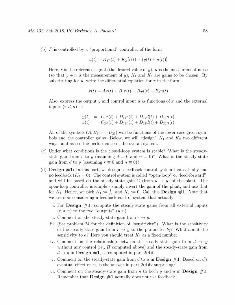
ME 132, Fall 2018, UC Berkeley, A. Packard 58
(b) P is controlled by a “proportional” controller of the form
u(t) = K1r(t) +K2 [r(t)− (y(t) + n(t))]
Here, r is the reference signal (the desired value of y), n is the measurement noise(so that y + n is the measurement of y), K1 and K2 are gains to be chosen. Bysubstituting for u, write the differential equation for x in the form
x(t) = Ax(t) +B1r(t) +B2d(t) +B3n(t)
Also, express the output y and control input u as functions of x and the externalinputs (r, d, n) as
y(t) = C1x(t) +D11r(t) +D12d(t) +D13n(t)u(t) = C2x(t) +D21r(t) +D22d(t) +D23n(t)
All of the symbols (A,B1, . . . , D23) will be functions of the lower-case given sym-bols and the controller gains. Below, we will “design” K1 and K2 two differentways, and assess the performance of the overall system.
(c) Under what conditions is the closed-loop system is stable? What is the steady-state gain from r to y (assuming d ≡ 0 and n ≡ 0)? What is the steady-stategain from d to y (assuming r ≡ 0 and n ≡ 0)?
(d) Design #1: In this part, we design a feedback control system that actually hadno feedback (K2 = 0). The control system is called “open-loop” or ‘feed-forward”,and will be based on the steady-state gain G (from u → y) of the plant. Theopen-loop controller is simple - simply invert the gain of the plant, and use thatfor K1. Hence, we pick K1 := 1
G, and K2 := 0. Call this Design #1. Note that
we are now considering a feedback control system that actually
i. For Design #1, compute the steady-state gains from all external inputs(r, d, n) to the two “outputs” (y, u).
ii. Comment on the steady-state gain from r → y.
iii. (See problem 24 for the definition of “sensitivity”). What is the sensitivityof the steady-state gain from r → y to the parameter b2? What about thesensitivity to a? Here you should treat K1 as a fixed number.
iv. Comment on the relationship between the steady-state gain from d → ywithout any control (ie., H computed above) and the steady-state gain fromd→ y in Design #1, as computed in part 2(d)i.
v. Comment on the steady-state gain from d to u in Design #1. Based on d’seventual effect on u, is the answer in part 2(d)iv surprising?
vi. Comment on the steady-state gain from n to both y and u in Design #1.Remember that Design #1 actually does not use feedback...

ME 132, Fall 2018, UC Berkeley, A. Packard 59
vii. What it the time-constant of the system with Design #1.
viii. In this part we have considered a control system that actually had no feedback(K2 = 0). Consequently, this is called open-loop control, or feedforward control(since the control input is just a function of the reference signal r, “fed-forwardto the process”), or control-by-calibration since the reciprical of the value ofof G is used in the control law.Write a short, concise (4 bullet points) quantitative summary of the effectof this strategy. Include a comparison of the process time-constant, and theresulting time-constant with the controller in place, as well as the trackingcapabilities (how y follows r), the sensitivity of the tracking capabilities toparameter changes, and the disturbance rejection properties.
(e) Now design a true feedback control system. This is Design #2. Pick K2 so thatthe closed-loop steady-state gain from d → y is at least 5 times less than theuncontrolled steady-state gain from d → y (which we called H). Constrain yourchoice of K2 so that the closed-loop system is stable. Since we are working fairlygeneral, for simplicity, you may assume a < 0 and b1 > 0, b2 > 0 and c > 0.
i. With K2 chosen, pick K1 so that the closed-loop steady-state gain from r → yis 1.
ii. With K1 and K2 both chosen as above, what is the sensitivity of the steady-state gain from r → y to the parameter b2?
iii. What is the time-constant of the closed-loop system?
iv. What is the steady-state gain from d → u? How does this compare to theprevious case (feedforward)?
v. With K2 6= 0, does the noise n now affect y?
(f) Let’s use specific numbers: a = −1, b1 = 1, b2 = 1, c = 1. Summarize all com-putations above in a table – one table for the feedforward case (Design #1),and one table for the true feedback case (Design #2). Include in the table allsteady-state gains, time constant, and sensitivity of r → y to b2.
(g) Plot the frequency responses from all external inputs to both outputs. Do this ina 2 × 3 matrix of plots that I delineate in class. Use Matlab, and the subplot
command. Use a frequency range of 0.01 ≤ ω ≤ 100. There should be two lineson each graph.
(h) Mark your graphs to indicate how Design #2 accomplishes tracking, disturbancerejection, and lower time-constant, but has increased sensitivity to noise.
(i) Keeping K1 and K2 fixed, change b2 from 1 to 0.8. Redraw the frequency re-sponses, now including all 4 lines. Indicate on the graph the evidence that De-sign #2 accomplishes good r → y tracking that is more insensitive to processparameter changes than Design #1 .

ME 132, Fall 2018, UC Berkeley, A. Packard 60
3. At this point, we can analyze (stability, steady-state gain, sinusoidal steady-state gains(FRFs), time-constant, etc.) of first-order, linear dynamical systems. In a previousproblem, we analyzed a 1st-order process model, and a proportional-control strategy.In this problem, we try a different situation, where the process is simply proportional,but the controller is a 1st-order, linear dynamical system. Specifically, suppose theprocess model is nondynamic (“static”) simply
y(t) = αu(t) + βd(t)
where α and β are constants. Depending on the situation (various, below) α may beconsidered known to the control designer, or unknown. In the case it is unknown, wewill still assume that the sign (ie., ±) is known. The control strategy is dynamic
x(t) = ax(t) + b1r(t) + b2ym(t)u(t) = cx(t) + d1r(t)
where ym(t) = y(t) + n(t) and the various “gains” (a, b1, . . . , d1) constitute the de-sign choices in the control strategy. Be careful, notation-wise, since (for example)d1 is a constant parameter, and d(t) is a signal (the disturbance). There are alot ofletters/parameters/signals to keep track of.
(a) Eliminate u and ym from the equations to obtain a differential equation for x ofthe form
x(t) = Ax(t) +B1r(t) +B2d(t) +B3n(t)
which governs the closed-loop behavior of x. Note that A,B1, B2, B3 are functionsof the parameters a, b1, . . . in the control strategy, as well as the process parametersα and β.
(b) What relations on (a, b1, . . . , d1, α, β) are equivalent to closed-loop system stabil-ity?
(c) As usual, we are interested in the effect (with feedback in place) of (r, d, n) on(y, u), the regulated variable, and the control variable, respectively. Find thecoefficients (in terms of (a, b1, . . . , d1, α, β)) so that
y(t) = C1x(t) +D11r(t) +D12d(t) +D13n(t)u(t) = C2x(t) +D21r(t) +D22d(t) +D23n(t)
(d) Suppose that Tc > 0 is a desired closed-loop time constant. Show that the follow-ing design objectives can be met with one design, assuming that the value of α isknown to the designer.
• closed-loop is stable
• closed-loop time constant is Tc
• steady-state gain from d→ y is 0

ME 132, Fall 2018, UC Berkeley, A. Packard 61
• steady-state gain from r → y is 1
A few things to look out for: the conditions above do not uniquely determineall of the parameters: indeed, only the product b2c can be determined; and anyarbitrary value for d1 is acceptable (although it’s particular value does affect otherproperties, like r → u, for instance).
(e) Assuming the choices above have been satisfied, what is the steady-state gainfrom d → u? Given that the steady-state gain from d → y is 0, does this makesense, in retrospect?
(f) Show that
a = 0, b1 = 1, b2 = −1; c =1
αTc, d1 = arbitrary
is one acceptable choice. Note that to achieve the desired time-constant, the valueof α must be known to the control designer. Write the controller equations withall these simplifications.
(g) Assume that α is not known, but it is known that 0 < αL ≤ α ≤ αU , where αLand αU are known bounds (and both are positive, as indicated). Suppose thatTc > 0 is a desired closed-loop time constant. Show that the following designobjectives can be met with one design.
• closed-loop is stable
• actual closed-loop time constant is guaranteed ≤ Tc;
• steady-state gain from d→ y is 0
• steady-state gain from r → y is 1
(h) Again assume that α is not known, but it is known that 0 < αL ≤ α ≤ αU , whereαL and αU are known bounds (and both are positive, say). Suppose that Tc > 0is a desired closed-loop time constant. Show that the following design objectivescan be met with one design.
• closed-loop is stable
• actual closed-loop time constant is guaranteed ≥ Tc;
• steady-state gain from d→ y is 0
• steady-state gain from r → y is 1
4. Let the plant (process to be controlled) be governed by the static (no differentialequations) model
y(t) = αu(t) + βd(t)
as in the lectures. Suppose nominal values of α and β are known. Consider an integralcontroller, of the form
x(t) = r(t)− ym(t)u(t) = KIx(t) +D1r(t)
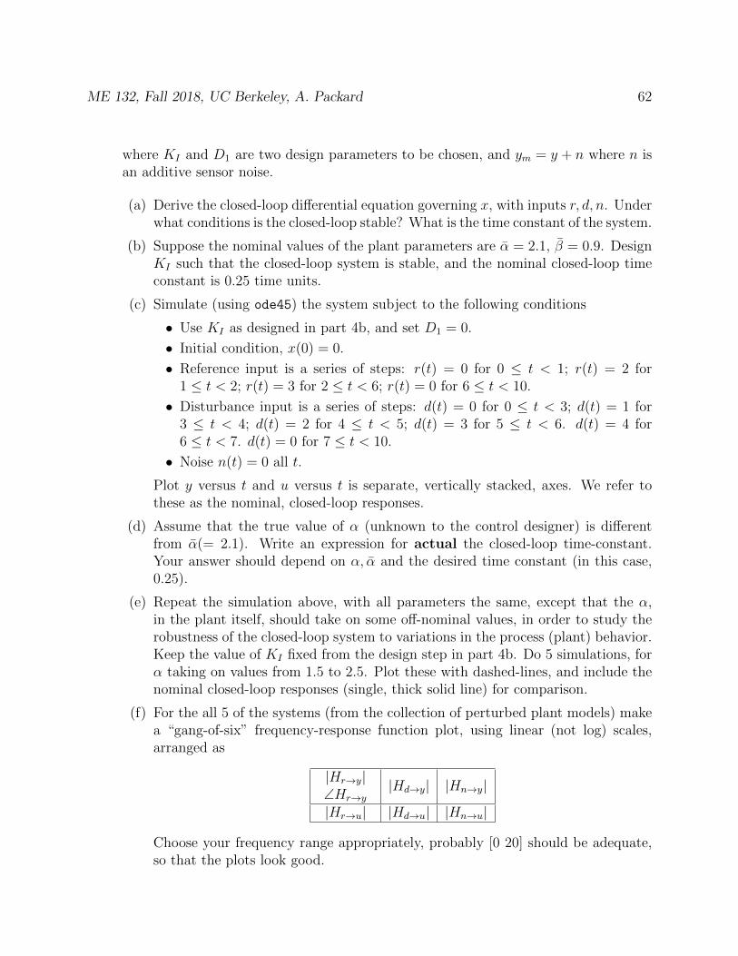
ME 132, Fall 2018, UC Berkeley, A. Packard 62
where KI and D1 are two design parameters to be chosen, and ym = y + n where n isan additive sensor noise.
(a) Derive the closed-loop differential equation governing x, with inputs r, d, n. Underwhat conditions is the closed-loop stable? What is the time constant of the system.
(b) Suppose the nominal values of the plant parameters are α = 2.1, β = 0.9. DesignKI such that the closed-loop system is stable, and the nominal closed-loop timeconstant is 0.25 time units.
(c) Simulate (using ode45) the system subject to the following conditions
• Use KI as designed in part 4b, and set D1 = 0.
• Initial condition, x(0) = 0.
• Reference input is a series of steps: r(t) = 0 for 0 ≤ t < 1; r(t) = 2 for1 ≤ t < 2; r(t) = 3 for 2 ≤ t < 6; r(t) = 0 for 6 ≤ t < 10.
• Disturbance input is a series of steps: d(t) = 0 for 0 ≤ t < 3; d(t) = 1 for3 ≤ t < 4; d(t) = 2 for 4 ≤ t < 5; d(t) = 3 for 5 ≤ t < 6. d(t) = 4 for6 ≤ t < 7. d(t) = 0 for 7 ≤ t < 10.
• Noise n(t) = 0 all t.
Plot y versus t and u versus t is separate, vertically stacked, axes. We refer tothese as the nominal, closed-loop responses.
(d) Assume that the true value of α (unknown to the control designer) is differentfrom α(= 2.1). Write an expression for actual the closed-loop time-constant.Your answer should depend on α, α and the desired time constant (in this case,0.25).
(e) Repeat the simulation above, with all parameters the same, except that the α,in the plant itself, should take on some off-nominal values, in order to study therobustness of the closed-loop system to variations in the process (plant) behavior.Keep the value of KI fixed from the design step in part 4b. Do 5 simulations, forα taking on values from 1.5 to 2.5. Plot these with dashed-lines, and include thenominal closed-loop responses (single, thick solid line) for comparison.
(f) For the all 5 of the systems (from the collection of perturbed plant models) makea “gang-of-six” frequency-response function plot, using linear (not log) scales,arranged as
|Hr→y|∠Hr→y
|Hd→y| |Hn→y|
|Hr→u| |Hd→u| |Hn→u|
Choose your frequency range appropriately, probably [0 20] should be adequate,so that the plots look good.
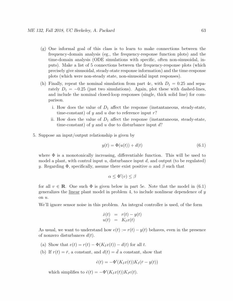
ME 132, Fall 2018, UC Berkeley, A. Packard 63
(g) One informal goal of this class is to learn to make connections between thefrequency-domain analysis (eg., the frequency-response function plots) and thetime-domain analysis (ODE simulations with specific, often non-sinusoidal, in-puts). Make a list of 5 connections between the frequency-response plots (whichprecisely give sinusoidal, steady-state response information) and the time-responseplots (which were non-steady state, non-sinusoidal input responses).
(h) Finally, repeat the nominal simulation from part 4c, with D1 = 0.25 and sepa-rately D1 = −0.25 (just two simulations). Again, plot these with dashed-lines,and include the nominal closed-loop responses (single, thick solid line) for com-parison.
i. How does the value of D1 affect the response (instantaneous, steady-state,time-constant) of y and u due to reference input r?
ii. How does the value of D1 affect the response (instantaneous, steady-state,time-constant) of y and u due to disturbance input d?
5. Suppose an input/output relationship is given by
y(t) = Φ(u(t)) + d(t) (6.1)
where Φ is a monotonically increasing, differentiable function. This will be used tomodel a plant, with control input u, disturbance input d, and output (to be regulated)y. Regarding Φ, specifically, assume there exist positive α and β such that
α ≤ Φ′(v) ≤ β
for all v ∈ R. One such Φ is given below in part 5e. Note that the model in (6.1)generalizes the linear plant model in problem 4, to include nonlinear dependence of yon u.
We’ll ignore sensor noise in this problem. An integral controller is used, of the form
x(t) = r(t)− y(t)u(t) = KIx(t)
As usual, we want to understand how e(t) := r(t)− y(t) behaves, even in the presenceof nonzero disturbances d(t).
(a) Show that e(t) = r(t)− Φ(KIx(t))− d(t) for all t.
(b) If r(t) = r, a constant, and d(t) = d a constant, show that
e(t) = −Φ′(KIx(t))KI(r − y(t))
which simplifies to e(t) = −Φ′(KIx(t))KIe(t).

ME 132, Fall 2018, UC Berkeley, A. Packard 64
(c) By chain rule, it is always true that
d(e2)
dt= 2e(t)e(t).
Substitute in expression for e to show that
d(e2)
dt= −2KIΦ
′(KIx(t))e2(t)
(d) Assume KI > 0. Define z(t) := e2(t). Note that z(t) ≥ 0 for all t, and show that
z(t) ≤ −2KIαz(t)
for all t. Hence z evolves similarly to the stable, 1st order system w(t) =−2KIαw(t), but may approach 0 even “faster” at times. Hence, we concludethat z approaches 0 at least as fast as w would, and hence can be thought of ashaving a maximum time-constant of 1
2KIα.
(e) Take, for example, Φ to be
Φ(v) :=2v + 0.1v3 for v ≥ 02v − 0.2v2 for v < 0
.
Plot this Φ function on the domain −5 ≤ v ≤ 5.
(f) Use ode45 or Simulink to simulate the closed-loop system, with KI = 0.25.Initialize the system at x(0) = 0, and consider the reference and disturbanceinputs as defined below: r(t) = 3 for 0 ≤ t < 10; r(t) = 6 for 10 ≤ t < 20;r(t) = 6+0.25(t−20) for 20 ≤ t < 40; r(t) = 11−0.4(t−40) for 40 ≤ t ≤ 60, andd(t) = sin( π
15t) for 0 ≤ t < 60. One on graph, plot y and r versus t. On another
axes, plot the control input u versus t.
(g) Consider an exercise machine that can be programmed to control a person’s heartrate by measuring the heart-rate, and adjusting the power input (from the person)that must be delivered (by the person) to continually operate the machine (eg, anelliptical trainer or “stairmaster”, where the resistance setting dictates the rateat which a person must take steps). Assume people using the machine are indecent enough shape to be exercising (as all machines have such warnings printedon the front panel). Explain, in a point-by-point list, how the problem you havejust solved above can be related to a simple integral-control strategy for this typeof workout machine. Make a short list of the issues that would come up in apreliminary design discussion about such a product.
6. A feedback system is shown below. All unmarked summing junctions are “plus”(+).
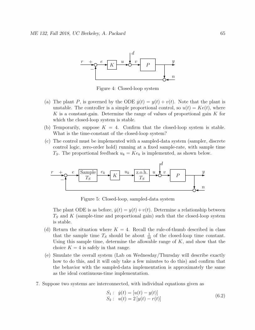
ME 132, Fall 2018, UC Berkeley, A. Packard 65
K P- fr e u
d
v y
n
+
−- - f? - -
?f6
Figure 4: Closed-loop system
(a) The plant P , is governed by the ODE y(t) = y(t) + v(t). Note that the plant isunstable. The controller is a simple proportional control, so u(t) = Ke(t), whereK is a constant-gain. Determine the range of values of proportional gain K forwhich the closed-loop system is stable.
(b) Temporarily, suppose K = 4. Confirm that the closed-loop system is stable.What is the time-constant of the closed-loop system?
(c) The control must be implemented with a sampled-data system (sampler, discretecontrol logic, zero-order hold) running at a fixed sample-rate, with sample timeTS. The proportional feedback uk = Kek is implemented, as shown below.
SampleTS
Kz.o.h.TS
P- fr e ek uk u
d
v
n
y+
−- - - - f? - -
?f6
Figure 5: Closed-loop, sampled-data system
The plant ODE is as before, y(t) = y(t) + v(t). Determine a relationship betweenTS and K (sample-time and proportional gain) such that the closed-loop systemis stable.
(d) Return the situation where K = 4. Recall the rule-of-thumb described in classthat the sample time TS should be about 1
10of the closed-loop time constant.
Using this sample time, determine the allowable range of K, and show that thechoice K = 4 is safely in that range.
(e) Simulate the overall system (Lab on Wednesday/Thursday will describe exactlyhow to do this, and it will only take a few minutes to do this) and confirm thatthe behavior with the sampled-data implementation is approximately the sameas the ideal continuous-time implementation.
7. Suppose two systems are interconnected, with individual equations given as
S1 : y(t) = [u(t)− y(t)]S2 : u(t) = 2 [y(t)− r(t)] (6.2)
ME 132, Fall 2018, UC Berkeley, A. Packard 66
(a) Consider first S1 (input u, output y): Show that for any initial condition y0, ifu(t) ≡ u (a constant), then y(t) approaches a constant y, that only depends onthe value of u. What is the steady-state gain of S1?
(b) Next consider S2 (input (r, y), output u): Show that if r(t) ≡ r and y(t) ≡ y(constants), then u(t) approaches a constant u, that only depends on the values(r, y).
(c) Now, assume that the closed-loop system also has the steady-state behavior –that is, if r(t) ≡ r, then both u(t) and y(t) will approach limiting values, u andy, only dependent on r. Draw a block-diagram showing how the limiting valuesare related, and solve for u and y in terms of r.
(d) Now check your answer in part 4c. Suppose y(0) = 0, and r(t) = 1 =: r for allt ≥ 0. Eliminate u from the equations 24.5, and determine y(t) for all t. Make asimple graph. Does the result agree with your answer in part 4c?
Lesson: since the assumption we made in part 4c was actually not valid, the analysisin part 4c is incorrect. That is why, for a closed-loop steady-state analysis to be basedon the separate component’s steady-state properties, we must know from other meansthat the closed-loop system also has steady-state behavior.
8. Suppose two systems are interconnected, with individual equations given as
S1 : y(t) = [u(t) + y(t)]S2 : u(t) = 2 [r(t)− y(t)]
(6.3)
(a) Consider first S1 (input u, output y): If u(t) ≡ u (a constant), then does y(t)approach a constant y, dependent only on the value of u?
(b) Next consider S2 (input (r, y), output u): If r(t) ≡ r and y(t) ≡ y (constants),then does u(t) approach a constant u, dependent only on the values r, y?
(c) Suppose y(0) = y0 is given, and r(t) =: r for all t ≥ 0. Eliminate u from theequations 24.6, and determine y(t) for all t. Also, plugging back in, determineu(t) for all t. Show that y and u both have limiting values that only depend onthe value r, and determine the simple relationship between r and (y, u).
Lesson: Even though S1 does not have steady-state behavior on its own, in feedbackwith S2, the overall closed-loop system does.
9. Consider the equations relating variables r, e, y, n, u and d. Assume P and C are givennumbers.
e = r − (y + n)u = Cey = P (u+ d)
ME 132, Fall 2018, UC Berkeley, A. Packard 67
So, this represents 3 linear equations in 6 unknowns. Solve these equations, expressinge, u and y as linear functions of r, d and n. The linear relationships will involve thenumbers P and C.
10. For a function F of a many variables (say two, for this problem, labeled x and y), the“sensitivity of F to x” is defined as “the ratio of the percentage change in F due to apercentage change in x.” Denote this by SFx .
(a) Suppose x changes by δ, to x+ δ. The percentage change in x is then
% change in x =(x+ δ)− x
x=δ
x
Likewise, the subsequent percentage change in F is
% change in F =F (x+ δ, y)− F (x, y)
F (x, y)
Show that for infinitesimal changes in x, the sensitivity is
SFx =x
F (x, y)
∂F
∂x
(b) Let F (x, y) = xy1+xy
. What is SFx .
(c) If x = 5 and y = 6, then xy1+xy
≈ 0.968. If x changes by 10%, using the quantity
SFx derived in part (10b), approximately what percentage change will the quantityxy
1+xyundergo?
(d) Let F (x, y) = 1xy
. What is SFx .
(e) Let F (x, y) = xy. What is SFx .
ME 132, Fall 2018, UC Berkeley, A. Packard 68
7 Two forms of high-order Linear ODEs, with forcing
The governing equations for the car, with integral controller can be expressed in two dis-tinct, but equivalent, forms. By writing down the governing equations for each componentindividually, and then eliminating the interconnection variable u gives
v(t) = 1m
[−αv(t) + EKIz(t) +Gw(t)]z(t) = vdes(t)− v(t)
This is two 1st order (only first derivative occurs), coupled (z affects v and v affects z) lineardifferential equations, with (in this case) two external inputs, vdes and w.
The general case of this situation has n dependent variables, x1, x2, . . . , xn, and m inputs,d1, d2, . . . , dm. The differential equations governing the evolution of the xi variables is
x1(t) = a11x1(t) + a12x2(t) + · · ·+ a1nxn(t) + b11d1(t) + b12d2(t) . . .+ b1mdm(t)x2(t) = a21x1(t) + a22x2(t) + · · ·+ a2nxn(t) + b21d1(t) + b22d2(t) . . .+ b2mdm(t)
... =...
xn(t) = an1x1(t) + an2x2(t) + · · ·+ annxn(t) + bn1d1(t) + bn2d2(t) . . .+ bnmdm(t)
In matrix notation, the equations can be written very concisely,
x(t) = Ax(t) +Bd(t)
where x, A, B, and d are vectors and matrices
x(t) :=
x1(t)x2(t)
...xn(t)
, d(t) :=
d1(t)d2(t)
...dm(t)
, A =
a11 a12 · · · a1n
a21 a22 · · · a2n...
.... . .
...an1 an2 · · · ann
, B =
b11 · · · b1m
b21 · · · b2m...
. . ....
bn1 · · · bnm
This is called a linear, state-space representation. For the cruise-control equations, it appearsas [
v(t)z(t)
]︸ ︷︷ ︸
x(t)
=
[ −αm
EKIm
−1 0
]︸ ︷︷ ︸
A
[v(t)z(t)
]︸ ︷︷ ︸
x(t)
+
[0 G
m
1 0
]︸ ︷︷ ︸
B
[vdes(t)w(t)
]︸ ︷︷ ︸
d(t)
We began the class by defining dynamical systems in this form, without the restriction oflinearity. So, this state-space form is a general, and useful system representation.
But, on the other hand, there was an alternative manner to write the system equations. Inthis other approach, we eliminated z from the original equations, to yield
v(t) +α
mv(t) +
EKI
mv(t) =
EKI
mvdes(t)−
G
mw(t) (7.1)
ME 132, Fall 2018, UC Berkeley, A. Packard 69
So, now the closed-loop system behavior is equivalently described with one 2nd order (2derivatives) differential equation, with two external inputs, vdes and w, although for w, onlyw explicitly appears. This is mathematically equivalent to the state-space form above, butof a different form.
First some notation, if y denotes a function (of a variable t, say), then y[k] or y(k) denotesthe k’th derivative of the function y,
y[k] =dky
dtk.
Then, for a system with (say) two inputs (u,w) and one output (y), the n’th order differentialequation relating the inputs to outputs is
y[n](t) + a1y[n−1](t) + · · ·+ an−1y
[1](t) + any(t)= b0u
[n](t) + b1u[n−1](t) + · · ·+ bn−1u
[1](t) + bnu(t)+c0w
[n](t) + c1w[n−1](t) + · · ·+ cn−1w
[1](t) + cnw(t)
We will refer to this as the SLODE (single, linear ODE) representation.
Both representations are useful, and in certain situations, advantageous over each other. Wewill study each in detail, starting with the state-space representation.
In section 19, we cover much of the mathematics to analyze the behavior of systems governedby the SLODE representation.
In section ??, we revisit the cruise control with integral control, and analyze the dynamicproperties we had observed. We also propose a more complex control architecture which hasmore desirable properties.
7.1 Problems
1. Suppose that (A1, B1, C1, D1) are the state-space matrices of a linear system with n1
states, m1 inputs and q1 outputs. Hence A1 ∈ Rn1×n1 , B1 ∈ Rn1×m1 , C1 ∈ Rq1×n1 ,D1 ∈ Rq1×m1 . Let x1 denote the n1 × 1 state vector (so here, the subscript “1” doesnot mean the first element, rather it is itself a vector, perhaps indexed as
x1 =
(x1)1
(x1)2...
(x1)n1
Similarly, let u1 denote the m1× 1 input vector and y1 denote the q1× 1 input vector.Likewise, suppose that (A2, B2, C2, D2) are the state-space matrices of a linear system
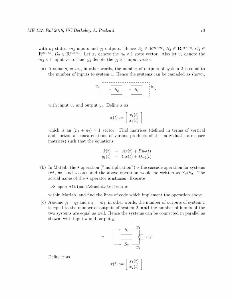
ME 132, Fall 2018, UC Berkeley, A. Packard 70
with n2 states, m2 inputs and q2 outputs. Hence A2 ∈ Rn2×n2 , B2 ∈ Rn2×m2 , C2 ∈Rq2×n2 , D2 ∈ Rq2×m2 . Let x2 denote the n2 × 1 state vector. Also let u2 denote them2 × 1 input vector and y2 denote the q2 × 1 input vector.
(a) Assume q2 = m1, in other words, the number of outputs of system 2 is equal tothe number of inputs to system 1. Hence the systems can be cascaded as shown,
S2 S1- - -
u2 y1
with input u2 and output y1. Define x as
x(t) :=
[x1(t)x2(t)
]which is an (n1 + n2) × 1 vector. Find matrices (defined in terms of verticaland horizontal concatenations of various products of the individual state-spacematrices) such that the equations
x(t) = Ax(t) +Bu2(t)y1(t) = Cx(t) +Du2(t)
(b) In Matlab, the * operation (”multiplication”) is the cascade operation for systems(tf, ss, and so on), and the above operation would be written as S1∗S2. Theactual name of the * operator is mtimes. Execute
>> open +ltipack\@ssdata\mtimes.m
within Matlab, and find the lines of code which implement the operation above.
(c) Assume q1 = q2 and m1 = m2, in other words, the number of outputs of system 1is equal to the number of outputs of system 2, and the number of inputs of thetwo systems are equal as well. Hence the systems can be connected in parallel asshown, with input u and output y.
S2
S1-
-
?
6d -u
y1
y2
y++
Define x as
x(t) :=
[x1(t)x2(t)
]
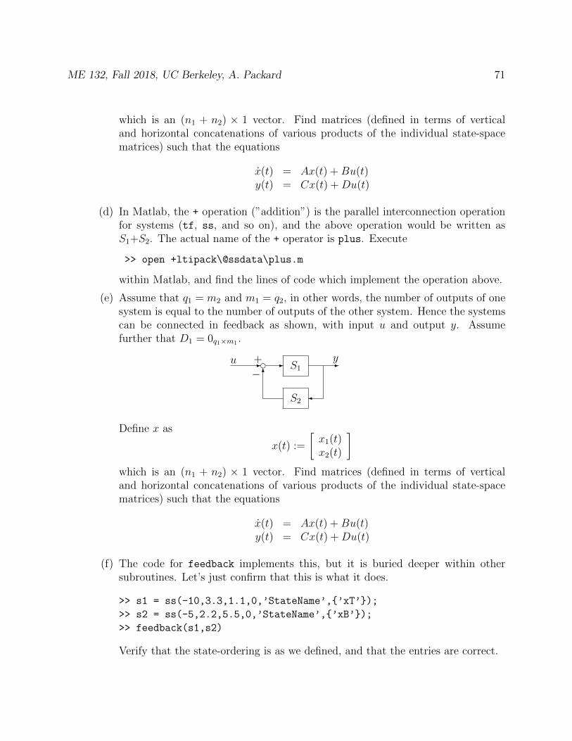
ME 132, Fall 2018, UC Berkeley, A. Packard 71
which is an (n1 + n2) × 1 vector. Find matrices (defined in terms of verticaland horizontal concatenations of various products of the individual state-spacematrices) such that the equations
x(t) = Ax(t) +Bu(t)y(t) = Cx(t) +Du(t)
(d) In Matlab, the + operation (”addition”) is the parallel interconnection operationfor systems (tf, ss, and so on), and the above operation would be written asS1+S2. The actual name of the + operator is plus. Execute
>> open +ltipack\@ssdata\plus.m
within Matlab, and find the lines of code which implement the operation above.
(e) Assume that q1 = m2 and m1 = q2, in other words, the number of outputs of onesystem is equal to the number of outputs of the other system. Hence the systemscan be connected in feedback as shown, with input u and output y. Assumefurther that D1 = 0q1×m1 .
S1
S2
- - -
6
du y+
−
Define x as
x(t) :=
[x1(t)x2(t)
]which is an (n1 + n2) × 1 vector. Find matrices (defined in terms of verticaland horizontal concatenations of various products of the individual state-spacematrices) such that the equations
x(t) = Ax(t) +Bu(t)y(t) = Cx(t) +Du(t)
(f) The code for feedback implements this, but it is buried deeper within othersubroutines. Let’s just confirm that this is what it does.
>> s1 = ss(-10,3.3,1.1,0,’StateName’,’xT’);
>> s2 = ss(-5,2.2,5.5,0,’StateName’,’xB’);
>> feedback(s1,s2)
Verify that the state-ordering is as we defined, and that the entries are correct.
ME 132, Fall 2018, UC Berkeley, A. Packard 72
Be sure to check that all of your matrix manipulations have the correct dimensions, andthat the concatenations have compatible dimensions (horizontal concatenations musthave the same number of rows, vertical concatenation must have the same number ofcolumns).
2. This problem may be out-of-place. It has some transfer function questionsAt one point, NASA was developing booster rockets and a crew exploration vehicleto replace the Space Shuttle. One main component of the Orion Crew ExplorationVehicle (CEV) is a conical crew module. This module has several thrusters to controlthe vehicle attitude on re-entry to the earth’s orbit. A linear model for the short-periodmode of the CEV pitch dynamics during re-entry is given by:
x(t) =
[2 1−36 2
]x(t) +
[01
]u(t)
y(t) =[
0 1]x(t) +
[0]u
where x(t) :=
[α(t)q(t)
], which are the angle-of-attack and the pitch-rate, respectively,
and u(t) is the pitch torque generated by the thrusters. The output y is the pitch rate,so y = x2 = q.
(a) Using the formula we derived in class, G(s) = D + C(sI − A)−1B, derive thetransfer function from u to y of this state-space model.
(b) Enter the matrices into Matlab, form a state-space object using the ss constructor.Type
>> disp(G)
>> size(G)
>> class(G)
and paste the results into your assignment.
(c) Use the command tf as a converter, and convert the model respresentation to atransfer function object. Confirm that your answer in part 4a is correct.
(d) If x is eliminated (through clever substitutions - which you know, and are key tothe state-space-to-transfer function conversion), what is the differential equationrelating u to y.
(e) With the transfer function obtained in part 4a, use the procedure derived in classto obtain a state-space model for the system.
(f) Note that the state-space model you obtain is not the same as the state-spacemodel we started with. Enter both systems into Matlab, and confirm with step
that the input/output behaviors of the two systems are indeed identical. Hencewe have seen that a system can have different state-space models (that yield theexact same input/output behavior).
ME 132, Fall 2018, UC Berkeley, A. Packard 73
8 Jacobian Linearizations, equilibrium points
In modeling systems, we see that nearly all systems are nonlinear, in that the differentialequations governing the evolution of the system’s variables are nonlinear. However, mostof the theory we have developed has centered on linear systems. So, a question arises: “Inwhat limited sense can a nonlinear system be viewed as a linear system?” In this sectionwe develop what is called a “Jacobian linearization of a nonlinear system,” about a specificoperating point, called an equilibrium point.
The section begins with a short review of derivatives, especially for functions of many vari-ables.
8.1 Jacobians and the Taylor Theorem
First consider a scalar values function φ(x1, x2, · · · , xn) of n variables. The Jacobian of φ isthe 1× n row vector
∇φ(x1, · · · , xn) =[
∂φ∂x1
· · · ∂φ∂xn
]For example for the function φ(x1, x2, x3) of three variables,
φ(x1, x2, x3) = x1x22 − 1/x1 + sin(x3)
the Jacobian is
∇φ =[
∂φ∂x1
∂φ∂x2
∂φ∂x3
]=[x2
2 + 1/x21 2x1x2 cos(x3)
]The Jacobian is a function of the variables x1, x2, x3. We can evaluate the Jacobian ata point ξ and get actual numbers. In this example, we could evaluate the Jacobian at(x1, x2, x3) = (1, 2, 0) to get
∇φ(x)|x=(1,2,0) =[
5 4 1]
Now consider a vector-valued function φ : Rn → Rm. What this actually means is that wehave m individual functions in n variables. These functions are collectively represented byφ, and the variables are collectively represented by x. Let us write this function as
φ(x) = φ(x1, x2, · · · , xn) =
φ1(x1, · · · , xn)...
φm(x1, · · · , xn)
ME 132, Fall 2018, UC Berkeley, A. Packard 74
The Jacobian of φ is the m× n matrix of functions
∇φ =
∂φ1∂x1
· · · ∂φ1∂xn
... · · · ...∂φm∂x1
· · · ∂φm∂xn
Fix a vector ξ ∈ Rn. We can evaluate the Jacobian at ξ to get an m×n matrix of numbers.Our notation for this is
∇φ(x)|x=ξ =
∂φ1∂x1
· · · ∂φ1∂xn
... · · · ...∂φm∂x1
· · · ∂φm∂xn
@ξ
For example, consider the function
φ(x1, x2, x3) =
[φ1(x1, x2, x3)φ2(x1, x2, x3)
]=
[x1 sin(x2)x2
2 cos(x3)
]The Jacobian of φ(x) evaluated at (1, π/2, 0) is
∇φ|x=(1,1,0) =
[sin(x2) x1 cos(x2) 0
0 2x2 cos(x3) x22 sin(x3)
]x=(1,π/2,0)
=
[1 1 00 π 0
]
Analogous to the classical Taylor series expansion of a scalar function of one variable, wecan write the Taylor series expansion of φ around ξ as
φ(x) = φ(ξ) + ∇φ|x=(ξ) (x− ξ) + higher order terms
The first two terms above are the linear approximation of φ around ζ. We can thereforeapproximate φ as
φ(x) ≈ φ(ξ) +∇φ(ξ) (x− ξ)
and this approximation will be good in some (possibly small) neighborhood of ξ.
8.2 Equilibrium Points
Consider a nonlinear differential equation
x(t) = f(x(t), u(t)) (8.1)
where f is a function mapping Rn ×Rm → Rn. A point x ∈ Rn is called an equilibriumpoint if there is a specific u ∈ Rm (called the equilibrium input) such that
f (x, u) = 0n
ME 132, Fall 2018, UC Berkeley, A. Packard 75
Suppose x is an equilibrium point (with equilibrium input u). Consider starting the system(8.1) from initial condition x(t0) = x, and applying the input u(t) ≡ u for all t ≥ t0. Theresulting solution x(t) satisfies
x(t) = x
for all t ≥ t0. That is why it is called an equilibrium point.
8.3 Deviation Variables
Suppose (x, u) is an equilibrium point and input. We know that if we start the system atx(t0) = x, and apply the constant input u(t) ≡ u, then the state of the system will remainfixed at x(t) = x for all t. What happens if we start a little bit away from x, and we applya slightly different input from u? Define deviation variables to measure the difference.
δx(t) := x(t)− xδu(t) := u(t)− u
In this way, we are simply relabling where we call 0. Now, the variables x(t) and u(t) arerelated by the differential equation
x(t) = f(x(t), u(t))
Substituting in, using the constant and deviation variables, we get
δx(t) = f (x+ δx(t), u+ δu(t))
This is exact. Now however, let’s do a Taylor expansion of the right hand side, and neglectall higher (higher than 1st) order terms
δx(t) ≈ f (x, u) +∂f
∂x
∣∣∣∣x=xu=u
δx(t) +∂f
∂u
∣∣∣∣x=xu=u
δu(t)
But f(x, u) = 0, leaving
δx(t) ≈∂f
∂x
∣∣∣∣x=xu=u
δx(t) +∂f
∂u
∣∣∣∣x=xu=u
δu(t)
This differential equation approximately governs (we are neglecting 2nd order and higherterms) the deviation variables δx(t) and δu(t), as long as they remain small. It is a linear,time-invariant, differential equation, since the derivatives of δx are linear combinations of theδx variables and the deviation inputs, δu. The matrices
A :=∂f
∂x
∣∣∣∣x=xu=u
∈ Rn×n , B :=∂f
∂u
∣∣∣∣x=xu=u
∈ Rn×m (8.2)
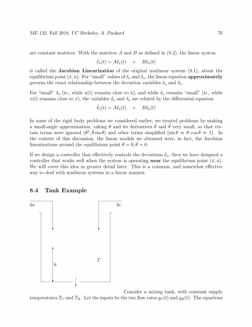
ME 132, Fall 2018, UC Berkeley, A. Packard 76
are constant matrices. With the matrices A and B as defined in (8.2), the linear system
δx(t) = Aδx(t) + Bδu(t)
is called the Jacobian Linearization of the original nonlinear system (8.1), about theequilibrium point (x, u). For “small” values of δx and δu, the linear equation approximatelygoverns the exact relationship between the deviation variables δu and δx.
For “small” δu (ie., while u(t) remains close to u), and while δx remains “small” (ie., whilex(t) remains close to x), the variables δx and δu are related by the differential equation
δx(t) = Aδx(t) + Bδu(t)
In some of the rigid body problems we considered earlier, we treated problems by makinga small-angle approximation, taking θ and its derivatives θ and θ very small, so that cer-tain terms were ignored (θ2, θ sin θ) and other terms simplified (sin θ ≈ θ, cos θ ≈ 1). Inthe context of this discussion, the linear models we obtained were, in fact, the Jacobianlinearizations around the equilibrium point θ = 0, θ = 0.
If we design a controller that effectively controls the deviations δx, then we have designed acontroller that works well when the system is operating near the equilibrium point (x, u).We will cover this idea in greater detail later. This is a common, and somewhat effectiveway to deal with nonlinear systems in a linear manner.
8.4 Tank Example
? ?
??
6
hT
qH qC
Consider a mixing tank, with constant supplytemperatures TC and TH . Let the inputs be the two flow rates qC(t) and qH(t). The equations

ME 132, Fall 2018, UC Berkeley, A. Packard 77
for the tank are
h(t) = 1AT
(qC(t) + qH(t)− cDAo
√2gh(t)
)TT (t) = 1
h(t)AT(qC(t) [TC − TT (t)] + qH(t) [TH − TT (t)])
Let the state vector x and input vector u be defined as
x(t) :=
[h(t)TT (t)
], u(t) :=
[qC(t)qH(t)
]f1(x, u) = 1
AT
(u1 + u2 − cDAo
√2gx1
)f2(x, u) = 1
x1AT(u1 [TC − x2] + u2 [TH − x2])
Intuitively, any height h > 0 and any tank temperature TT satisfying
TC ≤ TT ≤ TH
should be a possible equilibrium point (after specifying the correct values of the equilibriuminputs). In fact, with h and TT chosen, the equation f(x, u) = 0 can be written as[
1 1TC − x2 TH − x2
] [u1
u2
]=
[cDAo
√2gx1
0
]The 2× 2 matrix is invertible if and only if TC 6= TH . Hence, as long as TC 6= TH , there is aunique equilibrium input for any choice of x. It is given by[
u1
u2
]=
1
TH − TC
[TH − x2 −1x2 − TC 1
] [cDAo
√2gx1
0
]This is simply
u1 =cDAo
√2gx1 (TH − x2)
TH − TC, u2 =
cDAo√
2gx1 (x2 − TC)
TH − TCSince the ui represent flow rates into the tank, physical considerations restrict them tobe nonegative real numbers. This implies that x1 ≥ 0 and TC ≤ TT ≤ TH . Looking at thedifferential equation for TT , we see that its rate of change is inversely related to h. Hence, thedifferential equation model is valid while h(t) > 0, so we further restrict x1 > 0. Under thoserestrictions, the state x is indeed an equilibrium point, and there is a unique equilibriuminput given by the equations above.
Next we compute the necessary partial derivatives.
[∂f1∂x1
∂f1∂x2
∂f2∂x1
∂f2∂x2
]=
[− gcDAoAT√
2gx10
−u1[TC−x2]+u2[TH−x2]
x21AT
−(u1+u2)x1AT
]
ME 132, Fall 2018, UC Berkeley, A. Packard 78
[∂f1∂u1
∂f1∂u2
∂f2∂u1
∂f2∂u2
]=
[ 1AT
1AT
TC−x2x1AT
TH−x2x1AT
]
The linearization requires that the matrices of partial derivatives be evaluated at the equi-librium points. Let’s pick some realistic numbers, and see how things vary with differentequilibrium points. Suppose that TC = 10, TH = 90, AT = 3m2, Ao = 0.05m, cD = 0.7. Tryh = 1m and h = 3m, and for TT , try TT = 25 and TT = 75. That gives 4 combinations.Plugging into the formulae give the 4 cases
1.(h, TT
)= (1m, 25). The equilibrium inputs are
u1 = qC = 0.126 , u2 = qH = 0.029
The linearized matrices are
A =
[−0.0258 0
0 −0.517
], B =
[0.333 0.333−5.00 21.67
]2.(h, TT
)= (1m, 75). The equilibrium inputs are
u1 = qC = 0.029 , u2 = qH = 0.126
The linearized matrices are
A =
[−0.0258 0
0 −0.0517
], B =
[0.333 0.333−21.67 5.00
]3.(h, TT
)= (3m, 25). The equilibrium inputs are
u1 = qC = 0.218 , u2 = qH = 0.0503
The linearized matrices are
A =
[−0.0149 0
0 −0.0298
], B =
[0.333 0.333−1.667 7.22
]4.(h, TT
)= (3m, 75). The equilibrium inputs are
u1 = qC = 0.0503 , u2 = qH = 0.2181
The linearized matrices are
A =
[−0.0149 0
0 −0.0298
], B =
[0.333 0.333−7.22 1.667
]
ME 132, Fall 2018, UC Berkeley, A. Packard 79
We can try a simple simulation, both in the exact nonlinear equation, and the linearization,and compare answers.
We will simulate the systemx(t) = f(x(t), u(t))
subject to the following conditions
x(0) =
[1.1081.5
]and
u1(t) =
0.022 for 0 ≤ t ≤ 250.043 for 25 < t ≤ 100
u2(t) =
0.14 for 0 ≤ t ≤ 600.105 for 60 < t ≤ 100
This is close to equilibrium condition #2. So, in the linearization, we will use linearization#2, and the following conditions
δx(0) = x(0)−[
175
]=
[0.106.5
]and
δu1(t) := u1(t)− u1 =
−0.007 for 0 ≤ t ≤ 250.014 for 25 < t ≤ 100
δu2(t) := u2(t)− u2 =
0.014 for 0 ≤ t ≤ 60−0.021 for 60 < t ≤ 100
To compare the simulations, we must first plot x(t) from the nonlinear simulation. Thisis the “true” answer. For the linearization, we know that δx approximately governs thedeviations from x. Hence, for that simulation we should plot x + δx(t). These are shownbelow for both h and TT .
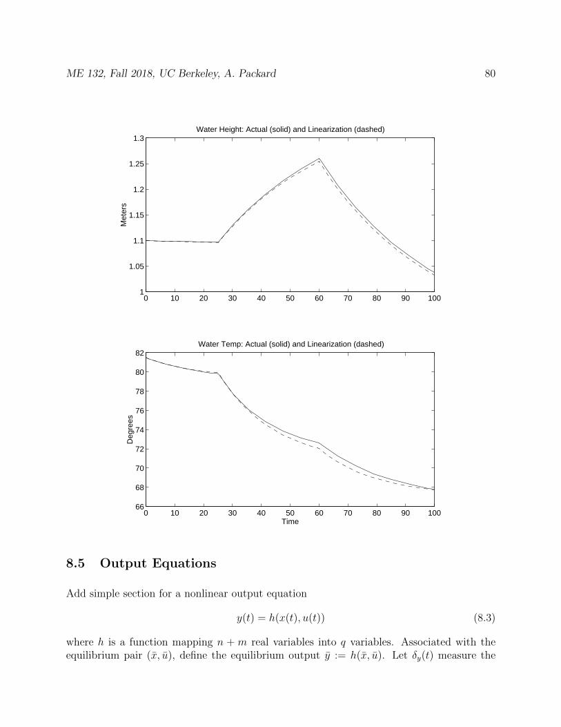
ME 132, Fall 2018, UC Berkeley, A. Packard 80
0 10 20 30 40 50 60 70 80 90 1001
1.05
1.1
1.15
1.2
1.25
1.3Water Height: Actual (solid) and Linearization (dashed)
Met
ers
0 10 20 30 40 50 60 70 80 90 10066
68
70
72
74
76
78
80
82Water Temp: Actual (solid) and Linearization (dashed)
Deg
rees
Time
8.5 Output Equations
Add simple section for a nonlinear output equation
y(t) = h(x(t), u(t)) (8.3)
where h is a function mapping n + m real variables into q variables. Associated with theequilibrium pair (x, u), define the equilibrium output y := h(x, u). Let δy(t) measure the
ME 132, Fall 2018, UC Berkeley, A. Packard 81
difference between actual output, and equilibrium output, so
δy(t) := y(t)− yWhat is the approximate relation between δx, δu and δy, while they remain small? Do aTaylor series approximation of equation (8.3) to obtain
δy(t) ≈∂h
∂x
∣∣∣∣x=xu=u
δx(t) +∂h
∂u
∣∣∣∣x=xu=u
δu(t)
The matrices
C :=∂h
∂x
∣∣∣∣x=xu=u
∈ Rq×n , D :=∂h
∂u
∣∣∣∣x=xu=u
∈ Rq×m (8.4)
are constant matrices.
8.6 Calculus for systems not in standard form
Often times, the system equations will not naturally be in the standard form, for example,they may be of the form
M(x(t))x(t) = q(x(t), u(t))
where M is a function mapping n variables into n×n invertible matrices, and q maps n+mvariables into n. Clearly, the equations can be rewritten as
x(t) = M−1(x(t))q(x(t), u(t))
This naturally suggests defining a function f(x, u) := M−1(x)q(x, u), and then proceed-ing with the linearization process, working with f . But, this creates alot of unnecessarycalculations, all of which cancel out in the end.
Use the notation
∂f
∂xj:=
∂f1∂xj∂f2∂xj
· · ·∂fn∂xj
Then by chain rule, we have
∂f
∂xj= −M−1(x)
∂M
∂xjM−1(x)q(x, u) +M−1(x)
∂q
∂xj
Since M(x) is invertible for all x, it is clear that
f(x, u) = 0n×1 ⇔ q(x, u) = 0n×1
Therefore, evaluating the partial of f at the equilibrium point leads to a very simple expres-sion
∂f
∂xj
∣∣∣∣x=xu=u
= M−1(x)∂q
∂xj
∣∣∣∣x=xu=u

ME 132, Fall 2018, UC Berkeley, A. Packard 82
8.7 Another common non-standard form
It is also common that the equations can be in the form
M(x(t))
[x(t)v(t)
]= q(x(t), u(t))
where v are other dependent-variables (ie., “outputs”) of the problem. For example, inapplying Newton’s laws to a system of interconnected rigid links, the internal forces ateach link are unknowns that must be introduced into the equations of motion, regardless ofwhether they are being sought after (in the case, Lagrange’s formulation may be simpler, asthe internal forces do not explicitly play a role in that methodology).
Assume M(x) is invertible for all x, and treat v as an output. The state/output equationsare [
x(t)v(t)
]= M−1(x(t))q(x(t), u(t)) =:
[f(x(t), u(t))h(x(t), u(t))
]An equilibrium point (x, u, v) satisfies
M(x)
[0v
]= q(x, u)
The linearization about the equilibrium point is obtained by taking partial derivatives of fand h with respect to components of x and u, and evaluating the expressions at (x, u, v).Since the horizontal stacking of f above h has a nice representation (ie., M−1h), it is easiestto write expressions for [
AC
],
[BD
]Specifically, for any matrix W , let W[i] represent the i’th column of W . Then[
AC
][i]
=
[ ∂f∂xi∂h∂xi
]x=x,u=u
,
[BD
][k]
=
[∂f∂uk∂h∂uk
]x=x,u=u
,
Direct calculation gives[AC
][i]
= M−1(x)
(−∂M∂xi
M−1(x)q(x, u) +∂q
∂xi
)∣∣∣∣x=x,u=u
Clearly,
[0v
]= M−1(x)q(x, u), so this simplifies to[
AC
][i]
= M−1(x)
(−∂M∂xi
[0v
]+∂q
∂xi
)∣∣∣∣x=x,u=u
Similarly [BD
][k]
= M−1(x)∂q
∂uk
∣∣∣∣x=x,u=u
ME 132, Fall 2018, UC Berkeley, A. Packard 83
8.8 Linearizing about general solution
In section 8.3, we discussed the linear differential equation which governs small deviationsaway from an equilibrium point. This resulted in a linear, time-invariant differential equation.
Often times, more complicated situations arise. Consider the task of controlling a rockettrajectory from Earth to the moon. By writing out the equations of motion, from Physics,we obtain state equations of the form
x(t) = f(t, x(t), u(t), d(t)) (8.5)
where u is the control input (thrusts), d are external disturbances.
Through much computer simulation, a preplanned input schedule is developed, which, underideal circumstances (ie., d(t) ≡ 0), would get the rocket from Earth to the moon. Denotethis preplanned input by u(t), and the ideal disturbance by d(t) (which we assume is 0).This results in an ideal trajectory x(t), which solves the differential equation,
˙x(t) = f(t, x(t), u(t), d(t)
)Now, small nonzero disturbances are expected, which lead to small deviations in x, whichmust be corrected by small variations in the pre-planned input u. Hence, engineers need tohave a model for how a slightly different input u(t) + δu(t) and slightly different disturbanced(t) + δd(t) will cause a different trajectory. Write x(t) in terms of a deviation from x(t),defining δx(t) := x(t)− x(t), giving
x(t) = x(t) + δx(t)
Now x, u and d must satisfy the differential equation, which gives
x(t) = f (t, x(t), u(t), d(t))˙x(t) + δx(t) = f
(t, x(t) + δx(t), u(t) + δu(t), d(t) + δd(t)
)≈ f (t, x(t), u(t), 0) + ∂f
∂x
∣∣x(t)=x(t)u(t)=u(t)d(t)=d(t)
δx(t) + ∂f∂u
∣∣x(t)=x(t)u(t)=u(t)d(t)=d(t)
δu(t) + ∂f∂d
∣∣x(t)=x(t)u(t)=u(t)d(t)=d(t)
δd(t)
But the functions x and u satisfy the governing differential equation, so ˙x(t) = f (x(t), u(t), 0, t),leaving the (approximate) governing equation for δx
δx(t) =∂f
∂x
∣∣∣∣x(t)=x(t)u(t)=u(t)d(t)=d(t)
δx(t) +∂f
∂u
∣∣∣∣x(t)=x(t)u(t)=u(t)d(t)=d(t)
δu(t) +∂f
∂d
∣∣∣∣x(t)=x(t)u(t)=u(t)d(t)=d(t)
δd(t)
Define time-varying matrices A, B1 and B2 by
A(t) :=∂f
∂x
∣∣∣∣x(t)=x(t)u(t)=u(t)d(t)=d(t)
B1(t) :=∂f
∂u
∣∣∣∣x(t)=x(t)u(t)=u(t)d(t)=d(t)
B2(t) :=∂f
∂d
∣∣∣∣x(t)=x(t)u(t)=u(t)d(t)=d(t)
ME 132, Fall 2018, UC Berkeley, A. Packard 84
The deviation variables are approximately governed by
δx(t) = A(t)δx(t) +B1(t)δu(t) +B2(t)δd(t) = A(t)δx(t) +[B1(t) B2(t)
] [ δu(t)δd(t)
]This is called the linearization of system (8.5) about the trajectory
(x, u, d
). This type of
linearization is a generalization of linearizations about equilibrium points. Linearizing aboutan equilibrium point yields a LTI system, while linearizing about a trajectory yields an LTVsystem.
In general, these types of calculations are carried out numerically,
• simulink to get solution x(t) given particular inputs u(t) and d(t)
• Numerical evaluation of ∂f∂x
, etc, evaluated at the solution points
• Storing the time-varying matrices A(t), B1(t), B2(t) for later use
In a simple case it is possible to analytically determine the time-varying matrices.
ME 132, Fall 2018, UC Berkeley, A. Packard 85
8.9 Problems
1. This purpose of this problem is to remind you how first-order Taylor series (ie., linearapproximation) are used to approximate a function of many variables. The temperaturein a particular 3-dimensional solid is a function of position, and is known to be
T (x, y, z) = 42 + (x− 2)2 + 3 (y − 4)2 − 5 (z − 6)2 + 2yz
(a) Find the first order approximation (linearization) of the temperature near thelocation (x = 4, y = 6, z = 0). Use δx, δy and δz as your deviation variables.
(b) What is the maximum error between the actual temperature and the first orderapproximation formula for |δx| ≤ 0.3, |δy| ≤ 0.2, |δz| ≤ 0.1? Solve this numerically,by simply sampling a dense grid over the 3-dimesional cube, and determining themaximum error.
(c) More generally, suppose that x ∈ R, y ∈ R, z ∈ R. Find the first order approxi-mation of the temperature near the location (x, y, z).
2. The pitching-axis of a tail-fin controlled missile is governed by the nonlinear stateequations
α(t) = K1Mfn (α(t),M) cosα(t) + q(t)q(t) = K2M
2 [fm (α(t),M) + Eu(t)]
Here, the states are x1 := α, the angle-of-attack, and x2 := q, the angular velocity ofthe pitching axis. The input variable, u, is the deflection of the fin which is mountedat the tail of the missile. K1, K2, and E are physical constants, with E > 0. M is thespeed (Mach) of the missile, and fn and fm are known, differentiable functions (fromwind-tunnel data) of α and M . Assume that M is a constant, and M > 0.
(a) Show that for any specific value of α, with |α| < π2, there is a unique pair (q, u)
such that [αq
], u
is an equilibrium point of the system (this represents a turn at a constant rate).Your answer should clearly show how q and u are functions of α, and will mostlikely involve the functions fn and fm.
(b) Calculate the Jacobian Linearization of the missile system about the equilibriumpoint. Your answer will mostly be symbolic, and depend on partial derivativesof the functions fn and fm. Be sure to indicate where the various terms areevaluated.
3. A magnetic levitation system is modeled by the nonlinear differential equations
x1(t) = x2(t)
ME 132, Fall 2018, UC Berkeley, A. Packard 86
x2(t) = g − γx23(t)
[2x1(t) + β]2
x3(t) =2x1(t) + β
α[u(t)−Rx3(t)] +
2x2(t)x3(t)
2x1(t) + β
Here, α, β, γ, R and g are positive constants. The input u(t) is a voltage applied to theelectromagnet. The state variables are x1 = position of suspended mass, x2 = velocityof suspended mass, x3 = current in armature.
(a) Take x1 to be a positive number. Find numbers x2, x3 and u such that (x, u) isan equilibrium point. NOTE: Your answers for x2, x3 and u will, in general, befunctions of x1, and involve the given constants.
(b) Define deviation variables η and v by
η(t) := x(t)− xv(t) := u(t)− u
Find the linear differential equations
η(t) = Aη(t) +Bv(t)
which approximately governs the relationship between v and η, while they remain“small”
4. In almost every situation, the sensor used to obtain the feedback measurement is adynamic system itself. A rate-gyro is an inertial instrument used to measure theangular velocity of a rigid body relative to an inertial frame.
You can look up schematic pictures of rate-gyros on the web. There is an outer-frame casing which is attached to the rigid-body in question. This casing/outer-framesupports another internal frame, with bearings. The internal frame is free to rotaterelative to casing frame. Let θ denote that angular rotation.
The outer frame is rigidly attached to the rigid body. θ is the angle that the gimbalmakes with the frame, and is easily measured (eg., using an angle encoder). The angularrate that the rigid-body (and hence the outer frame) is rotated about a vertical axisis denoted ψ(t). By measuring θ(t), we can obtain information about ψ(t).
The equation governing the relationship between θ and ψ is
Iθ(t) + cθ(t) + kθ(t) = coIzψ(t) cos θ(t)− Iψ2(t) cos θ(t) sin θ(t)
Obviously, since they are related, measuring θ gives information about ψ.
(a) Define state variables x1 := θ, x2 := θ, and input u := ψ. Rewrite the governingequations in first-order form,
x1(t) = f1(x1(t), x2(t), u(t))x2(t) = f2(x1(t), x2(t), u(t))
ME 132, Fall 2018, UC Berkeley, A. Packard 87
(b) Show that (x1 = 0, x2 = 0, u = 0) is an equilibrium point.
(c) Compute the Jacobian-linearization of the system about the equilibrium point.
(d) For the linearized system, what is the steady-state value of δx1 due to a steady-state input δu = α.
8.10 Additional Related Problems
These are related to linearization, but may require other concepts that are developed in laterchapters.
1. (Model taken from “Introduction to Dynamic Systems Analysis,” T.D. Burton, 1994,pg. 212, problem 23) Let f1(x1, x2) := x1− x3
1 + x1x2, and f2(x1, x2) := −x2 + 1.5x1x2.Consider the 2-state system x(t) = f(x(t)).
(a) Note that there are no inputs. Find all equilibrium points of this system. Hint:In this problem, there are 4 equilibrium points.
(b) Derive the Jacobian linearization which describes the solutions near each equilib-rium point. You will have 4 different linearizations, each of the form
η(t) = Aη(t)
with different A matrices dependent on which equilibrium point the linearizationhas been computed.
(c) Using eigenvalues, determine the stability of each of 4 Jacobian linearizations.Note: (for part 10f below)
• If the linearization is stable, it means that while the deviation of x(t) from xremains small, the variables x(t)− x approximately evolve by a linear differ-ential equation whose homogenous solutions all decay to zero. So, we wouldexpect that initial conditions near the equilibium point would converge to theequilibrium point.
• Conversely, if the linearization is unstable, it means that while the deviationof x(t) from x remains small, the variables x(t)− x approximately evolve by alinear differential equation that has some homogenous solutions which grow.So, we would expect that some initial conditions near the equilibium pointwould initially diverge away from the equilibrium point.
(d) Using Simulink, or ode45, simulate the system starting from 50 random initialconditions satisfying −3 ≤ x1(0) ≤ 3, and −3 ≤ x2(0) ≤ 3. Plot the resultingsolutions in x2 versus x1 plane (each solution will be a curve - parametrized bytime t). This is called a phase-plane graph, and we already looked at such plots,
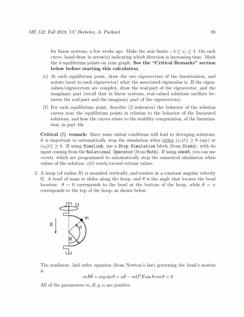
ME 132, Fall 2018, UC Berkeley, A. Packard 88
for linear systems, a few weeks ago. Make the axis limits −4 ≤ xi ≤ 4. On eachcurve, hand-draw in arrow(s) indicating which direction is increasing time. Markthe 4 equilibrium points on your graph. See the “Critical Remarks” sectionbelow before starting this calculation.
(e) At each equilibrium point, draw the two eigenvectors of the linearization, andnotate (next to each eigenvector) what the associated eigenvalue is. If the eigen-values/eigenvectors are complex, draw the real-part of the eigenvector, and theimaginary part (recall that in linear systems, real-valued solutions oscillate be-tween the real-part and the imaginary part of the eigenvectors).
(f) For each equilibrium point, describe (2 sentences) the behavior of the solutioncurves near the equilibrium points in relation to the behavior of the linearizedsolutions, and how the curves relate to the stability computation, of the lineariza-tion, in part 10c.
Critical (!) remark: Since some initial conditions will lead to diverging solutions,it is important to automatically stop the simulation when either |x1(t)| ≥ 8 (say) or|x2(t)| ≥ 8. If using Simulink, use a Stop Simulation block (from Sinks), with itsinput coming from the Relational Operator (from Math). If using ode45, you can useevents, which are programmed to automatically stop the numerical simulation whenvalues of the solution, x(t) reach/exceed certain values.
2. A hoop (of radius R) is mounted vertically, and rotates at a constant angular velocityΩ. A bead of mass m slides along the hoop, and θ is the angle that locates the beadlocation. θ = 0 corresponds to the bead at the bottom of the hoop, while θ = πcorresponds to the top of the hoop, as shown below.
The nonlinear, 2nd order equation (from Newton’s law) governing the bead’s motionis
mRθ +mg sin θ + αθ −mΩ2R sin θ cos θ = 0
All of the parameters m,R, g, α are positive.
ME 132, Fall 2018, UC Berkeley, A. Packard 89
(a) Let x1(t) := θ(t) and x2(t) := θ(t). Write the 2nd order nonlinear differentialequation in the state-space form
x1(t) = f1 (x1(t), x2(t))x2(t) = f2 (x1(t), x2(t))
(b) Show that x1 = 0, x2 = 0 is an equilibrium point of the system.
(c) Find the linearized systemη(t) = Aη(t)
which governs small deviations away from the equilibrium point (0, 0).
(d) Under what conditions (on m,R,Ω, g) is the linearized system stable?
(e) Show that x1 = π, x2 = 0 is an equilibrium point of the system.
(f) Find the linearized system η(t) = Aη(t) which governs small deviations away fromthe equilibrium point (π, 0).
(g) Under what conditions is the linearized system stable?
(h) It would seem that if the hoop is indeed rotating (with angular velocity Ω) thenthere would other equilibrium point (with 0 < θ < π/2). Do such equilibriumpoints exist in the system? Be very careful, and please explain your answer.
(i) Find the linearized system η(t) = Aη(t) which governs small deviations away fromthis equilibrium point.
(j) Under what conditions is the linearized system stable?
3. Car Engine Model (the reference for this problem is Cho and Hedrick, “AutomotivePowertrain Modelling for Control,” ASME Journal of Dynamic Systems, Measurementand Control, vol. 111, No. 4, December 1989): In this problem we consider a 1-statemodel for an automotive engine, with the transmission engaged in 4th gear. The enginestate is ma, the mass of air (in kilograms) in the intake manifold. The state of thedrivetrain is the angular velocity, ωe, of the engine. The input is the throttle angle, α,(in radians). The equations for the engine is
ma(t) = c1T (α(t))− c2ωe(t)ma(t)Te = c3ma(t)
where we treat ωe and α as inputs, and Te as an output. The drivetrain is modeled
ωe(t) =1
Je[Te(t)− Tf (t)− Td(t)− Tr(t)]
The meanings of the terms are as follows:

ME 132, Fall 2018, UC Berkeley, A. Packard 90
• T (α) is a throttle flow characteristic depending on throttle angle,
T (α) =
0.00032 for α < 0
1− cos (1.14α− 0.0252) for 0 ≤ α ≤ 1.41 for α > 1.4
• Te is the torque from engine on driveshaft, c3 = 47500 Nm/kg.
• Tf is engine friction torque (Nm), Tf = 0.106ωe + 15.1
• Td is torque due to wind drag (Nm), Td = c4ω2e , with c4 = 0.0026 Nms2
• Tr is torque due to rolling resistance at wheels (Nm), Tr = 21.5.
• Je is the effective moment of inertia of the engine, transmission, wheels, car,Je = 36.4kgm2
• c1 = 0.6kg/s, c2 = 0.095
• In 4th gear, the speed of car, v (m/s), is related to ωe as v = 0.129ωe.
(a) Combine these equations into state variable form.
x(t) = f(x(t), u(t))y(t) = h(x(t))
where x1 = ma, x2 = ωe, u = α and y = v.
(b) For the purpose of calculating the Jacobian linearization, explicitly write out thefunction f(x, u) (without any t dependence). Note that f maps 3 real numbers(x1, x2, u) into 2 real numbers. There is no explicit time dependence in thisparticular f .
(c) Use Matlab to plot the throttle flow characteristic T (α) for 0 ≤ α ≤ 1.4
(d) Let v > 0 denote an equilibium car speed. Find expressions for the correspondingequilibrium values ma, ωe and α. The expressions should all be functions of v.(In upcoming problems, for clarity, you will express various answers in terms ofthese expressions; there is no specific need to ”by-hand” subsitute the expressioninto your answers.)
(e) Based on the throttle flow characteristic, T , what is the maximum equilibriumspeed of the car?
(f) Compute the equilibrium values of ma, ωe and α so that the car travels at aconstant speed of 22 m/s (let v denote the equilibrium speed). Repeat calculationfor an equilibrium speed of v = 32 m/s. Make sure your formula are clear enoughthat you repeat this at any value of v.
ME 132, Fall 2018, UC Berkeley, A. Packard 91
(g) Consider deviations from these equilibrium values,
α(t) = α + δα(t)ωe(t) = ωe + δωe(t)ma(t) = ma + δma(t)y(t) = y + δy(t)
Find the (linear) differential equations that approximately govern these deviationvariables (Jacobian Linearzation discussed in class). Your answer should consistof 4 matrices which, in general, depend on v. Use the notation
A(v), B(v), C(v), D(v)
for the 4 matrices. Call this system Jv, to denote its dependence on the equilib-rium speed.
(h) Compute the numerical values of the Jacobian Linearization at two specific cases,namely v = 22 m/s and v = 32 m/s.
(i) Return attention to the full nonlinear model of the car/engine. Using Simulink,starting from the initial condition ωe(0) = ωe,ma(0) = ma, apply constantinput of
α(t) = α + β
for 6 values of β, β = ±0.01,±0.04,±0.1 and obtain the response for v and ma.Do this for two cases, v = 22 and v = 32.
(j) Compute (using a State-Space block in Simulink, or ode45) the response of theJacobian linearization starting from initial condition δωe(0) = 0 and δma(0) = 0,with the input δα(t) = β for for 6 values of β, β = ±0.01,±0.04,±0.1. Addthe responses δωe(t) and δma(t) to the equilibrium values ωe, ma and plot thesesums, which are approximations of the actual response. Compare the linearizedresponse with the actual response from part 3i Comment on the difference betweenthe results of the “true” nonlinear simulation and the results from the linearizedanalysis. Note: do this for both the equilibrium points – at 22 m/s and at 32m/s.
(k) Repeat this nonlinear/linear comparison, using a sinusoidal input of the form
α(t) = α + β sin(0.5t)
for 3 values of β, β = 0.01, 0.04, 0.1 and obtain the response for v and ma. Doan analogous simulation for the linearized system, and appropriately compare theresponses. Comment on the difference between the results of the “true” nonlinearsimulation and the results from the linearized analysis. Again, do this for bothcases, 22 m/s and 32 m/s..
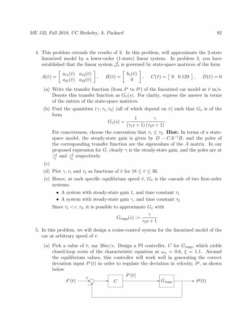
ME 132, Fall 2018, UC Berkeley, A. Packard 92
4. This problem extends the results of 3. In this problem, will approximate the 2-statelinearized model by a lower-order (1-state) linear system. In problem 3, you haveestablished that the linear system Jv is governed by state-space matrices of the form
A(v) =
[a11(v) a12(v)a21(v) a22(v)
], B(v) =
[b1(v)
0
], C(v) =
[0 0.129
], D(v) = 0
(a) Write the transfer function (from δu to δy) of the linearized car model at v m/s.Denote this transfer function as Gv(s). For clarity, express the answer in termsof the entries of the state-space matrices.
(b) Find the quantities (γ, τ1, τ2) (all of which depend on v) such that Gv is of theform
Gv(s) =1
(τ1s+ 1)
γ
(τ2s+ 1).
For concreteness, choose the convention that τ1 ≤ τ2. Hint: In terms of a state-space model, the steady-state gain is given by D − CA−1B, and the poles ofthe corresponding transfer function are the eigenvalues of the A matrix. In ourproposed expression for G, clearly γ is the steady-state gain, and the poles are at−1τ1
and −1τ2
respectively.
(c)
(d) Plot γ, τ1 and τ2 as functions of v for 18 ≤ v ≤ 36.
(e) Hence, at each specific equilibrium speed v, Gv is the cascade of two first-ordersystems:
• A system with steady-state gain 1, and time constant τ1
• A system with steady-state gain γ, and time constant τ2
Since τ1 << τ2, it is possible to approximate Gv with
Gvapp(s) :=γ
τ2s+ 1
5. In this problem, we will design a cruise-control system for the linearized model of thecar at arbitrary speed of v.
(a) Pick a value of v, say 26m/s. Design a PI controller, C for Gvapp, which yieldsclosed-loop roots of the characteristic equation at ωn = 0.6, ξ = 1.1. Aroundthe equilibrium values, this controller will work well in generating the correctdeviation input δu(t) in order to regulate the deviation in velocity, δy, as shownbelow
C Gvapp- - - -
6
i+
−δr(t)
δu(t)δy(t)

ME 132, Fall 2018, UC Berkeley, A. Packard 93
Here, δr is interpreted as a desired velocity deviation away from the equilibriumvalue of y.
(b) Since δr is the desired velocity deviation away from the equilibrium value of y, itmakes sense to interpret the actual velocity command r as r(t) = y+δr(t). So, thevelocity command is “near” y, but not necessarily equal to it. Therefore, we canimplement the control on the true nonlinear car/engine model, as shown below,with the equilibrium value of the throttle input shown adding to δu in order toget the correct input u.
CCar/
Engine- - - d -
6
-
6
i+
−(y + δr =) r δu
u
u y (= y + δy)
We can generate the equilibrium input α simply by setting the initial value (ie.,initial condition, as the cruise-control is activated) of the integrator to be equalto α
KI
Car/Engine
KP∫KI
- -
-
?- - i - -
6
i+
−r u y
Starting from equilibrium initial conditions, in the car, and with the correct initialvalue on the controller integrator, simulate the closed-loop system for the followingdesired velocity input
-
6
J
JJJJJJJ
10 20 40
50 60 65
30
28
24
t
r(t)
(c) Notice that the undershoot at t = 50 appears to be from integrator windup. Plotz and α and verify that integrator windup has occurred.
(d) Implement an anti-windup scheme for the PI controller. The left end of thedeadzone should be 0, and the right end should be 1.4. One approach is toimplement the PI controller as an S-function, for example PIaw.m. In that case,the pseudo-code for the implementation is of the form:
ME 132, Fall 2018, UC Berkeley, A. Packard 94
function [a1,a2,a3,a4] = PIaw(t,z,eInput,Message,ubar,uLimits,KP,KI)
switch Message
case 0
...
case 1
uProposed = KP*eInput + KI*z + ubar;
if uProposed>uLimits(2) && KI*eInput>0
a1 = 0; % make zdot=0 to avoid windup
elseif % Some analogous condition goes here
a1 = 0; % make zdot=0 to avoid windup
else
a1 = eInput; % standard zdot in PI control
end
case 3
...
end
Resimulate, and verify that the antiwindup controller reduces the undershoot att = 50.
(e) The controller gains, and various limit-values in the antiwindup scheme are allbased on the nominal values of the parameters in the car model, and the equi-librium speed at which the linearization was calculated. Keeping the parameterswithin the controller fixed, do a family of 50 simulations, randomly varying thecar/engine parameters (c1, c2, ...Je,.. etc) by ±20%. Use the desired-speed profileas in the previous simulation.
Plot three variables: the velocity response, the control input α, and the controllerintegrator signal z. Note the robustness of the feedback system to variations inthe car/engine behavior. Also notice that the speed (v) is relatively insensitive tothe parameter variations, but that the actual control input α is quite dependenton the variations. This is the whole point of feedback control – make theregulated variable insensitive to variations, through the use of feedbackstrategies which “automatically” cause the control variable to accom-modate these variations.
6. A common actuator in industrial and construction equipment is a hydraulic device,called a hydraulic servo-valve. A diagram is below.
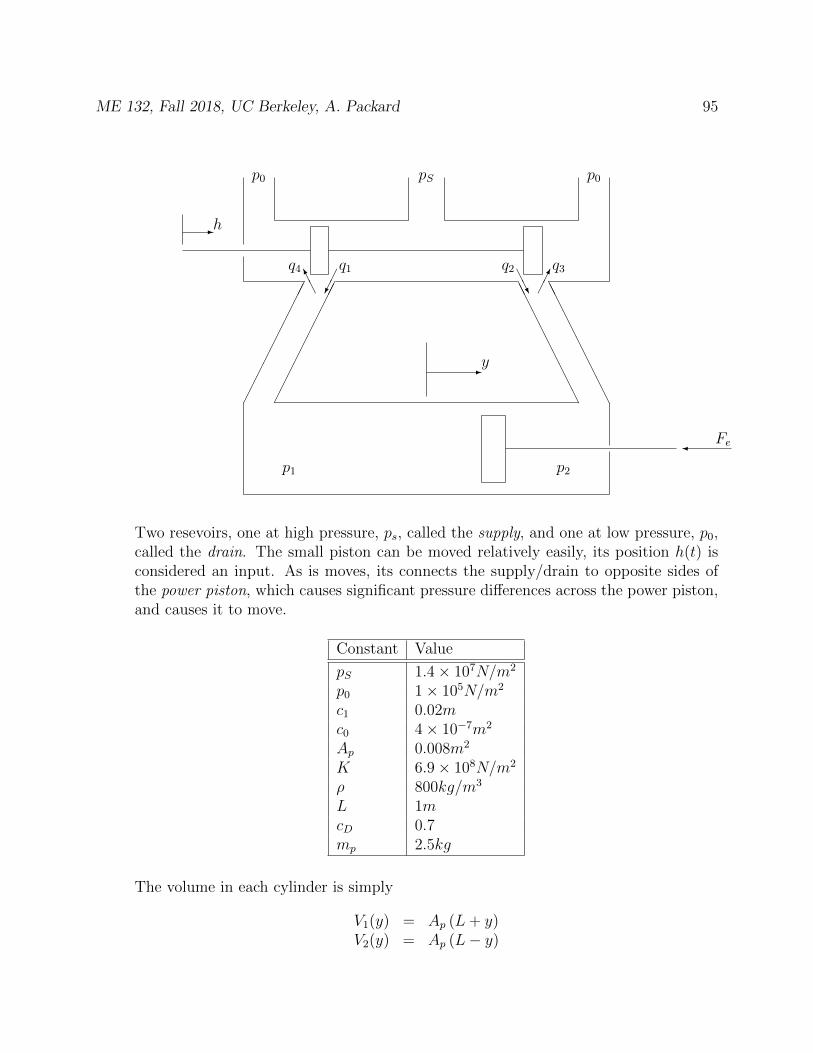
ME 132, Fall 2018, UC Berkeley, A. Packard 95
AAAAAAAAAA
AAAAAAAAAA
-h
p0 pS p0
p1 p2
-y
A
AKq4 q1
AAU
q2 q3
Fe
Two resevoirs, one at high pressure, ps, called the supply, and one at low pressure, p0,called the drain. The small piston can be moved relatively easily, its position h(t) isconsidered an input. As is moves, its connects the supply/drain to opposite sides ofthe power piston, which causes significant pressure differences across the power piston,and causes it to move.
Constant Value
pS 1.4× 10⁷N/m2
p0 1× 10⁵N/m2
c1 0.02mc0 4× 10⁻⁷m2
Ap 0.008m2
K 6.9× 10⁸N/m2
ρ 800kg/m3
L 1mcD 0.7mp 2.5kg
The volume in each cylinder is simply
V1(y) = Ap (L+ y)V2(y) = Ap (L− y)
ME 132, Fall 2018, UC Berkeley, A. Packard 96
The mass flows are
q1(t) = cDA1(h(t))√ρ (pS − p1(t))
q2(t) = cDA2(h(t))√ρ (pS − p2(t))
q3(t) = cDA3(h(t))√ρ (p2(t)− p0)
q4(t) = cDA4(h(t))√ρ (p1(t)− p0)
The valve areas are all given by the same underlying function A(h),
A(h) =4.0× 10⁻⁷ for h ≤ −0.00024.0× 10−7 + 0.02(u+ 0.0002) for −0.0002 < h < 0.0051.044× 10−4 for 0.005 < h
By symmetry, we have A1(h) = A(−h);, A2(h) = A(h);, A3(h) = A(−h);, A4(h) =A(h). Mass continuity (with compressibility) gives
q1(t)− q4(t) = ρ
[p1(t)V1(y(t))
1
K+ Apy(t)
]and
q2(t)− q3(t) = ρ
[p2(t)V2(y(t))
1
K− Apy(t)
]Finally, Newton’s law on the power piston gives
mpy(t) = Ap (p1(t)− p2(t))− Fe(t)
(a) Why can the small piston be moved easily?
(b) Define states x1 := p1, x2 := p2, x3 := y, x4 := y. Define inputs u1 := h, u2 := Fe.Define outputs y1 := y, y2 := y, y3 := y. Write state equations of the form
x(t) = f(x(t), u(t))y = g(x(t), u(t))
(c) Suppose that the power piston is attached to a mass M , which itself is also actedon by an external force w. This imposes the condition that Fe(t) = My(t) +w(t),where w is the external force acting on the mass. Substitute this in. The “inputs”to your system will now be h and w. Although it’s bad notation, call this pair u,with u1 = h, u2 = w. You will still have 4 state equations.
(d) Develop a Simulink model of the hydraulic servovalve, attached to a mass, M .Have y and y as outputs (used for feedback later), and h and w as inputs.
ME 132, Fall 2018, UC Berkeley, A. Packard 97
(e) Let y be any number satisfying −L < y < L. With the mass attached, computethe equilibrium values p1 and p2 such that
x :=
p1
p2
y0
, u :=
[00
]
is an equilibrium point. Hint: The value of M should not affect your answers forp1 and p2
(f) Derive (by hand) the linearization of the system, at the equilibrium point. withu and w as the inputs. The matrices will be parametrized by all of the area, fluidparameters, as well as M and y. Make y the output.
(g) Ignoring the disturbance force w, compute the transfer function of the linearizedmodel from h to y. Denote this by Gy,M(s), since it depends on y and M . Let Mvary from 10kg to 10000kg, and let y vary from −0.8 to 0.8. Plot the Bode plotof the frequency-response function from h→ y for at least 35 combinations of Mand y, namely 7 log-spaced values of M and 5 lin-spaced values of y. Place all onone plot.
(h) There are several simulations here. Consider two different cases with M = 30kgand separately M = 10000kg. Do short duration (Final Time is small, say 0.15)response with step inputs with h := 0.0001, w = 0, and h := 0.0004, w = 0, andh := 0.001, w = 0, and h := 0.004, w = 0, and h := 0.01, w = 0. The powerpiston should accelerate to the left. Plot the power-piston y(t), normalized (ie.,divided by) by the constant value of h. (You should have 10 plots on one sheet).Note, had the system been linear, (which it is not), after normalizing by the sizeof the step, the outputs would be identical, which they are not. Comment onthe differences as the the forcing function step size gets larger (more deviationfrom equilibrium input of h = 0). Hints: Be careful with maximum step size (inParameters window), using small sizes (start with 0.0001) as well as the simulationtime. Make sure that y(t) does not exceed L. Note that a dominant aspect of thebehavior is that y is the integral (with a negative scaling factor) of h.
(i) On one figure, using many different values for M and y, plot∣∣∣∣Gy,M(jω)−G0,10000(jω)
G0,10000(jω)
∣∣∣∣versus ω, for ω in the range 0.01 ≤ ω ≤ 1000. This is a plot of percentage-variationof the linearized model away from the linearized model G0,10000.
(j) On one figure, using many different values for M and y, plot∣∣∣∣Gy,M(jω)−Gnom(jω)
Gnom(jω)
∣∣∣∣
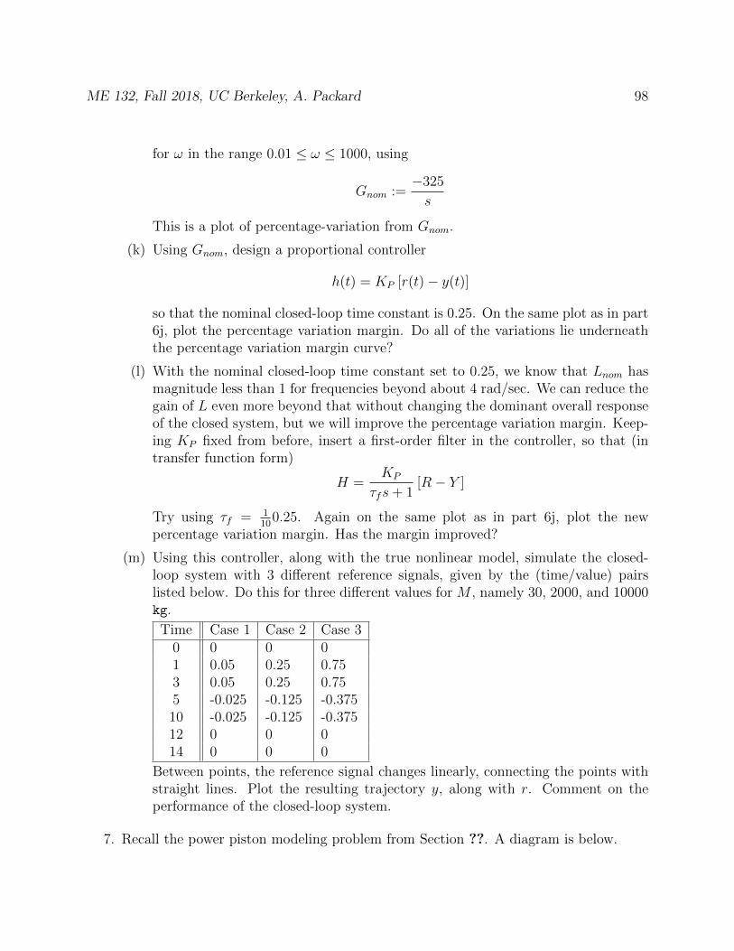
ME 132, Fall 2018, UC Berkeley, A. Packard 98
for ω in the range 0.01 ≤ ω ≤ 1000, using
Gnom :=−325
s
This is a plot of percentage-variation from Gnom.
(k) Using Gnom, design a proportional controller
h(t) = KP [r(t)− y(t)]
so that the nominal closed-loop time constant is 0.25. On the same plot as in part6j, plot the percentage variation margin. Do all of the variations lie underneaththe percentage variation margin curve?
(l) With the nominal closed-loop time constant set to 0.25, we know that Lnom hasmagnitude less than 1 for frequencies beyond about 4 rad/sec. We can reduce thegain of L even more beyond that without changing the dominant overall responseof the closed system, but we will improve the percentage variation margin. Keep-ing KP fixed from before, insert a first-order filter in the controller, so that (intransfer function form)
H =KP
τfs+ 1[R− Y ]
Try using τf = 110
0.25. Again on the same plot as in part 6j, plot the newpercentage variation margin. Has the margin improved?
(m) Using this controller, along with the true nonlinear model, simulate the closed-loop system with 3 different reference signals, given by the (time/value) pairslisted below. Do this for three different values for M , namely 30, 2000, and 10000kg.
Time Case 1 Case 2 Case 30 0 0 01 0.05 0.25 0.753 0.05 0.25 0.755 -0.025 -0.125 -0.37510 -0.025 -0.125 -0.37512 0 0 014 0 0 0
Between points, the reference signal changes linearly, connecting the points withstraight lines. Plot the resulting trajectory y, along with r. Comment on theperformance of the closed-loop system.
7. Recall the power piston modeling problem from Section ??. A diagram is below.

ME 132, Fall 2018, UC Berkeley, A. Packard 99
AAAAAAAAAA
AAAAAAAAAA
-h
p0 pS p0
p1 p2
-y
A
AKq4 q1
AAU
q2 q3
-qL
Fe
(a) Define states x1 := p1, x2 := p2, x3 := y, x4 := y. Define inputs u1 := h, u2 := Fe.Define outputs y1 := y, y2 := y, y3 := y. Write state equations of the form
x(t) = f(x(t), u(t))y = g(x(t), u(t))
(b) Suppose y is a constant, with −L < y < L. With a mass M attached, computethe equilibrium values p1 and p2 such that
x :=
p1
p2
y0
, u :=
[00
]
is an equilibrium point. Hint: The values of M and y will not affect your answersfor p1 and p2
(c) Derive (by hand) the linearization of the system, at the equilibrium point. withu and w as the inputs. The matrices will be parametrized by all of the area, fluidparameters, as well as M and y. Make y the outputs,
(d) Ignoring the disturbance force w, compute the transfer function of the linearizedmodel from h to y. Denote this by Gy,M(s), since it depends on y and M . Let Mvary from 10kg to 10000kg, and let y vary from −0.8 to 0.8. Plot the Bode plotfor at least 35 combinations of M and y, namely 7 log-spaced values of M and 5lin-spaced values of y. Place all on one plot.

ME 132, Fall 2018, UC Berkeley, A. Packard 100
(e) On one figure, using many different values for M and y, plot∣∣∣∣Gy,M(jω)−G0,10000(jω)
G0,10000(jω)
∣∣∣∣for ω in the range 0.01 ≤ ω ≤ 1000. This is a plot of percentage-variation fromG0,10000.
(f) On one figure, using many different values for M and y, plot∣∣∣∣Gy,M(jω)−Gnom(jω)
Gnom(jω)
∣∣∣∣for ω in the range 0.01 ≤ ω ≤ 1000, using
Gnom :=−325
s
This is a plot of percentage-variation from Gnom.
(g) Using the linearization as the model,
(h) Using the simple model Gnom, and the percentage-variation margin, design aproportional control to accomplish good positioning control of the mass. Theclosed-loop time constant should be on the order of 0.25-0.5 seconds.
(i) Using the controller on the true nonlinear model, simulate the closed-loop responseto the following inputs (T = 1).
-
6
J
JJJJJJJ
T 3T
5T 7T 8T
0.05
−0.025
t
r(t)
-
6
J
JJJJJJJ
T 3T
5T 7T 8T
0.25
−0.125
t
r(t)
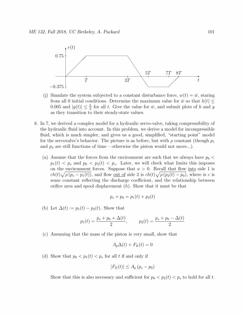
ME 132, Fall 2018, UC Berkeley, A. Packard 101
-
6
J
JJJJJJJ
T 3T
5T 7T 8T
0.75
−0.375
t
r(t)
(j) Simulate the system subjected to a constant disturbance force, w(t) = w, staringfrom all 0 initial conditions. Determine the maximum value for w so that h(t) ≤0.005 and |y(t)| ≤ L
2for all t. Give the value for w, and submit plots of h and y
as they transition to their steady-state values.
8. In 7, we derived a complex model for a hydraulic servo-valve, taking compressibility ofthe hydraulic fluid into account. In this problem, we derive a model for incompressiblefluid, which is much simpler, and gives us a good, simplified, “starting point” modelfor the servovalve’s behavior. The picture is as before, but with ρ constant (though p1
and p2 are still functions of time – otherwise the piston would not move...).
(a) Assume that the forces from the environment are such that we always have p0 <p1(t) < ps and p0 < p2(t) < ps. Later, we will check what limits this imposeson the environment forces. Suppose that u > 0. Recall that flow into side 1 isch(t)
√ρ (ps − p1(t)), and flow out of side 2 is ch(t)
√ρ (p2(t)− p0), where is c is
some constant reflecting the discharge coefficient, and the relationship betweenorifice area and spool displacement (h). Show that it must be that
ps + p0 = p1(t) + p2(t)
(b) Let ∆(t) := p1(t)− p2(t). Show that
p1(t) =ps + p0 + ∆(t)
2, p2(t) =
ps + p0 −∆(t)
2
(c) Assuming that the mass of the piston is very small, show that
Ap∆(t) + FE(t) = 0
(d) Show that p0 < p1(t) < ps for all t if and only if
|FE(t)| ≤ Ap (ps − p0)
Show that this is also necessary and sufficient for p0 < p2(t) < ps to hold for all t.
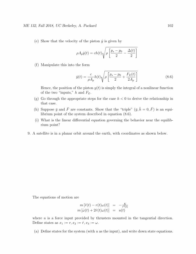
ME 132, Fall 2018, UC Berkeley, A. Packard 102
(e) Show that the velocity of the piston y is given by
ρApy(t) = ch(t)
√ρ
[ps − p0
2− ∆(t)
2
](f) Manipulate this into the form
y(t) =c
ρAph(t)
√ρ
[ps − p0
2+FE(t)
2Ap
](8.6)
Hence, the position of the piston y(t) is simply the integral of a nonlinear functionof the two “inputs,” h and FE.
(g) Go through the appropriate steps for the case h < 0 to derive the relationship inthat case.
(h) Suppose y and F are constants. Show that the “triple” (y, h = 0, F ) is an equi-librium point of the system described in equation (8.6).
(i) What is the linear differential equation governing the behavior near the equilib-rium point?
9. A satellite is in a planar orbit around the earth, with coordinates as shown below.
The equations of motion are
m [r(t)− r(t)ω(t)] = − Kr2(t)
m [ω(t) + 2r(t)ω(t)] = u(t)
where u is a force input provided by thrusters mounted in the tangential direction.Define states as x1 := r, x2 := r, x3 := ω.
(a) Define states for the system (with u as the input), and write down state equations.
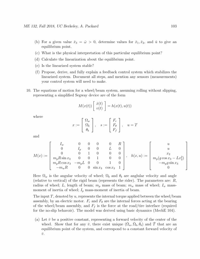
ME 132, Fall 2018, UC Berkeley, A. Packard 103
(b) For a given value x3 = ω > 0, determine values for x1, x2, and u to give anequilibrium point.
(c) What is the physical interpretation of this particular equilibrium point?
(d) Calculate the linearization about the equilibrium point.
(e) Is the linearized system stable?
(f) Propose, derive, and fully explain a feedback control system which stabilizes thelinearized system. Document all steps, and mention any sensors (measurements)your control system will need to make.
10. The equations of motion for a wheel/beam system, assuming rolling without slipping,representing a simplified Segway device are of the form
M(x(t))
[x(t)v(t)
]= h(x(t), u(t))
where
x :=
Ωw
Ωb
θb
, s :=
FrFθFf
, u = T
and
M(x) :=
Iw 0 0 0 0 R0 Ip 0 0 L 00 0 1 0 0 0
mpR sinx3 0 0 1 0 0mpR cosx3 −mpL 0 0 1 0−mwR 0 0 sinx3 cosx3 1
, h(x, u) :=
uux2
mp(g cosx3 − Lx22)
−mpg sinx3
0
Here Ωw is the angular velocity of wheel; Ωb and θb are anglular velocity and angle(relative to vertical) of the rigid beam (represents the rider). The parameters are: R,radius of wheel; L, length of beam; mp mass of beam; mw mass of wheel; Iw mass-moment of inertia of wheel; Ip mass-moment of inertia of beam.
The input T , denoted by u, represents the internal torque applied between the wheel/beamassembly, by an electric motor. Fr and Fθ are the internal forces acting at the bearingof the wheel/beam assembly, and Ff is the force at the road/tire interface (requiredfor the no-slip behavoir). The model was derived using basic dynamics (MechE 104).
(a) Let v be a positive constant, representing a forward velocity of the center of thewheel. Show that for any v, there exist unique (Ωw, Ωb, θb) and T that are anequilibrium point of the system, and correspond to a constant forward velocity ofv.
ME 132, Fall 2018, UC Berkeley, A. Packard 104
(b) Implement the equilibrium point calulation in Matlab. Write an m-file calledSegwayLinearize.m, with function declaration line
(c) Find the linearization of the system about the equilibrium point (which is parametrizedby v). For this, follow the procedure in section 8.7. Do all partial-differentiationanalytically (ie., by hand), but implement the overall procedure numerically, withMatlab.
ME 132, Fall 2018, UC Berkeley, A. Packard 105
9 Linear Algebra Review
9.1 Notation
1. R denotes the set of real numbers, C denotes the set of complex numbers. If weuse F, it means that within a definition/theorem/proof every occurance of F can beinterpreted either as R or C.
2. Rn will denote the set of all n× 1 vectors with real entries. Cn will denote the set ofall n× 1 vectors with complex entries. If v ∈ Fn, then vi denotes the i’th entry of v.
3. Rn×m denotes the set of all real, n ×m matrices. Here, the first integer denotes thenumber of rows, and the second integer denotes the number of columns. Similarly,Cn×m denotes the set of complex n × m matrices. If A ∈ Fn×m, then Aij (usually)denotes the (i, j)’th entry of v (i’th row, j’th column).
4. Addition of vectors: if v ∈ Fn and u ∈ Fn, then the sum u+ v ∈ Fn is defined by
(v + u)i := vi + ui
5. Addition of matrices: if A ∈ Fn×m and B ∈ Fn×m, then the sum A + B ∈ Fn×m isdefined by
(A+B)ij := Aij +Bij
6. Scalar multiplication: if α ∈ F and v ∈ Fn, then the product αv ∈ Fn is defined by
(αv)i := αvi
7. Scalar multiplication: if α ∈ F and A ∈ Fn×m, then the product αA ∈ Fn×m is definedby
(αA)ij := αAij
8. Matrix-Vector multiplication: if A ∈ Fn×m and v ∈ Fm, then the product Av ∈ Fn isdefined by
(Av)i :=m∑j=1
Aijvj
9. Matrix-Matrix Multiplication: if A ∈ Fn×m and B ∈ Fm×p, then the product AB ∈Fn×p is defined by
(AB)ij :=m∑k=1
AikBkj
10. Suppose x, y, z ∈ Fn and α, β ∈ F, then
ME 132, Fall 2018, UC Berkeley, A. Packard 106
• Addition is commutative and associative
x+ y = y + x, x+ (y + z) = (x+ y) + z
• The zero vector 0n is the only vector such that x+ 0n = x for all x ∈ Fn
• For each x ∈ Rn the vector −x is the unique vector such that
x+ (−x) = 0
• Scalar multiplication is associative and distributive with respect to scalar addition
α(βx) = (αβ)x, (α + β)x = αx+ βx
• Scalar multiplication is distributive with respect to vector addition
α(x+ y) = αx+ αy
11. Matrix addition is commutative, so for every matrix A and B of the same dimensions,
A+B = B + A
12. For every A,B ∈ Fn×m and every x, y ∈ Fm,
A(x+ y) = Ax+ Ay, (A+B)x = Ax+Bx
Hence vector addition distributes across matrix-vector multiplication, and matrix ad-dition distributes across matrix-vector multiplication.
13. Matrix multiplication is associative, so for every A ∈ Fn×p, B ∈ Fp×q, A ∈ Fq×m
A(BC) = (AB)C
14. For every A ∈ Fn×m, α ∈ F, and x ∈ Fm,
A(αx) = α(Ax) = (αA)x
15. Block Partitioned Matrices: Suppose that n1 + n2 = n,m1 +m2 = m, p1 + p2 = p. LetA ∈ Fn×m and B ∈ Fm×p be partitioned as
A =
[A11 A12
A21 A22
]B =
[B11 B12
B21 B22
]with each Aij ∈ Fni×mj and Bjk ∈ Fmj×pk . Then
AB =
[A11B11 + A12B21 A11B12 + A12B22
A21B11 + A22B21 A21B12 + A22B22
]Why is this easy to remember?
ME 132, Fall 2018, UC Berkeley, A. Packard 107
9.2 Determinants
1. Definition: If A ∈ F1×1, A = a11, then det (A) := a11.
2. Definition: If A ∈ Fn×n, then the (n − 1) × (n − 1) matrix obtained by eliminatingthe i’th row and j’th column is denoted A(i;j).
3. Definition: If A ∈ Fn×n, then det (A) is defined in terms of determinants of (n− 1)×(n− 1) matrices,
det (A) :=n∑j=1
a1j(−1)1+j det[A(1;j)
]4. Theorem: Given A ∈ Fn×n, and integers p, q with 1 ≤ p, q ≤ n,
det (A) =n∑j=1
apj(−1)p+j det[A(p;j)
]=
n∑i=1
aiq(−1)i+q det[A(i;q)
]5. Given A ∈ Fn×n. The following are true:
(a) if all elements of any row (or column) are zero, then det (A) = 0
(b) if all elements of any row (or column) are multiplied by a constant c to yield A,
then det(A)
= c det (A)
(c) if c is a scalar, then det (cA) = cn det (A)
(d) if A has two equal columns (or rows), then det (A) = 0
(e) If one column (or row) is a multiple of a different column, then det (A) = 0
(f) Interchanging two columns (or rows) of A to yield A gives det(A)
= − det (A).
(g) det (A) = det(AT)
6. X, Y ∈ Cn×n, thendet (XY ) = det (X) det (Y )
7. If X ∈ Cn×n, Z ∈ Cm×m Y ∈ Cn×m, then
det
([X Y0 Z
])= det (X) det (Z)
8. Suppose X ∈ Cn×m and Y ∈ Cm×n. Then
det (In +XY ) = det (Im + Y X)
Note: This holds for any dimensions n and m.
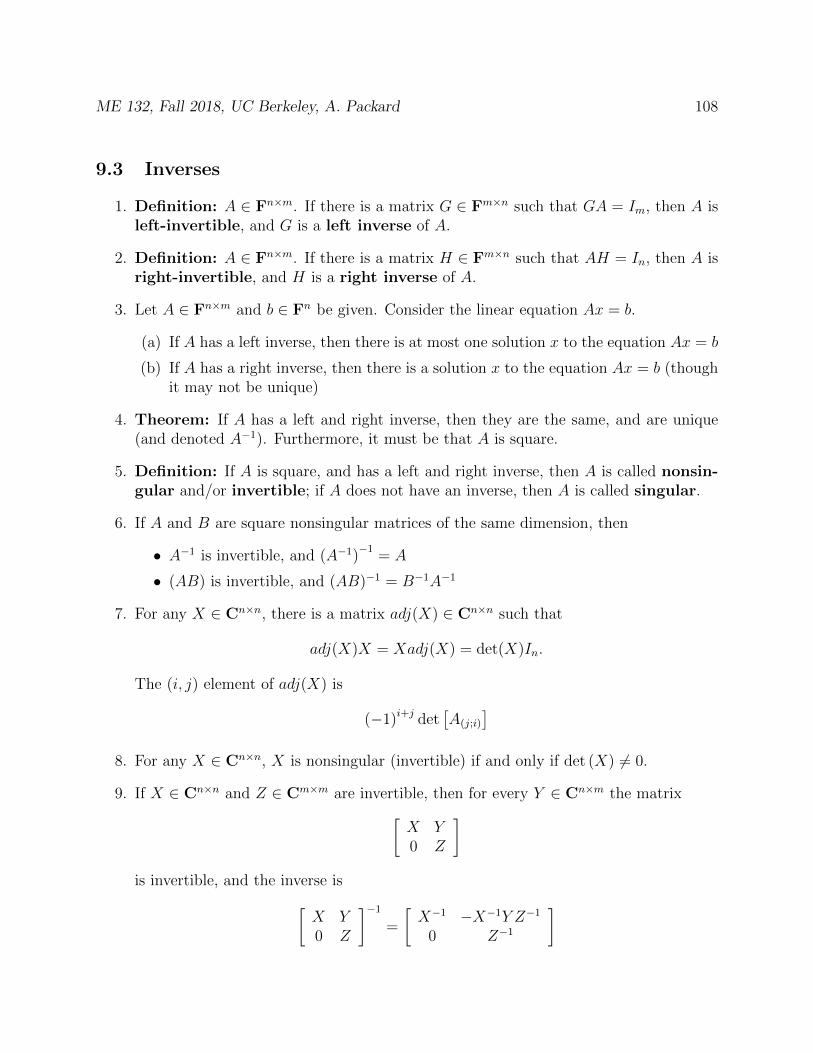
ME 132, Fall 2018, UC Berkeley, A. Packard 108
9.3 Inverses
1. Definition: A ∈ Fn×m. If there is a matrix G ∈ Fm×n such that GA = Im, then A isleft-invertible, and G is a left inverse of A.
2. Definition: A ∈ Fn×m. If there is a matrix H ∈ Fm×n such that AH = In, then A isright-invertible, and H is a right inverse of A.
3. Let A ∈ Fn×m and b ∈ Fn be given. Consider the linear equation Ax = b.
(a) If A has a left inverse, then there is at most one solution x to the equation Ax = b
(b) If A has a right inverse, then there is a solution x to the equation Ax = b (thoughit may not be unique)
4. Theorem: If A has a left and right inverse, then they are the same, and are unique(and denoted A−1). Furthermore, it must be that A is square.
5. Definition: If A is square, and has a left and right inverse, then A is called nonsin-gular and/or invertible; if A does not have an inverse, then A is called singular.
6. If A and B are square nonsingular matrices of the same dimension, then
• A−1 is invertible, and (A−1)−1
= A
• (AB) is invertible, and (AB)−1 = B−1A−1
7. For any X ∈ Cn×n, there is a matrix adj(X) ∈ Cn×n such that
adj(X)X = Xadj(X) = det(X)In.
The (i, j) element of adj(X) is
(−1)i+j det[A(j;i)
]8. For any X ∈ Cn×n, X is nonsingular (invertible) if and only if det (X) 6= 0.
9. If X ∈ Cn×n and Z ∈ Cm×m are invertible, then for every Y ∈ Cn×m the matrix[X Y0 Z
]is invertible, and the inverse is[
X Y0 Z
]−1
=
[X−1 −X−1Y Z−1
0 Z−1
]
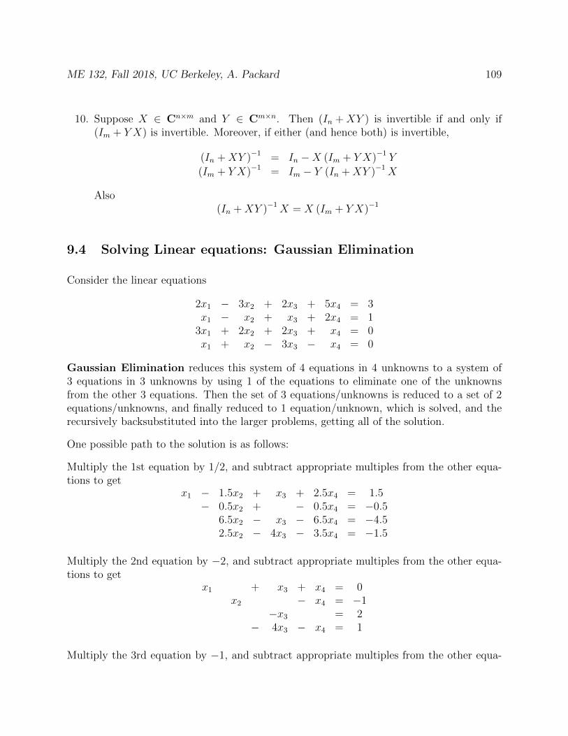
ME 132, Fall 2018, UC Berkeley, A. Packard 109
10. Suppose X ∈ Cn×m and Y ∈ Cm×n. Then (In +XY ) is invertible if and only if(Im + Y X) is invertible. Moreover, if either (and hence both) is invertible,
(In +XY )−1 = In −X (Im + Y X)−1 Y
(Im + Y X)−1 = Im − Y (In +XY )−1X
Also(In +XY )−1X = X (Im + Y X)−1
9.4 Solving Linear equations: Gaussian Elimination
Consider the linear equations
2x1 − 3x2 + 2x3 + 5x4 = 3x1 − x2 + x3 + 2x4 = 1
3x1 + 2x2 + 2x3 + x4 = 0x1 + x2 − 3x3 − x4 = 0
Gaussian Elimination reduces this system of 4 equations in 4 unknowns to a system of3 equations in 3 unknowns by using 1 of the equations to eliminate one of the unknownsfrom the other 3 equations. Then the set of 3 equations/unknowns is reduced to a set of 2equations/unknowns, and finally reduced to 1 equation/unknown, which is solved, and therecursively backsubstituted into the larger problems, getting all of the solution.
One possible path to the solution is as follows:
Multiply the 1st equation by 1/2, and subtract appropriate multiples from the other equa-tions to get
x1 − 1.5x2 + x3 + 2.5x4 = 1.5− 0.5x2 + − 0.5x4 = −0.5
6.5x2 − x3 − 6.5x4 = −4.52.5x2 − 4x3 − 3.5x4 = −1.5
Multiply the 2nd equation by −2, and subtract appropriate multiples from the other equa-tions to get
x1 + x3 + x4 = 0x2 − x4 = −1
−x3 = 2− 4x3 − x4 = 1
Multiply the 3rd equation by −1, and subtract appropriate multiples from the other equa-

ME 132, Fall 2018, UC Berkeley, A. Packard 110
tions to getx1 + x4 = 2
x2 − x4 = −1x3 = −2− x4 = −7
Multiply the 4th equation by −1, and subtract appropriate multiples from the other equa-tions to get
x1 = −5x2 = 6
x3 = −2x4 = 7
What we really were doing here was operating on the matrix [A b] ∈ R4×5,2 −3 2 5 31 −1 1 2 13 2 2 1 01 1 −3 −1 0
with elementary row operations (EROs), to reduce it to row-echeleon form. Recall thatelementary row operations are
1. multiply a row by a scalar
2. interchange 2 rows
3. replace a row by (itself + scalar multiple of another row)
9.5 Matrix functions of Time
Suppose that A is a matrix function of time, so that for each t ∈ R, A(t) ∈ Rn×m. We writethis as A : R → Rn×m. If each entry Aij of A is differentiable, then the derivative of A issimply the matrix of derivatives of the individual entries,
A(t) :=
ddtA11(t) d
dtA12(t) · · · d
dtA1m(t)
ddtA21(t) d
dtA22(t) · · · d
dtA2m(t)
......
. . ....
ddtAn1(t) d
dtAn2(t) · · · d
dtAnm(t)
Hence, the notation Aij is an ok notation, since you can interpret it to mean either the (i, j)entry of the matrix A, or the derivative of the (i, j) entry of A (since they are the samething).
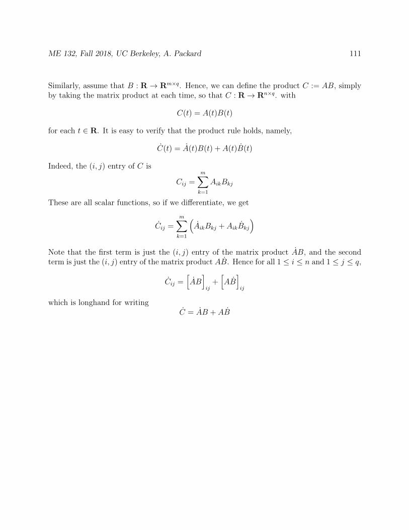
ME 132, Fall 2018, UC Berkeley, A. Packard 111
Similarly, assume that B : R→ Rm×q. Hence, we can define the product C := AB, simplyby taking the matrix product at each time, so that C : R→ Rn×q. with
C(t) = A(t)B(t)
for each t ∈ R. It is easy to verify that the product rule holds, namely,
C(t) = A(t)B(t) + A(t)B(t)
Indeed, the (i, j) entry of C is
Cij =m∑k=1
AikBkj
These are all scalar functions, so if we differentiate, we get
Cij =m∑k=1
(AikBkj + AikBkj
)Note that the first term is just the (i, j) entry of the matrix product AB, and the secondterm is just the (i, j) entry of the matrix product AB. Hence for all 1 ≤ i ≤ n and 1 ≤ j ≤ q,
Cij =[AB]ij
+[AB]ij
which is longhand for writingC = AB + AB
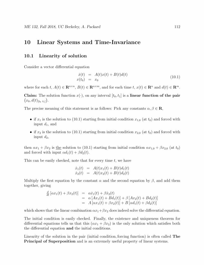
ME 132, Fall 2018, UC Berkeley, A. Packard 112
10 Linear Systems and Time-Invariance
10.1 Linearity of solution
Consider a vector differential equation
x(t) = A(t)x(t) +B(t)d(t)x(t0) = x0
(10.1)
where for each t, A(t) ∈ Rn×n, B(t) ∈ Rn×m, and for each time t, x(t) ∈ Rn and d(t) ∈ Rm.
Claim: The solution function x(·), on any interval [t0, t1] is a linear function of the pair(x0, d(t)[t0 t1]
).
The precise meaning of this statement is as follows: Pick any constants α, β ∈ R,
• if x1 is the solution to (10.1) starting from initial condition x1,0 (at t0) and forced withinput d1, and
• if x2 is the solution to (10.1) starting from initial condition x2,0 (at t0) and forced withinput d2,
then αx1 + βx2 is the solution to (10.1) starting from initial condition αx1,0 + βx2,0 (at t0)and forced with input αd1(t) + βd2(t).
This can be easily checked, note that for every time t, we have
x1(t) = A(t)x1(t) +B(t)d1(t)x2(t) = A(t)x2(t) +B(t)d2(t)
Multiply the first equation by the constant α and the second equation by β, and add themtogether, giving
ddt
[αx1(t) + βx2(t)] = αx1(t) + βx2(t)= α [Ax1(t) +Bd1(t)] + β [Ax2(t) +Bd2(t)]= A [αx1(t) + βx2(t)] +B [αd1(t) + βd2(t)]
which shows that the linear combination αx1+βx2 does indeed solve the differential equation.
The initial condition is easily checked. Finally, the existence and uniqueness theorem fordifferential equations tells us that this (αx1 + βx2) is the only solution which satisfies boththe differential equation and the initial conditions.
Linearity of the solution in the pair (initial condition, forcing function) is often called ThePrincipal of Superposition and is an extremely useful property of linear systems.
ME 132, Fall 2018, UC Berkeley, A. Packard 113
Note that in this setup, the coefficients of the differential equation (ie., the entries of thematrix A) are allowed to be functions of time. Linearity of solution to the pair (initialconditions, forcing) still followed.
Time-invariance is a separate issue from linearity, and is discussed next.
10.2 Time-Invariance
A separate issue, unrelated to linearity, is time-invariance. A system described by x(t) =f(x(t), d(t), t) is called time-invariant if (roughly) the behavior of the system does not dependexplicitly on the absolute time. In other words, shifting the time axis does not affect solutions.
Precisely, suppose that x1 is a solution for the system, starting from x10 at t = t0 subject tothe forcing d1(t), defined for t ≥ t0.
Now, let x be the solution to the equations starting from x0 at t = t0 + ∆, subject to theforcing d(t) := d(t−∆), defined for t ≥ t0 + ∆. Suppose that for all choices of t0,∆, x0 andd(·), the two responses are related by x(t) = x(t −∆) for all t ≥ t0 + ∆. Then the systemdescribed by x(t) = f(x(t), d(t), t) is called time-invariant.
In practice, the easiest manner to recognize time-invariance is that the right-hand side of thestate equations (the first-order differential equations governing the process) do not explicitlydepend on time. For instance, the system
x1(t) = 2 ∗ x2(t)− sin [x1(t)x2(t)d2(t)]x2(t) = − |x2(t)| − x2(t)d1(t)
is nonlinear, yet time-invariant.

ME 132, Fall 2018, UC Berkeley, A. Packard 114
11 Matrix Exponential
Recall that for the scalar differential equation
x(t) = ax(t) + bu(t)
x(t0) = x0
the solution for t ≥ t0 is given by the formula
x(t) = ea(t−t0) +
∫ t
t0
ea(t−τ)bu(τ)dτ
What makes this work is the special structure of the exponential function, namely that
d
dteat = aeat.
Now consider a vector differential equation
x(t) = Ax(t) +Bu(t)
x(t0) = x0
(11.1)
where A ∈ Rn×n, B ∈ Rn×m are constant matrices, and for each time t, x(t) ∈ Rn andu(t) ∈ Rm. The solution can be derived by proceeding analogously to the scalar case.
For a matrix A ∈ Cn×n define a matrix function of time, eAt ∈ Cn×n as
eAt :=∞∑k=0
tk
k!Ak
= I + tA+ t2
2!A2 + t3
3!A3 + · · ·
This is exactly the same as the definition in the scalar case. Now, for any T > 0, everyelement of this matrix power series converges absolutely and uniformly on the interval [0, T ].Hence, it can be differentiated term-by-term to correctly get the derivative. Therefore
ddteAt :=
∞∑k=0
k tk−1
k!Ak
= A+ tA2 + + t2
2!A3 + · · ·
= A(I + tA+ t2
2!A2 + · · ·
)= AeAt
This is the most important property of the function eAt. Also, in deriving this result, Acould have been pulled out of the summation on either side. Summarizing these importantidentities,
eA0 = In,d
dteAt = AeAt = eAtA
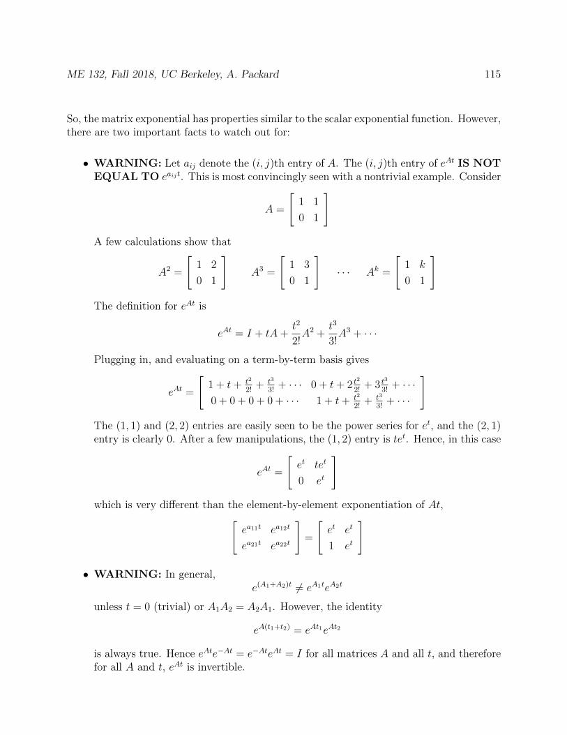
ME 132, Fall 2018, UC Berkeley, A. Packard 115
So, the matrix exponential has properties similar to the scalar exponential function. However,there are two important facts to watch out for:
• WARNING: Let aij denote the (i, j)th entry of A. The (i, j)th entry of eAt IS NOTEQUAL TO eaijt. This is most convincingly seen with a nontrivial example. Consider
A =
[1 1
0 1
]A few calculations show that
A2 =
[1 2
0 1
]A3 =
[1 3
0 1
]· · · Ak =
[1 k
0 1
]
The definition for eAt is
eAt = I + tA+t2
2!A2 +
t3
3!A3 + · · ·
Plugging in, and evaluating on a term-by-term basis gives
eAt =
[1 + t+ t2
2!+ t3
3!+ · · · 0 + t+ 2 t
2
2!+ 3 t
3
3!+ · · ·
0 + 0 + 0 + 0 + · · · 1 + t+ t2
2!+ t3
3!+ · · ·
]
The (1, 1) and (2, 2) entries are easily seen to be the power series for et, and the (2, 1)entry is clearly 0. After a few manipulations, the (1, 2) entry is tet. Hence, in this case
eAt =
[et tet
0 et
]which is very different than the element-by-element exponentiation of At,[
ea11t ea12t
ea21t ea22t
]=
[et et
1 et
]
• WARNING: In general,e(A1+A2)t 6= eA1teA2t
unless t = 0 (trivial) or A1A2 = A2A1. However, the identity
eA(t1+t2) = eAt1eAt2
is always true. Hence eAte−At = e−AteAt = I for all matrices A and all t, and thereforefor all A and t, eAt is invertible.

ME 132, Fall 2018, UC Berkeley, A. Packard 116
11.1 Diagonal A
If A ∈ Cn×n is diagonal, then eAt is easy to compute. Specifically, if A is diagonal, it is easyto see that for any k,
A =
β1 0 · · · 0
0 β2 · · · 0...
.... . .
...
0 0 · · · βn
Ak =
βk1 0 · · · 0
0 βk2 · · · 0...
.... . .
...
0 0 · · · βkn
In the power series definition for eAt, any off-diagonal terms are identically zero, and the i’thdiagonal term is simply [
eAt]ii
= 1 + tβi +t2
2!β2i +
t3
3!β3i + · · · = eβit
11.2 Block Diagonal A
If A1 ∈ Cn1×n1 and A2 ∈ Cn2×n2 , define
A :=
[A1 0
0 A2
]
Question: How is eAt related to eA1t and eA2t? Very simply – note that for any k ≥ 0,
Ak =
[A1 0
0 A2
]k=
[Ak1 0
0 Ak2
]
Hence, the power series definition for eAt gives
eAt =
[eA1t 0
0 eA2t
]
11.3 Effect of Similarity Transformations
For any invertible T ∈ Cn×n,eT
−1ATt = T−1eAtT
Equivalently,TeT
−1ATtT−1 = eAt
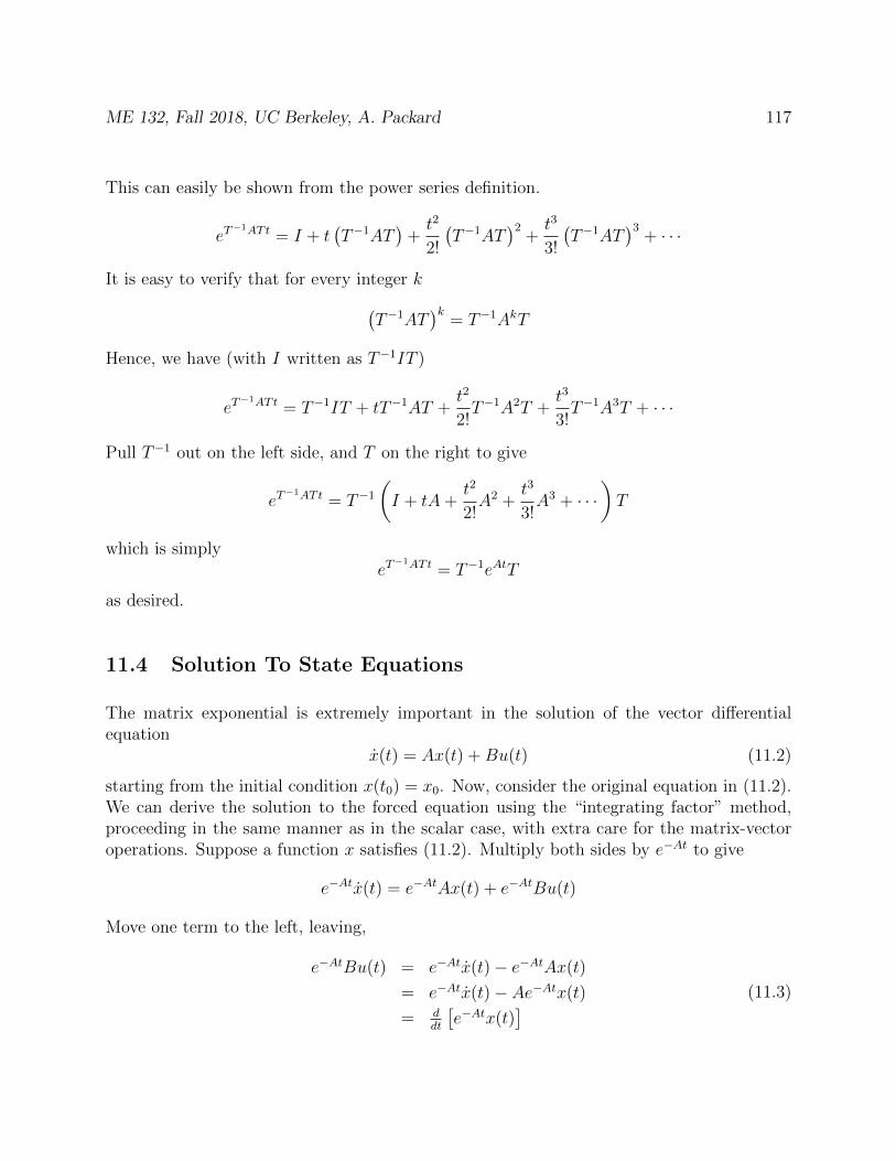
ME 132, Fall 2018, UC Berkeley, A. Packard 117
This can easily be shown from the power series definition.
eT−1ATt = I + t
(T−1AT
)+t2
2!
(T−1AT
)2+t3
3!
(T−1AT
)3+ · · ·
It is easy to verify that for every integer k(T−1AT
)k= T−1AkT
Hence, we have (with I written as T−1IT )
eT−1ATt = T−1IT + tT−1AT +
t2
2!T−1A2T +
t3
3!T−1A3T + · · ·
Pull T−1 out on the left side, and T on the right to give
eT−1ATt = T−1
(I + tA+
t2
2!A2 +
t3
3!A3 + · · ·
)T
which is simplyeT
−1ATt = T−1eAtT
as desired.
11.4 Solution To State Equations
The matrix exponential is extremely important in the solution of the vector differentialequation
x(t) = Ax(t) +Bu(t) (11.2)
starting from the initial condition x(t0) = x0. Now, consider the original equation in (11.2).We can derive the solution to the forced equation using the “integrating factor” method,proceeding in the same manner as in the scalar case, with extra care for the matrix-vectoroperations. Suppose a function x satisfies (11.2). Multiply both sides by e−At to give
e−Atx(t) = e−AtAx(t) + e−AtBu(t)
Move one term to the left, leaving,
e−AtBu(t) = e−Atx(t)− e−AtAx(t)
= e−Atx(t)− Ae−Atx(t)
= ddt
[e−Atx(t)
] (11.3)
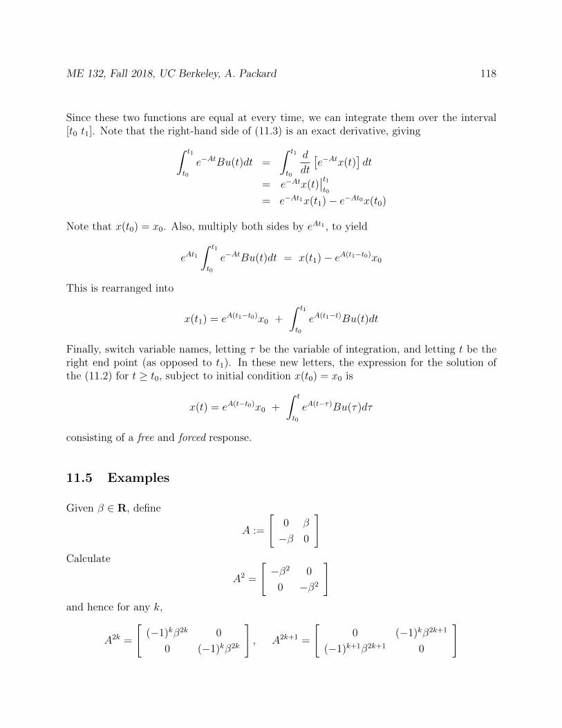
ME 132, Fall 2018, UC Berkeley, A. Packard 118
Since these two functions are equal at every time, we can integrate them over the interval[t0 t1]. Note that the right-hand side of (11.3) is an exact derivative, giving∫ t1
t0
e−AtBu(t)dt =
∫ t1
t0
d
dt
[e−Atx(t)
]dt
= e−Atx(t)∣∣t1t0
= e−At1x(t1)− e−At0x(t0)
Note that x(t0) = x0. Also, multiply both sides by eAt1 , to yield
eAt1∫ t1
t0
e−AtBu(t)dt = x(t1)− eA(t1−t0)x0
This is rearranged into
x(t1) = eA(t1−t0)x0 +
∫ t1
t0
eA(t1−t)Bu(t)dt
Finally, switch variable names, letting τ be the variable of integration, and letting t be theright end point (as opposed to t1). In these new letters, the expression for the solution ofthe (11.2) for t ≥ t0, subject to initial condition x(t0) = x0 is
x(t) = eA(t−t0)x0 +
∫ t
t0
eA(t−τ)Bu(τ)dτ
consisting of a free and forced response.
11.5 Examples
Given β ∈ R, define
A :=
[0 β
−β 0
]Calculate
A2 =
[−β2 0
0 −β2
]and hence for any k,
A2k =
[(−1)kβ2k 0
0 (−1)kβ2k
], A2k+1 =
[0 (−1)kβ2k+1
(−1)k+1β2k+1 0
]
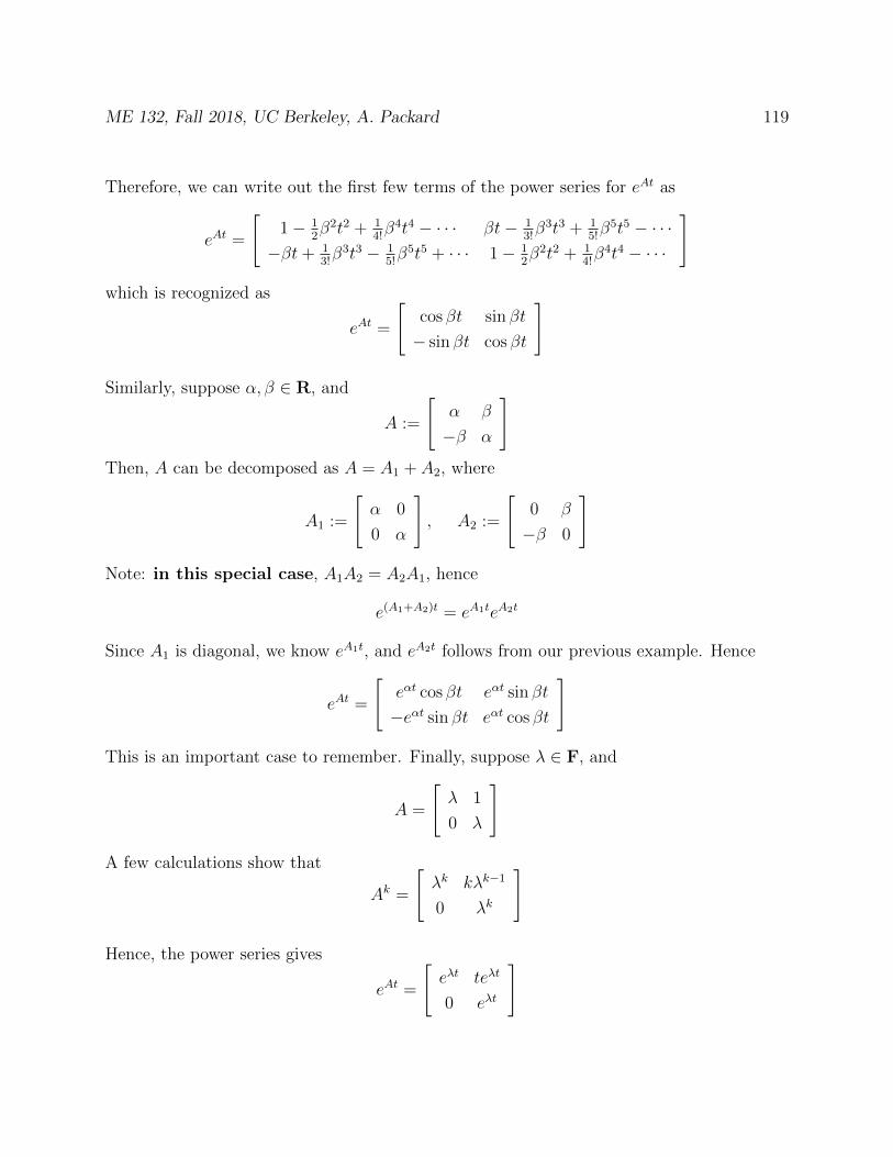
ME 132, Fall 2018, UC Berkeley, A. Packard 119
Therefore, we can write out the first few terms of the power series for eAt as
eAt =
[1− 1
2β2t2 + 1
4!β4t4 − · · · βt− 1
3!β3t3 + 1
5!β5t5 − · · ·
−βt+ 13!β3t3 − 1
5!β5t5 + · · · 1− 1
2β2t2 + 1
4!β4t4 − · · ·
]
which is recognized as
eAt =
[cos βt sin βt
− sin βt cos βt
]
Similarly, suppose α, β ∈ R, and
A :=
[α β
−β α
]Then, A can be decomposed as A = A1 + A2, where
A1 :=
[α 0
0 α
], A2 :=
[0 β
−β 0
]
Note: in this special case, A1A2 = A2A1, hence
e(A1+A2)t = eA1teA2t
Since A1 is diagonal, we know eA1t, and eA2t follows from our previous example. Hence
eAt =
[eαt cos βt eαt sin βt
−eαt sin βt eαt cos βt
]
This is an important case to remember. Finally, suppose λ ∈ F, and
A =
[λ 1
0 λ
]
A few calculations show that
Ak =
[λk kλk−1
0 λk
]
Hence, the power series gives
eAt =
[eλt teλt
0 eλt
]
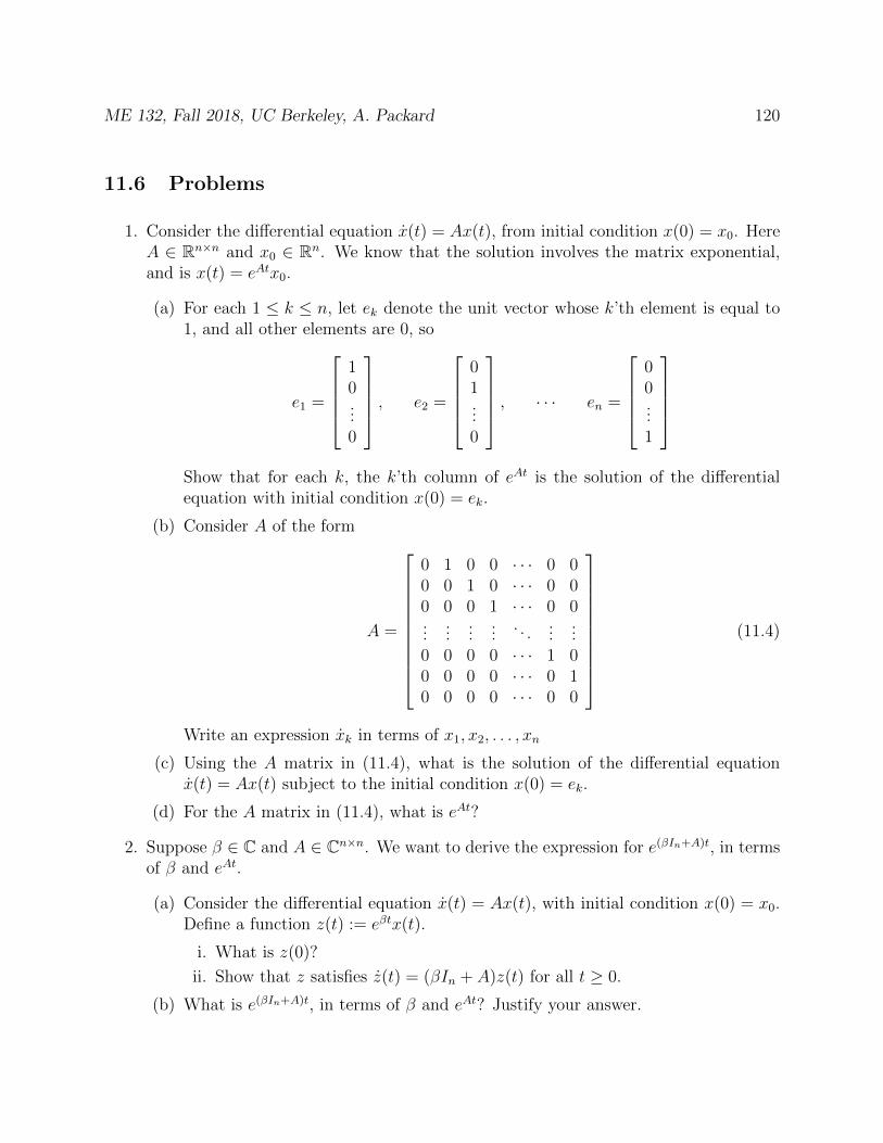
ME 132, Fall 2018, UC Berkeley, A. Packard 120
11.6 Problems
1. Consider the differential equation x(t) = Ax(t), from initial condition x(0) = x0. HereA ∈ Rn×n and x0 ∈ Rn. We know that the solution involves the matrix exponential,and is x(t) = eAtx0.
(a) For each 1 ≤ k ≤ n, let ek denote the unit vector whose k’th element is equal to1, and all other elements are 0, so
e1 =
10...0
, e2 =
01...0
, · · · en =
00...1
Show that for each k, the k’th column of eAt is the solution of the differentialequation with initial condition x(0) = ek.
(b) Consider A of the form
A =
0 1 0 0 · · · 0 00 0 1 0 · · · 0 00 0 0 1 · · · 0 0...
......
.... . .
......
0 0 0 0 · · · 1 00 0 0 0 · · · 0 10 0 0 0 · · · 0 0
(11.4)
Write an expression xk in terms of x1, x2, . . . , xn
(c) Using the A matrix in (11.4), what is the solution of the differential equationx(t) = Ax(t) subject to the initial condition x(0) = ek.
(d) For the A matrix in (11.4), what is eAt?
2. Suppose β ∈ C and A ∈ Cn×n. We want to derive the expression for e(βIn+A)t, in termsof β and eAt.
(a) Consider the differential equation x(t) = Ax(t), with initial condition x(0) = x0.Define a function z(t) := eβtx(t).
i. What is z(0)?
ii. Show that z satisfies z(t) = (βIn + A)z(t) for all t ≥ 0.
(b) What is e(βIn+A)t, in terms of β and eAt? Justify your answer.
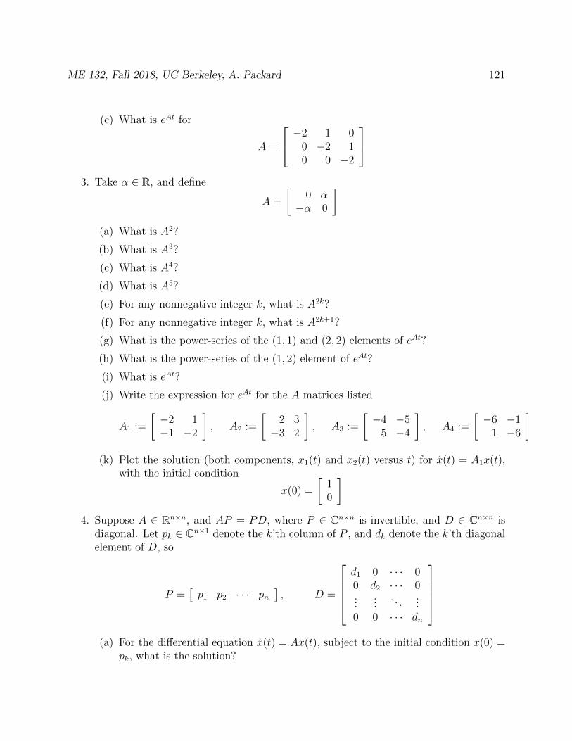
ME 132, Fall 2018, UC Berkeley, A. Packard 121
(c) What is eAt for
A =
−2 1 00 −2 10 0 −2
3. Take α ∈ R, and define
A =
[0 α−α 0
](a) What is A2?
(b) What is A3?
(c) What is A4?
(d) What is A5?
(e) For any nonnegative integer k, what is A2k?
(f) For any nonnegative integer k, what is A2k+1?
(g) What is the power-series of the (1, 1) and (2, 2) elements of eAt?
(h) What is the power-series of the (1, 2) element of eAt?
(i) What is eAt?
(j) Write the expression for eAt for the A matrices listed
A1 :=
[−2 1−1 −2
], A2 :=
[2 3−3 2
], A3 :=
[−4 −5
5 −4
], A4 :=
[−6 −1
1 −6
](k) Plot the solution (both components, x1(t) and x2(t) versus t) for x(t) = A1x(t),
with the initial condition
x(0) =
[10
]4. Suppose A ∈ Rn×n, and AP = PD, where P ∈ Cn×n is invertible, and D ∈ Cn×n is
diagonal. Let pk ∈ Cn×1 denote the k’th column of P , and dk denote the k’th diagonalelement of D, so
P =[p1 p2 · · · pn
], D =
d1 0 · · · 00 d2 · · · 0...
.... . .
...0 0 · · · dn
(a) For the differential equation x(t) = Ax(t), subject to the initial condition x(0) =
pk, what is the solution?
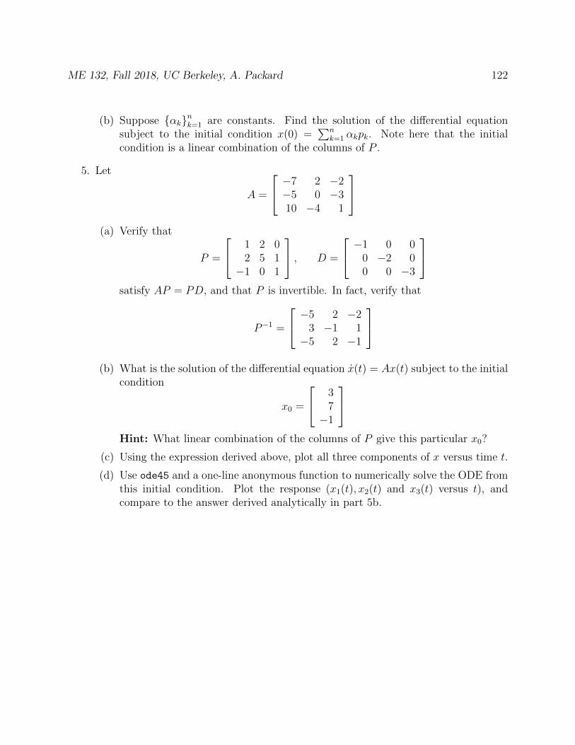
ME 132, Fall 2018, UC Berkeley, A. Packard 122
(b) Suppose αknk=1 are constants. Find the solution of the differential equationsubject to the initial condition x(0) =
∑nk=1 αkpk. Note here that the initial
condition is a linear combination of the columns of P .
5. Let
A =
−7 2 −2−5 0 −310 −4 1
(a) Verify that
P =
1 2 02 5 1−1 0 1
, D =
−1 0 00 −2 00 0 −3
satisfy AP = PD, and that P is invertible. In fact, verify that
P−1 =
−5 2 −23 −1 1−5 2 −1
(b) What is the solution of the differential equation x(t) = Ax(t) subject to the initial
condition
x0 =
37−1
Hint: What linear combination of the columns of P give this particular x0?
(c) Using the expression derived above, plot all three components of x versus time t.
(d) Use ode45 and a one-line anonymous function to numerically solve the ODE fromthis initial condition. Plot the response (x1(t), x2(t) and x3(t) versus t), andcompare to the answer derived analytically in part 5b.
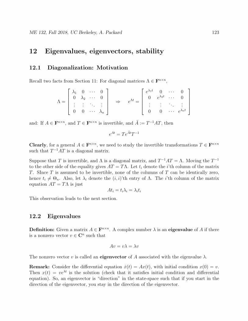
ME 132, Fall 2018, UC Berkeley, A. Packard 123
12 Eigenvalues, eigenvectors, stability
12.1 Diagonalization: Motivation
Recall two facts from Section 11: For diagonal matrices Λ ∈ Fn×n,
Λ =
λ1 0 · · · 00 λ2 · · · 0...
.... . .
...0 0 · · · λn
⇒ eΛt =
eλ1t 0 · · · 00 eλ2t · · · 0...
.... . .
...0 0 · · · eλnt
and: If A ∈ Fn×n, and T ∈ Fn×n is invertible, and A := T−1AT , then
eAt = TeAtT−1
Clearly, for a general A ∈ Fn×n, we need to study the invertible transformations T ∈ Fn×n
such that T−1AT is a diagonal matrix.
Suppose that T is invertible, and Λ is a diagonal matrix, and T−1AT = Λ. Moving the T−1
to the other side of the equality gives AT = TΛ. Let ti denote the i’th column of the matrixT . SInce T is assumed to be invertible, none of the columns of T can be identically zero,hence ti 6= Θn. Also, let λi denote the (i, i)’th entry of Λ. The i’th column of the matrixequation AT = TΛ is just
Ati = tiλi = λiti
This observation leads to the next section.
12.2 Eigenvalues
Definition: Given a matrix A ∈ Fn×n. A complex number λ is an eigenvalue of A if thereis a nonzero vector v ∈ Cn such that
Av = vλ = λv
The nonzero vector v is called an eigenvector of A associated with the eigenvalue λ.
Remark: Consider the differential equation x(t) = Ax(t), with initial condition x(0) = v.Then x(t) = veλt is the solution (check that it satisfies initial condition and differentialequation). So, an eigenvector is “direction” in the state-space such that if you start in thedirection of the eigenvector, you stay in the direction of the eigenvector.
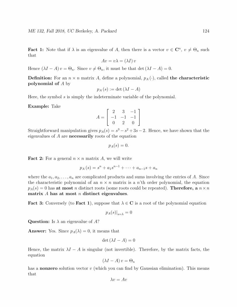
ME 132, Fall 2018, UC Berkeley, A. Packard 124
Fact 1: Note that if λ is an eigenvalue of A, then there is a vector v ∈ Cn, v 6= Θn suchthat
Av = vλ = (λI) v
Hence (λI − A) v = Θn. Since v 6= Θn, it must be that det (λI − A) = 0.
Definition: For an n× n matrix A, define a polynomial, pA (·), called the characteristicpolynomial of A by
pA (s) := det (λI − A)
Here, the symbol s is simply the indeterminate variable of the polynomial.
Example: Take
A =
2 3 −1−1 −1 −10 2 0
Straightforward manipulation gives pA(s) = s3− s2 + 3s− 2. Hence, we have shown that theeigenvalues of A are necessarily roots of the equation
pA(s) = 0.
Fact 2: For a general n× n matrix A, we will write
pA (s) = sn + a1sn−1 + · · ·+ an−1s+ an
where the a1, a2, . . . , an are complicated products and sums involving the entries of A. Sincethe characteristic polynomial of an n × n matrix is a n’th order polynomial, the equationpA(s) = 0 has at most n distinct roots (some roots could be repeated). Therefore, a n×nmatrix A has at most n distinct eigenvalues.
Fact 3: Conversely (to Fact 1), suppose that λ ∈ C is a root of the polynomial equation
pA(s)|s=λ = 0
Question: Is λ an eigenvalue of A?
Answer: Yes. Since pA(λ) = 0, it means that
det (λI − A) = 0
Hence, the matrix λI − A is singular (not invertible). Therefore, by the matrix facts, theequation
(λI − A) v = Θn
has a nonzero solution vector v (which you can find by Gaussian elimination). This meansthat
λv = Av
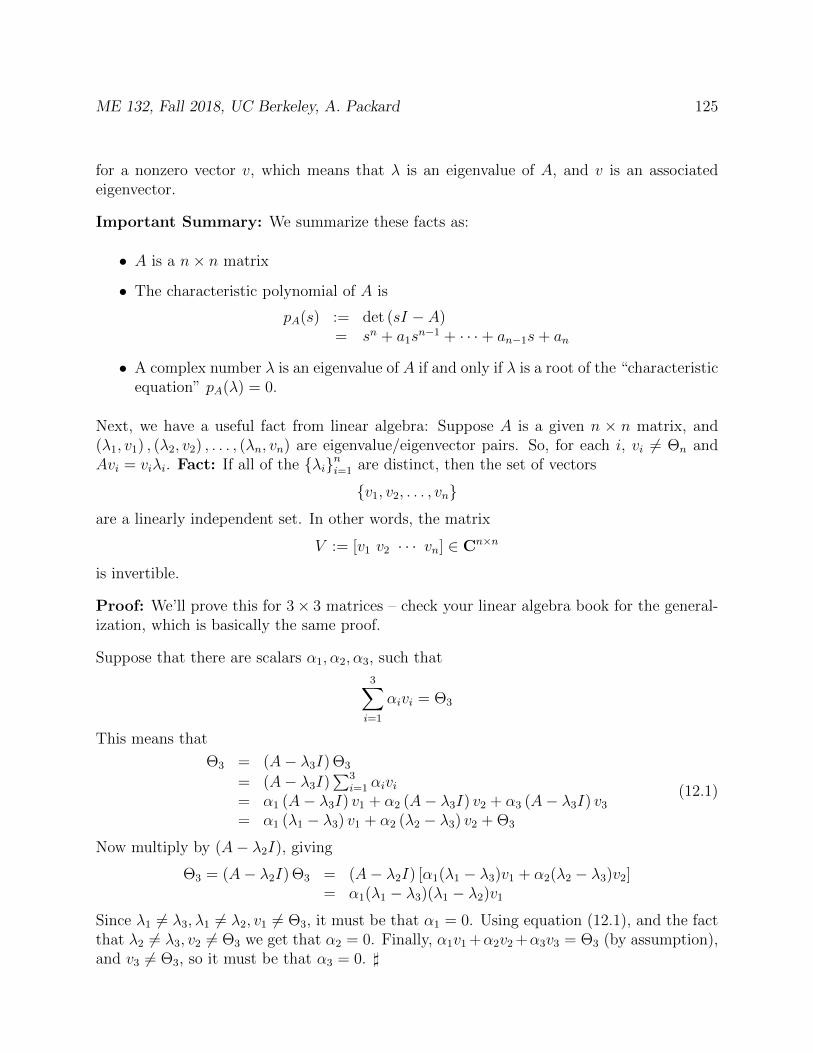
ME 132, Fall 2018, UC Berkeley, A. Packard 125
for a nonzero vector v, which means that λ is an eigenvalue of A, and v is an associatedeigenvector.
Important Summary: We summarize these facts as:
• A is a n× n matrix
• The characteristic polynomial of A is
pA(s) := det (sI − A)= sn + a1s
n−1 + · · ·+ an−1s+ an
• A complex number λ is an eigenvalue of A if and only if λ is a root of the “characteristicequation” pA(λ) = 0.
Next, we have a useful fact from linear algebra: Suppose A is a given n × n matrix, and(λ1, v1) , (λ2, v2) , . . . , (λn, vn) are eigenvalue/eigenvector pairs. So, for each i, vi 6= Θn andAvi = viλi. Fact: If all of the λini=1 are distinct, then the set of vectors
v1, v2, . . . , vn
are a linearly independent set. In other words, the matrix
V := [v1 v2 · · · vn] ∈ Cn×n
is invertible.
Proof: We’ll prove this for 3× 3 matrices – check your linear algebra book for the general-ization, which is basically the same proof.
Suppose that there are scalars α1, α2, α3, such that
3∑i=1
αivi = Θ3
This means that
Θ3 = (A− λ3I) Θ3
= (A− λ3I)∑3
i=1 αivi= α1 (A− λ3I) v1 + α2 (A− λ3I) v2 + α3 (A− λ3I) v3
= α1 (λ1 − λ3) v1 + α2 (λ2 − λ3) v2 + Θ3
(12.1)
Now multiply by (A− λ2I), giving
Θ3 = (A− λ2I) Θ3 = (A− λ2I) [α1(λ1 − λ3)v1 + α2(λ2 − λ3)v2]= α1(λ1 − λ3)(λ1 − λ2)v1
Since λ1 6= λ3, λ1 6= λ2, v1 6= Θ3, it must be that α1 = 0. Using equation (12.1), and the factthat λ2 6= λ3, v2 6= Θ3 we get that α2 = 0. Finally, α1v1 +α2v2 +α3v3 = Θ3 (by assumption),and v3 6= Θ3, so it must be that α3 = 0. ]
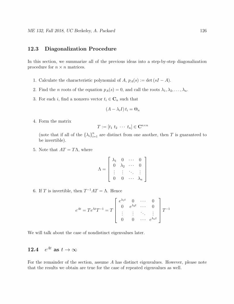
ME 132, Fall 2018, UC Berkeley, A. Packard 126
12.3 Diagonalization Procedure
In this section, we summarize all of the previous ideas into a step-by-step diagonalizationprocedure for n× n matrices.
1. Calculate the characteristic polynomial of A, pA(s) := det (sI − A).
2. Find the n roots of the equation pA(s) = 0, and call the roots λ1, λ2, . . . , λn.
3. For each i, find a nonzero vector ti ∈ Cn such that
(A− λiI) ti = Θn
4. Form the matrixT := [t1 t2 · · · tn] ∈ Cn×n
(note that if all of the λini=1 are distinct from one another, then T is guaranteed tobe invertible).
5. Note that AT = TΛ, where
Λ =
λ1 0 · · · 00 λ2 · · · 0...
.... . .
...0 0 · · · λn
6. If T is invertible, then T−1AT = Λ. Hence
eAt = TeΛtT−1 = T
eλ1t 0 · · · 00 eλ2t · · · 0...
.... . .
...0 0 · · · eλnt
T−1
We will talk about the case of nondistinct eigenvalues later.
12.4 eAt as t→∞
For the remainder of the section, assume A has distinct eigenvalues. However, please notethat the results we obtain are true for the case of repeated eigenvalues as well.

ME 132, Fall 2018, UC Berkeley, A. Packard 127
• if all of the eigenvalues (which may be complex) of A satisfy
Re (λi) < 0
then eλit → 0 as t→∞, so all entries of[eAt]
decay to zero
• If there is one (or more) eigenvalues of A with
Re (λi) ≥ 0
then
eλit → bounded 6= 0∞ as→∞
Hence, some of the entries of eAt either do not decay to zero, or, in fact, diverge to∞.
So, the eigenvalues are an indicator (the key indicator) of stability of the differential equation
x(t) = Ax(t)
• if all of the eigenvalues of A have negative real parts, then from any initial conditionx0, the solution
x(t) = eAtx0
decays to Θn as t→∞ (all coordinates of x(t) decay to 0 as t→∞). In this case, Ais said to be a Hurwitz matrix.
• if any of the eigenvalues of A have nonnegative real parts, then from some initialconditions x0, the solution to
x(t) = Ax(t)
does not decay to zero.
In the case of a repeated eigenvalue, say λ is repeated r times, then like repeated rootsof the characteristic polynomial, these repeated eigenvalues generally produce termslike tkeλt into eAt, where k in a integer, satisfying 0 ≤ k ≤ r − 1. As we have seenearlier, if Re(λ) < 0, this type of term decays to zero as t→∞, regardless of k, whereasif Re(λ) ≥ 0, then this type of term does not decay to zero. This is consistent withthe notion of stability covered above.
12.5 Complex Eigenvalues
In many systems, the eigenvalues are complex, rather than real. This seems unusual, sincethe system itself (ie., the physical meaning of the state and input variables, the coefficients

ME 132, Fall 2018, UC Berkeley, A. Packard 128
in the state equations, etc.) is very much Real. The procedure outlined in section 12.3 formatrix diagonalization is applicable to both real and complex eigenvalues, and if A is real,all intermediate complex terms will cancel, resulting in eAt being purely real, as expected.However, in the case of complex eigenvalues it may be more advantageous to use a differentsimilarity transformation, which does not lead to a diagonalized matrix. Instead, it leads toa real block-diagonal matrix, whose structure is easily interpreted.
Let us consider a second order system, with complex eigenvalues
x(t) = Ax(t) (12.2)
where A ∈ Rn×n, x ∈ R2 and
pA(λ) = det(λI2 − A) = (λ− σ)2 + ω2 . (12.3)
The two eigenvalues of A are λ1 = σ + jω and λ2 = σ − jω, while the two eigenvectors of Aare given by
(λ1I2 − A)v1 = Θ2 (λ2I2 − A)v2 = Θ2 . (12.4)
Notice that, since λ2 is the complex conjugate of λ1, v2 is the complex conjugate vector ofv1, i.e. if v1 = vr + jvi, then v2 = vr − jvi. This last fact can be verified as follows. Assumethat λ1 = σ + jω, v1 = vr + jvi and insert these expressions in the first of Eqs. (12.4).
[(σ + jω)I2 − A)] [vr + jvi] = Θ2 ,
Separating into its real and imaginary parts we obtain
[σvr − ωvi] + j [σvi + ωvr] = Avr + jAvi
[σvr − ωvi] = Avr (12.5)
[σvi + ωvr] = Avi .
Notice that Eqs. (12.5) hold if we replace ω by −ω and vi by −vi. Thus, if λ1 = σ + jωand v1 = vr + jvi are respectively an eigenvalue and eigenvector of A, then λ2 = σ− jω andv2 = vr − jvi are also respectively an eigenvalue and eigenvector.
Eqs. (12.5) can be rewritten in matrix form as follows
A[vr vi
]=[vr vi
] [ σ ω−ω σ
]. (12.6)
Thus, we can define the similarity transformation matrix
T =[vr vi
]∈ R2×2 (12.7)
ME 132, Fall 2018, UC Berkeley, A. Packard 129
and the matrix
Jc =
[σ ω−ω σ
](12.8)
such that
A = T Jc T−1, eAt = T eJct T−1 . (12.9)
The matrix exponential eJct is easy to calculate. Notice that
Jc =
[σ ω−ω σ
]= σI2 + S2
where
I2 =
[1 00 1
]and S2 =
[0 ω−ω 0
]is skew-symmetric, i.e. ST2 = −S2. Thus,
eS2t =
[cos(ωt) sin(ωt)− sin(ωt) cos(ωt)
].
This last result can be verified by differentiating with respect to time both sides of theequation:
d
dteS2t = S2 e
S2t
and
d
dt
[cos(ωt) sin(ωt)− sin(ωt) cos(ωt)
]=
[−ω sin(ωt) ω cos(ωt)−ω cos(ωt) −ω sin(ωt)
]=
[0 ω−ω 0
] [cos(ωt) sin(ωt)− sin(ωt) cos(ωt)
]= S2 e
S2t .
Since σI2 S2 = S2 σI2, then
eJct = eσt[
cos(ωt) sin(ωt)− sin(ωt) cos(ωt)
]. (12.10)
ME 132, Fall 2018, UC Berkeley, A. Packard 130
12.6 Alternate parametrization with complex eigenvalues
Suppose σ± jω is a complex-conjugate pair of eigenvalues with σ < 0 and ω > 0. These arethe roots of the polynomial
p(λ) := λ2 − 2σλ+ (σ2 + ω2) = (λ− σ)2 + ω2
Define two new constants (ξ, ωn), in terms of σ and ω, as
ωn :=√σ2 + ω2, ξ :=
−σωn
Since σ < 0 and ω > 0 it is clear that
ωn > 0, 0 < ξ < 1
Also is easy to “flip” this around, and give
σ = −ξωn, ω = ωn√
1− ξ2
In terms of (ξ, ωn), the polynomial is
p(λ) = λ2 + 2ξωnλ+ ω2n
In terms of these new constants, the functions that make up eAt are of the form
e−ξωnt cosωn√
1− ξ2t, e−ξωnt sinωn√
1− ξ2t
Note that functions like this are comprised of
1. an exponentially decaying envelope, e−ξωnt. Note that this decays to zero in approxi-mately 3
ξωn
2. sinosoidal oscillation terms, sinωn√
1− ξ2t and cosωn√
1− ξ2t. The period of oscil-lation is 2π
ωn√
1−ξ2.
Comparing these times, we expect “alot of oscillations before the function decays” if
2π
ωn√
1− ξ2<<
3
ξωn
Clearly ωn drops out of this comparison, and the above condition is equivalent to
2π
3
ξ√1− ξ2
<< 1
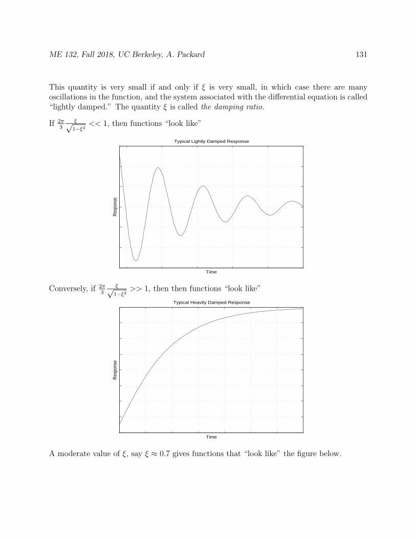
ME 132, Fall 2018, UC Berkeley, A. Packard 131
This quantity is very small if and only if ξ is very small, in which case there are manyoscillations in the function, and the system associated with the differential equation is called“lightly damped.” The quantity ξ is called the damping ratio.
If 2π3
ξ√1−ξ2
<< 1, then functions “look like”
Typical Lightly Damped Response
Time
Res
pons
e
Conversely, if 2π3
ξ√1−ξ2
>> 1, then then functions “look like”
Typical Heavily Damped Response
Time
Res
pons
e
A moderate value of ξ, say ξ ≈ 0.7 gives functions that “look like” the figure below.
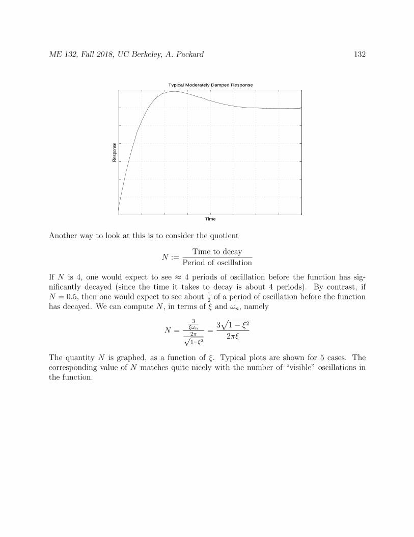
ME 132, Fall 2018, UC Berkeley, A. Packard 132
Typical Moderately Damped Response
Time
Res
pons
e
Another way to look at this is to consider the quotient
N :=Time to decay
Period of oscillation
If N is 4, one would expect to see ≈ 4 periods of oscillation before the function has sig-nificantly decayed (since the time it takes to decay is about 4 periods). By contrast, ifN = 0.5, then one would expect to see about 1
2of a period of oscillation before the function
has decayed. We can compute N , in terms of ξ and ωn, namely
N =
3ξωn2π√1−ξ2
=3√
1− ξ2
2πξ
The quantity N is graphed, as a function of ξ. Typical plots are shown for 5 cases. Thecorresponding value of N matches quite nicely with the number of “visible” oscillations inthe function.

ME 132, Fall 2018, UC Berkeley, A. Packard 133
0 0.1 0.2 0.3 0.4 0.5 0.6 0.7 0.8 0.9 10
1
2
3
4
5
6
7
8
9
10
ξ
N :=
Per
iod/
TTD
Finally, note that ωn enters yH very simply,
yH(t) = e−ξωnt[A cosωn
√1− ξ2t + B sinωn
√1− ξ2t
]Note, everywhere ωn or t appear, they appear together in a term ωnt. Hence, ωn simply“scales” the response yH(t) in t. The larger value of ωn, the faster the response.
12.6.1 Examples
Consider the system
x(t) = Ax(t) (12.11)
where x ∈ R2 and
A =
[−1.3 1.6−1.6 1.3
].
The two eigenvalues of A are λ1 = j and λ2 = −j. Their corresponding eigenvectors arerespectively
v1 =
[0.4243 + 0.5657j
0 + 0.7071j
]and v2 =
[0.4243− 0.5657j
0− 0.7071j
].
Defining
T =
[0.4243 0.5657
0 0.7071
](12.12)
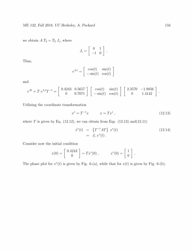
ME 132, Fall 2018, UC Berkeley, A. Packard 134
we obtain A T2 = T2 Jc, where
Jc =
[0 1−1 0
].
Thus,
eJct =
[cos(t) sin(t)− sin(t) cos(t)
]and
eAt = T eJctT−1 =
[0.4243 0.5657
0 0.7071
] [cos(t) sin(t)− sin(t) cos(t)
] [2.3570 −1.8856
0 1.4142
].
Utilizing the coordinate transformation
x∗ = T−1x x = Tx∗ , (12.13)
where T is given by Eq. (12.12), we can obtain from Eqs. (12.13) and(12.11)
x∗(t) =T−1AT
x∗(t) (12.14)
= Jc x∗(t) .
Consider now the initial condition
x(0) =
[0.4243
0
]= Tx∗(0) , x∗(0) =
[10
].
The phase plot for x∗(t) is given by Fig. 6-(a), while that for x(t) is given by Fig. 6-(b).
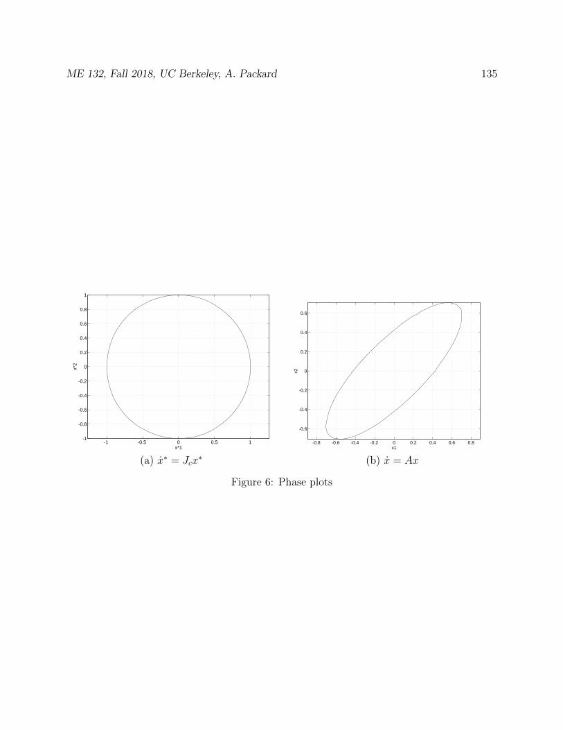
ME 132, Fall 2018, UC Berkeley, A. Packard 135
-1 -0.5 0 0.5 1-1
-0.8
-0.6
-0.4
-0.2
0
0.2
0.4
0.6
0.8
1
x*1
x*2
-0.8 -0.6 -0.4 -0.2 0 0.2 0.4 0.6 0.8
-0.6
-0.4
-0.2
0
0.2
0.4
0.6
x1
x2
(a) x∗ = Jcx∗ (b) x = Ax
Figure 6: Phase plots

ME 132, Fall 2018, UC Berkeley, A. Packard 136
12.7 Step response
Suppose the input is a constant, u(t) = u, where u ∈ Rm. What is the response startingfrom an initial condition x(0) = x0?
x(t) = eAtx0 +∫ t
0eA(t−τ)Bu(τ)dτ
= eAtx0 + eAt∫ t
0e−AτdτBu
= eAtx0 +−eAt(A−1 e−Aτ
∣∣t0
)Bu
= eAtx0 +−eAtA−1[e−At − I
]Bu
= eAtx0 +−eAt[e−At − I
]A−1Bu
= eAtx0 +[eAt − I
]A−1Bu
Hence, the output y(t) = Cx(t) +Du(t) equals
y(t) = CeAtx0 − CA−1Bu+ CeAtA−1Bu+Du
Expressed differently
y(t)− ((D − CA−1B)u) = CeAt(x0 − (−A−1Bu))
Assuming stability, eAt decays to 0 as t→∞. In that case, this expression again (as in the1st-order case) shows that the difference between y(t) and the limiting value of y decays asthe product of
• C,
• eAt, which is decaying to 0,
• difference between x0 and final value of x
It is important to note that even in the case that both u and y are scalar, the functionCeAt(x0 − (−A−1Bu)) has
• initial value equal to y(0)− yfinal;
• converges to a final value equal to 0; but...
• its magnitude does not necessarily monotonically decrease to zero, since eAt isa matrix, with different linear combinations of exponentials, and these can grow inmagnitude before they eventually decay.
So, the responses can look more interesting/complex than the responses we observed infirst-order systems. The eigenvalues of A tell some of the story, as do the eigenvectors, inan indirect manner. For exact value of response at a specific t, one needs to compute theresponse (numerically or analytically).

ME 132, Fall 2018, UC Berkeley, A. Packard 137
12.8 Quick estimate of unit-step-response of 2nd order system
Governing equation
x(t) = Ax(t) +Bu(t); y(t) = Cx(t) +Du(t), x(0) = 02
1. Determine characteristic polynomial,
pA(λ) := det(λI2 − A) = λ2 + a1λ+ a2
2. System is stable if and only if a1 > 0 and a2 > 0.
3. Are eigenvalues real or complex? Eigenvalues are real if and only is a21 − 4a2 ≥ 0.
If eigenvalues are real, compute them. If the eigenvalues are complex, try the (ξ, ωn)parametrization (as opposed to real/imag). Solve for (ξ, ωn) as
2ξωn = a1, ω2n = a2
4. Compute steady-state gain, −CA−1B
5. Compute the value of y(0), which is just CB.
6. The solution must transition from y(0) = 0, with the starting slope equal to thecomputed value of y(0) to the final value −CA−1B, with terms involving
eλ1t, eλ2t eigenvalue description
ore−ξωnt cos(ωn
√1− ξ2t), e−ξωnt sin(ωn
√1− ξ2t)
In the eigenvalue representation, the slowest (least negative) eigenvalue should (roughly)dominate the response, and its time-constant will determine the total elapsed time to“convergence” to the final value. In the (ξ, ωn) description, the time constant of theexponential envelope if 1
ξωn, the frequency of oscillation is ωn
√1− ξ2, and the ratio
time to decay
period of oscillation≈√
1− ξ2
2ξ≈ 1
2ξfor ξ < 0.4
Put another way,
• Settling time (Time to decay)= 3ξωn
• The period of oscillation = 2π
ωn√
1−ξ2.
ME 132, Fall 2018, UC Berkeley, A. Packard 138
• The number of oscillations that can be observed (during the settling time) is
N :=Time to decay
Period of oscillation=
3√
1− ξ2
2πξ
• Everywhere ωn appears together in a term ωnt. Hence, ωn simply “scales” theresponse yH(t) in t. The larger value of ωn, the faster the response. The time-constant of the exponential decay is 1
ξωn
12.9 Problems
1. Find, by hand calculation, the eigenvalues, the eigenvectors and eAt for the matrices
(a) A =
[5 −412 −9
](b) A =
[14 −824 −14
](c) A =
[0 1−9 −4.8
](d) A =
[−2.4 1.8−1.8 −2.4
]2. Find (by hand calculation) the eigenvalues and eigenvectors of the matrix
A =
−3 −2 25 7 −55 8 −6
Does eAt have all of its terms decaying to zero?
3. Consider the 4 systems given below. Note that all have 1 input, and 1 output, andfor simplicity, all share a common “A” matrix (which is from part (a) in problem 1above).
S1 : A =
[5 −412 −9
], B =
[10
], C =
[1 1
], D = 0
S2 : A =
[5 −412 −9
], B =
[01
], C =
[1 −3
], D = 0
S3 : A =
[5 −412 −9
], B =
[1
1.5
], C =
[2 −1
], D = 0
S4 : A =
[5 −412 −9
], B =
[12
], C =
[−1.5 1
], D = 0
ME 132, Fall 2018, UC Berkeley, A. Packard 139
(a) Compute the eigenvalues of the A matrix. Are the systems stable or unstable?
(b) If the systems are stable, compute the steady-state gain of each system.
(c) Compute (by hand) the unit-step response, starting from initial condition x(0) =0. To be clear, we are computing y(t), for t ≥ 0, with u(t) = 1, and x(0) = 0.
(d) After computing the step-response expressions, plot the responses.
(e) Make short comments about
• the (usual, but not always) dominance of the “slow” eigenvalue on the speedof response
• the convergence to the correct steady-state value
• the similarity and/or difference to the response of a first-order system x(t) =ax(t) + bu(t); y = cx(t)
4. Read about the MatLab command eig (using >> help eig, and the online documen-tation). Repeat problem 2 using eig, and explain any differences that you get. Hint:if a matrix has distinct eigenvalues, in what sense are the eigenvectors not unique?
5. Consider the differential equation x(t) = Ax(t), where x(t) is (3 × 1) and A is fromproblem (2) above. Suppose that the initial condition is
x(0) =
1−10
Write the initial condition as a linear combination of the eigenvectors, and find the so-lution x(t) to the differential equation, written as a time-dependent, linear combinationof the eigenvectors.
6. Suppose that we have a 2nd order system (x(t) ∈ R2) governed by the differentialequation
x(t) =
[0 −22 −5
]x(t)
Let A denote the 2× 2 matrix above.
(a) Find the eigenvalues an eigenvectors of A. In this problem, the eigenvectors canbe chosen to have all integer entries (recall that eigenvectors can be scaled)
(b) On the grid below (x1/x2 space), draw the eigenvectors.

ME 132, Fall 2018, UC Berkeley, A. Packard 140
-
-
-
-
-
-
-
-
-
-6 6 6 6 6 6 6 6 6 66
- x1
x2
(c) A plot of x2(t) vs. x1(t) is called a phase-plane plot. The variable t is not explicitlyplotted on an axis, rather it is the parameter of the tick marks along the plot.On the grid above, using hand calculations, draw the solution to the equationx(t) = Ax(t) for the initial conditions
x(0) =
[33
], x(0) =
[−22
], x(0) =
[−3−3
], x(0) =
[42
]HINT: Remember that if vi are eigenvectors, and λi are eigenvalues of A, thenthe solution to x(t) = Ax(t) from the initial condition x(0) =
∑2i=1 αivi is simply
x(t) =n∑i=1
αieλitvi
(d) Use Matlab to create a similar picture with many (say 20) different initial condi-tions spread out in the x1, x2 plane
7. Suppose A is a real, n× n matrix, and λ is an eigenvalue of A, and λ is not real, butλ is complex. Suppose v ∈ Cn is an eigenvector of A associated with this eigenvalueλ. Use the notation λ = λR + jλI and v = vr + jvI for the real and imaginary parts ofλ, and v ( j means
√−1).
(a) By equating the real and imaginary parts of the equation Av = λv, find twoequations that relate the various real and imaginary parts of λ and v.
(b) Show that λ (complex conjugate of λ) is also an eigenvalue of A. What is theassociated eigenvector?
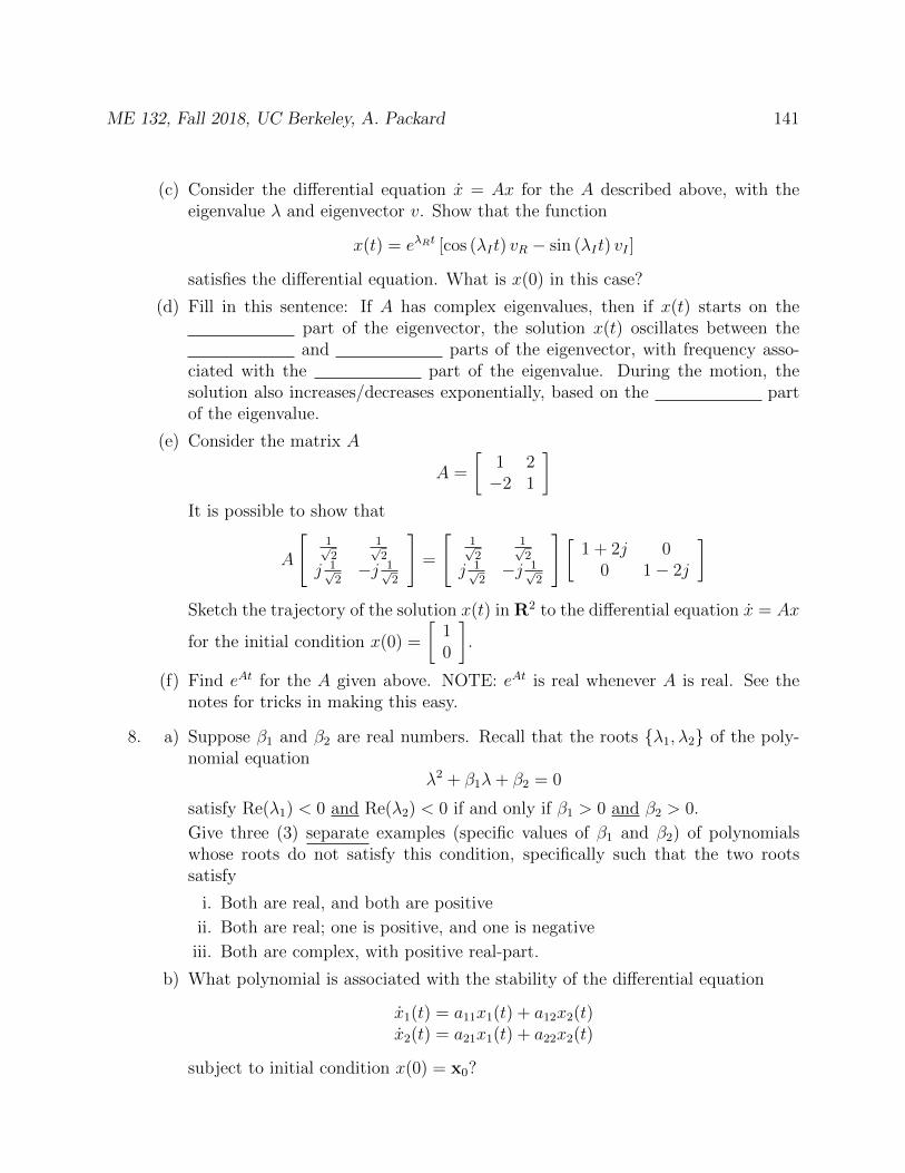
ME 132, Fall 2018, UC Berkeley, A. Packard 141
(c) Consider the differential equation x = Ax for the A described above, with theeigenvalue λ and eigenvector v. Show that the function
x(t) = eλRt [cos (λIt) vR − sin (λIt) vI ]
satisfies the differential equation. What is x(0) in this case?
(d) Fill in this sentence: If A has complex eigenvalues, then if x(t) starts on thepart of the eigenvector, the solution x(t) oscillates between theand parts of the eigenvector, with frequency asso-
ciated with the part of the eigenvalue. During the motion, thesolution also increases/decreases exponentially, based on the partof the eigenvalue.
(e) Consider the matrix A
A =
[1 2−2 1
]It is possible to show that
A
[1√2
1√2
j 1√2−j 1√
2
]=
[1√2
1√2
j 1√2−j 1√
2
][1 + 2j 0
0 1− 2j
]Sketch the trajectory of the solution x(t) in R2 to the differential equation x = Ax
for the initial condition x(0) =
[10
].
(f) Find eAt for the A given above. NOTE: eAt is real whenever A is real. See thenotes for tricks in making this easy.
8. a) Suppose β1 and β2 are real numbers. Recall that the roots λ1, λ2 of the poly-nomial equation
λ2 + β1λ+ β2 = 0
satisfy Re(λ1) < 0 and Re(λ2) < 0 if and only if β1 > 0 and β2 > 0.
Give three (3) separate examples (specific values of β1 and β2) of polynomialswhose roots do not satisfy this condition, specifically such that the two rootssatisfy
i. Both are real, and both are positive
ii. Both are real; one is positive, and one is negative
iii. Both are complex, with positive real-part.
b) What polynomial is associated with the stability of the differential equation
x1(t) = a11x1(t) + a12x2(t)x2(t) = a21x1(t) + a22x2(t)
subject to initial condition x(0) = x0?

ME 132, Fall 2018, UC Berkeley, A. Packard 142
c) Combine parts (a) and (b) to show that a 2-state system is stable if and only if
a11a22 − a12a21 > 0, a11 + a22 < 0
c) In a general linear system, expressed as
x(t) = Ax(t)
each state evolves with rate-of-change determined by a linear combination of thevalues of all the states. For example
x1(t) = A11x1(t) + A12x2(t) + · · ·+ A1nxn(t).
An abstract notion of “adding damping” to the dynamics of x1 is to replace A11
by A11 −D1, where D1 ≥ 0. Hence the dynamics become
x1(t) = (A11 −D1)x1(t) + A12x2(t) + · · ·+ A1nxn(t).
If we do this for all the states, then the new dynamic equation becomes
x(t) = (A−D)x(t)
where D is a diagonal matrix, with non-negative entries on the diagonal
D =
D1 0 · · · 00 D2 · · · 0...
.... . .
...0 0 · · · Dn
Show (by constructing an example) that this form of “adding damping” can (some-what surprisingly) change a system from being stable to being unstable.
Hint: Can this be done for system with only 1 state? If not, try a 2-state system.
9. In this problem, we look at the “damping-ratio, natural-frequency” parametrizationof complex roots, as opposed to the real/imaginary parametrization. The “damping-ratio, natural-frequency” description is a very common manner in which the locationof complex eigenvalues is described. For this problem, suppose that 0 < ξ < 1, andω > 0.
(a) What are the roots of the equation
s2 + 2ξωns+ ω2n = 0
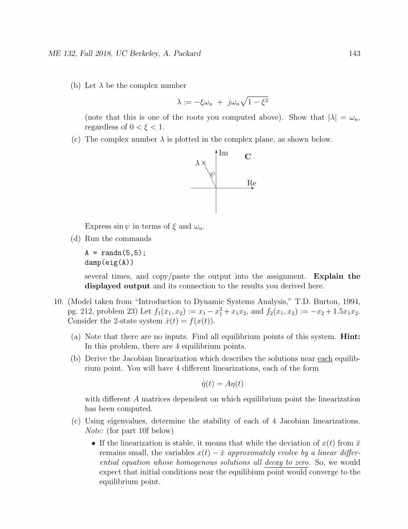
ME 132, Fall 2018, UC Berkeley, A. Packard 143
(b) Let λ be the complex number
λ := −ξωn + jωn√
1− ξ2
(note that this is one of the roots you computed above). Show that |λ| = ωn,regardless of 0 < ξ < 1.
(c) The complex number λ is plotted in the complex plane, as shown below.
-
6
λ×
AAAA
Re
Im C
ψ
Express sinψ in terms of ξ and ωn.
(d) Run the commands
A = randn(5,5);
damp(eig(A))
several times, and copy/paste the output into the assignment. Explain thedisplayed output and its connection to the results you derived here.
10. (Model taken from “Introduction to Dynamic Systems Analysis,” T.D. Burton, 1994,pg. 212, problem 23) Let f1(x1, x2) := x1− x3
1 + x1x2, and f2(x1, x2) := −x2 + 1.5x1x2.Consider the 2-state system x(t) = f(x(t)).
(a) Note that there are no inputs. Find all equilibrium points of this system. Hint:In this problem, there are 4 equilibrium points.
(b) Derive the Jacobian linearization which describes the solutions near each equilib-rium point. You will have 4 different linearizations, each of the form
η(t) = Aη(t)
with different A matrices dependent on which equilibrium point the linearizationhas been computed.
(c) Using eigenvalues, determine the stability of each of 4 Jacobian linearizations.Note: (for part 10f below)
• If the linearization is stable, it means that while the deviation of x(t) from xremains small, the variables x(t)− x approximately evolve by a linear differ-ential equation whose homogenous solutions all decay to zero. So, we wouldexpect that initial conditions near the equilibium point would converge to theequilibrium point.
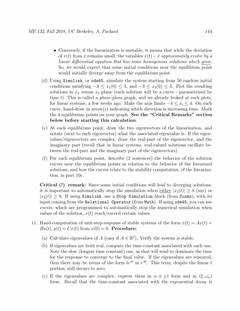
ME 132, Fall 2018, UC Berkeley, A. Packard 144
• Conversely, if the linearization is unstable, it means that while the deviationof x(t) from x remains small, the variables x(t)− x approximately evolve by alinear differential equation that has some homogenous solutions which grow.So, we would expect that some initial conditions near the equilibium pointwould initially diverge away from the equilibrium point.
(d) Using Simulink, or ode45, simulate the system starting from 50 random initialconditions satisfying −3 ≤ x1(0) ≤ 3, and −3 ≤ x2(0) ≤ 3. Plot the resultingsolutions in x2 versus x1 plane (each solution will be a curve - parametrized bytime t). This is called a phase-plane graph, and we already looked at such plots,for linear systems, a few weeks ago. Make the axis limits −4 ≤ xi ≤ 4. On eachcurve, hand-draw in arrow(s) indicating which direction is increasing time. Markthe 4 equilibrium points on your graph. See the “Critical Remarks” sectionbelow before starting this calculation.
(e) At each equilibrium point, draw the two eigenvectors of the linearization, andnotate (next to each eigenvector) what the associated eigenvalue is. If the eigen-values/eigenvectors are complex, draw the real-part of the eigenvector, and theimaginary part (recall that in linear systems, real-valued solutions oscillate be-tween the real-part and the imaginary part of the eigenvectors).
(f) For each equilibrium point, describe (2 sentences) the behavior of the solutioncurves near the equilibrium points in relation to the behavior of the linearizedsolutions, and how the curves relate to the stability computation, of the lineariza-tion, in part 10c.
Critical (!) remark: Since some initial conditions will lead to diverging solutions,it is important to automatically stop the simulation when either |x1(t)| ≥ 8 (say) or|x2(t)| ≥ 8. If using Simulink, use a Stop Simulation block (from Sinks), with itsinput coming from the Relational Operator (from Math). If using ode45, you can useevents, which are programmed to automatically stop the numerical simulation whenvalues of the solution, x(t) reach/exceed certain values.
11. Hand-computation of unit-step-response of stable systems of the form x(t) = Ax(t) +Bu(t), y(t) = Cx(t) from x(0) = 0. Procedure:
(a) Calculate eigenvalues of A (easy if A ∈ R2). Verify the system is stable.
(b) If eigenvalues are both real, compute the time-constant associated with each one.Note the slow (longest time constant) one, as that will tend to dominate the timefor the response to converge to the final value. If the eigenvalues are repeated,then there may be terms of the form teλt in eAt. This term, despite the linear tportion, still decays to zero.
(c) If the eigenvalues are complex, express them in α ± jβ form and in (ξ, ωn)form. Recall that the time-constant associated with the exponential decay is
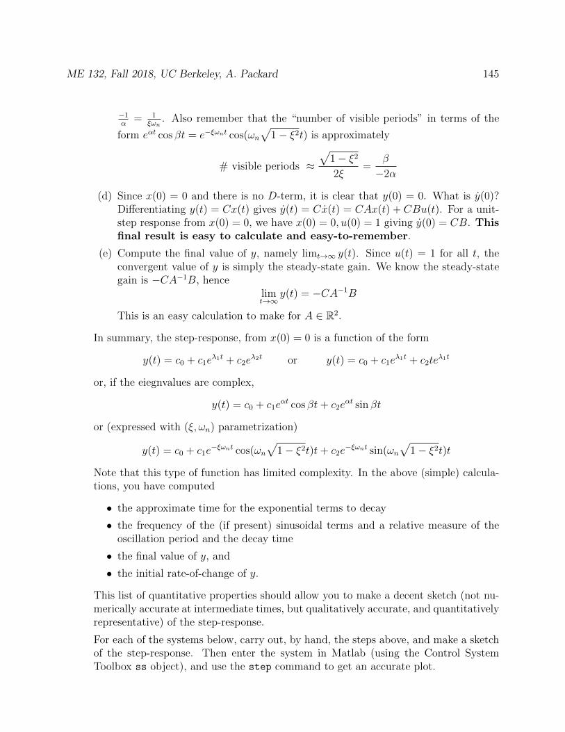
ME 132, Fall 2018, UC Berkeley, A. Packard 145
−1α
= 1ξωn
. Also remember that the “number of visible periods” in terms of the
form eαt cos βt = e−ξωnt cos(ωn√
1− ξ2t) is approximately
# visible periods ≈√
1− ξ2
2ξ=
β
−2α
(d) Since x(0) = 0 and there is no D-term, it is clear that y(0) = 0. What is y(0)?Differentiating y(t) = Cx(t) gives y(t) = Cx(t) = CAx(t) + CBu(t). For a unit-step response from x(0) = 0, we have x(0) = 0, u(0) = 1 giving y(0) = CB. Thisfinal result is easy to calculate and easy-to-remember.
(e) Compute the final value of y, namely limt→∞ y(t). Since u(t) = 1 for all t, theconvergent value of y is simply the steady-state gain. We know the steady-stategain is −CA−1B, hence
limt→∞
y(t) = −CA−1B
This is an easy calculation to make for A ∈ R2.
In summary, the step-response, from x(0) = 0 is a function of the form
y(t) = c0 + c1eλ1t + c2e
λ2t or y(t) = c0 + c1eλ1t + c2te
λ1t
or, if the eiegnvalues are complex,
y(t) = c0 + c1eαt cos βt+ c2e
αt sin βt
or (expressed with (ξ, ωn) parametrization)
y(t) = c0 + c1e−ξωnt cos(ωn
√1− ξ2t)t+ c2e
−ξωnt sin(ωn√
1− ξ2t)t
Note that this type of function has limited complexity. In the above (simple) calcula-tions, you have computed
• the approximate time for the exponential terms to decay
• the frequency of the (if present) sinusoidal terms and a relative measure of theoscillation period and the decay time
• the final value of y, and
• the initial rate-of-change of y.
This list of quantitative properties should allow you to make a decent sketch (not nu-merically accurate at intermediate times, but qualitatively accurate, and quantitativelyrepresentative) of the step-response.
For each of the systems below, carry out, by hand, the steps above, and make a sketchof the step-response. Then enter the system in Matlab (using the Control SystemToolbox ss object), and use the step command to get an accurate plot.
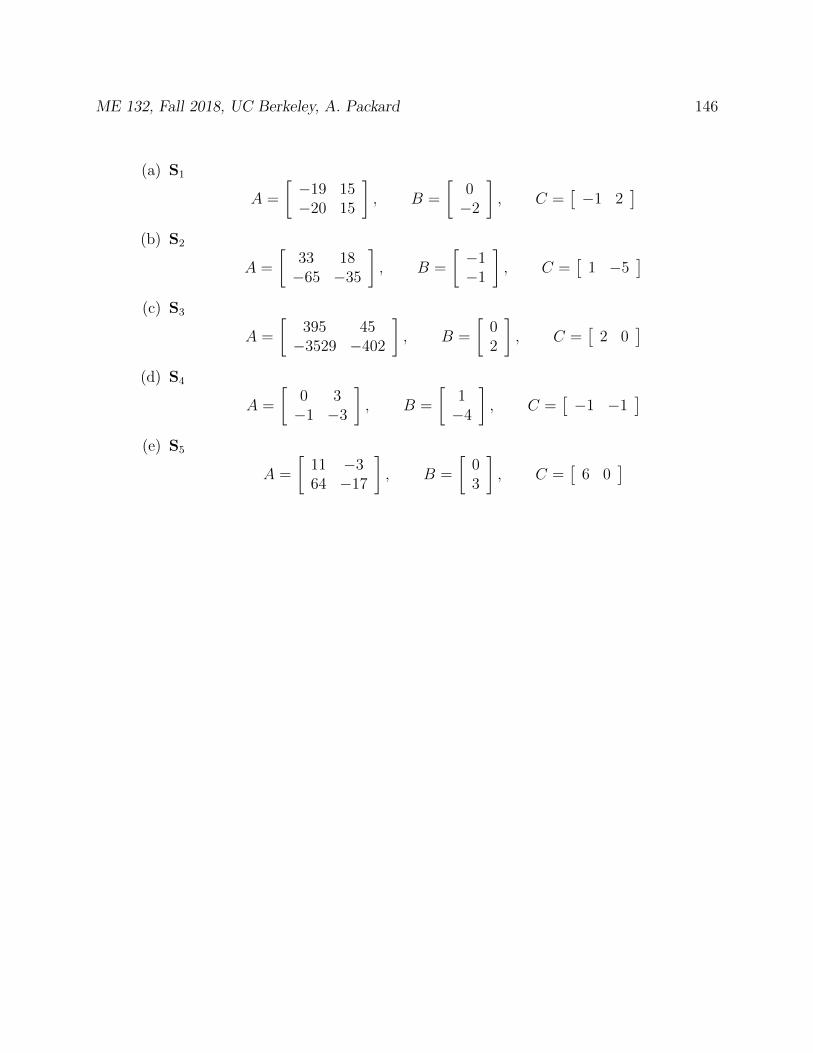
ME 132, Fall 2018, UC Berkeley, A. Packard 146
(a) S1
A =
[−19 15−20 15
], B =
[0−2
], C =
[−1 2
](b) S2
A =
[33 18−65 −35
], B =
[−1−1
], C =
[1 −5
](c) S3
A =
[395 45−3529 −402
], B =
[02
], C =
[2 0
](d) S4
A =
[0 3−1 −3
], B =
[1−4
], C =
[−1 −1
](e) S5
A =
[11 −364 −17
], B =
[03
], C =
[6 0
]
ME 132, Fall 2018, UC Berkeley, A. Packard 147
13 Frequency Response for Linear Systems: State-Space
representations
13.1 Theory for Stable System: Complex Input Signal
Consider the linear dynamical system
x(t) = Ax(t) +Bu(t)y(t) = Cx(t) +Du(t)
(13.1)
We assume that there are n states, m inputs, and q outputs (so A ∈ Rn×n, B ∈ Rn×m,C ∈ Rp×n, D ∈ Rp×m).
If the system is stable, (ie., all of A’s eigenvalues have negative real parts) it is “intuitively”clear that if u is a sinusoid, then y will approach a steady-state behavior that is sinusoidal,at the same frequency, but with different amplitude and phase. In this section, we make thisidea precise.
Take ω ≥ 0 as the input frequency, and let u ∈ Cm be a fixed complex vector (as before,we’ll derive results very easily with complex-valued inputs, and then reinterpret the resultsfor real-valued sine-wave inputs afterward). Take the input function u(t) to be
u(t) = uejωt
for t ≥ 0. Then, the response is
x(t) = eAtx0 +∫ t
0eA(t−τ)Bu(τ)dτ
= eAtx0 + eAt∫ t
0e−AτBuejωτdτ
= eAtx0 + eAt∫ t
0e(jωI−A)τdτBu
Now, since A is stable, all of the eigenvalues have negative real parts. This means that allof the eigenvalues of (jωI − A) have positive real parts. Hence (jωI − A) is invertible, andwe can write the integral as
x(t) = eAtx0 + eAt∫ t
0e(jωI−A)τdτBu
= eAt + eAt (jωI − A)−1 e(jωI−A)τ∣∣t0Bu
= eAtx0 + eAt (jωI − A)−1 [e(jωI−A)t − I]Bu
= eAtx0 + eAt[e(jωI−A)t − I
](jωI − A)−1Bu
= eAtx0 + eAt[ejωteAt − I
](jωI − A)−1Bu
= eAtx0 +[ejωt − eAt
](jωI − A)−1Bu
= eAt[x0 − (jωI − A)−1Bu
]+ (jωI − A)−1Buejωt
ME 132, Fall 2018, UC Berkeley, A. Packard 148
Hence, the output y(t) is
y(t) = CeAt[x0 − (jωI − A)−1Bu
]+ C (jωI − A)−1Buejωt +Duejωt
In the limit as t → ∞, the first term decays to 0 exponentially, leaving the steady-stateresponse
yss(t) =[D + C (jωI − A)−1B
]uejωt
Hence, we have verified our initial claim – if the input is a complex sinusoid, then the steady-state output is a complex sinusoid at the same exact frequency, but amplified by a complexgain of D + C (jωI − A)−1B.
The function G(ω)G(ω) := D + C (jωI − A)−1B (13.2)
is called the frequency response of the linear system in (13.1). Hence, for stable systems, wehave proven
u(t) := uejωt ⇒ yss(t) = G(ω)uejωt
More precisely, this is the frequency response from u to y, so we might also write Gyu(ω) toindicate what is the input (u) and what is the output (y). Gyu can be calculated rather easilyusing a computer, simply by evaluating the matrix expression in (13.2) at a large number offrequency points ω ∈ R.
13.2 MIMO Systems: Response due to real sinusoidal inputs
In the case where the system has multiple inputs and outputs, it is a bit more complicatedto write out the response due to sinusoidal inputs at a fixed frequency, since the differentinputs may all have different magnitudes and phases. As before, suppose that there are minputs, and q outputs (so B ∈ Rn×m, C ∈ Rp×n, D ∈ Rp×m). Take a ∈ Rm, b ∈ Rm, andω ≥ 0. Consider the input
u(t) = a cosωt + b sinωt
Note that this is the real part(Re) of a complex input, namely
u(t) = Re[(a− jb)ejωt
]Hence, the steady state output must be the real part of a function, specifically,
y(t) = Re[G(ω)(a− jb)ejωt
]So, in summary: To determine the steady-state response due to an input
u(t) = a cosωt + b sinωt,

ME 132, Fall 2018, UC Berkeley, A. Packard 149
let c ∈ Rq and d ∈ Rq be real vectors so that
c− jd = G(ω)(a− jb)
Then, the steady-state output is
yss(t) = c cosωt + d sinωt
13.3 Experimental Determination
Since the frequency response has the interpretation as a representation of the frequency-dependent amplitude gain and phase shift between a sinusoidal input and steady-state out-put, it is easy to obtain experimentally for a given physical system. This can be done byperforming several different forced-response experiments, with the forcing being a sinusoid,each experiment using a different frequency. We will try this procedure in lab (both simulatedon the computer, and with the EV3 systems)
13.4 Steady-State response
Suppose the input is a constant, u(t) = a, where a ∈ Rm. This is in the form of the sinusoidas derived above with ω = 0. Hence, the steady-state response is
yss(t) = G(0)a =(D − CA−1B
)a
For this reason, D − CA−1B is called the steady-state gain of a stable system.
ME 132, Fall 2018, UC Berkeley, A. Packard 150
14 Important special cases for designing closed-loop
systems
We now have the tools to study high-order closed-loop systems, but in this section, we lookat two situations which lead to 2nd-order closed-loop systems, and derive some very usefuldesign rules. Although the systems considered appear simple, this is an extremelyimportant section for students to learn in an introductory course on feedbacksystems. Understanding these examples, and the purpose of the control architecture iscritical to developing the proper intuition of feedback systems.
14.1 Roots of 2nd-order monic polynomial
The roots of λ2 + c1λ+ c2 = 0 are given by the quadratic formula, and are
λ1,2 =−c1 ±
√c2
1 − 4c2
2
Theorem: Both roots have negative real-parts if and only if c1 > 0 and c2 > 0.
Proof: If c1 > 0 and c2 > 0, then c21 − 4c2 is either
• nonegative, but less than c21, or
• negative.
In the first case, the square-root term is real, but less than c1. Hence, regardless of ±, thenumerator is a negative, real-number. Hence both roots are indeed negative real numbers.In the second case, the square-root is imaginary, and hence the real-part of both roots is − c1
2
which is negative.
Conversely, first suppose c1 ≤ 0. There are two cases:
• The quantity −4c2 ≥ 0. In this case, the square root is nonnegative, and the + of ±produces a real-root, whose value is nonnegative.
• The quantity −4c2 < 0. Hence the square-root is imaginary, and both roots havereal-part equal to − c1
2which is nonnegative.
The alternative is that c2 ≤ 0 (and take c1 > 0, since the case c1 ≤ 0 has already beenaddressed). The square-root is equal to c1, and hence the + in ± yields a root equal to 0.This completes the proof.
ME 132, Fall 2018, UC Berkeley, A. Packard 151
14.2 Setting the coefficients to attain certain roots
Suppose λ1 and λ2 are the real-valued, desired roots of a 2nd-order polynomial. Then, thepolynomial, in monic form, must be
(λ− λ1)(λ− λ2) = λ2 + (−λ1 − λ2)λ+ λ1λ2
Therefore, defining c1 := −λ1 − λ2 and c2 := λ1λ2, the polynomial λ2 + c1λ + c2 has rootsat (λ1, λ2). Likewise, if γ is a complex-valued number (with non-zero imaginary part), thenthe monic polynomial with roots at λ1 = γ and λ2 = γ is
(λ− γ)(λ− γ) = λ2 − 2Re(γ)λ+ |γ|2
Therefore (again) defining c1 := −2Re(γ) and c2 := |γ|2, the polynomial λ2 + c1λ + c2 hasroots at (γ, γ).
The message here is: if you have enough degrees-of-freedom to select the coefficients of apolynomial, then you can make the polynomial have any desired root-pattern. Use the rootsto determine the coefficients (as functions of the roots, not the other way around), and thenuse the degrees-of-freedom to set the coefficients as needed. In control design, this is called“eigenvalue placement.”
14.3 1st-order plant, 1st-order controller
1st-order plant, 1st-order controller. 2nd-order closed-loop system. Closed-loop dynamics,stability conditions, frequency-response functions, design-degrees of freedom.
Plant dynamicsx(t) = Ax(t) +B1d(t) +B2u(t)y(t) = Cx(t) +D1d(t)
Controller dynamicsq(t) = Fq(t) +G1r(t) +G2ym(t)u(t) = Hq(t) + J1r(t) + J2ym(t)
Measurement noiseym(t) = y(t) + n(t)
Assumption: u has an effect on x, so B2 6= 0. We also assume measuring y gives someinformation about x, so C 6= 0.
ME 132, Fall 2018, UC Berkeley, A. Packard 152
Careful, but elementary, substitution gives closed-loop dynamics as
x(t)q(t)y(t)u(t)
=
A+B2J2C B2H B2J1 B1 +B2J2D1 B2J2
G2C F G1 G2D1 G2
C 0 0 D1 0J2C H J1 J2D1 J2
x(t)q(t)r(t)d(t)n(t)
The closed-loop characteristic polynomial is
p(λ) = det
(λI2 −
[A+B2J2C B2H
G2C F
])= (λ− A−B2J2C)(λ− F )−B2HG2C= λ2 + (−A−B2J2C − F )λ+ (A+B2J2C)F −B2HG2C
Since this is a 2nd-order equation, the exact conditions for both roots to have negative realparts are simply
(−A−B2J2C − F ) > 0, (A+B2J2C)F −B2HG2C︸ ︷︷ ︸:=∆
> 0
Clearly, since B2C 6= 0, regardless of the plant parameters, and for any choice of F , thechoice of J2 sets the value of the first coefficient, while the subsequent choice of the productHG2 sets the value of the 2nd coefficient. Conclusion: complete freedom in “designing”the closed-loop characteristic polynomial, regardless of the plant data, and regardless of thechoice of controller parameter F .
Assuming stability, the steady-state gain from d→ y is
SSGd→y = D1 −[C 0
] [ A+B2J2C B2HG2C F
]−1 [B1 +B2J2D1
G2D1
]This is just
SSGd→y = D1 −[C 0
] 1
∆
[F −B2H−G2C A+B2J2C
] [B1 +B2J2D1
G2D1
]Making the substitutions gives
SSGd→y =D1(A−B2J2C)F − CF (B1 +B2J2D1)
∆=F (D1A− CB1)
∆
Note that if F = 0, then the steady-state gain from d to y is exactly 0. Thisis robust, in that with this choice, even if the plant parameters (A,B1, B2, C,D1)change a bit, the steady-state gain from d to y remains exactly 0. Moreover, if
ME 132, Fall 2018, UC Berkeley, A. Packard 153
F 6=, then the steady-state gain is generally not 0 (unless D1A − CB1 = 0, and then thiscondition is not robust to changes in the plant parameters). So, the only choice for robustlyachieving SSGd→y = 0 is F = 0.
Assuming F = 0 is the choice, the steady-state gain from r to y is (after simplification)
−G1
G2
Hence G2 := −G1 is a design rule, which renders the steady-state gain r to y equal to 1,also “robustly”, in that deviations in the plant parameters do not affect this steady-stategain! At this point, the controller equations are
q(t) = G1(r(t)− ym(t))u(t) = Hq(t) + J1r(t) + J2ym(t)
A block-diagram is shown below.
-
6
- - - - -
-
? ?
6
g g
J2
G1
∫dt H
J1r
ym
−+
+
u
Note that since G1 is a constant, for any signal e(t),
H
∫ t
0
G1e(τ)dτ = HG1
∫ t
0
e(τ)dτ
hence, only the product HG1 is important. Therefore without loss in generality, we takeG1 = 1. Traditionally, H is notated as KI , and J2 is denoted −KP . Finally, J1 is noted asKF . In terms of these three constants, the controller appears as
ME 132, Fall 2018, UC Berkeley, A. Packard 154
-
6
- - - -
-
? ?
6
g g
KP
∫dt KI
KFr
ym
−+
−u
The closed-loop characteristic equation is
λ2 + (−A+B2KPC)λ+B2KIC
It is still clear that by choice of KP and KI , the closed-loop characteristic equation can bedesigned arbitrarily. KF does not affect the closed-loop characteristic equation, but it doesplay a part in how r affects u (and subsequently y).
Problem-Statement Summary:
• Given a 1st-order plant; and
• a specified, desired closed-loop characteristic polynomial, λ2 + f1λ + f2, with roots inthe open-left-half plane (for stability)
• Design a feedback control system such that
1. The closed-loop system is stable; more specifically, achieve the given closed-loopcharacteristic polynomial, λ2 + f1λ+ f2;
2. The steady-state gain from d→ y is 0;
3. The steady-state gain from r → y is 1.
Solution:
• In order to achieve the two steady-state gain objectives, the PI-architecture abovemust be used, as just derived.
• In order to achieve the correct closed-loop polynomial, pick KI and KP such that
−A+B2KPC = f1, B2KIC = f2
This is always possible, since B2C 6= 0.
ME 132, Fall 2018, UC Berkeley, A. Packard 155
• Implement control strategy as shown.
• There are no constraints on KF . Adjust it to achieve a desired transient response of y(and u) due to reference comands r.
The effect that sensor noise n has on the plant output y and the control signal u was notexplicitly considered. The choice of desired closed-loop characteristic equation affects thesubsequent effect that n has on y and u. Tradeoffs must be considered when accounting forn.
ME 132, Fall 2018, UC Berkeley, A. Packard 156
14.4 2nd-order plant, constant-gain controller with derivative feed-back
The plant dynamics are
x1(t) = x2(t)x2(t) = A1x1(t) + A2x2(t) +B1d(t) +B2u(t)y(t) = x1(t)
(again, assume B2 6= 0). The regulated variable is y = x1. In this example though, both yand y are measured, and available for use in the feedback law. The presence of y inthe feedback law is the reason this is referred to as derivative feedback.
u(t) = K0r(t) +K1y(t) +K2y(t)= K0r(t) +K1x1(t) +K2x2(t)
Note that for this initial analysis, we will not focus on sensor noise.
The closed-loop equations are[x1(t)x2(t)
]=
[0 1
A1 +B2K1 A2 +B2K2
] [x1(t)x2(t)
]+
[0 0
B2K0 B1
] [r(t)d(t)
]The closed-loop characteristic polynomial is
det
(λI2 −
[0 1
A1 +B2K1 A2 +B2K2
])= λ(λ− (A2 +B2K2))− (A1 +B2K1)
= λ2 + (−A2 −B2K2)λ+ (−A1 −B2K1)
Clear that by proper choice of K1, K2, the closed-loop characteristic polynomial can beassigned arbitrarily. Write the polynomial in the (ξ, ωn) parametrization, λ2 + 2ξωnλ + ω2
n,and equate coefficients, giving
2ξωn = −A2 −B2K2, ω2n = −A1 −B2K1
Design equations
K1 = −A1 + ω2n
B2
, K2 = −A2 + 2ξωnB2
Note that in this case,
• Position-feedback, which refers to the K1y(t) term in u(t), sets ωn, the speed-of-response, and, with that chosen...
• Velocity feedback, refering to the K2y(t) term in u(t), provides the damping, ξ.
ME 132, Fall 2018, UC Berkeley, A. Packard 157
In the homework, you will consider the following issues:
• The steady-state gain from d→ y can also easily be derived. It will also be a functionof K1 and K2. Obvously, these 3 important closed-loop quantities
1. closed-loop ωn
2. closed-loop damping ratio, ξ, and
3. closed-loop steady-state gain from d→ y
cannot be set independently using the 2 feedback controller parameters K1 and K2.Accounting for the effect of noise, n, only increases the tradeoffs that must be consid-ered.
• By contrast, the steady-state gain from r → y is a function of K0, as well as the systemparameters, K1 and K2. Assuming system parameters are known, the steady-state gainfrom r → y can be adjusted to any desired value, once choices for K1 and K2 havebeen made.
14.5 Problems
1. Consider the Proportional-Integral control strategy derived in lecture
q(t) = r(t)− ym(t)u(t) = KIq(t) +KF r(t)−KPym(t)
as applied to a first-order plant with two separate disturbances, d1 and d2, specifically
x(t) = Ax(t) +B1d1(t) +B2u(t)y(t) = Cx(t) +D2d2(t)
with ym(t) = y(t) + n(t).
(a) Find the elements of the 4×6 matrix such that the equations below represent theclosed-loop system
x(t)q(t)y(t)u(t)
=
x(t)q(t)r(t)d1(t)d2(t)n(t)
(b) What is the closed-loop A matrix (from your array above)

ME 132, Fall 2018, UC Berkeley, A. Packard 158
(c) What is the closed-loop characteristic polynomial?
(d) Suppose the desired closed-loop eigenvalues are described in terms of the (ξ, ωn)parametrization. What are the design equations for gains KI and KP such thatthe eigenvalues of the closed-loop system are at this location. Your answer shouldbe KI and KP as functions of ξ, ωn, A,B1, . . . , D2.
(e) Ignoring u as an output, and n as an input, write the closed-loop equations in theform x(t)
q(t)y(t)
=
x(t)q(t)r(t)d1(t)d2(t)
This is simply drawn from your answer in part (a). Call the matrices Aclp ∈ R2×2,Bclp ∈ R2×3, Cclp ∈ R1×2, Dclp ∈ R1×3.
(f) Using the matrices from part (e), form
Dclp − CclpA−1clpBclp
which is the steady-state gain matrix from rd1
d2
→ y
Are these steady-state gains as expected?
(g) What is the instantaneous-gain (ie., FRF at ω =∞) from r → u?
2. Please read the problem though before starting. Pay special attention to the questionasked at the end in part (l).
Consider the general PI control architecture shown below
-
6
- - - -
-
? ?
6
f fKP
∫KI
KFr
ym
−
+
−u
Suppose the model of the process being controlled is x(t) = u(t) + d(t), y(t) = x(t)where y is the process output, and d is a disturbance that enters additively to thecontrol input u. For simplicity, assume there is no measurement noise, so ym = y.
ME 132, Fall 2018, UC Berkeley, A. Packard 159
(a) Under what conditions on KP and KI and KF is the closed-loop system stable?
(b) What is the closed-loop frequency-response function from r to y?
(c) What is the steady-state gain from r to y?
(d) What is the closed-loop frequency-response function from d to y.
(e) What is the steady-state gain from d to y?
(f) Which frequency-response functions are unaffected by the value of KF .
(g) Choose the values of KP and KI so that the closed-loop roots of the characteristicare described by (ξ = 0.707, ωn = 1).
(h) Show that regardless of the value of KF , the steady-state gain from r to y is 1.
(i) Consider the case when r is a unit-step, and all initial conditions are 0. UseMatlab (ode45 or Simulink or step) to compute and plot the response of thecontrol input u and the process output y for different values of KF , namely KF =KP , 0.5KP , 0.25KP , 0 and even −0.25KP (this is probably not a good idea, but itstill works... explain why). Quantitatively describe how KF affects the responsefrom r to both u and y.
(j) In what sense is the KF = KP case easier to implement than the general caseshown in the figure?
(k) Consider 3 different designs:
• the values of KP and KI chosen so that the closed-loop roots of the charac-teristic are described by (ξ = 0.707, ωn = 1)
• the values of KP and KI chosen so that the closed-loop roots of the charac-teristic are described by (ξ = 0.707, ωn = 2)
• the values of KP and KI chosen so that the closed-loop roots of the charac-teristic are described by (ξ = 0.707, ωn = 4)
all with KF = 0.25KP .
i. One one plot (with two axes), use Matlab to plot the FRF of r to y, Gr→y(ω)for all three designs. The top axes should be |Gr→y(ω)| versus ω, and thebottom axes should be ∠Gr→y(ω) versus ω. In both plots, use log-scale forω, and in the magnitude plot, also use log-scale for |G|. Read the help onloglog and semilogx if you have forgotten how to make these plots. Makesure the linetypes you use for the three designs are different, and include alegend (using legend) on the plots. Also label the axis using xlabel andylabel, and include a title (with title).
ii. One another plot, use Matlab to plot the FRF of d to y, Gd→y(ω), specifically|Gd→y(ω)| versus ω. Use log-scale for ω and log-scale for |G|. Make sure thelinetypes you use for the three designs are different, and should coincide withthe linetypes used in the r → y plots. Also include a legend and title, andlabel the axis.
ME 132, Fall 2018, UC Berkeley, A. Packard 160
iii. One another plot, use Matlab to plot the response y(t) versus t due to a unit-step reference input r. Take d(t) = 0 ∀t. The initial condition in the plantand controller should be 0. Make sure the linetypes you use for the threedesigns are different, and should coincide with the linetypes used in previousplots. Include a legend and title, and label the axis. Choose a final time of
80.707·1 , which is 8 time-constants of the slowest system.
iv. One another plot, use Matlab to plot the response y(t) versus t due to a unit-step disturbance input d. Take r(t) = 0 ∀t. The initial condition in the plantand controller should be 0. Make sure the linetypes you use for the threedesigns are different, and should coincide with the linetypes used in previousplots. Include a legend and title, and label the axis. Choose a final time of
80.707·1 , which is 8 time-constants of the slowest system.
v. Compare the time and frequency response plots. Make a short (4 items)list of comments about the general “consistency” between the informationpresented across the various plots.
(l) Comment only: Suppose you are asked to repeat the entire problem for a pro-cess with mathematical model x(t) = x(t) + u(t) + d(t), y(t) = x(t) and for aprocess with mathematical model x(t) = −x(t) + u(t) + d(t), y(t) = x(t). Haveyou set up your Matlab script so that completely repeating this problem for thisnew process would be quite easy (eg., 5-10 minutes of hand-calculations followedby changing 1 or 2 lines in a the script)? If your answer in no, consider rear-ranging your hand-calculations and script file so this is the case. If your answeris yes, consider carrying out these calculations, for your own practice.
ME 132, Fall 2018, UC Berkeley, A. Packard 161
15 Step response
Suppose the input is a constant, u(t) = u, where u ∈ Rm. What is the response startingfrom an initial condition x(0) = x0?
x(t) = eAtx0 +∫ t
0eA(t−τ)Bu(τ)dτ
= eAtx0 + eAt∫ t
0e−AτdτBu
= eAtx0 +−eAt(A−1 e−Aτ
∣∣t0
)Bu
= eAtx0 +−eAtA−1[e−At − I
]Bu
= eAtx0 +−eAt[e−At − I
]A−1Bu
= eAtx0 +[eAt − I
]A−1Bu
Hence, the output y(t) = Cx(t) +Du(t) equals
y(t) = CeAtx0 − CA−1Bu+ CeAtA−1Bu+Du
Expressed differently
y(t)− ((D − CA−1B)u) = CeAt(x0 − (−A−1Bu))
Assuming stability, eAt decays to 0 as t→∞. In that case, this expression again (as in the1st-order case) shows that the difference between y(t) and the limiting value of y decays asthe product of
• C,
• eAt, which is decaying to 0,
• difference between x0 and final value of x
It is important to note that even in the case that both u and y are scalar, the functionCeAt(x0 − (−A−1Bu)) has
• initial value equal to y(0)− yfinal;
• converges to a final value equal to 0; but...
• its magnitude does not necessarily monotonically decrease to zero, since eAt isa matrix, with different linear combinations of exponentials, and these can grow inmagnitude before they eventually decay.
So, the responses can look more interesting/complex than the responses we observed infirst-order systems. The eigenvalues of A tell some of the story, as do the eigenvectors, inan indirect manner. For exact value of response at a specific t, one needs to compute theresponse (numerically or analytically).
ME 132, Fall 2018, UC Berkeley, A. Packard 162
15.1 Quick estimate of unit-step-response of 2nd order system
Governing equation
x(t) = Ax(t) +Bu(t); y(t) = Cx(t) +Du(t), x(0) = 02
1. Determine characteristic polynomial,
pA(λ) := det(λI2 − A) = λ2 + a1λ+ a2
2. System is stable if and only if a1 > 0 and a2 > 0.
3. Are eigenvalues real or complex? Eigenvalues are real if and only is a21 − 4a2 ≥ 0.
If eigenvalues are real, compute them. If the eigenvalues are complex, try the (ξ, ωn)parametrization (as opposed to real/imag). Solve for (ξ, ωn) as
2ξωn = a1, ω2n = a2
4. Compute steady-state gain, −CA−1B
5. Compute the value of y(0), which is just CB.
6. The solution must transition from y(0) = 0, with the starting slope equal to thecomputed value of y(0) to the final value −CA−1B, with terms involving
eλ1t, eλ2t eigenvalue description
ore−ξωnt cos(ωn
√1− ξ2t), e−ξωnt sin(ωn
√1− ξ2t)
In the eigenvalue representation, the slowest (least negative) eigenvalue should (roughly)dominate the response, and its time-constant will determine the total elapsed time to“convergence” to the final value. In the (ξ, ωn) description, the time constant of theexponential envelope if 1
ξωn, the frequency of oscillation is ωn
√1− ξ2, and the ratio
time to decay
period of oscillation≈√
1− ξ2
2ξ≈ 1
2ξfor ξ < 0.4
Put another way,
• Settling time (Time to decay)= 3ξωn
• The period of oscillation = 2π
ωn√
1−ξ2.
ME 132, Fall 2018, UC Berkeley, A. Packard 163
• The number of oscillations that can be observed (during the settling time) is
N :=Time to decay
Period of oscillation=
3√
1− ξ2
2πξ
• Everywhere ωn appears together in a term ωnt. Hence, ωn simply “scales” theresponse yH(t) in t. The larger value of ωn, the faster the response. The time-constant of the exponential decay is 1
ξωn
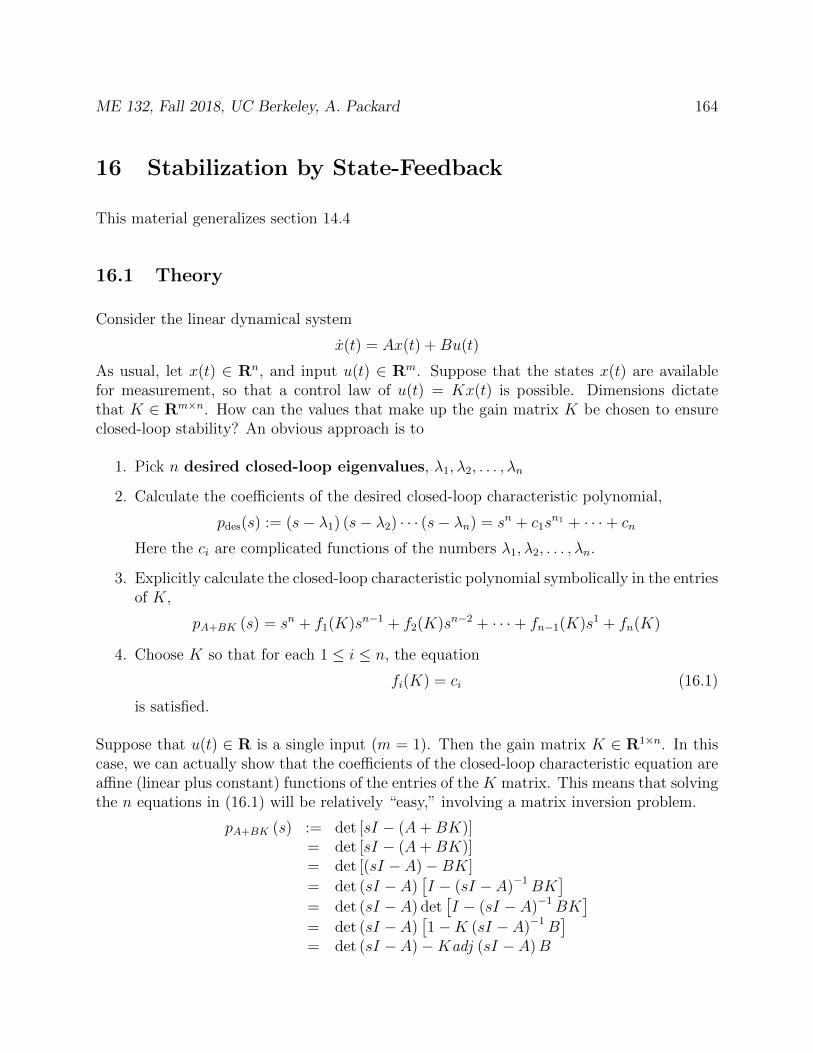
ME 132, Fall 2018, UC Berkeley, A. Packard 164
16 Stabilization by State-Feedback
This material generalizes section 14.4
16.1 Theory
Consider the linear dynamical system
x(t) = Ax(t) +Bu(t)
As usual, let x(t) ∈ Rn, and input u(t) ∈ Rm. Suppose that the states x(t) are availablefor measurement, so that a control law of u(t) = Kx(t) is possible. Dimensions dictatethat K ∈ Rm×n. How can the values that make up the gain matrix K be chosen to ensureclosed-loop stability? An obvious approach is to
1. Pick n desired closed-loop eigenvalues, λ1, λ2, . . . , λn
2. Calculate the coefficients of the desired closed-loop characteristic polynomial,
pdes(s) := (s− λ1) (s− λ2) · · · (s− λn) = sn + c1sn1 + · · ·+ cn
Here the ci are complicated functions of the numbers λ1, λ2, . . . , λn.
3. Explicitly calculate the closed-loop characteristic polynomial symbolically in the entriesof K,
pA+BK (s) = sn + f1(K)sn−1 + f2(K)sn−2 + · · ·+ fn−1(K)s1 + fn(K)
4. Choose K so that for each 1 ≤ i ≤ n, the equation
fi(K) = ci (16.1)
is satisfied.
Suppose that u(t) ∈ R is a single input (m = 1). Then the gain matrix K ∈ R1×n. In thiscase, we can actually show that the coefficients of the closed-loop characteristic equation areaffine (linear plus constant) functions of the entries of the K matrix. This means that solvingthe n equations in (16.1) will be relatively “easy,” involving a matrix inversion problem.
pA+BK (s) := det [sI − (A+BK)]= det [sI − (A+BK)]= det [(sI − A)−BK]
= det (sI − A)[I − (sI − A)−1BK
]= det (sI − A) det
[I − (sI − A)−1BK
]= det (sI − A)
[1−K (sI − A)−1B
]= det (sI − A)−Kadj (sI − A)B
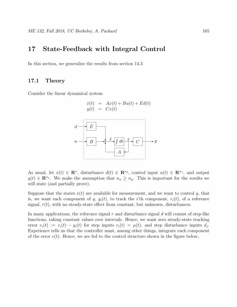
ME 132, Fall 2018, UC Berkeley, A. Packard 165
17 State-Feedback with Integral Control
In this section, we generalize the results from section 14.3
17.1 Theory
Consider the linear dynamical system
x(t) = Ax(t) +Bu(t) + Ed(t)y(t) = Cx(t)
B∫dt C
E
A
- -x -x y-
d -
u - ?
6b
As usual, let x(t) ∈ Rn, disturbance d(t) ∈ Rnd , control input u(t) ∈ Rnu , and outputy(t) ∈ Rny . We make the assumption that nu ≥ ny. This is important for the results wewill state (and partially prove).
Suppose that the states x(t) are available for measurement, and we want to control y, thatis, we want each component of y, yi(t), to track the i’th component, ri(t), of a referencesignal, r(t), with no steady-state effect from constant, but unknown, disturbances.
In many applications, the reference signal r and disturbance signal d will consist of step-likefunctions, taking constant values over intervals. Hence, we want zero steady-state trackingerror ei(t) := ri(t) − yi(t) for step inputs ri(t) = µ(t), and step disturbance inputs dj.Experience tells us that the controller must, among other things, integrate each componentof the error e(t). Hence, we are led to the control structure shown in the figure below,
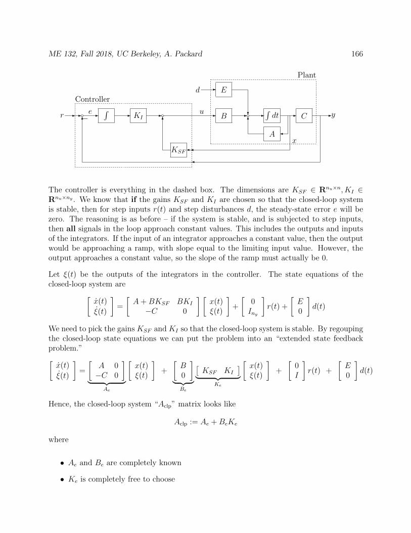
ME 132, Fall 2018, UC Berkeley, A. Packard 166
∫KI B
∫dt C
KSF
E
A
Plant
Controller
r -- -e - - -u - - - -y
x
d -
?
6
6
6b− b b
The controller is everything in the dashed box. The dimensions are KSF ∈ Rnu×n, KI ∈Rnu×ny . We know that if the gains KSF and KI are chosen so that the closed-loop systemis stable, then for step inputs r(t) and step disturbances d, the steady-state error e will bezero. The reasoning is as before – if the system is stable, and is subjected to step inputs,then all signals in the loop approach constant values. This includes the outputs and inputsof the integrators. If the input of an integrator approaches a constant value, then the outputwould be approaching a ramp, with slope equal to the limiting input value. However, theoutput approaches a constant value, so the slope of the ramp must actually be 0.
Let ξ(t) be the outputs of the integrators in the controller. The state equations of theclosed-loop system are[
x(t)
ξ(t)
]=
[A+BKSF BKI
−C 0
] [x(t)ξ(t)
]+
[0Iny
]r(t) +
[E0
]d(t)
We need to pick the gains KSF and KI so that the closed-loop system is stable. By regoupingthe closed-loop state equations we can put the problem into an “extended state feedbackproblem.”[x(t)
ξ(t)
]=
[A 0−C 0
]︸ ︷︷ ︸
Ae
[x(t)ξ(t)
]+
[B0
]︸ ︷︷ ︸Be
[KSF KI
]︸ ︷︷ ︸Ke
[x(t)ξ(t)
]+
[0I
]r(t) +
[E0
]d(t)
Hence, the closed-loop system “Aclp” matrix looks like
Aclp := Ae +BeKe
where
• Ae and Be are completely known
• Ke is completely free to choose

ME 132, Fall 2018, UC Berkeley, A. Packard 167
Hence, the stabilization problem is simply a state-feedback stabilization problem for theextended plant. Given A, B and C, one can form Ae and Be, and follow the derivationin section 16 to obtain the gain matrix Ke. Once calculated, Ke is partitioned into theappropriate state feedback, KSF , and integral gain, KI , and the controller is implementedas shown below
∫KI
KSF
r e−-- - - - - u
6
y
x
6b b
Note that the feedback structure, which contains the integrated error loop, ensures thatthere will be 0 steady-state errors to unit step reference inputs. It also ensures that therewill be 0 steady-state error due to step disturbances to the plant. Let’s prove this...
Theorem: Suppose KSF and KI are chosen so that[A+BKSF BKI
−C 0
]has all eigenvalues in open-left-half plane (ie., negative real parts). Hence it is an invertiblematrix. For a general, stable, linear system (A,B,C,), the expression for steady-state gainis D − CA−1B. Applying that here gives
SteadyStateGainr→y = −[C 0
] [ A+BKSF BKI
−C 0
]−1 [0I
]= I
and
SteadyStateGaind→y = −[C 0
] [ A+BKSF BKI
−C 0
]−1 [E0
]= 0
Proof: Denote
−[C 0
] [ A+BKSF BKI
−C 0
]−1
=:[X Y
]In other words, X and Y are the unique matrices which satisfy
−[C 0
]=[X Y
] [ A+BKSF BKI
−C 0
]Simple trial and error shows that X = 0, Y = I is a solution, and hence must be the solution.Plugging those in completes the proof.

ME 132, Fall 2018, UC Berkeley, A. Packard 168
17.2 Example
Consider a tank level control system, for illustrative purposes only. The physical setup isshown in the figure below.
6
66
R1 R12 R23 R3
h1
h2h3
d
?
u
?
For simplicity, everything is modeled as linear, giving the state equations
h1(t)
h2(t)
h3(t)
=
− 1A1
(1R1
+ 1R12
)1
A1R120
1A2R12
− 1A2
(1R12
+ 1R23
)1
A2R23
0 1A3R23
− 1A3
(1R23
+ 1R3
) h1(t)h2(t)h3(t)
+
010
u(t)+
100
d(t)
and
y(t) =[
0 1 0] h1(t)
h2(t)h3(t)
Hence, in terms of extended matrices, we have
Ae =
− 1A1
(1R1
+ 1R12
)1
A1R120 0
1A2R12
− 1A2
(1R12
+ 1R23
)1
A2R230
0 1A3R23
− 1A3
(1R23
+ 1R3
)0
0 −1 0 0
, Be =
0100
In order to keep the notation down to a minimum, define constants a, . . . , g so that
Ae =
a b 0 0c d e 00 f g 00 −1 0 0
It is easy to verify (expanding along top row for instance) that
det (λI4 − Ae) = λ4 + (−a− d− g)λ3 + (dg − ef + ad+ ag − bc)λ2 + (aef − adg + bcg)λ
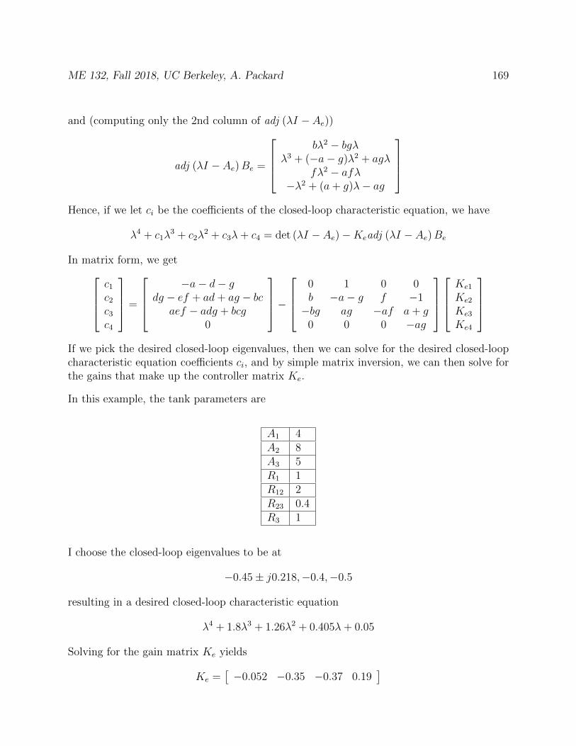
ME 132, Fall 2018, UC Berkeley, A. Packard 169
and (computing only the 2nd column of adj (λI − Ae))
adj (λI − Ae)Be =
bλ2 − bgλ
λ3 + (−a− g)λ2 + agλfλ2 − afλ
−λ2 + (a+ g)λ− ag
Hence, if we let ci be the coefficients of the closed-loop characteristic equation, we have
λ4 + c1λ3 + c2λ
2 + c3λ+ c4 = det (λI − Ae)−Keadj (λI − Ae)Be
In matrix form, we getc1
c2
c3
c4
=
−a− d− g
dg − ef + ad+ ag − bcaef − adg + bcg
0
−
0 1 0 0b −a− g f −1−bg ag −af a+ g
0 0 0 −ag
Ke1
Ke2
Ke3
Ke4
If we pick the desired closed-loop eigenvalues, then we can solve for the desired closed-loopcharacteristic equation coefficients ci, and by simple matrix inversion, we can then solve forthe gains that make up the controller matrix Ke.
In this example, the tank parameters are
A1 4A2 8A3 5R1 1R12 2R23 0.4R3 1
I choose the closed-loop eigenvalues to be at
−0.45± j0.218,−0.4,−0.5
resulting in a desired closed-loop characteristic equation
λ4 + 1.8λ3 + 1.26λ2 + 0.405λ+ 0.05
Solving for the gain matrix Ke yields
Ke =[−0.052 −0.35 −0.37 0.19
]
ME 132, Fall 2018, UC Berkeley, A. Packard 170
which partitions into
KSF =[−0.052 −0.35 −0.37
]KI = 0.19
A simulation is shown below. The initial condition is hi(0) = 0 for all tanks. The referenceinput is
r(t) = 5 for 0 ≤ t ≤ 80r(t) = 8 for 80 < t
and the disturbance flow is
d(t) = 0 for 0 ≤ t ≤ 30d(t) = 2 for 30 < t ≤ 50d(t) = −2 for 50 < t ≤ 70d(t) = 0 for 70 < t ≤ 90d(t) = 4 for 90 < t
This works great, in part because the control u enters tank 2 directly, which is the tankwhose height we are trying to control, while the disturbance enters tank 1. So, the controlhas a more direct effect.
Next, we simulate a different configuration, using the same control gains. In this simulation,the disturbance is modified:
• Instead of entering the 1st tank, the disturbance enters the 2nd tank.
• The magnitude of the disturbance flow is reduced by a factor of 5.
Simulations are shown below:
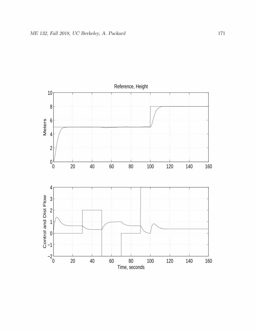
ME 132, Fall 2018, UC Berkeley, A. Packard 171
0 20 40 60 80 100 120 140 1600
2
4
6
8
10Reference, Height
Me
ters
0 20 40 60 80 100 120 140 160−2
−1
0
1
2
3
4
Co
ntr
ol a
nd
Dis
t F
low
Time, seconds

ME 132, Fall 2018, UC Berkeley, A. Packard 172
0 20 40 60 80 100 120 140 1600
2
4
6
8
10Reference, Height
Me
ters
0 20 40 60 80 100 120 140 160−0.5
0
0.5
1
1.5
Co
ntr
ol a
nd
Dis
t F
low
Time, seconds
ME 132, Fall 2018, UC Berkeley, A. Packard 173
17.3 Problems
1. Consider a system of the form
x1(t) = x2(t)x2(t) = A21x1(t) + A22x2(t) +B2u(t) + E2d(t)y(t) = x1(t)
(17.1)
We want to design a controller that uses measurements of y and y (note y = x2), aswell as a reference input r, such that
• the closed-loop system eigenvalues are at desired, specified location
• the steady-state gain from r → y equals 1, robustly (ie., even with modest varia-tions in A21, A22, B2, E2)
• the steady-state gain from d→ y equals 0, robustly (ie., even with modest varia-tions in A21, A22, B2, E2)
The controller architecture is a particular special case of Section 17, namely feedbackof the states (x1 and x2), as well as the integral of r − y,
η(t) = r(t)− ym(t)u(t) = KIη(t) +K0r(t) +K1ym(t) +K2ym(t)
(17.2)
where ym(t) = x1(t) + n1(t) and ym(t) = x2(t) + n2(t), and n1 and n2 are noises dueto the individual sensors measuring x1 and x2. This is called a “PI controller withrate-feedback”, since the feedback consists of a proportional and integral feedback ofy, as well as feedback of y. With this architecture, the control designer’s job is todecide on appropriate values for the gains, KI , K0, K1, K2.
(a) Find state-space model (4 inputs, 3 outputs, 3 states) of the closed-loop systemcombining the plant model (17.1) and controller dynamics (17.2). The inputsshould be (r, d, n1, n2) and outputs (y, y, u).
(b) Find closed-loop characteristic equation in terms of the plant parameters andcontroller gains.
(c) Show that by choice of KI , K1, K2, the 3rd-order closed-loop characteristic poly-nomial can be made equal to any 3rd-order polynomial. Assume that B2 6= 0.
(d) Follow the linear algebra derivation in Section 14.1 to conclude that if KI , K1, K2are chosen so that the closed-loop system is stable, then
• steady-state gain from r → y is 1 (insensitive to any changes in parameters,as long as closed-loop remains stable!)
• steady-state gain from d→ y is 0 (insensitive to any changes in parameters,as long as closed-loop remains stable!)

ME 132, Fall 2018, UC Berkeley, A. Packard 174
(e) There are 3 eigenvalues, with one of two possibilities
• a complex-conjugate pair (real and imaginary part, or (ωn, ξ) description),and one real eigenvalue
• 3 real eigenvalues
In either case, we have 3 parameters to describe the locations. For this purpose,introduce 3 parameters: (ωn, ξ, β), and take the characterstic equation as
pclosed−loop(λ) = (λ2 + 2ξωnλ+ ω2n)(λ+ βωn)
so that the roots are at
λ1,2 = −ξωn ± jωw√
1− ξ2, λ3 = −βωn
Again, ωn sets the “speed-of-response” of the complex-pair, ξ sets the damping,and β sets the speed-of-response of the real eigenvalue, relative to the complex-conjugate pair. Because of the ease in interpreting ωn, we can pick a good candi-date value for ωn, as well as a sensible candidate value for ξ, and then try varyingβ from (say) 0.33 to 3 and see the effect. Multiply out pclosed−loop, and develop“design equations” for KI , K1, K2 in terms of plant parameters and desiredeigenvalue locations.
(f) Assume A21 = A22 = 0 and B2 = E2 = 1. Let the desired eigenvalue locations bedescribed by
ωn = 1, ξ = 0.707, β = 0.33, 1, 3
(3 different choices for β). Find KI , K1, K2 for each of the 3 designs.
(g) For each design, temporarily set r = 0, and focus on disturbance rejection. Notethat K0 is not important (it only influences the effect r has on y and u), and canbe (for example) set to 0. Use ss objects, and step to plot the step-response ofy and u due to a unit-step disturbance d.
(h) Next, set d = 0, and focus on the effect r has on y (and u). Again do 3 simulations,with step-inputs for r, for the different values of β, all with K0 := −K1. Thismeans that the proportional feedback is of the form K0(r − ym), in other words,also proportional to error. As usual, plot y and u.
(i) Repeat the reference step-responses with K0 := 0, K0 = −0.5K1 and K0 =−1.5K1. So, this is now 9 plots (3 different β and 3 different K0). Commenton the effect of the immediate aggressiveness of the action of u in driving y to-wards r = 1. Again, plot y and u.
(j) Implement the example in Simulink, and verify that the results are identical.
2. This problem builds on the development in problem 1, using a plant model closer tothe EV3 motor, and just doing the implementation in Simulink. Connection to EV3

ME 132, Fall 2018, UC Berkeley, A. Packard 175
motor control: The Lego EV3 motor, using x1 := θ and x2 := Ω, we have indeedx1 = x2 and
x2 =1
J(−αΩ + T + d)
where T is the torque acting on shaft from EV3 electronics (as we can command it,so u) and d represents any other (external) torque (from the “environment”, eg., anadditional inertia attached to the shaft, an external disturbance torque, like your fingersgrabbing the motor shaft, and trying to stop it...). so that A21 = 0, A22 = −α
J, B2 = 1
J.
In the initial lab, you identified the time-constant τ and steady-state gain γ, (from Tto Ω) which relate to these parameters as
τ =J
α, γ =
1
α
which is equivalently
α =1
γ, J =
τ
γ
The units we used were degrees/sec (for Ω) and LegoTorque for T . Hence the units ofJ are not SI, but rather
units for J =LegoTorque · s2
degree
As mentioned, later we will do an experiment to estimate the correct conversion fromLegoTorque to N ·m, and then we can compute J in SI units. For consistency acrosseveryone’s assignments, take J = 0.01 and α = 0.125.
(a) Suppose an additional inertia is attached (rigidly, let’s say for now) to the mo-tor (common in a mechanical motion control application). Let JL denote theadditional inertia. The equation for Ω becomes
x2 =1
J + JL(−αΩ + T + d)
which changes both the steady-state gain and time-constant, in a known man-ner. Task: Build a Simulink Model of the EV3 motor, with additional inertia,using these equations. It should constructed in such a manner that it is easy tomodify the value of JL in the workspace, and have this propagate into the model.Once constructed, group as a subsystem, and (if desired, not required), mask the
subsystem block so that the user would enter J , JL and α to characterize thesystem.
(b) Add the controller architecture to the Simulink model. The controller has onestate, 3 inputs, (r, ym, ym) and one output, u. The controller equations are
ME 132, Fall 2018, UC Berkeley, A. Packard 176
η(t) = r(t)− ym(t)u(t) = KIη(t) +K0r(t) +K1ym(t) +K2ym(t)
(17.3)
It is defined by 4 parameters, (KI , K1, K2, K0). Again, group this as a subsystem,and (if desired), mask it so the user cleanly enters the 4 parameters in a nice dialogbox. Important Remark: Even though the EV3 only has a θ measurement,and we will be inferring Ω from numerical differentiation of θ, start in Simulinkas though you have independent measurements of θ and Ω in order to implementthe feedback law.
(c) Assume JL = 0.01. Design the controller gains so that the closed-loop eigenvaluesare at
ωn = 8, ξ = 0.9, β =
2
3, 1,
3
2
(d) Simulate the system, from zero initial conditions, with a 150 reference step input
(step occurs at t = 1), and a step-disturbance torque of 70 (in LegoTorque units)which occurs at t = 4. The simulation time should be 6 seconds. Plot both y andu. In all cases, define K0 = −0.25K1.
3. We will add several layers of “non-idealized” behavior to the Simulink model, and seethe effect this has on the overall control system performance.
(a) Create a new Simulink model (by copying, and then modifying as described be-low):
• Quantized measurement of y, with quantization level equal to 1
• Only sampled (in time) measurements of the quantized y is available. Use aZero-Order-Hold block to model the sampling, with a sample-time of 0.05.
• No direct measurement of y. Instead, estimate y as in the lab, using aDiscrete State-Space Block, implementing a 1st-order, backwards finitedifference estimate of y, from the quantized, sampled measurement of y.
• Quantize (also at quantization level equal to 1) the output of controller(LegoTorque command), and use Sample-Hold block too, with sample-timeof 0.05.
(b) Use Simulink to simulate this situation, with the same inputs (reference anddisturbance) as previous, using the gains obtained in the 3 cases. In all cases,define K0 = −0.25K1.
ME 132, Fall 2018, UC Berkeley, A. Packard 177
18 Linear-quadratic Optimal Control
Picking appropriate locations of the desired eigenvalues can be challenging. We only knowvaguely how they affect the response. The eigenvector matrix has a big influence on thebehavior of TeΛtT−1. In this section, we introduce an approach whereby the designerpicks/selects/dictates a different goal, and mathematics then determines what the state-feedback gain should be to optimize the goal. In many cases, this is more natural. Moreadvanced theory further tries to make the designer’s specifications even more natural, andagain use mathematics to turn those specifications into a control strategy.
The system dynamics are as usual,
x(t) = Ax(t) +Bu(t), x(0) = x0
where x(t) ∈ Rn and u(t) ∈ Rm.
Goal of control is to drive x(t)→ 0n, but the desired manner in which it gets to zero dependson the system and objectives. Suppose Q = QT ∈ Rn×n is a positive-semidefinite matrix,and any two non-zero values of x, say x[1] ∈ Rn and x[2] are considered “equally far awayfrom 0” if
xT[1]Qx[1] = xT[2]Qx[2].
Additionally, in getting x → 0, we desire to not use too “much” control action, as this is“costly” in some sense. Suppose R = RT ∈ Rm×m is a positive-definite matrix, and twonon-zero values of u, say u[1] and u[2] are considered “equally far away from 0” if
uT[1]Ru[1] = uT[2]Ru[2].
Finally, futher assume that a nonzero value of x and a nonzero value of u are considered“equally far away from 0” if
xTQx = uTRu.
With this level of “penalization” for nonzero x and u, one criterion that measures how faraway from 0 a particular (x(·), u(·)) trajectory is
J(x0, u(·)) :=
∫ ∞0
xT (t)Qx(t) + uT (t)Ru(t)dt
Note that the cost criterion depends on the initial condition and the entire control trajectoryu (since the resulting x() is a consequence of x0 and u). It is a quadratic function of theresulting state trajectory x(·) and the input u(·).
If one adopts J(x0, u(·)) as the quantity to make as small as possible, by choice of u, theoptimal control problem is: For a given initial condition x0, the optimization problem is
J∗(x0) := minu(·)
∫ ∞0
xT (t)Qx(t) + uT (t)Ru(t)dt, subject to x(t) = Ax(t) +Bu(t)

ME 132, Fall 2018, UC Berkeley, A. Packard 178
Clearly, the optimal control-input signal, u(t)|t∈[0,∞), depends on the initial condition x0.A particular input may be the optimal input starting from a particular initial condition.Starting from a different initial condition almost surely requires a different input.
Fact: Given the system model A and B, and the cost-function matrices Q and R, thereexists a matrix P = P T ∈ Rn×n and a matrix F ∈ Rm×n such that
• for all initial conditions x0, the optimal cost J(x0) is simply xT0 Px0;
• for all initial conditions, the optimal input trajectory u(t)|t∈[0,∞) can be calculated viaa feedback law, namely
u(t) = −Fx(t).
This form, expressed as a state-feedback, is referred to as the optimal linear-quadraticregulator.
Moreover P and F are easily calculated using matrix operations. We don’t have enoughtime to go into the specifics, but will be able to use the ideas in homework and lab. Thecommand lqr in Matlab’s Control System toolbox makes the calculation as
[F,P] = lqr(A,B,Q,R).
18.1 Learning more
In the next section, we consider an easier problem, still called linear quadratic control. Thetwo simplifying assumptions are discrete-time (the differential equation is replaced with adifference equation, so no calculus) and we only consider a fixed, finite-time interval. Thefinite-time interval is easier than the infinite-time horizon considered in this section, but ofcourse, in the finite-time derivation, we only determine what the control is over that period,hence in an actual implementation, the problem must be “over” at the end of the period.
ME 132, Fall 2018, UC Berkeley, A. Packard 179
19 Single, high-order, linear ODES (SLODE)
Throughout this section, if y denotes a function (of time, say), then y[k] or y(k) denotes thek’th derivative of the function y,
y[k] =dky
dtk
In the case of k = 1 and k = 2, it will be convenient to also use y and y.
19.1 Linear, Time-Invariant Differential Equations
Often, in this class, we will analyze a closed-loop feedback control system, and end up withan equation of the form
y(n)(t) + a1y(n−1)(t) + · · ·+ any(t) = v(t) (19.1)
where y is some variable of the plant that is of interest to us, and v is a forcing function,usually either a reference signal (ydes(t)) or a disturbance (ie., inclination of hill), or acombination of such signals. One job of the control designer is to analyze the resultingequation, and determine if the behavior of the closed-loop system is acceptable.
The differential equation in (19.1) is called a forced, linear, time-invariant differential equa-tion. For now, associate the fact that the aini=1 are constants with the term time-invariant,and the fact that the left-hand side (which contains all y terms) is a linear combination of yand its derivatives with the term linear.
The right-hand side function, v, is called the forcing function. For a specific problem, it willbe a given, known function of time.
Sometimes, we are given an initial time t0 and initial conditions for differential equation,that is, real numbers
y0, y0, y0, . . . , y(n−1)0 (19.2)
and we are looking for a solution, namely a function y that satisfies both the differentialequation (19.1) and the initial condition constraints
y(t0) = y0, y(t0) = y0, y(t0) = y0, . . . , y(n−1)(t0) = y(n−1)0 . (19.3)
For essentially all differential equations (even those that are not linear, and not time-invariant), there is a theorem which says that solutions always exist, and are unique:
Theorem (Existence and Uniqueness of Solutions): Given a forcing function v, definedfor t ≥ t0, and initial conditions of the form (19.3). Then, there exists a unique function ywhich satisfies the initial conditions and the differential equation (19.1).
ME 132, Fall 2018, UC Berkeley, A. Packard 180
19.2 Importance of Linearity
Suppose that yP is a function which satisfies (19.1) so that
y(n)P (t) + a1y
(n−1)P (t) + · · ·+ anyP (t) = v(t) (19.4)
and yH is a function which, for all t satisfies
y(n)H (t) + a1y
(n−1)H (t) + · · ·+ anyH(t) = 0 (19.5)
yH is called a homogeneous solution of (19.1), and the differential equation in (19.5) is calledthe homogeneous equation. The function yP is called a particular solution to (19.1), since itsatisfies the equation with the forcing function in place.
The derivative of yP + yH is the sum of the derivatives, so we add the equations satisfied byyP and yH to get
[yP + yH ](n) (t) + a1 [yP + yH ](n−1) (t) + · · · an [yP + yH ] (t) = v(t)
This implies that the function yP + yH also satisfies (19.1). Hence, adding a particularsolution to a homogeneous solution results in a new particular solution.
Conversely, suppose that yP1 and yP2 are two functions, both of which solve (19.1). Considerthe function yd := yP1 − yP2 . Easy manipulation shows that this function yd satisfies thehomogeneous equation. It is a trivial relationship that
yP1 = yP2 + (yP1 − yP2)= yP2 + yd
We have shown that any two particular solutions differ by a homogeneous solution. Henceall particular solutions to (19.1) can be generated by taking one specific particular solution,and adding to it every homogeneous solution. In order to get the correct initial conditions,we simply need to add the “right” homogeneous solution.
Remark: The main points of this section rely only on linearity, but not time-invariance.
19.3 Solving Homogeneous Equation
Let’s try to solve (19.5). Take a fixed complex number r ∈ C, and suppose that the functionyH , defined as
yH(t) = ert
ME 132, Fall 2018, UC Berkeley, A. Packard 181
is a solution to (19.5). Substituting in, using the fact that for any integer k > 0, y(k)H (t) =
rkert, gives (rn + a1r
n−1 + · · ·+ an)ert = 0
for all t. Clearly, ert 6= 0, always, so it can be divided out, leaving
rn + a1rn−1 + · · ·+ an = 0 (19.6)
Thus, if ert is a solution to the homogeneous equation, it must be that the scalar r satisfies(19.6).
Conversely, suppose that r is a complex number which satisfies (19.6), then simple substi-tution reveals that ert does satisfy the homogeneous equation. Moreover, if r is a repeatedroot, say l times, then substitution shows that the functions
ert, tert, . . . , tl−1ert
all satisfy
the homogeneous differential equation. This leads to the following nomenclature:
Let r1, r2, . . . , rn be the roots of the polynomial equation
λn + a1λn−1 + · · ·+ an = 0
This polynomial is called the characteristic polynomial associated with (19.1).
Fact 1 (requires proof): If the rini=1 are all distinct from one another , then yH satisfies(19.5) if and only if there exist complex constants c1, c2, . . . , cn such that
yH(t) =n∑i=1
cierit (19.7)
Fact 2 (requires proof): If the rini=1 are not distinct from one another, then group theroots r1, r2, · · · , rn as
p1, p1, . . . , p1︸ ︷︷ ︸l1
, p2, p2, . . . , p2︸ ︷︷ ︸l2
, · · · , pf , pf , . . . , pf︸ ︷︷ ︸lf
(19.8)
Hence, p1 is a root with multiplicity l1, p2 is a root with multiplicity l2 and so on. Then yHsatisfies (19.5) if and only if there exist complex constants cij (i = 1, . . . f , j = 0, . . . li − 1)such that
yH(t) =
f∑i=1
li−1∑j=0
cijepittj (19.9)
So, Fact 2 includes Fact 1 as a special case. Both indicate that by solving for the roots of thecharacteristic equation, it is easy to pick n linearly independent functions which form a basisfor the set of all homogeneous solutions to the differential equation. Here, we explicitly have
ME 132, Fall 2018, UC Berkeley, A. Packard 182
used the time-invariance (ie., the coefficients of the ODE are constants) to generate a basis(the exponential functions) for all homogeneous solutions. However, the fact that the spaceof homogenous solutions is n-dimensional only relies on linearity, and not time-invariance.
Basic idea: Suppose there are m solutions to the homogeneous differential equation, labeledy1,H , y2,H , . . . , ym,H , with m > n. Then, look at the n ×m matrix of these solutions initialconditions,
M :=
y
(0)1,H y
(0)2,H · · · y
(0)m,H
y(1)1,H y
(1)2,H · · · y
(1)m,H
......
. . ....
y(n−1)1,H y
(n−1)2,H · · · y
(n−1)m,H
Since m > n, this must have linearly dependent columns, so there is a nonzero m× 1 vectorα such that Mα = 0n×1. Define yz := α1y1,H + α2y2,H + · · · + αmym,H . Since this is a sumof homogeneous solutions, it itself is a homogeneous solution. Moreover, yz satisfies
y(0)z (t0) = 0, y(1)
z (t0) = 0, · · · , y(n−1)z (t0) = 0
Note that the function yI(t) ≡ 0 for all t also satisfies the same initial conditions as yz, andit satisfies the homogeneous differential equation as well. By uniqueness of solutions, it mustbe that yz(t) = yI(t) for all t. Hence, yz is actually the identically zero function. Hence, wehave shown that the set of homogeneous solutions is finite dimensional, and of dimension atmost n. Moreover, by the simple substitutions above, we already know how to construct nlinearly independent solutions to the homogeneous differential equation, so those must forma basis for all homogeneous solutions.
The reason that terms like tkert appear for differential equations whose characteristic equa-tion has repeated roots is partially explored in Problem 6.
19.3.1 Interpretation of complex roots to ODEs with real-coefficients
In all cases we consider, the differential equation has real coefficients (the a1, a2, . . . , an).This means that the characteristic equation has real coefficients, but it does not mean thatthe roots are necessarily real numbers (eg., even a real quadratic equation may have complexroots). However, since the coefficients are real, then complex roots will come in complex-conjugate pairs, so if λ := α + jβ is a root, and α and β are real numbers, and β 6= 0, thenit will also be true that α− jβ is a root of the characteristic equation as well.
Given the roots, we know that all homogeneous solutions are given by equation 19.9, wherethe constants vary over all choices of complex numbers. We will almost exclusively beinterested in solutions starting from real initial conditions, with real forcing functions, and
ME 132, Fall 2018, UC Berkeley, A. Packard 183
hence will only need to consider real homogeneous solutions. This raises the question of howto interpret the complex functions eλt which arise when λ (a root) is complex.
Suppose λ1 ∈ C is a complex root. Since the characteristic equation has real coefficients,it follows that that complex conjugate of λ1, λ2 = λ1 is also a root. Let α and β be realnumbers such that
λ1 = α + jβ, λ2 = α− jβ, β 6= 0
The terms of the homogeneous solution associated with these roots are
c1eλ1t + c2e
λ2t
where c1 and c2 are any complex numbers. We want to study under what conditions (on c1
and c2) will this function be purely real. Plugging in gives
c1eαt [cos βt+ j sin βt] + c2e
αt [cos βt− j sin βt]
Regrouping gives(eαt [(c1 + c2) cos βt+ j(c1 − c2) sin βt]
Since cos and sin are linearly independent functions, the only conditions for this to be apurely real function is that c1 + c2 be real, and j(c1 − c2) be real. This requires that c1 andc2 be complex-conjugates of one another. In other words, for the function
c1eαt [cos βt+ j sin βt] + c2e
αt [cos βt− j sin βt]
is real-valued, for all t if and only if c1 = c2.
Let c2 be any complex number, and let c1 := c2. Then c1 + c2 = 2A, where A is the real partof c2. Also, j(c1 − c2) = 2B, where B is the imaginary part of c2. Hence, the purely realhomogeneous solutions are of the form
(eαt [2A cos βt+ 2B sin βt]
where A and B are free real constants. Since they are free, it serves no purpose to write 2Aand 2B, and we can simply write that all real homogeneous solutions arising from the tworoots λ1 = α + jβ and λ2 = α− jβ are
(eαt [A cos βt+B sin βt]
where A and B are any real numbers.
With this is mind, we can rewrite a specialized version of Fact 2, for the case when thecoefficients of the ODE are real, and we are interested in writing down a description of justall real homogeneous solutions.
ME 132, Fall 2018, UC Berkeley, A. Packard 184
Fact 3: Assume that all coefficients a1, a2, . . . , an are real numbers. Group the n roots ofthe characteristic equation as
p1, p1, . . . , p1︸ ︷︷ ︸l1
, · · · , pd, pd, . . . , pd︸ ︷︷ ︸ld
,
α1 + jβ1, α1 + jβ1, . . . , α1 + jβ1︸ ︷︷ ︸h1
, α1 − jβ1, α1 − jβ1, . . . , α1 − jβ1︸ ︷︷ ︸h1
,
...αc + jβc, αc + jβc, . . . , αc + jβc︸ ︷︷ ︸
hc
, αc − jβc, α1 − jβc, . . . , αc − jβc︸ ︷︷ ︸hc
(19.10)
where each p, α and β are real, and each β 6= 0. Then yH is a real-valued function whichsatisfies (19.5) if and only if there exist real constants cij (i = 1, . . . d, j = 0, . . . li − 1),Aks, Bks (k = 1, . . . c, s = 0, . . . hk − 1)such that
yH(t) =d∑i=1
li−1∑j=0
cijepittj +
c∑k=1
hk−1∑s=0
eαktts [Aks cos βkt+Bks sin βkt] (19.11)
19.4 General Solution Technique
The general technique (conceptually, at least) for finding particular solutions of (19.1) whichalso satisfy the initial conditions is a combination of all of the above ideas. It is veryimportant conceptually, and somewhat important in actual use.
1. Find any particular solution yP
2. Choose constants cij so that the function
yP (t) +
f∑i=1
li−1∑j=0
cijtjepit
satisfies the initial conditions.
The resulting function is the solution. Note that in step 2, there are n equations, and nunknowns.

ME 132, Fall 2018, UC Berkeley, A. Packard 185
19.5 Behavior of Homogeneous Solutions as t→∞
In this section, we study the behavior of the class of homogeneous solutions as t→∞. If wecan show that all homogeneous solutions decay to 0 as t→∞, then it must be that for a giveforcing function, all particular solutions, regardless of the initial conditions, approach eachother. This will be useful in many contexts, to quickly understand how a system behaves.
Suppose r is a complex number, r ∈ C, and we decompose it into its real and imaginaryparts. Let α := Real(r) and β := Imag(r). Hence, both α and β are real numbers, andr = α+ jβ. We will always use j :=
√−1. The exponential function ert can be expressed as
ert = eαt [cos βt+ j sin βt]
Note that the real part of r, namely α, determines the qualitative behavior of ert as t→∞.Specifically,
• if α < 0, then limt→∞ ert = 0
• if α = 0, then ert does not decay to 0, and does not “explode,” but rather oscillates,with |ert| = 1 for all t
• if α > 0, then limt→∞ |ert| =∞
When all of the roots of the chracteristic polynomial are distinct, all homogeneous solu-tions are of the form ert where r is a root of the characteristic polynomial. Therefore, wesee that the roots of the characteristic polynomial determine the qualitative nature of thehomogeneous solutions.
If the characteristic polynomial has a root rp of multiplicity lp ≥ 1, then according to Eq.(19.9), the homogeneous solution modes associated the root rp are
erpt, t erpt, · · · , t(lp−1) erpt .
Notice that for any real constants m <∞, and α < 0,
limt→∞
tm eαt = 0 .
Therefore, the real part of the repeated root rp, namely αp, also determines the qualitativebehavior of the homogeneous solution modes associated with this repeated root as t → ∞.Specifically,
• if αp < 0, then limt→∞ tm erpt = 0 for m = 0, · · · lp − 1.
ME 132, Fall 2018, UC Berkeley, A. Packard 186
• if αp = 0, then |erpt| = 1 for all t, but
• if αp ≥ 0, then limt→∞ |tmert| =∞ for m = 1, · · · lp − 1
where lp ≥ 1 is the multiplicity of the root rp.
We summarize all of these results as follows:
• If all of the roots, rini=1, of the characteristic polynomial satisfy
Real(ri) < 0
then every homogeneous solution decays to 0 as t→ .∞
• If any of the roots, rini=1, of the characteristic polynomial satisfy
Real(ri) ≥ 0
then there are homogeneous solutions that do not decay to 0 as t→∞ .
19.6 Response of stable system to constant input (Steady-StateGain)
Suppose the system (input u, output y) is governed by the SLODE
y[n](t) + a1y[n−1](t) + · · ·+ an−1y
[1](t) + any(t)= b0u
[n](t) + b1u[n−1](t) + · · ·+ bn−1u
[1](t) + bnu(t)
Suppose initial conditions for y are given, and that the input u is specified to be a constant,u(t) ≡ u for all t ≥ t0. What is the limiting behavior of y?
If the system is stable, then this is easy to compute. First notice that the constant functionyP (t) ≡ bn
anu is a particular solution, although it does not satisfy any of the initial conditions.
The actual solution y differs from this particular solution by some homogeneous solution,yH . Hence for all t,
y(t) = yP (t) + yH(t)
=bnanu+ yH(t)
Now, take limits, since we know (by the stability assumption) that limt→∞ yH(t) = 0, giving
limt→∞
y(t) =bnanu
Hence, the steady-state gain of the system isbnan
.
ME 132, Fall 2018, UC Berkeley, A. Packard 187
19.7 Example
Consider the differential equation
y(t) + 4y(t) + y(t) = 1 (19.12)
subject to the initial conditions y(0) = y0, y(0) = y0. The characteristic equation is λ2 +4λ+ 1 = 0, which has roots at
λ = −2±√
3 ≈ −3.7,−0.3
Hence, all homogeneous solutions are of the form
yH(t) = c1e−3.7t + c2e
−0.3t
Terms of the form e−3.7t take about 0.8 time units to decay, while terms of the form e−0.3t
take about 10 time units to decay. In general then (though not always - it depends on theinitial conditions) homogeneous solutions will typically take about 10 time units to decay.
A particular solution to (19.12) is simply yP (t) = 1 for all t ≥ 0. Note that this choice of yPdoes not satisfy the initial conditions, but it does satisfy the differential equation.
As we have learned, all solutions to (19.12) are any particular solution plus all homogeneoussolutions. Therefore, the general solution is
y(t) = 1 + c1e(−2−
√3)t + c2e
(−2+√
3)t
which has as its derivative
y(t) = (−2−√
3)c1e(−2−
√3)t + (−2 +
√3)c2e
(−2+√
3)t
Evaluating these at t = 0, and equating to the given initial conditions yields
y(0) = 1 + c1 + c2
= y0
y(0) =(−2−
√3)c1 +
(−2 +
√3)c2
= y0
In matrix form, we have[1 1
−2−√
3 −2 +√
3
] [c1
c2
]=
[y0 − 1y0
]This is easy to invert. recall [
a bc d
]−1
=1
ad− bc
[d −b−c a
]
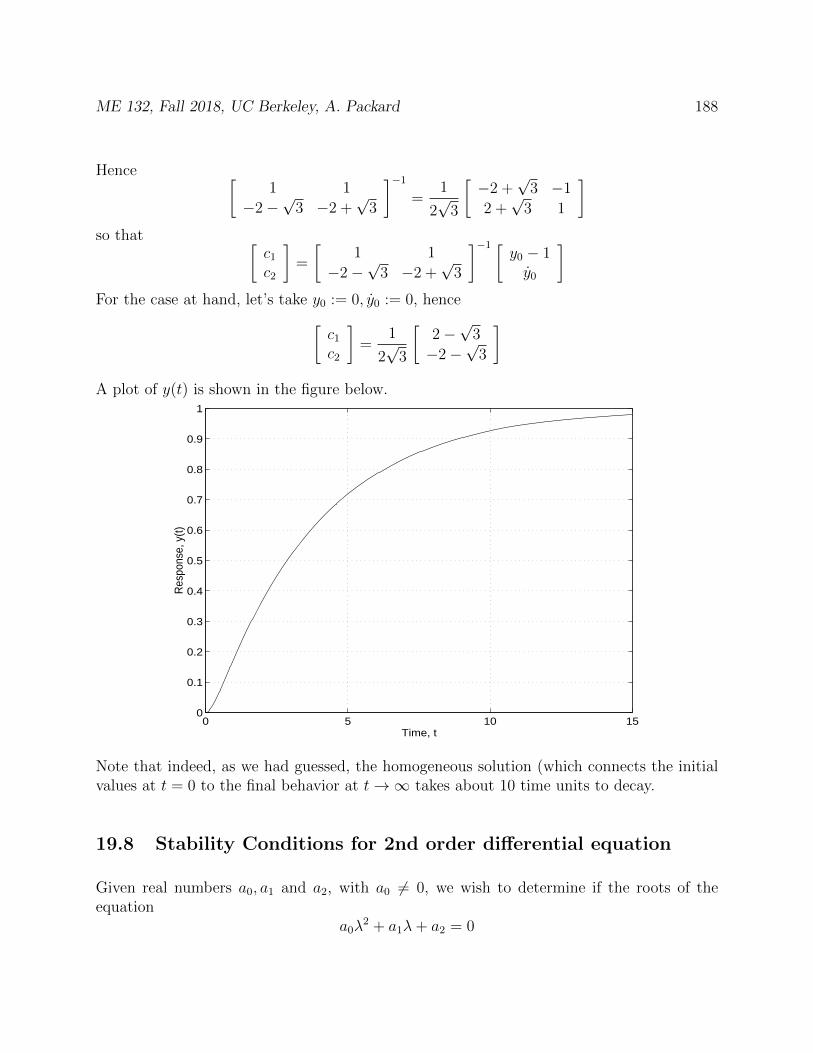
ME 132, Fall 2018, UC Berkeley, A. Packard 188
Hence [1 1
−2−√
3 −2 +√
3
]−1
=1
2√
3
[−2 +
√3 −1
2 +√
3 1
]so that [
c1
c2
]=
[1 1
−2−√
3 −2 +√
3
]−1 [y0 − 1y0
]For the case at hand, let’s take y0 := 0, y0 := 0, hence[
c1
c2
]=
1
2√
3
[2−√
3
−2−√
3
]A plot of y(t) is shown in the figure below.
0 5 10 150
0.1
0.2
0.3
0.4
0.5
0.6
0.7
0.8
0.9
1
Time, t
Res
pons
e, y
(t)
Note that indeed, as we had guessed, the homogeneous solution (which connects the initialvalues at t = 0 to the final behavior at t→∞ takes about 10 time units to decay.
19.8 Stability Conditions for 2nd order differential equation
Given real numbers a0, a1 and a2, with a0 6= 0, we wish to determine if the roots of theequation
a0λ2 + a1λ+ a2 = 0
ME 132, Fall 2018, UC Berkeley, A. Packard 189
have negative real parts. This question is important in determining the qualitative nature(exponential decay versus exponential growth) of the homogeneous solutions to
a0y(t) + a1y(t) + a2y(t) = 0
Since a0 6= 0 (so that we actually do have a quadratic, rather than linear equation) divideout by it, giving
y(t) +a1
a0
y(t) +a2
a0
y(t) = 0
Call b1 := a1a0, b2 := a2
a0. The characteristic equation is λ2 + b1λ+ b2 = 0. The roots are
λ1 =−b1 +
√b2
1 − 4b2
2, λ2 =
−b1 −√b2
1 − 4b2
2
Consider 4 cases:
1. b1 > 0, b2 > 0. In this case, the term b21 − 4b2 < b2
1, hence either
•√b2
1 − 4b2 is imaginary
•√b2
1 − 4b2 is real, but√b2
1 − 4b2 < b1.
In either situation, both Re(λ1) < 0 and Re(λ2) < 0.
2. b1 ≤ 0: Again, the square-root is either real or imaginary. If it is imaginary, then
Re(λi) = −b12≥ 0. If the square-root is real, then then Re(λ1) =
−b1+√b21−4b2
2≥ 0. In
either case, at least one of the roots has a nonnegative real part.
3. b2 ≤ 0: In this case, the square root is real, and hence both roots are real. However,√b2
1 − 4b2 ≥ |b1|, hence λ1 ≥ 0. so one of the roots has a non-negative real part.
This enumerates all possibilities. We collect these ideas into a theorem.
Theorem: For a second order polynomial equation λ2 +b1λ+b2 = 0, the roots have negativereal parts if and only if b1 > 0, b2 > 0.
If the leading coefficient is not 1, then we have
Theorem (RH2): For a second order polynomial equation b0λ2 + b1λ + b2 = 0, the roots
have negative real parts if and only if all of the bi are nonzero, and have the same sign(positive or negative).
Higher-order polynomials have more complicated conditions.
Theorem (RH3): For a third order polynomial equation λ3 + b1λ2 + b2λ + b3 = 0, all of
the roots have negative real parts if and only if b1 > 0, b3 > 0 and b1b2 > b3.
ME 132, Fall 2018, UC Berkeley, A. Packard 190
Note that the condition b1b2 > b3, coupled with the first two conditions, certainly impliesthat b2 > 0. However, the simpler conditions b1 > 0, b2 > 0, b3 > 0 are only necessary, notsufficient, as an example illustrates: the roots of λ3 +λ2 +λ+3 are −1.575, 0.2874± j1.35.So, use the exact conditions in theorem RH3 to determine the stability of a 3rd order systemby simple examination of its characteristic equation coefficients.
Theorem (RH4): For a fourth order polynomial equation λ4 +b1λ3 +b2λ
2 +b3λ+b4 = 0, allof the roots have negative real parts if and only if b1 > 0, b4 > 0, b1b2 > b3 and (b1b2−b3)b3 >b2
1b4.
These theorems are specific examples of the Routh-Hurwitz theorem which is often taught inundergraduate control courses. The Routh-Hurwitz theorem, proven around 1880, indepen-dently by Routh and Hurwitz, is interested in the determining if all roots of the polynomialequation
λn + b1λn−1 + · · ·+ bn−1λ+ bn = 0
have negative real-parts. The theorem states that all roots have negative real parts if andonly if n simple inequalities, involving polynomial expressions of the coefficients (the bk) aresatisfied. Note that the theorem does not find the roots - it merely proves, unequivocally, thatthe roots all lie in the open, left-half plane if and only if some easy-to-evaluate expressions,involving the coefficients, are negative. There is a pattern by which one can “simply” derivewhat the polynomial inequalities are. The three theorems above (RH2, RH3, and RH4)give the inequalities for n = 2, n = 3 and n = 4, respectively. As you notice, the conditionsbecome more complex with increasing order. For systems beyond 4th order, it is not clear howuseful (beyond the theoretical elegance) the formula are, especially in the context of modernlaptop computational power, where high-quality root-finding programs are easily accessible(eg., Matlab, Mathematica, etc). We encourage the student to memorize the 2nd, 3rd and4th order conditions and through their use, determine if knowing higher-order versions wouldbe useful. The interested student can find more information about Routh-Hurwitz on theweb.
19.9 Important 2nd order example
It is useful to study a general second order differential equation, and interpret it in a differentmanner. Start with
y(t) + a1y(t) + a2y(t) = bv(t) (19.13)
with y(0) = 0, y(0) = 0 and v(t) = 1 for all t ≥ 0. Assume that the homogeneous solutionsare exponentially decaying, which is equivalent to a1, a2 > 0. Rewrite using new variables
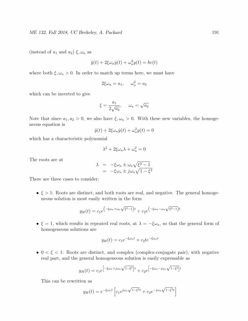
ME 132, Fall 2018, UC Berkeley, A. Packard 191
(instead of a1 and a2) ξ, ωn as
y(t) + 2ξωny(t) + ω2ny(t) = bv(t)
where both ξ, ωn > 0. In order to match up terms here, we must have
2ξωn = a1, ω2n = a2
which can be inverted to give
ξ =a1
2√a2
, ωn =√a2
Note that since a1, a2 > 0, we also have ξ, ωn > 0. With these new variables, the homoge-neous equation is
y(t) + 2ξωny(t) + ω2ny(t) = 0
which has a characteristic polynomial
λ2 + 2ξωnλ+ ω2n = 0
The roots are atλ = −ξωn ± ωn
√ξ2 − 1
= −ξωn ± jωn√
1− ξ2
There are three cases to consider:
• ξ > 1: Roots are distinct, and both roots are real, and negative. The general homoge-neous solution is most easily written in the form
yH(t) = c1e
(−ξωn+ωn
√ξ2−1
)t+ c2e
(−ξωn−ωn
√ξ2−1
)t
• ξ = 1, which results in repeated real roots, at λ = −ξωn, so that the general form ofhomogeneous solutions are
yH(t) = c1e−ξωnt + c2te
−ξωnt
• 0 < ξ < 1: Roots are distinct, and complex (complex-conjugate pair), with negativereal part, and the general homogeneous solution is easily expressable as
yH(t) = c1e
[−ξωn+jωn
√1−ξ2
]t+ c2e
[−ξωn−jωn
√1−ξ2
]t
This can be rewritten as
yH(t) = e−ξωnt[c1e
jωn√
1−ξ2t + c2e−jωn√
1−ξ2t]
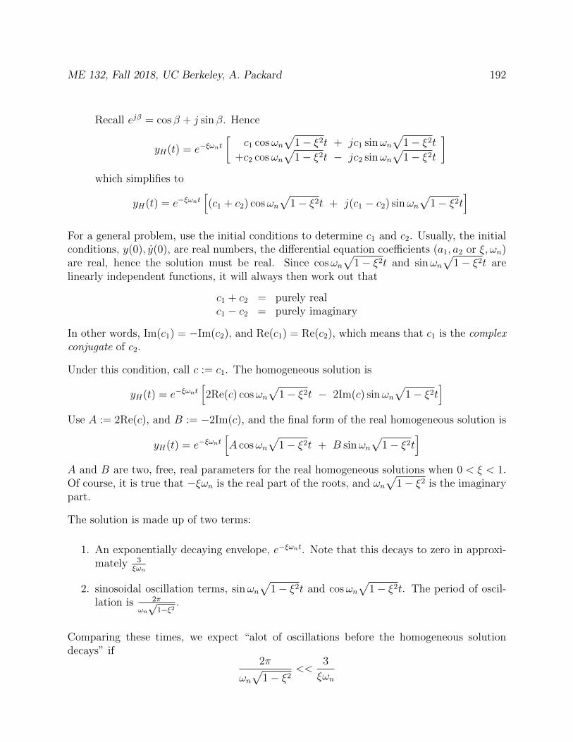
ME 132, Fall 2018, UC Berkeley, A. Packard 192
Recall ejβ = cos β + j sin β. Hence
yH(t) = e−ξωnt[
c1 cosωn√
1− ξ2t + jc1 sinωn√
1− ξ2t
+c2 cosωn√
1− ξ2t − jc2 sinωn√
1− ξ2t
]which simplifies to
yH(t) = e−ξωnt[(c1 + c2) cosωn
√1− ξ2t + j(c1 − c2) sinωn
√1− ξ2t
]For a general problem, use the initial conditions to determine c1 and c2. Usually, the initialconditions, y(0), y(0), are real numbers, the differential equation coefficients (a1, a2 or ξ, ωn)are real, hence the solution must be real. Since cosωn
√1− ξ2t and sinωn
√1− ξ2t are
linearly independent functions, it will always then work out that
c1 + c2 = purely realc1 − c2 = purely imaginary
In other words, Im(c1) = −Im(c2), and Re(c1) = Re(c2), which means that c1 is the complexconjugate of c2.
Under this condition, call c := c1. The homogeneous solution is
yH(t) = e−ξωnt[2Re(c) cosωn
√1− ξ2t − 2Im(c) sinωn
√1− ξ2t
]Use A := 2Re(c), and B := −2Im(c), and the final form of the real homogeneous solution is
yH(t) = e−ξωnt[A cosωn
√1− ξ2t + B sinωn
√1− ξ2t
]A and B are two, free, real parameters for the real homogeneous solutions when 0 < ξ < 1.Of course, it is true that −ξωn is the real part of the roots, and ωn
√1− ξ2 is the imaginary
part.
The solution is made up of two terms:
1. An exponentially decaying envelope, e−ξωnt. Note that this decays to zero in approxi-mately 3
ξωn
2. sinosoidal oscillation terms, sinωn√
1− ξ2t and cosωn√
1− ξ2t. The period of oscil-lation is 2π
ωn√
1−ξ2.
Comparing these times, we expect “alot of oscillations before the homogeneous solutiondecays” if
2π
ωn√
1− ξ2<<
3
ξωn
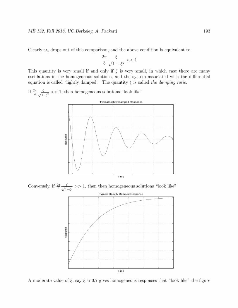
ME 132, Fall 2018, UC Berkeley, A. Packard 193
Clearly ωn drops out of this comparison, and the above condition is equivalent to
2π
3
ξ√1− ξ2
<< 1
This quantity is very small if and only if ξ is very small, in which case there are manyoscillations in the homogeneous solutions, and the system associated with the differentialequation is called “lightly damped.” The quantity ξ is called the damping ratio.
If 2π3
ξ√1−ξ2
<< 1, then homogeneous solutions “look like”
Typical Lightly Damped Response
Time
Res
pons
e
Conversely, if 2π3
ξ√1−ξ2
>> 1, then then homogeneous solutions “look like”
Typical Heavily Damped Response
Time
Res
pons
e
A moderate value of ξ, say ξ ≈ 0.7 gives homogeneous responses that “look like” the figure
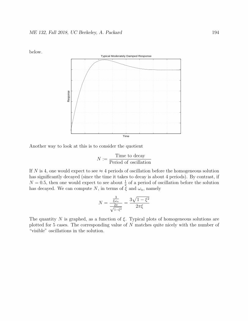
ME 132, Fall 2018, UC Berkeley, A. Packard 194
below.Typical Moderately Damped Response
Time
Res
pons
e
Another way to look at this is to consider the quotient
N :=Time to decay
Period of oscillation
If N is 4, one would expect to see ≈ 4 periods of oscillation before the homogeneous solutionhas significantly decayed (since the time it takes to decay is about 4 periods). By contrast, ifN = 0.5, then one would expect to see about 1
2of a period of oscillation before the solution
has decayed. We can compute N , in terms of ξ and ωn, namely
N =
3ξωn2π√1−ξ2
=3√
1− ξ2
2πξ
The quantity N is graphed, as a function of ξ. Typical plots of homogeneous solutions areplotted for 5 cases. The corresponding value of N matches quite nicely with the number of“visible” oscillations in the solution.
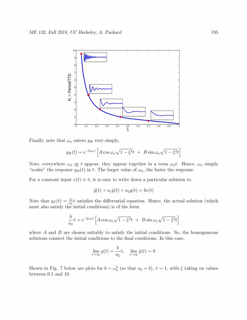
ME 132, Fall 2018, UC Berkeley, A. Packard 195
0 0.1 0.2 0.3 0.4 0.5 0.6 0.7 0.8 0.9 10
1
2
3
4
5
6
7
8
9
10
ξ
N :=
Per
iod/
TTD
Finally, note that ωn enters yH very simply,
yH(t) = e−ξωnt[A cosωn
√1− ξ2t + B sinωn
√1− ξ2t
]Note, everywhere ωn or t appear, they appear together in a term ωnt. Hence, ωn simply“scales” the response yH(t) in t. The larger value of ωn, the faster the response.
For a constant input v(t) ≡ v, it is easy to write down a particular solution to
y(t) + a1y(t) + a2y(t) = bv(t)
Note that yP (t) = ba2v satisfies the differential equation. Hence, the actual solution (which
must also satisfy the initial conditions) is of the form
b
a2
v + e−ξωnt[A cosωn
√1− ξ2t + B sinωn
√1− ξ2t
]where A and B are chosen suitably to satisfy the initial conditions. So, the homogeneoussolutions connect the initial conditions to the final conditions. In this case,
limt→∞
y(t) =b
a2
v, limt→∞
y(t) = 0
Shown in Fig. 7 below are plots for b = ω2n (so that a2 = b), v = 1, with ξ taking on values
between 0.1 and 10.
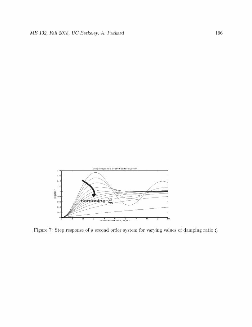
ME 132, Fall 2018, UC Berkeley, A. Packard 196
0 1 2 3 4 5 6 7 8 9 100
0.2
0.4
0.6
0.8
1
1.2
1.4
1.6
1.8
Normalized time, w_n t
Resp
onse
, y
Step response of 2nd order system
Figure 7: Step response of a second order system for varying values of damping ratio ξ.
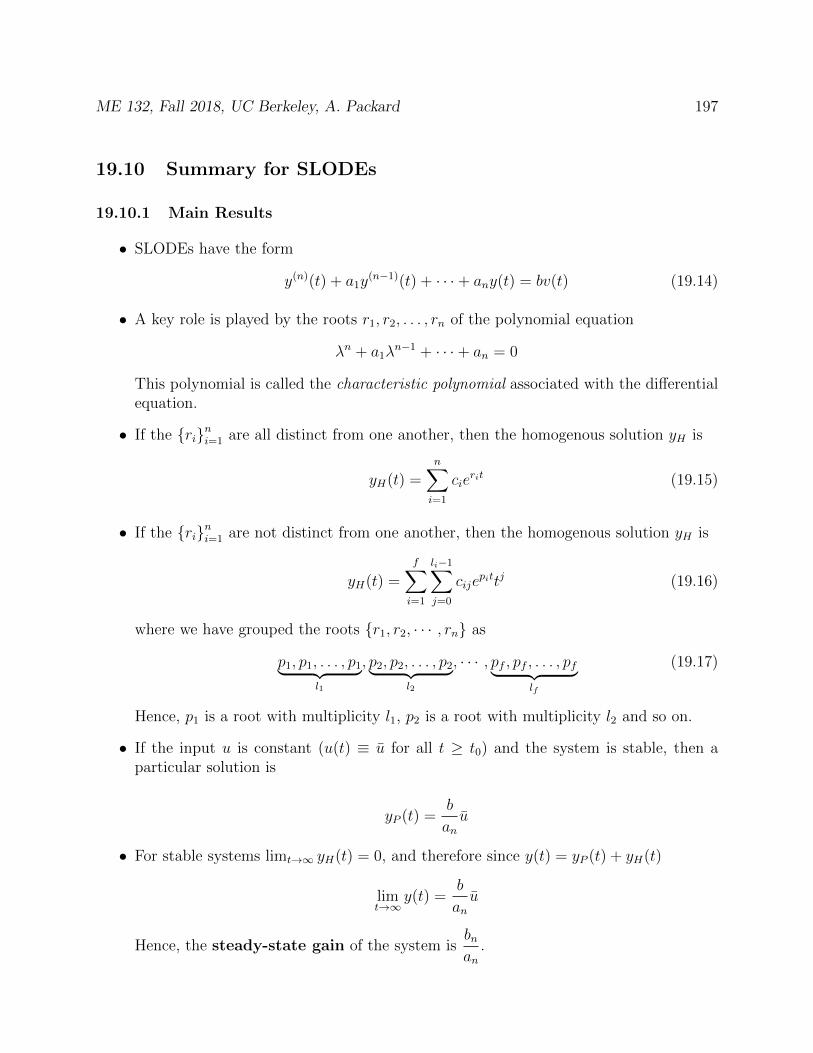
ME 132, Fall 2018, UC Berkeley, A. Packard 197
19.10 Summary for SLODEs
19.10.1 Main Results
• SLODEs have the form
y(n)(t) + a1y(n−1)(t) + · · ·+ any(t) = bv(t) (19.14)
• A key role is played by the roots r1, r2, . . . , rn of the polynomial equation
λn + a1λn−1 + · · ·+ an = 0
This polynomial is called the characteristic polynomial associated with the differentialequation.
• If the rini=1 are all distinct from one another, then the homogenous solution yH is
yH(t) =n∑i=1
cierit (19.15)
• If the rini=1 are not distinct from one another, then the homogenous solution yH is
yH(t) =
f∑i=1
li−1∑j=0
cijepittj (19.16)
where we have grouped the roots r1, r2, · · · , rn as
p1, p1, . . . , p1︸ ︷︷ ︸l1
, p2, p2, . . . , p2︸ ︷︷ ︸l2
, · · · , pf , pf , . . . , pf︸ ︷︷ ︸lf
(19.17)
Hence, p1 is a root with multiplicity l1, p2 is a root with multiplicity l2 and so on.
• If the input u is constant (u(t) ≡ u for all t ≥ t0) and the system is stable, then aparticular solution is
yP (t) =b
anu
• For stable systems limt→∞ yH(t) = 0, and therefore since y(t) = yP (t) + yH(t)
limt→∞
y(t) =b
anu
Hence, the steady-state gain of the system isbnan
.
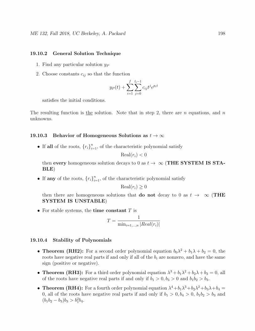
ME 132, Fall 2018, UC Berkeley, A. Packard 198
19.10.2 General Solution Technique
1. Find any particular solution yP
2. Choose constants cij so that the function
yP (t) +
f∑i=1
li−1∑j=0
cijtjepit
satisfies the initial conditions.
The resulting function is the solution. Note that in step 2, there are n equations, and nunknowns.
19.10.3 Behavior of Homogeneous Solutions as t→∞
• If all of the roots, rini=1, of the characteristic polynomial satisfy
Real(ri) < 0
then every homogeneous solution decays to 0 as t→ ∞ (THE SYSTEM IS STA-BLE)
• If any of the roots, rini=1, of the characteristic polynomial satisfy
Real(ri) ≥ 0
then there are homogeneous solutions that do not decay to 0 as t → ∞ (THESYSTEM IS UNSTABLE)
• For stable systems, the time constant T is
T =1
mini=1,...,n |Real(ri)|
19.10.4 Stability of Polynomials
• Theorem (RH2): For a second order polynomial equation b0λ2 + b1λ + b2 = 0, the
roots have negative real parts if and only if all of the bi are nonzero, and have the samesign (positive or negative).
• Theorem (RH3): For a third order polynomial equation λ3 + b1λ2 + b2λ+ b3 = 0, all
of the roots have negative real parts if and only if b1 > 0, b3 > 0 and b1b2 > b3.
• Theorem (RH4): For a fourth order polynomial equation λ4 +b1λ3 +b2λ
2 +b3λ+b4 =0, all of the roots have negative real parts if and only if b1 > 0, b4 > 0, b1b2 > b3 and(b1b2 − b3)b3 > b2
1b4.
ME 132, Fall 2018, UC Berkeley, A. Packard 199
19.10.5 2nd order differential equation
• General form isy(t) + a1y(t) + a2y(t) = bv(t) (19.18)
• For stable systems (a1 > 0, a2 > 0), rewrite using new variables ξ, ωn as
y(t) + 2ξωny(t) + ω2ny(t) = bv(t)
where both ξ, ωn > 0.
• We have2ξωn = a1, ω2
n = a2
which can be inverted to give
ξ =a1
2√a2
, ωn =√a2
Note that since a1, a2 > 0, we also have ξ, ωn > 0.
• The characteristic polynomial
λ2 + 2ξωnλ+ ω2n = 0
• The roots are atλ = −ξωn ± ωn
√ξ2 − 1
= −ξωn ± jωn√
1− ξ2
19.10.6 Solutions of 2nd order differential equation
• ξ > 1: Roots are distinct, and both roots are real, and negative.
yH(t) = c1e
(−ξωn+ωn
√ξ2−1
)t+ c2e
(−ξωn−ωn
√ξ2−1
)t
Settling time (Time to decay)= 3
|−ξωn+ωn√ξ2−1|
• ξ = 1: Roots are repeated real at λ = −ξωn,
yH(t) = c1e−ξωnt + c2te
−ξωnt
Settling time (Time to decay)= 3ξωn
ME 132, Fall 2018, UC Berkeley, A. Packard 200
• 0 < ξ < 1: Roots are distinct, and complex (complex-conjugate pair), with negativereal part
yH(t) = e−ξωnt[A cosωn
√1− ξ2t + B sinωn
√1− ξ2t
]or equivalently
yH(t) = e−ξωnt[√
(A2 +B2) sin(ωn√
1− ξ2t+ φ)]
where φ = atan(A/B)
– Settling time (Time to decay)= 3ξωn
– The period of oscillation = 2π
ωn√
1−ξ2.
– The number of oscillations that can be observed (during the settling time) is
N :=Time to decay
Period of oscillation=
3√
1− ξ2
2πξ
– Everywhere ωn appears together in a term ωnt. Hence, ωn simply “scales” theresponse yH(t) in t. The larger value of ωn, the faster the response.
19.11 Problems
1. Consider the differential equation
y(t) + 3y(t) + 2y(t) = 0 (19.19)
Let yH,1(t) := 2e−t − e−2t, and yH,2(t) := e−t − e−2t.
(a) Compute yH,1(0) and yH,1(0). Plot yH,1(t) versus t. Show that the function yH,1satisfies the differential equation in (19.19).
(b) Compute yH,2(0) and yH,2(0). Plot yH,2(t) versus t. Show that the function yH,2satisfies the differential equation in (19.19).
(c) For any two constants α and β, define
yc(t) := αyH,1(t) + βyH,2(t)
i. Does yc satisfy the ODE?
ii. What is yc(0)? Your answer will involve α and β.
iii. What is yc(0)? Your answer will involve α and β.
(d) What is the solution to the ODE with initial conditions y(0) = 6, y(0) = −4?
ME 132, Fall 2018, UC Berkeley, A. Packard 201
2. Consider the example equation from Section 19.7, y(t) + 4y(t) + y(t) = 1, with initialconditions y(0) = y0, y(0) = v0. Consider all possible combinations of initial conditionsfrom the lists below:
y0 = −2,−1, 0, 1, 2
andv0 = −2,−1, 0, 1, 2
(Now, do part (a) first!)
(a) Note that without explicitly solving the differential equation, one can easily com-pute 4 things: limiting value of y (as t → ∞), time constant of the “slowest”homogeneous solution, initial value (given) and initial slope (given). With thesenumbers, carefully sketch on graph paper how you think all 25 solutions will look.
(b) In the notes, the solution is derived for general initial conditions. Use Matlab (orsimilar) to plot these expressions. Compare to your simplistic approximations inpart 2a.
3. The response (with all appropriate initial conditions set to 0) of the systems listedbelow is shown. Match the ODE with the solution graph. Explain your reasoning.
(a) y(t) + y(t) = 1
(b) y(t) + 5y(t) = 5
(c) y(t) + 2y(t) + y(t) = 1
(d) y(t)− 2y(t)− y(t) = −1
(e) y(t)− 2y(t) + 9y(t) = 9
(f) y(t) + 0.4y(t) + y(t) = 1
(g) y(t) + 0.12y(t) + 0.09y(t) = 0.09
(h) y(t) + 11y(t) + 10y(t) = 10
(i) y(t) + 0.3y(t) + 0.09y(t) = 0.09
(j) y(t) + 3y(t) + 9y(t) = 9
(k) y(t) + 4.2y(t) + 9y(t) = 9
(l) y(t) + 0.2y(t) + y(t) = 1
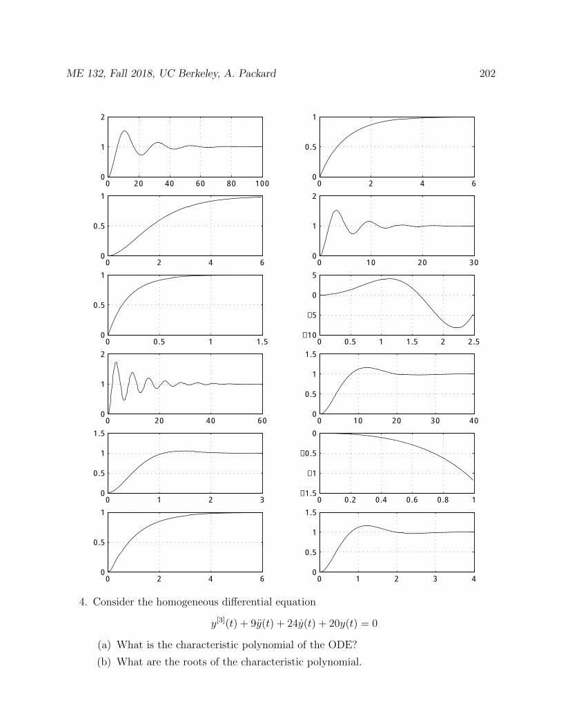
ME 132, Fall 2018, UC Berkeley, A. Packard 202
0 20 40 60 80 1000
1
2
0 2 4 60
0.5
1
0 2 4 60
0.5
1
0 10 20 300
1
2
0 0.5 1 1.50
0.5
1
0 0.5 1 1.5 2 2.5−10
−5
0
5
0 20 40 600
1
2
0 10 20 30 400
0.5
1
1.5
0 1 2 30
0.5
1
1.5
0 0.2 0.4 0.6 0.8 1−1.5
−1
−0.5
0
0 2 4 60
0.5
1
0 1 2 3 40
0.5
1
1.5
4. Consider the homogeneous differential equation
y[3](t) + 9y(t) + 24y(t) + 20y(t) = 0
(a) What is the characteristic polynomial of the ODE?
(b) What are the roots of the characteristic polynomial.
ME 132, Fall 2018, UC Berkeley, A. Packard 203
(c) Write the general form of a homogeneous solution. Explain what are the freeparameters.
(d) Show, by direct substitution, that yH(t) = te−2t is a solution.
(e) Show, by direct substitution, that yH(t) = t2e−2t is not a solution.
(f) Find the solution which satisfies initial conditions y(0) = 3, y(0) = 1, y[2](0) = 0.
(g) Find the solution which satisfies initial conditions y(0) = 3, y(0) = 1, y[3](0) = 0.
5. Suppose a < 0, and consider the function teat for t ≥ 0.
(a) For what value of t does the maximum occur?
(b) At what value(s) of t is the function equal to 0.05 of its maximum value. Forcomparison, recall that for the function eat, the function is equal to 0.05 of themaximum value at about 3
−a .
6. (a) Suppose λ ∈ C and k ≥ 0 is an integer. Show that x(t) := 1k+1
tk+1e−λt is asolution to the differential equation
x(t) + λx(t) = tke−λt
(b) Suppose y and z satisfy the differential equations
z(t) + λz(t) = y(t), y(t) + λy(t) = 0
Eliminate y, and find a 2nd-order differential equation governing z
(c) Suppose q satisfies the differential equation
q(t) + 2λq(t) + λ2q(t) = 0
Define r(t) := q(t) + λq(t). What differential equation does r satisfy? Hint:What is r(t) + λr(t)
7. In section 19.9, we considered differential equations of the form
y(t) + a1y(t) + a2y(t) = bv(t).
If a1 > 0 and a2 > 0, and a1 < 2√a2, then we chose to write the solution in terms of
the (ωn, ξ) parameters, which are derived from a1 and a2.
If the forcing function v is a constant, v(t) ≡ v, we derived that all particular solutionsare of the form
b
a2
v + e−ξωnt[A cosωn
√1− ξ2t + B sinωn
√1− ξ2t
]where A and B are free parameters.
Suppose the initial conditions are y(0) = y0 and y(0) = y0. Find the correct values forA and B so that the initial conditions are satisfied. Your answer should be in terms ofthe given initial conditions, and system parameters (ωn, ξ, b).
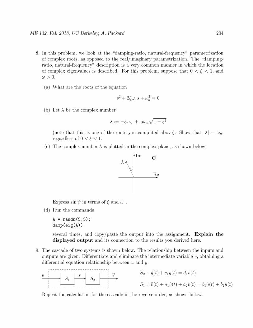
ME 132, Fall 2018, UC Berkeley, A. Packard 204
8. In this problem, we look at the “damping-ratio, natural-frequency” parametrizationof complex roots, as opposed to the real/imaginary parametrization. The “damping-ratio, natural-frequency” description is a very common manner in which the locationof complex eigenvalues is described. For this problem, suppose that 0 < ξ < 1, andω > 0.
(a) What are the roots of the equation
s2 + 2ξωns+ ω2n = 0
(b) Let λ be the complex number
λ := −ξωn + jωn√
1− ξ2
(note that this is one of the roots you computed above). Show that |λ| = ωn,regardless of 0 < ξ < 1.
(c) The complex number λ is plotted in the complex plane, as shown below.
-
6
λ×
AAAA
Re
Im C
ψ
Express sinψ in terms of ξ and ωn.
(d) Run the commands
A = randn(5,5);
damp(eig(A))
several times, and copy/paste the output into the assignment. Explain thedisplayed output and its connection to the results you derived here.
9. The cascade of two systems is shown below. The relationship between the inputs andoutputs are given. Differentiate and eliminate the intermediate variable v, obtaining adifferential equation relationship between u and y.
S1 S2- - -
u v y
S1 : v(t) + a1v(t) + a2v(t) = b1u(t) + b2u(t)
S2 : y(t) + c1y(t) = d1v(t)
Repeat the calculation for the cascade in the reverse order, as shown below.
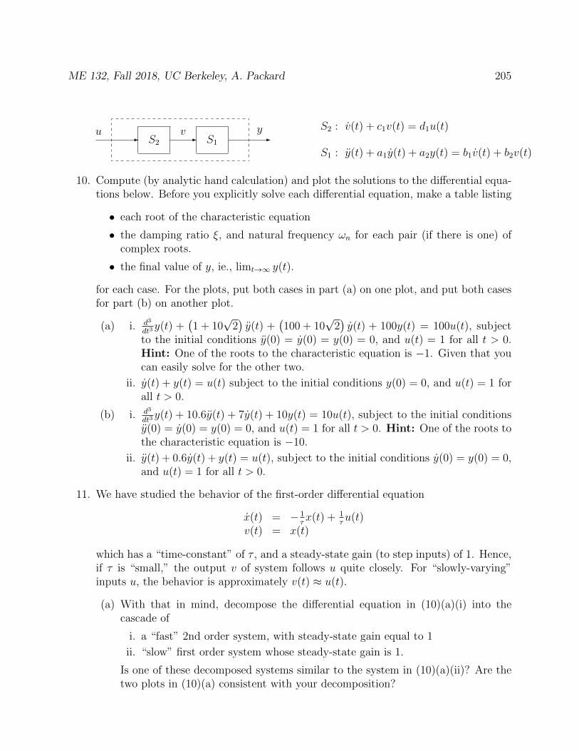
ME 132, Fall 2018, UC Berkeley, A. Packard 205
S2 S1- - -
u v y
S1 : y(t) + a1y(t) + a2y(t) = b1v(t) + b2v(t)
S2 : v(t) + c1v(t) = d1u(t)
10. Compute (by analytic hand calculation) and plot the solutions to the differential equa-tions below. Before you explicitly solve each differential equation, make a table listing
• each root of the characteristic equation
• the damping ratio ξ, and natural frequency ωn for each pair (if there is one) ofcomplex roots.
• the final value of y, ie., limt→∞ y(t).
for each case. For the plots, put both cases in part (a) on one plot, and put both casesfor part (b) on another plot.
(a) i. d3
dt3y(t) +
(1 + 10
√2)y(t) +
(100 + 10
√2)y(t) + 100y(t) = 100u(t), subject
to the initial conditions y(0) = y(0) = y(0) = 0, and u(t) = 1 for all t > 0.Hint: One of the roots to the characteristic equation is −1. Given that youcan easily solve for the other two.
ii. y(t) + y(t) = u(t) subject to the initial conditions y(0) = 0, and u(t) = 1 forall t > 0.
(b) i. d3
dt3y(t) + 10.6y(t) + 7y(t) + 10y(t) = 10u(t), subject to the initial conditions
y(0) = y(0) = y(0) = 0, and u(t) = 1 for all t > 0. Hint: One of the roots tothe characteristic equation is −10.
ii. y(t) + 0.6y(t) + y(t) = u(t), subject to the initial conditions y(0) = y(0) = 0,and u(t) = 1 for all t > 0.
11. We have studied the behavior of the first-order differential equation
x(t) = − 1τx(t) + 1
τu(t)
v(t) = x(t)
which has a “time-constant” of τ , and a steady-state gain (to step inputs) of 1. Hence,if τ is “small,” the output v of system follows u quite closely. For “slowly-varying”inputs u, the behavior is approximately v(t) ≈ u(t).
(a) With that in mind, decompose the differential equation in (10)(a)(i) into thecascade of
i. a “fast” 2nd order system, with steady-state gain equal to 1
ii. “slow” first order system whose steady-state gain is 1.
Is one of these decomposed systems similar to the system in (10)(a)(ii)? Are thetwo plots in (10)(a) consistent with your decomposition?
ME 132, Fall 2018, UC Berkeley, A. Packard 206
(b) Do a similar decomposition for (10)(b)(i), and again think/comment about theresponse of the 3rd order system in (10)(b)(i) and the 2nd order system’s responsein (10)(b)(ii).
12. (a) Suppose α is a fixed real number. If p(s) is a n’th order polynomial, with rootsλ1, λ2, . . . , λn, what are the roots of the n’th order polynomial g(s) defined by
g(s) := p(s− α)
(b) Do all of the roots of s3 + 7s2 + 22s+ 16 have real parts less than 0?
(c) Do all of the roots of s3 + 7s2 + 22s+ 16 real parts less than −1?
ME 132, Fall 2018, UC Berkeley, A. Packard 207
20 Frequency Responses of Linear Systems
In this section, we consider the steady-state response of a linear system due to a sinusoidalinput. The linear system is the standard one,
y[n](t) + a1y[n−1](t) + · · ·+ an−1y
[1](t) + any(t)= b0u
[n](t) + b1u[n−1](t) + · · ·+ bn−1u
[1](t) + bnu(t)(20.1)
with y the dependent variable (output), and u the independent variable (input).
Assume that the system is stable, so that the roots of the characteristic equation are in theopen left-half of the complex plane. This guarantees that all homogeneous solutions decayexponentially to zero as t→∞.
Suppose that the forcing function u(t) is chosen as a complex exponential, namely ω is a fixedreal number, and u(t) = ejωt. Note that the derivatives are particularly easy to compute,namely
u[k](t) = (jω)kejωt
It is easy to show that for some complex number H, one particular solution is of the form
yP (t) = Hejωt
How? Simply plug it in to the ODE, leaving
H [(jω)n + a1(jω)n−1 + · · ·+ an−1(jω) + an] ejωt
= [b0(jω)n + b1(jω)n−1 + · · ·+ bn−1(jω) + bn] ejωt
For all t, the quantity ejωt is never zero, so we can divide out leaving
H [(jω)n + a1(jω)n−1 + · · ·+ an−1(jω) + an]= [b0(jω)n + b1(jω)n−1 + · · ·+ bn−1(jω) + bn]
Now, since the system is stable, the roots of the polynomial
λn + a1λn−1 + · · ·+ an−1λ+ an = 0
all have negative real part. Hence, λ = jω, which has 0 real part, is not a root. Therefore,we can explicitly solve for H as
H =b0(jω)n + b1(jω)n−1 + · · ·+ bn−1(jω) + bn(jω)n + a1(jω)n−1 + · · ·+ an−1(jω) + an
(20.2)
Moreover, since actual solution differs from this particular solution by some homogeneoussolution, we must have
y(t) = yP (t) + yH(t)
ME 132, Fall 2018, UC Berkeley, A. Packard 208
In the limit, the homogeneous solution decays, regardless of the initial conditions, and wehave
limt→∞
y(t)− yP (t) = 0
Since yP is periodic, and y tends towards it asymptotically (the homogeneous solutions aredecaying), we call this specific particular solution the steady-state behavior of y, and denoteit yss.
The explanation we have given was valid at an arbitrary value of the forcing frequency, ω.The expression for H in (20.2) is still valid. Hence, we often write H(ω) to indicate thedependence of H on the forcing frequency.
H(ω) :=b0(jω)n + b1(jω)n−1 + · · ·+ bn−1(jω) + bn(jω)n + a1(jω)n−1 + · · ·+ an−1(jω) + an
(20.3)
This function is called the “frequency response” of the linear system in (20.1). Sometimesit is referred to as the “frequency response from u to y,” written as Hu→y(ω). For stablesystems, we have proven for fixed value u and fixed ω
u(t) := uejωt ⇒ yss(t) = H(ω)uejωt
20.1 Complex and Real Particular Solutions
What is the meaning of a complex solution to the differential equation (20.1)? Suppose thatfunctions u and y are complex, and solve the ODE. Denote the real part of the function u asuR, and the imaginary part as uI (similar for y). Then uR and uI are real-valued functions,and for all t u(t) = uR(t) + juI(t). Differentiating this k times gives
u[k](t) = u[k]R (t) + ju
[k]I (t)
Hence, if y and u satisfy the ODE, we have[y
[n]R (t) + jy
[n]I (t)
]+ a1
[y
[n−1]R (t) + jy
[n−1]I (t)
]+ · · ·+ an [yR(t) + jyI(t)] =
= b0
[u
[n]R (t) + ju
[n]I (t)
]+ b1
[u
[n−1]R (t) + ju
[n−1]I (t)
]+ · · ·+ bn [uR(t) + juI(t)]
But the real and imaginary parts must be equal individually, so exploiting the fact that thecoeffcients ai and bj are real numbers, we get
y[n]R (t) + a1y
[n−1]R (t) + · · ·+ an−1y
[1]R (t) + anyR(t)
= b0u[n]R (t) + b1u
[n−1]R (t) + · · ·+ bn−1u
[1]R (t) + bnuR(t)
andy
[n]I (t) + a1y
[n−1]I (t) + · · ·+ an−1y
[1]I (t) + anyI(t)
= b0u[n]I (t) + b1u
[n−1]I (t) + · · ·+ bn−1u
[1]I (t) + bnuI(t)
Hence, if (u, y) are functions which satisfy the ODE, then both (uR, yR) and (uI , yI) alsosatisfy the ODE.
ME 132, Fall 2018, UC Berkeley, A. Packard 209
20.2 Response due to real sinusoidal inputs
Suppose that H ∈ C is not equal to zero. Recall that ∠H is the real number (unique towithin an additive factor of 2π) which has the properties
cos∠H =ReH
|H|, sin∠H =
ImH
|H|
Then,Re(Hejθ
)= Re [(HR + jHI) (cos θ + j sin θ)]= HR cos θ −HI sin θ
= |H|[HR|H| cos θ − HI
|H| sin θ]
= |H| [cos∠H cos θ − sin∠H sin θ]= |H| cos (θ + ∠H)
Im(Hejθ
)= Im [(HR + jHI) (cos θ + j sin θ)]= HR sin θ +HI cos θ
= |H|[HR|H| sin θ + HI
|H| cos θ]
= |H| [cos∠H sin θ + sin∠H cos θ]= |H| sin (θ + ∠H)
Now consider the differential equation/frequency response case. Let H(ω) denote the fre-quency response function. If the input u(t) = cosωt = Re (ejωt), then the steady-stateoutput y will satisfy
y(t) = |H(ω)| cos (ωt+ ∠H(ω))
A similar calculation holds for sin, and these are summarized below.
Input Steady-State Output
1 H(0) = bnan
cosωt |H(ω)| cos (ωt+ ∠H(ω))sinωt |H(ω)| sin (ωt+ ∠H(ω))
20.3 Problems
1. Write a Matlab function which has three input arguments, A, B and Ω. A and B arerow vectors, of the form of the form
A = [a0 a1 a2 · · · an] , B = [b0 b1 b2 · · · bn]
where a0 6= 0. These represent the input/output system
a0y[n](t) + a1y
[n−1](t) + · · ·+ an−1y[1](t) + any(t)
= b0u[n](t) + b1u
[n−1](t) + · · ·+ bn−1u[1](t) + bnu(t)

ME 132, Fall 2018, UC Berkeley, A. Packard 210
with y the dependent variable (output), and u the independent variable (input). Ω is a1-by-N vector of real frequencies. The function should return one argument, H, whichwill be the same dimension as Ω, but in general will be complex. The value of H(i)should be the frequency-response function of the system above at frequency ω = Ω(i).
2. Using the Matlab function from above, draw the Bode plot of the frequency re-sponse function for the 3rd order system in problem 10(a)(i) in Section 19.11. Onthe same graph, plot the frequency response function for the 1st order system in prob-lem 10(a)(ii). Comment on the similarities and differences (eg., in what frequencyranges are they appreciably different?; in the frequency ranges where they are differ-ent, what is the magnitude of the response function as compared to the largest valueof the response magnitude?
3. Using the Matlab function from above, draw the Bode plot of the frequency responsefunction for the 3rd order system in problem 10(b)(i) in Section 19.11. On the samegraph, plot the frequency response function for the 2nd order system in problem10(b)(ii). Comment on the similarities and differences (eg., in what frequency rangesare they appreciably different?; in the frequency ranges where they are different, whatis the magnitude of the response function as compared to the largest value of theresponse magnitude?
4. Suppose the ODE for a system is
y(t) + 2ξωny(t) + ω2ny(t) = ω2
nu(t)
where u is the input, and y is the output. Assume that ξ > 0 and ωn > 0.
(a) Derive the frequency response function of the system. Let ω denote frequency,and denote the frequency response function as H(ω).
(b) What are |H(ω)| and |H(ω)|2. Is |H(ω)| (or |H(ω)|2) ever equal to 0?
(c) Work with |H(ω)|2. By dividing numerator and denominator by ω4n, derive
|H(ω)|2 =1[
1−(ωωn
)2]2
+ 4ξ2(ωωn
)2
What is |H(ω)| approximately equal to for for ω << ωn? What is log |H(ω)|approximately equal to for for ω << ωn?
(d) Work with |H(ω)|2. By dividing numerator and denominator by ω4, derive
|H(ω)|2 =
(ωnω
)4[(ωnω
)2 − 1]2
+ 4ξ2(ωnω
)2
ME 132, Fall 2018, UC Berkeley, A. Packard 211
Using this, show that for ω >> ωn, |H(ω)| ≈(ωnω
)2. As a function of logω, what
is log |H(ω)| approximately equal to for for ω >> ωn? Specifically, show that forω >> ωn,
log |H(ω)| ≈ 2 logωn − 2 logω
(e) What is ∠H(ω) for ω << ωn?
(f) What is ∠H(ω) for ω >> ωn?
(g) What are |H(ω)| and ∠H(ω) for ω = ωn?
(h) For a general function F (ω) that is never 0, show thatd
dω|F (ω)| = 0 at exactly
the same values of ω as whend
dω|F (ω)|2 = 0.
(i) Find the frequencies (real numbers) ω whered
dω|H(ω)| = 0.
(j) Show that if ξ < 1√2, then the maximum of |H(ω)| occurs at a non-zero frequency.
Denote the critical frequency by ωcrit, and show namely ωcrit = ωn√
1− 2ξ2.
(k) Assuming that ξ < 1√2. Show that
|H(ωcrit)| =1
2ξ√
1− ξ2
(l) Assuming that ξ < 1√2. Define φ := ∠H(ωcrit). What is tanφ?
(m) On graph paper, carefully sketch in all of the derived properties for four cases,ξ = 0.2, 0.5, 0.7, 0.9 and (in all cases) ωn = 1. Your plots should have the axeslog |H(ω)| versus logω, and ∠ |H(ω)| versus logω. In this problem, you havederived a few key features of the plots, but not the entire shape of the plot. Yoursketches should only include the facts that you have derived in this problem,namely parts 4c-4l.
(n) Using Matlab, generate the complete magnitude and angle plots for the two casesabove. Plot them for the range ω ∈ [0.001 1000]. Verify that the actual plotshave all of the features that you derived and sketched in the previous part.

ME 132, Fall 2018, UC Berkeley, A. Packard 212
21 Derivatives appearing on the inputs: Effect on the
forced response
Consider again the cruise control problem with a proportional/integral controller
u(t) = KIz(t)−KPvm(t) +K0r(t) (21.1)
z(t) = r(t)− vm(t)
where vm(t) = v(t) + n(t) is the measured speed, and n represents measurement noise.
The car dynamics are described by
v(t) = − αmv(t) +
E
mu(t) +
G
mw(t) (21.2)
where w(t) represents the hill incline.
So far, we have written this closed-loop system as a two-state linear system, driven byexternal inputs (r, w, n). Other representations are possible too.
Differentiate the car dynamics to obtain
v(t) = − αmv(t) +
E
mu(t) +
G
mw(t)
Differentiate the expression for u (in the controller equations) to obtain
u(t) = KI z(t)−KP (v(t) + n(t)) +K0r(t)
and substitute for z, giving
u(t) = KI(r(t)− v(t)− n(t))−KP (v(t) + n(t)) +K0r(t)
Finally, substitute this into the differentiated car dynamics equation to yield
v(t) +α + EKP
mv(t) +
EKI
mv(t) =
EKI
mr(t) +
EK0
mr(t) +
G
mw(t)− EKI
mn(t)− EKP
mn(t)
Main Question: It appears that r, w and n must be differentiable for this relationship tohold. That would mean that this is not suitable for determining the response to (for example)step changes in w and/or r. In this and the next section, we learn about distributions, andhow to make sense of differential equations when the right hand side is not classically defined.
ME 132, Fall 2018, UC Berkeley, A. Packard 213
21.1 Introduction
Suppose that through manipulation, we derive a relationship between the input (u) andoutput (y) of a system to be
y(t) + a1y(t) + a2y(t) = b1u(t) + b2u(t)
Next, suppose that we are given initial conditions y0 and y0, and are asked to computethe response to a unit-step input, applied just after the system is released from the initialconditions. Note that the input is not differentiable at t = 0, and hence the right-hand sideof the differential equation is not well defined. How do we get a solution in that case? Inorder to study this, we first consider particular solutions to a special class of nonconstantforcing functions.
21.2 Other Particular Solutions
We have already seen that the differential equation
y[n](t) + a1y[n−1](t) + · · ·+ an−1y(t) + any(t) = 1
has a particular solution yP (t) = 1an
for all t. Recall that all particular solutions can begenerated by adding all homogeneous solutions to any one particular solution.
What about a particular solution to the equation
y[n](t) + a1y[n−1](t) + · · ·+ an−1y(t) + any(t) = γ0 + γ1t
where γ0 and γ1 are some fixed constants. If we differentiate both sides, we see that aparticular solution is y taking a constant value, and hence we “guess” that there is a particularsolution of the form
yP (t) = αt+ β
for some proper choice of constants α and β. Indeed, note that yP = α, and all higher orderderivatives are identically zero. Plugging in, and equating gives
an−1α + an (αt+ β) = γ0 + γ1t
which must hold for all t. This gives
an−1α + anβ = γ0, anα = γ1
which can be easily solved, yielding
α =γ1
an, β =
γ0 − an−1α
an
This approach is easy to generalize for forcing functions of the form∑n
k=0 γktk.
ME 132, Fall 2018, UC Berkeley, A. Packard 214
21.3 Limits approaching steps
Return to the original problem, which is computing the step-response of
y(t) + a1y(t) + a2y(t) = b1u(t) + b2u(t) (21.3)
subject to initial conditions y(0) = Y0, y(0) = Y0, and the input u(t) = µ(t).
We begin with a simpler problem, which avoids the differentiability problems of the unitstep function. For each ε > 0, define a function µε as
µε(t) :=
0 for t < 01εt for 0 ≤ t < ε
1 for ε ≤ t
Note that this is continuous, and piecewise differentiable, with derivative
µε(t) =
0 for t < 01ε
for 0 < t < ε0 for ε < t
We want to determine the solution of the differential equation (21.3) subject to initial con-ditions y(0) = Y0, y(0) = Y0, and the input u(t) = µε(t). Let the solution be denoted byyε(t).
We break the problem into 2 time intervals: (0 ε) and (ε ∞).
• Over the first interval, (0 ε), we explicitly compute the solution in the standard manner,finding a particular solution, and then adding in the appropriate homogeneous solutionto match up the initial conditions at 0.
• Over the second interval, we follow the same procedure (since the qualitative behaviorof the right-hand-side of the differential equation is different in this time interval, weneed to start with a new particular solution), last values (ie., the values at t = ε) ofthe solution obtained in the first interval as initial conditions.
In order to achieve our original objective (response due to unit-step), after completing thesolution in the first interval, we take the limit as ε → 0 in order to compute the “initialconditions” for the second interval.
Reiterating – we want to determine properties of the solution at t = ε, in particular we wantto determine yε(ε), and yε(ε), and then take the limit as ε → 0 (ie., as the input functionbecomes more and more like a unit-step). We will denote these values as y(0+) and y(0+);
ME 132, Fall 2018, UC Berkeley, A. Packard 215
the values of y and y, just after the step change occurs. They become the initial conditionsfor the solution after the input’s step change has taken place.
During the interval (0, ε), the right-hand side of (21.3) is well defined, and is
b1u(t) + b2u(t) =b2
εt+
b1
ε
A particular solution (using the method we derived in Section 21.2) is yP (t) = αt+β, where
α =b2
a2ε, β =
b1a2 − a1b2
a22ε
Let λ1, λ2 be the roots of the characteristic polynomial,
λ2 + a1λ+ a2 = 0
For now, let’s assume that they are distinct (you could rework what we do here for the casewhen they are not distinct - it all works out the same). For a later calculation, please checkthat a1 = −λ1−λ2, and a2 = λ1λ2. Hence, the solution to the differential equation for t > 0must be
yε(t) = αt+ β + c1eλ1t + c2e
λ2t (21.4)
where c1 and c2 are uniquely chosen to satisfy the initial conditions yε(0) = Y0, yε(0) = Y0.Differentiating gives that
yε(t) = α + c1λ1eλ1t + c2λ2e
λ2t (21.5)
Satisfying the initial conditions at t = 0 gives conditions that the constants c1 and c2 mustsatisfy [
1 1λ1 λ2
] [c1
c2
]=
[Y0 − βY0 − α
]which can be solved as [
c1
c2
]=
1
λ2 − λ1
[λ2 −1−λ1 1
] [Y0 − βY0 − α
]In terms of c1 and c2, the value of yε and yε at t = ε are (using equations (21.4 and 21.5))[
yε(ε)yε(ε)
]=
[eλ1ε eλ2ε
λ1eλ1ε λ2e
λ2ε
] [c1
c2
]+
[αε+ βα
]Substituting, gives[
yε(ε)yε(ε)
]=
1
λ2 − λ1
[eλ1ε eλ2ε
λ1eλ1ε λ2e
λ2ε
] [λ2 −1−λ1 1
] [Y0 − βY0 − α
]+
[αε+ βα
]
ME 132, Fall 2018, UC Berkeley, A. Packard 216
Rearranging gives[yε(ε)yε(ε)
]=
1
λ2 − λ1
[λ2e
λ1ε − λ1eλ2ε eλ2ε − eλ1ε
λ2λ1
(eλ1ε − eλ2ε
)λ2e
λ2ε − λ1eλ1ε
] [Y0 − βY0 − α
]+
[αε+ βα
]
For notational purposes, let
Mε :=1
λ2 − λ1
[λ2e
λ1ε − λ1eλ2ε eλ2ε − eλ1ε
λ2λ1
(eλ1ε − eλ2ε
)λ2e
λ2ε − λ1eλ1ε
]
Then, we have [yε(ε)yε(ε)
]= Mε
[Y0 − βY0 − α
]+
[αε+ βα
]This is further manipulated into[
yε(ε)yε(ε)
]= Mε
[Y0
Y0
]+
(−Mε +
[1 ε0 1
])[βα
]But recall, α and β depend on ε, so that should be substituted,[
yε(ε)yε(ε)
]= Mε
[Y0
Y0
]+
1
ε
(−Mε +
[1 ε0 1
])[ b1a2−a1b2a22b2a2
]
Note thatlimε→0
Mε = I2
and using L’Hospital’s rule,
limε→0
1
ε
(−Mε +
[1 ε0 1
])=
[0 0
λ2λ1 −λ2 − λ1
]=
[0 0a2 a1
]
Hence, [y(0+)y(0+)
]:= lim
ε→0,ε>0
[yε(ε)yε(ε)
]=
[Y0
Y0 + b1
]=
[y(0−)y(0−)
]+
[0b1
]In summary, suppose the input waveform is such that the right-hand side (ie., forcing func-tion) of the differential equation has singularities at certain discrete instants in time. Betweenthose instants, all terms of the differential equation are well behaved, and we solve it in theclassical manner. However, at the instants of the singularity, some specific high order deriva-tive of y experiences a discontinuity in its value, and the discontinuity can be determined

ME 132, Fall 2018, UC Berkeley, A. Packard 217
from the differential equation. Essentially, we get “new” initial conditions for the differen-tial equation just after the singularity in terms of the solution of the ODE just before thesingularity and the ODE itself.
Key take-home points:
1. We have seen that the values of y and y at a time just before the input singularity arerelated to (but not equal to) the values of y and y just after the singularity.
2. Another point to notice: this calculation shows that the term b1u(t), which appearson the right-hand side of the ODE in equation (21.3) plays a role in the solution. So,both the left and right sides of an input/output ODE have qualitative and quantitativeeffects of the solution. We will formalize this as we proceed...
In the next section we learn some tricks that allow us to redo this type of calculation forgeneral systems (not just second order). Distributions are mathematical constructions that,in a rigorous manner, allow us to repeat the rigorous calculation we just did in this sectionin a less tedious fashion.
21.4 Problems
1. Consider the differential equation
y(t) + 4y(t) + 3y(t) = b1u(t) + 3u(t),
subject to the forcing function u(t) := µ(t), and initial conditions y(0−) = 0, y(0−) = 0.
(a) Determine:
• the conditions of y (and y) at t = 0+,
• the roots of the homogeneous equation (and their values of ξ and ωn if com-plex)
• the final value, limt→∞ y(t).
Some of these will be dependent on the parameter b1.
(b) Based on your answers, sketch a guess of the solution for 8 cases:
b1 = −6,−3,−0.3,−0.03, 0.03, 0.3, 3, 6.
Sketch them on the same axes.
(c) Determine the exact solution (by hand). Do as much of this symbolically as youcan (in terms of b1) so that you only need to the majority of the work once, andthen plug in the values of b1 several times. Use the plot command in MatLab(or other) to get a clean plot of the solution y(t) from 0+ to some suitable finaltime. Plot them on the same graph.

ME 132, Fall 2018, UC Berkeley, A. Packard 218
22 Distributions
In this section we learn some tricks that allow us to redo the calculation in the previoussection for general systems (not just second order). Distributions are mathematical con-structions that, in a rigorous manner, allow us to repeat the rigorous calculation we just didin section 21 in a less tedious fashion.
22.1 Introduction
Recall our goal: determine the response of
y[n](t) + a1y[n−1](t) + a2y
[n−2](t) + · · ·+ any(t) =b0u
[n](t) + b1u[n−1](t) + b2u
[n−2](t) + · · ·+ bnu(t)(22.1)
subject to u(t) = µ(t) (a unit step at t = 0) and initial conditions y(0−) = y[0]0 , y
[1](0−) =
y[1]0 , y
[2](0−) = y[2]0 , . . . , y
[n−1](0−) = y[n−1]0 . Here 0− refers to the time just before the unit-
step input is applied. So, the system is placed in initial conditions, and released, the releasetime being denoted 0−. At that instant, the input’s value is 0, so u(0−) = 0. An infinitesimaltime later, at 0+, the input value is changed to +1. The input is actually at unit-step att = 0, and the initial conditions are known just before the step-input is applied.
The difficulty is that the right-hand side of (22.1) is not classically defined, since u is notdifferentiable. However, we may obtain the solution by considering a sequence of problems,with smooth approximations to the unit step, and obtain the solution as a limiting process.Such a procedure goes as follows:
1. Define a n-times differentiable family of functions µε that have the property
µε(t) =
0 for t < 01 for t > ε
and which converge to the unit step µ as ε→ 0.
2. Compute solution yε(t) to the differential equation
y[n](t) + a1y[n−1](t) + a2y
[n−2](t) + · · ·+ any(t) =b0u
[n](t) + b1u[n−1](t) + b2u
[n−2](t) + · · ·+ bnu(t)
subject to the forcing function u(t) = µε(t) and initial conditions y(0) = y[0]0 , y
[1](0) =
y[1]0 , y
[2](0) = y[2]0 , . . . , y
[n−1](0) = y[n−1]0 .
ME 132, Fall 2018, UC Berkeley, A. Packard 219
3. Look at the values of yε(ε), yε(ε), yε(ε) . . . , y[n−1]ε (ε). Take the limit as ε → 0, and get
a relationship between the values of y, y, y, . . . , y[n−1] at t = 0− and t = 0+.
4. For t > 0, the right hand side of the ODE in (22.1) is well defined (in fact, it’s aconstant, bn), and the solution can be determined from finding any particular solu-tion, and combining with the family of homogeneous solutions to correctly match theconditions at t = 0+.
This procedure is tedious, though the following can be proven:
1. It gives the correct answer for the solution of the ODE subject to the unit step input
2. The final answer for the limits y[k]ε (ε) as ε → 0 are the same regardless of the form of
µε, as long as it satisfies the properties given.
Moreover, you can accomplish this in an easier fashion by using generalized functions, calleddistributions.
The most common distribution that is not a normal function is the Dirac-δ function. Togain intuition about this, consider an ε-approximation to the unit-step function of the form
µε(t) =
0 for t < 01εt for 0 < t < ε
1 for t ≥ 1
The derivative of this is
d
dtµε(t) =
0 for t < 01ε
for 0 < t < ε0 for t ≥ 1
Call this function δε. Note that for all values of ε > 0,∫ ∞−∞
δε(t)dt = 1
and that for t < 0 and t > ε, δε(t) = 0. Moreover, for any continuous function f
limε→0
∫ ∞−∞
f(t)δε(t)dt = f(0)
and for any t 6= 0, limε→0 δε(t) = 0. Hence, in the limit we can imagine a “function” δ whosevalue at nonzero t is 0, whose value at t = 0 is undefined, but whose integral is finite, namely1.

ME 132, Fall 2018, UC Berkeley, A. Packard 220
Now, we can start another level smoother. Let δε be defined as
δε(t) :=
0 for t < 0tε2
for 0 < t < ε2ε−tε2
for ε < t < 2ε0 for 2ε < t
Note that independent of ε we have ∫ ∞−∞
δε(t)dt = 1
and for any t 6= 0, limε→0 δε(t) = 0. The derivative is well defined, and satisfies
dδεdt
=
0 for t < 01ε2
for 0 < t < ε− 1ε2
for ε < t < 2ε0 for t > 2ε
Note that for any continuous function f , we have
limε→0
∫ ∞−∞
f(t)δε(t)dt = f(0)
and for any differentiable function f , we have
limε→0
∫ ∞−∞
f(t)dδεdtdt = −f(0)
and
limε→0
∫ ∞−∞
∣∣∣∣dδεdt∣∣∣∣ dt =∞
In the limit, we get an even more singular function, δ (or δ[1]), which has the property thatit is zero for all nonzero t, not well defined for t = 0, and even the integral of the absolutevalue is not well defined.
If we start with a smoother (quadratics) version of δε, then we can differentiate twice, gettingδε and δε, and look at their limiting behavior. Starting still smoother, we can continue theprocess, generating a collection of singular functions, δ[k], defined formally as
δ[0](t) := δ(t) :=dµ
dt, δ[k](t) =
dδ[k−1]
dt
As we have seen in the first few, each µ[k]ε is “more singular” than the preceeding one, µ
[k−1]ε .
Hence, there is no manner in which several lower order derivatives of µε-functions can belinearly combined to represent a µε-function of higher order. In other words, the functionµε along with derivatives of µε functions are a linearly independent set. Hence, in a equalityinvolving these types of functions, the coefficients of each function, on both sides of theequality, must match. This is used in the next section.

ME 132, Fall 2018, UC Berkeley, A. Packard 221
22.2 Procedure to get step response
Consider our general system differential equation (22.1), and suppose that u(t) = µ(t). Then,the highest order singularity in the right-hand side is associated with the u[n] term, whichhas µ[n]. Hence, this is the highest order singularity which must occur on the left-handside. If this order-of-singularity occurs in any of the terms y, y, . . . , y[n−1], then additionaldifferentiation will yield even a higher-order singularity in the y[n] term, which is not possible.Hence, the only term on the left-hand side with µ[n] is y[n]. This suggests that y[n] is of theform
y[n] = e1µ[n] + e2µ
[n−1] + · · ·+ enµ[1] + en+1µ+ fn
where fn is a continuous function, and the constants e1, e2, . . . , en+1 need to be determined.Note that if this is the form of the n’th derivative of y, then there are constraints on thelower order derivatives of y as well. Integrating, we get
y[n] = e1µ[n] + e2µ
[n−1] + · · · + enµ[1] + en+1µ + fn
y[n−1] = e1µ[n−1] + · · · + en−1µ
[1] + enµ + fn−1...
y[1] = e1µ[1] + e2µ + f2
y[0] = + e1µ + f1
where each of the fi are continuous functions. Plugging into the ODE, and equating thedifferent singularities gives n equations in n unknowns, expressed in matrix form below
1 0 0 · · · 0a1 1 0 · · · 0a2 a1 1 · · · 0...
......
. . ....
an−1 an−2 · · · a1 1
e1
e2
e3...en
=
b0
b1
b2...
bn−1
(22.2)
The matrix is always invertible, and the system of equations can be solved, yielding the evector. It is easy to see that it can be solved recursively, from e1 through en (and even en+1)as
e1 = b0
e2 = b1 − a1e1
e3 = b2 − a1e2 − a2e1...
...ek = bk−1 − a1ek−1 − a2ek−2 − · · · − ak−1e1

ME 132, Fall 2018, UC Berkeley, A. Packard 222
The e vector gives the discontinuity in each derivative of y at t = 0, namely
y(0+) = y(0−) + e1
y(0+) = y(0−) + e2
y[2](0+) = y[2](0−) + e3...
......
y[k](0+) = y[k](0−) + ek+1...
......
y[n−1](0+) = y[n−1](0−) + en
Given these “new” initial conditions at t = 0+, we can proceed with the solution of
y[n](t) + a1y[n−1](t) + a2y
[n−2](t) + · · ·+ any(t) = bn (22.3)
for t ≥ 0+ (that is why the RHS is so simple) by combining the family of all homogeneoussolutions, with one particular solution (for instance, yP (t) ≡ bn
an) to match the initial con-
ditions at t = 0+, completing the original solution task. You can/should write a generalMatLab function M-file to compute all of these quantities for given row vectors
A =[
1 a1 a2 · · · an−1 an], B =
[b0 b1 b2 · · · bn−1 bn
]

ME 132, Fall 2018, UC Berkeley, A. Packard 223
22.3 Summary: Solution of SLODEs with Derivatives on the in-puts
22.3.1 Introduction
• Goal: determine the response of
y[n](t) + a1y[n−1](t) + a2y
[n−2](t) + · · ·+ any(t) =b0u
[n](t) + b1u[n−1](t) + b2u
[n−2](t) + · · ·+ bnu(t)(22.4)
subject to u(t) = µ(t) (a unit step at t = 0) and initial conditions y(0−) = y[0]0 , y
[1](0−) =
y[1]0 , y
[2](0−) = y[2]0 , . . . , y
[n−1](0−) = y[n−1]0 .
• The time 0− refers to the time just before the unit-step input is applied.
• The initial conditions are known just before the step-input is applied, i.e. time 0−.
• At t = 0, the input value is changed to +1.
• The difficulty is that the right-hand side is not classically defined, since u is not differ-entiable at t = 0
• The solution can be obtained by considering a sequence of problems, with smoothapproximations to the unit step, and obtain the solution as a limiting process.
Main Concept for obtaining the solution
• For ε > 0, define a function µε as
µε(t) :=
0 for t < 01εt for 0 ≤ t < ε
1 for ε ≤ t
• Break the problem into 2 time intervals: [0, ε] and [ε, ∞). In the limit as ε→ 0, valueof signals at t = ε will be denoted as the value at 0+.
• Over the first interval, [0, ε], compute the solution in the standard manner, finding aparticular solution, and then adding in the appropriate homogeneous solution to matchup the initial conditions at 0.
• Over the second interval follow the same procedure starting from the values at t = εof the solution obtained in the first interval as initial conditions.
• Take the limit as ε→ 0 to compute the solution y(t) to the original problem.

ME 132, Fall 2018, UC Berkeley, A. Packard 224
• Note that the solution on the first interval, [0, ε], will affect the “initial conditions”for the second interval.
• As ε→ 0 we are only interested in computing the new initial conditions, i.e., the valuesof y and its derivatives just after the step change occurs (at t = ε, which, in the limitas ε→ 0 is denoted 0+).
Distributions
• Denote the function µε(t), defined above, as δε.
• Note that for all values of ε > 0, ∫ ∞−∞
δε(t)dt = 1
and that for t < 0 and t > ε, δε(t) = 0.
• Also, for any continuous function f
limε→0
∫ ∞−∞
f(t)δε(t)dt = f(0)
and for any t 6= 0, limε→0 δε(t) = 0.
• The functionδ(t) = limε→0δε
is the Dirac-δ function.
• The “function” δ is equal to 0 at all times with the exception of t = 0. At t = 0 it isundefined, but the integral is finite, namely 1.
• We proceed similarly and define the first derivative of the function δ(t), the secondderivative and so on..
δ[0](t) := δ(t) :=dµ
dt, δ[k](t) =
dδ[k−1]
dt
The procedure
• Consider our general system differential equation
y[n](t) + a1y[n−1](t) + a2y
[n−2](t) + · · ·+ any(t) =b0u
[n](t) + b1u[n−1](t) + b2u
[n−2](t) + · · ·+ bnu(t)(22.5)
and suppose that u(t) = µ(t).
ME 132, Fall 2018, UC Berkeley, A. Packard 225
• By using distribution properties we can argue that y[n] is of the form
y[n] = e1µ[n] + e2µ
[n−1] + · · ·+ enµ[1] + en+1µ+ fn(t)
where fn(t) is a continuous function, and the constants e1, e2, . . . , en+1 need to bedetermined.
• Integrating, we get
y[n] = e1δ[n−1] + e2δ
[n−2] + · · · + enδ + en+1µ + fn(t)y[n−1] = e1δ
[n−2] + · · · + en−1δ + enµ + fn−1(t)...
y[1] = e1δ + e2µ + f2(t)y[0] = + e1µ + f0(t)
where each of the fi(t) are continuous functions.
• Since fi(t) are continuous functions, they are continuous at 0.
f0(0−) = f0(0+) = y(0−)f1(0−) = f1(0+) = y(0−)f2(0−) = f2(0+) = y(0−)
......
...f[n−1](0
−) = f[n−1](0+) = y[n−1](0−)
Therefore the ei give the discontinuity in each derivative of y at t = 0+:
y(0+) = y(0−) + e1
y(0+) = y(0−) + e2
y[2](0+) = y[2](0−) + e3...
......
y[k](0+) = y[k](0−) + ek+1...
......
y[n−1](0+) = y[n−1](0−) + en
• Plugging into the ODE, and equating the different δ, δ[1], . . .,δ[n−1] functions gives nequations in n unknowns, expressed in matrix form below
1 0 0 · · · 0a1 1 0 · · · 0a2 a1 1 · · · 0...
......
. . ....
an−1 an−2 · · · a1 1
e1
e2
e3...en
=
b0
b1
b2...
bn−1
(22.6)

ME 132, Fall 2018, UC Berkeley, A. Packard 226
The matrix is always invertible, and the system of equations can be solved, yieldingthe e vector.
• It is easy to see that it can be solved recursively, from e1 through en as
e1 = b0
e2 = b1 − a1e1
e3 = b2 − a1e2 − a2e1...
...ek = bk−1 − a1ek−1 − a2ek−2 − · · · − ak−1e1
• Compute the new initial conditions at t = 0+:
y(0+) = y(0−) + e1
y(0+) = y(0−) + e2
y[2](0+) = y[2](0−) + e3...
......
y[k](0+) = y[k](0−) + ek+1...
......
y[n−1](0+) = y[n−1](0−) + en
• Given these “new” initial conditions at t = 0+, we can proceed with the solution of
y[n](t) + a1y[n−1](t) + a2y
[n−2](t) + · · ·+ any(t) = bn (22.7)
with the initial conditions at 0+ as shown in previous chapters. Note that since we areinterested in t ≥ 0+, the right-hand side (remember u is a unit-step input at t = 0), issimply bn.
• Note that in Matlab one can compactly solve the e quantities by using the command“A\b” where
A =
1 0 0 · · · 0a1 1 0 · · · 0a2 a1 1 · · · 0...
......
. . ....
an−1 an−2 · · · a1 1
, B =[b0 b1 b2 · · · bn−1 bn
]′
ME 132, Fall 2018, UC Berkeley, A. Packard 227
22.4 Problems
1. Consider a system with input u, and output y governed by the differential equation
y(t) + a1y(t) = u(t) + b1u(t) (22.8)
Find the unit-step response with initial conditions y(0−) = 0. Compare to answer(should be the same) as that obtained in problem 12 in section 5.6.
2. Considery[3](t) + 3.8y(t) + 6.8y(t) + 4y(t) = b2u(t) + 3u(t)
subject to the forcing function u(t) := µ(t), and initial conditions y(0−) = 0, y(0−) =0, y(0−) = 0. Follow the same instructions as in problem 1 in Section 21, handling the7 cases
b2 = −6,−3,−0.3,−0.03, 0.03, 0.3, 3, 6.
Since this is a higher order problem, you will need to also determine y(0+). Hint: Oneof the roots of the characteristic equation is −1. Also, if you proceed symbolically, youend up with the coefficients of the homogeneous components being of the form
c = M−1v(b2)
where M is a 3× 3 matrix made up of the three roots of the characteristic polynomial,and v is a 3 × 1 vector that depends on b2. On paper, leave it as that (don’t bothercomputing the inverse). Then, for each of the 6 cases, plug in a particular value forb2, and let MatLab compute the coefficients automatically. Set up your plotting scriptfile to accept a 3× 1 vector of homogeneous coefficients. In your solutions, include anyuseful M-files that you write.
3. Consider the three differential equations
y[4](t) + 5.8y[3](t) + 14.4y(t) + 17.6y(t) + 8y(t) = u(t)y[4](t) + 5.8y[3](t) + 14.4y(t) + 17.6y(t) + 8y(t) = 2u(t) + 2u(t) + u(t)y[4](t) + 5.8y[3](t) + 14.4y(t) + 17.6y(t) + 8y(t) = 2u(t)− 2u(t) + u(t)
Suppose that each is subject to the forcing function u(t) := µ(t), and initial conditionsy(0−) = 0, y(0−) = 0, y(0−) = 0, y[3](0−) = 0. Compute the roots (hint: one at −1,one at −2), get final value of y(t), compute “new” conditions of y (and derivatives) at0+, and sketch solutions. Then, derive the exact expression for the solutions, and plotusing MatLab.
ME 132, Fall 2018, UC Berkeley, A. Packard 228
23 Transfer functions
Associated with the linear system (input u, output y) governed by the ODE
y[n](t) + a1y[n−1](t) + · · ·+ an−1y
[1](t) + any(t)= b0u
[n](t) + b1u[n−1](t) + · · ·+ bn−1u
[1](t) + bnu(t)(23.1)
we write “in transfer function form”
Y =b0s
n + b1sn−1 + · · ·+ bn−1s+ bn
sn + a1sn−1 + · · ·+ an−1s+ anU (23.2)
The expression in (23.2) is interpreted to be equivalent to the ODE in (23.1), just a differentway of writing the coefficients. The notation in (23.2) is suggestive of multiplication, andwe will see that such an interpretation is indeed useful. The function
G(s) :=b0s
n + b1sn−1 + · · ·+ bn−1s+ bn
sn + a1sn−1 + · · ·+ an−1s+ an
is called the transfer function from u to y, and is sometimes denoted Gu→y(s) to indicatethis. At this point, the expression in equation (23.2),
Y = Gu→y(s)U
is nothing more than a new notation for the differential equation in (23.1).The differential equation itself has a well-defined meaning, and we understand what eachterm/symbol (derivative, multiplication, sum) represents, and the meaning of the equalitysign, =. By contrast, in the transfer function expression, (23.2), there is no specific meaningto the individual terms, or the equality symbol. The expression, as a whole, simply meansthe differential equation to which it is associated.
Nevertheless, in this section, we will see that, in fact, we can assign proper equality, andmake algebraic substitutions and manipulations of transfer function expressions, which willaid our manipulation of linear differential equations. But all of that requires proof, and thatis the purpose of this section.
23.1 Linear Differential Operators (LDOs)
Note that in the expression (23.2), the symbol s plays the role of ddt
, and higher powers of s
mean higher order derivatives, ie., sk means dk
dtk. If z is a function of time, let the notation[
b0dn
dtn+ b1
dn−1
dtn−1+ · · ·+ bn−1
d
dt+ bn
](z) := b0
dnz
dtn+ b1
dn−1z
dtn−1+ · · ·+ bn−1
dz
dt+ bnz
ME 132, Fall 2018, UC Berkeley, A. Packard 229
We will call this type of operation a linear differential operation, or LDO. For the purposesof this section, we will denote these by capital letters, say
L :=[dn
dtn+ a1
dn−1
dtn−1 + · · ·+ an−1ddt
+ an
]R :=
[b0
dn
dtn+ b1
dn−1
dtn−1 + · · ·+ bn−1ddt
+ bn
]Using this shorthand notation, we can write the original ODE in (23.5) as
L(y) = R(u)
With each LDO, we naturally associate a polynomial. Specifically, if
L :=
[dn
dtn+ a1
dn−1
dtn−1+ · · ·+ an−1
d
dt+ an
]then pL(s) is defined as
pL(s) := sn + a1sn−1 + · · ·+ an−1s+ an
Similarly, with each polynomial, we associate an LDO – if
q(s) := sm + b1sm−1 + · · ·+ bm−1s+ bm
then Lq is defined as
Lq :=
[dm
dtm+ b1
dm−1
dtm−1+ · · ·+ bm−1
d
dt+ bm
]
Therefore, if a linear system is governed by an ODE of the form L(y) = R(u), then thetransfer function description is simply
Y =pR(s)
pL(s)U
Similarly, if the transfer function description of a system is
V =n(s)
d(s)W
then the ODE description is Ld(v) = Ln(w).

ME 132, Fall 2018, UC Berkeley, A. Packard 230
23.2 Algebra of Linear differential operations
Note that two successive linear differential operations can be done in either order. Forexample let
L1 :=
[d2
dt2+ 5
d
dt+ 6
]and
L2 :=
[d3
dt3− 2
d2
dt2+ 3
d
dt− 4
]Then, on a differentiable signal z, simple calculations gives
L1 (L2(z)) =[d2
dt2+ 5 d
dt+ 6] ([
d3
dt3− 2 d2
dt2+ 3 d
dt− 4]
(z)]
=[d2
dt2+ 5 d
dt+ 6] (z[3] − 2z + 3z − 4z
)= z[5] − 2z[4] + 3z[3] − 4z[2]
5z[4] − 10z[3] + 15z[2] − 20z[1]
6z[3] − 12z[2] + 18z[1] − 24z= z[5] + 3z[4] − z[3] − z[2] − 2z[1] − 24z
which is the same as
L2 (L1(z)) =[d3
dt3− 2 d2
dt2+ 3 d
dt− 4] ([
d2
dt2+ 5 d
dt+ 6]
(z)]
=[d3
dt3− 2 d2
dt2+ 3 d
dt− 4] (z[2] + 5z + 6z
)= z[5] + 5z[4] + 6z[3]
−2z[4] − 10z[3] − 12z[2]
z[3] + 15z[2] + 18z[1]
−4z[2] − 20z[1] − 24z= z[5] + 3z[4] − z[3] − z[2] − 2z[1] − 24z
This equality is easily associated with the fact that multiplication of polynomials is a com-mutative operation, specifically
(s2 + 5s+ 6) (s3 − 2s2 + 3s− 4) = (s3 − 2s2 + 3s− 4) (s2 + 5s+ 6)= s5 + 3s4 − s3 − s2 − 2s+ 24
We will use the notation [L1 L2] to denote this composition of LDOs. The linear differentialoperator L1 L2 is defined as operating on an arbitrary signal z by
[L1 L2] (z) := L1 (L2(z))
Similarly, if L1 and L2 are LDOs, then the sum L1 + L2 is an LDO defined by its operationon a signal z as [L1 + L2] (z) := L1(z) + L2(z).
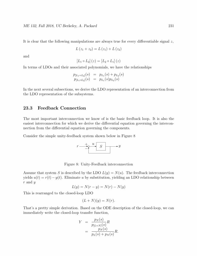
ME 132, Fall 2018, UC Berkeley, A. Packard 231
It is clear that the following manipulations are always true for every differentiable signal z,
L (z1 + z2) = L (z1) + L (z2)
and[L1 L2] (z) = [L2 L1] (z)
In terms of LDOs and their associated polynomials, we have the relationships
p[L1+L2](s) = pL1(s) + pL2(s)p[L1L2](s) = pL1(s)pL2(s)
In the next several subsections, we derive the LDO representation of an interconnection fromthe LDO representation of the subsystems.
23.3 Feedback Connection
The most important interconnection we know of is the basic feedback loop. It is also theeasiest interconnection for which we derive the differential equation governing the intercon-nection from the differential equation governing the components.
Consider the simple unity-feedback system shown below in Figure 8
S- d - -6
ru
y−+
Figure 8: Unity-Feedback interconnection
Assume that system S is described by the LDO L(y) = N(u). The feedback interconnectionyields u(t) = r(t)− y(t). Eliminate u by substitution, yielding an LDO relationship betweenr and y
L(y) = N(r − y) = N(r)−N(y)
This is rearranged to the closed-loop LDO
(L+N)(y) = N(r).
That’s a pretty simple derivation. Based on the ODE description of the closed-loop, we canimmediately write the closed-loop transfer function,
Y =pN(s)
p[L+N ](s)R
=pN(s)
pL(s) + pN(s)R.
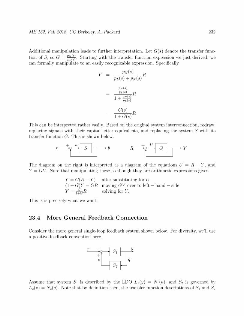
ME 132, Fall 2018, UC Berkeley, A. Packard 232
Additional manipulation leads to further interpretation. Let G(s) denote the transfer func-
tion of S, so G = pN (s)pL(s)
. Starting with the transfer function expression we just derived, wecan formally manipulate to an easily recognizable expression. Specifically
Y =pN(s)
pL(s) + pN(s)R
=
pN (s)pL(s)
1 + pN (s)pL(s)
R
=G(s)
1 +G(s)R
This can be interpreted rather easily. Based on the original system interconnection, redraw,replacing signals with their capital letter equivalents, and replacing the system S with itstransfer function G. This is shown below.
S- d - -6
ru
y−+
G- d - -6
RU
Y−+
The diagram on the right is interpreted as a diagram of the equations U = R − Y , andY = GU . Note that manipulating these as though they are arithmetic expressions gives
Y = G(R− Y ) after substituting for U(1 +G)Y = GR moving GY over to left− hand− sideY = G
1+GR solving for Y.
This is is precisely what we want!
23.4 More General Feedback Connection
Consider the more general single-loop feedback system shown below. For diversity, we’ll usea positive-feedback convention here.
S1
S2
- - -
6
dr y
qv
+
+
Assume that system S1 is described by the LDO L1(y) = N1(u), and S2 is governed byL2(v) = N2(q). Note that by definition then, the transfer function descriptions of S1 and S2

ME 132, Fall 2018, UC Berkeley, A. Packard 233
areY =
pN1
pL1︸︷︷︸:=G1
U, V =pN2
pL2︸︷︷︸:=G2
Q
The interconnection equations are u = r+v, and q = y. In order to eliminate v (for example),first substitute for u and q, leaving
L1(y) = N1(r + v) governing equation for S1
L2(v) = N2(y) governing equation for S2
Now apply L2 to first equation, and N1 to second equation, yielding (after using the notation for composing linear differential operators),
L2 L1(y) = L2 N1(r) + L2 N1(v)N1 L2(v) = N1 N2(y)
The expressions involving v cancel, leaving
[L2 L1 −N1 N2] (y) = L2 N1(r)
In transfer function terms, this is
Y =pL2N1
pL2L1−N1N2
R
which is easily rewritten as
Y =pL2pN1
pL2pL1 − pN1pN2
R
But, again, this can be formally manipulated into a recognizable expression involving the theindividual transfer functions of S1 and S2. Divide top and bottom of the transfer functionby pL1pL2 , to give
Y =
pL2pN1
pL2pL1
1− pN1pN2
pL2pL1
R
=G1
1−G2G1
R
Again, this can be interpreted rather easily. Based on the original system interconnection,redraw, replacing signals with their capital letter equivalents, and replacing the systems Siwith their transfer functions Gi. This is shown below.
S1
S2
- - -
6
dr y
qv
+
+G1
G2
- - -
6
dR Y
QV
+
+

ME 132, Fall 2018, UC Berkeley, A. Packard 234
The diagram on the right is interpreted as a diagram of the equations U = R − G2Y , andY = G1U . Note that manipulating these as though they are arithmetic expressions gives
Y = G1(R +G2Y ) after substituting for U(1−G1G2)Y = G1R moving G1G2Y over to left− hand− sideY = G1
1−G2G1R solving for Y.
This is is precisely what we want!
23.5 Cascade (or Series) Connection
Suppose that we have two linear systems, as shown below,
S1 S2- - -u y v
with S1 governed by
y[n](t) + a1y[n−1](t) + · · ·+ any(t) = b0u
[n](t) + b1u[n−1](t) + · · ·+ bnu(t)
and S2 governed by
v[m](t) + c1v[m−1](t) + · · ·+ cmv(t) = d0y
[m](t) + d1y[m−1](t) + · · ·+ dmy(t)
Let G1(s) denote the transfer function of S1, and G2(s) denote the transfer function of S2.Define the differential operations
L1 :=
[dn
dtn+ a1
dn−1
dtn−1+ · · ·+ an−1
d
dt+ an
]R1 :=
[b0dn
dtn+ b1
dn−1
dtn−1+ · · ·+ bn−1
d
dt+ bn
]and
L2 :=
[dm
dtm+ c1
dm−1
dtm−1+ · · ·+ cm−1
d
dt+ cm
]R2 :=
[d0dm
dtm+ d1
dm−1
dtm−1+ · · ·+ dm−1
d
dt+ dm
]Hence, the governing equation for system S1 is L1(y) = R1(u), while the governing equationfor system S2 is L2(v) = R2(y). Moreover, in terms of transfer functions, we have
G1(s) =pR1(s)
pL1(s), G2(s) =
pR2(s)
pL2(s)

ME 132, Fall 2018, UC Berkeley, A. Packard 235
Now, apply the differential operation R2 to the first system, leaving
R2 (L1(y)) = R2 (R1(u))
Apply the differential operation L1 to system 2, leaving
L1 (L2(v)) = L1 (R2(y))
But, in the last section, we saw that two linear differential operations can be applied in anyorder, hence L1 (R2(y)) = R2 (L1(y)). This means that the governing differential equationfor the cascaded system is
L1 (L2(v)) = R2 (R1(u))
which can be rearranged intoL2 (L1(v)) = R2 (R1(u))
or, in different notation[L2 L1] (v) = [R2 R1] (u)
In transfer function form, this means
V =p[R2R1](s)
p[L2L1](s)U
=pR2(s)pR1(s)
pL2(s)pL1(s)U
= G2(s)G1(s)U
Again, this has a nice interpretation. Redraw the interconnection, replacing the signals withthe capital letter equivalents, and the systems by their transfer functions.
S1 S2- - -u y v
G1 G2- - -U Y V
The diagram on the right depicts the equations Y = G1U , and V = G2Y . Treating these asarithmetic equalities allows substitution for Y , which yields V = G2G1U , as desired.
Example: Suppose S1 is governed by
y(t) + 3y(t) + y(t) = 3u(t)− u(t)
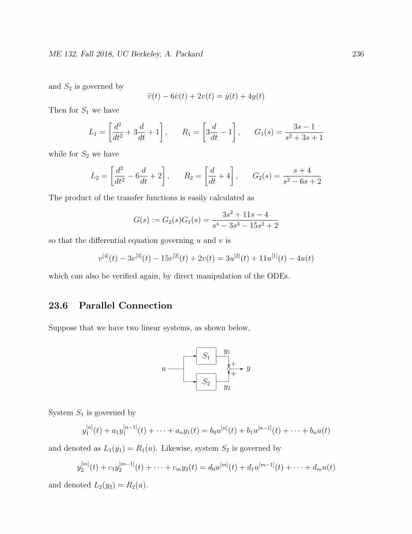
ME 132, Fall 2018, UC Berkeley, A. Packard 236
and S2 is governed byv(t)− 6v(t) + 2v(t) = y(t) + 4y(t)
Then for S1 we have
L1 =
[d2
dt2+ 3
d
dt+ 1
], R1 =
[3d
dt− 1
], G1(s) =
3s− 1
s2 + 3s+ 1
while for S2 we have
L2 =
[d2
dt2− 6
d
dt+ 2
], R2 =
[d
dt+ 4
], G2(s) =
s+ 4
s2 − 6s+ 2
The product of the transfer functions is easily calculated as
G(s) := G2(s)G1(s) =3s2 + 11s− 4
s4 − 3s3 − 15s2 + 2
so that the differential equation governing u and v is
v[4](t)− 3v[3](t)− 15v[2](t) + 2v(t) = 3u[2](t) + 11u[1](t)− 4u(t)
which can also be verified again, by direct manipulation of the ODEs.
23.6 Parallel Connection
Suppose that we have two linear systems, as shown below,
S2
S1-
-
?
6d -u
y1
y2
y++
System S1 is governed by
y[n]1 (t) + a1y
[n−1]1 (t) + · · ·+ any1(t) = b0u
[n](t) + b1u[n−1](t) + · · ·+ bnu(t)
and denoted as L1(y1) = R1(u). Likewise, system S2 is governed by
y[m]2 (t) + c1y
[m−1]2 (t) + · · ·+ cmy2(t) = d0u
[m](t) + d1u[m−1](t) + · · ·+ dmu(t)
and denoted L2(y2) = R2(u).

ME 132, Fall 2018, UC Berkeley, A. Packard 237
Apply the differential operation L2 to the governing equation for S1, yielding
L2 (L1(y1)) = L2 (R1(u)) (23.3)
Similarly, apply the differential operation L1 to the governing equation for S2, yielding and
L1 (L2(y2)) = L1 (R2(u))
But the linear differential operations can be carried out is either order, hence we also have
L2 (L1(y2)) = L1 (L2(y2)) (23.4)
Add the expressions in (23.3) and (23.4), to get
L2 (L1(y)) = L2 (L1(y1 + y2))= L2 (L1(y1)) + L2 (L1(y2))= L2 (R1(u)) + L1 (R2(u))= [L2 R1] (u) + [L1 R2] (u)= [L2 R1 + L1 R2] (u)
In transfer function form this is
Y =p[L2R1+L1R2](s)
p[L2L1](s)U
=p[L2R1](s) + p[L1R2](s)
pL2(s)pL1(s)U
=pL2(s)pR1(s) + pL1(s)pR2(s)
pL2(s)pL1(s)U
=
[pR1(s)
pL1(s)+pR2(s)
pL2(s)
]U
= [G1(s) +G2(s)]U
So, the transfer function of the parallel connection is the sum of the individual transferfunctions.
This is extremely important! The transfer function of an interconnection of systemsis simply the algebraic gain of the closed-loop systems, treating individual subsystems ascomplex gains, with their “gain” taking on the value of the transfer function.
ME 132, Fall 2018, UC Berkeley, A. Packard 238
23.7 General Connection
The following steps are used for a general interconnection of systems, each governed by alinear differential equation relating their inputs and outputs.
• Redraw the block diagram of the interconnection. Change signals (lower-case) to uppercase, and replace each system with its transfer function.
• Write down the equations, in transfer function form, that are implied by the diagram.
• Manipulate the equations as though they are arithmetic expressions. Addition andmultiplication commute, and the distributive laws hold.
23.8 Systems with multiple inputs
Associated with the multi-input, single-output linear ODE
L(y) = R1(u) +R2(w) +R3(v) (23.5)
we write
Y =pR1(s)
pL(s)U +
pR2(s)
pL(s)W +
pR3(s)
pL(s)V (23.6)
This may be manipulated algebraically.
23.9 Poles and Zeros of Transfer Functions
Consider to Linear Differential operators, L and R, and the input/output system describedby L(y) = R(u). Associated with L and R are polynomials, pL(s) and pR(s), and the transfer
function of the system is G := pR(s)pL(s)
.
As we already know, the roots of pL(s) = 0 give us complete information regarding the formof homogeneous solutions to the differential equation L(y) = 0. These roots, which are rootsof the denominator of the transfer function G are called the poles of the transfer function.
The zeros of the transfer function are defined as the roots of the numerator, in other words,roots of pR(s). Obviously, these roots yield complete information regarding homogeneoussolutions of the differential equation R(u) = 0. In sections 21 and 22, we saw the importanceof the right-hand-side of the differential equation on the forced response. Later we will learnhow to interpret this in terms of the number and location of the transfer function zeros.

ME 132, Fall 2018, UC Berkeley, A. Packard 239
23.10 Problems
1. Consider the feedback interconnection shown below. The signals r and w represent areference and disturbance input.
S1
S2
- - -
?e w
6
er y
q
u6
v
v
+
−
++
The system S1 is described by the LDO L1(y) = N1(u), and S2 is governed by L2(v) =N2(q). The interconnection equations are u = r − v and q = y + w.
(a) Find the differential equation relating (r and w) to y. The ODE will involvesums/differences/compositions of the Linear Differential Operators L1, N1, L2, N2.
(b) Find the differential equation relating (r and w) to v. The ODE will involvesums/differences/compositions of the Linear Differential Operators L1, N1, L2, N2.
(c) Find the differential equation relating (r and w) to u. The ODE will involvesums/differences/compositions of the Linear Differential Operators L1, N1, L2, N2.
What is the characteristic equation in each case? Note, in fact, that the characteristicequation is the same for all cases, whether the equations are written as y as influencedby (r, w), or v as influenced by (r, w), or u as influenced by (r, w).
2. Find the transfer function from u to y for the systems governed by the differentialequations
(a) y(t) = 1τ
[u(t)− y(t)]
(b) y(t) + a1y(t) = b0u(t) + b1u(t)
(c) y(t) = u(t) (explain connection to Simulink icon for integrator...)
(d) y(t) + 2ξωny(t) + ω2ny(t) = ω2
nu(t)
3. Consider the interconnection below. The transfer functions of systems S1 and S2 are
G1(s) =3
s+ 6, G2(s) =
s+ 2
s+ 1
Determine the differential equation governing the relationship between u and y.
S1 S2- - -u y
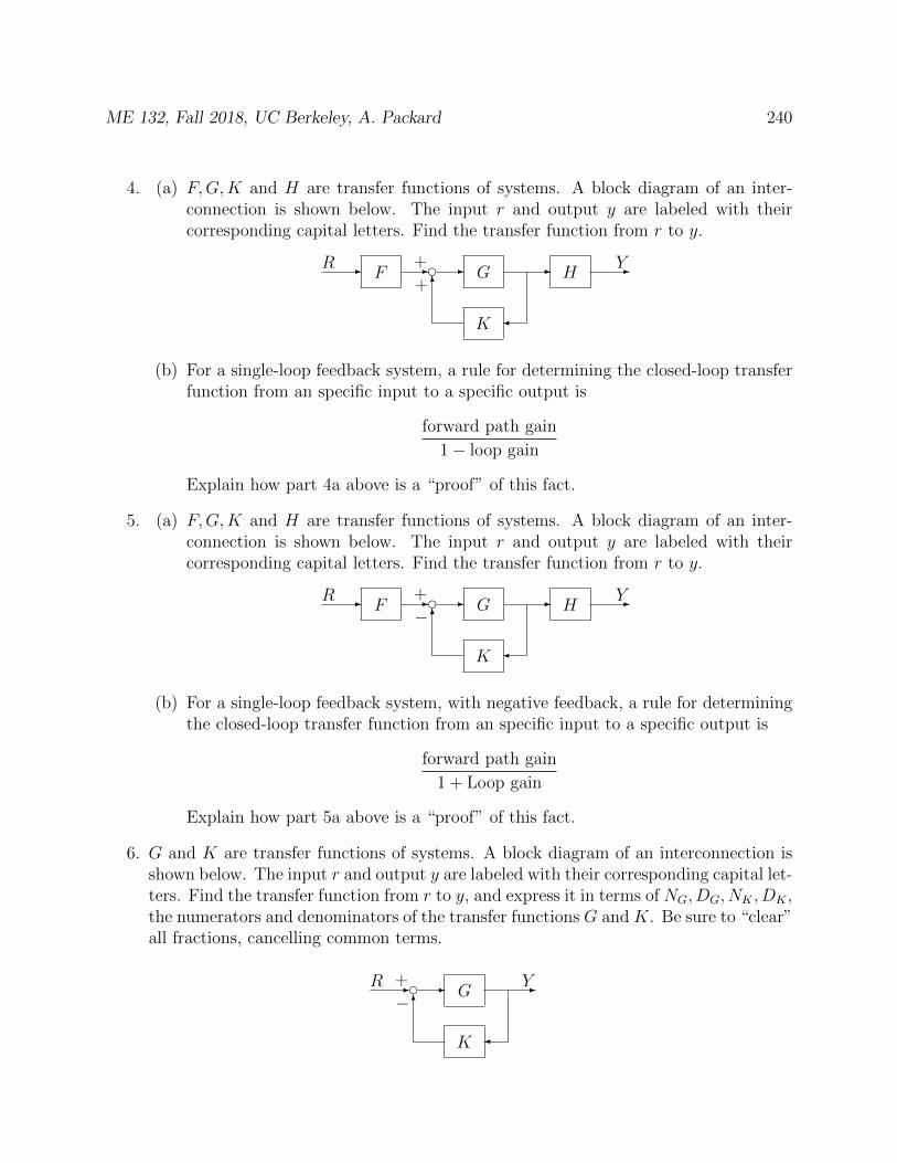
ME 132, Fall 2018, UC Berkeley, A. Packard 240
4. (a) F,G,K and H are transfer functions of systems. A block diagram of an inter-connection is shown below. The input r and output y are labeled with theircorresponding capital letters. Find the transfer function from r to y.
F G
K
H- - - - -
6
dR Y+
+
(b) For a single-loop feedback system, a rule for determining the closed-loop transferfunction from an specific input to a specific output is
forward path gain
1− loop gain
Explain how part 4a above is a “proof” of this fact.
5. (a) F,G,K and H are transfer functions of systems. A block diagram of an inter-connection is shown below. The input r and output y are labeled with theircorresponding capital letters. Find the transfer function from r to y.
F G
K
H- - - - -
6
dR Y+
−
(b) For a single-loop feedback system, with negative feedback, a rule for determiningthe closed-loop transfer function from an specific input to a specific output is
forward path gain
1 + Loop gain
Explain how part 5a above is a “proof” of this fact.
6. G and K are transfer functions of systems. A block diagram of an interconnection isshown below. The input r and output y are labeled with their corresponding capital let-ters. Find the transfer function from r to y, and express it in terms of NG, DG, NK , DK ,the numerators and denominators of the transfer functions G and K. Be sure to “clear”all fractions, cancelling common terms.
G
K
- - -
6
dR Y+
−
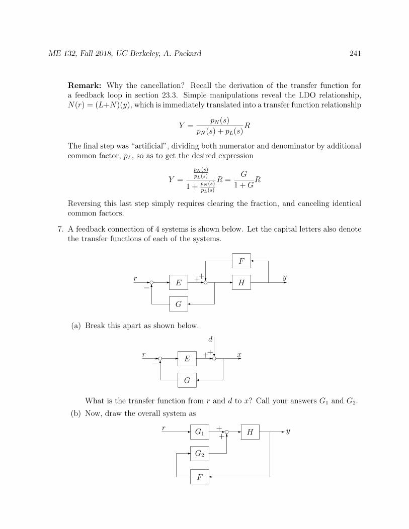
ME 132, Fall 2018, UC Berkeley, A. Packard 241
Remark: Why the cancellation? Recall the derivation of the transfer function fora feedback loop in section 23.3. Simple manipulations reveal the LDO relationship,N(r) = (L+N)(y), which is immediately translated into a transfer function relationship
Y =pN(s)
pN(s) + pL(s)R
The final step was “artificial”, dividing both numerator and denominator by additionalcommon factor, pL, so as to get the desired expression
Y =
pN (s)pL(s)
1 + pN (s)pL(s)
R =G
1 +GR
Reversing this last step simply requires clearing the fraction, and canceling identicalcommon factors.
7. A feedback connection of 4 systems is shown below. Let the capital letters also denotethe transfer functions of each of the systems.
d dG
E H
F
- - - - -
?
6−++r y
(a) Break this apart as shown below.
d dG
E- - - -?
6−++r x
d
What is the transfer function from r and d to x? Call your answers G1 and G2.
(b) Now, draw the overall system as
F
G2
G1 H- - d - -
-
6yr +
+
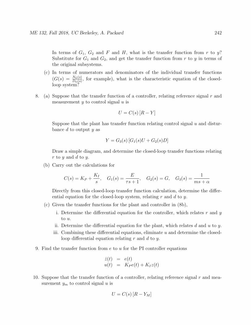
ME 132, Fall 2018, UC Berkeley, A. Packard 242
In terms of G1, G2 and F and H, what is the transfer function from r to y?Substitute for G1 and G2, and get the transfer function from r to y in terms ofthe original subsystems.
(c) In terms of numerators and denominators of the individual transfer functions
(G(s) = NG(s)DG(s)
, for example), what is the characteristic equation of the closed-loop system?
8. (a) Suppose that the transfer function of a controller, relating reference signal r andmeasurement y to control signal u is
U = C(s) [R− Y ]
Suppose that the plant has transfer function relating control signal u and distur-bance d to output y as
Y = G3(s) [G1(s)U +G2(s)D]
Draw a simple diagram, and determine the closed-loop transfer functions relatingr to y and d to y.
(b) Carry out the calculations for
C(s) = KP +KI
s, G1(s) =
E
τs+ 1, G2(s) = G, G3(s) =
1
ms+ α
Directly from this closed-loop transfer function calculation, determine the differ-ential equation for the closed-loop system, relating r and d to y.
(c) Given the transfer functions for the plant and controller in (8b),
i. Determine the differential equation for the controller, which relates r and yto u.
ii. Determine the differential equation for the plant, which relates d and u to y.
iii. Combining these differential equations, eliminate u and determine the closed-loop differential equation relating r and d to y.
9. Find the transfer function from e to u for the PI controller equations
z(t) = e(t)u(t) = KP e(t) +KIz(t)
10. Suppose that the transfer function of a controller, relating reference signal r and mea-surement ym to control signal u is
U = C(s) [R− YM ]
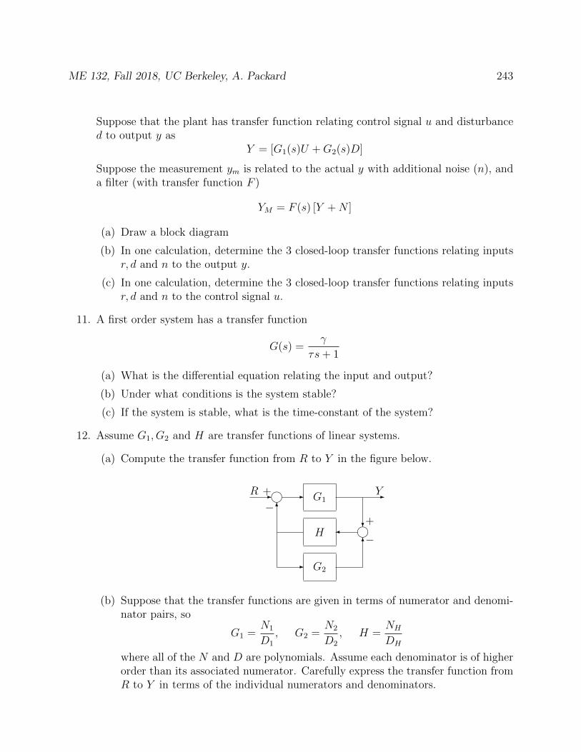
ME 132, Fall 2018, UC Berkeley, A. Packard 243
Suppose that the plant has transfer function relating control signal u and disturbanced to output y as
Y = [G1(s)U +G2(s)D]
Suppose the measurement ym is related to the actual y with additional noise (n), anda filter (with transfer function F )
YM = F (s) [Y +N ]
(a) Draw a block diagram
(b) In one calculation, determine the 3 closed-loop transfer functions relating inputsr, d and n to the output y.
(c) In one calculation, determine the 3 closed-loop transfer functions relating inputsr, d and n to the control signal u.
11. A first order system has a transfer function
G(s) =γ
τs+ 1
(a) What is the differential equation relating the input and output?
(b) Under what conditions is the system stable?
(c) If the system is stable, what is the time-constant of the system?
12. Assume G1, G2 and H are transfer functions of linear systems.
(a) Compute the transfer function from R to Y in the figure below.
G1
H
G2
- j - -
?j6
-
6
R Y
−+
−+
(b) Suppose that the transfer functions are given in terms of numerator and denomi-nator pairs, so
G1 =N1
D1
, G2 =N2
D2
, H =NH
DH
where all of the N and D are polynomials. Assume each denominator is of higherorder than its associated numerator. Carefully express the transfer function fromR to Y in terms of the individual numerators and denominators.

ME 132, Fall 2018, UC Berkeley, A. Packard 244
(c) What is the characteristic equation of the closed-loop system? Be sure that itsorder is the sum of the individual orders of the the 3 subsystems.
13. Consider a plant P with transfer function
P (s) =s
s2 − 1
The plant is a challenging to control. It is a simple model of an inverted pendulum,where the only control action u, represents the angular speed of a reaction wheel,mounted at the free-end (top) of the pendulum. By “torquing” the reaction wheel (rel-ative to the pendulum), equal/opposite torque act on the pendulum, which if properlydone, can stabilize it in the “up” position.
(a) Suppose the input to P is labeled u and the output y. What is the differentialequation governing the relationship between u and y.
(b) Is the plant stable?
(c) Consider a controller, C, with transfer function
C(s) =as+ b
s+ c
For the feedback loop consisting of P and C (with the usual negative (−) feedbackconvention), what is the closed-loop characteristic equation?
(d) Design: Find a, b and c (ie., parameters of the control law) so that the roots ofthe closed-loop characteristic equation are
−4,−2± j2
(e) The controller stabilizes P , in that the feedback loop consisting of P and C isstable. However, as we saw earlier, P is not stable on its own. Is C stable?
(f) Assume we relax the choice of the desired closed-loop roots, and only restrictthem to all have negative real-parts (since we want the closed-loop system to bestable). Are there any choice of such desired roots so that the controller (whichyields those closed-loop roots) is itself a stable system?
14. Read about the command tf in Matlab. Use the HTML help (available from themenubar, under Help, as well as the command-line (via >> help tf).
15. Read about the command step in Matlab. Use the HTML help (available from themenubar, under Help, as well as the command-line (via >> help step).
16. Execute the following commands

ME 132, Fall 2018, UC Berkeley, A. Packard 245
>> sys1 = tf(1,[1 3.8 6.8 4])
>> sys2 = tf([3 1],[1 3.8 6.8 4])
>> sys3 = tf([-3 1],[1 3.8 6.8 4])
>> step(sys1,sys2,sys3)
Relate these to problem 2 in Section 22.4.
17. Execute the following commands
>> sys1 = tf(1,[1 5.8 14.4 17.6 8])
>> sys2 = tf([2 2 1],[1 5.8 14.4 17.6 8])
>> sys3 = tf([2 -2 1],[1 5.8 14.4 17.6 8])
>> step(sys1,sys2,sys3)
Relate these to problem 3 in Section 22.4.
18. Execute the commands
>> sys1.den
>> class(sys1.den)
>> sys1.den1
>> class(sys1.den1)
>> size(sys1.den1)
>> roots(sys1.den1)
>> pole(sys1)
Explain what is being referenced and displayed. Recall that the “poles” of a transferfunction are the roots of the associated characteristic polynomial.

ME 132, Fall 2018, UC Berkeley, A. Packard 246
24 Arithmetic of Feedback Loops
Many important guiding principles of feedback control systems can be derived from thearithmetic relations, along with their sensitivities, that are implied by the figure below.
g C G gH
F
S
g
- - - -
-
? -
?
?
6
Process to be controlled
Sensor
Controller
Filter
r
d
e uy
nymyf
−
The analysis in this section is oversimplified, and at a detail-oriented level, not realistic.Nevertheless, the results we derive will reappear throughout the course (in more preciseforms) as we introduce additional realism and complexity into the analysis.
In this diagram,
• lines represent variables, and
• rectangular block represent operations that act on variables to produce a transformedvariable.
Here, r, d and n are independent variables. The variables e, u, y, ym, yf are dependent, beinggenerated (caused) by specific values of (r, d, n). The blocks with upper-case letters repre-sent multiplication operations, namely that the input variable is transformed into the outputvariable via multiplication by the number represented by the upper case letter in the block.For instance, the block labeled “Filter” indicates that the variables ym and yf are related byyf = Fym. Each circle represents a summing junction, where variables are added (or sub-tracted) to yield an output variable. Addition is always implied, with subtraction explicitlydenoted by a negative sign (−) next to the variable’s path. For example, the variables r, eand yf are related by e = r − yf .
ME 132, Fall 2018, UC Berkeley, A. Packard 247
Each summing junction and/or block can be represented by an equation which relates theinputs and outputs. Writing these (combining some steps) gives
e = r − yf generate the regulation erroru = Ce control strategyy = Gu+Hd process behaviorym = Sy + n sensor behavioryf = Fym filtering the measurement
(24.1)
Each block (or group of blocks) has a different interpretation.
Process: The process-to-be-controlled has two types of input variables: a freely manipu-lated control input variable u, and an unknown disturbance input variable d. Theseinputs affect the output variable y. As users of the process, we would like to regulate yto a desired value. The relationship between (u, d) and y is y = Gu+Hd. G is usuallyconsidered known, but with some modest potential error. Since d is unknown, and Gis slightly uncertain, the relationship between u and y is not perfectly known.
Controller: The controller automatically determines the control input u, based on thedifference between the desired value of y, which is the reference input r, and thefiltered measurement of the actual value of y.
Sensor: Measured variable is the noisy output of another system, called the sensor. Like theprocess, the sensor is also subjected to external disturbances. Because these corruptthe output of the sensor, which is supposed to represent the process output variable,the disturbance to the sensor is often called noise.
Filter: Electrical/Mechanical/Computational element to separate (as best as possible) thenoise n from the signal ym.
The goal (unattainable) of feedback (the S, F and C) is: for all reasonable (r, d, n), makey ≈ r, independent of d and n, and this behavior should be resilent to modest/small changesin G (once C is fixed).
Note that there is a cycle in the cause/effect relationships - specifically, starting at yf wehave
r, yf cause ee causes u
u, d cause yy, n cause ym
ym causes yf
This is called a feedback loop, and can be beneficial and/or detrimental. For instance,
ME 132, Fall 2018, UC Berkeley, A. Packard 248
• Note that d (and u) also affects y, and through the the feedback loop, ultimately affectsu, which in turn again affects y. So, although u explicitly only depends on e, throughthe feedback loop the control action, u, may in actuality compensate for disturbancesd.
• However, through the feedback loop, y is affected by the imperfection to which it ismeasured, n.
Eliminating the intermediate variables (such as e, yf and ym) yields the explicit dependenceof y on r, d, n. This is called the closed-loop relationship.
y =GC
1 +GCFS︸ ︷︷ ︸(r→y)CL
r +H
1 +GCFS︸ ︷︷ ︸(d→y)CL
d +−GCF
1 +GCFS︸ ︷︷ ︸(n→y)CL
n (24.2)
Note that y is a linear function of the independent variables (r, d, n), but a nonlinear functionof the various component behaviors (the G, H, F , C, etc). Each term which multiplies oneof the external variables is called a closed-loop gain, and the notation for a closed-loop gainis given.
Now, in more mathematical terms, the goals are:
1. Make the magnitude of (d→ y)CL significantly smaller than the uncontrolled effectthat d has on y, which is H.
2. Make the magnitude of (n→ y)CL “small,” relative to 1S
.
3. Make (r → y)CL gain approximately equal to 1
4. Generally, behavior should be insensitive to G.
Implications
• Goal 1 implies ∣∣∣∣ H
1 +GCFS
∣∣∣∣ << |H| ,which is “equivalent” to ∣∣∣∣ 1
1 +GCFS
∣∣∣∣ << 1
This, in turn, is “equivalent” to |GCFS| >> 1.
ME 132, Fall 2018, UC Berkeley, A. Packard 249
• Goal 2 implies that any noise injected at the sensor output should be significantlyattenuated at the process output y (with proper accounting for unit changes by S).This requires ∣∣∣∣ GCF
1 +GCFS
∣∣∣∣ << 1
|S|.
This is equivalent to requiring|GCFS| << 1.
So, Goals 1 and 2 are in direct conflict. Depending on which is followed, Goal 3 is accom-plished in different manners. By itself, goal 3 requires
GC
1 +GCFS≈ 1.
If Goal 1 is satisfied, then |GCFS| is large (relative to 1), so
GC
1 +GCFS≈ GC
GCFS=
1
FS.
Therefore, the requirement of Goals 1 and 3 are
1
FS≈ 1, |GC| >> 1. (24.3)
On the other hand, if Goal 2 is satisfied, then |GCFS| is small (relative to 1), so
GC
1 +GCFS≈ GC
Therefore, the requirement of Goals 2 and 3 are
|FS| << 1, GC ≈ 1 (24.4)
The requirements in (24.3) and (24.4) are completely different. Equation (24.3) representsa feedback strategy, and equation (24.4) an open-loop, calibration strategy.
Since goal 1 is in opposition to Goal 2, and both cannot be achieved, it is important tointroduce an additional goal, which can be achieved in both cases.
5. Ensure that (d→ y)CL is not much larger than the open-loop d→ y gain. For example,requiring that |(d→ y)CL| is less than 3 times the open-loop d → y gain constrainsGCFS to satisfy |1 +GCFS| > 1
3. Note that if |GCFS| >> 1 or |GCFS| << 1, this
condition holds. However, if |GCFS| ≈ 1, then it is possible that GCFS ≈ −1, whichwould violate this goal.
We will revisit this type of goal/constraint many times in later sections.
ME 132, Fall 2018, UC Berkeley, A. Packard 250
24.1 Tradeoffs
Several of the implications are at odds with each other. Let T (G,C, S, F ) denote the factorthat relates r to y
T (G,C, S, F ) =GC
1 +GCFSRecall that G represents the process behavior, how control action u influences the regulatedoutput y, and that S represents the sensor, which is a transducer (physical device) thatconverts the variable y into a measurable quantity ym. Typically both G and S are complexsystems, subject to the environment, and they may age/change slowly with time.
Use T to denote T (G,C, F, S) for short, and consider two sensitivities (see problem 10 fromSection 1.3): sensitivity of T to G, and sensitivity of T to S. Recall that for any variableX, the sensitivity of T to X is defined as
STX :=∂T
∂X
X
T
It is a unitless number, and it’s value is unaffected by changes in the units of, for exampleu (ie., if C → αC,G→ 1
αG), the value of STX is unchanged. Hence, a value of 1 means that
if G changes by 10%, then T (G,C, F, S) will also change by 10%.
Simple calculation gives
STG =1
1 +GCFS, STS =
−GCFS1 +GCFS
Note that (always!)STG = 1 + STS
Hence, if one of the sensitivity measures is very small, then the other sensitivity measurewill be approximately 1. So, if T is very insensitive to G (for example
∣∣STG∣∣ = 0.01), then Twill be nearly “1-to-1” sensitive to S, since the relation shows that
∣∣STS ∣∣ ≈ 1.
Note that while it is impossible for both sensitivity measures to be small (relative to 1),it is possible for both sensitivity measures to be large (an absolute value). For example, ifGCFS = −3
4, then SG = 4,SS = −3. Generally speaking, this would represent a bad design.
24.2 Signal-to-Noise ratio
Suppose r = 0, so the desired value of y is zero. Consider the effect of d and n on y. If nocontrol is used C = 0, then y = Hd. For notational purposes, call that yno control. Conversely,if control is used, then
ywith control =H
1 +GCFSd− GCF
1 +GCFSn
ME 132, Fall 2018, UC Berkeley, A. Packard 251
We want to compare the size of the disturbance d to the size of the noise n. However,they are in different units. By redrawing the block diagram, it is clear that Hd should becompared to 1
Sn.
Let’s look at the ratio of ∣∣∣∣ywith control
yno control
∣∣∣∣as compared to the signal-to-noise ratio, SNR,
SNR :=HdnS
, NSR :=1
SNR=
nS
Hd
Dividing out givesywith control
yno control= 1
1+GCFS+ −GCFS
1+GCFS
nS
Hd
= 11+GCFS
+ −GCFS1+GCFS
1SNR
= 11+GCFS
+ −GCFS1+GCFS
NSR
The desired value of this ratio is 0, since we want y = 0. What are the limits (as related tothe noise-to-signal ratio)?
• If Noise-to-Signal ratio is large (in magnitude) relative to 1, but with an unknownsign, the quotient can be made only so small, namely about 1, by choosing FC ≈ 0(no feedback). The lesson here is that if there is alot of measurement noise, as comparedto diturbance, then feedback should not be used, otherwise it is possible that the noiseintroduced by feedback will make matters worse.
• Conversely, if Noise-to-Signal ratio is small (relative to 1), then by using high-gain(|GCFS| >> 1), the quotient made about equal to the Noise-to-Signal. The lessonis that if the disturbance is very large relative to the noise, then feedback should beused, and the effect of the disturbance can be reduced, but ratio of noise-to-disturbancelimits the overall reduction possible.
24.3 What’s missing?
The most important thing missing from the analysis above is that the relationships are notin fact constant multiplications, and the special nature of the types of signals. Nevertheless,many, if not all, of the ideas presented here will be applicable even in the more generalsetting.

ME 132, Fall 2018, UC Berkeley, A. Packard 252
24.4 Problems
1. (a) For complex numbers A and B, it is a fact that |A+B| ≤ |A| + |B|. This iscalled the triangle inequality. Draw a picture (in the complex plane) to illustratethis in a few examples.
(b) Using the triangle inequality, show that for any complex numbers A and B,
|A±B| ≥ |A| − |B|
What is the simple reason that
|A±B| ≥ |B| − |A|
is also true?
2. Suppose L is a complex number, and 0 < ε < 1.
(a) Show that ∣∣∣∣ 1
1 + L
∣∣∣∣ ≤ ε ⇒ |L| ≥ 1
ε− 1
(b) Show that
|L| ≥ 1
ε+ 1 ⇒
∣∣∣∣ 1
1 + L
∣∣∣∣ ≤ ε
(c) If ε is very small compared to 1, then
1
ε− 1 ≈ 1
ε+ 1 ≈ 1
ε
Combine the first two parts of this problem into the following “quasi”-theorem:If L is a complex number, and 0 < ε << 1, then∣∣∣∣ 1
1 + L
∣∣∣∣ ≤ ε ⇔ |L| ≥ 1
ε
3. Suppose L is a complex number, and 0 < ε < 1.
(a) Show that ∣∣∣∣ L
1 + L
∣∣∣∣ ≤ ε ⇒ |L| ≤ ε
1− ε
(b) Show that
|L| ≤ ε
1 + ε⇒
∣∣∣∣ L
1 + L
∣∣∣∣ ≤ ε
ME 132, Fall 2018, UC Berkeley, A. Packard 253
(c) If ε is very small compared to 1, then
ε
1 + ε≈ ε
1− ε≈ ε
Combine the first two parts of this problem into the following “quasi”-theorem:If L is a complex number, and 0 < ε << 1, then∣∣∣∣ L
1 + L
∣∣∣∣ ≤ ε ⇔ |L| ≤ ε
4. Suppose two systems are interconnected, with individual equations given as
S1 : y(t) = [u(t)− y(t)]S2 : u(t) = 2 [y(t)− r(t)] (24.5)
(a) Consider first S1 (input u, output y): Show that for any initial condition y0, ifu(t) ≡ u (a constant), then y(t) approaches a constant y, that only depends onthe value of u. What is the steady-state gain of S1?
(b) Next consider S2 (input (r, y), output u): Show that if r(t) ≡ r and y(t) ≡ y(constants), then u(t) approaches a constant u, that only depends on the values(r, y).
(c) Now, assume that the closed-loop system also has the steady-state behavior –that is, if r(t) ≡ r, then both u(t) and y(t) will approach limiting values, u andy, only dependent on r. Draw a block-diagram showing how the limiting valuesare related, and solve for u and y in terms of r.
(d) Now check your answer in part 4c. Suppose y(0) = 0, and r(t) = 1 =: r for allt ≥ 0. Eliminate u from the equations 24.5, and determine y(t) for all t. Make asimple graph. Does the result agree with your answer in part 4c?
Lesson: since the assumption we made in part 4c was actually not valid, the analysisin part 4c is incorrect. That is why, for a closed-loop steady-state analysis to be basedon the separate component’s steady-state properties, we must know from other meansthat the closed-loop system also has steady-state behavior.
5. Suppose two systems are interconnected, with individual equations given as
S1 : y(t) = [u(t) + y(t)]S2 : u(t) = 2 [r(t)− y(t)]
(24.6)
(a) Consider first S1 (input u, output y): If u(t) ≡ u (a constant), then does y(t)approach a constant y, dependent only on the value of u?
(b) Next consider S2 (input (r, y), output u): If r(t) ≡ r and y(t) ≡ y (constants),then does u(t) approach a constant u, dependent only on the values r, y?
ME 132, Fall 2018, UC Berkeley, A. Packard 254
(c) Suppose y(0) = y0 is given, and r(t) =: r for all t ≥ 0. Eliminate u from theequations 24.6, and determine y(t) for all t. Also, plugging back in, determineu(t) for all t. Show that y and u both have limiting values that only depend onthe value r, and determine the simple relationship between r and (y, u).
Lesson: Even though S1 does not have steady-state behavior on its own, in feedbackwith S2, the overall closed-loop system does.
6. Consider a problem associated with the general block diagram of the section, involvingC, G, H, S and F . The transfer functions for each component are as follows
G(s) =40
s+ 60, H(s) =
−98
s+ 60, C(s) =
18.5s+ 6.25
s, F (s) =
1
0.01s+ 1, S(s) = 1
As is customary, we will use the same letter for
• the system,
• its transfer function, and
• its frequency-response function
Hence, the frequency-response function of each component is
G(ω) =40
jω + 60, H(ω) =
−98
jω + 60, C(ω) =
18.5jω + 6.25
jω, F (ω) =
1
0.01jω + 1, S(ω) = 1
The goal of this problem is to reinforce the idea that the arithmetic of feedback loopsapplies to the connection between frequency-responses of individual components andthe closed-loop frequency-responses.
(a) Show that the closed-loop system is stable.
(b) What are the values of the closed-loop poles?
(c) On a single axes, plot∣∣ 1
1+GCFS
∣∣ and∣∣ −GCFS
1+GCFS
∣∣. These should be log10-frequencyversus log10 magnitude. Refer to this as Plot #1.
(d) Directly below Plot #1, make a second plot, using the exact same frequency-range,showing |GCFS|. Refer to this as Plot #2.
(e) Directly below Plot #1 and #2, make a plot of∣∣1− GC
1+GCFS
∣∣ versus frequency,again using the same frequency-range. This reflects the reference input trackinggoal (Goal #3) which says that in the absence of d and n, y should behave liker. Mark the range of frequencies where this is less than 0.2.
(f) Directly below the existing plots, plot |GC| and |1− FS|. Refer to this as Plot#4. These are important quantities reflecting both Goal 1 and Goal 3. Explainhow these plots are consistent with the plots of Goal 1 and Goal 3, looking at theplots in part 8a and 8d.
ME 132, Fall 2018, UC Berkeley, A. Packard 255
(g) Directly below the existing plots, plot |1−GC| and |FS|. These are the impor-tant quantities reflecting both Goal 2 and Goal 3. Explain how these plots areconsistent with the plots of Goal 2 and Goal 3.
(h) On the plot in part (8a), mark the range of frequencies where Goal 1 (disturbancerejection) is being achieved. Also mark the range of frequencies where Goal 2(noise insensitivity) is being achieved. In lecture, we defined these as being someparticular gain (re-read the section to make sure you know which closed-loop gain)being “significantly less than 1.” For the purposes of your markings, let’s agreeon a convention that 0.5 will be the limit for “significantly less than 1.”
(i) Is there a range of frequencies where Goal 2 and Goal 3 are obtained? We can alsocheck the separate conditions that would have to hold. Directly below the existingplots, make a plot of the important quantities reflecting both Goal 2 and Goal 3.Specifically, plot |1−GC| and |FS|. Explain how these plots are consistent withthe plots of Goal 2 and Goal 3.
(j) Each axes has only a few (1 or 2) plots on them. Create a 2nd copy of the plots,and then, using dashed lines, add additional lines to the plots for 2 modificationsto F , listed below.
F (ω) =1
j0.001ω + 1, and F (ω) =
1
j0.1ω + 1
Roughly, in the frequency ranges where F was already small, we have changed itsmagnitude. How does this change manifest itself in Goal 1 and Goal 2.
(k) Create a 3rd copy of the original plots, and then, using dashed lines, add additionallines to the plots for 2 modifications to C, listed below.
C(ω) =j18.5ω + 2
jω, and C(ω) =
j18.5ω + 0.625
jω
Roughly, in the frequency ranges where C was large, we have changed its magni-tude. How does this change manifest itself in Goal 1 and Goal 2.
7. Consider a problem associated with the general block diagram of the section, involvingC, G, H, S and F . Assume that each component is stable, and hence has a frequency-response function (which we can derive directly from the state-space model of eachcomponent).
Also assume the the overall interconnection is stable (ie., by forming the closed-loopstate-space matrices, we could check the eigenvalues of the final, closed-loop “A” ma-trix).
Hence. the closed-loop system has a meaningful frequency-response function as well,from every external input, to every output-of-interest. The goal of this problem is
ME 132, Fall 2018, UC Berkeley, A. Packard 256
to convince you (we will carefully prove later) that the arithmetic of feedback loopsapplies to the connection between frequency-responses of individual components andthe closed-loop frequency-responses.
Below are the frequency-response functions of each component.
G(ω) =40
j1000ω + 60, H(ω) =
−98
j1000ω + 60, C(ω) =
j18.5ω + 6.25
jω
F (ω) =1
j0.01ω + 1, S(ω) = 1
Note that these would come from simple, first-order systems. Plot the following:
(a) On a single axes, plot∣∣ 1
1+GCFS
∣∣ and∣∣ −GCFS
1+GCFS
∣∣. These should be log10-frequencyversus log10 magnitude.
(b) On the plot above, mark the range of frequencies where Goal 1 (disturbance rejec-tion) is being achieved. Also mark the range of frequencies where Goal 2 (noiseinsensitivity) is being achieved. In lecture, we defined these as being some par-ticular gain (re-read the section to make sure you know which closed-loop gain)being “significantly less than 1.” For the purposes of your markings, let’s agreeon a convention that 0.5 will be the limit for “significantly less than 1.”
(c) Directly below the first plot, make a second plot, using the same frequency-range,showing |GCFS|. This plot relates to the first set of plots through problems 2and 3. Please make the connection between this plot and the plots in part 8a.
(d) Directly below the existing plots, make a plot reflecting Goal 3 (recall Goal 3 isreference input tracking, which is that the contribution of r to y is about 1). Inother words, in the absence of d and n, y should behave like r. Plot∣∣∣∣1− GC
1 +GCFS
∣∣∣∣Mark the range of frequencies where this is less than 0.2.
(e) Directly below the existing plots, make a plot of the important quantities reflectingboth Goal 1 and Goal 3. Specifically, plot |GC| and |1− FS|. Explain how theseplots are consistent with the plots of Goal 1 and Goal 3, looking at the plots inpart 8a and 8d.
(f) Is there a range of frequencies where Goal 2 and Goal 3 are obtained? We can alsocheck the separate conditions that would have to hold. Directly below the existingplots, make a plot of the important quantities reflecting both Goal 2 and Goal 3.Specifically, plot |1−GC| and |FS|. Explain how these plots are consistent withthe plots of Goal 2 and Goal 3.
ME 132, Fall 2018, UC Berkeley, A. Packard 257
(g) Each axes has only a few (1 or 2) plots on them. Create a 2nd copy of the plots,and then, using dashed lines, add additional lines to the plots for 2 modificationsto F , listed below.
F (ω) =1
j0.001ω + 1, and F (ω) =
1
j0.1ω + 1
Roughly, in the frequency ranges where F was already small, we have changed itsmagnitude. How does this change manifest itself in Goal 1 and Goal 2.
(h) Create a 3rd copy of the original plots, and then, using dashed lines, add additionallines to the plots for 2 modifications to C, listed below.
C(ω) =j18.5ω + 2
jω, and C(ω) =
j18.5ω + 0.625
jω
Roughly, in the frequency ranges where C was large, we have changed its magni-tude. How does this change manifest itself in Goal 1 and Goal 2.
8. Consider a problem associated with the general block diagram of the section, involvingC, G, H, S and F . Assume that each component has the steady-state, sinusoidal gainproperty (see end of Section 5.3 where this is defined). Also assume the the overallinterconnection has the SStG property as well (remember: as illustrated in problem4 above, the SStG property of an interconnection does not necessarily follow fromthe SStG property of the individual systems, since the interconnection may itself beunstable).
Below are the frequency-response functions of each component.
G(ω) =40
j1000ω + 60, H(ω) =
−98
j1000ω + 60, C(ω) =
j18.5ω + 6.25
jω
F (ω) =1
j0.01ω + 1, S(ω) = 1
Plot the following:
(a) On a single axes, plot∣∣ 1
1+GCFS
∣∣ and∣∣ −GCFS
1+GCFS
∣∣. These should be log10-frequencyversus log10 magnitude.
(b) On the plot above, mark the range of frequencies where Goal 1 (disturbance rejec-tion) is being achieved. Also mark the range of frequencies where Goal 2 (noiseinsensitivity) is being achieved. In lecture, we defined these as being some par-ticular gain being “significantly less than 1.” For the purposes of your markings,let’s agree on a convention that 0.5 will be the limit for “significantly less than1.”

ME 132, Fall 2018, UC Berkeley, A. Packard 258
(c) Directly below the first plot, make a second plot, using the same frequency-range,showing |GCFS|. This plot relates to the first set of plots through problems 2and 3. Please make the connection between this plot and the plots in part 8a.
(d) Directly below the existing plots, make a plot reflecting Goal 3 (recall Goal 3 isreference input tracking, which is that the contribution of r to y is about 1). Inother words, in the absence of d and n, y should behave like r. Plot∣∣∣∣1− GC
1 +GCFS
∣∣∣∣Mark the range of frequencies where this is less than 0.2.
(e) Directly below the existing plots, make a plot of the important quantities reflectingboth Goal 1 and Goal 3. Specifically, plot |GC| and |1− FS|. Explain how theseplots are consistent with the plots of Goal 1 and Goal 3, looking at the plots inpart 8a and 8d.
(f) Is there a range of frequencies where Goal 2 and Goal 3 are obtained? We can alsocheck the separate conditions that would have to hold. Directly below the existingplots, make a plot of the important quantities reflecting both Goal 2 and Goal 3.Specifically, plot |1−GC| and |FS|. Explain how these plots are consistent withthe plots of Goal 2 and Goal 3.
(g) Each axes has only a few (1 or 2) plots on them. Create a 2nd copy of the plots,and then, using dashed lines, add additional lines to the plots for 2 modificationsto F , listed below.
F (ω) =1
j0.001ω + 1, and F (ω) =
1
j0.1ω + 1
Roughly, in the frequency ranges where F was already small, we have changed itsmagnitude. How does this change manifest itself in Goal 1 and Goal 2.
(h) Create a 3rd copy of the original plots, and then, using dashed lines, add additionallines to the plots for 2 modifications to C, listed below.
C(ω) =j18.5ω + 2
jω, and C(ω) =
j18.5ω + 0.625
jω
Roughly, in the frequency ranges where C was large, we have changed its magni-tude. How does this change manifest itself in Goal 1 and Goal 2.
9. Use elementary algebra to derive (24.2) from equation (24.1).
10. We have seen many advantages of feedback, particularly the ability to reduce theeffect of external disturbances and to reduce the sensitivity of the of the overall systemto changes in the plant itself. Feedback also has a linearizing effect, which is used
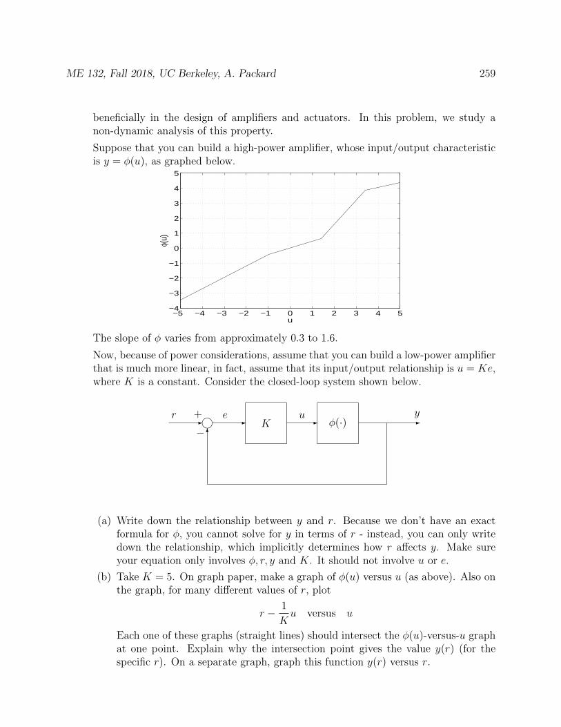
ME 132, Fall 2018, UC Berkeley, A. Packard 259
beneficially in the design of amplifiers and actuators. In this problem, we study anon-dynamic analysis of this property.
Suppose that you can build a high-power amplifier, whose input/output characteristicis y = φ(u), as graphed below.
−5 −4 −3 −2 −1 0 1 2 3 4 5−4
−3
−2
−1
0
1
2
3
4
5φ(
u)
u
The slope of φ varies from approximately 0.3 to 1.6.
Now, because of power considerations, assume that you can build a low-power amplifierthat is much more linear, in fact, assume that its input/output relationship is u = Ke,where K is a constant. Consider the closed-loop system shown below.
K φ(·)j−
+- - - -
6
r e u y
(a) Write down the relationship between y and r. Because we don’t have an exactformula for φ, you cannot solve for y in terms of r - instead, you can only writedown the relationship, which implicitly determines how r affects y. Make sureyour equation only involves φ, r, y and K. It should not involve u or e.
(b) Take K = 5. On graph paper, make a graph of φ(u) versus u (as above). Also onthe graph, for many different values of r, plot
r − 1
Ku versus u
Each one of these graphs (straight lines) should intersect the φ(u)-versus-u graphat one point. Explain why the intersection point gives the value y(r) (for thespecific r). On a separate graph, graph this function y(r) versus r.
ME 132, Fall 2018, UC Berkeley, A. Packard 260
(c) Using the relationship you derived in part 10a, and treating it as an implicitdescription of the dependence that y has on r, differentiate it with respect to r toget y′(r).
(d) What should be K be chosen as so that the slope of the closed-loop behaviorbetween y and r varies at most between 0.9 and 1.1.

ME 132, Fall 2018, UC Berkeley, A. Packard 261
25 Robustness Margins
Three common measures of insensitivity of a closed-loop system to variations are
• the time-delay margin,
• the gain margin, and
• the percentage variation margin.
All are easily computed, and provide a quantitative measure of the insensitivity of the closed-loop system to specific types of variations. The nominal closed-loop system is shown below.
C P- - - -
6
i+
−r(t)
e(t) u(t)y(t)
We assume that both P and C are governed by linear, ordinary differential equations, andthat the nominal closed-loop system is stable.
The perturbed closed-loop system is shown below, with both a gain variation in the plant,a time-delay in the feedback measurement, and a change in process from P to P .
C γ P
delay, T
- - - - -
6
i+
−r(t)
e(t) u(t)y(t)
f(t) = y(t− T )
Note that if T = 0, γ = 1 and P = P , then the perturbed system is simply the nominalclosed-loop system.
The time-delay margin is characterized by the minimum time delay T > 0 such that theclosed-loop system becomes unstable, with γ set equal to its nominal value, γ = 1, andP = P .
The gain margin is characterized by the largest interval(γ, γ), containing 1, such that the
closed-loop system is stable for all γ ∈(γ, γ), with T set to its nominal value, T = 0, and
P = P
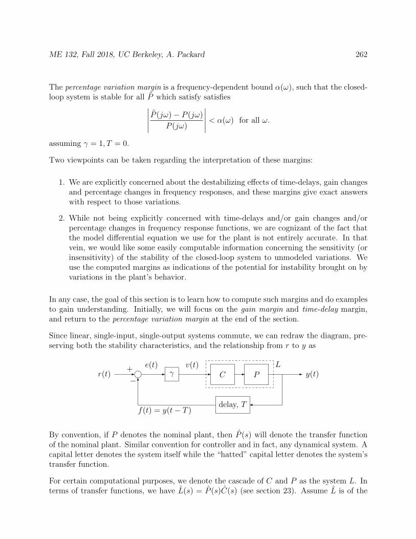
ME 132, Fall 2018, UC Berkeley, A. Packard 262
The percentage variation margin is a frequency-dependent bound α(ω), such that the closed-loop system is stable for all P which satisfy satisfies∣∣∣∣∣ P (jω)− P (jω)
P (jω)
∣∣∣∣∣ < α(ω) for all ω.
assuming γ = 1, T = 0.
Two viewpoints can be taken regarding the interpretation of these margins:
1. We are explicitly concerned about the destabilizing effects of time-delays, gain changesand percentage changes in frequency responses, and these margins give exact answerswith respect to those variations.
2. While not being explicitly concerned with time-delays and/or gain changes and/orpercentage changes in frequency response functions, we are cognizant of the fact thatthe model differential equation we use for the plant is not entirely accurate. In thatvein, we would like some easily computable information concerning the sensitivity (orinsensitivity) of the stability of the closed-loop system to unmodeled variations. Weuse the computed margins as indications of the potential for instability brought on byvariations in the plant’s behavior.
In any case, the goal of this section is to learn how to compute such margins and do examplesto gain understanding. Initially, we will focus on the gain margin and time-delay margin,and return to the percentage variation margin at the end of the section.
Since linear, single-input, single-output systems commute, we can redraw the diagram, pre-serving both the stability characteristics, and the relationship from r to y as
γ C PL
delay, T
- - - - -
6
i+
−r(t)
e(t) v(t)y(t)
f(t) = y(t− T )
By convention, if P denotes the nominal plant, then P (s) will denote the transfer functionof the nominal plant. Similar convention for controller and in fact, any dynamical system. Acapital letter denotes the system itself while the “hatted” capital letter denotes the system’stransfer function.
For certain computational purposes, we denote the cascade of C and P as the system L. Interms of transfer functions, we have L(s) = P (s)C(s) (see section 23). Assume L is of the
ME 132, Fall 2018, UC Berkeley, A. Packard 263
form
L(s) =b1s
n−1 + · · ·+ bn−1s+ bnsn + a1sn−1 + · · ·+ an−1s+ an
This is equivalent to the differential equation relating v to y as
y[n](t) + a1y[n−1](t) + · · ·+ an−1y
[1](t) + any(t) = b1v[n−1](t) + · · ·+ bn−1v
[1](t) + bnv(t)
Under both types of perturbations, we get that
v(t) = γ [r(t)− y(t− T )]
Note that for any k, v[k](t) = γ[r[k](t)− y[k](t− T )
]. Plugging in and rearranging gives the
closed-loop delay-differential equation
y[n](t) + a1y[n−1](t) + · · ·+ an−1y
[1](t) + any(t)+ γ
[b1y
[n−1](t− T ) + · · ·+ bn−1y[1](t− T ) + bny(t− T )
]= γ
[b1r
[n−1](t) + · · ·+ bn−1r[1](t) + bnr(t)
] (25.1)
It is from this equation that we begin our analysis, though most of our computations willultimately involve the transfer function L(s) evaluated along the imaginary axis s = jω.
25.1 Gain Margin
The setup for the gain margin problem is shown in Figure 25, with T = 0. Here, a plantand controller are in closed-loop along with a gain γ at the plant input. We assume thatthe closed-loop system is stable for γ = 1, and we wish to know the largest interval
(γ, γ)
such that closed-loop stability is maintained for all γ ∈(γ, γ). Since the closed-loop system
is stable for γ = 1, it is clear that γ < 1 < γ.
With the time-delay T = 0, the differential equation (25.1) becomes an ordinary differentialequation,
y[n](t) + (a1 + γb1) y[n−1](t) + · · ·+ (an−1 + γbn−1) y[1](t) + (an + γbn) y(t)= γ
[b1r
[n−1](t) + · · ·+ bn−1r[1](t) + bnr(t)
]Clearly, the closed-loop characteristic polynomial is a function of γ, namely
pγ(λ) = λn + (a1 + γb1)λn−1 + (a2 + γb2)λn−2 + · · ·+ (an−1 + γbn−1)λ+ (an + γbn)
It is a fact from mathematics that the roots of the characteristic polynomial are continuousfunctions of the parameter γ, hence as γ varies, the roots vary continuously. Therefore,the only way for a root of pγ to move (as γ changes) from the left-half planeinto the right-half plane is to cross the imaginary axis, either at 0, or at some
ME 132, Fall 2018, UC Berkeley, A. Packard 264
jβ, with β > 0 (since complex roots come in conjugate pairs, if they cross theimaginary axis, one will cross positively, and one negatively - we can focus onone or the other, and for no specific reason, we look at the positive crossing).Hence, in assessing the gain margin, we are looking for values γ and β, with γ close to 1,and β ≥ 0 such that λ = jβ is a root of pγ. Plugging in gives
(jβ)n + (a1 + γb1)(jβ)n−1 + (a2 + γb2)(jβ)n−2 + · · ·+ (an−1 + γbn−1)(jβ) + (an + γbn) = 0
Rearranging gives
[(jβ)n + a1(jβ)n−1 + a2(jβ)n−2 + · · ·+ an−1(jβ) + an]+ γ [b1(jβ)n−1 + b2(jβ)n−2 + · · ·+ bn−1(jβ) + bn] = 0
. (25.2)
This is two equations (since it relates complex quantities) in two real unknowns (β and γ).We need to find all solutions, and then isolate the solutions whose γ coordinate is closest to1.
First, we can look for solutions to (25.2) by looking for imaginary-axis roots (ie., real β) topγ=0(jβ) = 0, namely
(jβ)n + a1(jβ)n−1 + a2(jβ)n−2 + · · ·+ an−1(jβ) + an = 0.
If there are roots, then coupled with γ = 0, we have found some solutions to equation (25.2).There likely are others, with γ 6= 0, which are described below.
We can also look for solutions to (25.2) with (jβ)n+a1(jβ)n−1 +a2(jβ)n−2 + · · ·+an−1(jβ)+an 6= 0, so that after dividing, we manipulate equation (25.2) into
−1 = γb1(jβ)n−1 + b2(jβ)n−2 + · · ·+ bn−1(jβ) + bn
(jβ)n + a1(jβ)n−1 + a2(jβ)n−2 + · · ·+ an−1(jβ) + an
But, this is recognized as
−1 = γ L(s)∣∣∣s=jβ
This can be solved graphically, finding values of β for which L(s)∣∣∣s=jβ
is a real number (and
then taking a negative reciprocal to find the associated γ value).
Summarizing, a simple method to determine all solutions to equation (25.2) is
1. Let βi denote all (if any) of the real solutions to
(jβ)n + a1(jβ)n−1 + a2(jβ)n−2 + · · ·+ an−1(jβ) + an = 0.
If there are any, then the pairs (βi, 0) are solutions to equation 25.2.
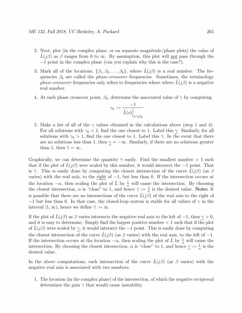
ME 132, Fall 2018, UC Berkeley, A. Packard 265
2. Next, plot (in the complex plane, or on separate magnitude/phase plots) the value ofL(jβ) as β ranges from 0 to ∞. By assumption, this plot will not pass through the−1 point in the complex plane (can you explain why this is the case?).
3. Mark all of the locations, β1, β2, . . . , βk, where L(jβ) is a real number. The fre-quencies βk are called the phase-crossover frequencies. Sometimes, the terminologyphase-crossover frequencies only refers to frequencies where where L(jβ) is a negativereal number.
4. At each phase crossover point, βk, determine the associated value of γ by computing
γk :=−1
L(s)∣∣∣s=jβk
5. Make a list of all of the γ values obtained in the calculations above (step 1 and 4).For all solutions with γk < 1, find the one closest to 1. Label this γ. Similarly, for allsolutions with γk > 1, find the one closest to 1. Label this γ. In the event that thereare no solutions less than 1, then γ = −∞. Similarly, if there are no solutions greaterthan 1, then γ =∞.
Graphically, we can determine the quantity γ easily. Find the smallest number > 1 suchthat if the plot of L(jβ) were scaled by this number, it would intersect the −1 point. Thatis γ. This is easily done by computing the closest intersection of the curve L(jβ) (as βvaries) with the real axis, to the right of −1, but less than 0. If the intersection occurs at
the location −α, then scaling the plot of L by 1α
will cause the intersection. By choosingthe closest intersection, α is “close” to 1, and hence γ := 1
αis the desired value. Note: It
is possible that there are no intersections of the curve L(jβ) of the real axis to the right of−1 but less than 0. In that case, the closed-loop system is stable for all values of γ in theinterval [1,∞), hence we define γ :=∞.
If the plot of L(jβ) as β varies intersects the negative real axis to the left of −1, then γ > 0,and it is easy to determine. Simply find the largest positive number < 1 such that if the plotof L(jβ) were scaled by γ, it would intersect the −1 point. This is easily done by computing
the closest intersection of the curve L(jβ) (as β varies) with the real axis, to the left of −1.If the intersection occurs at the location −α, then scaling the plot of L by 1
αwill cause the
intersection. By choosing the closest intersection, α is “close” to 1, and hence γ := 1α
is thedesired value.
In the above computations, each intersection of the curve L(jβ) (as β varies) with thenegative real axis is associated with two numbers:
1. The location (in the complex plane) of the intersection, of which the negative reciprocaldetermines the gain γ that would cause instability.
ME 132, Fall 2018, UC Berkeley, A. Packard 266
2. The value of β at which the intersection takes place, which determines the crossingpoint (on the imaginary axis) where the closed-loop root migrates from the left-halfplane into the right-half plane, and hence determines the frequency of oscillations justat the onset of instability due to the gain change.
25.2 Time-Delay Margin
The homogeneous equation, with γ = 1, but T > 0 of equation (25.1) is
y[n](t) + a1y[n−1](t) + · · ·+ an−1y
[1](t) + any(t)+ b1y
[n−1](t− T ) + · · ·+ bn−1y[1](t− T ) + bny(t− T ) = 0
(25.3)
Recall that we assume that for T = 0, the system is stable, and hence all homogeneoussolutions decay exponentially to 0 as t → ∞. It is a fact (advanced) that as T increasesthe system may eventually become unstable, and if it does, then at the criticalvalue of T for which stability is violated, sinusoidal solutions to the homoge-neous equation exist. In other words, the system “goes unstable” by first exhibiting purelysinusoidal homogeneous solutions. The frequency of this sinusoidal solution is not knowna-priori, and needs to be determined, along with the critical value of the time-delay.
The delay terms may cause a non-decaying homogeneous solution to exist. We pose thequestion: what is the minimum T and corresponding frequency ω such that a sinusoidalsolution to (25.3) of the form yH(t) = ejωt exists? If such a solution exists, then by pluggingit into (25.3), and canceling the common ejωt term, which is never 0, we get a necessaryalgebraic condition
(jω)n + a1 (jω)n−1 + · · ·+ an−1jω + ane−jωT
[b1 (jω)n−1 + · · ·+ bn−1jω + bn
]= 0
Rearranging gives
−1 = e−jωTb1(jω)n−1 + b2(jω)n−2 + · · ·+ bn−1(jω) + bn
(jω)n + a1(jω)n−1 + a2(jω)n−2 + · · ·+ an−1(jω) + an
But, this is recognized as
−1 = e−jωT L(s)∣∣∣s=jω
This is two equations (since it relates complex quantities) in two real unknowns (T and ω).We want to solve for solutions with T close to 0 (recall that 0 was the nominal value of T ,and we assumed that the closed-loop system was stable for that). Since ωT is real, it follows
that∣∣e−jωT ∣∣ = 1. This gives conditions on the possible values of ω, namely
∣∣∣L(jω)∣∣∣ = 1.
Once these values of ω are known, the corresponding values of T can be determined, andthe smallest such T becomes the time-delay margin.

ME 132, Fall 2018, UC Berkeley, A. Packard 267
In order to understand the graphical solution techniques described, recall that for any com-plex number Ψ, and any real number θ, we have
∠ejθΨ = θ + ∠Ψ
Hence, at any value of ω, we have
∠e−jωT L(jω) = −ωT + ∠L(jω)
Also, ∠(−1) = ±π.
Hence, a simple method to determine solutions is:
1. Plot (in the complex plane, or on separate magnitude/phase plots) the quantity L(jω)as ω varies from 0 to ∞.
2. Identify all of the frequencies ωi > 0 where∣∣∣L(jωi)
∣∣∣ = 1. These are called the gain-
crossover frequencies.
3. At each gain-crossover frequency ωi, (which necessarily has∣∣∣L(jωi)
∣∣∣ = 1), determine
the value of T > 0 such that e−jωiT L(jωi) = −1. Recall that multiplication of anycomplex number by e−jωiT simply rotates the complex number ωiT radians in theclockwise (negative) direction. Hence, each T can be determined by calculating theangle from L(jω) to −1, measured in a clockwise direction, and dividing this angleby ω. On a phase plot, determine the net angle change in the negative direction(downward) to get to the closest odd-multiple of π (or 180).
4. Repeat this calculation for each gain-crossover frequency, and choose the smallest ofall of the T ’s obtained.
25.3 Percentage Variation Margin
Suppose that P and C are the transfer functions of a plant and controller, respectively.Assume that the closed-loop system, shown below, is stable.
C P- j - - j? - -
6
u1
e1 e2y1 y2
u2
−

ME 132, Fall 2018, UC Berkeley, A. Packard 268
Hence all of the closed-loop transfer functions (from ui to ej and from ui to yk) have polesin the open-left-half plane.
Suppose that due to uncertainty, the actual plant transfer function is
Pactual = P (1 + ∆(s))
where ∆ is an unknown, stable system, representing the uncertainty in P . In block-diagramform, Pactual looks like
∆
P- - -e-
?
With this model, it follows that
∆ =Pactual − P
P
so in some sense, ∆ represents a relative uncertainty.
In this case, the closed-loop system is actually of the form
C P
∆
- - - - - -
6
e−
-
?e?e
Note that ∆ is effectively in positive feedback with the transfer function −PC1+PC
. In otherwords, the perturbed closed-loop system can be thought of as the feedback interconnectionof two stable systems, namely ∆ and −PC
1+PC. Since the nominal closed-loop is stable, PC
1+PCis
stable, and hence the addition of the stable transfer function ∆ can only lead to instabilityif the loop introduced by that ∆ introduces is unstable.
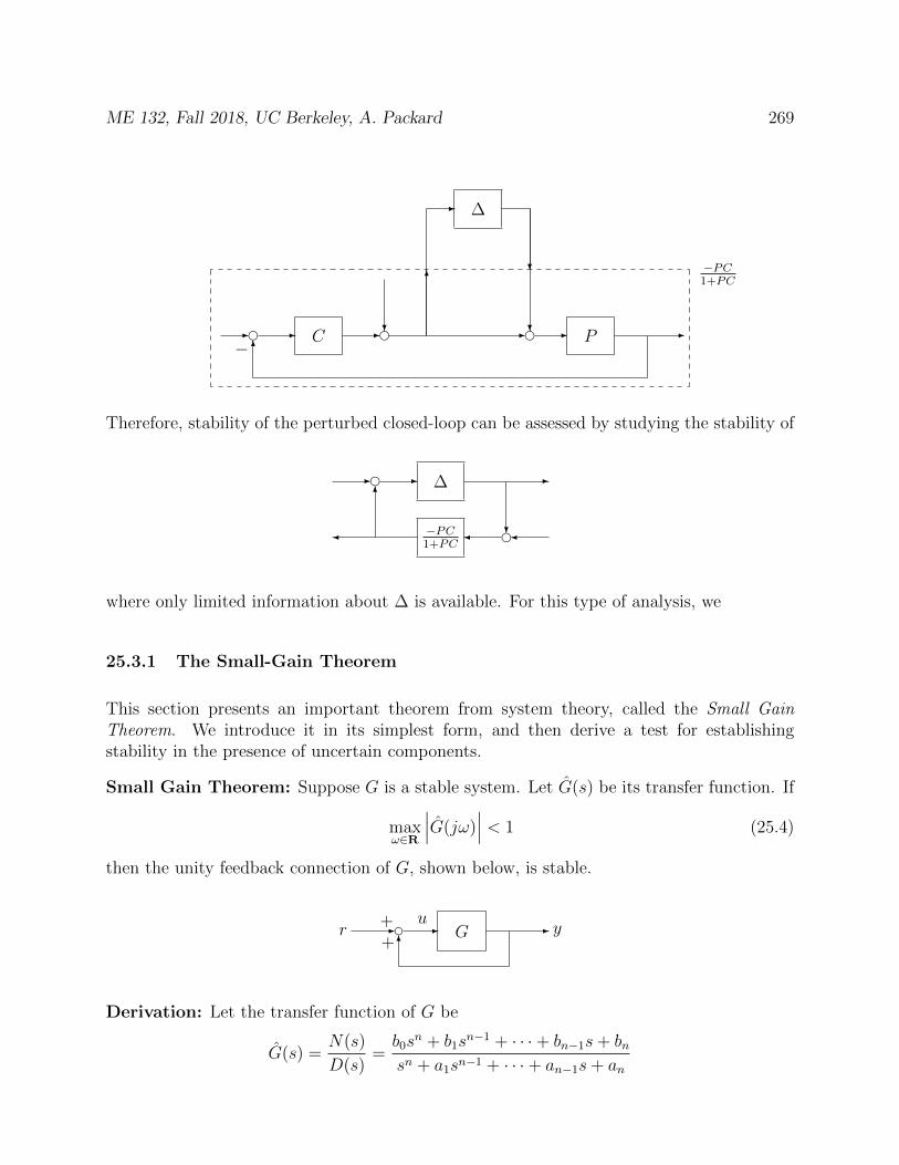
ME 132, Fall 2018, UC Berkeley, A. Packard 269
C P
∆
- - - - - -
6
e−
6
-
?
?
e?e−PC1+PC
Therefore, stability of the perturbed closed-loop can be assessed by studying the stability of
−PC1+PC
∆- - -
?
6
ee
where only limited information about ∆ is available. For this type of analysis, we
25.3.1 The Small-Gain Theorem
This section presents an important theorem from system theory, called the Small GainTheorem. We introduce it in its simplest form, and then derive a test for establishingstability in the presence of uncertain components.
Small Gain Theorem: Suppose G is a stable system. Let G(s) be its transfer function. If
maxω∈R
∣∣∣G(jω)∣∣∣ < 1 (25.4)
then the unity feedback connection of G, shown below, is stable.
G- d - -
6r
uy
++
Derivation: Let the transfer function of G be
G(s) =N(s)
D(s)=b0s
n + b1sn−1 + · · ·+ bn−1s+ bn
sn + a1sn−1 + · · ·+ an−1s+ an
ME 132, Fall 2018, UC Berkeley, A. Packard 270
where the N and D are polynomials. By assumption of stability of G, we know that theroots of D(s) = 0 are all in the left-half plane. Also, setting s = jω, and taking ω very large,the assumption in equation (25.4) implies that |b0| < 1.
The characteristic polynominal of the feedback connection is
p(s) = N(s)−D(s)
We want to verify that the roots of p(s) = 0 all have negative real-parts.
For 0 ≤ τ ≤ 1, consider the polynomial
pτ (s) = τN(s)−D(s)= (τb0 − 1)sn + (τb1 − a1)sn−1 + · · ·+ (τbn − an)
For every value of τ in between 0 and 1, this is an n’th order polynomial, and it has n roots.
Note that at τ = 0 and τ = 1, we have two extremes.
p0 = D(s), p1(s) = p(s)
• We ultimately want to conclude that p1 has no roots in the RHP.
• We know that the roots of p0 all have negative real parts.
• We know that the roots of pτ are continuous functions of τ .
Note: If we show that for every τ in between 0 and 1, the polynomial pτ has no roots onthe imaginary axes (ie., no roots with zero real-parts), then it must be that p0 and p1 havethe same number of roots in the left-half-plane (since as τ varied from 0 to 1, no roots crossthe imaginary axes).
So, pick any τ in between 0 and 1, and any ω. By assumption
|τG(jω)| =∣∣∣∣τN(jω)
D(jω)
∣∣∣∣ ≤ |G(jω)| < 1
Hence τN(jω)−D(jω) 6= 0. This shows that for every τ in between 0 and 1, the polynomialpτ has no roots on the imaginary axes, completing the proof.
Small Gain Theorem #2: Suppose G and H are both stable systems. If
maxω∈R
∣∣∣G(jω)H(jω)∣∣∣ < 1
then the feedback connection of G and H, shown below, is stable.

ME 132, Fall 2018, UC Berkeley, A. Packard 271
H
G- - -
?
6
ee
Derivation: The cascade of G and H is itself a stable system, and the frequency responsefunction of the cascade is the product of the individual frequency responses.
Corollary: Suppose G and H are both stable systems. If
maxω∈R
∣∣∣G(jω)∣∣∣maxω∈R
∣∣∣H(jω)∣∣∣ < 1
then the feedback connection of G and H is stable.
25.3.2 Necessary and Sufficient Version
Theorem NS1: Suppose G is a given, stable system. Given any γ > 0, if
maxω∈R
∣∣∣G(jω)∣∣∣ > γ,
then there is a stable system H such that
maxω∈R
∣∣∣H(jω)∣∣∣ < 1
γ
such that the feedback connection of G and H is unstable.
Theorem NS2: Suppose G is a given, stable system. Assume G(jω) 6= 0 for all ω ∈ R.For any frequency ω ∈ R with ω > 0, there exists a stable system Hω such that
1. for all ω ∈ R, ω 6= ω
|Hω(jω)| <∣∣∣∣ 1
G(jω)
∣∣∣∣2. at ω,
|Hω(jω)| =∣∣∣∣ 1
G(jω)
∣∣∣∣3. The feedback connection of G and H is unstable.

ME 132, Fall 2018, UC Berkeley, A. Packard 272
There are two independent facts about transfer functions that are used to prove these theo-rems
Fact 1: Given a positive ω > 0, and a complex number δ, with Imag (δ) 6= 0, there is aβ > 0 such that by proper choice of sign
± |δ| s− βs+ β
∣∣∣∣s=jω
= δ
Remark: In other words, given any positive frequency ω > 0, and any complex numberδ, there is a stable, first-order system, ∆(s) that has a flat frequency-response magnitude(across all frequency) and satisfies ∆(jω) = δ.
The proof is as follows (details provided in class): For a positive β, the plot ofs− βs+ β
as s
takes on values of jω, with ω ranging from 0 to +∞, traverses a circular arc in the complexplane, from −1 (at ω = 0) to 1 (as ω → +∞) clockwise, centered at 0, and in the top-half of
the complex plane. Similarly, the plot of −s− βs+ β
as s takes on values of jω, with ω ranging
from 0 to +∞, traverses from 1 (at ω = 0) to −1 (as ω → +∞) clockwise, in the bottom-halfplane. Therefore, the choice of + or − sign depends on the imaginary part of δ. Here is aconstructive procedure for the case Imag(δ) > 0 (verify that this is indeed correct).
1. Write δ as δ = |δ| ejφ for a real number φ.
2. Pick β := ω√
1−cosφ1+cosφ
If Imag(δ) < 0, use above procedure with −δ replacing δ. Then, add the (−) sign to thetransfer function.
Fact 2: For any ω > 0 and any 0 < ξ < 1, define the transfer function
I(s) :=2ξωs
s2 + 2ξωs+ ω2
Then
1. for all ω ∈ R, ω 6= ω
|I(jω)| <∣∣∣∣ 1
G(jω)
∣∣∣∣2. at ω,
I(jω) = 1
ME 132, Fall 2018, UC Berkeley, A. Packard 273
3. I is stable.
The proof of this is just simple verification of the claims.
Now, returning Theorem NS1. Suppose G is a given, stable system, γ > 0, and
maxω∈R
∣∣∣G(jω)∣∣∣ > γ,
Pick ω > 0 so that∣∣∣G(jω)
∣∣∣ > γ. Next, construct H using the “∆” construction above, with
δ := −1
G(jω). It follows that
maxω∈R
∣∣∣H(jω)∣∣∣ =
1∣∣∣G(jω)∣∣∣ < 1
γ
and(
1 + G(s)H(s))∣∣∣
s=jω= 0, implying that 1
1+GHhas a pole at s = jω.
Alternatively, for Theorem NS2, since G(jω) is never 0, it follows that you can write
G(s) =nL(s)nR(s)
d(s)
where the roots of nL(s) = 0 are in the open left-half plane, and the roots of nR(s) = 0 arein the open right-half plane. Define
Ω(s) :=d(s)
nL(s)nR(−s)
There are two relevant facts about the polynomial nR(−s), which are:
1. since the roots of nR(s) = 0 are in the open right-half plane, it follows that the rootsof nR(−s) = 0 are in the open left-half plane;
2. since the coefficients of nR(s) are real, it follows that nR(−jω) is the complex conjugateof nR(jω) and consequently the magnitudes are the same.
Therefore Ω is stable, and for all ω
|Ω(jω)| = 1
|G(jω)|
Now pick β > 0, and the proper choice of ± so that
±s− βs+ β
Ω(s)
∣∣∣∣s=jω
=1
G(jω)
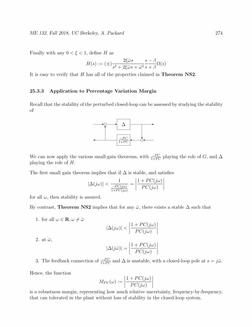
ME 132, Fall 2018, UC Berkeley, A. Packard 274
Finally with any 0 < ξ < 1, define H as
H(s) := (±)2ξωs
s2 + 2ξωs+ ω2
s− βs+ β
Ω(s)
It is easy to verify that H has all of the properties claimed in Theorem NS2.
25.3.3 Application to Percentage Variation Margin
Recall that the stability of the perturbed closed-loop can be assessed by studying the stabilityof
−PC1+PC
∆- - -
?
6
ee
We can now apply the various small-gain theorems, with −PC1+PC
playing the role of G, and ∆playing the role of H.
The first small gain theorem implies that if ∆ is stable, and satisfies
|∆(jω)| < 1−PC(jω)1+PC(jω)
=
∣∣∣∣1 + PC(jω)
PC(jω)
∣∣∣∣for all ω, then stability is assured.
By contrast, Theorem NS2 implies that for any ω, there exists a stable ∆ such that
1. for all ω ∈ R, ω 6= ω
|∆(jω)| <∣∣∣∣1 + PC(jω)
PC(jω)
∣∣∣∣2. at ω,
|∆(jω)| =∣∣∣∣1 + PC(jω)
PC(jω)
∣∣∣∣3. The feedback connection of −PC
1+PCand ∆ is unstable, with a closed-loop pole at s = jω.
Hence, the function
MPV (ω) :=
∣∣∣∣1 + PC(jω)
PC(jω)
∣∣∣∣is a robustness margin, representing how much relative uncertainty, frequency-by-frequency,that can tolerated in the plant without loss of stability in the closed-loop system.
ME 132, Fall 2018, UC Berkeley, A. Packard 275
25.4 Summary
We have introduced 3 margins. Each measure, in different senses, how close the loop gain, L,gets to the (-1) point. The gain margin measures the distance along the real axis; the time-delay margin measures the distance along a circular arc (the unit circle) and normalizes byfrequency; while the Percentage-Variation margin quantifies the distance in a more absolutemanner. All 3 margins are easy to compute, knowing the loop-gain, and should be computedand compared when understanding tradeoffs between multiple competing control systemdesigns.
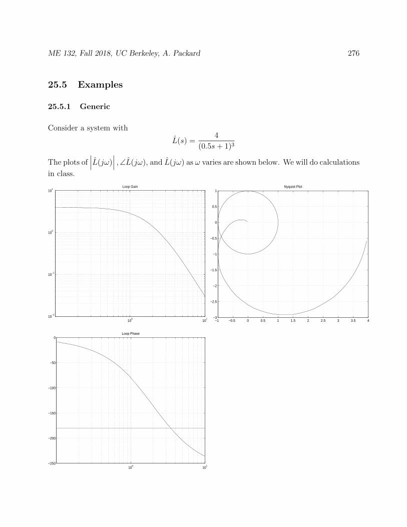
ME 132, Fall 2018, UC Berkeley, A. Packard 276
25.5 Examples
25.5.1 Generic
Consider a system with
L(s) =4
(0.5s+ 1)3
The plots of∣∣∣L(jω)
∣∣∣ ,∠L(jω), and L(jω) as ω varies are shown below. We will do calculations
in class.
100
101
10−2
10−1
100
101
Loop Gain
−1 −0.5 0 0.5 1 1.5 2 2.5 3 3.5 4−3
−2.5
−2
−1.5
−1
−0.5
0
0.5
1Nyquist Plot
100
101
−250
−200
−150
−100
−50
0Loop Phase
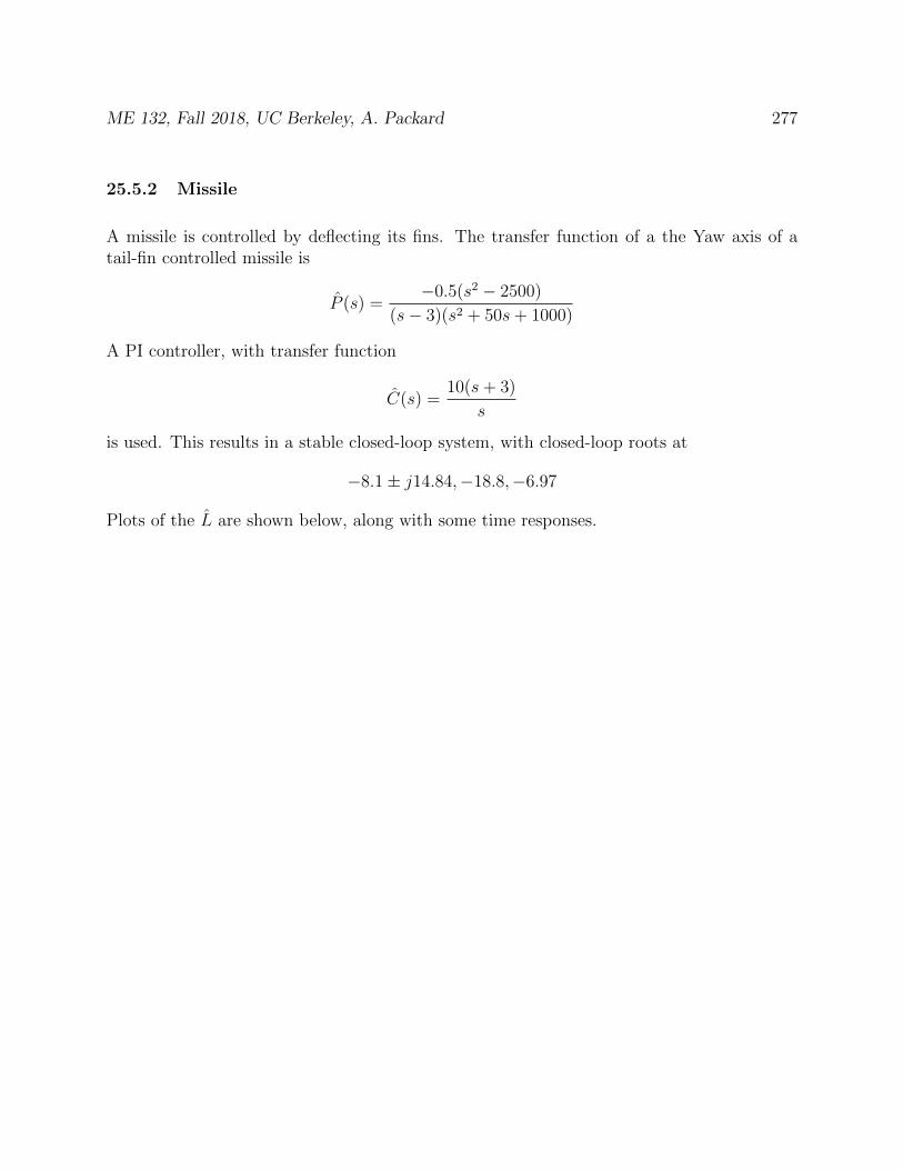
ME 132, Fall 2018, UC Berkeley, A. Packard 277
25.5.2 Missile
A missile is controlled by deflecting its fins. The transfer function of a the Yaw axis of atail-fin controlled missile is
P (s) =−0.5(s2 − 2500)
(s− 3)(s2 + 50s+ 1000)
A PI controller, with transfer function
C(s) =10(s+ 3)
s
is used. This results in a stable closed-loop system, with closed-loop roots at
−8.1± j14.84,−18.8,−6.97
Plots of the L are shown below, along with some time responses.
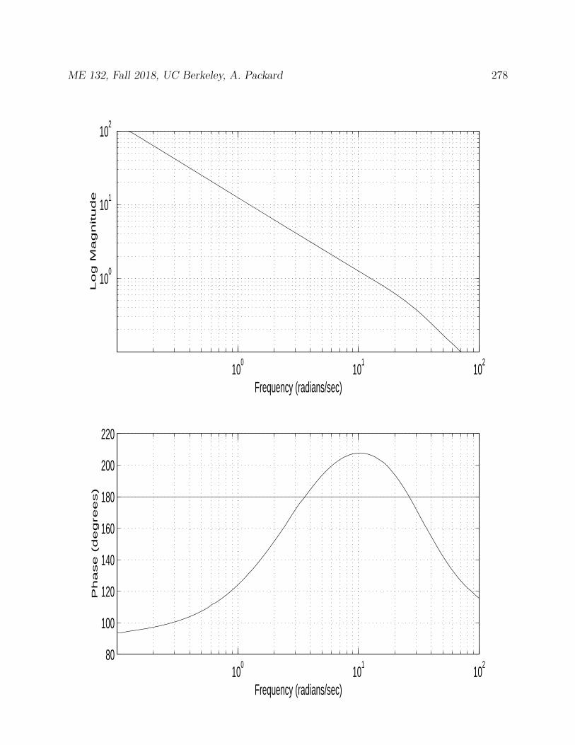
ME 132, Fall 2018, UC Berkeley, A. Packard 278
100
101
102
100
101
102
Log M
agnitude
Frequency (radians/sec)
100
101
102
80
100
120
140
160
180
200
220
Phase (
degrees)
Frequency (radians/sec)
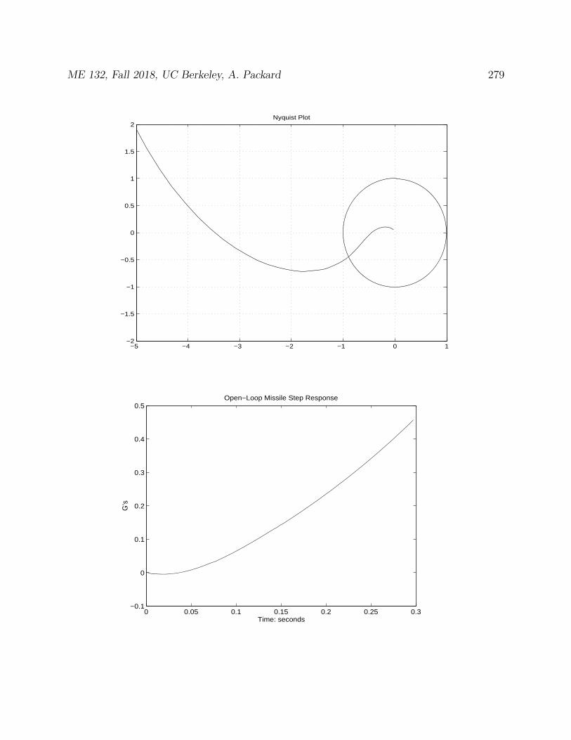
ME 132, Fall 2018, UC Berkeley, A. Packard 279
−5 −4 −3 −2 −1 0 1−2
−1.5
−1
−0.5
0
0.5
1
1.5
2Nyquist Plot
0 0.05 0.1 0.15 0.2 0.25 0.3−0.1
0
0.1
0.2
0.3
0.4
0.5
Time: seconds
G’s
Open−Loop Missile Step Response
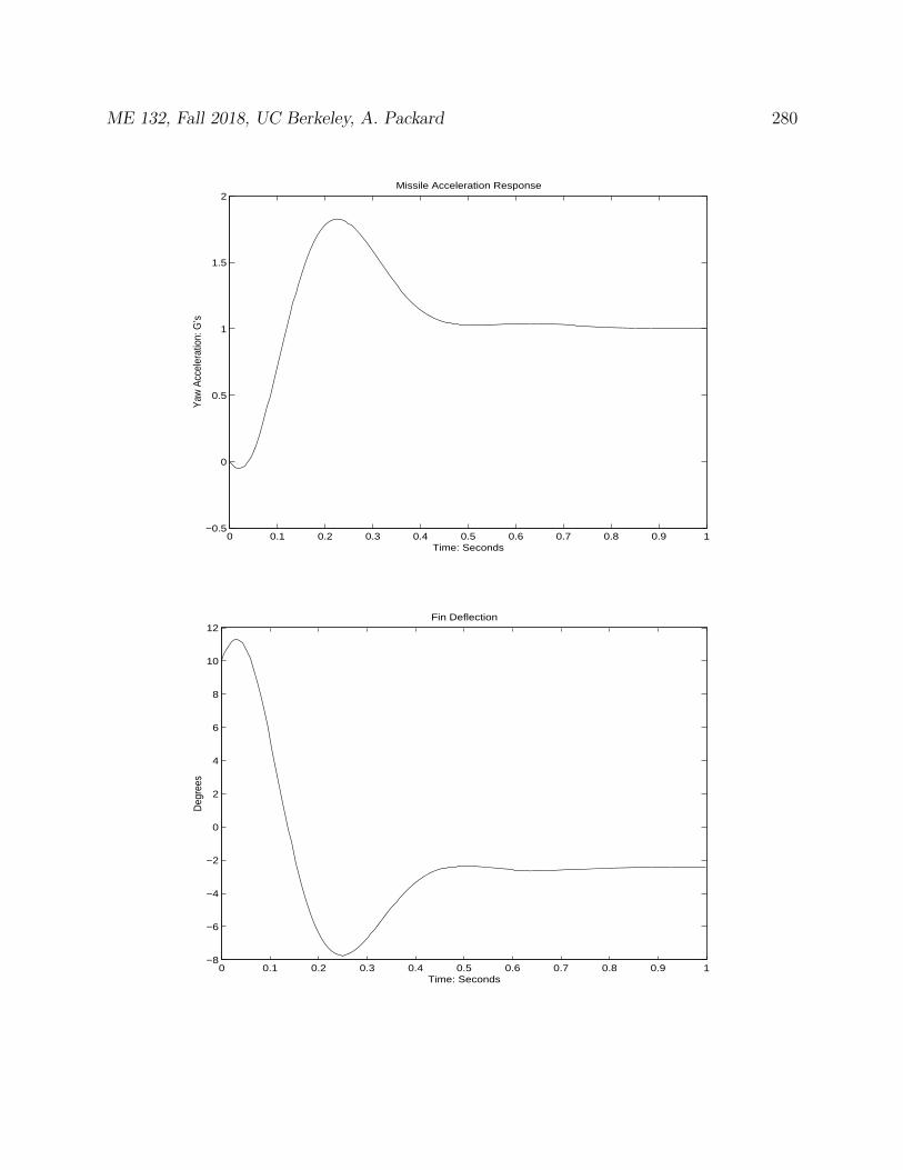
ME 132, Fall 2018, UC Berkeley, A. Packard 280
0 0.1 0.2 0.3 0.4 0.5 0.6 0.7 0.8 0.9 1−0.5
0
0.5
1
1.5
2Missile Acceleration Response
Time: Seconds
Yaw
Acc
eler
atio
n: G
’s
0 0.1 0.2 0.3 0.4 0.5 0.6 0.7 0.8 0.9 1−8
−6
−4
−2
0
2
4
6
8
10
12Fin Deflection
Time: Seconds
Deg
rees

ME 132, Fall 2018, UC Berkeley, A. Packard 281
25.5.3 Application to percentage variation margin
Take the missile example from Section 17,
P (s) =−0.5(s2 − 2500)
(s− 3)(s2 + 50s+ 1000), C(s) =
10(s+ 3)
s
We will also try
Pperturbed(s) = P (s)1
τs+ 1
Note this is the same as
P (s)1
τs+ 1= P (s)
[1 +
−τsτs+ 1
]Hence, the percentage variation in going from P to Pperturbed is
Pperturbed − PP
=−τsτs+ 1
Let’s plot the magnitude of this versus the percentage-variation margin for different valuesof τ .

ME 132, Fall 2018, UC Berkeley, A. Packard 282
100
101
102
103
10−3
10−2
10−1
100
101
102
103
100
101
102
103
80
100
120
140
160
180
200
220
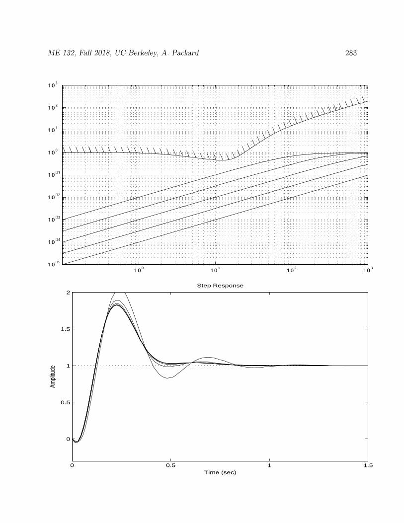
ME 132, Fall 2018, UC Berkeley, A. Packard 283
100
101
102
103
10−5
10−4
10−3
10−2
10−1
100
101
102
103
Step Response
Time (sec)
Ampl
itude
0 0.5 1 1.5
0
0.5
1
1.5
2
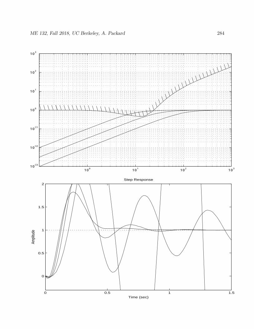
ME 132, Fall 2018, UC Berkeley, A. Packard 284
100
101
102
103
10−3
10−2
10−1
100
101
102
103
Step Response
Time (sec)
Ampl
itude
0 0.5 1 1.5
0
0.5
1
1.5
2
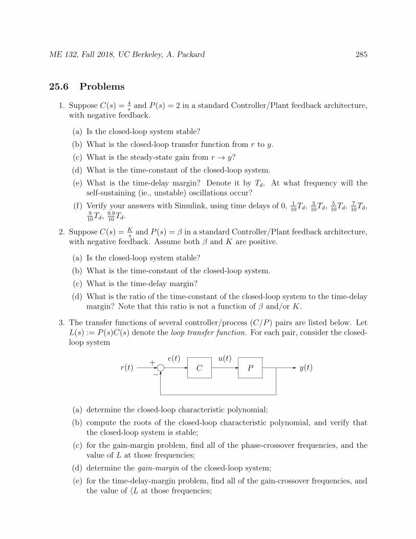
ME 132, Fall 2018, UC Berkeley, A. Packard 285
25.6 Problems
1. Suppose C(s) = 4s
and P (s) = 2 in a standard Controller/Plant feedback architecture,with negative feedback.
(a) Is the closed-loop system stable?
(b) What is the closed-loop transfer function from r to y.
(c) What is the steady-state gain from r → y?
(d) What is the time-constant of the closed-loop system.
(e) What is the time-delay margin? Denote it by Td. At what frequency will theself-sustaining (ie., unstable) oscillations occur?
(f) Verify your answers with Simulink, using time delays of 0, 110Td,
310Td,
510Td,
710Td,
910Td,
9.910Td.
2. Suppose C(s) = Ks
and P (s) = β in a standard Controller/Plant feedback architecture,with negative feedback. Assume both β and K are positive.
(a) Is the closed-loop system stable?
(b) What is the time-constant of the closed-loop system.
(c) What is the time-delay margin?
(d) What is the ratio of the time-constant of the closed-loop system to the time-delaymargin? Note that this ratio is not a function of β and/or K.
3. The transfer functions of several controller/process (C/P ) pairs are listed below. LetL(s) := P (s)C(s) denote the loop transfer function. For each pair, consider the closed-loop system
C P- - - -
6
i+
−r(t)
e(t) u(t)y(t)
(a) determine the closed-loop characteristic polynomial;
(b) compute the roots of the closed-loop characteristic polynomial, and verify thatthe closed-loop system is stable;
(c) for the gain-margin problem, find all of the phase-crossover frequencies, and thevalue of L at those frequencies;
(d) determine the gain-margin of the closed-loop system;
(e) for the time-delay-margin problem, find all of the gain-crossover frequencies, andthe value of 〈L at those frequencies;

ME 132, Fall 2018, UC Berkeley, A. Packard 286
(f) determine the time-delay-margin of the closed-loop system;
The systems are:
(a) C(s) = 2.4s+1s
, P (s) = 1s−1
(b) C(s) = 0.4s+1s
, P (s) = 1s+1
(c) C(s) = 10(s+3)s
, P (s) = −0.5(s2−2500)(s−3)(s2+50s+1000)
4. In problem 3 above, the first two cases, (a) and (b), have identical closed-loop char-acteristic polynomials, and hence identical closed-loop roots. Nevertheless, they havedifferent stability margins. In one case, the plant P is unstable, and in the other caseit is stable. Check which case has better stability margins in each of the differentmeasures. Make a conclusion (at least in the case) that all other things being equal, itis “harder” to reliably control an unstable plant than it is a stable one.
5. Let L(s) be the transfer function of a system L. Consider the diagram below.
d - d - L6−
6
?
6zq
p
Let N(s) denote the transfer function from q to z. Let S(s) denote the transfer functionfrom q to p.
(a) Derive N(s) and S(s) in terms of L(s).
(b) Derive L(s) in terms of N(s).
(c) Derive L(s) in terms of S(s).
Application: As we have learned, the gain-margin and time-delay margin can becomputed from a frequency-response plot of the open-loop system L (which is oftenPC). In this problem, we see that that through simple algebra/arithmetic, the valueof L can be inferred from certain closed-loop frequency responses, namely N or S. Inmany industries, a working, stable closed-loop system is available for experimentation,so that the frequency-response of N and/or S can be determined experimentally. Withthat data in hand, the value of L(jω) can be solved for, and then the margin analysiscarried out. In this manner, the margins are detemined from closed-loop frequency-response experiments, rather than from differential equation models of P and C.
6. In the diagram below,
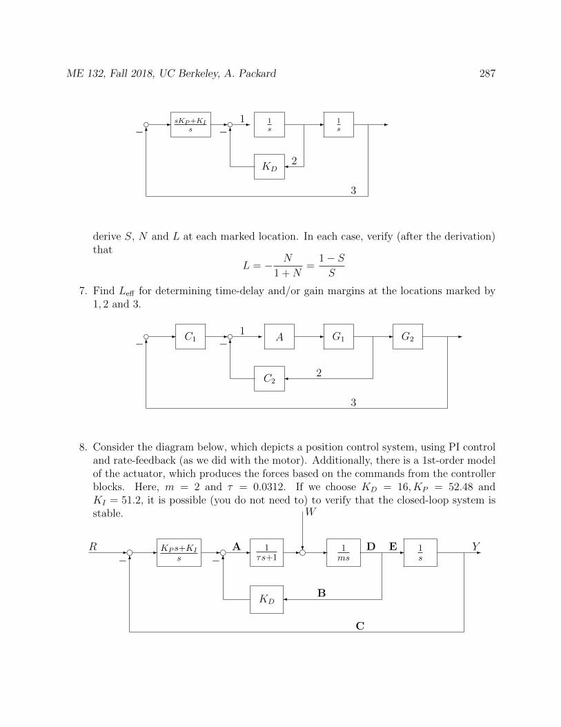
ME 132, Fall 2018, UC Berkeley, A. Packard 287
d dsKP+KIs
1s
1s
KD
- - - - -
6
6− −1
2
3
derive S, N and L at each marked location. In each case, verify (after the derivation)that
L = − N
1 +N=
1− SS
7. Find Leff for determining time-delay and/or gain margins at the locations marked by1, 2 and 3.
d dC1 A G1 G2
C2
- - - - - -
6
6− −1
2
3
8. Consider the diagram below, which depicts a position control system, using PI controland rate-feedback (as we did with the motor). Additionally, there is a 1st-order modelof the actuator, which produces the forces based on the commands from the controllerblocks. Here, m = 2 and τ = 0.0312. If we choose KD = 16, KP = 52.48 andKI = 51.2, it is possible (you do not need to) to verify that the closed-loop system isstable.
- e eKP s+KI
s1
τs+11ms
1s
KD
- - - - e? - - -
6
6− −R
W
YA
B
C
D E
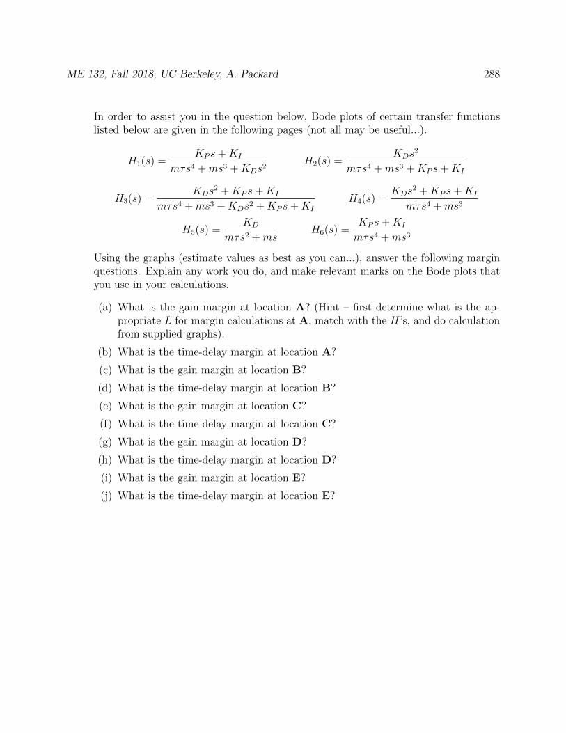
ME 132, Fall 2018, UC Berkeley, A. Packard 288
In order to assist you in the question below, Bode plots of certain transfer functionslisted below are given in the following pages (not all may be useful...).
H1(s) =KP s+KI
mτs4 +ms3 +KDs2H2(s) =
KDs2
mτs4 +ms3 +KP s+KI
H3(s) =KDs
2 +KP s+KI
mτs4 +ms3 +KDs2 +KP s+KI
H4(s) =KDs
2 +KP s+KI
mτs4 +ms3
H5(s) =KD
mτs2 +msH6(s) =
KP s+KI
mτs4 +ms3
Using the graphs (estimate values as best as you can...), answer the following marginquestions. Explain any work you do, and make relevant marks on the Bode plots thatyou use in your calculations.
(a) What is the gain margin at location A? (Hint – first determine what is the ap-propriate L for margin calculations at A, match with the H’s, and do calculationfrom supplied graphs).
(b) What is the time-delay margin at location A?
(c) What is the gain margin at location B?
(d) What is the time-delay margin at location B?
(e) What is the gain margin at location C?
(f) What is the time-delay margin at location C?
(g) What is the gain margin at location D?
(h) What is the time-delay margin at location D?
(i) What is the gain margin at location E?
(j) What is the time-delay margin at location E?

ME 132, Fall 2018, UC Berkeley, A. Packard 289
10−2
10−1
100
101
102
10−2
10−1
100
101
102
Bode Plot of H1
Magnitu
de
10−2
10−1
100
101
102
−260
−250
−240
−230
−220
−210
−200
−190
−180
−170
−160
−150
−140
−130
−120
Angle
(degre
es)
Frequency, Radians/Second
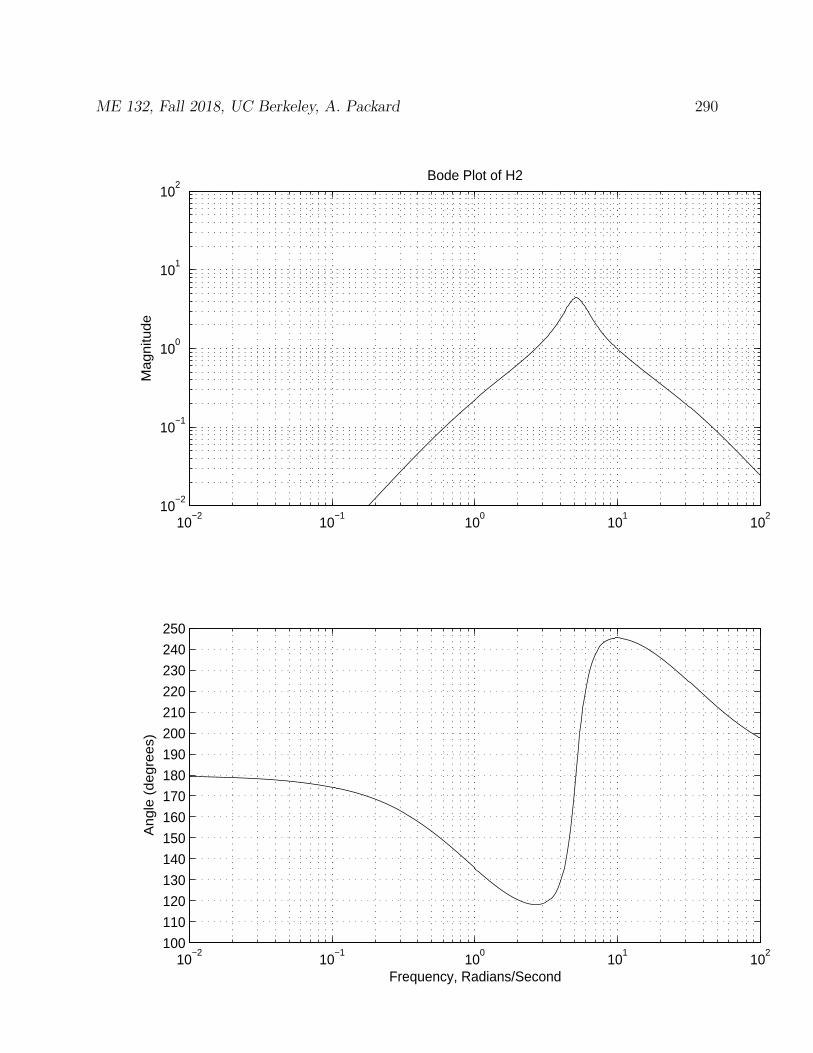
ME 132, Fall 2018, UC Berkeley, A. Packard 290
10−2
10−1
100
101
102
10−2
10−1
100
101
102
Bode Plot of H2
Magnitu
de
10−2
10−1
100
101
102
100
110
120
130
140
150
160
170
180
190
200
210
220
230
240
250
Angle
(degre
es)
Frequency, Radians/Second
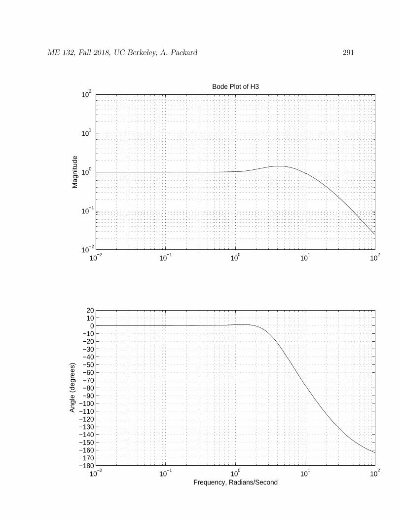
ME 132, Fall 2018, UC Berkeley, A. Packard 291
10−2
10−1
100
101
102
10−2
10−1
100
101
102
Bode Plot of H3
Magnitu
de
10−2
10−1
100
101
102
−180−170−160−150−140−130−120−110−100 −90 −80 −70 −60 −50 −40 −30 −20 −10
0 10 20
Angle
(degre
es)
Frequency, Radians/Second

ME 132, Fall 2018, UC Berkeley, A. Packard 292
10−2
10−1
100
101
102
10−2
10−1
100
101
102
Bode Plot of H4
Magnitu
de
10−2
10−1
100
101
102
80 90
100110120130140150160170180190200210220230240
Angle
(degre
es)
Frequency, Radians/Second

ME 132, Fall 2018, UC Berkeley, A. Packard 293
10−2
10−1
100
101
102
10−2
10−1
100
101
102
Bode Plot of H5
Magnitu
de
10−2
10−1
100
101
102
−170
−160
−150
−140
−130
−120
−110
−100
−90
Angle
(degre
es)
Frequency, Radians/Second

ME 132, Fall 2018, UC Berkeley, A. Packard 294
10−2
10−1
100
101
102
10−2
10−1
100
101
102
Bode Plot of H6
Magnitu
de
10−2
10−1
100
101
102
90
100
110
120
130
140
150
160
170
Angle
(degre
es)
Frequency, Radians/Second
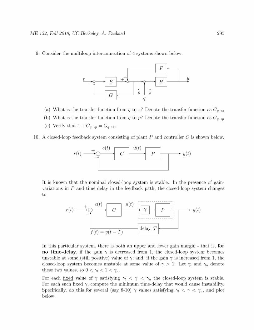
ME 132, Fall 2018, UC Berkeley, A. Packard 295
9. Consider the multiloop interconnection of 4 systems shown below.
d d d6
? ?
G
E H
F
- - - - - -
?
6−++r y
qzp
(a) What is the transfer function from q to z? Denote the transfer function as Gq→z
(b) What is the transfer function from q to p? Denote the transfer function as Gq→p
(c) Verify that 1 +Gq→p = Gq→z.
10. A closed-loop feedback system consisting of plant P and controller C is shown below.
C P- - - -
6
i+
−r(t)
e(t) u(t)y(t)
It is known that the nominal closed-loop system is stable. In the presence of gain-variations in P and time-delay in the feedback path, the closed-loop system changesto
C γ P
delay, T
- - - - -
6
i+
−r(t)
e(t) u(t)y(t)
f(t) = y(t− T )
In this particular system, there is both an upper and lower gain margin - that is, forno time-delay, if the gain γ is decreased from 1, the closed-loop system becomesunstable at some (still positive) value of γ; and, if the gain γ is increased from 1, theclosed-loop system becomes unstable at some value of γ > 1. Let γl and γu denotethese two values, so 0 < γl < 1 < γu.
For each fixed value of γ satisfying γl < γ < γu the closed-loop system is stable.For each such fixed γ, compute the minimum time-delay that would cause instability.Specifically, do this for several (say 8-10) γ values satisfying γl < γ < γu, and plotbelow.
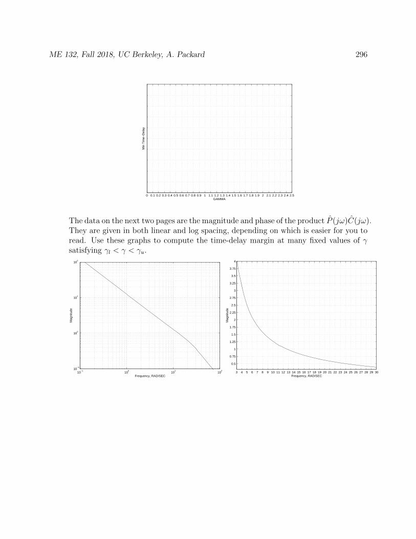
ME 132, Fall 2018, UC Berkeley, A. Packard 296
0 0.1 0.2 0.3 0.4 0.5 0.6 0.7 0.8 0.9 1 1.1 1.2 1.3 1.4 1.5 1.6 1.7 1.8 1.9 2 2.1 2.2 2.3 2.4 2.5GAMMA
Min
Tim
e−D
elay
The data on the next two pages are the magnitude and phase of the product P (jω)C(jω).They are given in both linear and log spacing, depending on which is easier for you toread. Use these graphs to compute the time-delay margin at many fixed values of γsatisfying γl < γ < γu.
10−1
100
101
102
10−1
100
101
102
Frequency, RAD/SEC
Mag
nitu
de
3 4 5 6 7 8 9 10 11 12 13 14 15 16 17 18 19 20 21 22 23 24 25 26 27 28 29 30
0.5
0.75
1
1.25
1.5
1.75
2
2.25
2.5
2.75
3
3.25
3.5
3.75
4
Frequency, RAD/SEC
Mag
nitu
de
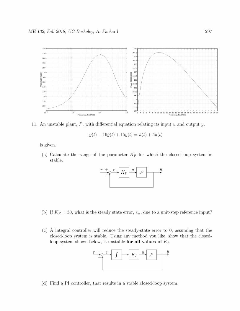
ME 132, Fall 2018, UC Berkeley, A. Packard 297
10−1
100
101
102
100
110
120
130
140
150
160
170
180
190
200
210
220
Frequency, RAD/SEC
Pha
se (
DE
GR
EE
S)
3 4 5 6 7 8 9 10 11 12 13 14 15 16 17 18 19 20 21 22 23 24 25 26 27 28 29 30170
172.5
175
177.5
180
182.5
185
187.5
190
192.5
195
197.5
200
202.5
205
207.5
210
Frequency, RAD/SEC
Pha
se (
DE
GR
EE
S)
11. An unstable plant, P , with differential equation relating its input u and output y,
y(t)− 16y(t) + 15y(t) = u(t) + 5u(t)
is given.
(a) Calculate the range of the parameter KP for which the closed-loop system isstable.
KP Pe−+- - - -
6
r e u y
(b) If KP = 30, what is the steady state error, ess, due to a unit-step reference input?
(c) A integral controller will reduce the steady-state error to 0, assuming that theclosed-loop system is stable. Using any method you like, show that the closed-loop system shown below, is unstable for all values of KI .∫
KI Pe−+- - - - -
6
r e u y
(d) Find a PI controller, that results in a stable closed-loop system.
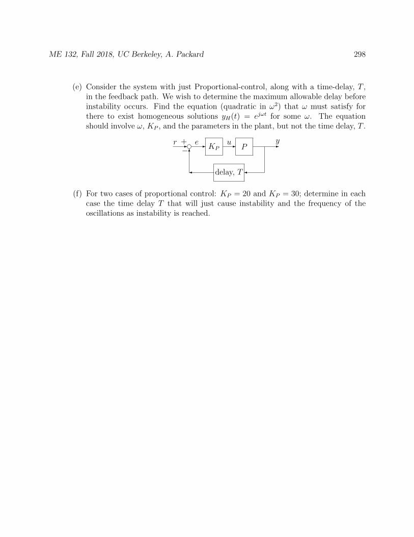
ME 132, Fall 2018, UC Berkeley, A. Packard 298
(e) Consider the system with just Proportional-control, along with a time-delay, T ,in the feedback path. We wish to determine the maximum allowable delay beforeinstability occurs. Find the equation (quadratic in ω2) that ω must satisfy forthere to exist homogeneous solutions yH(t) = ejωt for some ω. The equationshould involve ω, KP , and the parameters in the plant, but not the time delay, T .
KP P
delay, T
e−+- - - -
6
r e u y
(f) For two cases of proportional control: KP = 20 and KP = 30; determine in eachcase the time delay T that will just cause instability and the frequency of theoscillations as instability is reached.
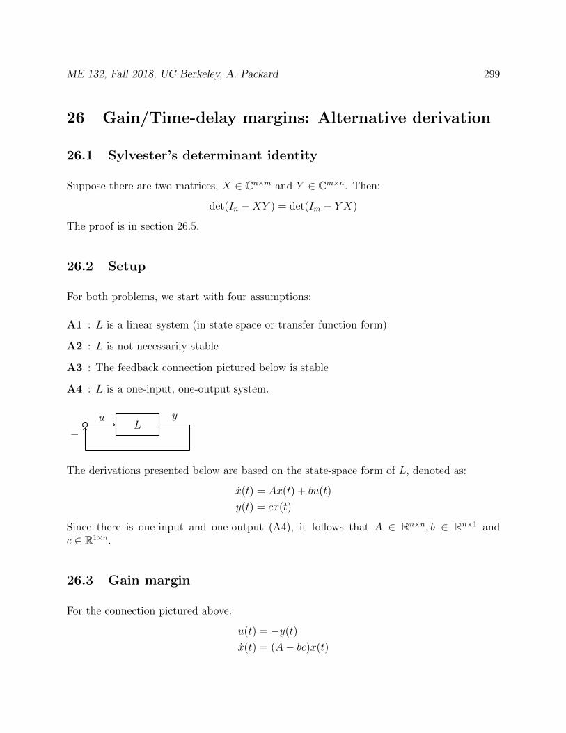
ME 132, Fall 2018, UC Berkeley, A. Packard 299
26 Gain/Time-delay margins: Alternative derivation
26.1 Sylvester’s determinant identity
Suppose there are two matrices, X ∈ Cn×m and Y ∈ Cm×n. Then:
det(In −XY ) = det(Im − Y X)
The proof is in section 26.5.
26.2 Setup
For both problems, we start with four assumptions:
A1 : L is a linear system (in state space or transfer function form)
A2 : L is not necessarily stable
A3 : The feedback connection pictured below is stable
A4 : L is a one-input, one-output system.
−L
u y
The derivations presented below are based on the state-space form of L, denoted as:
x(t) = Ax(t) + bu(t)
y(t) = cx(t)
Since there is one-input and one-output (A4), it follows that A ∈ Rn×n, b ∈ Rn×1 andc ∈ R1×n.
26.3 Gain margin
For the connection pictured above:
u(t) = −y(t)
x(t) = (A− bc)x(t)

ME 132, Fall 2018, UC Berkeley, A. Packard 300
Since the feedback connection is stable (A3), the eigenvalues of A− bc all have negative realparts.
The gain margin is the range of γ, containing γ = 1 for which the system pictured belowremains stable, where γ ≥ 0.
−γ L
u y
This means that the new feedback connection equations are:
x(t) = Ax(t) + γbu(t)
y(t) = cx(t)
u(t) = −y(t)
So we know that:
1. x(t) = (A− γbc)x(t) (from equations above)
2. By A3, the eigenvalues of A− bc all have negative real parts (from 1.1)
3. The eigenvalues are a continuous function of γ (since the matrix is a continuous functionof γ and the eigenvalues of a matrix are a continuous function of the entries of thematrix)
So, for γ = 1, all of the eigenvalues have negative real-parts (they are in the open left-halfplane). As γ varies (both less than 1, and greater than 1), the only way an eigenvalue canbecome unstable for some value of γ 6= 1, it must cross the imaginary axis at an intermediatevalue of γ (ie., closer to 1). Therefore, to compute the gain margin, we find all real valuesof γ and ω ≥ 0 where A− γbc has an eigenvalue on the imaginary axis (ie., at jω). Let
(γ1, ω1), (γ2, ω2), · · · (γN , ωN)
be all these pairs. From this list, select
• the smallest value of γ that is greater than 1, and call this the upper-gain margin, γU .If there is no γ > 1 in the list, then γU :=∞.
• the largest value of γ that is less than 1, and call this the lower-gain margin, γL. Ifthere is no γ ∈ [0, 1) in the list, then γL := 0.

ME 132, Fall 2018, UC Berkeley, A. Packard 301
To find all of the (γk, ωk) pairs, make a further assumption (denoted A5, which not neces-sary, but simplifies the derivation) that A has no imaginary-axis eigenvalues (but A can beunstable, as in A4). Then we find all (γ, ω) pairs where γ ∈ R, γ ≥ 0, ω ∈ R and
det(jωIn − (A− γbc)) = 0 ⇔ det((jωIn − A) + γbc) = 0⇔ det [(jωIn − A)(In + (jωIn − A)−1(γbc))] = 0⇔ det(jωIn − A) · det(In + (jωIn − A)−1(γbc)) = 0
We already have assumed (A5) that det(jωIn − A) 6= 0, so the pairs (γ, ω) must satisfy
det(In + γ(jωIn − A)−1bc) = 0
Define X := (jωIn −A)−1b and Y := c, then use Sylvester’s determinant identity to rewritethis equation, reducing its dimension to 1× 1 (so it no longer involves a determinant).
det(I1 + γc(jωI1 − A)−1b) = 0 ⇔ 1 + γc(jω − A)−1b = 0⇔ 1 + γL(jω) = 0
Since the unknown value of γ satisfies γ ∈ R, γ > 0, it must be that the value of ω is suchthat L(jω) ∈ R and L(jω) < 0. With such a frequency identified, the associated value of γis clearly γ := −1
L(jω).
Summary of the steps: To find all positive, real values of γ such that A−γbc has an eigenvalueon the imaginary axis
1. Find all ω ≥ 0 such that L(jω) is real and negative. Recall, a complex number β isreal and negative if and only if ∠β = ±π,±3π,±5π, · · · radians. On a Bode phaseplot of L, identify all frequencies where ∠L(jω) = ±π,±3π,±5π, · · · .
• These are called the phase-crossover frequencies (since the phase is “crossing” aparticular value - namely an odd multiple of π).
• In Matlab, with allmargin, these frequencies are listed in the GMFrequency field.
Denote these as ω1, ω2, · · · , ωN.
2. Associated with each phase-crossover frequency, define γk := −1L(jωk)
. By construction,all γk are real-valued, and positive. This gives several pairs,
ω1, γ1, ω2, γ2, . . . , ωN , γN
to consider.
3. The lower gain-margin, γL is the largest γk smaller than 1. If there are no γk ∈ [0, 1),then γL := 0.
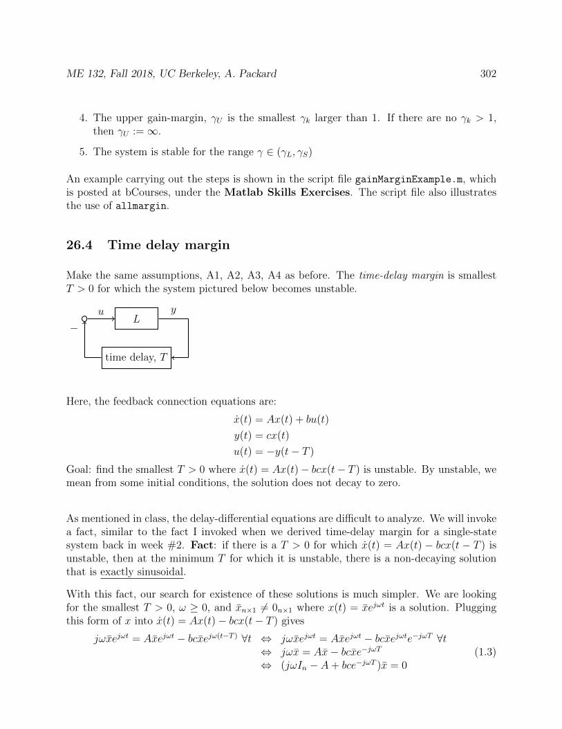
ME 132, Fall 2018, UC Berkeley, A. Packard 302
4. The upper gain-margin, γU is the smallest γk larger than 1. If there are no γk > 1,then γU :=∞.
5. The system is stable for the range γ ∈ (γL, γS)
An example carrying out the steps is shown in the script file gainMarginExample.m, whichis posted at bCourses, under the Matlab Skills Exercises. The script file also illustratesthe use of allmargin.
26.4 Time delay margin
Make the same assumptions, A1, A2, A3, A4 as before. The time-delay margin is smallestT > 0 for which the system pictured below becomes unstable.
−L
time delay, T
u y
Here, the feedback connection equations are:
x(t) = Ax(t) + bu(t)
y(t) = cx(t)
u(t) = −y(t− T )
Goal: find the smallest T > 0 where x(t) = Ax(t)− bcx(t− T ) is unstable. By unstable, wemean from some initial conditions, the solution does not decay to zero.
As mentioned in class, the delay-differential equations are difficult to analyze. We will invokea fact, similar to the fact I invoked when we derived time-delay margin for a single-statesystem back in week #2. Fact: if there is a T > 0 for which x(t) = Ax(t) − bcx(t − T ) isunstable, then at the minimum T for which it is unstable, there is a non-decaying solutionthat is exactly sinusoidal.
With this fact, our search for existence of these solutions is much simpler. We are lookingfor the smallest T > 0, ω ≥ 0, and xn×1 6= 0n×1 where x(t) = xejωt is a solution. Pluggingthis form of x into x(t) = Ax(t)− bcx(t− T ) gives
jωxejωt = Axejωt − bcxejω(t−T ) ∀t ⇔ jωxejωt = Axejωt − bcxejωte−jωT ∀t⇔ jωx = Ax− bcxe−jωT⇔ (jωIn − A+ bce−jωT )x = 0
(1.3)
ME 132, Fall 2018, UC Berkeley, A. Packard 303
Note that we used the fact that for any ω, and any t, the scalar ejωt 6= 0, and it was dividedout.
For fixed values of ω and T , the expression (jωIn − A + bce−jωT )x = 0n is true for somex 6= 0 if and only if
det(jωIn − A+ bcejωT ) = 0
Invoke A5 again (A has no imaginary axis eigenvalues), and simplify as
det(jωIn − A+ bcejωT ) = 0 ⇔ det[(jωIn − A)(In + (jωIn − A)−1bce−jωT )
]= 0
⇔ det(jωIn − A) · det(In + (jωIn − A)−1bce−jωT ) = 0⇔ det(In + (jωIn − A)−1bce−jωT ) = 0⇔ det(I1 + c(jωI1 − A)−1be−jωT ) = 0⇔ 1 + c(jω − A)−1be−jωT ) = 0⇔ e−jωTL(jω) = −1
Even though we don’t know the value of T or ω, both e−jωT and −1 both have a magnitudeof 1. Therefore, we are interested in values of ω for which |L(jω)| = 1.
So, suppose |L(jω)| = 1. So L(jω) is a complex number on the perimeter of the unitcircle in C (radius of 1, centered at 0). The factor e−jωT , when multiplying L(jω) rotatesthe complex number L(jω) by ωT radians, clockwise. We are interested in a rotation thatmakes e−jωTL(jω) = −1. Important: Hence we define θ, satisfying 0 < θ < 2π, as theangle of a bf clockwise rotation that takes L(jω) to −1. With θ defined, the correspondingT is simply T := θ
ω.
Summary of the steps: To find all T > 0, and associated ω ≥ 0 such that e−jωTL(jω) = −1
1. Find all ω ≥ 0 such that |L(jω)| = 1. On a Bode magnitude plot of L, identify allfrequencies where |L(jω)| = 1.
• These are called the gain-crossover frequencies (since the gain is “crossing” aparticular value - namely 1).
• In Matlab, with allmargin, these frequencies are listed in the DMFrequency field.
Denote these as ω1, ω2, · · · , ωN.
2. Associated with each gain-crossover frequency, define θk, satisfying 0 < θk < 2π, asthe angle of a clockwise rotation that takes L(jωk) exactly to −1. With θk defined,the corresponding Tk is simply Tk := θk
ωk.
3. The time-delay margin, T is the smallest such T . If there are no gain-crossover fre-quencies, then the time-delay margin is ∞

ME 132, Fall 2018, UC Berkeley, A. Packard 304
An example carrying out the steps is shown in the script file TimeDelayMarginExample.m,which is posted at bCourses, under the Matlab Skills Exercises. The script file alsoillustrates the use of allmargin.
26.5 Appendix
To prove Sylvester’s determinant identity, we define the block matrix of size (n+m)×(n+m)as:
Z :=
[In XY Im
]Then we can show, using the determinants of block matrices, that:[
In −X0m×n Im
] [In XY Im
]=
[In −XY 0n×m
Y Im
]det
[In −X
0m×n Im
]det
[In XY Im
]= det
[In −XY 0n×m
Y Im
](det(In +X(Im)−10m×n) det(Im)
)(det
[In XY Im
])= det((In −XY )− 0n×m(Im)−1Y ) det(Im)
det
[In XY Im
]= det(In −XY ) (1.1)
Similarly, we can show that: [In 0n×m−Y Im
] [In XY Im
]=
[In X
0m×n Im − Y X
]det
[In 0n×m−Y Im
]det
[In XY Im
]= det
[In X
0m×n Im − Y X
](det(In − 0n×m(Im)−1(−Y )) det(Im)
)(det
[In XY Im
])= det(In −X(Im − Y X)−10m×n) det(Im − Y X)
det
[In XY Im
]= det(Im − Y X) (1.2)
Since det(Z) is equal to (1.1) as well as (1.2), it must be that det(In−XY ) = det(Im−Y X)
ME 132, Fall 2018, UC Berkeley, A. Packard 305
27 Connection between Frequency Responses and Trans-
fer functions
Consider the standard linear system
y[n](t) + a1y[n−1](t) + · · ·+ an−1y
[1](t) + any(t)= b0u
[n](t) + b1u[n−1](t) + · · ·+ bn−1u
[1](t) + bnu(t)(27.1)
with y the dependent variable (output), and u the independent variable (input).
Assuming that the system is stable, we know that the steady-state response to a sinusoidalinput is also a sinusoid, with magnitude and phase determined by the system-dependentfrequency response function
H(ω) :=b0(jω)n + b1(jω)n−1 + · · ·+ bn−1(jω) + bn(jω)n + a1(jω)n−1 + · · ·+ an−1(jω) + an
(27.2)
For stable systems, we have proven for fixed value u and fixed ω ∈ R
u(t) := uejωt ⇒ yss(t) = H(ω)uejωt
Recall that the transfer function from u to y is the rational function G(s) given by
G(s) :=b0s
n + b1sn−1 + · · ·+ bn−1s+ bn
sn + a1sn−1 + · · ·+ an−1s+ an
Note that H(ω) = G(s)|s=jω.
So, we can immediately write down the frequency response function once we have derivedthe transfer function. Sometimes, we do not use different letters to distinguish the transferfunction and frequency response, typically writing G(s) to denote the transfer function andG(jω) to denote the frequency response function.
27.1 Interconnections
Frequency Responses are a useful concept when working with interconnections of linearsystems. Since the frequency response function, H(ω) turned out to be the transfer functionG(s) evaluated at s = jω, frequency response functions of interconnections follow the samerules as transfer functions of interconnections.
This is extremely important, so we reiterate it: The frequency response of astable interconnection of systems (which are individually possibly unstable)
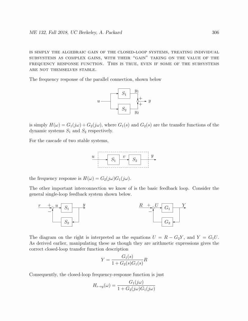
ME 132, Fall 2018, UC Berkeley, A. Packard 306
is simply the algebraic gain of the closed-loop systems, treating individualsubsystems as complex gains, with their “gain” taking on the value of thefrequency response function. This is true, even if some of the subsystemsare not themselves stable.
The frequency response of the parallel connection, shown below
S2
S1-
-
?
6d -u
y1
y2
y++
is simply H(ω) = G1(jω) +G2(jω), where G1(s) and G2(s) are the transfer functions of thedynamic systems S1 and S2 respectively.
For the cascade of two stable systems,
S1 S2- - -u v y
the frequency response is H(ω) = G2(jω)G1(jω).
The other important interconnection we know of is the basic feedback loop. Consider thegeneral single-loop feedback system shown below.
S1
S2
- - -
6
dr yu+
−G1
G2
- - -
6
dR YU+
−
The diagram on the right is interpreted as the equations U = R − G2Y , and Y = G1U .As derived earlier, manipulating these as though they are arithmetic expressions gives thecorrect closed-loop transfer function description
Y =G1(s)
1 +G2(s)G1(s)R
Consequently, the closed-loop frequency-response function is just
Hr→y(ω) =G1(jω)
1 +G2(jω)G1(jω)
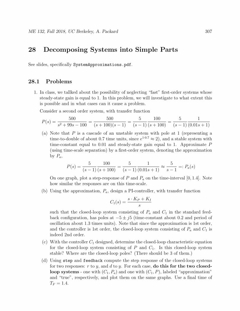
ME 132, Fall 2018, UC Berkeley, A. Packard 307
28 Decomposing Systems into Simple Parts
See slides, specifically SystemApproximations.pdf.
28.1 Problems
1. In class, we tallked about the possibility of neglecting “fast” first-order systems whosesteady-state gain is equal to 1. In this problem, we will investigate to what extent thisis possible and in what cases can it cause a problem.
Consider a second order system, with transfer function
P (s) =500
s2 + 99s− 100=
500
(s+ 100)(s− 1)=
5
(s− 1)
100
(s+ 100)=
5
(s− 1)
1
(0.01s+ 1)
(a) Note that P is a cascade of an unstable system with pole at 1 (representing atime-to-double of about 0.7 time units, since e1·0.7 ≈ 2), and a stable system withtime-constant equal to 0.01 and steady-state gain equal to 1. Approximate P(using time-scale separation) by a first-order system, denoting the approximationby Pa,
P (s) =5
(s− 1)
100
(s+ 100)=
5
(s− 1)
1
(0.01s+ 1)≈ 5
s− 1=: Pa(s)
On one graph, plot a step-response of P and Pa on the time-interval [0, 1.4]. Notehow similar the responses are on this time-scale.
(b) Using the approximation, Pa, design a PI-controller, with transfer function
C1(s) =s ·KP +KI
s
such that the closed-loop system consisting of Pa and C1 in the standard feed-back configuration, has poles at −5± j5 (time-constant about 0.2 and period ofoscillation about 1.3 times units). Note that since the approximation is 1st order,and the controller is 1st order, the closed-loop system consisting of Pa and C1 isindeed 2nd order.
(c) With the controller C1 designed, determine the closed-loop characteristic equationfor the closed-loop system consisting of P and C1. Is this closed-loop systemstable? Where are the closed-loop poles? (There should be 3 of them.)
(d) Using step and feedback compute the step response of the closed-loop systemsfor two responses: r to y, and d to y. For each case, do this for the two closed-loop systems - one with (C1, Pa) and one with (C1, P ), labeled “approximation”and “true”, respectively, and plot them on the same graphs. Use a final time ofTF = 1.4.

ME 132, Fall 2018, UC Berkeley, A. Packard 308
(e) Finally, with the usual inputs (r, d, n) and output (y, u), make a 2 × 3 array ofBode plots, with two lines/axes (one for (C,Pa) and one for (C1, P )). For r → y,plot both magnitude and phase; for all others, just plot magnitude. Look backin the early chapters where I called this the “gang-of-six” to see how it should beplotted.
(f) Based on time-domain, and frequency-domain plots, would you say that Pa is agood approximation of P for the purposes of this particular control designfor C1, where closed-loop poles are placed at −5± j5?
(g) Repeat this entire control design/analysis process for a different control design,namely again using the approximation, Pa, and designing a PI-controller, withtransfer function
C2(s) =s ·KP +KI
ssuch that the closed-loop system consisting of Pa and C2 in the standard feedbackconfiguration, has poles at −50 ± j50 (time-constant about 0.02 and period ofoscillation about 0.13 times units). Make the same time-domain and frequency-domain comparisons. In time-domain, use TF = 0.14.
(h) Based on time-domain, and frequency-domain plots, would you say that Pa is agood approximation of P for the purposes of this particular control designfor C2, where closed-loop poles are placed at −50± j50?
(i) Finally, plot a step-response of P and Pa on the time-interval [0, 0.14]. On thisshort time-scale, are there some more obvious differences? Compare this to thesimilarities you saw in part 1a, which was on a longer time-scale. Note that onthis short time-scale, we can see that the response of P looks similar (but notexactly) to a delayed (by 0.01 time-units) version of Pa.
(j) Based on the observation (approximate time-delay interpretation) on part 1i, andthe oscillatory responses obtained in part 1g, compute the time-delay margin ofthe closed-loop system consisting of (C2, Pa). Note that the value of the marginis actually similar to “approximate delay” that P seems to have relative to Pa.This partly explains why Pa is not a good approximation to P for the purposesof the C2 design.
(k) By contrast, compute the time-delay margin of the closed-loop system consistingof (C1, Pa). Note that the delay margin is much longer in this case, and hence thesmall “delay” between Pa and P is not as significant for the C1 design.
2. (a) Factor the transfer function below into a cascade of lower order systems.
G(s) =2s+ 1
0.11s4 + 2.025s3 − 3.26s2 + 4.935s+ 2.7
(b) Determine (this is a judgement call, but here the answer should be “yes”) if thereis a good, lower-order (2nd-order, in fact) approximation, GA.
ME 132, Fall 2018, UC Berkeley, A. Packard 309
(c) Find the approximation, and use Matlab to plot the step-response of the originalsystem and the approximation. As both are unstable, limit the step-response timeto 3 time-units.
(d) Using GA, design a 2nd-order controller with integral-action,
C(s) =as2 + bs+ c
s(s+ d)
such that the closed-loop poles are at
−32.5,−1.4± j2.8,−0.23
(e) Consider the generic closed-loop system described by equations e = r− ym, ym =y + n, u = C(e), and y = P (d + u), where C represents the controller, and Prepresents the plant (here P = G or P = GA). Confirm (using feedback andpole) that the closed-loop poles using the controller along with the approximateplant are as desired.
(f) Using this controller with original plant, G, what are the actual closed-loop poles?
(g) On the same axes, plot step-responses from r to y for both closed-loop systems.
(h) On the same axes, plot step-responses from d to y for both closed-loop systems.
(i) On the same axes, plot Bode-magnitude responses from n to u for both closed-loopsystems.
(j) For the particular design, comment on the suitability of the approximation.

ME 132, Fall 2018, UC Berkeley, A. Packard 310
29 Unfiled problems
1. This problem is motivated by thinking about a physical tug-of-war game, but playedin a virtual environment, by individuals in different locations, where the players are“linked” by a feedback system, which gives each one infomation about the other. Thegoal is, with (say) motors, to simulate the effect of player 1 on player 2, and visa-versa.Ultimately, we can build a small scale version of this with the EV3 system, using twomotors and one EV3 brick.
Two identical systems, G1 and G2, are operated in separate locations, but “controlled”by one central controller, K, as shown below. All unmarked summing junctions are“+”.
- -?
- -
6
-
-
?
6
e
ee
G2
12 K
G1F1
F2
y1
y2
+
−
−+u
The external inputs F1 and F2 represent inputs by operators to the individual systemsat each location. The goal of the “cooperative control” is:
• synchronization: the difference, ydiff := y1 − y2 should remain small relative toindependent forcings F1 and F2, and
• preserving open-loop dynamics: the average, yavg := y1+y22
should be approxi-mately equal to GF1+F2
2, written concisely as yavg ≈ GFavg , where G denotes the
(common) input/output behavior of G1 and G2.
Since G1 and G2 are separate, but identical, assume their models are of the form
G1 :x1(t) = Ax1(t) +Bu1(t)y1(t) = Cx1(t)
and
G2 :x2(t) = Ax2(t) +Bu2(t)y2(t) = Cx2(t)
where for each t, xi(t) ∈ Rn, ui(t) ∈ Rnu and yi(t) ∈ Rny . Note that each system, G1
and G2, has n state variables.
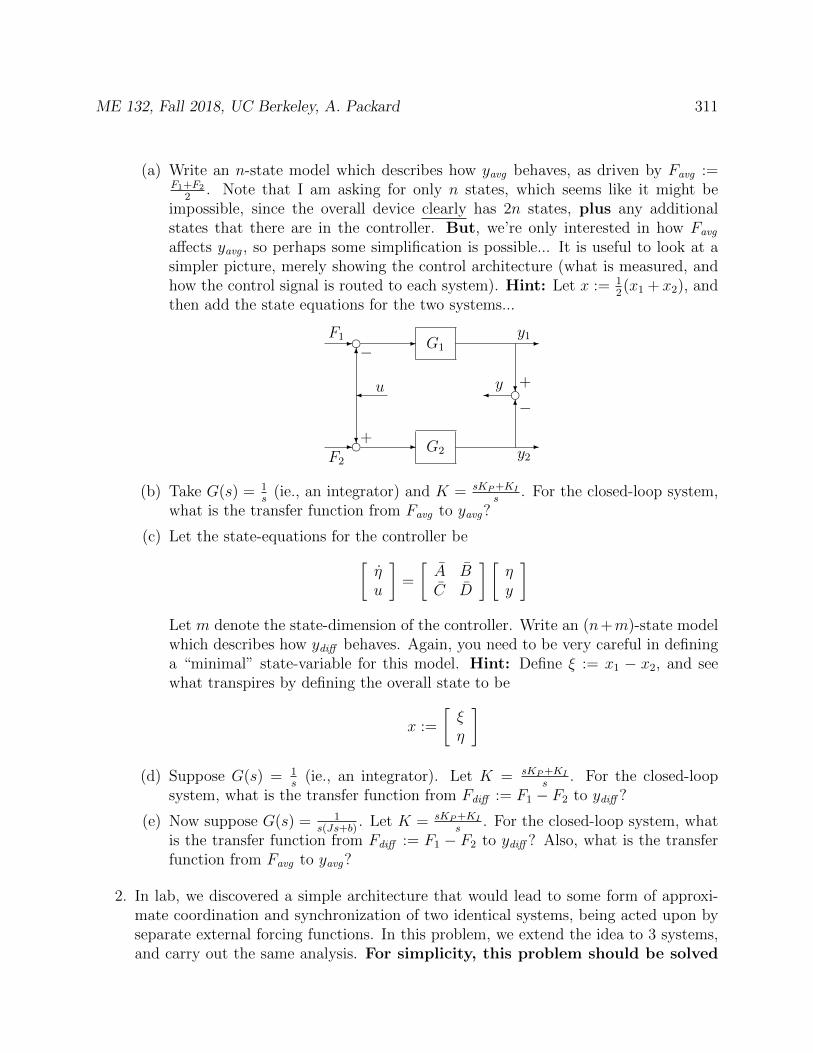
ME 132, Fall 2018, UC Berkeley, A. Packard 311
(a) Write an n-state model which describes how yavg behaves, as driven by Favg :=F1+F2
2. Note that I am asking for only n states, which seems like it might be
impossible, since the overall device clearly has 2n states, plus any additionalstates that there are in the controller. But, we’re only interested in how Favg
affects yavg , so perhaps some simplification is possible... It is useful to look at asimpler picture, merely showing the control architecture (what is measured, andhow the control signal is routed to each system). Hint: Let x := 1
2(x1 + x2), and
then add the state equations for the two systems...
- -?
- -
6
-
-
?
6
e
ee
G2
G1F1
F2
y1
y2
+
−
−+u y
(b) Take G(s) = 1s
(ie., an integrator) and K = sKP+KIs
. For the closed-loop system,what is the transfer function from Favg to yavg?
(c) Let the state-equations for the controller be[ηu
]=
[A BC D
] [ηy
]Let m denote the state-dimension of the controller. Write an (n+m)-state modelwhich describes how ydiff behaves. Again, you need to be very careful in defininga “minimal” state-variable for this model. Hint: Define ξ := x1 − x2, and seewhat transpires by defining the overall state to be
x :=
[ξη
](d) Suppose G(s) = 1
s(ie., an integrator). Let K = sKP+KI
s. For the closed-loop
system, what is the transfer function from Fdiff := F1 − F2 to ydiff ?
(e) Now suppose G(s) = 1s(Js+b)
. Let K = sKP+KIs
. For the closed-loop system, whatis the transfer function from Fdiff := F1 − F2 to ydiff ? Also, what is the transferfunction from Favg to yavg?
2. In lab, we discovered a simple architecture that would lead to some form of approxi-mate coordination and synchronization of two identical systems, being acted upon byseparate external forcing functions. In this problem, we extend the idea to 3 systems,and carry out the same analysis. For simplicity, this problem should be solved
ME 132, Fall 2018, UC Berkeley, A. Packard 312
completely in transfer function notation, simply applying arithmetic rules.We could verify everything in terms of state-space models (as we did in the lab), butthere is not time for that here. Again, just manipulate with addition, subtraction,multiplication, and division, as appropriate for transfer functions.
The 3 identical systems are each forced with a control input, Ui and an external inputFi. Each of the systems has a transfer function G, hence
Yi = G(Ui + Fi), i = 1, 2, 3
The architecture for control generalizes the 2-system case. Let K be the transferfunction of a linear system, and use
U1 = 13K(Y2 − Y1) + 1
3K(Y3 − Y1) = 1
3K(−2Y1 + Y2 + Y3)
U2 = 13K(Y3 − Y2) + 1
3K(Y1 − Y2) = 1
3K(−2Y2 + Y3 + Y1)
U3 = 13K(Y1 − Y3) + 1
3K(Y2 − Y3) = 1
3K(−2Y3 + Y1 + Y2)
(a) Find Y1 + Y2 + Y3 in terms of F1, F2, F3.
(b) Based on part (a), fill in the sentence: The of the systems outputsequals the transfer function times the of the externalinputs.
(c) By careful (but simple) manipulation, find a closed-loop expression for Y2 − Y1,in terms of K,G and F1, F2, F3.
(d) If K(s) = nK(s)dK(s)
and G(s) = nG(s)dG(s)
, what do you think is the characteristic equationof the closed-loop system?
(e) By symmetry, what are the closed-loop expressions for Y3 − Y2 and Y3 − Y1?
3. Consider a plant P with transfer function
P (s) =s
s2 − 1
The plant is a challenging to control. It is a simple model of an inverted pendulum,where the only control action u, represents the angular speed of a reaction wheel,mounted at the free-end (top) of the pendulum. By “torquing” the reaction wheel (rel-ative to the pendulum), equal/opposite torque act on the pendulum, which if properlydone, can stabilize it in the “up” position.
(a) Suppose the input to P is labeled u and the output y. What is the differentialequation governing the relationship between u and y.
(b) Is the plant stable?

ME 132, Fall 2018, UC Berkeley, A. Packard 313
(c) Consider a controller, C, with transfer function
C(s) =as+ b
s+ c
For the feedback loop consisting of P and C (with the usual negative (−) feedbackconvention), what is the closed-loop characteristic equation?
(d) Design: Find a, b and c (ie., parameters of the control law) so that the roots ofthe closed-loop characteristic equation are
−4,−2± j2
(e) The controller stabilizes P , in that the feedback loop consisting of P and C isstable. However, as we saw earlier, P is not stable on its own. Is C stable?
(f) Assume we relax the choice of the desired closed-loop roots, and only restrictthem to all have negative real-parts (since we want the closed-loop system to bestable). Are there any choice of such desired roots so that the controller (whichyields those closed-loop roots) is itself a stable system?
4. This problem may be out-of-place. It has some transfer function questionsAt one point, NASA was developing booster rockets and a crew exploration vehicleto replace the Space Shuttle. One main component of the Orion Crew ExplorationVehicle (CEV) is a conical crew module. This module has several thrusters to controlthe vehicle attitude on re-entry to the earth’s orbit. A linear model for the short-periodmode of the CEV pitch dynamics during re-entry is given by:
x(t) =
[2 1−36 2
]x(t) +
[01
]u(t)
y(t) =[
0 1]x(t) +
[0]u
where x(t) :=
[α(t)q(t)
], which are the angle-of-attack and the pitch-rate, respectively,
and u(t) is the pitch torque generated by the thrusters. The output y is the pitch rate,so y = x2 = q.
(a) Using the formula we derived in class, G(s) = D + C(sI − A)−1B, derive thetransfer function from u to y of this state-space model.
(b) Enter the matrices into Matlab, form a state-space object using the ss constructor.Type
>> disp(G)
>> size(G)
>> class(G)
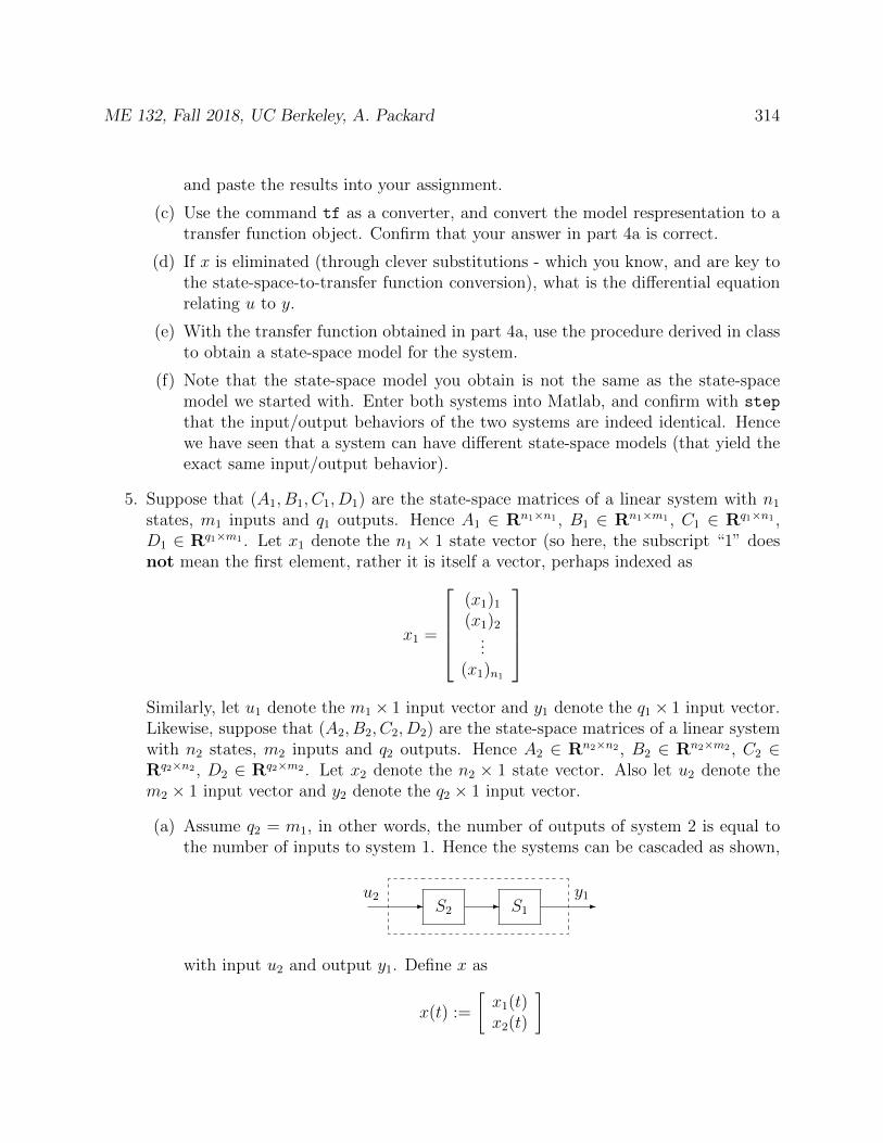
ME 132, Fall 2018, UC Berkeley, A. Packard 314
and paste the results into your assignment.
(c) Use the command tf as a converter, and convert the model respresentation to atransfer function object. Confirm that your answer in part 4a is correct.
(d) If x is eliminated (through clever substitutions - which you know, and are key tothe state-space-to-transfer function conversion), what is the differential equationrelating u to y.
(e) With the transfer function obtained in part 4a, use the procedure derived in classto obtain a state-space model for the system.
(f) Note that the state-space model you obtain is not the same as the state-spacemodel we started with. Enter both systems into Matlab, and confirm with step
that the input/output behaviors of the two systems are indeed identical. Hencewe have seen that a system can have different state-space models (that yield theexact same input/output behavior).
5. Suppose that (A1, B1, C1, D1) are the state-space matrices of a linear system with n1
states, m1 inputs and q1 outputs. Hence A1 ∈ Rn1×n1 , B1 ∈ Rn1×m1 , C1 ∈ Rq1×n1 ,D1 ∈ Rq1×m1 . Let x1 denote the n1 × 1 state vector (so here, the subscript “1” doesnot mean the first element, rather it is itself a vector, perhaps indexed as
x1 =
(x1)1
(x1)2...
(x1)n1
Similarly, let u1 denote the m1× 1 input vector and y1 denote the q1× 1 input vector.Likewise, suppose that (A2, B2, C2, D2) are the state-space matrices of a linear systemwith n2 states, m2 inputs and q2 outputs. Hence A2 ∈ Rn2×n2 , B2 ∈ Rn2×m2 , C2 ∈Rq2×n2 , D2 ∈ Rq2×m2 . Let x2 denote the n2 × 1 state vector. Also let u2 denote them2 × 1 input vector and y2 denote the q2 × 1 input vector.
(a) Assume q2 = m1, in other words, the number of outputs of system 2 is equal tothe number of inputs to system 1. Hence the systems can be cascaded as shown,
S2 S1- - -
u2 y1
with input u2 and output y1. Define x as
x(t) :=
[x1(t)x2(t)
]

ME 132, Fall 2018, UC Berkeley, A. Packard 315
which is an (n1 + n2) × 1 vector. Find matrices (defined in terms of verticaland horizontal concatenations of various products of the individual state-spacematrices) such that the equations
x(t) = Ax(t) +Bu2(t)y1(t) = Cx(t) +Du2(t)
(b) In Matlab, the * operation (”multiplication”) is the cascade operation for systems(tf, ss, and so on), and the above operation would be written as S1∗S2. Theactual name of the * operator is mtimes. Execute
>> open +ltipack\@ssdata\mtimes.m
within Matlab, and find the lines of code which implement the operation above.
(c) Assume q1 = q2 and m1 = m2, in other words, the number of outputs of system 1is equal to the number of outputs of system 2, and the number of inputs of thetwo systems are equal as well. Hence the systems can be connected in parallel asshown, with input u and output y.
S2
S1-
-
?
6d -u
y1
y2
y++
Define x as
x(t) :=
[x1(t)x2(t)
]which is an (n1 + n2) × 1 vector. Find matrices (defined in terms of verticaland horizontal concatenations of various products of the individual state-spacematrices) such that the equations
x(t) = Ax(t) +Bu(t)y(t) = Cx(t) +Du(t)
(d) In Matlab, the + operation (”addition”) is the parallel interconnection operationfor systems (tf, ss, and so on), and the above operation would be written asS1+S2. The actual name of the + operator is plus. Execute
>> open +ltipack\@ssdata\plus.m
within Matlab, and find the lines of code which implement the operation above.
(e) Assume that q1 = m2 and m1 = q2, in other words, the number of outputs of onesystem is equal to the number of outputs of the other system. Hence the systemscan be connected in feedback as shown, with input u and output y. Assumefurther that D1 = 0q1×m1 .
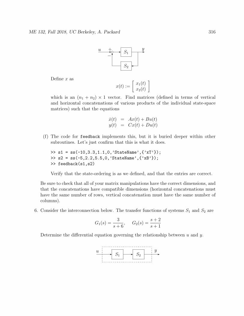
ME 132, Fall 2018, UC Berkeley, A. Packard 316
S1
S2
- - -
6
du y+
−
Define x as
x(t) :=
[x1(t)x2(t)
]which is an (n1 + n2) × 1 vector. Find matrices (defined in terms of verticaland horizontal concatenations of various products of the individual state-spacematrices) such that the equations
x(t) = Ax(t) +Bu(t)y(t) = Cx(t) +Du(t)
(f) The code for feedback implements this, but it is buried deeper within othersubroutines. Let’s just confirm that this is what it does.
>> s1 = ss(-10,3.3,1.1,0,’StateName’,’xT’);
>> s2 = ss(-5,2.2,5.5,0,’StateName’,’xB’);
>> feedback(s1,s2)
Verify that the state-ordering is as we defined, and that the entries are correct.
Be sure to check that all of your matrix manipulations have the correct dimensions, andthat the concatenations have compatible dimensions (horizontal concatenations musthave the same number of rows, vertical concatenation must have the same number ofcolumns).
6. Consider the interconnection below. The transfer functions of systems S1 and S2 are
G1(s) =3
s+ 6, G2(s) =
s+ 2
s+ 1
Determine the differential equation governing the relationship between u and y.
S1 S2- - -u y
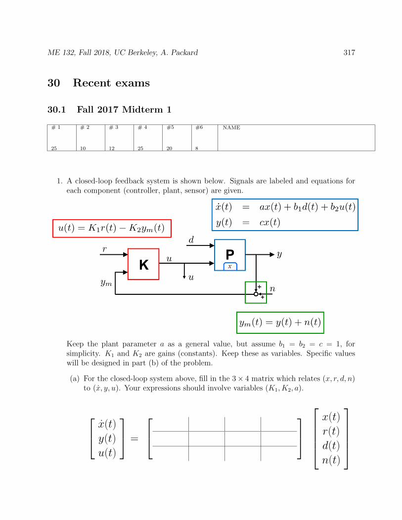
ME 132, Fall 2018, UC Berkeley, A. Packard 317
30 Recent exams
30.1 Fall 2017 Midterm 1
# 1
25
# 2
10
# 3
12
# 4
25
#5
20
#6
8
NAME
1. A closed-loop feedback system is shown below. Signals are labeled and equations foreach component (controller, plant, sensor) are given.
Keep the plant parameter a as a general value, but assume b1 = b2 = c = 1, forsimplicity. K1 and K2 are gains (constants). Keep these as variables. Specific valueswill be designed in part (b) of the problem.
(a) For the closed-loop system above, fill in the 3× 4 matrix which relates (x, r, d, n)to (x, y, u). Your expressions should involve variables (K1, K2, a).
x(t)y(t)
u(t)
=
x(t)
r(t)
d(t)
n(t)

ME 132, Fall 2018, UC Berkeley, A. Packard 318
(b) Now take a = −1 so that the plant, by itself, is stable, and hence has a time-constant of τP = 1. Suppose one goal of feedback control is to achieve closed-loop stability, and make the closed-loop system respond faster, so that theclosed-loop time constant is less than τP . Specifically, work in ratios, express-ing this design requirement that the closed-loop time-constant, τCL, should be afraction γ of the plant time constant, namely
Design Requirement #1 : τCL = γ · τP
where 0 < γ < 1 is a given design target. The other design requirement is
Design Requirement #2 : SSGr→y = 1
in words, the steady-state gain from r → y should equal 1. Task: As a functionof γ, find expressions for K1 and K2 which simultaneously achieve the two DesignRequirements.
ME 132, Fall 2018, UC Berkeley, A. Packard 319
(c) For the closed-loop system, what is the instantaneous gain from r → u, asa function of the design parameter γ? Is this gain increasing or decreasing asγ decreases? Explain this relationship intuitively (ie., “if we require the systemto respond more quickly, with perfect steady-state behavior from r → y, theinstantaneous effect that r must have on u....”).
(d) For the closed-loop system, what is the steady-state gain from r → u, as afunction of the design parameter γ? How is this affected as γ decreases? Explainthis relationship intuitively (ie., “if we require the system to respond more quickly,with perfect steady-state behavior from r → y, the steady-state effect that r musthave on u....”).
(e) For the closed-loop system, what is the steady-state gain from d → y, as afunction of the design parameter γ? How is this affected as γ decreases?
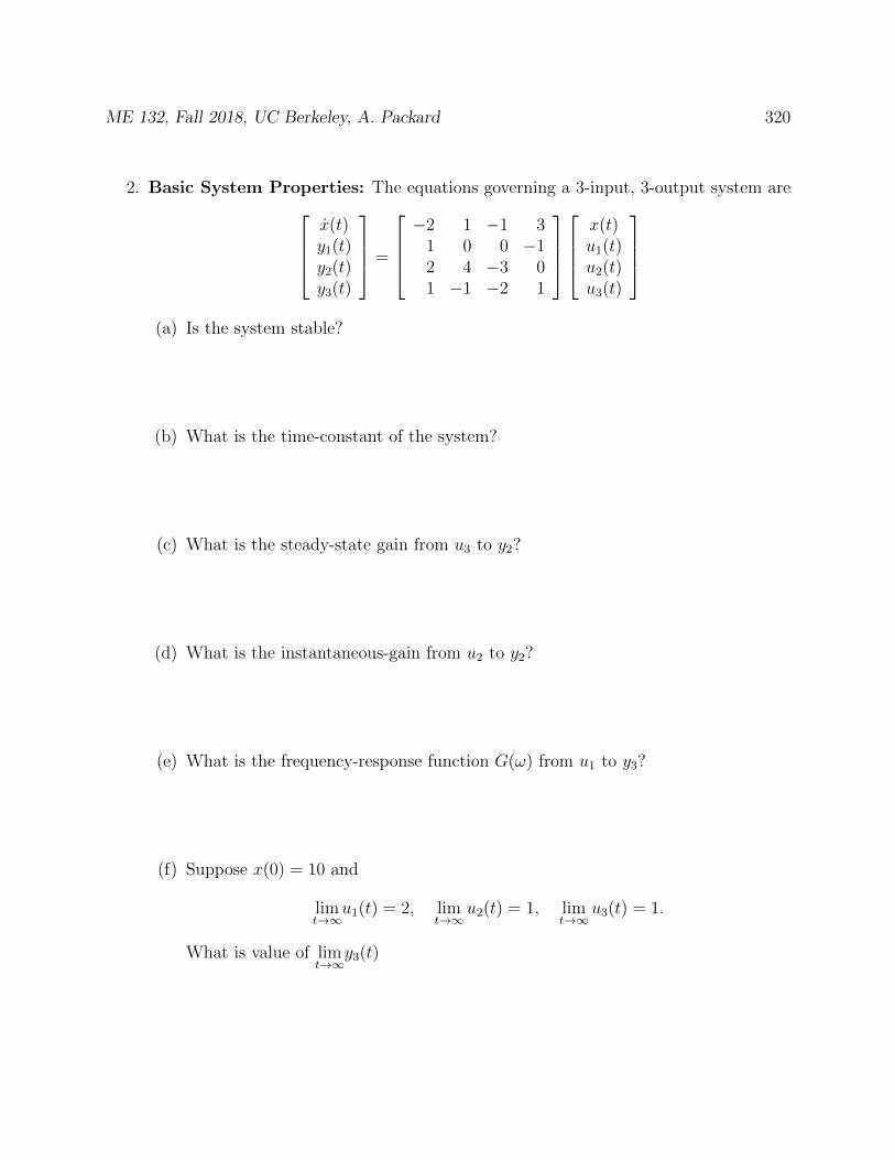
ME 132, Fall 2018, UC Berkeley, A. Packard 320
2. Basic System Properties: The equations governing a 3-input, 3-output system arex(t)y1(t)y2(t)y3(t)
=
−2 1 −1 3
1 0 0 −12 4 −3 01 −1 −2 1
x(t)u1(t)u2(t)u3(t)
(a) Is the system stable?
(b) What is the time-constant of the system?
(c) What is the steady-state gain from u3 to y2?
(d) What is the instantaneous-gain from u2 to y2?
(e) What is the frequency-response function G(ω) from u1 to y3?
(f) Suppose x(0) = 10 and
limt→∞
u1(t) = 2, limt→∞
u2(t) = 1, limt→∞
u3(t) = 1.
What is value of limt→∞
y3(t)
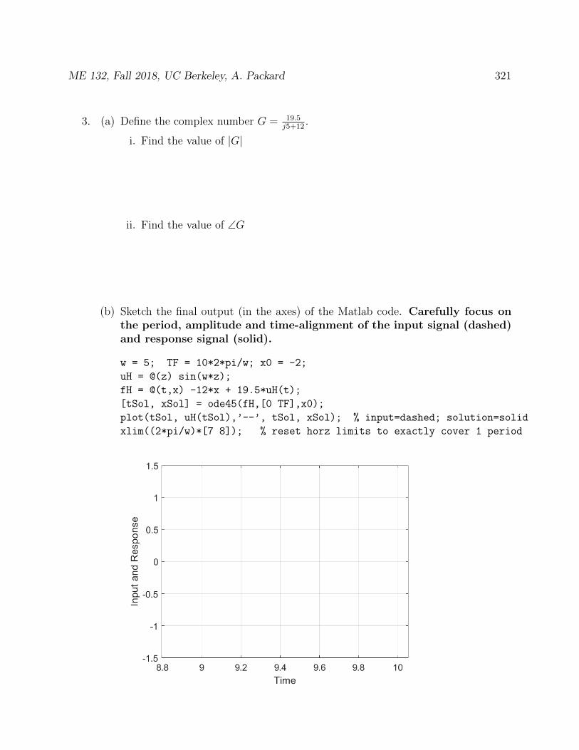
ME 132, Fall 2018, UC Berkeley, A. Packard 321
3. (a) Define the complex number G = 19.5j5+12
.
i. Find the value of |G|
ii. Find the value of ∠G
(b) Sketch the final output (in the axes) of the Matlab code. Carefully focus onthe period, amplitude and time-alignment of the input signal (dashed)and response signal (solid).
w = 5; TF = 10*2*pi/w; x0 = -2;
uH = @(z) sin(w*z);
fH = @(t,x) -12*x + 19.5*uH(t);
[tSol, xSol] = ode45(fH,[0 TF],x0);
plot(tSol, uH(tSol),’--’, tSol, xSol); % input=dashed; solution=solid
xlim((2*pi/w)*[7 8]); % reset horz limits to exactly cover 1 period

ME 132, Fall 2018, UC Berkeley, A. Packard 322
4. A closed-loop feedback system is shown below. Signals are labeled. Note that the onemarked summing junction has a − sign, as typical of our negative feedback convention.Treat all unmarked summing junctions as +.
Fill in the 3× 4 matrix which relates (x, r, d, n) to (x, y, u) as shown below
x(t)y(t)
u(t)
=
x(t)
r(t)
d(t)
n(t)
(a) What is the time-constant of the closed-loop system?
(b) What is the steady-state gain from r → y?
(c) What is the steady-state gain from d→ y?
(d) What is the instantaneous gain from r → y?
(e) What is the instantaneous gain from d→ y?

ME 132, Fall 2018, UC Berkeley, A. Packard 323
(f) The two axes below show a specific reference input r (solid) and disturbance inputd (dashed). These are the same in both axes. Assume n(t) ≡ 0 for all t. Theclosed-loop system starts from x(0) = −0.2, and is forced by this reference anddisturbance input. Make careful sketches of y(t) and u(t) in the top and bot-tom axes, respectively (note that they are individually marked with task “SketchOutput y” and “Sketch Input u”).

ME 132, Fall 2018, UC Berkeley, A. Packard 324
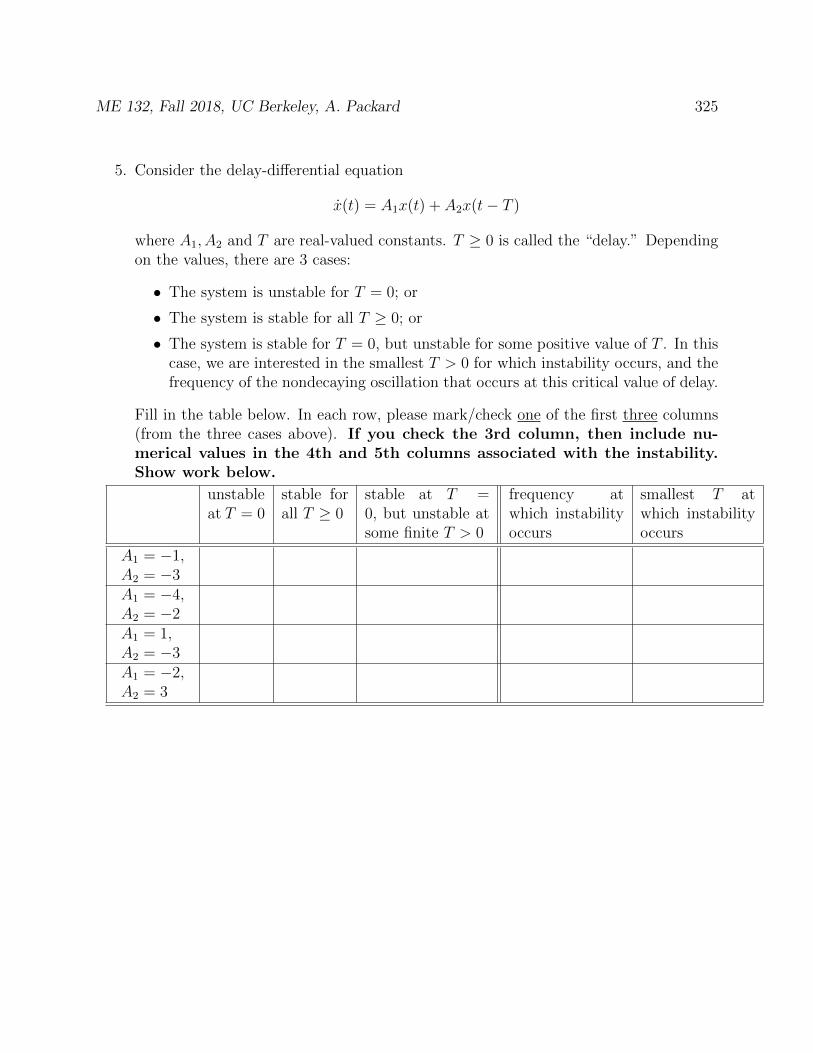
ME 132, Fall 2018, UC Berkeley, A. Packard 325
5. Consider the delay-differential equation
x(t) = A1x(t) + A2x(t− T )
where A1, A2 and T are real-valued constants. T ≥ 0 is called the “delay.” Dependingon the values, there are 3 cases:
• The system is unstable for T = 0; or
• The system is stable for all T ≥ 0; or
• The system is stable for T = 0, but unstable for some positive value of T . In thiscase, we are interested in the smallest T > 0 for which instability occurs, and thefrequency of the nondecaying oscillation that occurs at this critical value of delay.
Fill in the table below. In each row, please mark/check one of the first three columns(from the three cases above). If you check the 3rd column, then include nu-merical values in the 4th and 5th columns associated with the instability.Show work below.
unstableat T = 0
stable forall T ≥ 0
stable at T =0, but unstable atsome finite T > 0
frequency atwhich instabilityoccurs
smallest T atwhich instabilityoccurs
A1 = −1,A2 = −3A1 = −4,A2 = −2A1 = 1,A2 = −3A1 = −2,A2 = 3
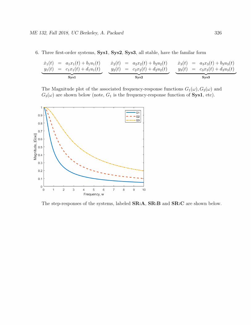
ME 132, Fall 2018, UC Berkeley, A. Packard 326
6. Three first-order systems, Sys1, Sys2, Sys3, all stable, have the familar form
x1(t) = a1x1(t) + b1u1(t)y1(t) = c1x1(t) + d1u1(t)︸ ︷︷ ︸
Sys1
x2(t) = a2x2(t) + b2u2(t)y2(t) = c2x2(t) + d2u2(t)︸ ︷︷ ︸
Sys2
x3(t) = a3x3(t) + b3u3(t)y3(t) = c3x3(t) + d3u3(t)︸ ︷︷ ︸
Sys3
The Magnitude plot of the associated frequency-response functions G1(ω), G2(ω) andG3(ω) are shown below (note, G1 is the frequency-response function of Sys1, etc).
The step-responses of the systems, labeled SR:A, SR:B and SR:C are shown below.
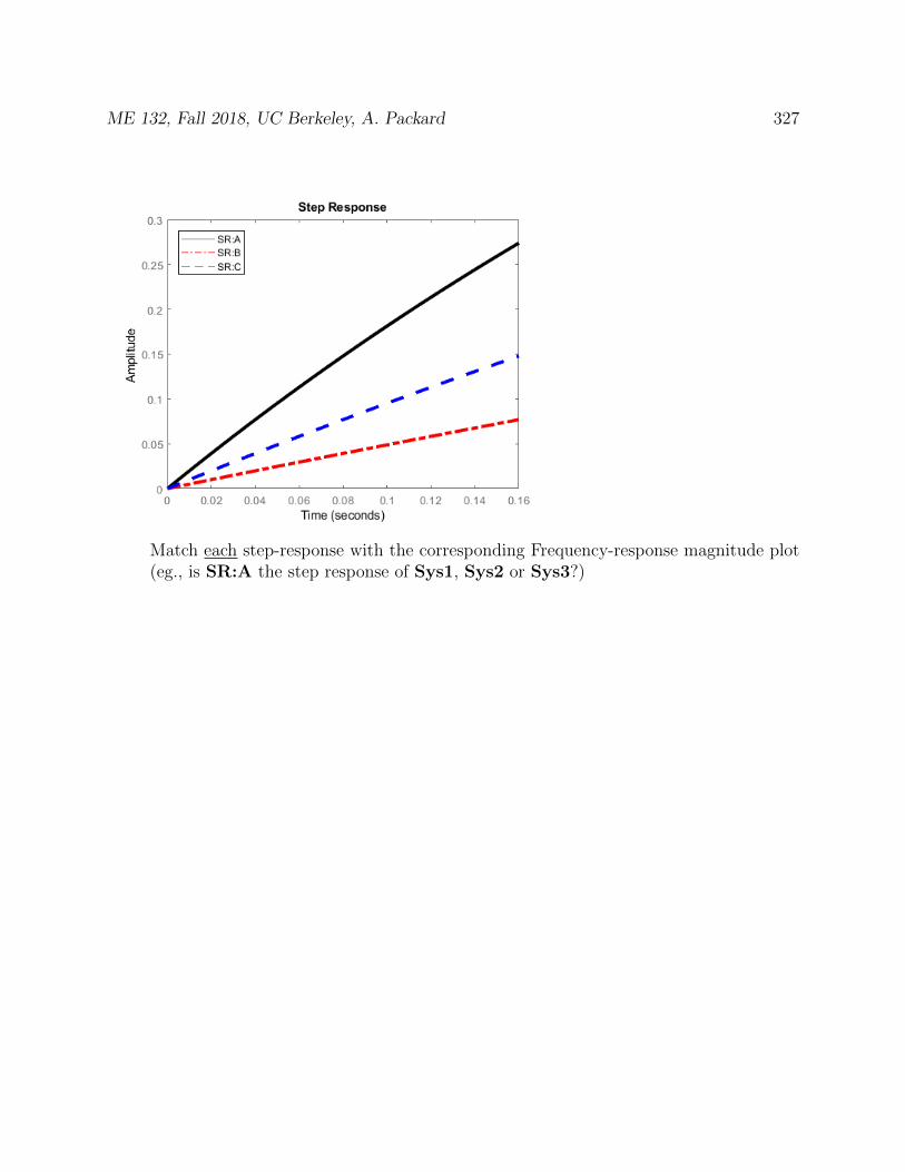
ME 132, Fall 2018, UC Berkeley, A. Packard 327
Match each step-response with the corresponding Frequency-response magnitude plot(eg., is SR:A the step response of Sys1, Sys2 or Sys3?)
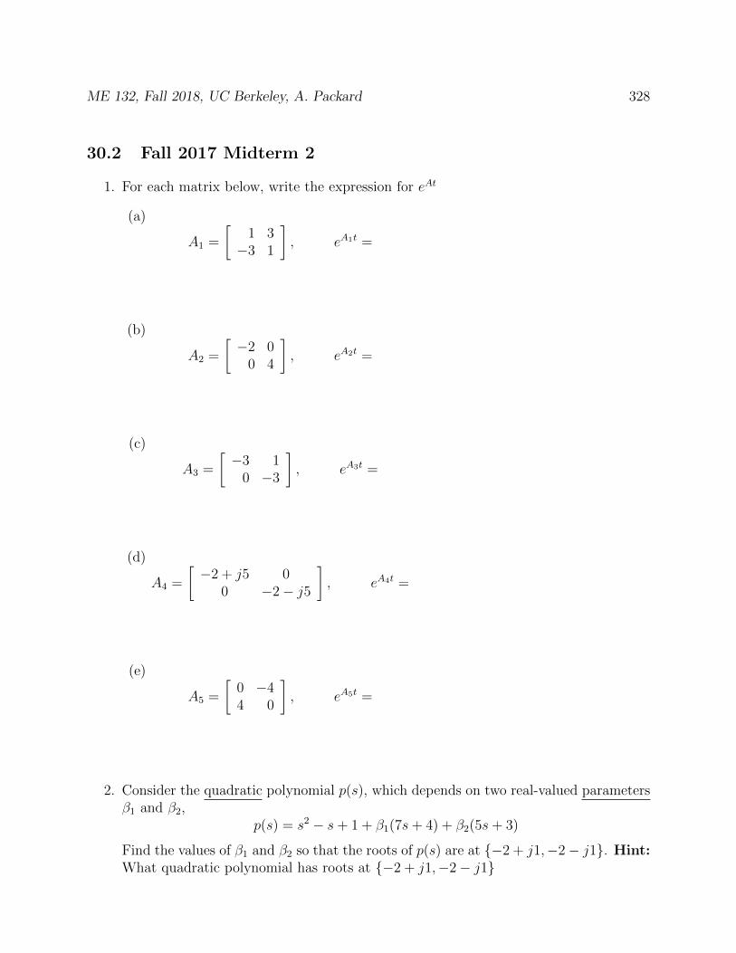
ME 132, Fall 2018, UC Berkeley, A. Packard 328
30.2 Fall 2017 Midterm 2
1. For each matrix below, write the expression for eAt
(a)
A1 =
[1 3−3 1
], eA1t =
(b)
A2 =
[−2 0
0 4
], eA2t =
(c)
A3 =
[−3 1
0 −3
], eA3t =
(d)
A4 =
[−2 + j5 0
0 −2− j5
], eA4t =
(e)
A5 =
[0 −44 0
], eA5t =
2. Consider the quadratic polynomial p(s), which depends on two real-valued parametersβ1 and β2,
p(s) = s2 − s+ 1 + β1(7s+ 4) + β2(5s+ 3)
Find the values of β1 and β2 so that the roots of p(s) are at −2 + j1,−2− j1. Hint:What quadratic polynomial has roots at −2 + j1,−2− j1
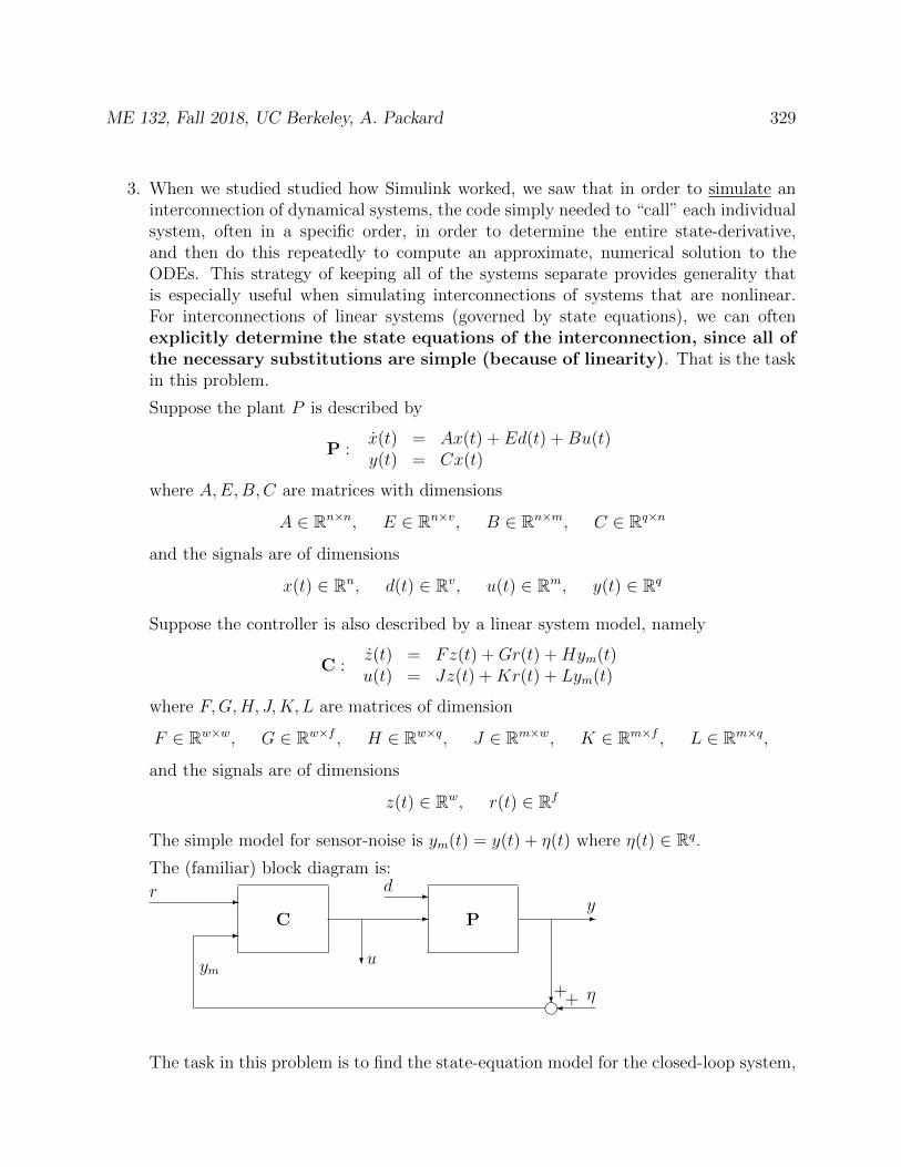
ME 132, Fall 2018, UC Berkeley, A. Packard 329
3. When we studied studied how Simulink worked, we saw that in order to simulate aninterconnection of dynamical systems, the code simply needed to “call” each individualsystem, often in a specific order, in order to determine the entire state-derivative,and then do this repeatedly to compute an approximate, numerical solution to theODEs. This strategy of keeping all of the systems separate provides generality thatis especially useful when simulating interconnections of systems that are nonlinear.For interconnections of linear systems (governed by state equations), we can oftenexplicitly determine the state equations of the interconnection, since all ofthe necessary substitutions are simple (because of linearity). That is the taskin this problem.
Suppose the plant P is described by
P :x(t) = Ax(t) + Ed(t) +Bu(t)y(t) = Cx(t)
where A,E,B,C are matrices with dimensions
A ∈ Rn×n, E ∈ Rn×v, B ∈ Rn×m, C ∈ Rq×n
and the signals are of dimensions
x(t) ∈ Rn, d(t) ∈ Rv, u(t) ∈ Rm, y(t) ∈ Rq
Suppose the controller is also described by a linear system model, namely
C :z(t) = Fz(t) +Gr(t) +Hym(t)u(t) = Jz(t) +Kr(t) + Lym(t)
where F,G,H, J,K, L are matrices of dimension
F ∈ Rw×w, G ∈ Rw×f , H ∈ Rw×q, J ∈ Rm×w, K ∈ Rm×f , L ∈ Rm×q,
and the signals are of dimensions
z(t) ∈ Rw, r(t) ∈ Rf
The simple model for sensor-noise is ym(t) = y(t) + η(t) where η(t) ∈ Rq.
The (familiar) block diagram is:
C P
-r
ym
-d
-
?u
-y
?g η++
-
The task in this problem is to find the state-equation model for the closed-loop system,
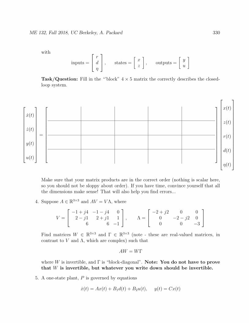
ME 132, Fall 2018, UC Berkeley, A. Packard 330
with
inputs =
rdη
, states =
[xz
], outputs =
[yu
]
Task/Question: Fill in the “’block” 4× 5 matrix the correctly describes the closed-loop system.
x(t)
z(t)
y(t)
u(t)
=
x(t)
z(t)
r(t)
d(t)
η(t)
Make sure that your matrix products are in the correct order (nothing is scalar here,so you should not be sloppy about order). If you have time, convince yourself that allthe dimensions make sense! That will also help you find errors...
4. Suppose A ∈ R3×3 and AV = V Λ, where
V =
−1 + j4 −1− j4 02− j1 2 + j1 1
6 6 −1
, Λ =
−2 + j2 0 00 −2− j2 00 0 −3
Find matrices W ∈ R3×3 and Γ ∈ R3×3 (note - these are real-valued matrices, incontrast to V and Λ, which are complex) such that
AW = WΓ
where W is invertible, and Γ is “block-diagonal”. Note: You do not have to provethat W is invertible, but whatever you write down should be invertible.
5. A one-state plant, P is governed by equations
x(t) = Ax(t) +B1d(t) +B2u(t), y(t) = Cx(t)
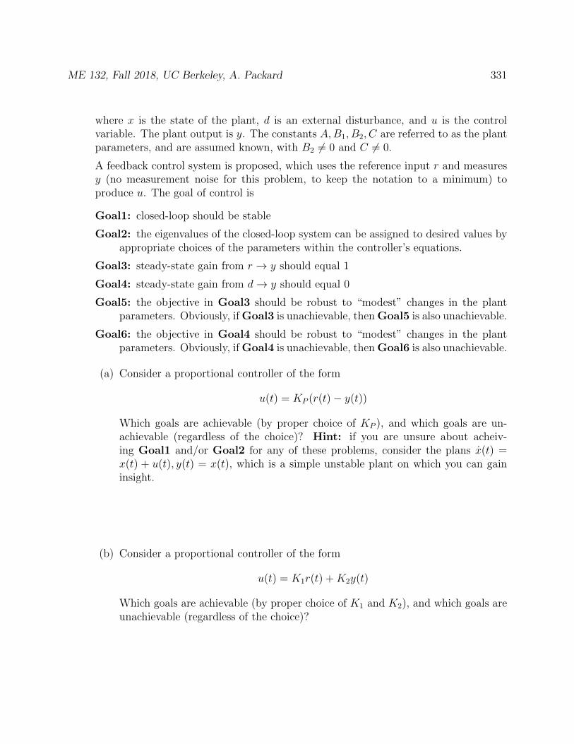
ME 132, Fall 2018, UC Berkeley, A. Packard 331
where x is the state of the plant, d is an external disturbance, and u is the controlvariable. The plant output is y. The constants A,B1, B2, C are referred to as the plantparameters, and are assumed known, with B2 6= 0 and C 6= 0.
A feedback control system is proposed, which uses the reference input r and measuresy (no measurement noise for this problem, to keep the notation to a minimum) toproduce u. The goal of control is
Goal1: closed-loop should be stable
Goal2: the eigenvalues of the closed-loop system can be assigned to desired values byappropriate choices of the parameters within the controller’s equations.
Goal3: steady-state gain from r → y should equal 1
Goal4: steady-state gain from d→ y should equal 0
Goal5: the objective in Goal3 should be robust to “modest” changes in the plantparameters. Obviously, if Goal3 is unachievable, then Goal5 is also unachievable.
Goal6: the objective in Goal4 should be robust to “modest” changes in the plantparameters. Obviously, if Goal4 is unachievable, then Goal6 is also unachievable.
(a) Consider a proportional controller of the form
u(t) = KP (r(t)− y(t))
Which goals are achievable (by proper choice of KP ), and which goals are un-achievable (regardless of the choice)? Hint: if you are unsure about acheiv-ing Goal1 and/or Goal2 for any of these problems, consider the plans x(t) =x(t) + u(t), y(t) = x(t), which is a simple unstable plant on which you can gaininsight.
(b) Consider a proportional controller of the form
u(t) = K1r(t) +K2y(t)
Which goals are achievable (by proper choice of K1 and K2), and which goals areunachievable (regardless of the choice)?
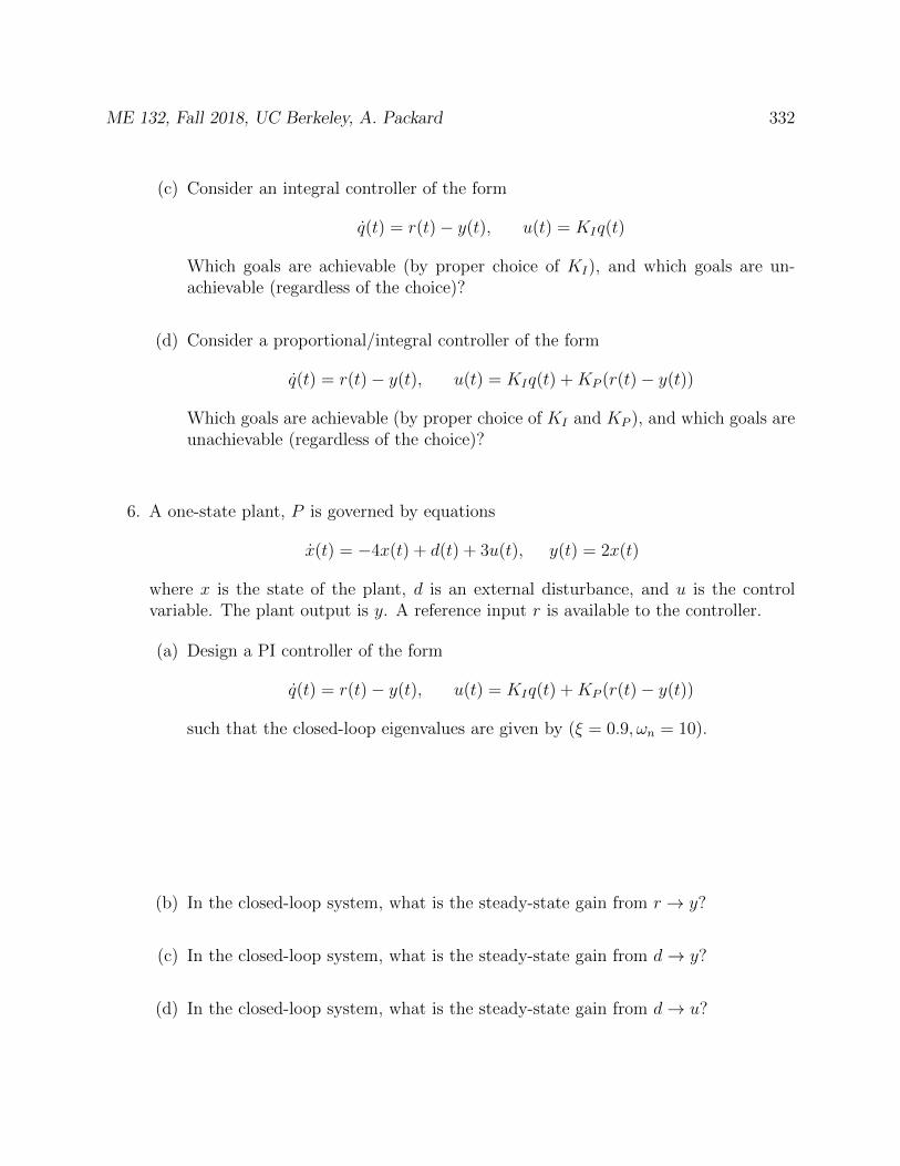
ME 132, Fall 2018, UC Berkeley, A. Packard 332
(c) Consider an integral controller of the form
q(t) = r(t)− y(t), u(t) = KIq(t)
Which goals are achievable (by proper choice of KI), and which goals are un-achievable (regardless of the choice)?
(d) Consider a proportional/integral controller of the form
q(t) = r(t)− y(t), u(t) = KIq(t) +KP (r(t)− y(t))
Which goals are achievable (by proper choice of KI and KP ), and which goals areunachievable (regardless of the choice)?
6. A one-state plant, P is governed by equations
x(t) = −4x(t) + d(t) + 3u(t), y(t) = 2x(t)
where x is the state of the plant, d is an external disturbance, and u is the controlvariable. The plant output is y. A reference input r is available to the controller.
(a) Design a PI controller of the form
q(t) = r(t)− y(t), u(t) = KIq(t) +KP (r(t)− y(t))
such that the closed-loop eigenvalues are given by (ξ = 0.9, ωn = 10).
(b) In the closed-loop system, what is the steady-state gain from r → y?
(c) In the closed-loop system, what is the steady-state gain from d→ y?
(d) In the closed-loop system, what is the steady-state gain from d→ u?
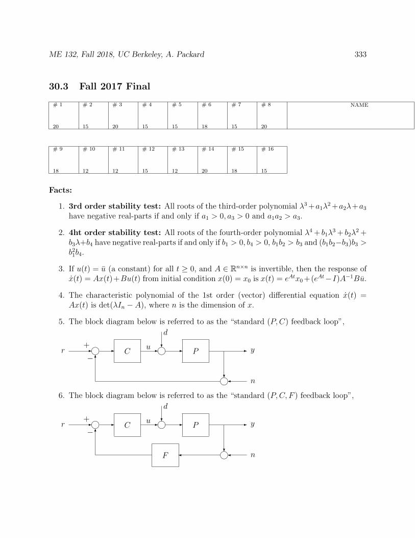
ME 132, Fall 2018, UC Berkeley, A. Packard 333
30.3 Fall 2017 Final
# 1
20
# 2
15
# 3
20
# 4
15
# 5
15
# 6
18
# 7
15
# 8
20
NAME
# 9
18
# 10
12
# 11
12
# 12
15
# 13
12
# 14
20
# 15
18
# 16
15
Facts:
1. 3rd order stability test: All roots of the third-order polynomial λ3 +a1λ2 +a2λ+a3
have negative real-parts if and only if a1 > 0, a3 > 0 and a1a2 > a3.
2. 4ht order stability test: All roots of the fourth-order polynomial λ4 + b1λ3 + b2λ
2 +b3λ+b4 have negative real-parts if and only if b1 > 0, b4 > 0, b1b2 > b3 and (b1b2−b3)b3 >b2
1b4.
3. If u(t) = u (a constant) for all t ≥ 0, and A ∈ Rn×n is invertible, then the response ofx(t) = Ax(t)+Bu(t) from initial condition x(0) = x0 is x(t) = eAtx0 +(eAt−I)A−1Bu.
4. The characteristic polynomial of the 1st order (vector) differential equation x(t) =Ax(t) is det(λIn − A), where n is the dimension of x.
5. The block diagram below is referred to as the “standard (P,C) feedback loop”,
C P- - - j -?
d
-
?j6
j+
−r u y
n
6. The block diagram below is referred to as the “standard (P,C, F ) feedback loop”,
C P
F
- - - j -?
d
-
?j
6
j+
−r u y
n
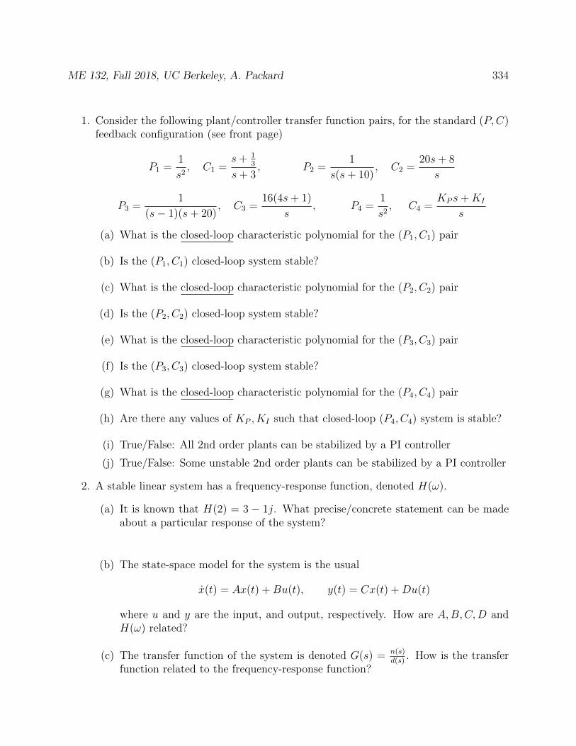
ME 132, Fall 2018, UC Berkeley, A. Packard 334
1. Consider the following plant/controller transfer function pairs, for the standard (P,C)feedback configuration (see front page)
P1 =1
s2, C1 =
s+ 13
s+ 3, P2 =
1
s(s+ 10), C2 =
20s+ 8
s
P3 =1
(s− 1)(s+ 20), C3 =
16(4s+ 1)
s, P4 =
1
s2, C4 =
KP s+KI
s
(a) What is the closed-loop characteristic polynomial for the (P1, C1) pair
(b) Is the (P1, C1) closed-loop system stable?
(c) What is the closed-loop characteristic polynomial for the (P2, C2) pair
(d) Is the (P2, C2) closed-loop system stable?
(e) What is the closed-loop characteristic polynomial for the (P3, C3) pair
(f) Is the (P3, C3) closed-loop system stable?
(g) What is the closed-loop characteristic polynomial for the (P4, C4) pair
(h) Are there any values of KP , KI such that closed-loop (P4, C4) system is stable?
(i) True/False: All 2nd order plants can be stabilized by a PI controller
(j) True/False: Some unstable 2nd order plants can be stabilized by a PI controller
2. A stable linear system has a frequency-response function, denoted H(ω).
(a) It is known that H(2) = 3 − 1j. What precise/concrete statement can be madeabout a particular response of the system?
(b) The state-space model for the system is the usual
x(t) = Ax(t) +Bu(t), y(t) = Cx(t) +Du(t)
where u and y are the input, and output, respectively. How are A,B,C,D andH(ω) related?
(c) The transfer function of the system is denoted G(s) = n(s)d(s)
. How is the transferfunction related to the frequency-response function?
ME 132, Fall 2018, UC Berkeley, A. Packard 335
3. The equations for a satellite orbiting a stationary mass are
x1(t) = x2(t), x2(t) = x1(t)x23(t)− β
x21(t)
, x3(t) =1
x1(t)(u(t)− 2x2(t)x3(t)) ,
where x1 is the radius, x2 is the rate-of-change of radius, and x3 is the orbital angularvelocity. The control u is a force applied in the tangential direction. The gravitationalconstant and mass of the stationary mass are collected into the single positive constantβ.
(a) Show that for any constant x1 > 0, there exist constants x2, x3 and u such that x1
x2
x3
, u
is an equilibrium point of the system. (Note - you can choose the equilibriumpoint that has x3 > 0).
(b) Find the Jacobian linearization of the system about the equilibrium point.
4. Suppose a linear system x(t) = Ax(t) +Bu(t) has state-space data
A =
0 1 0a 0 b0 −c 0
, B =
00d
,where a, b, c, d are positive constants.
(a) What is the characteristic polynomial of A?
(b) Given only the information that a, b, c, d are all positive, can you conclude any-thing about the stability (ie., all eigenvalues have negative real-parts) of the sys-tem?
(c) Define an output y(t) = Cx(t) with
C =[
0 0 1]
What is the transfer function from u to y?
5. Take the plant P , described by its transfer function,
P (s) =s2 − 4
s(s2 + 1)
which is quite challenging to control.
ME 132, Fall 2018, UC Berkeley, A. Packard 336
(a) Let u and y denote the input and output, respectively. What is the differentialequation governing the relationship between u and y
(b) Consider the standard (P,C) closed-loop configuration (see front page for defi-nition). Using a proportional controller, C(s) = KP , a constant-gain, can theclosed-loop system be made stable, by proper choice of KP ?
(c) In terms of transfer functions, what is the simplest controller form, C(s) you canpropose, such that if the controller coefficients are chosen properly, will renderthe closed-loop system (using standard (P,C) closed-loop configuration) stable?
6. Consider the standard (P,C) configuration. Let the transfer functions of P and C bedenoted
P (s) =nP (s)
dP (s), C(s) =
nC(s)
dC(s)
Match the defined transfer functions Mi or Ni with the closed-loop transfer functions(eg., Gr→y means closed-loop transfer function from r to y)
M1 :=nPnC
dPdC + nPnC, M2 :=
dPdCdPdC + nPnC
, M3 :=nPdC
dPdC + nPnC, M4 :=
dPnCdPdC + nPnC
N1 = −M1, N2 = −M2 N3 = −M3 N4 = −M4
(a) Gr→y =
(b) Gr→u =
(c) Gd→y =
(d) Gd→u =
(e) Gn→y =
(f) Gn→u =

ME 132, Fall 2018, UC Berkeley, A. Packard 337
7. Consider the standard (P,C, F ) configuration. Let the transfer functions of P and Cbe denoted
P (s) =nP (s)
dP (s), C(s) =
nC(s)
dC(s), F (s) =
nF (s)
dF (s)
We are interested in the closed-loop transfer functions, expressed similarly to the pre-vious problem (ie., simple fractions involving the individual n and d polynomials)
(a) What is the transfer function from r → u
(b) What is the transfer function from d→ y
(c) What is the transfer function from r → y
(d) What is the closed-loop characteristic polynomial of the system
8. The governing equations for a DC motor are
V (t)−RI(t)−Kω(t) = 0, Jω(t) = KI(t)− αω(t) + T (t)
• V (t) is the voltage across the motor winding, at the terminals; I(t) is the currentflowing through the motor windings; ω(t) is the angular velocity of the shaft; andT (t) is the sum of all torques applied externally to the motor shaft (interactionswith other linkages/inertias, disturbances, etc)
• J,K, α,R are positive constants, which are properties of the motor itself, namelythe shaft/gear inertia, the motor-constant, the viscous friction coefficient of thebearings, and the electrical resistance in the windings.
Consider two behaviors of the motor
shorted: the terminals are connected together so that V (t) = 0 for all t
open: the terminals are not connected to anything or to each other, so I(t) = 0 forall t
(a) Treating T as the single input, and (ω, I) as the two outputs, write state equationsfor the shorted system (hint: there is 1 state, and in this case, 1 input, and 2outputs)
(b) For the shorted system, what is the time-constant?
(c) For the shorted system, what is the transfer-function from T to ω?
(d) For the shorted system, what is the steady-state gain from T to ω?
ME 132, Fall 2018, UC Berkeley, A. Packard 338
(e) Treating T as the single input, and (ω, V ) as the 2 outputs, write state equationsfor the open system
(f) For the open system, what is the transfer-function from T to ω?
(g) For the open system, what is the steady-state gain from T to ω?
(h) For the open system, what is the time-constant?
(i) If you, with your hands/fingers, apply a torque to the two separate systems, whichwill be easier to turn? Why?
9. Consider the plant/controller pair (for the standard (P,C) configuration described onthe front page), described in transfer-function form
P (s) =1
s− α, C =
√5 · α (≈ 2.24α)
where α > 0 is a constant. Note that C is a constant gain. Remark: For the questionsbelow, if you have trouble, first work out the answers for the case α = 1, then go backand see how to generalize to an arbitrary, fixed, positive α.
(a) Is the plant P a stable system? Is the closed-loop system stable?
(b) Since the closed-loop system is a first-order system, what is the time-constant ofthe closed-loop system. Your answer will be in terms of α.
(c) Define L(s) := P (s)C. Using mathematical manipulations, find the frequencyωc ≥ 0 such that |L(jωc)| = 1. Your answer will be in terms of α.
(d) What is ∠L(jωc), in radians? Hint: Your answer will not depend on α.
(e) Make a simple sketch, in the complex-plane C, showing the unit-circle, and markthe value of L(jωc).
(f) What is the time-delay margin (in terms of α) for the closed-loop system?

ME 132, Fall 2018, UC Berkeley, A. Packard 339
10. The Bode plots (Magnitude and Phase) for 4 simple transfer functions,
G1(s) =1
−s+ 1, G2(s) = −s+ 1, G3(s) =
1
s+ 1, G4(s) = s+ 1
are shown below. Match each system to its corresponding plot
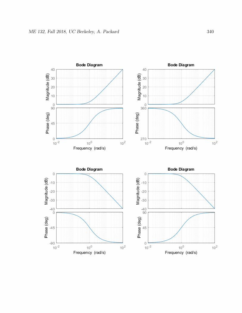
ME 132, Fall 2018, UC Berkeley, A. Packard 340
ME 132, Fall 2018, UC Berkeley, A. Packard 341
11. The Bode plots (Magnitude and Phase) for 4 simple transfer functions,
G1(s) =20
s+ 20, G2(s) =
0.2
s+ 0.2, G3(s) =
0.05
s+ 0.05, G4(s) =
5
s+ 5
are shown below. Match each system to its corresponding plot

ME 132, Fall 2018, UC Berkeley, A. Packard 342
ME 132, Fall 2018, UC Berkeley, A. Packard 343
12. Make a straight-line Bode plot (magnitude and phase) for the transfer function
G(s) = 9(−s+ 100)(s+ 1)
(s+ 3)(s+ 10)(s+ 30)
on the graph paper below. Be sure to normalize the terms properly (ie., write (s+ 30)as ( s
30+1), and account for all the accumulated scaling factors at the end with a single
gain adjustment). Important: The axes-limits on this graph paper are appropriatefor the final result. Use the graph-paper on the next page (which has wider limits, andeasier to get started with) to work out your solution, then transfer it to this page.

ME 132, Fall 2018, UC Berkeley, A. Packard 344
ME 132, Fall 2018, UC Berkeley, A. Packard 345

ME 132, Fall 2018, UC Berkeley, A. Packard 346
13. State whether each statement is True or False. No reasons need be given...
(a) For all A1, A2 ∈ Rn×n, and all t ≥ 0, e(A1+A2)t = eA1teA2t
(b) For all A ∈ Rn×n, and all t ∈ R, e(−A)t = eA(−t)
(c) For all A ∈ Rn×n, and all t ≥ 0, eAte−At = In
(d) For all A ∈ Rn×n, and all t ∈ R, the matrix eAt is invertible.
(e) For all A ∈ Rn×n, and all t1, t2 ∈ R, eA(t1+t2) = eAt2eAt1
(f) For all A ∈ Rn×n, and all t ∈ R, AeAt = eAtA
(g) For all A1, A2 ∈ Rn×n, and all t ≥ 0, A1eA2t = eA1tA2
(h) If A ∈ Rn×n is invertible, then for all t ∈ R, A−1eAt = eAtA−1
(i) If A ∈ Rn×n, then for all t ∈ R, and all ω ∈ R, (jωI − A)eAt = eAt(jωI − A)
(j) If A ∈ Rn×n has no imaginary eigenvalues, then for all t ∈ R, and all ω ∈ R,
(jωI − A)−1eAt = eAt(jωI − A)−1
(k) Consider the two expressions
E1 := (I + tA+t2
2A2)(I + tB +
t2
2B2), E2 := I + t(A+B) +
t2
2(A+B)2
where A,B ∈ Rn×n. Expand both expressions, and obtain the coefficient-matrixassociated with the t2 term. Are they equal, in general?
(l) Which disequality (circle your answer) comes from the reasoning in the previousproblem
e(A−B)t 6= eAte−Bt, BeAt 6= eBtA, eABt 6= eAteBt
ME 132, Fall 2018, UC Berkeley, A. Packard 347
14. A 2nd-order system, which represents the dynamical equations for a feedback controller,has state equations[
z1(t)z2(t)
]=
[1 23 4
] [z1(t)z2(t)
]+
[56
](r(t)− ymeas(t))
and output equation
u(t) =[
7 8] [ z1(t)
z2(t)
]+ 9(r(t)− ymeas(t))
The numbers are not necessarily realistic, but that is not the focus of the problem.Using the same ideas as in the lab, this control “strategy” is to implemented at asample-rate of 10 milliseconds (0.01 seconds).
Accessing the reference r and the measurement y is accomplished with 2 externalfunctions that we are free to call as needed:
• The reference signal is computed by an externally defined function named getReference.That function has one input argument (time, as an integer, in units of millisec-onds), and it returns a float.
• At any time, the process output, y can be measured and its value returned with thefunction makeMeasurement. This function has no input arguments, and returnsa float.
The control action, u(t) can be “sent” to the actuator with the command setControlValue.This function has one input argument, the value of the control action (as a float).The behavior of the function is that the control signal immediately gets set to thespecified value, and is held constant (at this value), until the function is called again.
On the next page, fill in the blank lines of the code to complete this program.
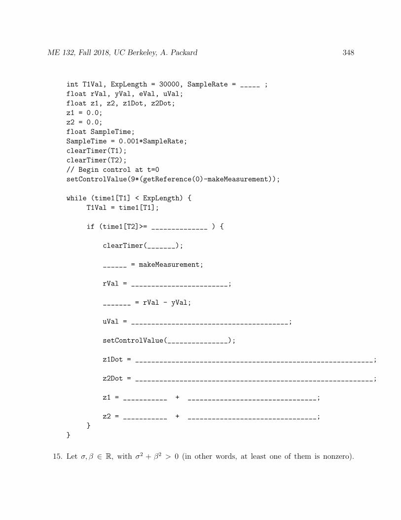
ME 132, Fall 2018, UC Berkeley, A. Packard 348
int T1Val, ExpLength = 30000, SampleRate = _____ ;
float rVal, yVal, eVal, uVal;
float z1, z2, z1Dot, z2Dot;
z1 = 0.0;
z2 = 0.0;
float SampleTime;
SampleTime = 0.001*SampleRate;
clearTimer(T1);
clearTimer(T2);
// Begin control at t=0
setControlValue(9*(getReference(0)-makeMeasurement));
while (time1[T1] < ExpLength)
T1Val = time1[T1];
if (time1[T2]>= ______________ )
clearTimer(_______);
______ = makeMeasurement;
rVal = ________________________;
_______ = rVal - yVal;
uVal = _______________________________________;
setControlValue(_______________);
z1Dot = ___________________________________________________________;
z2Dot = ___________________________________________________________;
z1 = ___________ + ________________________________;
z2 = ___________ + ________________________________;
15. Let σ, β ∈ R, with σ2 + β2 > 0 (in other words, at least one of them is nonzero).
ME 132, Fall 2018, UC Berkeley, A. Packard 349
Consider
A :=
[σ β−β σ
](a) What are the eigenvalues of A
(b) Is A invertible?
(c) What is the inverse of A
(d) A is a special matrix we studied in class. What is eAt
(e) What is (sI2 − A)−1
(f) What is A−1(eAt − In
)
16. Consider the linear system x(t) = Ax(t) +Bu(t), y(t) = Cx(t) for
A :=
[−4 3−3 −4
], B :=
[−2
3
], C =
[1 0
](a) What is the transfer function from u to y
(b) What is the exact expression for the response y(t) due to a unit-step input, u(t) =1 for all t, starting from initial condition x(0) = 0. See problem 15, and Facts onfront page if needed.
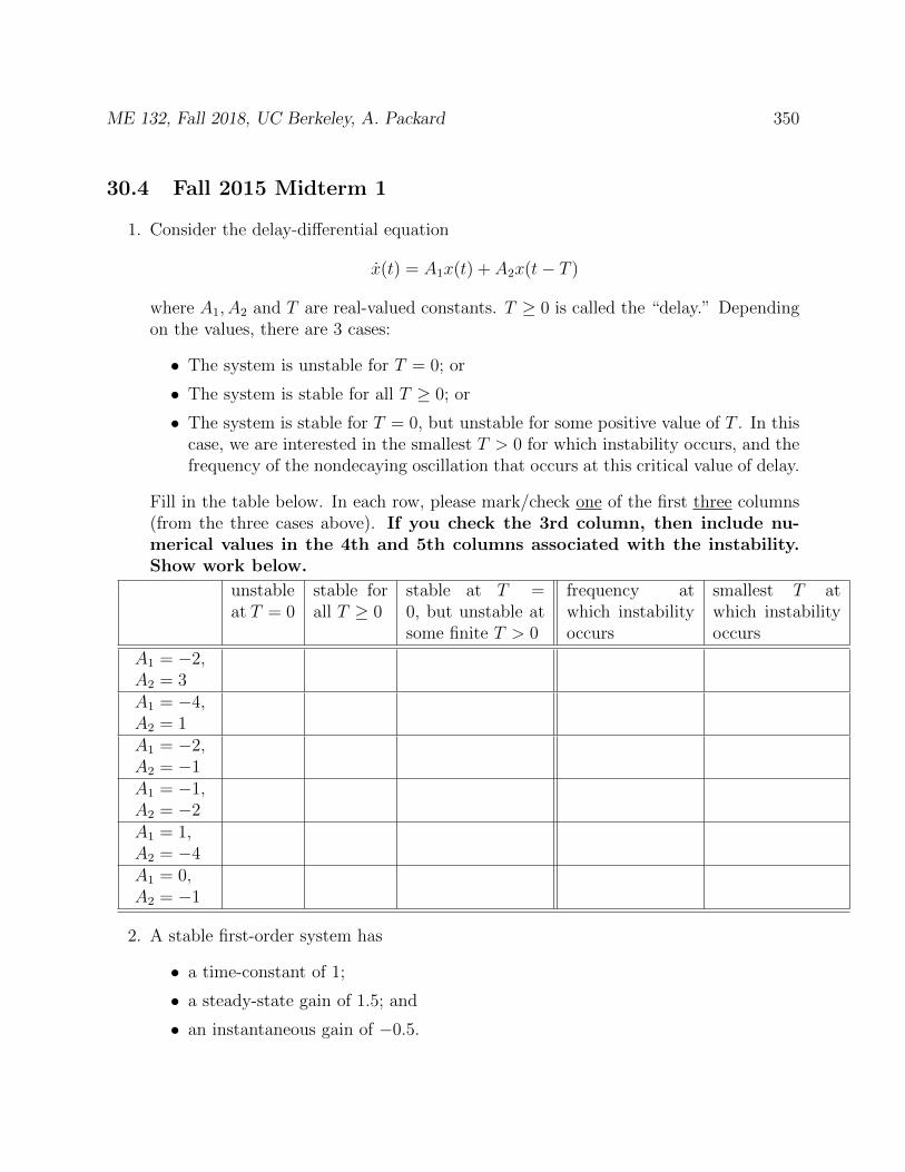
ME 132, Fall 2018, UC Berkeley, A. Packard 350
30.4 Fall 2015 Midterm 1
1. Consider the delay-differential equation
x(t) = A1x(t) + A2x(t− T )
where A1, A2 and T are real-valued constants. T ≥ 0 is called the “delay.” Dependingon the values, there are 3 cases:
• The system is unstable for T = 0; or
• The system is stable for all T ≥ 0; or
• The system is stable for T = 0, but unstable for some positive value of T . In thiscase, we are interested in the smallest T > 0 for which instability occurs, and thefrequency of the nondecaying oscillation that occurs at this critical value of delay.
Fill in the table below. In each row, please mark/check one of the first three columns(from the three cases above). If you check the 3rd column, then include nu-merical values in the 4th and 5th columns associated with the instability.Show work below.
unstableat T = 0
stable forall T ≥ 0
stable at T =0, but unstable atsome finite T > 0
frequency atwhich instabilityoccurs
smallest T atwhich instabilityoccurs
A1 = −2,A2 = 3A1 = −4,A2 = 1A1 = −2,A2 = −1A1 = −1,A2 = −2A1 = 1,A2 = −4A1 = 0,A2 = −1
2. A stable first-order system has
• a time-constant of 1;
• a steady-state gain of 1.5; and
• an instantaneous gain of −0.5.

ME 132, Fall 2018, UC Berkeley, A. Packard 351
(a) Sketch the approximate response of the system (starting from 0-initial condition)to the input shown. Remember that the steady-state gain is not equal to 1.
(b) Find values a, b, c, d such that system
x(t) = ax(t) + bu(t)y(t) = cx(t) + du(t)
has the specified properties (ie., time-constant, steady-state gain, and instan-taneous gain) as given above. Hint: Correct answer is not unique - differentcombinations of (a, b, c, d) all combine to achieve these 3 specified properties.
3. (a) Define the complex number g = 5j4+3
.
i. Find the value of Re(g)
ii. Find the value of Im(g)
iii. Find the value of |g|iv. Find the value of ∠g
(b) Sketch the final output (in the axes) of the Matlab code
uH = @(z) sin(4*z);
fH = @(t,x) -3*x + 5*uH(t);
[tSol, xSol] = ode45(fH,[0 100],-6);
plot(tSol, uH(tSol),’--’, tSol, xSol); % input=dashed; solution=solid
xlim((2*pi/4)*[20 21]); % resets horizontal limits
ME 132, Fall 2018, UC Berkeley, A. Packard 352
4. A process, with input u, disturbance d and output y is governed by
x(t) = 2x(t) + d(t) + 3u(t), y(t) = x(t)
(a) Is the process stable?
(b) Suppose x(0) = 1, and u(t) = d(t) ≡ 0 for all t ≥ 0. What is the solution x(t) fort ≥ 0.
(c) Consider a proportional-control strategy, u(t) = K1r(t) +K2 [r(t)− y(t)]. Deter-mine the closed-loop differential equation relating the variables (x, r, d).
(d) For what values of K1 and K2 is the closed-loop system stable?

ME 132, Fall 2018, UC Berkeley, A. Packard 353
(e) As a function of K2, what is the steady-state gain from d→ y in the closed-loopsystem?
(f) As a function of K1 and K2, what is the steady-state gain from r → y in theclosed-loop system?
(g) Choose K1 and K2 so that the steady-state gain from r → y equals 1, and thesteady-state gain from d→ y equals 0.1.

ME 132, Fall 2018, UC Berkeley, A. Packard 354
(h) With those gains chosen, sketch (try to be accurate) the two responses y(t) andu(t) for the following situation:
x(0) = 0, r(t) =
0 for 0 ≤ t ≤ 11 for 1 < t
, d(t) =
0 for 0 ≤ t ≤ 21 for 2 < t
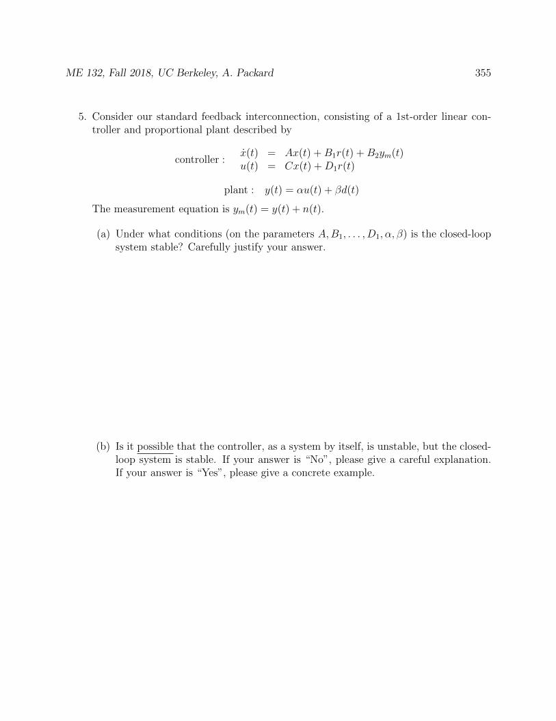
ME 132, Fall 2018, UC Berkeley, A. Packard 355
5. Consider our standard feedback interconnection, consisting of a 1st-order linear con-troller and proportional plant described by
controller :x(t) = Ax(t) +B1r(t) +B2ym(t)u(t) = Cx(t) +D1r(t)
plant : y(t) = αu(t) + βd(t)
The measurement equation is ym(t) = y(t) + n(t).
(a) Under what conditions (on the parameters A,B1, . . . , D1, α, β) is the closed-loopsystem stable? Carefully justify your answer.
(b) Is it possible that the controller, as a system by itself, is unstable, but the closed-loop system is stable. If your answer is “No”, please give a careful explanation.If your answer is “Yes”, please give a concrete example.
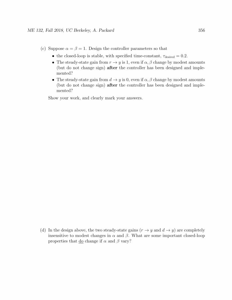
ME 132, Fall 2018, UC Berkeley, A. Packard 356
(c) Suppose α = β = 1. Design the controller parameters so that
• the closed-loop is stable, with specified time-constant, τdesired = 0.2.
• The steady-state gain from r → y is 1, even if α, β change by modest amounts(but do not change sign) after the controller has been designed and imple-mented?
• The steady-state gain from d→ y is 0, even if α, β change by modest amounts(but do not change sign) after the controller has been designed and imple-mented?
Show your work, and clearly mark your answers.
(d) In the design above, the two steady-state gains (r → y and d→ y) are completelyinsensitive to modest changes in α and β. What are some important closed-loopproperties that do change if α and β vary?
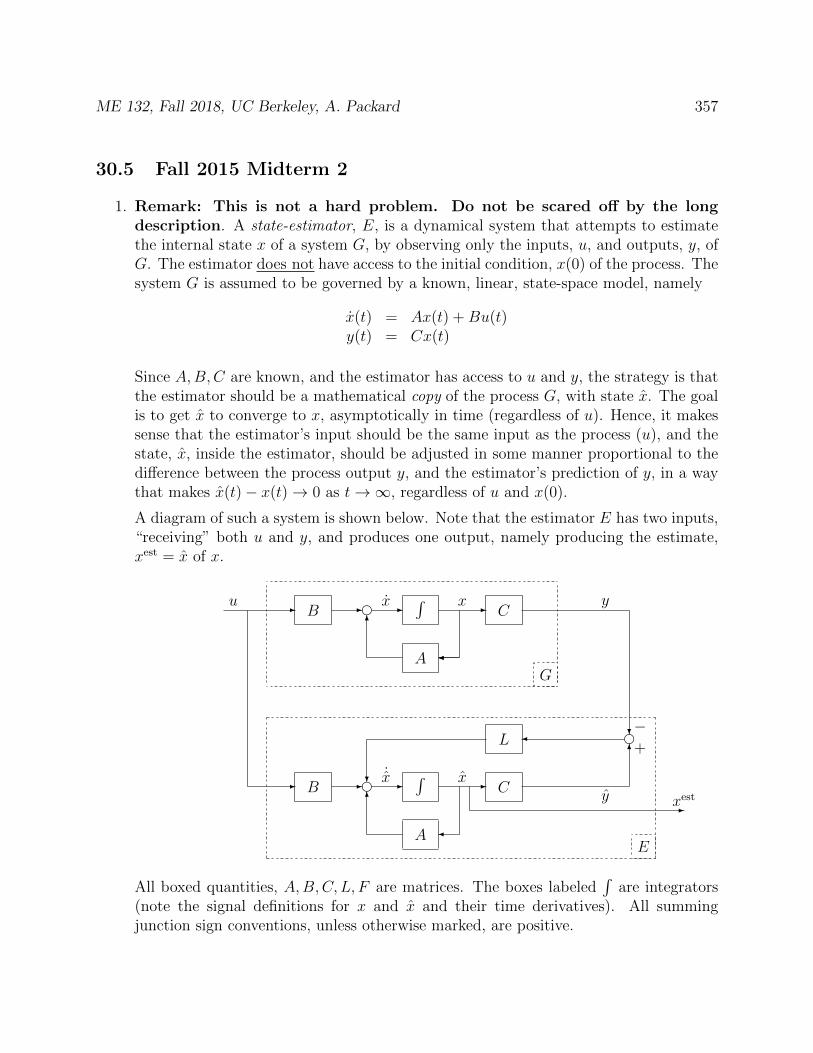
ME 132, Fall 2018, UC Berkeley, A. Packard 357
30.5 Fall 2015 Midterm 2
1. Remark: This is not a hard problem. Do not be scared off by the longdescription. A state-estimator, E, is a dynamical system that attempts to estimatethe internal state x of a system G, by observing only the inputs, u, and outputs, y, ofG. The estimator does not have access to the initial condition, x(0) of the process. Thesystem G is assumed to be governed by a known, linear, state-space model, namely
x(t) = Ax(t) +Bu(t)y(t) = Cx(t)
Since A,B,C are known, and the estimator has access to u and y, the strategy is thatthe estimator should be a mathematical copy of the process G, with state x. The goalis to get x to converge to x, asymptotically in time (regardless of u). Hence, it makessense that the estimator’s input should be the same input as the process (u), and thestate, x, inside the estimator, should be adjusted in some manner proportional to thedifference between the process output y, and the estimator’s prediction of y, in a waythat makes x(t)− x(t)→ 0 as t→∞, regardless of u and x(0).
A diagram of such a system is shown below. Note that the estimator E has two inputs,“receiving” both u and y, and produces one output, namely producing the estimate,xest = x of x.
E
G
B∫A
C- - -
6
f xx
x˙x ∫A
?f - -
-xest
6
6
f ?−+
B -
L
C
-u y
y-
All boxed quantities, A,B,C, L, F are matrices. The boxes labeled∫
are integrators(note the signal definitions for x and x and their time derivatives). All summingjunction sign conventions, unless otherwise marked, are positive.
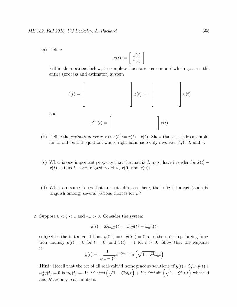
ME 132, Fall 2018, UC Berkeley, A. Packard 358
(a) Define
z(t) :=
[x(t)x(t)
]Fill in the matrices below, to complete the state-space model which governs theentire (process and estimator) system
z(t) =
z(t) +
u(t)
and
xest(t) =
[ ]z(t)
(b) Define the estimation error, e as e(t) := x(t)−x(t). Show that e satisfies a simple,linear differential equation, whose right-hand side only involves, A,C, L and e.
(c) What is one important property that the matrix L must have in order for x(t)−x(t)→ 0 as t→∞, regardless of u, x(0) and x(0)?
(d) What are some issues that are not addressed here, that might impact (and dis-tinguish among) several various choices for L?
2. Suppose 0 < ξ < 1 and ωn > 0. Consider the system
y(t) + 2ξωny(t) + ω2ny(t) = ωnu(t)
subject to the initial conditions y(0−) = 0, y(0−) = 0, and the unit-step forcing func-tion, namely u(t) = 0 for t = 0, and u(t) = 1 for t > 0. Show that the responseis
y(t) =1√
1− ξ2e−ξωnt sin
(√1− ξ2ωnt
)Hint: Recall that the set of all real-valued homogeneous solutions of y(t)+2ξωny(t)+
ω2ny(t) = 0 is yH(t) = Ae−ξωnt cos
(√1− ξ2ωnt
)+ Be−ξωnt sin
(√1− ξ2ωnt
)where A
and B are any real numbers.
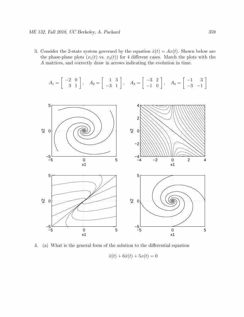
ME 132, Fall 2018, UC Berkeley, A. Packard 359
3. Consider the 2-state system governed by the equation x(t) = Ax(t). Shown below arethe phase-plane plots (x1(t) vs. x2(t)) for 4 different cases. Match the plots with theA matrices, and correctly draw in arrows indicating the evolution in time.
A1 =
[−2 0
3 1
], A2 =
[1 3−3 1
], A3 =
[−3 2−1 0
], A4 =
[−1 3−3 −1
]
−5 0 5−5
0
5
x1
x2
−4 −2 0 2 4−4
−2
0
2
4
x1
x2
−5 0 5−5
0
5
x1
x2
−5 0 5−5
0
5
x1
x2
4. (a) What is the general form of the solution to the differential equation
x(t) + 6x(t) + 5x(t) = 0

ME 132, Fall 2018, UC Berkeley, A. Packard 360
(b) What is the general form of the solution to the differential equation
x(t) + 6x(t) + 5x(t) = −10
Your expressions both should have two free constants.
5. A first-order process, with state x, input u, disturbance d and output y is governed by
x(t) = x(t) + u(t) + d(t), y(t) = x(t)
(a) Is the process stable?
(b) Suppose x(0) = −3, and u(t) = d(t) ≡ 0 for all t ≥ 0. What is the solution y(t)for t ≥ 0.
(c) A PI (Proportional plus Integral) controller is proposed
u(t) = KP [r(t)− y(t)] +KIz(t)z(t) = r(t)− y(t)
Define the state-vector q as
q(t) :=
[x(t)z(t)
]Write the state-space model of the closed-loop system, with state q, inputs (d, r)and outputs (y, u).

ME 132, Fall 2018, UC Berkeley, A. Packard 361
(d) What is the closed-loop characteristic polynomial?
(e) For what values of KP and KI is the closed-loop system stable?
(f) The closed-loop system is 2nd order. What are the appropriate values of KP andKI so that the closed-loop system eigenvalues are described by ξ = 0.8, ωn = 0.5?
(g) What are the appropriate values of KP and KI so that the closed-loop systemeigenvalues are described by ξ = 0.8, ωn = 1.0?
(h) What are the appropriate values of KP and KI so that the closed-loop systemeigenvalues are described by ξ = 0.8, ωn = 2.0?
6. A 2nd-order, unstable process, with control input u, disturbance input d, and outputy, is governed by the equation
y(t) + y(t)− y(t) = u(t) + d(t)
A PI (Proportional plus Integral) controller is proposed, both to stabilize the system,and provide good disturbance rejection,
u(t) = KP [r(t)− y(t)] +KIz(t)z(t) = r(t)− y(t)
Here r is a reference input.
(a) Using just the controller equations, express u(t) in terms of r, r, y and y.
(b) By differentiating the process equation, and substituting, derive the closed-loopdifferential equation relating r and d (and possibly their derivatives) to theoutput variable y (and its derivatives). The variable u should not appear in theseequations.
(c) Using the 3rd-order test for stability, determine the conditions on KP and KI
such that the closed-loop system is stable.
ME 132, Fall 2018, UC Berkeley, A. Packard 362
30.6 Fall 2015 Final
1. For each question, state whether the claim is True or False. Give a concise justifica-tion.
(a) True/False: First-order (1-state) linear systems can have an oscillatory free-response
(b) True/False:The steady-state response of a stable linear system, due to a sinu-soidal input, depends on the initial condition
(c) True/False:The 2-degree-of-freedom PI controller (with gains K1, K2, KI)
z(t) = r(t)− y(t)u(t) = K1r(t)−K2y(t) +KIz(t)
can stabilize some unstable linear plants that the 1-degree-of-freedom PI controller(with gains KP , KI),
z(t) = r(t)− y(t)u(t) = KP (r(t)− y(t)) +KIz(t)
cannot stabilize.

ME 132, Fall 2018, UC Berkeley, A. Packard 363
(d) Fact: Plants (call these “class L”) whose input signals (u) are limited betweenfixed upper and lower bounds (for example, it must be that −1 ≤ u(t) ≤ 1)are more challenging to control than plants whose input signals can take on anyvalues (call these plant, with no limit on u, “class U”).
i. True/False: AntiWindup logic fixes this deficiency, and make the two typesof plants (class L and class U) equally easy to control, regarding referencetracking, disturbance rejection and noise insensitivity.
ii. True/False: AntiWindup logic can be especially useful in dealing with plantsfrom class L, when being controlled with a proportional controller.
iii. True/False: AntiWindup logic can be especially useful in dealing with plantsfrom class L, when being controlled with an integral controller.
iv. True/False: AntiWindup logic can be especially useful in dealing with plantsfrom class L, when being controlled with an proportional+integral (PI) con-troller.
v. True/False: For AntiWindup logic to be effective, the lower limit on u mustbe equal and opposite to the upper limit on u
vi. True/False: Implementing AntiWindup logic in a PI controller is very com-plicated and computationally expensive, making it difficult and challengingto implement in many cases.
ME 132, Fall 2018, UC Berkeley, A. Packard 364
(e) True/False: For a nonlinear system x(t) = f(x(t), u(t)), with equilibrium point(x, u), the Jacobian linearization w(t) = Aw(t)+Bv(t) describes the approximatebehavior of w(t) := x(t)− x and v(t) := u(t)− u, while w and v remain small.
(f) True/False: For a nonlinear system x(t) = f(x(t), u(t)), with equilibrium point(x, u), the Jacobian linearization w(t) = Aw(t)+Bv(t) describes the approximatebehavior of w(t) := x(t)− x and v(t) := u(t)− u, while x and u remain small.
(g) True/False: Since many control systems are used to regulate a system nearan equilibrium point, the combination of Jacobian linearization and control tech-niques which apply to linear systems are a powerful combination to design controlsystems for nonlinear plants that are regulated near an equilibrium point.
ME 132, Fall 2018, UC Berkeley, A. Packard 365
(h) True/False: The plant
P (s) =(s+ 3)(s− 10)
(s− 1)(s+ 2)(s2 − 0.4s+ 1)
can be stabilized with a controller of the form
C(s) =b0s
3 + b1s2 + b2s+ b3
s3 + a1s2 + a2s+ a3
by proper choice of the bi, ai coefficients.
(i) True/False: The plant
P (s) =(s+ 3)(s− 10)
(s− 1)(s+ 2)(s2 − 0.4s+ 1)
cannot be stabilized with a controller of the form
C(s) =b0s
4 + b1s3 + b2s
3 + b3s+ b4
s(s3 + a1s2 + a2s+ a3)
by any choice of the bi, ai coefficients, because of the extra “s” term in thedenominator.
(j) True/False: Any 3rd-order plant of the form
P (s) =b1s
2 + b2s+ b3
s3 + a1s2 + a2s+ a3
can be stabilized with a controller of the form
C(s) =e0s+ e1
s+ f1
by proper choice of the e0, e1, f1 coefficients, but the roots of the closed-loopcharacteristic equation (which is 4th order) cannot be arbitrarily assigned sincethere are only 3 free parameters, (e0, e1, f1), to work with.
2. Consider the system described by state equations
x1(t) = x1(t) + 3x2(t) + u(t)x2(t) = −x1(t)− 2x2(t) + u(t)y(t) = x2(t)
with state x, input u and output y.
(a) Is the system stable?
(b) Eliminate x from the state equations below to obtain the differential equationrelating input u and output y
(c) What is the peak-magnitude of the steady-state response of the system due tothe input u(t) = sin t?
ME 132, Fall 2018, UC Berkeley, A. Packard 366
3. Find A, B C and D matrices, of appropriate dimension, such that the relationshipbetween u and y in the state-space model
x(t) = Ax(t) +Bu(t)y(t) = Cx(t) +Du(t)
isy[3](t) + 4y[2](t)− y[1](t) + 7y(t) = −2u[1](t) + 7u(t)
4. A plant P is described by the differential equation y(t) = 2y(t) + u(t) + d(t), where urepresents a control-input, and d is a disturbance.
(a) Using a proportional controller, u(t) = KP (r(t)− y(t)), what is the condition onKP for closed-loop stability?
(b) Assuming KP is chosen so that the closed-loop system is stable, what are thefollowing quantities
i. closed-loop time constant
ii. closed-loop steady-state gain from r → y
iii. closed-loop steady-state gain from d→ y
(c) Using a 2 degree-of-freedom proportional controller, u(t) = K1r(t)−K2y(t), whatare the conditions on K1 and K2 for closed-loop stability?
(d) Assuming (K1, K2) are chosen so that the closed-loop system is stable, what arethe following quantities
i. closed-loop time constant
ii. closed-loop steady-state gain from r → y
iii. closed-loop steady-state gain from d→ y
ME 132, Fall 2018, UC Berkeley, A. Packard 367
(e) Using a integral controller, u(t) = KIz(t); z(t) = r(t)−y(t), what is the conditionon KI for closed-loop stability?
(f) Using a PI controller, u(t) = KIz(t) + KP (r(t) − y(t)); z(t) = r(t) − y(t), whatare the conditions on (KI , KP ) for closed-loop stability
(g) Assuming (KI , KP ) are chosen so that the closed-loop system is stable, what arethe following quantities
i. closed-loop damping ratio
ii. closed-loop steady-state gain from r → y
iii. closed-loop steady-state gain from d→ y
5. In this problem, we see how an adjustment to the right-hand-side of an ODE modelcan approximately model the effect of a small time-delay.
(a) Suppose b is a fixed real number. Solve (for c1 and c2) the system of simultaneouslinear equations below
−1 + c1 + c2 = 0, −c1 + c2 = b
(b) Calculate the unit-step response (input u, output y) for the differential equation
y(t)− y(t) = bu(t) + u(t)
Initial conditions are y(0−1) = 0, y(0−) = 0. Your answer should involve b and t.
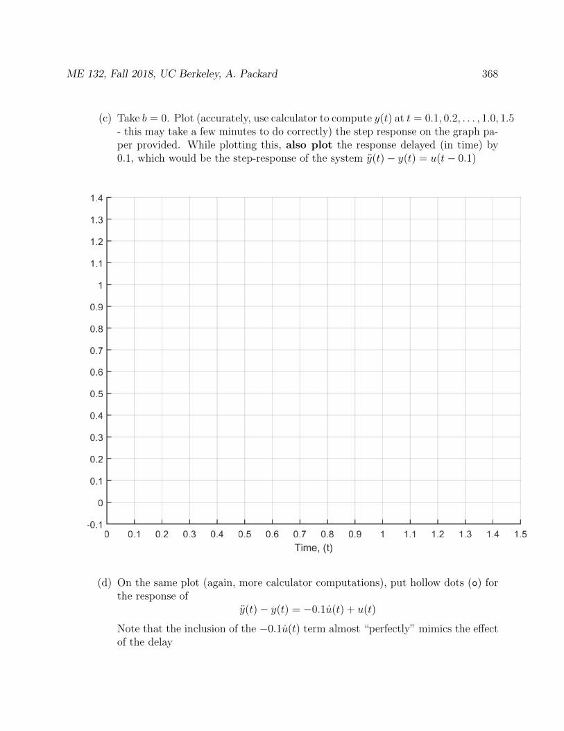
ME 132, Fall 2018, UC Berkeley, A. Packard 368
(c) Take b = 0. Plot (accurately, use calculator to compute y(t) at t = 0.1, 0.2, . . . , 1.0, 1.5- this may take a few minutes to do correctly) the step response on the graph pa-per provided. While plotting this, also plot the response delayed (in time) by0.1, which would be the step-response of the system y(t)− y(t) = u(t− 0.1)
(d) On the same plot (again, more calculator computations), put hollow dots (o) forthe response of
y(t)− y(t) = −0.1u(t) + u(t)
Note that the inclusion of the −0.1u(t) term almost “perfectly” mimics the effectof the delay
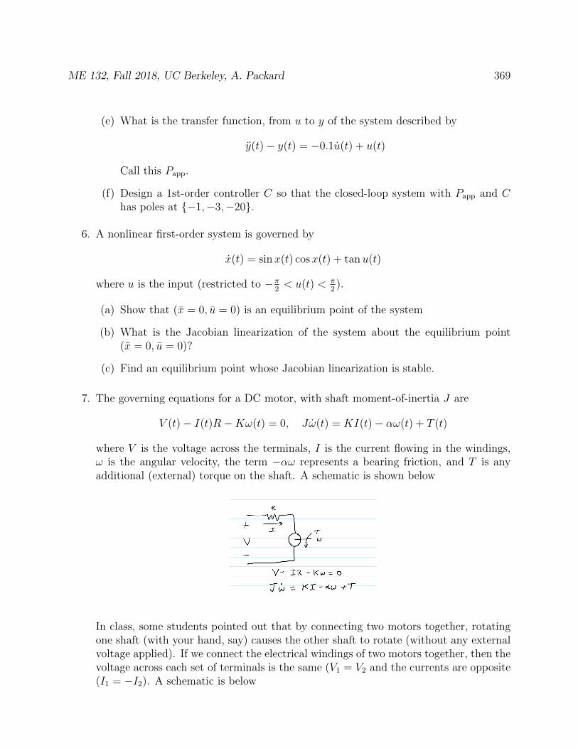
ME 132, Fall 2018, UC Berkeley, A. Packard 369
(e) What is the transfer function, from u to y of the system described by
y(t)− y(t) = −0.1u(t) + u(t)
Call this Papp.
(f) Design a 1st-order controller C so that the closed-loop system with Papp and Chas poles at −1,−3,−20.
6. A nonlinear first-order system is governed by
x(t) = sin x(t) cosx(t) + tanu(t)
where u is the input (restricted to −π2< u(t) < π
2).
(a) Show that (x = 0, u = 0) is an equilibrium point of the system
(b) What is the Jacobian linearization of the system about the equilibrium point(x = 0, u = 0)?
(c) Find an equilibrium point whose Jacobian linearization is stable.
7. The governing equations for a DC motor, with shaft moment-of-inertia J are
V (t)− I(t)R−Kω(t) = 0, Jω(t) = KI(t)− αω(t) + T (t)
where V is the voltage across the terminals, I is the current flowing in the windings,ω is the angular velocity, the term −αω represents a bearing friction, and T is anyadditional (external) torque on the shaft. A schematic is shown below
In class, some students pointed out that by connecting two motors together, rotatingone shaft (with your hand, say) causes the other shaft to rotate (without any externalvoltage applied). If we connect the electrical windings of two motors together, then thevoltage across each set of terminals is the same (V1 = V2 and the currents are opposite(I1 = −I2). A schematic is below
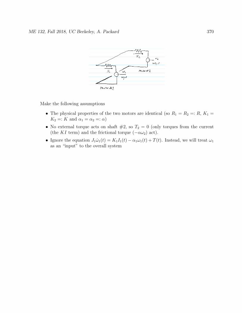
ME 132, Fall 2018, UC Berkeley, A. Packard 370
Make the following assumptions
• The physical properties of the two motors are identical (so R1 = R2 =: R, K1 =K2 =: K and α1 = α2 =: α)
• No external torque acts on shaft #2, so T2 = 0 (only torques from the current(the KI term) and the frictional torque (−αω2) act).
• Ignore the equation J1ω1(t) = K1I1(t)− α1ω1(t) + T (t). Instead, we will treat ω1
as an “input” to the overall system
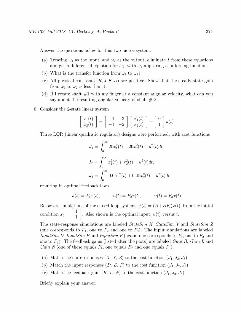
ME 132, Fall 2018, UC Berkeley, A. Packard 371
Answer the questions below for this two-motor system.
(a) Treating ω1 as the input, and ω2 as the output, eliminate I from these equationsand get a differential equation for ω2, with ω1 appearing as a forcing function.
(b) What is the transfer function from ω1 to ω2?
(c) All physical constants (R, J,K, α) are positive. Show that the steady-state gainfrom ω1 to ω2 is less than 1.
(d) If I rotate shaft #1 with my finger at a constant angular velocity, what can yousay about the resulting angular velocity of shaft # 2.
8. Consider the 2-state linear system[x1(t)x2(t)
]=
[1 3−1 −2
] [x1(t)x2(t)
]+
[01
]u(t)
Three LQR (linear quadratic regulator) designs were performed, with cost functions
J1 =
∫ ∞0
20x21(t) + 20x2
2(t) + u2(t)dt,
J2 =
∫ ∞0
x21(t) + x2
2(t) + u2(t)dt,
J3 =
∫ ∞0
0.05x21(t) + 0.05x2
2(t) + u2(t)dt
resulting in optimal feedback laws
u(t) = F1x(t), u(t) = F2x(t), u(t) = F3x(t)
Below are simulations of the closed-loop systems, x(t) = (A+BFi)x(t), from the initial
condition x0 =
[11
]. Also shown is the optimal input, u(t) versus t.
The state-response simulations are labeled StateSim X, StateSim Y and StateSim Z(one corresponds to F1, one to F2 and one to F3). The input simulations are labeledInputSim D, InputSim E and InputSim F (again, one corresponds to F1, one to F2 andone to F3). The feedback gains (listed after the plots) are labeled Gain H, Gain L andGain N (one of these equals F1, one equals F2 and one equals F3).
(a) Match the state responses (X, Y, Z) to the cost function (J1, J2, J3)
(b) Match the input responses (D, E, F) to the cost function (J1, J2, J3)
(c) Match the feedback gain (H, L, N) to the cost function (J1, J2, J3)
Briefly explain your answer.
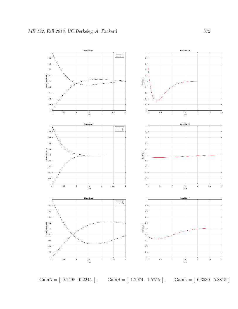
ME 132, Fall 2018, UC Berkeley, A. Packard 372
GainN =[
0.1498 0.2245], GainH =
[1.2974 1.5755
], GainL =
[6.3530 5.8815
]
ME 132, Fall 2018, UC Berkeley, A. Packard 373
9. In lab, we discovered a simple architecture that would lead to some form of approxi-mate coordination and synchronization of two identical systems, being acted upon byseparate external forcing functions. In this problem, we extend the idea to 3 systems,and carry out the same analysis. For simplicity, this problem should be solvedcompletely in transfer function notation, simply applying arithmetic rules.We could verify everything in terms of state-space models (as we did in the lab), butthere is not time for that here. Again, just manipulate with addition, subtraction,multiplication, and division, as appropriate for transfer functions.
The 3 identical systems are each forced with a control input, Ui and an external inputFi. Each of the systems has a transfer function G, hence
Yi = G(Ui + Fi), i = 1, 2, 3
The architecture for control generalizes the 2-system case. Let K be the transferfunction of a linear system, and use
U1 = 13K(Y2 − Y1) + 1
3K(Y3 − Y1) = 1
3K(−2Y1 + Y2 + Y3)
U2 = 13K(Y3 − Y2) + 1
3K(Y1 − Y2)
U3 = 13K(Y1 − Y3) + 1
3K(Y2 − Y3)
(a) Find Y1 + Y2 + Y3 in terms of F1, F2, F3.
(b) Based on part (a), fill in the sentence: The of the systems outputsequals the transfer function times the of the externalinputs.
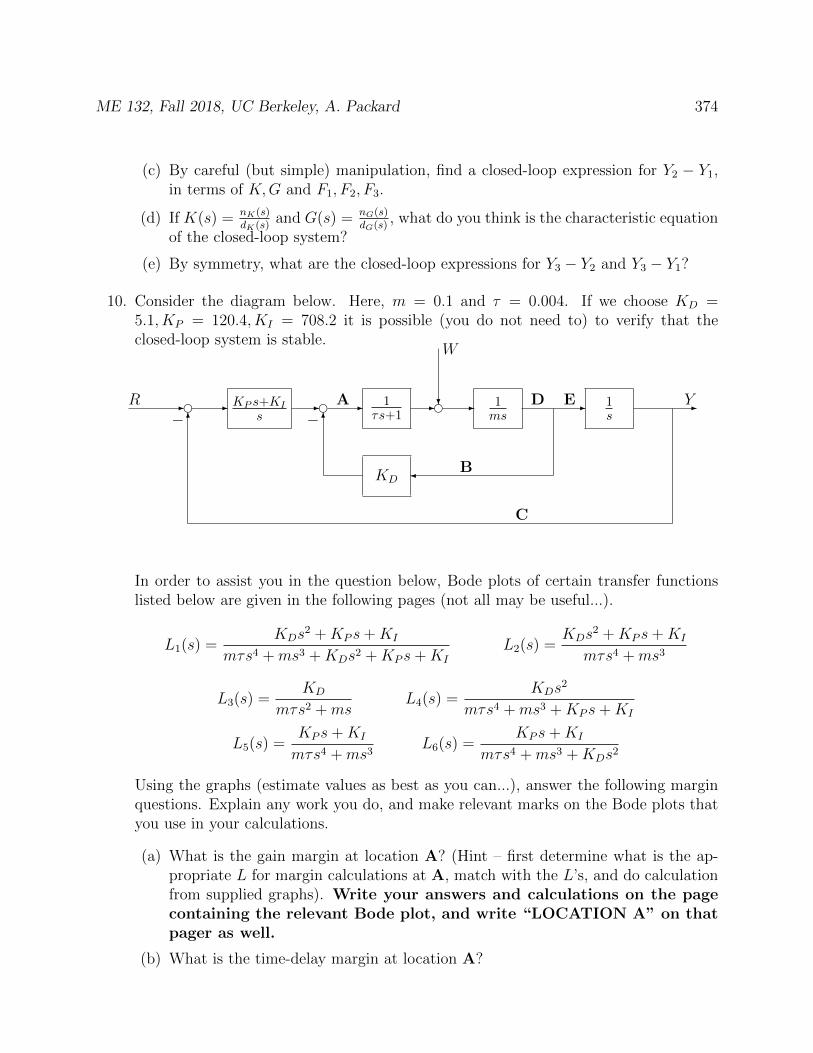
ME 132, Fall 2018, UC Berkeley, A. Packard 374
(c) By careful (but simple) manipulation, find a closed-loop expression for Y2 − Y1,in terms of K,G and F1, F2, F3.
(d) If K(s) = nK(s)dK(s)
and G(s) = nG(s)dG(s)
, what do you think is the characteristic equationof the closed-loop system?
(e) By symmetry, what are the closed-loop expressions for Y3 − Y2 and Y3 − Y1?
10. Consider the diagram below. Here, m = 0.1 and τ = 0.004. If we choose KD =5.1, KP = 120.4, KI = 708.2 it is possible (you do not need to) to verify that theclosed-loop system is stable.
- e eKP s+KI
s1
τs+11ms
1s
KD
- - - - e? - - -
6
6− −R
W
YA
B
C
D E
In order to assist you in the question below, Bode plots of certain transfer functionslisted below are given in the following pages (not all may be useful...).
L1(s) =KDs
2 +KP s+KI
mτs4 +ms3 +KDs2 +KP s+KI
L2(s) =KDs
2 +KP s+KI
mτs4 +ms3
L3(s) =KD
mτs2 +msL4(s) =
KDs2
mτs4 +ms3 +KP s+KI
L5(s) =KP s+KI
mτs4 +ms3L6(s) =
KP s+KI
mτs4 +ms3 +KDs2
Using the graphs (estimate values as best as you can...), answer the following marginquestions. Explain any work you do, and make relevant marks on the Bode plots thatyou use in your calculations.
(a) What is the gain margin at location A? (Hint – first determine what is the ap-propriate L for margin calculations at A, match with the L’s, and do calculationfrom supplied graphs). Write your answers and calculations on the pagecontaining the relevant Bode plot, and write “LOCATION A” on thatpager as well.
(b) What is the time-delay margin at location A?
ME 132, Fall 2018, UC Berkeley, A. Packard 375
(c) What is the gain margin at location B? Write your answers and calculationson the page containing the relevant Bode plot, and write “LOCATIONB” on that page as well.
(d) What is the time-delay margin at location B?
(e) What is the gain margin at location C? Write your answers and calculationson the page containing the relevant Bode plot, and write “LOCATIONC” on that pager as well.
(f) What is the time-delay margin at location C?
(g) What is the gain margin at location D? Write your answers and calculationson the page containing the relevant Bode plot, and write “LOCATIOND” on that pager as well.
(h) What is the time-delay margin at location D?
(i) What is the gain margin at location E? Write your answers and calculationson the page containing the relevant Bode plot, and write “LOCATIONE” on that pager as well.
(j) What is the time-delay margin at location E?
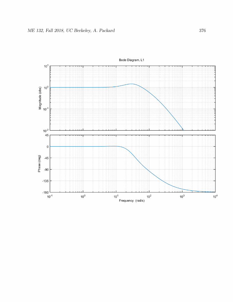
ME 132, Fall 2018, UC Berkeley, A. Packard 376
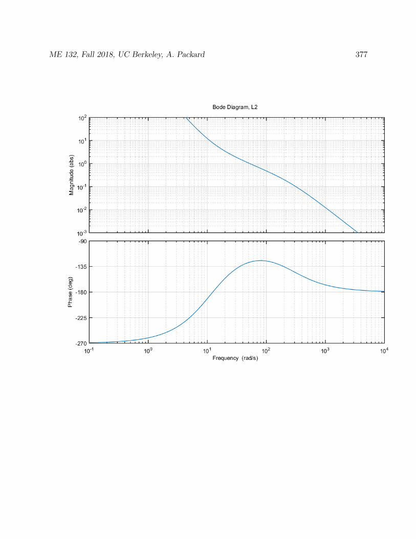
ME 132, Fall 2018, UC Berkeley, A. Packard 377
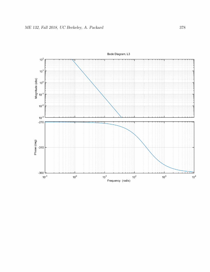
ME 132, Fall 2018, UC Berkeley, A. Packard 378
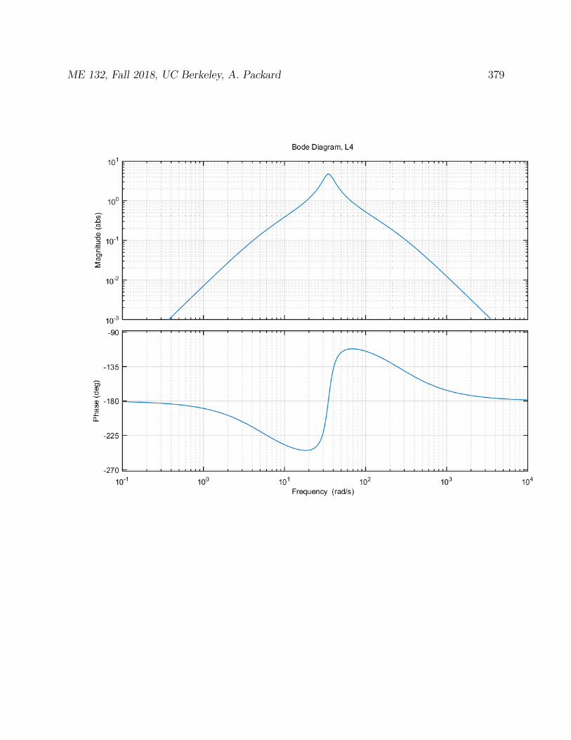
ME 132, Fall 2018, UC Berkeley, A. Packard 379

ME 132, Fall 2018, UC Berkeley, A. Packard 380

ME 132, Fall 2018, UC Berkeley, A. Packard 381
30.7 Spring 2014, Midterm 1
# 1
8
# 2
14
# 3
10
# 4
8
#5
10
NAME
1. Consider the following Matlab code:
wH = @(t) t>4;
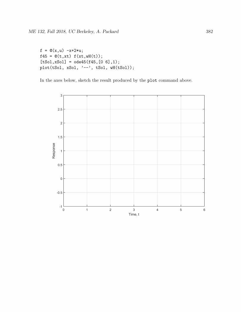
ME 132, Fall 2018, UC Berkeley, A. Packard 382
f = @(x,u) -x+2*u;
f45 = @(t,xt) f(xt,wH(t));
[tSol,xSol] = ode45(f45,[0 6],1);
plot(tSol, xSol, ’--’, tSol, wH(tSol));
In the axes below, sketch the result produced by the plot command above.
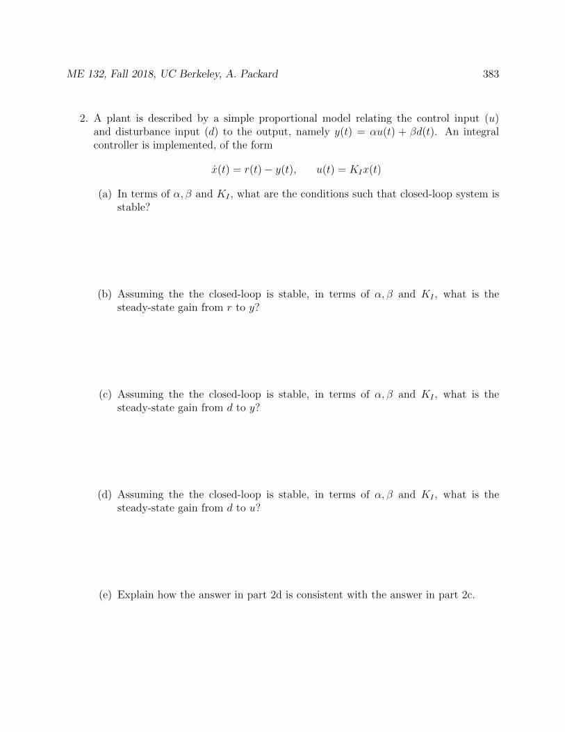
ME 132, Fall 2018, UC Berkeley, A. Packard 383
2. A plant is described by a simple proportional model relating the control input (u)and disturbance input (d) to the output, namely y(t) = αu(t) + βd(t). An integralcontroller is implemented, of the form
x(t) = r(t)− y(t), u(t) = KIx(t)
(a) In terms of α, β and KI , what are the conditions such that closed-loop system isstable?
(b) Assuming the the closed-loop is stable, in terms of α, β and KI , what is thesteady-state gain from r to y?
(c) Assuming the the closed-loop is stable, in terms of α, β and KI , what is thesteady-state gain from d to y?
(d) Assuming the the closed-loop is stable, in terms of α, β and KI , what is thesteady-state gain from d to u?
(e) Explain how the answer in part 2d is consistent with the answer in part 2c.

ME 132, Fall 2018, UC Berkeley, A. Packard 384
(f) Suppose α = 2 and β = 1 are the parameters of the plant. Design KI so thatthe closed-loop time-constant is 1
4. Assuming an initial condition of x(0) = 0, a
reference input r and disturbance d, shown below are applied. On the two graphsprovided, accurately sketch the response (u and y).
ME 132, Fall 2018, UC Berkeley, A. Packard 385
3. What is the smallest value of T > 0 such that for some real-valued ω, the functionz(t) = sin(ωt) satisfies the differential equation
z(t) = −4z(t− T )
ME 132, Fall 2018, UC Berkeley, A. Packard 386
4. Consider our standard feedback interconnection, consisting of a 1st-order linear con-troller and proportional plant described by
controller :x(t) = Ax(t) +B1r(t) +B2ym(t)u(t) = Cx(t) +D1r(t)
plant : y(t) = αu(t) + βd(t)
The measurement equation is ym(t) = y(t) + n(t).
(a) Under what conditions (on the parameters A,B1, . . . , D1, α, β) is the closed-loopsystem stable? Carefully justify your answer.
(b) Is it possible that the controller, as a system by itself, is unstable, but the closed-loop system is stable. If your answer is “No”, please give a careful explanation.If your answer is “Yes”, please give a concrete example.
ME 132, Fall 2018, UC Berkeley, A. Packard 387
5. A stable linear system of the form z(t) = Az(t) + Bu(t) is forced with a sine-waveinput, u(t) = sin 3t.
(a) What is the frequency of the resulting sinusoidal steady-state response z(t)?
(b) The resulting sinusoidal steady-state response z(t) has a magnitude of√
2, and“lags” the input u by 1
8of a period. Determine A and B.
firstOrderSystemID

ME 132, Fall 2018, UC Berkeley, A. Packard 388
30.8 Spring 2014, Midterm 2
1. Consider the following Matlab code:
P = ss(1,2,3,0);
P.u = ’uP’; P.y = ’yP’;
C = ss(0,1,2,1);
C.u = ’e’; C.y = ’ucmd’;
S1 = sumblk(’e=r-ym’);
S2 = sumblk(’uP = ucmd + d’);
S3 = sumblk(’ym = yP + n’);
H = connect(P,C,S1,S2,S3,’r’,’d’,’n’,’yP’,’ucmd’);
H.a
H.d
(without worrying about the format) Write down, separately, the two matrices thatwill be displayed in the Command Window, due to the last two commands.
2. An unstable plant is described by a 1st-order linear differential equation
x(t) = x(t) + d(t) + u(t)y(t) = x(t)
The variables are: x is the state of the plant, d is the disturbance input, u is thecontrol input, and y is the plant output. There is a measurement noise, n, so that themeasured output ym is defined by ym(t) = y(t) + n(t).
Design a 1st-order linear control system with the following properties:
• There are two inputs to the controller: a reference input r, and the measuredplant output, ym; The controller has one state, you can call it z, or whatever yourfavorite letter is for a controller state; There is one output of the controller, u,which becomes an input to the plant (ie., the “control input”)
• The 2nd-order closed-loop system is stable. In fact, expanding on closed-loopstability, the eigenvalues of the closed-loop “A” matrix should be at −2 and −3.
• The steady-state gain from r to y should be 1. The steady-state gain from d to yshould be 0. The instantaneous-gain from r to u should be 0.
3. The matrix A is
A =
[−3 2−1 0
](a) What are the eigenvalues of A?
ME 132, Fall 2018, UC Berkeley, A. Packard 389
(b) Find a 2× 2 diagonal matrix Λ such that AV = V Λ, where V is given by
V =
[1 21 1
]
(c) Confirm that the inverse matrix of V is
V −1 =
[−1 2
1 −1
]
(d) Find eAt.

ME 132, Fall 2018, UC Berkeley, A. Packard 3904. The step-response and Bode plot of the system x(t) = −x(t) + u(t), y(t) = x(t) isshown below. It is labeled TimeResponse, #1. Step-responses of 5 other systemsare shown as well (labeled #2 through #6).
Frequency-response functions of the same 6 systems are shown on the next page. TheFrequency-response for System #1 is marked. The others are not marked. Match(on the next page) each system’s Step-response with its associated Frequency-Response. Within each frequency-response axes boundaries, give a short (5-10words) justification for your choice.
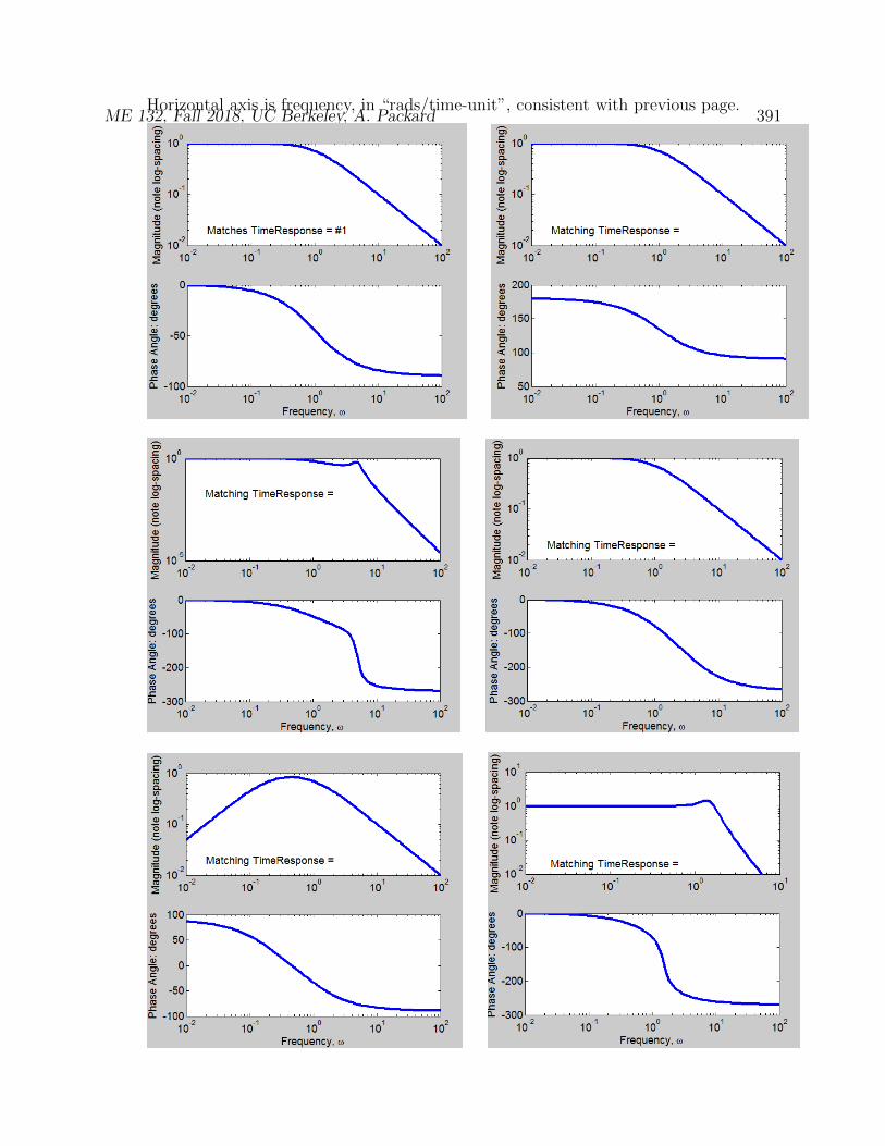
ME 132, Fall 2018, UC Berkeley, A. Packard 391Horizontal axis is frequency, in “rads/time-unit”, consistent with previous page.
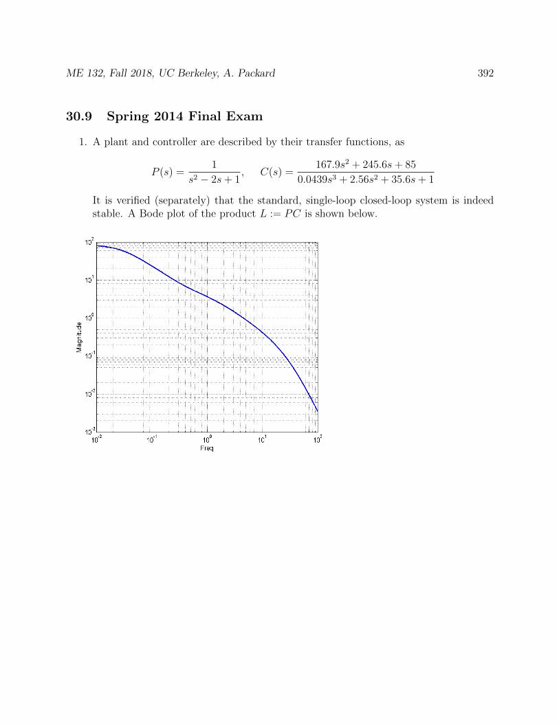
ME 132, Fall 2018, UC Berkeley, A. Packard 392
30.9 Spring 2014 Final Exam
1. A plant and controller are described by their transfer functions, as
P (s) =1
s2 − 2s+ 1, C(s) =
167.9s2 + 245.6s+ 85
0.0439s3 + 2.56s2 + 35.6s+ 1
It is verified (separately) that the standard, single-loop closed-loop system is indeedstable. A Bode plot of the product L := PC is shown below.

ME 132, Fall 2018, UC Berkeley, A. Packard 393
(a) Determine the phase-crossover frequencies, and the gain-margin of the system.
(b) Determine the gain-crossover frequencies, and the time-delay margin of the system
2. Suppose 0 < ξ < 1 and ωn > 0. Consider the system
y(t) + 2ξωny(t) + ω2ny(t) = ωnu(t)
subject to the initial conditions y(0−) = 0, y(0−) = 0, and the unit-step forcing func-tion, namely u(t) = 0 for t = 0, and u(t) = 1 for t > 0. Show that the responseis
y(t) =1√
1− ξ2e−ξωnt sin
(√1− ξ2ωnt
)Hint: Recall that the set of all real-valued homogeneous solutions of y(t)+2ξωny(t)+
ω2ny(t) = 0 is yH(t) = Ae−ξωnt cos
(√1− ξ2ωnt
)+ Be−ξωnt sin
(√1− ξ2ωnt
)where A
and B are any real numbers.
3. A block diagram is shown below. Each system is represented by its transfer function.Signals (such as r, y, e or v) are represented by lower-case signals, and associated capitalletters are used in the transfer function descriptions. Assume the parameter m > 0.
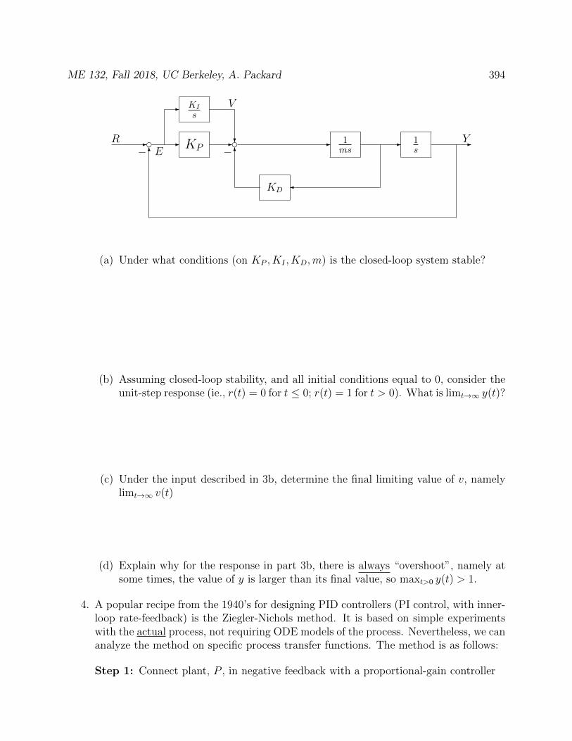
ME 132, Fall 2018, UC Berkeley, A. Packard 394
- d dKI
s
KP1ms
1s
KD
-
-
?- - - -
6
6− −R Y
V
E
(a) Under what conditions (on KP , KI , KD,m) is the closed-loop system stable?
(b) Assuming closed-loop stability, and all initial conditions equal to 0, consider theunit-step response (ie., r(t) = 0 for t ≤ 0; r(t) = 1 for t > 0). What is limt→∞ y(t)?
(c) Under the input described in 3b, determine the final limiting value of v, namelylimt→∞ v(t)
(d) Explain why for the response in part 3b, there is always “overshoot”, namely atsome times, the value of y is larger than its final value, so maxt>0 y(t) > 1.
4. A popular recipe from the 1940’s for designing PID controllers (PI control, with inner-loop rate-feedback) is the Ziegler-Nichols method. It is based on simple experimentswith the actual process, not requiring ODE models of the process. Nevertheless, we cananalyze the method on specific process transfer functions. The method is as follows:
Step 1: Connect plant, P , in negative feedback with a proportional-gain controller
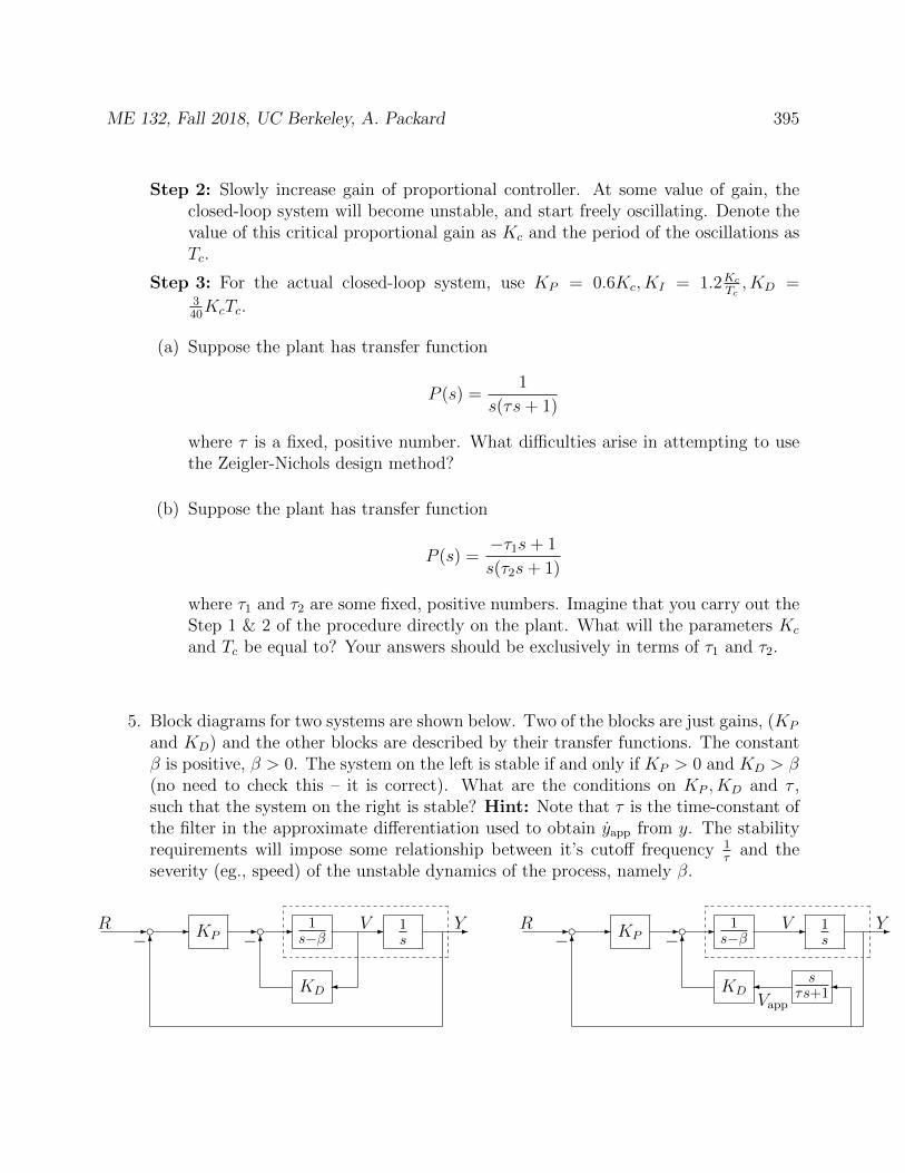
ME 132, Fall 2018, UC Berkeley, A. Packard 395
Step 2: Slowly increase gain of proportional controller. At some value of gain, theclosed-loop system will become unstable, and start freely oscillating. Denote thevalue of this critical proportional gain as Kc and the period of the oscillations asTc.
Step 3: For the actual closed-loop system, use KP = 0.6Kc, KI = 1.2KcTc, KD =
340KcTc.
(a) Suppose the plant has transfer function
P (s) =1
s(τs+ 1)
where τ is a fixed, positive number. What difficulties arise in attempting to usethe Zeigler-Nichols design method?
(b) Suppose the plant has transfer function
P (s) =−τ1s+ 1
s(τ2s+ 1)
where τ1 and τ2 are some fixed, positive numbers. Imagine that you carry out theStep 1 & 2 of the procedure directly on the plant. What will the parameters Kc
and Tc be equal to? Your answers should be exclusively in terms of τ1 and τ2.
5. Block diagrams for two systems are shown below. Two of the blocks are just gains, (KP
and KD) and the other blocks are described by their transfer functions. The constantβ is positive, β > 0. The system on the left is stable if and only if KP > 0 and KD > β(no need to check this – it is correct). What are the conditions on KP , KD and τ ,such that the system on the right is stable? Hint: Note that τ is the time-constant ofthe filter in the approximate differentiation used to obtain yapp from y. The stabilityrequirements will impose some relationship between it’s cutoff frequency 1
τand the
severity (eg., speed) of the unstable dynamics of the process, namely β.
- c cKP1
s−β1s
KD
- - - - -6
6− −YR V - c cKP
1s−β
1s
KD
- - - - -6
sτs+1
6− −
YR V
Vapp
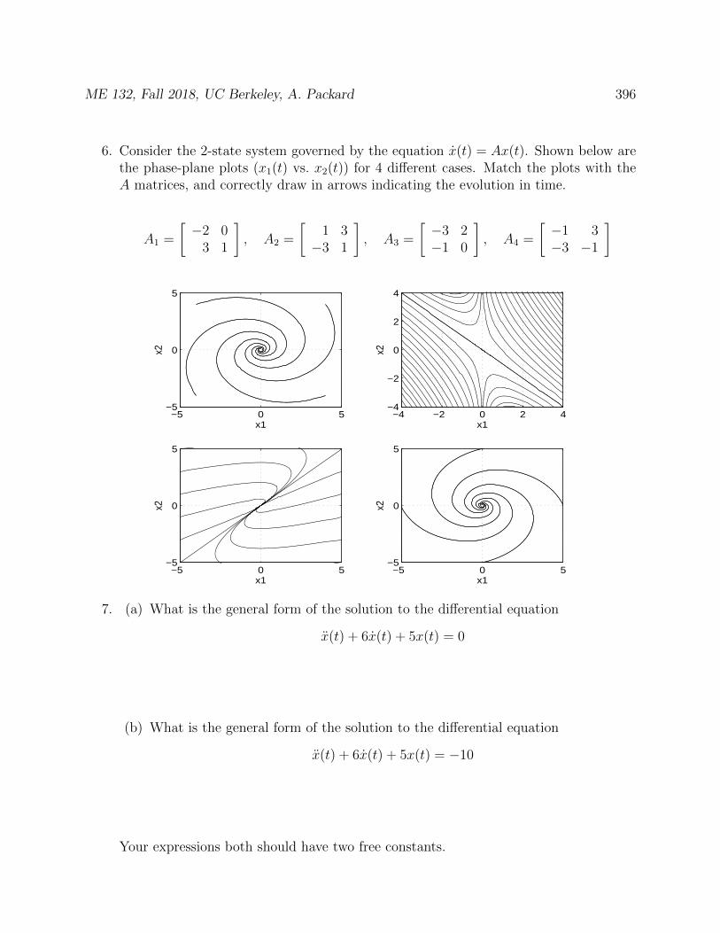
ME 132, Fall 2018, UC Berkeley, A. Packard 396
6. Consider the 2-state system governed by the equation x(t) = Ax(t). Shown below arethe phase-plane plots (x1(t) vs. x2(t)) for 4 different cases. Match the plots with theA matrices, and correctly draw in arrows indicating the evolution in time.
A1 =
[−2 0
3 1
], A2 =
[1 3−3 1
], A3 =
[−3 2−1 0
], A4 =
[−1 3−3 −1
]
−5 0 5−5
0
5
x1
x2
−4 −2 0 2 4−4
−2
0
2
4
x1
x2
−5 0 5−5
0
5
x1
x2
−5 0 5−5
0
5
x1
x2
7. (a) What is the general form of the solution to the differential equation
x(t) + 6x(t) + 5x(t) = 0
(b) What is the general form of the solution to the differential equation
x(t) + 6x(t) + 5x(t) = −10
Your expressions both should have two free constants.
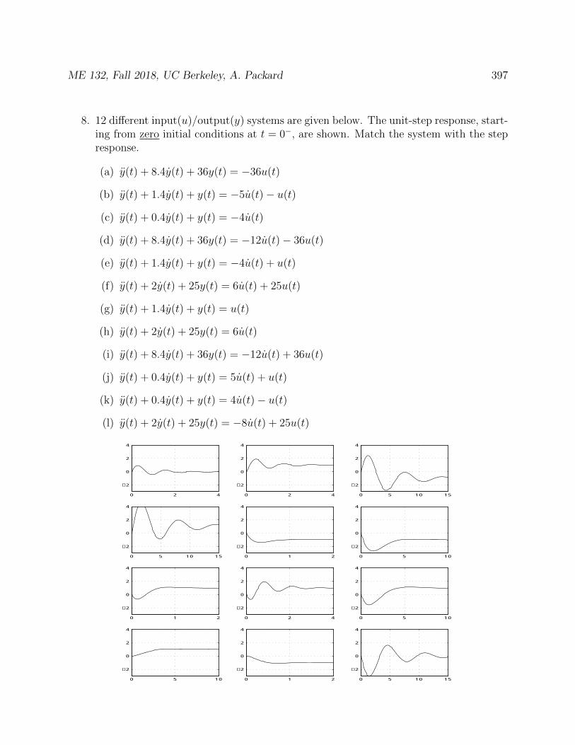
ME 132, Fall 2018, UC Berkeley, A. Packard 397
8. 12 different input(u)/output(y) systems are given below. The unit-step response, start-ing from zero initial conditions at t = 0−, are shown. Match the system with the stepresponse.
(a) y(t) + 8.4y(t) + 36y(t) = −36u(t)
(b) y(t) + 1.4y(t) + y(t) = −5u(t)− u(t)
(c) y(t) + 0.4y(t) + y(t) = −4u(t)
(d) y(t) + 8.4y(t) + 36y(t) = −12u(t)− 36u(t)
(e) y(t) + 1.4y(t) + y(t) = −4u(t) + u(t)
(f) y(t) + 2y(t) + 25y(t) = 6u(t) + 25u(t)
(g) y(t) + 1.4y(t) + y(t) = u(t)
(h) y(t) + 2y(t) + 25y(t) = 6u(t)
(i) y(t) + 8.4y(t) + 36y(t) = −12u(t) + 36u(t)
(j) y(t) + 0.4y(t) + y(t) = 5u(t) + u(t)
(k) y(t) + 0.4y(t) + y(t) = 4u(t)− u(t)
(l) y(t) + 2y(t) + 25y(t) = −8u(t) + 25u(t)
0 2 4
−2
0
2
4
0 2 4
−2
0
2
4
0 5 10 15
−2
0
2
4
0 5 10 15
−2
0
2
4
0 1 2
−2
0
2
4
0 5 10
−2
0
2
4
0 1 2
−2
0
2
4
0 2 4
−2
0
2
4
0 5 10
−2
0
2
4
0 5 10
−2
0
2
4
0 1 2
−2
0
2
4
0 5 10 15
−2
0
2
4

ME 132, Fall 2018, UC Berkeley, A. Packard 398
9. A hoop (of radius R) is mounted vertically, and rotates at a constant angular velocityΩ. A bead of mass m slides along the hoop, and θ is the angle that locates the beadlocation. θ = 0 corresponds to the bead at the bottom of the hoop, while θ = πcorresponds to the top of the hoop, as shown below.
The nonlinear, 2nd order equation (from Newton’s law) governing the bead’s motionis
mRθ +mg sin θ + αθ −mΩ2R sin θ cos θ = 0
All of the parameters m,R, g, α are positive.
(a) Let x1(t) := θ(t) and x2(t) := θ(t). Write the 2nd order nonlinear differentialequation in the state-space form
x1(t) = f1 (x1(t), x2(t))x2(t) = f2 (x1(t), x2(t))
(b) Show that x1 = 0, x2 = 0 is an equilibrium point of the system.
(c) Find the linearized systemη(t) = Aη(t)
which governs small deviations away from the equilibrium point (0, 0).
(d) Under what conditions (on m,R,Ω, g) is the linearized system stable?
(e) Show that x1 = π, x2 = 0 is an equilibrium point of the system.
(f) Find the linearized system η(t) = Aη(t) which governs small deviations away fromthe equilibrium point (π, 0).
(g) Under what conditions is the linearized system stable?
(h) It would seem that if the hoop is indeed rotating (with angular velocity Ω) thenthere would other equilibrium point (with 0 < θ < π/2). Do such equilibriumpoints exist in the system? Be very careful, and please explain your answer.
ME 132, Fall 2018, UC Berkeley, A. Packard 399
(i) Find the linearized system η(t) = Aη(t) which governs small deviations away fromthis equilibrium point.
(j) Under what conditions is the linearized system stable?
10. A process, with input u, disturbance d and output y is governed by
y(t) = 2y(t) + 3u(t) + d(t)
(a) Is the process stable?
(b) Suppose y(0) = 1, and u(t) = d(t) ≡ 0 for all t ≥ 0. What is the solution y(t) fort ≥ 0.
(c) Consider a proportional-control strategy, u(t) = K1r(t) +K2 [r(t)− y(t)]. Deter-mine the closed-loop differential equation relating the variables (y, r, d).
(d) For what values of K1 and K2 is the closed-loop system stable?

ME 132, Fall 2018, UC Berkeley, A. Packard 400
(e) As a function of K2, what is the steady-state gain from d→ y in the closed-loopsystem?
(f) As a function of K1 and K2, what is the steady-state gain from r → y in theclosed-loop system?
(g) Choose K1 and K2 so that the steady-state gain from r → y equals 1, and thesteady-state gain from d→ y equals 0.1.
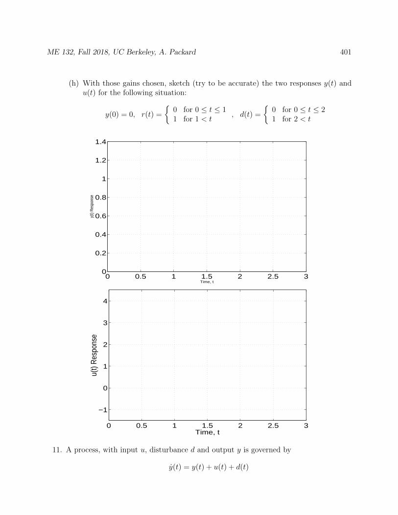
ME 132, Fall 2018, UC Berkeley, A. Packard 401
(h) With those gains chosen, sketch (try to be accurate) the two responses y(t) andu(t) for the following situation:
y(0) = 0, r(t) =
0 for 0 ≤ t ≤ 11 for 1 < t
, d(t) =
0 for 0 ≤ t ≤ 21 for 2 < t
0 0.5 1 1.5 2 2.5 30
0.2
0.4
0.6
0.8
1
1.2
1.4
Time, t
y(t)
Res
pons
e
0 0.5 1 1.5 2 2.5 3
−1
0
1
2
3
4
Time, t
u(t)
Res
pons
e
11. A process, with input u, disturbance d and output y is governed by
y(t) = y(t) + u(t) + d(t)

ME 132, Fall 2018, UC Berkeley, A. Packard 402
(a) Is the process stable?
(b) Suppose y(0) = −3, and u(t) = d(t) ≡ 0 for all t ≥ 0. What is the solution y(t)for t ≥ 0.
(c) A PI (Proportional plus Integral) controller is proposed
u(t) = KP [r(t)− y(t)] +KIz(t)z(t) = r(t)− y(t)
Eliminate z and u, and determine the closed-loop differential equation relatingthe variables (y, r, d).

ME 132, Fall 2018, UC Berkeley, A. Packard 403
(d) For what values of KP and KI is the closed-loop system stable?
(e) The closed-loop system is 2nd order. What are the appropriate values of KP andKI so that the closed-loop system characteristic polynomial has roots describedby ξ = 0.8, ωn = 0.5?
(f) What are the appropriate values of KP and KI so that the closed-loop systemcharacteristic polynomial has roots described by ξ = 0.8, ωn = 1.0?
(g) What are the appropriate values of KP and KI so that the closed-loop systemcharacteristic polynomial has roots described by ξ = 0.8, ωn = 2.0?
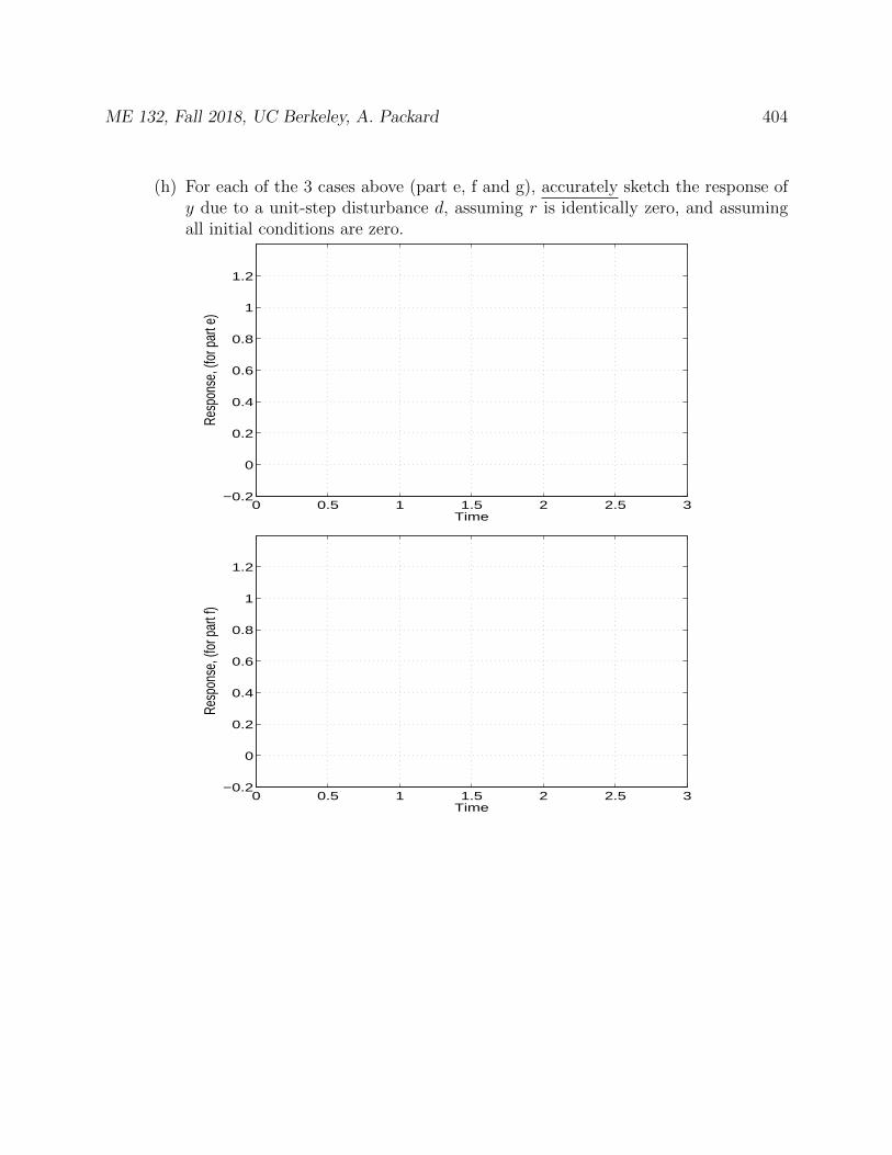
ME 132, Fall 2018, UC Berkeley, A. Packard 404
(h) For each of the 3 cases above (part e, f and g), accurately sketch the response ofy due to a unit-step disturbance d, assuming r is identically zero, and assumingall initial conditions are zero.
0 0.5 1 1.5 2 2.5 3−0.2
0
0.2
0.4
0.6
0.8
1
1.2
Time
Resp
onse
, (fo
r par
t e)
0 0.5 1 1.5 2 2.5 3−0.2
0
0.2
0.4
0.6
0.8
1
1.2
Time
Resp
onse
, (fo
r par
t f)
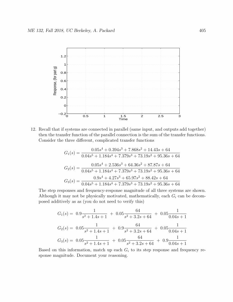
ME 132, Fall 2018, UC Berkeley, A. Packard 405
0 0.5 1 1.5 2 2.5 3−0.2
0
0.2
0.4
0.6
0.8
1
1.2
Time
Resp
onse
, (fo
r par
t g)
12. Recall that if systems are connected in parallel (same input, and outputs add together)then the transfer function of the parallel connection is the sum of the transfer functions.Consider the three different, complicated transfer functions
G1(s) =0.05s4 + 0.394s3 + 7.868s2 + 14.43s+ 64
0.04s5 + 1.184s4 + 7.379s3 + 73.19s2 + 95.36s+ 64
G2(s) =0.05s4 + 2.536s3 + 64.36s2 + 87.87s+ 64
0.04s5 + 1.184s4 + 7.379s3 + 73.19s2 + 95.36s+ 64
G3(s) =0.9s4 + 4.27s3 + 65.97s2 + 88.42s+ 64
0.04s5 + 1.184s4 + 7.379s3 + 73.19s2 + 95.36s+ 64
The step responses and frequency-response magnitude of all three systems are shown.Although it may not be physically motivated, mathematically, each Gi can be decom-posed additively as as (you do not need to verify this)
G1(s) = 0.91
s2 + 1.4s+ 1+ 0.05
64
s2 + 3.2s+ 64+ 0.05
1
0.04s+ 1
G2(s) = 0.051
s2 + 1.4s+ 1+ 0.9
64
s2 + 3.2s+ 64+ 0.05
1
0.04s+ 1
G3(s) = 0.051
s2 + 1.4s+ 1+ 0.05
64
s2 + 3.2s+ 64+ 0.9
1
0.04s+ 1
Based on this information, match up each Gi to its step response and frequency re-sponse magnitude. Document your reasoning.
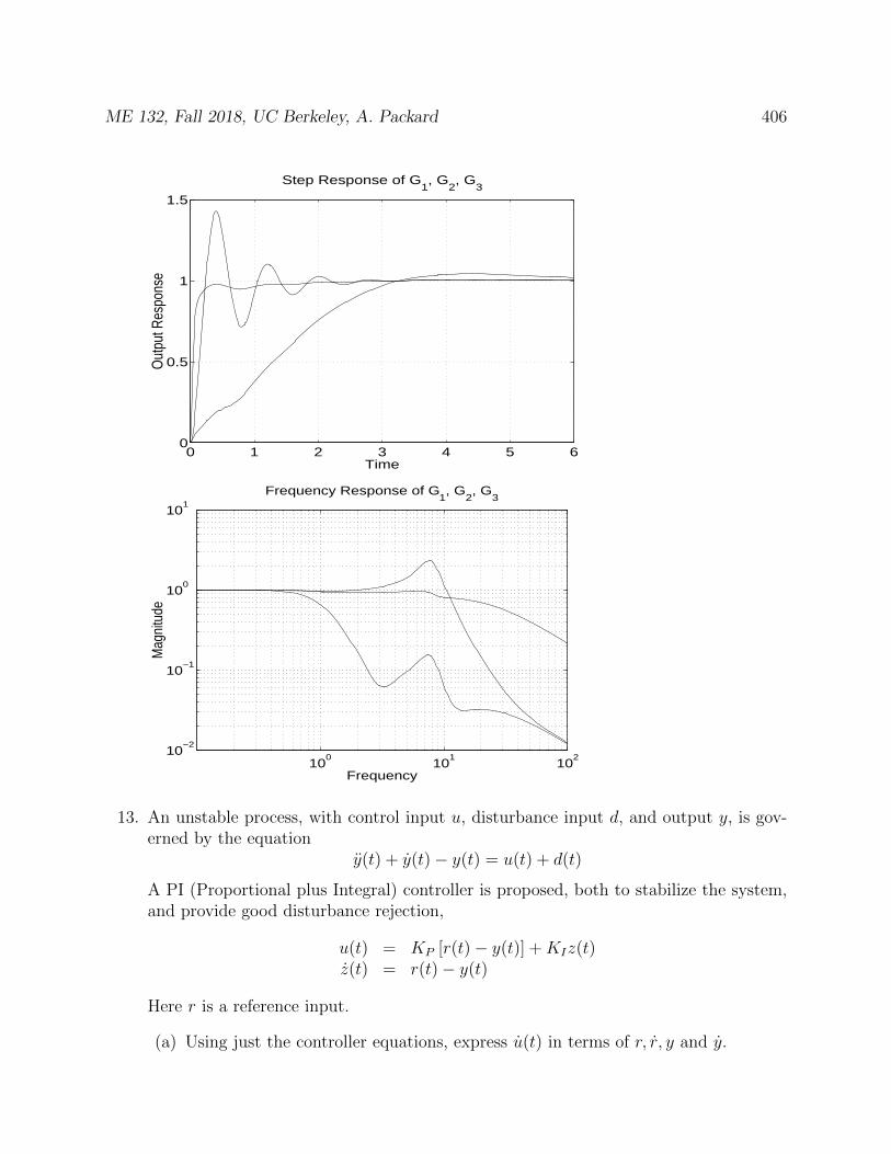
ME 132, Fall 2018, UC Berkeley, A. Packard 406
0 1 2 3 4 5 60
0.5
1
1.5
Time
Out
put R
espo
nse
Step Response of G1, G
2, G
3
100
101
102
10−2
10−1
100
101
Frequency
Mag
nitu
de
Frequency Response of G1, G
2, G
3
13. An unstable process, with control input u, disturbance input d, and output y, is gov-erned by the equation
y(t) + y(t)− y(t) = u(t) + d(t)
A PI (Proportional plus Integral) controller is proposed, both to stabilize the system,and provide good disturbance rejection,
u(t) = KP [r(t)− y(t)] +KIz(t)z(t) = r(t)− y(t)
Here r is a reference input.
(a) Using just the controller equations, express u(t) in terms of r, r, y and y.
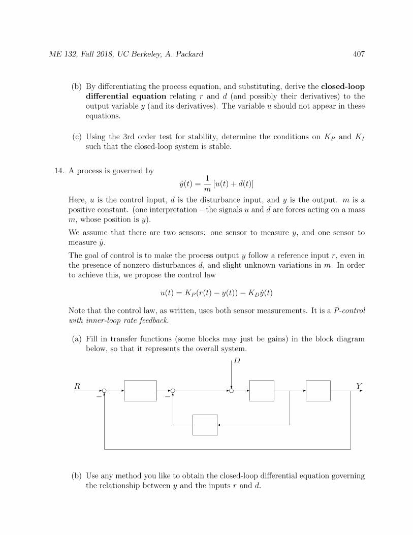
ME 132, Fall 2018, UC Berkeley, A. Packard 407
(b) By differentiating the process equation, and substituting, derive the closed-loopdifferential equation relating r and d (and possibly their derivatives) to theoutput variable y (and its derivatives). The variable u should not appear in theseequations.
(c) Using the 3rd order test for stability, determine the conditions on KP and KI
such that the closed-loop system is stable.
14. A process is governed by
y(t) =1
m[u(t) + d(t)]
Here, u is the control input, d is the disturbance input, and y is the output. m is apositive constant. (one interpretation – the signals u and d are forces acting on a massm, whose position is y).
We assume that there are two sensors: one sensor to measure y, and one sensor tomeasure y.
The goal of control is to make the process output y follow a reference input r, even inthe presence of nonzero disturbances d, and slight unknown variations in m. In orderto achieve this, we propose the control law
u(t) = KP (r(t)− y(t))−KDy(t)
Note that the control law, as written, uses both sensor measurements. It is a P-controlwith inner-loop rate feedback.
(a) Fill in transfer functions (some blocks may just be gains) in the block diagrambelow, so that it represents the overall system.
- e e- - - e? - - -
6
6− −R
D
Y
(b) Use any method you like to obtain the closed-loop differential equation governingthe relationship between y and the inputs r and d.
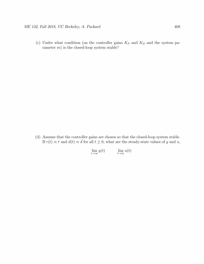
ME 132, Fall 2018, UC Berkeley, A. Packard 408
(c) Under what condition (on the controller gains KP and KD and the system pa-rameter m) is the closed-loop system stable?
(d) Assume that the controller gains are chosen so that the closed-loop system stable.If r(t) ≡ r and d(t) ≡ d for all t ≥ 0, what are the steady-state values of y and u,
limt→∞
y(t) limt→∞
u(t)
ME 132, Fall 2018, UC Berkeley, A. Packard 409
(e) Assume that m = 1. Choose the controller gains so that the roots of the closed-loop characteristic polynomial are given by ξ = 0.7, ωn = 4.
ME 132, Fall 2018, UC Berkeley, A. Packard 410
(f) Using the gains calculated above, neatly sketch your best “guess” (you can calcu-late/compute/derive as much as you like) of the responses y(t) and u(t) versus t,when the system starts with all initial conditions equal to 0, for the case when ris a unit step and d is identically 0. You should get the time-scale correct (marktime-axis) as well as the qualitative aspects of the plots (recall interpretation -a mass is being accelerated from rest and then brought back to rest in a newposition...).
15. A block diagram is shown below. Each system is represented by its transfer function.

ME 132, Fall 2018, UC Berkeley, A. Packard 411
- d dKP s+KI
s1
τs+11s
1s
KD
- - - - d? - - -
6
6− −R
D
Y
(a) In terms of KP , KI , KD, τ , what is the transfer function from R to Y (hint: thedenominator should be 4th order).
(b) In terms of KP , KI , KD, τ , what is the transfer function from D to Y (hint: sameas above).
(c) In terms of KP , KI , KD, τ , what is the characteristic polynomial of the closed-loopsystem?
(d) In terms of KP , KI , KD, τ , what is the differential equation relating r and d to y?
16. In computing gain and time-delay margins, we solve equations of the form
−1 = γL(jω) − 1 = e−jωTL(jω)
using an appropriate L, depending on the system under consideration.
For the system below, what is the appropriate L in order to compute gain and time-delay margins at the point marked by ×.
- c cKP1
s−β1s
KD ×
- - - - -6
6− −yr y
ME 132, Fall 2018, UC Berkeley, A. Packard 412
17. A 1st order processy(t) = u(t) + d(t)
is controlled by a proportional control
u(t) = KP [r(t)− ym(t)]
where ym(t) = y(t) + n(t). The interpretation of signals is: u is control input; y isprocess output; d is external disturbance on process; r is a reference input, representinga desired value of y; n is measurement noise.
(a) Eliminate u from the equations, and get the closed-loop differential equation re-lating (r, d, n) to y.
(b) Under what conditions on KP is the closed-loop system stable?
(c) How is the time-constant of the closed-loop system related to KP ?

ME 132, Fall 2018, UC Berkeley, A. Packard 413
(d) Shown below are the closed-loop frequency responses from (r, d, n) → y, as KP
increases from 0.1 to 10. Indicate on each graph with an arrow “cutting” acrossthe plots, the direction of increasing KP .
10−2
100
102
−100
−80
−60
−40
−20
0
Frequency
10−2
100
102
10−3
10−2
10−1
100
10−2
100
102
10−2
10−1
100
101
Frequency10
−210
010
210
−3
10−2
10−1
100
Frequency
(e) Shown below are the closed-loop frequency responses from (r, d, n) → u, as KP
increases from 0.1 to 10. Indicate on each graph with an arrow “cutting” acrossthe plots, the direction of increasing KP .
10−2
100
102
10−2
10−1
100
101
Frequency10
−210
010
210
−3
10−2
10−1
100
Frequency10
−210
010
210
−2
10−1
100
101
Frequency
ME 132, Fall 2018, UC Berkeley, A. Packard 414
31 Older exams
31.1 Spring 2012, Midterm 1
# 1
20
# 2
14
# 3
6
# 4
10
TOTAL
50
NAME
1. A plant, with control input u, disturbance input d, internal state x, and output y isgoverned by the equations
x(t) = Ax(t) +B1d(t) +B2u(t)y(t) = Cx(t)
where A,B1, B2 and C are constant numbers. A proportional controller, designed toregulate the output y, even in the presence of disturbances is of the form
u(t) = −Kym(t)
where ym(t) = y(t) + n(t), and n represents additive measurement noise.
(a) Express the equations for the closed-loop interconnection (plant/controller/sensor)in the form
x(t) = ax(t) + b1d(t) + b2n(t)y(t) = c1x(t) + d11d(t) + d21n(t)u(t) = c2x(t) + d21d(t) + d22n(t)
where the entries a, b1, b2, . . . , d22 are constants (and generally all are functions ofA,B1, B2, C,K).
(b) Under what condition is the closed-loop system stable? Your condition should beexpressed in terms of (A,B1, B2, C,K).
(c) Assuming closed-loop stability, what is the steady-state gain from d to y. Youranswer should be expressed in terms of (A,B1, B2, C,K).
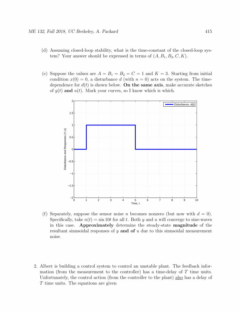
ME 132, Fall 2018, UC Berkeley, A. Packard 415
(d) Assuming closed-loop stability, what is the time-constant of the closed-loop sys-tem? Your answer should be expressed in terms of (A,B1, B2, C,K).
(e) Suppose the values are A = B1 = B2 = C = 1 and K = 3. Starting from initialcondition x(0) = 0, a disturbance d (with n = 0) acts on the system. The time-dependence for d(t) is shown below. On the same axis, make accurate sketchesof y(t) and u(t). Mark your curves, so I know which is which.
0 1 2 3 4 5 6 7 8 9 10−2
−1.5
−1
−0.5
0
0.5
1
1.5
2
Time, t
Dis
turb
ance
and
Res
pons
es (
Y,U
)
Disturbance, d(t)
(f) Separately, suppose the sensor noise n becomes nonzero (but now with d = 0).Specifically, take n(t) = sin 10t for all t. Both y and u will converge to sine-wavesin this case. Approximately determine the steady-state magnitude of theresultant sinusoidal responses of y and of u due to this sinusoidal measurementnoise.
2. Albert is building a control system to control an unstable plant. The feedback infor-mation (from the measurement to the controller) has a time-delay of T time units.Unfortunately, the control action (from the controller to the plant) also has a delay ofT time units. The equations are given
ME 132, Fall 2018, UC Berkeley, A. Packard 416
• The plant is described by differential equations. For all t, the relationship betweenthe signals are (as usual)
x(t) = Ax(t) +B1d(t) +B2u(t)y(t) = Cx(t)
where A,B1, B2 and C are constant numbers.
• The measurement signal, available at the controller, is denoted ym and for all t isgiven by
ym(t) = y(t− T ) + n(t− T )
where T ≥ 0 is the fixed time-delay in the measurement system, and n representsadditive measurement noise.
• The controller derives a requested control action, ur based on the reference inputr and measurement signal ym. For all t, it is
ur(t) = K1r(t)−K2ym(t)
where K1 and K2 are constant numbers.
• Finally, the actual control signal is a delayed version of the requested controlaction, namely
u(t) = ur(t− T ) for all t
(a) Find the delay-differential equation governing the relationship between x, x, r,d and n. Because of the time-delay, the value of x(t) can be expressed as com-binations of the values of x, r, d and n at t, t − T and t − 2T (although not allcombinations will appear).
ME 132, Fall 2018, UC Berkeley, A. Packard 417
(b) Suppose A = 3, B1 = B2 = C = 1, K1 = 2, K2 = 5. Show that the closed-loopsystem is stable for T = 0.
(c) What is the smallest positive T such that the closed-loop system is unstable?
(d) At the critical value of T for which instability occurs (determined by you in partc), what is the frequency of oscillation of the sinusoidal homogeneous solutions?
3. The 5 lines of code below are executed in the Matlab command window
f = @(tau,z) -z+1;
v0 = 5;
[T,V] = ode45(f,[0 1],v0);
N = length(V);
disp(V(N)) % equivalently disp(X(end))
Recall that the disp command is a simple formatted display command, and it willprint out a number (for example) in a nice form. What is the approximate valuethat will be printed by the line disp(V(N))?
4. A first-order systemx(t) = Ax(t) +Bu(t)
is forced with a sin-wave input (u(t) = sin t) as shown below (the experimenter cannotset the initial condition, and the initial condition is effectively random each time theexperiment is run). The resulting value of x is also shown. Approximately determinethe values of A and B (you can assume that the experimenter knows that B is positive,on physical grounds).
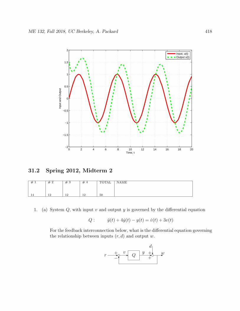
ME 132, Fall 2018, UC Berkeley, A. Packard 418
0 2 4 6 8 10 12 14 16 18 20−2
−1.5
−1
−0.5
0
0.5
1
1.5
2
Time, t
Inpu
t and
Out
put
Input, u(t)Output x(t)
31.2 Spring 2012, Midterm 2
# 1
14
# 2
12
# 3
12
# 4
12
TOTAL
50
NAME
1. (a) System Q, with input v and output y is governed by the differential equation
Q : y(t) + 4y(t)− y(t) = v(t) + 3v(t)
For the feedback interconnection below, what is the differential equation governingthe relationship between inputs (r, d) and output w.
Q- d - - d -6
?r
d
v wy−+ +
+
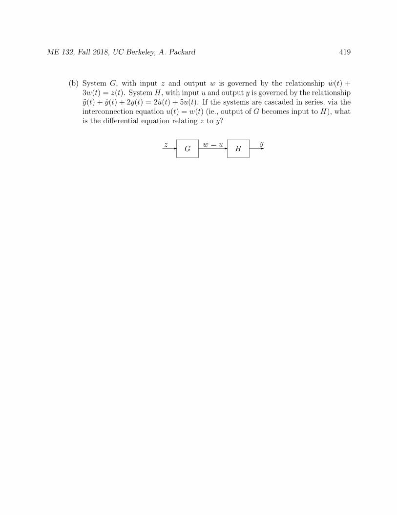
ME 132, Fall 2018, UC Berkeley, A. Packard 419
(b) System G, with input z and output w is governed by the relationship w(t) +3w(t) = z(t). System H, with input u and output y is governed by the relationshipy(t) + y(t) + 2y(t) = 2u(t) + 5u(t). If the systems are cascaded in series, via theinterconnection equation u(t) = w(t) (ie., output of G becomes input to H), whatis the differential equation relating z to y?
zG- -w = u
H -y
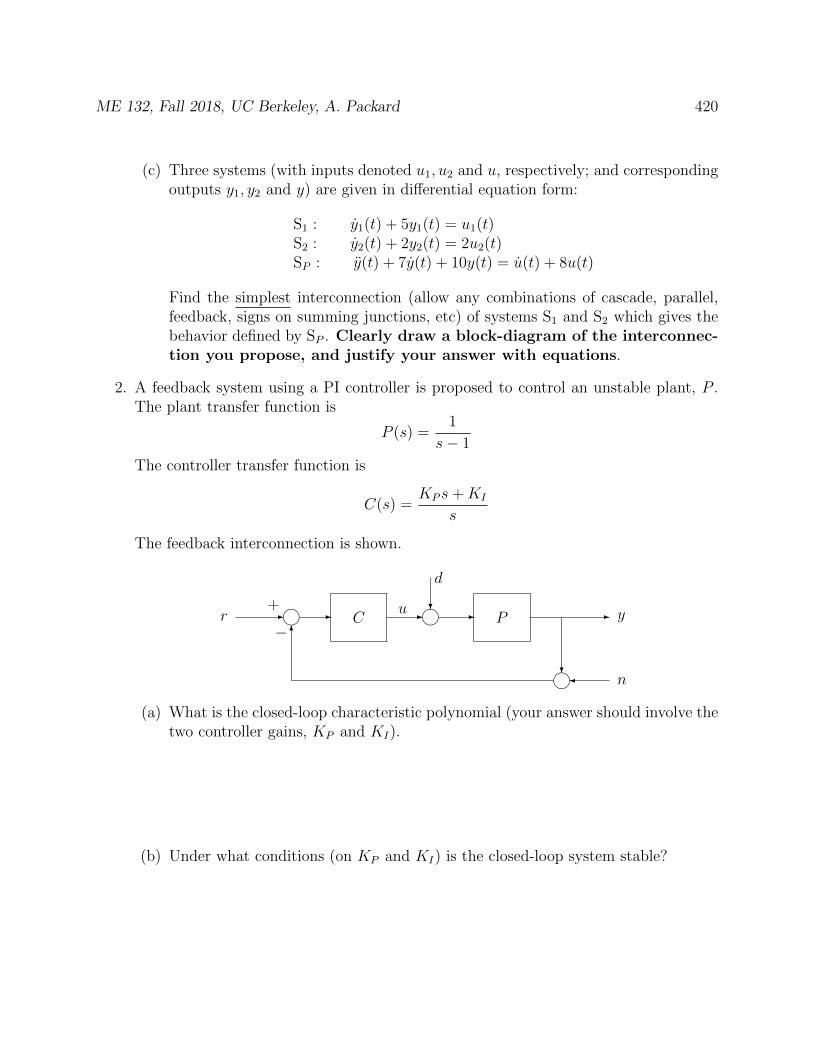
ME 132, Fall 2018, UC Berkeley, A. Packard 420
(c) Three systems (with inputs denoted u1, u2 and u, respectively; and correspondingoutputs y1, y2 and y) are given in differential equation form:
S1 : y1(t) + 5y1(t) = u1(t)S2 : y2(t) + 2y2(t) = 2u2(t)SP : y(t) + 7y(t) + 10y(t) = u(t) + 8u(t)
Find the simplest interconnection (allow any combinations of cascade, parallel,feedback, signs on summing junctions, etc) of systems S1 and S2 which gives thebehavior defined by SP . Clearly draw a block-diagram of the interconnec-tion you propose, and justify your answer with equations.
2. A feedback system using a PI controller is proposed to control an unstable plant, P .The plant transfer function is
P (s) =1
s− 1
The controller transfer function is
C(s) =KP s+KI
s
The feedback interconnection is shown.
C P- - - k -?
d
-
?k6
k+
−r u y
n
(a) What is the closed-loop characteristic polynomial (your answer should involve thetwo controller gains, KP and KI).
(b) Under what conditions (on KP and KI) is the closed-loop system stable?
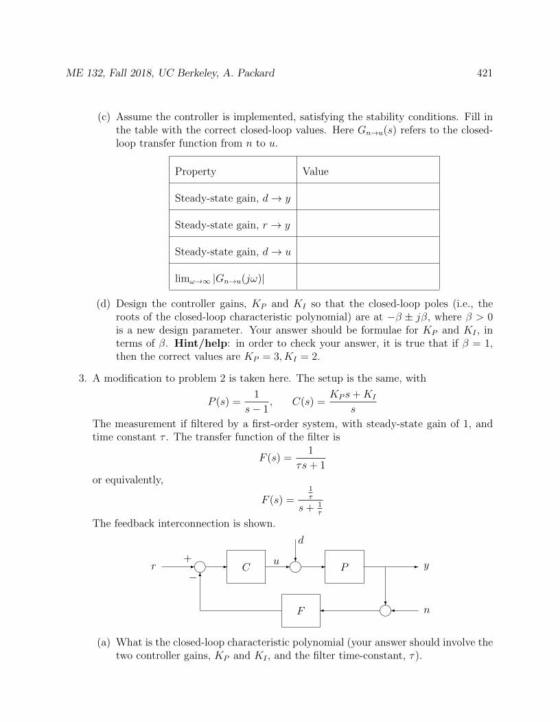
ME 132, Fall 2018, UC Berkeley, A. Packard 421
(c) Assume the controller is implemented, satisfying the stability conditions. Fill inthe table with the correct closed-loop values. Here Gn→u(s) refers to the closed-loop transfer function from n to u.
Property Value
Steady-state gain, d→ y
Steady-state gain, r → y
Steady-state gain, d→ u
limω→∞ |Gn→u(jω)|
(d) Design the controller gains, KP and KI so that the closed-loop poles (i.e., theroots of the closed-loop characteristic polynomial) are at −β ± jβ, where β > 0is a new design parameter. Your answer should be formulae for KP and KI , interms of β. Hint/help: in order to check your answer, it is true that if β = 1,then the correct values are KP = 3, KI = 2.
3. A modification to problem 2 is taken here. The setup is the same, with
P (s) =1
s− 1, C(s) =
KP s+KI
s
The measurement if filtered by a first-order system, with steady-state gain of 1, andtime constant τ . The transfer function of the filter is
F (s) =1
τs+ 1
or equivalently,
F (s) =1τ
s+ 1τ
The feedback interconnection is shown.
C P
F
- - - k -?
d
-
?k
6
k+
−r u y
n
(a) What is the closed-loop characteristic polynomial (your answer should involve thetwo controller gains, KP and KI , and the filter time-constant, τ).
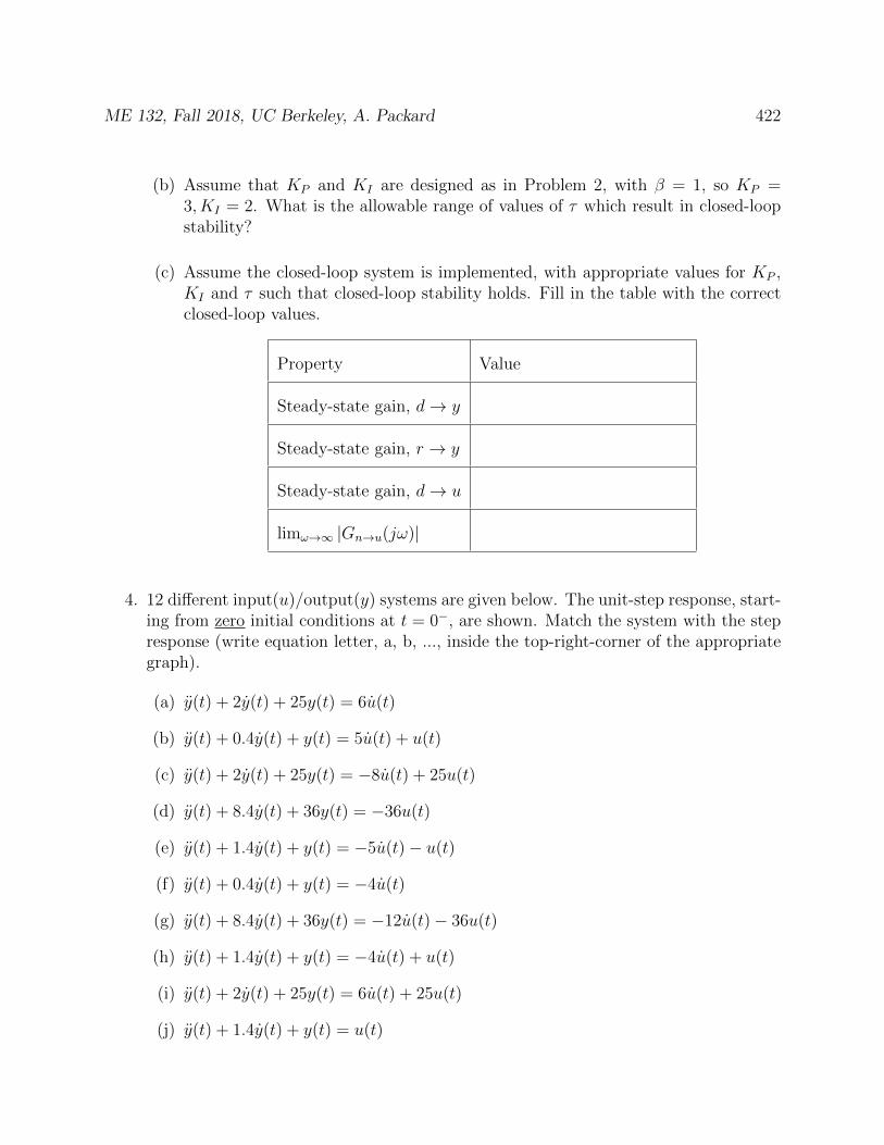
ME 132, Fall 2018, UC Berkeley, A. Packard 422
(b) Assume that KP and KI are designed as in Problem 2, with β = 1, so KP =3, KI = 2. What is the allowable range of values of τ which result in closed-loopstability?
(c) Assume the closed-loop system is implemented, with appropriate values for KP ,KI and τ such that closed-loop stability holds. Fill in the table with the correctclosed-loop values.
Property Value
Steady-state gain, d→ y
Steady-state gain, r → y
Steady-state gain, d→ u
limω→∞ |Gn→u(jω)|
4. 12 different input(u)/output(y) systems are given below. The unit-step response, start-ing from zero initial conditions at t = 0−, are shown. Match the system with the stepresponse (write equation letter, a, b, ..., inside the top-right-corner of the appropriategraph).
(a) y(t) + 2y(t) + 25y(t) = 6u(t)
(b) y(t) + 0.4y(t) + y(t) = 5u(t) + u(t)
(c) y(t) + 2y(t) + 25y(t) = −8u(t) + 25u(t)
(d) y(t) + 8.4y(t) + 36y(t) = −36u(t)
(e) y(t) + 1.4y(t) + y(t) = −5u(t)− u(t)
(f) y(t) + 0.4y(t) + y(t) = −4u(t)
(g) y(t) + 8.4y(t) + 36y(t) = −12u(t)− 36u(t)
(h) y(t) + 1.4y(t) + y(t) = −4u(t) + u(t)
(i) y(t) + 2y(t) + 25y(t) = 6u(t) + 25u(t)
(j) y(t) + 1.4y(t) + y(t) = u(t)

ME 132, Fall 2018, UC Berkeley, A. Packard 423
(k) y(t) + 0.4y(t) + y(t) = 4u(t)− u(t)
(l) y(t) + 8.4y(t) + 36y(t) = −12u(t) + 36u(t)
0 2 4
−2
0
2
4
0 2 4
−2
0
2
4
0 5 10 15
−2
0
2
4
0 5 10 15
−2
0
2
4
0 1 2
−2
0
2
4
0 5 10
−2
0
2
4
0 1 2
−2
0
2
4
0 2 4
−2
0
2
4
0 5 10
−2
0
2
4
0 5 10
−2
0
2
4
0 1 2
−2
0
2
4
0 5 10 15
−2
0
2
4
31.3 Spring 2012, Final Exam
# 1
25
# 2
25
# 3
25
# 4
30
# 5
25
# 6
25
# 7
25
NAME
1. Consider the PI controller architecture shown below.
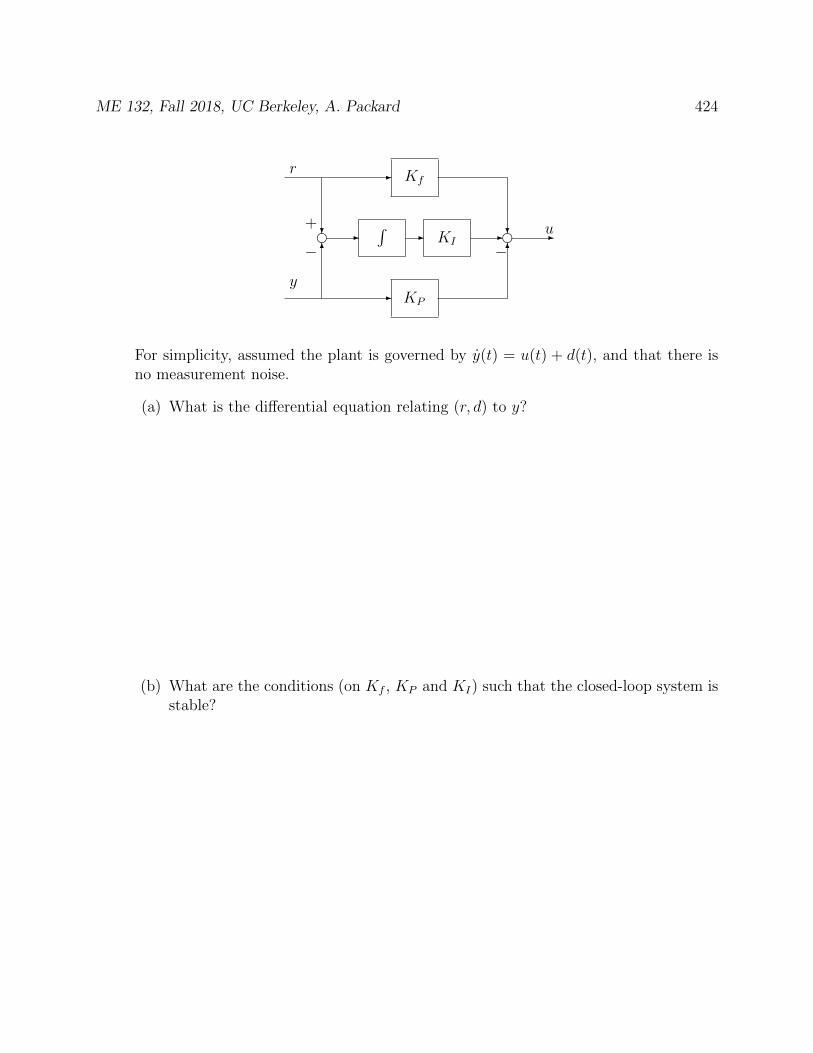
ME 132, Fall 2018, UC Berkeley, A. Packard 424
-
6
- - - -
-
? ?
6
f fKP
∫KI
Kfr
y
−
+
−u
For simplicity, assumed the plant is governed by y(t) = u(t) + d(t), and that there isno measurement noise.
(a) What is the differential equation relating (r, d) to y?
(b) What are the conditions (on Kf , KP and KI) such that the closed-loop system isstable?
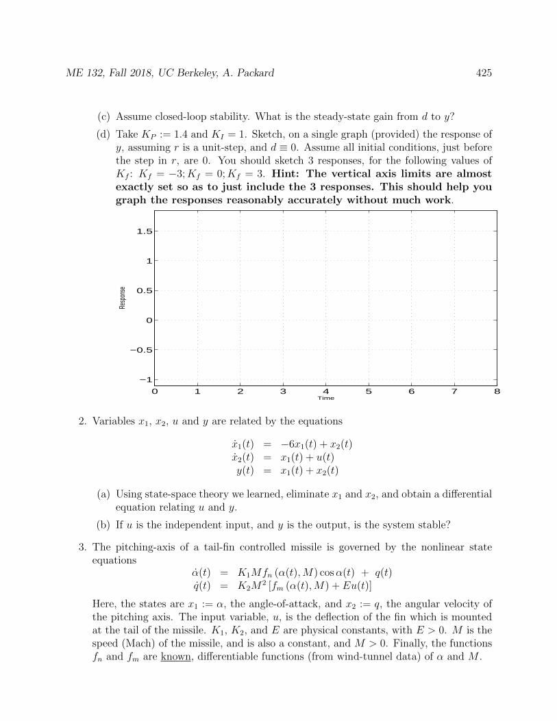
ME 132, Fall 2018, UC Berkeley, A. Packard 425
(c) Assume closed-loop stability. What is the steady-state gain from d to y?
(d) Take KP := 1.4 and KI = 1. Sketch, on a single graph (provided) the response ofy, assuming r is a unit-step, and d ≡ 0. Assume all initial conditions, just beforethe step in r, are 0. You should sketch 3 responses, for the following values ofKf : Kf = −3;Kf = 0;Kf = 3. Hint: The vertical axis limits are almostexactly set so as to just include the 3 responses. This should help yougraph the responses reasonably accurately without much work.
0 1 2 3 4 5 6 7 8
−1
−0.5
0
0.5
1
1.5
Resp
onse
Time
2. Variables x1, x2, u and y are related by the equations
x1(t) = −6x1(t) + x2(t)x2(t) = x1(t) + u(t)y(t) = x1(t) + x2(t)
(a) Using state-space theory we learned, eliminate x1 and x2, and obtain a differentialequation relating u and y.
(b) If u is the independent input, and y is the output, is the system stable?
3. The pitching-axis of a tail-fin controlled missile is governed by the nonlinear stateequations
α(t) = K1Mfn (α(t),M) cosα(t) + q(t)q(t) = K2M
2 [fm (α(t),M) + Eu(t)]
Here, the states are x1 := α, the angle-of-attack, and x2 := q, the angular velocity ofthe pitching axis. The input variable, u, is the deflection of the fin which is mountedat the tail of the missile. K1, K2, and E are physical constants, with E > 0. M is thespeed (Mach) of the missile, and is also a constant, and M > 0. Finally, the functionsfn and fm are known, differentiable functions (from wind-tunnel data) of α and M .

ME 132, Fall 2018, UC Berkeley, A. Packard 426
(a) Show that for any specific value of α, with |α| < π2, there is a pair (q, u) such that[
αq
], u
is an equilibrium point of the system (this represents a turn at a constant rate).Your answer should clearly show how q and u are functions of α, and will involvethe functions fn and fm. Again - the functions fn and fm are assumedknown, so your answer can depend on these.
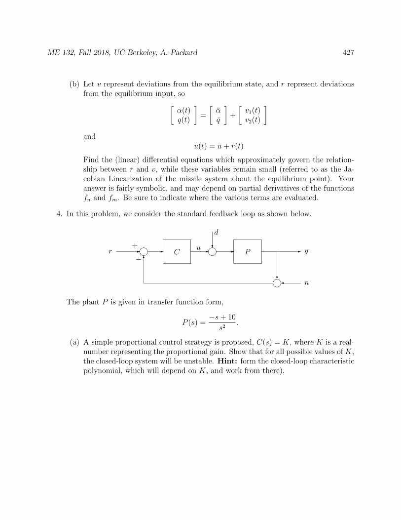
ME 132, Fall 2018, UC Berkeley, A. Packard 427
(b) Let v represent deviations from the equilibrium state, and r represent deviationsfrom the equilibrium input, so[
α(t)q(t)
]=
[αq
]+
[v1(t)v2(t)
]and
u(t) = u+ r(t)
Find the (linear) differential equations which approximately govern the relation-ship between r and v, while these variables remain small (referred to as the Ja-cobian Linearization of the missile system about the equilibrium point). Youranswer is fairly symbolic, and may depend on partial derivatives of the functionsfn and fm. Be sure to indicate where the various terms are evaluated.
4. In this problem, we consider the standard feedback loop as shown below.
C P- - - k -?
d
-
?k6
k+
−r u y
n
The plant P is given in transfer function form,
P (s) =−s+ 10
s2.
(a) A simple proportional control strategy is proposed, C(s) = K, where K is a real-number representing the proportional gain. Show that for all possible values of K,the closed-loop system will be unstable. Hint: form the closed-loop characteristicpolynomial, which will depend on K, and work from there).
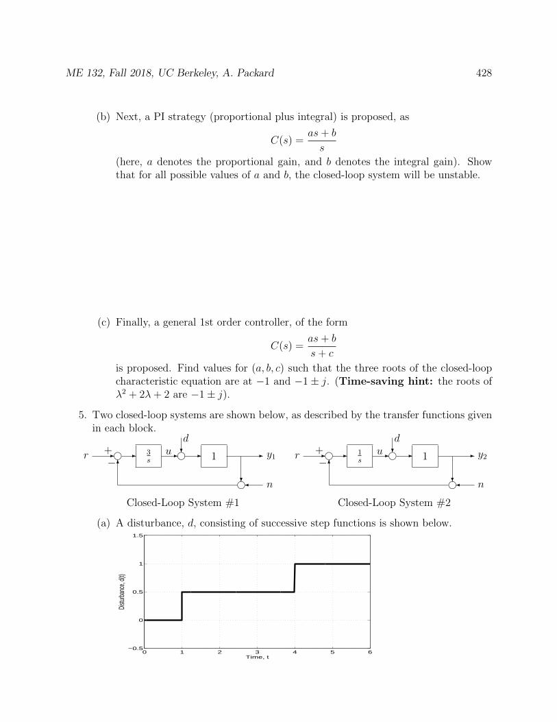
ME 132, Fall 2018, UC Berkeley, A. Packard 428
(b) Next, a PI strategy (proportional plus integral) is proposed, as
C(s) =as+ b
s
(here, a denotes the proportional gain, and b denotes the integral gain). Showthat for all possible values of a and b, the closed-loop system will be unstable.
(c) Finally, a general 1st order controller, of the form
C(s) =as+ b
s+ c
is proposed. Find values for (a, b, c) such that the three roots of the closed-loopcharacteristic equation are at −1 and −1± j. (Time-saving hint: the roots ofλ2 + 2λ+ 2 are −1± j).
5. Two closed-loop systems are shown below, as described by the transfer functions givenin each block.
3s 1- - - g -?d -
?g6
g+−
r u y1
n
Closed-Loop System #1
1s 1- - - g -?d -
?g6
g+−
r u y2
n
Closed-Loop System #2
(a) A disturbance, d, consisting of successive step functions is shown below.
0 1 2 3 4 5 6−0.5
0
0.5
1
1.5
Time, t
Distu
rbanc
e, d(t
)

ME 132, Fall 2018, UC Berkeley, A. Packard 429
The resulting output y (with r = 0, n = 0) is shown below. Two separate graphsare shown. One is the response of closed-loop system #1, and the other is theresponse of closed-loop system #2. Clearly mark which y response corresponds towhich system. Justify your answer below (answers will receive no credit withoutadequate justification).
0 1 2 3 4 5 6−0.5
0
0.5
1
Time, t
Resp
onse
to D
isturb
ance
0 1 2 3 4 5 6−0.5
0
0.5
1
Time, t
Resp
onse
to D
isturb
ance
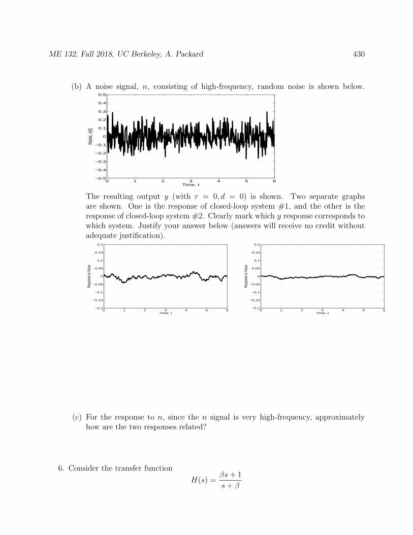
ME 132, Fall 2018, UC Berkeley, A. Packard 430
(b) A noise signal, n, consisting of high-frequency, random noise is shown below.
0 1 2 3 4 5 6−0.5
−0.4
−0.3
−0.2
−0.1
0
0.1
0.2
0.3
0.4
0.5
Time, t
Noise
, n(t)
The resulting output y (with r = 0, d = 0) is shown. Two separate graphsare shown. One is the response of closed-loop system #1, and the other is theresponse of closed-loop system #2. Clearly mark which y response corresponds towhich system. Justify your answer below (answers will receive no credit withoutadequate justification).
0 1 2 3 4 5 6−0.2
−0.15
−0.1
−0.05
0
0.05
0.1
0.15
0.2
Time, t
Resp
onse
to N
oise
0 1 2 3 4 5 6−0.2
−0.15
−0.1
−0.05
0
0.05
0.1
0.15
0.2
Time, t
Resp
onse
to N
oise
(c) For the response to n, since the n signal is very high-frequency, approximatelyhow are the two responses related?
6. Consider the transfer function
H(s) =βs+ 1
s+ β

ME 132, Fall 2018, UC Berkeley, A. Packard 431
(a) Sketch a Magnitude plot of H, for β = 5 on the graph below
10−2
10−1
100
101
102
10−1
100
101
Frequency
Magn
itude
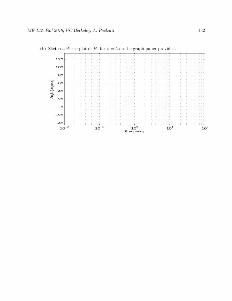
ME 132, Fall 2018, UC Berkeley, A. Packard 432
(b) Sketch a Phase plot of H, for β = 5 on the graph paper provided.
10−2
10−1
100
101
102
−40
−20
0
20
40
60
80
100
120
Frequency
Angle
(deg
rees)
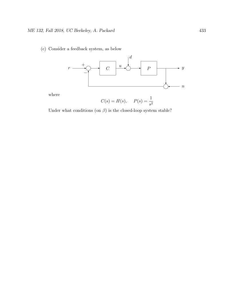
ME 132, Fall 2018, UC Berkeley, A. Packard 433
(c) Consider a feedback system, as below
C P- - - k -?
d
-
?k6
k+
−r u y
n
where
C(s) = H(s), P (s) =1
s2
Under what conditions (on β) is the closed-loop system stable?
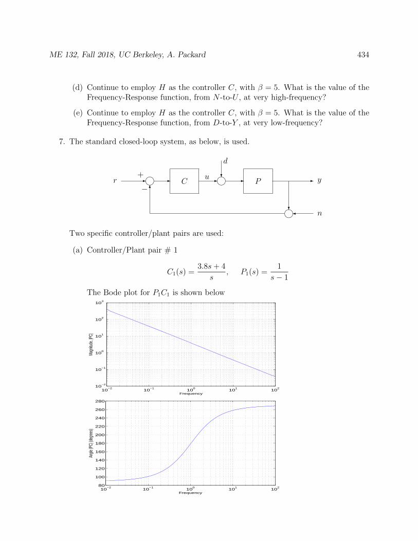
ME 132, Fall 2018, UC Berkeley, A. Packard 434
(d) Continue to employ H as the controller C, with β = 5. What is the value of theFrequency-Response function, from N -to-U , at very high-frequency?
(e) Continue to employ H as the controller C, with β = 5. What is the value of theFrequency-Response function, from D-to-Y , at very low-frequency?
7. The standard closed-loop system, as below, is used.
C P- - - k -?
d
-
?k6
k+
−r u y
n
Two specific controller/plant pairs are used:
(a) Controller/Plant pair # 1
C1(s) =3.8s+ 4
s, P1(s) =
1
s− 1
The Bode plot for P1C1 is shown below
10−2
10−1
100
101
102
10−2
10−1
100
101
102
103
Frequency
Magn
itude
, |PC|
10−2
10−1
100
101
102
80
100
120
140
160
180
200
220
240
260
280
Frequency
Angle
|PC|
(deg
rees)

ME 132, Fall 2018, UC Berkeley, A. Packard 435
(b) Controller/Plant pair # 2
C2(s) =1.8s+ 4
s, P2(s) =
1
s+ 1
The Bode plot for P2C2 is shown below
10−2
10−1
100
101
102
10−2
10−1
100
101
102
103
Frequency
Magn
itude
, |PC|
10−2
10−1
100
101
102
−115
−110
−105
−100
−95
−90
Frequency
Angle
|PC|
(deg
rees)
You will answer 4 questions for each system

ME 132, Fall 2018, UC Berkeley, A. Packard 436
For system # 1, determine
(a) the closed-loop characteristic polynomial
(b) the closed-loop transfer function from D to Y
(c) the Gain-Margin (Bode plots of L := PC are provided)
(d) the Time-Delay-Margin (Bode plots of L := PC are provided)
ME 132, Fall 2018, UC Berkeley, A. Packard 437
For system # 2, determine
(a) the closed-loop characteristic polynomial
(b) the closed-loop transfer function from D to Y
(c) the Gain-Margin (Bode plots of L := PC are provided)
(d) the Time-Delay-Margin (Bode plots of L := PC are provided)
31.4 Spring 2009, Midterm 1
1. The solutions to the differential equations listed below are shown on the next page.Match the ODE with the solution graph. Make a table with pertinent informationthat justifies your answers. In each case, all appropriate initial conditions are 0. Bythat, I mean that if the differential equation is first-order, then the initial condition isy(0) = 0. If the differential equation is second order, then the initial conditions arey(0) = 0, y(0) = 0.
(a) y(t) + y(t) = 1
(b) y(t) + 5y(t) = 5
(c) y(t)− y(t) = 1
(d) y(t) + 10y(t) = 10
(e) y(t)− 2y(t)− y(t) = −1
(f) y(t)− 2y(t) + 9y(t) = 9
(g) y(t) + 0.4y(t) + y(t) = 1
(h) y(t) + 0.12y(t) + 0.09y(t) = 0.09
(i) y(t) + 6y(t) + 5y(t) = 5
(j) y(t) + 0.3y(t) + 0.09y(t) = 0.09
(k) y(t) + 3y(t) + 9y(t) = 9
(l) y(t) + 1.8y(t) + 9y(t) = 9
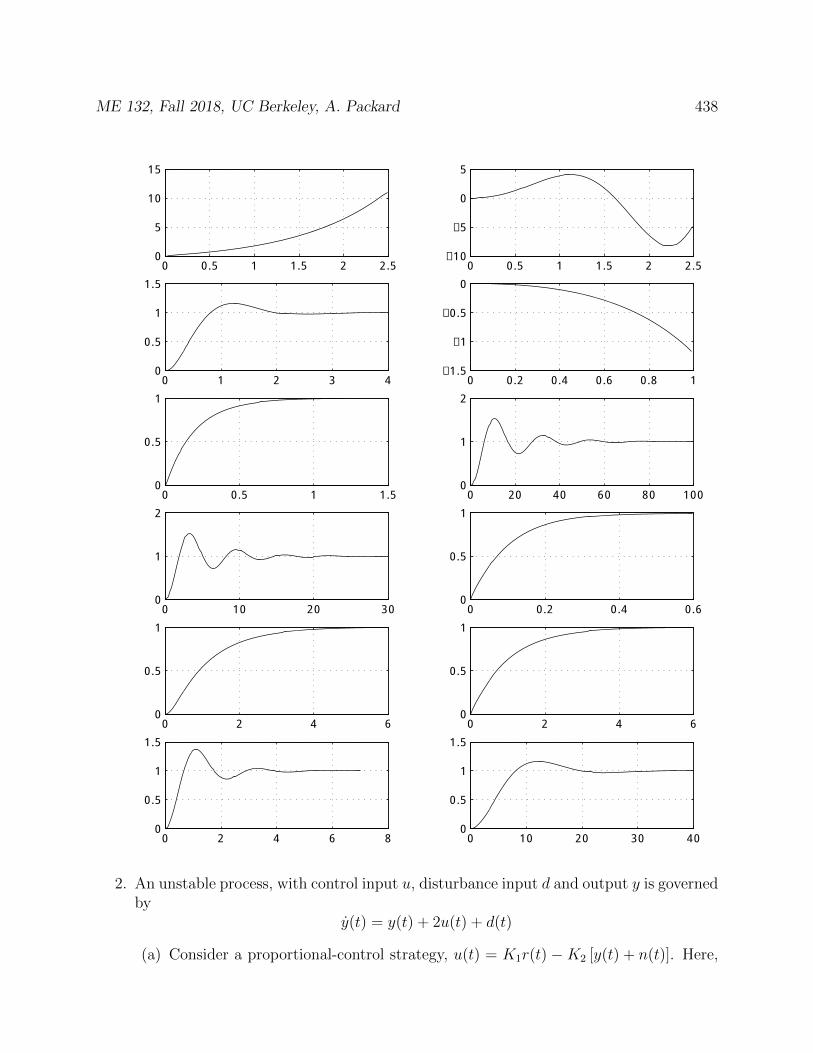
ME 132, Fall 2018, UC Berkeley, A. Packard 438
0 0.5 1 1.5 2 2.50
5
10
15
0 0.5 1 1.5 2 2.5−10
−5
0
5
0 1 2 3 40
0.5
1
1.5
0 0.2 0.4 0.6 0.8 1−1.5
−1
−0.5
0
0 0.5 1 1.50
0.5
1
0 20 40 60 80 1000
1
2
0 10 20 300
1
2
0 0.2 0.4 0.60
0.5
1
0 2 4 60
0.5
1
0 2 4 60
0.5
1
0 2 4 6 80
0.5
1
1.5
0 10 20 30 400
0.5
1
1.5
2. An unstable process, with control input u, disturbance input d and output y is governedby
y(t) = y(t) + 2u(t) + d(t)
(a) Consider a proportional-control strategy, u(t) = K1r(t) −K2 [y(t) + n(t)]. Here,
ME 132, Fall 2018, UC Berkeley, A. Packard 439
r is a reference-command input, and n is measurement noise. Combine withthe process model to eliminate u, and determine the closed-loop differentialequation relating the variables (y, r, d, n).
(b) For what values of K1 and K2 is the closed-loop system stable?
(c) Assuming closed-loop stability, what is the time-constant of the closed-loop system(in terms of K1 and K2)?
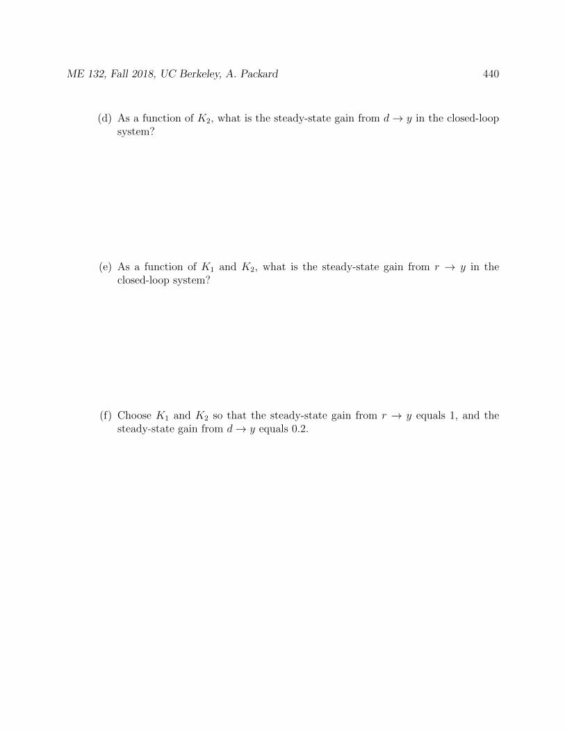
ME 132, Fall 2018, UC Berkeley, A. Packard 440
(d) As a function of K2, what is the steady-state gain from d→ y in the closed-loopsystem?
(e) As a function of K1 and K2, what is the steady-state gain from r → y in theclosed-loop system?
(f) Choose K1 and K2 so that the steady-state gain from r → y equals 1, and thesteady-state gain from d→ y equals 0.2.
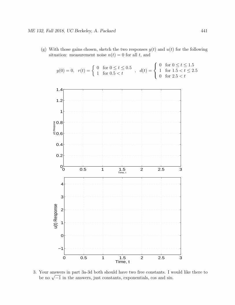
ME 132, Fall 2018, UC Berkeley, A. Packard 441
(g) With those gains chosen, sketch the two responses y(t) and u(t) for the followingsituation: measurement noise n(t) = 0 for all t, and
y(0) = 0, r(t) =
0 for 0 ≤ t ≤ 0.51 for 0.5 < t
, d(t) =
0 for 0 ≤ t ≤ 1.51 for 1.5 < t ≤ 2.50 for 2.5 < t
0 0.5 1 1.5 2 2.5 30
0.2
0.4
0.6
0.8
1
1.2
1.4
Time, t
y(t)
Res
pons
e
0 0.5 1 1.5 2 2.5 3
−1
0
1
2
3
4
Time, t
u(t)
Res
pons
e
3. Your answers in part 3a-3d both should have two free constants. I would like there tobe no
√−1 in the answers, just constants, exponentials, cos and sin.
ME 132, Fall 2018, UC Berkeley, A. Packard 442
(a) What is the general form of all real solutions to the differential equation
x(t) + 5x(t) + 6x(t) = 0
(b) What is the general form of all real solutions to the differential equation
x(t) + 5x(t) + 6x(t) = 12
(c) What is the general form of all real solutions to the differential equation
y(t) + 2y(t) + 17y(t) = 0
(d) What is the general form of all real solutions to the differential equation
y(t) + 2y(t) + 17y(t) = −51
(e) The solutions in part 3c are made up of an exponentially decaying envelope,superimposed on a sinusoid. What (approximately) is the ratio
Time− to−Decay
Period− of −Oscillation
4. An unstable process, with control input u, disturbance input d and output y is governedby
y(t) = y(t) + u(t) + d(t)
(a) A PI (Proportional plus Integral) controller is proposed
u(t) = KP [r(t)− y(t)− n(t)] +KIz(t)z(t) = r(t)− y(t)− n(t)
Here z is the variable representing the integrator, r is a command-reference in-put, and n is measurement noise. Combine with the governing equation for theprocess, and eliminate z and u, determining the closed-loop differential equa-tion relating the variables (y, r, d, n). Note that derivatives of the external inputs(r, d, n) may appear.

ME 132, Fall 2018, UC Berkeley, A. Packard 443
(b) For what values of KP and KI is the closed-loop system stable?
(c) The closed-loop system is 2nd order. What are the appropriate values of KP andKI so that the closed-loop system characteristic polynomial has roots describedby ξ = 0.8, ωn = 0.5?
(d) What are the appropriate values of KP and KI so that the closed-loop systemcharacteristic polynomial has roots described by ξ = 0.8, ωn = 1.0?
(e) What are the appropriate values of KP and KI so that the closed-loop systemcharacteristic polynomial has roots described by ξ = 0.8, ωn = 2.0?
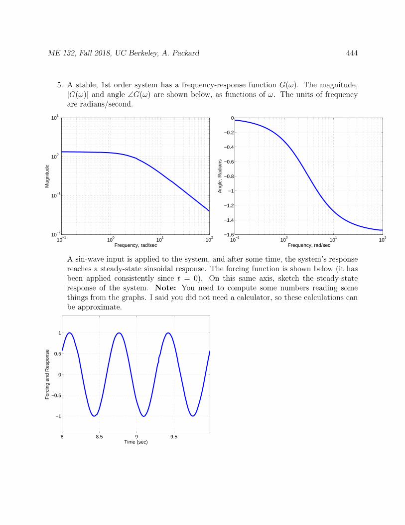
ME 132, Fall 2018, UC Berkeley, A. Packard 444
5. A stable, 1st order system has a frequency-response function G(ω). The magnitude,|G(ω)| and angle ∠G(ω) are shown below, as functions of ω. The units of frequencyare radians/second.
10−1
100
101
102
10−2
10−1
100
101
Mag
nitu
de
Frequency, rad/sec10
−110
010
110
2−1.6
−1.4
−1.2
−1
−0.8
−0.6
−0.4
−0.2
0
Ang
le, R
adia
ns
Frequency, rad/sec
A sin-wave input is applied to the system, and after some time, the system’s responsereaches a steady-state sinsoidal response. The forcing function is shown below (it hasbeen applied consistently since t = 0). On this same axis, sketch the steady-stateresponse of the system. Note: You need to compute some numbers reading somethings from the graphs. I said you did not need a calculator, so these calculations canbe approximate.
8 8.5 9 9.5
−1
−0.5
0
0.5
1
For
cing
and
Res
pons
e
Time (sec)
ME 132, Fall 2018, UC Berkeley, A. Packard 445
31.5 Spring 2009, Midterm 2
Cannot find this one...
31.6 Spring 2009, Final Exam
Cannot find this one...
31.7 Spring 2005 Midterm 1
1. Your answers in part 1a and 1c both should have two free constants. I would like thereto be no
√−1 in the answers, just exponentials, cos and sin.
(a) What is the general form of real (as opposed to complex) solutions to the differ-ential equation
y(t) + 2y(t) + 17y(t) = 0
(b) The solutions in part 1a are made up of an exponentially decaying envelope,superimposed on a sinusoid. What (approximately) is the ratio
Period− of −Oscillation
Time− to−Decay
Explain.
(c) What is the general form of real solutions to the differential equation
y(t) + 2y(t) + 17y(t) = −51
ME 132, Fall 2018, UC Berkeley, A. Packard 446
2. A process has a very simple model,
y(t) = Hu(t) + w(t).
The control input is u, the disturbance input is w and the output is y. Here, H issimply a gain, ie., the behavior of the system is “static” - it is not governed by adifferential equation.
The goal of control is to make the process output y follow a reference input r, even inthe presence of nonzero disturbances w, and slight unknown variations in H. In orderto achieve this, we use an integral controller
z(t) = r(t)− y(t)u(t) = KIz(t)
Here, r is the reference input.
(a) Combine the the process model, and the controller equations to (eliminating z andu) get a relationship between the process output y, the two “forcing” functions rand w, and any of their derivatives.
(b) Under what conditions (on H and KI) is the closed-loop system stable?
ME 132, Fall 2018, UC Berkeley, A. Packard 447
(c) Assume that KI is chosen so that the closed-loop system is stable. Does a 20%change in H (ie., H changing to 0.8H or 1.2H) affect stability of the closed-loopsystem?
(d) Assume that KI is chosen so that the closed-loop system is stable. If r(t) ≡ rand w(t) ≡ w for all t ≥ 0 (r and w are some fixed constant values), what are thesteady-state values (in terms of r, w,KI , H) of y and u, defined as
limt→∞
y(t) limt→∞
u(t)
(e) How does a 20% change in H affect (approximately) the steady-state values of yand u derived in part (2d) above?
(f) Assume that KI is chosen so that the closed-loop system is stable. What is thetime-constant of the closed-loop system? Approximately how does a 20% changein H (ie., H changing to 0.8H or 1.2H) affect (approximately) the time constant?
ME 132, Fall 2018, UC Berkeley, A. Packard 448
3. A closed-loop system is shown below. Here H and K are positive constants, namelyH = 4, and K = 1.
(a) By eliminating y and u from the equations, find the constants A,B1, B2 andB3 such that the internal variable z is related to the external forcing functions(r, w, n) in the form
z(t) = Az(t) +B1r(t) +B2w(t) +B3n(t)
(b) Express the variable y as a combination of z, r, w, n, namely find the constantsC1, D11, D12 and D13 such that
y(t) = C1z(t) +D11r(t) +D12w(t) +D13n(t)
ME 132, Fall 2018, UC Berkeley, A. Packard 449
(c) Express the variable u as a combination of z, r, w, n, namely find the constantsC2, D21, D22 and D23 such that
u(t) = C2z(t) +D21r(t) +D22w(t) +D23n(t)
(d) Shown on the next page is the frequency-response matrix (2× 3) from the threeexternal inputs (r, w, n) to the two “outputs-of-interest” (y, u). In 5 of the cases,only the magnitude is shown. In the case of input/output pair (r, y), both mag-nitude and phase are shown.
In each axes, 3 or 4 lines are shown, though only one is correct. In each case,mark the correct frequency response curve.
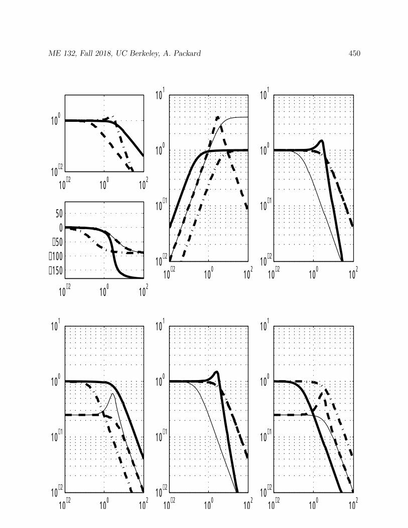
ME 132, Fall 2018, UC Berkeley, A. Packard 450
10−2
100
102
10−2
100
10−2
100
102
−150−100
−500
50
10−2
100
102
10−2
10−1
100
101
10−2
100
102
10−2
10−1
100
101
10−2
100
102
10−2
10−1
100
101
10−2
100
102
10−2
10−1
100
101
10−2
100
102
10−2
10−1
100
101
ME 132, Fall 2018, UC Berkeley, A. Packard 451
31.8 Spring 2005 Midterm 2
1. Consider the closed loop system shown below.
The transfer function for the controller is
C(s) =s+ 25
3
s(31.1)
The transfer function for the process is
P (s) =3
s+ 5(31.2)
(a) Assume all initial conditions are zero. Suppose that the reference input, r, is aunit step function, and the disturbance input, d is identically zero. Shown beloware several possible responses for the output variable y. Only one of them iscorrect. Clearly mark the correct one. Show work/reasoning.

ME 132, Fall 2018, UC Berkeley, A. Packard 452
0 2 4 60
0.5
1
1.5
Step Response
Time (sec)
Am
plitu
de
0 0.5 1 1.50
0.5
1
1.5
Step Response
Time (sec)
Am
plitu
de
0 0.5 1 1.50
0.5
1
1.5
Step Response
Time (sec)
Am
plitu
de
0 0.1 0.2 0.30
0.5
1
1.5
Step Response
Time (sec)
Am
plitu
de
0 2 4 60
0.5
1
1.5
2
Step Response
Time (sec)
Am
plitu
de
0 0.1 0.2 0.30
0.5
1
1.5
Step Response
Time (sec)
Am
plitu
de
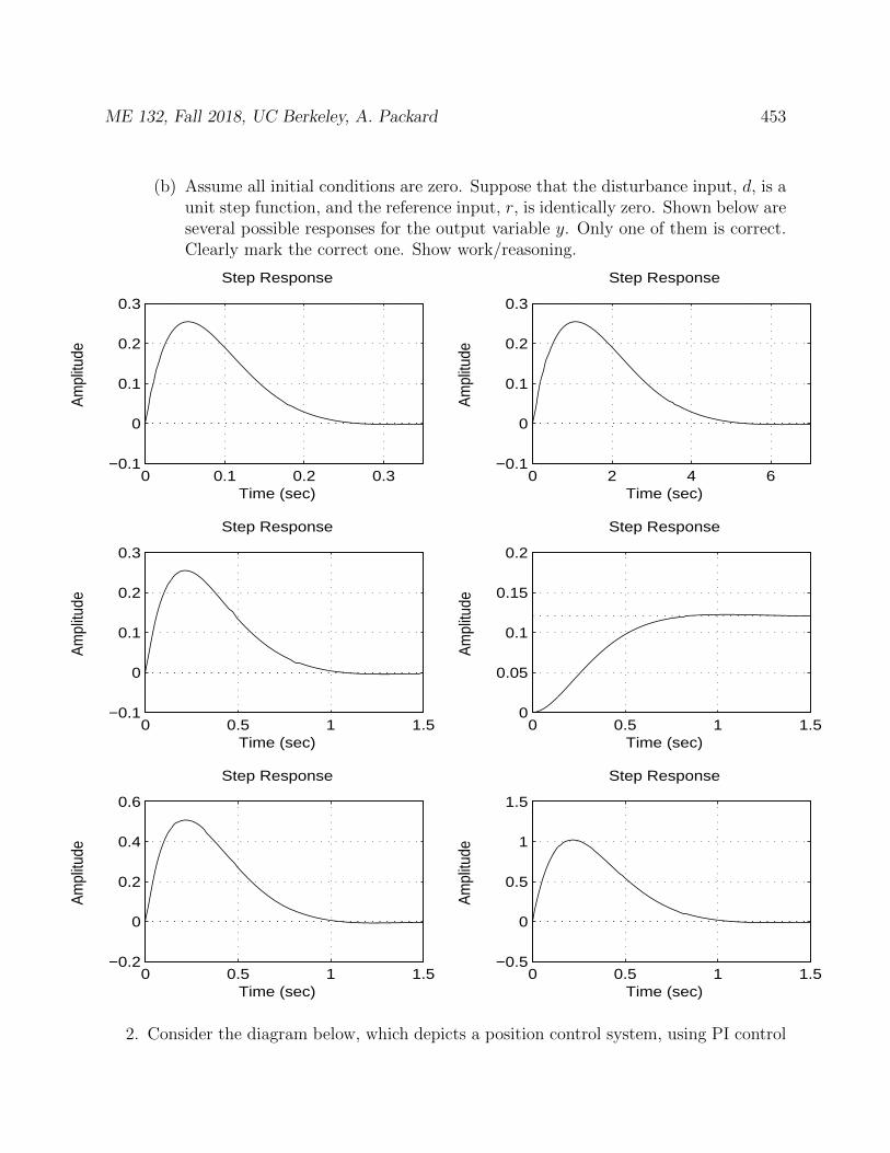
ME 132, Fall 2018, UC Berkeley, A. Packard 453
(b) Assume all initial conditions are zero. Suppose that the disturbance input, d, is aunit step function, and the reference input, r, is identically zero. Shown below areseveral possible responses for the output variable y. Only one of them is correct.Clearly mark the correct one. Show work/reasoning.
0 0.1 0.2 0.3−0.1
0
0.1
0.2
0.3
Step Response
Time (sec)
Am
plitu
de
0 2 4 6−0.1
0
0.1
0.2
0.3
Step Response
Time (sec)
Am
plitu
de
0 0.5 1 1.5−0.1
0
0.1
0.2
0.3
Step Response
Time (sec)
Am
plitu
de
0 0.5 1 1.50
0.05
0.1
0.15
0.2
Step Response
Time (sec)
Am
plitu
de
0 0.5 1 1.5−0.2
0
0.2
0.4
0.6
Step Response
Time (sec)
Am
plitu
de
0 0.5 1 1.5−0.5
0
0.5
1
1.5
Step Response
Time (sec)
Am
plitu
de
2. Consider the diagram below, which depicts a position control system, using PI control
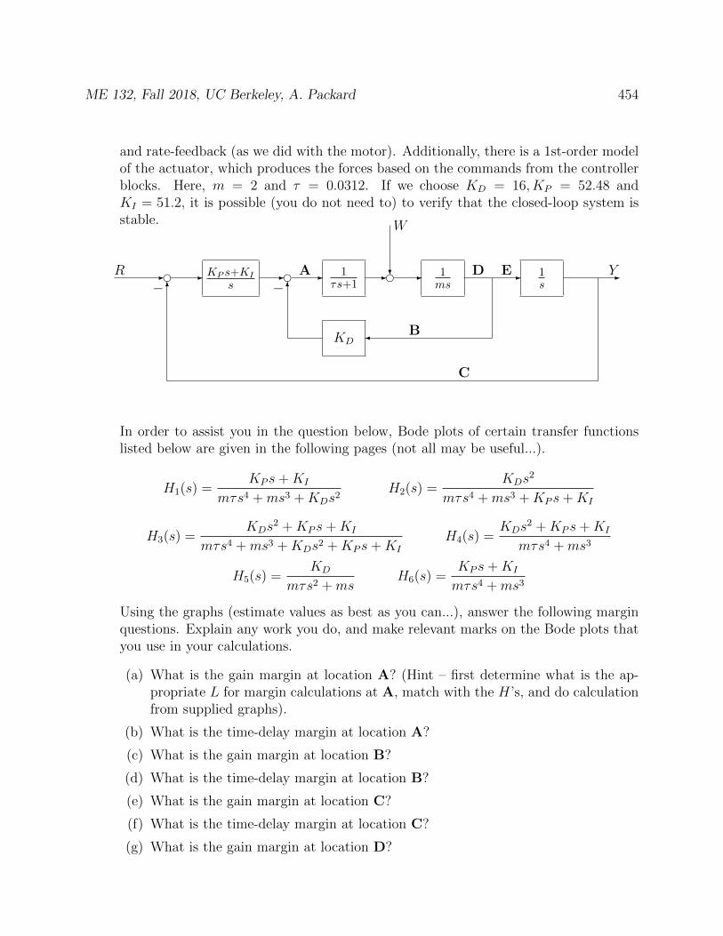
ME 132, Fall 2018, UC Berkeley, A. Packard 454
and rate-feedback (as we did with the motor). Additionally, there is a 1st-order modelof the actuator, which produces the forces based on the commands from the controllerblocks. Here, m = 2 and τ = 0.0312. If we choose KD = 16, KP = 52.48 andKI = 51.2, it is possible (you do not need to) to verify that the closed-loop system isstable.
- e eKP s+KI
s1
τs+11ms
1s
KD
- - - - e? - - -
6
6− −R
W
YA
B
C
D E
In order to assist you in the question below, Bode plots of certain transfer functionslisted below are given in the following pages (not all may be useful...).
H1(s) =KP s+KI
mτs4 +ms3 +KDs2H2(s) =
KDs2
mτs4 +ms3 +KP s+KI
H3(s) =KDs
2 +KP s+KI
mτs4 +ms3 +KDs2 +KP s+KI
H4(s) =KDs
2 +KP s+KI
mτs4 +ms3
H5(s) =KD
mτs2 +msH6(s) =
KP s+KI
mτs4 +ms3
Using the graphs (estimate values as best as you can...), answer the following marginquestions. Explain any work you do, and make relevant marks on the Bode plots thatyou use in your calculations.
(a) What is the gain margin at location A? (Hint – first determine what is the ap-propriate L for margin calculations at A, match with the H’s, and do calculationfrom supplied graphs).
(b) What is the time-delay margin at location A?
(c) What is the gain margin at location B?
(d) What is the time-delay margin at location B?
(e) What is the gain margin at location C?
(f) What is the time-delay margin at location C?
(g) What is the gain margin at location D?

ME 132, Fall 2018, UC Berkeley, A. Packard 455
(h) What is the time-delay margin at location D?
(i) What is the gain margin at location E?
(j) What is the time-delay margin at location E?
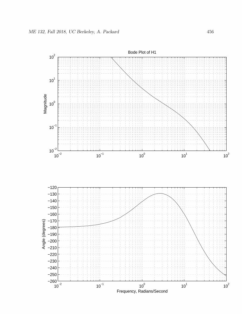
ME 132, Fall 2018, UC Berkeley, A. Packard 456
10−2
10−1
100
101
102
10−2
10−1
100
101
102
Bode Plot of H1
Magnitu
de
10−2
10−1
100
101
102
−260
−250
−240
−230
−220
−210
−200
−190
−180
−170
−160
−150
−140
−130
−120
Angle
(degre
es)
Frequency, Radians/Second
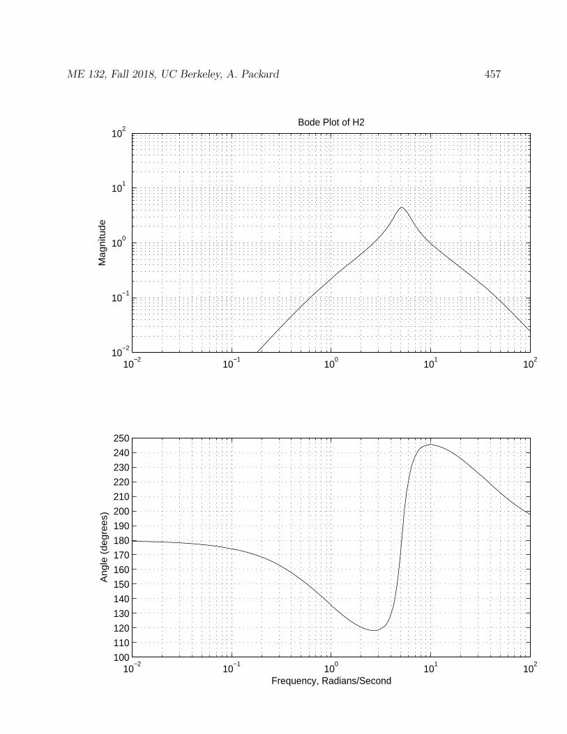
ME 132, Fall 2018, UC Berkeley, A. Packard 457
10−2
10−1
100
101
102
10−2
10−1
100
101
102
Bode Plot of H2
Magnitu
de
10−2
10−1
100
101
102
100
110
120
130
140
150
160
170
180
190
200
210
220
230
240
250
Angle
(degre
es)
Frequency, Radians/Second

ME 132, Fall 2018, UC Berkeley, A. Packard 458
10−2
10−1
100
101
102
10−2
10−1
100
101
102
Bode Plot of H3
Magnitu
de
10−2
10−1
100
101
102
−180−170−160−150−140−130−120−110−100 −90 −80 −70 −60 −50 −40 −30 −20 −10
0 10 20
Angle
(degre
es)
Frequency, Radians/Second
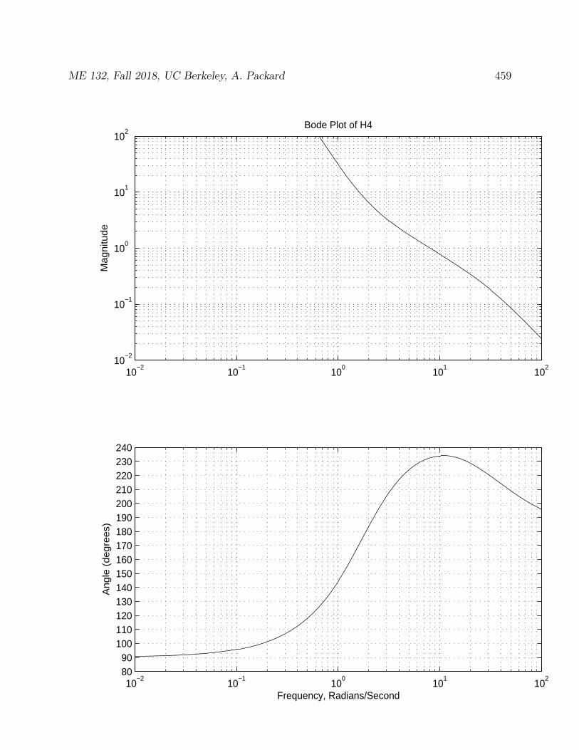
ME 132, Fall 2018, UC Berkeley, A. Packard 459
10−2
10−1
100
101
102
10−2
10−1
100
101
102
Bode Plot of H4
Magnitu
de
10−2
10−1
100
101
102
80 90
100110120130140150160170180190200210220230240
Angle
(degre
es)
Frequency, Radians/Second
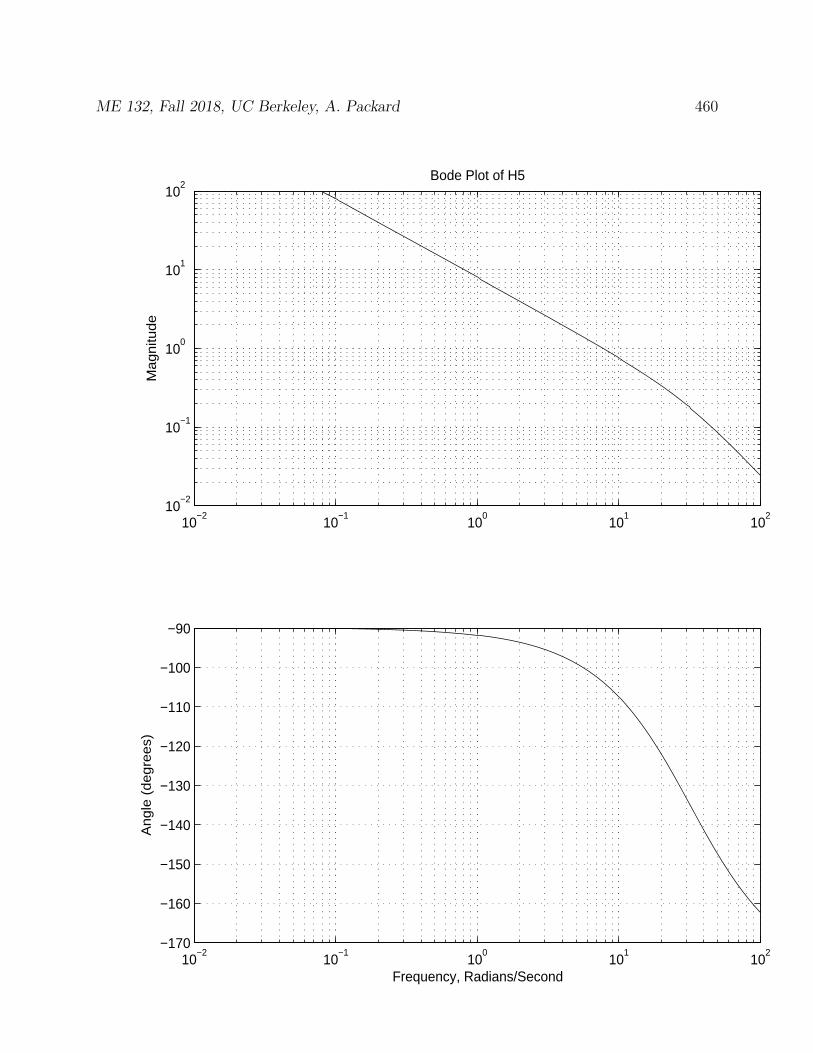
ME 132, Fall 2018, UC Berkeley, A. Packard 460
10−2
10−1
100
101
102
10−2
10−1
100
101
102
Bode Plot of H5
Magnitu
de
10−2
10−1
100
101
102
−170
−160
−150
−140
−130
−120
−110
−100
−90
Angle
(degre
es)
Frequency, Radians/Second
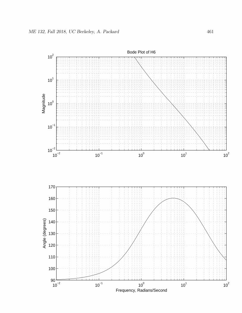
ME 132, Fall 2018, UC Berkeley, A. Packard 461
10−2
10−1
100
101
102
10−2
10−1
100
101
102
Bode Plot of H6
Magnitu
de
10−2
10−1
100
101
102
90
100
110
120
130
140
150
160
170
Angle
(degre
es)
Frequency, Radians/Second
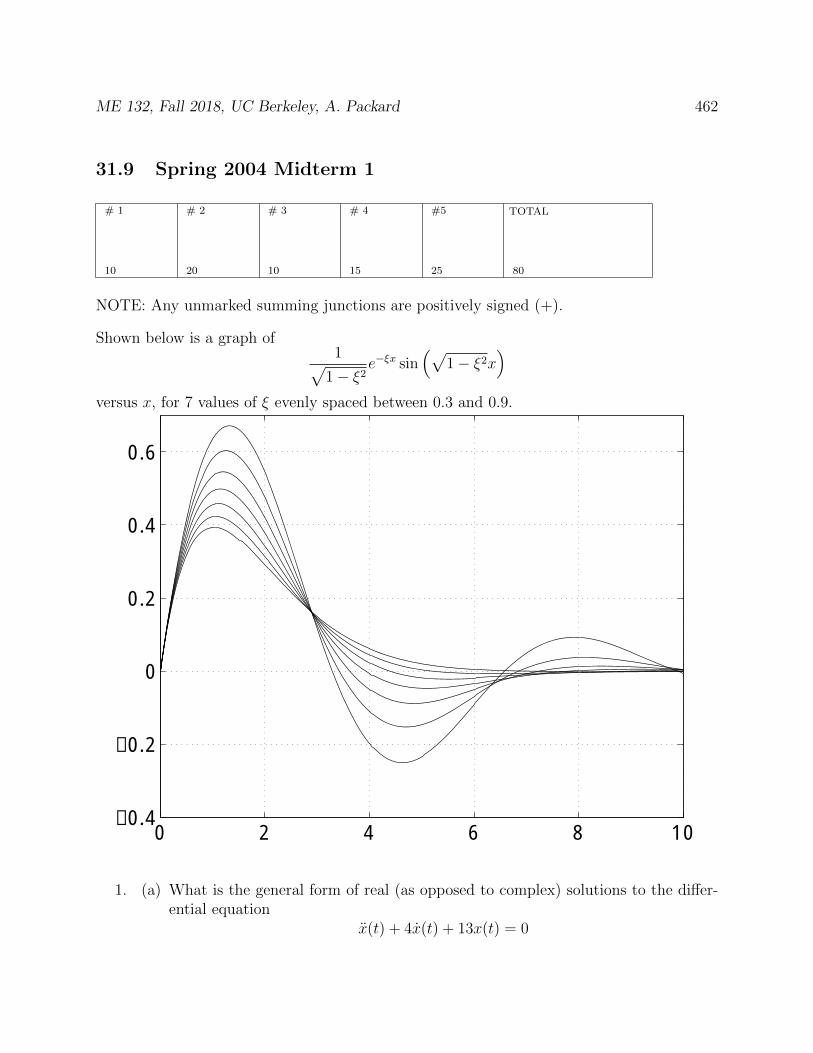
ME 132, Fall 2018, UC Berkeley, A. Packard 462
31.9 Spring 2004 Midterm 1
# 1
10
# 2
20
# 3
10
# 4
15
#5
25
TOTAL
80
NOTE: Any unmarked summing junctions are positively signed (+).
Shown below is a graph of1√
1− ξ2e−ξx sin
(√1− ξ2x
)versus x, for 7 values of ξ evenly spaced between 0.3 and 0.9.
0 2 4 6 8 10−0.4
−0.2
0
0.2
0.4
0.6
1. (a) What is the general form of real (as opposed to complex) solutions to the differ-ential equation
x(t) + 4x(t) + 13x(t) = 0
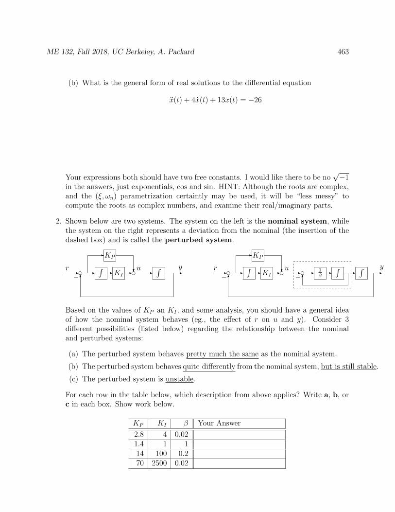
ME 132, Fall 2018, UC Berkeley, A. Packard 463
(b) What is the general form of real solutions to the differential equation
x(t) + 4x(t) + 13x(t) = −26
Your expressions both should have two free constants. I would like there to be no√−1
in the answers, just exponentials, cos and sin. HINT: Although the roots are complex,and the (ξ, ωn) parametrization certaintly may be used, it will be “less messy” tocompute the roots as complex numbers, and examine their real/imaginary parts.
2. Shown below are two systems. The system on the left is the nominal system, whilethe system on the right represents a deviation from the nominal (the insertion of thedashed box) and is called the perturbed system.
∫KI
KP
- d - - - d - ∫-
6
-
?−
r u y ∫KI
KP-
?- d - - - d - d - 1β-∫
-∫
-6 6− −
r u y
Based on the values of KP an KI , and some analysis, you should have a general ideaof how the nominal system behaves (eg., the effect of r on u and y). Consider 3different possibilities (listed below) regarding the relationship between the nominaland perturbed systems:
(a) The perturbed system behaves pretty much the same as the nominal system.
(b) The perturbed system behaves quite differently from the nominal system, but is still stable.
(c) The perturbed system is unstable.
For each row in the table below, which description from above applies? Write a, b, orc in each box. Show work below.
KP KI β Your Answer
2.8 4 0.021.4 1 114 100 0.270 2500 0.02

ME 132, Fall 2018, UC Berkeley, A. Packard 464
3. Neatly/accurately sketch the solution (for t ≥ 0) to the differential equation
x(t) = −2x(t) + u(t)
subject to the initial condition x(0) = 2, and forcing function
u(t) = 0 for 0 ≤ t ≤ 2.5u(t) = −2 for 2.5 < t ≤ 4.5u(t) = 8 for 4.5 < t ≤ 6
0 1 2 3 4 5 6−1
0
1
2
3
4
5
6
4. Suppose 0 < ξ < 1 and ωn > 0. Consider the system
y(t) + 2ξωny(t) + ω2ny(t) = ωnu(t)
subject to the initial conditions y(0−) = 0, y(0−) = 0, and the unit-step forcing func-tion, namely u(t) = 0 for t = 0, and u(t) = 1 for t > 0. Show that the responseis
y(t) =1√
1− ξ2e−ξωnt sin
(√1− ξ2ωnt
)Hint: Recall that the set of all real-valued homogeneous solutions of y(t)+2ξωny(t)+
ω2ny(t) = 0 is yH(t) = Ae−ξωnt cos
(√1− ξ2ωnt
)+ Be−ξωnt sin
(√1− ξ2ωnt
)where A
and B are any real numbers.
ME 132, Fall 2018, UC Berkeley, A. Packard 465
5. A process, with input u, disturbance d and output y is governed by
y(t) = y(t) + u(t) + d(t)
(a) Is the process stable?
(b) Suppose y(0) = −3, and u(t) = d(t) ≡ 0 for all t ≥ 0. What is the solution y(t)for t ≥ 0.
(c) A PI (Proportional plus Integral) controller is proposed
u(t) = KP [r(t)− y(t)] +KIz(t)z(t) = r(t)− y(t)
Eliminate z and u, and determine the closed-loop differential equation relatingthe variables (y, r, d).
ME 132, Fall 2018, UC Berkeley, A. Packard 466
(d) For what values of KP and KI is the closed-loop system stable?
(e) The closed-loop system is 2nd order. What are the appropriate values of KP andKI so that the closed-loop system characteristic polynomial has roots describedby ξ = 0.8, ωn = 0.5?
(f) What are the appropriate values of KP and KI so that the closed-loop systemcharacteristic polynomial has roots described by ξ = 0.8, ωn = 1.0?
(g) What are the appropriate values of KP and KI so that the closed-loop systemcharacteristic polynomial has roots described by ξ = 0.8, ωn = 2.0?

ME 132, Fall 2018, UC Berkeley, A. Packard 467
(h) For each of the 3 cases above (part e, f and g), accurately sketch the response ofy due to a unit-step disturbance d, assuming r is identically zero, and assumingall initial conditions are zero.
0 0.5 1 1.5 2 2.5 3−0.2
0
0.2
0.4
0.6
0.8
1
1.2
Time
Resp
onse
, (fo
r par
t e)
0 0.5 1 1.5 2 2.5 3−0.2
0
0.2
0.4
0.6
0.8
1
1.2
Time
Resp
onse
, (fo
r par
t f)
ME 132, Fall 2018, UC Berkeley, A. Packard 468
0 0.5 1 1.5 2 2.5 3−0.2
0
0.2
0.4
0.6
0.8
1
1.2
Time
Resp
onse
, (fo
r par
t g)
31.10 Fall 2003 Midterm 1
1. Neatly/accurately sketch the solution (for t ≥ 0) to the differential equation
x(t) = −3x(t) + 6u(t)
subject to the initial condition x(0) = −1, and forcing function
u(t) = 0 for 0 ≤ t ≤ 2u(t) = 3 for 2 < t ≤ 4u(t) = 2 for 4 < t ≤ 4.33u(t) = 1 for 4.33 < t ≤ 6

ME 132, Fall 2018, UC Berkeley, A. Packard 469
0 1 2 3 4 5 6−1
0
1
2
3
4
5
6
2. (a) What is the general form of the solution to the differential equation
x(t) + 6x(t) + 5x(t) = 0
(b) What is the general form of the solution to the differential equation
x(t) + 6x(t) + 5x(t) = −10
Your expressions both should have two free constants.
3. The solutions to the differential equations listed below are shown on the next page.Match the ODE with the solution graph. Make a table with pertinent informationthat justifies your answers. In each case, all appropriate initial conditions are 0. Bythat, I mean that if the differential equation is first-order, then the initial condition is

ME 132, Fall 2018, UC Berkeley, A. Packard 470
y(0) = 0. If the differential equation is second order, then the initial conditions arey(0) = 0, y(0) = 0.
(a) y(t) + y(t) = 1
(b) y(t) + 5y(t) = 5
(c) y(t)− y(t) = 1
(d) y(t) + 10y(t) = 10
(e) y(t)− 2y(t)− y(t) = −1
(f) y(t)− 2y(t) + 9y(t) = 9
(g) y(t) + 0.4y(t) + y(t) = 1
(h) y(t) + 0.12y(t) + 0.09y(t) = 0.09
(i) y(t) + 6y(t) + 5y(t) = 5
(j) y(t) + 0.3y(t) + 0.09y(t) = 0.09
(k) y(t) + 3y(t) + 9y(t) = 9
(l) y(t) + 1.8y(t) + 9y(t) = 9
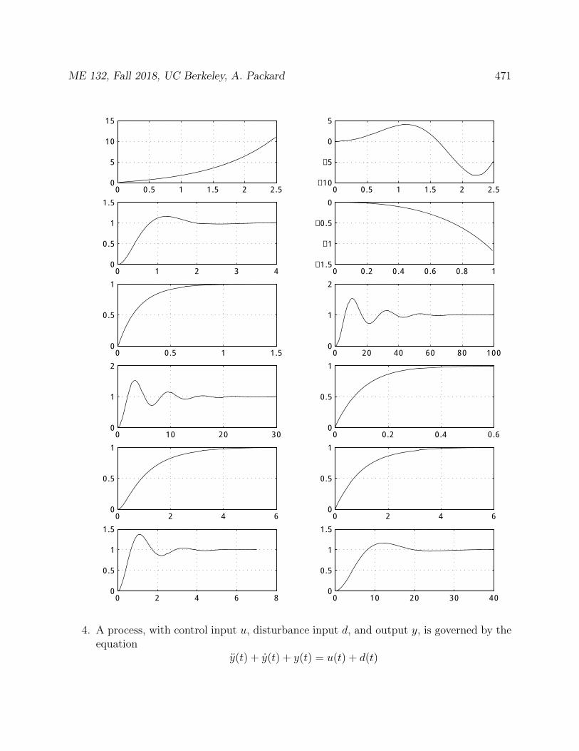
ME 132, Fall 2018, UC Berkeley, A. Packard 471
0 0.5 1 1.5 2 2.50
5
10
15
0 0.5 1 1.5 2 2.5−10
−5
0
5
0 1 2 3 40
0.5
1
1.5
0 0.2 0.4 0.6 0.8 1−1.5
−1
−0.5
0
0 0.5 1 1.50
0.5
1
0 20 40 60 80 1000
1
2
0 10 20 300
1
2
0 0.2 0.4 0.60
0.5
1
0 2 4 60
0.5
1
0 2 4 60
0.5
1
0 2 4 6 80
0.5
1
1.5
0 10 20 30 400
0.5
1
1.5
4. A process, with control input u, disturbance input d, and output y, is governed by theequation
y(t) + y(t) + y(t) = u(t) + d(t)
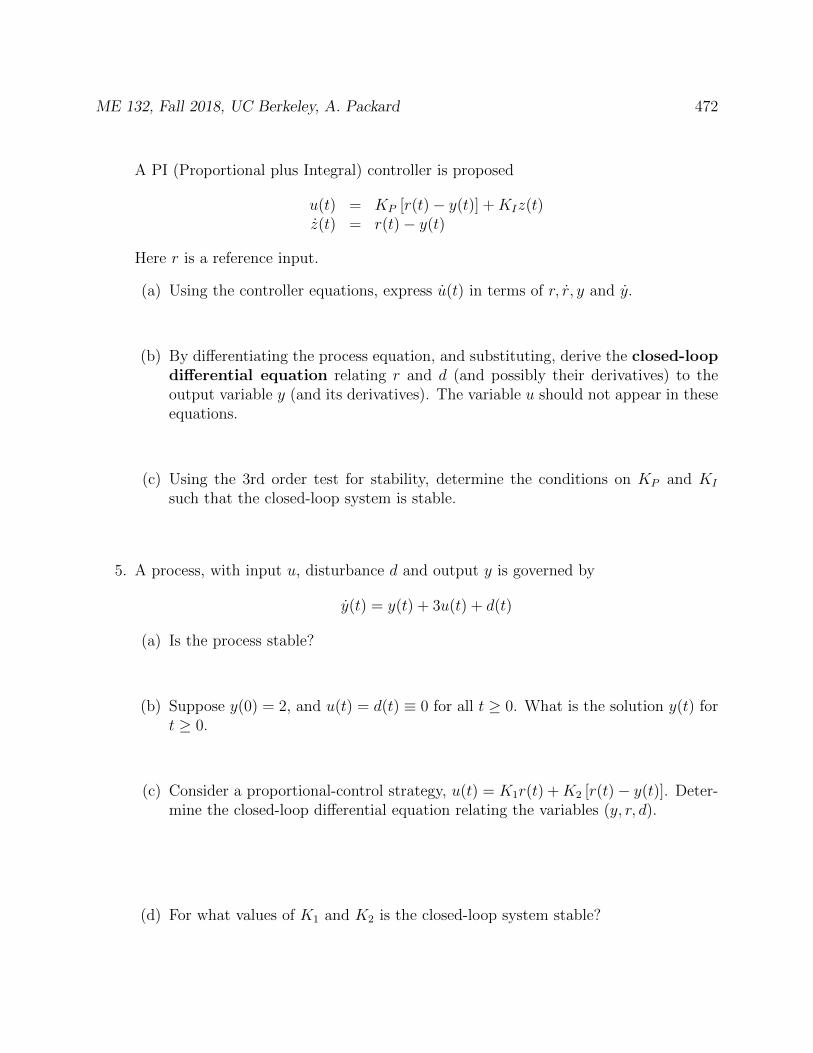
ME 132, Fall 2018, UC Berkeley, A. Packard 472
A PI (Proportional plus Integral) controller is proposed
u(t) = KP [r(t)− y(t)] +KIz(t)z(t) = r(t)− y(t)
Here r is a reference input.
(a) Using the controller equations, express u(t) in terms of r, r, y and y.
(b) By differentiating the process equation, and substituting, derive the closed-loopdifferential equation relating r and d (and possibly their derivatives) to theoutput variable y (and its derivatives). The variable u should not appear in theseequations.
(c) Using the 3rd order test for stability, determine the conditions on KP and KI
such that the closed-loop system is stable.
5. A process, with input u, disturbance d and output y is governed by
y(t) = y(t) + 3u(t) + d(t)
(a) Is the process stable?
(b) Suppose y(0) = 2, and u(t) = d(t) ≡ 0 for all t ≥ 0. What is the solution y(t) fort ≥ 0.
(c) Consider a proportional-control strategy, u(t) = K1r(t) +K2 [r(t)− y(t)]. Deter-mine the closed-loop differential equation relating the variables (y, r, d).
(d) For what values of K1 and K2 is the closed-loop system stable?

ME 132, Fall 2018, UC Berkeley, A. Packard 473
(e) As a function of K2, what is the steady-state gain (just at zero frequency) fromd→ y in the closed-loop system?
(f) As a function of K1 and K2, what is the steady-state gain (again, just at zerofrequency) from r → y in the closed-loop system?
(g) Choose K1 and K2 so that the steady-state gain from r → y equals 1, and thesteady-state gain from d→ y equals 0.2.
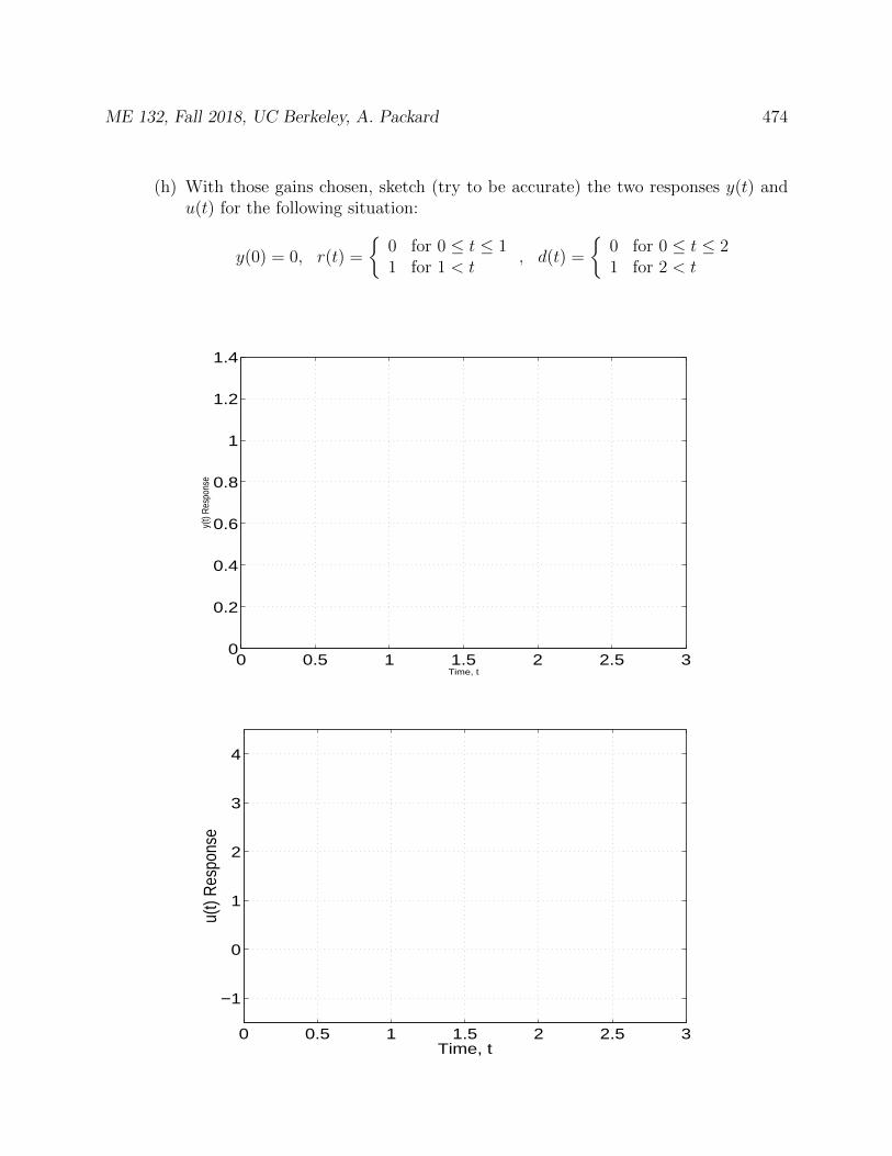
ME 132, Fall 2018, UC Berkeley, A. Packard 474
(h) With those gains chosen, sketch (try to be accurate) the two responses y(t) andu(t) for the following situation:
y(0) = 0, r(t) =
0 for 0 ≤ t ≤ 11 for 1 < t
, d(t) =
0 for 0 ≤ t ≤ 21 for 2 < t
0 0.5 1 1.5 2 2.5 30
0.2
0.4
0.6
0.8
1
1.2
1.4
Time, t
y(t)
Res
pons
e
0 0.5 1 1.5 2 2.5 3
−1
0
1
2
3
4
Time, t
u(t)
Res
pons
e

ME 132, Fall 2018, UC Berkeley, A. Packard 475
31.11 Fall 2003 Midterm 2
1. The input u, and output y, of a single-input, single-output system are related by
y[3](t) + 6y[2](t) + 2y[1](t) + 3y(t) = 2u[2](t)− 5u[1](t)− 5u(t)
(a) Find the transfer function from U to Y
(b) Show that this is a stable system.
(c) If u(t) ≡ 2 for all t ≥ 0, what is the limiting value of y, namely limt→∞?
(d) Suppose the input is sinusoidal, u(t) = sin(100t). In the steady state, what is theapproximate amplitude of the sinusoidal output y?
2. Two masses are connected by a linear, massless spring. An external force f is appliedto Mass #1. Suppose that v1 is the velocity of m1, v2 is the velocity of m2 (bothmeasured relative to the same inertial frame).
Since the spring is massless, the forces at each end must balance, and are equal to k∆,where ∆ is the stretch in the spring (from its unstretched length L). This is shownabove, right.
(a) Interpret the meaning of each of the equations below. Draw a Free-body diagram,or other appropriate picture to assist in your explanation.
i. f(t) + k∆(t) = m1v1(t)
ii. −k∆(t) = m2v2(t)
iii. ∆(t) = v2(t)− v1(t)
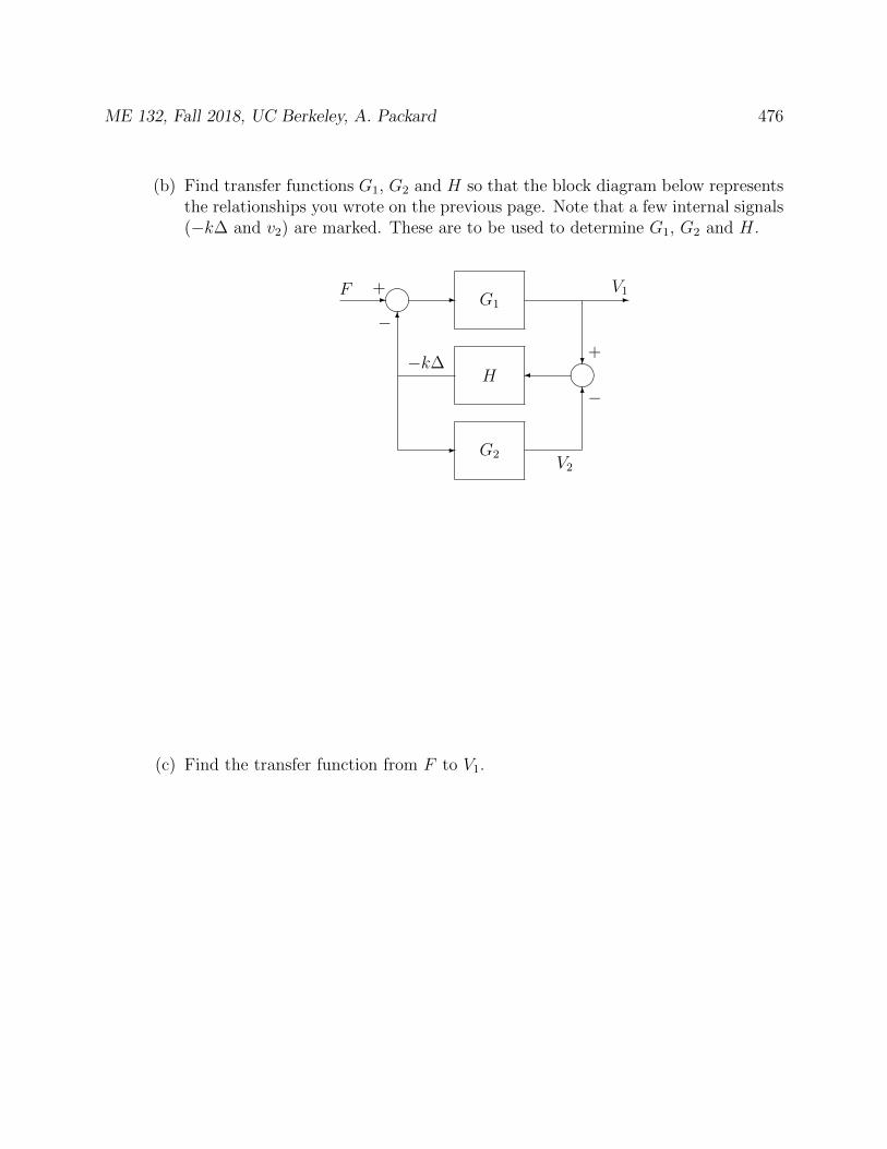
ME 132, Fall 2018, UC Berkeley, A. Packard 476
(b) Find transfer functions G1, G2 and H so that the block diagram below representsthe relationships you wrote on the previous page. Note that a few internal signals(−k∆ and v2) are marked. These are to be used to determine G1, G2 and H.
G1
H
G2
- - -
? 6
6
-
F V1
−
+
−
+−k∆
V2
(c) Find the transfer function from F to V1.
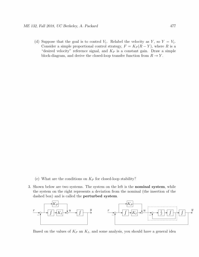
ME 132, Fall 2018, UC Berkeley, A. Packard 477
(d) Suppose that the goal is to control V1. Relabel the velocity as Y , so Y = V1.Consider a simple proportional control strategy, F = KP (R − Y ), where R is a“desired velocity” reference signal, and KP is a constant gain. Draw a simpleblock-diagram, and derive the closed-loop transfer function from R→ Y .
(e) What are the conditions on KP for closed-loop stability?
3. Shown below are two systems. The system on the left is the nominal system, whilethe system on the right represents a deviation from the nominal (the insertion of thedashed box) and is called the perturbed system.
∫KI
KP
- d - - - d - ∫-
6
-
?−
r u y ∫KI
KP-
?- d - - - d - d - 1β-∫
-∫
-6 6− −
r u y
Based on the values of KP an KI , and some analysis, you should have a general idea
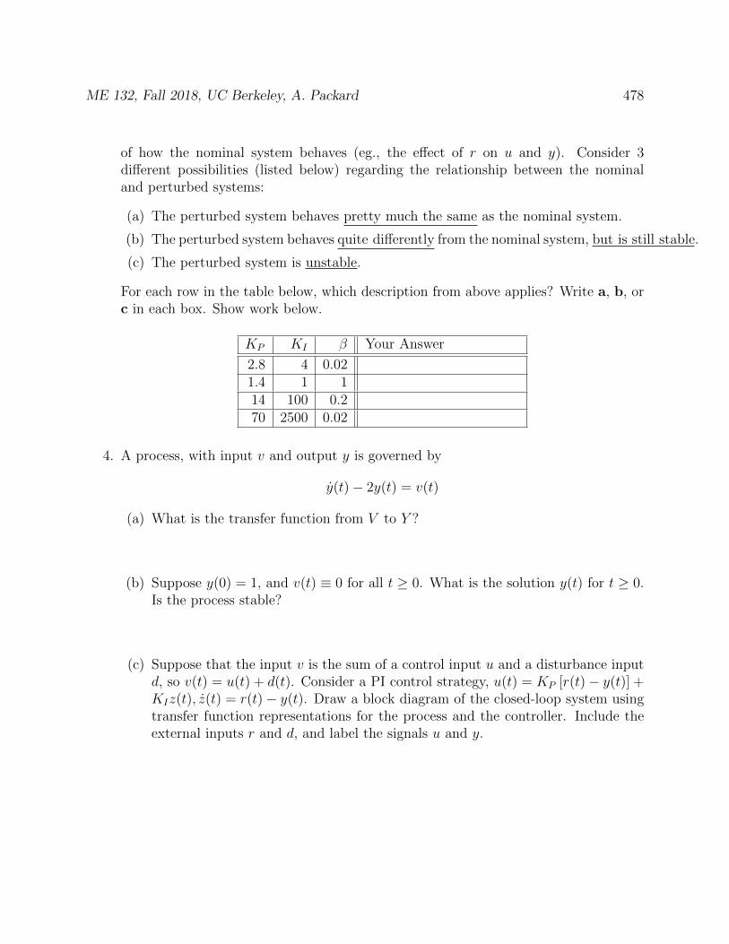
ME 132, Fall 2018, UC Berkeley, A. Packard 478
of how the nominal system behaves (eg., the effect of r on u and y). Consider 3different possibilities (listed below) regarding the relationship between the nominaland perturbed systems:
(a) The perturbed system behaves pretty much the same as the nominal system.
(b) The perturbed system behaves quite differently from the nominal system, but is still stable.
(c) The perturbed system is unstable.
For each row in the table below, which description from above applies? Write a, b, orc in each box. Show work below.
KP KI β Your Answer
2.8 4 0.021.4 1 114 100 0.270 2500 0.02
4. A process, with input v and output y is governed by
y(t)− 2y(t) = v(t)
(a) What is the transfer function from V to Y ?
(b) Suppose y(0) = 1, and v(t) ≡ 0 for all t ≥ 0. What is the solution y(t) for t ≥ 0.Is the process stable?
(c) Suppose that the input v is the sum of a control input u and a disturbance inputd, so v(t) = u(t) + d(t). Consider a PI control strategy, u(t) = KP [r(t)− y(t)] +KIz(t), z(t) = r(t)− y(t). Draw a block diagram of the closed-loop system usingtransfer function representations for the process and the controller. Include theexternal inputs r and d, and label the signals u and y.
ME 132, Fall 2018, UC Berkeley, A. Packard 479
(d) In the closed-loop, what are the transfer functions from R to Y and from D to Y .
(e) In the closed-loop, what are the transfer functions from R to U and from D to U .
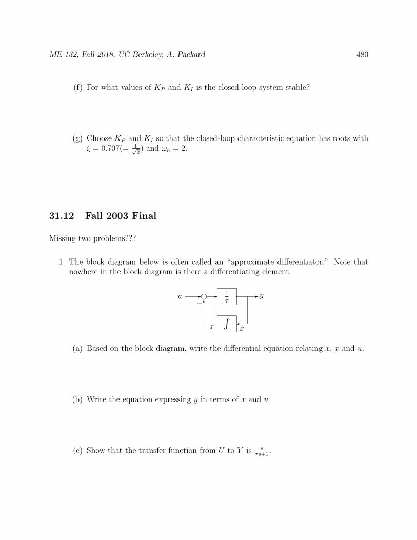
ME 132, Fall 2018, UC Berkeley, A. Packard 480
(f) For what values of KP and KI is the closed-loop system stable?
(g) Choose KP and KI so that the closed-loop characteristic equation has roots withξ = 0.707(= 1√
2) and ωn = 2.
31.12 Fall 2003 Final
Missing two problems???
1. The block diagram below is often called an “approximate differentiator.” Note thatnowhere in the block diagram is there a differentiating element.
1τ∫
- g- -
6−u
x x
y
(a) Based on the block diagram, write the differential equation relating x, x and u.
(b) Write the equation expressing y in terms of x and u
(c) Show that the transfer function from U to Y is sτs+1
.
ME 132, Fall 2018, UC Berkeley, A. Packard 481
(d) Suppose that the initial condition is x(0) = 0. Apply a step input at t = 0, sou(t) = u for t > 0 (here, u is just some constant value). Compute the responsex(t), for t ≥ 0.
(e) With x(t) computed above, compute the output y(t), and sketch below.
0 0.5 1 1.5 2 2.5 3 3.5 4 4.5 50
0.5
1
1.5
2
2.5
3
3.5
4
4.5
5
Time (seconds)
Resp
onse
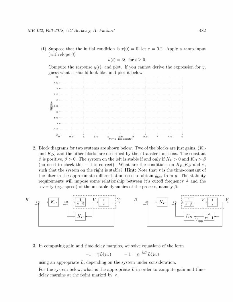
ME 132, Fall 2018, UC Berkeley, A. Packard 482
(f) Suppose that the initial condition is x(0) = 0, let τ = 0.2. Apply a ramp input(with slope 3)
u(t) = 3t for t ≥ 0.
Compute the response y(t), and plot. If you cannot derive the expression for y,guess what it should look like, and plot it below.
0 0.5 1 1.5 2 2.5 3 3.5 4 4.5 50
0.5
1
1.5
2
2.5
3
3.5
4
4.5
5
Time (seconds)
Resp
onse
2. Block diagrams for two systems are shown below. Two of the blocks are just gains, (KP
and KD) and the other blocks are described by their transfer functions. The constantβ is positive, β > 0. The system on the left is stable if and only if KP > 0 and KD > β(no need to check this – it is correct). What are the conditions on KP , KD and τ ,such that the system on the right is stable? Hint: Note that τ is the time-constant ofthe filter in the approximate differentiation used to obtain yapp from y. The stabilityrequirements will impose some relationship between it’s cutoff frequency 1
τand the
severity (eg., speed) of the unstable dynamics of the process, namely β.
- c cKP1
s−β1s
KD
- - - - -6
6− −YR V - c cKP
1s−β
1s
KD
- - - - -6
sτs+1
6− −
YR V
Vapp
3. In computing gain and time-delay margins, we solve equations of the form
−1 = γL(jω) − 1 = e−jωTL(jω)
using an appropriate L, depending on the system under consideration.
For the system below, what is the appropriate L in order to compute gain and time-delay margins at the point marked by ×.
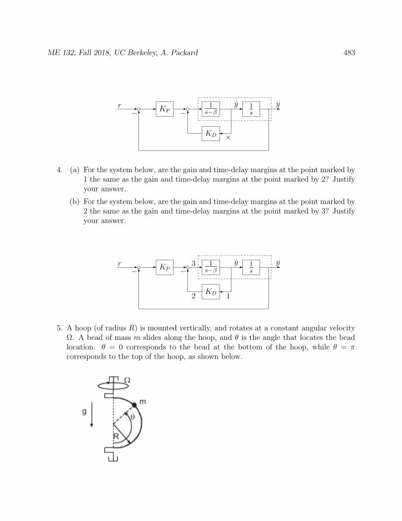
ME 132, Fall 2018, UC Berkeley, A. Packard 483
- c cKP1
s−β1s
KD ×
- - - - -6
6− −yr y
4. (a) For the system below, are the gain and time-delay margins at the point marked by1 the same as the gain and time-delay margins at the point marked by 2? Justifyyour answer.
(b) For the system below, are the gain and time-delay margins at the point marked by2 the same as the gain and time-delay margins at the point marked by 3? Justifyyour answer.
- c cKP1
s−β1s
KD 12
3- - - - -6
6− −yr y
5. A hoop (of radius R) is mounted vertically, and rotates at a constant angular velocityΩ. A bead of mass m slides along the hoop, and θ is the angle that locates the beadlocation. θ = 0 corresponds to the bead at the bottom of the hoop, while θ = πcorresponds to the top of the hoop, as shown below.
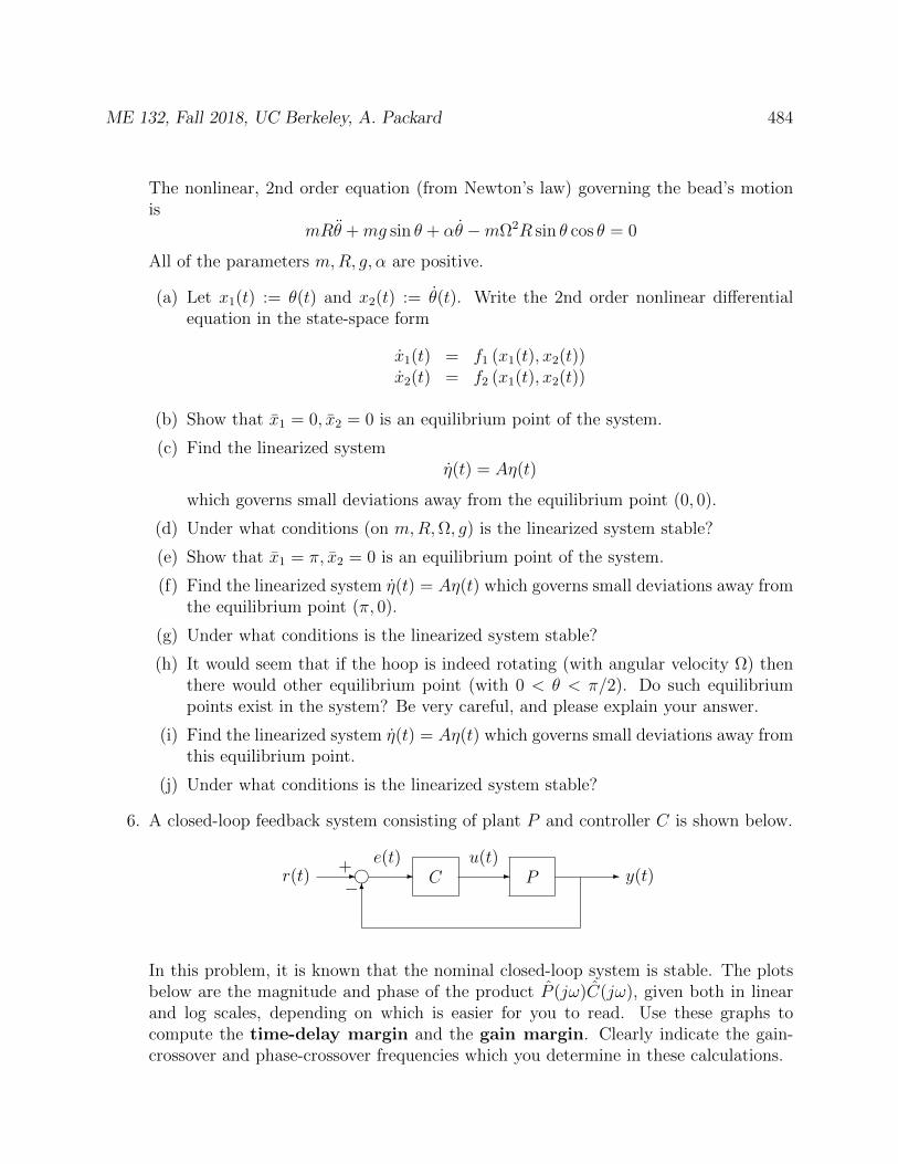
ME 132, Fall 2018, UC Berkeley, A. Packard 484
The nonlinear, 2nd order equation (from Newton’s law) governing the bead’s motionis
mRθ +mg sin θ + αθ −mΩ2R sin θ cos θ = 0
All of the parameters m,R, g, α are positive.
(a) Let x1(t) := θ(t) and x2(t) := θ(t). Write the 2nd order nonlinear differentialequation in the state-space form
x1(t) = f1 (x1(t), x2(t))x2(t) = f2 (x1(t), x2(t))
(b) Show that x1 = 0, x2 = 0 is an equilibrium point of the system.
(c) Find the linearized systemη(t) = Aη(t)
which governs small deviations away from the equilibrium point (0, 0).
(d) Under what conditions (on m,R,Ω, g) is the linearized system stable?
(e) Show that x1 = π, x2 = 0 is an equilibrium point of the system.
(f) Find the linearized system η(t) = Aη(t) which governs small deviations away fromthe equilibrium point (π, 0).
(g) Under what conditions is the linearized system stable?
(h) It would seem that if the hoop is indeed rotating (with angular velocity Ω) thenthere would other equilibrium point (with 0 < θ < π/2). Do such equilibriumpoints exist in the system? Be very careful, and please explain your answer.
(i) Find the linearized system η(t) = Aη(t) which governs small deviations away fromthis equilibrium point.
(j) Under what conditions is the linearized system stable?
6. A closed-loop feedback system consisting of plant P and controller C is shown below.
C P- - - -
6
h+
−r(t)
e(t) u(t)y(t)
In this problem, it is known that the nominal closed-loop system is stable. The plotsbelow are the magnitude and phase of the product P (jω)C(jω), given both in linearand log scales, depending on which is easier for you to read. Use these graphs tocompute the time-delay margin and the gain margin. Clearly indicate the gain-crossover and phase-crossover frequencies which you determine in these calculations.
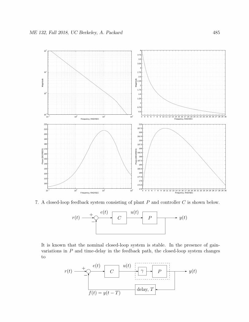
ME 132, Fall 2018, UC Berkeley, A. Packard 485
10−1
100
101
102
10−1
100
101
102
Frequency, RAD/SEC
Mag
nitu
de
3 4 5 6 7 8 9 10 11 12 13 14 15 16 17 18 19 20 21 22 23 24 25 26 27 28 29 30
0.5
0.75
1
1.25
1.5
1.75
2
2.25
2.5
2.75
3
3.25
3.5
3.75
4
Frequency, RAD/SEC
Mag
nitu
de
10−1
100
101
102
100
110
120
130
140
150
160
170
180
190
200
210
220
Frequency, RAD/SEC
Pha
se (
DE
GR
EE
S)
3 4 5 6 7 8 9 10 11 12 13 14 15 16 17 18 19 20 21 22 23 24 25 26 27 28 29 30170
172.5
175
177.5
180
182.5
185
187.5
190
192.5
195
197.5
200
202.5
205
207.5
210
Frequency, RAD/SEC
Pha
se (
DE
GR
EE
S)
7. A closed-loop feedback system consisting of plant P and controller C is shown below.
C P- - - -
6
i+
−r(t)
e(t) u(t)y(t)
It is known that the nominal closed-loop system is stable. In the presence of gain-variations in P and time-delay in the feedback path, the closed-loop system changesto
C γ P
delay, T
- - - - -
6
i+
−r(t)
e(t) u(t)y(t)
f(t) = y(t− T )

ME 132, Fall 2018, UC Berkeley, A. Packard 486
In this particular system, there is both an upper and lower gain margin - that is, forno time-delay, if the gain γ is decreased from 1, the closed-loop system becomesunstable at some (still positive) value of γ; and, if the gain γ is increased from 1, theclosed-loop system becomes unstable at some value of γ > 1. Let γl and γu denotethese two values, so 0 < γl < 1 < γu.
For each fixed value of γ satisfying γl < γ < γu the closed-loop system is stable.For each such fixed γ, compute the minimum time-delay that would cause instability.Specifically, do this for several (say 8-10) γ values satisfying γl < γ < γu, and plotbelow.
0 0.1 0.2 0.3 0.4 0.5 0.6 0.7 0.8 0.9 1 1.1 1.2 1.3 1.4 1.5 1.6 1.7 1.8 1.9 2 2.1 2.2 2.3 2.4 2.5GAMMA
Min
Tim
e−D
elay
The data on the next two pages are the magnitude and phase of the product P (jω)C(jω).They are given in both linear and log spacing, depending on which is easier for you toread. Use these graphs to compute the time-delay margin at many fixed values of γsatisfying γl < γ < γu.
10−1
100
101
102
10−1
100
101
102
Frequency, RAD/SEC
Mag
nitu
de
3 4 5 6 7 8 9 10 11 12 13 14 15 16 17 18 19 20 21 22 23 24 25 26 27 28 29 30
0.5
0.75
1
1.25
1.5
1.75
2
2.25
2.5
2.75
3
3.25
3.5
3.75
4
Frequency, RAD/SEC
Mag
nitu
de
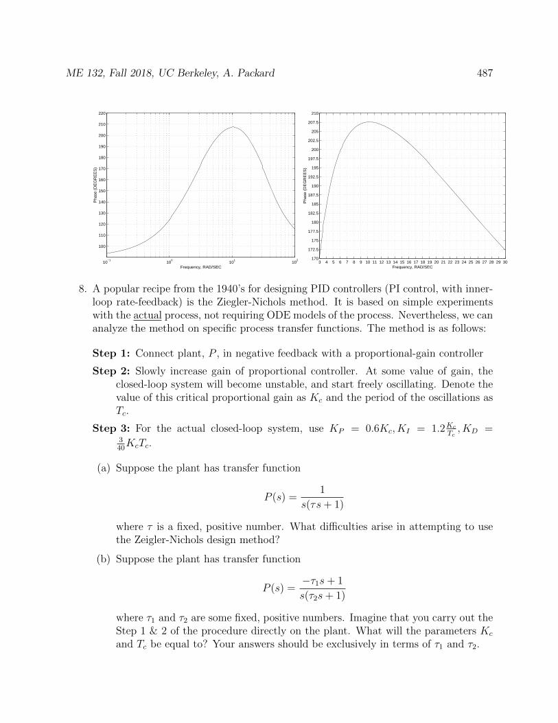
ME 132, Fall 2018, UC Berkeley, A. Packard 487
10−1
100
101
102
100
110
120
130
140
150
160
170
180
190
200
210
220
Frequency, RAD/SEC
Pha
se (
DE
GR
EE
S)
3 4 5 6 7 8 9 10 11 12 13 14 15 16 17 18 19 20 21 22 23 24 25 26 27 28 29 30170
172.5
175
177.5
180
182.5
185
187.5
190
192.5
195
197.5
200
202.5
205
207.5
210
Frequency, RAD/SEC
Pha
se (
DE
GR
EE
S)
8. A popular recipe from the 1940’s for designing PID controllers (PI control, with inner-loop rate-feedback) is the Ziegler-Nichols method. It is based on simple experimentswith the actual process, not requiring ODE models of the process. Nevertheless, we cananalyze the method on specific process transfer functions. The method is as follows:
Step 1: Connect plant, P , in negative feedback with a proportional-gain controller
Step 2: Slowly increase gain of proportional controller. At some value of gain, theclosed-loop system will become unstable, and start freely oscillating. Denote thevalue of this critical proportional gain as Kc and the period of the oscillations asTc.
Step 3: For the actual closed-loop system, use KP = 0.6Kc, KI = 1.2KcTc, KD =
340KcTc.
(a) Suppose the plant has transfer function
P (s) =1
s(τs+ 1)
where τ is a fixed, positive number. What difficulties arise in attempting to usethe Zeigler-Nichols design method?
(b) Suppose the plant has transfer function
P (s) =−τ1s+ 1
s(τ2s+ 1)
where τ1 and τ2 are some fixed, positive numbers. Imagine that you carry out theStep 1 & 2 of the procedure directly on the plant. What will the parameters Kc
and Tc be equal to? Your answers should be exclusively in terms of τ1 and τ2.