mathematical modelling of construction of ship turning

Scientific Journal of Gdynia Maritime University

Scientific Journal of Gdynia Maritime University, No. 118, June 2021 7

No. 118/21, 7–23 Submitted: 02.05.2021 ISSN 2657-6988 (online) Accepted: 24.05.2021 ISSN 2657-5841 (printed) Published: 30.06.2021 DOI: 10.26408/118.01 UDC:004.94:656.61:629.562

MATHEMATICAL MODELLING OF CONSTRUCTION OF SHIP TURNING TRAJECTORY USING AUTONOMOUS BOW

THRUSTER WORK AND RESEARCH OF BOW THRUSTER CONTROL SPECIFICS

Oleksandr Kupraty Odessa National Maritime University, Mechnikova 34, Odessa 65029, Ukraine, ORCID: 0000-0003-3519-504X, e-mail:[email protected] Abstract: The article proposes a method of constructing the trajectory of a ship’s turn using a control device. Mathematical modelling of the turn trajectory is performed using MS Excel in conjunction with the MATLAB environment. To construct a trajectory, a conditional centre of turn will be used, it will be guided by a control device, such as a radio buoy, or a lighthouse with pre-known coordinates. The construction of this trajectory has two features: a step course change when rotated equal to a sector step, and the accuracy of the trajectory is achieved by using the Kalman filter, simplified to the amplification factor. The bow thruster moment is calculating using the bow thruster shoulder. The angular velocity of turning depends on the linear speed, therefore, the angular velocity can be adjusted not only by changing the bow thruster mode of operation, but also by changing the linear speed of the vessel. The article provides the program code for constructing a trajectory in the MATLAB environment, which takes its initial data from MS Excel. Therefore, the work forms the basic view of autonomous bow thruster control.

Keywords: accuracy of trajectory, Kalman filter, step course change, sector step, bow thruster shoulder.

1. INTRODUCTION

To program autonomous ship control, you need to solve the problem of autonomous control of the bow thrusters and develop a method of constructing a curved trajectory, ensuring the accuracy of this trajectory. When entering the port often not enough steering gear work, is especially true for limited areas, therefore, you need to use a bow thruster. When programming an electronic control device, there is a need not only to program scenarios, but also to construct precise trajectories in narrow, winding channels.

If we approach the issue comprehensively, it is necessary to consider the efficiency of the bow thruster depending on the longitudinal component of the linear

Oleksandr Kupraty

8 Scientific Journal of Gdynia Maritime University, No. 118, June 2021

speed of the vessel and control the main engine during the turn, focussing on the work of the bow thruster. Based on all of the above, this topic seems relevant.

2. LITERATURE ANALYSIS AND FORMULATING THE PROBLEM

In today’s environment, the development of autonomous control systems is a priority in all modes of transport. For this article, the literature on the bow thruster was analysed. In particular, the works [Judin 2010; Kopczyński 2015] are the basics for developing ship autonomous control software for turning, and describe the specifics of the bow thruster control. Work related to the Kalman filter [Cadet 2003; Maszarov 2011] was also analysed, which describes how the Kalman filter works as a powerful mathematical tool. The works [Morgas and Kopacz 2013; Botniev and Ustinov 2014; Kupraty 2020] describe the solution to direct and reverse geodesic tasks, such as the calculation of the course and distance between two points. In [Kupraty 2020], an algorithm for calculating the course between points on a rhumb line and a method of constructing the turning circle of a vessel based on the rudder angle was proposed. It contains six real variations, with the choice of the variation used in the solution depending on the size of the remainder of the divisions of longitude differences by 2π and the value of the summand of the isometric latitudes difference, R. The above documents contain the basic rules for the creation of autonomous vessels, which were adopted by the Maritime Safety Committee at its 100 and 101 sessions [IMO 2018; Interim Guidelines for Mass Trials 2019]. The work [Wieremiej 2016] is dedicated to mean square multi-purpose optimisation, including the synthesis of a course management system based on sea excitement taking into account the ship’s hydrodynamic parameters, control forces and external influences.

3. METHODS AND MATERIALS

In the study of the bow thruster, the calculation-experimental method was used, as well as the Kalman filter in a simplified form, and trigonometric formulas were used to develop the software code to construct the reversal of the vessel using the bow thruster. The Kalman filter is nowadays used in DP systems.

A characteristic feature of the bow thruster is that at low linear speeds, the bow thruster turns a vessel more efficiently, and at high linear speeds, the influence factor increases, which is why a vessel should decrease her speed before using the bow thruster.

A sector step is an arc encased between two trajectory radii, the value of which is equal to the vessel step course change between the start point and the end point of this arc.

Mathematical Modelling of Construction of Ship Turning Trajectory Using Autonomous Bow Thruster Work and Research of Bow Thruster Control Specifics


4. THE AIM AND TASKS

The aim of the work is to develop a mathematical model of the construction of a ship turning trajectory using autonomous bow thruster work control and research of bow thruster control specifics.

Tasks: • using a known pattern of changing the influence factor of the longitudinal

component of the linear speed on the efficiency of the bow thruster, construct a polynomial trend in MS Excel and identify a function in MS Excel that can be used to manage this factor numerically;

• add the bow thruster force and moment in a non-linear differential system and propose a method to control the angle speed;

• develop a program code to construct the trajectory of the ship’s reversal (rotation) using the bow thruster in MATLAB.

5. RESEARCH AND ELABORATION

5.1. Change in the value of the influence factor, determining its function

To understand how the bow thruster influence factor changes, the effectiveness of the bow thruster should be illustrated under three conditions: the vessel has no movement relative to the water, low speed of the vessel, high speed of the vessel (Fig. 1 a,b,c). At zero speed, the resulting vector exits the channel of the bow thruster and the resultant force has the highest magnitude, at low speeds, the resultant force shifts to the stern and the vector decreases, and at high speeds, the resultant force comes out of the bow thruster channel, but the vector of the resulting force is decreased even more, which is evidenced by the change in the influence factor.

a) b) c)

Fig. 1 a, b, c. Changing the point of the application and the value of the resulting force depending on the speed

ZERO SPEED SLOW SPEED HIGH SPEED

RESULTING FORCE RESULTING FORCE RESULTING FORCE

Oleksandr Kupraty


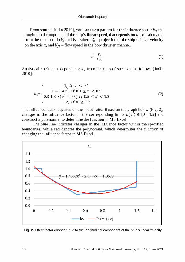
From source [Judin 2010], you can use a pattern for the influence factor 𝑘𝑘𝑣𝑣 the longitudinal component of the ship’s linear speed, that depends on 𝑣𝑣′, 𝑣𝑣′ calculated from the relationship 𝑉𝑉𝑥𝑥 and 𝑉𝑉𝑓𝑓𝑓𝑓, where 𝑉𝑉𝑥𝑥 – projection of the ship’s linear velocity on the axis x, and 𝑉𝑉𝑓𝑓𝑓𝑓 – flow speed in the bow thruster channel.

𝑣𝑣′= 𝑉𝑉𝑥𝑥

𝑉𝑉𝑓𝑓𝑓𝑓 (1)

Analytical coefficient dependence 𝑘𝑘𝑣𝑣 from the ratio of speeds is as follows [Judin 2010]:

The influence factor depends on the speed ratio. Based on the graph below (Fig. 2), changes in the influence factor in the corresponding limits 𝑘𝑘(𝑣𝑣′) ∈ [0 ; 1.2] and construct a polynomial to determine the function in MS Excel.

The blue line indicates changes in the influence factor within the specified boundaries, while red denotes the polynomial, which determines the function of changing the influence factor in MS Excel.

Fig. 2. Effect factor changed due to the longitudinal component of the ship’s linear velocity

𝑘𝑘𝑣𝑣=

⎩⎨

⎧1, 𝑖𝑖𝑖𝑖 𝑣𝑣′ < 0.1

1 − 1.4𝑣𝑣′ , 𝑖𝑖𝑖𝑖 0.1 ≤ 𝑣𝑣′ < 0.50.3 + 0.3(𝑣𝑣′ − 0.5), 𝑖𝑖𝑖𝑖 0.5 ≤ 𝑣𝑣′ < 1.2

1.2, 𝑖𝑖𝑖𝑖 𝑣𝑣′ ≥ 1.2

(2) (2)



Therefore: 𝑘𝑘(𝑣𝑣′) = 1.4332(𝑣𝑣′)2 ̶ 2.0559𝑣𝑣′+1.0628, 𝑘𝑘(𝑣𝑣′) ∈ [0 ; 1.2] (3)

Based on this function, the electronic control device will be able to

autonomously adjust the revs of the main engine and the bow thruster to keep the influence factor of the longitudinal component of the ship’s linear velocity within the specified limits.

Therefore, the main engine will be controlled adaptively. However, it is also especially important to say that wind forces must be

calculated for effective motion control. Table 1 shows the wind force moments for m/v “UMM QARN”.

Table 1. Wind force moments [kN∙m]

Wind direct. [deg.]

Wind speed in [m/s]

5 10 15 20 25 30 35 40

0.0 0.0 0.0 0.0 0.0 0.0 0.0 0.0 0.0

10.0 -1085 -4342 -9769 -17367 -27135 -39075 -53185 -69466

20.0 -1707 -6827 -15361 -27308 -42669 -61443 -83631 -109232

30.0 -2193 -8770 -19733 -35082 -54815 -78934 -107437 -140326

40.0 -2111 -8445 -19001 -33779 -52779 -76002 -103447 -135115

50.0 -1966 -7863 -17693 -31454 -49146 -70770 -96326 -125814

60.0 -1726 -6903 -15531 -27611 -43143 -62125 -84560 -110445

70.0 -1359 -5434 -12226 -21735 -33962 -48905 -66565 -86942

80.0 -793 -3171 -7134 -12683 -19816 -28536 -38840 -50730

90.0 -183 -731 -1644 -2922 -4566 -6575 -8950 -11689

100.0 654 2615 5884 10461 16345 23536 32035 41842

110.0 1453 5811 13075 23244 36319 52299 71185 92976

120.0 2127 8509 19144 34034 53178 76576 104229 136135

130.0 2331 9322 20976 37290 58265 83902 114200 149159

140.0 2489 9956 22402 39826 62228 89608 121967 159303

Oleksandr Kupraty


150.0 2261 9044 20349 36176 56525 81396 110788 144703

160.0 1721 6886 15493 27543 43036 61972 84350 110172

170.0 962 3849 8661 15397 24058 34643 47153 61588

180.0 0.0 0.0 0.0 0.0 0.0 0.0 0.0 0.0

190.0 -962 -3849 -8661

-15397

-24058 -34643 -47153 -61588

200.0 -1721 -6886 -15493 -27543 -43036 -61972 -84350 -110172

210.0 -2261 -9044 -20349 -36176 -56525 -81396 -110788 -144703

220.0 -2489 -9956 -22402 -39826 -62228 -89608 -121967 -159303

230.0 -2331 -9322 -20976 -37290 -58265 -83902 -114200 -149159

240.0 -2127 -8509 -19144 -34034 -53178 -76576 -104229 -136135

250.0 -1453 -5811 -13075 -23244 -36319 -52299 -71185 -92976

260.0 -654 -2615 -5884 -10461 -16345 -23536 -32035 -41842

270.0 183 731 1644 2922 4566 6575 8950 11689

280.0 793 3171 7134 12683 19816 28536 38840 50730

290.0 1359 5434 12226 21735 33962 48905 66565 86942

300.0 1726 6903 15531 27611 43143 62125 84560 110445

310.0 1966 7863 17693 31454 49146 70770 96326 125814

320.0 2111 8445 19001 33779 52779 76002 103447 135115

330.0 2193 8770 19733 35082 54815 78934 107437 140326

340.0 1707 6827 15361 27308 42669 61443 83631 109232

350.0 1085 4342 9769 17367 27135 39075 53185 69466

360.0 0.0 0.0 0.0 0.0 0.0 0.0 0.0 0.0

The bow thruster longitudinal coordinates 𝑋𝑋𝐵𝐵𝐵𝐵 = 336 m (from APP). The moment of the wind force changes depending on the wind speed and direction. The bow thruster is located 336 metres from APP. This coordinate is used to calculate the necessary force via Formula 4: 𝐹𝐹 = |𝑀𝑀|

𝑋𝑋𝐵𝐵𝐵𝐵 ; (4)

cont. Table 1



For example, calculation of the force to keep a vessel on course for a wind speed of 10 m/s from the wind direction 250º F is executed as follows: 𝐹𝐹 = |−5811kN|

336m ≈ 17.295 kN.

The required power can be calculated proportionally:

𝑘𝑘𝐵𝐵 = 𝐹𝐹𝐵𝐵

; (5)

𝑘𝑘𝐵𝐵 = 17.295kN257 kN

≈ 0.0673

𝑃𝑃𝐵𝐵 = 𝑘𝑘𝐵𝐵 × 𝑃𝑃; (6)

𝑛𝑛𝐵𝐵 = 𝑘𝑘𝐵𝐵 × 𝑛𝑛; (7)

𝑃𝑃𝐵𝐵 = 0.0673×1800 = 121.14 kwt;

𝑛𝑛𝐵𝐵 = 0.0673 × 287 ≈ 19.3 rpm;

Thus, this method can be used to calculate the necessary force of the bow

thruster to hold the ship in position.

5.2. Kinematic and hydrodynamic specifics of bow thruster control during turning

Some important basics should be kept in mind when calculating the kinematics of ship turning: Linear acceleration a = v∙ω, a = ω²∙R, because v = ω∙R.

ω = 𝜔𝜔 0 + 1𝑚𝑚

·F·t. (8)

For a ship, it should be described in ideal conditions as follows:

ω = 𝜔𝜔 0 + 1𝑚𝑚(1+𝑘𝑘66)

·F·t, (9)

where 𝑘𝑘66 = 2𝐵𝐵𝐵𝐵

. As was mentioned above, Δψ is the sector step and course change step at same

time, therefore, the ship angle speed relative to the centre of turning and relative to the pivot point are the same:

𝛥𝛥𝜓𝜓𝑠𝑠𝛥𝛥𝛥𝛥

= 𝛥𝛥𝜓𝜓𝐵𝐵𝑇𝑇𝛥𝛥𝛥𝛥

. (10)

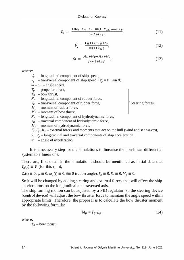
By supplementing the basic system [10] of non-linear differential equations with the bow thrust, we get the following system:

Oleksandr Kupraty


�̇�𝑉𝑥𝑥 = 1.8𝐵𝐵𝑣𝑣−𝑋𝑋𝐻𝐻−𝑋𝑋𝑅𝑅+𝑚𝑚(1−𝑘𝑘22)𝑉𝑉𝑦𝑦𝜔𝜔+𝐹𝐹𝑥𝑥𝑚𝑚(1+𝑘𝑘11)

; (11)

�̇�𝑉 = 𝑌𝑌𝐻𝐻+𝑌𝑌𝑅𝑅+𝐵𝐵𝐵𝐵+𝐹𝐹𝑦𝑦𝑚𝑚(1+𝑘𝑘22)

; (12)

�̇�𝜔 = 𝛭𝛭𝐻𝐻+𝛭𝛭𝑅𝑅+𝛭𝛭𝐵𝐵+𝑀𝑀𝑧𝑧𝐽𝐽𝑍𝑍𝑍𝑍(1+𝑘𝑘66)

; (13)

where: 𝑉𝑉𝑥𝑥 – longitudinal component of ship speed, 𝑉𝑉𝑦𝑦 – transversal component of ship speed; (𝑉𝑉𝑦𝑦 = 𝑉𝑉 ∙ sin𝛽𝛽), ω – 𝜔𝜔𝑧𝑧 – angle speed, 𝑇𝑇𝑣𝑣 – propeller thrust, 𝑇𝑇𝐵𝐵 – bow thrust, 𝑋𝑋𝑅𝑅 – longitudinal component of rudder force, 𝑌𝑌𝑅𝑅 – transversal component of rudder force, Steering forces; 𝑀𝑀𝑅𝑅 – moment of rudder force, 𝑀𝑀𝐵𝐵 – moment of bow thrust, 𝑋𝑋𝐻𝐻 – longitudinal component of hydrodynamic force, 𝑌𝑌𝐻𝐻 – traversal component of hydrodynamic force, 𝑀𝑀𝐻𝐻 – moment of hydrodynamic force, 𝐹𝐹𝑥𝑥 ,𝐹𝐹𝑦𝑦 ,𝑀𝑀𝑧𝑧 – external forces and moments that act on the hull (wind and sea waves), �̇�𝑉𝑥𝑥, �̇�𝑉𝑦𝑦 – longitudinal and traversal components of ship acceleration, �̇�𝜔 – angle of acceleration.

It is a necessary step for the simulations to linearise the non-linear differential system to a linear one.

Therefore, first of all in the simulationit should be mentioned as initial data that 𝑉𝑉𝑥𝑥(t) ≡ 𝑉𝑉 (for this rpm), 𝑉𝑉𝑦𝑦(t) ≡ 0, 𝜑𝜑 ≡ 0, 𝜔𝜔0(t) ≡ 0, δ≡ 0 (rudder angle), 𝐹𝐹𝑥𝑥 ≡ 0,𝐹𝐹𝑦𝑦 ≡ 0,𝑀𝑀𝑧𝑧 ≡ 0.

So it will be changed by adding steering and external forces that will effect the ship accelerations on the longitudinal and traversed axis. The ship turning motion can be adjusted by a PID regulator, so the steering device (control device) will adjust the bow thruster force to maintain the angle speed within appropriate limits. Therefore, the proposal is to calculate the bow thruster moment by the following formula:

𝑀𝑀𝐵𝐵 = 𝑇𝑇𝐵𝐵 ∙𝐿𝐿𝐵𝐵 , (14)

where: 𝑇𝑇𝐵𝐵 – bow thrust,

y



𝐿𝐿𝐵𝐵 – shoulder of bow thruster which is measured on the longitudinal axis from the ship’s centre of gravity to the bow thruster propeller.

Therefore, if ω0(t) ≡ 0, then ω = ω̇ ∙ t.

Thus, by complementing the system of differential equations with the bow thrust and the moment of the bow thrust, it is possible to control the angle speed of the vessel by changing the bow thrust moment in an adaptive autonomous mode. The bow thruster shoulder should be calculated automatically based on changes in the position of the centre of gravity.

5.3. Mathematical modelling of the construction of ship turning trajectory using autonomous bow thruster work

When constructing a turn trajectory (reversal) with the help of the bow thruster, it should be understood that at low speeds the efficiency of the steering gear decreases, and the efficiency of the bow thruster increases. When constructing a turn trajectory (reversal) the vessel with the help of a steering gear involves only the steering gear and the main engine or engines.

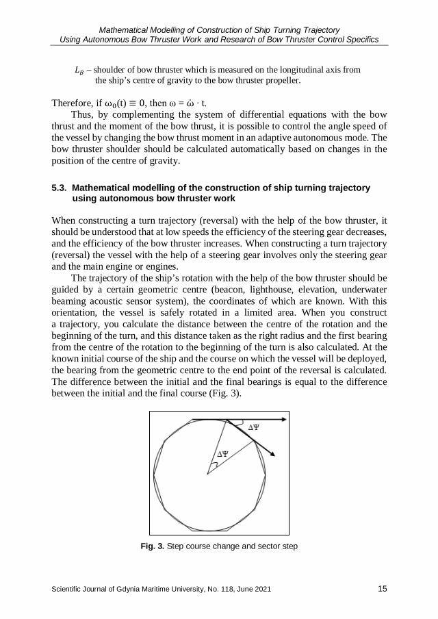
The trajectory of the ship’s rotation with the help of the bow thruster should be guided by a certain geometric centre (beacon, lighthouse, elevation, underwater beaming acoustic sensor system), the coordinates of which are known. With this orientation, the vessel is safely rotated in a limited area. When you construct a trajectory, you calculate the distance between the centre of the rotation and the beginning of the turn, and this distance taken as the right radius and the first bearing from the centre of the rotation to the beginning of the turn is also calculated. At the known initial course of the ship and the course on which the vessel will be deployed, the bearing from the geometric centre to the end point of the reversal is calculated. The difference between the initial and the final bearings is equal to the difference between the initial and the final course (Fig. 3).

Fig. 3. Step course change and sector step

Oleksandr Kupraty


It is clearly visible in Figure 3 that the course change and the sector step between the two points are equal.

The autonomous control system will allow you to hold the necessary angular speed steady on a given trajectory.

The initial radius of the turn is accepted as correct, so subsequent radii, calculated trigonometrically, require adjustment.

The most effective tool is the Kalman filter, but in this case, it should be simplified to a gain factor. The initial form of the Kalman filter is as follows:

Xk+1 = K𝑘𝑘+1 ∙ Xk + ε𝑘𝑘+1 (15)

To convert εk+1 to zero, εk+1 = 0. As the first radius is correct, the gain factor K is calculated by formula (16):

K𝑘𝑘+1 = RRk+1

, (16)

where Rk+1 ˂˃ R, because it is counted on another bearing and/or to another point. R and Rk+1 were calculated as great circle distance.

Figure 4 shows an example of such a turnaround. Effective work of the bow thruster is provided at slow speed. The radius of the turning circle doesn’t change and doesn’t depend on the linear or angle speed. The angle speed changes proportionally to the linear speed. Under normal conditions, rotation should be provided by the steering device at speed 2.5 knots. In normal practice, the bow thruster is ineffective at a ship speed greater than 3 knots.

Fig. 4. Geometry of the ship’s rotation trajectory The bearing changes at the same time as the change of course. Since the radii

and coordinates of the circle points are calculated trigonometrically, it is necessary to adjust 𝛥𝛥𝜑𝜑𝑘𝑘+1 by the appropriate gain factor K.

𝜑𝜑𝑘𝑘+1 = 𝜑𝜑0 + 𝛫𝛫𝑘𝑘+1×R×cos𝑃𝑃𝐿𝐿𝑘𝑘+1

𝜑𝜑𝜅𝜅+1= 𝜑𝜑0 + 𝛫𝛫𝑘𝑘+1×𝛥𝛥𝜑𝜑𝑘𝑘+1 (17)

𝑅𝑅

𝑅𝑅𝑘𝑘+1

𝑅𝑅𝑘𝑘+2

𝑅𝑅𝑘𝑘+3

𝑻𝑻𝑻𝑻𝒊𝒊

𝑻𝑻𝑻𝑻𝒇𝒇



This adjustment can be depicted as a matrix:

�

�

𝛥𝛥𝜑𝜑1𝛥𝛥𝜑𝜑2𝛥𝛥𝜑𝜑3𝛥𝛥𝜑𝜑4𝛥𝛥𝜑𝜑5𝛥𝛥𝜑𝜑6𝛥𝛥𝜑𝜑7

�

�

=

�

�

�

𝛥𝛥𝜑𝜑1𝑘𝑘+1𝛥𝛥𝜑𝜑2𝑘𝑘+1𝛥𝛥𝜑𝜑3𝑘𝑘+1𝛥𝛥𝜑𝜑4𝑘𝑘+1𝛥𝛥𝜑𝜑5𝑘𝑘+1𝛥𝛥𝜑𝜑6𝑘𝑘+1𝛥𝛥𝜑𝜑7𝑘𝑘+1

�

�

�

×

�

�

�

𝛫𝛫1𝑘𝑘+1𝛫𝛫2𝑘𝑘+1𝛫𝛫3𝑘𝑘+1𝛫𝛫4𝑘𝑘+1𝛫𝛫5𝑘𝑘+1𝛫𝛫6𝑘𝑘+1𝛫𝛫7𝑘𝑘+1

�

�

�

or

�

�

𝛥𝛥𝜑𝜑1𝛥𝛥𝜑𝜑2𝛥𝛥𝜑𝜑3𝛥𝛥𝜑𝜑4𝛥𝛥𝜑𝜑5𝛥𝛥𝜑𝜑6𝛥𝛥𝜑𝜑7

�

�

=

�

�

�

𝛥𝛥𝜑𝜑1𝑘𝑘+1𝛥𝛥𝜑𝜑2𝑘𝑘+1𝛥𝛥𝜑𝜑3𝑘𝑘+1𝛥𝛥𝜑𝜑4𝑘𝑘+1𝛥𝛥𝜑𝜑5𝑘𝑘+1𝛥𝛥𝜑𝜑6𝑘𝑘+1𝛥𝛥𝜑𝜑7𝑘𝑘+1

�

�

�

×

�

�

�

𝑅𝑅/𝑅𝑅1𝑘𝑘+1𝑅𝑅/𝑅𝑅2𝑘𝑘+1𝑅𝑅/𝑅𝑅3𝑘𝑘+1𝑅𝑅/𝑅𝑅4𝑘𝑘+1𝑅𝑅/𝑅𝑅5𝑘𝑘+1𝑅𝑅/𝑅𝑅6𝑘𝑘+1𝑅𝑅/𝑅𝑅7𝑘𝑘+1

�

�

�

(18)

And the final type of calculation of the matrix of geographical coordinates takes the following form:

�

�

𝜑𝜑1𝑘𝑘+1𝜑𝜑2𝑘𝑘+1𝜑𝜑3𝑘𝑘+1𝜑𝜑4𝑘𝑘+1𝜑𝜑5𝑘𝑘+1𝜑𝜑6𝑘𝑘+1𝜑𝜑7𝑘𝑘+1

�

�=�

�

𝜑𝜑0𝜑𝜑0𝜑𝜑0𝜑𝜑0𝜑𝜑0𝜑𝜑0𝜑𝜑0

�

�+

�

�

�

𝛫𝛫1𝑘𝑘+1𝛫𝛫2𝑘𝑘+1𝛫𝛫3𝑘𝑘+1𝛫𝛫4𝑘𝑘+1𝛫𝛫5𝑘𝑘+1𝛫𝛫6𝑘𝑘+!

𝛫𝛫7𝑘𝑘+1

�

�

�

×�

�

𝑅𝑅𝑅𝑅𝑅𝑅𝑅𝑅𝑅𝑅𝑅𝑅𝑅𝑅

�

�×

�

�

�

cos𝑃𝑃𝐿𝐿1𝑘𝑘+1cos𝑃𝑃𝐿𝐿2𝑘𝑘+1cos𝑃𝑃𝐿𝐿3𝑘𝑘+1cos𝑃𝑃𝐿𝐿4𝑘𝑘+1cos𝑃𝑃𝐿𝐿5𝑘𝑘+1cos𝑃𝑃𝐿𝐿6𝑘𝑘+1cos𝑃𝑃𝐿𝐿7𝑘𝑘+1

�

�

�

(19)

The geographic coordinates are filtered by the gain factor 𝛫𝛫𝑘𝑘+1 in such a way. Figure 4 shows the trajectory of the vessel, in which the initial course is 95º,

and the final is 186º. At the same time, the difference between the initial and the final bearing from the centre of the reversal of the vessel is equal to the difference between the initial and the final course. The bearings were calculated in MS Excel using the algorithm outlined in the source [Kupraty 2020].

The sector step is calculated in MS Excel by the following formula: 𝑆𝑆𝑆𝑆 = 𝛥𝛥𝛥𝛥𝛥𝛥

𝐼𝐼𝐼𝐼𝐵𝐵(𝛥𝛥𝛥𝛥𝛥𝛥/𝑆𝑆𝑆𝑆𝑖𝑖) (20)

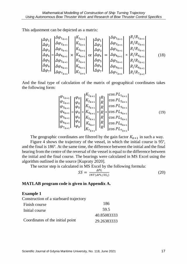
MATLAB program code is given in Appendix A. Example 1 Construction of a starboard trajectory Finish course 186 Initial course 59.5

Coordinates of the initial point 40.85083333 29.26383333

Oleksandr Kupraty


Coordinates of the geometric centre of the rotation

40.84483333 29.26950000

Initial radius (distance from the centre of turning to the initial point)

0.4432

Sector step 8.272727273 PERMIT (“TURN” in MORSE CODE) 1 001 010 10 Board (port side – “0”, starboard side – “1”) 1 First bearing 324.46

The word “TURN” in Morse code is used for the permit code. Calculation matrix of bearings PL in MS Excel based on the turning board: PL = [324.46 332.89 341.33 349.76 358.20 6.63 15.06 23.50 31.93 40.37 48.80 57.24 65.67 74.11 82.54 90.98] K = [1.0132 1.0073 1.0027 0.9996 0.9983 0.9988 1.0012 1.0052 1.0106 1.0169 1.0237 1.0304 1.0363 1.0409 1.0438 1.0446] Based on all of the above data, MATLAB calculates the coordinates of the turning matrix.

TM = 40.85083333 40.85145723 40.85185038 40.85209979 40.85220390 40.85216217 40.85197481

29.26383333 29.26521662 29.26650419 29.26784194 29.26920668 29.27057614 29.27192820

Fig. 5. Trajectory simulation of a starboard turn in MATLAB

40.85164288 40.85116874 40.85055675 40.84981421 40.84895230 40.84798692 ... ... 40.84470182

29.27324016 29.27448806 29.27564634 29.27668801 29.27758536 29.27831142 ... ... 29.27924605



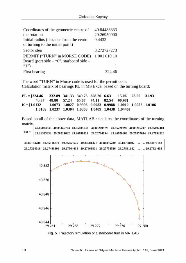
Fig. 6. Illustration of a starboard turn in OpenCPN 5.2.4 (Tuzla Shipyard Entrance)

Example 2 Constructing of a port side trajectory Finish course 90 Initial course 81.1

Coordinates of the initial point 40.83791525 29.22261913

Coordinates of the geometric centre of the rotation

40.84855000 29.21783333

Initial radius (distance from the turning centre to the initial point) 0.6753

Sector step 8.165116279 PERMIT (“TURN” in MORSE CODE) 1 001 010 10 Board (port side – “0”, starboard side – “1”) 0 First bearing 161.20

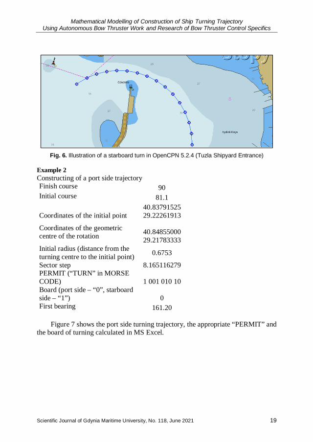
Figure 7 shows the port side turning trajectory, the appropriate “PERMIT” and

the board of turning calculated in MS Excel.

Oleksandr Kupraty


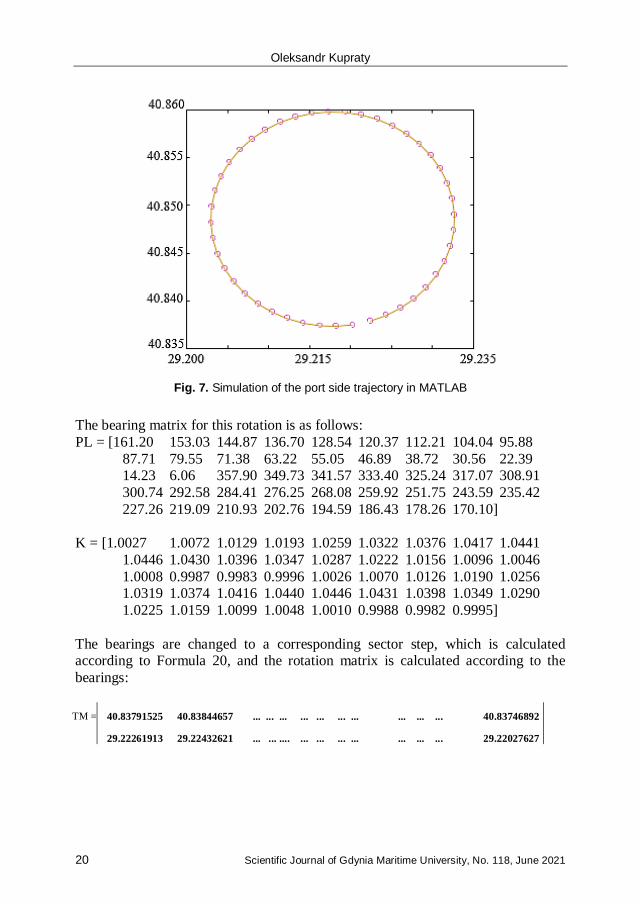
Fig. 7. Simulation of the port side trajectory in MATLAB

The bearing matrix for this rotation is as follows: PL = [161.20 153.03 144.87 136.70 128.54 120.37 112.21 104.04 95.88 87.71 79.55 71.38 63.22 55.05 46.89 38.72 30.56 22.39 14.23 6.06 357.90 349.73 341.57 333.40 325.24 317.07 308.91 300.74 292.58 284.41 276.25 268.08 259.92 251.75 243.59 235.42 227.26 219.09 210.93 202.76 194.59 186.43 178.26 170.10] K = [1.0027 1.0072 1.0129 1.0193 1.0259 1.0322 1.0376 1.0417 1.0441 1.0446 1.0430 1.0396 1.0347 1.0287 1.0222 1.0156 1.0096 1.0046 1.0008 0.9987 0.9983 0.9996 1.0026 1.0070 1.0126 1.0190 1.0256 1.0319 1.0374 1.0416 1.0440 1.0446 1.0431 1.0398 1.0349 1.0290 1.0225 1.0159 1.0099 1.0048 1.0010 0.9988 0.9982 0.9995] The bearings are changed to a corresponding sector step, which is calculated according to Formula 20, and the rotation matrix is calculated according to the bearings:

40.83791525 40.83844657 ... ... ... ... ... ... ... ... ... ... 40.83746892

29.22261913 29.22432621 ... ... .... ... ... ... ... ... ... ... 29.22027627

TM =



Fig. 8. Illustration of port side turning in OpenCPN 5.2.4

Thus, the code is correct for both starboard side rotation and port side rotation,

constructing a trajectory as a set of points. If analysing the gain factor, it can be noted that even the first coefficients in the

matrix are not equal to one. This is because, when the coordinates of the initial point are calculated, there is a margin of error, which is eliminated by the Kalman filter gain factor. The Kalman filter in this case is used in a simplified form, but this does not affect the accuracy of the trajectory in any way. The developed code can be used to simulate the trajectory of the vessel using adaptive control of the bow thruster and the ship’s engine. In determining the gain factors, the distance between the initial point of movement of the vessel, the coordinates of which are known, and the conditional centre of rotation, the coordinates of which are also known, is taken. This distance is used as the right radius of rotation, which minimises the error.

6. CONCLUSIONS

A polynomial function is proposed to control the bow thruster autonomously, which can be used to control the value of the longitudinal factor of the linear velocity. Therefore, the steering will be controlled adaptively, adjusting the angular velocity in such a way as to maintain the radius of rotation. To construct the trajectory of the ship, a program code for data processing and charting the trajectory of the rotation has been written in MATLAB.

The proposed method of autonomous regulation of the ship’s angular velocity allows the control device to be programmed according to the position of the centre of gravity and the maximum power of the bow thruster. Using the proposed method of calculating the moment of thrust of the bow thruster, the bow thruster revs can be adjusted by checking the mathematical model with a real angular acceleration.

Oleksandr Kupraty


The Kalman filter gain factor is used to filter the coordinates of the trajectory points. Filtering is done by calculating the initial radius between the starting point and the centre of rotation, the coordinates of which are known. Calculating the radius for the first bearing, it was noticed that the coordinates of the calculated starting point are different from their observatory values; this difference was reflected in the coefficients 1.0132 and 1.0027 for the first and second example, respectively. This means that the proposed method will provide sufficient accuracy of the rotational trajectory of the ship. The proposed code can also be used in a variety of autonomous systems where accuracy of the rotational trajectory must be provided.

The main scientific contribution of this work is to offer methods of constructing the trajectory of the ship’s rotational movement and autonomous control of the steering device, which in turn will allow in the future the control device of a large vessel to be programmed to the fourth level of autonomy.

REFERENCES

Botniev, W.A., Ustinov, S.M., 2014, Mietody reszenija priamoj i obratnoj geodeziczeskich zadacz s wysokoj tocznostiu, Naucznotiechniczeskije Wiedomosti SPbGPU 3'(198), Informatika. Tielekommunikacii. Uprawlenije//Matiematiczeskoje modielirowanije: mietody, algoritmy, tiechnologii, pp. 49–58.

Cadet, O., 2003, Introduction to Kalman Filter – Application to DP, Dynamic Positioning Conference, September 16–17, pp. 1–33.

IMO, 2018, Framework for the Regulatory Scoping Exercise for the Use of Maritime Autonomous Surface Ships (MASS), MSC 100/20/Add.1, Annex 2.

Interim Guidelines for Mass Trials, 2019, MSC.1/Circ.1604, June 14. Judin, J.I., 2010, Маtiematiczeskoje modelirowanije raboty podruliwajuszczego ustrojstwa burowogo

sudna, Viestnik MGTU, vol. 13, no. 4/2, pp. 839–844. Kopczyński, A.M., 2015, Analiza i projektowanie układów sterowania sterami strumieniowymi statków

z zastosowaniem systemu z bazą wiedzy, Autoreferat rozprawy doktorskiej, Gdańsk. Kupraty, O., 2020, Implementation of the Algorithm for Calculation Course (Bearing) on Rhumb Line

and Constructing the Trajectory of the Ship's Turning Circle in the MATLAB Programming Environment, The Scientific Heritage, Budapest, vol. 1, no. 60(60), pp. 40–45.

Маszarov, K.W., 2011, Primienienije filtra Kalmana dla ocenki koordinat celi w RLS, Viestnik SibGUTI, no 3, pp. 59–66.

Morgaś, W., Kopacz, Z., 2013, Rhumb-Line Sailing by Compution, Versita, Reports on Geodesy, vol. 94, pp. 14–26.

Wieriemiej, E.I., 2016, Sriedniekwadraticznaja mnogocielewaja optimizacija: uczeb. posobije, SPb, St. Petersburg.

https://cyberleninka.ru/article/n/metody-resheniya-pryamoy-i-obratnoy-geodezicheskih-zadach-s-vysokoy-tochnostyu/viewer




https://dynamic-positioning.com/proceedings/dp2003/design_cadet.pdf

https://dynamic-positioning.com/proceedings/dp2003/design_cadet.pdf

https://maiif.org/wp-content/uploads/2019/06/MSC-100_20-Annex-20-1.pdf

https://maiif.org/wp-content/uploads/2019/06/MSC-100_20-Annex-20-1.pdf

https://wwwcdn.imo.org/localresources/en/MediaCentre/HotTopics/Documents/MSC.1-Circ.1604%20-%20Interim%20Guidelines%20For%20Mass%20Trials%20(Secretariat).pdf

http://vestnik.mstu.edu.ru/v13_5_n42/articles/01_yudin.pdf

http://vestnik.mstu.edu.ru/v13_5_n42/articles/01_yudin.pdf

https://eia.pg.edu.pl/documents/10623/30567653/Autoreferat%20-%20Andrzej%20Kopczy%C5%84ski.pdf

https://eia.pg.edu.pl/documents/10623/30567653/Autoreferat%20-%20Andrzej%20Kopczy%C5%84ski.pdf

http://vestnik.sibsutis.ru/uploads/1322123732_4751.pdf

http://vestnik.sibsutis.ru/uploads/1322123732_4751.pdf

https://drive.google.com/file/d/12wRcfTd1-w88TQfdt1PQmOm_GG7KkQKF/view?usp=sharing

https://drive.google.com/file/d/12wRcfTd1-w88TQfdt1PQmOm_GG7KkQKF/view?usp=sharing

https://play.google.com/store/books/details?id=HwxADwAAQBAJ&rdid=book-HwxADwAAQBAJ&rdot=1&source=gbs_vpt_read&pcampaignid=books_booksearch_viewport

https://play.google.com/store/books/details?id=HwxADwAAQBAJ&rdid=book-HwxADwAAQBAJ&rdot=1&source=gbs_vpt_read&pcampaignid=books_booksearch_viewport



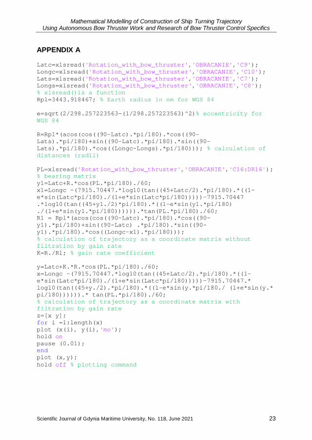
APPENDIX A

Latc=xlsread('Rotation_with_bow_thruster','OBRACANIE','C9'); Longc=xlsread('Rotation_with_bow_thruster','OBRACANIE','C10'); Lats=xlsread('Rotation_with_bow_thruster','OBRACANIE','C7'); Longs=xlsread('Rotation_with_bow_thruster','OBRACANIE','C8'); % xlsread()is a function Rpl=3443.918467; % Earth radius in nm for WGS 84 e=sqrt(2/298.257223563-(1/298.257223563)^2)% eccentricity for WGS 84 R=Rpl*(acos(cos((90-Latc).*pi/180).*cos((90-Lats).*pi/180)+sin((90-Latc).*pi/180).*sin((90-Lats).*pi/180).*cos((Longc-Longs).*pi/180))); % calculation of distances (radii) PL=xlsread('Rotation_with_bow_thruster','OBRACANIE','C16:DR16'); % bearing matrix y1=Latc+R.*cos(PL.*pi/180)./60; x1=Longc -(7915.70447.*log10(tan((45+Latc/2).*pi/180).*((1-e*sin(Latc*pi/180)./(1+e*sin(Latc*pi/180)))))-7915.70447 .*log10(tan((45+y1./2)*pi/180).*((1-e*sin(y1.*pi/180) ./(1+e*sin(y1.*pi/180)))))).*tan(PL.*pi/180)./60; R1 = Rpl*(acos(cos((90-Latc).*pi/180).*cos((90-y1).*pi/180)+sin((90-Latc) .*pi/180).*sin((90-y1).*pi/180).*cos((Longc-x1).*pi/180))); % calculation of trajectory as a coordinate matrix without filtration by gain rate K=R./R1; % gain rate coefficient y=Latc+K.*R.*cos(PL.*pi/180)./60; x=Longc -(7915.70447.*log10(tan((45+Latc/2).*pi/180).*((1-e*sin(Latc*pi/180)./(1+e*sin(Latc*pi/180)))))-7915.70447.* log10(tan((45+y./2).*pi/180).*((1-e*sin(y.*pi/180./ (1+e*sin(y.* pi/180)))))).* tan(PL.*pi/180)./60; % calculation of trajectory as a coordinate matrix with filtration by gain rate z=[x y]; for i =1:length(x) plot (x(i), y(i),'mo'); hold on pause (0.01); end plot (x,y); hold off % plotting command