Journal of Marine Systems 75 (2009) 56–69

Contents lists available at ScienceDirect

Journal of Marine Systems

j ourna l homepage: www.e lsev ie r.com/ locate / jmarsys

Mass and heat transports in the NE Barents Sea: Observations and models

Tor Gammelsrød a,b,⁎, Øyvind Leikvin a,b,e, Vidar Lien c, W. Paul Budgell c,Harald Loeng c, Wieslaw Maslowski d

a Geofysisk Institutt, University of Bergen, 5007 Norwayb The University Centre in Svalbard, P.O. Box 156, 9171 Longyearbyen, Norwayc Institute of Marine Research, P.O. Box 1870, Nordnes, 5817 Bergen, Norwayd Oceanography Department, Naval Postgraduate School, Monterey, California, USAe Akvaplan-niva, Polar Environmental Centre, 9296 Tromsø, Norway

a r t i c l e i n f o

⁎ Corresponding author. Geofysisk Institutt, UniveNorway.

E-mail address: torg@gfi.uib.no (T. Gammelsrød).

0924-7963/$ – see front matter © 2008 Elsevier B.V.doi:10.1016/j.jmarsys.2008.07.010

a b s t r a c t

Article history:Received 17 March 2008Received in revised form 17 July 2008Accepted 21 July 2008Available online 26 July 2008

The strait between Novaya Zemlya and Frans Josef Land, here called the Barents Sea Exit (BSX) isinvestigated using data obtained from a current-meter array deployed in 1991–1992, and twonumerical models (ROMS and NAME). Combining the observations and models the net volumeflux towards the Arctic Ocean was estimated to 2.0±0.6 Sv (1 Sv=106 m3s−1). The observationsindicate that about half of this transport consists of dense, Cold Bottom Water, which maypenetrate to great depths and contribute to the thermohaline circulation. Both models givequite similar net transport, seasonal variations and spatial current structures, and thediscrepancies from the observations were related to the coarse representation of the bottomtopography in the models. Also the models indicate that actual deployment did not capture themain in- and outflows through the BSX. A snapshot of the hydrographic structure (CTD section)indicates that both models are good at reproducing the salinity. Nevertheless, they reactdifferently to atmospheric cooling, although the same meteorological forcing was applied. Thismay be due to the different parameterisation of sea ice and that tides were included in only oneof the models (ROMS). Proxies for the heat transport are found to be small at the BSX, and it cannot be ruled out that the Barents Sea is a heat sink rather than a heat source for the Arctic Ocean.

© 2008 Elsevier B.V. All rights reserved.

Keywords:Barents SeaCurrent measurementsNumerical modelsOcean circulationThermohaline circulationWater masses

1. Introduction

Processes within the Arctic Ocean and the Arctic Medi-terranean produce dense water and therefore contribute tothe global thermohaline circulation. Cooling and ice forma-tion with subsequent brine release is most effective inpolynyas on the vast shallow shelves in the Arctic. TheBarents Sea is of particular interest since it is one of the largestshallow shelves adjacent to the Arctic Ocean, and also thedeepest shelf with an average depth of about 230 m. Some ofthe dense water formed here (Midttun, 1985) is observed tocontribute to the deep water formation in the Arctic, e.g.Rudels (1987), Quadfasel et al. (1988), Rudels et al. (1994),Schauer et al. (1997) and Schauer et al. (2002).

rsity of Bergen, 5007

All rights reserved.

Observations (e.g. Schauer et al., 2002) and model experi-ments, (Karcher and Oberhuber, 2002; Maslowski et al., 2004;Budgell, 2005) indicate thatmost of the locally produced densewater will leave the Barents Sea via the strait between NovayaZemlya and Frans Josef Land (Fig. 1), here designated as theBarents Sea Exit (BSX). Thiswater continues via St. Anna Trough(Schauer et al., 2002) and enters the Eurasian Basin, where itmay sink to more than 1000 m depth (Rudels et al., 1994).

The major influx to the Barents Sea takes place via thestrait between Fugløya and Bjørnøya, often called the BarentsSea Opening (BSO). Based on a current-meter array, (Ingvald-sen et al., 2002, 2004), now extended to 10 years (1997–2006)Skagseth et al. (2008), found that the net flow into the BarentsSea was 1.8 Sv. The inflow consisted mainly of warm andsaline Atlantic Water (AW). This compares well with theestimate by O'Dwyer et al. (2001) of 1.6 Sv based onhydrography and ADCP sections repeated 13 times in theperiod 1997–1999.

Fig. 1. Barents Sea bottom topography and schematic current system. Inset: Section between Frans Josef Land and Novaya Zemlya. The filled circles denote the 23CTD-casts during deployment of the current-meter moorings, while the tails of the arrows and the numbers in parenthesis denote the mooring locations (1–4). Thearrows represent the mean current vectors with the deepest instrument having the thickest arrow. Dark blue: deepest instrument, Red: 2nd from bottom, Green:3rd from bottom, Light blue: closest to the surface. Note that at the southernmost station, there are only 3 instruments.

57T. Gammelsrød et al. / Journal of Marine Systems 75 (2009) 56–69

Changes in the oceanographic climate in the Arctic Oceanhave been linked to anomalous heat transport in the AW fromthe Nordic Seas. Furevik (2001), using 16 years of data,discussed the variability of the AW inflow to the Barents Seaand related it to variability in the AW inflow to the NorwegianSea, changes in the advection speed and interactions with theatmosphere. The variability of the AW flow may in turn belinked to the North Atlantic Oscillation; e.g. Furevik andNilsen (2005). Two model experiments presented in Drangeet al. (2005), and the experiments by Zhang et al. (1998) andMaslowski et al. (2004) indicate that the Norwegian AtlanticCurrent splits up into two major branches, one entering theBarents Sea via the BSO, while the other continues north-wards as the West Spitsbergen Current (WSC). WSC divesbelow the surface and becomes insulated from direct atmo-spheric cooling, and is believed to be the larger heat source for

the Arctic Ocean of the two branches. On the contrary, in therelatively shallow Barents Sea the AW is effectively modifiedby cooling and mixing due to wind and tidal currents andgradually looses its heat content on its way to the Arctic Ocean(Pfirman et. al., 1994). This denser, modified water is probablydirectly contributing to the deep water formation and there-fore the thermohaline circulation; see for instance Meinckeet al. (1997), Schauer et al. (1997) and Schauer et al. (2002).

The modification of the water masses in the Barents Seacritically depends on the ice cover and polynya activity (Pease,1987; Martin and Cavalieri, 1989; Ivanov and Shapiro, 2005). Intheir model experiments Gerdes et al. (2003) demonstrate howan anomalous low heat inflow via the BSO in the 1960's did notproduce a similar low signal in the heat flow through the BSX,because the Barents Sea was ice-covered and thus protectedfrom atmospheric cooling. Conversely, a high heat inflow

58 T. Gammelsrød et al. / Journal of Marine Systems 75 (2009) 56–69

through the BSO in the 1990's did not result in a strong signal intheBSX,when the ice extentwas less. The sea-ice extent, in turn,seems to be connected to the cyclone activity in the East Siberiaand south of the Barents Sea (Sorteberg and Kvingedal, 2006).High cyclonic activity in the East Siberia seems to be related tocoldwinds from the north, stimulating ice growth and transportof ice from the Arctic into the Barents Sea (Kwok et al., 2005). Inaddition, a high cyclonic activity south of the Barents Sea alsosupports a large sea-ice extent, because thewinds then seem toslow down the inflowing warm AW.

The Barents Sea provides for an important fishing area. Ithas been shown that a vast year to year variation of thebiomass of the different stocks is the rule rather than theexception (Sakshaug et al., 1994). This variability is closelylinked to the climatic variability in the Barents Sea, which inparticular influences the spring bloom regarding time andintensity (Olsen et al., 2003). Our investigation area is situateddownstream of a vast off-shore oil and gas field on the NovayaZemlya shelf, and the ecosystem in the region is, of course,extremely vulnerable to eventual hazards.

Since the water masses entering the Arctic Ocean via theBSX may contribute to both the global thermohaline circula-tion and to the melting of the arctic ice cap, it is of particularinterest to investigate this area in detail. While the AW inflowthrough the BSO has been monitored since 1997 (Skagsethet al., 2008), the BSX is sadly under-sampled.

In order to assess the physical oceanography of the area, weseek assistance from both historical data and output fromnumerical models. The observational data set consists of anarray of 4 current-meter moorings deployed for almost 1 yearfrom 1991 to 1992 (Loeng et al., 1993), see Fig. 1 for positions.Also CTD-casts across the strait during deployment andrecovery of the moorings were obtained. The same data setwasusedby Schauer et al. (2002) in a studyof the fate of theAWin the Barents and Kara Seas. Here, the water mass character-istics, currents and fluxes through the BSX are discussed.Results from two numerical models: NPS Arctic ModellingEffort (NAME) byMaslowski et al. (2004) and a newexperimentbased on the Regional Ocean Model System (ROMS) are alsopresented. Bothmodelswere forcedwith the sameatmosphericfields. In the next section we present the data sources and the

Table 1List of the current meters utilised in the analysis

Instrument ID Depth [m] Last measurement U [cm/s] V [cm/s]

1a60 60 09.07. 3.1 3.71b100 100 13.07. 3.7 3.61c144 144 08.09. 3.3 2.82a65 65 25.07. 2.2 4.72b105 105 08.09. 2.1 4.72c240 240 08.09. 4.0 8.02d333 333 06.09. 3.5 7.73a65 65 07.09. −0.7 −1.43b170 170 07.09. −0.6 −0.63c270 270 07.09. 0.6 −0.03d343 343 07.09. 2.2 1.64a75 75 13.08. 1.3 0.44b115 115 19.07. 1.9 0.14c180 180 09.09. 2.4 0.44d230 230 25.08. 3.2 −0.4

The observation depths (the lowermost current meters at each mooring were locatedvalues from the sensors are given. The current meters were deployed September 2details, see Schauer et al. (2002).

numericalmodels. Thereafter, the hydrographical conditions, aswell as the spatial and temporal structure of the observedcurrents in the BSX, are discussed. The volume transportcalculations derived from the current-meter array are used forvalidation of the models, and the simulated current fields areanalyzed anddiscussed to improve our transport estimates. Thereasons for the apparent discrepancies between observationsand models are commented upon. A proxy for heat transportcalculations based on models and observations are compared.The different behaviours of themodels are also discussed aswellas the role of winds, tides and ice cover. Some conclusions fromthis study are given in the final summary.

2. Instruments and methods

2.1. Current measurements

An array of four moorings carrying 15 current meters intotal, located between 77°19′N, 62°56′E and 78°50′N, 58°39′E(Fig. 1), was deployed on September 24th (mooring 4) andOctober 1st (mooring 1–3) 1991 and recovered in September1992. A fifthmooring located further northwas not recovered.The mooring array spanned approximately 200 km, with adistance between two adjacent moorings ranging from 60 kmin the south to 80 km in the north. Aanderaa RCM-7 currentmeters were utilised, except at mooring 4 at 180 m depth,where a RCM-4 was used. These current meters use rotors tomeasure speed. Positions, observation depths and dates ofrecovery are given in Table 1. For convenience, the currentmeters are identified using a code where for instance 2c240 isthe instrument at the second mooring, instrument no. 3 fromthe top and situated at 240 m depth. The sampling intervalwas 20 min for all the instruments, except for 4c180, whichwas set to one hour intervals.

The RCM registered speed, direction, temperature andconductivity accurate to ±1 cm/s, ±5°, ±0.05 °C and±0.1 mmho/cm, respectively. The conductivity data showeda negative drift for some of the instruments, which did notmatch the CTD surveys at deployment and recovery. Thisobscures the interpretation of the salinity recordings onseasonal and longer time scales. The RCM data were checked,

Sal Temp [°C] Dir [deg] Speed [cm/s] St. dev. [cm/s

34.66 −1.09 40 4.9 4.534.90 −0.29 46 5.2 4.634.79 −0.20 49 4.3 4.934.52 −1.15 25 5.2 4.634.72 −0.01 24 5.1 5.135.04 −0.36 26 8.9 5.434.90 −0.39 24 8.5 6.134.42 −1.50 208 1.5 2.534.80 1.12 227 0.9 2.834.94 0.43 90 0.6 2.334.86 −0.39 55 2.7 4.034.44 −1.57 73 1.4 2.234.52 −1.16 86 1.9 2.4– −0.39 82 2.5 2.134.87 −0.33 96 3.2 2.8

about 10m above the seabed), date of last measurements (1992) and average4th (mooring M4) and October 1st (moorings M1, M2, M3) 1991. For further

]

59T. Gammelsrød et al. / Journal of Marine Systems 75 (2009) 56–69

and obvious erratic points were replaced by interpolationfrom the same time series. Erratic data, found at the end of thedata series due to failure in the rotors, were removed. Fortransport calculations (see Section 2.3), such missing dataperiods were reconstructed by extrapolation using instru-ments located nearby.

To eliminate tidal signals, the data series were filtered usinga pl64tap-filter (Rosenfeld, 1983), with a cut-off-period of 33 h.The time series are folded over and cosine tapered at each endto return a filtered, phase preserving time series of the samelength. For the purpose of error estimates, the degrees offreedom (M) were determined by the time taken for theautocorrelation function to fall to 1/e, usually 3 to 5 days. Thestandard error was obtained by dividing the standard devia-tionsby √M. This errorwas then combinedwithother sources oferror such as choice of area representing each current meter toproduce the final error estimates for the transports.

2.2. CTD measurements

A Neil Brown CTD system was used. The accuracy of thetemperature sensors is better than 0.005 °C. The conductivitysensor was calibrated using water samples analyzed on aGuideline Portasal salinometer, and the accuracy of thesalinity was found to be better than 0.01. The data wereaveraged over 5 dbar bins.

2.3. Mass transport calculations

To calculate mass transport, a simple objective method wasapplied; each current meter has been designated an area formass transport calculation. The division lines were set half-waybetween the instruments both in the horizontal and verticalplane. The outer moorings were given a horizontal dimensionequal to the distance to the neighbouring instrument. In thevertical thewater column is naturally limited by the surface andthe bottom. As can be observed from Table 1, some of theinstruments failedbefore the recovery 7–9September 1992. Themissing records are reconstructed using the nearest instrumentat the same mooring. The least square linear regression wasused for calculating the actual values. This method worked forall moorings except mooring 1, where all rotors measuringspeed had failed by August 8. Therefore the record 1c144 wasprolonged first using the instruments 2b105 and 2c240. Thentheprocedure described abovewasused to construct 1b100 and1a60. Since all current-meter moorings were recovered bySeptember 9th, this month is under-sampled.

2.4. Model experiments

In addition to the current-meter data and CTD sections, wehave analyzed data from two different ice-ocean numericalmodel experiments. Both models were forced with atmo-spheric fields from the European Centre for Medium RangeWeather Forecasting (ECMWF).

2.4.1. The NAME modelThis is a pan-Arctic simulation called NAME (Naval

Postgraduate School Arctic Modelling Effort), described byMaslowski et al. (2004). The model domain was chosen toinclude all major out- and inflows to the Arctic Ocean far from

the artificial boundaries in the Atlantic and Pacific Oceans.The model boundaries are closed, and an artificial channelthrough Canada is introduced to balance the net northwardtransport through the Bering Strait. The model grid size istypically 9 km, and in the vertical there are 45 z-coordinatelevels. In the Arctic, the 2.5 km resolution digital bathymetrydata set from Jakobsson et al. (2000) is utilised. The modelapplies a free surface. The ice model uses the plastic icerheology (Zhang and Hibler, 1997) and the heat conductionthrough ice following Semtner (1976). The surface heatbudget proposed by Parkinson and Washington (1979)is applied. The model was initialized using the temperatureand salinity fields from the University of Washington PolarScience Center Hydrographic Climatology (Steele et al., 2001).A 27-year period of spin up was performed using 15-yearmean, annual cycle of daily forcing fields (ERA15) from theECMWF. To approach the initial conditions for the actual1979–2001 experiment, the model was forced for 20 yearsusing combinations of daily averages for 1979 as well as forthe 1979–1981 period. The 23 years run was forced withERA40. More model details and results of the simulations aregiven in Maslowski et al. (2004).

2.4.2. The ROMS modelThe Regional Ocean Model System (ROMS), see e.g.

Shchepetkin and McWilliams (2003), utilises topographyfollowing s-coordinates in the vertical that allows forenhanced resolution near the surface and bottom. TheROMS experiment presented here applies the same atmo-spheric forcing (the ERA40 data set from ECMWF) as in NAMEto facilitate the comparisons between the two models. InBudgell (2005) the NCEP (Kalnay et al., 1996) wind stress wasapplied, otherwise the two model set ups are the same.Surface heat fluxes were calculated with cloud fractionsmodified using satellite derived data from the InternationalSatellite Cloud Climatology Project (Schiffer and Rossow,1985). The grid spacing in the Barents Sea corresponds to thatof the NAME model, ~9 km resolution in the horizontal, andwith 32 layers in the vertical. The model was forced at theboundaries using 5-day mean fields from a regional modelcovering the North Atlantic, and with tidal velocities and freesurface heights from the 8 dominant constituents provided byPadman and Erofeeva (2004). The ice model component isbased on the elastic-viscous-plastic rheology, see Hunke(2001). The ice thermodynamics is taken mainly fromHäkkinen and Mellor (1992), and uses two ice layers and asnow layer (Mellor and Kantha, 1989). Initial conditions forthe Barents Sea model were taken from 5-day averages of theregional model from January 1, 1990. The period 1990–2002was simulated.

3. Results and discussion

3.1. Observations

3.1.1. Water massesA T–S diagram obtained from the CTD-casts at themooring

positions during fall 1991 is shown in Fig. 2, wherewatermassdefinitions also are indicated. Since thesemeasurementswereperformed from late September to early October, the SurfaceWater (SW) is still influenced by summer heating andmelting.

Fig. 2. T–S diagram covering the CTD stations (September–October 1991)corresponding to the four moorings deployed between Frans Josef Land andNovaya Zemlya, 1991–1992. The markers are placed at 5 m depth intervals.The major water mass definitions, Arctic Water (ARW), Atlantic Water (AW),Cold Bottom Water (CBW) and Surface Water (SW), are also marked.

Fig. 3. Daily averaged values of a) temperature and b) salinity at mooring 1.The apparent trend in the salinity data at 144 m depth is obviously due to adrift in the conductivity cell.

60 T. Gammelsrød et al. / Journal of Marine Systems 75 (2009) 56–69

Atlantic Water (AW) was observed at moorings 2 and 3, whilethe moorings in the extreme south and north were moreinfluenced by the Arctic Water (ARW). Cold Bottom Water(CBW) was observed at all 4 locations.

The temperature and salinity time series at mooring 1 areshown in Fig. 3. Here we observe that from the middle ofDecember, the temperaturewas close to the freezing point fora few months at the uppermost instrument (60 m). Simulta-neously, the salinity was gradually increasing, an indicationof freezing and brine rejection. However, this signal neverpenetrated down to the instruments at 100 or 144 m. Thusthe process was not strong enough to provoke convection tothe bottom. Similar patterns were observed at the other 3moorings. This does not rule out that dense water may haveformed in the polynya west of Novaya Zemlya, cascadingthrough the BSX south of our mooring array (Midttun, 1985;Martin and Cavalieri, 1989; Ivanov and Shapiro, 2005).Weekly ice distribution maps, compiled by Kvingedal(personal communication, 2007) and presented in Fig. 4,illustrate the ice distribution and its variation during March1992. It seems that a substantial polynya activity took place;early in this month there were large areas with open drift ice,only to disappear in the middle of the March and re-establishas drift ice together with young ice by the end of the month.This indicates that conditions were favourable for surfacecooling, ice formation and brine rejection and thus formationof CBW.

3.1.2. Current measurementsThe mean observed velocity vectors are plotted on the

map in Fig. 1, see also Table 1. The currents show mainly acomponent towards North-East and East, with the strongestcurrent in the southern and deepest part of the section. Alsonote that the currents tend to amplify towards the bottom.

The maximum average current (9 cm/s) was observed at240 m depth at mooring 2.

The nature of the time variability is given in Fig. 5, wherethe de-tided current vectors at 60 m for the southernmostmooring (M1) are shown. There are episodes with highspeeds (N25 cm/s) in December, and the currents are ratheruni-directional.

The monthly averaged cross-section velocity component(Fig. 6) shows a significant seasonal variability. Compared tothe pattern in October, the December pattern seems to be abarotropic increase in the outward current speed of 4–5 cm/sat the two southernmost moorings. The December currentstructure is associated with the strongest horizontal andvertical shear of the whole year. During summer the currentswere weaker. The return flow near mooring M3 was presentthroughout the year with a maximum in September. Even inDecember, when the outflow at mooring M2 was thestrongest, the counter-current penetrated down to ~200 mdepth. The monthly averages for each individual currentmeter are given in Schauer et al. (2002).

The marked seasonal variations of the current field (Figs. 5and 6) are believed to be caused by changes in the wind field.The average winter (DJFM) and summer (JJAS) atmosphericcirculations are shown in Fig. 7. During winter a low pressurein the central Barents Sea sets up strong winds towards thenorth in the study area. The corresponding Ekman transportwill be towards the east, and water may pile up at the NovayaZemlya coast giving a high water level there. The correspond-ing barotropic component of the current structure, see Fig. 6,may be due to the sea level sloping upwards towards NovayaZemlya.

Fig. 4. Ice distribution variability in the Barents Sea,1992, a) March 2nd, b)March 16th and c)March 30th (Kvingedal, pers. comm., 2007). See also Kvingedal (2005).

61T. Gammelsrød et al. / Journal of Marine Systems 75 (2009) 56–69

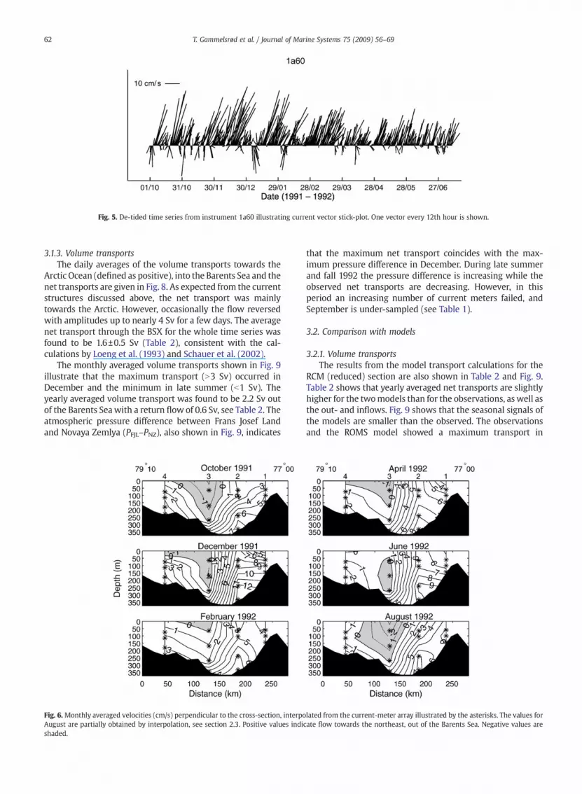
Fig. 5. De-tided time series from instrument 1a60 illustrating current vector stick-plot. One vector every 12th hour is shown.

62 T. Gammelsrød et al. / Journal of Marine Systems 75 (2009) 56–69

3.1.3. Volume transportsThe daily averages of the volume transports towards the

Arctic Ocean (defined as positive), into the Barents Sea and thenet transports are given in Fig. 8. As expected from the currentstructures discussed above, the net transport was mainlytowards the Arctic. However, occasionally the flow reversedwith amplitudes up to nearly 4 Sv for a few days. The averagenet transport through the BSX for the whole time series wasfound to be 1.6±0.5 Sv (Table 2), consistent with the cal-culations by Loeng et al. (1993) and Schauer et al. (2002).

The monthly averaged volume transports shown in Fig. 9illustrate that the maximum transport (N3 Sv) occurred inDecember and the minimum in late summer (b1 Sv). Theyearly averaged volume transport was found to be 2.2 Sv outof the Barents Seawith a return flow of 0.6 Sv, see Table 2. Theatmospheric pressure difference between Frans Josef Landand Novaya Zemlya (PFJL–PNZ), also shown in Fig. 9, indicates

Fig. 6.Monthly averaged velocities (cm/s) perpendicular to the cross-section, interpoAugust are partially obtained by interpolation, see section 2.3. Positive values indishaded.

that the maximum net transport coincides with the max-imum pressure difference in December. During late summerand fall 1992 the pressure difference is increasing while theobserved net transports are decreasing. However, in thisperiod an increasing number of current meters failed, andSeptember is under-sampled (see Table 1).

3.2. Comparison with models

3.2.1. Volume transportsThe results from the model transport calculations for the

RCM (reduced) section are also shown in Table 2 and Fig. 9.Table 2 shows that yearly averaged net transports are slightlyhigher for the twomodels than for the observations, as well asthe out- and inflows. Fig. 9 shows that the seasonal signals ofthe models are smaller than the observed. The observationsand the ROMS model showed a maximum transport in

lated from the current-meter array illustrated by the asterisks. The values forcate flow towards the northeast, out of the Barents Sea. Negative values are

Table 2Volume transports (Sv) through the BSX 1991–1992 calculated from current-meter data (RCM) and the ROMS and NAME models for the corresponding‘reduced’ section

Method RCM ROMS NAME

Net Out In Net Out In Net Out In

RCM section 1.6 2.2 −0.6 1.9 3.3 −1.4 2.0 3.1 −1.1AW 0.0 0.2 −0.2 0.1 0.2 −0.1 1.2 1.9 −0.7CBW 1.0 1.0 0.0 1.7 2.7 1.0 0.0 0.1 −0.1ARW 0.2 0.4 −0.2 0.0 0.1 −0.1 0.0 0.1 −0.1SW 0.1 0.1 0.0 0.0 0.0 0.0 0.3 0.3 0.0

Whole section – – – 2.6 3.9 −1.4 2.3 3.4 −1.1AW – – – 0.3 0.4 −0.1 1.3 2.0 −0.7CBW – – – 2.1 3.0 −0.9 0.1 0.2 −0.1ARW – – – 0.0 0.0 0.0 0.0 0.1 −0.1SW – – – 0.0 0.0 0.0 0.1 0.2 0.0

In the lower half of Table 2, model calculations for the whole section areshown. Positive values are out of the Barents Sea and into the Arctic Ocean.The transports divided into the major water masses are also given.

Fig. 7. The average wind during a)winter (December–March) and b)summer(June–September) 1991–1992 plotted together with the mean isobars at sealevel in the area of study. The data are from the ERA40 re-analysis (EuropeanCenter for Medium range Weather Forecast (ECMWF)).

63T. Gammelsrød et al. / Journal of Marine Systems 75 (2009) 56–69

December, while the peak transport in the NAME modeloccurred in January. Both models also seem to respond to anincrease in the pressure difference towards the end of the

Fig. 8. Volume fluxes (Sv) through the strait between Frans Josef Land andNovaya Zemlya 1991–1992. The positive values are towards the Arctic Ocean.

time series, while the observations indicate a decrease involume transport, but again the month of September wasunder-sampled. Panteleev et al. (2004), using a CTD stationset defining a closed area in the eastern Barents Sea obtained

Fig. 9. Monthly average volume transports (net) based on observations,ROMS and NAME models for the section corresponding to the RCM array(redsec) and the data for the section constructed by Virtual Current Meters(VCM) only. The atmospheric pressure difference (ERA40) between FransJosef Land and Novaya Zemlya is also given.

Fig. 10. Yearly averages (1991–1992) of velocity components normal to thesection for observations (upper), the ROMS model (middle) and the NAMEmodel (lower). Current-meter positions (real and virtual) are indicated with ⁎.Negative values are shaded.

64 T. Gammelsrød et al. / Journal of Marine Systems 75 (2009) 56–69

in September 1997, found that the transport through the BSXon that occasion was close to zero.

As the model velocities represent an area of roughly9×9 km2, a comparison with point measurements is notstraightforward. From Figs. 1 and 6 it seems like the currentsare steered by the topography. This is justified by theconservation of potential vorticity argument. The best wayof comparing data with the models would probably be toselect positions where the model bottom inclination com-pares with the inclination at the moorings. As there aredifferent representations of the vertical in the two models(ROMS is terrain-following whereas NAME uses a fixed levelz-coordinate), we have instead chosen to interpolate themodel outputs to the exact positions of the current-metermoorings. Thereafter, the model values were interpolated inthe vertical to the depths corresponding to the individualinstruments. Theoretical volume transports were calculatedbased on these Virtual Current Meters (VCM) only. Theseresults are also given in Fig. 9. The VCMmodel calculations forthe net transport are 0.9 Sv too small, although the relativeseasonal amplitude is comparable with the full modelestimate. An inspection of the modelled current fieldscompared to the observations is needed to clarify thisdiscrepancy.

3.2.2. Current structureIn Fig.10 the yearly averages of the current fields normal to

the section are given for the models and observations. Thecurrent fields of the models (Fig. 10, middle and Fig. 10, lower)indicate that the moorings M1, M2 and M4 are situated inareas with large horizontal velocity gradients. Taking intoconsideration that the currents are steered by the topography,and the fact that the model topographies do not match(compare the bottom profiles in Fig. 10), the discrepancybetween the observations and the models may at least partlybe explained by the coarse representation of the topography.It was sufficient to move the model virtual moorings one gridpoint (~9 km) to obtain a better fit with the observations;0.2 Sv too low for NAME and 0.4 Sv too low for ROMS.However, the poor horizontal resolution of the 4 current-meter moorings is also an obvious explanation for thedifference between the observational and simulated currentfields at the BSX.

The model simulations indicate that the current-metermoorings were located such that theymissed the current flowmaxima (Fig. 10, middle and Fig. 10, lower). Themajor outflowseems to be situated between moorings 1 and 2, and themaximum inflowwas modelled between moorings 3 and 4 inboth models. This information may be used as guidelines forfuture field experiments.

The current measurements (Fig. 10, upper) indicate thatthe flow is mainly barotropic, except for a bottom intensifiedNE flow, particularly at mooring 2. This bottom intensifica-tion, which is likely to be related to a density driven behaviourof the current, is not reproduced by the models. One reasoncould be an absence or shortage of such dense water near thebottom; e.g. lack of CBW in the NAME model (Table 2).Another possibility could be the different representation ofbottom topography in the models. Fig. 1 illustrates that themoorings were situated east of a saddle point with a down-slope gradient towards the Arctic. The density section given

by Schauer et al. (2002), displays a pycnocline about 100 mabove the bottom hugging the southern slope. This indicates adense (σθN28) bottom layer, whichmay be subject to a down-slope acceleration. Too strong bottom friction in the modelsmay also explain the lack of the bottom intensified current.

It is remarkable how well the two quite differentmodelling approaches discussed here compare. The modelsagree on the positions and strength of the jets in the centralpart of the section. In the northern part of the section bothmodels indicate a jet (5–10 cm/s) towards the Arctic. Exceptfor the topography-related differences from the observedcurrent fields, it can not be concluded that the models fail toreproduce a realistic picture of the current fields. The modeltransport calculations for the whole section are given inTable 2 and show that the ROMS model gives a net transportof 2.6 Sv and the NAME model 2.3 Sv. Only future measure-ment campaigns will show if the model transports are closer

Table 3Same as Table 2 for heat transports (TW)

Method RCM ROMS NAME

Net Out In Net Out In Net Out In

RCM section −3.6 2.6 −6.2 −6.0 5.9 −11.9 7.5 10.5 −3.0AW −0.3 0.8 −1.0 0.2 0.4 −0.2 5.5 7.2 −1.7CBW −1.1 0.1 −1.2 −6.5 3.9 −10.4 0.0 0.1 −0.1ARW −1.3 1.4 −2.7 −0.1 0.3 −0.4 0.1 0.3 −0.3SW −0.1 0.0 −0.2 0.1 0.1 0 0.2 0.5 −0.2

Whole section – – – −5.6 5.3 −10.9 7.4 11 −3.6AW – – – 0.8 1.0 −0.2 5.7 7.4 −1.7CBW – – – −7.7 3.7 −11.4 −0.2 0.1 −0.3ARW – – – −0.1 0.2 −0.3 −0.1 0.3 −0.5SW – – – 0.0 0.2 −0.2 0.2 0.4 −0.2

65T. Gammelsrød et al. / Journal of Marine Systems 75 (2009) 56–69

to reality than the calculations based on the widely spacedcurrent meters. Results from another model experiment inthe area, conducted by the Alfred Wegener Institute (AWI)(Gerdes et al., 2003), have been kindly provided by MichaelKarcher. Based on monthly averages, we calculated a volumetransport of 1.8 Sv through the BSX for the measuring period.

It is interesting to note that both models seem to respondto the secondary maximum in the pressure difference inMarch, and to a less extent to the third maximum in May, seeFig. 9. These features are not captured by the measurements.An inspection of the weekly ice maps (Fig. 4) illustrates thatthe BSX was completely covered by close drift ice as the iceedge was oriented E–W at the latitude of the northern tip ofNovaya Zemlya in March 1992. This may have changed thewind stress on the ocean surface. Representing sea ice innumerical models is still a major challenge, and modelexperiments with ice forced into the model from satellitedatamight turn out useful in this respect. However, inspectingthe individual current meters, Schauer et al. (2002) found thatM1 showed the secondary transportmaximum inMarch 1992,and some of the currentmeters revealed theMaymaximumatM1, M2 and M3. Hence, with a different weighting ofcontributions from each mooring, it is possible to removethis apparent discrepancy between the observations and themodels.

3.3. Heat transport through the BSX

A proxy for the heat flux (Qj) passing a current meterrepresenting an area Aj is traditionally calculated as:

Q j ¼ cwρwAj ∑ivi Ti−Trefð Þ ð1Þ

where vi is the observed velocity and Ti is the temperature atthe time step i, cw is the specific heat of seawater assumed to be4000 J kg−1 K−1, ρw is the water density, and Tref is a referencetemperature. The recommended value for the referencetemperature, when studying heat budgets for the ArcticOcean, is Tref=−0.1 °C (Simonsen and Haugan, 1996). This isthe estimated temperature of the overall outflow from theArctic Ocean (Aagaard andGreisman,1975). Although this valueprobably is not themost representative for the Barents Sea heatbudget, we use Tref=−0.1 °C in order tomake comparisons withprevious estimates (e.g. Maslowski et al., 2004). The latent andsensible heat exchanges due to melting/freezing of sea ice andadvection of sea ice are also neglected here.

The results are given in Table 3, where positive valuesindicate a heat flux from the Barents Sea towards the Arctic.The current meters indicate a small (−3.6 TW) net westwardheat transport from the Arctic towards the Barents Sea. TheROMSmodel also shows awestward heat transport across theRCM section, while NAME indicates an eastward heattransport of 7.5 TW. When extended to the whole section,the heat transport of the two models only changed with asmall amount. When splitting the net transports into watermass transports, we note from Table 2 that in the ROMSmodel only a small fraction of the transport through the BSXis AW. Most of the water is transformed to CBW, while in theNAME model most of the water is identified as AW, see alsosalt transports (Table 4). This also explains why the net heattransports in the twomodels have opposite signs (Table 3). To

investigate this discrepancy, we look into the temperatureand salinity structure at the BSX, comparing bothmodels witha CTD section.

The CTD section obtained over 3 days in September–October 1991 (Fig. 11) shows that the upper ~50 m wasdominated by Surface Water (SW), separated from the ArcticWater (ARW) below by a strong thermocline and halocline.The SW with temperature typically above −0.1 °C is probablyformed from ARWby summerwarming andmelting of sea iceand river run-off. A core of Atlantic Water (AW) was foundnear the centre of the section with maximum temperatureabove 1.5 °C and salinity above 34.8. This AW is believed toenter the Arctic Ocean via the Fram Strait, following thecontinental slope and flow around Frans Josef Land to enterthe Barents Sea from the east, see Schauer et al. (2002). Thedense Cold Bottom Water (CBW) dominated the near bottomlayers with temperatures down to −0.7 °C and maximumsalinities at about 34.9, with σθN28, see Fig. 2. However, theextremely dense CBW occasionally reported from the areawith temperature near freezing point and salinities above 35(Midttun, 1985), was not observed on this occasion.

In Fig. 11, daily model averages (October 1st) of tempera-ture and salinity distributions are also shown. The modelsalinities compare very well with the observations, both inabsolute values and in structure. The salinity is dominatingthe density structure in this area, and the temperature maybe considered more like a tracer. Both models span thesame temperature range as the observations (from −1.5 °Cto +2.0 °C). Table 2 shows that in the ROMS model CBW isdominating the transport, while in the NAME model AWyields the major contribution to the BSX transport. The sameimpression is given by Fig. 11 as the deep saline layers in theROMS model seem to be on the cold side and in the NAMEmodel at the warm side compared to observations. Althoughthe snapshots given in Fig. 11 could change substantially, aseddies of time scales of a few days may pass through the BSX,we will look into possible explanations for the differentbehaviour of the two models.

The present hindcast with the ROMS model seems to givetoo high heat content in the Barents Sea interior. This ismanifested by a 0.6 °C bias (model too high) betweenobserved and modelled temperature in the Kola Sectionat 33°30′E (not shown). This may cause too much icemelting, which in turn gives a higher rate of heat loss to theatmosphere in the eastern Barents Sea. If NAME tends to havetoo much ice, this will lead to an insulation of the water

Table 4Same as Table 2 for salt transports (kT/s)

Method RCM ROMS NAME

Net Out In Net Out In Net Out In

RCM section 51 72 −21 65 114 −49 65 105 −40AW 0 8 −8 4 8 −4 43 68 −25CBW 33 34 −2 60 94 −34 −1 3 −4ARW 7 15 −8 0.0 2 −2 0 2 −2SW 0.0 0.0 0.0 0.0 1 −1 3 5 −1

Whole section – – – 89 137 −48 82 122 −40AW – – – 11 14 −3 48 73 −25CBW – – – 74 104 −30 3 8 −5ARW – – – 0.0 2 −2 1 3 −2SW – – – 65 114 −49 65 105 −40

Fig.11. Snapshot of salinity (left) and temperature (right) from CTD section (upper) comparedwith ROMS (middle) and NAME (lower) models. Temperatures belowzero are shaded.

66 T. Gammelsrød et al. / Journal of Marine Systems 75 (2009) 56–69

below, allowing AW to survive all the way to the BSX, asdemonstrated by Gerdes et al. (2003). Furthermore, tides areincluded in ROMS, but not in NAME. Tides keep polynyasopen, particularly near coasts and islands, and also producedivergences in the open ocean. Harms et al. (2005) found thattidal mixing contributes significantly to the air-sea heatbudget in the Barents Sea; see also Martin and Cavalieri(1989). Another possible explanation of the cooling discre-pancy is the different parameterisations of sea-ice processesin the two models.

It is worth noting that the differences from differentatmospheric forcing data sets using a single model are largerthan the differences between models using the same forcingdata, i.e. compare the ROMS hindcast presented here with theNCEP forced experiment presented by Budgell (2005). Thelarge sensitivity of atmospheric forcing parameterisation was

67T. Gammelsrød et al. / Journal of Marine Systems 75 (2009) 56–69

also demonstrated by Harms et al. (2005) applying theHAMSOM model in the Barents Sea.

3.4. Comparing fluxes through the BSO and the BSX

The nearly 10-year long (1997–2006) current measure-ment program in the BSO gave a net volume flux into theBarents Sea of 1.8 Sv, with a positive trend of about 0.1 Sv/year,(Skagseth et al., 2008). This current-meter array did notinclude the Norwegian Coastal Current (NCC). According tothe model experiments discussed here, NCC contributes withabout 1 Sv, adding up the total transport through the BSO to2.8 Sv. Our estimate for the BSX is of the same order ofmagnitude, (2.0±0.6 Sv). Various model simulations indicatethat the exchanges via the other openings are about one orderof magnitude smaller, e.g. Gerdes et al. (2003) and Maslowskiet al. (2004), in accordance with the few observationsavailable from the area (Aagaard et al., 1983). Obviously, theBSX and the BSO are the main openings for the Barents Sea.

The heat flux into the Barents Sea via the current-meterarray in the BSO was estimated to be 48 TW (Skagseth et al.,2008), and to 40 TW from the repeated combined ADCP andhydrography section by O'Dwyer et al. (2001). Including thecontribution from NCC, the total heat flux is about 65 TWaccording to the 23-year model mean given by Maslowskiet al. (2004) and 73 TW from the ROMS climatic mean. Themodel simulations reported by Drange et al. (2005), indicate49 TW (NOASIM model) and 86 TW (MICOM model).

Observations show that the subsurface layers at the BSX aredominated by water of Atlantic origin (AW), with maximumtemperature less than 1.5 °C, and Cold BottomWater (CBW), seeTable 2 and Fig. 11. The latter is presumably formed by directcooling of AW and/or ice formation and brine release on theshallow shelves in the NE Barents Sea (Schauer et al., 2002), seeFigs. 2 and 3. Thus, the water masses are subject to a strongmodificationwhen crossing the Barents Sea. The heat transportacross the BSX based on the current-meter observations, wassmall but negative (−3.6 TW), indicating a heat flux from theArctic Ocean into the Barents Sea.

The NAME (7.4 TW) and ROMS (−5.6 TW) models alsogave small heat transports in the BSX in 1991–1992, and the23-year model mean by Maslowski et al. (2004) indicate thatthe heat transport is not significantly different from zero (2.2±3.5 TW). These results indicate a heat loss of about 70 TW fromthe water on its journey through the Barents Sea. Simonsenand Haugan (1996) investigated several parameterisationsof the atmospheric surface heat fluxes and found that theaverage atmospheric cooling of the Barents Sea is about140 TW. Thus the ocean heat transport by advection, as wehave calculated here, do not balance the average atmosphericcooling estimated by Simonsen and Haugan (1996). We havetested the sensitivities of the reference temperature Treffor the proxy heat calculation by varying it from freezingpoint to +1 °C, but the heat fluxes stayed low; between 24 TW(Tref=−1.8 °C) for NAME and −22 TW (Tref=+1 °C) for ROMS.

4. Summary and conclusions

Measurements from CTD-casts and a current-meter arraydeployed in the NE Barents Sea between Frans Josef Land andNovaya Zemlya (BSX) for almost a year in 1991–1992, are

presented. The prevailing currents were towards NE, out ofthe Barents Sea, and evident bottom intensificationwas foundin the central part of the strait. The range of day to dayvariability of volume transport was up to 10 Sv (Fig. 8), andthe seasonal amplitude was found to be above 2 Sv (Fig. 9)with maximum in December–January. The seasonality seemsmainly to be related to changes in the atmospheric pressureconditions and the belonging wind fields. The average nettransport through the section, defined by the current meters,was found to be 1.6 Sv.

The current-meter array was compared with the NAMEand ROMS models by extracting model values from the exactpositions of the instruments. Both models gave the same(Fig. 9), but too low average transports (0.9 Sv) compared tothe calculations based on the current meters. The modelsindicate (Fig. 10, middle and Fig. 10, lower) that three out offour moorings were situated in areas with strong horizontalvelocity gradients. Therefore, it can not be concluded that themodels fail to simulate realistic currents, but exact position-ing is distorted because of the coarse representation of thebottom topography. Using all grid points in the ‘reduced’section corresponding to the current meters, gave highertransports; 2.0 Sv for NAME and 1.9 Sv for ROMS (see Table 2).The model current structures (Fig. 10, middle and Fig. 10,lower) indicate that the deployed instruments missed themajor outflow jet from the Barents Sea towards the ArcticOcean.

The current-meter array covered only about half of thesection (Fig. 10, upper vs. Fig. 10, middle and Fig. 10, lower).The total transport through the whole section was calculatedfrom the models as 2.3 Sv for NAME and 2.6 Sv for ROMS.Combining the two model results with the observations, weestimate the net transport through the BSX to be 2.0±0.6 Sv.

The estimated influx of ~1.8 Sv to the Barents Sea in thewest via the BSO between Fugløya and Bjørnøya (Skagsethet al., 2008) is larger than the BSX transport with errormargins, when the contribution of the NCC (~1.0 Sv from theROMS model set up) is added. However, the BSO transport isfound to have a positive trend of 0.1 Sv/year, suggesting that ade-trended value of the BSO transport would resemble that ofthe estimated 1991–1992 BSX transport. The BSO waterconsists mainly of AW with an average temperature ofabout 6 °C (Blindheim, 1995). Observations show that thesubsurface layers at the BSX are dominated by water ofAtlantic origin (AW) with maximum temperature less than1.5 °C and Cold BottomWater (CBW) less than 0 °C, see Figs. 2,11 and Table 2. Thus the water masses are subject to a strongmodification crossing the Barents Sea, see also Schauer et al.(2002).

The cooling of the water masses was stronger in theROMS- than in the NAME-simulations. This may be becausethe two models use different parameterisations of ice and/orthe lack of tides in the NAME model. The tides seem to beimportant for the air-sea heat transfer in the Barents Sea(Harms et al., 2005). This resulted in different signs on theheat transports in the BSX for the NAME (7.4 TW) and ROMS(−5.6 TW)models. We have also seen here with ROMS, as alsoconfirmed by HAMSOM (Harms et al., 2005), that the modelsare highly sensitive to the atmospheric forcing. This indicatesthat the choice of atmospheric forcing could be moreimportant than the type of model.

68 T. Gammelsrød et al. / Journal of Marine Systems 75 (2009) 56–69

Maslowski et al. (2004), using the whole 1979–2001period simulation, found the average heat flux to be 2.2±3.5 TW. Thus it remains open if the Barents Sea is a heat sinkfor the Arctic Ocean, rather than a heat source.

The CBWwater passing the BSX is so dense, that it has thepotential to reach below the depth of the sills (~800 m) of theArctic Mediterranean between Greenland and Scotland andtherefore contribute to the overflow and renewal of the worldocean deep water. Based on the current meters the CBWtransport in the BSX is estimated to 1 Sv. Schauer et al. (2002)indicate that most of this water cascades via the St. AnnaTrough as a bottom intensified flow towards the Arctic Ocean,where it penetrates down below the AW stemming from theFram Strait. Observations (Foldvik et al., 2004) and models(Killworth, 1977) of Cold Bottom Water plumes indicatethat the volume flux may increase by a factor of 2 to 4 byentrainment of surrounding water when cascading towardsgreat depths. The Greenland–Scotland overflow is estimatedto 6 Sv (Hansen and Østerhus, 2000), so the BSX contributionmay be significant.

Acknowledgements

This study has received support from the IPYproject BipolarAtlantic Thermohaline Circulation (BIAC, IPY Cluster # 23)supported by The Norwegian Research Council.

References

Aagaard, K., Foldvik, A., Gammelsrød, T., Vinje, T., 1983. One year records ofcurrents and bottom pressure in the Strait between Nordaustlandet andKvitøya, Svalbard, 1980–1981. Polar Res. 1, 107–113.

Aagaard, K., Greisman, P., 1975. Toward new mass and heat budgets for theArctic Ocean. J. Geophys. Res. 80 (27), 3821–3827.

Blindheim, J., 1995. Report on the working group on oceanic hydrography.Oban. ICES, pp. 26–28. April 1995.

Budgell, P., 2005. Numerical simulation of ice-ocean variability in the BarentsSea region: towards dynamical downscaling. Ocean Dyn. 55, 370–387.doi:10.1007/s10236-005-0008-3.

Drange, H., Gerdes, R., Gao, Y., Karcher, M., Kauker, F., Bentsen, M., 2005.Ocean general circulation modelling of the Nordic Seas. In: Drange, H.,Dokken, T., Furevik, T., Gerdes, R., Berger, W. (Eds.), The Nordic Seas: AnIntegrated Perspective. Geophysical Monograph Series, vol. 158. AGU,Washington DC, pp. 199–219. doi:10.1029/158GM14.

Foldvik, A., Gammelsrød, T., Østerhus, S., Fahrbach, E., Nicholls, K.W., Padman,L., Woodgate, R.A., Rohardt, G., Schröder, M., 2004. Ice shelf wateroverflow and bottom water formation in the southern Weddell Sea.J. Geophys. Res. 109, C02015. doi:10.1029/2003JC001811.

Furevik, T., Nilsen, J.E.O., 2005. Large-scale atmospheric circulation variabilityand its impacts on the nordic seas ocean climate — a review. In: Drange,H., Dokken, T., Furevik, T., Gerdes, R., Berger, W. (Eds.), The Nordic Seas:An Integrated Perspective. Geophysical Monograph Series, vol. 158. AGU,Washington DC, pp. 105–137.

Furevik, T., 2001. Annual and interannual variability of the Atlantic Watertemperatures in the Norwegian and the Barents Seas: 1980–1996. DeepSea Res. I 48, 383–404.

Gerdes, R., Karcher, M.J., Kauker, F., Schauer, U., 2003. Causes anddevelopment of repeated Arctic Ocean warming events. Geophys. Res.Lett. 30 (19), 1980. doi:10.1029/2003GL018080.

Häkkinen, S., Mellor, G.L., 1992. Modelling the seasonal variability of acoupled arctic ice-ocean system. J. Geophys. Res. 97C (12), 20285–20304.

Hansen, B., Østerhus, S., 2000. North Atlantic–Nordic seas exchanges. Prog.Oceanogr. 45, 109–208.

Harms, I.H., Schrum, C., Hatten, K., 2005. Numerical sensitivity studies on thevariability of climate-relevant processes in the Barents Sea. J. Geophys.Res. 110, C06002. doi:10.1029/2004JC002559.

Hunke, E.C., 2001. Viscous-plastic sea ice dynamics with the EVP model:linearization issues. J. Comput. Phys. 170 (1), 18–38.

Ingvaldsen, R., Asplin, L., Loeng, H., 2004. The seasonal cycle in the Atlantictransport to the Barents Sea. Cont. Shelf Res. 24 (9), 1015–1032.doi:10.1016/j.csr.2004.02.011.

Ingvaldsen, R., Loeng, H., Asplin, L., 2002. Variability in the Atlantic inflow to theBarents Sea based on a one-year time series from moored current meters.Cont. Shelf Res. 22 (3), 505–519. doi:10.1016/S0278-4343(01)00070-X.

Ivanov, V.V., Shapiro, G.I., 2005. Formation of a dense water cascade in themarginal ice zone in the Barents Sea. Deep Sea Res. I 52 (9), 1699–1717.doi:10.1016/j.dsr.2005.04.004.

Jakobsson, M., Cherkis, N., Woodward, J., Coakley, B., Macnab, R., 2000. A newgrid of Arctic bathymetry: a significant resource for scientists andmapmakers. EOS Transactions. AGU. 81, 89, 93, 96.

Kalnay, E., Co-authors, 1996. The NCEP/NCAR 40 year re-analyses project.Bull. Am. Met. Soc. 77 (3), 437–471.

Karcher, M.J., Oberhuber, J.M., 2002. Pathways and modification of the upperand intermediate waters of the Arctic Ocean. J. Geophys. Res. l07 (C6),3049. doi:10.1029/2000JC000530.

Killworth, P.D., 1977. Mixing on Weddel Sea continental slope. Deep Sea Res.24 (5), 427–448.

Kvingedal, B., 2005. Sea ice extent and variability in the Nordic Seas, 1967–2002. In: Drange, H., Dokken, T., Furevik, T., Gerdes, R., Berger, W. (Eds.),The Nordic Seas: An Integrated Perspective. Geophysical MonographSeries, vol. 158. AGU, Washington DC, pp. 39–51.

Kwok, R., Maslowski, W., Laxon, S.W., 2005. On large outflows of Arctic sea iceinto the Barents Sea. Geophys. Res. Lett. 32 (22), L22503. doi:10.1029/2005GL024485.

Loeng, H., Sagen, H., Ådlandsvik, B. and Ozighin, V., 1993. Currentmeasurements between Novaya Zemlya and Frans Josef Land, September1991–September 1992. Institute of Marine Research, Norway. Depart-ment of Marine Environment. Report 2/1993, pp 23 + 4 appendices.

Martin, S., Cavalieri, D.J., 1989. Contributions of the Siberian shelf polynyas tothe Arctic Ocean intermediate and deep-water. J. Geophys. Res. 94 (C9),12725–12738.

Maslowski,W., Marble, D.,Walczowski,W., Schauer, U., Clement, J.L., Semtner,A.J., 2004. On climatological mass, heat, and salt transports through theBarents Sea and Fram Strait from a pan-Arctic coupled ice-ocean modelsimulation. J. Geophys. Res. 109, C03032. doi:10.1029/2001JC0010139.

Meincke, J., Rudels, B., Friedrich, H.J., 1997. The Arctic Ocean–Nordic Seasthermohaline system. ICES J. Mar. Sci. 54 (3), 283–299.

Mellor, G.L., Kantha, L., 1989. An ice-ocean coupled model. J. Geophys. Res.94 (C8), 10937–10954.

Midttun, L., 1985. Formation of dense bottom water in the Barents Sea. DeepSea Res. A 32, 1233–1241.

O, Dwyer, J., Kasajima, Y., Nøst, O.A., 2001. North Atlantic Water in the BarentsSea opening. Polar Res 20 (2), 209–216.

Olsen, A., Johannessen, T., Rey, F., 2003. On the nature of the factors thatcontrol spring bloom development at the entrance to the Barents Sea andtheir interannual variability Sarsia 88 (6) , 379–393.

Padman, Erofeeva, S., 2004. A barotropic inverse tidal model for the ArcticOcean. Geophys. Res. Lett. 31 (2), L02303.

Panteleev, G., Ikeda, M., Grotov, A., Nechaev, D., Yaremchuk, M., 2004. Mass,heat and salt balances in the eastern Barents Sea obtained by inversion ofhydrographic section data. J. Oceanogr. 60, 613–623.

Parkinson, C.L., Washington, W.M., 1979. Large-scale numerical-model of seaice. J. Geophys. Res. 84 (NC1), 311–337.

Pease, C.H.,1987. The size ofwind-driven coastal polynyas. J. Geophys. Res. 92 (C7),7049–7059.

Pfirman, S.L., Bauch, D., Gammelsrød, T., 1994. The Northern Barents Sea:water mass distribution and modification. In: Johannessen, O.M.,Muench, R.D., Overland, J.E. (Eds.), The Polar Oceans and their Rolein Shaping the Global Environment. Geophysical Monograph Series,vol. 85. AGU, Washington DC, pp. 77–94.

Quadfasel, D., Rudels, B., Kurz, K., 1988. Outflow of dense water from aSvalbard fjord into the Fram Strait. Deep Sea Res. A 35 (7), 1143–1150.

Rosenfeld, 1983. WHOI. Technical Report 85–35, 21.Rudels, B., Jones, E.P., Anderson, L.G., Kattner, G., 1994. On the Intermediate

depth waters of the Arctic Ocean. In: Johannessen, O.M., Muench, R.D.,Overland, J.E. (Eds.), The Polar Oceans and their Role in Shaping theGlobal Environment. Geophysical Monograph Series, vol. 84. AGU,Washington DC, pp. 33–46.

Rudels, B., 1987. On the mass balance of the Polar Ocean, with specialemphasis on the Fram Strait. Skrift 188, 1–53.

Sakshaug, E., Bjørge, A., Gulliksen, B., Loeng, H., Mehlum, F., 1994. Structure,biomass distribution and energetics of the pelagic ecosystem in theBarents Sea: a synopsis. Polar Biol. 14 (6), 405–411.

Schauer, U., Loeng, H., Rudels, B., Ozhigin, V.K., Dieck, W., 2002. Atlantic waterinflow through the Barents and Kara Seas. Deep Sea Res. I 49 (12),2281–2298.

Schauer, U., Muench, R., Rudels, B., Timokov, L., 1997. Impact of eastern Arctic shelfwaters on the Nansen Basin intermediate layers. J. Geophys. Res. 102 (C2),3371–3382.

Schiffer, R.A., Rossow, W.B., 1985. ISCCP global radiance data set — a newresource for climate research. Bull. Am. Met. Soc. 66 (12), 1498–1505.

69T. Gammelsrød et al. / Journal of Marine Systems 75 (2009) 56–69

Semtner, A.J., 1976. Model for thermodynamic growth of sea ice in numericalinvestigations of climate. J. Phys. Oceanogr. 6 (3), 379–389.

Shchepetkin, A.F., McWilliams, J.C., 2003. A method for computing horizontalpressure-gradient force in an oceanic model with a nonaligned verticalcoordinate. J. Geophys. Res. 108 (C3). doi:10.1029/2001JC001047.

Simonsen, K., Haugan, P.M., 1996. Heat budgets of the Arctic Mediterraneanand sea surface heat flux parameterizations for the Nordic Seas.J. Geophys. Res. 101 (C3), 6553–6576.

Skagseth, Ø., Furevik, T., Ingvaldsen, R., Loeng, H., Mork, K.A., Orvik, K.A.,Ozhigin, V., 2008. Volume and heat transports to the Arctic via theNorwegian and Barents Seas. In: ‘Arctic–Subarctic Ocean fluxes. In:

Dickson, R., Meincke, J., Rhines, P. (Eds.), Defining the role of the NorthernSeas in Climate. Springer, Netherlands. doi:10.1007/978-1-4020-6774-7.

Sorteberg, A., Kvingedal, B., 2006. Atmospheric forcing on the Barents Seawinter ice extent. J. Clim. 19 (19), 4772–4784.

Steele, M., Morley, R., Ermold, W., 2001. PHC: a global ocean hydrographywith a high quality Arctic Ocean. J. Clim. 14 (9), 2079–2087.

Zhang, J.L., Hibler, W.D., 1997. On an efficient numerical method for modelingsea ice dynamics. J. Geophys. Res. 102 (C4), 8691–8702.

Zhang, J.L., Rothrock, D.A., Steele, M., 1998. Warming of the Arctic Ocean by astrengthened Atlantic inflow: model results. Geophys. Res. Lett. 25 (10),1745–1748.