December 2004 / Vol. 54 No. 12 • BioScience 1101

Articles

Management action to conserve biodiversity ismost appropriately planned and implemented at

regional or local scales. However, conservation assessments ata global scale can help to justify and stimulate such local ac-tivity by providing a big-picture perspective on the currentand projected status of biodiversity on the planet. Such as-sessments may also be used to guide the allocation of con-servation resources globally and to provide a broad contextwithin which to evaluate regional-scale conservation prior-

ities. All global conservation assessments—whether focusedon the coverage of protected areas (Rodrigues et al. 2004a),the impacts of habitat loss (Gaston et al. 2003), or the potentialeffects of climate change (Thomas et al. 2004)—require in-formation on the spatial distribution of elements of bio-diversity. This knowledge of biodiversity pattern providesthe essential foundation on which to build more sophisticatedassessments of ecological, evolutionary, and socioeconomicprocesses.

Simon Ferrier (e-mail: simon.ferrier@environment.nsw.gov.au) is a principal research officer, Glenn Manion is a software development consultant, and Kellie Man-

tle is a conservation data officer in the Spatial Information and Analysis Section, New South Wales Department of Environment and Conservation, Armidale, New

South Wales 2350, Australia. George V. N. Powell and Neil D. Burgess are senior conservation scientists, and Thomas F. Allnutt is a senior conservation specialist, with

the Conservation Science Program, World Wildlife Fund, Washington, DC 20037. Karen S. Richardson is a research fellow with the Rainforest Cooperative Research

Centre, University of Queensland, Brisbane, Queensland 4072, Australia. Jake M. Overton is a research scientist at Landcare Research, Hamilton 2001, New Zealand.

Susan E. Cameron is with the graduate group in ecology, Department of Environmental Science and Policy, University of California, Davis, CA 95616. Daniel P. Faith

is a principal research scientist at the Australian Museum, Sydney, New South Wales 2010, Australia. John F. Lamoreux is a PhD student with the Department of

Environmental Sciences, University of Virginia, Charlottesville, VA 22904. Gerold Kier is a doctoral student at the Nees Institute for Biodiversity of Plants, University

of Bonn, D-53115 Bonn, Germany. Robert J. Hijmans is an associate specialist in GIS and biodiversity informatics, Museum of Vertebrate Zoology, University of

California, Berkeley, CA 94720. Vicki A. Funk is senior curator at the US National Herbarium, Department of Botany, National Museum of Natural History, Smith-

sonian Institution, Washington, DC 20560. Gerasimos A. Cassis is head, and Paul Flemons is GIS (geographic information system) manager, at the Centre for

Biodiversity and Conservation Research, Australian Museum. Brian L. Fisher is curator of entomology at the California Academy of Sciences, San Francisco, CA 94103.

David Lees is Leverhulme Postdoctoral Fellow with the Department of Entomology, Natural History Museum, London, SW7 5BD, United Kingdom. Jon C. Lovett is

a senior lecturer with the Environment Department, University of York, York, YO10 5DD, United Kingdom. Renaat S. A. R. Van Rompaey is a research scientist with

the Laboratory of Plant Systematics and Phytosociology, Free University of Brussels, Brussels 1050, Belgium. © 2004 American Institute of Biological Sciences.

Mapping More of TerrestrialBiodiversity for GlobalConservation Assessment

SIMON FERRIER, GEORGE V. N. POWELL, KAREN S. RICHARDSON, GLENN MANION, JAKE M. OVERTON, THOMASF. ALLNUTT, SUSAN E. CAMERON, KELLIE MANTLE, NEIL D. BURGESS, DANIEL P. FAITH, JOHN F. LAMOREUX,GEROLD KIER, ROBERT J. HIJMANS, VICKI A. FUNK, GERASIMOS A. CASSIS, BRIAN L. FISHER, PAUL FLEMONS,DAVID LEES, JON C. LOVETT, AND RENAAT S. A. R. VAN ROMPAEY

Global conservation assessments require information on the distribution of biodiversity across the planet. Yet this information is often mapped at a very coarse spatial resolution relative to the scale of most land-use and management decisions. Furthermore, such mapping tends to focus selec-tively on better-known elements of biodiversity (e.g., vertebrates). We introduce a new approach to describing and mapping the global distributionof terrestrial biodiversity that may help to alleviate these problems. This approach focuses on estimating spatial pattern in emergent properties ofbiodiversity (richness and compositional turnover) rather than distributions of individual species, making it well suited to lesser-known, yet highlydiverse, biological groups. We have developed a global biodiversity model linking these properties to mapped ecoregions and fine-scale environmen-tal surfaces. The model is being calibrated progressively using extensive biological data sets for a wide variety of taxa. We also describe an analyticalapproach to applying our model in global conservation assessments, illustrated with a preliminary analysis of the representativeness of the world’sprotected-area system. Our approach is intended to complement, not compete with, assessments based on individual species of particular conserva-tion concern.

Keywords: biodiversity, global, mapping, protected areas, representativeness

The difficulty of mapping spatial pattern in biodiversity de-pends on the level of biodiversity of interest (e.g., ecosystems,species, or genes). Distributions of broad ecosystems are nowrelatively easy to map and monitor, thanks to the advent ofsatellite-based remote sensing. However, satellite imagerytells little about patterns of species composition within ecosys-tems. Mapping the distributions of species is far more chal-lenging, because the vast majority of species can be detectedonly through direct field observation or sampling. Currentknowledge of species distributions is therefore grossly in-complete. Only a fraction of the planet’s species has been described to date (Heywood 1995), and distributional infor-mation sufficient to be of any direct use in conservation assessment is available for only a small proportion of theseknown species (Ferrier 2002). Conservation assessmentstherefore need to rely heavily on the use of biodiversity “sur-rogates”—mapped entities whose distributions are likely toconcord with spatial pattern in biodiversity as a whole (Mar-gules and Pressey 2000).

Surrogates employed in recent global assessments of ter-restrial biodiversity include mapped ranges of vertebratespecies (Rodrigues et al. 2004a, 2004b), major habitat typesor biomes (Gaston et al. 2003, Brooks et al. 2004), and bio-geographical regions or ecoregions (Olson and Dinerstein2002).While each of these surrogates has particular strengths,they share a potential weakness in the way they have been em-ployed in global assessments. All three surrogates tend to bemapped at a coarse spatial resolution relative to the scale atwhich land-use or management decisions are typically madeon the ground. This mismatch of scales may limit the extentto which these assessments can detect finer-scale bias in thedistribution of habitat loss (e.g., toward more productiveparts of a landscape) or in the location of protected areas(Pressey et al. 1996, Armesto et al. 1998), especially if themapped distribution of each surrogate entity encompassesconsiderable environmental and biological heterogeneity.Such problems are likely to be particularly acute for nonver-tebrate components of biodiversity, including invertebratesand plants, because taxa within these groups often exhibithigher rates of spatial turnover (replacement of species) thando vertebrates (Ferrier et al. 1999, Moritz et al. 2001). For ex-ample, protecting a portion of the range of a given vertebratespecies, or of an ecoregion, does not necessarily ensure goodrepresentation of all elements of biodiversity if this protectionis biased environmentally or geographically within the mappeddistribution of the surrogate entity concerned.

This mismatch between the scale of global assessmentsand the scale at which actual land-use and management de-cisions shape regional landscapes may result in a tendency forsuch assessments to overestimate the representativeness of theworld’s protected-area system or, conversely, to underestimatethe global consequences of habitat loss. Furthermore, in using global assessments based on coarse-resolution surro-gates to direct conservation attention to priority regions or“hotspots,” there is a risk that important finer-scale priorities

may be overlooked, and therefore never receive the conser-vation attention they deserve (Ferrier 2002).

To help alleviate these problems, we introduce a new sur-rogate approach to estimating and mapping spatial patternin terrestrial biodiversity for global conservation assessments.This approach arose out of work conducted by an informalconsortium in the 6 months leading up to the fifth World ParksCongress (Durban, South Africa, September 2003), aimed atproviding “proof of concept”of an alternative strategy for as-sessing the representativeness of the world’s protected-area sys-tem (i.e., the extent to which this system includes samples ofall elements of biodiversity). The approach is intended tocomplement, not compete with, other assessments based onvertebrate distributions, biomes, or ecoregions.As in those as-sessments, we use coarse-scale surrogates to provide a solidbiogeographical foundation for our approach. However, wethen add value to these surrogates by using higher-resolutionmapping of environmental attributes to predict spatial pat-tern in biodiversity at finer scales. The link between biodiversitypattern and mapped environmental attributes is calibratedthrough statistical modeling of available biological and en-vironmental data.

Our modeling takes advantage of revolutionary advancesin the availability and quality of two major sources of data:(1) global coverage of digital terrain, climate, soil, and land-cover surfaces, now available at relatively fine spatial resolu-tion (mostly 1-kilometer [km] grids), thanks to recentadvances in remote sensing technology, and (2) data setsfrom biological surveys and specimen collections, containingthe locations of observation or collection for large numbersof species across a wide range of higher taxa. The accessibil-ity of such data is improving dramatically as a result of rapidadvances in the field of biodiversity informatics, particularlythe digitization of museum and herbarium specimen collec-tions (Bisby 2000, Graham et al. 2004).

Here we outline the analytical strategy we are using to de-velop a global biodiversity model by integrating varioussources of biological and environmental data, with a summaryof progress made to date in accessing and processing these datasources. We then describe how our biodiversity model can beemployed in global conservation assessments, illustrated witha preliminary analysis of the representativeness of the world’sprotected-area system.

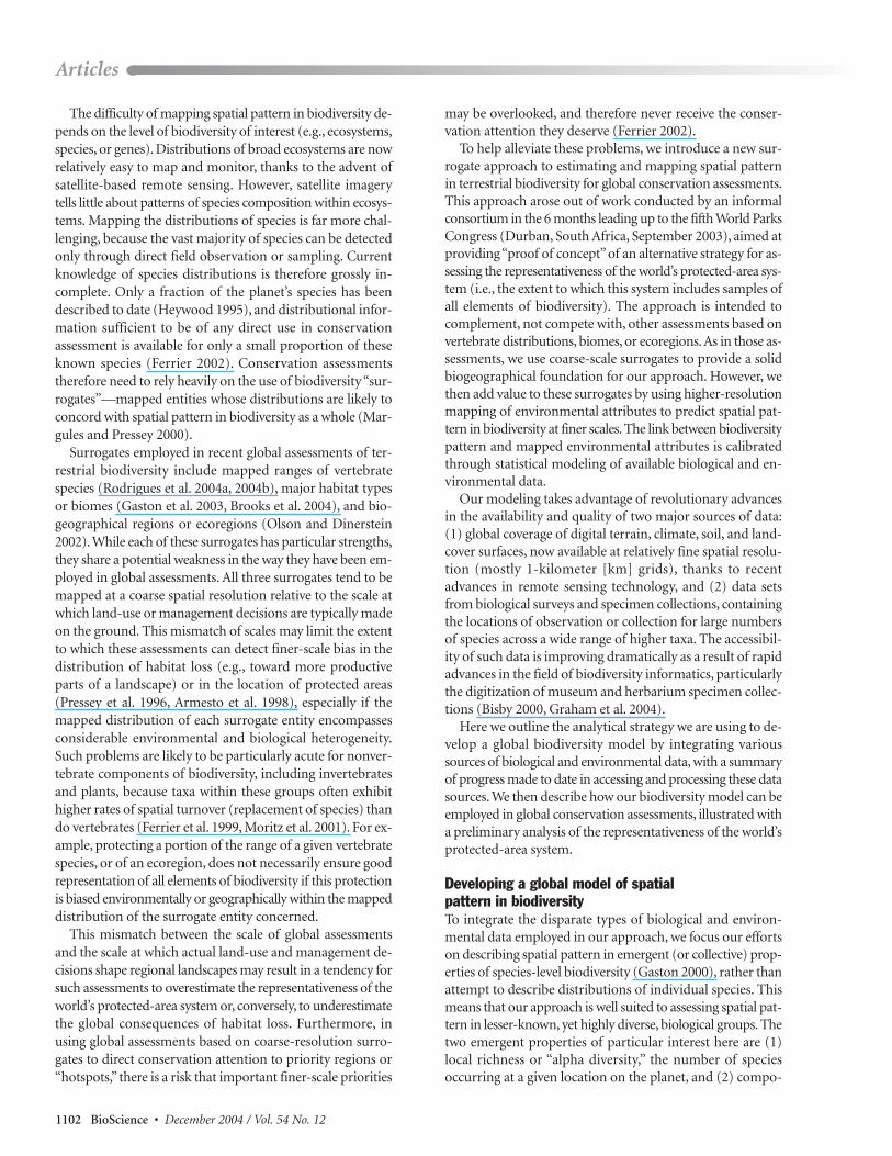
Developing a global model of spatial pattern in biodiversityTo integrate the disparate types of biological and environ-mental data employed in our approach, we focus our effortson describing spatial pattern in emergent (or collective) prop-erties of species-level biodiversity (Gaston 2000), rather thanattempt to describe distributions of individual species. Thismeans that our approach is well suited to assessing spatial pat-tern in lesser-known, yet highly diverse, biological groups. Thetwo emergent properties of particular interest here are (1) local richness or “alpha diversity,” the number of species occurring at a given location on the planet, and (2) compo-

1102 BioScience • December 2004 / Vol. 54 No. 12

Articles

sitional turnover or “beta diversity,” the dif-ference in species composition between dif-ferent locations (Whittaker 1972, Ferrier 2002).

The concept of compositional turnover hasrarely been addressed explicitly in the conser-vation biology literature, despite its direct re-lationship with the more widely studiedconcept of endemism. The level of endemismexhibited by species occupying a given area isclearly a function of compositional turnover be-tween this area and all other areas. However, aswe demonstrate below, there is much to begained by working directly with turnover itselfin conservation assessment, as this approach retains more information on the pattern ofcomplementarity (sensu Margules and Pressey2000) between areas. Several recent ecologicalpapers on the partitioning of regional bio-diversity into components of alpha and beta diversity have helped to provide a strong the-oretical foundation for the richness–turnoverview of biodiversity adopted here (Arita andRodriguez 2002, Gering et al. 2003).

To develop our global model of spatial pat-tern in biodiversity, we model richness andturnover as functions of mapped biogeographical units andenvironmental surfaces with complete global coverage. Themodel is being calibrated using a wide variety of biological data(figure 1).

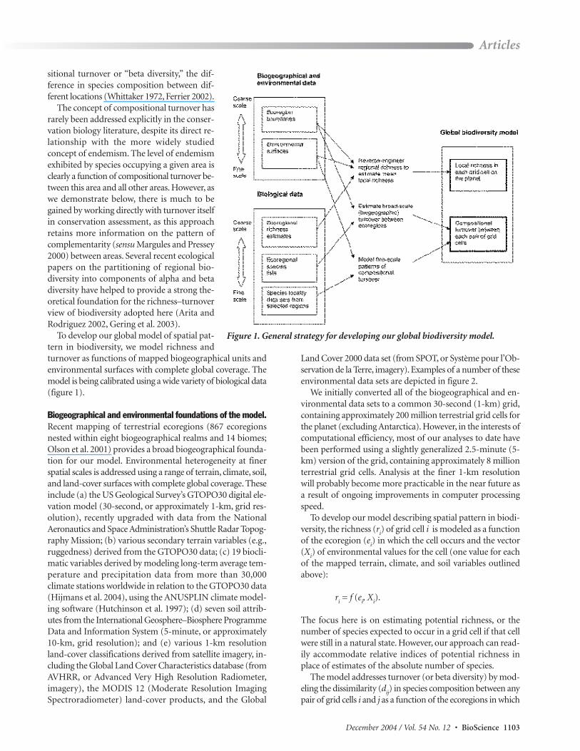
Biogeographical and environmental foundations of the model.Recent mapping of terrestrial ecoregions (867 ecoregionsnested within eight biogeographical realms and 14 biomes;Olson et al. 2001) provides a broad biogeographical founda-tion for our model. Environmental heterogeneity at finerspatial scales is addressed using a range of terrain, climate, soil,and land-cover surfaces with complete global coverage. Theseinclude (a) the US Geological Survey’s GTOPO30 digital ele-vation model (30-second, or approximately 1-km, grid res-olution), recently upgraded with data from the NationalAeronautics and Space Administration’s Shuttle Radar Topog-raphy Mission; (b) various secondary terrain variables (e.g.,ruggedness) derived from the GTOPO30 data; (c) 19 biocli-matic variables derived by modeling long-term average tem-perature and precipitation data from more than 30,000climate stations worldwide in relation to the GTOPO30 data(Hijmans et al. 2004), using the ANUSPLIN climate model-ing software (Hutchinson et al. 1997); (d) seven soil attrib-utes from the International Geosphere–Biosphere ProgrammeData and Information System (5-minute, or approximately10-km, grid resolution); and (e) various 1-km resolutionland-cover classifications derived from satellite imagery, in-cluding the Global Land Cover Characteristics database (fromAVHRR, or Advanced Very High Resolution Radiometer,imagery), the MODIS 12 (Moderate Resolution ImagingSpectroradiometer) land-cover products, and the Global

Land Cover 2000 data set (from SPOT, or Système pour l’Ob-servation de la Terre, imagery). Examples of a number of theseenvironmental data sets are depicted in figure 2.

We initially converted all of the biogeographical and en-vironmental data sets to a common 30-second (1-km) grid,containing approximately 200 million terrestrial grid cells forthe planet (excluding Antarctica). However, in the interests ofcomputational efficiency, most of our analyses to date havebeen performed using a slightly generalized 2.5-minute (5-km) version of the grid, containing approximately 8 millionterrestrial grid cells. Analysis at the finer 1-km resolutionwill probably become more practicable in the near future asa result of ongoing improvements in computer processingspeed.

To develop our model describing spatial pattern in biodi-versity, the richness (ri) of grid cell i is modeled as a functionof the ecoregion (ei) in which the cell occurs and the vector(Xi) of environmental values for the cell (one value for eachof the mapped terrain, climate, and soil variables outlinedabove):

ri = f (ei, Xi).

The focus here is on estimating potential richness, or thenumber of species expected to occur in a grid cell if that cellwere still in a natural state. However, our approach can read-ily accommodate relative indices of potential richness inplace of estimates of the absolute number of species.

The model addresses turnover (or beta diversity) by mod-eling the dissimilarity (dij) in species composition between anypair of grid cells i and j as a function of the ecoregions in which

December 2004 / Vol. 54 No. 12 • BioScience 1103

Articles

Figure 1. General strategy for developing our global biodiversity model.

the two cells occur and the environmental values for thecells:

dij = (ei, Xi, ej, Xj).

Dissimilarity is defined here as the mean proportion of speciesoccurring in one cell that are not expected to occur in the othercell (Wilson and Shmida 1984, Faith et al. 1987), again esti-mated as if both of these cells were still in a natural state. The

vectors Xi and Xj can also include the latitude and longitudeof each site, thereby allowing the dissimilarity of sites to beshaped by geographical separation in addition to environ-mental difference.

Calibrating the model using available biological data. If ourglobal biodiversity model is to contribute usefully to conser-vation assessment, it must make predictions that match realpatterns of biological richness and turnover as closely as pos-

sible. To achieve this, we use various sources of bio-logical data to define and calibrate the functions inour model that link richness and turnover to mappedecoregions and environmental surfaces. We viewthis calibration as an incremental process. Althoughwe have already accessed and analyzed a large num-ber of biological data sets since commencing thiswork in early 2003, we suspect that these data sets rep-resent only the tip of the iceberg in relation to the to-tal pool of biological data that could be used tocalibrate our model. The model therefore has con-siderable potential for ongoing refinement.

To date, we have directed more effort to calibrat-ing the turnover component of our model than tocalibrating the richness component. Given our ini-tial interest in assessing the representativeness of theworld’s protected-area system, we felt that turnover(beta diversity) would be likely to play a much moresignificant role in determining representativenessthan would variation in local richness. To calibratethe turnover component of our model, we are usingbiological data recorded at two very different spatialscales. Broad biogeographic turnover between ecore-gions is addressed by analyzing compiled lists ofspecies occurring in each ecoregion. At present, suchlists are available across all ecoregions only for ver-tebrates, in an extensive data set compiled by one ofus (J. F. L.). This data set records the presence or ab-sence of more than 26,000 mammal, bird, reptile, andamphibian species in each of the world’s 867 ecore-gions. These data allow ready estimation of the broadlevel of compositional dissimilarity between all pos-sible pairs of ecoregions. Rapidly improving accessto digitized specimen-locality data sets should allowthe estimation of turnover between ecoregions to beextended to plants and invertebrates within the nextfew years.

Finer-scale turnover within regions is being ex-plored through statistical analysis of selected bio-logical survey and collection data sets. These data aresubjected to generalized dissimilarity modeling(GDM), a new nonlinear technique for analyzingturnover in species composition between pairs ofsurvey or collection localities in relation to environ-mental differences between, and geographical sepa-ration of, these localities (Faith and Ferrier 2002,Ferrier 2002, Ferrier et al. 2002). Once such a model

1104 BioScience • December 2004 / Vol. 54 No. 12

Articles

Figure 2. Examples of the data used to develop the global biodiversitymodel. Black lines in the detailed maps are ecoregion boundaries. Thetemperature surface is derived from WorldClim (Hijmans et al. 2004).Plant specimen localities are from the Missouri Botanical Garden’sTROPICOS database. The vertebrate species range is based on the lists of species occurring within each ecoregion compiled by one of us (J. F. L.). The land-cover map is based on the Global Land Cover 2000data set. The ruggedness surface is derived from the GTOPO30 digitalelevation model. The soil data are from the International Geosphere–Biosphere Programme Data and Information System.

has been derived with GDM, it can be used to predict the levelof compositional dissimilarity expected between any pair oflocalities (in this case, 5-km grid cells) within a region, basedpurely on environmental and geographical attributes.

To date we have focused our analysis of finer-scale turnoveron plants and invertebrates, partly to complement an exist-ing vertebrate-based global assessment (Rodrigues et al.2004a, 2004b), but also because plants and invertebrates ex-hibit more rapid spatial turnover in species compositionthan do vertebrates. However, there is considerable scope forextending the approach to include vertebrates in the future.Ideally, we would hope to acquire biological data to analyzeturnover patterns within every individual ecoregion. In reality,however, this is made difficult by the sheer number of ecore-gions and by the absence or unavailability of suitable data formany of these. At this stage, we are working with a relativelysparse sample of biological data sets from across the planet.To date, our statistical modeling of finer-scale turnover pat-terns has employed more than 1.1 million locality records formore than 98,000 species of plants and invertebrates (mostlyarthropods and, to a lesser extent, mollusks). This data set hasbeen collated from a large number of sources and includes atleast some data for every combination of biogeographicalrealm and major biome. In general, however, our study hasaddressed the tropical moist forest biome more rigorously thanthe other biomes, as this was a particular focus of our initialdata acquisition efforts.

To cope with gaps in the geographical coverage of ourturnover analyses, we take the predictive capability of GDMone step further and use models of turnover derived from se-lected regions to extrapolate patterns across similar regions(e.g., in the same realm and biome). To do this, we assume thatrates of turnover—that is, the amounts of compositionalturnover expected per unit change in each environmental vari-able and per unit geographical separation—are reasonablyconsistent between these regions. Any problems arising fromviolations of this assumption (e.g., marked discontinuities inpatterns of turnover) should diminish as we improve thegeographical coverage of our analyses by incorporating ad-ditional biological data sets. To gain a better understandingof the magnitude of such problems, some of us are workingon a related research project using biological data from anumber of moist tropical forest regions to evaluate how ef-fectively models fitted to data from any one region performin predicting turnover patterns in the other regions.

Our current approach to calibrating the local-richnesscomponent of our model relies heavily on estimates, gener-ated by the Nees Institute for Biodiversity of Plants at the Uni-versity of Bonn, of the total number of vascular plant speciesoccurring in each of the world’s 867 terrestrial ecoregions. Thetotal richness of a given ecoregion is likely to be a function ofboth the average local richness and the level of composi-tional turnover between locations within that region. To re-move the contribution of turnover, we use generalized additivemodeling (Lehmann et al. 2002) to fit a regression model re-lating the estimates of ecoregional richness to the area of

each ecoregion, and to the mean and standard deviation ofeach of the fine-scale environmental variables within theecoregion. This model is then used to reverse-engineer theecoregional richness values to estimate the average richnessexpected in a 5-km grid cell (in a natural state) within eachecoregion (by setting the area variable to 25 km2 and each ofthe standard deviation variables to zero). All cells in a givenecoregion are therefore assumed to have the same potentiallocal richness, but this richness is allowed to vary betweenecoregions. In the future, we hope to remove the need for thisassumption of constant potential richness within an ecore-gion by pursuing more rigorous approaches to estimatingfiner-scale spatial variation in richness, including statisticalanalysis of local richness estimates (derived from biologicalsurvey or collection data) in relation to mapped environmentalsurfaces (Leathwick et al. 1998).

Applying the model to global conservation assessmentOur global model of spatial pattern in biodiversity couldbenefit greatly from further refinement, and from further eval-uation of predictions against expert knowledge. However, weare confident that, once implemented more fully, the modelwill add considerable value to existing global conservation as-sessments. We have already developed and tested an analyt-ical approach to using predictions from our model to assessthe representativeness of protected-area systems.

Our approach is founded on well-established principles ofthe species–area relationship (Rosenzweig 1995), which de-scribes the relationship between number of species (S) andarea (A) as a power-law function:

S = cAz,

where c and z are constants. This relationship is often used topredict the proportion of species that will be retained in a re-gion if the habitat in that region is reduced to a specified pro-portion of the original area:

Sretained / Soriginal = (Aretained / Aoriginal)z.

While this approach is most often used to estimate the effects of habitat loss, it also has direct applicability to as-sessing the representativeness of protected-area systems(Zurlini et al. 2002). This involves treating the habitat in protected areas as if it were the only habitat retained in a region, and estimating the proportion of species retained or represented accordingly. This hypothetical scenario isinvoked purely as a means of assessing the representative-ness of protected areas, not as a means of assessing reten-tion of biodiversity in the landscape as a whole (for whichthe benefits to biodiversity of other types of land use wouldneed to be properly considered).

The species–area approach is usually applied to relativelylarge areas: to whole biogeographical regions, for example, orto the global distribution of whole biomes (Malcolm and

December 2004 / Vol. 54 No. 12 • BioScience 1105

Articles

Markham 2000, Brooks et al. 2002, Thomas et al. 2004). Thisassumes that reduction in habitat is distributed randomlyacross the region or biome of interest (Ferrier 2002). How-ever, as demonstrated by Seabloom and colleagues (2002), vio-lations of this assumption—resulting, for example, from biasin habitat reduction toward certain parts of a region orbiome—may lead to overestimation of the proportion ofspecies retained. Unfortunately, such bias in the distributionof habitat reduction (or, conversely, protection) is likely to bethe rule rather than the exception in most parts of the world(Pressey et al. 1996, Armesto et al. 1998). Here we address thisproblem head-on by adapting the traditional species–area ap-proach to work with our continuous model of spatial patternin the distribution of biodiversity. To do this, we draw on prin-ciples of the “environmental diversity” approach proposedoriginally by Faith and Walker (1996) as a means of assess-ing the representativeness of protected areas within a con-tinuous environmental or biological space.

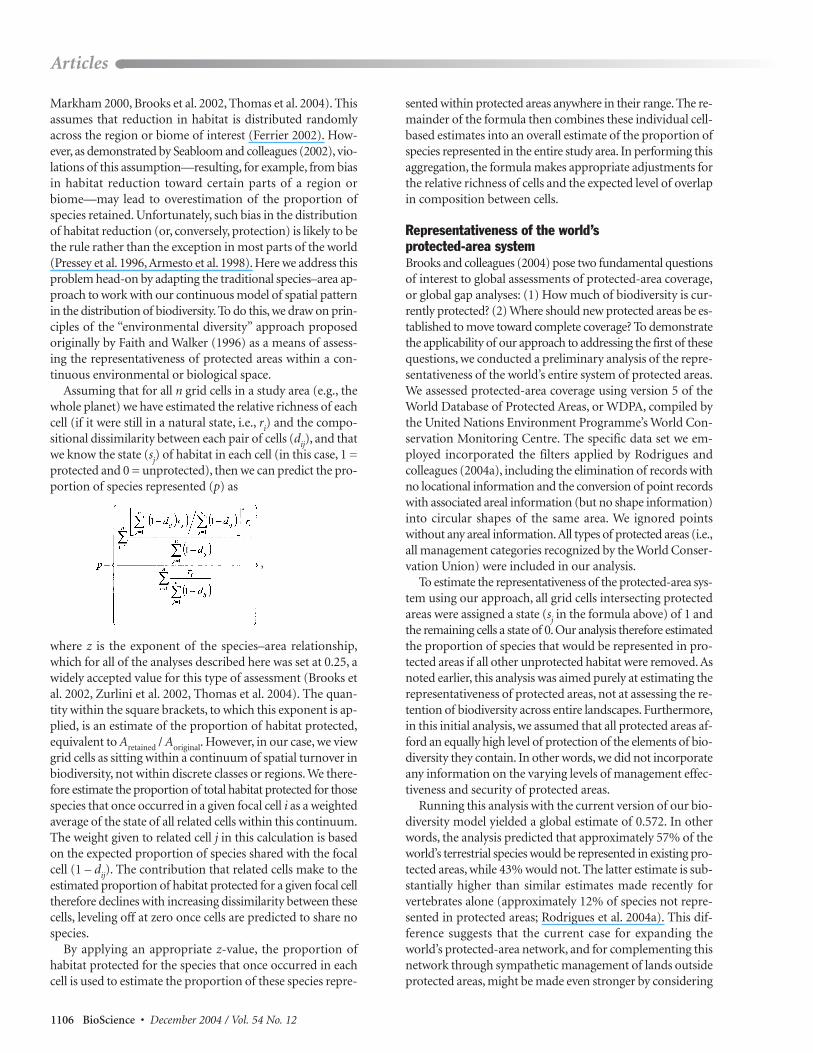
Assuming that for all n grid cells in a study area (e.g., thewhole planet) we have estimated the relative richness of eachcell (if it were still in a natural state, i.e., ri) and the compo-sitional dissimilarity between each pair of cells (dij), and thatwe know the state (sj) of habitat in each cell (in this case, 1 =protected and 0 = unprotected), then we can predict the pro-portion of species represented (p) as

where z is the exponent of the species–area relationship,which for all of the analyses described here was set at 0.25, awidely accepted value for this type of assessment (Brooks etal. 2002, Zurlini et al. 2002, Thomas et al. 2004). The quan-tity within the square brackets, to which this exponent is ap-plied, is an estimate of the proportion of habitat protected,equivalent to Aretained / Aoriginal. However, in our case, we viewgrid cells as sitting within a continuum of spatial turnover inbiodiversity, not within discrete classes or regions. We there-fore estimate the proportion of total habitat protected for thosespecies that once occurred in a given focal cell i as a weightedaverage of the state of all related cells within this continuum.The weight given to related cell j in this calculation is basedon the expected proportion of species shared with the focalcell (1 – dij). The contribution that related cells make to theestimated proportion of habitat protected for a given focal celltherefore declines with increasing dissimilarity between thesecells, leveling off at zero once cells are predicted to share nospecies.

By applying an appropriate z-value, the proportion ofhabitat protected for the species that once occurred in eachcell is used to estimate the proportion of these species repre-

sented within protected areas anywhere in their range. The re-mainder of the formula then combines these individual cell-based estimates into an overall estimate of the proportion ofspecies represented in the entire study area. In performing thisaggregation, the formula makes appropriate adjustments forthe relative richness of cells and the expected level of overlapin composition between cells.

Representativeness of the world’s protected-area system Brooks and colleagues (2004) pose two fundamental questionsof interest to global assessments of protected-area coverage,or global gap analyses: (1) How much of biodiversity is cur-rently protected? (2) Where should new protected areas be es-tablished to move toward complete coverage? To demonstratethe applicability of our approach to addressing the first of thesequestions, we conducted a preliminary analysis of the repre-sentativeness of the world’s entire system of protected areas.We assessed protected-area coverage using version 5 of theWorld Database of Protected Areas, or WDPA, compiled bythe United Nations Environment Programme’s World Con-servation Monitoring Centre. The specific data set we em-ployed incorporated the filters applied by Rodrigues andcolleagues (2004a), including the elimination of records withno locational information and the conversion of point recordswith associated areal information (but no shape information)into circular shapes of the same area. We ignored pointswithout any areal information.All types of protected areas (i.e.,all management categories recognized by the World Conser-vation Union) were included in our analysis.

To estimate the representativeness of the protected-area sys-tem using our approach, all grid cells intersecting protectedareas were assigned a state (sj in the formula above) of 1 andthe remaining cells a state of 0. Our analysis therefore estimatedthe proportion of species that would be represented in pro-tected areas if all other unprotected habitat were removed. Asnoted earlier, this analysis was aimed purely at estimating therepresentativeness of protected areas, not at assessing the re-tention of biodiversity across entire landscapes. Furthermore,in this initial analysis, we assumed that all protected areas af-ford an equally high level of protection of the elements of bio-diversity they contain. In other words, we did not incorporateany information on the varying levels of management effec-tiveness and security of protected areas.

Running this analysis with the current version of our bio-diversity model yielded a global estimate of 0.572. In otherwords, the analysis predicted that approximately 57% of theworld’s terrestrial species would be represented in existing pro-tected areas, while 43% would not. The latter estimate is sub-stantially higher than similar estimates made recently forvertebrates alone (approximately 12% of species not repre-sented in protected areas; Rodrigues et al. 2004a). This dif-ference suggests that the current case for expanding theworld’s protected-area network, and for complementing thisnetwork through sympathetic management of lands outsideprotected areas, might be made even stronger by considering

1106 BioScience • December 2004 / Vol. 54 No. 12

Articles

,

finer-scale patterns of turnover andrichness for nonvertebrate componentsof biodiversity. The difference warrantscloser investigation, particularly in re-lation to earlier published predictionsthat taxa such as plants and insectswith higher rates of spatial turnover,and therefore higher levels of en-demism, require a larger total area ofprotection to achieve comparable lev-els of representation (Rodrigues andGaston 2001, Rodrigues et al. 2004a).

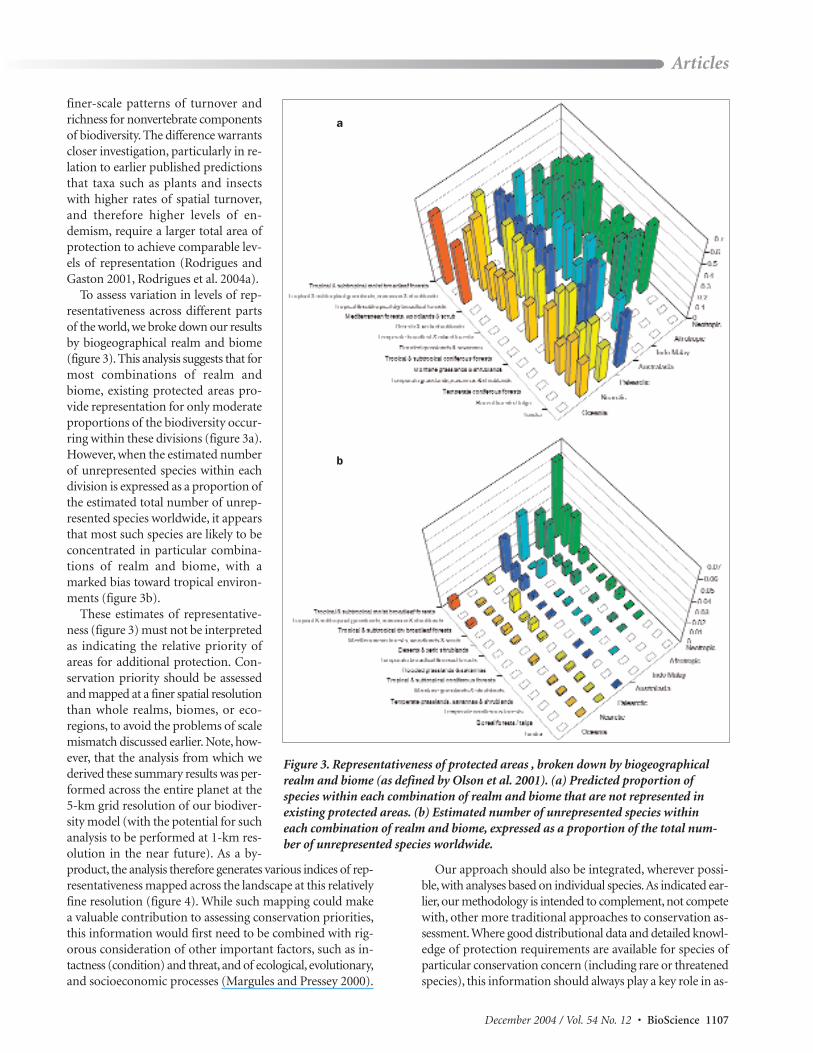
To assess variation in levels of rep-resentativeness across different partsof the world, we broke down our resultsby biogeographical realm and biome(figure 3). This analysis suggests that formost combinations of realm andbiome, existing protected areas pro-vide representation for only moderateproportions of the biodiversity occur-ring within these divisions (figure 3a).However, when the estimated numberof unrepresented species within eachdivision is expressed as a proportion ofthe estimated total number of unrep-resented species worldwide, it appearsthat most such species are likely to beconcentrated in particular combina-tions of realm and biome, with amarked bias toward tropical environ-ments (figure 3b).

These estimates of representative-ness (figure 3) must not be interpretedas indicating the relative priority ofareas for additional protection. Con-servation priority should be assessedand mapped at a finer spatial resolutionthan whole realms, biomes, or eco-regions, to avoid the problems of scalemismatch discussed earlier. Note, how-ever, that the analysis from which we derived these summary results was per-formed across the entire planet at the5-km grid resolution of our biodiver-sity model (with the potential for suchanalysis to be performed at 1-km res-olution in the near future). As a by-product, the analysis therefore generates various indices of rep-resentativeness mapped across the landscape at this relativelyfine resolution (figure 4). While such mapping could makea valuable contribution to assessing conservation priorities,this information would first need to be combined with rig-orous consideration of other important factors, such as in-tactness (condition) and threat, and of ecological, evolutionary,and socioeconomic processes (Margules and Pressey 2000).

Our approach should also be integrated, wherever possi-ble, with analyses based on individual species.As indicated ear-lier, our methodology is intended to complement, not competewith, other more traditional approaches to conservation as-sessment.Where good distributional data and detailed knowl-edge of protection requirements are available for species ofparticular conservation concern (including rare or threatenedspecies), this information should always play a key role in as-

December 2004 / Vol. 54 No. 12 • BioScience 1107

Articles

Figure 3. Representativeness of protected areas , broken down by biogeographicalrealm and biome (as defined by Olson et al. 2001). (a) Predicted proportion ofspecies within each combination of realm and biome that are not represented in existing protected areas. (b) Estimated number of unrepresented species within each combination of realm and biome, expressed as a proportion of the total num-ber of unrepresented species worldwide.

b

a

sessments of conservation adequacy and priority. Our pro-posed approach is designed to supplement such species-based assessments by providing information on the extent towhich protected areas provide representation of highly diversebiological groups whose distribution and conservation re-quirements are little known.

ConclusionsThe methodology described here offers a powerful and effective means of refining the resolution with which spatialpattern in biodiversity is mapped for global conservation assessments. By integrating disparate sources of biological andenvironmental data, our approach takes advantage of thecomplementary strengths of these different types of infor-mation. The ecoregional classification provides a sound biogeographical foundation on which we then build con-siderations of fine-scale pattern in biodiversity relating tofine-scale environmental variation. Calibrating our model using available biological data ensures that its predictionsmatch reality as closely as possible. By focusing on emergentproperties of biodiversity (richness and turnover), ratherthan on individual species, we can more easily accommodatedata for lesser-known, yet highly diverse, biological groups.

As noted earlier, the biological data we have analyzed to daterepresent only a small fraction of the total pool of such datathat could be used to calibrate, and thereby refine, our modelin the future. Emerging collaborative initiatives such as theGlobal Biodiversity Information Facility, or GBIF, are alreadyrevolutionizing the accessibility of data sets containing specieslocations from across the planet. Rapid advances in remote-sensing technology are also likely to provide ongoing refine-ment of the environmental surfaces used to analyze andmodel patterns within the biological data. However, more at-tention needs to be devoted in the future to understanding andquantifying the effects that error and uncertainty in data in-puts (both biological and environmental) have on the relia-bility of predictions from our model. Finally, there is muchpotential to extend and refine the potential application of ourbiodiversity model in global conservation assessment, throughbetter consideration of biodiversity management and reten-tion outside protected areas, and through closer integrationwith species-based assessments and other environmental,social, and economic data and models. As a first step towardsuch integration, we are currently extending our approach toassess the likely impacts of habitat loss and climate change onglobal biodiversity.

1108 BioScience • December 2004 / Vol. 54 No. 12

Articles

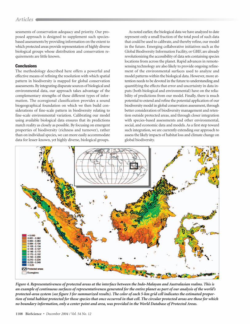
Figure 4. Representativeness of protected areas at the interface between the Indo-Malayan and Australasian realms. This isan example of continuous surfaces of representativeness generated for the entire planet as part of our analysis of the world’sprotected-area system (see figure 3 for summarized results). The color of each 5-km grid cell indicates the estimated propor-tion of total habitat protected for those species that once occurred in that cell. The circular protected areas are those for whichno boundary information, only a center point and area, was provided in the World Database of Protected Areas.

AcknowledgmentsWe express our sincere thanks to the various institutionsthat provided biological data for use in this study, includingthe Australian Museum, the Australian National Herbarium,Brussels University (Université Libre de Bruxelles), CalFlora,the California Academy of Sciences, the Canadian Biodiver-sity Information Facility, Mexico’s National Commission forthe Knowledge and Use of Biodiversity (Comisión NacionalPara el Conocimiento y Uso de la Biodiversidad, orCONABIO), the Environmental Resources Information Net-work, the Global Biodiversity Information Facility, CostaRica’s National Biodiversity Institute (Instituto Nacional deBiodiversidad), Jepson Herbarium (University of California–Berkeley), Landcare Research, the Missouri Botanical Garden,the Natural History Museum, the New South Wales Depart-ment of Environment and Conservation, Princeton Univer-sity, the Rainforest Cooperative Research Centre, theSmithsonian Institution, the University of Bonn, the Universityof Virginia, the University of York, and the World WildlifeFund (United States). We also thank the following individu-als, who assisted us in accessing biological and environmen-tal data or in formulating our approach to data analysis:Gary Barker, Philip Desmet, Maia Dickerson, Claire Kre-men, Wolfgang Küper, Betty Loiselle, Meghan McKnight,Jens Mutke, Sue Palminteri, Taylor Ricketts, George Schatz,Jorge Soberón, and James Solomon. Finally, we thank ThomasBrooks, Jeffrey McNeely, Townsend Peterson, Ana Rodrigues,and an anonymous referee for providing comments thatgreatly helped to improve the manuscript.

References citedArita HT, Rodriguez P. 2002. Geographic range, turnover rate and the

scaling of species diversity. Ecography 25: 541–550.Armesto JJ, Rozzi R, Smith-Ramirez C, Arroyo MTK. 1998. Conservation

targets in South American temperate forests. Science 282: 1271–1272.Bisby FA. 2000. The quiet revolution: Biodiversity informatics and the

Internet. Science 289: 2309–2312.Brooks TM, et al. 2002. Habitat loss and extinction in the hotspots of

biodiversity. Conservation Biology 16: 909–923.Brooks TM, et al. 2004. Coverage provided by the global protected-area

system: Is it enough? BioScience 54: 1081–1091.Faith DP, Ferrier S. 2002. Linking beta diversity, environmental variation, and

biodiversity assessment. Science 295 [Online], 22 July. (18 October 2004;www.sciencemag.org/cgi/eletters/295/5555/636)

Faith DP,Walker PA. 1996. Environmental diversity: On the best-possible useof surrogate data for assessing the relative biodiversity of sets of areas.Biodiversity and Conservation 5: 399–415.

Faith DP, Minchin PR, Belbin L. 1987. Compositional dissimilarity as a robust measure of ecological distance. Vegetatio 69: 57–68.

Ferrier S. 2002. Mapping spatial pattern in biodiversity for regional conser-vation planning: Where to from here? Systematic Biology 51: 331–363.

Ferrier S, Gray MR, Cassis GA,Wilkie L. 1999. Spatial turnover in species com-position of ground-dwelling arthropods, vertebrates and vascular plantsin north-east New South Wales: Implications for selection of forest reserves. Pages 68–76 in Ponder W, Lunney D, eds. The Other 99%: TheConservation and Biodiversity of Invertebrates. Sydney: Royal Zoolog-ical Society of New South Wales.

Ferrier S, Drielsma M, Manion G, Watson G. 2002. Extended statistical approaches to modelling spatial pattern in biodiversity in north-east NewSouth Wales, II: Community-level modelling. Biodiversity and Conser-vation 11: 2309–2338.

Gaston KJ. 2000. Global patterns in biodiversity. Nature 405: 220–227.Gaston KJ, Blackburn TM, Goldewijk KK. 2003. Habitat conversion and global

avian biodiversity loss. Proceedings: Biological Sciences 270: 1293–1300.Gering JC, Crist TO, Veech JA. 2003. Additive partitioning of species diver-

sity across multiple spatial scales: Implications for regional conservationof biodiversity. Conservation Biology 17: 488–499.

Graham CH, Ferrier S, Huettman F, Moritz C, Peterson AT. 2004. New developments in museum-based informatics and applications in bio-diversity analysis. Trends in Ecology and Evolution 19: 497–503.

Heywood VH. 1995. Global Biodiversity Assessment. Cambridge (UnitedKingdom): Cambridge University Press.

Hijmans RJ, Cameron S, Parra J. 2004. WorldClim,Version 1.3. (18 October2004; http://biogeo.berkeley.edu/worldclim/worldclim.htm)

Hutchinson MF, Belbin L, Nicholls AO, Nix HA, McMahon JP, Ord KD. 1997.BioRap Rapid Assessment of Biodiversity, vol. 2: Spatial Modelling Tools.Canberra (Australia): Australian BioRap Consortium, CSIRO.

Leathwick JR, Burns BR, Clarkson BD. 1998. Environmental correlates of treealpha-diversity in New Zealand primary forests. Ecography 21: 235–246.

Lehmann A, Overton JM, Leathwick JR. 2002. GRASP: Generalized Regres-sion Analysis and Spatial Predictions. Ecological Modelling 157: 187–205.

Malcolm JR, Markham A. 2000. Global Warming and Terrestrial BiodiversityDecline. Gland (Switzerland): World Wide Fund for Nature.

Margules CR, Pressey RL. 2000. Systematic conservation planning. Nature405: 243–253.

Moritz C, Richardson KS, Ferrier S, Monteith GB, Stanisic J, Williams SE,Whiffin T. 2001. Biogeographic concordance and efficiency of taxonindicators for establishing conservation priority in a tropical rainforestbiota. Proceedings: Biological Sciences 268: 1875–1881.

Olson DM, Dinerstein E. 2002. The Global 200: Priority ecoregions forglobal conservation. Annals of the Missouri Botanical Garden 89:199–224.

Olson DM, et al. 2001. Terrestrial ecoregions of the world: A new map of lifeon Earth. BioScience 51: 933–938.

Pressey RL, Ferrier S, Hager TC, Woods CA, Tully SL, Weinman KM. 1996.How well protected are the forests of north-eastern New South Wales?Analyses of forest environments in relation to formal protection measures, land tenure, and vulnerability to clearing. Forest Ecology andManagement 85: 311–333.

Rodrigues ASL, Gaston KJ. 2001. How large do reserve networks need to be?Ecology Letters 4: 602–609.

Rodrigues ASL, et al. 2004a. Effectiveness of the global protected area network in representing species diversity. Nature 428: 640–643.

Rodrigues ASL, et al. 2004b. Global gap analysis: Priority regions for expandingthe global protected-area network. BioScience 54: 1092–1100.

Rosenzweig M. 1995. Species Diversity in Space and Time. Cambridge(United Kingdom): Cambridge University Press.

Seabloom EW, Dobson AP, Stoms DM. 2002. Extinction rates under non-random patterns of habitat loss. Proceedings of the National Academyof Sciences 99: 11229–11234.

Thomas CD, et al. 2004. Extinction risk from climate change. Nature 427:145–148.

Whittaker RH. 1972. Evolution and measurement of species diversity. Taxon21: 213–251.

Wilson MV, Shmida A. 1984. Measuring beta diversity with presence–absencedata. Journal of Ecology 72: 1055–1064.

Zurlini G, Grossi L, Rossi O. 2002. Spatial-accumulation pattern and extinctionrates of Mediterranean flora as related to species confinement to habi-tats in preserves and larger areas. Conservation Biology 16: 948–963.

December 2004 / Vol. 54 No. 12 • BioScience 1109

Articles