The Effect of the US Sub-prime Crisis on Canadian Banks

Satiprasad Bandyopadhyay

Ranjini Jha

Duane Kennedy*#

School of Accounting and Finance

University of Waterloo

Waterloo, Ontario N2L 3G1

Canada

January 7, 2014

1

*Corresponding author: Telephone: (519) 888-4752; Email: dkennedy@uwaterloo.ca.# We gratefully acknowledge the financial support the Lois Claxton Humanities and Social Sciences Award from the University of Waterloo. We thank participants at the Canadian Academic Accounting Association Annual Conference 2011, and the Annual Conference of the Canadian Operational Research Society, 2011, for useful feedback

.

2

The Effect of the US Sub-prime Crisis on Canadian Banks

Abstract

We examine whether the Canadian banking sector was afflicted

by financial contagion from the 2008 sub-prime crisis in the

United States financial sector. We examine this issue by using a

sample of the five largest Canadian banks and the 19 largest US

banks based on the value of total assets at the end of 2005. We

follow two approaches, namely, (i) a correlation framework and

(ii) incidences of simultaneous occurrences of extreme negative

stock returns. We find while both the US banks and Canadian banks

were affected by contagion, the Canadian banks were affected

later, relative to the US banks. We also find evidence consistent

with superior quality of monitoring of Canadian banks versus US

banks during and after the crisis period.

1

The Effect of the US Sub-prime Crisis on Canadian Banks

1. Introduction

In this paper we examine the nature of impact of the recent

sub-prime crisis in the United States (US) financial sector on

Canadian banks.1 There appears to be a broad consensus in the

financial press and among members of the international financial

institutions that Canadian banks managed to withstand the ravages

of the US sub-prime crisis.2 However, while the ability of

Canadian banks to withstand the adverse effects of the recent

financial crisis has been commented upon in the financial press,

there has been little academic work on this issue. This work is

intended to fill this void.

Commentators have attributed the strength of Canadian banks

to two distinct sets of reasons. For example, Ratnovsky and Huang

(2009), in an IMF working paper, argue that Canadian banks’

reliance on depository funding rather than other sources of

1 The sub-prime financial crisis that had its origin in large-scale delinquencies in sub-prime mortgage loans made by US mortgage lenders, have been extensively discussed in the literature. For a detailed discussion of thecrisis and its implications, see Demyanyk and Hemert (2011). 2 There has been a lot of discussion in the financial press about the extent to which the Canadian financial sector has been isolated from the sub-prime crisis. See for example, Heinrich (2008), Durocher (2008), Kay (2008), Carswell (2009) and many others.

pg. 2

funding, low leverage and low levels of securitized loans, are

the most important determinants of their ability to withstand

financial difficulties that faced US and European banks. Richburg

(2008) suggests that the resilience of Canadian banks also arises

from their higher liquidity and larger capital bases. In

contrast, Krugman (2010) focuses on the strength of Canadian

banks arising from better monitoring by Canadian regulators.

Other commentators, in different contexts, have commented on the

resilience of the Canadian banking system vis-à-vis US banks. For

example, Saunders and Wilson (1999) provide a detailed background

of the evolution of both the Canadian and US banking systems

since the late 1800s. They point out that “… US historically

combined a weak safety net with restrictions on branching and

other activities that resulted in a system prone to disruptive

banking crises and bank failures. By contrast, both Canada and

the UK evolved consolidated and highly branched banking systems

that proved resilient to economic crises such as those during the

1930s.” In this paper, we not only examine the extent to which

Canadian banks were affected adversely during the crisis (or

pg. 3

isolated from it), but we also attempt to compare the effects of

regulatory monitoring of US versus Canadian banks.

We rely on the concept of “contagion” of financial crises

over geographical boundaries and across financial institutions to

examine the spread of the sub-prime crisis from US financial

institutions to Canadian banks. While early work (e.g., Glick and

Rose (1999), Mason (1999), Kaminiski and Reinhart (1998) and

others) on contagion related to the spread of currency crises

across national boundaries and continents, more recent work on

contagion has examined how markets for risky securities have

experienced “meltdowns” that spread across geographical

boundaries (e.g., Bae, Karolyi and Stulz 2003).

Our examination of the contagion of the sub-prime crisis

from US to Canada consists of two closely related methodologies.

First, we estimate the probability with which extreme negative

stock returns of Canadian banks are correlated with the extreme

negative movements of the index of US banks, during and

surrounding the financial crisis period. Also, following Bae,

Karolyi and Stutlz (2003), we examine the number of times that

sample banks (US versus Canadian banks) exhibit greater frequency

pg. 4

of simultaneous extreme negative returns over simultaneous

extreme positive returns (daily as well as monthly returns)

during the pre-crisis, crisis period and the post-crisis period.

We use a sample of five Canadian banks to estimate the

extent of the sub-prime crisis contagion from USA to Canada. We

present results based on a sample consisting of 19 US banks with

total assets greater than $100 billion in 2005. Our results find

support for financial contagion from the US banks to the Canadian

banks. We find that while the Canadian banks were affected by

contagion, the Canadian banks were affected later relative to the

US banks.

In order to examine the effects of regulation on bank

operations, we adopt an indirect approach by examining

differences in accounting transparency across Canadian and US

banks. The relation between transparency on the one hand and bank

monitoring and effective bank regulation on the other hand, has

been long recognized. For example, the Basel Committee on Bank

Regulation (2000, page 3) states that “The Committee views

increased disclosure, enhanced transparency and market discipline

as becoming an ever more important tool of supervision.” The US

pg. 5

banking regulator, the Federal Deposit Insurance Corporation

(FDIC 2002) reiterates the same view; “accounting standards and

regulatory framework can or should be modified to better ensure

financial transparency and protect and inform the investor.”

Transparent reporting about the quality of bank assets is viewed

as the foundation of effective bank regulation and monitoring

both in Bank Regulation and the academic literature and as well.

For example, the Federal Reserve Board (FRB 2006) urges Bank

Examiners to evaluate banks’ accounting systems that recognizes

and reports of Allowance for Loan and Lease Losses in order to

provide credible information about the quality of bank assets.

The relation between effective regulation and transparency

of asset quality, as measured by the Allowance for Loan and Lease

Losses (ALLL), has also been examined in the academic literature.

For example, Ng and Rusticus (2011) find that the larger the

deviation of ALLL from an economic model of loan loss provisions,

the greater the proportion of banks’ non-performing loans and the

more likely that the bank will fail.3 Following Ng and Rusticus

3 In a multi-country study, Bushman and Williams (2009) show that income smoothing through managerial discretion on the magnitude of ALLL adversely affects the information content of bank financial statements.

pg. 6

(2011), we measure bank transparency and quality of bank

regulatory monitoring as the standard deviation of the residual

of the regression of ALLL on the amount of loan and lease write

offs (and other variables) for the surrounding period. The larger

the standard deviation, the more unpredictable the deviation of

reported ALLL values from an economic model and less the

transparency of disclosures of quality of bank assets and less

the effectiveness of regulation of the banking activities (see

FRB 2006 above).

Our paper makes a number of contributions to the literature.

As stated earlier, while there have been extensive discussions in

the financial press about the extent to which Canadian banks were

isolated from the US subprime crisis, there has been a lack of

academic studies on this issue. Our study will provide some

preliminary findings on this issue. Second, in this study we

attempt to identify both the regulatory and firm specific reasons

that caused Canadian banks and US banks to behave differently

during the sub-prime crisis. The foregoing distinction between

regulatory versus firm-specific reasons is important for a number

of reasons. In the wake of the financial crisis that started in

pg. 7

US and then spread to other parts of the world, the Canadian

banking system has been held up as an example of good governance

that permitted Canada to avoid the economic downturn to which

many other industrialized countries were subject. Governments and

regulators around the world are currently studying different

financial regulatory models that might avoid a recurrence of the

crisis.4 Our results about the transparency of Canadian bank

disclosure (specifically ALLL) have implications for these

decisions.

Our results show that extreme negative Canadian bank returns

were concentrated more during the post-crisis period as compared

to the pre-crisis and crisis periods. This is the first

systematic evidence that the Canadian banks were indeed affected

by the financial crisis but it happened with a lag. Our results

also show that the Canadian banks’ returns are more correlated

with US banks returns during downswings as compared to upswings,

specifically during the post-crisis period, rather than the

crisis period, which is another indication of delayed financial

contagion in Canadian banks. We also provide indirect evidence

4 See, for example, Avgouleas (2009).

pg. 8

supporting the media speculation that Canadian banks withstood

the effects of the financial crisis better because they were

better capitalized and demonstrated better liquidity. Our results

show that Canadian banks that were more capitalized and liquid,

demonstrated fewer negative returns.

The co-exceedance analyses, motivated by Bae et al. (2011)

also support the notion that while Canadian banks were affected

by the financial crisis, it happened with a lag. The excess of

the frequency of simultaneous extreme negative returns (bottom 5

percentile of returns) over simultaneous extreme positive returns

(top 5 percentile of returns) occurred during the post-crisis

period rather the crisis period for Canadian banks. On the other

hand, the excess of negative over positive extreme returns co-

exceedances occurred both during the crisis period and the post-

crisis period as well for US banks

Our tests of transparency tests for Canadian versus US

banks’ disclosures show that the standard deviation of the ALLL

residuals (Ng and Rusticus 2011) of Canadian banks was smaller

than that of US banks, during the crisis and the post-crisis

period. The situation was reversed during the pre-crisis period

pg. 9

when the transparency of US bank reporting was better. This is

consistent with the notion that Canadian banks were subject to

better quality regulatory monitoring during the crisis and post-

crisis periods.

The rest of the paper is organized as follows. The next

section reviews the prior literature on contagion and the

Canadian response to the financial crisis. The third section

discusses the research design, the fourth section examines the

results and the fifth section summarizes the conclusions.

2. Literature Review

Financial integration has increased dramatically in recent

years among advanced economies due to capital account openness

and financial market reforms. While integration has resulted in

increased international risk sharing, it has also increased the

risk of transmitting financial shocks across borders. Claessens,

Dell’Arriccia, Igan, and Laeven (2010) report that during the

recent financial crisis, “the increasing interconnectedness of

financial institutions and markets and more highly correlated

financial risks intensified cross-border spillovers early on

through many channels—including liquidity pressures, global sell-

pg. 10

off in equities (particularly, financial stocks), and depletion

of bank capital.” Allen, Babus, and Carletti (2009) note that

Lehman’s demise in September 2008 compelled markets to re-assess

risk and precipitated contagion. The authors note that contagion

was the most important market failure during the recent financial

crisis and needs to be investigated.

There is a rich literature in economics and financial

economics that examines the spread (or contagion) of financial

crisis from one country to another (see e.g., Allen et al. (2009)

for a recent overview). The notion of contagion refers to the

increase in co-movement of returns of risky securities (or market

indices) during crisis periods relative to stable periods (Bae,

Karolyi and Stulz 2003) though the concept of contagion has been

hard to define for measurement purposes (Dornbusch, Park and

Claessens 2001; Allen et al. 2009). Most of the early work on

contagion was related to the currency crisis that occurred in

different parts of the world and how it was transmitted across

national boundaries. These early articles, for example, Glick and

Rose (1999), Mason (1999), Kaminiski and Reinhart (1998) and many

others, compared the pairwise correlation of changes in currency

pg. 11

exchange rates between different countries. The broad consensus

in these papers was that a currency crisis in one part of the

world is quickly transmitted to other parts of the world and the

correlations are stronger during crisis periods as compared to

tranquil periods. The problem with this approach is the

underlying volatility of currency exchange rate changes is

greater during crisis periods and this can overstate correlations

during crisis periods. (See De Bandt and Hartmann (2000) for a

survey). Later papers adopted a different methodological approach

to address the foregoing spurious correlation problem and also

considered the effect of contagion, if any, on stock prices. For

example, Bae, Karolyi and Stulz (2003) and Boyson, Stahl and

Stulz (2008) pioneered the estimation of probability of joint

occurrence of extreme events across countries on the same day or

with a lag, and in particular whether this probability is higher

during economic downturns as compared to upturns. The first paper

found that stock return contagion among Latin American emerging

markets was greater than that in Asian emerging markets over a

nine-year period from 1992 to 2000. The second paper, using the

same methodology for hedge funds, found evidence of contagion

pg. 12

across different hedge fund styles. In this paper, we use this

methodology to examine the nature of the spread of the financial

crisis from US financial institutions to Canadian banks.

Commentators have attributed a number of reasons why

Canadian banks remained relatively unaffected by the financial

turmoil. Krugman (2010) attributes the strength of Canadian banks

to their better monitoring by Canadian regulators. This is

consistent with the views of Saunders and Wilson (1999) and

others that Canadian banks are more resilient and in a better

position to withstand periodic crises. In addition to these

reasons, Richburg (2008) suggests that the resilience of Canadian

banks also arises from their higher liquidity and larger capital

bases. Ratnovsky and Huang (2009), in an IMF working paper,

provide preliminary evidence that Canadian banks’ reliance on

depository funding rather than other sources of funding, the low

levels of exposure to US subprime-based assets and low levels of

securitized loans, as the most important determinants of their

ability to withstand financial difficulties that faced US and

European banks. In our paper, we examine the nature of the impact

of the sub-prime crisis on the Canadian banks, whether the

pg. 13

Canadian banks escaped the severity experienced in the US and

elsewhere and attempt to distinguish between regulatory versus

firm-specific reasons that might have permitted them to escape

the problems that decimated much of the financial sector in many

jurisdictions.

3. Research Design

Empirical tests are based on a sample of five largest

Canadian banks and the 19 largest US banks with total assets

greater than $100 billion at the end of 2005 and are listed in

the Appendix. This date is used in selecting the banks so that

the asset amounts are not affected by the crisis period.5 Both

the US and Canadian banks in this sample are banks that are “too

big to fail.”

The sample period extends from 1999 to 2011 which covers the

subprime crisis. We classify the sub-periods based on the crisis

timeline provide by the St. Louis Federal Reserve

(http://timeline.stlouisfed.org/pdf/CrisisTimeline.pdf). We

5 Two additional samples were used to test the sensitivity of results. One sample consists of the 13 banks used by Khan (2009) in his test of contagion in the US banking sector and the second sample consists of the 19 banks used in the study by King (2009).

pg. 14

define three sub-periods, namely, the pre-crisis period from

January 1999 to March 2007, the crisis period from April 2007 to

September 2008, and the post-crisis or recovery period from

October 2008 to December 2011. Many economists agree that the

financial crisis started in 2007. In April 2007, New Century

Financial Corporation, a leading sub-prime mortgage lender, filed

for Chapter 11 bankruptcy protection. Bear Stearns announced in

June 2007 that its two hedge funds, worth an estimated $1.5

billion at the end of 2006, were almost worthless. American Home

Mortgage Investment Corporation filed for Chapter 11 bankruptcy

in August 2007. Bear Stearns itself was in distress and was

acquired by J. P. Morgan Chase in March 2008. In September 2008,

the Treasury Department took over Fannie Mae and Freddie Mac,

Lehman declared bankruptcy, Merrill sold itself to Bank of

America, the Federal Reserve bailed out AIG, and Washington

Mutual was acquired by J. P. Morgan Chase with FDIC’s assistance.

Accordingly, we define the crisis period as the period from April

2007 to September 2008.

On October 1, 2008 the U.S. Congress passed the Troubled

Asset Relief Program (TARP). The U.S. Federal Reserve, the

pg. 15

Treasury and FDIC implemented various measures to prevent a

credit crisis and to provide liquidity to the system. The

measures included making available capital to banks by buying

their preferred stock, reducing costs of borrowing for the banks,

creation of a Commercial Paper Funding Facility and the Term

Asset-Backed Securities Lending Facility. These measures

stabilized the markets and paved the road for recovery.

Accordingly, we define the post-crisis period as the period from

October 2008 to December 2011.

We utilize monthly income statement data and quarterly

balance sheets for the Canadian banks available from the Office

of the Superintendent of Financial Institution of Canada (OSFI)

website. Stock returns for Canadian banks and Canadian market

data are obtained from the Canadian Financial Markets Research

Centre (CFMRC) with comparable data for the US available through

the Center for Research in Security Prices (CRSP). Additional

financial data are collected from Compustat.

Empirical tests.

pg. 16

We identify the sub periods during which the probability

with which Canadian banks’ negative returns were associated with

the negative index returns of a sample of US banks, by estimating

the following model (Bae, Karolyi and Stulz 2003 and Khan 2009):

ExtremNegit = 1 + It+ control variables + error

(1)

where:

ExtremNegit = 1 if the return for Canadian bank i in period t

is in the bottom 10% of the returns for the time series of

monthly returns from January 1999 to December 2009; and 0

otherwise.

It = 1 if the US Bank index in period t is the bottom

quartile of the index return for the sample period from January

1999 to December 2009; and 0 otherwise.

A positive and significant estimate of is consistent with

the notion that the financial crisis in US spread to Canadian

banks by contagion.

Examination of whether the bank characteristics listed in

the previous section influenced the extent of contagion in

pg. 17

Canadian banks implies the coefficient in equation (1) is a

function of those bank characteristics. In other words,

= 1 + 2 Capitalization + 3 Liquidity + 4 Deposit Funding

+ error (2)

Replacing in equation (1) results in

ExtremNeg it = 1 + (1 + 2Capitalization + 3 Liquidity + 4

Deposit Funding) It+ control variables + error

(3)

Negative and significant coefficients for 2, 3 and 4 are

consistent with the contagion being reduced for high

capitalization, high liquidity and high deposit funding banks.

The coefficient 1 reflects factors that are common to all

Canadian banks.

Co-exceedance tests

In order to examine whether the financial crisis spread to

Canada and if so, whether Canadian banks were less affected than

comparable US banks, we follow the univariate methodology used by

Bae, Karolyi and Stulz (2003, Table 2). In the analysis, we

compare, first over the entire sample period, and then for each

sub period, the number of trading days that US and Canadian banks

pg. 18

exhibit extreme negative returns simultaneously versus the number of

days that banks exhibited simultaneous extreme positive returns.

According to Bae, Karolyi and Stulz (2003, Table 2), contagion

exists if the number of joint occurrences of extreme negative

returns exceed the number of joint occurrences of extreme

positive returns during a pre-specified time period. A comparison

of the results for the US versus the Canadian banks indicates

which of the two subsamples suffered more from the financial

crisis by contagion and during which sub period, namely, pre-

crisis, crisis and post-crisis period. The greater the excess of

the negative joint occurrences over positive joint occurrences,

the greater the contagion.

Tests of Asset Quality Transparency

Following Ng and Rusticus (2011, equation 2) we estimate the

following equations separately for Canadian and US banks and

compare standard deviation of their residuals:6

6 “ LLR (t-1) is the loan loss reserves at time t-1, i.e., the loan loss reserves at the end of the prior period, reflect an estimate of the loans thatwere expected to be charged-off. During the period, actual net charge-offs reduce the available reserve. The loan loss provisions are then used to increase the loan loss reserves, such that the ending balance reflects the loan losses that are expected to occur in the future (Wall and Koch, 2000). This set-up suggests the following two drivers of the loan loss provisions made at time t. First, banks are expected to make more loss loan provisions ifthe beginning loan loss reserves were insufficient to cover current charge-

pg. 19

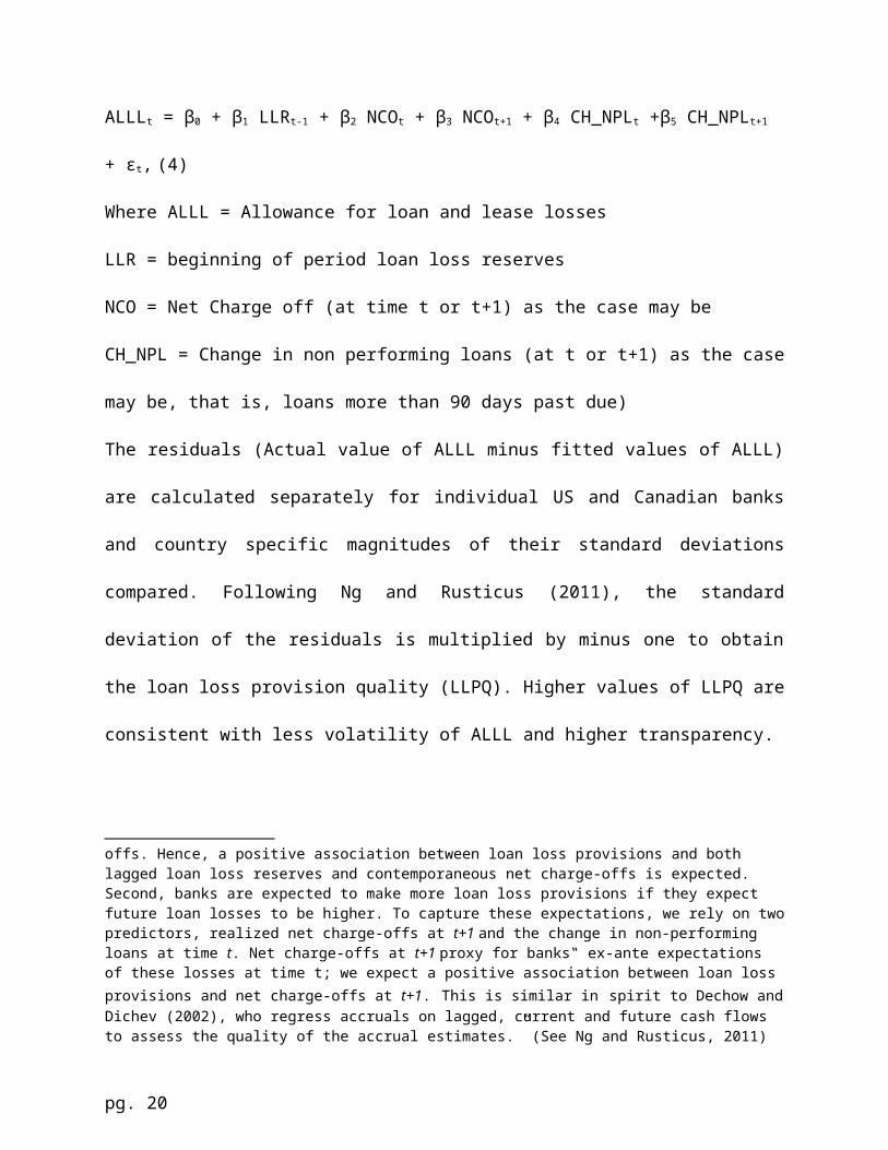
ALLLt = β0 + β1 LLRt-1 + β2 NCOt + β3 NCOt+1 + β4 CH_NPLt +β5 CH_NPLt+1

+ εt, (4)

Where ALLL = Allowance for loan and lease losses

LLR = beginning of period loan loss reserves

NCO = Net Charge off (at time t or t+1) as the case may be

CH_NPL = Change in non performing loans (at t or t+1) as the case

may be, that is, loans more than 90 days past due)

The residuals (Actual value of ALLL minus fitted values of ALLL)

are calculated separately for individual US and Canadian banks

and country specific magnitudes of their standard deviations

compared. Following Ng and Rusticus (2011), the standard

deviation of the residuals is multiplied by minus one to obtain

the loan loss provision quality (LLPQ). Higher values of LLPQ are

consistent with less volatility of ALLL and higher transparency.

offs. Hence, a positive association between loan loss provisions and both lagged loan loss reserves and contemporaneous net charge-offs is expected. Second, banks are expected to make more loan loss provisions if they expect future loan losses to be higher. To capture these expectations, we rely on twopredictors, realized net charge-offs at t+1 and the change in non-performing loans at time t. Net charge-offs at t+1 proxy for banks‟ ex-ante expectations of these losses at time t; we expect a positive association between loan loss provisions and net charge-offs at t+1. This is similar in spirit to Dechow andDichev (2002), who regress accruals on lagged, current and future cash flows to assess the quality of the accrual estimates.” (See Ng and Rusticus, 2011)

pg. 20

4. Results

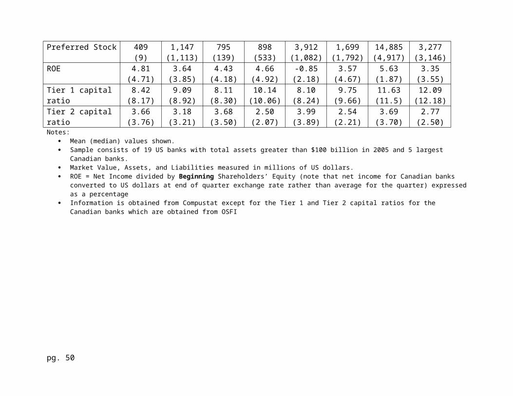
Table 1 reports descriptive statistics for the 19 largest US

banks and the 5 largest Canadian banks for the time periods

before, during and after the financial crisis.7 Tier 1 ratio, a

measure of soundness of bank operations, appeared fairly stable

over the whole period for both US and Canadian banks except for

the post-crisis period, which exhibits a big jump in this ratio

for both countries. Figure 1 completes this picture. The Tier 1

ratios have been higher for Canadian banks relative to US banks

throughout the sample period. In comparison with US banks,

Canadian banks have had lower Tier 2 capitalization ratios

throughout the sample period.

Table 1 and Figure 2 show that both US and Canadian banks

exhibit steady increase in the reported value of bank (total)

assets over the entire sample period. However, Figure 3 appears

to indicate that reported book values of US banks’ common equity

track their market values less closely as compared to Canadian

banks. For example, while the average market value of US banks

7 The pre-crisis period is divided into two sub-periods for purposes of the descriptive statistics due to the substantial growth of both the Canadian and US banks during the pre-crisis.

pg. 21

fell sharply during the crisis and some more during the post-

crisis periods (after peaking during April 2005 to March 2007),

the book value of common equity continued to rise during this

period . In contrast, as Figure 3 shows, Canadian banks’ book

values are better able to track their market values. Both market

values and book value of common equity for Canadian banks rose

during the crisis and post-crisis periods.8

These contrasting patterns of reported values of net assets

against their market values for US versus Canadian banks likely

have implications for the relative quality of regulatory

monitoring of financial institutions in these two countries. This

issue will be discussed later in this section. Another related

financial reporting issue is the pattern of intertemporal changes

in bank ROEs over time in the two countries, as shown in Figure

4. While both US and Canadian ROEs exhibit similar pattern during

the pre-crisis period, US banks’ ROEs exhibit an extremely

volatile pattern during the crisis and post-crisis periods. We

will return to this issue later in this section.

8 The market value of Canadian banks fell in the first 2 quarters of the post-crisis period.

pg. 22

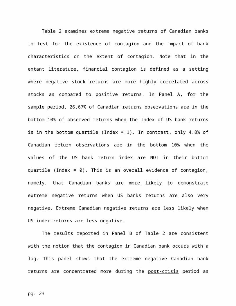
Table 2 examines extreme negative returns of Canadian banks

to test for the existence of contagion and the impact of bank

characteristics on the extent of contagion. Note that in the

extant literature, financial contagion is defined as a setting

where negative stock returns are more highly correlated across

stocks as compared to positive returns. In Panel A, for the

sample period, 26.67% of Canadian returns observations are in the

bottom 10% of observed returns when the Index of US bank returns

is in the bottom quartile (Index = 1). In contrast, only 4.8% of

Canadian return observations are in the bottom 10% when the

values of the US bank return index are NOT in their bottom

quartile (Index = 0). This is an overall evidence of contagion,

namely, that Canadian banks are more likely to demonstrate

extreme negative returns when US banks returns are also very

negative. Extreme Canadian negative returns are less likely when

US index returns are less negative.

The results reported in Panel B of Table 2 are consistent

with the notion that the contagion in Canadian bank occurs with a

lag. This panel shows that the extreme negative Canadian bank

returns are concentrated more during the post-crisis period as

pg. 23

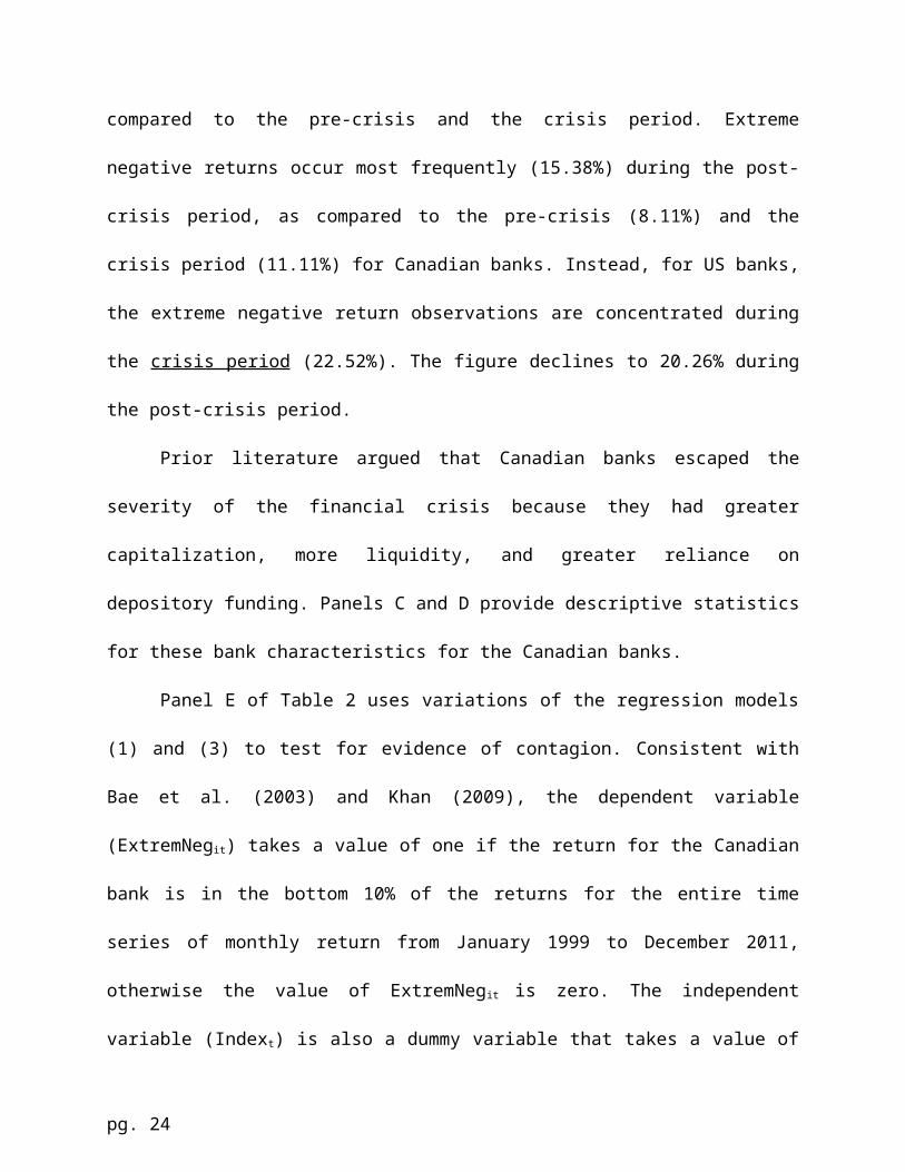
compared to the pre-crisis and the crisis period. Extreme

negative returns occur most frequently (15.38%) during the post-

crisis period, as compared to the pre-crisis (8.11%) and the

crisis period (11.11%) for Canadian banks. Instead, for US banks,

the extreme negative return observations are concentrated during

the crisis period (22.52%). The figure declines to 20.26% during

the post-crisis period.

Prior literature argued that Canadian banks escaped the

severity of the financial crisis because they had greater

capitalization, more liquidity, and greater reliance on

depository funding. Panels C and D provide descriptive statistics

for these bank characteristics for the Canadian banks.

Panel E of Table 2 uses variations of the regression models

(1) and (3) to test for evidence of contagion. Consistent with

Bae et al. (2003) and Khan (2009), the dependent variable

(ExtremNegit) takes a value of one if the return for the Canadian

bank is in the bottom 10% of the returns for the entire time

series of monthly return from January 1999 to December 2011,

otherwise the value of ExtremNegit is zero. The independent

variable (Indext) is also a dummy variable that takes a value of

pg. 24

one if the US Bank index is the bottom quartile of the index

return for the entire sample period from January 1999 to

September 2011. The other variables, namely, Capitalization,

Liquidity, Deposit Fund, TBill and MktRet, are control variables

that could affect the frequency of negative bank returns.

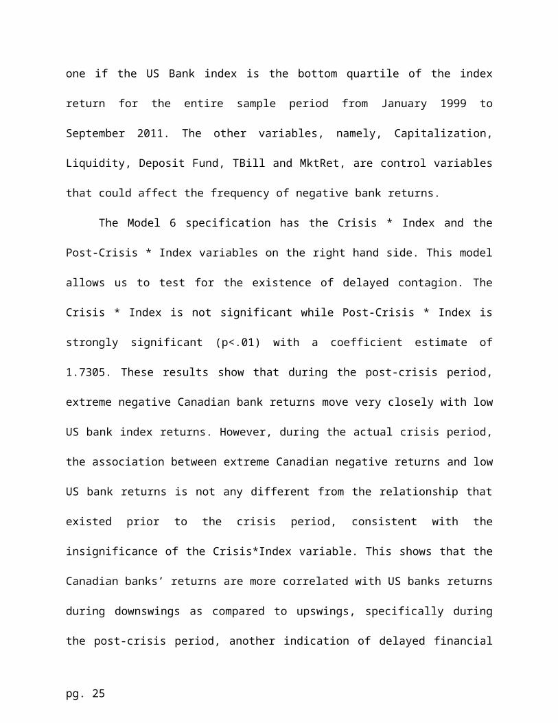
The Model 6 specification has the Crisis * Index and the

Post-Crisis * Index variables on the right hand side. This model

allows us to test for the existence of delayed contagion. The

Crisis * Index is not significant while Post-Crisis * Index is

strongly significant (p<.01) with a coefficient estimate of

1.7305. These results show that during the post-crisis period,

extreme negative Canadian bank returns move very closely with low

US bank index returns. However, during the actual crisis period,

the association between extreme Canadian negative returns and low

US bank returns is not any different from the relationship that

existed prior to the crisis period, consistent with the

insignificance of the Crisis*Index variable. This shows that the

Canadian banks’ returns are more correlated with US banks returns

during downswings as compared to upswings, specifically during

the post-crisis period, another indication of delayed financial

pg. 25

contagion in Canadian banks. In Models 3 and 5, the crisis period

and the post-crisis-period variables both enter the models as

main effects and not in interaction with the Index variable.

However we observe the same pattern as above, namely that the

post-crisis period is significant and the crisis period is not

significant.

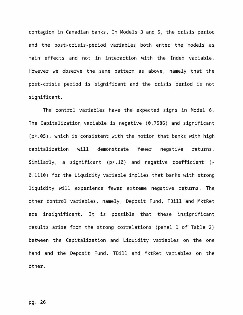
The control variables have the expected signs in Model 6.

The Capitalization variable is negative (0.7586) and significant

(p<.05), which is consistent with the notion that banks with high

capitalization will demonstrate fewer negative returns.

Similarly, a significant (p<.10) and negative coefficient (-

0.1110) for the Liquidity variable implies that banks with strong

liquidity will experience fewer extreme negative returns. The

other control variables, namely, Deposit Fund, TBill and MktRet

are insignificant. It is possible that these insignificant

results arise from the strong correlations (panel D of Table 2)

between the Capitalization and Liquidity variables on the one

hand and the Deposit Fund, TBill and MktRet variables on the

other.

pg. 26

Analyses of Co-exceedances

Table 3 examines financial contagion using the results of

the co-exceedances analyses based on daily returns. Consistent

with Bae et al. (2003), this analysis consists of comparing,

first over the entire sample period, and then for each sub

period, the number of trading days that a specified number of US

banks and Canadian banks exhibit simultaneous extreme negative

returns versus the number of banks that exhibit simultaneous

extreme positive returns. Extreme positive and negative returns

are measured as the top and bottom 5% of the return observations

during each sample period. Bae et al. (2003) argue that contagion

exists if the number of joint occurrences of extreme negative

returns exceeds the number of joint occurrences of extreme

positive returns.

Table 3 compares the number of negative co-exceedances

versus the number of positive co-exceedances for each of the sub-

period for Canadian banks and US banks separately using daily

returns. Table 4 does the same comparison using monthly returns.

Tables 5 and 6 compare the number of actual number of negative

pg. 27

(positive) co-exceedances to the expected number of negative

(positive) co-exceedances using Monte Carlo simulation.

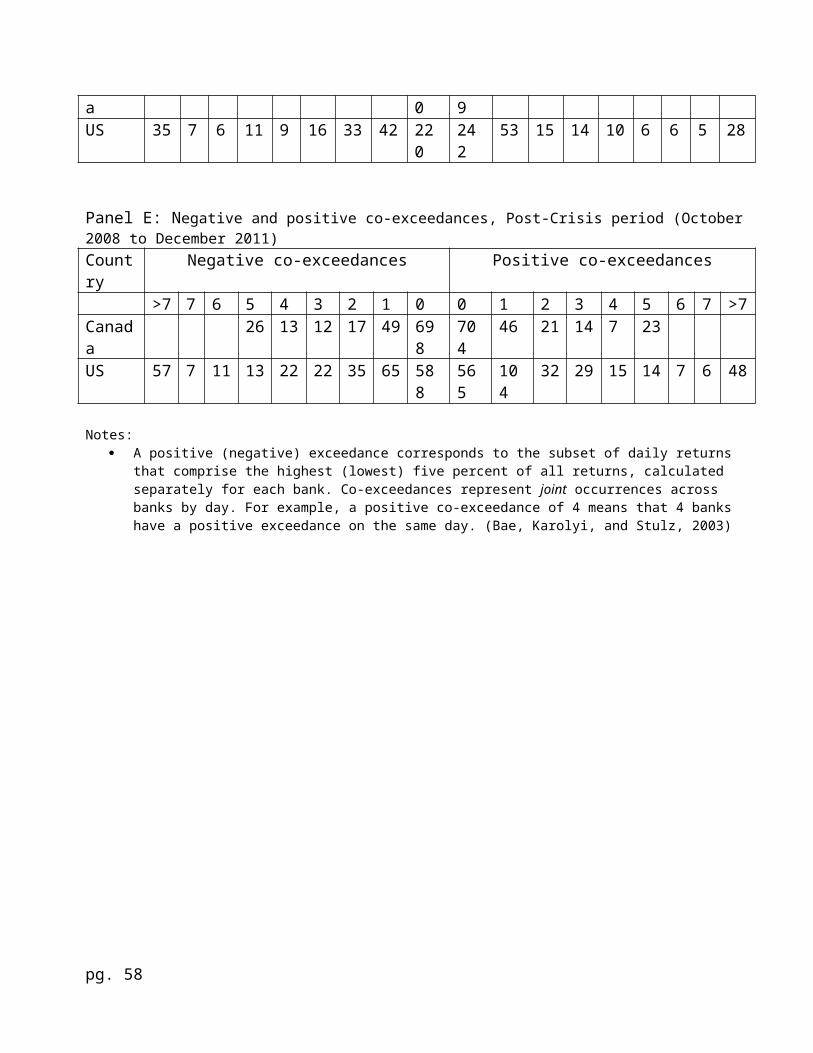
Panels A and B of Table 3 report the number of co-

exceedances for the entire period. Panels C, D and E of Table 3

report the number of positive and negative co-exceedances of US

and Canadian banks for the three sub-periods.

In panel C, for the pre-crisis period, the number of times

that 3 or more Canadian banks exhibit an extreme negative return

on the same day (i.e., a co-exceedance greater than or equal to

3) is 43 (10 + 11 + 22) versus 53 positive co-exceedances (9 + 15

+ 29). Since the number of negative co-exceedances is smaller

than the number of positive co-exceedances, per Bae et al.

(2003), there are no indications of a contagion in the Canadian

banks during the pre-crisis periods. The corresponding negative

versus positive co-exceedances for US banks follows a similar

pattern. For example, during this period, the number of times

that the US sample banks exhibit negative co-exceedance of 3 or

more is 116 (27 + 9 + 11 + 15 + 20 + 34) versus 135 positive co-

exceedances (38 + 14 + 13 + 21 + 22 + 27). These results show

pg. 28

lack of contagion amongst both US and Canadian banks during the

pre-crisis period of January 1999 to March 31, 2007.

Panel D of Table 3 provides negative and positive values of

co-exceedances during the crisis period. For Canadian banks, the

frequency of negative and positive co-exceedances in 3 or more

banks are 21and 22 respectively, again indicating that there is

probably no contagion in Canadian banks during the crisis period.

Note however that the crisis period is defined in terms of the

financial crisis that exhibited itself in the US. Not

surprisingly, the number of negative co-exceedances in 3 or more

US banks is 84 versus 69 positive co-exceedances. This indicates

the existence of contagion in the financial crisis across major

US banks.

Panel E of Table 3 reports results of co-exceedances for the

post-crisis period. The number of negative co-exceedances of 3 or

more Canadian banks is now 51 (26+13+12), which is greater than

the number of 44 positive co-exceedances (23+7+14) during the

period, implying contagion. The corresponding figures for the US

sample banks are 132 negative co-exceedances, which are greater

than 119 positive co-exceedances for 3 or more banks. This shows

pg. 29

that the contagion continued to affect US banks in the post-

crisis period.

These results show that while both US and Canadian banks

were affected by the financial crisis, the Canadian banks were

affected later relative to the US banks. For the April 2007 to

September 2008 (crisis) period, the US banks but not Canadian

banks exhibit more negative co-exceedances than positive ones.

This shows that US banks were affected during this period by the

financial crisis but not Canadian banks. In contrast, for the

October 2008 to December 2011 period, Canadian banks as well as

US banks, exhibit more negative co-exceedances than positive

ones. These findings are consistent with the financial crisis

affecting Canadian banks with a lag.

Table 4 reports results of the co-exceedances analyses based

on monthly returns. Panel A reports the number of co-exceedances

for the entire period and Panels B, C, and D report the positive

and negative co-exceedances of US and Canadian banks for the

three sub-periods. For the pre-crisis period, in Panel B, the

number of times that 3 or more Canadian banks exhibit extreme

negative returns in the same month is 0 whereas the figure for

pg. 30

positive co-exceedances is 1, suggesting no indications of a

contagion in the Canadian banks during the pre-crisis periods.

Panel C provides negative and positive values of co-exceedances

during the crisis period. For Canadian banks, the number of

negative and positive co-exceedances in 3 or more Canadian banks

is 1and 0 respectively, indicating that there is probably little

or no contagion in Canadian banks during the crisis period.

Interestingly, the number of negative co-exceedances in 3 or more

US banks is 8 versus 2 positive co-exceedances, indicating the

existence of contagion in the financial crisis across major US

banks.

Panel D reports results of co-exceedances for the post-

crisis period. The number of negative co-exceedances in 3 or more

Canadian banks is now 4, which is greater than 2 positive co-

exceedances during the period, supporting contagion. The

corresponding US figures are 6 negative as well as 6 positive co-

exceedances in 3 or more US banks. As in the case with daily

returns, these results show that while both US and Canadian banks

were affected by contagion, the Canadian banks were affected

later relative to the US banks.

pg. 31

Tables 5 and 6 shows the results of Monte Carlo simulations

for the co-exceedances for Canadian and US banks using

multivariate normal and Student t distributions, respectively. A

Monte Carlo simulation is used to evaluate the number of co-

exceedances for each set of banks. The sample mean and variance-

covariance matrix is calculated and then 5,000 random

realizations are generated using either a multivariate normal

distribution or a multivariate t-distribution with 5 degrees of

freedom. For each realization, the number of co-exceedances are

calculated using a 5% threshold, similar to Table 4. The

simulated p-value is calculated as the number of replications

with co-exceedances in a specific category which exceed the

actual number of co-exceedances.

In Table 5, we assume that the returns are jointly

distribution as multivariate normal. Panel B, reports the results

for Canadian banks for the crisis period. There are 7 instances

of 3 Canadian banks exhibiting extreme negative returns during

this period, which are not significantly different (p=.27) from

6.17 expected number of such instances assuming multivariate

normal distribution of bank returns. There are 8 occurrences of

pg. 32

extreme positive co-exceedances in 3 Canadian banks, which again

are not significantly different (p=.14) from the expected 6.17

occasions. The frequency of 4 banks exhibiting extreme negative

co-exceedances is 4 but that is also not significantly different

from the expected 3.73. On the other hand, the 7 actual instances

of 4 positive co-exceedances are significantly more (p=.01) than

the expected 3.71 instances. The frequencies of positive 5 co-

exceedances (7) and negative 5 co-exceedances (10) are

significantly greater than their respective expected values. That

is, there are 22 (8+7+7) occurrences of positive co-exceedances

in 3 or more Canadian banks that are greater than expected

values. The corresponding figure for negative co-exceedances in 3

or more Canadian banks is 21. This evidence is not consistent

with the contagion which implies more frequent negative rather

than positive co-exceedances.

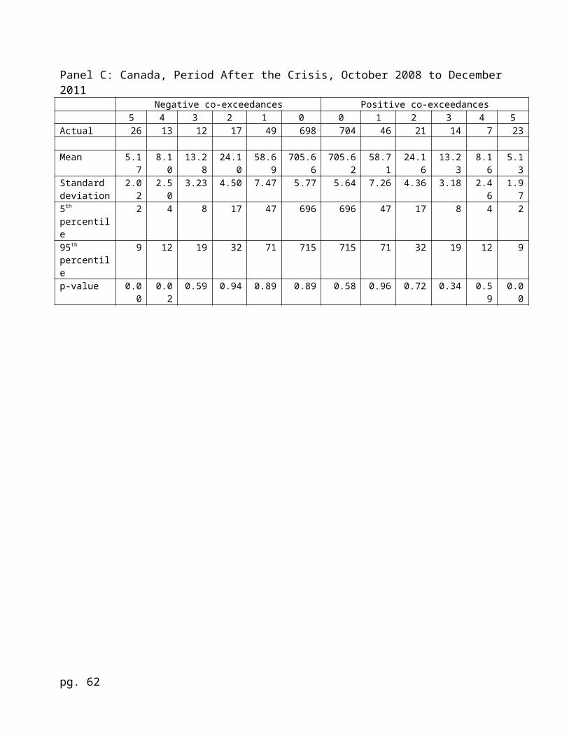
Results reported in Panel C of Table 5 for the post-crisis

period are dramatically different. The frequency of negative co-

exceedances in 4 or more Canadian banks that are significantly

greater than their expected values is 39 (26+13). The

corresponding figure for 4 or more positive co-exceedances is 30.

pg. 33

Thus, the results in Panel C are consistent with contagion

amongst Canadian banks for the post-crisis period. This implies

that the economic crisis did affect Canadian banks, but with a

lag.

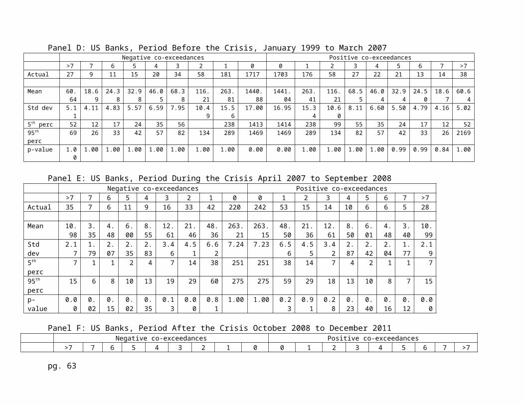
Panel E of Table 5 shows the co-exceedances for US banks for

the crisis period. The frequency of 5 or more negative co-

exceedances that are greater than expected values is 59 (35 + 7 +

6 +11) as compared to only 45 cases of 5 or more positive co-

exceedances greater than their expected values. This implies that

the banking crisis affected had a greater negative effect on US

banks as compared to the Canadian banks during the actual crisis

period. Panel F of Table 5 shows the simulation results for the

post-crisis period for US banks. It is interesting to note that

the observed frequencies of 7 or less negative and 7 or less

positive co-exceedances are not different from their expected

values. The frequency of more than 7 negative co-exceedances is

57 which is significantly (p=.00) greater than its expected

value. Similarly, the frequency of more than 7 positive co-

exceedances is 48 which is significantly (p=.00) greater than its

expected value.

pg. 34

The results reported in Panels E and F are consistent with

the notion that US banks were affected more negatively than

Canadian banks during the actual crisis period. However, the

situation seems to have reversed itself after the crisis period.

While US banks still are affected negatively, Canadian banks were

worst affected in the post-crisis period.

Panels B, C, E, and F indicate that the assumption of a

multivariate normal distribution of bank returns does not

generate simulated co-exceedances as large as in the actual

sample observations. To test sensitivity of the results, we use

the Student t distributional assumption to accommodate fat tails

in the joint distribution of returns. These results are reported

in Table 6.

The findings in Table 6 are similar to those in Table 5 for

Canadian and U.S. banks. The Student's t distributional

assumption cannot deliver simulated co-exceedances as indicated

for the actual sample. For example, in Panel C, the frequency of

negative co-exceedances in 5 Canadian banks at 26 is

significantly greater than their expected values of 7.55 with the

corresponding figure for 5 or more positive co-exceedances being

pg. 35

23 that is significantly greater than the expected value of 7.47.

While the expected values are greater under the t-distribution

(7.55 and 7.47 for 5 negative and positive co-exceedances) in

comparison with the normal distribution (5.17 and 5.13 for 5

negative and positive co-exceedances), the actual occurrences are

still significantly greater than their expected values.

The results in Tables 5 and 6, while providing support for a

delay in contagion from US to Canadian markets, also indicate

that the distributional assumptions of multivariate normal and

Student t do not explain the actual pattern of co-exceedances

exhibited during and after the crisis in both US and Canadian

markets.

Quality of Loan Loss Provision

As discussed earlier, one possible explanation for the

difference between the Canadian versus the US banks’ reaction to

the financial crisis is the difference in the relative quality of

bank monitoring, if any, between these two jurisdictions. The

financial press and several commentators have proposed that

pg. 36

Canadian banks were able to avoid the disastrous effects of the

financial crisis because of better quality monitoring by the

Canadian bank regulators. In this section, we provide results of

tests that attempt to capture the relative quality of bank

monitoring in the two jurisdictions. The underlying notion is

that the efficacy of bank monitoring is reflected in the quality

of bank assets. As a practical matter, bank regulators are

concerned about the quality of allowance of loan losses

recognized by banks. For example, the Federal Reserve Board (FRB

2006) urges Bank Examiners to evaluate banks’ accounting systems

that recognize and report Allowance for Loan and Lease Losses

(ALLL) in order to provide credible information about the quality

of bank assets.

A number of academic studies have examined the quality of

loan loss provisions recognized by banks. For example, Ng and

Rusticus (2011) find that the larger the deviation of ALLL from

an economic model of loan loss provisions, the greater the

proportion of banks’ non-performing loans and more likely the

bank to fail. Table 7 provides results for estimating equation

(4). Panels A and B show the descriptive statistics for the loan

pg. 37

loss provision (ALLL) related variables for US banks and Canadian

banks respectively. The ALLL variable exhibits a 3 fold increase

from the 1999-2006 pre-crisis period (median = 0.53) to the 2009-

2011 crisis and post-crisis period (median = 2.18). This increase

is not surprising because of the sharp increase of the Net Charge

Off (NCO) variable during the crisis/post-crisis period

reflecting the poor quality of bank assets that had to be written

off. The NCO variable rose from 0.56 to 1.72 over from the pre-

crisis to the crisis/post-crisis period. ALLL is significantly

related to NCO as shown the highly significant coefficient on the

NCO variable (coefficient estimate of 1.42, ‘t’ = 7.48) for the

2007-2011 period regression in Panel C.

Note that the NCO variable actually exhibits a decline from

0.51 to 0.47 for Canadian banks in Panel B of Table 7, from the

pre-crisis period to the crisis/post-crisis period. The increase

in the ALLL variable from 0.40 to 0.50 for the Canadian banks is

relatively more modest as compared to US banks.

Consistent with Ng and Rusticus (2011) the quality of ALLL

recognized by banks is measured by the volatility of the

residuals from the economic model for ALLL. Panels C and D report

pg. 38

the regression results for the economic models for ALLL for US

and Canadian banks. The more volatile the residuals from the

models reported in Panels C and D, the more unpredictable the

ALLL and the lower its quality. Panel E of Table 7 provides

comparative measures of Loan Loss Provision Quality for the two

jurisdictions for the pre-crisis versus crisis/post-crisis

period. For the pre-crisis 1999-2006 period, LLPQ for US banks is

-0.192 versus -0.263 for Canadian banks implying better

monitoring quality for US banks. The figures reverse dramatically

in the crisis period when LLPQ for US banks is -0.517 versus -

0.170 for Canadian banks implying better monitoring quality for

Canadian banks. In the post-crisis period, the related figures

are -0.318 for US banks and -.07 for Canadian banks. This

indicates that while the loan loss provision quality for both US

and Canadian banks improved in the post-crisis period, the

difference between the two sets of banks widened in the post-

crisis period. The ALLL quality data in Table 7, Panel E is

consistent with the pattern of market values and book values of

equity in Figure 3 discussed earlier. For US banks market values

and book values moved in opposite directions, during and after

pg. 39

the crisis period, indicating a disconnect between reported

values of assets and market values of assets. This disconnect in

Figure 3, is probably at least partly captured in the higher

standard deviation of ALLL residuals. This implies that allowance

for loan losses were recognized at values that could not be

explained by the level of charge-offs, nonperforming loans and

the magnitude of loan loss reserves. This caused net asset values

to rise while their market values fell during and after the

crisis period. Also note the higher volatility of ALLL residuals

is consistent with the higher ROE volatility of US banks in

crisis and post-crisis period shown in Figure 4. On the other

hand, the quality of loan loss provisions for Canadian banks has

steadily improved in the crisis and post-crisis period compared

to the pre-crisis period. This implies that in the crisis/post-

crisis period the Canadian banks’ monitoring is superior to that

experienced by US banks.

5. Conclusion

The Canadian banking system has been held up an example of

good governance that permitted Canada to avoid the economic

pg. 40

downturn to which many other industrialized countries were

subject in the aftermath of the 2008 sub-prime crisis that

started in the US. In this paper, we investigate whether the

Canadian banking sector was afflicted by the financial contagion

from crisis in the United States financial sector using two

approaches. We find while both the US banks and Canadian banks

were affected by contagion, the Canadian banks were affected with

a lag, relative to the US banks. Our results indicate that the

Canadian banks’ returns are more correlated with US banks returns

during downswings as compared to upswings during the post-crisis

period, rather than the crisis period, supporting the notion of

delayed financial contagion in Canadian banks. We also provide

indirect evidence supporting the media speculation that Canadian

banks withstood the effects of the financial crisis better

because they were better capitalized and demonstrated better

liquidity. Our analysis of loan loss provision quality supports

superior quality of monitoring of Canadian banks versus US banks

during and after the crisis period. However, though the quality

of Canadian regulatory monitoring appears to have improved in the

crisis period and the post-crisis period, it could not totally

pg. 41

prevent the spread of financial contagion from US banks to

Canadian banks.

pg. 42

References

Acharya, Viral V., Stephen Schaefer, and Yili Zhang. 2008. “Liquidity Risk and Correlation Risk: A clinical study of the General Motors and Ford downgrade of May 2005.” Working Paper. London School of Business.

Allen, Franklin, Ana Babus and Elena Carletti. 2009. “Financial crises: Theory and Evidence.” Annual Review of Financial Economics.1: 97-116.

Allen, Franklin and Elena Carletti. 2007. “Mark-to-market accounting and liquidity pricing.” Journal of Accounting and Economics. 45: 358-378.

Avgouleas, E. 2009. “Financial regulation, behavioral finance andthe global credit crisis.” University of Manchester working paper. SSRN abstract no. 1132665

Badertscher, Brad, Jeffrey J. Burks and Peter D. Easton. 2010. “Aconvenient scapegoat: Fair value accounting by commercial banks during the financial crisis.” Working Paper. Mendoza College of Business, University of Notre Dame. Available at http://www.ssrn.com/abstract=1569673

Bae, Kee-Hong, G. Andrew Karolyi and Rene M. Stulz. 2003. “A new approach to measuring financial contagion.” The Review of Financial Studies. 16 (3): 717-763.

Basel Committee on Banking Supervision (Basel). 2000. A new capital adequacy framework: Pillar 3 market discipline. Electronic version: http://www.bis.org/publ/bcbs65.pdf.

Boyson, N.M., C.W. Stahel, and R. M. Stulz. 2008. “Hedge fund contagion and liquidity.” Fisher College of Business Working Paper 2008-03-007. Available at http://www.ssrn.com/abstract=1135793

pg. 43

Bushman, R.M., and C.D.Williams. 2009. “Accounting discretion, loan loss provisioning, and discipline of banks’ risk taking.” Working paper, University of North Carolina.

Carswell, S. 2009. “Does Canada have the answer?” Irish Times. Sept. 4, 2009.

Cifuentes, R., G. Ferrucci, and H.S. Shin. 2005. “Liquidity risk and contagion.” Journal of the European Economic Association. 3: 556-566.

Claessens, Stijn, Giovanni Dell’Ariccia, Deniz Igan, and Luc Laeven, 2010. “Lessons and policy implications from the global financial crisis.” IMF Working paper.

Coudert, Virginie and Mathieu Gex. 2010. “Contagion inside the credit default swaps market: The case of the GM and Ford crisis in 2005.” Journal of International Financial Markets, Institutions & Money. 20: 109-134.

De Bandt, O., and P. Hartmann. 2000. “Systemic risk: A survey” European Central Bank Working Paper No. 35. Available at http://papers.ssrn.com/sol3/papers.cfm?abstract_id=258066

Dechow, P., and I. Dichev. 2002. “The quality of accruals and earnings: The role of accrual estimation errors.” The Accounting Review.77 (Supplement): 35–59.

Demyanyk.Y., and O. Van Hemert. 2011. “Understanding the subprimemortgage crisis.” The Review of Financial Studies. 24, 1848-1880.

Dornbusch, R., Y.C. Park, and S. Claessens. 2001. “Contagion: Howdoes it spread and how it can be stopped.” In Stijn Claessens andKristin J. Forbes (eds), International Financial Contagion, New York: Kluwer Academic Publishers.

Durocher. 2008. “The impact of the financial crisis is Canada.” Economic Viewpoint. Desjardines Economic Studies. October 2008.

Federal Deposit Insurance Corporation (FDIC). 2002. Enhancing

pg. 44

financial transparency: A symposium sponsored by the FDIC. Bank Trends July 2002. Electronic version: http://www.fdic.gov/bank/analytical/bank/bt0206.html.

Federal Reserve Board (FRB). 2006. Interagency policy statement on the allowance for loan and lease losses. Electronic version: http://www.federalreserve.gov/boarddocs/srletters/2006/SR0617a1.pdf.

Forbes, Kristin J. and Roberto Rigobon. 2001. “Measuring contagion: conceptual and empirical issues.” In Stijn Claessens and Kristin J. Forbes (eds), International Financial Contagion, New York:Kluwer Academic Publishers.

Forbes, Kristin J. and Roberto Rigobon. 2002. “No contagion, onlyinterdependence: Measuring stock market comovements.” The Journal of Finance. 57 (5): 2223-2261.

Gartenberg, Claudine Madras and George Sarafeim. 2009. “Did Fair Valuation Depress Equity Values during the 2008 Financial Crisis?” Working Paper, Harvard Business School.

Glick, Reuven and Andrew K Rose. 1999. “Contagion and trade: Why are currency crises regional?” Journal of International Money and Finance.18 (4): 603-617.

Heinrich. E. 2008. “Why Canada’s banks don’t need help.” Time. Nov10, 2008

Jorion, Phillipe and Gaiyan Zhang. 2009. “Credit contagion from counterparty risk.” Journal of Finance 64 (5): 2053-2087.

Kaminsky, Graciela L. and Carmen M. Reinhart. 1998. “Financial crisis in Asia and Latin America: Then and now.” The American Economic Review. 88 (2): 444-448.

Kay, J. 2008. “The financial crisis for dummies: Why Canada is immune from a US style mortgage meltdown?” Financial Post. Oct. 2, 2008.

pg. 45

Khan, Urooj. 2009. “Does fair value accounting contribute to systemic risk in the banking industry?” Working Paper, Columbia Business School.

King, Michael R. 2009. “Time to buy or just buying time? The market reaction to bank rescue packages.” Working Paper. Bank forInternational Settlements.

Krugman, Paul. 2010. “In banking, boring is good; The US could learn a lot from how Canada regulates its banks.” New York Times. 3February 2010

Laeven, Luc, and Ross Levine. 2009. “Bank governance, regulation,and risk taking.” Journal ofFinancial Economics, 93(2): 259-275.

Laux, Christian, and Christian Leuz. 2010, “Did fair-value accounting contribute to the financial crisis?” Journal of Economic Perspectives 24 (1): 93–118

Magnan, Michel L. 2009. “Fair value accounting and the financial crisis: Messenger or contributor?” Accounting Perspectives. 8 (3): 189-213.

Mason P. 1999. “Contagion.” Journal of International Money and Finance. 18: 587-602

Ng, J., and T.O. Rusticus. 2011. “Banks' Survival during the Financial Crisis: The Role of Financial Reporting Transparency.” Working Paper.

Ratnovsky, Lev, and Rocco Huang. 2009. “Why are Canadian banks more resilient?” IMF Working Paper.

Richburg, Keith B. 2008. “Worldwide financial crisis largely bypasses Canada.” Washington Post. October 16, 2008

pg. 46

Saunders, A, and B.Wilson. 1999. The impact of consolidation and safety-net support on Canadian, US and UK banks: 1893-1992.” Journal of Banking and Finance. 23: 537-571.

Wall, D. L., and Koch, T. W. 2000. Bank loan-loss accounting: A review of theoretical and empirical evidence. Economic Review Q2 2000:1-20.

pg. 47

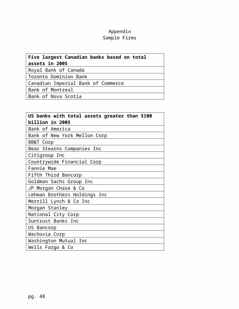
AppendixSample Firms

Five largest Canadian banks based on total assets in 2005Royal Bank of CanadaToronto Dominion BankCanadian Imperial Bank of CommerceBank of MontrealBank of Nova Scotia

US banks with total assets greater than $100 billion in 2005Bank of AmericaBank of New York Mellon CorpBB&T CorpBear Stearns Companies IncCitigroup IncCountrywide Financial CorpFannie MaeFifth Third BancorpGoldman Sachs Group IncJP Morgan Chase & CoLehman Brothers Holdings IncMerrill Lynch & Co IncMorgan StanleyNational City CorpSuntrust Banks IncUS BancorpWachovia CorpWashington Mutual IncWells Fargo & Co

pg. 48

Table 1Descriptive Statistics

Before, During, and After the Crisis PeriodSample Period: January 1999 to December 2011

Crisis Period: April 2007 to September 2008

Jan 1999 toMar2005

Pre-crisisperiod

Apr 2005 toMar2007

Pre-crisisperiod

Apr 2007 toSep2008

Crisis period

Oct 2008 toDec2011

Post-crisisperiod

USBanks

CdnBanks

USBanks

CdnBanks

USBanks

CdnBanks

USBanks

CdnBanks

Market Value 50,440(34,797

)

16,949(15,344

)

70,903(47,372

)

35,175(33,751

)

60,477(43,356

)

44,185(46,388

)

58,318(38,546

)

45,334(40,108

)Assets 345,185

(249,154)

196,413(185,98

3)

573,877(437,38

9)

314,164(293,34

3)

732,906(605,86

1)

429,762(384,48

1)

1,009,093

(794,939)

493,274(480,67

0)

Liabilities 323,863(236,77

0)

186,628(177,37

6)

534,783(404,68

1)

299,196(279,32

5)

687,208(568,25

7)

409,600(366,26

1)

934,863(724,84

5)

465,533(450,99

8)Shareholders’ Equity

21,242(15,397

)

9,267(8,698)

38,618(25,975

)

14,116(13,432

)

46,006(28,957

)

19,556(19,691

)

73,181(43,479

)

26,824(25,720

)Common Equity 20,841

(14,204)

8,121(7,558)

37,853(22,596

)

13,218(13,004

)

42,474(26,324

)

17,857(18,064

)

58,296(37,086

)

23,547(23,108

)

pg. 49

Preferred Stock 409(9)

1,147(1,113)

795(139)

898(533)

3,912(1,082)

1,699(1,792)

14,885(4,917)

3,277(3,146)

ROE 4.81(4.71)

3.64(3.85)

4.43(4.18)

4.66(4.92)

-0.85(2.18)

3.57(4.67)

5.63(1.87)

3.35(3.55)

Tier 1 capital ratio

8.42(8.17)

9.09(8.92)

8.11(8.30)

10.14(10.06)

8.10(8.24)

9.75(9.66)

11.63(11.5)

12.09(12.18)

Tier 2 capital ratio

3.66(3.76)

3.18(3.21)

3.68(3.50)

2.50(2.07)

3.99(3.89)

2.54(2.21)

3.69(3.70)

2.77(2.50)

Notes: Mean (median) values shown. Sample consists of 19 US banks with total assets greater than $100 billion in 2005 and 5 largest

Canadian banks. Market Value, Assets, and Liabilities measured in millions of US dollars. ROE = Net Income divided by Beginning Shareholders’ Equity (note that net income for Canadian banks

converted to US dollars at end of quarter exchange rate rather than average for the quarter) expressedas a percentage

Information is obtained from Compustat except for the Tier 1 and Tier 2 capital ratios for the Canadian banks which are obtained from OSFI

pg. 50

Table 2Tests for the Existence of Contagion Surrounding the Financial Crisis

Sample Period: January 1999 to December 2011Crisis Period: April 2007 to September 2008

Panel A: Extreme Low Canadian Bank Returns Number of Observations

ExtremNeg Values (%)

Index = 0 583 4.80Index = 1 195 26.67Total no. of observations

778

Panel B: Extreme Low Bank Returns by Time PeriodCanadian Banks US Banks

Number ofObs

ExtremNegValues(%)

Numberof Obs

ExtremNegValues(%)

Before the crisis 493 8.11 1876 5.65During the crisis (April 2007 to September 2008)

90 11.11 333 22.52

After the crisis 195 15.38 459 20.26Total no. of observations

778 2668

Panel C: Descriptive StatisticsVariable Number

of ObsMean Std Dev Median Minimum Maximum

Capitalization

779 4.7477 0.6216 4.6638 3.4917 7.1248

Liquidity 779 21.7078 3.0993 21.4156 15.6260 34.0206Deposit Fund

779 66.2806 3.3225 66.7438 55.0256 72.9968

TBill 780 2.8337 1.5753 2.7205 0.1700 5.7510MktRet 780 0.0132 0.0592 0.0200 -0.2569 0.2154

Panel D: Correlations (p-values in parentheses)pg. 51

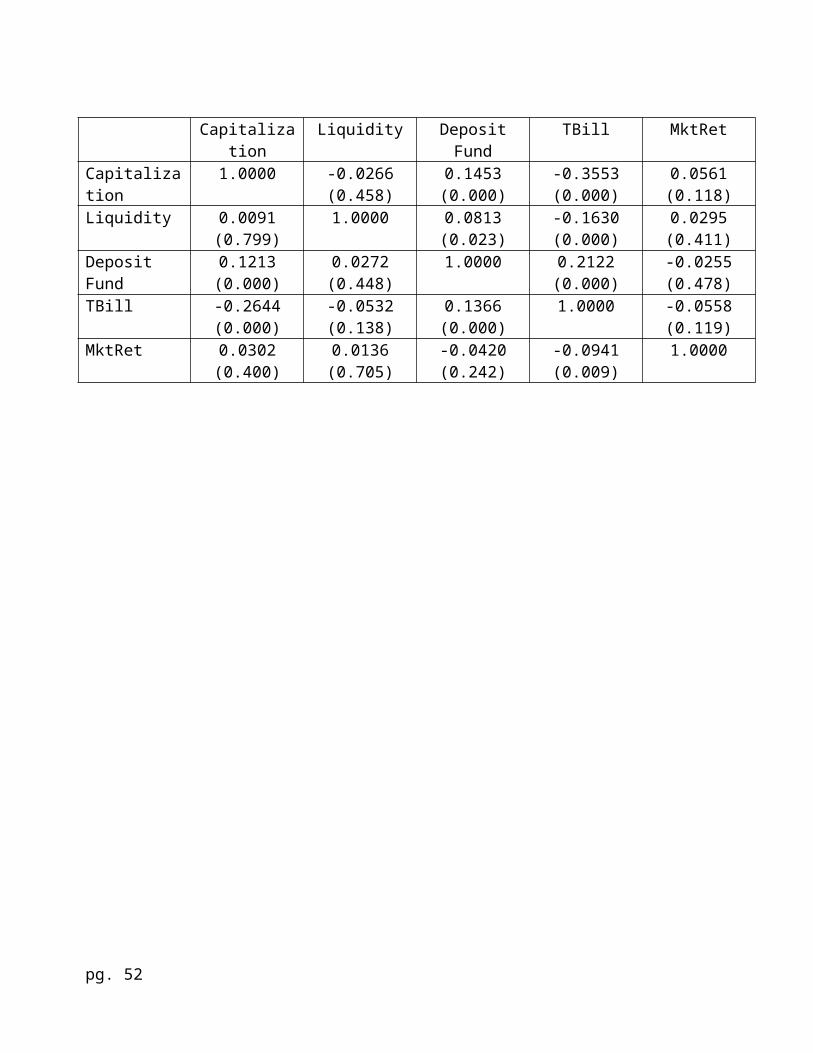
Capitalization

Liquidity DepositFund

TBill MktRet

Capitalization

1.0000 -0.0266(0.458)

0.1453(0.000)

-0.3553(0.000)

0.0561(0.118)

Liquidity 0.0091(0.799)

1.0000 0.0813(0.023)

-0.1630(0.000)

0.0295(0.411)

Deposit Fund

0.1213(0.000)

0.0272(0.448)

1.0000 0.2122(0.000)

-0.0255(0.478)

TBill -0.2644(0.000)

-0.0532(0.138)

0.1366(0.000)

1.0000 -0.0558(0.119)

MktRet 0.0302(0.400)

0.0136(0.705)

-0.0420(0.242)

-0.0941(0.009)

1.0000

pg. 52

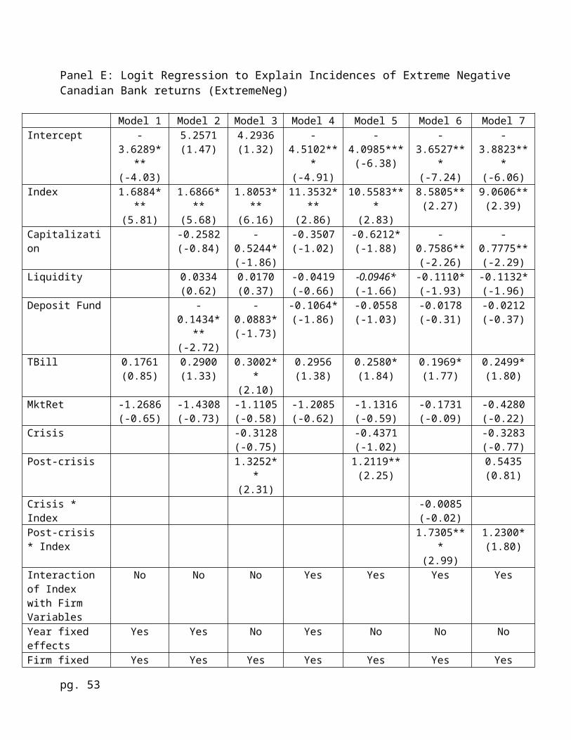
Panel E: Logit Regression to Explain Incidences of Extreme Negative Canadian Bank returns (ExtremeNeg)

Model 1 Model 2 Model 3 Model 4 Model 5 Model 6 Model 7Intercept -

3.6289***

(-4.03)

5.2571(1.47)

4.2936(1.32)

-4.5102**

*(-4.91)

-4.0985***(-6.38)

-3.6527**

*(-7.24)

-3.8823**

*(-6.06)

Index 1.6884***

(5.81)

1.6866***

(5.68)

1.8053***

(6.16)

11.3532***

(2.86)

10.5583***

(2.83)

8.5805**(2.27)

9.0606**(2.39)

Capitalization

-0.2582(-0.84)

-0.5244*(-1.86)

-0.3507(-1.02)

-0.6212*(-1.88)

-0.7586**(-2.26)

-0.7775**(-2.29)

Liquidity 0.0334(0.62)

0.0170(0.37)

-0.0419(-0.66)

-0.0946*(-1.66)

-0.1110*(-1.93)

-0.1132*(-1.96)

Deposit Fund -0.1434*

**(-2.72)

-0.0883*(-1.73)

-0.1064*(-1.86)

-0.0558(-1.03)

-0.0178(-0.31)

-0.0212(-0.37)

TBill 0.1761(0.85)

0.2900(1.33)

0.3002**

(2.10)

0.2956(1.38)

0.2580*(1.84)

0.1969*(1.77)

0.2499*(1.80)

MktRet -1.2686(-0.65)

-1.4308(-0.73)

-1.1105(-0.58)

-1.2085(-0.62)

-1.1316(-0.59)

-0.1731(-0.09)

-0.4280(-0.22)

Crisis -0.3128(-0.75)

-0.4371(-1.02)

-0.3283(-0.77)

Post-crisis 1.3252**

(2.31)

1.2119**(2.25)

0.5435(0.81)

Crisis * Index

-0.0085(-0.02)

Post-crisis * Index

1.7305***

(2.99)

1.2300*(1.80)

Interaction of Index with Firm Variables

No No No Yes Yes Yes Yes

Year fixed effects

Yes Yes No Yes No No No

Firm fixed Yes Yes Yes Yes Yes Yes Yes

pg. 53

effectsN 778 777 777 777 777 777 777

pg. 54

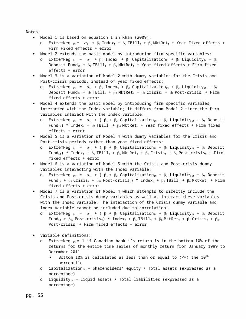
Notes: Model 1 is based on equation 1 in Khan (2009):

o ExtremNeg it = 1 + 1 Indext + 5 TBillt + 6 MktRett + Year Fixed effects +Firm Fixed effects + error

Model 2 extends the basic model by introducing firm specific variables:o ExtremNeg it = 1 + 1 Indext + 2 Capitalizationit + 3 Liquidityit + 4

Deposit Fundit + 5 TBillt + 6 MktRett + Year fixed effects + Firm fixed effects + error

Model 3 is a variation of Model 2 with dummy variables for the Crisis and Post-crisis periods, instead of year fixed effects:o ExtremNeg it = 1 + 1 Indext + 2 Capitalizationit + 3 Liquidityit + 4

Deposit Fundit + 5 TBillt + 6 MktRett + 7 Crisist + 8 Post-crisist + Firm fixed effects + error

Model 4 extends the basic model by introducing firm specific variables interacted with the Index variable; it differs from Model 2 since the firm variables interact with the Index variable:o ExtremNeg it = 1 + ( 1 + 2 Capitalizationit + 3 Liquidityit + 4 Deposit

Fundit) * Indext + 5 TBillt + 6 MktRett + Year fixed effects + Firm fixed effects + error

Model 5 is a variation of Model 4 with dummy variables for the Crisis and Post-crisis periods rather than year fixed effects:o ExtremNeg it = 1 + ( 1 + 2 Capitalizationit + 3 Liquidityit + 4 Deposit

Fundit) * Indext + 5 TBillt + 6 MktRett + 7 Crisist + 8 Post-crisist + Firm fixed effects + error

Model 6 is a variation of Model 5 with the Crisis and Post-crisis dummy variables interacting with the Index variable:o ExtremNeg it = 1 + ( 1 + 2 Capitalizationit + 3 Liquidityit + 4 Deposit

Fundit + 9 Crisist + 10 Post-crisist) * Indext + 5 TBillt + 6 MktRett + Firmfixed effects + error

Model 7 is a variation of Model 4 which attempts to directly include the Crisis and Post-crisis dummy variables as well as interact these variables with the Index variable. The interaction of the Crisis dummy variable and Index variable cannot be included due to correlation:o ExtremNeg it = 1 + ( 1 + 2 Capitalizationit + 3 Liquidityit + 4 Deposit

Fundit + 10 Post-crisist) * Indext + 5 TBillt + 6 MktRett + 7 Crisist + 8

Post-crisist + Firm fixed effects + error

Variable definitions:o ExtremNeg it = 1 if Canadian bank i’s return is in the bottom 10% of the

returns for the entire time series of monthly return from January 1999 toDecember 2011. Bottom 10% is calculated as less than or equal to (<=) the 10th

percentileo Capitalizationit = Shareholders’ equity / Total assets (expressed as a

percentage) o Liquidityit = Liquid assets / Total liabilities (expressed as a

percentage)

pg. 55

o Deposit Fundit = Depository funding / Total assets (expressed as a percentage)

o Indext = 1 if the index, constructed from the set of 19 US Banks in the sample, is in the bottom quartile of the index return for the sample period from January 1999 to December 2011.

o MktRett is Canadian equally weighted market return. o TBillt is Canadian Treasury Bill rate.o Crisist = 1 for the crisis period from April 2007 to September 2008o Post-crisist = 1 for the period from October 2008 to December 2011

pg. 56

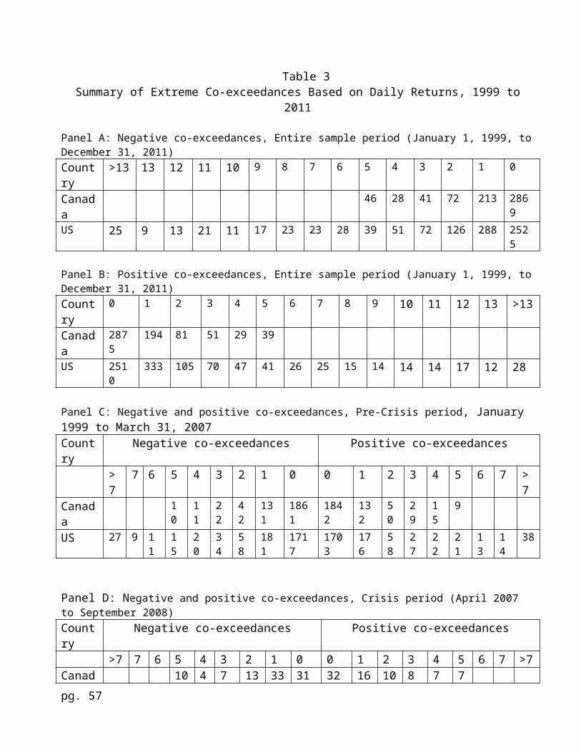
Table 3Summary of Extreme Co-exceedances Based on Daily Returns, 1999 to

2011

Panel A: Negative co-exceedances, Entire sample period (January 1, 1999, toDecember 31, 2011)Country

>13 13 12 11 10 9 8 7 6 5 4 3 2 1 0

Canada

46 28 41 72 213 2869

US 25 9 13 21 11 17 23 23 28 39 51 72 126 288 2525

Panel B: Positive co-exceedances, Entire sample period (January 1, 1999, toDecember 31, 2011)Country

0 1 2 3 4 5 6 7 8 9 10 11 12 13 >13

Canada

2875

194 81 51 29 39

US 2510

333 105 70 47 41 26 25 15 14 14 14 17 12 28

Panel C: Negative and positive co-exceedances, Pre-Crisis period, January 1999 to March 31, 2007Country

Negative co-exceedances Positive co-exceedances

>7

7 6 5 4 3 2 1 0 0 1 2 3 4 5 6 7 >7

Canada

10

11

22

42

131

1861

1842

132

50

29

15

9

US 27 9 11

15

20

34

58

181

1717

1703

176

58

27

22

21

13

14

38

Panel D: Negative and positive co-exceedances, Crisis period (April 2007 to September 2008)Country

Negative co-exceedances Positive co-exceedances

>7 7 6 5 4 3 2 1 0 0 1 2 3 4 5 6 7 >7Canad 10 4 7 13 33 31 32 16 10 8 7 7pg. 57

a 0 9US 35 7 6 11 9 16 33 42 22

0242

53 15 14 10 6 6 5 28

Panel E: Negative and positive co-exceedances, Post-Crisis period (October2008 to December 2011)Country

Negative co-exceedances Positive co-exceedances

>7 7 6 5 4 3 2 1 0 0 1 2 3 4 5 6 7 >7Canada

26 13 12 17 49 698

704

46 21 14 7 23

US 57 7 11 13 22 22 35 65 588

565

104

32 29 15 14 7 6 48

Notes: A positive (negative) exceedance corresponds to the subset of daily returns

that comprise the highest (lowest) five percent of all returns, calculated separately for each bank. Co-exceedances represent joint occurrences across banks by day. For example, a positive co-exceedance of 4 means that 4 banks have a positive exceedance on the same day. (Bae, Karolyi, and Stulz, 2003)

pg. 58

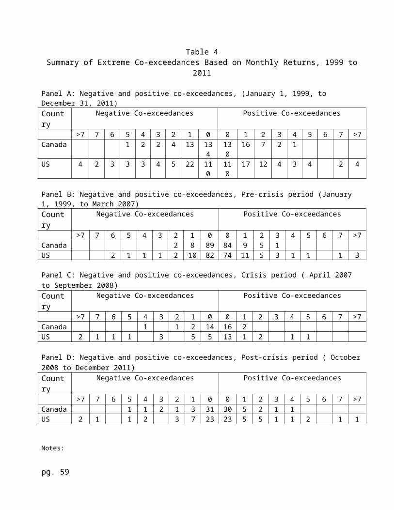
Table 4Summary of Extreme Co-exceedances Based on Monthly Returns, 1999 to

2011

Panel A: Negative and positive co-exceedances, (January 1, 1999, to December 31, 2011)Country

Negative Co-exceedances Positive Co-exceedances

>7 7 6 5 4 3 2 1 0 0 1 2 3 4 5 6 7 >7Canada 1 2 2 4 13 13

4130

16 7 2 1

US 4 2 3 3 3 4 5 22 110

110

17 12 4 3 4 2 4

Panel B: Negative and positive co-exceedances, Pre-crisis period (January 1, 1999, to March 2007)Country

Negative Co-exceedances Positive Co-exceedances

>7 7 6 5 4 3 2 1 0 0 1 2 3 4 5 6 7 >7Canada 2 8 89 84 9 5 1US 2 1 1 1 2 10 82 74 11 5 3 1 1 1 3

Panel C: Negative and positive co-exceedances, Crisis period ( April 2007 to September 2008)Country

Negative Co-exceedances Positive Co-exceedances

>7 7 6 5 4 3 2 1 0 0 1 2 3 4 5 6 7 >7Canada 1 1 2 14 16 2US 2 1 1 1 3 5 5 13 1 2 1 1

Panel D: Negative and positive co-exceedances, Post-crisis period ( October2008 to December 2011)Country

Negative Co-exceedances Positive Co-exceedances

>7 7 6 5 4 3 2 1 0 0 1 2 3 4 5 6 7 >7Canada 1 1 2 1 3 31 30 5 2 1 1US 2 1 1 2 3 7 23 23 5 5 1 1 2 1 1

Notes:

pg. 59

A positive (negative) exceedance corresponds to the subset of monthly returnsthat comprise the highest (lowest) five percent of all returns, calculated separately for each bank. Co-exceedances represent joint occurrences across banks by month. For example, a positive co-exceedance of 4 means that 4 bankshave a positive exceedance on the same month. (Bae, Karolyi, and Stulz, 2003)

pg. 60

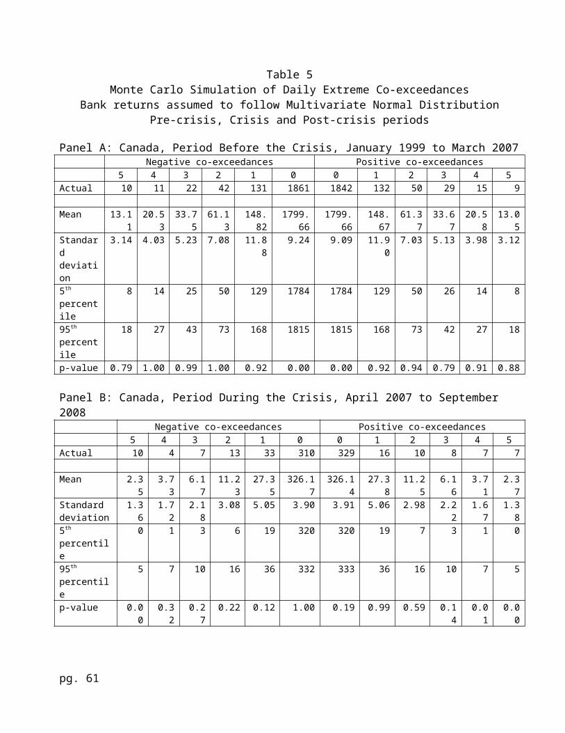
Table 5Monte Carlo Simulation of Daily Extreme Co-exceedances

Bank returns assumed to follow Multivariate Normal DistributionPre-crisis, Crisis and Post-crisis periods

Panel A: Canada, Period Before the Crisis, January 1999 to March 2007Negative co-exceedances Positive co-exceedances

5 4 3 2 1 0 0 1 2 3 4 5Actual 10 11 22 42 131 1861 1842 132 50 29 15 9

Mean 13.11

20.53

33.75

61.13

148.82

1799.66

1799.66

148.67

61.37

33.67

20.58

13.05

Standard deviation

3.14 4.03 5.23 7.08 11.88

9.24 9.09 11.90

7.03 5.13 3.98 3.12

5th percentile

8 14 25 50 129 1784 1784 129 50 26 14 8

95th percentile

18 27 43 73 168 1815 1815 168 73 42 27 18

p-value 0.79 1.00 0.99 1.00 0.92 0.00 0.00 0.92 0.94 0.79 0.91 0.88

Panel B: Canada, Period During the Crisis, April 2007 to September 2008

Negative co-exceedances Positive co-exceedances5 4 3 2 1 0 0 1 2 3 4 5

Actual 10 4 7 13 33 310 329 16 10 8 7 7

Mean 2.35

3.73

6.17

11.23

27.35

326.17

326.14

27.38

11.25

6.16

3.71

2.37

Standard deviation

1.36

1.72

2.18

3.08 5.05 3.90 3.91 5.06 2.98 2.22

1.67

1.38

5th percentile

0 1 3 6 19 320 320 19 7 3 1 0

95th percentile

5 7 10 16 36 332 333 36 16 10 7 5

p-value 0.00

0.32

0.27

0.22 0.12 1.00 0.19 0.99 0.59 0.14

0.01

0.00

pg. 61

Panel C: Canada, Period After the Crisis, October 2008 to December 2011

Negative co-exceedances Positive co-exceedances5 4 3 2 1 0 0 1 2 3 4 5

Actual 26 13 12 17 49 698 704 46 21 14 7 23

Mean 5.17

8.10

13.28

24.10

58.69

705.66

705.62

58.71

24.16

13.23

8.16

5.13

Standard deviation

2.02

2.50

3.23 4.50 7.47 5.77 5.64 7.26 4.36 3.18 2.46

1.97

5th percentile

2 4 8 17 47 696 696 47 17 8 4 2

95th percentile

9 12 19 32 71 715 715 71 32 19 12 9

p-value 0.00

0.02

0.59 0.94 0.89 0.89 0.58 0.96 0.72 0.34 0.59

0.00

pg. 62

Panel D: US Banks, Period Before the Crisis, January 1999 to March 2007Negative co-exceedances Positive co-exceedances

>7 7 6 5 4 3 2 1 0 0 1 2 3 4 5 6 7 >7Actual 27 9 11 15 20 34 58 181 1717 1703 176 58 27 22 21 13 14 38

Mean 60.64

18.69

24.38

32.98

46.05

68.38

116.21

263.81

1440.88

1441.04

263.41

116.21

68.55

46.04

32.94

24.50

18.67

60.64

Std dev 5.11

4.11 4.83 5.57 6.59 7.95 10.49

15.56

17.00 16.95 15.34

10.60

8.11 6.60 5.50 4.79 4.16 5.02

5th perc 52 12 17 24 35 56 238 1413 1414 238 99 55 35 24 17 12 5295th perc

69 26 33 42 57 82 134 289 1469 1469 289 134 82 57 42 33 26 2169

p-value 1.00

1.00 1.00 1.00 1.00 1.00 1.00 1.00 0.00 0.00 1.00 1.00 1.00 1.00 0.99 0.99 0.84 1.00

Panel E: US Banks, Period During the Crisis April 2007 to September 2008Negative co-exceedances Positive co-exceedances

>7 7 6 5 4 3 2 1 0 0 1 2 3 4 5 6 7 >7Actual 35 7 6 11 9 16 33 42 220 242 53 15 14 10 6 6 5 28

Mean 10.98

3.35

4.48

6.00

8.55

12.61

21.46

48.36

263.21

263.15

48.50

21.36

12.61

8.50

6.01

4.48

3.40

10.99

Std dev

2.17

1.79

2.07

2.35

2.83

3.46

4.51

6.62

7.24 7.23 6.56

4.55

3.42

2.87

2.42

2.04

1.77

2.19

5th perc

7 1 1 2 4 7 14 38 251 251 38 14 7 4 2 1 1 7

95th perc

15 6 8 10 13 19 29 60 275 275 59 29 18 13 10 8 7 15

p-value

0.00

0.02

0.15

0.02

0.35

0.13

0.00

0.81

1.00 1.00 0.23

0.91

0.28

0.23

0.40

0.16

0.12

0.00

Panel F: US Banks, Period After the Crisis October 2008 to December 2011Negative co-exceedances Positive co-exceedances

>7 7 6 5 4 3 2 1 0 0 1 2 3 4 5 6 7 >7

pg. 63

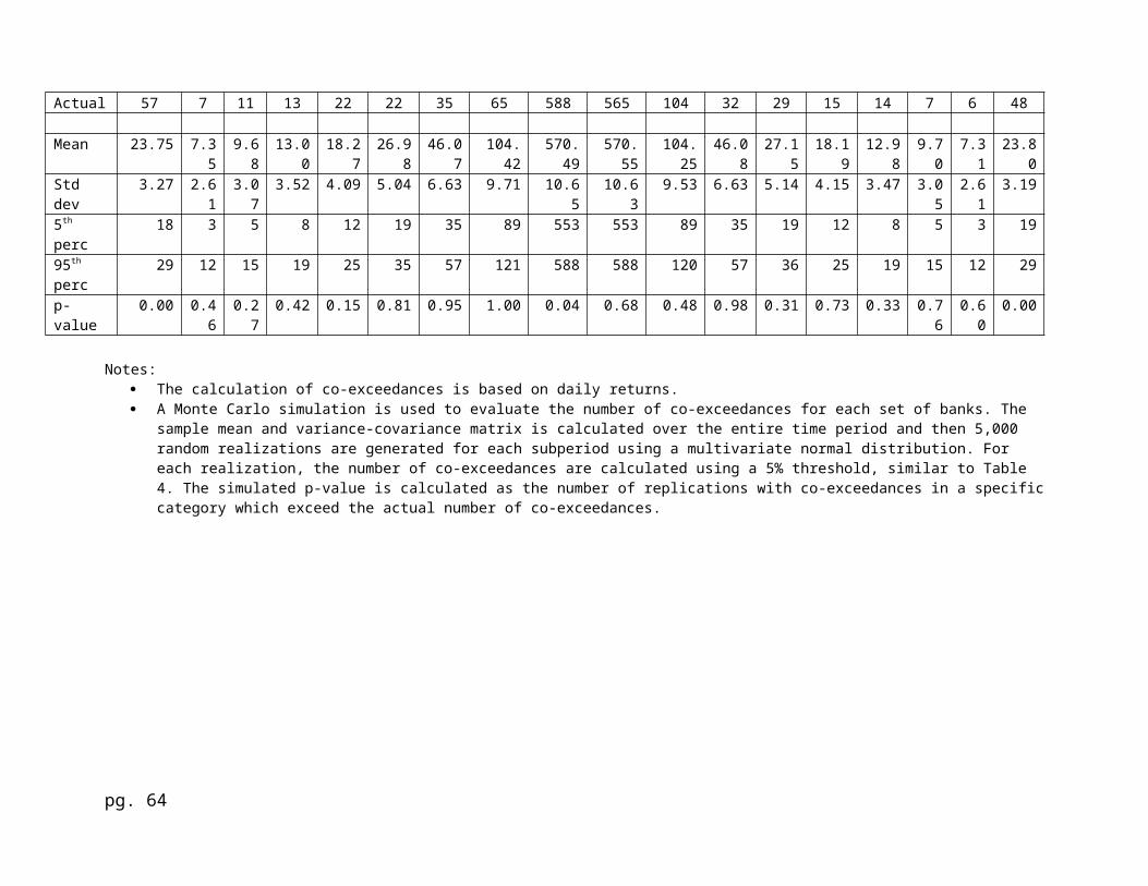
Actual 57 7 11 13 22 22 35 65 588 565 104 32 29 15 14 7 6 48

Mean 23.75 7.35

9.68

13.00

18.27

26.98

46.07

104.42

570.49

570.55

104.25

46.08

27.15

18.19

12.98

9.70

7.31

23.80

Std dev

3.27 2.61

3.07

3.52 4.09 5.04 6.63 9.71 10.65

10.63

9.53 6.63 5.14 4.15 3.47 3.05

2.61

3.19

5th perc

18 3 5 8 12 19 35 89 553 553 89 35 19 12 8 5 3 19

95th perc

29 12 15 19 25 35 57 121 588 588 120 57 36 25 19 15 12 29

p-value

0.00 0.46

0.27

0.42 0.15 0.81 0.95 1.00 0.04 0.68 0.48 0.98 0.31 0.73 0.33 0.76

0.60

0.00

Notes: The calculation of co-exceedances is based on daily returns. A Monte Carlo simulation is used to evaluate the number of co-exceedances for each set of banks. The

sample mean and variance-covariance matrix is calculated over the entire time period and then 5,000 random realizations are generated for each subperiod using a multivariate normal distribution. For each realization, the number of co-exceedances are calculated using a 5% threshold, similar to Table 4. The simulated p-value is calculated as the number of replications with co-exceedances in a specificcategory which exceed the actual number of co-exceedances.

pg. 64

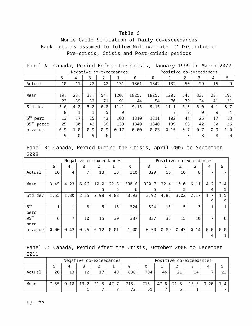
Table 6Monte Carlo Simulation of Daily Co-exceedances

Bank returns assumed to follow Multivariate ‘t’ DistributionPre-crisis, Crisis and Post-crisis periods

Panel A: Canada, Period Before the Crisis, January 1999 to March 2007Negative co-exceedances Positive co-exceedances

5 4 3 2 1 0 0 1 2 3 4 5Actual 10 11 22 42 131 1861 1842 132 50 29 15 9

Mean 19.23

23.39

33.32

54.71

120.91

1825.44

1825.54

120.70

54.79

33.34

23.41

19.21

Std dev 3.68

4.21

5.21

6.85

11.19

9.15 9.15 11.17

6.88

5.09

4.19

3.74

5th perc 13 17 25 43 103 1810 1811 102 44 25 17 1395th perce 25 30 42 66 139 1840 1840 139 66 42 30 26p-value 0.9

91.00

0.99

0.96

0.17 0.00 0.03 0.15 0.73

0.78

0.98

1.00

Panel B: Canada, Period During the Crisis, April 2007 to September 2008

Negative co-exceedances Positive co-exceedances5 4 3 2 1 0 0 1 2 3 4 5

Actual 10 4 7 13 33 310 329 16 10 8 7 7

Mean 3.45 4.23 6.06 10.05

22.55

330.66

330.75

22.42

10.05

6.11 4.24

3.45

Std dev 1.55 1.80 2.25 2.98 4.83 3.93 3.92 4.81 3.02 2.17 1.79

1.59

5th perc

1 1 3 5 15 324 324 15 5 3 1 1

95th perc

6 7 10 15 30 337 337 31 15 10 7 6

p-value 0.00 0.42 0.25 0.12 0.01 1.00 0.50 0.89 0.43 0.14 0.04

0.01

Panel C: Canada, Period After the Crisis, October 2008 to December 2011

Negative co-exceedances Positive co-exceedances5 4 3 2 1 0 0 1 2 3 4 5

Actual 26 13 12 17 49 698 704 46 21 14 7 23

Mean 7.55 9.18 13.21

21.57

47.77

715.72

715.61

47.87

21.55

13.31

9.20 7.47

pg. 65

Std dev 2.34 2.60 3.28 4.40 7.05 5.77 5.62 6.98 4.37 3.27 2.65 2.32

5th perc 4 5 8 14 37 706 706 37 15 8 5 495th perc

11 14 19 29 60 725 725 60 29 19 14 11

p-value 0.00 0.05 0.57 0.82 0.39 1.00 0.97 0.57 0.50 0.35 0.73 0.00

pg. 66

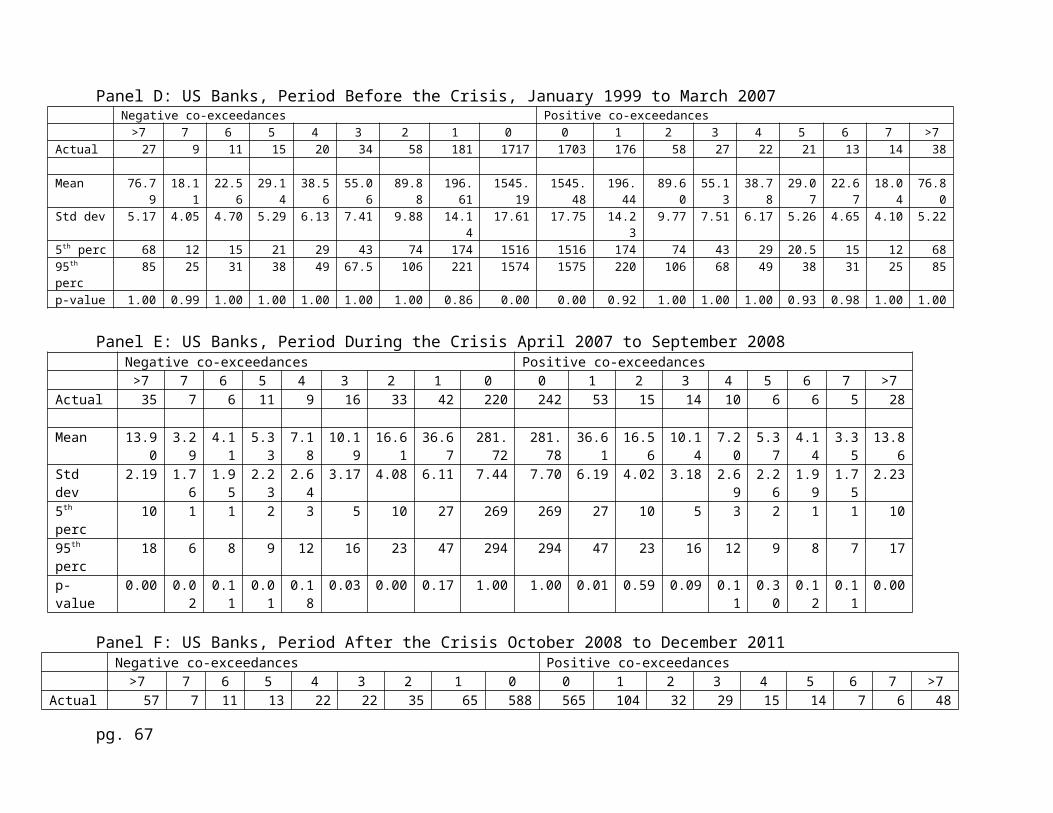
Panel D: US Banks, Period Before the Crisis, January 1999 to March 2007Negative co-exceedances Positive co-exceedances>7 7 6 5 4 3 2 1 0 0 1 2 3 4 5 6 7 >7

Actual 27 9 11 15 20 34 58 181 1717 1703 176 58 27 22 21 13 14 38

Mean 76.79

18.11

22.56

29.14

38.56

55.06

89.88

196.61

1545.19

1545.48

196.44

89.60

55.13

38.78

29.07

22.67

18.04

76.80

Std dev 5.17 4.05 4.70 5.29 6.13 7.41 9.88 14.14

17.61 17.75 14.23

9.77 7.51 6.17 5.26 4.65 4.10 5.22

5th perc 68 12 15 21 29 43 74 174 1516 1516 174 74 43 29 20.5 15 12 6895th perc

85 25 31 38 49 67.5 106 221 1574 1575 220 106 68 49 38 31 25 85

p-value 1.00 0.99 1.00 1.00 1.00 1.00 1.00 0.86 0.00 0.00 0.92 1.00 1.00 1.00 0.93 0.98 1.00 1.00

Panel E: US Banks, Period During the Crisis April 2007 to September 2008Negative co-exceedances Positive co-exceedances>7 7 6 5 4 3 2 1 0 0 1 2 3 4 5 6 7 >7

Actual 35 7 6 11 9 16 33 42 220 242 53 15 14 10 6 6 5 28

Mean 13.90

3.29

4.11

5.33

7.18

10.19

16.61

36.67

281.72

281.78

36.61

16.56

10.14

7.20

5.37

4.14

3.35

13.86

Std dev

2.19 1.76

1.95

2.23

2.64

3.17 4.08 6.11 7.44 7.70 6.19 4.02 3.18 2.69

2.26

1.99

1.75

2.23

5th perc

10 1 1 2 3 5 10 27 269 269 27 10 5 3 2 1 1 10

95th perc

18 6 8 9 12 16 23 47 294 294 47 23 16 12 9 8 7 17

p-value

0.00 0.02

0.11

0.01

0.18

0.03 0.00 0.17 1.00 1.00 0.01 0.59 0.09 0.11

0.30

0.12

0.11

0.00

Panel F: US Banks, Period After the Crisis October 2008 to December 2011Negative co-exceedances Positive co-exceedances>7 7 6 5 4 3 2 1 0 0 1 2 3 4 5 6 7 >7

Actual 57 7 11 13 22 22 35 65 588 565 104 32 29 15 14 7 6 48

pg. 67

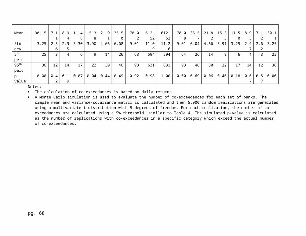
Mean 30.15 7.11

8.94

11.48

15.38

21.91

35.50

78.02

612.52

612.52

78.08

35.57

21.82

15.35

11.50

8.93

7.12

30.11

Std dev

3.25 2.56

2.95

3.30 3.90 4.66 6.08 9.01 11.09

11.26

9.01 6.04 4.66 3.91 3.29 2.97

2.62

3.25

5th perc

25 3 4 6 9 14 26 63 594 594 64 26 14 9 6 4 3 25

95th perc

36 12 14 17 22 30 46 93 631 631 93 46 30 22 17 14 12 36

p-value

0.00 0.42

0.19

0.07 0.04 0.44 0.49 0.92 0.98 1.00 0.00 0.69 0.06 0.46 0.18 0.67

0.57

0.00

Notes: The calculation of co-exceedances is based on daily returns. A Monte Carlo simulation is used to evaluate the number of co-exceedances for each set of banks. The

sample mean and variance-covariance matrix is calculated and then 5,000 random realizations are generatedusing a multivariate t-distribution with 5 degrees of freedom. For each realization, the number of co-exceedances are calculated using a 5% threshold, similar to Table 4. The simulated p-value is calculated as the number of replications with co-exceedances in a specific category which exceed the actual number of co-exceedances.

pg. 68

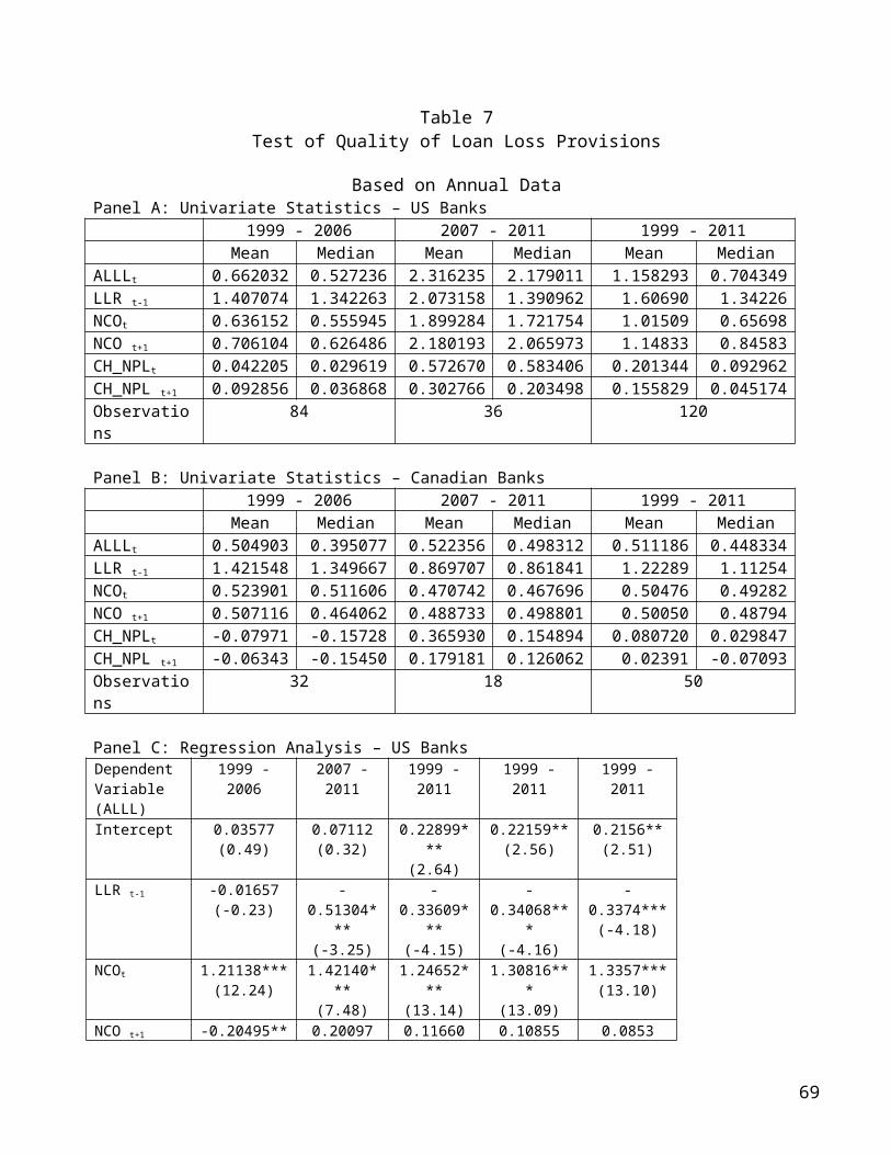
Table 7Test of Quality of Loan Loss Provisions

Based on Annual DataPanel A: Univariate Statistics – US Banks

1999 - 2006 2007 - 2011 1999 - 2011Mean Median Mean Median Mean Median

ALLLt 0.662032 0.527236 2.316235 2.179011 1.158293 0.704349LLR t-1 1.407074 1.342263 2.073158 1.390962 1.60690 1.34226NCOt 0.636152 0.555945 1.899284 1.721754 1.01509 0.65698NCO t+1 0.706104 0.626486 2.180193 2.065973 1.14833 0.84583CH_NPLt 0.042205 0.029619 0.572670 0.583406 0.201344 0.092962CH_NPL t+1 0.092856 0.036868 0.302766 0.203498 0.155829 0.045174Observations

84 36 120

Panel B: Univariate Statistics – Canadian Banks1999 - 2006 2007 - 2011 1999 - 2011

Mean Median Mean Median Mean MedianALLLt 0.504903 0.395077 0.522356 0.498312 0.511186 0.448334LLR t-1 1.421548 1.349667 0.869707 0.861841 1.22289 1.11254NCOt 0.523901 0.511606 0.470742 0.467696 0.50476 0.49282NCO t+1 0.507116 0.464062 0.488733 0.498801 0.50050 0.48794CH_NPLt -0.07971 -0.15728 0.365930 0.154894 0.080720 0.029847CH_NPL t+1 -0.06343 -0.15450 0.179181 0.126062 0.02391 -0.07093Observations

32 18 50

Panel C: Regression Analysis – US BanksDependent Variable (ALLL)

1999 -2006

2007 -2011

1999 -2011

1999 -2011

1999 -2011

Intercept 0.03577(0.49)

0.07112(0.32)

0.22899***

(2.64)

0.22159**(2.56)

0.2156**(2.51)

LLR t-1 -0.01657(-0.23)

-0.51304*

**(-3.25)

-0.33609*

**(-4.15)

-0.34068**

*(-4.16)

-0.3374***(-4.18)

NCOt 1.21138***(12.24)

1.42140***

(7.48)

1.24652***

(13.14)

1.30816***

(13.09)

1.3357***(13.10)

NCO t+1 -0.20495** 0.20097 0.11660 0.10855 0.0853

69

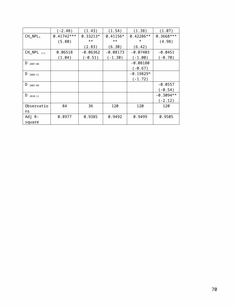
(-2.48) (1.43) (1.54) (1.38) (1.07)CH_NPLt 0.41742***

(5.80)0.33213*

**(2.83)

0.41156***

(6.30)

0.42286***

(6.42)

0.3668***(4.98)

CH_NPL t+1 0.06518(1.04)

-0.06362(-0.51)

-0.08173(-1.30)

-0.07403 (-1.00)

-0.0451(-0.70)

D 2007-08 -0.08180(-0.67)

D 2009-11 -0.19829*(-1.72)

D 2007-09 -0.0557(-0.54)

D 2010-11 -0.3094**(-2.12)

Observations

84 36 120 120 120

Adj R-square

0.8977 0.9385 0.9492 0.9499 0.9505

70

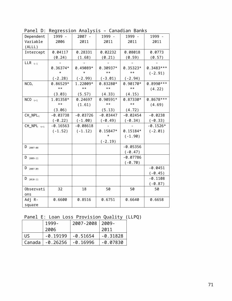
Panel D: Regression Analysis – Canadian BanksDependentVariable (ALLL)

1999 -2006

2007 -2011

1999 -2011

1999 -2011

1999 -2011

Intercept 0.04117(0.24)

0.28331(1.68)

0.02232(0.21)

0.08018(0.59)

0.0773(0.57)

LLR t-1 -0.36374*

*(-2.28)

-0.49089*

*(-2.99)

-0.30937*

**(-3.01)

-0.35323*

**(-2.94)

-0.3483***(-2.91)

NCOt 0.86529***

(3.03)

1.22009***

(5.57)

0.83280***

(4.33)

0.90170***

(4.15)

0.8990***(4.22)

NCO t+1 1.01358***

(3.06)

0.24697(1.61)

0.90591***

(5.13)

0.87330***

(4.72)

0.8678***(4.69)

CH_NPLt -0.03738(-0.22)

-0.03726(-1.00)

-0.03447(-0.49)

-0.02454(-0.34)

-0.0238(-0.33)

CH_NPL t+1 -0.16563(-1.52)

-0.08618(-1.12)

-0.15847*

*(-2.19)

-0.15184*(-1.90)

-0.1526*(-2.01)

D 2007-08 -0.05356(-0.47)

D 2009-11 -0.07786(-0.70)

D 2007-09 -0.0451(-0.45)

D 2010-11 -0.1108(-0.87)

Observations

32 18 50 50 50

Adj R-square

0.6600 0.8516 0.6751 0.6640 0.6658

Panel E: Loan Loss Provision Quality (LLPQ)1999-2006

2007-2008 2009-2011

US -0.19199 -0.51654 -0.31828Canada -0.26256 -0.16996 -0.07830

71

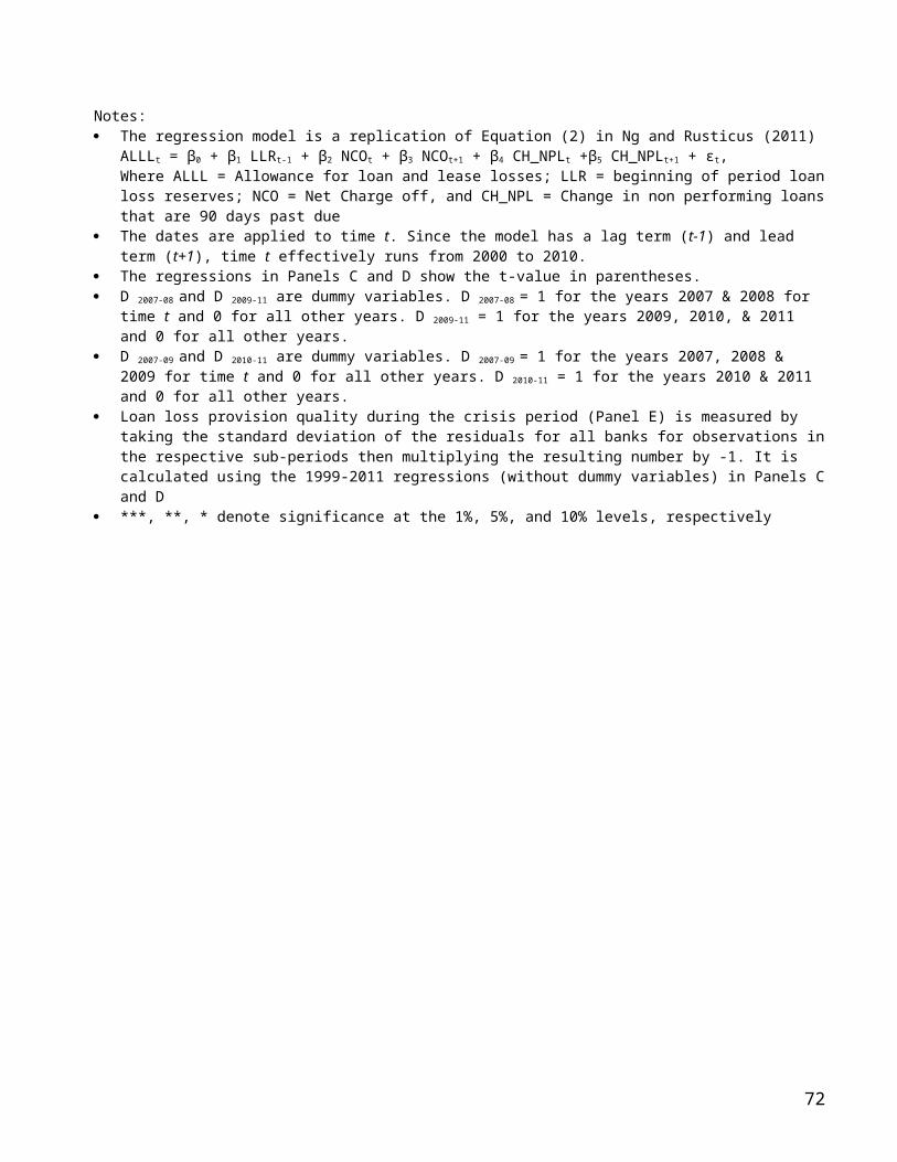
Notes: The regression model is a replication of Equation (2) in Ng and Rusticus (2011)

ALLLt = β0 + β1 LLRt-1 + β2 NCOt + β3 NCOt+1 + β4 CH_NPLt +β5 CH_NPLt+1 + εt,Where ALLL = Allowance for loan and lease losses; LLR = beginning of period loanloss reserves; NCO = Net Charge off, and CH_NPL = Change in non performing loansthat are 90 days past due

The dates are applied to time t. Since the model has a lag term (t-1) and lead term (t+1), time t effectively runs from 2000 to 2010.

The regressions in Panels C and D show the t-value in parentheses. D 2007-08 and D 2009-11 are dummy variables. D 2007-08 = 1 for the years 2007 & 2008 for

time t and 0 for all other years. D 2009-11 = 1 for the years 2009, 2010, & 2011 and 0 for all other years.

D 2007-09 and D 2010-11 are dummy variables. D 2007-09 = 1 for the years 2007, 2008 & 2009 for time t and 0 for all other years. D 2010-11 = 1 for the years 2010 & 2011 and 0 for all other years.

Loan loss provision quality during the crisis period (Panel E) is measured by taking the standard deviation of the residuals for all banks for observations inthe respective sub-periods then multiplying the resulting number by -1. It is calculated using the 1999-2011 regressions (without dummy variables) in Panels Cand D

***, **, * denote significance at the 1%, 5%, and 10% levels, respectively

72

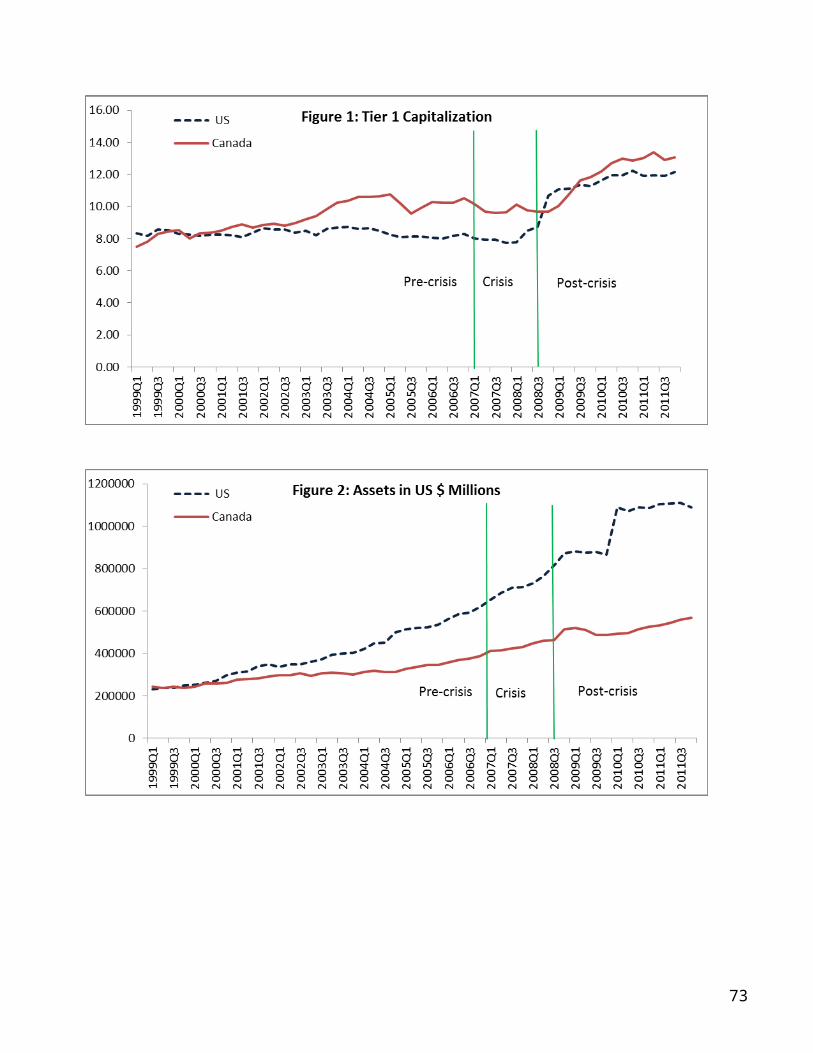
73

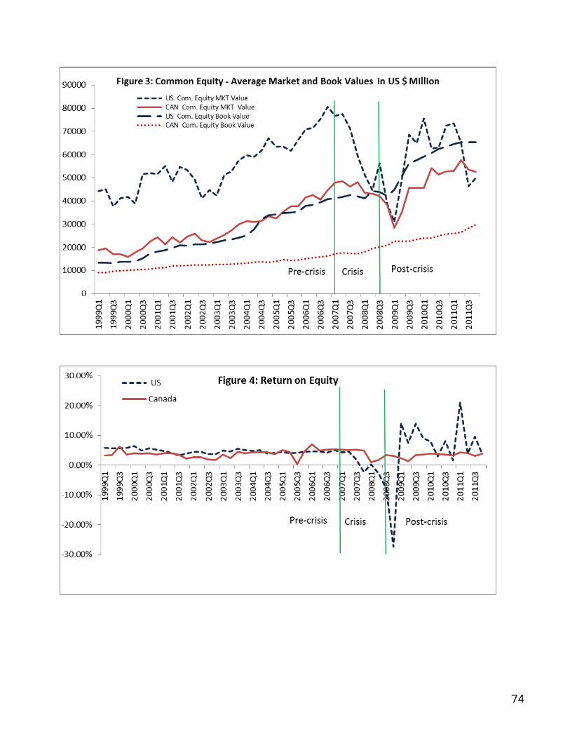
74

75