managing future oil revenue in uganda for agricultural development and poverty reduction: a cge...
TRANSCRIPT
IFPRI Discussion Paper 01122
September 2011
Managing Future Oil Revenue in Uganda for Agricultural Development and Poverty Reduction
A CGE Analysis of Challenges and Options
Manfred Wiebelt
Karl Pauw
John Mary Matovu
Evarist Twimukye
Todd Benson
Development Strategy and Governance Division
INTERNATIONAL FOOD POLICY RESEARCH INSTITUTE
The International Food Policy Research Institute (IFPRI) was established in 1975. IFPRI is one of 15 agricultural research centers that receive principal funding from governments, private foundations, and international and regional organizations, most of which are members of the Consultative Group on International Agricultural Research (CGIAR).
PARTNERS AND CONTRIBUTORS IFPRI gratefully acknowledges the generous unrestricted funding from Australia, Canada, China, Denmark, Finland, France, Germany, India, Ireland, Italy, Japan, the Netherlands, Norway, the Philippines, South Africa, Sweden, Switzerland, the United Kingdom, the United States, and the World Bank.
AUTHORS Manfred Wiebelt, Kiel Institute for the World Economy [email protected]
Karl Pauw, International Food Policy Research Institute Postdoctoral Fellow, Development Strategy and Governance Division [email protected]
John Mary Matovu, Economic Policy Research Centre, Uganda [email protected]
Evarist Twimukye, Economic Policy Research Centre, Uganda [email protected]
Todd Benson, International Food Policy Research Institute Senior Research Fellow, Development Strategy and Governance Division [email protected]
Notices IFPRI Discussion Papers contain preliminary material and research results. They have been peer reviewed, but have not been subject to a formal external review via IFPRI’s Publications Review Committee. They are circulated in order to stimulate discussion and critical comment; any opinions expressed are those of the author(s) and do not necessarily reflect the policies or opinions of IFPRI.
Copyright 2011 International Food Policy Research Institute. All rights reserved. Sections of this material may be reproduced for personal and not-for-profit use without the express written permission of but with acknowledgment to IFPRI. To reproduce the material contained herein for profit or commercial use requires express written permission. To obtain permission, contact the Communications Division at [email protected].
iii
Contents
Abstract v
Acknowledgments vi
1. Introduction 1
2. Investing Oil Revenues: Options, Needs, and Challenges 3
3. Data, CGE Model, and Simulation Setup 10
4. Model Results 22
5. Conclusion 36
Technical Appendix 39
References 42
iv
List of Tables
2.1—Share of some of the infrastructural sectors in GDP and growth performance in Uganda, 1988–2008 7
2.2—Infrastructure investments and current spending in Uganda, by sector, 2008 7
2.3—Annual infrastructure spending needs in Uganda ($ million), 2006–15 8
3.1—Sectoral share of real GDP by sector, 1970–2009 10
3.2—Input structures for crude oil and refining sectors in Nigeria, 2006 10
3.3—Production and trade characteristics in Uganda, 2007 12
3.4—Summary of modeled baseline and oil scenarios 20
4.1—GDP growth and sectoral composition: No productivity spillover scenarios during oil expansion period, 2007–17, and entire oil extraction period, 2007–46 23
4.2—Annual growth rate of sectoral production (GDP at factor cost): All scenarios during the oil expansion period, 2007–17 25
4.3—Equivalent variation results: No productivity spillover scenarios, 2007–46 27
4.4—Poverty rate and depth of poverty: No productivity spillover scenarios, 2007–46 27
4.5—GDP growth and sectoral composition: Productivity spillover scenarios during oil expansion and peak production period, 2007–26 32
4.6—Equivalent variation results: Productivity spillover scenarios, 2007–26 33
4.7—Poverty rate and depth of poverty: Productivity spillover scenarios, 2007–26 33
5.1—Ranking of public spending options 38
A.1—Oil production and revenue forecast: 1,200 million barrels reserves at $75/barrel 39
A.2—Macro SAM for Uganda 2007 including oil production and refining (billions of Uganda shillings) 41
List of Figures
2.1—Projected oil revenues and government revenues, 2010–40 3
3.1—Forecasted and modeled government oil revenue flows, 2007–46 19
4.1—Cumulative fund values when half of oil revenue is saved (FND50INV), 2010–46 28
4.2—Average per capita income and per capita transfer values (FND00I&H), 2017 29
v
ABSTRACT
With the recent discovery of crude oil reserves along the Albertine Rift, Uganda is set to establish itself as an oil producer in the coming decade. Total oil reserves are believed to be two billion barrels, with recoverable reserves estimated at 0.8–1.2 billion barrels. At peak production, likely to be reached by 2017, oil output will range from 120,000 to 210,000 barrels per day, with a production period spanning up to 30 years. Depending on the exact production levels, the extraction period, the future oil price, and revenue sharing agreements with oil producers, the Ugandan government is set to earn revenue equal to 10–15 percent of GDP at peak production. The discovery of crude oil therefore has the potential to provide significant stimulus to the Ugandan economy and address its development objectives. However, this is subject to careful management of oil revenues to avoid the potential pitfall of a sudden influx of foreign exchange. Dominating the concerns is the potential appreciation in the real exchange rate and subsequent loss of competitiveness in the nonresource tradable goods sectors such as agriculture or manufacturing (Dutch Disease). These sectors are often major employers in developing countries and the engines of growth. Several mitigation measures can be employed by government to counter Dutch Disease, including measures that directly counter the real exchange rate appreciation or measures that offer direct support to traditional export sectors in the form of subsidies.
With the aid of a recursive-dynamic computable general equilibrium (CGE) model this study evaluates the economic implications of the future oil boom in Uganda. We also consider various options open to the Ugandan government for saving, spending, or investing forecasted oil revenues with the aim of promoting economic development and reducing poverty, but also countering possible Dutch Disease effects. We find that generally urban sectors and households will be better able to capture rents generated by the oil revenues leading to growing rural–urban and regional inequality.
Yet, despite these potential risks, Uganda’s oil economy presents an unparalleled opportunity for the agricultural sector and for poverty reduction in particular. On the one hand, domestic demand for food, such as cereals, root crops, pulses, and matooke (cooking banana), but especially higher valued products, such as horticulture and livestock products, will increase as incomes rise. Moreover, higher urban income and urban consumer preferences will lead to increasing demand for processed foods and foods with greater domestic value-added, such as meat, fish, and so on. Provided Uganda’s tradable food sectors can remain competitive, this provides an opportunity for both farming and the food-processing manufacturing sector. On the other hand, there is the immediate danger of losing market shares in agricultural export markets, which might be extremely hard to regain after the oil boom. As shown in this paper, the outcomes for agriculture, rural–urban income differentials and poverty reduction depend very much on whether government revenues for public investment in the agricultural sector will increase and help alleviate chronic underinvestment in public goods that is constraining agricultural growth in Uganda.
Keywords: Uganda, crude oil, Dutch Disease, agricultural competitiveness, general equilibrium modeling
vi
ACKNOWLEDGMENTS
This research was financially supported by the Uganda office of the Department for International Development (DFID) of the Government of the United Kingdom through their support to the International Food Policy Research Institute under the Uganda Agricultural Strategy Support Program (UASSP) project. The authors also are grateful to the participants of the workshop held in Kampala on November 25, 2010, to discuss preliminary results of this analysis for their valuable comments and suggestions for improvement. Finally, we would like to acknowledge the extensive efforts by James Thurlow in developing the original Ugandan CGE model used in this study. We also thank him for modeling support provided.
1
1. INTRODUCTION
With the recent discovery of crude oil reserves along the Albertine Rift, Uganda is set to establish itself as an oil producer in the coming decade. Total oil reserves are believed to be two billion barrels, with recoverable reserves estimated at 0.8–1.2 billion barrels. This is comparable to the level of oil reserves in African countries such as Chad (0.9 billion barrels), Republic of the Congo (1.9 billion barrels), and Equatorial Guinea (1.7 billion barrels) (World Bank 2010) but far short of Angola (13.5 billion) and Nigeria (36.2 billion) (World Bank 2010). Using a reserve scenario of 800 million barrels, peak production, likely to be reached by 2017, is estimated by the World Bank to range from 120,000 to 140,000 barrels per day, with a production period spanning 30 years. A more optimistic scenario in this study is based on 1.2 billion barrels and sets peak production at 210,000 barrels per day (see Appendix for details). Although final stipulations of the revenue sharing agreements with oil producers are not yet known, government revenue from oil will be substantial. One estimate, based on an average oil price of US $75 per barrel, puts revenues at approximately 10–15 percent of GDP at peak production (World Bank 2010) (note all $ prices quoted in the paper are in US $ terms). The discovery of crude oil therefore has the potential to provide significant stimulus to the Ugandan economy and to enable it to better address its development objectives, provided oil revenues are managed in an appropriate manner.
Prior to the discovery of oil the Ugandan economy performed well, growing at over 5 percent per year since 2000. However, this growth was driven largely by nonagricultural growth. Agricultural growth was slow (around 2 percent per year), erratic, and driven largely by land expansion as opposed to yield improvements (Benin et al. 2008). As a result of this unequal development, rural poverty, at 34.3 percent, remains high relative to the urban poverty rate of 13.8 percent. In addition to this, Uganda’s population growth rate, which averaged 3.4 percent per year between 1992 and 2002, is one of the highest in the world (Klasen 2004). Although this rate is predicted to decline systematically over the next three decades to reach about 2 percent per year by 2050, it still implies a population of almost 100 million by the time oil reserves run out in 2046. This is three times the size of the population today. The challenge is, therefore, to use oil revenue in a manner that would not only reduce existing poverty and rural–urban inequities, but also ensure lasting gains of oil revenues in the face of a rapidly growing population.
If the experience of other resource-abundant countries is anything to go by, the prospects are alarming. Cross-country evidence suggests that resource-abundant countries lag behind comparable countries in terms of real GDP growth (Sachs and Warner 1995, 2001; Gelb 1988; IMF 2003); that the negative relationship between resource abundance and economic growth is stronger for oil, minerals, and other point-source resources than for agriculture; and that this relationship is remarkably robust (Sala-i-Martin and Subramanian 2003; Stevens 2003). Nonetheless, several countries have managed to avoid this so-called resource curse. Indonesia’s economy grew by an average of 4 percent per year during 1965–90, while oil and gas exports rose quickly in the 1970s, reaching 50 percent of exports in the early 1980s (Bevan, Collier, and Gunning 1999). Botswana achieved double-digit growth in the 1970s and 1980s despite rapidly growing diamond exports since the 1970s, and this development occurred despite the enclave character of the mineral industry (that is, low backward and forward linkages to other sectors) (Acemoglu, Johnson, and Robinson 2003). Other resource-rich countries, such as Malaysia, Australia, and Norway, have successfully diversified their production structures, laying the ground for broad-based balanced growth.
The anxiety about the effects of resource booms partly reflects reservations about the absorptive and managerial capacity of public sectors—particularly in developing countries—to manage large-scale investment programs or to rapidly step up service delivery without a loss in quality. In part, it also reflects even deeper reservations about resource dependency and the impact of windfall profits on the domestic political economy (Ross 2001; Leite and Weidmann 1999; Easterly 2001). However, more traditional concerns about the macroeconomics of resource booms also figure large, and these are the focus in this study. Dominating these concerns is the fear that the additional foreign exchange arising from the exploitation and exportation of natural resources may cause an appreciation of the real exchange rate. Although a strong domestic currency is good news for importers, Rodrik (2003) warns of the danger an uncompetitive real exchange rate holds for overall economic growth and development. The subsequent loss of competitiveness in the nonresource tradable goods sectors—or Dutch Disease—may hamper growth in traditional export sectors such as manufacturing or agriculture. These sectors are often major employers in developing countries and serve as the engines of growth. Of course, exportation of natural resources does not inevitably have
2
negative consequences for the economy; for example, if the resource flow emanating from the newly exploited natural resource is small relative to overall trade flows, or there are underemployed factors of production that can be used in the expanding natural resource exploitation sectors with little opportunity cost, or both, an expansion in natural resource exports will not necessarily lead to Dutch Disease (see Hausmann and Rigobon 2002; Sala-i-Martin and Subramanian 2003).
In instances where Dutch Disease poses a real threat, two different types of measures can be adopted to counter its negative effects. The first set of measures aims to sterilize the exchange rate effect by reducing the net foreign exchange inflow. This could be achieved by stimulating demand for imports through, for example, the lifting of import tariffs. Alternatively, oil revenue can be transferred back to citizens, with the resulting increase in household disposable income raising demand for imports. This effect will be stronger when the import propensity of marginal consumption is high, as is often the case in African countries. Another option is to change the composition of public spending such that the import content thereof increases. For example, public infrastructure projects typically have higher import intensities than recurrent government expenditures on salaries, health, or education. Thus, by spending relatively more of the oil revenues on infrastructure, the real exchange rate appreciation can be countered. Lastly, a real exchange rate appreciation may be mitigated by accumulating foreign reserves or by investing abroad rather than domestically. Typically this involves setting up foreign oil funds (for example, a stabilization fund [SF] or a permanent income fund [PIF]), which allow better control over export revenue flows back into the domestic economy. These types of funds are explained in more detail in the following section.
A second set of measures directly supports growth, productivity, or employment in traditional export sectors such as manufacturing or agriculture whose competitiveness is harmed by the appreciating real exchange rate. Short-term measures may include the introduction of production subsidies (for example, wage subsidies, direct production price subsidies, or input cost subsidies) that raise firms’ competitiveness in international markets, thus allowing them to maintain at least some of their market share despite the real exchange rate appreciation. Those exporters that use imported intermediate inputs may already benefit from cheaper inputs; hence, production subsidies may need to be targeted carefully to those sectors that rely on local inputs. Trade policy reforms could also benefit exporters; for example, by lifting export tariffs (or providing export subsidies), exporters will receive a higher domestic price for their goods, thus lessening the disincentive to export. Similarly, a removal of import tariffs by a country’s trading partners will raise demand for its exports. A more sustainable option—and certainly one of the central topics of discussion in the debate around how to spend oil revenues in Uganda (see Uganda, Ministry of Energy and Mineral Development 2008)—is to invest in public infrastructure that ultimately raises productivity, lowers production or transport costs, and promotes the adoption of productivity-enhancing technologies in traditional export sectors.
This study considers the impact of crude oil extraction and exportation on the Ugandan economy with a specific focus on how it might affect the agricultural sector. We also consider various options open to the Ugandan government for saving, spending, or investing forecasted oil revenues over the coming three decades. For this analysis we modify a recursive-dynamic computable general equilibrium (CGE) model of Uganda by including crude oil extraction and refining industries. These industries are allowed to grow and shrink over time in line with the forecasted oil production trend (see Figure 2.1), while oil revenues accruing to government are either saved abroad in an oil fund (this sterilizes the exchange rate effect) or spent domestically. Several spending scenarios consider the effects of using the balance of oil funds (that is, after deducting amounts saved) to develop public infrastructure. Here we consider scenarios where infrastructure investments only contribute to long-term growth through raising productive capacity, or where they also have productivity spillover effects in targeted sectors (for example, in agricultural or nonagricultural sectors specifically). Scenarios where oil revenues are distributed to citizens in the form of household welfare transfers or used to subsidize prices (for example, fuel subsidies) are also modeled.
The paper is structured as follows. Section 2 extends the introductory discussions above by providing further background information on forecasted oil revenues in Uganda and options for spending these revenues. Particular attention is given to infrastructural investments and their effects in developing countries, as well as the current infrastructure needs in Uganda. Section 3 discusses the CGE model, data, and simulation setup and design, while Section 4 presents and discusses the model results. Section 5 draws conclusions. A technical appendix provides detail about oil revenue forecasts underlying the future scenarios modeled. We also explain the modifications made to the social accounting matrix (SAM—the database for the CGE model), which were necessary in order to introduce an oil sector that does not exist at present.
3
2. INVESTING OIL REVENUES: OPTIONS, NEEDS, AND CHALLENGES
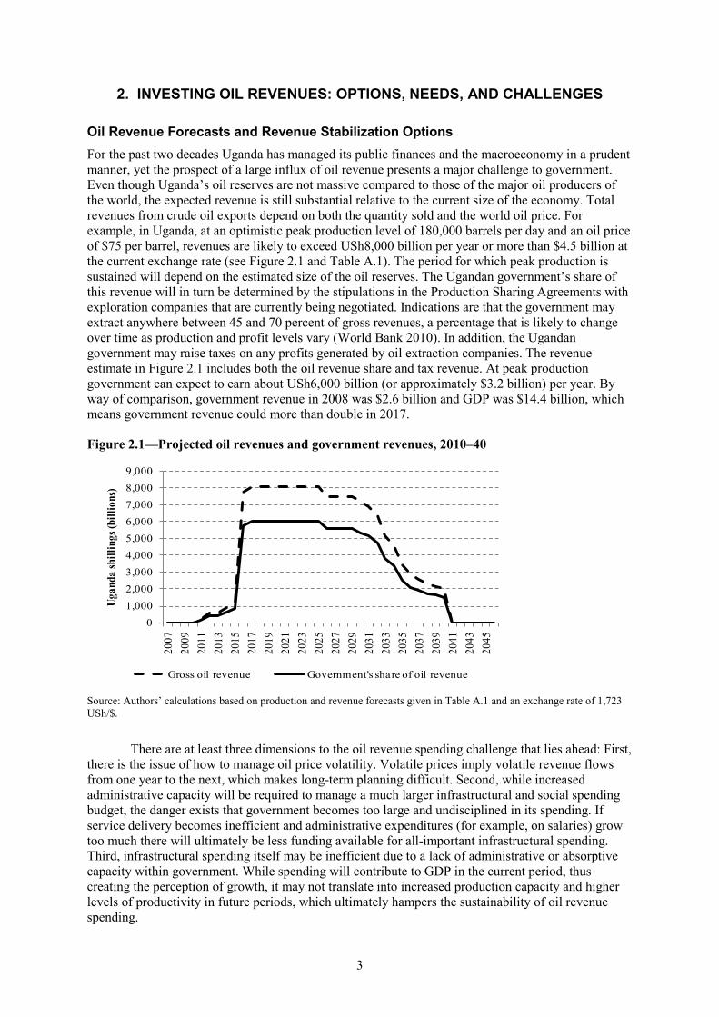
Oil Revenue Forecasts and Revenue Stabilization Options For the past two decades Uganda has managed its public finances and the macroeconomy in a prudent manner, yet the prospect of a large influx of oil revenue presents a major challenge to government. Even though Uganda’s oil reserves are not massive compared to those of the major oil producers of the world, the expected revenue is still substantial relative to the current size of the economy. Total revenues from crude oil exports depend on both the quantity sold and the world oil price. For example, in Uganda, at an optimistic peak production level of 180,000 barrels per day and an oil price of $75 per barrel, revenues are likely to exceed USh8,000 billion per year or more than $4.5 billion at the current exchange rate (see Figure 2.1 and Table A.1). The period for which peak production is sustained will depend on the estimated size of the oil reserves. The Ugandan government’s share of this revenue will in turn be determined by the stipulations in the Production Sharing Agreements with exploration companies that are currently being negotiated. Indications are that the government may extract anywhere between 45 and 70 percent of gross revenues, a percentage that is likely to change over time as production and profit levels vary (World Bank 2010). In addition, the Ugandan government may raise taxes on any profits generated by oil extraction companies. The revenue estimate in Figure 2.1 includes both the oil revenue share and tax revenue. At peak production government can expect to earn about USh6,000 billion (or approximately $3.2 billion) per year. By way of comparison, government revenue in 2008 was $2.6 billion and GDP was $14.4 billion, which means government revenue could more than double in 2017.
Figure 2.1—Projected oil revenues and government revenues, 2010–40
Source: Authors’ calculations based on production and revenue forecasts given in Table A.1 and an exchange rate of 1,723 USh/$.
There are at least three dimensions to the oil revenue spending challenge that lies ahead: First, there is the issue of how to manage oil price volatility. Volatile prices imply volatile revenue flows from one year to the next, which makes long-term planning difficult. Second, while increased administrative capacity will be required to manage a much larger infrastructural and social spending budget, the danger exists that government becomes too large and undisciplined in its spending. If service delivery becomes inefficient and administrative expenditures (for example, on salaries) grow too much there will ultimately be less funding available for all-important infrastructural spending. Third, infrastructural spending itself may be inefficient due to a lack of administrative or absorptive capacity within government. While spending will contribute to GDP in the current period, thus creating the perception of growth, it may not translate into increased production capacity and higher levels of productivity in future periods, which ultimately hampers the sustainability of oil revenue spending.
01,0002,0003,0004,0005,0006,0007,0008,0009,000
2007
2009
2011
2013
2015
2017
2019
2021
2023
2025
2027
2029
2031
2033
2035
2037
2039
2041
2043
2045
Ugan
da sh
illin
gs (b
illio
ns)
Gross oil revenue Government's share of oil revenue
4
One way to deal with revenue volatility and concerns about spending inefficiency is to transfer oil revenues into a foreign “oil fund” from which a smaller or a more stable revenue flow is extracted. The first option is to set up a budget stabilization fund (SF), which involves allocating a certain share of government oil revenues to a fund that can be tapped when low oil prices cause revenues to drop below projected flows. Examples include the SF of the Russian Federation or the State Oil Fund in Azerbaijan. When using an SF government may still plan to spend all oil revenues during the oil extraction period, in which case the SF is only used to smooth the revenue flow as it deviates from projected revenues. However, such a fund could also be used to extend the spending period beyond the oil extraction period by saving a greater share of annual revenue and continuing to draw on accrued savings that remain at the end of the oil extraction period. A second option is a permanent income fund (PIF) or heritage fund. Here all revenue from oil is transferred to the fund and only the interest earned on accumulated funds is allocated to the government budget. The Norwegian Government Pension Fund and the Kuwaiti Future Generations Fund are good examples of such PIFs. A PIF provides a much smaller flow of revenue compared to the default option of spending all revenues immediately, but the income stream is perpetual, thus having the potential of benefiting future generations. The revenue stream is also likely to be fairly stable or predictable, especially when long-term fixed interest rates are earned on the accumulated funds.
Although the development challenges loom large in Uganda, a prudent spending approach is desirable. This means not succumbing to the temptation of spending too much too soon. Proponents of a spend-all approach may appeal more to the masses, with arguments that the country cannot afford to hoard revenue amidst crumbling infrastructure and developmental backlogs. However, ideally speaking, spending levels should only gradually increase in line with the pace at which government capacity grows. Uganda has taken advice of this nature on board in announcing that an oil fund will indeed be set up and managed by the Central Bank (see Uganda, Ministry of Energy and Mineral Development 2008, 51). The way in which the fund is managed (that is, how funds are deposited or withdrawn over time) should be explicitly governed by the legal and regulatory framework for oil revenue. Such a framework, combined with a gradually enhanced institutional capacity, should cushion the country from pressure from those who would want to see quick but unsustainable gains from oil.
Investment Spending Options
Investment for Economic Growth and Poverty Reduction The pace at which public infrastructure is developed is an important determinant of the development process. Numerous studies highlight the importance of the stock of public infrastructure as one necessary ingredient for agricultural productivity growth (Binswanger, Khandker, and Rosenzweig 1993; Ram 1996; Esfahani and Ramirez 2002). Hulten (1996) argues it is not only the level of public investment that matters, but also the spending efficiency and the effectiveness with which existing capital stocks are used by citizens (see also Calderón and Servén 2005, 2008; Reinikka and Svensson 2002). Microeconomic studies tend to focus more on the latter aspect, and show that improved access to public infrastructure positively influences the adoption of productivity-enhancing technologies by farm households or firms (Antle 1984; Ahmed and Hossain 1990; Renkow, Hallstroma, and Karanjab 2004). Access to and utilization of public infrastructure also has important welfare effects, including the reduction of rural poverty (Fan, Hazell, and Thorat 2000; Fan and Zhang 2008; Gibson and Rozelle 2003) and rural inequality (Calderón and Servén 2005; Fan, Zhang, and Zhang 2003). The strength of these welfare effects, however, depends on the institutional setup in countries (Duflo and Pande 2007), while strong complementarities exist between physical and human capital (Canning and Bennathan 1999). The latter suggests that investments in education, training, or rural extension services would enhance the effectiveness of infrastructural investments.
The overwhelming message is that infrastructural investments matter for development, especially when measures are in place to improve access to that infrastructure. However, it is less clear precisely where to invest in order to maximize growth and poverty outcomes. The agricultural sector stands out as a strong candidate. Agriculture is an important sector in many developing countries in terms of its share of national GDP and employment. Agricultural growth is therefore
5
particularly important in determining the pace of poverty reduction (Diao, Hazell, and Thurlow 2010; Valdés and Foster 2010). In Uganda the agricultural sector is relatively small, contributing less than one-third to national GDP. However, it remains a significant employer, with 81 percent of the population living in households that are directly involved in agricultural activities (see Benin et al. 2008). Farming is by no means exclusively a rural activity in Uganda (27.8 percent of urban households are engaged in agricultural activities), but it is clear from population statistics that a focus on rural agriculture is warranted: 9 in 10 farm households live in rural areas, and one in three rural inhabitants are poor, compared to 13.8 percent of urban people. This implies that growth in the agricultural sector has the potential to significantly reduce poverty in Uganda. Weak historical agricultural growth, low agricultural yields, and poor infrastructure in Uganda all point to the great potential for this sector to grow rapidly should significant public investments, particularly in infrastructure, reach this sector.
Using a recursive-dynamic CGE model, Benin et al. (2008) are able to demonstrate how rapid agricultural growth achieved through yield improvements under the Comprehensive African Agricultural Development Plan (CAADP) in Uganda contributes to overall growth and poverty reduction. CAADP aims to achieve 6 percent agricultural growth by committing countries to allocate 10 percent of their overall budgets to the agricultural sector in the form of infrastructure investments, research and development, and extension services. In Uganda the 6 percent growth target implies a doubling of the agricultural growth rate, which, historically, has remained at just below 3 percent. Benin et al. (2008) show that if agricultural growth is maintained at 6 percent over the period 2005–15, the national GDP growth rate in Uganda will increase by one percentage point (that is, from 5.1 to 6.1 percent). Agricultural growth also has spillover effects into the rest of the economy, with agroprocessing or food-processing and trade and transport sectors benefiting from more rapid growth. More importantly, however, are the poverty-reducing effects of rapid agricultural growth. Benin et al. (2008) show that under an accelerated agricultural growth path the poverty rate in 2015 will be 7.6 percentage points lower than the forecasted level under the business as usual growth path. This is equivalent to an additional 2.9 million people being lifted out of poverty by 2015.
Benin et al. (2008) extend their analysis to focus on specific agricultural subsectors’ effectiveness at reducing poverty and generating growth through size and economic linkage effects. In this regard they find that horticultural crops, root crops, livestock, and cereals have the greatest poverty-reducing potential in Uganda. This is due both to the crop choices of resource-poor farmers and to the preferences of poor consumers (increased productivity lowers farmers’ unit production costs and benefits consumers via price reductions). Given their initial size, growth potential, and economic linkages, growth in subsectors such as roots, matooke (cooking banana), pulses and oilseeds, and export crops contribute most to overall growth.
Using a similar methodology, Dorosh and Thurlow (2009) focus more closely on the relative impacts of rural versus urban public investments in Uganda. In general, they find that improving agricultural productivity generates more broad-based welfare improvements in both rural and urban areas than investing in the capital city, Kampala. Although investing in Kampala accelerates economic growth, it has little effect on other regions’ welfare because of the city’s weak regional growth linkages and small migration effects. In a study in Peru, Thurlow, Morley, and Pratt (2008) find that by investing in the leading (more urbanized) region, that country may be undermining the economy in the lagging (mostly rural) region by increasing import competition and internal migration. The authors also show that the divergence between the leading and lagging regions can only be bridged by investing in the lagging region’s productivity through providing extension services and improved rural roads.
This brief overview suggests that public investments in rural areas and agriculture should be a critical part of the development strategy in Uganda if the country is to achieve its goals of reducing (rural) poverty and narrowing the welfare gap between urban and rural areas. Studies cited show that investments in cities or major urban centers such as Kampala, although good for growth there, may in fact be harmful or at best neutral for growth or welfare in rural areas. Either way, such investments will lead to rising rural–urban inequality, which is an undesirable socioeconomic outcome. The challenge is to be strategic about how and where to invest so that productivity gains in priority sectors or subsectors are maximized. Certain types of investments have obvious impacts; for example, investments in rural roads, irrigation infrastructure, or water storage will benefit agriculture, and
6
depending on the exact location (or agronomic zone) of those investments, specific subsectors within agriculture. For other types of investments, such as telecommunications, it is likely that urban-based manufacturing sectors would benefit more, but there may still be intended or unintended productivity spillovers into other sectors. It is also important to realize that there may be a lag from the time the investment in agriculture is made until productivity spillovers materialize and rural poverty declines. The immediate beneficiaries of increased agricultural investment spending are more likely to be those nonpoor workers supplying investment services or producing investment goods rather than poor farming households themselves.
Uganda’s Investment Needs As Uganda gears up toward becoming an oil producer, the first priority is to install infrastructure that would facilitate the oil extraction, transportation, and (possibly) refining processes. Substantial investment—a figure of $10 billion has been mentioned—will be required to set up the oil industry, and production will probably only reach its peak by 2017 (World Bank 2010). There are some challenges; for example, the quality of the crude oil is said to be waxy and viscous, thus requiring some heating in order to transport it via pipeline. Also, the oil fields are located in a fairly remote part of Uganda, which means good rail and road networks will be required to link the oil fields to export markets or local refineries or both.
The issue of whether local refining capacity should be developed is still being discussed. Some argue that the size of the domestic or regional market does not warrant the cost of developing the required infrastructure, and that Uganda should instead export all its crude oil via a pipeline connecting Uganda with the coast of Kenya. However, a recent study by Foster Wheeler (2010), a Swiss consultancy firm, has recommended that Uganda refine oil in the country instead of exporting crude oil. They argue that the costs and risks associated with the building of an oil refinery or pipeline are similar, which means they may as well invest domestically and benefit from the value addition in the country, however small. Domestic refining capacity, they further argue, would ensure more secure domestic fuel supplies, create more jobs, and have a more favorable outcome on the balance of payments and exchange rate compared to a model where all crude oil is exported. Another idea under consideration is that of developing a refinery in the Kenyan coastal town of Mombasa under a joint venture with this neighboring country. Its location would facilitate international trade of crude oil and refined crude oil products (should that need exist), while a pipeline would connect this location with the oil fields in Uganda.
Once the up-front investment needs have been met and oil production is under way, the expectation is that oil revenues will be used in part to narrow the infrastructure gap in Uganda. Infrastructure services in the country are considered weak (World Bank 2007). This is especially true for the transport sector. Despite fairly rapid growth over the past two decades—at times in excess of 9 percent per year—the share of the transport sector in GDP has only increased marginally from around 3 percent in 1998 to 3.4 percent in 2008 (see Table 2.1). Only about 4 percent of domestic cargo freight is transported via the country’s largely dysfunctional railway system, which currently operates at 26 percent capacity. This stands in contrast to China and India, where over 90 percent of cargo is transported via rail. The remaining cargo is transported via the road network, which is also underdeveloped (for example, only 4 percent of the Ugandan road network is paved). It costs more than three times as much to transport goods by road than by rail, yet the fact that 96 percent of goods are still moved via road is indicative of just how inefficient railway transport is. Inefficiencies and weak transport infrastructure therefore add significantly to the cost of doing business in Uganda, while they also act as implicit barriers to domestic and international trade (for example, some estimates suggest that excessive transport costs in Uganda vis-à-vis those of competitors are equivalent to a 25 percent tax on Ugandan exports).
7
Table 2.1—Share of some of the infrastructural sectors in GDP and growth performance in Uganda, 1988–2008
Percentage share in nominal GDP Growth performance (percent)
1988 1997 2004 2007 2008 1988–97 1998–2002 2004–08 2007 2008
Transport 3.0 3.9 3.2 3.3 3.4 9.3 5.3 6.8 9.6 6.9
Energy and water 0.6 1.3 3.5 4.5 4.1 7.6 6.2 2.0 5.3 4.0
Trade 14.7 10.0 12.7 14.1 14.3 7.6 6.5 10.3 13.0 13.6
Financial services - 2.3 2.8 2.9 3.2 - 5.5 11.2 -3.9 11.1
Source: Uganda Bureau of Statistics (UBOS) Statistical Abstract (various).
The energy and water sectors also face major challenges. Although these sectors’ share of GDP increased from 0.6 percent in 1988 to 4.1 percent in 2008, growth has been erratic and appears to have slowed down since the 2000s relative to the previous decade. Uganda has one of the lowest per capita electricity consumption levels in the world at only 60 kilowatt-hours per year. In comparison, annual usage in South Africa and Egypt is 4,200 kilowatt-hours and 1,200 kilowatt-hours, respectively. Low electricity use relates partly to only 11 percent of the population being connected to the grid. However, low usage rates also are explained by excessively high electricity tariffs. Consumers in Uganda face some of the highest tariffs in the world, which at $0.22 per kilowatt-hour is second only to Sweden and significantly higher than the cost of electricity in neighboring Tanzania ($0.08 per kilowatt-hour) and Kenya ($0.13 per kilowatt-hour). The state of water supply and sanitation is equally worrying. At an annual consumptive use of water for production of 21 cubic meters per capita, Uganda’s usage is far below the world average (599 cubic meters per capita). Furthermore, only 63 percent of the rural population and 72 percent of the urban population have access to safe water.
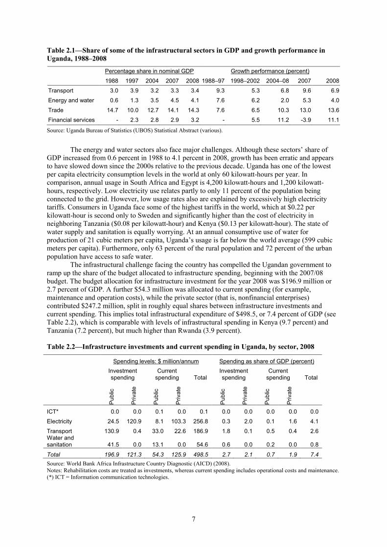
The infrastructural challenge facing the country has compelled the Ugandan government to ramp up the share of the budget allocated to infrastructure spending, beginning with the 2007/08 budget. The budget allocation for infrastructure investment for the year 2008 was $196.9 million or 2.7 percent of GDP. A further $54.3 million was allocated to current spending (for example, maintenance and operation costs), while the private sector (that is, nonfinancial enterprises) contributed $247.2 million, split in roughly equal shares between infrastructure investments and current spending. This implies total infrastructural expenditure of $498.5, or 7.4 percent of GDP (see Table 2.2), which is comparable with levels of infrastructural spending in Kenya (9.7 percent) and Tanzania (7.2 percent), but much higher than Rwanda (3.9 percent).
Table 2.2—Infrastructure investments and current spending in Uganda, by sector, 2008
Spending levels: $ million/annum Spending as share of GDP (percent)
Investment spending
Current spending Total
Investment spending
Current spending Total
Pub
lic
Priv
ate
Pub
lic
Priv
ate
Pub
lic
Priv
ate
Pub
lic
Priv
ate
ICT* 0.0 0.0 0.1 0.0 0.1 0.0 0.0 0.0 0.0 0.0
Electricity 24.5 120.9 8.1 103.3 256.8 0.3 2.0 0.1 1.6 4.1
Transport 130.9 0.4 33.0 22.6 186.9 1.8 0.1 0.5 0.4 2.6 Water and sanitation 41.5 0.0 13.1 0.0 54.6 0.6 0.0 0.2 0.0 0.8
Total 196.9 121.3 54.3 125.9 498.5 2.7 2.1 0.7 1.9 7.4 Source: World Bank Africa Infrastructure Country Diagnostic (AICD) (2008). Notes: Rehabilitation costs are treated as investments, whereas current spending includes operational costs and maintenance. (*) ICT = Information communication technologies.
8
The infrastructure spending estimates in Table 2.2 indicate that improvement in electricity provisioning is a priority in Uganda, with just over half of the overall infrastructure spending allocated to this sector. Most of the spending was paid for by the private sector. Infrastructure spending in the transport and water and sanitation sectors amounted to $186.9 million (38 percent) and $54.6 million (11 percent), respectively, with the bulk of costs covered by government.
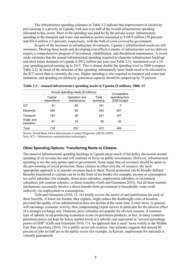
In spite of the increases in infrastructure investments, Uganda’s infrastructural needs are still enormous. Meeting these needs and developing cost-effective modes of infrastructure service delivery require a comprehensive program of investment, rehabilitation, and disciplined maintenance. A recent study estimates that the annual infrastructural spending required to eliminate infrastructure backlogs and meet future demands in Uganda is $912 million per year (see Table 2.3), maintained over a 10-year spending period running up to 2015. This is almost double the spending level in 2008 (compare Table 2.2). In terms of the structure of this spending, substantially more funds need to be allocated to the ICT sector than is currently the case. Higher spending is also required in transport and water and sanitation, and spending on electricity generation capacity should be ramped up by 75 percent.
Table 2.3—Annual infrastructure spending needs in Uganda ($ million), 2006–15
Annual spending needs ($ millions) Comparative spending from 2008 budget
Capital expenditure
Operation and maintenance
Total spending
ICT 81 80 161 0
Electricity 385 65 450 257
Transport 183 38 221 187 Water and sanitation 61 19 80 55
Total 710 202 912 499
Source: World Bank Africa Infrastructure Country Diagnostic (AICD) (2009). Note: ICT = Information communication technologies
Other Spending Options: Transferring Rents to Citizens The massive infrastructural spending backlogs in Uganda mean much of the policy discussion around spending of oil revenue has and will continue to focus on public investments. However, infrastructural spending is not the only option open to government. Some argue that oil revenues should be spent on the provisioning of social protection: Since citizens in effect own the oil resource, the most appropriate approach is to transfer revenues back to them. Social protection can be broadly defined. Benefits transferred to citizens can be in the form of tax breaks (for example, income or consumption tax cuts); subsidies (for example, direct price subsidies, employment subsidies, or investment subsidies); job creation schemes; or direct transfers (Gelb and Grasmann 2010). Not all these transfer mechanisms necessarily involve a direct transfer from government to households; some work indirectly via employment or consumption.
Gelb and Grasmann (2010, 12–16) briefly review the merits of and justification for each of these benefits. A lower tax burden, they explain, might reduce the deadweight costs of taxation, provided the quality of tax administration does not decline at the same time. Lower taxes, in general, will encourage economic activity, thus compensating export sectors in particular for the adverse effect of a stronger exchange rate. Domestic price subsidies are popular for obvious reasons. A common type of subsidy in oil-producing economies is one on petroleum products; in fact, in many countries petroleum prices are kept far below market levels at a subsidy cost equivalent to “several percentage points of GDP” (Gelb and Grasmann 2010, 13). An approach that is used “more widely in the Middle East than elsewhere (2010, 14) is public-sector job creation. One estimate suggests that around 80 percent of jobs in Gulf are in the public sector (for example, in Kuwait, employment for nationals is virtually guaranteed).
9
Very few countries have considered the use of oil revenues to finance direct welfare transfers. However, there is increasing interest in distribution mechanisms such as those pioneered in Alaska “as the shortcomings of other approaches become more apparent” (Gelb and Grasmann 2010, 14). Cash transfers or grants have two primary functions: They reduce short-term poverty and inequality, and they provide safety nets that enable households to manage risk (Pauw and Mncube 2007). There are several design options. First, grants can be targeted or universal. Targeted grants are more costly to administer, but targeting improves efficiency in terms of reductions in poverty and inequality. Under a universal grant scheme all citizens have access to a grant, irrespective of their socioeconomic status. Second, grants can be conditional or unconditional. Conditional grants, as the name suggests, are only accessible by households that comply with certain provisions, such as attending school or visiting health clinics.
The successes of conditional programs such as Bolsa Familia in Brazil and Opportunidades in Mexico have been widely reported (see, for example, Adato and Hoddinott 2010). However, just like targeting, conditionality increases the administrative burden of these programs, both for administrators who need to determine eligibility of prospective participants and for health and education service providers who need to deal with the mandatory increase in demand for these services. For this reason conditionality may not always a good idea, especially in countries where administrative capacity is low or where social service delivery is weak (Pauw and Mncube 2007). The alternative (that is, a nontargeted unconditional grant scheme) is costly, but the large influx of oil revenues in Uganda puts the country in a position where it can probably afford such a basic income grant. Although a uniformly distributed grant will not improve inequality, it will reduce poverty, while at the same time policymakers can avoid sensitivities that may arise when oil revenues—seen by all as a national resource—are unequally distributed.
10
3. DATA, CGE MODEL, AND SIMULATION SETUP
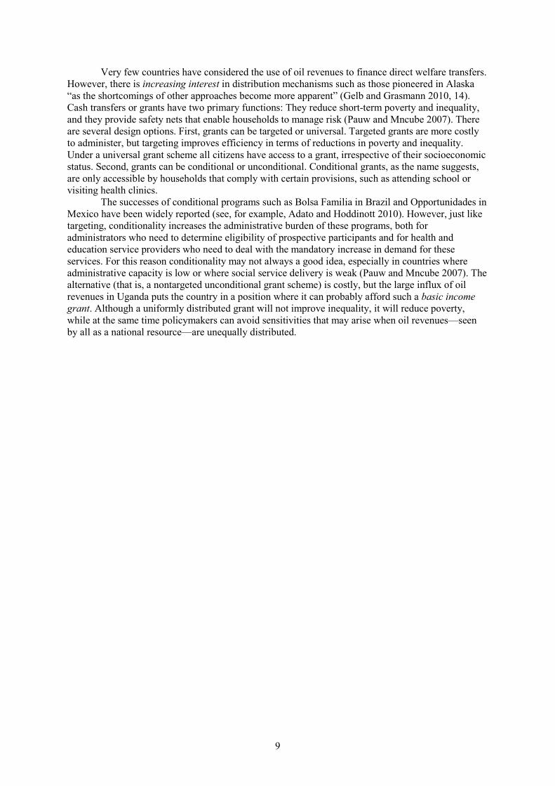
Evolution and Structure of the Ugandan Economy Recent GDP figures reflect a continuation of the restructuring process that has been a feature of Uganda’s economy over the past three decades. This has seen the importance of agricultural output decline in favor of production in industry and services (Table 3.1). At 50 percent of GDP, the services sector is now the largest sector in the economy. It is also the most dynamic, with rapid growth in recent years in areas such as telecommunications, financial services, trade, and hotels and restaurants. Despite its declining size in terms of output, agriculture remains the largest employer, with an estimated 80 percent of the population living in households that earn income from farming activities. Although there has been a significant increase in export crop production, subsistence farming still provides the bulk of food production and accounts for almost half of agricultural output. Industry accounts for around a quarter of GDP (Economic Intelligence Unit 2009). High growth in this sector has been restricted by the country’s poor transport and energy infrastructure (see earlier discussion).
Table 3.1—Sectoral share of real GDP by sector, 1970–2009
1970 1980 1990 2000 2005 2009
Agriculture 53.8 72.0 56.6 29.4 26.7 24.7
Industry 13.7 4.5 11.1 22.9 25.0 25.8
Manufacturing 9.2 4.3 5.7 7.6 7.5 8.0
Services 32.5 23.5 32.4 47.7 48.3 49.5 Total 100.0 100.0 100.0 100.0 100.0 100.0
Source: World Bank 2011.
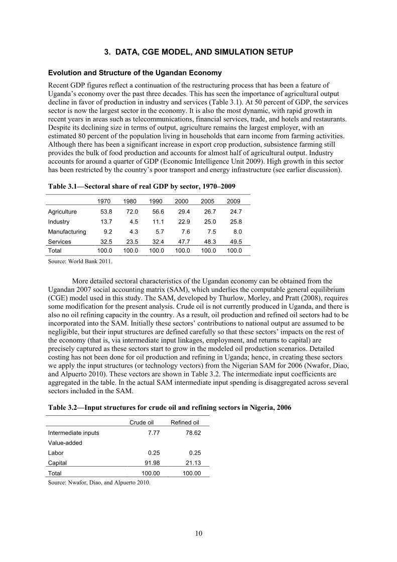
More detailed sectoral characteristics of the Ugandan economy can be obtained from the Ugandan 2007 social accounting matrix (SAM), which underlies the computable general equilibrium (CGE) model used in this study. The SAM, developed by Thurlow, Morley, and Pratt (2008), requires some modification for the present analysis. Crude oil is not currently produced in Uganda, and there is also no oil refining capacity in the country. As a result, oil production and refined oil sectors had to be incorporated into the SAM. Initially these sectors’ contributions to national output are assumed to be negligible, but their input structures are defined carefully so that these sectors’ impacts on the rest of the economy (that is, via intermediate input linkages, employment, and returns to capital) are precisely captured as these sectors start to grow in the modeled oil production scenarios. Detailed costing has not been done for oil production and refining in Uganda; hence, in creating these sectors we apply the input structures (or technology vectors) from the Nigerian SAM for 2006 (Nwafor, Diao, and Alpuerto 2010). These vectors are shown in Table 3.2. The intermediate input coefficients are aggregated in the table. In the actual SAM intermediate input spending is disaggregated across several sectors included in the SAM.
Table 3.2—Input structures for crude oil and refining sectors in Nigeria, 2006
Crude oil Refined oil
Intermediate inputs 7.77 78.62
Value-added
Labor 0.25 0.25
Capital 91.98 21.13
Total 100.00 100.00 Source: Nwafor, Diao, and Alpuerto 2010.
11
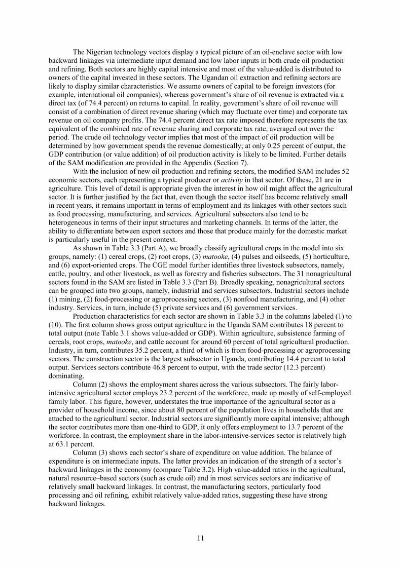
The Nigerian technology vectors display a typical picture of an oil-enclave sector with low backward linkages via intermediate input demand and low labor inputs in both crude oil production and refining. Both sectors are highly capital intensive and most of the value-added is distributed to owners of the capital invested in these sectors. The Ugandan oil extraction and refining sectors are likely to display similar characteristics. We assume owners of capital to be foreign investors (for example, international oil companies), whereas government’s share of oil revenue is extracted via a direct tax (of 74.4 percent) on returns to capital. In reality, government’s share of oil revenue will consist of a combination of direct revenue sharing (which may fluctuate over time) and corporate tax revenue on oil company profits. The 74.4 percent direct tax rate imposed therefore represents the tax equivalent of the combined rate of revenue sharing and corporate tax rate, averaged out over the period. The crude oil technology vector implies that most of the impact of oil production will be determined by how government spends the revenue domestically; at only 0.25 percent of output, the GDP contribution (or value addition) of oil production activity is likely to be limited. Further details of the SAM modification are provided in the Appendix (Section 7).
With the inclusion of new oil production and refining sectors, the modified SAM includes 52 economic sectors, each representing a typical producer or activity in that sector. Of these, 21 are in agriculture. This level of detail is appropriate given the interest in how oil might affect the agricultural sector. It is further justified by the fact that, even though the sector itself has become relatively small in recent years, it remains important in terms of employment and its linkages with other sectors such as food processing, manufacturing, and services. Agricultural subsectors also tend to be heterogeneous in terms of their input structures and marketing channels. In terms of the latter, the ability to differentiate between export sectors and those that produce mainly for the domestic market is particularly useful in the present context.
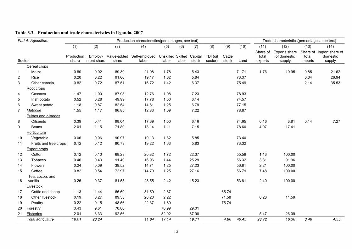
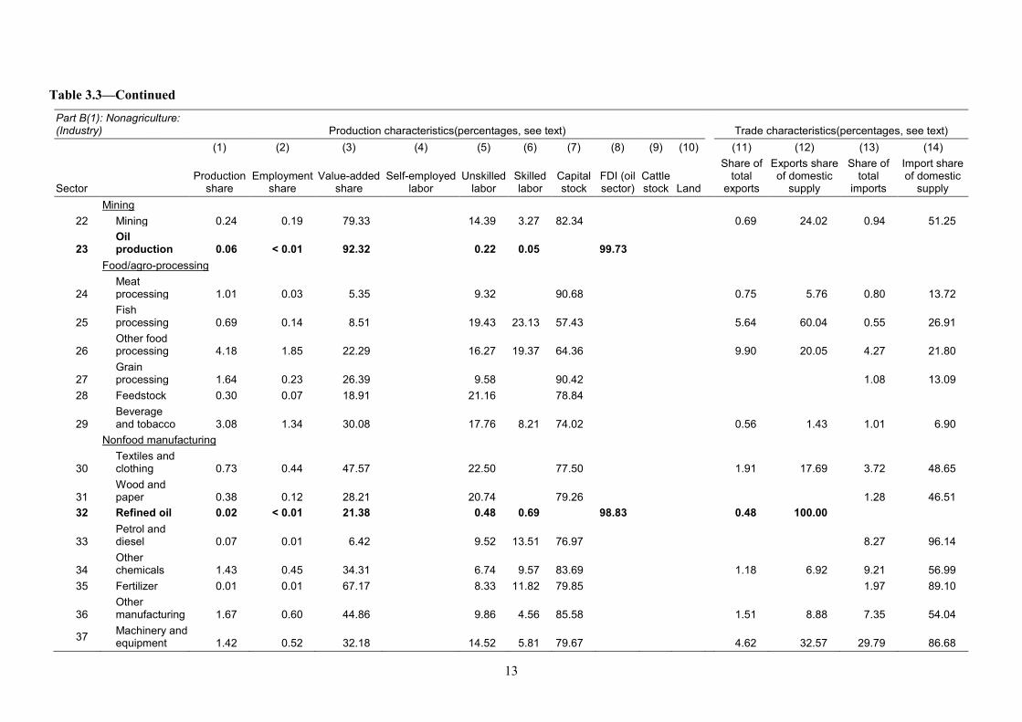
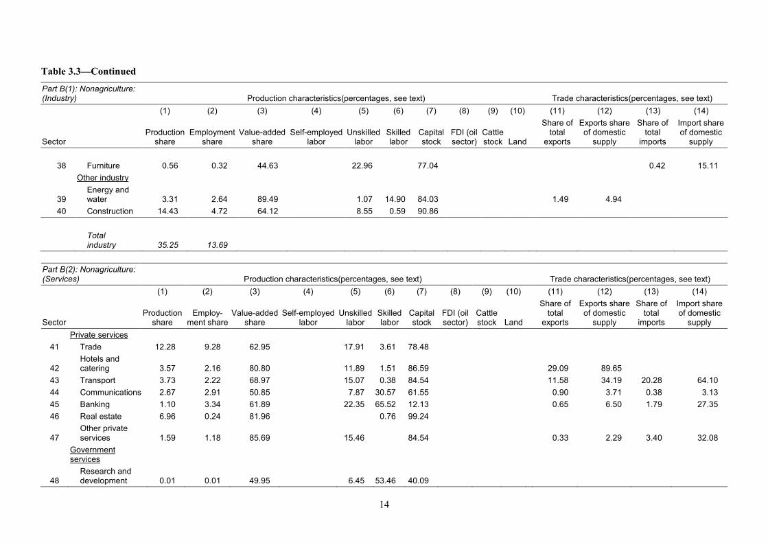
As shown in Table 3.3 (Part A), we broadly classify agricultural crops in the model into six groups, namely: (1) cereal crops, (2) root crops, (3) matooke, (4) pulses and oilseeds, (5) horticulture, and (6) export-oriented crops. The CGE model further identifies three livestock subsectors, namely, cattle, poultry, and other livestock, as well as forestry and fisheries subsectors. The 31 nonagricultural sectors found in the SAM are listed in Table 3.3 (Part B). Broadly speaking, nonagricultural sectors can be grouped into two groups, namely, industrial and services subsectors. Industrial sectors include (1) mining, (2) food-processing or agroprocessing sectors, (3) nonfood manufacturing, and (4) other industry. Services, in turn, include (5) private services and (6) government services.
Production characteristics for each sector are shown in Table 3.3 in the columns labeled (1) to (10). The first column shows gross output agriculture in the Uganda SAM contributes 18 percent to total output (note Table 3.1 shows value-added or GDP). Within agriculture, subsistence farming of cereals, root crops, matooke, and cattle account for around 60 percent of total agricultural production. Industry, in turn, contributes 35.2 percent, a third of which is from food-processing or agroprocessing sectors. The construction sector is the largest subsector in Uganda, contributing 14.4 percent to total output. Services sectors contribute 46.8 percent to output, with the trade sector (12.3 percent) dominating.
Column (2) shows the employment shares across the various subsectors. The fairly labor-intensive agricultural sector employs 23.2 percent of the workforce, made up mostly of self-employed family labor. This figure, however, understates the true importance of the agricultural sector as a provider of household income, since about 80 percent of the population lives in households that are attached to the agricultural sector. Industrial sectors are significantly more capital intensive; although the sector contributes more than one-third to GDP, it only offers employment to 13.7 percent of the workforce. In contrast, the employment share in the labor-intensive-services sector is relatively high at 63.1 percent.
Column (3) shows each sector’s share of expenditure on value addition. The balance of expenditure is on intermediate inputs. The latter provides an indication of the strength of a sector’s backward linkages in the economy (compare Table 3.2). High value-added ratios in the agricultural, natural resource–based sectors (such as crude oil) and in most services sectors are indicative of relatively small backward linkages. In contrast, the manufacturing sectors, particularly food processing and oil refining, exhibit relatively value-added ratios, suggesting these have strong backward linkages.
12
Table 3.3—Production and trade characteristics in Uganda, 2007
Part A: Agriculture Production characteristics(percentages, see text) Trade characteristics(percentages, see text) (1) (2) (3) (4) (5) (6) (7) (8) (9) (10) (11) (12) (13) (14)
Sector
Production share
Employ-ment share
Value-added share
Self-employed labor
Unskilled labor
Skilled labor
Capital stock
FDI (oil sector)
Cattle stock Land
Share of total
exports
Exports share of domestic
supply
Share of total
imports
Import share of domestic
supply Cereal crops 1 Maize 0.80 0.92 89.30 21.08 1.78 5.43 71.71 1.76 19.95 0.85 21.62 2 Rice 0.20 0.22 91.66 19.17 1.62 5.84 73.37 0.34 26.94 3 Other cereals 0.82 0.72 87.51 16.72 1.42 6.37 75.49 2.14 35.53 Root crops 4 Cassava 1.47 1.00 87.98 12.76 1.08 7.23 78.93 5 Irish potato 0.52 0.28 49.99 17.78 1.50 6.14 74.57 6 Sweet potato 1.18 0.87 82.54 14.81 1.25 6.79 77.15 7 Matooke 1.55 1.17 96.85 12.83 1.09 7.22 78.87 Pulses and oilseeds 8 Oilseeds 0.39 0.41 98.04 17.69 1.50 6.16 74.65 0.16 3.81 0.14 7.27 9 Beans 2.01 1.15 71.80 13.14 1.11 7.15 78.60 4.07 17.41 Horticulture 10 Vegetable 0.06 0.06 90.97 19.13 1.62 5.85 73.40 11 Fruits and tree crops 0.12 0.12 90.73 19.22 1.63 5.83 73.32 Export crops 12 Cotton 0.12 0.10 68.28 20.32 1.72 22.37 55.59 1.13 100.00 13 Tobacco 0.46 0.43 91.40 16.96 1.44 25.29 56.32 3.81 91.96 14 Flowers 0.24 0.09 39.52 14.71 1.25 27.23 56.81 2.21 100.00 15 Coffee 0.82 0.54 72.97 14.79 1.25 27.16 56.79 7.48 100.00
16 Tea, cocoa, and vanilla 0.26 0.37 81.55 28.55 2.42 15.23 53.81
2.40 100.00
Livestock 17 Cattle and sheep 1.13 1.44 66.60 31.59 2.67 65.74 18 Other livestock 0.19 0.27 89.33 26.20 2.22 71.58 0.23 11.59 19 Poultry 0.22 0.15 48.56 22.37 1.89 75.74 20 Forestry 3.43 9.61 70.80 70.99 29.01 21 Fisheries 2.01 3.33 92.56 32.02 67.98 5.47 26.09 Total agriculture 18.01 23.24 11.84 17.14 19.71 4.86 46.45 28.72 16.36 3.48 4.55
13
Table 3.3—Continued
Part B(1): Nonagriculture: (Industry) Production characteristics(percentages, see text)
Trade characteristics(percentages, see text)
(1) (2) (3) (4) (5) (6) (7) (8) (9) (10) (11) (12) (13) (14)
Sector
Production share
Employment share
Value-added share
Self-employed labor
Unskilled labor
Skilled labor
Capital stock
FDI (oil sector)
Cattle stock Land
Share of total
exports
Exports share of domestic
supply
Share of total
imports
Import share of domestic
supply Mining
22 Mining 0.24 0.19 79.33 14.39 3.27 82.34 0.69 24.02 0.94 51.25
23 Oil production 0.06 < 0.01 92.32 0.22 0.05 99.73
Food/agro-processing
24 Meat processing 1.01 0.03 5.35 9.32 90.68
0.75 5.76 0.80 13.72
25 Fish processing 0.69 0.14 8.51 19.43 23.13 57.43
5.64 60.04 0.55 26.91
26 Other food processing 4.18 1.85 22.29 16.27 19.37 64.36
9.90 20.05 4.27 21.80
27 Grain processing 1.64 0.23 26.39 9.58 90.42
1.08 13.09
28 Feedstock 0.30 0.07 18.91 21.16 78.84
29 Beverage and tobacco 3.08 1.34 30.08 17.76 8.21 74.02
0.56 1.43 1.01 6.90
Nonfood manufacturing
30 Textiles and clothing 0.73 0.44 47.57 22.50 77.50
1.91 17.69 3.72 48.65
31 Wood and paper 0.38 0.12 28.21 20.74 79.26
1.28 46.51
32 Refined oil 0.02 < 0.01 21.38 0.48 0.69 98.83 0.48 100.00
33 Petrol and diesel 0.07 0.01 6.42 9.52 13.51 76.97
8.27 96.14
34 Other chemicals 1.43 0.45 34.31 6.74 9.57 83.69
1.18 6.92 9.21 56.99
35 Fertilizer 0.01 0.01 67.17 8.33 11.82 79.85 1.97 89.10
36 Other manufacturing 1.67 0.60 44.86 9.86 4.56 85.58
1.51 8.88 7.35 54.04
37 Machinery and equipment 1.42 0.52 32.18 14.52 5.81 79.67
4.62 32.57 29.79 86.68
14
Table 3.3—Continued
Part B(1): Nonagriculture: (Industry) Production characteristics(percentages, see text)
Trade characteristics(percentages, see text)
(1) (2) (3) (4) (5) (6) (7) (8) (9) (10) (11) (12) (13) (14)
Sector
Production share
Employment share
Value-added share
Self-employed labor
Unskilled labor
Skilled labor
Capital stock
FDI (oil sector)
Cattle stock Land
Share of total
exports
Exports share of domestic
supply
Share of total
imports
Import share of domestic
supply
38 Furniture 0.56 0.32 44.63 22.96 77.04 0.42 15.11 Other industry
39 Energy and water 3.31 2.64 89.49 1.07 14.90 84.03
1.49 4.94
40 Construction 14.43 4.72 64.12 8.55 0.59 90.86
Total industry 35.25 13.69
Part B(2): Nonagriculture: (Services) Production characteristics(percentages, see text)
Trade characteristics(percentages, see text)
(1) (2) (3) (4) (5) (6) (7) (8) (9) (10) (11) (12) (13) (14)
Sector
Production share
Employ-ment share
Value-added share
Self-employed labor
Unskilled labor
Skilled labor
Capital stock
FDI (oil sector)
Cattle stock Land
Share of total
exports
Exports share of domestic
supply
Share of total
imports
Import share of domestic
supply Private services
41 Trade 12.28 9.28 62.95 17.91 3.61 78.48
42 Hotels and catering 3.57 2.16 80.80 11.89 1.51 86.59
29.09 89.65
43 Transport 3.73 2.22 68.97 15.07 0.38 84.54 11.58 34.19 20.28 64.10 44 Communications 2.67 2.91 50.85 7.87 30.57 61.55 0.90 3.71 0.38 3.13 45 Banking 1.10 3.34 61.89 22.35 65.52 12.13 0.65 6.50 1.79 27.35 46 Real estate 6.96 0.24 81.96 0.76 99.24
47 Other private services 1.59 1.18 85.69 15.46 84.54
0.33 2.29 3.40 32.08
Government services
48 Research and development 0.01 0.01 49.95 6.45 53.46 40.09
15
Table 3.3—Continued
Part B(2): Nonagriculture: (Services) Production characteristics(percentages, see text)
Trade characteristics (percentages, see text)
(1) (2) (3) (4) (5) (6) (7) (8) (9) (10) (11) (12) (13) (14)
Sector
Production share
Employ-ment share
Value-added share
Self-employed labor
Unskilled labor
Skilled labor
Capital stock
FDI (oil sector)
Cattle stock Land
Share of total
exports
Exports share of domestic
supply
Share of total
imports
Import share of domestic
supply
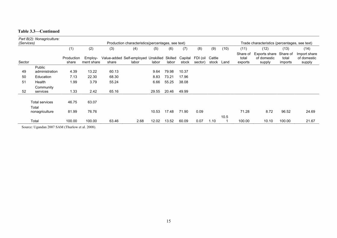
49 Public administration 4.39 13.22 60.13 9.64 79.98 10.37
50 Education 7.13 22.30 68.30 8.83 73.21 17.96 51 Health 1.99 3.79 55.24 6.66 55.25 38.08
52 Community services 1.33 2.42 65.16 29.55 20.46 49.99
Total services 46.75 63.07
Total nonagriculture 81.99 76.76 10.53 17.48 71.90 0.09
71.28 8.72 96.52 24.69
Total 100.00 100.00 63.46 2.68 12.02 13.52 60.09 0.07 1.10 10.5
1
100.00 10.10 100.00 21.67
Source: Ugandan 2007 SAM (Thurlow et al. 2008).
16
Columns (4) to (10) show the factor income shares within sectors (that is, the row entries across these seven columns sum to 100). The SAM includes three main labor categories, namely, self-employed farm labor (only employed in agriculture), unskilled workers (employed across all sectors), and skilled workers (only employed in nonagricultural sectors). Other factors include capital stock (a separate capital stock category was created for capital stock employed in the newly created oil production and refining sectors), cattle, and land (the latter two factors are only employed in agriculture). Within agriculture, food and cash crop sectors are land intensive, with returns to land representing about 50 percent of value-added. Returns on livestock average about 70 percent of value-added. The production structures in the forestry and fisheries sectors are more akin to those in industrial sectors, that is, a relatively large share of value-added goes to capital (for example, in fisheries) or unskilled labor (for example, in forestry). Industrial and services sectors are generally capital intensive, the exception being banking and public sectors, which are more skilled-labor intensive. Labor use in capital-intensive industrial and services sectors also follows a fairly predictable pattern, with food-processing and consumer goods sectors spending relatively more on unskilled labor, whereas the other manufacturing sectors are relatively skilled-labor intensive.
The final four columns in Table 3.3 provide information on each sector’s share in total foreign exchange earnings and expenditures together with each sector’s trade orientation. Column (12) indicates that agriculture exports about 16 percent of its production, with cotton, tobacco, flowers, coffee, tea, cocoa, and vanilla being the most export-oriented sectors in the economy. Other sectors with a high share of exports in domestic production are fish processing and hotels and catering. Overall, nonagriculture is less export-oriented than agriculture, with exports only accounting for about 9 percent of total supply. The single most important foreign exchange earner is the tourism sector (hotels and catering), which contributes almost 30 percent to total foreign exchange earnings from exports. On the import side, the sectoral shares of total import expenditures in column (13) and the shares of imports in sectoral demand in column (14) are of interest. These show that about 70 percent of import expenditures are on imports of capital and intermediate goods, as well as the related transport services.
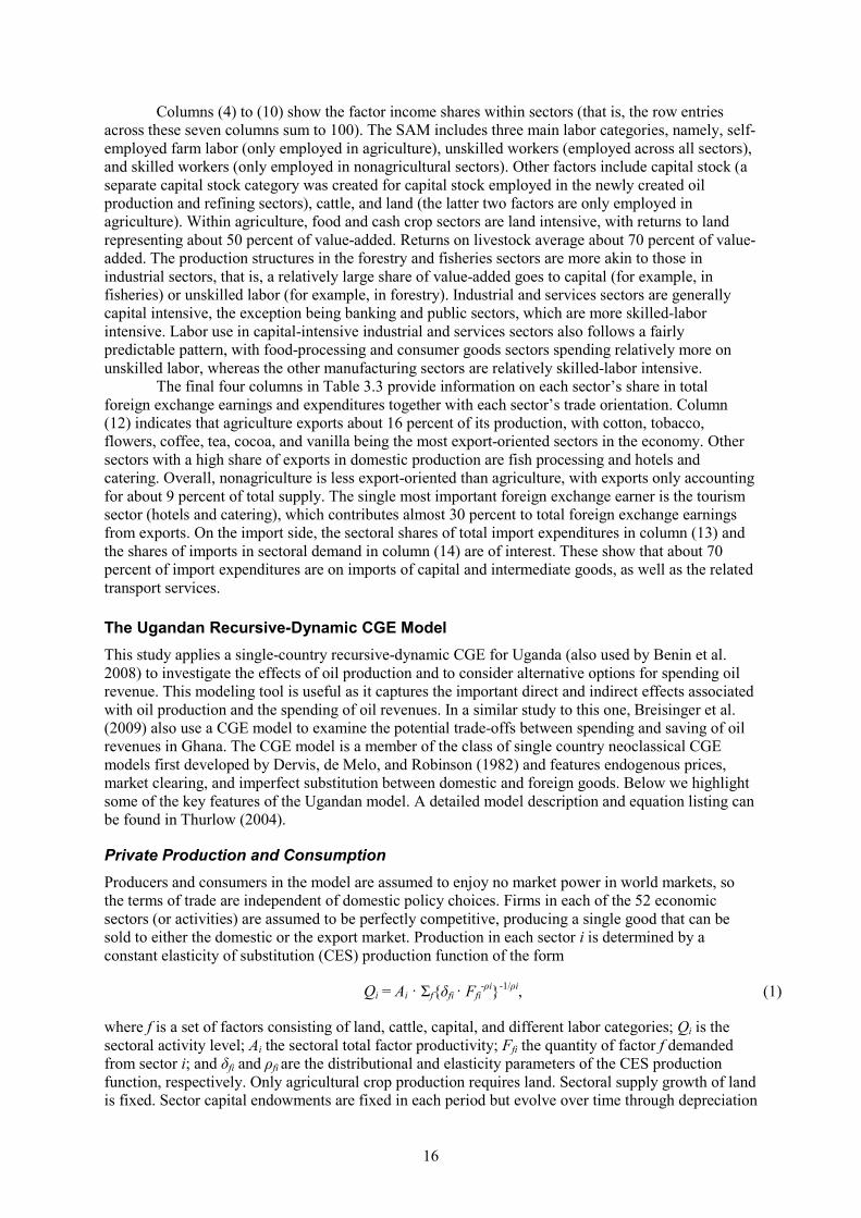
The Ugandan Recursive-Dynamic CGE Model This study applies a single-country recursive-dynamic CGE for Uganda (also used by Benin et al. 2008) to investigate the effects of oil production and to consider alternative options for spending oil revenue. This modeling tool is useful as it captures the important direct and indirect effects associated with oil production and the spending of oil revenues. In a similar study to this one, Breisinger et al. (2009) also use a CGE model to examine the potential trade-offs between spending and saving of oil revenues in Ghana. The CGE model is a member of the class of single country neoclassical CGE models first developed by Dervis, de Melo, and Robinson (1982) and features endogenous prices, market clearing, and imperfect substitution between domestic and foreign goods. Below we highlight some of the key features of the Ugandan model. A detailed model description and equation listing can be found in Thurlow (2004).
Private Production and Consumption Producers and consumers in the model are assumed to enjoy no market power in world markets, so the terms of trade are independent of domestic policy choices. Firms in each of the 52 economic sectors (or activities) are assumed to be perfectly competitive, producing a single good that can be sold to either the domestic or the export market. Production in each sector i is determined by a constant elasticity of substitution (CES) production function of the form
Qi = Ai · Σf{δfi · Ffi-ρi}-1/ρi, (1)
where f is a set of factors consisting of land, cattle, capital, and different labor categories; Qi is the sectoral activity level; Ai the sectoral total factor productivity; Ffi the quantity of factor f demanded from sector i; and δfi and ρfi are the distributional and elasticity parameters of the CES production function, respectively. Only agricultural crop production requires land. Sectoral supply growth of land is fixed. Sector capital endowments are fixed in each period but evolve over time through depreciation
17
and investment. Capital and labor markets are competitive so that these factors are employed in each sector up to the point that they are paid the value of their marginal product. Private-sector output is also determined by the level of infrastructure, which is provided costless by the government. We assume that total sector factor productivity Ai depends on the availability of public infrastructure.
Consumption for each household type is defined by a constant elasticity of substitution linear expenditure system, which allows for the income elasticity of demand for different goods to deviate from unity. The CGE model endogenously estimates the impact of alternative growth paths on the incomes of various household groups. These household groups include farm and nonfarm households and are disaggregated across rural areas, the major city of Kampala, and other smaller urban centers. Each of the households questioned in the 2005/06 Uganda National Household Survey (UNHS5) are linked directly to their corresponding representative household in the CGE model. This is the microsimulation component of the Ugandan model. Changes in representative households’ consumption and prices in the CGE model are passed down to the corresponding households in the survey, where standard poverty measures and changes in poverty are calculated.
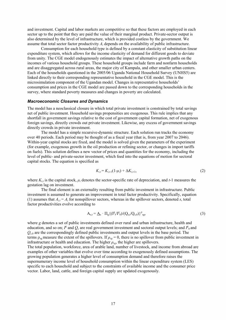
Macroeconomic Closures and Dynamics The model has a neoclassical closure in which total private investment is constrained by total savings net of public investment. Household savings propensities are exogenous. This rule implies that any shortfall in government savings relative to the cost of government capital formation, net of exogenous foreign savings, directly crowds out private investment. Likewise, any excess of government savings directly crowds in private investment.
The model has a simple recursive-dynamic structure. Each solution run tracks the economy over 40 periods. Each period may be thought of as a fiscal year (that is, from year 2007 to 2046). Within-year capital stocks are fixed, and the model is solved given the parameters of the experiment (for example, exogenous growth in the oil production or refining sector, or changes in import tariffs on fuels). This solution defines a new vector of prices and quantities for the economy, including the level of public- and private-sector investment, which feed into the equations of motion for sectoral capital stocks. The equation is specified as
Ki,t = Ki,t-1(1-μi) + ΔKi,t-1, (2)
where Ki,t is the capital stock, μi denotes the sector-specific rate of depreciation, and t-1 measures the gestation lag on investment.
The final element is an externality resulting from public investment in infrastructure. Public investment is assumed to generate an improvement in total factor productivity. Specifically, equation (1) assumes that Αi,t = Αi for nonspillover sectors, whereas in the spillover sectors, denoted s, total factor productivities evolve according to
As,t = As · Πg{(Igt/Ig
0)/(Qs,t/Qs,0)}ρsg, (3)
where g denotes a set of public investments defined over rural and urban infrastructure, health and education, and so on; Ig and Qs are real government investment and sectoral output levels; and Ig
0 and Qs,0 are the correspondingly defined public investments and output levels in the base period. The terms ρsg measure the extent of the spillovers. If ρsg = 0, there is no spillover from public investment in infrastructure or health and education. The higher ρsg, the higher are spillovers. The total population, workforce, area of arable land, number of livestock, and income from abroad are examples of other variables that evolve over time according to exogenously defined assumptions. The growing population generates a higher level of consumption demand and therefore raises the supernumerary income level of household consumption within the linear expenditure system (LES) specific to each household and subject to the constraints of available income and the consumer price vector. Labor, land, cattle, and foreign capital supply are updated exogenously.
18
Simulation Setup
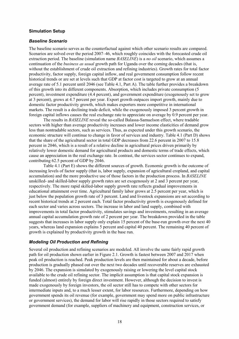
Baseline Scenario The baseline scenario serves as the counterfactual against which other scenario results are compared. Scenarios are solved over the period 2007–46, which roughly coincides with the forecasted crude oil extraction period. The baseline (simulation name BASELINE) is a no oil scenario, which assumes a continuation of the business as usual growth path for Uganda over the coming decades (that is, without the establishment of crude oil extraction and refining industries). Growth rates for total factor productivity, factor supply, foreign capital inflow, and real government consumption follow recent historical trends or are set at levels such that GDP at factor cost is targeted to grow at an annual average rate of 5.1 percent until 2046 (see Table 4.1, Part A). The table further provides a breakdown of this growth into its different components. Absorption, which includes private consumption (5 percent), investment expenditure (4.4 percent), and government expenditure (exogenously set to grow at 3 percent), grows at 4.7 percent per year. Export growth outpaces import growth, mainly due to domestic factor productivity growth, which makes exporters more competitive in international markets. The result is a declining trade deficit, while the exogenously imposed 3 percent growth in foreign capital inflows causes the real exchange rate to appreciate on average by 0.9 percent per year.
The results in BASELINE reveal the so-called Balassa-Samuelson effect, where tradable sectors with higher than average productivity increases and lower income elasticities of demand grow less than nontradable sectors, such as services. Thus, as expected under this growth scenario, the economic structure will continue to change in favor of services and industry. Table 4.1 (Part D) shows that the share of the agricultural sector in total GDP decreases from 22.6 percent in 2007 to 15.8 percent in 2046, which is a result of a relative decline in agricultural prices driven primarily by relatively lower domestic demand for agricultural products and domestic terms of trade effects, which cause an appreciation in the real exchange rate. In contrast, the services sector continues to expand, contributing 62.5 percent of GDP by 2046.
Table 4.1 (Part E) shows the different sources of growth. Economic growth is the outcome of increasing levels of factor supply (that is, labor supply, expansion of agricultural cropland, and capital accumulation) and the more productive use of those factors in the production process. In BASELINE unskilled- and skilled-labor supply growth rates are set exogenously at 2 and 3 percent per year, respectively. The more rapid skilled-labor supply growth rate reflects gradual improvements in educational attainment over time. Agricultural family labor grows at 2.5 percent per year, which is just below the population growth rate of 3 percent. Land and livestock expansions are set according to recent historical trends at 2 percent each. Total factor productivity growth is exogenously defined for each sector and varies across sectors. The increase in labor and land supply, combined with improvements in total factor productivity, stimulates savings and investments, resulting in an average annual capital accumulation growth rate of 2 percent per year. The breakdown provided in the table suggests that increases in labor supply only explain 15 percent of the base-run growth over the next 40 years, whereas land expansion explains 5 percent and capital 40 percent. The remaining 40 percent of growth is explained by productivity growth in the base run.
Modeling Oil Production and Refining Several oil production and refining scenarios are modeled. All involve the same fairly rapid growth path for oil production shown earlier in Figure 2.1. Growth is fastest between 2007 and 2017 when peak oil production is reached. Peak production levels are then maintained for about a decade, before production is gradually phased out over the next two decades until recoverable reserves are exhausted by 2046. The expansion is simulated by exogenously raising or lowering the level capital stock available to the crude oil refining sector. The implicit assumption is that capital stock expansion is funded (almost) entirely by foreign direct investment. However, although the decision to invest is made exogenously by foreign investors, the oil sector still has to compete with other sectors for intermediate inputs and, to a much lesser extent, for labor resources. Furthermore, depending on how government spends its oil revenue (for example, government may spend more on public infrastructure or government services), the demand for labor will rise rapidly in those sectors required to satisfy government demand (for example, suppliers of machinery and equipment, construction services, or
19
public service providers). All crude oil is supplied to the refining sector. Supply bottlenecks are avoided by applying a similar capital stock growth rate to the refining sector as the one that determines crude oil production levels.
The CGE model assumes full employment, which means that total labor supply is determined by the long labor supply growth rates, whereas an increase in labor demanded per unit of capital raises workers’ relative wages. Profits—or returns to capital stock—generated in the oil production and refining sectors are shared between the foreign owners of capital (their share is repatriated) and the Ugandan government (revenue is transferred via a 74.4 percent tax on returns to capital). These profits originate by and large from refined oil exports. All crude oil is supplied to the oil refineries, and for the sake of simplicity all refined oil is assumed to be exported. Domestic demand for petroleum products is, in turn, met by imports. In reality, some of the refined oil product will be retained for domestic consumption and the country will cease to import petroleum products, but modeling it in this manner is simpler and does not affect results since the balance of payments effect is symmetrical.
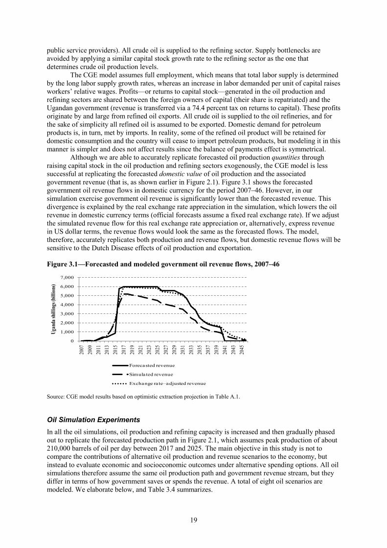
Although we are able to accurately replicate forecasted oil production quantities through raising capital stock in the oil production and refining sectors exogenously, the CGE model is less successful at replicating the forecasted domestic value of oil production and the associated government revenue (that is, as shown earlier in Figure 2.1). Figure 3.1 shows the forecasted government oil revenue flows in domestic currency for the period 2007–46. However, in our simulation exercise government oil revenue is significantly lower than the forecasted revenue. This divergence is explained by the real exchange rate appreciation in the simulation, which lowers the oil revenue in domestic currency terms (official forecasts assume a fixed real exchange rate). If we adjust the simulated revenue flow for this real exchange rate appreciation or, alternatively, express revenue in US dollar terms, the revenue flows would look the same as the forecasted flows. The model, therefore, accurately replicates both production and revenue flows, but domestic revenue flows will be sensitive to the Dutch Disease effects of oil production and exportation.
Figure 3.1—Forecasted and modeled government oil revenue flows, 2007–46
Source: CGE model results based on optimistic extraction projection in Table A.1.
Oil Simulation Experiments In all the oil simulations, oil production and refining capacity is increased and then gradually phased out to replicate the forecasted production path in Figure 2.1, which assumes peak production of about 210,000 barrels of oil per day between 2017 and 2025. The main objective in this study is not to compare the contributions of alternative oil production and revenue scenarios to the economy, but instead to evaluate economic and socioeconomic outcomes under alternative spending options. All oil simulations therefore assume the same oil production path and government revenue stream, but they differ in terms of how government saves or spends the revenue. A total of eight oil scenarios are modeled. We elaborate below, and Table 3.4 summarizes.
0
1,000
2,000
3,000
4,000
5,000
6,000
7,000
2007
2009
2011
2013
2015
2017
2019
2021
2023
2025
2027
2029
2031
2033
2035
2037
2039
2041
2043
2045
Ugan
da sh
illing
s (bil
lions
)
Forecasted revenue
Simulated revenue
Exchange rate–adjusted revenue
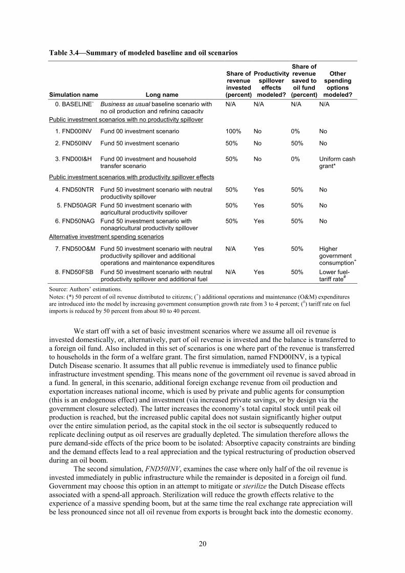
20
Table 3.4—Summary of modeled baseline and oil scenarios
Simulation name Long name
Share of revenue invested (percent)
Productivity spillover effects
modeled?
Share of revenue saved to oil fund
(percent)
Other spending options
modeled? 0. BASELINE` Business as usual baseline scenario with
no oil production and refining capacity N/A N/A N/A N/A
Public investment scenarios with no productivity spillover
1. FND00INV Fund 00 investment scenario 100% No 0% No
2. FND50INV Fund 50 investment scenario 50% No 50% No
3. FND00I&H Fund 00 investment and household transfer scenario
50% No 0% Uniform cash grant*
Public investment scenarios with productivity spillover effects
4. FND50NTR Fund 50 investment scenario with neutral productivity spillover
50% Yes 50% No
5. FND50AGR Fund 50 investment scenario with agricultural productivity spillover
50% Yes 50% No
6. FND50NAG Fund 50 investment scenario with nonagricultural productivity spillover
50% Yes 50% No
Alternative investment spending scenarios
7. FND50O&M Fund 50 investment scenario with neutral productivity spillover and additional operations and maintenance expenditures
N/A Yes 50% Higher government consumption+
8. FND50FSB Fund 50 investment scenario with neutral productivity spillover and additional fuel
N/A Yes 50% Lower fuel-tariff rate#
Source: Authors’ estimations. Notes: (*) 50 percent of oil revenue distributed to citizens; (+) additional operations and maintenance (O&M) expenditures are introduced into the model by increasing government consumption growth rate from 3 to 4 percent; (#) tariff rate on fuel imports is reduced by 50 percent from about 80 to 40 percent.
We start off with a set of basic investment scenarios where we assume all oil revenue is invested domestically, or, alternatively, part of oil revenue is invested and the balance is transferred to a foreign oil fund. Also included in this set of scenarios is one where part of the revenue is transferred to households in the form of a welfare grant. The first simulation, named FND00INV, is a typical Dutch Disease scenario. It assumes that all public revenue is immediately used to finance public infrastructure investment spending. This means none of the government oil revenue is saved abroad in a fund. In general, in this scenario, additional foreign exchange revenue from oil production and exportation increases national income, which is used by private and public agents for consumption (this is an endogenous effect) and investment (via increased private savings, or by design via the government closure selected). The latter increases the economy’s total capital stock until peak oil production is reached, but the increased public capital does not sustain significantly higher output over the entire simulation period, as the capital stock in the oil sector is subsequently reduced to replicate declining output as oil reserves are gradually depleted. The simulation therefore allows the pure demand-side effects of the price boom to be isolated: Absorptive capacity constraints are binding and the demand effects lead to a real appreciation and the typical restructuring of production observed during an oil boom.
The second simulation, FND50INV, examines the case where only half of the oil revenue is invested immediately in public infrastructure while the remainder is deposited in a foreign oil fund. Government may choose this option in an attempt to mitigate or sterilize the Dutch Disease effects associated with a spend-all approach. Sterilization will reduce the growth effects relative to the experience of a massive spending boom, but at the same time the real exchange rate appreciation will be less pronounced since not all oil revenue from exports is brought back into the domestic economy.
21
Although this may benefit export sectors in the short run, the net effect in the long run is not certain since investment flows and capital stock formation is lower in this scenario.
A third simulation, FND00I&H, investigates the option of using oil revenues to finance an unconditional uniform cash transfer scheme. This simulation assumes no deposit in a foreign oil fund; instead, half of oil revenue is spent on infrastructural investments (as in FND50INV) and the remainder is distributed equally among Uganda’s citizens. The cash transfer is modeled as a nonuniform income tax cut across all household groups. The extent of the tax break varies across household groups in the model such that each citizen, irrespective of his or her age, receives the same per capita transfer in absolute terms (that is, initial average income tax rates and the size of household groups are taken into account in the calculation of the applicable tax cuts). In relative terms, therefore, poorer citizens receive a much larger welfare transfer than wealthy citizens. Since average tax rates are low in Uganda, several household groups end up with a negative tax rate, which effectively means their earnings from welfare transfers exceed income tax payments. If such a uniform grant scheme ever became a reality in Uganda it could be justified on the basis that each citizen in Uganda is entitled to an equal share of oil revenue. The design of the transfer mechanism implies that household incomes will rise across the board by the same absolute magnitude, causing poverty rates to decline, but income inequality will remain virtually unchanged. In contrast to the earlier scenarios, this simulation will lead to an increase in private disposable income, which is used by households to increase consumption and savings. The latter, in turn, finances private investment formation. Low savings rates, however, suggest that most of the additional income will be spent on household consumption.
Whereas the first set of oil simulations assume zero productivity spillover effects from public investments, the second set of simulations explore the importance of such productivity spillover. The aim here is to demonstrate not only the importance, in general, of ensuring that public investments are indeed productivity-enhancing, but also to show how investments that aim to raise productivity in specific sectors in the economy (for example, through direct targeting of agricultural or nonagricultural sectors) may ultimately have important growth and welfare or distributional implications. The scenarios all follow the same basic setup as FND50INV (that is, half of revenues are saved abroad and the other half is allocated to public infrastructure investments), but now assume that government infrastructure investment raises productivity relative to the growth already assumed in BASELINE. In FND50NTR the productivity-enhancing effect is uniform or neutral across sectors, whereas in FND50AGR and FND50NAG total factor productivity growth is biased in favor of agricultural/food-processing and nonagricultural sectors, respectively.
The extent of the total factor productivity spillover effects in each sector is linked directly to the level of spending on each of several budget items. Equation (3) defines this relationship. Thus, as explained before, any increase (or decrease) in the real government investment index Ig
t/Ig0 in relation
to the sector production index Qs,t/Qs,0 raises (or reduces) sectoral total factor productivity As,t, with the extent of the increase (reduction) determined by the spillover parameter ρsg. In the first set of investment simulations ρsg was set to zero, whereas in the spillover simulations ρsg = 0.1. Since the structure of government spending is likely to have a bearing on sectoral productivity spillover effects (Fan, Mogues, and Benin 2009), FND50AGR and FND50NAG assume both an increase in total government investment spending (as in FND50INV) and also a change in the composition of that spending. Data on the current budget composition are obtained from Sennoga and Matovu (2010) and Twimukye et al. (2010). In FND50AGR we increase the allocation to agriculture by 20 percent (or 0.8 percentage points) from 3.8 to 4.6 percent of total budgetary resources, while at the same the expenditure share to roads is reduced by 0.8 percentage points. In FND50NAG we assume the opposite, that is, the expenditure share on agriculture is reduced by 0.8 percent and vice versa for roads. Next, growth-expenditure elasticities (from Benin et al. 2008) are applied to calculate the marginal effect of the absolute and compositional shift in public expenditure sectoral productivity. The growth-expenditure elasticity for agricultural spending is 1.4, whereas it is 2.7 for roads. The result is that total factor productivities in agriculture and food-processing sectors increase by about 25 percent in FND50AGR, while they decrease by about 10 percent in other manufacturing and trade and transport sectors (these changes are relative to the growth rate in BASELINE). The effects are the exact opposite in FND50NAG. In the neutral spending scenario (FND50NTR) there is no compositional shift in spending, hence productivity across all sectors grows by the same margin.
22
4. MODEL RESULTS
Public Investment Scenarios with No Productivity Spillover Effects
Spending All Revenues on Infrastructure (FND00INV) The major effects and transmission channels of the oil boom in Uganda are described with reference to the results of scenario FND00INV, which serves as the benchmark for other oil scenarios. Public investment expenditures are linked directly to government oil revenue and will therefore increase until peak oil production is reached in 2017. Thereafter these expenditures gradually decline due to declining government oil revenues (which in turn is linked to the real exchange rate appreciation) and the gradual winding down of oil production activities (see Figure 3.1). The recursive-dynamic computable general equilibrium (CGE) model is set up so that public investments in the current period raise the total capital stock in the next period. In addition to these investments being assumed to have no productivity spillover effects (that is, total factor productivity growth is the same as in BASELINE), the declining investment levels after 2017 imply that the oil boom does not sustain significantly higher levels of output in the long run.
Under FND00INV the Ugandan economy grows rapidly at 6.9 percent per year until 2017, mainly because of the large increase in real public-sector investment (see Table 4.1, Part A). Overall investment grows at 9.5 percent per year over this period. Household income also rises in these scenarios, which leads to an increase in private consumption (by 5.1 percent during 2007–17) and savings. However, private savings as a share of GDP actually declines (not reported in Table 4.1), which suggests the oil boom crowds out private-sector investment, at least in relative terms. A further factor is the real exchange rate appreciation. Although in general such an appreciation would mean imported capital goods become less expensive, capital formation in Uganda is in fact intensive in nontradable goods (for example, nontradable construction goods make up 78 percent of investments). This means that foreign capital inflows, which are assumed to grow at 3 percent annually in all scenarios, finance less and less real investment over time. Diminishing oil reserves means the real exchange rate appreciation weakens over time, but this is not sufficient to reverse the trend of declining non-oil exports. In fact, the initial welfare gains associated with the surge in public-sector investment weaken over time as other components of GDP (for example, private investments, consumption, and exports) fail to grow more rapidly when public investments eventually decline.
A comparison of FND00INV with BASELINE reveals the typical characteristics of Dutch Disease. The consumer price index increases at an average annual rate of 1.2 percent during 2007–46, while the (trade-weighted) real exchange rate appreciates by 1.3 percent between 2007 and 2017 or by 1.2 percent per year over the entire 2007–46 period. Relative to BASELINE, the spending of windfall revenues leads to a 0.2 and 1.5 percentage point contraction in agriculture and services, respectively, in the medium term (2007–17; see Table 4.1, Part B). These two sectors’ shares of GDP also decline dramatically by 4.6 and 16.4 percentage points relative to the base (2007–17; see Table 4.1, Part D). The services sector regains growth momentum in the long run, but agricultural growth only improves marginally relative to the base. Thus, while real GDP at factor cost increases, the agricultural sector actually suffers a decline in GDP, both absolutely (compared to BASELINE) during the oil expansion period and relative to other sectors over the oil extraction period (Table 4.1, Part B). The services sector also realizes absolute income losses in the medium term, but a reversal of fortunes sees this sector become the engine of long-term growth (Table 4.1, Part C). Of course, the observed structural shift is also a feature of the BASELINE scenario, and is, to a large extent, a natural outcome for any developing country’s growth path.
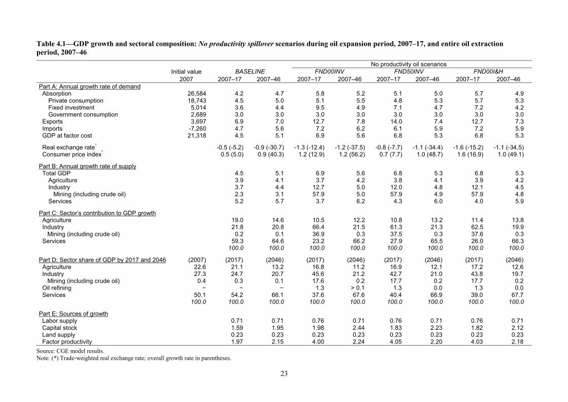
23
Table 4.1—GDP growth and sectoral composition: No productivity spillover scenarios during oil expansion period, 2007–17, and entire oil extraction period, 2007–46 No productivity oil scenarios Initial value BASELINE FND00INV FND50INV FND00I&H 2007 2007–17 2007–46 2007–17 2007–46 2007–17 2007–46 2007–17 2007–46 Part A: Annual growth rate of demand Absorption 26,584 4.2 4.7 5.8 5.2 5.1 5.0 5.7 4.9
Private consumption 18,743 4.5 5.0 5.1 5.5 4.8 5.3 5.7 5.3 Fixed investment 5,014 3.6 4.4 9.5 4.9 7.1 4.7 7.2 4.2 Government consumption 2,689 3.0 3.0 3.0 3.0 3.0 3.0 3.0 3.0
Exports 3,697 6.9 7.0 12.7 7.8 14.0 7.4 12.7 7.3 Imports -7,260 4.7 5.6 7.2 6.2 6.1 5.9 7.2 5.9 GDP at factor cost 21,318 4.5 5.1 6.9 5.6 6.8 5.3 6.8 5.3 Real exchange rate* -0.5 (-5.2) -0.9 (-30.7) -1.3 (-12.4) -1.2 (-37.5) -0.8 (-7.7) -1.1 (-34.4) -1.6 (-15.2) -1.1 (-34.5) Consumer price index* 0.5 (5.0) 0.9 (40.3) 1.2 (12.9) 1.2 (56.2) 0.7 (7.7) 1.0 (48.7) 1.6 (16.9) 1.0 (49.1) Part B: Annual growth rate of supply Total GDP 4.5 5.1 6.9 5.6 6.8 5.3 6.8 5.3
Agriculture 3.9 4.1 3.7 4.2 3.8 4.1 3.9 4.2 Industry 3.7 4.4 12.7 5.0 12.0 4.8 12.1 4.5 Mining (including crude oil) 2.3 3.1 57.9 5.0 57.9 4.9 57.9 4.8 Services 5.2 5.7 3.7 6.2 4.3 6.0 4.0 5.9
Part C: Sector’s contribution to GDP growth Agriculture 19.0 14.6 10.5 12.2 10.8 13.2 11.4 13.8 Industry 21.8 20.8 66.4 21.5 61.3 21.3 62.5 19.9 Mining (including crude oil) 0.2 0.1 36.9 0.3 37.5 0.3 37.6 0.3 Services 59.3 64.6 23.2 66.2 27.9 65.5 26.0 66.3 100.0 100.0 100.0 100.0 100.0 100.0 100.0 100.0 Part D: Sector share of GDP by 2017 and 2046 (2007) (2017) (2046) (2017) (2046) (2017) (2046) (2017) (2046) Agriculture 22.6 21.1 13.2 16.8 11.2 16.9 12.1 17.2 12.6 Industry 27.3 24.7 20.7 45.6 21.2 42.7 21.0 43.8 19.7 Mining (including crude oil) 0.4 0.3 0.1 17.6 0.2 17.7 0.2 17.7 0.2 Oil refining − − − 1.3 > 0.1 1.3 0.0 1.3 0.0 Services 50.1 54.2 66.1 37.6 67.6 40.4 66.9 39.0 67.7 100.0 100.0 100.0 100.0 100.0 100.0 100.0 100.0 100.0 Part E: Sources of growth Labor supply 0.71 0.71 0.76 0.71 0.76 0.71 0.76 0.71 Capital stock 1.59 1.95 1.98 2.44 1.83 2.23 1.82 2.12 Land supply 0.23 0.23 0.23 0.23 0.23 0.23 0.23 0.23 Factor productivity 1.97 2.15 4.00 2.24 4.05 2.20 4.03 2.18
Source: CGE model results. Note: (*) Trade-weighted real exchange rate; overall growth rate in parentheses.
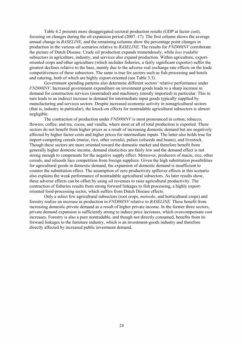
24
Table 4.2 presents more disaggregated sectoral production results (GDP at factor cost), focusing on changes during the oil expansion period (2007–17). The first column shows the average annual change in BASELINE, and the remaining columns show the percentage point changes in production in the various oil scenarios relative to BASELINE. The results for FND00INV corroborate the picture of Dutch Disease. Crude oil production expands tremendously, while less tradable subsectors in agriculture, industry, and services also expand production. Within agriculture, export-oriented crops and other agriculture (which includes fisheries, a fairly significant exporter) suffer the greatest declines relative to the base, mainly due to the adverse real exchange rate effects on the trade competitiveness of these subsectors. The same is true for sectors such as fish processing and hotels and catering, both of which are highly export-oriented (see Table 3.3).
Government spending patterns also determine different sectors’ relative performance under FND00INV. Increased government expenditure on investment goods leads to a sharp increase in demand for construction services (nontraded) and machinery (mostly imported) in particular. This in turn leads to an indirect increase in demand for intermediate input goods typically supplied by manufacturing and services sectors. Despite increased economic activity in nonagricultural sectors (that is, industry in particular), the knock-on effects for nontradable agricultural subsectors is almost negligible.
The contraction of production under FND00INV is most pronounced in cotton; tobacco; flowers; coffee; and tea, cocoa, and vanilla, where most or all of total production is exported. These sectors do not benefit from higher prices as a result of increasing domestic demand but are negatively affected by higher factor costs and higher prices for intermediate inputs. The latter also holds true for import-competing cereals (maize, rice, other cereals), pulses (oilseeds and beans), and livestock. Though these sectors are more oriented toward the domestic market and therefore benefit from generally higher domestic income, demand elasticities are fairly low and the demand effect is not strong enough to compensate for the negative supply effect. Moreover, producers of maize, rice, other cereals, and oilseeds face competition from foreign suppliers. Given the high substitution possibilities for agricultural goods in domestic demand, the expansion of domestic demand is insufficient to counter the substitution effect. The assumption of zero productivity spillover effects in this scenario also explains the weak performance of nontradable agricultural subsectors. As later results show, these adverse effects can be offset by using oil revenues to raise agricultural productivity. The contraction of fisheries results from strong forward linkages to fish processing, a highly export-oriented food-processing sector, which suffers from Dutch Disease effects.
Only a select few agricultural subsectors (root crops, matooke, and horticultural crops) and forestry realize an increase in production in FND00INV relative to BASELINE. These benefit from increasing domestic private demand as a result of higher private income. In the former three sectors, private demand expansion is sufficiently strong to induce price increases, which overcompensate cost increases. Forestry is also a pure nontradable, and though not directly consumed, benefits from its forward linkages to the furniture industry, which is an investment-goods industry and therefore directly affected by increased public investment demand.
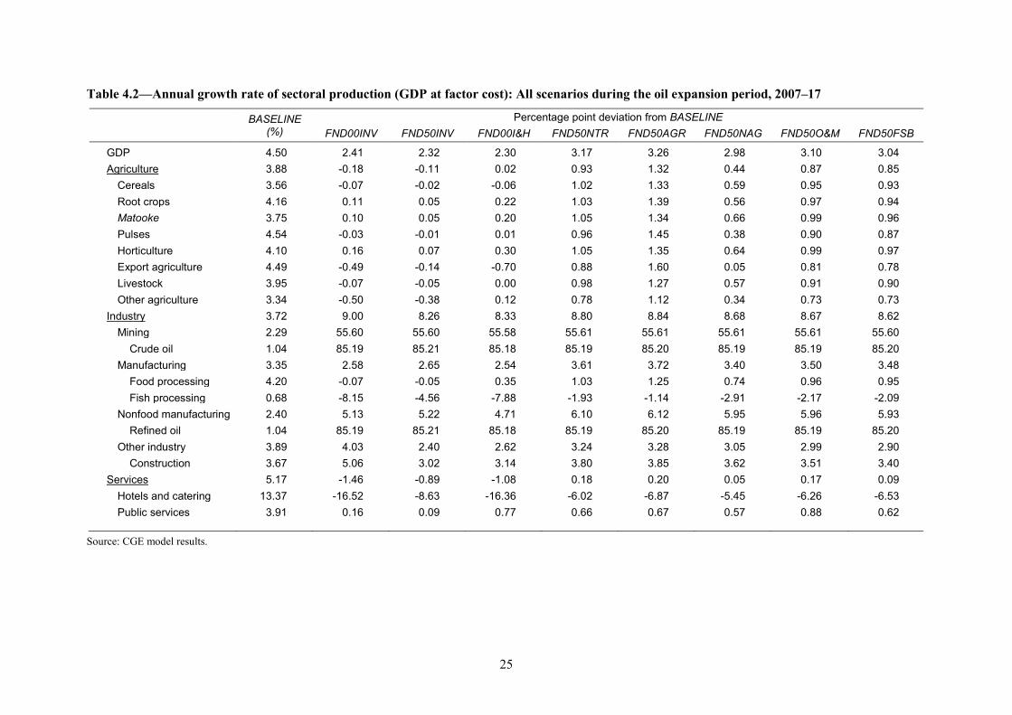
25
Table 4.2—Annual growth rate of sectoral production (GDP at factor cost): All scenarios during the oil expansion period, 2007–17
BASELINE (%)
Percentage point deviation from BASELINE FND00INV FND50INV FND00I&H FND50NTR FND50AGR FND50NAG FND50O&M FND50FSB
GDP 4.50 2.41 2.32 2.30 3.17 3.26 2.98 3.10 3.04 Agriculture 3.88 -0.18 -0.11 0.02 0.93 1.32 0.44 0.87 0.85
Cereals 3.56 -0.07 -0.02 -0.06 1.02 1.33 0.59 0.95 0.93 Root crops 4.16 0.11 0.05 0.22 1.03 1.39 0.56 0.97 0.94 Matooke 3.75 0.10 0.05 0.20 1.05 1.34 0.66 0.99 0.96 Pulses 4.54 -0.03 -0.01 0.01 0.96 1.45 0.38 0.90 0.87 Horticulture 4.10 0.16 0.07 0.30 1.05 1.35 0.64 0.99 0.97 Export agriculture 4.49 -0.49 -0.14 -0.70 0.88 1.60 0.05 0.81 0.78 Livestock 3.95 -0.07 -0.05 0.00 0.98 1.27 0.57 0.91 0.90 Other agriculture 3.34 -0.50 -0.38 0.12 0.78 1.12 0.34 0.73 0.73
Industry 3.72 9.00 8.26 8.33 8.80 8.84 8.68 8.67 8.62 Mining 2.29 55.60 55.60 55.58 55.61 55.61 55.61 55.61 55.60 Crude oil 1.04 85.19 85.21 85.18 85.19 85.20 85.19 85.19 85.20 Manufacturing 3.35 2.58 2.65 2.54 3.61 3.72 3.40 3.50 3.48 Food processing 4.20 -0.07 -0.05 0.35 1.03 1.25 0.74 0.96 0.95 Fish processing 0.68 -8.15 -4.56 -7.88 -1.93 -1.14 -2.91 -2.17 -2.09 Nonfood manufacturing 2.40 5.13 5.22 4.71 6.10 6.12 5.95 5.96 5.93 Refined oil 1.04 85.19 85.21 85.18 85.19 85.20 85.19 85.19 85.20 Other industry 3.89 4.03 2.40 2.62 3.24 3.28 3.05 2.99 2.90 Construction 3.67 5.06 3.02 3.14 3.80 3.85 3.62 3.51 3.40
Services 5.17 -1.46 -0.89 -1.08 0.18 0.20 0.05 0.17 0.09 Hotels and catering 13.37 -16.52 -8.63 -16.36 -6.02 -6.87 -5.45 -6.26 -6.53 Public services 3.91 0.16 0.09 0.77 0.66 0.67 0.57 0.88 0.62
Source: CGE model results.
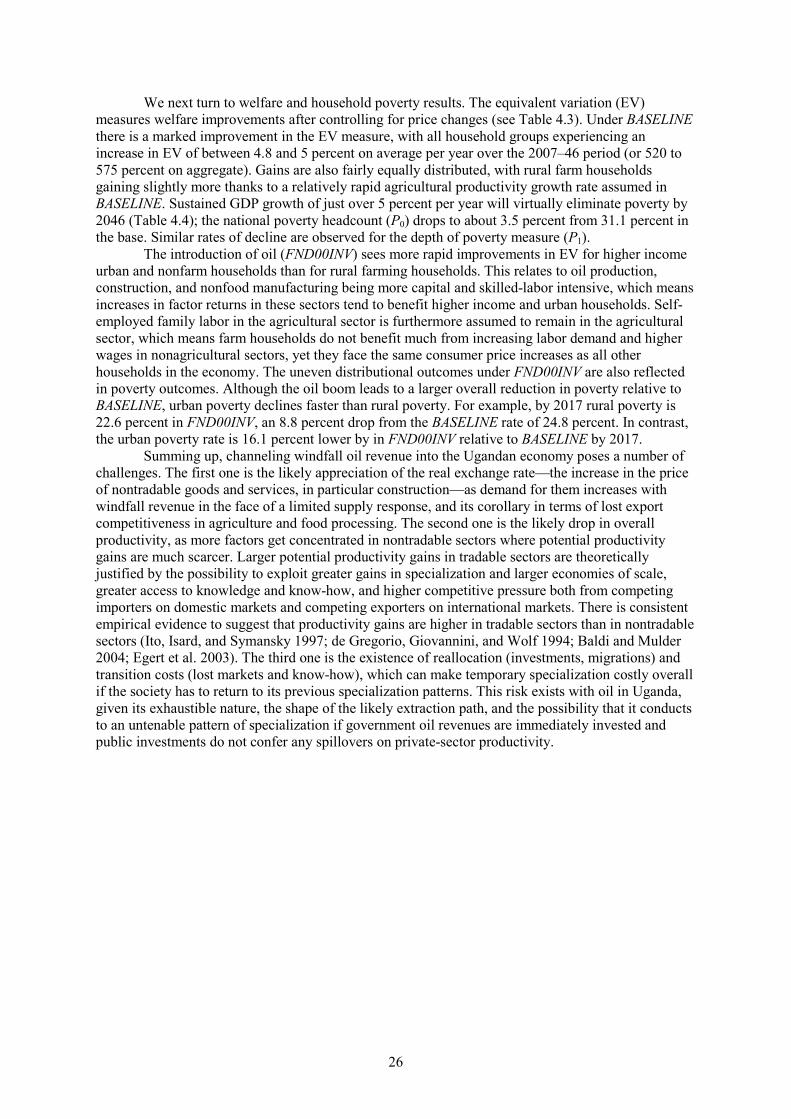
26
We next turn to welfare and household poverty results. The equivalent variation (EV) measures welfare improvements after controlling for price changes (see Table 4.3). Under BASELINE there is a marked improvement in the EV measure, with all household groups experiencing an increase in EV of between 4.8 and 5 percent on average per year over the 2007–46 period (or 520 to 575 percent on aggregate). Gains are also fairly equally distributed, with rural farm households gaining slightly more thanks to a relatively rapid agricultural productivity growth rate assumed in BASELINE. Sustained GDP growth of just over 5 percent per year will virtually eliminate poverty by 2046 (Table 4.4); the national poverty headcount (P0) drops to about 3.5 percent from 31.1 percent in the base. Similar rates of decline are observed for the depth of poverty measure (P1).
The introduction of oil (FND00INV) sees more rapid improvements in EV for higher income urban and nonfarm households than for rural farming households. This relates to oil production, construction, and nonfood manufacturing being more capital and skilled-labor intensive, which means increases in factor returns in these sectors tend to benefit higher income and urban households. Self-employed family labor in the agricultural sector is furthermore assumed to remain in the agricultural sector, which means farm households do not benefit much from increasing labor demand and higher wages in nonagricultural sectors, yet they face the same consumer price increases as all other households in the economy. The uneven distributional outcomes under FND00INV are also reflected in poverty outcomes. Although the oil boom leads to a larger overall reduction in poverty relative to BASELINE, urban poverty declines faster than rural poverty. For example, by 2017 rural poverty is 22.6 percent in FND00INV, an 8.8 percent drop from the BASELINE rate of 24.8 percent. In contrast, the urban poverty rate is 16.1 percent lower by in FND00INV relative to BASELINE by 2017.
Summing up, channeling windfall oil revenue into the Ugandan economy poses a number of challenges. The first one is the likely appreciation of the real exchange rate—the increase in the price of nontradable goods and services, in particular construction—as demand for them increases with windfall revenue in the face of a limited supply response, and its corollary in terms of lost export competitiveness in agriculture and food processing. The second one is the likely drop in overall productivity, as more factors get concentrated in nontradable sectors where potential productivity gains are much scarcer. Larger potential productivity gains in tradable sectors are theoretically justified by the possibility to exploit greater gains in specialization and larger economies of scale, greater access to knowledge and know-how, and higher competitive pressure both from competing importers on domestic markets and competing exporters on international markets. There is consistent empirical evidence to suggest that productivity gains are higher in tradable sectors than in nontradable sectors (Ito, Isard, and Symansky 1997; de Gregorio, Giovannini, and Wolf 1994; Baldi and Mulder 2004; Egert et al. 2003). The third one is the existence of reallocation (investments, migrations) and transition costs (lost markets and know-how), which can make temporary specialization costly overall if the society has to return to its previous specialization patterns. This risk exists with oil in Uganda, given its exhaustible nature, the shape of the likely extraction path, and the possibility that it conducts to an untenable pattern of specialization if government oil revenues are immediately invested and public investments do not confer any spillovers on private-sector productivity.
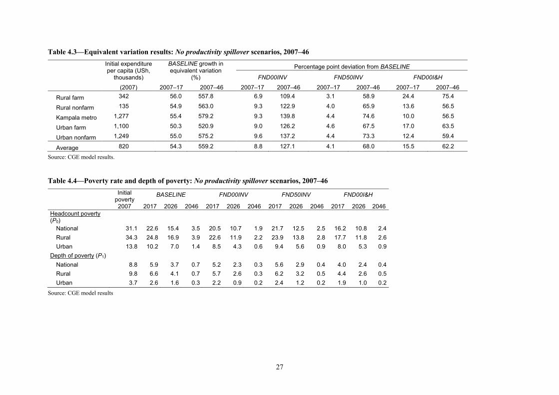
27
Table 4.3—Equivalent variation results: No productivity spillover scenarios, 2007–46
Initial expenditure per capita (USh,
thousands)
BASELINE growth in equivalent variation
(%)
Percentage point deviation from BASELINE
FND00INV FND50INV FND00I&H
(2007) 2007–17 2007–46 2007–17 2007–46 2007–17 2007–46 2007–17 2007–46
Rural farm 342 56.0 557.8 6.9 109.4 3.1 58.9 24.4 75.4
Rural nonfarm 135 54.9 563.0 9.3 122.9 4.0 65.9 13.6 56.5
Kampala metro 1,277 55.4 579.2 9.3 139.8 4.4 74.6 10.0 56.5
Urban farm 1,100 50.3 520.9 9.0 126.2 4.6 67.5 17.0 63.5
Urban nonfarm 1,249 55.0 575.2 9.6 137.2 4.4 73.3 12.4 59.4
Average 820 54.3 559.2 8.8 127.1 4.1 68.0 15.5 62.2
Source: CGE model results.
Table 4.4—Poverty rate and depth of poverty: No productivity spillover scenarios, 2007–46
Initial poverty 2007
BASELINE FND00INV FND50INV FND00I&H
2017 2026 2046 2017 2026 2046 2017 2026 2046 2017 2026 2046 Headcount poverty (P0)
National 31.1 22.6 15.4 3.5 20.5 10.7 1.9 21.7 12.5 2.5 16.2 10.8 2.4 Rural 34.3 24.8 16.9 3.9 22.6 11.9 2.2 23.9 13.8 2.8 17.7 11.8 2.6 Urban 13.8 10.2 7.0 1.4 8.5 4.3 0.6 9.4 5.6 0.9 8.0 5.3 0.9
Depth of poverty (P1) National 8.8 5.9 3.7 0.7 5.2 2.3 0.3 5.6 2.9 0.4 4.0 2.4 0.4 Rural 9.8 6.6 4.1 0.7 5.7 2.6 0.3 6.2 3.2 0.5 4.4 2.6 0.5 Urban 3.7 2.6 1.6 0.3 2.2 0.9 0.2 2.4 1.2 0.2 1.9 1.0 0.2
Source: CGE model results
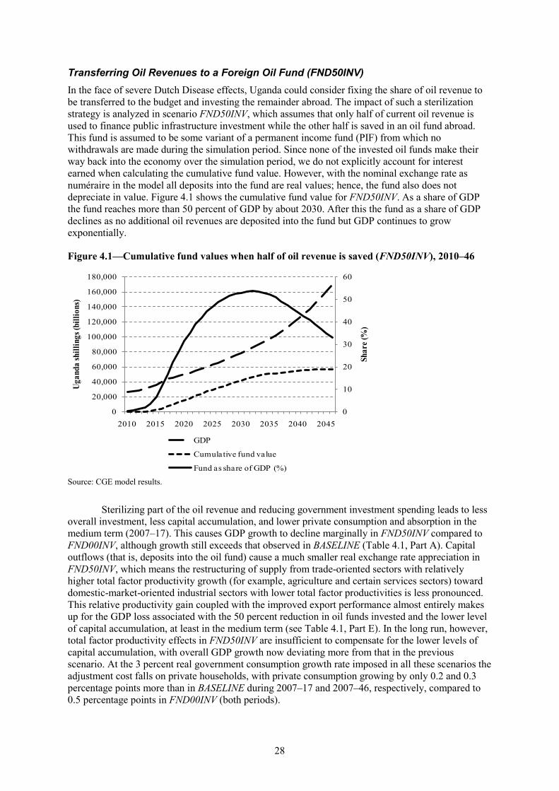
28
Transferring Oil Revenues to a Foreign Oil Fund (FND50INV) In the face of severe Dutch Disease effects, Uganda could consider fixing the share of oil revenue to be transferred to the budget and investing the remainder abroad. The impact of such a sterilization strategy is analyzed in scenario FND50INV, which assumes that only half of current oil revenue is used to finance public infrastructure investment while the other half is saved in an oil fund abroad. This fund is assumed to be some variant of a permanent income fund (PIF) from which no withdrawals are made during the simulation period. Since none of the invested oil funds make their way back into the economy over the simulation period, we do not explicitly account for interest earned when calculating the cumulative fund value. However, with the nominal exchange rate as numéraire in the model all deposits into the fund are real values; hence, the fund also does not depreciate in value. Figure 4.1 shows the cumulative fund value for FND50INV. As a share of GDP the fund reaches more than 50 percent of GDP by about 2030. After this the fund as a share of GDP declines as no additional oil revenues are deposited into the fund but GDP continues to grow exponentially.
Figure 4.1—Cumulative fund values when half of oil revenue is saved (FND50INV), 2010–46
Source: CGE model results.
Sterilizing part of the oil revenue and reducing government investment spending leads to less overall investment, less capital accumulation, and lower private consumption and absorption in the medium term (2007–17). This causes GDP growth to decline marginally in FND50INV compared to FND00INV, although growth still exceeds that observed in BASELINE (Table 4.1, Part A). Capital outflows (that is, deposits into the oil fund) cause a much smaller real exchange rate appreciation in FND50INV, which means the restructuring of supply from trade-oriented sectors with relatively higher total factor productivity growth (for example, agriculture and certain services sectors) toward domestic-market-oriented industrial sectors with lower total factor productivities is less pronounced. This relative productivity gain coupled with the improved export performance almost entirely makes up for the GDP loss associated with the 50 percent reduction in oil funds invested and the lower level of capital accumulation, at least in the medium term (see Table 4.1, Part E). In the long run, however, total factor productivity effects in FND50INV are insufficient to compensate for the lower levels of capital accumulation, with overall GDP growth now deviating more from that in the previous scenario. At the 3 percent real government consumption growth rate imposed in all these scenarios the adjustment cost falls on private households, with private consumption growing by only 0.2 and 0.3 percentage points more than in BASELINE during 2007–17 and 2007–46, respectively, compared to 0.5 percentage points in FND00INV (both periods).
0
10
20
30
40
50
60
0
20,000
40,000
60,000
80,000
100,000
120,000
140,000
160,000
180,000
2010 2015 2020 2025 2030 2035 2040 2045
Shar
e (%
)
Ugan
da sh
illin
gs (b
illio
ns)
GDP
Cumulative fund value
Fund as share of GDP (%)
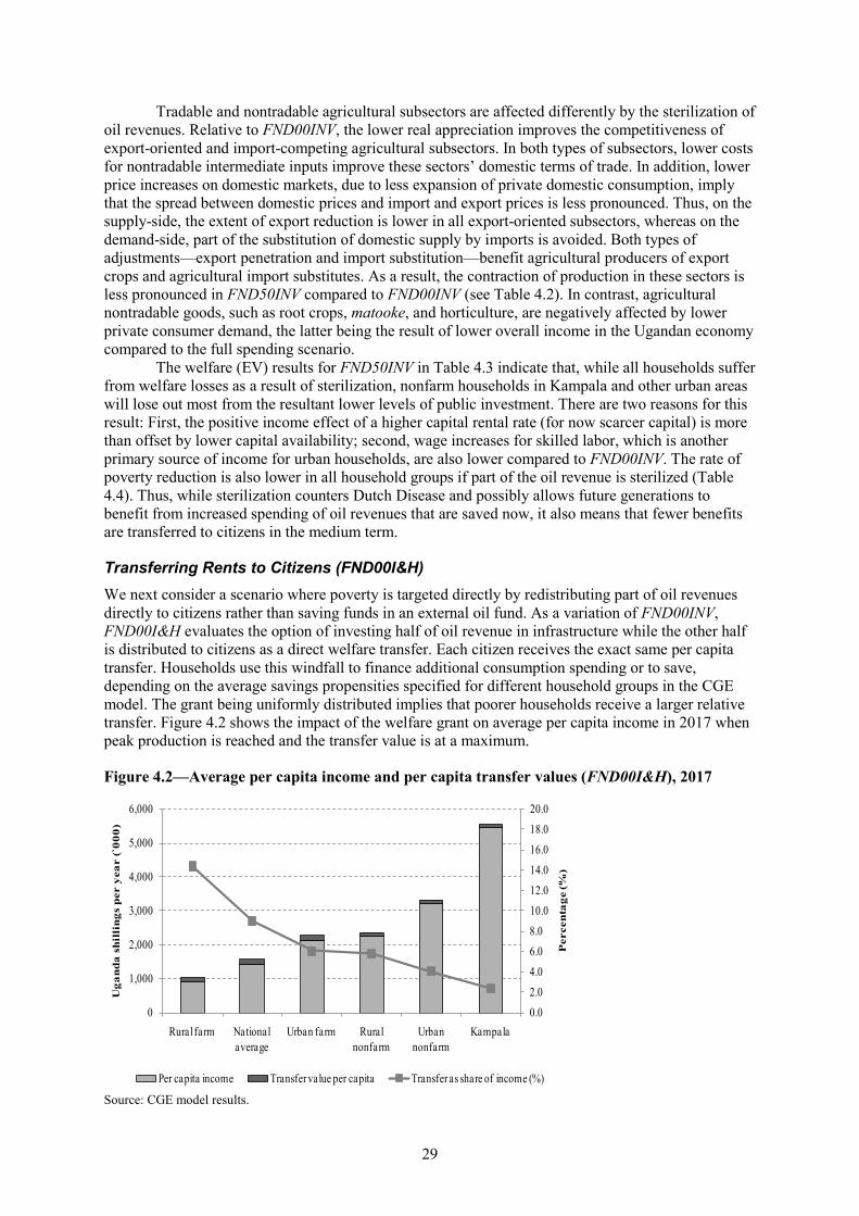
29
Tradable and nontradable agricultural subsectors are affected differently by the sterilization of oil revenues. Relative to FND00INV, the lower real appreciation improves the competitiveness of export-oriented and import-competing agricultural subsectors. In both types of subsectors, lower costs for nontradable intermediate inputs improve these sectors’ domestic terms of trade. In addition, lower price increases on domestic markets, due to less expansion of private domestic consumption, imply that the spread between domestic prices and import and export prices is less pronounced. Thus, on the supply-side, the extent of export reduction is lower in all export-oriented subsectors, whereas on the demand-side, part of the substitution of domestic supply by imports is avoided. Both types of adjustments—export penetration and import substitution—benefit agricultural producers of export crops and agricultural import substitutes. As a result, the contraction of production in these sectors is less pronounced in FND50INV compared to FND00INV (see Table 4.2). In contrast, agricultural nontradable goods, such as root crops, matooke, and horticulture, are negatively affected by lower private consumer demand, the latter being the result of lower overall income in the Ugandan economy compared to the full spending scenario.
The welfare (EV) results for FND50INV in Table 4.3 indicate that, while all households suffer from welfare losses as a result of sterilization, nonfarm households in Kampala and other urban areas will lose out most from the resultant lower levels of public investment. There are two reasons for this result: First, the positive income effect of a higher capital rental rate (for now scarcer capital) is more than offset by lower capital availability; second, wage increases for skilled labor, which is another primary source of income for urban households, are also lower compared to FND00INV. The rate of poverty reduction is also lower in all household groups if part of the oil revenue is sterilized (Table 4.4). Thus, while sterilization counters Dutch Disease and possibly allows future generations to benefit from increased spending of oil revenues that are saved now, it also means that fewer benefits are transferred to citizens in the medium term.
Transferring Rents to Citizens (FND00I&H) We next consider a scenario where poverty is targeted directly by redistributing part of oil revenues directly to citizens rather than saving funds in an external oil fund. As a variation of FND00INV, FND00I&H evaluates the option of investing half of oil revenue in infrastructure while the other half is distributed to citizens as a direct welfare transfer. Each citizen receives the exact same per capita transfer. Households use this windfall to finance additional consumption spending or to save, depending on the average savings propensities specified for different household groups in the CGE model. The grant being uniformly distributed implies that poorer households receive a larger relative transfer. Figure 4.2 shows the impact of the welfare grant on average per capita income in 2017 when peak production is reached and the transfer value is at a maximum.
Figure 4.2—Average per capita income and per capita transfer values (FND00I&H), 2017
Source: CGE model results.
0.02.04.06.08.010.012.014.016.018.020.0
0
1,000
2,000
3,000
4,000
5,000
6,000
Rural farm National average
Urban farm Rural nonfarm
Urban nonfarm
Kampala
Per
cent
age
(%)
Uga
nda
shil
ling
s pe
r ye
ar (`
000)
Per capita income Transfer value per capita Transfer as share of income (%)
30
The figure shows that prior to receiving the welfare grant, rural farm households have a per capita income of USh900,000 per year in 2017 (approximately $375, or just more than $1 per person per day). The welfare transfer, modeled as a tax rebate, adds a further USh129,000 to their income ($50–60 per person per year); thus, as a share of income the transfer is worth 14.4 percent to these households. At the other end of the income spectrum are citizens of Kampala with a per capita income of USh5.4 million. To these people the transfer of USh129,000 is worth only 2.4 percent of their income. About three-quarters of Ugandans live in rural farm households; hence, the national average per capita income is only slightly above that of rural farm households (USh1.4 million), whereas the transfer is worth 9 percent of income.
Despite price increases, the expansion of private household consumption benefits the agricultural sector as a whole, with overall agricultural GDP growth in FND00I&H marginally higher than in BASELINE (agricultural growth declined relative to BASELINE in both FND00INV and FND50INV). However, the real exchange rate appreciation accompanying the expansion of private consumption induces structural changes both across and within agricultural subsectors in terms of production for the domestic and world markets (see Table 4.2). In particular, the expansion of private consumption benefits producers of nontradable agricultural goods such as root crops, matooke, horticulture, livestock, and forestry. Export agriculture is now even more negatively affected compared to FND50INV due to production cost increases and a stronger real exchange rate. Similarly, import-competing agricultural subsectors, such as cereals and oilseeds, also contract as a result of production cost increases and stronger competition from abroad. In all these subsectors, the demand effect from increased private consumption is not sufficiently strong to compensate for the negative import substitution effect that results from the real exchange rate appreciation. With relatively inelastic demand and strong substitution possibilities between domestic and imported agricultural foodcrops, the substitution effect overcompensates the demand effect.
Compared to the first two experiments, the redistribution of rents creates more employment opportunities in agriculture and leads to significantly higher land rentals and prices for livestock. Thus, a larger share of factor income accrues to rural households, who in turn spend a larger share of their incomes on goods produced domestically and in rural areas. This is corroborated by changes in the EV presented in Table 4.3. These results indicate that welfare improves more rapidly for lower income rural and urban farm households than for higher income nonfarm households. Of course, this result also stems directly from the welfare transfer itself, which in relative terms causes incomes of poorer households to increase more than that of wealthier households (Figure 4.2). Moreover, the redistribution of oil rents leads to more consumption by all households, and since production of consumption goods (agricultural and food products in particular) is more land and unskilled-labor intensive, the resulting increases in these factor returns benefit lower income and rural households more.
The uneven distributional impacts are also reflected in poverty outcomes (Table 4.4). Between 2007 and 2017 the redistribution of oil rents leads to a significant decline in poverty at the national level, and also relative to BASELINE and the first two oil production scenarios. Moreover, rural poverty declines more rapidly than urban poverty. In fact, redistribution is twice as effective at reducing poverty among rural households compared to other rent spending options considered. By 2046, however, poverty outcomes under FND00INV are superior to those under FND00I&H. This suggests that investments have longer lasting benefits in terms of production capacity and employment in the future. This benefits the poor more in the longer term than welfare handouts in the medium term. Of course, there are several caveats, one of which is the fact that we assume households’ expenditure patterns remain unchanged after receiving welfare transfers. In reality, households may choose to invest extra income earned in (say) education, which will raise their productivity and future employability. We also do not consider productivity spillover effects of the investments themselves, which is the focus of the next set of experiments.
Public Investment Scenarios with Productivity Spillover Effects In this set of simulations we once again model an increase in public investments, now assuming that these investments have productivity spillover effects in the private sector. All scenarios use FND50INV as the basis, with productivity spillover effects determined by both the level of investment
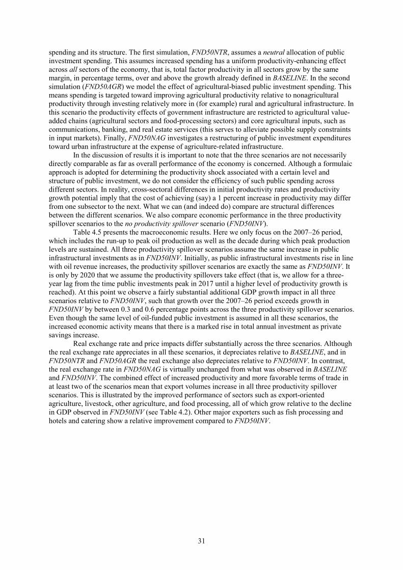
31
spending and its structure. The first simulation, FND50NTR, assumes a neutral allocation of public investment spending. This assumes increased spending has a uniform productivity-enhancing effect across all sectors of the economy, that is, total factor productivity in all sectors grow by the same margin, in percentage terms, over and above the growth already defined in BASELINE. In the second simulation (FND50AGR) we model the effect of agricultural-biased public investment spending. This means spending is targeted toward improving agricultural productivity relative to nonagricultural productivity through investing relatively more in (for example) rural and agricultural infrastructure. In this scenario the productivity effects of government infrastructure are restricted to agricultural value-added chains (agricultural sectors and food-processing sectors) and core agricultural inputs, such as communications, banking, and real estate services (this serves to alleviate possible supply constraints in input markets). Finally, FND50NAG investigates a restructuring of public investment expenditures toward urban infrastructure at the expense of agriculture-related infrastructure.
In the discussion of results it is important to note that the three scenarios are not necessarily directly comparable as far as overall performance of the economy is concerned. Although a formulaic approach is adopted for determining the productivity shock associated with a certain level and structure of public investment, we do not consider the efficiency of such public spending across different sectors. In reality, cross-sectoral differences in initial productivity rates and productivity growth potential imply that the cost of achieving (say) a 1 percent increase in productivity may differ from one subsector to the next. What we can (and indeed do) compare are structural differences between the different scenarios. We also compare economic performance in the three productivity spillover scenarios to the no productivity spillover scenario (FND50INV).
Table 4.5 presents the macroeconomic results. Here we only focus on the 2007–26 period, which includes the run-up to peak oil production as well as the decade during which peak production levels are sustained. All three productivity spillover scenarios assume the same increase in public infrastructural investments as in FND50INV. Initially, as public infrastructural investments rise in line with oil revenue increases, the productivity spillover scenarios are exactly the same as FND50INV. It is only by 2020 that we assume the productivity spillovers take effect (that is, we allow for a three-year lag from the time public investments peak in 2017 until a higher level of productivity growth is reached). At this point we observe a fairly substantial additional GDP growth impact in all three scenarios relative to FND50INV, such that growth over the 2007–26 period exceeds growth in FND50INV by between 0.3 and 0.6 percentage points across the three productivity spillover scenarios. Even though the same level of oil-funded public investment is assumed in all these scenarios, the increased economic activity means that there is a marked rise in total annual investment as private savings increase.
Real exchange rate and price impacts differ substantially across the three scenarios. Although the real exchange rate appreciates in all these scenarios, it depreciates relative to BASELINE, and in FND50NTR and FND50AGR the real exchange also depreciates relative to FND50INV. In contrast, the real exchange rate in FND50NAG is virtually unchanged from what was observed in BASELINE and FND50INV. The combined effect of increased productivity and more favorable terms of trade in at least two of the scenarios mean that export volumes increase in all three productivity spillover scenarios. This is illustrated by the improved performance of sectors such as export-oriented agriculture, livestock, other agriculture, and food processing, all of which grow relative to the decline in GDP observed in FND50INV (see Table 4.2). Other major exporters such as fish processing and hotels and catering show a relative improvement compared to FND50INV.
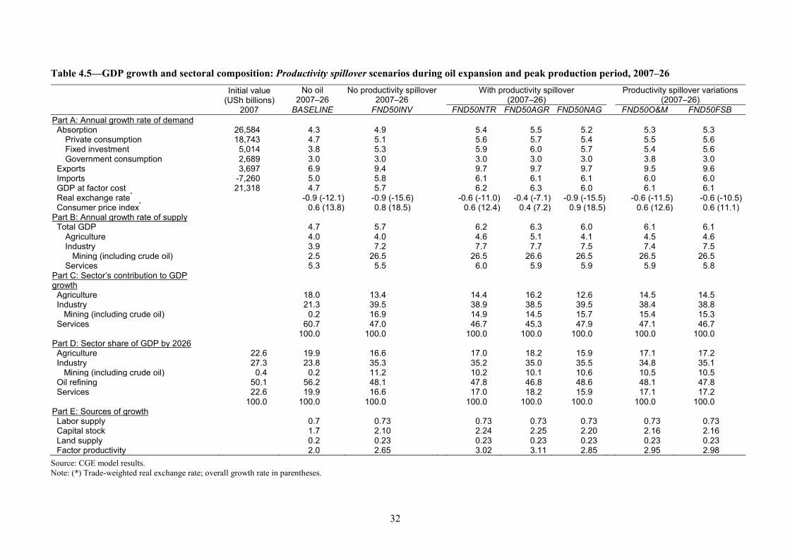
32
Table 4.5—GDP growth and sectoral composition: Productivity spillover scenarios during oil expansion and peak production period, 2007–26
Initial value
(USh billions) 2007
No oil 2007–26
No productivity spillover 2007–26
With productivity spillover (2007–26) Productivity spillover variations
(2007–26) BASELINE FND50INV FND50NTR FND50AGR FND50NAG FND50O&M FND50FSB
Part A: Annual growth rate of demand Absorption 26,584 4.3 4.9 5.4 5.5 5.2 5.3 5.3
Private consumption 18,743 4.7 5.1 5.6 5.7 5.4 5.5 5.6 Fixed investment 5,014 3.8 5.3 5.9 6.0 5.7 5.4 5.6 Government consumption 2,689 3.0 3.0 3.0 3.0 3.0 3.8 3.0
Exports 3,697 6.9 9.4 9.7 9.7 9.7 9.5 9.6 Imports -7,260 5.0 5.8 6.1 6.1 6.1 6.0 6.0 GDP at factor cost 21,318 4.7 5.7 6.2 6.3 6.0 6.1 6.1 Real exchange rate* -0.9 (-12.1) -0.9 (-15.6) -0.6 (-11.0) -0.4 (-7.1) -0.9 (-15.5) -0.6 (-11.5) -0.6 (-10.5) Consumer price index* 0.6 (13.8) 0.8 (18.5) 0.6 (12.4) 0.4 (7.2) 0.9 (18.5) 0.6 (12.6) 0.6 (11.1) Part B: Annual growth rate of supply Total GDP 4.7 5.7 6.2 6.3 6.0 6.1 6.1
Agriculture 4.0 4.0 4.6 5.1 4.1 4.5 4.6 Industry 3.9 7.2 7.7 7.7 7.5 7.4 7.5 Mining (including crude oil) 2.5 26.5 26.5 26.6 26.5 26.5 26.5 Services 5.3 5.5 6.0 5.9 5.9 5.9 5.8
Part C: Sector’s contribution to GDP growth
Agriculture 18.0 13.4 14.4 16.2 12.6 14.5 14.5 Industry 21.3 39.5 38.9 38.5 39.5 38.4 38.8 Mining (including crude oil) 0.2 16.9 14.9 14.5 15.7 15.4 15.3 Services 60.7 47.0 46.7 45.3 47.9 47.1 46.7 100.0 100.0 100.0 100.0 100.0 100.0 100.0 Part D: Sector share of GDP by 2026 Agriculture 22.6 19.9 16.6 17.0 18.2 15.9 17.1 17.2 Industry 27.3 23.8 35.3 35.2 35.0 35.5 34.8 35.1 Mining (including crude oil) 0.4 0.2 11.2 10.2 10.1 10.6 10.5 10.5 Oil refining 50.1 56.2 48.1 47.8 46.8 48.6 48.1 47.8 Services 22.6 19.9 16.6 17.0 18.2 15.9 17.1 17.2 100.0 100.0 100.0 100.0 100.0 100.0 100.0 100.0 Part E: Sources of growth Labor supply 0.7 0.73 0.73 0.73 0.73 0.73 0.73 Capital stock 1.7 2.10 2.24 2.25 2.20 2.16 2.16 Land supply 0.2 0.23 0.23 0.23 0.23 0.23 0.23 Factor productivity 2.0 2.65 3.02 3.11 2.85 2.95 2.98 Source: CGE model results. Note: (*) Trade-weighted real exchange rate; overall growth rate in parentheses.
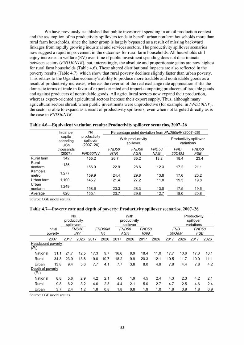
33
We have previously established that public investment spending in an oil production context and the assumption of no productivity spillovers tends to benefit urban nonfarm households more than rural farm households, since the latter group is largely bypassed as a result of missing backward linkages from rapidly growing industrial and services sectors. The productivity spillover scenarios now suggest a rapid improvement in the outcomes for rural farm households. All households still enjoy increases in welfare (EV) over time if public investment spending does not discriminate between sectors (FND50NTR), but, interestingly, the absolute and proportionate gains are now highest for rural farm households (Table 4.6). These altered distributional impacts are also reflected in the poverty results (Table 4.7), which show that rural poverty declines slightly faster than urban poverty. This relates to the Ugandan economy’s ability to produce more tradable and nontradable goods as a result of productivity increases, whereas the reversal of the real exchange rate appreciation shifts the domestic terms of trade in favor of export-oriented and import-competing producers of tradable goods and against producers of nontradable goods. All agricultural sectors now expand their production, whereas export-oriented agricultural sectors increase their export supply. Thus, although many agricultural sectors shrank when public investments were unproductive (for example, in FND50INV), the sector is able to expand as a result of productivity spillovers, even when not targeted directly as is the case in FND50NTR.
Table 4.6—Equivalent variation results: Productivity spillover scenarios, 2007–26
Initial per capita
spending USh
thousands (2007)
No productivity
spillover (2007–26)
Percentage point deviation from FND50INV (2007–26)
With productivity
spillover Productivity spillover variations
FND50INV FND50
NTR FND50 AGR
FND50NAG
FND 50O&M
FND50 FSB
Rural farm 342 155.2 26.7 35.2 13.2 18.4 23.4 Rural nonfarm 135 156.0 22.9 28.6 12.3 17.2 21.1 Kampala metro 1,277 159.9 24.4 29.8 13.8 17.6 20.2 Urban farm 1,100 145.7 21.4 27.2 11.0 19.5 19.8 Urban nonfarm 1,249 158.6 23.3 28.3 13.0 17.5 19.6 Average 820 155.1 23.7 29.8 12.7 18.0 20.8
Source: CGE model results.
Table 4.7—Poverty rate and depth of poverty: Productivity spillover scenarios, 2007–26
Initial
poverty
No productivity spillovers
With productivity
spillover
Productivity spillover
variations
FND50
INV FND50N
TR FND50 AGR
FND50NAG
FND 50O&M
FND50 FSB
2007 2017 2026 2017 2026 2017 2026 2017 2026 2017 2026 2017 2026 Headcount poverty (P0)
National 31.1 21.7 12.5 17.3 9.7 16.6 8.9 18.4 11.0 17.7 10.6 17.3 10.1 Rural 34.3 23.9 13.8 19.0 10.7 18.2 9.9 20.3 12.1 19.5 11.7 19.0 11.1 Urban 13.8 9.4 5.6 7.7 4.1 7.7 3.8 8.0 4.9 7.8 4.4 7.8 4.2
Depth of poverty (P1)
National 8.8 5.6 2.9 4.2 2.1 4.0 1.9 4.5 2.4 4.3 2.3 4.2 2.1 Rural 9.8 6.2 3.2 4.6 2.3 4.4 2.1 5.0 2.7 4.7 2.5 4.6 2.4 Urban 3.7 2.4 1.2 1.8 0.8 1.8 0.8 1.9 1.0 1.8 0.9 1.8 0.9
Source: CGE model results.
34
In the case where nonagricultural sectors are targeted (FND50NAG), additional public investment spending on urban road infrastructure increases total factor productivity growth in the tradable nonfood-manufacturing sectors (that is, textiles, wood and paper, other manufacturing, machinery, and furniture) and in the trade, hotel and catering, and transport services sectors. At the same time we assume lower levels of spending on rural infrastructure, which reduces total factor productivity growth in all agricultural and food-processing sectors as well as in the less-tradable communications, banking, real estate, and community services sectors. As expected, when productivity growth is lower in sectors that predominantly supply goods for the domestic market (these are also goods that cannot easily be substituted by imports), the spending of oil revenues causes a larger (relative) appreciation of the real exchange rate than in the case of neutral productivity spillovers. Hence, although the manufacturing export performance is slightly stronger in machinery and equipment, hotels and catering, and transport, the agricultural sector is hit relatively hard when productivity gains are biased against it. At 4.1 percent per year, average agricultural growth in FND50NAG is half a percentage point lower than in FND50NTR, and the agricultural sector’s share in GDP declines by more than a percentage point by 2026 vis-à-vis a neutral allocation of investment spending.
When public investment spending is biased in favor of agriculture and food processing (FND50AGR), outcomes are markedly different. Increased supply of agricultural goods and food items is sufficiently strong to more than offset the demand effects of the oil boom, such that the initial real exchange rate appreciation observed in FND50INV is reversed within a relatively short time. The effects on exports are a mirror image of those in FND50NAG; agriculture exports recover more strongly than in the former experiment, but lower productivity growth in nonfood manufacturing results in a more sluggish recovery in manufacturing exports.
The most striking difference between the two public investment options, though, is the effect on real household disposable incomes, welfare (Table 4.6) and poverty (Table 4.7). Compared to FND50NTR, a manufacturing bias (FND50NAG) sharply moderates real income and welfare growth in the economy. The total rise in EV relative to FND50INV is only 12.7 percentage points in FND50NAG compared to 23.7 percentage points in FND50NTR. Moreover, the income gain is spread somewhat unevenly across household groups, with rural farm households now faring worse than Kampala households. This contrasts sharply with the outcome under FND50AGR, which generates markedly higher aggregate real income gains in the medium term (29.8 percentage points), and one that benefits poorer rural households more. Poverty outcomes for rural and urban households improve in the agricultural-biased scenario relative to the neutral scenario, whereas in the manufacturing-biased scenario poverty rates are higher compared to the neutral growth scenario. In all productivity scenarios, however, poverty rates decline more rapidly than in FND50INV.
Given the significant impact on agricultural growth and on the welfare of rural households of the agricultural productivity spillovers from the increased public investments arising from Uganda’s oil revenue, it is critical that the Government of Uganda put in place mechanisms by which these productivity spillovers can be maximized. What is needed, in particular, is a well-coordinated set of interventions aimed at improving competitiveness in the agricultural sector, which would serve as a platform sustainable growth in the economy. However, at 3.8 percent of the budget, current spending on agriculture in Uganda is well below the 10 percent target committed to under the Comprehensive African Agricultural Development Program (CAADP). Research by Fan, Mogues, and Benin (2009) suggests that agricultural research and development, infrastructure (such as rural roads), and investments in education and skills have the highest payoffs in terms of agricultural productivity gains and increased competitiveness of the sector.
Variations on Productivity-Enhancing Investment Spending Scenarios The final two simulations both use the assumptions underlying FND50NTR as a starting point, and then introduce slight variations to the way these simulations are set up. In the first, FND50O&M, we assume that increased public capital stock would also require a higher level of operations and maintenance (O&M) expenditure; hence, in this scenario, the growth rate of real government consumption is raised from 3 to 3.8 percent. O&M costs are financed through oil revenues, thereby reducing investment spending and lowering the extent of productivity spillovers seen in FND50NTR.
35
In the second scenario (FND50FSB) we assume the Ugandan government introduces a fuel subsidy (FSB) equivalent to a 50 percent reduction in fuel-import tariffs on fuel (this tariff is 80 percent in the base). As in the previous scenario the cost of the FSB is recovered from oil revenues.
Additional O&M expenditure has fairly strong adverse effects on the economy. The opportunity costs of having oil revenues but then spending them on current expenditure rather than investments are high (Table 4.5). Fixed investments decline by half a percentage point relative to FND50NTR, which ultimately causes GDP growth to weaken as the rate of capital formation slows down. Households realize significant welfare losses relative to FND50NTR (Table 4.6). Urban households are less affected, mainly because an expansion of government consumption essentially implies an enlargement of public administration, a sector that employs a large number of skilled urban workers. However, the increase in skilled wages is not enough to compensate for higher prices that result from the real exchange rate appreciation and the overall decline in economic activity. Rural farm households are adversely affected in two ways: They are isolated from the direct demand effects of higher government consumption and their competitiveness suffers as a result of the Dutch Disease associated with the real exchange rate appreciation.
A reduction of fuel-import tariffs, as in FND50FSB, holds important benefits for fuel- or energy-intensive industries and households that spend a large portion of their budgets on fuel or transport. Lower fuel-import tariffs in general also reduce deadweight costs of taxation, provided the quality of tax administration does not decline at the same time. A low-taxation environment could further encourage private investment in the non-oil economy (both in agriculture and industry), which, if successful, would allow the economy to continue diversifying rather than concentrating too many resources in the oil sector. This may also compensate for the adverse effect on profitability of the real exchange rate appreciation.
Yet, given the low private marginal propensities to save in Uganda, which range from 8 percent for rural farm households to 9.8 percent for Kampala households (in the Uganda social accounting matrix [SAM] for 2007), most of the additional factor income that results from lower tariffs will be spent on private consumption. Moreover, since the real government expenditure growth is once again fixed at 3 percent per year in this scenario, lower tariff revenues reduce public investment spending and lower the extent of productivity spillovers. Thus, the macro effects are similar to what was observed in FND50O&M. The redistribution of income between the public and the private sector leads to a slight restructuring of final demand from government to private consumption (Table 4.5). Moreover, the intermediate input cost reductions that result from lower fuel prices are not strong enough to compensate for sectoral productivity losses and cost reductions are almost identical across sectors. As a result, under the FND50FSB scenario, all sectors experience real income losses compared to FND50NTR during the boom period until 2017, and these are slightly higher than in FND50O&M (Table 4.2). As in scenario FND50O&M, the costs of having oil revenue but then using it for consumption expenditures are high. Although energy-intensive agricultural sectors such as other cereals, vegetables, and fruits and tree crops benefit directly from lower fuel costs or indirectly from lower transport costs, these cost reductions are insufficient to compensate negative demand effects that result from low-income elasticities of private consumption demand.
As shown in Table 4.6, although the 50 percent reduction in tariff rates on fuel would lower overall welfare compared to FND50NTR, the welfare losses would be distributed progressively with rural households and urban farm households being relatively less negatively affected by productivity losses and benefiting relatively more from lower energy costs. This also implies that the increases in poverty rates are insignificantly low (Table 4.5).
36
5. CONCLUSION
Even at conservative prices of $70–80 per barrel, future oil revenue in Uganda will be considerable, potentially doubling government revenue within 6 to 10 years and constituting an estimated 10–15 percent of GDP at peak production. The economic impact of oil production on the country’s agricultural performance and the livelihood of rural households could be profound, particularly during the first phase of the projected extraction when massive additional inflows of foreign exchange need to be managed by the Ugandan government. The so-called Dutch Disease effects may affect the international competitiveness of export sectors, such as agriculture in particular, and it is likely to make the country’s growth strategy—with its emphasis on value-added, export diversification, and manufacturing—harder to achieve. This would threaten to increase, rather than decrease, the urban–rural income gap.
Agriculture and related processing currently contribute about 27 percent to GDP. Food and agriculture-related processing make up about 50 percent of household consumption expenditure. Poverty is higher in rural than in urban households and within rural households it is highest among nonfarm households. Even with no oil revenue, agriculture’s share of GDP is projected to decrease by 6.8 percentage points from 22.6 percent in 2007 to 15.8 percent over the next 40 years, as increasing factor productivities in tradable sectors and increasing per capita income and consumption will be leading toward a restructuring of production in favor of services.
The spending of oil revenues results in a further relative contraction of agriculture, with the extent depending on spending options—consumption versus capital investment, domestic capital investment versus investment in a foreign oil fund, unproductive versus productive capital investment and infrastructure development, government consumption versus redistribution to citizens (private consumption and investment), or revising tax versus trade policies.
It is important to differentiate between medium- and long-term impacts of oil revenue spending, since structural impacts differ and asymmetric adjustment flexibilities (ratchet effects) in factor markets (investments, migrations) and foreign trade (lost markets and know-how) can make temporary specialization costly if the Ugandan society has to return to its previous specialization patterns because of the exhaustible nature of oil reserves.
The impacts of oil extraction will be felt by Uganda mostly indirectly through higher government expenditures on consumption (largely administration) and investment; direct effects through higher domestic factor income in oil extraction and refining and through backward linkages will be minimal given production technologies and the economic enclave character of the oil industry. Results of this discussion paper suggest that the extraction and refining of oil will increase overall GDP growth, increase national and rural real household incomes, and benefit the poor in Uganda. In the medium term, that is, from the starting of oil extraction (2011 in this analysis) until reaching peak production (2017), overall average annual GDP growth will be between 2.3 and 3.3 percentage points higher than in a comparable baseline projection without oil. In the long term over the total extraction path of 40 years, the average growth rate will be between 0.2 and 0.5 percentage points higher. The differences depend on how oil revenues are spent, on whether public infrastructure confers any spillovers on private-sector productivity, and in which sectors these spillovers occur.
Several conclusions emerge from the simulations presented in this paper. First, with the projected oil extraction path and recently high oil prices, a real appreciation of the Uganda shilling is almost inevitable. Although policies designed to limit absorption through tight fiscal and monetary policies would reduce the pressure on the exchange rate over the short to medium term, they are unlikely to be sufficient to eliminate it. A rapid buildup of foreign exchange reserves and the accumulation of government oil revenue in some kind of external resource fund could mitigate the pressure but at the expense of domestic investment, the fiscal position, and private household welfare and consumption, as well as poverty reduction. In any case, agriculture and the rural population will be discriminated against by the expected oil boom. As net producers of tradable goods and net consumers of nontradable goods they suffer twice, from increased production costs and higher prices for consumer goods. Only a few select agricultural subsectors that produce exclusively for the domestic market, such as root crops, matooke, and horticulture, realize income gains as a result of generally higher income and consumption. Transferring part of the oil rent to citizens—rather than to
37
a foreign oil fund—would directly increase household welfare and accelerate poverty reduction efforts. Moreover, agriculture as a whole would regain growth momentum. However, the real appreciation accompanying the oil-rent-financed expansion of private consumption would induce strong structural changes both across and within agricultural subsectors, which might be difficult to reverse once oil revenues dry out. Thus, there is the real danger of losing long-run competitiveness vis-à-vis foreign suppliers both on world markets for agricultural export commodities as well as on domestic markets for food products.
Second, Uganda’s oil discovery comes at an opportune moment as the country battles with the challenges of marked infrastructural backlogs. In this situation of initial scarcity of public infrastructure, oil-funded increases in public infrastructure may lead to potentially large medium-term welfare gains, despite the presence of Dutch Disease effects. This is particularly true when public infrastructure augments the productivity of private factors. Yet, the sectoral and distributional consequences of these investments are highly sensitive to the structure and quality of public investment spending, which has an influence on the location of productivity effects, as well as the characteristics of demand.
Third, a neutral allocation of investment spending, which leads to a balanced sectoral supply response, is broadly beneficial to the Ugandan economy in terms of boosting aggregate growth and investment, welfare, and exports while moderating appreciation of the real exchange rate and reducing poverty on a significant scale, with rural poverty declining even faster than urban poverty. This relates to the Ugandan economy’s ability to produce more goods—both tradable and nontradable—as a result of productivity increases, whereas a reversal of the real exchange rate appreciation shifts the domestic terms of trade in favor of export-oriented and import-competing agriculture. Thus, even though many agricultural subsectors would be indirectly discriminated against if there were no productivity-enhancing public infrastructure, these sectors are able to expand as a result of productive public investment, even when not targeted directly. In contrast, agriculture is hit relatively hard when a reallocation of public investment spending leads to a nonagricultural bias in the supply response.
Fourth, outcomes are markedly different when public investment spending is biased in favor of agriculture and food processing. In this case results suggest that (1) the supply response of agriculture would be sufficiently strong to more than offset the demand effects of the oil boom; (2) agriculture exports would recover more strongly than with a neutral or a nonagricultural, industry-biased allocation of investment spending; (3) the supply response would generate higher aggregate real income gains; and (4) poorer rural households will benefit the most, but without sacrificing urban poverty reduction. With respect to the latter, a highly significant outcome is that poverty falls for both rural and urban households under an agriculture-biased public investment spending scenario (relative to a neutral spending strategy), whereas industry-biased spending would lead to comparably higher poverty in both regions.
Although direct comparisons of scenario results should be done with great caution, a simple ranking of public spending options according to growth, real income, and poverty reduction effects (Table 5.1) suggests an agriculture-biased investment strategy is the preferred option. Such a strategy would not only increase agricultural growth and rural incomes most, but would also have significant and positive spillover effects into the rest of the economy, thereby benefiting all segments of society. The recommendation is less clear in the zero-spillover scenarios. In this case, there is a trade-off between increasing investment (and therefore relatively higher overall growth) and increasing consumption (and therefore relatively higher agricultural growth). The latter (increased consumption), which is achieved by redistributing oil revenues to Uganda’s citizens via a welfare transfer scheme, is associated with larger reductions in poverty, at the national level and particularly in poorer rural areas.
These conclusions must, of course, be qualified by a number of caveats. Among these is that absorption capacity and, consequently, the quality and efficiency of public investments for economic growth are critically important. Having oil revenues but then having to incur high economic and social costs in attempting to spend these revenues will lower the net benefits of oil. For balanced growth and poverty reduction to materialize a well-coordinated set of interventions aimed at improving competitiveness in the agricultural sector is needed. These may include investments in
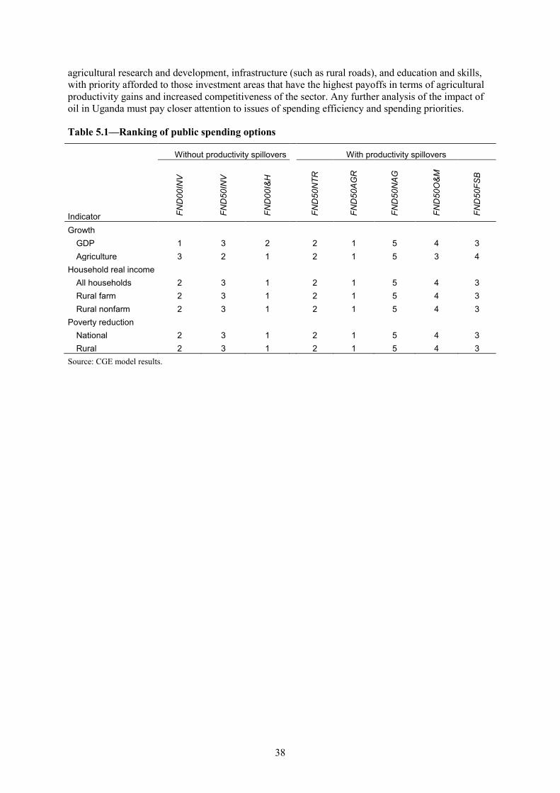
38
agricultural research and development, infrastructure (such as rural roads), and education and skills, with priority afforded to those investment areas that have the highest payoffs in terms of agricultural productivity gains and increased competitiveness of the sector. Any further analysis of the impact of oil in Uganda must pay closer attention to issues of spending efficiency and spending priorities.
Table 5.1—Ranking of public spending options
Without productivity spillovers With productivity spillovers
Indicator FND
00IN
V
FND
50IN
V
FND
00I&
H
FND
50N
TR
FND
50A
GR
FND
50N
AG
FND
50O
&M
FND
50FS
B
Growth GDP 1 3 2 2 1 5 4 3 Agriculture 3 2 1 2 1 5 3 4
Household real income All households 2 3 1 2 1 5 4 3 Rural farm 2 3 1 2 1 5 4 3 Rural nonfarm 2 3 1 2 1 5 4 3
Poverty reduction National 2 3 1 2 1 5 4 3 Rural 2 3 1 2 1 5 4 3
Source: CGE model results.
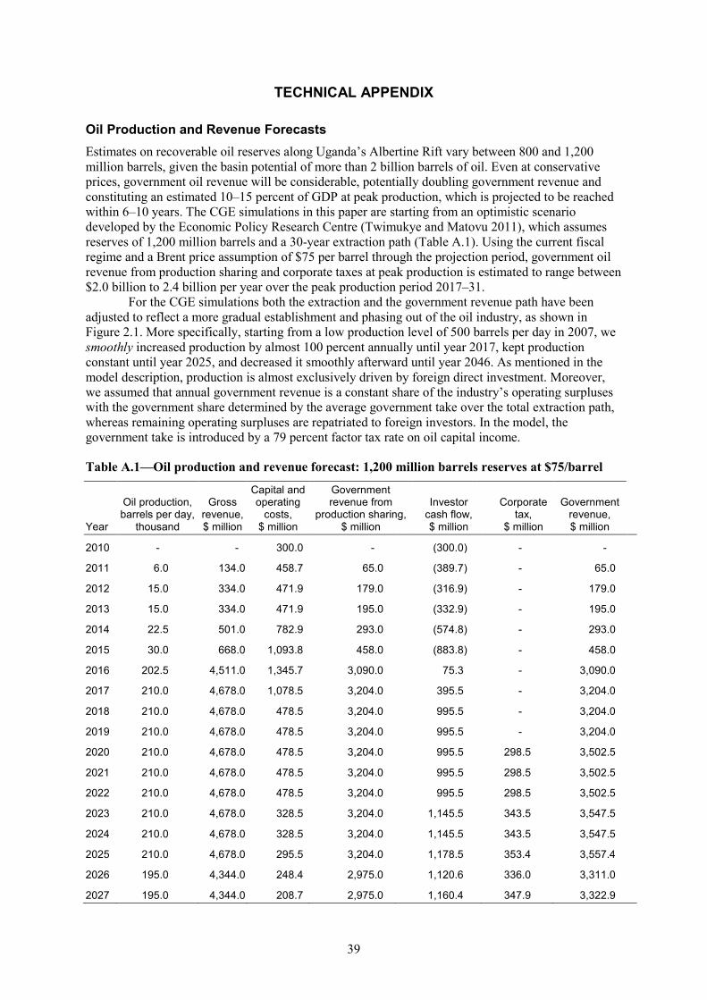
39
TECHNICAL APPENDIX
Oil Production and Revenue Forecasts Estimates on recoverable oil reserves along Uganda’s Albertine Rift vary between 800 and 1,200 million barrels, given the basin potential of more than 2 billion barrels of oil. Even at conservative prices, government oil revenue will be considerable, potentially doubling government revenue and constituting an estimated 10–15 percent of GDP at peak production, which is projected to be reached within 6–10 years. The CGE simulations in this paper are starting from an optimistic scenario developed by the Economic Policy Research Centre (Twimukye and Matovu 2011), which assumes reserves of 1,200 million barrels and a 30-year extraction path (Table A.1). Using the current fiscal regime and a Brent price assumption of $75 per barrel through the projection period, government oil revenue from production sharing and corporate taxes at peak production is estimated to range between $2.0 billion to 2.4 billion per year over the peak production period 2017–31.
For the CGE simulations both the extraction and the government revenue path have been adjusted to reflect a more gradual establishment and phasing out of the oil industry, as shown in Figure 2.1. More specifically, starting from a low production level of 500 barrels per day in 2007, we smoothly increased production by almost 100 percent annually until year 2017, kept production constant until year 2025, and decreased it smoothly afterward until year 2046. As mentioned in the model description, production is almost exclusively driven by foreign direct investment. Moreover, we assumed that annual government revenue is a constant share of the industry’s operating surpluses with the government share determined by the average government take over the total extraction path, whereas remaining operating surpluses are repatriated to foreign investors. In the model, the government take is introduced by a 79 percent factor tax rate on oil capital income.
Table A.1—Oil production and revenue forecast: 1,200 million barrels reserves at $75/barrel
Year
Oil production, barrels per day,
thousand
Gross revenue, $ million
Capital and operating
costs, $ million
Government revenue from
production sharing, $ million
Investor cash flow, $ million
Corporate tax,
$ million
Government revenue, $ million
2010 - - 300.0 - (300.0) - -
2011 6.0 134.0 458.7 65.0 (389.7) - 65.0
2012 15.0 334.0 471.9 179.0 (316.9) - 179.0
2013 15.0 334.0 471.9 195.0 (332.9) - 195.0
2014 22.5 501.0 782.9 293.0 (574.8) - 293.0
2015 30.0 668.0 1,093.8 458.0 (883.8) - 458.0
2016 202.5 4,511.0 1,345.7 3,090.0 75.3 - 3,090.0
2017 210.0 4,678.0 1,078.5 3,204.0 395.5 - 3,204.0
2018 210.0 4,678.0 478.5 3,204.0 995.5 - 3,204.0
2019 210.0 4,678.0 478.5 3,204.0 995.5 - 3,204.0
2020 210.0 4,678.0 478.5 3,204.0 995.5 298.5 3,502.5
2021 210.0 4,678.0 478.5 3,204.0 995.5 298.5 3,502.5
2022 210.0 4,678.0 478.5 3,204.0 995.5 298.5 3,502.5
2023 210.0 4,678.0 328.5 3,204.0 1,145.5 343.5 3,547.5
2024 210.0 4,678.0 328.5 3,204.0 1,145.5 343.5 3,547.5
2025 210.0 4,678.0 295.5 3,204.0 1,178.5 353.4 3,557.4
2026 195.0 4,344.0 248.4 2,975.0 1,120.6 336.0 3,311.0
2027 195.0 4,344.0 208.7 2,975.0 1,160.4 347.9 3,322.9
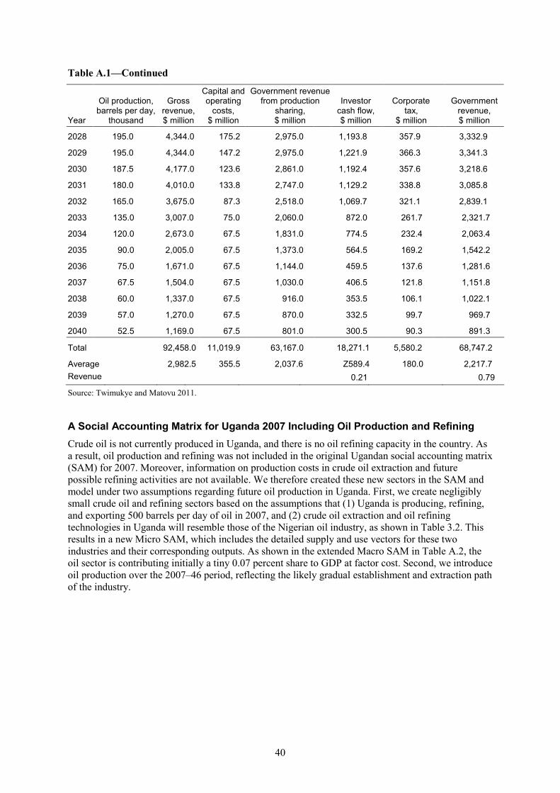
40
Table A.1—Continued
Year
Oil production, barrels per day,
thousand
Gross revenue, $ million
Capital and operating
costs, $ million
Government revenue from production
sharing, $ million
Investor cash flow, $ million
Corporate tax,
$ million
Government revenue, $ million
2028 195.0 4,344.0 175.2 2,975.0 1,193.8 357.9 3,332.9
2029 195.0 4,344.0 147.2 2,975.0 1,221.9 366.3 3,341.3
2030 187.5 4,177.0 123.6 2,861.0 1,192.4 357.6 3,218.6
2031 180.0 4,010.0 133.8 2,747.0 1,129.2 338.8 3,085.8
2032 165.0 3,675.0 87.3 2,518.0 1,069.7 321.1 2,839.1
2033 135.0 3,007.0 75.0 2,060.0 872.0 261.7 2,321.7
2034 120.0 2,673.0 67.5 1,831.0 774.5 232.4 2,063.4
2035 90.0 2,005.0 67.5 1,373.0 564.5 169.2 1,542.2
2036 75.0 1,671.0 67.5 1,144.0 459.5 137.6 1,281.6
2037 67.5 1,504.0 67.5 1,030.0 406.5 121.8 1,151.8
2038 60.0 1,337.0 67.5 916.0 353.5 106.1 1,022.1
2039 57.0 1,270.0 67.5 870.0 332.5 99.7 969.7
2040 52.5 1,169.0 67.5 801.0 300.5 90.3 891.3
Total 92,458.0 11,019.9 ……..63,167.0 18,271.1 5,580.2 68,747.2
Average 2,982.5 355.5 ………2,037.6 Z589.4 180.0 2,217.7 Revenue
0.21 0.79
Source: Twimukye and Matovu 2011.
A Social Accounting Matrix for Uganda 2007 Including Oil Production and Refining Crude oil is not currently produced in Uganda, and there is no oil refining capacity in the country. As a result, oil production and refining was not included in the original Ugandan social accounting matrix (SAM) for 2007. Moreover, information on production costs in crude oil extraction and future possible refining activities are not available. We therefore created these new sectors in the SAM and model under two assumptions regarding future oil production in Uganda. First, we create negligibly small crude oil and refining sectors based on the assumptions that (1) Uganda is producing, refining, and exporting 500 barrels per day of oil in 2007, and (2) crude oil extraction and oil refining technologies in Uganda will resemble those of the Nigerian oil industry, as shown in Table 3.2. This results in a new Micro SAM, which includes the detailed supply and use vectors for these two industries and their corresponding outputs. As shown in the extended Macro SAM in Table A.2, the oil sector is contributing initially a tiny 0.07 percent share to GDP at factor cost. Second, we introduce oil production over the 2007–46 period, reflecting the likely gradual establishment and extraction path of the industry.
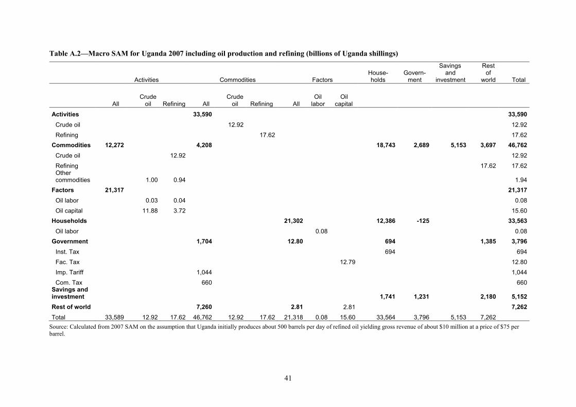
41
Table A.2—Macro SAM for Uganda 2007 including oil production and refining (billions of Uganda shillings)
Activities Commodities Factors House-holds
Govern-ment
Savings and
investment
Rest of
world Total
All Crude
oil Refining All Crude
oil Refining All Oil
labor Oil
capital
Activities 33,590 33,590 Crude oil 12.92 12.92
Refining 17.62 17.62 Commodities 12,272 4,208 18,743 2,689 5,153 3,697 46,762
Crude oil 12.92 12.92
Refining 17.62 17.62 Other commodities 1.00 0.94 1.94
Factors 21,317 21,317 Oil labor 0.03 0.04 0.08
Oil capital 11.88 3.72 15.60 Households 21,302 12,386 -125 33,563
Oil labor 0.08 0.08 Government 1,704 12.80 694 1,385 3,796
Inst. Tax 694 694
Fac. Tax 12.79 12.80
Imp. Tariff 1,044 1,044
Com. Tax 660 660 Savings and investment 1,741 1,231 2,180 5,152 Rest of world 7,260 2.81 2.81 7,262 Total 33,589 12.92 17.62 46,762 12.92 17.62 21,318 0.08 15.60 33,564 3,796 5,153 7,262
Source: Calculated from 2007 SAM on the assumption that Uganda initially produces about 500 barrels per day of refined oil yielding gross revenue of about $10 million at a price of $75 per barrel.
42
REFERENCES
Acemoglu, D., S. Johnson, and J. Robinson. 2003. “Botswana—An African Success Story.” In In Search of Prosperity: Analytical Narratives on Economic Growth, edited by D. Rodrik. Princeton, NJ, US: Princeton University Press.
Adato, M., and J. Hoddinott. 2010. Conditional Cash Transfers in Latin America. Baltimore: Johns Hopkins University Press.
Ahmed, R., and M. Hossain. 1990. Developmental Impact of Rural Infrastructure in Bangladesh. IFPRI Research Report 83. Washington, DC: International Food Policy Research Institute.
Antle, J. 1984. “Human Capital, Infrastructure, and the Productivity of Indian Rice Farmers.” Journal of Development Economics 14:163–181.
Baldi, A.-L., and N. Mulder. 2004. The Impact of Exchange Rate Regimes on Real Exchange Rates in South America, 1990–2002. OECD Economics Department Working Papers No. 396. Paris: OECD.
Benin, S., J. Thurlow, X. Diao, A. Kebba, and N. Ofwono. 2008. Agricultural Growth and Investment Options for Poverty Reduction in Uganda. IFPRI Discussion Paper 790. Washington, DC: International Food Policy Research Institute.
Bevan, D., P. Collier, and J. Gunning. 1999. The Political Economy of Poverty, Equity, and Growth: Nigeria and Indonesia, A World Bank Comparative Study. New York: Oxford University Press.
Binswanger, H. P., S. R. Khandker, and M .R. Rosenzweig. 1993. “How Infrastructure and Financial Institutions Affect Agricultural Output and Investment in India.” Journal of Development Economics 41:337–366.
Breisinger, C., X. Diao, R. Schweickert, and M. Wiebelt. 2009. Managing Future Oil Revenues in Ghana. An Assessment of Alternative Allocation Options. IFPRI Discussion Paper 893. Washington, DC: International Food Policy Research Institute.
Calderón, C., and L. Servén. 2005. The Effects of Infrastructure Development on Growth and Income Distribution. World Bank Policy Research Working Paper 3643. Washington, DC: World Bank.
Calderón, C., and L. Servén. 2008. Infrastructure and Economic Development in Sub-Saharan Africa. World Bank Policy Research Working Paper W4712. Washington, DC: World Bank.
Canning, D., and E. Bennathan. 1999. The Social Rate of Return on Infrastructure Investments. World Bank Policy Research Working Paper W2390. Washington, DC: World Bank.
de Gregorio, J., A. Giovannini, and H. Wolf. 1994. “International Evidence on Tradables and Non-Tradables Inflation.” European Economic Review 38:1225–1244.
Dervis, K., J. de Melo, and S. Robinson. 1982. General Equilibrium Models for Development Policy. Cambridge: Cambridge University Press.
Diao, X., P. Hazell, and J. Thurlow. 2010. “The Role of Agriculture in African Development.” World Development 38 (10): 1375–1383.
Dorosh, P., and J. Thurlow. 2009. Agglomeration, Migration, and Regional Growth. A CGE Analysis for Uganda. IFPRI Discussion Paper 848. Washington, DC: International Food Policy Research Institute.
Duflo E., and R. Pande. 2007. “Dams.” Quarterly Journal of Economics 122 (2): 601–646.
Easterly, W. 2001. The Elusive Quest for Growth. Economists’ Adventures and Misadventures in the Tropics. Cambridge, MA, US: MIT Press.
Economic Intelligence Unit. 2009. Uganda Country Profile 2009. London: Economic Intelligence Unit.
Egert, B., I. Drine, K. Lommatzsch, and C. Rault. 2003. “The Balassa-Samuelson Effect in Central and Eastern Europe: Myth or Reality.” Journal of Comparative Economics 31 (3): 552–572.
Esfahani, H., and M. T. Ramirez. 2002. “Institutions, Infrastructure and Economic Growth.” Journal of Development Economics 70:443–477.
43
Fan, S., P. Hazell, and S. Thorat. 2000. “Government Spending, Growth, and Poverty in Rural India.” American Journal of Agricultural Economics 82 (4): 1038–1051.
Fan, S., T. Mogues, and S. Benin. 2009. Setting Priorities for Public Spending for Agricultural and Rural Development in Africa. IFPRI Policy Brief 12. Washington, DC: International Food Policy Research Institute.
Fan, S., and X. Zhang. 2008. “Public Expenditure, Growth, and Poverty Reduction in Rural Uganda.” African Development Review 20 (3): 466–496.
Fan, S., L. Zhang, and X. Zhang. 2003. Growth, Inequality, and Poverty in Rural China: The Role of Public Investments. Research Report No. 125. Washington DC: International Food Policy Research Institute.
Foster Wheeler. 2010. Uganda Refinery Study. Final Report Submitted to the Ministry of Energy and Mineral Development, Kampala, Uganda.
Gelb, A. 1988. Oil Windfalls: Blessing or Curse? New York: Oxford University Press for the World Bank.
Gelb, A., and S. Grasmann. 2010. How Should Oil Exporters Spend Their Rents? Working Paper 221. Washington, DC: Center for Global Development.
Gibson J., and S. Rozelle. 2003. “Poverty and Access to Roads in Papua New Guinea.” Economic Development and Cultural Change 52 (1): 159–185.
Hausmann, R., and R. Rigobon. 2002. An Alternative Interpretation of the “Resource Curse”: Theory and Policy Implications. NBER Working Paper 9424. Cambridge, MA, US: National Bureau of Economic Research.
Hulten, C. 1996. Infrastructure Capital and Economic Growth: How Well You Use It May Be More Important than How Much You Have. NBER Working Paper 5847. Cambridge, MA, US: National Bureau of Economic Research.
International Monetary Fund. 2003. World Economic Outlook, September. Washington, DC: International Monetary Fund.
Klasen, S. 2004. Population Growth, (Per Capita) Economic Growth, and Poverty Reduction in Uganda: A brief Summary of Theory and Evidence. Report prepared for the Ministry of Finance, Planning and Economic Development, Uganda, March 5, 2004.
Ito, T., P. Isard, and S. Symansky. 1997. Economic Growth and Real Exchange Rate: An Overview of the Balassa-Samuelson Hypothesis in Asia. NBER Working Papers 5979.
Leite, C., and J. Weidmann. 1999. Does Mother Nature Corrupt? IMF Working Paper 99/85. Washington, DC: International Monetary Fund.
Nwafor, M., X. Diao, and V. Alpuerto. 2010. A 2006 Social Accounting Matrix for Nigeria: Methodology and Results. Report No. NSSP007. Washington, DC: International Food Policy Research Institute.
Pauw, K., and L. Mncube. 2007. Expanding the Social Security Net in South Africa: Opportunities, Challenges and Constraints. DPRU Working Paper No. 07/128. Cape Town, South Africa: University of Cape Town, Development Policy Research Unit.
Ram, R. 1996. “Productivity of Public and Private Investment in Developing Countries: A Broad International Perspective.” World Development 24:1373–1378.
Reinikka, E., and J. Svensson. 2002. “Coping with Poor Public Capital.” Journal of Development Economics 69 (1): 51–69.
Renkow, M., D. G. Hallstroma, and D. Karanjab. 2004. “Rural Infrastructure, Transactions Costs and Market Participation in Kenya.” Journal of Development Economics 73 (1): 349–367.
Rodrik, D. 2003. “What Do We Learn from Country Narratives?” In In Search of Prosperity: Analytical Narratives on Economic Growth, edited by D. Rodrik. Princeton, NJ, US: Princeton University Press.
Ross, M. L. 2001. “Does Oil Hinder Democracy?” World Politics 53:325–361.
44
Sachs, J .D., and A. M. Warner. 1995. Natural Resource Abundance and Economic Growth. NBER Working Paper 5398. Cambridge, MA, US: National Bureau of Economic Research.
Sachs, J. D., and A. M. Warner. 2001. “The Curse of Natural Resources.” European Economic Review 45 (4-6): 827-838.
Sala-i-Martin, X., and A. Subramanian. 2003. Addressing the Natural Resource Curse: An Illustration from Nigeria. IMF Working Paper 03/139. Washington, DC: International Monetary Fund.
Sennoga, E. B., and J. M. Matovu. 2010. Public Spending Composition and Public Sector Efficiency: Implications for Growth and Poverty Reduction in Uganda. Research Series No. 66. Kampala, Uganda: Economic Policy Research Centre.
Stevens, P. 2003. “Resource Impact—Curse or Blessing? A Literature Survey.” Journal of Energy Literature 9.
Thurlow, J. 2004. A Dynamic Computable General Equilibrium (CGE) Model for South Africa: Extending the Static IFPRI Model. TIPS Working Paper 1–2004. Pretoria, South Africa: Trade and Industrial Policy Strategies.
Thurlow, J., S. Morley, and A. N. Pratt. 2008. Lagging Regions and Development Strategies. IFPRI Discussion Paper 898. Washington, DC: International Food Policy Research Institute.
Twimukye, E., and J. M. Matovu. 2011. The Impact of Oil Production in Uganda: A Background Paper to the Project Entitled “Managing Future Oil Revenues in Uganda for Agricultural Development.” Kampala, Uganda: Economic Policy Research Centre.
Twimukye, E., J. M. Matovu, S. Levine, and P. Birungi. 2010. Sectoral and Welfare Effects of the Global Economic Crisis on Uganda: A Recursive Dynamic CGE Analysis. Research Series No. 73. Kampala, Uganda: Economic Policy Research Centre.
Uganda, Ministry of Energy and Mineral Development. 2008. National Oil and Gas Policy for Uganda. Kampala, Uganda: Ministry of Energy and Mineral Development.
Valdés, A., and W. Foster. 2010. “Reflections on the Role of Agriculture in Pro-Poor Growth.” World Development 38 (10): 1362–1374.
World Bank. 2007. “Uganda, Moving Beyond Recovery: Investment & Behavior Change for Growth.” In Country Economic Memorandum Volume II: Overview. Report No. 39221–UG, Poverty Reduction and Economic Management Unit, Africa Region. Washington, DC: World Bank.
World Bank. 2010. Country Assistance Strategy for the Republic of Uganda for the Period FY 2011–2015. Washington, DC: World Bank.
World Bank. 2011. World Development Indicators. http://data.worldbank.org/data-catalog/world-development-indicators, last accessed March 14, 2011.
RECENT IFPRI DISCUSSION PAPERS
For earlier discussion papers, please go to http://www.ifpri.org/publications/results/taxonomy%3A468. All discussion papers can be downloaded free of charge.
1121. Impacts of an early education intervention on students’ learning achievement: Evidence from the Philippines. Futoshi Yamauchi and Yanyan Liu, 2011.
1120. Supply and demand for cereals in Nepal, 2010–2030. Sanjay K. Prasad, Hemant Pullabhotla, and A. Ganesh-Kumar, 2011.
1119. Which trade integration scheme can best help Sub-Saharan Africa develop and export more processed agricultural goods?. Mathilde Douillet, 2011.
1118. Women cotton farmers—Their perceptions and experiences with transgenic varieties: A case study for Colombia. Patricia Zambrano, Jorge H. Maldonado, Sandra L. Mendoza, Lorena Ruiz, Luz Amparo Fonseca, and Iván Cardona, 2011.
1117. Can water allocation in the Yellow River basin be improved?: Insights from a multi-agent system model. Ximing Cai, Yi-Chen E. Yang, Jianshi Zhao, and Claudia Ringler, 2011.
1116. Using the regression discontinuity design with implicit partitions: The impacts of Comunidades Solidarias Rurales on schooling in El Salvador. Alan de Brauw and Daniel Gilligan, 2011.
1115. The quiet revolution in India’s food supply chains. Thomas Reardon and Bart Minten, 2011.
1114. A review of input and output policies for cereals production in Nepal. Hemant Pullabhotla, Ganga Shreedhar, A. Ganesh-Kumar, and Ashok Gulati, 2011.
1113. Do shocks affect men’s and women’s assets differently?: A review of literature and new evidence from Bangladesh and Uganda. Agnes R. Quisumbing, Neha Kumar, and Julia A. Behrman, 2011.
1112. Overcoming successive bottlenecks: The evolution of a potato cluster in China. Xiaobo Zhang and Dinghuan Hu, 2011.
1111. The impact of land titling on labor allocation: Evidence from rural Peru. Eduardo Nakasone, 2011.
1110. A multiregion general equilibrium analysis of fiscal consolidation in South Africa. Margaret Chitiga, Ismael Fofana, and Ramos Mabugu, 2011.
1109. How far do shocks move across borders?:Examining volatility transmission in major agricultural futures markets. Manuel A. Hernandez, Raul Ibarra, and Danilo R. Trupkin, 2011.
1108. Prenatal seasonality, child growth, and schooling investments: Evidence from rural Indonesia. Futoshi Yamauchi, 2011.
1107. Collective Reputation, Social Norms, and Participation. Alexander Saak, 2011.
1106. Food security without food transfers?: A CGE analysis for Ethiopia of the different food security impacts of fertilizer subsidies and locally sourced food transfers. A. Stefano Caria, Seneshaw Tamru, and Gera Bizuneh, 2011.
1105. How do programs work to improve child nutrition?: Program impact pathways of three nongovernmental organization intervention projects in the Peruvian highlands. Sunny S. Kim, Jean-Pierre Habicht, Purnima Menon, and Rebecca J. Stoltzfus, 2011.
1104. Do marketing margins change with food scares?: Examining the effects of food recalls and disease outbreaks in the US red meat industry. Manuel Hernandez, Sergio Colin-Castillo, and Oral Capps Jr., 2011.
1103. The seed and agricultural biotechnology industries in India: An analysis of industry structure, competition, and policy options. David J. Spielman, Deepthi Kolady, Anthony Cavalieri, and N. Chandrasekhara Rao, 2011.
1102. The price and trade effects of strict information requirements for genetically modified commodities under the Cartagena Protocol on Biosafety. Antoine Bouët, Guillaume Gruère, and Laetitia Leroy, 2011
1101. Beyond fatalism: An empirical exploration of self-efficacy and aspirations failure in Ethiopia. Tanguy Bernard, Stefan Dercon, and Alemayehu Seyoum Taffesse, 2011.
1100. Potential collusion and trust: Evidence from a field experiment in Vietnam. Maximo Torero and Angelino Viceisza, 2011.
1099. Trading in turbulent times: Smallholder maize marketing in the Southern Highlands, Tanzania. Bjorn Van Campenhout, Els Lecoutere, and Ben D’Exelle, 2011.
46
INTERNATIONAL FOOD POLICY RESEARCH INSTITUTE
www.ifpri.org
IFPRI HEADQUARTERS
2033 K Street, NW Washington, DC 20006-1002 USA Tel.: +1-202-862-5600 Fax: +1-202-467-4439 Email: [email protected]
IFPRI KAMPALA 15 East Naguru Road Kampala Uganda Tel.: +256-41-285-060/4; +256-312-226-613 Fax: +256-41-285-079 Email: [email protected]
IFPRI LILONGWE OFFICE
PO Box 31666 Lilongwe 3 Malawi Tel.: +265-1-789747 Email: [email protected]