macroeconomic synchronization between mexico and its

Macroeconomic Synchronization between Mexico and its NAFTA Partners

Alfredo Cuevas, Miguel Messmacher and Alejandro Werner♣ ,⊗

June 2002

Abstract In this study we analyze changes in the degree of macroeconomic synchronization between Mexico and its NAFTA partners. In particular, we compare the change in the degree of synchronization before and after NAFTA was implemented. For this, we use several samples and control variables. The first is a sample of different countries, the second is of sectors of economic activity, the third consists of components of aggregate demand and supply and finally we analyze the evolution of employment at the regional level in Mexico and the US. We find that synchronization seems to have increased due to NAFTA and this has occurred in a large number of pro-cyclical economic sectors and regions, reinforcing traditional links between the Mexico and its NAFTA partners. In terms of policy implications, even though optimal stabilization policies will be qualitatively more similar in the future for the three countries, we find that idiosyncratic shocks are still important for Mexico and common shocks also have stronger effects in this economy in a context of different policy transmission channels. Therefore, the magnitude of this desired policy response would not be similar. 1. Introduction and Review of the Literature In this document we try to assess whether macroeconomic synchronization of business cycles has increased between Canada, Mexico and the USA as a result of NAFTA. Given that a close relationship already existed between Canada and the USA, most of our focus is on whether Mexico’s business cycle is more similar to those of its major trading partners. In this respect, there are two different, though related, issues to consider. The first is whether the Mexican economy has become more sensitive to developments in its NAFTA partners, i.e. whether the business cycle in Canada or the USA generates a larger response in the Mexican business cycle than before. The second issue is whether shocks to growth in

♣ The first two authors are Economic Research Officers and the third is Director of Economic Research, General Direction of Economic Studies, Banco de Mexico. ⊗ The authors would like to thank Luz Marina Arias and Leonardo Armas for their assistance. We would also like to thank Daniel Lederman, Luis Serven and the participants at the “NAFTA Brainstorming Workshop” at the World Bank for their comments. The opinions included in this document are exclusively those of the authors and do not represent the point of view of Banco de México. This study was prepared as a background paper for a wide ranging analysis by the World Bank on the effects of free trade agreements, and particularly NAFTA, on economic activity.

2

Canada or the USA have become a more important source of volatility relative to other types of shocks, i.e. whether the business cycle in these countries represents a more significant source of volatility for the Mexican economy than other types of shocks, such as terms of trade, financial contagion or domestic aggregate demand shocks. Why is it important to distinguish between these two issues? The sensitivity of the Mexican economy to developments in Canada or the USA may have increased, which ceteris paribus, would lead to higher synchronization of business cycles. However, if idiosyncratic shocks to the Mexican economy are still quite large or increase, then the increase in the sensitivity of the Mexican economy to developments in Canada and the USA may not be enough to make these the main sources of volatility for the Mexican economy. In this case, even though the degree of synchronization would increase, it wouldn’t really be fair to speak of a synchronized business cycle. This phenomenon could also work in opposite direction, i.e., that the Mexican economy has not suffered significant idiosyncratic shocks in the period after the balance of payments crisis in 1995, so we find that the Mexican business cycle is highly correlated with those of its NAFTA partners, even though this would not be a robust finding in a larger sample that includes future idiosyncratic shocks. Finally, if empirically we found that developments in Canada and the USA were more important in explaining volatility in Mexico, but without an increase in sensitivity, it would mean that the frequency and magnitude of the idiosyncratic shocks affecting Mexico are smaller, not that the relationship between Mexico and its trading partners is larger due to NAFTA.1 Thus, we would need to observe the two phenomenon in order to argue that there is a stronger synchronization due to the free trade agreement. There are also practical arguments for making the distinction. Since the implementation of NAFTA in 1994, Mexico has been subjected to important shocks that did not affect Canada or the USA in significant ways. The Mexican balance of payments crisis of 1994-1995 and the Russian and Brazilian crises are “idiosyncratic” shocks to Mexico with respect to Canada and the USA, even though some of them are common shocks from the point of view of emerging markets. In addition, during the 1994-2001 period there has really been only one business cycle in Canada and the USA, and not even a complete one. Thus, it is likely that, given the absence of long frequency data needed to study business cycles after NAFTA, we could be overestimating the importance of idiosyncratic shocks versus common shocks in accounting for volatility in Mexican business cycles. However, finding an increase in the sensitivity of Mexican GDP to developments in the US would suggest that synchronization is likely to increase in the future, in the absence of an increase in the frequency and magnitude of future idiosyncratic shocks to Mexico. In addition, the policy implications of the two events are quite different. The presence of important idiosyncratic shocks probably requires that Mexican authorities follow macroeconomic policies that may be quite different from those implemented in its trading 1 Of course, it is possible that due to NAFTA, the frequency and magnitude of idiosyncratic shocks is smaller. This could occur because of several reasons. If the trade agreement leads to a more diversified export base, then Mexico would be less sensitive to specific terms of trade shocks such as changes in the price of oil. In addition, the legal changes associated to NAFTA may have given greater certainty to investors about future Mexican economic policies, thus leading to higher and more stable investment. These are different from traditional arguments for synchronization due to higher trade flows between two countries.

3

partners, even if Mexico is more sensitive to developments in these countries. On the other hand, if shocks within the NAFTA group are similar and are the main source of shocks, then Mexico would benefit from the stabilization policies followed by its trading partners, and its own desired policy adjustments would be similar to those desired for the other two countries.2 Thus, in what follows we analyze both issues: whether Mexico is more sensitive to developments in its trading partners, with particular emphasis on the USA, and if developments in the USA account for a larger proportion of the variability in Mexican growth rates. The methodology of analysis we use is explained in detail in section 2. Given that it has been argued that the world is becoming more integrated as a whole, section 3 of the document compares recent changes for Mexico with those for other countries, in order to assess if we can really attribute the change to NAFTA rather than to the widespread effect of globalization that affected every country similarly or to a general increase in international trade. In addition, we include a section that reviews the case of Ireland, Portugal and Spain in the European Union to see if developments in Mexico mirror those in these three countries. It is also important to compare the Mexican relationship with the US with that of this country and Canada, as this last case can be used as a benchmark for very close integration. We do this at the national level but also at the sectorial (section 4.1), aggregate demand (section 4.2) and regional level (section 4.3). This should also allow us to be more confident that a stronger synchronization is really due to NAFTA by comparing changes in tradable and non-tradable goods sectors, as well as regions that should have benefited more from NAFTA with those less likely to have experienced significant changes. In section 5 we discuss the policy implications from our analysis while section 6 concludes. We also include a summary of the results at the end of sections 3 and 4, in case the reader wishes to get a brief impression of the main empirical results from the extensive statistical analysis that is presented in each of these sections. Literature Review There is an extensive theoretical and empirical literature on international business cycles and comovement of growth across countries.3 However, most of it analyzes comovement across industrial countries, given the availability of the long time series necessary to undertake business cycle analysis. In the more scarce literature that compares industrial with developing countries it is found that the comovement between industrial countries tends to be much larger than that between industrial and developing countries or between developing countries in general.4 Obviously, this does not mean that developing countries 2 The policy adjustments would probably be similar in direction, though the different structural conditions of the Mexican economy compared with those of Canada and the USA might imply that changes need to be of different magnitudes. 3 See for example Backus and Kehoe (1992), Backus, Kehoe and Kydland (1992, 1995), Stockman (1990). 4 See for example Hoffmaister and Roldos (1997), Loayza, Lopez and Ubide (2001), Hall, Monge and Robles (1999), Agenor, McDermott and Prasad (1999).

4

are not affected by developments in the industrial countries or among themselves. Instead, it probably signals that in addition to these common effects there are large idiosyncratic shocks that mute more general shocks. This seems to be confirmed by the work of Arora and Vamvakidis (2001) where they analyze the coefficient of US growth in long run growth regressions.5 They find that the point estimate on US growth for a large sample of developing countries is close to 1, while that for a sample of industrial countries is in the range of 0.3-0.4. Thus, in the long run, growth in the US (or other industrialized countries) is very important for developing countries, though in the short run there may be significant idiosyncratic shocks. An alternative explanation is that idiosyncratic shocks tend to be more transitory in character, while permanent shocks are of a more international nature. Loayza, Lopez and Ubide (2001) do a more detailed analysis of comovement using an error components model comparing the results from three blocks of countries: Latin America, East Asia and Europe. They find that common shocks explain a substantial part of the variation in growth rates in East Asia and Europe, but idiosyncratic shocks are clearly dominant for Latin America.6 Monges, Hall and Robles (1999) find a similar preponderance of idiosyncratic shocks in an analysis for Central American countries and Mexico. In spite of their analysis for several Latin American countries, their results are not directly related with the main objectives of our study because of three reasons. First, they don’t do an analysis of the relationship between Canada, Mexico and the USA. Second, both studies are done using a long term perspective, while for our purposes it is very important to look at changes over time in order to assess if NAFTA had any impact. Finally, their methodology would allow us to distinguish if in the more recent period the effect of common shocks in Canada, Mexico and the USA account for a larger part of the variability in Mexico’s production, but we would not be able to separate how much of this is due to a larger shock in the USA or smaller idiosyncratic shocks than observed in the past (two events presumably unrelated to NAFTA) and the extent to which this is due to a higher sensitivity of Mexican production to shocks in the USA (related with NAFTA).7 Del Negro (2001) uses a technique combining factor analysis with identified VAR models to study output comovements across US states, Mexican states and Canadian provinces, using annual data for the period 1971-1998. He finds interesting results that suggest that in this period there existed some comovement between Mexican states and some US states and Canadian provinces, but this is probably due to common exogenous shocks. In particular, his results from cluster analysis show a large degree of comovement between Mexican states and oil producing states or provinces in Canada and the US. A second cluster is formed by most US states and the Eastern provinces of Canada. Unfortunately, his

5 Specifically, they regress five year rates of growth of GDP per capita for the period 1980-1998 on the contemporary growth rate of the US together with some variables that have traditionally been used in growth regressions, such as initial level of GDP per capita and population growth rate. The number of countries varies with the specification employed, but normally ranges between 100 and 140 countries. 6 Karras (2000) uses a similar methodology when considering if the Americas are an optimal currency area and finds similar results. 7 As mentioned, if NAFTA leads to a change in the composition of Mexican exports, in the institutional background for foreign investment in Mexico or in risk perception about the Mexican economy it could also modify the distribution of idiosyncratic shocks. However, in order to assess this in a statistically significant way we would probably need longer time series after the implementation of the trade agreement.

5

analysis is also subject to the criticisms that it is focused on long term effects and does not allow us to differentiate between a larger sensitivity of Mexico to developments in its partners’ economies or just that its idiosyncratic shocks are smaller (and common shocks are larger). The studies mentioned don’t look at the possible effect of NAFTA or other trade agreements. However, there is an important literature on the effects of trade agreements and business cycle consolidation. Theoretical analysis has shown that cycles and shocks could become more or less idiosyncratic. In particular, the degree of business cycle synchronization could fall if a free trade agreement leads countries to higher specialization, with sectorial shocks being large (Eichengreen (1992), Kenen (1969), and Krugman (1993)).8 On the other hand if demand or common shocks are more important or if most trade is of intra-industry type, then business cycles would become more synchronized. Frankel and Rose (FR, 1998) is a seminal paper that tried to assess which of the two hypothesis is the correct one, using a sample of twenty industrialized countries over thirty years. They found that closer trade links actually led to more highly correlated business cycles. This is not a direct test of the effect of free trade agreements, but it is suggestive of what to expect from them. In fact, in an estimation they use later on to construct instrumental variables they find that, for their sample of countries, free trade agreements lead to very significant increases in trade. FR’s study focused on the European Union and the adoption of a common currency. Their intention was to show that the conditions for an optimal currency area are endogenous, as a monetary union would lead to higher trade, and higher trade in turn to higher synchronization of business cycles. Other studies following a similar objective and using similar methodology are: Artis and Zhang (1995), who find that European economies were highly correlated with the US from 1961-1979 but more with Germany since joining the ERM; Fidrmuc (2001), who estimates the relationship between trade and the correlation of business cycles using a sample that includes Central and Eastern European countries and also the level intra-industry trade which is found to be positive and significant; Fontagné and Freudenberg (1999) find the same results as FR looking at more disaggregated trade data for the European Union; Anderson, Kwark and Vahid (1999) again find similar results using more sophisticated measures of comovement compared with the simple correlations employed by FR. Imbs (1998) casts an important doubt on the results of FR (1998) and those derived using the same methodology, as he finds that their results may not be robust to the inclusion of fixed effects or of other possible determinants of both trade and synchronization, such as gravity effects. Thus, it seems as if FR’s results could be strongly driven by cross sectional variation, possibly due to other effects, and not time variation in trade and synchronization.

8 It has also been argued that capital market integration that leads to higher risk sharing may also lead to higher specialization, see for example Kalemi-Ozcan, Sorensen and Yosha (2000). However, as higher risk sharing is the force driving the specialization it would actually increase comovement in income and consumption, though not in production.

6

It is worth noting that in our study we put particular emphasis on the time variation, so our results don’t seem subject to Imbs’ criticism. With an alternative specification, Imbs (2000) finds that cycle synchronization is more responsive to similarities in the structure of production rather than to trade intensity, suggesting that sectorial shocks are an important factor driving comovement. Again, this is less likely to be driving changes in comovement across the Mexican economy and those of its NAFTA partners, given that the sectorial composition of GDP is more different between them than in a sample of industrial countries. This implies that even if there is a strong and positive relationship between trade intensity and the correlation of business cycles in a sample of industrialized countries it could be arising from the fact that they have similar factor endowments, so a higher degree of specialization due to trade is limited. It might be the case that we only observe sufficient marginal specialization in cases of significant trade between countries that have very different factor endowments. In this sense, it is more likely to find less synchronization in a case like the Mexican one, where relative factor endowments are significantly different from those in the US and Canada, unless trade is mostly intra-industry in character.9 The empirical evidence for the effect of higher trade between industrial and emerging market on synchronization of business cycles is mixed. The adjustment of trade patterns following the transitional recession of the early 1990’s seems to have led to a higher correlation of the business cycle between Germany and several Central and Eastern European countries according to Fidrmuc (2001). Achy and Milgram (2001) argue that a free trade agreement between Morocco and the European Union is very likely to lead to higher specialization in Morocco and a less synchronized business cycle. Ahumada and Martirena-Mantel (2001) do the same analysis as FR for a sample of some Mercosur countries plus Chile in order to assess whether an increase in trade volumes across these countries has led to higher synchronization. This is an interesting case that is somewhat different from the European or NAFTA contexts, as the exports of these countries are generally intensive in natural resources, at least with third countries. The authors find suggestive evidence that higher trade has led to higher comovement, but the strongest factor driving their results is the change in correlations between Argentina and Brazil from 1987-1992 to 1993-1999.10 It would be interesting to assess if this result still holds when considering the recent Argentine crisis. Torres and Vela (2002) analyze in detail the degree of correlation of several quarterly variables between Mexico and the US for the period 1992-2001, with particular emphasis on the leads and lags structure of the correlations. They find a positive correlation between GDP in the US and GDP or manufacturing production in Mexico, though their results are puzzling as the strongest correlation is with the first lag of the Mexican variables. A 9 Another potential counter argument against finding a smaller correlation are the large differences in size, particularly between Mexico and the US. A relatively small demand shock for the size of the US economy could be very large for Mexico. 10 The correlations between Argentina-Uruguay, Brazil-Uruguay, Argentina-Chile, Brazil-Chile and Chile-Uruguay change little between both periods and in some cases fall in the second period.

7

possibility is that the demand for Mexican exports responds more quickly to the business cycle than other components of US GDP. In terms of the relationship between Mexican exports and GDP, they find that the highest correlation is contemporary and is substantially larger for the period 1996-2001 than for their whole sample 1992-2001. The correlation of imports with GDP is quite high for the whole period. Unfortunately, they don’t analyze changes over time in the correlation between US variables and Mexican ones. The only result that is strongly suggestive of a marginal effect from NAFTA is the substantial increase of the correlation between exports and GDP in Mexico. 2. General Methodology Throughout this document, we analyze economic synchronization of economic variables for different samples and levels of aggregation (national, sectorial and regional levels). The methodology of analysis is essentially the same for all cases, and we point out any differences in the specific sections where this occurs. The analysis is done using annual growth rates of the variables. These are used because the calculation of business cycles by means of filters may depend in an important way on the use of seasonally adjusted data, which is not available in many cases. In addition, they might be more sensitive to measurement error problems, as the annual growth rates are incorporating information from the last twelve months. There is one important consideration related with the interpretation of correlations of annual growth rates. The correlation between two series of annual growth rates would increase if there is a larger effect from changes in one on the other, but also if the effect takes place sooner, even if the size of the effect has not changed.11 In section 4.1 we make an analysis of changes in the speed with which shocks in the US affect manufacturing in Mexico. The following methods are used in all cases: i) Correlations. We do two types of analysis using correlations. The first is a comparison of correlations between the different variables for the longest possible time period, depending on the availability of data, and then for a shorter time period meant to capture the effect of NAFTA. In addition, we analyze three year moving correlations. In all cases, we place particular emphasis on the correlation with respect to the same variable in the USA. This allows us to observe: i) if the correlation between the Mexican and USA variables has increased more than that between other countries and the USA, in the case of international comparisons, and ii) if the correlation between Mexican and USA sectors, components of aggregate demand or regions has increased more for those cases where we would expect a larger effect from NAFTA. 11 This is discussed in greater detail in Appendix 1.

8

ii) Basic regression analysis. We regress the annual growth rate of production, demand or employment variables against contemporaneous and lagged observations of themselves and contemporaneous observations of the same variable in the USA. The general form of the regressions is the following:

UStiitiiUStiitiiit xdTxdTdTxxx ∆⋅+∆⋅++∆+∆+=∆ −− δλµγβα 11 (1) where itx∆ is the annual growth rate of variable x in country, region or sector i, UStx∆ is the annual growth rate of the same variable in the USA,12 and dT is a time dummy to capture whether the sensitivity of the variable to developments in the USA has changed.13 The regressions are initially estimated on a country by country (sector, demand component or region within a country) basis. There are two options for dT, and we report results for both of them. The first option is a d94, which is one from 1994 to the end of period, and zero for previous periods. The second, d97, is one from 1997 on. Even though NAFTA was implemented in 1994, the large balance of payments crisis that took place in Mexico in 1995 and the fast subsequent recovery in 1996 are large shocks, presumably unrelated with NAFTA and that might make it more difficult to find any significant effects from the trade agreement. These simple regressions allow us to compare three things. The first is how sensitive the variable is to developments in the USA (γ), the second is how this sensitivity has changed over time (δ), and finally the R2 can tell us how much of the variables’ variation can be accounted for by developments in the USA (restricting β=0).14 A country may be quite responsive to developments in the USA, but if it is also subject to other significant shocks we could find a high γ but a low R2. We used three specific forms of equation (1) throughout the analysis. The first is merely to include a constant plus the contemporary growth rate of the variable in the US (with and without interaction with time dummys). The second was to add one lag of the dependent variable. Finally, we added more lags of the dependent variable as well as for the US variable, so we had 2 lags of the dependent variables and the contemporary and 2 lagged values of the variable in the US, with and without interacting with the post-NAFTA dummys. In the case of variables with quarterly frequency, more than one lag for the

12 In the case of regions, it corresponds to total US employment growth, and in the case of sectors of economic activity it corresponds to the growth rate of the same sector of economic activity in the USA. 13 This methodology is very similar to that used by Frankel, Schmukler and Serven (2002) to assess how responsive interest rates are under different currency regimes to changes in rates in the USA. 14 In addition, the coefficient β tells us the degree of persistence in the variable, while α/(1-β) gives us the long-run growth trend if growth in the USA was zero. We do not discuss the results on α or β in detail, as we are more interested in looking at the relationship with the USA.

9

dependent variable and any lag for the variable in the US were seldom significant and did not affect the results in terms of the overall relationship of a variable or changes in the relationship between the pre and post-NAFTA periods. In the case of monthly industrial production growth rates, the two lags of the dependent variable were typically significant so we reestimated using four lags of the dependent variable plus the contemporary value and two lags for the US variable. Thus, we discuss in detail the results when including longer lags in the sections on multi-country industrial production data and on industrial subcomponents in Mexico. Given that the four quarter (or 12 month) filter implicit in working with annual growth may not remove all sources of seasonality we also did all the regressions with seasonal dummys. These were never significant and their inclusion did not affect in any important way the estimated parameters nor their significance. Thus, it seems that the annual filters do a good work in removing seasonality and in the text we report the results without including the seasonal dummys. iii) Factor analysis The factor analysis employed is a simple specification. This is again conditioned by the fact that we specifically want to look for changes in the post-NAFTA period, which limits sample size considerably and thus the type of procedures we can use. We use maximum likelihood estimation to decompose growth rates of a set of i variables into k factors:

ufyi +Λ+=∆ µ (2) where ∆yi is the growth rate of our variable of interest, the subindex i will stand for countries, sectors of activity, regions or components of aggregate demand, µ is a constant, Λ is a matrix of factor loadings, f is a vector of factors and u is a vector of idiosyncratic shocks. The number of factors included in each estimation is determined by a χ2 test against the hypothesis of including more factors, and the reported factor loadings correspond to those obtained from varimax rotations. Factor analysis complements the correlation and regression analysis by incorporating all the information available in the cross correlations of all the variables in the sample, in comparison with the bivariate regression analysis, while at the same time expressing this information in a way that is easier to analyze than the complete matrix of cross correlations. 3. National Economic Aggregates In this section, we measure the degree of synchronization among the economies of Mexico, the US and Canada, and compare it to that observed between each one of those countries

10

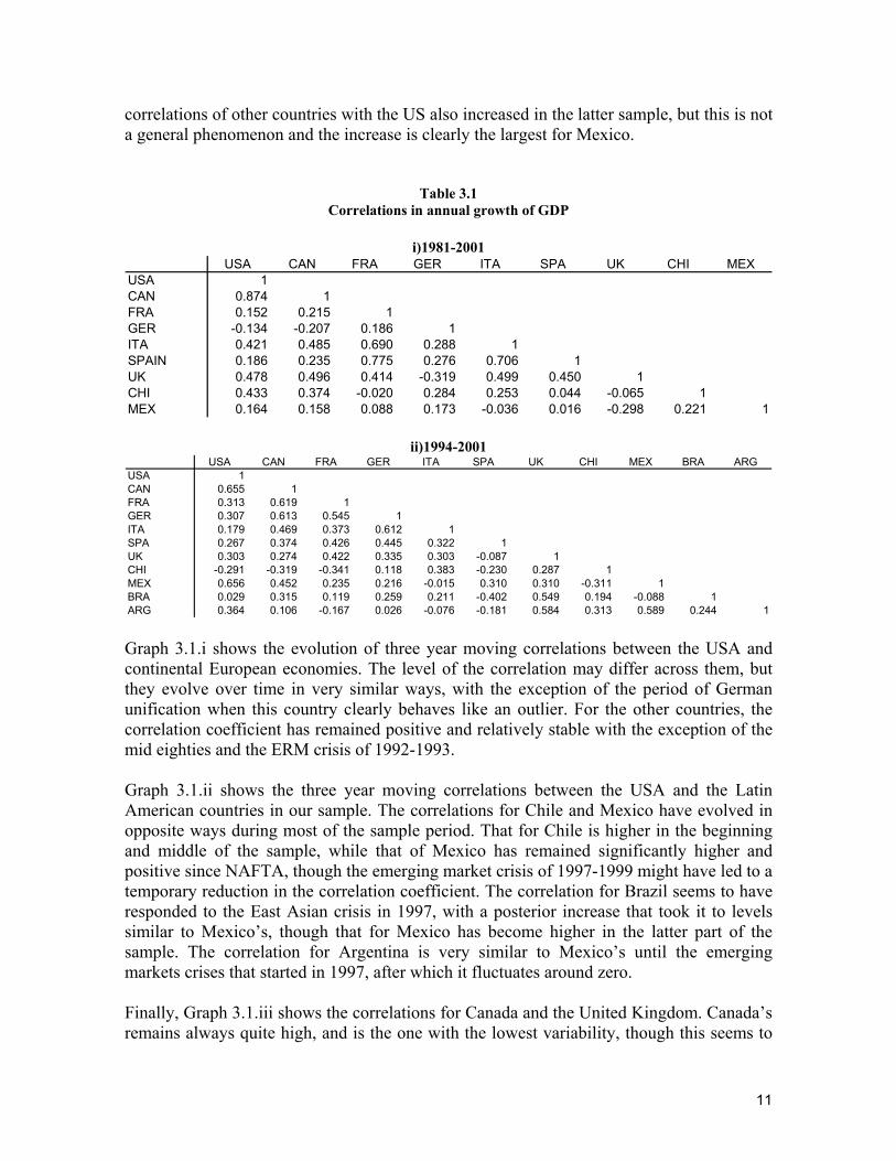
with other countries in Latin America and Europe.15 The data employed are annual rates of growth of GDP (at quarterly frequency) and of industrial production (at monthly frequency). The source of the data for all the countries is IFS of the IMF with the exception of the industrial production of Argentina, Brazil and Chile. For these three countries, the data on industrial production are from FIEL16 in Argentina and the National Institutes of Statistics of Brazil and Chile. In addition, we present a brief summary of the results other authors have found in the case of Portugal and Spain in the context of the European Union and compare these with those found for Mexico. 3.1. Results with a sample of different countries Analysis of correlations across countries and with the USA Table 3.1 shows the correlation coefficients between annual growth rates of GDP for the sample of countries during the periods 1981Q1-2001Q2 and 1994Q1-2001Q2.17 In the longer sample, the correlation coefficient between Canada and the USA is quite high, followed by a large margin by those of the United Kingdom, Chile and Italy. The correlation of Mexico with Canada and the USA is positive, but low. Nevertheless, they are the highest correlation coefficients Mexico has with any of the countries in the sample with the exception of Chile and, surprisingly, Germany. In the shorter and more recent time period, the highest correlations with the USA are those of Canada and Mexico, both with very similar values. However, it is interesting to notice that while this coefficient increases for Mexico it falls for Canada compared with that for the full sample. These are also the highest correlation coefficients of these two countries with any other country. The correlation with the USA of all the European countries is positive, though at an intermediate level. Argentina’s coefficient is similar to those of European countries, Brazil’s is virtually nil, and Chile’s is negative. The correlation between Canada and Mexico is higher than for the whole sample. However, in the Canadian case, its correlation coefficient with several European countries is higher than that with Mexico. In the Mexican case, its correlation is only higher with Argentina, presumably because of the effects the Tequila crisis had on the South American country. Its correlation also increased with most European economies in the sample, though the increase is much smaller than that with the US. This last phenomenon is consistent with the general opening to trade followed by Mexico since the mid eighties. Some of the

15 The American countries included in the sample are: Argentina, Brazil, Canada, Chile, Mexico and the USA. The European countries are France, Germany, Ireland, Italy, Portugal, Spain and the United Kingdom. Ireland and Portugal are not always included in the analysis due to data limitations. 16 The Fundación de Investigaciones Económicas Latinoamericanas is the institution that has carried out a public monthly survey of industrial production (EMI, Encuesta Mensual Industrial) in Argentina for the longest time. 17 The date of the second sample is conditioned by the fact that we don’t have quarterly GDP data for Argentina until 1993. Brazil is not included in the correlation calculations for the first sample as its series of quarterly GDP starts in 1990.

11

correlations of other countries with the US also increased in the latter sample, but this is not a general phenomenon and the increase is clearly the largest for Mexico.

Table 3.1 Correlations in annual growth of GDP

i)1981-2001

USA CAN FRA GER ITA SPA UK CHI MEXUSA 1CAN 0.874 1FRA 0.152 0.215 1GER -0.134 -0.207 0.186 1ITA 0.421 0.485 0.690 0.288 1SPAIN 0.186 0.235 0.775 0.276 0.706 1UK 0.478 0.496 0.414 -0.319 0.499 0.450 1CHI 0.433 0.374 -0.020 0.284 0.253 0.044 -0.065 1MEX 0.164 0.158 0.088 0.173 -0.036 0.016 -0.298 0.221 1

ii)1994-2001

USA CAN FRA GER ITA SPA UK CHI MEX BRA ARGUSA 1CAN 0.655 1FRA 0.313 0.619 1GER 0.307 0.613 0.545 1ITA 0.179 0.469 0.373 0.612 1SPA 0.267 0.374 0.426 0.445 0.322 1UK 0.303 0.274 0.422 0.335 0.303 -0.087 1CHI -0.291 -0.319 -0.341 0.118 0.383 -0.230 0.287 1MEX 0.656 0.452 0.235 0.216 -0.015 0.310 0.310 -0.311 1BRA 0.029 0.315 0.119 0.259 0.211 -0.402 0.549 0.194 -0.088 1ARG 0.364 0.106 -0.167 0.026 -0.076 -0.181 0.584 0.313 0.589 0.244 1 Graph 3.1.i shows the evolution of three year moving correlations between the USA and continental European economies. The level of the correlation may differ across them, but they evolve over time in very similar ways, with the exception of the period of German unification when this country clearly behaves like an outlier. For the other countries, the correlation coefficient has remained positive and relatively stable with the exception of the mid eighties and the ERM crisis of 1992-1993. Graph 3.1.ii shows the three year moving correlations between the USA and the Latin American countries in our sample. The correlations for Chile and Mexico have evolved in opposite ways during most of the sample period. That for Chile is higher in the beginning and middle of the sample, while that of Mexico has remained significantly higher and positive since NAFTA, though the emerging market crisis of 1997-1999 might have led to a temporary reduction in the correlation coefficient. The correlation for Brazil seems to have responded to the East Asian crisis in 1997, with a posterior increase that took it to levels similar to Mexico’s, though that for Mexico has become higher in the latter part of the sample. The correlation for Argentina is very similar to Mexico’s until the emerging markets crises that started in 1997, after which it fluctuates around zero. Finally, Graph 3.1.iii shows the correlations for Canada and the United Kingdom. Canada’s remains always quite high, and is the one with the lowest variability, though this seems to

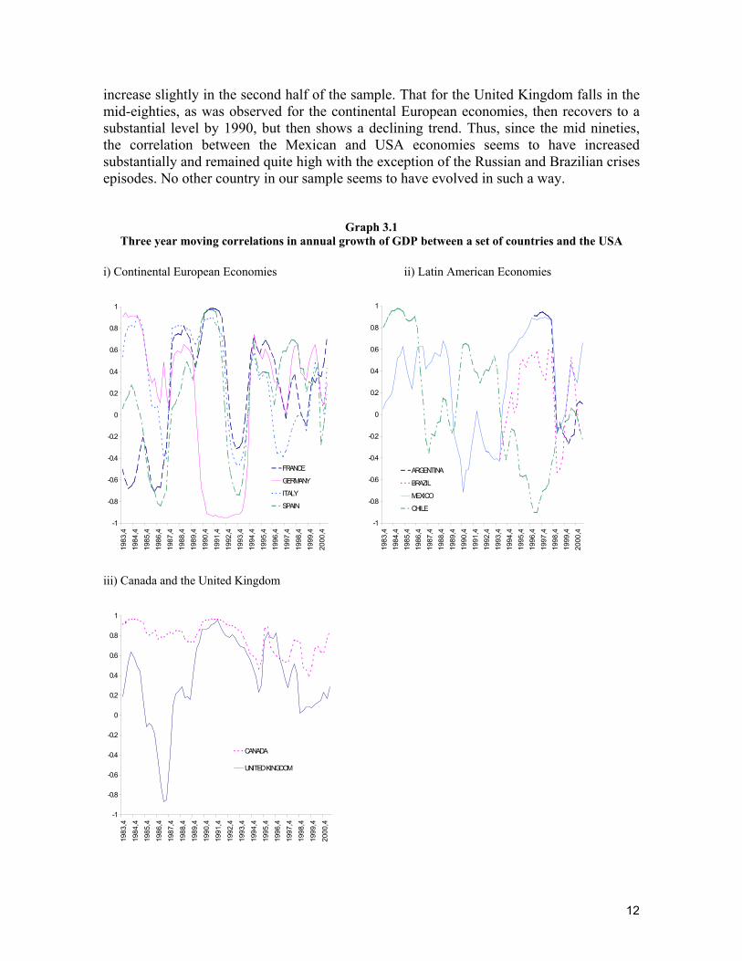
12

increase slightly in the second half of the sample. That for the United Kingdom falls in the mid-eighties, as was observed for the continental European economies, then recovers to a substantial level by 1990, but then shows a declining trend. Thus, since the mid nineties, the correlation between the Mexican and USA economies seems to have increased substantially and remained quite high with the exception of the Russian and Brazilian crises episodes. No other country in our sample seems to have evolved in such a way.

Graph 3.1 Three year moving correlations in annual growth of GDP between a set of countries and the USA

i) Continental European Economies ii) Latin American Economies

-1

-0.8

-0.6

-0.4

-0.2

0

0.2

0.4

0.6

0.8

1

1983

,419

84,4

1985

,419

86,4

1987

,419

88,4

1989

,419

90,4

1991

,419

92,4

1993

,419

94,4

1995

,419

96,4

1997

,419

98,4

1999

,420

00,4

FRANCE

GERMANY

ITALY

SPAIN

-1

-0.8

-0.6

-0.4

-0.2

0

0.2

0.4

0.6

0.8

1

1983

,419

84,4

1985

,419

86,4

1987

,419

88,4

1989

,419

90,4

1991

,419

92,4

1993

,419

94,4

1995

,419

96,4

1997

,419

98,4

1999

,420

00,4

ARGENTINA

BRAZIL

MEXICO

CHILE

iii) Canada and the United Kingdom

-1

-0.8

-0.6

-0.4

-0.2

0

0.2

0.4

0.6

0.8

1

1983

,419

84,4

1985

,419

86,4

1987

,419

88,4

1989

,419

90,4

1991

,419

92,4

1993

,419

94,4

1995

,419

96,4

1997

,419

98,4

1999

,420

00,4

CANADA

UNITED KINGDOM

13

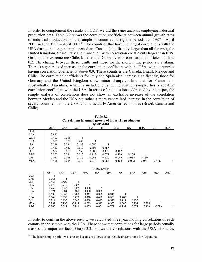
In order to complement the results on GDP, we did the same analysis employing industrial production data. Table 3.2 shows the correlation coefficients between annual growth rates of industrial production for the sample of countries during the periods Jan 1987 – April 2001 and Jan 1995 – April 2001.18 The countries that have the largest correlations with the USA during the longer sample period are Canada (significantly larger than all the rest), the United Kingdom, Spain, Italy and France, all with correlation coefficients larger than 0.39. On the other extreme are Chile, Mexico and Germany with correlation coefficients below 0.2. The change between these results and those for the shorter time period are striking. There is a generalized increase in the correlation coefficient with the USA, with 4 countries having correlation coefficients above 0.9. These countries are Canada, Brazil, Mexico and Chile. The correlation coefficients for Italy and Spain also increase significantly, those for Germany and the United Kingdom show minor changes, while that for France falls substantially. Argentina, which is included only in the smaller sample, has a negative correlation coefficient with the USA. In terms of the questions addressed by this paper, the simple analysis of correlations does not show an exclusive increase of the correlation between Mexico and the USA but rather a more generalized increase in the correlation of several countries with the USA, and particularly American economies (Brazil, Canada and Chile).

Table 3.2 Correlations in annual growth of industrial production

i)1987-2001 USA CAN GER FRA ITA SPA UK BRA CHI MEX

USA 1CAN 0.883 1GER 0.102 0.028 1FRA 0.391 0.339 0.785 1ITA 0.396 0.394 0.488 0.655 1SPA 0.467 0.430 0.652 0.804 0.657 1UK 0.597 0.659 0.153 0.368 0.478 0.402 1BRA 0.262 0.334 0.026 0.113 0.072 0.153 0.155 1CHI -0.013 -0.098 -0.145 -0.041 0.220 -0.056 0.083 0.135 1MEX 0.168 0.054 0.312 0.278 -0.056 0.160 -0.033 0.051 -0.135 1

ii)1995-2001

USA CAN GER FRA ITA SPA UK BRA CHI MEX ARGUSA 1CAN 0.961 1GER 0.156 0.423 1FRA -0.576 -0.779 -0.897 1ITA 0.757 0.547 -0.527 0.098 1SPA 0.821 0.631 -0.436 -0.006 0.995 1UK 0.593 0.347 -0.703 0.317 0.975 0.946 1BRA 0.942 0.998 0.479 -0.818 0.493 0.581 0.287 1CHI 0.912 0.990 0.547 -0.860 0.423 0.515 0.211 0.997 1MEX 0.931 0.795 -0.214 -0.239 0.943 0.973 0.845 0.754 0.700 1ARG -0.266 0.011 0.911 -0.635 -0.831 -0.769 -0.934 0.074 0.153 -0.599 1

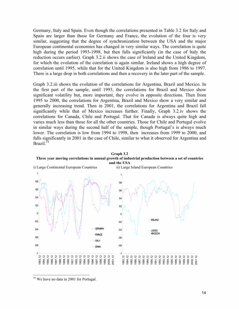
In order to confirm the above results, we calculated three year moving correlations of each country in the sample with the USA. These show that correlations for large periods actually mask some important facts. Graph 3.2.i shows the correlations with the USA of France, 18 The latter sample period was chosen because it allows us to include observations for Argentina.

14

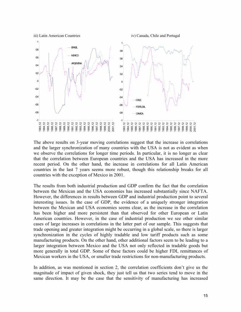
Germany, Italy and Spain. Even though the correlations presented in Table 3.2 for Italy and Spain are larger than those for Germany and France, the evolution of the four is very similar, suggesting that the degree of synchronization between the USA and the major European continental economies has changed in very similar ways. The correlation is quite high during the period 1993-1998, but then falls significantly (in the case of Italy the reduction occurs earlier). Graph 3.2.ii shows the case of Ireland and the United Kingdom, for which the evolution of the correlation is again similar. Ireland shows a high degree of correlation until 1995, while that for the United Kingdom is also high from 1986 to 1997. There is a large drop in both correlations and then a recovery in the later part of the sample. Graph 3.2.iii shows the evolution of the correlations for Argentina, Brazil and Mexico. In the first part of the sample, until 1993, the correlations for Brazil and Mexico show significant volatility but, more important, they evolve in opposite directions. Then from 1995 to 2000, the correlations for Argentina, Brazil and Mexico show a very similar and generally increasing trend. Then in 2001, the correlations for Argentina and Brazil fall significantly while that of Mexico increases further. Finally, Graph 3.2.iv shows the correlations for Canada, Chile and Portugal. That for Canada is always quite high and varies much less than those for all the other countries. Those for Chile and Portugal evolve in similar ways during the second half of the sample, though Portugal’s is always much lower. The correlation is low from 1994 to 1998, then increases from 1999 to 2000, and falls significantly in 2001 in the case of Chile, similar to what it observed for Argentina and Brazil.19

Graph 3.2 Three year moving correlations in annual growth of industrial production between a set of countries

and the USA i) Large Continental European Countries ii) Large Island European Countries

-1

-0.8

-0.6

-0.4

-0.2

0

0.2

0.4

0.6

0.8

1

1983

,12

1984

,12

1985

,12

1986

,12

1987

,12

1988

,12

1989

,12

1990

,12

1991

,12

1992

,12

1993

,12

1994

,12

1995

,12

1996

,12

1997

,12

1998

,12

1999

,12

2000

,12

2001

,12

GERMANY

FRANCE

ITALY

SPAIN

-1

-0.8

-0.6

-0.4

-0.2

0

0.2

0.4

0.6

0.8

1

1983

,12

1984

,12

1985

,12

1986

,12

1987

,12

1988

,12

1989

,12

1990

,12

1991

,12

1992

,12

1993

,12

1994

,12

1995

,12

1996

,12

1997

,12

1998

,12

1999

,12

2000

,12

2001

,12

IRELAND

UNITEDKINGDOM

19 We have no data in 2001 for Portugal.

15

iii) Latin American Countries iv) Canada, Chile and Portugal

-1

-0.8

-0.6

-0.4

-0.2

0

0.2

0.4

0.6

0.8

119

83,1

219

84,1

219

85,1

219

86,1

219

87,1

219

88,1

219

89,1

219

90,1

219

91,1

219

92,1

219

93,1

219

94,1

219

95,1

219

96,1

219

97,1

219

98,1

219

99,1

220

00,1

220

01,1

2

BRAZIL

MEXICO

ARGENTINA

-1

-0.8

-0.6

-0.4

-0.2

0

0.2

0.4

0.6

0.8

1

1983

,12

1984

,12

1985

,12

1986

,12

1987

,12

1988

,12

1989

,12

1990

,12

1991

,12

1992

,12

1993

,12

1994

,12

1995

,12

1996

,12

1997

,12

1998

,12

1999

,12

2000

,12

2001

,12

CHILE

PORTUGAL

CANADA

The above results on 3-year moving correlations suggest that the increase in correlations and the larger synchronization of many countries with the USA is not as evident as when we observe the correlations for longer time periods. In particular, it is no longer as clear that the correlation between European countries and the USA has increased in the more recent period. On the other hand, the increase in correlations for all Latin American countries in the last 7 years seems more robust, though this relationship breaks for all countries with the exception of Mexico in 2001. The results from both industrial production and GDP confirm the fact that the correlation between the Mexican and the USA economies has increased substantially since NAFTA. However, the differences in results between GDP and industrial production point to several interesting issues. In the case of GDP, the evidence of a uniquely stronger integration between the Mexican and USA economies seems clear, as the increase in the correlation has been higher and more persistent than that observed for other European or Latin American countries. However, in the case of industrial production we see other similar cases of large increases in correlations in the latter part of our sample. This suggests that trade opening and greater integration might be occurring in a global scale, so there is larger synchronization in the cycles of highly tradable and low tariff products such as some manufacturing products. On the other hand, other additional factors seem to be leading to a larger integration between Mexico and the USA not only reflected in tradable goods but more generally in total GDP. Some of these factors could be higher FDI, remittances of Mexican workers in the USA, or smaller trade restrictions for non-manufacturing products. In addition, as was mentioned in section 2, the correlation coefficients don’t give us the magnitude of impact of given shock, they just tell us that two series tend to move in the same direction. It may be the case that the sensitivity of manufacturing has increased

16

generally, but much more so in the Mexican case, leading to larger effects on consumption and investment explaining the results for correlation of GDP. Simple regression analysis of macroeconomic synchronization with the USA Simple regressions of the type of (1) were estimated for annual growth rates of GDP and industrial production for each country. For those countries where the data allows it, the regressions cover the period 1981-2001 in the case of GDP and 1987-2001 for industrial production. For countries with shorter data series, the sample starts with the first available observation. Table 3.3 shows the results for GDP. The columns have each of the countries while six sections of rows contain the results from each specification. In this way, it is straightforward to make comparisons across countries. The results in the first section of rows correspond to a regression with only a constant and the contemporary growth rate of GDP in the USA. The second and third section of rows present the results for the regressions that add interactive dummys for 1994 and 1997 to the original specification. The fourth section of rows presents the results when we include the lagged rate of growth in the country, without any dummys. The fifth and sixth sections have the results when the interactive dummys are added to the regression of row 4. Countries are ordered according to whether they are members of NAFTA, other Latin American countries and European countries. We first review the results when the rate of growth of GDP in a country was regressed only on the rate of growth of GDP in the US. These regressions indicate the degree to which developments in the US economy are related with those in the country, what is the degree of sensitivity of the country to developments in the US, and also how much of the variability in the growth rate is accounted for by variability in the US. Without the 1994 or 1997 dummys, there are three countries for which the coefficient on US growth is positive and significant: Canada, Chile, Italy, Spain and the UK. The point estimate in the Mexican regression is the fourth in magnitude (out of nine countries) after Chile, Canada and the UK, but it is not significant. The close historical relationship between the US, Canada and the UK is known. The Chilean case might respond to the fact that it is a small, fairly open economy, whose growth depends importantly on its level of exports and commodity prices. In addition, it has been the most stable economy in Latin America, so idiosyncratic shocks might be less important. These results are confirmed by the R2 in the regressions. The regression explains a very large proportion of the variability in Canadian GDP growth. Next, with much smaller levels, come the UK, Chile and Italy. For the other countries, the R2 is very low, suggesting either no or very low relationships with the USA (France, Germany, Spain), or high volatility due to idiosyncratic shocks so a very small part of the volatility is explained by that in the USA (Brazil and Mexico). When we include the interactive dummys for 1994 onwards, there are several important changes. The point estimate of the interactive dummy is negative for those countries that had a high relationship with the USA during the whole period (Canada, Chile, Italy and the UK, significant only for Chile). On the other hand, the coefficient for Mexico increases

17

very substantially, making it the highest of all, and is significant. The R2 and adjusted R2 statistics increase slightly for most of the countries, though Mexico’s increase very substantially, now with similar levels to those of Chile and the UK. There is an important caveat with the above results for Mexico. The constant dummy for 1994 is also significant, negative and large in absolute terms. A possibility is that the dummy is really capturing the period 1994-1996 associated with the balance of payments crisis, and that is why the R2s are so much larger. That could also be biasing the estimation of the coefficient on US growth as the coefficient are capturing both post-NAFTA and balance of payments crisis. The estimation using dummys for 1997 should not have these problems, though the fewer number of observations may lead to more imprecise estimations as well as identifying the effects of particular shocks instead of long run changes in trends and in the relationship with the USA. We again find that the point estimate on the interactive dummy shows a fall in the relationship with the USA in the case of the countries that had the highest point estimates for the entire period (Canada, Chile and the UK, significant for Canada), and it falls also for Argentina and Brazil.20 In the case of Mexico we still observe the largest increase in the point estimate, making it again the largest for the period after 1997, though it is not significant. Nevertheless, the fact that it does not fall, as is the case for all other Latin American countries, in a period of high shocks to emerging markets, suggests that in reality we might have an important increase.21 The increase in the R2 and adjusted R2 statistics is again largest for Mexico22, though it is much smaller and is still quite below those of Canada, Chile and the UK. This suggests that a large part of the increase in the R2 observed when using the 1994 dummy does respond to the fact that it captures some of the volatility associated with the 1994 crisis. The regressions when including the autoregressive coefficient separates partially between idiosyncratic shocks and the effects coming from growth in the US. In the case without time dummys we find that the point estimate for growth in the US is highest and significant for Canada, Chile and Mexico, respectively. It is also significant for Italy and France, but of much smaller magnitude. The most significant differences with respect to the case when we did not include the autoregressive coefficient is that the Mexican point estimate is now significant (though of similar magnitude), while those for all the other countries are smaller, very substantially in the case of Canada and of Chile, and sometimes they are no longer significant, as in the case of Spain and the UK. The R2’s are naturally much larger, except in the case of Brazil, and out of all the other countries Mexico’s is the next to lowest, again confirming the fact that Latin American economies are more volatile, with the exception of Chile. When we include the dummy for 1994, the interactive coefficient with US growth increases significantly for Brazil, Mexico, Spain and France. The largest increases are for Brazil and

20 The level and change in the point estimates for Argentina suggest that we might just be capturing the increasing and then decreasing trend in Argentina’s growth rates. In addition, the small number of observations, both before and after 1997, might be leading to very imprecise estimates. 21 The East Asian, Russian, Brazilian, Turkish and the beginning of the Argentine crisis occurred during this period. 22 With the exception of Argentina.

18

Mexico.23 As in the case without the autoregressive term, the point estimate falls for Canada and Chile. Finally, positive and significant point estimates for the period previous to 1994 are only found for Canada, Chile, Mexico and Italy, in decreasing order of magnitude. The results for Mexico using the 1994 dummy could again be reflecting the 1994-1996 balance of payments crisis. The results when using the 1997 dummy are similar for most countries, though many of the estimates associated with the dummy are no longer significant. The point estimate on the interactive dummy with US growth for Mexico is again the largest, though now non-significant. The only significant increase is now that for Italy.24 The estimates for Canada and Chile are again negative, though non-significant. The point estimates on US growth for the period before 1997 are significant for Canada, Chile, Mexico and Italy, in decreasing order. Summarizing, the results from the regressions on economic growth suggest the following. There has traditionally been an important relationship between the USA, Canada and Chile. That between Mexico and the USA was important, but explained little of the variability in Mexican GDP due to the presence of important idiosyncratic shocks. However, in more recent periods, Mexico has become more sensitive to developments in the USA, as evidenced by the increase in the point estimate associated with US growth in the regressions when the dummys are included.25 Table 3.4 includes the results from the same type of regressions using the annual growth rate of industrial production at a monthly frequency, for the period 1987-2001. In the case without interactive dummys and the autoregressive term we find large and significant point estimates for Canada, Ireland and Brazil. Italy, the UK, France have intermediate and significant levels. In general, the point estimates are larger than those found for GDP, with the exception of Chile, whose point estimate is close to zero and non-significant. The coefficient for Mexico is larger and now significant, with a level close to those of Italy, the UK and France. In terms of the explained volatility, Canada again has a very high R2, much larger than that for any other country. It is followed by the UK, Ireland and Spain. The R2 for the Latin American countries is still quite low, though larger than for GDP in the case of Brazil and Mexico. When we include the dummy for 1994 we find significant increases in the estimates for Mexico (with the largest increase), Germany, Spain and France. Those for Canada and the UK fall. The results seem consistent with what was found in the GDP regressions. The results are very similar when using the dummy for 1997, though in that case the only significant increase is that for Mexico. Thus, the higher sensitivity of Mexico to

23 The point estimates for Brazil change significantly between the two periods, and are also quite different when using the 1997 dummy, so this is probably a case when we are capturing a particular shock or trend with the 1994 dummy. 24 The result for Argentina again makes no economic sense. 25 And it also explains a larger part of the volatility. The adjusted R2s of the regressions without the autoregresive coefficient are –0.020 for the period 1981-1993 and 0.347 for the period 1997-2001.

19

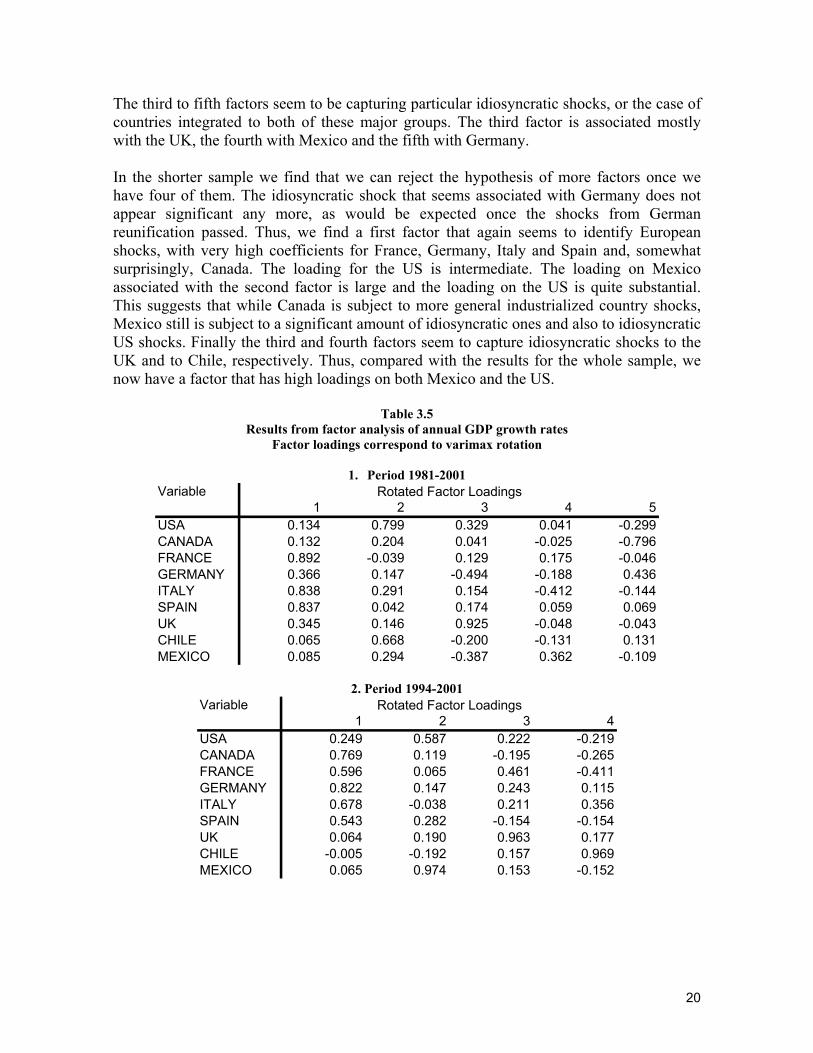
developments in the US seems a robust finding, and is significantly larger than that observed for any other country.26 When we include one or more lags of the dependent and variables and the rate of growth of industrial production in the US, without the time dummys, we find large but temporary effect of US growth for Mexico and Brazil (Table 3.3). The effects for Canada, UK, France, Germany, Ireland and Italy tend to be smaller initially but more persistent. When we include the 1994 dummy, we find a large and significant increase in the sensitivity to US growth for Mexico and Brazil, and smaller ones for France and Spain, in the specification with just one lag for the dependent variable and no lags for US growth. When we include more lags, these coefficients loose significance, except in the case of Brazil. In the case of the 1997 dummy, the only increase in sensitivity found to be significant is that for Italy with only one lag for the dependent variable, though that for Mexico is the largest increase in magnitude in all the lag specifications. The above results suggest that, even though the Mexican economy has become more sensitive to developments in the USA, and more so than any other country according to the point estimates on the rate of growth of GDP and industrial production in the USA, it is still subject to important idiosyncratic shocks, presumably risk aversion and contagion, terms of trade, policy and oil price shocks, as evidenced by the still low R2 from the GDP regressions. On the other hand, a very substantial part of the volatility of industrial production in the more recent period is explained by developments in the US, suggesting that synchronization in the tradable sector of the economy is already quite substantial. These results lead to a different interpretation from that obtained solely on the basis of correlations. While the correlations increased in the latter years to very large levels for Latin American countries, this may simply be due to the fact that the cycles tend to move in more similar directions but the correlations don’t tell us anything about the sensitivity of the variables in the different countries with respect to the US. Factor analysis We did three factor analysis exercises with GDP growth rates by country, following equation (2). The first was done for the whole sample, 1981-2001, the second was done for the sample period 1994-2001, and finally we included Argentina and Brazil in this second sample.27 For the whole period, we could not reject the hypothesis that more than four factors were necessary for explaining the variability of the series, while we did so for five factors. The results from the analysis using 5 factors are reported in table 3.5. The first factor seems to be a European one, finding high factor loadings for France, Italy and Spain, and intermediate ones for Germany and the UK. The second one seems to be a US factor, with high loading for the US, and Chile, and intermediate ones for Canada, Italy and Mexico.

26 Volatility of industrial growth in the US also explains a much larger proportion of that in Mexico. The adjusted R2s of the regressions without the autoregresive coefficient are –0.011 for the period 1987-1993 and 0.615 for the period 1997-2001. 27 The exercise for the sample 1997-2001 was not done due to degrees of freedom considerations.

20

The third to fifth factors seem to be capturing particular idiosyncratic shocks, or the case of countries integrated to both of these major groups. The third factor is associated mostly with the UK, the fourth with Mexico and the fifth with Germany. In the shorter sample we find that we can reject the hypothesis of more factors once we have four of them. The idiosyncratic shock that seems associated with Germany does not appear significant any more, as would be expected once the shocks from German reunification passed. Thus, we find a first factor that again seems to identify European shocks, with very high coefficients for France, Germany, Italy and Spain and, somewhat surprisingly, Canada. The loading for the US is intermediate. The loading on Mexico associated with the second factor is large and the loading on the US is quite substantial. This suggests that while Canada is subject to more general industrialized country shocks, Mexico still is subject to a significant amount of idiosyncratic ones and also to idiosyncratic US shocks. Finally the third and fourth factors seem to capture idiosyncratic shocks to the UK and to Chile, respectively. Thus, compared with the results for the whole sample, we now have a factor that has high loadings on both Mexico and the US.

Table 3.5 Results from factor analysis of annual GDP growth rates

Factor loadings correspond to varimax rotation

1. Period 1981-2001 Variable

1 2 3 4 5USA 0.134 0.799 0.329 0.041 -0.299CANADA 0.132 0.204 0.041 -0.025 -0.796FRANCE 0.892 -0.039 0.129 0.175 -0.046GERMANY 0.366 0.147 -0.494 -0.188 0.436ITALY 0.838 0.291 0.154 -0.412 -0.144SPAIN 0.837 0.042 0.174 0.059 0.069UK 0.345 0.146 0.925 -0.048 -0.043CHILE 0.065 0.668 -0.200 -0.131 0.131MEXICO 0.085 0.294 -0.387 0.362 -0.109

Rotated Factor Loadings


1 2 3 4USA 0.249 0.587 0.222 -0.219CANADA 0.769 0.119 -0.195 -0.265FRANCE 0.596 0.065 0.461 -0.411GERMANY 0.822 0.147 0.243 0.115ITALY 0.678 -0.038 0.211 0.356SPAIN 0.543 0.282 -0.154 -0.154UK 0.064 0.190 0.963 0.177CHILE -0.005 -0.192 0.157 0.969MEXICO 0.065 0.974 0.153 -0.152


21

3. Period 1994-2001. Sample includes Argentina and Brazil

Variable1 2 3 4

USA 0.467 0.302 -0.395 0.298CANADA 0.677 -0.164 -0.279 -0.347FRANCE 0.385 0.421 -0.483 -0.472GERMANY 0.704 0.335 0.022 -0.316ITALY 0.559 0.303 0.308 -0.416SPAIN 0.615 -0.087 -0.214 -0.132UK 0.000 1.000 -0.002 0.000CHILE 0.000 0.289 0.957 0.000MEXICO 0.483 0.309 -0.418 0.615BRAZIL -0.143 0.549 0.037 -0.176ARGENTINA 0.042 0.585 0.151 0.734


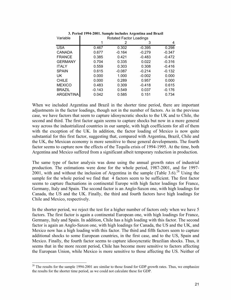
When we included Argentina and Brazil in the shorter time period, there are important adjustments in the factor loadings, though not in the number of factors. As in the previous case, we have factors that seem to capture idiosyncratic shocks to the UK and to Chile, the second and third. The first factor again seems to capture shocks but now in a more general way across the industrialized countries in our sample, with high coefficients for all of them with the exception of the UK. In addition, the factor loading of Mexico is now quite substantial for this first factor, suggesting that, compared with Argentina, Brazil, Chile and the UK, the Mexican economy is more sensitive to these general developments. The fourth factor seems to capture now the effects of the Tequila crisis of 1994-1995. At the time, both Argentina and Mexico suffered from a significant albeit temporary reduction in production. The same type of factor analysis was done using the annual growth rates of industrial production. The estimations were done for the whole period, 1987-2001, and for 1997-2001, with and without the inclusion of Argentina in the sample (Table 3.6).28 Using the sample for the whole period we find that 4 factors seem to be sufficient. The first factor seems to capture fluctuations in continental Europe with high factor loadings for France, Germany, Italy and Spain. The second factor is an Anglo-Saxon one, with high loadings for Canada, the US and the UK. Finally, the third and fourth factors have high loadings for Chile and Mexico, respectively. In the shorter period, we reject the test for a higher number of factors only when we have 5 factors. The first factor is again a continental European one, with high loadings for France, Germany, Italy and Spain. In addition, Chile has a high loading with this factor. The second factor is again an Anglo-Saxon one, with high loadings for Canada, the US and the UK, and Mexico now has a high loading with this factor. The third and fifth factors seem to capture additional shocks to some European countries, in the first case, and to the US, Spain and Mexico. Finally, the fourth factor seems to capture idiosyncratic Brazilian shocks. Thus, it seems that in the more recent period, Chile has become more sensitive to factors affecting the European Union, while Mexico is more sensitive to those affecting the US. Neither of

28 The results for the sample 1994-2001 are similar to those found for GDP growth rates. Thus, we emphasize the results for the shorter time period, as we could not calculate these for GDP.

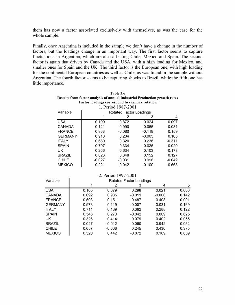
22

them has now a factor associated exclusively with themselves, as was the case for the whole sample. Finally, once Argentina is included in the sample we don’t have a change in the number of factors, but the loadings change in an important way. The first factor seems to capture fluctuations in Argentina, which are also affecting Chile, Mexico and Spain. The second factor is again that driven by Canada and the USA, with a high loading for Mexico, and smaller ones for Spain and the UK. The third factor is the European one, with high loading for the continental European countries as well as Chile, as was found in the sample without Argentina. The fourth factor seems to be capturing shocks to Brazil, while the fifth one has little importance.

Table 3.6 Results from factor analysis of annual Industrial Production growth rates

Factor loadings correspond to varimax rotation 1. Period 1987-2001

Variable1 2 3 4

USA 0.199 0.872 0.024 0.097CANADA 0.121 0.990 -0.065 -0.031FRANCE 0.863 -0.080 -0.118 0.159GERMANY 0.910 0.234 -0.005 0.105ITALY 0.680 0.320 0.236 -0.311SPAIN 0.797 0.334 -0.026 -0.029UK 0.266 0.634 0.103 -0.178BRAZIL 0.023 0.348 0.152 0.127CHILE -0.027 -0.031 0.998 -0.042MEXICO 0.221 0.042 -0.100 0.663



1 2 3 4 5USA 0.105 0.679 0.298 0.021 0.606CANADA 0.092 0.985 -0.011 -0.006 0.142FRANCE 0.503 0.151 0.487 0.408 0.001GERMANY 0.978 0.119 -0.007 -0.031 0.169ITALY 0.711 0.139 0.362 0.288 0.122SPAIN 0.546 0.273 -0.042 0.009 0.625UK 0.326 0.414 0.079 0.402 0.055BRAZIL 0.047 -0.012 0.060 0.942 0.052CHILE 0.657 -0.006 0.245 0.430 0.375MEXICO 0.320 0.442 -0.072 0.169 0.659


23

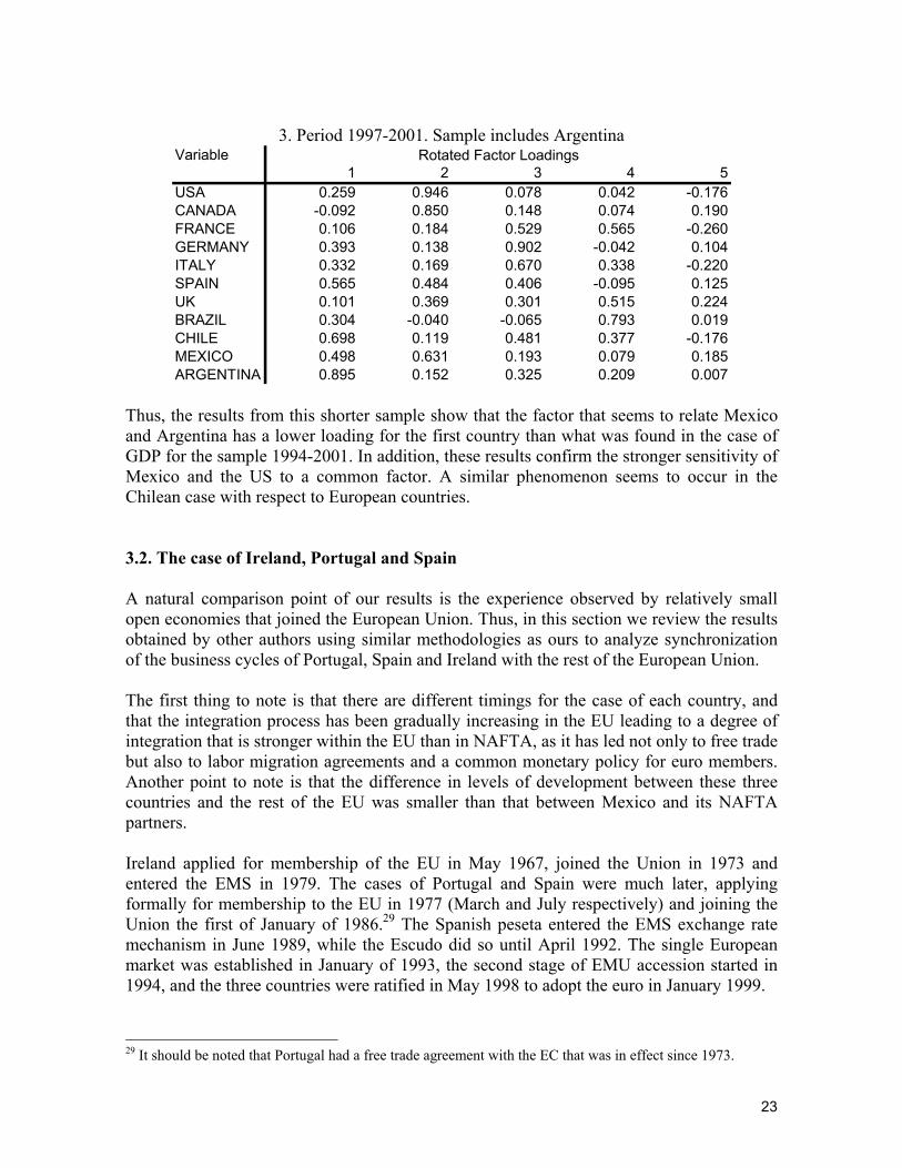
3. Period 1997-2001. Sample includes Argentina

Variable1 2 3 4 5

USA 0.259 0.946 0.078 0.042 -0.176CANADA -0.092 0.850 0.148 0.074 0.190FRANCE 0.106 0.184 0.529 0.565 -0.260GERMANY 0.393 0.138 0.902 -0.042 0.104ITALY 0.332 0.169 0.670 0.338 -0.220SPAIN 0.565 0.484 0.406 -0.095 0.125UK 0.101 0.369 0.301 0.515 0.224BRAZIL 0.304 -0.040 -0.065 0.793 0.019CHILE 0.698 0.119 0.481 0.377 -0.176MEXICO 0.498 0.631 0.193 0.079 0.185ARGENTINA 0.895 0.152 0.325 0.209 0.007


Thus, the results from this shorter sample show that the factor that seems to relate Mexico and Argentina has a lower loading for the first country than what was found in the case of GDP for the sample 1994-2001. In addition, these results confirm the stronger sensitivity of Mexico and the US to a common factor. A similar phenomenon seems to occur in the Chilean case with respect to European countries. 3.2. The case of Ireland, Portugal and Spain A natural comparison point of our results is the experience observed by relatively small open economies that joined the European Union. Thus, in this section we review the results obtained by other authors using similar methodologies as ours to analyze synchronization of the business cycles of Portugal, Spain and Ireland with the rest of the European Union. The first thing to note is that there are different timings for the case of each country, and that the integration process has been gradually increasing in the EU leading to a degree of integration that is stronger within the EU than in NAFTA, as it has led not only to free trade but also to labor migration agreements and a common monetary policy for euro members. Another point to note is that the difference in levels of development between these three countries and the rest of the EU was smaller than that between Mexico and its NAFTA partners. Ireland applied for membership of the EU in May 1967, joined the Union in 1973 and entered the EMS in 1979. The cases of Portugal and Spain were much later, applying formally for membership to the EU in 1977 (March and July respectively) and joining the Union the first of January of 1986.29 The Spanish peseta entered the EMS exchange rate mechanism in June 1989, while the Escudo did so until April 1992. The single European market was established in January of 1993, the second stage of EMU accession started in 1994, and the three countries were ratified in May 1998 to adopt the euro in January 1999.

29 It should be noted that Portugal had a free trade agreement with the EC that was in effect since 1973.

24

Artis and Zhang (1995, 1997) constitutes seminal work about changes in the degree of macroeconomic synchronization in European countries due to closer integration.30 However, their focus was not on integration increasing due to trade but rather to monetary and exchange rate policies, particularly the establishment of the European Monetary System (EMS) and within it the ERM (Exchange Rate Mechanism), occurring in 1979. Thus, they compare the correlation of business cycle measures of industrial production in several European countries with those in Germany and the US in the pre-ERM period (1961:1 –1979:3) and in the ERM period (1979:4 – 1993:12). These authors find that there is a very sharp increase in the correlation of Portuguese and Spanish business cycles with those of Germany, while this increase in not observed with respect to US fluctuations. In addition, whilst in the pre-ERM period they lagged the German business cycle more than that in the US, in the ERM period this is reversed. However, as mentioned, Portugal and Spain don’t join the ERM until 1992 and 1989, respectively. Thus, it is difficult to conclude that the higher correlation is actually due to common monetary or exchange rate policies. This is something the authors also caution about. It seems more likely that the increase in the correlation in the case of these countries is due to their earlier entry into the European Union in 1986. Comparing their results with the ones found here for industrial production, we find that the initial level of correlation rates was actually higher for Portugal and Spain, but the increase in the correlation between Mexico and the US in the post-NAFTA period is higher than for these countries in the post-ERM period with Germany. An interesting case that puts some doubt that ERM was the cause of the higher synchronization compared with greater trade flows is that of Ireland. As mentioned, this country joined ERM in 1979, and thus we would expect higher increase in the degree of synchronization than for Portugal and Spain if it was mostly driven by the EMS and ERM. In the pre-ERM period its correlation with Germany’s industrial production is similar to those of Portugal and Spain, but we don’t observe an increase of this correlation in the post-ERM period as in the other two countries. The same occurs with the UK, which participated in the ERM longer than Portugal in the time period used by the authors. An important, if not the main, difference between these four countries is the degree of integration with the US economy through trade links.31 Thus, their evidence may be interpreted as supporting the positive effect of greater international trade instead of common monetary and exchange rate policies.32 Several other studies have followed the research by Artis and Zhang using other variables, longer time periods, and different methodologies. We focus on those that put particular attention to the Irish, Portuguese and Spanish experiences. 30 Frankel and Rose’s (1998) work focuses on the effect of free trade on business cycle synchronization but they don’t analyze in special detail the case of particular European economies and, specially, the change in synchronization over time. 31 Financial links are also important. 32 It also suggests that trade agreements are one among several determinants of trade. Ireland and the UK were members of the EU since 1973, yet still maintain a significantly diversified trade structure between the EU continental economies and the US.

25

Angeloni and Dedola (1999) look at the correlation, between GDP and industrial production of these countries and that of the EU, with a longer time period and separating their sample in four (pre ERM, soft ERM, hard ERM, pre EMU; the total time period covered is 1965-1997). Using this finer sample partitioning and a longer post ERM period, they find that correlations for both variables were higher for Portugal and Spain in since the hard ERM period compared with before, though again the increase is smaller than that we found for Mexico. There seems to be no such increase in correlations for Ireland (as for the UK). They also find that the increase in the correlation of output was more gradual than that of industrial production, also suggesting that part of the increase in correlation is driven by cycles in tradable goods and not only common policies. Belo (2001) calculates correlations, concordance and Spearman’s rank correlations of industrial production for several countries and the Euro zone in the period 1960-1999, splitting the sample in two in 1979, coinciding with ERM. The results using the three measures of business cycle association are similar to those found in the other studies, though he finds an initially lower association in the case of Ireland, and thus an increase over time, albeit the smallest in the sample.33 Finally, Boone(1997) uses a VAR system to identify demand and supply shocks for the countries in the European Union (and some other countries as controls), using a methodology similar to that used by Bayoumi and Eichengreen (1996). Then he analyzes the degree of correlation between demand and supply shocks of each country with Germany. In the case of supply shocks, he finds it is fairly constant for Ireland and Spain in the period 1974-1990, and increases in 1991-1994. In the case of Portugal, it is already quite low in the period 1980-1990 but then increases additionally in 1991-1994. As for demand shocks, the correlation increases substantially from 1974-1979 to 1980-1990, but then falls in 1991-1994. For Ireland and Portugal, the correlation falls strongly from 1974-1979 to 1980-1990, and remains constant in 1991-1994. As in the case of previous studies, this evidence seems more consistent with gradually increasing trade integration than with common policies. The increase in correlation of supply shocks should actually be driven by trade integration, not common demand management policies. In terms of demand shocks, the fact that correlation does not increase additionally after Portugal and Spain join the ERM is likely to be due to the ERM crisis of 1992-1993. Thus, comparing these results with those found for the Mexican case it seems safe to conclude that macroeconomic synchronization seems to increase through trade integration, first through tradables and latter on non-tradables that are procyclical. The initial correlations of Portugal and Spain with the EU were larger than those of Mexico with its NAFTA partners, though the increase in these is larger in the latter case. Thus, in the context on the discussions around the effect of trade integration on macroeconomic synchronization, if higher trade does not lead to larger specialization in production, and intra-industry trade increases, then the increase in synchronization may be much larger for dissimilar countries than for those with more similar levels of development. 33 Borodo, González and Rodríguez (1998) find similar results looking at five year moving correlations.

26

3.3. Summary The analysis of correlations between GDP growth rates shows that there was a large increase in the post-NAFTA period in the correlation of GDP in Mexico with those of Canada and the US, an increase not seen for any other country. In the case of industrial production correlations, the increase in the correlation in the more recent time period is observed for other countries, particularly in Latin America. This suggests that globalization has led to higher correlation of a more general type in the production of tradable goods, while the more intensive integration due to NAFTA has led to synchronization in other sectors of economic activity. Moving 3 year correlations suggest that the higher correlation of GDP in the Mexican case is mostly due to the recent deceleration in the NAFTA countries. The regression analysis points in the same direction. The coefficient on US growth interacted with a post-NAFTA dummy is much larger for Mexico than for other countries and its typically the only dummy that is significant. Finally, the factor analysis shows that, for the whole sample period, Mexico typically had an idiosyncratic factor. In the later, post NAFTA period, the highest factor loadings for Mexico correspond to those factors that have a high loading for the US. This change in the structure of factor loadings with respect to the US is not seen for any other country. This increase in the sensitivity of Mexican variables to the evolution of those in its NAFTA partners is similar to that observed for Portugal and Spain since the 1980’s. However, in the case of the European countries, different authors have typically associated the increase in synchronization with common policies and, in particular, the establishment of the EMS, not so much with trade. This interpretation is dubious, as the synchronization of the Irish economy with the EU has not increased to the same degree, even though Ireland was a member of the EU and participated in the ERM before the Iberian countries. Probably the main difference is due to the fact that Ireland has kept very close trade links with the UK and the US, suggesting that trade is really the cause of the higher correlation of the Iberian countries. More work needs to be done in the European case to choose between these alternative interpretations. 4. Integration by Sectors and Regions In this section we explore higher synchronization between Canada, Mexico and the USA at the subnational, aggregate demand and sectorial levels using similar methods as those employed in the previous section. Subsection 4.1 presents the results for the sectorial analysis, subsection 4.2 those on aggregate demand and subsection 4.3 has the results of the regional analysis.

27

4.1. Sectors of Economic Activity In this section we analyze the relationship between growth rates of different sectors of economic activity in Canada, Mexico and the USA. This allows us to see if the relationship between Mexico and the other two countries changed due to NAFTA, and also if the Mexico-USA relationship is becoming similar to the one between Canada and the USA. In addition, we can compare across sectors of economic activity. Our working hypothesis is that the increase in the degree of synchronization of tradable goods sectors that benefited from the trade agreement should have been larger than that of other sectors. The data employed in this section corresponds to: i) quarterly GDP measures by 1-digit sector of economic activity for Canada and

Mexico, while the data for the USA is national gross income, also by 1-digit sector of economic activity.

ii) monthly industrial production by 2-digit sector of economic activity for Mexico and the USA. Unfortunately, Statistics Canada has not been producing monthly industrial production data for some time.

The sources for the data are: INEGI in the Mexican case, CANSIM for Canada, and the BEA for the USA. The sample period used for the quarterly data is 1987Q1 – 2001Q2, while that for the monthly data is 1980M1 – 2001 M11. Both sample periods are determined by the availability of data. Analysis of correlations between Canada, Mexico and the USA Table 4.1 shows the correlation coefficient between growth in a sector of economic activity in the US with either Mexico or Canada. When using the whole sample, in those cases when the correlation between a US and Canadian sector is high, it is larger than that between the US and Mexican sectors. In general, these last correlations of US sectors with Mexican sectors are low during 1988-2001. However, after NAFTA, and specially after the balance of payments crisis that coincided with the start of the trade agreement, the correlation between Mexican and US sectors increased significantly for several areas, reaching levels similar to those observed for Canada. In particular, the correlation increased quite noticeably for manufacturing, transport and communications, and general services.

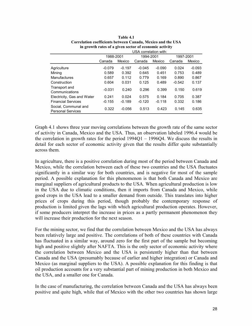
28

Table 4.1

Correlation coefficients between Canada, Mexico and the USA in growth rates of a given sector of economic activity

Canada Mexico Canada Mexico Canada Mexico

Agriculture -0.079 -0.197 -0.045 -0.090 0.024 -0.093Mining 0.589 0.392 0.645 0.451 0.753 0.489Manufactures 0.657 0.112 0.779 0.169 0.890 0.867Construction 0.604 0.031 0.125 0.489 -0.542 0.137Transport and Communications -0.031 0.240 0.296 0.399 0.150 0.619

Electricity, Gas and Water 0.241 0.024 0.575 0.184 0.705 0.387Financial Services -0.155 -0.189 -0.120 -0.118 0.332 0.186Social, Communal and Personal Services 0.322 -0.056 0.513 0.423 0.145 0.635

1988-2001 1994-2001 1997-2001USA correlation with:

Graph 4.1 shows three year moving correlations between the growth rate of the same sector of activity in Canada, Mexico and the USA. Thus, an observation labeled 1996.4 would be the correlation in growth rates for the period 1994Q1 – 1996Q4. We discuss the results in detail for each sector of economic activity given that the results differ quite substantially across them. In agriculture, there is a positive correlation during most of the period between Canada and Mexico, while the correlation between each of these two countries and the USA fluctuates significantly in a similar way for both countries, and is negative for most of the sample period. A possible explanation for this phenomenon is that both Canada and Mexico are marginal suppliers of agricultural products to the USA. When agricultural production is low in the USA due to climatic conditions, then it imports from Canada and Mexico, while good crops in the USA lead to a smaller demand from outside. This translates into higher prices of crops during this period, though probably the contemporary response of production is limited given the lags with which agricultural production operates. However, if some producers interpret the increase in prices as a partly permanent phenomenon they will increase their production for the next season. For the mining sector, we find that the correlation between Mexico and the USA has always been relatively large and positive. The correlations of both of these countries with Canada has fluctuated in a similar way, around zero for the first part of the sample but becoming high and positive slightly after NAFTA. This is the only sector of economic activity where the correlation between Mexico and the USA is persistently higher than that between Canada and the USA (presumably because of earlier and higher integration) or Canada and Mexico (as marginal suppliers to the USA). A possible explanation for this finding is that oil production accounts for a very substantial part of mining production in both Mexico and the USA, and a smaller one for Canada. In the case of manufacturing, the correlation between Canada and the USA has always been positive and quite high, while that of Mexico with the other two countries has shown large

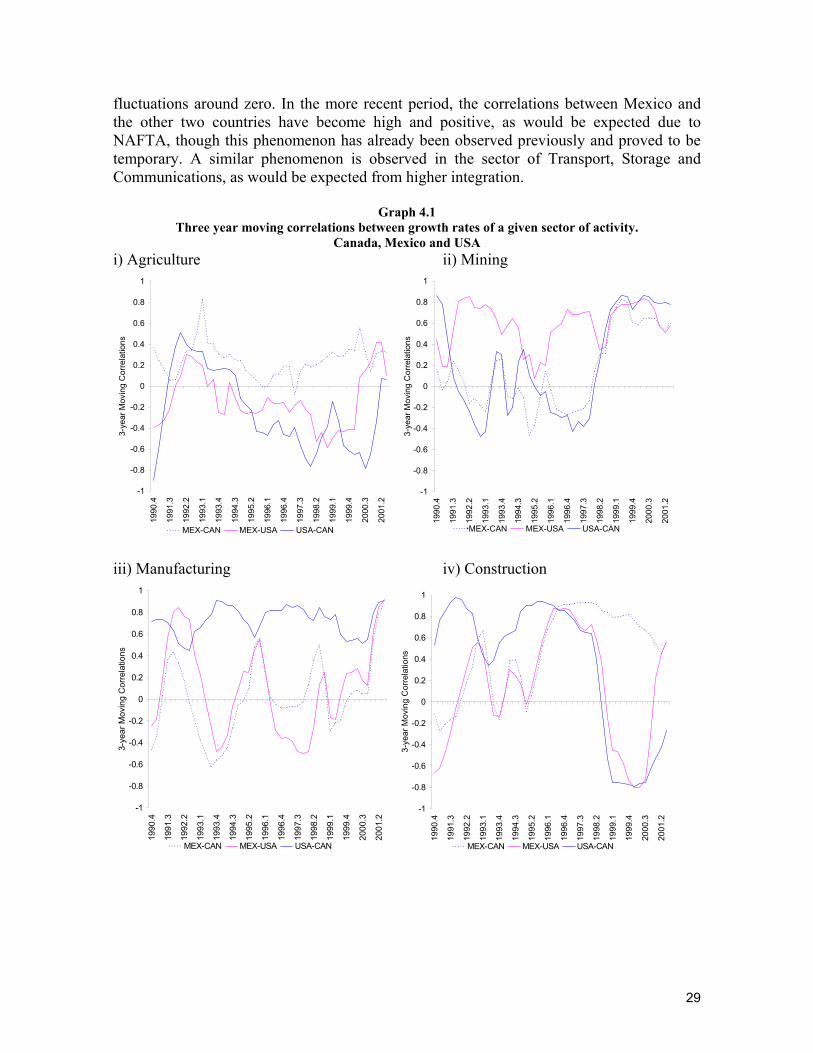
29

fluctuations around zero. In the more recent period, the correlations between Mexico and the other two countries have become high and positive, as would be expected due to NAFTA, though this phenomenon has already been observed previously and proved to be temporary. A similar phenomenon is observed in the sector of Transport, Storage and Communications, as would be expected from higher integration.

Graph 4.1 Three year moving correlations between growth rates of a given sector of activity.

Canada, Mexico and USA i) Agriculture ii) Mining

-1

-0.8

-0.6

-0.4

-0.2

0

0.2

0.4

0.6

0.8

1

1990

.4

1991

.3

1992

.2

1993

.1

1993

.4

1994

.3

1995

.2

1996

.1

1996

.4

1997

.3

1998

.2

1999

.1

1999

.4

2000

.3

2001

.2

3-ye

ar M

ovin

g C

orre

latio

ns

MEX-CAN MEX-USA USA-CAN

-1

-0.8

-0.6

-0.4

-0.2

0

0.2

0.4

0.6

0.8

1

1990

.4

1991

.3

1992

.2

1993

.1

1993

.4

1994

.3

1995

.2

1996

.1

1996

.4

1997

.3

1998

.2

1999

.1

1999

.4

2000

.3

2001

.2

3-ye

ar M

ovin

g C

orre

latio

ns

MEX-CAN MEX-USA USA-CAN iii) Manufacturing iv) Construction

-1

-0.8

-0.6

-0.4

-0.2

0

0.2

0.4

0.6

0.8

1

1990

.4

1991

.3

1992

.2

1993

.1

1993

.4

1994

.3

1995

.2

1996

.1

1996

.4

1997

.3

1998

.2

1999

.1

1999

.4

2000

.3

2001

.2

3-ye

ar M

ovin

g C

orre

latio

ns


-1

-0.8

-0.6

-0.4

-0.2

0

0.2

0.4

0.6

0.8

1

1990

.4

1991

.3

1992

.2

1993

.1

1993

.4

1994

.3

1995

.2

1996

.1

1996

.4

1997

.3

1998

.2

1999

.1

1999

.4

2000

.3

2001

.2

3-ye

ar M

ovin

g C

orre

latio

ns


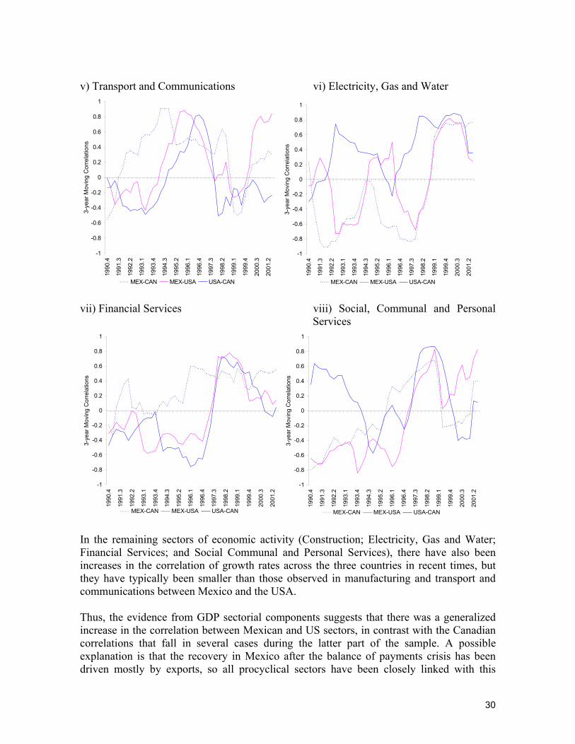
30

v) Transport and Communications vi) Electricity, Gas and Water

-1

-0.8

-0.6

-0.4

-0.2

0

0.2

0.4

0.6

0.8

119

90.4

1991

.3

1992

.2

1993

.1

1993

.4

1994

.3

1995

.2

1996

.1

1996

.4

1997

.3

1998

.2

1999

.1

1999

.4

2000

.3

2001

.2

3-ye

ar M

ovin

g C

orre

latio

ns


-1

-0.8

-0.6

-0.4

-0.2

0

0.2

0.4

0.6

0.8

1

1990

.4

1991

.3

1992

.2

1993

.1

1993

.4

1994

.3

1995

.2

1996

.1

1996

.4

1997

.3

1998

.2

1999

.1

1999

.4

2000

.3

2001

.2

3-ye

ar M

ovin

g C

orre

latio

nsMEX-CAN MEX-USA USA-CAN

vii) Financial Services viii) Social, Communal and Personal

Services

-1

-0.8

-0.6

-0.4

-0.2

0

0.2

0.4

0.6

0.8

1

1990

.4

1991

.3

1992

.2

1993

.1

1993

.4

1994

.3

1995

.2

1996

.1

1996

.4

1997

.3

1998

.2

1999

.1

1999

.4

2000

.3

2001

.2

3-ye

ar M

ovin

g C

orre

latio

ns


-1

-0.8

-0.6

-0.4

-0.2

0

0.2

0.4

0.6

0.8

1

1990

.4

1991

.3

1992

.2

1993

.1

1993

.4

1994

.3

1995

.2

1996

.1

1996

.4

1997

.3

1998

.2

1999

.1

1999

.4

2000

.3

2001

.2

3-ye

ar M

ovin

g C

orre

latio

ns

MEX-CAN MEX-USA USA-CAN In the remaining sectors of economic activity (Construction; Electricity, Gas and Water; Financial Services; and Social Communal and Personal Services), there have also been increases in the correlation of growth rates across the three countries in recent times, but they have typically been smaller than those observed in manufacturing and transport and communications between Mexico and the USA. Thus, the evidence from GDP sectorial components suggests that there was a generalized increase in the correlation between Mexican and US sectors, in contrast with the Canadian correlations that fall in several cases during the latter part of the sample. A possible explanation is that the recovery in Mexico after the balance of payments crisis has been driven mostly by exports, so all procyclical sectors have been closely linked with this

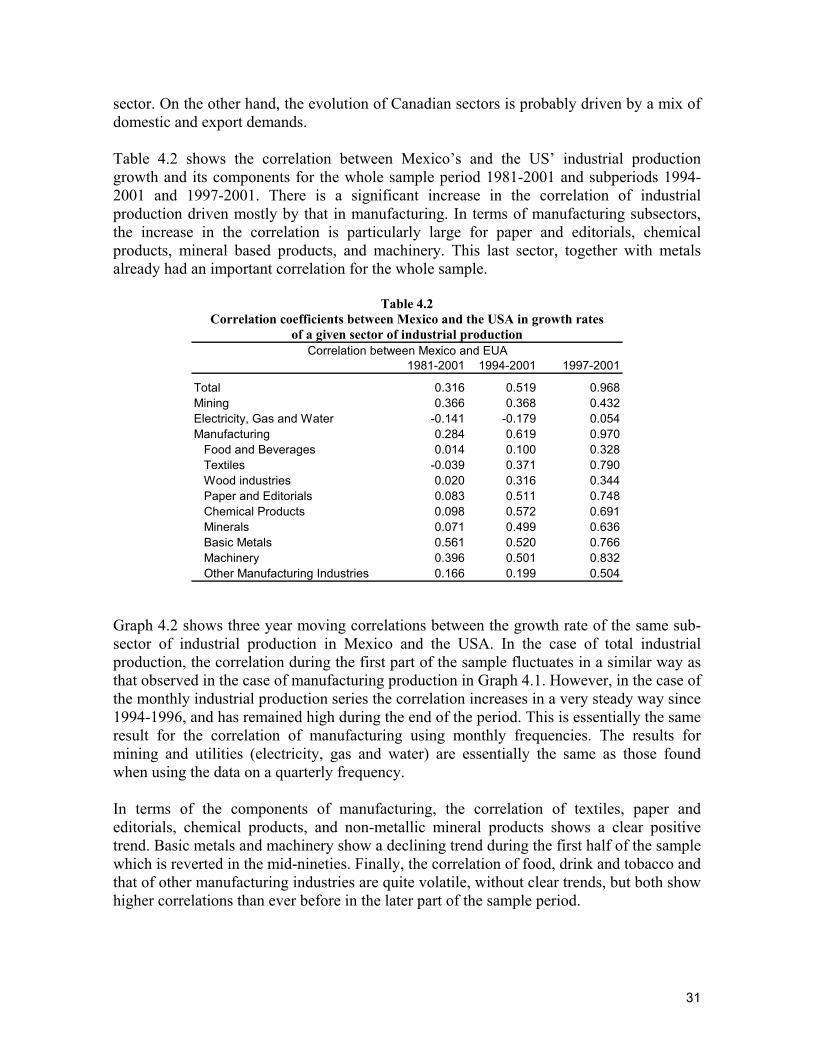
31

sector. On the other hand, the evolution of Canadian sectors is probably driven by a mix of domestic and export demands. Table 4.2 shows the correlation between Mexico’s and the US’ industrial production growth and its components for the whole sample period 1981-2001 and subperiods 1994-2001 and 1997-2001. There is a significant increase in the correlation of industrial production driven mostly by that in manufacturing. In terms of manufacturing subsectors, the increase in the correlation is particularly large for paper and editorials, chemical products, mineral based products, and machinery. This last sector, together with metals already had an important correlation for the whole sample.

Table 4.2 Correlation coefficients between Mexico and the USA in growth rates

of a given sector of industrial production

1981-2001 1994-2001 1997-2001

Total 0.316 0.519 0.968Mining 0.366 0.368 0.432Electricity, Gas and Water -0.141 -0.179 0.054Manufacturing 0.284 0.619 0.970 Food and Beverages 0.014 0.100 0.328 Textiles -0.039 0.371 0.790 Wood industries 0.020 0.316 0.344 Paper and Editorials 0.083 0.511 0.748 Chemical Products 0.098 0.572 0.691 Minerals 0.071 0.499 0.636 Basic Metals 0.561 0.520 0.766 Machinery 0.396 0.501 0.832 Other Manufacturing Industries 0.166 0.199 0.504

Correlation between Mexico and EUA

Graph 4.2 shows three year moving correlations between the growth rate of the same sub-sector of industrial production in Mexico and the USA. In the case of total industrial production, the correlation during the first part of the sample fluctuates in a similar way as that observed in the case of manufacturing production in Graph 4.1. However, in the case of the monthly industrial production series the correlation increases in a very steady way since 1994-1996, and has remained high during the end of the period. This is essentially the same result for the correlation of manufacturing using monthly frequencies. The results for mining and utilities (electricity, gas and water) are essentially the same as those found when using the data on a quarterly frequency. In terms of the components of manufacturing, the correlation of textiles, paper and editorials, chemical products, and non-metallic mineral products shows a clear positive trend. Basic metals and machinery show a declining trend during the first half of the sample which is reverted in the mid-nineties. Finally, the correlation of food, drink and tobacco and that of other manufacturing industries are quite volatile, without clear trends, but both show higher correlations than ever before in the later part of the sample period.

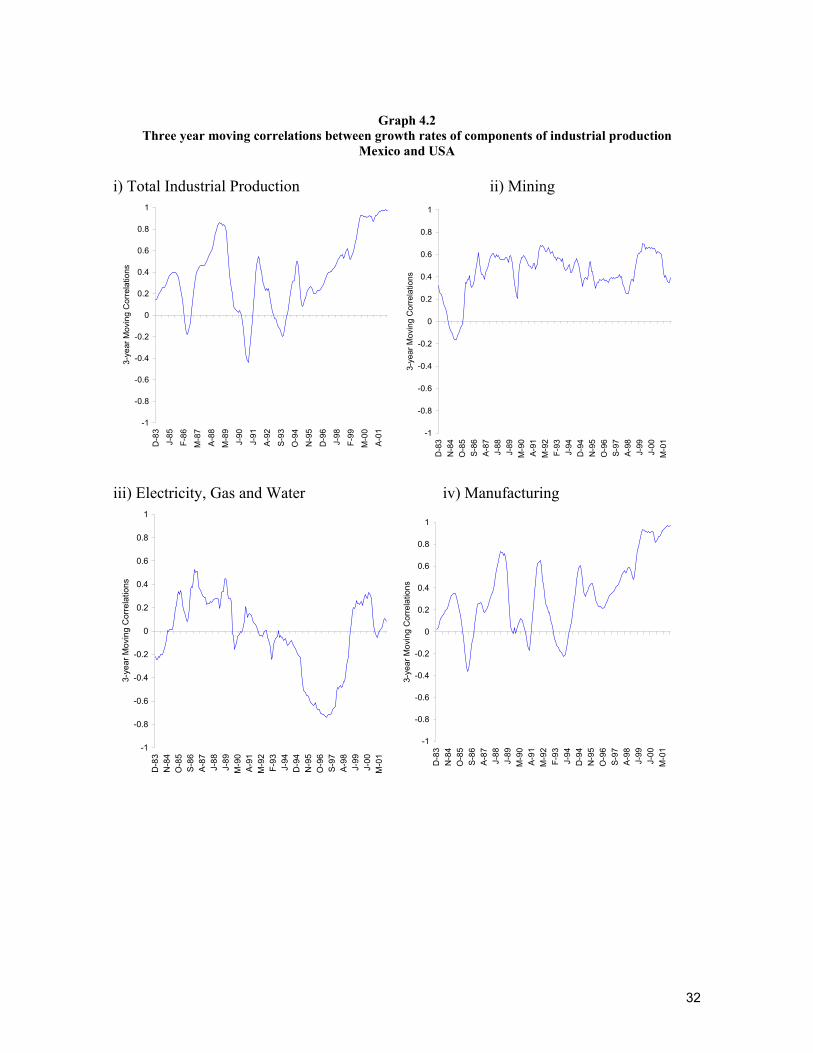
32

Graph 4.2

Three year moving correlations between growth rates of components of industrial production Mexico and USA

i) Total Industrial Production ii) Mining

-1

-0.8

-0.6

-0.4

-0.2

0

0.2

0.4

0.6

0.8

1

D-8

3J-

85F-

86M

-87

A-88

M-8

9J-

90J-

91A-

92S-

93O

-94

N-9

5D

-96

J-98

F-99

M-0

0A-

01

3-ye

ar M

ovin

g C

orre

latio

ns

-1

-0.8

-0.6

-0.4

-0.2

0

0.2

0.4

0.6

0.8

1

D-8

3N

-84

O-8

5S-

86A-

87J-

88J-

89M

-90

A-91

M-9

2F-

93J-

94D

-94

N-9

5O

-96

S-97

A-98

J-99

J-00

M-0

1

3-ye

ar M

ovin

g C

orre

latio

ns

iii) Electricity, Gas and Water iv) Manufacturing

-1

-0.8

-0.6

-0.4

-0.2

0

0.2

0.4

0.6

0.8

1

D-8

3N

-84

O-8

5S-

86A-

87J-

88J-

89M

-90

A-91

M-9

2F-

93J-

94D

-94

N-9

5O

-96

S-97

A-98

J-99

J-00

M-0

1

3-ye

ar M

ovin

g C

orre

latio

ns

-1

-0.8

-0.6

-0.4

-0.2

0

0.2

0.4

0.6

0.8

1

D-8

3N

-84

O-8

5S-

86A-

87J-

88J-

89M

-90

A-91

M-9

2F-

93J-

94D

-94

N-9

5O

-96

S-97

A-98

J-99

J-00

M-0

1

3-ye

ar M

ovin

g C

orre

latio

ns

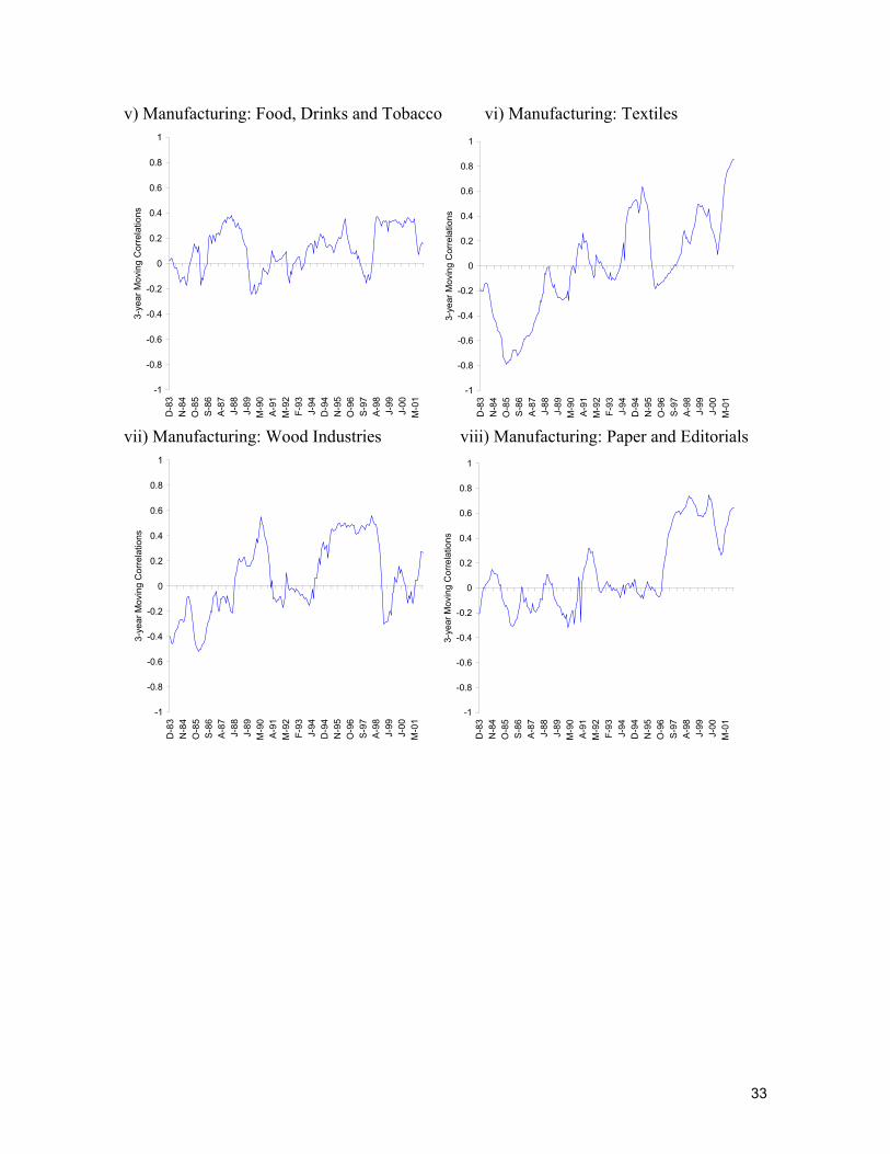
33

v) Manufacturing: Food, Drinks and Tobacco vi) Manufacturing: Textiles

-1

-0.8

-0.6

-0.4

-0.2

0

0.2

0.4

0.6

0.8

1

D-8

3N

-84

O-8

5S-

86A-

87J-

88J-

89M

-90

A-91

M-9

2F-

93J-

94D

-94

N-9

5O

-96

S-97

A-98

J-99

J-00

M-0

1

3-ye

ar M

ovin

g C

orre

latio

ns

-1

-0.8

-0.6

-0.4

-0.2

0

0.2

0.4

0.6

0.8

1

D-8

3N

-84

O-8

5S-

86A-

87J-

88J-

89M

-90

A-91

M-9

2F-

93J-

94D

-94

N-9

5O

-96

S-97

A-98

J-99

J-00

M-0

1

3-ye

ar M

ovin

g C

orre

latio

ns

vii) Manufacturing: Wood Industries viii) Manufacturing: Paper and Editorials

-1

-0.8

-0.6

-0.4

-0.2

0

0.2

0.4

0.6

0.8

1

D-8

3N

-84

O-8

5S-

86A-

87J-

88J-

89M

-90

A-91

M-9

2F-

93J-

94D

-94

N-9

5O

-96

S-97

A-98

J-99

J-00

M-0

1

3-ye

ar M

ovin

g C

orre

latio

ns

-1

-0.8

-0.6

-0.4

-0.2

0

0.2

0.4

0.6

0.8

1

D-8

3N

-84

O-8

5S-

86A-

87J-

88J-

89M

-90

A-91

M-9

2F-

93J-

94D

-94

N-9

5O

-96

S-97

A-98

J-99

J-00

M-0

1

3-ye

ar M

ovin

g C

orre

latio

ns

34

ix) Manufacturing: Chemical Products x) Manufacturing: Minerals

-1

-0.8

-0.6

-0.4

-0.2

0

0.2

0.4

0.6

0.8

1D

-83

N-8

4O

-85

S-86

A-87

J-88

J-89

M-9

0A-

91M

-92

F-93

J-94

D-9

4N

-95

O-9

6S-

97A-

98J-

99J-

00M

-01

3-ye

ar M

ovin

g C

orre

latio

ns

-1

-0.8

-0.6

-0.4

-0.2

0

0.2

0.4

0.6

0.8

1

D-8

3N

-84

O-8

5S-

86A-

87J-

88J-

89M

-90

A-91

M-9

2F-

93J-

94D

-94

N-9

5O

-96

S-97

A-98

J-99

J-00

M-0

1

3-ye

ar M

ovin

g C

orre

latio

ns

xi) Manufacturing: Basic Metals xii) Manufacturing: Machinery

-1

-0.8

-0.6

-0.4

-0.2

0

0.2

0.4

0.6

0.8

1

D-8

3N

-84

O-8

5S-

86A-

87J-

88J-

89M

-90

A-91

M-9

2F-

93J-

94D

-94

N-9

5O

-96

S-97

A-98

J-99

J-00

M-0

1

3-ye

ar M

ovin

g C

orre

latio

ns

-1

-0.8

-0.6

-0.4

-0.2

0

0.2

0.4

0.6

0.8

1D

-83

N-8

4O

-85

S-86

A-87

J-88

J-89

M-9

0A-

91M

-92

F-93

J-94

D-9

4N

-95

O-9

6S-

97A-

98J-

99J-

00M

-01

3-ye

ar M

ovin

g C

orre

latio

ns

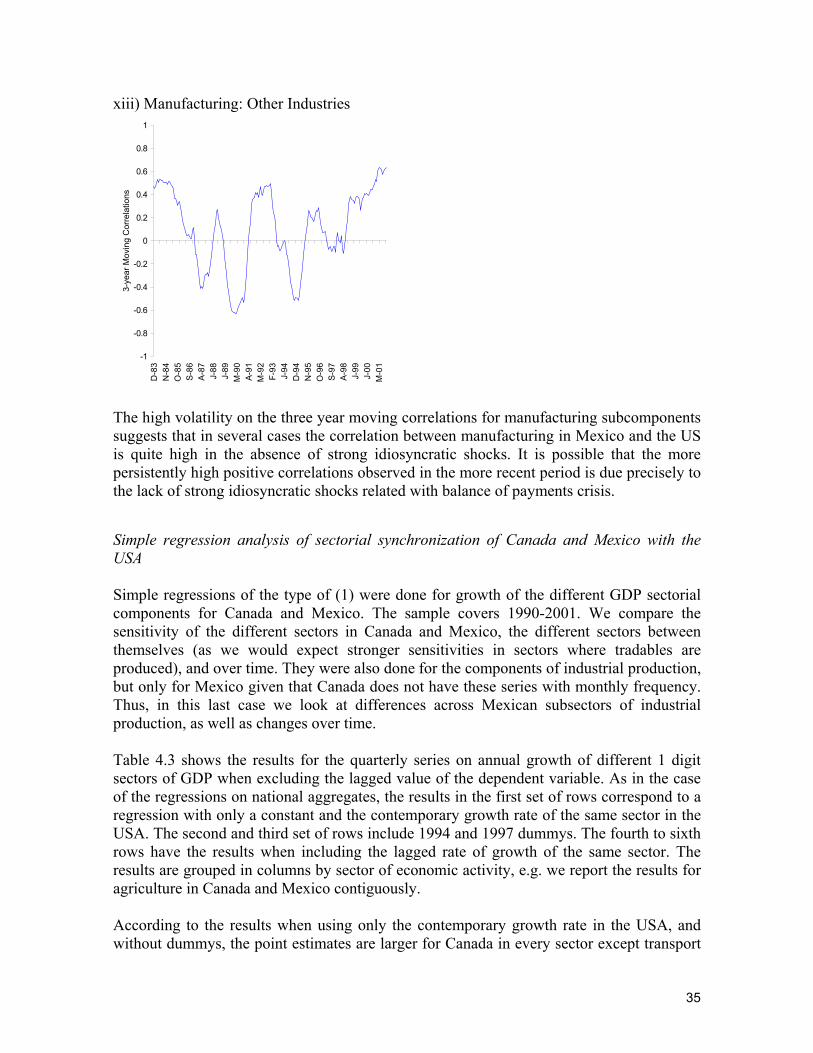
35

xiii) Manufacturing: Other Industries

-1

-0.8

-0.6

-0.4

-0.2

0

0.2

0.4

0.6

0.8

1

D-8

3N

-84

O-8

5S-

86A-

87J-

88J-

89M

-90

A-91

M-9

2F-

93J-

94D

-94

N-9

5O

-96

S-97

A-98

J-99

J-00

M-0

1

3-ye

ar M

ovin

g C

orre

latio

ns

The high volatility on the three year moving correlations for manufacturing subcomponents suggests that in several cases the correlation between manufacturing in Mexico and the US is quite high in the absence of strong idiosyncratic shocks. It is possible that the more persistently high positive correlations observed in the more recent period is due precisely to the lack of strong idiosyncratic shocks related with balance of payments crisis. Simple regression analysis of sectorial synchronization of Canada and Mexico with the USA Simple regressions of the type of (1) were done for growth of the different GDP sectorial components for Canada and Mexico. The sample covers 1990-2001. We compare the sensitivity of the different sectors in Canada and Mexico, the different sectors between themselves (as we would expect stronger sensitivities in sectors where tradables are produced), and over time. They were also done for the components of industrial production, but only for Mexico given that Canada does not have these series with monthly frequency. Thus, in this last case we look at differences across Mexican subsectors of industrial production, as well as changes over time. Table 4.3 shows the results for the quarterly series on annual growth of different 1 digit sectors of GDP when excluding the lagged value of the dependent variable. As in the case of the regressions on national aggregates, the results in the first set of rows correspond to a regression with only a constant and the contemporary growth rate of the same sector in the USA. The second and third set of rows include 1994 and 1997 dummys. The fourth to sixth rows have the results when including the lagged rate of growth of the same sector. The results are grouped in columns by sector of economic activity, e.g. we report the results for agriculture in Canada and Mexico contiguously. According to the results when using only the contemporary growth rate in the USA, and without dummys, the point estimates are larger for Canada in every sector except transport

36

and communications. In the Canadian case we find a positive and significant coefficient for manufacturing (the largest by far); social, personal and communal services; mining; and utilities (electricity, gas and water). Agriculture also has a high point estimate, but it is not significant. The only two sectors for which these specifications explain a substantial proportion of volatility are manufacturing (0.43) and mining (0.35). In the Mexican case, the point estimate associated with US sectorial growth is significant only for transport and communications and mining. The point estimate in the manufacturing regression is higher than that of mining but is not significant. The R2s are quite low for all cases, with the highest being 0.15 for mining. The above results clearly suggest that for the period as a whole the relationship between Canada and the USA was stronger than that between Mexico and the USA. Point estimates and the proportion of volatility explained by US growth are larger for Canada. A puzzling point is that the R2s and many of the estimated coefficients are lower than those found in GDP regressions. A possible explanation is that growth in a given sector is more closely related to overall growth in the USA than with growth in the same sector. In addition, it is possible that specific sectors are subject to higher volatility that is compensated at the GDP level. When we include the 1994 dummy, the point estimates associated with the dummy and growth of the sector in the USA are always positive for Mexico and significantly larger than those for Canada with the exception of utilities. In terms of magnitude of the coefficients, the largest changes in the Mexican case are for construction, transport and communications, and social, communal and personal services.34 In the Canadian case there are large increases in the point estimate for utilities, transport and communications and services, but none of them are significant. The only significant coefficient for Canada is a fall in the point estimate for construction. When including the 1997 dummy, we find again that the implied increase in the point estimate is either larger for Mexico, or similar for both countries. There isn’t any case when the increase for Canada is substantially larger. As for 1994, the estimate on the interactive dummy is always positive. It is now significant in the Mexican case for manufacturing and utilities. The only significant positive case for Canada is financial services, while the coefficient on construction is negative and significant. The results are very similar to those found in the regressions using the dummy for 1994 onwards. The results when including the lagged value of the dependent variable are very similar (Table 4.4). The only substantial differences we find are that the interactive dummy for manufacturing in Mexico is now significant for both 1994 and 1997, and those for construction and mining are significant for 1997. Summarizing, we observe a generalized increase in point estimates in the Mexican case, though few of them are significant. As in the case of GDP, this is probably due to the fact that idiosyncratic shocks to Mexican GDP were still important during the first half of the

34 The large change in the constant for construction and services suggest that the change in coefficients might be contaminated by the 1994 crisis.

37

period since the implementation of NAFTA, and that we have few observations due to the quarterly frequency of this data. In addition, we have not seen a complete cycle in the USA since the implementation of NAFTA. Our results also suggest an interesting issue concerning the analysis of synchronization of business cycles at the sectorial level. If a country’s business cycle becomes more synchronized with that of another country due to higher trade, then one might expect that, at the sectorial level, we would observe a larger increase in synchronization of tradable than of non-tradable goods. The results suggest that this might not always be the case. We find more synchronization for manufacturing, but also for general services and construction. A possible explanation is that these two non-tradable sectors are more closely related to the business cycle of the economy and to manufacturing production than other tradable goods sectors, such as agriculture, that are subject to higher idiosyncratic shocks. Thus, if the business cycle between Mexico and the US is becoming more synchronized due to trade in manufacturing and its driven by exports, the links of this sector with construction and services imply that we also see higher synchronization in these non-tradable sectors.35 Table 4.5 shows the results of the same type of regression using the annual growth rate of different components of industrial production for the period 1981-2001, excluding the lagged value of the dependent variable. With respect to the analysis on more general sectors of activity, we have a slightly shorter period but a higher frequency of data. Unfortunately, as mentioned, Canada does not have these data with a monthly frequency, so more than focusing on differences between the Canadian and Mexican results we look at the changes over time. The previous results already suggest that changes were much more important for Mexico than for Canada. In the case of components of industrial production, we find a large positive and significant point estimate for the whole period in the case of total industrial production, mining, manufacturing and the following subsectors of manufacturing: basic metals, machinery and “other manufacturing industries”. The R2s of basic metals and machinery are much larger than any others. When including the time dummys, without the lagged value of the dependent variable, we find positive and significant coefficients for total industrial production, manufacturing and the following subcomponents: textiles, wood industries, paper and editorials, chemical products, mineral based manufacturing, and basic metals. For the other three subcomponents of manufacturing (food and beverages; machinery; and “other manufacturing industries”) we find an increase but its not significant. The results are essentially the same when we include one lag of the endogenous variable, as can be seen in Table 4.6.36

35 This result is also consistent with factor price equalization across Mexican sectors. 36 The results are also very similar when including more lags of both variables. Tables reporting these results are available from the authors.

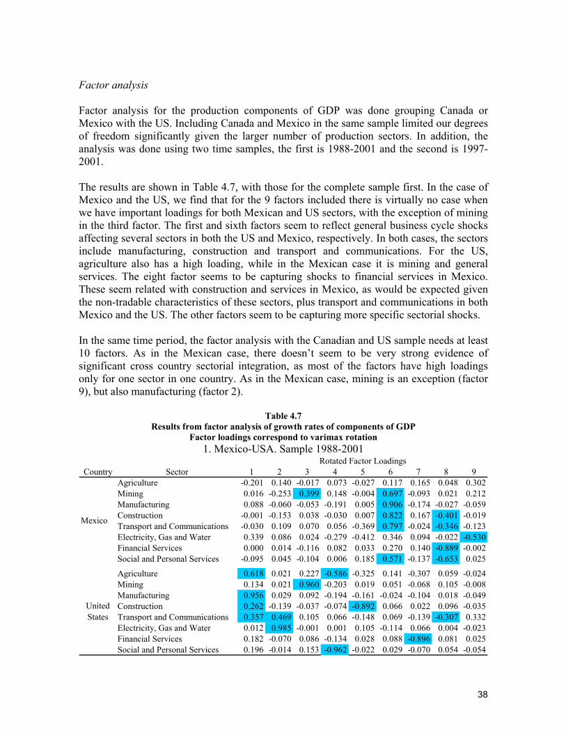
38

Factor analysis Factor analysis for the production components of GDP was done grouping Canada or Mexico with the US. Including Canada and Mexico in the same sample limited our degrees of freedom significantly given the larger number of production sectors. In addition, the analysis was done using two time samples, the first is 1988-2001 and the second is 1997-2001. The results are shown in Table 4.7, with those for the complete sample first. In the case of Mexico and the US, we find that for the 9 factors included there is virtually no case when we have important loadings for both Mexican and US sectors, with the exception of mining in the third factor. The first and sixth factors seem to reflect general business cycle shocks affecting several sectors in both the US and Mexico, respectively. In both cases, the sectors include manufacturing, construction and transport and communications. For the US, agriculture also has a high loading, while in the Mexican case it is mining and general services. The eight factor seems to be capturing shocks to financial services in Mexico. These seem related with construction and services in Mexico, as would be expected given the non-tradable characteristics of these sectors, plus transport and communications in both Mexico and the US. The other factors seem to be capturing more specific sectorial shocks. In the same time period, the factor analysis with the Canadian and US sample needs at least 10 factors. As in the Mexican case, there doesn’t seem to be very strong evidence of significant cross country sectorial integration, as most of the factors have high loadings only for one sector in one country. As in the Mexican case, mining is an exception (factor 9), but also manufacturing (factor 2).

Table 4.7 Results from factor analysis of growth rates of components of GDP

Factor loadings correspond to varimax rotation 1. Mexico-USA. Sample 1988-2001

Country Sector 1 2 3 4 5 6 7 8 9Agriculture -0.201 0.140 -0.017 0.073 -0.027 0.117 0.165 0.048 0.302Mining 0.016 -0.253 0.399 0.148 -0.004 0.697 -0.093 0.021 0.212Manufacturing 0.088 -0.060 -0.053 -0.191 0.005 0.906 -0.174 -0.027 -0.059Construction -0.001 -0.153 0.038 -0.030 0.007 0.822 0.167 -0.401 -0.019Transport and Communications -0.030 0.109 0.070 0.056 -0.369 0.797 -0.024 -0.346 -0.123Electricity, Gas and Water 0.339 0.086 0.024 -0.279 -0.412 0.346 0.094 -0.022 -0.530Financial Services 0.000 0.014 -0.116 0.082 0.033 0.270 0.140 -0.889 -0.002Social and Personal Services -0.095 0.045 -0.104 0.006 0.185 0.571 -0.137 -0.653 0.025

Agriculture 0.618 0.021 0.227 -0.586 -0.325 0.141 -0.307 0.059 -0.024Mining 0.134 0.021 0.960 -0.203 0.019 0.051 -0.068 0.105 -0.008Manufacturing 0.956 0.029 0.092 -0.194 -0.161 -0.024 -0.104 0.018 -0.049Construction 0.262 -0.139 -0.037 -0.074 -0.892 0.066 0.022 0.096 -0.035Transport and Communications 0.357 0.469 0.105 0.066 -0.148 0.069 -0.139 -0.307 0.332Electricity, Gas and Water 0.012 0.985 -0.001 0.001 0.105 -0.114 0.066 0.004 -0.023Financial Services 0.182 -0.070 0.086 -0.134 0.028 0.088 -0.896 0.081 0.025Social and Personal Services 0.196 -0.014 0.153 -0.962 -0.022 0.029 -0.070 0.054 -0.054


Mexico

United States

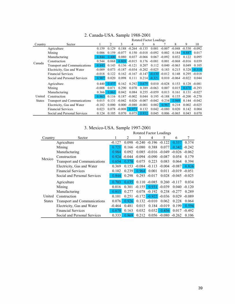
39

2. Canada-USA. Sample 1988-2001

Country Sector 1 2 3 4 5 6 7 8 9 10Agriculture 0.159 0.129 0.188 -0.264 -0.135 0.001 -0.007 -0.048 -0.530 -0.092Mining 0.006 0.159 -0.077 0.150 -0.018 -0.092 0.002 0.184 0.887 0.017Manufacturing 0.844 0.400 0.080 0.037 -0.066 0.067 -0.092 0.032 0.122 0.095Construction 0.544 0.068 0.809 -0.015 0.176 -0.081 0.001 -0.068 -0.016 0.039Transport and Communications 0.843 0.143 0.136 -0.121 0.207 0.112 0.040 -0.063 0.049 0.105Electricity, Gas and Water -0.009 0.073 -0.187 -0.034 -0.202 -0.025 0.183 0.215 0.328 -0.518Financial Services -0.018 0.122 0.162 -0.167 -0.147 -0.630 -0.012 0.148 0.295 -0.018Social and Personal Services 0.907 0.020 0.098 0.111 0.214 -0.321 0.010 -0.064 -0.022 0.044

Agriculture 0.440 0.437 0.162 0.292 0.675 0.010 -0.028 0.153 0.128 -0.081Mining -0.008 0.071 0.290 0.070 0.389 -0.063 0.007 0.015 0.670 -0.293Manufacturing 0.366 0.863 0.042 0.084 0.255 -0.059 0.013 0.161 0.131 -0.027Construction 0.863 0.116 0.187 -0.002 0.044 0.195 -0.188 0.135 -0.200 -0.270Transport and Communications 0.015 0.131 -0.042 0.026 -0.007 -0.042 0.234 0.949 0.144 -0.042Electricity, Gas and Water -0.102 0.000 0.000 -0.080 -0.001 0.002 0.967 0.218 0.002 -0.025Financial Services 0.023 0.078 -0.008 0.973 0.132 0.042 -0.080 0.020 0.142 0.004Social and Personal Services 0.124 0.105 0.070 0.075 0.932 0.045 0.006 -0.065 0.043 0.070


Canada

United States

3. Mexico-USA. Sample 1997-2001

Country Sector 1 2 3 4 5 6 7Agriculture -0.127 0.098 -0.240 -0.196 -0.122 0.337 0.374Mining 0.721 0.166 -0.080 0.388 0.077 0.342 -0.242Manufacturing 0.984 0.092 0.085 -0.016 -0.049 -0.026 -0.062Construction 0.924 -0.044 -0.094 -0.090 -0.087 0.054 0.179Transport and Communications 0.654 0.570 0.075 0.223 0.083 0.064 0.394Electricity, Gas and Water 0.369 0.153 -0.084 -0.113 -0.004 -0.087 0.826Financial Services 0.102 0.239 0.964 0.001 0.011 -0.019 -0.051Social and Personal Services 0.844 0.298 0.293 -0.017 0.028 -0.045 -0.025

Agriculture 0.703 0.635 0.110 -0.085 0.260 -0.117 0.034Mining 0.016 0.301 -0.155 0.931 -0.039 0.040 -0.120Manufacturing 0.815 0.277 0.078 -0.192 0.238 -0.277 0.289Construction 0.101 0.251 -0.172 -0.922 -0.036 0.029 -0.089Transport and Communications 0.076 0.926 0.132 -0.010 0.062 0.228 0.064Electricity, Gas and Water -0.464 0.481 0.015 0.184 -0.019 0.199 0.594Financial Services 0.670 0.163 0.032 0.032 0.456 0.017 -0.492Social and Personal Services 0.333 0.869 0.212 0.056 -0.080 -0.262 0.106

Mexico

United States


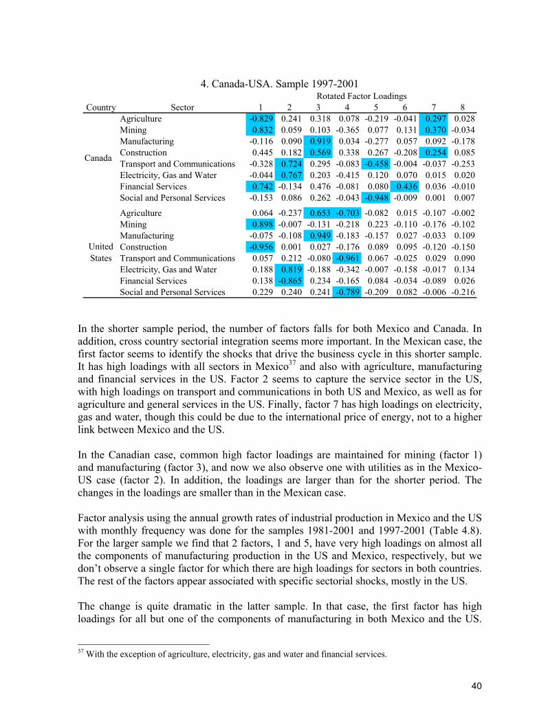
40

4. Canada-USA. Sample 1997-2001

Country Sector 1 2 3 4 5 6 7 8Agriculture -0.829 0.241 0.318 0.078 -0.219 -0.041 0.297 0.028Mining 0.832 0.059 0.103 -0.365 0.077 0.131 0.370 -0.034Manufacturing -0.116 0.090 0.919 0.034 -0.277 0.057 0.092 -0.178Construction 0.445 0.182 0.569 0.338 0.267 -0.208 0.254 0.085Transport and Communications -0.328 0.724 0.295 -0.083 -0.458 -0.004 -0.037 -0.253Electricity, Gas and Water -0.044 0.767 0.203 -0.415 0.120 0.070 0.015 0.020Financial Services 0.742 -0.134 0.476 -0.081 0.080 0.436 0.036 -0.010Social and Personal Services -0.153 0.086 0.262 -0.043 -0.948 -0.009 0.001 0.007

Agriculture 0.064 -0.237 0.653 -0.703 -0.082 0.015 -0.107 -0.002Mining 0.898 -0.007 -0.131 -0.218 0.223 -0.110 -0.176 -0.102Manufacturing -0.075 -0.108 0.949 -0.183 -0.157 0.027 -0.033 0.109Construction -0.956 0.001 0.027 -0.176 0.089 0.095 -0.120 -0.150Transport and Communications 0.057 0.212 -0.080 -0.961 0.067 -0.025 0.029 0.090Electricity, Gas and Water 0.188 0.819 -0.188 -0.342 -0.007 -0.158 -0.017 0.134Financial Services 0.138 -0.865 0.234 -0.165 0.084 -0.034 -0.089 0.026Social and Personal Services 0.229 0.240 0.241 -0.789 -0.209 0.082 -0.006 -0.216


Canada

United States

In the shorter sample period, the number of factors falls for both Mexico and Canada. In addition, cross country sectorial integration seems more important. In the Mexican case, the first factor seems to identify the shocks that drive the business cycle in this shorter sample. It has high loadings with all sectors in Mexico37 and also with agriculture, manufacturing and financial services in the US. Factor 2 seems to capture the service sector in the US, with high loadings on transport and communications in both US and Mexico, as well as for agriculture and general services in the US. Finally, factor 7 has high loadings on electricity, gas and water, though this could be due to the international price of energy, not to a higher link between Mexico and the US. In the Canadian case, common high factor loadings are maintained for mining (factor 1) and manufacturing (factor 3), and now we also observe one with utilities as in the Mexico-US case (factor 2). In addition, the loadings are larger than for the shorter period. The changes in the loadings are smaller than in the Mexican case. Factor analysis using the annual growth rates of industrial production in Mexico and the US with monthly frequency was done for the samples 1981-2001 and 1997-2001 (Table 4.8). For the larger sample we find that 2 factors, 1 and 5, have very high loadings on almost all the components of manufacturing production in the US and Mexico, respectively, but we don’t observe a single factor for which there are high loadings for sectors in both countries. The rest of the factors appear associated with specific sectorial shocks, mostly in the US. The change is quite dramatic in the latter sample. In that case, the first factor has high loadings for all but one of the components of manufacturing in both Mexico and the US.

37 With the exception of agriculture, electricity, gas and water and financial services.

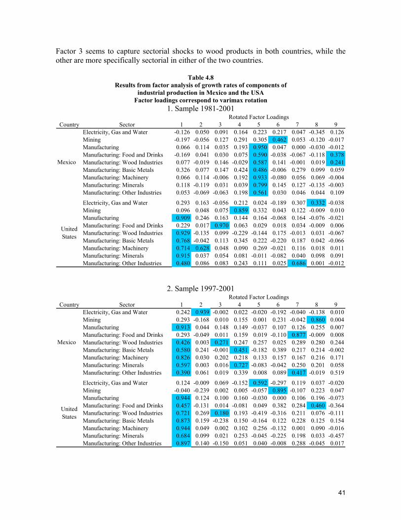
41

Factor 3 seems to capture sectorial shocks to wood products in both countries, while the other are more specifically sectorial in either of the two countries.

Table 4.8 Results from factor analysis of growth rates of components of

industrial production in Mexico and the USA Factor loadings correspond to varimax rotation

1. Sample 1981-2001

Country Sector 1 2 3 4 5 6 7 8 9Electricity, Gas and Water -0.126 0.050 0.091 0.164 0.223 0.217 0.047 -0.345 0.126Mining -0.197 -0.056 0.127 0.291 0.305 0.462 0.053 -0.120 -0.017Manufacturing 0.066 0.114 0.035 0.193 0.950 0.047 0.000 -0.030 -0.012Manufacturing: Food and Drinks -0.169 0.041 0.030 0.075 0.590 -0.038 -0.067 -0.118 0.378Manufacturing: Wood Industries 0.077 -0.019 0.146 -0.029 0.587 0.141 -0.001 0.019 0.241Manufacturing: Basic Metals 0.326 0.077 0.147 0.424 0.486 -0.006 0.279 0.099 0.059Manufacturing: Machinery 0.066 0.114 -0.006 0.192 0.933 -0.080 0.056 0.069 -0.004Manufacturing: Minerals 0.118 -0.119 0.031 0.039 0.799 0.145 0.127 -0.135 -0.003Manufacturing: Other Industries 0.053 -0.069 -0.063 0.198 0.561 0.030 0.046 0.044 0.109

Electricity, Gas and Water 0.293 0.163 -0.056 0.212 0.024 -0.189 0.307 0.332 -0.038Mining 0.096 0.048 0.075 0.859 0.332 0.043 0.122 -0.009 0.010Manufacturing 0.909 0.246 0.163 0.144 0.164 -0.068 0.164 -0.076 -0.021Manufacturing: Food and Drinks 0.229 0.017 0.970 0.063 0.029 0.018 0.034 -0.009 0.006Manufacturing: Wood Industries 0.929 -0.135 0.099 -0.229 -0.144 0.175 -0.013 0.031 -0.067Manufacturing: Basic Metals 0.768 -0.042 0.113 0.345 0.222 -0.220 0.187 0.042 -0.066Manufacturing: Machinery 0.714 0.628 0.048 0.090 0.269 -0.021 0.116 0.018 0.011Manufacturing: Minerals 0.915 0.037 0.054 0.081 -0.011 -0.082 0.040 0.098 0.091Manufacturing: Other Industries 0.480 0.086 0.083 0.243 0.111 0.025 0.686 0.001 -0.012


Mexico

United States

2. Sample 1997-2001

Country Sector 1 2 3 4 5 6 7 8 9Electricity, Gas and Water 0.242 0.939 -0.002 0.022 -0.020 -0.192 -0.040 -0.138 0.010Mining 0.293 -0.168 0.010 0.155 0.001 0.231 -0.042 0.860 0.004Manufacturing 0.913 0.044 0.148 0.149 -0.037 0.107 0.126 0.255 0.007Manufacturing: Food and Drinks 0.293 -0.049 0.011 0.159 0.019 -0.110 0.877 -0.009 0.008Manufacturing: Wood Industries 0.426 0.003 0.271 0.247 0.257 0.025 0.289 0.280 0.244Manufacturing: Basic Metals 0.580 0.241 -0.001 0.451 -0.182 0.389 0.217 0.214 -0.002Manufacturing: Machinery 0.826 0.030 0.202 0.218 0.133 0.157 0.167 0.216 0.171Manufacturing: Minerals 0.597 0.003 0.016 0.727 -0.083 -0.042 0.250 0.201 0.058Manufacturing: Other Industries 0.390 0.061 0.019 0.339 0.008 0.089 0.417 -0.019 0.519

Electricity, Gas and Water 0.124 -0.009 0.069 -0.152 0.592 -0.297 0.119 0.037 -0.020Mining -0.040 -0.239 0.002 0.005 -0.057 0.895 -0.107 0.223 0.047Manufacturing 0.944 0.124 0.100 0.160 -0.030 0.000 0.106 0.196 -0.073Manufacturing: Food and Drinks 0.457 -0.131 0.014 -0.081 0.049 0.382 0.284 0.460 -0.364Manufacturing: Wood Industries 0.721 0.269 0.180 0.193 -0.419 -0.316 0.211 0.076 -0.111Manufacturing: Basic Metals 0.873 0.159 -0.238 0.150 -0.164 0.122 0.228 0.125 0.154Manufacturing: Machinery 0.944 0.049 0.002 0.102 0.256 -0.132 0.001 0.090 -0.016Manufacturing: Minerals 0.684 0.099 0.021 0.253 -0.045 -0.225 0.198 0.033 -0.457Manufacturing: Other Industries 0.897 0.140 -0.150 0.051 0.040 -0.008 0.288 -0.045 0.017

Mexico

United States


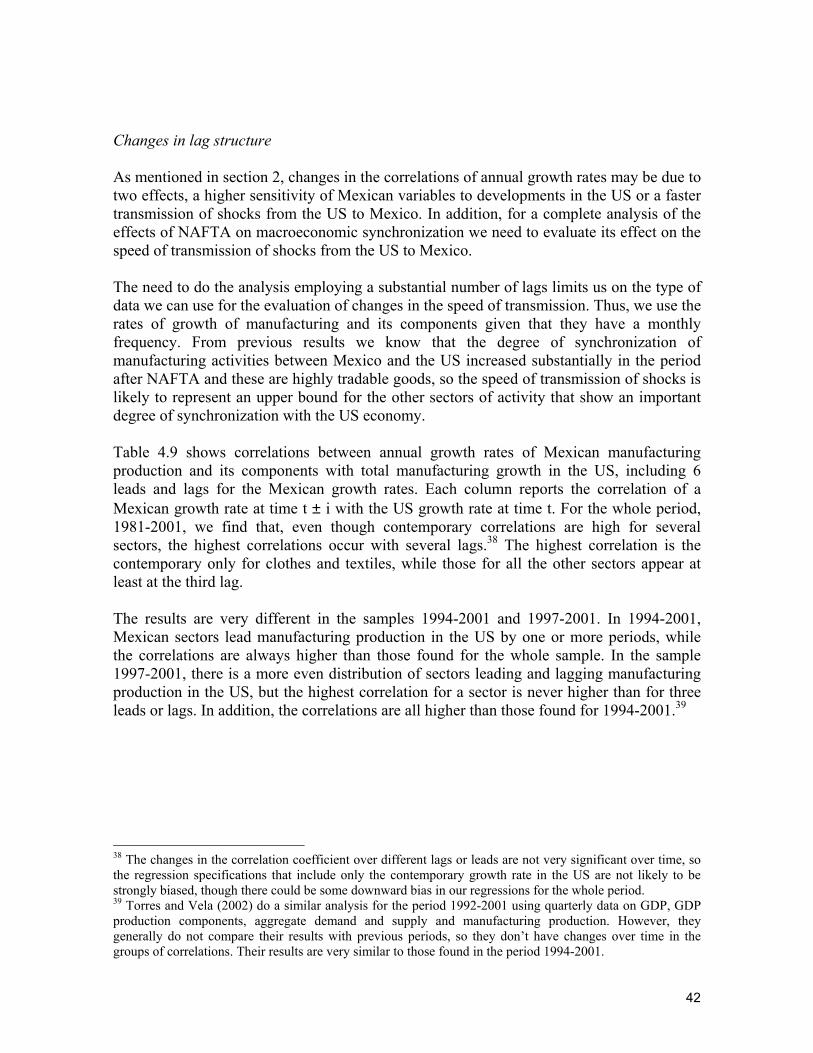
42

Changes in lag structure As mentioned in section 2, changes in the correlations of annual growth rates may be due to two effects, a higher sensitivity of Mexican variables to developments in the US or a faster transmission of shocks from the US to Mexico. In addition, for a complete analysis of the effects of NAFTA on macroeconomic synchronization we need to evaluate its effect on the speed of transmission of shocks from the US to Mexico. The need to do the analysis employing a substantial number of lags limits us on the type of data we can use for the evaluation of changes in the speed of transmission. Thus, we use the rates of growth of manufacturing and its components given that they have a monthly frequency. From previous results we know that the degree of synchronization of manufacturing activities between Mexico and the US increased substantially in the period after NAFTA and these are highly tradable goods, so the speed of transmission of shocks is likely to represent an upper bound for the other sectors of activity that show an important degree of synchronization with the US economy. Table 4.9 shows correlations between annual growth rates of Mexican manufacturing production and its components with total manufacturing growth in the US, including 6 leads and lags for the Mexican growth rates. Each column reports the correlation of a Mexican growth rate at time t ± i with the US growth rate at time t. For the whole period, 1981-2001, we find that, even though contemporary correlations are high for several sectors, the highest correlations occur with several lags.38 The highest correlation is the contemporary only for clothes and textiles, while those for all the other sectors appear at least at the third lag. The results are very different in the samples 1994-2001 and 1997-2001. In 1994-2001, Mexican sectors lead manufacturing production in the US by one or more periods, while the correlations are always higher than those found for the whole sample. In the sample 1997-2001, there is a more even distribution of sectors leading and lagging manufacturing production in the US, but the highest correlation for a sector is never higher than for three leads or lags. In addition, the correlations are all higher than those found for 1994-2001.39 38 The changes in the correlation coefficient over different lags or leads are not very significant over time, so the regression specifications that include only the contemporary growth rate in the US are not likely to be strongly biased, though there could be some downward bias in our regressions for the whole period. 39 Torres and Vela (2002) do a similar analysis for the period 1992-2001 using quarterly data on GDP, GDP production components, aggregate demand and supply and manufacturing production. However, they generally do not compare their results with previous periods, so they don’t have changes over time in the groups of correlations. Their results are very similar to those found in the period 1994-2001.

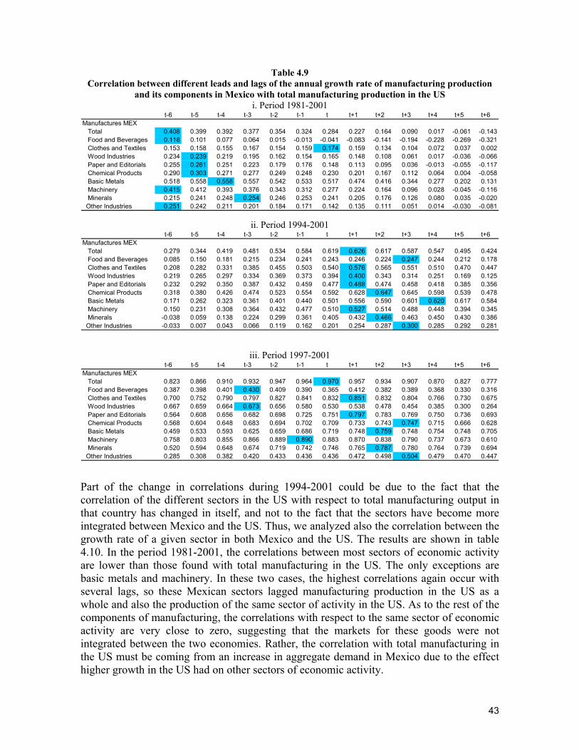
43

Table 4.9 Correlation between different leads and lags of the annual growth rate of manufacturing production

and its components in Mexico with total manufacturing production in the US i. Period 1981-2001

t-6 t-5 t-4 t-3 t-2 t-1 t t+1 t+2 t+3 t+4 t+5 t+6Manufactures MEX Total 0.408 0.399 0.392 0.377 0.354 0.324 0.284 0.227 0.164 0.090 0.017 -0.061 -0.143 Food and Beverages 0.118 0.101 0.077 0.064 0.015 -0.013 -0.041 -0.083 -0.141 -0.194 -0.228 -0.269 -0.321 Clothes and Textiles 0.153 0.158 0.155 0.167 0.154 0.159 0.174 0.159 0.134 0.104 0.072 0.037 0.002 Wood Industries 0.234 0.239 0.219 0.195 0.162 0.154 0.165 0.148 0.108 0.061 0.017 -0.036 -0.066 Paper and Editorials 0.255 0.261 0.251 0.223 0.179 0.176 0.148 0.113 0.095 0.036 -0.013 -0.055 -0.117 Chemical Products 0.290 0.303 0.271 0.277 0.249 0.248 0.230 0.201 0.167 0.112 0.064 0.004 -0.058 Basic Metals 0.518 0.558 0.558 0.557 0.542 0.533 0.517 0.474 0.416 0.344 0.277 0.202 0.131 Machinery 0.415 0.412 0.393 0.376 0.343 0.312 0.277 0.224 0.164 0.096 0.028 -0.045 -0.116 Minerals 0.215 0.241 0.248 0.254 0.246 0.253 0.241 0.205 0.176 0.126 0.080 0.035 -0.020 Other Industries 0.251 0.242 0.211 0.201 0.184 0.171 0.142 0.135 0.111 0.051 0.014 -0.030 -0.081

ii. Period 1994-2001

t-6 t-5 t-4 t-3 t-2 t-1 t t+1 t+2 t+3 t+4 t+5 t+6Manufactures MEX Total 0.279 0.344 0.419 0.481 0.534 0.584 0.619 0.626 0.617 0.587 0.547 0.495 0.424 Food and Beverages 0.085 0.150 0.181 0.215 0.234 0.241 0.243 0.246 0.224 0.247 0.244 0.212 0.178 Clothes and Textiles 0.208 0.282 0.331 0.385 0.455 0.503 0.540 0.576 0.565 0.551 0.510 0.470 0.447 Wood Industries 0.219 0.265 0.297 0.334 0.369 0.373 0.394 0.400 0.343 0.314 0.251 0.169 0.125 Paper and Editorials 0.232 0.292 0.350 0.387 0.432 0.459 0.477 0.488 0.474 0.458 0.418 0.385 0.356 Chemical Products 0.318 0.380 0.426 0.474 0.523 0.554 0.592 0.628 0.647 0.645 0.598 0.539 0.478 Basic Metals 0.171 0.262 0.323 0.361 0.401 0.440 0.501 0.556 0.590 0.601 0.620 0.617 0.584 Machinery 0.150 0.231 0.308 0.364 0.432 0.477 0.510 0.527 0.514 0.488 0.448 0.394 0.345 Minerals -0.038 0.059 0.138 0.224 0.299 0.361 0.405 0.432 0.466 0.463 0.450 0.430 0.386 Other Industries -0.033 0.007 0.043 0.066 0.119 0.162 0.201 0.254 0.287 0.300 0.285 0.292 0.281

iii. Period 1997-2001 t-6 t-5 t-4 t-3 t-2 t-1 t t+1 t+2 t+3 t+4 t+5 t+6

Manufactures MEX Total 0.823 0.866 0.910 0.932 0.947 0.964 0.970 0.957 0.934 0.907 0.870 0.827 0.777 Food and Beverages 0.387 0.398 0.401 0.430 0.409 0.390 0.365 0.412 0.382 0.389 0.368 0.330 0.316 Clothes and Textiles 0.700 0.752 0.790 0.797 0.827 0.841 0.832 0.851 0.832 0.804 0.766 0.730 0.675 Wood Industries 0.667 0.659 0.664 0.673 0.656 0.580 0.530 0.538 0.478 0.454 0.385 0.300 0.264 Paper and Editorials 0.564 0.608 0.656 0.682 0.698 0.725 0.751 0.797 0.783 0.769 0.750 0.736 0.693 Chemical Products 0.568 0.604 0.648 0.683 0.694 0.702 0.709 0.733 0.743 0.747 0.715 0.666 0.628 Basic Metals 0.459 0.533 0.593 0.625 0.659 0.686 0.719 0.748 0.759 0.748 0.754 0.748 0.705 Machinery 0.758 0.803 0.855 0.866 0.889 0.890 0.883 0.870 0.838 0.790 0.737 0.673 0.610 Minerals 0.520 0.594 0.648 0.674 0.719 0.742 0.746 0.765 0.787 0.780 0.764 0.739 0.694 Other Industries 0.285 0.308 0.382 0.420 0.433 0.436 0.436 0.472 0.498 0.504 0.479 0.470 0.447

Part of the change in correlations during 1994-2001 could be due to the fact that the correlation of the different sectors in the US with respect to total manufacturing output in that country has changed in itself, and not to the fact that the sectors have become more integrated between Mexico and the US. Thus, we analyzed also the correlation between the growth rate of a given sector in both Mexico and the US. The results are shown in table 4.10. In the period 1981-2001, the correlations between most sectors of economic activity are lower than those found with total manufacturing in the US. The only exceptions are basic metals and machinery. In these two cases, the highest correlations again occur with several lags, so these Mexican sectors lagged manufacturing production in the US as a whole and also the production of the same sector of activity in the US. As to the rest of the components of manufacturing, the correlations with respect to the same sector of economic activity are very close to zero, suggesting that the markets for these goods were not integrated between the two economies. Rather, the correlation with total manufacturing in the US must be coming from an increase in aggregate demand in Mexico due to the effect higher growth in the US had on other sectors of economic activity.

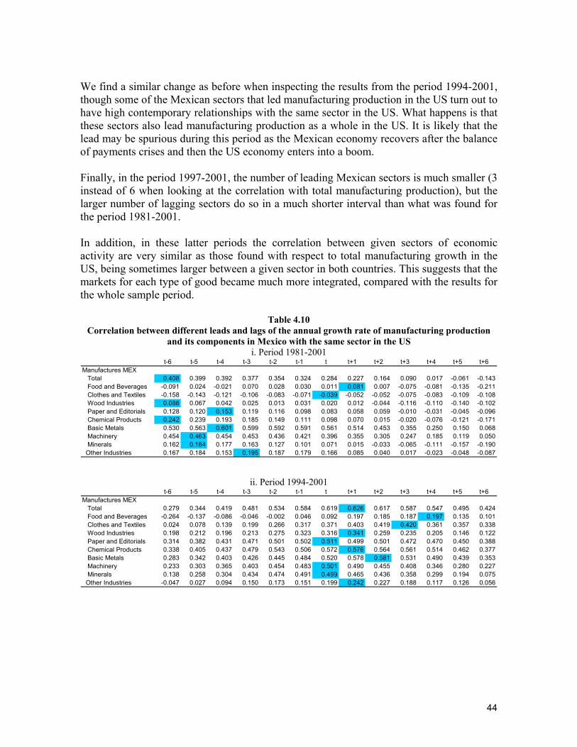
44

We find a similar change as before when inspecting the results from the period 1994-2001, though some of the Mexican sectors that led manufacturing production in the US turn out to have high contemporary relationships with the same sector in the US. What happens is that these sectors also lead manufacturing production as a whole in the US. It is likely that the lead may be spurious during this period as the Mexican economy recovers after the balance of payments crises and then the US economy enters into a boom. Finally, in the period 1997-2001, the number of leading Mexican sectors is much smaller (3 instead of 6 when looking at the correlation with total manufacturing production), but the larger number of lagging sectors do so in a much shorter interval than what was found for the period 1981-2001. In addition, in these latter periods the correlation between given sectors of economic activity are very similar as those found with respect to total manufacturing growth in the US, being sometimes larger between a given sector in both countries. This suggests that the markets for each type of good became much more integrated, compared with the results for the whole sample period.

Table 4.10 Correlation between different leads and lags of the annual growth rate of manufacturing production

and its components in Mexico with the same sector in the US i. Period 1981-2001

t-6 t-5 t-4 t-3 t-2 t-1 t t+1 t+2 t+3 t+4 t+5 t+6Manufactures MEX Total 0.408 0.399 0.392 0.377 0.354 0.324 0.284 0.227 0.164 0.090 0.017 -0.061 -0.143 Food and Beverages -0.091 0.024 -0.021 0.070 0.028 0.030 0.011 0.081 0.007 -0.075 -0.081 -0.135 -0.211 Clothes and Textiles -0.158 -0.143 -0.121 -0.106 -0.083 -0.071 -0.039 -0.052 -0.052 -0.075 -0.083 -0.109 -0.108 Wood Industries 0.088 0.067 0.042 0.025 0.013 0.031 0.020 0.012 -0.044 -0.116 -0.110 -0.140 -0.102 Paper and Editorials 0.128 0.120 0.153 0.119 0.116 0.098 0.083 0.058 0.059 -0.010 -0.031 -0.045 -0.096 Chemical Products 0.242 0.239 0.193 0.185 0.149 0.111 0.098 0.070 0.015 -0.020 -0.076 -0.121 -0.171 Basic Metals 0.530 0.563 0.601 0.599 0.592 0.591 0.561 0.514 0.453 0.355 0.250 0.150 0.068 Machinery 0.454 0.463 0.454 0.453 0.436 0.421 0.396 0.355 0.305 0.247 0.185 0.119 0.050 Minerals 0.162 0.184 0.177 0.163 0.127 0.101 0.071 0.015 -0.033 -0.065 -0.111 -0.157 -0.190 Other Industries 0.167 0.184 0.153 0.195 0.187 0.179 0.166 0.085 0.040 0.017 -0.023 -0.048 -0.087

ii. Period 1994-2001 t-6 t-5 t-4 t-3 t-2 t-1 t t+1 t+2 t+3 t+4 t+5 t+6

Manufactures MEX Total 0.279 0.344 0.419 0.481 0.534 0.584 0.619 0.626 0.617 0.587 0.547 0.495 0.424 Food and Beverages -0.264 -0.137 -0.086 -0.046 -0.002 0.046 0.092 0.197 0.185 0.187 0.197 0.135 0.101 Clothes and Textiles 0.024 0.078 0.139 0.199 0.266 0.317 0.371 0.403 0.419 0.420 0.361 0.357 0.338 Wood Industries 0.198 0.212 0.196 0.213 0.275 0.323 0.316 0.341 0.259 0.235 0.205 0.146 0.122 Paper and Editorials 0.314 0.382 0.431 0.471 0.501 0.502 0.511 0.499 0.501 0.472 0.470 0.450 0.388 Chemical Products 0.338 0.405 0.437 0.479 0.543 0.506 0.572 0.576 0.564 0.561 0.514 0.462 0.377 Basic Metals 0.283 0.342 0.403 0.426 0.445 0.484 0.520 0.578 0.581 0.531 0.490 0.439 0.353 Machinery 0.233 0.303 0.365 0.403 0.454 0.483 0.501 0.490 0.455 0.408 0.346 0.280 0.227 Minerals 0.138 0.258 0.304 0.434 0.474 0.491 0.499 0.465 0.436 0.358 0.299 0.194 0.075 Other Industries -0.047 0.027 0.094 0.150 0.173 0.151 0.199 0.242 0.227 0.188 0.117 0.126 0.056

45

iii. Period 1997-2001

t-6 t-5 t-4 t-3 t-2 t-1 t t+1 t+2 t+3 t+4 t+5 t+6Manufactures MEX Total 0.823 0.866 0.910 0.932 0.947 0.964 0.970 0.957 0.934 0.907 0.870 0.827 0.777 Food and Beverages -0.044 0.122 0.163 0.241 0.396 0.337 0.317 0.419 0.314 0.259 0.229 0.102 0.184 Clothes and Textiles 0.777 0.796 0.843 0.859 0.846 0.814 0.790 0.765 0.737 0.726 0.660 0.643 0.618 Wood Industries 0.519 0.505 0.457 0.470 0.464 0.425 0.344 0.325 0.305 0.309 0.292 0.224 0.234 Paper and Editorials 0.605 0.673 0.720 0.754 0.776 0.750 0.748 0.759 0.729 0.701 0.661 0.607 0.505 Chemical Products 0.594 0.652 0.662 0.706 0.716 0.636 0.691 0.639 0.612 0.619 0.571 0.536 0.455 Basic Metals 0.546 0.631 0.718 0.734 0.755 0.768 0.766 0.755 0.737 0.644 0.597 0.557 0.459 Machinery 0.604 0.670 0.734 0.762 0.806 0.834 0.832 0.821 0.775 0.700 0.623 0.523 0.423 Minerals 0.278 0.379 0.438 0.577 0.617 0.586 0.636 0.624 0.638 0.630 0.636 0.602 0.521 Other Industries 0.183 0.282 0.383 0.473 0.458 0.455 0.504 0.508 0.491 0.476 0.410 0.401 0.387

Thus, there seems to be a very important change in the speed with which shocks to manufacturing in the US are transmitted to the same sectors in Mexico. Currently, all sectors but one in manufacturing have their highest correlations in a time span between 2 lead and 3 lagged months from the change in the same sector in the US. Thus, part of the more rapid response of Mexican sectors to total US manufacturing is due changes themselves in the correlation of sectors in the US with total manufacturing in that country, but not exclusively. The presence of leads in the period 1997-2001 for some sectors may be explained by the fact that Mexican manufacturing could be playing the role of marginal supplier in certain sectors of the US, so they respond more quickly to economic shocks than US production. Another possible explanation is that the definition of sectors is not sufficiently disaggregated so we could still have very heterogeneous products within these categories. 4.2. Components of Aggregate Demand and Supply In addition to the analysis in section 4.1. focusing on different sectors of productive activity, it is also important to analyze the comovement between different components of aggregate demand. This is a particularly important issue in terms of policy implications, as the different components of aggregate demand respond differently to policy variables. Thus, in order to stabilize the economy in response to a shock from the USA, the optimal policies to be followed could be different from those necessary to counteract other types of shocks. This obviously has important implications on the scope of policy coordination. The data used are annual growth rates of private consumption, public consumption, investment, exports and imports with quarterly frequency for Canada, Mexico and the USA, and the sample period is 1981Q1-2001Q3. The methods of analysis are the same as those employed in section 4.1. First we look at correlations, then at simple regressions analysis and finally perform a factor analysis. From this analysis we expect to find a strong correlation of investment due to financial linkages and open capital accounts and a weaker one with consumption, though in theory this should be higher than that of output if there is consumption smoothing and integration of financial markets while output is subject to more idiosyncratic shocks. We don’t have any strong priors about government spending. If both countries followed counter cyclical

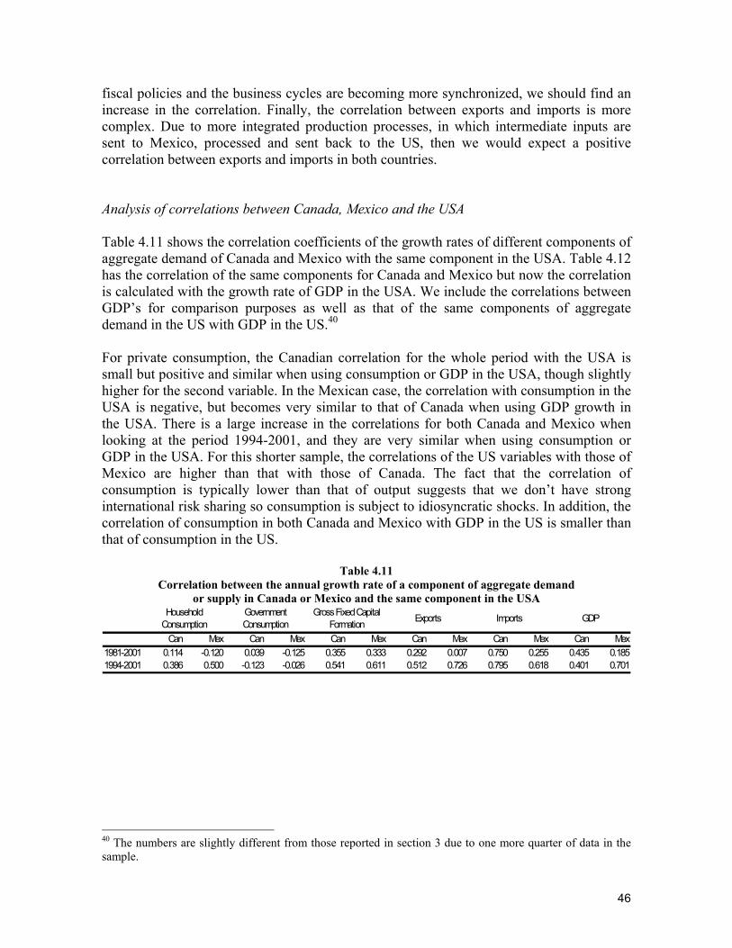
46

fiscal policies and the business cycles are becoming more synchronized, we should find an increase in the correlation. Finally, the correlation between exports and imports is more complex. Due to more integrated production processes, in which intermediate inputs are sent to Mexico, processed and sent back to the US, then we would expect a positive correlation between exports and imports in both countries. Analysis of correlations between Canada, Mexico and the USA Table 4.11 shows the correlation coefficients of the growth rates of different components of aggregate demand of Canada and Mexico with the same component in the USA. Table 4.12 has the correlation of the same components for Canada and Mexico but now the correlation is calculated with the growth rate of GDP in the USA. We include the correlations between GDP’s for comparison purposes as well as that of the same components of aggregate demand in the US with GDP in the US.40 For private consumption, the Canadian correlation for the whole period with the USA is small but positive and similar when using consumption or GDP in the USA, though slightly higher for the second variable. In the Mexican case, the correlation with consumption in the USA is negative, but becomes very similar to that of Canada when using GDP growth in the USA. There is a large increase in the correlations for both Canada and Mexico when looking at the period 1994-2001, and they are very similar when using consumption or GDP in the USA. For this shorter sample, the correlations of the US variables with those of Mexico are higher than that with those of Canada. The fact that the correlation of consumption is typically lower than that of output suggests that we don’t have strong international risk sharing so consumption is subject to idiosyncratic shocks. In addition, the correlation of consumption in both Canada and Mexico with GDP in the US is smaller than that of consumption in the US.

Table 4.11 Correlation between the annual growth rate of a component of aggregate demand

or supply in Canada or Mexico and the same component in the USA

Can Mex Can Mex Can Mex Can Mex Can Mex Can Mex1981-2001 0.114 -0.120 0.039 -0.125 0.355 0.333 0.292 0.007 0.750 0.255 0.435 0.1851994-2001 0.386 0.500 -0.123 -0.026 0.541 0.611 0.512 0.726 0.795 0.618 0.401 0.701

Gross Fixed Capital Formation Exports Imports GDPHousehold

Consumption Government Consumption

40 The numbers are slightly different from those reported in section 3 due to one more quarter of data in the sample.

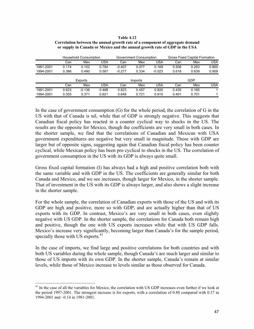
47

Table 4.12

Correlation between the annual growth rate of a component of aggregate demand or supply in Canada or Mexico and the annual growth rate of GDP in the USA

Can Mex USA Can Mex USA Can Mex USA1981-2001 0.174 0.152 0.784 -0.407 0.077 0.169 0.506 0.263 0.8651994-2001 0.386 0.490 0.567 -0.277 0.334 -0.023 0.618 0.639 0.909

Can Mex USA Can Mex USA Can Mex USA1981-2001 0.623 -0.136 0.468 0.823 0.457 0.820 0.435 0.185 11994-2001 0.355 0.371 0.621 0.648 0.721 0.915 0.401 0.701 1

Household Consumption Government Consumption Gross Fixed Capital Formation

Exports Imports GDP

In the case of government consumption (G) for the whole period, the correlation of G in the US with that of Canada is nil, while that of GDP is strongly negative. This suggests that Canadian fiscal policy has reacted in a counter cyclical way to shocks in the US. The results are the opposite for Mexico, though the coefficients are very small in both cases. In the shorter sample, we find that the correlations of Canadian and Mexican with USA government expenditures are negative but very small in magnitude. Those with GDP are larger but of opposite signs, suggesting again that Canadian fiscal policy has been counter cyclical, while Mexican policy has been pro cyclical to shocks in the US. The correlation of government consumption in the US with its GDP is always quite small. Gross fixed capital formation (I) has always had a high and positive correlation both with the same variable and with GDP in the US. The coefficients are generally similar for both Canada and Mexico, and we see increases, though larger for Mexico, in the shorter sample. That of investment in the US with its GDP is always larger, and also shows a slight increase in the shorter sample. For the whole sample, the correlation of Canadian exports with those of the US and with its GDP are high and positive, more so with GDP, and are actually higher than that of US exports with its GDP. In contrast, Mexico’s are very small in both cases, even slightly negative with US GDP. In the shorter sample, the correlations for Canada both remain high and positive, though the one with US exports increases while that with US GDP falls. Mexico’s increase very significantly, becoming larger than Canada’s for the sample period, specially those with US exports.41 In the case of imports, we find large and positive correlations for both countries and with both US variables during the whole sample, though Canada’s are much larger and similar to those of US imports with its own GDP. In the shorter sample, Canada’s remain at similar levels, while those of Mexico increase to levels similar as those observed for Canada.

41 In the case of all the variables for Mexico, the correlation with US GDP increases even further if we look at the period 1997-2001. The strongest increase is for exports, with a correlation of 0.88 compared with 0.37 in 1994-2001 and –0.14 in 1981-2001.

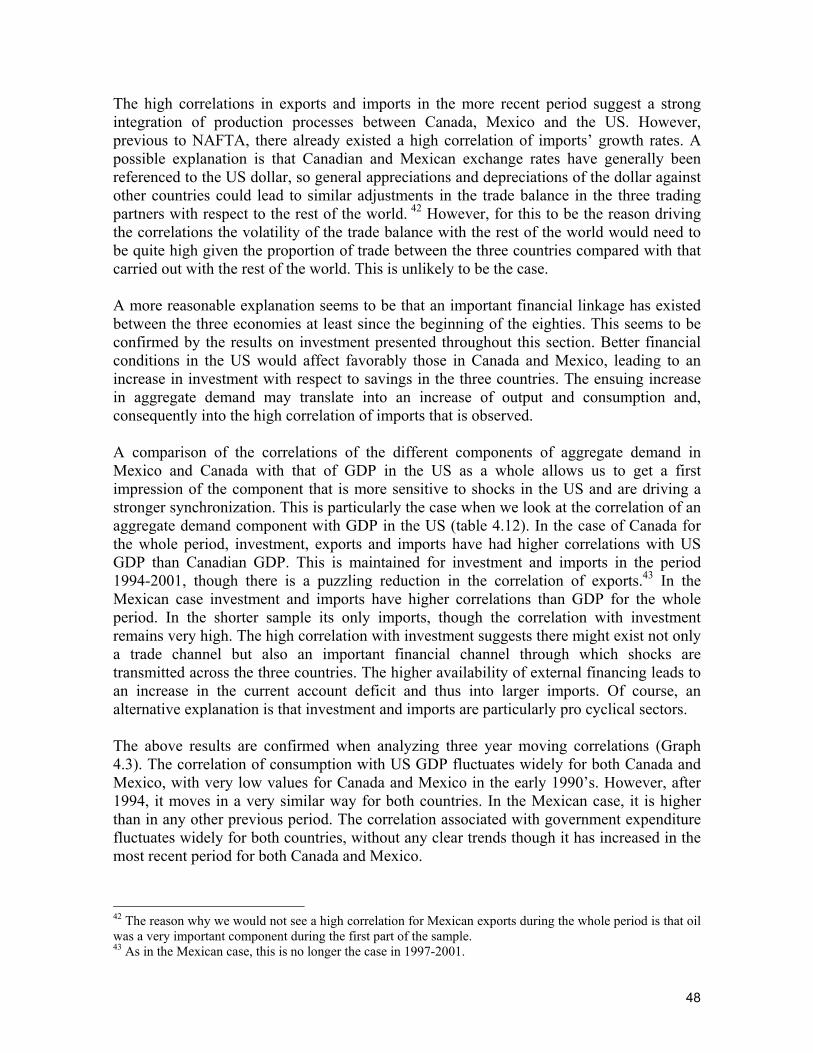
48

The high correlations in exports and imports in the more recent period suggest a strong integration of production processes between Canada, Mexico and the US. However, previous to NAFTA, there already existed a high correlation of imports’ growth rates. A possible explanation is that Canadian and Mexican exchange rates have generally been referenced to the US dollar, so general appreciations and depreciations of the dollar against other countries could lead to similar adjustments in the trade balance in the three trading partners with respect to the rest of the world. 42 However, for this to be the reason driving the correlations the volatility of the trade balance with the rest of the world would need to be quite high given the proportion of trade between the three countries compared with that carried out with the rest of the world. This is unlikely to be the case. A more reasonable explanation seems to be that an important financial linkage has existed between the three economies at least since the beginning of the eighties. This seems to be confirmed by the results on investment presented throughout this section. Better financial conditions in the US would affect favorably those in Canada and Mexico, leading to an increase in investment with respect to savings in the three countries. The ensuing increase in aggregate demand may translate into an increase of output and consumption and, consequently into the high correlation of imports that is observed. A comparison of the correlations of the different components of aggregate demand in Mexico and Canada with that of GDP in the US as a whole allows us to get a first impression of the component that is more sensitive to shocks in the US and are driving a stronger synchronization. This is particularly the case when we look at the correlation of an aggregate demand component with GDP in the US (table 4.12). In the case of Canada for the whole period, investment, exports and imports have had higher correlations with US GDP than Canadian GDP. This is maintained for investment and imports in the period 1994-2001, though there is a puzzling reduction in the correlation of exports.43 In the Mexican case investment and imports have higher correlations than GDP for the whole period. In the shorter sample its only imports, though the correlation with investment remains very high. The high correlation with investment suggests there might exist not only a trade channel but also an important financial channel through which shocks are transmitted across the three countries. The higher availability of external financing leads to an increase in the current account deficit and thus into larger imports. Of course, an alternative explanation is that investment and imports are particularly pro cyclical sectors. The above results are confirmed when analyzing three year moving correlations (Graph 4.3). The correlation of consumption with US GDP fluctuates widely for both Canada and Mexico, with very low values for Canada and Mexico in the early 1990’s. However, after 1994, it moves in a very similar way for both countries. In the Mexican case, it is higher than in any other previous period. The correlation associated with government expenditure fluctuates widely for both countries, without any clear trends though it has increased in the most recent period for both Canada and Mexico.

42 The reason why we would not see a high correlation for Mexican exports during the whole period is that oil was a very important component during the first part of the sample. 43 As in the Mexican case, this is no longer the case in 1997-2001.

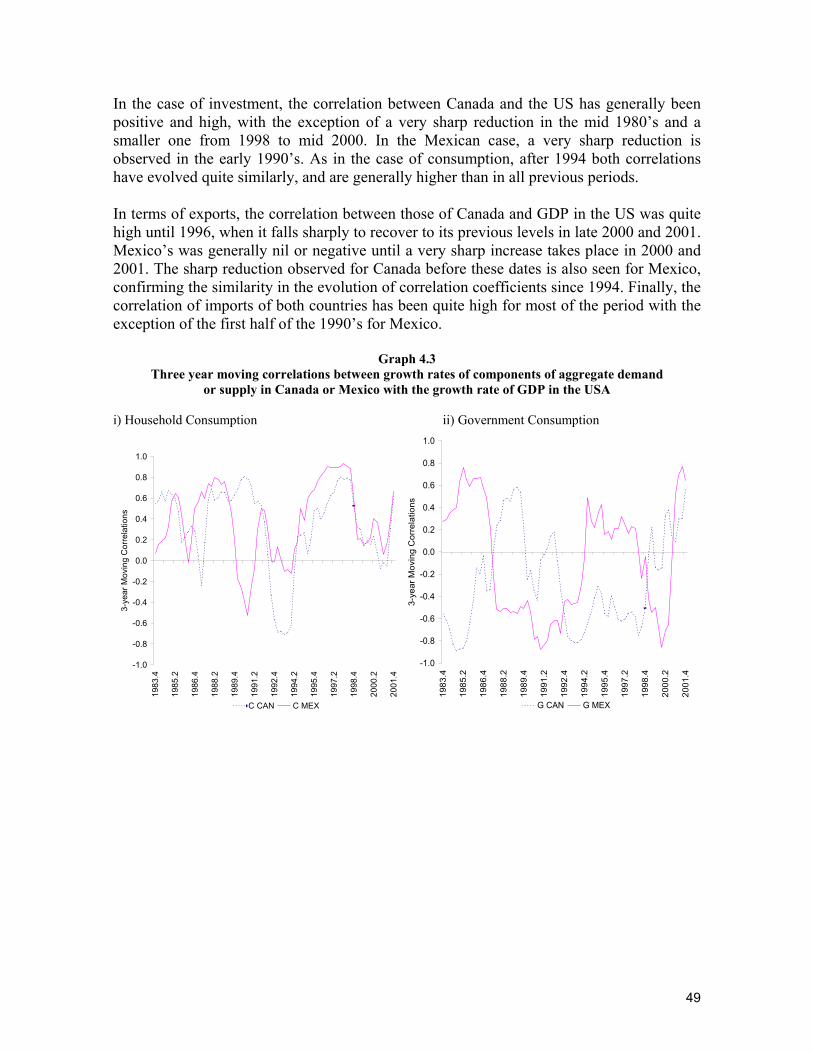
49

In the case of investment, the correlation between Canada and the US has generally been positive and high, with the exception of a very sharp reduction in the mid 1980’s and a smaller one from 1998 to mid 2000. In the Mexican case, a very sharp reduction is observed in the early 1990’s. As in the case of consumption, after 1994 both correlations have evolved quite similarly, and are generally higher than in all previous periods. In terms of exports, the correlation between those of Canada and GDP in the US was quite high until 1996, when it falls sharply to recover to its previous levels in late 2000 and 2001. Mexico’s was generally nil or negative until a very sharp increase takes place in 2000 and 2001. The sharp reduction observed for Canada before these dates is also seen for Mexico, confirming the similarity in the evolution of correlation coefficients since 1994. Finally, the correlation of imports of both countries has been quite high for most of the period with the exception of the first half of the 1990’s for Mexico.

Graph 4.3 Three year moving correlations between growth rates of components of aggregate demand

or supply in Canada or Mexico with the growth rate of GDP in the USA

i) Household Consumption ii) Government Consumption

-1.0

-0.8

-0.6

-0.4

-0.2

0.0

0.2

0.4

0.6

0.8

1.0

1983

.4

1985

.2

1986

.4

1988

.2

1989

.4

1991

.2

1992

.4

1994

.2

1995

.4

1997

.2

1998

.4

2000

.2

2001

.4

3-ye

ar M

ovin

g C

orre

latio

ns

C CAN C MEX

-1.0

-0.8

-0.6

-0.4

-0.2

0.0

0.2

0.4

0.6

0.8

1.019

83.4

1985

.2

1986

.4

1988

.2

1989

.4

1991

.2

1992

.4

1994

.2

1995

.4

1997

.2

1998

.4

2000

.2

2001

.4

3-ye

ar M

ovin

g C

orre

latio

ns

G CAN G MEX

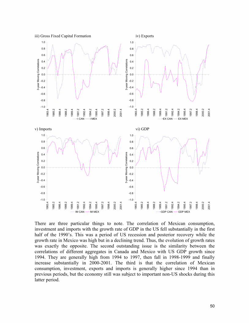
50

iii) Gross Fixed Capital Formation iv) Exports

-1.0

-0.8

-0.6

-0.4

-0.2

0.0

0.2

0.4

0.6

0.8

1.0

1983

.4

1985

.2

1986

.4

1988

.2

1989

.4

1991

.2

1992

.4

1994

.2

1995

.4

1997

.2

1998

.4

2000

.2

2001

.4

3-ye

ar M

ovin

g C

orre

latio

ns

I CAN I MEX

-1.0

-0.8

-0.6

-0.4

-0.2

0.0

0.2

0.4

0.6

0.8

1.0

1983

.4

1985

.2

1986

.4

1988

.2

1989

.4

1991

.2

1992

.4

1994

.2

1995

.4

1997

.2

1998

.4

2000

.2

2001

.4

3-ye

ar M

ovin

g C

orre

latio

ns

EX CAN EX MEX v) Imports vi) GDP

-1.0

-0.8

-0.6

-0.4

-0.2

0.0

0.2

0.4

0.6

0.8

1.0

1983

.4

1985

.2

1986

.4

1988

.2

1989

.4

1991

.2

1992

.4

1994

.2

1995

.4

1997

.2

1998

.4

2000

.2

2001

.4

3-ye

ar M

ovin

g C

orre

latio

ns

IM CAN IM MEX

-1.0

-0.8

-0.6

-0.4

-0.2

0.0

0.2

0.4

0.6

0.8

1.019

83.4

1985

.2

1986

.4

1988

.2

1989

.4

1991

.2

1992

.4

1994

.2

1995

.4

1997

.2

1998

.4

2000

.2

2001

.4

3-ye

ar M

ovin

g C

orre

latio

ns

GDP CAN GDP MEX There are three particular things to note. The correlation of Mexican consumption, investment and imports with the growth rate of GDP in the US fell substantially in the first half of the 1990’s. This was a period of US recession and posterior recovery while the growth rate in Mexico was high but in a declining trend. Thus, the evolution of growth rates was exactly the opposite. The second outstanding issue is the similarity between the correlations of different aggregates in Canada and Mexico with US GDP growth since 1994. They are generally high from 1994 to 1997, then fall in 1998-1999 and finally increase substantially in 2000-2001. The third is that the correlation of Mexican consumption, investment, exports and imports is generally higher since 1994 than in previous periods, but the economy still was subject to important non-US shocks during this latter period.

51

Simple regression analysis of synchronization of the components of aggregate demand of Canada and Mexico with the USA In order to analyze changes in the sensitivity of the components of aggregate demand in Canada and Mexico to developments in the US we did regressions of the type of (1) on both the growth rates of the same sector or of GDP in the US, and using the different specifications employed in previous analysis. The results are qualitatively similar when using the growth rate of the same sector or of GDP in the US as well as when we don’t include the lagged value of the variable so we only report those associated with GDP growth in the USA as a regressor for space reasons. Table 4.13 has the results when including the lagged rate of growth of the same variable in both Canada and Mexico. When we don’t include the time dummys for the periods after 1994 or 1997, we find that the coefficient on US GDP growth is positive and significant for investment, export and imports in the case of Canada and for private consumption, investment and imports in the Mexican case. The coefficients are larger for Mexico in the case of every variable with the exception of exports, when it is negative and non-significant. In terms of the magnitude of the coefficients, the largest for Canada are imports, exports and investment suggesting a strong sensitivity of these components of demand. Those for Mexico are imports, investment and consumption. The adjusted R2’s are always lower for Mexico, suggesting a higher presence of idiosyncratic shocks, but they are nevertheless high with the exception of exports and government consumption. The results when including the dummys for the periods after 1994 and 1997 suggest there is an increase in the sensitivity of Mexican variables to developments in the US as the dummys always have large positive coefficients, though they are generally non-significant. The only case when there is a significant change is for exports, for both dummys. For this variable, the coefficient is found to be significant but negative in the earlier period, while positive and quite large in the period associated with the dummys. In the Canadian case, the dummys are also positive44 but always smaller than in the Mexican case and only significant for exports when using the dummy for the period after 1994. Factor analysis In the case of aggregate demand and supply, given the reduced number of components compared with sectorial components of production, the factor analysis was done jointly for Canada, Mexico and the US, for the whole period 1981-2001 and for the subperiod 1997-2001 (Table 4.14). For the whole sample, the hypothesis test of more factors is rejected when we have nine factors. The first one seems to identify the general business cycle in Mexico, with positive high loadings on private consumption, investment and imports, with its counterpart in exports in the US. In addition, it seems to be related with positive financial conditions in

44 With two exceptions, government consumption with the 1994 dummy and investment with the 1997 dummy. In both cases, the coefficients are not significant.

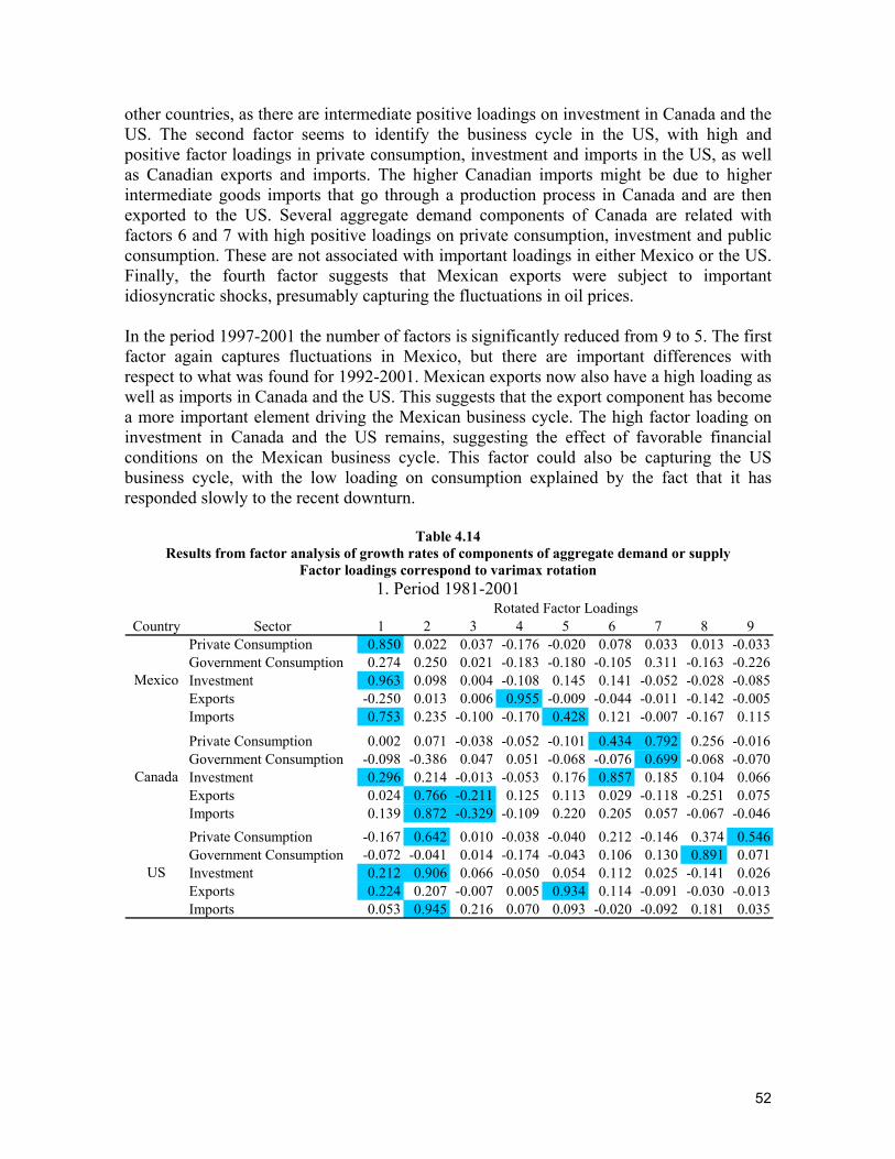
52

other countries, as there are intermediate positive loadings on investment in Canada and the US. The second factor seems to identify the business cycle in the US, with high and positive factor loadings in private consumption, investment and imports in the US, as well as Canadian exports and imports. The higher Canadian imports might be due to higher intermediate goods imports that go through a production process in Canada and are then exported to the US. Several aggregate demand components of Canada are related with factors 6 and 7 with high positive loadings on private consumption, investment and public consumption. These are not associated with important loadings in either Mexico or the US. Finally, the fourth factor suggests that Mexican exports were subject to important idiosyncratic shocks, presumably capturing the fluctuations in oil prices. In the period 1997-2001 the number of factors is significantly reduced from 9 to 5. The first factor again captures fluctuations in Mexico, but there are important differences with respect to what was found for 1992-2001. Mexican exports now also have a high loading as well as imports in Canada and the US. This suggests that the export component has become a more important element driving the Mexican business cycle. The high factor loading on investment in Canada and the US remains, suggesting the effect of favorable financial conditions on the Mexican business cycle. This factor could also be capturing the US business cycle, with the low loading on consumption explained by the fact that it has responded slowly to the recent downturn.

Table 4.14 Results from factor analysis of growth rates of components of aggregate demand or supply

Factor loadings correspond to varimax rotation 1. Period 1981-2001

Country Sector 1 2 3 4 5 6 7 8 9Private Consumption 0.850 0.022 0.037 -0.176 -0.020 0.078 0.033 0.013 -0.033Government Consumption 0.274 0.250 0.021 -0.183 -0.180 -0.105 0.311 -0.163 -0.226Investment 0.963 0.098 0.004 -0.108 0.145 0.141 -0.052 -0.028 -0.085Exports -0.250 0.013 0.006 0.955 -0.009 -0.044 -0.011 -0.142 -0.005Imports 0.753 0.235 -0.100 -0.170 0.428 0.121 -0.007 -0.167 0.115

Private Consumption 0.002 0.071 -0.038 -0.052 -0.101 0.434 0.792 0.256 -0.016Government Consumption -0.098 -0.386 0.047 0.051 -0.068 -0.076 0.699 -0.068 -0.070Investment 0.296 0.214 -0.013 -0.053 0.176 0.857 0.185 0.104 0.066Exports 0.024 0.766 -0.211 0.125 0.113 0.029 -0.118 -0.251 0.075Imports 0.139 0.872 -0.329 -0.109 0.220 0.205 0.057 -0.067 -0.046Private Consumption -0.167 0.642 0.010 -0.038 -0.040 0.212 -0.146 0.374 0.546Government Consumption -0.072 -0.041 0.014 -0.174 -0.043 0.106 0.130 0.891 0.071Investment 0.212 0.906 0.066 -0.050 0.054 0.112 0.025 -0.141 0.026Exports 0.224 0.207 -0.007 0.005 0.934 0.114 -0.091 -0.030 -0.013Imports 0.053 0.945 0.216 0.070 0.093 -0.020 -0.092 0.181 0.035

US


Mexico

Canada

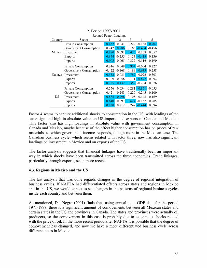
53

2. Period 1997-2001

Rotated Factor LoadingsCountry Sector 1 2 3 4 5

Private Consumption 0.452 0.041 0.222 -0.188 0.702Government Consumption 0.242 0.286 0.166 -0.494 -0.456Investment 0.870 0.091 0.423 0.159 0.057Exports 0.854 -0.255 0.123 -0.415 0.136Imports 0.905 -0.065 0.327 -0.116 0.190

Private Consumption 0.246 0.049 0.904 -0.004 0.227Government Consumption -0.422 -0.168 0.189 -0.635 0.258Investment 0.532 -0.031 0.787 0.072 -0.303Exports 0.309 0.058 0.111 -0.892 0.092Imports 0.725 0.432 0.359 -0.284 0.076Private Consumption 0.256 0.034 -0.281 -0.851 -0.055Government Consumption -0.421 -0.243 0.229 -0.245 -0.100Investment 0.885 0.298 0.105 -0.148 -0.169Exports 0.640 0.097 0.624 -0.157 0.285Imports 0.830 0.212 0.247 -0.444 0.094

US

Mexico

Canada

Factor 4 seems to capture additional shocks to consumption in the US, with loadings of the same sign and high in absolute value on US imports and exports of Canada and Mexico. This factor also has high loadings in absolute value with government consumption in Canada and Mexico, maybe because of the effect higher consumption has on prices of raw materials, to which government income responds, though more in the Mexican case. The Canadian business cycle, which seems related with factor three, now has also significant loadings on investment in Mexico and on exports of the US. The factor analysis suggests that financial linkages have traditionally been an important way in which shocks have been transmitted across the three economies. Trade linkages, particularly through exports, seem more recent. 4.3. Regions in Mexico and the US The last analysis that was done regards changes in the degree of regional integration of business cycles. If NAFTA had differentiated effects across states and regions in Mexico and in the US, we would expect to see changes in the patterns of regional business cycles inside each country and between them. As mentioned, Del Negro (2001) finds that, using annual state GDP data for the period 1971-1998, there is a significant amount of comovements between all Mexican states and certain states in the US and provinces in Canada. The states and provinces were actually oil producers, so the comovement in this case is probably due to exogenous shocks related with the price of oil. In the more recent period after NAFTA it is possible that the degree of comovement has changed, and now we have a more differentiated business cycle across different states in Mexico.

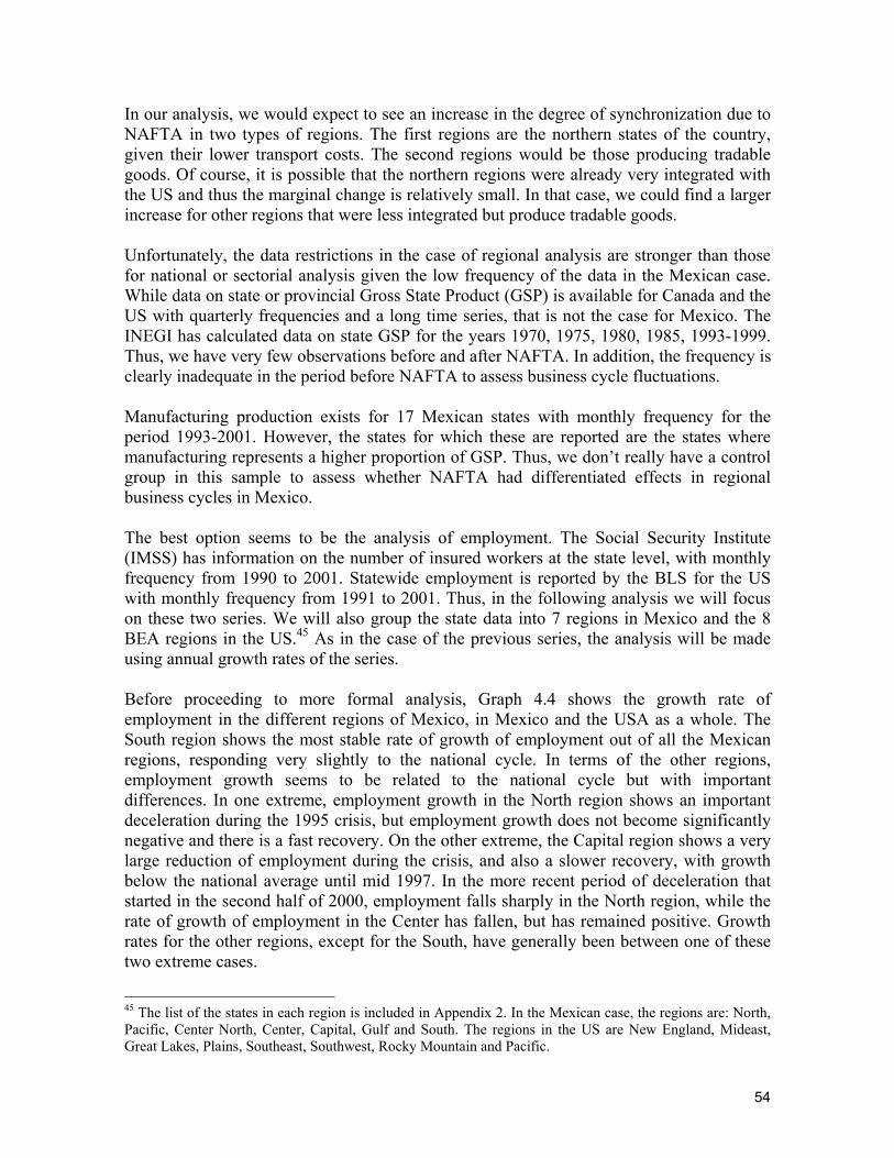
54

In our analysis, we would expect to see an increase in the degree of synchronization due to NAFTA in two types of regions. The first regions are the northern states of the country, given their lower transport costs. The second regions would be those producing tradable goods. Of course, it is possible that the northern regions were already very integrated with the US and thus the marginal change is relatively small. In that case, we could find a larger increase for other regions that were less integrated but produce tradable goods. Unfortunately, the data restrictions in the case of regional analysis are stronger than those for national or sectorial analysis given the low frequency of the data in the Mexican case. While data on state or provincial Gross State Product (GSP) is available for Canada and the US with quarterly frequencies and a long time series, that is not the case for Mexico. The INEGI has calculated data on state GSP for the years 1970, 1975, 1980, 1985, 1993-1999. Thus, we have very few observations before and after NAFTA. In addition, the frequency is clearly inadequate in the period before NAFTA to assess business cycle fluctuations. Manufacturing production exists for 17 Mexican states with monthly frequency for the period 1993-2001. However, the states for which these are reported are the states where manufacturing represents a higher proportion of GSP. Thus, we don’t really have a control group in this sample to assess whether NAFTA had differentiated effects in regional business cycles in Mexico. The best option seems to be the analysis of employment. The Social Security Institute (IMSS) has information on the number of insured workers at the state level, with monthly frequency from 1990 to 2001. Statewide employment is reported by the BLS for the US with monthly frequency from 1991 to 2001. Thus, in the following analysis we will focus on these two series. We will also group the state data into 7 regions in Mexico and the 8 BEA regions in the US.45 As in the case of the previous series, the analysis will be made using annual growth rates of the series. Before proceeding to more formal analysis, Graph 4.4 shows the growth rate of employment in the different regions of Mexico, in Mexico and the USA as a whole. The South region shows the most stable rate of growth of employment out of all the Mexican regions, responding very slightly to the national cycle. In terms of the other regions, employment growth seems to be related to the national cycle but with important differences. In one extreme, employment growth in the North region shows an important deceleration during the 1995 crisis, but employment growth does not become significantly negative and there is a fast recovery. On the other extreme, the Capital region shows a very large reduction of employment during the crisis, and also a slower recovery, with growth below the national average until mid 1997. In the more recent period of deceleration that started in the second half of 2000, employment falls sharply in the North region, while the rate of growth of employment in the Center has fallen, but has remained positive. Growth rates for the other regions, except for the South, have generally been between one of these two extreme cases.

45 The list of the states in each region is included in Appendix 2. In the Mexican case, the regions are: North, Pacific, Center North, Center, Capital, Gulf and South. The regions in the US are New England, Mideast, Great Lakes, Plains, Southeast, Southwest, Rocky Mountain and Pacific.

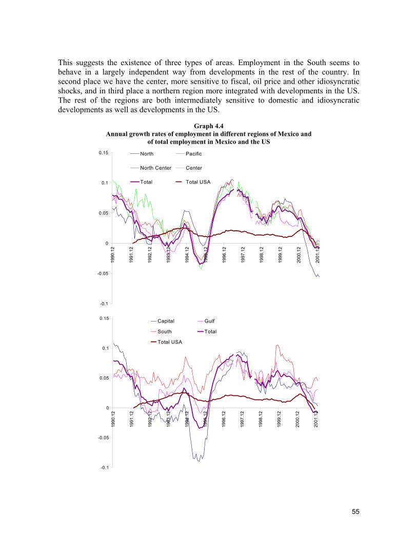
55

This suggests the existence of three types of areas. Employment in the South seems to behave in a largely independent way from developments in the rest of the country. In second place we have the center, more sensitive to fiscal, oil price and other idiosyncratic shocks, and in third place a northern region more integrated with developments in the US. The rest of the regions are both intermediately sensitive to domestic and idiosyncratic developments as well as developments in the US.

Graph 4.4

Annual growth rates of employment in different regions of Mexico and of total employment in Mexico and the US

-0.1

-0.05

0

0.05

0.1

0.15

1990

.12

1991

.12

1992

.12

1993

.12

1994

.12

1995

.12

1996

.12

1997

.12

1998

.12

1999

.12

2000

.12

2001

.12

North Pacific

North Center Center

Total Total USA

-0.1

-0.05

0

0.05

0.1

0.15

1990

.12

1991

.12

1992

.12

1993

.12

1994

.12

1995

.12

1996

.12

1997

.12

1998

.12

1999

.12

2000

.12

2001

.12

Capital Gulf

South Total

Total USA

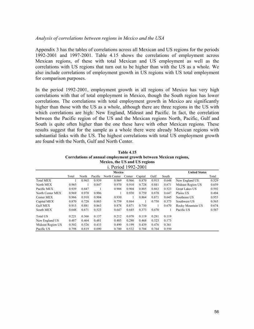
56

Analysis of correlations between regions in Mexico and the USA Appendix 3 has the tables of correlations across all Mexican and US regions for the periods 1992-2001 and 1997-2001. Table 4.15 shows the correlations of employment across Mexican regions, of these with total Mexican and US employment as well as the correlations with US regions that turn out to be higher than with the US as a whole. We also include correlations of employment growth in US regions with US total employment for comparison purposes. In the period 1992-2001, employment growth in all regions of Mexico has very high correlations with that of total employment in Mexico, though the South region has lower correlations. The correlations with total employment growth in Mexico are significantly higher than those with the US as a whole, although there are three regions in the US with which correlations are high: New England, Mideast and Pacific. In fact, the correlation between the Pacific region of the US and the Mexican regions North, Pacific, Gulf and South is quite often higher than the one these have with other Mexican regions. These results suggest that for the sample as a whole there were already Mexican regions with substantial links with the US. The highest correlations with total US employment growth are found with the North, Gulf and North Center.

Table 4.15 Correlations of annual employment growth between Mexican regions,

Mexico, the US and US regions i. Period 1992-2001

Total North Pacific North Center Center Capital Gulf South TotalTotal MEX 1 0.965 0.939 0.969 0.966 0.870 0.915 0.648 New England US 0.529North MEX 0.965 1 0.847 0.970 0.910 0.728 0.881 0.671 Mideast Region US 0.659Pacific MEX 0.939 0.847 1 0.906 0.904 0.885 0.863 0.523 Great Lakes US 0.592North Center MEX 0.969 0.970 0.906 1 0.930 0.759 0.878 0.647 Plains US 0.494Center MEX 0.966 0.910 0.904 0.930 1 0.864 0.871 0.645 Southeast US 0.953Capital MEX 0.870 0.728 0.885 0.759 0.864 1 0.750 0.373 Southwest US 0.565Gulf MEX 0.915 0.881 0.863 0.878 0.871 0.750 1 0.670 Rocky Mountain US 0.674South MEX 0.648 0.671 0.523 0.647 0.645 0.373 0.670 1 Pacific US 0.587

Total US 0.221 0.366 0.137 0.212 0.070 0.119 0.281 0.119New England US 0.487 0.464 0.481 0.485 0.280 0.468 0.323 0.173Mideast Region US 0.502 0.526 0.433 0.490 0.199 0.439 0.476 0.361Pacific US 0.798 0.819 0.690 0.700 0.532 0.704 0.764 0.550

Mexico United States

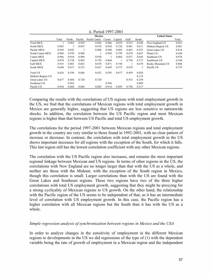
57

ii. Period 1997-2001

Total North Pacific North Center Center Capital Gulf South TotalTotal MEX 1 0.965 0.939 0.969 0.966 0.870 0.915 0.648 New England US 0.921North MEX 0.965 1 0.847 0.970 0.910 0.728 0.881 0.671 Mideast Region US 0.801Pacific MEX 0.939 0.847 1 0.906 0.904 0.885 0.863 0.523 Great Lakes US 0.814North Center MEX 0.969 0.970 0.906 1 0.930 0.759 0.878 0.647 Plains US 0.446Center MEX 0.966 0.910 0.904 0.930 1 0.864 0.871 0.645 Southeast US 0.978Capital MEX 0.870 0.728 0.885 0.759 0.864 1 0.750 0.373 Southwest US 0.348Gulf MEX 0.915 0.881 0.863 0.878 0.871 0.750 1 0.670 Rocky Mountain US 0.804South MEX 0.648 0.671 0.523 0.647 0.645 0.373 0.670 1 Pacific US 0.755

Total US 0.626 0.550 0.686 0.632 0.593 0.677 0.459 0.024Mideast Region US 0.118Great Lakes US 0.677 0.684 0.720 0.720 0.553 0.259Southeast US 0.562 0.596 0.049Pacific US 0.934 0.884 0.864 0.885 0.914 0.859 0.794 0.517

Mexico United States

Comparing the results with the correlations of US regions with total employment growth in the US, we find that the correlations of Mexican regions with total employment growth in Mexico are generally higher, suggesting that US regions are less sensitive to nationwide shocks. In addition, the correlation between the US Pacific region and most Mexican regions is higher than that between US Pacific and total US employment growth. The correlations for the period 1997-2001 between Mexican regions and total employment growth in the country are very similar to those found in 1992-2001, with no clear pattern of increase or decrease. In contrast, the correlation with total employment growth in the US shows important increases for all regions with the exception of the South, for which it falls. This last region still has the lowest correlation coefficient with any other Mexican regions. The correlation with the US Pacific region also increases, and remains the most important regional linkage between Mexican and US regions. In terms of other regions in the US, the correlations with New England are no longer larger than that with the US as a whole, and neither are those with the Mideast, with the exception of the South region in Mexico, though this correlation is small. Larger correlations than with the US are found with the Great Lakes and Southeast regions. These two regions have two of the three higher correlations with total US employment growth, suggesting that they might be proxying for a strong cyclicality of Mexican regions to US growth. On the other hand, the relationship with the Pacific region of the US seems to be independent of that, as it has an intermediate level of correlation with US employment growth. In this case, the Pacific region has a higher correlation with all Mexican regions but the South than it has with the US as a whole. Simple regression analysis of synchronization between regions in Mexico and the USA In order to analyze changes in the sensitivity of employment in the different Mexican regions to developments in the US we did regressions of the type of (1) with the dependent variable being the rate of growth of employment in a Mexican region and the independent

58

variable being that for the US as a whole. We did the same regressions including employment growth in US regions as the dependent variable for comparison purposes. Table 4.16 shows the results for Mexican regions. Without including dummys for the periods after 1994 or 1997 we find high positive and significant coefficients for Mexico as a whole and for the North, North Center and Gulf regions. The estimated parameters are larger than one in these four cases, and higher than two in the case of the North region. The coefficient for the Capital region is close to one, but not significant, while those for Pacific, Center and South are much smaller. In all cases, the adjusted R2s are quite small, suggesting the presence of important idiosyncratic shocks in the sample. When the dummys for the period after 1994 and 1997 are included we can distinguish an important change over time between the period before and after NAFTA. However, in the case of 1994, it is likely that some of the results are driven by the balance of payments crisis of that year, and thus are not clear reflections of any structural change. In particular, the dummys have large negative values for the period after 1994, while the coefficient on the US is large and negative before 1994 and large and positive in its interaction with the 1994 dummy. The results using the dummy for 1997 and after seem more robust. In that case the dummy variable is less significant and is both positive and negative. The coefficient on the US is both positive and negative in the period before 1997, and is normally non-significant. The coefficient on US growth is close to one for the North and Gulf regions in the period before 1997, though only significant for the Gulf. In the period after 1997, we find a very large and significant increase in the coefficient associated with employment growth in the US for all regions except the Gulf and the South. The change is the largest for the Center and Pacific regions, and similar for North, North Center and Capital regions. This suggests that employment in several regions of Mexico has effectively become more sensitive to developments in the US after NAFTA, with the exception of the Gulf and the South. In order to identify the most sensitive regions to developments in the US in the post-NAFTA period, we added both coefficients on the US, with and without the dummy. The ordering depending on the size of the sum of the coefficients is: North, Pacific, North Center, Center, Capital, Gulf and South, with North being much higher than the rest, then Pacific, North Center, Center and Capital with similar high values, and finally Gulf and South with much lower coefficients. Finally, even though the adjusted R2s are much higher with than without the dummys, there remains a very substantial degree of variability unexplained by the regressions. This suggests that there is a strong effect from US shocks, but idiosyncratic shocks also remain important. Table 4.17 shows the results for US regions. For the sample as a whole we find positive and significant point estimates, always close to 1. Thus, regions as the North in Mexico seem more sensitive to nationwide developments in the US than some regions in that country. The adjusted R2s are higher than those for any Mexican region, but are not that high, so there seem to be important idiosyncratic shocks to regions in the US. When we include the NAFTA dummys, the interpretation of changes is different than in the Mexican case when considering whether there is a higher degree of synchronization between US regions. After all, the national growth rate is approximately a weighted average of the region growth rates,

59

so on average they can not all increase. What we should see is that the coefficients for all regions become closer to one if indeed there is higher integration and the R2s should increase. We do find that, in both cases of dummys, when the initial coefficient is below one that associated with the dummy is positive, and vice versa. Thus, there seems to have been an increase in the degree of synchronization even within US regions, though there are still important differences from a coefficient of 1 in most cases. The R2s also increase significantly for most regions. Factor analysis Factor analysis for the period 1992-2001 shows that we should include at least 10 factors. The first factor seems to capture a shock that affects a set of regions in the US, though not all of them. In particular, New England, Mideast and Pacific seem to respond to different shocks. The second factor affects all regions in Mexico in a strong way, again with the lowest loading for the South. The Pacific region of the US has a significant loading with respect to this factor. All the other factors seem to be capturing more localized regional shocks, whether for a group of regions or for one in particular. The third factor has high loading for the Pacific region in the US and the North region in Mexico, being likely that it captures some regional border effect. The fourth has high factor loadings for the New England and Mideast regions of the US. The other factors are less important, and are generally loaded in one specific region.

Table 4.18 Results from factor analysis of growth rates of employment in Mexican and US regions

Factor loadings correspond to varimax rotation i. 1992-2001

Country Region 1 2 3 4 5 6 7 8 9 10North -0.002 0.665 0.327 0.292 -0.494 0.137 -0.133 0.048 -0.118 -0.178Pacific -0.188 0.916 0.080 0.252 -0.150 0.047 -0.058 0.036 -0.114 0.055North Center -0.071 0.904 0.042 0.272 -0.239 0.006 -0.146 0.050 0.044 -0.139Center -0.029 0.945 -0.015 0.009 -0.106 0.046 -0.133 -0.183 0.103 -0.002Capital -0.208 0.858 0.178 0.264 0.030 -0.227 -0.080 0.091 0.090 0.132Gulf -0.057 0.738 0.294 0.180 -0.300 -0.121 -0.004 0.374 -0.056 -0.006South -0.112 0.519 0.104 0.089 -0.749 0.003 -0.080 0.023 0.051 0.028

New England 0.018 0.268 0.095 0.926 0.076 0.048 -0.087 -0.115 -0.060 -0.014Mideast 0.127 0.219 0.088 0.890 -0.229 -0.069 0.070 0.169 0.078 0.008Great Lakes 0.861 -0.133 -0.124 -0.036 -0.093 0.456 0.039 -0.065 0.037 -0.002Plains 0.587 -0.357 -0.044 -0.010 0.101 0.016 0.718 0.000 -0.013 0.005Southeast 0.887 0.068 0.138 0.377 -0.132 -0.118 0.117 0.011 -0.009 -0.044Southwest 0.689 -0.317 0.248 -0.107 0.204 -0.082 0.299 0.081 -0.326 -0.019Rocky Mountain 0.953 -0.083 -0.037 -0.042 0.185 -0.068 0.045 0.004 0.038 0.032Pacific 0.099 0.555 0.655 0.447 -0.217 -0.062 -0.035 0.037 -0.016 0.009


Mexico

United States

60

ii: 1997-2001

Country Region 1 2 3 4 5 6 7North 0.227 -0.140 0.925 -0.081 0.144 -0.176 -0.098Pacific 0.406 0.046 0.844 -0.206 -0.225 0.046 0.051North Center 0.347 -0.084 0.911 -0.117 0.131 -0.017 0.003Center 0.162 0.019 0.965 0.047 -0.074 0.027 0.114Capital 0.232 0.241 0.799 0.035 -0.444 0.034 -0.010Gulf 0.139 -0.095 0.890 -0.164 -0.022 -0.022 0.009South -0.018 -0.644 0.665 0.031 0.039 -0.054 0.214

New England 0.916 0.245 0.267 0.067 -0.097 0.056 -0.037Mideast 0.957 -0.017 0.199 0.048 -0.034 0.052 0.034Great Lakes 0.764 0.091 0.470 -0.181 0.047 -0.390 0.009Plains 0.469 0.534 -0.428 0.514 -0.033 0.090 0.014Southeast 0.687 0.405 0.497 0.286 0.060 -0.049 -0.093Southwest 0.015 0.987 -0.120 0.025 0.064 -0.049 0.069Rocky Mountain 0.371 0.832 0.330 0.072 -0.203 0.048 -0.066Pacific 0.331 0.052 0.890 0.192 -0.118 -0.061 -0.154

Mexico

United States


In the analysis for the period 1997-2001 we found that we need at least 7 factors. There seems to be an important change in terms of integration within the US and between the US and Mexico. The first factor seems to capture shocks to New England and Mideast, but now other regions in the US also have a significant factor loading, and that of Mexican regions also increased. The second factor is quite similar to the first factor for the period 1992-2001, with high factor loading only for some regions in the US. An important difference is that the Great Lakes region previously had a high factor loading when these regions had it. This is no longer the case. The third factor captures shocks to Mexican employment and is similar to factor 2 for the period 1992-2001. However, the loadings tend to be slightly higher for Mexican regions, while the loading of the Pacific US region is considerably higher. The rest of the factors typically have a high loading for only one region, but the reduction in the number of factors needed is an important one, suggesting that these type of idiosyncratic shocks are less important in the sample, both for Mexico and for the US. 4.4. Summary Production components The intention of the more detailed analysis of components of production was to compare changes in synchronization across tradable and non-tradable goods, and also to identify if the relationship between Mexico and the US is becoming more like that observed between Canada and the US. We found that the correlation of manufacturing growth increased substantially between Mexico and the US, to a level similar to that observed between this last country and Canada. In contrast, correlations for both Canada and Mexico in sectors driven by shocks to commodity prices, such as agriculture and mining, remained at similar levels during the entire period. The main difference between the Canadian and Mexican

61

cases is that in the more recent period, the correlation of services between Mexico and the US increased to a level higher than that observed with Canada at any period of time. This suggests that the Mexican business cycle in the more recent period has been mostly driven by the export sector, and thus we also see a strong increase of the correlation in pro-cyclical non-tradable sectors. In the regression analysis, depending on the specification and time period, we find increases in the post-NAFTA sensitivity to developments in the US for the following sectors of activity in Mexico: Manufacturing, Transport and Communications, Services and Construction. These increases are typically larger than those found for Canada. These results confirm the interpretation given to those from the correlation analysis. Finally, the result from factor analysis show the presence of separate idiosyncratic factors for Mexico and the US when using the whole sample period, while in the post-NAFTA period there is one main common factor for both economies. If we look in detail at the correlation between more disaggregated components of manufacturing, we find that there were some sectors that had a high correlation with the US before NAFTA, such as basic metal products and machinery. However, in the post-NAFTA period there is a generalized increase for all components of manufacturing. Regression analysis shows the same results. Basic metal products, Machinery and Other manufacturing products have a high and significant sensitivity to developments in the US for the whole period. In the post-NAFTA period, this is found to be the case for all sub-components of manufacturing with the exception of foods and beverages. Factor analysis shows the same results, with a single factor with high loadings for the components of manufacturing in both countries during the post-NAFTA period. Lag structure In terms of the analysis of the lead and lag structure of the components of manufacturing, we found that the correlation of a Mexican sector with total manufacturing production was typically very small at all leads and lags, with the exception of basic metals and machinery. In the case of these two variables, the highest correlation is found at a lag between 4 and 6 months. However, in the post-NAFTA period, the correlation is much higher for all components of manufacturing and the highest one is now between a lead or a lag of three months. A similar change occurs when we look at the correlation of a Mexican sector with the same sector in the US. Thus, this evidence, together with that of other sectors of economic activity, suggests that the Mexican economy has become more sensitive to developments in the US and also shocks are propagated with a smaller lag between both economies. Components of aggregate demand and supply The analysis of components of aggregate demand and supply is important to identify if the increase in synchronization is mostly due to an increase in trade or if there are other factors that are also affecting aggregate demand in both countries, in particular financial links.

62

The correlation analysis suggests that there were strong financial and trade links between Canada and the US at least since 1980, as evidenced by the high correlations of investment, imports and exports. In the Mexican case, there is also a high correlation but only for investment and imports, suggesting the presence of a financial link so more favorable financial conditions in the US led to higher investment there and in Mexico, which in turn translated into higher imports. In the post-NAFTA period, the correlation of Mexican exports increases and becomes similar to Canada’s so the trade channel seems to become important in the Mexican case. The regression analysis confirms these results, as the only component of aggregate demand for which we find a significant change in the post-NAFTA period are exports in Mexico.46 Factor analysis leads to the same conclusion. For the whole period, we find there is factor with high loadings for C, I and M in Mexico, I in Canada and I and M in the US. In the shorter, post-NAFTA sample, the factor has high loadings with C, I, M and X in Mexico, I and M in Canada and I, X and M in the US. Regional analysis of employment The final subsection analyzes the relationship between regional employment in Mexico and the US. We find that there was a high correlation of all Mexican regions except the south with the Pacific region in the US. In addition, employment the North region of Mexico had an intermediate positive correlation with total employment in the US. In the post-NAFTA period, the correlation with the Pacific region of the US is reinforced, but there a very generalized increase in the correlation of all Mexican regions, but the south, with total employment in the US. The same results are found in the regression analysis. In this case, the North, North Center and Gulf regions have significant relationships with the US for the whole sample period, but then in the post-NAFTA period we see a generalized increase in the sensitivity to developments in the US, again with the exception of the South. The increase in the sensitivity is generally smaller for those regions that already had a significant relationship with the US. The results from factor analysis show the presence of two main factors, one for most US regions and another for Mexican regions plus US Pacific. In the post-NAFTA period, the loading on Mexican regions associated with the factor for most US regions is higher, but the Mexican-US Pacific factor remains. This suggests that, even though the sensitivity of employment to developments in the US has increased, there still remains an important segmentation in terms of the evolution of regional labor markets.

46 In addition, consumption in Mexico has a significant sensitivity to growth in the US, and a coefficient higher than Canada’s. This is probably due to the presence of stronger liquidity constraints in Mexico than in Canada. Thus, an improvement in the availability of funds due to better financial conditions in the US leads to both higher investment and consumption in Mexico.

63

5. Policy Coordination In terms of the implications of higher or lower business cycle synchronization and the need for policy coordination, there is a very large literature related theoretically with the discussion on optimal currency areas, and empirically with the establishment of the European Union, the EMU and adoption of the Euro, and the Maastricht criteria. Here we only highlight some of the main discussions. Presumably, the starting point should be what we consider to be policy coordination, as there are several possibilities. On the one hand, we could have implicit or explicit agreements between authorities about how they will be following their own separate policies against shocks determined solely by national considerations. This is important in the context of free trade agreements, as the perception that a country is persistently maintaining a depreciated real exchange rate to export more and import less from its trading partners could lead to political pressures to abandon the trade agreement. In a sense, its really a compromise between countries not to follow destabilizing policies. This is in each countries’ self-interest and thus does not depend on the degree of macroeconomic synchronization across them. A second dimension is that policy makers take into account the effects of their actions on the other countries. For example, if the US would decide to follow a less restrictive monetary policy not because of a deceleration of growth and low inflation in the US but because Mexico was subject to a strong and negative idiosyncratic shock. Obviously, there is a self-interested reason to do so, as otherwise the shock in Mexico could lead to lower US exports, aggregate demand and production. This would implicitly lead to policy coordination. The probability that we see such a phenomenon probably depends on observing similar sized countries and that they trade extensively with each other. Finally, the most extreme case is that of a common policy that will be followed for the different countries due to the adoption of a common currency or agreements through which fiscal resources are shared. In addition, a set of common rules may be established to determine the type of policies that can be followed depending on different shocks, an example of which are the fiscal rules established in the European Union’s stability pact. Our focus will be on this last type of policy coordination, as its desirability clearly depends on the degree of business cycle synchronization across countries. If macroeconomic synchronization is high then it is more likely that a given common policy fits all countries relatively well. However, even with high synchronization it may not be optimal to adopt a common policy if the business cycle leads to larger fluctuations in one country compared with the others or if the sensitivity of the economy to variations in the policy instruments differ.

64

5.1. Higher policy coordination: the case of Mexico within NAFTA The evidence from the previous sections shows that the degree of macroeconomic synchronization of Mexico with its NAFTA partners has increased significantly and the sensitivity of the Mexican economy to developments in the US has also increased. However, these results are probably not sufficient to argue that Mexico should reduce its ability to carry out independent monetary and fiscal policies. In first place, even though the amount of variability of Mexican economic variables explained by developments in the US has increased in the 1997-2001 period, there remains a significant amount of variability explained by other types of shocks and this is clearly higher than in the Canadian case. Thus, even though idiosyncratic shocks are less important, they remain sufficiently so as to justify maintaining independent policies. In second place, the increase in the sensitivity of Mexican variables to its US counterparts has been such that the estimated coefficient is quite often larger than one, implying that the Mexican economy reacts more than one-to-one to developments in the US economy. Thus, unless the Mexican economy is more sensitive to changes in policy variables, these need to react in a stronger way for stabilization purposes than in the US and Canada. There are good reasons that suggest that the effect of different policy instruments and channels differ across the three economies. Regarding monetary policy, the lower level of financial development and credit to the private sector by domestic financial institutions in Mexico implies that the interest rate and credit channels are likely to be weaker than in the case of the US and Canada. Given that trade to GDP is much higher for Canada and Mexico than the US, the exchange rate channel is likely to be more important for the first two countries. Even though we don’t have substantial evidence suggesting that the channels through which fiscal policy works in the three countries may be different, higher liquidity constraints in the Mexican economy would suggest that the effect of counter cyclical fiscal policies could have stronger effects in Mexico than in the other countries due to the fact that Ricardian Equivalence is less likely to hold in the Mexican case. Another issue is whether Mexico can effectively carry out independent counter cyclical policies. In terms of monetary policy, Frankel, Schmukler and Serven (2002) do a regression analysis of interest rates in a large sample of countries against the interest rate of the US, Germany or Japan. They find that, in the medium term, the evolution of interest rates for all the other countries is determined by rates in either one of these three, irrespectively of the exchange rate regime in the country. Thus, the ability of the rest of the world to carry a strongly independent monetary policy is presumably limited. However, in the short term there may be significant deviations, and a flexible exchange rate regime allows these deviations to last for longer.47 Thus, the adoption of a flexible exchange rate has increased Mexico’s ability to carry out an independent monetary policy at least temporarily, as has clearly been the case during the current disinflationary episode. 47 In a strict sense, monetary policy can only affect the level of real rates in the short run in any country.

65

In terms of fiscal policy, it is likely that Mexico is less able to carry out counter cyclical policies. Past periods of strong fiscal imbalances and balance of payments crises imply that a larger deficit is more likely to be interpreted as a permanent increase in expenditure that may lead to a deterioration of the public sector’s solvency instead of as a temporary counter cyclical measure. Thus, it could lead to large increases in the interest rate, with a significant crowding out effect, and in an extreme case leading to a confidence crisis. This potential loss of credibility is also a factor that limits the ability to carry counter cyclical monetary policy given past episodes of disinflation that failed, particularly that preceding the 1995 crisis. Thus, for Mexico to be able to carry stronger counter cyclical policies credibility would need to be reinforced by attaining a period of low and stable inflation and balanced budgets, together with a fiscal reform that reduces the vulnerability of government income to fluctuations in the price of oil. To the extent that sound macroeconomic policies are followed reinforced by additional structural reforms that reinforce credibility, it would be expected that the ability to carry out counter cyclical policies would increase in the future. Thus, the evidence of larger synchronization suggest that Mexico’s optimal policies will be qualitatively more similar to those followed by its NAFTA partners than in the past. However, Mexico still seems subject to important idiosyncratic shocks, particularly when compared with Canada, but even in the absence of these the magnitude of policy adjustments would probably need to be higher in Mexico than in the other countries. 5.2. Has there been higher synchronization of policies? Nevertheless, it is worthwhile to review if the policies in Mexico’s NAFTA partners have become more similar to those followed by Mexican authorities, with particular emphasis on the US, and what has been the correlation of US policy with the Mexican business cycle.48 Thus, we look at the evolution of fiscal balances and government current expenditures to GDP as measures of fiscal policy as well as the growth rate of real money balances (M2) and the evolution of real interest rates as a measure of monetary policy.49 Graph 5.1 shows the evolution of these policy variables for Mexico and the US. When looking at the fiscal variables, the first thing to note is that the fiscal balance is much more volatile in Mexico than in the US. Both countries have important fiscal deficits during most of the eighties that are corrected in the nineties. The correction in Mexico is a fast and large one in the last years of the eighties, leading to a large surplus in the early nineties. Since then, the surplus falls gradually, becoming a small deficit since mid-nineties. In contrast, that in the US is much more gradual, achieving a surplus in 1997 that peaks in 2000,

48 This comparison is also important to gauge if the higher synchronization might be due to more similar policies instead of higher trade between the countries. 49 The fiscal balance to GDP is obtained from the IFS Statistics prepared by the IMF. Government current expenditures are obtained from each country’s Ministry of Finance (SHCP for Mexico, Department of the Treasury for the US). M2 is obtained from each central bank. The sources for price indices are Banco de México and the Department of Commerce. Finally, to construct real interest rates we used the nominal rates on three month government bonds and divided those by the actual inflation in the three months following the date of issue. Unfortunately, we do not have data on inflation expectations in both countries for a sufficiently long period of time.

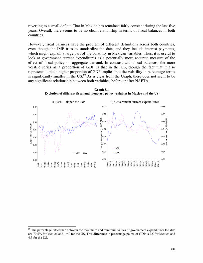
66

reverting to a small deficit. That in Mexico has remained fairly constant during the last five years. Overall, there seems to be no clear relationship in terms of fiscal balances in both countries. However, fiscal balances have the problem of different definitions across both countries, even though the IMF tries to standardize the data, and they include interest payments, which might explain a large part of the volatility in Mexican variables. Thus, it is useful to look at government current expenditures as a potentially more accurate measure of the effect of fiscal policy on aggregate demand. In contrast with fiscal balances, the more volatile series as a proportion of GDP is that in the US, though the fact that it also represents a much higher proportion of GDP implies that the volatility in percentage terms is significantly smaller in the US.50 As is clear from the Graph, there does not seem to be any significant relationship between both variables, before or after NAFTA.

Graph 5.1 Evolution of different fiscal and monetary policy variables in Mexico and the US

i) Fiscal Balance to GDP ii) Government current expenditures

-0.05

-0.04

-0.03

-0.02

-0.01

0.00

0.01

0.02

1980

.119

81.2

1982

.319

83.4

1985

.119

86.2

1987

.319

88.4

1990

.119

91.2

1992

.319

93.4

1995

.119

96.2

1997

.319

98.4

2000

.120

01.2

budg

et s

urpl

us (%

GD

P)

MEX USA

0.00

0.01

0.02

0.03

0.04

0.05

0.06

0.0719

80.1

1981

.219

82.3

1983

.419

85.1

1986

.219

87.3

1988

.419

90.1

1991

.219

92.3

1993

.419

95.1

1996

.219

97.3

1998

.420

00.1

2001

.2

curre

nt e

xpen

ditu

re (%

GD

P) M

EX

0.26

0.27

0.28

0.29

0.3

0.31

0.32

0.33

curre

nt e

xpen

ditu

re (%

GD

P) U

SA

MEX

USA

50 The percentage difference between the maximum and minimum values of government expenditures to GDP are 70.5% for Mexico and 16% for the US. This difference in percentage points of GDP is 2.5 for Mexico and 4.5 for the US.

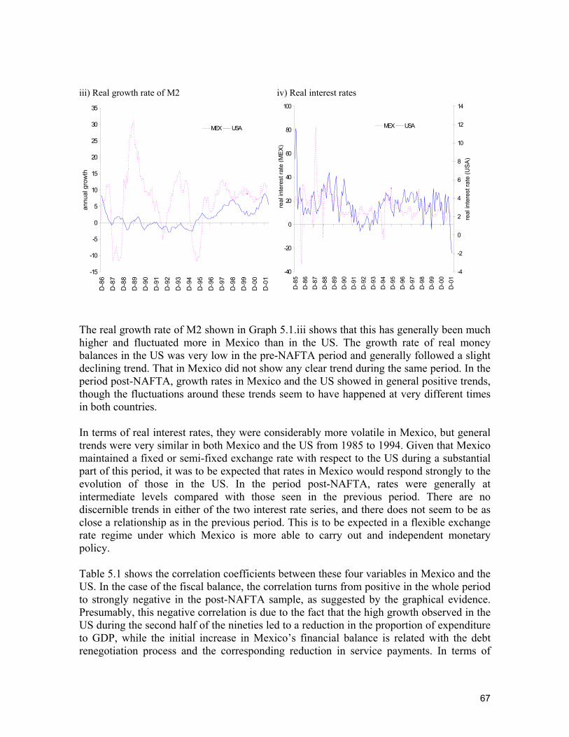
67

iii) Real growth rate of M2 iv) Real interest rates

-15

-10

-5

0

5

10

15

20

25

30

35D

-86

D-8

7

D-8

8D

-89

D-9

0D

-91

D-9

2D

-93

D-9

4

D-9

5D

-96

D-9

7D

-98

D-9

9D

-00

D-0

1

annu

al g

row

th

MEX USA

-40

-20

0

20

40

60

80

100

D-8

5D

-86

D-8

7D

-88

D-8

9D

-90

D-9

1D

-92

D-9

3D

-94

D-9

5D

-96

D-9

7D

-98

D-9

9D

-00

D-0

1

real

inte

rest

rate

(MEX

)-4

-2

0

2

4

6

8

10

12

14

real

inte

rest

rate

(USA

)

MEX USA

The real growth rate of M2 shown in Graph 5.1.iii shows that this has generally been much higher and fluctuated more in Mexico than in the US. The growth rate of real money balances in the US was very low in the pre-NAFTA period and generally followed a slight declining trend. That in Mexico did not show any clear trend during the same period. In the period post-NAFTA, growth rates in Mexico and the US showed in general positive trends, though the fluctuations around these trends seem to have happened at very different times in both countries. In terms of real interest rates, they were considerably more volatile in Mexico, but general trends were very similar in both Mexico and the US from 1985 to 1994. Given that Mexico maintained a fixed or semi-fixed exchange rate with respect to the US during a substantial part of this period, it was to be expected that rates in Mexico would respond strongly to the evolution of those in the US. In the period post-NAFTA, rates were generally at intermediate levels compared with those seen in the previous period. There are no discernible trends in either of the two interest rate series, and there does not seem to be as close a relationship as in the previous period. This is to be expected in a flexible exchange rate regime under which Mexico is more able to carry out and independent monetary policy. Table 5.1 shows the correlation coefficients between these four variables in Mexico and the US. In the case of the fiscal balance, the correlation turns from positive in the whole period to strongly negative in the post-NAFTA sample, as suggested by the graphical evidence. Presumably, this negative correlation is due to the fact that the high growth observed in the US during the second half of the nineties led to a reduction in the proportion of expenditure to GDP, while the initial increase in Mexico’s financial balance is related with the debt renegotiation process and the corresponding reduction in service payments. In terms of

68

government current expenditures to GDP, the correlation is close to zero for any of the periods. The real growth rate of M2 shows a zero correlation for the whole period, but in the post-NAFTA period we observe a positive and intermediate degree of correlation. However, given the instability of money demand in the short run, M2 is hardly a good measure of the monetary policy stance. In addition, it is quite possible that the evolution of money is determined by the effect of changes in income on money demand, and the higher correlation could turn out to be really a reflection of the higher correlation in output between the two countries. Thus, real interest rates are a better measure of the monetary policy stance. The correlation between these is slightly positive for the whole period, consistent with a more rigid exchange rate regime, and negative after 1997. In any case, the coefficients are extremely close to zero, suggesting there is no clear relationship between the two variables.51

Table 5.1 Correlations between different fiscal and monetary policy variables in Mexico and the US

(Correlation between the same variable in Mexico and the US)

i) Fiscal variables ii) Monetary variables

Financial Balance

Government Current

Expenditure1980:1 - 2001:4 0.282 -0.0441994:1 - 2001:4 -0.514 0.0051997:1 - 2001:4 -0.497 -0.087

Growth in Real Money

Balances*

Real Interest Rate (accurate expectations)*

Whole period 0.066 0.1741994:01 - 2001:12 0.328 0.0341997:01 - 2001:12 0.401 -0.110

* The whole period is 1986:12-2001:12 for real money balances and 1985:12-2001:12 for the real interest rate.

Thus, the evidence presented above suggests that even though there is a higher degree of macroeconomic synchronization, this has not been reflected in similar movements of policy variables. In this respect, Mexico’s ability to carry out counter-cyclical fiscal policies has probably been limited by three main factors: i) the perception that an increase in the budget deficit in bad times could translate into a loss of confidence in the country’s economic policies and thus make a bad situation turn worse; ii) oil related revenues still represent around a third of government income; and iii) debt interest payments accounted for 15.5% of total expenditures on average in the period 1997-2001, being an expenditure that can not be adjusted in the short term and has high volatility. The second and third factors imply that non-interest expenditures are very sensitive to the price of oil and the level of interest rates. In terms of monetary policy, while the Federal Reserve has adjusted interest rates depending on the fluctuations in the US seen in the last ten years, monetary policy in 51 Given that the period before 1997 was one of higher volatility and probably stronger surprises in the observed rate of inflation, which is the one used to calculate real interest rates, the correlation between real interest rates might be biased towards zero during this period.

69

Mexico has been conditioned by two disinflation processes, one strong balance of payments crisis between them and a slighter one associated with the Russian and Brazilian crises. Thus, in the post NAFTA period the objective of Banco de México has been to reduce the rate of inflation. It’s not surprising that we don’t find any short run relationship between rates in this period. Finally, while policies in Mexico did not coincide with those in the US, given different abilities to carry out counter-cyclical policies, it may be that policies in the US nevertheless had a stabilizing impact in the Mexican economy given the higher correlation in output. Table 5.2 shows the correlation between the four policy variables for the US and the growth rate of Mexican GDP. The correlation between GDP and financial public balance is positive for the whole period, though it becomes less so during the latter part of the sample. That of government current expenditure changes from negative for the whole period to positive for 1997-2001, though the coefficient is not very high. These two results suggest that fiscal policy in the US did not adjust in such a way that it would have had a counter cyclical effect with regards to the Mexican economy.

Table 5.2 Correlations between the rate of growth of Mexican GDP and different fiscal and

monetary policy variables in the US

Financial Balance

Government Current

Expenditure

Growth in Real Money

Balances*

Real Interest Rate (rational

expectations)*Whole period 0.328 -0.380 -0.009 0.0071994:1 - 2001:4 0.302 -0.340 0.134 0.0571997:1 - 2001:4 0.121 0.202 -0.746 0.632

* The whole period is 1981:1-2001:4 for the financial balance and government current expenditure, 1987:1-2001-4 for real money balances and 1986:1-2001:4 for the real interest rate.

On the other hand, the correlations with money growth and real interest rates changed from zero in the whole period to strongly negative and positive, respectively, since 1997. Given that interest rates are more accurate indicators of the stance of monetary policy, this implies that US monetary policy has tended to have a stronger counter-cyclical effect on the Mexican economy. This implies that the main counter cyclical policy in the US probably did contribute to promote higher stability of Mexican GDP during the recent period. 6. Conclusions This study has several important implications as to the effects of free trade agreements both in general and between more and less developed countries. The first is that, in spite of the important differences between Mexico and its NAFTA partners, the free trade agreement translated into higher synchronization, as has been observed in the case of trade agreements between mostly industrialized countries. Thus, even in a case of larger differences in factor endowments, we don’t see an increase in specialization that would translate into a higher sensitivity to idiosyncratic shocks. This does not mean that this would never happen, but it

70

indicates that factor endowment differences probably need to be even larger than that observed within NAFTA in order to detect less synchronization as a result of closer trade. The second is that Mexico already had important linkages with the US before NAFTA. Some subsectors of manufacturing production, employment in some regions and investment and imports had a high sensitivity to developments in the US. In particular, there seems to have been an important financial link through which better financial conditions in the US translated into higher investment, imports and, to a lesser degree, consumption. What NAFTA did was to reinforce the relationship through a strong link with more sectors of economic activity, more regions in Mexico and the establishment of a stronger trade link through which shocks are also transmitted. Two important findings are that non-tradable pro-cyclical sectors also have a stronger relationship with developments in the US, and that the largest increases in sensitivity were observed in those sectors that were not strongly linked to the US before NAFTA. In terms of policy implications, the higher degree of synchronization implies that optimal counter-cyclical policies will be qualitatively more similar between Mexico and its NAFTA partners. In fact, there is evidence that monetary policy in the US probably contributed to smooth out Mexico’s business cycle in the more recent period. However, in terms of extreme policy coordination, such as the adoption of common stabilization policies there are two issues that point towards the convenience of maintaining independent policies. The first is that, even though sensitivity to developments in the US has increased, there still remains a significant amount of idiosyncratic volatility in Mexico compared with Canada. The second is that the respond of Mexican variables to US shocks is larger than one for one, so in the absence of stronger effects in Mexico of the same policy adjustment, those optimal to be carried out in its NAFTA partners are likely to be insufficient. In fact, we suspect that the same policy adjustment in the US would have smaller effects in Mexico, particularly monetary policy given the lower degree of financial development in this last country.

71

References Achy, Lahcen and Juliette Milgram, 2001, “Does a Free Trade Area Favor an Optimum Currency Area? The case of Morocco and the European Union”, mimeo, Université Libre de Bruxelles. Agenor, Pierre-Richard, John McDermott and Eswar Prasad, 1999, “Macroeconomic fluctuations in Developing Countries: Some stylized facts”, IMF WP/99/35, March. Ahumada, Hildegart and Ana Martirena-Mantel, 2001, “Towards a potential monetary union in Latin America: testing the endogeneity criteria for Mercosur”, mimeo, Universidad Torcuato Di Tella and Instituto Torcuato Di Tella. Anderson, Heather, Noh-Sun Kwark and Farshid Vahid, 1999, “Does International Trade Synchronize Business Cycles?”, WP 8/99, Department of Econometrics and Business Statistics, Monash University. Angeloni I. And L. Dedola, 1999, “From the ERM to the Euro: New Evidence on Economic and Policy Convergence among EU Countries”, European Central Bank, Working Paper No. 4, May. Arora, Vivek and Athanasios Vamvakidis, 2001, “The impact of US Economic Growth on the Rest of the World: How much does it matter?”, IMF WP/01/119, August. Artis, Michael and Wenda Zhang, 1995, “International Business Cycles and the ERM: is there a European Business Cycle?”, CEPR Discussion Paper no 1191, August. Artis, M.J. and W. Zhang, 1997, “International Business Cycles and the ERM: Is There a European Business Cycle?”, International Journal of Finance Economics, Vol. 2, 1-16. Backus, D. and P. Kehoe, 1992, “International evidence on the historical properties of business cycles”, American Economic Review, 82(4), 864-888. Backus, D., P. Kehoe and F. Kydland, 1992, “International real business cycles”, Journal of Political Economy, 100(4), 745-775. Backus, D., P. Kehoe and F. Kydland, 1995, “International real business cycles: theory and evidence”, in Frontiers of Business Cycle Research, ed. Tom Cooley, New Jersey, Princeton Univesity Press. Bayoumi, Tamim and Barry Eichengreen, 1993, “Shocking Aspects of European Monetary Unification”, in Adjustment and Growth in the European Monetary Union, eds. F. Torres and F. Giavazzi, Cambridge, Cambridge University Press.

72

Bayoumi, Tamim and Eswar Prasad, 1997, “Currency Unions, Economic Fluctuations and Adjustment: Some new empirical evidence”, IMF Staff Papers, 44(1), 37-58. Belo, Federico, 2001, “Some Facts about the Cyclical Convergence in the Euro Zone”, Banco de Portugal, Working Paper 7-01, September. Boone, Laurence, 1997, “Symmetry and Asymmetry of Supply and Demand Shocks in the European Union: A Dynamic Analysis”, CEPII Working Paper No. 97-03. Borondo, Carlos, Yolanda González and Beatriz Rodríguez, 1998, “Cyclical Convergence inside the EU: The Case of Spain”, FAE Working Paper 98-10, July. Del Negro, Marco, 2001, “Monetary policy identification in a factor model”, mimeo, Federal Reserve Bank of Atlanta and ITAM. Eichengreen, Barry, 1992, “Should the Maastricht Treaty be saved?”, Princeton Studies in International Finance, no 74, International Finance Section, Princeton University, December. Fidrmuc, Jarko, 2001, “The Endogeneity of the Optimum Currency Area Criteria, Intraindustry Trade, and EMU Enlargement”, mimeo, Oesterreichische Nationalbank. Fontagné, Lionel and Michael Freudenberg, 1999, “Endogenous Symmetry of Shocks in a Monetary Union”, Open Economies Review 10, 263-287. Frankel, Jeffrey and Andrew Rose, 1998, “The Endogeneity of the Optimum Currency Area Criteria”, Economic Journal 108, July, 753-760. Frankel, Jeffrey, Sergio Schmukler and Luis Serven, 2002, “Global Transmission of Interest Rates: Monetary Independence and Currency Regime”, NBER WP 8828, March. Hall, Luis, and Alexander Hoffmaister, 1999, “Transmission of US and Mexico Shocks in Central America”, in “Fluctuations, Trends and Transmission of Shocks in Central America, Mexico and USA”, Hall, Hoffmaister, Monge and Robles, study for the Regional Studies Committee, Latin America and the Caribbean Region, World Bank. Hall, Luis, Alexander Monge and Edgar Robles, 1999, “Fluctuations, Co-Movements and Trends in Central America, Mexico and USA”, in “Fluctuations, Trends and Transmission of Shocks in Central America, Mexico and USA”, Hall, Hoffmaister, Monge and Robles, study for the Regional Studies Committee, Latin America and the Caribbean Region, World Bank. Hoffmaister, Alexander and Jorge Roldos, 1997, “Are Business Cycles different in Asia and Latin America?”, IMF WP/97/9, January. Imbs, Jean, 1998, “Fluctuations, Bilateral Trade and the Exchange Rate Regime”, mimeo, University of Lausanne and New York University.

73

Imbs, Jean, 2000, “Sectors and the OECD Business Cycle”, CEPR Discussion Paper no. 2473, June. Kalemi-Ozcan, Sebnem, Bent Sorensen and Oved Yosha, 2000, “Risk Sharing and Industrial Specialization: Regional and International Evidence”, Research Division, Federal Reserve Bank of Kansas City RWP 00-06, December. Karras, Georgios, 2000, “The Prospect of Dollarization: Are the Americas an Optimum Currency Area?”, mimeo, University of Illinois at Chicago. Kenen, Peter, 1969, “The Theory of Optimum Currency Areas: An Eclectic View”, in R. Mundell and A. Swoboda, eds., Monetary Problems in the International Economy, University of Chicago Press. Krugman, Paul, 1993, “Lessons of Massachusetts for EMU”, in F. Giavazzi and F. Torres, eds., The Transition to Economic and Monetary Union in Europe, Cambridge University Press, New York, 241-256. Loayza, Norman, Humberto Lopez and Angel Ubide, 2001, “Comovements and Sectoral Interdependence: Evidence for Latin America, East Asia and Europe”, IMF Staff Papers, 48(2), 367-396. Marimon, Ramon and Fabrizio Zilibotti, 1998, “Actual versus Virtual Unemployment in Europe: Is Spain Different?”, European Economic Review, 42, 123-153. Stockman, A., 1990, “International transmissions and real business-cycle models”, American Economic Review (Papers and Proceedings), 80(2), 134-138. Torres, Alberto and Oscar Vela, 2002, “Integración Comercial y Coordinación de los Ciclos Económicos de México y los Estados Unidos”, mimeo, Dirección General de Investigación Económica, Banco de México.

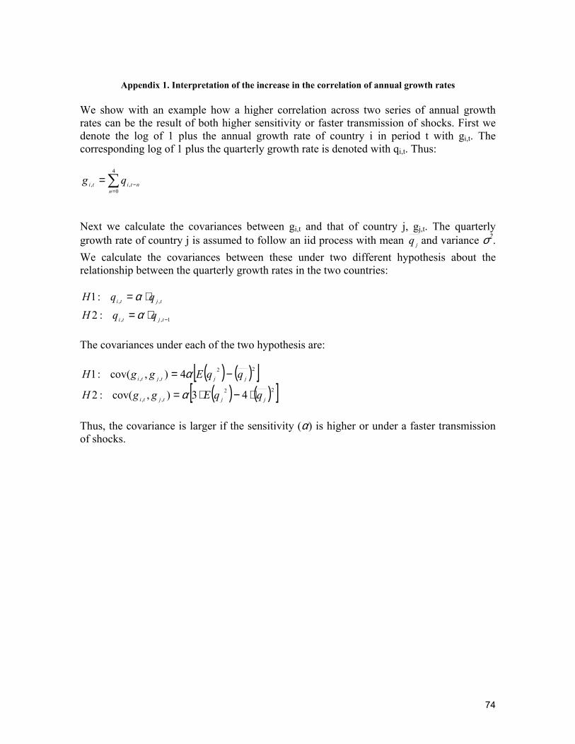
74

Appendix 1. Interpretation of the increase in the correlation of annual growth rates

We show with an example how a higher correlation across two series of annual growth rates can be the result of both higher sensitivity or faster transmission of shocks. First we denote the log of 1 plus the annual growth rate of country i in period t with gi,t. The corresponding log of 1 plus the quarterly growth rate is denoted with qi,t. Thus:

∑=

−=4

0,,

nntiti qg

Next we calculate the covariances between gi,t and that of country j, gj,t. The quarterly growth rate of country j is assumed to follow an iid process with mean jq and variance σ2. We calculate the covariances between these under two different hypothesis about the relationship between the quarterly growth rates in the two countries:

1,,

,,

:2:1

−⋅=⋅=

tjti

tjti

qqHqqH

αα

The covariances under each of the two hypothesis are:

( ) ( )[ ]( ) ( )[ ]22

,,

22,,

43),cov(:2

4),cov(:1

jjtjti

jjtjti

qqEggH

qqEggH

⋅−⋅=

−=

α

α

Thus, the covariance is larger if the sensitivity (α) is higher or under a faster transmission of shocks.

75

Appendix 2. Classification of Mexican and US States into regions

Mexican Regions USA Regions

North Baja California New England ConnecticutChihuahua MaineCoahuila MassachusettsNuevo Leon New HampshireSonora Rhode IslandTamaulipas Vermont

Pacific Baja California Sur Mideast Region DelawareColima District of ColumbiaJalisco MarylandNayarit New JerseySinaloa New York

PennsylvaniaNorth Center Aguascalientes

Durango Great Lakes IllinoisGuanajuato IndianaQueretaro MichiganSan Luis Potosí OhioZacatecas Wisconsin

Center Hidalgo Plains IowaMorelos KansasPuebla MinnesotaTlaxcala Missouri

NebraskaCapital DF North Dakota

Mexico South Dakota

Gulf Campeche Southeast AlabamaQuintana Roo ArkansasTabasco FloridaVeracruz GeorgiaYucatán Kentucky

LouisianaSouth Chiapas Mississippi

Guerrero North CarolinaMichoacán South CarolinaOaxaca Tennessee

VirginiaWest Virginia

Southwest ArizonaNew MexicoOklahomaTexas

Rocky Mountain ColoradoIdahoMontanaUtahWyoming

Pacific AlaskaCaliforniaHawaiiNevadaOregonWashington

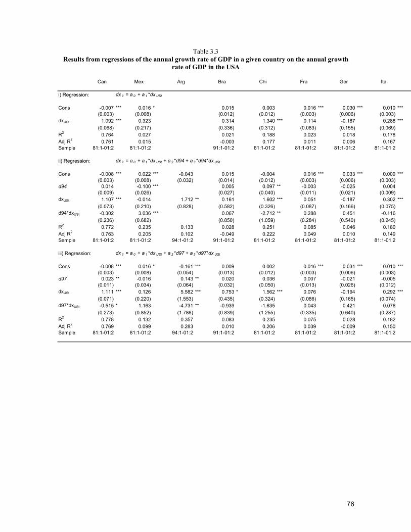
76

Table 3.3 Results from regressions of the annual growth rate of GDP in a given country on the annual growth

rate of GDP in the USA

Can Mex Arg Bra Chi Fra Ger Ita

i) Regression: dx it = a 0 + a 1 *dx USt

Cons -0.007 *** 0.016 * 0.015 0.003 0.016 *** 0.030 *** 0.010 ***(0.003) (0.008) (0.012) (0.012) (0.003) (0.006) (0.003)

dxUSt 1.092 *** 0.323 0.314 1.340 *** 0.114 -0.187 0.288 ***(0.068) (0.217) (0.336) (0.312) (0.083) (0.155) (0.069)

R2 0.764 0.027 0.021 0.188 0.023 0.018 0.178Adj R2 0.761 0.015 -0.003 0.177 0.011 0.006 0.167Sample 81:1-01:2 81:1-01:2 91:1-01:2 81:1-01:2 81:1-01:2 81:1-01:2 81:1-01:2

ii) Regression: dx it = a 0 + a 1 *dx USt + a 2 *d94 + a 3 *d94*dx USt

Cons -0.008 *** 0.022 *** -0.043 0.015 -0.004 0.016 *** 0.033 *** 0.009 ***(0.003) (0.008) (0.032) (0.014) (0.012) (0.003) (0.006) (0.003)

d94 0.014 -0.100 *** 0.005 0.097 ** -0.003 -0.025 0.004(0.009) (0.026) (0.027) (0.040) (0.011) (0.021) (0.009)

dxUSt 1.107 *** -0.014 1.712 ** 0.161 1.602 *** 0.051 -0.187 0.302 ***(0.073) (0.210) (0.828) (0.582) (0.326) (0.087) (0.166) (0.075)

d94*dxUSt -0.302 3.036 *** 0.067 -2.712 ** 0.288 0.451 -0.116(0.236) (0.682) (0.850) (1.059) (0.284) (0.540) (0.245)

R2 0.772 0.235 0.133 0.028 0.251 0.085 0.046 0.180Adj R2 0.763 0.205 0.102 -0.049 0.222 0.049 0.010 0.149Sample 81:1-01:2 81:1-01:2 94:1-01:2 91:1-01:2 81:1-01:2 81:1-01:2 81:1-01:2 81:1-01:2

iii) Regression: dx it = a 0 + a 1 *dx USt + a 2 *d97 + a 3 *d97*dx USt

Cons -0.008 *** 0.016 * -0.161 *** 0.009 0.002 0.016 *** 0.031 *** 0.010 ***(0.003) (0.008) (0.054) (0.013) (0.012) (0.003) (0.006) (0.003)

d97 0.023 ** -0.016 0.143 ** 0.020 0.036 0.007 -0.021 -0.005(0.011) (0.034) (0.064) (0.032) (0.050) (0.013) (0.026) (0.012)

dxUSt 1.111 *** 0.126 5.582 *** 0.753 * 1.562 *** 0.076 -0.194 0.292 ***(0.071) (0.220) (1.553) (0.435) (0.324) (0.086) (0.165) (0.074)

d97*dxUSt -0.515 * 1.163 -4.731 ** -0.939 -1.635 0.043 0.421 0.076(0.273) (0.852) (1.786) (0.839) (1.255) (0.335) (0.640) (0.287)

R2 0.778 0.132 0.357 0.083 0.235 0.075 0.028 0.182Adj R2 0.769 0.099 0.283 0.010 0.206 0.039 -0.009 0.150Sample 81:1-01:2 81:1-01:2 94:1-01:2 91:1-01:2 81:1-01:2 81:1-01:2 81:1-01:2 81:1-01:2

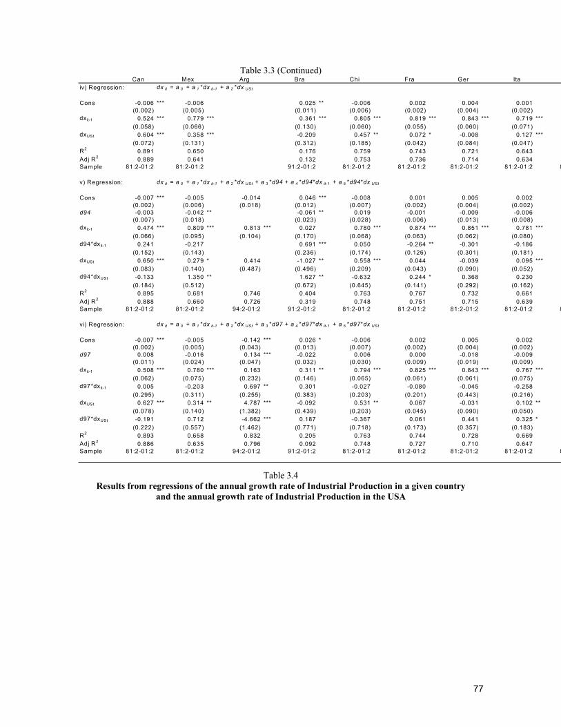
77

Table 3.3 (Continued) Can Mex Arg Bra Chi Fra Ger Ita

iv) Regression: dx it = a 0 + a 1 *dx it-1 + a 2 *dx USt

Cons -0.006 *** -0.006 0.025 ** -0.006 0.002 0.004 0.001(0.002) (0.005) (0.011) (0.006) (0.002) (0.004) (0.002)

dxit-1 0.524 *** 0.779 *** 0.361 *** 0.805 *** 0.819 *** 0.843 *** 0.719 ***(0.058) (0.066) (0.130) (0.060) (0.055) (0.060) (0.071)

dxUSt 0.604 *** 0.358 *** -0.209 0.457 ** 0.072 * -0.008 0.127 ***(0.072) (0.131) (0.312) (0.185) (0.042) (0.084) (0.047)

R2 0.891 0.650 0.176 0.759 0.743 0.721 0.643Adj R2 0.889 0.641 0.132 0.753 0.736 0.714 0.634Sample 81:2-01:2 81:2-01:2 91:2-01:2 81:2-01:2 81:2-01:2 81:2-01:2 81:2-01:2 8

v) Regression: dx it = a 0 + a 1 *dx it-1 + a 2 *dx USt + a 3 *d94 + a 4 *d94*dx it-1 + a 5 *d94*dx USt

Cons -0.007 *** -0.005 -0.014 0.046 *** -0.008 0.001 0.005 0.002(0.002) (0.006) (0.018) (0.012) (0.007) (0.002) (0.004) (0.002)

d94 -0.003 -0.042 ** -0.061 ** 0.019 -0.001 -0.009 -0.006(0.007) (0.018) (0.023) (0.028) (0.006) (0.013) (0.008)

dxit-1 0.474 *** 0.809 *** 0.813 *** 0.027 0.780 *** 0.874 *** 0.851 *** 0.781 ***(0.066) (0.095) (0.104) (0.170) (0.068) (0.063) (0.062) (0.080)

d94*dxit-1 0.241 -0.217 0.691 *** 0.050 -0.264 ** -0.301 -0.186(0.152) (0.143) (0.236) (0.174) (0.126) (0.301) (0.181)

dxUSt 0.650 *** 0.279 * 0.414 -1.027 ** 0.558 *** 0.044 -0.039 0.095 ***(0.083) (0.140) (0.487) (0.496) (0.209) (0.043) (0.090) (0.052)

d94*dxUSt -0.133 1.350 ** 1.627 ** -0.632 0.244 * 0.368 0.230(0.184) (0.512) (0.672) (0.645) (0.141) (0.292) (0.162)

R2 0.895 0.681 0.746 0.404 0.763 0.767 0.732 0.661Adj R2 0.888 0.660 0.726 0.319 0.748 0.751 0.715 0.639Sample 81:2-01:2 81:2-01:2 94:2-01:2 91:2-01:2 81:2-01:2 81:2-01:2 81:2-01:2 81:2-01:2 8

vi) Regression: dx it = a 0 + a 1 *dx it-1 + a 2 *dx USt + a 3 *d97 + a 4 *d97*dx it-1 + a 5 *d97*dx USt

Cons -0.007 *** -0.005 -0.142 *** 0.026 * -0.006 0.002 0.005 0.002(0.002) (0.005) (0.043) (0.013) (0.007) (0.002) (0.004) (0.002)

d97 0.008 -0.016 0.134 *** -0.022 0.006 0.000 -0.018 -0.009(0.011) (0.024) (0.047) (0.032) (0.030) (0.009) (0.019) (0.009)

dxit-1 0.508 *** 0.780 *** 0.163 0.311 ** 0.794 *** 0.825 *** 0.843 *** 0.767 ***(0.062) (0.075) (0.232) (0.146) (0.065) (0.061) (0.061) (0.075)

d97*dxit-1 0.005 -0.203 0.697 ** 0.301 -0.027 -0.080 -0.045 -0.258(0.295) (0.311) (0.255) (0.383) (0.203) (0.201) (0.443) (0.216)

dxUSt 0.627 *** 0.314 ** 4.787 *** -0.092 0.531 ** 0.067 -0.031 0.102 **(0.078) (0.140) (1.382) (0.439) (0.203) (0.045) (0.090) (0.050)

d97*dxUSt -0.191 0.712 -4.662 *** 0.187 -0.367 0.061 0.441 0.325 *(0.222) (0.557) (1.462) (0.771) (0.718) (0.173) (0.357) (0.183)

R2 0.893 0.658 0.832 0.205 0.763 0.744 0.728 0.669Adj R2 0.886 0.635 0.796 0.092 0.748 0.727 0.710 0.647Sample 81:2-01:2 81:2-01:2 94:2-01:2 91:2-01:2 81:2-01:2 81:2-01:2 81:2-01:2 81:2-01:2 8

Table 3.4 Results from regressions of the annual growth rate of Industrial Production in a given country

and the annual growth rate of Industrial Production in the USA

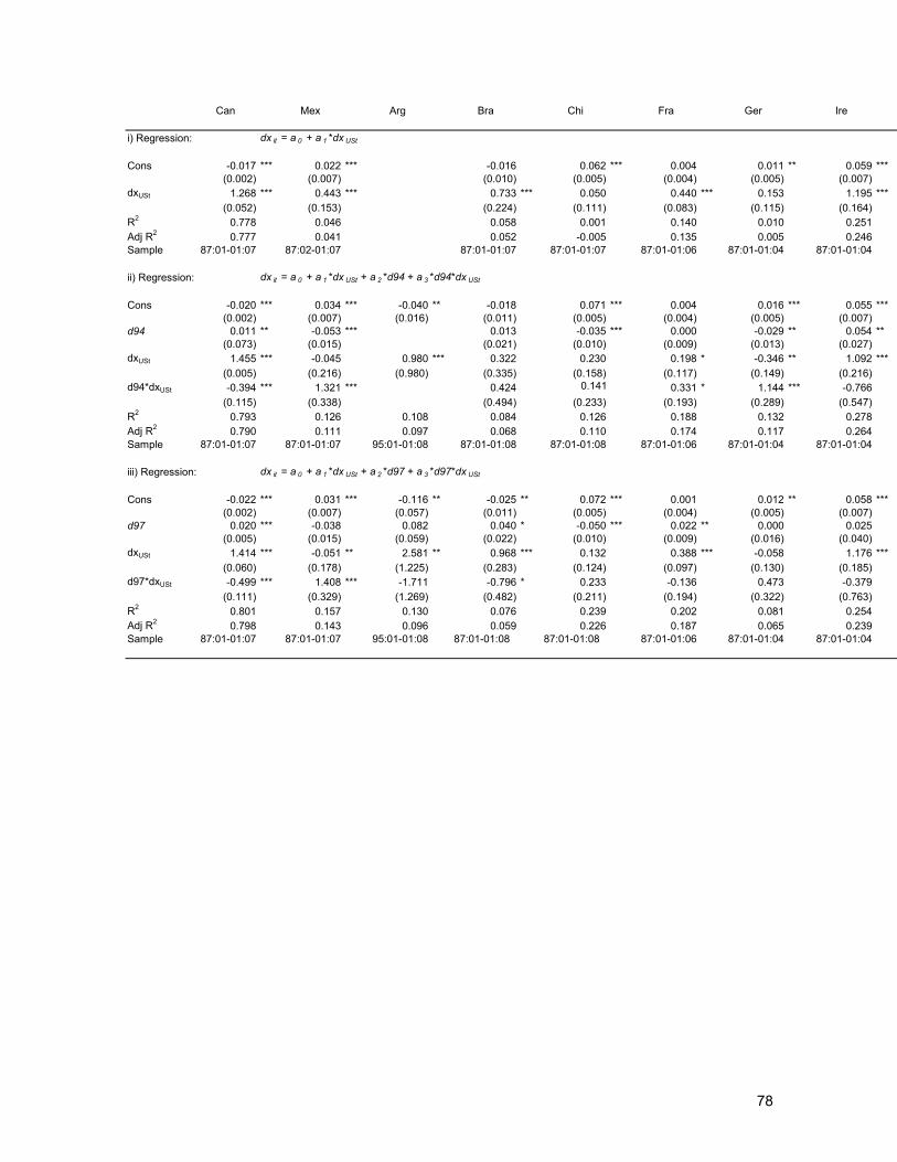
78

Can Mex Arg Bra Chi Fra Ger Ire


Cons -0.017 *** 0.022 *** -0.016 0.062 *** 0.004 0.011 ** 0.059 ***(0.002) (0.007) (0.010) (0.005) (0.004) (0.005) (0.007)

dxUSt 1.268 *** 0.443 *** 0.733 *** 0.050 0.440 *** 0.153 1.195 ***(0.052) (0.153) (0.224) (0.111) (0.083) (0.115) (0.164)

R2 0.778 0.046 0.058 0.001 0.140 0.010 0.251Adj R2 0.777 0.041 0.052 -0.005 0.135 0.005 0.246Sample 87:01-01:07 87:02-01:07 87:01-01:07 87:01-01:07 87:01-01:06 87:01-01:04 87:01-01:04


Cons -0.020 *** 0.034 *** -0.040 ** -0.018 0.071 *** 0.004 0.016 *** 0.055 ***(0.002) (0.007) (0.016) (0.011) (0.005) (0.004) (0.005) (0.007)

d94 0.011 ** -0.053 *** 0.013 -0.035 *** 0.000 -0.029 ** 0.054 **(0.073) (0.015) (0.021) (0.010) (0.009) (0.013) (0.027)

dxUSt 1.455 *** -0.045 0.980 *** 0.322 0.230 0.198 * -0.346 ** 1.092 ***(0.005) (0.216) (0.980) (0.335) (0.158) (0.117) (0.149) (0.216)

d94*dxUSt -0.394 *** 1.321 *** 0.424 0.141 0.331 * 1.144 *** -0.766(0.115) (0.338) (0.494) (0.233) (0.193) (0.289) (0.547)

R2 0.793 0.126 0.108 0.084 0.126 0.188 0.132 0.278Adj R2 0.790 0.111 0.097 0.068 0.110 0.174 0.117 0.264Sample 87:01-01:07 87:01-01:07 95:01-01:08 87:01-01:08 87:01-01:08 87:01-01:06 87:01-01:04 87:01-01:04


Cons -0.022 *** 0.031 *** -0.116 ** -0.025 ** 0.072 *** 0.001 0.012 ** 0.058 ***(0.002) (0.007) (0.057) (0.011) (0.005) (0.004) (0.005) (0.007)

d97 0.020 *** -0.038 0.082 0.040 * -0.050 *** 0.022 ** 0.000 0.025(0.005) (0.015) (0.059) (0.022) (0.010) (0.009) (0.016) (0.040)

dxUSt 1.414 *** -0.051 ** 2.581 ** 0.968 *** 0.132 0.388 *** -0.058 1.176 ***(0.060) (0.178) (1.225) (0.283) (0.124) (0.097) (0.130) (0.185)

d97*dxUSt -0.499 *** 1.408 *** -1.711 -0.796 * 0.233 -0.136 0.473 -0.379(0.111) (0.329) (1.269) (0.482) (0.211) (0.194) (0.322) (0.763)

R2 0.801 0.157 0.130 0.076 0.239 0.202 0.081 0.254Adj R2 0.798 0.143 0.096 0.059 0.226 0.187 0.065 0.239Sample 87:01-01:07 87:01-01:07 95:01-01:08 87:01-01:08 87:01-01:08 87:01-01:06 87:01-01:04 87:01-01:04

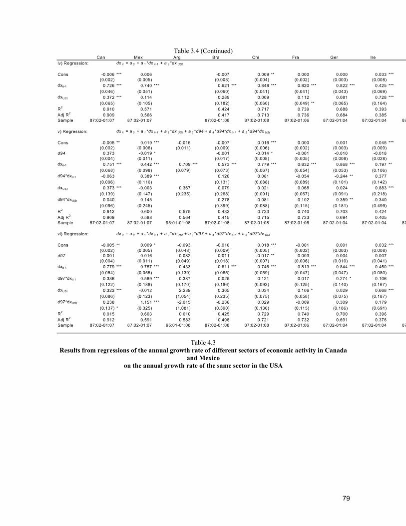
79

Table 3.4 (Continued) Can Mex Arg Bra Chi Fra Ger Ire

iv) Regression: dx it = a 0 + a 1 *dx it-1 + a 2 *dx USt

Cons -0.006 *** 0.006 -0.007 0.009 ** 0.000 0.000 0.033 ***(0.002) (0.005) (0.008) (0.004) (0.002) (0.003) (0.008)

dxit-1 0.726 *** 0.740 *** 0.621 *** 0.848 *** 0.820 *** 0.822 *** 0.425 ***(0.046) (0.051) (0.060) (0.041) (0.041) (0.043) (0.069)

dxUSt 0.372 *** 0.114 0.289 0.009 0.112 0.081 0.728 ***(0.065) (0.105) (0.182) (0.060) (0.049) ** (0.065) (0.164)

R2 0.910 0.571 0.424 0.717 0.739 0.688 0.393Adj R2 0.909 0.566 0.417 0.713 0.736 0.684 0.385Sample 87:02-01:07 87:02-01:07 87:02-01:08 87:02-01:08 87:02-01:06 87:02-01:04 87:02-01:04 87

v) Regression: dx it = a 0 + a 1 *dx it-1 + a 2 *dx USt + a 3 *d94 + a 4 *d94*dx it-1 + a 5 *d94*dx USt

Cons -0.005 ** 0.019 *** -0.015 -0.007 0.016 *** 0.000 0.001 0.045 ***(0.002) (0.006) (0.011) (0.009) (0.006) (0.002) (0.003) (0.009)

d94 0.373 -0.019 * -0.001 -0.014 * -0.001 -0.010 -0.018(0.004) (0.011) (0.017) (0.008) (0.005) (0.008) (0.028)

dxit-1 0.751 *** 0.442 *** 0.709 *** 0.573 *** 0.779 *** 0.832 *** 0.868 *** 0.197 **(0.068) (0.098) (0.079) (0.073) (0.067) (0.054) (0.053) (0.106)

d94*dxit-1 -0.063 0.389 *** 0.120 0.081 -0.054 -0.244 ** 0.377(0.096) (0.116) (0.131) (0.088) (0.089) (0.101) (0.142)

dxUSt 0.373 *** -0.003 0.367 0.079 0.021 0.068 0.024 0.883 ***(0.139) (0.147) (0.235) (0.268) (0.091) (0.067) (0.091) (0.218)

d94*dxUSt 0.040 0.145 0.278 0.081 0.102 0.359 ** -0.340(0.096) (0.245) (0.399) (0.088) (0.115) (0.181) (0.499)

R2 0.912 0.600 0.575 0.432 0.723 0.740 0.703 0.424Adj R2 0.909 0.588 0.564 0.415 0.715 0.733 0.694 0.405Sample 87:02-01:07 87:02-01:07 95:01-01:08 87:02-01:08 87:02-01:08 87:02-01:06 87:02-01:04 87:02-01:04 87

vi) Regression: dx it = a 0 + a 1 *dx it-1 + a 2 *dx USt + a 3 *d97 + a 4 *d97*dx it-1 + a 5 *d97*dx USt

Cons -0.005 ** 0.009 * -0.093 -0.010 0.018 *** -0.001 0.001 0.032 ***(0.002) (0.005) (0.048) (0.009) (0.005) (0.002) (0.003) (0.008)

d97 0.001 -0.016 0.082 0.011 -0.017 ** 0.003 -0.004 0.007(0.004) (0.011) (0.049) (0.018) (0.007) (0.006) (0.010) (0.041)

dxit-1 0.779 *** 0.757 *** 0.433 0.611 *** 0.746 *** 0.813 *** 0.844 *** 0.450 ***(0.054) (0.055) (0.139) (0.065) (0.059) (0.047) (0.047) (0.080)

d97*dxit-1 -0.336 -0.589 *** 0.387 0.025 0.121 -0.017 -0.274 * -0.106(0.122) (0.188) (0.170) (0.186) (0.093) (0.125) (0.140) (0.167)

dxUSt 0.323 *** -0.012 2.239 0.365 0.034 0.106 * 0.029 0.668 ***(0.086) (0.123) (1.054) (0.235) (0.075) (0.058) (0.075) (0.187)

d97*dxUSt 0.238 1.151 *** -2.015 -0.236 0.029 -0.009 0.309 0.179(0.137) * (0.325) (1.081) (0.390) (0.130) (0.115) (0.186) (0.691)

R2 0.915 0.603 0.610 0.425 0.729 0.740 0.700 0.396Adj R2 0.912 0.591 0.583 0.408 0.721 0.732 0.691 0.376Sample 87:02-01:07 87:02-01:07 95:01-01:08 87:02-01:08 87:02-01:08 87:02-01:06 87:02-01:04 87:02-01:04 87

Table 4.3 Results from regressions of the annual growth rate of different sectors of economic activity in Canada

and Mexico on the annual growth rate of the same sector in the USA

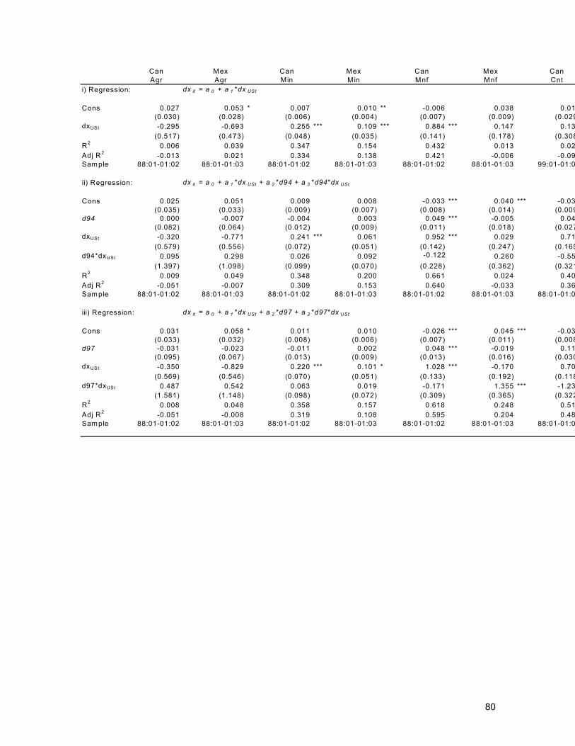
80

Can Mex Can Mex Can Mex CanAgr Agr Min Min Mnf Mnf Cnt


Cons 0.027 0.053 * 0.007 0.010 ** -0.006 0.038 0.01(0.030) (0.028) (0.006) (0.004) (0.007) (0.009) (0.029

dxUSt -0.295 -0.693 0.255 *** 0.109 *** 0.884 *** 0.147 0.13(0.517) (0.473) (0.048) (0.035) (0.141) (0.178) (0.308

R2 0.006 0.039 0.347 0.154 0.432 0.013 0.02Adj R2 -0.013 0.021 0.334 0.138 0.421 -0.006 -0.09Sample 88:01-01:02 88:01-01:03 88:01-01:02 88:01-01:03 88:01-01:02 88:01-01:03 99:01-01:0


Cons 0.025 0.051 0.009 0.008 -0.033 *** 0.040 *** -0.03(0.035) (0.033) (0.009) (0.007) (0.008) (0.014) (0.009

d94 0.000 -0.007 -0.004 0.003 0.049 *** -0.005 0.04(0.082) (0.064) (0.012) (0.009) (0.011) (0.018) (0.027

dxUSt -0.320 -0.771 0.241 *** 0.061 0.952 *** 0.029 0.71(0.579) (0.556) (0.072) (0.051) (0.142) (0.247) (0.165

d94*dxUSt 0.095 0.298 0.026 0.092 -0.122 0.260 -0.55(1.397) (1.098) (0.099) (0.070) (0.228) (0.362) (0.321

R2 0.009 0.049 0.348 0.200 0.661 0.024 0.40Adj R2 -0.051 -0.007 0.309 0.153 0.640 -0.033 0.36Sample 88:01-01:02 88:01-01:03 88:01-01:02 88:01-01:03 88:01-01:02 88:01-01:03 88:01-01:0


Cons 0.031 0.058 * 0.011 0.010 -0.026 *** 0.045 *** -0.03(0.033) (0.032) (0.008) (0.006) (0.007) (0.011) (0.008

d97 -0.031 -0.023 -0.011 0.002 0.048 *** -0.019 0.11(0.095) (0.067) (0.013) (0.009) (0.013) (0.016) (0.030

dxUSt -0.350 -0.829 0.220 *** 0.101 * 1.028 *** -0.170 0.70(0.569) (0.546) (0.070) (0.051) (0.133) (0.192) (0.118

d97*dxUSt 0.487 0.542 0.063 0.019 -0.171 1.355 *** -1.23(1.581) (1.148) (0.098) (0.072) (0.309) (0.365) (0.322

R2 0.008 0.048 0.358 0.157 0.618 0.248 0.51Adj R2 -0.051 -0.008 0.319 0.108 0.595 0.204 0.48Sample 88:01-01:02 88:01-01:03 88:01-01:02 88:01-01:03 88:01-01:02 88:01-01:03 88:01-01:0

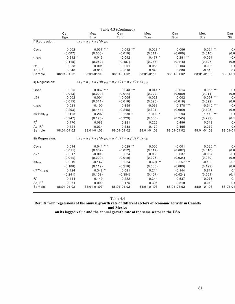
81

Table 4.3 (Continued) Can Mex Can Mex Can Mex CanEgw Egw Tcm Tcm Scs Scs Sfi


Cons 0.002 0.037 *** 0.042 *** 0.028 * 0.006 0.024 ** 0.0(0.007) (0.005) (0.010) (0.014) (0.009) (0.010) (0.00

dxUSt 0.212 * 0.015 -0.042 0.477 * 0.281 ** -0.051 -0.0(0.118) (0.082) (0.187) (0.265) (0.115) (0.127) (0.06

R2 0.058 0.001 0.001 0.058 0.103 0.003 0.0Adj R2 0.040 -0.018 -0.018 0.040 0.086 -0.016 0.0Sample 88:01-01:02 88:01-01:03 88:01-01:02 88:01-01:03 88:01-01:02 88:01-01:03 88:01-01


Cons 0.005 0.037 *** 0.043 *** 0.041 * -0.014 0.055 *** 0.0(0.013) (0.009) (0.014) (0.022) (0.009) (0.011) (0.00

d94 -0.002 0.001 -0.005 -0.023 0.002 -0.097 *** 0.0(0.015) (0.011) (0.018) (0.028) (0.019) (0.022) (0.00

dxUSt -0.021 -0.100 -0.355 -0.063 0.378 *** -0.340 *** -0.0(0.203) (0.144) (0.248) (0.391) (0.099) (0.123) (0.09

d94*dxUSt 0.403 0.207 0.630 * 1.008 * 0.293 1.119 *** 0.0(0.247) (0.175) (0.329) (0.503) (0.245) (0.292) (0.12

R2 0.170 0.088 0.281 0.225 0.496 0.312 0.0Adj R2 0.121 0.034 0.238 0.179 0.465 0.272 -0.0Sample 88:01-01:02 88:01-01:03 88:01-01:02 88:01-01:03 88:01-01:02 88:01-01:03 88:01-01


Cons 0.014 0.041 *** 0.029 ** 0.006 -0.001 0.026 ** 0.0(0.011) (0.007) (0.012) (0.017) (0.007) (0.010) (0.00

d97 -0.017 -0.003 0.024 0.038 0.037 -0.057 -0.0(0.014) (0.009) (0.019) (0.025) (0.034) (0.039) (0.0

dxUSt -0.019 -0.147 0.024 0.604 ** 0.257 *** -0.109 -0.1(0.180) (0.119) (0.216) (0.300) (0.086) (0.129) (0.06

d97*dxUSt 0.424 0.348 ** 0.091 0.214 -0.144 0.817 0.3(0.241) (0.159) (0.354) (0.467) (0.424) (0.501) (0.13

R2 0.114 0.149 0.222 0.344 0.537 0.073 0.1Adj R2 0.061 0.099 0.175 0.305 0.510 0.019 0.0Sample 88:01-01:02 88:01-01:03 88:01-01:02 88:01-01:03 88:01-01:02 88:01-01:03 88:01-01

Table 4.4 Results from regressions of the annual growth rate of different sectors of economic activity in Canada

and Mexico on its lagged value and the annual growth rate of the same sector in the USA

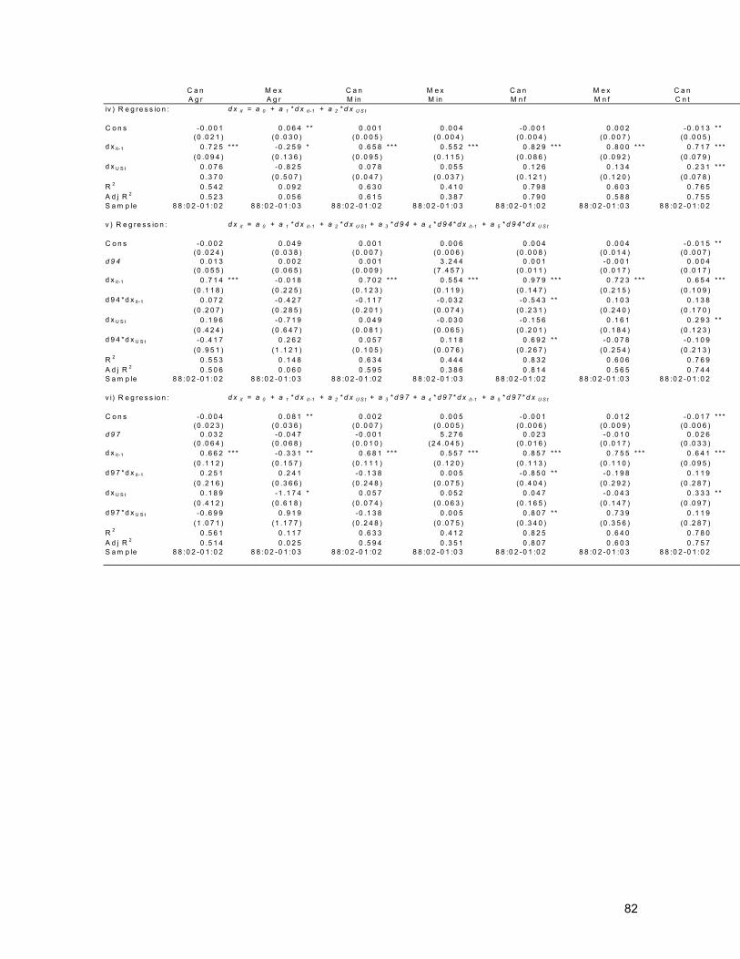
82

C a n M e x C a n M e x C a n M e x C a nA g r A g r M in M in M n f M n f C n t

iv ) R e g re s s io n : d x it = a 0 + a 1 *d x it-1 + a 2 *d x U S t

C o n s -0 .0 0 1 0 .0 6 4 * * 0 .0 0 1 0 .0 0 4 -0 .0 0 1 0 .0 0 2 -0 .0 1 3 * *(0 .0 2 1 ) (0 .0 3 0 ) (0 .0 0 5 ) (0 .0 0 4 ) (0 .0 0 4 ) (0 .0 0 7 ) (0 .0 0 5 )

d x it-1 0 .7 2 5 ** * -0 .2 5 9 * 0 .6 5 8 * * * 0 .5 5 2 ** * 0 .8 2 9 ** * 0 .8 0 0 * * * 0 .7 1 7 * * *(0 .0 9 4 ) (0 .1 3 6 ) (0 .0 9 5 ) (0 .1 1 5 ) (0 .0 8 6 ) (0 .0 9 2 ) (0 .0 7 9 )

d x U S t 0 .0 7 6 -0 .8 2 5 0 .0 7 8 0 .0 5 5 0 .1 2 6 0 .1 3 4 0 .2 3 1 * * *0 .3 7 0 (0 .5 0 7 ) (0 .0 4 7 ) (0 .0 3 7 ) (0 .1 2 1 ) (0 .1 2 0 ) (0 .0 7 8 )

R 2 0 .5 4 2 0 .0 9 2 0 .6 3 0 0 .4 1 0 0 .7 9 8 0 .6 0 3 0 .7 6 5A d j R 2 0 .5 2 3 0 .0 5 6 0 .6 1 5 0 .3 8 7 0 .7 9 0 0 .5 8 8 0 .7 5 5S a m p le 8 8 :0 2 -0 1 :0 2 8 8 :0 2 -0 1 :0 3 8 8 :0 2 -0 1 :0 2 8 8 :0 2 -0 1 :0 3 8 8 :0 2 -0 1 :0 2 8 8 :0 2 -0 1 :0 3 8 8 :0 2 -0 1 :0 2

v ) R e g re s s io n : d x it = a 0 + a 1 *d x it-1 + a 2 *d x U S t + a 3 *d 9 4 + a 4 *d 9 4 *d x it-1 + a 5 *d 9 4 *d x U S t

C o n s -0 .0 0 2 0 .0 4 9 0 .0 0 1 0 .0 0 6 0 .0 0 4 0 .0 0 4 -0 .0 1 5 * *(0 .0 2 4 ) (0 .0 3 8 ) (0 .0 0 7 ) (0 .0 0 6 ) (0 .0 0 8 ) (0 .0 1 4 ) (0 .0 0 7 )

d 9 4 0 .0 1 3 0 .0 0 2 0 .0 0 1 3 .2 4 4 0 .0 0 1 -0 .0 0 1 0 .0 0 4(0 .0 5 5 ) (0 .0 6 5 ) (0 .0 0 9 ) (7 .4 5 7 ) (0 .0 1 1 ) (0 .0 1 7 ) (0 .0 1 7 )

d x it-1 0 .7 1 4 ** * -0 .0 1 8 0 .7 0 2 * * * 0 .5 5 4 ** * 0 .9 7 9 ** * 0 .7 2 3 * * * 0 .6 5 4 * * *(0 .1 1 8 ) (0 .2 2 5 ) (0 .1 2 3 ) (0 .1 1 9 ) (0 .1 4 7 ) (0 .2 1 5 ) (0 .1 0 9 )

d 9 4 *d x it-1 0 .0 7 2 -0 .4 2 7 -0 .1 1 7 -0 .0 3 2 -0 .5 4 3 ** 0 .1 0 3 0 .1 3 8(0 .2 0 7 ) (0 .2 8 5 ) (0 .2 0 1 ) (0 .0 7 4 ) (0 .2 3 1 ) (0 .2 4 0 ) (0 .1 7 0 )

d x U S t 0 .1 9 6 -0 .7 1 9 0 .0 4 9 -0 .0 3 0 -0 .1 5 6 0 .1 6 1 0 .2 9 3 * *(0 .4 2 4 ) (0 .6 4 7 ) (0 .0 8 1 ) (0 .0 6 5 ) (0 .2 0 1 ) (0 .1 8 4 ) (0 .1 2 3 )

d 9 4 *d x U S t -0 .4 1 7 0 .2 6 2 0 .0 5 7 0 .1 1 8 0 .6 9 2 ** -0 .0 7 8 -0 .1 0 9(0 .9 5 1 ) (1 .1 2 1 ) (0 .1 0 5 ) (0 .0 7 6 ) (0 .2 6 7 ) (0 .2 5 4 ) (0 .2 1 3 )

R 2 0 .5 5 3 0 .1 4 8 0 .6 3 4 0 .4 4 4 0 .8 3 2 0 .6 0 6 0 .7 6 9A d j R 2 0 .5 0 6 0 .0 6 0 0 .5 9 5 0 .3 8 6 0 .8 1 4 0 .5 6 5 0 .7 4 4S a m p le 8 8 :0 2 -0 1 :0 2 8 8 :0 2 -0 1 :0 3 8 8 :0 2 -0 1 :0 2 8 8 :0 2 -0 1 :0 3 8 8 :0 2 -0 1 :0 2 8 8 :0 2 -0 1 :0 3 8 8 :0 2 -0 1 :0 2

v i) R e g re s s io n : d x it = a 0 + a 1 *d x it-1 + a 2 *d x U S t + a 3 *d 9 7 + a 4 *d 9 7 *d x it-1 + a 5 *d 9 7 *d x U S t

C o n s -0 .0 0 4 0 .0 8 1 * * 0 .0 0 2 0 .0 0 5 -0 .0 0 1 0 .0 1 2 -0 .0 1 7 * * *(0 .0 2 3 ) (0 .0 3 6 ) (0 .0 0 7 ) (0 .0 0 5 ) (0 .0 0 6 ) (0 .0 0 9 ) (0 .0 0 6 )

d 9 7 0 .0 3 2 -0 .0 4 7 -0 .0 0 1 5 .2 7 6 0 .0 2 3 -0 .0 1 0 0 .0 2 6(0 .0 6 4 ) (0 .0 6 8 ) (0 .0 1 0 ) (2 4 .0 4 5 ) (0 .0 1 6 ) (0 .0 1 7 ) (0 .0 3 3 )

d x it-1 0 .6 6 2 ** * -0 .3 3 1 * * 0 .6 8 1 * * * 0 .5 5 7 ** * 0 .8 5 7 ** * 0 .7 5 5 * * * 0 .6 4 1 * * *(0 .1 1 2 ) (0 .1 5 7 ) (0 .1 1 1 ) (0 .1 2 0 ) (0 .1 1 3 ) (0 .1 1 0 ) (0 .0 9 5 )

d 9 7 *d x it-1 0 .2 5 1 0 .2 4 1 -0 .1 3 8 0 .0 0 5 -0 .8 5 0 ** -0 .1 9 8 0 .1 1 9(0 .2 1 6 ) (0 .3 6 6 ) (0 .2 4 8 ) (0 .0 7 5 ) (0 .4 0 4 ) (0 .2 9 2 ) (0 .2 8 7 )

d x U S t 0 .1 8 9 -1 .1 7 4 * 0 .0 5 7 0 .0 5 2 0 .0 4 7 -0 .0 4 3 0 .3 3 3 * *(0 .4 1 2 ) (0 .6 1 8 ) (0 .0 7 4 ) (0 .0 6 3 ) (0 .1 6 5 ) (0 .1 4 7 ) (0 .0 9 7 )

d 9 7 *d x U S t -0 .6 9 9 0 .9 1 9 -0 .1 3 8 0 .0 0 5 0 .8 0 7 ** 0 .7 3 9 0 .1 1 9(1 .0 7 1 ) (1 .1 7 7 ) (0 .2 4 8 ) (0 .0 7 5 ) (0 .3 4 0 ) (0 .3 5 6 ) (0 .2 8 7 )

R 2 0 .5 6 1 0 .1 1 7 0 .6 3 3 0 .4 1 2 0 .8 2 5 0 .6 4 0 0 .7 8 0A d j R 2 0 .5 1 4 0 .0 2 5 0 .5 9 4 0 .3 5 1 0 .8 0 7 0 .6 0 3 0 .7 5 7S a m p le 8 8 :0 2 -0 1 :0 2 8 8 :0 2 -0 1 :0 3 8 8 :0 2 -0 1 :0 2 8 8 :0 2 -0 1 :0 3 8 8 :0 2 -0 1 :0 2 8 8 :0 2 -0 1 :0 3 8 8 :0 2 -0 1 :0 2

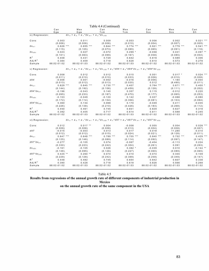
83

Table 4.4 (Continued) C a n M e x C a n M e x C a n M e x C a nE g w E g w T c m T c m S c s S c s S f i

iv ) R e g re s s io n : d x it = a 0 + a 1 *d x it-1 + a 2 *d x U S t

C o n s 0 .0 0 3 0 .0 1 1 0 .0 0 9 -0 .0 0 3 0 .0 0 6 0 .0 0 2 0 .0 2 1 * * *(0 .0 0 6 ) (0 .0 0 6 ) (0 .0 0 6 ) (0 .0 1 0 ) (0 .0 0 4 ) (0 .0 0 7 ) (0 .0 0 5 )

d x it-1 0 .6 2 6 ** * 0 .6 5 5 ** * 0 .8 4 4 * * * 0 .7 7 4 * * * 0 .9 2 1 ** * 0 .7 7 9 ** * 0 .5 4 1 * * *(0 .1 1 5 ) (0 .1 0 5 ) (0 .0 7 3 ) (0 .0 8 5 ) (0 .0 6 5 ) (0 .0 9 1 ) (0 .1 1 8 )

d x U S t 0 .0 2 3 0 .0 2 7 -0 .0 7 2 0 .2 9 9 * -0 .0 5 8 0 .0 3 1 -0 .0 9 7 * *(0 .1 0 1 ) (0 .0 6 3 ) (0 .0 9 9 ) (0 .1 6 7 ) (0 .0 5 8 ) (0 .0 8 5 ) (0 .0 5 4 )

R 2 0 .4 0 8 0 .4 3 1 0 .7 2 9 0 .6 4 2 0 .8 1 8 0 .5 8 9 0 .3 0 6A d j R 2 0 .3 8 4 0 .4 0 9 0 .7 1 8 0 .6 2 8 0 .8 1 0 0 .5 7 3 0 .2 7 8S a m p le 8 8 :0 2 -0 1 :0 2 8 8 :0 2 -0 1 :0 3 8 8 :0 2 -0 1 :0 2 8 8 :0 2 -0 1 :0 3 8 8 :0 2 -0 1 :0 2 8 8 :0 2 -0 1 :0 3 8 8 :0 2 -0 1 :0 2

v ) R e g re s s io n : d x it = a 0 + a 1 *d x it-1 + a 2 *d x U S t + a 3 *d 9 4 + a 4 *d 9 4 *d x it-1 + a 5 *d 9 4 *d x U S t

C o n s 0 .0 0 8 0 .0 1 2 0 .0 1 2 0 .0 1 5 0 .0 0 1 0 .0 1 7 * 0 .0 2 4 * * *(0 .0 1 1 ) (0 .0 1 0 ) (0 .0 1 0 ) (0 .0 3 3 ) (0 .0 0 6 ) (0 .0 1 0 ) (0 .0 0 8 )

d 9 4 -0 .0 0 6 0 .0 0 1 -0 .0 0 2 -0 .0 1 6 (0 .0 0 6 ) 1 .1 8 4 -0 .0 0 4(0 .0 1 3 ) (0 .0 1 2 ) (0 .0 1 3 ) (0 .0 3 5 ) 0 .0 1 2 (6 .4 9 0 ) (0 .0 1 1 )

d x it-1 0 .6 2 9 ** * 0 .6 4 5 ** * 0 .7 3 0 * * * 0 .4 0 7 0 .7 6 4 ** * 0 .6 7 1 ** * 0 .4 0 0 *(0 .1 4 4 ) (0 .1 9 2 ) (0 .1 0 6 ) (0 .4 5 9 ) (0 .1 2 8 ) (0 .1 1 1 ) (0 .2 0 2 )

d 9 4 *d x it-1 -0 .1 9 6 -0 .0 4 3 0 .1 4 0 0 .3 5 7 0 .1 1 5 -0 .0 1 2 0 .2 2 0(0 .2 6 5 ) (0 .2 3 3 ) (0 .1 8 7 ) (0 .4 7 0 ) (0 .1 7 7 ) (0 .0 6 5 ) (0 .2 5 3 )

d x U S t -0 .1 5 3 -0 .0 4 9 -0 .1 2 0 0 .1 4 2 0 .0 2 7 -0 .0 8 8 -0 .0 8 0(0 .1 7 2 ) (0 .1 1 4 ) (0 .1 5 4 ) (0 .3 5 6 ) (0 .0 8 1 ) (0 .1 0 3 ) (0 .0 8 4 )

d 9 4 *d x U S t 0 .3 6 0 0 .1 3 4 0 .0 6 8 0 .1 7 0 -0 .0 4 9 0 .4 1 1 -0 .0 3 5(0 .2 2 6 ) (0 .1 3 8 ) (0 .2 1 0 ) (0 .4 2 6 ) (0 .1 8 3 ) (0 .2 6 8 ) (0 .1 1 2 )

R 2 0 .4 5 0 0 .4 6 1 0 .7 4 5 0 .6 5 1 0 .8 2 9 0 .6 2 7 0 .3 1 8A d j R 2 0 .3 9 2 0 .4 0 5 0 .7 1 7 0 .6 1 4 0 .8 1 1 0 .5 8 8 0 .2 4 5S a m p le 8 8 :0 2 -0 1 :0 2 8 8 :0 2 -0 1 :0 3 8 8 :0 2 -0 1 :0 2 8 8 :0 2 -0 1 :0 3 8 8 :0 2 -0 1 :0 2 8 8 :0 2 -0 1 :0 3 8 8 :0 2 -0 1 :0 2

v i) R e g re s s io n : d x it = a 0 + a 1 *d x it-1 + a 2 *d x U S t + a 3 *d 9 7 + a 4 *d 9 7 *d x it-1 + a 5 *d 9 7 *d x U S t

C o n s 0 .0 1 2 0 .0 1 7 ** 0 .0 0 4 -0 .0 0 8 0 .0 0 5 0 .0 0 4 0 .0 2 8 * * *(0 .0 0 9 ) (0 .0 0 8 ) (0 .0 0 8 ) (0 .0 1 3 ) (0 .0 0 4 ) (0 .0 0 8 ) (0 .0 0 7 )

d 9 7 -0 .0 1 5 -0 .0 0 3 0 .0 1 3 0 .0 1 7 0 .0 1 8 1 1 .2 8 0 -0 .0 1 4(0 .0 1 2 ) (0 .0 1 2 ) (0 .0 1 5 ) (0 .0 2 4 ) (0 .0 2 1 ) (9 .1 2 8 ) (0 .0 1 1 )

d x it-1 0 .6 4 7 ** * 0 .6 4 8 ** * 0 .7 8 9 * * * 0 .7 0 5 * * * 0 .8 4 0 ** * 0 .7 5 2 ** * 0 .4 2 9 * * *(0 .1 2 5 ) (0 .1 4 6 ) (0 .0 8 9 ) (0 .1 1 4 ) (0 .0 9 2 ) (0 .0 9 7 ) (0 .1 4 7 )

d 9 7 *d x it-1 -0 .2 7 7 -0 .1 0 5 0 .0 7 4 -0 .0 6 7 -0 .4 0 4 -0 .1 1 3 0 .2 2 4(0 .3 3 0 ) (0 .2 2 3 ) (0 .2 4 2 ) (0 .3 0 4 ) (0 .2 6 1 ) 0 .0 9 1 (0 .2 9 3 )

d x U S t -0 .1 6 1 -0 .1 0 5 0 .0 2 6 0 .3 8 2 * -0 .0 3 9 0 .0 1 0 -0 .1 4 4 * *(0 .1 4 8 ) (0 .0 9 5 ) (0 .1 2 6 ) (0 .2 2 7 ) (0 .0 6 0 ) (0 .0 8 9 ) (0 .0 6 5 )

d 9 7 *d x U S t 0 .4 2 5 ** 0 .2 6 0 ** 0 .0 7 4 0 .0 1 0 0 .0 7 4 0 .3 5 5 0 .1 0 9(0 .2 2 9 ) (0 .1 2 8 ) (0 .2 4 2 ) (0 .3 9 9 ) (0 .2 5 9 ) (0 .3 4 9 ) (0 .1 4 7 )

R 2 0 .4 4 8 0 .4 8 2 0 .7 4 5 0 .6 5 4 0 .8 4 2 0 .6 0 7 0 .3 3 8A d j R 2 0 .3 9 0 0 .4 2 8 0 .7 1 8 0 .6 1 8 0 .8 2 6 0 .5 6 6 0 .2 6 8S a m p le 8 8 :0 2 -0 1 :0 2 8 8 :0 2 -0 1 :0 3 8 8 :0 2 -0 1 :0 2 8 8 :0 2 -0 1 :0 3 8 8 :0 2 -0 1 :0 2 8 8 :0 2 -0 1 :0 3 8 8 :0 2 -0 1 :0 2

Table 4.5 Results from regressions of the annual growth rate of different components of industrial production in

Mexico on the annual growth rate of the same component in the USA

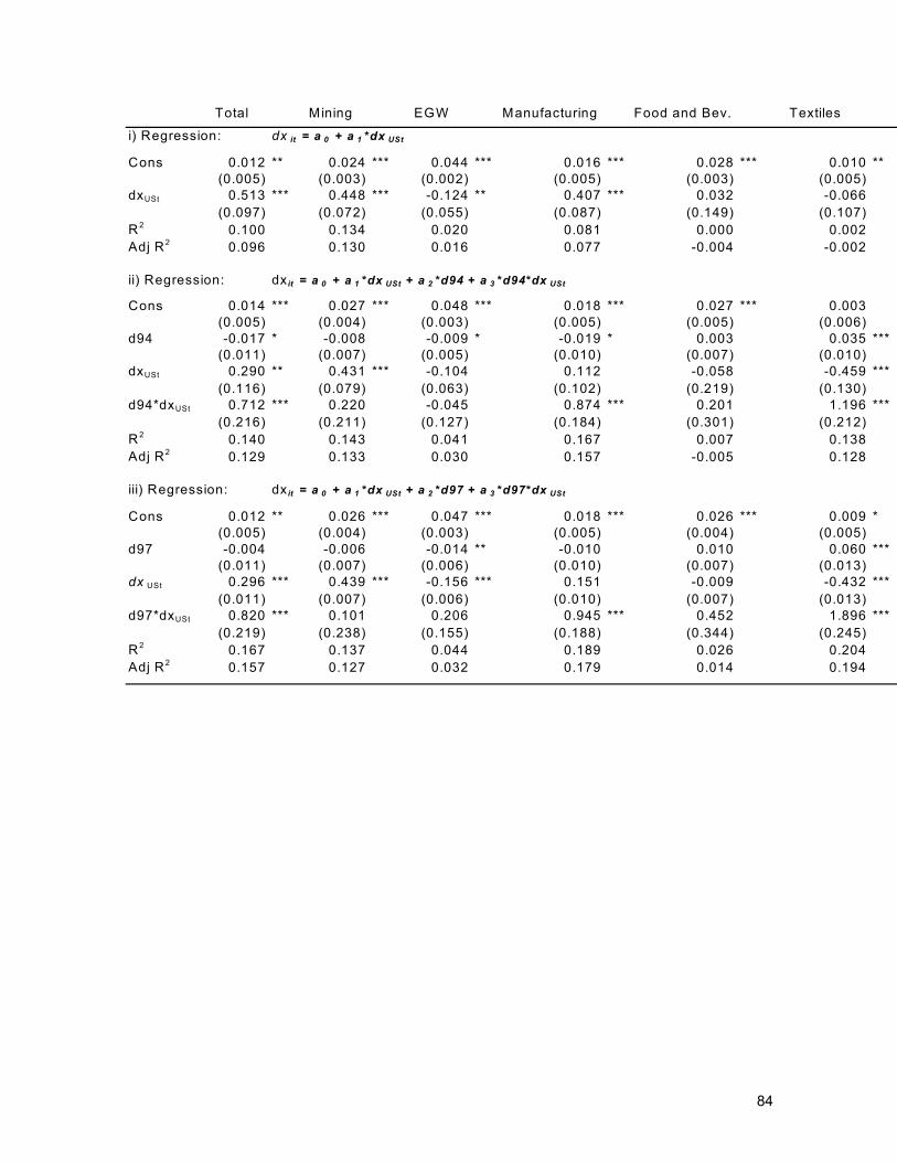
84

Total Mining EGW Manufacturing Food and Bev. Textiles


Cons 0.012 ** 0.024 *** 0.044 *** 0.016 *** 0.028 *** 0.010 **(0.005) (0.003) (0.002) (0.005) (0.003) (0.005)

dxUSt 0.513 *** 0.448 *** -0.124 ** 0.407 *** 0.032 -0.066(0.097) (0.072) (0.055) (0.087) (0.149) (0.107)

R2 0.100 0.134 0.020 0.081 0.000 0.002Adj R2 0.096 0.130 0.016 0.077 -0.004 -0.002


Cons 0.014 *** 0.027 *** 0.048 *** 0.018 *** 0.027 *** 0.003(0.005) (0.004) (0.003) (0.005) (0.005) (0.006)

d94 -0.017 * -0.008 -0.009 * -0.019 * 0.003 0.035 ***(0.011) (0.007) (0.005) (0.010) (0.007) (0.010)

dxUSt 0.290 ** 0.431 *** -0.104 0.112 -0.058 -0.459 ***(0.116) (0.079) (0.063) (0.102) (0.219) (0.130)

d94*dxUSt 0.712 *** 0.220 -0.045 0.874 *** 0.201 1.196 ***(0.216) (0.211) (0.127) (0.184) (0.301) (0.212)

R2 0.140 0.143 0.041 0.167 0.007 0.138Adj R2 0.129 0.133 0.030 0.157 -0.005 0.128


Cons 0.012 ** 0.026 *** 0.047 *** 0.018 *** 0.026 *** 0.009 *(0.005) (0.004) (0.003) (0.005) (0.004) (0.005)

d97 -0.004 -0.006 -0.014 ** -0.010 0.010 0.060 ***(0.011) (0.007) (0.006) (0.010) (0.007) (0.013)

dx USt 0.296 *** 0.439 *** -0.156 *** 0.151 -0.009 -0.432 ***(0.011) (0.007) (0.006) (0.010) (0.007) (0.013)

d97*dxUSt 0.820 *** 0.101 0.206 0.945 *** 0.452 1.896 ***(0.219) (0.238) (0.155) (0.188) (0.344) (0.245)

R2 0.167 0.137 0.044 0.189 0.026 0.204Adj R2 0.157 0.127 0.032 0.179 0.014 0.194

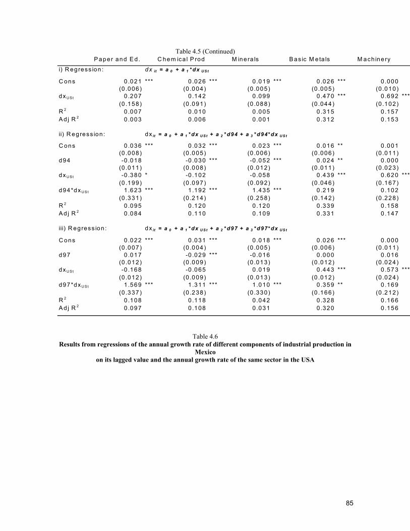
85

Table 4.5 (Continued) P aper and E d . C hem ica l P rod M inera ls B as ic M e ta ls M ach ine ry

i) R egress ion : dx it = a 0 + a 1 *d x U S t

C ons 0.021 *** 0 .026 *** 0 .019 *** 0 .026 *** 0 .000(0 .006 ) (0 .004 ) (0 .005) (0 .005) (0 .010)

dx U S t 0 .207 0 .142 0 .099 0 .470 *** 0 .692 ***(0 .158 ) (0 .091 ) (0 .088) (0 .044) (0 .102)

R 2 0 .007 0 .010 0 .005 0 .315 0.157A d j R 2 0 .003 0 .006 0 .001 0 .312 0.153

ii) R egress ion : dx it = a 0 + a 1 *d x U S t + a 2 *d 94 + a 3 *d 94*d x U S t

C ons 0.036 *** 0 .032 *** 0 .023 *** 0 .016 ** 0 .001(0 .008 ) (0 .005 ) (0 .006) (0 .006) (0 .011)

d94 -0 .018 -0 .030 *** -0 .052 *** 0 .024 ** 0 .000(0 .011 ) (0 .008 ) (0 .012) (0 .011) (0 .023)

dx U S t -0 .380 * -0 .102 -0 .058 0 .439 *** 0 .620 ***(0 .199 ) (0 .097 ) (0 .092) (0 .046) (0 .167)

d94*dx U S t 1 .623 *** 1 .192 *** 1 .435 *** 0 .219 0 .102(0 .331 ) (0 .214 ) (0 .258) (0 .142) (0 .228)

R 2 0 .095 0 .120 0 .120 0 .339 0.158A d j R 2 0 .084 0 .110 0 .109 0 .331 0.147

iii) R egress ion : dx it = a 0 + a 1 *d x U S t + a 2 *d 97 + a 3 *d 97*d x U S t

C ons 0.022 *** 0 .031 *** 0 .018 *** 0 .026 *** 0 .000(0 .007 ) (0 .004 ) (0 .005) (0 .006) (0 .011)

d97 0.017 -0 .029 *** -0 .016 0 .000 0.016(0 .012 ) (0 .009 ) (0 .013) (0 .012) (0 .024)

dx U S t -0 .168 -0 .065 0 .019 0 .443 *** 0 .573 ***(0 .012 ) (0 .009 ) (0 .013) (0 .012) (0 .024)

d97*dx U S t 1 .569 *** 1 .311 *** 1 .010 *** 0 .359 ** 0 .169(0 .337 ) (0 .238 ) (0 .330) (0 .166) (0 .212)

R 2 0 .108 0 .118 0 .042 0 .328 0.166A d j R 2 0 .097 0 .108 0 .031 0 .320 0.156

Table 4.6

Results from regressions of the annual growth rate of different components of industrial production in Mexico

on its lagged value and the annual growth rate of the same sector in the USA

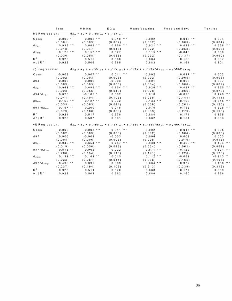
86

T o ta l M in in g E G W M a n u f a c tu r in g F o o d a n d B e v . T e x t i le s

iv ) R e g r e s s io n : d x i t = a 0 + a 1 * d x i t - 1 + a 2 * d x U S t

C o n s - 0 .0 0 2 * 0 .0 0 8 * * * 0 .0 1 0 * * * - 0 .0 0 2 0 .0 1 8 * * * 0 .0 0 4( 0 .0 0 1 ) ( 0 .0 0 3 ) ( 0 .0 0 2 ) ( 0 .0 0 2 ) ( 0 .0 0 3 ) ( 0 .0 0 4 )

d x i t - 1 0 .9 3 8 * * * 0 .6 4 9 * * * 0 .7 6 0 * * * 0 .9 2 1 * * * 0 .4 1 1 * * * 0 .5 5 8 * * *( 0 .0 1 8 ) ( 0 .0 4 7 ) ( 0 .0 4 3 ) ( 0 .0 2 2 ) ( 0 .0 5 8 ) ( 0 .0 5 3 )

d x U S t 0 .1 2 6 * * * 0 .1 5 7 * * * 0 .0 2 7 0 .1 1 5 * * * - 0 .0 4 0 0 .0 0 0( 0 .0 3 0 ) ( 0 .0 5 8 ) ( 0 .0 3 8 ) ( 0 .0 3 2 ) ( 0 .1 3 7 ) ( 0 .0 9 0 )

R 2 0 .9 2 3 0 .5 1 0 0 .5 6 8 0 .8 8 4 0 .1 6 8 0 .3 0 7A d j R 2 0 .9 2 2 0 .5 0 6 0 .5 6 5 0 .8 8 3 0 .1 6 1 0 .3 0 1

v ) R e g r e s s io n : d x i t = a 0 + a 1 * d x i t - 1 + a 2 * d x U S t + a 3 * d 9 4 + a 4 * d 9 4 * d x i t - 1 + a 5 * d 9 4 * d x U S t

C o n s - 0 .0 0 3 0 .0 0 7 * * 0 .0 1 1 * * * - 0 .0 0 2 0 .0 1 7 * * * 0 .0 0 2( 0 .0 0 2 ) ( 0 .0 0 3 ) ( 0 .0 0 3 ) ( 0 .0 0 2 ) ( 0 .0 0 5 ) ( 0 .0 0 5 )

d 9 4 0 .0 0 3 0 .0 0 2 - 0 .0 0 3 0 .0 0 1 0 .0 0 3 0 .0 0 7( 0 .0 0 3 ) ( 0 .0 0 5 ) ( 0 .0 0 6 ) ( 0 .0 0 4 ) ( 0 .0 0 8 ) ( 0 .0 0 9 )

d x i t - 1 0 .9 4 1 * * * 0 .6 9 8 * * * 0 .7 5 4 * * * 0 .9 2 6 * * * 0 .4 2 7 * * * 0 .2 6 5 * * *( 0 .0 2 3 ) ( 0 .0 5 6 ) ( 0 .0 4 9 ) ( 0 .0 2 8 ) ( 0 .0 6 6 ) ( 0 .0 7 8 )

d 9 4 * d x i t - 1 0 .0 2 5 - 0 .1 8 5 * 0 .0 0 2 0 .0 1 0 - 0 .0 9 5 0 .4 4 9 * * *( 0 .0 4 1 ) ( 0 .1 0 4 ) ( 0 .1 0 5 ) ( 0 .0 5 5 ) ( 0 .1 4 4 ) ( 0 .1 1 1 )

d x U S t 0 .1 6 8 * * * 0 .1 2 7 * * 0 .0 3 2 0 .1 3 4 * * * - 0 .1 0 6 - 0 .3 1 5 * * *( 0 .0 3 5 ) ( 0 .0 6 3 ) ( 0 .0 4 4 ) ( 0 .0 3 8 ) ( 0 .2 0 1 ) ( 0 .1 2 0 )

d 9 4 * d x U S t - 0 .1 5 7 * * 0 .2 0 0 - 0 .0 1 5 - 0 .0 7 0 0 .1 5 6 0 .5 2 5 * * *( 0 .0 7 3 ) ( 0 .1 6 8 ) ( 0 .0 8 8 ) ( 0 .0 8 3 ) ( 0 .2 7 9 ) ( 0 .1 9 5 )

R 2 0 .9 2 4 0 .5 1 7 0 .5 7 0 0 .8 8 4 0 .1 7 1 0 .3 7 5A d j R 2 0 .9 2 3 0 .5 0 7 0 .5 6 1 0 .8 8 2 0 .1 5 4 0 .3 6 3

v i) R e g r e s s io n : d x i t = a 0 + a 1 * d x i t - 1 + a 2 * d x U S t + a 3 * d 9 7 + a 4 * d 9 7 * d x i t - 1 + a 5 * d 9 7 * d x U S t

C o n s - 0 .0 0 2 0 .0 0 8 * * * 0 .0 1 1 * * * - 0 .0 0 2 0 .0 1 7 * * * 0 .0 0 5( 0 .0 0 2 ) ( 0 .0 0 3 ) ( 0 .0 0 3 ) ( 0 .0 0 2 ) ( 0 .0 0 4 ) ( 0 .0 0 5 )

d 9 7 0 .0 0 6 - 0 .0 0 1 - 0 .0 0 3 0 .0 0 6 0 .0 0 9 0 .0 5 3( 0 .0 0 4 ) ( 0 .0 0 6 ) ( 0 .0 0 6 ) ( 0 .0 0 5 ) ( 0 .0 1 0 ) ( 0 .0 1 6 )

d x i t - 1 0 .9 4 8 * * * 0 .6 5 4 * * * 0 .7 5 7 * * * 0 .9 3 0 * * * 0 .4 0 5 * * * 0 .4 8 4 * * *( 0 .0 1 9 ) ( 0 .0 5 0 ) ( 0 .0 4 8 ) ( 0 .0 2 4 ) ( 0 .0 6 1 ) ( 0 .0 6 1 )

d 9 7 * d x i t - 1 - 0 .5 1 3 * * - 0 .0 6 2 - 0 .0 2 2 - 0 .5 7 1 * * * - 0 .1 2 9 - 0 .3 2 1 * * *( 0 .2 0 8 ) ( 0 .1 5 4 ) ( 0 .1 1 5 ) ( 0 .1 9 1 ) ( 0 .2 2 8 ) ( 0 .1 7 3 )

d x U S t 0 .1 3 9 * * * 0 .1 4 9 * * 0 .0 1 5 0 .1 1 2 * * * - 0 .0 8 2 - 0 .2 1 3 * *( 0 .0 3 3 ) ( 0 .0 6 1 ) ( 0 .0 4 1 ) ( 0 .0 3 6 ) ( 0 .1 6 5 ) ( 0 .1 0 8 )

d 9 7 * d x U S t 0 .4 9 8 * * 0 .0 9 2 0 .0 6 9 0 .6 0 4 * * * 0 .3 7 7 1 .4 5 6 * * *( 0 .2 3 7 ) ( 0 .1 9 4 ) ( 0 .1 0 5 ) ( 0 .2 1 3 ) ( 0 .3 3 9 ) ( 0 .3 1 2 )

R 2 0 .9 2 5 0 .5 1 1 0 .5 7 0 0 .8 8 8 0 .1 7 7 0 .3 6 9A d j R 2 0 .9 2 3 0 .5 0 1 0 .5 6 2 0 .8 8 6 0 .1 6 0 0 .3 5 6

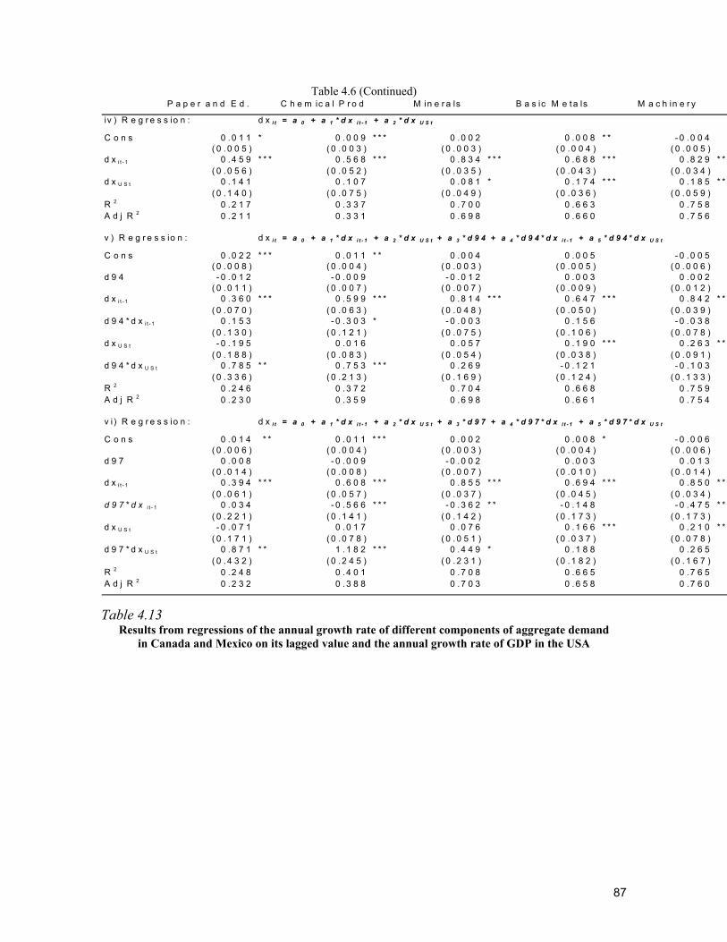
87

Table 4.6 (Continued) P a p e r a n d E d . C h e m ic a l P r o d M in e r a ls B a s ic M e t a ls M a c h in e r y

iv ) R e g r e s s io n : d x i t = a 0 + a 1 * d x i t - 1 + a 2 * d x U S t

C o n s 0 . 0 1 1 * 0 . 0 0 9 * * * 0 . 0 0 2 0 . 0 0 8 * * - 0 .0 0 4( 0 . 0 0 5 ) ( 0 .0 0 3 ) ( 0 . 0 0 3 ) ( 0 .0 0 4 ) ( 0 . 0 0 5 )

d x i t - 1 0 . 4 5 9 * * * 0 . 5 6 8 * * * 0 . 8 3 4 * * * 0 . 6 8 8 * * * 0 .8 2 9 * * *( 0 . 0 5 6 ) ( 0 .0 5 2 ) ( 0 . 0 3 5 ) ( 0 .0 4 3 ) ( 0 . 0 3 4 )

d x U S t 0 . 1 4 1 0 . 1 0 7 0 . 0 8 1 * 0 . 1 7 4 * * * 0 .1 8 5 * * *( 0 . 1 4 0 ) ( 0 .0 7 5 ) ( 0 . 0 4 9 ) ( 0 .0 3 6 ) ( 0 . 0 5 9 )

R 2 0 . 2 1 7 0 . 3 3 7 0 . 7 0 0 0 . 6 6 3 0 .7 5 8A d j R 2 0 . 2 1 1 0 . 3 3 1 0 . 6 9 8 0 . 6 6 0 0 .7 5 6

v ) R e g r e s s io n : d x i t = a 0 + a 1 * d x i t - 1 + a 2 * d x U S t + a 3 * d 9 4 + a 4 * d 9 4 * d x i t - 1 + a 5 * d 9 4 * d x U S t

C o n s 0 . 0 2 2 * * * 0 . 0 1 1 * * 0 . 0 0 4 0 . 0 0 5 - 0 .0 0 5( 0 . 0 0 8 ) ( 0 .0 0 4 ) ( 0 . 0 0 3 ) ( 0 .0 0 5 ) ( 0 . 0 0 6 )

d 9 4 - 0 . 0 1 2 - 0 . 0 0 9 - 0 . 0 1 2 0 . 0 0 3 0 .0 0 2( 0 . 0 1 1 ) ( 0 .0 0 7 ) ( 0 . 0 0 7 ) ( 0 .0 0 9 ) ( 0 . 0 1 2 )

d x i t - 1 0 . 3 6 0 * * * 0 . 5 9 9 * * * 0 . 8 1 4 * * * 0 . 6 4 7 * * * 0 .8 4 2 * * *( 0 . 0 7 0 ) ( 0 .0 6 3 ) ( 0 . 0 4 8 ) ( 0 .0 5 0 ) ( 0 . 0 3 9 )

d 9 4 * d x i t - 1 0 . 1 5 3 - 0 . 3 0 3 * - 0 . 0 0 3 0 . 1 5 6 - 0 .0 3 8( 0 . 1 3 0 ) ( 0 .1 2 1 ) ( 0 . 0 7 5 ) ( 0 .1 0 6 ) ( 0 . 0 7 8 )

d x U S t - 0 . 1 9 5 0 . 0 1 6 0 . 0 5 7 0 . 1 9 0 * * * 0 .2 6 3 * * *( 0 . 1 8 8 ) ( 0 .0 8 3 ) ( 0 . 0 5 4 ) ( 0 .0 3 8 ) ( 0 . 0 9 1 )

d 9 4 * d x U S t 0 . 7 8 5 * * 0 . 7 5 3 * * * 0 . 2 6 9 - 0 . 1 2 1 - 0 .1 0 3( 0 . 3 3 6 ) ( 0 .2 1 3 ) ( 0 . 1 6 9 ) ( 0 .1 2 4 ) ( 0 . 1 3 3 )

R 2 0 . 2 4 6 0 . 3 7 2 0 . 7 0 4 0 . 6 6 8 0 .7 5 9A d j R 2 0 . 2 3 0 0 . 3 5 9 0 . 6 9 8 0 . 6 6 1 0 .7 5 4

v i) R e g r e s s io n : d x i t = a 0 + a 1 * d x i t - 1 + a 2 * d x U S t + a 3 * d 9 7 + a 4 * d 9 7 * d x i t - 1 + a 5 * d 9 7 * d x U S t

C o n s 0 . 0 1 4 * * 0 . 0 1 1 * * * 0 . 0 0 2 0 . 0 0 8 * - 0 .0 0 6( 0 . 0 0 6 ) ( 0 .0 0 4 ) ( 0 . 0 0 3 ) ( 0 .0 0 4 ) ( 0 . 0 0 6 )

d 9 7 0 . 0 0 8 - 0 . 0 0 9 - 0 . 0 0 2 0 . 0 0 3 0 .0 1 3( 0 . 0 1 4 ) ( 0 .0 0 8 ) ( 0 . 0 0 7 ) ( 0 .0 1 0 ) ( 0 . 0 1 4 )

d x i t - 1 0 . 3 9 4 * * * 0 . 6 0 8 * * * 0 . 8 5 5 * * * 0 . 6 9 4 * * * 0 .8 5 0 * * *( 0 . 0 6 1 ) ( 0 .0 5 7 ) ( 0 . 0 3 7 ) ( 0 .0 4 5 ) ( 0 . 0 3 4 )

d 9 7 * d x i t - 1 0 . 0 3 4 - 0 . 5 6 6 * * * - 0 . 3 6 2 * * - 0 . 1 4 8 - 0 .4 7 5 * * *( 0 . 2 2 1 ) ( 0 .1 4 1 ) ( 0 . 1 4 2 ) ( 0 .1 7 3 ) ( 0 . 1 7 3 )

d x U S t - 0 . 0 7 1 0 . 0 1 7 0 . 0 7 6 0 . 1 6 6 * * * 0 .2 1 0 * * *( 0 . 1 7 1 ) ( 0 .0 7 8 ) ( 0 . 0 5 1 ) ( 0 .0 3 7 ) ( 0 . 0 7 8 )

d 9 7 * d x U S t 0 . 8 7 1 * * 1 . 1 8 2 * * * 0 . 4 4 9 * 0 . 1 8 8 0 .2 6 5( 0 . 4 3 2 ) ( 0 .2 4 5 ) ( 0 . 2 3 1 ) ( 0 .1 8 2 ) ( 0 . 1 6 7 )

R 2 0 . 2 4 8 0 . 4 0 1 0 . 7 0 8 0 . 6 6 5 0 .7 6 5A d j R 2 0 . 2 3 2 0 . 3 8 8 0 . 7 0 3 0 . 6 5 8 0 .7 6 0

Table 4.13 Results from regressions of the annual growth rate of different components of aggregate demand

in Canada and Mexico on its lagged value and the annual growth rate of GDP in the USA

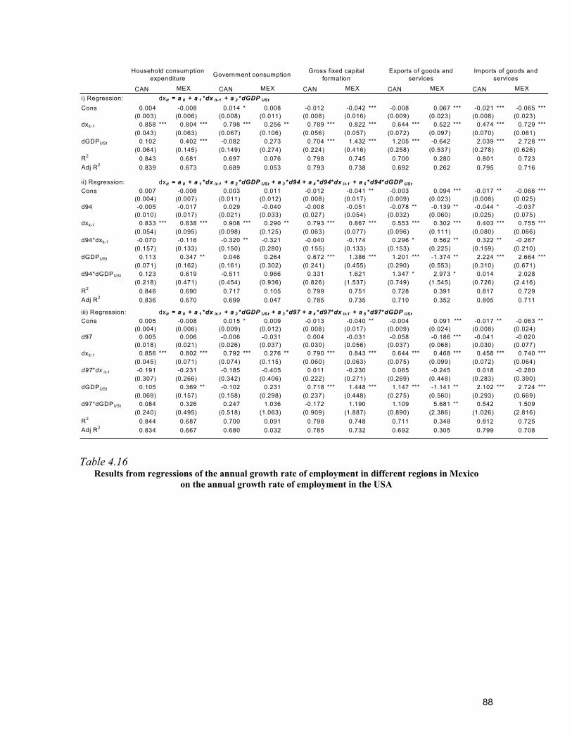
88

CAN MEX CAN MEX CAN MEX CAN MEX CAN MEXi) Regression: dxit = a 0 + a 1 *dx it-1 + a 2 *dGDP USt

Cons 0.004 -0.008 0.014 * 0.008 -0.012 -0.042 *** -0.008 0.067 *** -0.021 *** -0.065 ***(0.003) (0.006) (0.008) (0.011) (0.008) (0.016) (0.009) (0.023) (0.008) (0.023)

dxit-1 0.858 *** 0.804 *** 0.798 *** 0.256 ** 0.789 *** 0.822 *** 0.644 *** 0.522 *** 0.474 *** 0.729 ***(0.043) (0.063) (0.067) (0.106) (0.056) (0.057) (0.072) (0.097) (0.070) (0.061)

dGDPUSt 0.102 0.402 *** -0.082 0.273 0.704 *** 1.432 *** 1.205 *** -0.642 2.039 *** 2.728 ***(0.064) (0.145) (0.149) (0.274) (0.224) (0.416) (0.258) (0.537) (0.278) (0.626)

R2 0.843 0.681 0.697 0.076 0.798 0.745 0.700 0.280 0.801 0.723Adj R2 0.839 0.673 0.689 0.053 0.793 0.738 0.692 0.262 0.795 0.716

ii) Regression: dxit = a 0 + a 1 *dx it-1 + a 2 *dGDP USt + a 3 *d94 + a 4 *d94*dx it-1 + a 5 *d94*dGDP USt

Cons 0.007 -0.008 0.003 0.011 -0.012 -0.041 ** -0.003 0.094 *** -0.017 ** -0.066 ***(0.004) (0.007) (0.011) (0.012) (0.008) (0.017) (0.009) (0.023) (0.008) (0.025)

d94 -0.005 -0.017 0.029 -0.040 -0.008 -0.051 -0.078 ** -0.139 ** -0.044 * -0.037(0.010) (0.017) (0.021) (0.033) (0.027) (0.054) (0.032) (0.060) (0.025) (0.075)

dxit-1 0.833 *** 0.838 *** 0.908 *** 0.290 ** 0.793 *** 0.867 *** 0.553 *** 0.302 *** 0.403 *** 0.755 ***(0.054) (0.095) (0.098) (0.125) (0.063) (0.077) (0.096) (0.111) (0.080) (0.066)

d94*dxit-1 -0.070 -0.116 -0.320 ** -0.321 -0.040 -0.174 0.296 * 0.562 ** 0.322 ** -0.267(0.157) (0.133) (0.150) (0.280) (0.155) (0.133) (0.153) (0.225) (0.159) (0.210)

dGDPUSt 0.113 0.347 ** 0.046 0.264 0.672 *** 1.386 *** 1.201 *** -1.374 ** 2.224 *** 2.664 ***(0.071) (0.162) (0.161) (0.302) (0.241) (0.455) (0.290) (0.553) (0.310) (0.671)

d94*dGDPUSt 0.123 0.619 -0.511 0.966 0.331 1.621 1.347 * 2.973 * 0.014 2.028(0.218) (0.471) (0.454) (0.936) (0.826) (1.537) (0.749) (1.545) (0.726) (2.416)

R2 0.846 0.690 0.717 0.105 0.799 0.751 0.728 0.391 0.817 0.729Adj R2 0.836 0.670 0.699 0.047 0.785 0.735 0.710 0.352 0.805 0.711

iii) Regression: dxit = a 0 + a 1 *dx it-1 + a 2 *dGDP USt + a 3 *d97 + a 4 *d97*dx it-1 + a 5 *d97*dGDP USt

Cons 0.005 -0.008 0.015 * 0.009 -0.013 -0.040 ** -0.004 0.091 *** -0.017 ** -0.063 **(0.004) (0.006) (0.009) (0.012) (0.008) (0.017) (0.009) (0.024) (0.008) (0.024)

d97 0.005 0.006 -0.006 -0.031 0.004 -0.031 -0.058 -0.186 *** -0.041 -0.020(0.018) (0.021) (0.026) (0.037) (0.030) (0.056) (0.037) (0.068) (0.030) (0.077)

dxit-1 0.856 *** 0.802 *** 0.792 *** 0.276 ** 0.790 *** 0.843 *** 0.644 *** 0.468 *** 0.458 *** 0.740 ***(0.045) (0.071) (0.074) (0.115) (0.060) (0.063) (0.075) (0.099) (0.072) (0.064)

d97*dx it-1 -0.191 -0.231 -0.185 -0.405 0.011 -0.230 0.065 -0.245 0.018 -0.280(0.307) (0.266) (0.342) (0.406) (0.222) (0.271) (0.269) (0.448) (0.283) (0.390)

dGDPUSt 0.105 0.369 ** -0.102 0.231 0.718 *** 1.448 *** 1.147 *** -1.141 ** 2.102 *** 2.724 ***(0.069) (0.157) (0.158) (0.298) (0.237) (0.448) (0.275) (0.560) (0.293) (0.669)

d97*dGDPUSt 0.084 0.326 0.247 1.036 -0.172 1.190 1.109 5.681 ** 0.542 1.509(0.240) (0.495) (0.518) (1.063) (0.909) (1.887) (0.890) (2.386) (1.026) (2.816)

R2 0.844 0.687 0.700 0.091 0.798 0.748 0.711 0.348 0.812 0.725Adj R2 0.834 0.667 0.680 0.032 0.785 0.732 0.692 0.305 0.799 0.708

Household consumption expenditure Government consumption Gross fixed capital

formationExports of goods and

servicesImports of goods and

services

Table 4.16 Results from regressions of the annual growth rate of employment in different regions in Mexico

on the annual growth rate of employment in the USA

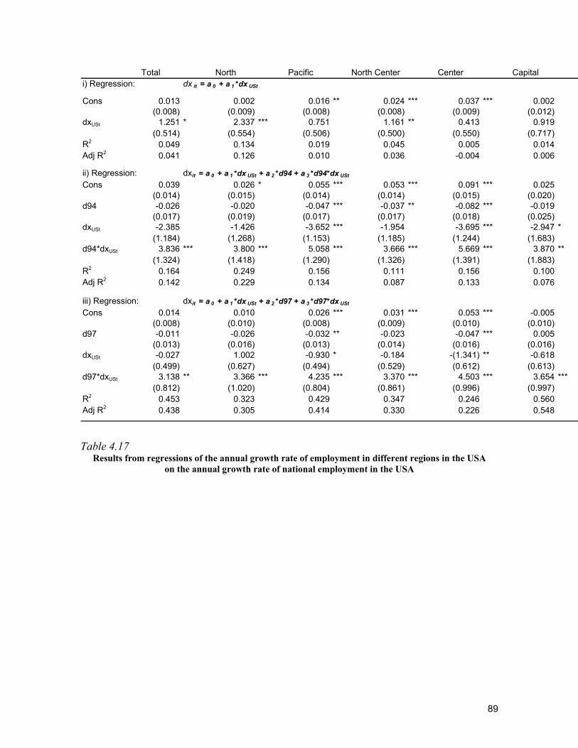
89

Total North Pacific North Center Center Capitali) Regression: dx it = a 0 + a 1 *dx USt

Cons 0.013 0.002 0.016 ** 0.024 *** 0.037 *** 0.002(0.008) (0.009) (0.008) (0.008) (0.009) (0.012)

dxUSt 1.251 * 2.337 *** 0.751 1.161 ** 0.413 0.919(0.514) (0.554) (0.506) (0.500) (0.550) (0.717)

R2 0.049 0.134 0.019 0.045 0.005 0.014Adj R2 0.041 0.126 0.010 0.036 -0.004 0.006

ii) Regression: dxit = a 0 + a 1 *dx USt + a 2 *d94 + a 3 *d94*dx USt

Cons 0.039 0.026 * 0.055 *** 0.053 *** 0.091 *** 0.025(0.014) (0.015) (0.014) (0.014) (0.015) (0.020)

d94 -0.026 -0.020 -0.047 *** -0.037 ** -0.082 *** -0.019(0.017) (0.019) (0.017) (0.017) (0.018) (0.025)

dxUSt -2.385 -1.426 -3.652 *** -1.954 -3.695 *** -2.947 *(1.184) (1.268) (1.153) (1.185) (1.244) (1.683)

d94*dxUSt 3.836 *** 3.800 *** 5.058 *** 3.666 *** 5.669 *** 3.870 **(1.324) (1.418) (1.290) (1.326) (1.391) (1.883)

R2 0.164 0.249 0.156 0.111 0.156 0.100Adj R2 0.142 0.229 0.134 0.087 0.133 0.076

iii) Regression: dxit = a 0 + a 1 *dx USt + a 2 *d97 + a 3 *d97*dx USt

Cons 0.014 0.010 0.026 *** 0.031 *** 0.053 *** -0.005(0.008) (0.010) (0.008) (0.009) (0.010) (0.010)

d97 -0.011 -0.026 -0.032 ** -0.023 -0.047 *** 0.005(0.013) (0.016) (0.013) (0.014) (0.016) (0.016)

dxUSt -0.027 1.002 -0.930 * -0.184 -(1.341) ** -0.618(0.499) (0.627) (0.494) (0.529) (0.612) (0.613)

d97*dxUSt 3.138 ** 3.366 *** 4.235 *** 3.370 *** 4.503 *** 3.654 ***(0.812) (1.020) (0.804) (0.861) (0.996) (0.997)

R2 0.453 0.323 0.429 0.347 0.246 0.560Adj R2 0.438 0.305 0.414 0.330 0.226 0.548

Table 4.17

Results from regressions of the annual growth rate of employment in different regions in the USA on the annual growth rate of national employment in the USA

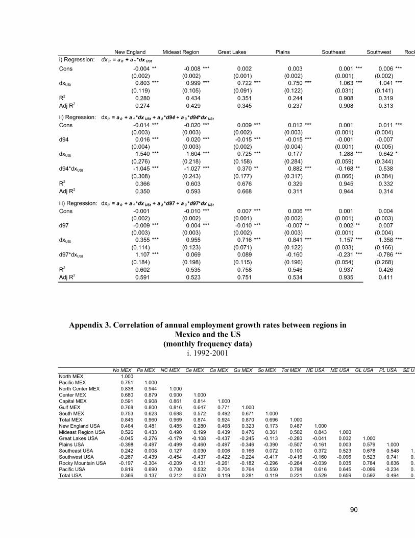
90

New England Mideast Region Great Lakes Plains Southeast Southwest Rocki) Regression: dx it = a 0 + a 1 *dx USt

Cons -0.004 ** -0.008 *** 0.002 0.003 0.001 *** 0.006 ***(0.002) (0.002) (0.001) (0.002) (0.001) (0.002)

dxUSt 0.803 *** 0.999 *** 0.722 *** 0.750 *** 1.063 *** 1.041 ***(0.119) (0.105) (0.091) (0.122) (0.031) (0.141)

R2 0.280 0.434 0.351 0.244 0.908 0.319Adj R2 0.274 0.429 0.345 0.237 0.908 0.313

ii) Regression: dxit = a 0 + a 1 *dx USt + a 2 *d94 + a 3 *d94*dx USt

Cons -0.014 *** -0.020 *** 0.009 *** 0.012 *** 0.001 0.011 ***(0.003) (0.003) (0.002) (0.003) (0.001) (0.004)

d94 0.016 *** 0.020 *** -0.015 *** -0.015 *** -0.001 -0.007(0.004) (0.003) (0.002) (0.004) (0.001) (0.005)

dxUSt 1.540 *** 1.604 *** 0.725 *** 0.177 1.288 *** 0.642 *(0.276) (0.218) (0.158) (0.284) (0.059) (0.344)

d94*dxUSt -1.045 *** -1.027 *** 0.370 ** 0.882 *** -0.168 ** 0.538(0.308) (0.243) (0.177) (0.317) (0.066) (0.384)

R2 0.366 0.603 0.676 0.329 0.945 0.332Adj R2 0.350 0.593 0.668 0.311 0.944 0.314

iii) Regression: dxit = a 0 + a 1 *dx USt + a 2 *d97 + a 3 *d97*dx USt

Cons -0.001 -0.010 *** 0.007 *** 0.006 *** 0.001 0.004(0.002) (0.002) (0.001) (0.002) (0.001) (0.003)

d97 -0.009 *** 0.004 *** -0.010 *** -0.007 ** 0.002 ** 0.007(0.003) (0.003) (0.002) (0.003) (0.001) (0.004)

dxUSt 0.355 *** 0.955 0.716 *** 0.841 *** 1.157 *** 1.358 ***(0.114) (0.123) (0.071) (0.122) (0.033) (0.166)

d97*dxUSt 1.107 *** 0.069 0.089 -0.160 -0.231 *** -0.786 ***(0.184) (0.198) (0.115) (0.196) (0.054) (0.268)

R2 0.602 0.535 0.758 0.546 0.937 0.426Adj R2 0.591 0.523 0.751 0.534 0.935 0.411

Appendix 3. Correlation of annual employment growth rates between regions in Mexico and the US

(monthly frequency data) i. 1992-2001

No MEX Pa MEX NC MEX Ce MEX Ca MEX Gu MEX So MEX Tot MEX NE USA ME USA GL USA PL USA SE US

North MEX 1.000Pacific MEX 0.751 1.000North Center MEX 0.836 0.944 1.000Center MEX 0.680 0.879 0.900 1.000Capital MEX 0.591 0.908 0.861 0.814 1.000Gulf MEX 0.768 0.800 0.816 0.647 0.771 1.000South MEX 0.753 0.623 0.688 0.572 0.492 0.671 1.000Total MEX 0.845 0.960 0.969 0.874 0.924 0.870 0.696 1.000New England USA 0.464 0.481 0.485 0.280 0.468 0.323 0.173 0.487 1.000Mideast Region USA 0.526 0.433 0.490 0.199 0.439 0.476 0.361 0.502 0.843 1.000Great Lakes USA -0.045 -0.276 -0.179 -0.108 -0.437 -0.245 -0.113 -0.280 -0.041 0.032 1.000Plains USA -0.398 -0.497 -0.499 -0.460 -0.497 -0.346 -0.390 -0.507 -0.161 0.003 0.579 1.000Southeast USA 0.242 0.008 0.127 0.030 0.006 0.166 0.072 0.100 0.372 0.523 0.678 0.548 1.0Southwest USA -0.267 -0.439 -0.454 -0.437 -0.422 -0.224 -0.417 -0.416 -0.160 -0.096 0.523 0.741 0.5Rocky Mountain USA -0.197 -0.304 -0.209 -0.131 -0.261 -0.182 -0.296 -0.264 -0.039 0.035 0.784 0.636 0.8Pacific USA 0.819 0.690 0.700 0.532 0.704 0.764 0.550 0.798 0.616 0.645 -0.099 -0.234 0.4Total USA 0.366 0.137 0.212 0.070 0.119 0.281 0.119 0.221 0.529 0.659 0.592 0.494 0.9

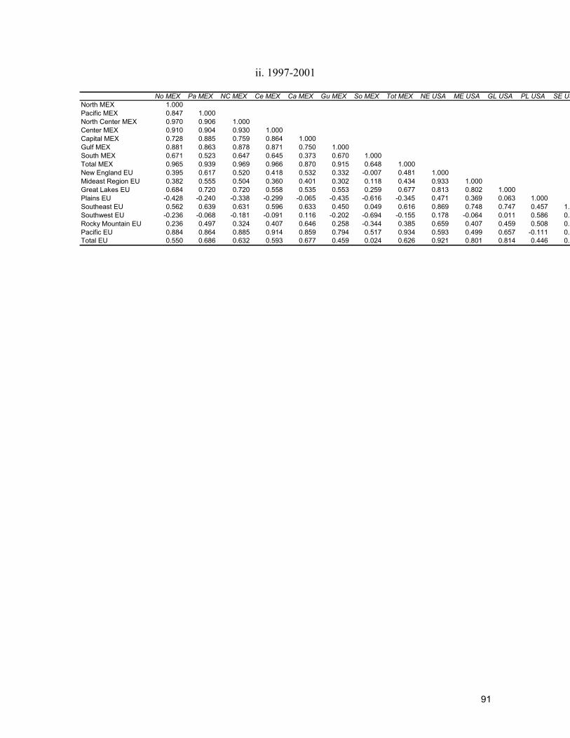
91

ii. 1997-2001

No MEX Pa MEX NC MEX Ce MEX Ca MEX Gu MEX So MEX Tot MEX NE USA ME USA GL USA PL USA SE USNorth MEX 1.000Pacific MEX 0.847 1.000North Center MEX 0.970 0.906 1.000Center MEX 0.910 0.904 0.930 1.000Capital MEX 0.728 0.885 0.759 0.864 1.000Gulf MEX 0.881 0.863 0.878 0.871 0.750 1.000South MEX 0.671 0.523 0.647 0.645 0.373 0.670 1.000Total MEX 0.965 0.939 0.969 0.966 0.870 0.915 0.648 1.000New England EU 0.395 0.617 0.520 0.418 0.532 0.332 -0.007 0.481 1.000Mideast Region EU 0.382 0.555 0.504 0.360 0.401 0.302 0.118 0.434 0.933 1.000Great Lakes EU 0.684 0.720 0.720 0.558 0.535 0.553 0.259 0.677 0.813 0.802 1.000Plains EU -0.428 -0.240 -0.338 -0.299 -0.065 -0.435 -0.616 -0.345 0.471 0.369 0.063 1.000Southeast EU 0.562 0.639 0.631 0.596 0.633 0.450 0.049 0.616 0.869 0.748 0.747 0.457 1.0Southwest EU -0.236 -0.068 -0.181 -0.091 0.116 -0.202 -0.694 -0.155 0.178 -0.064 0.011 0.586 0.3Rocky Mountain EU 0.236 0.497 0.324 0.407 0.646 0.258 -0.344 0.385 0.659 0.407 0.459 0.508 0.7Pacific EU 0.884 0.864 0.885 0.914 0.859 0.794 0.517 0.934 0.593 0.499 0.657 -0.111 0.7Total EU 0.550 0.686 0.632 0.593 0.677 0.459 0.024 0.626 0.921 0.801 0.814 0.446 0.9

macroeconomic synchronization between mexico and its

Documents