Improving Macroeconomic Model Validity and Forecasting

Performance with Pooled Country Data using Structural,

Reduced Form, and Neural Network Models

Cameron Fen and Samir Undavia∗

March 15, 2022

We show that pooling countries across a panel dimension to macroeconomic data can improve by astatistically significant margin the generalization ability of structural, reduced form, and machine learning(ML) methods to produce state-of-the-art results. Using GDP forecasts evaluated on an out-of-sample testset, this procedure reduces root mean squared error by 12% across horizons and models for certain reduced-form models and by 24% across horizons for dynamic structural general equilibrium models. RemovingUS data from the training set and forecasting out-of-sample country-wise, we show that reduced-form andstructural models are more policy-invariant when trained on pooled data, and outperform a baseline thatuses US data only. Given the comparative advantage of ML models in a data-rich regime, we demonstratethat our recurrent neural network model and automated ML approach outperform all tested baseline eco-nomic models. Robustness checks indicate that our outperformance is reproducible, numerically stable, andgeneralizable across models.

JEL Codes: E27, C45, C53, C32Keywords: Neural Networks, Deep Learning, Policy-Invariance, GDP Forecasting, Pooled Data

∗Corresponding author Cameron Fen is PhD student at the University of Michigan, Ann Arbor, MI, 48104 (E-mail: camfen@umich.edu. Website: cameronfen.github.io.). Samir Undavia is an ML and NLP engineer (E-mail:samir@undavia.com). The authors thank Xavier Martin Bautista, Thorsten Drautzburg, Florian Gunsilius, JeffreyLin, Daniil Manaenkov, Matthew Shapiro, Eric Jang, and the member participants of the European Winter Meetingof the Econometric society, the ASSA conference, the Midwestern Economic Association conference, EconWorldconference, and the EcoMod conference for helpful discussion and/or comments. We would also like to thank NimartaKumari for research assistance assembling the DSGE panel data set and AI Capital Management for computationalresources. All errors are our own.

arX

iv:2

203.

0654

0v1

[ec

on.G

N]

13

Mar

202

2

I. Introduction

A central problem in both reduced-form and structural macroeconomics is the dearth of under-

lying data. For example, GDP is a quarterly dataset that only extends back to around the late

1940s, which results in around 300 timesteps. Thus generalization and external validity of these

models are a pertinent problem. In forecasting, this approach is partially addressed by using simple

linear models. In structural macroeconomics the use of micro-founded parameters and Bayesian

estimation attempts to improve generalization to a limited effect. More flexible and nonparametric

models would likely produce more accurate forecasts, but with limited data, this avenue is not

available. However, pooling data across many different countries allows economists to forecast and

even estimate larger structural models which have both better external validity and forecasting,

without having to compromise on internal validity or model design.

We show that the effectiveness of pooling US or other single country data with other countries in

conjunction with large DSGE models and machine learning leads to improvements in external valid-

ity and economic forecasting. This pooling approach adds more data, rather than more covariates

and leads to consistent and significant improvements in external validity as measured by timestep

out-of-sample forecasts and other metrics. For example, our data goes from 211 timesteps of US

data for our AutoML model, to 2581 timesteps over all countries in our pooled data. This not only

leads to significant improvements in forecasting for standard models, but also allows more flexible

models to be used without overfitting. Pooling a panel of countries also leads to parameters that

are a better fit to the underlying data generating process – almost for free – without any change to

the underlying equations governing the models and only changing the interpretation from a single

country parameter to an average world parameter. Even in this case we show that the stability of

parameters over space – across countries – may be better than the alternative–going back further

in time for more single country data.

A central theme throughout this paper is that more flexible models benefit more from pooling.

We start with the linear models as a good baseline. Even in this case, pooling improves performance.

Estimating traditional reduced-form models – AR(2) (Walker, 1931), VAR(1), VAR(4) models

1

(Sims, 1980) – we show that we can reduce RMSE by an average of 12% across horizons and models.

Outside of pure forecasting, analysis of our pooling procedure across models suggests improvements

in external validity in other ways – making models more policy/regime invariant. To show this,

we estimate both linear and nonlinear models on data from all countries except the target country

being forecasted. Thus, our test data is not only time step out-of-sample, which we implement in all

our forecast evaluations, but also country out-of-sample, which we add to illustrate generalizability.

Across most models and forecasting horizons, our out-of-sample forecasts outperforms the typical

procedure of estimation models on only the data of the country of interest. This time and country

out-of-sample analysis leads to about 80% of the improvement gained from moving all the way to

forecasting with the full data set. We believe this provides evidence that this data augmentation

scheme can help make reduced-form as well as more nonlinear models more policy-invariant.

Moving to a more flexible model, we proceed to apply our panel data augmentation scheme

to the Smets-Wouters structural 45+ parameter DSGE models (Smets and Wouters, 2007). Our

augmentation statistically improves the generalization of this model by an average of 24% across

horizons. We again test our model in a country out-of-sample manner, and show improvements

while estimating over a single country baselines. This suggests that even DSGE models are not

immune to the Lucas critique and the use of country panel data can improve policy/country in-

variance. Given the consistent improvements across all horizons and reduced-form models, we are

confident this approach will generalize to the estimation of other structural models. We advo-

cate applying this approach to calibration, generalized method of moments (Hansen and Singleton,

1982), and Bayesian estimation (Fernandez-Villaverde and Rubio-Ramırez, 2007), where the targets

are moments from a cross-section of countries instead of just one region like the United States.

Recognizing that this augmentation increases the effective number of observations by a factor of

10, we also demonstrate that pooling can overcome overfitting in flexible machine learning models

that can now outperform traditional forecasting models in this high data regime. This is in line

with the trend of larger models having a comparative advantage in terms of forecasting improve-

ment given more data. We use two different algorithms. The first, AutoML, runs a horse race

with hundreds of machine learning models to determine the best performing model on the vali-

2

dation set, which is ultimately evaluated on the test set. We view AutoML as a proxy for great

machine learning performance, but also expect individual model tuning can improve performance

even further. As different models perform better under the low-data (US) regime and the high-

data (pooled) regime under AutoML, we also test an RNN to show the improvement of a single

model under both data regimes. The model improvement indicates that while these approaches are

competitive in the low data regime, machine learning methods consistently outperforms baseline

economic models – VAR(1), VAR(4), AR(2), Smets-Wouters, and factor models – in the high data

regime. Furthermore, while some of the baseline models use a cross-section of country data, we only

use three covariates – GDP, consumption, and unemployment lags. In contrast, the DSGE model

uses 11 different covariates, the factor model uses 248, and the Survey of Professional Forecasters

(SPF) (None, 1968) uses just as many covariates along with real time data, suggesting our machine

learning models still have room for improvement. Over most horizons, our model approaches SPF

median forecast performance, albeit evaluated on 2020 vintage data (see Appendix C), resulting

in outperformance over SPF benchmark at 5 quarters ahead. Moreover, the outperformance of

our model over the SPF benchmark is noteworthy as the SPF is an ensemble of both models and

human decision makers, and many recessions like the recent COVID-19 recession are not generally

predicted by models.

The paper proceeds as follows: Section II. reviews the literature on forecasting and recurrent

neural networks and describes how our paper merges these two fields; Section III. discusses feed-

forward neural networks, linear state space models, and gated recurrent units (Cho et al., 2014);

Section V. describes the data; Section III.B. briefly mentions our model architecture; Section IV.

discusses the benchmark economic models and the SPF that we compare our model to; Section VI.

and Appendix G.2 provide the main results and robustness checks; and Section VII. concludes the

paper.

3

II. Literature Review

This paper connects multiple strands of literature: machine learning, time-series econometrics,

and panel macroeconomic analysis.

As our pooling technique leads to larger datasets, this creates an opportunity to either increase

the parameter count in models or proceed to more powerful tools. In the area of machine learning,

when combined with additional data, even models with billions of parameters still exhibit continued

log linear improvements in accuracy (Kaplan et al., 2020). This opens up an avenue to explore

whether the outperformance of linear models is due more to 1) the lack of data or 2) their attractive

properties in fitting the underlying data generating process. The results of pooling across countries

suggests that the advantage of linear models is due to the former.

We applied a recent machine learning technique to our economic data, AutoML, a technique

introduced and improved on as machine learning models became more complicated with more layers

and hyperparameters to tune (Thornton et al., 2013). Unlike the case with deep learning, many

innovations came from the software industry to automate estimation techniques. However, there

is a vibrant academic literature following its introduction (F et al., 2014). The basic premise is to

automate the model training and discovery portion of machine learning. H2O (LeDell and Poirier,

2020), the AutoML platform we use, takes data and automatically runs a horse race of machine

learning models on the validation set then returns the best performing model. Hence, we view the

output model as a proxy for a well trained and effective predictive model by a data scientist, even if

some additional fine tuning can improve performance. While there is room for human improvements

over a automated machine learning process, removing the human from the process entirely in our

AutoML algorithm shields us from most p-hacking critiques.

The second machine learning procedure we used was the estimation of a RNN, which is a state

space model much like the linear state space models often used in economics. Innovations in deep

learning have improved the predictive power of these models over what economists are used to for

their linear counterparts. RNNs have been around in many forms, but were mainly popularized in

the 1980s (Rumelhart, Hinton and Williams, 1986). The popularity and performance of RNNs grew

4

with the introduction of long short-term memory (LSTM) networks by Hochreiter and Schmidhuber

(1997). The model uses gates to prevent unbounded or vanishing gradients giving this model the

ability to have states that can “remember” many timesteps into the past. In addition to its pervasive

use in language modeling, LSTMs are used in fields as disparate as robot control (Mayer et al.,

2006), protein homology detection (Hochreiter, Heusel and Obermayer, 2007), and rainfall detection

(Shi et al., 2015). We use a modification of long short-term memory networks called a gated

recurrent unit (Cho et al., 2014). RNNs and other deep learning architectures like convolutional

neural networks have been used to forecast unemployment (Smalter Hall and Cook, 2017). Within

economics, gated recurrent units (GRUs) have been applied in stock market prediction (Minh et al.,

2018) and power grid load forecasting (Li, Zhuang and Zhang, 2020).

Moving from machine learning models to economics models, autoregressive models have been

the workhorse forecasting models since the late 1930s Diebold (1998), Walker (1931)). Even the

machine learning models maintain an autoregressive structure in its inputs. Despite its simplicity

and age, the model is still used among practitioners and as a baseline in many papers (Watson,

2001). One advancement in forecasting stems from the greater adoption of structural or pseudo-

structural time series models like the Smets-Wouters DSGE models (Smets and Wouters, 2007).

While DSGE forecasting is widely used in the literature, they are competitive with – but often

times no better than – a simple AR(2), with more bespoke DSGE models performing poorer (Edge,

Kiley and Laforte, 2010). However, the use of DSGE models for counterfactual analysis is an

important and unique benefit of these models. The final economic baseline is the factor model

(Stock and Watson, 2002a), which attempts to use a large cross-section of data resulting in a more

comprehensive picture of the economy to perform forecasting.

Details on all these models and our implementation can be found in Appendix D. In addition,

our paper uses tools from forecast evaluation (West, 1996), (Pesaran and Timmermann, 1992),

and (Diebold and Mariano, 2002), as well as model averaging (Koop, Leon-Gonzalez and Strachan,

2012), (Timmermann, 2006), and (Wright, 2008).

Moving to structural economics, there is a scant but robust literature on panel data and dynamic

general equilibrium models (Breitung, 2015). Most of the literature focuses on the use of panel

5

data to better identify the effects of interest that vary across country. Much of it is theoretical

and adopts microeconometric panel techniques to macroeconomic data (Banerjee, Marcellino and

Osbat, 2004). This literature also studies the use of cross-sectional data to improve counterfactual

analysis in general equilibrium models (Miyamoto, Nguyen and Sergeyev, 2018), (Crandall, Lehr

and Litan, 2007) to have a more microeconomic forecasting focus (Baltagi, 2008). There is also

literature looking at specific panel models applied to macroeconomics like dynamic panel models

(Doran and Schmidt, 2006), (Bai and Ng, 2010), and (Diebold, Rudebusch and Aruoba, 2006).

At the same time, the approach of pooling countries has faced some resistance for theoretical

reasons. Pesaran and Smith (1995) argue that structural parameters lose meaning as they turn into

a mean value across countries rather than an estimate for the true value in one country. However,

our results suggest that even if using a spatial dimension across countries, the econometrician still

needs a minimum amount of data for good parameter identification. If one pools across a large

spatial cross-section one can use data that is more recent. As we show empirically, more recent

data but spread across different countries has the same – if not – more predictive power than data

that is constrained to a single country but extends further into the past. This finding suggests that

even though it might be neater to use single country data extending further back in time, countries

are somewhat artificial boundaries. The stability and predictive power of parameters are at least

as strong across space as across time.

III. Machine Learning Models

III.A. Automated Machine Learning

AutoML software is designed to provide end-to-end solutions for machine learning problems

by efficiently training and evaluating a number of different models and ultimately returning the

best model. In order to provide a proxy for the performance of a good “nonparametric” machine

learning model, we tested the open-source automated machine learning (AutoML) software H2O1.

We created a pipeline for each prediction horizon, trained the model using our international cross-

1. https://www.h2o.ai/

6

sectional data, evaluated on US validation data, and lastly predicted using our US data test set.

In contrast with our own custom model, setting up H2O and training on our dataset was almost

entirely automated.

The benefit of automation is that while humans can improve performance, there was little we

could do either via tinkering with architecture or devoting more computational resources to influence

the performance of the procedure. From predicting one quarter ahead to five quarters ahead,

the AutoML software picked a different model for each horizon, respectively: XGBoost, gradient

boosting machine, gradient boosting machine, distributed random forest, and deep learning. We

noticed that the software generally picked deep learning models for the quarters that were further

away (four and five quarters ahead) compared to predicting gradient boosted techniques for closer

quarters (one and two quarters ahead). This is not surprising, as decision-tree-based techniques

have relatively few degrees of freedom and good inductive biases for many problems but deep

learning techniques ultimately are more flexible and scale better on larger datasets because of

larger parameter counts. Ultimately, AutoML had very strong results and can be applied to other

prediction problems in economics.

Additionally, because the AutoML selects a different model for a given horizon and data set

size, we also estimated an RNN on the both the reduced USA dataset and the pooled world data

set. This allows us to show the effect of the increase in data size holding the model architecture

fixed. The RNN also has the advantage of not being a model considered by AutoML, which gives

broader coverage of the universe of machine learning models that are being considered in our paper.

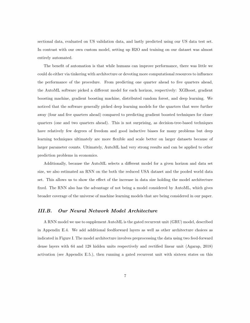
III.B. Our Neural Network Model Architecture

A RNN model we use to supplement AutoML is the gated recurrent unit (GRU) model, described

in Appendix E.4. We add additional feedforward layers as well as other architecture choices as

indicated in Figure I. The model architecture involves preprocessing the data using two feed-forward

dense layers with 64 and 128 hidden units respectively and rectified linear unit (Agarap, 2018)

activation (see Appendix E.5.), then running a gated recurrent unit with sixteen states on this

7

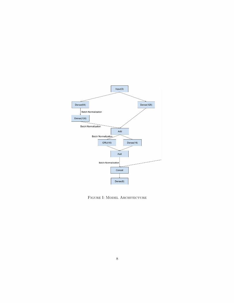
Figure I: Model Architecture

8

preprocessed data.2 Finally the output of the GRU is concatenated with the original input (lagged

GDP, consumption and unemployment) and fed into a linear layer which forecasts an output.

Our model contains parallel dense layers between each operation; the layers were originally skip

connections (He et al., 2015), but we modified them to allow for learning of linear parameters. The

final skip connection concatenates the input with the output of the network so that the neural

network would nest an VAR(1) model. These design choices all improved forecasting performance.

Between all of our non-skip connection layers, we also use batch normalization (Ioffe and Szegedy,

2015). More details on batch normalization can also be found in Appendix E.6. Ultimately, our

model comprises about 17,000 parameters which explains the comparative outperformance on a

data rich regime.

IV. Economic Models

We tested the predictive power of a series of machine learning and traditional macroeconomic

models estimated on our panel of countries using our novel data pooling method. We found that the

more complex the model, the more our data augmentation helped. The machine learning models

tended to be more flexible, but even among economic models the trend still held. Additionally, we

provided comparisons to the Survey of Professional Forecasters (None, 1968) median GDP forecast,

which is seen as a proxy for state-of-the-art performance. A discussion of the Survey of Professional

Forecasters and our attempt to evaluate their forecasts is contained in Appendix C. The baseline

economic models we used are the AR(2) autoregressive model, the Smets-Wouters 2007 DSGE

model (Smets and Wouters, 2007), and a factor model (Stock and Watson, 2002a), (Stock and

Watson, 2002b) and a VAR(4)/VAR(1) (Sims, 1980). A more detailed explanation of these models

is contained in Appendix D. For the linear models, getting cross country data is straightforward,

thus we compare those models estimated only on US data as well as on our data set of 50 countries.

2. While we use the word preprocessed, the approach is trained entirely end-to-end and is not a two step processas the word preprocess might imply. The neural network projects the input data – consumption growth, GDP growthand the unemployment rate – into a high dimensional state that the gated recurrent unit finds easier to work withmuch like pre-processing would. The end-to-end procedure learns the pre-processing and the gated recurrent unitanalysis at the same time

9

For the Smets-Wouters DSGE, we also assembled a panel of 27 rich and developing countries to

estimate the structural model on.

As is standard with economic forecasting, the baseline models were trained in a pseudo-out-of-

sample fashion where the training set/validation set expands as the forecast date becomes more

recent. However, with our neural network and AutoML, we keep the training set and validation

set fixed due to computational costs and programming constraints. We expect that our model will

improve if we use a pseudo-out-of-sample approach.

V. Data and Method

When initially training our complex neural network models, we found that United States macroe-

conomic data was not sufficient so, in order to train the model, we use data from 49 other developed

and developing countries as listed in Appendix A. We source cross country data from Trading Eco-

nomics via the Quandl platform API3 as well as GDP data from the World Bank.4 We used GDP,

consumption, and the unemployment rate as inputs to the model. GDP and consumption were all

expressed in growth rates. Unemployment was expressed as a rate as well. As mentioned earlier,

we also assembled 11 different covariates across 27 countries for a panel of data used to estimate the

Smets-Wouters DSGE. Data came from the Federal Reserve Economic Data (FRED), World Bank,

Eurostat, the Organization for Economic Cooperation (OECD) and the International Monetary

Fund (IMF).

We split our data into training, validation, and test sets. We forecast GDP, and evaluated

with RMSE. The test set was from 2008-Q4 to 2020-Q1, either testing only US data or world data

depending on the particular problem. The validation consisted of data from 2003-Q4 to 2008-Q3,

which was only used for the RNN. This data was in the training set for all other models. AutoML,

which was not a sequential model, used k-fold cross validation on the entire training set, comprised

of the remainder of data not in test or validation sets. We chose these periods so that both the

test set and the validation set would have periods of both expansion and recession, based on the

3. https://www.quandl.com/tools/api4. World Development Indicators, The World Bank

10

US business cycle. Including the 2001 recession in the validation set would leave the model without

enough training data, so we split the data of the Great Recession over the test and validation set.

The quarter with the fall of Lehman Brothers and the largest dip in GDP was the first quarter in

our test set, 2008-Q4. Two quarters with negative growth preceding this were in the validation set.

We estimated all models from a horizon of one quarter ahead to five quarters ahead. The metric of

choice for forecast evaluation was RMSE.

VI. Results

Our first set of results shows the benefit of pooled data on reduced-form models VARs and

ARs, showing significantly improved GDP forecasting accuracy. Despite the relative parsimony

of these models adding pooled data improves RMSE performance almost uniformly by an average

of 12%. Our second set of results shows that the panel data augmentation improved the chances

of building externally and potentially, internally valid structural models, using the Smets-Wouters

DSGE model as the main benchmark. These models benefited more due to the pooled data as

they had a higher parameter count, improving RMSE by 24%. Our third set of results took all the

models and demonstrates the forecasting power of “nonparametric” machine learning models over

all the previously mentioned traditional economic models in this relatively data rich regime. As

these models were the largest and most data hungry, the use of pooled data improved performance

from slightly above average forecasters to providing state-of-the-art predictions across the board.

The RMSE of the RNN-based model improved by 23%, which was smaller than the structural

models. However, the RMSE starting point was much better than that of the structural models

and proportional performance was more difficult the better the original baseline. Ultimately, we

present an interesting finding in the improvement in performance as model capacity increased,

moving from the US data set to the pooled world data set. This suggests that more complex

models benefit from increasingly larger datasets and that pooling can address overfitting.

11

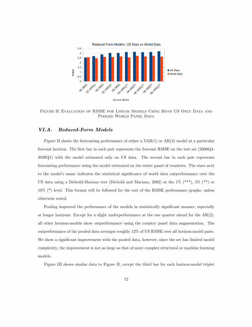
Figure II: Evaluation of RMSE for Linear Models Using Both US Only Data andPooled World Panel Data

VI.A. Reduced-Form Models

Figure II shows the forecasting performance of either a VAR(1) or AR(2) model at a particular

forecast horizon. The first bar in each pair represents the forecast RMSE on the test set (2008Q4-

2020Q1) with the model estimated only on US data. The second bar in each pair represents

forecasting performance using the model estimated on the entire panel of countries. The stars next

to the model’s name indicates the statistical significance of world data outperformance over the

US data using a Diebold-Mariano test (Diebold and Mariano, 2002) at the 1% (***), 5% (**) or

10% (*) level. This format will be followed for the rest of the RMSE performance graphs, unless

otherwise noted.

Pooling improved the performance of the models in statistically significant manner, especially

at longer horizons. Except for a slight underperformance at the one quarter ahead for the AR(2),

all other horizon-models show outperformance using the country panel data augmentation. The

outperformance of the pooled data averages roughly 12% of US RMSE over all horizon-model pairs.

We show a significant improvement with the pooled data, however, since the set has limited model

complexity, the improvement is not as large as that of more complex structural or machine learning

models.

Figure III shows similar data to Figure II, except the third bar for each horizon-model triplet

12

Figure III: Reduced-Form Time Out-of-Sample as Well as Country Out-of-SampleForecasts

shows forecasting performance on the same US test data, but for a model that is both time step and

country out-of-sample. For example, since we forecasted US GDP, we used every country but the US

to forecast US GDP. This test enables us to show that using panel data can lead to models that are

policy/country invariant and can generalize even to country data that the model lacked access to.

In all cases, the RMSE of the out-of-sample forecasts were statistically indistinguishable from the

RMSE of the model estimated on the full panel of countries but significant over the US baseline with

stars indicating significance of the out-of-sample forecast. Again the models were mainly significant

at longer horizons, but any significance is nevertheless impressive since the outperforming model

uses no US data to forecast US GDP, for example. Excluding the H1 AR(2) pair and using only

the out-of-sample data led to capturing 79%, on average, of the outperformance of the world panel

over US only data forecasts. Ultimately, there was an improvement in performance due to the use

of the pooled data over single country training data.

We performed the same tests over our entire cross-section of countries, in Table I. For example,

for each local forecast, we used only French data to forecast French GDP. Likewise, for world

forecasts, we used the entire data set to estimate a single model, then for each country we used

the same model to jointly forecast the GDP of every country and average RMSE values across

countries. For out-of-sample data, a different model is trained to forecast each country, but each

13

TABLE I: Average Forecasting Performance Evaluated over the World

Time (Q’s Ahead) 1Q 2Q 3Q 4Q 5QAR(2)

Local Data 5.22 5.33 5.51 5.56 5.60World Data 4.88 4.98 5.10 5.19 5.19Out-of-Sample Data 5.07 5.13 5.36 5.36 5.38

VAR(1)Local Data 5.10 5.17 5.19 5.29 5.26World Data 4.80 4.94 5.04 5.11 5.12Out-of-Sample Data 4.92 5.00 5.07 5.20 5.25

VAR(4)Local Data 7.90 7.05 7.74 7.87 9.27World Data 4.72 4.90 5.03 5.10 5.11Out-of-Sample Data 4.70 4.87 5.02 5.17 5.26

model is estimated using every country but the country of forecasting interest. Aside from providing

an additional robustness test regarding the outperformance of world data and even out-of-sample

data, this table shows additional policy-invariance both from the out-of-sample tests as well as the

world data tests, where the same model can jointly forecast all countries better than custom tailored

models for each country. Additionally, this model seems to indicate a diminishing return in terms

of RMSE for linear models when using pooling data and it seems like all linear models converge

to a similar RMSE, although the larger VAR(4) models seem to have the best performance and

suggests improvement when moving to more complex structural and machine learning models.

VI.B. Structural Models

Considering the success of data pooling for reduced-form models, we also tested the procedure

on structural models and achieved even greater success. Since the DSGE model requires 11 different

variables, we assembled our own data from the World Bank, OECD, Eurostat, and FRED. This

panel has only a 27 country cross-section which is smaller than the 50-country panel used in our

reduced-form models. The performance of our structural models demonstrates that this pooling of

data likely leads to performance gains across models, including DSGE models that should generalize

to out-of-sample data because of their resilience to the Lucas critique. Combined with the results

14

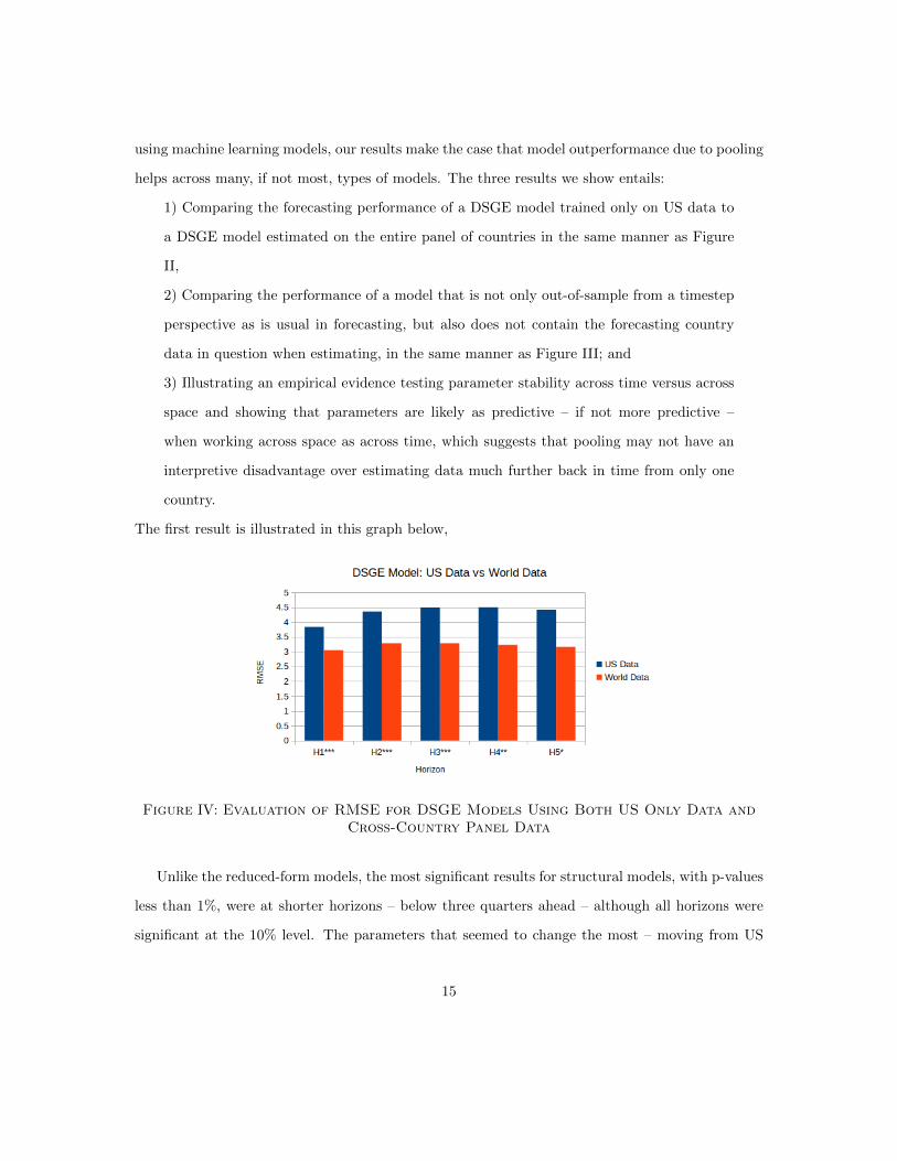
using machine learning models, our results make the case that model outperformance due to pooling

helps across many, if not most, types of models. The three results we show entails:

1) Comparing the forecasting performance of a DSGE model trained only on US data to

a DSGE model estimated on the entire panel of countries in the same manner as Figure

II,

2) Comparing the performance of a model that is not only out-of-sample from a timestep

perspective as is usual in forecasting, but also does not contain the forecasting country

data in question when estimating, in the same manner as Figure III; and

3) Illustrating an empirical evidence testing parameter stability across time versus across

space and showing that parameters are likely as predictive – if not more predictive –

when working across space as across time, which suggests that pooling may not have an

interpretive disadvantage over estimating data much further back in time from only one

country.

The first result is illustrated in this graph below,

Figure IV: Evaluation of RMSE for DSGE Models Using Both US Only Data andCross-Country Panel Data

Unlike the reduced-form models, the most significant results for structural models, with p-values

less than 1%, were at shorter horizons – below three quarters ahead – although all horizons were

significant at the 10% level. The parameters that seemed to change the most – moving from US

15

only data to world data – were the shocks and the moving averages of the shock variable, monetary

policy Taylor-rule variables, and variables governing wages and inflation. While the increasing

variance of the shocks did not affect expected forecasts due to certainty equivalence, the model is

both less confident and closer to correct when using pooled world data. Perhaps it is unsurprising

that variables focusing on monetary policy and inflation are different when estimated on world data.

Inflation, especially among rich developing countries, along with the monetary response to them,

was a more pernicious problem outside the US than within (Azam and Khan, 2020). For more

information on the changes in structural variables when moving from US data to pooled world data

see Appendix F.3.

Despite the increased uncertainty of the model as illustrated by the increase in the standard

deviation of the shocks, the parameters were more reliable when estimated under world data.

The improvement in RMSE averages over 25% over all horizons, which was more than double the

percentage improvement for reduced-form models. Part of the outperformance was due to weaker

performance of the models estimated on US data. This suggests that the Smets-Wouters model is

no better at generalizing across policy regimes or countries than reduced-form models and benefits

more because of its higher parameter count.

Figure V: DSGE Time Out-of-Sample as Well as Country Out-of-Sample Forecasts

In Figure V, we also provide a structural chart that parallels the out-of-sample chart in Figure

III in the reduced-form section. As a reminder, the out-of-sample DSGE model was estimated

16

on the panel of 26 countries (removing the US) so that the GDP forecast was country out-of-

sample as well as time step out-of-sample. The out-of-sample performance was 9% better, on

average, than even the performance of a DSGE estimated on the entire world data. However, the

Diebold-Mariano tests are less significant with only the first two horizons having p-values with

less than 1% and no significance in horizon four and five. This suggests that the out-of-sample

outperformance may in part be due to chance, and we studied this in further detail below. Since

the United States was the only country which has data that extends much before 2000 across

all our needed variables, we hypothesized that DSGE model parameters were more stable across

countries than across time. Removing the US made the data closer in time to the test set. This

addresses an internal validity criticism of our panel approach arguing that when pooled structural

parameters have different values across countries, estimating a single model on all countries strips

the parameters of economic meaning (Pesaran and Smith, 1995). For example the parameter no

longer represents the depreciation rate of the United States, but an average depreciation rate across

30 countries. This result provides a suggestive counter argument to that claim, by pointing out

that, considering one needs a certain number of data points to get accurate predictions to begin

with, using data across a cross section of countries provides forecasts that at least as good as using

data the extends further in time.

Probing this hypothesis led to results that were somewhat mixed. We estimated a model trained

on the entire panel of countries with data from 1995-Q1 onward. This affected three countries –

the US, Japan and New Zealand. This procedure isolates more sharply the effect of similarity

across space versus across time on model generalization, rather than just removing all US data.

The US lost about 140-190 data points (as the test set requires rolling forecasts), and New Zealand

and Japan both lost about 15-60 timesteps. Figure VI, illustrates this experiment to compare the

performance of models estimated on data since 1995 to models estimated with full country and

timesteps.

Figure VI shows GDP forecasts on the same test set: 2008Q4-2020Q1. The first bar in each

triplet is the DSGE model performance estimated using world data across all periods in time. The

second bar is the out-of-sample performance as shown in Figure V. The third bar is the performance

17

Figure VI: This Graph Compares Parameter Stability via Forecasts Going Back inTime Versus Space

of a DSGE model estimated on all country data, but only since 1995 to make the data more relevant

across time to the test set. The 1995 onwards data performed worse than the out-of-sample test

which could suggest some of the outperformance of the out-of-sample DSGE model was due to

chance. However, it seems that the 1995 data performed at least as well as a model estimated on

world data both pre and post-1995, despite our robust results suggesting that more data is generally

better. This makes some practical sense when considering something like the advent of software,

the depreciation rate in France in 2015 plausibly shares more in similarities with the depreciation

rate in the US in 2020 than the depreciation rate of the US in 1960. As one needs a set number

of data points to identify structural models anyway, our results provide suggestive evidence that

getting cross-sectional data results in parameters that are no less stable than parameters going back

in time. The results seem inconclusive but certainly don’t suggest any more parameter stability

across time than space, in contrast with the potential pitfall highlighted by Pesaran and Smith

(1995) and generally accepted in the literature.

The DSGE models we estimated generally underperformed the parameters recovered in the

original Smets and Wouters (2007), because we focused on maximum likelihood estimation with-

out priors, optimized only with gradient descent. Despite the forecasting success of (Smets and

Wouters, 2007) and other Bayesian DSGE models (Herbst and Schorfheide, 2015), (Fernandez-

18

Villaverde, Rubio-Ramırez and Schorfheide, 2016), we chose to use to use a maximum likelihood

approach to maintain comparability to the reduced-form and machine learning experiments as well

as a large portion of the applied literature that focuses on point estimate techniques ranging from

calibration, maximum likelihood, to generalized method of moments (Hansen and Singleton, 1982).

However, Figure V as well as Appendix G.1 shows the performance of a model estimated via max-

imum likelihood outperformed along some horizons the parameters of Smets and Wouters (2007).

Given the limitations of maximum likelihood and our differing focus, we see this outperformance

as an endorsement of the use of the pooling approach. We show that the use of pooled data re-

sults in the Smets-Wouters DSGE model outperforming DSGE models estimated only on US data.

Furthermore, we provided suggestive evidence that is possible that models are more externally and

internally valid if one uses data across countries in addition to the statistically significant improve-

ment in generalization. Using our out-of-sample tests, we show that these models can improve

the out-of-sample generalization of the Smets-Wouters DSGE model even if they are theoretically

policy-invariant. The data shown in the charts are also be displayed in Appendix G.1. As a final

note, while it is difficult to quantify improved performance of calibration and generalized methods

of moments, based on the generalization improvements from estimation for both reduced-form and

structural models, we imagine these results should generalize and macroeconomists would benefit

from calibrating to moments as well as other methods that feature a large number of countries.

VI.C. Nonparametric Machine Learning Models

Given the improvement in forecasting performance for both the reduced-form and structural

models and the improving relative performance of complex models, we decided to test the per-

formance of nonparametric models that are even more flexible than the DSGEs and some of the

larger VARs. We tested both a RNN, as well as an AutoML algorithm. While the improvement in

performance was less than the DSGE improvement from pooled data, it still seems more impressive

given that the flexible models had much better performance even on US data. This again illustrates

the trend that increased parameter count leads to a gain in performance that came from pooling.

Two charts below illustrate performance of the RNN and AutoML models on both US and

19

pooled world data.

Figure VII: Evaluation of RMSE for RNN models Using Both US Only Data andCross-Country Panel Data

We compared estimation on US data as well as pooled world data, for both models. For the

RNN, Figure VII shows the improvement in RMSE from estimating a recurrent neural network using

only US data to using the entire cross-section of 50 countries. The improvement was statistically

significant for all horizons except five quarters ahead. The average improvement was around 23%

over all horizons, which was similar to the improvement for the Smets-Wouters model and almost

double the improvement of linear models. This is a reassuring confirmation as the RNN is a data

hungry model that benefits more from data rich regimes. We also attempted to add a country

identifier term to our model. For example, using GDP per capita at the time of prediction as an

input to localize the pooled data to some degree. While this might be expected to reduce bias, it

didn’t improve out of sample performance to any degree. This potentially suggests that countries

are more similar than different and the bias of pooling different countries has a limited effect, while

adding in such a covariate leads to more overfitting.

Our second chart in Figure VIII, shows the same performance graph for AutoML. The perfor-

mance gain is not as easily interpreted as AutoML benefits from the pooled data but can also pick

different models that gains relatively in both data poor and data rich regimes. Because of that,

the large gains of the RNN are more representative of performance gains from moving to pooled

20

Figure VIII: Evaluation of RMSE for AutoML Using Both US Only Data andCross-Country Panel Data

data on a fixed machine learning models. It has the least improvement in performance when using

the panel of countries as training data, with average improvements in RMSE of about 7.5%. Only

the first two horizons show statistically significant forecast performance. It’s worth pointing out

that the improvements are still significant along some horizons, especially in light of nearly state-

of-the-art performance using only US data to begin with. Even so, only in four quarters ahead does

the AutoML model outperform all the baseline models trained on US data. When estimated on

world data, AutoML outperforms all economic models on all horizons except three quarters ahead

and its performance at one quarter ahead rivals the Survey of Profession Forecasters, despite being

estimated only on lags of GDP, consumption, and unemployment and no real time data.

VI.D. Summary

The previous sections outlined performance of all reduced-form, structural, and machine learning

models. This section takes all the data and provides results from a holistic perspective. We

first compare forecasting models using all approaches, estimated on both pooled and US data.

This table demonstrates the effectiveness of the machine learning forecasting methods in data

rich regimes. AutoML estimated on world data outperforms all baseline economic models on four

of the five horizons and the RNN outperforms on longer term horizons. We do not report the

21

maximum likelihood of the Smets-Wouters model, as the original Bayesian parameterization has

better performance than either of our maximum likelihood Smets-Wouters models estimated on

world or US data. Introducing our other DSGE variations, would be difficult to justify and would

also have no effect on the results of the horse race. Regardless, all of our models that outperform

all baseline models on a horizon are bolded. No baseline model ever outperformed both our models

along any horizon and the best performing model along all horizons was either an AutoML model

or an RNN model, likely because the additional pooled data allowed a more powerful model to be

used without overfitting.

TABLE II: RMSE of Our RNN, AutoML, and Baseline Models

Time (Q’s Ahead) 1Q 2Q 3Q 4Q 5QVAR(4)

US Data 2.99 3.03 3.10 3.08 3.08World Data 2.37 2.52 2.56 2.63 2.63

AR(2)US Data 2.53 2.88 3.03 3.14 3.13World Data 2.57 2.62 2.67 2.72 2.72

Smets-Wouters DSGE BayesianUS Data 2.79 2.95 2.89 2.80 2.71

FactorUS Data 2.24 2.48 2.50 2.67 2.86

RNN (Ours)US Data 3.46 3.37 3.01 3.23 3.30World Data 2.35 2.52 2.50 2.62 2.60

AutoML (Ours)US Data 2.41 2.58 2.71 2.45 2.92World Data 1.97 2.32 2.59 2.62 2.61

SPF Median 1.86 2.11 2.36 2.46 2.65

To illustrate the effect that pooling data has on forecasting, we show a graph that orders RMSE

performance based on increasing model complexity with RMSE performance, comparing the trend

when estimated on US data versus pooled data.

As the image shows, when using increasingly complex models with only the three hundred or

so US timesteps, the most parsimonious model, the AR(2),performs the best and the models get

progressively worse. However, when using the pooled data, the picture is entirely different. The

AR(2) model actually performs a little bit worse – likely due to chance. However, each progressively

22

Figure IX: RMSE and Model Complexity

larger model improves on the AR(2) performance. Even if the RMSE decline is less striking in this

latter case, this decline is never less compelling as the improvement is actually quite large but

looks small as the US data RNN performs so poorly, it would never be used. In fact, despite the

appearance of only a small improvement due to model complexity, the performance of the RNN on

pooled data is state-of-the-art, while the performance of the AR(2) on pooled data is somewhat

pedestrian. A similar story holds across other horizons with less striking consistency compared to

the one period ahead story.

We also provide a graph of the forecasts of five of the models: AR(2), factor, DSGE, RNN, and

AutoML, as well as the true data. This graph is useful in disentangling why our machine learning

models outperform. To illustrate the relative strengths of the models, we display the one quarter

ahead forecasts in Figure X here and the rest of the graphs are in Appendix B.

AutoML, factor, and RNN models all did a good job at forecasting the Great Recession, with

AutoML forecasting the best at one quarter ahead. The AR(2) and DSGE did not detect a regime

change for the recessionary periods and are also upwardly biased leading to even worse performance

during recession onset.5 However, the XGBoost model that performed the best in AutoML was sat-

isfactory forecast the expansions both in terms of the average level as well as individual movements

in the quarterly data. Neither the factor model nor the RNN were able to forecast the quarter by

5. More information on the biases and variances of the different models can be found in Appendix F.2.

23

Figure X: One Quarter Ahead - Forecasts

quarter movements with such accuracy. More information about the performance, with a focus on

our RNN model, is labeled in our robustness checks in Appendix G.2.

VII. Conclusion

In this paper we show how estimating macroeconomic models on a panel of countries, as opposed

to a single country can significantly improve external validity. Using a panel of countries as a training

set, we statistically improved the RMSE performance of reduced-form models – AR(2), VAR(1),

and VAR(4) – by roughly 12%. We further show that we can make these reduced-form models more

policy/country invariant, suggesting that these models have learned to generalize GDP forecasting

even to countries the model has never been trained on.

We also showed that a similar training set of a panel of countries can improve external validity

of structural models which again are typically estimated only on a single country of interest. We

focus on the Smets-Wouters model (Smets and Wouters, 2007). Using a panel of countries improves

the forecasting performance of the Smets-Wouters model estimated with maximum likelihood by

roughly 24% averaged across horizons. These results are again statistically significant. We then

demonstrated that we can again improve policy-invariance and generalization to out-of-sample

24

countries by using a panel of countries in our training set. Additionally, we addressed one potential

roadblock to the adoption of pooling country data, which is the fact that the structural parameters

may not be stable across countries and hence the pooled parameter value can only be interpreted

as a mean value. While our results are less conclusive on this front, we argue that based on a

forecasting exercise that parameter generalization and stability are likely as good across space as

across time. Finally, concluding our section on structural models, we capitalize on the consistency of

improvements and discuss the likelihood that our results will extend to other estimation techniques

like generalized method of moments, calibration, and Bayesian approaches.

Our last set of results, recognizes that our dataset has increased from 300 timesteps to around

3000 timestep-countries, showing that nonparametric machine learning models are able to outper-

form all the economic baseline models even after being estimated in this more data rich regime.

Our RNN outperforms all economic baselines for horizons longer than two periods ahead. Likewise,

our AutoML model outperforms all baselines for all horizons except for the three quarters ahead.

Combined, the best performing model over all horizons is either an AutoML model or a recurrent

neural network model which suggests there is likely much more room to test other nonparametric

models in the more data rich macroeconomic regime.

25

References

Adjemian, Stephane, Houtan Bastani, Michel Juillard, Frederic Karame, JuniorMaih, Ferhat Mihoubi, Willi Mutschler, George Perendia, Johannes Pfeifer,Marco Ratto, and Sebastien Villemot. 2011. “Dynare: Reference Manual Version 4.”CEPREMAP Dynare Working Papers 1.

Agarap, Abien Fred. 2018. “Deep Learning using Rectified Linear Units (ReLU).” CoRR,abs/1803.08375.

Azam, Muhammad, and Saleem Khan. 2020. “Threshold effects in the relationship betweeninflation and economic growth: Further empirical evidence from the developed and developingworld.” International Journal of Finance & Economics.

Bai, Jushan, and Serena Ng. 2010. “Instrumental variable estimation in a data rich environ-ment.” Econometric Theory, 1577–1606.

Baltagi, Badi H. 2008. “Forecasting with panel data.” Journal of forecasting, 27(2): 153–173.Banerjee, Anindya, Massimiliano Marcellino, and Chiara Osbat. 2004. “Some cautions

on the use of panel methods for integrated series of macroeconomic data.” The EconometricsJournal, 7(2): 322–340.

Breitung, Joerg. 2015. “The analysis of macroeconomic panel data.” In The Oxford Handbookof Panel Data.

Cho, KyungHyun, Bart van Merrienboer, Dzmitry Bahdanau, and Yoshua Bengio.2014. “On the Properties of Neural Machine Translation: Encoder-Decoder Approaches.”CoRR, abs/1409.1259.

Chung, Junyoung, Caglar Gulcehre, KyungHyun Cho, and Yoshua Bengio. 2014. “Em-pirical evaluation of gated recurrent neural networks on sequence modeling.” arXiv preprintarXiv:1412.3555.

Crandall, Robert W, William Lehr, and Robert E Litan. 2007. “The effects of broadbanddeployment on output and employment: A cross-sectional analysis of US data.”

Diebold, Francis X. 1998. Elements of forecasting. South-Western College Pub.Diebold, Francis X, and Robert S Mariano. 2002. “Comparing predictive accuracy.” Journal

of Business & economic statistics, 20(1): 134–144.Diebold, Francis X, Glenn D Rudebusch, and S Boragan Aruoba. 2006. “The macroe-

conomy and the yield curve: a dynamic latent factor approach.” Journal of econometrics,131(1-2): 309–338.

Doran, Howard E, and Peter Schmidt. 2006. “GMM estimators with improved finite sampleproperties using principal components of the weighting matrix, with an application to thedynamic panel data model.” Journal of econometrics, 133(1): 387–409.

Edge, Rochelle M, Michael T Kiley, and Jean-Philippe Laforte. 2010. “A comparison offorecast performance between federal reserve staff forecasts, simple reduced-form models, anda DSGE model.” Journal of Applied Econometrics, 25(4): 720–754.

Fernandez-Villaverde, Jesus, and Juan F Rubio-Ramırez. 2007. “Estimating macroeco-nomic models: A likelihood approach.” The Review of Economic Studies, 74(4): 1059–1087.

Fernandez-Villaverde, Jesus, Juan Francisco Rubio-Ramırez, and Frank Schorfheide.2016. “Solution and estimation methods for DSGE models.” In Handbook of macroeconomics.Vol. 2, 527–724. Elsevier.

26

F, Hutter, Caruana R, Bardenet R, Bilenko M, Guyon, Kegl B, and Larochelle H.2014. “AutoML 2014 @ ICML.”

Hansen, Lars Peter, and Kenneth J Singleton. 1982. “Generalized instrumental variablesestimation of nonlinear rational expectations models.” Econometrica: Journal of the Econo-metric Society, 1269–1286.

He, Kaiming, Xiangyu Zhang, Shaoqing Ren, and Jian Sun. 2015. “Deep Residual Learn-ing for Image Recognition.”

Herbst, Edward P, and Frank Schorfheide. 2015. Bayesian estimation of DSGE models.Princeton University Press.

Hochreiter, Sepp, and Jurgen Schmidhuber. 1997. “Long Short-Term Memory.” NeuralComput., 9(8): 1735–1780.

Hochreiter, Sepp, Martin Heusel, and Klaus Obermayer. 2007. “Fast model-based proteinhomology detection without alignment.” Bioinformatics, 23(14): 1728–1736.

Hornik, Kurt, Maxwell Stinchcombe, and Halbert White. 1989. “Multilayer feedforwardnetworks are universal approximators.” Neural Networks, 2(5): 359 – 366.

Ioffe, Sergey, and Christian Szegedy. 2015. “Batch Normalization: Accelerating Deep Net-work Training by Reducing Internal Covariate Shift.”

Kaplan, Jared, Sam McCandlish, Tom Henighan, Tom B. Brown, Benjamin Chess,Rewon Child, Scott Gray, Alec Radford, Jeffrey Wu, and Dario Amodei. 2020.“Scaling Laws for Neural Language Models.” CoRR, abs/2001.08361.

Kingma, Diederik P., and Jimmy Ba. 2014. “Adam: A Method for Stochastic Optimization.”Koop, Gary, Roberto Leon-Gonzalez, and Rodney Strachan. 2012. “Bayesian model aver-

aging in the instrumental variable regression model.” Journal of Econometrics, 171(2): 237–250.LeDell, Erin, and S Poirier. 2020. “H2o automl: Scalable automatic machine learning.”Li, Xiaohua, Weijin Zhuang, and Hong Zhang. 2020. “Short-term Power Load Forecasting

Based on Gate Recurrent Unit Network and Cloud Computing Platform.” 1–6.Mayer, H., F. Gomez, D. Wierstra, I. Nagy, A. Knoll, and J. Schmidhuber. 2006. “A

System for Robotic Heart Surgery that Learns to Tie Knots Using Recurrent Neural Networks.”543–548.

McCracken, Michael W, and Serena Ng. 2016. “FRED-MD: A monthly database for macroe-conomic research.” Journal of Business & Economic Statistics, 34(4): 574–589.

Minh, Dang Lien, Abolghasem Sadeghi-Niaraki, Huynh Duc Huy, Kyungbok Min,and Hyeonjoon Moon. 2018. “Deep learning approach for short-term stock trends predictionbased on two-stream gated recurrent unit network.” Ieee Access, 6: 55392–55404.

Miyamoto, Wataru, Thuy Lan Nguyen, and Dmitriy Sergeyev. 2018. “Government spend-ing multipliers under the zero lower bound: Evidence from Japan.” American Economic Jour-nal: Macroeconomics, 10(3): 247–77.

None. 1968. “Survey of Professional Forecasters.” https: // www. philadelphiafed. org/

research-and-data/ real-time-center/ survey-of-professional-forecasters , Ac-cessed: 2020-09-01.

Pesaran, M Hashem, and Allan Timmermann. 1992. “A simple nonparametric test of pre-dictive performance.” Journal of Business & Economic Statistics, 10(4): 461–465.

Pesaran, M Hashem, and Ron Smith. 1995. “Estimating long-run relationships from dynamicheterogeneous panels.” Journal of econometrics, 68(1): 79–113.

Polyak, Boris. 1964. “Some methods of speeding up the convergence of iteration methods.” UssrComputational Mathematics and Mathematical Physics, 4: 1–17.

27

Rumelhart, David E, Geoffrey E Hinton, and Ronald J Williams. 1986. “Learning rep-resentations by back-propagating errors.” nature, 323(6088): 533–536.

Shi, Xingjian, Zhourong Chen, Hao Wang, Dit-Yan Yeung, Wai-kin Wong, and Wang-chun Woo. 2015. “Convolutional LSTM Network: A Machine Learning Approach for Precipi-tation Nowcasting.” In Advances in Neural Information Processing Systems 28. , ed. C. Cortes,N. D. Lawrence, D. D. Lee, M. Sugiyama and R. Garnett, 802–810. Curran Associates, Inc.

Sims, Christopher A. 1980. “Macroeconomics and Reality.” Econometrica, 48(1): 1–48.Smalter Hall, Aaron, and Thomas R Cook. 2017. “Macroeconomic indicator forecasting

with deep neural networks.” Federal Reserve Bank of Kansas City Working Paper, , (17-11).Smets, Frank, and Rafael Wouters. 2007. “Shocks and frictions in US business cycles: A

Bayesian DSGE approach.” The American Economic Review, 97(3): 586–606.Stock, James H, and Mark W Watson. 2002a. “Forecasting using principal components from

a large number of predictors.” Journal of the American statistical association, 97(460): 1167–1179.

Stock, James H, and Mark W Watson. 2002b. “Macroeconomic forecasting using diffusionindexes.” Journal of Business & Economic Statistics, 20(2): 147–162.

Thornton, Chris, Frank Hutter, Holger H Hoos, and Kevin Leyton-Brown. 2013. “Auto-WEKA: Combined selection and hyperparameter optimization of classification algorithms.”847–855.

Tieleman, T., and G. Hinton. 2012. “Lecture 6.5—RmsProp: Divide the gradient by a runningaverage of its recent magnitude.” COURSERA: Neural Networks for Machine Learning.

Timmermann, Allan. 2006. “Forecast combinations.” Handbook of economic forecasting, 1: 135–196.

Walker, Gilbert Thomas. 1931. “On periodicity in series of related terms.” 131(818): 518–532.Watson, MW. 2001. “Time series: economic forecasting.” International Encyclopedia of the

Social & Behavioral Sciences, 15721–15724.West, Kenneth D. 1996. “Asymptotic inference about predictive ability.” Econometrica: Journal

of the Econometric Society, 1067–1084.Wright, Jonathan H. 2008. “Bayesian model averaging and exchange rate forecasts.” Journal

of Econometrics, 146(2): 329–341.Zerroug, A, L Terrissa, and A Faure. 2013. “Chaotic dynamical behavior of recurrent neural

network.” Annu. Rev. Chaos Theory Bifurc. Dyn. Syst, 4: 55–66.

28

VIII. Appendix

A Selected Countries

Countries in reduced-form data set: Australia, Austria, Belgium, Brazil, Canada, Switzerland,

Chile, Columbia, Cyprus, Czech Republic, Germany, Denmark, Spain, Estonia, European Union,

Finland, France, Great Britain, Greece, Hong Kong, Croatia, Hungry, Ireland, Israel, Italy, Japan,

Korea, Luxembourg, Latvia, Mexico, Mauritius, Malaysia, Netherlands, Norway, New Zealand,

Peru, Philippines, Poland, Portugal, Romania, Russia, Singapore, Slovakia, Slovenia, Sweden, Thai-

land, Turkey, USA and South Africa.

Countries in structural data set: Australia, Austria, Belgium, Canada, Chile, Columbia, Ger-

many, Denmark, Spain, Estonia, Finland, France, Iceland, Israel, Italy, Japan, Korea, Lithuania,

Luxembourg, Mexico, Netherlands, New Zealand, Poland, Portugal, Slovakia, Slovenia, Sweden,

USA

B Selected Performance: Graphs

Figure XI: One Quarter Ahead - Forecasts

29

Figure XII: Two Quarters Ahead - Forecasts

Figure XIII: Three Quarters Ahead - Forecasts

30

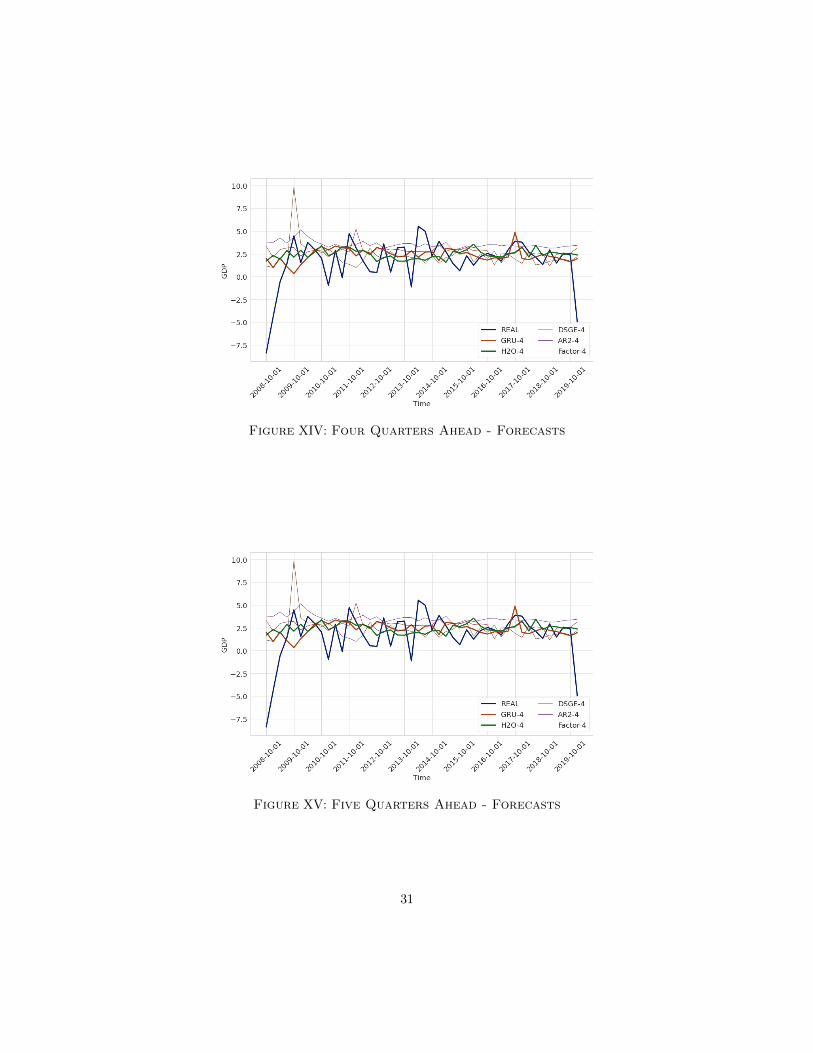
Figure XIV: Four Quarters Ahead - Forecasts

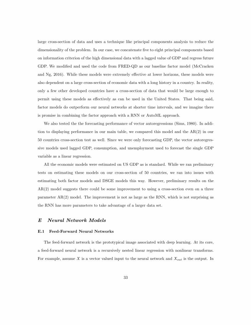
Figure XV: Five Quarters Ahead - Forecasts

31

C Details on the Survey of Professional Forecasters

While our model used the 2020 vintage of data, in reality, the forecasters for the Survey of

Professional Forecasters were working with pseudo-out-of-sample vintages when forecasting over

the entire test. While reproducing this would be possible from using old vintages, it would require

estimating the model at every time step of the test set as the data would change every period. We

wanted to avoid this pseudo-out-of-sample forecasting as it would result in estimating 4600 models

instead of 100 at each horizon. Beyond this, the benefit of this increased computation was not

clear as we would still be using 2020 vintage data for countries outside the US, many of which old

vintages are difficult or impossible to find. So, it was easier to compare the SPF performance on the

2020 vintage. Plus, all our baseline models including world forecasts were estimated and evaluated

using the 2020 vintage as well, so this choice allowed us to compare the SPF performance with the

performance of all the baseline models.

D Detailed Description of Economic Baseline Models

A first model we use is the autoregressive model, AR(n). An oft-used benchmark model, it

estimates a linear relationship using the independent variable lagged N times. In terms of forecasting

ability, this model is competitive with or outperforms the other economic models in our tests which

is consistent with Diebold (1998). We used an autoregressive model with two lags and a constant

term.

Additionally, we compared the Smets-Wouters 2007 model (Smets and Wouters, 2007), as DSGE

models share many similarities with recurrent neural networks and Smets-Wouters (2007) suggests

that this particular model can outperform VARs and BVARs in forecasting. When running this, we

used the standard Smets-Wouters Dynare code contained on the published paper’s data appendix.

We take the point forecasts from the Smets and Wouters (2007) and use that to forecast. Like

Smets and Wouters (2007), we use Dynare (Adjemian et al., 2011) to solve and estimate the model.

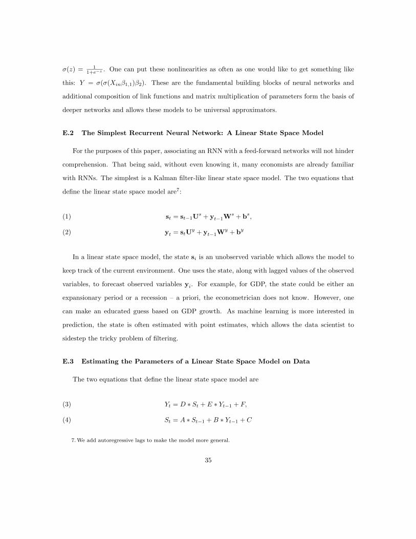
A final model we included in our baseline economic models were factor models (see Stock and

Watson (2002a) and Stock and Watson (2002b)). In short, the factor model approach takes a

32

large cross-section of data and uses a technique like principal components analysis to reduce the

dimensionality of the problem. In our case, we concatenate five to eight principal components based

on information criterion of the high dimensional data with a lagged value of GDP and regress future

GDP. We modified and used the code from FRED-QD as our baseline factor model (McCracken

and Ng, 2016). While these models were extremely effective at lower horizons, these models were

also dependent on a large cross-section of economic data with a long history in a country. In reality,

only a few other developed countries have a cross-section of data that would be large enough to

permit using these models as effectively as can be used in the United States. That being said,

factor models do outperform our neural networks at shorter time intervals, and we imagine there

is promise in combining the factor approach with a RNN or AutoML approach.

We also tested the the forecasting performance of vector autoregressions (Sims, 1980). In addi-

tion to displaying performance in our main table, we compared this model and the AR(2) in our

50 countries cross-section test as well. Since we were only forecasting GDP, the vector autoregres-

sive models used lagged GDP, consumption, and unemployment used to forecast the single GDP

variable as a linear regression.

All the economic models were estimated on US GDP as is standard. While we ran preliminary

tests on estimating these models on our cross-section of 50 countries, we ran into issues with

estimating both factor models and DSGE models this way. However, preliminary results on the

AR(2) model suggests there could be some improvement to using a cross-section even on a three

parameter AR(2) model. The improvement is not as large as the RNN, which is not surprising as

the RNN has more parameters to take advantage of a larger data set.

E Neural Network Models

E.1 Feed-Forward Neural Networks

The feed-forward network is the prototypical image associated with deep learning. At its core,

a feed-forward neural network is a recursively nested linear regression with nonlinear transforms.

For example, assume X is a vector valued input to the neural network and Xout is the output. In

33

Figure XVI: An Example of a Feed-Forward Neural Network

a typical linear regression, Xout = Xinβ1. The insight for composing a feed-forward network is to

take the output and feed that into another linear regression: Y = Xoutβ2. In Figure XVI, Xin

would be the input layer, Xout would be the hidden layer and Y would be the output layer. The

problem is not all that interesting if Xout is a scalar. If Xin is a matrix of dimension timesteps by

regressors, Xout can be a matrix of dimension timesteps by hidden units. Here in the figure, the

dimension of the hidden layer is four, so β1 has to be a matrix of dimension three by four (regressors

by hidden units). Thus, we make Xout an input into multidimensional regression for the second

layer, Y = Xoutβ2, if the first layer is a vector regression.6 This can be repeated for as many layers

as desired.

Now a composition of two layers will result in: Y = Xoutβ2 = (Xinβ1)β2. A product of two

matrices is still another matrix, which means the model is still linear. Clearly this will hold no

matter how many layers are added. However, an early result in the literature showed that if between

every regression, eg Xout = Xinβ1, one inserts an almost arbitrary nonlinear link function this allows

a neural network to approximate any continuous function (Hornik, Stinchcombe and White, 1989).

For example, inserting a logistic transformation between Xin and Xout i.e. Xout = σ(Xinβ1) where

6. Note: this regression is not a vector autoregression as Xout is a latent variable

34

σ(z) = 11+e−z . One can put these nonlinearities as often as one would like to get something like

this: Y = σ(σ(Xinβ1,1)β2). These are the fundamental building blocks of neural networks and

additional composition of link functions and matrix multiplication of parameters form the basis of

deeper networks and allows these models to be universal approximators.

E.2 The Simplest Recurrent Neural Network: A Linear State Space Model

For the purposes of this paper, associating an RNN with a feed-forward networks will not hinder

comprehension. That being said, without even knowing it, many economists are already familiar

with RNNs. The simplest is a Kalman filter-like linear state space model. The two equations that

define the linear state space model are7:

st = st−1Us + yt−1W

s + bs,(1)

yt = stUy + yt−1W

y + by(2)

In a linear state space model, the state si is an unobserved variable which allows the model to

keep track of the current environment. One uses the state, along with lagged values of the observed

variables, to forecast observed variables yi. For example, for GDP, the state could be either an

expansionary period or a recession – a priori, the econometrician does not know. However, one

can make an educated guess based on GDP growth. As machine learning is more interested in

prediction, the state is often estimated with point estimates, which allows the data scientist to

sidestep the tricky problem of filtering.

E.3 Estimating the Parameters of a Linear State Space Model on Data

The two equations that define the linear state space model are

Yt = D ∗ St + E ∗ Yt−1 + F,(3)

St = A ∗ St−1 +B ∗ Yt−1 + C(4)

7. We add autoregressive lags to make the model more general.

35

We use Equations (3) and (4) to recursively substitute for the model prediction at a particular

time period so the forecast for period 1 then is:

y1 = D ∗ (A ∗ 0 +B ∗ Y0 + C) + E ∗ Y0 + F(5)

and the forecast for period 2 is:

y2 = D ∗ (A ∗ (A ∗ 0 +B ∗ Y0 + C) +B ∗ Y1 + C) + E ∗ Y1 + F(6)

Hatted variables indicate predictions and unhatted variables correspond to actual data. Additional

time periods would be solved by iteratively substituting for the state using Equations (3) and (4) for

the previous state. In order to update the parameters matrices A,B,C,D,E, and F , the gradient

is derived for each matrix and each parameter is updated via hill climbing. We will illustrate the

process of hill climbing by taking the gradient of one parameter B:

∂∑∀t L(y − y)

∂B=∂L(y1 − y1)

∂B+∂L(y2 − y2)

∂B(7)

Here L() indicates the loss function. Substituting for y′1 and y′2 with Equations (5) and (6) into

(7) and using squared error as the loss function, we arrive at an equation with which we can take

partial derivatives for with respect to A:

(8)∂

∂BL =

∂

∂B

1

2(y1 −D ∗ (A ∗ 0 +B ∗ Y0 + C) + E ∗ Y0 + F )2

+∂

∂B

1

2(y2 −D ∗ (A ∗ (A ∗ 0 +B ∗ Y0 + C) +B ∗ Y1 + C) + E ∗ Y1 + F )2

Distributing all the B’s and taking the derivative of (8) results in ∂∂BL = −(y1−D ∗ (A∗0+B ∗

36

Y0+C)+E∗Y0+F )∗D∗Y0−(y2−D∗(A∗(A∗0+B∗Y0+C)+B∗Y1+C)+E∗Y1+F )∗(D∗A∗Y0+D∗Y1)

which provide the gradients for hill climbing. In practice, the derivatives are taken automatically

in code.

E.4 Gated Recurrent Units

Gated recurrent units (Cho et al., 2014) were introduced to improve upon the performance over

previous RNNs that resembled linear state space models and can deal with the exploding gradient

problem.

The problem with linear state space models is that if one does not apply filtering, the state vector

either blows up or goes to a steady state value. This can be seen by recognizing that each additional

timestep results in the state vector getting multiplied by Us an additional time. Depending on if

the eigenvectors of Us are greater than or less than one, the states will ultimately explode (go to

infinity) or go to a steady state. More sophisticated RNNs like gated recurrent units (Cho et al.,

2014) we use, fix this with the use of gates.

First, we redefine sigma as the logistic link function:

σ(x) =eβx

1 + eβx(9)

The idea behind the gate, is to allow the model to control the magnitude of the state vector. A

simple gated recurrent neural network looks like the linear state space model with an added gate

equation:

yt = htUy + E ∗ yt−1W

y + by(10)

zt = σ(ht−1Uh + yt−1W

h + bh)(11)

st = ht−1Us + yt−1W

s + bs(12)

ht = zt � st(13)

37

The output of σ() is a number between zero and one which is element-wise multiplied by st, the

first draft of the state. The operation � indicates element-wise multiplication or the Hadamard

product. Variables are subscripted with the time period they are observed in (t or t − 1). Weight

matrices, which are not a function of the inputs, are superscripted with the equation name they

feed into. All elements are considered vectors and matrices, and matrix multiplication is implied

when no operation is present.

The presence of the gate controls the behavior of the state, which means that even if the

eigenvalues of Us were greater than one, or equivalently even if ht would explode without the

gate, the gate can keep the state bounded. Additionally, the steady state distribution of the state

does not have to converge to a number. The behavior could be periodic, or even chaotic (Zerroug,

Terrissa and Faure, 2013). This allows for the modeling of more complex behavior as well as the

ability of the state vector to “remember” behavior over longer time periods (Chung et al., 2014).

The equations of the gated recurrent unit are:

yt = htUy + E ∗ yt−1W

y + by(14)

zt = σ(xtUz + ht−1W

z)(15)

rt = σ(xtUr + ht−1W

r)(16)

st = tanh(xtUs + (ht−1 � rt)W

s)(17)

ht = (1− zt)� st + zt � ht−1(18)

Tanh is defined as the hyperbolic tangent:

tanh(x) =e2∗x − 1

e2∗x + 1(19)

Like the linear state space model, the state vector of the gated recurrent unit persists over

timesteps in the model. Mapping these equations to Equation (10)-(13), Equation (18) is the

measurement equation (analogous to Equation (10)). Equation (15) and (16) are both gates and

analogous to Equation (11). Equation (17) is the first draft of the state before the gate zt is applied

38

and resembles Equation (12). Equation (18) is the final draft of the state after zt is applied and

resembles Equation (13).

The recurrent neural network is optimized using gradient descent, where the derivative of the loss

function with respect to the parameters is calculated via the chain rule/reverse mode differentiation.

The gradient descent optimizer algorithm we use is Adam (Kingma and Ba, 2014), which shares

similarities with a quasi-Newton approach. See Appendix E.7 for more information.

E.5 The Rectified Linear Unit

A nonlinearity used in our architecture, but not in the gated recurrent unit layers is the rectified

linear unit (ReLU) (Agarap, 2018). The rectified linear unit is defined as:

ReLU(x) = max(0, x)(20)

The ReLU is the identity operation with a floor of zero much like the payoff of a call option.

Despite being almost the identity map, this nonlinearity applied in a wide enough neural network

can approximate any function (Hornik, Stinchcombe and White, 1989).

E.6 Skip Connections and Batch Norm

Skip connections (He et al., 2015) allow the input to skip the operation in a given layer. The

input is then just added onto the output of the skipped layer, forming the final output of the layer.

This allows the layer being skipped to learn a difference between the “correct” output and input,

instead of learning a transformation. Additionally, if the model is overfitting, the neural network

can learn the identity map easily. Skip connections are used when the input and the output are the

same dimension which allows each input to correspond to one output. Because our network does

not have this property, we learn a linear matrix that converts to the input to the output dimension.

All the skip connections are linear operations and have no activation or batch norm, which differs

from the pair of dense layers at the beginning of the network which have both batch norm and

rectified linear unit activations.

39

Batch normalizing (Ioffe and Szegedy, 2015) is used to prevent drift of output through a deep

neural network. Changes to parameters in the early layers will cause an out-sized effect on the

output values for the later layers. Batch norm fixes this problem by normalizing the output to look

like a standard normal distribution after the output of each layer. Thus the effect of changes in

parameters will not greatly effect the magnitude of output vector as between each output the data

is re-normalized to have a mean of 0 and a standard deviation on 1.

E.7 Adam Optimizer

Adam combines momentum (Polyak, 1964) – a technique that uses recent history to smooth out

swings orthonormal to the objective direction – with RMSprop (Tieleman and Hinton, 2012) – a

technique used to adjust step size based on gradient volatility.

Traditional gradient descent hill climbing updates the parameters with a single equation:

θt = θt−1 − λ ∗ ∇θLθ(x, y)(21)

Here ∇θLθ(x, y) denotes taking the gradient of the loss with respect to θ, the parameters of the

model. For convenience, I will denote this term gt. By subtracting the gradient multiplied by a

small step size λ, this is moving the parameters theta in the direction the reduces the loss the most

at θt−1

If we wanted to use information from the second derivative to inform optimization, we can use

Newton-Raphson instead:

θt = θt−1 −H−1t ∗ gt(22)

This uses the Hessian to determine an optimal step size based on steepness in the loss function.

Typically, this approach is not used in deep learning as deep learning models typically have a large

number of parameters and calculating the Hessian has a quadratic cost in the number of parameters

and inverting also has a super-linear cost. However, there are quasi-Newton methods that attempt

to approximate the Hessian to determine the step size without the high computational cost. Adam

40

is similar to these methods. The equations that define Adam are as follows:

νt = β1 ∗ νt−1 − (1− β1)gt(23)

st = β2 ∗ st−1 − (1− β2) ∗ g2t(24)

δθt = −η νt√st + ε

∗ gt(25)

θt+1 = θt + δθt(26)

The first equation is a moving average of the gradient. This “momentum” term is used because

often in training the direction of the gradient would move nearly perpendicular to the direction

towards the optimum. Gradient descent would spend a lot of time zig-zagging while only making

slow progress towards an optimum (see Figure XVII). Taking a moving average of previous gradients

preserves the principal direction while the orthogonal directions cancel each other out.

Figure XVII: Momentum

Likewise, the st equation is a moving average approximation for the Hessian. The approximate

Hessian is used for adjusting the step size of the algorithm based on the curvature of the loss

function at a given point. β1 and β2 are hyperparameters that determine the smoothness of the

moving average. Again the resulting update term is applied to the previous values of the parameters.

This approach is empirically shown to lead to more stable optimization and even better optima than

simpler gradient descent approaches for large networks.

41

F Additional Forecasting Information

F.1 Information Content Regressions

We regress true GDP on a varying collection of forecasts to test for statistically significant

contribution of a given forecast like our gated recurrent unit model. An interpretation of significant

coefficients would be that the given forecast method is adding statistically significant information

when pooled with the other regressions.

42

Here is the H2O forecast compared to the SPF on the baseline test set ranging from one-quarter

ahead forecasts to five-quarters ahead:

TABLE III

Real GDP Growth

(1-Qtr) (2-Qtrs) (3-Qtrs) (4-Qtrs) (5-Qtrs)

SPF 0.796∗∗∗ 1.554∗∗∗ 3.042∗∗∗ 2.888∗∗∗ 1.218(0.238) (0.346) (0.607) (0.742) (1.025)

H2O 0.505∗∗ 0.564 0.511 0.213 0.337(0.236) (0.399) (0.571) (0.669) (0.666)

N 46 46 46 46 46R2 0.532 0.474 0.409 0.271 0.033Adjusted R2 0.510 0.449 0.382 0.237 −0.012Residual Std. Error (df = 43) 1.790 1.898 2.012 2.235 2.573F Statistic (df = 2; 43) 24.464∗∗∗ 19.366∗∗∗ 14.879∗∗∗ 7.997∗∗∗ 0.743

Notes: ∗∗∗Significant at the 1 percent level.∗∗Significant at the 5 percent level.∗Significant at the 10 percent level.

43

The following table contains regressions comparing the information content of the H2O and

baselines, excluding the SPF:

TABLE IV

Real GDP Growth

(1-Qtr) (2-Qtrs) (3-Qtrs) (4-Qtrs) (5-Qtrs)

H2O 0.778∗∗∗ 1.385∗∗∗ 1.198∗ 0.665 0.151(0.259) (0.427) (0.691) (0.779) (0.684)

DSGE 0.724 −0.041 0.138 0.047 0.081(0.478) (0.581) (0.647) (0.679) (0.712)

AR2 −0.554 −1.102 −0.981 −0.797 −1.576(0.438) (0.781) (1.759) (1.088) (1.634)

Factor 0.358∗ 0.657∗ 0.898 0.501 0.506(0.188) (0.354) (0.539) (0.323) (0.463)

N 46 46 46 46 46R2 0.501 0.291 0.127 0.070 0.031Adjusted R2 0.453 0.222 0.041 −0.021 −0.063Residual Std. Error (df = 41) 1.893 2.257 2.505 2.586 2.638F Statistic (df = 4; 41) 10.307∗∗∗ 4.202∗∗∗ 1.485 0.767 0.329

Notes: ∗∗∗Significant at the 1 percent level.∗∗Significant at the 5 percent level.∗Significant at the 10 percent level.

44

This final table performs the same regression but has the SPF, H2O, and all baseline models:

TABLE V

REAL

(1-Qtr) (2-Qtrs) (3-Qtrs) (4-Qtrs) (5-Qtrs)

H2O 0.614∗∗ 0.629 0.495 0.233 0.254(0.239) (0.403) (0.594) (0.693) (0.689)

SPF 1.071∗∗∗ 1.648∗∗∗ 3.085∗∗∗ 2.835∗∗∗ 1.256(0.326) (0.394) (0.693) (0.776) (1.145)

DSGE 0.544 −0.141 −0.220 −0.332 −0.123(0.433) (0.492) (0.542) (0.605) (0.734)

AR(2) −1.029∗∗ −0.981 0.776 −0.749 −1.672(0.420) (0.660) (1.509) (0.954) (1.632)

Factor 0.003 0.115 0.101 0.321 0.418(0.201) (0.326) (0.481) (0.287) (0.469)

N 46 46 46 46 46R2 0.607 0.506 0.416 0.302 0.059Adjusted R2 0.558 0.445 0.343 0.215 −0.058Residual Std. Error (df = 40) 1.701 1.907 2.074 2.267 2.632F Statistic (df = 5; 40) 12.363∗∗∗ 8.208∗∗∗ 5.697∗∗∗ 3.467∗∗ 0.505

Notes: ∗∗∗Significant at the 1 percent level.∗∗Significant at the 5 percent level.∗Significant at the 10 percent level.

None of the models except the SPF have consistent statistically significant information above

and beyond the other models.

45

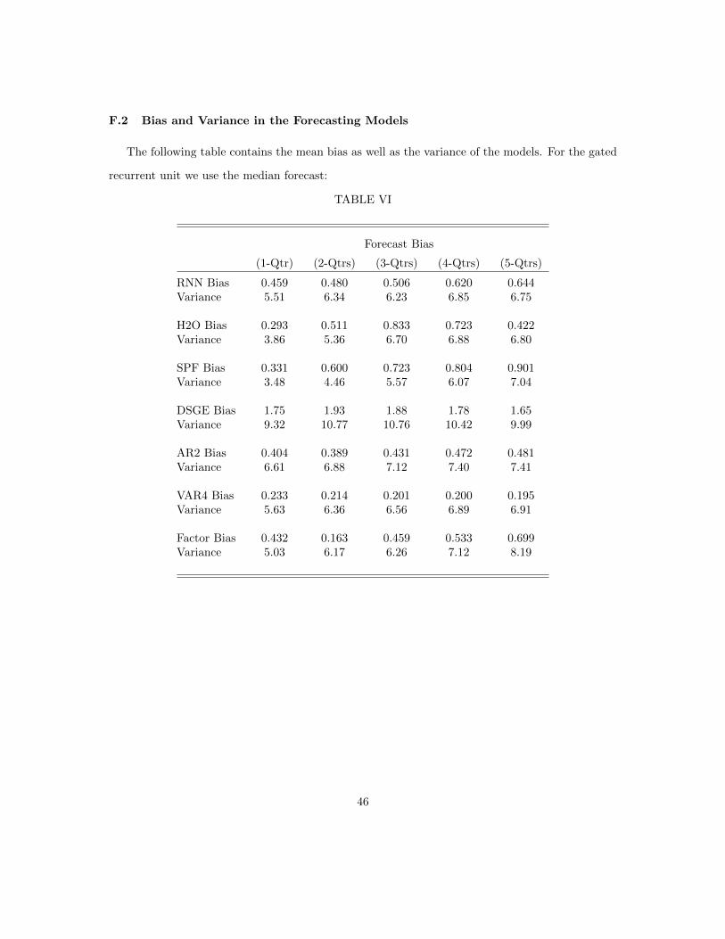
F.2 Bias and Variance in the Forecasting Models

The following table contains the mean bias as well as the variance of the models. For the gated

recurrent unit we use the median forecast:

TABLE VI

Forecast Bias

(1-Qtr) (2-Qtrs) (3-Qtrs) (4-Qtrs) (5-Qtrs)

RNN Bias 0.459 0.480 0.506 0.620 0.644Variance 5.51 6.34 6.23 6.85 6.75

H2O Bias 0.293 0.511 0.833 0.723 0.422Variance 3.86 5.36 6.70 6.88 6.80

SPF Bias 0.331 0.600 0.723 0.804 0.901Variance 3.48 4.46 5.57 6.07 7.04

DSGE Bias 1.75 1.93 1.88 1.78 1.65Variance 9.32 10.77 10.76 10.42 9.99

AR2 Bias 0.404 0.389 0.431 0.472 0.481Variance 6.61 6.88 7.12 7.40 7.41

VAR4 Bias 0.233 0.214 0.201 0.200 0.195Variance 5.63 6.36 6.56 6.89 6.91

Factor Bias 0.432 0.163 0.459 0.533 0.699Variance 5.03 6.17 6.26 7.12 8.19

46

F.3 Parameter Comparison across US DSGE Model and World DSGE Model

The table shows the parameters of the DSGE model estimated on world data versus US data

as well as the standard deviations of the parameters over time. This illustrates the important

parameters that change when adding in global data. In addition to the model growing less confident

and more accurate when world data is added, the parameters that are most modified are parameters

governing wage stickiness and inflation.

47

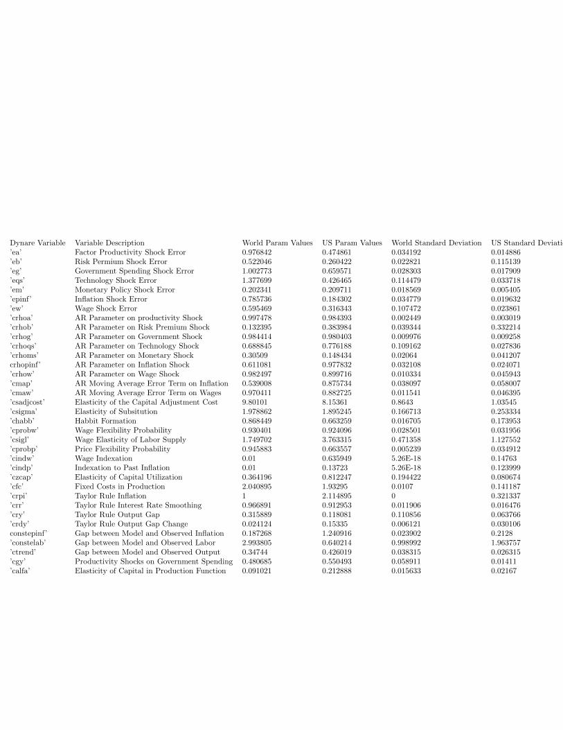
Dynare Variable Variable Description World Param Values US Param Values World Standard Deviation US Standard Deviation’ea’ Factor Productivity Shock Error 0.976842 0.474861 0.034192 0.014886’eb’ Risk Permium Shock Error 0.522046 0.260422 0.022821 0.115139’eg’ Government Spending Shock Error 1.002773 0.659571 0.028303 0.017909’eqs’ Technology Shock Error 1.377699 0.426465 0.114479 0.033718’em’ Monetary Policy Shock Error 0.202341 0.209711 0.018569 0.005405’epinf’ Inflation Shock Error 0.785736 0.184302 0.034779 0.019632’ew’ Wage Shock Error 0.595469 0.316343 0.107472 0.023861’crhoa’ AR Parameter on productivity Shock 0.997478 0.984393 0.002449 0.003019’crhob’ AR Parameter on Risk Premium Shock 0.132395 0.383984 0.039344 0.332214’crhog’ AR Parameter on Government Shock 0.984414 0.980403 0.009976 0.009258’crhoqs’ AR Parameter on Technology Shock 0.688845 0.776188 0.109162 0.027836’crhoms’ AR Parameter on Monetary Shock 0.30509 0.148434 0.02064 0.041207crhopinf’ AR Parameter on Inflation Shock 0.611081 0.977832 0.032108 0.024071’crhow’ AR Parameter on Wage Shock 0.982497 0.899716 0.010334 0.045943’cmap’ AR Moving Average Error Term on Inflation 0.539008 0.875734 0.038097 0.058007’cmaw’ AR Moving Average Error Term on Wages 0.970411 0.882725 0.011541 0.046395’csadjcost’ Elasticity of the Capital Adjustment Cost 9.80101 8.15361 0.8643 1.03545’csigma’ Elasticity of Subsitution 1.978862 1.895245 0.166713 0.253334’chabb’ Habbit Formation 0.868449 0.663259 0.016705 0.173953’cprobw’ Wage Flexibility Probability 0.930401 0.924096 0.028501 0.031956’csigl’ Wage Elasticity of Labor Supply 1.749702 3.763315 0.471358 1.127552’cprobp’ Price Flexibility Probability 0.945883 0.663557 0.005239 0.034912’cindw’ Wage Indexation 0.01 0.635949 5.26E-18 0.14763’cindp’ Indexation to Past Inflation 0.01 0.13723 5.26E-18 0.123999’czcap’ Elasticity of Capital Utilization 0.364196 0.812247 0.194422 0.080674’cfc’ Fixed Costs in Production 2.040895 1.93295 0.0107 0.141187’crpi’ Taylor Rule Inflation 1 2.114895 0 0.321337’crr’ Taylor Rule Interest Rate Smoothing 0.966891 0.912953 0.011906 0.016476’cry’ Taylor Rule Output Gap 0.315889 0.118081 0.110856 0.063766’crdy’ Taylor Rule Output Gap Change 0.024124 0.15335 0.006121 0.030106constepinf’ Gap between Model and Observed Inflation 0.187268 1.240916 0.023902 0.2128’constelab’ Gap between Model and Observed Labor 2.993805 0.640214 0.998992 1.963757’ctrend’ Gap between Model and Observed Output 0.34744 0.426019 0.038315 0.026315’cgy’ Productivity Shocks on Government Spending 0.480685 0.550493 0.058911 0.01411’calfa’ Elasticity of Capital in Production Function 0.091021 0.212888 0.015633 0.02167

48

G Selected Additional Information

G.1 Smets-Wouters Model: US Data vs. World Data

TABLE VII: Smets-Wouters Root Mean Squared Error

The performance forecasts for the performance of Smets-Wouters model on thetest set 2009-Q1 to 2020-Q1 (Lower is better)

Time (Q’s Ahead) 1Q 2Q 3Q 4Q 5QSmets-Wouters DSGE Max Like

US Data 3.83 4.36 4.49 4.50 4.2World Data 3.05*** 3.28*** 3.28*** 3.22** 3.16*Out-Of-Sample Data 2.59*** 2.75*** 2.89** 3.04 3.181995+ 2.77*** 3.09** 3.22* 3.26 3.28

Smets-Wouters DSGE BayesianUS Data 2.79 2.95 2.89 2.80 2.71

∗ Significance indicates outperformance of world data models over US data models

G.2 Recurrent Neural Network Robustness Checks

For our RNN model, we found we could improve forecasting performance by taking the mean

prediction of many models estimated by stochastic gradient descent. The ensembling improves

performance slightly, but later graphs will show it also improves model stability and variance.

Bolded entries indicate outperformance over all economic models.

TABLE VIII: RNN Mean, Median and Best forecasts

Time (Q’s Ahead) 1Q 2Q 3Q 4Q 5QRNN with World Data

Best Model 2.4 2.5 2.5 2.6 2.6Mean Model 2.3 2.5 2.5 2.6 2.6Median Model 2.3 2.5 2.5 2.6 2.6

We provide a Monte Carlo simulation (Table IX), estimating our RNN model at each time

horizon 100 times. At every horizon, the average root mean squared error of our simulated models

indicates competitive, if not outperformance, against baseline models. Interestingly, it seems like

the best performing model on validation data, when tested on the test data, often performs worse

49

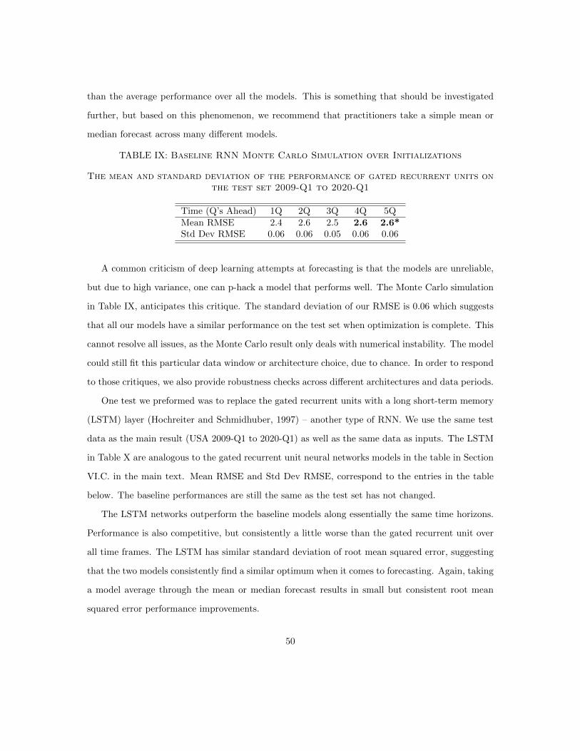
than the average performance over all the models. This is something that should be investigated

further, but based on this phenomenon, we recommend that practitioners take a simple mean or

median forecast across many different models.

TABLE IX: Baseline RNN Monte Carlo Simulation over Initializations

The mean and standard deviation of the performance of gated recurrent units onthe test set 2009-Q1 to 2020-Q1

Time (Q’s Ahead) 1Q 2Q 3Q 4Q 5QMean RMSE 2.4 2.6 2.5 2.6 2.6*Std Dev RMSE 0.06 0.06 0.05 0.06 0.06

A common criticism of deep learning attempts at forecasting is that the models are unreliable,

but due to high variance, one can p-hack a model that performs well. The Monte Carlo simulation

in Table IX, anticipates this critique. The standard deviation of our RMSE is 0.06 which suggests

that all our models have a similar performance on the test set when optimization is complete. This

cannot resolve all issues, as the Monte Carlo result only deals with numerical instability. The model

could still fit this particular data window or architecture choice, due to chance. In order to respond

to those critiques, we also provide robustness checks across different architectures and data periods.

One test we preformed was to replace the gated recurrent units with a long short-term memory

(LSTM) layer (Hochreiter and Schmidhuber, 1997) – another type of RNN. We use the same test

data as the main result (USA 2009-Q1 to 2020-Q1) as well as the same data as inputs. The LSTM

in Table X are analogous to the gated recurrent unit neural networks models in the table in Section

VI.C. in the main text. Mean RMSE and Std Dev RMSE, correspond to the entries in the table

below. The baseline performances are still the same as the test set has not changed.

The LSTM networks outperform the baseline models along essentially the same time horizons.

Performance is also competitive, but consistently a little worse than the gated recurrent unit over

all time frames. The LSTM has similar standard deviation of root mean squared error, suggesting

that the two models consistently find a similar optimum when it comes to forecasting. Again, taking

a model average through the mean or median forecast results in small but consistent root mean

squared error performance improvements.

50

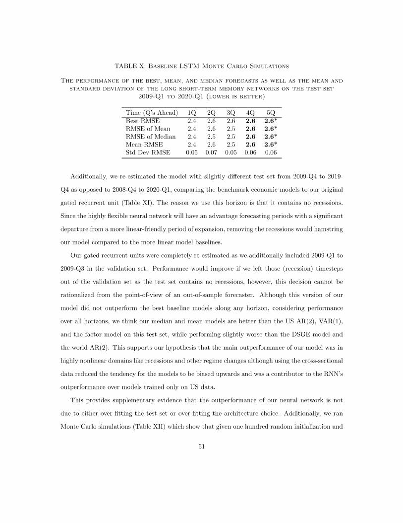
TABLE X: Baseline LSTM Monte Carlo Simulations

The performance of the best, mean, and median forecasts as well as the mean andstandard deviation of the long short-term memory networks on the test set

2009-Q1 to 2020-Q1 (lower is better)

Time (Q’s Ahead) 1Q 2Q 3Q 4Q 5QBest RMSE 2.4 2.6 2.6 2.6 2.6*RMSE of Mean 2.4 2.6 2.5 2.6 2.6*RMSE of Median 2.4 2.5 2.5 2.6 2.6*Mean RMSE 2.4 2.6 2.5 2.6 2.6*Std Dev RMSE 0.05 0.07 0.05 0.06 0.06

Additionally, we re-estimated the model with slightly different test set from 2009-Q4 to 2019-

Q4 as opposed to 2008-Q4 to 2020-Q1, comparing the benchmark economic models to our original

gated recurrent unit (Table XI). The reason we use this horizon is that it contains no recessions.

Since the highly flexible neural network will have an advantage forecasting periods with a significant

departure from a more linear-friendly period of expansion, removing the recessions would hamstring

our model compared to the more linear model baselines.

Our gated recurrent units were completely re-estimated as we additionally included 2009-Q1 to

2009-Q3 in the validation set. Performance would improve if we left those (recession) timesteps

out of the validation set as the test set contains no recessions, however, this decision cannot be

rationalized from the point-of-view of an out-of-sample forecaster. Although this version of our

model did not outperform the best baseline models along any horizon, considering performance

over all horizons, we think our median and mean models are better than the US AR(2), VAR(1),

and the factor model on this test set, while performing slightly worse than the DSGE model and

the world AR(2). This supports our hypothesis that the main outperformance of our model was in

highly nonlinear domains like recessions and other regime changes although using the cross-sectional

data reduced the tendency for the models to be biased upwards and was a contributor to the RNN’s

outperformance over models trained only on US data.

This provides supplementary evidence that the outperformance of our neural network is not

due to either over-fitting the test set or over-fitting the architecture choice. Additionally, we ran

Monte Carlo simulations (Table XII) which show that given one hundred random initialization and

51

TABLE XI: Expansion Root Mean Squared Error

Performance of the Best, Mean, and Median forecasts for gated recurrent unitson the test set 2009-Q4 to 2019-Q4

Time (Q’s Ahead) 1Q 2Q 3Q 4Q 5QVAR(1)

US data 2.3 2.6 2.9 3.0 3.0World data 2.1 2.2 2.2 2.2 2.2

AR(2)US data 1.7 1.7 1.8 1.9 1.9World data 1.6 1.6 1.6 1.5 1.5*

Smets Wouters DSGEUS data 1.8 1.8 1.7 1.6 1.5*

FactorUS data 1.6 1.6 1.6 1.9 2.1

RNN*Best 1.8 2.3 2.0 2.0 1.9Mean Forecast 1.7 1.7 1.7 1.7 1.7Median Forecast 1.7 1.7 1.7 1.7 1.7

SPF Median 1.4 1.5 1.5 1.5 1.5

∗All RNN models use entire world data cross-section

52

optimization routines over all five horizons, the model still consistently achieves low root mean

squared error and has a low standard deviation – demonstrating stability and reproducability.

TABLE XII: Expansion RNN Monte Carlo Simulations

The mean and standard deviation of the performance of gated recurrent units onthe test set 2009-Q4 to 2019-Q4

Time (Q’s Ahead) 1Q 2Q 3Q 4Q 5QMean RMSE 1.8 1.8 1.8 1.8 1.7Std Dev RMSE 0.18 0.18 0.21 0.11 0.08

53

Department of Economics, University of Michigan, Ann Arbor

54