machine learning classification and accuracy assessment
TRANSCRIPT
remote sensing
Article
Machine Learning Classification and Accuracy Assessmentfrom High-Resolution Images of Coastal Wetlands
Ricardo Martínez Prentice 1,* , Miguel Villoslada Peciña 1, Raymond D. Ward 1,2 , Thaisa F. Bergamo 1,Chris B. Joyce 2 and Kalev Sepp 1
�����������������
Citation: Martínez Prentice, R.;
Villoslada Peciña, M.; Ward, R.D.;
Bergamo, T.F.; Joyce, C.B.; Sepp, K.
Machine Learning Classification and
Accuracy Assessment from
High-Resolution Images of Coastal
Wetlands. Remote Sens. 2021, 13, 3669.
https://doi.org/10.3390/rs13183669
Academic Editors: Jeremy L. May and
Sergio Vargas Zesati
Received: 26 July 2021
Accepted: 10 September 2021
Published: 14 September 2021
Publisher’s Note: MDPI stays neutral
with regard to jurisdictional claims in
published maps and institutional affil-
iations.
Copyright: © 2021 by the authors.
Licensee MDPI, Basel, Switzerland.
This article is an open access article
distributed under the terms and
conditions of the Creative Commons
Attribution (CC BY) license (https://
creativecommons.org/licenses/by/
4.0/).
1 Institute of Agriculture and Environmental Sciences, Estonian University of Life Sciences, Kreutzwaldi 5,EE-51006 Tartu, Estonia; [email protected] (M.V.P.); [email protected] (R.D.W.);[email protected] (T.F.B.); [email protected] (K.S.)
2 Centre for Aquatic Environments, School of the Environment and Technology, University of Brighton,Cockcroft Building, Moulsecoomb, Brighton BN2 4GJ, UK; [email protected]
* Correspondence: [email protected]
Abstract: High-resolution images obtained by multispectral cameras mounted on Unmanned AerialVehicles (UAVs) are helping to capture the heterogeneity of the environment in images that canbe discretized in categories during a classification process. Currently, there is an increasing use ofsupervised machine learning (ML) classifiers to retrieve accurate results using scarce datasets withsamples with non-linear relationships. We compared the accuracies of two ML classifiers using apixel and object analysis approach in six coastal wetland sites. The results show that the RandomForest (RF) performs better than K-Nearest Neighbors (KNN) algorithm in the classification of pixelsand objects and the classification based on pixel analysis is slightly better than the object-basedanalysis. The agreement between the classifications of objects and pixels is higher in Random Forest.This is likely due to the heterogeneity of the study areas, where pixel-based classifications are mostappropriate. In addition, from an ecological perspective, as these wetlands are heterogeneous, thepixel-based classification reflects a more realistic interpretation of plant community distribution.
Keywords: UAV; machine learning; Random Forest; KNN; classification; comparison
1. Introduction
Studying the vegetation structure within plant communities is key for environmentalsciences because they play a major role in detecting the environmental change and moni-toring the ecological condition [1–4]. Remote sensing has been increasingly used in ecologyas a powerful method to monitor large areas using direct measurements of vegetation [5].Satellite imagery is being used successfully to monitor large areas [6–8], although the spatialresolution of their images is not always adequate to capture the spectral details of spatiallyheterogeneous vegetation types, such as grassland, heathland or wetland vegetation. Usinghigh-resolution images in ecology offers the possibility to capture the heterogeneity of anarea of interest with variations in plant community cover with a small pixel resolution(≈10 cm) [9–11].
The most common tool used to capture these types of images are multispectral camerasmounted on Unmanned Aerial Vehicles (UAVs). UAVs offer a platform for the rapidmeasurement of relatively large areas by overflying remote or inaccessible locations usingnon-destructive, cost-effective and near-real-time monitoring routines [10] with the capacityto precisely monitor changes in vegetation at a local scale as well as measuring the spatialdistribution of plant communities [11]. This supplements intensive surveying of speciesand also expands the potential application of field survey methods, while accounting forchanges in vegetation over time [12]. In addition to the applications of multispectral sensors,RGB (Red, Green, Blue) cameras can also capture elevation data using recent improvements
Remote Sens. 2021, 13, 3669. https://doi.org/10.3390/rs13183669 https://www.mdpi.com/journal/remotesensing
Remote Sens. 2021, 13, 3669 2 of 27
in point cloud reconstruction methods, such as Structure from Motion [13], detectingmicrotopographical variations and generating accurate digital elevation models [14].
Classifying the pixel values of images is a common process in ecological studiesusing remotely sensed data. This involves collecting field data from a series of plots as aninput for training a classification model. The model or classifier algorithm labels pixelsaccording to their spectral similarity to the initial values overlapping the plots, and thefinal classification reveals patterns of distribution in the image, which can be valuable tosupport management and conservation decision making [9,15,16].
Traditional supervised classifiers assume the normal distribution of remotely sensed datavalues [17] from datasets, where the Maximum Likelihood classifier is the most commonalgorithm used [18]. Nevertheless, datasets can hide complex and non-linear relations thatvary in space; thus, classifiers do not fit into classical statistical methods [19,20].
Machine learning (ML) has emerged as a field of artificial intelligence that deals withcomplex reference data to build a classifier based on data-driven decisions. For this reason,studies in remote sensing have been increasingly using different ML algorithms becausethey can outperform traditional classifiers in ecology and Earth science applications andthey are fundamentally non-parametric [20,21].
From the ML algorithms evaluated for classifying remote sensing images, the mostcommonly used are Support Vector Machines, Random Forest and boosted Decision Trees,although there is no general agreement on which algorithm performs better becausethis depends on the training data, explanatory variables and number of categories tobe classified [22]. The K-Nearest Neighbors (KNN) classifier does not train a modelbut computes a comparison of an unknown sample to the training data and is also anon-parametric classifier [23]. This algorithm is widely used for its capacity to predictmultiple response variables simultaneously by finding the best K parameter [24]. RandomForest (RF) is a robust algorithm, which is not overly affected by parameter settingsand its classification accuracy does not decrease significantly when using small trainingdatasets [25].
Typically, classification in remote sensing is a process that directly uses pixels; never-theless, in recent years, some studies have addressed the task of classification with a priorprocess of segmentation, obtaining groups of pixels, called objects, with homogeneous spec-tral characteristics and non-spectral attributes, such as shape, relationship and adjacencymetrics [26,27]. This approach, called object-based image analysis (OBIA), shows someadvantages over the pixel-based image analysis (PBIA), particularly where objects have aspatial context and represent homogeneous patches that can represent plant communitieslarger than the data pixel size [27,28].
In order to compare the accuracy of classifications using OBIA and PBIA approachesof spectrally similar and spatially heterogeneous categories, we tested two ML classificationalgorithms on plant community data from coastal wetlands. Plant communities in suchecosystems consist of patches of vegetation, where hydrology, topography and humanmanagement are often the main factors that influence their distribution [29], resultingin a heterogeneous distribution. Thus far, there are studies comparing the two differentapproaches in wetlands but using a coarser image resolution [30,31]. Thus, the main focusof this study is to perform a classification of high-resolution images from a UAV platformbased on two ML algorithms using both the OBIA and PBIA approaches.
The main objectives are to: (1) classify plant communities in coastal wetlands usingtwo different ML algorithms from high-resolution UAV images; (2) compare the classi-fication accuracies of pixels and objects; (3) perform a quality assessment between eachclassification map.
2. Materials and Methods2.1. Study Areas
This study was undertaken in six coastal wet grasslands of Estonia, which belong to theclassification ‘Boreal Baltic coastal meadows’ according to Annex I of the EU Habitats Directive
Remote Sens. 2021, 13, 3669 3 of 27
(1992). These coastal wetlands are located in an extensive transitional zone from the sea toterrestrial ecosystems, characterized by a gradient of hydrological conditions and differentinundation that largely determines the distribution of the plant communities [32,33]. Severalstudies have shown that microtopography also has an important influence on the locationand extent of plant communities [34], including in Estonian coastal wetlands, where the totalelevation differences are typically between 0 and 3 m, the tidal variation is negligible (0.02 m)and the range of plant communities is maintained through low-intensity grazing [35,36].
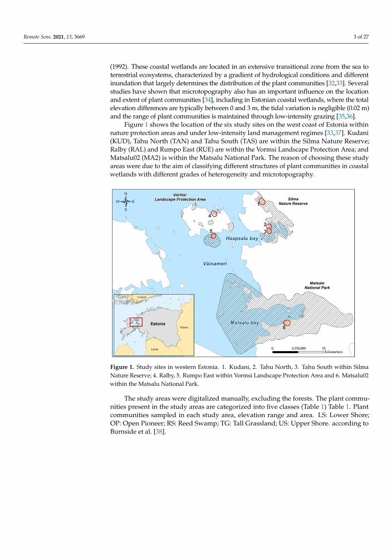
Figure 1 shows the location of the six study sites on the west coast of Estonia withinnature protection areas and under low-intensity land management regimes [33,37]. Kudani(KUD), Tahu North (TAN) and Tahu South (TAS) are within the Silma Nature Reserve;Ralby (RAL) and Rumpo East (RUE) are within the Vormsi Landscape Protection Area; andMatsalu02 (MA2) is within the Matsalu National Park. The reason of choosing these studyareas were due to the aim of classifying different structures of plant communities in coastalwetlands with different grades of heterogeneity and microtopography.
Figure 1. Study sites in western Estonia. 1. Kudani, 2. Tahu North, 3. Tahu South within SilmaNature Reserve; 4. Ralby, 5. Rumpo East within Vormsi Landscape Protection Area and 6. Matsalu02within the Matsalu National Park.
The study areas were digitalized manually, excluding the forests. The plant commu-nities present in the study areas are categorized into five classes (Table 1) Table 1. Plantcommunities sampled in each study area, elevation range and area. LS: Lower Shore;OP: Open Pioneer; RS: Reed Swamp; TG: Tall Grassland; US: Upper Shore. according toBurnside et al. [38].
Remote Sens. 2021, 13, 3669 4 of 27
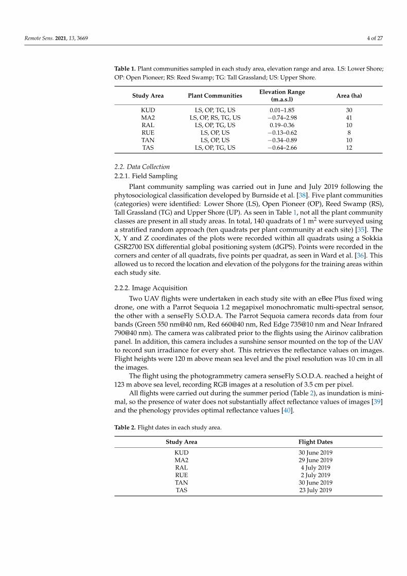
Table 1. Plant communities sampled in each study area, elevation range and area. LS: Lower Shore;OP: Open Pioneer; RS: Reed Swamp; TG: Tall Grassland; US: Upper Shore.
Study Area Plant Communities Elevation Range(m.a.s.l) Area (ha)
KUD LS, OP, TG, US 0.01–1.85 30MA2 LS, OP, RS, TG, US −0.74–2.98 41RAL LS, OP, TG, US 0.19–0.36 10RUE LS, OP, US −0.13–0.62 8TAN LS, OP, US −0.34–0.89 10TAS LS, OP, TG, US −0.64–2.66 12
2.2. Data Collection2.2.1. Field Sampling
Plant community sampling was carried out in June and July 2019 following thephytosociological classification developed by Burnside et al. [38]. Five plant communities(categories) were identified: Lower Shore (LS), Open Pioneer (OP), Reed Swamp (RS),Tall Grassland (TG) and Upper Shore (UP). As seen in Table 1, not all the plant communityclasses are present in all study areas. In total, 140 quadrats of 1 m2 were surveyed usinga stratified random approach (ten quadrats per plant community at each site) [35]. TheX, Y and Z coordinates of the plots were recorded within all quadrats using a SokkiaGSR2700 ISX differential global positioning system (dGPS). Points were recorded in thecorners and center of all quadrats, five points per quadrat, as seen in Ward et al. [36]. Thisallowed us to record the location and elevation of the polygons for the training areas withineach study site.
2.2.2. Image Acquisition
Two UAV flights were undertaken in each study site with an eBee Plus fixed wingdrone, one with a Parrot Sequoia 1.2 megapixel monochromatic multi-spectral sensor,the other with a senseFly S.O.D.A. The Parrot Sequoia camera records data from fourbands (Green 550 nm@40 nm, Red 660@40 nm, Red Edge 735@10 nm and Near Infrared790@40 nm). The camera was calibrated prior to the flights using the Airinov calibrationpanel. In addition, this camera includes a sunshine sensor mounted on the top of the UAVto record sun irradiance for every shot. This retrieves the reflectance values on images.Flight heights were 120 m above mean sea level and the pixel resolution was 10 cm in allthe images.
The flight using the photogrammetry camera senseFly S.O.D.A. reached a height of123 m above sea level, recording RGB images at a resolution of 3.5 cm per pixel.
All flights were carried out during the summer period (Table 2), as inundation is mini-mal, so the presence of water does not substantially affect reflectance values of images [39]and the phenology provides optimal reflectance values [40].
Table 2. Flight dates in each study area.
Study Area Flight Dates
KUD 30 June 2019MA2 29 June 2019RAL 4 July 2019RUE 2 July 2019TAN 30 June 2019TAS 23 July 2019
Remote Sens. 2021, 13, 3669 5 of 27
2.3. Image Processing2.3.1. Positional Accuracy
RINEX observation and navigation files were used to carry out post-processed kine-matic (PPK) correction of the multispectral images to improve the positional accuracy [41],using ESTPOS Estonian GNSS-RTK permanent stations network (Eesti Maa-amet) as a ref-erence. There were 7615 images geographically positioned using the Estonian CoordinateSystem of 1997 (EPSG: 3301) and the PPK retrieved an accuracy value under 7 cm accuracyusing the software eMotion 3®. The resulting orthomosaics were used as an input for thePix4D v.4.3.31® software to obtain five orthomosaics per study area [42].
The accuracy of the PPK corrections was assessed using Root Mean Square Error(RMSE) and Mean Absolute Error (MAE) calculations. RMSE and MAE were used toestimate the differences between the ground control points (GCPs) location in the imagesand the independent GCPs locations measured with the dGPS [43]
2.3.2. Digital Elevation Models
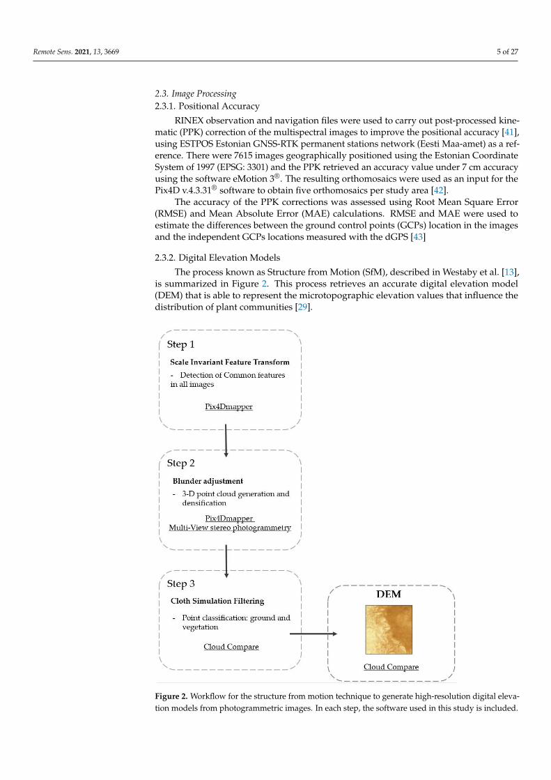
The process known as Structure from Motion (SfM), described in Westaby et al. [13],is summarized in Figure 2. This process retrieves an accurate digital elevation model(DEM) that is able to represent the microtopographic elevation values that influence thedistribution of plant communities [29].
Figure 2. Workflow for the structure from motion technique to generate high-resolution digital eleva-tion models from photogrammetric images. In each step, the software used in this study is included.
Remote Sens. 2021, 13, 3669 6 of 27
The main objective of the SfM is to find matching locations in the multiple imagesto extract the photogrammetric points. Pix4Dmapper software is used with the Multi-View stereo photogrammetry module (SfM-MVS) to find common features within all theimages [44], as seen in Step 1 (Figure 2). In Step 2, a bundler adjustment where a low-densitypoint cloud was extracted from the common points using the view stereo photogrammetry,followed by its densification, where an enhanced 3D point cloud is built from differentcamera positions [44]. Finally, in Step 3, the point cloud is classified in two categories:ground and non-ground, using the cloth simulation filtering. This technique is based onthe interaction between a cloth model and the inverted point cloud to select the shape ofthat cloth model [45]. This last process is computed in CloudCompare software. Only twoparameters had to be set, the “rigidness” and the “ST”, in order to control how the clothmodel lies over the inverted point cloud. The final DEM is extracted by performing aninterpolation from the filtered point cloud (Figure 2). After processing, the RMSE wasbetween 5 and 18 cm using the dGPS measurements.
Each DEM was resampled to the pixel size of the spectral bands in each study area,using the Nearest Neighbor method.
2.3.3. Vegetation Indices
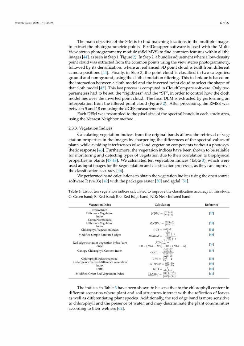
Calculating vegetation indices from the original bands allows the retrieval of veg-etation properties in the images by sharpening the differences of the spectral values ofplants while avoiding interferences of soil and vegetation components without a photosyn-thetic response [46]. Furthermore, the vegetation indices have been shown to be reliablefor monitoring and detecting types of vegetation due to their correlation to biophysicalproperties in plants [47,48]. We calculated ten vegetation indices (Table 3), which wereused as input images for the segmentation and classification processes, as they can improvethe classification accuracy [46].
We performed band calculations to obtain the vegetation indices using the open sourcesoftware R (v4.03) [49] with the packages raster [50] and rgdal [51].
Table 3. List of ten vegetation indices calculated to improve the classification accuracy in this study.G: Green band; R: Red band; Rre: Red Edge band; NIR: Near Infrared band.
Vegetation Index Calculation Reference
NormalizedDifference Vegetation
IndexNDVI = (NIR−R)
(NIR+R)[52]
Green NormalizedDifference Vegetation
IndexGNDVI = (NIR−G)
(NIR+G)[53]
Chlorophyll Vegetation Index CVI = NIR×RG2 [54]
Modified Simple Ratio (red edge) MSRred =
(NIRRre
)−1√(
NIRRre
)+1
[55]
Red edge triangular vegetation index (coreonly)
RTVIcore =100 × (NIR − Rre)− 10 × (NIR − G)
[56]
Canopy Chlorophyll Content Index CCCI =(NIR−Rre)(NIR+Rre)(NIR−R)(NIR+R)
[57]
Chlorophyll Index (red edge) CIre = NIRRre − 1 [58]
Red edge normalized difference vegetationindex NDVIre = NIR−Rre
NIR+Rre [59]
Datt4 datt4 = R(G×Rre) [60]
Modified Green Red Vegetation Index MGRVI = ((G2)−(R2))
((G2)+(R2))[61]
The indices in Table 3 have been shown to be sensitive to the chlorophyll content indifferent scenarios where plant and soil structures interact with the reflection of leavesas well as differentiating plant species. Additionally, the red edge band is more sensitiveto chlorophyll and the presence of water, and may discriminate the plant communitiesaccording to their wetness [62].
Remote Sens. 2021, 13, 3669 7 of 27
2.4. Classification of Images
We performed an image classification using two different approaches: Pixel-BasedImage Analysis (PBIA) and Object-Based Image Analysis (OBIA). The former has been usedin since the first Landsat satellite took the first remotely sensed images, where coarse spatialresolution images are classified, and a single pixel is big enough to represent an object ofinterest. With the recent increasing resolution of satellite images and the use of UAV torecord high-resolution images, single pixels may not always represent meaningful units,but a group of pixels as objects can do so. In OBIA, an image segmentation is performedto create a homogeneous group of pixels [63] and represent the objects for classification.In supervised classifications, an unknown sample (pixel or object) is assigned to a classbased on an original training dataset, from an n-dimensional space (feature space) ofexplanatory variables. These variables are the bands extracted from spectral measurements,combinations of them or ancillary geographical data [64].
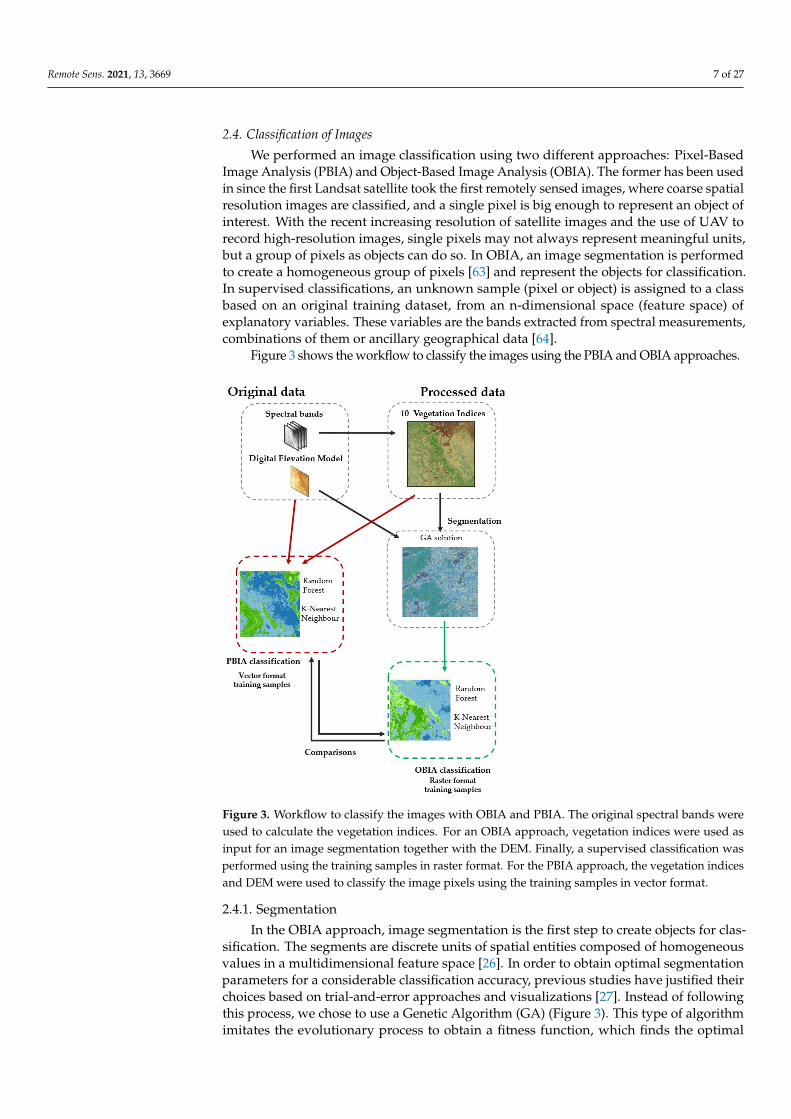
Figure 3 shows the workflow to classify the images using the PBIA and OBIA approaches.
Figure 3. Workflow to classify the images with OBIA and PBIA. The original spectral bands wereused to calculate the vegetation indices. For an OBIA approach, vegetation indices were used asinput for an image segmentation together with the DEM. Finally, a supervised classification wasperformed using the training samples in raster format. For the PBIA approach, the vegetation indicesand DEM were used to classify the image pixels using the training samples in vector format.
2.4.1. Segmentation
In the OBIA approach, image segmentation is the first step to create objects for clas-sification. The segments are discrete units of spatial entities composed of homogeneousvalues in a multidimensional feature space [26]. In order to obtain optimal segmentationparameters for a considerable classification accuracy, previous studies have justified theirchoices based on trial-and-error approaches and visualizations [27]. Instead of followingthis process, we chose to use a Genetic Algorithm (GA) (Figure 3). This type of algorithmimitates the evolutionary process to obtain a fitness function, which finds the optimal
Remote Sens. 2021, 13, 3669 8 of 27
solution to solve a complex computational problem [65]. It has been shown that the GeneticAlgorithms improve the classification accuracy for a large number of variables (bands) [66].
To carry out the segmentation of images, we chose the SegOptim package written inR [67]. This package integrates a complete workflow for segmentation and classificationof images. First, the R package uses the functions of third-party software to perform theimage segmentation after tuning the parameters for the segmentation by applying a GA.
In this study, we chose the Large-scale Mean-shift algorithm [68] for the followingreasons: it is executed in SegOptim by calling the Orfeo Toolbox library [69], (also open-source software); the tuning parameters consist of setting the spectral and the spatial rangeof pixels in the feature space and establishes the minimum size of the segments; it performsa stable and efficient segmentation of images as it splits the image into tiles. The SpectralRange indicates the search radius in multispectral space; Spatial Range, the similarity ofneighbors; and the minimum size of segments in pixel units.
The input variables for the GA were the vegetation indices (Table 3), the DEM andthe training samples. The training samples, originally in vector format, were rasterized,as SegOptim only accepts the training samples as a grid of category values. The meansize of the training areas in the raster format was 11 pixels. Each raster is then assigned tothe segment based on a threshold value. Due to the small size of the training areas, thisthreshold was set to 5%, meaning that the segments covered by 5% or more by the trainingpixels were considered as valid cases for the classification, characterized by the mean andstandard deviation of the values of variables [55].
Finally, the fitness value in SegOptim retrieved the best parameters to apply to thesegmentation in each study area for the following classification using RF or KNN. The resultwas a segmented image in raster format (Figure 3).
In order to see if there were differences between the training areas as segments (valid casesfor training the classifiers) and polygon features, we compared the mean values of each variable(input vegetation indices and DEM). To do so, we carried out a Kruskal–Wallis non-parametrictest between the medians of the training samples and segments with the characteristics ofthe training samples in each plant community because the values did not follow a normaldistribution.
2.4.2. ML Classifiers
To perform a PBIA and an OBIA, we chose the RF and KNN classifiers (Figure 3).RF is a nonparametric ensemble classifier (multiple classifications on the same data)
that grows multiple decision trees from a subset of training samples with replacement(bagging) [70]. The group of trees make a final decision based on the most repeated vote(modal category) and label the final category to an unknown sample. While the forest isbeing built, the samples not used for training are the out of bag (OOB) fraction, whichestimates the internal performance with an error rate [70]. This OOB is also used in thecalculation of the variable importance by randomly replacing one input variable in theout of bag fraction by another variable randomly selected. If there is an increase in theOOB error, the variable was important to reduce the error, and thus, it is considered moreimportant in the tree [71].
The KNN algorithm is a nonparametric classifier, which assigns a class label to anunknown sample based on its statistical distance to the training samples. The Euclideandistance is used by default in the caret package applying the KNN method. Once thedistance is calculated, it selects the K-Nearest Neighbors to assign the modal category inthose k training samples. We searched for the best accuracy between 1 and 20 K-NearestNeighbors. These minimum and maximum k values were set initially between 1 and 26, asthis resulted from the average k of all the study areas after calculating the square root ofn (n = number of pixels in training samples) [72]. However, in all cases, after k = 20, theaccuracy decreased.
For a PBIA classification, we used the caret package [73], which can perform an RF andKNN classification by changing the arguments in the required functions (method = “rf” or
Remote Sens. 2021, 13, 3669 9 of 27
“knn”, respectively). This function requires the input variables in grid format to be stacked in amultiband raster and use the training areas as vector format (polygons).
For the OBIA classification, the output segmentation obtained in the previous stepwas used to classify the objects. Prior to classification, a calibration phase was undertaken,where the category values of the training samples are assigned to the segments containingthose pixels, based on a threshold value. This classification, as mentioned before, wascarried out using the SegOptim package.
We carried out four classifications in each study area: RF and KNN based on PBIAand RF and KNN based on OBIA.
2.4.3. Classification Accuracy and Variable Importance
We consider the accuracy as the agreement between a classified value previouslyunknown and the training samples, accepted as true values [74]. The classifications wereevaluated using the User accuracy, Producer accuracy, overall accuracy and Kappa statisticwith a 10-fold cross-validation to construct the confusion matrices for each classification.For RF classification based on PBIA and OBIA, we extracted the Mean Decrease Gini(MDG) to report the variable importance in each study area. The MDG is based on the Giniimpurity criterion, which calculates the chance to misclassify a new sample. Replacing thepurest variable in a node with another one will increase the chance to classify incorrectly thenew sample, so that the previous variable was more important (pure) to split the node [25].The higher the MDG is, the more important the variable is.
2.5. Map Comparisons
A common task in remote sensing is to perform a comparison between classificationsin order to assess the differences in thematic maps [75]. Despite the widely used parametersderived from kappa statistics to compare categorical maps [76,77], called Khisto, Klocationand Kquantity, these parameters are not sufficient to compare accuracies as they havea randomness component [78]. To overcome these limitations, within this study, a newmeasure of overall agreement is used as a simpler measurement. It is composed of twometrics, quantity and allocation disagreement. The first component refers to the proportionof differences of unmatching categories and the second one to the differences due to thedisplacement of categories in the area [78]. These comparisons are performed betweenmaps with the same pixel size.
The ML algorithm with the highest classification accuracy was chosen as the referencemap. Comparisons were performed between PBIA and OBIA of the best classifier. We re-ported the percentage of agreement and disagreement areas between maps and the overallpercentages of quantity and allocation agreement and disagreement relative to each studyarea using the Rsenal [79] package in R software [49]. The variation in the quantity of eachcategory (plant communities) refers to the differences in their composition throughout thearea and the variation in allocation, to the differences in their spatial configuration [80].This allowed the interpretation, in a spatial context, of the differences among the classifica-tions. We also calculated the changes of categories within the disagreement areas.
The remaining percentage (the sum of quantity and allocation agreement and dis-agreement is not 100%) corresponds to the proportion of agreement that is expected tooccur by chance (chance agreement).
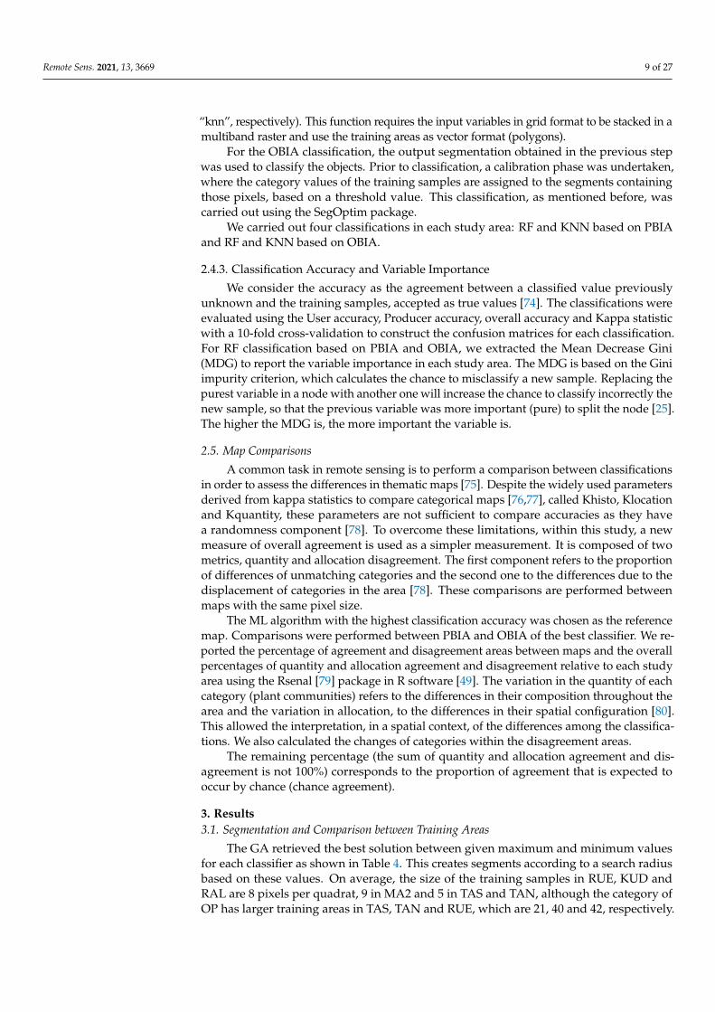
3. Results3.1. Segmentation and Comparison between Training Areas
The GA retrieved the best solution between given maximum and minimum valuesfor each classifier as shown in Table 4. This creates segments according to a search radiusbased on these values. On average, the size of the training samples in RUE, KUD andRAL are 8 pixels per quadrat, 9 in MA2 and 5 in TAS and TAN, although the category ofOP has larger training areas in TAS, TAN and RUE, which are 21, 40 and 42, respectively.
Remote Sens. 2021, 13, 3669 10 of 27
The Kruskal–Wallis test did not show any differences between these segments and theinitial training polygons.
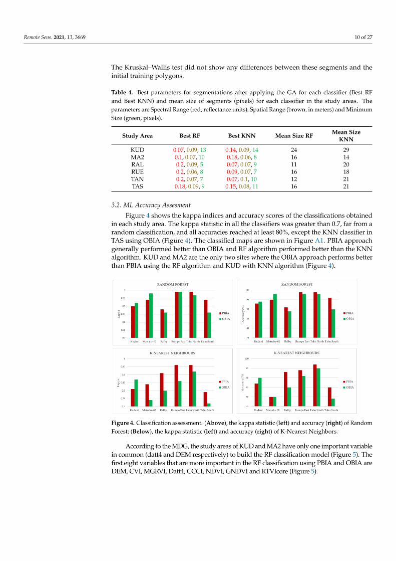
Table 4. Best parameters for segmentations after applying the GA for each classifier (Best RFand Best KNN) and mean size of segments (pixels) for each classifier in the study areas. Theparameters are Spectral Range (red, reflectance units), Spatial Range (brown, in meters) and MinimumSize (green, pixels).
Study Area Best RF Best KNN Mean Size RF Mean SizeKNN
KUD 0.07, 0.09, 13 0.14, 0.09, 14 24 29MA2 0.1, 0.07, 10 0.18, 0.06, 8 16 14RAL 0.2, 0.09, 5 0.07, 0.07, 9 11 20RUE 0.2, 0.06, 8 0.09, 0.07, 7 16 18TAN 0.2, 0.07, 7 0.07, 0.1, 10 12 21TAS 0.18, 0.09, 9 0.15, 0.08, 11 16 21
3.2. ML Accuracy Assesment
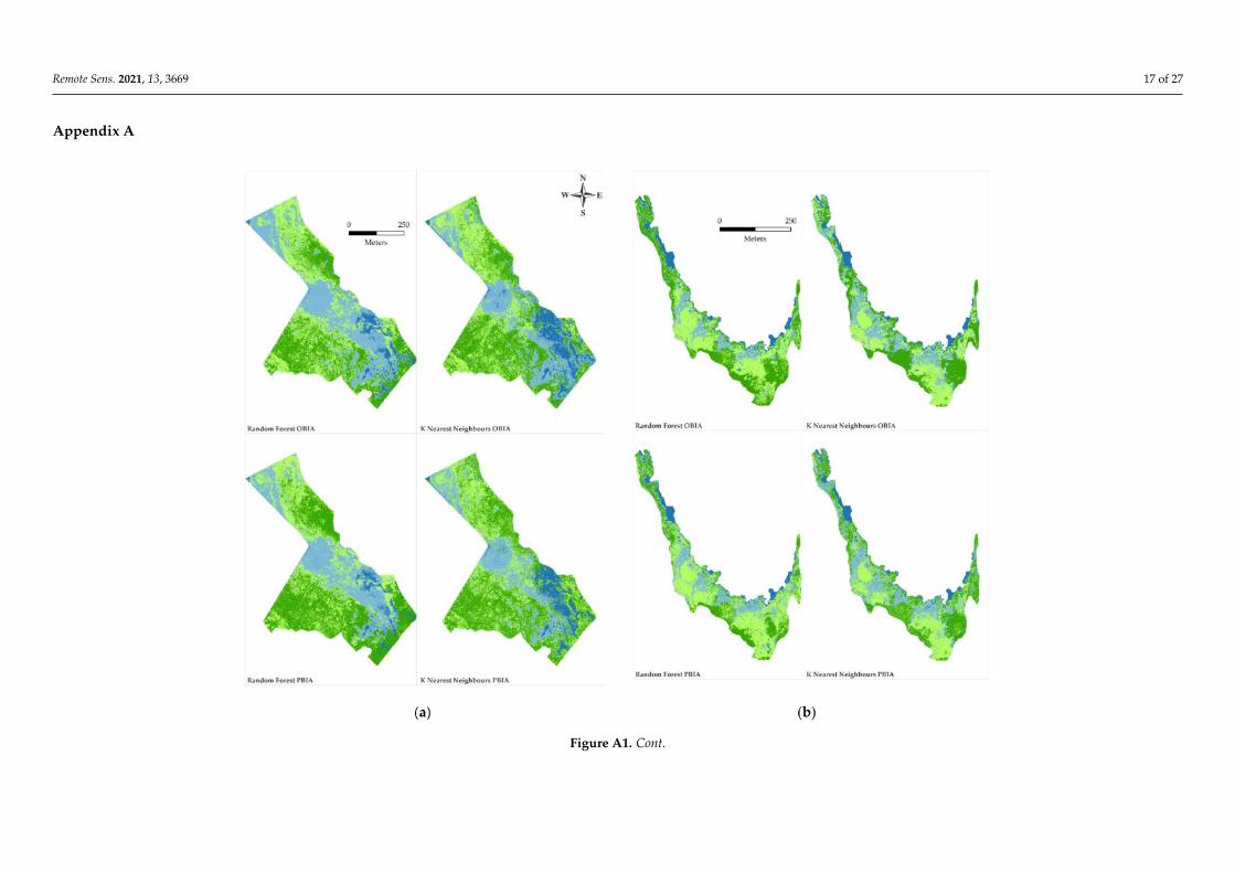
Figure 4 shows the kappa indices and accuracy scores of the classifications obtainedin each study area. The kappa statistic in all the classifiers was greater than 0.7, far from arandom classification, and all accuracies reached at least 80%, except the KNN classifier inTAS using OBIA (Figure 4). The classified maps are shown in Figure A1. PBIA approachgenerally performed better than OBIA and RF algorithm performed better than the KNNalgorithm. KUD and MA2 are the only two sites where the OBIA approach performs betterthan PBIA using the RF algorithm and KUD with KNN algorithm (Figure 4).
Figure 4. Classification assessment. (Above), the kappa statistic (left) and accuracy (right) of RandomForest; (Below), the kappa statistic (left) and accuracy (right) of K-Nearest Neighbors.
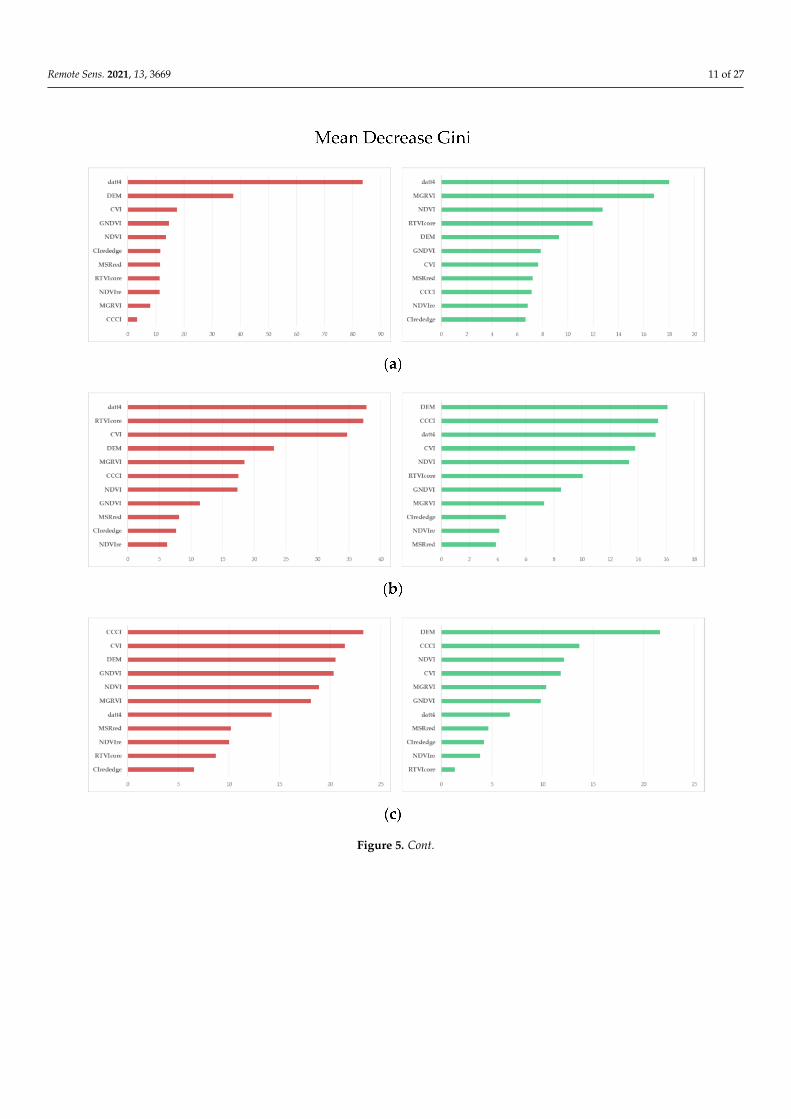
According to the MDG, the study areas of KUD and MA2 have only one important variablein common (datt4 and DEM respectively) to build the RF classification model (Figure 5). Thefirst eight variables that are more important in the RF classification using PBIA and OBIA areDEM, CVI, MGRVI, Datt4, CCCI, NDVI, GNDVI and RTVIcore (Figure 5).
Remote Sens. 2021, 13, 3669 11 of 27
Figure 5. Cont.
Remote Sens. 2021, 13, 3669 12 of 27
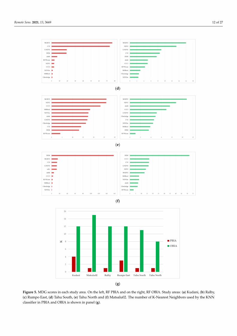
Figure 5. MDG scores in each study area. On the left, RF PBIA and on the right, RF OBIA. Study areas: (a) Kudani, (b) Ralby,(c) Rumpo East, (d) Tahu South, (e) Tahu North and (f) Matsalu02. The number of K-Nearest Neighbors used by the KNNclassifier in PBIA and OBIA is shown in panel (g).
Remote Sens. 2021, 13, 3669 13 of 27
The number of nearest neighbors (k) is higher in OBIA (Figure 5), probably due tothe more homogeneous characteristics of the segments, which is why the classifier chose alarger distance for the training samples than in PBIA.
3.3. Map Comparisons
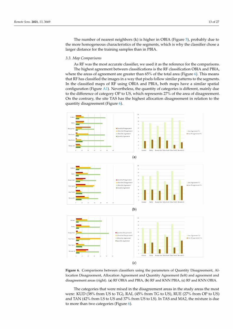
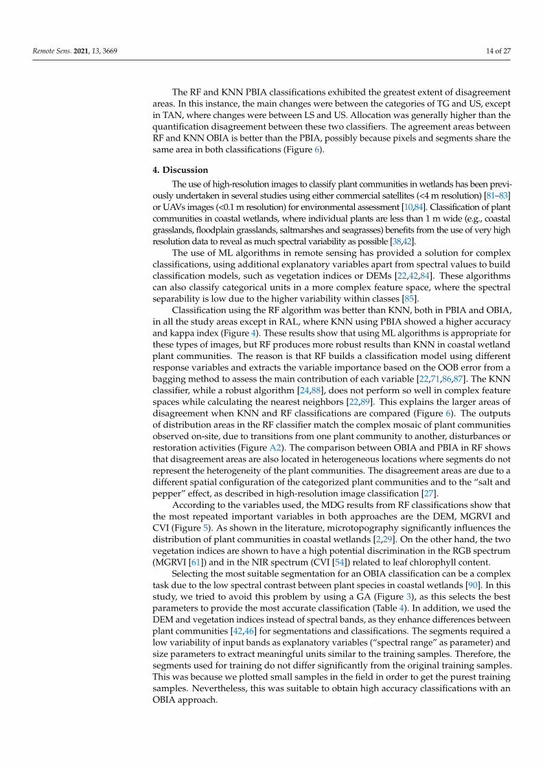
As RF was the most accurate classifier, we used it as the reference for the comparisons.The highest agreement between classifications is the RF classification OBIA and PBIA,
where the areas of agreement are greater than 65% of the total area (Figure 6). This meansthat RF has classified the images in a way that pixels follow similar patterns to the segments.In the classified maps of RF using OBIA and PBIA, both maps have a similar spatialconfiguration (Figure A1). Nevertheless, the quantity of categories is different, mainly dueto the difference of category OP to US, which represents 27% of the area of disagreement.On the contrary, the site TAS has the highest allocation disagreement in relation to thequantity disagreement (Figure 6).
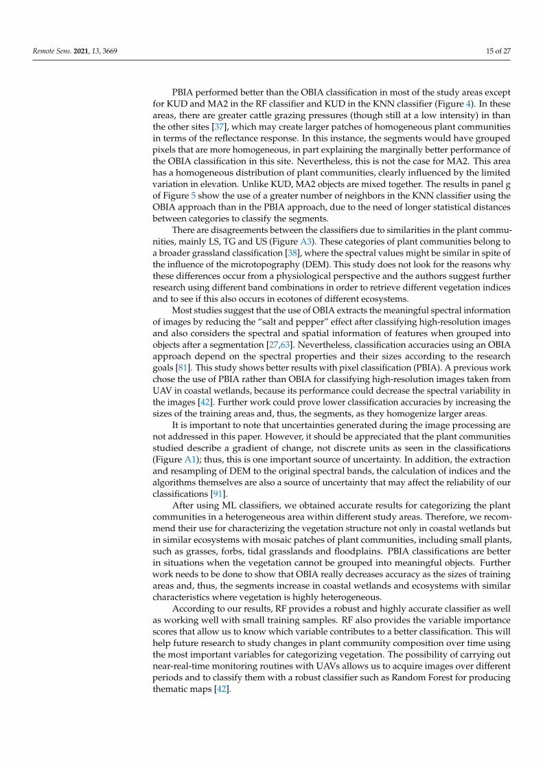
Figure 6. Comparisons between classifiers using the parameters of Quantity Disagreement, Al-location Disagreement, Allocation Agreement and Quantity Agreement (left) and agreement anddisagreement areas (right). (a) RF OBIA and PBIA, (b) RF and KNN PBIA, (c) RF and KNN OBIA.
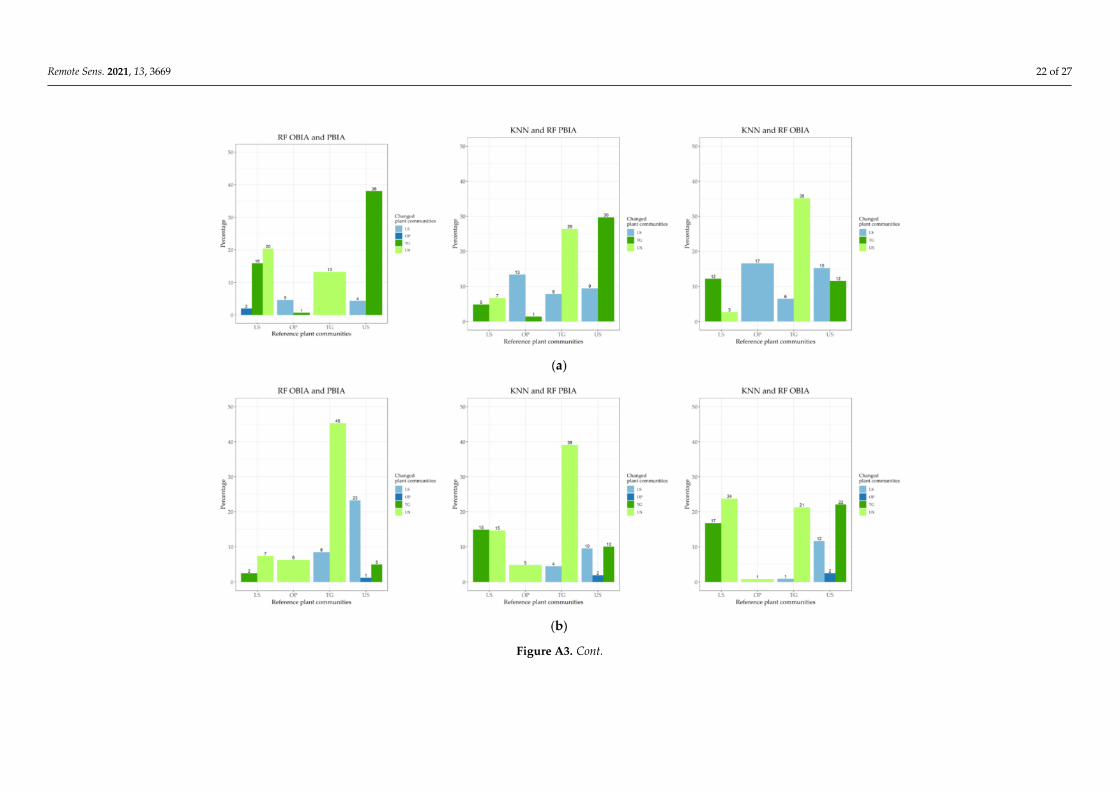
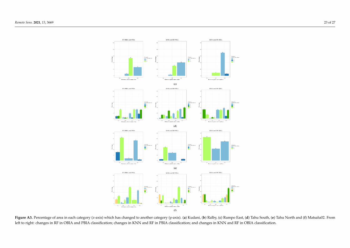
The categories that were mixed in the disagreement areas in the study areas the mostwere: KUD (38% from US to TG), RAL (45% from TG to US), RUE (27% from OP to US)and TAN (42% from LS to US and 37% from US to LS). In TAS and MA2, the mixture is dueto more than two categories (Figure 6).
Remote Sens. 2021, 13, 3669 14 of 27
The RF and KNN PBIA classifications exhibited the greatest extent of disagreementareas. In this instance, the main changes were between the categories of TG and US, exceptin TAN, where changes were between LS and US. Allocation was generally higher than thequantification disagreement between these two classifiers. The agreement areas betweenRF and KNN OBIA is better than the PBIA, possibly because pixels and segments share thesame area in both classifications (Figure 6).
4. Discussion
The use of high-resolution images to classify plant communities in wetlands has been previ-ously undertaken in several studies using either commercial satellites (<4 m resolution) [81–83]or UAVs images (<0.1 m resolution) for environmental assessment [10,84]. Classification of plantcommunities in coastal wetlands, where individual plants are less than 1 m wide (e.g., coastalgrasslands, floodplain grasslands, saltmarshes and seagrasses) benefits from the use of very highresolution data to reveal as much spectral variability as possible [38,42].
The use of ML algorithms in remote sensing has provided a solution for complexclassifications, using additional explanatory variables apart from spectral values to buildclassification models, such as vegetation indices or DEMs [22,42,84]. These algorithmscan also classify categorical units in a more complex feature space, where the spectralseparability is low due to the higher variability within classes [85].
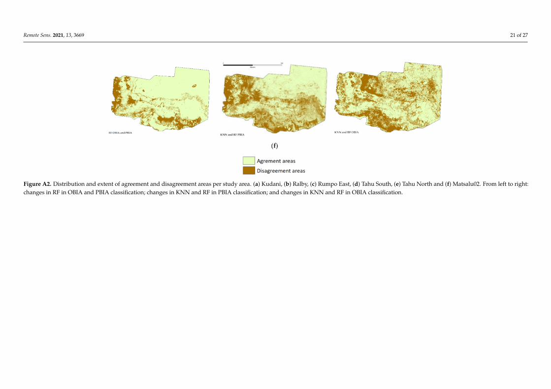
Classification using the RF algorithm was better than KNN, both in PBIA and OBIA,in all the study areas except in RAL, where KNN using PBIA showed a higher accuracyand kappa index (Figure 4). These results show that using ML algorithms is appropriate forthese types of images, but RF produces more robust results than KNN in coastal wetlandplant communities. The reason is that RF builds a classification model using differentresponse variables and extracts the variable importance based on the OOB error from abagging method to assess the main contribution of each variable [22,71,86,87]. The KNNclassifier, while a robust algorithm [24,88], does not perform so well in complex featurespaces while calculating the nearest neighbors [22,89]. This explains the larger areas ofdisagreement when KNN and RF classifications are compared (Figure 6). The outputsof distribution areas in the RF classifier match the complex mosaic of plant communitiesobserved on-site, due to transitions from one plant community to another, disturbances orrestoration activities (Figure A2). The comparison between OBIA and PBIA in RF showsthat disagreement areas are also located in heterogeneous locations where segments do notrepresent the heterogeneity of the plant communities. The disagreement areas are due to adifferent spatial configuration of the categorized plant communities and to the “salt andpepper” effect, as described in high-resolution image classification [27].
According to the variables used, the MDG results from RF classifications show thatthe most repeated important variables in both approaches are the DEM, MGRVI andCVI (Figure 5). As shown in the literature, microtopography significantly influences thedistribution of plant communities in coastal wetlands [2,29]. On the other hand, the twovegetation indices are shown to have a high potential discrimination in the RGB spectrum(MGRVI [61]) and in the NIR spectrum (CVI [54]) related to leaf chlorophyll content.
Selecting the most suitable segmentation for an OBIA classification can be a complextask due to the low spectral contrast between plant species in coastal wetlands [90]. In thisstudy, we tried to avoid this problem by using a GA (Figure 3), as this selects the bestparameters to provide the most accurate classification (Table 4). In addition, we used theDEM and vegetation indices instead of spectral bands, as they enhance differences betweenplant communities [42,46] for segmentations and classifications. The segments required alow variability of input bands as explanatory variables (“spectral range” as parameter) andsize parameters to extract meaningful units similar to the training samples. Therefore, thesegments used for training do not differ significantly from the original training samples.This was because we plotted small samples in the field in order to get the purest trainingsamples. Nevertheless, this was suitable to obtain high accuracy classifications with anOBIA approach.
Remote Sens. 2021, 13, 3669 15 of 27
PBIA performed better than the OBIA classification in most of the study areas exceptfor KUD and MA2 in the RF classifier and KUD in the KNN classifier (Figure 4). In theseareas, there are greater cattle grazing pressures (though still at a low intensity) in thanthe other sites [37], which may create larger patches of homogeneous plant communitiesin terms of the reflectance response. In this instance, the segments would have groupedpixels that are more homogeneous, in part explaining the marginally better performance ofthe OBIA classification in this site. Nevertheless, this is not the case for MA2. This areahas a homogeneous distribution of plant communities, clearly influenced by the limitedvariation in elevation. Unlike KUD, MA2 objects are mixed together. The results in panel gof Figure 5 show the use of a greater number of neighbors in the KNN classifier using theOBIA approach than in the PBIA approach, due to the need of longer statistical distancesbetween categories to classify the segments.
There are disagreements between the classifiers due to similarities in the plant commu-nities, mainly LS, TG and US (Figure A3). These categories of plant communities belong toa broader grassland classification [38], where the spectral values might be similar in spite ofthe influence of the microtopography (DEM). This study does not look for the reasons whythese differences occur from a physiological perspective and the authors suggest furtherresearch using different band combinations in order to retrieve different vegetation indicesand to see if this also occurs in ecotones of different ecosystems.
Most studies suggest that the use of OBIA extracts the meaningful spectral informationof images by reducing the “salt and pepper” effect after classifying high-resolution imagesand also considers the spectral and spatial information of features when grouped intoobjects after a segmentation [27,63]. Nevertheless, classification accuracies using an OBIAapproach depend on the spectral properties and their sizes according to the researchgoals [81]. This study shows better results with pixel classification (PBIA). A previous workchose the use of PBIA rather than OBIA for classifying high-resolution images taken fromUAV in coastal wetlands, because its performance could decrease the spectral variability inthe images [42]. Further work could prove lower classification accuracies by increasing thesizes of the training areas and, thus, the segments, as they homogenize larger areas.
It is important to note that uncertainties generated during the image processing arenot addressed in this paper. However, it should be appreciated that the plant communitiesstudied describe a gradient of change, not discrete units as seen in the classifications(Figure A1); thus, this is one important source of uncertainty. In addition, the extractionand resampling of DEM to the original spectral bands, the calculation of indices and thealgorithms themselves are also a source of uncertainty that may affect the reliability of ourclassifications [91].
After using ML classifiers, we obtained accurate results for categorizing the plantcommunities in a heterogeneous area within different study areas. Therefore, we recom-mend their use for characterizing the vegetation structure not only in coastal wetlands butin similar ecosystems with mosaic patches of plant communities, including small plants,such as grasses, forbs, tidal grasslands and floodplains. PBIA classifications are betterin situations when the vegetation cannot be grouped into meaningful objects. Furtherwork needs to be done to show that OBIA really decreases accuracy as the sizes of trainingareas and, thus, the segments increase in coastal wetlands and ecosystems with similarcharacteristics where vegetation is highly heterogeneous.
According to our results, RF provides a robust and highly accurate classifier as wellas working well with small training samples. RF also provides the variable importancescores that allow us to know which variable contributes to a better classification. This willhelp future research to study changes in plant community composition over time usingthe most important variables for categorizing vegetation. The possibility of carrying outnear-real-time monitoring routines with UAVs allows us to acquire images over differentperiods and to classify them with a robust classifier such as Random Forest for producingthematic maps [42].
Remote Sens. 2021, 13, 3669 16 of 27
Performing a rapid mapping assessment of vegetation is essential to provide quickdecisions in environmental management and conservation. The use of a rapid methodologyto obtain high-resolution images and their classification using Machine Learning algorithmsretrieves high accuracies, which can be used to monitor environmental changes over timeand to compare different sites at the same time if we keep parameters constant for theclassification and image acquisition. Further studies could use more training samples andcategories to see whether the classifications of wetlands decrease due to a more complexfeature space of the values in a pixel-based approach. In addition, the spatial variabilityof categories at the present scale of study could be compared to smaller scales usingsatellite-mounted sensors to perform upscaling of the images.
5. Conclusions
The use of ML algorithms is valuable to classify high-resolution images when thecomposition of study areas is complex. In this study, we have shown that RF and KNNclassifications are accurate and robust when using vegetation indices and digital elevationmodels, but RF retrieved better results when classifying plant communities in coastalwetlands. In spite of the high accuracies in both PBIA and OBIA classifications, our resultsshow that object-based classifications perform slightly worse than pixel-based approaches,because these ecosystems exhibit a high variability when using high-resolution imagesand grouping pixels masks some of that variability. PBIA is more suitable for classifyinghigh-resolution images in coastal wetlands, where the goal is to show the variability in thestudy area. It could be useful to use OBIA as a post-process, such as generalizing plantcommunity patterns or when larger training samples are available, allowing us to performa segmentation using higher thresholds.
As shown in Figure 6, RF retrieves lower scores of disagreement between pixel andobject classifications. Nevertheless, this depends on the study area and similarities betweenplant communities. It would be possible to improve the agreement between the RF classifi-cation of objects and pixels using images taken in flights from other dates or using othervegetation indices to discriminate other plant characteristics than those used in this study.
Author Contributions: Conceptualization, R.M.P., M.V.P. and R.D.W.; methodology, R.M.P., C.B.J.,M.V.P., T.F.B. and R.D.W.; software, R.M.P. and M.V.P.; validation, R.M.P., M.V.P. and R.D.W.; formalanalysis, R.M.P.; investigation, R.M.P., M.V.P., T.F.B., C.B.J. and R.D.W.; resources, R.D.W. andK.S.; data curation, R.M.P., M.V.P. and R.D.W.; writing—original draft preparation, R.M.P., M.V.P.and R.D.W.; writing—review and editing, R.M.P., M.V.P., R.D.W. and C.B.J.; visualization, R.M.P.;supervision, M.V.P., R.D.W. and K.S.; project administration, R.D.W. and K.S.; funding acquisition,R.D.W. and K.S. All authors have read and agreed to the published version of the manuscript.
Funding: This research was funded by the Doctoral School of Earth Sciences and Ecology, financedby the European Union, European Regional Development Fund (Estonian University of Life SciencesASTRA project “Value-chain based bio-economy”).
Institutional Review Board Statement: Not applicable.
Informed Consent Statement: Not applicable.
Conflicts of Interest: The authors declare no conflict of interest. The funders had no role in the designof the study; in the collection, analyses or interpretation of data; in the writing of the manuscript, orin the decision to publish the results.
Remote Sens. 2021, 13, 3669 17 of 27
Appendix A
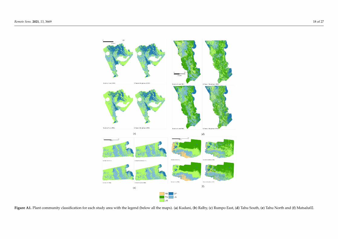
Figure A1. Cont.
Remote Sens. 2021, 13, 3669 18 of 27
Figure A1. Plant community classification for each study area with the legend (below all the maps). (a) Kudani, (b) Ralby, (c) Rumpo East, (d) Tahu South, (e) Tahu North and (f) Matsalu02.
Remote Sens. 2021, 13, 3669 19 of 27
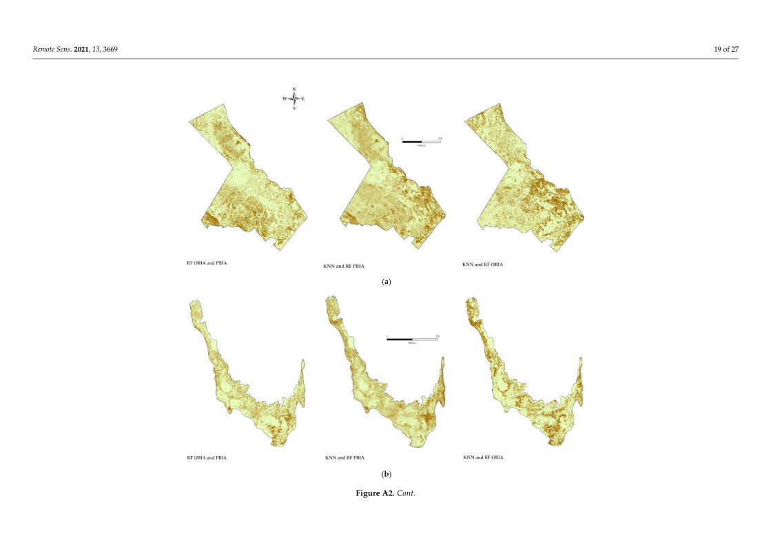
Figure A2. Cont.
Remote Sens. 2021, 13, 3669 20 of 27
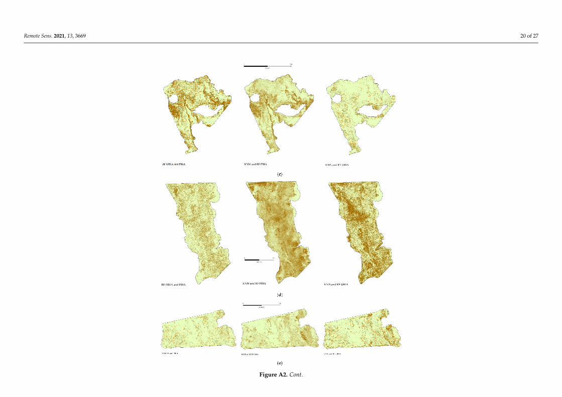
Figure A2. Cont.
Remote Sens. 2021, 13, 3669 21 of 27
Figure A2. Distribution and extent of agreement and disagreement areas per study area. (a) Kudani, (b) Ralby, (c) Rumpo East, (d) Tahu South, (e) Tahu North and (f) Matsalu02. From left to right:changes in RF in OBIA and PBIA classification; changes in KNN and RF in PBIA classification; and changes in KNN and RF in OBIA classification.
Remote Sens. 2021, 13, 3669 22 of 27
Figure A3. Cont.
Remote Sens. 2021, 13, 3669 23 of 27
Figure A3. Percentage of area in each category (x-axis) which has changed to another category (y-axis). (a) Kudani, (b) Ralby, (c) Rumpo East, (d) Tahu South, (e) Tahu North and (f) Matsalu02. Fromleft to right: changes in RF in OBIA and PBIA classification; changes in KNN and RF in PBIA classification; and changes in KNN and RF in OBIA classification.
Remote Sens. 2021, 13, 3669 24 of 27
References1. LaPaix, R.L.; Freedman, B.F.; Patriquin, D.P. Ground vegetation as an indicator of ecological integrity. Environ. Rev. 2009, 17,
249–265. [CrossRef]2. Berg, M.; Joyce, C.; Burnside, N. Differential responses of abandoned wet grassland plant communities to reinstated cutting
management. Hydrobiologia 2012, 692, 83–97. [CrossRef]3. Pärtel, M.; Chiarucci, A.; Chytrý, M.; Pillar, V.D. Mapping plant community ecology. J. Veg. Sci. 2017, 28, 1–3. [CrossRef]4. Van der Maarel, E. Vegetation Ecology—An Overview; van der Maarel, E., Ed.; Vegetation Ecology; Blackwell Publishing: Oxford,
UK, 2015; pp. 1–3.5. Martínez-López, J.; Carreño, M.F.; Palazón-Ferrando, J.A.; Martínez-Fernández, J.; Esteve, M.A. Remote sensing of plant
communities as a tool for assessing the condition of semiarid Mediterranean saline wetlands in agricultural catchments. Int. J.Appl. Earth Obs. Geoinf. 2014, 26, 193–204. [CrossRef]
6. Pettorelli, N.; Laurance, W.F.; O’Brien, T.G.; Wegmann, M.; Nagendra, H.; Turner, W. Satellite remote sensing for appliedecologists: Opportunities and challenges. J. Appl. Ecol. 2014, 51, 839–848. [CrossRef]
7. Kaplan, G.; Avdan, U. Mapping and monitoring wetlands using Sentinel-2 satellite imagery. ISPRS Ann. Photogramm Remote Sens.Spat. Inf. Sci. 2017, IV-4/W4, 271–277. [CrossRef]
8. Ceaus, u, S.; Apaza-Quevedo, A.; Schmid, M.; Martín-López, B.; Cortés-Avizanda, A.; Maes, J.; Brotons, L.; Queiroz, C.; Pereira,H.M. Ecosystem service mapping needs to capture more effectively the biodiversity important for service supply. Ecosyst. Serv.2021, 48, 101259. [CrossRef]
9. Corbane, C.; Lang, S.; Pipkins, K.; Alleaume, S.; Deshayes, M.; García Millán, V.E.; Strasser, T.; Vanden Borre, J.; Toon, S.; Michael,F. Remote sensing for mapping natural habitats and their conservation status—New opportunities and challenges. Int. J. Appl.Earth Obs. Geoinf. 2015, 37, 7–16. [CrossRef]
10. Díaz-Delgado, R.; Cazacu, C.; Adamescu, M. Rapid assessment of ecological integrity for LTER wetland sites by using UAVmultispectral mapping. Drones 2019, 3, 3. [CrossRef]
11. Baena, S.; Boyd, D.S.; Moat, J. UAVs in pursuit of plant conservation—Real world experiences. Ecol. Inform. 2018, 47, 2–9.[CrossRef]
12. Palmer, M.W.; Earls, P.G.; Hoagland, B.W.; White, P.S.; Wohlgemuth, T. Quantitative tools for perfecting species lists. Environmetrics2002, 13, 121–137. [CrossRef]
13. Westoby, M.J.; Brasington, J.; Glasser, N.F.; Hambrey, M.J.; Reynolds, J.M. ‘Structure-from-Motion’ photogrammetry: A low-cost,effective tool for geoscience applications. Geomorphology 2012, 179, 300–314. [CrossRef]
14. Meza, J.; Marrugo, A.G.; Ospina, G.; Guerrero, M.; Romero, L.A. A Structure-from-motion pipeline for generating digital elevationmodels for surface-runoff analysis. J. Phys. Conf. Ser. 2019, 1247, 012039. [CrossRef]
15. Cullum, C.; Rogers, K.H.; Brierley, G.; Witkowski, E.T.F. Ecological classification and mapping for landscape management andscience: Foundations for the description of patterns and processes. Prog. Phys. Geogr. Earth Environ. 2016, 40, 38–65. [CrossRef]
16. KopeL, D.; Michalska-Hejduk, D.; Berezowski, T.; Borowski, M.; Rosadzifski, S.; Chormafski, J. Application of multisensoralremote sensing data in the mapping of alkaline fens natura 2000 habitat. Ecol. Indic. 2016, 70, 196–208. [CrossRef]
17. Jensen, J.R. Introductory Digital Image Processing: A Remote Sensing Perspective, 4th ed.; Pearson Series in Geographic InformationScience; Pearson: London, UK, 2015; ISBN 978-0-13-405816-0.
18. Yu, L.; Liang, L.; Wang, J.; Zhao, Y.; Cheng, Q.; Hu, L.; Liu, S.; Yu, L.; Wang, X.; Zhu, P.; et al. Meta-discoveries from a synthesis ofsatellite-based land-cover mapping research. Int. J. Remote Sens. 2014, 35, 4573–4588. [CrossRef]
19. Oddi, F.J.; Miguez, F.E.; Ghermandi, L.; Bianchi, L.O.; Garibaldi, L.A. A nonlinear mixed-effects modeling approach for ecologicaldata: Using temporal dynamics of vegetation moisture as an example. Ecol. Evol. 2019, 9, 10225–10240. [CrossRef] [PubMed]
20. Thessen, A.E. Adoption of machine learning techniques in ecology and earth science. One Ecosyst. 2016, 1, e8621. [CrossRef]21. Olden, J.D.; Lawler, J.J.; Poff, N.L. Machine learning methods without tears: A primer for ecologists. Q. Rev. Biol. 2008, 83,
171–193. [CrossRef]22. Maxwell, A.E.; Warner, T.A.; Fang, F. Implementation of machine-learning classification in remote sensing: An applied review.
Int. J. Remote Sens. 2018, 39, 2784–2817. [CrossRef]23. Brosofske, K.D.; Froese, R.E.; Falkowski, M.J.; Bans4kota, A. A review of methods for mapping and prediction of inventory
attributes for operational forest management. For. Sci. 2013, 60, 733–756. [CrossRef]24. Chirici, G.; Mura, M.; McInerney, D.; Py, N.; Tomppo, E.O.; Waser, L.T.; Travaglini, D.; McRoberts, R.E. A meta-analysis and
review of the literature on the k-Nearest Neighbors technique for forestry applications that use remotely sensed data. RemoteSens. Environ. 2016, 176, 282–294. [CrossRef]
25. Rodriguez-Galiano, V.F.; Ghimire, B.; Rogan, J.; Chica-Olmo, M.; Rigol-Sanchez, J.P. An assessment of the effectiveness of arandom forest classifier for land-cover classification. ISPRS J. Photogramm. Remote Sens. 2012, 67, 93–104. [CrossRef]
26. Blaschke, T. Object based image analysis for remote sensing. ISPRS J. Photogramm. Remote Sens. 2010, 65, 2–16. [CrossRef]27. Dronova, I. Object-Based Image Analysis in Wetland Research: A Review. Remote Sens. 2015, 7, 6380–6413. [CrossRef]28. Räsänen, A.; Virtanen, T. Data and resolution requirements in mapping vegetation in spatially heterogeneous landscapes. Remote
Sens. Environ. 2019, 230, 111207. [CrossRef]
Remote Sens. 2021, 13, 3669 25 of 27
29. Ward, R.D.; Burnside, N.G.; Joyce, C.B.; Sepp, K. Importance of microtopography in determining plant community distribution inbaltic coastal Wetlands. J. Coast. Res. 2016, 32, 1062–1070. [CrossRef]
30. Berhane, T.M.; Lane, C.R.; Wu, Q.; Anenkhonov, O.A.; Chepinoga, V.V.; Autrey, B.C.; Liu, H. Comparing Pixel- and Object-basedapproaches in effectively classifying wetland-dominated landscapes. Remote Sens. 2018, 10, 46. [CrossRef]
31. Çiçekli, S.Y.; Sekertekin, A.; Arslan, N.; Donmez, C. Comparison of pixel and object-based classification methods in Wetlandsusing sentinel-2 Data. Int. J. Environ. Geoinf. 2018, 7, 213–220.
32. Kimmel, K. Ecosystem Services of Estonian Wetlands. Ph.D. Thesis, Department of Geography, Institute of Ecology and EarthSciences, Faculty of Science and Technology, University of Tartu, Tartu, Estonia, 2009.
33. Rannap, R.; Briggs, L.; Lotman, K.; Lepik, I.; Rannap, V.; Põdra, P. Coastal Meadow Management—Best Practice Guidelines; Ministryof the Environment of the Republic of Estonia: Tallinn, Estonia, 2004; Volume 1, p. 100.
34. Larkin, D.J.; Bruland, G.L.; Zedler, J.B. Heterogeneity theory and ecological restoration. In Foundations of Restoration Ecology;Palmer, M.A., Zedler, J.B., Falk, D.A., Eds.; Island Press/Center for Resource Economics: Washington, DC, USA, 2016; pp. 271–300.ISBN 978-1-61091-698-1.
35. Ward, R.D.; Burnside, N.G.; Joyce, C.B.; Sepp, K.; Teasdale, P.A. Improved modelling of the impacts of sea level rise on coastalwetland plant communities. Hydrobiologia 2016, 774, 203–216. [CrossRef]
36. Ward, R.D.; Burnside, N.G.; Joyce, C.B.; Sepp, K. The use of medium point density LiDAR elevation data to determine plantcommunity types in Baltic coastal wetlands. Ecol. Indic. 2013, 33, 96–104. [CrossRef]
37. Villoslada Peciña, M.; Bergamo, T.F.; Ward, R.D.; Joyce, C.B.; Sepp, K. A novel UAV-based approach for biomass prediction andgrassland structure assessment in coastal meadows. Ecol. Indic. 2021, 122, 107227. [CrossRef]
38. Burnside, N.G.; Joyce, C.B.; Puurmann, E.; Scott, D.M. Use of vegetation classification and plant indicators to assess grazingabandonment in Estonian coastal wetlands. J. Veg. Sci. 2007, 18, 645–654. [CrossRef]
39. Kutser, T.; Paavel, B.; Verpoorter, C.; Ligi, M.; Soomets, T.; Toming, K.; Casal, G. Remote sensing of black lakes and using 810 nmreflectance peak for retrieving water quality parameters of optically complex waters. Remote Sens. 2016, 8, 497. [CrossRef]
40. Karabulut, M. An examination of spectral reflectance properties of some wetland plants in Göksu Delta, Turkey. J. Int. Environ.Appl. Sci. 2018, 13, 194–203.
41. Tadrowski, T. Accurate mapping using drones (UAV’s). GeoInformatics 2014, 17, 18.42. Villoslada, M.; Bergamo, T.F.; Ward, R.D.; Burnside, N.G.; Joyce, C.B.; Bunce, R.G.H.; Sepp, K. Fine scale plant community
assessment in coastal meadows using UAV based multispectral data. Ecol. Indic. 2020, 111, 105979. [CrossRef]43. Strong, C.J.; Burnside, N.G.; Llewellyn, D. The potential of small-Unmanned Aircraft Systems for the rapid detection of threatened
unimproved grassland communities using an enhanced normalized difference vegetation index. PLoS ONE 2017, 12, e0186193.[CrossRef] [PubMed]
44. Smith, M.W.; Carrivick, J.L.; Quincey, D.J. Structure from motion photogrammetry in physical geography. Prog. Phys. Geogr. EarthEnviron. 2016, 40, 247–275. [CrossRef]
45. Cai, S.; Zhang, W.; Liang, X.; Wan, P.; Qi, J.; Yu, S.; Yan, G.; Shao, J. Filtering airborne LiDAR data through complementary clothsimulation and progressive TIN densification filters. Remote Sens. 2019, 11, 1037. [CrossRef]
46. Fletcher, R.S. Using vegetation indices as input into random forest for soybean and weed classification. Am. J. Plant. Sci. 2016, 7,2186–2198. [CrossRef]
47. Filho, M.G.; Kuplich, T.M.; Quadros, F.L.F.D. Estimating natural grassland biomass by vegetation indices using Sentinel 2 remotesensing data. Int. J. Remote Sens. 2020, 41, 2861–2876. [CrossRef]
48. Xue, J.; Su, B. Significant remote sensing vegetation indices: A review of developments and applications. J. Sens. 2017, 2017,e1353691. [CrossRef]
49. R Core Team. R: A Language and Environment for Statistical Computing; R Foundation for Statistical Computing: Vienna, Austria,2013.
50. Hijmans, R.J. Raster: Geographic Data Analysis and Modeling. R Package Version 3.4-5. 2020. Available online: https://CRAN.R-project.org/package=raster (accessed on 10 September 2021).
51. Bivand, R.; Keitt, T.; Barry, R. Rgdal: Bindings for the “Geospatial” Data Abstraction Library. R Package Version 1.5-18. Availableonline: https://CRAN.R-project.org/package=rgdal (accessed on 10 September 2021).
52. Rouse, J.W.; Haas, R.H.; Schell, J.A.; Deering, D.W. Monitoring vegetation systems in the Great Plains with ERTS. Monit. Veg. Syst.Gt. Plains ERTS 1974, 351, 309–317.
53. Gitelson, A.A.; Kaufman, Y.J.; Merzlyak, M.N. Use of a green channel in remote sensing of global vegetation from EOS-MODIS.Remote Sens. Environ. 1996, 58, 289–298. [CrossRef]
54. Vincini, M.; Frazzi, E.; D’Alessio, P. A broad-band leaf chlorophyll vegetation index at the canopy scale. Precis. Agric. 2008, 9,303–319. [CrossRef]
55. Wu, C.; Niu, Z.; Tang, Q.; Huang, W. Estimating chlorophyll content from hyperspectral vegetation indices: Modeling andvalidation. Agric. For. Meteorol. 2008, 148, 1230–1241. [CrossRef]
56. Chen, P.-F.; Tremblay, N.; Wang, J.-H.; Vigneault, P.; Huang, W.-J.; Li, B.-G. New index for crop canopy fresh biomass estimation.Guang Pu Xue Yu Guang Pu Fen XiSpectroscopy Spectr. Anal. 2010, 30, 512–517.
Remote Sens. 2021, 13, 3669 26 of 27
57. Barnes, E.M.; Clarke, T.R.; Richards, S.E.; Colaizzi, P.D.; Haberland, J.; Kostrzewski, M.; Waller, P.; Choi, C.; Riley, E.; Thompson,T. Coincident detection of crop water stress, nitrogen status and canopy density using ground-based multispectral data. InProceedings of the 5th International Conference on Precision Agriculture, Bloomingt, MN, USA, 16–19 July 2000.
58. Gitelson, A.A.; Viña, A.; Arkebauer, T.J.; Rundquist, D.C.; Keydan, G.; Leavitt, B. Remote estimation of leaf area index and greenleaf biomass in maize canopies. Geophys. Res. Lett. 2003, 30, 1248. [CrossRef]
59. Gitelson, A.; Merzlyak, M.N. Spectral reflectance changes associated with autumn senescence of Aesculus hippocastanum L. andAcer platanoides L. leaves. spectral features and relation to chlorophyll estimation. J. Plant. Physiol. 1994, 143, 286–292. [CrossRef]
60. Datt, B. Remote sensing of Chlorophyll a, Chlorophyll b, Chlorophyll a+b, and total carotenoid content in eucalyptus leaves.Remote Sens. Environ. 1998, 66, 111–121. [CrossRef]
61. Bendig, J.; Yu, K.; Aasen, H.; Bolten, A.; Bennertz, S.; Broscheit, J.; Gnyp, M.L.; Bareth, G. Combining UAV-based plant heightfrom crop surface models, visible, and near infrared vegetation indices for biomass monitoring in barley. Int. J. Appl. Earth Obs.Geoinf. 2015, 39, 79–87. [CrossRef]
62. Turpie, K.R. Explaining the spectral red-edge features of inundated marsh vegetation. J. Coast. Res. 2013, 29, 1111–1117. [CrossRef]63. Cheng, G.; Xie, X.; Han, J.; Guo, L.; Xia, G.-S. Remote sensing image scene classification meets deep learning: Challenges, methods,
benchmarks, and opportunities. IEEE J. Sel. Top. Appl. Earth Obs. Remote Sens. 2020, 13, 3735–3756. [CrossRef]64. Egorov, A.V.; Hansen, M.C.; Roy, D.P.; Kommareddy, A.; Potapov, P.V. Image interpretation-guided supervised classification
using nested segmentation. Remote Sens. Environ. 2015, 165, 135–147. [CrossRef]65. Kuhn, M.; Johnson, K. Applied Predictive Modeling; Springer: New York, NY, USA, 2013; ISBN 978-1-4614-6848-6.66. Lin, Z.; Zhang, G. Genetic algorithm-based parameter optimization for EO-1 Hyperion remote sensing image classification. Eur. J.
Remote Sens. 2020, 53, 124–131. [CrossRef]67. Gonçalves, J.; Pôças, I.; Marcos, B.; Mücher, C.A.; Honrado, J.P. SegOptim—A new R package for optimizing object-based image
analyses of high-spatial resolution remotely-sensed data. Int. J. Appl. Earth Obs. Geoinf. 2019, 76, 218–230. [CrossRef]68. Michel, J.; Youssefi, D.; Grizonnet, M. Stable mean-shift algorithm and its application to the segmentation of arbitrarily large
remote sensing images. IEEE Trans. Geosci. Remote Sens. 2015, 53, 952–964. [CrossRef]69. Grizonnet, M.; Michel, J.; Poughon, V.; Inglada, J.; Savinaud, M.; Cresson, R. Orfeo toolbox: Open source processing of remote
sensing images. Open Geospatial Data Softw. Stand. 2017, 2, 15. [CrossRef]70. Breiman, L. Random Forests. Mach. Learn. 2001, 45, 5–32. [CrossRef]71. Gislason, P.O.; Benediktsson, J.A.; Sveinsson, J.R. Random forests for land cover classification. Pattern Recognit. Lett. 2006, 27,
294–300. [CrossRef]72. Abu Alfeilat, H.A.; Hassanat, A.B.A.; Lasassmeh, O.; Tarawneh, A.S.; Alhasanat, M.B.; Eyal Salman, H.S.; Prasath, V.B.S. Effects of
distance measure choice on K-nearest neighbor classifier performance: A review. Big Data 2019, 7, 221–248. [CrossRef] [PubMed]73. Kuhn, M. Building predictive models in R using the caret package. J. Stat. Softw. 2008, 28, 1–26. [CrossRef]74. Yang, X.; Blower, J.D.; Bastin, L.; Lush, V.; Zabala, A.; Masó, J.; Cornford, D.; Díaz, P.; Lumsden, J. An integrated view of data
quality in earth observation. Philos. Trans. R. Soc. Math. Phys. Eng. Sci. 2013, 371, 20120072. [CrossRef]75. Foody, G.M. Thematic map comparison. Photogramm. Eng. Remote Sens. 2004, 70, 627–633. [CrossRef]76. Pontius, R.G. Quantification error versus location error in comparison of categorical maps. Photogramm. Eng. Amp Remote Sens.
2000, 66, 1011–1016.77. Hagen-Zanker, A. Multi-method assessment of map similarity. In Proceedings of the 5th AGILE Conference on Geographic
Information Science, Boulder, CO, USA, 25–28 September 2002.78. Pontius, R.G., Jr.; Millones, M. Death to Kappa: Birth of quantity disagreement and allocation disagreement for accuracy
assessment. Int. J. Remote Sens. 2011, 32, 4407–4429. [CrossRef]79. Appelhans, T.; Otte, I.; Kuehnlein, M.; Meyer, H.; Forteva, S.; Nauss, T.; Detsch, F. Rsenal: Magic R Functions for Things Various; R
Package Version 0.6.10; R Foundation for Statistical Computing: Vienna, Austria, 2021.80. Remmel, T.K. Investigating global and local categorical map configuration comparisons based on coincidence matrices. Geogr.
Anal. 2009, 41, 144–157. [CrossRef]81. Dronova, I.; Gong, P.; Wang, L.; Zhong, L. Mapping dynamic cover types in a large seasonally flooded wetland using extended
principal component analysis and object-based classification. Remote Sens. Environ. 2015, 158, 193–206. [CrossRef]82. Dribault, Y.; Chokmani, K.; Bernier, M. Monitoring seasonal hydrological dynamics of minerotrophic peatlands using multi-date
GeoEye-1 very high resolution imagery and object-based classification. Remote Sens. 2012, 4, 1887–1912. [CrossRef]83. Lane, C.R.; Liu, H.; Autrey, B.C.; Anenkhonov, O.A.; Chepinoga, V.V.; Wu, Q. Improved wetland classification using eight-band
high resolution satellite imagery and a hybrid approach. Remote Sens. 2014, 6, 12187–12216. [CrossRef]84. Doughty, C.L.; Ambrose, R.F.; Okin, G.S.; Cavanaugh, K.C. Characterizing spatial variability in coastal wetland biomass across
multiple scales using UAV and satellite imagery. Remote Sens. Ecol. Conserv. 2021. [CrossRef]85. Carleer, A.P.; Debeir, O.; Wolff, E. Assessment of very high spatial resolution satellite image segmentations. Photogramm. Eng.
Remote Sens. 2005, 71, 1285–1294. [CrossRef]86. Belgiu, M.; Drăgut, L. Random forest in remote sensing: A review of applications and future directions. ISPRS J. Photogramm.
Remote Sens. 2016, 114, 24–31. [CrossRef]87. Hayes, M.M.; Miller, S.N.; Murphy, M.A. High-resolution landcover classification using random forest. Remote Sens. Lett. 2014, 5,
112–121. [CrossRef]

Remote Sens. 2021, 13, 3669 27 of 27
88. Maselli, F.; Chirici, G.; Bottai, L.; Corona, P.; Marchetti, M. Estimation of Mediterranean forest attributes by the application ofk-NN procedures to multitemporal Landsat ETM+ images. Int. J. Remote Sens. 2005, 26, 3781–3796. [CrossRef]
89. Wieland, M.; Pittore, M. Performance evaluation of machine learning algorithms for urban pattern recognition from multi-spectralsatellite images. Remote Sens. 2014, 6, 2912–2939. [CrossRef]
90. Moffett, K.B.; Gorelick, S.M. Distinguishing wetland vegetation and channel features with object-based image segmentation. Int.J. Remote Sens. 2013, 34, 1332–1354. [CrossRef]
91. van der Wel, F. Assessment and Visualisation of Uncertainty in Remote Sensing Land Cover Classifications; University of Utrecht:Utrecht, The Netherlands, 2000; ISBN 90-6266-181-5.