Journal of Animal Ecology

2008 doi: 10.1111/j.1365-2656.2008.01415.x

© 2008 The Authors. Journal compilation © 2008 British Ecological Society

J A E 1 4 1 5

Operator:

LinPing

Dispatch:

30.05.08

PE:

Penny Baker

Journal Name Manuscript No.

Proofreader:

Chen Xiaoming

No. of Pages:

11

Copy-editor:

John Wiley & Sons Ltd

UNCORRECTED PROOF

123456789

101112131415161718192021222324252627282930313233343536373839404142434445464748495051525354555657

Blackwell Publishing Ltd

Low genetic variability, female-biased dispersal and high

movement rates in an urban population of Eurasian

badgers

Meles meles

Maren Huck

1,2*

, Alain C. Frantz

2

, Deborah A. Dawson

2

, Terry Burke

2

and Timothy J. Roper

1

1

Department of Biology and Environmental Science, University of Sussex, Brighton, BN1 9QG, UK; and

2

Department of

Animal and Plant Sciences, University of Sheffield, S10 2TN, UK

Summary

1.

Urban and rural populations of animals can differ in their behaviour, both in order to meet theirecological requirements and due to the constraints imposed by different environments. The studyof urban populations can therefore offer useful insights into the behavioural flexibility of a species asa whole, as well as indicating how the species in question adapts to a specifically urban environment.

2.

The genetic structure of a population can provide information about social structure andmovement patterns that is difficult to obtain by other means. Using non-invasively collected hairsamples, we estimated the population size of Eurasian badgers

Meles meles

in the city of Brighton,England, and calculated population-specific parameters of genetic variability and sex-specific ratesof outbreeding and dispersal.

3.

Population density was high in the context of badger densities reported throughout their range.This was due to a high density of social groups rather than large numbers of individuals per group.

4.

The allelic richness of the population was low compared with other British populations. However,the rate of extra-group paternity and the relatively frequent (mainly temporary) intergroup movementssuggest that, on a local scale, the population was outbred. Although members of both sexes visitedother groups, there was a trend for more females to make intergroup movements.

5.

The results reveal that urban badgers can achieve high densities and suggest that while somepopulation parameters are similar between urban and rural populations, the frequency of inter-group movements is higher among urban badgers. In a wider context, these results demonstrate theability of non-invasive genetic sampling to provide information about the population density, socialstructure and behaviour of urban wildlife.

Key-words:

group size, outbreeding, population density, sex-biased dispersal, spatial geneticstructure, sex typing.

Introduction

Eurasian badgers (

Meles meles

L. 1758) have been known forsome time to inhabit urban environments (e.g. Harris 1982;Cheeseman

et al

. 1988), where they can achieve burrow (‘sett’)densities comparable to those of most rural UK populations(Huck, Davison & Roper, in press). When urban and ruralpopulations of the same species are compared, variousanimal taxa have been found to differ behaviourally in various

respects (Ditchkoff, Saalfeld & Gibson 2006): for example,urban and rural Cooper’s hawks (

Accipiter cooperii

Bonaparte1828; Estes & Mannan 2003) differed in prey delivery rates,while urban red foxes (

Vulpes vulpes

L. 1758) have less stableterritories than is typical of rural populations (Doncaster &Macdonald 1991). The same applies to badgers, in so far asurban badgers show less intense territorial behaviour thanrural populations (Cheeseman

et al

. 1988), have smaller homeranges and differ in their pattern of sett use (Davison 2007).The study of urban populations can therefore offer usefulinsights into the behavioural flexibility of a species as a whole,as well as indicating how the species in question adapts to aspecifically urban environment.

*Correspondence author. M. Huck, Department of Biology andEnvironmental Science, University of Sussex, Brighton BN1 9QG,UK. E-mail: maren_huck@hotmail.com

1

2

M. Huck

et al.

© 2008 The Authors. Journal compilation © 2008 British Ecological Society,

Journal of Animal Ecology

UNCORRECTED PROOF

123456789

101112131415161718192021222324252627282930313233343536373839404142434445464748495051525354555657

Mating systems may also vary between different habitats(e.g. Langbein & Thirgood 1989), leading to variation in thegenetic structure of the populations in question.

The genetic structure of a population can in turn provideinformation about social structure and movement patterns – and thus indirectly about some behaviours that might bedifficult to obtain by other means such as radio-tracking ordirect observation (e.g. Favre

et al

. 1997; Huck, Roos &Heymann 2007). In the case of badgers, microsatellite analysisbased on blood samples has recently provided detailedinformation about the mating system and genetic structure oftwo rural populations (Carpenter

et al

. 2005; Dugdale

et al

.2007, 2008), while DNA from non-invasively collected hairsamples has been used to estimate badger population sizesand to track movements of badgers between social groups(Frantz

et al

. 2004; Scheppers

et al

. 2007). However, geneticinformation about urban badgers is completely lacking andthere has been only one previous attempt to estimate populationdensity in urban badgers (Harris & Cresswell 1987).

Our study used non-invasively collected genomic DNA(extracted from hair samples) in order to: (1) estimate thepopulation density of badgers in a restricted urban areawithin the city of Brighton, England; and (2) determinepopulation-specific parameters of genetic variability, and sex-specific estimates of outbreeding and dispersal. These resultswere compared to those of previous studies of rural badgerpopulations, in order to determine whether urban and ruralpopulations differ with respect to these parameters.

Methods

STUDY

AREA

Our core study area comprised the areas of Kemptown and White-hawk within the city of Brighton, England, where badgers had beensubject to a radio-tracking study since September 2004 (Davison

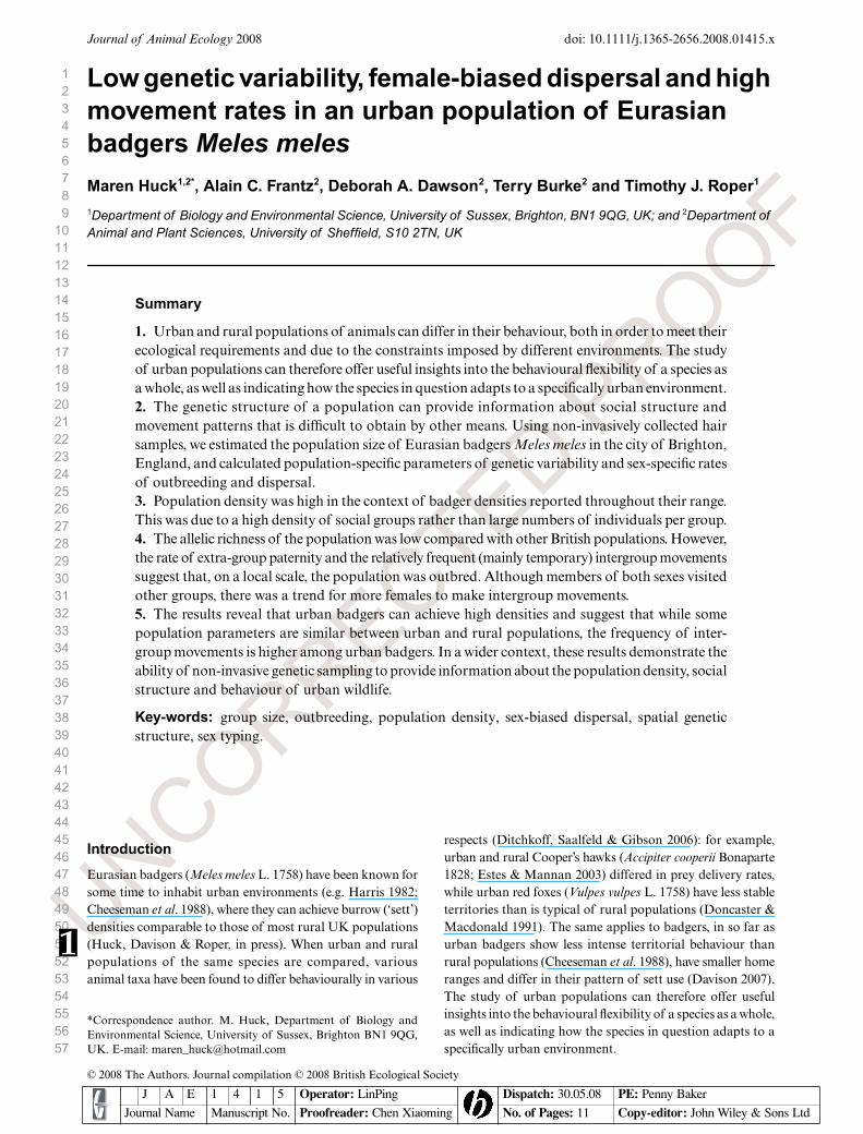
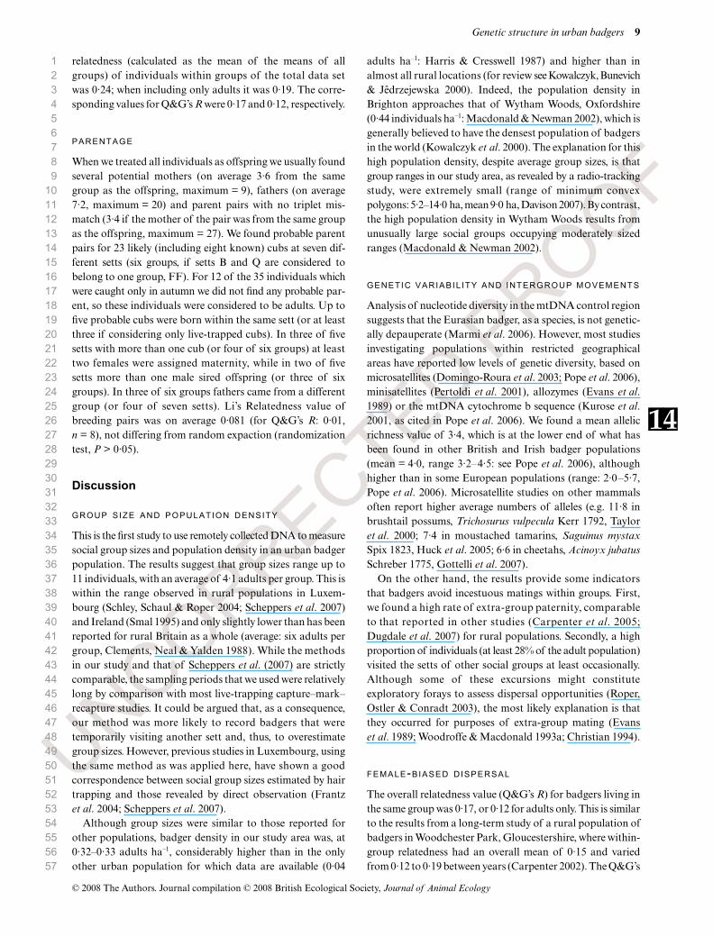
2007). The area in question (minimum convex polygon around allsampled setts) covered 195·6 ha, including 136·9 ha of urban habitatconsisting of private gardens, small patches of scrub unused byhumans, allotments, public parks and areas of mown grass on playingfields and around housing estates. The area contained six main setts(urban setts F, K, M, S, WT, WH), several small setts that wereknown to be outliers of these main setts, and five setts whosestatus was unclear (B, H, Q, C, RR; see Fig. 1). These latter setts wereusually separated by a larger distance from the nearest main settthan known outliers or were never visited by radio-collaredindividuals from adjoining main setts. In addition, data were collectedfrom an adjacent suburban sett (R) and from the nearest rural sett(SV).

SAMPLE

COLLECTION

AND

DNA

EXTRACTION

The collection of hair samples followed the method described byScheppers

et al

. (2007). Hair traps consisted of a strand of barbedwire supported by two metal stakes, placed approximately 30 cmapart and with the highest point of the wire about 22 cm aboveground. Traps were placed across well-used badger paths (‘runs’),where possible well hidden in vegetation such as brambles, orbeneath fences, and usually in close proximity to a sett. Sett S waslocated on private school ground, and therefore was not accessibleduring the first period of hair collection, so that runs at some distancefrom the sett had to be used. For the second time-period, however, itwas possible to collect samples from the runs around this sett.

We collected guard hair samples during two periods in 2006: from20 March to 24 April and from 9 October to 16 November, exceptfor sett S where samples were collected from 10 to 25 August. Theseperiods were chosen because they coincide with peaks of reproductiveactivity in British badgers (Cresswell

et al

. 1992), thus enhancing thepossibility of detecting the intergroup movements which were occu-rring for mating purposes. In addition, we wanted to calculate populationdensities before (spring) and after (autumn) the emergence of cubs fromthe dens. The sampling period of 4 weeks was based on previous studies(Frantz

et al

. 2004; Scheppers

et al

. 2007), but was prolonged in somecases where trapping proved difficult because of insufficiently densevegetation or because traps were vandalized.

2

Fig. 1. Badger setts in Brighton where hairsamples were collected. Large asterisks andunderlined letters denote main setts, smallasterisks setts of uncertain status. Dots showall known occupied badger setts in thevicinity of the study area that were notstudied. The study area is bordered by thethin-lined polygon (195·6 ha). The dark back-ground shows urbanized habitats (136·9 hawithin study area). Bold-lined polygonssignify group home ranges (Davison et al.,submitted), with the exception of group WTthat shows only the combined range of twofemales, while the range of a male is shown ingrey. Outlier setts where no sampling tookplace are not depicted.

3

Genetic structure in urban badgers

3

© 2008 The Authors. Journal compilation © 2008 British Ecological Society,

Journal of Animal Ecology

UNCORRECTED PROOF

123456789

101112131415161718192021222324252627282930313233343536373839404142434445464748495051525354555657

Hairs were collected daily using forceps. After each collection weflamed both the forceps and the barbed wire in order to avoid samplecross-contamination. Hairs collected from the same barb wereconsidered to constitute one sample. Hairs from different barbs ofthe same trap were classed initially as separate samples, but afterfurther analysis were considered separate only if shown to begenetically different. We also collected hair samples from eight cubs(caught during attempts to capture adults, Davison

et al

., submitted;see section ‘Sex determination’). Samples were stored in separatepaper envelopes at room temperature until DNA extraction.Genomic DNA was usually extracted on the day of collection andalways within 2 days of collection.

Following the reasoning of Scheppers

et al

. (2007), we used onlysingle hairs for both a main and a back-up extraction. Extractionstook place in a laboratory where no previous work on badger DNAhad been performed, using a Chelex protocol (Chelex-100; Bio-Rad,Hercules, CA, USA; Walsh, Metzger & Higuchi 1991) described byFrantz

et al

. (2004).

POLYMERASE

CHAIN

REACTION

(

PCR

)

AND

GENOTYPING

DNA amplification and genotyping took place after each period ofsample collection at the University of Sheffield. We tested a total of32 badger microsatellite loci for their variability in our study popu-lation. The loci were developed originally by Bijlsma

et al

. (2000),Domingo-Roura

et al

. (2003), Carpenter

et al

. (2003) and D.A.Dawson (unpublished data). Six loci were not variable in a subset ofsamples, four appeared unreliable for scoring (where PCR productsregularly included more than two electropherogram peaks), and twowere discarded at a later stage of analysis (see below and Table 1),leaving 20 microsatellite loci available for the final analyses.

PCRs were set up and conducted in a separate room where nowork with concentrated badger DNA had been performed previously,under an ultraviolet hood. The hood was cleaned thouroughly withbleach after setting up each PCR and was switched on daily afterwork for 20 min to remove potential for cross-contamination. Forsamples from the first sampling period, PCRs were performed assingle or double-plex reactions using the conditions described inCarpenter

et al

. (2005) and Pope

et al

. (2006). Loci were amplifiedusing the touchdown-profile described by Frantz

et al

. (2003). Thetotal reaction volume was initially 25

μ

L, including 5

μ

L of DNAextract, but for some loci (Mel15, Mel101 and Mel105) this volumewas reduced to 10

μ

L using the same concentrations of constituents,and with 1–5

μ

L of extracted genomic DNA extract.DNA from the samples collected during the second sampling

period was amplified in multiplex reactions, using the Qiagen Mul-tiplex Kit (Qiagen, Hilden, Germany). Each multiplex reaction con-tained 1

×

Qiagen Multiplex Master Mix, 0·2

μ

m

of each primer and0·5

×

Q-solution. After drying 1

μ

L of DNA (

c

. 1–10 ng mL

–1

) (or5

μ

L in the case of some DNA extractions of poor yield or quality)for

c

. 15 min at 37

°

C in a 384-well PCR plate (Greiner Bio-One,Stonehouse, UK), multiplex reactions were performed in a totalvolume of 2

μ

L. A touch-down profile was used, starting with 15 mindenaturation at 95

°

C, followed by denaturation at 94

°

C for 30 s,annealing at initially 61

°

C for 90 s and extension at 72

°

C for 1min.The annealing temperature was then reduced by 1

°

C per cycle forfive cycles, then kept at 55

°

C for the remaining 29 cycles. Finalincubation was at 60

°

C for 30min. A negative control, usingdouble-distilled water instead of badger DNA, was included in eachset of PCRs. Reactions were performed using a DNA EngineTetrad thermocycler (MJ Research). PCR products were separated

using an ABI 3730 automated DNA sequencer (Applied Biosystems,Warrington, UK) with the ABgene dye set DS-30, filter set D andROX 500 size standard®, and the data were analysed using GeneM-apper version 3·7 (Applied Biosystems). When fewer than four lociremained unscored in a sample, we reverted to single or duplex PCRas used for the initial genotyping performed, but reduced the totalreaction volume to 10

μ

L. To ensure that allele size names wereconsistent using both amplification methods we genotyped at leastthree samples per locus using both methods (i.e. ‘normal’ PCR andQiagen Multiplex Kit®).

SEX

DETERMINATION

The only sex-typing marker currently available for badgers is basedon the

SRY

gene (Griffiths & Tiwari 1993), which therefore amplifies inmales (XY) but not in females (XX). An autosomal marker (micro-satellite locus Mel7 or Mel109) was included in each sex-typingPCR. Samples that amplified the positive control without amplifyingthe

SRY

fragment were scored as females, while those that amplifiedboth fragments were scored as males. This control is particularlyimportant when working on non-invasive genomic DNA, which arepotentially of low quality and quantity and therefore more liable toamplification failure. For sex-specific analyses, individuals wereclassified as females only if three repeat PCRs did not amplify a

SRY

fragment.Griffiths & Tiwari (1993) described primers for the amplification

of a 216 base pairs (bp)-long fragment of the

SRY

gene. We useda shorter version of the forward primer RG4 in this study: 5

′

-GGTCAAGCGACCCATGAACG-3

′

. The sequences published inGriffiths & Tiwari (1993) were used to design a reverse primer (5

′

-AAGCATTTTCCACTGGCACCCCAA-3

′

) to amplify a shorterfragment (122 bp) that would be suitable for amplification in non-invasively collected DNA samples. Frantz

et al

. (2006) tested thesesex marker primers on 12 individuals of known gender (six males,six females), which were all sexed correctly. For this study, we testedthe sex marker with hair samples collected from a total of 23 adults(15 males, eight females) that were live-captured for purposes ofradio-collaring (Davison

et al

., submitted), found dead in the studyarea or live-trapped at other locations in Britain, and whose sex wastherefore known. Hair samples had been stored in an envelope atroom temperature for up to 11 months, so we included approximately10–20 hairs in each extraction. In 22 cases the results of the geneticsexing confirmed the previously known sex based on morphology.One individual that was caught as a subadult in October 2005(estimated to have been born in 2004) was thought to be a femalewhen caught, but the genetic results of several independent PCRsfrom different samples suggested it was a male. Testicles of badgersundergo significant weight changes throughout the year with lowestweights in autumn (Page, Ross & Langton 1994). Furthermore,about 4% of males have only one descended testicle (Page

et al

.1994), which might result in misidentifying a male badger as a female.With the high proportion of correctly PCR-sexed individuals we areconfident that the sex of this single badger was mistaken at the timeof capture and that the

SRY

marker is a reliable indicator of sexfor badgers.

COMPIL ING

CONSENSUS

GENOTYPES

When identifying individuals through genotyping, a trade-off existsbetween the number of loci needed to (a) ensure detection of allindividuals, prevent ‘shadow effect’ individuals (Mills

et al

. 2000)

4

5

6

4

M. Huck

et al.

© 2008 The Authors. Journal compilation © 2008 British Ecological Society,

Journal of Animal Ecology

UNCORRECTED PROOF

123456789

101112131415161718192021222324252627282930313233343536373839404142434445464748495051525354555657 T

able

1.

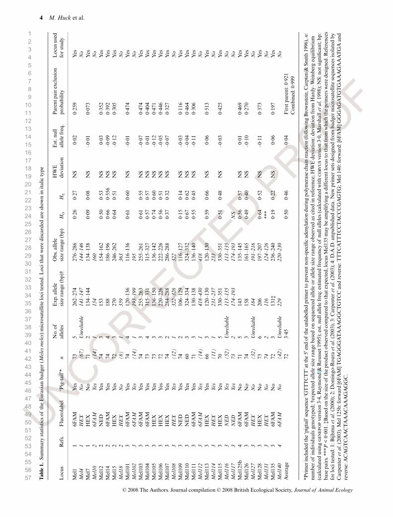
Sum

mar

y st

atis

tics

of

the

Eur

asia

n ba

dger

(M

eles

mel

es)

mic

rosa

telli

te lo

ci t

este

d. L

oci t

hat

wer

e di

scar

ded

are

show

n in

ital

ic t

ype

Loc

usR

efs.

Flu

orol

abel

‘Pig

-tai

l’*n

No.

of

alle

les

Exp

. alle

le

size

ran

ge (

bp)†

Obs

. alle

le

size

ran

ge (

bp)

HO

HE

HW

E

devi

atio

nE

st. n

ull

alle

le f

req.

Par

ent p

air e

xclu

sion

pr

obab

ility

Loc

us u

sed

for

stud

y

Mel

11

6FA

MY

es73

526

2–27

427

6–28

60·

260·

27N

S0·

020·

259

Yes

Mel

41

HE

XN

o(67)

Unre

liabl

e141–147

144–146

No

Mel

71

HE

XN

o71

213

4–14

413

4–13

80·

090·

08N

S–0

·01

0·07

3Y

esM

el10

26F

AM

Yes

(14)

1154

160

No

Mel

122

NE

DY

es74

315

315

4–16

20·

500·

53N

S0·

030·

352

Yes

Mel

142

6FA

MY

es74

418

818

6–19

60·

660·

556

NS

–0·0

90·

392

Yes

Mel

152

HE

XY

es72

327

024

6–26

20·

640·

51N

S–0

·12

0·30

5Y

esM

el18

2H

EX

No

(8)

1359

363

No

Mel

101

36F

AM

Yes

744

120–

136

116–

136

0·61

0·60

NS

–0·0

10·

474

Yes

Mel

102

36F

AM

Yes

(14)

1193–199

195

No

Mel

103

36F

AM

Yes

743

255–

263

255–

261

0·61

0·55

NS

–0·0

70·

474

Yes

Mel

104

36F

AM

Yes

734

315–

331

315–

327

0·57

0·57

NS

0·01

0·40

4Y

esM

el10

53

HE

XY

es73

313

6–15

013

6–14

20·

740·

60N

S–0

·12

0·47

1Y

esM

el10

63

HE

XY

es72

322

0–22

622

2–22

60·

560·

51N

S–0

·05

0·44

6Y

esM

el10

73

HE

XY

es74

228

4–28

828

6–28

80·

370·

32N

S–0

·07

0·32

7Y

esM

el108

3H

EX

Yes

(12)

1322–326

322

No

Mel

109

3N

ED

Yes

742

106–

129

116–

127

0·15

0·14

NS

–0·0

30·

116

Yes

Mel

110

3N

ED

Yes

603

324–

334

324–

332

0·67

0·62

NS

–0·0

40·

464

Yes

Mel

111

36F

AM

Yes

713

130–

138

136–

140

0·55

0·45

NS

–0·1

10·

306

Yes

Mel

112

36F

AM

Yes

(14)

1418–430

418

No

Mel

113

3H

EX

Yes

663

120–

130

120–

130

0·59

0·66

NS

0·06

0·51

3Y

esM

el114

3H

EX

Yes

(11)

1231–237

233

No

Mel

115

3H

EX

Yes

705

330–

351

330–

351

0·51

0·48

NS

–0·0

30·

425

Yes

Mel

116

3N

ED

Yes

(52)

Unre

liabl

e113–135

113–135

No

Mel

117

3N

ED

Yes

73

2174–193

174–193

NS

No

Mel

125b

46F

AM

No

715

143

135–

145

0·56

0·57

NS

0·01

0·46

9Y

esM

el12

63

6FA

MN

o74

315

816

1–16

50·

490·

40N

S–0

·10

0·27

0Y

esM

el127

3H

EX

No

(32)

Unre

liabl

e184

191–216

No

Mel

128

3H

EX

No

736

206

197–

207

0·64

0·52

NS

–0·1

10·

373

Yes

Mel

131

3H

EX

No

74

2116

124–126

***

No

Mel

135

36F

AM

No

723

131‡

236–

240

0·19

0·22

NS

0·06

0·19

7Y

esM

el140

46F

AM

No

(42)

Unre

liabl

e229

220–230

No

Ave

rage

723·

450·

500·

46–

0·04

Fir

st p

aren

t: 0

·921

Com

bine

d: 0

·999

*Pri

mer

incl

uded

the

‘pig

tail’

seq

uenc

e ‘G

TT

TC

TT

’ at t

he 5

′ end

of

the

unla

belle

d pr

imer

to p

reve

nt n

on-s

peci

fic a

deny

latio

n du

ring

pol

ymer

ase

chai

n re

actio

n (f

ollo

win

g B

row

nste

in, C

arpt

en &

Sm

ith 1

996)

, n:

num

ber

of in

divi

dual

s ge

noty

ped;

†ex

pect

ed a

llele

siz

e ra

nge

base

d on

seq

uenc

ed a

llele

or

alle

le s

ize

rang

e ob

serv

ed a

s ci

ted

in r

efer

ence

; HW

E d

evia

tion

: dev

iati

on f

rom

Har

dy–W

einb

erg

equi

libri

um

(cal

cula

ted

usin

g g

enep

op

ver

sion

3·4

, Ray

mon

d &

Rou

sset

199

5); e

st. n

ull a

llele

freq

: est

imat

ed fr

eque

ncy

of n

ull a

llele

s (c

alcu

late

d w

ith

cer

vu

s ve

rsio

n 3·

0, M

arsh

all e

t al.

1998

); N

S: n

ot s

igni

fican

t; b

p:

base

pai

rs. *

**P

< 0

·001

. ‡B

ased

on

the

size

of

the

prod

uct o

bser

ved

com

pare

d to

that

exp

ecte

d, lo

cus

Mel

135

may

be

ampl

ifyi

ng a

dif

fere

nt lo

cus

to th

at fr

om w

hich

the

prim

ers

wer

e de

sign

ed. R

efer

ence

sfo

r lo

ci te

sted

: 1: B

ijlsm

a et

al.

(200

0); 2

: Dom

ingo

-Rou

ra e

t al.

(200

3); 3

: Car

pent

er e

t al.

(200

3); 4

: D.A

.D. u

npub

lishe

d da

ta. N

ew p

rim

er s

ets

desi

gned

from

bad

ger

mic

rosa

telli

te s

eque

nces

isol

ated

by

Car

pent

er e

t al.

(200

3). M

el 1

25b:

forw

ard

[6FA

M] T

GA

GG

GA

TA

AA

GG

CT

GT

CC

and

rev

erse

: TT

TC

AT

TT

CC

TA

CC

CG

AG

TG

; Mel

140

: for

war

d: [6

FAM

] GG

GA

GA

TG

TG

AA

AG

AA

AT

GA

and

re

vers

e: A

CA

GT

CA

AC

TA

AA

CA

AA

GA

GG

C.

Genetic structure in urban badgers 5

© 2008 The Authors. Journal compilation © 2008 British Ecological Society, Journal of Animal Ecology

UNCORRECTED PROOF

123456789

101112131415161718192021222324252627282930313233343536373839404142434445464748495051525354555657

and perform paternity analyses, and (b) minimize the cumulativeprobability of genotyping errors, leading to ‘false’ genotypes. Earlierstudies (e.g. Domingo-Roura et al. 2003; Pope et al. 2006) suggestedthat the available microsatellite loci were not very polymorphic andthat a large number would be needed to conduct parentage analysis.While other studies (e.g. Frantz et al. 2003) found that seven lociwere enough to differentiate even among siblings in badgers, wefound that seven (10%) individuals in our population would havebeen not detected using only the seven most informative loci. There-fore, we typed individual samples at a minimum of nine loci or moreuntil the probability among siblings (Pisib; Waits, Luikart & Teberlet2001) was less than 0·001. (Note that because of the combination ofprimers in the multiplex sets, most samples were typed at a minimum of15 loci.) PIsib was calculated with the program gencap version 1·2(Wilberg & Dreher 2004), which we also used to identify samplesthat were complete matches and those that differed only by one ortwo alleles. We repeated genotyping until the same alleles wereobserved at least twice in a heterozygous individual, or seven timesin a homozygous individual (Taberlet & Luikart 1999a; Taberlet,Waits & Luikart 1999b). If after this process two genotypes differedat only one or two loci, with at least one of the samples beinghomozygous, and if – excluding the mismatching loci – PIsib < 0·001,we treated these samples as stemming from one individual in orderto avoid overestimating the population size. We chose these thresholdsbecause the comparison of some known siblings (five live-trappedcubs in group S, and three in group WT) gave a mean number ofmismatches between the siblings of 5·2 in group S and 7·3 in groupWT (minimum 3·0), and an average PIsib in group S of 0·003 and ingroup WT of 0·009. Thus, it is unlikely that this compilation ofgenotypes resulted in an underestimate of population size.

The program dropout version 2·0 (McKelvey & Schwartz 2004,2005) indicates how many loci should be typed to avoid the ‘shadoweffect’ (Mills et al. 2000; see above). The indicated threshold was 16loci for a PIsib value of less than 0·001. Individual samples that couldbe typed at only 15 or fewer loci and that did not match with anyother sample were therefore not included in further analyses, as theywere difficult to type, and so even the remaining loci might havebeen unreliable.

DATA CHECKING

Because of the large number of loci typed, the probability ofgenotyping error was relatively high. We calculated the initial (i.e.before data checking and compiling of genotypes) error rate manuallyby dividing the number of incorrectly genotyped PCR samples bythe total number of genotyped PCR samples, averaged over all loci.The initial error rate was 0·08, with allelic dropout accounting for0·04. After applying a multiple-tubes approach (Taberlet & Luikart1999a; Taberlet et al. 1999b) and compiling genotypes as describedabove we used two further approaches to check our final data set forerrors. The software micro-checker version 2·2·3 (van Oosterhoutet al. 2004) tests the data for the presence of errors due to null alleles,allelic dropout of larger alleles, and stuttering because of errors duringthe PCR. This program indicated that none of these posed a problemin our data. Progam dropout version 2·0 (McKelvey & Schwartz2004; McKelvey & Schwartz 2005) identifies samples and loci thatare likely to contain errors that would affect the estimation ofpopulation size by conducting two tests. The ‘bimodal test’ calculatesthe number of loci that are different between each pair of samples.A bimodal distribution would indicate an excess of incorrect geno-types. The ‘difference in capture history test’ determines those locithat produce most errors. Briefly, the test first identifies how many

and which loci are needed to obtain a sufficiently low PI and PIsib toguarantee that individuals should be identified correctly. Theprogram then calculates the number of unique individuals obtainedwith this combination of loci (the tag) and compares it to thenumber of unique individuals generated through adding additionalloci and changing the composition of the tag. The addition oferror-free loci will not result in more individuals being inferred. Byrotating the order of loci the program evaluates the errors generatedby each locus. If new individuals are produced when a particularlocus is added then this locus is considered problematic. This testindicated that the genotypes at locus Mel117 were not reliable, so wediscarded this locus from further analyses. The bimodal test, whenused with the data set including genotypes that differed at only oneor two loci, but with PIsib of less than 0·001 (see above), showed twopeaks, but not if these ambiguous cases were considered to belongto the same individual. Together, these results show that our methodsto minimize errors were successful.

We checked whether any locus deviated from Hardy–Weinbergand linkage equilibrium using the program genepop version 3·4(Raymond & Rousset 1995) using 1000 dememorizations, 100batches and 1000 iterations, with a false discovery rate control formultiple testing (Miller et al. 2001) that assumed the tests to bedependent. Only locus Mel131 was not in Hardy–Weinberg equilib-rium, so genotypes obtained for this locus were not used in furtheranalyses. Four pairs of loci showed significant linkage disequilibria(Mel12 and Mel14, Mel110 and Mel111, Mel12 and Mel109,Mel109 and Mel125). Given the high proportion of individualssampled over a relatively small area, we expect a high proportion ofrelatives to be present in the data which may lead to the artefact of manyloci appearing to be linked. As no consistent linkage disequilibriawere observed among these loci in other populations (e.g. Frantzet al. 2003; Pope et al. 2006; Dugdale et al. 2007) suggesting thatthese loci were not physically linked. Therefore, we retained theseloci in the analysis.

INTERGROUP MOVEMENTS

Genotypes that were represented by a single sample were assignedto the sett where this sample was collected. However, some geno-types were found at more than one sett. If the majority of samples(more than twice as many) came from one sett we assumed this to bethe main sett of the corresponding badger, and that the animal hadonly ‘visited’ the other location. If a similar number of samples wascollected at more than one sett (i.e. not more than twice as many) wedid not assign a main sett to the badgers in question and excludedthese individuals (‘floaters’) from group-related analyses. If severalsamples of one genotype were found only or mainly at one sett inone of the sample periods, and only or mainly at another sett in thesecond period, we assumed a change of main sett (‘dispersal’).

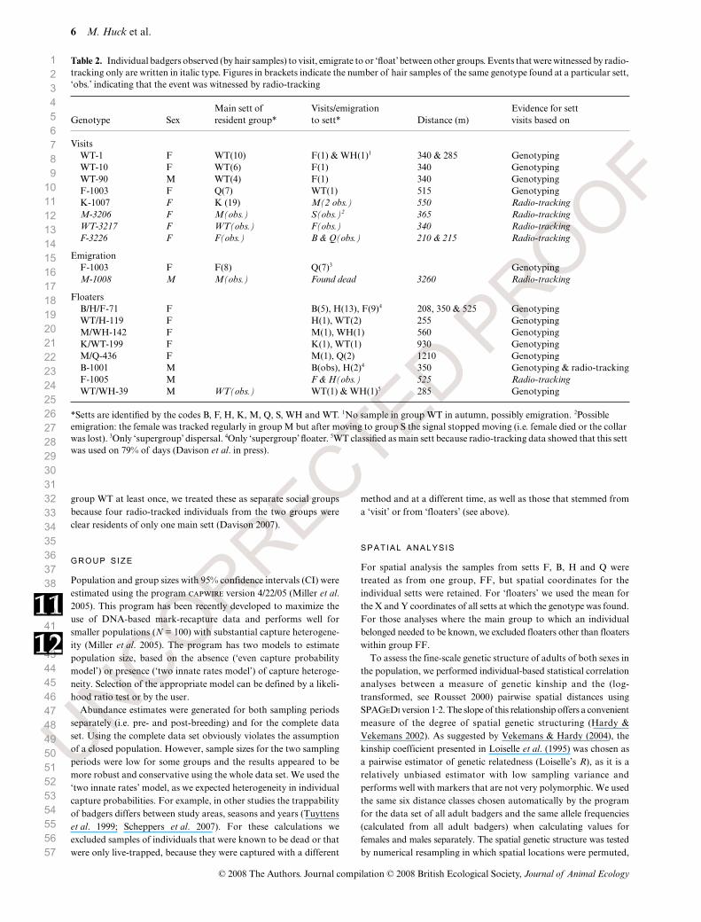
Five individuals (including two radio-tracked badgers: Davisonet al. submitted) made visits or floated between the setts F, Q, B andH (Table 2). These four setts seemed therefore to be associated moreclosely than other setts. Setts Q, B and H were small (one to twoentrance holes), although breeding took place in at least two of them(Q and B, and in other years in F). These setts might therefore beeither one main sett with three outliers or might house a ‘supergroup’,i.e. an association of badger groups that use different setts for breedingbut have overlapping ranges and that sleep frequently during theday in one another’s setts (Evans et al. 1989; T. Scheppers, unpublisheddata). For spatial analyses, samples from these setts were treated asstemming from one group, FF. Although one male floated regularlybetween setts WT and WH, and one individual from WH visited

7

8 9

10

6 M. Huck et al.

© 2008 The Authors. Journal compilation © 2008 British Ecological Society, Journal of Animal Ecology

UNCORRECTED PROOF

123456789

101112131415161718192021222324252627282930313233343536373839404142434445464748495051525354555657

group WT at least once, we treated these as separate social groupsbecause four radio-tracked individuals from the two groups wereclear residents of only one main sett (Davison 2007).

GROUP SIZE

Population and group sizes with 95% confidence intervals (CI) wereestimated using the program capwire version 4/22/05 (Miller et al.2005). This program has been recently developed to maximize theuse of DNA-based mark-recapture data and performs well forsmaller populations (N = 100) with substantial capture heterogene-ity (Miller et al. 2005). The program has two models to estimatepopulation size, based on the absence (‘even capture probabilitymodel’) or presence (‘two innate rates model’) of capture heteroge-neity. Selection of the appropriate model can be defined by a likeli-hood ratio test or by the user.

Abundance estimates were generated for both sampling periodsseparately (i.e. pre- and post-breeding) and for the complete dataset. Using the complete data set obviously violates the assumptionof a closed population. However, sample sizes for the two samplingperiods were low for some groups and the results appeared to bemore robust and conservative using the whole data set. We used the‘two innate rates’ model, as we expected heterogeneity in individualcapture probabilities. For example, in other studies the trappabilityof badgers differs between study areas, seasons and years (Tuyttenset al. 1999; Scheppers et al. 2007). For these calculations weexcluded samples of individuals that were known to be dead or thatwere only live-trapped, because they were captured with a different

method and at a different time, as well as those that stemmed froma ‘visit’ or from ‘floaters’ (see above).

SPATIAL ANALYSIS

For spatial analysis the samples from setts F, B, H and Q weretreated as from one group, FF, but spatial coordinates for theindividual setts were retained. For ‘floaters’ we used the mean forthe X and Y coordinates of all setts at which the genotype was found.For those analyses where the main group to which an individualbelonged needed to be known, we excluded floaters other than floaterswithin group FF.

To assess the fine-scale genetic structure of adults of both sexes inthe population, we performed individual-based statistical correlationanalyses between a measure of genetic kinship and the (log-transformed, see Rousset 2000) pairwise spatial distances usingSPAGEDI version 1·2. The slope of this relationship offers a convenientmeasure of the degree of spatial genetic structuring (Hardy &Vekemans 2002). As suggested by Vekemans & Hardy (2004), thekinship coefficient presented in Loiselle et al. (1995) was chosen asa pairwise estimator of genetic relatedness (Loiselle’s R), as it is arelatively unbiased estimator with low sampling variance andperforms well with markers that are not very polymorphic. We usedthe same six distance classes chosen automatically by the programfor the data set of all adult badgers and the same allele frequencies(calculated from all adult badgers) when calculating values forfemales and males separately. The spatial genetic structure was testedby numerical resampling in which spatial locations were permuted,

11

Table 2. Individual badgers observed (by hair samples) to visit, emigrate to or ‘float’ between other groups. Events that were witnessed by radio-tracking only are written in italic type. Figures in brackets indicate the number of hair samples of the same genotype found at a particular sett,‘obs.’ indicating that the event was witnessed by radio-tracking

Genotype SexMain sett of resident group*

Visits/emigration to sett* Distance (m)

Evidence for sett visits based on

VisitsWT-1 F WT(10) F(1) & WH(1)1 340 & 285 GenotypingWT-10 F WT(6) F(1) 340 GenotypingWT-90 M WT(4) F(1) 340 GenotypingF-1003 F Q(7) WT(1) 515 GenotypingK-1007 F K (19) M(2 obs.) 550 Radio-tracking

M-3206 F M(obs.) S(obs.)2 365 Radio-tracking

WT-3217 F WT(obs.) F(obs.) 340 Radio-tracking

F-3226 F F(obs.) B & Q(obs.) 210 & 215 Radio-tracking

EmigrationF-1003 F F(8) Q(7)3 GenotypingM-1008 M M(obs.) Found dead 3260 Radio-tracking

FloatersB/H/F-71 F B(5), H(13), F(9)4 208, 350 & 525 GenotypingWT/H-119 F H(1), WT(2) 255 GenotypingM/WH-142 F M(1), WH(1) 560 GenotypingK/WT-199 F K(1), WT(1) 930 GenotypingM/Q-436 F M(1), Q(2) 1210 GenotypingB-1001 M B(obs), H(2)4 350 Genotyping & radio-trackingF-1005 M F & H(obs.) 525 Radio-tracking

WT/WH-39 M WT(obs.) WT(1) & WH(1)5 285 Genotyping

*Setts are identified by the codes B, F, H, K, M, Q, S, WH and WT. 1No sample in group WT in autumn, possibly emigration. 2Possible emigration: the female was tracked regularly in group M but after moving to group S the signal stopped moving (i.e. female died or the collar was lost). 3Only ‘supergroup’ dispersal. 4Only ‘supergroup’ floater. 5WT classified as main sett because radio-tracking data showed that this sett was used on 79% of days (Davison et al. in press).

12

Genetic structure in urban badgers 7

© 2008 The Authors. Journal compilation © 2008 British Ecological Society, Journal of Animal Ecology

UNCORRECTED PROOF

123456789

101112131415161718192021222324252627282930313233343536373839404142434445464748495051525354555657

a procedure equivalent to a Mantel test (Hardy & Vekemans 2002).We compared the slopes (calculated from the mean values per distanceclass) for adult females and males using a t-test (program SSSversion 1·0b, Engel 1998) after checking that the residuals weredistributed normally.

Additionally, we compared mean relatedness values for individualsof the same sex living either in the same or in different groups byusing matched-pair randomization (10 000 randomizations) orexact permutation tests calculated with the program SsS 1·0b (Engel1998). Because Loiselle’s R, although performing better in spatialanalysis, has lower accuracy and precision, here we used Li’sRelatedness value (Li’s R: see Hardy & Vekemans 2002). For thesecalculations we had a value pair (i.e. one value for mean relatedness toindividuals from the same group and one value for mean relatednessto individuals from a different group) for each individual, minimizingthe degree of dependence of values. For comparison with otherstudies we calculated additionally the more commonly used Queller& Goodnight’s R (Q&G’s R: Queller & Goodnight 1989), calculatedwithout bias-correction with SPAGEDI (Hardy et al. 2002). Li’s Rand Q&G’s R were highly correlated (adjusted R2 between Q&G’s &Li’s R = 0·78, n = 2701, randomization test: P < 0·001).

PARENTAGE

We employed the program cervus version 3·0·3 (Kalinowski, Taper& Marshall 2007) to determine potential parent pairs. For thesimulation determining confidence levels we used 10 000 ‘offspring’.The minimum number of loci typed was 16. We considered allindividuals as adults, and thus as potential parents, except thosethat were live-trapped as cubs and individuals that were sampledonly in autumn and for which parents were found in the parentageanalysis. We calculated the proportion of sampled females andmales by dividing the number of potential parents of each sex by theestimated population size (see above), plus the live-caught individuals,minus the number of cubs and minus the number of individuals ofthe opposite sex. This resulted in 87% sampled females and 88%sampled males. To include potentially related individuals wedetermined the number of adult same-sex pairs with Li’s R > 0·25,and calculated the mean of this value for each sex and the proportionof same-sex relatives in the whole population. Thirteen per cent ofthe females had Li’s R > 0·25, with a mean of 0·389, while 42% ofmales were thus related, with an average of Li’s R = 0·422. The errorrate was set at 0·001, because the error-checking programs used (seeabove) indicated a low remaining error rate. As potential mothers weincluded only females from the same sett as the cub (or in the caseof cubs from setts B, Q or F, females from setts B, Q, F or H), becauseit is unlikely that either mothers or cubs would migrate so soon afterindependence of the cubs (Cheeseman et al. 1988; da Silva, Macdonald& Evans 1994). All males were included as potential fathers.

Results

We obtained 395 reliable genotypes from 416 DNA samples(200 spring, 186 autumn) collected at hair traps or fromlive-trapped animals, stemming from a total of 74 badgers. Ofthese, 35 were male and 23 (scored at least three times) or 32(scored at least once) female. For the remaining samples it wasnot possible to determine the sex due to poor sample quality.On average, 97% of the individuals were genotyped at any onelocus. The initially high error rate of 0·08 shows that datachecking procedures are essential to obtain reliable results,

and that the ease with which badger hair DNA can be ampli-fied from single hair samples may differ between studies(compare to Frantz et al. 2004; Scheppers et al. 2007). The 20loci used had on average 3·45 alleles per locus (Table 1), givingan average allelic richness of 3·40.

INTERGROUP MOVEMENTS

Seven females (or six, if ‘supergroup’ visits are excluded) andone male visited other setts (Table 2). One male and possiblyone female emigrated, and one female (F-1003) changed hermain sett within the ‘supergroup’. For five females and threemales, or four females and two males if ‘supergroup’ floatersare excluded, it was not possible to determine the main sett(‘floaters’). This leads to a total of 17 (14 excluding super-group movements) of 74 individuals, or 23% (18·9%), that leftthe original group range at least once. More females thanmales moved, but this difference was not significant (G-test,G = 2·89, d.f. = 1, P = 0·089; excluding super-group movements:G = 3·29, P = 0·069). Assuming that cubs do not migratebefore maturity, and calculating the value relative to thenumber of adult individuals (n = 50), the proportion is evenhigher (34%, or 28% excluding supergroup movements).

GROUP SIZE AND POPULATION DENSITY

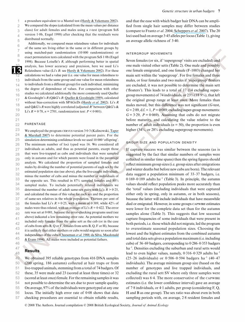
If capture success was similar between the seasons (as issuggested by the fact that similar numbers of samples werecollected in similar time spans) then the spring figures shouldreflect minimum group sizes (i.e. group sizes after emigrationsand winter deaths but before new cubs are born). The relevantdata suggest a population minimum of 33–37 badgers, i.e.0·169–0·189 adults ha–1 (Table 3). In principle, the autumnvalues should reflect population peaks more accurately thanthe ‘total’ values (including individuals that were capturedeither only in spring, only in autumn, or in both seasons),because the latter will include individuals that have meanwhiledied or emigrated. However, in some groups capwire estimateswere lower for the complete data set than for the autumnsamples alone (Table 3). This suggests that low seasonalcapture frequencies of some individuals that were present inboth periods, i.e. those which did not migrate, led the programto overestimate seasonal population sizes. Choosing thelowest and the highest estimates from the combined autumnand total data sets gives a population maximum (i.e. includingcubs) of 56–69 badgers, corresponding to 0·286–0·353 badgersha–1. Densities excluding the suburban and rural setts wouldlead to even higher values, namely, 0·316–0·329 adults ha–1

(25–26 individuals) or 0·506–0·594 badgers ha–1 (40–47individuals). The average minimum group size (based on thenumber of genotypes and live trapped individuals, andexcluding the rural sett SV where only three samples werecollected) was 6·4. The more conservative of the capwire

estimates (i.e. the lower confidence interval) gave an averageof 7·8 individuals, or 4·1 adults, per group (considering F, Q,H and B as one group). The sex ratio was about even in bothsampling periods with, on average, 2·8 resident females and

13

8 M. Huck et al.

© 2008 The Authors. Journal compilation © 2008 British Ecological Society, Journal of Animal Ecology

UNCORRECTED PROOF

123456789

101112131415161718192021222324252627282930313233343536373839404142434445464748495051525354555657

3·3 resident males per group in each season (and 0·7 individualsof unknown sex).

SPATIAL ANALYSIS

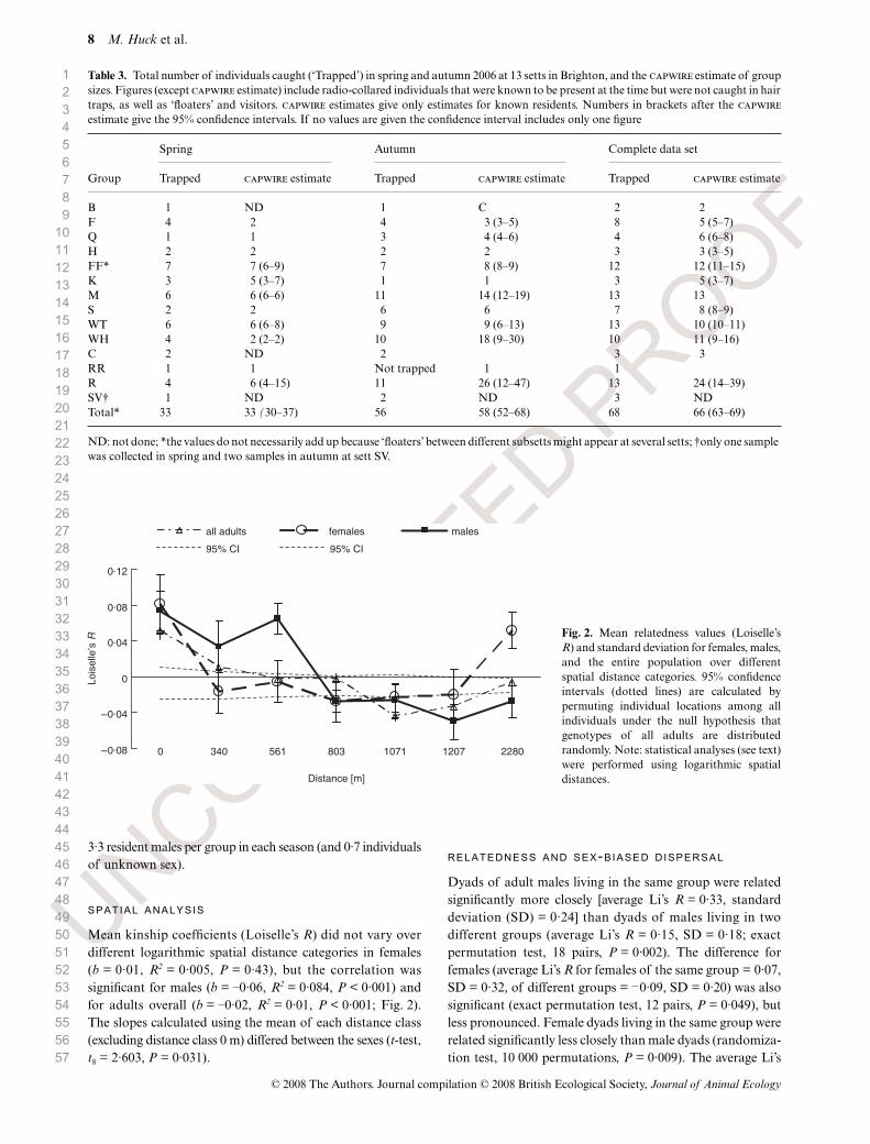
Mean kinship coefficients (Loiselle’s R) did not vary overdifferent logarithmic spatial distance categories in females(b = 0·01, R2 = 0·005, P = 0·43), but the correlation wassignificant for males (b = –0·06, R2 = 0·084, P < 0·001) andfor adults overall (b = –0·02, R2 = 0·01, P < 0·001; Fig. 2).The slopes calculated using the mean of each distance class(excluding distance class 0 m) differed between the sexes (t-test,t8 = 2·603, P = 0·031).

RELATEDNESS AND SEX-BIASED DISPERSAL

Dyads of adult males living in the same group were relatedsignificantly more closely [average Li’s R = 0·33, standarddeviation (SD) = 0·24] than dyads of males living in twodifferent groups (average Li’s R = 0·15, SD = 0·18; exactpermutation test, 18 pairs, P = 0·002). The difference forfemales (average Li’s R for females of the same group = 0·07,SD = 0·32, of different groups = –0·09, SD = 0·20) was alsosignificant (exact permutation test, 12 pairs, P = 0·049), butless pronounced. Female dyads living in the same group wererelated significantly less closely than male dyads (randomiza-tion test, 10 000 permutations, P = 0·009). The average Li’s

Table 3. Total number of individuals caught (‘Trapped’) in spring and autumn 2006 at 13 setts in Brighton, and the capwire estimate of groupsizes. Figures (except capwire estimate) include radio-collared individuals that were known to be present at the time but were not caught in hairtraps, as well as ‘floaters’ and visitors. capwire estimates give only estimates for known residents. Numbers in brackets after the capwire

estimate give the 95% confidence intervals. If no values are given the confidence interval includes only one figure

Group

Spring Autumn Complete data set

Trapped capwire estimate Trapped capwire estimate Trapped capwire estimate

B 1 ND 1 C 2 2F 4 2 4 3 (3–5) 8 5 (5–7)Q 1 1 3 4 (4–6) 4 6 (6–8)H 2 2 2 2 3 3 (3–5)FF* 7 7 (6–9) 7 8 (8–9) 12 12 (11–15)K 3 5 (3–7) 1 1 3 5 (3–7)M 6 6 (6–6) 11 14 (12–19) 13 13S 2 2 6 6 7 8 (8–9)WT 6 6 (6–8) 9 9 (6–13) 13 10 (10–11)WH 4 2 (2–2) 10 18 (9–30) 10 11 (9–16)C 2 ND 2 3 3RR 1 1 Not trapped 1 1R 4 6 (4–15) 11 26 (12–47) 13 24 (14–39)SV† 1 ND 2 ND 3 NDTotal* 33 33 (30–37) 56 58 (52–68) 68 66 (63–69)

ND: not done; *the values do not necessarily add up because ‘floaters’ between different subsetts might appear at several setts; †only one sample was collected in spring and two samples in autumn at sett SV.

Fig. 2. Mean relatedness values (Loiselle’sR) and standard deviation for females, males,and the entire population over differentspatial distance categories. 95% confidenceintervals (dotted lines) are calculated bypermuting individual locations among allindividuals under the null hypothesis thatgenotypes of all adults are distributedrandomly. Note: statistical analyses (see text)were performed using logarithmic spatialdistances.

Genetic structure in urban badgers 9

© 2008 The Authors. Journal compilation © 2008 British Ecological Society, Journal of Animal Ecology

UNCORRECTED PROOF

123456789

101112131415161718192021222324252627282930313233343536373839404142434445464748495051525354555657

relatedness (calculated as the mean of the means of allgroups) of individuals within groups of the total data setwas 0·24; when including only adults it was 0·19. The corre-sponding values for Q&G’s R were 0·17 and 0·12, respectively.

PARENTAGE

When we treated all individuals as offspring we usually foundseveral potential mothers (on average 3·6 from the samegroup as the offspring, maximum = 9), fathers (on average7·2, maximum = 20) and parent pairs with no triplet mis-match (3·4 if the mother of the pair was from the same groupas the offspring, maximum = 27). We found probable parentpairs for 23 likely (including eight known) cubs at seven dif-ferent setts (six groups, if setts B and Q are considered tobelong to one group, FF). For 12 of the 35 individuals whichwere caught only in autumn we did not find any probable par-ent, so these individuals were considered to be adults. Up tofive probable cubs were born within the same sett (or at leastthree if considering only live-trapped cubs). In three of fivesetts with more than one cub (or four of six groups) at leasttwo females were assigned maternity, while in two of fivesetts more than one male sired offspring (or three of sixgroups). In three of six groups fathers came from a differentgroup (or four of seven setts). Li’s Relatedness value ofbreeding pairs was on average 0·081 (for Q&G’s R: 0·01,n = 8), not differing from random expaction (randomizationtest, P > 0·05).

Discussion

GROUP SIZE AND POPULATION DENSITY

This is the first study to use remotely collected DNA to measuresocial group sizes and population density in an urban badgerpopulation. The results suggest that group sizes range up to11 individuals, with an average of 4·1 adults per group. This iswithin the range observed in rural populations in Luxem-bourg (Schley, Schaul & Roper 2004; Scheppers et al. 2007)and Ireland (Smal 1995) and only slightly lower than has beenreported for rural Britain as a whole (average: six adults pergroup, Clements, Neal & Yalden 1988). While the methodsin our study and that of Scheppers et al. (2007) are strictlycomparable, the sampling periods that we used were relativelylong by comparison with most live-trapping capture–mark–recapture studies. It could be argued that, as a consequence,our method was more likely to record badgers that weretemporarily visiting another sett and, thus, to overestimategroup sizes. However, previous studies in Luxembourg, usingthe same method as was applied here, have shown a goodcorrespondence between social group sizes estimated by hairtrapping and those revealed by direct observation (Frantzet al. 2004; Scheppers et al. 2007).

Although group sizes were similar to those reported forother populations, badger density in our study area was, at0·32–0·33 adults ha–1, considerably higher than in the onlyother urban population for which data are available (0·04

adults ha–1: Harris & Cresswell 1987) and higher than inalmost all rural locations (for review see Kowalczyk, Bunevich& Jêdrzejewska 2000). Indeed, the population density inBrighton approaches that of Wytham Woods, Oxfordshire(0·44 individuals ha–1: Macdonald & Newman 2002), which isgenerally believed to have the densest population of badgersin the world (Kowalczyk et al. 2000). The explanation for thishigh population density, despite average group sizes, is thatgroup ranges in our study area, as revealed by a radio-trackingstudy, were extremely small (range of minimum convexpolygons: 5·2–14·0 ha, mean 9·0 ha, Davison 2007). By contrast,the high population density in Wytham Woods results fromunusually large social groups occupying moderately sizedranges (Macdonald & Newman 2002).

GENETIC VARIABIL ITY AND INTERGROUP MOVEMENTS

Analysis of nucleotide diversity in the mtDNA control regionsuggests that the Eurasian badger, as a species, is not genetic-ally depauperate (Marmi et al. 2006). However, most studiesinvestigating populations within restricted geographicalareas have reported low levels of genetic diversity, based onmicrosatellites (Domingo-Roura et al. 2003; Pope et al. 2006),minisatellites (Pertoldi et al. 2001), allozymes (Evans et al.1989) or the mtDNA cytochrome b sequence (Kurose et al.2001, as cited in Pope et al. 2006). We found a mean allelicrichness value of 3·4, which is at the lower end of what hasbeen found in other British and Irish badger populations(mean = 4·0, range 3·2–4·5: see Pope et al. 2006), althoughhigher than in some European populations (range: 2·0–5·7,Pope et al. 2006). Microsatellite studies on other mammalsoften report higher average numbers of alleles (e.g. 11·8 inbrushtail possums, Trichosurus vulpecula Kerr 1792, Tayloret al. 2000; 7·4 in moustached tamarins, Saguinus mystax

Spix 1823, Huck et al. 2005; 6·6 in cheetahs, Acinoyx jubatus

Schreber 1775, Gottelli et al. 2007).On the other hand, the results provide some indicators

that badgers avoid incestuous matings within groups. First,we found a high rate of extra-group paternity, comparableto that reported in other studies (Carpenter et al. 2005;Dugdale et al. 2007) for rural populations. Secondly, a highproportion of individuals (at least 28% of the adult population)visited the setts of other social groups at least occasionally.Although some of these excursions might constituteexploratory forays to assess dispersal opportunities (Roper,Ostler & Conradt 2003), the most likely explanation is thatthey occurred for purposes of extra-group mating (Evanset al. 1989; Woodroffe & Macdonald 1993a; Christian 1994).

FEMALE-BIASED DISPERSAL

The overall relatedness value (Q&G’s R) for badgers living inthe same group was 0·17, or 0·12 for adults only. This is similarto the results from a long-term study of a rural population ofbadgers in Woodchester Park, Gloucestershire, where within-group relatedness had an overall mean of 0·15 and variedfrom 0·12 to 0·19 between years (Carpenter 2002). The Q&G’s

14

10 M. Huck et al.

© 2008 The Authors. Journal compilation © 2008 British Ecological Society, Journal of Animal Ecology

UNCORRECTED PROOF

123456789

101112131415161718192021222324252627282930313233343536373839404142434445464748495051525354555657

R-values in this latter study, as well as our own, were calculatedwithout using the bias correction recommended by Queller &Goodnight (1989). Without a bias correction, relatednessvalues will be underestimated. A more recent study on theWytham Woods population that used the bias correctionreported slightly higher values (average within-group related-ness: 0·2, Dugdale et al. 2008). The within-group relatednessfor females was significantly lower than for males (Li’sR = 0·07 vs. 0·33, Q&G’s R = 0·07 vs. 0·24). Furthermore, forfemale dyads Loiselle’s R dropped steeply even when femaleslived relatively close together, while for males these valuesremained higher for distances up to about 560 m (Fig. 2).This suggests that males have more relatives in neighbouringsetts than females. Together with the lower within-grouprelatedness of females this indicates that females are the maindispersers, at least on a relatively small scale as studied here.In contrast, Dugdale et al. (2008) found significantly highervalues for females (Q&G’s R with bias-correction = 0·25 vs.0·16 for adult females and males, respectively).

Our findings suggesting female-biased dispersal areconsistent with some previous studies (da Silva 1989, as citedin Woodroffe & Macdonald 1993a; Woodroffe, Macdonald& da Silva 1993b; Christian 1994; Tuyttens et al. 2000),although other studies have indicated male-biased dispersalin badgers (Kruuk & Parish 1987; Cheeseman et al. 1988;Roper et al. 2003). Whether the female bias in dispersal inour study reflects only the current population structure (e.g.current effective sex ratios) in our population, or is typical ofurban badgers, remains to be determined.

OVERALL CONCLUSION

Two major conclusions can be drawn from this study. First,badgers can attain locally very high population densities inan urban environment, showing that they can adapt assuccessfully to urban as to rural habitats. However, in our studyarea, unlike in rural habitats, high population density hasresulted from small group range sizes rather than large socialgroups (Davison 2007). Secondly, the results indicate a com-bination of relatively low genetic variability (by comparisonwith other mammals) together with outbreeding at a localscale (i.e. frequent matings between groups rather than withingroups). Possibly, our population is subject to a relatively highinfluence of genetic drift by comparison with mutation orlong-distance dispersal. Drift might keep genetic variabilitylow if long-distance dispersal is rare, even if short-distancedispersal and breeding between groups are common.

Most of the characteristics of our population fell within therange of those exhibited by rural badger populations, themost notable exception being the high rate of intergroupmovements. In the only previous study of urban badgers, therate of intergroup movements was similarly high, at 30·8%(calculated from Cheeseman et al. 1988). By contrast, a pre-vious study of rural badgers in Luxembourg, using the samemethodology as ours, reported that 13% of genotype profileswere found at more than one sett (Scheppers et al. 2007),while data from a capture–mark–recapture study of rural

badgers in Britain showed an intergroup movement rate of12·2% (Cheeseman et al. 1988). Thus, the available datasuggest that movements between groups are more frequent inurban than in rural populations. The proximate and ultimatereasons for this difference require further investigation.

Acknowledgements

We thank J. Davison for help with the setting of hair traps and occasionalcollection of hair samples and A. Ward for providing additional hair samplesfor the validation of the sex marker. Genotyping was conducted in the SheffieldMolecular Ecology Laboratory, with the help of J. Chittock, A. Krupa and L.Pope. We also thank T. Scheppers for additional advice, and J. Davison, H.Dugdale, D. Macdonald, L. Pope and an anonymous reviewer for comments onearlier drafts.

References

Bijlsma, R., Van De Vliet, M., Pertoldi, C., Van Apeldoorn, R.C. & Van DeZande, L. (2000) Microsatellite primers from the Eurasian badger, Meles

meles. Molecular Ecology, 9, 2216–2217.Brownstein, M., Carpten, J. & Smith, J. (1996) Modulation of non-templated

nucleotide addition by Taq DNA polymerase: primer modifications thatfacilitate genotyping. Biotechniques, 20, 1004–1010.

Carpenter, P.J. (2002) A study of mating systems, inbreeding avoidance and TB

resistance in the Eurasian badger (Meles meles) using microsatellite markers.

PhD thesis, University of Sheffield, Sheffield.Carpenter, P.J., Dawson, D.A., Greig, C., Parham, A., Cheeseman, C.L. &

Burke, T. (2003) Isolation of 39 polymorphic microsatellite loci and thedevelopment of a fluorescently labelled marker set for the Eurasian badger(Meles meles) (Carnivora: Mustelidae). Molecular Ecology Notes, 3, 610–615.

Carpenter, P.J., Pope, L.C., Greig, C., Dawson, D.A., Rogers, L.M., Erven, K.,Wilson, G.J., Delahay, R.J., Cheeseman, C.L. & Burke, T. (2005) Mating sys-tem of the Eurasian badger, Meles meles, in a high density population.Molecular Ecology, 14, 273–284.

Cheeseman, C.L., Cresswell, W.J., Harris, S. & Mallinson, P.J. (1988) Comparisonof dispersal and other movements in two badger (Meles meles) populations.Mammal Review, 18, 51–59.

Christian, S.F. (1994) Dispersal and other inter-group movements in badgers,Meles meles. Zeitschrift für Säugetierkunde, 59, 218–223.

Clements, E.D., Neal, E.G. & Yalden, D. (1988) The national badger sett survey.Mammal Review, 18, 1–9.

Cresswell, W.J., Harris, S., Cheeseman, C.L. & Mallinson, P.J. (1992) To breedor not to breed: an analysis of the social and density-dependent constraints onthe fecundity of female badgers (Meles meles). Philosophical Transactions

of the Royal Society of London, Series B, 338, 393–407.Davison, J. (2007) Ecology and behaviour of urban badgers. PhD thesis, University

of Sussex, Brighton.Davison, J., Huck, M., Delahay, R.J. & Roper, T.J. (in press) Urban badger

setts: characteristics, patterns of use and management implications. Journal

of Zoology, London, in press.Ditchkoff, S.S., Saalfeld, S.T. & Gibson, C.J. (2006) Animal behavior in urban

ecosystems: modifications due to human-induced stress. Urban Ecosystems,9, 5–12.

Domingo-Roura, X., Macdonald, D.W., Roy, M.S., Marmi, J., Terradas, J.,Woodroffe, R., Burke, T. & Wayne, R.K. (2003) Confirmation of low geneticdiversity and multiple breeding females in a social group of Eurasian badgersfrom microsatellite and field data. Molecular Ecology, 12, 533–539.

Doncaster, P. & Macdonald, D.W. (1991) Drifting territoriality in the red foxVulpes vulpes. Journal of Animal Ecology, 60, 423–439.

Dugdale, H.L., Macdonald, D.W., Pope, L.C. & Burke, T. (2007) Polygynandry,extra-group paternity and multiple-paternity litters in European badger(Meles meles) social groups. Molecular Ecology, 16, 5294–5306.

Dugdale, H.L., Macdonald, D.W., Pope, L.C., Johnson, P.J. & Burke, T. (2008)Reproductive skew and relatedness in social groups of European badgersMeles meles. Molecular Ecology, 17, 1815–1827.

Engel, J. (1998) SsS – Selten Schöne Statistikprogramme, version 1·0b.Rubisoft Software GmbH, Eichenau.

Estes, W.A. & Mannan, R.W. (2003) Feeding behavior of Cooper’s hawks aturban and rural nests in southeastern Arizona. Condor, 105, 107–116.

Evans, P.G.H., Macdonald, D.W. & Cheeseman, C.L. (1989) Social structure ofthe Eurasian badger (Meles meles): genetic evidence. Journal of Zoology,

London, 218, 587–595.

1516

17

18

Genetic structure in urban badgers 11

© 2008 The Authors. Journal compilation © 2008 British Ecological Society, Journal of Animal Ecology

UNCORRECTED PROOF

123456789

101112131415161718192021222324252627282930313233343536373839404142434445464748495051525354555657

Favre, L., Balloux, F., Goudet, J. & Perrin, N. (1997) Female-biased dispersalin the monogamous mammal Crocidura russula: evidence from field dataand microsatellite patterns. Proceedings of the Royal Society of London,

Series B, 264, 127–132.Frantz, A.C., Fack, F., Muller, C.P. & Roper, T.J. (2006) Faecal DNA typing as

a tool for investigating territorial behaviour of badgers (Meles meles).European Wildlife Research, 52, 138–141.

Frantz, A.C., Pope, L.C., Carpenter, P.J., Roper, T.J., Wilson, G.J. & Delahay,R.J. (2003) Reliable microsatellite genotyping of the Eurasian badger (Meles

meles) using faecal DNA. Molecular Ecology, 12, 1649–1661.Frantz, A.C., Schaul, M., Pope, L.C., Fack, F., Schley, L., Muller, C.P. &

Roper, T.J. (2004) Estimating population size by genotyping remotelyplucked hair: the Eurasian badger. Journal of Applied Ecology, 41, 985–995.

Gottelli, D., Wang, J., Bashir, S. & Durant, S.M. (2007) Genetic analysis revealspromiscuity among female cheetahs. Proceedings of the Royal Society of

London, Series B, 274, 1993–2001.Griffiths, R. & Tiwari, B. (1993) Primers for the differential amplification of the

sex-determining region Y gene in a range of mammal species. Molecular

Ecology, 2, 405–406.Hardy, O.J. & Vekemans, X. (2002) SPAGeDi: a versatile computer program to

analyse spatial genetic structure at the individual or population levels.Molecular Ecology Notes, 2, 618–620.

Harris, S. (1982) Activity patterns and habitat utilization of badgers (Meles

meles) in suburban Bristol: a radio tracking study. Symposium of the Zoo-

logical Society of London, 49, 301–323.Harris, S. & Cresswell, W.J. (1987) Dynamics of a suburban badger (Meles meles)

population. Symposium of the Zoological Society of London, 58, 295–311.Huck, M., Davison, J. & Roper, T.J. (in press) Predicting European badger sett

distribution in urban environments. Wildlife Biology, in press.Huck, M., Löttker, P., Böhle, U.-R. & Heymann, E.W. (2005) Paternity and

kinship patterns in polyandrous moustached tamarins (Saguinus mystax).American Journal of Physical Anthropology, 127, 449–464.

Huck, M., Roos, C. & Heymann, E.W. (2007) Spatio-genetic populationstructure in moustached tamarins, Saguinus mystax. American Journal of

Physical Anthropology, 132, 576–583.Kalinowski, S.T., Taper, M.L. & Marshall, T.C. (2007) Revising how the com-

puter program cervus accommodates genotyping error increases success inpaternity assignment. Molecular Ecology, 16, 1099–1106.

Kowalczyk, R., Bunevich, A.N. & Jêdrzejewska, B. (2000) Badger density anddistribution of setts in Bialowieza Primeval Forest (Poland and Belarus)compared to other Eurasian populations. Acta Theriologica, 45, 395–408.

Kruuk, H.H. & Parish, T. (1987) Changes in the size of groups and ranges of theEuropean badger (Meles meles L.) in an area in Scotland. Journal of Animal

Ecology, 56, 351–364.Langbein, J. & Thirgood, S.J. (1989) Variation in mating systems of fallow deer

(Dama dama) in relation to ecology. Ethology, 83, 195–214.Loiselle, B.A., Sork, V.L., Nason, J. & Graham, C. (1995) Spatial genetic

structure of a tropical understorey shrub Psychotria officinalis (Rubiaceae).American Journal of Botany, 82, 1420–1425.

Macdonald, D.W. & Newman, C. (2002) Population dynamics of badgers(Meles meles) in Oxfordshire, U.K.: numbers, density and cohort life histories,and a possible role of climate change in population growth. Journal of Zoology,

London, 256, 121–138.Marmi, J., López-Giráldez, F., Macdonald, D.W., Calafell, F., Zholnerovskaya,

E. & Domingo-Roura, X. (2006) Mitochondrial DNA reveals a strongphylogeographic structure in the badger across Eurasia. Molecular Ecology,15, 1007–1020.

Marshall, T.C., Slate, J., Kruuk, L.E.B. & Pemberton, J.M. (1998) Statisticalconfidence for likelihood-based paternity inference in natural populations.Molecular Ecology, 7, 639–655.

McKelvey, K.S. & Schwartz, M.K. (2004) Genetic errors associated withpopulation estimation using non-invasive molecular tagging: problems andnew solutions. Journal of Wildlife Management, 68, 439–448.

McKelvey, K.S. & Schwartz, M.K. (2005) dropout: a program to identifyproblem loci and samples for noninvasive genetic samples in a capture–mark–recapture framework. Molecular Ecology Notes, 5, 716–718. Available at:http://www.fs.fed.us/rm/wildlife/genetics/software.php.

Miller, C.J., Genovese, C., Nichol, R.C., Wasserman, L., Connolly, A., Reichart,D., Hopkins, A., Schneider, J. & Moore, A. (2001) Controlling the false-discoveryrate in astrophysical data analysis. Astronomical Journal, 122, 3492–3505.

Mills, L.S., Citta, J.J., Lair, K.P., Schwartz, M.K. & Tallmon, D.A. (2000)Estimating animal abundance using noninvasive DNA sampling: promiseand pitfalls. Ecological Applications, 10, 283–294.

van Oosterhout, C., Hutchinson, W.F., Wills, D.P.M. & Shipley, P. (2004)micro-checker: software for identifying and correcting genotyping errorsin microsatellite data. Molecular Ecology Notes, 4, 535–538. Available at:http://www.microchecker.hull.ac.uk.

Page, R.J.C., Ross, J. & Langton, S.D. (1994) Seasonality of reproduction in theEuropean badger Meles meles in south-west England. Journal of Zoology,

London, 233, 69–91.Pertoldi, C., Loeschcke, V., Madsen, A.B., Randi, E. & Ucci, N. (2001) Effects

of habitat fragmentation on the Eurasian badger (Meles meles) subpopulationsin Denmark. Hystrix – Italian Journal of Mammalogy, 12, 1–6.

Pope, L.C., Domingo-Roura, X., Erven, K. & Burke, T. (2006) Isolation bydistance and gene flow in the Eurasian badger (Meles meles) at both a localand broad scale. Molecular Ecology, 15, 371–386.

Queller, D.C. & Goodnight, K.F. (1989) Estimating relatedness using geneticmarkers. Evolution, 43, 258–275.

Raymond, M. & Rousset, F. (1995) genepop version 1·2: population geneticssoftware for exact tests and ecumenicism. Journal of Heredity, 86, 248–249.

Roper, T.J., Ostler, J.R. & Conradt, L. (2003) The process of dispersal in badgersMeles meles. Mammal Review, 33, 314–318.

Rousset, F. (2000) Genetic differentiation between individuals. Journal of

Evolutionary Biology, 13, 58–62.Scheppers, T.L.J., Frantz, A.C., Schaul, M., Engel, E., Breyne, P., Schley, L. &

Roper, T.J. (2007) Estimating social group size of Eurasian badgers Meles

meles by genotyping remotely plucked single hairs. Wildlife Biology, 13,195–207.

Schley, L., Schaul, M. & Roper, T.J. (2004) Distribution and population den-sity of badgers Meles meles in Luxembourg. Mammal Review, 34, 233–240.

da Silva, J., Macdonald, D.W. & Evans, P.G.H. (1994) Net costs of group livingin a solitary forager, the Eurasian badger (Meles meles). Behavioral Ecology,5, 151–158.

Smal, C. (1995) The Badger and Habitat Survey of Ireland. National Parks &Wildlife Service and Department of Agriculture, Food & Forestry, Dublin.

Taberlet, P. & Luikart, G. (1999a) Non-invasive genetic sampling and individualidentification. Biological Journal of the Linnean Society, 68, 41–55.

Taberlet, P., Waits, L.P. & Luikart, G. (1999b) Noninvasive genetic sampling:look before you leap. Trends in Ecology and Evolution, 14, 323–327.

Taylor, A.C., Cowan, P.E., Fricke, B.L. & Cooper, D.W. (2000) Genetic analysisof the mating system of the common brushtail possum (Trichosurus vulpecula)in New Zealand farmland. Molecular Ecology, 9, 869–879.

Tuyttens, F.A.M., Delahay, R.J., Macdonald, D.W., Cheeseman, C.L., Long,B. & Donnelly, C.A. (2000) Spatial perturbation caused by a badger (Meles

meles) culling operation: implications for the function of territoriality andthe control of bovine tuberculosis (Mycobacterium bovis). Journal of Animal

Ecology, 69, 815–828.Tuyttens, F.A.M., Macdonald, D.W., Delahay, R.J., Rogers, L.M., Mallinson,

P.J., Donnelly, C.A. & Newman, C. (1999) Differences in trappability ofEuropean badgers Meles meles in three populations in England. Journal of

Applied Ecology, 36, 1051–1062.Vekemans, X. & Hardy, O.J. (2004) New insights from fine-scale spatial genetic

structure analyses in plant populations. Molecular Ecology, 13, 921–935.Waits, L.P., Luikart, G. & Taberlet, P. (2001) Estimating the probability of iden-

tity among genotypes in natural populations: cautions and guidelines.Molecular Ecology, 10, 249–256.

Walsh, P.S., Metzger, D.A. & Higuchi, R. (1991) Chelex® 100 as a medium forsimple extraction of DNA for PCR-based typing from forensic material.Biotechniques, 10, 506–513.

Wilberg, M.J. & Dreher, B.P. (2004) genecap: a program for analysis ofmultilocus genotype data for non-invasive sampling and capture–recapturepopulation estimation. Molecular Ecology Notes, 4, 783–785.

Woodroffe, R. & Macdonald, D.W. (1993a) Badger sociality – models of spatialgrouping. Symposium of the Zoological Society of London, 65, 145–169.

Woodroffe, R., Macdonald, D.W. & da Silva, J. (1993b) Dispersal andphilopatry in the European badger, Meles meles. Journal of Zoology, London,237, 227–239.

Received 22 August 2007; revised version accepted 16 March 2008

Handling Editor: Stan Boutin

19

20

21

Author Query Form

Journal: Journal of Animal Ecology

Article: jae_1415.fm

Dear Author,

During the copy-editing of your paper, the following queries arose. Please respond to these bymarking up your proofs with the necessary changes/additions. Please write your answers on the querysheet if there is insufficient space on the page proofs. Please write clearly and follow the conventionsshown on the attached corrections sheet. If returning the proof by fax do not write too close to thepaper’s edge. Please remember that illegible mark-ups may delay publication.

Many thanks for your assistance.

No. Query Remarks

1 Au: Can we change Huck et al . from ‘in press’ to 2008?

2 Harris et al. 1987 has been changed to Harris & Cresswell 1987 so that this citation matches the list

3 Au: has Davison et al . been accepted yet? If not, please change to ‘unpublished’

4 Au: has Davison et al. been accepted yet? If not, please change to ‘unpublished’

5 Au: please supply location of company

6 Au: has Davison et al. been accepted yet? If not, please change to ‘unpublished’

7 Taberlet et al. 1999a has been changed to Taberlet & Luikart 1999a so that this citation matches the list

8 McKelvey et al. 2004 has been changed to McKelvey & Schwartz 2004 so that this citation matches the list

9 McKelvey et al. 2005 has been changed to McKelvey & Schwartz 2005 so that this citation matches the list

10 Au: has Davison et al. been accepted yet? If not, please change to ‘unpublished’

11 Miller et al. 2005 has not been included in the list

12 Miller et al. 2005 has not been included in the list

13 Hardy et al. 2002 has been changed to Hardy & Vekemans 2002 so that this citation matches the list

14 Kurose et al. 2001 has not been included in the list

15 da Silva 1989 has not been included in the list

16 Woodroffe et al. 1993a has been changed to Woodroffe & Macdonald 1993a so that this citation matches the list

17 Au: Has Davison et al. been accepted? Please complete details if possible

18 Au: is Eichenau the correct location for Rubisoft?

19 Au: please complete details for Huck et al. (in press) if possible

20 Au: when accessed?

21 Au: when accessed?

No. Query Remarks

MARKED PROOF

Please correct and return this set

Instruction to printer

Leave unchanged under matter to remain

through single character, rule or underline

New matter followed byor

or

or

or

or

or

or

or

or

and/or

and/or

e.g.

e.g.

under character

over character

new character new characters

through all characters to be deleted

through letter orthrough characters

under matter to be changedunder matter to be changedunder matter to be changedunder matter to be changedunder matter to be changed

Encircle matter to be changed

(As above)

(As above)

(As above)

(As above)

(As above)

(As above)

(As above)

(As above)

linking characters

through character orwhere required

between characters orwords affected

through character orwhere required

or

indicated in the marginDelete

Substitute character orsubstitute part of one ormore word(s)

Change to italicsChange to capitalsChange to small capitalsChange to bold typeChange to bold italicChange to lower case

Change italic to upright type

Change bold to non-bold type

Insert ‘superior’ character

Insert ‘inferior’ character

Insert full stop

Insert comma

Insert single quotation marks

Insert double quotation marks

Insert hyphenStart new paragraph

No new paragraph

Transpose

Close up

Insert or substitute spacebetween characters or words

Reduce space betweencharacters or words

Insert in text the matter

Textual mark Marginal mark

Please use the proof correction marks shown below for all alterations and corrections. If you

in dark ink and are made well within the page margins.wish to return your proof by fax you should ensure that all amendments are written clearly