Location-then-price Competition withUncertain Consumer Tastes

Kieron J. MeagherSchool of Economics

University of New South WalesSydney, NSW 2052, Australia

Klaus G. Zauner∗

Department of Business StudiesUniversity of Vienna, A-1090 Vienna, Austria

January 30, 2003

Keywords: Location, Product Differentiation, Uncertainty, Hotelling.JEL Classification Numbers: C72, D43, D81, L10, L13, R30, R39.

AbstractWe investigate Hotelling’s duopoly game of location-then-price

choices with quadratic transportation costs and uniformly distributedconsumers under the assumption that firms are uncertain about con-sumer tastes. When the uncertainty has a uniform distribution onthe closed interval [−L

2 , L2 ], with 0 < L < ∞, we characterize the

unique equilibrium and the socially optimal locations. Contrary tothe individual-level random utility models, we find that uncertainty isa differentiation force. For small (large) sizes of the uncertainty, thereis excessive (insufficient) differentiation. More uncertainty about con-sumer tastes can have positive or negative welfare effects, dependingon the size of the uncertainty.

∗Corresponding author’s address: Department of Business Studies, University of Vi-enna, Berggasse 17/2/17, A-1090 Vienna, Austria, email: klaus.zauner@univie.ac.at,phone: +43/1/4277-38267, fax: +43/1/4277-38264.

1

1 Introduction

Uncertainty is a common phenomenon. Nowhere is this more apparent thanin the ever shifting and evolving markets for consumer products. Clothingfashions change from year to year but uncertainty about what consumerswill want also pervades many less fickle markets for differentiated products.For example, in the late 1980s, Honda suffered a significant decline in profitsand market shares in Japan. Many attribute these problems in large partto Honda’s failure to respond to a shift in preferences in the Japanese automarket. Honda’s problem was that in the face of the uncertainty aboutconsumer preferences it guessed wrong and offered an unattractive bundle ofcharacteristics.1

Location and the product are important ingredients in the marketing mixof firms (see Kotler (1999)). Hotelling-style location models are a standardway of analyzing how geographic or product characteristic choices by a firmwill determine its success and profitability.2 The importance of uncertaintyabout consumer preferences in analyzing the behavior of firms and markets ishardly a new insight. Unfortunately, location models are typically analyzedunder the assumption that firms are completely informed about demand con-ditions when they locate/launch their new product. Here, we investigate howaggregate uncertainty about consumer preferences affects the types of prod-ucts firms offer or the location of firms in geographical space. We generalizethe Hotelling-style location model by including aggregate uncertainty whilemaintaining all the structure of the original model.

We introduce uncertainty of firms over uniformly distributed consumertastes/locations into the standard spatial duopoly model with quadratictransportation costs. The uncertainty over consumer tastes/locations is de-scribed by a common draw of the mean of the consumer distribution (calleddemand location uncertainty). Firms have to choose locations simultane-ously before the exact location of the consumer distribution becomes known.Following the resolution of the uncertainty, each firm chooses its price with

1See, for example, Brickley et al. (2001, p. 285).2Hotelling’s (1929) model of location-then-price competition among firms has been

thoroughly analyzed under various assumptions. See, for example, D’Aspremont, Gab-szewicz, and Thisse (1979), Economides (1986), (1989), Anderson, de Palma, and Thisse(1992), Gabszewicz and Thisse (1992), Bester, de Palma, Leininger, Thomas, and VonThadden (1996), Anderson, Goeree, and Ramer (1997), Irmen and Thisse (1998), and thereferences therein.

2

complete information about the location of its competitor and market con-ditions, but subject to its previous location choice.3

When the uncertainty has a uniform distribution on the closed interval[−L

2, L

2], with 0 < L < ∞, we characterize the unique subgame-perfect equi-

librium of the location-then-price game and the socially optimal locationsunder uncertainty. Our findings can be summarized as follows. First, lo-cation uncertainty is a differentiation force. This means, the introductionof the uncertainty or an increase in uncertainty raises both the socially op-timal and the equilibrium differentiation between the two firms. Second,we transcend the insufficient differentiation result which holds in almost allquadratic transport cost models. For small uncertainty in our model, thereis excessive differentiation, while for large uncertainty, there is insufficientdifferentiation. Third, the welfare effects of uncertainty are non-monotonic.For small and very large uncertainty in our model, welfare losses increasewith uncertainty, but, for mid-range uncertainty, welfare losses decrease withuncertainty. Thus, increased uncertainty can have positive or negative affectson welfare. Fifth, the standard Hotelling results occur as the limiting case asthe uncertainty vanishes. To the best of our knowledge, all of these resultsare new.

The intuition behind the differentiation result is as follows. In the stan-dard Hotelling model, where firms’ have exact information about the locationof demand, the move of a firm away from its competitor has a positive effectof weakened price competition and a negative effect of reducing the demandof the firm. In other words, by moving away from its competitor or by moredifferentiation, a firm raises equilibrium prices which has a positive effect onthe firm’s profit (strategic effect) and, at the same time, the firm suffers aloss in market share which has a negative effect on the firm’s profit (demandeffect). Under quadratic transportation costs, firms will choose to differenti-ate from their competition, since the first effect is more important than thesecond.

If firms face uncertainty about the location of demand, the move of afirm away from its competitor has the positive effect of weakened price com-petition by forcing the competitor to increase its prices in all realizationsof the uncertainty (compared to the original locations). This has a similarpositive effect on the firm’s (expected) profit as before. But, in contrast tothe certainty case, the negative effect of losing market share will not be as

3Cf. footnote 11.

3

dramatic as in the certainty case, since the firm can capture a higher marketshare in some realizations of the uncertainty when it finds itself better lo-cated with regard to consumers. Put differently, the negative demand effectis (relatively) weakened when firms entertain uncertainty about the locationof demand.

Taken together, when firms are uncertain about the location of demand,it is more attractive for firms to differentiate themselves more than in thecase when they are certain about the location of demand. An increase of theuncertainty will weaken the negative demand effect even more and firms willdifferentiate themselves even more.

Our results are strikingly different from the results obtained in the spa-tial competition models with individual level uncertainty about tastes but noaggregate uncertainty (random utility models). The individual level uncer-tainty takes the form of partially unobserved consumer taste heterogeneityor random utility which disappears in the aggregate due to the law of largenumbers (for example, see Anderson, de Palma, and Thisse (1992, Section9.4.3.), De Palma, Ginsburgh, Papageorgiou, and Thisse (1985)). In thesemodels, an increase in taste heterogeneity or decision noise of consumersleads to a decrease in differentiation. “[T]aste heterogeneity can be seen asan agglomeration force” (Anderson, de Palma, and Thisse (1992, p. 373)),since differentiation of tastes of consumers substitutes for differentiation inlocation. Heterogeneity or consumers’ decision noise (that does not dependon the location of the consumer) introduces a factor that mitigates price com-petition between firms, so they move closer, and will agglomerate in someconditions.

Other papers incorporate uncertainty in the Hotelling model in a differ-ent fashion and/or in much less generality than we do here.4 Moscarini andOttaviani (2001) study the price equilibria in the Hotelling model for givenlocations of firms but where the demand side has private information aboutthe relative quality of the products of firms.5 Casado-Izaga (2000) presentsan example in which a parameter drawn from a uniform distribution on theclosed unit interval, [0, 1], shifts the consumer distribution to the right. Hecompares the case of no uncertainty to the case of uniform uncertainty on the

4Some models differ substantially from the original Hotelling framework. See Park andMathur (1990) for models where firms choose optimal locations between input sources andthe product market.

5The relationship of their model to ours is discussed later.

4

closed unit interval. The example does not allow for a comparative staticsanalysis of the uncertainty. Harter (1996) provides simulation results for thesequential location choices of firms (facing demand uncertainty) followed byprice competition. Jovanovic (1981) considers entry and locations for n firmswith individual signals about the location of the consumer distribution. BothHarter and Jovanovic assume demand to be zero for any firm located outsidethe consumer distribution, deviating from the location structure inherent inthe standard certainty model. Meagher (1996) looks at the monopoly caseof our model with a normally distributed and time-dependent shift parame-ter. Balvers and Szerb (1996) consider uncertainty over the common qualityassessment of a firm’s product under fixed prices.

The plan of the paper is as follows. Section 2 reviews the location-then-price game under certainty. This is the foundation for the investigation ofthe location game under uncertainty in Section 3. Section 4 concludes. Thefinal section of the paper is an appendix containing the proofs of the results.

2 Hotelling’s Location-then-price Game

In this section, we investigate the location-then-price game under certainty.This serves as a benchmark outcome and allows us to characterize (andparametrize) the profit functions. This section provides the foundations forthe model under uncertainty.

Price-taking consumers are uniformly distributed6 (in geographic or prod-uct characteristic space)7 over [M − 1

2,M + 1

2], with −∞ < M < ∞. Each

consumer demands one unit of the good and has sufficient income, y, to buyone unit of the good. A consumer located at (geographic location or “ideal”point) x ∈ [M − 1

2,M + 1

2] derives utility of y units from consuming the

good and incurs two kinds of costs: (i) transportation costs (or utility lossesfrom not consuming his ideal product) that depend on the squared8 distance

6See Neven (1986), Caplin and Nalebuff (1991 a), (1991 b), Dierker (1991), Tabuchiand Thisse (1995), and Anderson, Goeree, and Ramer (1997) for results using otherdistributions.

7See Irmen and Thisse (1998) for results in multi-dimensional characteristics spaces.8Quadratic transportation costs are important to obtain a pure equilibrium of the price

game for all location pairs. Other functional forms of transportation costs may lead toequilibrium existence problems. See D’ Aspremont et al. (1979) for the case of linear andAnderson (1988) for the case of “linear-quadratic” transportation costs.

5

between his location or ideal point, x, and the location xi ∈ < of the firmfrom which he buys, τ(x − xi)

2, with τ > 0, and (ii) the (mill) price, pi,that firm i, at its location xi, charges. A consumer’s utility at location x isquasi-linear and his (indirect) utility from consuming the product is given by

V (x, xi, pi) = y − pi − τ(xi − x)2. (1)

There are two firms, i = 1, 2, in this market that compete for consumers.The marginal cost of production of each firm is constant and normalized to0. Firms choose locations xi ∈ < (i = 1, 2 and, without loss of generality,x1 ≤ x2) simultaneously, observe the location of the competitor, and thenchoose prices simultaneously.

We want to characterize the pure-strategy subgame-perfect Nash equi-libria of this two-stage location-then-price game.9 Since we use subgameperfection, we characterize the price equilibrium in the second stage, i. e. af-ter the location choices first. If consumers buy from the firm that gives themthe highest (net) utility, firm 1 will have buyers whose locations or idealpoints x satisfy V (x, x1, p1) ≥ V (x, x2, p2). Since consumers are distributeduniformly on [M − 1

2,M + 1

2], it follows that there exists a unique point ξ

where consumers are indifferent between buying from firm 1 and buying fromfirm 2. This point ξ is uniquely determined by the equation

y − p1 − τ(x1 − ξ)2 = y − p2 − τ(x2 − ξ)2. (2)

Solving for ξ gives the unique solution

ξ =−p1 + p2

2τ(x2 − x1)+

x2 + x1

2. (3)

The profit functions for the two firms are therefore given by

Π1 =

0 if −∞ < ξ < M − 12

p1(ξ − (M − 12)) if M − 1

2≤ ξ ≤ M + 1

2

p1 if M + 12

< ξ < ∞(4)

9For an analysis of mixed strategy equilibria in the price subgame in the case of lineartransportation costs see Osborne and Pitchik (1986), (1987), for an analysis of mixedstrategy location equilibria in the case of quadratic transportation costs see Bester, dePalma, Leininger, Thomas, and Von Thadden (1996).

6

Π2 =

p2 if −∞ < ξ < M − 12

p2((M + 1

2

)− ξ) if M − 1

2≤ ξ ≤ M + 1

2

0 if M + 12

< ξ < ∞.

(5)

If ξ is in the support of the uniform distribution, i. e. ξ ∈ [M − 12,M + 1

2],

then the price equilibrium is given by the solution of the two first orderconditions of the profit maximization problem with respect to the prices. Inthis case, the (unique) equilibrium prices are given by

p∗1 =2

3τ(x2 − x1)(

x1 + x2

2− (M − 3

2)) (6)

p∗2 = −2

3τ(x2 − x1)(

x1 + x2

2− (M +

3

2)).

If x1+x2

2− 3

2> M , it is straightforward to show that the equilibrium

prices are given by p∗1 = 2τ(x2 − x1)(x1+x2

2− (M + 1

2)) and p∗2 = 0. To see

this, note the following. In the case considered, one firm is farther away fromthe consumer distribution than its competitor. In equilibrium, the closer firmwill charge a price such that it gains all the demand when its competitor (themore distant firm) sets a price of zero. If x1+x2

2− 3

2> M , firm 1 is “closer”

to the consumer distribution. When the more distant firm 2 sets a price of0, firm 1 sets a price such that it gains all demand, i. e. a price, p1, such thatξ = M+ 1

2. Using (3) and p∗2 = 0, this yields p∗1 = 2τ(x2−x1)(

x1+x2

2−(M+ 1

2)).

If x1+x2

2+ 3

2< M , a similar argument as in the preceding paragraph shows

that the equilibrium prices are given by p∗1 = 0 and p∗2 = −2τ(x2−x1)(x1+x2

2−

(M − 12)).

Given the equilibrium prices for the pricing subgame, we can determinethe unique location of the indifferent consumer in equilibrium, ξ∗, by

ξ∗ =

M + 12

if −∞ < M < x1+x2

2− 3

216(x1 + x2 + 4M) if x1+x2

2− 3

2≤ M ≤ x1+x2

2+ 3

2

M − 12

if x1+x2

2+ 3

2< M < ∞.

(7)

Substituting the equilibrium prices into the profit equations gives the equi-

7

librium levels of profit for any pair of locations (x1, x2), namely,

Π∗1 =

2τ(x2 − x1)(x1+x2

2− (M + 1

2)) if −∞ < M < x1+x2

2− 3

229τ(x2 − x1)(

x1+x2

2− (M − 3

2))2 if x1+x2

2− 3

2≤ M ≤ x1+x2

2+ 3

2

0 if x1+x2

2+ 3

2< M < ∞

(8)and

Π∗2 =

0 if −∞ < M < x1+x2

2− 3

229τ(x2 − x1)(

x1+x2

2− (M + 3

2))2 if x1+x2

2− 3

2≤ M ≤ x1+x2

2+ 3

2

−2τ(x2 − x1)(x1+x2

2− (M − 1

2)) if x1+x2

2+ 3

2< M < ∞.

(9)Now it is easy to characterize the equilibrium (in locations and prices)

and the social optimum under certainty. Note that the locations are notrequired to lie within the consumer distribution as in the textbook Hotellinggame.10

Result The unique equilibrium locations for the location-then-price gameunder certainty are given by the pair

xec1 = −3

4+ M if −∞ < M < ∞

xec2 =

3

4+ M if −∞ < M < ∞

The equilibrium prices are pec1 = pec

2 = 3τ2. The equilibrium differentiation

under certainty, ∆ec, is given by xec2 − xec

1 = 32. The equilibrium profits of

firm 1 and firm 2 are 3τ4. The aggregate transport costs in equilibrium are

given by 13τ48

.The socially optimal locations under certainty are given by

xsoc1 = −1

4+ M if −∞ < M < ∞

xsoc2 =

1

4+ M if −∞ < M < ∞.

The socially optimal differentiation under certainty, ∆soc, is given by

10Except for the M , the result is well-known. See Anderson (1988) and Anderson,Goeree, and Ramer (1997, Corollary 1, p. 116 and pp. 122–125).

8

xsoc2 − xsoc

1 = 12. There is excessive differentiation ∆ec−∆soc = 3

2− 1

2= 1 > 0.

The aggregate transport costs in the social optimum are given by τ48

. Thewelfare losses under certainty are given by τ

4.

3 The Location Game with Uncertain Tastes

3.1 Equilibrium

We turn to the location game under demand location uncertainty. This is thesituation in which both firms experience the same shock to consumer demandafter they have chosen their locations, but before they have to choose theirprices. This corresponds to the simple and realistic scenario where firms areuncertain about the exact location of consumer demand.

The uncertainty about consumer demand is over the location of con-sumers’ ideal points (location of consumers). We describe the uncertaintyby assuming that the center of the market, M , is a random variable, uni-formly distributed on the closed interval [−L

2, L

2], with 0 < L < ∞. Note

that the (realized) market area or demand does not increase because of theuncertainty.

Locations are chosen simultaneously before firms receive information aboutthe realization of M . Both firms observe the realization of M , then theychoose prices simultaneously.11 Hence, risk neutral firms choose locations tomaximize expected profits. In the real world, it is easier for firms to changeprices than the characteristics of a product or the geographic location of a

11Thus, we assume that the demand uncertainty is revealed before the price game. Iffirms observe the realization of M only after the price game, we are back to the originalHotelling model. Since firms do not get any information on the realization between thelocation and the price decision, firms’ location and price decisions depend on two factors,the consumer demand (density) and the uncertainty. Define a new random variable as thesum of the random variable related to the uncertainty and the random variable relatedto the consumer distribution. The density of this new random variable is given by theconvolution of these two densities and serves as the new consumer distribution. In thiscase, an increase in the length of the support, L, can be interpreted as an increase inuncertainty or an increase in risk. The analysis given in Anderson, Goeree, and Ramer(1997) is now relevant, in particular, the discussion on the impact of the consumer densityvariance: A higher variance of the consumer density leads to higher prices and higherdifferentiation. Note, however, that a convolution of two uniform densities on [− 1

2 , 12 ]

leads to a triangular density for which only asymmetric equilibria exist (see Tabuchi andThisse (1995)).

9

shop or factory. Thus, when a firm launches a new product into a marketabout which it has imperfect information, sales data will quickly indicate a“wrong” price, and price can readily be adjusted up or down in response.We approximate this fact by assuming a firm can instantaneously adjust itsprice to the profit-maximizing level once market conditions are revealed (Mbecomes known).12

Taking into account the parametrized profit functions given in equations(8) and (9) and, without loss of generality, x1 ≤ x2, we can derive theexpected profits of the two firms. There are two cases, the case of smalluncertainty, when L ≤ 3, and the case of large uncertainty, when L > 3.

If L ≤ 3 and firms share the market in all possible realizations of theuncertainty, i. e. [−L

2, L

2] ⊂ [x1+x2

2− 3

2, x1+x2

2+ 3

2],13 firm 1’s profits are given

by

E[Π∗1] =

∫ L/2

−L/2

2

9τ(x2 − x1)(

x1 + x2

2− (M − 3

2))2 1

LdM.

=τ

54(x2 − x1)(L

2 + 3(3 + x1 + x2)2).

Similarly, in this case, firm 2’s profits are given by

E[Π∗2] =

∫ L/2

−L/2

2

9τ(x2 − x1)(

x1 + x2

2− (M +

3

2))2 1

LdM

=τ

54(x2 − x1)(L

2 + 3(−3 + x1 + x2)2).

12For work that considers the question of learning about demand through experimen-tation given exogenous product characteristics see Aghion, Espinosa, and Jullien (1993),Harrington (1995), and Keller and Rady (1999). For models that explore the effect of prod-uct differentiation on collusive prices see Chang (1991), Ross (1992), and Raith (1996).

13It is easy, but very tedious, to check that all equilibria satisfy the condition that thesupport of the uncertainty is contained in the area where firms share the market. If thiscondition is not satisfied, then (at least) one firm has an incentive to move closer to thecompetitor until this condition is satisfied. More precisely, if the necessary first orderconditions for the profit maximization problems of firms are satisfied (ignoring complexsolutions of the first order conditions), but the above condition is not satisfied, then eitherone of the second order conditions for the profit maximization problems of firms is violatedor one firm makes zero profits. Such locations cannot be equilibria and in the sequel, we cansafely ignore considerations where firms do not share the market in all possible realizations.

10

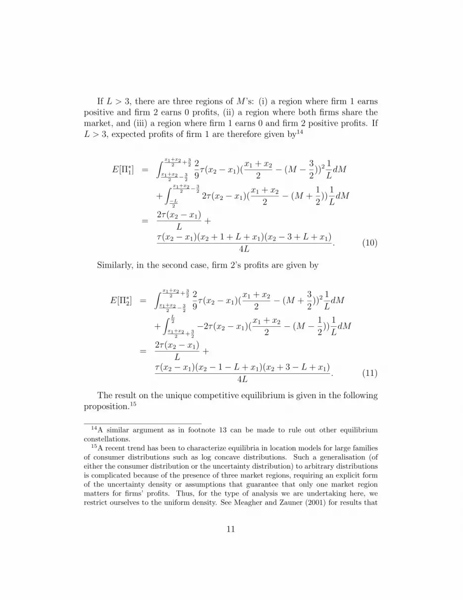
If L > 3, there are three regions of M ’s: (i) a region where firm 1 earnspositive and firm 2 earns 0 profits, (ii) a region where both firms share themarket, and (iii) a region where firm 1 earns 0 and firm 2 positive profits. IfL > 3, expected profits of firm 1 are therefore given by14

E[Π∗1] =

∫ x1+x22

+ 32

x1+x22

− 32

2

9τ(x2 − x1)(

x1 + x2

2− (M − 3

2))2 1

LdM

+∫ x1+x2

2− 3

2

−L2

2τ(x2 − x1)(x1 + x2

2− (M +

1

2))

1

LdM

=2τ(x2 − x1)

L+

τ(x2 − x1)(x2 + 1 + L + x1)(x2 − 3 + L + x1)

4L. (10)

Similarly, in the second case, firm 2’s profits are given by

E[Π∗2] =

∫ x1+x22

+ 32

x1+x22

− 32

2

9τ(x2 − x1)(

x1 + x2

2− (M +

3

2))2 1

LdM

+∫ L

2

x1+x22

+ 32

−2τ(x2 − x1)(x1 + x2

2− (M − 1

2))

1

LdM

=2τ(x2 − x1)

L+

τ(x2 − x1)(x2 − 1− L + x1)(x2 + 3− L + x1)

4L. (11)

The result on the unique competitive equilibrium is given in the followingproposition.15

14A similar argument as in footnote 13 can be made to rule out other equilibriumconstellations.

15A recent trend has been to characterize equilibria in location models for large familiesof consumer distributions such as log concave distributions. Such a generalisation (ofeither the consumer distribution or the uncertainty distribution) to arbitrary distributionsis complicated because of the presence of three market regions, requiring an explicit formof the uncertainty density or assumptions that guarantee that only one market regionmatters for firms’ profits. Thus, for the type of analysis we are undertaking here, werestrict ourselves to the uniform density. See Meagher and Zauner (2001) for results that

11

Proposition 1 (Equilibrium under Uniform Demand Uncertainty)The duopoly location-then-price game under demand uncertainty with con-sumers uniformly distributed on the closed interval [M − 1

2,M + 1

2] and the

demand uncertainty M uniformly distributed on the closed interval [−L2, L

2],

with 0 < L < ∞, has the following unique location-then-price equilibriumwith locations given by:

−x∗1 = x∗2 =1

36(27 + L2) if 0 < L ≤ 3

−x∗1 = x∗2 =5 + L2 − 2L

4(L− 1)if 3 < L < ∞.

• The equilibrium differentiation ∆e = x2 − x1 is given by

1

18(27 + L2) if 0 < L ≤ 3,

5 + L2 − 2L

2(L− 1)if 3 < L < ∞.

• The expected equilibrium prices, E(p1) and E(p2), are given by

τ

18(27 + L2) if 0 < L ≤ 3,

τ(5 + L2 − 2L)(9− 2L + L2)

8L(L− 1)if 3 < L < ∞.

• Expected profits of each firm in equilibrium are

τ

972(27 + L2)2 if 0 < L ≤ 3,

do not require a parametric form of the density of the uncertainty, but a restriction ofthe length of the support of the uncertainty to less or equal than unity. The assumptionof simultaneous moves is also an important here — the substitution of one quadraticfirst-order condition into another to calculate a Stackelberg equilibrium yields a quarticfunction which is analytically unwieldy.

12

τ(5 + L2 − 2L)2

8L(L− 1)if 3 < L < ∞.

As L → 0, the results of the standard Hotelling location-then-price gameunder certainty obtain.

Proof: See appendix. 2

In equilibrium, increases in the size of the uncertainty, L, lead to higherexpected equilibrium prices, higher differentiation, and higher profits.16 Theintuition for this result is as follows. If firms face uncertainty about thelocation of demand, the move of a firm away from its competitor has thepositive effect of weakened price competition by forcing the competitor toincrease its prices in all realizations of the uncertainty. This has a positiveeffect on the firm’s (expected) profit as in the original Hotelling game. But,the negative effect of losing market share will not be as pronounced, since thefirm can capture a higher market share in some realizations of the uncertaintywhen it finds itself better located with regard to consumers. Put differently,the negative demand effect is weakened when firms entertain uncertaintyabout the location of demand.

Our result of uncertainty as a differentiation force is in contrast to randomutility or consumer heterogeneity approaches. In random utility models withidiosyncratic uncertainty and sufficient heterogeneity, firms have an “extra di-mension” that allows them to differentiate themselves. Firms will substituteheterogeneity for differentiation in the product characteristic/geographicalspace and agglomerate. In contrast, aggregate uncertainty does not intro-duce another “dimension” and firms will choose to differentiate themselvesmore in the product characteristic/geographical space.

Moscarini and Ottaviani (2001) investigate the price equilibria in theHotelling model where the consumer posesses private information about therelative quality of the products of firms. The outcome of (price) competitiondepends on the prior of the relative preference and the quality of privateinformation. They fully characterize equilibria, study comparative statics,and show that competition is fierce when the private information has lowquality and the prior is relatively favorable to one of the firms. In addition,

16For a model that looks at the effect of cost variability on the returns to productdifferentiation see Chang and Harrington (1996).

13

they show that firms’ equilibrium profits are non-convex in the prior andnon-monotone in the quality of private information.

Even though product characteristics are fixed in their model, one couldinterpret their model as a Hotelling model where firms are uncertain aboutrelative preferences. Following this interpretation, the prior of relative prefer-ences in their model plays some of the role of the mean of the uncertainty17 inour model and the quality of private information of the demand side looselymaps to the size (variance) of the uncertainty, L, in our model. In contrast toMoscarini and Ottaviani (2001), in our model, firms’ profits and locations18

are monotone in the size of the uncertainty (variance). However, in theirmodel, due to Bayes law, the prior and the quality of private informationinteract and affect simultaneously the location and distribution of the con-sumer distribution. This leads to their non-monotonicity result in the qualityof private information. This interaction between mean and the variance (sizeof the uncertainty) is absent in our model. This is one the main differencesto our model. Apart from the fixed locations, another important differenceis the timing of the resolution of the uncertainty. In Moscarini and Otta-viani (2001) the uncertainty is resolved after prices are chosen, whereas inour model, the uncertainty is resolved before the price stage. Third, the con-sumer distribution in Moscarini and Ottaviani (2001) is discrete, supportedon two points, whereas ours is continuous.

3.2 Welfare

In order to examine the welfare properties of the equilibrium, we must firstdetermine the socially optimal locations. It is natural to assume that anyregulator or social planner is no better informed than the firms. Thus, thelocations chosen by the planner, have to be chosen before the realizationof the uncertainty, and, after the setting of the locations by the plannerand the realization of the uncertainty, consumers are served by the closerfirm.19 Therefore, the socially optimal locations can be found by minimizing

17For simplicity and without loss of generality, the mean of the uncertainty µ is assumedto be zero in our model.

18Since firms’ locations are fixed in Moscarini and Ottaviani’s model, it is not possibleto compare the models in this respect.

19Without loss of generality, we assume the social planner sets price equal to marginalcost (zero).

14

the expected aggregate transportation costs in serving the unit demands ofcustomers from the closest location. The result is given in the followingproposition.

Proposition 2 (Optimum under Uniform Demand Uncertainty) Theduopoly location-then-price game under demand uncertainty has the followingsocially optimal locations:

−xso1 = xso

2 =3 + L2

12if 0 < L ≤ 1

−xso1 = xso

2 =1 + 3L2

12Lif 1 < L < ∞.

The socially optimal differentiation ∆so = xso2 − xso

1 is given by

3 + L2

6if 0 < L ≤ 1,

1 + 3L2

6Lif 1 < L < ∞.

As L → 0, the results of the standard Hotelling location-then-price gameobtain.

Proof: See appendix. 2

Figure 1 plots the equilibrium and socially optimal locations as a functionof the size of the uncertainty, L, (the location of firm 1 is in the negativerange and the location of firm 2 is in the positive range).

The equilibrium and socially optimal locations are both symmetric andmove further apart as the uncertainty increases. However, they move apartat different rates causing them to cross at 7

3+ 2

3

√13 ≈ 4.737. As a result, the

equilibrium locations are further apart than the socially optimal locationsfor low levels of uncertainty, L < 4.737, giving the excessive differentiationpresent in essentially all models with quadratic transport costs. Howeverfor higher levels of uncertainty, L > 4.737, we get a result contrary to thenorm: the equilibrium locations are closer together than the socially opti-mal locations, indicating insufficient differentiation. When L = 4.737, thecompetitively chosen locations coincide with the socially optimal locations.

15

Note also that, at L = 3, in equilibrium, a “hinterland” for each firmbegins to appear. By “hinterland” we mean the area where a firm is shieldedfrom competition and does not compete for consumers, i. e. the area outsideof the interval [x1+x2

2− 3

2, x1+x2

2+ 3

2]. The appearance of a “hinterland” causes

firms to move slightly closer together. In Figure 1, this can be seen as thekink of the equilibrium locations at L = 3.

As the uncertainty tends to 0, the locations approach the locations undercertainty. This is true for the equilibrium locations as well as the sociallyoptimal locations. Thus, to summarize, uncertainty acts, initially, to re-duce the excessive amount of differentiation which occurs in the competitiveequilibrium and, later, to increase the insufficient differentiation.

2 4 6 8 10L

-2

-1

1

2

x1,x2

optimum

equilibrium

Figure 1: Socially Optimal and Equilibrium Locations as a Function of theSize of the Uniform Uncertainty L (τ = 1) Note. Firm 1’s locations are inthe lower half-plane.

16

2 4 6 8 10 12 14L

0.18

0.2

0.22

0.24

0.26

0.28

Welfare Losses

Figure 2: Expected Welfare Losses as a Function of the Size of the UniformUncertainty L (τ = 1).

Corollary 1 (Welfare Losses under Uniform Demand Uncertainty)Under demand uncertainty, the expected welfare losses, E[T c]− E[T so], aregiven by

τ(243 + 5L4)

972if 0 < L ≤ 1,

τ(27 + 891L2 + 81L4 − 7L6)

3888L2if 1 < L ≤ 3,

τ(1− 92L + 358L2 − 156L3 + 33L4)

144(−1 + L)2L2if 3 < L < ∞,

Proof: See Appendix. 2

17

We can now analyze welfare losses. Since demand is inelastic, the welfarelosses due to competition, at a given level of uncertainty, are the differencebetween the expected total transport costs in the competitive equilibriumand in the socially optimal configuration. These expected welfare losses aregiven in the corollary and are plotted as a function of the uncertainty, L, inFigure 2 (with τ = 1).

As the corollary or Figure 2 indicates, uncertainty can have positive ornegative effects on welfare, depending on the size of the uncertainty, L. For0 < L < 2.393 and 5.718 < L < ∞, more uncertainty (higher L) leads tohigher welfare losses, but for 2.393 < L < 5.718, more uncertainty leads tolower welfare losses. Transport costs are convex in distance, and it is this ef-fect which initially dominates as uncertainty increases, causing welfare lossesto increase. However, we know from Figure 1 the competitive and socially op-timal locations are initially getting closer together and it is this effect whichdominates for L > 2.393 causing the welfare losses due to competition todecrease for intermediate levels of L. The competitive and socially optimallocations eventually diverge, so it is not surprising that the welfare losseseventually increase.

A subtle result is that the minimum of the expected welfare losses (L ≈5.718) does not occur at a point where the competitive locations and thesocially optimal locations coincide (L ≈ 4.737). This is due to the fact thatthe locations are only one part of the story. The other part is the price choice.At the social optimum, consumers go to the closest firm, which is achievedthrough the imposition of an identical price of 0 (for all possible realizations ofM) for both firms by the planner. In the competitive equilibrium, firms playsubgame-perfect equilibrium prices which are identical (and equal to 0) withprobability zero, since, given symmetric equilibrium locations, the probabilitythat M = 0 (to obtain identical prices) is zero. The more distant firm chargesa lower price to inefficiently attract consumers.20 Thus, the coincidence of thesocially optimal and the equilibrium locations does not imply that welfareis at the maximum possible value. More uncertainty (higher L) leads tohigher equilibrium differentiation and this effect reduces the inefficency of the(subgame-perfect) price equilibrium, so that the minimum of the expectedwelfare losses occurs at a higher level of uncertainty than at the point where

20See the discussion of the subgame-perfect price equilibrium following equation (6) insection 2 and note that M is realized after the location choices but before the price choices.

18

social optimal and equilibrium locations coincide.21

It is possible to compare the aggregate expected transport costs in equi-librium (for given L), given in the proof of the corollary, to the aggregatetransport costs in equilibrium under certainty. The aggregate transport costsin the standard Hotelling location-then-price game under certainty are 13τ

48

(see the result in the second section). This gives a measure of the cost in-crease for consumers when going from the certainty model to the model underuncertainty. As it is easily verified, these costs rise sharply with the size ofthe uncertainty.

We can also compare the aggregate expected transport costs in the socialoptimum (for given L), given in the proof of the corollary, to the aggre-gate transport costs in the social optimum under certainty, τ

48. This differ-

ence measures the costs of the uncertainty absent the effects of competition.Again, these costs rise sharply with the size of the uncertainty.

4 Conclusion

When introducing a new product or choosing locations, firms face competi-tion from other firms and usually entertain uncertainty about the product’sdemand. In this paper, we introduce uncertainty about the location of de-mand in a version of Hotelling’s (1929) location game. In our location-then-price game with quadratic transportation costs and uniformly distributedconsumers, firms are uncertain about the location of the consumer distribu-tion before they simultaneously choose locations. We characterize the uniquesubgame-perfect equilibrium of this generalization of the standard locationmodel, and examine the welfare properties of the equilibrium.

Uncertain tastes are a differentiation force. The unique competitive equi-librium exhibits excessive or insufficient differentiation, depending on thelevel of uncertainty. For small and large uncertainty, welfare losses increasewith the size of the uncertainty, but for mid-range uncertainty, welfare lossesactually decrease with the size of the uncertainty. Thus, more uncertaintastes can have positive or negative welfare effects.

In the standard spatial model, a unilateral move closer to the competi-tor has a negative effect (increased price competition) and a positive effect

21The existence of welfare losses raises the issue of regulation. This is beyond the scopeof this paper. See, for example, Viscusi, Vernon, and Harrington (2000).

19

(more demand). The first effect is more important than the second effect, sofirms choose to differentiate themselves. Individual level uncertainty aboutthe heterogeneity of consumers or noisy decisions by consumers leads to ag-glomeration since the extra factor softens price competition. As this papershows, location uncertainty has the opposite effect, acting as a differentiationforce. Intuitively, an increase in the uncertainty makes the price competitioneffect relatively more important than the demand effect.

Firms who are uncertain of consumer preferences selling differentiatedproducts is a realistic description of many markets. We have taken somefirst steps in analyzing the competitive and socially optimal outcomes in acanonical model. Our approach could usefully be applied in the future to avariety of classical location problems such as entry, price discrimination, andstrategic trade.

5 Appendix: Proofs

Proof of Proposition 1:The case 0 < L < 3. If the support of the uncertainty, [−L

2, L

2], does not

overlap the competitive area, [x1+x2

2− 3

2, x1+x2

2+ 3

2], profits of firms are 0 and

such locations cannot be location equilibria. Equilibria where the supportoverlaps either the left side of the competitive area, i. e. −L

2< x1+x2

2− 3

2, or

the right side of the competitive area, i. e. x1+x2

2+ 3

2< L

2, do not exist since

one firm can increase profits by deviating to a location such that the supportis entirely contained in the competitive area.

If [−L2, L

2] ⊂ [x1+x2

2− 3

2, x1+x2

2+ 3

2], firm 1’s profits are given by

E[Π∗1] =

∫ L/2

−L/2

2

9τ(x2 − x1)(

x1 + x2

2− (M − 3

2))2 1

LdM.

=τ

54(x2 − x1)(L

2 + 3(3 + x1 + x2)2).

and firm 2’s profits by

E[Π∗2] =

∫ L/2

−L/2

2

9τ(x2 − x1)(

x1 + x2

2− (M − 3

2))2 1

LdM.

=τ

54(x2 − x1)(L

2 + 3(3 + x1 + x2)2).

20

Solving the first-order conditions,

∂E[Π∗1]

∂x1

= − τ

54(27 + L2 + 9x2

1 − 3x22 + 6x1x2 + 36x1) = 0

∂E[Π∗2]

∂x2

=τ

54(27 + L2 + 9x2

2 − 3x21 + 6x1x2 − 36x2) = 0,

yields three solutions,

x∗1 = − 1

36(27 + L2) (12)

x∗2 =1

36(27 + L2), (13)

x21 =

1

6(−9−

√3√

27− L2) (14)

x22 =

1

6(9−

√3√

27− L2), (15)

and

x31 =

1

6(−9 +

√3√

27− L2) (16)

x32 =

1

6(9 +

√3√

27− L2). (17)

The second-order derivatives at the {first} (second) [third] solution are{−4τ

9,−4τ

9}, ( τ

27(−9 + 2

√3√

27− L2,− τ27

(9 + 2√

3√

27− L2), and [− τ27

(9 +

2√

3√

27− L2, τ27

(−9 + 2√

3√

27− L2]. For L ≤ 3, only the first solutionsatisfies the second order conditions of the profit maximization problem. Atthe first candidate equilibrium, each firm earns profits of τ

972(27 + L2)2.

Next, we check whether firms have the incentive to deviate from thecandidate equilibrium such that their own hinterland disappears. Given firm2 locates at the candidate equilibrium 1

36(27 + L2) and firm 1 deviates to

136

(81− 36L−L2), i. e. to a location where firm 1’s hinterland disappears (orwhere −L

2= x1+x2

2− 3

2), firms profits are τ

243(27− 9L+L2)(−27+18L+L2).

Firm 1’s profits in the candidate equilibrium are τ972

(27+L2)2 and, for L ≤ 3,these profits are larger than firm 1’s profits after the deviation. A similar

21

argument applies for the second firm.Firms do not have an incentive to deviate to a location even further

than where their own hinterland disappears, i. e. to a location where eitherx1+x2

2− 3

2< −L

2or where x1+x2

2+ 3

2> L

2. As we saw in the beginning of this

proof, for such constellations, equilibria do not exist.The final step in establishing that the candidate equilibrium is in fact an

equilibrium for the case L ≤ 3 is checking a jump-over condition, i. e. werequire that firm 1 (firm 2) does not find it attractive to deviate from thecandidate equilibrium to any point to the right (left) of firm 2 (1). Considerfirm 1. At the candidate equilibrium, firm 1’s profits are τ

972(27+L2)2. Given

firm 2 locates at the candidate equilibrium, firm 1’s unique best response(with x1 ≥ x2) is 1

108(189 − L2 − 2

√729− 378L2 + L4. For L ≤ 1.3923 (to

obtain a real solution for the best response), the profits after this deviationare dominated by firm 1’s profits in the candidate equilibrium. For 1.3923 <L ≤ 3, the profits in the candidate equilibrium also dominate the profits tothe right of firm 2. Therefore, the region to the right of firm 2’s candidateequilibrium location offers less profits for firm 1 than in firm 1’s candidateequilibrium. A similar argument applies to firm 2.

The equilibrium differentiation is given by x2−x1 = 118

(27+L2). The ex-

pected equilibrium price charged by firm 1 is given by∫ L/2−L/2

2τ3(x2−x1)(

x1+x2

2−

(M− 32)) 1

LdM = τ

18(27+L2). Firm 1 earns profits of

∫ L/2−L/2

2τ9(x2−x1)(

x1+x2

2−

(M − 32))2 1

LdM = τ

972(27 + L2)2. The same expressions can be derived for

firm 2.

The case 3 < L < ∞. In order to calculate the Nash equilibrium, wedifferentiate a firm’s expected profit with respect to its own location, xi,holding the opponent’s location, x−i, constant. The first order conditionsare given by

−τ(5− x22 + 2x1x2 − 2L− 4x1 + L2 + 4x1L + 3x2

1)

4L= 0

(18)

and

τ(5 + L2 − 2L− 4x2L + 4x2 + 3x22 + 2x1x2 − x2

1)

4L= 0.

(19)

22

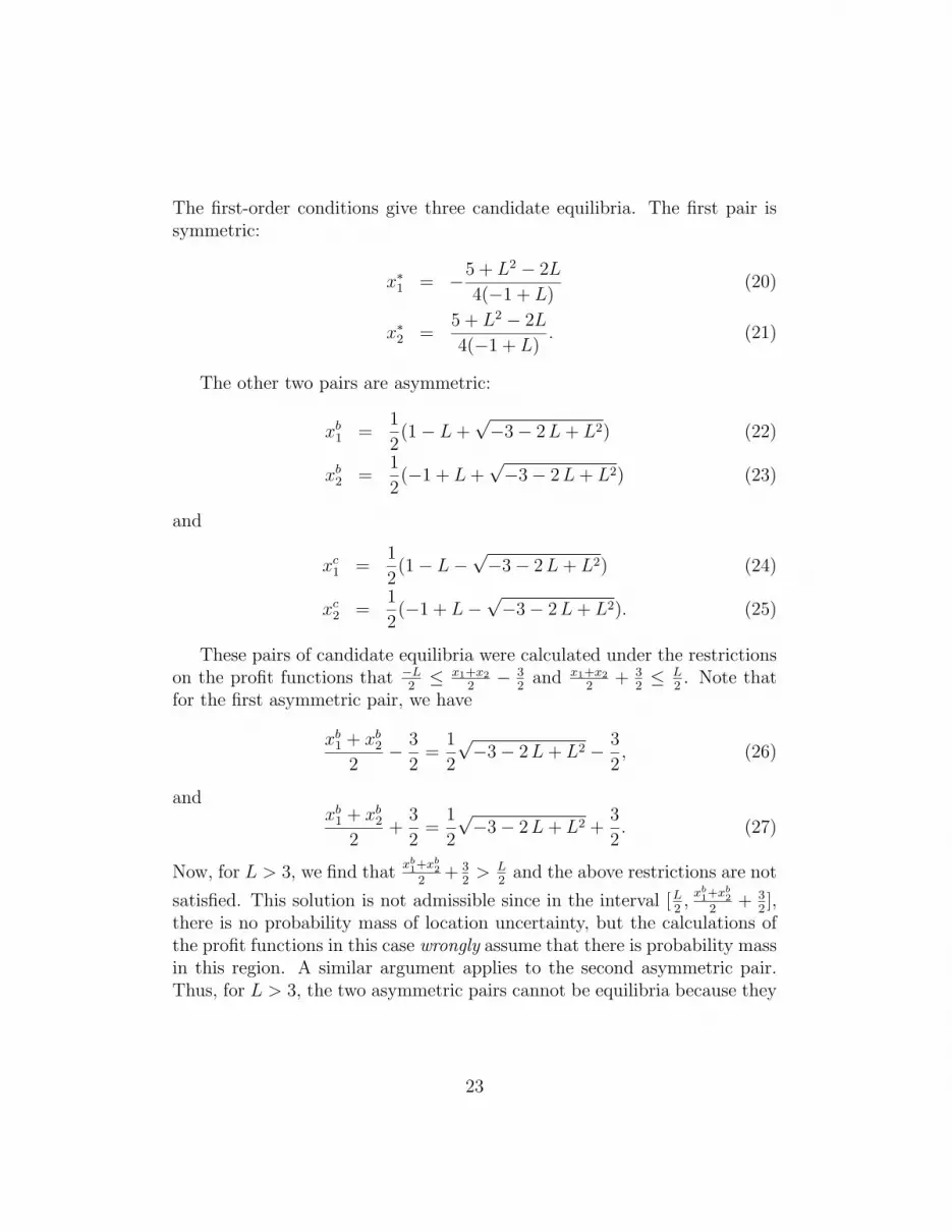
The first-order conditions give three candidate equilibria. The first pair issymmetric:

x∗1 = −5 + L2 − 2L

4(−1 + L)(20)

x∗2 =5 + L2 − 2L

4(−1 + L). (21)

The other two pairs are asymmetric:

xb1 =

1

2(1− L +

√−3− 2 L + L2) (22)

xb2 =

1

2(−1 + L +

√−3− 2 L + L2) (23)

and

xc1 =

1

2(1− L−

√−3− 2 L + L2) (24)

xc2 =

1

2(−1 + L−

√−3− 2 L + L2). (25)

These pairs of candidate equilibria were calculated under the restrictionson the profit functions that −L

2≤ x1+x2

2− 3

2and x1+x2

2+ 3

2≤ L

2. Note that

for the first asymmetric pair, we have

xb1 + xb

2

2− 3

2=

1

2

√−3− 2 L + L2 − 3

2, (26)

andxb

1 + xb2

2+

3

2=

1

2

√−3− 2 L + L2 +

3

2. (27)

Now, for L > 3, we find thatxb1+xb

2

2+ 3

2> L

2and the above restrictions are not

satisfied. This solution is not admissible since in the interval [L2,

xb1+xb

2

2+ 3

2],

there is no probability mass of location uncertainty, but the calculations ofthe profit functions in this case wrongly assume that there is probability massin this region. A similar argument applies to the second asymmetric pair.Thus, for L > 3, the two asymmetric pairs cannot be equilibria because they

23

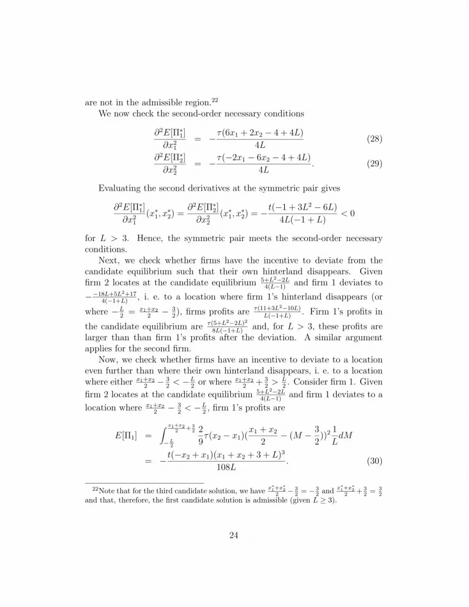
are not in the admissible region.22

We now check the second-order necessary conditions

∂2E[Π∗1]

∂x21

= −τ(6x1 + 2x2 − 4 + 4L)

4L(28)

∂2E[Π∗2]

∂x22

= −τ(−2x1 − 6x2 − 4 + 4L)

4L. (29)

Evaluating the second derivatives at the symmetric pair gives

∂2E[Π∗1]

∂x21

(x∗1, x∗2) =

∂2E[Π∗2]

∂x22

(x∗1, x∗2) = −t(−1 + 3L2 − 6L)

4L(−1 + L)< 0

for L > 3. Hence, the symmetric pair meets the second-order necessaryconditions.

Next, we check whether firms have the incentive to deviate from thecandidate equilibrium such that their own hinterland disappears. Givenfirm 2 locates at the candidate equilibrium 5+L2−2L

4(L−1)and firm 1 deviates to

−−18L+5L2+174(−1+L)

, i. e. to a location where firm 1’s hinterland disappears (or

where −L2

= x1+x2

2− 3

2), firms profits are τ(11+3L2−10L)

L(−1+L). Firm 1’s profits in

the candidate equilibrium are τ(5+L2−2L)2

8L(−1+L)and, for L > 3, these profits are

larger than than firm 1’s profits after the deviation. A similar argumentapplies for the second firm.

Now, we check whether firms have an incentive to deviate to a locationeven further than where their own hinterland disappears, i. e. to a locationwhere either x1+x2

2− 3

2< −L

2or where x1+x2

2+ 3

2> L

2. Consider firm 1. Given

firm 2 locates at the candidate equilibrium 5+L2−2L4(L−1)

and firm 1 deviates to a

location where x1+x2

2− 3

2< −L

2, firm 1’s profits are

E[Π1] =∫ x1+x2

2+ 3

2

−L2

2

9τ(x2 − x1)(

x1 + x2

2− (M − 3

2))2 1

LdM

= −t(−x2 + x1)(x1 + x2 + 3 + L)3

108L. (30)

22Note that for the third candidate solution, we have x∗1+x∗22 − 3

2 = − 32 and x∗1+x∗2

2 + 32 = 3

2and that, therefore, the first candidate solution is admissible (given L ≥ 3).

24

The derivative with respect to x1 is given by

−τ(x1 + x2 + 3 + L)2(4x1 − 2x2 + 3 + L)

108L. (31)

Given firm 2 is located at the candidate equilibrium x2 = 5+L2−2L4(L−1)

and firm

1 selects a location such that x1+x2

2− 3

2< −L

2, this derivative is strictly

positive23 , and firm 1 can increase profits by moving to the right. Thisshows that, given firm 2 locates at the candidate equilibrium, for firm 1,there are no profitable deviations to a location such that x1+x2

2− 3

2< −L

2. A

similar argument applies to firm 2.The final step in establishing that the candidate equilibrium is in fact an

equilibrium is checking a jump-over condition, i. e. we require that firm 1(firm 2) does not find it attractive to deviate from the candidate equilibriumto any point to the right (left) of firm 2 (1). Consider firm 1. At the

candidate equilibrium, firm 1’s profits are t(5+L2−2L)2

8L(−1+L). Given firm 2 locates

at the candidate equilibrium, firm 1’s unique best response (with x1 ≥ x2) is13(−2+2L−x2−

√−11− 2L + L2 + 4x2 − 4Lx2 + 4x2

2). For L ≥ 8.4641 (toobtain a real solution for the best response), the profits after this deviationare dominated by firm 1’s profit at the candidate equilibrium. For 3 < L <8.4641, the profits in the candidate equilibrium also dominate the profits tothe right of firm 2. Therefore, in the candidate equilibrium, the region tothe right of firm 2 offers less demand to firm 1 and worse opportunities fordifferentiation to soften price competition. A similar argument applies to firm2. Since, for each firm, there are no profitable deviations from the candidateequilibrium, the candidate equilibrium is, in fact, a unique equilibrium.

We calculate the equilibrium differentiation, the expected prices and prof-its of firms at the equilibrium x∗1 = −5+L2−2L

4(−1+L), x∗2 = 5+L2−2L

4(−1+L). The equilibrium

differentiation is given by x∗2− x∗1 = 5+L2−2L2(L−1)

. The expected price charged byfirm 1 is given by

E[p∗1] =∫ x∗1+x∗2

2+ 3

2

x∗1+x∗

22

− 32

2

3τ(x∗2 − x∗1)(

x∗1 + x∗22

− (M − 3

2))

1

LdM

23The term (4x1 − 2x2 + 3 + L) is negative, since L > 3, x2 = 5+L2−2L4(L−1) , and x1 at most

−−18L+5L2+174(−1+L) .

25

+∫ x∗1+x∗2

2− 3

2

−L2

2τ(x∗2 − x∗1)(x∗1 + x∗2

2− (M +

1

2))

1

LdM

=τ(5 + L2 − 2L)(9− 2L + L2)

8L(L− 1),

(32)

and the expected profits of firm 1 are given by

E[Π∗1] =

∫ x∗1+x∗22

+ 32

x∗1+x∗

22

− 32

2

9τ(x∗2 − x∗1)(

x∗1 + x∗22

− (M − 3

2))2 1

LdM

+∫ x∗1+x∗2

2− 3

2

−L2

2τ(x∗2 − x∗1)(x∗1 + x∗2

2− (M +

1

2))

1

LdM

=τ(5 + L2 − 2L)2

8L(L− 1).

(33)

The same expressions can be derived for firm 2. 2

Proof of Proposition 2:First, we determine the expected aggregate transportation costs in serving

the unit demands of consumers taking into account that it is optimal to serveeach costumer from the closer firm. Then, we determine the socially optimallocations by minimizing the expected aggregate transportation costs. Theproof splits in 2 cases, namely, the case 1 < L < ∞ and the case 0 < L ≤ 1.

The case 1 < L < ∞. We need to determine the expected total transportcosts for all values of M ∈ [−L/2, L/2]. Since the consumer distribution issymmetric and the uncertainty distribution is symmetric, we can focus onsymmetric optimal locations, i. e. locations of firm 1, xso

1 , and firm 2, xso2 ,

such that xso1 = −xso

2 , with xso2 > 0, and simplify matters by just calculating

transport cost for M ∈ [−L/2, 0] and doubling the result. For the sociallyoptimal case, consumers go to whichever firm is closest, i. e. for any valueof M , all the consumers to the left of 0 go to firm 1, located at x1, whileconsumers to the right of 0 go to firm 2, located at x2.

The calculation splits into two cases, depending on whether there are anyconsumers to the right of 0 or not, for a particular value of M . Consumers,x, are uniformly distributed on the closed interval [M− 1

2,M + 1

2]. Therefore,

26

all consumers will be to the left of 0 (and go to firm 1), if M + 12

< 0, orequivalently, if −L

2≤ M < −1

2. Integrating over this range of M ’s gives the

first integral in the expression below.Consumers will be to the right of 0, if M + 1

2> 0, or equivalently, if

M > −12. Integrating over these M ’s gives the second and third integrals in

the expression below. The integral for x ∈ [M − 12, 0] are the transport costs

for consumers who go to firm 1, −x2, and the integral for x ∈ [0,M + 12] are

the transport costs for consumers who go to firm 2, x2, for a particular valueof M . The expected aggregate transport costs are therefore given by

E[T so] = 2∫ − 1

2

−L2

(∫ M+ 1

2

M− 12

τ(−x2 − x)2 1

Ldx)dM

+2∫ 0

− 12

∫ 0

M− 12

τ(−x2 − x)2 1

Ldx)dM

+2∫ 0

− 12

∫ M+ 12

0τ(x2 − x)2 1

Ldx)dM

=τ(L3 − 2x2 − 6x2L

2 + L + 12x22L)

12L. (34)

Choosing x2 to minimize this expression gives the socially optimal loca-tions. The first order condition yields

∂T so

∂x2

=τ(−2− 6L2 + 24x2L)

12L= 0, (35)

and solving for x2 gives the solution xso2 = 1+3L2

12L. The solution for firm 1 is

symmetric and is given by xso1 = −1+3L2

12L. At the solution the second-order

condition for a minimum is satisfied since the second-order derivative of theexpected aggregate transport costs evaluated at the solution is 2τ > 0.

The case 0 < L ≤ 1. Note, that in this case, the first term in the calculationof the expected aggregate transport costs (see equation (34)) is 0 and theexpected aggregate transport costs reduce to

E[T so] = 2∫ 0

−L2

∫ 0

M− 12

τ(−x2 − x)2 1

Ldx)dM

27

+2∫ 0

−L2

∫ M+ 12

0τ(x2 − x)2 1

Ldx)dM

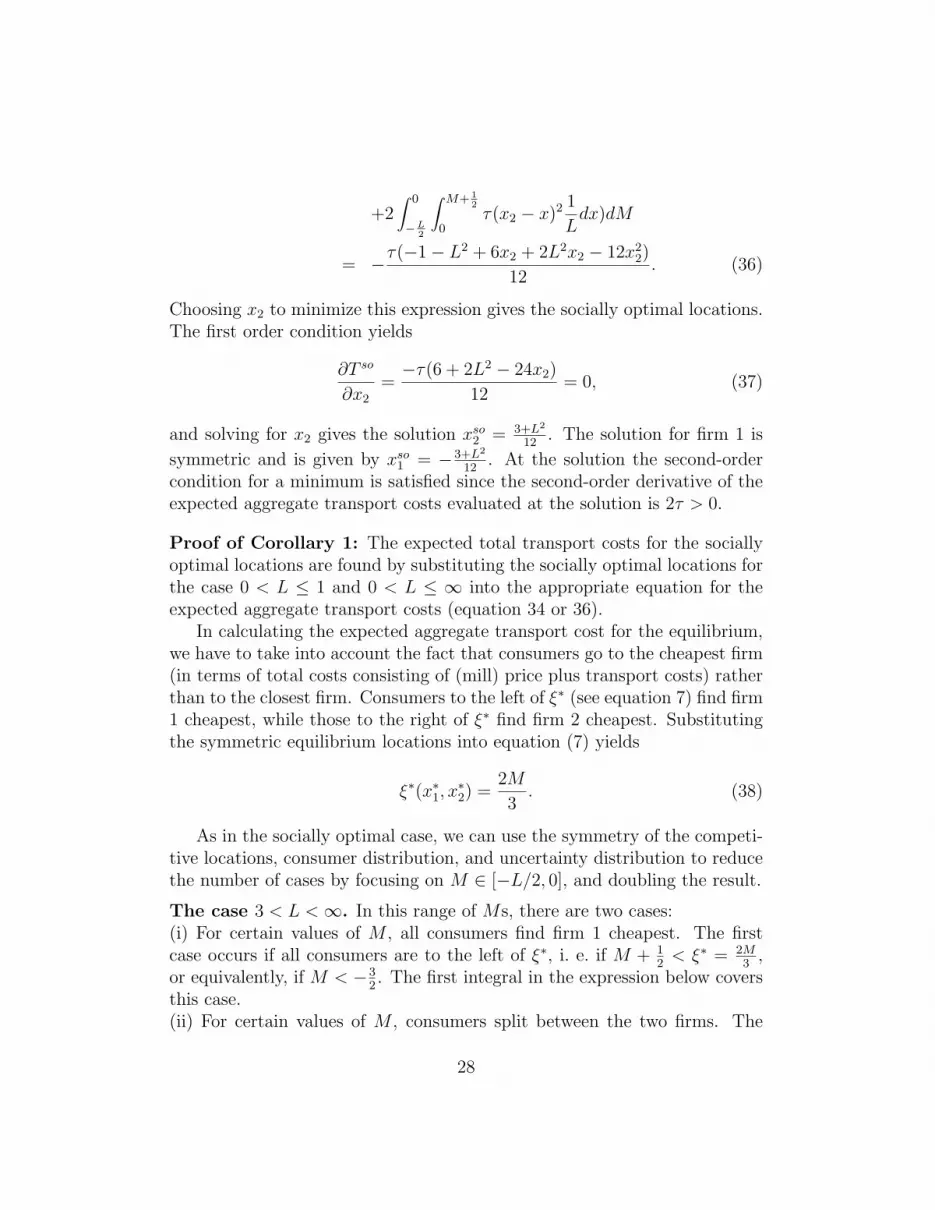
= −τ(−1− L2 + 6x2 + 2L2x2 − 12x22)

12. (36)

Choosing x2 to minimize this expression gives the socially optimal locations.The first order condition yields

∂T so

∂x2

=−τ(6 + 2L2 − 24x2)

12= 0, (37)

and solving for x2 gives the solution xso2 = 3+L2

12. The solution for firm 1 is

symmetric and is given by xso1 = −3+L2

12. At the solution the second-order

condition for a minimum is satisfied since the second-order derivative of theexpected aggregate transport costs evaluated at the solution is 2τ > 0.

Proof of Corollary 1: The expected total transport costs for the sociallyoptimal locations are found by substituting the socially optimal locations forthe case 0 < L ≤ 1 and 0 < L ≤ ∞ into the appropriate equation for theexpected aggregate transport costs (equation 34 or 36).

In calculating the expected aggregate transport cost for the equilibrium,we have to take into account the fact that consumers go to the cheapest firm(in terms of total costs consisting of (mill) price plus transport costs) ratherthan to the closest firm. Consumers to the left of ξ∗ (see equation 7) find firm1 cheapest, while those to the right of ξ∗ find firm 2 cheapest. Substitutingthe symmetric equilibrium locations into equation (7) yields

ξ∗(x∗1, x∗2) =

2M

3. (38)

As in the socially optimal case, we can use the symmetry of the competi-tive locations, consumer distribution, and uncertainty distribution to reducethe number of cases by focusing on M ∈ [−L/2, 0], and doubling the result.

The case 3 < L < ∞. In this range of Ms, there are two cases:(i) For certain values of M , all consumers find firm 1 cheapest. The firstcase occurs if all consumers are to the left of ξ∗, i. e. if M + 1

2< ξ∗ = 2M

3,

or equivalently, if M < −32. The first integral in the expression below covers

this case.(ii) For certain values of M , consumers split between the two firms. The

28

second case occurs if consumers are to the right of ξ∗, i. e. if M+ 12

> ξ∗ = 2M3

,or equivalently, if M > −3

2. The second integral in the expression below

covers the case of consumers going to firm 1 and the third integral in theexpression below covers the case of consumers going to firm 2, with 2M

3being

the equilibrium indifferent consumer. The expected aggregate transport costsin the equilibrium are therefore given by

E[T c] = 2∫ − 3

2

−L2

(∫ M+ 1

2

M− 12

τ(x∗1 − x)2 1

Ldx)dM

+2∫ 0

− 32

∫ 2M3

M− 12

τ(x∗1 − x)2 1

Ldx)dM

+2∫ 0

− 32

∫ M+ 12

2M3

τ(x∗2 − x)2 1

Ldx)dM

=τ(−30 + 121L− 56L2 + 14L3 − 2L4 + L5)

48L(−1 + L)2. (39)

The case 0 < L ≤ 3. Note, that in this case, the first term in the calculationof the expected aggregate transport costs in equilibrium (see equation (39))is 0 and the expected aggregate transport costs in equilibrium reduce to

E[T c] = 2∫ 0

−L2

∫ 2M3

M− 12

τ(x∗1 − x)2 1

Ldx)dM

+2∫ 0

−L2

∫ M+ 12

2M3

τ(x∗2 − x)2 1

Ldx)dM

=τ(1053 + 162L2 − 7L4)

3888. (40)

The expected welfare losses can now be computed by subtracting theappropriate branch of E[T so] from the appropriate branch of E[T c]. 2

29

6 References

Aghion, P., Espinosa, M., and B. Jullien, 1993, Dynamic duopoly with learningthrough market experimentation, Economic Theory 3, 517–539.

Anderson, S. P. 1988, Equilibrium existence in a linear model of spatial competi-tion, Economica 55, 369–398.

Anderson, S. P., de Palma, A., and J.-F. Thisse, 1992, Discrete choice theory ofproduct differentiation (MIT Press, Cambridge, Massachusetts).

Anderson, S. P., Goeree, J. K., and R. Ramer, 1997, Location, location, location,Journal of Economic Theory 77, 102–127.

Balvers, R. and L. Szerb, 1996, Location in the Hotelling duopoly model withdemand uncertainty, European Economic Review 40, 1453–1461.

Bester, H., de Palma, A., Leininger, W., Thomas, J., and E. L. Von Thadden,1996, A non-cooperative analysis of Hotelling’s location game, Games andEconomic Behavior 12, 165–186.

Brickley, J., C. Smith, and J. Zimmerman, 2001, Managerial Economics and Or-ganisational Architecture (2nd ed), McGraw-Hill, New York.

Caplin, A. and B. Nalebuff, 1991a, Aggregation and imperfect competition: Onthe existence of equilibrium, Econometrica 59, 25–59.

Caplin, A. and B. Nalebuff, 1991b, Aggregation and social choice: A mean votertheorem, Econometrica 59, 1–23.

Casado-Izaga, F. J., 2000, Location decisions: the role of uncertainty about con-sumer tastes, Journal of Economics 71, 31–46.

Chang, M., 1991, The effects of product differentiation on collusive pricing, Inter-national Journal of Industrial Organization 9, 453-469.

Chang, M. and J. Harrington, 1996, The interactive effect of product differentiationand cost variability on profit, Journal of Economics and Management Strategy5, 175–193.

D’Aspremont, C., Gabszewicz, J. J., and J.-F. Thisse, 1979, On Hotelling’s “Sta-bility in Competition”, Econometrica 47, 1145–1150.

De Palma, A., Ginsburgh, V., Papageorgiou, Y. Y., and J.-F. Thisse, 1985, Theprinciple of minimum differentiation holds under sufficient heterogeneity, Econo-metrica 53, 767–781.

30

Dierker, E., 1991, Competition for customers, in: B. Cornet, C. d’Aspremont, andA. Mas-Collel, eds., Equilibrium theory and applications (Cambridge Univer-sity Press, Cambridge), 383–402.

Economides, N. 1986, Minimal and maximal product differentiation in Hotelling’sduopoly, Economics Letters 21, 67–71.

Economides, N. 1989, Symmetric equilibrium existence and optimality in differen-tiated product markets, Journal of Economic Theory 47, 178–194.

Gabszewicz, J. J. and J.-F. Thisse, 1992, Location, in: R. J. Aumann and S. Hart,eds., Handbook of game theory, Vol. 1 (North Holland, Amsterdam), 281–304.

Harrington, J., 1995, Experimentation and learning in a differentiated productsduopoly, Journal of Economic Theory, 66, 275-288.

Harter, J., 1996, Hotelling’s competition with demand location uncertainty, Inter-national Journal of Industrial Organization 15, 327–334.

Hay, D. A., 1976, Sequential entry and entry-deterring strategies in spatial com-petition, Oxford Economic Papers 28, 240–257.

Hotelling, H., 1929, Stability in competition, Economic Journal 39, 41–57.

Irmen, A. and J.-F. Thisse, 1998, Competition in multi-characteristics spaces:Hotelling was almost right, Journal of Economic Theory 78, 76–102.

Jovanovic, B., 1981, Entry with private information, Bell Journal of Economics12, 649–660.

Keller, G. and Rady, S., 1999, Optimal experimentation in a changing environment,Review of Economic Studies 66, 475-507.

Kotler, P., 1999, Marketing Management, 10th edition, Prentice Hall, New York.

Lane, W. J., 1980, Product differentiation in a market with endogenous sequentialentry, Bell Journal of Economics 11, 237–260.

Meagher, K. J., 1996, Managing change and the success of niche products, SantaFe Institute Working Paper.

Meagher, K. J. and Zauner, K., 2001, Product Differentiation and Location De-cisions Under Demand Uncertainty, mimeo., Department of Business Studies,University of Vienna and Department of Economics, The University of NewSouth Wales.

Moscarini, G., and Ottaviani, M., 2001, Price competition for an informed buyer,Journal of Economic Theory 101, 457–493.

31

Neven, D. J., 1986, On Hotelling’s competition with non-uniform customer distri-butions, Economic Letters 21, 121–126.

Neven, D. J., 1987, Endogenous sequential entry in a spatial model, InternationalJournal of Industrial Organization 5, 419–434.

Osborne, M. and C. Pitchik, 1986, The nature of equilibrium in a location model,International Economic Review 27, 223–337.

Osborne, M. and C. Pitchik, 1987, Equilibrium in Hotelling’s model of spatialcompetition, Econometrica 55, 911–922.

Park, K. and V. Mathur, 1990, Uncertainty in location, Journal of Urban Eco-nomics 27, 362–380.

Raith, M., 1996, Product differentiation, uncertainty and the stability of collu-sion, London School of Economics, STICERD Discussion Paper Series EI/16,October.

Ross, T., 1992, Cartel stability and product differentiation, International Journalof Industrial Organization 10, 1–13.

Tabuchi, T. and J.-F. Thisse, 1995, Asymmetric equilibria in spatial competition,International Journal of Industrial Organization 13, 213–227.

Viscusi, W. K., Vernon, J., and Harrington, J. (2000), The Economics of Regula-tion and Antitrust, Third Edition, Cambridge, Mass., MIT Press.

32