Location-aware MapReduce in Virtual Cloud Yifeng Geng

1,2, Shimin Chen

3, YongWei Wu

1*, Ryan Wu

3, Guangwen Yang

1,2, Weimin Zheng

1

1Department of Computer Science and Technology,

Tsinghua National Laboratory for Information Science and Technology (TNLIST)

Tsinghua University, Beijing 100084, China;

Research Institute of Tsinghua University in Shenzhen, Shenzhen 518057, China 2

Ministry of Education Key Laboratory for Earth System Modeling, Center for Earth System Science,

Institute for Global Change Studies, Tsinghua University, Beijing, China 3

Intel Labs

*wuyw@tsinghua.edu.cn Abstract—MapReduce is an important programming model for

processing and generating large data sets in parallel. It is

commonly applied in applications such as web indexing, data

mining, machine learning, etc. As an open-source implementation

of MapReduce, Hadoop is now widely used in industry.

Virtualization, which is easy to configure and economical to use,

shows great potential for cloud computing. With the increasing

core number in a CPU and involving of virtualization technique,

one physical machine can hosts more and more virtual machines,

but I/O devices normally do not increase so rapidly. As

MapReduce system is often used to running I/O intensive

applications, decreasing of data redundancy and load unbalance,

which increase I/O interference in virtual cloud, come to be

serious problems. This paper builds a model and defines metrics

to analyze the data allocation problem in virtual environment

theoretically. And we design a location-aware file block allocation

strategy that retains compatibility with the native Hadoop. Our

model simulation and experiment in real system shows our new

strategy can achieve better data redundancy and load balance to

reduce I/O interference. Execution time of applications such as

RandomWriter, TextSort and WordCount are reduced by up to

33% and 10% on average.

Keywords-MapReduce, Virtualization, Data allocation, I/O

interference, Load balance

I. INTRODUCTION

MapReduce is first proposed by Google, as a programming

model for processing and generating large data sets. Hundreds

of MapReduce programs on its clusters every day[1]. As one

of the open-source implementation of MapReduce, Hadoop is

now widely used in Yahoo, Facebook, IBM, etc.[2]

Nowadays, virtualization is getting more and more popular

in cloud computing, as it helps to utilize and deploy

computing resources. One good example is Amazon Elastic

MapReduce[3], which utilizes Hadoop technology to enable

MapReduce computing and is based on virtual machines. A

computer with a multi-core CPU supporting virtualization

technology can run two or more virtual machines (VMs)

simultaneously, which share the I/O resources and appear the

same as physical machines to users.

MapReduce is usually set up on a distributed file system.

Goolge uses GFS and Hadoop uses HDFS. Normally, one file

block has one or two copies in a distributed file system in case

of data corruption. When MapReduce runs in a virtual

environment, three major problems emerge.

Disk sharing results in unbalanced data distribution and therefore leads to unbalanced workload. Data distribution in virtual environment has two aspects in physical view. One is the number distribution of file blocks that physical machines hold. The other is the number of file block collisions that exists in the system. File block collision occurs when two replicas of a file block are in the same physical machine though in different virtual machines. When running MapTask in MapReduce, it prefers to choose the local machine containing the file block [1], or the file block must be transferred from other machine. So one physical machine contains more file blocks or more replicas of a file block, it is likely to be allocated more workload.

I/O interference caused by data unbalance and load unbalance is more serious in a virtual environment because of I/O virtualization implementation. I/O interference decreases the average I/O bandwidth and increases response time. I/O performance of virtual cloud like EC2 suffers from such interference [16]. Some researchers claim that I/O virtualization is the bottleneck in cloud computing [17].

Disk sharing reduces the data redundancy. As distributed file system treats all virtual machines as physical machines, the replicas of a file block are allocated in different virtual disks, but actually they maybe are in the same physical disk. If the physical machine breaks down, file blocks whose replicas are all in that disk become unavailable.

MapReduce is often used for I/O intensive applications, so

it’s beneficial to design deliberate strategy to achieve more

balanced data and workload in virtual environment.

Optimization of MapReduce system is a hot issue. Most of

existing work focused on resource provision and task

scheduling by static application analysis or dynamic prediction

in physical environment. We have the insight on the

importance of data locality in virtual MapReduce system. Our

method uses data locality to balance the workload and

improve the data redundancy to reduce the degree of I/O

interference natively.

In this paper, we abstract a model and define evaluation

metrics to analyze the data pattern and task pattern of

MapReduce in virtual cloud. Moreover, we propose a

location-aware file block allocation strategy for Hadoop. In

the new strategy, HDFS is aware of the locations of the virtual

machines. Our strategy allocates file blocks across all physical

machines evenly and the replicas of a block are located in

different physical machines. In sampling simulation, metrics

of our strategy is better. Our experiment in real system also

verifies that the following three main benefits can be achieved

by using our strategy.

MapReduce’s workload is more balanced. MapTask workload is related to data distribution. Our strategy can balance data distribution so balance MapTask's workload as well

Our strategy reduces I/O interference and improves HDFS’s performance, especially the writing performance. When writing a file block to HDFS, all the replicas of the block have to be written. If these replicas exist in the same physical disk, the I/O interference is intensive. Our new strategy can eliminate this situation by allocating all file blocks locate across all physical disks on average. By doing so, the writing load is balanced and the total throughput increases.

Our strategy retains data’s redundancy as in physical environment. As replicas of each block are allocated in different physical machines, the data are still recoverable in case that one physical machine is down.

The rest of the paper is organized as follows. Section II gives a background introduction of I/O interference and I/O virtualization. Section III describes virtualized Hadoop. In Section IV we build a model and evaluation metrics to analyze the Hadoop’s problem in virtual environment. Then we propose our new allocation strategy. Section V describes the implementation of our strategy in Hadoop. We evaluate our implementation both in a sampling simulation and real experiments in Section VI. Section VII discusses detailed results of our evaluation and some related issues.

II. BACK GROUND

A. I/O interference

There are two traditional kinds of I/O interference, disk

interference and network interference.

Disk interference occurs when multiple processes try to

access the same disk simultaneously. Disk has limits on both

accesses and the amount of data they can transfer per second.

People often consider disk performance under two situations,

sequence read/write (SR/SW) and random read/write

(RR/RW). Traditional magnetic disk uses the

mechanical heads for reading and writing. Its throughput of

random read/write is much smaller than that of sequence

read/write. The reason is that the heads have to frequently

change positions in RR/RW while in SR/SW the heads are

more stable. Recent years Flash based solid state device has

emerged as a good candidate for the next generation of storage.

It provides low access latency, low energy consumption,

shock resistance and lightweight. Detailed analysis on it

performance shows that Flash are excellent sequential stores

while problematic for random access. The Flash’s throughput

of RW is even worse than that of mechanical disk [4]. So the

gap between the sequence access and random access are still

big. Parallel accessing with a high degree makes multiple

sequential accessing patterns degenerate to random accessing

patterns, which causes performance degeneration [5]. Network interference mainly considers the latency and

throughput. All network resources are limited, including link bandwidth, switch and router processing time, etc. Implementations of connection-based protocol, such as TCP, have congestion avoidance algorithms to watch for packet losses and latency to adjust the transfer speed of connections. Research on parallel TCP [6] shows, as the number of simultaneous TCP connections increases, the total throughput will increase until the network becomes congested. The packet loss rate begins to increase depending on the number of connections and the congestion degree. Then the congestion mechanism reduces the congestion window, which decrease the transfer rate. As the number of parallel TCP connections increases, the effects of higher packet loss rates decreases the impact of multiple sockets, the TCP throughput will stop increasing or begin to decrease. Another interesting work on parallel TCP [7] indicates 90% utilization would already be achieved by as few as 3 TCP sockets.

B. I/O virtualization

There are two basic kinds of virtualization: full

virtualization (e.g.,KVM[8]) and paravirtualization (e.g.,

Xen[9]). Full virtualization is a complete simulation of the

underlying hardware while paravirtualization provides a

software interface to virtual machines and the interface is

similar but not identical to that of the underlying hardware. In

either case, virtualization is enabled by a layer called virtual

machine monitor (VMM) or hypervisor. Virtual machines

share CPUs and memory well, but not I/O.

When sending or receiving a network packet, the VMM

domain and the virtual machine domain must be scheduled

correctly before a network packet can be sent or

received[10].The total overhead is much higher than that of

CPU or memory virtualization. For example, Linux is only

able to achieve only about 30% of the network throughput

with Xen that it can achieve running natively [11]. Moreover,

network I/O virtualization increases overheads in the

utilization of device such as CPU. So it can cause loss of

bandwidth utilization from a virtual machine because of

CPU’s limitation [12].

Compared with network I/O, virtualization for disk is

simpler. In network virtualization, the system must be

prepared to receive and respond to request for its virtual

machines at any time. Disk access occurs only when requested

by the virtual machine. But the overhead of disk virtualization

is not negligible. Xen shows about 15% degradation of disk

performance and KVM shows about 7% degradation of write

performance and almost no degradation of read performance

[13].

As one physical machine can host more and more virtual

machines, the isolation must be considered. Different

virtualization shows different characteristics. For example,

Xen shows good isolation for disk I/O and poor isolation for

network I/O, while KVM shows good isolation for network

I/O and poor isolation for disk I/O [13].

III. HADOOP IN VIRTUAL CLOUD

A. Virtualized Hadoop

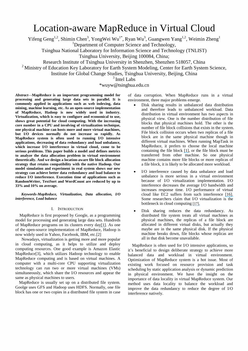
The basic MapReduce’s architecture [1] consists of one

master and many workers. Hadoop is one of the most

commonly-applied implementation of MapReduce. Figure 1

shows virtualized Hadoop architecture. NameNode is the

master of a collection of DataNodes and it is responsible for

their management and file maintenance. JobTracker is the

master of a collection of TaskTraker and in charge of their

management and task maintenance. A DataNode process and a

TaskTracker process run on the same machine to utilize data

locality. The TaskTracker should copy the data that it’s

needed from other machines through network if the data is not

local. NameNode and JobTracker can be separated in different

machines to achieve better performance. When the machine

number is huge, this separation is necessary. In virtual environment, virtual machines in a physical

machine share the hardware resources such as CPU, memory, disk and network. Due to the isolation of virtualization, virtual machines appear to each other like physical machines. NameNode and JobTracker can also run in virtual machines though less efficient. In Hadoop’s architecture view, there is no big difference between virtual environment and physical environment. But in Hadoop’s performance view, differences emerge. Virtualization introduces extra overhead and interference, especially on I/O. And lack of virtual machines’ locality brings other problems. When allocating three replicas of a file block, the three replicas are allocate in difference machines in Hadoop’s view. But if these machines are virtualized, actually two or three replicas of a file block may in the same physical machine. So it causes imbalanced workload. And if one physical machine fails, the data may not be recoverable.

VMM

datanode tasktracker

…………………

datanode tasktracker

VMM

datanode tasktracker

…………………

datanode tasktracker

namenode jobtracker

Figure 1 Virtualized Hadoop architecture

B. Hadoop’s Allocation Strategy

HDFS is used as Hadoop’s distributed file system, which

commonly uses replica mechanism. Here we set 3 as the

replica numbers, which is common in Hadoop cluster. A

cluster may be consisted of many racks of computers. HDFS is

rack-aware, which can support tree hierarchical network

topology. “In most cases, network bandwidth between

machines in the same rack is greater than network bandwidth

between machines in different racks”[14]. If there is no rack,

all the computers are in one rack called default-rack.

In Hadoop’s allocation strategy, when a block is created, the

first replica is placed on the local node that contains the source

data. If the node containing the source data is not the

DataNode of HDFS, HDFS will randomly choose a DataNode

for the first replica. Next, if there are many racks, the second

replica is placed on a DataNode in remote-rack compared to

the first DataNode. Then HDFS chooses another different

DataNode for the third replica in the same rack with the

second DataNode. It ensures that no more than one replica is

placed at one DataNode and no more than two replicas are

placed in the same rack when the number of replicas is less

than twice of its rack number. But if there is only one rack, the

second and the third replicas are placed randomly in different

DataNodes.

IV. MODELING AND NEW STRATEGY

A. Modeling

We build a generation model of data and task pattern to analyze different allocation strategies. To simply the problem for analyzing, we make the following assumptions.

Each physical machine hosts the same number of virtual machines, which using the same I/O devices. Here we use a physical disk to present the I/O devices, as it determines the data’s locality and number of network devices is no more than that of disks in common case.

All the virtual machines are in local area network and the network topology is flat which can be easily achieved by running Hadoop by default without providing any rack information. We do not consider a physical machine as a rack because network bandwidth between virtual machines in the same physical machine is not greater than network bandwidth between virtual machines in different physical machines, which is measured in real cluster.

There is no limitation for workload to be randomly assigned to each virtual machine. There is no mechanism such as taking into account the average load or limitation of task slots when running MapReduce.

The total file size has linear relationship with total block number. One simple example is that all file blocks have the same size.

Now suppose we have a cluster containing p physical

machines, each has a hard disk and the replica number is 3.

Then n file blocks are put into the cluster from another

computer out of the cluster or generated randomly in the

cluster. So the model is about the data pattern generation and

task pattern generation with a certain data pattern. A block has

the same probability to be placed on physical machines that

host the same number of virtual machine.

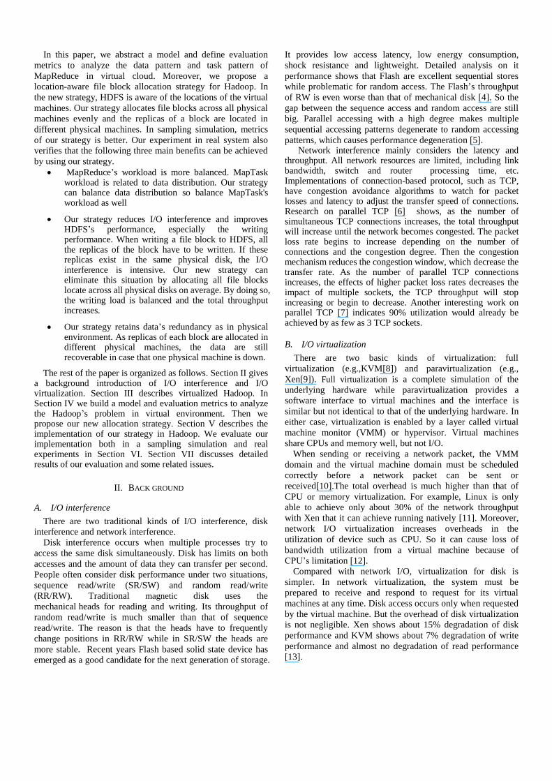
Take p=8 (p0~p7), n=8(0~7) for example, a data pattern

may occurs as Figure 2 using Hadoop’s strategy. It can be

seen that replicas of file 2 are all on p5 and the distribution is

not well balanced.

Next we consider the task pattern when reading these files.

If all the file blocks are accessed by MapTasks, MapReduce

tries to choose local node to run the MapTask. In the example

above, physical machines’ MapTask task pattern may be

assignedNum[8] =[1,2,1,1,0,2,0,1], means p0 has 1 task ,p1

has 2 tasks ,etc. The ideal pattern is [1,1,1,1,1,1,1,1], but is

less possible to happen.

6

6

3

7 2

1 6 7 5 2

1 4 4 3 2 5

0 1 3 0 5 0 4 7

disk[] p0 p1 p2 p3 p4 p5 p6 p7

blockNum[] 3 3 3 4 1 7 2 1fileNum[] 2 3 3 4 1 4 2 1

Figure 2 An example data pattern may be generated using

Hadoop’s strategy, blockNum[] shows number of file blocks in

each disk. fileNum[] shows number of different file blocks in each

disk, it is smaller than blockNum[] if two replicas of a file block

are in the same physical disk .

B. Evaluation Metrics

How to evaluate the data pattern and task pattern? Here we consider three metrics as follows for data pattern:

1

0

1[ ]

p

i

actualReplicaNum fileNum in

(a)

max( [0], , [p-1])maxBlockNum blockNum blockNum (b)

12

0

1 *( [ ] )

p

i

replicaNum nblockNumSigma blockNum i

p p

(c)

max( [0], , [p-1])maxAssignedNum assignedNum assignedNum (d)

12

0

1( [ ] )

p

i

nassignedNumSigma assignedNum i

p p

(e)

actualReplicaNum (a) is the average number of unique file

blocks in a physical machine. The ideal value is 3 when the

replica number is 3. If the file number is much larger than the

disk number, the difference between actualReplicaNum and

the ideal value becomes significant. Take n=1000, p=8 for

example, the actualReplicaNum is small, but considering n*

actualReplicaNum, there are many file blocks that having two

or three replicas in the same disk. It is very possible that each

disk contains all replicas of the same file block. If one disk is

down, the data on the disk will not be recoverable.

maxBlockNum (b) shows the maximum number of blocks

in a physical machine, which is the bottleneck in parallel

writing. The disk with maxBlockNum generally takes the

longest time to finish the write operations in a distributed file

system.

blockNumSigma (c) shows the variation of the pattern. The

idea value is 0, which means that all blocks are evenly

allocated. This parameter reveals the load balance of the

distribution when writing files.

In the example of Figure 2, actualReplicaNum=2.5

maxBlockNum=7 blockNumSigma=1.343

We also can use the similar method as above to evaluate the

task pattern. Since only one replica of each file block are

needed when reading file, the taskNumAvg is useless. There

are two metrics as follows.

maxAssignedNum (d) shows the max number of task that a

physical machine is assigned. Similar with maxBlockNum,

maxAssignedNum will be the longest tail in parallel executing.

assignedNumSigma (e) reveals the load balance of the task

pattern. Because of the locality, the load includes not only

reading but also processing the data which may generate great

load.

For[1,2,1,1,0,2,0,1],maxAssignedNum=2,assignedNumSigm

a=0.707. The data pattern and task pattern above occurs with

a probability. Considering the full permutation, there are 3np

permutations for the data pattern and 3n permutations for the

task pattern. If n is small, we can enumerate the full

permutation. If n is big, we can only use sampling simulation

to evaluate the strategy. For the data pattern in Figure 2, the

enumeration average results for task pattern are as follows:

maxAssignedNumAvg=2.6452,assignedNumSigmaAvg=0.922

0.

C. NEW STRATEGY

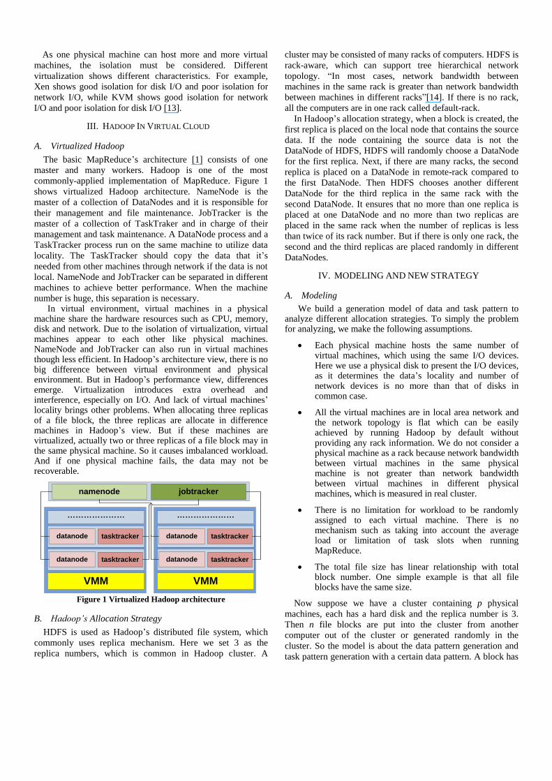
We design a new allocation strategy to allocate replicas of a

file block to different physical machines and keeps balance of

the block number of each physical machine. There are many

ways to achieve the new strategy. Here we present two

intuitive ways. One is round-robin allocation and the other is

“serpentine allocation” used in this paper.

Take p=8 and n=8 for example, Figure 3 shows the round–

robin allocation which is easy to understand. Figure 4 shows

the serpentine allocation. The third replica of file 2 is supposed

to be placed in p7 but p7 has file 2, also p6 has file 2. So at last

the third block of file 2 is placed on p5.

The evaluation metrics for data pattern in Figure 3 and

Figure 4 are the same and the best (actualReplicaNum=3,

maxBlockNum=3, blockNumSigma=0)

The enumeration average results for task patterns of Figure

3 are as follows:

maxAssignedNum=2.2724,assignedNumSigma=0.7943

The enumeration average results for task patterns of Figure

4 are as follows:

maxAssignedNum=2.2705 assignedNumSigma=0.79323

So the difference between round-robin and serpentine

allocation is little. It should be pointed out that the

enumeration average result of task patterns of the new strategy

is not always better than those of Hadoop’s strategy. See an

extreme example showed in Figure 5, the average evaluation

results are as follows:

maxAssignedNum=1 assignedNumSigma=0.

But the actualReplicaNum of this pattern is only 1. The reason

is that all replicas of each file block are located in the same

disk. So there is only one pattern that the task with this block

can choose. So we must consider all the metrics of data pattern

and task pattern and also the probability that a pattern occurs.

Our model reveals basic characteristics of the allocation

strategy though it has some limitations that are discussed in

Section VII.

5 5 6 6 6 7 7 7

2 3 3 3 4 4 4 5

0 0 0 1 1 1 2 2

disk[] p0 p1 p2 p3 p4 p5 p6 p7

blockNum[] 3 3 3 3 3 3 3 3fileNum[] 3 3 3 3 3 3 3 3

Figure 3 An example of round-robin allocation

6 5 5 6 6 7 7 7

5 4 4 4 3 2 3 3

0 0 0 1 1 1 2 2

disk[] p0 p1 p2 p3 p4 p5 p6 p7

blockNum[] 3 3 3 3 3 3 3 3fileNum[] 3 3 3 3 3 3 3 3

Figure 4 An example of serpentine allocation

0 1 2 3 4 5 6 7

0 1 2 3 4 5 6 7

0 1 2 3 4 5 6 7

disk[] p0 p1 p2 p3 p4 p5 p6 p7

blockNum[] 3 3 3 3 3 3 3 3fileNum[] 1 1 1 1 1 1 1 1

Figure 5 A extreme data pattern that may occur with Hadoop’s

strategy

V. IMPLEMENTATION

In the real implementation for Hadoop, we choose

serpentine allocation because it can slightly reduce the cost of

scheduling in our implementation.

The location of virtual machine and the number of file

blocks are needed for the new strategy. Since Hadoop

supported tree hierarchical network topology, we add the

location information of virtual node into the network topology.

For example, if there is only one rack among the physical

machines, the network location of a virtual node may be

changed from /default-rack to /Phy0, means that the virtual

node is on Physical machine 0; if there are some racks among

the physical machines, the network location of a virtual node

may be changed from /rack1 to /rack1/Phy0, means that it is

on the Physical machine 0 of rack1.The main idea is to add a

layer beneath the network location of the physical node. This

mechanism makes it easy to keep compatibility with the native

Hadoop. We can make special label starting with “Phy” to

identify locations of virtual machines. Our strategy works only

when locations of virtual machines are provided in

configuration file.

To maintain the block information for each virtual node, we

add a sorted list by the number of blocks in NameNode of

Hadoop. For each allocation for a replica, the list will be

updated and the update is exclusive in case of concurrent

access. When the block is removed or corrupted, the list will

also be updated. In the update, we first update the block

number of the virtual node, and then update its position in the

sorted list. When adding blocks, round-robin allocation moves

its position to where next position’s block number is bigger,

while serpentine allocation moves its position to where next

position’s block number is not smaller.

Data structure like heap may be better for maintaining the

information of block number. The block information scales

just with the number of virtual machines, and the operation is

done in NameNode’s memory. The real problem may be the

synchronization cost when the system is busy with

manipulating large number of files concurrently. But usually

the I/O hit the peak first and NameNode’s scheduling time is

much smaller than that of I/O transfer time. In our experiment,

choosing of three replicas is finished in several milliseconds.

The linear data structure is good enough though not the best.

There are some special files like job configure file that have

many replicas when the job is running. So we randomly place

replicas exceeding the configured replica number among all

virtual nodes.

Now we can make sure that three replicas of a file block are

allocated in three different physical machine and the blocks is

almost well balanced across all virtual machines. If the

number of virtual machine in each physical machine is the

same, the blocks are also balanced across all physical

machines. It is useful if some physical machine is less

powerful and can host less number of virtual machines. We

can adjust the load of a physical machine with the number of

its virtual machine. Also our new strategy makes it possible to

shut down nodes by the unit of a physical machine instead of a

virtual machine, which achieves faster resource shrinking.

VI. EVALUATION

A. Simulation Evaluation

When n or p is large, it is impossible to calculate the five

metrics with the full permutation. So we use sampling

simulation to compare our new strategy (serpentine allocation)

with Hadoop’s original strategy. Each sampling unit consists

of allocating a data pattern of 3n file blocks and generating a

task pattern of reading n file blocks with such generated data

pattern using corresponding strategy.

We have set the parameter n=256, and p =

[8,16,32,64,128,256], the sampling number is set to 1,000,000.

8 16 32 64 128 2560

20

40

60

80

100

120

p

valu

e

maxBlockNum of Original

maxBlockNum of New

Figure 6 maxBlockNum’s comparison of Hadoop’s original

strategy and our new strategy using sampling

8 16 32 64 128 2560

0.5

1

1.5

2

2.5

3

3.5

4

p

valu

e

fileNumAvg of Original

fileNumAvg of New

Figure 7 actualReplicaNum’s comparison of Hadoop’s original

strategy and our new strategy using sampling

8 16 32 64 128 2560

0.5

1

1.5

2

2.5

3

3.5

4

4.5

5

p

valu

e

blockNumSigma of Original

blockNumSigma of New

0

Figure 8 blockNumSigma’s Comparison of Hadoop’s original

strategy and our new strategy using sampling

8 16 32 64 128 2560

5

10

15

20

25

30

35

40

p

valu

e

maxAssignedNum of Original

maxAssignedNum of New

Figure 9 maxAssignedNum’s comparison of Hadoop’s original

strategy and our new strategy using sampling

8 16 32 64 128 2560

0.5

1

1.5

2

2.5

3

3.5

4

4.5

p

valu

e

assignedNumSigma of Original

assignedNumSigma of New

Figure 10 assignedNumSigma’s comparison of Hadoop’s original

strategy and our new strategy using sampling

TABLE I. COMPARISON OF HADOOP’S ORIGINAL STRATEGY AND OUR NEW

STRATEGY WHEN (N=224 P=8 SAMPLING NUMBER=1,000,000)

Original New

Average of actualReplicaNum 2.0657 3

Average of maxBlockNum 90.5798 84

Average of blockNumSigma 4.1722 0

Average of maxAssignedNum 33.7660 34.5946

Average of assignedNumSigma 3.6256 4.14939

The average metrics’ results of data pattern are showed in

Figure 6(maxBlockNum), Figure 7(actualReplicaNum) and

Figure 8(blockNumSigma). In data pattern evaluation, three

metrics of our new strategy are all better than those of

Hadoop’s original one. And when p is getting smaller,

actualReplicaNum drops dramatically. The average metrics’

results of task pattern are showed in Figure

9(maxAssignedNum) and Figure 10 (assignedNumSigma),

when p>=16 maxAssignedNum and assignedNumSigma of our

strategy are better.

Here we also present the result of (n=224 p=8) in TABLE I,

because it fits our experiments configuration in a real system.

Notice that when (n=256 or 224, p=8), maxAssignedNum and

assignedNumSigma of Hadoop’s strategies are better than

those of ours. The reason is similar to Figure 5 as we

mentioned above, imbalanced data pattern may achieve

balanced task pattern. When n=8, actualReplicaNum is close

to 2, it means that each task with a file block has only about

two physical locations to choose.

Now we get a clear understanding about the data allocation

in virtual environment. However, how these metrics affect the

real system’s performance is more complicated than the

numerical values we see here. For example, task pattern of our

strategy is still better when n=8 in real experiment, we explain

this in Section VII.

B. Experiment Evaluation

1) Testbed Description

We build our cluster with 8 HP x2600 Workstations. Each

physical machine hosts 7 virtual machines, so we have 56

virtual machines in the virtual cloud. TABLE II shows the

hardware and software details in our experiment. What’s

more, Tashi [18] is used to manage the virtual machines.

There is another machine with 4 CPU and 8G memory used as

Hadoop’s NameNode, JobTracker and ganglia server, which

makes it simple to analyze the workload with ganglia. The

network bandwidth between these machines is 1Gbps.

TABLE II. EXPERIMENT SETUP

SW

Hadoop Hadoop 0.20.0

Guest OS Ubuntu 8.04 1CPU

1GB Memory 1Gbps Ethernet

Host OS Ubuntu 8.04

Virtualization KVM 1Gbps Ethernet

HW

CPU 2x4 2.83GHz

Memory 16G

Disk 250G 7200rmp

Network 1Gbps Ethernet

2) Applications

The MapReduce applications we use for evaluation are

RandomWriter TextSort and WordCount.

RandomWriter randomly chooses words from a small

vocabulary (100 words), forms them into lines in MapTask.

The map outputs are directly committed to distributed file

system, so there is no ReduceTask in RandomWriter. TextSort

sorts each line in existing text files by vocabulary order. The

map and reduce functions in TextSort are both identity

functions and the sort of the texts is realized by the inherent

merge sort of MapReduce framework. WordCount counts the

appearance frequency of words in the text. The input text of

TextSort and WordCount are the RandomWriter’s outputs.

3) Profiling with Ganglia

Ganglia[19] is a scalable distributed monitoring system for

high-performance computing systems. We have deployed

Ganglia to the physical cluster, so we can get information

about the usage of CPU, memory, disk I/O and network in

real-time. We modified Ganglia to display all metrics in ten

minutes. The collection interval is set to 3s. Before each

experiment, the previous data of Ganglia was cleared. So the

metric pictures became more readable.

4) Experiment Design

We have done two groups of experiments use Hadoop’s

default configuration. The difference of the two groups is

whether speculative execution of map and reduce turns on.

Original New Original with SC New with SC0

20

40

60

80

100

120

140

160Results of RandomWriter

Runnnin

g T

ime (

s)

11.1%

33.5%

Figure 11 Experiment results of RandomWriter’s execution time

Original New Original with SC New with SC0

50

100

150

200

250

300

350Results of TextSort

Runnnin

g T

ime (

s)

10.6%8.3%

Figure 12 Experiment results of TextSort’s execution time

Original New Original with SC New with SC0

20

40

60

80

100

120

140

160

180

200Results of WordCount

Runnnin

g T

ime (

s)

10.6%

0.2%

Figure 13 Experiment results of WordCount’s execution time

Speculative execution (SC) is like backup task which is

used to reduce the long tail of parallel execution. First we turn

off the speculative execution to get a better understanding how

our new strategy affects the system. Then we turn on

speculative execution (Hadoop’s default) which is often used

in real systems to see whether our new strategy is better.

The input data is 224*61.5MB, which is generated using

RandomWriter. TextSort’s reducer number is set to 56 and

WordCount’s reducer number is set to 1. 5 experiments have

been done for each application in the group with speculative

execution off and 3 experiments have been done for that with

speculative execution on. Then we take the average execution

time and standard deviation of each case. The results are

showed in Figure 11, Figure 12 and Figure 13. We can see that

our strategy is generally better in all three applications. With

SC off, we reduce about 10% execution time of three

applications with the new strategy. With SC turn on,

RandomWriter reduces 33.5% execution time, TextSort

reduces 8.3% execution time, but WordCount’s improvement

is little.

VII. DISCUSSION

A. Model’s limitation

Some of our model’s assumptions break down in real

system, but still shows the general characteristics.

Physical machines may host different number of virtual

machines, but our strategy can still reduce block collisions and

balance the workload according to the number of virtual

machine in a physical machine.

When choosing DataNode for a replica, HDFS calculates an

average load based on number of active connections. If the

chosen DataNode’s load is bigger than two times of average

load, another selection will be performed. This can control the

maximum load in a DataNode in real-time, but has limit effect

on balancing the data pattern. Figure 14 shows a data pattern

generated by RandomWriter with Hadoop’s strategy. The data

pattern is not well balanced and is close to our sampling

simulation results.

Hadoop assigns MapTasks when the TaskTracker sends

heartbeat to the JobTracker. We can take the procedure as a

random selection. However, Each TaskTracker in Hadoop has

task slots which can hold 2 tasks by default at the same time.

New task will be accepted only when the TaskTracker has a

free slot. This mechanism prevents too many tasks to be

assigned to a node. And Hadoop schedules some MapTasks to

run on DataNodes not containing the source file. However,

this schedule balances MapTask load at the expense of extra

network transfer .On Averagy about 85% of MapTasks are

local and the rest 15% are non-local. So our model for task

pattern is not fully consistent with the real system. But it tells

us that the node that has more file blocks, are likely been

assigned more workload.

B. Evaluation Analysis

1) Our strategy is better in sampling and experiment

evaluation. But how it works in real system and where is the

improvement comes from? So the experiment design and result

need to be discussed.

The benefit of our new strategy with small workload size is

not very impressive. We choose 224*61.5MB as the workload

size, which stresses the whole cluster and leads to reasonable

execution time. We also tried larger workload size, the

improvement was a bit more obvious, but the experiment took

much more time.

2) Effect of speculative execution

We can run exactly the number of MapTask and

ReduceTask with SC off. It will eliminate unnecessary

interference. With SC turning on, SC will run extra map and

reduce tasks when it detects some slow tasks.

p0 p1 p2 p3 p4 p5 p6 p70

10

20

30

40

50

60

70

80

90

100A data pattern generated by RandomWriter

num

ber

of

blo

cks

ideal value(84)

Figure 14 A data pattern generated by RandomWriter with

Hadoop’s strategy. Its execution time is 132s. The evaluation

results of this data pattern are maxBlockNum=91,

blockNumSigma=5.099. And the sampling average results are:

maxBlockNumAvg=90.58, blockNumSigmaAvg=4.172

As showed in Figure 11, Figure 12 and Figure 13, SC

generally reduces the variation not the execution time. But it

increases the execution time of RandomWriter of original

strategy and TextSort of both strategies. The reason is that

RandomWriter and TextSort are I/O intensive while

WordCount is CPU intensive. The CPU usage of the physical

machine are up to 85% (7 of 8 CPUs are used for Virtual

Machines) when WordCount running. SC runs extra map and

reduce tasks consuming the resources. Considering I/O

interference when the system is stressed, SC’s extra load takes

more negative effects than the benefit of long-tail cutting. The

interesting one is the RandomWriter of new Strategy, its

execution time significant decreases with SC on. The possible

reason is that our new strategy reduces the I/O interference so

SC’s benefit overcomes its extra workload.

3) Ganglia’s result

RandomWriter is I/O intensive, Figure 15 shows network

throughput of the cluster when RandomWriter runs. The

pillar’s width shows the execution time. The pillar’ area shows

the total amount of network transfer. The throughput of our

new strategy can reach more than 700MB/s while that of

original one is about 600MB/s. So the total network

throughput of the system has been improved, which benefit

the total execution time. The total amount of network transfer

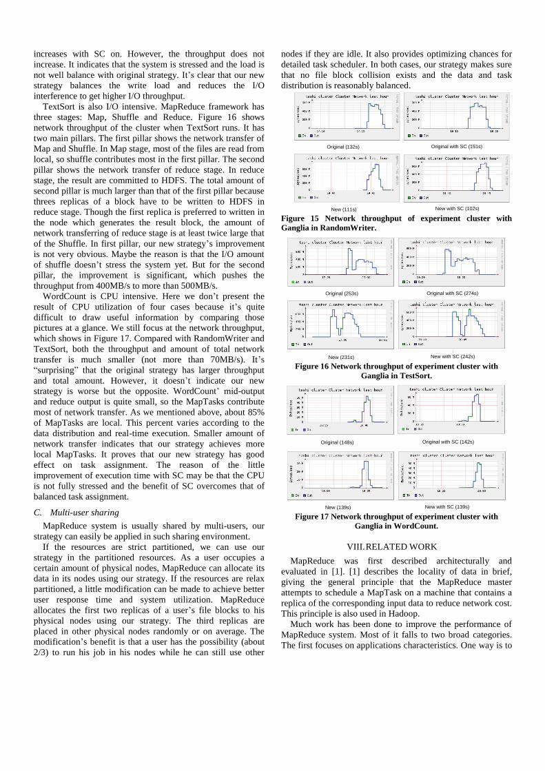
increases with SC on. However, the throughput does not

increase. It indicates that the system is stressed and the load is

not well balance with original strategy. It’s clear that our new

strategy balances the write load and reduces the I/O

interference to get higher I/O throughput.

TextSort is also I/O intensive. MapReduce framework has

three stages: Map, Shuffle and Reduce. Figure 16 shows

network throughput of the cluster when TextSort runs. It has

two main pillars. The first pillar shows the network transfer of

Map and Shuffle. In Map stage, most of the files are read from

local, so shuffle contributes most in the first pillar. The second

pillar shows the network transfer of reduce stage. In reduce

stage, the result are committed to HDFS. The total amount of

second pillar is much larger than that of the first pillar because

threes replicas of a block have to be written to HDFS in

reduce stage. Though the first replica is preferred to written in

the node which generates the result block, the amount of

network transferring of reduce stage is at least twice large that

of the Shuffle. In first pillar, our new strategy’s improvement

is not very obvious. Maybe the reason is that the I/O amount

of shuffle doesn’t stress the system yet. But for the second

pillar, the improvement is significant, which pushes the

throughput from 400MB/s to more than 500MB/s.

WordCount is CPU intensive. Here we don’t present the

result of CPU utilization of four cases because it’s quite

difficult to draw useful information by comparing those

pictures at a glance. We still focus at the network throughput,

which shows in Figure 17. Compared with RandomWriter and

TextSort, both the throughput and amount of total network

transfer is much smaller (not more than 70MB/s). It’s

“surprising” that the original strategy has larger throughput

and total amount. However, it doesn’t indicate our new

strategy is worse but the opposite. WordCount’ mid-output

and reduce output is quite small, so the MapTasks contribute

most of network transfer. As we mentioned above, about 85%

of MapTasks are local. This percent varies according to the

data distribution and real-time execution. Smaller amount of

network transfer indicates that our strategy achieves more

local MapTasks. It proves that our new strategy has good

effect on task assignment. The reason of the little

improvement of execution time with SC may be that the CPU

is not fully stressed and the benefit of SC overcomes that of

balanced task assignment.

C. Multi-user sharing

MapReduce system is usually shared by multi-users, our

strategy can easily be applied in such sharing environment.

If the resources are strict partitioned, we can use our

strategy in the partitioned resources. As a user occupies a

certain amount of physical nodes, MapReduce can allocate its

data in its nodes using our strategy. If the resources are relax

partitioned, a little modification can be made to achieve better

user response time and system utilization. MapReduce

allocates the first two replicas of a user’s file blocks to his

physical nodes using our strategy. The third replicas are

placed in other physical nodes randomly or on average. The

modification’s benefit is that a user has the possibility (about

2/3) to run his job in his nodes while he can still use other

nodes if they are idle. It also provides optimizing chances for

detailed task scheduler. In both cases, our strategy makes sure

that no file block collision exists and the data and task

distribution is reasonably balanced.

Original (132s)

New (111s)

Original with SC (151s)

New with SC (102s) Figure 15 Network throughput of experiment cluster with

Ganglia in RandomWriter.

Original (253s)

New (231s)

Original with SC (274s)

New with SC (242s) Figure 16 Network throughput of experiment cluster with

Ganglia in TestSort.

Original (148s)

New (139s)

Original with SC (142s)

New with SC (139s) Figure 17 Network throughput of experiment cluster with

Ganglia in WordCount.

VIII. RELATED WORK

MapReduce was first described architecturally and

evaluated in [1]. [1] describes the locality of data in brief,

giving the general principle that the MapReduce master

attempts to schedule a MapTask on a machine that contains a

replica of the corresponding input data to reduce network cost.

This principle is also used in Hadoop.

Much work has been done to improve the performance of

MapReduce system. Most of it falls to two broad categories.

The first focuses on applications characteristics. One way is to

analyze and compare resource consumption of the application

at hand, and then use this information to set optimized

configurations for different applications [20]. Another is to

monitoring the usage of system’s resources to adjust resource

allocations to fit the requirements of different job stages

[21][22]. Virtual machine monitor can be modified to

dynamic allocate resources to VMs according to resource

usage of applications [23].

The second category focuses on MapReduce System itself.

A new scheduling algorithm for speculative execution is

designed for Hadoop in heterogeneous environments [24].

Cloudlet[25] is design is to overcome the overhead of VM by

adding a local reducer for virtual machines in each physical

machine. Differing from existing work, our work focuses on

the data locality’s influence on MapReduce in virtual

environment. Our work is also related with job scheduler

considering data locality [26], though it doesn’t care about

virtual environment.

IX. CONCLUSION

We address fundamental problems of data allocation and its

impact on MapReduce system in a virtual environment. We

build a theory model and define evaluation metrics to evaluate

the data pattern and task pattern. Based on it, we propose a

new strategy for file block allocation in Hadoop. It uses the

locality of virtual machines to achieve new data distribution,

which balances the workload and reduces I/O interference.

Our simulation and real experiments results prove the good

characteristics of our new allocation strategy both in theory

and in practice.

As core number of CPU increases fast, our work indicates

that it’s beneficial to be aware of the virtual machines’

locations when serving I/O intensive system like MapReduce

in virtual cloud.

ACKNOWLEDGMENT

Wenlong Li, Sirui Yang in Intel lab gives useful advice about paper’s organization. Zhiming Shen has done great work on tashi, which helps us to build the experiment environment quickly and easily. This Work is supported by National Basic

Research (973) Program of China (2011CB302505 ，2007CB310900), Natural Science Foundation of China (61073165, 61040048, 60803121, 60911130371, 90812001, 60963005), National High-Tech R&D (863) Program of China (2010AA012302, 2010AA012401, 2009AA01A132).

REFERENCES

[1] J. Dean and S. Ghemawat. MapReduce: Simplified dataprocessing on large clusters. In Symposium on OperatingSystem Design and Implementation, 2004.

[2] http://wiki.apache.org/hadoop/PoweredBy

[3] http://aws.amazon.com/elasticmapreduce/

[4] T. Härder, K.S. 0002, Y. Ou, and S. Bächle, “Towards Flash Disk Use in Databases - Keeping Performance While Saving Energy?,” BTW, J.C. Freytag, T. Ruf, W. Lehner, and G. Vossen, eds., GI, 2009, pp. 167-186.

[5] L. Bouganim, B. Jónsson, and P. Bonnet, “uFLIP: Understanding flash IO patterns,” Proceedings of the 4th Biennial Conference on Innovative Data Systems Research (CIDR’09), 2009.

[6] T. Hacker, B. Athey, and B. Noble, “The end-to-end performance effects of parallel TCP sockets on a lossy wide-area network,” Proceedings of the 16th IEEE-CS/ACM International Parallel and Distributed Processing Symposium (IPDPS), 2002, pp. 434–443.

[7] E. Altman, D. Barman, B. Tuffin, and M. Vojnovic, “Parallel tcp sockets: Simple model, throughput and validation,” Proceedings of the IEEE INFOCOM, 2006.

[8] A. Kivity, Y. Kamay, D. Laor, U. Lublin, and A. Liguori, “kvm: the Linux virtual machine monitor,” Linux Symposium, 2007.

[9] P. Barham, B. Dragovic, K. Fraser, S. Hand, T. Harris, A. Ho, R. Neugebauer, I. Pratt, and A. Warfield, “Xen and the art of virtualization,” Proceedings of the nineteenth ACM symposium on Operating systems principles, Bolton Landing, NY, USA: ACM, 2003, pp. 164-177.

[10] S. Rixner, “Network Virtualization: Breaking the Performance Barrier,” Queue, vol. 6, 2008, pp. 36-ff.

[11] J. Lakshmi and S.K. Nandy, “I/O Device Virtualization in the Multi-core era, a QoS Perspective,” Grid and Pervasive Computing Conference, Workshops at the, Los Alamitos, CA, USA: IEEE Computer Society, 2009, pp. 128-135.

[12] P. Willmann, J. Shafer, D. Carr, A. Menon, S. Rixner, A.L. Cox, and W. Zwaenepoel, “Concurrent direct network access for virtual machine monitors,” Proceedings of the 2007 IEEE 13th International Symposium on High Performance Computer Architecture, 2007, pp. 306–317.

[13] T. Deshane, Z. Shepherd, J.N. Matthews, M. Ben-Yehuda, A. Shah, and B. Rao, “Quantitative comparison of Xen and KVM,” Xen Summit, Boston, MA, USA, 2008, pp. 1–2.

[14] http://hadoop.apache.org/common/docs/current/hdfs_design.html

[15] J.N. Matthews, W. Hu, M. Hapuarachchi, T. Deshane, D. Dimatos, G. Hamilton, M. McCabe, and J. Owens, “Quantifying the performance isolation properties of virtualization systems,” Proceedings of the 2007 workshop on Experimental computer science, San Diego, California: ACM, 2007, p. 6.

[16] M. Armbrust, A. Fox, R. Griffith, A. Joseph, R. Katz, A. Konwinski, G. Lee, D. Patterson, A. Rabkin, I. Stoica, M. Zaharia. Above the Clouds: A Berkeley View of Cloudcomputing. Technical Report No. UCB/EECS-2009-28, University of California at Berkley, USA, Feb. 10, 2009.

[17] J. Shafer, “I/O virtualization bottlenecks in cloud computing today,” in Proceedings of the 2nd conference on I/O virtualization, p. 5, 2010.

[18] http://incubator.apache.org/tashi/

[19] http://ganglia.sourceforge.net/

[20] K.Kambatla, A.Pathak, H.Pucha, Towards Optimizing Hadoop Provisioning in the Cloud. HotCloud, San Diego, CA, Jun 2009

[21] L. T. Phan, Z. Zhang, B. T. Loo, and I. Lee, “Real-time MapReduce Scheduling,” Technical Reports (CIS), p. 942, 2010.

[22] Sandholm, T. & Lai, K. (2009), MapReduce optimization using regulated dynamic prioritization., in John R. Douceur; Albert G. Greenberg; Thomas Bonald & Jason Nieh, ed., 'SIGMETRICS/Performance' , ACM, , pp. 299-310

[23] J. Fang, S. Yang, W. Zhou, and H. Song, “Evaluating I/O Scheduler in Virtual Machines for Mapreduce Application,” in 2010 Ninth International Conference on Grid and Cloud Computing, pp. 64–69, 2010.

[24] M. Zaharia, A. Konwinski, A. D. Joseph, R. Katz, and I. Stoica. Improving MapReduce performance in heterogeneous environments. In OSDI’08: 8th USENIX Symposium on Operating Systems Design and Implementation , 2008.

[25] Ibrahim, Shadi; Jin, Hai; Cheng, Bin; Cao, Haijun; Wu, Song & Qi, Li: CLOUDLET: towards mapreduce implementation on virtual machines. ACM (2009) , S. 65-66 .

[26] M. Zaharia, D. Borthakur, J. S. Sarma, K. Elmeleegy, S. Shenker, and I. Stoica. Job scheduling for multi-user mapreduce clusters. Technical Report UCB/EECS-2009-55, UC Berkeley.