localized states in bi-pattern systems

Hindawi Publishing CorporationAdvances in Nonlinear OpticsVolume 2009, Article ID 926810, 9 pagesdoi:10.1155/2009/926810

Research Article

Localized States in Bi-Pattern Systems

U. Bortolozzo,1 M. G. Clerc,2 F. Haudin,1 R. G. Rojas,3 and S. Residori1

1 l’Institut Non Lineaire de Nice (INLN), Centre National de la Recherche Scientifique (CNRS),Universite de Nice Sophia Antipolis, 1361 Route des Lucioles, 06560 Valbonne, France

2 Departamento de Fısica, Facultad de Ciencias Fısicas y Matematicas, Universidad de Chile, Casilla 487-3,Blanco Encalada 2008, Santiago, Chile

3 Instituto de Fısica, Pontificia Univesidad Catolica de Valparaıso, Casilla 4059, Avenida Brasil 2950, Valparaıso, Chile

Correspondence should be addressed to M. G. Clerc, [email protected]

Received 4 February 2009; Accepted 7 May 2009

Recommended by M. Tlidi

We present a unifying description of localized states observed in systems with coexistence of two spatially periodic states, calledbi-pattern systems. Localized states are pinned over an underlying lattice that is either a self-organized pattern spontaneouslygenerated by the system itself, or a periodic grid created by a spatial forcing. We show that localized states are generic andrequire only the coexistence of two spatially periodic states. Experimentally, these states have been observed in a nonlinear opticalsystem. At the onset of the spatial bifurcation, a forced one-dimensional amplitude equation is derived for the critical modes,which accounts for the appearance of localized states. By numerical simulations, we show that localized structures persist on two-dimensional systems and exhibit different shapes depending on the symmetry of the supporting patterns.

Copyright © 2009 U. Bortolozzo et al. This is an open access article distributed under the Creative Commons Attribution License,which permits unrestricted use, distribution, and reproduction in any medium, provided the original work is properly cited.

1. Introduction

Spatial patterns appear spontaneously in out-of-equilibriumsystems and are observed in many different physical contexts[1]. During the last two decades, spatial pattern formationhas been largely studied, leading to the identification ofvarious types of spatiotemporal instabilities and symmetryselection processes in the general frameworks of dynamicalsystems and bifurcation theory [2, 3]. Localized structures,that is, patterns extended over a restricted spatial domain,have received, in particular, a large interest, and from theearly observations of magnetic domains in ferromagneticmaterials [4], localized states have been successively observedin such different systems as liquid crystals [5], plasmas [6],chemical reactions [7], fluid surface waves [8], granularmedia [9, 10], and thermal convection [11, 12]. In nonlinearoptics localized structures were first predicted as solitarywaves in bistable optical cavities [13], and successively alsoexplained in terms of diffractive auto-solitons [14]. Opticallocalized structures attract nowadays a lot of interest sincethey are potential candidates for optical memories [15].

In one-dimensional systems, localized structures orlocalized patterns can be described as homoclinic orbits

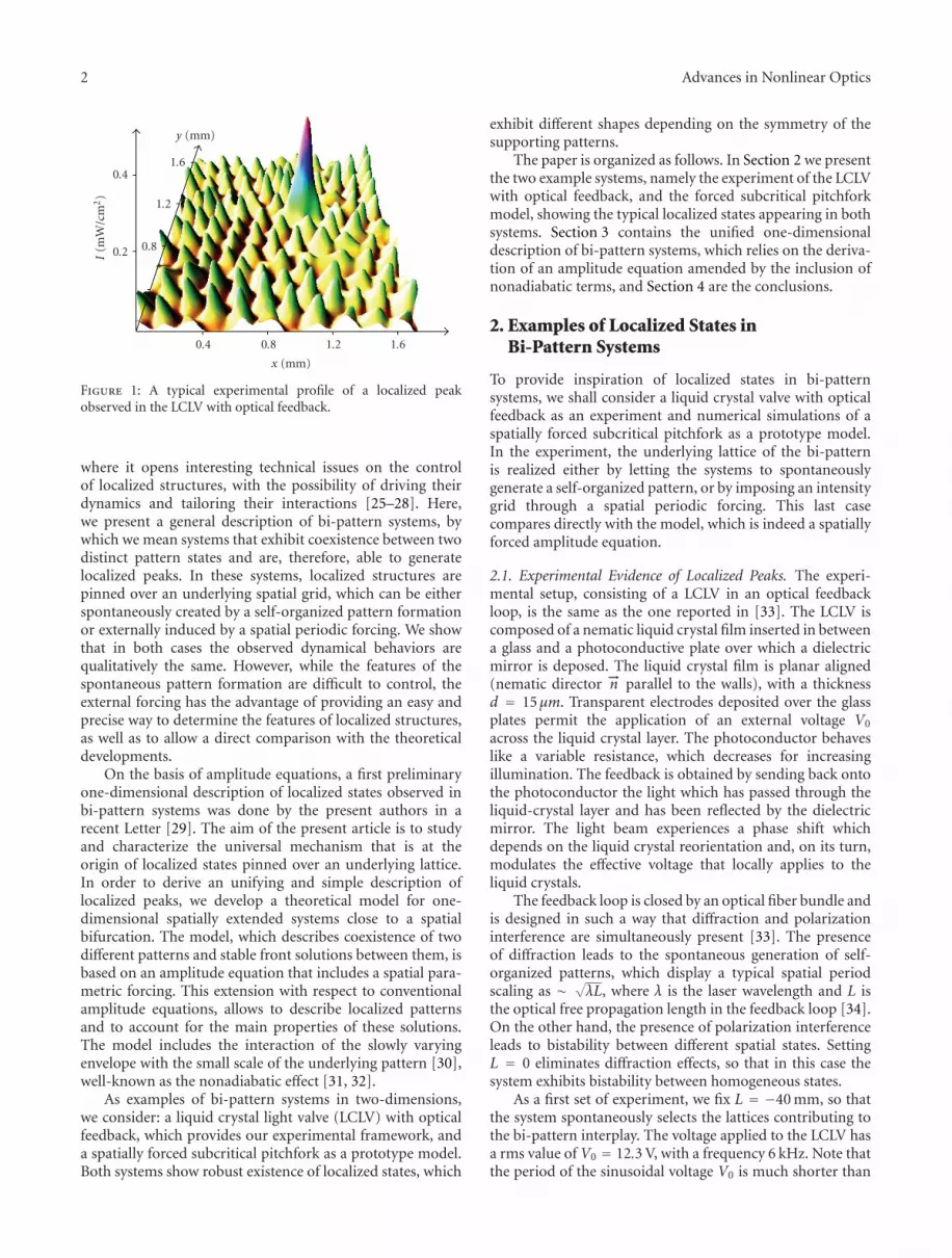
passing close to a spatially oscillatory state [1, 16], or tothe ghost of a spatial pattern [17, 18], and converging to anhomogeneous state, whereas domains are seen as heteroclinictrajectories joining the fixed points of the correspondingdynamical system [19]. Recently, in a nematic liquid crystallight valve with optical feedback it has been found exper-imentally a different type of localized states, appearing aslarge amplitude peaks nucleating over a lower amplitudepattern, therefore called localized peaks [20]. Figure 1 showsthe typical localized peak observed in the light valve withoptical feedback. More recently, similar observations havebeen numerically reported in other optical systems, such as inatomic vapors with optical feedback [21] and in intracavityphotonic crystals [22]. Moreover, localized peaks appearalso in a Newtonian fluid, when nonlinear surface wavesare parametrically excited with two frequencies [23], and inmonoatomic layer deposition [24]. Thus, these examples oflocalized states appearing over a patterned background [20–24] seem to constitute a different universal class of structureswith respect to the localized states that rise up from anuniform background [1, 4–9, 11–13, 16, 19].

The interplay of localized states with a structuredbackground is particularly interesting in nonlinear optics,

2 Advances in Nonlinear Optics

I(m

W/c

m2)

0.2

0.4

y (mm)

0.8

1.2

1.6

x (mm)

0.4 0.8 1.2 1.6

Figure 1: A typical experimental profile of a localized peakobserved in the LCLV with optical feedback.

where it opens interesting technical issues on the controlof localized structures, with the possibility of driving theirdynamics and tailoring their interactions [25–28]. Here,we present a general description of bi-pattern systems, bywhich we mean systems that exhibit coexistence between twodistinct pattern states and are, therefore, able to generatelocalized peaks. In these systems, localized structures arepinned over an underlying spatial grid, which can be eitherspontaneously created by a self-organized pattern formationor externally induced by a spatial periodic forcing. We showthat in both cases the observed dynamical behaviors arequalitatively the same. However, while the features of thespontaneous pattern formation are difficult to control, theexternal forcing has the advantage of providing an easy andprecise way to determine the features of localized structures,as well as to allow a direct comparison with the theoreticaldevelopments.

On the basis of amplitude equations, a first preliminaryone-dimensional description of localized states observed inbi-pattern systems was done by the present authors in arecent Letter [29]. The aim of the present article is to studyand characterize the universal mechanism that is at theorigin of localized states pinned over an underlying lattice.In order to derive an unifying and simple description oflocalized peaks, we develop a theoretical model for one-dimensional spatially extended systems close to a spatialbifurcation. The model, which describes coexistence of twodifferent patterns and stable front solutions between them, isbased on an amplitude equation that includes a spatial para-metric forcing. This extension with respect to conventionalamplitude equations, allows to describe localized patternsand to account for the main properties of these solutions.The model includes the interaction of the slowly varyingenvelope with the small scale of the underlying pattern [30],well-known as the nonadiabatic effect [31, 32].

As examples of bi-pattern systems in two-dimensions,we consider: a liquid crystal light valve (LCLV) with opticalfeedback, which provides our experimental framework, anda spatially forced subcritical pitchfork as a prototype model.Both systems show robust existence of localized states, which

exhibit different shapes depending on the symmetry of thesupporting patterns.

The paper is organized as follows. In Section 2 we presentthe two example systems, namely the experiment of the LCLVwith optical feedback, and the forced subcritical pitchforkmodel, showing the typical localized states appearing in bothsystems. Section 3 contains the unified one-dimensionaldescription of bi-pattern systems, which relies on the deriva-tion of an amplitude equation amended by the inclusion ofnonadiabatic terms, and Section 4 are the conclusions.

2. Examples of Localized States inBi-Pattern Systems

To provide inspiration of localized states in bi-patternsystems, we shall consider a liquid crystal valve with opticalfeedback as an experiment and numerical simulations of aspatially forced subcritical pitchfork as a prototype model.In the experiment, the underlying lattice of the bi-patternis realized either by letting the systems to spontaneouslygenerate a self-organized pattern, or by imposing an intensitygrid through a spatial periodic forcing. This last casecompares directly with the model, which is indeed a spatiallyforced amplitude equation.

2.1. Experimental Evidence of Localized Peaks. The experi-mental setup, consisting of a LCLV in an optical feedbackloop, is the same as the one reported in [33]. The LCLV iscomposed of a nematic liquid crystal film inserted in betweena glass and a photoconductive plate over which a dielectricmirror is deposed. The liquid crystal film is planar aligned(nematic director −→n parallel to the walls), with a thicknessd = 15μm. Transparent electrodes deposited over the glassplates permit the application of an external voltage V0

across the liquid crystal layer. The photoconductor behaveslike a variable resistance, which decreases for increasingillumination. The feedback is obtained by sending back ontothe photoconductor the light which has passed through theliquid-crystal layer and has been reflected by the dielectricmirror. The light beam experiences a phase shift whichdepends on the liquid crystal reorientation and, on its turn,modulates the effective voltage that locally applies to theliquid crystals.

The feedback loop is closed by an optical fiber bundle andis designed in such a way that diffraction and polarizationinterference are simultaneously present [33]. The presenceof diffraction leads to the spontaneous generation of self-organized patterns, which display a typical spatial periodscaling as ∼

√λL, where λ is the laser wavelength and L is

the optical free propagation length in the feedback loop [34].On the other hand, the presence of polarization interferenceleads to bistability between different spatial states. SettingL = 0 eliminates diffraction effects, so that in this case thesystem exhibits bistability between homogeneous states.

As a first set of experiment, we fix L = −40 mm, so thatthe system spontaneously selects the lattices contributing tothe bi-pattern interplay. The voltage applied to the LCLV hasa rms value of V0 = 12.3 V, with a frequency 6 kHz. Note thatthe period of the sinusoidal voltage V0 is much shorter than

Advances in Nonlinear Optics 3

(a) (b) (c)

Figure 2: Hexagonal patterns and localized peaks observed in the LCLV system for Iin = (a) 0.32, (b) 0.38 and (c) 0.52 mW/cm2. From [20].

the liquid crystal response time and of the typical times forelectroconvection [35], thus, liquid crystals are sensitive onlyto the rms value of the applied voltage and perform a staticreorientation. Hydrodynamical effects, such as backflow, areavoided and the molecular realignment is a pure Freedericksztransition [36].

By increasing the input light intensity Iin we observe asequence of transitions, as shown by the experimental snap-shots of Figure 2. First, the homogeneous steady-state loosesstability and develops a pattern of hexagons (Figure 2(a)). Byfurther increasing Iin, localized peaks of higher amplitudeappear over the hexagonal background (cf. Figures 1 and2(b)). For higher values of Iin the system exhibits a novelpattern state, which has a small coexistence region with thehexagonal pattern [20]. Figure 2(c) shows the pattern stateobserved for high Iin.

The theoretical model for the LCLV feedback systemwas previously derived in [37] and consists in two coupledequations, one for the average director tilt θ(−→r , t), 0 ≤ θ ≤π/2, and one for the feedback light intensity Iw. The equationfor the director reads as

τ∂tθ = l2∇2⊥θ − θ + f (θ), (1)

where l is the electric coherence length, τ the local relaxationtime and f (θ) a function taking into account the response ofthe photoconductor to the feedback intensity Iw: f (θ) = 0when V ≤ ΓVFT and f (θ) = π/2(1 − √ΓVFT/V) when V >ΓVFT, with V the voltage that effectively applies to the liquidcrystals

V = ΓV0 + αIw(θ) (2)

and VFT the threshold voltage for the Freedericksz transition.Γ is the impedance of the LCLV dielectric layers and αa phenomenological parameter summarizing, in the linearapproximation, the response of the photoconductor. After afree propagation length L, the feedback light intensity is givenby

Iw = Iin

4

∣∣∣ei(Lλ/4π)∇2

⊥(

1− e−iβcos2θ)∣∣∣

2(3)

I(x, y)

y

x

Figure 3: Numerical profile of the intensity showing a localizedpeak in the LCLV system.

the diffraction being accounted for by the operatorei(Lλ/4π)∇2⊥ . Similar relationships between the tilt angle andthe optical intensity distribution have been previouslyderived for light diffraction in electroconvective liquidcrystal cells, where far-field diffraction [38] or shadowgraphmethods [39] were employed for pattern visualization, butwithout any feedback of light onto the tilt angle. Recently,electro-hydrodynamic convection in a nematic liquid crystalcell with a photoconductive electrode has been reported [40].In such a case, though there was no feedback, the light beamwas acting as an external photocontrol, locally modifying thevoltage applied to the liquid crystal.

We have performed numerical simulations of our modelequations (1), (2), and (3) by taking as values of theparameters Γ = 0.15, α = 5.5 Vcm2/mW, VFT = 3.0 V,l = 30μm, λ = 632 nm, L = −40 mm. In Figure 3 isdisplayed a numerical intensity profile showing a localizedpeak over a hexagonal pattern. By comparing with Figures 1and 2, we can see that the numerical profile is in a fairly goodagreement with the experimental profile and snapshot for thelight intensity.


In brief, it exists a large range of parameters withinwhich the LCLV with optical feedback spontaneously is a bi-pattern system, exhibiting localized states pinned over a self-organized lattice generated by the system itself.

2.2. Spatially Forced Subcritical Pitchfork Model. A prototypemodel of bistability is the subcritical pitchfork model

∂tu = μu + νu3 − u5 +∇2⊥u, (4)

where u(x, t) is a scalar field, μ is the bifurcation parameter,ν characterizes the type of bifurcation, which is subcritical(supercritical) for positive (negative) ν and ∇2

⊥ ≡ ∂xx + ∂yy .The steady states of the above model are u0 = 0 and

u±,± = ±√

ν±√

ν2 + 4μ, (5)

where u = {0,u±,+} and u = {u±,−} are stable and unstableuniform states, respectively. Figure 4 depicts the bifurcationdiagram of subcritical pitchfork model (4) and the respectivecritical points that characterize the bifurcation, namely thebeginning of the bistability B, the Maxwell point μM and thetransition point T .

In order to have a bi-pattern system, we consider thefollowing spatially forced model

∂tu = μu + νu3 − u5 +∇2u + a cos(kx)

+ b cos

(

kx −√3y

2

)

+ c cos

(

kx +

√3y

2

)

,(6)

where {a, b, c} and k are the amplitude and wave numberof the spatial forcing. For small identical forcing amplitudes(a = b = c) or antisymmetrical one (b = c = −a), theuniform stable state of the subcritical pitchfork model (4)becomes a hexagonal or, respectively, honeycomb patternwith amplitude proportional to a. Hence, in the bistabilityregion, the above spatially forced equation is a bi-patternsystem with hexagonal symmetry. In Figure 5 are shownthe typical hexagonal patterns observed and the interfacebetween them.

Hence, in the bi-pattern region we observe front solu-tions and localized states between the two patterns. As aconsequence of the interplay between the envelope variationsand the wave number of the underlying pattern, the frontsolutions are motionless in a region of parameters, so-calledthe pinning range. Close to this region we expect to observea family of localized states [30, 31]. Figure 6 illustrates atypical localized state observed in the hexagonally forcedmodel (6), that appears as a localized peak over a structuredbackground. In the experiment of the LCLV with feedback, ithas been recently shown that the effect of a hexagonal spatialforcing induces regular arrays of localized structures [26].

To illustrate that the localized peaks exhibit differentshapes depending on the supporting pattern, we consider thesubcritical pitchfork model with an orthogonal forcing

∂tu = μu + νu3 − u5 +∇2u + a cos(kx) + a sin(ky), (7)

B TμM

u0

u+,+

u+,−

μ

Figure 4: Bifurcation diagram of model (4), the continuous anddashed curves stand for the stable, respectively, unstable uniformstate. B, μM and T stand for beginning of bistability, Maxwell andtransition points.

ky/

2π

123456

kx/2π1 2 3 4 5 6

1 0 ky/2π

21

kx/2π

12

34

5

Figure 5: Interface between the two hexagonal patterns exhibitedby model (6) with μ = −0.18, ν = 1.0, and a = b = c = 0.02. Theinset figure shows the density plot of the field u(x, t).

where a is the amplitude of the spatial forcing. For smallforcing, the uniform stable states of the subcritical pitchforkmodel (4) become square patterns with amplitude propor-tional to a. Hence, in the bistability region, the above spatiallyforced equation is also a bi-pattern system. In Figure 7 isshown the typical localized states observed in model (7).

2.3. Spatially Forced Experiment: Bi-Patterns and LocalizedStates. Recently, we have shown in the LCLV experiment thata spatially periodic grid can be imposed, by means of a spatiallight modulator, on the profile of the input beam [26]. Insuch a case, localized structures are pinned over the grid,which controls their dynamical behavior. Here, we have setto zero the free propagation length in the feedback loop, thatis, L = 0, hence no spatial scale is spontaneously selected bythe system itself. Then, by using the previous technique, wehave imposed on the input beam a spatial grid of the desiredsymmetry and period. In doing so, we are strongly motivatedby the possibility of establishing a direct comparison with theabove model, (6) or (8).

We have imposed on the system either a hexagonal ora square intensity grid. For both grids, the input intensityis 1.1 mW/cm2 with an amplitude modulation of approxi-mately 10%. For the square grid, the spatial period is setto 130μm whereas for the hexagonal grid it is 150μm. The


ky/

2π

1

2

3

4

5

kx/2π1 2 3 4 5 ky/2π

21

kx/2π

1

2

3

4

5

Figure 6: Localized peak observed in the spatially forced model (6)for a hexagonal forcing, a = b = c = 0.02, and μ = −0.18, ν = 1.0.The inset figure shows the corresponding density plot of the fieldu(x, t).

ky/

2π

1

2

3

4

5

kx/2π

1 2 3 4 5

ky/2π

21

kx/2π

1

2

3

4

5

Figure 7: Localized peak observed in the spatially forced model (7)for an orthogonal forcing, a = 0.01, and μ = −0.18, ν = 1.0. Theinset figure shows the corresponding density plot of the field u(x, t).

voltage applied to the LCLV is slightly changed around V0 =5.5 V, with a fixed frequency of 5 kHz. For this values ofparameters the system is bistable and, being spatially forcedby the intensity grid, it displays bi-patterns an localizedstates. By setting a specific initial condition, we can selecteither to induce an interface between the two patterns or tocreate localized peaks.

As examples of bi-patterns, we show in Figures 8(a)and 8(b) the interface between a high and a low amplitudepattern obtained with (a) a square and (b) a hexagonal grid,respectively. For the same grids, but changing the initialconditions, we can easily induce localized peaks. An exampleof localized peak is shown in Figure 9 for a square grid.

We can notice a good qualitative agreement betweenthe experimental profiles and those obtained by numericalsimulation of the spatially forced models (6) and (7), fora hexagonal and a square forcing, respectively. Moreover,the qualitative behavior of the spatially forced systems, boththe experiment and the model, is very similar to the onedisplayed, in a certain range of parameters, by the unforcedsystem with diffraction playing the role of forcing. Indeed, inthe region of parameters where the unforced system displayslocalized peaks, the qualitative dynamical features are veryclosely the same as those displayed by the forced systems.However, when the input intensity is increased, the unforced

I(g

ray

leve

ls)

050

100150200250

y(m

m)

0.6

0.4

0.2

0

x (mm)0 0.2 0.4 0.6 0.8 1

(a)

I(g

ray

leve

ls)

050

100150200250

y (mm

)

0.60.5

0.40.3

0.20.1

0x (mm)0 0.2 0.4 0.6 0.8

1 1.2

(b)

Figure 8: Interface between the two patterns observed in thespatially forced experiment: (a) square grid, (b) hexagonal grid. Thevoltage applied to the LCLV is (a) V0 = 5.45 V, (b) V0 = 5.65 V. Thegray levels of the intensity go from zero to 1.1 mW/cm2.

system shows a transition to a spatiotemporal chaotic state,which is not the case for the spatially forced system.

In conclusion, localized states in bi-pattern systems arerobust phenomena and appear naturally when bistability isaccompanied by a mechanism of spatial periodic forcing.This can be either externally imposed, or generated by thesystem itself in a certain range of parameters. In the nextsection we will present an unified description of localizedstates in one-dimensional bi-pattern systems.

3. Unified Description

As we have seen, the main ingredient for the appearance oflocalized peaks is the coexistence of two spatially periodicstates, and this, in some sense, regardless the way in whichthe two patterns have been created. In order to providea generic description of such a situation, we consider a aone-dimensional spatially extended system that exhibits asequence of spatial bifurcations as shown in Figure 10, that is,the primary bifurcation is supercritical while the secondaryone is of subcritical type. Let −→u (x; t) be a vector field thatdescribes the system under study and satisfies the partialdifferential equation

∂t−→u = −→f (−→u , ∂x, {λi}

), (8)

6 Advances in Nonlinear OpticsI

(gra

yle

vels

)

0

100

200

300

y (mm

)

2

1.5

1

0.5

0x

(mm

)0

0.5

1

1.5

2

Figure 9: Localized peak observed in the spatially forced experi-ment for a square grid. The voltage applied to the LCLV is V0 =5.40 V.

|A|

Patternstate

μMB1 B2 μ

Π2

Π1

Figure 10: A typical bifurcation diagram allowing for the appear-ance of localized peaks: at a certain value of μ a secondary subcriticalbifurcation takes place; dashed lines mark the beginning (end) B1

(B2) of the bistable region and the Maxwell point μM . From [29].

where {λi} is a set of parameters. For a critical value of oneof the parameters, the system exhibits a spatial instability at agiven wave number qc. Close to this spatial instability, we usethe Ansatz

−→u = A(X ,T)eiqcxu + A(X ,T)e−iqcxu + · · · (9)

and the standard amplitude equations reads as [1]

∂TA = μA− ν|A|2A + α|A|4A− |A|6A + ∂XXA, (10)

where μ is the bifurcation parameter and {ν,α} control thetype of the bifurcation (first- or second-order depending onthe sign of these coefficients). Higher-order terms are ruledout by scaling analysis, since ν ∼ μ2/3, α ∼ μ1/3, |A| ∼ μ1/6,∂t ∼ μ, ∂x ∼ μ1/2, and μ 1. Note that this approach is phaseinvariant (A → Aeiϕ), but the initial system under study doesnot necessarily have this symmetry.

As depicted in Figure 10, for a given range of parametervalues the system shows coexistence between two differ-ent spatially periodic states, each one corresponding to ahomogeneous state for the amplitude equation. Thus, it

is a bi-pattern system. The coexistence region is B1 <μ < B2. The extended stationary solution of the amplitudeequation (10), has the form A = R(x)eiθ(x), where R(x)and θ(x) are the envelope modulus and phase, respectively.These functions satisfy the relation θ(x) = ∫ ε/R(x)2dx. Foruniform modulus solution (Ro), one has the expression forthe envelope

A = Roei(γ/R2

o)X , (11)

with

μ− γ2

R4o− νR2

o + αR4o − R6

o = 0, (12)

and γ is an arbitrary constant related to the initial phaseinvariance. It is worth to note that in the case of positive γ, thewave number of the pattern is modified by the inverse of thesquare amplitude R2

0, so that patterns with larger amplitudehave smaller wave number. At variance, when γ is negativethe patterns with larger amplitude have smaller wavelength[29].

For given values of the parameters, the two stableuniform stationary states of (10) have the same energy, thatis, the system is at the Maxwell point, where the front betweenthe two states is motionless [41]. By moving away from theMaxwell point, the front dynamics is usually characterizedby the motion of the core of the front, which is definedas the front position with the largest slope. In order tohave a localized states, we consider the interaction of twoof these motionless fronts close to the Maxwell point. Asa consequence of the asymptotic behavior of the front atinfinity, the front interaction is attractive, and has the form[42]

Δ = −ae−λΔ + δ, (13)

where Δ is the distance between the cores of each front, δ isthe separation from the Maxwell point, which is proportionalto μ − μM , λ characterizes the exponential decay of the frontto a given constant value at infinity, and a is a positivecoefficient that characterizes the properties of the interactionand is determined by the form of the front. The interactionlaw (13) has an unstable fixed point Δ∗ = − ln(δ/a)/λ, whichis the nucleation barrier between the two homogeneousstates. Hence, the conventional amplitude equation, (10),does not exhibit stable localized states, due to the scaleseparation used to derive the amplitude equation. But nearthe front’s core, the previous Ansatz is no more valid. Indeed,in these locations the slowly varying envelope A(X ,T)shows oscillations of the same (or comparable) size as thesmall scale of the underlying pattern. This phenomenon isdenominated as the nonadiabatic effect [30–32].

3.1. Amended Amplitude Equation. In order to take intoaccount the nonadiabatic effect, we compute the correctionsof the amplitude equation by including the nonresonant


terms, that is, the solvability condition for the amplitude Ahas the form

∂TA =qc2π

∫ X+2π/qc

Xf(|A|2, ∂XX

)A + ∂XXAdx

+N∑

m−n−1 /= 1

gmnqc2π

∫ X+2π/qc

XAmA

ne−(iqc(1+n−m)x/√μ)dx,

(14)

with f (|A|2) = μ− ν|A|2 + α|A|4 − |A|6 + O(|A|8,A∂XXA),O(|A|8,A∂XXA) stands for high order terms, m,n ≥ 0, gmn

are real numbers of order one and N is the degree of highestnonlinearity. The resonant terms are obtained by imposing asolvability condition, where one assumes that there is a scaleseparation between the spatial variation of the envelope andthat of the underlying pattern, that is, the spatial variationof the envelope is large enough with respect to the patternwavelength (∂XA qcA). Hence in this limit, we canapproach

qc2π

∫ X+2π/qc

Xf(|A|2

)Adx ≈ f

(|A|2

)A,

qc2π

∫ X+2π/qc

XAmA

ne−(iqc(1+n−m)x/√μ)dx ≈ 0.

(15)

However, the above assumption is often not satisfied closeto the front core. To take into account this coupling, we cancompute the integral of the solvability condition with thestationary phase method, thus

qc2π

∫ X+2π/qc

XAmA

ne−(iqc(1+n−m)x)/√μdx

≈√μ

iqc(m− n− 1)AmA

ne−(iqc(1+n−m)/√μ)x

2π/qc

∣∣∣∣∣

X+2π/qc

X

≈√μ∂X

[AmA

n]

iqc(m− n− 1)e−(iqc(1+n−m)/

√μ)X ,

(16)

which allows us to take into account the effect of nonresonantterms. Finally, the amended amplitude equation reads as [43]

∂TA = μA− ν|A|2A + α|A|4A− |A|6A + ∂XXA

+√μ

N∑

m,n≥0

gmn

∂X[AmA

n]

iqc(m− n− 1)e−i(qc(1+n−m)/√μ)X ,

(17)

where gmn are real numbers of order one and N is the degreeof highest nonlinearity. Hence, the resulting amplitude equa-tion is parametrically forced in space by the nonresonantterms, which are higher order terms with the asymptoticscaling under consideration. It is important to remark thatthe nonresonant terms do not change the uniform states,because these terms are proportional to the spatial derivativeof the envelope. Notice that the Ansatz for −→u satisfies the

symmetries {x → −x,A → A}, and {x → x + xo,A →Aeiqcxo}, thus restoring the original symmetry, while thespatial translation and phase invariance are independentsymmetries of (10). Recently, we have derived a phenomeno-logical model in which the spatial forcing has an amplitudeproportional to a polynomial development of the slowlyvarying amplitude [29]. In this case, the nonadiabatic effect isoverestimated since the nonresonant terms are proportionalto √μ, however the qualitative dynamics of both models arevery similar.

To illustrate the effect of nonresonant terms we keep theleading term n = 0 and m = 2. Then the forced amplitudeequation takes the form

∂TA = μA− ν|A|2A + α|A|4A− |A|6A + ∂XXA

+√μη

A∂XA

iqcei(qc/

√μ)X .

(18)

The slowly varying amplitude is now spatially forced witha frequency qc/2π

√μ and an amplitude proportional to

η ≡ g02. As a consequence of the spatial forcing, thefront solution between the spatially periodic states exhibitsa pinning range, that is, the front is motionless for a rangeof parameters around the Maxwell point. We have to notethat the amplitude of the forcing is proportional to thegradient of the slowly varying amplitude, ∂XA, thus theforcing is effective at the interfaces, where the amplitudechanges rapidly, and zero elsewhere.

In order to obtain the change of the front interaction as aresult of the spatial forcing, we consider the front solution ofthe resonant equation

A±(x − xo) = R±(x − xo)ei∫ε/R2

±,dx (19)

where R±(x − xo) satisfies

μR− νR3 + αR5 − R7 + ∂xxR− ε2

R3= 0, (20)

xo is the position of the front core and the lower index + (−)corresponds to a front monotonically rising (decreasing).As the nonresonant term is a rapid spatial oscillation, weconsider this term as perturbative-type and use the Anstaz

A = A+(x − x1(t)) + A−(x − x2(t))

− (Ao,+ − Ao,−)

+ δWeiδϕ(21)

in (18), where Ao,± = Ro,±eiεx/R2o,± , and {δW , δϕ} are small

functions, and Ro,± are the stable equilibrium states ofthe resonant amplitude equation (10) and Ro,+ > Ro,−.After straightforward calculations, we obtain the followingsolvability condition for the δW function (front interactionlaw)

Δ = −ae−λΔ + δ + γ cos

(qc√μΔ

)

, (22)


|A| |A|

|A|

Δ

Δ

Figure 11: Oscillatory interaction force between two front solu-tions. The inset figures are the stable localized patterns observed atthe Maxwell points (black dots), where the interaction changes itssign.

with

a =−2〈3μR2+ − 5νR4

+ + 7αR6+ − 3εR−4

+ | ∂xR+〉〈∂xR+ | ∂xR+〉

,

δ =F(R+)− F(R−)〈∂xR+ | ∂xR+〉

,

γ ≈√μη⟨∂xR2

+ | R+ sin((

qc/√μ)x)⟩

qc〈∂xR+ | ∂xR+〉,

(23)

where

F(R) = μR2

2− νR4

4+αR6

6− R8

8+

2ε2

R2, (24)

and 〈 f | g〉 ≡ ∫∞−∞ f (x)g(x)dx.As a consequence of the spatial forcing the front inter-

action law close to the pinning range, (22), has an extraterm and now alternates between attractive and repulsiveforces. It is important to remark that √μγ is a parameterexponentially small, proportional to η, and is of order δ,that is, the source of the periodical force is the spatialforcing in the (18). Therefore, close to the Maxwell point thesystem exhibits a family of equilibrium points, dΔ/dt = 0.Each equilibrium point correspond to a localized solutionnucleating over a pattern state. These solutions correspondto localized patterns. The lengths of localized patterns aremultiple of a basic length, corresponding to the shortestlocalized state. These shortest states are the localized-peaks,corresponding to the experimental observations reported in[20]. In Figure 11, it is depicted the front interaction law andthe family of equilibrium points.

Due to the oscillatory nature of the front interaction,which alternates between attractive and repulsive forces (cf.Figure 11), we can deduce the dynamical evolution andbifurcation diagram of localized patterns. By decreasing δ orincreasing η, the family of localized patterns disappears bysuccessive saddle-node bifurcations and only localized peakssurvive.

4. Conclusions

Bi-pattern systems are spatially extended systems that displaycoexistence of two pattern states. They exhibit a rich varietyof localized solutions, in particular, localized peaks arepinned over a spatial grid, that can be either spontaneouslygenerated by the system itself, or externally imposed. Theselocalized states are of particular interest in nonlinear optics,where they constitute the elementary pixels of opticalmemories. The interplay with a structured backgroundopen new technical perspectives on the control of theirdynamics. We have derived an unified and simple descriptionof localized peaks in one-dimensional spatially extendedsystems close to a spatial bifurcation. This model allows usto understand the mechanism underlying the formation oflocalized states, which is based on the coupling between thespatial variations of the envelope and the wavelength of thebackground pattern. In two-dimensions, we show that theselocalized states persist and exhibit different shapes dependingon the symmetry of the supporting patterns. However, anatural extension of the front interaction law, for instance aninterface tension, is not yet available. Work in this directionis in progress.

Acknowledgments

The simulation software DimX, developed at INLN, hasbeen used for all the numerical simulations presented inthis paper. The second author acknowledges the financialsupport of FONDECYT Project 1090045, and FONDAPGrant 11980002. The third author thanks the financialsupport FONDECYT Project 11080286. The first and thefourth authors thank the financial support of the ANR-07-BLAN-0246-03, turbonde.

References

[1] M. C. Cross and P. C. Hohenberg, “Pattern formation outsideof equilibrium,” Reviews of Modern Physics, vol. 65, no. 3, pp.851–1112, 1993.

[2] S. H. Strogatz, Nonlinear Dynamics and Chaos: With Applica-tions to Physics, Biology, Chemistry and Engineering, Addison-Wesley, Reading, Mass, USA, 1994.

[3] S. Wiggins, Introduction to Applied Nonlinear DynamicalSystems and Chaos, Springer, New York, NY, USA, 2003.

[4] H. A. Eschenfelder, Magnetic Bubble Technology, Springer,Berlin, Germany, 1981.

[5] S. Pirkl, P. Ribiere, and P. Oswald, “Forming process and sta-bility of bubble domains in dielectrically positive cholestericliquid crystals,” Liquid Crystals, vol. 13, no. 3, pp. 413–425,1993.

[6] Y. A. Astrov and Y. A. Logvin, “Formation of clusters oflocalized states in a gas discharge system via a self-completionscenario,” Physical Review Letters, vol. 79, no. 16, pp. 2983–2986, 1997.

[7] K.-J. Lee, W. D. McCormick, J. E. Pearson, and H. L.Swinney, “Experimental observation of self-replicating spotsin a reaction-diffusion system,” Nature, vol. 369, no. 6477, pp.215–218, 1994.


[8] W. S. Edwards and S. Fauve, “Patterns and quasi-patterns inthe Faraday experiment,” Journal of Fluid Mechanics, vol. 278,pp. 123–148, 1994.

[9] P. B. Umbanhowar, F. Melo, and H. L. Swinney, “Localizedexcitations in a vertically vibrated granular layer,” Nature, vol.382, no. 6594, pp. 793–796, 1996.

[10] M. G. Clerc, P. Cordero, J. Dunstan, et al., “Liquid-solid-liketransition in quasi-one-dimensional driven granular media,”Nature Physics, vol. 4, no. 3, pp. 249–254, 2008.

[11] R. Heinrichs, G. Ahlers, and D. S. Cannell, “Traveling wavesand spatial variation in the convection of a binary mixture,”Physical Review A, vol. 35, no. 6, pp. 2761–2764, 1987.

[12] P. Kolodner, D. Bensimon, and C. M. Surko, “Traveling-waveconvection in an annulus,” Physical Review Letters, vol. 60, no.17, pp. 1723–1726, 1988.

[13] D. W. Mc Laughlin, J. V. Moloney, and A. C. Newell, “Solitarywaves as fixed points of infinite-dimensional maps in anoptical bistable ring cavity,” Physical Review Letters, vol. 51, no.2, pp. 75–78, 1983.

[14] N. N. Rosanov and G. V. Khodova, “Autosolitons in bistableinterferometers,” Optics and Spectroscopy, vol. 65, pp. 449–450,1988.

[15] M. Tlidi, P. Mandel, and R. Lefever, “Localized structuresand localized patterns in optical bistability,” Physical ReviewLetters, vol. 73, no. 5, pp. 640–643, 1994.

[16] P. Coullet, C. Riera, and C. Tresser, “Stable static localizedstructures in one dimension,” Physical Review Letters, vol. 84,no. 14, pp. 3069–3072, 2000.

[17] U. Bortolozzo, M. G. Clerc, and S. Residori, submitted to NewJournal of Physics.

[18] U. Bortolozzo, M. G. Clerc, and S. Residori, “Local theory ofthe slanted homoclinic snaking bifurcation diagram,” PhysicalReview E, vol. 78, no. 3, Article ID 036214, 4 pages, 2008.

[19] W. van Saarloos and P. C. Hohenberg, “Pulses and frontsin the complex Ginzburg-Landau equation near a subcriticalbifurcation,” Physical Review Letters, vol. 64, no. 7, pp. 749–752, 1990.

[20] U. Bortolozzo, R. G. Rojas, and S. Residori, “Spontaneousnucleation of localized peaks in a multistable nonlinearsystem,” Physical Review E, vol. 72, no. 4, Article ID 045201,4 pages, 2005.

[21] Y. A. Logvin, B. Schapers, and T. Ackemann, “Stationary anddrifting localized structures near a multiple bifurcation point,”Physical Review E, vol. 61, no. 4, pp. 4622–4625, 2000.

[22] D. Gomila and G.-L. Oppo, “Subcritical patterns and dissi-pative solitons due to intracavity photonic crystals,” PhysicalReview A, vol. 76, no. 4, Article ID 043823, 7 pages, 2007.

[23] H. Arbell and J. Fineberg, “Temporally harmonic oscillons inNewtonian fluids,” Physical Review Letters, vol. 85, no. 4, pp.756–759, 2000.

[24] M. G. Clerc, E. Tirapegui, and M. Trejo, “Pattern formationand localized structures in monoatomic layer deposition,” TheEuropean Physical Journal, vol. 146, no. 1, pp. 407–425, 2007.

[25] P. L. Ramazza, E. Benkler, U. Bortolozzo, S. Boccaletti, S.Ducci, and F. T. Arecchi, “Tailoring the profile and interactionsof optical localized structures,” Physical Review E, vol. 65, no.6, Article ID 066204, 4 pages, 2002.

[26] U. Bortolozzo and S. Residori, “Storage of localized structurematrices in nematic liquid crystals,” Physical Review Letters,vol. 96, no. 3, Article ID 037801, 4 pages, 2006.

[27] F. Pedaci, S. Barland, E. Caboche, et al., “All-optical delay lineusing semiconductor cavity solitons,” Applied Physics Letters,vol. 92, no. 1, Article ID 011101, 3 pages, 2008.

[28] C. Cleff, B. Gutlich, and C. Denz, “Gradient induced motioncontrol of drifting solitary structures in a nonlinear opticalsingle feedback experiment,” Physical Review Letters, vol. 100,no. 23, Article ID 233902, 4 pages, 2008.

[29] U. Bortolozzo, M. G. Clerc, C. Falcon, S. Residori, and R. G.Rojas, “Localized states in bistable pattern-forming systems,”Physical Review Letters, vol. 96, no. 21, Article ID 214501, 4pages, 2006.

[30] M. G. Clerc and C. Falcon, “Localized patterns and holesolutions in one-dimensional extended systems,” Physica A,vol. 356, no. 1, pp. 48–53, 2005.

[31] D. Bensimon, B. I. Shraiman, and V. Croquette, “Nonadiabaticeffects in convection,” Physical Review A, vol. 38, no. 10, pp.5461–5464, 1988.

[32] Y. Pomeau, “Front motion, metastability and subcriticalbifurcations in hydrodynamics,” Physica D, vol. 23, no. 1–3,pp. 3–11, 1986.

[33] S. Residori, “Patterns, fronts and structures in a liquid-crystal-light-valve with optical feedback,” Physics Reports, vol. 416, no.5-6, pp. 201–272, 2005.

[34] E. Pampaloni, S. Residori, and F. T. Arecchi, “Roll-hexagontransition in a Kerr-like experiment,” Europhysics Letters, vol.24, no. 8, pp. 647–652, 1993.

[35] L. Kramer and W. Pesch, “Electrohydrodynamic instabilitiesin nematic liquid crystals in pattern formation in liquidcrystals,” in Pattern Formation in Liquid Crystals, A. Buka andL. Kramer, Eds., pp. 221–255, Springer, New York, NY, USA,1996.

[36] P. G. de Gennes and J. Prost, The Physics of Liquid Crystals,Oxford Science, Clarendon Press, Oxford, UK, 2nd edition,1993.

[37] M. G. Clerc, A. Petrossian, and S. Residori, “Bouncinglocalized structures in a liquid-crystal light-valve experiment,”Physical Review E, vol. 71, no. 1, Article ID 015205, 4 pages,2005.

[38] T. O. Carroll, “Liquid-crystal diffraction grating,” Journal ofApplied Physics, vol. 43, no. 3, pp. 767–770, 1972.

[39] S. Rasenat, G. Hartung, B. L. Winkler, and I. Rehberg, “Theshadowgraph method in convection experiments,” Experi-ments in Fluids, vol. 7, no. 6, pp. 412–420, 1989.

[40] M. Henriot, J. Burguete, and R. Ribotta, “Entrainment of aspatially extended nonlinear structure under selective forcing,”Physical Review Letters, vol. 91, no. 10, Article ID 104501, 4pages, 2003.

[41] P. Collet and J. P. Eckmann, Instabilities and Fronts in ExtendedSystems, Princeton University Press, Princeton, NJ, USA, 1990.

[42] K. Kawasaki and T. Ohta, “Kink dynamics in one-dimensionalnonlinear systems,” Physica A, vol. 116, no. 3, pp. 573–593,1982.

[43] M. G. Clerc, S. Coulibaly, D. Escaff, C. Falcon, C. Fernandez,and R. G. Rojas, in preparation.

localized states in bi-pattern systems

Documents