Localized modulated waves in microtubulesSlobodan Zdravkovi, Aleksandr N. Bugay, Guzel F. Aru, and Aleksandra Maluckov

Citation: Chaos: An Interdisciplinary Journal of Nonlinear Science 24, 023139 (2014); doi: 10.1063/1.4885777 View online: http://dx.doi.org/10.1063/1.4885777 View Table of Contents: http://scitation.aip.org/content/aip/journal/chaos/24/2?ver=pdfcov Published by the AIP Publishing Articles you may be interested in Reduction of low-density lipoprotein cholesterol, plasma viscosity, and whole blood viscosity by the application ofpulsed corona discharges and filtration Rev. Sci. Instrum. 84, 034301 (2013); 10.1063/1.4797478 Nanomechanical properties of lipid bilayer: Asymmetric modulation of lateral pressure and surface tension due toprotein insertion in one leaflet of a bilayer J. Chem. Phys. 138, 065101 (2013); 10.1063/1.4776764 Lectin-functionalized microchannels for characterizing pluripotent cells and early differentiation Biomicrofluidics 6, 024122 (2012); 10.1063/1.4719979 Combinatorial growth of oxide nanoscaffolds and its influence in osteoblast cell adhesion J. Appl. Phys. 111, 102810 (2012); 10.1063/1.4714727 Communication: Accurate determination of side-chain torsion angle 1 in proteins: Phenylalanine residues J. Chem. Phys. 134, 061101 (2011); 10.1063/1.3553204

This article is copyrighted as indicated in the article. Reuse of AIP content is subject to the terms at: http://scitation.aip.org/termsconditions. Downloaded to IP: 147.91.1.45

On: Mon, 30 Jun 2014 14:07:15

Localized modulated waves in microtubules

Slobodan Zdravkovic,1,a) Aleksandr N. Bugay,2,b) Guzel F. Aru,2,c)

and Aleksandra Maluckov1,d)

1Laboratorija za Atomsku Fiziku (040), Institut za Nuklearne Nauke Vinca, Univerzitet u Beogradu,Po�stanski fah 522, 11001 Beograd, Serbia2Joint Institute for Nuclear Research, Joliot-Curie 6, 141980, Dubna, Moscow Region, Russia

(Received 8 May 2014; accepted 18 June 2014; published online 30 June 2014)

In the present paper, we study nonlinear dynamics of microtubules (MTs). As an analytical

method, we use semi-discrete approximation and show that localized modulated solitonic waves

move along MT. This is supported by numerical analysis. Both cases with and without viscosity

effects are studied. VC 2014 AIP Publishing LLC. [http://dx.doi.org/10.1063/1.4885777]

Biological systems are nonlinear in their nature primarily

due to existence of weak interactions. Among the most

important of them are microtubules. Together with actin

filaments, microtubules (MTs) represent a crucial part of

cytoskeleton as well as a network for motor proteins.

Also, they play an active role in cell division. Very inter-

esting solutions of certain nonlinear differential equations

are solitonic waves. They are especially important as they

exercise stability, which is crucial for biological systems.

Some classes of these solitonic waves are kinks, envelope

type solitons, localized modulated waves called breathers,

etc. In this paper, we show how nonlinear dynamics of

MTs can be explained using breathers.

I. INTRODUCTION

It is well-known that MTs are major cytoskeleton and,

also, serve as a network for motor proteins. They are holly

cylinders formed usually by 13 long structures called protofi-

laments (PFs). Elementary units of PFs are dimers. They are

about l ¼ 8 nm long electric dipoles.

There are a few models describing interesting but com-

plicated nonlinear dynamics of MTs. All of them assume

only one degree of freedom per dimer. If this is a radial one,

we talk of a radial model. Such a model has been described

recently, and this is what we rely on in this work.1 It was

shown that kink-solitons move along PFs.

The paper is organized as follows. In Sec. II, we very

briefly outline the radial model of MTs, which we call as

u�model.1 At least four mathematical procedures bring

about kink-solitons as solutions of the crucial differential

equation. In Sec. III, we use a different mathematical

method. This is semi-discrete approximation, which yields

completely different solution. This is a localized modulated

wave, usually called as breathers, and we believe that they

might have even more physical sense than the kink-solitons.

In Sec. IV, viscosity effects are taken into consideration

while Sec. V deals with some estimations. Finally, Sec. VI is

devoted to concluding remarks.

II. u2MODEL OF MICROTUBULES

It is well-known that interaction between dimers belong-

ing to the same PFs is much stronger than interaction

between the dimers that belong to different PFs.2,3 This,

practically, means that Hamiltonian for MT describes a sin-

gle PF only. This does not mean that the influence of the

neighbouring PFs is completely ignored. This influence is

taken into consideration through the electric field. Namely,

each dimer exists in the electric field coming from all other

dimers. As was mentioned above, we assume only one radial

degree of freedom per dimer. This is an angle un, represent-

ing an angular displacement of the dimer at the position nwith respect to a direction of PF. In the nearest neighbour

approximation, the Hamiltonian is1

H ¼X

n

I

2_un

2 þ k

2unþ1 � unð Þ2 � pE cos un

� �; (1)

where the dot means a first derivative with respect to time, Iis a moment of inertia of the dimer, k is an intra-dimer stiff-

ness parameter, p is an electric dipole moment, and E is the

intrinsic electric field strength. It is assumed that p > 0 and

E > 0. Obviously, the first term in Eq. (1) represents a

kinetic energy, the second one is a potential energy of

the chemical interaction between the dimers belonging to the

same PF and the last one is dipolar potential energy of the

dimer in the electric field E.

From Eq. (1), we can straightforwardly obtain an appro-

priate equation of motion. To simplify this equation, it is

convenient to use a function wn, defined as

un ¼ffiffiffi6p

wn: (2)

Also, for small displacements, we should perform the

transformation

wn ¼ e Un; e� 1: (3)

All this and the generalized coordinate qn ¼ Un and momen-

tum pn ¼ I _Un bring about the dynamical equation of motion

a)Author to whom correspondence should be addressed. Electronic mail:

szdjidji@vinca.rsb)Email: bugay_aleksandr@mail.ruc)Email: lilj69@mail.rud)Email: sandram@vinca.rs

1054-1500/2014/24(2)/023139/7/$30.00 VC 2014 AIP Publishing LLC24, 023139-1

CHAOS 24, 023139 (2014)

This article is copyrighted as indicated in the article. Reuse of AIP content is subject to the terms at: http://scitation.aip.org/termsconditions. Downloaded to IP: 147.91.1.45

On: Mon, 30 Jun 2014 14:07:15

I €Un ¼ k ðUnþ1 þ Un�1 � 2UnÞ � pEUn þ pEe2Un3 þ Oðe3Þ;

(4)

where a series expansion of sine function was performed.

This is a crucial equation whose solution explains nonlinear

dynamics of MTs.

III. SEMI-DISCRETE APPROXIMATION

One of possible solutions of Eq. (4) is the kink-soliton.

In fact, for continuous approximation and keeping the cosine

term instead of the series expansion, we come up with the

well-known sine-Gordon equation. The main goal of

this work is to study a completely different solution of this

equation. For this to be done, we use semi-discrete approxi-

mation.4 A mathematical basis for the method is a multiple-

scale method or a derivative-expansion method.5,6

According to the semi-discrete approximation, we look

for wave solutions of the form

UnðtÞ ¼ FðnÞeihn þ e F0ðnÞ þ ccþ Oðe2Þ; (5)

n ¼ ðenl; etÞ; hn ¼ nql� xt; (6)

where x is the optical frequency of the linear approximation,

q ¼ 2p=k is the wave number whose role will be discussed

later, cc represents complex conjugate terms, and the func-

tion F0 is real. A more general version of Eq. (5) would

include a term eF2ðnÞ ei2hn . However, the procedure that will

be explained in what follows yields to F2ðnÞ ¼ 0.

The function F1 represents an envelope. It will be

treated in a continuum limit. The function eihn , including

discreteness, is the carrier component. As the frequency of

the carrier wave is much higher than the frequency of the

envelope, we need two time scales, t and et, for those two

functions. Of course, the same holds for the coordinate

scales.

The continuum limit nl! z and new transformations

Z ¼ ez; T ¼ e t (7)

yield to the following continuum approximation:

F e n61ð Þl;et� �

!F Z;Tð Þ6FZ Z;Tð Þelþ1

2FZZ Z;Tð Þe2l2; (8)

where indexes Z and ZZ denote the first and the second

derivative with respect to Z. This brings about a new expres-

sion for the function UnðtÞ, that is

UnðtÞ ! FðZ; TÞ eih þ e F0ðZ; TÞ þ cc

¼ F eih þ e F0 þ F� e� ih; (9)

where � stands for complex conjugate and F � FðZ; TÞ. All

this allow us to obtain the expressions for €Un and Un3 as

well as

Unþ1þUn�1�2Un¼f2F cosðqlÞ�1½ �þ2ielFZ sinðqlÞþe2l2FZZ cosðqlÞgeihþcc; (10)

and Eq. (4) becomes

ðe2FTT � 2iexFT � x2FÞ eih þ e3F0TT þ cc

¼ k

I2F cosðqlÞ � 1½ � þ 2ielFZ sinðqlÞ�þ e2l2FZZ cosðqlÞg eih � pE

IF eih þ eF0

� �þe2 pE

IF3 ei3h þ 3eF2F0 ei2h þ 3e2FF0

2 eih�

þ 3jFj2F eih þ 6ejFj2F0 þ ccÞ þ Oðe4Þ: (11)

This crucial expression represents a starting point for a

couple of important expressions. These formulae can be

obtained equating the coefficients for the various harmonics,

starting with lower ones. This, practically, means that only

harmonics eih and ei0 ¼ 1 should be taken into consideration.

Hence, equating the coefficients for eih and neglecting all the

terms with e one obtains a dispersion relation

x2 ¼ x20 þ

4k

Isin2 ql=2ð Þ; x0 ¼

ffiffiffiffiffiffiffiffiffiffipE=I

p(12)

as well as the expression for the group velocity dx=dq as

Vg ¼l k

Ixsin qlð Þ; (13)

where x0 is the lowest frequency of the oscillations.

In the same way, equating the coefficients for ei0 ¼ 1,

we easily obtain

F0 ¼ 0: (14)

This is something we could expect. Namely, F0 is a long-

wave term. It is clear from Eq. (12) that any low-amplitude

excitation has nonzero frequency as xðqlÞ � x0. On the

other hand, the spectrum of long-wave excitations has maxi-

mum near zero frequency.

Using Eqs. (11)–(14) and new coordinates S and s,

defined as

S ¼ Z � Vg T; s ¼ e T; (15)

we come up with the well-known nonlinear Schr€odinger

equation (NLSE) for the function F

iFs þ P FSS þ Q jFj2F ¼ 0; (16)

where the dispersion coefficient P and the coefficient of non-

linearity Q are given by

P ¼ 1

2xl2k

Icos qlð Þ � Vg

2

� �; (17)

and

Q ¼ 3pE

2Ix: (18)

Before we proceed, we want to explain why the parame-

ter e exists in the time scaling in Eq. (15) but is absent in the

space scaling. It was pointed out that the carrier component

of Eq. (5) changes faster than the envelope function F. This

023139-2 Zdravkovic et al. Chaos 24, 023139 (2014)

This article is copyrighted as indicated in the article. Reuse of AIP content is subject to the terms at: http://scitation.aip.org/termsconditions. Downloaded to IP: 147.91.1.45

On: Mon, 30 Jun 2014 14:07:15

means that the small parameter e is present only in the enve-

lope components F and this is why the scaling given by

Eq. (7) was introduced. On the other hand, the coordinates

introduced by Eq. (15) ensure that the time variation of the

envelope of the function F, in units 1=x, is smaller than the

space variation in units l.7,8

A well known solution of Eq. (16), for PQ > 0, is9–14

F S; sð Þ ¼ A0 sechS� ues

Le

� exp

iueðS� ucsÞ2P

; (19)

where the velocities ue and uc satisfy

ue > 2uc: (20)

In this paper, we assume P > 0 and Q > 0.12 The envelope

amplitude A0 and its width Le have the forms

A0 ¼

ffiffiffiffiffiffiffiffiffiffiffiffiffiffiffiffiffiffiffiffiffiffiffiue

2 � 2ueuc

2PQ

s; Le ¼

2Pffiffiffiffiffiffiffiffiffiffiffiffiffiffiffiffiffiffiffiffiffiffiffiffiffiue

2 � 2 ueuc

p : (21)

A next step is a determination of the function wnðtÞ,defined by Eqs. (3) and (5). However, the mathematical pa-

rameters ue, uc, and e deserve a short explanation. A careful

investigation of all the formulae shows that only two of them

are relevant and they are eue and euc. Also, e is a “working”

parameter, helping us to distinguish big and small terms in

Eq. (5) and does not have any physical meaning. Hence, we

expect that e does not exist in the final solution wnðtÞ. Also,

the intervals for ue and uc are not known. However, these

problems can be solved introducing new parameters Ue and

g defined as15

Ue ¼ eue; g ¼ uc

ue; 0 � g < 0:5: (22)

Finally, we can easily obtain the expression for wnðtÞ.According to Eqs. (3), (5)–(7), (14), (15), (19), (21), and

(22), the angular displacement of the dimer at the position nis

wnðtÞ ¼ 2A sechnl� Vet

L

� cos Hnl� Xtð Þ; (23)

where

A � eA0 ¼ Ue

ffiffiffiffiffiffiffiffiffiffiffiffiffiffi1� 2g2PQ

s; (24)

and

L � Le

e¼ 2P

Ue

ffiffiffiffiffiffiffiffiffiffiffiffiffiffi1� 2gp : (25)

The envelope velocity Ve, the wave number H, and the fre-

quency X are given by

Ve ¼ Vg þ Ue; H ¼ qþ Ue

2P; (26)

and

X ¼ xþ ðVg þ gUeÞUe

2P: (27)

As parameter g remains constrained, we only need to

estimate the values of Ue that can be done by considering

selected types of solutions. Here, we rely on the idea of a

coherent mode (CM), assuming that the envelope and the

carrier wave velocities are equal.16 Hence, according to

Eq. (23), this equality is

Ve ¼XH: (28)

This means that the wave wnðtÞ, being one phase function,

preserves its shape in time. In other words, wnðtÞ is the same

at any position n. From Eqs. (26)–(28), one can easily obtain

the function UeðgÞ, which is

Ue ¼P

1� g�qþ q

ffiffiffiffiffiffiffiffiffiffiffiffiffiffiffiffiffiffiffiffiffiffiffiffiffiffiffiffiffiffiffiffiffiffiffiffiffiffiffiffiffiffiffiffiffiffiffi1þ 2 1� gð Þ

Pq2x� qVgð Þ

s24

35: (29)

Notice that the expression x� qVg is a function of ql and

one can show that it is positive for any ql. The expression

(29) means that g or Ue remains the single mathematical pa-

rameter that significantly simplifies the estimations.

To calculate the moment of inertia of the dimer, we

assume that it is an ellipsoid. Its width and length are 8nm

and 4nm.17,18 Hence, we calculate

I ¼ m

5ða2 þ b2Þ þ ma2 ¼ 5

16ml2; (30)

as a ¼ l=2 and b ¼ l=4.

It is convenient to express the wave number q as

q ¼ 2pNl; N integer: (31)

Finally, we can plot the function wnðtÞ, given by

Eq. (23). This is shown in Fig. 1 for t ¼ 10 ns. To plot this

figure, the following values of the relevant parameters

are used: N ¼ 40, g ¼ 0:48, m ¼ 1:8 10�22 kg,19,20 p¼ 337Db ¼ 1:12 10�27 cm,17,18,21 E ¼ 1:7 107 N=C,22

and k ¼ 0:1 eV. A short analysis regarding some of these

values is given in Sec. V.

It is obvious that the function w is a modulated localized

wave, usually called breather. Its width K can be defined as

1

L¼ 2p

K; (32)

which is suggested by Eq. (23). For the combination of the

parameters chosen for Fig. 1, this value is around 23 in units

of l. Also, the solitonic velocity is Ve ¼ 23 m=s and its

frequency is X=2p ¼ 0:7 GHz.

IV. MT DYNAMICS TAKING VISCOSITY EFFECTS INTOCONSIDERATION

The impact of the medium can be taken into considera-

tion by adding a viscous momentum

023139-3 Zdravkovic et al. Chaos 24, 023139 (2014)

This article is copyrighted as indicated in the article. Reuse of AIP content is subject to the terms at: http://scitation.aip.org/termsconditions. Downloaded to IP: 147.91.1.45

On: Mon, 30 Jun 2014 14:07:15

Mv ¼ �C _Un (33)

to Eq. (4), where C represents a damping coefficient.19,23,24

We replace hn and x by hnc � hc and xc. Also, qc ¼ q is

assumed, which will be verified later. It is convenient to

introduce the damping coefficient b defined as

b ¼ C=2I: (34)

Following the procedure explained in Sec. III, one can

straightforwardly obtain a new term in the right side of the

basic Eq. (11), which is

NT ¼ ½�eFTeihc þ ixcFeihc � e2F0T �CIþ cc; (35)

as well as the following expressions for xc and Vc:

xc2 ¼ x2� i2bxc; Vc � Vgc ¼

l

I

k sinðqlÞxcþ ib

¼ xVg

xc þ ib: (36)

Notice that x in Eq. (36) is the same as x in Eq. (12) as

qc ¼ q is assumed. For x > b, Eq. (36) yields

xc þ ib ¼ffiffiffiffiffiffiffiffiffiffiffiffiffiffiffiffix2 � b2

q; Vc ¼

xVgffiffiffiffiffiffiffiffiffiffiffiffiffiffiffiffix2 � b2

p : (37)

Notice that xc is complex but xc þ ib is real, which means

that the group velocity Vc is also real. All this bring about

the final expression for NLSE, which is

iFs þ Pc FSS þ Qc jFj2F ¼ 0; (38)

where

S � Sc ¼ Z � VcT; s ¼ e T; (39)

Pc ¼1

2ffiffiffiffiffiffiffiffiffiffiffiffiffiffiffiffix2 � b2

p kl2

Icos qlð Þ � Vc

2

� �; (40)

and

Qc ¼3pE

2Iffiffiffiffiffiffiffiffiffiffiffiffiffiffiffiffix2 � b2

p : (41)

Therefore, NLSE is obtained again, but with different

values of the nonlinear and the viscosity parameters. Notice

that F in Eq. (38) should be understood as Fc but the index chas been omitted.

Hence

F�Fc Sc;sð Þ¼A0c sechSc�ues

Lec

� exp

iueðSc�ucsÞ2Pc

; (42)

where expressions for A0c and Lec can be obtained from

Eq. (21) by replacing P and Q with Pc and Qc. Finally, we

can obtain the function corresponding to Eq. (23). Notice

that hnc comprises a complex term, i.e.,

hnc ¼ nql� xct; (43)

where xc is given by Eq. (37). Hence, following the proce-

dure explained above we straightforwardly obtain

wncðtÞ ¼ 2Ace�b t sech

nl� Vect

Lc

� cos Hcnl� Xctð Þ; (44)

where

Vec ¼ Vc þ Ue; (45)

the expressions for Ac, Lc, and Hc can be obtained from Eqs.

(24)–(26) by replacing P and Q with Pc and Qc and

Xc ¼ffiffiffiffiffiffiffiffiffiffiffiffiffiffiffiffix2 � b2

qþ ðVc þ gUeÞUe

2Pc: (46)

Finally, Eq. (29) becomes

Ue � Uec

¼ Pc

1� g�qþ q

ffiffiffiffiffiffiffiffiffiffiffiffiffiffiffiffiffiffiffiffiffiffiffiffiffiffiffiffiffiffiffiffiffiffiffiffiffiffiffiffiffiffiffiffiffiffiffiffiffiffiffiffiffiffiffiffiffiffiffiffiffiffiffiffiffiffiffi1þ 2 1� gð Þ

Pcq2

ffiffiffiffiffiffiffiffiffiffiffiffiffiffiffiffix2 � b2

q� qVc

� s24

35:

(47)

V. ESTIMATIONS

A purpose of this section is to study the values of a couple

of the parameters important for the function wnðtÞ. Let us start

with the wave number q. It was explained above that both Pc

and Qc are positive. From Eq. (41), we see that Qc > 0 for

any ql. On the other hand, the requirement Pc > 0 allows us

to obtain appropriate intervals for q. Figure 2 shows how the

parameter Pc depends on ql.The figure allows us to conclude that there should be

either ql < q1l or ql > q2l. Notice that q1l ¼ 1:2 rad and

q2l ¼ 5:1 rad do not depend on the value of the moment of

inertia. According to Eq. (31), we see that there should be

N > 2p=q1l or N < 2p=q2l, which yield to

N � 6: (48)

FIG. 1. The function w as a function of the position for t ¼ 10 ns.

023139-4 Zdravkovic et al. Chaos 24, 023139 (2014)

This article is copyrighted as indicated in the article. Reuse of AIP content is subject to the terms at: http://scitation.aip.org/termsconditions. Downloaded to IP: 147.91.1.45

On: Mon, 30 Jun 2014 14:07:15

Therefore, our previous choice N ¼ 40, used for Fig. 1, is in

agreement with the requirement (48). Notice that Fig. 2 prac-

tically does not depend on b up to about b ¼ 0:7x0, which is

extremely big value as will be shown in what follows.

Let us discuss the value of the parameter k. Our previous

choice k ¼ 0:1 eV is comparable with pE ¼ 0:12 eV. It is

interesting to calculate the value of the whole term compris-

ing k. In continuum approximation, this energy can be calcu-

lated as

Ek ¼k

2

1

l

ðþ1�1

l2 @u@x

� 2

dx: (49)

For b ¼ 0, we can easily calculate Ek ¼ 0:44 eV, which is

somewhat higher than the energy released by hydrolysis of

guanosine triphosphate (0.31 eV) and about the energy released

by hydrolysis of adenosine triphosphate (0.41–0.62 eV). Of

course, this energy is smaller when viscosity is taken into con-

sideration. Therefore, the assumed values for N and k make

sense but a serious parameter selection, which is extremely te-

dious work, should be performed and published in a separate

publication. Notice that the energy (49) is not proportional to kas this parameter is involved in the expression for u.

Finally, we should estimate the value for b. The question

is what distance s the wave can pass in a reasonable time, for

example, 1=b. Normally, we expect that this distance should

be at least a few times higher than the solitonic width,

defined by Eq. (32). Hence, the ratio

R � s

K¼ V

2pbL(50)

is relevant and is shown in Table I for a couple of values for b,

where K and s are expressed in units of l. One can see that only

very small values of b may have physical sense. Of course, for

b < 0:01x0 we can neglect b2 in comparison to x2. This

means that the only impact of viscosity is the term e�b t exist-

ing in Eq. (44), which is, of course, not present in Eq. (23).

We want to mention one different attempt for estimation

of b. This is coming from hydrodynamic calculations of

MTs where b is related to relaxation time sV ¼ log 2=b¼ 0:26 ns.25 Taking x0=2p ¼ 0:37 GHz, which can be cal-

culated from Eq. (12), we obtain overdamping b ¼ 1:1x0.

However, quasi-macroscopic estimations are probably not

well applicable to nanosystems. Since there is lack of direct

measurements for MT, we mention dielectric measurements

for relaxation of DNA in sub-GHz range.26 This gives relax-

ation times from 10 to 1000 ns. In that case, respective ratio

b=x0 for DNA system is 0:0002 < b=x0 < 0:02 suggesting

slightly damped oscillations.

VI. NUMERICAL ANALYSIS

In order to extend the analytical results, we have

performed numerical integration of equations of motion that

correspond to Hamiltonian (1). This general case differs

from Eq. (4) by sine term instead of power expansion and

the viscosity term (33) is included.

A set of 1000 nonlinear equations was solved by

conventional fourth order Runge-Kutta numerical scheme.

FIG. 2. Dispersion parameter Pc as a function of ql for b ¼ 0:1x0.

TABLE I. Parameter R for different values of the viscosity parameter b.

bðxÞ 0:3 0:1 0:01 0:001

KðlÞ 23.7 22.7 22.5 22.5

R 0.17 0.55 5.5 55

FIG. 3. Low-amplitude breather (dots) compared with a general-type analytical solution (thin red line) with parameters: N ¼ 40, g ¼ 0:49, and Ue ¼ 3 m=s.

The propagation time was t ¼ 500 ns both in the viscosity free case b ¼ 0 (a) and in the case of low viscosity b ¼ 0:001x0 (b).

023139-5 Zdravkovic et al. Chaos 24, 023139 (2014)

This article is copyrighted as indicated in the article. Reuse of AIP content is subject to the terms at: http://scitation.aip.org/termsconditions. Downloaded to IP: 147.91.1.45

On: Mon, 30 Jun 2014 14:07:15

The initial wave packet was taken as close as possible to

(23) and then evolved for a time up to 1000 ns. Both cases

b ¼ 0 and b 6¼ 0 were studied.

It follows that analytical approach works well for rather

small amplitude breathers with jwnj 0:1 rad or less, which

could be expected according to Eq. (3). This is shown in

Fig. 3. The viscosity effects behaved exactly as expected

from respective formulae given in Sec. IV. As seen from

Fig. 3, even low viscosity significantly affects breather

amplitude.

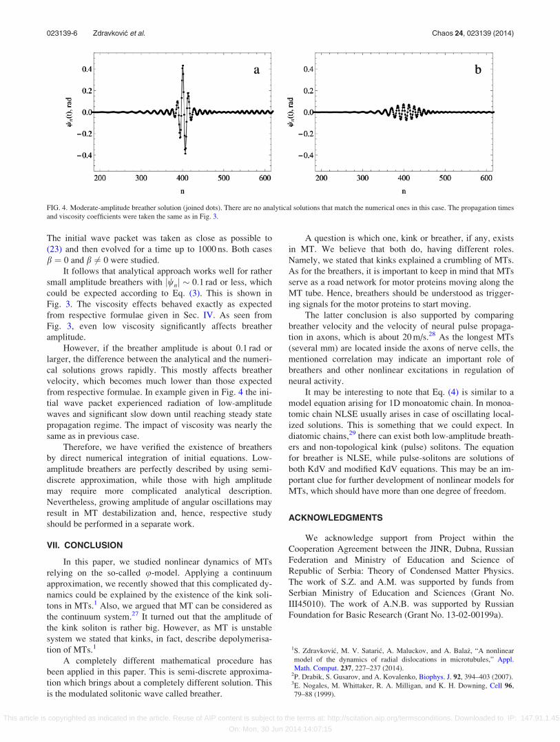
However, if the breather amplitude is about 0.1 rad or

larger, the difference between the analytical and the numeri-

cal solutions grows rapidly. This mostly affects breather

velocity, which becomes much lower than those expected

from respective formulae. In example given in Fig. 4 the ini-

tial wave packet experienced radiation of low-amplitude

waves and significant slow down until reaching steady state

propagation regime. The impact of viscosity was nearly the

same as in previous case.

Therefore, we have verified the existence of breathers

by direct numerical integration of initial equations. Low-

amplitude breathers are perfectly described by using semi-

discrete approximation, while those with high amplitude

may require more complicated analytical description.

Nevertheless, growing amplitude of angular oscillations may

result in MT destabilization and, hence, respective study

should be performed in a separate work.

VII. CONCLUSION

In this paper, we studied nonlinear dynamics of MTs

relying on the so-called u-model. Applying a continuum

approximation, we recently showed that this complicated dy-

namics could be explained by the existence of the kink soli-

tons in MTs.1 Also, we argued that MT can be considered as

the continuum system.27 It turned out that the amplitude of

the kink soliton is rather big. However, as MT is unstable

system we stated that kinks, in fact, describe depolymerisa-

tion of MTs.1

A completely different mathematical procedure has

been applied in this paper. This is semi-discrete approxima-

tion which brings about a completely different solution. This

is the modulated solitonic wave called breather.

A question is which one, kink or breather, if any, exists

in MT. We believe that both do, having different roles.

Namely, we stated that kinks explained a crumbling of MTs.

As for the breathers, it is important to keep in mind that MTs

serve as a road network for motor proteins moving along the

MT tube. Hence, breathers should be understood as trigger-

ing signals for the motor proteins to start moving.

The latter conclusion is also supported by comparing

breather velocity and the velocity of neural pulse propaga-

tion in axons, which is about 20 m/s.28 As the longest MTs

(several mm) are located inside the axons of nerve cells, the

mentioned correlation may indicate an important role of

breathers and other nonlinear excitations in regulation of

neural activity.

It may be interesting to note that Eq. (4) is similar to a

model equation arising for 1D monoatomic chain. In monoa-

tomic chain NLSE usually arises in case of oscillating local-

ized solutions. This is something that we could expect. In

diatomic chains,29 there can exist both low-amplitude breath-

ers and non-topological kink (pulse) solitons. The equation

for breather is NLSE, while pulse-solitons are solutions of

both KdV and modified KdV equations. This may be an im-

portant clue for further development of nonlinear models for

MTs, which should have more than one degree of freedom.

ACKNOWLEDGMENTS

We acknowledge support from Project within the

Cooperation Agreement between the JINR, Dubna, Russian

Federation and Ministry of Education and Science of

Republic of Serbia: Theory of Condensed Matter Physics.

The work of S.Z. and A.M. was supported by funds from

Serbian Ministry of Education and Sciences (Grant No.

III45010). The work of A.N.B. was supported by Russian

Foundation for Basic Research (Grant No. 13-02-00199a).

1S. Zdravkovic, M. V. Sataric, A. Maluckov, and A. Bala�z, “A nonlinear

model of the dynamics of radial dislocations in microtubules,” Appl.

Math. Comput. 237, 227–237 (2014).2P. Drabik, S. Gusarov, and A. Kovalenko, Biophys. J. 92, 394–403 (2007).3E. Nogales, M. Whittaker, R. A. Milligan, and K. H. Downing, Cell 96,

79–88 (1999).

FIG. 4. Moderate-amplitude breather solution (joined dots). There are no analytical solutions that match the numerical ones in this case. The propagation times

and viscosity coefficients were taken the same as in Fig. 3.

023139-6 Zdravkovic et al. Chaos 24, 023139 (2014)

This article is copyrighted as indicated in the article. Reuse of AIP content is subject to the terms at: http://scitation.aip.org/termsconditions. Downloaded to IP: 147.91.1.45

On: Mon, 30 Jun 2014 14:07:15

4M. Remoissenet, “Low-amplitude breather and envelope solitons in

quasi-one-dimensional physical models,” Phys. Rev. B 33, 2386–2392

(1986).5R. K. Dodd, J. C. Eilbeck, J. D. Gibbon, and H. C. Morris, Solitons andNonlinear Wave Equations (Academic Press, Inc., London, 1982).

6T. Kawahara, “The derivative-expansion method and nonlinear dispersive

waves,” J. Phys. Soc. Jpn. 35, 1537–1544 (1973).7M. Remoissenet and M. Peyrard, “Soliton dynamics in new models with

parameterized periodic double-well and asymmetric substrate potentials,”

Phys. Rev. B 29, 3153–3166 (1984).8S. Zdravkovic, “Helicoidal Peyrard-Bishop model of DNA dynamics,”

J. Nonlinear Math. Phys. 18(2), 463–484 (2011).9V. E. Zakharov and A. B. Shabat, “Exact theory of two-dimensional self-

focusing and one-dimensional self-modulation of waves in nonlinear

media,” Sov. Phys. JETP 34, 62–69 (1972).10A. C. Scott, F. Y. F. Chu, and D. W. McLaughlin, “The soliton: A new

concept in applied science,” Proc. IEEE 61, 1443–1483 (1973).11T. Dauxois, “Dynamics of breather modes in a nonlinear “helicoidal”

model of DNA,” Phys. Lett. A 159, 390–395 (1991).12T. Dauxois and M. Peyrard, Physics of Solitons (Cambridge University

Press, Cambridge, UK, 2006).13R. Kohl, A. Biswas, D. Milovic, and E. Zerrad, “Optical soliton perturba-

tion in a non-Kerr law media,” Opt. Laser Tech. 40, 647–662 (2008).14A. Biswas and S. Konar, Introduction to Non-Kerr Law Optical Solitons

(CRC Press, Boca Raton, FL, USA, 2006).15S. Zdravkovic and M. V. Sataric, “Nonlinear Schr€odinger equation and

DNA dynamics,” Phys. Lett. A 373, 126–132 (2008).16S. Zdravkovic and M. V. Sataric, “Single molecule unzippering experi-

ments on DNA and Peyrard-Bishop-Dauxois model,” Phys. Rev. E 73,

021905 (2006).

17D. Havelka, M. Cifra, O. Kucera, J. Pokorn�y, and J. Vrba, J. Theor. Biol.

286, 31–40 (2011).18D. Havelka, M. Cifra, and J. Vrba, “What is more important for radiated

power from cells—Size or geometry?,” J. Phys.: Conf. Series 329, 012014

(2011).19M. V. Sataric, J. A. Tuszy�nski, and R. B. �Zakula, “Kinklike excitations as

an energy-transfer mechanism in microtubules,” Phys. Rev. E 48, 589–597

(1993).20J. Pokorn�y, F. Jelinek, V. Trkal, I. Lamprecht, and R. H€olzel, “Vibrations

in microtubules,” Astrophys. Space Sci. 23, 171–179 (1997).21J. E. Schoutens, J. Biol. Phys. 31, 35–55 (2005).22S. Zdravkovic, M. V. Sataric, and S. Zekovic, “Nonlinear dynamics of

microtubules—A longitudinal model,” Europhys. Lett. 102, 38002 (2013).23T. Das and S. Chakraborty, “A generalized Langevin formalism of com-

plete DNA melting transition,” Europhys. Lett. 83, 48003 (2008).24C. B. Tabi, A. Mohamadou, and T. C. Kofan�e, “Modulated wave packets

in DNA and impact of viscosity,” Chin. Phys. Lett. 26, 068703 (2009).25K. R. Foster and J. W. Baish, “Viscous damping of vibrations in micro-

tubules,” J. Biol. Phys. 26, 255–260 (2000).26D. J. Bakewell, I. Ermolina, H. Morgan, J. Milner, and Y. Feldman,

“Dielectric relaxation measurements of 12 kbp plasmid DNA,” Biochim.

Biophys. Acta 1493, 151–158 (2000).27S. Zdravkovic, A. Maluckov, M. -Dekic, S. Kuzmanovic, and M. V.

Sataric, “Are microtubules discrete or continuum systems?,” Appl. Math.

Comput. 242, 353–360 (2014).28A. L. Hodgkin and A. F. Huxley, “A quantitative description of membrane

current and its application to conduction and excitation in nerve,”

J. Physiol. 117, 500–544 (1952).29St. Pnevmatikos, N. Flytzanis, and M. Remoissenet, “Soliton dynamics of

nonlinear diatomic lattices,” Phys. Rev. B 33, 2308–2321 (1986).

023139-7 Zdravkovic et al. Chaos 24, 023139 (2014)

This article is copyrighted as indicated in the article. Reuse of AIP content is subject to the terms at: http://scitation.aip.org/termsconditions. Downloaded to IP: 147.91.1.45

On: Mon, 30 Jun 2014 14:07:15