local and non-local correlations in topological insulators and
TRANSCRIPT

International School for Advanced Studies
PhD Thesis
Local and non-local correlations inTopological Insulators and Weyl Semimetals
Candidate: Lorenzo CrippaSupervisors : Prof. Massimo Capone
Dr. Adriano Amaricci
September 2020

Contents
Introduction 4
1 A short introduction to topological matter 71.1 From Landau theory to topological order . . . . . . . . . . . . . . . . . . . . . . 71.2 Quantum Hall effect . . . . . . . . . . . . . . . . . . . . . . . . . . . . . . . . . 101.3 Quantum Anomalous Hall Effect and Haldane model . . . . . . . . . . . . . . . 121.4 Quantum Spin Hall Insulators and Z2 invariant . . . . . . . . . . . . . . . . . . 161.5 The Bernevig-Hughes-Zhang model . . . . . . . . . . . . . . . . . . . . . . . . . 20
2 Concepts and models for interacting electron systems 252.1 Landau-Fermi liquid theory . . . . . . . . . . . . . . . . . . . . . . . . . . . . . 262.2 Many-Body concepts in band theory . . . . . . . . . . . . . . . . . . . . . . . . 272.3 Green’s function and spectral weight . . . . . . . . . . . . . . . . . . . . . . . . 282.4 Correlation effects on the Green’s function . . . . . . . . . . . . . . . . . . . . . 292.5 Hamiltonian models for interacting systems . . . . . . . . . . . . . . . . . . . . . 322.6 Correlation-driven phase transitions . . . . . . . . . . . . . . . . . . . . . . . . . 352.7 Interacting topological invariants . . . . . . . . . . . . . . . . . . . . . . . . . . 36
2.7.1 TFT invariant for (2+1)-dimensional QHAE . . . . . . . . . . . . . . . . 382.7.2 TFT invariant for a (4+1)-dimensional TRS system . . . . . . . . . . . . 392.7.3 TFT invariants for TRS and IS systems . . . . . . . . . . . . . . . . . . 39
3 Dynamical Mean-Field Theory and Cluster Methods for Strongly Corre-lated Fermions 413.1 Dynamical Mean-Field Theory . . . . . . . . . . . . . . . . . . . . . . . . . . . . 43
3.1.1 Derivation by cavity method . . . . . . . . . . . . . . . . . . . . . . . . . 443.1.2 Hamiltonian formulation . . . . . . . . . . . . . . . . . . . . . . . . . . . 473.1.3 Mott transition and Phase Diagram . . . . . . . . . . . . . . . . . . . . . 48
3.2 Cluster methods . . . . . . . . . . . . . . . . . . . . . . . . . . . . . . . . . . . . 503.2.1 Cluster DMFT . . . . . . . . . . . . . . . . . . . . . . . . . . . . . . . . 523.2.2 Self-Energy Functional Theory and derivatives . . . . . . . . . . . . . . . 533.2.3 Observables and periodization . . . . . . . . . . . . . . . . . . . . . . . . 58
4 Massively parallel exact diagonalization algorithm for impurity problems 594.1 The Exact Diagonalization method . . . . . . . . . . . . . . . . . . . . . . . . . 60
4.1.1 The Fock space and conserved quantum numbers . . . . . . . . . . . . . 614.1.2 Basis states construction . . . . . . . . . . . . . . . . . . . . . . . . . . . 624.1.3 Hamiltonian matrix representation . . . . . . . . . . . . . . . . . . . . . 644.1.4 The Lanczos method . . . . . . . . . . . . . . . . . . . . . . . . . . . . . 664.1.5 Matrix-vector product: parallel algorithm . . . . . . . . . . . . . . . . . 68
4.2 Benchmarks . . . . . . . . . . . . . . . . . . . . . . . . . . . . . . . . . . . . . . 724.3 Application to (C)DMFT and SFT methods . . . . . . . . . . . . . . . . . . . . 76
4.3.1 Dynamical response functions . . . . . . . . . . . . . . . . . . . . . . . . 764.3.2 DMFT and derivatives: bath construction and fit . . . . . . . . . . . . . 79
2

CONTENTS 3
4.3.3 VCA: calculation of Ω . . . . . . . . . . . . . . . . . . . . . . . . . . . . 81
5 A model for interacting Weyl Semimetals 835.1 Generalities on Weyl semimetals . . . . . . . . . . . . . . . . . . . . . . . . . . . 84
5.1.1 Hamiltonian and topology . . . . . . . . . . . . . . . . . . . . . . . . . . 845.1.2 Surface states . . . . . . . . . . . . . . . . . . . . . . . . . . . . . . . . . 865.1.3 Topological response . . . . . . . . . . . . . . . . . . . . . . . . . . . . . 87
5.2 A microscopic model for Weyl semimetals . . . . . . . . . . . . . . . . . . . . . 885.3 Weyl semimetals and electron-electron interaction . . . . . . . . . . . . . . . . . 92
5.3.1 Effective Topological Hamiltonian . . . . . . . . . . . . . . . . . . . . . . 945.3.2 Topological characterization: phase diagram . . . . . . . . . . . . . . . . 955.3.3 Dynamical Nature of the DMFT results: Spectral functions and Self-
Energies . . . . . . . . . . . . . . . . . . . . . . . . . . . . . . . . . . . . 985.3.4 Discontinuous Topological Phase Transition and Annihilation of Weyl
points . . . . . . . . . . . . . . . . . . . . . . . . . . . . . . . . . . . . . 1005.3.5 Degree of Correlation and Discontinuous Transition . . . . . . . . . . . . 1025.3.6 Robustness of the results with respect to model parameters . . . . . . . . 1055.3.7 First-order topological transitions, second-order endpoints and critical
phenomena . . . . . . . . . . . . . . . . . . . . . . . . . . . . . . . . . . 108
6 Non-local correlation effects in the interacting BHZ model 1106.1 Model and methods . . . . . . . . . . . . . . . . . . . . . . . . . . . . . . . . . . 111
6.1.1 Single-site description . . . . . . . . . . . . . . . . . . . . . . . . . . . . 1116.1.2 Cluster description . . . . . . . . . . . . . . . . . . . . . . . . . . . . . . 1136.1.3 A note on antiferromagnetism . . . . . . . . . . . . . . . . . . . . . . . . 115
6.2 Nonlocal effects and Topological characterization . . . . . . . . . . . . . . . . . 1166.3 Discontinuous topological phase transition . . . . . . . . . . . . . . . . . . . . . 121
6.3.1 Self-Energies . . . . . . . . . . . . . . . . . . . . . . . . . . . . . . . . . . 1216.3.2 Topological condition . . . . . . . . . . . . . . . . . . . . . . . . . . . . . 1226.3.3 Poles of the Green’s function . . . . . . . . . . . . . . . . . . . . . . . . . 1246.3.4 Stability of the solutions: Energy perspective . . . . . . . . . . . . . . . 127
6.4 Mott transition . . . . . . . . . . . . . . . . . . . . . . . . . . . . . . . . . . . . 129
Conclusions 135
Appendices 138
A Derivation of known topological invariants and models 139A.1 Z2 invariant for TRS and IS systems . . . . . . . . . . . . . . . . . . . . . . . . 139A.2 Z2 invariant with inversion symmetry . . . . . . . . . . . . . . . . . . . . . . . . 141A.3 Z2 classification of the BHZ Hamiltonian . . . . . . . . . . . . . . . . . . . . . . 143A.4 Simplified expression for the interacting TKNN invariant . . . . . . . . . . . . . 144
B Methods: some explicit calculations 147B.1 The cavity method derivation of DMFT . . . . . . . . . . . . . . . . . . . . . . 147B.2 Properties of the Luttinger-Ward functional . . . . . . . . . . . . . . . . . . . . 149
References 151

Introduction
The study of topologically ordered phases of matter has experienced a rapidly growing interestin recent years. Such phases elude the conventional classification based on broken symmetry,as they differ one from another in a more subtle way than a liquid from a solid or a paramagnetfrom a ferromagnet. Indeed, two samples of the same material in the same external conditionscould have different topological phases, merely as a consequence of their thickness or of thedirection of their surface. As abstract as the concept may be, the experimental consequencesof topology are definitely real and observable: a conveniently engineered material in a specifictopological phase can, for example, exhibit dissipation-less conducting states at the boundary,whereas a topologically trivial sample is insulating.
What does topology have to do with the classification of the phases of matter? Generallyspeaking, topology concerns the study of the properties of an object which remain unaltered bycontinuous deformations. At a formal level, such deformations are defined in terms of suitablemaps, named homeomorphisms, from the parameter space the system depends upon to thespace of physical states of the system itself. The topological properties of the system are thenrevealed by studying the properties of any such map against deformations.
Consistently with this very broad definition, topological phases have little requirements onthe specific constituents of the system. Hence, theoretical and experimental realizations oftopologically nontrivial systems vary wildly: from bosons to fermions, from electronic crystalsto optical lattices, from metamaterials to circuits to classical setups made up of masses andsprings, carefully engineered samples can exhibit nontrivial physical responses.
It is natural to ask what role topology can play in the realm of solid state physics. In thiscase, the response properties of materials arise from the behavior of the conduction electrons,hence we consider the map relating the periodic k-space, i.e. the Brillouin zone, with thespace of Bloch electronic wavefunctions. Then, Band Theory of solids allows us to derivea dispersion law for the energies eigenvalues of the system as a function of k which formthe band structure. This, in turn, is at the base of the usual classification of materials asmetals or insulators depending on the filling of the bands. The concept of topology adds anew flavour to this classification, showing that not all the insulators are equal. Indeed, thetopological characterization introduces a finer distinction among band insulating states basedon the geometrical properties of the Bloch states.
The topological state of the system can be characterized by means of dimensionless, dis-crete quantities, known as topological invariants. These invariants identify a class of systemsall topologically equivalent under smooth deformations. As such, the topological invariants canonly change across a continuous topological quantum phase transition, going from one class toanother. Yet, the change of the invariant itself can only be discontinuous, signalling an overallmodification of the properties of the system class, with consequent abrupt variation of all thefeatures mentioned above. By contrast, as long as the topological invariants are nonzero, all
4

INTRODUCTION 5
the nontrivial topological properties are protected, i.e. they are (generally) not destroyed byperturbations or disorder.For the systems we will encounter in this work, topological protection is guaranteed by sym-metries, such as for example Time-Reversal symmetry which forbids hybridization betweencounter-propagating edge states.
However, it is well established that the Band Theory description does not alone exhaustthe variety of materials that solid state physics deals with: some elements and compounds, byvirtue of the properties of their atomic orbitals, can not be described in terms of a single-particletheory. These systems, known as strongly correlated materials, show a variety of features thatone-particle band theory cannot adequately explain. The most paradigmatic hallmark of strongcorrelation is the Mott insulator, a material in which strong interactions lead to the localizationof the electrons, hence to an insulating behaviour in a partially filled band, in striking constrastwith the Band Theory description. The Mott insulator, and very often the states realized in itsproximity, will therefore be inaccessible to Band Theory, and hence to the standard topologicalclassification based on it. In light of these limitations, the topological description of stronglycorrelated materials had to adapt. Indeed, an entire framework known as Topological FieldTheory has been developed in order to describe the geometric properties of phases where theband structure does not correctly capture the relevant physics of the system.
From a theoretical point of view, it is possible to start from a non-interacting system forwhich Band Theory works perfectly and to continuously “turn on” electronic interaction. Asopposed to the variation of single-particle parameters, there is no reason why the topologicalnature of the solutions should be protected from the inclusion of interactions. The increase ofelectronic interactions forces us to redefine the mapping in the larger context of TopologicalField Theory. Accordingly, all the topological invariants of the noninteracting system have to beextended or reformulated, as the hopping structure of the system, at the root of their definition,is now competing with the localization effects following from high electronic correlation.
Many intriguing questions therefore arise: is it possible to define an “adiabatic” continuationof topological phases for increasing values of electronic interaction? Is there a substantialdifference between local and momentum-dependent effects of correlation on the topologicalmapping? In the case the topology of the noninteracting system is not completely washedaway, what is the effect of interaction on the topological protection of the relevant quantitiesof the system, and on the features of the relative phase transitions?
In this thesis we will answer some of these questions studying concrete models of interactingtopological systems, namely two-dimensional Quantum Spin Hall insulator and Weyl semimet-als. We will investigate the evolution of the topological phases of the system, as well as thetransitions among them, for increasing values of the electronic interaction. We will uncoversome interesting phenomena which will ultimately put to the test the intrinsic protection of thetopological properties.
The thesis is organized as follows:
• In Chapter 1 we will give a brief excursus on the description of topological phases of mat-ter, from their experimental discovery to their systematization as a consequence of quan-tum entanglement and symmetry. We will then follow the historical path that broughtto the definition of the Quantum Spin-Hall insulators, and provide a derivation of theassociated topological invariants. Among these systems, we will especially focus on theBernevig-Hughes-Zhang (BHZ) Hamiltonian, the first Quantum Spin Hall insulator tofind experimental proof in a quantum-well setup. Due to its simplicity and versatility,
INTRODUCTION 6
this will constitute the theoretical model at the base of our study.
• In Chapter 2 we will concentrate on the second half of the picture, outlining a path thatleads from the Band Theory of solids to the discovery of strongly correlated effects andphases. We will briefly touch on the theory of Landau-Fermi liquid and those states thatfall outside its description, and describe the Green’s function framework which is at thebase of many methods devoted to the study of strongly correlated systems. We will thenderive the most used expressions for the interaction Hamiltonians of such systems. Finally,we will see how the definition of topological invariants can be conveniently broadenedbeyond Band Theory to account for the presence of interaction.
• Chapter 3 will be devoted to the illustration of the main solution methods we employ inour work, the most well-known of which is Dynamical Mean-Field theory (DMFT). We willthen introduce some cluster-based solution methods, which aim to describe the physicsof the full interacting system by directly solving a finite subset of sites. In particular, wewill concentrate on the Cluster-DMFT, an extension of the previously mentioned single-site DMFT, and on the Variational Cluster Approximation, which draws its roots in adifferent approach known as Self-Energy Functional Theory.
• In Chapter 4 we will show the practical implementation of the previously outlined meth-ods: in particular, we will describe the technical realization of an Exact Diagonalization-based solver for the interacting fermion problem. We will touch on the way the Fockspace is constructed and how its exponentially increasing size can be kept under con-trol through some assumptions on conserved quantum numbers. We will present somebenchmarks related to our implementation of the code, and comment on the way the EDroutine can serve as the core of a general-purpose (C)-DMFT or VCA solver.
• Chapter 5 will contain our analysis on a derivative of the BHZ model introduced inChapter 1. In particular, we will focus on a perturbed version of its three-dimensionalextension, breaking Time-Reversal symmetry. We will describe the interesting topologicalphase this system supports, touching on the protection of the gapless points of the bandstructure and their related topological invariants. Making use of the notions of Chapter2 and single-site DMFT we will then describe the way the topological transitions areaffected by the presence of electronic interaction, finding surprising consequences for thetopological protection of the previously listed quantities.
• Finally, in Chapter 6 we will return to the original 2d BHZ, which in the context ofsingle-site DMFT is known to show a discontinuous topological phase transition at highvalues of electronic interaction. We will seek confirmation for these results under the lensof the cluster methods described in Chapter 3, assessing the role of non-local effects ofcorrelations in the determination of the topology of the interacting system.

Chapter 1
A short introduction to topologicalmatter
1.1 From Landau theory to topological order
Physical matter organizes into a plethora of different configurations, resulting in a rich variety ofstructures and phases, the careful classification of which is indeed an extraordinary task. Thesize of this challenge can be dramatically reduced considering that microscopically differentsystems can show the same properties and behaviour. If we find a systematic way to groupphysical systems based on a unifying principle, their classification becomes far easier and, atthe same time, provides us with a powerful descriptive theory.
The realization of this intuition is due to Landau, who introduced the concept of orderparameter to characterize the different phases of matter and the transitions between them. Theorder parameter is a local quantity, often an observable, whose value discriminates univocallybetween two different phases of matter. Based on this idea, Landau formulated his theory ofphase transitions [1] which provides an effective description of the transformation of a systemfrom one phase to another, where the complexity of the microscopical system is replaced by asimplified expression of the free energy function written in terms of the order parameter andexternal fields.
The Landau theory of phase transitions underlines the important relation between thephysical properties of a system and its symmetries, i.e. the invariance of such system under theaction of specific transformations. The idea of this relation, although conceptually simple, isindeed very general and deeply rooted in the laws of nature, and provides a natural explanationto many physical phenomena. For example, the electric field emanating from a point chargehas no reason to privilege a spatial direction, since every spatial direction can be transformedinto another by rotation. Hence the field is radial, and the potential is spheric.If the order parameter can be described as a vector, in absence of an explicitly symmetrybreaking term, such as the coupling with an external field, there is no reason for Landau’s freeenergy to privilege a certain direction of the order parameter. Hence the energy functional canonly depend on its modulus.However, in the phase where it is finite, the order parameter must necessarily assume oneamong the possible values, therefore spontaneously reducing the symmetry of the system. Themodel will still be symmetric, but the solution is not. This mechanism is known as spontaneoussymmetry breaking.
7

CHAPTER 1. TOPOLOGICAL MATTER 8
Landau’s approach is considerably general and allows to describe a huge variety of phenomena:from boiling water to magnetization loss in a overheated magnet, to superconductivity. Thesimplest version of the theory is, however, based on the assumption that the order parameter is ahomogeneous quantity. It is, in other words, a mean-field theory. A significant advance towardsan accurate description of the phase transitions came with the development of Landau-GinzburgTheory (LGT) [2]. The order parameter becomes a function of the position and, accordingly,the free energy becomes a functional. The inclusion of these spatial fluctuations of the orderparameter plays indeed a prominent role in the description of phase transitions. For instance,the correlation length of fluctuations diverges at the critical temperature, where the phasetransition from a disordered to an ordered phase happens. More than that, the fluctuationscan destroy a mean-field order parameter. This happens when the dimensionality is reducedaccording to what has been called the Ginzburg criterion.
The fluctuations of the order parameter also unveil an intriguing consequence of spontaneoussymmetry breaking. A gapless excitation, known as the Goldstone mode, exists for every brokencontinuous symmetry. A Goldstone mode is a collective excitation with vanishing energy for anarbitrary low momentum and is, in a sense, the way the system remembers that it has singledout one ground state among infinitely many others. For example, an ordered ferromagnetsupports spin waves whose energy cost vanishes with the increase of their wavelength.
The theory of spontaneous symmetry breaking and associated gapless excitations has farreaching consequences. It is at the base of the description of an enormous range of phenom-ena, from the rotational invariance-breaking in magnetic ordering with the already mentionedspin waves (or magnons) to the translational symmetry-breaking liquid-solid transition, withassociated acoustic vibrations (phonons), to superconductivity and superfluidity. In particular,this latter example is historically at the base of the formulation of the Anderson-Higgs mecha-nism [3], which accounts for the Goldstone modes becoming massive due to interaction with agauge field. Remarkably, this was the starting point of crucial results in condensed matter (asthe field-theoretical explanation of the Meissner effect) and particle physics [4].
Given the many successes of the LGT it is very hard to overstate its descriptive power. Onthe contrary, precisely because the theory is so general and far-reaching, for a long period itwas believed to completely exhaust the description of phase transitions. This conception wasput to the test by Anderson [5, 6], who introduced a new theoretical phase of matter calledQuantum Spin Liquid (QSL) in relation with high-Tc superconductivity. The QSL is an elusivephase whose existence has been for a long time subject of debate. A broad definition describesit as a system of spins which are highly correlated, but do not order even at zero temperature[7]. The main feature of a QSL is therefore its long-range entanglement, as is apparent by theillustrative example of the so called Kitaev toric code [8]. This is a two-dimensional periodicsquare lattice model in which spin-1/2 particles sit on the links between lattice sites. Two typesof operators act on the model: they are called “stars” and “plaquettes”. These correspond tothe product of the spin-x component of the links around a vertex and the spin-z componentaround a minimal lattice square, as shown in figure Fig. 1.1. The elementary excitations ofsuch a model are obtained by flipping the sign of such operators, changing the sign of an oddnumber of spin-x per star or spin-z per plaquette.
Interestingly, there is no way to write an eigenstate of this model as a product state in apurely local basis. If one attempts such a description, e.g. in the local σxi basis, the groundstate eigenvectors will be superpositions of states having a given number of closed “loops” offlipped x-component spins encircling the torus in the x and y direction. Moreover, one will find

CHAPTER 1. TOPOLOGICAL MATTER 9
Figure 1.1: Scheme of the toric code lattice model with associated star and plaquette operators.Figure taken from [7]. A “loop” operator, showing the flipping of spin around a close contour,is also shown. This particular loop does not wind around one of the torus directions, so a statepresenting it is equivalent to the trivial ground state.
the ground-state is actually only 4-fold degenerate, with the orthogonal eigenvectors differingby the parity of the number of loops encircling the torus in the two spatial directions.
This structure of the ground state poses a serious challenge to a Landau-Ginzburg descrip-tion of this phase: any local observable -that is, any observable relative to an area smaller thanthe whole loop- cannot effectively distinguish one ground state from the others. Nevertheless,the ground states can be distinguished in a different perspective, that mathematicians wouldcall “topological”, i.e. related to a discrete quantity (the parity of the number of loops) whichis unresponsive to local perturbations.
Hence, a new paradigm to describe phases of matter had to be developed. It has becomeknown as the theory of topological order, and its birth can be dated back to Wen [9]. Differentlyfrom LGT, in this framework quantum systems are classified according to their entanglement.Let us consider as an example the transverse field Ising model:
H = −B∑i
σx − J∑i,j
σzi σzj (1.1)
and focus on the two opposite limits J = 0 and B = 0. In the σz basis, the two limiting groundstates are, respectively, ⊗(| ↑〉 + | ↓〉)i and the degenerate ⊗| ↑〉i and ⊗| ↓〉i. These two statesare in different Landau-Ginzburg classes, since they behave differently under the spin-inversionsymmetry σz → −σz. Yet, they can both be written as a direct product state. Hence froman entanglement range perspective they belong to the same topological classification. Wen’sdescription of topological phases classifies the ground state of gapped systems [10, 11] in termsof a local unitary evolution mapping one ground state into the other. If such an evolutionoperator exists, the two ground states belong to the same phase in a topological order sense.

CHAPTER 1. TOPOLOGICAL MATTER 10
Based on this definition, all the states connected to non-entangled direct product statesbelong to the same short-range entangled (SRE) trivial topological phase. In contrast, differententanglement patterns belong to distinct non-trivial long-range entangled (LRE) topologicalphases like the ground states of the toric code. The classification becomes even richer if weinclude symmetries into the picture. If we consider, among local unitary evolution operators,those that respect certain symmetries of the model, the SRE class breaks up. Some SREstates belong to equivalence classes with different broken symmetries. In this classification werecover, for example, the phase distinction of the two ground states of the transverse field Isingmodel. Other states belong to different SRE classes even without breaking any symmetry butmerely because of the lack of a suitable local unitary evolution. Among these states, whichshow symmetry-protected topological order, we find systems we will briefly comment on in thischapter, such as the Haldane model and, crucially for the main topic of this thesis, topologicaland band insulators, the topological order of which is protected by Time-Reversal symmetry.
Once a classification of topologically ordered phases is established, it is necessary to findappropriate quantities (which replace the order parameter of Landau phase transitions) todistinguish one phase from the other. These are called topological invariants and stem frommany sources: they can be related to experimentally measurable quantities such as the Hallconductance, and their derivations have historically been based, among others, on the Kuboformula, modern theory of polarization, form and number of surface states in a finite sampleor parity considerations on the eigenstates of the bulk system. Recent works [12, 13] havealso considered topological invariants, such as the so-called entanglement Chern number, basedon the properties of quantum entanglement in a many-body ground state, a perspective moreclosely related to the concept of topological order we have briefly outlined. In the followingsections we will rapidly go over a series of topological effects and models, which historicallylead to the discovery of the Time-Reversal Symmetry protected Quantum Spin Hall effect and,relatedly, to the formulation of the Bernevig-Hughes-Zhang model, that will be the basis onwhich the results of this thesis will be built.
1.2 Quantum Hall effect
Although the concepts of topological states of matter and of topological invariants might seemcloser to a mathematical classification than to a physical one, they have prominent observableconsequences.
In fact, the first evidence of the insurgence of topological effects was obtained experimentally,before a theoretical explanation was derived. The introduction of the concept of topology in acondensed matter framework usually dates back to 1980, with the discovery of the QuantumHall Effect (QHE) by Von Klitzing, Dorda and Pepper [14]. As the name suggests, the QHEis an extension beyond the classical Drude model of the Hall effect, i.e. the occurrence of avoltage drop in the direction perpendicular to the flow of a current, in presence of a magneticfield along the out-of-plane direction. The Hall potential is a response to the effect of the Lorentzforce, that bends the trajectory of the electrons away from the direction of the external electricfield. As such, the classical theory predicts a linear behaviour for the transverse resistivity ρxy,according to the relation
ρxy =B
ne(1.2)
where n is the density of charge carriers. The experimental results, however, show a series of

CHAPTER 1. TOPOLOGICAL MATTER 11
Figure 1.2: The longitudinal and transverse Hall resistivity as a function of the magnetic feld(Kosmos 1986). The plateaux of the transverse Hall resistivity are clearly visible. The series ofspikes represent the behaviour of the longitudinal resistance, which is zero inside the plateaux:this is due to the fact that, if n Landau levels are completely filled, there cannot be longitudinalcurrent, and therefore in turn no dissipation.
plateaux of resistivity for increasing B, following the ladder law
ρxy =2π~e2ν
(1.3)
ν being measured to be an integer with a stunning precision (one part in 109). Given the formof this relation and the physical quantities involved, this behaviour was readily linked to thephysics of Landau levels, when the Fermi energy of the system sits in the gap between two suchlevels. The width of the plateaux was associated to the presence of localized states due to dis-order in the sample, that do not contribute to conduction. At this level already, the stability ofthe plateaux in spite of (and actually precisely due to) disorder starts to unveil the topologicalnature of this phenomenon. A subsequent step was to recognize that, as the filled-Landau-levelsystem is a bulk insulator with zero longitudinal conductance, the Hall current must be dueto states localized on the border. The work by Halperin [15] and Laughlin [16], showed thatthe finite Hall conductance manifested itself to probing (hence for a finite size sample) viaconducting states localized purely at the edge. In addition, Laughlin’s argument showed thatthe origin of the different Hall conductance values was gauge related, which he accomplishedusing a cylindrical-geometric Hall effect sample threaded by a gauge magnetic flux, its variationacting as a control parameter.This was the first instance of what in Topological Band Theory is known as bulk-edge corre-spondence, a distinctive feature of topological systems which associates the non-trivial natureof the bulk insulating band structure to the presence of surface states crossing the bandgap.

CHAPTER 1. TOPOLOGICAL MATTER 12
Such correspondence, verified for many different systems, is strictly related to the topologicalprotection of the gap: this can only close at the interface of systems belonging to differentphases with different values for the invariants (included the trivial case of the vacuum).
For lattice systems, the relation between the Quantum Hall conductance and the propertiesof the Bloch wavefunctions of the material was elucidated in the pioneering work of Thouless,Kohmoto, Nightingale and den Nijs (TKNN) [17]. A two-dimensional lattice with periodicboundary conditions and in presence of magnetic and electric fields is considered. From theKubo formula applied to the Hall conductivity the authors obtain an expression, known asTKNN formula, for the Quantum Hall conductance σxy:
σxy =ie2
~∑α
∫MBZ
d2k
(2π)2〈∂yuαk|∂xuαk〉 − 〈∂xuαk|∂yuαk〉 (1.4)
where |uαk〉 is the α-th occupied Bloch state and k lives in the 2-dimensional Magnetic BrillouinZone, i.e. the shrunk Brillouin zone accounting for the reduced translational invariance of thelattice due to the presence of the magnetic field. A requirement for this expression, consistentwith the previous observations, is for the system to be a bulk insulator, with a finite bandgapeverywhere in the k-space.
The TKNN formula is remarkable for different reasons. It is a very general relation, whichdoes not in principle depend on the presence of specific terms, such an external magnetic field,but only on the possibility of defining Bloch states in a periodic k-space. Second, it links forthe first time a measurable quantity, i.e. the Quantum Hall conductance, to the geometryof the Bloch states. Indeed, the expression under the integral is nothing else but the Berrycurvature, which in turn is linked to the geometrical phase acquired by a wave-function over aclose loop in a parameter space, in this case the momentum space. Incidentally, the insulatingcharacter of the band structure is required for of the calculation of this phase, since it relieson the hypotheses of the Adiabatic theorem. Finally and most importantly, the result of theintegral is a constant integer, called first Chern number, as follows from a variety of argumentsboth physical (Dirac quantization of charge) and mathematical (Gauss-Bonnet theorem andtheory of homotopy groups). The TKNN invariant for a Quantum Hall system is thereforegenerally considered the first historical example of topological invariant.
1.3 Quantum Anomalous Hall Effect and Haldane model
As we discussed in the previous section, the TKNN formula for quantum Hall conductance doesnot explicitly rely on the presence of a magnetic potential. The evaluation of the conductancerequires only to know the form of the eigenvectors of the system in a periodic parameter space.The most natural example is the Brillouin Zone, which is defined under the only necessaryhypothesis that the relative lattice system is translational invariant.It is now important to determine the conditions under which the invariant is nonzero. We startfrom the simplest realization of a two-dimensional system with two bands, which is the minimalmodel to have a gap in the absence of interactions. The simplest Bloch Hamiltonian will thenbe expressed, as for any 2× 2 Hermitian matrix, in the general form
H(k) = ~q(k) · ~σ + ε(k) · I (1.5)

CHAPTER 1. TOPOLOGICAL MATTER 13
Figure 1.3: Original images adapted from Haldane’s 1988 paper [18]. a) The schematicrealization of the model, a honeycomb lattice with first and second nearest neighbour hopping.The nnn hopping has a phase (black arrow) due to the magnetic field. The red line shows theshape of the “zig-zag” border of a honeycomb lattice. b) Double-sinusoid phase diagram in theM − φ plane (the values of ν are inverted with respect to the text by an overall phase choice).
where k lives in the 2-dimensional toroidal BZ and σx,y,z are the Pauli matrices. The energy gapbetween the two bands is given by 2|~q(k)|, so the system will be an insulator provided that ~q 6= 0everywhere. The topological characterization of such a system is thusly obtained: if we considerthe versor ~n(k) in the direction of ~q(k), it spans a 2-dimensional spherical surface known asthe Bloch sphere. Hence, the Hamiltonian can be seen as a map from the 2-dimensional torusT, where k-vectors live, to such a sphere. The Chern number is in this case defined as
C =1
4π
∫T
~n ·(∂~n
∂kx× ∂~n
∂ky
)(1.6)
and represents winding number of the torus on the sphere, which is the number of times theformer “wraps” around the latter via the map given by H. This integer quantity will be thetopological invariant of the system. A system with a non-zero Chern number will be calledChern insulator.Historically, the first theoretical system describing a non-trivial Chern insulator was introducedin 1988 by Haldane [18], who considered a two-dimensional honeycomb lattice which is invariantunder time-reversal, inversion and C3 symmetries and displays a two-atom unit cell formingtwo sub-lattices A and B, which plays the role of a chiral degree of freedom. As it is universallyknow, this is nothing but graphene, which has been experimentally realized in 2004 by Geimand Novoselov [20].
Interestingly, the electronic dispersion of graphene shows two gapless points
K(K ′) =2π
3a
(1,± 1√
3
),
where a is the bond length, related by Time-Reversal symmetry.Near these points the linearized Bloch Hamiltonan has a linear Dirac form, i.e. it can be proven

CHAPTER 1. TOPOLOGICAL MATTER 14
K K' K K'
Figure 1.4: On the left, band structure for a stripe of graphene with open boundary conditionsalong a zig-zag edge (picture from [19]). This example in particular refers to a sample withan even number of sites in the finite direction, so that the sites on opposite surfaces belong toopposite sublattices. In the middle and right panels, the effect of a Semenoff and an Haldanemass term on the gap, respectively. The red and blue surface states are localized on oppositesublattices and surfaces. The use of a dotted line in the right panel reminds that the two statesdo not live on the same edge of the stripe.
to satisfy
HK(k) = H(K + k) = vf (kxτx + kyτy)
HK′(k) = H(K ′ + k) = H(−K + k) = vf (−kxτx + kyτy)(1.7)
where the coefficient vf is called Fermi velocity. We have used the notation τi for the Paulimatrices to highlight the fact that they refer to a sublattice and not a spin degree of freedom.In order to have a Chern insulator, a gap must be open. If the topology of the system isnontrivial, gap-closing edge states will then appear. We consider a stripe of graphene withopen boundary conditions in one spatial direction. In particular we will focus on the so-called“zig-zag” border, where the open edge consists of alternating A and B sublattice sites alongthe red line drawn in Fig. 1.3a.The band structure for this setup, in the one-dimensional Brillouin zone corresponding to theperiodic spatial direction, features edge states with vanishing energy in the thermodynamiclimit. An example for a stripe with an even number of sites in the finite direction is given inFig. 1.4 (though the form of the edge states heavily depends on the specifics of the stripe, asthoroughly analysed for example in [19]). The two zero energy states live on the sublattices Aand B respectively, and on the opposite edges of the stripe. They merge with the bulk bandsat the projections of the Dirac points K and K ′.A trivial way to open a gap in this system would be to break inversion symmetry by includinga term proportional to τz in the Hamiltonian, which is known as Semenoff mass. Its presencewould shift the energies of the sites A and B upwards and downwards respectively, detachingthe relative surface states from zero energy and leaving the gap open, as schematically shownin the middle panel of Fig. 1.4. Since no gap-closing surface state is present, the system will inthis case be topologically trivial.

CHAPTER 1. TOPOLOGICAL MATTER 15
A more ingenious way of gapping the spectrum is to add a time-reversal symmetry (TRS)-breaking Haldane mass term, that adds a mass of opposite sign to the Dirac points at K and K ′.Due to the different behaviour at the high-symmetry points, this term has to be k-dependent,and its effect will not be a rigid energy shift of the two A and B sublattices. In this case,the surface states will still connect the detached vertices of the cones according to the mass.However, since K and K ′ will have masses of different sign, the edge modes will have to connectthe cones by crossing the gap, as sketched in the right panel of Fig. 1.4. The presence of thegap-closing edge mode, related to a nontrivial Hall conductance, is a hallmark of the topologicalcharacter for such a TRS-breaking system.
These ideas are included in a simple tight-binding model, which builds upon a Hubbardmodel on the honeycomb lattice and cleverly relies on the presence of a magnetic field, whosetotal flux per plaquette is however zero (mod 2π). This setup preserves translational symmetrywhile avoiding Landau levels. It then provides a description of the Quantum analogous of theAnomalous Hall Effect (QAHE), which in its classical form depends on the magnetization ofthe material and not on an external magnetic field.Haldane’s Hamiltonian has the following tight-binding form in second quantization1:
H = t1∑〈ij〉
c†icj + t2∑〈〈ij〉〉
e−iνijφc†icj +M∑i
αic†ici (1.8)
where αi = ±1 if i ∈ A, B sublattice, φ is a phase factor associated to the next-nearest-neighbour hopping term due to the presence of the magnetic field. The direction of the next-nearest-neighbour hopping is given by
νij = sign(d1 × d2)z = ±1
where d1 and d2 are the vectors along the two bonds constituting the next nearest-neighbourhopping path. It has to be noted that the system preserves Time-Reversal and Inversionsymmetries only for φ = 0, π and M = 0 respectively. Therefore, for a generic φ the Diracpoints are no longer TRS-related. In the k-space the Haldane Hamiltonian has the form
H =∑k
Ψ†kH(k)Ψk (1.9)
where Ψ(†)k = (c
(†)kA, c
(†)kB) and the Hamiltonian matrix H(k) has the wanted Chern insulator form
H(k) = ε(k)I +3∑i=1
di(k)τi
where ε and di are conveniently defined trigonometric functions of the momentum components.A direct computation of the Berry curvature, and the associated Chern number for the Hal-dane model, allows to construct the well-known “double-sinusoid” phase-diagram reported inFig. 1.3b. The topology of the system is determined by the phase φ and the ratio M
t2. The
Chern number is −sign(φ) inside the lobes delimited by the equation Mt2
= ±3√
3 sin(φ).The phase diagram of the Haldane model helps to clarify the role of gapless points. Let us
1we will use henceforth the “hat” notation to refer to operators in second quantization, except for thecreation/annihilation operators c†, c and arrays of the same.

CHAPTER 1. TOPOLOGICAL MATTER 16
consider the system in a fictitious three-dimensional space kx, ky, λ = M/t2 for a fixed φ > 0.This can be thought of as a stack of “planes”, each of which is actually a two-dimensional Bril-louin zone. We can now draw a parallel between this situation and two charges of opposite signemitting an electric field in a three-dimensional space. The calculation of the flux of the fieldis possible everywhere except on the planes on which the charges sit, since the field strength isdiverging at the origin.Accordingly, if we interpret the two gapless points at K and K ′ as sources of “Berry fluxes”with opposite sign (which manifests in the opposite Chern number), the flux of the regionsoutside the interval (λ1, λ2) will cancel our, whereas inside the same interval the total flux willbe finite. The calculation of the Berry flux is not possible on the planes λ1,2, where the systemis not gapless. Thus, in our analogy, as a charge is a source for the electric field a gapless Diracpoint in the electronic band structure can be seen as a source of the Berry flux. We will expandon this notion in Chapter 5, where we will more thoroughly address the properties of the DiracHamiltonian in the context of topological semimetals.The ground-breaking result of Haldane has hinted at the possibility of realizing a non-trivialtopological state without an applied magnetic field, by simply breaking TRS. Yet, the veryexistence of such an anomalous Quantum Hall insulator has been proven experimentally onlyin 2013 [21], measuring the Hall conductance of a thin layer of the topologically nontrivial com-pound Cr0.15(Bi0.1Sb0.9)1.85Te3 with TRS-breaking ferromagnetic ordering and so, in a sense,proceeding in the opposite direction of our narration, as we shell see.
1.4 Quantum Spin Hall Insulators and Z2 invariant
Figure 1.5: Band diagrams for a one-dimensional Kane-Mele strip in the the QSH and trivialstates, with λSO = 0.06t and λR = 0.05t. λV is 0.1t and 0.4t respectively. The color representsthe states living on the same edge, which cross at a TRIM. In the middle, the diamond QSHphase diagram as a function of λR and λv. Image taken from [22].
The Haldane model realizes a QAHE insulator, which exhibits nontrivial Hall conductancewithout the need for Landau levels, at the cost of breaking Time-Reversal symmetry. Many

CHAPTER 1. TOPOLOGICAL MATTER 17
years from the seminal work of Haldane, the search for alternative mechanisms to gap at theDirac cones led to the discovery of novel states of matter and the individuation of systems withnon-trivial topological character preserving TRS. These topological insulators are not distinctfrom trivial band insulators in the sense of the Landau theory of phase transitions, but theyhave a symmetry-protected topological order.
The rising interest in spin currents following to the experimental work of Kato [23] and, onthe theoretical side, of Murakami, Nagaosa and Zhang [24], led to the breakthrough proposalof a Quantum Spin Hall Insulator (QSHI) in the fundamental work of Kane and Mele [25]. Theauthors considered the effects of Spin-Orbit Coupling (SOC) as a mean to open a gap at theDirac nodes. Interestingly, it was realized that the SOC term in graphene naturally takes theform of a chiral-dependent next-nearest-neighbour term similar to all intents and purposes to theHaldane mass, but preserving TRS through the inclusion of spin into the picture. Accordingly,the Kane-Mele model consists of two copies of the Haldane model, one per spin orientation,related by TRS.A suitable form of the mass term near the Dirac points and in a continuum model can be derivedimposting the correct symmetries. First of all, it has to anticommute with the unperturbedHamiltonian in the sublattice space. This is necessary to open a gap, otherwise the result ofthe perturbation would simply be a shift of the gapless points. Given the form of the DiracHamiltonian near the gapless points, which is proportional to kiτi for i = x, y, this entails adependence to the Pauli matrix τz in the sublattice space.The mass term has then to apply to both spin blocks of the Hamiltonian, either with thesame value in each block, which trivially corresponds to two copies of the Inversion-symmetry-breaking mass-term of the Haldane model, or with opposite sign for the two spins, which impliesa dependence on the Pauli matrix σz in the spin space.Finally, we recall that the Dirac points K and K ′ are TRS-related. The expression of the Toperators in the spin and sublattice spaces is, respectively,
T = −iσyK and T = τ0K (1.10)
where K is the complex conjugation operator and we use the notation σ0, τ0 = I2×2. Recallingthe form of the Dirac Hamiltonian around K and K ′ (1.7), and the general relation for TRSinvariance of the Hamiltonian matrix
H(−k) = TH(k)T−1,
we can see that TRS between the K and K ′ points will be preserved if the Hamiltonian hasthe following form:
HK(k) = vf (kxσ0 ⊗ τx + kyσ0 ⊗ τy) + λSOσz ⊗ τzHK′(k) = vf (−kxσ0 ⊗ τx + kyσ0 ⊗ τy)− λSOσz ⊗ τz
(1.11)
where the terms in parenthesis simply represent the two opposite-spin copies of the Dirac Hamil-tonian. From (1.11) we note that the presence of the spin degree of freedom allows us to writea Haldane mass term (with opposite sign at the two Dirac points) while preserving TRS. Thesubscript SO in the λ coefficient reflects the fact that this mass term, which couples momentumwith spin degrees of freedom, can only arise from spin-orbit coupling. The eigenvalues of (1.11),degenerate in spin and identical at the two Dirac points, will be of the form
E±,σ = ±√v2f (k
2x + k2
y) + λ2SO. (1.12)

CHAPTER 1. TOPOLOGICAL MATTER 18
where the first term is the Dirac dispersion and the second is the TRS-preserving mass gap.
The tight-binding expression of the Kane-Mele Hamiltonian on a honeycomb lattice is thefollowing [22]:
H = t∑〈i,j〉
Ψ†iΨj + iλSO∑〈〈i,j〉〉
νi,jΨ†iσzΨj + iλR
∑〈i,j〉
Ψ†i (−→s × dij)zΨj + λv
∑i
αiΨ†iΨi. (1.13)
where the creation and annihilation operators are written in the combined spin notation Ψ(†)i =
(c(†)i↑ , c
(†)i↓ ). The first term is the usual nearest-neighbour hopping in the honeycomb lattice. The
second is responsible for the TRS-preserving opening of the gap, by giving an opposite Haldanemass to the two spin blocks. The factor
νij =2√3
(d1 × d2)z = ±1
is, similarly to the Haldane model, defined in terms of the versors in the direction of the twobonds constituting the path of the electron going from site i to site j. The other terms areincluded to test the robustness of the topological phase: the third term, a nearest neighbourRashba coupling, is responsible for the breaking of the mirror symmetry z → −z, while thelast one violates inversion symmetry, in a way similar to the M term of the Haldane model.In reciprocal space, the Hamiltonian of the model has a form of the type (1.9), where now Ψ
(†)k
is the four-dimensional operator (c(†)k,A↑, c
(†)kB↑, c
(†)kA↓, c
(†)kB↓) and the Hamiltonian matrix is
H(k) =5∑
a=1
da(k)Γa +5∑
a<b=1
dab(k)Γab. (1.14)
The d terms are trigonometric functions of the momentum components, and the Γ matrices spanthe 16 generators of the SU(4) matrix group except for Γ0, the identity matrix. In particular,the five Γa are the so-called Dirac matrices satisfying the Clifford algebra
[Γµ,Γν ]+ = 2δµνI4×4
while the remaining Γab are obtained from the commutators of the Dirac matrices,
Γµν =1
2i[Γµ,Γν ].
We will not derive the formal expression for the Kane-Mele model in reciprocal space. We willhowever deal more thoroughly with the Dirac matrices in the context of the Bernevig-Hughes-Zhang model we will define in the next section.We now have to identify the invariant that accounts for the nontrivial topology of the Kane-Mele model. A possible choice is the sum of the Chern numbers of each spin block. However, itcan be deduced from the form of the λSO term that the two spin blocks always contribute withequal and opposite Chern numbers, since they correspond to symmetric points on the M = 0line of the Haldane phase diagram in Fig. 1.3b.We can approach the search for the topological invariant from a different angle by consideringa finite sample of the Kane-Mele model, again with a zig-zag border, and studying its edge
CHAPTER 1. TOPOLOGICAL MATTER 19
states. It is known that, in a fermionic TRS systems, every band has an orthogonal “twin”,called Kramers partner, that satisfies E1(k) = E2(−k) for every k in the Brillouin zone. Thetwo bands will be degenerate in k-points that are invariant under TRS, the so-called Time-Reversal Invariant Momenta (TRIMs). In this model, due to the symmetries of the system,the Kramers partners have opposite spins. Therefore, we will have at each edge of the systema number of pairs of counter-propagating helical edge states crossing at TRIMs.The way such states could open a gap would be through backscattering, and here it becomesclear how the topological phase of the Kane-Mele model is protected by Time-Reversal sym-metry. Indeed, the time-reversal operator for fermionic systems is antiunitary, and satisfies therelation
T 2 = ±1
for systems with total integer and half-integer spin respectively. Accordingly, from the definitionof the TRS operator (1.10) it can be shown that the scattering probability for a state and itsKramers partners has to satisfy
〈Tφ|H|φ〉 = −〈Tφ|H|φ〉 = 0. (1.15)
In general, if we consider the combined scattering probability of n helical modes with theircounter-propagating Kramers partners we get an overall factor (−1)n.Then, if the number of Kramers pairs of edge states is odd there is no single-particle backscat-tering term that can open a gap in the band structure, while such a term can exist for an evennumber of Kramers pairs. Accordingly, the invariant associated to a TRS-protected topologicalinsulator has to do with the parity of the number of Kramers pairs at the edge, which suggestsa binary Z2 classification.We refer to these systems as Quantum Spin Hall insulators (QSHI). Although no overall Hallconductance is present, in the non-trivial phase the spin currents for the different spins will becounter-propagating, realizing the so-called helical or spin-momentum locking, with a net “spinvoltage drop” as pictured in Fig. 1.8.By directly solving the Hamiltonian of a finite Kane-Mele model, and assessing the presence ofgap-closing surface states, the topological phase diagram can be obtained: it is usually repre-sented as a diamond in the λr − λv plane (see Fig. 1.5), the nontrivial phase being the innerregion. For λr = 0, the system experiences a topological transition for λv = 3
√3λSO. The
topologically nontrivial phase can survive, at least for small values of λv, if the Rashba term isfinite but smaller than 2
√3λSO.
There are many equivalent ways to derive the Z2 topological invariant considering bulkproperties instead of the edge states. The original Kane-Mele derivation is geometrical andbased on the Pfaffian of the matrix of occupied Bloch states. In a subsequent work, Fu andKane [26] started from the modern theory of polarization [27] to qualify the Z2 invariant interms of a time-reversal polarization, or geometrically as an obstruction to the definition of asmooth gauge in the BZ.
The existence of Z2 invariants has also been extended to three-dimensional systems: amathematical argument based on homotopy was developed by Moore and Balents [28], but amore intuitive one based on relations between two- and three-dimensional Brillouin zones waspresented by Fu, Kane and Mele [29]. We will briefly present the derivation of the bulk Z2
invariant in Appendix A, along with the simplified expression for the invariant in the case the

CHAPTER 1. TOPOLOGICAL MATTER 20
system also possesses Inversion symmetry, which will turn out to be of the general form [30]
(−1)ν =∏i
∏n
ξ2n(Λi) (1.16)
where ν is the topological invariant, Λi is the i-th TRIM in the Brillouin zone and ξ2n is theparity eigenvalue of the 2n-th occupied band, or equivalently of the n-th Kramers pair.
1.5 The Bernevig-Hughes-Zhang model
Figure 1.6: Band structure for aCdTe/HgTe/CdTe quantum well, as per [31]. a) The banddispersion of CdTe, following the standard order, and of HgTe, with an inverted bandgap betweenthe Γ6 and light-heavy hole Γ8 bands. b) The relevant subband structure of the quantum well:for d < dc the system behaves like CdTe, while increasing the width HgTe-like behaviour takesover.
The key idea put forward with the introduction of the Kane-Mele model is that the presenceof SOC can introduce non-trivial topological states in the graphene lattice. Following thisoriginal proposal a quest to discover or realize such novel phases of matter began. Unfortunately,

CHAPTER 1. TOPOLOGICAL MATTER 21
it turned out pretty soon that graphene was not a good candidate to realize QSHI. Indeed thegap opened by the spin-orbit interaction was found out to be only of the order of 10−3 meV [32].A different approach, based on HgTe/CdTe quantum well as possible candidate to realize aQSHI, was proposed in 2006 by Bernevig, Hughes and Zhang (BHZ) [31].They predicted the existence of a pair of helical edge states over a critical value dc of thethickness of the heterostructure, which would instead be a trivial insulator for d < dc. Thepeculiar topological properties of this compound are a consequence of the electronic structurenear the Fermi level. Both HgTe and CdTe have, near the Γ point, a s-like band Γ6 and twop-type bands split by spin-orbit coupling into a J = 3
2Γ8 (made out of the angular momentum
1 of the p-orbitals and electron spin 1/2) and a J = 12
Γ7. While CdTe has a large energygap between the valence Γ7 and Γ8 bands and the conduction Γ6 band, HgTe crucially presentsan inverted bandgap around the Γ point. This effect is due to the large mass of Hg, whichultimately pushes the s-like band Γ6 below the Fermi level and, thus, below Γ8 [31, 33]. Aschematic representation of the situation can be seen in Fig. 1.6. Neglecting the Γ7 band,which is always firmly in the valence region, the system can be described by the six-componentspinor made out by the two atomic states for Γ6 and the four atomic states for Γ8.When the quantum well is grown, for example in the z direction, the cubic symmetry is reducedto an axial rotational symmetry in the plane. In this case, the six bands combine to form thespin up and down states of three quantum well subbands known as E1, H1 and L1. Of these,the L1 subband is separate in energy from the other two, that sit close enough to the Fermilevel to let us describe the physics of the system by an effective 4-band model. At the Γ point,where the in-plane momentum vanishes, mJ is still a good quantum number. Here, the 4 statescan be described as |E1,±〉, linear combination of the Γ6 and Γ8 bands with mJ = ±1
2, and
|H1,±〉, linear combination of the Γ8 bands with mJ = ±32. Away from Γ, these states can mix.
Since |Γ6,mJ = ±12〉 and |Γ8,mJ = ±3
2〉 have opposite parity under two-dimensional spatial
reflection, any coupling element between E1 and H1 has to be odd in momentum. Moreover,as the |H1〉 bands are linear combinations of the p-orbitals px ± ipy, to preserve rotationalsymmetry the matrix elements will have to be proportional to kx ± iky, which will requirethe diagonal elements of a matrix Hamiltonian formulation to be even functions of kx and ky,including k-independent terms. A detailed derivation of these properties, starting from the6-dimensional Kane Hamiltonian and making use of the k · p perturbation theory, is presentedin the supplemental material of the original article [31].Following such symmetry considerations it is possible to derive the Hamiltonian describing thesystem in proximity of the Γ point:
Heff (k) =
(H(k) 0
0 H∗(−k)
)(1.17)
where the two spin-blocks, related by TRS analogously to the Kane-Mele case, have the formof an Haldane-like Chern insulator: H(k) = ε(k)I + di(k)σi.Actually, real HgTe features a small inversion-symmetry breaking term coupling the two spinblocks. However this term is in general too weak to close the bandgap, hence the inversionsymmetric system is in the same topological phase by adiabaticity.The experimental confirmation of the existence of a QSHI in HgTe/CdTe quantum wells wasobtained in Wurzburg by the group of Molenkamp [34]. This breakthrough experiment demon-strated the presence of topologically protected gapless edge states in absence of applied magneticfield. A brief overview of the relevant results is provided in Fig. 1.8.

CHAPTER 1. TOPOLOGICAL MATTER 22
To correctly describe the topological phase diagram of the system, it is important to iden-tify what is the control parameter driving the topological quantum phase transitions. In theHgTe/CdTe quantum well realization of the BHZ model, topology is governed by the width ofthe well. For a thin quantum well, the physics is dominated by the “normal” CdTe behaviour,the bands being conventionally ordered. Once the thickness is increased over a critical valuedc ≈ 6.35nm, HgTe-like behaviour takes over and the bandgap is inverted around Γ. Formally,since the phenomenon determining the topological phase is the subband inversion near Γ, therelevant parameter will take the form of a local mass term.
-4
-3
-2
-1
0
1
2
3
4
-Y Γ Y M X Γ -X
M<2ε
-5
-4
-3
-2
-1
0
1
2
3
4
5
-Y Γ Y M X Γ -X
M>2ε
Γ=(0,0) X=(π,0)
Y=(0,π) M=(π,π)
Figure 1.7: Band structure for the model (1.18) in the two distinct topological phases: in thenontrivial phase (M < 2ε) the orbital character of the bandgap is inverted around Γ, while it isnot in the trivial phase (M > 2ε). The bands are plotted along a high-symmetry bath touchingthe points highlighted in the scheme on the left (and their symmetric one with respect to Γ).
In this thesis we study the momentum-space version of a tight-binding Hamiltonian whichrespects the symmetries of the BHZ theory and it reproduces the above dispersion when lin-earized around the Γ point. Its derivation is reported in Appendix A, along with that of theZ2 topological invariant and the classification of the model. The resulting H(k) for a two-dimensional square Brillouin zone has the following form:
H(k) =[M − ε(cos(kx) + cos(ky))
]Γ5 + λSO sin(kx)Γ
1 + λSO sin(ky)Γ2 (1.18)
where Γi are the 4× 4 Dirac matrices acting in the spin and orbital subspaces defined as
Γ0 = σ0 ⊗ τ0, Γ1 = σz ⊗ τx, Γ2 = −σ0 ⊗ τyΓ3 = σx ⊗ τx, Γ4 = −σy ⊗ τx, Γ5 = σ0 ⊗ τz
(1.19)
It is easy to verify that the k-dependent terms satisfy the symmetries of the quantum-well setupintroduced above. The first term, which is proportional to the diagonal Γ5 matrix, dependsfrom a “mass” term M and an hopping energy ε coupled to an even function of kx,y. The firstquantity in particular is related to the energy difference between the two orbitals (which in thequantum well realization correspond to the subbands E1 and H1), and it will ve the controlparameter to drive the system across the topological transition.
The off-diagonal terms of the Hamiltonian are, instead, odd functions of the momentum,which is again in agreement with the requirements of the BHZ setup.The system has naturally four bands with dispersion
E±,σ = ±√[
M − ε(
cos(kx) + cos(ky))]2
+ λ2SO
(sin2(kx) + sin2(ky)
). (1.20)

CHAPTER 1. TOPOLOGICAL MATTER 23
The bands are doubly degenerate in spin, and the topology of the system depends on thespecifics of their orbital character.As previously stated, the topological character of the solution of the model is governed by themass M. In particular the gap closes at Γ for
M = 2ε (1.21)
Here, the dispersion around the Γ point has the typical Dirac cone shape.As proven in Appendix A, and as it can be seen in Fig. 1.7, for lower values of M the bandgaparound the Γ point is inverted. Considering the different parity of the two orbitals, this cor-responds to a change of the parity eigenvalue of the occupied Kramers partners in one TRIM,and gives an overall nonzero topological invariant as obtained by (1.16). For higher values ofM , the parity eigenvalues of the occupied states are the same at every TRIM, and the value ofν is 0.The Hamiltonian (1.18) has some important advantages with respect to the Kane-Mele model.It is defined on a cubic lattice, which is easier to treat than the honeycomb one. Moreover, in-stead of the sublattice degree of freedom, it is based on a local orbital degree of freedom, whichmakes it perfectly suitable to be studied within Dynamical Mean-Field theory, that maps thelattice model onto an effective dynamical local theory (see Chapter 3). With minor modifi-cations it can be extended to three spatial dimensions, and TRS or IS-breaking terms can beadded, generating fascinating gapless topological phases, that we will thoroughly indroduce inChapter 5. We will therefore use this expression, or others closely related to it, as the non-interacting part of a many-body Hamiltonian aimed at investigating the combined effects ofelectronic correlation and topological order.

CHAPTER 1. TOPOLOGICAL MATTER 24
a)
b)
Figure 1.8: Experimental confirmation of QSHE as per [34]. a) Schematic setup of the Hall barused to measure conductance. The applied voltage is between electrodes 1 and 4, with four probepoints transversally placed. b) The lines refer to the longitudinal resistance R1,4/2,3 = V23/I14.The curves are centered around the value Vthr of maximum resistance. Curve I refers to athin QW, for which a trivial behaviour is expected. Indeed, when the applied voltage sits inan energy gap for the system, the huge resistance indicates an insulating behaviour. CurveII refers to a QW thicker than the critical value dc ≈ 6.35nm: in this care the resistanceis greatly reduced, therefore gap-closing states appear. Decreasing the distance L between theprobes, the results become cleaner and nearer to Landauer’s expected value of conductance for2 non-backscattering modes 2e2
h(curves III and IV). The inset shows how these states have to
be localized at the edge: the two curves show the resistivity plateaux for values of W differingby a factor 2. The substantial equivalence of the results confirms that the width of the sampledoes not affect resistance, hence the conductive modes have to be localized at the edge. Noticehow the conductance and resistance measured is longitudinal, not transverse: it is not a Hallconductance. Then again, this is not a QHI. If we imagine to remove terminals 3 and 5 fromthe scheme in a), we have that the electrons emitted in the system from 1 are spin-separated toterminals 2 and 6, creating a “spin Hall voltage” transverse to the applied one.

Chapter 2
Concepts and models for interactingelectron systems
The theory of topological properties of matter we presented in the previous chapter heavily relieson the Band Theory of solids [35], a framework that has proven do be extremely successful. Aswe shall briefly discuss in the following, this approach assumes a single-particle picture, in whichthe many-body electronic states are simply built by populating the eigenstates of an effectivesingle-particle Hamiltonian. This assumes that the effects of the interaction are neglected ortreated in terms of a one-body potential. However, in several materials this approximationbreaks down because the interaction has a major effect on the electronic properties. These arethe so-called strongly correlated electrons materials, a name which refers to the fact that theelectrons can no longer be seen as independent one from another. In this chapter we brieflyreview some important aspects of the physics of strongly interacting electronic systems whichare useful to introduce the new results of this thesis.The band theory of solids moves its steps from the work of Bloch [36], that recognized that aparticle moving in a periodic potential has eigenstates of the form
ψn,k(r) = eik·run,k(r) (2.1)
where k is a quantum number known as quasi-momentum or crystal momentum, living inthe reciprocal space of the ionic lattice, and un,k is a periodic function. The index n, whichis known as band index, labels the eigenstates. Though k is not the linear momentum of theelectron, all quantum mechanical relations, such as the semiclassical equations of motions basedon Ehrenfest’s theorem, can be expressed in term of the eigenvalues εn(k) of an effective single-particle Schrodinger equation for the associated un,k, and the crystal momentum itself.Consistently with the name of the relative index n, the eigenvalues form bands with a givendispersion in k and possibly separated by energy gaps. In the absence of explicit interactionterms, the ground state is obtained by filling the low-energy levels with the given number ofelectrons. This construction leads to the first success of the band theory of solids, namely theclassifications of metals and insulators. When the chemical potential of the system sits in a gapbetween a completely full and an empty band, the system is known as an insulator, and anyexcitation has a finite energy cost. On the other hand if the highest populated band is onlypartially filled, low-energy excitations are possible and the system is a metal. The partiallyfilled band is called conduction band.A handy derivation of the band structure of solids is the tight-binding approximation: this
25

CHAPTER 2. INTERACTING ELECTRONS 26
technique recognizes that the inner electrons are completely localized around the atom at eachlattice site, partially screening its charge. As a result, the outer electrons are less bound, livingin the so-called “extended states”: their atomic orbitals, which constitute the periodic part ofa Bloch wavefunction, partially overlap. The corresponding overlap integral gives the hoppingamplitude t. The tight-binding Hamiltonian so obtained is therefore defined as a function ofthe on-site energies and the hopping amplitudes. In real space, an analogous formulation canbe obtained through the Wannier wavefunctions [37], defined as the Fourier transform of theBloch waves in the crystal lattice basis.The extension of this formalism to second quantization is straightforward: an Hamiltonianhaving on-site energy ε0 and hopping amplitude tij from site j to site i will have the form(disregarding the spin index)
H =∑i
ε0c†ici +
∑ij
tijc†icj. (2.2)
By introducing the formalism of second quantization, and considering a ground state madeup of filled levels, we are naturally stepping in the territory of many-body problems. Thiscomes with a fundamental complication: in multi-particle systems the inter-electron Coulombinteraction cannot be idly disregarded. Even accounting for the effect of screening, it is stillcomparable with the kinetic energy even in good metals. The explanation of the robustnessof this method against Coulomb interaction stems from adiabatic evolution, and came by thework of Landau in 1956 on 3He, later expanded by Abrikosov and Khalatnikov [38].
2.1 Landau-Fermi liquid theory
The idea at the base of Landau’s Fermi liquid theory is that the electrons in a metal are usuallyat a temperature which is vastly inferior than the Fermi temperature scale of the system, whichis of the order of ∼ 104K. We can therefore consider only low-lying excited states. Landau’sargument starts by considering a non-interacting ground state and adds a particle whose en-ergy and momentum lie just outside the Fermi sphere. Then, interactions are assumed to beadiabatically turned on, with the process sufficiently slow as not to permit level crossing in theevolution of the Hamiltonian. Landau’s conclusion is then that the fully interacting systemexcitations can be described in complete analogy with the non-interacting ones. The differ-ence between the non-interacting and the interacting systems, disregarded in the form of theHamiltonian, will be reabsorbed into the definition of the excitations, which will no longer beelectrons but quasiparticles. Crucially, the distribution function of these quasiparticles will stillbe a sharp Fermi distribution, and accordingly a Fermi sphere will be defined, whose volumewill not vary from that of a non-interacting system as stated by Luttinger’s theorem [39].The key concepts that make this paradigm work are the presence of the Fermi surface, a sharpcutoff between occupied and free energy states, and the Pauli principle, that only allows tran-sitions from below to above the Fermi surface. The excitation processes we consider are ofthis type: an electron with momentum slightly higher than the Fermi momentum is added tothe system. As long as energy and momentum conservation are respected, it can interact withan electron inside the Fermi sphere promoting it to another low-lying excited state, creatingtherefore a hole inside the sphere itself. The added electron, which has energy ω, can only digω1 < ω deep inside the Fermi surface, and the promoted electron can have at most ω+ω1 energyoutside the Fermi sphere. Therefore, by Fermi’s golden rule, the probability of transition, which

CHAPTER 2. INTERACTING ELECTRONS 27
G
–10
–5
0
5
10
Ge
L X X XGL
L1
L2’
L3’
L3
L2’
L1
LΓ
Γ25’
Γ2’
Γ15χ1
χ4
χ1
Γ1
Figure 2.1: Band diagrams for Ge (composite image from [40]) for LDA, GW and Hartree-Fock approximations. The middle panel approximates quite well the photoemission and inversephotoemission data (circles). The bandgap problem is evident for the other two approximations:Hartree-Fock captures well the insulating character of Ge, but screening of Coulomb interac-tion is not well accounted for, leading to a much too large bandgap. By contrast, Kohn-Shameigenvalues underestimate the gap, describing Ge as a metal.
is proportional to the inverse lifetime of the excitation, will be ∝ ω2. The lifetime thereforegrows faster, for excitations near the Fermi energy, than the period of the wavefunction, hencefor a low-lying excitation the quasiparticle behaves just like an infinite-lived real particle.This result is remarkable: in presence of electronic interactions, the system near the Fermi levelcan be described as a gas of noninteracting particle-like quantities, with vanishing scatteringprobability. We can picture a quasiparticle in this way: an added electron surrounded by acloud of particle-hole excitations, thus having different effective mass than a free electron butequally vanishing scattering probability.
2.2 Many-Body concepts in band theory
Landau-Fermi liquid theory can shine a new light on the electronic band structure: if an elec-tron is added to an interacting system, the whole band structure is not washed away. Rather,the corresponding quasiparticle progressively fills the available spots in the bands.As previously stated, the distinction between metals and insulators from a band theory per-spective stems from the position of the Fermi energy in relation to the bands: if it crosses apartially occupied band the system is a metal, while if it lies inside a forbidden bandgap betweenoccupied and empty bands the system is an insulator.The bandgap is in itself a many-body concept, since it compares the energy of system with adifferent number of electrons living in different sectors of the Fock space. The estimation of
CHAPTER 2. INTERACTING ELECTRONS 28
the bandgap has crucial applications in everyday technology, and is therefore the subject ofintensive study.The “bandgap problem” shows the limitations of mean-field methods in the description of realsystem, such as Hartree-Fock (a Slater determinant based mean-field technique) or DFT (whichrelies on en auxiliary noninteracting system described by the Kohn-Sham Hamiltonian) in theLDA approximation: famously, the estimated gap of Ge is underestimated by DFT-LDA andoverestimated by HF, as it can be seen it Fig. 2.1. While in the first case the band structure isnot really an appropriate tool to the end of bandgap estimation, due to the way the auxiliarysystem is introduced, Hartree-Fock is in principle a completely legitimate approach: precisely,by Koopman’s theorem, the HF excitation energy is the energy cost of adding or removing anelectron if the rest of the electrons are not allowed to reorganize, every fluctuation being frozenin a non-interacting Slater determinant [41]. The failure of Hartree-Fock to correctly estimatethe bandgap of certain solids clearly shows that the paradigm of independent particles, that“see” each other only by Fermi statistics, does not include important effects which determinethe value of the energy gap, even for simple systems in which the single-particle approximationsdescribe accurately the groundstate properties. Here lies the reason for the one of the generaldefinitions of correlation as “everything beyond Hartree-Fock”.
2.3 Green’s function and spectral weight
The validity of a specific theory is, as always, to be supported by experimental results. Theway the predicted properties of a solid state system can be investigated is by measuring itsresponse to an appropriate probe. This is usually done by adding or removing a particle fromthe system at hand, for example via excitation through the shining of light of a certain energyand momentum.Given a perturbation term
H ′ =
∫dr(η(r, t)c†r + η∗(r, t)cr) (2.3)
for suitable Grassmann variables η, η∗ [42], that acts as a source/sink of particles ad a givenpoint, we can measure the average of the destruction operator at a certain position and timein response to such a perturbation. By the theory of linear response, this would depend on aresponse function, the single-particle Green’s function, defined as
G(r2 − r1, t2 − t1) = −iθ(t2 − t1)〈[cr2,t2 , c†r1,t1 ]〉 (2.4)
where the square brackets denote a fermionic anticommutator and the θ-function is includedto preserve causality. This expression can be also written in momentum space so that, for atranslational-invariant system, the Green’s function has the form
G(k, t2 − t1) = −iθ(t2 − t1)〈[ck,t2 , c†k,t1
]〉 (2.5)
As customary in linear response theory, we can express its Fourier-transform in frequencydomain via the Lehmann spectral representation
G(k, ω) =1
Z
∑n,m
〈n|ck|m〉〈m|c†k|n〉e−βEn + e−βEm
ω + En − Em + iδ(2.6)

CHAPTER 2. INTERACTING ELECTRONS 29
where Z is the partition function, |m〉 and |n〉 are eigenstates of the Hamiltonian of the systemwith eigenvalues En and En, and the term iδ is the usual convergence factor.This quantity can be analytically continued to the whole complex plane and generally expressedas
G(k, ω) =
∫dzA(k, z)
1
ω − z(2.7)
where A(k, z) is known as the spectral function, which from the two previous equation has theform
A(k, ω) =1
Z
∑mn
(e−βEn + e−βEm
)∣∣∣∣〈n|ck|m〉∣∣∣∣2δ(ω − Em + En). (2.8)
This expression has a precise physical meaning: it is the density of states for a transition froma state to another involving the creation of a single particle excitation with momentum k andenergy ω. Not surprisingly, for a non-interacting Hamiltonian the spectral function is just acollection of deltas, reflecting the fact that the only allowed excitation of a non-interactingsystem are those that sit on the electronic band structure. Relatedly, the Green’s function of anon-interacting system will have the form
G(k, ω) =1
ω − εk(2.9)
the poles of which correspond to the eigenvalues of the Hamiltonian, and so to the infinitely-lived single-particle excitations of a non-interacting system.The spectral function is precisely what’s measured in photoemission experiments, where photonsof given k and ω are used to create single-particle excitations. The Green’s function approachtherefore seems well sounded as a starting point to examine the spectrum of excitations of acorrelated system, which shows nontrivial effects beyond band theory.
2.4 Correlation effects on the Green’s function
In the previous section we have stressed that the existence of single particle excitations with aninfinite lifetime is associated to a specific form of the Green’s function, showing a pole at thefrequency corresponding to the excitation energy, and to a delta contribution at that frequencyin the spectral function. In this section we discuss how this analytical structure is altered bythe interactions.We expect that, when the Landau theory holds, even in the presence of interactions, thelow-energy excitations retain the behaviour of the non-interacting system at least at low tem-perature. However, the validity of the Landau scheme is based on the assumption that theinteraction does not induce phase transitions. When the interaction becomes large, as it hap-pens typically for materials characterized by narrow bands (for example materials where thebands have 3d and 4f character), the Green’s function may exhibit properties that render adescription in terms of quasiparticles no longer possible.
In completely general terms, the effect of the interaction on the single-particle Green’sfunction is embodied by the Self-Energy Σ(k, ω), entering the definition of the Green’s functionas
G(k, ω) =1
ω − εk − Σ(k, ω)(2.10)

CHAPTER 2. INTERACTING ELECTRONS 30
Ak(ω)
ω
Zk1-Zk
Ek
Figure 2.2: Graphical representation of the spectral function Ak(ω) at a fixed k as a functionof ω for a Landau Fermi liquid. The shape of a peak, a delta for a non-interacting system, isnow a broadened Lorentzian. The broadening is controlled by the inverse lifetime 1
τ, which is
proportional to ImΣk(ω). The area enclosed in the Lorentzian corresponds to a (not in scale)fraction Zk of the normalized spectral weight, the rest being an incoherent background. Thevalue of Zk, as well as the position of the peak close to the Fermi energy, is related to the realpart of the Self-Energy ReΣk(ω). Real and imaginary parts are, of course, in turn related byKramers-Kronig relation.
which, given (2.9), is a way of rewriting of the usual Dyson’s equation relating the bare Green’sfunction to the fully dressed one. Calculating the Self-Energy amounts to solving the many-bodyproblem through one of the very many methods available, both perturbative in the interaction(with Feynman-diagram derived techniques as GW) and non-perturbative (as in DMFT, whereno expansion in the interaction term is made).We now discuss the effect of the Self-Energy in general terms: the expression for A(k, ω) canbe recast as
A(k, ω) = − 1
π
ImΣ(k, ω)
(ω − εk − ReΣ(k, ω))2 + ImΣ(k, ω)2(2.11)
where we see that the real and imaginary part of Σ contribute in different ways.Let us consider the effect of Σ(k, ω) on a Landau-Fermi liquid quasiparticle peak: the δ dis-tribution is now a Lorentzian (see Fig. 2.2) with a broadening given by the imaginary part ofthe Self-Energy. Transformed back in the time domain, this implies a damping factor on theGreen’s function, which is related to the inverse of ImΣ and is identified to be the lifetimeof the quasiparticle. From the considerations of the previous sections, a Landau-Fermi liquidSelf-Energy has to have an imaginary part vanishing as ω2 for ω → 0.The energy of the excitation is instead given by the first term in parenthesis at the denominatorof (2.11): the real part of the Self-Energy is therefore responsible for the shift in energy of thepoles of the Green’s function, providing a renormalization of the effective Hamiltonian band
CHAPTER 2. INTERACTING ELECTRONS 31
structure. This shift of the poles can dramatically alter the properties of the system, and eveninfluence its phase transitions as we will see in chapters 5 and 6.In the Landau-Fermi liquid framework, we are mostly interested in excitations near the Fermienergy. Let us therefore consider the linearized dispersion relations near kF (dropping forsimplicity of notation the vector character) for the non-interacting and renormalized energyeigenvalues:
ε(k) =kFm
(k − kF ) ε(k) =kFm∗
(k − kF ) (2.12)
where the two parameters m and m∗ have the meaning of masses. The second especially isthe “effective mass” of the quasiparticle, and encloses all the effects of the interaction. We canrelate the effective mass to the Self-Energy by expanding the expression for ε obtained from(2.11):
dε(k)
dk=
dε(k)
dk+∂ReΣ(k, ω)
∂k+∂ReΣ(k, ω)
∂ω
∣∣∣∣ω=ε(k)
∂ε(k)
∂k(2.13)
and then use (2.12) near the Fermi momentum to get a relation between the effective mass andthe Self-Energy:
m
m∗=
1 +m
kF
∂ReΣ(k,EF )
∂k
∣∣∣∣kF
1− ∂ReΣ(k, ω)
∂ω
∣∣∣∣εF
(2.14)
The real part of the Self-Energy has a further effect on the quasiparticle description of thesystem: from the properties of the δ-function, the spectral function of the quasiparticle (disre-garding lifetime) can be rewritten as
A(k, ω) = Zkδ(ω − ε(k)) (2.15)
where Zk is the quasiparticle weight given by
Zk =
[∂
∂ω(ω − ε(k)− ReΣ(k, ω))
∣∣∣∣εF
]−1
=1
1− ∂ReΣ(k, ω)
∂ω
∣∣∣∣εF
(2.16)
which is in general smaller than 1.This means that the excitation of a Landau-Fermi liquid can be described by quasi-particles
with a weight Zk, the rest being contained in an incoherent background with no clear energy-momentum relation.As we anticipated above, photoemission experiments access directly the spectral function, andtherefore the parameters we just introduced like the renormalized dispersion, effective mass andquasiparticle weight. In particular, the so-called Angle-resolved photoemission (ARPES, seeFig. 2.3) allows to measure the momentum dependence of this properties, which is evidentlycrucial for the description of the electronic structure. This kind of experiments allows both toextract Fermi-liquid parameters and to detect deviations from -or even a breakdown of- theLFL paradigm. This can be associated to a change in the functional form of the low-energystate, which can give rise to non-Fermi liquid metals, or a complete disappearance of weight:for example, if the Self-Energy in (2.11) experiences a divergence in its imaginary part nearthe Fermi level, a spectral gap will open in the corresponding Green’s function. Moreover, by

CHAPTER 2. INTERACTING ELECTRONS 32
n(k)
1
kF k
Non-interacting electron systemN-1 N+1 EEF
k k
Fermi liquid systemN-1 N+1 EEF
n(k)
1
kF k
Zk
Photoemission geometry
e-
Sample
z
y
x
hν
ϕ
ϑ
Electronanalyzer
Figure 2.3: Representation (adapted from [43] through [40]) of the spectral function as re-trieved by photoemission experiments: a) ARPES measurement setup b) Spectral weight anddistribution function for a non-interacting electron system and c) for an interacting one. Thepeaks have broadened, signalling a finite lifetime for the quasiparticles. Part of the spectralweight is depleted into the high-frequency sidebands, and the sharp cutoff at the Fermi momen-tum is replaced by a reduced jump of height proportional to Zk. Incidentally, the persistence ofthe jump signals the possibility of still describing the system as a Landau-Fermi liquid. WhenZk → 0 this description breaks down and there is no longer a defined Fermi surface.
Kramers-Kronig relations, the quasiparticle weight Zk will be reduced to 0 and the descriptionin terms of a renormalized band structure will lose its meaning. As we shall see, this behaviouris associated to a correlation-induced metal-insulators transition, which goes under the nameof Mott Hubbard transition.
2.5 Hamiltonian models for interacting systems
The Green’s function is, as we have seen, a very powerful tool to describe interacting systems,both theoretically and by comparison with experimental results. At the core of its definitionrests the temporal evolution of the system, which is governed by its Hamiltonian. We will nowcomment on the best way of enclosing into a tight-binding Hamiltonian formulation the effectsof Coulomb interaction.Depending on their quantum numbers, atomic orbitals have wildly varying shapes and char-acteristics: some of those (s and p) are generally very delocalized, meaning that their radialcomponent decays slowly away from the atomic nucleus, and therefore present a high enoughoverlap in crystals as to make a mean-field single-particle description based on band theory wellsound. Other orbitals however, as the d and f , which especially characterize transition metalsor heavy-elements compounds, decay much more rapidly away from the nucleus: electrons sit-ting in these orbitals will “feel” each other much more strongly, and a description based on asingle-particle pictures becomes inaccurate. When modelling a system presenting both kinds oforbitals, it is a common procedure to select the appropriate “low-energy” subspace responsiblefor the relevant physics, treating the effects of the other degrees of freedom in terms of bothrenormalization of the system parameters and screening of the Coulomb interaction, which isexplicitly considered only for the relevant orbitals.This procedure goes by the name of downfolding ; let us see an example of its application for

CHAPTER 2. INTERACTING ELECTRONS 33
a generic system presenting both delocalized orbitals (e.g. p) and highly localized d orbitals,the latter near the Fermi energy. Since the metal-insulator character of the system will mostlydepend on the behaviour of the d orbitals, we can write the Hamiltonian as [44](
Hpp Hpd
Hdp Hdd
)[|k, p〉|k, d〉
]= ε
(Ipp 00 Idd
)[|k, p〉|k, d〉
](2.17)
and then obtain, by the usual formula for block diagonalization of a matrix, the reduced operatorfor the eigenvalue equation in the d basis as
Hεdd = Hdd −Hdp(Hpp − εIpp)−1Hpd (2.18)
The Hamiltonian for the relevant d subspace is expressed in a basis having the same symmetriesas the atomic orbitals under consideration, but will account for the effects of the downfoldeddegrees of freedom by having renormalized hopping integrals. These will introduce distortionssuch as, for example, inter-orbital hopping, a wider radial wavefunction than that of the atomicorbitals or a a shift of the barycentre of the bands, what is called a crystal-field splitting.Once the renormalized hopping integrals in the chosen tight-binding basis have been obtained,the interaction term is added. In principle, in considering the interaction between electronsin different orbitals and lattice sites one has to include every term of the Coulomb interactiontensor with elements
Uα′β′βα =
∫dr1dr2ψ
∗α′(r2)ψ∗β′(r1)V (r1 − r2)ψβ(r1)ψα(r2) (2.19)
which represents the coulomb interaction between two electron that scatter from orbitals α, βto α
′, β
′. This is the general expression of Coulomb interaction, not accounting for screening
effects. Obviously, this expression requires the calculation of a great quantity of terms, so somesimplifications are in order. One may, for example, consider only local interactions, that isexclude all integrals where the orbitals are not on the same site.A further simplification, assuming spherical symmetry, comes from the expression of the atomicwavefunction in spherical coordinates in the form ψnlm(r) = Rnl(r)Y
lm(θ, φ) where n, l,m are
the usual quantum numbers. The Coulomb interaction term has a space dependence given by
1
|r1 − r2|=∞∑k=0
min(r1, r2)k
max(r1, r2)k+1
4π
2k + 1
k∑q=−k
Y kq (θ2, φ2)Y ∗kq (θ1, φ1) (2.20)
which, inserted in (2.19), determines the form of the U coefficients via angular integrals, whichcan be calculated in terms of Clebsch-Gordan coefficients, and radial Slater integrals [45] definedas
Fk =
∫dr1r
21
∫dr2r
22R
2nl(r1)
min(r1, r2)k
max(r1, r2)k+1R2nl(r2) (2.21)
The number of integrals to be calculated can also be reduced by using some famous simplifiedexpressions, the most known of which is due to Kanamori [46] and involves only a subset of theprevious integrals, namely
U =
∫dr1dr2|ψα(r1)|2V (r1 − r2)|ψα(r2)|2 (2.22)

CHAPTER 2. INTERACTING ELECTRONS 34
U ′ =
∫dr1dr2|ψα(r1)|2V (r1 − r2)|ψβ(r2)|2 (2.23)
J =
∫dr1dr2ψ
∗α(r1)ψ∗β(r1)V (r1 − r2)ψα(r2)ψβ(r2) (2.24)
J ′ =
∫dr1dr2ψ
∗α(r1)ψ∗α(r1)V (r1 − r2)ψβ(r2)ψβ(r2) (2.25)
In the common case of narrow d-orbitals the wavefunctions can be chosen real, so that thelast two coefficients, J and J
′are equal. The full many-body atomic Hamiltonian in second
quantization then takes on each site the form [47]
Hint = U∑α
nα↑nα↓ + U′∑α 6=β
nα↑nβ↓ + (U′ − J)
∑α<β,σ
nασnβσ−
J∑α 6=β
c†α↑cα↓c†β↓cβ↑ + J
∑α 6=β
c†α↑c†α↓cβ↓cβ↑
(2.26)
where nασ = c†ασcασ. The first three terms involve only density-density interactions, betweenelectrons with opposite spins in the same orbital (U), opposite spins in different orbitals (U
′<
U) and parallel spins in different orbitals. The last two are the aptly-named spin-flip and pair-hopping terms, which describe processes in which two electrons change spin or hop togetherfrom an orbital to another respectively.Though the form of the Kanamori Hamiltonian neglects some of the integrals (2.19), andtherefore encloses some assumptions on the effects of screening that are not completely general,it has two properties that make it very appealing: first, it is consistent with the Hund rules [48],which aim to determine the preferred electronic ground state configuration for a multi-orbitalatom; the one that, in order,
• Maximizes the total spin S
• Maximizes the total angular momentum L
• For less(more) than half-filling minimizes(maximizes) |L− S|.
The general idea between these rules is the minimization of Coulomb potential for the stableelectronic configuration: famously, the first one for a couple of atoms favours an antisymmetricradial wavefunction, which intuitively puts the electrons further apart.Another advantage of the Kanamori formulation is that, provided a suitable relation between itsparameters, it exhibits full rotational invariance with respect to composite charge-spin-orbitaltransformations, denoted as U(1)⊗ SU(2)⊗O(3) symmetry: the usual example is that of thed-orbitals in transition metal oxides, which in a cubic crystal field are split in the lower energy3-fold degenerate t2g and higher energy eg orbitals. For the t2g case, rotational invariance isapparent if we define the charge, spin and pseudospin operators1
N =∑ασ
nασ−→S =
1
2
∑α
∑σσ′
c†ασ−→τ σσ′cασ′ Tα =
1
2
∑σ
c†βσεαβγcγ,σ (2.27)
1to avoid confusion, we indicate the Pauli matrices by τ , while εαβγ is the antisymmetric tensor
CHAPTER 2. INTERACTING ELECTRONS 35
and impose U ′ = U − 2J . The Hamiltonian takes the fully rotational-invariant form
Ht2g = (U − 3J)N(N − 1)
2− 2J
−→S 2 − J
2
−→T 2 +
5
2JN (2.28)
The requirement U ′ = U − 2J is also valid for the eg doublet and assuming cubic symmetry,as was shown by Castellani et al. in the case of V2O3 [49]. The cubic-symmetric Kanamoriinteraction then takes the form
Heg = (U − J)N(N − 1)
2+ 2J(T 2
x + T 2z )− JN (2.29)
where the pseudospin operator−→T is now given in terms of the Pauli matrices τ analogously to−→
S . It is important to stress that these formulations of interactions are, at this stage, purelytheoretical. It is then a matter of deciding which one best fits the real material at hand, andwhich values of the parameters are optimal (various techniques have been developed to thisend, such as CLDA [50] or CRPA [51]).
2.6 Correlation-driven phase transitions
As we have seen, the standard procedure to study correlation effects in any real or toy modelis to identify the relevant bands, derive an appropriate non-interacting Hamiltonian for thesubspace spanned by the corresponding atomic orbitals and then add the Coulomb interactionin one of its many formulations, with an eye to the specific symmetries of the model.The minimal example of the application of this procedure is the one-orbital Hubbard model,proposed and developed in a series of papers in 1963-67 [52–55], which in real space correspondsto a collection of lattice sites each of which supports a maximum of two electrons with oppositespin. This model doesn’t feature any of the many effects of Hund physics (such as increase ordecrease of the Coulomb repulsion by Hund coupling depending on the filling, or the loweringof the Kondo temperature in an impurity problem), but is perfectly adequate to investigate theinterplay between delocalization and correlation effects. A suitable tight binding expression ofthe Hamiltonian is
H = −t∑〈ij〉,σ
c†iσcjσ + U∑i
n†i ni (2.30)
where the non-interacting part is reduced to the mere hopping between lattice sites (in thiscase restricted to nearest-neighbour), and the effect of the Coulomb interaction is to discouragethe double-occupation of each lattice site, with an associate energy cost U .Equation (2.30) gives a formal expression to a thought experiment setup originally conceivedby Mott in 1949 [56]: he considered an array of hydrogen atoms not allowed to form molecules;if the atoms are close to each other, a band description for the system will be feasible dueto the strong overlap between the outer orbitals. In the opposite limit, if the atoms are farapart each one will behave as isolated and the system as a whole will be in an insulating state,with the band structure losing any meaning. At the same time, one limit encourages while theother forbids electron hopping. Intuitively then, for a certain value of interatomic distance, thesystem undergoes a transition between a metallic state and an insulating one, which is knownas a Mott insulator. This is not associated to the usual definition of an insulator in terms of a

CHAPTER 2. INTERACTING ELECTRONS 36
bandgap, but is entirely driven by correlation, more specifically the energetic price to pay fortwo electrons to reside in the same orbital. The Mott transition is therefore to be sought as afunction of the ratio between the bandwidth W , depending on t, and the interaction U .In its formal simplicity, the Hubbard model has established itself as the theoretical go-to modelfor the description of interacting electrons, and is at the base of the explanation of intriguinginsulating behaviour presented by many compounds, such as NiO [57] or V2O3 [58].The 1-dimensional Hubbard chain was solved exactly by Lieb and Wu [59] by means of theBethe ansatz: at T=0 the system is a metal for any U/t, except at half-filling; there, for everyfinite value of U the system becomes a Mott insulator, presenting a characteristic two-peakedspectral function at ω = 0 and ω = U , the so-called Hubbard bands associated to the absenceor presence of doubly-occupied sites respectively. In any case, the one-dimensional Hubbardmodel shows no Mott transition as a function of U/t.In higher dimensions this transition does appear at a finite U/t: however, while the 1-dimensionalsolution is exact, in any other case we can only rely on approximate solution methods. Thesecan be perturbative or non-perturbative in the interaction, and are based on different numer-ical frameworks. In the next chapter we will present some of the most well-established non-perturbative solution methods, namely Dynamical Mean-Field theory and its cluster derivatives,and the related but philosophically distinct Self-Energy Functional Theory, in the context ofan Exact Diagonalization-based solver.
2.7 Interacting topological invariants
The formulation of topological invariants provided in Chapter 1, from the TKNN index associ-ated to Quantum Hall Effect to the Z2 formula for a Quantum Spin Hall system in presence ofTime-Reversal and Inversion symmetries, relies on the definition of Bloch states in the frame-work of band theory. Therefore, all these concepts have in principle no obvious extension tothe realm of interacting systems, especially those system in which Landau-Fermi liquid theoryis not applicable.However, it is possible to extend the definitions of topological invariants to a more generalrealm in which the band structure is not explicit or even defined, relying on the TopologicalField Theory, an effective field-theoretical framework [60] specifically designed to overcome thedifficulties exhibited by Topological Band Theory (TBT) in describing interacting systems.Within this framework, one retains direct access to the relevant observables, such as the Hallconductance, and to the related topological invariants, which are however defined in terms ofthe Green’s function of the system. As we have seen in the previous sections, the Green’sfunction is perfectly suited to describe the properties of both interacting and non-interactingsystems, so through the field-theoretical approach the topological properties of systems such asMott insulators [61] become well defined, as well as the topological phase diagrams in presenceof interaction, as shown in Fig. 2.4.At its core, the Topological Field Theory is a response theory: given a fermionic system cou-pled to an external field, its nontrivial topological properties will be encoded in the responsefunction to the field. Let us take as an example the (2+1)-dimensional Quantum Hall system,which was the starting point of our study of topological invariants. In this case, the externalfield is obviously the electromagnetic field A. From the action of the whole system, an effectiveaction depending only on the external field is obtained by integrating out the fermions, giving
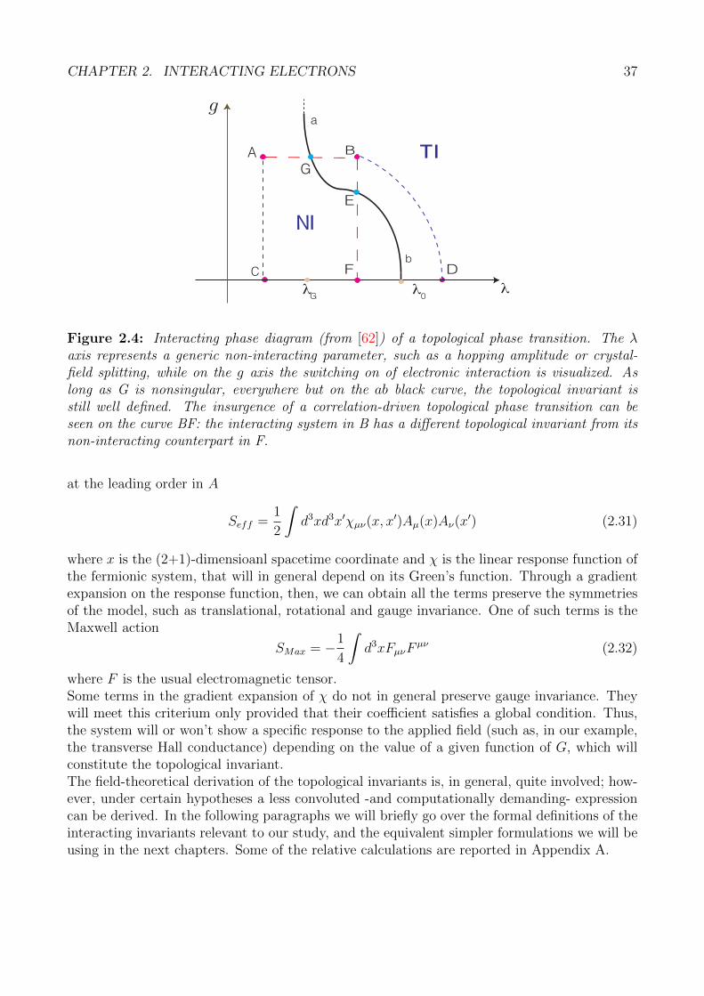
CHAPTER 2. INTERACTING ELECTRONS 37
A B
C
λ λ λ
F D
a
b
TI
NI
E
G
0G
Figure 2.4: Interacting phase diagram (from [62]) of a topological phase transition. The λaxis represents a generic non-interacting parameter, such as a hopping amplitude or crystal-field splitting, while on the g axis the switching on of electronic interaction is visualized. Aslong as G is nonsingular, everywhere but on the ab black curve, the topological invariant isstill well defined. The insurgence of a correlation-driven topological phase transition can beseen on the curve BF: the interacting system in B has a different topological invariant from itsnon-interacting counterpart in F.
at the leading order in A
Seff =1
2
∫d3xd3x′χµν(x, x
′)Aµ(x)Aν(x′) (2.31)
where x is the (2+1)-dimensioanl spacetime coordinate and χ is the linear response function ofthe fermionic system, that will in general depend on its Green’s function. Through a gradientexpansion on the response function, then, we can obtain all the terms preserve the symmetriesof the model, such as translational, rotational and gauge invariance. One of such terms is theMaxwell action
SMax = −1
4
∫d3xFµνF
µν (2.32)
where F is the usual electromagnetic tensor.Some terms in the gradient expansion of χ do not in general preserve gauge invariance. Theywill meet this criterium only provided that their coefficient satisfies a global condition. Thus,the system will or won’t show a specific response to the applied field (such as, in our example,the transverse Hall conductance) depending on the value of a given function of G, which willconstitute the topological invariant.The field-theoretical derivation of the topological invariants is, in general, quite involved; how-ever, under certain hypotheses a less convoluted -and computationally demanding- expressioncan be derived. In the following paragraphs we will briefly go over the formal definitions of theinteracting invariants relevant to our study, and the equivalent simpler formulations we will beusing in the next chapters. Some of the relative calculations are reported in Appendix A.
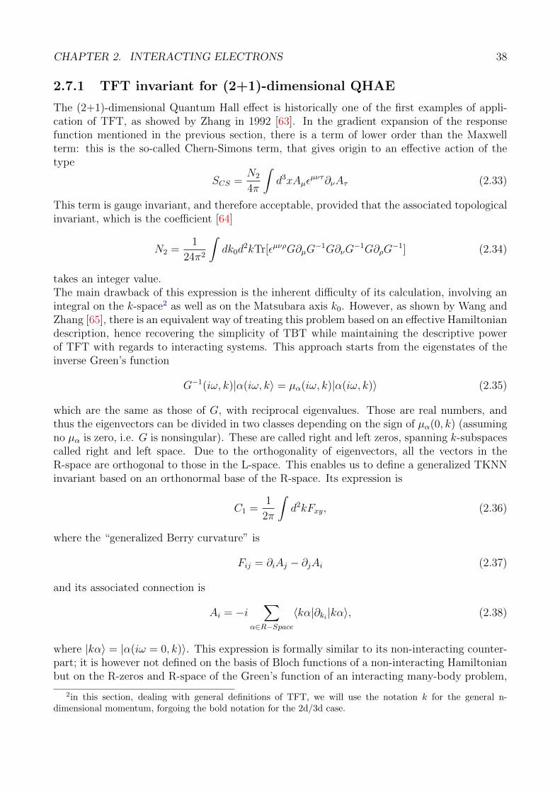
CHAPTER 2. INTERACTING ELECTRONS 38
2.7.1 TFT invariant for (2+1)-dimensional QHAE
The (2+1)-dimensional Quantum Hall effect is historically one of the first examples of appli-cation of TFT, as showed by Zhang in 1992 [63]. In the gradient expansion of the responsefunction mentioned in the previous section, there is a term of lower order than the Maxwellterm: this is the so-called Chern-Simons term, that gives origin to an effective action of thetype
SCS =N2
4π
∫d3xAµε
µντ∂νAτ (2.33)
This term is gauge invariant, and therefore acceptable, provided that the associated topologicalinvariant, which is the coefficient [64]
N2 =1
24π2
∫dk0d
2kTr[εµνρG∂µG−1G∂νG
−1G∂ρG−1] (2.34)
takes an integer value.The main drawback of this expression is the inherent difficulty of its calculation, involving anintegral on the k-space2 as well as on the Matsubara axis k0. However, as shown by Wang andZhang [65], there is an equivalent way of treating this problem based on an effective Hamiltoniandescription, hence recovering the simplicity of TBT while maintaining the descriptive powerof TFT with regards to interacting systems. This approach starts from the eigenstates of theinverse Green’s function
G−1(iω, k)|α(iω, k〉 = µα(iω, k)|α(iω, k)〉 (2.35)
which are the same as those of G, with reciprocal eigenvalues. Those are real numbers, andthus the eigenvectors can be divided in two classes depending on the sign of µα(0, k) (assumingno µα is zero, i.e. G is nonsingular). These are called right and left zeros, spanning k-subspacescalled right and left space. Due to the orthogonality of eigenvectors, all the vectors in theR-space are orthogonal to those in the L-space. This enables us to define a generalized TKNNinvariant based on an orthonormal base of the R-space. Its expression is
C1 =1
2π
∫d2kFxy, (2.36)
where the “generalized Berry curvature” is
Fij = ∂iAj − ∂jAi (2.37)
and its associated connection is
Ai = −i∑
α∈R−Space
〈kα|∂ki |kα〉, (2.38)
where |kα〉 = |α(iω = 0, k)〉. This expression is formally similar to its non-interacting counter-part; it is however not defined on the basis of Bloch functions of a non-interacting Hamiltonianbut on the R-zeros and R-space of the Green’s function of an interacting many-body problem,
2in this section, dealing with general definitions of TFT, we will use the notation k for the general n-dimensional momentum, forgoing the bold notation for the 2d/3d case.
CHAPTER 2. INTERACTING ELECTRONS 39
though in the non-interacting limit the two concepts evidently coincide. A further step thatbrings the calculation of interacting topological invariants closer to familiar TBT concepts in-volves a way of dealing with the dynamical properties of the Green’s function. As shown inAppendix A, it’s possible to derive the interacting topological invariant from the properties ofthe Green’s function at zero frequency or, equivalently, from the band dispersion of an effectivetopological Hamiltonian
Htop(k) = −G−1(0, k) = H(k) + Σ(k, 0) (2.39)
thereby making the calculation of the invariant fully analogous to the TBT case.
2.7.2 TFT invariant for a (4+1)-dimensional TRS system
The form of the topological term in the (2+1)-dimensional effective action breaks time-reversalsymmetry, under which A0 → A0 and A→ −A. TRS is instead preserved in 4+1 dimensions,where the effective topological action takes the form
Seff =N4
24π2
∫d5xεµνρστAµ∂νAρ∂σAτ (2.40)
and the topological invariant is the coefficient [62]
N4 =π2
15
∫dk0d
4k
(2π)5Tr[εµνρστG∂µG
−1G∂νG−1G∂ρG
−1G∂σG−1G∂τG
−1]
(2.41)
in which again k0 is the Matsubara frequency. Similarly to the two-dimensional case, an equiv-alence can be proven between this expression and the second Chern number
C2 =1
32π2
∫d4kεijklTr[FijFkl] (2.42)
where the generalized Berry curvature
Fαβij = ∂iA
αβj − ∂jA
αβi + i[Ai, Aj]
αβ (2.43)
is is obtained from
Aαβi (k) = −i〈kα| ∂∂ki|kβ〉 (2.44)
where again |kα〉 is an orthonormal base of the R-space. This again reduces to the expressionfor the second Chern number as defined from the Bloch wavefunctions for a non-interactingsystem. The (4+1)-dimensional TRS topological insulator can be considered the starting pointto define the TFT invariants for (2 + 1) and (3 + 1)-dimensional TRS topological insulators.
2.7.3 TFT invariants for TRS and IS systems
In 2008, Qi, Hughes and Zhang [60] developed, starting from (2.40), the general TFT for(2+1) and (3+1)-dimensional time-reversal invariant systems by means of a procedure knownas dimensional reduction. Later work by Wang and Zhang have determined the form of ageneral topological invariant for TRS systems, which in 3d has the expression [62]
P3 =π
6
∫ 1
0
du
∫d4k
(2π)4Tr[εµνρσG∂µG
−1G∂νG−1G∂rhoG
−1G∂σG−1G∂uG
−1] (2.45)

CHAPTER 2. INTERACTING ELECTRONS 40
in which k is the quadrimomentum with imaginary first component and u is what is called aWeiss-Zumino-Witten (WZW) extension parameter, that continuously connects the full Green’sfunction G(iω, k, u = 0) with a trivial constant reference function G(iω, k, u = 1). The deriva-tion of this result, while quite involved, is conceptually similar to the way in which the time-reversal polarization for the non-interacting system was derived by Fu and Kane.The form of this invariant again makes it rather difficult to practically calculate. However, ifthe system possesses Inversion symmetry in addition to TRS, the calculation of the invariantcan be dramatically simplified, as proven by Wang, Qi and Zhang in 2012 [66].The derivation of the expression makes use of the same concepts involved in the N2 = C1
demonstration provided in Appendix A. Essentially, it again relies on the concept of R-spaceand R-zero, based on the sign of the eigenvalues of the Green’s function at zero frequencyand at a TRIM µα(0,Λi). The associated eigenvector |α〉 is chosen as to be simultaneously aneigenvector of the parity operator Π, since G and Π commute at the TRIMs.The topological invariant ∆ is defined as
(−1)∆ =∏
R−zero
η1/2α (2.46)
where the product is restricted to the states |α(0,Λi)〉 whose associated eigenvalue µα(0,Λi) ispositive, and ηα is the parity eigenvalue for the state.A R-zero can be transformed in a L-zero, and vice-versa, providing that during the transfor-mation the Green’s function experiences a singularity, which in TBT language corresponds tothe closure of the gap. This happens when an eigenvalue of G−1 is passing through the origin(or through the compactified ∞ point, making detG = 0, with similar consequences).At the core of the demonstration is the proof of the equivalence mod 2 of the variation of ∆ and2P3 if the Green’s function undergoes a deformation, parametrized by a conveniently chosenparameter λ, that involves passing through a singularity when λ = 0.From symmetry requirements on G, it can be shown that at λ = 0 a couple of degenerateR(L)-zeros with negative parity cross the singularity and change topological class from R to Lor vice-versa, contributing an overall factor of −1 in (2.46).The consequent variation of ∆ by 1 mod 2 is then seen to coincide with that of 2P3. This is donevia geometrical considerations, following from the fact that (2.45) can be rewritten to representthe winding number W from the five-dimensional space spanned by frequency, momentum andWZW extension parameter to the space of Green’s functions GL(N,C).Together with the fact that, in the non-interacting limit, the relation 2P3 = ∆ mod 2 holds[67], this proves that the expression for ∆ is a good Z2 topological quantum number for three-dimensional TRS and IS systems. Once again, the calculation of the topological invariant foran interacting Hamiltonian based on the BHZ model is then greatly simplified, reduced to thecalculation of the same invariant for an effective topological Hamiltonian
Htop(k) = H(k) + Σ(k, ω = 0). (2.47)
The derivation of the two-dimensional counterpart of this invariant (and therefore also of the“weak” 3d topological invariants) is completely analogous, the only difference being the numberof the TRIMs. This invariants are well-defined as long as a gap is open; in this thesis wewill consider two and three-dimensional system with TRS and IS, and TRS-breaking three-dimensional systems for which the Z2 invariants will be only considered in the gapped phase.In all cases, the use of a formula of the type (2.46) is fully justified.

Chapter 3
Dynamical Mean-Field Theory andCluster Methods for StronglyCorrelated Fermions
In the previous chapter we have commented on the effects of Coulomb interaction on electronicsystems, showing how correlation can substantially modify the single-particle picture, alter-ing the expected values of some quantities (such as the bandgap of insulating systems) andeven rendering the description in term of electronic band structure meaningless. We have alsotouched on the fascinating subject of correlation-driven phase transitions, addressing the MottHubbard transition occurring in systems with narrow atomic orbitals such as transition metalsand related compounds.As we briefly mentioned, even the simplest correlated model, the single-band Hubbard model,has not been solved exactly beyond the peculiar one-dimensional case. The study of this modeland of the Mott-Hubbard transition has historically been the driving force towards the devel-opment of approximate solution methods for correlated electronic systems, both perturbativein the interaction and nonperturbative. We will concentrate, in this chapter, on the latterkind of approaches. Various fundamental steps towards the solution of the Mott transitionproblem occurred already in the 1960s, when the model was introduced by Hubbard, Kanamoriand Gutzwiller. The first and third authors also pioneered two complementary approximateapproaches which are more suited for the insulating and metallic sides of the transition, respec-tively. The two approximations can only certain aspects of the behaviour of the system nearthe Mott transition, which will be somehow reconciled and summed up nicely by the techniqueswe will examine in this chapter.
The Gutzwiller approach to the Mott transition [68–70] is based on a variational ansatzfollowed by a further approximation. The wave function is a Slater determinant (the non-interacting solution of the model in the original formulation) multiplied by a function whichgives different weights to configurations with different number of doubly occupied sites:
|ΨG〉 =N∏i
gni↑ni↓ |Ψ0〉 (3.1)
where g is a variational parameter and N is the number of sites. The energy of the systemis then minimized with respect to such ground state, usually through variational Monte Carloalgorithms. However, the expectation value of the Hamiltonian in this state can not be com-
41

CHAPTER 3. METHODS 42
ω
Gutzwiller
Gutzwiller
Gutzwiller
Hubbard
Hubbard
Hubbard
Noninteracting
DOS
Figure 3.1: Sketch of the evolution of spectral weight distribution in the Gutzwiller and Hub-bard III approximations for a semicircular density of states. The two methods address theinsurgence of a correlation-driven insulating phases from a low-energy and high-energy perspec-tive respectively.
puted exactly and one usually resorts to a further approximation which turns out to becomethe exact expectation value only in the limit of infinite coordination. Within this approach, theonset of correlations is described in terms of a progressive “destruction” on the non-interactinggroundstate, which describes a metal. In particular the solution describes a metal with thesame Fermi surface of the non-interacting system, but a reduced bandwidth (i.e. an increasedeffective mass) as long as such a solution exists. As we stated in the previous chapter, a Motttransition is expected to take place, in more than one dimension, for half-filling and a finite in-teraction U. In Gutzwiller’s picture, as applied by Brinkman and Rice [71], this is associated tothe shrinking of the density of states around the Fermi level with U up until a critical value Uc,after which the solution has zero kinetic energy and no double occupancy. The effective massof the quasiparticle excitations diverges at Uc, signalling the breakdown of the Landau-Fermiliquid description and the insurgence of a phase transition.A different approach to the Mott transition was devised by Hubbard in a series of seminalpapers [52–55], and is based on a Green’s function description. Starting from the atomic limitt = 0, the lattice hopping is introduced as a correction to the one-particle Green’s function,which in turn takes the form:
Gσ(k, ω) =1
[ω − ε0 − Σσ(ω)]−∆ε(k)(3.2)
where the expression in parenthesis is completely referred to the isolated interacting sites, while

CHAPTER 3. METHODS 43
∆ε(k) = ε(k)− ε0 represents the lattice effects in the noninteracting limit. This expression forthe Green’s function is at the base of various approximations, designed to be exact in the non-interacting case (Σ = 0) and in the atomic limit (∆ = 0). The first approximation proposed byHubbard was to assume Σ and ∆ to be completely oblivious to one another. Although capableof capturing the insurgence of Hubbard bands, this approximation is rather crude, as it predictsthe opening of a spectral gap for any finite value of U and any partial filling. An improvementwas obtained using the so-called “Hubbard III” approximation, in which each electron is seenas propagating in an alloy-like system made up by all opposite-spin electrons, treated as fixedscatterers. The local Green’s function for the interacting lattice, obtained through a k-spacesummation of an expression of the type (3.2), is then compared with the weighted average ofthe Green’s functions for a site with or without an opposite spin electron, namely
Gσ(ω) = n−σ1
ω − ε0 −∆(ω)− Σ(ω)+ (1− n−σ)
1
ω − ε0 − U −∆(ω)− Σ(ω)(3.3)
where ∆ is the hybridization due to the crystal and the n−σ is the weight of the average.Equations (3.2) and (3.3) form a close set of self-consistent expressions, through which Σ can bedetermined. The Hubbard III approximation accounts qualitatively for the solution we expectin in the Mott insulating phase, with two “Hubbard bands” separated by a Mott gap. Still,it approximates the local dynamics of the system with a static disorder, therefore incorrectlypicturing the Landau-Fermi liquid physics near the Fermi level. As we can see in Fig. 3.1, theevolution of the spectral function is different for the two approaches: the Gutzwiller schemecaptures well the evolution of the effective mass and density of states near the Fermi level inproximity of the Mott transition, but it does not account for the high energy Hubbard bandsthat characterize the Mott insulating state. On the contrary, by treating the local Green’sfunction as an average of those of the two Hubbard bands, the Hubbard III approximationincorrectly describes the low-energy physics of the system, for example attributing a finitelifetime to excitations at the Fermi level in a metal (which is at odds with the Landau-Fermiliquid description). We will see that Dynamical Mean-Field Theory somehow keeps the goodaspects of the two methods connecting them in a unifying picture.
3.1 Dynamical Mean-Field Theory
In the context of the Green’s function approach, the problem of strongly interacting fermionicsystems has found a new, powerful method of solution in the Dynamical Mean-Field Theoryand in its extensions. These methods, analogously to the classical description of magnetismin an Ising model [72], aim to obtain an approximate description of a correlated lattice fromthe perspective of a single-site effective problem, embedded in a conveniently defined “bath”describing the coupling between the degrees of freedom of the correlated site and the rest ofthe lattice. The effects of the latter will be encoded into a Weiss field, which in the parallelwith the Ising mean-field case corresponds to the effective magnetic field coupled to the localspin of the site.The great improvement is that, in contrast with classic models, here the mean-field descriptionis dynamical because, while disregarding the spatial fluctuations of the relevant quantities athand (as for magnetization in the mean-field Ising analogy) it fully takes into account thequantum dynamics in the time (or frequency) domain. The Green’s function of the effectivesingle-site model will correctly describe all the processes in which fermions are created and

CHAPTER 3. METHODS 44
destroyed at the correlated site, coming from and returning to the bath.As in the static mean-field approaches, the optimal form of the effective field will be self-consistently determined by requiring that the Green’s function of the effective local theorycoincides with the local component of the lattice Green’s function.
However, the Weiss field which describes the effect of the lattice on every given site is nownot a number but a time (or frequency) dependent quantity, obtained through the exact solutionof a finite quantum many body problem. The effective problem will be described by an actionof the form
Seff = −∫ β
0
dτ
∫ β
0
dτ′∑
σ
c†0σ(τ)G−10 (τ − τ ′
)c0σ(τ′) + U
∫ β
0
dτn0↑(τ)n0↓(τ) (3.4)
where the role of the Weiss field G0 is that of a bare Green’s function in a Gaussian integral,and the second term explicitly treats the local Coulomb interaction. Since it is dependent on ω,the Weiss field is capable of describing all the energy scales of the interacting problem. In thissense, it constitutes an improvement over mean-field techniques such as Hartree-Fock, that canonly address one energy scale through the use of static order parameters, hence being accurateonly in some restricted scenarios such as the Landau-Fermi liquid regime. Dynamical mean-fieldmethods are well suited to address the Mott transition, where the characteristic energy scaledefining the physics of the system varies drastically; we therefore can expect, through their use,a “reconciliation” of the features exhibited by the Gutzwiller and Hubbard III approximations.Historically, the idea of providing a solution for quantum many-body problems via this localinteracting self-consistent approximation methods originated with the work of Metzner andVollhardt [73] and Muller-Hartmann [74] on the limit of infinite dimension. Since the methodis still mean-field, it is in fact expected to be exact in this limit. As we shall see, the correctscaling of the hopping amplitude in the limit of infinite dimensions is at the basis of theapproximation producing the effective action of DMFT.The biggest step towards a derivation of a viable self-consistent method for a dynamical Mean-Field theory came from the work of Georges and Kotliar in 1992 [75], where the mappingbetween the fully interacting lattice model and a local impurity problem coupled to a conductionband was proposed.
3.1.1 Derivation by cavity method
Among the derivations of the DMFT self-consistency equations (see for example [76, 77] and[78, 79]), the “cavity method” is the most well known and instructive, due to its parallel withthe static Mean-Field construction, of which it represents an extension. This approach aims toconstruct an effective local theory for a single arbitrary site by averaging out all the non-localdegrees of freedom. A review of the calculations involved can be found in Appendix B, yet webriefly discuss the derivation for the case of single-band Hubbard model to provide an overviewof the self-consistent DMFT construction. The aim of the method is to provide an explicit wayof obtaining and updating the Weiss function defined in (3.4). We start by expressing the fullaction of the interacting lattice as the sum of three terms,
S = S(o) + S0 + ∆S (3.5)

CHAPTER 3. METHODS 45
Ut
Bath
Figure 3.2: Scheme of the DMFT approximation in the cavity method derivation: one site isremoved from the lattice and treated separately. The isolated site is solved numerically as animpurity coupled to a “conduction band” represented by a noninteracting bath.
where
S0 =
∫ β
0
dτ
[∑σ
c†0σ(τ)(∂
∂τ− µ)c0σ(τ) + Un0↑(τ)n0↓(τ)
](3.6)
is the local action of the cavity,
∆S = −∫ β
0
dτ∑iσ
[ti0c†iσ(τ)c0σ(τ) + h.c.
](3.7)
describes the hybridization between the cavity and the rest of the lattice and the last term S(o)
is relative to the rest of the lattice alone. The lattice degrees of freedom are then traced out inthe partition function, that can be written as
Z =
∫ ∏i
Dc†0σDc0σe−S0
∫ ∏i 6=0
Dc†iσDciσe−S(o)−∆S (3.8)
or, in terms of an ensemble average over S(o)
Z = Z(o)
∫ ∏σ
Dc†0σDc0σe−S0⟨e−∆S
⟩(o)
(3.9)
Concerning the last exponential, using linked-cluster theorem, it is straightforward to recognizein it the generator of the connected (cavity) Green’s functions. Expanding in power seriesthe resulting term gives rise to cavity Green’s function to all orders. Up to this point noapproximation has been made. Now, an important simplification is obtained considering the
∞-dimension limit: the scaling of the hopping amplitude between sites i and j as 1/√d|i−j|
,necessary so that kinetic and interaction energies remain of the same order of magnitude, impliesthat every term of order > 2 decays at least as 1/d. As a result, the only surviving terms are

CHAPTER 3. METHODS 46
those corresponding to the single-particle Green’s function G(o)ij . The resulting effective action
takes the form
Seff = S0 +
∫ β
0
dτ1
∫ β
0
dτ2
∑σ
c†0σ(τ1)∑ij
ti0t0jG(o)ij (τ1 − τ2)c0σ(τ2). (3.10)
We now make use of the relation between he Green’s function of the full lattice with that ofthe lattice with the cavity removed,
G(o)ij = Gij −
Gi0G0j
G00
(3.11)
to obtain an explicit form for the Weiss Green’s function in (3.4):
G−10 (iωn) = iωn + µ−
∑ij
ti0t0j[Gij(iωn)−Gi0(iωn)G−1
00 (iωn)G0j(iωn)]
(3.12)
which establishes a relation between the Mean-Field Green’s function and that of the fullyinteracting lattice.Through (3.12) we can obtain the self-consistency condition for the DMFT method: given anexpression for the Weiss field, the effective problem Eq. (3.4) is solved to obtain the impurityGreen’s function Gimp(iωn) and, ultimately, the impurity self-energy function Σ(iωn) whichsatisfies the Dyson equation
Σ(iωn) = G−10 (iωn)−G−1
imp(iωn). (3.13)
Σ, which due to the mean-field nature of the method is completely local, is instrumental inobtaining the local interacting Green’s function of the original system as
Gloc(iωn) =∑k
G(k, iωn) (3.14)
where
G(k, iωn) =1
iωn + µ− εk − Σ(iωn)(3.15)
which corresponds in real space to the ij summation appearing in (3.12). After some algebraiccalculations, the local Green’s function Gloc is shown to satisfy the self-consistency condition
G0(iωn)−1 = iωn + µ+Gloc(iωn)−1 −R[Gloc(iωn)] . (3.16)
The last term is the reciprocal function of the Hilbert transform of the density of states of thelattice defined as
D(z) =
∫ ∞−∞
dεD(ε)
z − ε, R[D(z)] = z (3.17)
in which D(ε) is the noninteracting density of states
D(ε) =∑k
δ(ε− εk). (3.18)
Once the method has converged, the self-consistency condition (3.16) implies that Gloc(iωn) isidentified with the full impurity Green’s function Gimp(iωn).
CHAPTER 3. METHODS 47
In the infinite dimension limit, where mean-field is exact, the previous relations are simpli-fied, as it is famously shown in the slightly different situation of a lattice without a definitedimensionality but a definite coordination number, the Cayley tree. In this system, each siteis connected to each other by only one path, creating a distinctive branch structure. We willin particular consider the z → ∞ situation, known as Bethe lattice, which is for all intentsand purposes analogous to the infinite-dimension limit. In this situation, the nearest-neighbourhopping scales as tij → t/
√z and the noninteracting density of states has the semicircular
shape [80]
D(ε) =1
2πt2
√4t2 − ε2 (3.19)
which is nonzero in the range [−2t; 2t]. The great simplification of the Bethe lattice stemsfrom equation (3.11). If a site is removed, the only path connecting its neighbours is severed,
therefore the relative Green’s function in the presence of the cavity G(o)ij becomes diagonal. The
removal of a link changes the coordination of a factor 1/z, so that in the limit z → ∞ theeffect is negligible. These observations, together with the complete translational invariance ofthe lattice, make it possible to assume instead of (3.11) the much simpler form
G(o)ij = δijG
(o)ii = Gii = G00. (3.20)
This leads to the simplified Hilbert and inverse Hilbert transforms
D(z) =z − s
√z2 − 4t2
2t2R(G) = t2G+ 1/G (3.21)
which immediately satisfy the self-consistency condition with
G−10 (iωn) = iωn + µ− t2G(iωn). (3.22)
Other than in the infinite dimensions limit, DMFT is exact in two other scenarios: the nonin-teracting limit U = 0, where Gloc = G0, and the atomic limit, where the density of states is a δfunction and it holds:
G−10 (iωn) = iων + µ (3.23)
The Green’s function of each isolated site is then
G(iωn) =1− n/2iωn + µ
+n/2
iωn + µ− U(3.24)
with
n/2 =eβµ + e2βµ−βU
1 + 2eβµ + e2βµ−2U(3.25)
which is the same results we can get directly from Lehmann representation calculations on anisolated site.
3.1.2 Hamiltonian formulation
As discussed above the crux of DMFT is to replace the full interacting lattice problem withan effective model consisting of an interacting site coupled to an effective self-consistent bath.
CHAPTER 3. METHODS 48
Such single-site system is yet a complex quantum many-body problem, which describes the localquantum fluctuations of the lattice problem. It is straightforward to observe the similarity of theeffective problem described by the action Eq. (3.10) with a single-impurity Anderson model [81](SIAM). The SIAM Hamiltonian has the form
HAIM =∑σ
ε0c†0σc0,σ +
∑lσ
εla†lσalσ +
∑lσ
Vl(a†lσc0σ + c†0σalσ)− µ
∑σ
c†0σc0σ + Un0↑n0↓, (3.26)
that is quadratic in the operators a, a† associated to the conduction band. The expression ofthe action for this impurity model can be split in two of two parts, which we can express as
S0 =
∫ β
0
∑σ
c†0σ(τ)(∂τ + ε0 − µ)c0σ(τ) + Un0↑(τ)n0↓(τ) (3.27)
∆S =
∫ β
0
dτ∑lσ
a†lσ(τ)(∂τ + εl)alσ(τ) + Vl(a†lσ(τ)c0σ(τ) + h.c.) (3.28)
where the first term relates to the impurity and the second refers to the bath electrons and thebath-impurity hybridization term. Once we pass to the frequency domain, and integrate outthe bath degrees of freedom, we can express the effective action for the impurity as the sum ofthe interacting part ∫ β
0
dτUn0↑(τ)n0↓(τ)
and a noninteracting quadratic term governed by the AIM Green’s function
G−10 (iωn)AIM = iωn + µ− ε0 −
∫ ∞−∞
dω∆(ω)
iωn − ω. (3.29)
Here, the hybridization function ∆ is has the form
∆(ω) =∑lσ
V 2l δ(ω − εl) (3.30)
and corresponds to a density of states associated to the conduction band. As such, the SIAMprovides a Hamiltonian representation of the effective action for the impurity problem in termsof the (infinitely many) bath parameters ε and V . These two sets of parameters determiningthe hybridization function have then to be self-consistently determined in order to solve theDMFT equations.
3.1.3 Mott transition and Phase Diagram
As we recall, the Gutzwiller and Hubbard approaches to the Mott transition predict, for thesemicircular DOS, two different scenarios. The first shows the shrinking of the spectral distribu-tion around the Fermi level, corresponding to an increase of the effective mass of quasiparticlesthat eventually diverges at the phase transition. The second predicts a progressive broadeningof the DOS at high frequencies and the eventual creation of a gap around the Fermi level.In DMFT, the distribution of the spectral weight for increasing U assumes the distinctivethree-peak structure shown in of Fig. 3.3, which can be nicely compared to the combined pic-ture presented by Gutzwiller and Hubbard III approximations in Fig. 3.1. The central peak

CHAPTER 3. METHODS 49
Figure 3.3: DOS of the Bethe lattice in the infinite correlation limit for increasing U =1, 2, 2.7, 3, 4 respectively. The results were obtained from a simpler perturbative approach (IPT),that works best for low values of U but can capture correctly the physics of a Half-filled Hub-bard model for higher interaction values [82]. A comparison with Fig. 3.1 shows that DMFTeffectively sums up the low-energy Gutzwiller and high energy Hubbard descriptions.
corresponds to the quasiparticle part of the spectrum and has a Fermi liquid behaviour witha fraction of the total spectral weight Z. The two broad bands at high and low frequenciesare the Hubbard bands accounting for the atomic-like non Fermi liquid behaviour, they areseparated in energy by a factor of order U and have spectral weight (1 − Z). The behaviourof the central peak follows a Brinkman-Rice type evolution, with an increase of the effectivequasiparticle mass approaching the Mott transition; the sidebands gap, linearly growing withU , follows instead a Hubbard-like behaviour.Fig. 3.4 sketches a phase diagram for the paramagnetic solution of a two-dimensional Hubbardmodel as a function of the ratio U/D and the temperature T/D where D = 2t, as obtainedby different methods. Let us concentrate on the first one, which refers to single-site DMFTwe presented in the previous sections: in the shaded region, there is coexistence between themetallic and insulating solution. For a finite temperature, the insulating solution extends up toUc1 where, in the Hubbard picture, the two sidebands merge eliminating the gap at the Fermienergy. The metallic solution is instead present up to Uc2, where the quasiparticle weight Zvanishes and the effective mass diverges, as in the Brinkman-Rice picture. For low temper-ature, the values of Uc1 and Uc2 are approximatively ≈ 2.35D and ≈ 2.9D respectively. Atzero temperature, the first-order phase transition line touches the boundary of the coexistenceregion at a the critical point Uc2.

CHAPTER 3. METHODS 50
Figure 3.4: Sketches of the phase diagram for the metal-insulator transition as predicted byDMFT, CDMFT and VCA in the paramagnetic phase. The shaded areas (light-dark grey)correspond to the metal and insulator-stable phases inside the coexistence region of the twosolutions. The line traversing the coexistence region is the first-order phase transition line, thatterminates in a critical point at finite T (over which a crossover region is present). For DMFT,the slope of the line is negative, while it is positive for CDMFT and VCA. The line terminatesin a critical point at the border of the coexistence region in DMFT (and cluster derivatives)while SFT-based methods may show the persistence of the 1st-order character of the transitioneven at T=0, as shown on the right panel of Fig. 3.7.
One of the possible objections to this picture is that, at least in its paramagnetic declina-tion, it does not include the effects of magnetic correlations (such as antiferromagnetism) andtherefore describes an insulator with an entropy which approaches asymptotically the extensivevalue ≈ N ln 2. This clearly favours the insulator at higher temperatures and determines thenegative slope of the first-order transition line. These potential limitations of the method can beaddressed via cluster extensions of the single-site DMFT method, such as the Cluster-DMFT,which we will explicitly treat in the next section and whose phase diagram is represented in themiddle panel of Fig. 3.4. In this framework, the insulator has lower entropy due to short-rangesinglet formation [83], and the slope of the transition line is positive.Within DMFT it can be shown rigorously [84] that the zero-temperature Mott transition pointcoincides with the upper Uc2, while in CDMFT it appears numerically to coincide with Uc1.However, there is no a priori reason why Uc should coincide with one of the spinodals. In thethird panel in Fig. 3.4 is related to Variational Cluster Approximation, a technique we will alsointroduce in the following sections, which is related to DMFT but moves its step from a differ-ent underlying principle. The related phase diagram [85] shows the persistence of a first-orderphase transition down to zero temperature, with the metallic/insulating character of the stablephase changing inside the coexistence region.
3.2 Cluster methods
As previously discussed DMFT is characterized by a momentum-independent self-energy Σ(ω),which only depends on frequency. This can be computed in the effective local theory, hence itis a purely local which normalizes the lattice Green’s function. All the space fluctuations are

CHAPTER 3. METHODS 51In
tens
ity (
arb.
uni
ts)
–0.1 0.0 0.1Energy relative to EF (eV)
39o
34o
29o
24o
20o
15o
10o
6o
1o
Figure 3.5: Two examples of nontrivial effects recovered by cluster-based methods: a) thepseudogap behaviour as measured by ARPES in a sample of Bi2Sr2CaCu2O8+x (cfr. [40]); theangle corresponds to different k-directions in the Brillouin Zone. b) density as a function ofthe chemical potential for a Hubbard chain: the CDMFT result, which correctly replicates theexact Bethe Ansatz one, features a divergence in compressibility (the derivative of the plottedquantity), which is not present in single-site DMFT results. Picture taken from [86].
frozen and this gives rise to some issues like the previously cited overestimation of the insulatingstate entropy.
An interesting experimental example [87] of a situation in which a local self-energy may beinadequate comes from high-temperature superconductors based on CuO2 planes. For a verylow doping and T > Tc, ARPES measurements give a well-defined peak at the Fermi energy inthe diagonal direction of the BZ, but near the boundary at (0, π) the emission spectrum has aminimum at the Fermi energy, that is referred to as a “pseudogap”. This is clearly an effectof correlation, and therefore any information regarding this effect must be embedded in theSelf-Energy of the model, that in turn has to be momentum-dependent to correctly capture thepseudogap behaviour.
A further example of a feature that can not be captured by single-site DMFT is the density-driven Mott transition in a one-dimensional Hubbard model [86]: while the exact Bethe ansatzsolution predicts a divergence in compressibility κ = ∂n/∂µ at the Mott transition, single-siteDMFT finds no such behaviour. In recent years, many cluster-oriented extensions of DMFThave been proposed, both in real space (CDMFT) and in reciprocal space (DCA [88]). Adifferent approach to the cluster problem has also been developed from a variational principlebased on the Self-Energy. We will focus on the real-space Cluster DMFT, and on a differentapproach called Self-Energy Functional theory, more specifically on one of its derivate methodswhich is the previously mentioned VCA.

CHAPTER 3. METHODS 52
3.2.1 Cluster DMFT
A well-known and successful extension of DMFT is the real-space Cluster-DMFT [89, 90].It replaces the single impurity with a set of N lattice sites with open boundary conditions,coupled to a frequency dependent bath again determined self-consistently. Correspondingly,all the dynamical correlation functions and the Weiss field have an additional N × N matrixstructure, i.e. an explicit dependence on the spatial non-local degrees of freedom inside thecluster. Given a cluster self-energy function Σc(iωn), the local cluster Green’s function reads:
G(iωn) =∑
k∈RBZ
1
(iωn + µ)I−H(k)−Σc(iωn)(3.31)
Here, H(k) is the one-body part of the Hamiltonian of the lattice expressed in a base thatpreserves translational invariance.For example, dividing a n-dimensional cubic lattice in Nx1 × ... × Nxn-sized clusters redefinesthe length of Bravais lattice vector, which in turn shrinks the size of the Brillouin Zone byNxi in the ki direction. Any quantity can then be rewritten in the mixed (i, k) representation,where i labels the internal site of the cluster and k the k-vector in the Reduced Brillouin Zone,i.e. the Brillouin zone corresponding to the unit cell created by cluster itself.
The 1-dimensional case can be used as an illustrative example. The hopping matrix of a1-dimensional Hubbard model with lattice spacing a = 1 and hopping amplitude t is H(k) =−2t cos(k). If the lattice is divided in 2-site clusters, the same kinetic part of the Hamiltonianwill be written in the mixed representation as
H(k) =
[0 −t(1 + e−2ik)
−t(1 + e2ik) 0
](3.32)
where now k ∈ the Reduced Brillouin Zone [−π/2, π/2].We will henceforth use the bold notation to indicate matrices in the mixed representation orgenerally in the cluster basis, and intend fractions as (3.31) as a formal matrix inversion.All the self-consistency equations valid for the single-site DMFT are translated into the clusterextension, making use of this mixed representation. The original periodicity, along with thedependence on k ∈ BZ of the quantities that are local in the cluster basis, can be recoveredthrough periodization, which will be discussed later. However, the determination of the effectivebath can be a little more subtle with respect to the single-site DMFT. In particular, to easethe computation, the symmetries of the cluster can be taken into account when generating thebath. A way to do that is to set up a block-diagonal structure consistent with the irreduciblerepresentations of the symmetries exhibited by the cluster [91]. In this way, the symmetriesfor each block of the bath Green’ function are explicitly selected. Another way to immediatelytake the symmetries of the cluster into account is to consider a bath whose Green’s function isbased on a replica of the cluster Hamiltonian [92], using the so-called reduced parametrizationscheme, which we will briefly comment on in Chapter 4.
A substantial difference between DMFT and its cluster extension has to be underlined.While for DMFT the limit d → ∞ is exact and the method is well suited to describe latticeproblems with a high coordination number, applying the same limit to the CDMFT wouldlead to the decay of nonlocal terms in the expansion of Seff , therefore producing a local Self-Energy and taking us back to the single-site picture. Then again, in a finite-dimensionallimit the approximation in the derivation of Seff becomes more crude. CDMFT is therefore

CHAPTER 3. METHODS 53
= + + +Φ
Figure 3.6: First terms of the skeleton expansion of the Luttinger-Ward functional, picturefrom [96].
“intrinsically” an approximation, whose quality depends in a systematic way on the size of thecluster, a trait that it shares with a class of cluster frameworks based on a different inspiringprinciple, that we will now introduce.
3.2.2 Self-Energy Functional Theory and derivatives
A different, though related, approach to the solution of interacting electron systems is basedon a variational principle called Self-Energy Functional Theory. This approach was originallyproposed by Potthoff [93] and is based on the framework of Cluster Perturbation Theory (CPT)[94, 95]: at the core of this method is the fact that, while we cannot access the exact solutionfor an infinite correlated lattice, we can solve finite-size systems through various numericaltechniques, some of which we will show in the next chapter. Then, we can approximate thefull lattice of interacting fermions with a collection of clusters related by a one-body hoppingHamiltonian. The relation between the cluster and full lattice Green’s function has a formsimilar to the Dyson equation, if one treats the inter-cluster coupling as a perturbation:
G(ω) =1
G′(ω)−1 −V(3.33)
where G and G′ refer to the lattice and cluster Green’s function and V is the inter-clusterhopping. This relation is exact in the noninteracting limit, where G and G′ only depend onthe hopping matrix H (and the coupling V); its extension to the interacting realm constitutesthe core of the CPT approximation. A crucial observation comes from the fact that both G′
and V can be redefined in terms of other hopping parameters t = t + ∆t. While this has noeffect in the noninteracting case, it generates a different approximated result for the interactingG for every choice of one-body hopping Hamiltonian. Hence, there is a way of improving overthe CPT approximation by finding a way of “sorting” the reference systems and choosing thebest. To this end, a variational principle is needed.
Luttinger-Ward generating functional
The Luttinger-Ward functional ΦU [G]1, introduced in 1960, is a scalar functional withoutexplicit physical meaning originally derived [39] order by order in a diagrammatic perturbationexpansion. It is defined as the the sum at any order of all closed, connected, and fully dressedskeleton diagrams, i.e. closed Feynman diagrams without self-energy insertions and with all
1The hat notation is used in this case to identify the functionals, and not second quantization operators.However, due to the different spaces in which these quantities are defined, this should cause no confusion.

CHAPTER 3. METHODS 54
free propagators replaced by fully interacting ones, as it can be seen in Fig. 3.6. The domainof the functional is a space of functions to which the physical Green’s function of the systemwith the given interaction U belongs. The Luttinger-Ward functional has these very usefulproperties:
• its functional derivative with respect to its argument is
1
T
δΦU [G]
δG= ΣU [G] (3.34)
where the functional ΣU is, if evaluated at a physical G, the associated Self-Energy ΣH,U
• if evaluated on the physical G, its value ΦU [Gt,U ] = ΦH,U is related to the Grand potentialof the system by
ΩH,U = ΦH,U + Tr ln GH,U − Tr(ΣH,UGH,U) (3.35)
• it only depends on U , therefore it is universal for all the systems with the same expressionfor the interaction
• it vanishes at the noninteracting limit
A derivation of these properties is presented in Appendix B.
SFT and Ω potential
The derivation of the SFT variational principle is based on the invertibility assumption for thefunctional ΣU [G], which is assumed to hold at least locally. This assumption is generally safeaway from a critical point. Then, the Legendre transform of the functional can be constructedin term of the inverse functional of Σ, which we will call G, in the form
FU [Σ] = ΦU [GU [Σ]]− Tr(ΣGU [Σ]) (3.36)
which satisfies the functional derivative
1
T
δFU [Σ]
δΣ= −GU [Σ] (3.37)
We can then define the Self-Energy functional that gives name to the theory as
Ω[Σ] = Tr log1
G−10 −Σ
+ FU [Σ] (3.38)
where the trace is intended as a sum over frequencies and site indices (or wavevectors). Fromthe property relating the grand potential to the Luttinger-Ward functional and from Dyson’sequation, it’s easy to note that if G and Σ are the dynamical quantities of a physical system,Ω is its grand potential. Moreover, it can be immediately seen that the Dyson’s equation foran interacting system is satisfied when
δΩH,U [Σ]
δΣ= 0 (3.39)

CHAPTER 3. METHODS 55
which constitutes the variational principle at the core of SFT.The last step to the formulation of the theory is to recognize that, as a functional of Σ livingin the space of Self-Energies, the first term in (3.38) is purely non-interacting and depends onthe characteristics of the hopping matrix embedded in G0, while the second, which involves theLegendre transform of the Luttinger-Ward functional Φ, is universal for all system sharing thesame interaction form irrespective of the features of the hopping matrix. Hence the arduoustask of calculating ΦH,U can be avoided entirely, as long as a reference system with the sameinteraction part as the whole lattice is used, by calculating
Ω[Σ] = Ω′ + Tr log1
G−10 −Σ
− Tr log1
G′−10 −Σ
(3.40)
Here, Ω′
is the evaluation of Ω for the physical system consisting of the reference finite cluster,which is directly obtainable as its grand potential, and the remaining terms are non-interactingand easily obtainable in practice as a functional of Σ or, in turn, as a function of a certainparametrization of Σ depending on some parameters, as represented inf Fig. 3.7.
Just like DMFT this approach it is non-perturbative, hence it is well suited to describephenomena like the Kondo effect [97]. Remarkably, the internal energy of the physical systemis immediately obtained as the value of the Ω functional at the stationary points. This enablesus to rapidly analyse the details of a phase transition. Differently from the self-consistentDMFT approach, this method allows to find and classify all the physical solutions accordingto their energy.
Interestingly, equation (3.38) unveils the relation between the SFT approach and the DMFTself-consistency: let us consider the derivative of this equation with respect to some parametersh on which Σ depends. Using the universality of F , we obtain
∂
∂hΩ[Σh] =
1
β
∑nijσ
(Tr
1
G−10 (iωn)−Σ(iωn)
−G′(iωn)
)ijσ
∂Σjiσ(iωn)
∂h, (3.41)
where the meaning of the trace is a k-sum. In the case in which the auxiliary system is asingle-site Anderson impurity model coupled with a bath (which will clearly not be present inthe original lattice Green’s function), the Self-Energy will in this case be completely on-siteand the functional trace effectively gives us the local Green’s function for the lattice. Then, theformula in parenthesis is precisely the DMFT self-consistency relation between the local Green’sfunction an the impurity one calculated from the effective action. The difference between thetwo methods stems from the fact that, while DMFT strives to make the expression in parenthesisas small as possible, SFT seeks to nullify the total derivative, to which end making it orthogonalto ∂Σ/∂h is sufficient.
VCA
In principle. SFT requires the calculation of the optimal Self-Energy satisfying the stationaritycondition. We need however to find a systematic way to travel in the Σ space until we find thestationary point. This leads to the definition of the Variational Cluster Approximation: insteadof moving in the full space of Self-Energies, we restrict ourselves to a subspaces of Σs whichshare a functional dependence on some parameters: these can be, for example, an enhancedintra-cluster hopping t
′, a staggered magnetic field, an hybridization V and on-site energy ε for
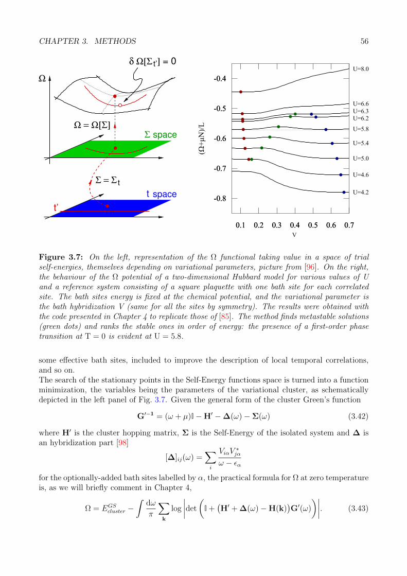
CHAPTER 3. METHODS 56
-0.8
-0.7
-0.6
-0.5
-0.4
0.1 0.2 0.3 0.4 0.5 0.6 0.7
(Ω+μN)/L
U=4.2
U=4.6
U=5.0
U=5.4
U=5.8
U=6.2U=6.3U=6.6
U=8.0
-0.8
-0.7
-0.6
-0.5
-0.4
0.1 0.2 0.3 0.4 0.5 0.6 0.7V
Figure 3.7: On the left, representation of the Ω functional taking value in a space of trialself-energies, themselves depending on variational parameters, picture from [96]. On the right,the behaviour of the Ω potential of a two-dimensional Hubbard model for various values of Uand a reference system consisting of a square plaquette with one bath site for each correlatedsite. The bath sites energy is fixed at the chemical potential, and the variational parameter isthe bath hybridization V (same for all the sites by symmetry). The results were obtained withthe code presented in Chapter 4 to replicate those of [85]. The method finds metastable solutions(green dots) and ranks the stable ones in order of energy: the presence of a first-order phasetransition at T = 0 is evident at U = 5.8.
some effective bath sites, included to improve the description of local temporal correlations,and so on.The search of the stationary points in the Self-Energy functions space is turned into a functionminimization, the variables being the parameters of the variational cluster, as schematicallydepicted in the left panel of Fig. 3.7. Given the general form of the cluster Green’s function
G′−1 = (ω + µ)I−H′ −∆(ω)−Σ(ω) (3.42)
where H′ is the cluster hopping matrix, Σ is the Self-Energy of the isolated system and ∆ isan hybridization part [98]
[∆]ij(ω) =∑i
ViαV∗jα
ω − εαfor the optionally-added bath sites labelled by α, the practical formula for Ω at zero temperatureis, as we will briefly comment in Chapter 4,
Ω = EGScluster −
∫dω
π
∑k
log
∣∣∣∣det
(I +(H′ + ∆(ω)−H(k)
)G′(ω)
)∣∣∣∣. (3.43)
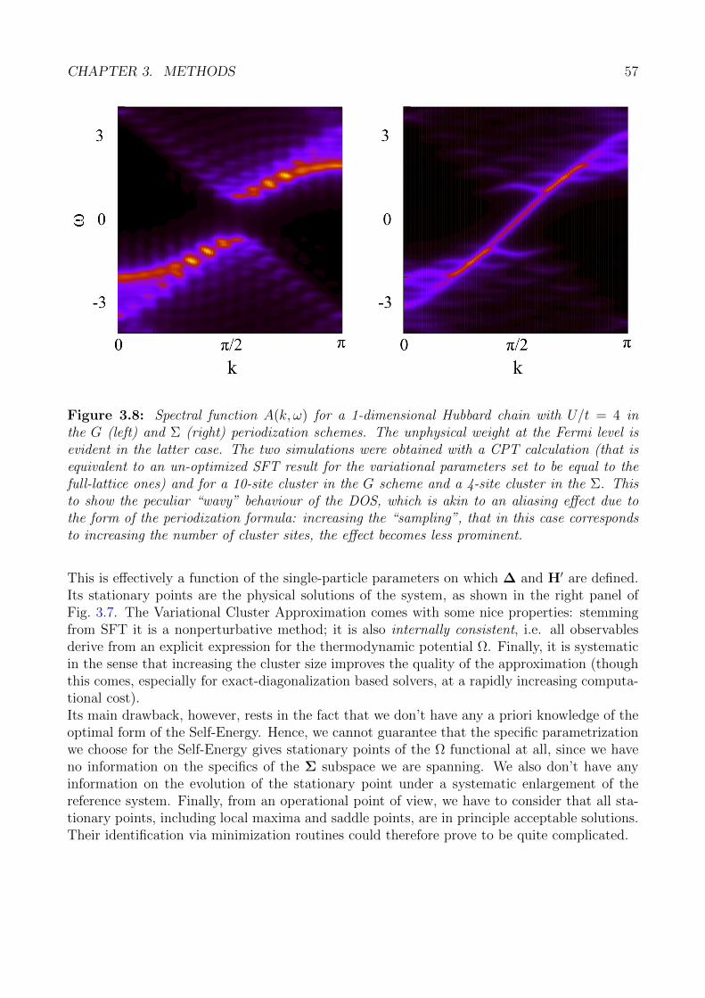
CHAPTER 3. METHODS 57
Figure 3.8: Spectral function A(k, ω) for a 1-dimensional Hubbard chain with U/t = 4 inthe G (left) and Σ (right) periodization schemes. The unphysical weight at the Fermi level isevident in the latter case. The two simulations were obtained with a CPT calculation (that isequivalent to an un-optimized SFT result for the variational parameters set to be equal to thefull-lattice ones) and for a 10-site cluster in the G scheme and a 4-site cluster in the Σ. Thisto show the peculiar “wavy” behaviour of the DOS, which is akin to an aliasing effect due tothe form of the periodization formula: increasing the “sampling”, that in this case correspondsto increasing the number of cluster sites, the effect becomes less prominent.
This is effectively a function of the single-particle parameters on which ∆ and H′ are defined.Its stationary points are the physical solutions of the system, as shown in the right panel ofFig. 3.7. The Variational Cluster Approximation comes with some nice properties: stemmingfrom SFT it is a nonperturbative method; it is also internally consistent, i.e. all observablesderive from an explicit expression for the thermodynamic potential Ω. Finally, it is systematicin the sense that increasing the cluster size improves the quality of the approximation (thoughthis comes, especially for exact-diagonalization based solvers, at a rapidly increasing computa-tional cost).Its main drawback, however, rests in the fact that we don’t have any a priori knowledge of theoptimal form of the Self-Energy. Hence, we cannot guarantee that the specific parametrizationwe choose for the Self-Energy gives stationary points of the Ω functional at all, since we haveno information on the specifics of the Σ subspace we are spanning. We also don’t have anyinformation on the evolution of the stationary point under a systematic enlargement of thereference system. Finally, from an operational point of view, we have to consider that all sta-tionary points, including local maxima and saddle points, are in principle acceptable solutions.Their identification via minimization routines could therefore prove to be quite complicated.
CHAPTER 3. METHODS 58
3.2.3 Observables and periodization
All the quantities obtained via the cluster methods introduced above are defined in the cluster-superlattice mixed representation. This basis is perfectly fine to determine many properties ofthe material, such as the one-body observables, through the general formula [99]
O =1
N
∑k∈RBZ
∫ ∞0
dω
πRe
Tr
[s(k)G(k, iω)
]− Tr s(k)
iω − a
(3.44)
where s is the general 1-body matrix expression of the observable operator, G is the latticeGreen’s function obtained from
G(k, ω) =1
(ω + µ)I−H(k)−Σ(ω)(3.45)
and the last term, dependent on a real parameter a ≈ 1, is included for normalization reasons.To our ends, since topological properties are related to the gap, the unperiodized system isagain perfectly adequate.Nevertheless, it might be interesting to retrieve the original periodicity of the results, for exam-ple to achieve a good comparison between cluster and single-site description and in general toobtain k-dependent quantities inaccessible from a DMFT perspective. There are many ad-hocprescriptions to achieve such a goal: they generally rely on the residual translational invariancein the superlattice to recover a k-dependent quantity from its site-dependent analogous; thedifference between the schemes is the quantity to be periodized.The most well-known (though not unique) periodization schemes are the aptly named G-scheme [95], where the cluster Green’s function is recast into a k-dependent form via
Gper(k, ω) =1
Nc
∑ij
e−ik·(ri−rj)[G]ij(k, ω) (3.46)
where the original Green’s function (3.45) is evaluated at the original lattice k-points, and theΣ-scheme [86, 89], where a similar procedure is done on the Self-Energy via
Σper(k, ω) =1
Nc
∑ij
e−ik·(ri−rj)[Σ]ij(ω). (3.47)
In both cases, the other relevant quantities are obtained through Dyson’s equation, given theeasy form of the noninteracting Green’s function in the original basis.These schemes have a certain degree of conventionality, as they are in fact weighted averages ofquantities that may not be well-behaved. A well-known example is the unphysical results givenby the Σ-scheme in describing the Mott transition, which are pictured in Fig. 3.8. In this case,the Self-energy presents a divergence near the Fermi level, which accounts for the breakdownof the Landau-Fermi liquid description. The Sigma scheme, therefore, is effectively averagingdivergent quantities, which leads to the wrong result of nonzero spectral weight inside the Mottgap. The Σ-scheme is, though, accurate inside the Landau-Fermi liquid phase, where the Self-Energy has no divergence. That, along with its being much faster computation-wise, is thereason why, whenever resorting to a periodization scheme will be required, we will henceforthbe able to safely rely on the Σ-scheme, as the topological phases we will be considering are notinside the Mott insulator regime.

Chapter 4
Massively parallel exact diagonalizationalgorithm for impurity problems
The methods outlined in the previous chapter to treat strongly correlated systems ultimatelyrely on the solution of effective models which, although simplified, still describe complex quan-tum many-body problems. Such effective models belong to a class of quantum impurity prob-lems, featuring one or few interacting electronic levels possibly coupled to an effective bath ofnon-interacting electrons. The early success of DMFT and SFT methods has largely pushedthe development of numerical techniques to tackle quantum impurity models. We arbitrarilydivide these numerical methods in two sets: namely Hamiltonian and non-Hamiltonian basedmethods. The Hamiltonian based methods rely on the determination of a discretized Hamil-tonian spectrum whereas the non-Hamiltonian ones do not need to inspect the Hamiltonianspectrum to construct the solution, although a formal Hamiltonian expression might still berequired in some cases.
A suitable example of non-Hamiltonian based methods is the continuous-time QuantumMonte Carlo (CT-QMC) [100]. This method of solution relies on the effective action repre-sentation of the quantum impurity problem, allowing for different approximation schemes toconstruct the solution. The CT-QMC algorithm essentially consists in a Monte Carlo samplingacross arbitrary perturbative orders in a suitable, non-self-consistent, expansion of one term ofthe action. Different types of perturbative expansions can be envisaged, giving rise to differ-ent flavours of the CT-QMC algorithm. The common feature of this kind of methods is theirability to deal with an infinite effective bath, which is described in terms of the hybridizationfunction with the impurity. The CT-QMC algorithm proved over the years to be extremelyefficient and several improvements have been devised. Yet, some limitations are still intrinsicto the method. The most important being the Fermi sign problem, which can prevent theuse of CT-QMC method in some multi-orbital systems or require the use of suitable (some-time non-justified) approximations in some particular circumstances. Moreover, the CT-QMCalgorithm is limited to finite temperature and can access directly dynamical quantities onlythe Matsubara axis (at equilibrium). As such, an ill-defined analytic continuation has to beperformed to get quantities on the real-axis to be compared to experiments.
The Hamiltonian based methods includes, for example, the Exact Diagonalization (ED),the Numerical Renormalization Group (NRG) [101, 102], the Density Matrix RenormalizationGroup (DMRG) [103–106]. The key approximation here is to introduce a discretization of thequantum impurity problem, which ultimately allows to obtain the spectrum of the effective
59

CHAPTER 4. EXACT DIAGONALIZATION ALGORITHM 60
system. The knowledge of the Hamiltonian spectrum gives access to a number of benefits:zero and extremely low temperature calculations, dynamical quantities in the entire complexplane, arbitrary form of the interaction or presence of any off-diagonal coupling. The mostserious problem suffered by any Hamiltonian based method is represented by the exponentialgrowth of the Fock space, which in turn limits the size of the discretized problem weakeningthe approximation. The use of renormalization group schemes has recently allowed to alleviatethis issue by truncating the Fock basis in some way [107, 108] at the cost of loosing some ofthe benefits listed above. In the context of ED methods, the need to reach larger systemssizes and/or to improve the execution time has pushed the search for stable multi-threaded,distributed memory parallel algorithms [109]. It is important to stress that reaching the highestlevel of optimization is not only desirable to speed-up the calculations, but it is mandatory whendealing with clusters of few sites and/or fully interacting multi-orbital problems. In this casethe number of degrees of freedom is so large that the ED problem can only be tackled exploitingmassively parallel scaling in large scale HPC facilities.
In this chapter, we describe the details of a massively parallel ED algorithm for multi-orbitalquantum impurity systems, to be used in combination with any of the methods outlined in theprevious chapter. First we will discuss the specifics of the exact diagonalization algorithm, itsparallel implementation and optimization. Then we will briefly comment on the different pathsdeparting from the ED solution: the application to (C)DMFT, which require an appropriatebath fitting procedure, and the search for stationary points of the SFT functional.
4.1 The Exact Diagonalization method
Exact Diagonalization is a generic numerical method to solve the eigenvalue problem for afinite system, obtaining the spectrum of a matrix or at least a part of its eigenvalues andeigenvectors. This method applies with relatively few modifications to a variety of problems,from spin systems to fermions or bosons on small lattices with suitable boundary conditions, toelectron-phonon coupled systems and more. In the following we will focus on the ED algorithmas a method to solve strongly correlated electron systems, such as the generic quantum impurityproblems emerging in the context of DMFT, CDMFT or SFT. From a general point of viewthe ED algorithm can be divided in few steps:
1. Organization of the Hilbert space and basis representation.
2. Construction of the Hamiltonian matrix, solution of the eigenvalue problem.
3. Calculation of the quantities of interests.
The Hamiltonian is solved in real space, directly expressing the elements of the basis interms of electronic configurations. It is quite intuitive to realize that the dimensionality of afinite system grows exponentially with the number of sites. Thus, already for small systems offew sites the matrix representing the Hamiltonian becomes too large, making it impossible tostore it, let alone to diagonalize it.
A simplification of the problem comes from the observation that the Hamiltonian matrixis sparse, i.e. has a largely reduced number of finite entries with respect to the total. Thisallows to largely reduce the memory space required for the matrix, by only storing the values ofthe non-zero elements along with their location. The sparse nature of the matrix also impacts

CHAPTER 4. EXACT DIAGONALIZATION ALGORITHM 61
on the determination of the spectrum, as testified by the vast field of powerful and genericalgorithms specifically devised to solve this type of problem [110–113]. The common trait ofsuch methods is their reliance on a linear operation such as the matrix-vector product. Thisconstitutes by far the biggest portion of the required computational time, taking often morethan 90% of the total execution time. Thus, optimizing this part of the algorithm is criticalto reduce the overall computational effort and solve lager systems. In the following we willdiscuss how to achieve a massively parallel scaling of the ED algorithm by optimizing the waythe matrix-vector product is executed.
In the following we consider a system of Ns electronic levels. In order to make contact withgeneralized quantum impurity problems, we henceforth assume that a fraction Nimp of suchelectrons interact via a local repulsion term, while the remaining Ns−Nimp (the “bath” levels)are non-interacting. In a typical setup, considering for example a set of interacting electrons onNl sites and Nα orbitals, each coupled to a set of Nb bath levels, the total number of electroniclevels is Ns = Nl×Nα×(Nb+1). The generic Hamiltonian of the system we want to solve can bewritten in second-quantized form (where aiασ and ciασ respectively refer to the noninteractingand interacting levels at site i, orbital α and spin σ):
H =∑iαβσ
H locαβσc
†iασciβσ +
∑i 6=jαβσ
Hijαβσc†iασcjβσ + h.c.+ Hint(c
†, c)
+∑ναβσ
hναβσa†νασaνβσ + h.c.
+∑iνασ
Viνασc†iασaνασ + h.c.
(4.1)
where H loc and H are, respectively, the non-interacting part of the local and non-local Hamilto-nians of the impurity electrons. Hint is the local multi-orbital interaction in one of its establishedexpressions, such as the Kanamori formulation introduced in Chapter 2. Finally, h is the Hamil-tonian for the bath electrons and V the hybridization among the impurity and bath electrons.By specifying explicitly the form of the different terms appearing in (4.1) we realize differentmodels which apply equivalently to either DMFT, CDMFT or VCA.
4.1.1 The Fock space and conserved quantum numbers
The starting point of any ED algorithm is the construction of the Fock space of the problem.The local Hilbert space of the electrons on a single site is H = |0〉, | ↑〉, | ↓〉, | ↑↓〉. The Fockspace of an Ns-level system is then:
F =Ns⊕n=0
S+H⊗n ,
where S+ is the anti-symmetrization operator,⊕
is the direct sum and⊗
the tensor product.The Fock space has a total dimension of dim(H)Ns = 4Ns = 22Ns , exponentially growing withthe number of electronic levels Ns. The last equality points out the equivalence among thesystem of Ns interacting electrons and a system of 2Ns interacting spins.
The solution of the eigenvalue problem can be simplified by taking into account the conservedquantities of the model. From a general point of view, the Hamiltonian (4.1) conserves thecharge N and the spin component Sz, at least if we assume that no terms which break the spin

CHAPTER 4. EXACT DIAGONALIZATION ALGORITHM 62
conservation are present, (e.g. local spin-orbital coupling, in-plane magnetic field, etc.). Thisfact can be conveniently expressed as a conservation of the number of spin ↑ and ↓ electrons, i.e.N↑, N↓. Moreover, if the terms H loc, H and h are diagonal, the number of spin ↑ and ↓ electrons
per orbital are conserved, i.e. Nα↑ , Nα
↓ , where α = 1, . . . , Nα. In order to formally unify thetreatment of such two cases, we introduce some convenient parameters: namely the number ofconserved operators per spin Nud = 1 (Nα) and the number of bits Nbit = Ns (Ns/Nα), whosemeaning will become clear in the following, for conserved total (orbital-resolved) number ofelectrons with ↑ and ↓ spin. In the following, we will indicate the set of conserved quantumnumbers (QN)s with the tuple [ ~N↑, ~N↓], where (σ =↑, ↓):
~Nσ =
N1σ ≡ Nσ, if Nud = 1
[N1σ, . . . , NNασ], if Nud = Nα
(4.2)
The existence of a set of conserved QNs introduces a great simplification in the treatmentof the problem: the Fock space of the system factorizes in a number of sub-spaces of reduceddimension, each corresponding to a given value of the QNs tuple. We indicate such reducedspace with the term sector and the symbol S([ ~N↑, ~N↓]) or just S where no confusion can arise.The dimension of each sector is given by the number of ways we can arrange Nασ elements intoNbit positions:
dimS([ ~N↑, ~N↓]) =
Nud∏α=1
(Nbit
Nα↑
) Nud∏α=1
(Nbit
Nα↓
)=
Nud∏α=1
Dα↑
Nud∏α=1
Dα↓def= D↑D↓ = DS (4.3)
where we introduced the symbols Dσ and Dασ to indicate the dimension of total and orbitalspin sub-space associated to the given set of QNs. Note that Dσ ≡ D1,σ for Nud = 1.
4.1.2 Basis states construction
A natural representation of the basis states for the Fock space F is obtained in the occupationnumber formalism of second quantization. Such Fock basis for a finite system of Ns electronsis composed of states of the form
|~n〉 = |n1↑, . . . , nNs↑, n1↓, . . . , nNs↓〉
where each element naσ = 0, 1 describes the absence or the presence of an electron with spinσ at the level a. Together to such states we introduce the non-Hermitian annihilation andcreation operators, respectively caσ and c†aσ, which act on the states |~n〉 as:
caσ|~n〉 =
(−1)
∑iσ′<aσ niσ′ |n1↑, . . . , naσ − 1, . . . , nNs↓〉, ifnaσ = 1
= 0, otherwise(4.4)
c†aσ|~n〉 =
(−1)
∑iσ′<aσ niσ′ |n1↑, . . . , naσ + 1, . . . , nNs↓〉, ifnaσ = 0
= 0, otherwise(4.5)
and satisfy anti-commutation relations. Each state |~n〉 of the Fock basis can then be obtainedby applying a suitable product string of construction and annihilation operators onto the emptystate |~0〉.

CHAPTER 4. EXACT DIAGONALIZATION ALGORITHM 63
It is straightforward to realize that each state is then represented as a string of zeros andones, i.e. the binary representation of a given integer number. Thus, the Fock basis of anelectronic (or spin) system is naturally described by the set of integer numbers such that|~n〉 = |I〉 with I = 0, . . . , 22Ns − 1. This observation suggests to encode each state of the Fockbasis in a computer using a sequence of 2Ns bits or, equivalently, an integer number in a fixed32bit representation (though modern architectures make 64bit representations also accessible,extending the reach of this approach). However, as we discussed above, the exponentiallygrowing size of the Fock space will make such representation quickly unpractical. A solution tothis problem is achieved by exploiting the previously outlined symmetries of the model. Givena set of QNs [ ~N↑, ~N↓] we can decompose the Fock state |~n〉 as
|~n〉 =
Nud∏α=1
∏σ=↑↓
|n1 . . . nNbit〉ασ =
|~n↑〉|~n↓〉, if Nud = 1
|~n1↑〉 · · · |~nNud↑〉|~n1↓〉 · · · |~nNud↓〉, if Nud = Nα
(4.6)
so that, if total number of spin ↑, ↓ electrons are conserved any state is identified by twobinary sequences of Nbit = Ns bits, one per spin orientation. If moreover the number of spin↑, ↓ electrons are conserved for each orbital, the states are decomposed into two sets of binarysequences (one set per spin orientation), with each sequence made of Nbit = Ns/Nα bits. Thisclarifies the meaning of the parameter Nbit.
It is natural to associate each binary sequence to a suitable tuple of integer numbers suchas to univocally identify the Fock state. This procedure has been put forward in [114] for thecase of Nud = 1. Here we extend it to the case where the number of electrons is conserved notonly per spin but also per orbital. As such, we have:
I → [~I↑, ~I↓]
where I = 0, . . . , 22Ns − 1 and ~Iσ = [I1σ, . . . , INudσ] with Iασ = 0, . . . , 2Nbit − 1. Throughthis decomposition, each state can be described by the smallest bit set compatible with theconserved QNs. The relation between the Fock state index I and its tuple decomposition canbe easily inverted:
I = I1 +
2Nud∑i=2
(Ii − 1)2Nbit(i−1) (4.7)
where we rearranged the tuple as [~I↑, ~I↓] = [I1, . . . , I2Nud ].Such organization of the Fock states can be readily used to construct a suitable basis for
any sector S([ ~N↑, ~N↓]). The goal of the procedure is to identify the Fock states which hold
exactly [ ~N↑, ~N↓] electrons in each channel, i.e. the states which binary decomposition containsexactly Nασ particles in each channel. In this way we associate to a given Fock state |~n〉 and itsinteger representation I, containing the correct bit decomposition dictated by the QNs, a state|i〉 and an integer i, with i = 1, . . . , DS . In our implementation this procedure is performedkeeping track of the QNs based decomposition of the states. Thus, we introduce a suitable map~M, operationally consisting of a data structure which holds 2Nud integer arrays. Each array
in ~M has a length Dασ (see (4.3)). The arrays are constructed iteratively by looping over theintegers Iασ = 0, . . . , 2Nbit − 1, for any α = 1, . . . , Nud, σ =↑, ↓, the index is appended into thearray if its bit decomposition corresponds to the required QNs value, as shown in listing 1.
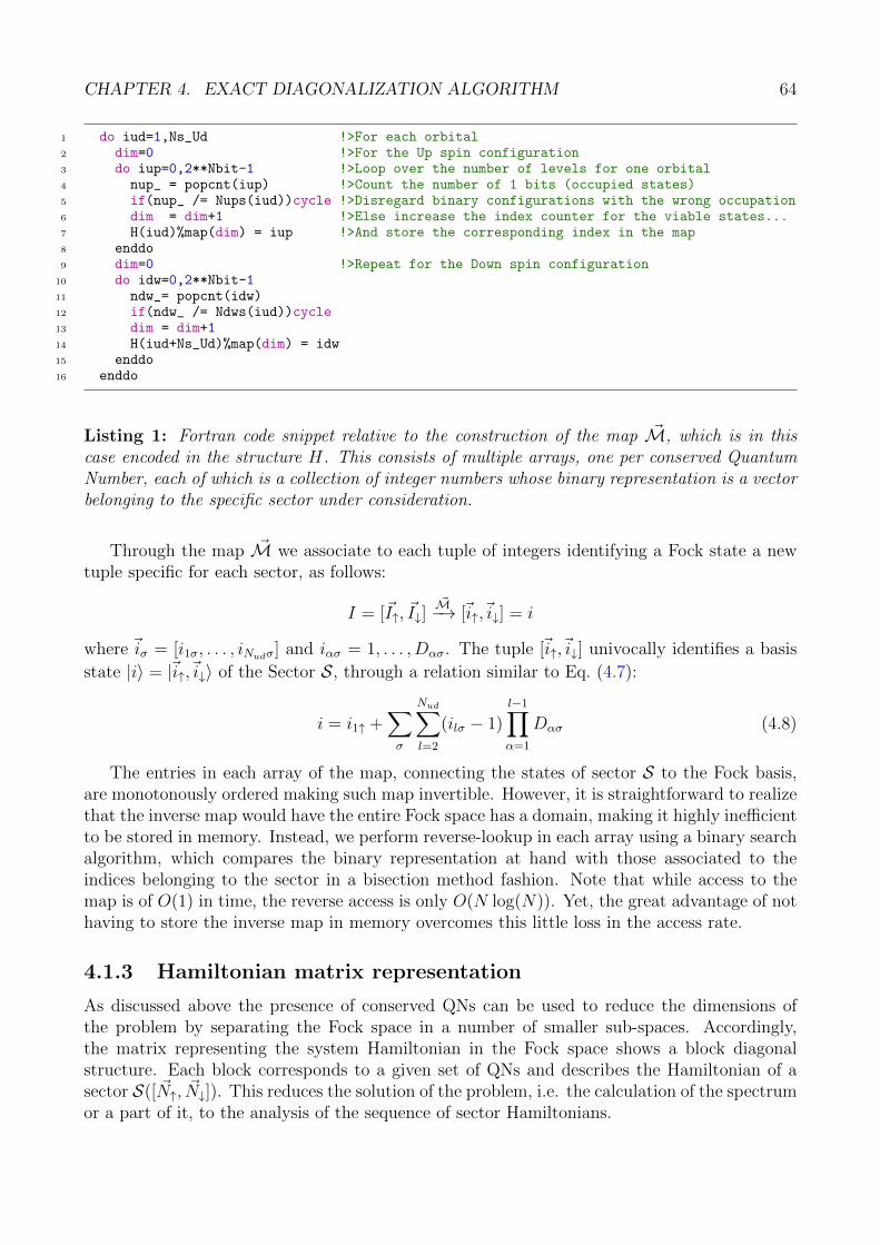
CHAPTER 4. EXACT DIAGONALIZATION ALGORITHM 64
1 do iud=1,Ns_Ud !>For each orbital2 dim=0 !>For the Up spin configuration3 do iup=0,2**Nbit-1 !>Loop over the number of levels for one orbital4 nup_ = popcnt(iup) !>Count the number of 1 bits (occupied states)5 if(nup_ /= Nups(iud))cycle !>Disregard binary configurations with the wrong occupation6 dim = dim+1 !>Else increase the index counter for the viable states...7 H(iud)%map(dim) = iup !>And store the corresponding index in the map8 enddo9 dim=0 !>Repeat for the Down spin configuration
10 do idw=0,2**Nbit-111 ndw_= popcnt(idw)12 if(ndw_ /= Ndws(iud))cycle13 dim = dim+114 H(iud+Ns_Ud)%map(dim) = idw15 enddo16 enddo
Listing 1: Fortran code snippet relative to the construction of the map ~M, which is in thiscase encoded in the structure H. This consists of multiple arrays, one per conserved QuantumNumber, each of which is a collection of integer numbers whose binary representation is a vectorbelonging to the specific sector under consideration.
Through the map ~M we associate to each tuple of integers identifying a Fock state a newtuple specific for each sector, as follows:
I = [~I↑, ~I↓]~M−→ [~i↑,~i↓] = i
where ~iσ = [i1σ, . . . , iNudσ] and iασ = 1, . . . , Dασ. The tuple [~i↑,~i↓] univocally identifies a basis
state |i〉 = |~i↑,~i↓〉 of the Sector S, through a relation similar to Eq. (4.7):
i = i1↑ +∑σ
Nud∑l=2
(ilσ − 1)l−1∏α=1
Dασ (4.8)
The entries in each array of the map, connecting the states of sector S to the Fock basis,are monotonously ordered making such map invertible. However, it is straightforward to realizethat the inverse map would have the entire Fock space has a domain, making it highly inefficientto be stored in memory. Instead, we perform reverse-lookup in each array using a binary searchalgorithm, which compares the binary representation at hand with those associated to theindices belonging to the sector in a bisection method fashion. Note that while access to themap is of O(1) in time, the reverse access is only O(N log(N)). Yet, the great advantage of nothaving to store the inverse map in memory overcomes this little loss in the access rate.
4.1.3 Hamiltonian matrix representation
As discussed above the presence of conserved QNs can be used to reduce the dimensions ofthe problem by separating the Fock space in a number of smaller sub-spaces. Accordingly,the matrix representing the system Hamiltonian in the Fock space shows a block diagonalstructure. Each block corresponds to a given set of QNs and describes the Hamiltonian of asector S([ ~N↑, ~N↓]). This reduces the solution of the problem, i.e. the calculation of the spectrumor a part of it, to the analysis of the sequence of sector Hamiltonians.

CHAPTER 4. EXACT DIAGONALIZATION ALGORITHM 65
In each sector, the Hamiltonian of the system has the following general form:
HS = Hd +H↑ ⊗ I↓ + I↑ ⊗H↓ +Hnd (4.9)
where Hd is a diagonal term containing the local part of the Hamiltonian and the density-density terms of the Kanamori interaction, the Hσ components describe all the hopping terms ofelectrons with spin σ =↑, ↓ and the term Hnd contains all the remaining non-diagonal elements,namely the spin-exchange and pair-hopping part of the Kanamori interaction.
1 do i=1,Dim !> Loop over the states of Sector S2 call state2indices(i,[DimUps,DimDws],Indices) !> Tuple decomposition of i3 do iud=1,Ns_Ud4 mup = Hs(iud)%map(Indices(iud)) !> Map iα,σ → Iασ5 mdw = Hs(iud+Ns_Ud)%map(Indices(iud+Ns_ud))6 Nups(iud,:) = Bdecomp(mup,Ns_Orb) !> Binary decomposition with Ns_Orb-bits7 Ndws(iud,:) = Bdecomp(mdw,Ns_Orb)8 enddo9 !> Insert element in position Hd(i, i)
10 enddo
Listing 2: Fortran code snipped relative to the Hamiltonian Hd construction.
Indeed, if the QNs are conserved per orbital, i.e. if Hnd ≡ 0 and no inter-orbital localhopping terms are present, Hσ further splits into a sum of smaller terms:
Hσ =Nα∑α=1
I1σ ⊗ · · · ⊗Hασ ⊗ · · · ⊗ INασ
The particular decomposition of the sector Hamiltonian in Eq. 4.9 has a twofold beneficeffect on the diagonalization procedure: the matrix-vector product operation is considerablysped up and the memory storage of the Hamiltonian matrix is greatly reduced.
In any given sector S, the Hamiltonian matrix is a square hermitian matrix of dimensionD2S . The overall low connectivity of the electronic systems we consider is reflected into a very
sparse nature of the Hamiltonian matrix, which hosts at most O(Ns) DS elements on eachrow. A suitable data structure can be designed to store all the non-zero elements value andpositions of such matrix, while keeping access along each row to order O(1). We achieve this byusing a suitable hash-table, set up as a set of 2DS rows with dynamic length separately holdingthe values and position of each entry. The memory cost of such sparse matrix storage wouldthen be bounded above by O(NsDS). Yet, this storage guarantees O(1) access to the matrixelement, which is a key feature in performing matrix-vector products.
However, thanks to the Hamiltonian structure in Eq. 4.9 we can achieve a further gainin the memory footprint storing each matrix component separately. The diagonal term Hd
corresponds to a single vector of length DS . The tensor product structure of the hoppingterms can be readily reconstructed by storing each Hασ in a tuple of sparse matrices, the totaldimension of which is at most of order O(NudNs max(Dασ)), in general much smaller thanO(NsDS). Finally, Hnd can only be stored as a separate sparse matrix with leading dimensionDS . However, this matrix has a very sparse nature containing at most few, i.e. of the order ofone or two, elements per row. Thus, its memory cost is well bounded.

CHAPTER 4. EXACT DIAGONALIZATION ALGORITHM 66
1 !> Loop over all conserved QNs for spin=↑, iorb= α2 do iorb=1,Ns_Ud3 !> Loop over the states/integers jα↑ for this component4 do jup=1,DimUps(iorb)5 !> Map jα↑ in the sector into Jα↑ in Fock space6 mup = Hs(iorb)%map(jup)7 !> Binary decomposition with Ns_Orb bits8 Nups(iorb,:) = bdecomp(mup,Ns_Orb)9 !... (condition for the finiteness of the hopping element)
10 !> Apply c†2c1|Jα↑〉 = |Iα↑〉11 call c(1,mup,k1,sg1)12 call cdg(2,k1,k2,sg2)13 !> Map back Iα↑ to iα↑14 iup = binary_search(Hs(iorb)%map,k2)15 !>16 !> Insert element in Hα↑(i, j)17 !...18 enddo19 enddo
Listing 3: Fortran code snippet related to the construction of the Hamiltonian term Hα↑
The construction of the Hamiltonian matrix is performed independently on each term, usingan iterative loop across the different components of the sector basis. Note that the constructionof the small matrices Hασ only involves loop over the components |iασ〉 of the sector basis:
〈~i↑~i↓|HS |~j↑~j↓〉 = 〈~i↑~i↓|Hd +H↑ ⊗ I↓ + I↑ ⊗H↓ +Hnd|~j↑~j↓〉= 〈~i↑~i↓|Hd|~i↑~i↓〉+ 〈~i↑~i↓|Hnd|~j↑~j↓〉+ 〈~i↑|H↑|~j↑〉δ~i↓~j↓ + δ~i↑~j↑〈~i↓|H↓|~j↓〉
(4.10)
As an example we report in the listings 2 and 3 a fragment of the code which build thediagonal matrix Hd and Hα↑, respectively.
Finally, it is worth observing that for very large systems storing the Hamiltonian matricesin the memory in highly inefficient. In such cases, we rely on a storage-free diagonalizationalgorithm which performs the necessary matrix-vector products on-the-fly, i.e. without storingthe sparse matrix. This algorithm has in general a considerably negative impact onto theexecution time, which however can be managed with a good scaling in a massively parallelframework.
4.1.4 The Lanczos method
The sector Hamiltonians thus obtained have now to be diagonalized in order to find the groundstate. One of the simplest and most widespread methods for the approximate solution ofan eigenvalue problem is the Lanczos method for hermitian matrices [110], which falls in thepreviously mentioned category of methods requiring a computationally demanding matrix-vector product as the only problem-dependent input. At its core, the method is an extensionof the steepest descent one, and amounts to a clever change of basis for the Hamiltonian, whichis then diagonalized in a subset of the new basis. The larger the subset, the more accurate theresult.
Let us consider a N ×N hermitian Hamiltonian; starting from a random normalized vector|v0〉 we construct the basis of the so-called Krylov space [112] asK = span|v0〉, H|v0〉, . . . , Hd|v0〉

CHAPTER 4. EXACT DIAGONALIZATION ALGORITHM 67
(where, crucially, d n) in the following way:
b1|v1〉 = H|v0〉 − a0|v0〉 (4.11)
and
b2|v2〉 = H|v2〉 −1∑i=0
|vi〉〈vi|H|v1〉 = H|v1〉 − a1|v1〉 − b1|v0〉 (4.12)
where all the vectors are normalized to 1 and the relevant parameters are an = 〈vn|H|vn〉 andbn, which is the norm of the unnormalized n-th basis vector. It is easy to prove that such basisvectors are orthogonal.
The key observation is that, from the fourth basis vector on, this construction method onlyinvolves the two preceding ones: as an example, for |v3〉 the i = 0 term of the sum in (4.12) is
〈v0|H|v2〉 = b1〈v1|v2〉+ a0〈v0|v2〉 = 0 (4.13)
as immediately follows from the hermiticity of the problem and from the definition and orthog-onality of the previously obtained vectors. This construction has two positive consequences:the expression of the Hamiltonian in the Krylov basis is tridiagonal and of the form
HK =
a0 b1 0 · · · 0b1 a1 b2 · · · 00 b2 a2 · · · 0...
......
. . ....
0 0 0 ad−1 bd0 0 0 bd ad
(4.14)
and the only quantities necessary to the determination of the ground state eigenvalue are thecoefficients an and bn, that can be easily stored. Indeed, if the eigenvalue is the only quantitywe are interested in, we will only need to keep in memory two vectors at a time, by virtue of thespecifics of the basis construction. Clearly, the approximation rapidly improves with increasingd, and convergence to the ground state is exponential, as proven by Kaniel and Paige [115].As previously stated, the pivotal part of the Lanczos method is the matrix-vector productcalculation. Note that, for a sparse system the matrix-vector product is an operation of orderO(n), with respect to a conventional order O(n2) of a dense matrix.
The simple Lanczos method, although powerful, suffers from several problems. The mostimportant is given by the emergence of the so-called ghosts states: spurious unphysical solutionsappearing as an effect of the lack of orthogonality in the numerically-determined Krylov basis.
To overcome this issues successive improvements of the Lanczos method have been devised.The most straightforward generalization is the so-called block Lanczos scheme. This featuresthe use of a collection of initial orthogonal vectors |v1〉, . . . , |vM〉 rather than a single one. Ateach step the Hamiltonian is multiplied by all the vectors, generating a much larger Krylov basisand faster tridiagonal reduction of the matrix itself. Imposing orthogonality across the blockvectors at each step ensure a more stable calculation and a reduction of the ghost problem. Afurther refinement of the methods is obtained performing a partial re-orthogonalization withinthe Krylov basis or using Arnoldi implicit restarting [111]. In the majority of cases, e.g. inabsence of severe degeneracies in the spectrum, these improvements guarantee a numericallyexact calculation of suitable parts of the spectrum at the price of a larger numerical cost
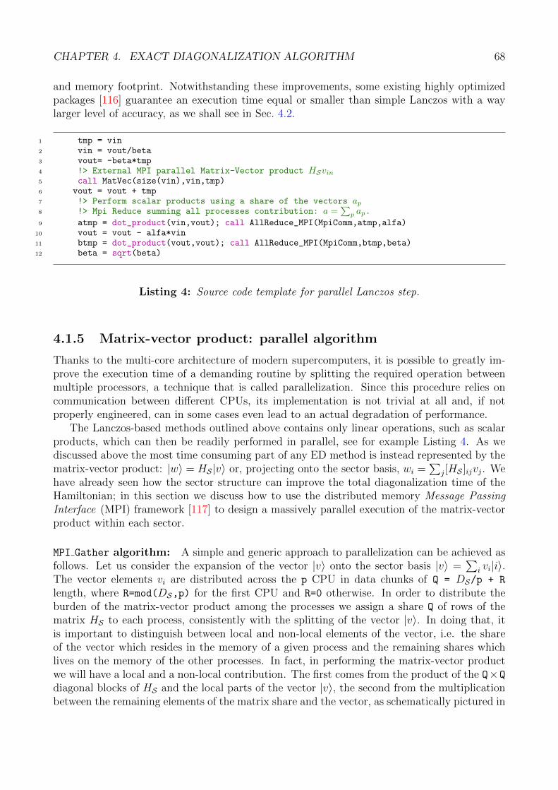
CHAPTER 4. EXACT DIAGONALIZATION ALGORITHM 68
and memory footprint. Notwithstanding these improvements, some existing highly optimizedpackages [116] guarantee an execution time equal or smaller than simple Lanczos with a waylarger level of accuracy, as we shall see in Sec. 4.2.
1 tmp = vin2 vin = vout/beta3 vout= -beta*tmp4 !> External MPI parallel Matrix-Vector product HSvin5 call MatVec(size(vin),vin,tmp)6 vout = vout + tmp7 !> Perform scalar products using a share of the vectors ap8 !> Mpi Reduce summing all processes contribution: a =
∑p ap.
9 atmp = dot_product(vin,vout); call AllReduce_MPI(MpiComm,atmp,alfa)10 vout = vout - alfa*vin11 btmp = dot_product(vout,vout); call AllReduce_MPI(MpiComm,btmp,beta)12 beta = sqrt(beta)
Listing 4: Source code template for parallel Lanczos step.
4.1.5 Matrix-vector product: parallel algorithm
Thanks to the multi-core architecture of modern supercomputers, it is possible to greatly im-prove the execution time of a demanding routine by splitting the required operation betweenmultiple processors, a technique that is called parallelization. Since this procedure relies oncommunication between different CPUs, its implementation is not trivial at all and, if notproperly engineered, can in some cases even lead to an actual degradation of performance.
The Lanczos-based methods outlined above contains only linear operations, such as scalarproducts, which can then be readily performed in parallel, see for example Listing 4. As wediscussed above the most time consuming part of any ED method is instead represented by thematrix-vector product: |w〉 = HS |v〉 or, projecting onto the sector basis, wi =
∑j[HS ]ijvj. We
have already seen how the sector structure can improve the total diagonalization time of theHamiltonian; in this section we discuss how to use the distributed memory Message PassingInterface (MPI) framework [117] to design a massively parallel execution of the matrix-vectorproduct within each sector.
MPI Gather algorithm: A simple and generic approach to parallelization can be achieved asfollows. Let us consider the expansion of the vector |v〉 onto the sector basis |v〉 =
∑i vi|i〉.
The vector elements vi are distributed across the p CPU in data chunks of Q = DS/p + R
length, where R=mod(DS,p) for the first CPU and R=0 otherwise. In order to distribute theburden of the matrix-vector product among the processes we assign a share Q of rows of thematrix HS to each process, consistently with the splitting of the vector |v〉. In doing that, itis important to distinguish between local and non-local elements of the vector, i.e. the shareof the vector which resides in the memory of a given process and the remaining shares whichlives on the memory of the other processes. In fact, in performing the matrix-vector productwe will have a local and a non-local contribution. The first comes from the product of the Q×Q
diagonal blocks of HS and the local parts of the vector |v〉, the second from the multiplicationbetween the remaining elements of the matrix share and the vector, as schematically pictured in

CHAPTER 4. EXACT DIAGONALIZATION ALGORITHM 69
X =
loc
loc
locnon-local
non-local
-localnon- +
H v w
loc non-local
a) b)
Figure 4.1: Schematic representation of the parallel execution of the HS |v〉 matrix-vectorproduct. The vector is distributed onto the different process. Similarly, a share of the rowsof the matrix are stored on each process, dividing the local part of the diagonal block fromthe remaining entries. The MPI AllGatherV procedure is used to aggregate the vector beforeperforming the product.
Fig. 4.1. While the first part of the product can be executed locally on each process, the secondpart requires to reconstruct the distributed vector |v〉. This is achieved using the MPI functionMPI AllGatherV, which involves the communication of the vector share from each process toall the other processes. The implementation of this algorithm is reported in listing 5.
The analysis of the parallel scaling of algorithm 5 however reveals a major flaw. Uponincreasing the number of MPI processes p, the gain deriving from the decreased size Q of thevector share (' 1/p) is rapidly balanced and overcome by the inter-processors communication inMPI AllGatherV. Each call to this MPI procedure requires a massive amount of data transferacross all processors, which is the main bottleneck of the algorithm. Such communicationcongestion ultimately prevents to achieve an optimal parallel scaling. In practice, under normalconditions the speed up already saturates for a number of processes of the order of ten.
MPI AlltoAll algorithm: A much better parallelization procedure can be devised by exploit-ing the setup we introduced above. First we observe that, in the sector basis |~i↑~i↓〉, a genericvector |v〉 can be decomposed as:
|v〉 =∑i
vi|i〉 =∑~i↑~i↓
α~i↑α~i↓|~i↑~i↓〉 =
D↑∑i↑=1
D↓∑i↓=1
αi↑αi↓|i↑〉|i↓〉 (4.15)
where each parameter α~iσ is a tuple of complex numbers given by the projections of the vector|v〉 onto each of the element of the basis, i.e. 〈v|iασ〉. In the last equality we rearranged theterms noting that, using the relation (4.8), the tuples α~i↑α~i↓ and the states |~i↑~i↓〉 can be recast,
respectively, in a couple of scalars α↑α↓ and states of the form |i↑〉|i↓〉. The sector basis statesare ordered so that the spin-↑ index runs faster than the spin-↓ one. We can then rearrange

CHAPTER 4. EXACT DIAGONALIZATION ALGORITHM 70
1 !> MatVec(Nloc,v,Hv)2 MpiShift = spH0%Ishift !shift the total index to the process index3 Hv=0d04 !> The size of the diagonal block (Q in the text)5 do i=1,Nloc6 !> Run through the nonzero elements stored in the sparse matrix structure's7 !> local component8 do j=1,spH0%loc(i)%Size9 Hv(i) = Hv(i) + spH0%loc(i)%vals(j)*v(spH0%loc(i)%cols(j)-MpiShift)
10 end do11 end do12 !13 !> Non-Local part: auxiliary indices for vector gathering14 allocate(Counts(0:MpiSize-1)) ; Counts(0:)=015 allocate(Offset(0:MpiSize-1)) ; Offset(0:)=016 Counts(0:) = N/MpiSize17 Counts(MpiSize-1) = N/MpiSize+mod(N,MpiSize)18 do i=1,MpiSize-119 Offset(i) = Counts(i-1) + Offset(i-1)20 enddo21 allocate(vin(N)) ; vin = zero22 !> Gather the vector on each core23 call MPI_Allgatherv(&24 v(1:Nloc),Nloc,MPI_Double_Complex,&25 vin ,Counts,Offset,MPI_Double_Complex,&26 MpiComm,MpiIerr)27 !> Perform the matrix-vector product for the nonlocal part28 do i=1,Nloc29 matmul: do j=1,spH0%row(i)%Size30 Hv(i) = Hv(i) + spH0%row(i)%vals(j)*vin(spH0%row(i)%cols(j))31 end do matmul32 end do
Listing 5: Source code for the parallel execution of the matrix-vector product using theMPI AllGatherV procedure, a schematic view of which is presented in Fig. 4.1
the representation of any vector |v〉 in terms of a matrix, whose columns correspond to a set ofspin-↑ components for a given fixed spin-↓ configuration:
vii=1,...,D↑D↓.=
α1↑α1↓...
αD↑α1↓...
α1↑αD↓...
αD↑αD↓
=
α1↑α1↓ α1↑α2↓ . . . α1↑αD↓
α2↑α1↓ α2↑α2↓ . . . α2↑αD↓
. . . . . .αD↑α1↓ αD↑α2↓ . . . αD↑αD↓
(4.16)
Here lies a great simplification in the product with the Hamiltonian (4.9). In particular,exploiting the decomposition in (4.10), we can design a massively parallel algorithm for thematrix-vector product which overcomes the severe limitations related to the inter-processorscommunication.
To begin with, we distribute the vector parameters across the MPI processes. We assignto each process a number Q↓ = D↓/p of columns. The rest R↓ = mod(D↓, p), if present, is

CHAPTER 4. EXACT DIAGONALIZATION ALGORITHM 71
1↑1↓ 2↑1↓ 3↑1↓
1↑1↓ 2↑1↓ 3↑1↓
1↑2↓ 2↑2↓ 3↑2↓
2↑2↓ 3↑2↓1↑2↓
1↑3↓ 2↑3↓ 3↑3↓ 1↑4↓ 2↑4↓ 3↑4↓
1↑3↓ 1↑4↓ 2↑3↓ 2↑4↓ 3↑3↓ 3↑4↓
V
V'
MPI_transpose
1↑1↓ 1↑2↓ 1↑3↓ 1↑4↓
2↑1↓ 2↑2↓ 2↑3↓ 2↑4↓
3↑1↓ 3↑2↓ 3↑3↓ 3↑4↓
1↑1↓ 2↑1↓ 3↑1↓
1↑2↓ 2↑2↓ 3↑2↓
1↑3↓ 2↑3↓ 3↑3↓
1↑4↓ 2↑4↓ 3↑4↓
H↓1↑1↓ 1↑2↓ 1↑3↓ 1↑4↓
2↑1↓ 2↑2↓ 2↑3↓ 2↑4↓
3↑1↓ 3↑2↓ 3↑3↓ 3↑4↓
V VT (H↓VT)T
MPI_transpose
a)
b)
Figure 4.2: Schematic representation of the parallel execution of the H|v〉 matrix-vector prod-uct for the ↓ spin. For sake of simplicity we indicate each component component ai↑ai↓ using itssubscripts i↑i↓ only. a) Schematic representation of the MPI AlltoAllv execution on a vectorwith D↑ = 3, D↓ = 4. The different main colors of the blocks represents the parts of the vectorhandled by different processes p = 4. The transformed vector V
′has contiguous elements in the
memory along the ↓ index. b) Representation of the matrix-vector H↓ · v product based on theparallel transposition of the input vector and its resultant as described in listing 6.
reassigned to the first R↓ processes. Differently to the previous case, this partitioning of thematrix corresponds to distributing Q = D↑ × Q↓ vector elements to each process.
Each term in (4.10) contributing to the matrix-vector product is then separately evaluatedas follows:
Hd: the diagonal term Hd of the Hamiltonian is scattered among processes, assigning Q rows,i.e. elements, to each CPU. Notably, the multiplication Hd|v〉 takes place locally in the memoryon each process, i.e. with no need of further MPI communication.
H↑ ⊗ I↓: The matrix-vector product with of the term H↑⊗ I↓ involves only ↑-electrons config-urations. This corresponds to run along the elements of each column of the matrix defined in(4.16). Within our MPI decomposition, these elements are stored contiguously in the memoryof each process. As such, like for the diagonal part, this term of the product is performedlocally in the memory, provided the (small) Hamiltonian H↑ is known to each process.

CHAPTER 4. EXACT DIAGONALIZATION ALGORITHM 72
I↑ ⊗H↓: The multiplication with the term I↑ ⊗ H↓ involves only spin-↓ configurations. Thiscorresponds to run along the rows of the matrix (4.16), which ultimately leads to a highlynon-local access to the memory. In a serial implementation this introduces only a small perfor-mance degradation due to irregular cache access. However, in a parallel setup such non-localityrepresents a serious possible bottleneck, since heavy MPI communication is necessary to trans-fer columns among different processes. A simple, yet effective, solution to this problem is toexchange the ↑- and ↓-electrons indices [~i↑,~i↓]→ [~i↓,~i↑]. This corresponds to a transposition ofthe matrix (4.16). As a consequence, the matrix-vector product is performed by running overcolumns of the transposed matrix thus recovering the locality in the memory. The collectivetransposition of a data set requires a suitable all-to-all communication. To this purpose, theMPI library makes available a parallel procedure, MPI AlltoAllv [109, 117], which transfersdata such that the j-block, sent from the process i, is received by process j and placed as blocki. The corresponding communication pattern is schematically depicted in Fig. 4.2a. Althoughapparently heavy, the communicational burden involved in the interexchange of data amongall processes in MPI AlltoAllv involves the minimum amount of data transfer. As such, weexpect this operation to unlock excellent parallel scaling.
A template of the source code for this task is shown in listing 6: we first determine (lines5-10) the number of elements to send for each process. By construction the amount of datato be received in the transposed buffer is obtained by transposing the Sendcounts array itself,(lines 11-13). The relative offset is quickly evaluated summing over the number of elementsto send/receive, see lines 15-28. We perform the matrix transposition proceeding column-by-column, see lines 30-35. Note that some process may run out of columns to send because ofthe incommensurability of the matrix size with the number of processes. In this case MPIallows sending empty arrays. The final array is arranged in row-major mode, as such a localtransposition (within each process) is required to reorder the data in column-major mode [109].
The resulting matrix-vector product of the ↓-electrons part of the Hamiltonian proceeds inthree steps: i) the vector |v〉 is transposed using collective MPI communication; ii) multiplica-tion is performed locally on each process; iii) the resulting vector is transposed back and addedup to the result. A template of the source code for the spin-↓ matrix-vector product is reportedin listing 7.
Hnd: Finally we need to take care of the non-diagonal term Hnd in the sector Hamiltonian.This matrix, which contains the few elements coming from spin-exchange and pair-hoppingterms of the Kanamori interaction, can not be reduced to any favourable form to perform aparallel matrix-vector product. For this term we need to rely on the less-scalable MPI Gather-algorithm. As discussed above, this amount to perform a collective gathering of the distributedvector, while the Hnd matrix gets row-distributed among all processes. As we will see in the nextsection, the inclusion of this term leads to a dramatic reduction of the parallel scalability of thealgorithm, yet a substantial gain is achieved for a reasonable number of processes. However, thisconsideration offers a valid (though admittedly operational) reason to choose, where possible,the density-density Kanamori as the full expression for the interaction.
4.2 Benchmarks
In this section we present some benchmark results for the massively parallel ED algorithmoutlined above. The calculations have been performed on the Ulysses HPC in Trieste, using

CHAPTER 4. EXACT DIAGONALIZATION ALGORITHM 73
1 counts = Nrow/MpiSize2 Ntot = Ncol/MpiSize; if(mod(Ncol,MpiSize)/=0)Ntot=Ntot+13 !4 do i=1,qcol5 do irank=0,MpiSize-16 send_counts(irank,i) = counts7 if(irank < mod(Nrow,MpiSize))send_counts(irank,i) = counts+18 enddo9 enddo
10 do i=1,Ntot11 call MPI_AllToAll(send_counts(0:,i),1,MPI_INTEGER,&12 recv_counts(0:,i),1,MPI_INTEGER,&13 MpiComm,ierr)14 enddo15 !16 do i=1,Ntot17 do irank=1,MpiSize-118 send_offset(irank,i) = send_counts(irank-1,i) + send_offset(irank-1,i)19 enddo20 enddo21 recv_offset(0,1) = 022 do i=2,Ntot23 recv_offset(0,i) = sum(recv_counts(0,:i-1))24 enddo25 do i=1,Ntot26 do irank=1,MpiSize-127 recv_offset(irank,i) = recv_offset(irank-1,i) + sum(recv_counts(irank-1,:))28 enddo29 enddo30 !31 do j=1,Ntot32 call MPI_AllToAllV(&33 A(:,j),send_counts(:,j),send_offset(:,j),MPI_DOUBLE_PRECISION,&34 B(:,:),recv_counts(:,j),recv_offset(:,j),MPI_DOUBLE_PRECISION,&35 MpiComm,ierr)36 enddo37 call local_transpose(b,ncol,qrow)
Listing 6: Source code for the MPI transpose routine referenced in Fig. 4.2b.
Intel Xeon E5-2680 v2 processors with 2 sockets, 10 cores, 2 threads per core and 40 GB RAM.We considered a multi-orbital single impurity Anderson model with a total of Ns sites, usingrandom energies levels for the effective bath and constant hopping amplitude. The tests havebeen executed in the half-filling sector n↑ = n↓ using total spin-dependent occupation QNs.This setup corresponds to the worst case scenario for our implementation. We evaluated thelowest state of the spectrum using the Lanczos algorithm. In order to reduce the intrinsic errors,we performed repeated calculation for each set of parameters. The data presented below havebeen averaged over such repeated calculations.
To begin with, we analysed the net speed-up of the diagonalization algorithm. The resultsare reported in Fig. 4.3 for an increasing number of total electronic levels Ns. For small systems,i.e. Ns = 12, the speed-up saturates for a number of CPU n > 300. This should be associated tothe ratio between calculation and communication time which, for such a small system, quicklybecomes unfavourable. The situation gradually improves for larger systems. In particular, weobserved a sub-ideal scaling for Ns = 15 with a slight tendency to saturation only for the largest

CHAPTER 4. EXACT DIAGONALIZATION ALGORITHM 74
1 mpiQup=DimUp/MpiSize2 if(MpiRank<mod(DimUp,MpiSize))MpiQup=MpiQup+13 !> Get transposed input vector:4 call vector_transpose_MPI(DimUp,MpiQdw,v,DimDw,MpiQup,vt)5 !> Execute product: local and contiguous in memory.6 Hvt=0d07 do idw=1,MpiQup !<= Transposed order: column-wise DW <--> UP8 do iup=1,DimDw !<= Transposed order: column-wise DW <--> UP9 i = iup + (idw-1)*DimDw
10 hxv_dw: do jj=1,spH0dws(1)%row(iup)%Size11 jup = spH0dws(1)%row(iup)%cols(jj)12 jdw = idw13 j = jup + (jdw-1)*DimDw14 val = spH0dws(1)%row(iup)%vals(jj)15 Hvt(i) = Hvt(i) + val*vt(j)16 end do hxv_dw17 enddo18 end do19 !> Transpose back result:20 call vector_transpose_MPI(DimDw,mpiQup,Hvt,DimUp,mpiQdw,vt)21 !> Add up.22 Hv = Hv + Vt
Listing 7: Source code for the parallel matrix-vector product of the spin-↓ part of the sectorHamiltonian with a given input vector.
accessible number of processes (see inset). For Ns = 18 the scaling remains nearly ideal up ton > 200.
Next, to test the solidity of the scaling with respect to the intrinsic properties of the Lanczosalgorithm, we compared a rather simple Lanczos implementation with respect to a fully fledgedParallel-ARPACK method [118]. The memory footprint, as well as the number of matrix-vector operations, can be dramatically different for the two methods. In particular, for the P-ARPACK calculations we used a block of ncv = 10 vectors. As such one can in principle expecta dramatically different scaling behavior. Yet, the results reported in the left panel of Fig. 4.4,showing the behavior of the total elapsed time as a function of the CPU number, reveal thatthe scaling of the two methods is very similar (i.e. the same order of magnitude). Interestingly,despite its higher complexity, the more optimized P-ARPACK algorithm performed consistentlybetter than the simple and less-optimized Lanczos method.
An important aspect to consider, in anticipation of the analysis of the next chapters, is thescaling behaviour with respect to the number of orbitals. The presence of multiple orbitalsintroduces two major changes in the Hamiltonian. The first is in the interaction term. Thedensity-density terms of the interactions are diagonal and, thus, do not affect the scaling. Onthe contrary, the pair-hopping and spin-exchange can have a dramatic impact on the parallelexecution, thus we neglect such term for now and postpone the analysis of their influence tothe next paragraphs. The second change affects the hopping terms. In a multi-orbital systemthe hopping matrices generally include more values than the single orbital, due to the presenceof several hopping channels among orbitals.In order to characterize this aspect, we studied the scaling of the algorithm as a function ofincreasing orbital number. In the right panel of Fig. 4.4 we show the evolution of the timeper Lanczos iteration as a function of the CPU number, for a system of Ns = 15 and different

CHAPTER 4. EXACT DIAGONALIZATION ALGORITHM 75
100 200 300n [cpu]
0
50
100
150
200
250
T1/T
n[M
PI
gain
]
IdealN
s=12
Ns=15
Ns=18
64 128 256 512
n
0
100
200
300
400
T1/T
n
Figure 4.3: Speedup for a system of a Ns-level system as a function of the number of CPUused, as compared to an ideal (linear) scaling. In the inset a wider range of CPUs is plotted forNs = 15 using a log-scale along the x-axis. The result shows the saturation of the parallel gainfor n > 512.
number of orbitals. Our results show that the single Lanczos iteration time is essentiallyindependent of the number of orbitals. However, as shown in the inset of the figure, the numberof iterations required to determine the lowest eigenstate increases linearly with the number oforbitals. We conclude that, although the resulting total time has an excellent sub-linear scalingwith the number of processes, it linearly depends on the number of orbitals, i.e. the more theorbitals the larger the solution time for a fixed number of processes.
Finally, we characterized how the inclusion of non-diagonal terms of in the sector Hamilto-nian affect the scaling behavior of our algorithm. As we discussed above, terms like pair-hoppingand spin-exchange cannot be reduced to hopping events involving the single spin orientation.As such we can not take advantage of the special properties of the basis states to perform theparallel matrix-vector product. This is expected to largely affect the nearly optimal scalingobserved for the case of density-density interaction only. In order to quantify this effect wereport in Fig. 4.5 the speed-up as a function of the CPU number comparing density-densityand full Kanamori interactions in two systems with three and five orbitals. In agreement withprevious results, the density-density interaction gives rise to a sublinear scaling, which tendsto saturates at n > 600 processes. For the full Kanamori case the behavior is very different.An initial good speed-up obtained with few tens of processes, rapidly saturates to a value of50− 75 for any number of CPU n > 100. In fact, above this threshold the burden of the MPIcommunication needed to reconstruct the vector and perform the matrix-vector product forHnd becomes predominant and prevents further improvement of the scaling.
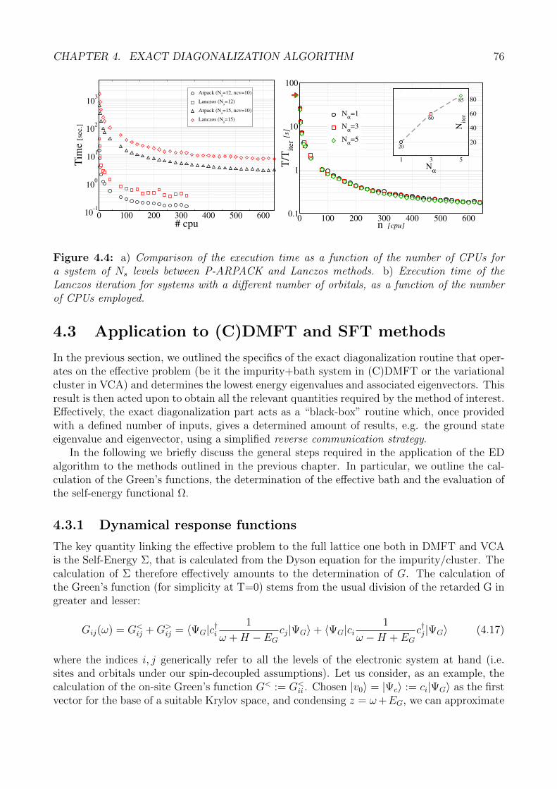
CHAPTER 4. EXACT DIAGONALIZATION ALGORITHM 76
0 100 200 300 400 500 600# cpu
10-1
100
101
102
103
Tim
e [s
ec.]
Arpack (Ns=12, ncv=10)
Lanczos (Ns=12)
Arpack (Ns=15, ncv=10)
Lanczos (Ns=15)
0 100 200 300 400 500 600n [cpu]
0.1
1
10
100
T/T
iter
[s]
Nα=1
Nα=3
Nα=5
20
60
85
1 3 5
Nα
20
40
60
80
Nit
er
Figure 4.4: a) Comparison of the execution time as a function of the number of CPUs fora system of Ns levels between P-ARPACK and Lanczos methods. b) Execution time of theLanczos iteration for systems with a different number of orbitals, as a function of the numberof CPUs employed.
4.3 Application to (C)DMFT and SFT methods
In the previous section, we outlined the specifics of the exact diagonalization routine that oper-ates on the effective problem (be it the impurity+bath system in (C)DMFT or the variationalcluster in VCA) and determines the lowest energy eigenvalues and associated eigenvectors. Thisresult is then acted upon to obtain all the relevant quantities required by the method of interest.Effectively, the exact diagonalization part acts as a “black-box” routine which, once providedwith a defined number of inputs, gives a determined amount of results, e.g. the ground stateeigenvalue and eigenvector, using a simplified reverse communication strategy.
In the following we briefly discuss the general steps required in the application of the EDalgorithm to the methods outlined in the previous chapter. In particular, we outline the cal-culation of the Green’s functions, the determination of the effective bath and the evaluation ofthe self-energy functional Ω.
4.3.1 Dynamical response functions
The key quantity linking the effective problem to the full lattice one both in DMFT and VCAis the Self-Energy Σ, that is calculated from the Dyson equation for the impurity/cluster. Thecalculation of Σ therefore effectively amounts to the determination of G. The calculation ofthe Green’s function (for simplicity at T=0) stems from the usual division of the retarded G ingreater and lesser:
Gij(ω) = G<ij +G>
ij = 〈ΨG|c†i1
ω +H − EGcj|ΨG〉+ 〈ΨG|ci
1
ω −H + EGc†j|ΨG〉 (4.17)
where the indices i, j generically refer to all the levels of the electronic system at hand (i.e.sites and orbitals under our spin-decoupled assumptions). Let us consider, as an example, thecalculation of the on-site Green’s function G< := G<
ii . Chosen |v0〉 = |Ψc〉 := ci|ΨG〉 as the firstvector for the base of a suitable Krylov space, and condensing z = ω+EG, we can approximate

CHAPTER 4. EXACT DIAGONALIZATION ALGORITHM 77
100 200 300 400 500 600#cpu
0
50
100
150
200
250
300
T1/T
n
α=3, Density-Density
α=5, Density-Density
α=3, Full Kanamori
α=5, Full Kanamori
10 100 1000
# cpu
10
100
1000
10000
T (
s)
Figure 4.5: Speedup of the parallel method with respect to the ideal scaling (dotted blue lune)for a system with α orbitals and different forms of the interaction: while the density-densityKanamori scales sub-linearly, the inclusion of Hnd quickly saturates the gain.
the Green’s function as
G<(ω) ≈⟨
Ψc
∣∣∣∣ 1
z −HK
∣∣∣∣Ψc
⟩=
Nlanc∑n=0
〈Ψc|Ψn〉〈Ψn|Ψc〉ω − En + EG
(4.18)
where En and |Ψn〉 are the first Nlanc approximated eigenvalues and eigenvectors of the originalproblem obtained by Lanczos and HK is the associated tridiagonal matrix. Evidently, there isan abuse of notation in (4.18), since the dimensions of Ψc and HK do not in general check out.Let us however assume the Krylov space has the same dimension as the original one (meaningthe Lanczos approximation is now simply a change of basis): in order to calculate the Green’sfunction, we are only interested in the element (z −HK)−1
00 which, from Cramer’s theorem andthe Laplace formula for determinants, can be found from the solution of the continuous fraction
1
z − a0 −b2
1
ω − a1 −b2
z − a2 − ...
. (4.19)
In practice, a truncation will happen at the Nlanc-th element, restoring the approximation.There is an alternative way of calculating the Green’s function [109, 119], which will provehandy in storing the minimal amount of information required to recover the full form of Gat any frequency. The spectral representation of the Green’s function is indeed the simple

CHAPTER 4. EXACT DIAGONALIZATION ALGORITHM 78
collection of poles
G<(ω) =
Nlanc∑n=0
|ψ0n|2
ω − En + EG(4.20)
where ψln is the l-th component of the of the n-th eigenvector of the tridiagonal matrix (4.14)and |vl〉 is the Lanczos basis constructed from |Ψc〉. As a consequence of the Lanczos procedureit holds, for the n-th approximated eigenvector of the problem,
|Ψn〉 =
Nlanc∑l=0
ψln|vl〉. (4.21)
The matrix element 〈Ψc|Ψn〉 in (4.18) is therefore ψ0n, and the Green’s function can thus be
recovered: starting from the Ground State eigenvector of the effective problem, resulting fromexact diagonalization, we obtain the starting Lanczos vector |Ψc〉 by applying the annihilationoperator in the same way as previously described. The operator is applied by a single core, andthe resulting vector is then broadcast to all the other ones. The parallel Lanczos tridiagonal-ization procedure outlined in listing 4 is then invoked, and the diagonal a and subdiagonal b ofHK are obtained. The Lanczos matrix is then exactly diagonalized to retrieve the eigenvaluesEn and the eigenvector matrix Z, whose first row is made up of the needed ψ0
n coefficients. Thereduced size of the Lanczos matrix makes it viable to use serial exact diagonalization proceduresto this end. The Green’s function is then calculated as a simple sum of poles, given by theeigenvalues, weighted by the ψ coefficients. The same procedure (with opposite sign on E atthe denominator) is performed for the greater G.Both the continuous fraction and spectral sum approaches rely on the fact that |Ψc〉 appearsin both bra and ket in equation (4.18). However, in the multi-orbital and cluster cases, G isactually a matrix with nondiagonal entries which also have to be calculated. A clever trick toachieve this goal is to consider the response function defined as
G+(ω) = 〈ΨG|(c†i + c†i )1
ω +H − Eg(ci + ci)|ΨG〉 (4.22)
(where i, j are the generic site-orbital indices) and then obtaining, from it and the previouslycalculated diagonal components, the off-diagonal part as
Gij(ω) =1
2
(G+(ω)−Gii(ω)−Gjj(ω)
)(4.23)
This equation works if we assume Gab = Gba. Under the more general hypothesis where thisdoesn’t hold we have to calculate the two auxiliary Green’s functions
G1(ω) = 〈ΨG|(c†i + c†j)1
ω +H − Eg(ci + cj)|ΨG〉 (4.24)
and
Gi(ω) = 〈ΨG|(c†i − ic†j)
1
ω +H − Eg(ci + icj)|ΨG〉 (4.25)
to obtain
Gij(ω) =1
2
(G1(ω) +Gi(ω)− (1− i)Gii(ω)− (1− i)Gjj(ω)
)(4.26)
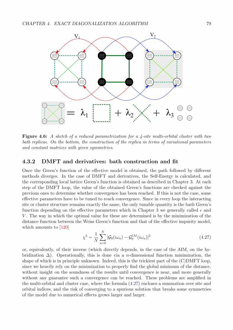
CHAPTER 4. EXACT DIAGONALIZATION ALGORITHM 79
V1 V2
= λ1 + λ2 + λ3
Figure 4.6: A sketch of a reduced parametrization for a 4-site multi-orbital cluster with twobath replicas. On the bottom, the construction of the replica in terms of variational parametersand constant matrices with given symmetries.
4.3.2 DMFT and derivatives: bath construction and fit
Once the Green’s function of the effective model is obtained, the path followed by differentmethods diverges. In the case of DMFT and derivatives, the Self-Energy is calculated, andthe corresponding local lattice Green’s function is obtained as described in Chapter 3. At eachstep of the DMFT loop, the value of the obtained Green’s functions are checked against theprevious ones to determine whether convergence has been reached. If this is not the case, someeffective parameters have to be tuned to reach convergence. Since in every loop the interactingsite or cluster structure remains exactly the same, the only tunable quantity is the bath Green’sfunction depending on the effective parameters which in Chapter 3 we generally called ε andV . The way in which the optimal value for these are determined is by the minimization of thedistance function between the Weiss Green’s function and that of the effective impurity model,which amounts to [120]
χ2 =1
N
N∑n=0
|G0(iωn)− GIM0 (iωn)|2 (4.27)
or, equivalently, of their inverse (which directly depends, in the case of the AIM, on the hy-bridization ∆). Operationally, this is done via a n-dimensional function minimization, theshape of which is in principle unknown. Indeed, this is the trickiest part of the (C)DMFT loop,since we heavily rely on the minimization to properly find the global minimum of the distance,without insight on the soundness of the results until convergence is near, and more generallywithout any guarantee such a convergence can be reached. These problems are amplified inthe multi-orbital and cluster case, where the formula (4.27) encloses a summation over site andorbital indices, and the risk of converging to a spurious solution that breaks some symmetriesof the model due to numerical effects grows larger and larger.

CHAPTER 4. EXACT DIAGONALIZATION ALGORITHM 80
For the single-site case, the usual form of the Anderson impurity model requires a bath madeup of different decoupled levels, with hybridization between each level and the interacting ef-fective system. In the case of many orbitals, each bath site has the same internal structure ofthe interacting site. Considering the number of hybridization parameters, this amounts to atotal of (Nbath+1) ·Norb variables to be fitted, with the number doubling if we consider distinctspins. We can restrict the parametrization by imposing, between the orbitals, every symmetrythe original lattice system exhibits, thereby having to fit only a fraction of the total number ofparameters. While this may not be a huge computational relief, we are effectively preventingany unwanted loss of symmetry due to numerical effects.The situation becomes more complicated in the cluster case, where each interacting site in thecluster in principle has an hybridization V with each bath site. A great simplification, thatpreserves the symmetries of the model and reduces the number of fit parameters, comes fromthe so-called reduced or constrained parametrization [121] which trades the diagonal form of thebath on-site energies for that of the hybridization matrix V . The bath is made up of “replica”clusters (cfr. Fig. 4.6) of the same size of the interacting one, and each interacting site coupleswith its counterpart in the i-th replica with the same amplitude Vi. The complexity is shiftedinto the replicas, which now have an internal hopping structure that, to preserve the symmetriesof the model, can be chosen to mimic that of the interacting cluster. The way this is realizedin practice is by implementing a bath replica structure of the type
Hbath =∑i
λiOi (4.28)
where λi are real parameters and Oi are constant matrices that couple to each parameterso that the final form of Hbath is that of an Hermitian hopping matrix of our choice. This isextremely convenient, since the minimization routine will always act on a real vector and we canin principle choose what part of lattice hopping Hamiltonian we want the replicas to possess,enhance or suppress. The explicit expression of the bath makes it also easier to calculate thegradient of the χ2 function, which is required by any conjugate-gradient-based minimizationroutine. In fact, considering the properties of the derivative of the inverse of a matrix, weobtain for the hybridization function ∆, identifying the vector of parametersV, λ := x,
d∆
dx=
d
dx
∑i
V 2i
(ε+ µ)I−∑
j λjOj
=
[2Vi
(ε+ µ)I−∑
j λjOj
i
,
V 2i
1
(ε+ µ)I−∑
j λjOjOi
1
(ε+ µ)I−∑
j λjOj
i
] (4.29)
and the gradient of the Weiss Green’s function by definition is simply
dG0
dx= −G−1
0
(− d∆
dx
)G−1
0 (4.30)
Through this expression, the exact gradient of the function χ2 can be calculated, and thefunction itself minimized with respect to the parameters V, λ. The Exact Diagonalizationroutine will then be called with the updated bath Hamiltonian, and so on until convergence isreached.

CHAPTER 4. EXACT DIAGONALIZATION ALGORITHM 81
4.3.3 VCA: calculation of Ω
In VCA, the main output of the ED routine we are interested in is the full Green’s function ofthe reference cluster: in fact, the goal of the method is the derivation of the Ω potential fromthe expression
Ω = Ω′ − Tr log(G−1
0 −Σ)
+ Tr log(G
′−10 −Σ
)(4.31)
where the trace is intended over k-points, residual degrees of freedom (orbitals, spin ecc.) andMatsubara frequencies. Through some algebraic manipulation [98] and making use of Dyson’sequation for the reference system, the operational form of the previous equation becomes
Ω = EGScluster −
1
π
∫ ∞0
dω∑k
log
∣∣∣∣det
(I +(H′ + ∆(ω)−H(k)
)G′(iω)
)∣∣∣∣ (4.32)
where G′(ω) is the cluster Green’s function as derived in the previous section, ∆(ω) is thehybridization function of the “dummy” bath (if present), H′ and H(k) are the hopping matricesappearing in G′0 and G0 respectively, expressed in the mixed representation outlined in Chapter3, and k lives in the Reduced Brillouin Zone.This equation can then be solved in two ways: the first is analytical, and involves explicitlycalculating the integral over the Matsubara frequencies obtaining [122]
Ω = Ω′ −∑ω′r<0
ω′r +
∫RBZ
∑ωr(k)<0
ωr(k) (4.33)
where ω and ω′ are the poles of the full lattice Green’s function and the cluster one in Lehmannrepresentation. While the first sum is rapidly obtained, the second entails the calculation of thepoles of the Green’s function G(k) = (G0(k)−Σ)−1 for each k-point in the reduced Brillouinzone through a method similar to the one outlined in the previous section, which is a processof order NkN
3lanc [98]. As discussed by Senechal, and proven via direct calculation [123], a
generally faster way of calculating the Ω functional is a direct numerical computation of thesum over k-vectors in the RBZ (obtained through a fixed or dynamically adjustable mesh)followed by an integration, again numeric, on the frequency axis.This method is in particular suited to our way of recovering the Green’s function G′(iω). Oncethe Green’s function’s weight and poles have been found, with the process previously described,the value of G at any frequency is obtained via a simple summation. Then, we can collect allthe Green’s functions weights and poles decomposition into a suitable data structure in orderto to make the calculation of G′(iω) readily available through a single function call. As this isthe only interacting quantity appearing under the integral in (4.32), no other diagonalizationprocedure is required, apart from the calculation of the determinant of a comparatively tinymatrix.The numerical integration over frequencies can be easily taken care of by functions such as QAGI,belonging to the QUADPACK library [124], addressing integration on semi-infinite or infiniteintervals. The finite T case, where Matsubara frequencies are discrete, requires the calculationof more than one Lanczos eigenvalues and eigenvectors (which is well in the capability ofARPACK) and some non cataclysmic modifications to the routine, as detailed in [125].
In VCA, the whole ED routine has as main aim the calculation of the scalar quantity Ω.Therefore, all the above described procedures can be seen as an overall function Ω = Ω(−→x )where −→x is the full set of variational parameters considered.

CHAPTER 4. EXACT DIAGONALIZATION ALGORITHM 82
The solution of the method will therefore be given by a wrapping minimization function, rangingfrom simple one-dimensional Brent methods, to multidimensional simplex or conjugate-gradienttechniques. Choosing the best cluster approximation and minimization routine for a givenproblem is effectively a single task, since one has to carefully evaluate the shape of the Ωsurface for the chosen parametrization of Σ, and consequently estimate the computational costof each method (a gradient based method, for example, becomes increasingly costly for a highernumber of parameters since the unknown shape of Ω(−→x ) dictates that ∇Ω has to be obtainednumerically). Constrained minimization methods (such for example l-BFGS-b [126]) are alsoan useful tool to be considered, since the behaviour of Ω for diverging values of the parameterscould be monotonically decreasing, rendering a search for local minima quite complicated.Finally, it is important to note that VCA doesn’t strictly require the localization of the minimaof Ω, but is satisfied by maxima and, trickily, saddle points. If no minimum is found, the costlypossibility of searching for minima of the modulus of the gradient of Ω has to be considered.Once the wanted stationary point of Ω has been found, the corresponding Σ is used in thecalculation of the full Green’s function of the lattice model through
G(k, ω) = (G−10 (k)−Σ(ω))−1. (4.34)
This quantity can be equivalently calculated from G′ via the hypotheses of VCA, by remem-bering that
G(k, ω) =1
(ω + µ)I−H(k)−Σ(ω)=[G′(ω)−1 + H′ + ∆−H(k)
]−1. (4.35)
All the one-body observables and periodized quantities can then be obtained with the formulasincluded in Chapter 3.

Chapter 5
A model for interacting WeylSemimetals
In Chapter 1 we have shown that the existence of a topological insulating state is strictly relatedto the presence of a gap. More than that, the gap itself is topologically protected, meaningthat its closure can only happen at a topological phase transition.However, the realm of topologically nontrivial systems extends beyond the insulating phase,though the conserved quantities and topological responses become more subtly defined.A crucial result has been reported in [127], where a gapless phase emerges in a finite regionconnecting a Quantum Spin Hall insulator and a trivial band insulator in a three-dimensionalsystem where one between Time-Reversal and Inversion symmetry is broken.We can picture this result as a broadening, in the parameter space, of the gapless transitionpoint, which in the symmetric case displays a doubly-degenerate Dirac cone, into a semimetallicregion where the degeneracy on the cone is lifted and two non-degenerate cones appear in theBrillouin zone, separated in momentum space.Moving towards the boundary of the topologically trivial phase, the cones shift along a tra-jectory in the momentum space, and eventually come to coincide: only then a gap can beopened. These systems have been baptized as Weyl semimetals, because they can be describedmathematically in terms of the Weyl solution of Dirac equation.Weyl semimetals exhibit fascinating transport phenomena, related to the chiral anomaly, whichwe will briefly address in the first part of this chapter, and relativistic electronic dispersion atlow energy, and have recently become a major focus of theoretical and experimental research,in a variety of materials ranging from pyrochlore iridates and tantalum monopnictides [128–140] to synthetic materials such as optical lattices with laser-assisted tunneling or Josephsonjunctions [141–143].In general, it seems that what is protected in these systems is precisely their gapless nature.The question now is what is protecting it, what is the associated topological invariant and whatnontrivial responses the gapless phase possesses.In this chapter we contribute to the debate on Weyl semimetals considering a simple generaliza-tion of the BHZ model which features this solution and supplementing it with a Hubbard-likeinteraction.
83

CHAPTER 5. A MODEL FOR INTERACTING WEYL SEMIMETALS 84
-0.50.0
0.5-0.5 0.0 0.5
-0.4
-0.2
0.0
0.2
0.4 a)
kx kz
Ea)
Figure 5.1: Band structure of a Weyl Semimetal along the plane on which the Weyl pointssit: the picture refers to the 4-band model we will study in the chapter. Two band-touchingpoints can be seen as sources and sinks of Berry curvature, and the gaplessness of the systemis protected by their separation in k-space. When the Weyl points coincide the system can begapped. Picture originally from [144].
5.1 Generalities on Weyl semimetals
5.1.1 Hamiltonian and topology
We begin our discussion from a general treatment of the topological properties of Weyl semimet-als before discussing a microscopic model which presents these states. Since the Hamiltoniannear a gapless point comes from that of a Dirac cone with lifted degeneracy, it is linear in thecrystal momentum relative to that of the node, and has the general expression
H(k) =∑
i,j=[x,y,z]
vijkiσj (5.1)
where the v matrix has the meaning of a velocity and obviously determines the slope of the cone,while ki and σi are the components of the momentum and of the spin in a three-dimensionalspace.Assuming spatial isotropy we can always diagonalize the matrix via a rotation in momentumspace yielding the 3× 3 identity and the equation can be recast in the familiar form
H(k) = χvk · −→σ (5.2)
where v is now a real number. This formula is strikingly similar to that describing a masslessspin-1/2 Weyl fermion, which can be seen as half of a Dirac fermion. For this reason we will referto the position of the point as a Weyl point and we will name the dispersion accordingly. Thefactor χ is in general given by the sign of the determinant of [vij], and will play an importantrole in determining the topological invariant of the system.In the first chapter we mentioned how the Dirac cones in graphene could be easily split by meansof a local mass term coupled to σz, introducing an energy offset between the two sublattices.This was possible since none of the terms in the unperturbed Hamiltonian was coupled to σz. If

CHAPTER 5. A MODEL FOR INTERACTING WEYL SEMIMETALS 85
we consider instead a three-dimensional cone in the vicinity of a gapless point, we can representthe Hamiltonian of the two levels that touch at the gapless point in the following way [145]:
H =
(δE ψ1 + iψ2
ψ1 − iψ2 −δE
). (5.3)
with real δE, ψ1, φ2, which is the most general way of writing a 2× 2 Hermitian matrix exceptfor a rigid energy shift. The separation between the eigenvalues is ∆E = 2
√δE2 + ψ2
1 + ψ22,
and a gapless point is obtained if all the three independent parameters are exactly zero. Per-turbing any parameter from zero should in principle open a gap.However, since we are in three dimensions, the three parameters can be put in correspondencewith the three components of the momentum. Therefore any perturbation of the three param-eters δE, ψ1, ψ2 can be reabsorbed by varying the three momentum-space coordinates for theposition of the node, hence the gapless point survives. This is the reason why Weyl fermionsare massless and it explains the robustness of the gapless state in a Weyl semimetal.The Hamiltonian (5.2) is also similar to that of the Chern insulator we introduced in Chapter 1,but it entails a crucial difference. In the three-dimensional case, the system is not an insulatorand the Chern number can not be used as a global topological invariant, since the momentumsum will include the point where −→q (k) = k = 0.Nevertheless, the gapless point provides in a sense a topological characterization of its sur-roundings, as it acts as a source or sink of Berry flux according to the value of χ.The Weyl Hamiltonian (5.2) has the same form of a spin in a magnetic field, H = B · −→σ ,where the role of the magnetic field is played by the momentum vector χvk. Expressing theeigenstates of the spin in the direction of the field in spherical coordinates as
ψ 12(θ, φ) =
(cos(θ/2)e−iφ
sin(θ/2)
)ψ− 1
2(θ, φ) =
(sin(θ/2)
− cos(θ/2)eiφ
)(5.4)
and calculating the corresponding Berry curvature, the total Berry flux of the occupied bandthrough a sphere enclosing the origin (which corresponds to the Weyl point) will be 2πχ. Thelast quantity, which is ±1, is known as the chirality of the node. According to Gauss’s law,this flux is constant no matter the surface we choose around the node, as long as it encirclesonly one Weyl point.The chirality seems therefore a good candidate to play the role of a topological invariant for thethree-dimensional system, at least in the region close to a node. Let us consider a circle in thethree-dimensional Brillouin zone on the kx−ky plane where the Weyl point sits, containing thenode and being parametrized by λ ∈ [0, 2π] through kλ = [kx(λ), ky(λ)]. We can construct asurface by translating the circle along the kz direction assuming periodic boundary conditions,as sketched in Fig. 5.2. In this way we have the two-dimensional Brillouin zone of an insulatingmaterial (as the surface never crosses the node, which is in our hypothesis the only gaplesspoint) in the periodic space [λ, kz], the Hamiltonian of which is in one-to-one correspondencewith the three-dimensional original one through
H(λ, kz)→ H(kλ, kz). (5.5)
Following the same argument we used for the Haldane model, this system has nonzero Chernnumber because it is traversed by the nonzero Berry flux originating from the monopole withcharge χ; it is therefore a two-dimensional Quantum Hall insulator. This dimensional reduction

CHAPTER 5. A MODEL FOR INTERACTING WEYL SEMIMETALS 86
Figure 5.2: Schematic representation of the surface states of a Weyl semimetal (picture takenfrom [147]). On the left, a projection of the cone on a two-dimensional space. The red cylinderis unwound in the middle panel, and corresponds to an effective Brillouin zone presenting agapless edge state. This will cross the Fermi energy at some value of kλ, and the collection ofthe relative points will form a zero-energy Fermi arc.
argument can be directly applied also in the TFT formulation of the invariant, since the equiv-alence between the first Chern number calculated from the Green’s function and that obtainedfrom the topological Hamiltonian has been firmly established, as shown in Appendix A. Thisargument has an immediate intuitive consequence, which incidentally constitutes a proof ofthe fermion-doubling theorem by Nielsen and Ninomiya [146]: making use of the analogy withflux originating from a monopole, we consider a cylindrical surface in the three-dimensionalBZ as the Gauss surface, growing its base until it merges with the boundary of the BZ. Theonly surfaces left will be the top and bottom ones, which have opposite normal vectors andtherefore contribute with opposite sign to the total flux, which as we know is proportionalto χ. From this, it follows that if we imagine to “sweep past” the Weyl point with a two-dimensional surface, the associated Chern number with vary by χ upon passing the node. Butsince the three-dimensional Brillouin Zone is periodic, there must be an even number of varia-tions through a complete sweep of it with a two-dimensional plane, hence the total number ofWeyl points is even, and they come in the same quantity for each chirality.To sum up, a three-dimensional semimetal with broken TRS or IS, that accounts for a non-degenerate band crossing, can have a nontrivial topological character: this is encoded in thenumber of band-crossings that exhibit a nonzero Chern flux through any surface enclosing eachand only one of them. The gaplessness of the system is topologically protected, not by discretesymmetries as in graphene or other two-dimensional materials, but by dimensionality, whichforbids the opening of a mass gap in the Weyl equation, and by translational invariance, sincethe Weyl points of opposite chirality survive by being separate in the Brillouin zone.
5.1.2 Surface states
We have established that a three-dimensional system can locally “inherit” the topology of agapped Chern insulator and be in a nontrivial phase even without the presence of a bandgap for

CHAPTER 5. A MODEL FOR INTERACTING WEYL SEMIMETALS 87
every k-point in the Brillouin zone. In order to qualify as topologically nontrivial, this systemshould display gapless surface states and peculiar responses to the application of an externalfield. The Weyl semimetal shows indeed both.Let us focus again on the two-dimensional toroidal surface enclosing the gapless point in thethree-dimensional BZ and now suppose to give the system a border in real space, for exampleat z = 0: we expect a chiral gapless surface state for the associated two-dimensional system,that will cross 0 energy at some value λ0, that is at certain [kx(λ0), ky(λ0)](see the middle andright panels of Fig. 5.2). This argument can be applied for any surface, as long as the totalchirality of the enclosed Weyl points is 6= 0. In the end, the three-dimensional system with areal-space border will show a surface band separated in energy from the bulk away from theWeyl points. The bulk-surface gap will then vanish at the nodes. If we assume the bulk systemto be half-filled, with a vanishing Fermi surface limited to the Weyl points, the correspondingzero-energy edge states for the finite-size sample will consist in a “string” in k-space, knownas Fermi arc, originating and ending from the projections of the Weyl points on the surfaceBrillouin Zone. The connectivity of the Weyl points is an interesting subject: given a set of 2Nnodes with chiralities equally split between positive and negative, how should their projectionsbe connected on the surface BZ? There is no general answer, since the k-direction in which azero-energy state has a normalizable expression depends on the specifics of the Hamiltonian.More than that, the connectivity and the shape of the arcs can be tuned in a toy model byvarying specific parameters in the Hamiltonian, as it was proven in various recent works bothnumerically and analytically using transfer matrix techniques, see for example [148].
5.1.3 Topological response
The anomalous current response associated to the Weyl semimetal is quite fascinating. It is,in fact, a condensed matter manifestation of the Adler-Bell-Jackiw anomaly of field theory, asshown by Nielsen an Ninomiya [149], and accordingly it has a very elegant derivation fromTopological Field Theory, a brief review of which can for example be found in [150]. Wewill provide a more practical approach to this effect, which can be seen as an imbalance ofoccupation of electrons at Weyl points with opposite chiralities in the presence of a magneticand an electric field.Let us consider an A × Lz chunk of material exhibiting Weyl semimetal behaviour, with anapplied magnetic field B. This will cause the electron states to split in Landau levels withdensity AB/Φ0 where Φ0 is the flux quantum. Nielsen and Ninomiya proved that, in thiscase, the levels are one-dimensional modes dispersing along the direction of the applied field:in particular, the zeroth Landau level near a Weyl point has a linear dispersion, whose groupvelocity is positive or negative depending on the chirality of the node and given by
ε0 = −χv~k ·B (5.6)
If an electric field is applied in the same direction as B, the electrons will be acceleratedaccording to
~k = −eE (5.7)
which will have the effect of transferring electrons from the surroundings of one Weyl node tothe other. This will create an electron number imbalance in the 1d Landau level given by
dN1dχ
dt=
χk
Lz/2π= −eχLz
E
h. (5.8)

CHAPTER 5. A MODEL FOR INTERACTING WEYL SEMIMETALS 88
The explanation of the previous formula is simple: the difference in the number of electronsaround the two Weyl points is increased by one if the variation in momentum provided by theelectric field equals the spacing in momentum for the electrons in the Landau level (Lz/2π).This formula is easily extended to three dimensions remembering the Landau level density, sothat the total number difference is
dNχ
dt= −χLzA
e2
h2EB (5.9)
In the most general formulation, the expression of charge density imbalance due to the chiralanomaly is then the famous formula
dnχdt
= −χe2
h2E ·B (5.10)
This formula provides another argument in favour of Nielsen-Ninomiya theorem: the necessityof having an equal number of opposite-chirality Weyl point is in fact a direct consequence of theconservation of charge. Of course, the electrons do not simply disappear from a Weyl point toreappear in the other: the Weyl points are connected via bulk states and, if there is a surface,viaFermi arcs. In fact, an electron can travel through the bulk with a given wavevector, reach thesurface of the material, scatter to the opposite wavevector through the Fermi arc as an effectof the Lorentz force and resume its journey into the bulk. Accordingly, for a slab of material,there will be two Fermi arcs living on the two opposite surfaces, connecting the projections ofthe Weyl point on those.The chiral anomaly has many interesting consequences which lend themselves to experimentalproof: an immediate one is the fact that the separation in momentum space between the Weylnodes requires a large momentum scattering for the charge imbalance to be relaxed. Hence, thelongitudinal conductivity along the direction of B grows linearly with B, a phenomenon thatis known as negative magnetorisistence, which has been observed experimentally by Kim et al.on a compound of Bi0.97Sb0.03 [151].The Weyl semimetals present other intriguing phenomena such as an anomalous Hall effect [152]and nonlocal transport [153], that however fall outside the scope of this work. To our ends, wewill consider the bulk properties of a 4-band theoretical model with broken TRS, and discussthe behaviour of the Weyl points in presence of interaction, briefly commenting also on theFermi arcs.
5.2 A microscopic model for Weyl semimetals
As originally proposed by Murakami in [127], a region of Weyl semimetal can be obtainedstarting from a three-dimensional model which features a topological phase transition andboth time-reversal and inversion symmetry. Breaking one of the two symmetry, the doublydegenerate gapless point is split, yielding, in three dimensions, the Weyl semimetallic state.In this section we present the construction of the three-dimensional generalization of the two-dimensional BHZ model that was outlined at the end of Chapter 1. After introducing themodel, we will include strong interactions and will discuss the effect on the Weyl semimetalphase.Recalling the Dirac matrices and their expression in terms of a couple of Pauli matrices σi and

CHAPTER 5. A MODEL FOR INTERACTING WEYL SEMIMETALS 89
ky
kx
kz
(0,0,0)
(π,0,0)
(0,π,0)
(0,0,π)
Figure 5.3: 3d BHZ High-Symmetry points location (adapted from [154]).
τi acting on the spin and orbital subspaces respectively,
Γ0 = I⊗ I Γ1 = σz ⊗ τx Γ2 = −I⊗ τy Γ3 = σx ⊗ τx Γ4 = −σy ⊗ τx Γ5 = I⊗ τz, (5.11)
we can write the BHZ Hamiltonian operator as
HBHZ =∑k
Ψ†(k)H(k)Ψ(k) (5.12)
in the basis spanned by the the 4-component operator Ψ(k) = (cka↑ , ckb↑ , cka↓ , ckb↓). Themomentum k lives in the two-dimensional Brillouin zone of the square lattice and the matrixH(k) has the form
H(k) =[M − ε(cos(kx) + cos(ky))
]Γ5 + λ sin(kx)Γ
1 + λ sin kyΓ2 (5.13)
We generalize the BHZ model by simply including a hopping along the third dimension kz.This amounts to an obvious change in the diagonal term proportional to the unit matrix Γ5
which becomes simply
Γ5 ·[M − ε(cos(kx) + cos(ky) + cos(kz))
](5.14)
In three dimensions we define a four-component vector of Z2 topological invariants (ν0; ν1, ν2, ν3),which can be evaluated according to the relation
(−1)νc =∏
i∈Ac,α
η1/2iα (5.15)
where the index α runs on the occupied bands and the index i on the TRIMS belonging to aspecific path. ηiα = ±1 are the eigenvalues of the parity at the TRIMs. For the three “weak”topological indices ν1,2,3 these are the corners of the face of the three-dimensional Brillouin Zoneparallel to each Cartesian direction, while for ν0 the index runs on all 8 the High-Symmetrypoints, as shown in Fig. 5.3.

CHAPTER 5. A MODEL FOR INTERACTING WEYL SEMIMETALS 90
We can classify the topological phase of the system by looking at the value of the Z2 invarianton two opposite faces of the cube in Fig. 5.3, for example kz = 0 and kz = π. With this choicewe can easily use the same condition on band inversion that we have used to compute thetopological invariant for the BHZ model, treating cos(kz) as a fixed parameter.The model projected on the kz = 0 plane is trivial if M > 3ε and topological if M < 3ε, whilefor the model in the kz = π plane the gap closes at M = ε. So, restricting ourselves to thepositive M region, the topological phase diagram will present three different phases
• 0 < M < ε : Z2(kz = 0) = 1 and Z2(kz = π) = 1→ Weak TI
• ε < M < 3ε : Z2(kz = 0) = 1 and Z2(kz = π) = 0→ Strong TI
• M > 3ε : Z2(kz = 0) = 0 and Z2(kz = π) = 0→ Trivial insulator
However, the three-dimensional Hamiltonian we defined is not yet the model we are lookingfor. It is straightforward to find that the eigenvalues of the Hamiltonian in the 3d k-space arespin-degenerate and they read
E±,σ = ±
√(M − ε
(cos(kx) + cos(ky) + cos(kz)
))2
+ λ2
(sin2(kx) + sin2(ky)
). (5.16)
It’s easy to note that they present gapless points for every value of 0 < kz < π. To protectthe gap, and therefore the topology of the system, we can introduce a spin-orbit coupling termalong the kz direction. Furthermore in order to preserve TRS, the new term has to couple thetwo TR-connected blocks and to be an odd function of kz, since spin is odd under TRS. Thesimplest term that accomplishes this is of the form
λz sin(kz)σx ⊗ τx.
In the following we will drop the pedex in the SOC coupling, assuming therefore λz = λ, andexpress all energies in units of ε.The Hamiltonian for the three-dimensional BHZ model will still be of the form (5.12), but withk = [kx, ky, kz] living in a three-dimensional cubic Brillouin zone and
H(k) =[M − ε(cos(kx) + cos(ky) + cos(kz))
]Γ5
+λ(
sin(kx)Γ1 − sin(ky)Γ
2 + sin(kz)Γ3).
(5.17)
Eq. (5.17) has the same phase diagram we outlined above, namely it is a trivial insulator forM > 3, a STI for 1 < M < 3 and a WTI for 0 < M < 1. At the transition points, for M = 1the model has doubly degenerate Dirac cones at the X, X′ and Z points of the BZ, while forM = 3 only at the Γ point. In principle, the two transition points are expected to turn intowindows of Weyl semimetal once a time-reversal breaking perturbation is added. It will turnout that the transition between STI and band insulator is the most interesting in this context,hence we will mainly focus on range of M around 3.We now finally come to the inclusion of the time-reversal-breaking term which is expected tostabilize the Weyl semimetal. A perturbation of the type bzσz⊗τz is the most natural candidate,since it is conveniently diagonal in our basis and evidently breaks TRS between the two spinblocks of the Hamiltonian. We will restrict ourselves to the case bz <
λ2, which leads to the

CHAPTER 5. A MODEL FOR INTERACTING WEYL SEMIMETALS 91
-0.04
-0.02
0.00
0.02
0.04
Γ
E
-0.04
-0.02
0.00
0.02
0.04
Γ
Figure 5.4: Band dispersion close to the Fermi level along −Z → Γ → Z for λ = 0.5 andin the proximity of M ≈ 3 − bz. The colour represents the orbital character and is relatedto the parity eigenvalue. a) for bz = 0.3, the perturbation value determines a splitting of theopposite-spin bands such that multiple gap-closing points arise. The two innermost points thenmerge together, leaving the remaining two as the only Weyl points couple left for the entirety ofthe WSM region. b) for bz = 0.1, the bands only touch at Γ, creating a single couple of Weylpoints.
simplest scenario for the gap opening. Indeed for larger bz, as it can be seen in Fig. 5.4, thelarge value of the perturbation determines such a big splitting of the opposite-spin bands thatmultiple gapless points arise in the proximity of M = 3− bz. In our case, instead, the numberof Weyl points generating from each band-touching is always two.
A finite value of bz breaks the TRS and lifts the spin degeneracy, though without giving riseto a net magnetization. As a consequence the Dirac cone at the transition point splits into twoWeyl cones separated in momentum space.While the full expression of the eigenvalues of the Hamiltonian is quite long and not particularlyinsightful, we can however have an idea of the trajectories followed by the Weyl points as theperturbation is changed by considering the linearized version of H around the Γ point, wherecos(ki) ≈ 1 and sin(ki) ≈ ki. Here the four eigenvalues have the form
E±,σ ≈ ±√(
M − 3)2
+ b2z + λ2
(k2x + k2
y + k2z
)+ σ2bz
√(λkz)2
+(M − 3
)2
= ±
√(λkx)2
+(λky)2
+
(√(λkz)2
+(M − 3
)2+ σbz
)2(5.18)
where σ = ±1 identifies the spin species. From this expression it is clear that the Weyl pointsmove symmetrically along kz with respect to the high-symmetry point, where they annihilateat the borders of the semimetallic region.In Fig. 5.5 we show the evolution of the band structure as a function of M in a region aroundM = 3. As expected, we find a Weyl semimetal region intruding between the topological QSHIand the trivial band insulator.For M < 3 − bz we recover the inverted-gap QSHI of the BHZ model. It is important tonotice that the classification of the gapped phase has been made with respect to the topological

CHAPTER 5. A MODEL FOR INTERACTING WEYL SEMIMETALS 92
invariant of the unperturbed system, even if the the relative formula is in principle inapplicableto a TRS-breaking system. However, by virtue of the preservation of the bandgap, the twostates belong to the same topological phase, since a phase transition can only be achieved withthe closure of the gap for a noninteracting system. The Z2 topological invariant is thereforestill adequate to describe the insulating states of the system.For M = 3 − bz, which marks the boundary of the WSM region, the two spin blocks aredecoupled at the Γ point. In this specific point only the spin-up block will present a gaplesspoint for k = 0, while the spin-down block is gapped. An analogous situation, with spin upand down exchanging their roles, is realized at the other boundary of the semimetallic regionM = 3 + bz. For other values of M inside the semimetallic region, clearly the two spin blocksare not decoupled at the Weyl nodes, since they sit at kz 6= 0. However, this behaviour at theborders of the semimetal region suggests that, for every M inside the region, another couple ofdegenerate points have to be present.These arise at M = 3 for positive and negative energy, giving rise to an “inverted cone” bandstructure also highlighted in [155]. It’s important to notice that these points are not Weylnodes, since they can be easily destroyed moving away from M = 3. This degeneracy has aclose relation to band inversion: indeed, it determines the inversion of the orbital character ofthe gap, along with the parity eigenvalue in Γ, for the bands that do not show Weyl points. Theparity eigenvalue of the other two bands similarly changes by virtue of the usual gap inversionassociated with the WSM phase so that, once the system exits it, the bandgap sign is consistentwith the topological character of the insulating phase.
5.3 Weyl semimetals and electron-electron interaction
In this section we finally move to the main result of this chapter, namely the effect of theelectron-electron interactions on the topological properties of the model. Therefore, as wediscussed in Chapter 2, we supplement the single-particle Hamiltonian (5.17) with an electron-electron interaction term which we take as local. In this work we do connect the results toa specific material, therefore we consider a model expression for the interaction Hamiltonian,namely a two-orbital Hubbard model which only features the density-density interaction terms,i.e. neglecting the spin-flip and pair-hopping terms from the Kanamori Hamiltonian
Hint =U∑il
nil↑nil↓+
U ′∑il 6=l′
nil↑nil′↓+
(U ′ − J)∑il<l′
(nil↑nil′↑ + nil↓nil′↓)
(5.19)
where nασ = c†ασcασ.Following the popular Kanamori parametrization we further impose U ′ = U − 2J , reducing thefree parameters of the interaction to two constants U and J . The first term in (5.19) discouragesdouble occupations of the same orbital with an energy cost U . The second and third terms givea reduced energy cost to configurations with electrons singly-occupying orbitals with oppositeand parallel spins, respectively, therefore favouring local configuration with a high-value of thespin quantum number. If we consider the model with an integer number of fermions per site,

CHAPTER 5. A MODEL FOR INTERACTING WEYL SEMIMETALS 93
-6.0
-2.0
2.0
6.0
M X Γ A R Z Γ
-6.0
-2.0
2.0
6.0
M X Γ A R Z Γ
-0.4
0.0
0.4
-0.4
0.0
0.4
M = 3-bz
-1.0
0.0
1.0
-1.0
0.0
1.0
M < 3-bz
-0.4
0.0
0.4
-0.4
0.0
0.4
3-bz < M < 3-0.4
0.0
0.4
-0.4
0.0
0.4
M = 3
-0.4
0.0
0.4
-0.4
0.0
0.4
3 < M < 3+bz
-0.4
0.0
0.4
-0.4
0.0
0.4
M = 3+bz
X'X'
Figure 5.5: Band structure along an high-symmetry path (cfr Fig. 5.3). The relevant parame-ters of the model are λ = 0.5, bz = 0.1. The six couples of plot snippets correspond to the shadedregions in the top panel for different values of M . For M < 3 − bz the system is a topologicalinsulator, for which the relevant invariant is still the one calculated for the three-dimensionalBHZ by virtue of the conservation of the gap. At M = 3− bz the gap closes at Γ, and the twoWeyl points progressively detach and move symmetrically along the kz direction, while along theother directions the system is gapped. For M = 3 the 4-band dispersion assumes the shape ofan inverted cone: this is a consequence of the fact that at this value of M the bandgap aroundΓ is inverted, which means that the parity eigenvalue at the Γ point changes. The two Weylpoints remain separate until M = 3 + bz, where they touch again. For greater M (not shown),the system is a trivial band insulator.

CHAPTER 5. A MODEL FOR INTERACTING WEYL SEMIMETALS 94
for example two electrons, as in the calculations that we show below, the interaction U drives aMott transition towards a state with two electrons per site, while the J term favours high-spinconfigurations, so that the Mott insulator will be in a state with Sz = ±1.
5.3.1 Effective Topological Hamiltonian
The key parameters of the model are the interaction strength U and the energy differencebetween the orbitals M (as we already mentioned, all quantities are measured in terms of thekinetic term ε). The two parameters indeed are the control parameters for the correlation-induced physics, including the Mott transition, and for the topological transition respectively.We do not investigate in equal details the role of the precise value of the TRS-breaking field bzor the spin-orbit coupling λ, which are however expected to have a mostly quantitative effect,as long as they are not unrealistically large.On the other hand, the value of J , which favours high-spin configurations, has an importanteffect on the overall shape of the phase diagram in the U -M plane, leading to substantiallydifferent slopes of the transition lines. However, as it was already shown in the two-dimensionaland three-dimensional BHZ models [154, 156], the presence or absence of J does not influencequalitatively the effect of electron interaction on the topological properties. In the following wewill mainly focus on cases in which J = 0, considering the finite-J case when we will addressthe stability of our results. We will always consider the system with a density correspondingto two electrons per site, and study how the topological properties change in the whole U -Mphase diagram using the formulas for interacting topological invariants derived in Chapter 2.We also monitor the effects of strong correlations, even if, as we shall see soon, in this modelfor J = 0 we do not have a Mott transition because the band insulator prevails for large valuesof U .To study the different topological phases we rely on the topological Hamiltonian defined as
Htop(k) = H(k) + Σ(ω = 0) (5.20)
where in our case Σ is a 4 × 4 matrix living in the same space as H(k). We can label thecomponents of such matrix as Σασ,βσ′ in the spin-orbital indices, reflecting the way the spacedefined by Ψk is organized. An immediate simplification arises from the observation that, thesystem only ever being an insulator or a semimetal in the relevant region of parameters, ImΣ(ω)vanishes for ω → 0. Thus only the real part of the Self-Energy enters in Htop, which remainshermitian. The Self-Energy thus enters simply as an additive normalization of the the single-particle matrix elements of the bare Hamiltonian.A second simplification comes from the dependence on the spin and orbital indices of theSelf-Energy. In all our calculations we find (see Fig. 5.7 below for some explicit results) that
• All the off-diagonal elements are zero: Σ(ω)ασ,βσ′ = δαβδσσ′Σασ,ασ(ω)
• All the diagonal elements have the same symmetry of the corresponding terms of thenon-interacting Hamiltonian, namely
Σaσ,aσ = −Σbσ,bσ.
Therefore, all the information about the effect of the interaction on the topological properties isembodied by two numbers, the zero-frequency values of the spin-up and spin-down Self-Energy
CHAPTER 5. A MODEL FOR INTERACTING WEYL SEMIMETALS 95
in a given orbital. These can be used to define two effective parameters with the obviousmeaning of correlation-corrected splitting and magnetic field
Meff =M + Tr[Γ5Σ(0)]/4 (5.21)
andbeff =bz + Tr[σzτzΣ(0)]/4, (5.22)
where the Pauli matrices select the spin-symmetric and orbital antisymmetric components inthe expression for Meff and the spin-antisymmetric and orbital-symmetric components for beff.In other words, the topological Hamiltonian is exactly identical to the non-interacting onewith interaction-renormalized parameters. Meff will now control the effective energy separationbetween the interaction-modified orbitals, while beff corresponds to the effective lifting of thespin degeneracy in the presence of interactionThe topological invariants of the system are of immediate derivation: for the gapped phases,we will resort to the 4-dimensional ν of the unperturbed three-dimensional BHZ, which issimply (5.15) calculated with respect to the eigenvalues of the topological Hamiltonian. Forthe chirality of the Weyl points in the semimetallic phase, we will directly calculate the Berryflux of the occupied bands of Htop on a surface enclosing the gapless point in the followingway [157]: once obtained the occupied eigenvalues |un(k)〉 we calculate the overlap matrix andthe associated “discretized Berry phase”
Smn(k,k′) = 〈um(k)|un(k′)〉 ϕ(k,k′) = Im ln det [Smn](k,k′) (5.23)
the chirality will then be obtained, by Stokes’ theorem, from∮dϕ ≈ Im ln
N−1∏s=0
det [Smn](k,k′) (5.24)
for a discretize N -step path running along the edges of a surface around the node. With thesetools, we can properly construct the topological phase diagram of the system.
5.3.2 Topological characterization: phase diagram
We will consider the phase diagram of the system in the U − M plane, with fixed ε = 1,λ = 0.5 and bz = 0.1. In Fig. 5.6 we present the topological phase diagram obtained in a staticmean-field (left) and with the more accurate DMFT, which includes local quantum fluctuationsbeyond mean-field.In general terms, a static mean-field is obtained by decoupling the two-particle operators in theinteraction term Hint in terms of single-particle operators (where α − δ denote generic labelsfor the fermions, which in our case are site, spin and orbital)
Uαβγδc†αc†βcγcδ → Uαβγδ∆γδc
†αc†β (5.25)
with the parameters ∆γδ := 〈ΦHF |c†γcδ|ΦHF 〉 variationally determined by the condition
δ
δ∆µν
(E[∆]− 1
2
∑αβγδ
∆αβ∆γδ
(Uαγδβ − Uαγβδ
))= 0 (5.26)

CHAPTER 5. A MODEL FOR INTERACTING WEYL SEMIMETALS 96
U
0 1 2 3 4 5 60 1 2 3 4 5 6
WTI
STI
BI
Discontinuous
WSM End
0.5
0.6
0.7
0.8
5.5 5.6 5.7 5.8 5.90.5
0.6
0.7
0.8
5.5 5.6 5.7 5.8 5.9
-0.5
-0.4
-0.3
-0.2
-0.1
0.0p
M
0.0
0.5
1.0
1.5
2.0
2.5
3.0
3.5
0.0
0.5
1.0
1.5
2.0
2.5
3.0
3.5
U
0 1 2 3 4 5 60 1 2 3 4 5 6
WTI
STI
BI
Figure 5.6: Phase diagrams of the interacting system in (left) a mean-field framework and(right) according to DMFT. The three phases are distinguished by the value of the three-dimensional topological invariant: increasing M the system passes from a weak topological in-sulator with ν = (0; 111) to a strong one with ν = (1; 000) to a trivial band insulator withν = (0; 000). The left plot highlights the width of the semimetallic regions (found by directlysearching for nonzero chirality points), the width of which barely changes with U. The heatmapshows the difference in orbital polarization, which varies smoothly with M and U, signalling acontinuous phase transition. On the DMFT side, data have been collected along vertical linesfor fixed U. The black dots represent the transition points between the regions for each set ofdata; the inset shows the closing of the semimetallic region at high values of U. The WSM phasetransition is discontinuous over a critical value of U ≈ 4.5. DMFT phase diagram originallyfrom [144].
where E[∆] is the ground-state energy of the effective single-particle model obtained replacingthe interaction with the mean-field terms according to (5.25).In our case we consider only the density terms ∆i,a,σi,a,σ := 〈ΦHF |c†i,a,σci,a,σ|ΦHF 〉 = ni,a,σ. Wealso assume a uniform solution ni,a,σ ≡ naσ, which leaves us with just four parameters. Ifwe fix the density to half-filling, we are left with three parameters, the orbital polarizationp = 1/4(
∑σ naσ − nbσ) and the magnetizations of the two orbitals mα = 1/2(nα↑ − nα↓) and
express the densities as
na↑ =1
2+ma + p nb↑ =
1
2+mb − p
na↓ =1
2−ma + p nb↓ =
1
2−mb − p
(5.27)
Then the energy is minimized with respect to the three remaining parameters, obtaining thefinal solution in the mean-field approximation, which is by definition a Slater determinant,hence a many-body state composed by single particle states. It is straightforward to computethe topological invariants from the groundstate of the single-particle Hamiltonian.In Fig. 5.6 we report the results, where we superimpose the transition lines separating thedifferent insulators (BI, STI, WTI) and the WSM regions to a colour plot of the orbital polar-ization p, which measures the relative population of the two orbitals.

CHAPTER 5. A MODEL FOR INTERACTING WEYL SEMIMETALS 97
For U = 0 we naturally recover the non-interacting phase diagram, which reproduces the se-quence of phases of the three-dimensional BHZ model, namely a WTI for small M followedby an STI and finally by the topologically trivial band insulator. Because of the bz term thetransition lines widen into semimetallic regions on width 2bz centred around M = 1 and M = 3.The gap closes continuously as the system enters the semimetallic phase, and the positions ofthe Weyl points evolve continuously as before, annihilating at the phase boundaries.When we introduce and increase U we clearly see that all the transition points decrease mono-tonically with U so that the topological insulators regions shrink, while the trivial solutioninvades most of the diagram. The regions of WSM retain their width of 2bz at every valueof U . This behavior can be easily understood because for J = 0 the Hubbard term wants tolocalize two electrons per site and, as far as the interaction is concerned, all the configurationswith two electrons per site have the same energy. This means that it is always favourable toput two electrons in the lowest-lying level, which implies favouring the band insulator witha completely filled lower band. For finite and sizeable J the situation changes, because thelocal configurations with Sz = ±1 are favoured. This occupation contrasts the band insulator,which is unfavoured, and leads to a Mott transition to a high-spin Mott insulator when U issufficiently large.Irrespective of the value of J , since the Hartree-Fock approximation produces an effective single-particle system, the behavior of the Weyl points at the transition (not shown) remains exactlythe same as in the non-interacting case, with a continuous annihilation at the transition points.As mentioned above, the heatmap seen in the plot shows the value of the orbital polariza-tion p in each point of the phase diagram. It is apparent that the behavior of this quantitycorrelates with the topological transitions. On the other hand ma/b are quite small and theirbehavior is not particularly important to shape up the phase diagram. As a matter of fact, themain effect of the interaction within the mean-field approximation is to change the polarizationwhich increases in magnitude as the interaction grows, signalling that interactions favour thepopulation imbalance between the orbitals and consequently leads to a wider region of bandinsulating behavior.In the topological phase, the value of p is small: This implies that the occupied bands have mixedorbital characters, and therefore there is gap inversion. Moreover, the value of p is smaller inthe weak topological insulator, where the gap inversion happens at three high-symmetry points,than in the strong topological insulator, where the gap inversion happens around Γ alone. Inthe trivial insulator, instead, p assumes the maximum value −0.5: one orbital is completelyfull, the other completely empty as it follows from the definition of a band insulator.
Let us now compare these observations with the DMFT results, which are summarized inthe phase diagram in the right panel of Fig. 5.6. We first comment on the phase diagram andcompare it with the mean-field version, postponing to the next sections a more in-depth analysisof the DMFT data which will highlight important differences with respect to mean-field. Onceagain, the topological regions are identified based on the values of the topological invariantsdefined above.While the overall shape of the phase diagram appears similar, we have some important differ-ences. Also in DMFT all the transition lines decrease with U even if all the evolutions are lesssharp than in Hartree Fock. As a result, the WTI remains stable for a much larger window ofU , which indeed does not appear to close in the range of interactions we considered, and theband insulator, while still strongly favoured by the interaction, extends to a smaller region with

CHAPTER 5. A MODEL FOR INTERACTING WEYL SEMIMETALS 98
respect to the static mean-field picture. Coming to the most important part of the diagram,we see that, while the WSM region between the WTI and the STI retains the same width forevery value of U , the upper WSM region originating between the STI and the band insulatorprogressively shrinks as U grows and it appears to close at a critical interaction strength, asit can be better appreciated in the inset which magnifies this region. This behavior, which isclearly due to the dynamical correlations featured in DMFT but not in Hartree-Fock, will beinvestigated in details in the following sections.
5.3.3 Dynamical Nature of the DMFT results: Spectral functionsand Self-Energies
Before discussing the nature of the topological phase transition, we enter in more details in thedynamical observables which are accessible with DMFT. We focus on two quantities: (i) theimaginary part of the Green’s function computed on the real-frequency axis, which is propor-tional to the interacting density of states and (ii) the real-part of the Self-Energy in imaginaryfrequency. The former gives us direct information about the spectrum of the interacting sys-tem, so it enables us to support the information about the different topological phases, whilethe second, as discussed above, is instrumental to compute the effective parameters Meff andbeff . Some representative results for U = 5.2 and three values of M (0.65, 0.8, 0.9) which spanthe three different phases QSHI, WSM and BI, are reported in Fig. 5.7. The two orbitals aredifferentiated by colour, while the two spin components correspond to solid and dashed lines.As discussed above, the real part of the Self-Energy affects the single-particle excitations andrenormalizes M into Meff . Comparing the right and left columns, we clearly see that ReΣ haspositive sign for the unoccupied orbitals and negative sign for the occupied ones, this impliesthat the crystal-field splitting is enhanced by interaction, i.e. Meff > M . The behavior of thespectral function reflects the information we obtained from the topological invariants. In thenoninteracting system, the topology was associated with an inverted gap around Γ: in the firstpanel, we can see how the spectral weight associated to each orbital is mainly concentratedabove or below the Fermi level, as a consequence of the symmetry dictated by M . However,there is also a distinct narrow peak of opposite orbital character across the Fermi energy, whichis the signature of the band inversion qualifying the topological insulator.For higher values of M (third panel), the spectral weight is instead completely above or belowEF for the two orbitals and we obtain a trivial band insulator. The middle panel shows howthe Weyl semimetal phase reflects in the local density of states. The spectral weight is finitefor every value of ω except 0, namely the system is gapless only in a discrete subset of k-points.We finally notice that, in the three examples, but also in any other point of the phase dia-gram, the self-energies never change sign as a function of frequency and they always show asimilar behavior. The absolute value is minimum at zero frequency (which is the value whichdetermines the topological Hamiltonian) and it increases gently as the frequency grows, wherewe recover a kind of static mean-field behavior. As we discuss in the following section, thedegree of correlation of the system can be connected with the difference between the zero andlarge-frequency limits.

CHAPTER 5. A MODEL FOR INTERACTING WEYL SEMIMETALS 99
-0.9
-0.8
-0.7
-0.6
-0.5
-0.4
-0.3
-0.2
-0.1
0.0
ImG
-0.9
-0.8
-0.7
-0.6
-0.5
-0.4
-0.3
-0.2
-0.1
0.0
-3.0
-2.0
-1.0
1.0
2.0
3.0
ReΣ
-3.0
-2.0
-1.0
1.0
2.0
3.0
-0.9
-0.8
-0.7
-0.6
-0.5
-0.4
-0.3
-0.2
-0.1
0.0
-10 -5 0 5 10
ImG
ω
-0.9
-0.8
-0.7
-0.6
-0.5
-0.4
-0.3
-0.2
-0.1
0.0
-10 -5 0 5 10
-3.0
-2.0
-1.0
1.0
2.0
3.0
0 5 10 15 20 25 30 35 40
ReΣ
ωn
-3.0
-2.0
-1.0
1.0
2.0
3.0
0 5 10 15 20 25 30 35 40
-0.9
-0.8
-0.7
-0.6
-0.5
-0.4
-0.3
-0.2
-0.1
0.0
ImG
-0.9
-0.8
-0.7
-0.6
-0.5
-0.4
-0.3
-0.2
-0.1
0.0
-3.0
-2.0
-1.0
1.0
2.0
3.0
ReΣ
-3.0
-2.0
-1.0
1.0
2.0
3.0a)
b)
c)
Figure 5.7: Imaginary part of the local Green’s function along the real frequency axis (left)and Real part of the Self-Energy along the Matsubara axis(right) for U=5.2 and different valuesof M (0.65, 0.8, 0.9 respectively). The colors represent the orbitals, the dotted and full linesshow the lifting of the spin-degeneracy due to bz. a) STI phase: the dynamical dependence ofthe Self-Energy is high, since the gap is small and inverted, as it can be seen from the spectralweight of each orbital across the Fermi energy (red dots). The absence of gap in 0 is purelya numerical effect due to broadening, and the imaginary part of the Self-Energy vanishes forω → 0 as expected for an insulator. b) Inside the WSM phase: the gap vanishes only at ω = 0,the frequency dependence of Σ is less pronounced. c) Band insulator: the large bandgap due toM makes dynamical effects less relevant, one band is completely full and one completely empty.

CHAPTER 5. A MODEL FOR INTERACTING WEYL SEMIMETALS 100
2.90
3.00
3.10
U=3.02.90
3.00
3.10
2.60
3.00
3.40
U=5.52.60
3.00
3.40
2.50
3.00
3.50
-0.10 -0.05 0.00 0.05 0.10
Meff
Meff
Meff
M-M0
U=5.92.50
3.00
3.50
-0.10 -0.05 0.00 0.05 0.10
Figure 5.8: Behaviour of Meff (coloured lines) and beff (half of the width of the region enclosedin the dotted lines) for different values of U as a function of the bare M . The plots are centredat the value M0 for which Meff = 3. Picture originally from [144].
5.3.4 Discontinuous Topological Phase Transition and Annihilationof Weyl points
We now turn to the most intriguing region identified in the DMFT phase diagram, namely thefinal branch of the upper semimetallic region for intermediate-to-high values of U ( & 4.5).In order to characterize the transition in this region, we discuss the behavior of the two ef-fective parameters Meff and beff which is reported in Fig. 5.8. First we observe that theeffective parameters are properly defined, in the sense that the Weyl semimetallic region isalways located around Meff = 3 and its width is given by 2beff , in total correspondence withthe non-interacting results. Therefore in Fig. 5.8 we plot the evolution of Meff as a func-tion of Meff − M0, where M0 is the point around which the WSM region is located (i.e.,where Meff = 3). We then plot with two dotted lines the “expected” extent of the Weylsemimetallic region on the effective parameter axis, (for values of U where it is present), namely[3 − beff , 3 − beff ]. This width is compared with the yellow shaded region, representing therange of M for which nonzero chirality Weyl points were found by means of (5.24). Indeed, theshaded region and the dotted lines intercept the Meff (M) curve at the same points, supportingour identification of bz as relating to the renormalized width of the WSM phase.It is evident that the behaviour of the curves Meff undergoes a qualitative change with theincrease of interaction: for low values of U (top panel), the behaviour is an “adiabatic” con-tinuation of the noninteracting one, though we observe a clear correlation-induced shrinking ofthe WSM region, which would span the whole range [-0.1;0.1] in the noninteracting limit.For the intermediate value of U = 5.5, the evolution of the observables as a function of M be-comes discontinuous. As long as the WSM region is present, the band-inversion value Meff = 3

CHAPTER 5. A MODEL FOR INTERACTING WEYL SEMIMETALS 101
0.000.050.100.150.200.250.300.350.400.45
ΔM eff
0.000.050.100.150.200.250.300.350.400.45
0.0000.0050.0100.0150.0200.0250.030
5.0 5.1 5.2 5.3 5.4 5.5 5.6 5.7 5.8
Δb eff
U
0.0000.0050.0100.0150.0200.0250.030
5.0 5.1 5.2 5.3 5.4 5.5 5.6 5.7 5.8
STI-WSM transition
WSM-BI transition
STI-WSM transition
WSM-BI transition
Figure 5.9: Height of jump in the effective parameters Meff (first panel) and beff (secondpanel) as a function of U. The first jump, from STI to WSM, is always bigger than the secondwith a notable exception: for lower values of U, the second jump in beff is bigger. This canbe tentatively attributed to the fact that both the STI and WSM phases, with partially invertedgap, are more similarly affected by the lifting of the spin degeneracy than the BI. For highervalues of U , however, the frequency dependence of Σ is so strong that it overrides this effect.
falls inside its boundaries.Therefore, we clearly find a surprising and new result, namely that the transitions connectingthe Weyl semimetal to the neighbouring phases are both discontinuous in a sizeable window ofparameters, in sharp contrast with the result we discussed for the non-interacting system. Aswe shall see in the following, a discontinuous disappearance of a Weyl semimetal implies thatthe two Weyl points on the kz direction around Γ abruptly appear at distinct value of crystalmomentum. They evolve continuously inside the semimetallic phase but never touch, and thegap opens discontinuously at the two ends of the WSM region.Finally, after a second U threshold around U = 5.8 (see the third panel), the Weyl semimetalregion closes, and the Meff curve experiences a single jump which marks the topological tran-sition from the STI to the BI, skipping the gap-closing value Meff = 3. We have therefore adiscontinuous topological phase transition, consistently with what was observed for the two-dimensional [156] and three-dimensional [154] BHZ model without TRS-breaking perturbations.Before discussing the behavior of the Weyl points, we briefly comment on the amplitude of thejumps at the two boundaries of the WSM region and their dependence on U . The results areshown in Fig. 5.9, which shows both the jump of Meff and that of beff . Interestingly the twojumps of Meff are very similar for the smallest values of U where the transition is discontinuous,but then the jump at the transition between STI and WSM becomes significantly larger thanthe one at the WSM-BI transition, leading to a distinctively asymmetric behavior.

CHAPTER 5. A MODEL FOR INTERACTING WEYL SEMIMETALS 102
-0.2
0.0
0.2
kz
-0.2
0.0
0.2
-0.2
0.0
0.2
kz
-0.2
0.0
0.2
-0.2
0.0
0.2
-0.10 -0.05 0.00 0.05 0.10
kz
M-M0
-0.2
0.0
0.2
-0.10 -0.05 0.00 0.05 0.10
TI WSM BI
TI WSM BI
TI BI
-0.45
-0.04
-0.09
Meff=3
Meff=3
Meff=3
-0.10
-0.22-0.10
U
Figure 5.10: Position of Weyl nodes along kz (for kx = ky = 0 ) as a function of M−M0
for increasing values of U and bz = 0.1. The background colors in the main panels reflect thebehavior of the correlation strength Ξ as defined in (5.28). Picture originally from [144].
In Fig. 5.10 we finally come to the evolution of the position of the Weyl points as a functionof M . We plot the value of the kz coordinates of the gap-closing points for the topologicalHamiltonian for the same three values of interaction as in figure Fig. 5.8. Here we find anexplicit confirmation of the above speculation about the fate of the Weyl points in the presenceof a discontinuous transition.For small U we recover the standard result of non-interacting systems, with the Weyl pointsmoving as a function of M and merging at the transition points where the Weyl cones leavethe stage to the two gapped phases. For intermediate U we find instead that the Weyl pointstill move as M changes, but they do not coalesce at the transition point, instead disappearingwhen they are at a given distance in momentum space. Obviously no Weyl points are presentfor larger U , when the system undergoes a direct discontinuous transition between the STI andthe BI.
5.3.5 Degree of Correlation and Discontinuous Transition
In Fig. 5.10 we also connect the nature of the transition to the WSM region with an estimatorof the degree of correlation of the system, which is directly related to the ideas we discussed sofar. We have repeatedly underlined that the effect of the correlations, as far as the topologicalphase transition is concerned, is embodied by the zero-frequency limit of the real part of theSelf-Energy. We also know, and we verified explicitly, that a Hartree-Fock calculation, whichneglects the dynamical character of the interaction effects, cannot describe a discontinuoustopological phase transition. Thus we expect that our results stem directly from the dynamicalnature of the Self-Energy or, in other words, from the dependence on frequency of this quantity.As we have seen already in the plots of Fig. 5.7, the typical behavior of the Self-Energy is quitesmooth on the Matsubara axis. It starts from a zero-frequency value and then gently evolves

CHAPTER 5. A MODEL FOR INTERACTING WEYL SEMIMETALS 103
0.00
0.50
1.00
1.50
2.00
2.50
3.00
3.50
0 20 40 60 80 100
iω
0.00
0.50
1.00
1.50
2.00
2.50
3.00
3.50
0 20 40 60 80 100
U=2.0
U=3.0
U=6.0
U=5.0
U=4.0Re(Σa↑
),a↑
Figure 5.11: Self-Energy behaviour on the Matsubara axis for M = 0.75 and different valuesof U. Only one component is plotted, the others being either related by symmetry or slightlyperturbed due to the TRS-breaking term. Picture originally from [144].
to a nearly constant high-frequency behavior. Therefore we can define an estimator for thecorrelation strength
Ξ =Tr [Γ5Σ(0)− Γ5Σ(iωn →∞)]]
Tr [Γ5Σ(0)], (5.28)
which is simply the symmetrized difference between the zero-frequency and high-frequency realpart of the Self-Energy. Since for ω → ∞ the Self-Energy is essentially flat, this limit can beregarded as a static Mean-Field “Hartree-Fock-like” limit.For small values of U the DMFT Self-Energy is relatively small and frequency-independent,so the results are not different from a Hartree-Fock approximation, and we recover also acontinuous phase transition. On the other hand, when U grows, we expect an increase of thedynamical effects measured by Ξ. Moreover, it is natural to expect that the STI will have alarger Ξ then the BI because the latter phase is an essentially non-interacting state, while theformer can host important interaction effects despite being gapped. These different correlationeffects on two sides of the transition conspire to make it discontinuous.
We superimpose a color plot of Ξ to the data showing the evolution of the positions of theWeyl points in Fig. 5.10. The plot shows that for the weakly correlated system the degree ofcorrelation is weak and it smoothly evolves as a function of M while the Weyl point evolvecontinuously and merge. In the intermediate panel, where we observe the discontinuous dis-appearance of the Weyl points, we find that the STI becomes more correlated and that thetransition occurs through two discontinuous jumps also of Ξ, which in turn evolves continuouslywithin the WSM region. Finally, in the large-U regime, we find a sudden jump in the degreeof correlation at a first-order topological phase transition.

CHAPTER 5. A MODEL FOR INTERACTING WEYL SEMIMETALS 104
-0.2
-0.1
0.0
0.1
0.2
M=0.665 M=0.670
Γ Γ
Figure 5.12: Electronic structure of a slab geometry near the Γ point at U = 5.6. The twopanels report the behavior for two different values of the mass term M across the WSM to BItransition. Left panel: the points (red and blue) indicate the Weyl nodes with opposite chirality.The band segment connecting them is the Fermi arc. Picture originally from [144].
We end the analysis of the degree of correlation by showing some of the self-energies inFig. 5.11. This shows the form of the real part of a diagonal element of the Self-Energy ma-trix (the others being related by symmetry or slightly perturbed as in Fig. 5.7) for a fixed Mand increasing U . M is chosen so as to intercept, on an horizontal line in the phase diagram,almost every phase in it exhibited, except for the WTI which however does not show peculiarproperties.The diagram can be read in two ways: if we group the results by phase, we immediately noticehow the STI curves (depicted in blue) have generally a more pronounced value of Ξ than theWSM (yellow) and the BI (orange). This intuitively explains why the semimetallic region inFig. 5.8 shrinks more thoroughly approaching Meff = 3 from the STI side. It also explains whythe jumps from STI to WSM (red curves in Fig. 5.9) are higher than the ones from WSM toBI: the Self-Energy has a rather similar behaviour in the BI and the WSM, while the STI hasa decisively more pronounced frequency dependence.We can also read Fig. 5.11 focusing on the behaviour of Σ(ω) within the same region: theupper WSM is more correlated than the lower, which is a possible explanation for the absenceof peculiar behaviour around the WTI-STI transition. Inside the STI, higher U means highercorrelation, that is consistent with the insurgence of the discontinuous transition in Fig. 5.8.In the BI, instead, there is no strong increase of Ξ with U : the system has a fully occupiedorbital and an empty one separated by a gap, and is therefore not reactive to correlation effects.
We finally discuss the effect of the discontinuous nature of the transition on the surfacestates. In the presence of Weyl semimetals, this is equivalent to a question about the effectof interactions on the Fermi arcs. In order to attack this problem, it it necessary to considera system which actually has edges. This is unfortunately impossible to treat with standardDMFT, which assumes translation invariance. Therefore we resort to real-space DMFT, an

CHAPTER 5. A MODEL FOR INTERACTING WEYL SEMIMETALS 105
-1.0
-0.9
-0.8
-0.7
-0.6
-0.5
-0.4
-0.3
-0.2
-0.1
0.0
-15 -10 -5 0 5 10 15
ImG
-1.0
-0.9
-0.8
-0.7
-0.6
-0.5
-0.4
-0.3
-0.2
-0.1
0.0
-15 -10 -5 0 5 10 15
-3.0
-2.0
-1.0
0.0
1.0
2.0
3.0
0 5 10 15 20 25 30 35 40
ReΣ
-3.0
-2.0
-1.0
0.0
1.0
2.0
3.0
0 5 10 15 20 25 30 35 40ω ωn
Figure 5.13: Imaginary part of the local Green’s function along the real frequency axis andreal part of the Self-Energy along the Matsubara axis for U = 13.5, M = 5.22 and J = 0.25U
extension of DMFT which allows to treat a finite number of inequivalent sites. In particular,we consider a layer version, where the three-dimensional system is decomposed into a numberof two dimensional layers. Within each layer we enforce translational symmetry, while the dif-ferent layers are inequivalent. From a technical point of view, an independent impurity modelis introduced for every layers, and the layers are coupled by the self-consistency conditions.The resulting Self-Energy function Σ is site-independent within each layer while it is still localbut layer dependent in the open direction, i.e. Σij = Σiδij where i is layer index.In the noninteracting picture, approaching the topological transition is associated to the pro-gressive shortening of the Fermi arcs until the two ends touch and the system gaps out to aninsulating phase. In presence of interaction we expect the non-local annihilation of the Weylpoints to provoke the sudden disappearance of a finite Fermi arc, since its very existence stemsfrom the nonzero Berry flux of which Weyl nodes in the bulk. To show the effects of elec-tronic interaction to the boundary states, we show in Fig. 5.12 the spectrum of the model forour layered system. Our results illustrate the sudden (dis)appearance of the Fermi arcs acrossthe transition for a large value of the interaction U , reflecting the first-order character of thetransition observed in the bulk system.
5.3.6 Robustness of the results with respect to model parameters
In this section we briefly discuss the effect of a finite value of the Hund’s coupling J . Weremind that we only consider the density-density interaction. We do not present a completephase diagram for different values of J , but we provide some crucial information which hasalready been discussed in previous papers on the BHZ model.In Fig. 5.13 we report again the imaginary part of the Green’s function on the real frequencyaxis and the real part of the Self-Energy on the Matsubara axis for a relatively large ratioJ/U = 0.25. If we compare with Fig. 5.7, an important difference strikes the eye, namely theSelf-Energy changes sign with respect to J = 0. This is a completely general result that affectsthe overall shape of the phase diagram.

CHAPTER 5. A MODEL FOR INTERACTING WEYL SEMIMETALS 106
2.702.802.903.003.103.20
4.630 4.640 4.650 4.660 4.670 4.680 4.690 4.700 4.710 4.720
Mef
f
U=11.0
2.702.802.903.003.103.20
4.630 4.640 4.650 4.660 4.670 4.680 4.690 4.700 4.710 4.720
2.702.802.903.003.103.20
5.244 5.246 5.248 5.250 5.252 5.254 5.256 5.258 5.260 5.262
Mef
f
U=13.5
2.702.802.903.003.103.20
5.244 5.246 5.248 5.250 5.252 5.254 5.256 5.258 5.260 5.262
2.402.502.602.702.802.903.003.103.20
5.387 5.388 5.389 5.390 5.391 5.392 5.393 5.394 5.395 5.396
Mef
f
M
U=14.0
2.402.502.602.702.802.903.003.103.20
5.387 5.388 5.389 5.390 5.391 5.392 5.393 5.394 5.395 5.396
Figure 5.14: Effective mass and splitting for J = 0.25U . Picture originally from [144].
This means that, in this setup, the effect of Σ actually competes with M , leading to Meff < M .This implies that the band insulator is disfavoured by increasing U and phases with small po-larization like the STI are favoured. Therefore, the position in M of the transition points willincrease with U in sharp contrast with J = 0.However, as shown in Fig. 5.14, we still find the qualitative behavior that we discussed forJ = 0, namely increasing U we move from the standard continuous transitions delimiting theWSM region to an intermediate interaction regime where the two boundaries of the WSM arecharacterized by a discontinuous transition and finally we observe a disappearance of the WSMand we are left with a first-order topological transition between STI and BI. The only maindifference with respect to the J = 0 case is that the whole region is shifted to substantiallylarger values of U , but the main message remains unaffected. As we mentioned above, forfinite J/U the phase diagram is different also because a Mott insulating solution is found forsufficiently large U [154, 156, 158]. This is not immediately relevant for the physics of thetopological WSM phase transition, but shows a peculiar behaviour if studied under a clusterapproach, and is therefore more directly investigated in Chapter 6.In Fig. 5.15 we discuss another parametrization, where we only consider two parameters U andU ′ and take J = 0. The case U = U ′ coincides with the model we studied in most of thischapter, for which, as discussed at length, the Self-Energy increases the effective M pushingthe bands further apart.The more we decrease U ′, the more we favor local configurations where the two orbitals areoccupied with respect to those where one orbital is doubly occupied. This implies that the
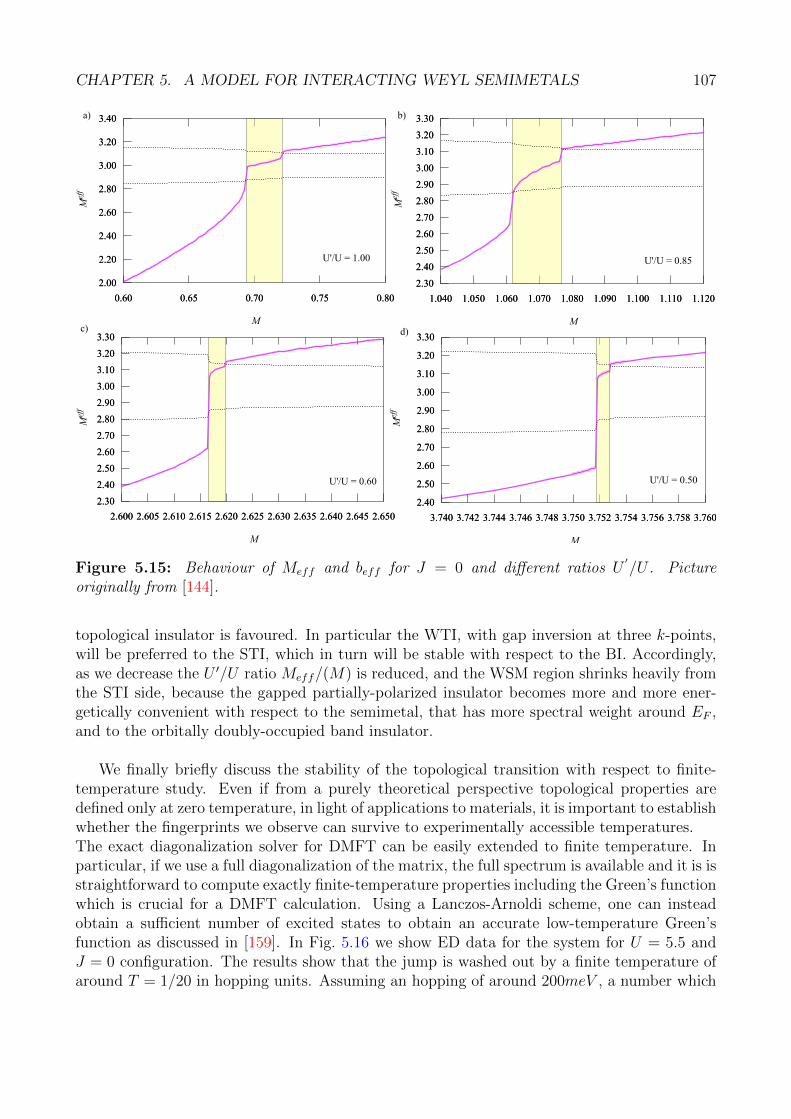
CHAPTER 5. A MODEL FOR INTERACTING WEYL SEMIMETALS 107
2.40
2.50
2.60
2.70
2.80
2.90
3.00
3.10
3.20
3.30
3.740 3.742 3.744 3.746 3.748 3.750 3.752 3.754 3.756 3.758 3.760
Meff
M
U'/U = 0.50
2.40
2.50
2.60
2.70
2.80
2.90
3.00
3.10
3.20
3.30
3.740 3.742 3.744 3.746 3.748 3.750 3.752 3.754 3.756 3.758 3.760
eff
M
2.30
2.40
2.50
2.60
2.70
2.80
2.90
3.00
3.10
3.20
3.30
2.600 2.605 2.610 2.615 2.620 2.625 2.630 2.635 2.640 2.645 2.650
M
U'/U = 0.60
2.30
2.40
2.50
2.60
2.70
2.80
2.90
3.00
3.10
3.20
3.30
2.600 2.605 2.610 2.615 2.620 2.625 2.630 2.635 2.640 2.645 2.650
2.30
2.40
2.50
2.60
2.70
2.80
2.90
3.00
3.10
3.20
3.30
1.040 1.050 1.060 1.070 1.080 1.090 1.100 1.110 1.120
Meff
M
U'/U = 0.85
2.30
2.40
2.50
2.60
2.70
2.80
2.90
3.00
3.10
3.20
3.30
1.040 1.050 1.060 1.070 1.080 1.090 1.100 1.110 1.120
2.00
2.20
2.40
2.60
2.80
3.00
3.20
3.40
0.60 0.65 0.70 0.75 0.80
Meff
M
U'/U = 1.00
2.00
2.20
2.40
2.60
2.80
3.00
3.20
3.40
0.60 0.65 0.70 0.75 0.80
a) b)
d)c)
Figure 5.15: Behaviour of Meff and beff for J = 0 and different ratios U′/U . Picture
originally from [144].
topological insulator is favoured. In particular the WTI, with gap inversion at three k-points,will be preferred to the STI, which in turn will be stable with respect to the BI. Accordingly,as we decrease the U ′/U ratio Meff/(M) is reduced, and the WSM region shrinks heavily fromthe STI side, because the gapped partially-polarized insulator becomes more and more ener-getically convenient with respect to the semimetal, that has more spectral weight around EF ,and to the orbitally doubly-occupied band insulator.
We finally briefly discuss the stability of the topological transition with respect to finite-temperature study. Even if from a purely theoretical perspective topological properties aredefined only at zero temperature, in light of applications to materials, it is important to establishwhether the fingerprints we observe can survive to experimentally accessible temperatures.The exact diagonalization solver for DMFT can be easily extended to finite temperature. Inparticular, if we use a full diagonalization of the matrix, the full spectrum is available and it is isstraightforward to compute exactly finite-temperature properties including the Green’s functionwhich is crucial for a DMFT calculation. Using a Lanczos-Arnoldi scheme, one can insteadobtain a sufficient number of excited states to obtain an accurate low-temperature Green’sfunction as discussed in [159]. In Fig. 5.16 we show ED data for the system for U = 5.5 andJ = 0 configuration. The results show that the jump is washed out by a finite temperature ofaround T = 1/20 in hopping units. Assuming an hopping of around 200meV , a number which

CHAPTER 5. A MODEL FOR INTERACTING WEYL SEMIMETALS 108
2.00
2.20
2.40
2.60
2.80
3.00
3.20
3.40
0.600 0.650 0.700 0.750 0.800
Meff
M
Zero temperature
β = 100
β = 50
β = 20
2.00
2.20
2.40
2.60
2.80
3.00
3.20
3.40
0.600 0.650 0.700 0.750 0.800
Figure 5.16: Behaviour of Meff and beff for U = 5.5, J = 0 and different temperatures.Picture adapted from [144].
is reasonable for strongly correlated oxides, this would correspond to a temperature around100K. This leaves us with a sizeable -and potentially accessible in experiments- temperaturewindow where this phenomenon may be revealed.
5.3.7 First-order topological transitions, second-order endpoints andcritical phenomena
Up to now, we have referred to the topological phase transition above U ≈ 4.5 as discontinuous.In this section we touch upon the “temptation” to treat it as a first-order phase transition inthe Landau sense. This idea stems from the discontinuous behaviour of the first derivativeof the Free energy across the phase transition. We will treat explicitly the behaviour of thisquantity in the next chapter, where we will compare single-site and cluster results for a simplertwo-dimensional BHZ model. Here, we just provide some suggestion that point towards a moreconventional description of interaction-driven topological phase transitions.In the above discussion we have introduced the concept of orbital polarization, which in thecontext of Hartree-Fock was related to the variational parameter p. We also remarked how thisis a key observable whose evolution parallels the topological phase transition. Times a factor,we can relate this quantity to the operator T zi =
∑σ niaσ − nibσ, that we can evaluate locally
on the converged DMFT ground state, obtaining the expected value T z. We can then definethe related orbital compressibility as
κ = ∂T z/∂M. (5.29)
This is a well-defined thermodynamical response function. The behaviour of κ as a functionof M for different U is reported in Fig. 5.17. Its value shows local maxima at the border ofthe semimetallic phase already for small U. Approaching the discontinuous phase transitions,this maxima get sharper and sharper and they tend to develop divergences which remind of a
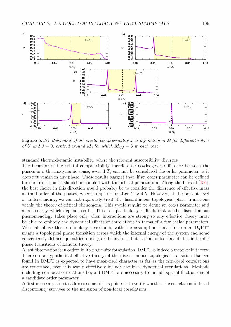
CHAPTER 5. A MODEL FOR INTERACTING WEYL SEMIMETALS 109
-0.10 -0.05 0.00 0.05 0.10 M-M0
-0.10 -0.05 0.05 0.100.000.200.400.600.801.001.201.401.60
κU=4.75
0.000.200.400.600.801.001.201.401.60
-5.000.005.0010.0015.0020.0025.0030.0035.0040.0045.00
κ
U=5.9
-5.000.005.0010.0015.0020.0025.0030.0035.0040.0045.00
-0.10 -0.05 0.00 0.05 0.10 M-M0
-0.10 -0.05 0.00 0.05 0.10-2.000.002.004.006.008.0010.0012.0014.0016.00
κ
U=5.5
-2.000.002.004.006.008.0010.0012.0014.0016.00
-0.10 -0.05 0.00 0.05 0.10 M-M0
-0.10 -0.05 0.00 0.05 0.10
0.000.100.200.300.400.500.600.700.800.90
κ
U=4.5
0.000.100.200.300.400.500.600.700.800.90
-0.10 -0.05 0.00 0.05 0.10 M-M0
-0.10 -0.05 0.05 0.100.150.200.250.300.350.400.450.500.55
κ
U=3.0
0.150.200.250.300.350.400.450.500.55
-0.10 -0.05 0.00 0.05 0.10
M-M0
-0.10 -0.05 0.05 0.10
a) b)
c)
d) e)
Figure 5.17: Behaviour of the orbital compressibility k as a function of M for different valuesof U and J = 0, centred around M0 for which Meff = 3 in each case.
standard thermodynamic instability, where the relevant susceptibility diverges.The behavior of the orbital compressibility therefore acknowledges a difference between thephases in a thermodynamic sense, even if Tz can not be considered the order parameter as itdoes not vanish in any phase. These results suggest that, if an order parameter can be definedfor our transition, it should be coupled with the orbital polarization. Along the lines of [156],the best choice in this direction would probably be to consider the difference of effective massat the border of the phases, where jumps occur after U ≈ 4.5. However, at the present levelof understanding, we can not rigorously treat the discontinuous topological phase transitionswithin the theory of critical phenomena. This would require to define an order parameter anda free-energy which depends on it. This is a particularly difficult task as the discontinuousphenomenology takes place only when interactions are strong so any effective theory mustbe able to embody the dynamical effects of correlations in terms of a few scalar parameters.We shall abuse this terminology henceforth, with the assumption that “first order TQPT”means a topological phase transition across which the internal energy of the system and someconveniently defined quantities undergo a behaviour that is similar to that of the first-orderphase transitions of Landau theory.A last observation is in order: in its single-site formulation, DMFT is indeed a mean-field theory.Therefore a hypothetical effective theory of the discontinuous topological transition that wefound in DMFT is expected to have mean-field character as far as the non-local correlationsare concerned, even if it would effectively include the local dynamical correlations. Methodsincluding non-local correlations beyond DMFT are necessary to include spatial fluctuations ofa candidate order parameter.A first necessary step to address some of this points is to verify whether the correlation-induceddiscontinuity survives to the inclusion of non-local correlations.

Chapter 6
Non-local correlation effects in theinteracting BHZ model
The studies reported in [154], [156], [144] and in Chapter 5 have shown consistently thata topological phase transition in various versions of the BHZ model becomes discontinuousfor sufficiently large repulsion, while it retains the standard continuous character when theinteraction is small, and they lead to a nice consistent picture where the topological transitionshares similarities with a thermodynamic transition. The key to explain these phenomena isidentified in a different renormalization of the topological phase and the trivial phase, connectedwith the dynamical nature of the correlations as measured by the frequency dependence of thereal part of the Self-Energy.
All these results have be obtained within Dynamical Mean-Field Theory, in which the Self-Energy is by construction momentum independent. Hence, all the non-trivial nature of thecorrelations is embodied in the frequency dependence, which becomes more and more pro-nounced as the correlations grow. The non-local correlations are instead treated in in a staticmean-field way. The use of DMFT has been motivated by the fact that it can describe prop-erly the competition between the local repulsion (and other local interactions like the Hund’scoupling) and the mass term M which controls the topological transition. A natural question,which has not been addressed so far, is whether and to which extent this picture survives theinclusion of non-local correlations. This question is particularly pressing considering that thetopological phases of the system are defined by the mapping from the k-space to the Hilbertspace of wavefunctions (or equivalently, in Topological Field Theory language, the space of theGreen’s functions), and the topological invariants distinguishing those phase are derived fromthe properties of the system in specific regions of the Brillouin zone (chirality of the Weyl pointsin the Weyl semimetal) or in the entire BZ (Z2 topological indices).In this picture, the local Self-Energy obtained from DMFT renormalizes only the local pa-rameters of the model, such as the crystal-field splitting, while all the non-local terms areuniformly renormalized by the momentum-independent quasiparticle weight Z. In principle, afully momentum-dependent Self-Energy Σ(k, ω) might heavily modify the mapping from thek-space to the space of the Green’s functions, for instance altering the condition for the closureof the bandgap, or even removing the topological protection of the gap itself and the definitionof the topological phases along with it.To address these concerns we can rely on the cluster methods outlined in Chapter 3, Cluster-Dynamical Mean-Field Theory and Variational Cluster Approximation. In all these methods
110

CHAPTER 6. NON-LOCAL CORRELATION EFFECTS 111
0.1 0.2 0.3 0.41/U
0.2
0.25
0.3
0.35
0.4
0.45
0.5
Quant
um S
pin H
all In
sulat
or
Band Insulator
Mot
t Ins
ulat
orQuantum Critical Point
Triple point
(a)Uncorrelated
topological transition[HgTe/CdTe quantum wells]
10
1
0.1
Figure 6.1: Phase diagram of the 2d interacting BHZ model solved in the single-site DMFTapproach (adapted from [156])
the Self-Energy in real space is not uniform, but it acquires non-local components within thecluster. Through a suitable periodization, the resulting Self-Energy can be recast in a k-dependent form that in principle allows us to evaluate the full phase diagram of the topologicalHamiltonian and the associated renormalized dispersion.In this chapter we will consider the 2d BHZ model first introduced in Chapter 1. We willexamine it through the lens of both CDMFT and VCA, taking advantage of the different per-spectives they provide and seeking confirmation of the single-site results. As we will see, theinclusion of non-local effects does not modify the picture substantially and, most importantly,does not spoil the nature of the topological transition determined by the local Self-Energy.The non-local features mainly lead to a modulation on top of a DMFT-like effect. Hence thedynamical behavior of the local part of the Self-Energy remains the main responsible for theonset of a discontinuous topological transition. We will also briefly comment on the Mott tran-sition exhibited by the system under a specific interaction form and on the presence of magneticordering.
6.1 Model and methods
6.1.1 Single-site description
As in the previous chapter, our starting point is the formulation of the 2d BHZ model givenwith respect to the 4× 4 Dirac matrices
Γ0 = I⊗ I, Γ1 = σz⊗ τx, Γ2 = −I⊗ τy, Γ3 = σx⊗ τx, Γ4 = −σy⊗ τx, Γ5 = I⊗ τz (6.1)

CHAPTER 6. NON-LOCAL CORRELATION EFFECTS 112
In the space of spins (↑, ↓) and orbitals (a, b) spanned by Ψ(†)k = (c
(†)ka↑ c
(†)kb↑ , c
(†)ka↓ , c
(†)kb↓), the Bloch
Hamiltonian matrix has the well known form
H(k) =[M − ε(cos(kx) + cos(ky))
]Γ5 + λ sin(kx)Γ
1 + λ sin(ky)Γ2 (6.2)
We take ε = 2t, where t is the nearest-neighbour hopping, as our energy unit, M is the crystal-field splitting responsible for the energy offset between the orbitals and λ is the spin-orbitcoupling responsible for the protection of the topological bandgap. In this chapter we willconsider λ = 0.3, in order to compare our results with the single-site ones obtained in [156].The interaction will again be defined in the density-density Kanamori form
Hint = U∑il
nil↑nil↓ + (U − 2J)∑il 6=l′
nil↑nil′↓ + (U − 3J)∑il<l
′
(nil↑nil′↑ + nil↓nil′↓) (6.3)
depending on the Hubbard U and the Hund’s coupling J , which in the present calculation isfixed to J = U
4as representative of a regime of relatively large local exchange. The topological
phase diagram of the noninteracting BHZ model presents, as previously shown, a gapless Diracpoint for M = 2ε. For lower values of M , the system is a Quantum Spin Hall insulator (QSHI),for higher M a trivial Band Insulator (BI). The associated topological invariant is the Z2 scalarindex given by the product of the parity eigenvalues of the occupied bands at the four High-Symmetry points of the 2d Brillouin zone: the inverted bandgap around Γ is, as in the originalQuantum Well example, responsible for the nontrivial topology.As in the previous chapter, the interacting phase diagram can be recovered from the study ofthe effective topological Hamiltonian
Htop(k) = H(k) + ReΣ(k, ω = 0) (6.4)
where Σ is a 4 × 4 matrix, the components of which we can again label as Σασ,βσ′ in the spinand orbital indices.As we discussed previously, if the model is solved using DMFT, the Self-Energy is completelylocal in space and it depends only on the frequency. In the absence of spontaneous symmetrybreaking and/or of local terms connecting different spin sectors, it is diagonal in the spin-orbitbasis and satisfies the symmetries of the system. Since its imaginary part vanishes for ω → 0,consistently with the system being an insulator, the topological Hamiltonian only receives thecontribution of the real part, which can be expressed as
ReΣ = Σa↑,a↑Γ5 (6.5)
From this formulation and (6.2), it is clear that the only renormalized parameter of the systemis the effective mass
Meff = M + Σa↑,a↑ (6.6)
The single-site DMFT phase diagram for the 2d BHZ at T = 0 is shown in Fig. 6.1. In this case,the phases are plotted with respect to the reciprocal of the bare mass 1
Mand of the interaction
strength 1U
. The topological phase transition between the QSH and BI phases is discontinuousup to a critical value of 1
U, after which (i.e. for low interaction values) the system passes from
a phase to the other in the usual way, through gap closing at the Γ point for Meff = 2. Thepresence of a finite J allows, similarly to what we found in the previous chapter, the insurgenceof a Mott insulating region, exhibiting an uniform occupation of the orbitals at each site. The

CHAPTER 6. NON-LOCAL CORRELATION EFFECTS 113
Hc
HB HB
V1V2
1 2a)
Hc
VV
b)
λ' t'
c)
M'
Figure 6.2: Clusters used in different methods. Filled circles are interacting sites, emptycircles are non-interacting ones. Dashed lines represent variable quantities, full lines representfixed quantities (local cluster hamiltonian). a) CDMFT b) VCA c) Bathlesss VCA
transition from the Mott region to the Quantum Spin Hall one is again discontinuous, and thewidth of the latter is progressively reduced till it disappears at a “triple point” for high enoughU. As in the J 6= 0 case studied in the previous chapter, the slope of the Meff = 2 transitionline is positive as a function of U.
6.1.2 Cluster description
To study the same system from a cluster perspective, the Hamiltonian matrix needs to berewritten in the mixed representation outlined in Chapter 3. Accordingly, we will use the boldnotation for quantities expressed in this representation, and in general in the cluster basis. Theinteraction part, being on-site, is completely unaffected. On the contrary, the noninteractingpart has to be recast in this representation. In particular, the Hamiltonian matrix will now be4×N -dimensional, where N is the number of cluster sites, and it will be defined in the reducedBrillouin Zone corresponding to the chosen cluster. Inside the cluster, the Hamiltonian willhave a block structure: overall, it will consist of two decoupled spin blocks, as in the originalformulation. We now introduce the structure of each spin block, which is based on the 2 × 2T-matrices living in the orbital space (with σ = ±1 being the spin eigenvalue)
T0 =
[M 00 −M
]Tx =
[−t iλ
2σ
iλ2σ t
]Ty =
[−t −λ
2λ2
t
]. (6.7)
T0 is the on-site energy matrix, while Tx and Ty refer to the hopping along the positive x andy real space directions. The up and down spin blocks of H can be written as an N ×N matrix(in the site space) whose elements are orbital 2× 2 matrices.
H↑/↓ =
T0 T12 · · · T1N
T ∗12 T0 · · · T2N...
.... . .
...T ∗1N T ∗2N · · · T0
(6.8)
where T ∗ab := (conjg Tab)T . The nondiagonal Tij matrices can be 0, Tx, Ty or their hermitian
conjugate depending on the relative position of the sites i and j, and the consequent hoppingmatrix between them. To complete the expression in mixed representation, the bordering sitesof different clusters are coupled by terms of the form
T (∗)x e∓ikxRx + T (∗)
y e∓ikyRy (6.9)

CHAPTER 6. NON-LOCAL CORRELATION EFFECTS 114
where kx(y) lives in the Reduced Brillouin Zone and Rx(y) is the distance of the sites in the givendirection.We will consider three cluster definitions in the context of our study, as shown in Fig. 6.2:
a) CDMFT: The cluster consists of two correlated sites along the x direction (though wehave checked for a restricted set of values that the properties for a cluster along y are analogous).The block-Hamiltonian for spin ↑ and ↓ of such a cluster in the mixed representation will havethe form
H(k) =
[T0 TxT ∗x T0
]+
[T ∗y e
iky + Tye−iky T ∗xe
i2kx
Txe−i2kx T ∗y e
iky + Tye−iky
](6.10)
Unfortunately, the 2× 2 plaquette, respecting the symmetries of the original lattice, makes ourcalculations significantly heavier, hence the results of CDMFT calculation will inevitably dealwith an unphysical asymmetry between the x and y directions. However, since the behaviourof the 2-sites clusters along x and y are analogous, we can safely assume we are not overlookingany relevant renormalization effect.
b) VCA: The results of CDMFT are compared with those obtained via VCA using clusterb. The Hamiltonian of the cluster is identical to that of the previous case; what varies is theexpression for the noninteracting bath, that in this case consists of two 2-orbital sites withlocal energy fixed at the chemical potential and hybridization V. This is treated as the solevariational parameter of the model. The number of levels per spin is in this case only 8, whichconsiderably speeds up the calculation. While the choice of a one-dimensional variational spacemay seem to be too crude an approximation, we have indeed checked that the shape of Ω withrespect to the inclusion of other parameters, such as an energy offset between the bath orbitalsor hopping between the cluster sites, shows stationary points precisely at (or very near to) thefixed values we have in the end chosen. The relevant effects of the phase transition are thereforewell captured by the variation of the hybridization V alone. This simplification turns out to bevery useful to visualize the physical content of our results. Relatedly, we have also checked thestability of the topological phases with respect to antiferromagnetism, as we will briefly reportin the next section.
c) Bathless VCA: The inclusion of a noninteracting “auxiliary” bath is one of the toolsVCA can exploit to enhance its descriptive power. It is however not required in principle forthe implementation of the method, that can rely on the sole variation of the isolated clusterparameters. This scenario has been addressed with the help of cluster 6.2c, in which thevariational parameters are the hopping amplitude t′, the spin-orbit coupling λ′ and the crystal-field splitting M ′. The exclusion of the bath sites allows us to consider a square plaquette,respecting the symmetries of the original lattice while keeping the number of levels per spinthe same as the previous case. The Hamiltonian in mixed representation will in this case havethe form
H(k) =
T0 Tx 0 TyT ∗x T0 Ty 00 T ∗y T0 T ∗xT ∗y 0 Tx T0
+
0 T ∗xe
i2kx 0 T ∗y ei2ky
Txe−i2kx 0 T ∗y e
i2ky 00 Tye
−i2ky 0 Txe−i2kx
Tye−i2ky 0 T ∗xe
i2kx 0
(6.11)

CHAPTER 6. NON-LOCAL CORRELATION EFFECTS 115
where the labelling of the sites runs counterclockwise from the bottom left one. In this instance,the computation time will be affected by the necessities of the multidimensional minimizationroutine, which will require multiple evaluations of the numerical gradient of Ω. Calculationshave been made both with the l-BFGS-b and Nelder-Mead methods, giving similar results.While the definition of this cluster as the reference system is completely legitimate, its adequacyrests with the existence of stationary points for Ω, which is in principle not guaranteed as wewill see in the following sections.
6.1.3 A note on antiferromagnetism
0 0.05 0.1 0.15 0.2 0.25 0.3 0.35 0.4 0.45 0.5
V
-0.4
-0.3
-0.2
-0.1
0
0.1
0.2
0.3
0.4
B'
-14.4825
-14.4830
-14.4802
-14.4815
-14.4810
-14.4805
-14.4800
-14.4795
-14.4790
-14.4785
-14.4780
0.4 0.45 0.5 0.55 0.6 0.65 0.7 0.75 0.8 0.85
V
0.2
0.4
0.6
0.8
1
1.2
1.4
1.6
1.8
2
-13.4585
-13.4580
-13.4575
-13.4570
-13.4565
-13.4560
-13.4555
-13.4550
ΩΩ
Figure 6.3: Shape of Ω as a function of hybridization V and effective AFM field B′ for U=8and M in the band insulator and Mott region respectively. The paramagnetic solution is stablearound the topological transition, while antiferromagnetic effects dominate in the Mott region.
The presence of crystal-field splitting and spin-orbit coupling spoils the perfect nesting ofthe Fermi surface characteristic of the two-dimensional Hubbard model. This implies that,in contrast with the Hubbard model, we do not expect antiferromagnetism to manifest forarbitrarily low interaction.
This has been verified within DMFT both for the 2d and 3d BHZ cases [154, 156]. However,such a solution may very well be stable around the region of the phase diagram occupied bythe Mott insulator, i.e. for large U, and, since the width of the non trivial region is dramat-ically shrunk in that area, it is better to check the stability of the solution with respect toantiferromagnetic ordering also in presence of nonlocal correlation effects before proceeding inour analysis.In single-site DMFT, antiferromagnetic solutions are achieved by doubling the size of the cell toconsider two independent sites in the spirit of real-space DMFT, and by breaking the symmetryof the bath relative to the two sites. This is however not immediately done with the replicaconstruction we are employing, so it is easier to rely, to our end, on the VCA framework.In absence of symmetry-breaking perturbations, the solution of a finite Hubbard cluster hasto be SU(2)-invariant, from which derives the inability of Cluster Perturbation Theory in itsoriginal “divide et impera” formulation to describe spontaneous symmetry breaking [93]. VCA

CHAPTER 6. NON-LOCAL CORRELATION EFFECTS 116
is, in this case, a clear improvement: we can take advantage of the ability to include any nonin-teracting term (as long as the interacting part of Ω is universal) and add a fictitious staggeredmagnetic field [160] of the form
bAFM = −B′∑iσ
zi(ni↑ − ni↓) (6.12)
to the cluster defined in Fig. 6.2b, where zi is ±1 for site 1 and 2 and the orbitals are identicallyaffected. This staggered magnetic field will then be used, together with the previously definedV , as a variational parameter. In Fig. 6.3 we show, as an example, the heatmap of Ω(V,B′) fora 2d BHZ system in a region close to the topological transition and inside the Mott insulatorrespectively for U = 8, which is high enough to warrant, in the single-site case and for suitablevalues of M, both the insurgence of an antiferromagnetic solution and a discontinuous topolog-ical phase transition. All the fixed parameters of the model are those defined in the previoussection. As we can see from the right panel, antiferromagnetic ordering is indeed stable in theMott region, as the stationary point is found for a nonzero value of B′ (Ω has to be even withrespect to the staggered field, so another equivalent minimum is found for opposite B′). How-ever, near the topological phase transition the two local minima of Ω, the meaning of which willbe elucidated in the following sections, are located at different values of V and zero staggeredfield. Hence, at least near the topological phase transition, the paramagnetic solution is indeedstable with respect to magnetically ordering, which is limited to the Mott insulating region.
6.2 Nonlocal effects and Topological characterization
All the information on the effects of correlations on the single-particle properties is encoded inthe cluster Self-Energy. This is made up of various components which we can label as Σiασ,jβσ′ ,where σ, σ′ refer to the spin, i, j to the site and α, β to the orbital degrees of freedom, whichcollectively form a square matrix Σ of size
Nsites ×Norb ×Nspin,
in our case equal to 8 in the mixed representation for clusters 6.2a and b. In principle, Σ has 64entries for each frequency ω. However, the number of independent entries is strongly reducedby the symmetries of the interacting cluster.First of all, we assume as an hypothesis that the two spin blocks are decoupled and identical,retaining the symmetry of the Hamiltonian, which allows us to take advantage of the spin-decoupled ED method described in Chapter 4. In the following we will consider the symmetryproperties of the ↑-spin block, the other following a similar behaviour.
In order to study the topological phases of the system, we are interested in the behaviourof Σ at ω = 0. Any component with vanishing real and imaginary parts for ω → 0 will notaffect the topology of the interacting system. This is, for example, the case of the componentsΣiaσ,ibσ, relating the two orbitals on the same site, which has an identically zero imaginary partand a tiny finite real part that vanishes at ω = 0: to the end of determining the topologicalphase of the system, its presence is completely irrelevant.All the other components, for which at least one among the real and imaginary parts of Σ isfinite in 0, have been collected in Fig. 6.4, where they are plotted along the Matsubara axis.The plots are relative to CDMFT data, though we verified that the VCA Self-Energies satisfy

CHAPTER 6. NON-LOCAL CORRELATION EFFECTS 117
ReΣ
ReΣ
ReΣ
1a
1b 2a 2b1a
1b
2a
2b
1a
1b 2a 2b1a
1b
2a
2b
1a
1b 2a 2b1a
1b
2a
2b
ΣM
Σt
Σλ
1a
1b 2a 2b1a
1b
2a
2b
1a
1b 2a 2b1a
1b
2a
2b
1a
1b 2a 2b1a
1b
2a
2b
ReΣ
ReΣ
ReΣ
ImΣ
ImΣ
ImΣ
-0.600
-0.400
-0.200
-0.400
-0.200
0.0000.000
-0.120-0.120
-0.080-0.080
-0.040-0.040
0.0000.000
-0.002-0.0010.0000.0010.002
-0.002-0.0010.0000.0010.002
ImΣ
ImΣ
ImΣ
-0.600
-0.400
-0.200
0.000
-0.600
-0.400
-0.200
0.000
-0.080
-0.120-0.120
-0.080
-0.040-0.040
0.0000.000
-0.002-0.0010.0000.0010.002
ωn
-0.002-0.0010.0000.0010.002
0.00 2.00 4.00 6.00 8.00 10.000.00 2.00 4.00 6.00 8.00 10.00
0.00 2.00 4.00 6.00 8.00 10.000.00 2.00 4.00 6.00 8.00 10.00
0.400
1.200
1.600
0.0200.0400.0600.080
0.0000.0200.0400.0600.080
0.000
0.001
ωn
-0.001
0.000
0.001
0.800
0.00 2.00 4.00 6.00 8.00 10.000.00 2.00 4.00 6.00 8.00 10.00
-1.600
-1.200
-0.800
-1.600
-1.200
-0.800
-0.400-0.400
-0.080-0.060-0.040-0.020
-0.080-0.060-0.040-0.0200.0000.000
-0.001
0.000
0.001
-0.001
0.000
0.001
0.00 2.00 4.00 6.00 8.00 10.000.00 2.00 4.00 6.00 8.00 10.00
H↑
Figure 6.4: CDMFT Self-Energy components for the 2-site cluster at low (U=2, dotted lines)and high (U=8, solid lines) interaction values, plotted along the Matsubara axis, for a value ofM inside the topological insulating region. The first and last three plots respectively refer to aaand bb terms for the intra-orbital components and to ab and ba terms for the inter-orbital ones.In each case, the plotted components of the Self-Energy are identified by coloured squares in theblock structures at the left, representing the 4 × 4 H↑ Hamiltonian, where sites are labelled bynumber and orbitals by letter. In the case of off-diagonal components in the site space, if thetwo entries in the Σ matrix not identical they are represented by different shades of the samecolor.

CHAPTER 6. NON-LOCAL CORRELATION EFFECTS 118
the same symmetries. The diagrams on the left of the plot refer to the block structure of thespin-up Hamiltonian H↑ to which the plotted Self-Energy components correspond. We willomit the spin index henceforth. In each plot, the solid and dotted lines refer to the Self-Energyvalues obtained for an indicative low (U=2) and high (U=8) value of interaction respectively.The three different colors refer to Σ components relating different sites and orbitals, accordingto the following scheme:
In green we plotted the diagonal Self-Energies relating the same sites and orbitals. Thesehave to satisfy the causality constraint which imposes a negative sign on their imaginary part,as is indeed the case. It is also to be noted that the imaginary parts vanish for ω = 0, denotingthe insulating character of the model. The components relative to the two orbitals show thesame behaviour for the imaginary part, while the real part is opposite in sign, consistentlywith what we obtained for the single-site case. As we would expect, the renormalization givenby the real part of the Self-Energy drastically increases with the interaction. The sign of thecomponent is opposite to that of M for each orbital, which reflects the symmetry of the single-particle Hamiltonian [156]. Considering the symmetries, with a convenient sign the value ofthis class of Self-Energies in zero is determined by ReΣ1a,1a(0), which we will refer to as ΣM ,where the meaning of the pedex will become clear in the following.
In red we find the components of the Self-Energy relating the same orbital on two differentsites, which corresponds to processes analogous to the nearest-neighbour hopping. The corre-sponding imaginary parts are still identical for each orbital, and the real parts are opposite insign. Again, the magnitude of the component increases with interaction. The value of this classof Self-Energies in 0 will be called, similarly to the previous case, ReΣ1a,2a(0) := Σt.
In blue the components of Σ relating different orbitals on different sites are depicted, whichcorresponds to processes analogous to the λ terms of the bare Hamiltonian.. The behaviourof this component is peculiar: the real part is identically 0, while the imaginary part is equaland opposite for the components Σ1α2α and Σ2α,1α for both orbitals α = a, b. Since these areoff-diagonal, we are not bound by any requirement on the sign of ImΣ. As the previously con-sidered ones, these components have opposite value for different orbitals and exhibit a strongerfrequency dependence for higher values of U. With a sign dictated by symmetries, the value ofthis class of components of Self-Energy in 0 is defined as i ImΣ1a,2b(0) := i Σλ.
To better visualize the way in which these terms enter in the topological Hamiltonian,and the reasons of the labels we attributed to the various entries of the Self-Energy, we recallthe expression for the Σ-scheme periodization introduced in Chapter 3 for every spin-orbitalcomponent:
[Σper]ασ,βσ′(k, ω) =1
Nc
∑ij
e−ik(ri−rj)Σiασ,jβσ′(ω), (6.13)
where the resulting periodized Self-Energy can be expressed in a 4× 4 matrix in the spin-orbitspace which now depends on momenta in the whole Brillouin zone. This periodization is themost reliable in a regime where the Self-Energy is well behaved and does not show singularities.From the definition of the Γ matrices, and using (6.13), we can recall the symmetry propertiesof each component of Σ shown in Fig. 6.4 (as well as those, not shown, for the opposite spin)

CHAPTER 6. NON-LOCAL CORRELATION EFFECTS 119
and verify that the 4× 4 k-dependent zero-frequency Self-Energy is given by
Σper(k, ω = 0) = ΣMΓ5 + Σt cos(kx)Γ5 − Σλ sin(kx)Γ
1 (6.14)
in the spin-orbital space. If we compare this expression with the noninteracting Hamiltonian(6.2) we immediately see that each of the Self-Energy terms corresponds to a term in the single-particle Hamiltonian. Coherently with their definition, then ΣM will renormalize additively M,Σt will do the same for the ε = 2t term and Σλ for the spin-orbit coupling. Clearly, theasymmetry in the coupling of the last two terms, which do not renormalize hopping along y,derives from the chosen form of the cluster. The eigenvalues of the topological Hamiltonian,given by the sum of the noninteracting H and the periodized Σper(k, 0), are the spin-degenerate
E±,σ = ±
√((M + ΣM
)−(ε− Σt
)cos(kx)− ε cos(ky)
)2
+(λ− Σλ
)2sin2(kx) + λ2 sin2(ky)
(6.15)Our analysis then concludes that the effect of the interaction can be nicely summarized, atleast at the level of the topological Hamiltonian, in terms of very transparent independentrenormalizations of the different single-particle parameters.
In particular, the Σλ component, coupling to λ, affects the protection of the topological gapalong the kx direction. In principle, a strong enough renormalization, matching the value ofthe spin-orbit coupling, could cancel the sin2(kx) term with the consequent closing of the gapand destruction of the topological phase. However, in the case we consider, we are not evenclose to this situation. From the data of Fig. 6.4 and for similar data for other parameters, wesee that the value of Σλ, by far the smallest of the three independent components, is even athigh interaction values at least two orders of magnitude smaller than the value of λ, hence itappears to have a rather limited impact.
On the other hand, the renormalization of the hopping term is more significant, as the valueof Σt is four to five times smaller than that of t. Since the λ terms in (6.15) are finite, the gapclosing, associated to the phase transition, happens at Γ if the first term is zero. The Diraccone will in this case be asymmetric in the two k directions as a consequence of the form ofthe cluster, and the requirement Meff < (>)2 for the topological transition in the single-sitepicture will be replaced by the topological condition
M + ΣM
ε− Σt2
< (>)2. (6.16)
In order to identify the topological phase of the system, and to compare the results with thesingle-site case, we will need to evaluate the behaviour of the previous expression as a functionof M .
The precise low-energy behaviour of the Green’s function in the context of the topologicalphase transition will be investigated in the following sections. However, we can get an intuitiveidea of the effect on Σper on the low-energy physics by looking at the bands of the renormalizedtopological Hamiltonian defined by
Zk
(H(k) + Σper(k, ω = 0)
)where Zk is the quasiparticle weight defined in Chapter 2, which has also a matrix structurein the spin-orbital space. This expression, which can be derived from the form of the Green’s

CHAPTER 6. NON-LOCAL CORRELATION EFFECTS 120
-2.5
-2
-1.5
-1
-0.5
0
0.5
1
1.5
2
2.5
-Y Γ Y M X Γ -X
Figure 6.5: Comparison between CDMFT (coloured) and DMFT (dashed) data for the renor-malized Topological Hamiltonian Z ·(H(k)+Σ(k)) at U=8 and M inside the QSHI region, whichgives an approximate representation of the location of the poles of G near zero frequency. As itcan be seen, the effect of Z accounts for a loss of symmetry in the two high-symmetry directions−XΓX and −Y ΓY , while the purely local Self-Energy in the single-site approach makes for auniform “compression” of the bands. The inverted gap region, however, is minimally affected,thus preserving the topological characterization of the system.
function
G(k, ω → 0) =
[ωI−H(k)−Σper(k, 0)− ∂ReΣper
∂ω
∣∣∣∣0
ω
]−1
=
[ωI−Zk
(H(k)−Σper(k, 0)
)]−1
Z−1k
approximately coincides for low ω with the maxima of the spectral function A(k, ω), and iden-tifies the energies of the quasiparticle excitations.
The relative band diagram is plotted in Fig. 6.5, along with the analogous result for thesingle-site case. From a topological point of view, we again see that the nontrivial phase is de-scribed, in band theory, by an inverted gap around the Γ point. It is more interesting to noticethe way the bands are modified by interaction: since the Self-Energy is momentum-independentin the single-site picture, the quasiparticle weight is a constant. Consequently, the renormal-ized bands in DMFT are rigidly compressed. With a 2-site cluster, instead, the momentumdependence of Σper leads to a quasiparticle weight that varies inside the Brillouin zone, andaccordingly the dispersion is non-uniformly distorted in the two k-directions, especially aroundthe (π, π) M-point.From these observations, it is possible to assert the existence of nonlocal effects of correlation,and their interplay with the noninteracting form of the Hamiltonian to alter the low-energyexcitations’ properties. It is now to be understood if and how these effects will alter the dis-continuous character of the topological phase transition reported by single-site DMFT.

CHAPTER 6. NON-LOCAL CORRELATION EFFECTS 121
6.3 Discontinuous topological phase transition
To gain more insight into the destiny of the topological phase transition for high values of inter-action, we will take advantage of the different but related perspectives that CDMFT and VCAoffer on a cluster-based calculation. In the previous chapter, we have qualified the topologicaltransition for large interactions as discontinuous by assessing the presence of jumps in the evo-lution of the Self-Energy with M , and later used the term first order in a thermodynamic senseby highlighting the presence of divergences in the orbital compressibility κ. In this chapter,we will first analyse the behaviour of the relevant components of the Self-Energy defined inthe previous section near the topological phase transition, then we will characterize it in termsof the poles of the interacting Green’s function and of the internal energy of the system. Toidentify the topological phase of the system we will use the topological condition defined inthe previous character. While in deriving it we have made use of the Σ-scheme periodizationprocedure, its definition is actually general, depending only on the competition between thecoefficients ΣM and Σt. Even in the Reduced Brillouin Zone, when the value of the topologicalcondition (6.16) is 2 the gap in the topological Hamiltonian is closed in Γ, and the orbitalcharacter of the gap is direct or inverted depending on the value of expression (6.16). There areother ways to assess the topological character of the system, such as the use of Wilson loopsand Wannier centres of charge [161]. While we have checked the consistency of the results, wewill stick to the use of expression (6.16), for the sake of an easier visualization and comparisonwith the single-site case.
6.3.1 Self-Energies
Each topological phase of the system is related to a specific form of the Self-Energy. In thesingle-site case, the pronounced frequency dependence of Σ in the QSHI phase, as opposed tothe weaker one in the BI (and WSM), is responsible for the insurgence of a discontinuous phasetransition: the strong correlation effects felt by the partially orbital-polarized topological insu-lator made impossible a continuous evolution of the Ground-State. This was instead achievedfor lower values of interaction, where the Self-Energy, weakly dependent on frequency to thepoint of being almost constant, simply summed up with the crystal-field splitting M , shiftingthe transition point but keeping its continuous character.In Fig. 6.6 we show the behaviour of the relevant components of Σ defined in the previoussection (only one representative for each class has been plotted) for values of M immediatelypreceding and following the transition point. The plotted data refer only to the high interactioncase U = 8 as, for lower values of U, the behaviour of the phase transition is continuous. Thetwo columns of the plot refer to CDMFT and VCA data respectively; given the qualitativeagreement of the behaviour of the Σ components, the two methods provide mutual validation.As in the single-site case, the correlation strength, which we estimate from the frequency de-pendence of the Self-Energy, is decidedly higher in the QSH region for both the ΣM and Σt
components. Interestingly enough, the situation is reversed for Σλ: here the absolute value ofthe Self-Energy in 0 is greater in the BI region. The fact that this is the case both for CDMFTand VCA in a sense validates the results given by the fit procedure of the former, which canlead to non-optimal solutions especially in the proximity of phase transitions. However, giventhe small magnitude of the Σλ component we can expect its variation to simply provide a slightmodifications of the system parameters in the orbitally-polarized BI phase.

CHAPTER 6. NON-LOCAL CORRELATION EFFECTS 122
ωn
-1.400
-1.300
-1.200
-1.100
-1.000
-1.400
-1.300
-1.200
-1.100
-1.000
-0.050-0.040-0.030-0.020-0.0100.0000.010
-0.050-0.040-0.030-0.020-0.0100.0000.010
0.000
0.002
0.004
0.006
0.00 2.00 4.00 6.00 8.00 10.00
0.000
0.002
0.004
0.006
0.00 2.00 4.00 6.00 8.00 10.00ωn
-1.5000-1.4000-1.3000-1.2000-1.1000-1.0000
-1.5000-1.4000-1.3000-1.2000-1.1000-1.0000
-0.0120
-0.0080
-0.0040
0.0000
0.0040
-0.0120
-0.0080
-0.0040
0.0000
0.00000.00040.00080.00120.00160.0020
0.00 2.00 4.00 6.00 8.00 10.00
0.00000.00040.00080.00120.0016
0.00 2.00 4.00 6.00 8.00 10.00
ReΣ
ImΣ
ReΣ
Figure 6.6: Comparison between CDMFT (left) and VCA (right) data for the independentcomponents of the cluster Self-Energy at the M values immediately before (solid line) and after(dashed line) the transition for U=8. The 3 panels show respectively the ΣM , Σt and Σλ
components. The VCA approximation captures a jump with comparable width only in the Mchannel, the other two being in comparison much smaller than their CDMFT counterparts.
Already looking at Fig. 6.6 we can advance an hypothesis on the behaviour of the topologicalphase transition: the jump in the local component ΣM is by far the most relevant being aroundten times bigger than that of Σt, which is in turn greater than that of Σλ. The local effects ofcorrelations appear therefore to dominate, and accordingly we expect that the behavior of theobservables and the overall physical picture to be close to that discussed in Chapter 5 and inRefs. [154, 156].
6.3.2 Topological condition
We now use the zero-frequency values of the Self-Energy to compute the topological condition(6.16) as a function of the crystal-field splitting M for both CDMFT and VCA results. Inaddition, we can directly compare both with the single-site data, where the only significant dif-ference is that Σt = 0 identically. A cumulative resume of the results is provided in Fig. 6.7. Ingeneral, the two cluster methods exhibit a good agreement with each other and with single-siteresults: CDMFT in particular is well in agreement with DMFT in the QSH region, while it isnearer to VCA in the band insulator. Most importantly, for sufficiently high interaction thediscontinuous jump of the topological condition, with associated absence of gap-closing pointsin the topological Hamiltonian, is preserved and the location in M of the transition point is

CHAPTER 6. NON-LOCAL CORRELATION EFFECTS 123
1.50
1.60
1.70
1.80
1.90
2.00
2.10
2.20
2.30
2.40
3.25 3.3 3.35 3.4 3.45
Topo
logi
cal C
ondi
tion
M
DMFT
CDMFT
VCA
1.50
1.60
1.70
1.80
1.90
2.00
2.10
2.20
2.30
2.40
3.25 3.3 3.35 3.4 3.45
Figure 6.7: (Color online) aTopological characterization of the system for U=8: the topologicalphase of the system, as obtained via the Topological Hamiltonian, depends on the ratio betweenM and ε The plots refer to the single-site DMFT results, the CDMFT one and the VCA onewith reference cluster b.
very close to the DMFT value.The shaded region refers to one of the useful features of VCA, namely its ability to find multi-ple physically significant solutions for the system, and to determine their stability in terms ofinternal energy. In the shaded region, as we will see in the following sections, the VCA solverindeed finds two solutions as a function of the variational hybridization V.CDMFT, by contrast, does not provide a similar information about the stability of solutions,and the information on coexistence can only be obtained by moving back and forth in thephase diagram and observing two solutions, coming respectively from large and small M, beingcompresent in an determinate region.As it is apparent from Fig. 6.7, the right boundary of the region where VCA stops findingtwo available physical solutions coincides with that of the CDMFT coexistence region definedabove: here, the QSH solution can no longer be carried over. This again shows that the twomethods, applied on clusters Fig. 6.2a and Fig. 6.2b, are in good agreement in describing thetopological phases of the system.On this note, let us now consider the third cluster system proposed in Fig. 6.2c, which is thebathless square plaquette. With both minimization methods used (constrained BFGS and sim-plex), no solution following the behavior of Fig. 6.7 is found near the phase transition. Instead,the lowest stationary points exhibited by Ω are in regions where the variational M
′is 2 to 3
times bigger than the real system one: the related Self-Energy is almost frequency independent,and the only relevant components are the diagonal ones. We can attribute this result to the lackof resolution in frequency domain of this approach. Indeed, the results of CDMFT and VCA inpresence of bath suggest that, analogously to the one-site case, the discontinuous topological

CHAPTER 6. NON-LOCAL CORRELATION EFFECTS 124
1.80
1.90
2.00
2.10
2.20
2.30
2.40
2.50
2.60
2.70
2.80
2.90
2.8 3 3.2 3.4 3.6 3.8
Topo
logi
calC
ondi
tion
M
Mean Field
Bathless VCA
1.80
1.90
2.00
2.10
2.20
2.30
2.40
2.50
2.60
2.70
2.80
2.90
2.8 3 3.2 3.4 3.6 3.8
Figure 6.8: Comparison between the topological condition for cluster Fig. 6.2c and a staticMean-Field result.
phase transition is mainly a consequence of local quantum correlations, which, within VCA, areprecisely addressed by the uncorrelated bath sites that this simple approach lacks. In principle,a better result could come by an increase of the cluster size, which would however start to growtoo big to be solved with an ED routine.Interestingly, this VCA solution with a “quasi-static” Self-Energy is rather in agreement with astatic mean-field result obtained along the lines outlined in Chapter 5, using the average orbitalmagnetizations ma, mb and polarization p as variational parameters. This agreement can beseen from Fig. 6.8, where we have plotted the value of the topological condition for clusterFig. 6.2c and the renormalized crystal-field splitting of the effective HF Hamiltonian.
6.3.3 Poles of the Green’s function
As previously stated, the renormalized topological Hamiltonian shown in Fig. 6.5 describes thelow-energy behaviour of the interacting system. There is a more quantitative way to showthe behavior of the gap at the topological phase transition: the low energy excitations can bedirectly obtained from the poles of the interacting Green’s function. For the single-band case,we recall that the shifted poles satisfy the equation
ω − εk − ReΣ(k, ω) = 0
the shift being due to the real part of the Self-Energy. In the general multi-band case, where Σand G are matrices, this shift is provided in a diagonal basis by the real part of the eigenvaluesof
H(k) + Σ(k, ω)
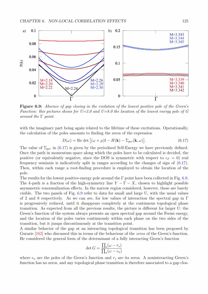
CHAPTER 6. NON-LOCAL CORRELATION EFFECTS 125P(k)
0
0.02
0.04
0.06
0.08
0.1
0
0.02
0.04
0.06
0.08
0.1
0
0.05
0.1
0.15
0.2
0
0.05
0.1
0.15
0.2
Γ
M=2.18M=2.20M=2.22 M=2.24
M=2.26M=2.28M=2.30
Γ
M=3.343M=3.344M=3.345
M=3.339M=3.340M=3.341M=3.342
a) b)
Figure 6.9: Absence of gap closing in the evolution of the lowest positive pole of the Green’sFunction: this pictures shows for U=2.0 and U=8.0 the location of the lowest energy pole of Garound the Γ point.
with the imaginary part being again related to the lifetime of these excitations. Operationally,the calculation of the poles amounts to finding the zeros of the expression
D(ω) = Re det[(ω + µ)I−H(k)− Σper(k, ω)
]. (6.17)
The value of Σper in (6.17) is given by the periodized Self-Energy we have previously defined.Once the path in momentum space along which the poles have to be calculated is decided, thepositive (or equivalently negative, since the DOS is symmetric with respect to εF = 0) realfrequency semiaxis is indicatively split in ranges according to the changes of sign of (6.17).Then, within each range a root-finding procedure is employed to obtain the location of thepole.The results for the lowest positive-energy pole around the Γ point have been collected in Fig. 6.9.The k-path is a fraction of the high-symmetry line Y − Γ − X, chosen to highlight possibleasymmetric renormalization effects. In the narrow region considered, however, these are barelyvisible. The two panels of Fig. 6.9 refer to data for small and large U, with the usual valuesof 2 and 8 respectively. As we can see, for low values of interaction the spectral gap in Γis progressively reduced, until it disappears completely at the continuous topological phasetransition. As expected from all the previous results, the picture is different for larger U: theGreen’s function of the system always presents an open spectral gap around the Fermi energy,and the location of the poles varies continuously within each phase on the two sides of thetransition, but it jumps discontinuously at the transition point.A similar behavior of the gap at an interacting topological transition has been proposed byGurarie [162] who discussed this in terms of the behaviour of the zeros of the Green’s function.He considered the general form of the determinant of a fully interacting Green’s function
detG =
∏s(ω − rs)∏n(ω − εn)
where εn are the poles of the Green’s function and rs are its zeros. A noninteracting Green’sfunction has no zeros, and any topological phase transition is therefore associated to a gap clos-

CHAPTER 6. NON-LOCAL CORRELATION EFFECTS 126
0.00
0.05
0.10
0.15
0.20
Γ
ω
0.00
0.05
0.10
0.15
0.20
Γ
BI
QSH(d)
E
Figure 6.10: On the left, an example in which the behaviour of zeros and poles of the Green’sfunction can trigger a topological phase transition without the closing of the spectral gap (imagetaken from [162]. On the right, the calculated lowest pole and zero of the Green’s function beforeand after the transition: neither crosses ω = 0.
ing. However, for an interacting system it has been demonstrated that a topological invariantcan be defined in terms of the number of negative poles and zeros, through what is known asmode counting [163]:
N1 =∑n
sgn εn −∑s
sgn rs
It is apparent that if a zero of the Green’s function crosses the Fermi energy the topologicalinvariant can change without any gap closing. An example of this behaviour is show on theleft panel of Fig. 6.10. Panel (a) exhibits a topological system with a gap-closing level ina parameter space λ. As interactions are increased, zeros and poles of the relative Green’sfunction appear together. If the zeros move closer to the positions of the original poles, theycan “annihilate” with the latter, which amounts to a simplification of the corresponding factorsin detG. Then, the system in panel (d) will have the same topological invariant as that in panel(a) (since the variations of the signs of zeros and poles compensate each other), but withoutany gap-closing state.This mechanism, however, appears not to apply to our case, as it can be seen from the rightpanel of Fig. 6.10: here, the poles and zeros for the Green’s function at M values at the borderof the topological phases have been plotted. The data refer only to the high interaction case.The calculation of the zeros is analogous to that of the poles, with the only difference that thesearch procedure is performed on the inverse of (6.17). Both zeros and poles are in this casewell separated from ω = 0, hence no modification of the topological index can occur via theabove described mechanism. It is important to notice that the zeros and poles, though veryclose to each other, do not coincide in Γ. If this were the case, neither of them would be seenas the corresponding factors would annihilate in detG.

CHAPTER 6. NON-LOCAL CORRELATION EFFECTS 127
6.3.4 Stability of the solutions: Energy perspective
-18.46
-18.44
-18.42
-18.4
-18.38
-18.36
-18.34
-18.32
3.31 3.315 3.32 3.325 3.33 3.335 3.34
M
-18.46
-18.44
-18.42
-18.4
-18.38
-18.36
-18.34
-18.32
3.31 3.315 3.32 3.325 3.33 3.335 3.34
<H<
Figure 6.11: Internal energy of the CDMFT solution for U=8: the arrows show the directionin M in which the data have been collected, the system is shown to carry the solution over thetransition point (black dot) where it becomes energetically unfavourable.
Though we have no solid argument to conclude that the topological phase transition isproperly first order in the Landau sense, we can use this terminology without inaccuracy whentalking about the behaviour of the internal energy of the system. This is defined as
〈H〉 = K + V
where the first term is the kinetic energy and the second the potential. In our interacting modelwe will identify the two terms with the one-body and many-body parts of the fully interactingHamiltonian respectively. Notice that in this way also the expectation values of the M andλ terms are included in the kinetic energy. The way of calculating the average of the twoterms reflects their different nature [164]: the first term is effectively the average of a one-bodyobservable with matrix representation given by H(k), the noninteracting Hamiltonian of thesystem in mixed cluster-superlattice representation. As such, it can be evaluated from theGreen’s function via the expression
K =1
N
∑k∈RBZ
∫ ∞0
dω
πRe
Tr
[H(k)G(k, iω)
]− Tr H(k)
iω − a
(6.18)

CHAPTER 6. NON-LOCAL CORRELATION EFFECTS 128
-14.51
-14.52
-14.5
-14.49
-14.48
-14.47
-14.46
-14.45
-14.44
-14.43
3.335 3.34 3.345 3.35 3.355
Ω
M
-14.51
-14.52
-14.5
-14.49
-14.48
-14.47
-14.46
-14.45
-14.44
-14.43
3.335 3.34 3.345 3.35 3.355
Ω
V0.05 0.50
Ω
V0.05 0.50
ΔΩ=0.001
ΔΩ=0.001
Figure 6.12: Grand potential in the VCA framework for U=8: two solutions, QSHI and BI,are present in a region of coexistence around the transition point. The relative position of theminima flips at the transition.
which we have encountered in Chapter 3. Here, the interacting k-dependent Green’s functionis obtained from
G(k, ω) =1
(ω + µ)I−H(k)−Σ(ω),
where Σ is the Self-Energy of the cluster , without resorting to any periodization.Unfortunately, we cannot rely on (6.18) for the calculation of the second average, since it isnot a one-body observable. Rather, we have to compute directly the expectation value of theimpurity (cluster) interaction term
V = 〈ΦGS|Hint|ΦGS〉 (6.19)
where Hint is (6.3) and |ΦGS〉 is the Ground State eigenvector as obtained from the exact di-agonalization procedure. Once the two averages have been independently calculated, the totalform of the internal energy can be obtained and plotted, as it has been done in Fig. 6.11.As we briefly commented when talking about the topological condition, it is customary in aDMFT-based approach to start the convergence loop for a given point in parameter space fromthe converged form of the bath obtained for a point nearby. This speeds up convergence andin general assures us that, once a stable solution has been found, we can follow it in its fullregion of existence. Let us however look at Fig. 6.11: the two series of data, denoted by redand blue dots, have been obtained from converged solutions firmly in the QSH and BI phases

CHAPTER 6. NON-LOCAL CORRELATION EFFECTS 129
respectively, by progressively increasing/decreasing the value of M. As a result of the fit proce-dure, the system tends to follow the trajectory of each solution past the point where it becomesenergetically unfavourable (black dot). After a certain interval in M, it is no longer possible tofollow the original solution and the algorithm falls on the stable branch. In the sense of theenergy behaviour, the topological phase transition is then bona fide first order: the internalenergy of the system shows a kink at the black dot, where the phase transition happens. Ac-cordingly its first derivative with respect to M will be discontinuous.
As opposed to CDMFT, where the energy is only computed a posteriori, within VCA theinformation about different solutions and their stability is a direct outcome of the calculation.We can then immediately follow the evolution of the internal energy with respect to M , asit is represented in Fig. 6.12 for the reference cluster of Fig. 6.2b. Again, the red and bluecurve represent the QSH and BI solutions. As in the previous case, the two solutions followthe positions of two minima in the function Ω(V ), which continuously evolve upon varying thecrystal-field splitting M . For values of M inside the coexistence region depicted in Fig. 6.7,both solutions are present: in fact, it can be clearly seen from the two insets in Fig. 6.12 thatΩ shows two local minima separated by a local maximum. This is in principle an acceptablesolution in itself, but it is always metastable and therefore not interesting to our analysis. Theinsets show the positions of the minima for values of M immediately preceding and followingthe phase transition: it is easy to see that the relative energy difference changes sign going overthe black dot. Coherently, the favoured minimum is the more strongly hybridized one insidethe QSH region, and the less hybridized one in the BI. This reflects the stronger dependenceon ω of the Self-Energy of the topological insulator. Following the stable solution, the energycurve again experiences a discontinuity in its first derivative at the transition point.It is important to notice, at this point, how remarkably interaction affects the topological tran-sition: for lower values of U , the Ω curve only shows one local minimum. This is consistentwith the usual mechanics of topological phase transitions, where the ground state, which deter-mines the topological mapping, is uniquely defined for each set of noninteracting parameters.Instead, adding interaction to the picture makes different topological phases compete, with their(meta)-stable characters changing inside a coexistence region.We conclude our analysis of the properties of the internal energy of the system with an intrigu-ing parallel. In the CDMFT framework, each solution is prolonged past the actual transitioninto the region where it is metastable: this process is interestingly similar to the hysteresis cyclea ferromagnet experiences when subject to an external magnetic field variation. Accordingly,the two-well shape of the Ω potential in the VCA framework well resembles the shape of theFree Energy of a magnetic system as a function of an external magnetic field h. Again, theseparallels strengthen the case of an emergent thermodynamic description for our interactingtopological transition and its change from continuous to discontinuous.
6.4 Mott transition
We can summarize the considerations on the phase diagram of a 2d BHZ model in presence ofinteraction via a sketch such as that of the left panel of Fig. 6.13. As previously stated, thepresence of J in the formulation of the density-density Kanamori interaction implies a positiveslope in U for the topological transition line.We will now briefly consider the third phase of the system, the Mott insulator, which for

CHAPTER 6. NON-LOCAL CORRELATION EFFECTS 130
-8.0
-7.0
-6.0
-5.0
-4.0
-3.0
-2.0
-1.0
0.0
-15 -10 -5 0 5 10 15
ImGM
ImΣM/10
-8.0
-7.0
-6.0
-5.0
-4.0
-3.0
-2.0
-1.0
0.0
-15 -10 -5 0 5 10 15
0
0.5
1
1.5
2
2.5
3
3.5
4
4.5
0 2 4 6 8 10 12
M
U ω
Band Insulator
TopologicalInsulator Mott insulator
QCP
Figure 6.13: On the left, a summary sketch of the phase diagram of the system (adapted from[165]). On the right, GM and ΣM along the real frequency axis. The data refer to the CDMFTapproach, VCA being completely analogous.
this model and filling can only exist for a sizeable value of the Hund’s exchange coupling,determining an even occupation of the orbitals. This is in turn instrumental to stabilize, forlarge U, a high-spin Mott insulator over the band insulating state.
Indeed, as previously mentioned, in this region the 2d BHZ actually shows a stable antifer-romagnetic solution. Nevertheless, as customary, we first focus on the paramagnetic solution,which highlights the pure correlation effects disentangling them from the ordering tendencywhich is often dominated by single-particle physics. Again, we compare results obtained viaDMFT, CDMFT and VCA. We will refer to clusters Fig. 6.2a and b respectively. In this para-magnetic solution, the results for spin ↑ and ↓ spin will be identical.
In Fig. 6.13 we plotted the local components Σ1a↑,1a↑ := ΣM and G1a↑,1a↑ := GM on the realfrequency axis. The imaginary part of ΣM displays a divergence which for the single-band caseis located at ω = 0, and for the multi-band case is shifted [156, 158]: in our case, the two bandsare symmetric with respect to 0, and so will be the behaviour of the respective Self-Energycomponents. As a result, by Kramers-Kronig relations, the real part of ΣM will also be verylarge in the same region of ω, and therefore the Green’s function will exhibit no poles in thearea and a spectral gap will open. The poles of the Green’s function will be centred aroundthe two Hubbard bands typical of the Mott insulator.As expected, this is the situation we encounter both in single-site and cluster methods for highU and low enough M (the data refer to the yellow dot in Fig. 6.13). However, both CDMFT andVCA show, in a narrow region near the phase transition to the topological insulator (aroundthe purple dot), a peculiar behaviour which is reported, for the CDMFT case, in Fig. 6.14. TheSelf-Energy again shows a divergent behaviour, but its structure has become more complicated:in addition to a divergence inside the spectral gap, other peaks appear near the Fermi energy.At the same time, the spectral weight distribution of the Green’s function becomes less clear:

CHAPTER 6. NON-LOCAL CORRELATION EFFECTS 131
-4.0
-3.5
-3.0
-2.5
-2.0
-1.5
-1.0
-0.5
0.0
-15 -10 -5 0 5 10 15
ImGMImΣM/10
-4.0
-3.5
-3.0
-2.5
-2.0
-1.5
-1.0
-0.5
0.0
-15 -10 -5 0 5 10 15ω
Figure 6.14: GM and ΣM for points inside the Mott region of Fig. 6.13, but near the boundarywith the topological insulator.
while in the “standard” Mott region one of the two Hubbard bands was entirely below theFermi energy and the other above, consistently with the expected 1 − 1 orbital occupation ateach site, here the lower band has spread out, with spectral weight close to the Fermi energyboth above and below, and a tiny spectral gap for ω = 0.We can check the effect of this behaviour on the observables of the system by following, forexample, the occupation of one orbital on the cluster as a function of M. In Fig. 6.15 the dataobtained via single-site DMFT are compared with the CDMFT results (the VCA ones beingqualitatively analogous to the latter). In the DMFT case, the discontinuous phase transitionbetween the Mott insulator and the QSH is signalled by a jump in occupation from an even1− 1 distribution to a fractional one, governed by the inverted bandgap region around Γ whichthen evolves continuously as M increases. In CDMFT, a “plateau” of occupation close to 0.5is created between these two regions, while the single-site DMFT results are reproduced farfrom the transition. In the plateau region, the spectral weight of the Green’s functions isaccordingly distributed with respect to the Fermi level, as reported for one site (the other onebeing completely analogous) in the right panel of Fig. 6.15.This behaviour is indeed what we expect for the occupation of an isolated finite cluster of two-orbital sites with the symmetries of our model: increasing M, one orbital becomes more andmore favourable in energy; therefore, starting from the evenly-occupied Mott configuration, it

CHAPTER 6. NON-LOCAL CORRELATION EFFECTS 132
0.2
0.3
0.4
0.5
0.6
0.7
0.8
0.9
1.0
2.8 2.85 2.9 2.95 3 3.05 3.1 3.15 3.2
n a
M
CDMFT
DMFT
0.2
0.3
0.4
0.5
0.6
0.7
0.8
0.9
1.0
2.8 2.85 2.9 2.95 3 3.05 3.1 3.15 3.2
-1.0
-0.9
-0.8
-0.7
-0.6
-0.5
-0.4
-0.3
-0.2
-0.1
0.0
-15 -10 -5 0 5 10 15
ω
-1.0
-0.9
-0.8
-0.7
-0.6
-0.5
-0.4
-0.3
-0.2
-0.1
0.0
-15 -10 -5 0 5 10 15
ImG
,
Figure 6.15: a) Occupation of the lowest occupied orbital for various M, CDMFT vs DMFTdata b)Local Green’s function for site 1 of the cluster and both orbitals inside the “plateau” of0.5-1.5 occupation (site 2 is completely analogous)
is reasonable to assume that the system will progressively transfer charge from the unfavourableto the favourable orbital. In a finite cluster, this happens in discrete steps of one electron ata time, and therefore the average occupation of one orbital over the cluster will decrease insteps of 1
Nc, where Nc is the cluster size, the other one increasing by the same amount. We can
see this process at work in Fig. 6.16, where we considered two isolated clusters of size 3 and 4respectively, and solved the system exactly. As we can see, the average occupation, depictedby a red line, follows the behaviour above outlined. The orange and green curves refer to theoccupations of orbital a at each site in both cases. They are related by symmetry: in the 3-sitecluster, the middle site will have a different behaviour from that of the two equivalent bordersites (thicker lines), as it will be for the internal and border sites of the 4-site case.It would appear that the CDMFT solution follows, in a narrow region between the standardMott and QSH ones, the behaviour of an isolated cluster.
This result is however not trivial, since the hybridizations V are in fact finite throughout thewhole region. We can check this assumption by considering the VCA results in the same area,which exhibit the same plateau-like behaviour. The shape of Ω as a function of the variationalparameter V for the purple dot in the phase diagram of Fig. 6.13 is reported in the left panel ofFig. 6.17, and exhibits an interesting behaviour. As we previously saw for the first-order topo-logical transition, two minima are present, separated by a metastable maximum. Observing theevolution of the curve increasing M we will see the minima relative energy change sign whenthe system stabilizes in the QSH phase. The right local minimum, denoted with a white dot, istherefore the topological insulator solution, while the left, signalled by a black dot, correspondsto the anomalous Mott-plateau behaviour. Between the two there will be a discontinuous phasetransition, consistently with the behaviour of the occupation n1 depicted in Fig. 6.15.
An observation regarding the V = 0 local minimum is in order: in the context of VCA, thestatus of the minima for which the optimal variational parameter is 0 is somewhat peculiar.

CHAPTER 6. NON-LOCAL CORRELATION EFFECTS 133
0.00
0.20
0.40
0.60
0.80
1.00
2.8 2.85 2.9 2.95 3 3.05 3.1 3.15 3.2 3.25
n 1
0.00
0.20
0.40
0.60
0.80
1.00
2.8 2.85 2.9 2.95 3 3.05 3.1 3.15 3.2 3.25
0.00
0.20
0.40
0.60
0.80
1.00
2.8 2.85 2.9 2.95 3 3.05 3.1 3.15 3.2 3.25
0.00
0.20
0.40
0.60
0.80
1.00
2.8 2.85 2.9 2.95 3 3.05 3.1 3.15 3.2 3.25
0.66
0.33
0.75
0.50
0.25
Nc=3 Nc=4
M M
Figure 6.16: Occupation for one orbital in the isolated cluster case: two clusters of 3 and 4sites have been considered. In each graph, the red line corresponds to the average occupationamong the sites.)
It is referred to as a trivial stationary point [166] and is, in general, a less reliable solutionthan others, because it effectively decouples the reference systems and reduces the size ofthe variational space in which the Self-Energy can be determined. Therefore, in general, ifother stationary points are present they should be preferred to the trivial one. However, thisobservation is true in the context of a systematic improvement of the description of the model,that is, if we study the same VCA problem via increasingly large and complicated referenceclusters: in this case, a zero variational parameter would spoil the additional resolution gainedincreasing the size of the variational space.The situation is slightly different in our case: we are, in fact, not considering a systematicimprovement of the approximation via progressively more complicated clusters, but simplychanging the external parameters of the full lattice model. While this does not allow us toconclude how much this solution is representative of the actual solution of the model, the factthat the system chooses this solution only for some values of the parameter suggests a physicalreason for this result, also confirmed by the comparison with CDMFT.
In the right panel of Fig. 6.17 we consider CDMFT data for a series of systems at thesame value of interaction (the usual U = 8) but different spin-orbit coupling λ. Since this iseffectively a hopping term, increasing it should intuitively have the effect of shrinking the Mottregion, and favouring the QSH solution, whose bandgap is protected by virtue of λ. In fact, forλ = 0.5 we can see that the anomalous flat plateau is shrunk by both sides, with the QSH beingstable for higher values of M and a configuration with occupations continuously deviating from1− 1 for lower crystal-field splitting. For λ = 0.7, the plateau is completely washed away.
The combination of the VCA and CDMFT results appears to suggest that, in the regionclose to the transition, the Mott insulating solution is very similar to that an isolated cluster,even in the CDMFT framework which features a finite value of hybridization V throughout the

CHAPTER 6. NON-LOCAL CORRELATION EFFECTS 134
-13.490
-13.485
-13.480
-13.475
-13.470
-13.465
-13.460
0 0.1 0.2 0.3 0.4 0.5 0.6
V
-13.490
-13.485
-13.480
-13.475
-13.470
-13.465
-13.460
0 0.1 0.2 0.3 0.4 0.5 0.6
Ω
0.0
0.2
0.4
0.6
0.8
1.0
2.85 2.9 2.95 3 3.05 3.1
n a
M
λ=0.3
λ=0.5
λ=0.7
0.0
0.2
0.4
0.6
0.8
1.0
2.85 2.9 2.95 3 3.05 3.1
Figure 6.17: a) Shape of the Ω potential inside the plateau, the decoupled and QSHI solutionsare identified by a black and white dot respectively. b) Occupation for various values of λ.
whole M range. We also notice that, in general, DMFT and CDMFT methods are perfectlyable to tune the density to intermediate values which can not be obtained in the cluster. In thislight, the fact that the actual solution “prefers” to retain the features of the isolated clusteris not a trivial drawback of the method; on the contrary, it seems to suggest the presenceof a specific underlying behaviour. On the other hand, we can not conclude whether thispossibility is realized without considering larger clusters, which may confirm or disprove thepicture. Current implementations of the approach do not allow to perform these calculationswhich are left for future investigations.

Conclusions and Outlook
At the end of our analysis we can answer, at least for the systems we specifically considered,the question that we posed in the beginning. The topological phases of the BHZ model, as wellas the Weyl semimetal region in a properly modified version of the same model, survive to thepresence of strong correlations. Yet, the fingerprints of electron-electron interactions are visibleand they strongly influence the topological phases and transitions.
A general result, observed in all the models we considered, is that the nature of the topolog-ical phase transition is qualitatively modified. In fact, the very concept of protection of the gapis challenged: in the presence of sizeable electron-electron interactions a topological quantumphase transition becomes discontinuous and can happen without gap closing.
The first results in this direction have been reported in previous literature that motivatedthe work reported in this thesis. The discontinuous character of the topological transition in thetwo- and three-dimensional BHZ model has been indeed shown using Dynamical Mean-FieldTheory in Refs. [156] and [154] respectively.
One of the main new results we obtained has been to extend this analysis to the caseof a three-dimensional BHZ model where a TRS-breaking term introduces regions of Weylsemimetal, centered around the transition points of the time-reversal symmetric model. Alsoin this case, we find that topological protection is affected by electron correlations. While inthe context of noninteracting topological theory the Weyl points can disappear only if theycoalesce and annihilate in the same point, in some region of parameters we find that couples ofWeyl points with opposite chirality appear and disappear discontinuously without annihilating.
In all the above mentioned models the topological phase transitions has a different characterin different regions of the parameter space. In particular, for low values of interaction they re-tain the continuous character of the non-interacting transitions, with the standard gap closing,whereas at higher values of the interaction they become discontinuous. Thus the point wherethe transition changes from continuous to discontinuous shares similarities with the criticalpoint of a standard phase transition in the Landau sense, suggesting that, in our interactingframework, the topological transition acquires some similarity with thermodynamical phasetransitions.We associate this behavior to a connection between the topological transition and a strongresponse in the orbital channel which leads to a divergence of the orbital compressibility, whichis a proper response function connected to a thermodynamic instability.The discontinuous nature of the topological transitions in all the above models results froma different impact of electronic interactions on the two phases. While the topologically non-trivial phases experience a significant frequency-dependent renormalization as measured by theSelf-Energy, the band insulator is basically unaffected. This different behaviour inhibits a con-tinuous connection between the two phases as soon as the correlation effects in the topological
135

CONCLUSIONS 136
phase are significant. Finally, performing calculations in a geometry with open edges, we high-light that the abrupt formation and destruction of the Weyl semimetals is reflected in a similardestiny of the characteristic Fermi arcs observed at the surface.
The second part of the novel work of this thesis is a study of the effect of non-local cor-relations on the picture we just described. In fact, all the results we discussed have beenobtained with DMFT, which treats non-local correlations at a mean-field level, while the localcorrelations retain their dynamical character. We have therefore implemented two differentmethods that explicitly address non-local correlations, the Variational Cluster Approximation(VCA) and Cluster Dynamical Mean-Field Theory (CDMFT) in the case of the two-dimensionalBHZ model. We have indeed confirmed, through two complementary methods, that the localfrequency-dependent properties of the Self-Energy are the driving force behind the discontinu-ous topological behaviour, while nonlocal renormalization effects and their dynamical characterare significantly smaller than the local ones. They therefore play a minor role in affecting thetopological phase transitions and they simply lead to mild dynamical corrections to the single-particle parameters, like the hopping and the spin-orbit coupling terms. This result stronglystrengthens the generality of the results we discussed.We finally show that the cluster methods also contribute to connect more firmly our resultswith the theory of thermodynamical phase transitions. Indeed within VCA, the grandcanonicalpotential is found to display two minima corresponding to the topological and trivial solutionswhich exchange their role as the overall minimum on the two sides of the transition. Also withinCDMFT, the computation of the energy shows a clear first-order behavior of the internal energyas a function of the mass parameter M , confirming that this quantity, which is coupled withthe density difference between the orbitals, acts like the relevant external field.
A further step in this direction will be the study of the three dimensional Weyl semimetalwith the same cluster methods. In this system the role of k-space is prominent. The topo-logical protection of the gapless Weyl points is precisely due to their separation in momentumspace, and the Fermi arcs are only defined in some regions of the Brillouin zone. It is thennatural that the ideal candidates to assess the effects of strong correlation on such a system arecluster methods, that give access to k-dependent Green’s functions and Self-Energies. Beyondthe static “compression” of the bands of the Topological Hamiltonian obtained within DMFT,such quantities could in principle affect differently various areas of the Brillouin Zone, withconsequences on the position of the Weyl points and on the size and shape of the Fermi arcs.From a computational point of view this poses some challenges: indeed, the kz dependent termin the Hamiltonian of the three-dimensional BHZ model derived in Chapter 5 couples the spinblocks. It therefore becomes impossible to make use of the great computational advantagederiving from the decoupling of the spin blocks, with the dramatic consequences in terms ofscaling evidenced in Chapter 4. A clever choice of cluster could, however, help to mitigate theseproblems.
The cluster picture has also lead to some puzzling features, such as the plateaux region nearthe Mott-QSHI transition. Here, it will be important to analyse the effects of antiferromag-netism that, while not relevant in the QSHI-BI phase transition, become prominent in the areaoccupied by the Mott insulator. Indeed, the inability of finding a correct description of the sys-tem in this area could be a consequence of the paramagnetic constraint we are assuming both

CONCLUSIONS 137
in CDMFT and VCA. While the practical inclusion of antiferromagnetism might be trickier inthe case of CDMFT with our replica bath setup, VCA is, as stated in the text, perfectly suitedto undertake this analysis, and indeed preliminary results for a small set of points confirm thatthe antiferromagnetic solution is correctly accounted for.
The use of cluster-based methods also allows to address, e.g., the Kane-Mele model, wherethe role of the two local orbitals in the BHZ model is now played by the inequivalent atomsin the unit cell, rendering this system better suited for a cluster than a single-site DMFTtreatment. The persistence of these nontrivial discontinuous effects across different modelsand setups would be a key element in favour of the presence of an underlying general criticalbehaviour due to the interplay between topology and strong correlation.

Appendices
138

Appendix A
Derivation of known topologicalinvariants and models
In this chapter, we will obtain the Z2 topological invariants for TRS and IS systems followingthe derivation originally developed by Fu and Kane, as pedagogically presented in [167]. Thisinvariant will be useful in determining, from a bulk perspective, the topological character ofthe BHZ Hamiltonian as a function of its parameters.
A.1 Z2 invariant for TRS and IS systems
Let us start by finding a representation of the time-reveral operator for Fermions T = −iσyKin the Bloch wavefunction basis for a Kramers pair |uk,1〉, |uk,2〉. Defining
wαβ(k) = 〈uα,−k|T |uβ,k〉 (A.1)
and considering the consequent relation
|uα,−k〉 =∑β
w∗αβ(k)T |uβ,k〉 (A.2)
we conclude that w is a unitary matrix and satisfies
wβ,α(−k) = −wαβ(k). (A.3)
This greatly simplifies the expression of w at a TRIM:
w(Λ) = −iw12(Λ)σy (A.4)
An important property relates the w matrix to the Berry connection, which in general isrepresented by the set of matrices a = (ax, ay, az), with elements
aαβ(k) = −i〈uα,k|∇k|uβ,k〉. (A.5)
If we apply the T operator in its w-matrix representation to a and we take the trace, we findthe following relation:
Tr[a(k)] = Tr[a(−k)] + iTr[w†(k)∇kw(k)] (A.6)
139

APPENDIX A. DERIVATION OF KNOWNTOPOLOGICAL INVARIANTS ANDMODELS140
We now apply this relation in the context of a 1D TRS-preserving system in order to derive anexpression for the Z2 invariant. Let us assume that the system parameters vary in time withperiodicity T . Time periodicity and TRS imply
H(t+ T ) = H(t) and H(−t) = TH(t)T−1 (A.7)
from which it follows that the Kramers partners are degenerate for any k at t = 0 and t = T2.
In the expression for w at these TRS-symmetric times, this implies, from the degeneracy ofKramers partners, the following expression for w:
w =
(0 e−iξ(k)
−e−iξ(−k) 0
)(A.8)
where ξ(k) is a generic phase factor. The Berry connection then satisfies the relation
a11(−k) = a22(k)− ∂
∂kξ(k). (A.9)
We now refer to the charge polarization Pρ that can be expressed, from the modern theory offerroelectricity as developed by Resta and Vanderbilt[27], in terms of the trace of the Berryconnection as
Pρ =
∫ π
−π
dk
2πTr[a(k)] =
∫ π
−π
dk
2πa11(k) +
∫ π
−π
dk
2πa22(k) = P1 + P2 (A.10)
where we split the contribution due to each Kramers partner. We can then define the Time-Reversal polarization as
Pθ = P1 − P2 = 2P1 − Pρ. (A.11)
Let us now calculate this quantity at the TR symetric times. We start from the definition ofP1, splitting the integral in positive and negative k and using (A.9) and χ(k) = i logw12(k) :
P1 =1
2π
(∫ π
0
dka11(k) +
∫ 0
−πdka11(k)
)=
∫ π
0
dk
2πtr[a(k)]− 1
2π[ξ(π)− ξ(0)]
=
∫ π
0
dk
2πtr[a(k)]− i
2πlog
w12(π)
w12(0)
(A.12)
which leads to
Pθ = 2P1 − Pρ =
∫ π
0
dk
2π[A(k)− A(−k)]− i
πlog
w12(π)
w12(0). (A.13)
Now (A.5) comes into play: through it and some algebraic manipulation we can rewrite thetime-reversal polarization as
Pθ = i
∫ π
0
dk
2π
∂
∂klog(det[w(k)])− i
πlog
w12(π)
w12(0)
=i
π
1
2log
det [w(π)]
det [w(0)]− i
πlog
w12(π)
w12(0)
=1
iπlog
(√w2
12(0)
w12(0)
w12(π)√w2
12(π)
).
(A.14)
APPENDIX A. DERIVATION OF KNOWNTOPOLOGICAL INVARIANTS ANDMODELS141
where in the last equivalence we used the relation det [w] = w212.
The argument of the log is ±1; therefore, restricting the codomain of the log function to [0, 2π]we will get or the time-reversal polarization the two possible values of 0 and 1. We can nowconsider the difference in Pθ calculated at t = 0 and t = T
2. This effectively creates a partition
of the Hilbert space based on the mapping between the periodic (k, t) space to the space ofwavefunctions. The difference in Pθ is the Z2 invariant for a 1d TRS system.We can extend this derivation to a multi-band case rather easily: in the case of 2N bandsforming N Kramers partners, the w matrix will assume the generalized form
w(k) =
0 e−iξ1(k) 0 0 · · ·
−e−iξ1(k) 0 0 0 · · ·0 0 0 e−iξ2(k)
0 0 −e−iξ2(k) 0 · · ·...
......
.... . .
(A.15)
which is antisymmetric at the TR times, where it holds
w12(Λi)w34(Λi)w2N−1,2N(Λi) = e−i∑n=1N ξn(Λi) = Pf[w(Λi)] (A.16)
where we used the definition of thethe Pfaffian of the skew-symmetric w matrix. A derivationanalogous to that presented in the 2-band case can be repeated for the multi-band scenario,giving the expression for the topological invariant as
(−1)ν =4∏i=1
Pf[w(Λi)]√det [w(Λi)]
(A.17)
where Λi are the four Time-Reversal invariant point in the toroidal (k, t) space. An intuitiveextension to the 2d case can be achieved by identifying the time coordinate with the seconddirection in k-space.
A.2 Z2 invariant with inversion symmetry
The inversion operator is a unitary operator which satisfies, in momentum spaces,
Π|k, σ〉 = | − k, σ〉 (A.18)
and has eigenvalues ±1. An Hamiltonian H is symmetric under Π if
H(−k) = H(k) (A.19)
Let us now consider the trace of the Berry connection A(k) = tr[a(k)] and define its associatedcurvature
F(k) = ∇k ×A(k) (A.20)
Considering both TRS and IS, the curvature has to satisfy
TRS → F(−k) = −F(k)
IS → F(−k) = +F(k)(A.21)

APPENDIX A. DERIVATION OF KNOWNTOPOLOGICAL INVARIANTS ANDMODELS142
and is therefore identically 0 for every k. Then, it exists a gauge in which the trace of a alsovanishes. We find that gauge by considering the matrix
ναβ(k) = 〈uαk|ΠT |uβk〉 (A.22)
which is a unitary antisymmetric matrix that satisfies
A(k) =i
2tr[ν†∇kν] =
i∇k
2log(det[ν(k)]) = i∇klogPf[ν(k)] (A.23)
so, in order to nullify the trace we have to choose the phase in |u〉 that satisfies Pf[ν(k)] = 1.We can then calculate the w-matrix of a IS system: remembering that Π2 = 1, we can writefor a TRIM Λi
wαβ(Λi) = 〈uα(−Λi)|ΠΠT |uβ(Λi)〉= ξα(Λi)〈uα(Λi)|ΠT |uβ(Λi)〉= ξα(Λi)ναβ(Λi)
(A.24)
where ξα = ±1 is the eigenvalue of Π for band α at Λi. Since w and ν are antisymmetric,ξα = ξβ when wab 6= 0, that is when the bands are in a Kramers pair, hence ξα = ξβ = ξ2n ifthe two bands constitute the n-th Kramers pair in a total of 2N bands. Finally, from the formof the w matrix in the case of N Kramers pairs (A.15), we have
Pf[w(Λi)] = Pf[ν(Λi)]N∏n=1
ξ2n(Λi) (A.25)
which, with our condition on Pf[ν(k)] = 1, gives that the contributions to the product (A.17)are
Pf[w(Λi)]√det[w(Λi)]
=N∏n=1
ξ2n(Λi) (A.26)
therefore the Z2 index ν is given by
(−1)ν =4∏i=1
N∏n=1
ξ2n(Λi) (A.27)
A beautiful extension of the Z2 invariant to 3d systems has been proposed by Moore and Balentsbased on general homotopy arguments. However, an intuitive way of derive its formulation isthe following, due to Fu, Kane and Mele[29]: considering for simplicity a cubic lattice, thereare 8 TRIMs in 3d. Each face of this cube has the symmetry of a 2 BZ, therefore having anassociated Z2 topological invariant. However, only 3 of these 6 invariants are independent,since the product of the invariant for opposite faces involves the parity eigenvalue at all 8TRIMs and is therefore fixed. So, the 3d system can topologically be described by a 4-vector ofinvariants (ν0; ν1, ν2, ν3). The second to fourth indices are the topological invariants of the 2dBZ equivalent to the kx,y,z = π faces of the cubic BZ, respectively. ν0 is, instead, the uniquely3d topological invariant derived from a product over the 8 TRIMS. Equivalently, it is nonzeroif the 2d topological invariant for opposite ki = 0 and ki = π faces are different. These fourinvariants define the two topologically non-trivial phasese of the 3d system: if ν0 = 0, thesystem is said to be a weak topological insulator; it is a strong one if ν0 = 1, the definitionbeing based on the persistence of the surface states in presence of disorder.
APPENDIX A. DERIVATION OF KNOWNTOPOLOGICAL INVARIANTS ANDMODELS143
A.3 Z2 classification of the BHZ Hamiltonian
In order to obtain a suitable tight-binding formulation for a general BHZ Hamiltonian, we startfrom a 2-dimensional square lattice with two orbitals per site. This is a reasonable assumptionwith respect to the Quantum Well construction, since HgTe crystallizes in the cubic zinc-blende structure, hence the in-plane Hamiltonian will be that of a square lattice, and the twoorbitals and spin degrees of freedom will correspond to the relevant subbands. We write thetight-binding Hamiltonian in second quantization as [30]
HBHZ =∑i
∑α=a,b
∑s=↑↓
εαc†i,α,σci,α,σ −
∑i
∑a,b
∑µ=±x,±y
∑s=↑↓
tαβµs c†i+µ,α,σci,β,σ (A.28)
fo site i, orbitals a, b and spin ↑, ↓. The hopping term has the following representation:
tµ,σ =
(taa tabe
iszθµ
tabe−iszθµ −tbb
)(A.29)
where sz = ±1 depending on spin and θµ can conventionally be chosen as the angle betweenthe negative y-axis and the bond direction. Once rewritten in k-space and acting on the spinorspace Ψ(k) = (cka↑ ckb↑ , cka↓ , ckb↓), the k-dependent Hamiltonian matrix has the followingformulation:
H(k) =5∑
a=0
da(k)Γa (A.30)
where the Dirac Γ matrices in the spin-orbital basis, including the identity, are made from thePauli matrices σi and τi in the following way:
Γ0 = I⊗ I =
(I 00 I
)(A.31)
Γ1 = σz ⊗ τx =
(τx 00 −τx
)(A.32)
Γ2 = −I⊗ τy =
(−τy 0
0 −τy
)(A.33)
Γ3 = σx ⊗ τx =
(0 τxτx 0
)(A.34)
Γ4 = −σy ⊗ τx =
(0 −iτxiτx 0
)(A.35)
Γ5 = I⊗ τz =
(τz 00 τz
)(A.36)
and the coefficients are the following;
d0 =εa + εb
2− (taa − tbb)(cos(kx) + cos(ky)) (A.37)
d1 = 2tab sin(kx) (A.38)
d2 = 2tab sin(ky) (A.39)

APPENDIX A. DERIVATION OF KNOWNTOPOLOGICAL INVARIANTS ANDMODELS144
d3 = 0 (A.40)
d4 = 0 (A.41)
d5 =εa − εb
2− (taa + tbb)(cos(kx) + cos(ky)), (A.42)
which satisfy the symmetry requirements of the BHZ model near the Γ point.In the spin-orbital basis, Γ5 also coincides with the representation of the inversion operator.Therefore, since Γ0 and Γ5 are symmetric under both T and Π, and the Hamiltonian at theTRIMs has the form
H(Λi) = d0(Λi)Γ0 + d5(Λi)Γ
5, (A.43)
the model is both TRS and IS invariant, hence the use of (A.27) is justified. Kramers degeneracywill also imply the equivalence of a and b eigenvalues for opposite spin at the TRIMs, so thatthe two energy eigenstates will be, considering that the eigenvalues of Π = Γ5 are ±1,
〈+|H(Λi)|+〉 = d0(Λi) + d5(Λi) = E+
〈−|H(Λi)|−〉 = d0(Λi)− d5(Λi) = E−(A.44)
where we have labelled the eigenstates in terms of their parity. Depending on the relativeposition of the two orbitals (which in the original QW realization depends on the relativeposition of the subbands given by the thickness of the well) the parity eigenvalue of the occupiedeigenstate will be ±1. This will determine a topological invariant based on the product of thefollowing quantities, for each of the TRIMs Λi = [0/π, 0/π]:
δ(Λi) = −sgn[d5(Λi)]
= −sgn
[εa − εb
2− (taa + tbb)
((−1)Λi(x)/π + (−1)Λi(y)/π
)] (A.45)
The topological condition then reduces to the following: if εa− εb > 4(taa + tbb), δ < 0 for everyTRIM, so the system is in a trivial phase. If instead εa − εb > 4(taa + tbb), δ([0, 0]) changessign, and the system becomes a TI. If we consider a simplified version of the model, in whichεa = −εb = M and taa = tbb = ε/2, the condition simplifies to
M > 2ε→ ν = 0
M < 2ε→ ν = 1(A.46)
which is the condition used throughout this work.
A.4 Simplified expression for the interacting TKNN in-
variant
As an example of the relation between the interacting topological invariants and their simplerformulation in terms of “R-zeros”, we show the simple case of the first Chern number, the otherdemonstrations being more involved but conceptually similar.The starting point of Wang and Zhang’s demonstration of the equivalence between (N2) and
APPENDIX A. DERIVATION OF KNOWNTOPOLOGICAL INVARIANTS ANDMODELS145
(C1), as presented in [65], is the Lehmann representation of the Green’s function on the Mat-subara axis at T=0
Gαβ(iω, k) =∑m
[〈0|ckα|m〉〈m|c†kβ|0〉iω − (Em − E0)
+〈m|ckα|0〉〈0|c†kβ|m〉iω + (Em − E0)
](A.47)
where |0〉 is the GS and |m〉 are the eigenvectors of the full Hamiltonian. The next step is todecompose G in its real and imaginary parts G = G1 + iG2, which are both hermitian. Then
(G2)αβ = −∑m
ω
ω2 + (Em − E0)2
[〈0|ckα|m〉〈m|c†kβ|0〉+ 〈m|ckα|0〉〈0|c†kβ|m〉
]= −
∑m
dm[u∗mα(k)umβ(k) + v∗mα(k)vmβ(k)]
(A.48)
where clearly sign(dm) = sign(ω) and therefore, for a vector |α〉,
sign(〈α|G2|α〉) = −sign(ω). (A.49)
If |α〉 is an eigenvector of G with eigenvalue µ−1α this, along with tha fact that G1 and G2 are
hermitian, impliessign[Im(µα(iω, k))] = sign(ω) (A.50)
After this preparation, the crucial step of the demonstration is to introduce a smooth trajectory
G(iω, k, λ) = (1− λ)G(iω.k) + λ[iω +G−1(0, k)]−1 (A.51)
which is indeed smooth in the sense that it doesn’t contain singularities. This can be shown bynoting that the eigenvalues at every λ are nonzero. They are nonzero for iω = 0 by hypothesis,and for iω 6= 0 because
Im[µ−1α (iω, k, λ)] = 〈α|α〉−1
[(1− λ)〈α|G2(iω, k)|α〉 − λω
∑s
|αs|2(ω2 + ε2s)−1
](A.52)
where we used the expansion
|α(iω, k, λ)〉 =∑s
αs(iω, k, λ)|s(k)〉 (A.53)
for |s(k)〉 orthonormal eigenvectors of −G−1(0, k) and εs the associated eigenvalues. Therefore,since the deformation is smooth, R-zeros and L-zeros are kept separate and the topologicalinvariant N2 is preserved. As a consequence of its nature as a topological invariant, then,N2(λ = 0) = N2(λ = 1).We now need to prove that N2(λ = 1) = C1: to do so, we express the Green’s function in thebasis of the eigenvectors of G−1(0, k) defined in chapter 2,
G(iω, k, 1) =1
iω −H(k)=∑α
|kα〉〈kα|iω − µα(0, k)
(A.54)

APPENDIX A. DERIVATION OF KNOWNTOPOLOGICAL INVARIANTS ANDMODELS146
where we identified H(k) = −G−1(0, k) for brevity and then write, from the definition of N2,
N2 =1
24π2
∫dk0d
2kTr[εµνρG∂µG−1G∂νG
−1G∂ρG−1]
=
∫i dω d2k
8π2Tr
[G∂iωG
−1
(G∂kxG
−1G∂kyG−1 −G∂kyG−1G∂kxG
−1
)]= i
∫d2k
4π
∫dω
2πεij∑αβγδ
〈αk| |βk〉〈βk|iω − µβ(0, k)
|γk〉〈γk|iω − µγ(0, k)
∂kiH(k)|δk〉〈δk|
iω − µδ(0, k)∂kjH(k)|αk〉
(A.55)
We then sum over complete sets to obtain
N2 = i
∫d2k
4π
∫dω
2πεij∑αβ
〈ak|∂kxH(k)|βk〉〈βk|∂kyH(k)|αk〉(iω − µα(0, k))2(iω − µβ(0, k)) (A.56)
and solve the integral over frequencies, which has opposite residues at−iµα(0, k) and−iµβ(0, k),meaning that only terms in which |αk〉 is a R-zero and |βk〉 is a L-zero or vice-versa give afinite contribute to N2. We can then rewrite the previous expression as
N2 = i
∫d2k
4π
(2εij
∑α∈R−spaceβ∈L−spacw
〈αk|∂kiH(k)|βk〉〈βk|∂kjH(k)|αk〉(µα(0, k)− µβ(0, k))2
)(A.57)
which is strikingly similar to the Kubo formula that enters the derivation of the first Chernnumber. Indeed, it is now a simple matter of manipulation: substituting, due to orthogonalityof L and R spaces ∑
β∈L−space
|βk〉〈βk| → I−∑
α∈R−space
|αk〉〈αk|
and considering that
〈αk|∂kiH(k)|βk〉 = 〈αk|∂ki(H(k)|βk〉
)− 〈αk|H|∂kiβk〉
=(µβ(0, k)− µα(0, k)
)〈βk|∂kiαk〉
= −(µβ(0, k)− µα(0, k)
)〈∂kiβk|αk〉
(A.58)
we get
N2 =1
2π
∫d2k(−i)
∑α∈R−space
〈∂kxαk|∂kyαk〉 − 〈∂kyαk|∂kxαk〉 =1
2π
∫d2Fxy = C1. (A.59)

Appendix B
Methods: some explicit calculations
B.1 The cavity method derivation of DMFT
We will derive the DMFT self-consistency equations through the cavity construction[84] for a1 band Hubbard model, the general Hamiltonian of which is written as
H = −∑ij,σ
tij(c†iσcjσ + h.c.)− µ
∑iσ
niσ + U∑i
ni↑ni↓ (B.1)
to which it corresponds a partition function that can be written in the path-integral formalismin term of the Grassmann variables c, c† as
Z =
∫D[c†, c]e−S (B.2)
The action in imaginary time is given by
S =
∫ β
0
dτL[τ, c†, c]
=
∫ β
0
(∑iσ
c†iσ(τ)(∂τ − µ)ciσ(τ)−∑ij,σ
tij(c†iσ(τ)cjσ(τ) + h.c.
)+ U
∑i
ni↑(τ)ni↓(τ)
) (B.3)
and can be rewritten as to single out the contribution of a specific site as the sum of the threeterms
S0 =
∫ β
0
dτ
(∑σ
c†0σ(τ)(∂τ − µ)c0σ(τ) + Un0↑(τ)n0↓(τ)
)(B.4)
S(o) =
∫ β
0
dτ
( ∑i 6=0,σ
c†iσ(τ)(∂τ − µ)ciσ(τ)−∑ij 6=0,σ
tij(c†iσ(τ)cjσ(τ) + h.c.
)+ U
∑i 6=0
ni↑(τ)ni↓(τ)
)(B.5)
∆S = −∫ β
0
dτ∑iσ
(c†iσ(τ)ηiσ(τ) + h.c.) (B.6)
where the last first term is the on-site contribution, the second the contribution of the latticein presence of the “cavity”, that is with site 0 removed, and the third is the hybridization partbetween the two components, in which the “source terms” ηi = ti0c0σ and its conjugate have
147

APPENDIX B. METHODS: SOME EXPLICIT CALCULATIONS 148
been defined.It is now a matter of integrating out from the partition function all the fermionic degrees offreedom not related to site 0, to obtain an effective action
1
Zeffe−Seff [c†0σ ,c0σ ] =
1
Z
∫ ∏i 6=0,σ
Dc†iσDciσe−S (B.7)
which, under the split expression of S, gives
Seff = S0 + const.+ ln⟨e−
∫ β0 dτ∆S
⟩S(0) (B.8)
The last term is the generating functional of the Green’s function of the cavity, hence the linkedcluster theorem can be applied to rewrite it as a series in the n-point Greens functions
∞∑n=1
∑i1...jn
∫ β
0
dτi1 ...dτjnη†ii
(τi1)...η†inG
(o)i1...jn
ηj1 ...ηjn (B.9)
where the cavity Green’s functions G(o) represent the propagation of electrons leaving andreturning to the cavity site.Now the dimensionality argument of Metzner and Vollhardt on the scaling of the hoppingamplitude comes into play. In the limit of ∞-dimenions, any n-point Green’s function aboven = 2 gives a vanishing contribution: this has to do with the the tij term embedded in ηscales as ( 1√
d)|i−j|, and can be verified by looking at the lowest order terms: the two-point
Green’s function scales as d−|i−j|/2,so considering the two contribution by η and η† and thed-dimensional summation outside the integral the total contribution is of order 1.The 4-points Green’s function instead falls off like (1/
√d)|i−j|(1/
√d)|i−k|(1/
√d)|i−l|. When
i 6= j 6= k 6= l, there are four sums contributing a factor d4 and four t factors contributing d−2.Since |i− j|, |i− l| and |i− k| are at least 2, the total contribution scales as 1/d.If, instead, i = j 6= k 6= l there are three sums contributing d3, four factors t contributing d−2
and the Green’s function contribution which is also d−2, so the result again scales as 1/d. Asimilar argument holds for any higher order.The expression for the effective action is therefore greatly simplified and assumes a quadraticform
Seff =
∫ β
0
dτdτ ′∑ij
ti0t0jc†0σ(τ)c0σ(τ ′)G(o)(τ, τ ′) + S0 (B.10)
whch lets us introduce the Weiss field encountered in the text with the form, in frequency space,
G−10 (iωn) = iωn + µ−
∑ij
ti0t0jG(o)ij (iωn) (B.11)
end rewrite the effective action in the form
Seff = −∫ β
0
dτdτ ′c†0σ(τ)G−10 c0σ(τ ′) +
∫ β
0
dτUn0↑(τ)n0↓(τ) (B.12)
The final step is to obtain a self-consistency relation: to that end, we establish the relationbetween the Green’s function of the lattice in presence of the cavity and that of the full lattice.These are related by
G(o)ij = Gij −
Gi0G0j
G00
(B.13)

APPENDIX B. METHODS: SOME EXPLICIT CALCULATIONS 149
which can be interpreted as the removal of all the path that visit site 0 only once. The WeissGreen’s function then can be rewritten as
G−10 = iωn + µ−
∑ij
ti0t0j[Gij(iωn)−Gi0(iωn)G−1
00 (iωn)G0j(iωn)]
(B.14)
Now we pass in Fourier space through
Gij(iωn) =∑k
eik·RijG(k, iωn) ε(k) =∑ij
tijeik·Rij (B.15)
and consider the local Green’s function of the original lattice obtained as the sum over thek-vectors. We then transform the sum into an integral over the energy weighted by the non-interacting density of states
D(ε) =∑k
δ(ε− εk) (B.16)
to rewrite the expression of the Weiss field in terms of ζ = iωn + µ− Σ(iωn):
G−10 (iωn) = iωn + µ−
∫ +∞
−∞dεD(ε)ε2
ζ − ε+
(∫ ∞−∞
dεD(ε)ε
ζ − ε
)2
/
∫ ∞−∞
dεD(ε)
ζ − ε(B.17)
Using the general algebraic relations∫ ∞−∞
dεD(ε)ε2
ζ − ε= ζ
∫ ∞−∞
dεD(ε)ε
ζ − ε(B.18)
∫ ∞−∞
dεD(ε)ε
ζ − ε= −1 + ζ
∫ ∞−∞
dεD(ε)
ζ − ε(B.19)
we finally obtain by direct calculation
G−10 (iωn) = iωn + µ− ζ + [D(iωn + µ− Σ)]−1 = Σ + [D(iωn + µ− Σ)]−1 (B.20)
which from the definition of the inverse of the Hilbert transform is equivalent to the self-concistency condition and, once convergence of the iterative solving method has been reached,to the Dyson equation for the impurity problem.
B.2 Properties of the Luttinger-Ward functional
We will follow the demonstrations as presented in [166] The usual diagrammatic derivation ofthe Luttinger-Ward functional implies all the properties enunciated in chapter 3. As in themain text, will distinguish the functional ΦU from its value at a certain point ΦH,U (where His the noninteracting hopping matrix and U the interaction), the same convention applying toΣ and G. The bold quantities will again refer to matricial entities in the mixed representation.The functional is universal by construction, as it depends on the fully interacting G belongingto the “space of Green’s functions”, and any diagram only depends on U and G. Since thereis no zero-order diagram in the functional’s expansion, it reduces to 0 in the noninteractinglimit. The functional derivative of Φ corresponds to the removal of a propagator from each of

APPENDIX B. METHODS: SOME EXPLICIT CALCULATIONS 150
the diagrams, which gives the usual formulation of the Self-Energy in skeleton expansion. Thisproves the relation
1
T
δΦU [G]
δG= ΣU [G] (B.21)
We now address the property
ΩH,U = ΦH,U + Tr ln GH,U − Tr(ΣH,UGH,U) (B.22)
by taking the derivative with respect to the chemical potential µ. Deriving the first term onRHS we have
∂
∂µΦH,U =
∂
∂µΦU [GH,U ] =
∑αβ
∑n
δΦU [GH,U ]
δ[GH,U ]αβ(iωn)
∂[GH,U ]α,β(iωn)
∂µ(B.23)
that, making use of the functional derivative, gives
∂
∂µΦH,U = Tr
(ΣH,U
∂GH,U
∂µ
)(B.24)
The second term gives∂
∂µTr[ln[GH,U ]
]= Tr
(G−1
H,U
∂GH,U
∂µ
)(B.25)
and the third∂
∂µTr(ΣH,UGH,U) = Tr
(∂ΣH,U
∂µGH,U
)+
(ΣH,U
∂GH,U
∂µ
)(B.26)
Now, remembering that G and Σ here are the physical quantities of a system, hence Dyson’sequation holds, we have, by combining some terms of the previous two equations
Tr
(G−1
H,U
∂GH,U
∂µ
)− Tr
(∂ΣH,U
∂µGH,U
)=
Tr
[(G−1
H,U
∂GH,U
∂µG−1
H,U −∂ΣH,U
∂µ
)GH,U
]=
Tr
[∂(−G−1
H,U −ΣH,U)
∂µGH,U
]=
Tr
[−(∂
∂µG−1
0H
)GH,U
]=
− TrGH,U
(B.27)
from which, remembering TrGH,U = 〈N〉H,U = −∂ΩH,U
∂µwe get the result
∂
∂µ
(ΦH,U + Tr ln GH,U − TrΣH,UGH,U
)=∂ΩH,U
∂µ(B.28)

References
[1] L. Landau, “On the theory of phase transitions,” Zh. Eksp. Teor. Fiz. 7, 19–32 (1937).
[2] V. Ginzburg and L. Landau, “On the Theory of superconductivity,” Zh. Eksp. Teor. Fiz.20, 1064–1082 (1950).
[3] P. W. Anderson, “Plasmons, gauge invariance, and mass,” Phys. Rev. 130, 439–442(1963).
[4] Y. Nambu, “Nobel lecture: Spontaneous symmetry breaking in particle physics: A caseof cross fertilization,” Rev. Mod. Phys. 81, 1015–1018 (2009).
[5] P. Anderson, “Resonating valence bonds: A new kind of insulator?” Materials ResearchBulletin 8, 153 – 160 (1973).
[6] P. W. Anderson, “The resonating valence bond state in la2cuo4 and superconductivity,”Science 235, 1196–1198 (1987).
[7] L. Savary and L. Balents, “Quantum spin liquids: a review,” Reports on Progress inPhysics 80, 016502 (2016).
[8] A. Kitaev, “Fault-tolerant quantum computation by anyons,” Annals of Physics 303, 2– 30 (2003).
[9] X.-G. Wen, “Topological orders and edge excitations in fractional quantum hall states,”Advances in Physics 44, 405–473 (1995).
[10] M. B. Hastings and X.-G. Wen, “Quasiadiabatic continuation of quantum states: Thestability of topological ground-state degeneracy and emergent gauge invariance,” Phys.Rev. B 72, 045141 (2005).
[11] X. Chen, Z.-C. Gu, and X.-G. Wen, “Local unitary transformation, long-range quantumentanglement, wave function renormalization, and topological order,” Phys. Rev. B 82,155138 (2010).
[12] T. Fukui and Y. Hatsugai, “Entanglement chern number for an extensive partition of atopological ground state,” Journal of the Physical Society of Japan 83, 113705 (2014).
[13] H. Araki, T. Fukui, and Y. Hatsugai, “Entanglement chern number for three-dimensionaltopological insulators: Characterization by weyl points of entanglement hamiltonians,”Phys. Rev. B 96, 165139 (2017).
151

REFERENCES 152
[14] K. v. Klitzing, G. Dorda, and M. Pepper, “New method for high-accuracy determinationof the fine-structure constant based on quantized hall resistance,” Phys. Rev. Lett. 45,494–497 (1980).
[15] B. I. Halperin, “Quantized hall conductance, current-carrying edge states, and the ex-istence of extended states in a two-dimensional disordered potential,” Phys. Rev. B 25,2185–2190 (1982).
[16] R. B. Laughlin, “Quantized hall conductivity in two dimensions,” Phys. Rev. B 23, 5632–5633 (1981).
[17] D. J. Thouless, M. Kohmoto, M. P. Nightingale, and M. den Nijs, “Quantized hall con-ductance in a two-dimensional periodic potential,” Phys. Rev. Lett. 49, 405–408 (1982).
[18] F. D. M. Haldane, “Model for a quantum hall effect without landau levels: Condensed-matter realization of the ”parity anomaly”,” Phys. Rev. Lett. 61, 2015–2018 (1988).
[19] B. Bernevig and T. Hughes, Topological Insulators and Topological Superconductors(Princeton University Press, 2013).
[20] K. S. Novoselov, A. K. Geim, S. V. Morozov, D. Jiang, Y. Zhang, S. V. Dubonos, I. V.Grigorieva, and A. A. Firsov, “Electric field effect in atomically thin carbon films,” Sci-ence 306, 666–669 (2004), https://science.sciencemag.org/content/306/5696/666.full.pdf.
[21] C.-Z. Chang, J. Zhang, X. Feng, J. Shen, Z. Zhang, M. Guo, K. Li, Y. Ou, P. Wei, L.-L.Wang, Z.-Q. Ji, Y. Feng, S. Ji, X. Chen, J. Jia, X. Dai, Z. Fang, S.-C. Zhang, K. He,Y. Wang, L. Lu, X.-C. Ma, and Q.-K. Xue, “Experimental observation of the quantumanomalous hall effect in a magnetic topological insulator,” Science 340, 167–170 (2013).
[22] C. L. Kane and E. J. Mele, “Z2 topological order and the quantum spin hall effect,” Phys.Rev. Lett. 95, 146802 (2005).
[23] Y. K. Kato, R. C. Myers, A. C. Gossard, and D. D. Awschalom, “Observation of thespin hall effect in semiconductors,” Science 306, 1910–1913 (2004).
[24] S. Murakami, N. Nagaosa, and S.-C. Zhang, “Spin-hall insulator,” Phys. Rev. Lett. 93,156804 (2004).
[25] C. L. Kane and E. J. Mele, “Quantum spin hall effect in graphene,” Phys. Rev. Lett. 95,226801 (2005).
[26] L. Fu and C. L. Kane, “Time reversal polarization and a Z2 adiabatic spin pump,” Phys.Rev. B 74, 195312 (2006).
[27] R. Resta and D. Vanderbilt, “Theory of polarization: A modern approach,” in Physicsof Ferroelectrics: A Modern Perspective (Springer Berlin Heidelberg, Berlin, Heidelberg,2007) pp. 31–68.
[28] J. E. Moore and L. Balents, “Topological invariants of time-reversal-invariant band struc-tures,” Phys. Rev. B 75, 121306 (2007).

REFERENCES 153
[29] L. Fu, C. L. Kane, and E. J. Mele, “Topological insulators in three dimensions,” Phys.Rev. Lett. 98, 106803 (2007).
[30] L. Fu and C. L. Kane, “Topological insulators with inversion symmetry,” Phys. Rev. B76, 045302 (2007).
[31] B. A. Bernevig, T. L. Hughes, and S.-C. Zhang, “Quantum spin hall effect and topologicalphase transition in hgte quantum wells,” Science 314, 1757–1761 (2006).
[32] Y. Yao, F. Ye, X.-L. Qi, S.-C. Zhang, and Z. Fang, “Spin-orbit gap of graphene: First-principles calculations,” Phys. Rev. B 75, 041401 (2007).
[33] D. G. Rothe, R. W. Reinthaler, C.-X. Liu, L. W. Molenkamp, S.-C. Zhang, and E. M.Hankiewicz, “Fingerprint of different spin–orbit terms for spin transport in HgTe quantumwells,” New Journal of Physics 12, 065012 (2010).
[34] M. Konig, S. Wiedmann, C. Brune, A. Roth, H. Buhmann, L. W. Molenkamp, X.-L. Qi,and S.-C. Zhang, “Quantum spin hall insulator state in hgte quantum wells,” Science318, 766–770 (2007).
[35] N. Ashcroft and N. Mermin, Solid State Physics (Saunders College, Philadelphia, 1976).
[36] F. Bloch, “Uber die quantenmechanik der elektronen in kristallgittern,” Zeitschrift furPhysik 52, 555–600 (1929).
[37] G. H. Wannier, “The structure of electronic excitation levels in insulating crystals,” Phys.Rev. 52, 191–197 (1937).
[38] A. A. Abrikosov and I. M. Khalatnikov, “The theory of a fermi liquid (the properties ofliquid 3he at low temperatures),” Reports on Progress in Physics 22, 329–367 (1959).
[39] J. M. Luttinger and J. C. Ward, “Ground-state energy of a many-fermion system. ii,”Phys. Rev. 118, 1417–1427 (1960).
[40] R. Martin, L. Reining, and D. Ceperley, Interacting Electrons: Theory and ComputationalApproaches (Cambridge University Press, 2016).
[41] T. Koopmans, “Uber die zuordnung von wellenfunktionen und eigenwerten zu den einzel-nen elektronen eines atoms,” Physica 1, 104 – 113 (1934).
[42] A. Zee, Quantum Field Theory in a Nutshell: Second Edition, In a Nutshell (PrincetonUniversity Press, 2010) Chap. II.5, pp. 123–131.
[43] A. Damascelli, Z. Hussain, and Z.-X. Shen, “Angle-resolved photoemission studies of thecuprate superconductors,” Rev. Mod. Phys. 75, 473–541 (2003).
[44] E. Pavarini, E. Koch, D. Vollhardt, A. Lichtenstein, and eds, The LDA+DMFT approachto strongly correlated materials, chapter 6 (2011).
[45] J. Slater, Quantum Theory of Atomic Structure, International series in pure and appliedphysics No. v. 2 (McGraw-Hill, 1960).

REFERENCES 154
[46] J. Kanamori, “Electron Correlation and Ferromagnetism of Transition Metals,” Progressof Theoretical Physics 30, 275–289 (1963).
[47] A. Georges, L. d. Medici, and J. Mravlje, “Strong correlations from hund’s coupling,”Annual Review of Condensed Matter Physics 4, 137–178 (2013).
[48] F. Hund, “Zur deutung verwickelter spektren, insbesondere der elemente scandium bisnickel,” Zeitschrift fur Physik 33, 345–371 (1925).
[49] C. Castellani, C. R. Natoli, and J. Ranninger, “Magnetic structure of v2o3 in the insu-lating phase,” Phys. Rev. B 18, 4945–4966 (1978).
[50] O. Gunnarsson, O. K. Andersen, O. Jepsen, and J. Zaanen, “Density-functional calcu-lation of the parameters in the anderson model: Application to mn in cdte,” Phys. Rev.B 39, 1708–1722 (1989).
[51] F. Aryasetiawan, M. Imada, A. Georges, G. Kotliar, S. Biermann, and A. I. Lichtenstein,“Frequency-dependent local interactions and low-energy effective models from electronicstructure calculations,” Phys. Rev. B 70, 195104 (2004).
[52] J. Hubbard, “Electron Correlations in Narrow Energy Bands,” Proc. R. Soc. A Math.Phys. Eng. Sci. 276, 238–257 (1963).
[53] J. Hubbard, “Electron correlations in narrow energy bands. ii. the degenerate band case,”Proc. Roy. Soc. (London), Ser. A 277 (1964), 10.1098/rspa.1964.0019.
[54] J. Hubbard and B. H. Flowers, “Electron correlations in narrow energy bands iii. animproved solution,” Proceedings of the Royal Society of London. Series A. Mathematicaland Physical Sciences 281, 401–419 (1964).
[55] J. Hubbard and B. H. Flowers, “Electron correlations in narrow energy bands - iv. theatomic representation,” Proceedings of the Royal Society of London. Series A. Mathe-matical and Physical Sciences 285, 542–560 (1965).
[56] N. F. Mott, “The basis of the electron theory of metals, with special reference to thetransition metals,” Proceedings of the Physical Society. Section A 62, 416–422 (1949).
[57] J. H. de Boer and E. J. W. Verwey, “Semi-conductors with partially and with completelyfilled3d-lattice bands,” Proceedings of the Physical Society 49, 59–71 (1937).
[58] D. B. McWhan, A. Menth, J. P. Remeika, W. F. Brinkman, and T. M. Rice, “Metal-insulator transitions in pure and doped v2o3,” Phys. Rev. B 7, 1920–1931 (1973).
[59] E. H. Lieb and F. Y. Wu, “Absence of mott transition in an exact solution of the short-range, one-band model in one dimension,” Phys. Rev. Lett. 20, 1445–1448 (1968).
[60] X.-L. Qi, T. L. Hughes, and S.-C. Zhang, “Topological field theory of time-reversalinvariant insulators,” Phys. Rev. B 78, 195424 (2008).
[61] S. Raghu, X.-L. Qi, C. Honerkamp, and S.-C. Zhang, “Topological mott insulators,”Phys. Rev. Lett. 100, 156401 (2008).

REFERENCES 155
[62] Z. Wang, X.-L. Qi, and S.-C. Zhang, “Topological order parameters for interactingtopological insulators,” Phys. Rev. Lett. 105, 256803 (2010).
[63] S. C. ZHANG, “The chern–simons–landau–ginzburg theory of the fractional quantumhall effect,” International Journal of Modern Physics B 06, 25–58 (1992).
[64] K. Ishikawa and T. Matsuyama, “Magnetic field induced multi-component qed3 and quan-tum hall effect,” Zeitschrift fur Physik C Particles and Fields 33, 41–45 (1986).
[65] Z. Wang and S.-C. Zhang, “Simplified topological invariants for interacting insulators,”Phys. Rev. X 2, 031008 (2012).
[66] Z. Wang, X.-L. Qi, and S.-C. Zhang, “Topological invariants for interacting topologicalinsulators with inversion symmetry,” Phys. Rev. B 85, 165126 (2012).
[67] Z. Wang, X.-L. Qi, and S.-C. Zhang, “Equivalent topological invariants of topologicalinsulators,” New Journal of Physics 12, 065007 (2010).
[68] M. C. Gutzwiller, “Effect of correlation on the ferromagnetism of transition metals,”Phys. Rev. Lett. 10, 159–162 (1963).
[69] M. C. Gutzwiller, “Effect of correlation on the ferromagnetism of transition metals,”Phys. Rev. 134, A923–A941 (1964).
[70] M. C. Gutzwiller, “Correlation of electrons in a narrow s band,” Phys. Rev. 137, A1726–A1735 (1965).
[71] W. F. Brinkman and T. M. Rice, “Application of gutzwiller’s variational method to themetal-insulator transition,” Phys. Rev. B 2, 4302–4304 (1970).
[72] K. Huang, Statistical Mechanics (Wiley, 1987).
[73] W. Metzner and D. Vollhardt, “Correlated lattice fermions in d =∞ dimensions,” Phys.Rev. Lett. 62, 324–327 (1989).
[74] E. Muller-Hartmann, “Correlated fermions on a lattice in high dimensions,” Zeitschriftfur Physik B Condensed Matter 74, 507–512 (1989).
[75] A. Georges and G. Kotliar, “Hubbard model in infinite dimensions,” Phys. Rev. B 45,6479–6483 (1992).
[76] W. Metzner, “Linked-cluster expansion around the atomic limit of the hubbard model,”Phys. Rev. B 43, 8549–8563 (1991).
[77] G. Hulsenbeck and F. Stephan, “Hubbard-like models in high spatial dimensions,”Zeitschrift fur Physik B Condensed Matter 94, 281–289 (1994).
[78] V. Janis, “A new construction of thermodynamic mean-field theories of itinerant fermions:application to the falicov-kimball model,” Zeitschrift fur Physik B Condensed Matter 83,227–235 (1991).

REFERENCES 156
[79] V. JANIS and D. VOLLHARDT, “Comprehensive mean field theory for the hubbardmodel,” International Journal of Modern Physics B 06, 731–747 (1992).
[80] E. Economou, Green’s Functions in Quantum Physics , Springer Series in Solid-StateSciences (Springer Berlin Heidelberg, 1983).
[81] P. W. Anderson, “Localized magnetic states in metals,” Phys. Rev. 124, 41–53 (1961).
[82] X. Y. Zhang, M. J. Rozenberg, and G. Kotliar, “Mott transition in the d=∞ hubbardmodel at zero temperature,” Phys. Rev. Lett. 70, 1666–1669 (1993).
[83] H. Park, K. Haule, and G. Kotliar, “Cluster dynamical mean field theory of the motttransition,” Phys. Rev. Lett. 101, 186403 (2008).
[84] A. Georges, G. Kotliar, W. Krauth, and M. J. Rozenberg, “Dynamical mean-field theoryof strongly correlated fermion systems and the limit of infinite dimensions,” Rev. Mod.Phys. 68, 13–125 (1996).
[85] M. Balzer, B. Kyung, D. Senechal, A.-M. S. Tremblay, and M. Potthoff, “First-ordermott transition at zero temperature in two dimensions: Variational plaquette study,”EPL (Europhysics Letters) 85, 17002 (2009).
[86] M. Capone, M. Civelli, S. S. Kancharla, C. Castellani, and G. Kotliar, “Cluster-dynamicalmean-field theory of the density-driven mott transition in the one-dimensional hubbardmodel,” Phys. Rev. B 69, 195105 (2004).
[87] M. Hashimoto, I. M. Vishik, R.-H. He, T. P. Devereaux, and Z.-X. Shen, “Energy gapsin high-transition-temperature cuprate superconductors,” Nature Physics 10, 483–495(2014).
[88] M. H. Hettler, A. N. Tahvildar-Zadeh, M. Jarrell, T. Pruschke, and H. R. Krishnamurthy,“Nonlocal dynamical correlations of strongly interacting electron systems,” Phys. Rev. B58, R7475–R7479 (1998).
[89] G. Kotliar, S. Y. Savrasov, G. Palsson, and G. Biroli, “Cellular dynamical mean fieldapproach to strongly correlated systems,” Phys. Rev. Lett. 87, 186401 (2001).
[90] G. Biroli and G. Kotliar, “Cluster methods for strongly correlated electron systems,”Phys. Rev. B 65, 155112 (2002).
[91] E. Koch, G. Sangiovanni, and O. Gunnarsson, “Sum rules and bath parametrization forquantum cluster theories,” Phys. Rev. B 78, 115102 (2008).
[92] M. Civelli, Investigation of strongly correlated electron systems with cellular dynamicalmean field theory, Ph.D. thesis, Rutgers The State University of New Jersey - NewBrunswick (2006).
[93] M. Potthoff, “Self-energy-functional approach to systems of correlated electrons,” TheEuropean Physical Journal B - Condensed Matter and Complex Systems 32, 429–436(2003).

REFERENCES 157
[94] C. Gros and R. Valentı, “Cluster expansion for the self-energy: A simple many-bodymethod for interpreting the photoemission spectra of correlated fermi systems,” Phys.Rev. B 48, 418–425 (1993).
[95] D. Senechal, D. Perez, and M. Pioro-Ladriere, “Spectral weight of the hubbard modelthrough cluster perturbation theory,” Phys. Rev. Lett. 84, 522–525 (2000).
[96] E. Pavarini, E. Koch, D. Vollhardt, and A. Lichtenstein, DMFT at 25: Infinite Dimen-sions: Lecture Notes of the Autumn School on Correlated Electrons 2014 , Schriften desForschungszentrums Julich Reihe Modeling and Simulation (Forschungszentrum Julich,2014).
[97] M. Nuss, E. Arrigoni, M. Aichhorn, and W. von der Linden, “Variational cluster approachto the single impurity anderson model,” (2011), arXiv:1110.4533 [cond-mat.str-el] .
[98] D. Senechal, “An introduction to quantum cluster methods,” (2008), arXiv:0806.2690[cond-mat.str-el] .
[99] D. Senechal, “Cluster perturbation theory,” in Strongly Correlated Systems: Theoreti-cal Methods , edited by A. Avella and F. Mancini (Springer Berlin Heidelberg, Berlin,Heidelberg, 2012) pp. 237–270.
[100] E. Gull, A. J. Millis, A. I. Lichtenstein, A. N. Rubtsov, M. Troyer, and P. Werner,“Continuous-time monte carlo methods for quantum impurity models,” Rev. Mod. Phys.83, 349–404 (2011).
[101] K. G. Wilson, “The renormalization group: Critical phenomena and the kondo problem,”Rev. Mod. Phys. 47, 773–840 (1975).
[102] R. Bulla, T. A. Costi, and T. Pruschke, “Numerical renormalization group method forquantum impurity systems,” Rev. Mod. Phys. 80, 395–450 (2008).
[103] S. R. White, “Density matrix formulation for quantum renormalization groups,” Phys.Rev. Lett. 69, 2863–2866 (1992).
[104] U. Schollwock, “The density-matrix renormalization group,” Rev. Mod. Phys. 77, 259–315 (2005).
[105] D. J. Garcıa, K. Hallberg, and M. J. Rozenberg, “Dynamical mean field theory with thedensity matrix renormalization group,” Phys. Rev. Lett. 93, 246403 (2004).
[106] I. Peschel, X. Want, M. Kaulke, and K. Hallberg, Density matrix renormalization :a new numerical method in physics : lectures of a seminar and workshop held at theMax-Planck-Institut fur Physik komplexer Systeme, Dresden, Germany, August 24th toSeptember 18th, 1998 , Vol. 528 (1999).
[107] D. Bauernfeind, M. Zingl, R. Triebl, M. Aichhorn, and H. G. Evertz, “Fork tensor-product states: Efficient multiorbital real-time dmft solver,” Phys. Rev. X 7, 031013(2017).
REFERENCES 158
[108] M. Ganahl, M. Aichhorn, H. G. Evertz, P. Thunstrom, K. Held, and F. Verstraete,“Efficient dmft impurity solver using real-time dynamics with matrix product states,”Phys. Rev. B 92, 155132 (2015).
[109] A. Dolfen, Massively parallel exact diagonalization of strongly correlated systems (206).
[110] C. Lanczos, “An iteration method for the solution of the eigenvalue problem of lineardifferential and integral operators,” J. Res. Natl. Bur. Stand. B 45, 255–282 (1950).
[111] W. E. ARNOLDI, “The principle of minimized iterations in the solution of the matrixeigenvalue problem,” Quarterly of Applied Mathematics 9, 17–29 (1951).
[112] A.Krylov, “De la resolution numerique de l’equation servant a determiner dans des ques-tions de mecanique appliquee les frequences de petites oscillations des systemes materiels,”Bulletin de l’Academie des Sciences de l’URSS , 491–539 (1931).
[113] E. Polizzi, “Density-matrix-based algorithm for solving eigenvalue problems,” Phys. Rev.B 79, 115112 (2009).
[114] H. Lin, J. Gubernatis, H. Gould, and J. Tobochnik, “Exact diagonalization methods forquantum systems,” Computers in Physics 7, 400–407 (1993).
[115] C. C. Paige, The computation of eigenvalues and eigenvectors of very large sparse matri-ces., Ph.D. thesis, University of London (1971).
[116] R. Lehoucq, D. Sorensen, and C. Yang, ARPACK Users’ Guide: Solution of Large-scaleEigenvalue Problems with Implicitly Restarted Arnoldi Methods , Software, Environments,Tools (Society for Industrial and Applied Mathematics, 1998).
[117] M. P. Forum, MPI: A Message-Passing Interface Standard, Tech. Rep. (USA, 1994).
[118] K. J. ”Maschhoff and D. C. Sorensen, “P arpack: An efficient portable large scale eigen-value package for distributed memory parallel architectures,” in Applied Parallel Com-puting Industrial Computation and Optimization, edited by J. ”Wasniewski, J. Dongarra,K. Madsen, and D. Olesen (Springer Berlin Heidelberg, Berlin, Heidelberg, 1996) pp.478–486.
[119] E. Pavarini, E. Koch, A. Lichtenstein, and D. E. Vollhardt, The LDA+DMFT approachto strongly correlated materials, chapter 8 , Schriften des Forschungszentrums Julich :Modeling and Simulation, Vol. 1 (2011).
[120] M. Caffarel and W. Krauth, “Exact diagonalization approach to correlated fermions ininfinite dimensions: Mott transition and superconductivity,” Phys. Rev. Lett. 72, 1545–1548 (1994).
[121] M. Civelli, Investigation of Strongly Correlated Electron Systems with Cellular DynamicalMean Field Theory, Ph.D. thesis (2007).
[122] M. Aichhorn, E. Arrigoni, M. Potthoff, and W. Hanke, “Variational cluster approach tothe hubbard model: Phase-separation tendency and finite-size effects,” Phys. Rev. B 74,235117 (2006).

REFERENCES 159
[123] D. Senechal, “The variational cluster approximation for hubbard models: Practical im-plementation,” in 2008 22nd International Symposium on High Performance ComputingSystems and Applications (2008) pp. 9–15.
[124] R. Piessens, Quadpack: A Subroutine Package for Automatic Integration, ComputationalMathematics Series (Springer-Verlag, 1983).
[125] K. Seki, T. Shirakawa, and S. Yunoki, “Variational cluster approach to thermody-namic properties of interacting fermions at finite temperatures: A case study of thetwo-dimensional single-band hubbard model at half filling,” Phys. Rev. B 98, 205114(2018).
[126] R. H. Byrd, P. Lu, J. Nocedal, and C. Zhu, “A limited memory algorithm for boundconstrained optimization,” SIAM Journal on Scientific Computing 16, 1190–1208 (1995).
[127] S. Murakami, “Phase transition between the quantum spin hall and insulator phases in3d: emergence of a topological gapless phase,” New Journal of Physics 9, 356–356 (2007).
[128] L. Lu, Z. Wang, D. Ye, L. Ran, L. Fu, J. D. Joannopoulos, and M. Soljacic, “Experimentalobservation of weyl points,” Science 349, 622–624 (2015).
[129] L. X. Yang, Z. K. Liu, Y. Sun, H. Peng, H. F. Yang, T. Zhang, B. Zhou, Y. Zhang, Y. F.Guo, M. Rahn, D. Prabhakaran, Z. Hussain, S.-K. Mo, C. Felser, B. Yan, and Y. L. Chen,“Weyl semimetal phase in the non-centrosymmetric compound TaAs,” Nature Physics11, 728 EP – (2015).
[130] S.-Y. Xu, I. Belopolski, N. Alidoust, M. Neupane, G. Bian, C. Zhang, R. Sankar,G. Chang, Z. Yuan, C.-C. Lee, S.-M. Huang, H. Zheng, J. Ma, D. S. Sanchez, B. Wang,A. Bansil, F. Chou, P. P. Shibayev, H. Lin, S. Jia, and M. Z. Hasan, “Discovery of aweyl fermion semimetal and topological fermi arcs,” Science 349, 613 (2015).
[131] S. Nakatsuji, N. Kiyohara, and T. Higo, “Large anomalous hall effect in a non-collinearantiferromagnet at room temperature,” Nature 527, 212 EP – (2015).
[132] K. Deng, G. Wan, P. Deng, K. Zhang, S. Ding, E. Wang, M. Yan, H. Huang, H. Zhang,Z. Xu, J. Denlinger, A. Fedorov, H. Yang, W. Duan, H. Yao, Y. Wu, S. Fan, H. Zhang,X. Chen, and S. Zhou, “Experimental observation of topological Fermi arcs in type-IIWeyl semimetal MoTe2,” Nat. Phys. 12, 1105–1110 (2016).
[133] B. Q. Lv, N. Xu, H. M. Weng, J. Z. Ma, P. Richard, X. C. Huang, L. X. Zhao, G. F.Chen, C. E. Matt, F. Bisti, V. N. Strocov, J. Mesot, Z. Fang, X. Dai, T. Qian, M. Shi,and H. Ding, “Observation of Weyl nodes in TaAs,” Nat. Phys. 11, 724–727 (2015).
[134] M. Ikhlas, T. Tomita, T. Koretsune, M.-T. Suzuki, D. Nishio-Hamane, R. Arita, Y. Otani,and S. Nakatsuji, “Large anomalous nernst effect at room temperature in a chiral anti-ferromagnet,” Nature Physics 13, 1085 EP – (2017).
[135] J. Jiang, Z. K. Liu, Y. Sun, H. F. Yang, C. R. Rajamathi, Y. P. Qi, L. X. Yang, C. Chen,H. Peng, C. C. Hwang, S. Z. Sun, S. K. Mo, I. Vobornik, J. Fujii, S. S. Parkin, C. Felser,B. H. Yan, and Y. L. Chen, “Signature of type-II Weyl semimetal phase in MoTe2,” Nat.Commun. 8, 1–6 (2017).

REFERENCES 160
[136] K. Kuroda, T. Tomita, M. T. Suzuki, C. Bareille, A. A. Nugroho, P. Goswami, M. Ochi,M. Ikhlas, M. Nakayama, S. Akebi, R. Noguchi, R. Ishii, N. Inami, K. Ono, H. Ku-migashira, A. Varykhalov, T. Muro, T. Koretsune, R. Arita, S. Shin, T. Kondo, andS. Nakatsuji, “Evidence for magnetic weyl fermions in a correlated metal,” Nature Ma-terials 16, 1090 EP – (2017).
[137] B. Q. Lv, H. M. Weng, B. B. Fu, X. P. Wang, H. Miao, J. Ma, P. Richard, X. C. Huang,L. X. Zhao, G. F. Chen, Z. Fang, X. Dai, T. Qian, and H. Ding, “Experimental discoveryof weyl semimetal TaAs,” Phys. Rev. X 5, 1–8 (2015).
[138] C.-H. Min, H. Bentmann, J. N. Neu, P. Eck, S. Moser, T. Figgemeier, M. Unzelmann,K. Kissner, P. Lutz, R. J. Koch, C. Jozwiak, A. Bostwick, E. Rotenberg, R. Thomale,G. Sangiovanni, T. Siegrist, D. Di Sante, and F. Reinert, “Orbital fingerprint of topo-logical fermi arcs in the weyl semimetal TaP,” Phys. Rev. Lett. 122, 116402 (2019).
[139] S.-M. Huang, S.-Y. Xu, I. Belopolski, C.-C. Lee, G. Chang, B. Wang, N. Alidoust,G. Bian, M. Neupane, C. Zhang, S. Jia, A. Bansil, H. Lin, and M. Z. Hasan, “A WeylFermion semimetal with surface Fermi arcs in the transition metal monopnictide TaAsclass,” Nature Communications 6, 7373 EP – (2015).
[140] T. Ohtsuki, Z. Tian, A. Endo, M. Halim, S. Katsumoto, Y. Kohama, K. Kindo, M. Lipp-maa, and S. Nakatsuji, “Strain-induced spontaneous hall effect in an epitaxial thin filmof a luttinger semimetal,” Proceedings of the National Academy of Sciences 116, 8803(2019).
[141] L. Lu, L. Fu, J. D. Joannopoulos, and M. Soljacic, “Weyl points and line nodes in gyroidphotonic crystals,” Nature Photonics 7, 294 EP – (2013), article.
[142] T. Dubcek, C. J. Kennedy, L. Lu, W. Ketterle, M. Soljacic, and H. Buljan, “Weylpoints in three-dimensional optical lattices: Synthetic magnetic monopoles in momentumspace,” Phys. Rev. Lett. 114, 225301 (2015).
[143] P. Kotetes, M. T. Mercaldo, and M. Cuoco, “Synthetic weyl points and chiral anomalyin majorana devices with nonstandard andreev-bound-state spectra,” Phys. Rev. Lett.123, 126802 (2019).
[144] L. Crippa, A. Amaricci, N. Wagner, G. Sangiovanni, J. C. Budich, and M. Capone,“Nonlocal annihilation of weyl fermions in correlated systems,” Phys. Rev. Research 2,012023 (2020).
[145] A. Turner and A. Vishwanath, Topological Insulators: Chapter 11. Beyond Band In-sulators: Topology of Semimetals and Interacting Phases , Contemporary Concepts ofCondensed Matter Science (Elsevier Science, 2013).
[146] H. Nielsen and M. Ninomiya, “Absence of neutrinos on a lattice: (ii). intuitive topologicalproof,” Nuclear Physics B 193, 173 – 194 (1981).
[147] X. Wan, A. M. Turner, A. Vishwanath, and S. Y. Savrasov, “Topological semimetal andfermi-arc surface states in the electronic structure of pyrochlore iridates,” Phys. Rev. B83, 205101 (2011).

REFERENCES 161
[148] V. Dwivedi and S. T. Ramamurthy, “Connecting the dots: Time-reversal symmetric weylsemimetals with tunable fermi arcs,” Phys. Rev. B 94, 245143 (2016).
[149] H. B. Nielsen and M. Ninomiya, “ADLER-BELL-JACKIW ANOMALY AND WEYLFERMIONS IN CRYSTAL,” Phys. Lett. B 130, 389–396 (1983).
[150] P. Hosur and X. Qi, “Recent developments in transport phenomena in weyl semimet-als,” Comptes Rendus Physique 14, 857 – 870 (2013), topological insulators / Isolantstopologiques.
[151] H.-J. Kim, K.-S. Kim, J.-F. Wang, M. Sasaki, N. Satoh, A. Ohnishi, M. Kitaura,M. Yang, and L. Li, “Dirac versus weyl fermions in topological insulators: Adler-bell-jackiw anomaly in transport phenomena,” Phys. Rev. Lett. 111, 246603 (2013).
[152] A. G. Grushin, “Consequences of a condensed matter realization of lorentz-violating qedin weyl semi-metals,” Phys. Rev. D 86, 045001 (2012).
[153] S. A. Parameswaran, T. Grover, D. A. Abanin, D. A. Pesin, and A. Vishwanath, “Probingthe chiral anomaly with nonlocal transport in three-dimensional topological semimetals,”Phys. Rev. X 4, 031035 (2014).
[154] A. Amaricci, J. C. Budich, M. Capone, B. Trauzettel, and G. Sangiovanni, “Strongcorrelation effects on topological quantum phase transitions in three dimensions,” Phys.Rev. B 93, 235112 (2016).
[155] C. J. Tabert and J. P. Carbotte, “Optical conductivity of weyl semimetals and signaturesof the gapped semimetal phase transition,” Phys. Rev. B 93, 085442 (2016).
[156] A. Amaricci, J. C. Budich, M. Capone, B. Trauzettel, and G. Sangiovanni, “First-OrderCharacter and Observable Signatures of Topological Quantum Phase Transitions,” Phys.Rev. Lett. 114, 185701 (2015).
[157] R. Resta, “Macroscopic polarization in crystalline dielectrics: the geometric phase ap-proach,” Rev. Mod. Phys. 66, 899–915 (1994).
[158] P. Werner and A. J. Millis, “High-Spin to Low-Spin and Orbital Polarization Transitionsin Multiorbital Mott Systems,” Phys. Rev. Lett. 99, 126405 (2007).
[159] M. Capone, L. de’ Medici, and A. Georges, “Solving the dynamical mean-field theory atvery low temperatures using the lanczos exact diagonalization,” Phys. Rev. B 76, 245116(2007).
[160] C. Dahnken, M. Aichhorn, W. Hanke, E. Arrigoni, and M. Potthoff, “Variational clus-ter approach to spontaneous symmetry breaking: The itinerant antiferromagnet in twodimensions,” Phys. Rev. B 70, 245110 (2004).
[161] A. A. Soluyanov and D. Vanderbilt, “Computing topological invariants without inversionsymmetry,” Phys. Rev. B 83, 235401 (2011).
[162] V. Gurarie, “Single-particle green’s functions and interacting topological insulators,”Phys. Rev. B 83, 085426 (2011).

REFERENCES 162
[163] G. E. Volovik, “Quantum phase transitions from topology in momentum space,” in Quan-tum Analogues: From Phase Transitions to Black Holes and Cosmology , edited by W. G.Unruh and R. Schutzhold (Springer Berlin Heidelberg, Berlin, Heidelberg, 2007) pp. 31–73.
[164] D. Senechal, “Bath optimization in the cellular dynamical mean-field theory,” Phys. Rev.B 81, 235125 (2010).
[165] J. C. Budich, B. Trauzettel, and G. Sangiovanni, “Fluctuation-driven topological hundinsulators,” Phys. Rev. B 87, 235104 (2013).
[166] M. Potthoff, “Static and dynamic variational principles for strongly correlated electronsystems,” AIP Conference Proceedings 1419, 199–258 (2011).
[167] Y. Ando, “Topological insulator materials,” Journal of the Physical Society of Japan 82,102001 (2013).