load balanced implementation of standard clock method

Load balanced implementation of standard clockmethod

Osman Darcan, Ali Rõza Kaylan *

Department of Industrial Engineering, Bo�gazicßi University, Bebek 80815, Istanbul, Turkey

Received 15 November 1999; received in revised form 2 June 2000

Abstract

Standard clock approach is used to simulate a number of parametric variants of a single

system. In this paper, we discuss a distributed implementation of the standard clock approach

to simulation on networks of heterogeneous UNIX workstations. The implementation follows

the client/server model, each server process that runs on a separate workstation, simulates a

certain number of variants. The goal of the research is to determine the reduction in the total

simulation time as more workstations are added to the run. The simulation completion time,

which is considered as the performance measure, depends on the assignment of variants to

workstations. We use two di�erent load balancing techniques: (1) a static load balancing that

is based on estimated cost of each variant and (2) a dynamic load balancing that migrates vari-

ants between workstations, based on their estimated performance during the simulation pro-

cess. Simple queuing models are used to study the performance. Numerical results obtained

from real-time simulations on a network of up to seven workstations are used to investigate

the speedup and the e�ciency of both the implementation and the load balancing tech-

niques. Ó 2000 Elsevier Science B.V. All rights reserved.

Keywords: Discrete event simulation; Standard clock; Parallel processing; Load balancing

1. Introduction

Simulation of discrete event dynamic systems (DEDSs) may have di�erent objec-tives. When the simulation is performed to understand the behavior of a single largeand complex DEDS, a single simulation experiment is decomposed into tasks thatcan be run on separate computers. Simulation technique can also be used to guidethe selection of design parameters and operating strategies of a model. For this

www.elsevier.nl/locate/simpra

Simulation Practice and Theory 8 (2000) 177±199

* Corresponding author. Fax: +90-212-2651800.

E-mail address: [email protected] (A. Rõza Kaylan).

0928-4869/00/$ - see front matter Ó 2000 Elsevier Science B.V. All rights reserved.

PII: S 0 9 2 8 - 4 8 6 9 ( 0 0 ) 0 0 0 2 2 - 7

purpose, simulation of a large number of parametric variants of the same model haveto be experimented. The ultimate goal of the simulation experiments is to determinethe best designs as well as the direction of improvement.

The models which are investigated in such simulation studies are mainly queuingtheoretic models dealing with analysis of service systems. Each service station is de-scribed basically by the underlying arrival process, service distribution and numberof available servers. These systems are evaluated on performance measures such asaverage time spent in the system and the queue as well as the average number of cus-tomers [11,17].

Standard clock (SC) method introduced by Vakili, is a time synchronous ap-proach that is convenient for parallel simulation of parametrically di�erent andstructurally similar variants of a single model [22]. The basic idea is to use a singleclock mechanism to drive the simulation of all experiments. In the method, genericevents are generated at the ``maximal'' rate that is calculated from the individualrates of actual events. Each experiment consists of a transformation process and astate update process. The transformation process does thinning that rejects someevents based on local parameters and state information. For the sake of illustration,the simulation analysis of a single server, Poisson arrival, exponential service timequeuing designated as M/M/1 is experimented. These queues are characterized by ar-rival rates ki and service rates li for i � 1; . . . ;N , where each experiment correspondsto a variant i of the model, generic events are generated at the rate

K � kmax � lmax; where kmax � maxifkig and lmax � max

iflig: �1�

The events are classi®ed as arrival events with probability kmax/K and as departureevents with lmax/K. The experiment, say i, thins the arrival events with probabilityki/kmax, similarly the departure events with probability li/l:max. The event typedetermination and thinning are performed by means of random numbers, i.e., anevent is accepted if the random number is less than or equal to the above ratio. Inaddition, the events corresponding to a departure from an empty queue are dis-carded. The method is restricted to Markovian queues. However, nonexponentialdistributions can also be incorporated using shifted exponential and hyperexpo-nential approximations [4].

The SC method is mainly experimented on massively parallel computers for dif-ferent purposes [10,21,23]. On the other end, networks of computers present e�ectiveand economical platforms for high performance parallel computing. Obviously, animportant factor a�ecting the performance of the simulation is the allocation of vari-ants to workstations since an ine�cient assignment may lead to long run times. Theobjective in making an assignment is to minimize the completion time of the entiresystem. Hence, the design of a mapping strategy, known as load balancing, becomesimportant for their e�cient utilization.

Load balancing techniques can be classi®ed as static or dynamic. The static loadbalancing technique is based on the prior knowledge of the workload in the appli-cation as well as the processing capacity of each processing node. The workload isthen balanced before the execution using this prior knowledge. Simplest static load

178 O. Darcan, A. Rõza Kaylan / Simulation Practice and Theory 8 (2000) 177±199

balancing technique is to assign workloads to nodes according to either some cy-cling schedule or given probabilities determined statistically according to factorssuch as execution rate of each processor [15,20,24]. Load balancing problem is alsosolved by the well-known task scheduling heuristics [18,20]. Some static and dy-namic load balancing strategies in the distributed simulation ®eld, are discussedin [16].

The dynamic load balancing, on the other hand, attempts to maximize the utili-zation of the environment at all times (or at some check points) by migrating theworkload among processors during the runtime. In essence, dynamic load balancingstrategy may be viewed as an ongoing decision process with the goal of improvingthe performance of the application. The dynamic load balancing can be classi®ed in-to three di�erent models depending on how the workload is redistributed. Dynamicload balancing operations may be centralized in a dedicated processor which is re-sponsible for maintaining a global state of the system. Based on the gathered infor-mation, the central processor reschedules the workload to individual processors[2,9,13,19]. In a fully distributed model, processors of the system build their ownviews of the global state and make autonomous decisions based on the informationexchanged with other processors [5,8,12]. A semi-distributed model combines the ad-vantages of both of the above discussed models, i.e., a centralized node per clusterand distributed cooperation between neighbored clusters [3,7].

In this paper, we analyze the load-balanced implementation of the SC method ona network of workstations in terms of e�ciency and scalability criteria. We only re-port the experimental results for an M/M/1 system. However, the SC simulation of anetwork of queues proceeds in the same manner as for a single queue. The rest of thepaper is structured as follows. After summarizing some previous work on the distrib-uted implementation of SC method in the next section, we describe our implementa-tion on a network of workstations for the purpose of highlighting its di�erent partsof the program. In Sections 4 and 5, the details of the static and dynamic load bal-ancing techniques are discussed, respectively. Section 6 presents the experimentalresults. Finally, Section 7 concludes the paper.

2. Previous work

The implementation of SC method on networks of computers is discussed in tworecent papers [1,15]. Both implementations follow the client server model. In thework of Bhatti and Vakili, the model is implemented on a subnetwork of homoge-neous workstations, one-way communication based on the broadcast protocol, isused between client and server processes. Load balancing is achieved by running dif-ferent update mechanisms on each server workstation in order to determine the num-ber of variants to be run on the remaining workstations so that the consumption andproduction rates of events are close. However, not only the applicability of broadcastprotocol is limited to subnetworks, but also the subnetworks of homogeneous work-stations might be unreachable. It may not be unreasonable to reserve one worksta-tion for the clock mechanism for a large number of variants.

O. Darcan, A. Rõza Kaylan / Simulation Practice and Theory 8 (2000) 177±199 179

Another implementation of the SC method for simulating general queueing net-work systems with complex structures is given in [14]. The distributed version ofthe same algorithm is implemented on a network of heterogeneous Macintoshcomputers communicating via Apple Events [15]. Three di�erent queuing models ±M/M/1/K, three-node Tandem and a multiclass M/M/1 are simulated to investigatethe reduction in the total simulation time as more computers are added to the run.The load is balanced by distributing variants to computers in proportion to theirstatic normalized performance index computed by a benchmark. Results show thata sublinear speedup is obtained with an e�ciency value greater than 80%. The loadbalancing used is simple in the sense that it does not include di�erent processing timerequirement of each variant.

3. Architecture

3.1. Components

The well-known client±server model is used. The program consists of two di�erenttypes of processes; the client process and a collection of server processes. The clockmechanism is carried out in the client process, which acts as the controller of the en-tire simulation. Hence, it is the dispatcher of simulation runs as well as the compilerand analyzer of the output data. The server process, on the other hand, simulates aset of individual variants. There exist as many server processes as the number ofworkstations. These processes operate simultaneously and independently and theycommunicate with the client process for the transfer of events and with each otherfor the migration of variant data. It should be noted that the client±server concepthere might be contradictory to normal practice, in which a powerful machine is usedas the server computer. The pictorial view of the simulation on three workstations isgiven in Fig. 1.

Fig. 1. Simulation using three workstations.


3.1.1. The client processThe administrative work is done by the client process in a three-phased algorithm,

where each phase is executed sequentially. The working sequence of each phase isgiven below:1. The setup phase, in which the model and the update information as well as the

system parameters are read and the necessary computations for the clock mech-anism are performed. The static load balancing decisions are made. The decisionconsists of the number as well as the list of variants to be run on a particularworkstation. After having sent the model and the corresponding updates to eachserver, the simulation is started.

2. It keeps on generating events, and dispatching them to servers iteratively in accor-dance with the server requests. If a dynamic load balancing is used, in addition tofeeding servers with events, the client process behaves like a regulator in this step.By periodically monitoring the simulation progress, it decides when to performvariant migrations as well as the number of variants for each server involved inthe reassignment of variants and sends the necessary information to these serversinstead of the next batch of events.

3. It collects the simulation results when all servers terminate their simulation variants.

3.1.2. The server processThe server process is mainly responsible for the processing of events of the

assigned variants. It consists of three phases as described below:1. It creates model variants based on the information received from the client.2. During the simulation phase, each server processes sequentially the events (the

event set) transferred from the client for each variant that it simulates. Processinginvolves thining the events and updating the state. It keeps on requesting newevents and processing them until the predetermined number of events. Afterhaving received a message for migration, the server communicates with anotherserver to ful®ll data migration.

3. Finally, simulation results are sent to the client.

3.2. Communication issues

3.2.1. ProtocolIn the computer network, communication between the servers and the client is

carried out as message passing which is accomplished by the socket system calls.We use the UDP/IP protocol i.e., connectionless datagram service because it is lessexpensive than the TCP/IP protocol. Considering the fact that UDP is an inherentlyunreliable protocol, stop-and-wait ¯ow control ± acknowledgement and error check-ing ± is used to ensure the correct transfer of data to/from the client that concurrentlycommunicates with all servers.

3.2.2. Event dispatchingLoad balancing tries to achieve a balanced partition of the variants into servers

so that each progresses at the same rate. However, the error made in estimating the


speed of each workstation may cause an imbalance among the partitions and theevents requested by each server is likely to di�er at a certain time of the simulationexecution. Consequently, the client has to trace the progress of the simulation ineach server. Besides, since the messages may be lost because of the tra�c loadcongestion, the client keeps all the events for a possible retransmission. This isaccomplished by using a sliding window control. To avoid the communicationoverhead, a batch of events is sent in each message. The appropriate batch sizeis determined via initial experimentation so that no data lost is encounteredbecause of fragmentation.

3.2.3. Data conversionThe number of data to be sent depends on the model and the number of update

information, thus, the experiment data and results are sent in the stream format. Ac-knowledgement messages are sent in server's binary format. All conversions betweenphysical representations are performed by the client, this approach keeps the serverindependent of the processor type. Any message sent to client carries a ®eld identityfrom which type of the processor can be determined. The information in the messageis converted into the server's format before handling the request. Events are also sentin binary format. The main reason for this approach apart from the conversion over-head, is that it is possible to send more events in one message. Server process main-tains one additional window of batches for each type of processor whose datarepresentation is di�erent from its own format. Converted copies of each new eventare stored in these windows. Events from the appropriate window are sent to theclient.

4. Static load balancing

4.1. Total time requirement of simulation

The total simulation time (TST) can be broken into three terms:TA: setup time composed of data input of model speci®cations, load balancingcomputations, and model transfer to the servers;TS : simulation execution time;TF : the time spent for collecting results.

TST � TA � TS � TF : �2�

The sum of TA and TF is negligible with respect to total processing time; therefore thetotal simulation time becomes close to TS . Besides, as it can be seen in Fig. 2, TS isactually composed of two components;

TCi: the communication time necessary for the transfer of the batch i betweenclient and server processes, and

TEi: the processing time of the batch i.


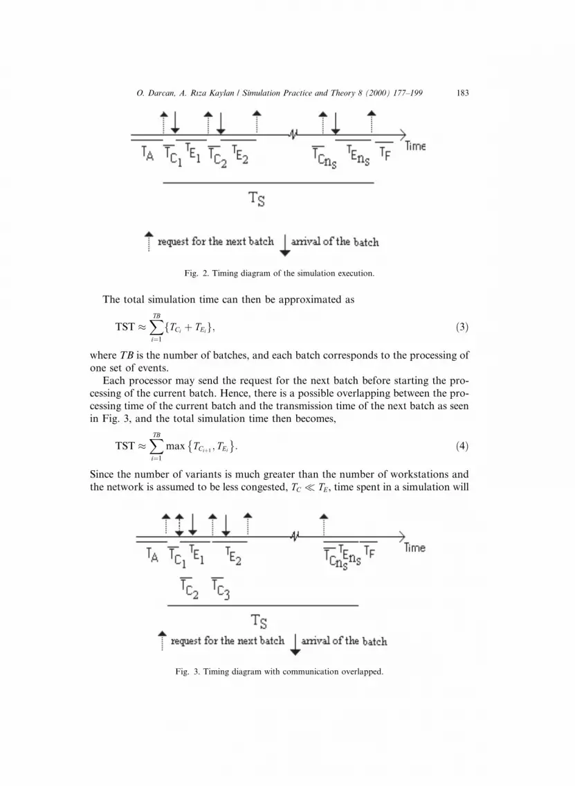
The total simulation time can then be approximated as

TST �XTB

i�1

TCif � TEig; �3�

where TB is the number of batches, and each batch corresponds to the processing ofone set of events.

Each processor may send the request for the next batch before starting the pro-cessing of the current batch. Hence, there is a possible overlapping between the pro-cessing time of the current batch and the transmission time of the next batch as seenin Fig. 3, and the total simulation time then becomes,

TST �XTB

i�1

max TCi�1; TEi

� : �4�

Since the number of variants is much greater than the number of workstations andthe network is assumed to be less congested, TC � TE, time spent in a simulation will

Fig. 3. Timing diagram with communication overlapped.

Fig. 2. Timing diagram of the simulation execution.


be dominated by the processing time TE. The total processing time requirement ofthe variants is the total load assigned to any workstation, TL, which can beapproximated by TE.

4.2. Estimated load of variants

In SC simulation, each event is subject to two distinct sets of operations; thinning(rate thinning and state thinning) and the state update operations. Let A and B bethe average computational load due to thinning and state update, respectively, dur-ing the whole simulation process and ki be rate for the event i in SC simulation. Allevents are checked for feasibility but only the surviving ones, whose probability tosurvive is referred to as the acceptance rate, rk

i , will cause the state update in the vari-ant k. For K di�erent event types, Tk, the load of variant k, can be expressed in termsof the parameters de®ned above as

Tk � BXK

i�1

rki � KA; �5�

where K is the total event rate for the system.The total load for E variants is

TL �XE

k�1

Tk � BXE

k�1

XK

i�1

rki � EKA �6�

and load, Lw, allocated to any workstation w which executes Mw variants will be

Lw � BXk2Sw

XK

i�1

rki �MwKA; �7�

where Sw is the set of variants assigned.

4.3. Static load balancing strategy

The basic idea in our load balancing strategy is to balance the total load of eachworkstation so that they spend more or less the same time to complete the simula-tion. For this purpose, we consider two di�erent cases; namely, the case in which1. the communication overhead is overlapped;2. the communication overhead is included in the load balance calculations.

4.3.1. Case 1. Load balancing with the communication overhead overlappedIn case 1, load balancing can be achieved in our problem by simply distributing

variants into workstations in proportion to their relative processing power, in sucha way that each subset will progress at approximately the same rate.

Load balanced distribution aims to balance the number of thinning and stateupdate operations in each of the workstations. The previous load formulas havetwo components. The ratio of A to B is hard to de®ne and furthermore it is


implementation dependent, hence, it is more reasonable to satisfy the proportionalityfor each component.

Considering the second component, the number of operations necessary for eachvariant (K events are processed in each variant) is the same for thinning. Thereforeload balancing due to thinning is based on the number of variants allocated to eachworkstation. The number of variants, Mw, allocated to the workstation w must beproportional to its processing power, Pw

Mw � PwEPP

� �; �8�

where PP is the total processing power of the network of workstations. The mea-surement of Pw is further discussed in Section 6.1. Since it may not be possible toallocate all the variants due to their integrity, the remaining variants are allocatedusing the largest processing time (LPT) algorithm [6].

Similarly, to balance the load due to state update, the total number of acceptedevents of variants allocated to any workstation w must also be proportional toPw. To simplify, let

Rk �XK

i�1

rki for k � 1; . . . ;E �9�

be the total number of accepted events per unit time in variant k, then the balanceformula becomesP

k2SwRk

Pw�PE

k�1 Rk

PP: �10�

Each variant k with Rk is to be assigned to one of the workstations. The objectivebecomes to ®nd a partition of the set of variants such that the maximum ratio of thetotal number of events accepted to the processing power in each workstation, isminimized. This can be stated more formally as: Given a set, S, consisting of Evariants, each with estimated computational cost Rk and a set of P workstationswith powers P1; P2; . . . ; PP , where �E > P� select a disjoint partition of S �S1 [ S2 [ � � � [ SP such that

min max16w6 P

Pk2Sw

Rk

Pw

� �� s:t: kSwk � Mw for 16w6 P : �11�

The load balancing is reduced to the so-called minimum makespan or multiprocessorscheduling problem in which the number variants to be allocated to each worksta-tion is determined in advance. The problem is known to be NP complete, and theLPT algorithm is used to solve this problem. The idea in determining the numbervariants to be allocated to each workstation before partitioning, is to require fasterworkstations to get any of the remaining variant k since its Rk value is small com-pared to K and KA is expected to dominate BRk.


4.3.2. The heuristic static load balancing algorithmThe load balancing algorithm used for distribution of E variants has three steps;Step 1: Compute the maximum number of variants, Mw, to be allocated to work-

station wCompute Mw � EPw

PP

� �for each w � 1; . . . ;P:

Let Z � EÿPPw�1 Mw:

If Z > 0 �distribute the remaining Z variants� increment Mw

by 1 for min16w6 PMw�1

Pw

n oStep 2: Distribute the variants using LPT scheduling algorithm in which the cost

of an variant k, is Rk.Sort E variants in a nondecreasing order of R; such that R1> R2>

� � �> RE: Let Sw �£;Hw � 0

�workload assigned to workstation w�; and the number ofvariant currently assigned to workstation w; Nw � 0 for w � 1; . . . ;PRepeat the following for j � 1; . . . ;EFind the workstation w for which min16W 6 P

HW �RkPW

n oand Nw < Mw:

Set Sw � Sw [ fjg;Nw � Nw�1; and Hw � Hw � Rk.Step 3: This step does workload tuning. The basic idea in this step is to reduce the

maximum workload by a series of pairwise exchange of variants between the mostheavily loaded workstation and the other workstations.Repeat the following steps until no exchange is possible

Let Dw � Hw ÿ PwTLPP for w � 1; . . . ;P

Sort loads in a nondecreasing order of D.Let m be the workstation with Dm � max16w6 P

Dwf g; to which the set Sm be assigned.Repeat the following steps for each workstation w � 1; . . . ;mÿ 1;Let a � Dm ÿ Dw� �=2If there exist two variants x and y such that

d � maxx2Sm;y2Sk

Rx ÿ Ry

� for 06d6a

then set Sm � Sm [ fyg ÿ fxg; Sk � Sk [ fxg ÿ fyg;Hm � Hm ÿ d; and Hk � Hk � d:

4.3.3. Case 2. Computation of processing power values with communication overheadLet PC1and CC1 be the average execution time of a batch for one variant in the

®rst server and the required communication time for transferring one batch betweenthe client and server. The total processing requirement of the simulation can bewritten in terms of the above parameters as

TST � TB CC1� � EPC1 �: �12�On the other hand, the average computation times for other servers can be computedfrom the processing power ratios such that

PCw � PC1

Pw

P1

: �13�


Let Fw be the fraction of set of variants assigned to server w, that can complete theexecution of one batch in

Tw � CCw � FwEPCw: �14�Then the equations that govern the relations among various variables and param-eters in the system are the following:

T1 � CC1 � F1EPC1

..

.

Tp � CCp � FpEPCp

�15�

and the fraction of number of variants should sum to 1

F1 � F2 � � � � � FP � 1: �16�Since we want to minimize the maximum completion time, this becomes

min maxw�1;...;P

Tw� �: �17�

The completion time of the simulation is the time when last processor ®nishesprocessing and the minimum ®nish time is achieved when all processor stops at thesame time, that is when

T1 � T2 � � � � � TP : �18�The optimal values for F can be calculated by solving the following set of equations:

Tw � Tw�1 for w � 1; . . . ; P ÿ 1: �19�Finally the new processing powers for the nonoverlapped simulation becomesPw � Fw. These new processing power values are used in the heuristic algorithm thatfollows to distribute variants.

5. Dynamic load balancing

Dynamic load balancing attempts to maximize utilization of the environment atall times (or at some checkpoints) by migrating the tasks among processors duringthe runtime. One of the policies used in dynamic load balancing is the centralizedone, in which a dedicated processor is responsible for maintaining a global stateof the system. This policy can easily be applied to standard clock simulation withoutany additional overhead due to information collection since the client has informa-tion about the current progress made by each workstation as well as the number ofvariants assigned. The client computes periodically the performance of each work-station from this information, then, estimates the completion time. When a load im-balance is detected, it decides whether or not the migration of a certain number ofvariants is pro®table to reduce the total simulation time. Hence, the objective ofour dynamic load balancing is to coordinate all workstations on the unprocessedwork by redistributing it among the workstations proportionally to their present


performance so that they all spend more or less the same time to complete thesimulation.

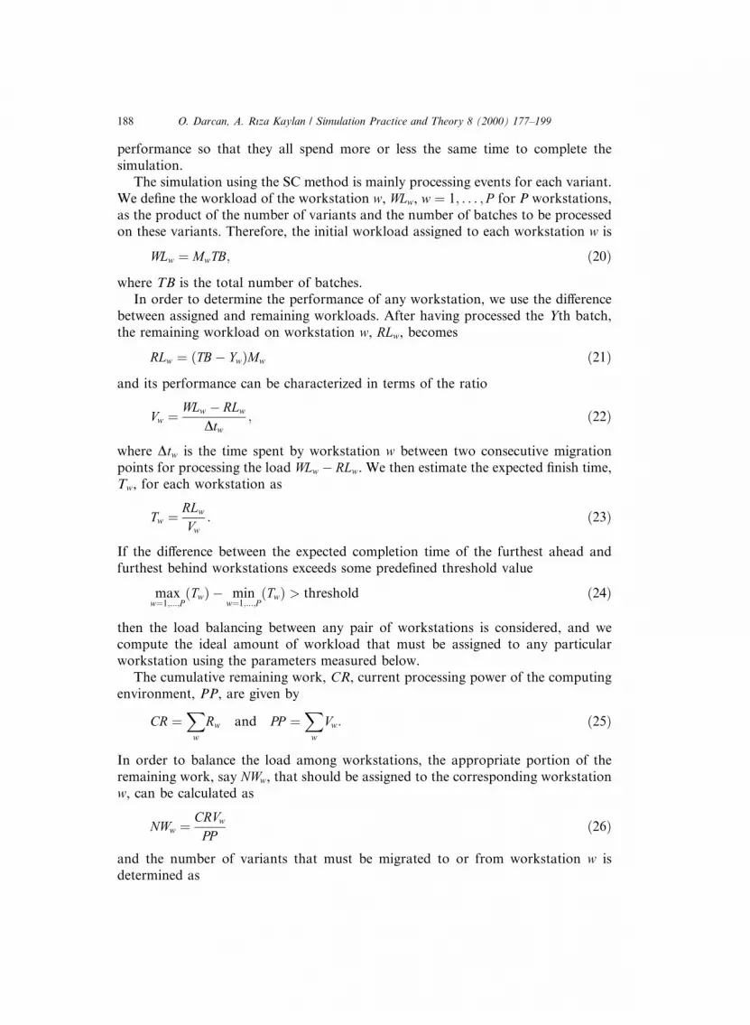
The simulation using the SC method is mainly processing events for each variant.We de®ne the workload of the workstation w, WLw, w � 1; . . . ; P for P workstations,as the product of the number of variants and the number of batches to be processedon these variants. Therefore, the initial workload assigned to each workstation w is

WLw � MwTB; �20�where TB is the total number of batches.

In order to determine the performance of any workstation, we use the di�erencebetween assigned and remaining workloads. After having processed the Yth batch,the remaining workload on workstation w, RLw, becomes

RLw � TB� ÿ Yw�Mw �21�and its performance can be characterized in terms of the ratio

Vw � WLw ÿ RLw

Dtw; �22�

where Dtw is the time spent by workstation w between two consecutive migrationpoints for processing the load WLw ÿ RLw. We then estimate the expected ®nish time,Tw, for each workstation as

Tw � RLw

Vw: �23�

If the di�erence between the expected completion time of the furthest ahead andfurthest behind workstations exceeds some prede®ned threshold value

maxw�1;...;P

Tw� � ÿ minw�1;...;P

Tw� � > threshold �24�

then the load balancing between any pair of workstations is considered, and wecompute the ideal amount of workload that must be assigned to any particularworkstation using the parameters measured below.

The cumulative remaining work, CR, current processing power of the computingenvironment, PP, are given by

CR �X

w

Rw and PP �X

w

Vw: �25�

In order to balance the load among workstations, the appropriate portion of theremaining work, say NWw, that should be assigned to the corresponding workstationw, can be calculated as

NWw � CRVw

PP�26�

and the number of variants that must be migrated to or from workstation w isdetermined as


Xw � NWw ÿ RLw

TBÿ Yw

� �: �27�

Each workstation with Xw > 0 is overloaded, hence, becomes a candidate sender,similarly, more variants can be run on the workstation with Xw < 0. Ideally, wewould like Xw for most of the workstations to be zero, as this will indicate theseworkstations are being utilized to ®nish the simulation process on time. Candidatematching mechanism is simple; the best-®t heuristic is used to ®nd the number ofvariants to be migrated from senders to receivers. Migration between candidates isallowed if it ful®lls the following inequalities· YS < YR i.e., the sender is behind of the receiver in terms of simulated events

� MS ÿ XS� � TBÿ YS� �VS

>MR TBÿ YR� � � XS TBÿ YS� ��

VR� TS;RXS

i.e., communication cost between workstations S and R does not make the loadbalancing pro®table.

6. Experimental results

6.1. Network environment

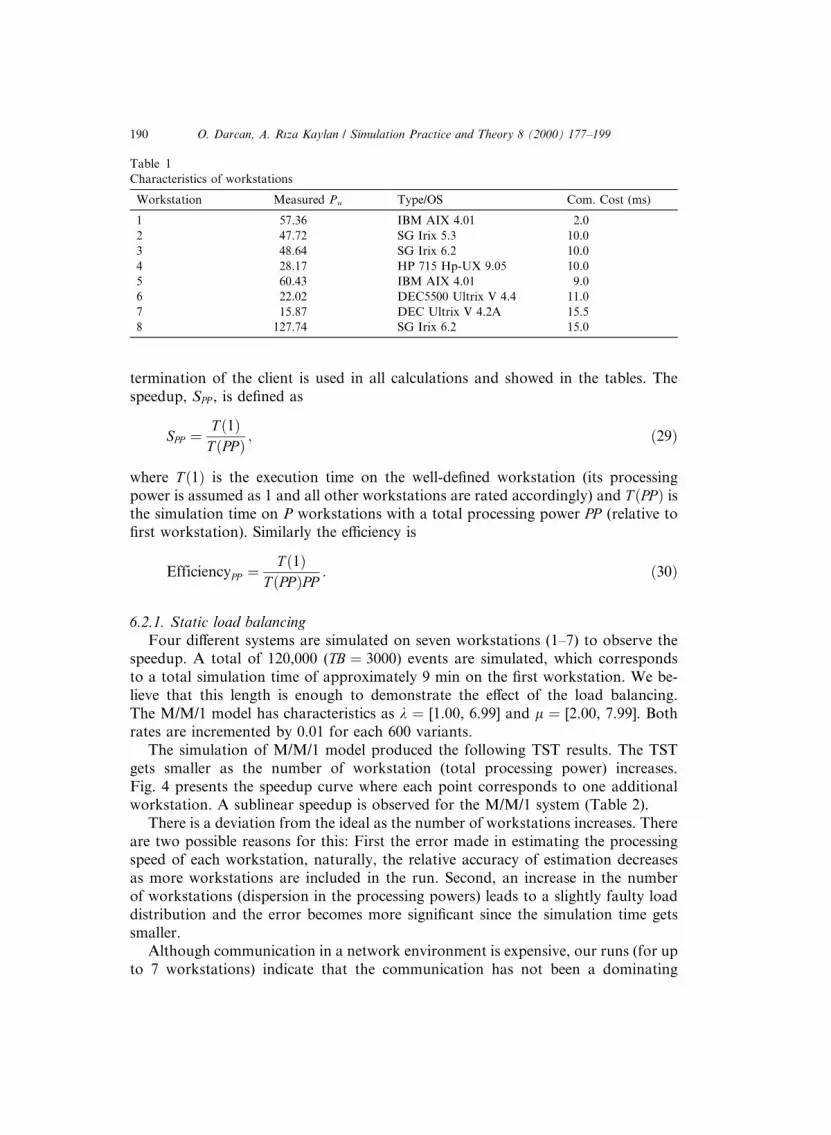
Runs have been carried out using up to seven workstations in the Campus net-work. The heterogeneous framework consists of two IBM, three Silicon Graphics,one HP and two Dec machines. Workstations are connected to three di�erent localsubnetworks in which they are all loosely coupled via Ethernet. The client and one ofthe servers are concurrently run on the ®rst workstation. The timing results can bea�ected by the load on the workstations. This e�ect is minimized by running simu-lation experiments when the workstations are idle. In order to compute the process-ing power of each workstation a ``benchmark'' simulation is concurrently run. Theprogram simulates N replicas of an M/M/1 system with q � 0:5 and 10 initial entities.The processing power, Pw, for each workstation is de®ned as

Pw � NExecutionTimew

; �28�

where ExecutionTimew corresponds to TS of workstation w. Characteristics of eachworkstation used in the runs, is given in Table 1. N is speci®ed as 50 for thisinvestigation.

6.2. Experiments by varying number of workstation

In this section, we study the performance of the distributed simulation as thenumber of workstations varies. TST is the time elapsed between the start and the


termination of the client is used in all calculations and showed in the tables. Thespeedup, SPP , is de®ned as

SPP � T �1�T �PP � ; �29�

where T �1� is the execution time on the well-de®ned workstation (its processingpower is assumed as 1 and all other workstations are rated accordingly) and T �PP� isthe simulation time on P workstations with a total processing power PP (relative to®rst workstation). Similarly the e�ciency is

EfficiencyPP �T �1�

T �PP �PP: �30�

6.2.1. Static load balancingFour di�erent systems are simulated on seven workstations (1±7) to observe the

speedup. A total of 120,000 (TB � 3000) events are simulated, which correspondsto a total simulation time of approximately 9 min on the ®rst workstation. We be-lieve that this length is enough to demonstrate the e�ect of the load balancing.The M/M/1 model has characteristics as k � [1.00, 6.99] and l � [2.00, 7.99]. Bothrates are incremented by 0.01 for each 600 variants.

The simulation of M/M/1 model produced the following TST results. The TSTgets smaller as the number of workstation (total processing power) increases.Fig. 4 presents the speedup curve where each point corresponds to one additionalworkstation. A sublinear speedup is observed for the M/M/1 system (Table 2).

There is a deviation from the ideal as the number of workstations increases. Thereare two possible reasons for this: First the error made in estimating the processingspeed of each workstation, naturally, the relative accuracy of estimation decreasesas more workstations are included in the run. Second, an increase in the numberof workstations (dispersion in the processing powers) leads to a slightly faulty loaddistribution and the error becomes more signi®cant since the simulation time getssmaller.

Although communication in a network environment is expensive, our runs (for upto 7 workstations) indicate that the communication has not been a dominating

Table 1

Characteristics of workstations

Workstation Measured Pw Type/OS Com. Cost (ms)

1 57.36 IBM AIX 4.01 2.0

2 47.72 SG Irix 5.3 10.0

3 48.64 SG Irix 6.2 10.0

4 28.17 HP 715 Hp-UX 9.05 10.0

5 60.43 IBM AIX 4.01 9.0

6 22.02 DEC5500 Ultrix V 4.4 11.0

7 15.87 DEC Ultrix V 4.2A 15.5

8 127.74 SG Irix 6.2 15.0


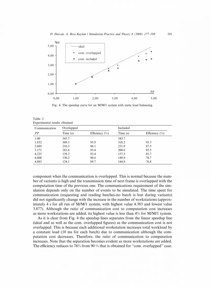
component when the communication is overlapped. This is normal because the num-ber of variants is high and the transmission time of next frame is overlapped with thecomputation time of the previous one. The communications requirement of the sim-ulation depends only on the number of events to be simulated. The time spent forcommunication (requesting and reading batches-no batch is lost during variants)did not signi®cantly change with the increase in the number of workstations (approx-imately 4 s for all run of M/M/1 system, with highest value 4.383 and lowest value3.877). Although the ratio of communication cost to computation cost increasesas more workstations are added, its highest value is less than 4% for M/M/1 system.

As it is clear from Fig. 4 the speedup lines separates from the linear speedup line(ideal and as well as the com. overlapped ®gures) as the communication cost is notoverlapped. This is because each additional workstation increases total workload bya constant load (10 ms for each batch) due to communication although the com-putation cost decreases. Therefore, the ratio of communication to computationincreases. Note that the separation becomes evident as more workstations are added.The e�ciency reduces to 76% from 90 % that is obtained for ``com. overlapped'' case.

Fig. 4. The speedup curve for an M/M/1 system with static load balancing.

Table 2

Experimental results obtained

Communication Overlapped Included

PP Time (s) E�ciency (%) Time (s) E�ciency (%)

1.00 543.7 543.7

1.832 309.5 95.9 318.2 93.3

2.689 210.3 96.1 231.9 87.5

3.171 183.6 93.4 200.6 85.5

4.225 139.3 92.4 157.5 81.7

4.608 130.2 90.6 149.9 78.7

4.885 124.1 89.7 144.9 76.8


As to the time spent for generation and dispatching of events in the server process,it is proportional to the number of events generated as well as the number of work-stations used in the run. During the simulation of the M/M/1 system in a singleworkstation, 120,000 events are created and sent in 3.5 s while this value rises to9.3 s. when the simulation is done on seven workstations.

Finally, two negligible ®gures are the overhead for collecting simulation resultswhich is less than 2 s and the time spent in setup phase is less than 1 s for all variants.

6.2.2. Possible static allocation strategiesIn this part, four alternative allocation strategies are compared. They are de®ned

as:A1: proposed load balanced allocation strategy;A2: random splitting (assignment) in which each workstation w is allocated anvariant with the probability Pw=PP ;A3: linear assignment from workstation 1 through 7. First M1 variants are allo-cated to workstation 1, next M2 variants are allocated to workstation 2 and so on;A4: similar to A3, but variants are assigned in the reverse order, i.e., from work-station 7 through 1.The results for the M/M/1 system, in Table 3 show the longest execution time

(TS) obtained for A1 and three di�erent allocation strategies as well as the percent-age of deterioration in between. (For A2, the smallest of 5 runs is reported as thetypical value) A1 outperforms all other strategies. Therefore, the acceptance ratesplays an important role in distributing the load of our M/M/1 model (on the av-erage 53% of the events are simulated). As it can be seen, A1 is marginally betterthan A2, the percentage of deterioration of A1 over A2 varies only from 4% to8%. The A2 algorithm produces a distribution in which one or two workstationsare slightly overloaded in terms of the number of variants and events to besimulated.

The last two allocation strategies A3 and A4 are tested to examine the worst casebehavior. They are signi®cantly worse than any one of the previous strategies with apercentage of deterioration varying from 17% up to 46% although the number ofvariants assigned to each workstation is proportional to its power. The longest exe-cution time is determined by the most heavily loaded workstation which is the ®rstand the last one in A3 and A4, respectively.

Table 3

Results of di�erent allocation strategies for M/M/1 system

Workstation PP A1 A2 A3 A4

2 1.832 303.35 317.77 423.76 355.71

3 2.680 206.28 215.31 281.89 258.89

4 3.171 179.52 193.26 262.42 226.00

5 4.225 134.19 145.26 184.24 178.20

6 4.608 125.53 132.20 174.76 164.00

7 4.885 117.91 127.58 166.20 158.60


6.2.3. E�ect of communication overlappingIn order to ®nd out the e�ect of communication overlapping, we run simulations

by varying the number of variants and the number of batches. Since the acceptednumber of events may e�ect the simulation time, the same M/M/1 system with aver-age acceptance rate of 56% is used in all runs. Note that this observation in this sec-tion is valid for our network environment with speci®cation given in Table 1.

In this section, we ®xed the number of events and varied the number of variants.We simulated ®ve set of M/M/1 system, (multiple of 25 variants in each set) on up to®ve workstations. With the ®rst set containing 25 variants, the simulation time didchange by additional workstations, resulting in a constant speedup value that is ap-proximately equal to 1.30. By increasing the number of variants to 50, we observed adecrease in the simulation time (up to three workstations) then it remained constant.The reason for a constant speedup value is that the communication time is high rel-ative to the computation time that is further reduced due to additional workstations.For the set containing more than 75 variants, we see a better increase in the speedupfor four workstations (PP � 3:171) as depicted in Fig. 5.

The change in the simulation time can be seen in Fig. 6. The simulation executiontime becomes more ``computation intensive'' after approximately 60 variants.

6.2.4. Dynamic load balancingIn order to evaluate the e�ectiveness of the dynamic load balancing, the M/M/1

system is simulated on ®ve workstations (1±4 and 8) for 120,000 events. Load im-balance is periodically checked for every 50 batches. The threshold value is chosenas 2 s.

We carry out two di�erent sets of variants; the sets di�er in the way the variantsare initially distributed to each workstation:

Fig. 5. Speedup curve vs processing power for di�erent number of variants.


· Even distribution, i.e., without any prior knowledge about the system.· Static load balancing in Section 4.3.1 andthe distribution is then balanced through migration during the execution as neces-sary.

The simulation of the M/M/1 system with two di�erent initial distributions pro-duced the following results presented in Table 4.

As seen in Table 4, the total simulation time gets smaller as the number of work-stations (i.e., total processing power) increases. Initial distribution of variants ac-cording to a performance rating of workstations results in a slight improvementabout 2±6%.

Fig. 7 presents the speedup curve where each point corresponds to one additionalworkstation. Similar to the results obtained in Section 6.2.3 without dynamic loadbalancing, a sublinear speed up is also observed on four workstations with e�ciencyvalues over 90%, however, an additional much faster workstation drops the e�cien-cy to 84%. The deviation from the ideal as the number of workstations is due to factthat the re-mapping is based on the estimated speed values.

Table 4

Experimental results obtained with dynamic load balancing

PP No initial balancing With initial balancing

Time E�ciency (%) Time E�ciency (%)

1.000 573.88

1.832 339.64 92.2 330.53 94.8

2.680 235.28 91.0 232.22 93.0

3.171 200.23 90.4 193.30 93.6

5.385 126.52 84.2 118.32 90.1

Fig. 6. Computation and communication levels.


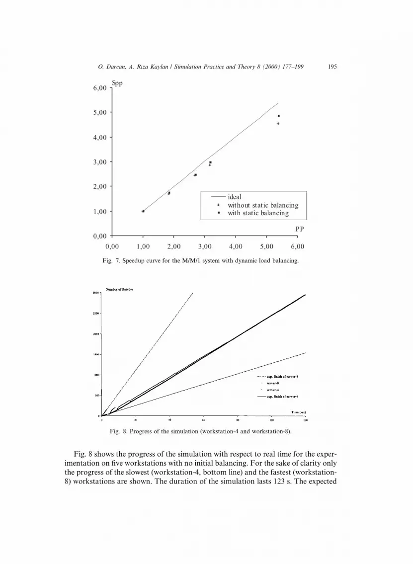
Fig. 8 shows the progress of the simulation with respect to real time for the exper-imentation on ®ve workstations with no initial balancing. For the sake of clarity onlythe progress of the slowest (workstation-4, bottom line) and the fastest (workstation-8) workstations are shown. The duration of the simulation lasts 123 s. The expected

Fig. 8. Progress of the simulation (workstation-4 and workstation-8).

Fig. 7. Speedup curve for the M/M/1 system with dynamic load balancing.


®nish times for the slowest and fastest workstations without any load balancing are238 s and 54 s, respectively as marked with dashed lines. Note that the processingpowers are benchmarked as 1.00±4.53 (from Table 1, 28.17 and 127.17).

Fig. 9 depicts the magni®cation of the beginning (the ®rst 20 s) of Fig. 7,where most of the load migrations took place. After receiving some new variants,workstation-8 slowed down. (The fast increase in the curve for workstation-8following the migration is due to the simulation of unprocessed events on migrat-ed variants) On the contrary, workstation-4 accelerates after the migration. Thediscontinuity in any progress line in Fig. 9 shows the time needed for themigration.

As mentioned before, the migration only entails sending the data segment. Thenecessary communication of the current data set has yielded on the average anadditional delay of 20 ms per variant. When more workstations with di�erentprocessing powers are added to the run, the attempts for load balancing as wellas number of variants migrated get substantially higher with no initial load balanc-ing, as shown in Table 5. The number of migrations is much less if workloads areinitially balanced.

Fig. 9. First 20 s of the simulation progress.

Table 5

Number of migrations occurred

Workstation Count Number Count Number

2 8 63 4 18

3 10 70 5 22

4 9 124 4 12

8 16 224 3 8


6.3. Experiments by varying parameters

In this section, we are interested in determining how parameters of the system af-fect the performance with the aim of examining the relation between the simulationtime and the number of events accepted. For this purpose, a set of runs is carried outsuch that the total number of events accepted has increased for each run while thenumber of events processed is kept constant. Since the acceptance rate depends onthe acceptance rate, each run consists of a set of variants with di�erent arrival ratesbut similar service rates. More speci®cally, for the set of M/M/1 system shown inTable 6, the range of arrival rate of each set is designed in such a way that 2.5%of the total events generated is accepted in the ®rst run, 12.5% of them is acceptedin the second run, and so on. In order to make the global rate of events constantfor all runs, the service rate l is 10 for all variants and the arrival rate of the last vari-ant k is 10 such that global rate K � 20.

Each set is run on network that consists of 3, 5 and 7 workstations. As depicted inFig. 10, the results of the simulation runs show that the simulation time increases byincreasing the number of event accepted for each speci®c run.

Table 6

Parameter setting for di�erent experiments

Run k Range Percent of events accepted (%)

1 [0.0, 0.498] 2.5

2 [0.0, 2.49] 12.5

3 [0.0, 4.98] 25.0

4 [0.0, 7.47] 37.5

5 [0.0, 9.96] 50.0

6 [5.0, 7.49] 62.5

7 [5.0, 9.98] 75.0

8 [7.5, 9.99] 87.5

Fig. 10. Speedup curves obtained for various acceptance rates.


7. Conclusion

In this paper, we have described a distributed implementation of SC method as-sociated with two di�erent load balancing techniques in the UNIX environment. Animportant conclusion is that both runs produced a promising result of a sublinearspeedup as more workstations are added to the run. The e�ciency obtained is high,this is because we have tested the algorithm in an ideal experimentation environmentand communication cost is not signi®cant compared to the computational work be-cause of the large number of variants.

It is clear from the results that the static load balancing does a good job of variantallocation, because it partitions the set of all variants into subsets based on the work-stations performance rating as well as the utilization of events in each variant. How-ever, its application is limited to the models for which the simulated event rate can bedetermined or at least predicted in advance.

As an alternative to static load balancing, we described a dynamic load balancingapproach. Although the dynamic load balancing described in this paper has pro-duced promising results, it is simple in the sense that other factors such as the net-work topology, transferred data size, data conversion due to internal formattingof processors are not considered in the decisions. We believe that more complex sys-tems ± for shorter simulations and network of M/M/1 systems ± require more sophis-ticated decision strategies since the migration time can be signi®cant compared to thetime spent in simulation.

References

[1] G. Bhatti, P. Vakili, Parallel/distributed simulation for parametric study of wireless communication

networks, Computer Science Department, Boston University, 1997 (obtained through personal

communication, e-mail: [email protected].).

[2] C. Burdorf, J. Marti, Load balancing strategies for time warp on multi-user workstation, The

Computer Journal 36 (1993) 168±176.

[3] R. Calinescu, D.J. Evans, A parallel simulation model for load balancing in clustered distributed

systems, Parallel Computing 20 (1994) 77±91.

[4] C.H. Chen, Y.C. Ho, An approximation approach of the standard clock method for general discrete-

event simulation, IEEE Transactions on Control Systems Technology 3 (3) (1995) 309±317.

[5] G. Cybenko, Dynamic load balancing for distributed memory multiprocessors, Journal of Parallel

and Distributed Computing 7 (1989) 279±301.

[6] G. Dobson, Scheduling independent tasks on uniform processors, SIAM Journal of Computing 13 (4)

(1984) 705±716.

[7] D.J. Evans, W.U.N. Butt, Local balancing with network partitioning using Host groups, Parallel

Computing 20 (1994) 325±345.

[8] M. Franklin, V. Govindan, A general matrix iterative model for dynamic load balancing, Parallel

Computing 22 (1996) 969±989.

[9] M. Hamdi, C.K. Lee, Dynamic load-balancing of image processing applications on clusters of

workstations, Parallel Computing 22 (1997) 1477±1492.

[10] J.Q. Hu, Parallel simulation of DEDS via event synchronization, Discrete Event Dynamic Systems:

Theory and Applications 5 (1995) 167±186.

[11] L. Kleinrock, Queueing Systems, vol 1, Wiley, NewYork, 1975.


[12] G.A. Kohring, Dynamic load balancing for parallelized particle simulations on MIMD computers,

Parallel Computing 21 (1995) 683±693.

[13] H. Lu, K. Tan, Load-balanced join processing in shared-nothing systems, Journal of Parallel and

Distributed Computing 23 (1994) 382±398.

[14] L. Mollamustafao�glu, Standard clock method in parallel simulation of several simulation

experiments, Research Report, FBE-IE-08/92-10, Bo�gazicßi University, 1992.

[15] L. Mollamustafao�glu, Discs: An object oriented framework for distributed discrete-event simulation

with the standard clock method, Simulation 70 (2) (1998) 75±89.

[16] D.M. Nicol, R.M. Fujimoto, Parallel simulation today, in: O Balcõ (Ed.), Annals of Operations

Research, 53 (J.C. Baltzer AG 1994) 249±285.

[17] S.M. Ross, Introduction to probability Models, sixth ed., Academic Press, New York, 1997.

[18] S. Selvakumar, C.S.R. Murthy, Static task allocation of concurrent programs for distributed

computing systems with processor and resource heterogenity, Parallel Computing 20 (1994) 835±851.

[19] R. Schlagenhaft, M. Runwandl, C. Sporrer, H. Bauer, Dynamic load balancing of a multi-cluster

simulator on a network of workstations, in: Proceedings of the Ninth Workshop on Parallel and

Distributed Simulation, June 1995, pp. 175±180.

[20] B.A. Shirazi, A.R. Hurson, K.M. Kavi, Scheduling and Load Balancing in Parallel and Distributed

Systems, IEEE Computer Society Press, Silver Spring, MD, 1995.

[21] S.G. Strickland, R.G. Phelan, Massively parallel SIMD simulation of Markovian DEDS: event and

time synchronous methods, Discrete Event Dynamic Systems: Theory and Applications 5 (1995)

141±166.

[22] P. Vakili, Massively parallel and distributed simulation of a class of discrete event systems: a di�erent

perspective, ACM Transactions on Modeling and Computer Simulation 2 (3) (1992) 214±238.

[23] P. Vakili, L. Mollamustafao�glu, Y.C. Ho, Massively parallel simulation of a class of discrete events,

in: Proceedings of the Fourth Symposium on Frontiers of Massively Parallel Computation, IEEE

Computer Society Press, Silver Spring, MD, 1992, pp. 412±419.

[24] Y. Wang, R.J.T. Morris, Load sharing in distributed systems, IEEE Transactions in Distributed

Systems 34 (3) (1985) 204±217.


load balanced implementation of standard clock method

Documents