linking ecology to land mosaics: an ecosystem perspective

In: Ecology of Hierarchical Landscapes: ISBN 1-60021-047-3 Ed: Jiquan Chen et al., pp. 91-124 © 2006 Nova Science Publishers, Inc.

Chapter 4

WATER AND CARBON CYCLES IN HETEROGENEOUS LANDSCAPES: AN ECOSYSTEM PERSPECTIVE

Asko Noormets1, Brent Ewers2, Ge Sun3, Scott Mackay4, Daolan Zheng1, Steve McNulty3, Jiquan Chen1

1 University of Toledo 2 University of Wyoming

3 Southern Global Change Program, USDA Forest Service 4 State University of New York at Buffalo

1. ABSTRACT Ecosystems, the elementary units in a landscape, determine landscape properties through their interactions of with one another, with the environment, and the combined actions of individual organisms within them. In this chapter, we discuss how water and carbon cycles connect the organizational levels of organisms, ecosystem, and landscape, and what we know of the mechanisms of their operation. We first describe the obstacles that one faces trying to connect these different levels and the ways to tackle them. In the second part of the chapter we use data from Chequamegon-Nicolet National Forest (CNNF) in Wisconsin, USA, and examples from other published work to illustrate current research questions and approaches. To date, greater progress has been made connecting the plant and ecosystem levels, and more unanswered questions remain about the relationships between ecosystem and landscape levels. The uniqueness of ecosystem ecology among other life sciences is defined by its focus on the interactions between the biotic elements of ecosystems and their abiotic environment, and the field has evolved rapidly over the past two decades. Recognition of the dynamic and evolving nature of ecosystems has caused ecologists to re-examine the basic assumptions behind the concept. The current focus on spatiotemporal variability and the resultant changes in current ecosystem science leads to linking ecosystem and landscape ecology. By establishing the vocabulary and methodology to work across hierarchical levels and taxonomic units, we are expanding the holistic understanding of the functioning of the natural systems around us.

Asko Noormets, Brent Ewers, Ge Sun et al. 92

2. INTRODUCTION The distinction between an ecosystem and a landscape is more vague than that between

ecosystem ecology and landscape ecology. The scale of ecosystems and landscapes, as defined in recent literature, is not necessarily mutually exclusive. Ecosystems, originally defined as distinct units by Tansley (1935), are “spatially explicit units of Earth that include all organisms, along with components of the abiotic environment within their boundaries” (Turner et al., 2001). Landscape, on the other hand, was defined by Turner et al. (2001) as an “area that is spatially heterogeneous in at least one factor of interest”. Thus, for different questions, the spatial scope of these two terms may be vastly different. For a particular question, however, we can still view “landscape” as the more comprehensive and inclusive term, relative to “ecosystem”. These terms form the framework for this chapter, and we view ecosystems as the elementary units of a landscape. As ecosystem ecology is the study of trophic interactions that connect individuals (Vitousek, 1993), so is landscape ecology the study of interactions that connect ecosystems. The composition of and the interactions between individual ecosystems determine landscape properties and processes. Landscape ecology addresses the spatial configuration of ecosystems relative to one another and the different outcomes that result from different spatial configurations (Turner et al., 2001). In order to understand the landscape-level processes we must be familiar with the hierarchical relationships between different organizational levels as well as with interactions within a level.

Let’s first look at how ecosystems are related to organizational levels above and below them. Later we will discuss how ecosystems interact with one another and what are the processes connecting them are. The properties of an ecosystem are determined by its constituents: vegetation, climate, landform, soil, flora, and fauna, as well as the physical, chemical and biological interactions among between these components. Understanding these linkages is critical since we are faced with questions of larger scale for which we lack direct data as well as clear understanding of their regulation. Since few measurements are possible directly at the ecosystem level, we often rely on existing data collected at smaller spatial and shorter temporal scales and draw inferences for larger scales (Miller et al., 2004). The difficulties come not as much from quantifying all important processes but from integrating processes that operate at different temporal and spatial scales and that interact with one another. Frequently, the transitions from leaf and plant levels to that of an ecosystem center around a canopy gas exchange model, as this represents the greatest fluxes of matter in the system and can be used as a reference for other processes. Yet, the underlying assumptions of the conceptual model developed for leaf level gas exchange (Farquhar et al., 1980; von Caemmerer and Farquhar, 1981) have rarely been tested at the canopy level (DePury and Farquhar, 1997). The additional processes of heterotrophic life, the structural complexity of the plant canopy, and the modifying influence of ecosystems on the micro-environment lead to interactions and feedbacks not present in lower level models. This inevitably leads to greater variability in data and greater uncertainty in model estimates as (i) interactions may be non-linear (Hu and Islam, 1997), (ii) the relationships may be scale-dependent (Walsh et al., 1997), and (iii) measurement of model parameters and validation of model accuracy may not be straightforward. The transposition of models to a different scale (specifically, from leaf and canopy to ecosystem) rests on the simplifying and fragile assumption that the spatial

https://www.researchgate.net/publication/228770978_Spatial_Extrapolation_The_Science_of_Predicting_Ecological_Patterns_and_Processes?el=1_x_8&enrichId=rgreq-e4ade825-eec4-40d4-a3f2-d99e573e705d&enrichSource=Y292ZXJQYWdlOzI1Nzg3MzM5MTtBUzoxNzI4NjcwNjA3NzI4NjRAMTQxODIyNjEyNzI5Nw==

Water and Carbon Cycles in Heterogeneous Landscapes 93

effects can be explained by underlying and quantifiable gradients in geological, climatic and edaphic features. Although this may initially seem counter-intuitive, hierarchy theory (Allen and Starr, 1982; O'Neill et al., 1986; both as cited in Reynolds et al., 1993) suggests that the predictive power of a model will not increase when we increase the number of lower levels of organization in the model, since we are limited by the assumptions made on the first step down towards finer spatiotemporal scales. However, the factors that exercise predominant control over a process need not necessarily reside in the next hierarchical level of organization, in which case hierarchical model structure may prove very powerful (Raupach and Finnigan, 1988). For example, since in forested ecosystems the majority of evapotranspiration (ET) comes from transpiration, changes in stomatal conductance have direct effects on ecosystem-level flux. Thus, from the perspective of water and carbon cycles, we need to understand the process of interest and determine the minimum amount of required detail from the organ and species level to match the accuracy of models as defined by the assumptions made when transcending from canopy to ecosystem level (Chen et al., 2004). In some cases this may require almost no sub-canopy detail, while in others physiological differences among species could be central to accurately predicting ecosystem processes.

The transition from ecosystem to landscape scale is one of aggregation (Table 1), even though a simple summing approach may be inadequate as we will see later (Section 5.4.3). Bradford and Reynolds (2006) and Gardner et al. (2001) emphasized that despite much of the data from smaller scale experiments being potentially useful for landscape-level studies, the majority of small-scale measurements are not amenable for scaling because of limitations of experimental design and (lack of) consideration of factors that have relevance across different scales. The specific requirements for spatial extrapolation of small-scale data regard adequate characterization of larger-scale variability, which affects confidence with which predictions can be made. Once the uncertainty of the data is known, their usefulness for making predictions increases greatly (Law et al., 2006; Li and Wu, 2006; Wu, 1999).

Another component of uncertainty in scaling from lower levels to the ecosystem level derives from the fact that ecosystems, as we understand them now (Chapin et al., 2002), are partially open systems. The cycles of energy, water, and carbon are not constrained to individual ecosystems, but operate on a continental or even global scale. The cycles of mineral nutrients (e.g. N, P), on the other hand, are closed, and the finite amount of nutrients is repeatedly cycled through the ecosystem’s various components (although long-distance transport of nutrients can occur through either natural or anthropogenic phenomena (Goudie and Middleton, 2001; Husar et al., 2001; Lelieveld et al., 2002; Prospero, 1999)). The nature of these depletable resources leads to feedbacks by which different ecosystem processes are related to one another and stabilize the system. It is important to note, however, that the interplay between stabilizing (usually internal) and destabilizing (usually external) influences, the mechanisms involved, and even the metrics of stability, are still a matter of active debate (O'Neill, 2001; Wu, 2004; Wu and Loucks, 1995).

In this chapter we will discuss water and carbon fluxes in temperate forest ecosystems, the methods of verifying and constraining various estimates, and what is known of the variation in these fluxes between different ecosystems. Most of the examples are based on work conducted in the Chequamegon-Nicolet National Forest (CNNF) in Wisconsin, USA.

https://www.researchgate.net/publication/225552354_Net_Ecosystem_Exchanges_of_Carbon_Water_and_Energy_in_Young_and_Old-growth_Douglas-Fir_Forests?el=1_x_8&enrichId=rgreq-e4ade825-eec4-40d4-a3f2-d99e573e705d&enrichSource=Y292ZXJQYWdlOzI1Nzg3MzM5MTtBUzoxNzI4NjcwNjA3NzI4NjRAMTQxODIyNjEyNzI5Nw==


Table 1. Organizational levels above and below ecosystem as relevant for scaling carbon and water fluxes (the abiotic components of ecosystem are not shown in this

representation). We differentiate between change in organizational level (shown with arrows) and simple aggregation. Since ecosystem and landscape are on the same

organizational level, the scaling between them is relatively straightforward. Scaling to an ecosystem from the lower level, on the other hand, includes transition of

organizational levels and is relatively more complex and vulnerable to error.

Region, Biome

LandscapeEcosystem

CommunityOrganism

(Canopy)

Organ (Leaf)Tissue

AggregateOrganizational level

Region, Biome

LandscapeEcosystem

CommunityOrganism

(Canopy)

Organ (Leaf)Tissue

AggregateOrganizational level

Change of organization / hierarchical level

3. SCALING PLANT AND ECOSYSTEM PROCESSES TO THE LANDSCAPE LEVEL

3.1. The Principles of Scaling

The need for scaling arises from our interest in answering questions at large spatial and

long temporal scales on the basis of information that is limited in both dimensions (Jarvis, 1995). Scaling has been argued to be of central importance in all aspects of ecology (Levin, 1992) as it helps us formalize our understanding of processes that drive the behavior of broader systems and of interactions between processes acting at different spatiotemporal dimensions. Without understanding the numerous interactions and feedbacks that constitute and contribute to the behavior at higher organizational scales, our power to predict and generalize is limited (Bradford and Reynolds, 2006; Norman, 1993).

When we think of scaling between different organizational levels, we start with a certain verifiable conceptual model, a hypothesis of how the processes of interest are regulated. For scaling water and carbon cycles, we assume that the chain of reactions proceeds as follows: radiation input and energy balance set constraints to water balance, which in turn constrains


carbon balance. The radiation balance of an ecosystem is modified by the albedo of the vegetation, which, in turn, is determined by soil type and water availability but can be modified by frequency of disturbance. These feedbacks that operate in both time and space determine the behavior of the system. The extent to which a process can reach its full capacity or biological potential depends upon feedbacks from other co-occurring processes. Thus, at the ecosystem level we are interested in identifying the key feedbacks across the leaf-to-plant-to-ecosystem-to-landscape hierarchy.

The simplest approach to scaling is summation. However, the greater the transition in scale (either spatial or temporal), the greater the chance that this method will not suffice. In Table 1 we have presented the organizational levels below and above the ecosystem and shown the transitions of scale that are encountered. We have also highlighted within-scale aggregation designs where the whole can be approximated as the sum of individual components without invoking any rules of higher organization.

The generalized steps for scaling were outlined by Caldwell et al. (1993) as follows: (1) assessing the scale of the phenomenon in question, (2) identifying the boundary conditions and constraints, (3) searching for consistencies at different scales, (4) streamlining bottom-up models to incorporate only the salient features, (5) incorporating feedbacks (both positive and negative) that may operate on some scales but not necessarily on other scales, and (6) testing the results on different scales with independent studies. Another aspect of scaling includes iterative steps of formalizing, verifying and simplifying relationships that are known to operate in the system.

3.2. Complexities of Ecosystem-to-Landscape Scaling One of the first tasks when modeling processes across multiple scales is to find

dimensions that are common for different organizational levels and would lend a common measure to the question of interest. In terms of water and carbon fluxes, both energy balance and gas exchange are properties measurable at leaf, canopy and ecosystem scale. Nevertheless, when transcending a level of organization (Table 1), additional components and processes come into play and may alter the process of interest. For example, it is understood that carbon exchange at the leaf level is driven by: (i) sink/source strength of the leaf, (ii) CO2 availability in the bulk media, and (iii) stomatal conductance (GS) (Baldocchi, 1993). At the ecosystem level, however, a significant (if not the dominant) fraction of exchange occurs by turbulent transfer, and molecular diffusion plays only a minor role (Jarvis and McNaughton, 1986; McNaughton and Jarvis, 1991). The importance of turbulent transfer of air is that this method can transport CO2 and H2O against the concentration gradient, whereas at the leaf level the exchange is driven by the concentration gradient. Boundary layer conductance affects gas exchange at both leaf and canopy scales, even though the breaking of this layer has a more dramatic effect on canopy than on leaf gas exchange. Likewise, the regulation of leaf- and canopy-level energy balance is controlled by different factors. Leaf energy balance is determined by the incoming and outgoing radiation, the balance between short- and long-wave components, and the partitioning of incoming radiation to sensible and latent heat fluxes. Canopy energy balance, on the other hand, additionally depends on the transfers of heat and water vapor inside the canopy and across the landscape, which are affected by advective flows, the energy balance of underlying soil and energy storage in vegetation and in


the canopy air space. The energy balance of an ecosystem depends primarily on vertical energy fluxes. Although the lateral transfer of energy in soil is possible, the vertical gradients and fluxes dominate over lateral ones (Noormets et al., 2004).

The proper level of detail to include in the scaling process may vary with the question to be answered. For modeling gas exchange, it has been suggested that since energy exchange between vegetation and the atmosphere occurs at the top of the plant canopy, only the dominant canopy species need to be characterized (Chapin, 1993). This approach is exemplified by models that describe canopy-level behavior in reference to a single layer of leaves (Ball and Berry, 1991; Collatz et al., 1991; Farquhar et al., 1980; Norman, 1993).

It has been recommended that model “mechanisms” be constrained to one organizational level lower than the level of interest and that the individual drivers at the lower level be expressed phenomenologically (Reynolds et al., 1993). Cleaning models of excessive detail of lower-level variation (Bazzaz, 1993) and retaining only significant factors and processes is a continuous process and represents the refinement of a model for a particular application. For example, models of ecosystem productivity usually operate at an hourly or daily time scale and use respective mean or maximum radiation levels as input. Yet we know that light can be very heterogeneous in the forest canopy (Fladeland et al., 2003). All leaves, except those at the topmost canopy positions, are exposed to light conditions that vary over a few seconds or minutes. Whether it is important to include such details depends on if these factors contribute to explaining potential feedback mechanisms that stabilize the system. Of course, the structure and level of detail in the model should support its purpose. For example, the significance of sunflecks is expected to be greater on photosynthesis than on transpiration, as the sun-shade transition has greater implications on local radiation than on air vapor pressure deficit (VPD). The level of required mechanistic detail also increases with increasing structural complexity of the system (Meyers and Paw U, 1986), but in general, understanding the negative feedbacks between system components provides the main mechanism for model simplification (McNaughton and Jarvis, 1991).

4. WATER FLUXES

4.1. Ecosystem Water Balance The hydrological cycle, describing the circulation of water between different pools, is

depicted in Figure 1. The primary storage compartments for water include the oceans, permanent ice, ground water, soil water, fresh water bodies and rivers, the atmosphere, and the biosphere (plants and animals). The processes of water transfer between the storage compartments include precipitation, evaporation, transpiration, infiltration, runoff, and groundwater flow. Detailed understanding of the dynamics of these pools and the mechanistic regulation of the transformations among them are required to assess the quantity and quality of regional and global water resources (Entekhabi et al., 1999; Hutjes et al., 1998). In this section, we will focus on the components that link plant-level water use to ecosystem water balance to landscape water balance and ultimately to the regional water cycle.


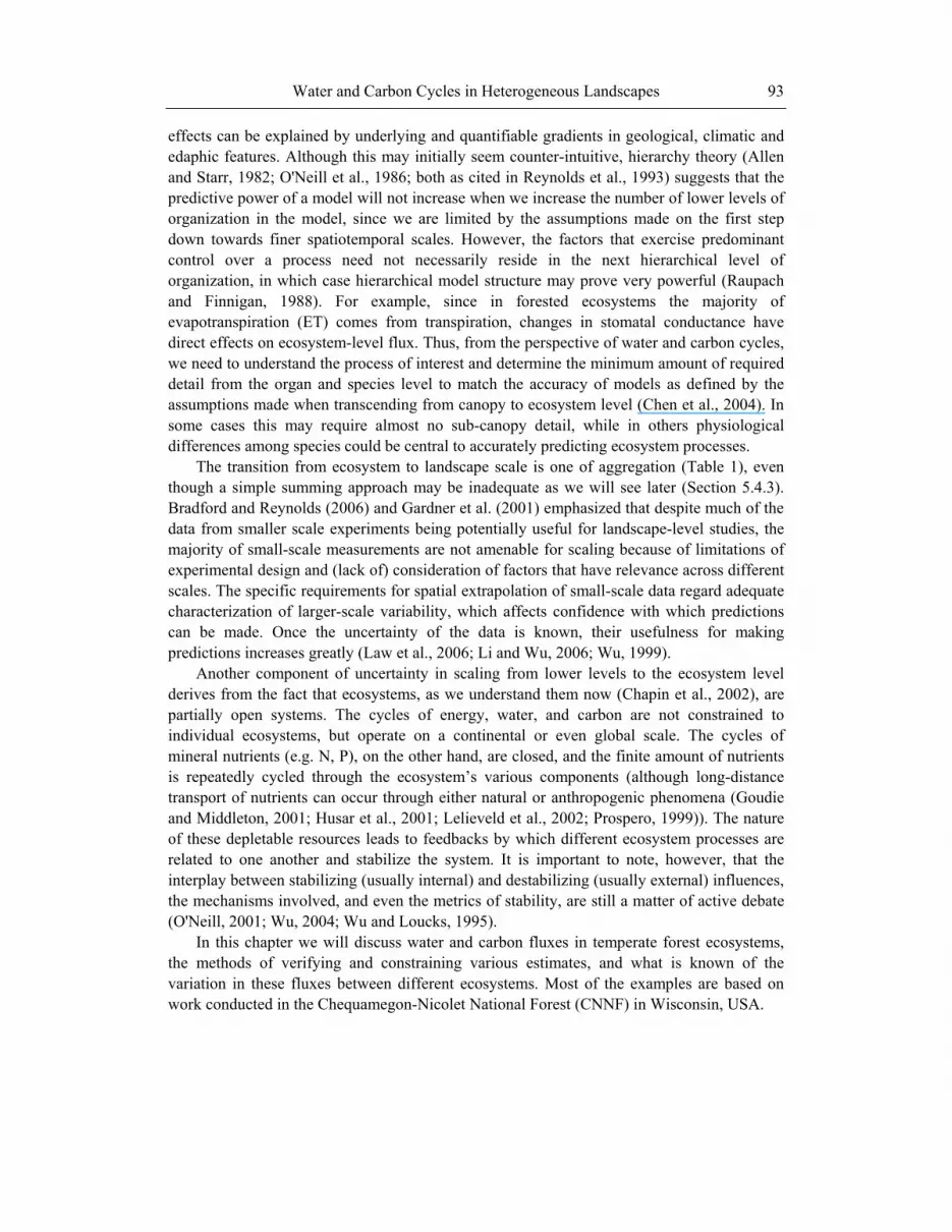
Figure 1. Major water fluxes in a forested watershed. The insets describe components of biological control of transpiration: (i) stomatal conductance (GS) increases in response to light levels (Q), (ii) GS declines with increasing vapor pressure deficit (D) and (iii) decrease in hydraulic conductance (k) of the soil-plant continuum in response to water potential (Ψ) gradients between soil and leaves (vulnerability curves).

The hydrologic cycle is driven primarily by large-scale motions of air masses, which are caused by differences in the amount of heating from solar radiation at different latitudes and between land and water. Air masses moving over land and water pick up some water from evaporation from oceans and ET from continents, move this water in vapor form, and release it as precipitation. The ET flux represents a combination of several water loss components (ordered from high to low magnitude): plant transpiration, canopy and litter interception, and evaporation from soil and vegetation surfaces. In addition to environmental factors, plant transpiration rate is related to leaf area index (LAI) and sapwood area (Andreassian, 2004; Gholz and Clark, 2002; Gholz et al., 1990). Canopy interception of precipitation can account for up to 20% of total rainfall in North American forests (Helvey and Patric, 1988). Interception is related to canopy and branch structures, LAI, and the intensity and frequency of precipitation. Soil evaporation in forests is generally minimal unless the soil is saturated (Currie, 1991). Next to precipitation, ET is the second largest water flux in the water balance in terrestrial systems. On average, about two thirds of annual precipitation returns to the atmosphere as ET (Baumgartner and Reichel, 1975). This flux is closely related to ecosystem productivity (Law et al., 2002; Rosenzweig, 1968) and biodiversity (Currie, 1991).

Available water that is not evaporated contributes either to run-off (Q, 0-50% of precipitation) or change in water storage pools (ΔS). Runoff includes both surface and subsurface flows, and at a watershed scale can be quantified as streamflow. Surface flow


rarely occurs and is uncommon in forested ecosystems because forest soils have high infiltration capacity. Subsurface flow rates are controlled by soil texture and structure and associated physical properties such as hydraulic conductivity, soil water retention, and hydraulic gradients that are often dictated by surface and subsurface land topography. Runoff is typically higher in moist than in dry ecosystems – in tropical rainforests (Shuttleworth, 1988) and temperate forests (Waring et al., 1981), about 50% of precipitation contributes to runoff and 50% to evaporation, whereas in grasslands and steppes 100% of precipitation leaves as ET (Floret et al., 1982; Massman, 1992). ET originates almost completely from terrestrial surfaces, with only about 3% coming from lakes and rivers. Thus, at least 60% of all circulating water within continental areas moves through the biosphere to the atmosphere. Since only about one percent of this water is stored in plant or animal tissues at any given time, the rates of water fluxes are high in comparison to the amount of water stored. The residual term, change in storage pools, is negligible in the temperate zone over multiple years, but on short temporal scales, it can change significantly. These changes may also be difficult to quantify due to the heterogeneity of soil, geology and topography, and different subpools of saturated and unsaturated zones.

4.2. Stomatal Control of Transpiration In physical terms, the evaporation of water from wet surfaces is described with the

Penman-Monteith equation (Monteith, 1965) that combines earlier mass-transfer and energy balance-based approaches:

))(a

cw

aapn

rr

rVPDcR

E+(1+Δ

+Δ=

γλρ

ρ Eq. 1

where E is evapotranspiration, Δ is the slope of the saturation vapor pressure-temperature curve, Rn is canopy net radiation, cp is the specific heat capacity of air, ρa is the density of air, VPD is vapor pressure deficit from canopy to air, ra is the bulk vegetation aerodynamic resistance, ρw is the density of water, λ is the latent heat of evaporation, γ is the psychrometric constant, and rc is canopy resistance. Aerodynamic resistance, ra, is affected by canopy properties and the flow of air through and above the canopy, while rc = (GSL)-1, where GS is canopy average stomatal conductance and L is canopy leaf area.

While maximum potential ET is determined solely by physical conditions (water availability and demand), actual ET from the leaf surface is regulated by stomatal guard cells that help maintain plant water status even under high atmospheric water demand. In physiological terms, this means that the hydraulic conductance of the soil-plant continuum will be functionally linked to stomatal conductance (Sperry et al., 2002).

The response of stomatal conductance to environmental conditions is the key plant level control over whole plant hydraulic conductance. Many studies going back to the early 1970s (Lange et al., 1971; Schulze et al., 1972) have shown decreasing stomatal conductance with


increasing VPD. Such a response leads to a non-linear saturating response between VPD and transpiration (Ewers et al., 2005) and even a decrease at extremely high VPD (Jarvis, 1980; Monteith, 1995; Pataki et al., 2000). The cue for this decline in stomatal conductance was cleverly shown to be linked to transpiration rather than directly to VPD by Mott and Parkhurst (1991). Although several empirical models have been developed (Ball et al., 1987; Jarvis, 1976) and have confirmed the involvement of hydraulic feedback loop between guard cell water potential and transpiration rate (Franks, 2004), the exact mechanism of regulation remains elusive. Nevertheless, the control of transpiration by GS is heavily utilized in climate (Avissar and Pielke, 1989; Sellers et al., 1997), ecosystem (Aber and Federer, 1992; Foley et al., 1996, 2000; Running and Coughlan, 1988; Running and Hunt, 1993; Running et al., 1989) and hydrologic modeling (Band et al., 1993; Famiglietti and Wood, 1994; Mackay and Band, 1997; Vertessy et al., 1996; Wigmosta et al., 1994).

4.3. Potential Mechanisms Governing Stomatal Control of Transpiration Stomatal closure under high VPD conditions is probably a response to low leaf water

potential, ΨL (Oren et al., 1999b), and reduced transpiration (Monteith, 1995) helps to minimize potentially fatal xylem cavitation (Sperry, 2004; Tyree and Sperry, 1989). Stomatal regulation provides the universal control point that regulates the benefits of CO2 uptake for photosynthesis in exchange for transpired water, and it operates between the demands of VPD and availability of water as determined by environmental parameters (soil water release properties; Sperry, 1998) and plant hydraulic properties (Katul et al., 2003).

The regulation of ΨL is ultimately governed by the properties of the water conducting xylem in the plant and the texture of the soil. It has been shown that hydraulic conductance scales linearly with plant leaf area, a relationship that holds across many plant species and environmental conditions. Yet, any change in environmental conditions that increases resource availability decreases the efficiency of hydraulic conductance per unit leaf area (Mencuccini, 2003), which will ultimately affect both the magnitude of transpiration and its response to environmental conditions. Factors that may alter hydraulic conductivity include changes in soil texture, vapor pressure deficit, CO2 concentration, and soil nutrients (Mencuccini, 2003).

4.4. Modeling Stomatal Conductance Response to Internal and External Signals

Quantifying the response of GS to VPD is not a trivial matter since the latter is closely

correlated with radiation and temperature regime of the underlying surface. However, Rayment (2000) devised a statistically based method for data filtering that allows the VPD effect on GS to be isolated from the effects of other environmental variables. Conditional filtering was used to develop the concept of reference stomatal conductance (GSref; Ewers et al., 2001), leading to significant simplification of the Jarvis (1976) stomatal conductance model (Oren et al., 1999a):


VPDmGG lnSrefS ⋅−= Eq. 2

where -m is the logarithmic sensitivity of the GS response to VPD. GSref is defined as maximum GS at VPD=1 kPa. This model is preferred over the Ball-Berry stomatal conductance model (Ball et al., 1987) because of its use of relative humidity as the driving factor instead of VPD. The Ball-Berry model is also outperformed by the Jarvis (1976) approach in comprehensive multiple model comparisons (Katul et al., 2000). The advantage of the Jarvis model variants (Oren et al., 1999b) for hydrologic processes is that it directly addresses plant response to vapor pressure deficit as a proxy for water loss rate, which means it works best when the rate of water loss is high and hence hydrologically significant. Recently, Katul et al. (2003) presented a coupled water and carbon model that bridges the gap between the carbon-oriented models using the Ball-Berry equation and the water-oriented models using the Jarvis equation.

GSref (mmol m-2 s-1)

0 100 200 300 400

m (m

mol

m-2

s-1

ln(k

Pa)

-1)

0

50

100

150

200

250Oren et al. (1999) relationship E. nevadensis, L.. tridentata 12 - 151 year old P. marianaSeven tree species year 1

Seven tree species year 2

Figure 2. Relationship between reference canopy stomatal conductance (GSref, defined as GS at VPD=1 kPa) and the sensitivity of GS to VPD (m; Eq. 1). The solid line (with slope 0.6) represents species that regulate minimum leaf water potential (Oren et al., 1999b). Species that do not regulate minimum leaf water potential (Ephedra nevadensis, Larrea tridentata and Picea mariana) have lower -m at any given GSref as a result of declining leaf water potentials with changing sapwood:leaf area ratios. Seven tree species from the temperate Chequamegon Ecosystem-Atmopshere Study (ChEAS) area from two contrasting years closely follow the 0.6 line despite defoliation, water level change, and leaf area dynamics.

Across a large range of species, and even environmental conditions within species, -m is 0.6 GSref (Figure 2). Since the original review of Oren et al. (1999b), many other species and effects of environmental conditions with species have been analyzed (Addington et al., 2004; Ewers et al., 2001, 2005; Gunderson et al., 2002; Oren et al., 1999a). The 0.6 proportionality between -m and GSref results from the regulation of minimum ΨL to prevent excessive xylem


cavitation. Species or individuals with high GSref have the disadvantage of having a proportionally high -m and greater absolute reduction in GS with increasing VPD, while species with low GSref have the advantage of having a low -m and smaller absolute reduction in GS with increasing VPD. Important deviations from the 0.6 proportionality occur (i) in species where the minimum ΨL decreases with increasing VPD, (ii) when the range of VPD increases, or (iii) when the ratio of boundary layer conductance to stomatal conductance is low (Oren et al., 1999b). The first two conditions result in a ratio of -m to GSref less than 0.6 as the result of plants that have less strict regulation of ΨL (Figure 2) such as drought tolerant desert species Ephedra nevadensis and Larrea tridentata (Ogle and Reynolds, 2002; Oren et al., 1999b) or trees that maintain a low sapwood-to-leaf area ratio as seen in Picea mariana with increasing age (Ewers et al., 2005). The third condition results in a ratio of -m to GSref that is greater than 0.6 (Oren et al., 1999b).

4.5. Scaling Transpiration Measurements and Models The earlier summing approaches to canopy gas exchange required over 30 simultaneous

gas exchange measurements to be taken at any given point in time at different levels of the canopy (Leverenz et al., 1982). Clearly, such a low efficiency is prohibitive for larger domains. Data on stem sap flow can now provide a continuous record of a much greater portion of plant water use (Ewers and Oren, 2000; Granier et al., 1996). For stand-level applications, measurements of sap flow first must be scaled to plant level ET using radial and circumferential measurements (Ewers et al., 2002; Ewers and Oren, 2000; James et al., 2002; Lu et al., 2000; Lundblad et al., 2001; Oren et al., 1999b; Phillips et al., 1996) and then to stand level through estimates of stand sapwood area (Oren et al., 1998). Such studies have shown that radial and circumferential trends change both within and among species and may change with time (Ford et al., 2004). Considering these trends, estimates from leaf-level gas exchange and whole tree sap flux measurements show a good agreement (Figure 3).

If new additions of stomatal conductance measurements confirm the GSref-VPD relationship for plants that regulate minimum leaf water potential (Figure 2), they may open new avenues of scaling in both time and space. Recent studies even suggest that species that do not regulate minimum water potential can be successfully modeled by incorporating the dropping water potentials with increasing VPD (Ewers et al., 2005; Ogle and Reynolds, 2002), further confirming the mechanistic underpinnings of Eq. 2. Since only GSref needs to be quantified, relatively few measurements are required for populating a spatially heterogeneous landscape (Figure 4). Landscape gradients could be quantified with the efficient, spatially-explicit 2-D measurement design as proposed by Burrows et al. (2002). This approach uses non-uniform, non-random location assignment of point-pairs, considering underlying landscape gradients and heterogeneity, and is particularly well suited for geostatistical analyses. The use of a sampling design that minimizes the number of required point-pairs for acceptable confidence limits makes this method particularly suited for scaling other sparsely sampled properties, including ecosystem-level fluxes of water and CO2.


gS (mmol m-2 s-1)

0 125 250

GS

(mm

ol m

-2 s

-1)

0

125

250CIFIF

Pinus taedaScotland Co., NC July 24, 29 1998

Figure 3. Comparison of porometry-based stomatal conductance (gs) and sap-flux based stomatal conductance (GS) in control (C), irrigated (I), fertilized (F), and irrigated/fertilized (IF) Pinus taeda trees in three positions: upper branches (open symbols), lower branches (gray symbols) and stems (closed symbols). The dashed line represents the 1:1 line. Data reanalyzed from Ewers and Oren (2000).

Figure 4. Major cover types around the WLEF tower (Davis et al., 2003). Ecosystem transpiration flux saturates with increasing vapor pressure deficit, whereas free evaporation from the saturated soils and open water surfaces increases linearly. Comparison of measured eddy covariance evapotranspiration flux with area-weighted sum of scaled-up sap-flux measurements and free evaporation at the WLEF site showed good agreement, whereas generic biome-based scaling was inaccurate.


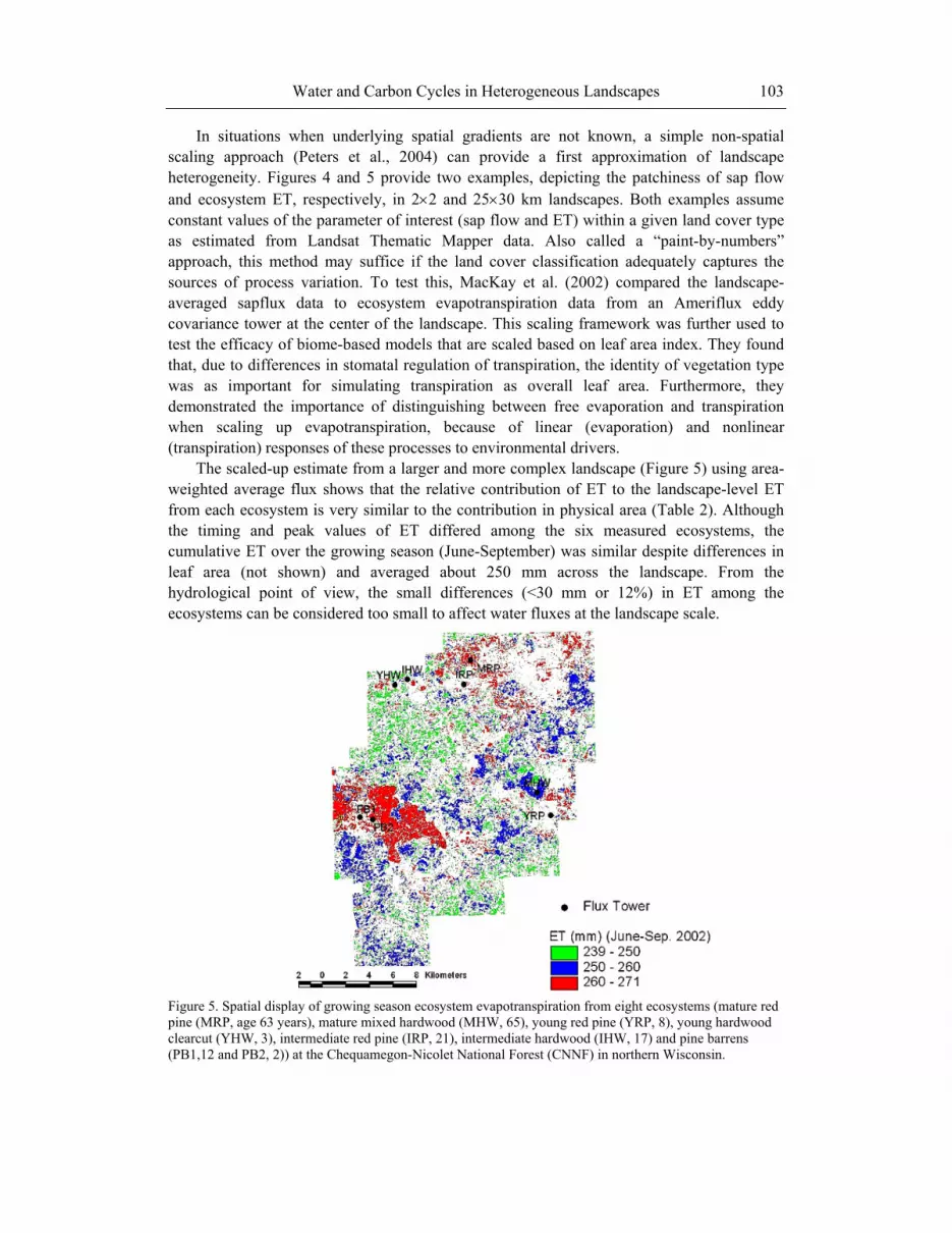
In situations when underlying spatial gradients are not known, a simple non-spatial scaling approach (Peters et al., 2004) can provide a first approximation of landscape heterogeneity. Figures 4 and 5 provide two examples, depicting the patchiness of sap flow and ecosystem ET, respectively, in 2×2 and 25×30 km landscapes. Both examples assume constant values of the parameter of interest (sap flow and ET) within a given land cover type as estimated from Landsat Thematic Mapper data. Also called a “paint-by-numbers” approach, this method may suffice if the land cover classification adequately captures the sources of process variation. To test this, MacKay et al. (2002) compared the landscape-averaged sapflux data to ecosystem evapotranspiration data from an Ameriflux eddy covariance tower at the center of the landscape. This scaling framework was further used to test the efficacy of biome-based models that are scaled based on leaf area index. They found that, due to differences in stomatal regulation of transpiration, the identity of vegetation type was as important for simulating transpiration as overall leaf area. Furthermore, they demonstrated the importance of distinguishing between free evaporation and transpiration when scaling up evapotranspiration, because of linear (evaporation) and nonlinear (transpiration) responses of these processes to environmental drivers.

The scaled-up estimate from a larger and more complex landscape (Figure 5) using area-weighted average flux shows that the relative contribution of ET to the landscape-level ET from each ecosystem is very similar to the contribution in physical area (Table 2). Although the timing and peak values of ET differed among the six measured ecosystems, the cumulative ET over the growing season (June-September) was similar despite differences in leaf area (not shown) and averaged about 250 mm across the landscape. From the hydrological point of view, the small differences (<30 mm or 12%) in ET among the ecosystems can be considered too small to affect water fluxes at the landscape scale.

Figure 5. Spatial display of growing season ecosystem evapotranspiration from eight ecosystems (mature red pine (MRP, age 63 years), mature mixed hardwood (MHW, 65), young red pine (YRP, 8), young hardwood clearcut (YHW, 3), intermediate red pine (IRP, 21), intermediate hardwood (IHW, 17) and pine barrens (PB1,12 and PB2, 2)) at the Chequamegon-Nicolet National Forest (CNNF) in northern Wisconsin.

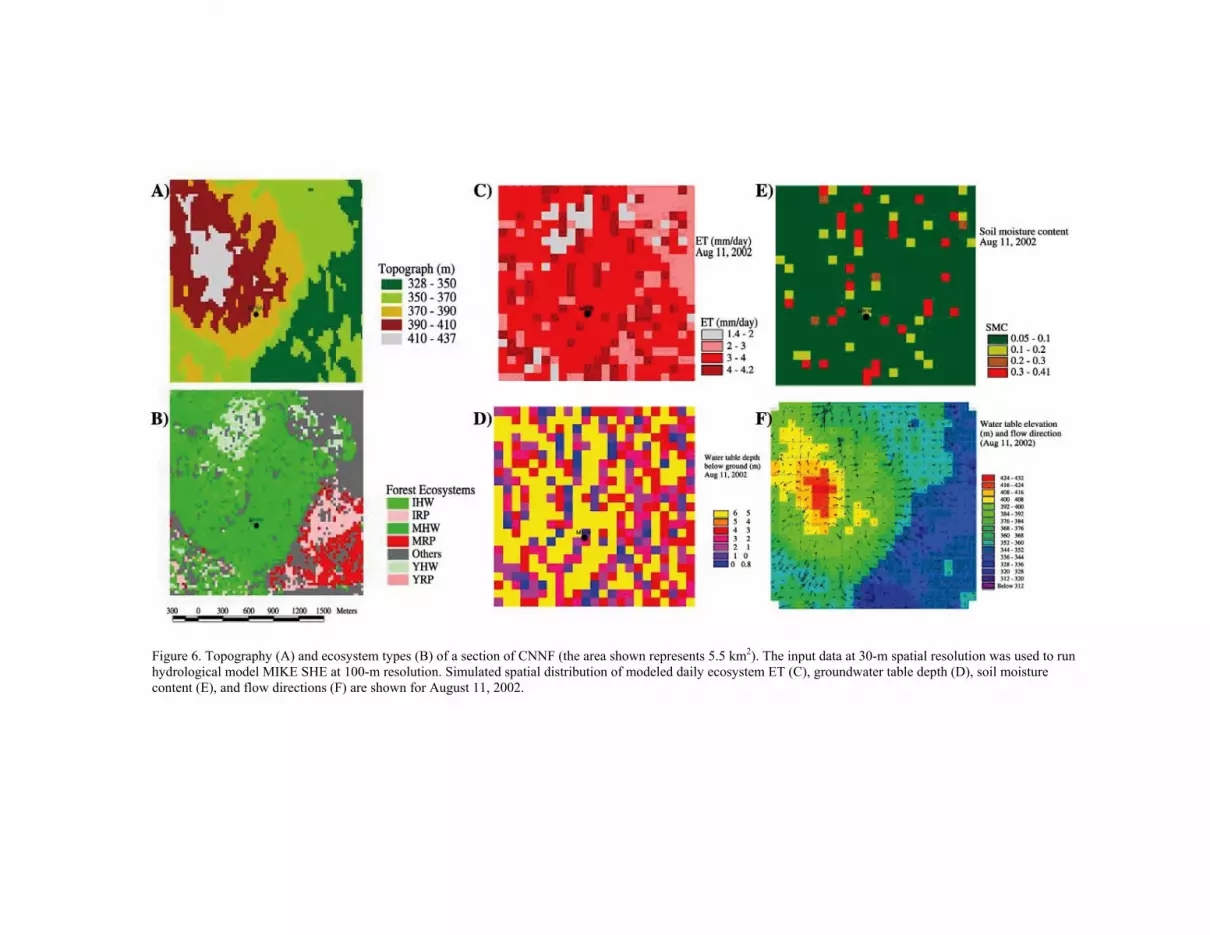
Figure 6. Topography (A) and ecosystem types (B) of a section of CNNF (the area shown represents 5.5 km2). The input data at 30-m spatial resolution was used to run hydrological model MIKE SHE at 100-m resolution. Simulated spatial distribution of modeled daily ecosystem ET (C), groundwater table depth (D), soil moisture content (E), and flow directions (F) are shown for August 11, 2002.


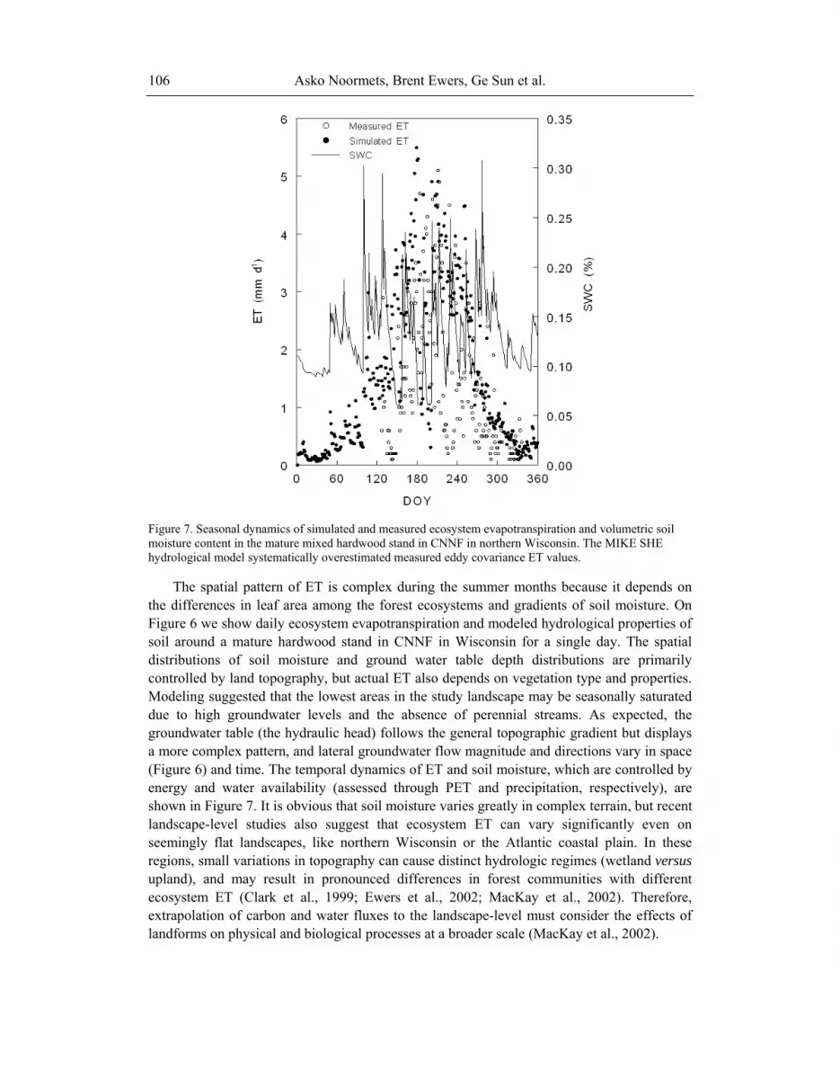
Table 2. Growing season evapotranspiration for five ecosystems and their relative contributions at a landscape scale in northern Wisconsin. MRP – mature red pine plantation (age 63 years), MHW – mature mixed northern hardwood stand (65), YRP – young mixed red and jack pine plantation (8), PB – pine barrens (12), YHW – young hardwood clearcut (3).

Cover Area (ha) Area contribution ET (mm) ET contribution MRP 1796 0.15 271 0.16 MHW 4688 0.40 251 0.40 YRP 283 0.02 270 0.03 PB 1876 0.16 265 0.17 YHW 3058 0.26 239 0.25

Summary Sum

11702 Sum 1.00

Mean 253

Sum 1.00

4.6. Simulating Landscape Hydrology Having quantified individual ecosystem-level ET, we can analyze its dynamic response to

site properties (topography, soil properties, climate, etc.) by simulating water movement and vegetation-atmosphere interactions at different spatial and temporal scales (Chen et al., 2005). On Figure 6 we show daily ecosystem evapotranspiration and modeled hydrological properties of soil around the mature hardwood stand in Chequamegon-Nicolet National Forest (CNNF), Wisconsin. The hydrological model, MIKE SHE (Abbott et al., 1986a, 1986b; DHI, 2004; Im et al., 2004), utilizes spatially explicit information on vegetation type and properties, soil, and topography, and it simulates the full water cycle characteristic of a forest ecosystem, including ET and vertical soil water movement in the unsaturated soil zone to the underlying groundwater system. The ET sub-model of MIKE SHE interacts with soil moisture content dynamically at multiple layers. The total ET flux was controlled by the potential evapotranspiration (PET), which in this study was calculated externally using Hamon’s method (Lu et al., 2005) as a function of measured air temperature and calculated daytime length using site location (latitude) and date. Water loss through canopy interception was modeled as a function of PET and of LAI, which varies on a daily basis. Plant transpiration (T) is described in MIKE SHE as a function of PET, LAI, root distribution, and soil moisture content in the rooting zone. Soil evaporation was simulated in the procedure as a function of PET, LAI, soil moisture, and residual water availability (PET-T). Vertical movement of water infiltration was modeled using 1-D Richard’s equation while groundwater movement was simulated as 2-D flow. Groundwater and overland water flows link all the simulation units, which in this case are 100×100 m cells. The model inputs were generalized spatial soil and vegetation parameters (LAI and plant rooting depth), but daily climatic variables of air temperature and rainfall were used to constrain model behavior with measured data.


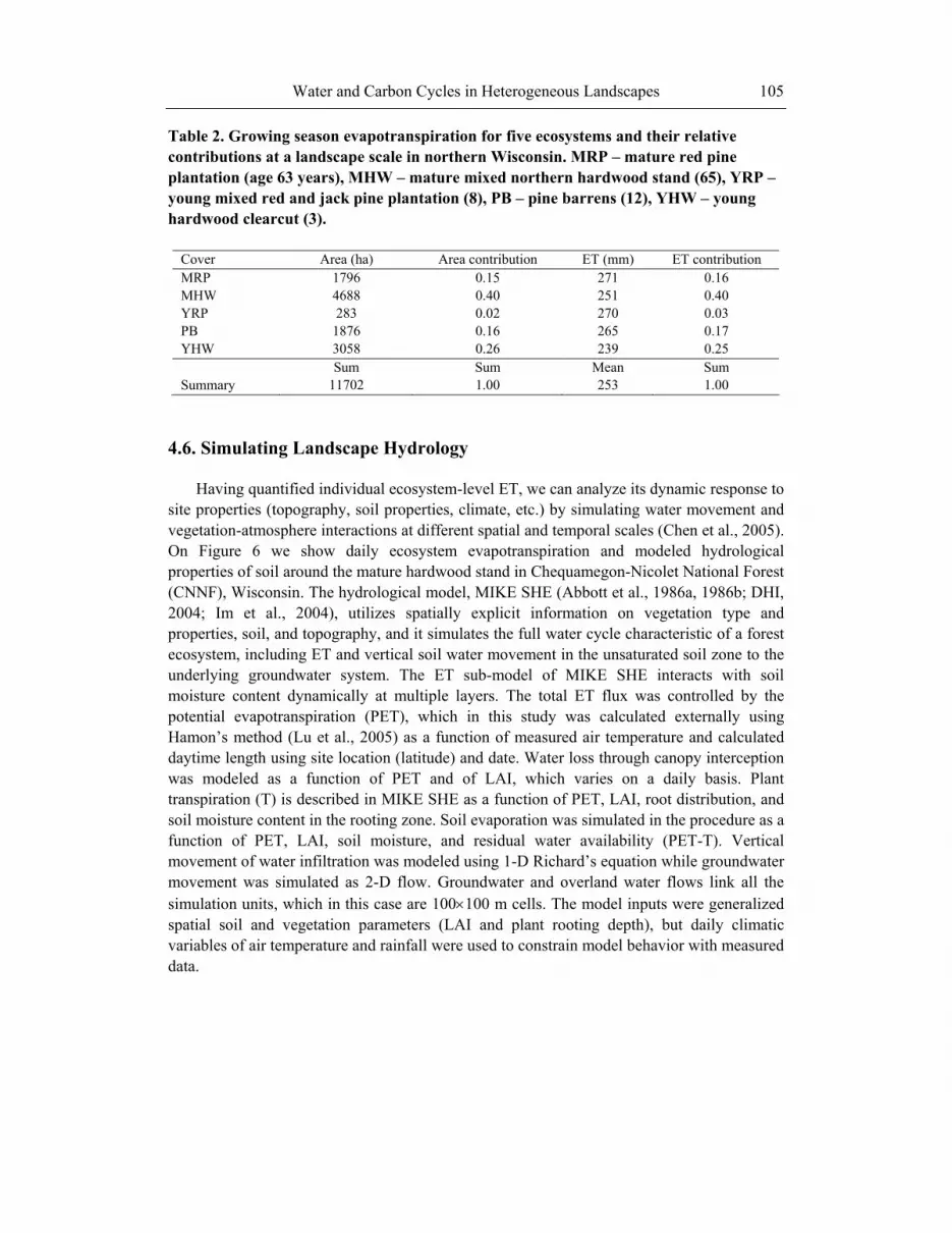
Figure 7. Seasonal dynamics of simulated and measured ecosystem evapotranspiration and volumetric soil moisture content in the mature mixed hardwood stand in CNNF in northern Wisconsin. The MIKE SHE hydrological model systematically overestimated measured eddy covariance ET values.

The spatial pattern of ET is complex during the summer months because it depends on the differences in leaf area among the forest ecosystems and gradients of soil moisture. On Figure 6 we show daily ecosystem evapotranspiration and modeled hydrological properties of soil around a mature hardwood stand in CNNF in Wisconsin for a single day. The spatial distributions of soil moisture and ground water table depth distributions are primarily controlled by land topography, but actual ET also depends on vegetation type and properties. Modeling suggested that the lowest areas in the study landscape may be seasonally saturated due to high groundwater levels and the absence of perennial streams. As expected, the groundwater table (the hydraulic head) follows the general topographic gradient but displays a more complex pattern, and lateral groundwater flow magnitude and directions vary in space (Figure 6) and time. The temporal dynamics of ET and soil moisture, which are controlled by energy and water availability (assessed through PET and precipitation, respectively), are shown in Figure 7. It is obvious that soil moisture varies greatly in complex terrain, but recent landscape-level studies also suggest that ecosystem ET can vary significantly even on seemingly flat landscapes, like northern Wisconsin or the Atlantic coastal plain. In these regions, small variations in topography can cause distinct hydrologic regimes (wetland versus upland), and may result in pronounced differences in forest communities with different ecosystem ET (Clark et al., 1999; Ewers et al., 2002; MacKay et al., 2002). Therefore, extrapolation of carbon and water fluxes to the landscape-level must consider the effects of landforms on physical and biological processes at a broader scale (MacKay et al., 2002).


5. CARBON FLUXES

5.1. Variation Among Ecosystems For ecosystem processes to be integrated over landscape to global scales, spatially

continuous parameters must be estimated from remotely sensed (RS) information. It has been shown that disparity of spatial resolution between ecosystem level heterogeneity (Law et al., 2006) and landscape level patchiness on one hand and the coarseness of some RS data on the other (Turner et al., 2003; Zheng et al., 2004) can significantly alter estimates of regionally integrated carbon and water balances. Therefore, we must understand the sources of landscape-level variability on carbon and water exchange and the mechanisms behind it.

Figure 8. Growing season cumulative NEE, ER, and GEP in stands of different ages in the CNNF in Wisconsin, USA. Panel (A) depicts the age relationship across all stands, whereas panel (B) distinguishes between deciduous (black) and coniferous stands (red). NEE is expressed by sign convention by which negative values indicate fluxes from atmosphere towards the surface (uptake by vegetation) and positive values indicate fluxes from surface to the atmosphere (release by vegetation and soil). ER and GEP are both positive and NEE = ER – GEP.

In a managed forest landscape in northern Wisconsin, we found that the differences in net ecosystem exchange of carbon (NEE) among 10 different forest stands were better explained by mean tree age than by stand biomass, LAI, species composition or any environmental variable measured (Figure 8). The age-dependence was strongest for NEE, which exhibited both steeper slope and greater R2 than its two component fluxes, gross ecosystem productivity (GEP) and ecosystem respiration (ER). In fact, the directional change with age was stronger in ER than in GEP, suggesting that further increases in GEP with age may be limited by self-


shading (Oker-Blom and Kellomäki, 1983) or edaphic constraints. The effect of stand-replacing disturbance on ER lasted longer than that on GEP, possibly as the result of disturbance-generated coarse woody debris as well as soil disturbance. It has to be noted, however, that the age-dependent changes in carbon fluxes depend on the nature of the disturbance. For example, a chronosequence study of burned black spruce stands in Canada found that ER was lowest in the youngest stand and increased with age (Litvak et al., 2003). This is attributable to the loss of coarse woody debris and litter in the fire, which does not happen in the case of conventional timber harvest. Furthermore, the age-dependence may vary with species composition of the stand (Ewers et al., 2005). In Figure 8 the separation of forests into deciduous and coniferous types shows that while the nature of age-dependence of NEE is similar between the two types, that of ER is stronger for deciduous than for coniferous stands and that of GEP is stronger for coniferous than for deciduous stands. Thus, analyzing the response of NEE alone would have given an incomplete picture, since similar pattern in age-dependent change in NEE was due to two different mechanisms in these forest types. Nevertheless, identifying the mechanistic connections behind landscape-level patterns in ecosystem behavior may be difficult since several age-related parameters (e.g., stand basal area, biomass, percent canopy cover, leaf area index, soil aeration, and post-disturbance change in substrate availability and type) are confounding or autocorrelated.

In addition to functional differences, variability of carbon fluxes among ecosystems may be conferred by other, less obvious factors. These include the effects of underlying terrain, the activities of animals, and temporal shifts in the magnitudes of these and other predominant processes. First, the underlying topography may contribute to functional heterogeneity in the landscape. For example, Boerner and Kooser (1989) found that the lateral transfer of leaf litter down-slope exhibited strong seasonality and contributed to maintaining pre-existing soil fertility gradients. Given the time that is required for litter to become inoculated with fungi, and the complex fungal succession in litter decay (Rosenbrock et al., 1995; Wardle, 1993), the timing of such a transfer may have biogeochemical implications. In addition, lateral transfer of material (litter, seeds, soil, nutrients and water) can be facilitated by wind and water, which, in turn, may depend on the underlying topography of the landscape. Second, animal activities may contribute significantly to ecosystem elemental cycles and, in fact, may link the cycles of different ecosystems through transfer of matter. For example, the transport and metabolism of organic matter by herbivores is thought to significantly modify elemental cycling in ecosystems by short-circuiting the decomposition loop, releasing nutrients in mineral form faster than by microbial decomposition alone (Chapin, 1993). Furthermore, the homeothermy of large herbivores consumes more energy and may further contribute to faster biogeochemical cycling. However, the significance of large herbivores in biogeochemical cycling of elements is yet to be quantitatively demonstrated and is currently being contested by different views. A modeling study by Pastor and Cohen (1997) concluded that since herbivore choice of food is based on the same chemical properties that determine decomposition rates (i.e. higher nutrient content and faster growth and decomposition rates due to lower energy requirements), the nutrient and energy flow through the ecosystem may remain unaltered by the presence of large herbivores. Thus, the effect of different functional groups of organisms on ecosystem function remains an open question. Finally, the processes in ecosystems and differences between them do change over time. For example, the role of herbivores in affecting an ecosystem’s elemental cycles may depend on the seasonality of the food source or suitability of the environment for shelter and breeding. The seasonality of ant


and rodent activity has been implicated in affecting the species composition in desert plant communities (Inouye et al., 1980) through both feeding preferences as well as by transfer of seeds. Recognition of the number and complexity of interactions at the system level has sparked interest in identifying the fate and metabolic history of resources as a potential tool for understanding the functional stability of ecosystems.

5.2. Response to Environmental Cues The factors causing differences between ecosystem carbon fluxes may vary regionally,

and may include primary environmental factors that limit biological productivity (temperature, precipitation, light or nutrients) as well as ecosystem properties (LAI, rooting depth, phenology). Factors that are currently viewed as potential drivers of ecosystem carbon fluxes and recorded as standard parameters include photosynthetically active radiation (PAR), air and soil temperature, VPD, and soil moisture content or matric potential. Measures of site fertility are generally assessed on a more limited scale. Although physical properties and carbon and nutrient content of the soil change slowly in time, the spatial heterogeneity of these parameters is significant (Bjørnlund and Christensen, 2005; Wijesinghe et al., 2005) and not well understood. It is this heterogeneity of soil conditions that makes terrestrial ecosystems some of the hardest to describe with models (Jørgensen et al., 1996). Yet, some ecosystem functional properties are better related to soil than to biological characteristics. For example, Reich et al. (1997) concluded that the relationship between aboveground NPP and nitrogen mineralization across 50 temperate forest stands was explained better by soil type and parent material than by stand type or species composition.

While the theory addressing ecosystem interactions in landscapes is still being developed, applying leaf-level gas exchange models at a canopy or ecosystem level and basic models of ecosystem respiration has enabled researchers to construct reasonable estimates of annual ecosystem carbon balances (Falge et al., 2001; Ruimy et al., 1996). Even though the variation in the light response parameters of assimilation and temperature response parameters of respiration is much greater at the ecosystem than at the leaf level (Figure 9A), weekly model fits can yield surprisingly tight and stable parameter estimates. The dynamic change in Pmax and conservative standard errors of the estimates in five contrasting ecosystems at the CNNF (Figure 9B) suggest that the phenological and climatological patterns did not interfere with the parameter estimates at this time scale. Nevertheless, the cross-site differences in the parameters of light and temperature response functions were not as clear as differences in the fluxes themselves. The parameters of the temperature response function of ecosystem respiration showed no unidirectional age dependence (Noormets et al., In press).

5.3. Spatial Heterogeneity Integration of individual ecosystem data across landscapes requires spatial information

about the factors affecting between-ecosystem variation. In our study area, the most important scaling parameter was stand age. Until recently, age could not be assessed from remote sensing data and presented a serious hindrance to extrapolating ecosystem-level carbon fluxes


Figure 9. Net ecosystem exchange of carbon (NEE) as a function of ambient photosynthetically active radiation (PAR) in a mature red pine plantation in CNNF in Wisconsin over the entire growing season (A) and seasonal dynamics of light-saturated photosynthesis (Pmax) in five different forest stands (B) (abbreviations as in Figure 5).

to broader regions. It was not until recently that methods for deriving stand age from satellite data (Landsat Thematic Mapper) have been developed (Cohen et al., 2001; Zheng et al., 2004). The approach of Zheng et al. (2004) was further used to link remotely sensed land cover information (Bresee et al., 2004) with ecosystem carbon fluxes, measured by eddy covariance. The resulting spatial representations of carbon fluxes (Figure 10) can be analyzed for regional patterns and the area’s carbon sequestration potential. The fluxes were measured using the eddy covariance method (Baldocchi, 2003); ER was estimated from the response of nighttime fluxes to temperature, and GEP was estimated as the difference between ER and


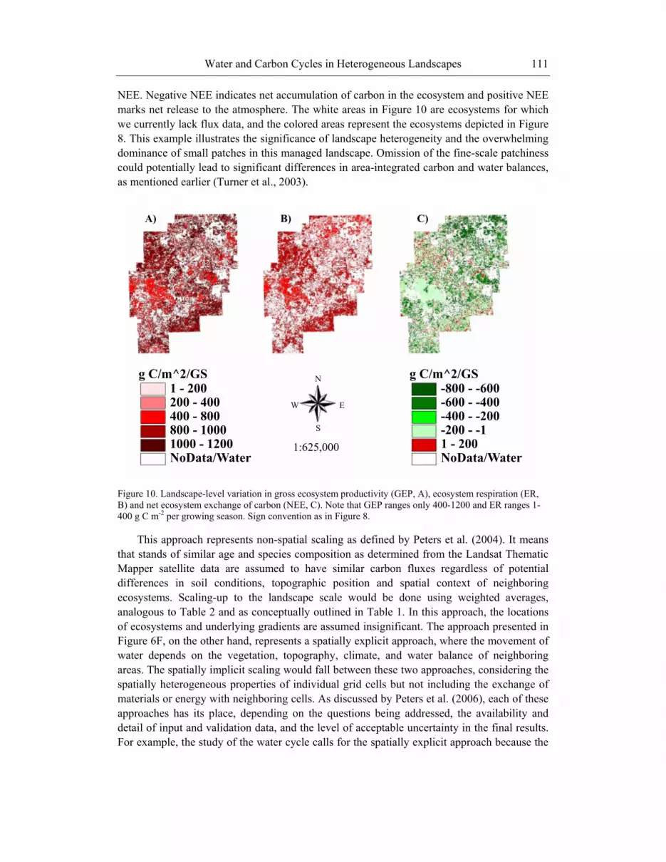
NEE. Negative NEE indicates net accumulation of carbon in the ecosystem and positive NEE marks net release to the atmosphere. The white areas in Figure 10 are ecosystems for which we currently lack flux data, and the colored areas represent the ecosystems depicted in Figure 8. This example illustrates the significance of landscape heterogeneity and the overwhelming dominance of small patches in this managed landscape. Omission of the fine-scale patchiness could potentially lead to significant differences in area-integrated carbon and water balances, as mentioned earlier (Turner et al., 2003).

Figure 10. Landscape-level variation in gross ecosystem productivity (GEP, A), ecosystem respiration (ER, B) and net ecosystem exchange of carbon (NEE, C). Note that GEP ranges only 400-1200 and ER ranges 1-400 g C m-2 per growing season. Sign convention as in Figure 8.

This approach represents non-spatial scaling as defined by Peters et al. (2004). It means that stands of similar age and species composition as determined from the Landsat Thematic Mapper satellite data are assumed to have similar carbon fluxes regardless of potential differences in soil conditions, topographic position and spatial context of neighboring ecosystems. Scaling-up to the landscape scale would be done using weighted averages, analogous to Table 2 and as conceptually outlined in Table 1. In this approach, the locations of ecosystems and underlying gradients are assumed insignificant. The approach presented in Figure 6F, on the other hand, represents a spatially explicit approach, where the movement of water depends on the vegetation, topography, climate, and water balance of neighboring areas. The spatially implicit scaling would fall between these two approaches, considering the spatially heterogeneous properties of individual grid cells but not including the exchange of materials or energy with neighboring cells. As discussed by Peters et al. (2006), each of these approaches has its place, depending on the questions being addressed, the availability and detail of input and validation data, and the level of acceptable uncertainty in the final results. For example, the study of the water cycle calls for the spatially explicit approach because the

A) B) C)

g C/m^2/GS1 - 200200 - 400400 - 800800 - 10001000 - 1200NoData/Water

g C/m^2/GS-800 - -600-600 - -400-400 - -200-200 - -11 - 200NoData/Water

1:625,000

N

W E

S


water table at a location is tied to the water table in neighboring locations, horizontal flux is tied to underlying topography, and the lateral exchange cannot be ignored. Study of the carbon cycle, however, can be successfully implemented using a spatially implicit approach, since horizontal exchange of the material may occur but is much smaller in magnitude than the fluxes determined by the intrinsic properties of individual ecosystems – assimilating leaf area, allocation and metabolic rates of assimilated carbon. However, special situations may exist (like transport of litter downhill, described in section 5.1.), when the identity and exchange with the neighboring locations are significant. Thus, the choice of the modeling framework must be based on detailed analysis of the processes of interest.

The transition from individual ecosystem to spatially-explicit framework introduces additional complexity as the analysis of spatially-heterogeneous data departs from common ecological methodology. Spatial autocorrelation and cross-correlation of various environmental and ecosystem parameters calls for geostatistical and spatially-explicit analyses (Legendre, 1993; Rossi et al., 1992), which are increasingly being used in ecological research.

In addition to creating spatial heterogeneity, the boundaries delineating different ecosystems have sometimes been viewed as distinctly different units in the landscape (e.g., see Chen and Saunders, Chapter 1, this volume; Ripple et al., 1991; Spies et al., 1994). Chen et al. (1995) showed that distinct microclimatic gradients exist across the boundaries of different ecosystems. Light levels decreased relatively rapidly from clearcut-forest boundary into the forest, reaching the mean value of the ecosystem interior at 30-60 m, whereas gradients in air humidity, wind speed and air temperature were significant over a 240 m zone. Air and soil temperature showed intermediate depth of edge influence. Some variables have been shown to be uniquely dependent on the forest-to-open area light gradient (VPD, temperature and litter moisture), whereas edge-dependent gradients in shrub cover were independent of direct beam radiation (Matlack, 1993). We have also found that the effect of edges is further complicated by aspect and topographic position (Chen et al., 1995), which require complex spatial analysis tools and a spatially-explicit sampling scheme (Quattrochi and Goodchild, 1997). Our studies have shown significant changes in the distribution of carbon pools across ecosystem edges (Chen et al., 1992; Rademacher, 2004) and these, in combination with the gradients in microclimate, are likely to affect ecosystem carbon fluxes in these zones. The depth of edge influence was found to be greater for above- than for below-ground carbon pools (Rademacher, 2004).

The complexities of scaling the heterogeneous pattern of ecosystems to the landscape level (Figure 10) have been recognized (Smithwick et al., 2003), even though the methodology for addressing the neighbor-specific edge effects is still being developed (Law et al., 2006; Peters et al., 2004, 2006; Turner et al., 2003). Understanding the mechanisms and constraining scaled-up estimates with top-down measurements and modeling are the keys to reliable transitions from ecosystem to landscape levels. Using such a multilevel approach is expected to help us answer questions like the one facing the Chequamegon Ecosystem-Atmosphere Study (ChEAS) network. Here the regionally averaged eddy covariance measurements from a very tall tower (highest measurement level 396 m) and atmospheric 13C isotope concentrations suggest that the relevant area of northern Wisconsin is a source of carbon to the atmosphere (Davis et al., 2003), whereas all ecosystem-level eddy covariance data suggest the opposite – that the area is decidedly a carbon sink (Desai et al., 2005, In press; Noormets et al., In press). With a long-term data record of atmospheric trace gas


concentrations and fluxes (Bakwin et al., 1995, 1998, 2004), constrained by evapotranspiration analyses (Ewers et al., 2002; MacKay et al., 2002), some of the highest densities of eddy covariance measurement stations in the world, and parameterized plant growth (Baker et al., 2003) and atmospheric transport models (Denning et al., 2003), the answers to the above challenges are bound to emerge.

6. CONCLUSION Recognition of the urgent need to understand the operation of the background

biogeochemical cycles and the magnitude of human impacts on those cycles has led to rapid development of mechanistically based models, from microscopic to global scales. Most relevant for issues discussed in this chapter are leaf- and canopy-level gas exchange models, radiation transfer models, atmospheric transport models and the general circulation models. Modern models are increasingly complex and often modular and hierarchical in nature – finer scale processes are represented by individual sub-models that operate either independently, iteratively with one another, or are constrained by direct measurements, thus simulating natural feedback processes. Quantifying known uncertainties of modeling, as well as those of field measurements used in calibration and validation is becoming increasingly common (Houghton et al., 2001) and represents an important development in quantitative earth system science. Knowing the limits of prediction further aids in choosing aspects for further and more detailed study (Baldocchi, 1993).

Current challenges in scaling ecosystem processes to landscapes include more dynamic representation of spatial gradients in environmental drivers and the flux responses they invoke. The traditional approach of measuring fluxes in centers of stands, deriving model parameters from these fluxes, and then assigning these parameters to the entire stand can be questioned because of the known underlying gradients. In section 4.6. we discussed the significance of horizontal exchange for the water cycle through the effects of geological and topographic influences on ground water and surface water flow. Thus, while traditional approaches may yield parameter differences based on crisp boundaries between generalized patches of a landscape (Figure 11A), new spatially-explicit approaches may allow for these parameters to be characterized as transitions across the landscape (Figure 11B). This may be key if the underlying spatial variability of environmental drivers is not well-represented by the patches or if evapotranspiration responses are nonlinearly related to these drivers. For example, hydrologists have for years recognized the importance of nonlinearity of hydrologic responses at the hillslope scale to spatial gradients in soil moisture, which have been characterized with soil-topography indices (Beven et al., 1984; O'Loughlan, 1981) and explicit measurements of soil moisture (Grayson and Bloschl, 2000; Seyfried and Wilcox, 1995). Gradients of nutrient cycling (Jackson and Caldwell, 1993a, 1993b), leaf area index (Burrows et al., 2002), and vapor pressure deficit (Mackay, 2001) all appear to be important for representing physiological responses to environmental drivers.


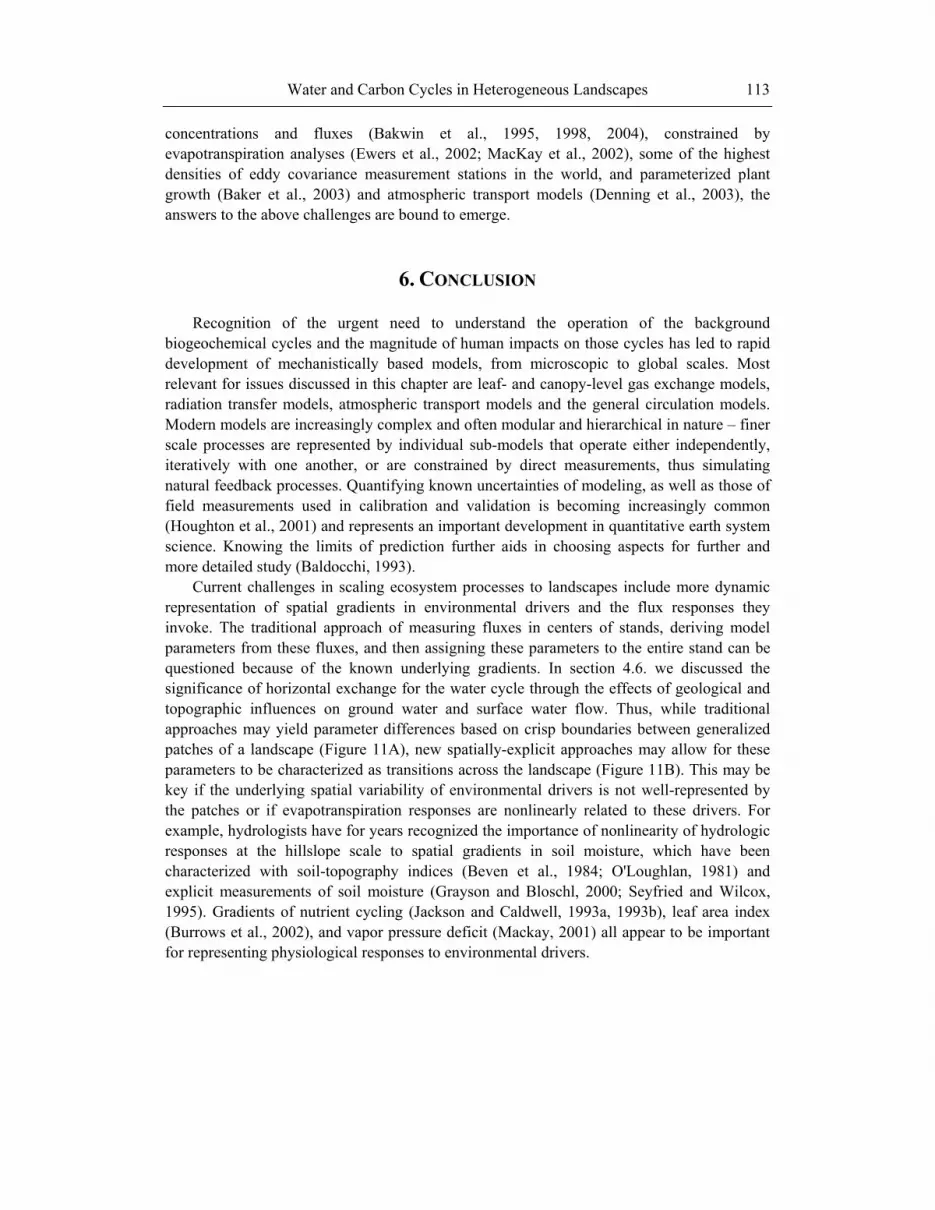
Figure 11. The traditional approach (A) to landscape level integration assumes uniform properties across a patch that is characterized at a “representative” central location. In (A-i) the black regions represent one forest type with a sharp boundary with another forest or non-forest patch. This sharp boundary is a representational convenience, and may not occur in natural systems. An alternative spatial gradient approach (B-i) explicitly tests this assumption by quantifying spatial gradients of processes within the stands. A potential application of this approach using the concept of reference stomatal conductance, GSref, is illustrated. The response of GS to VPD can be simplified (Eq. 2, Figure 2) because the sensitivity, -m, of GS to VPD is proportional to the magnitude of GS at low VPD (GSref) (A and B-ii). This simplification results in a linear relationship between GSref and m (A and B-iii). In the traditional approach, a single point on the linear relationship would describe each forest stand or other patch type (A-iii). The spatial gradient approach would allow GSref and -m to vary in response to spatial gradients (e.g., soil properties, micrometeorology, leaf nitrogen) within and between stands (B-iii). Proper representation of spatial variability is increasingly important as landscapes become more fragmented, with large areas falling into transitional edge zones.

7. ACKNOLWEDGEMENTS Support for this work was provided by NSF (JC, BEE, DSM), NASA (DSM) and USDA

FS Southern Global Change Program (JC, AN, SG). We gratefully acknowledge the help from graduate and undergraduate students and technical personnel who contributed to various components of the study.

8. REFERENCES

Abbott, M.B., Bathurst, J.C., Cunge, J.A., O'Connell, P.E. and Rasmussen, J. (1986a). An introduction to the European Hydrological System-Systeme Hydrologique Europeen SHE. 2. Structure of a physical-based, distributed modelling system. Journal of Hydrology, 87, 61-77.


Abbott, M.B., Bathurst, J.C., Cunge, J.A., O'Connell, P.E. and Rasmussen, J. (1986b). An introduction to the European Hydrological System-Systeme Hydrologique Europeen, "SHE", 1. History and philosophy of a physical-based, distributed modeling system. Journal of Hydrology, 87, 45-59.

Aber, J.D. and Federer, C.A. (1992). A generalized, lumped-parameter model of photosynthesis, evapotranspiration and net primary production in temperate and boreal forest ecosystems. Oecologia, 92, 463-474.

Addington, R.N., Mitchell, R.J., Oren, R. and Donovan, L.A. (2004). Stomatal sensitivity to vapor pressure deficit and its relationship to hydraulic conductance in Pinus palustris. Tree Physiology, 24, 561-569.

Allen, T.F.H. and Starr, T.B. (1982). Hierarchy: Perspectives for ecological complexity. Chicago, Illinois, USA: University of Chicago Press.

Andreassian, V. (2004). Waters and forests: from historical controversy to scientific debate. Journal of Hydrology, 291, 1-27.

Avissar, R. and Pielke, R.A. (1989). A parameterization of heterogeneous land surfaces for atmospheric numerical models and its impact on regional meteorology. Monthly Weather Review, 117, 2113-2136.

Baker, I., Denning, A.S., Hanan, N., Prihodko, L., Uliasz, M., Vidale, P.L., Davis, K.J. and Bakwin, P.S. (2003). Simulated and observed fluxes of sensible and latent heat and CO2 at the WLEF-TV tower using SiB2.5. Global Change Biology, 9, 1262-1277.

Bakwin, P.S., Davis, K.J., Yi, C., Wofsy, S.C., Munger, J.W. and Haszpra, L. (2004). Regional carbon dioxide fluxes from mixing ratio data. Tellus, 56B, 301-311.

Bakwin, P.S., Tans, P.P., Hurst, D.F. and Zhao, C.L. (1998). Measurements of carbon dioxide on very tall towers: results of the NOAA/CMDL program. Tellus Series B - Chemical and Physical Meteorology, 50, 401-415.

Bakwin, P.S., Tans, P.P., Zhao, C.L., Ussler, W. and Quesnell, E. (1995). Measurements of carbon dioxide on a very tall tower. Tellus Series B - Chemical and Physical Meteorology, 47, 535-549.

Baldocchi, D.D. (1993). Scaling water vapor and carbon dioxide exchange from leaves to a canopy: rules and tools. In J.R. Ehleringer and C.B. Field (Eds.), Scaling physiological processes (pp. 77-114). San Diego, CA, USA: Academic Press.

Baldocchi, D.D. (2003). Assessing the eddy covariance technique for evaluating carbon dioxide exchange rates of ecosystems: past, present and future. Global Change Biology, 9, 479-492.

Ball, J.T., Woodrow, I.E. and Berry, J.A. (1987). A model predicting stomatal conductance and its contribution to the control of photosynthesis under different environmental conditions. In J. Biggens (Ed.), Progress in Photosynthesis Research (pp. 221-229). Dordrecht, the Netherlands: Martinus Nijhoff Publishers.

Band, L.E., Patterson, P., Nemani, R. and Running, S.W. (1993). Forest ecosystem processes at the watershed scale - incorporating hillslope hydrology. Agricultural and Forest Meteorology, 63, 93-126.

Baumgartner, A. and Reichel, E. (1975). The world water balance. Amsterdam, The Netherlands: Elsevier.

Bazzaz, F.A. (1993). Scaling in biological systems: Population and community perspectives. In J.R. Ehleringer and C.B. Field (Eds.), Scaling physiological processes (pp. 233-254). San Diego, CA, USA: Academic Press.


Beven, K., Kirkby, M.J., Schofield, N. and Tagg, A.F. (1984). Testing a physically based flood forecasting model (TOPMODEL) for three UK catchments. Journal of Hydrology, 69, 119-143.

Bjørnlund, L. and Christensen, S. (2005). How does litter quality and site heterogeneity interact on decomposer food webs of a semi-natural forest? Soil Biology and Biochemistry, 37, 203-213.

Boerner, R.E.J. and Kooser, J.G. (1989). Leaf litter redistribution among forest patches within an Alleghany Plateau watershed. Landscape Ecology, 2, 81-92.

Bradford, M.A. and Reynolds, J.F. (2006). Scaling terrestrial biogeochemical processes in time and space: contrasting intact and model experimental systems. In J. Wu, K.B. Jones, H. Li and O.L. Loucks (Eds.), Scaling and uncertainty analysis in ecology: methods and applications (pp. 109-130). New York, New York, USA: Columbia University Press.

Bresee, M.K., LeMoine, J., Mather, S.V., Crow, T.R., Brosofske, K. and Chen, J. (2004). Detecting landscape dynamics in Chequamegon National Forest in northern Wisconsin, from 1972 to 2001, using Landsat imagery. Landscape Ecology, 19, 291-309.

Burrows, S.N., Gower, S.T., Clayton, M.K., Mackay, D.S., Ahl, D.E., Norman, J.M. and Diak, G. (2002). Application of geostatistics to characterize leaf area index (LAI) from flux tower to landscape scales using a cyclic sampling design. Ecosystems, 5, 667-679.

Caldwell, M.M., Matson, P.A., Wessmann, C. and Gamon, J.A. (1993). Prospects for scaling. In J.R. Ehleringer and C.B. Field (Eds.), Scaling physiological processes (pp. 223-230). San Diego, CA, USA: Academic Press.

Chapin, F.S. (1993). Functional role of growth forms in ecosystem and global processes. In J.R. Ehleringer and C.B. Field (Eds.), Scaling physiological processes (pp. 287-312). San Diego, CA, USA: Academic Press.

Chapin, F.S., Matson, P.A. and Mooney, H.A. (Editors) (2002). Principles of terrestrial ecosystem ecology. New York, New York, USA: Springer-Verlag.

Chen, J., Franklin, J.F. and Spies, T.A. (1992). Vegetation responses to edge environments in old-growth douglas-fir forests. Ecological Applications, 2, 387-396.

Chen, J., Franklin, J.F. and Spies, T.A. (1995). Growing-season microclimatic gradients from clear-cut edges into old-growth Douglas-fir forests. Ecological Applications, 5, 74-86.

Chen, J., Paw U, K.T., Ustin, S.L., Suchanek, T.H., Bond, B.J., Brosofske, K.D. and Falk, M. (2004). Net ecosystem exchanges of carbon, water, and energy in young and old-growth Douglas-fir forests. Ecosystems, 7, 534–544.

Chen, J.M., Chen, X., Ju, W. and Geng, X. (2005). Distributed hydrological model for mapping evapotranspiration using remote sensing inputs. Journal of Hydrology, 305, 15-39.

Clark, K.L., Gholz, H.L., Moncrieff, J.B., Cropley, F. and Loescher, H.W. (1999). Environmental controls over net exchanges of carbon dioxide from contrasting Florida ecosystems. Ecological Applications, 9, 936-948.

Cohen, W.B., Maiersperger, T.K., Spies, T.A. and Oetter, D.R. (2001). Modelling forest cover attributes as continuous variables in a regional context with Thematic Mapper data. International Journal of Remote Sensing, 22, 2279-2310.

Collatz, G.J., Ball, J.T., Grivet, C. and Berry, J.A. (1991). Physiological and environmental regulation of stomatal conductance, photosynthesis and transpiration - A model that includes a laminar boundary-layer. Agricultural and Forest Meteorology, 54, 107-136.


Currie, D.J. (1991). Energy and large-scale patterns of animal- and plant- species richness. The American Naturalist, 137, 27-49.

Davis, K.J., Bakwin, P.S., Yi, C., Berger, B.W., Zhao, C., Teclaw, R.M. and Isebrands, J.G. (2003). The annual cycles of CO2 and H2O exchange over a northern mixed forest as observed from a very tall tower. Global Change Biology, 9, 1278-1293.

Denning, A.S., Nicholls, M., Prihodko, L., Baker, I., Vidale, P.L., Davis, K.J. and Bakwin, P.S. (2003). Simulated variations in atmospheric CO2 over a Wisconsin forest using a coupled ecosystem-atmosphere model. Global Change Biology, 9, 1241-1250.

DePury, D.G.G. and Farquhar, G.D. (1997). Simple scaling of photosynthesis from leaves to canopies without the errors of big-leaf models. Plant, Cell and Environment, 20, 537-557.

Desai, A., Bolstad, P., Cook, B.D., Davis, K. and Carey, E.V. (2005). Comparing net ecosystem exchange of carbon dioxide between an old-growth and mature forest in the upper Midwest, USA. Agricultural and Forest Meteorology, 128, 33-55.

Desai, A.R., Noormets, A., Bolstad, P.V., Chen, J., Cook, B.D., Davis, K.J., Euskirchen, E.S., Gough, C., Martin, J.M., Ricciuto, D.M., Schmid, H.P., Tang, J. and Wang, W. Influence of vegetation type, stand age and climate on carbon dioxide fluxes across the Upper Midwest, USA: Implications for regional scaling of carbon flux. Agricultural and Forest Meteorology, In press.

DHI (2004). MIKE SHE User Guide. In: D. Software (Editor), Denmark, pp. 194. Entekhabi, D., Asrar, G.R., Betts, A.K., Beven, K.J., Bras, R.L., Duffy, C.J., Dunne, T.,

Koster, R.D., Lettenmaier, D.P., McLaughlin, D.B., Shuttleworth, W.J., van Genuchten, M.T., Wei, M.-Y. and Wood, E.F. (1999). An agenda for land surface hydrology research and a call for the second international hydrological decade. Bulletin of the American Meteorological Society, 80, 2043–2058.

Ewers, B.E., Gower, S.T., Bond-Lamberty, B. and Wang, C.K. (2005). Effects of stand age and tree species composition on transpiration and canopy conductance of boreal forest stands. Plant, Cell and Environment, 28, 660-678.

Ewers, B.E., Mackay, D.S., Gower, S.T., Ahl, D.E., Burrows, S.N. and Samanta, S.S. (2002). Tree species effects on stand transpiration in northern Wisconsin. Water Resources Research, 38, 1-11, art. no. 1103.

Ewers, B.E. and Oren, R. (2000). Analyses of Assumptions and Errors in the Calculation of Stomatal Conductance From Sap Flux Measurements. Tree Physiology, 20, 579-589.

Ewers, B.E., Oren, R., Phillips, N., Strömgren, M. and Linder, S. (2001). Mean canopy stomatal conductance responses to water and nutrient availabilities in Picea abies and Pinus taeda. Tree Physiology, 21, 841-850.

Falge, E., Baldocchi, D., Olson, R., Anthoni, P., Aubinet, M., Bernhofer, C., Burba, G., Ceulemans, R., Clement, R., Dolman, H., Granier, A., Gross, P., Grünwald, T., Hollinger, D., Jensen, N.-O., Katul, G., Keronen, P., Kowalski, A., Lai, C.T., Law, B.E., Meyers, T., Moncrieff, J., Moors, E., Munger, J.W., Pilegaard, K., Rannik, Ü., Rebmann, C., Suyker, A., Tenhunen, J., Tu, K., Verma, S., Vesala, T., Wilson, K. and Wofsy, S. (2001). Gap filling strategies for defensible annual sums of net ecosystem exchange. Agricultural and Forest Meteorology, 107, 43-69.

Famiglietti, J.S. and Wood, E.F. (1994). Multiscale modeling of spatially-variable water energy-balance processes. Water Resources Research, 30, 3061-3078.


Farquhar, G.D., von Caemmerer, S. and Berry, J.A. (1980). A biochemical model of photosynthetic CO2 assimilation in leaves of C3 species. Planta, 149, 78-90.

Fladeland, M.M., Ashton, M.S. and Lee, X. (2003). Landscape variations in understory PAR for a mixed deciduous forest in New England, USA. Agricultural and Forest Meteorology, 118, 137-141.

Floret, C., Pontanier, R. and Rambal, S. (1982). Measurement and modeling of primary production and water-use in a South Tunisian steppe. Journal of Arid Environments, 5, 77-90.

Foley, J.A., Levis, S., Costa, M.H., Cramer, W. and Pollard, D. (2000). Incorporating dynamic vegetation cover within global climate models. Ecological Applications, 10, 1620-1632.

Foley, J.A., Prentice, I.C., Ramankutty, N., Levis, S., Pollard, D., Sitch, S. and Haxeltine, A. (1996). An integrated biosphere model of land surface processes, terrestrial carbon balance, and vegetation dynamics. Global Biogeochemical Cycles, 10, 603-628.

Ford, C.R., Gorason, C.E., Mitchell, R.J., Will, R.E. and Teskey, R.O. (2004). Diurnal and seasonal variability in the radial distribution of sap flow: predicting total stem flow in Pinus taeda trees. Tree Physiology, 24, 951-960.

Franks, P.J. (2004). Stomatal control and hydraulic conductance, with special reference to tall trees. Tree Physiology, 24, 865-878.

Gardner, R.H., Kemp, W.M., Kennedy, V.S. and Petersen, J.E. (Editors) (2001). Scaling relations in experimental ecology. New York, New York, USA: Columbia University Press.

Gholz, H.L. and Clark, K.L. (2002). Energy exchange across a chronosequence of slash pine forests in Florida. Agricultural and Forest Meteorology, 112, 87-102.

Gholz, H.L., Ewel, K.C. and Teskey, R.O. (1990). Water and forest productivity. Forest Ecology and Management, 30, 1-18.

Goudie, A.S. and Middleton, N.J. (2001). Saharan dust storms: nature and consequences. Earth Science Reviews, 56, 179–204.

Granier, A., Biron, P., Breda, N., Pontailler, J.-Y. and Saugier, B. (1996). Transpiration of trees and forest stands: short and longterm monitoring using sapflow methods. Global Change Biology, 2, 265-274.

Grayson, R. and Bloschl, G. (Editors) (2000). Spatial patterns in catchment hydrology: observations and modeling. Cambridge, UK: Cambridge University Press.

Gunderson, C.A., Sholtis, J.D., Wullschleger, S.D., Tissue, D.T., Hanson, P.J. and Norby, R.J. (2002). Environmental and stomatal control of photosynthetic enhancement in the canopy of a sweetgum (Liquidambar styraciflua L.) plantation during 3 years of CO2 enrichment. Plant, Cell and Environment, 25, 379-393.

Helvey, J.D. and Patric, J.H. (1988). Research on interception losses and soil moisture relationships. In W.T. Swank and D.A.J. Crossley (Eds.), Forest Hydrology and Ecology at Coweeta (pp. 129-137). New York, New York, USA: Springer-Verlag.

Houghton, J.T., Ding, Y., Griggs, D.J., Noguer, M., Van der Linden, P.J., Da, X., Maskell, K. and Johnson, C.A. (Editors) (2001). Climate Change 2001: The Scientific Basics. Cambridge, England: Cambridge University Press.

Hu, Z. and Islam, S. (1997). A framework for analyzing and designing scale invariant remote sensing algorithms. IEEE Transactions on Geosciences and Remote Sensing, 35, 747-754.


Husar, R.B., Tratt, D.M., Schichtel, B.A., Falke, S.R., Li, F., Jaffe, D., Gasso, S., Gill, T., Laulauinen, N.S., Lu, F., Reheis, M.C., Chun, Y., Westphal, D., Holben, B.N., Gueymard, C., McKendry, I., Kuring, N., Feldman, G.C., McClain, C., Frouin, R.J., Merrill, J., DuBois, D., Vignola, F., Murayama, T., Nickovic, S., Wilson, W.E., Sassen, K., Sugimoto, N. and Malm, W.C. (2001). Asian dust events of April 1998. Journal of Geophysical Research - Atmospheres, 106, 18317–18330.

Hutjes, R.W.A., Kabat, P., Running, S.W., Shuttleworth, W.J., Field, C., Bass, B., Dias, M.A.F.D., Avissar, R., Becker, A., Claussen, M., Dolman, A.J., Feddes, R.A., Fosberg, M., Fukushima, Y., Gash, J.H.C., Guenni, L., Hoff, H., Jarvis, P.G., Kayane, I., Krenke, A.N., Liu, C., Meybeck, M., Nobre, C.A., Oyebande, L., Pitman, A., Pielke, R.A., Raupach, M., Saugier, B., Schulze, E.-D., Sellers, P.J., Tenhunen, J.D., Valentini, R., Victoria, R.L. and Vorosmarty, C.J. (1998). Biospheric aspects of the hydrological cycle - Preface. Journal of Hydrology, 213, 1-21.

Im, S., Kim, H., Kim, C. and Jang, C. (2004). Evaluation of MIKE SHE modeling system to forested watershed in Korea, ASAE/CSAE Meeting, St. Joseph, Michigan, USA, paper No. 042104.

Inouye, R.S., Byers, G.S. and Brown, J.H. (1980). Effects of predation and competition on survivorship, fecundity, and community structure of desert annuals. Ecology, 6, 1344-1351.

Jackson, R.B. and Caldwell, M.M. (1993a). Geostatistical patterns of soil heterogeneity around individual perennial plants. Journal of Ecology, 81, 683-692.

Jackson, R.B. and Caldwell, M.M. (1993b). The scale of nutrient heterogeneity around individual plants and its quantification with geostatistics. Ecology, 74, 612-614.

James, S.A., Clearwater, M.J., Meinzer, F.C. and Goldstein, G. (2002). Heat dissipation sensors of variable length for the measurement of sap flow in trees with deep sapwood. Tree Physiology, 22, 277-283.

Jarvis, P.G. (1976). The interpretation of the variations in leaf water potential and stomatal conductance found in canopies in the field. Philosophical Transactions of The Royal Society of London Series B - Biological Sciences, 273, 593-610.

Jarvis, P.G. (1980). Stomatal response to water stress in conifers. In N.C. Turner and P.J. Kramer (Eds.), Adaptation of plants to water and high temperature stress (pp. 105-122). New York, New York, USA: John Wiley and Sons.

Jarvis, P.G. (1995). Scaling processes and problems. Plant, Cell and Environment, 18, 1079-1089.

Jarvis, P.G. and McNaughton, K.G. (1986). Stomatal control of transpiration: scaling up from leaf to region. Advances in Ecological Research, 15, 1-49.

Jørgensen, S.E., Halling-Sørensen, B. and Nielsen, S.N. (Editors) (1996). Handbook of environmental and ecological modeling. Boca Raton, Florida, USA: CRC Press.

Katul, G., Leuning, R. and Oren, R. (2003). Relationship between plant hydraulic and biochemical properties derived from a steady-state coupled water and carbon transport model. Plant, Cell and Environment, 26, 399-350.

Katul, G.G., Ellsworth, D.S. and Lai, C.T. (2000). Modelling assimilation and intercellular CO2 from measured conductance: a synthesis of approaches. Plant, Cell and Environment, 23, 1313-1328.

Lange, O.L.R., Lösch, R., Schulze, E.-D. and Kappen, L. (1971). Responses of stomata to changes in humidity. Planta, 100, 76-86.


Law, B.E., Falge, E., Guc, L., Baldocchi, D.D., Bakwin, P.S., Berbigier, P., Davis, K.J., Dolman, A.J., Falk, M., Fuentes, J.D., Goldstein, A.H., Granier, A., Grelle, A., Hollinger, D., Janssens, I.A., Jarvis, P.G., Jensen, N.-O., Katul, G., Malhi, Y., Matteucci, G., Meyers, T., Monson, R.K., Munger, J.W., Oechel, W., Olson, R., Pilegaard, K., Paw U, K.T., Thorgeirsson, H., Valentini, R., Verma, S., Vesala, T., Wilson, K. and Wofsy, S. (2002). Environmental controls over carbon dioxide and water vapor exchange of terrestrial vegetation. Agricultural and Forest Meteorology, 113, 97-120.

Law, B.E., Turner, D.P., Campbell, J., Lefsky, M.A., Guzy, M., Sun, O., Van Tuyl, S. and Cohen, W.B. (2006). Carbon fluxes across regions: observational constraints at multiple scales. In J. Wu, K.B. Jones, H. Li and O.L. Loucks (Eds.), Scaling and uncertainty analysis in ecology: methods and applications (pp. 167-190). New York, New York, USA: Columbia University Press.

Legendre, P. (1993). Spatial autocorrelation: trouble or new paradigm? Ecology, 74, 1659-1673.

Lelieveld, J., Berresheim, H., Borrmann, S., Crutzen, P.J., Dentener, F.J., Fischer, H., Feichter, J., Flatau, P.J., Heland, J., Holzinger, R., Korrmann, R., Lawrence, M.G., Levin, Z., Markowicz, K.M., Mihalopoulos, N., Minikin, A., Ramanathan, V., de Reus, M., Roelofs, G.J., Scheeren, H.A., Sciare, J., Schlager, H., Schultz, M., Siegmund, P., Steil, B., Stephanou, E.G., Stier, P., Traub, M., Warneke, C., Williams, J. and Ziereis, H. (2002). Global air pollution crossroads over the Mediterranean. Science, 298, 794-799.

Leverenz, J., Deans, J.D., Ford, E.D., Jarvis, P.G., Milne, R. and Whitehead, D. (1982). Systematic spatial variation of stomatal conductance in a sitka spruce plantation. Journal of Applied Ecology, 19, 835-851.

Levin, S.A. (1992). The problem of pattern and scale in ecology. Ecology, 73, 1943-1967. Li, H. and Wu, J. (2006). Uncertainty analysis in ecological studies: an overview. In J. Wu,

K.B. Jones, H. Li and O.L. Loucks (Eds.), Scaling and uncertainty analysis in ecology: methods and applications (pp. 45-66). New York, New York, USA: Columbia University Press.

Litvak, M., Miller, S., Wofsy, S.C. and Goulden, M. (2003). Effect of stand age on whole ecosystem CO2 exchange in the Canadian boreal forest. Journal of Geophysical Research - Atmospheres, 108, art. no. 8225.

Lu, J., Sun, G., Amatya, D.M. and McNulty, S.G. (2005). A comparison of six potential evapotranspiration methods for regional use in the Southeastern United States. Journal of American Water Resources Association, 41, 621-633.

Lu, P., Müller, W.J. and Chacko, E.K. (2000). Spatial variations in xylem sap flux density in the trunk of orchard-grown, mature mango trees under changing soil water conditions. Tree Physiology, 20, 683-692.

Lundblad, M., Lagergren, F. and Lindroth, A. (2001). Evaluation of heat balance and heat dissipation methods for sapflow measurements in pine and spruce. Annales des Sciences Forestieres, 58, 625-638.

Mackay, D.S. (2001). Evaluation of hydrologic equilibrium in a mountainous watershed: Incorporating forest canopy spatial adjustment to soil biogeochemical processes. Advances in Water Resources, 24, 1211-1227.

MacKay, D.S., Ahl, D.E., Ewers, B.E., Gower, S.T., Burrows, S.N., Samanta, S. and Davis, K.J. (2002). Effects of aggregated classifications of forest composition on estimates of evapotranspiration in a northern Wisconsin forest. Global Change Biology, 8, 1253-1265.


Mackay, D.S. and Band, L.E. (1997). Forest ecosystem processes at the watershed scale: Dynamic coupling of distributed hydrology and canopy growth. Hydrological Processes, 11, 1197-1217.

Massman, W.J. (1992). A surface energy balance method for partitioning evapotranspiration data into plant and soil components for a surface with partial canopy cover. Water Resources Research, 28, 1723-1732.

Matlack, G.R. (1993). Microenvironment variation within and among forest edge sites in th Eastern United States. Biological Conservation, 66, 185-194.

McNaughton, K.G. and Jarvis, P.G. (1991). Effects of spatial scale on stomatal control of transpiration. Agricultural and Forest Meteorology, 54, 279-301.

Mencuccini, M. (2003). The ecological significance of long-distance water transport: short-term regulation, long-term acclimation and the hydraulic costs of stature across plant life forms. Plant, Cell and Environment, 26, 163-182.

Meyers, T. and Paw U, K.T. (1986). Testing a higher-order closure model for modeling airflow within and above plant canopies. Boundary-Layer Meteorology, 37, 297-311.

Miller, J.R., Turner, M.G., Smithwick, E.A.H., Dent, C.L. and Stanley, E.H. (2004). Spatial extrapolation: The science of predicting ecological patterns and processes. BioScience, 54, 310-320.

Monteith, J.L. (1965). Evaporation and environment. The state and movement of water in living organisms, Symp. Soc. Exp. Biol. 19. Academic Press, pp. 205-234.

Monteith, J.L. (1995). A reinterpretation of stomatal responses to humidity. Plant, Cell and Environment, 18, 357-364.

Mott, K.A. and Parkhurst, D.F. (1991). Stomatal response to humidity in air and helox. Plant, Cell and Environment, 14, 509-515.

Noormets, A., Chen, J., Bridgham, S.D., Weltzin, J.F., Pastor, J., Dewey, B. and LeMoine, J. (2004). The effects of infrared loading and water table on soil energy fluxes in northern peatlands. Ecosystems, 7, 573-582.

Noormets, A., Desai, A., Cook, B.D., Ricciuto, D.M., Euskirchen, E.S., Davis, K., Bolstad, P., Schmid, H.P., Vogel, C.S., Carey, E.V., Su, H.-B. and Chen, J. Moisture sensitivity of ecosystem respiration: comparison of 14 forest ecosystems in the Upper Great Lakes Region, USA. Agricultural and Forest Meteorology, In press.

Norman, J.M. (1993). Scaling processes between leaf and canopy levels. In J.R. Ehleringer and C.B. Field (Eds.), Scaling physiological processes: leaf to globe (pp. 41-76). San Diego, California, USA: Academic Press.

Ogle, K. and Reynolds, J.F. (2002). Desert dogma revisited: coupling of stomatal conductance and photosynthesis in the desert shrub, Larrea tridentata. Plant, Cell and Environment, 25, 909-921.

Oker-Blom, P. and Kellomäki, S. (1983). Effects of grouping of foliage on the within-stand and within-crown light regime: comparison of random and grouping canopy models. Agricultural Meteorology, 28, 143-155.

O'Loughlan, E.M. (1981). Saturation regions in catchments and their relations to soil and topographic properties. Journal of Hydrology, 53, 229-246.

O'Neill, R.V. (2001). Is it time to bury the ecosystem concept? (With full military honors, of course!). Ecology, 82, 3275–3284.

O'Neill, R.V., DeAngelis, D.L., Wade, J.B. and Allen, T.F.H. (1986). A hierarchical concept of ecosystems. Princeton, New Jersey, USA: Princeton University Press.


Oren, R., Phillips, N., Ewers, B.E., Pataki, D.E. and Megonigal, J.P. (1999a). Sap-flux-scaled transpiration responses to light, vapor pressure deficit, and leaf area reduction in a flooded Taxodium distichum forest. Tree Physiology, 19, 337-347.

Oren, R., Phillips, N., Katul, G., Ewers, B.E. and Pataki, D.E. (1998). Scaling xylem sap flux and soil water balance and calculating variance: a method for partitioning water flux in forests. Annales des Sciences Forestieres, 55, 191-216.

Oren, R., Sperry, J.S., Katul, G.G., Pataki, D.E., Ewers, B.E., Phillips, N. and Schafer, K.V.R. (1999b). Survey and synthesis of intra- and interspecific variation in stomatal sensitivity to vapour pressure deficit. Plant, Cell and Environment, 22, 1515-1526.

Pastor, J. and Cohen, Y. (1997). Herbivores, the functional diversity of plants species, and the cycling of nutrients in ecosystems. Theoretical Population Biology, 51, 165-179.

Pataki, D.E., Oren, R. and Smith, W.K. (2000). Sap flux of co-occurring species in a western subalpine forest during seasonal soil drought. Ecology, 81, 2557-2566.

Peters, D.P.C., Herrick, J.E., Urban, D.L., Gardner, R.H. and Breshears, D.D. (2004). Strategies for ecological extrapolation. Oikos, 106, 627-636.

Peters, D.P.C., Yao, J., Huenneke, L.F., Gibbens, R.P., Havstad, K.M., Herrick, J.E., Rango, A. and Schlesinger, W.H. (2006). A framework and methods for simplifying complex landscapes to reduce uncertainty in predictions. In J. Wu, K.B. Jones, H. Li and O.L. Loucks (Eds.), Scaling and uncertainty analysis in ecology: methods and applications. pp. 131-146. New York, New York, USA: Columbia University Press.

Phillips, N., Oren, R. and Zimmermann, R. (1996). Radial patterns of xylem sap flow in non-diffuse- and ring-porous tree species. Plant, Cell and Environment, 19, 983-990.

Prospero, J.M. (1999). Long-range transport of mineral dust in the global atmosphere: Impact of African dust on the environment of the southeastern United States. Proceedings of The National Academy of Sciences of The United States of America, 96, 3396–3403.

Quattrochi, D.A. and Goodchild, M.F. (Editors) (1997). Scale in Remote Sensing and GIS. Boca Raton, Florida, USA: Lewis Publishers, CRC Press.

Rademacher, J. (2004). Forest structure and carbon allocation within and between two northern mixed hardwood edges. M.S. Thesis, Toledo, Ohio, USA: The University of Toledo.

Raupach, M.R. and Finnigan, J.J. (1988). Single-layer models of evaporation from plant canopies are incorrect but useful, whereas multilayer models are correct but useless. Australian Journal of Plant Physiology, 15, 705-716.

Rayment, M.B. (2000). Closed chamber systems underestimate soil CO2 efflux. European Journal of Soil Science, 51, 107-110.

Reich, P.B., Grigal, D.F., Aber, J.D. and Gower, S.T. (1997). Nitrogen mineralization and productivity in 50 hardwood and conifer stands on diverse soils. Ecology, 78, 335-347.

Reynolds, J.F., Hilbert, D.W. and Kemp, P.R. (1993). Scaling ecophysiology from the plant to the ecosystem: a conceptual framework. In J.R. Ehleringer and C.B. Field (Eds.), Scaling physiological processes (pp. 127-140). San Diego, CA, USA: Academic Press.

Ripple, W.J., Bradshaw, G.A. and Spies, T.A. (1991). Measuring forest landscape patterns in the Cascade Range of Oregon, USA. Biological Conservation, 57, 73-88.

Rosenbrock, P., Buscot, F. and Munch, J.-C. (1995). Fungal succession and changes in the fungal degradation potential during the initial stage of litter decomposition in black alder forest (Alnus glutinosa (L.) Gaertn.). European Journal of Soil Biology, 31, 1-11.


Rosenzweig, M.L. (1968). Net primary productivity of terrestrial communities: prediction from climatological data. The American Naturalist, 102, 67-74.

Rossi, R.E., Mulla, D.J., Journel, A.G. and Franz, E.H. (1992). Geostatistical tools for modeling and interpreting ecological spatial dependence. Ecological Monographs, 62, 277-314.

Ruimy, A., Kergoat, L. and Field, C.B. (1996). The use of CO2 flux measurements in models of the global terrestrial carbon budget. Global Change Biology, 2, 287-296.

Running, S.W. and Coughlan, J.C. (1988). A general model of forest ecosystem process for regional applications I. Hydrologic balance, canopy gas exchange and primary production processes. Ecological Modelling, 42, 125-154.

Running, S.W. and Hunt, R.E. (1993). Generalization of a forest ecosystem process model for other biomes, BIOME-BGC, and an application for global-scale models. In J.R. Ehleringer and C. Field (Eds.), Scaling physiological processes (pp. 141-158). San Diego, CA, USA: Academic Press.

Running, S.W., Nemani, R.R., Peterson, D.L., Band, L.E., Potts, D.F., Pierce, L.L. and Spanner, M.A. (1989). Mapping regional forest evapotranspiration and photosynthesis by coupling satellite data with ecosystem simulation. Ecology, 70, 1090-1101.

Schulze, E.-D., Lange, O.L.R., Buschbom, U., Kappen, L. and Evenari, M. (1972). Stomatal responses to changes in humidity in plants growing in the desert. Planta, 108, 259-270.

Sellers, P.J., Dickinson, R.E., Randall, D.A., Betts, A.K., Hall, F.G., Berry, J.A., Collatz, G.J., Denning, A.S., Mooney, H.A., Nobre, C.A., Sato, N., Field, C.B. and Henderson-Sellers, A. (1997). Modeling the exchanges of energy, water, and carbon between continents and the atmosphere. Science, 275, 502-509.

Seyfried, M.S. and Wilcox, B.P. (1995). Scale and the nature of spatial variability: Field examples having implications for hydrology modeling. Water Resources Research, 31, 173-184.

Shuttleworth, W.J. (1988). Evaporation from Amazonian rainforest. Proceedings of the Royal Society of London Series B - Biological Sciences, 233, 321-346.

Smithwick, E.A., Harmon, M.A. and Domingo, J.B. (2003). Modeling multiscale effects of light limitations and edge-induced mortality on carbon stores in forest landscapes. Landscape Ecology, 18, 701-721.

Sperry, J.S. (2004). Coordinating stomatal and xylem functioning - an evolutionary perspective. New Phytologist, 162, 568-570.

Sperry, J.S., Adler, F.R., Campbell, G.S. and Comstock, J.P. (1998). Limitation of plant water use by rhizosphere and xylem conductance: results from a model. Plant, Cell and Environment, 21, 347-359.

Sperry, J.S., Hacke, U.G., Oren, R. and Comstock, J.P. (2002). Water deficits and hydraulic limits to leaf water supply. Plant, Cell and Environment, 25, 251-263.

Spies, T.A., Ripple, W.J. and Bradshaw, G.A. (1994). Dynamics and pattern of a managed coniferous forest landscape in Oregon. Ecological Applications, 4, 555-568.

Tansley, A.G. (1935). The use and abuse of vegetational concepts and terms. Ecology, 16, 284-307.

Turner, D.P., Guzy, M., Lefsky, M.A., Van Tuyl, S., Sun, O., Daly, C. and Law, B.E. (2003). Effects of land use and fine-scale environmental heterogeneity on net ecosystem production over a temperate coniferous forest landscape. Tellus Series B - Chemical and Physical Meteorology, 55, 657-668.


Turner, M.G., Gardner, R.H. and O'Neill, R.V. (2001). Landscape ecology in theory and practice: Pattern and process. New York, New York, USA: Springer-Verlag.

Tyree, M.T. and Sperry, J.S. (1989). Vulnerability of xylem to cavitation and embolism. Annual Review of Plant Physiology and Plant Molecular Biology, 40, 19-38.

Vertessy, R.A., Hatton, T.J., Benyon, R.G. and Dawes, W.R. (1996). Long-term growth and water balance predictions for a mountain ash (Eucalyptus regnans) forest catchment subject to clear-felling and regeneration. Tree Physiology, 16, 221-232.

Vitousek, P.M. (1993). Global dynamics and ecosystem processes: scaling up or scaling down. In J.R. Ehleringer and C.B. Field (Eds.), Scaling physiological processes (pp. 169-177). San Diego, CA, USA: Academic Press.

von Caemmerer, S. and Farquhar, G.D. (1981). Some relationships between the biochemistry of photosynthesis and the gas exchange of leaves. Planta, 153, 376-387.

Walsh, S.J., Moody, A., Allen, T.R. and Brown, G. (1997). Scale dependence of NDVI and its relationship to mountainous terrain. In D.A. Quattrochi and M.F. Goodchild (Eds.), Scale in Remote Sensing and GIS (pp. 27-55). Boca Raton, Florida, USA: Lewis Publisher.

Wardle, D.A. (1993). Changes in the microbial biomass and metabolic quotient during leaf litter succession in some New Zealand forest and scrubland ecosystems. Functional Ecology, 7, 346-355.

Waring, R.H., Schroeder, P.E. and Oren, R. (1981). Application of the pipe model theory to predict canopy leaf area. Canadian Journal of Forest Research, 12, 556-560.

Wigmosta, M.S., Vail, L.W. and Lettenmaier, D.P. (1994). A distributed hydrology-vegetation model for complex terrain. Water Resources Bulletin, 30, 1665-1679.

Wijesinghe, D.K., John, E.A. and Hutchings, M.J. (2005). Does pattern of soil resource heterogeneity determine plant community structure? An experimental investigation. Journal of Ecology, 93, 99-112.

Wu, J. (1999). Hierarchy and scaling: extrapolating information along a scaling ladder. Canadian Journal of Remote Sensing, 25, 367-380.

Wu, J.G. (2004). Effects of changing scale on landscape pattern analysis: scaling relations. Landscape Ecology, 19, 125-138.

Wu, J.G. and Loucks, O.L. (1995). From balance of nature to hierarchical patch dynamics: A paradigm shift in ecology. Quarterly Review of Biology, 70, 439-466.

Zheng, D., Rademacher, J., Chen, J., Crow, T.R., Bresee, M.K., LeMoine, J. and Ryu, S.-R. (2004). Estimating aboveground biomass using Landsat 7 ETM+ data across a managed landscape in northern Wisconsin, USA. Remote Sensing of Environment, 93, 402-411.

linking ecology to land mosaics: an ecosystem perspective

Documents