landscape ecology

LANDSCAPE

ECOLOGY IN

THEORY AND

PRACTICE

2888_afm1 3/2/01 2:53 PM Page i

2888_afm1 3/2/01 2:54 PM Page ii

M o n i c a G . T u r n e r

R o b e r t H . G a r d n e r

R o b e r t V . O ’ N e i l l

LANDSCAPE

ECOLOGY IN

THEORY AND

PRACTICE

P a t t e r n a n d P r o c e s s

2888_afm1 3/2/01 2:54 PM Page iii

Monica G. TurnerDepartment of ZoologyBirge HallUniversity of WisconsinMadison, WI [email protected]

Robert H. GardnerAppalachian LaboratoryUniversity of Maryland301 Braddock RoadFrostburg, MD [email protected]

Robert V. O’NeillEnvironmental Sciences DivisionOak Ridge National LaboratoryOak Ridge, TN [email protected]

© 2001 Springer-Verlag New York, Inc.

Printed on acid-free paper.

All rights reserved. This work may not be translatedor copied in whole or in part without the writtenpermission of the publisher (Springer-Verlag NewYork, Inc., 175 Fifth Avenue, New York, NY 10010,USA), except for brief excerpts in connection withreviews or scholarly analysis. Use in connection withany form of information storage and retrieval, elec-tronic adaptation, computer software, or by similaror dissimilar methodology now known or hereafterdeveloped is forbidden.The use of general descriptive names, trade names,trademarks, etc., in this publication, even if the for-mer are not especially identified, is not to be takenas a sign that such names, as understood by the TradeMarks and Merchandise Marks Act, may accord-ingly be used freely by anyone.

Production coordinated by WordCrafters EditorialServices, Inc., Sterling, VA, and managed by StevenPisano. Manufacturing supervised by Jacqui Ashri.Typeset by Matrix Publishing Services, York, PA.Printed and bound by Edwards Brothers, Inc., AnnArbor, MI.

Library of Congress Cataloging-in-Publication DataLandscape ecology in theory and practice : pattern

and process / Monica G. Turner, Robert H. Gardner,Robert V. O’Neill.

p. cm.Includes bibliographical references (p. ).ISBN 0-387-95122-9 (alk. paper)ISBN 0-387-95123-7 (softcover : alk. paper)1. Landscape ecology. I. Gardner, R.H.

II. O’Neill, R.V. (Robert V.), 1940– III. Title.QH541.15.L35T87 2001577—dc21 00-047094

Printed in the United States of America.

9 8 7 6 5 4 3 2 1

ISBN 0-387-95122-9 SPIN 10778231 (hardcover)ISBN 0-387-95123-7 SPIN 10778249 (softcover)

Springer-Verlag New York Berlin HeidelbergA member of BertelsmannSpringer Science+Business Media GmbH

2888_afm1 3/2/01 2:54 PM Page iv

Preface

Landscape ecology is not a distinct discipline or simply a branch of ecology, but rather is the synthetic

intersection of many related disciplines that focus on the spatial-temporal pattern of the landscape.

Risser et al., 1984

The emergence of landscape ecology as a discipline has catalyzed a shift in paradigms among ecologists,

. . . resource managers and land-use planners. Having now seen the faces of spatial pattern and scale

. . . we can never go back to the old ways of viewing things. Wiens, 1999

This book presents the perspective of three ecologists on the concepts andapplications of landscape ecology, a discipline that has shown expansive

growth during the past two decades. Although landscape ecology is a multidisci-plinary subject involving components as diverse as economics and sociology, theearth sciences and geography, remote sensing and computer applications, we fo-cus here on what ecologists need to know about landscapes.

Landscape ecology served as the integrating theme of our collaborative researchfor nearly 15 years, including a 7-year period during which we worked togetherat Oak Ridge National Laboratory. We became acquainted in January 1986 atthe first annual United States Landscape Ecology symposium held at the Univer-sity of Georgia and organized by Monica Turner and Frank Golley. Landscapeecology was, at that time, a new subject in the United States. The first U.S. work-shop on landscape ecology, organized by Paul Risser, Richard Forman, and JimKarr, had occurred less than 3 years prior (Risser et al., 1984). One of us (O’Neill)was a participant in that workshop, and two of us (O’Neill and Gardner) wereresearch scientists in the Environmental Sciences Division of Oak Ridge National

2888_afm1 3/2/01 2:54 PM Page v

vi

Laboratory (ORNL) who had collaborated for several years on many aspects ofecosystem ecology and ecological modeling. Turner had a newly minted Ph.D. andwas continuing as a postdoctoral research associate at the University of Georgia,where Frank Golley (also a participant at the 1993 workshop and Turner’s Ph.D.advisor) was actively engaging his colleagues in the developing ideas in landscapeecology. The mutual interests shared by Turner, Gardner, and O’Neill, coupledwith the excitement and challenge of working in a newly emerging branch of ecol-ogy, led to Turner’s move to ORNL in July 1987. The subsequent seven years inwhich we collaborated so closely were among the most exciting times that any ofus have had in our careers. There are times and places at which creativity seemsto be fostered more than others, and that time and place had it. The writing ofthis book was precipitated, in part, by the fact that although we are now locatedat different institutions, we shared the desire to provide a synthesis of the field inwhich we have worked so closely together.

As ecologists embraced the challenges of understanding spatial complexity,landscape ecology moved from being a tangential subdiscipline in the early 1980sto one that is now mainstream. Indeed, a landscape approach, or the landscapelevel, is now considered routinely in all types of ecological studies. It is our hopethat this text will provide a synthetic overview of landscape ecology, including itsdevelopment, the methods and techniques that are employed, the major questionsaddressed, and the insights that have been gained. The enclosed CD contains allfigures for this book, including the color images. We hope that this will enhancethe utility of the book, especially for teaching. The companion volume (Gergeland Turner, 2001) provides opportunities for hands-on learning of many of themethods and concepts employed by landscape ecologists. It is our hope that ourbooks might serve to inspire others to embark on landscape ecological studies, forthere is much yet to be learned. As we begin this new century, we look forwardto the many contributions that landscape ecologists will make in the future andto the continued growth of this exciting discipline.

A c k n o w l e d g m e n t s

Research that we have conducted over the past 15 years and that led to the de-velopment of this book has been funded by a variety of agencies, and we grate-fully acknowledge research support from the National Science Foundation (Long-term Ecological Research, Ecosystem Studies, and Ecology programs), Departmentof Energy, USDA Competitive Grants Program, National Geographic Society,

2888_afm1 3/2/01 2:54 PM Page vi

vii

Environmental Protection Agency (EMAP and STAR programs), and the Univer-sity of Wisconsin-Madison Graduate School.

Our ideas have evolved over the years and been shaped by fruitful and oftenspirited discussions with many colleagues. Among the most memorable of thesewere discussions with Don DeAngelis, Jeff Klopatek, John Krummel, and GeorgeSugihara in the “prelandscape” years at ORNL that crystallized much of the phi-losophy and approach adopted in our research. Virginia Dale, Kim With, ScottPearson, and Bill Romme have been regular collaborators as well as supportivefriends. Although it is impossible to mention everyone at ORNL who contributedideas and assisted us with their expertise, we would be remiss not to acknowledgethe valuable contributions of Steve Bartell, Antoinette Brenkert, Carolyn Hun-saker, Tony King, and Robin Graham. While at Oak Ridge we hosted a numberof visitors from other institutions, including Bill Romme, Linda Wallace, BruceMilne, Tim Kratz, Sandra Lavorel, Tim Allen, Eric Gustafson, and Roy Plotnick.These colleagues made substantial contributions to and lasting impacts on ourideas, and we thank them all for engaging interactions and fruitful collaborations.

Special thanks are due to Richard Forman, Frank Golley, and John Wiens forlongstanding collegial relationships, the sharing of their ideas (and students!) thatoften challenged our thinking, and their invaluable reviews and critiques over theyears. Turner also sincerely thanks Hazel Delcourt (University of Tennessee) andDavid Mladenoff (University of Wisconsin), with whom she has jointly taughtlandscape ecology courses over the past decade; co-teaching has been inspiringand fun and has certainly helped shape her thinking.

This book benefited tremendously from valuable critical comments providedby numerous colleagues. We especially thank David Mladenoff and Sarah Gergel,who both read nearly the entire manuscript and provided constructive criticismthat has been enormously helpful. David Mladenoff actually read the whole man-uscript twice, and Turner especially thanks him for being such a good colleague.In addition, we are grateful to the following friends and colleagues for reviewingone or more chapters: Jeff Cardille, Steve Carpenter, F. S. (Terry) Chapin, MarkDixon, Tony Ives, Dan Kashian, Jim Miller, Bill Romme, Tania Schoennagel, SteveSeagle, Emily Stanley, Dan Tinker, Phil Townshend, and Kim With. Commentson draft chapters from the students in Principles of Landscape Ecology, taught atthe University of Wisconsin-Madison during the spring 1999 semester, were alsovery helpful.

The graphics and illustrations for this book were prepared by Michael Turner,and we are indebted to him for greatly improving the visual communication of

2888_afm1 3/2/01 2:54 PM Page vii

viii

the concepts and examples in this book. We are delighted with the clarity andconsistency of the figures throughout the text. We thank Kandis Elliot (Universityof Wisconsin) and Michael Mac (Biological Resources Division, U.S. GeologicalSurvey) for sharing visual resources. Sandi Gardner and Sally Tinker providedvaluable editorial assistance in the final stages of manuscript preparation. Finally,we thank the two editors with whom we worked at Springer-Verlag, initially RobGarber and then Robin Smith, for their patience and support of this effort, espe-cially given the time it has taken us to complete it.

Monica G. TurnerMadison, Wisconsin

Robert H. GardnerFrostburg, Maryland

Robert V. O’NeillOak Ridge, Tennessee

� R E F E R E N C E S

GERGEL, S. E., AND M. G. TURNER, editors. 2001. Learning Landscape Ecology: A

Practical Guide to Concepts and Techniques. Springer-Verlag, New York.

RISSER, P. G., J. R. KARR, AND R. T. T. FORMAN. 1984. Landscape Ecology: Directions

and Approaches. Special Publication Number. Illinois Natural History Survey,

Champaign, Illinois.

WIENS, J. A. 1999. The science and practice of landscape ecology, in J. M. Klopatek

and R. H. Gardner, eds. Landscape Ecological Analysis: Issues and Applications,

pp. 371–383. Springer-Verlag, New York.

2888_afm1 3/2/01 2:54 PM Page viii

Contents

Preface v

Chapter 1 � Introduction to Landscape Ecology 1

What Is Landscape Ecology? 2Why Landscape Ecology Has Emerged as a

Distinct Area of Study 7The Intellectual Roots of Landscape Ecology 10

Objectives of This Book 20

Summary 21

Discussion Questions 22

Recommended Readings 23

Chapter 2 � The Critical Concept of Scale 25

Scale Terminology and Its Practical Application 27

Scale Problems 32

2888_afm1 3/2/01 2:54 PM Page ix

x

Scale Concepts and Hierarchy Theory 34

Identifying the “Right” Scale(s) 38

Reasoning About Scale 40

Scaling Up 40

Summary 43



Chapter 3 � Introduction to Models 47

What are Models and Why Do We Use Them? 47

Steps in Building a Model 56

Landscape Models 64

Caveats in the Use of Models 66

Summary 67



Chapter 4 � Causes of Landscape Pattern 71

Abiotic Causes of Landscape Pattern 73

Biotic Interactions 83

Human Land Use 86

Disturbance and Succession 90

Summary 90



Chapter 5 � Quantifying Landscape Pattern 93

Why Quantify Pattern? 93

Data Used in Landscape Analyses 95

Caveats for Landscape Pattern Analysis, or “Read This First” 99

Metrics for Quantifying Landscape Pattern 108

Geostatistics or Spatial Statistics 125

2888_afm1 3/2/01 2:54 PM Page x

xi

Summary 132



Chapter 6 � Neutral Landscape Models 135

Random Maps: The Simplest Neutral Model 138

Maps with Hierarchical Structure 147

Fractal Landscapes 149

Neutral Models Relating Pattern to Process 153

General Insights from the Use of NLMs 153

Summary 155



Chapter 7 � Landscape Disturbance Dynamics 157

Disturbance and Disturbance Regimes 159

Influence of the Landscape on Disturbance Pattern 162

Influence of Disturbance on Landscape Pattern 174

Concepts of Landscape Equilibrium 188

Summary 196



Chapter 8 � Organisms and Landscape Pattern 201

Conceptual Development of Organism-Space Interactions 204

Scale-Dependent Nature of Organism Responses 221

Effects of Spatial Pattern on Organisms 229

Spatially Explicit Population Models 240

Summary 243



2888_afm1 3/2/01 2:54 PM Page xi

xii

Chapter 9 � Ecosystem Processes in the Landscape249

Spatial Heterogeneity in Ecosystem Processes 251

Effects of Landscape Position on Lake Ecosystems 261

Land–Water Interactions 265

Linking Species and Ecosystems 280

Searching for General Principles 284

Summary 285



Chapter 10 � Applied Landscape Ecology 289

Land Use 290

Forest Management 307

Regional Risk Assessment 314

Continental-Scale Monitoring 319

Summary 321



Chapter 11 � Conclusions and Future Directions 327

What Have We Learned? 328

Research Directions 329

Conclusion 331



References 333

Index 389

2888_afm1 3/2/01 2:54 PM Page xii

C H A P T E R

Introduction to Landscape Ecology

Landscape ecology offers new concepts, theory, and methods that arerevealing the importance of spatial patterning on the dynamics of inter-

acting ecosystems. Landscape ecology has come to the forefront of ecology andland management and is still expanding very rapidly. The last decade has seen adramatic growth in the number of studies and variety of topics that fall under thebroad banner of landscape ecology. Interest in landscape studies has been fueledby many factors, the most important being the critical need to assess the impactof rapid, broad-scale changes in our environment.

Most of us have an intuitive sense of the term landscape; we think of the ex-panse of land and water that we observe from a prominent point and distinguishbetween agricultural and urban landscapes, lowland and mountainous landscapes,natural and developed landscapes. Any of us could list components of these land-scapes, for example, farms, fields, forests, wetlands, and the like. If we considerhow organisms other than humans may see their landscape, our own sense of land-scape may be broadened to encompass components relevant to a honey bee, bee-tle, vole, or bison. In all cases, our intuitive sense includes a variety of differentelements that comprise the landscape, change through time, and influence eco-

1

2888_e01_p1-24 2/27/01 1:20 PM Page 1

2

L A N D S C A P E

E C O L O G Y I N

T H E O R Y A N D

P R A C T I C E

logical dynamics. In his 1983 editorial in BioScience, Richard T. T. Forman usedtangible examples to bring these ideas to the attention of ecologists:

What do the following have in common? Dust-bowl sediments from the west-

ern plains bury eastern prairies, introduced species run rampant through na-

tive ecosystems, habitat destruction upriver causes widespread flooding down

river, and acid rain originating from distant emissions wipes out Canadian fish.

Or closer to home: a forest showers an adjacent pasture with seed, fire from

a fire-prone ecosystem sweeps through a residential area, wetland drainage dec-

imates nearby wildlife populations, and heat from a surrounding desert desic-

cates an oasis. In each case, two or more ecosystems are linked and interact-

ing. (Forman, 1983)

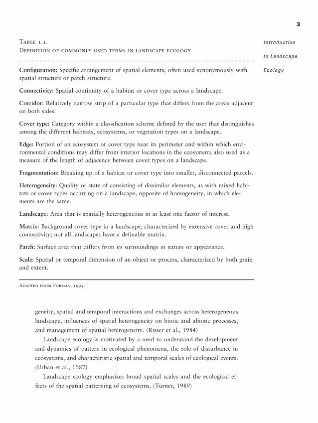
In this chapter, we define landscape ecology, discuss the importance of land-scape studies within ecology, briefly review the intellectual roots of landscape, andpresent an overview of the remainder of the book. In addition, some commonlyused terms in landscape ecology are defined in Table 1.1.

W H A T I S L A N D S C A P E E C O L O G Y ?

Landscape ecology emphasizes the interaction between spatial pattern and eco-logical process, that is, the causes and consequences of spatial heterogeneity acrossa range of scales. The term landscape ecology was introduced by the German bio-geographer Carl Troll (1939), arising from the European traditions of regional ge-ography and vegetation science and motivated particularly by the novel perspec-tive offered by aerial photography. Landscape ecology essentially combined thespatial approach of the geographer with the functional approach of the ecologist(Naveh and Lieberman, 1984; Forman and Godron, 1986). During the past twodecades, the focus of landscape ecology has been defined in various ways:

Landscape ecology . . . focuses on (1) the spatial relationships among land-

scape elements, or ecosystems, (2) the flows of energy, mineral nutrients, and

species among the elements, and (3) the ecological dynamics of the landscape

mosaic through time. (Forman, 1983)

Landscape ecology focuses explicitly upon spatial patterns. Specifically,

landscape ecology considers the development and dynamics of spatial hetero-

�

2888_e01_p1-24 2/27/01 1:20 PM Page 2

geneity, spatial and temporal interactions and exchanges across heterogeneous

landscape, influences of spatial heterogeneity on biotic and abiotic processes,

and management of spatial heterogeneity. (Risser et al., 1984)

Landscape ecology is motivated by a need to understand the development

and dynamics of pattern in ecological phenomena, the role of disturbance in

ecosystems, and characteristic spatial and temporal scales of ecological events.

(Urban et al., 1987)

Landscape ecology emphasizes broad spatial scales and the ecological ef-

fects of the spatial patterning of ecosystems. (Turner, 1989)

3

Introduct ion

to Landscape

Ecology

Table 1.1.Definition of commonly used terms in landscape ecology

Configuration: Specific arrangement of spatial elements; often used synonymously withspatial structure or patch structure.

Connectivity: Spatial continuity of a habitat or cover type across a landscape.

Corridor: Relatively narrow strip of a particular type that differs from the areas adjacenton both sides.

Cover type: Category within a classification scheme defined by the user that distinguishesamong the different habitats, ecosystems, or vegetation types on a landscape.

Edge: Portion of an ecosystem or cover type near its perimeter and within which envi-ronmental conditions may differ from interior locations in the ecosystem; also used as ameasure of the length of adjacency between cover types on a landscape.

Fragmentation: Breaking up of a habitat or cover type into smaller, disconnected parcels.

Heterogeneity: Quality or state of consisting of dissimilar elements, as with mixed habi-tats or cover types occurring on a landscape; opposite of homogeneity, in which ele-ments are the same.

Landscape: Area that is spatially heterogeneous in at least one factor of interest.

Matrix: Background cover type in a landscape, characterized by extensive cover and highconnectivity; not all landscapes have a definable matrix.

Patch: Surface area that differs from its surroundings in nature or appearance.

Scale: Spatial or temporal dimension of an object or process, characterized by both grainand extent.

Adapted from Forman, 1995.

2888_e01_p1-24 2/27/01 1:20 PM Page 3

Landscape ecology deals with the effects of the spatial configuration of mo-

saics on a wide variety of ecological phenomena. (Wiens et al., 1993)

Landscape ecology is the study of the reciprocal effects of spatial pattern

on ecological processes; it promotes the development of models and theories

of spatial relationships, the collection of new types of data on spatial pattern

and dynamics, and the examination of spatial scales rarely addressed in ecol-

ogy. (Pickett and Cadenasso, 1995)

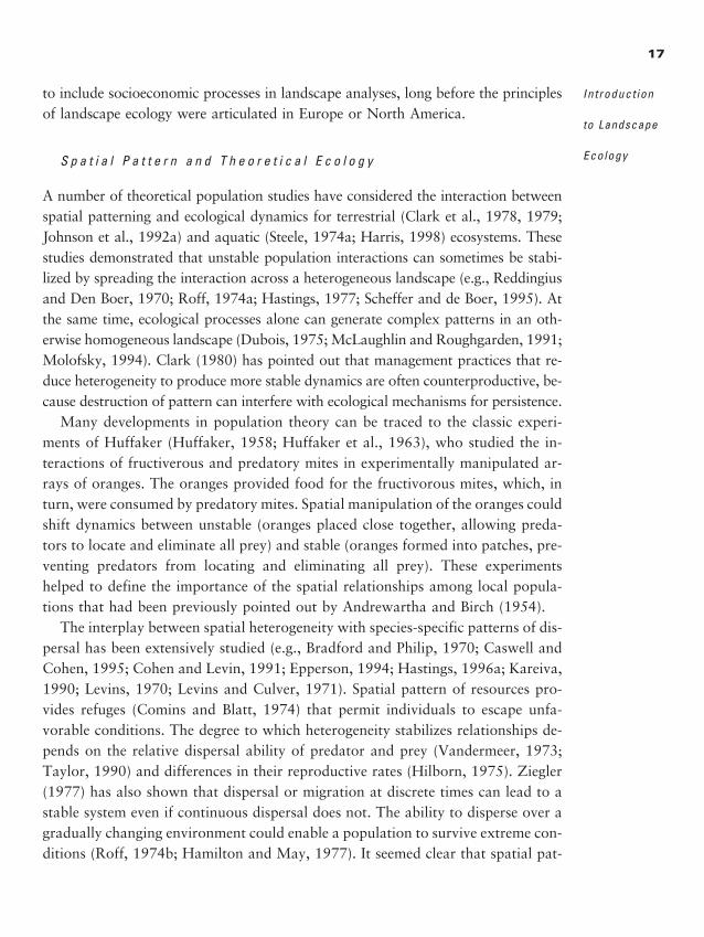
Collectively, this set of definitions clearly emphasizes two important aspects oflandscape ecology that distinguish it from other subdisciplines within ecology. First,landscape ecology explicitly addresses the importance of spatial configuration forecological processes. Landscape ecology is not only concerned with how much thereis of a particular component, but also with how it is arranged. The underlying premiseof landscape ecology is that the explicit composition and spatial form of a landscapemosaic affect ecological systems in ways that would be different if the mosaic com-position or arrangement were different (Wiens, 1995). Most ecological understand-ing previously had implicitly assumed an ability to average or extrapolate over spa-tially homogeneous areas. Ecological studies often attempted to achieve a predictiveknowledge about a particular type of system, such as a salt marsh or forest stand,without consideration of its size or position in a broader mosaic. Considered in thisway, with its emphasis on spatial heterogeneity, landscape ecology is applied acrossa wide range of scales (Figure 1.1). Studies might address the response of a beetle tothe patch structure of its environment within square meters (e.g., Johnson et al.,1992a), the influence of topography and vegetation patterns on ungulate foragingpatterns (e.g., Pearson et al., 1995), or the effects of land-use arrangements on ni-trogen dynamics in a watershed (e.g., Kesner and Meentemeyer, 1989).

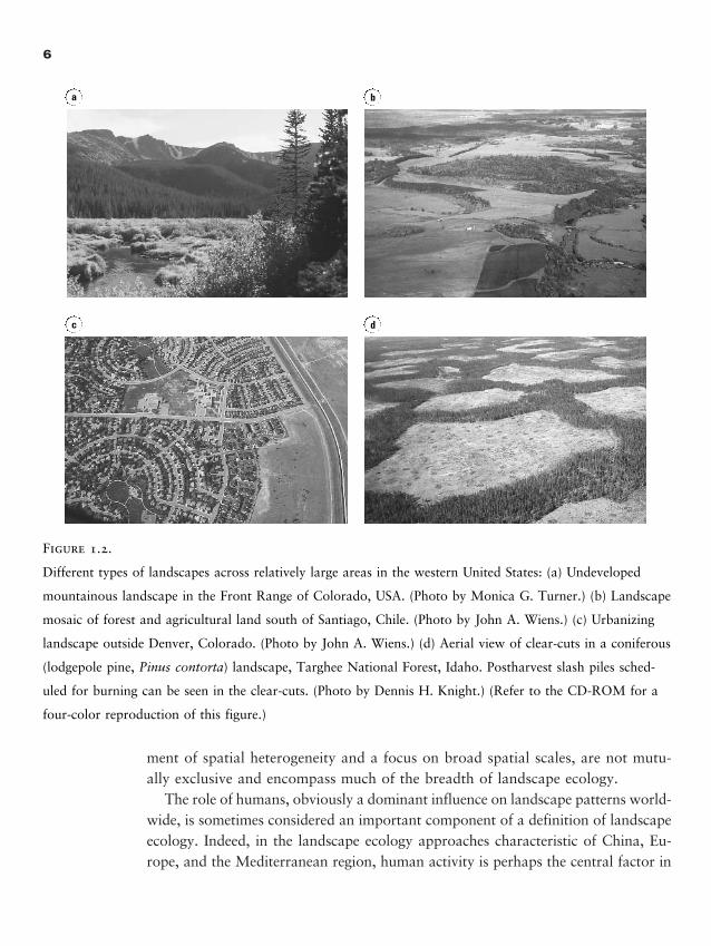
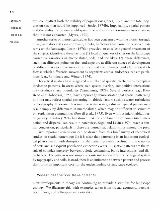
Second, landscape ecology often focuses on spatial extents that are much largerthan those traditionally studied in ecology, often, the landscape as seen by a hu-man observer (Figure 1.2). In this sense, landscape ecology addresses many kindsof ecological dynamics across large areas such as the Southern Appalachian Moun-tains, Yellowstone National Park, the Mediterranean, or the rain forests of Ron-donia, Brazil. However, it is important to note that, although these areas are typ-ically larger than those used in most community- or ecosystem-level studies, thespatial scales are not absolutes. We deal with issues of scale in the next chapterand throughout this book, but suffice it to say here that landscape ecology doesnot define, a priori, specific spatial scales that may be universally applied; rather,the emphasis is to identify scales that best characterize relationships between spa-tial heterogeneity and the processes of interest. These two aspects, explicit treat-

4

L A N D S C A P E

E C O L O G Y I N

T H E O R Y A N D

P R A C T I C E

2888_e01_p1-24 2/27/01 1:20 PM Page 4

5

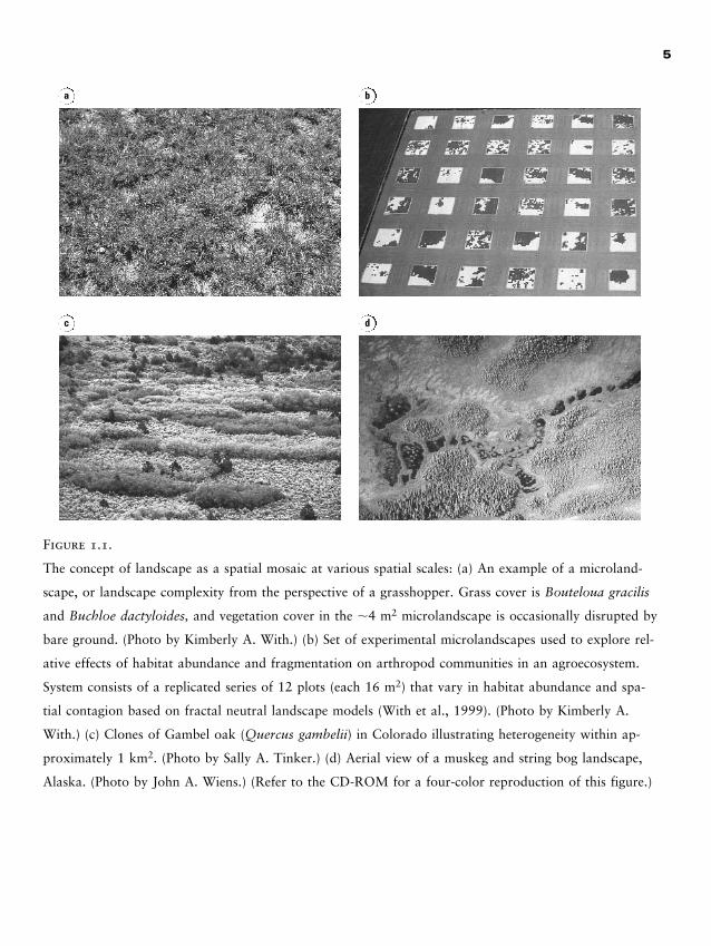
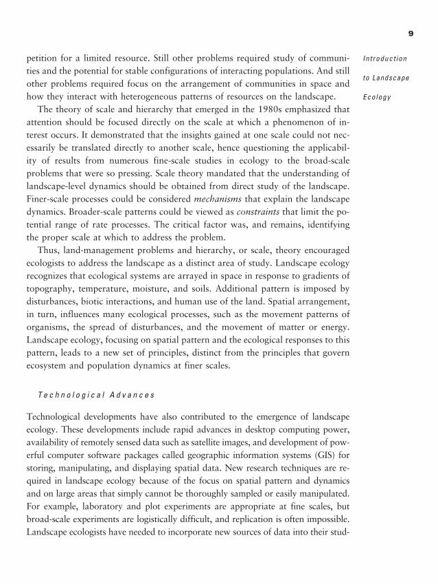
Figure 1.1.

The concept of landscape as a spatial mosaic at various spatial scales: (a) An example of a microland-

scape, or landscape complexity from the perspective of a grasshopper. Grass cover is Bouteloua gracilis

and Buchloe dactyloides, and vegetation cover in the �4 m2 microlandscape is occasionally disrupted by

bare ground. (Photo by Kimberly A. With.) (b) Set of experimental microlandscapes used to explore rel-

ative effects of habitat abundance and fragmentation on arthropod communities in an agroecosystem.

System consists of a replicated series of 12 plots (each 16 m2) that vary in habitat abundance and spa-

tial contagion based on fractal neutral landscape models (With et al., 1999). (Photo by Kimberly A.

With.) (c) Clones of Gambel oak (Quercus gambelii) in Colorado illustrating heterogeneity within ap-

proximately 1 km2. (Photo by Sally A. Tinker.) (d) Aerial view of a muskeg and string bog landscape,

Alaska. (Photo by John A. Wiens.) (Refer to the CD-ROM for a four-color reproduction of this figure.)

a b

c d

2888_e01_p1-24 2/27/01 1:20 PM Page 5

ment of spatial heterogeneity and a focus on broad spatial scales, are not mutu-ally exclusive and encompass much of the breadth of landscape ecology.

The role of humans, obviously a dominant influence on landscape patterns world-wide, is sometimes considered an important component of a definition of landscapeecology. Indeed, in the landscape ecology approaches characteristic of China, Eu-rope, and the Mediterranean region, human activity is perhaps the central factor in

6

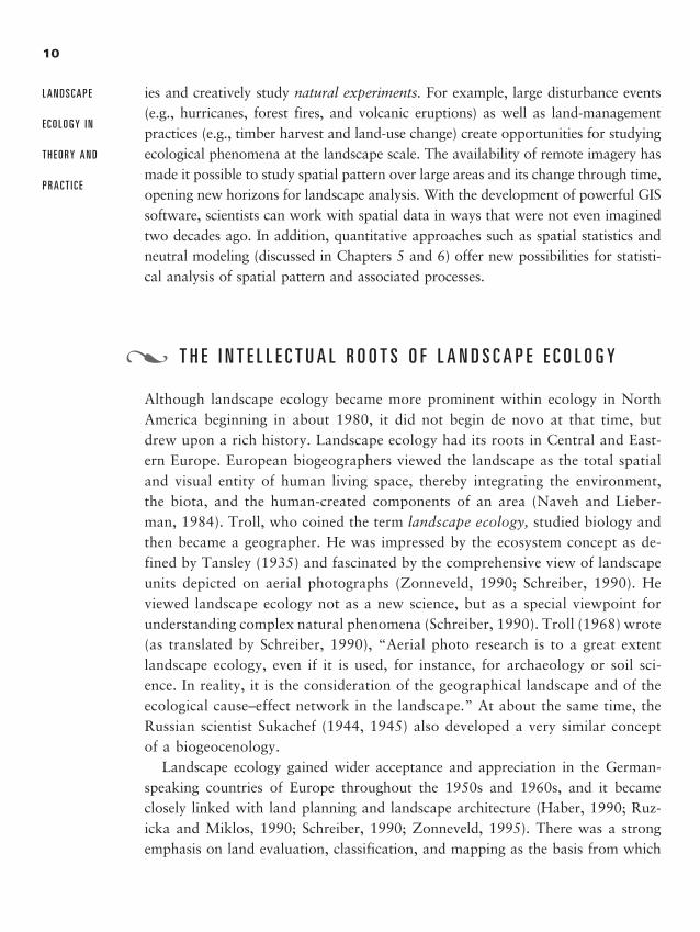
Figure 1.2.

Different types of landscapes across relatively large areas in the western United States: (a) Undeveloped

mountainous landscape in the Front Range of Colorado, USA. (Photo by Monica G. Turner.) (b) Landscape

mosaic of forest and agricultural land south of Santiago, Chile. (Photo by John A. Wiens.) (c) Urbanizing

landscape outside Denver, Colorado. (Photo by John A. Wiens.) (d) Aerial view of clear-cuts in a coniferous

(lodgepole pine, Pinus contorta) landscape, Targhee National Forest, Idaho. Postharvest slash piles sched-

uled for burning can be seen in the clear-cuts. (Photo by Dennis H. Knight.) (Refer to the CD-ROM for a

four-color reproduction of this figure.)

a b

c d

2888_e01_p1-24 2/27/01 1:20 PM Page 6

landscape ecological studies. Landscape ecology is sometimes considered to be aninterdisciplinary science dealing with the interrelation between human society andits living space—its open and built up landscapes (Naveh and Lieberman, 1984).Landscape ecology draws from a variety of disciplines, many of which emphasizesocial sciences, including geography, landscape architecture, regional planning, eco-nomics, forestry, and wildlife ecology. Throughout this book, the role of humansin shaping and responding to landscapes will be considered in many ways. The sci-entific contributions of landscape ecology are essential for land-management andland-use planning. However, we do not think it necessary to include a human com-ponent explicitly in the definition of landscape ecology, because humans are but oneof the factors creating and responding to spatial heterogeneity.

What, then, is a landscape? We suggest a general definition that does not re-quire an absolute scale: a landscape is an area that is spatially heterogeneous inat least one factor of interest. Although at the human scale we may observe “akilometers-wide mosaic over which local ecosystems recur” (Forman, 1995), it isimportant to recognize that landscape ecology may deal with landscapes that ex-tend over tens of meters rather than kilometers, and a landscape may even be de-fined in an aquatic system. In addition, we might observe a landscape representedby a gradient across which ecosystems do not necessarily repeat or recur. Thusour definition is general enough to permit consideration of both aspects of land-scape ecology described above.

W H Y L A N D S C A P E E C O L O G Y H A S E M E R G E D A S A D I S T I N C T A R E A O F S T U D Y

The recent emergence of landscapes as appropriate subjects for ecological studyresulted from three main factors: (1) broad-scale environmental issues and land-management problems, (2) the development of new scale-related concepts in ecol-ogy, and (3) technological advances, including the widespread availability of spa-tial data, the computers and software to manipulate these data, and the rapid risein computational power.

B r o a d - S c a l e E n v i r o n m e n t a l I s s u e s

Demand for the scientific underpinnings of managing large areas and incorpo-rating the consequences of spatial heterogeneity into land-management decisions

7

Introduct ion

to Landscape

Ecology

�

2888_e01_p1-24 2/27/01 1:20 PM Page 7

has been growing since the 1970s and is now enormous. The paradigm of ecosys-tem management, for example, carries with it an implicit focus on the landscape(Agee and Johnson, 1988; Slocombe, 1993; Christensen et al., 1996). Appliedproblems and resource-management needs have clearly helped to catalyze the de-velopment and emergence of landscape ecology. For example, questions of howto manage populations of native plants and animals over large areas as land useor climate changes, how to mediate the effects of habitat fragmentation or loss,how to plan for human settlement in areas that experience a particular naturaldisturbance regime, and how to reduce the deleterious effects of nonpoint sourcepollution in aquatic ecosystems all demand basic understanding and managementsolutions at landscape scales. Federal agencies concerned with conservation in theUnited States are faced with many of these challenges. The cumulative loss ofwetlands and riparian forests from many landscapes poses challenges for the man-agement of animal populations and of water flow and quality. The U.S. ForestService continues to wrestle with resource-management questions regarding frag-mentation of contiguous old-growth forests in the northwestern United States.The patchwork quilt of overgrazed lands in the western United States poses man-agement difficulties for the Bureau of Land Management that extend over mul-tiple states. The National Park Service must attempt to determine whether exist-ing parklands are of sufficient size to sustain biotic populations and naturalprocesses over the long term. These problems require a spatially explicit, broad-scale approach, yet much of ecology had focused on mechanistic studies in rela-tively small homogeneous areas over relatively short time periods. Landscape ecol-ogy provides concepts and methods that complement those that have beentraditionally employed in ecology.

C o n c e p t s o f S c a l e

The importance of scale (see Chapter 2) became widely recognized in ecology onlyin the 1980s, despite a long history of attention to the effect of quadrat size onmeasurements and recognition of species–area relationships. The development ofconceptual frameworks focused on scale (Allen and Starr, 1982; Delcourt et al.,1983; O’Neill et al., 1986; Allen and Hoekstra, 1992) prompted ecologists tothink hard about the patterns and processes that were important at different scalesof space and time. It became clear that no single scale was appropriate for thestudy of all ecological problems. Some problems required focus on an individualorganism and its physiological response to environmental changes. Other prob-lems required study of how numbers of individuals or species change with com-

8

L A N D S C A P E

E C O L O G Y I N

T H E O R Y A N D

P R A C T I C E

2888_e01_p1-24 2/27/01 1:20 PM Page 8

petition for a limited resource. Still other problems required study of communi-ties and the potential for stable configurations of interacting populations. And stillother problems required focus on the arrangement of communities in space andhow they interact with heterogeneous patterns of resources on the landscape.

The theory of scale and hierarchy that emerged in the 1980s emphasized thatattention should be focused directly on the scale at which a phenomenon of in-terest occurs. It demonstrated that the insights gained at one scale could not nec-essarily be translated directly to another scale, hence questioning the applicabil-ity of results from numerous fine-scale studies in ecology to the broad-scaleproblems that were so pressing. Scale theory mandated that the understanding oflandscape-level dynamics should be obtained from direct study of the landscape.Finer-scale processes could be considered mechanisms that explain the landscapedynamics. Broader-scale patterns could be viewed as constraints that limit the po-tential range of rate processes. The critical factor was, and remains, identifyingthe proper scale at which to address the problem.

Thus, land-management problems and hierarchy, or scale, theory encouragedecologists to address the landscape as a distinct area of study. Landscape ecologyrecognizes that ecological systems are arrayed in space in response to gradients oftopography, temperature, moisture, and soils. Additional pattern is imposed bydisturbances, biotic interactions, and human use of the land. Spatial arrangement,in turn, influences many ecological processes, such as the movement patterns oforganisms, the spread of disturbances, and the movement of matter or energy.Landscape ecology, focusing on spatial pattern and the ecological responses to thispattern, leads to a new set of principles, distinct from the principles that governecosystem and population dynamics at finer scales.

T e c h n o l o g i c a l A d v a n c e s

Technological developments have also contributed to the emergence of landscapeecology. These developments include rapid advances in desktop computing power,availability of remotely sensed data such as satellite images, and development of pow-erful computer software packages called geographic information systems (GIS) forstoring, manipulating, and displaying spatial data. New research techniques are re-quired in landscape ecology because of the focus on spatial pattern and dynamicsand on large areas that simply cannot be thoroughly sampled or easily manipulated.For example, laboratory and plot experiments are appropriate at fine scales, butbroad-scale experiments are logistically difficult, and replication is often impossible.Landscape ecologists have needed to incorporate new sources of data into their stud-

9

Introduct ion

to Landscape

Ecology

2888_e01_p1-24 2/27/01 1:20 PM Page 9

ies and creatively study natural experiments. For example, large disturbance events(e.g., hurricanes, forest fires, and volcanic eruptions) as well as land-managementpractices (e.g., timber harvest and land-use change) create opportunities for studyingecological phenomena at the landscape scale. The availability of remote imagery hasmade it possible to study spatial pattern over large areas and its change through time,opening new horizons for landscape analysis. With the development of powerful GISsoftware, scientists can work with spatial data in ways that were not even imaginedtwo decades ago. In addition, quantitative approaches such as spatial statistics andneutral modeling (discussed in Chapters 5 and 6) offer new possibilities for statisti-cal analysis of spatial pattern and associated processes.

T H E I N T E L L E C T U A L R O O T S O F L A N D S C A P E E C O L O G Y

Although landscape ecology became more prominent within ecology in NorthAmerica beginning in about 1980, it did not begin de novo at that time, butdrew upon a rich history. Landscape ecology had its roots in Central and East-ern Europe. European biogeographers viewed the landscape as the total spatialand visual entity of human living space, thereby integrating the environment,the biota, and the human-created components of an area (Naveh and Lieber-man, 1984). Troll, who coined the term landscape ecology, studied biology andthen became a geographer. He was impressed by the ecosystem concept as de-fined by Tansley (1935) and fascinated by the comprehensive view of landscapeunits depicted on aerial photographs (Zonneveld, 1990; Schreiber, 1990). Heviewed landscape ecology not as a new science, but as a special viewpoint forunderstanding complex natural phenomena (Schreiber, 1990). Troll (1968) wrote(as translated by Schreiber, 1990), “Aerial photo research is to a great extentlandscape ecology, even if it is used, for instance, for archaeology or soil sci-ence. In reality, it is the consideration of the geographical landscape and of theecological cause–effect network in the landscape.” At about the same time, theRussian scientist Sukachef (1944, 1945) also developed a very similar conceptof a biogeocenology.

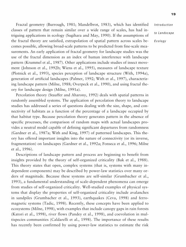
Landscape ecology gained wider acceptance and appreciation in the German-speaking countries of Europe throughout the 1950s and 1960s, and it becameclosely linked with land planning and landscape architecture (Haber, 1990; Ruz-icka and Miklos, 1990; Schreiber, 1990; Zonneveld, 1995). There was a strongemphasis on land evaluation, classification, and mapping as the basis from which

10

L A N D S C A P E

E C O L O G Y I N

T H E O R Y A N D

P R A C T I C E

�

2888_e01_p1-24 2/27/01 1:20 PM Page 10

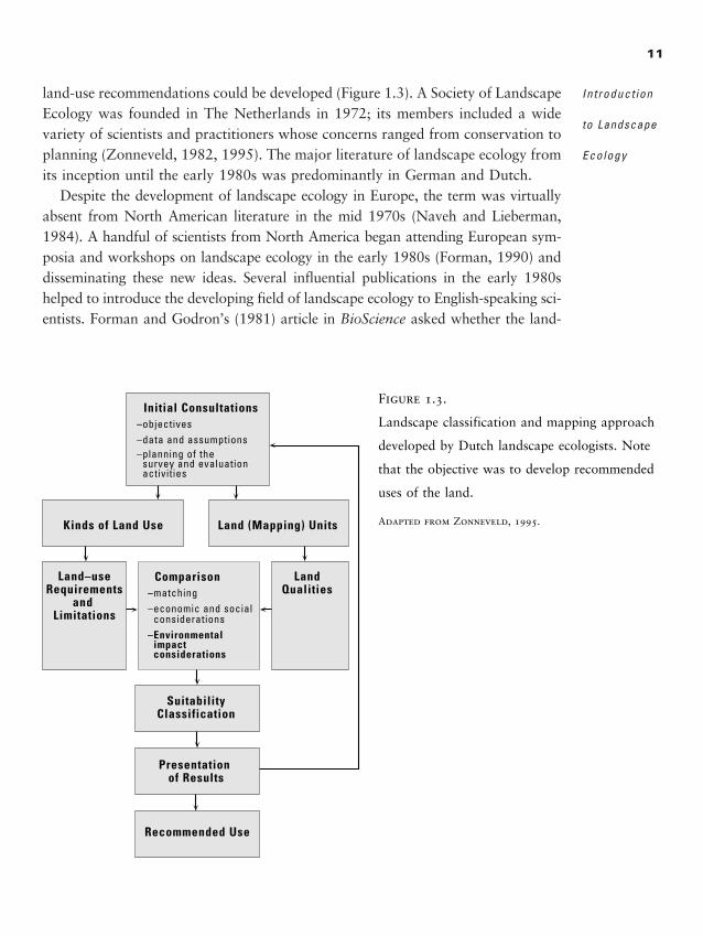
land-use recommendations could be developed (Figure 1.3). A Society of LandscapeEcology was founded in The Netherlands in 1972; its members included a widevariety of scientists and practitioners whose concerns ranged from conservation toplanning (Zonneveld, 1982, 1995). The major literature of landscape ecology fromits inception until the early 1980s was predominantly in German and Dutch.

Despite the development of landscape ecology in Europe, the term was virtuallyabsent from North American literature in the mid 1970s (Naveh and Lieberman,1984). A handful of scientists from North America began attending European sym-posia and workshops on landscape ecology in the early 1980s (Forman, 1990) anddisseminating these new ideas. Several influential publications in the early 1980shelped to introduce the developing field of landscape ecology to English-speaking sci-entists. Forman and Godron’s (1981) article in BioScience asked whether the land-

11

Introduct ion

to Landscape

Ecology

Initial Consultations–objectives–data and assumptions–planning of the survey and evaluation activities

Comparison–matching–economic and social considerations–Environmental impact considerations

Kinds of Land Use

SuitabilityClassification

Presentation of Results

Recommended Use

Land–useRequirements

and Limitations

LandQualities

Land (Mapping) Units

Figure 1.3.

Landscape classification and mapping approach

developed by Dutch landscape ecologists. Note

that the objective was to develop recommended

uses of the land.

Adapted from Zonneveld, 1995.

2888_e01_p1-24 2/27/01 1:20 PM Page 11

scape was a recognizable and useful unit in ecology and provided a set of terms, suchas patch, corridor, and matrix, that remain within the common parlance of land-scape ecology. Naveh, an ecologist who focused on vegetation science, fire ecology,and landscape restoration, largely in Mediterranean climates, published a review thatlaid out a conceptual basis for landscape ecology (Naveh, 1982); his writing em-phasized the integral relationship between humans and the landscape and the im-portance of a systems approach. These ideas were developed further as a book (Navehand Lieberman, 1984) that delved into both concepts and applications of landscapeecology and stimulated much discussion among ecologists. Forman’s (1983) editor-ial in BioScience, from which we quoted earlier, identified landscape ecology as thecandidate idea for the decade, with a richness of empirical study, emergent theory,and applications lying ahead. And although not part of the infusion of ideas fromEurope to North America, Romme’s study of fire history in Yellowstone NationalPark (Romme, 1982; Romme and Knight, 1982) offered a breakthrough in the de-velopment of new metrics to quantify changes in the landscape through time.

Two pivotal meetings in the early 1980s helped to define the current scope oflandscape ecology. A 1983 workshop held at Allerton Park, Illinois, brought to-gether a group of North American ecologists to explore the ideas and potentialof landscape ecology concepts (Risser et al., 1984). This meeting came soon afteran influential meeting in The Netherlands that drew together landscape ecologistsin Europe (Tjallingii and de Veer, 1982), and it represented the coalescence of sev-eral independent lines of research in the United States. The report that emerged(Risser et al., 1984) still makes for good reading. In many respects, the organizedsearch for principles governing the interaction of pattern and process at the land-scape scale began at these two meetings. The emphasis of landscape ecology inNorth American is somewhat different from Europe, where the association withland planning is so much closer and where the landscape itself has been more in-tensively managed for a much longer time. However, landscape ecology has grownout of intellectual developments that extended back many decades. The questionsaddressed by landscape ecologists typically couple the observation that landscapemosaics have spatial structure with topics that have interested ecologists for a longtime (Wiens, 1995). Next we highlight several of the important precursors to theconcepts of landscape ecology.

P h y t o s o c i o l o g y a n d B i o g e o g r a p h y

Phytosociologists in Europe and the United States had long studied the spatial dis-tribution of major plant associations (Braun-Blanquet, 1932), even going back

12

L A N D S C A P E

E C O L O G Y I N

T H E O R Y A N D

P R A C T I C E

2888_e01_p1-24 2/27/01 1:20 PM Page 12

to the observations of von Humboldt (1807) and Warming (1925). For example,it was well known that vegetation distributions in space responded to thenorth–south gradient of temperature combined with an east–west gradient of mois-ture. Vegetation pattern was further determined by topographic gradients in mois-ture, temperature, soils, and exposure. Thus, at broad scales, it was well estab-lished that ecological systems interacted with spatially distributed environmentalfactors to form distinct patterns.

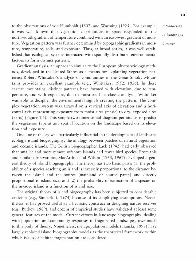
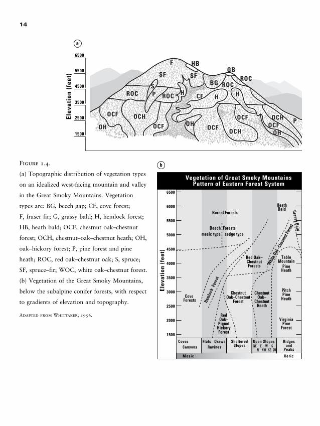
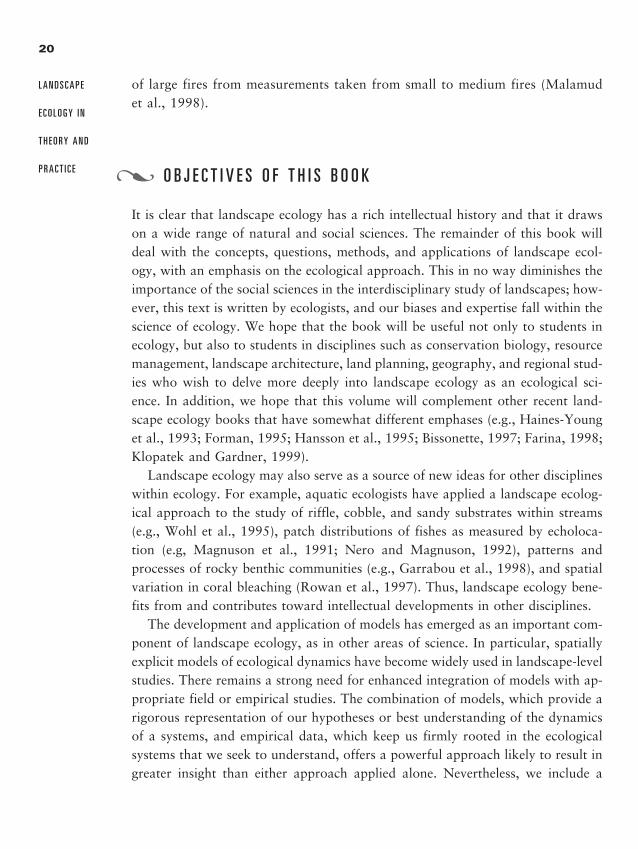
Gradient analysis, an approach similar to the European phytosociology meth-ods, developed in the United States as a means for explaining vegetation pat-terns; Robert Whittaker’s analysis of communities in the Great Smoky Moun-tains provides an excellent example (e.g., Whittaker, 1952, 1956). In theseeastern mountains, distinct patterns have formed with elevation, due to tem-perature, and with exposure, due to moisture. In a classic analysis, Whittakerwas able to decipher the environmental signals creating the pattern. The com-plex vegetation system was arrayed on a vertical axis of elevation and a hori-zontal axis representing exposure from moist sites (mesic) to dry, exposed sites(xeric) (Figure 1.4). This simple two-dimensional diagram permits us to predictthe vegetation type at any spatial location on the landscape based on its eleva-tion and exposure.

One line of theory was particularly influential in the development of landscapeecology: island biogeography, the analogy between patches of natural vegetationand oceanic islands. The British biogeographer Lack (1942) had early observedthat smaller and more remote offshore islands had fewer bird species. From thisand similar observations, MacArthur and Wilson (1963, 1967) developed a gen-eral theory of island biogeography. The theory has two basic parts: (1) the prob-ability of a species reaching an island is inversely proportional to the distance be-tween the island and the source (mainland or source patch) and directlyproportional to island size, and (2) the probability of extinction of a species onthe invaded island is a function of island size.

The original theory of island biogeography has been subjected to considerablecriticism (e.g., Simberloff, 1974) because of its simplifying assumptions. Never-theless, it has proved useful as a heuristic construct in designing nature reserves(e.g., Burkey, 1989), and dozens of empirical studies have validated at least somegeneral features of the model. Current efforts in landscape biogeography, dealingwith population and community responses to fragmented landscapes, owe muchto this body of theory. Nonetheless, metapopulation models (Hanski, 1998) havelargely replaced island biogeography models as the theoretical framework withinwhich issues of habitat fragmentation are considered.

13

Introduct ion

to Landscape

Ecology

2888_e01_p1-24 2/27/01 1:20 PM Page 13

14

OCH

ROC

Elev

atio

n (f

eet)

5500

6500

4500

3500

2500

1500

OCF

OCF OCFOH

ROCPS

SF

F HB

SFBG

GBROC

ROC

OCH

OCF

HH

OCH P

CF

OH

H

OH OCF

a

Vegetation of Great Smoky MountainsPattern of Eastern Forest System

Mesic

CovesCanyons

Flats Draws Ridgesand

Peaks

ShelteredSlopes

Boreal Forests

Cove Forests

RedOak–

PignutHickoryForest

ChestnutOak–Chestnut

Forest

Red Oak–ChestnutForests

ChestnutOak–

ChestnutHeath

HeathBald Grassy Bald

Heml

ock

Fore

st

TableMountain

PineHeath

PitchPine

Heath

VirginiaPine

Forest

Beech Forestsmesic type sedge type

Open SlopesRavines

1500

2000

2500

3000

3500

4000

4500

5000

5500

6000

6500

Xeric

NE E W S N NW SE SW

Elev

atio

n (f

eet)

Whit

e Oak

–Che

stnut

Fore

st

bFigure 1.4.

(a) Topographic distribution of vegetation types

on an idealized west-facing mountain and valley

in the Great Smoky Mountains. Vegetation

types are: BG, beech gap; CF, cove forest;

F, fraser fir; G, grassy bald; H, hemlock forest;

HB, heath bald; OCF, chestnut oak–chestnut

forest; OCH, chestnut–oak–chestnut heath; OH,

oak–hickory forest; P, pine forest and pine

heath; ROC, red oak–chestnut oak; S, spruce;

SF, spruce–fir; WOC, white oak–chestnut forest.

(b) Vegetation of the Great Smoky Mountains,

below the subalpine conifer forests, with respect

to gradients of elevation and topography.

Adapted from Whittaker, 1956.

2888_e01_p1-24 2/27/01 1:20 PM Page 14

L a n d s c a p e P l a n n i n g , D e s i g n , a n d M a n a g e m e n t

The relationship between human societies and landscape change has been a fun-damental concern of ecologists in Europe for many years (see Naveh, 1982). In-deed, the history of human-induced change is clearly apparent throughout Europe,with roads and viaducts constructed during the Roman Empire still having a vis-ible effect in many regions (Marc Antrop, personal communication). The empha-sis of ecological studies in North American has been on relatively undisturbed sys-tems (Risser et al., 1984), but an awareness of human effects on landscapes hasbeen evident for more than 140 years (Marsh, 1864, as cited by Turner and Meyer,1993). The writings of a number of authors have provided an important contextfor integrating ecological effects with landscape planning, including the develop-ment of map overlay techniques (a precursor to current GIS methods) by McHarg(1969), the studies of Watt (1947) that focused on patch structure as fundamen-tal to understanding vegetation pattern, an overview of the effects of ecosystemfragmentation in human-dominated landscapes edited by Burgess and Sharpe(1981), and the development of concepts of adaptive management by Holling(1978).

The goals of landscape planning, design, and management include the identifi-cation and protection of ecological resources and control of their use throughplans that ensure the sustainability of these resources (Fabos, 1985). The result isthat landscape planning is a primary basis for collaboration and knowledge ex-change between landscape planners and landscape ecologists (Ahern, 1999). Per-haps the best examples of the integration of landscape planning, design, and man-agement can be found in The Netherlands, where a national plan for a sustainablelandscape is being implemented (Vos and Opdam, 1993). In North America, thebest examples include the current plans for ecosystem management of nationalforests (Bartuska, 1999) and studies aimed at conservation design (Diamond andMay, 1976; Mladenoff et al., 1994; Ando et al., 1998).

M u l t i d i s c i p l i n a r y S t u d i e s a n d R e g i o n a l M o d e l i n g

The geographic sciences have made important contributions to the methodologyof landscape ecology. Satellite imagery, classified to cover type, has been an in-valuable resource. Software developments (e.g., GIS and image analysis programs,spatial statistics) provide computer capabilities for displaying, superimposing, andanalyzing spatial patterns. These analytical tools and the geographer’s experience

15

Introduct ion

to Landscape

Ecology

2888_e01_p1-24 2/27/01 1:20 PM Page 15

in handling large spatial databases have been a stimulus and critical resource forlandscape ecologists.

During the 1960s, a number of diverse projects resulted in the development oflarge regional models. The result was the application of systems analysis and com-puter modeling at landscape scales that clearly established the broad-scale impactof human development. These models were often associated with urban develop-ment programs (Lowry, 1967) concerned with the interaction of spatial patternsand socioeconomic processes, a topic that remains important today. Transporta-tion models were developed to link human activities at different positions on thelandscape. Large-scale urban renewal programs (Pittsburgh Community RenewalProject, 1962) theorized about the optimal spatial arrangement of economic ac-tivities on the urban landscape. The central theme of these studies was the inter-actions by which socioeconomic processes produced spatial pattern and the pat-terns, in turn, encouraged or constrained human activities (Hemens, 1970). By theend of the 1960s, studies on pattern–process interactions had resulted in a con-siderable body of theory. Much of the development was synthesized under the ti-tles of urban dynamics (Forester, 1969) and regional science (Isard, 1960, 1972,1975). Considerable effort was expended toward linking spatial activities on thelandscape with socioeconomic theory (Smith, 1976).

An important set of studies considered the spatial allocation of processes fromthe perspective of central place theory (Herbert and Stevens, 1960; Steger, 1964),which predicts that human activities will radiate outward from a center of eco-nomic activity, such as a city, transportation center, or highway intersection. Thistheory was later applied to the spatial pattern of foraging by animals (Aronsonand Givnish, 1983), including ants (Harkness and Maroudas, 1985) and birds(Andersson, 1981) that forage outward from a nest. Central place theory was alsoused to predict land-use change following the installation of a sawmill in a ruralarea (Hett, 1971).

In subsequent years, regional modeling became concerned with predicting the ef-fects of socioeconomic activities on the environment. Example applications with astrong spatial component included studies of the impact of large-scale energy devel-opments (Basta and Bower 1982; Krummel et al., 1984) and the planning of river-basin systems (Hamilton et al., 1969). These studies resulted in new theoretical con-structs to link socioeconomic and ecological variables in the same model (Klopateket al., 1983), which were later applied to such diverse problems as modeling oil andgas extraction in the western United States (Mankin et al., 1981) and cattle herdingsocieties in Africa (Krummel et al., 1986). All these studies focused on the interac-tion between landscape pattern and ecological processes and emphasized the need

16

L A N D S C A P E

E C O L O G Y I N

T H E O R Y A N D

P R A C T I C E

2888_e01_p1-24 2/27/01 1:20 PM Page 16

to include socioeconomic processes in landscape analyses, long before the principlesof landscape ecology were articulated in Europe or North America.

S p a t i a l P a t t e r n a n d T h e o r e t i c a l E c o l o g y

A number of theoretical population studies have considered the interaction betweenspatial patterning and ecological dynamics for terrestrial (Clark et al., 1978, 1979;Johnson et al., 1992a) and aquatic (Steele, 1974a; Harris, 1998) ecosystems. Thesestudies demonstrated that unstable population interactions can sometimes be stabi-lized by spreading the interaction across a heterogeneous landscape (e.g., Reddingiusand Den Boer, 1970; Roff, 1974a; Hastings, 1977; Scheffer and de Boer, 1995). Atthe same time, ecological processes alone can generate complex patterns in an oth-erwise homogeneous landscape (Dubois, 1975; McLaughlin and Roughgarden, 1991;Molofsky, 1994). Clark (1980) has pointed out that management practices that re-duce heterogeneity to produce more stable dynamics are often counterproductive, be-cause destruction of pattern can interfere with ecological mechanisms for persistence.

Many developments in population theory can be traced to the classic experi-ments of Huffaker (Huffaker, 1958; Huffaker et al., 1963), who studied the in-teractions of fructiverous and predatory mites in experimentally manipulated ar-rays of oranges. The oranges provided food for the fructivorous mites, which, inturn, were consumed by predatory mites. Spatial manipulation of the oranges couldshift dynamics between unstable (oranges placed close together, allowing preda-tors to locate and eliminate all prey) and stable (oranges formed into patches, pre-venting predators from locating and eliminating all prey). These experimentshelped to define the importance of the spatial relationships among local popula-tions that had been previously pointed out by Andrewartha and Birch (1954).

The interplay between spatial heterogeneity with species-specific patterns of dis-persal has been extensively studied (e.g., Bradford and Philip, 1970; Caswell andCohen, 1995; Cohen and Levin, 1991; Epperson, 1994; Hastings, 1996a; Kareiva,1990; Levins, 1970; Levins and Culver, 1971). Spatial pattern of resources pro-vides refuges (Comins and Blatt, 1974) that permit individuals to escape unfa-vorable conditions. The degree to which heterogeneity stabilizes relationships de-pends on the relative dispersal ability of predator and prey (Vandermeer, 1973;Taylor, 1990) and differences in their reproductive rates (Hilborn, 1975). Ziegler(1977) has also shown that dispersal or migration at discrete times can lead to astable system even if continuous dispersal does not. The ability to disperse over agradually changing environment could enable a population to survive extreme con-ditions (Roff, 1974b; Hamilton and May, 1977). It seemed clear that spatial pat-

17

Introduct ion

to Landscape

Ecology

2888_e01_p1-24 2/27/01 1:20 PM Page 17

tern could affect both the stability of populations (Jones, 1975) and the total pop-ulation size that could be supported (Steele, 1974b). Importantly, spatial patternand the ability to disperse could spread the utilization of a resource over space sothat it is not exhausted (Myers, 1976).

Another series of theoretical studies has been concerned with the biotic (Sprugel,1976) and abiotic (Levin and Paine, 1974a, b) factors that cause the observed pat-terns on the landscape. Levin (1976a) provided an excellent general treatment ofthe subject, identifying three factors: (1) local uniqueness of sites on the landscapecaused by variations in microhabitat, soils, and the likes, (2) phase differences,such that different points on the landscape are at different stages of developmentor different stages of recovery from localized disturbances, and (3) dispersal ef-fects in which differential movement by organisms across landscapes leads to patch-iness (e.g., Criminale and Winter, 1974).

Theoretical studies have suggested a number of specific mechanisms to explainlandscape patterns. In areas where two species overlap, competitive interactionsmay produce sharp boundaries (Yamamura, 1976). Several workers (e.g., Kier-stead and Slobodkin, 1953) have empirically demonstrated that spatial patterningin biota may reflect spatial patterning in abiotic factors such as water turbulenceor topography. If a system has multiple stable states, a distinct spatial pattern mayresult simply by differences in microhabitat, which may be sufficient to structurephytoplankton communities (Powell et al., 1975). Even without microhabitat het-erogeneity, Okubo (1974) has shown that the combination of competitive inter-action and dispersal can result in patchiness. Segal and Levin (1976) reach a sim-ilar conclusion, particularly if there are mutualistic relationships among the prey.

Two important conclusions can be drawn from this brief survey of theoreticalstudies on spatial patterning: (1) it is clear that patterning is an important ecologi-cal phenomenon, with disruption of the pattern possibly resulting in the eruptionof pests and subsequent population extinction events; (2) spatial patterns are the re-sult of complex interplay between abiotic constraints, biotic interactions, and dis-turbances. The pattern is not simply a constraint imposed on the ecological systemby topography and soils. Instead, there is an intimate tie between pattern and processthat forms an important core for the understanding of landscape ecology.

R e c e n t T h e o r e t i c a l D e v e l o p m e n t s

New developments in theory are continuing to provide a stimulus for landscapeecology. We illustrate this with examples taken from fractal geometry, percola-tion theory, and self-organized criticality.

18

L A N D S C A P E

E C O L O G Y I N

T H E O R Y A N D

P R A C T I C E

2888_e01_p1-24 2/27/01 1:20 PM Page 18

Fractal geometry (Burrough, 1981; Mandelbrot, 1983), which has identifiedclasses of pattern that remain similar over a wide range of scales, has had in-triguing applications in ecology (Sugihara and May, 1990). If the assumptions ofthe fractal theory are satisfied, extrapolation of spatial pattern across scales be-comes possible, allowing broad-scale patterns to be predicted from fine-scale mea-surements. An early application of fractal geometry for landscape studies was theuse of the fractal dimension as an index of human interference with landscapepattern (Krummel et al., 1987). Other applications include studies of insect move-ment (Johnson et al., 1992b; Wiens et al., 1995), measures of landscape texture(Plotnick et al., 1993), species perception of landscape structure (With, 1994a),generation of artificial landscapes (Palmer, 1992; With et al., 1997), characteriz-ing landscape pattern (Milne, 1988; Overpeck et al., 1990), and using fractal the-ory for landscape design (Milne, 1991a).

Percolation theory (Stauffer and Aharony, 1992) deals with spatial patterns inrandomly assembled systems. The application of percolation theory to landscapestudies has addressed a series of questions dealing with the size, shape, and con-nectivity of habitats as a function of the percentage of a landscape occupied bythat habitat type. Because percolation theory generates pattern in the absence ofspecific processes, the comparison of random maps with actual landscapes pro-vides a neutral model capable of defining significant departures from randomness(Gardner et al., 1987a; With and King, 1997) of patterned landscapes. This the-ory has offered important insights into the nature of connectivity (or its inverse,fragmentation) on landscapes (Gardner et al., 1992a; Fonseca et al., 1996; Milneet al., 1996).

Descriptions of landscape pattern and process are beginning to benefit frominsights provided by the theory of self-organized criticality (Bak et al., 1988).This theory states that open, complex systems (that is, systems with many in-dependent components) may be described by power-law statistics over many or-ders of magnitude. Because these systems are self-similar (Grumbacher et al.,1993), a fundamental understanding of scale-dependent phenomena can emergefrom studies of self-organized criticality. Well-studied examples of physical sys-tems that display the properties of self-organized criticality include avalanchesin sandpiles (Grumbacher et al., 1993), earthquakes (Ceva, 1998) and ferro-magnetic systems (Tadic, 1998). Recently, these concepts have been applied toecosystems (Milne, 1998), with examples that include canopy gaps in rain forests(Katori et al., 1998), river flows (Pandey et al., 1998), and coevolution in mul-tispecies communities (Caldarelli et al., 1998). The importance of these resultshas recently been confirmed by using power-law statistics to estimate the risk

19

Introduct ion

to Landscape

Ecology

2888_e01_p1-24 2/27/01 1:20 PM Page 19

of large fires from measurements taken from small to medium fires (Malamudet al., 1998).

O B J E C T I V E S O F T H I S B O O K

It is clear that landscape ecology has a rich intellectual history and that it drawson a wide range of natural and social sciences. The remainder of this book willdeal with the concepts, questions, methods, and applications of landscape ecol-ogy, with an emphasis on the ecological approach. This in no way diminishes theimportance of the social sciences in the interdisciplinary study of landscapes; how-ever, this text is written by ecologists, and our biases and expertise fall within thescience of ecology. We hope that the book will be useful not only to students inecology, but also to students in disciplines such as conservation biology, resourcemanagement, landscape architecture, land planning, geography, and regional stud-ies who wish to delve more deeply into landscape ecology as an ecological sci-ence. In addition, we hope that this volume will complement other recent land-scape ecology books that have somewhat different emphases (e.g., Haines-Younget al., 1993; Forman, 1995; Hansson et al., 1995; Bissonette, 1997; Farina, 1998;Klopatek and Gardner, 1999).

Landscape ecology may also serve as a source of new ideas for other disciplineswithin ecology. For example, aquatic ecologists have applied a landscape ecolog-ical approach to the study of riffle, cobble, and sandy substrates within streams(e.g., Wohl et al., 1995), patch distributions of fishes as measured by echoloca-tion (e.g, Magnuson et al., 1991; Nero and Magnuson, 1992), patterns andprocesses of rocky benthic communities (e.g., Garrabou et al., 1998), and spatialvariation in coral bleaching (Rowan et al., 1997). Thus, landscape ecology bene-fits from and contributes toward intellectual developments in other disciplines.

The development and application of models has emerged as an important com-ponent of landscape ecology, as in other areas of science. In particular, spatiallyexplicit models of ecological dynamics have become widely used in landscape-levelstudies. There remains a strong need for enhanced integration of models with ap-propriate field or empirical studies. The combination of models, which provide arigorous representation of our hypotheses or best understanding of the dynamicsof a systems, and empirical data, which keep us firmly rooted in the ecologicalsystems that we seek to understand, offers a powerful approach likely to result ingreater insight than either approach applied alone. Nevertheless, we include a

20

L A N D S C A P E

E C O L O G Y I N

T H E O R Y A N D

P R A C T I C E �

2888_e01_p1-24 2/27/01 1:20 PM Page 20

chapter on modeling to familiarize readers with the fundamental concepts of thisimportant topic.

This is also not a textbook for geographic information systems (GIS) or remotesensing, although landscape ecology makes extensive use of these technologies.Often, landscape ecologists use the final products of GIS manipulations or the in-terpretation of spectral data, but many are not technically proficient in all the in-tricacies of the processes involved. Many fine texts are excellent resources for thelandscape ecologist who needs a more thorough introduction to these subjects.For GIS, we suggest Burrough (1986), Bonham-Carter (1994), Fotheringham andRogerson (1994), and Burrough and McDonnell (1998); for remote sensing, wesuggest Lillesand and Kiefer (1994) or Jensen (1996).

We have organized the book in a sequence comparable to what we teach in alandscape ecology course. The first three chapters provide an introduction to thesubject and its development (Chapter 1), a treatment of scale (Chapter 2), whichinfluences everything that follows, and an introduction to basic modeling concepts(Chapter 3). We then examine the causes of landscape pattern (Chapter 4), in-cluding both biotic and abiotic factors, and consider observed changes over ex-tended temporal scales. The quantification of landscape pattern, which is a nec-essary component of understanding the interaction between pattern and process,is presented in detail in Chapter 5. The use of neutral models in landscape ecol-ogy, which is closely related to quantification of pattern and to linkages of pat-tern with process, is considered in Chapter 6. The next three chapters deal withparticular phenomena that have received considerable attention in landscape stud-ies during the past two decades: disturbance dynamics (Chapter 7), the responsesof organisms to spatial heterogeneity (Chapter 8), and ecosystem processes at land-scape scales (Chapter 9). We then deal explicitly with the many applications oflandscape ecology (Chapter 10) and, finally, suggest conclusions and future di-rections for the field (Chapter 11).

S U M M A R Y

Landscape ecology has come to the forefront of ecology and land management inrecent decades, and it is still expanding very rapidly. Landscape ecology empha-sizes the interaction between spatial pattern and ecological process, that is, thecauses and consequences of spatial heterogeneity across a range of scales. Twoimportant aspects of landscape ecology distinguish it from other subdisciplines

21

Introduct ion

to Landscape

Ecology

�

2888_e01_p1-24 2/27/01 1:20 PM Page 21

within ecology. First, landscape ecology explicitly addresses the importance of spa-tial configuration for ecological processes. Second, landscape ecology often focuseson spatial extents that are much larger than those traditionally studied in ecol-ogy. These two aspects, explicit treatment of spatial heterogeneity and a focus onbroad spatial scales, are complementary and encompass much of the breadth oflandscape ecology.

The recent emergence of landscapes as an appropriate scale for ecological studyresulted from (1) broad-scale environmental issues and land-management problems,(2) the development of new scale-related concepts in ecology, and (3) technologicaladvances, including the widespread availability of spatial data, the software to ma-nipulate these data, and the rapid rise in computational power. However, landscapeecology has a history, with its roots in Central and Eastern Europe. The major lit-erature of landscape ecology from its inception in the late 1930s through the early1980s was predominantly in German and Dutch; the term landscape ecology wasvirtually absent from North American literature in the mid 1970s. The recent searchfor principles governing the interaction of pattern and process at the landscape scalebegan with two influential workshops in the early 1980s in Europe and North Amer-ica. The questions addressed by landscape ecologists typically couple the observa-tion that landscape mosaics have spatial structure with topics that have interestedecologists for a long time. Landscape ecology has grown out of intellectual devel-opments that extended back many decades and include phytosociology and bio-geography, landscape design and management, geography, regional modeling, the-oretical ecology, island biogeography, and mathematical theory.

� D I S C U S S I O N Q U E S T I O N S

1. Reconcile the two different ways in which ecologists use the concept of landscape:

as a relatively large area composed of elements that we recognize and as a theoret-

ical construct for considering spatial heterogeneity at any scale (see Pickett and Ca-

denasso, 1995). Are these notions mutually exclusive or complementary? Do they

confuse or enhance our understanding of landscape ecology?

2. Describe three current environmental issues that require consideration of the land-

scape, either as a causal factor or a response. What information or understanding

is lost if a landscape perspective is not taken?

3. How has landscape ecology been influenced by the historical development of ideas

in ecology? In landscape design and management?

22

L A N D S C A P E

E C O L O G Y I N

T H E O R Y A N D

P R A C T I C E

2888_e01_p1-24 2/27/01 1:20 PM Page 22

4. Is landscape ecology defined by its questions or by its techniques? Do you consider

it to be a broad or narrow avenue of inquiry within ecology?

� R E C O M M E N D E D R E A D I N G S

Pickett, S. T. A., and M. L. Cadenasso. 1995. Landscape ecology: spatial hetero-

geneity in ecological systems. Science 269:331–334.

Turner, M. G. 1989. Landscape ecology: the effect of pattern on process. Annual Re-

view of Ecology and Systematics 20:171–197.

Urban, D. L., R. V. O’Neill, and H. H. Shugart. 1987. Landscape ecology. Bio-

Science 37:119–127.

23

Introduct ion

to Landscape

Ecology

2888_e01_p1-24 2/27/01 1:20 PM Page 23

This page intentionally left blank

C H A P T E R

The Critical Concept of Scale

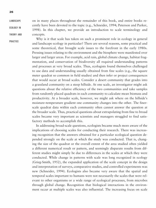
Nearly all ecologists now recognize that scale is a critical conceptin the physical and natural sciences. In his MacArthur Award Address

to the Ecological Society of America, Simon Levin noted that “the problem of re-lating phenomena across scales is the central problem in biology and in all of sci-ence” (Levin, 1992). Elsewhere in his address, Levin (1992) stated that

we must find ways to quantify patterns of variability in space and time, to un-

derstand how patterns change with scale, and to understand the causes and

consequences of pattern. This is a daunting task that must involve remote sens-

ing, spatial statistics, and other methods to quantify pattern at broad scales;

theoretical work to suggest mechanisms and explore relationships; and exper-

imental work, carried out both at fine scales and through whole system ma-

nipulations, to test hypotheses.

Indeed, scale is a prominent topic in landscape ecology and rightfully so; it in-fluences the conclusions drawn by an observer and whether the results can be ex-trapolated to other times or locations. Issues associated with scale will be touched

2

2888_e02_p25-46 3/2/01 2:54 PM Page 25

26

L A N D S C A P E

E C O L O G Y I N

T H E O R Y A N D

P R A C T I C E

on in many places throughout the remainder of this book, and entire books re-cently have been devoted to the topic (e.g., Schneider, 1994; Peterson and Parker,1998). In this chapter, we provide an introduction to scale terminology and concepts.

Why is it that scale has taken on such a prominent role in ecology in generaland landscape ecology in particular? There are several reasons, some practical andsome theoretical, that brought scale issues to the forefront in the early 1980s.Pressing issues relating to the environment and the biosphere were manifested overlarger and larger areas. For example, acid rain, global climate change, habitat frag-mentation, and conservation of biodiversity all required understanding patternsand processes at very broad scales. Thus, ecologists found themselves challengedto use data and understanding usually obtained from fine scales (e.g., the squaremeter quadrat so common in field studies) and then infer or project consequencesthat would occur at broad scales. Consider a desert community that grades intoa grassland community on a steep hillside. At one scale, an investigator might askquestions about the relative efficiency of the two communities and take samplesfrom randomly placed quadrats in each community to calculate mean biomass andproductivity. At a broader scale, however, we might ask where on the hillside’smoisture–temperature gradient one community changes into the other. The finer-scale quadrat data within each community often cannot answer the question atthe broader scale. Thus, practical questions about extrapolating from fine to broadscales became very important as scientists and managers struggled to find satis-factory methods to accomplish this.

In addressing broad-scale questions, ecologists became much more aware of theimplications of choosing scales for conducting their research. There was increas-ing recognition that the answers obtained for a particular ecological question de-pended strongly on the scale at which the study was conducted. That is, chang-ing the size of the quadrat or the overall extent of the area studied often yieldeda different numerical result or pattern, and seemingly disparate results from dif-ferent studies might simply be due to differences in the scales at which they wereconducted. While change in patterns with scale was long recognized in ecology(Grieg-Smith, 1952), the expanded application of the scale concept in the designand interpretation of surveys, comparative studies, and controlled experiments wasnew (Schneider, 1994). Ecologists also became very aware that the spatial andtemporal scales important to humans were not necessarily the scales that were rel-evant to other organisms or a wide range of ecological processes, from microbesthrough global change. Recognition that biological interactions in the environ-ment occur at multiple scales was also influential. The increasing focus on scale

2888_e02_p25-46 3/2/01 2:54 PM Page 26

appears to be an enduring change in the way that ecological research is pursued(Schneider, 1998).

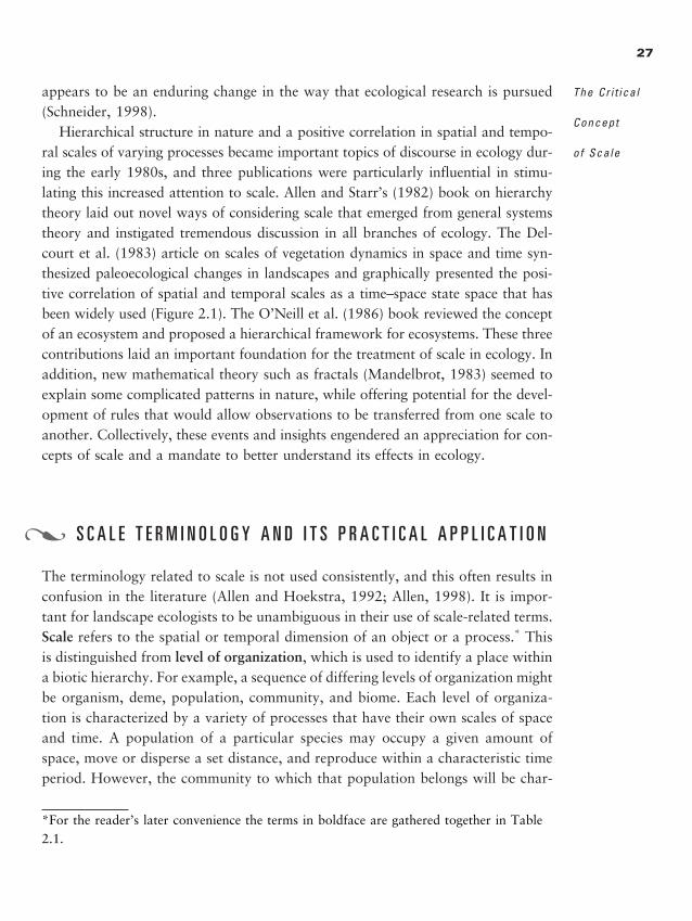
Hierarchical structure in nature and a positive correlation in spatial and tempo-ral scales of varying processes became important topics of discourse in ecology dur-ing the early 1980s, and three publications were particularly influential in stimu-lating this increased attention to scale. Allen and Starr’s (1982) book on hierarchytheory laid out novel ways of considering scale that emerged from general systemstheory and instigated tremendous discussion in all branches of ecology. The Del-court et al. (1983) article on scales of vegetation dynamics in space and time syn-thesized paleoecological changes in landscapes and graphically presented the posi-tive correlation of spatial and temporal scales as a time–space state space that hasbeen widely used (Figure 2.1). The O’Neill et al. (1986) book reviewed the conceptof an ecosystem and proposed a hierarchical framework for ecosystems. These threecontributions laid an important foundation for the treatment of scale in ecology. Inaddition, new mathematical theory such as fractals (Mandelbrot, 1983) seemed toexplain some complicated patterns in nature, while offering potential for the devel-opment of rules that would allow observations to be transferred from one scale toanother. Collectively, these events and insights engendered an appreciation for con-cepts of scale and a mandate to better understand its effects in ecology.

S C A L E T E R M I N O L O G Y A N D I T S P R A C T I C A L A P P L I C A T I O N

The terminology related to scale is not used consistently, and this often results inconfusion in the literature (Allen and Hoekstra, 1992; Allen, 1998). It is impor-tant for landscape ecologists to be unambiguous in their use of scale-related terms.Scale refers to the spatial or temporal dimension of an object or a process.* Thisis distinguished from level of organization, which is used to identify a place withina biotic hierarchy. For example, a sequence of differing levels of organization mightbe organism, deme, population, community, and biome. Each level of organiza-tion is characterized by a variety of processes that have their own scales of spaceand time. A population of a particular species may occupy a given amount ofspace, move or disperse a set distance, and reproduce within a characteristic timeperiod. However, the community to which that population belongs will be char-

27

The Cr i t ica l

Concept

of Scale

�

*For the reader’s later convenience the terms in boldface are gathered together in Table2.1.

2888_e02_p25-46 3/2/01 2:54 PM Page 27

28

100 104 108

1012100 104 108

1012100 104 108

1012

Environmental Disturbance Regimes Biotic Responses Vegetational Patterns

Spatial scale (m2 )

100

103

106

109

100

103

106

109

100 104 108 1012 100 104 108 1012 100 104 108 1012

Plate Tectonics

Evolution ofthe Biota

Fire Regime

Pathogen Outbreak

Human Activities

Ecosystem change

Speciation

Extinction

Competition

Productivity

Species Migration

SecondarySuccession

Gap–phasereplacement

45

6

7

89. Global terrestrial vegetation8. F.M. zone7. Formation6. Type5. Subtype4. Stand3. Tree2. Shrub1. Herb

Macroscale

Megascale

Microscale

Tem

pora

l sca

le (y

r)

Glacial–InterglacialClimatic Cycles

Climatic Fluctuations

Soil Development

*Disturbance Events

*Examples: Wildfire Clear Cut Flood Earthquake

3

2

1

9

Figure 2.1.

Space–time hierarchy diagram proposed by Delcourt et al. (1983). Environmental disturbance regimes,

biotic responses, and vegetational patterns are depicted in the context of space–time domains in which

the scale for each process or pattern reflects the sampling intervals required to observe it. The time

scale for the vegetation patterns is the time interval required to record their dynamics.

Modified from Delcourt et al., 1983.

acterized by spatial and temporal scales associated with the collection of popula-tions composing the community.

Scale is characterized by grain and extent (Figure 2.2). Grain refers to the finestspatial resolution within a given data set; for example, grain refers to the cell sizefor gridded maps or the minimum mapping unit of maps drawn with polygons.Extent refers to the size of the overall study area. Grain and extent are easy tothink of when considering remote imagery. Different satellite sensors have differ-ent cell sizes, or grain; for example, there is a cell size of 10 m by 10 m for SPOTpanchromatic imagery, 30 m by 30 m for Landsat Thematic Mapper imagery, and

2888_e02_p25-46 3/2/01 2:54 PM Page 28

29

Table 2.1.Definitions of scale-related terminology and concepts.

Term Definition

Absolute scale Actual distance, direction, shape, and geometry.

Cartographic Degree of spatial reduction indicating the length used to represent ascale larger unit of measure; ratio of distance on the map to distance on

Earth’s surface represented by the map, usually expressed in termssuch as 1: 10,000. In cartography, large scale means fine resolutionand small scale means coarse resolution.

Critical Point at which there is an abrupt change in a quality, property, orthreshold phenomenon.

Extent Size of the study area or the duration of time under consideration.

Extrapolate To infer from known values; to estimate a value from conditions of the argument not used in the process of estimation; to transform in-formation (1) from one scale to another (either grain size or extent)or (2) from one system (or data set) to another system at the samescale.

Grain Finest level of spatial resolution possible within a given data set.

Hierarchy System of interconnections or organization wherein the higher levelsconstrain and control the lower levels to various degrees dependingon the time constraints of the behavior.

Holon Representation of an entity as a two-way window through which theenvironment influences the parts and parts communicate as a unit tothe rest of the universe (Koestler, 1967).

Level of Place within a biotic hierarchy (e.g., organism, deme, population).organization

Relative scale Transformation of absolute scale to a scale that describes the relativedistance, direction, or geometry based on some functional relation-ship.

Resolution Precision of measurement; grain size, if spatial.

Scale Spatial or temporal dimension of an object of process, characterized by both grain and extent.

2888_e02_p25-46 3/2/01 2:54 PM Page 29

30

L A N D S C A P E

E C O L O G Y I N

T H E O R Y A N D

P R A C T I C E

90 m by 90 m for the earlier Landsat Multispectral Scanner imagery. The detailthat can be gleaned from these different sensors varies, in part because of the dif-ferences in grain. Extent can vary independently of grain, although there is somedegree of correlation; for example, a small extent will require a small grain size.When we say that a pattern, process, or phenomenon is scale dependent, we meanthat it changes with the grain or the extent of the measurement. Schneider (1994)defines scale-dependent processes as those in which the ratio of one rate to an-other varies with either resolution (grain) or range (extent) or measurement.

One source of confusion is that ecologists and geographers usually mean theopposite when they say large or small scale. The long-standing use in geographyof cartographic scale refers to the degree of spatial reduction indicating the lengthused to represent a larger unit of measure. Cartographic scale is typically expressedas the ratio or representative fraction (RF) of distance on the map to distance onthe surface of Earth that is represented on a map or aerial photograph, for ex-ample, 1:10,000 or 1:100,000. When geographers and cartographers say largescale, they mean very fine resolution (e.g., 1:500), which in practice means a very

Increasing Grain Size

Increasing Extent

a = 400

n = 4n = 1

a = 16

a = 81

a

b

Figure 2.2.

Schematic of two components of spatial scale:

(a) grain and (b) extent. The number of cells

aggregated to form the new data unit (i.e.,

new grain size) are indicated by n; total area, or

extent, is indicated by a.

Modified from Turner et al., 1989b.

2888_e02_p25-46 3/2/01 2:54 PM Page 30

large map of a small spatial extent; similarly, when they say small scale, they meanvery coarse resolution, or maps of large areas that do not contain much detail(e.g., 1:250,000). This use of small and large is opposite to what ecologists usu-ally mean by these terms! To avoid confusion, we recommend and use here theterms fine and broad to modify scale such that fine-scale refers to small areas,greater resolution, and more detail and broad-scale refers to larger areas, lowerresolution, and less detail.

In practical terms, the scale at which you make any measurement, for exam-ple, the size of the quadrat, length of transect, area of census, or size of the gridcell in remotely sensed data, influences the numerical answer obtained. Thespecies–area curve (Figure 2.3) is an early example of this phenomenon. In tryingto determine the species richness for a particular community, ecologists soon re-alized that the number of species detected would increase asymptotically with thesize of the area that was censused. Thus, to avoid erroneous inferences due to mis-matches in scale, the study area size had to be accounted for before estimates ofspecies richness among sites or through time could be compared.

Another consideration in scale terminology is the distinction between absoluteand relative scale. We generally talk about absolute scale, that is, the actual dis-tance, time, area, or the like. On the other hand, we might consider distance rel-ative to the energy that an animal would need to expend to travel between dif-ferent points on a landscape. With this relative scale, two points that are closestto each other as the crow flies may be far apart if they are separated by a largepeak or ravine that would require much energy to traverse; two points fartherapart as the crow flies, but connected by level ground that is easily traversed, mayhave a closer relative distance.

When we seek to extrapolate, we attempt to infer from known values, that is,to estimate a value from conditions beyond the range of the data used in theprocess of estimation. For example, we extrapolate when we use a regression lineto predict values of y based on a value of x that is beyond our original data. Wealso extrapolate when we transfer information from one scale to another (eithergrain size or extent) or from one system (or data set) to another system at thesame scale. Searching for techniques or algorithms to extrapolate across scales oramong landscapes remains an important research topic in landscape ecology. Inpractical terms, this occurs because scientists never have all the data they need atall the right scales. Extrapolating may be straightforward in some cases when therelationship of a variable with changes in scale is linear, or additive; however, ifthe relationship is nonlinear and there are critical thresholds at which there is anabrupt change in some quality, then extrapolation is problematic.

31

The Cr i t ica l

Concept

of Scale

2888_e02_p25-46 3/2/01 2:54 PM Page 31

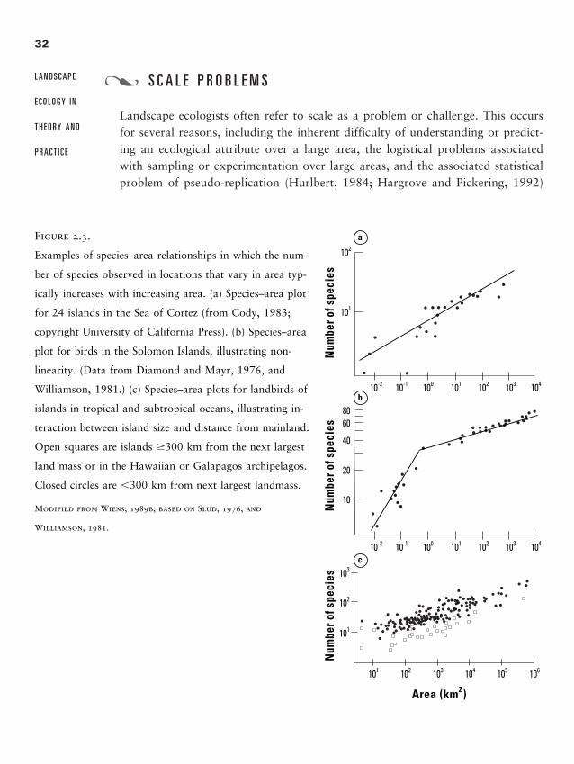
S C A L E P R O B L E M S

Landscape ecologists often refer to scale as a problem or challenge. This occursfor several reasons, including the inherent difficulty of understanding or predict-ing an ecological attribute over a large area, the logistical problems associatedwith sampling or experimentation over large areas, and the associated statisticalproblem of pseudo-replication (Hurlbert, 1984; Hargrove and Pickering, 1992)

32

L A N D S C A P E

E C O L O G Y I N

T H E O R Y A N D

P R A C T I C E

�

Area (km2 )

Num

ber o

f spe

cies

Num

ber o

f spe

cies

Num

ber o

f spe

cies

101 102 103 104 105 106

101

102

103

10-2 10-1 100 101 102 103 104

10

20

10-2 10-1 100 101 102 103 104

40

6080

101

102

a

c

b

Figure 2.3.

Examples of species–area relationships in which the num-

ber of species observed in locations that vary in area typ-

ically increases with increasing area. (a) Species–area plot

for 24 islands in the Sea of Cortez (from Cody, 1983;

copyright University of California Press). (b) Species–area

plot for birds in the Solomon Islands, illustrating non-

linearity. (Data from Diamond and Mayr, 1976, and

Williamson, 1981.) (c) Species–area plots for landbirds of

islands in tropical and subtropical oceans, illustrating in-

teraction between island size and distance from mainland.

Open squares are islands �300 km from the next largest

land mass or in the Hawaiian or Galapagos archipelagos.

Closed circles are �300 km from next largest landmass.

Modified from Wiens, 1989b, based on Slud, 1976, and

Williamson, 1981.

2888_e02_p25-46 3/2/01 2:54 PM Page 32

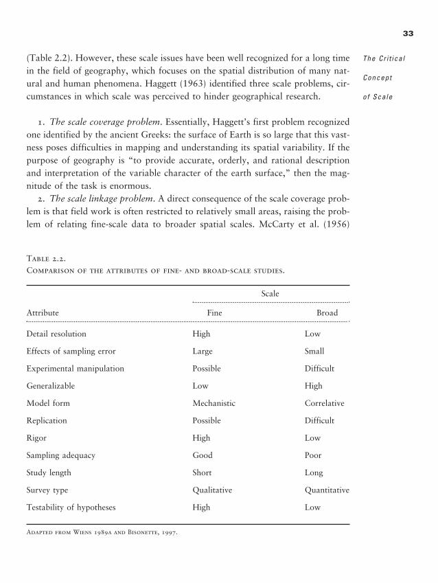
(Table 2.2). However, these scale issues have been well recognized for a long timein the field of geography, which focuses on the spatial distribution of many nat-ural and human phenomena. Haggett (1963) identified three scale problems, cir-cumstances in which scale was perceived to hinder geographical research.

1. The scale coverage problem. Essentially, Haggett’s first problem recognizedone identified by the ancient Greeks: the surface of Earth is so large that this vast-ness poses difficulties in mapping and understanding its spatial variability. If thepurpose of geography is “to provide accurate, orderly, and rational descriptionand interpretation of the variable character of the earth surface,” then the mag-nitude of the task is enormous.

2. The scale linkage problem. A direct consequence of the scale coverage prob-lem is that field work is often restricted to relatively small areas, raising the prob-lem of relating fine-scale data to broader spatial scales. McCarty et al. (1956)

33

The Cr i t ica l

Concept

of Scale

Table 2.2.Comparison of the attributes of fine- and broad-scale studies.

Scale

Attribute Fine Broad

Detail resolution High Low

Effects of sampling error Large Small

Experimental manipulation Possible Difficult

Generalizable Low High

Model form Mechanistic Correlative

Replication Possible Difficult

Rigor High Low

Sampling adequacy Good Poor

Study length Short Long

Survey type Qualitative Quantitative

Testability of hypotheses High Low

Adapted from Wiens 1989a and Bisonette, 1997.

2888_e02_p25-46 3/2/01 2:54 PM Page 33

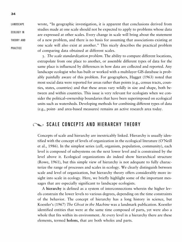
34

L A N D S C A P E

E C O L O G Y I N

T H E O R Y A N D

P R A C T I C E

�

wrote, “In geographic investigation, it is apparent that conclusions derived fromstudies made at one scale should not be expected to apply to problems whose dataare expressed at other scales. Every change in scale will bring about the statementof a new problem, and there is no basis for assuming that associations existing atone scale will also exist at another.” This nicely describes the practical problemof comparing data obtained at different scales.

3. The scale standardization problem. The ability to compare different locations,extrapolate from one place to another, or assemble different types of data for thesame place is influenced by differences in how data are collected and reported. Anylandscape ecologist who has built or worked with a multilayer GIS database is prob-ably painfully aware of this problem. For geographers, Hagget (1963) noted thatmost social data were reported for areas rather than points (e.g., census tracts, coun-ties, states, countries) and that these areas vary wildly in size and shape, both be-tween and within countries. This issue is very relevant for ecologists when we con-sider the political–ownership boundaries that have been superimposed on ecologicalunits such as watersheds. Developing methods for combining different types of data(e.g., point- and area-based measures) remains an active research area today.

S C A L E C O N C E P T S A N D H I E R A R C H Y T H E O R Y

Concepts of scale and hierarchy are inextricably linked. Hierarchy is usually iden-tified with the concept of levels of organization in the ecological literature (O’Neillet al., 1986). In the simplest series (cell, organism, population, community), eachlevel is composed of subsystems on the next lower level and is constrained by thelevel above it. Ecological organizations do indeed show hierarchical structure(Rowe, 1961), but this simple view of hierarchy is not adequate to fully charac-terize the range of processes and scales in ecology. We clearly distinguish betweenscale and level of organization, but hierarchy theory offers considerably more in-sight into scale in ecology. Here, we briefly highlight some of the important mes-sages that are especially significant to landscape ecologists.

A hierarchy is defined as a system of interconnections wherein the higher lev-els constrain the lower levels to various degrees, depending on the time constraintsof the behavior. The concept of hierarchy has a long history in science, butKoestler’s (1967) The Ghost in the Machine was a landmark publication. Koestleridentified entities that were at the same time composed of parts, yet were also awhole that fits within its environment. At every level in a hierarchy there are theseelements, termed holons, that are both wholes and parts.

2888_e02_p25-46 3/2/01 2:54 PM Page 34

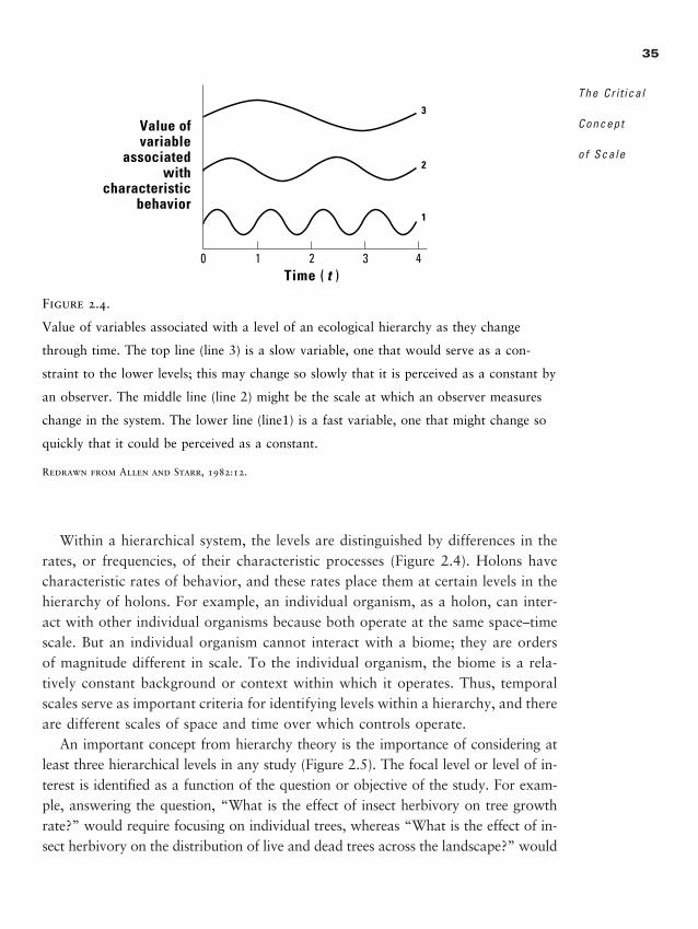
Within a hierarchical system, the levels are distinguished by differences in therates, or frequencies, of their characteristic processes (Figure 2.4). Holons havecharacteristic rates of behavior, and these rates place them at certain levels in thehierarchy of holons. For example, an individual organism, as a holon, can inter-act with other individual organisms because both operate at the same space–timescale. But an individual organism cannot interact with a biome; they are ordersof magnitude different in scale. To the individual organism, the biome is a rela-tively constant background or context within which it operates. Thus, temporalscales serve as important criteria for identifying levels within a hierarchy, and thereare different scales of space and time over which controls operate.

An important concept from hierarchy theory is the importance of considering atleast three hierarchical levels in any study (Figure 2.5). The focal level or level of in-terest is identified as a function of the question or objective of the study. For exam-ple, answering the question, “What is the effect of insect herbivory on tree growthrate?” would require focusing on individual trees, whereas “What is the effect of in-sect herbivory on the distribution of live and dead trees across the landscape?” would

35

The Cr i t ica l

Concept

of Scale

3

2

1

Value ofvariable

associatedwith

characteristicbehavior

Time ( t ) 0 1 2 3 4

Figure 2.4.

Value of variables associated with a level of an ecological hierarchy as they change

through time. The top line (line 3) is a slow variable, one that would serve as a con-

straint to the lower levels; this may change so slowly that it is perceived as a constant by

an observer. The middle line (line 2) might be the scale at which an observer measures

change in the system. The lower line (line1) is a fast variable, one that might change so

quickly that it could be perceived as a constant.

Redrawn from Allen and Starr, 1982:12.

2888_e02_p25-46 3/2/01 2:54 PM Page 35

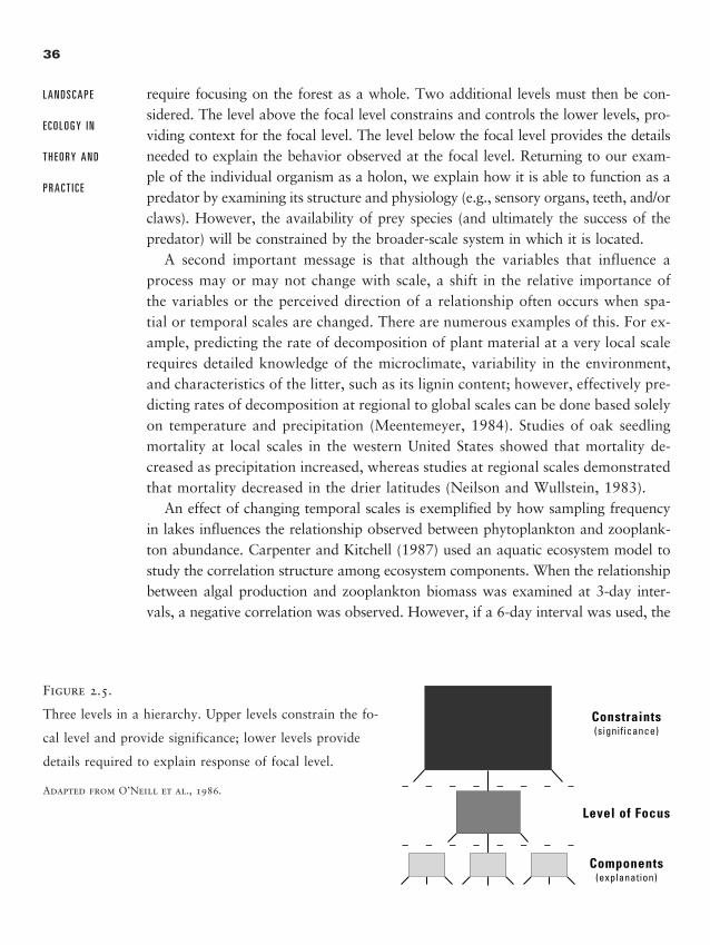
require focusing on the forest as a whole. Two additional levels must then be con-sidered. The level above the focal level constrains and controls the lower levels, pro-viding context for the focal level. The level below the focal level provides the detailsneeded to explain the behavior observed at the focal level. Returning to our exam-ple of the individual organism as a holon, we explain how it is able to function as apredator by examining its structure and physiology (e.g., sensory organs, teeth, and/orclaws). However, the availability of prey species (and ultimately the success of thepredator) will be constrained by the broader-scale system in which it is located.

A second important message is that although the variables that influence aprocess may or may not change with scale, a shift in the relative importance ofthe variables or the perceived direction of a relationship often occurs when spa-tial or temporal scales are changed. There are numerous examples of this. For ex-ample, predicting the rate of decomposition of plant material at a very local scalerequires detailed knowledge of the microclimate, variability in the environment,and characteristics of the litter, such as its lignin content; however, effectively pre-dicting rates of decomposition at regional to global scales can be done based solelyon temperature and precipitation (Meentemeyer, 1984). Studies of oak seedlingmortality at local scales in the western United States showed that mortality de-creased as precipitation increased, whereas studies at regional scales demonstratedthat mortality decreased in the drier latitudes (Neilson and Wullstein, 1983).

An effect of changing temporal scales is exemplified by how sampling frequencyin lakes influences the relationship observed between phytoplankton and zooplank-ton abundance. Carpenter and Kitchell (1987) used an aquatic ecosystem model tostudy the correlation structure among ecosystem components. When the relationshipbetween algal production and zooplankton biomass was examined at 3-day inter-vals, a negative correlation was observed. However, if a 6-day interval was used, the

36

L A N D S C A P E

E C O L O G Y I N

T H E O R Y A N D

P R A C T I C E

Figure 2.5.

Three levels in a hierarchy. Upper levels constrain the fo-

cal level and provide significance; lower levels provide

details required to explain response of focal level.

Adapted from O’Neill et al., 1986.

Constraints(significance)

Components(explanation)

Level of Focus

2888_e02_p25-46 3/2/01 2:54 PM Page 36

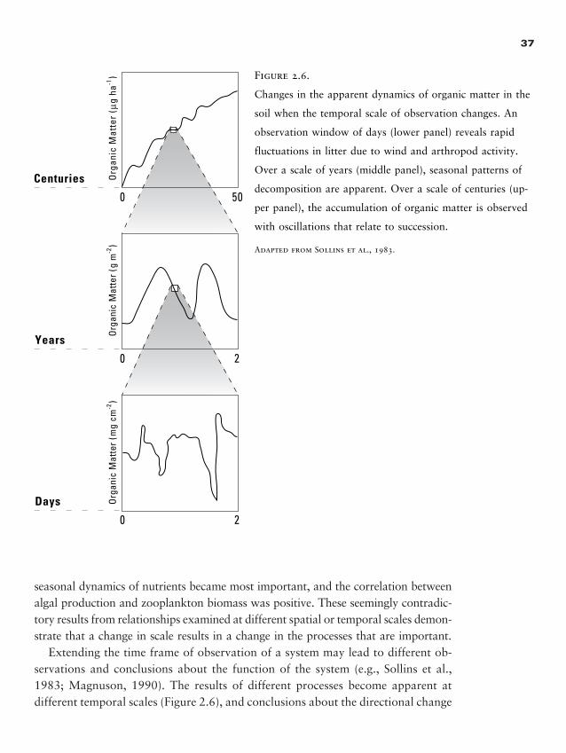
seasonal dynamics of nutrients became most important, and the correlation betweenalgal production and zooplankton biomass was positive. These seemingly contradic-tory results from relationships examined at different spatial or temporal scales demon-strate that a change in scale results in a change in the processes that are important.

Extending the time frame of observation of a system may lead to different ob-servations and conclusions about the function of the system (e.g., Sollins et al.,1983; Magnuson, 1990). The results of different processes become apparent atdifferent temporal scales (Figure 2.6), and conclusions about the directional change

37

Centuries Org

anic

Mat

ter

(µg

ha-1

)

500

Years

Org

anic

Mat

ter (

g m

-2)

20

Days Org

anic

Mat

ter (

mg

cm-2

)

20

Figure 2.6.

Changes in the apparent dynamics of organic matter in the

soil when the temporal scale of observation changes. An

observation window of days (lower panel) reveals rapid

fluctuations in litter due to wind and arthropod activity.

Over a scale of years (middle panel), seasonal patterns of

decomposition are apparent. Over a scale of centuries (up-

per panel), the accumulation of organic matter is observed

with oscillations that relate to succession.

Adapted from Sollins et al., 1983.

2888_e02_p25-46 3/2/01 2:54 PM Page 37

may change qualitatively as observation time increases. The constraint of havinga limited observation window has been characterized as “the invisible present”(Magnuson, 1990), and this has been illustrated numerous times with long-termecological data.

Hierarchy theory also suggests that multiple scales of pattern will exist in land-scapes because of the multiple scales at which processes are acting. Consider theprocesses that may give rise to pattern in a hypothetical forest landscape. Overbroad scales of space and time, geomorphological processes result in distributionsof substrate and soil that influence the tree species might occur at different posi-tions. Within the forest that develops, the pattern and frequency of large distur-bances, such as fire or pathogen epidemics, may generate a coarse-grained patternof different successional stages across the landscape. Local processes of individ-ual tree death may result in small canopy gaps distributed throughout the forestlandscape. Collectively, then, the spatial pattern of forest communities at any giventime in this landscape may reflect these three processes operating over differentscales of space and time. An analysis of the spatial pattern of the forest commu-nities across the landscape may well detect these multiple scales of pattern (e.g.,Kuuluvainen et al., 1998).

Thus, hierarchy theory tells us that attention should be focused directly onthe scales at which phenomena of interest occur, that there is no single cor-rect scale for studying landscapes or any other ecological system, and that ifwe change the scales, the relevant processes or even the direction of relation-ships that we observe may well change. The scale of interest must be dictatedby the question or phenonenon of interest. Finer-scale processes may be viewedas the details required to explain the phenomena at the focal scale, whilebroader-scale patterns are the constraints that limit the potential range of rateprocesses. These concepts are rich and provocative, but still leave us with thecritical challenge of identifying the proper scale at which to address a givenproblem.

I D E N T I F Y I N G T H E “ R I G H T ” S C A L E ( S )

Returning to Levin’s (1992) MacArthur address, we read “That there is no singlecorrect scale or level at which to describe a system does not mean that all scalesserve equally well or that there are not scaling laws.” Developing the rules foridentifying the correct scale for a particular question continues to be an impor-

38

L A N D S C A P E

E C O L O G Y I N

T H E O R Y A N D

P R A C T I C E

�

2888_e02_p25-46 3/2/01 2:54 PM Page 38

tant topic of current research. However, ecologists must recognize that identify-ing the “right” scale still requires combining art with science, because satisfactoryalgorithms do not currently exist.

The developing field of spatial statistics offers a variety of techniques that isuseful in identifying scales (see Chapter 5). For example, O’Neill et al. (1991b)analyzed vegetation transect data from three locations to determine if multiplescales of pattern could be detected. Data were obtained from a semiarid grasslandin New Mexico, calcareous openings in a deciduous forest in Tennessee, and ashrub–steppe system in Washington. Analyses revealed that between three and fivescales of pattern could be identified on all three sites.

Spatial statistics techniques may also be used to identify the spatial scales overwhich successive sampling points are correlated. Data compared at scales wherethe correlation is near zero can be regarded as statistically independent, an im-portant assumption for many statistical tests. Pearson et al. (1995) used this ap-proach to identify the range of distances over which measurements of ungulateforaging intensity were autocorrelated. After identifying these relationships, thedata were resampled to select observations greater than the correlation length. Theresampled data then met the independence criterion of regression analyses relat-ing grazing intensity to environmental heterogeneity.

Concepts such as ecological neighborhoods (Addicott et al., 1987, discussed inChapter 8) use frequency distributions for the space and time components of thebehavior of organisms to determine the correct scale of analysis. They suggest thata process, such as foraging or reproduction, be selected first and the activity ofthe organism then be monitored to determine the spatial scale relevant to theprocess. The spatial extent that encompasses most of the organism’s activity rel-evant to the process (and over a relevant amount of time) is then the appropriatescale for this process.

Multiple regression can be used to quantify the explanatory power of a set ofvariables at different scales (e.g., Pearson, 1993; Pearson et al., 1995; Gergel etal., 1999). The approach used by Pearson (1993) to examine the relationship be-tween the presence and abundance of wintering birds in the Georgia, USA, pied-mont and environmental variation at different spatial scales has been widely ap-plied (e.g., Rescia et al., 1997; Sisk et al., 1997; Elliot et al., 1999; Estades andTemple, 1999). This approach has confirmed that there is no single appropriatescale at which ecologists may expect to analyze their data. Rather, the identifica-tion of a suite of appropriate scales, or multiscale analysis, must continue to be employed as the science of scale identification and interpretation continues tomature.

39

The Cr i t ica l

Concept

of Scale

2888_e02_p25-46 3/2/01 2:54 PM Page 39

R E A S O N I N G A B O U T S C A L E

In the introductory chapter to his book Quantitative Ecology, Spatial and Tem-poral Scaling, Schneider (1994) provides an insightful discussion of the ways inwhich scale is used as a routine part of research and reasoning in disciplines otherthan ecology. The explicit treatment of scale is found in a very high percentageof research articles in the physical sciences (e.g., geophysical fluid dynamics), en-gineering, and measurement science. Scale issues are also familiar to biologists,who have routinely used allometric scaling of form and function to body sizethroughout the 20th century. Indeed, most ecologists are familiar with relation-ships among life history characteristics such as longevity, generation time, fecun-dity and body size in animals. Schneider (1994) observes that “The most impor-tant characteristic of quantitative reasoning . . . is directed at scaled quantitiesobtained by measurement or by calculations from measurement.” Reasoning aboutscaled quantities includes questions such as these: What are the algebraic rules forrescaling quantities? What is the best way to visualize and verify these operations?How are these operations used in solving ecological problems?

S C A L I N G U P

Issues of extrapolating to broader scales in space and time, or scaling up, continueto be on the cutting edge of research in landscape ecology. Ecologists remain vexedby the need to make predictions at broad scales when most measurements havebeen made at relatively fine scales. How can it be done and what is the currentstate of knowledge? The challenges of scaling up lie in (1) correctly defining thespatial and temporal heterogeneity of the fine-scale information and (2) correctlyintegrating or aggregating this heterogeneity to the broader scale (King, 1991).

The simplest approach to scaling across space is to multiply a measurementmade at one scale (e.g., unit of area) to predict at a broader scale. For example,a standing biomass for a 10,000-ha forest might be predicted by multiplying theamount of biomass measured in a 1-ha stand by the factor of 10,000. Termed“lumping” by King (1991), this approach assumes that the properties of the sys-tem do not change with scale and that the broader-scale system behaves like theaverage finer-scale system. From a modeling perspective (see Chapter 3), this as-sumption holds only if the equations describing the system are linear. Lumping isknown to lead to considerable bias, because it does not account for variability

40

L A N D S C A P E

E C O L O G Y I N

T H E O R Y A N D

P R A C T I C E

�

�

2888_e02_p25-46 3/2/01 2:54 PM Page 40

(spatial or temporal) in the scaling process and ignores nonlinear changes in thevariable of interest with changes in scale (Rastetter et al., 1992). The nature ofthe bias depends on the specifics of the spatial dependencies and/or nonlinearitiesin the system (O’Neill, 1979a, b). This approach should only be used with care-ful consideration of the potential errors and biases that may result.

An improvement on the simple multiplicative approach to scaling is an addi-tive approach that accounts for spatial variability within an area of relatively largeextent. King (1991) identifies two general methods for this type of scaling. Thefirst, direct extrapolation, uses data or model simulations from a tractable num-ber of discrete elements within a landscape. For example, instead of assuming thatbiomass is the same throughout the 10,000-ha forest, we recognize that biomassvaries with stand age and composition and that we can account for this spatialvariability by mapping or using a remote image. In this case, we use empiricalmeasurements to estimate the biomass in each type defined and then multiply bythe area of each type within the 10,000-ha forested landscape and sum the results.Within a modeling framework, King (1991) notes that this approach is probablythe most widely used. The direct extrapolation approach works reasonably wellfor quantities such as biomass or net primary production, which themselves donot interact spatially and which can be related to attributes that can be measuredremotely over large areas (e.g., color of the ocean, vegetation composition).

For translating models across spatial scales, a variation on this theme is King’s(1991) second method, extrapolation by expected value. The general algorithmfor this approach entails (1) a model simulating local behavior of a system, (2) alarger landscape over which the model is to be extrapolated, (3) the frequency dis-tributions of variables that describe landscape heterogeneity, and (4) calculationof expected values of the system behavior as a function of the variables describ-ing the heterogeneity of the landscape. The principal source of error in this ap-proach lies in the estimation of the probability or frequency distributions of thelandscape variables. However, like direct extrapolation, the more simple ap-proaches to extrapolation by expected value also do not account for spatial in-teractions or feedbacks.

It is important to note that the error, or variance, associated with the originalmeasurements should also be scaled accordingly to estimate confidence in predic-tions at the broader scale. However, this problem is easier to recognize than toresolve; confidence intervals around a measurement made at one scale may nottranslate directly to another scale (Schneider, 1994). Some quantities increase invariance as scale increases, the so-called pink or red noise identified by spectralanalysis (Platt and Denman, 1975; Ripley, 1978; Caswell and Cohen, 1995; Co-

41

The Cr i t ica l

Concept

of Scale

2888_e02_p25-46 3/2/01 2:54 PM Page 41

hen et al., 1998). This may occur when the extent of observations is increased andgreater environmental heterogeneity is encountered. For example, the air temper-ature of a small area might be characterized by a mean temperature, say 11°C,with a small range of values, say �1°C. As extent increases in topographicallyrough terrain, sites with temperatures ranging from 6° and 24° may be included,resulting in an increase in the variance even if the mean value remains constant.Thus, as the grain becomes coarser the cell characterized by a single temperaturemay also have greater variability.

Rastetter et al. (1992) and Wiens et al. (1993) suggest that a combination ofapproaches is needed to scale up. The multiplicative approach can be implementedas a first approximation with the recognition that it may work in some cases, butbe widely off the mark in others. Additional detail can be added as needed, eitherthrough improving the computations at the finer scales (Wiens et al., 1993) to re-duce the error that would be translated to the broader scale or by identifying thespatial subunits across which extrapolations can be summed (Rastetter et al., 1992).

Mandelbrot (1967) was the first to point out that simple geometric relation-ships can be used to quantify changes in the measured properties of objects withchanges in scale. This new concept was illustrated with a power-law relationshipbetween the scale of a ruler and the measured length of the coast of Britain: L(�) �

K�1�D, where L is the length of the coast, K is a constant, � the scale of the ruler,and D the dimension of the object. The range of scales over which this power-lawholds defines the range of self-similarity of the object. Unlike smooth geometricobjects (squares, circles, etc.), the value of D is not always an integer, but may takeon fractional values. Objects with fractional values of D are therefore referred toas fractals (also see Chapter 5). Since introduced by Mandelbrot in 1967, fractalshave had an immense appeal and impact for addressing problems of scale and hi-erarchy (Sugihara and May, 1990). The fractal nature of many objects has beenconfirmed (see Hastings and Sugihara, 1993), and departures from the power-lawrelationship have been used to identify scales where processes may alter patterns(see Krummel et al., 1987). A fractal dimension may be estimated for almost anyobject, but this alone does not guarantee a self-similar or scaling relationship (therange of the power-law relationship may be uselessly small). The use of fractals forextrapolating across scales requires two things: estimation of the fractal dimension,D, and verification of the range of the power-law relationship.

Although our discussion has emphasized the processes associated with scalingup, that is, moving from fine-scale measurements to predictions at broad scales,the inverse process of scaling down is also important. For example, the tempera-ture and precipitation patterns predicted by the general circulation models used

42

L A N D S C A P E

E C O L O G Y I N

T H E O R Y A N D

P R A C T I C E

2888_e02_p25-46 3/2/01 2:54 PM Page 42

to simulate potential changes in global climate typically have a coarse resolutionof 1° or 2° latitude and longitude. However, we know that precipitation and tem-perature vary considerably within areas that are 100 km by 100 km in size andthat this variability is important for local ecological processes (Lynn et al., 1995;Kennedy, 1997; Russo and Zack, 1997). Using a rather different example, tabu-lations of population density or housing units for a census tract do not accountfor the spatial variability within the census tract, yet this variation may be mostimportant for predicting future patterns of land-use change or the movement ofnutrients from land to water. Recognition of the importance of developing meth-ods for extrapolating information from coarse to fine grains has increased greatlywith the wide use of GIS technologies. However, progress in this arena has beenslowed by the immense data requirements for verifying these extrapolations.

S U M M A R Y

Scale is a prominent topic in landscape ecology because it influences the conclu-sions drawn by an observer and whether inferences can be extrapolated to otherplaces, times, or scales. Scale refers to the spatial or temporal dimension of an ob-ject or a process, and this is distinct from level of organization, which is used toidentify a place within a biotic hierarchy. Scale is characterized by grain, the finestlevel of spatial resolution possible within a given data set, and extent, the size ofthe overall study area. The related concept of cartographic scale refers to the de-gree of spatial reduction indicating the length used to represent a larger unit ofmeasure. In practical terms, the scale at which you make any measurement influ-ences the numerical answer obtained.

Scale issues are problematic for several reasons. The magnitude of the task ofdescribing and understanding patterns and processes over large areas is enormous.Because observations are influenced by the scales at which they are made, assem-bling and comparing data from studies conducted at different scales is tedious andtime consuming. Although considerable progress is being made, general methodsfor extrapolating information across scales have not yet been established.

Hierarchy theory is closely related to scale and provides a framework for or-ganizing the complexity of ecological systems. A hierarchy is defined as a systemof interconnections wherein the higher levels constrain and control the lower lev-els to various degrees, depending on the time constraints of the behavior. The lev-els within a hierarchy are differentiated by their rates of behavior. Ecological stud-

43

The Cr i t ica l

Concept

of Scale

�

2888_e02_p25-46 3/2/01 2:54 PM Page 43

ies should consider three levels within a hierarchy: the focal level, the level above,which provides constraint and context, and the level below, which provides mech-anism. When scales change, a shift in the relative importance of variables or theperceived direction of a relationship may also change.

Scale issues often arise in attempting to extrapolate ecological studies to largeror smaller scales. The current understanding has led to a few useful rules of thumbfor extrapolation. First, scale changes may be ignored in homogeneous space, butnot under conditions of spatial heterogeneity. Average dynamics can be appliedto a larger area only when the area is homogeneous for the characteristic of in-terest. If the spatial heterogeneity is present, but is random rather than occurringwith a structured pattern, then the average plus the variance can be used to ap-ply local measurements to the broader area. Second, as long as major processesand constraints do not change, the theory of fractals shows that under certainconditions quantities may be extrapolated across scales. Third, when spatial het-erogeneity combines with nonlinear dynamics and the possibility of major changesin constraints, extrapolation becomes a very difficult problem that does not, atpresent, have any simple solution.

There is no right scale for landscape ecological studies. Scales must be selectedbased on the question or objective of a study. However, identifying the appro-priate scale remains challenging, and developing methods for doing so remains atopic of current research. Indeed, most of the topics covered in this chapter havemany unknowns associated with them. Ecologists are still learning how to takethe knowledge we have gleaned about patterns and processes at multiple scalesinto consideration when developing field studies and models and the techniquesfor extrapolating across scales and landscapes.


1. Select a landscape of your choice and list the important ecological processes that

occur in the landscape. Next, estimate the temporal and spatial scales over which

these processes operate and plot these in a time–space state space (see Figure 2.1).

How might such a diagram assist you in selecting appropriate scales for a field study

or model? What scales are appropriate for different hypotheses that you might test?

2. Do you think that scale issues will be of passing or enduring interest to ecologists?

Provide a rationale for your opinion.

3. Describe how scale may be considered as a problem as well as an opportunity.

44

L A N D S C A P E

E C O L O G Y I N

T H E O R Y A N D

P R A C T I C E

2888_e02_p25-46 3/2/01 2:54 PM Page 44


Delcourt, H. R., P. A. Delcourt, and T. Webb. 1983. Dynamic plant ecology: the

spectrum of vegetation change in space and time. Quaternary Science Review 1:

153–175.

King, A. W. 1997. Hierarchy theory: a guide to system structure for wildlife biolo-

gists. In J. A. Bissonette, ed. Wildlife and Landscape Ecology. Effects of Pattern and

Scale, pp. 185–212. Springer-Verlag, New York.

Levin, S. A. 1992. The problem of pattern and scale in ecology. Ecology 73:1943–1983.

O’Neill, R. V., D. L. DeAngelis, J. B. Waide, and T. F. H. Allen. 1986. A Hier-

archical Concept of Ecosystems. Princeton University Press, Princeton, New Jersey.

Schneider, D. C. 1994. Quantitative Ecology. Spatial and Temporal Scaling. Acade-

mic Press, San Diego, California.

Wiens, J. A. 1989. Spatial scaling in ecology. Functional Ecology 3:385–397.

45

The Cr i t ica l

Concept

of Scale

2888_e02_p25-46 3/2/01 2:54 PM Page 45

C H A P T E R

Introduction to Models

Models are important tools IN LANDSCAPE ECOLOGY, as they are inmany scientific disciplines. Spatial models, in particular, are playing a

more and more prominent role for investigating the consequences of heterogeneousdistributions of ecological resources. Because we refer to models throughout thisbook and because we are aware that many students have not had any formal train-ing in modeling or systems ecology, this chapter presents an elementary set of con-cepts and terms for students to understand what models are, why they are used,and how models are constructed and evaluated. Our purpose is to introduce mod-els and their development, define what we mean by a spatial model, and indicatewhen spatial models are important. Students interested in the modeling process ingreater depth are referred to the recommended readings at the end of the chapter.

W H A T A R E M O D E L S A N D W H Y D O W E U S E T H E M ?

W h a t I s a M o d e l ?

A model is an abstract representation of a system or process. Models can be for-mulated in many different ways. Physical models are material replicas of the object

3

�

2888_e03_p47-70 3/2/01 2:56 PM Page 47

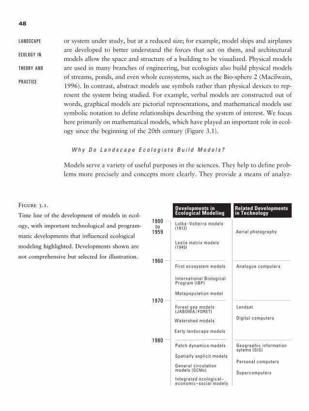
48

L A N D S C A P E

E C O L O G Y I N

T H E O R Y A N D

P R A C T I C E

or system under study, but at a reduced size; for example, model ships and airplanesare developed to better understand the forces that act on them, and architecturalmodels allow the space and structure of a building to be visualized. Physical modelsare used in many branches of engineering, but ecologists also build physical modelsof streams, ponds, and even whole ecosystems, such as the Bio-sphere 2 (Macilwain,1996). In contrast, abstract models use symbols rather than physical devices to rep-resent the system being studied. For example, verbal models are constructed out ofwords, graphical models are pictorial representations, and mathematical models usesymbolic notation to define relationships describing the system of interest. We focushere primarily on mathematical models, which have played an important role in ecol-ogy since the beginning of the 20th century (Figure 3.1).

W h y D o L a n d s c a p e E c o l o g i s t s B u i l d M o d e l s ?

Models serve a variety of useful purposes in the sciences. They help to define prob-lems more precisely and concepts more clearly. They provide a means of analyz-

1900to

1959

1960

1970

1980

Aerial photography

Lotka–Volterra models(1912)

Leslie matrix models(1945)

Watershed models

Early landscape models

Patch dynamics models

Spatially explicit models

General circulation models (GCMs)

Integrated ecological–economic–social models

First ecosystem models

International Biological Program (IBP)

Metapopulation model

Analogue computers

Landsat

Digital computers

Geographic informationsytems (GIS)

Personal computers

Supercomputers

Forest gap models (JABOWA / FORET)

Developments inEcological Modeling

Related Developments in Technology

Figure 3.1.

Time line of the development of models in ecol-

ogy, with important technological and program-

matic developments that influenced ecological

modeling highlighted. Developments shown are

not comprehensive but selected for illustration.

2888_e03_p47-70 3/2/01 2:56 PM Page 48

ing data and communicating results. Finally, and perhaps most importantly, mod-els allow us to make predictions. However, landscape models should be regardedas tools or methods to achieve an end and should not be considered as goals untothemselves. Because knowledge is incomplete, assumptions are always requiredwithin models to fill in the blanks. Consequently, most models are employed toexplore the consequences of our hypotheses regarding system structure and dynamics.

Landscape ecologists have found models to be an important part of their toolbox for several reasons. When faced with studying a large and complex landscape,it is difficult, and sometimes impossible, to conduct experiments at the appropri-ate scale. Experimental manipulation of large landscapes with the appropriatenumber of independent replicates is not very common because of the high costand logistical difficulty involved, although landscape-management actions frame-work (e.g., agricultural systems and forest harvesting) can be studied experimen-tally. Experimental manipulations of microlandscapes avoid this difficulty, andthis approach is being used to gain insights into the response of insects, smallmammals, and some plants to alternative landscape patterns (e.g., Johnson et al.,1992a; Glenn and Collins, 1993; Imes et al., 1993; Wiens et al., 1995, 1999).However, extrapolation of results from small experimental landscapes to large re-gions remains a perplexing problem. More common are field studies that providecorrelative relationships, for example, by comparing locations that vary in a vari-able of interest, say the abundance of land cover or connectivity of a specific habi-tat. Landscape ecologists also take advantage of natural, uncontrolled events (es-pecially natural disturbances, such as fires, storms, and floods) and study theireffects from an experimental viewpoint (see Chapter 7). However, these serendip-itous opportunities result in a limited range of conditions being studied and donot allow either replication or controlled manipulation. Under these circumstances,the unique features of each landscape and disturbance event may dominate re-sults. Models relax these empirical restraints, providing a means of systematiccomparison across a broad range of conditions.

Landscape models help to formalize our understanding and develop theoryabout how spatial patterns and ecological processes interact, producing generalinsights into landscape dynamics. Models may also generate testable hypothesesthat can be used to guide field studies by exploring conditions that cannot be ma-nipulated in the field. For example, scientists do not have the option to implementlarge, severe disturbances, yet it may be very important for both basic and appliedscience to have expectations of what the effects of large disturbances may be (Daleet al., 1998). Models may also be used to explore ecological responses to a broaderrange or combination of conditions than could be established in a field experi-

49

Introduct ion

to Models

2888_e03_p47-70 3/2/01 2:56 PM Page 49

ment. For example, a landscape simulation model was used to explore the effectsof a wide range of fire sizes (10% to 90% of the landscape) and spatial arrange-ments (random to clumped) on wintering ungulates in northern Yellowstone Na-tional Park (Turner et al., 1993a, 1994a). These simulation experiments clearlycould not be implemented in the field.

C l a s s i f i c a t i o n o f M o d e l s

Models may be described and classified in various ways, and it is helpful to un-derstand some commonly used terms. We review the terms often used to describeecological models; similar distinctions are also presented by Grant et al. (1997).

Deterministic versus StochasticA model is deterministic if the outcome is always the same once inputs, parame-ters, and variables have been specified. In other words, deterministic models haveno uncertainty or variability, producing identical results for repeated simulationsof a particular set of conditions. However, if the model contains an element ofuncertainty (chance), such that repeated simulations produce somewhat differentresults, then the model is regarded as stochastic. In practice, the heart of a sto-chastic simulation is the selection of random numbers from a suitable generator.For example, suppose that periodic movements of an organism are being simu-lated within a specified time interval. It may be likely that the organism will move,but it is not certain when this event will occur. One solution is to represent themovement event as a probability, say 0.75, and the probability of not moving as(1.0 � 0.75) � 0.25. Selection of a random number between 0.0 and 1.0 is doneto decide randomly if movement occurs during a specific time interval. If the sim-ulation is repeated, the time-dependent pattern of movement will be different, al-though the statistics of many movement events will be very similar. Inclusion ofstochastic events within a model produces variable responses across repeated sim-ulations, a result that is very similar to our experience of repeated experiments.

Analytical versus SimulationThese terms refer to two broad categories of models that either have a closed-form mathematical solution (an analytical model) or lack a closed-form solutionand therefore must rely on computer methods (a simulation model) to obtainmodel solutions. For analytical models, mathematical analysis reveals general so-lutions that apply to a broad class of model behaviors. For instance, the equationthat describes exponential growth in a population is an example of an analytical

50

L A N D S C A P E

E C O L O G Y I N

T H E O R Y A N D

P R A C T I C E

2888_e03_p47-70 3/2/01 2:56 PM Page 50

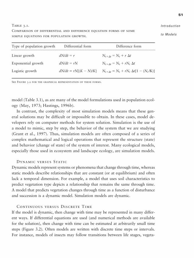
model (Table 3.1), as are many of the model formulations used in population ecol-ogy (May, 1973; Hastings, 1996b).

In contrast, the complexity of most simulation models means that these gen-eral solutions may be difficult or impossible to obtain. In these cases, model de-velopers rely on computer methods for system solution. Simulation is the use ofa model to mimic, step by step, the behavior of the system that we are studying(Grant et al., 1997). Thus, simulation models are often composed of a series ofcomplex mathematical and logical operations that represent the structure (state)and behavior (change of state) of the system of interest. Many ecological models,especially those used in ecosystem and landscape ecology, are simulation models.

Dynamic versus StaticDynamic models represent systems or phenomena that change through time, whereasstatic models describe relationships that are constant (or at equilibrium) and oftenlack a temporal dimension. For example, a model that uses soil characteristics topredict vegetation type depicts a relationship that remains the same through time.A model that predicts vegetation changes through time as a function of disturbanceand succession is a dynamic model. Simulation models are dynamic.

Continuous versus Discrete TimeIf the model is dynamic, then change with time may be represented in many differ-ent ways. If differential equations are used (and numerical methods are availablefor the solution), then change with time can be estimated at arbitrarily small timesteps (Figure 3.2). Often models are written with discrete time steps or intervals.For instance, models of insects may follow transitions between life stages, vegeta-

51

Introduct ion

to Models

Table 3.1.Comparison of differential and difference equation forms of some simple equations for population growth.

Type of population growth Differential form Difference form

Linear growth dN/dt � r Nt��t � Nt � r �t

Exponential growth dN/dt � rN Nt��t � Nt � rNt �t

Logistic growth dN/dt � rN[(K � N)/K] Nt��t � Nt � rNt �t[1 � (Nt /K)]

See Figure 3.2 for the graphical representation of these forms.

2888_e03_p47-70 3/2/01 2:56 PM Page 51

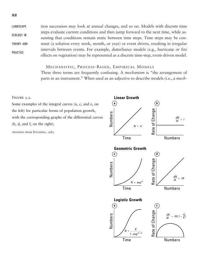
tion succession may look at annual changes, and so on. Models with discrete timesteps evaluate current conditions and then jump forward to the next time, while as-suming that conditions remain static between time steps. Time steps may be con-stant (a solution every week, month, or year) or event driven, resulting in irregularintervals between events. For example, disturbance models (e.g., hurricane or fireeffects on vegetation) may be represented as a discrete time-step, event-driven model.

Mechanistic, Process-Based, Empirical ModelsThese three terms are frequently confusing. A mechanism is “the arrangement ofparts in an instrument.” When used as an adjective to describe models (i.e., a mech-

52

L A N D S C A P E

E C O L O G Y I N

T H E O R Y A N D

P R A C T I C E

Linear Growth

Geometric Growth

Logistic Growth

N = rt

N = exprt

Time

Time

Time

Numbers

Numbers

Numbers

Num

bers

Num

bers

Num

bers

Rate

of C

hang

eRa

te o

f Cha

nge

Rate

of C

hang

e

dN = rdt

dN = rNdt

dN = rN ( 1 – N )dt K

1 – expa – rt N = K

a b

c d

e f

Figure 3.2.

Some examples of the integral curves (a, c, and e, on

the left) for particular forms of population growth,

with the corresponding graphs of the differential curves

(b, d, and f, on the right).

Adapted from Kitching, 1983.

2888_e03_p47-70 3/2/01 2:56 PM Page 52

anistic model), the term implies a model with parts arranged to explain the whole.In the best sense of the term, a mechanistic model attempts to represent dynamicsin a manner consistent with real-world phenomena (e.g., mass and energy conser-vation laws or the laws of chemistry). Although there has been waning support formechanistic approaches to ecological modeling (Breckling and Muller, 1994), theuse of mechanistic in the strictest sense distinguishes these models from black-boxmodels that grasp at any formulation that might satisfactorily represent system dy-namics. Confusion arises when the term mechanistic is loosely applied to distin-guish less detailed models from more detailed ones. Often the implication is thatmechanistic models are more desirable than less mechanistic (less detailed) mod-els. Unfortunately, the assertion that additional detail produces a more reliablemodel must be demonstrated on a case by case basis (Gardner et al., 1982).

A process-based model implies that model components were specifically devel-oped to represent specific ecological processes; for example, equations for birth,death, growth, photosynthesis, and respiration are used to estimate biomass yields,rather than simpler, more direct estimates of yields from the driving variables oftemperature, precipitation, and sunlight. Although this concept seems clear, thereis no a priori criterion defining formulations that qualify (or conversely do notqualify) as process models. Thus, depending on the level of detail, it is possible tohave a mechanistic process-based model or an empirical process-based model.

An empirical model usually refers to a model with formulations based on sim-ple, or correlative, relationships. This term also implies that model parametersmay have been derived from data (the usual case for most ecological models). Re-gression models (as well as a variety of other statistical models) are typically em-pirical, because the equation was fitted to the data.

The problem of distinguishing between types of model is illustrated by the sim-ulation of diffusive processes based on well-defined theoretical constructs (Okubo,1980). These formulations of diffusion allow simple empirical measurements todefine the coefficients estimating diffusive spread. Thus, there is a strong theoret-ical base along with empirically based parameters. Is such a model considered em-pirical or theoretical? Should complex formulations always be considered moretheoretical or simply harder to parameterize?

The essential quarrel with each of these three terms is that most ecological mod-els are a continuum of parts, processes, and empirical estimations. Separating mod-els into these arbitrary and ill-defined classifications lacks rigor and repeatability.One person’s mechanistic model is the next person’s process-based model, and soon. There does not appear to be a compelling reason to use these vague and of-ten confusing terms to distinguish between alternative model formulations.

53

Introduct ion

to Models

2888_e03_p47-70 3/2/01 2:56 PM Page 53

S p a t i a l M o d e l s

A model is spatial when the variables, inputs, or processes have explicit spatial lo-cations. Spatial models are useful when the heterogeneity of resources and processesis required to represent and predict system dynamics properly. Although such mod-els have received considerable attention in recent years, the complexity and diffi-culty of formulating a spatial model may not be necessary to address every land-scape question. A spatial model is only needed when explicit space—what is presentand how it is arranged—is an important determinant of the process being studied.Although this condition is easily stated, it is often difficult to determine a priori.There are three general conditions for which spatial models are important.

1. Spatial pattern (abundance and configuration of elements) may be one of theindependent variables in the analysis. That is, we are particularly interestedin how some ecological response variable changes as a function of the con-figuration of landscape elements. Questions that illustrate this requirement in-clude these: What is the effect of different arrangements of the same amountof habitat on species diversity? How does input of nitrogen to an aquaticecosystem vary with the positioning of vegetation or land-cover types in a wa-tershed? How does the spatial patterning of resources influence movement orforaging dynamics of a species? How is the spread of disturbance influencedby the spatial pattern of areas that are or are not susceptible to a disturbance?A spatial model developed to address these types of questions would use spa-tial pattern as one of the input variables. Most often, using a map for one ofthe driving variables does this; this map may or may not change through time.

2. A spatial model is needed when predicting spatial variation of an attribute ofinterest and how it changes through time (Figure 3.3). General questions in-clude these: How will disturbance, land-use activity, or land management af-fect land-use change? How does habitat pattern affect the distribution andabundance of species within the landscape? These questions require the initialspatial patterns as input to a model that then simulates pattern change throughtime (Turner, 1987a; Costanza et al., 1990; Sklar and Costanza, 1990).

3. A spatial model is required when the question involves sets of processes orbiotic interactions that generate pattern. This situation is often explored intheoretical population ecology (Holmes et al., 1994; Ives et al., 1998). Ques-tions might include these: If two or more species compete for space, how dotheir interactions lead to heterogeneous distributions of the species acrossthe landscape? What happens to the patterns of species distributions if re-

54

L A N D S C A P E

E C O L O G Y I N

T H E O R Y A N D

P R A C T I C E

2888_e03_p47-70 3/2/01 2:56 PM Page 54

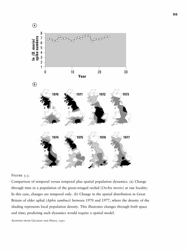
55

1970 1971 1972 1973

1974 1975 1976 1977

0 10 20 30

87654321

In spik

e nu

mbe

rs(O

. mor

io)

Year

a

b

Figure 3.3.

Comparison of temporal versus temporal plus spatial population dynamics. (a) Change

through time in a population of the green-winged orchid (Orchis morio) at one locality.

In this case, changes are temporal only. (b) Change in the spatial distribution in Great

Britain of elder aphid (Aphis sambuci) between 1970 and 1977, where the density of the

shading represents local population density. This illustrates changes through both space

and time; predicting such dynamics would require a spatial model.

Adapted from Gillman and Hails, 1997.

2888_e03_p47-70 3/2/01 2:56 PM Page 55

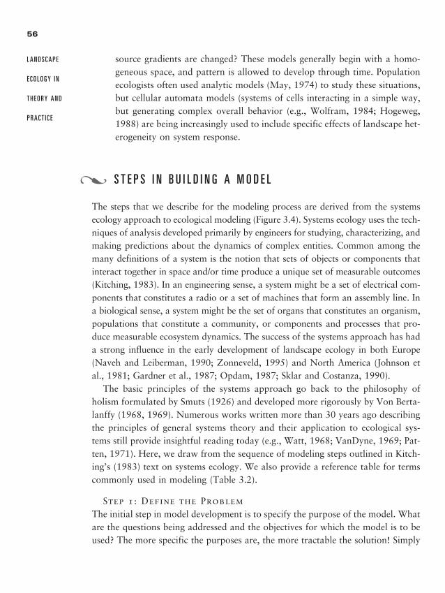
source gradients are changed? These models generally begin with a homo-geneous space, and pattern is allowed to develop through time. Populationecologists often used analytic models (May, 1974) to study these situations,but cellular automata models (systems of cells interacting in a simple way,but generating complex overall behavior (e.g., Wolfram, 1984; Hogeweg,1988) are being increasingly used to include specific effects of landscape het-erogeneity on system response.

S T E P S I N B U I L D I N G A M O D E L

The steps that we describe for the modeling process are derived from the systemsecology approach to ecological modeling (Figure 3.4). Systems ecology uses the tech-niques of analysis developed primarily by engineers for studying, characterizing, andmaking predictions about the dynamics of complex entities. Common among themany definitions of a system is the notion that sets of objects or components thatinteract together in space and/or time produce a unique set of measurable outcomes(Kitching, 1983). In an engineering sense, a system might be a set of electrical com-ponents that constitutes a radio or a set of machines that form an assembly line. Ina biological sense, a system might be the set of organs that constitutes an organism,populations that constitute a community, or components and processes that pro-duce measurable ecosystem dynamics. The success of the systems approach has hada strong influence in the early development of landscape ecology in both Europe(Naveh and Leiberman, 1990; Zonneveld, 1995) and North America (Johnson etal., 1981; Gardner et al., 1987; Opdam, 1987; Sklar and Costanza, 1990).

The basic principles of the systems approach go back to the philosophy ofholism formulated by Smuts (1926) and developed more rigorously by Von Berta-lanffy (1968, 1969). Numerous works written more than 30 years ago describingthe principles of general systems theory and their application to ecological sys-tems still provide insightful reading today (e.g., Watt, 1968; VanDyne, 1969; Pat-ten, 1971). Here, we draw from the sequence of modeling steps outlined in Kitch-ing’s (1983) text on systems ecology. We also provide a reference table for termscommonly used in modeling (Table 3.2).

Step 1: Define the ProblemThe initial step in model development is to specify the purpose of the model. Whatare the questions being addressed and the objectives for which the model is to beused? The more specific the purposes are, the more tractable the solution! Simply

56

L A N D S C A P E

E C O L O G Y I N

T H E O R Y A N D

P R A C T I C E

�

2888_e03_p47-70 3/2/01 2:56 PM Page 56

57

Introduct ion

to Models

having a lot of data that may appear useful is not sufficient grounds for devel-oping a model; there must be a clear and compelling reason for the model. Modelobjectives provide the framework for model development, the standard for modelevaluation, and the context within which simulation results must be interpreted.Thus, a clear statement of objectives is arguably the most crucial step in the en-tire modeling process (Grant et al., 1997). Definition of the problem will influ-

ComputerImplementation

ModelExperiments

andOutput

Define Problem

Develop ConceptualModel

SelectModelType

DevelopModel

EstimateParameters

EvaluateModel

Conceptual Framework

Analysis ofRelationships

TestingRefining

Evaluating

Application

Figure 3.4.

Flow chart of the major steps in building a model.

2888_e03_p47-70 3/2/01 2:56 PM Page 57

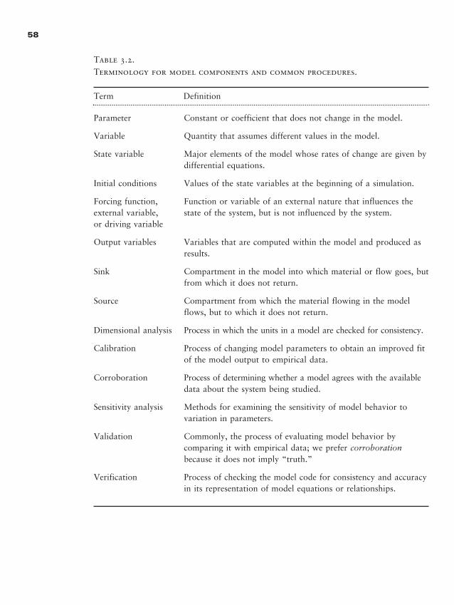
58

Table 3.2.Terminology for model components and common procedures.

Term Definition

Parameter Constant or coefficient that does not change in the model.

Variable Quantity that assumes different values in the model.

State variable Major elements of the model whose rates of change are given bydifferential equations.

Initial conditions Values of the state variables at the beginning of a simulation.

Forcing function, Function or variable of an external nature that influences the external variable, state of the system, but is not influenced by the system.or driving variable

Output variables Variables that are computed within the model and produced as results.

Sink Compartment in the model into which material or flow goes, but from which it does not return.

Source Compartment from which the material flowing in the model flows, but to which it does not return.

Dimensional analysis Process in which the units in a model are checked for consistency.

Calibration Process of changing model parameters to obtain an improved fit of the model output to empirical data.

Corroboration Process of determining whether a model agrees with the availabledata about the system being studied.

Sensitivity analysis Methods for examining the sensitivity of model behavior to variation in parameters.

Validation Commonly, the process of evaluating model behavior bycomparing it with empirical data; we prefer corroborationbecause it does not imply “truth.”

Verification Process of checking the model code for consistency and accuracy in its representation of model equations or relationships.

2888_e03_p47-70 3/2/01 2:56 PM Page 58

ence the form of the model, the degree of complexity needed, and the spatial andtemporal scales at which it will operate. Surprisingly, however, this step often re-ceives far less attention than its importance warrants. The danger is that igno-rance of a model’s purpose ultimately results in the misapplication and/or misin-terpretation of the results.

Step 2: Develop the Conceptual ModelBased on a clear statement of the model purpose or objectives, a conceptual orqualitative model of the system follows. This phase includes identification of sys-tem boundaries, categorizing model components and identifying the relationshipsamong them, and describing the expected patterns of model behavior. Kitching(1983) notes that “The ecological modeler, having decided that the problem be-ing faced demands the construction of a model, is immediately confronted withthe necessity of defining the system which he or she is going to study.” What isto be included within the scope of the model? What are the important variablesand parameters (coefficients that control model processes, but do not themselveschange)? What drives the system? [Driving variables (Table 3.2) influence modelbehavior, but are external to the model; that is, they are not affected by vari-ables within the model.] What outputs will be generated? What is the appropri-ate level of spatial and temporal resolution for the model? Specifying the scale ofthe model is an important step, because the same model may produce differentresults if spatial or temporal scales are changed (Figure 3.5). What are the initialconditions (state of variables at the outset of the model run) going to be? Con-ceptual development of a model is often the most intellectually challenging phaseand frequently results in a valuable refining and/or redefinition of the model prob-lem (Figure 3.4).

There are two different approaches that modelers frequently take in definingtheir model system (Kitching, 1983). The first is to make the initial selection ofsystem components as simple as possible, including only those variables that themodeler is confident are necessary. Alternatively, the initial model might includeall variables that might conceivably have an effect on the problem of interest, withthe assumption that the modeling process will prune unnecessary variables andmodel components.

Once the initial selection of variables and processes is made, the modeler mustconsider how the components interact with each other. Flow diagrams or flowcharts are common techniques used in this phase of modeling as precursors towriting equations for these interactions. Essentially, flow diagrams are a formalrepresentation of the qualitative relationships of the conceptual model.

59

Introduct ion

to Models

2888_e03_p47-70 3/2/01 2:56 PM Page 59

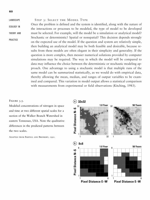
Step 3: Select the Model TypeOnce the problem is defined and the system is identified, along with the nature ofthe interactions or processes to be modeled, the type of model to be developedmust be selected. For example, will the model be a simulation or analytical model?Stochastic or deterministic? Spatial or nonspatial? This decision depends stronglyon the expected use of the model. If the question and system are relatively simple,then building an analytical model may be both feasible and desirable, because re-sults from these models are often elegant in their simplicity and generality. If thequestion is more complex, then messier numerical solutions provided by computersimulations may be required. The way in which the model will be compared todata may influence the choice between the deterministic or stochastic modeling ap-proach. One advantage to using a stochastic model is that multiple runs of thesame model can be summarized statistically, as we would do with empirical data,thereby allowing the mean, median, and ranges of output variables to be exam-ined and compared. This variation in model output allows a statistical comparisonwith measurements from experimental or field observations (Kitching, 1983).

60

L A N D S C A P E

E C O L O G Y I N

T H E O R Y A N D

P R A C T I C E

1.0 Year

1.0 Year

50 Years

50 Years

Pixe

l Dis

tanc

e N

–SPi

xel D

ista

nce

N–S

Pixel Distance E–W Pixel Distance E–W

1

32

32 32

8 8

1

32

1

8

1

1 1

1 1

8

32x32

8x8

a

b

Figure 3.5.

Modeled concentrations of nitrogen in space

and time at two different spatial scales for a

section of the Walker Branch Watershed in

eastern Tennessee, USA. Note the qualitative

differences in the predicted patterns between

the two scales.

Adapted from Bartell and Brenkert, 1991.

2888_e03_p47-70 3/2/01 2:56 PM Page 60

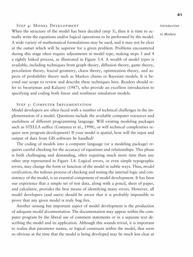
Step 4: Model DevelopmentWhen the structure of the model has been decided (step 3), then it is time to ac-tually write the equations and/or logical operations to be performed by the model.A wide variety of mathematical formulations may be used, and it may not be clearat the outset which will be superior for a given problem. Problems encounteredduring this stage often require adjustments in model type, making steps 3 and 4a tightly linked process, as illustrated in Figure 3.4. A wealth of model types isavailable, including techniques from graph theory, diffusion theory, game theory,percolation theory, fractal geometry, chaos theory, optimization theory, and as-pects of probability theory such as Markov chains or Bayesian models. It is be-yond our scope to review and describe these techniques here. Readers should re-fer to Swartzman and Kaluzny (1987), who provide an excellent introduction tospecifying and coding both linear and nonlinear simulation models.

Step 5: Computer ImplementationModel developers are often faced with a number of technical challenges in the im-plementation of a model. Questions include the available computer resources andusefulness of different programming language. Will existing modeling packagessuch as STELLA suffice (Costanza et al., 1998), or will technical complexities re-quire new program development? If your model is spatial, how will the input andoutput of data from GIS software be handled?

The coding of models into a computer language (or a modeling package) re-quires careful checking for the accuracy of equations and relationships. This phaseis both challenging and demanding, often requiring much more time than anyother step represented in Figure 3.4. Logical errors, or even simple typographicerrors, may change the form or function of the model in subtle ways. Thus, modelverification, the tedious process of checking and testing the internal logic and con-sistency of the model, is an essential component of model development. It has beenour experience that a simple set of test data, along with a pencil, sheet of paper,and calculator, provides the best means of identifying many errors. However, allmodel developers (and users) should be aware that it is probably impossible toprove that any given model is truly bug free.

Another unsung but important aspect of model development is the productionof adequate model documentation. The documentation may appear within the com-puter program by the liberal use of comment statements or in a separate text de-scribing the model and its application. Although this sounds trivial, it is importantto realize that parameter names, or logical constructs within the model, that seemso obvious at the time that the model is being developed may be much less clear at

61

Introduct ion

to Models

2888_e03_p47-70 3/2/01 2:56 PM Page 61

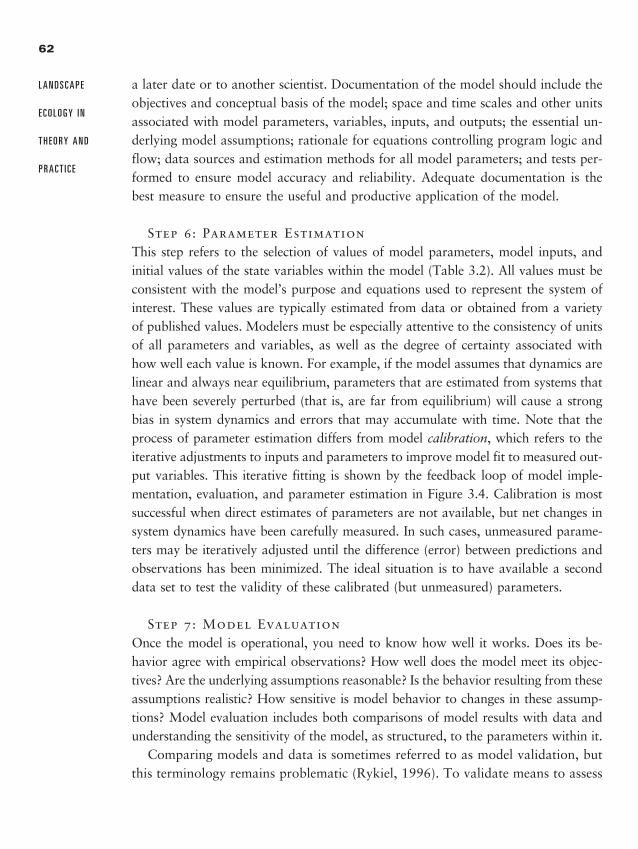
a later date or to another scientist. Documentation of the model should include theobjectives and conceptual basis of the model; space and time scales and other unitsassociated with model parameters, variables, inputs, and outputs; the essential un-derlying model assumptions; rationale for equations controlling program logic andflow; data sources and estimation methods for all model parameters; and tests per-formed to ensure model accuracy and reliability. Adequate documentation is thebest measure to ensure the useful and productive application of the model.

Step 6: Parameter EstimationThis step refers to the selection of values of model parameters, model inputs, andinitial values of the state variables within the model (Table 3.2). All values must beconsistent with the model’s purpose and equations used to represent the system ofinterest. These values are typically estimated from data or obtained from a varietyof published values. Modelers must be especially attentive to the consistency of unitsof all parameters and variables, as well as the degree of certainty associated withhow well each value is known. For example, if the model assumes that dynamics arelinear and always near equilibrium, parameters that are estimated from systems thathave been severely perturbed (that is, are far from equilibrium) will cause a strongbias in system dynamics and errors that may accumulate with time. Note that theprocess of parameter estimation differs from model calibration, which refers to theiterative adjustments to inputs and parameters to improve model fit to measured out-put variables. This iterative fitting is shown by the feedback loop of model imple-mentation, evaluation, and parameter estimation in Figure 3.4. Calibration is mostsuccessful when direct estimates of parameters are not available, but net changes insystem dynamics have been carefully measured. In such cases, unmeasured parame-ters may be iteratively adjusted until the difference (error) between predictions andobservations has been minimized. The ideal situation is to have available a seconddata set to test the validity of these calibrated (but unmeasured) parameters.

Step 7: Model EvaluationOnce the model is operational, you need to know how well it works. Does its be-havior agree with empirical observations? How well does the model meet its objec-tives? Are the underlying assumptions reasonable? Is the behavior resulting from theseassumptions realistic? How sensitive is model behavior to changes in these assump-tions? Model evaluation includes both comparisons of model results with data andunderstanding the sensitivity of the model, as structured, to the parameters within it.

Comparing models and data is sometimes referred to as model validation, butthis terminology remains problematic (Rykiel, 1996). To validate means to assess

62

L A N D S C A P E

E C O L O G Y I N

T H E O R Y A N D

P R A C T I C E

2888_e03_p47-70 3/2/01 2:56 PM Page 62

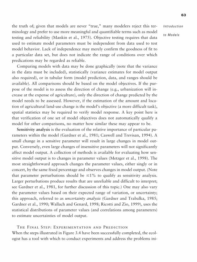
the truth of; given that models are never “true,” many modelers reject this ter-minology and prefer to use more meaningful and quantifiable terms such as modeltesting and reliability (Mankin et al., 1975). Objective testing requires that dataused to estimate model parameters must be independent from data used to testmodel behavior. Lack of independence may merely confirm the goodness of fit toa particular data set, but does not indicate the range of conditions over whichpredications may be regarded as reliable.

Comparing models with data may be done graphically (note that the variancein the data must be included), statistically (variance estimates for model outputalso required), or in tabular form (model prediction, data, and ranges should beavailable). All comparisons should be based on the model objectives. If the pur-pose of the model is to assess the direction of change (e.g., urbanization will in-crease at the expense of agriculture), only the direction of change predicted by themodel needs to be assessed. However, if the estimation of the amount and loca-tion of agricultural land-use change is the model’s objective (a more difficult task),spatial statistics may be required to verify model response. A key point here isthat verification of one set of model objectives does not automatically qualify amodel for other comparisons, no matter how similar these may appear to be.

Sensitivity analysis is the evaluation of the relative importance of particular pa-rameters within the model (Gardner et al., 1981; Caswell and Trevisan, 1994). Asmall change in a sensitive parameter will result in large changes in model out-put. Conversely, even large changes of insensitive parameters will not significantlyaffect model output. A collection of methods is available for evaluating how sen-sitive model output is to changes in parameter values (Metzger et al., 1998). Themost straightforward approach changes the parameter values, either singly or inconcert, by the same fixed percentage and observes changes in model output. (Notethat parameter perturbations should be �1% to qualify as sensitivity analysis.Larger perturbations produce results that are unreliable and difficult to interpret;see Gardner et al., 1981, for further discussion of this topic.) One may also varythe parameter values based on their expected range of variation, or uncertainty;this approach, referred to as uncertainty analysis (Gardner and Trabalka, 1985;Gardner et al., 1990; Wallach and Genard, 1998; Ricotti and Zio, 1999), uses thestatistical distributions of parameter values (and correlations among parameters)to estimate uncertainties of model output.

The Final Step: Experimentation and PredictionWhen the steps illustrated in Figure 3.4 have been successfully completed, the ecol-ogist has a tool with which to conduct experiments and address the problems ini-

63

Introduct ion

to Models

2888_e03_p47-70 3/2/01 2:56 PM Page 63

tially defined. Model predictions, and associated comparison with data, are usu-ally the most desired endpoint of model development. The verification of predic-tions across a range of conditions confirms the model hypotheses and assump-tions and increases our confidence that we have new insight and understandingof system behavior. As our confidence builds, model applications will move fromhypothesis testing to more serious applications, such as conservation planning(Baker, 1989a; Bender et al., 1998), landscape management and design (Baskent,1997), and assessment of potential changes due to land development or climatechange (Baker et al., 1991; Neilson and Koerper, 1992; He et al., 1999). Caremust be taken at each stage of model development to assure the accuracy and ad-equacy of the model. The widely available software now available for model de-velopment can also make model development very easy; however, the danger re-mains that jumping directly to computer implementation (step 5) without usingsteps 1 through 4 is extremely dangerous. However, no amount of care will guar-antee that a model is a perfect representation of the ecological system that it wasintended to mimic. Therefore, wise use and application requires an awareness ofthe problems and pitfalls common to the use of all models.

L A N D S C A P E M O D E L S

It has been more than 10 years since Baker (1989b) and Sklar and Costanza (1990)reviewed landscape models. Focused reviews on specific topics have been publishedsince then (e.g., Turner and Romme, 1994; Roberts and Gilliam, 1995; Lambin,1997; Fries et al., 1998; Mladenoff and Baker, 1999), but no comprehensiveoverview has been provided. To assess current models and modeling methods inlandscape ecology quickly, we performed an informal survey. ISI’s Web-of-Science(1999) was searched for papers published in the last 5 years (1994–1999) refer-encing “landscapes” and “model.” This search located 177 papers from 34 differ-ent journals (books, proceedings, and technical reports were not included in thissearch), and the abstracts and keywords were downloaded and reviewed. Only orig-inal papers discussing simulation models were retained, and multiple publicationsof the same model were eliminated, giving a final database of 101 manuscripts. Thejournals most frequently cited were Ecological Modelling (23), Landscape Ecology(11), Ecology (9), Ecological Applications (9), and Oikos (6).

The review of these papers showed a broad diversity of approaches and sub-ject matter currently being considered by landscape models and also illustrated

64

L A N D S C A P E

E C O L O G Y I N

T H E O R Y A N D

P R A C T I C E

�

2888_e03_p47-70 3/2/01 2:56 PM Page 64

the difficulty of placing these models into discrete categories. The most frequentsubject of these models (37%) concerned single-species issues, including metapop-ulation dynamics (12 of 37), effects of habitat fragmentation (15 of 37), corridors(5 of 37), and dispersal or invasion processes (17 of 37). Models of disturbanceeffects (17%) and vegetation dynamics (15%) were the next two largest categories.Fire was the most frequent disturbance type (11 of 17) and forests the most fre-quently modeled vegetation type (11 of 15). Nine papers concerned managementissues, including forestry (6 of 9), cultivation (1 of 9), and socioeconomic factorsaffecting landscapes (2 of 9). Surprisingly, only 6 papers were found that dealtexplicitly with human effects through economic change and its impact on land-scape change. This extremely important topic received far less attention than ex-pected. However, modeling human impacts on landscapes requires an immenseamount of information and the consideration of multiple impacts on landscapes,making the construction of these models a daunting task. Physical factors includ-ing hydrology and meteorology composed 11% of the papers, while 6% of themanuscripts dealt with simulation tools (languages, analysis methods, and the like)required to compare models among themselves and against landscape data.

Not surprisingly, the simulation methods used to tackle these problems are asdiverse as the subjects being studied. Simple sets of categories to describe thesemodels are probably impossible to construct and would not adequately conveythe diversity of approaches being employed. Dispersal models are continuing toincrease, with multiple approaches being used, including reaction–diffusion meth-ods (e.g., Bevers and Flather, 1999), individual-based random-walk models (e.g.,Gustafson and Gardner, 1996; Liu and Ashton, 1998), and probabilistic-basedcellular automata models (e.g., Zhou and Liebhold, 1995; Darwen and Green,1996). Approaches to modeling disturbance effects are also varied, ranging frompartial differential equations (e.g., Emanuel, 1996; Jin and Wu, 1997), probabil-ity distributions and stochastic simulations (e.g., Boychuk and Perera, 1997; Heand Mladenoff, 1999), to specialized methods for unique disturbance effects (e.g.,hurricanes studied by Boose et al., 1994). Models of vegetation change includeMarkov chain models (e.g., Li, 1995; Thornton and Jones, 1998), continued ex-tensions of the familiar JABOWA-FORET forest succession models (e.g., Acevedoet al., 1996; Malanson and Armstrong, 1996; Pausas et al., 1997), as well as fuzzyset theory combined with vital attributes modeling (Roberts, 1996). Linkages toGIS data layers is an active area of research, with new models and methods be-ing developed (e.g., Schippers et al., 1996; DeAngelis et al., 1998; Baker, 1995;Butcher, 1999). The diversity of approaches is a healthy sign of a growing fieldof research. Modeling approaches to landscape issues continues to reflect the di-

65

Introduct ion

to Models

2888_e03_p47-70 3/2/01 2:56 PM Page 65

versity of subjects of interest to landscape ecologists, and this will become ap-parent throughout the remainder of this book. Clear and simple paradigms forsolving similar sets of problems have yet to emerge.

C A V E A T S I N T H E U S E O F M O D E L S

Models are extremely important tools in landscape ecology. Indeed, it may wellbe that all research of spatially extensive systems requires the use of a variety ofmodels and associated theory to understand the dynamics of change (Hartway etal., 1998). Wise application of these tools should recognize the pitfalls and prob-lems of model development and interpretation. We review here, in concise form,what we consider to be the most important caveats for modeling in landscapeecology:

1. Know thy model. The performance of each model is the logical consequenceof the hypotheses and assumptions on which the model is based. Alterna-tive assumptions regarding systems behavior might be equally viable, butproduce dramatically different results. Comparison among alternative modelformulations is extremely desirable and should be attempted where possible(e.g., Rose et al., 1991a, b; VEMAP, 1995; Pan et al., 1998).

2. Errors propagate. Small errors in sensitive parameters can lead to large er-rors in outputs (Rose et al., 1991c). Techniques for analysis of the effectsof parameter errors are available (Metzger et al., 1998) and should alwaysbe employed before predictions are made. Assessment of errors of spatiallyexplicit models remains a challenge (Cherril and McClean, 1995; Henebry,1995; Heuvelink, 1998), largely because of the added complexity of evalu-ating qualitative and quantitative spatial predictions.

3. All models are simplifications of reality. This is not a casual philosophicalstatement. It simply means that no single model will ever be a completelyadequate description of reality. Therefore, the goal of model studies shouldbe to define the applications for which a given model provides reliable anduseful results. New applications of old models are not released from this re-quirement.

4. There are never enough data. The incomplete nature of data often requiresparameter values to be estimated from a diversity of sources. Inconsistency

66

L A N D S C A P E

E C O L O G Y I N

T H E O R Y A N D

P R A C T I C E

�

2888_e03_p47-70 3/2/01 2:56 PM Page 66

in the methods of data collection and parameter estimation may result inmodel biases that are difficult to identify. Gaps in empirical information thatdo not allow adequate estimation of key parameters are often the greatestsource of uncertainty in model predictions.

5. High-tech methods do not guarantee a good model. Technologically ad-vanced methodologies, including the availability of higher-level program-ming languages that facilitate model coding, do not assure the accuracy orreliability of results. When developing or interpreting models, it is criticalfor the user to understand fully the structure of the model, the assumptionsthat went into its development, and the constraints (such as spatial or tem-poral scales) on its appropriate use.

6. Keep an open mind. There is no single paradigm for spatial modeling oflandscapes. Model development and testing require a broad perspective oflandscape ecology and systems analysis techniques.

S U M M A R Y

A model is an abstraction or representation of a system or process. There are many differ-ent kinds of models, and mathematical models are commonly used in ecology. In landscapeecology, model development is an important tool that complements empirical techniques.Models permit the landscape ecologist to explore a broader range of conditions than canusually be set forth experimentally. Landscape models help to formalize our understandingand develop theory about how spatial patterns and processes interact, producing general in-sights into landscape dynamics.

Models are characterized in various ways: for example, models may be deter-ministic or stochastic; analytical or simulation; dynamics or static; and representtime as continuous or discrete. A model is spatial when the variables, inputs, orprocesses have explicit spatial locations represented in the model. A spatial modelis only needed when explicit space, that is, what is present and how it is arranged,is an important determinant of the process being studied.

The process of building a model is multifaceted and includes the following steps:(1) Define the problem. (2) Develop the conceptual model. (3) Select the modeltype. (4) Develop the model by writing out the mathematical equations and rela-tionships. (5) Computer implementation, including verification and documenta-tion of the code. (6) Estimate the parameters, and calibrate if necessary. (7) Eval-

67

Introduct ion

to Models

�

2888_e03_p47-70 3/2/01 2:56 PM Page 67

uate the model by comparison with empirical observation and perform a sensi-tivity or uncertainty analysis. (8) Use the model for experiments and prediction.

A broad diversity of approaches and subjects are represented in landscape mod-els. Many landscape models address metapopulation dynamics, habitat fragmen-tation, and dispersal and invasion processes. Disturbance and vegetation dynam-ics are also well represented in the landscape modeling literature. Integrated modelsof ecological and socioeconomic processes are becoming a presence in the litera-ture, but less attention is given to this important topic than it deserves. Approachesto implementing models of landscape patterns and processes are very diverse, al-though linking models to GIS data is common.

Models are and will remain extremely important tools in landscape ecology.Wise application of these models requires care, however, particularly with the fol-lowing points: (1) Performance of any model results from the hypotheses and as-sumptions on which it is built. Comparing alternative model formulations is ex-tremely valuable. (2) Understanding the sensitivity of models to error in estimatingparameters is critical; however, assessing error propagation in spatial models re-mains challenging. (3) All models are simplifications of reality, and the domainof applicability for each model must be defined. (4) Gaps in empirical data for es-timating key parameters are often a great source of uncertainty in model predic-tions. The empirical database that contributes to a model must be understood. (5) Technologically advanced methodologies do not assure the accuracy or relia-bility of model results!


1. What are the distinguishing characteristics of landscape models? Is any spatial model

also a landscape model? Must all landscape models have a spatial component?

2. Can parameter values estimated for simple models be directly used in models with

more complicated formulations? Refer to Table 3.1 to illustrate your answer.

3. The survey of recent models presented in this chapter provides an overview of cur-

rent modeling activities. Are models being applied in a balanced manner to the broad

spectrum of landscape issues? What areas of landscape ecology are missing from

the list of topics reviewed? Why?

4. Technological advances may eventually allow complex spatial simulations to be eas-

ily performed within GIS software. What should be the key concerns of landscape

ecologists for the development and application of these methods?

68

L A N D S C A P E

E C O L O G Y I N

T H E O R Y A N D

P R A C T I C E

2888_e03_p47-70 3/2/01 2:56 PM Page 68


E c o l o g i c a l M o d e l i n g : G e n e r a l R e f e r e n c e

Grant, W. E., E. K. Pedersen, and S. L. Marin. 1997. Ecology and Natural Resource

Management. Systems Analysis and Simulation. John Wiley & Sons, Inc., New York.

Kitching, R. L. 1983. Systems Ecology. University of Queensland Press, St. Lucia,

Queensland, Australia.

Starfield, A. M., and A. L. Bleloch. 1986. Building Models for Conservation and

Management. Macmillan Publishing Company, New York.

Swartzman, G. L., and S. P. Kaluzny. 1987. Ecological Simulation Primer. Macmil-

lan Publishing Company, New York.

S p a t i a l M o d e l i n g

Baker, W. L. 1989. A review of models of landscape change. Landscape Ecology

2:111–133.

Kareiva, P. 1990. Population dynamics in spatially complex environments: theory and

data. Philosophical Transactions of the Royal Society of London, B 33:175–1990.

Sklar, F. H., and R. Costanza. 1990. The development of spatial simulation mod-

eling for landscape ecology. In M. G. Turner and R. H. Gardner, eds. Quantitative

Methods in Landscape Ecology, pp. 239–288. Springer-Verlag, New York.

Tilman, D., and P. Kareiva. 1997. Spatial ecology: The role of space in population

dynamics and interspecific interactions. Monographs in Population Biology. Prince-

ton University Press, Princeton, New Jersey, 367 p.

69

Introduct ion

to Models

2888_e03_p47-70 3/2/01 2:56 PM Page 69

C H A P T E R

Causes of Landscape Pattern

When we view a landscape, we look at its composition and spatialconfiguration: the elements present and how these elements are

arranged. In an agricultural landscape, we may observe forests occurring alongstreams and on steep ridges, whereas croplands and pastures occupy upland ar-eas of gentler slope. In a fire-dominated boreal forest landscape, we may observelarge contiguous areas of old forest, young forest, and early successional vegeta-tion. In a deciduous forest, we may observe small gaps in an otherwise continu-ous canopy of trees, and we may detect transitions between forest communitiesdominated by different species of trees. In a coastal landscape, we may observelong narrow bands of similar vegetation as one moves from the land–water mar-gin further inland. In landscapes of small extent (e.g., 100 m by 100 m), we mayobserve complex patterns of vegetated and unvegetated surfaces. How do all thesedifferent patterns develop? How do they change through time?

Today’s landscapes result from many causes, including variability in abioticconditions such as climate, topography, and soils; biotic interactions that gener-ate spatial patterning even under homogeneous environmental conditions; pastand present patterns of human settlement and land use; and the dynamics of nat-

4

2888_e04_p71-92 2/27/01 1:38 PM Page 71

72

L A N D S C A P E

E C O L O G Y I N

T H E O R Y A N D

P R A C T I C E

ural disturbance and succession. Broad-scale variability in the abiotic environmentsets the constraints within which biotic interactions and disturbances act. In thischapter, we discuss a variety of ways in which patterns develop on landscapes andprovide a longer temporal context for understanding present-day patterns.

Much of what we as humans observe as landscape pattern is actually the spa-tial distribution of dominant vegetation types: for example, forest versus grasslandsversus desert. The dominant vegetation establishes the resource base for the rest ofthe ecosystem. The pattern in the dominant vegetation, therefore, affects the spa-tial patterning of all components of the system. The patterning of the dominantvegetation may be defined by ecotones, the spatial divisions between vegetationtypes used to identify patches of similar vegetation or land cover. The ecotone formsthe demarcation line that divides the dominant vegetation types and structures thebasic spatial pattern on the landscape. In general, conditions of steep environmentalgradients or recent disturbance lead to sharper boundaries between communities.

Levin (1976a) identified three general categories of causes of spatial pattern.The first category, local uniqueness, deals with unique features of a point in space,such as abiotic variability or unique land uses imposed by society. In addition tounique constraints at a local point, there are also the vagaries of colonization. Ina sort of founder’s effect, the seeds of a long-lived plant can become establishedand determine unique local features for decades. Chance alone may determinewhich of several different long-lived species arrives first at a site and becomes es-tablished. Finally, local uniqueness may depend on the existence of multiple sta-ble states that may result from competition. That is, competition among interact-ing populations at a particular site may result in different relative abundances ofthese populations.

Levin’s second category, phase difference, deals with spatial pattern resultingfrom disturbances (also see Chapter 7). The ecosystem responds to a local dis-turbance by going through succession. When viewed at any point in time, the land-scape will have a number of disturbance sites of different age and in differentstages of succession, that is, different phases. The individual sites will be in dif-ferent phases of recovery, and the result will be a patchy pattern of vegetation.

Levin’s third category, dispersal, prevents the landscape from becoming uni-formly covered with a single, dominant population. The mechanism is a simple“fugitive” strategy (Platt and Weis, 1985). Prairie plants found in small patchesof disturbed ground provide an example of this strategy. By producing many seedsthat disperse far and wide, a fugitive species can establish itself whenever an op-portunity arises, such as when ground squirrels or badgers have dug holes and

2888_e04_p71-92 2/27/01 1:38 PM Page 72

displaced the prior vegetation. The fugitive species reach adulthood and produceseeds their first year, and plants from the surrounding undisturbed prairie spreadslowly over the disturbed area. Given spatial heterogeneity of the landscape, fre-quent small disturbances, and limited dispersal ability of the dominant species, afugitive species can maintain itself at isolated places throughout the landscape. Fi-nally, interacting populations with differential dispersal abilities can also imposea quasi-periodic pattern on the landscape.

The following sections introduce a variety of factors that contribute to the pat-terns observed in landscapes, including abiotic factors, biotic interactions, humanland-use patterns, and disturbance and succession. Climate, physiography, andsoils establish the template for biotic interactions characteristic of each landscape.Because these abiotic factors are spatially and temporally variable, spatial pat-terning in soil formation and vegetation growth naturally occurs. Other processes,including disturbance and recovery from disturbance, as well as variability in hu-man land use, may amplify this heterogeneity over a broad range of spatial andtemporal scales.

A B I O T I C C A U S E S O F L A N D S C A P E P A T T E R N

Landscape patterns result, in part, from variability in climate and landform. Cli-mate refers to the composite, long-term, or generally prevailing weather of a re-gion (Bailey, 1996), and climate acts as a strong control on biogeographic pat-terns through the distribution of energy and water. Climate effects are modifiedby landform, the characteristic geomorphic features of the landscape, which re-sult from geologic processes producing patterns of physical relief and soil devel-opment. Together, climate and landform establish the template on which the soilsand biota of a region develop.

All landscapes have a history; understanding landscape pattern and process re-quires an understanding of landscape history. Paleoecology is the study of indi-viduals, populations, and communities of plants and animals that lived in the pastand their interactions with and dynamic responses to changing environments. Thisfield offers a wealth of insight into the long-term development of today’s land-scapes. Although we do not attempt to review this rich field, we draw on pale-oecological studies to discuss the role of climate in the spatial structuring of thebiota and the role of prehistoric humans in influencing landscapes.

73

Causes of

Landscape

Pat tern

�

2888_e04_p71-92 2/27/01 1:38 PM Page 73

C l i m a t e

General climatic patterns will be familiar to all ecologists from introductory classesin biology or geography. At the broadest scale, climate varies with latitude, whichinfluences both temperature and the distribution of moisture, and with continen-tal position. Because of differential heating of land and water, coastal regions ata given latitude differ from inland regions. The distributions of biomes on Earthresult from these broad-scale climate patterns. However, the effects of both lati-tude and continental position are then modified locally by topography, leading tofiner-scale heterogeneity in climate patterns (Bailey, 1996). Temperatures gener-ally decrease with increasing elevation, and north- and south-facing slopes expe-rience different levels of solar radiation and hence different temperatures and evap-oration rates.

Long-term Climate ChangeThe distribution of plant and animal communities, and indeed of entire biomes,has varied tremendously with past changes in climate, even in the absence of hu-man activities. The spatial distribution of life forms today as a function of latitudeand longitude look very different compared to those of 5000 or 10,000 years (yr)before present (BP). Furthermore, present assemblages of plants and animals rep-resent only a portion of the ecosystems that have existed during Earth’s history.

Climatic changes on Earth during the past 500,000 yr have been dramatic (Fig-ure 4.1). Each glacial–interglacial cycle is about 100,000 yr in duration, with90,000 yr of gradual climatic cooling, followed by rapid warming and 10,000 yrof interglacial warmth. The peak of the last glacial period, or ice age, was about18,000 yr BP and ended approximately 10,000 yr BP. These long climate cyclesmay be produced by cyclic changes in solar irradiance resulting from long-termand complex variation in Earth’s orbital pattern (the Milankovitch cycles) as Earthwobbles on its rotational axis (Crowley and Kim, 1994). This orbital eccentricityresults in approximately 3.5% variation in the total amount of solar radiation re-ceived by Earth and changes its latitudinal distribution.

Looking more closely at the most recent climate cycle, we can examine changesin mean global temperature for the past 150,000 yr. Mean global temperature isthe only reliable expression of global surface air temperature because climatolo-gists want to remove the spatial variability in climate to detect trends in the entireglobal climate system; thus, small changes in mean global temperature may reflectvery large fluctuations in temperature at many locations on Earth. During the past150,000 yr, there was a 5°C shift in average global temperature between the glacial

74

L A N D S C A P E

E C O L O G Y I N

T H E O R Y A N D

P R A C T I C E

2888_e04_p71-92 2/27/01 1:38 PM Page 74

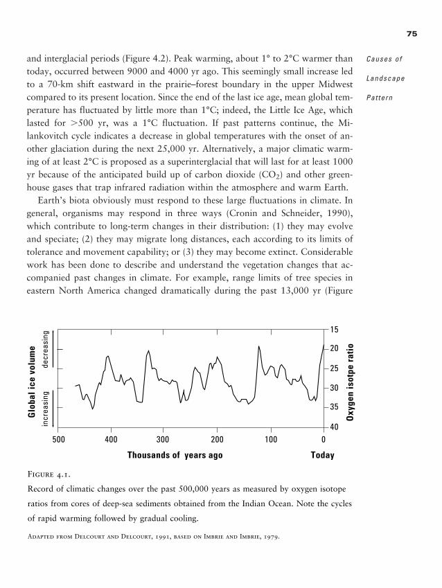
and interglacial periods (Figure 4.2). Peak warming, about 1° to 2°C warmer thantoday, occurred between 9000 and 4000 yr ago. This seemingly small increase ledto a 70-km shift eastward in the prairie–forest boundary in the upper Midwestcompared to its present location. Since the end of the last ice age, mean global tem-perature has fluctuated by little more than 1°C; indeed, the Little Ice Age, whichlasted for �500 yr, was a 1°C fluctuation. If past patterns continue, the Mi-lankovitch cycle indicates a decrease in global temperatures with the onset of an-other glaciation during the next 25,000 yr. Alternatively, a major climatic warm-ing of at least 2°C is proposed as a superinterglacial that will last for at least 1000yr because of the anticipated build up of carbon dioxide (CO2) and other green-house gases that trap infrared radiation within the atmosphere and warm Earth.

Earth’s biota obviously must respond to these large fluctuations in climate. Ingeneral, organisms may respond in three ways (Cronin and Schneider, 1990),which contribute to long-term changes in their distribution: (1) they may evolveand speciate; (2) they may migrate long distances, each according to its limits oftolerance and movement capability; or (3) they may become extinct. Considerablework has been done to describe and understand the vegetation changes that ac-companied past changes in climate. For example, range limits of tree species ineastern North America changed dramatically during the past 13,000 yr (Figure

75

Causes of

Landscape

Pat tern

Oxy

gen

isot

pe r

atio

Thousands of years ago Today

Glo

bal i

ce v

olum

ein

crea

sing

decr

easi

ng

15

0100200300400500

20

25

30

35

40

Figure 4.1.

Record of climatic changes over the past 500,000 years as measured by oxygen isotope

ratios from cores of deep-sea sediments obtained from the Indian Ocean. Note the cycles

of rapid warming followed by gradual cooling.

Adapted from Delcourt and Delcourt, 1991, based on Imbrie and Imbrie, 1979.

2888_e04_p71-92 2/27/01 1:38 PM Page 75

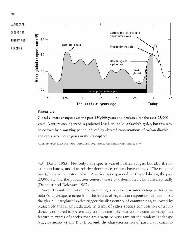
4.3) (Davis, 1983). Not only have species varied in their ranges, but also the lo-cal abundances, and thus relative dominance, of taxa have changed. The range ofoak (Quercus) in eastern North America has expanded northward during the past20,000 yr, and the population centers where oak dominated also varied spatially(Delcourt and Delcourt, 1987).

Several points important for providing a context for interpreting patterns ontoday’s landscapes emerge from the studies of vegetation response to climate. First,the glacial–interglacial cycles trigger the disassembly of communities, followed byreassembly that is unpredictable in terms of either species composition or abun-dance. Compared to present-day communities, the past communities at many sitesfeature mixtures of species that are absent or very rare on the modern landscape(e.g., Barnosky et al., 1987). Second, the characterization of past plant commu-

76

L A N D S C A P E

E C O L O G Y I N

T H E O R Y A N D

P R A C T I C E

Thousands of years ago Today

Mea

n gl

obal

tem

pera

ture

(°F)

Last interglacial

Last glacial

Present interglacial

Beginnings ofagriculture

Carbon dioxide–inducedsuper interglacial

150 125 100 75 50

50

55

60

65

25 0 -25

Last major climatic cycle

Figure 4.2.

Global climate changes over the past 150,000 years and projected for the next 25,000

years. A future cooling trend is projected based on the Milankovitch cycles, but this may

be delayed by a warming period induced by elevated concentrations of carbon dioxide

and other greenhouse gases in the atmosphere.

Adapted from Delcourt and Delcourt, 1991, based on Imbrie and Imbrie, 1979.

2888_e04_p71-92 2/27/01 1:38 PM Page 76

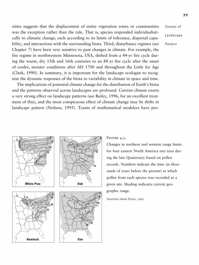
77

Causes of

Landscape

Pat tern

White Pine Oak

Hemlock Elm

642

8

10

12

8

10

12

14

86

10

1214

2 46

8

10

12

nities suggests that the displacement of entire vegetation zones or communitieswas the exception rather than the rule. That is, species responded individualisti-cally to climatic change, each according to its limits of tolerance, dispersal capa-bility, and interactions with the surrounding biota. Third, disturbance regimes (seeChapter 7) have been very sensitive to past changes in climate. For example, thefire regime in northwestern Minnesota, USA, shifted from a 44-yr fire cycle dur-ing the warm, dry 15th and 16th centuries to an 88-yr fire cycle after the onsetof cooler, moister conditions after AD 1700 and throughout the Little Ice Age(Clark, 1990). In summary, it is important for the landscape ecologist to recog-nize the dynamic responses of the biota to variability in climate in space and time.

The implications of potential climate change for the distribution of Earth’s biotaand the patterns observed across landscapes are profound. Current climate exertsa very strong effect on landscape patterns (see Bailey, 1996, for an excellent treat-ment of this), and the most conspicuous effect of climate change may be shifts inlandscape pattern (Neilson, 1995). Teams of mathematical modelers have pro-

Figure 4.3.

Changes in northern and western range limits

for four eastern North America tree taxa dur-

ing the late Quaternary based on pollen

records. Numbers indicate the time (in thou-

sands of years before the present) at which

pollen from each species was recorded at a

given site. Shading indicates current geo-

graphic range.

Adapted from Davis, 1983.

2888_e04_p71-92 2/27/01 1:38 PM Page 77

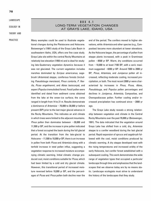
78

L A N D S C A P E

E C O L O G Y I N

T H E O R Y A N D

P R A C T I C E

B O X 4 . 1LONG-TERM VEGETATION CHANGES

AT GRAYS LAKE, IDAHO, USA

Many examples could be used to illustrate vegeta-

tional changes during the Pleistocene and Holocene.

Beiswenger’s (1991) study of the Grays Lake Basin in

southeastern Idaho, USA, offers one fine case study.

Grays Lake sits within the central Rocky Mountains at

relatively low elevation (1950 m) and is ideal for study-

ing late-Quaternary vegetation dynamics because it

was not glaciated. The current vegetation includes

marshes dominated by Scirpus americanus, sage-

brush (Artemisia) steppe, coniferous forests (includ-

ing Pseudotsuga menziessii, Pinus contorta, P. flex-

ilis, Picea engelmannii, and Abies lasiocarpa), and

aspen (Populus tremuloides) forest. Fossil pollen were

identified and dated from sediment cores obtained

from the lake at the snow–ice surface; the cores

ranged in length from 14 to 21 m. Results demonstrate

a dominance of Artemisia �70,000 to 30,000 yr before

present (BP) prior to the last major glacial advance in

the Rocky Mountains. This indicates an arid climate

in which trees were limited to the adjacent mountains.

Pinus pollen then dominates between �30,000 and

11,500 yr BP, and the increase in pine pollen indicated

that a forest occupied the basin during the full glacial

period. At the transition from the late-glacial to

Holocene �11,500 to 10,000 yr BP, there is an increase

in pollen from both Picea and Artemisia along with a

tenfold increase in total pollen influx, suggesting a

vegetation response to increased moisture accompa-

nying climatic warming. Initial climatic change pro-

duced cool, moist conditions suitable for Picea, which

had been limited by a cold and dry glacial climate.

However, this transitional period of increased mois-

ture reversed before 10,000 yr BP, and the percent-

ages of Picea and Pinus pollen both decline near the

end of the period. The conifers moved to higher ele-

vations, while Artemisia and other species (e.g., Com-

positae) became more abundant at lower elevations.

As the Holocene began, the percentage of pollen from

steppe plants increased, with a peak in Gramineae

pollen �8500 yr BP. Warm, dry conditions occurred

from �10,000 to at least 7100 BP, with a xeric maxi-

mum suggested �8200 yr BP. Around 7300 to 2000 yr

BP, Pinus, Artemisia, and Juniperus pollen all in-

creased, reflecting moderate cooling, increased pre-

cipitation, or both. The most recent 2000 yr were char-

acterized by increases in Pinus, Picea, Abies,

Pseudotsuga, and Populus pollen percentages and

declines in Juniperus, Artemisia, Compositae, and

Chenopodiaceae pollen. Further cooling and/or in-

creased precipitation has continued since �2000 yr

ago.

The Grays Lake study reveals a strong relation-

ship between vegetation and climate in the Central

Rocky Mountains over the past 70,000 yr (Beiswenger,

1991). The data indicated that the vegetation around

Grays Lake has shifted from a cold, dry, Artemisia

steppe to a conifer woodland during the last glacial

period. Rapid expansion of spruce and sagebrush fol-

lowed with the cool, moist conditions produced by

climatic warming. A dry steppe developed next with

the rising temperatures and increased aridity of the

early Holocene, but conifer forest established with a

subsequent cooling. This work demonstrates the wide

range of vegetation types that occupied a particular

landscape through time and emphasizes that the land-

scapes that we observe today are by no means sta-

tic. Landscape ecologists must strive to understand

the history of the landscapes that they study.

2888_e04_p71-92 2/27/01 1:38 PM Page 78

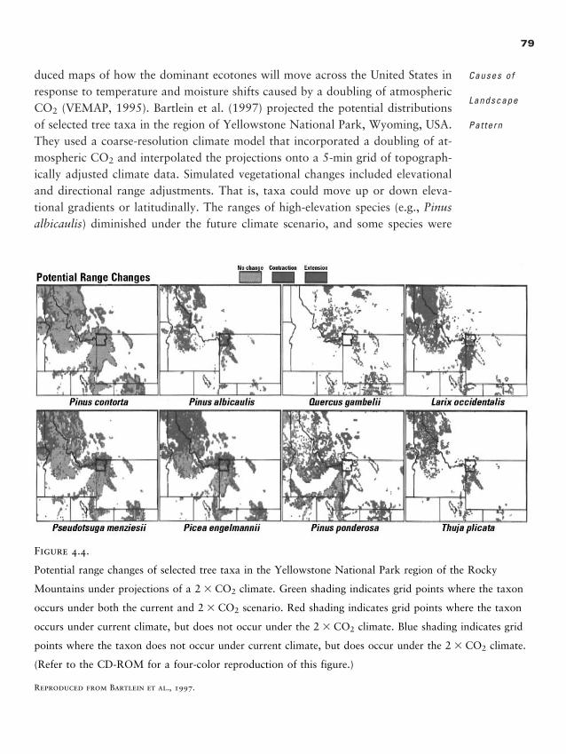
duced maps of how the dominant ecotones will move across the United States inresponse to temperature and moisture shifts caused by a doubling of atmosphericCO2 (VEMAP, 1995). Bartlein et al. (1997) projected the potential distributionsof selected tree taxa in the region of Yellowstone National Park, Wyoming, USA.They used a coarse-resolution climate model that incorporated a doubling of at-mospheric CO2 and interpolated the projections onto a 5-min grid of topograph-ically adjusted climate data. Simulated vegetational changes included elevationaland directional range adjustments. That is, taxa could move up or down eleva-tional gradients or latitudinally. The ranges of high-elevation species (e.g., Pinusalbicaulis) diminished under the future climate scenario, and some species were

79

Causes of

Landscape

Pat tern

Figure 4.4.

Potential range changes of selected tree taxa in the Yellowstone National Park region of the Rocky

Mountains under projections of a 2 � CO2 climate. Green shading indicates grid points where the taxon

occurs under both the current and 2 � CO2 scenario. Red shading indicates grid points where the taxon

occurs under current climate, but does not occur under the 2 � CO2 climate. Blue shading indicates grid

points where the taxon does not occur under current climate, but does occur under the 2 � CO2 climate.

(Refer to the CD-ROM for a four-color reproduction of this figure.)

Reproduced from Bartlein et al., 1997.

2888_e04_p71-92 2/27/01 1:38 PM Page 79

extirpated locally (Figure 4.4). Projected mild, wet winters also produced new ar-eas of suitable habitat for other taxa (e.g., Pinus ponderosa, Larix occidentalis,and Quercus gambelii) (Figure 4.4). Of particular note was that the new com-munities had no analogue in the present-day vegetation, because low-elevationmontane species currently in the region were mixed with species that might colo-nize from the northern and central Rocky Mountains and the Pacific Northwest.In addition, the potential range adjustments projected for different species equaledor exceeded the changes seen in the paleoecological record during previous warm-ing intervals (Bartlein et al., 1997).

L a n d f o r m

Landforms range from nearly flat plains to rolling, irregular plains, to hills, to lowmountains, to high mountains (Bailey, 1996) and are identified on the basis ofthree major characteristics: (1) relative amount of gently sloping (�8%) land, (2)local relief, and (3) generalized profile, that is, where and how much of the gen-tly sloping land is located in valley bottoms or in uplands (Bailey, 1996). Land-forms may be described further by considering the topographic sequence of vari-ation, or soil catena, of soils and associated vegetation types within each landform.For example, a mountainous landform may have a toposequence that includesridgetops, steep slopes, shallow slopes, toe slopes, and protected coves. If differ-ent areas are composed of similar landforms with similar geology, then soil cate-nas and vegetation types may also be expected to be similar.

Four general effects of landform on ecosystem patterns and processes (Figure4.5) were categorized by Swanson et al. (1988).

1. The elevation, aspect, parent materials, and slope of landforms affect air andground temperature and the quantities of moisture, nutrients, and other ma-terials available at sites within a landscape. For example, south-facing slopesreceive more solar radiation than northward slopes, resulting in warmer,drier conditions. These topographic patterns are strongly related to the dis-tribution of vegetation across a landscape (e.g., Whittaker, 1956).

2. Landforms affect the flow of many quantities, including organisms, propag-ules, energy, and matter through a landscape. The funneling of winds, forexample, may lead to dispersal pathways for wind-blown seeds. The posi-tion of lakes relative to groundwater-flow pathways may strongly influencethe chemical and biological characteristics of these lakes (Kratz et al., 1991;also see Chapter 9).

80

L A N D S C A P E

E C O L O G Y I N

T H E O R Y A N D

P R A C T I C E

2888_e04_p71-92 2/27/01 1:38 PM Page 80

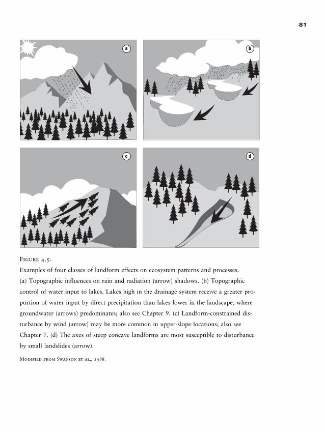
81

a b

c d

Figure 4.5.

Examples of four classes of landform effects on ecosystem patterns and processes.

(a) Topographic influences on rain and radiation (arrow) shadows. (b) Topographic

control of water input to lakes. Lakes high in the drainage system receive a greater pro-

portion of water input by direct precipitation than lakes lower in the landscape, where

groundwater (arrows) predominates; also see Chapter 9. (c) Landform-constrained dis-

turbance by wind (arrow) may be more common in upper-slope locations; also see

Chapter 7. (d) The axes of steep concave landforms are most susceptible to disturbance

by small landslides (arrow).

Modified from Swanson et al., 1988.

2888_e04_p71-92 2/27/01 1:38 PM Page 81

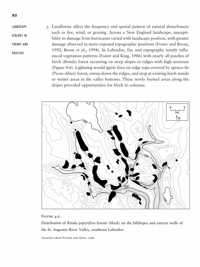
3. Landforms affect the frequency and spatial pattern of natural disturbancessuch as fire, wind, or grazing. Across a New England landscape, suscepti-bility to damage from hurricanes varied with landscape position, with greaterdamage observed in more exposed topographic positions (Foster and Boose,1992; Boose et al., 1994). In Labrador, fire and topography jointly influ-enced vegetation patterns (Foster and King, 1986) with nearly all patches ofbirch (Betula) forest occurring on steep slopes or ridges with high moisture(Figure 4.6). Lightning would ignite fires on ridge tops covered by spruce–fir(Picea–Abies) forest, sweep down the ridges, and stop at existing birch standsor wetter areas in the valley bottoms. These newly burned areas along theslopes provided opportunities for birch to colonize.

82

L A N D S C A P E

E C O L O G Y I N

T H E O R Y A N D

P R A C T I C E

1500

1500

0 3

N

km1000

500

1000

Figure 4.6.

Distribution of Betula papyrifera forests (black) on the hillslopes and canyon walls of

the St. Augustin River Valley, southeast Labrador.

Adapted from Foster and King, 1986.

2888_e04_p71-92 2/27/01 1:38 PM Page 82

4. Landforms constrain the spatial pattern and rate or frequency of geomor-phic processes, the mechanical transport of organic and inorganic material,that alter biotic characteristics and processes. Portions of a landscape maybe more or less susceptible to landslides or to shifts in river channels. Takentogether, landforms significantly contribute to the development and main-tenance of spatial heterogeneity across a landscape through their multipleeffects on soils, vegetation, and animals (Swanson et al., 1988). Even in ar-eas of relatively little topographic relief, such as the glacial landforms of theupper Midwest of the United States, landform explains a great deal of thevariability in successional pathways (Host et al., 1987) and biomass (Hostet al., 1988) across the landscape.

B I O T I C I N T E R A C T I O N S

Interactions among organisms, such as competition and predation, may lead tospatial structuring even in a completely homogeneous space. Theoretical popula-tion ecology focuses much attention on these dynamics (Ives et al., 1998), withan emphasis on how interactions within and among populations can generate spa-tial patterns and how these patterns influence the outcome of interactions. Theproduct of these theoretical approaches often is a map of species distributions.

Competition between two species in a landscape without any abiotic variationtheoretically could result in homogeneous spatial distribution (i.e., one species re-maining) through competitive exclusion (Gause, 1934). The best competitor wouldwin out and establish itself throughout the landscape, resulting in a homogeneousdistributional pattern. However, there are important exceptions to competitive exclusion.

Groups of competing organisms may interact in complex ways so that final dis-tributions take on one of many alternative stable states. These multiple stable states(Sutherland, 1974) may often occur when several different species can potentiallyoccupy and dominate a site. Which species actually occurs on a specific site is de-termined by very small stochastic changes in the initial conditions. Once in oneof these states, the community may remain dominant in spite of minor distur-bances. However, a major disruption may result in a new configuration that isdifferent, but also stable. This type of shifting, stochastic pattern may be observednear ecotones between major community types. For example, small, stable stands

83

Causes of

Landscape

Pat tern

�

2888_e04_p71-92 2/27/01 1:38 PM Page 83

of trees may extend out into grassland, and small stable patches of grasses mayintrude into the forest. Along this ecotonal edge, both communities are stable, andthere are very small differences in the competitive advantage of one communityover the other. Chance plays a role in which community is established, and onceestablished this community can maintain itself until a major disruption occurs.

Competition between vegetation types can also form ecotones, resulting in asharp line between vegetation, even when differences in environmental conditionson either side of the ecotone are small. Along a north–south transect, for exam-ple, temperature and moisture may change gradually and continuously, with nosharp discontinuities. Conditions to the south may favor one species and condi-tions to the north, another. Somewhere along the transect, conditions will be suit-able for the growth of both species. Competition for space may form a sharp eco-tone between them, rather than a gradation or intermingling.

A different sort of pattern emerges from reaction–diffusion models of interact-ing populations (Okubo, 1975). In these models, the growing and competing pop-ulations are also dispersing across a uniform environment. In many cases (Levin,1978), the expected uniform distribution is destabilized by the action of diffusion,and the system spontaneously assumes a patchy, periodic spatial distribution. Forexample, in predator–prey models, a patchy distribution results if the diffusioncoefficient of the predator is sufficiently larger than the prey. A fixed spatial pat-tern with peaks and troughs in the density of both predators and prey can result.This mechanism of diffusive instability has been suggested as the cause of patchydistribution in plankton (Kierstead and Slobodkin, 1953; Steele, 1974a; Edelstein-Keshet, 1986; Murray, 1989). We might suspect this type of mechanism when-ever a periodic or quasi-periodic pattern is detected on the landscape.

Pattern also results from the activities of a keystone species. Paine (1974, 1976)studied the interactions between the mussel Mytilus californianus and its starfishpredator, Pisaster ochraceous, in the intertidal zone. The mussel is a superior com-petitor, but predation by the starfish keeps the mussel population in check. Higherup on the shoreline, the starfish has difficulty reaching the mussels. The musselscompletely dominate the rock surfaces and eventually grow too large for thestarfish to handle. Farther down the shoreline, the starfish consumes all youngmussels. The result is a very distinct striped pattern on the rocks, mussel above,but not below this line. When Paine (1974) experimentally removed the starfish,the mussels moved down the surface of the rock, outcompeting and eliminating23 other species of invertebrates. The starfish is clearly the keystone predator thatcreates and maintains the spatial pattern. Holling (1992) believes that keystonespecies and processes are a common cause of pattern, stating that “All ecosystems

84

L A N D S C A P E

E C O L O G Y I N

T H E O R Y A N D

P R A C T I C E

2888_e04_p71-92 2/27/01 1:38 PM Page 84

are controlled and organized by a small number of key plant, animal, and abioticprocesses that structure the landscape at different scales.”

I n f l u e n c e o f D o m i n a n t O r g a n i s m s

In many respects, it is the dominant organisms that define spatial pattern on thelandscape. It is, for example, the patches of trees or natural vegetation that de-fine the pattern on most natural terrestrial landscapes. Within the context of theabiotic template, the dominants alter the abiotic conditions and provide resourcebase and substrate for the other populations in the ecosystem. In these cases, therest of the ecosystem is constrained to operate within the spatial pattern of thedominants. The interactions of the plants with the soil, climate, and topographyproduce the underlying spatial context. This is not only true in terrestrial ecosys-tems; for example, coral is a dominant organism along tropical shorelines. Thecoral forms the substrate and resource base for the entire food web, and its spa-tial distribution dictates the spatial pattern for the rest of the ecosystem.

A common example of a dominant consumer that may produce and maintainspatial pattern is a lethal pest. Insects such as the spruce budworm (Choristoneurafumiferana) and the balsam wooly adelgid (Adeiges picea) act very much like otherdisturbances in causing patches to revert to earlier successional stages. The barkbeetle provides a simple example (Rykiel et al., 1988). Lightning strikes and killsa single tree and permits the beetle to invade. Once established, the beetle can at-tack adjacent trees and spread from this original point of attack. Eventually, alarge patch is opened and reverts to early successional stages.

The beaver (Castor canadensis) provides a fascinating example of landscapepattern resulting from the activities of a dominant organism. The beaver uses sticksand mud to dam a second- to fifth-order stream, impounding water behind thedam (Johnston and Naiman, 1990a). Aerial photography (Johnston and Naiman,1990b) shows that as much as 13% of the landscape can be altered in this way.The animals also affect the riparian vegetation and saturate the soils, forming wet-lands (Naiman et al., 1986). When the dam breaks down and the pond is aban-doned, a characteristic beaver meadow remains as a distinct spatial feature on thelandscape (Remillard et al., 1987).

A similar story can be told of the American bison (Bison bison). At one timethere were 75 million bison in North America (Roe, 1951). Huge herds migratedregularly and determined plant composition along these linear routes, both bypreferential grazing and by recycling nutrients in dung. The animals also used dustbaths to control skin parasites and formed characteristic circular patches on the

85

Causes of

Landscape

Pat tern

2888_e04_p71-92 2/27/01 1:38 PM Page 85

landscape. In general, large mammals will act as a mechanism in pattern forma-tion (Botkin et al., 1981). More generally, large mammals often directly alter veg-etation and rates of nutrient recycling (Dyer et al., 1986). A moose, for example,consumes five to six metric tons of food a year (Pastor et al., 1988), increasingnutrient recycling and altering patterns of productivity. By selectively browsinghardwoods (Pastor et al., 1993), moose also directly affect species composition atlandscape scales. An effect of excluding elephants from their native habitat is achange in the pattern of vegetation (Harton and Smart, 1984).

H U M A N L A N D U S E

Patterns of land use can alter both the rate and direction of natural processes, andland-use patterns interact with the abiotic template to create the environment inwhich organisms must live, reproduce, and disperse. Land use refers to the wayin which and the purposes for which humans employ the land and its resources(Meyer, 1995). For example, humans may use land for food production, housing,industry, or recreation (Nir, 1983). A related term, land cover, refers to the habi-tat or vegetation type present, such as forest, agriculture, and grassland. Althoughthey are related, it is important to note the distinction between these terms: anarea of forest cover may be put to a variety of uses, including low-density hous-ing, logging, or recreation. We use land-use change to encompass all the ways inwhich human uses of the land have varied through time. The ways in which hu-mans use the land are important contributors to landscape pattern and process.

P r e h i s t o r i c I n f l u e n c e s

Prehistoric humans had a major role in influencing landscapes, and their past ef-fects contribute to present-day landscape patterns. Using the pollen record, indi-cations of human activities can be traced back thousands of years, and discreteepisodes of human disturbance can be correlated with archeological data. Con-sider, for example, the historical expansion of human influences in Europe (Del-court and Delcourt, 1991). In the early Holocene, there was broad-based forag-ing throughout the Mediterranean region. The switch from a nomadic to a moresedentary way of life was just beginning �10,000 BP, and by �8000 BP perma-nent settlements were established in Greece. These settlements included cultiva-tion of crops and maintenance of livestock, and food production became more la-

86

L A N D S C A P E

E C O L O G Y I N

T H E O R Y A N D

P R A C T I C E

�

2888_e04_p71-92 2/27/01 1:38 PM Page 86

bor intensive. Cereal cultivation caused a major shift in patterns of land use be-cause the permanent fields needed weeding and required nutrient replenishment,both of which were activities requiring considerable human labor. By about 6500BP, farming expanded north of Greece as winters became warmer and precipita-tion increased. Development of more efficient technologies also contributed to thecontinued expansion of agriculture in Europe. Use of the ard, a tool that used theangle between the trunk and roots of a tree to break through the soil and thatwas pulled by an oxen, became prevalent �5000 BP. Further human expansionbecame based on the maintenance of work animals, because the oxen-drawn plowthat could both furrow and turn over the soil was developed and used by �3000BP. More efficient bronze sickles also replaced wooden sickles.

What were the effects of this expansion of human activities in Europe on na-tive vegetation? The impact of the axe and spade on ecosystems began to trans-form natural landscapes into cultural ones through plowing, burning, and tram-pling. The ard, because it did not overturn the soil, left perennial roots intact. Theplow, however, removed perennials from the soil and encouraged establishmentof annual plants. The process of deforestation and conversion of land to pastureor crop cultivation changed the landscape from a natural to a cultural mosaic(Delcourt, 1987). This also occurred in North America, although early settlementsof Native Americans were more restricted to floodplains; uplands were used muchlater than in Europe (Delcourt, 1987). However, Native Americans in North Amer-ica profoundly influenced the landscape by establishing settlements, practicing agri-culture, hunting, and using fire to induce vegetation changes (Denevan, 1992).

The influences of prehistoric humans on landscapes were characterized by Del-court (1987) into five main types.

1. Humans changed the relative abundances of plants, especially the dominancestructure in forest communities. In the pollen record from Crawford Lake,Ontario, land clearance and maize cultivation by the Iroquois is documentedby pollen sequences spanning the 14th to 17th centuries. During this time,the dominance of tree species in the surrounding forest changed from late-successional species such as beech (Fagus grandifolia) and sugar maple (Acersaccharum) to forest of oak (primarily Quercus rubra) and white pine (Pi-nus strobus).

2. Humans extended or truncated the distributional ranges of plant species(woody and herbaceous). In Europe, for example, the range of olives (Oleaeuropaea) after 3000 yr BP was extended through cultivation from theMediterranean coast only to throughout southern Europe. Truncation of the

87

Causes of

Landscape

Pat tern

2888_e04_p71-92 2/27/01 1:38 PM Page 87

range of a native tree species by prehistoric humans has been documentedfor bald cyprus (Taxodium distichum) in the central Mississippi and lowerIllinois valleys in eastern North America. Charcoal evidence suggests a pref-erence for cyprus wood during the period from 2000 yr BP to AD 1450,with the species becoming locally extinct as human populations increased(Delcourt, 1987).

3. Opportunities were created for the invasion of weedy species into disturbedareas. In many places, weedy species assemblages associated with cultivatedfields increase in abundance in the pollen record, and these increases are cor-related with archeological evidence of human occupation (Delcourt, 1987).

4. The nutrient status of soils was altered through both depletion and fertil-ization.

5. The landscape mosaic was altered, especially the distribution of forest andnonforest. This last change is also easiest to detect in the paleoecologicalrecord by examining ratios of tree to herbaceous pollen.

A key point from this brief discussion of the long-term development of the cul-tural landscape is that the landscapes we may perceive to be natural today prob-ably have a history of human influence that dates back a long time. Of course,there is variability in the degree to which humans influenced different ecosystemson different continents. However, humans have long been a presence in manylandscapes, and their role in creating landscape pattern should not be discounted.

H i s t o r i c a n d P r e s e n t - D a y E f f e c t s

Both worldwide and in the United States, land-cover patterns today are alteredprincipally by direct human use: by agriculture, raising of livestock, forest har-vesting, and construction (Meyer, 1995). Human society relies on natural habi-tats for a variety of services, including productivity, recycling of nutrients, break-down of wastes, and maintenance of clean air, water, and soil. In North America,land-use changes have been particularly profound since Europeans settled the con-tinent three centuries ago. Landscapes have become mosaics of natural and human-influenced patches, and once-continuous natural habitats are becoming in-creasingly fragmented (e.g., Burgess and Sharpe, 1981; Harris, 1984).

Land-use changes in the United States serve as a handy example. At the timeof European settlement, forest covered about half the present lower 48 states. Mostof the forestland was in the moister east and northwest regions, and it had al-ready been altered by Native American land-use practices (Williams, 1989). Clear-

88

L A N D S C A P E

E C O L O G Y I N

T H E O R Y A N D

P R A C T I C E

2888_e04_p71-92 2/27/01 1:38 PM Page 88

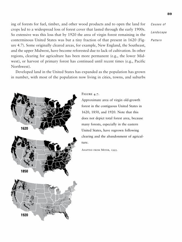
89

Causes of

Landscape

Pat tern

ing of forests for fuel, timber, and other wood products and to open the land forcrops led to a widespread loss of forest cover that lasted through the early 1900s.So extensive was this loss that by 1920 the area of virgin forest remaining in theconterminous United States was but a tiny fraction of that present in 1620 (Fig-ure 4.7). Some originally cleared areas, for example, New England, the Southeast,and the upper Midwest, have become reforested due to lack of cultivation. In otherregions, clearing for agriculture has been more permanent (e.g., the lower Mid-west), or harvest of primary forest has continued until recent times (e.g., PacificNorthwest).

Developed land in the United States has expanded as the population has grownin number, with most of the population now living in cities, towns, and suburbs

1620

1850

1920

Figure 4.7.

Approximate area of virgin old-growth

forest in the contiguous United States in

1620, 1850, and 1920. Note that this

does not depict total forest area, because

many forests, especially in the eastern

United States, have regrown following

clearing and the abandonment of agricul-

ture.

Adapted from Meyer, 1995.

2888_e04_p71-92 2/27/01 1:38 PM Page 89

rather than on farms. Americans spread out more across the land as transporta-tion technologies improved, especially as the automobile became the primary modeof transportation. Present-day patterns of settlement take up more land per per-son than in the past, and homes and subdivisions are more dispersed across thelandscape. A frontier of rapid and sometimes chaotic land-use change surroundsurban areas (Meyer, 1995). Trends in developed land are unique because they runin only one direction; that is, developed land expands and does not revert to othercategories. Thus, the distribution of developed land across the United States willleave a long-lasting footprint on the landscape (Turner et al., 1998a). The mostremarkable aspect of the landscape of the United States since European settlementis its continual change. Effects of these vast changes are long lasting and crucialto our understanding of the present-day plants and animals that inhabit our land-scapes (Foster, 1992; Dale et al., 2000).

D I S T U R B A N C E A N D S U C C E S S I O N

Disturbance and the subsequent development of vegetation are key contributorsto pattern on the landscape. By disturbance, we mean any relatively discrete eventin time that disrupts ecosystem, community, or population structure and changesresource availability, substrate, or the physical environment (White and Pickett,1985). Examples include fires, volcanic eruptions, floods, and storms. Disturbancesare often described by a variety of attributes, including their spatial distribution,frequency, spatial extent, and magnitude. The spread of disturbance and spatialpatterns of recovery have received considerable attention in landscape ecology,and we devote a chapter to exploring these dynamics (see Chapter 7). Here, wesimply recognize disturbance as an important agent of pattern creation at a vari-ety of spatial and temporal scales.

S U M M A R Y

Today’s landscapes result from many causes, including variability in abiotic condi-tions such as climate, topography, and soils; biotic interactions that generate spa-tial patterning even under homogeneous conditions; past and present patterns ofhuman settlement and land use; and the dynamics of natural disturbance and suc-

90

L A N D S C A P E

E C O L O G Y I N

T H E O R Y A N D

P R A C T I C E

�

�

2888_e04_p71-92 2/27/01 1:38 PM Page 90

cession. Three general causes of spatial pattern were identified by Levin (1976a):(1) local uniqueness, that is, the unique features of a point in space, such as abioticvariability or unique land uses imposed by society; (2) phase differences, or varia-tion in spatial pattern resulting from disturbances; and (3) dispersal, which preventslandscapes from becoming uniformly covered with a single, dominant population.

Landscape patterns result, in part, from variability in climate and landform;these broad-scale abiotic drivers constrain other causes of landscape change. Cli-mate refers to the composite, long-term, or generally prevailing weather of a re-gion (Bailey, 1996). Climate effects are modified by landform, which includes bothgeology and topography, or physical relief. The distribution of plant and animalcommunities and indeed of entire biomes has varied tremendously with pastchanges in climate, even in the absence of human activities. Not only have speciesvaried in their ranges, but also the local abundances and thus the relative domi-nance of taxa have changed. Landforms are important influences on landscapepattern because they influence moisture, nutrients, and materials at sites within alandscape; they affect flows of many quantities; they may influence the distur-bance regime; and they constrain the pattern and rate of geomorphic processes.It is important for the landscape ecologist to understand the influence of climateand landform on the biota and to recognize the dynamic responses of the biotato variability in climate in space and time.

Interactions among organisms, such as competition and predation, may lead tospatial structure, even in the absence of abiotic variation. Keystone species or dom-inant organisms may define spatial pattern on a landscape. Disturbance and suc-cession (see Chapter 7) are key contributors to landscape pattern. Humans are alsoa strong driver of landscape patterns, because land-use patterns interact with theabiotic template to create the environment in which organisms must live, repro-duce, and disperse. Nearly all landscapes, even those that we perceive as naturaltoday, probably have a history of human influence that dates back a long time.Many landscapes today have become mosaics of natural and human-influencedpatches, and once-continuous natural habitats have become increasingly frag-mented. Effects of past land use are increasingly recognized as important deter-minants of the present-day biota that inhabit our landscapes.

The understanding of what causes landscape pattern and pattern change withtime is often translated into models used to project future landscape scenarios(Baker, 1989b). These models simulate changes in the abundance and spatialarrangement of elements on the landscape, such as vegetation or cover classes. De-veloping predictive models of landscape pattern and how such patterns varythrough time is an active, rapidly changing field.

91

Causes of

Landscape

Pat tern

2888_e04_p71-92 2/27/01 1:38 PM Page 91


1. For a landscape of your choice, define its spatial extent and describe the dominant

factors causing landscape pattern in each of the following categories: abiotic fac-

tors, biotic interactions, human land use, and disturbance and succession. Repeat

this exercise after reducing the extent of the landscape to 10% of its original size.

Does the importance of the factors shift when the scale is changed? Why or why

not?

2. Consider the variety of factors that create landscape pattern. How would you rank

their relative importance? Do you think this ranking has changed through time? Ex-

plain your answers.

3. How do abiotic factors provide the template for the development of landscape pat-

tern?

4. Why is it important to understand the history of a landscape? What types of effects

of events from the past may remain in present-day landscape patterns?


Bailey, R. G. 1996. Ecosystem Geography. Springer-Verlag, New York.

Delcourt, H. R., and P. A. Delcourt. 1988. Quaternary landscape ecology: rele-

vant scales in space and time. Landscape Ecology 2:23–44.

Johnston, C. A., and R. J. Naiman. 1990. Aquatic patch creation in relation to beaver

population trends. Ecology 71:1617–1621.

Knapp, A. K., J. M. Blair, J. M. Briggs, S. L. Collins, D. C. Hartnett, L. C. John-

son, and E. G. Towne. 1999. The keystone role of bison in North American tall-

grass prairie. BioScience 49:39–50.

Swanson, F. J., T. K. Kratz, N. Caine, and R. G. Woodmansee. 1988. Landform

effects on ecosystem patterns and processes. BioScience 38:92–98.

92

L A N D S C A P E

E C O L O G Y I N

T H E O R Y A N D

P R A C T I C E

2888_e04_p71-92 2/27/01 1:38 PM Page 92

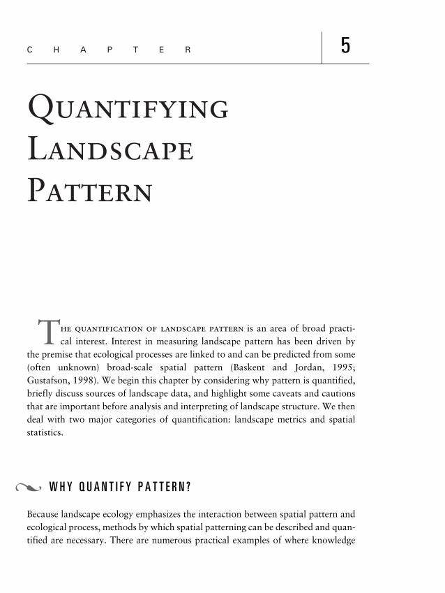
C H A P T E R

Quantifying Landscape Pattern

The quantification of landscape pattern is an area of broad practi-cal interest. Interest in measuring landscape pattern has been driven by

the premise that ecological processes are linked to and can be predicted from some(often unknown) broad-scale spatial pattern (Baskent and Jordan, 1995;Gustafson, 1998). We begin this chapter by considering why pattern is quantified,briefly discuss sources of landscape data, and highlight some caveats and cautionsthat are important before analysis and interpreting of landscape structure. We thendeal with two major categories of quantification: landscape metrics and spatialstatistics.

W H Y Q U A N T I F Y P A T T E R N ?

Because landscape ecology emphasizes the interaction between spatial pattern andecological process, methods by which spatial patterning can be described and quan-tified are necessary. There are numerous practical examples of where knowledge

5

�

2888_e05_p93-134 2/27/01 1:39 PM Page 93

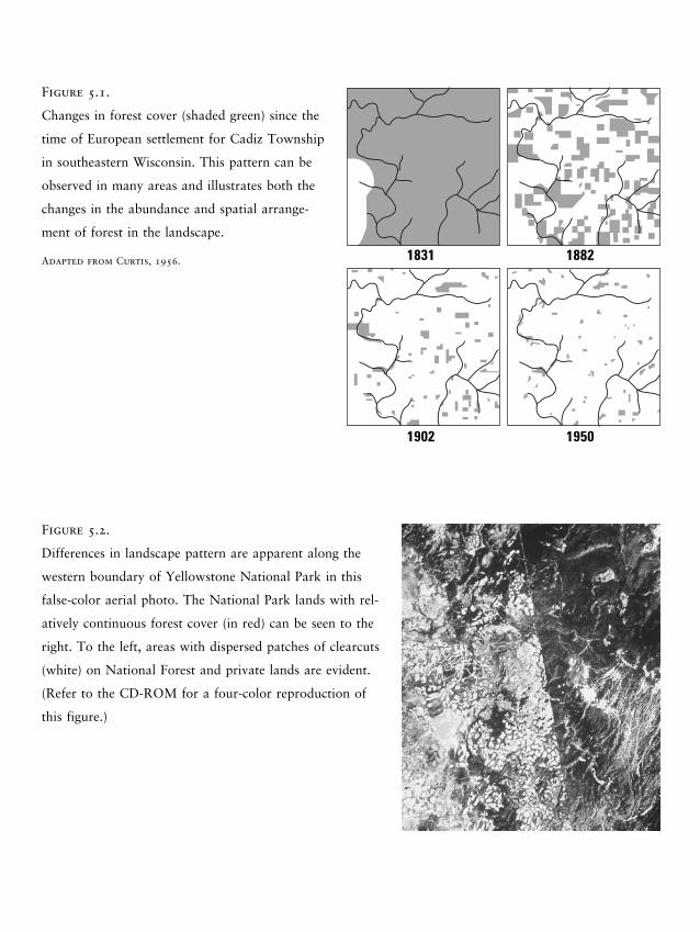
1831 1882

1902 1950

Figure 5.1.

Changes in forest cover (shaded green) since the

time of European settlement for Cadiz Township

in southeastern Wisconsin. This pattern can be

observed in many areas and illustrates both the

changes in the abundance and spatial arrange-

ment of forest in the landscape.

Adapted from Curtis, 1956.

Figure 5.2.

Differences in landscape pattern are apparent along the

western boundary of Yellowstone National Park in this

false-color aerial photo. The National Park lands with rel-

atively continuous forest cover (in red) can be seen to the

right. To the left, areas with dispersed patches of clearcuts

(white) on National Forest and private lands are evident.

(Refer to the CD-ROM for a four-color reproduction of

this figure.)

2888_e05_p93-134 2/27/01 1:39 PM Page 94

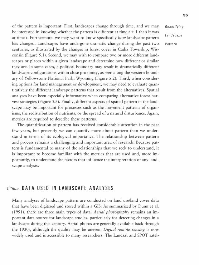
95

Quant i fy ing

Landscape

Pat tern

of the pattern is important. First, landscapes change through time, and we maybe interested in knowing whether the pattern is different at time t � 1 than it wasat time t. Furthermore, we may want to know specifically how landscape patternhas changed. Landscapes have undergone dramatic change during the past twocenturies, as illustrated by the changes in forest cover in Cadiz Township, Wis-consin (Figure 5.1). Second, we may wish to compare two or more different land-scapes or places within a given landscape and determine how different or similarthey are. In some cases, a political boundary may result in dramatically differentlandscape configurations within close proximity, as seen along the western bound-ary of Yellowstone National Park, Wyoming (Figure 5.2). Third, when consider-ing options for land management or development, we may need to evaluate quan-titatively the different landscape patterns that result from the alternatives. Spatialanalyses have been especially informative when comparing alternative forest har-vest strategies (Figure 5.3). Finally, different aspects of spatial pattern in the land-scape may be important for processes such as the movement patterns of organ-isms, the redistribution of nutrients, or the spread of a natural disturbance. Again,metrics are required to describe these patterns.

The quantification of pattern has received considerable attention in the pastfew years, but presently we can quantify more about pattern than we under-stand in terms of its ecological importance. The relationship between patternand process remains a challenging and important area of research. Because pat-tern is fundamental to many of the relationships that we seek to understand, itis important to become familiar with the metrics that are used and, more im-portantly, to understand the factors that influence the interpretation of any land-scape analysis.

D A T A U S E D I N L A N D S C A P E A N A L Y S E S

Many analyses of landscape pattern are conducted on land use/land cover datathat have been digitized and stored within a GIS. As summarized by Dunn et al.(1991), there are three main types of data. Aerial photography remains an im-portant data source for landscape studies, particularly for detecting changes in alandscape during this century. Aerial photos are generally available back throughthe 1930s, although the quality may be uneven. Digital remote sensing is nowwidely used and is accessible to many researchers. The Landsat and SPOT satel-

�

2888_e05_p93-134 2/27/01 1:39 PM Page 95

lites have provided frequent and spatially extensive coverage worldwide and area very useful source of digital data. Airborne imaging scanners may also be usedto provide fine-resolution data for a particular locale. Published data and censusesprovide a valuable source of landscape data, particularly for temporal compar-isons that extend back beyond the record of aerial photography. For example, theU.S. General Land Office Survey data have been used extensively to describe veg-etation prior to European settlement (e.g., McIntosh, 1962; Lorimer, 1977; Whit-ney, 1986; White and Mladenoff, 1994; Delcourt and Delcourt, 1996; Silbernagelet al., 1997). In addition to these three sources, field mapped data may be usedfor landscapes of smaller extent in which the investigator might map the spatial

96

L A N D S C A P E

E C O L O G Y I N

T H E O R Y A N D

P R A C T I C E

1972

1976

1981

1984

1988

Private PublicFigure 5.3.

Changes in conifer (green) and other forest types for a pri-

vate and public landscape (2500 ha) with similar initial

conditions and rates of change that are relatively high for

the ownership types. Landscape metrics were used to

quantify the differences in landscape pattern between

ownerships.

Redrawn from Spies et al., 1994.

2888_e05_p93-134 2/27/01 1:39 PM Page 96

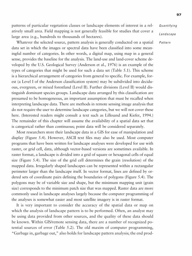
patterns of particular vegetation classes or landscape elements of interest in a rel-atively small area. Field mapping is not generally feasible for studies that cover alarge area (e.g., hundreds to thousands of hectares).

Whatever the selected source, pattern analysis is generally conducted on a spatialdata set in which the images or spectral data have been classified into some mean-ingful number of categories. In other words, a digital map, using map in a generalsense, provides the baseline for the analysis. The land-use and land-cover scheme de-veloped by the U.S. Geological Survey (Anderson et al., 1976) is an example of thetypes of categories that might be used for such a data set (Table 5.1). This schemeis a hierarchical arrangement of categories from general to specific. For example, for-est (a Level I of the Anderson classification system) may be subdivided into decidu-ous, evergreen, or mixed forestland (Level II). Further divisions (Level II) would dis-tinguish dominant species groups. Landscape data arranged by this classification arepresumed to be homogeneous, an important assumption that must be recalled wheninterpreting landscape data. There are methods in remote sensing image analysis thatdo not require the user to determine landscape categories, but we will not cover thesehere. (Interested readers might consult a text such as Lillesand and Kiefer, 1994.)The remainder of this chapter will assume the availability of a spatial data set thatis categorical rather than continuous; point data will be considered separately.

Most researchers store their landscape data in a GIS for ease of manipulation anddisplay (Figure 5.4). However, ASCII text files may also be used. Most computerprograms that have been written for landscape analyses were developed for use withraster, or grid cell, data, although vector-based versions are sometimes available. Inraster format, a landscape is divided into a grid of square or hexagonal cells of equalsize (Figure 5.4). The size of the grid cell determines the grain (resolution) of themapped data. Irregularly shaped landscapes can be represented within a rectangularperimeter larger than the landscape itself. In vector format, lines are defined by or-dered sets of coordinate pairs defining the boundaries of polygons (Figure 5.4). Thepolygons may be of variable size and shape, but the minimum mapping unit (grainsize) corresponds to the minimum patch size that was mapped. Raster data are morecommonly used in landscape analyses largely because the computer programming ofthe analyses is somewhat easier and most satellite imagery is in raster format.

It is very important to consider the accuracy of the spatial data or map onwhich the analysis of landscape pattern is to be performed. Often, an analyst maybe using data provided from other sources, and the quality of these data shouldbe known. Within GIS/remote sensing data, there are a number of recognized po-tential sources of error (Table 5.2). The old maxim of computer programming,“Garbage in, garbage out,” also holds for landscape pattern analysis; the end prod-

97

Quant i fy ing

Landscape

Pat tern

2888_e05_p93-134 2/27/01 1:39 PM Page 97

98

Table 5.1.USGS land-use, land-cover classification systems: an example of a hierarchical classification system that can be used in landscape analyses.

Level I Level II

1. Urban or built-up land 11. Residential12. Commercial or services13. Industrial14. Transportation, communication, or utilities15. Industrial and commercial16. Mixed urban or built up

2. Agricultural land 21. Cropland and pasture22. Orchards, groves, vineyards, horticulture23. Confined feeding operations24. Other agricultural land

3. Rangelands 31. Herbaceous rangelands32. Shrub and brush rangelands33. Mixed rangelands

4. Forest land 41. Deciduous forest land42. Evergreen forest land43. Mixed forest land

5. Water 51. Streams and canals52. Lakes53. Reservoirs54. Bays and estuaries

6. Wetland 61. Forested wetlands62. Nonforested wetlands

7. Barren land 71. Dry salt flats72. Beaches73. Sandy areas, except beaches74. Bare exposed rock75. Strip mines, quarries, gravel pits76. Transitional areas77. Mixed barren land

8. Tundra

9. Perennial snow or ice

From Anderson et al., 1976

2888_e05_p93-134 2/27/01 1:39 PM Page 98

uct is only as good as the data on which the analysis is based. Understanding thesensitivity of landscape metrics to error in the input data is an active topic of cur-rent research (e.g., Cardille et al., 1996; Wickham et al., 1997).

C A V E A T S F O R L A N D S C A P E P A T T E R N A N A L Y S I S , O R “ R E A D T H I S F I R S T ”

The widespread availability of spatial data in the past two decades—indeed, analmost exponential increase—has presented numerous opportunities for landscapepatterns to be analyzed for many different purposes. Before embarking on theanalysis of landscape pattern, however, several important issues should be deter-mined. At present, it is easy to fall into the trap of generating a lot of numbers

99

Quant i fy ing

Landscape

Pat tern

2 2 2 2 2 2 2 2 2 2 2 2 3 3 3 3 3 3 3 32 2 2 2 2 2 2 2 2 2 2 3 2 3 3 3 3 3 3 32 2 2 2 2 2 2 2 2 2 3 3 3 3 3 3 3 3 3 32 2 2 2 2 2 2 2 3 3 3 3 3 3 3 3 3 3 3 32 2 2 2 2 2 1 1 1 1 1 1 3 3 3 3 3 3 3 32 2 2 1 1 1 1 1 1 1 1 1 3 3 3 3 3 3 3 32 2 1 1 1 1 1 1 1 1 1 1 3 3 3 3 3 3 3 32 1 1 1 1 1 2 2 1 1 1 1 3 3 3 3 3 3 3 32 2 1 1 1 2 2 2 2 1 2 3 3 3 3 3 3 3 3 32 2 2 2 2 2 2 2 2 2 2 2 3 3 3 3 3 3 3 32 2 2 2 2 2 2 2 2 2 2 2 2 2 3 3 3 3 3 3

Base Map

Vector

Grass

LakeForest

Cell

Figure 5.4.

Two principal methods for representing spatial data in a GIS: vector-based representa-

tion and raster, or cell-based, representation.

Adapted from Coulson et al., 1991.

�

2888_e05_p93-134 2/27/01 1:39 PM Page 99

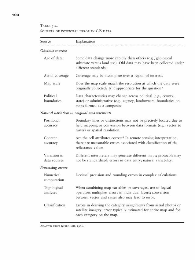
100

Table 5.2.Sources of potential error in GIS data.

Source Explanation

Obvious sources

Age of data Some data change more rapidly than others (e.g., geologicalsubstrate versus land use). Old data may have been collected underdifferent standards.

Aerial coverage Coverage may be incomplete over a region of interest.

Map scale Does the map scale match the resolution at which the data wereoriginally collected? Is it appropriate for the question?

Political Data characteristics may change across political (e.g., county,boundaries state) or administrative (e.g., agency, landowners) boundaries on

maps formed as a composite.

Natural variation in original measurements

Positional Boundary lines or distinctions may not be precisely located due toaccuracy field mapping or conversion between data formats (e.g., vector to

raster) or spatial resolution.

Content Are the cell attributes correct? In remote sensing interpretation,accuracy there are measurable errors associated with classification of the

reflectance values.

Variation in Different interpreters may generate different maps; protocols maydata sources not be standardized; errors in data entry; natural variability.

Processing errors

Numerical Decimal precision and rounding errors in complex calculations.computation

Topological When combining map variables or coverages, use of logicalanalyses operators multiplies errors in individual layers; conversion

between vector and raster also may lead to error.

Classification Errors in deriving the category assignments from aerial photos orsatellite imagery; error typically estimated for entire map and foreach category on the map.

Adapted from Burrough, 1986.

2888_e05_p93-134 2/27/01 1:39 PM Page 100

without having a clear idea of the purpose and limitations of the variety of avail-able metrics. Without a clear a priori statement of the objectives of the analysisand/or hypothesized pattern changes (e.g., disturbances will cause a decline in thediversity of land-cover types), the comparisons among multiple metrics may bemisleading. The problem of multiple comparisons is further exacerbated by the is-sue of pseudoreplication (Hurlbert, 1984; Hargrove and Pickering, 1992), whichoccurs when comparisons are made among samples that are not truly indepen-dent. The dangers of pseudoreplication are relevant to landscape ecology becausethe unique attributes of each landscape make statistical controls difficult and in-dependent replicate samples nearly impossible.

T h e C l a s s i f i c a t i o n S c h e m e I s C r i t i c a l

The categories selected for use in the analysis have an extremely strong influence onthe numerical results of any pattern analysis. For example, consider the pattern ofvegetation mapped from remote imagery for a section of a landscape, but classifiedin different ways (Figure 5.5). It is clear that these two landscape representationslook very different and that the quantitative descriptions of these two data sets wouldbe quite dissimilar. Thus, the choice of the categories to include in a pattern analy-sis is critical. The classes must be selected for the particular question or objectiveand the classification rules rigorously applied across all landscapes being compared.For example, general categories (e.g., Level I in Anderson et al., 1976) would be ap-propriate to study landscape patterns in the eastern United States, but to study veg-etation patterns within a forested landscape such as the Great Smoky MountainsNational Park, descriptions of a variety of forest community types may be more de-sirable. Once classified, analyses of categorical maps generally assume homogeneitywithin each category. All categories may, in some sense, be considered an aggregateof a more detailed set of subcategories. As categories become more aggregated therelationship between pattern and process will become difficult to establish.

Even after the decision is made about the categories to be included in a dataset, the actual interpretation of these categories from some primary data sourcemay need further specification. Gustafson (1998) poses the example of studyingthe distribution of aspen in the Wisconsin Northwoods and the need to specifyhow much aspen must be present in order to be classified as an aspen stand. Thethreshold density for classification should be specified, and the use of differentdensity levels among similar maps should be avoided. It is clear that each deci-sion in the mapping process will affect the determination and analysis of spatialstructure (Gustafson, 1998).

101

Quant i fy ing

Landscape

Pat tern

2888_e05_p93-134 2/27/01 1:39 PM Page 101

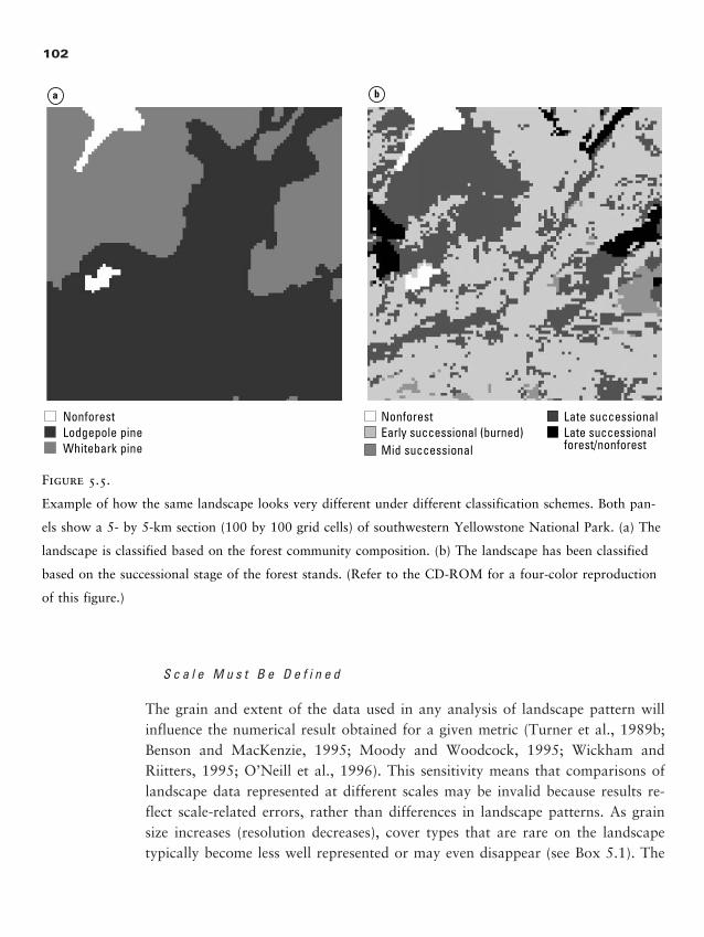
S c a l e M u s t B e D e f i n e d

The grain and extent of the data used in any analysis of landscape pattern willinfluence the numerical result obtained for a given metric (Turner et al., 1989b;Benson and MacKenzie, 1995; Moody and Woodcock, 1995; Wickham and Riitters, 1995; O’Neill et al., 1996). This sensitivity means that comparisons oflandscape data represented at different scales may be invalid because results re-flect scale-related errors, rather than differences in landscape patterns. As grainsize increases (resolution decreases), cover types that are rare on the landscapetypically become less well represented or may even disappear (see Box 5.1). The

102

NonforestLodgepole pineWhitebark pine

NonforestEarly successional (burned)Mid successional

Late successional Late successional forest/nonforest

a b

Figure 5.5.

Example of how the same landscape looks very different under different classification schemes. Both pan-

els show a 5- by 5-km section (100 by 100 grid cells) of southwestern Yellowstone National Park. (a) The

landscape is classified based on the forest community composition. (b) The landscape has been classified

based on the successional stage of the forest stands. (Refer to the CD-ROM for a four-color reproduction

of this figure.)

2888_e05_p93-134 2/27/01 1:39 PM Page 102

boundaries between different cover types also become underestimated with in-creasing grain size as the shapes depicted become less complex and details are lost(Figure 5.6). By changing grain in a Landsat image from 30- by 30-m to 1- by 1-km, Moody and Woodcock (1995) showed that scale-induced changes in the pro-portion of the landscape occupied by different cover types influenced landscape

103

Quant i fy ing

Landscape

Pat tern

B O X 5 . 1ANALYTICAL EQUATIONS FOR

AGGREGATION ERRORS

Significant errors in spatial data can occur as the re-

sult of aggregation of fine-grained information into

coarser scales of resolution. The loss of information

with successive levels of aggregation is a well-stud-

ied problem (e.g., Costanza and Maxwell, 1994;

Henderson-Sellers et al., 1985; Meentemeyer and Box,

1987; Pierce and Running, 1995; Turner et al., 1989b;

Mladenoff et al., 1997), and analytical equations have

been developed to quantify aggregation effects

(Turner et al., 1989b; Peitgen et al., 1992). The rule used

to aggregate always results in error, but the nature of

this error and the degree to which it affects landscape

pattern can be quantified. Suppose that the resolution

of a square grid composed of randomly placed cells

of two types, a and b, will be changed by aggregation

of 2 by 2 subsets of the grid into a single cell, thus re-

ducing the number of cells in the aggregated grid to

one-fourth of the original. If the proportion of cells of

type a and b is equal to p and 1.0 � p, respectively,

then the proportion of cells of type a in the aggregated

map, p, using the majority rule (at least three cells

must be of type a) will be

p � p4 � 4p3(1.0 � p)

If a 50% rule for aggregation is invoked (at least two

cells must be of type a) then

p � p 4 � 4p3 (1.0 � p) � 6p2(1.0 � p)2

Both rules result in substantial aggregation errors,

shifting the proportion of cells of type a by as much

as 22%. However, the values of p that produce the

greatest error differ between rules; in both cases the

error is zero when p is equal to 0.0 and 1.0 (an unin-

teresting result), but is also zero at p � 0.76 for the

majority rule and at p � 0.24 for the 50% rule. A third

rule, which produces zero error when p � 0.50, can

be formulated as an average of the majority rule and

the 50% rule. This averaging rule is equivalent to as-

signing the aggregated cell to type a or b at random

when there are exactly two of each type in the 2 by 2

grid unit and using the majority rule otherwise. Con-

sideration of the combinatorics for the random ag-

gregation rule gives

p � p4 � 3(p3(1.0 � p)) � 3(p2(1.0 � p) � p(1.0 � p)3)

This rule is globally the most accurate rule because

it preserves the value of p for all land-cover types,

even over successive aggregations. Local errors (the

accuracy in the representation of the amount and

physical appearance of dominant land-cover types at

fine scales) will increase. The effect of the random

aggregation rule on local errors has not been thor-

oughly investigated. For additional details regarding

these methods, see Milne and Johnson (1993) and

Gardner (1999).

2888_e05_p93-134 2/27/01 1:39 PM Page 103

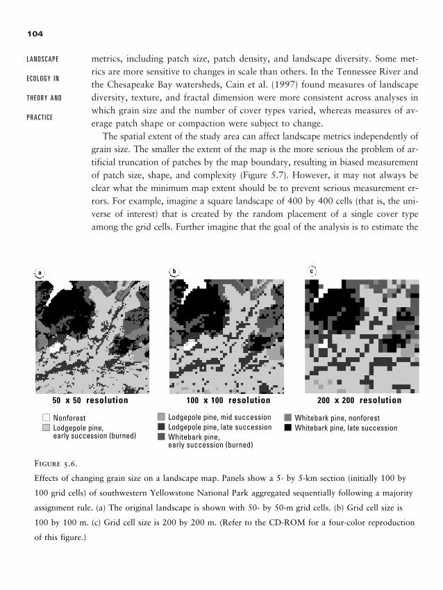
104

L A N D S C A P E

E C O L O G Y I N

T H E O R Y A N D

P R A C T I C E

metrics, including patch size, patch density, and landscape diversity. Some met-rics are more sensitive to changes in scale than others. In the Tennessee River andthe Chesapeake Bay watersheds, Cain et al. (1997) found measures of landscapediversity, texture, and fractal dimension were more consistent across analyses inwhich grain size and the number of cover types varied, whereas measures of av-erage patch shape or compaction were subject to change.

The spatial extent of the study area can affect landscape metrics independently ofgrain size. The smaller the extent of the map is the more serious the problem of ar-tificial truncation of patches by the map boundary, resulting in biased measurementof patch size, shape, and complexity (Figure 5.7). However, it may not always beclear what the minimum map extent should be to prevent serious measurement er-rors. For example, imagine a square landscape of 400 by 400 cells (that is, the uni-verse of interest) that is created by the random placement of a single cover typeamong the grid cells. Further imagine that the goal of the analysis is to estimate the

a b C

Figure 5.6.

Effects of changing grain size on a landscape map. Panels show a 5- by 5-km section (initially 100 by

100 grid cells) of southwestern Yellowstone National Park aggregated sequentially following a majority

assignment rule. (a) The original landscape is shown with 50- by 50-m grid cells. (b) Grid cell size is

100 by 100 m. (c) Grid cell size is 200 by 200 m. (Refer to the CD-ROM for a four-color reproduction

of this figure.)

a b c

2888_e05_p93-134 2/27/01 1:39 PM Page 104

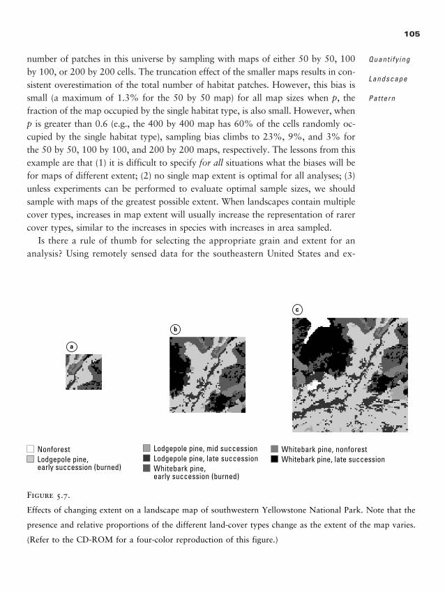
number of patches in this universe by sampling with maps of either 50 by 50, 100by 100, or 200 by 200 cells. The truncation effect of the smaller maps results in con-sistent overestimation of the total number of habitat patches. However, this bias issmall (a maximum of 1.3% for the 50 by 50 map) for all map sizes when p, thefraction of the map occupied by the single habitat type, is also small. However, whenp is greater than 0.6 (e.g., the 400 by 400 map has 60% of the cells randomly oc-cupied by the single habitat type), sampling bias climbs to 23%, 9%, and 3% forthe 50 by 50, 100 by 100, and 200 by 200 maps, respectively. The lessons from thisexample are that (1) it is difficult to specify for all situations what the biases will befor maps of different extent; (2) no single map extent is optimal for all analyses; (3)unless experiments can be performed to evaluate optimal sample sizes, we shouldsample with maps of the greatest possible extent. When landscapes contain multiplecover types, increases in map extent will usually increase the representation of rarercover types, similar to the increases in species with increases in area sampled.

Is there a rule of thumb for selecting the appropriate grain and extent for ananalysis? Using remotely sensed data for the southeastern United States and ex-

105

Quant i fy ing

Landscape

Pat tern

a

b

c

Figure 5.7.

Effects of changing extent on a landscape map of southwestern Yellowstone National Park. Note that the

presence and relative proportions of the different land-cover types change as the extent of the map varies.

(Refer to the CD-ROM for a four-color reproduction of this figure.)

2888_e05_p93-134 2/27/01 1:40 PM Page 105

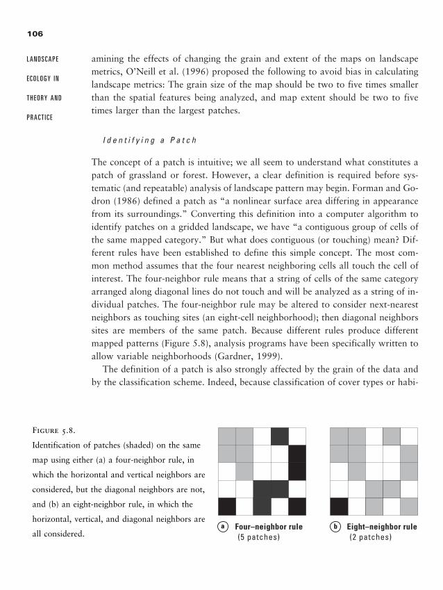
amining the effects of changing the grain and extent of the maps on landscapemetrics, O’Neill et al. (1996) proposed the following to avoid bias in calculatinglandscape metrics: The grain size of the map should be two to five times smallerthan the spatial features being analyzed, and map extent should be two to fivetimes larger than the largest patches.

I d e n t i f y i n g a P a t c h

The concept of a patch is intuitive; we all seem to understand what constitutes apatch of grassland or forest. However, a clear definition is required before sys-tematic (and repeatable) analysis of landscape pattern may begin. Forman and Go-dron (1986) defined a patch as “a nonlinear surface area differing in appearancefrom its surroundings.” Converting this definition into a computer algorithm toidentify patches on a gridded landscape, we have “a contiguous group of cells ofthe same mapped category.” But what does contiguous (or touching) mean? Dif-ferent rules have been established to define this simple concept. The most com-mon method assumes that the four nearest neighboring cells all touch the cell ofinterest. The four-neighbor rule means that a string of cells of the same categoryarranged along diagonal lines do not touch and will be analyzed as a string of in-dividual patches. The four-neighbor rule may be altered to consider next-nearestneighbors as touching sites (an eight-cell neighborhood); then diagonal neighborssites are members of the same patch. Because different rules produce differentmapped patterns (Figure 5.8), analysis programs have been specifically written toallow variable neighborhoods (Gardner, 1999).

The definition of a patch is also strongly affected by the grain of the data andby the classification scheme. Indeed, because classification of cover types or habi-

106

L A N D S C A P E

E C O L O G Y I N

T H E O R Y A N D

P R A C T I C E

Four–neighbor rule (5 patches)

Eight–neighbor rule (2 patches)

a b

Figure 5.8.

Identification of patches (shaded) on the same

map using either (a) a four-neighbor rule, in

which the horizontal and vertical neighbors are

considered, but the diagonal neighbors are not,

and (b) an eight-neighbor rule, in which the

horizontal, vertical, and diagonal neighbors are

all considered.

2888_e05_p93-134 2/27/01 1:40 PM Page 106

107

Quant i fy ing

Landscape

Pat tern

tats can be dramatically different among species or for different ecologicalprocesses, a single map may need to be reclassified to perform patch-based analy-ses for various species or processes. Any subsequent quantitative analyses basedon patches (e.g., average patch size, distribution of patches by size, perimeter-to-area relationships) are a function of all the factors inherent in defining patches,and this definition process should be well thought out. Patches are not fixed ele-ments of the landscape, but rather are useful spatial constructs that vary with theobjectives of a given study.

M o s t M e t r i c s A r e C o r r e l a t e d

As with the classification scheme and spatial scale of the data, the metrics chosen foranalysis must also be selected based on the objectives of the study. In addition, manymetrics are strongly correlated with one another, containing redundant information.Riitters et al. (1995) examined the correlations among 55 different landscape met-rics by factor analysis and identified only five independent factors. Thus, many typ-ical landscape metrics are not measuring different qualities of spatial pattern. In theRiitters et al. (1995) analysis, the five independent factors represented (1) the num-ber of classes or cover types on the map, (2) whether the texture of the landscapepattern was fine or coarse, (3) the degree to which patches were compact or dis-sected, (4) whether patches were linear or planar, and (5) whether patch perimeterswere complicated or simple in shape. Thus, the analyst should select metrics that arerelatively independent of one another, with each metric (or grouping of metrics) ableto detect ecologically meaningful landscape properties. It is often necessary to havemore than one metric to characterize a landscape because there simply is not onenumber that “says it all.” However, reporting ten highly correlated metrics does notyield new information, but only makes interpretations more difficult. Just becausesomething can be computed does not mean that it should be computed!

W h a t C o n s t i t u t e s a S i g n i f i c a n t C h a n g e ?

One challenge still facing landscape ecologists is that the statistical properties andbehavior of some landscape metrics are not well known. In cases where a singlenumber is reported for a landscape, we may have little understanding of the degreeto which landscape pattern must change to be able to detect an ecologically im-portant or statistically significant change in the numerical value of the metric (Wick-ham et al., 1997). While this remains an important area of current research and de-velopment, the user should definitely consider the criteria that will be applied to

2888_e05_p93-134 2/27/01 1:40 PM Page 107

determine whether an observed change is or is not meaningful. Presently, there is aneed to build a collective library of empirical studies in which ecological responsesare related to particular landscape configurations. Unfortunately, we have the powerto measure and report more about landscape pattern than we can interpret in termsof effects on ecological processes. Therefore, serious attention must be paid to therigor with which the metrics are applied and interpreted. Neutral landscape mod-els (see Chapter 6) may be of particular use in elucidating the behavior of individ-ual metrics and providing some measure of their statistical reliability.

M E T R I C S F O R Q U A N T I F Y I N G L A N D S C A P E P A T T E R N

Caveats thus stated, numerous metrics can be computed for a landscape data set,too many for us to review in this text. The recommended readings listed at theend of this chapter provide excellent and very comprehensive treatments of thecalculation and interpretation of nearly 100 metrics in total. Box 5.2 also con-tains practical information on some readily available software packages that canbe used to analyze landscape pattern. In this section, we review some of the com-monly used metrics within three broad categories: metrics of landscape composi-tion; measures of spatial configuration, including contagion and patch-based met-rics; and fractals. We then present examples of studies in which landscape metricswere used, and we address the challenge of the interpretation of multiple metrics.

M e t r i c s o f L a n d s c a p e C o m p o s i t i o n

Metrics that quantify the composition of the landscape are not usually spatiallyexplicit. That is, they measure what is present and in their relative amounts, orproportions, without reference to where on the landscape they may be located.However, nonspatial metrics may be important descriptors measuring landscapeconstraints of values of spatially explicit metrics. For example, the proportion ofthe landscape occupied by a given cover type limits the range of patch numberand sizes (Gardner et al., 1987; Gustafson and Parker, 1992).

Fraction or Proportion (pi) OccupiedA simple but useful number to calculate is the proportion, pi, of the landscapethat is occupied by each cover type i, where i � 1 to s, and s is the total numberof cover types on the map. The pi values are estimated by counting the number

108

L A N D S C A P E

E C O L O G Y I N

T H E O R Y A N D

P R A C T I C E

�

2888_e05_p93-134 2/27/01 1:40 PM Page 108

of grid cells of each cover type and then dividing by the total number of grid cellspresent on the entire landscape. The expected value of the pi’s is equal to 1/s, mak-ing this statistic marginally useful as a landscape metric, although deviations ofthe pi’s from the expected value may be a useful indicator of landscape hetero-geneity. The pi’s have a strong influence on other aspects of pattern, such as patchsize or length of edge in the landscape (Gardner et al., 1987); therefore, these re-lationships will be further explored in the section on neutral models. The pi’s havebeen used to calculate a variety of landscape metrics, resulting in correlationsamong the metrics sharing this information.

Relative RichnessThis simple metric calculates the number of cover types present, without regardto how they are spatially arranged, as a percent of the total number of possiblecover types. Thus,

R � �sm

s

ax� � 100

109

Quant i fy ing

Landscape

Pat tern

B O X 5 . 2THE PRACTICAL SIDE: SOFTWARE FOR

SPATIAL PATTERN ANALYSIS

Most GIS systems have only a limited capability to per-

form the types of landscape pattern analyses de-

scribed in the text, although this is changing rapidly.

However, a variety of researchers has developed com-

puter programs for spatial analysis that can be read-

ily obtained. A widely used package is FRAGSTATS

(McGarigal and Marks, 1995), developed at Oregon

State University and available by anonymous ftp or

on the CD provided with Gergel and Turner (2001).

FRAGSTATS is comprehensive and available for both

raster and vector maps, and McGarigal and Marks

provided excellent documentation. Users interested

in running landscape analyses might begin with

FRAGSTATS. Another analysis program designed for

both raster and ASCII input data is APACK, developed

by Mladenoff and colleagues at the University of Wis-

consin–Madison; interested users should visit the

following web site for further information: http://flel.

forest.wisc.edu/projects/apack/. For users of the GIS

GRASS, Baker and Cai (1992) developed the r.le pro-

grams that interface with the GRASS system and are

also available by anonymous ftp. A program called

RULE (Gardner, 1999) can be used to explore the im-

plications of different patch-definition rules on land-

scape maps, as well as to generate neutral land-

scape models (see Chapter 6); RULE is also available

on the CD provided by Gergel and Turner (2001) or

by ftp.

2888_e05_p93-134 2/27/01 1:40 PM Page 109

where s � the number of cover types present, smax is the maximum number ofcover types possible, and the multiplication by 100 converts the fraction to a per-cent. The value of smax is arbitrary (see prior discussion of classification scheme),but should be based on the maximum number of cover types observed for simi-lar landscapes. Relative richness is especially useful for comparisons of landscapesbefore and after natural disturbances and the regeneration of vegetation covertypes through time.

Diversity and DominanceMetrics derived from information theory were first applied to landscape analysesby Romme (1982) to describe changes in the area occupied by forests of varyingsuccessional stage through time in a watershed in Yellowstone National Park,Wyoming. Two related indexes are dominance and diversity (O’Neill et al., 1988a),which provide the same information about the landscape. Diversity, or relativeevenness, refers to how evenly the proportions of cover types are distributed. Forexample, if three cover types are present, does each occupy 33% of the landscape,or does one occupy 90% and the others only 5% each? The equation is given by

H �

��s

i�1(pi) ln (pi)

ln (s)

where H � diversity, pi � the proportion of the landscape occupied by cover typei, and s � the number of cover types present. Dividing through by ln (s) normal-izes the index to range between zero and one. A high value of H indicates greaterevenness, and a low value indicates less evenness.

Closely related to diversity is dominance, which is simply the deviation fromthe maximum possible diversity:

D �

Hmax � �s

i�1pi ln (pi)

Hmax

where D � dominance, pi � the proportion of the landscape occupied by covertype i, and Hmax � ln (s), which is the maximum possible diversity for a landscapehaving s cover types. Again, this index ranges between zero and one, with a highvalue indicating dominance by one or a few cover types and a low value indicat-ing that the cover types are present in similar proportions. Note that the summa-

110

L A N D S C A P E

E C O L O G Y I N

T H E O R Y A N D

P R A C T I C E

2888_e05_p93-134 2/27/01 1:40 PM Page 110

tion in the numerator actually represents a deviation from Hmax because the log-arithms of values �1.0 are negative.

Two important points should be noted here. First, dominance and diversity areredundant, so any analysis need not report both. Second, and reflecting a moregeneral issue for metrics of this type, dominance and diversity may return verysimilar numerical values for landscapes that are qualitatively different. For ex-ample, a landscape occupied by 80% agriculture, 10% forest, and 10% wetlandwould have the same diversity value as one occupied by 80% forest, 10% agri-culture, and 10% wetland. Thus, the usefulness of these metrics is rather limited.

ConnectivityIf a pattern across a landscape can be represented as a series of nodes and link-ages, the gamma index described in Forman and Godron (1986) is a useful over-all measure:

� � �Lm

L

ax� � �

3(VL� 2)�

where L � the number of links in the network and V � the number of nodes inthe network. This index can range between zero to one, with low values indicat-ing less connectivity and high values indicated higher connectivity.

M e a s u r e s o f S p a t i a l C o n f i g u r a t i o n I : C o n t a g i o n

Probabilities of AdjacencyThe metrics described so far do not account for the spatial arrangement of habi-tat types. Probabilities of adjacency, that is, the probability that a grid cell of covertype i is adjacent to a grid cover type j, are sensitive to the fine-scale spatial dis-tribution of cover types. These probabilities can be computed simply as

qi,j � �nni

i

,j�

where ni � the number of grid cells of cover type i and ni,j � the number of in-stances when cover type i is adjacent to cover type j. Note that this initial calcu-lation assumes a single one-directional pass through the data matrix, e.g., hori-zontal or vertical. These probabilities can be computed directionally to detectdirectionality in the pattern (anisotropy), and average values can also be deter-

111

Quant i fy ing

Landscape

Pat tern

2888_e05_p93-134 2/27/01 1:40 PM Page 111

mined. If you calculate the probabilities simultaneously in four directions, the de-nominator must be modified to reflect the correct potential number of neighbors.

The qi,i values, which are the diagonals of the Q matrix, give a useful measureof the degree of clumping found in each cover type. The qi,i’s give the likelihoodthat cells of the same cover type are found adjacent to each other. High qi,i val-ues indicate a highly aggregated cover type, and low qi,i values indicate that thecover type tends to occur in isolated grid cells or small patches. Thus, this metriccan be used to characterize relatively fine scale detail of the spatial pattern and isuseful in providing data on each cover type.

ContagionThe contagion metric (O’Neill et al., 1988a; Li and Reynolds, 1993) distinguishesbetween overall landscape patterns that are clumped or rather dissected. The equa-tion is given by

C �

1 � �s

i�1�s

j�1(Pij) ln (Pij)

2 ln (s)

where Pi,j � the probability that two randomly chosen adjacent pixels belong tocover types i and j, respectively, that is, Pij � PiPj/i ; and s is the number of covertypes on the landscape. Note that the equation for contagion can be formulateddifferently if the probabilities of adjacency are computed by another algorithm(see Li and Reynolds, 1993, for details). The metric ranges from zero to one, witha high value indicating generally clumped patterns of cover across the landscapeand a low value indicating a landscape with a dispersed pattern of cover types.Contagion is useful in capturing relatively fine scale differences in pattern that re-late to the texture or graininess of the map.

M e a s u r e s o f S p a t i a l C o n f i g u r a t i o n I I : P a t c h - B a s e d M e t r i c s

Given a landscape data set in which the grid cells are assigned to discrete cate-gories, patches, which are contiguous areas of the same cover type, can be iden-tified and their distributions described. Again, the importance of the classificationscheme used cannot be overstated. Patches are commonly identified in the dataset by either of two rules. First, a patch may consist of adjacent cells in only thenorth–south and east–west directions on the grid, that is, the four nearest neigh-bors, excluding the diagonals. Alternatively, a patch may consist of adjacent cells

112

L A N D S C A P E

E C O L O G Y I N

T H E O R Y A N D

P R A C T I C E

2888_e05_p93-134 2/27/01 1:40 PM Page 112

from among the eight nearest neighbors, including both the adjacent and diago-nal neighbors. Choice of this rule will influence the results of any patch-basedmeasurements (see Figure 5.7). Patch-based measures of pattern include patch size,perimeter, number, shape, and density.

Patch Area and PerimeterOnce patches are located, some simple summaries can be computed easily. Thearea and perimeter of each patch can be determined. These results can then besummarized for the landscape or, more meaningfully for each cover type, by dis-playing a frequency distribution of numbers of patches by patch size, a cumula-tive frequency distribution of patch sizes, the simple mean and standard deviationof patch size, or the area-weighted mean patch size. The simple mean patch sizeis sensitive to the number of small or single-celled patches in the landscape; useof an area-weighted mean patch size avoids this problem.

Perimeter to area ratios (P/A) also serve as useful indexes of shape complexity.For a given area, a high P/A ratio indicates a complex or elongated boundaryshape, and a low P/A ratio indicates a more compact and simple shape. However,P/A is sensitive to patch size, decreasing as patch size increases for a given shape.A variety of shape indexes are based on perimeter and area measurements, someof which correct for the size problem (e.g., see Baker and Cai, 1992). If computedfor each patch, means, standard deviations, and frequency distributions can againsummarize these ratios.

ConnectivityOnce patches have been demarcated in the data set, some measures of connectiv-ity for individual cover types can be computed. One very simple metric is simplythe relative size of the largest patch of habitat k:

RSi � �pi �

LmCi

� n�

where LCi � the size of the largest patch of cover type, pi � the proportion of thelandscape in cover type i, and m � n gives the size of the landscape that containsm rows and n columns. If all of cover type k occurs as a single patch, the valueof the index equals 1.0, indicating complete connectivity. When the cover type isdispersed into very small patches, the index approaches zero.

Another measure of connectivity (or its inverse, fragmentation) of a habitat typeis to calculate the average distance between patches. This is often done in one of

113

Quant i fy ing

Landscape

Pat tern

2888_e05_p93-134 2/27/01 1:40 PM Page 113

two ways. First, the distance can be computed from the center of one patch to thecenter of the next nearest patch. This method requires an algorithm for deter-mining patch centroids. Second, the distance can be computed from the grid cellson each of two patches that are closest to one another, thereby providing a min-imum interpatch distance.

Proximity IndexThe degree to which patches in the landscape are isolated from other patches ofthe same cover type may be of importance, especially when species habitat-usepatterns are of interest. Gustafson and Parker (1992) developed an index that canbe computed for each patch on a landscape to determine the relative isolation ofthe patches. This index is given by

PXi � ��

�

�nsk

k�

where PXi is the proximity index for focal patch i, and then within a specifiedsearch distance (which must be set by the user), sk is the area of patch k withinthe search buffer and nk is the nearest-neighbor distance between a grid cell ofthe focal patch and the nearest grid cell of patch k. This index is not normalizedbut returns an absolute number. Low values indicate patches that are relativelyisolated from other patches within the specified buffer distance, and high valuesindicate patches that are relatively connected to other patches.

Area-Weighted Average Patch SizeThe frequency distribution of patch sizes on many landscapes is frequently skewed;a few large patches will be found surrounded by many smaller patches. Underthese conditions, the simple arithmetic average does not reflect the expected patchsize that would be encountered by a simple random placement of points on themap. A more useful method of averaging is to weight patch sizes by area (Stauf-fer and Aharony, 1992). If there are n patches on the landscape and Sk is the sizeof the kth patch, then the area-weighted average patch size is

Sa �� (Sk

2)

� (Sk)

Area weighting of other indexes has been employed when skewed frequency dis-tributions result in a disproportionate effect of small patches on the metric of in-terest (McGarigal and Marks, 1995).

114

L A N D S C A P E

E C O L O G Y I N

T H E O R Y A N D

P R A C T I C E

2888_e05_p93-134 2/27/01 1:40 PM Page 114

F r a c t a l s

Fractals are considered separately here because, although their calculation is gen-erally based on the spatial distribution of cover types or patches in the landscape,they may be reported in various ways: overall for the whole map or landscape,overall for each cover type, or for individual patches. In this section, we explainfractals briefly, focusing here on their use as a descriptor of spatial pattern. Webegin by explaining very basically the development of fractals and some impor-tant concepts in their meaning. However, the use and application of fractals isvery rich, and we refer interested readers especially to Milne (1991b) and Sugi-hara and May (1990) for more detailed treatments.

Many years ago, the scientist Lewis Fry Richardson studied the relation be-tween the measured length of a coastline or lake perimeter and the scale at whichit was mapped. Fry found that the length of the coastline as estimated by the mapincreased logarithmically with increasing map resolution. Why did this occur? Asthe resolution of the map was increased, more and more previously unresolvedfeatures could be delineated; in the limit, the length of the coastline is infinite (seeChapter 2). For shapes like coastlines, the curves are never actually as smooth asthe drawn lines would have us believe. These findings were incorporated into thetheory of fractals proposed by the mathematician Mandelbrot (1983).

The essence of fractals is the recognition that, for many phenomena, the amountof resolvable detail is a function of scale. An important corollary is that increas-ing the resolution does not result in an absolute increase in precision, but ratherit reveals variation that passed unnoticed before. Consider, for example, two idealfractal curves (Figure 5.9). If we measure the distance from A to B and measureby units of length x, we observe that in Figure 5.9a the distance � 4. If we de-crease the resolution by a factor of 3 so that units are x/3 � y, more detail is seen;in Figure 5.9b, the distance from A to C is now 4 units of y, but the total dis-tance between A and B will be longer in units of y than in units of x. Because thecurves in Figure 5.9 behave similarly at all scales, once the properties are knownat one scale they can be deduced from another merely by applying a scaling pa-rameter. The level of variation present at all scales can be described by a singleparameter, the fractal dimension, defined by Mandelbrot (1983) as

D � �lloogg

Nr

�

where N � number of steps used to measure a pattern unit length, and r is thescale ratio. In Figure 5.9a and b, N � 4 and r � 3, so D � 1.2618.

115

Quant i fy ing

Landscape

Pat tern

2888_e05_p93-134 2/27/01 1:40 PM Page 115

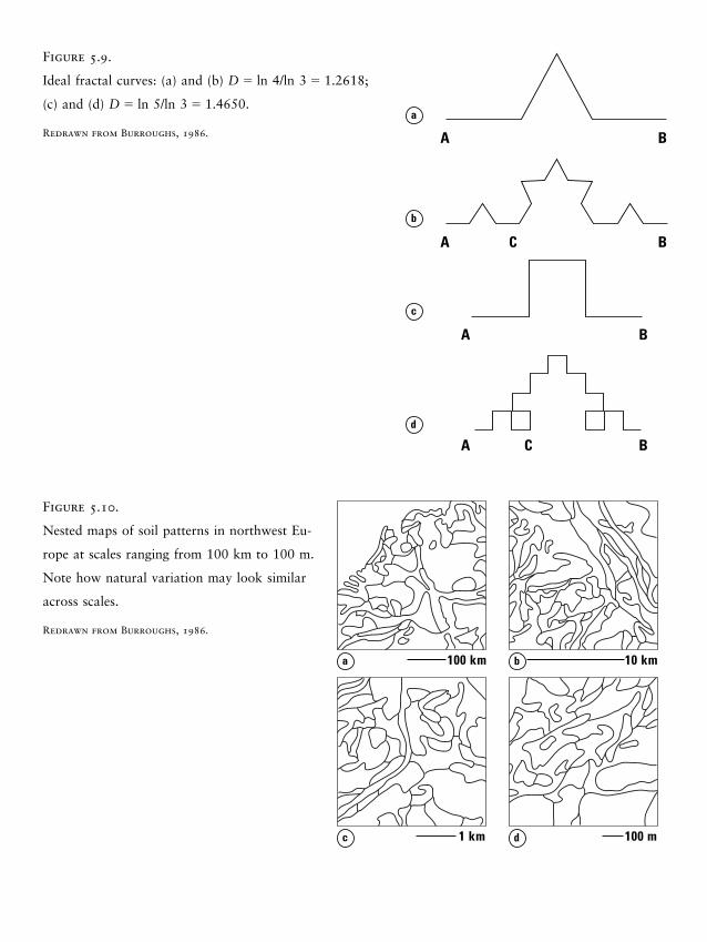
A B

A B

A C B

A C B

a

b

c

d

Figure 5.9.

Ideal fractal curves: (a) and (b) D � ln 4/ln 3 � 1.2618;

(c) and (d) D � ln 5/ln 3 � 1.4650.

Redrawn from Burroughs, 1986.

100 km 10 km

1 km 100 m

a b

c d

Figure 5.10.

Nested maps of soil patterns in northwest Eu-

rope at scales ranging from 100 km to 100 m.

Note how natural variation may look similar

across scales.

Redrawn from Burroughs, 1986.

2888_e05_p93-134 2/27/01 1:40 PM Page 116

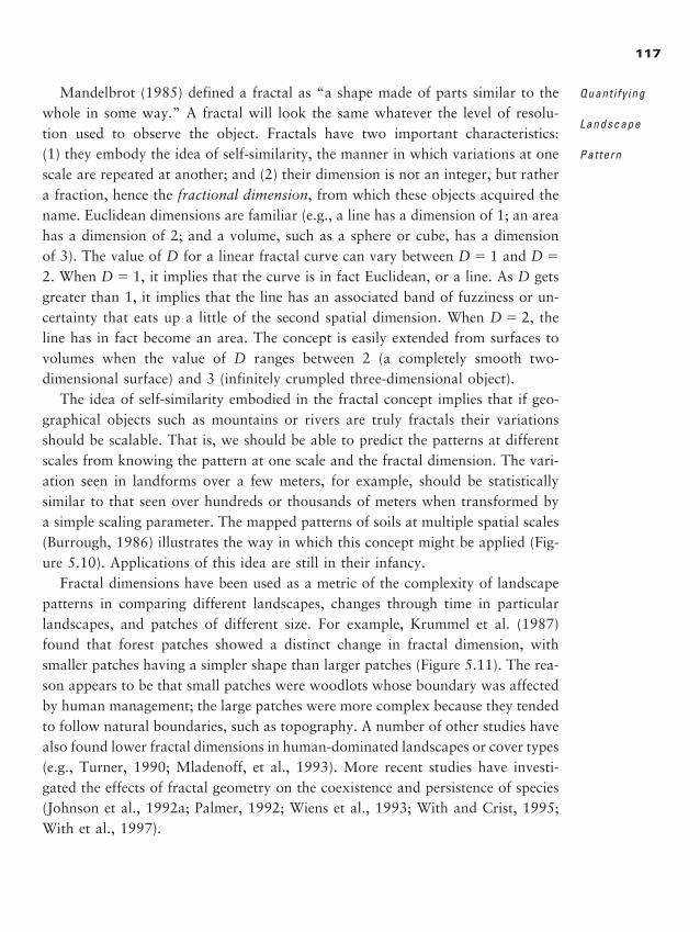
Mandelbrot (1985) defined a fractal as “a shape made of parts similar to thewhole in some way.” A fractal will look the same whatever the level of resolu-tion used to observe the object. Fractals have two important characteristics: (1) they embody the idea of self-similarity, the manner in which variations at onescale are repeated at another; and (2) their dimension is not an integer, but rathera fraction, hence the fractional dimension, from which these objects acquired thename. Euclidean dimensions are familiar (e.g., a line has a dimension of 1; an areahas a dimension of 2; and a volume, such as a sphere or cube, has a dimensionof 3). The value of D for a linear fractal curve can vary between D � 1 and D �

2. When D � 1, it implies that the curve is in fact Euclidean, or a line. As D getsgreater than 1, it implies that the line has an associated band of fuzziness or un-certainty that eats up a little of the second spatial dimension. When D � 2, theline has in fact become an area. The concept is easily extended from surfaces tovolumes when the value of D ranges between 2 (a completely smooth two-dimensional surface) and 3 (infinitely crumpled three-dimensional object).

The idea of self-similarity embodied in the fractal concept implies that if geo-graphical objects such as mountains or rivers are truly fractals their variationsshould be scalable. That is, we should be able to predict the patterns at differentscales from knowing the pattern at one scale and the fractal dimension. The vari-ation seen in landforms over a few meters, for example, should be statisticallysimilar to that seen over hundreds or thousands of meters when transformed bya simple scaling parameter. The mapped patterns of soils at multiple spatial scales(Burrough, 1986) illustrates the way in which this concept might be applied (Fig-ure 5.10). Applications of this idea are still in their infancy.

Fractal dimensions have been used as a metric of the complexity of landscapepatterns in comparing different landscapes, changes through time in particularlandscapes, and patches of different size. For example, Krummel et al. (1987)found that forest patches showed a distinct change in fractal dimension, withsmaller patches having a simpler shape than larger patches (Figure 5.11). The rea-son appears to be that small patches were woodlots whose boundary was affectedby human management; the large patches were more complex because they tendedto follow natural boundaries, such as topography. A number of other studies havealso found lower fractal dimensions in human-dominated landscapes or cover types(e.g., Turner, 1990; Mladenoff, et al., 1993). More recent studies have investi-gated the effects of fractal geometry on the coexistence and persistence of species(Johnson et al., 1992a; Palmer, 1992; Wiens et al., 1993; With and Crist, 1995;With et al., 1997).

117

Quant i fy ing

Landscape

Pat tern

2888_e05_p93-134 2/27/01 1:40 PM Page 117

The Fractal as a Measure of Patch ShapeThe fractal dimension of a patch is easy to calculate and has proved to be a use-ful indicator of shape complexity (Krummel et al., 1987; Sugihara and May, 1990).However, unless care is taken in the estimation of this metric, serious errors canresult. Avoiding these errors requires (1) a clear understanding of the algebraic re-lationships among area, perimeter, and the fractal dimension, (2) elimination ofbiases in the fractal dimension resulting from inclusion of small patches in theanalysis, and (3) specification of the level of change of the fractal dimension thatcorresponds to a significant change in patch complexity.

Mandelbrot (1983) defined the relationship between perimeter and area for atwo-dimensional object as A � (kP)d, where A is the area and P is some measureof the perimeter of the patch, that is, the radius, diameter, length of the patch, orthe actual measured perimeter; k is a constant that takes on different values de-

118

L A N D S C A P E

E C O L O G Y I N

T H E O R Y A N D

P R A C T I C E

Log A ( m2 )12.5

1.1

1.2

13.0 13.5 14.0 14.5 15.0

D

1.3

1.4

1.5

1.6

a

b c

Figure 5.11.

(a) Fractal dimension (D) of forest patches in the

vicinity of Natchez, Mississippi, as a function of

patch size. (b) Section of the original map illustrat-

ing how small patches tend to be simple in shape.

(c) Section of the original map illustrating the

more complex shapes associated with the larger

patches.

Redrawn from Krummel et al., 1987.

2888_e05_p93-134 2/27/01 1:40 PM Page 118

pending on the way that P is estimated; and d is the fractal dimension. To solvefor d, we take the logs of both sides of the equation

d �

The fractal dimension, d, will have the value of 2.0 for two-dimensional objectssuch as circles and squares and will equal 1.0 for a straight line if the length ofone side of the object is used to estimate P and k is equal to 1.0. If this is the case,then k can be dropped from the equation [ln (k) � 0.0], and the method for esti-mating the fractal simplifies to

d �

If the actual perimeter of the patch is used to estimate P, then k must be set equalto 0.25, and k cannot be dropped from the equation! Failure to properly relate kand P can produce errors much greater than the range of observed values of thefractal for patches of land cover.

Although the algebra used to estimate the fractal dimension is simple andstraightforward, a variety of alternative formulations has been used to estimatethe fractal dimension, resulting in considerable confusion when attempting to makecomparisons between studies. One alternative formulation is the reversal of therelationship between perimeter and area (assuming that k � 1.0), which gives kP �

AD. It is clear from simple algebra that this fractal, D, is equal to 1/d. Substitut-ing 1/d and taking logarithms (assuming that k � 1.0), we obtain, as before, d �

ln (A)/ln (P). Other forms of the fractal dimension can be found, including the re-lationship, P � (A1/2)d� (Lovejoy, 1985; Burrough, 1986; Lovejoy et al., 1987; Mc-Garigal and Marks, 1995). Obviously, there is no single correct (or preferred)form for estimating fractals, but authors should clearly state the algebra used tocalculate this metric so that comparisons among studies can be reliably effected.

The fractal has often been estimated by regressing the logarithms of perimeteron area (or vice versa), with the slope of the line being a statistical estimation ofthe fractal. However, unless all patches are large (patches sizes greater than 100cells), the grain size of the data set will bias the regression analysis. The value ofk must also be considered by setting the regression intercept equal to ln (k). Theextent of the map plays an important role in the estimation of the fractal, withsmaller maps resulting in fewer patches that escape the truncation effects of the

ln (A)�ln (P)

ln (A)��ln (P) � ln (k)

119

Quant i fy ing

Landscape

Pat tern

2888_e05_p93-134 2/27/01 1:40 PM Page 119

map boundary (Gardner et al., 1987). Presently, little effort has been made to linktogether these problems and establish a rigorous sampling theory for fractals(Loehle and Li, 1996). Only when samples are extremely large (e.g., Lovejoy, 1985;Krummel et al., 1987) can reliable estimates of the fractal be ensured.

O t h e r U s e f u l M e t r i c s

There are numerous other quantities that can be assigned to a grid cell or poly-gon on a landscape map and that may have important ecological implications. Forexample, in regions that have road networks, which includes most landscapes,road length, road density, or distance to the nearest road may be important in-dexes of certain functional aspects of landscape structure. In a broad-scale analy-sis of habitat-use patterns of recolonizing gray wolves (Canis lupus) in northernWisconsin, USA, Mladenoff et al. (1995) found road density to be an importantpredictor of where pack territories would be located.

The length of riparian vegetation (nonagricultural and nonurban) is anothermetric that may have important ecological implications because of the ability ofriparian corridors to buffer nutrient transfers from land to water (e.g., Peterjohnand Correll, 1984). Population density, which is now readily available for recentyears in digital format from the U.S. Bureau of the Census at the resolution ofcensus tracts, may also serve as a useful metric of processes in a landscape (e.g.,Turner et al., 1996; Wear et al., 1996).

A p p l i c a t i o n s o f L a n d s c a p e P a t t e r n A n a l y s e s

In numerous studies, landscape metrics have been used to describe changes in alandscape through time or to compare landscapes (e.g., Whitney and Somerlot,1985; Iverson, 1988; Turner and Ruscher, 1988; LaGro and DeGloria, 1992; Kien-ast, 1993; and many others). We discuss just a few here to provide examples ofthe insights that have been produced by the application of landscape metrics; otherexamples of the use of landscape metrics in empirical studies and spatial modelswill be found in subsequent chapters.

Spies et al. (1994) studied the process of forest fragmentation in a 2589-km2

managed forest landscape in northwest Oregon, USA, between 1972 and 1988 us-ing Landsat data. Management for timber production in this region has convertedextensive areas of old-growth forest to young conifer plantations. Spies et al. (1994)focused on changes in closed-canopy conifer forest (CF) and examined differencesin landscape pattern among different classes of landowner (see Figure 5.3). Re-

120

L A N D S C A P E

E C O L O G Y I N

T H E O R Y A N D

P R A C T I C E

2888_e05_p93-134 2/27/01 1:40 PM Page 120

sults revealed a decline in CF from 71% to 58% during the study period, but therates of decline varied among landowners and were highest on private lands. Theamount of edge habitat increased and the amount of interior habitat decreased onall ownerships. Large remaining patches (�5000 ha) of contiguous interior forestwere restricted to public lands on which timber harvesting was restricted. In astudy with similar objectives, Turner et al. (1996) compared the spatial patternof forested landscapes between landowner categories in the southern AppalachianMountains and the Olympic Peninsula, Washington. Differences in landscape pat-tern were observed between the two study regions and between different cate-gories of land ownership. In both regions, private lands contained less forest cover,but a greater number of small forest patches than did public lands. Differences inlandscape patterns were interpreted in terms of the management objectives of dif-ferent types of landowner. This study demonstrated that the way in which humanendeavors are organized through the institutions and scale of land ownership pro-duces qualitatively different landscape patterns and dynamics (Turner et al., 1996).

In a study of forested landscapes of the upper Midwest, USA, Mladenoff et al.(1993) compared landscape patterns in an undisturbed old-growth area and anearby area subjected to forest management and harvest (Figure 5.12). Managedforests were distinctly different from the natural old-growth landscape, which wasdominated by large areas of eastern hemlock (Tsuga canadensis), sugar maple(Acer saccharum), and yellow birch (Betula allegheniensis). The disturbed land-scape had smaller, remnant patches of old-growth ecosystems scattered amongearly successional forests. Forest patches were also significantly simpler in shape(lower fractal dimension) in the fragmented landscape. Important ecosystem jux-tapositions of the old-growth landscape, such as hemlock associated with lowlandconifers, were lost, and characteristic patterns of heterogeneity due to landformpatterns in this glaciated region were altered by human disturbances.

M a k i n g S e n s e O u t o f M u l t i p l e M e t r i c s

The description of landscape pattern requires more than one metric, so the ques-tion now becomes how to select a relevant subset. Determining how many met-rics to use and how to combine the metrics so that the results are meaningful andinterpretable remains challenging. The subset should explain pattern variabilityacross the landscape, but redundancy should be minimized, particularly with in-dexes that may be highly correlated with each other. O’Neill et al. (1988a) ob-served that landscape scenes from across the eastern United States could be dif-ferentiated from one another by using three metrics, dominance, contagion, and

121

Quant i fy ing

Landscape

Pat tern

2888_e05_p93-134 2/27/01 1:40 PM Page 121

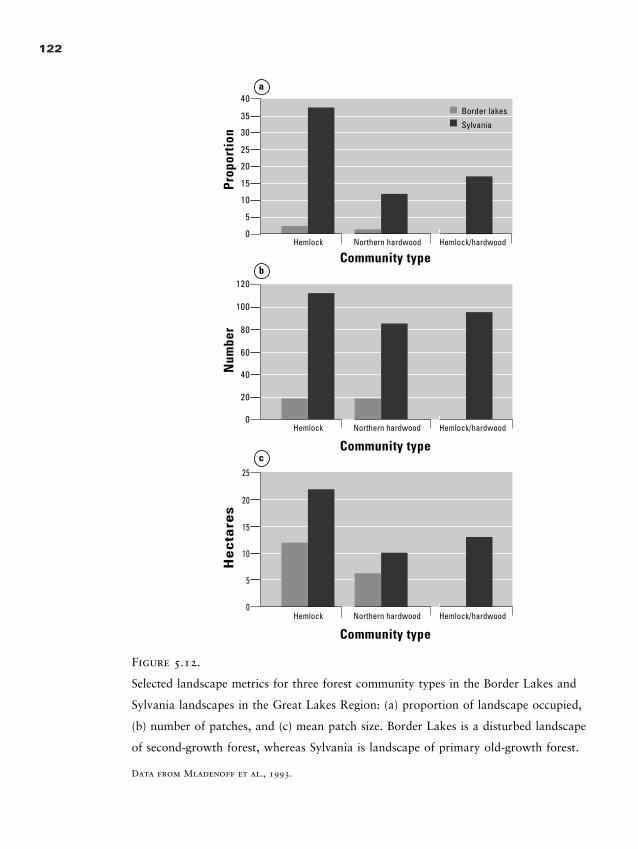
122

Prop

orti

onN

umbe

rHemlock Northern hardwood Hemlock/hardwood

10

20

30

40

0

5

15

25

35 Border lakes

Sylvania

Community type

Community type

Community type

Hemlock Northern hardwood Hemlock/hardwood

40

80

120

0

20

60

100

He

cta

res

Hemlock Northern hardwood Hemlock/hardwood

10

20

0

5

15

25

a

b

c

Figure 5.12.

Selected landscape metrics for three forest community types in the Border Lakes and

Sylvania landscapes in the Great Lakes Region: (a) proportion of landscape occupied,

(b) number of patches, and (c) mean patch size. Border Lakes is a disturbed landscape

of second-growth forest, whereas Sylvania is landscape of primary old-growth forest.

Data from Mladenoff et al., 1993.

2888_e05_p93-134 2/27/01 1:40 PM Page 122

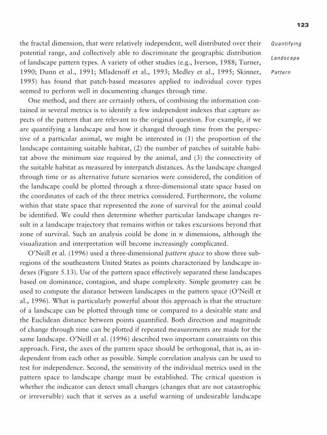
the fractal dimension, that were relatively independent, well distributed over theirpotential range, and collectively able to discriminate the geographic distributionof landscape pattern types. A variety of other studies (e.g., Iverson, 1988; Turner,1990; Dunn et al., 1991; Mladenoff et al., 1993; Medley et al., 1995; Skinner,1995) has found that patch-based measures applied to individual cover typesseemed to perform well in documenting changes through time.

One method, and there are certainly others, of combining the information con-tained in several metrics is to identify a few independent indexes that capture as-pects of the pattern that are relevant to the original question. For example, if weare quantifying a landscape and how it changed through time from the perspec-tive of a particular animal, we might be interested in (1) the proportion of thelandscape containing suitable habitat, (2) the number of patches of suitable habi-tat above the minimum size required by the animal, and (3) the connectivity ofthe suitable habitat as measured by interpatch distances. As the landscape changedthrough time or as alternative future scenarios were considered, the condition ofthe landscape could be plotted through a three-dimensional state space based onthe coordinates of each of the three metrics considered. Furthermore, the volumewithin that state space that represented the zone of survival for the animal couldbe identified. We could then determine whether particular landscape changes re-sult in a landscape trajectory that remains within or takes excursions beyond thatzone of survival. Such an analysis could be done in n dimensions, although thevisualization and interpretation will become increasingly complicated.

O’Neill et al. (1996) used a three-dimensional pattern space to show three sub-regions of the southeastern United States as points characterized by landscape in-dexes (Figure 5.13). Use of the pattern space effectively separated these landscapesbased on dominance, contagion, and shape complexity. Simple geometry can beused to compute the distance between landscapes in the pattern space (O’Neill etal., 1996). What is particularly powerful about this approach is that the structureof a landscape can be plotted through time or compared to a desirable state andthe Euclidean distance between points quantified. Both direction and magnitudeof change through time can be plotted if repeated measurements are made for thesame landscape. O’Neill et al. (1996) described two important constraints on thisapproach. First, the axes of the pattern space should be orthogonal, that is, as in-dependent from each other as possible. Simple correlation analysis can be used totest for independence. Second, the sensitivity of the individual metrics used in thepattern space to landscape change must be established. The critical question iswhether the indicator can detect small changes (changes that are not catastrophicor irreversible) such that it serves as a useful warning of undesirable landscape

123

Quant i fy ing

Landscape

Pat tern

2888_e05_p93-134 2/27/01 1:40 PM Page 123

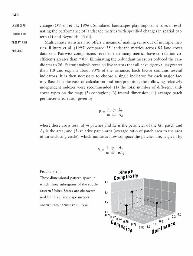
change (O’Neill et al., 1996). Simulated landscapes play important roles in eval-uating the performance of landscape metrics with specified changes in spatial pat-tern (Li and Reynolds, 1994).

Multivariate statistics also offers a means of making sense out of multiple met-rics. Riitters et al. (1995) compared 55 landscape metrics across 85 land-coverdata sets. Pairwise comparisons revealed that many metrics have correlation co-efficients greater than 0.9. Eliminating the redundant measures reduced the can-didates to 26. Factor analysis revealed five factors that all have eigenvalues greaterthan 1.0 and explain about 83% of the variance. Each factor contains several indicators. It is then necessary to choose a single indicator for each major fac-tor. Based on the ease of calculation and interpretation, the following relativelyindependent indexes were recommended: (1) the total number of different land-cover types on the map; (2) contagion; (3) fractal dimension; (4) average patchperimeter–area ratio, given by

P � �m1

� �m

k�1�AEk

k�

where there are a total of m patches and Ek is the perimeter of the kth patch andAk is the area; and (5) relative patch area (average ratio of patch area to the areaof an enclosing circle), which indicates how compact the patches are, is given by

R � �m1

� �m

k�1�

ALk

k�

124

L A N D S C A P E

E C O L O G Y I N

T H E O R Y A N D

P R A C T I C E

0.70 0.72 0.74

0.76 0.78

0.80 0.8

0.6 0.4

0.2 0.0

1.0

1.6

1.4

1.2

1.0

ShapeComplexity

Contagion Dominance

Figure 5.13.

Three-dimensional pattern space in

which three subregions of the south-

eastern United States are character-

ized by three landscape metrics.

Adapted from O’Neill et al., 1996.

2888_e05_p93-134 2/27/01 1:40 PM Page 124

where Lk is one-half of the longest straight line that can be drawn within thepatch. Notice that the denominator is the area of a circle, with Lk as the radius,that will approximately enclose the patch. These five metrics provide a minimumset of independent measures of qualitatively different aspects of spatial patternbased on 85 landscapes scattered across the United States. Therefore, these fivemetrics should be useful in many applications, at least in temperate zones.

Other studies have also suggested a subset of measurements that might char-acterize landscape pattern. McGarigal and Marks (1995) also conducted a prin-cipal components analysis of 30 different metrics calculated for late-successionalforests in the northwestern United States. Their analysis revealed three indepen-dent factors: (1) patch shape and edge contrast, (2) patch density, and (3) patchsize. Li and Reynolds (1994, 1995) used theoretical considerations to propose fivedifferent aspects of spatial heterogeneity that could be computed: (1) number ofland-cover types and (2) proportion of each type on the landscape; (3) spatialarrangement of patches; (4) patch shape; and (5) contrast between neighboringpatches. We would then select a metric to quantify each of these fundamentallydifferent aspects of pattern to avoid redundancy among metrics.

Methods for quantification of spatial pattern on categorical maps continue todevelop rapidly. We have discussed a number of basic calculations here, but havenot attempted to present all the metrics that have been proposed. Readers inter-ested in additional metrics are referred especially to Baker and Cai (1992), Baskentand Jordan (1995), McGarigal and Marks (1995), Riitters et al. (1995), Haines-Young and Chopping (1996), and Gustafson (1998). In addition, readers inter-ested in gaining practical experience in computing these metrics should consultGergel and Turner (2000).

G E O S T A T I S T I C S O R S P A T I A L S T A T I S T I C S

In addition to the landscape metrics that we have discussed so far, methods basedon spatial statistics (e.g., Ripley, 1981; Cressie, 1991) and geostatistical methods(e.g., Rossi et al. 1992; Deutsch and Journel, 1998) for point data are being in-creasingly applied in the analysis of landscape pattern. Spatial statistics are gener-ally used (1) to identify the spatial scales over which patterns (or processes) remainconstant (or, alternatively, the scales at which significant changes in pattern andprocess can be detected) and (2) to interpolate or extrapolate point data to infer thespatial distributions of variables of interest. Spatial statistics and geostatistics use

125

Quant i fy ing

Landscape

Pat tern

�

2888_e05_p93-134 2/27/01 1:40 PM Page 125

point data for some property that is assumed to be spatially continuous across thelandscape. Thus, they do not require categorization of the landscape nor do they as-sume a patchy structure or the presence of boundaries. In the example discussed ear-lier regarding mapping the distribution of aspen in the Wisconsin Northwoods, aspatial statistics approach would involve sampling aspen density at points across thelandscape, rather than deciding a priori what density of aspen is sufficient to char-acterize the stand as aspen. As Gustafson (1998) notes, the categorical and point-data approaches to the description of spatial heterogeneity are seldom combined inmost studies, leading to the appearance that they are not complementary. However,each approach offers advantages and disadvantages that depend both on the ques-tions being asked and the nature of the system being measured. Two questions ad-dressed by spatial statistics are of particular importance for landscape studies.

1. What is the appropriate scale at which to conduct an analysis? In this case, theobjective is the identification of the spatial or temporal scale at which a sampled vari-able exhibits maximum variance. These applications are common in sampling design(Ball et al., 1993; Istok et al., 1993) to avoid problems in statistical analyses, becausestandard parametric statistics require that the data be spatially independent. Positiverelationships at short distances distort statistical tests such as correlation, regression,and ANOVA, creating a greater possibility of Type II errors (statistical significancefalsely detected). If the scale of autocorrelation can be identified, the spacing of fieldsampling or other measurements can be specified such that spatial independence ofthe dependent variable is assured, thereby allowing the appropriate use of traditionalstatistical methods. An example of this approach can be found in Pearson et al.(1996), where the semivariance was used to determine the spatial scale at which mea-surements were independent. A subsample of measurements was then selected foranalysis as independent measures defined by the semivariance.

2. What is the nature of the spatial structure of a particular variable? In thiscase, quantification of the scale of variability exhibited by natural patterns of avariable of interest (e.g., soil type, pH, density, or biomass) is conducted to detectspatial structure. This approach has been used by ecologists seeking enhanced un-derstanding of how patterns of environmental heterogeneity influence ecologicalprocesses (e.g., Legendre and Fortin, 1989; S. Turner et al., 1991; O’Neill et al.,1991b; Bell et al., 1993). The coincidence in the scales of variability of differentecological features, for example, plants and soil nutrients (Greig-Smith, 1979) orseabirds and their prey (Schneider and Piatt, 1986), can indicate the possibility ofdirect linkages. However, it is important to note that coincidence of the spatialstructure does not mean causality, but rather suggests reason to test for causal

126

L A N D S C A P E

E C O L O G Y I N

T H E O R Y A N D

P R A C T I C E

2888_e05_p93-134 2/27/01 1:40 PM Page 126

mechanisms. In practical terms, obtaining adequate data to characterize scale de-pendencies among multiple variables is difficult, because it requires simultaneousestimation of relevant physical and biological variables. Ocean sciences have hadnotable successes in this area, characterizing biotic changes as a result of frequencyand extent of changes in the physical environment (Steele, 1989).

There is a growing variety of tools for the analysis of spatial scale, includingcorrelograms (Legendre and Fortin, 1989; Legendre, 1993), semivariance analy-sis (Deutsch and Journel, 1992), lacunarity analysis (Plotnick et al., 1993; Plot-nick and Prestegaard, 1995), spectral analysis (Platt and Denman, 1975), thepaired-quadrat technique (Greig-Smith, 1983), and a variety of fractal-based meth-ods (Sugihara and May, 1990). Discussion of all these methods is beyond the scopeof this text, and the reader is referred to the review by Gardner (1998) and therecommended list of readings at the end of the chapter. Readers interested ingreater depth are referred to Cressie (1991) and Upton and Fingleton (1985a, b).We briefly discuss the use of autocorrelation and semivariance because an under-standing of general techniques may be frequently required.

C o r r e l o g r a m s

The heart of spatial statistics is the concept of correlation of spatially distributedvariables. A variable is said to be spatially autocorrelated if a significant associa-tion, as measured by the correlation coefficient, can be detected between pointsas a function of their spatial location. Estimating the autocorrelation requires thecalculation of the covariance between points separated by distance h:

C(h) � �N

1(h)� �

N(h)

i�1(xi � mi)(xi�h) � mi�h

where xi and xi�h are, respectively, the tail and head of the data pair, and mi andmi�h are the corrections for mean values of the tail and head, respectively. Theestimated autocorrelation is then

D(h) �

where Si and Si�h are the standard deviations of the data points comprising the tailand head, respectively. The correlogram provides a visualization of the change inspatial relationships by plotting the autocorrelation values on the ordinate and the

C(h)�SiSi�h

127

Quant i fy ing

Landscape

Pat tern

2888_e05_p93-134 2/27/01 1:40 PM Page 127

lagged distances, h, on the abscissa. Indications of ecological scale can be verifiedby statistically testing the peak values of the correlogram (both positive and nega-tive) for significant differences from zero (Carlile et al., 1989). The conditions forvalid tests for the significance of these peaks are restrictive, requiring that (1) thedata be equally spaced, (2) gradients of change or trends in the data be removed (seeLegendre, 1993, for other restrictions in the analysis of gradients and autocorrelateddata), and (3) residuals be normally distributed (Legendre and Legendre, 1983).

Correlograms are often analyzed by examining their shape, since characteristicshapes are associated with different spatial structures (Legendre and Fortin, 1989)(Figure 5.14). The alternating of positive and negative values is an indication ofpatchiness. However, correlograms cannot distinguish between real data repre-senting a sharp step and a subtle gradient (Legendre and Fortin, 1989). In addi-tion, correlograms cannot be used for interpolation between data points; this iswhere semivariograms and kriging techniques are needed. Correlogram analysisshould not be computed using �50 sample points and should not be performedon data with many zeros or missing values. When data are lacking, the degree ofautocorrelation will be overestimated. When Euclidean distances, d, are relative,the data plotted in the correlogram may be transformed by 1/d or 1/d2.

S e m i v a r i o g r a m s

One great difficulty in the study of landscapes is the development and use of meth-ods for converting point data to spatial data, that is, the development of a spatial dis-tribution for a variables (or set of variables) from a small sample of location-specificmeasurements. Although point data are valuable descriptors of landscape pattern andprocess (e.g., weather measurements, evapotranspiration rates, soil descriptions, andproductivity estimates), the collection of such data is expensive and time consuming.Geostatistical techniques, such as variogram analysis and kriging, have been specifi-cally developed to provide estimates of the spatial distributions from limited sets ofpoint data. Rossi et al. (1992) provide an in-depth discussion of the assumptions,methods, and pitfalls of the application of these techniques to a variety of ecologicalproblems. Semivariograms and related measures (e.g., covariogram and correlogram)used in spatial statistics may be applied to linear or two-dimensional data sets.

The semivariogram (Figure 5.15) defines the spatial scales over which patternsare dependent. The semivariogram

�(h) � �2N

1(h)� �

N(h)

i�1(xi � xi�h)2

128

L A N D S C A P E

E C O L O G Y I N

T H E O R Y A N D

P R A C T I C E

2888_e05_p93-134 2/27/01 1:40 PM Page 128

129

Distance Classes1 2 3 4 5 6 7 8 9 10 11 12

1 2 3 4 5 6 7 8 9 10 11 12

0.0

-0.1

-0.2

0.1

0.2

0.3

-2.0

-2.5

-1.5

-1.0

-0.5

0.0

0.5

Mor

an’s

I

0.1

neighbouring points

distance between peak and trough

distance betweensuccesive peaks

distance to the next peak

1 2 3 4 5 6 7 8 9 10 11 12

0.0

0.05

0.10

-0.10

-0.15

-0.05

a

b

c

Figure 5.14.

All-directional spatial correlograms of artificial land-

scapes: (a) random landscape, (b) landscape with a gradi-

ent, and (c) landscape with a repeating pattern, the “nine

fat bumps” shown below. Note that Moran’s I behaves

like a correlation coefficient.

Adapted from Legendre and Fortin, 1989.

2888_e05_p93-134 2/27/01 1:40 PM Page 129

130

L A N D S C A P E

E C O L O G Y I N

T H E O R Y A N D

P R A C T I C E

is calculated by rearranging the data into N data pairs (xi and xi�h) separated bydistance h, with N(h) equal to the number of such pairs. The summation is madeover all possible pairs and lagged distances, h. (In practice, at least 50 data pairsare also needed to adequately estimate the semivariance for each lagged distance,h.) Assuming that the two-dimensional data set is isotropic, data pairs can be con-structed by taking transects in all directions. Alternatively, if anisotropic propertiesof the spatial data are of interest, then values of the semivariance for specific di-rections can be compared. A variogram is used to visualize the results by plottingthe semivariance, �(h), on the ordinate against the lagged distances, h, on the ab-scissa. A relatively flat variogram indicates a pattern that lacks spatial dependencies(a random pattern). If a spatial data set is nonrandom and has been adequately sam-pled (that is, the spatial extent of the data provides an adequate representation ofthe pattern of interest), the variogram will ascend from an initial value at h � 0 toan asymptotic value. The geostatistical jargon for these two values are the nuggetand the sill, respectively (Figure 5.15). The difference between the nugget and sillreflects the proportion of the total variance due to spatial dependencies within thedata set. The value of h at which the semivariogram reaches an asymptote indicatesthe spatial extent, or range, over which spatial dependencies can be detected.

The semivariogram (or variogram) is related to spatial correlograms and is thebasis for the kriging method of contouring, or interpolating between points. Whenprospecting, mining engineers needed a method for predicting the most likely placeto strike a deposit of minerals or oil. In landscape ecology, if we cannot samplethe entire landscape, these techniques can provide a means to extrapolate pointobservations over space. Variograms assume stationary data (that is, mean andvariance in the data are the same in various parts of the data set) and may reveal

Sem

ivar

ianc

e

Lag

Range

Sill

Nugget

Figure 5.15.

Idealized semivariogram showing the

nugget, sill, and range; see text for ex-

planations.

2888_e05_p93-134 2/27/01 1:40 PM Page 130

a coarse-grained spatial structure while failing to detect finer-grained spatial struc-tures. In addition, the variogram does not lend itself to any statistical test of hy-pothesis (in contrast to the correlogram). Like the correlogram, the variogram isoften interpreted by visual inspection (Figure 5.16). A relatively flat variogram in-dicates a pattern that lacks spatial structure. If there are spatial dependencies, thevalue of h at which the semivariogram asymptotes (the range) indicates the extentover which spatial dependencies can be detected.

S p a t i a l S t a t i s t i c s a n d C a t e g o r i c a l A n a l y s e s :

A F i n a l C o m p a r i s o n

Spatial statistics use point data to analyze the scale of patchiness, identify hierar-chies of scale in the data, and determine whether the spatial distribution is ran-

131

Quant i fy ing

Landscape

Pat tern

Sem

ivar

ianc

e

Lag distance (m)

0

35

70

105

140

0 2500 5000 7500 10,000 12,500

Corr

elat

ion

Lag distance (m)

00.10.20.30.40.50.60.70.80.9

0 2500 5000 7500 10,000 12,500

a

b

Figure 5.16.

Example semivariogram and correlogram computed for a

landscape in northern Yellowstone National Park. Note

that the shape of the correlogram is nearly identical, al-

though inverted, to the shape of the semivariogram of the

same data. These two approaches may be used inter-

changeably for exploratory analyses that do not require

the use of statistical tests.

Adapted from Meisel and Turner, 1998.

2888_e05_p93-134 2/27/01 1:40 PM Page 131

dom, aggregated, or uniform (Gardner, 1998; Gustafson, 1998). Spatial statisticsalso allow interpolation from point data to areas that have not been sampled.However, it remains difficult to collect sufficient data over broad spatial scales todetect multiple scales of variability in ecological data and relate these scales to theprocesses that generated the patterns (Carlile et al., 1989; Cullinan and Thomas,1992; Meisel and Turner, 1998). Patch-based or categorical techniques, by defi-nition, require an a priori assignment of the landscape into classes. This simplifi-cation affects the outcome of the analysis, but is often more amenable to inter-pretations with regard to ecological function. At the present time, it appears thatthe categorical analyses are more directly relevant to ecological theory than arepoint-based techniques. Thus, each method has its particular strengths, providinglandscape ecologists with a diverse toolbox for tackling the problem of analysisof spatial pattern and its relationship to ecological processes.

S U M M A R Y

The quantification of landscape pattern is useful, indeed necessary, for under-standing the effects of pattern on ecological processes and for documenting eithertemporal changes in a landscape or differences between two or more landscapes.A useful set of metrics to quantify landscape pattern should meet several criteria:(1) the metrics should be selected to answer a particular question or meet a par-ticular objective; (2) the measured values of the metrics should be distributed overthe full range of potential values and the behavior of the metrics should be known;and (3) the indexes should be relatively independent of each other. This can beeasily tested by examining the correlation structure within a set of potential can-didates. In addition, the analysis must recognize (and carefully choose) the classi-fication scheme used to categorize the data and the spatial scale of the data. Col-lectively, this set of decisions places important constraints on the analysis andinterpretation of landscape pattern. As a first approximation, the extent of thestudy landscape should be two to five times larger than landscape patches to avoidbias in calculating landscape metrics; grain size should be two to five times smallerthan the spatial features of interest.

Many metrics are readily available for use in landscape pattern analysis. Onemetric is insufficient to characterize a landscape, yet there is no standard recipe fordetermining how many and which metrics are needed. One major limitation of over-all metrics of pattern, that is, those reported for a whole landscape rather than by

132

L A N D S C A P E

E C O L O G Y I N

T H E O R Y A N D

P R A C T I C E

�

2888_e05_p93-134 2/27/01 1:40 PM Page 132

cover type, is that the same numerical value can be returned for a variety of qual-itatively different landscapes. Based on ease of calculation and interpretation, wesuggest a set of five metrics that are relatively independent of each other.

Spatial statistics reflect another large body of methods available for quantify-ing aspects of landscape pattern. These methods are typically used to detect thespatial scales of autocorrelation for landscape elements or to interpolate point datato infer spatial distributions of a variable of interest.

Although the development of landscape pattern analysis has been rapid, there arethree major areas in which further understanding is sorely needed: (1) the statisticalproperties and behavior of metrics requires better knowledge, (2) the relative sensi-tivity of different metrics to detecting changes in the landscape is not known, and(3) the empirical relationships between landscape patterns and ecological processesof interest must be better documented. Collectively, progress in each of these threeresearch areas will help ecologists to determine what is worth measuring and whyand when a change in a metric is significant both statistically and ecologically.


1. Landscape metrics are difficult to relate to landscape processes. Why does there con-

tinue to be a high level of interest in the development of new landscape metrics? Do

you think the development of new metrics is a fruitful endeavor? Why or why not?

2. Imagine that two landscapes have been analyzed by a series of metrics and a num-

ber of differences have been detected. What assurances regarding the reliability and

usefulness of the data should be examined before conclusions are drawn about dif-

ferences between the two landscapes?

3. Classification of landscape data is required for most spatial metrics. How will al-

ternative classifications affect the analysis of pattern? (Hint: You may use a land-

scape data set of your choice to explore this.) Design an experiment to test the ef-

fect of classification schemes on analysis results.

4. Why is the detection of spatial scales important in landscape studies? Given realis-

tic constraints on data acquisition, is there a single most desirable method for defin-

ing spatial pattern and changes in pattern with scale?

5. Imagine that you are charged with designing the protocol for monitoring change

through time in a large region (you should select a region on which to focus). De-

scribe the steps that you would take to develop your monitoring scheme. How would

you select the metrics to be included?

133

Quant i fy ing

Landscape

Pat tern

2888_e05_p93-134 2/27/01 1:40 PM Page 133


L a n d s c a p e P a t t e r n A n a l y s i s

Gustafson, E. J. 1998. Quantifying landscape spatial pattern: what is the state of the

art? Ecosystems 1:143–156.

Haines-Young, R., and M. Chopping. 1996. Quantifying landscape structure: A re-

view of landscape indices and their application to forested landscapes. Progress in

Physical Geography 20:418–445.

McGarigal, K., and B. J. Marks. 1995. FRAGSTATS. Spatial Analysis Program for

Quantifying Landscape Structure. USDA Forest Service General Technical Report

PNW-GTR-351.

Riitters, K. H., R. V. O’Neill, C. T. Hunsaker, J. D. Wickham, D. H. Yankee,

S. P. Timmons, K. B. Jones, and B. L. Jackson. 1995. A factor analysis of land-

scape pattern and structure metrics. Landscape Ecology 10:23–40.

Wickham, J. D., and D. J. Norton. 1994. Mapping and analyzing landscape pat-

terns. Landscape Ecology 9:7–23.

S p a t i a l S t a t i s t i c s a n d G e o s t a t i s t i c a l M e t h o d s

Bell, G., M. J. Lechowica, A. Appenzeller, M. Chandler, E. DeBlois, L. Jack-

son, B. Mackenzie, R. Preziosi, M. Schallenberg, and N. Tinker. 1993. The

spatial structure of the physical environment. Oecologia 96:114–121.

Cressie, N. A. C. 1991. Statistics for Spatial Data. John Wiley & Sons, New York.

(Note: This is an in-depth reference book.)

Gardner, R. H. 1998. Pattern, process and the analysis of spatial scales. In D. L. Pe-

tersen and V. T. Parker, eds. Ecological Scale: Theory and Applications, pp. 17–34.

Columbia University Press, New York.

Fortin, M.-J., P. Drapeau, and P. Legendre. 1989. Spatial autocorrelation and sam-

pling design in ecology. Vegetatio 83:209–222.

Meisel, J. E., and M. G. Turner. 1998. Scale detection in real and artificial land-

scapes using semivariance analysis. Landscape Ecology 13:347–362.

Turner, S. J., R. V. O’Neill, W. Conley, M. R. Conley, and H. C. Humphries.

1991. Pattern and scale: statistics for landscape ecology. In M. G. Turner and R. H.

Gardner, eds. Quantitative Methods in Landscape Ecology, pp. 17–50. Springer-Ver-

lag, New York.

134

L A N D S C A P E

E C O L O G Y I N

T H E O R Y A N D

P R A C T I C E

2888_e05_p93-134 2/27/01 1:40 PM Page 134

C H A P T E R

Neutral Landscape Models

Progress in science is ideally made by the sequential development of hy-potheses and the execution of experiments designed to test these hypothe-

ses (Platt, 1964; Quinn and Dunham, 1983). Indeed, hypothesis testing “is . . .characteristic of all experimentation” (Fisher, 1935). The simplest hypothesis thatwe may construct is the null hypothesis of no effect. A properly formed null hy-pothesis provides the required reference point against which alternatives may becontrasted. Strong (1980) noted that the physical (or “atomistic”) sciences havebeen extremely successful with this approach, in part because they deal with sys-tems that can be characterized by a limited number of variables, and examples ofthe success of this approach abound. Two examples cited by Strong (1980) arethe following: (1) A null hypothesis in chemistry is that molecular properties ofliving systems are not unique. Therefore, any chemical synthesized by protoplasmcan also be synthesized in the laboratory. Modern biochemistry has failed to dis-prove this null hypothesis. (2) In the post-Newtonian era of physics, it was statedthat time is a variable that is independent of all other factors. Modern physics hasrejected this hypothesis and replaced it with the alternative that time can be afunction of space and relative velocities.

6

2888_e06_p135-156 2/27/01 1:42 PM Page 135

136

L A N D S C A P E

E C O L O G Y I N

T H E O R Y A N D

P R A C T I C E

The ecological sciences, including landscape ecology, have not relied as stronglyon the use of the null hypothesis. This difference is due in part to the large num-ber of variables affecting ecological systems and the importance of stochastic ef-fects that make ecological phenomena difficult to measure in a repeatable fash-ion. Thus, observed patterns for particular landscapes reflect complex histories ofinteractions between natural forces and events (e.g., climate, terrain, soils, wateravailability, biota, and natural disturbances) and those due to land-use alteration(e.g., urbanization, agriculture, and forestry management; see Chapter 4). The mul-titude of possible combinations of natural and anthropogenic forces and eventsproduces landscape patterns that are recognizably unique. Under these circum-stances, phenomenological and corroborative methods tend to dominate over theexperimentation and hypothesis testing typical of sciences studying simpler sys-tems (see Strong, 1980, for further discussion). The difficulty with corroborativestudies is essentially the lack of design and replication. When treatment effects(e.g., different landscapes) are tested without true replication, the validity of thecomparisons is often suspect (Hurlbert, 1984; Hargrove and Pickering, 1992).

How can null hypotheses be used in landscape studies to avoid these ills? Onemeans of testing differences between landscapes when experimental manipulationand/or replication is not feasible is to develop a simple standard against whichcomparisons may be made. The simplest standard for landscape pattern is a ran-dom map (Figure 6.1), which lacks all factors that might organize or structure thepattern (Gardner et al., 1987). Tests of observed landscapes against replicate ran-dom maps can then reveal the magnitude and significance of differences due tothe structure of actual landscapes. Random maps are neutral landscape models(NLM) against which effects of processes that structure actual landscapes may betested. Studies of NLMs have shown that surprisingly rich patterns can be gener-ated by random processes alone and also that actual landscapes may not alwaysbe measurably different from these random patterns (Gardner et al., 1993a).

The development of the first NLM is an interesting story of synthesis among mul-tiple disciplines. In the summer of 1986, a Gordon Conference on fractals was heldin New Hampshire. Our work at Oak Ridge National Laboratory on the use offractals for landscape analysis was just beginning (Krummel et al., 1987). The Gor-don Conference (attended by Gardner) provided an opportunity to hear and discusswith experts from diverse disciplines how to use fractal geometry to understandlandscape pattern. One stimulating speaker at that conference was Dietrich Stauf-fer, who had recently written a text on percolation theory (Stauffer, 1985). Stauffer’s presentation of randomly generated two-dimensional patterns and theiranalysis by percolation theory was remarkable. Percolation theory was designed toaddress questions regarding aggregation and clustering in material systems, but the

2888_e06_p135-156 2/27/01 1:42 PM Page 136

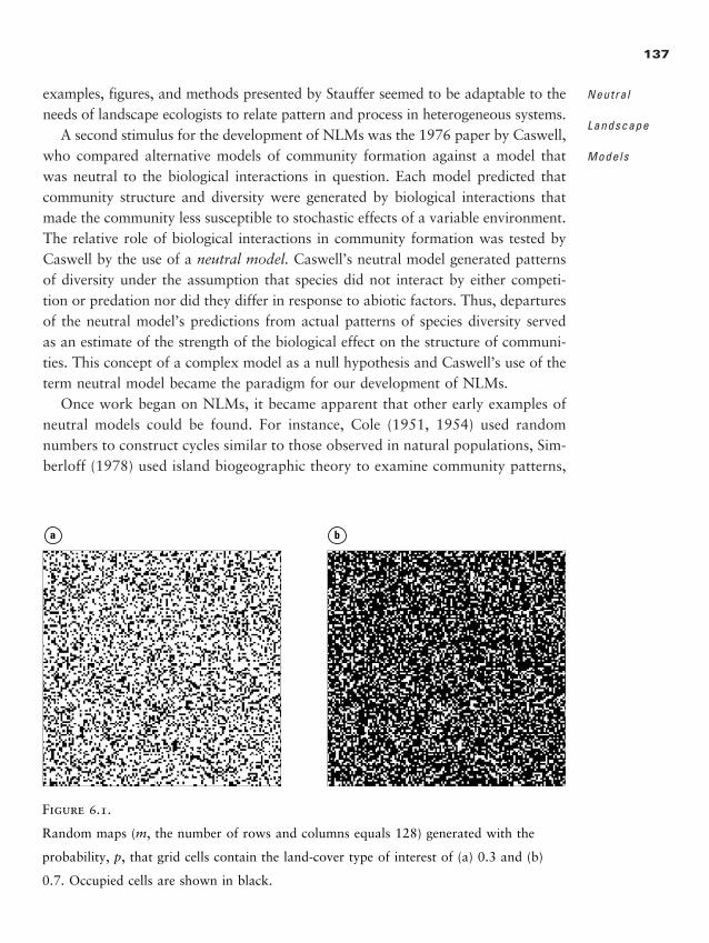
examples, figures, and methods presented by Stauffer seemed to be adaptable to theneeds of landscape ecologists to relate pattern and process in heterogeneous systems.

A second stimulus for the development of NLMs was the 1976 paper by Caswell,who compared alternative models of community formation against a model thatwas neutral to the biological interactions in question. Each model predicted thatcommunity structure and diversity were generated by biological interactions thatmade the community less susceptible to stochastic effects of a variable environment.The relative role of biological interactions in community formation was tested byCaswell by the use of a neutral model. Caswell’s neutral model generated patternsof diversity under the assumption that species did not interact by either competi-tion or predation nor did they differ in response to abiotic factors. Thus, departuresof the neutral model’s predictions from actual patterns of species diversity servedas an estimate of the strength of the biological effect on the structure of communi-ties. This concept of a complex model as a null hypothesis and Caswell’s use of theterm neutral model became the paradigm for our development of NLMs.

Once work began on NLMs, it became apparent that other early examples ofneutral models could be found. For instance, Cole (1951, 1954) used randomnumbers to construct cycles similar to those observed in natural populations, Sim-berloff (1978) used island biogeographic theory to examine community patterns,

137

Neutra l

Landscape

Models

ba

Figure 6.1.

Random maps (m, the number of rows and columns equals 128) generated with the

probability, p, that grid cells contain the land-cover type of interest of (a) 0.3 and (b)

0.7. Occupied cells are shown in black.

2888_e06_p135-156 2/27/01 1:42 PM Page 137

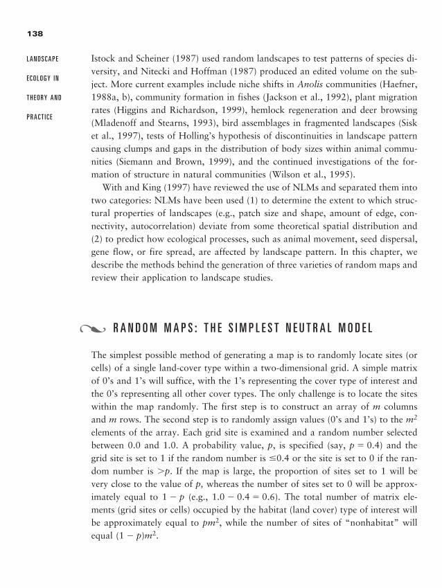
Istock and Scheiner (1987) used random landscapes to test patterns of species di-versity, and Nitecki and Hoffman (1987) produced an edited volume on the sub-ject. More current examples include niche shifts in Anolis communities (Haefner,1988a, b), community formation in fishes (Jackson et al., 1992), plant migrationrates (Higgins and Richardson, 1999), hemlock regeneration and deer browsing(Mladenoff and Stearns, 1993), bird assemblages in fragmented landscapes (Sisket al., 1997), tests of Holling’s hypothesis of discontinuities in landscape patterncausing clumps and gaps in the distribution of body sizes within animal commu-nities (Siemann and Brown, 1999), and the continued investigations of the for-mation of structure in natural communities (Wilson et al., 1995).

With and King (1997) have reviewed the use of NLMs and separated them intotwo categories: NLMs have been used (1) to determine the extent to which struc-tural properties of landscapes (e.g., patch size and shape, amount of edge, con-nectivity, autocorrelation) deviate from some theoretical spatial distribution and(2) to predict how ecological processes, such as animal movement, seed dispersal,gene flow, or fire spread, are affected by landscape pattern. In this chapter, wedescribe the methods behind the generation of three varieties of random maps andreview their application to landscape studies.

R A N D O M M A P S : T H E S I M P L E S T N E U T R A L M O D E L

The simplest possible method of generating a map is to randomly locate sites (orcells) of a single land-cover type within a two-dimensional grid. A simple matrixof 0’s and 1’s will suffice, with the 1’s representing the cover type of interest andthe 0’s representing all other cover types. The only challenge is to locate the siteswithin the map randomly. The first step is to construct an array of m columnsand m rows. The second step is to randomly assign values (0’s and 1’s) to the m2

elements of the array. Each grid site is examined and a random number selectedbetween 0.0 and 1.0. A probability value, p, is specified (say, p � 0.4) and thegrid site is set to 1 if the random number is �0.4 or the site is set to 0 if the ran-dom number is �p. If the map is large, the proportion of sites set to 1 will bevery close to the value of p, whereas the number of sites set to 0 will be approx-imately equal to 1 � p (e.g., 1.0 � 0.4 � 0.6). The total number of matrix ele-ments (grid sites or cells) occupied by the habitat (land cover) type of interest willbe approximately equal to pm2, while the number of sites of “nonhabitat” willequal (1 � p)m2.

138

L A N D S C A P E

E C O L O G Y I N

T H E O R Y A N D

P R A C T I C E

�

2888_e06_p135-156 2/27/01 1:42 PM Page 138

As the grid is filled with 0’s and 1’s, clusters, or patches, will be seen to form (Fig-ure 6.1). Clusters are usually defined as groups of sites of the same land-cover typewith at least one horizontal or vertical (but not diagonal) edge in common. This rulefor patch identification is usually referred to as the four-neighbor or nearest-neigh-bor rule (see discussion in Chapter 5 and Figure 5.8). When a series of maps is gen-erated with increasing values of p, the number of patches increases as p increasesover the range 0.0 � p � 0.3. Patch numbers decline as p continues to increase, be-cause small patches begin to coalesce into larger ones (Gardner et al., 1987; see Fig-ure 6.2a). The amount of edge on the map is also affected by p, with the maximumamount of edge occurring when p � 0.5 (Gardner et al., 1987; see Figure 6.2b).

139

Neutra l

Landscape

Models

Num

ber

of c

lust

ers

p

5000

6000

4000

3000

2000

1000

0

0.0 0.1 0.2 0.3 0.4 0.5 0.6 0.7 0.8 0.9 1.0

0.0 0.1 0.2 0.3 0.4 0.5 0.6 0.7 0.8 0.9 1.0

4000

3000

2000

1000

0Size

of l

arge

st c

lust

ers

p

a

b

Figure 6.2.

(a) The number of clusters and (b) size of the

largest cluster for random maps that vary in the

probability, p, that a grid cell contains the habi-

tat type of interest. Plotted from data reported

in Tables 1 and 2 of Gardner et al. (1987) for

maps with 200 rows and columns.

2888_e06_p135-156 2/27/01 1:42 PM Page 139

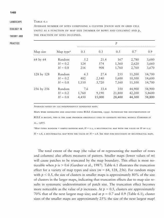
The total extent of the map (the value of m representing the number of rowsand columns) also affects measures of pattern. Smaller maps (lower values of m)will cause patches to be truncated by the map boundary. This effect is most no-ticeable when p is � 0.6 (Gardner et al., 1987). Table 6.1 illustrates the truncationeffect for a variety of map types and sizes (m � 64, 128, 256). For random mapswith p � 0.5, the size of clusters in smaller maps is approximately 80% of the sizeof clusters in the larger maps, indicating that truncation effects due to map size re-sults in systematic underestimation of patch size. The truncation effect becomesmore noticeable as the value of p increases. At p � 0.5, clusters are approximately70% that of the next largest map size; and at p � 0.7 and 0.9 (Table 6.1), clustersizes of the smaller maps are approximately 25% the size of the next largest map!

140

L A N D S C A P E

E C O L O G Y I N

T H E O R Y A N D

P R A C T I C E

Table 6.1Average number of sites composing a cluster (patch size in grid cell units) as a function of map size (number of rows and columns) and p, the fraction of sites occupied.

P

Map size Map typea 0.1 0.3 0.5 0.7 0.9

64 by 64 Random 5.2 21.4 167 2,780 3,680H � 0.2 124 574 1,360 2,620 3,660H � 0.8 216 908 1,760 2,760 3,670

128 by 128 Random 6.3 27.4 255 11,200 14,700H � 0.2 482 2,140 5,600 10,500 14,600H � 0.8 1,110 3,720 7,160 11,100 14,700

256 by 256 Random 7.6 33.4 350 44,900 58,900H � 0.2 1,760 9,190 21,800 42,200 5,8600H � 0.8 4,450.0 15,000.0 28,400 44,300 58,800

Averages based on 100 independently generated maps.

Maps were generated and analyzed using RULE (Gardner, 1999). Although the documentation of

RULE is recent, this is the same program originally used to generate neutral models (Gardner et

al., 1987).

aMap types: random � simple random map; H � 0.2, a multifractal map with the value of H of 0.2;

H � 0.8, a multifractal map with the value of H � 0.8. See text for discussion of multifractal maps.

2888_e06_p135-156 2/27/01 1:42 PM Page 140

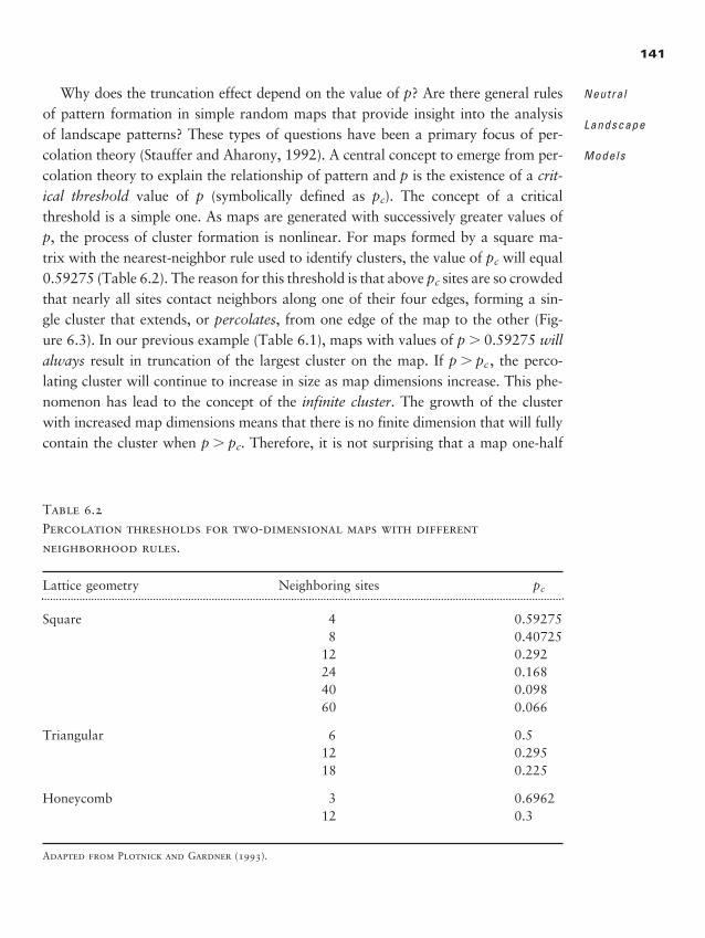
Why does the truncation effect depend on the value of p? Are there general rulesof pattern formation in simple random maps that provide insight into the analysisof landscape patterns? These types of questions have been a primary focus of per-colation theory (Stauffer and Aharony, 1992). A central concept to emerge from per-colation theory to explain the relationship of pattern and p is the existence of a crit-ical threshold value of p (symbolically defined as pc). The concept of a criticalthreshold is a simple one. As maps are generated with successively greater values ofp, the process of cluster formation is nonlinear. For maps formed by a square ma-trix with the nearest-neighbor rule used to identify clusters, the value of pc will equal0.59275 (Table 6.2). The reason for this threshold is that above pc sites are so crowdedthat nearly all sites contact neighbors along one of their four edges, forming a sin-gle cluster that extends, or percolates, from one edge of the map to the other (Fig-ure 6.3). In our previous example (Table 6.1), maps with values of p � 0.59275 willalways result in truncation of the largest cluster on the map. If p � pc , the perco-lating cluster will continue to increase in size as map dimensions increase. This phe-nomenon has lead to the concept of the infinite cluster. The growth of the clusterwith increased map dimensions means that there is no finite dimension that will fullycontain the cluster when p � pc. Therefore, it is not surprising that a map one-half

141

Neutra l

Landscape

Models

Table 6.2Percolation thresholds for two-dimensional maps with different neighborhood rules.

Lattice geometry Neighboring sites pc

Square 4 0.592758 0.40725

12 0.29224 0.16840 0.09860 0.066

Triangular 6 0.512 0.29518 0.225

Honeycomb 3 0.696212 0.3

Adapted from Plotnick and Gardner (1993).

2888_e06_p135-156 2/27/01 1:42 PM Page 141

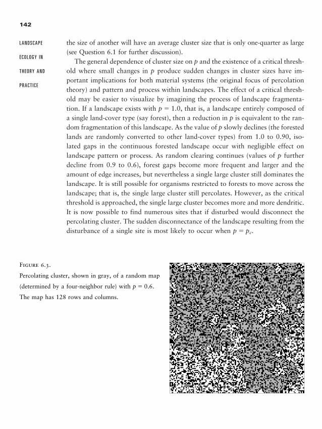
the size of another will have an average cluster size that is only one-quarter as large(see Question 6.1 for further discussion).

The general dependence of cluster size on p and the existence of a critical thresh-old where small changes in p produce sudden changes in cluster sizes have im-portant implications for both material systems (the original focus of percolationtheory) and pattern and process within landscapes. The effect of a critical thresh-old may be easier to visualize by imagining the process of landscape fragmenta-tion. If a landscape exists with p � 1.0, that is, a landscape entirely composed ofa single land-cover type (say forest), then a reduction in p is equivalent to the ran-dom fragmentation of this landscape. As the value of p slowly declines (the forestedlands are randomly converted to other land-cover types) from 1.0 to 0.90, iso-lated gaps in the continuous forested landscape occur with negligible effect onlandscape pattern or process. As random clearing continues (values of p furtherdecline from 0.9 to 0.6), forest gaps become more frequent and larger and theamount of edge increases, but nevertheless a single large cluster still dominates thelandscape. It is still possible for organisms restricted to forests to move across thelandscape; that is, the single large cluster still percolates. However, as the criticalthreshold is approached, the single large cluster becomes more and more dendritic.It is now possible to find numerous sites that if disturbed would disconnect thepercolating cluster. The sudden disconnectance of the landscape resulting from thedisturbance of a single site is most likely to occur when p � pc.

142

L A N D S C A P E

E C O L O G Y I N

T H E O R Y A N D

P R A C T I C E

Figure 6.3.

Percolating cluster, shown in gray, of a random map

(determined by a four-neighbor rule) with p � 0.6.

The map has 128 rows and columns.

2888_e06_p135-156 2/27/01 1:42 PM Page 142

A physical analogue to the process of landscape fragmentation was presentedby D. Stauffer at the 1986 Gordon Conference. The bombardment of delicate goldfoil electrodes by micrometeorites in space has been a serious problem, becauseimpacts with micrometeorites degrade the foil and ultimately result in failure ofthe electrode. The question is how much of the electrode can be destroyed beforethe electrical circuit fails. In laboratory experiments, bombarding electrodes withsand showed that a critical threshold existed as predicted by percolation theory(p � 0.5982). At the critical threshold, a single sand grain impacting the gold foilwas likely to cause the circuit to fail.

The numerical value of a critical threshold depends on the neighborhood ruleused to identify clusters. When an eight-neighbor rule is used to identify clusters,the value of pc drops to 0.40725 (Table 6.2; see Figure 6.4). Because diagonalneighbors are now also counted as cluster members, potential neighbors are far-ther away from each other. With the inclusion of more distant neighbors withinthe cluster, large dendritic structures form and percolate across the grid at lowervalues of p. The ecological justification for the analysis of landscape pattern withdifferent neighborhood rules is process dependent. For instance, if dispersal of adisturbance is slow and by immediate contact (e.g., some fungal diseases), thenthe nearest-neighbor rule might be applied and a critical threshold of the spreadof the fungus would occur at p � 0.59275. However, short-distance dispersal oflarge seeds might cover a neighborhood of considerable area, resulting in a re-vised definition of connectance among neighboring sites. It may also be necessaryto change the neighborhood rule if the resolution of the map were to change. Forinstance, a four-neighbor rule applied to maps with 90-m grid cells might bechanged to a 21-neighbor rule if map resolution were increased to 30 m (otheralternatives exist and may be explored in the lab exercises associated with thischapter). The value of the critical threshold has also been shown to vary with mapgeometry (Table 6.2), primarily because different map geometries have a differ-ent number of neighbors (e.g., a triangular grid has three neighbors associatedwith each site, whereas a honeycomb grid would have eight neighbors). Eventhough the value of the threshold may change, the general response of the systemis similar no matter what rule is applied (Figure 6.4).

An initial misunderstanding in the use of random maps as NLMs was the ideathat NLMs were intended to represent actual landscape patterns. When the orig-inal neutral model paper was presented at the U.S. IALE meeting in Charlottesville,Virginia, in the spring of 1987, one comment that was heard was “Why wouldanyone want to use random methods to represent actual landscapes? Landscapesaren’t random—they are organized in complex ways.” This question is a natural

143

Neutra l

Landscape

Models

2888_e06_p135-156 2/27/01 1:42 PM Page 143

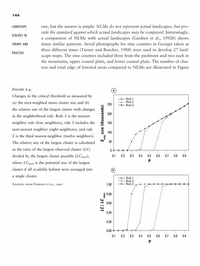
one, but the answer is simple: NLMs do not represent actual landscapes, but pro-vide the standard against which actual landscapes may be compared. Interestingly,a comparison of NLMs with actual landscapes (Gardner et al., 1992b) showsmany similar patterns. Aerial photographs for nine counties in Georgia taken atthree different times (Turner and Ruscher, 1988) were used to develop 27 land-scape maps. The nine counties included three from the piedmont and two each inthe mountains, upper coastal plain, and lower coastal plain. The number of clus-ters and total edge of forested areas compared to NLMs are illustrated in Figure

144

L A N D S C A P E

E C O L O G Y I N

T H E O R Y A N D

P R A C T I C E

LC /

LC m

ax

P

1.00

0.80

0.60

0.40

0.20

0.000.1 0.2 0.3 0.4 0.5 0.6 0.7 0.8 0.9

S avg s

ize

(tho

usan

ds)

P

250

200

150

100

50

00.1 0.2 0.3 0.4 0.5 0.6 0.7 0.8 0.9

Rule 1Rule 2Rule 3

Rule 1Rule 2Rule 3

a

b

Figure 6.4.

Changes in the critical threshold as measured by

(a) the area-weighted mean cluster size and (b)

the relative size of the largest cluster with changes

in the neighborhood rule. Rule 1 is the nearest-

neighbor rule (four neighbors), rule 2 includes the

next-nearest neighbor (eight neighbors), and rule

2 is the third nearest-neighbor (twelve neighbors).

The relative size of the largest cluster is calculated

as the ratio of the largest observed cluster (LC)

divided by the largest cluster possible (LCmax),

where LCmax is the potential size of the largest

cluster if all available habitat were arranged into

a single cluster.

Adapted from Pearson et al., 1996.

2888_e06_p135-156 2/27/01 1:42 PM Page 144

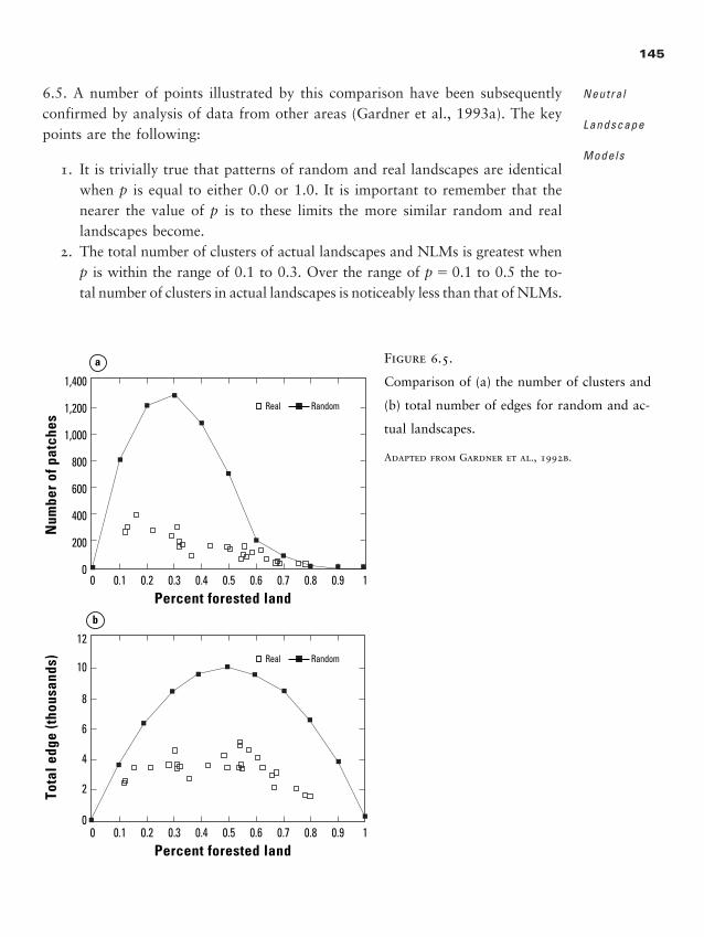
6.5. A number of points illustrated by this comparison have been subsequentlyconfirmed by analysis of data from other areas (Gardner et al., 1993a). The keypoints are the following:

1. It is trivially true that patterns of random and real landscapes are identicalwhen p is equal to either 0.0 or 1.0. It is important to remember that thenearer the value of p is to these limits the more similar random and reallandscapes become.

2. The total number of clusters of actual landscapes and NLMs is greatest whenp is within the range of 0.1 to 0.3. Over the range of p � 0.1 to 0.5 the to-tal number of clusters in actual landscapes is noticeably less than that of NLMs.

145

Neutra l

Landscape

Models

Num

ber

of p

atch

es

Percent forested land 0

1,200

1,400

1,000

800

600

400

200

00.1 0.2 0.3 0.4 0.5 0.6 0.7 0.8 0.9 1

Tota

l edg

e (t

hous

ands

)

Percent forested land 0

12

10

8

6

4

2

00.1 0.2 0.3 0.4 0.5 0.6 0.7 0.8 0.9 1

Real Random

Real Random

a

b

Figure 6.5.

Comparison of (a) the number of clusters and

(b) total number of edges for random and ac-

tual landscapes.

Adapted from Gardner et al., 1992b.

2888_e06_p135-156 2/27/01 1:42 PM Page 145

3. In actual landscapes and NLMs, the total amount of edge is at a maximumnear p � 0.5, but, like the cluster numbers, the amount of edge in actuallandscapes is much less than in random ones.

4. The degree of connectivity (as measured by the presence of a single clusterspanning the map) was equivalent to the NLMs in 25 of 27 actual land-scapes. The two landscapes that differed from NLMs either percolated atp � 0.43 or failed to percolate at p � 0.68. The causes of this deviation werethe interaction of topography (ridge and valleys) and the process of humanland-use conversion.

The qualitative trends in pattern in actual landscapes and NLMs are similar al-though the magnitude (e.g., number of clusters, amount of edge) is less and thevariability greater in actual landscapes. These differences are produced by a com-plex suite of factors that organize patterns on actual landscapes, causing notice-able differences from patterns produced by simple random processes.

The most fascinating aspect of percolation theory is the existence of criticalthresholds—and the implications that these thresholds hold for relating landscapepattern to ecological processes. Analysis clearly shows that, although landscapesare not random, critical thresholds still exist where sudden changes in landscapepattern may occur with small shifts in disturbance regimes or changes in land use.The factors that organize actual landscapes make the prediction of the exact valueof pc for any given landscape uncertain (see Question 6.3). Nevertheless, criticalthresholds for real landscapes do exist! Thus, above pc we can expect landscapepattern to be dominated by a single very large cluster, whereas landscapes withvalues of p below pc will be characterized by numerous, smaller, fragmentedpatches. If the value of pc is estimated from a specific neighborhood rule (e.g., theneighborhood defined according to species or disturbance specific parameters), thenecological dynamics can be expected to shift at the critical threshold. Such shiftsin pattern that result from small changes in land use have important implicationsfor metapopulation dynamics and the conservation of species diversity (Dale et al.,1994b; Pearson et al., 1996; also see Chapter 8). Metapopulation dynamics existin landscapes below pc, whereas a single, large population dominates dynamics inlandscapes where the amount of habitat is above pc. Conservation efforts shouldbe cognizant of the implications of critical thresholds and connectivity in actuallandscapes. Because small changes in available habitat near the critical thresholdsresult in disproportionately large changes in the degree of landscape fragmentation,efforts to preserve continuous tracts of habitat are highly vulnerable to disturbanceeffects when the amount of habitat is near the critical threshold.

146

L A N D S C A P E

E C O L O G Y I N

T H E O R Y A N D

P R A C T I C E

2888_e06_p135-156 2/27/01 1:42 PM Page 146

A practical application of NLMs has been their use to test the performance ofdifferent landscape metrics across a range of conditions (e.g., number of habitattypes, map sizes, values of p). The evaluation of spatial indexes by NLMs beforethey are applied to actual landscapes and the systematic comparison among sim-ilar landscape indexes provide important information on the reliability of differ-ent metrics to identify unique patterns on actual landscapes (Gardner and O’Neill,1991; Gustafson and Parker, 1992; Gardner et al., 1993a; Schumaker, 1996). Sev-eral essential messages from these studies bear repeating. The first is that the valueof p is a dominant factor affecting the value of nearly all landscape metrics. In-deed, p often enters directly into the calculation of the metric itself (e.g., diver-sity, contagion) or indirectly as an indication of the amount of habitat found onthe map. As p increases, the number of possible arrangements of land cover de-creases. Obviously, differences in landscape pattern as a result of differences in pare not surprising. Relating these differences to processes that affect pattern mustfirst account for processes that have altered the value of p! The second caveat isthat the critical threshold causes a transition from many small to fewer large clus-ters on the map. Therefore, large differences in landscape metrics should be ex-pected above and below this critical threshold. It is questionable whether metricsinsensitive to this transition will provide useful insight into landscape pattern andprocess. Finally, it is very clear that the introduction of new indexes without priortesting by a series of neutral models should be regarded as a serious omission.

M A P S W I T H H I E R A R C H I C A L S T R U C T U R E

Analysis of actual landscapes frequently reveals shifts in pattern with changes inscale (see Chapter 1), and the factors that contribute to landscape pattern oper-ate over a wide range of scales (see Chapter 4). Thus, many landscapes exhibitpatterns that can be detected at multiple spatial scales. For instance, Anderson(1971) found multiple scales of pattern in three Australian dry-land communities;Krummel et al. (1987) used the fractal dimension to reveal two distinct scales oflandscape pattern; changes in pattern with scale were found by O’Neill et al.(1991a) when the change in variance of habitat types was plotted against samplearea; and an analysis of replicate transect data revealed three to five scales of dis-tribution of vegetation (O’Neill et al., 1991b). The contagion index (see Chapter5) can be used to control pattern at a single spatial scale by producing varyingdegrees of habitat clumping (Gardner and O’Neill, 1991; Fall and Fall, 1996).

147

Neutra l

Landscape

Models

�

2888_e06_p135-156 2/27/01 1:42 PM Page 147

Random patterns constrained by contagion result in shifts in patch number, size,and shape (Gardner and O’Neill, 1991).

A general and flexible method of generating NLMs with scale-dependent pat-terns is by recursive procedures used to construct maps with hierarchical patterns(O’Neill et al., 1992a; Lavorel et al., 1993). A recursive procedure is one that ref-erences itself. For instance, we can use recursion to calculate a factorial (n!) us-ing the simple relationship that n! � n � (n � 1)! and calling this procedure re-peatedly. This repeated calling of the same routine as n becomes successivelysmaller (assuming that n is �0) is a simple example of a recursive algorithm. Hi-erarchically structured random maps, also known as curdled systems in fractalgeometry (Mandelbrot 1983), can be produced by recursion (for more examplesof fractal geometry and recursion see Barnsley et al., 1988). Recursion in the cur-dling algorithm (Figure 6.6a) simply defines a series of scales and then successivelygenerates random pattern within each scale. The sequence of steps requires sev-eral parameters to control the process, including the number of hierarchical lev-els L and the size, mi, and probability, pi, of sites being set to 1 at each level. Theresulting patterns (Figure 6.6b) allow a variety of scale-dependent structures to besimulated, while maintaining the overall size (M) and the probability (P) of habi-tat within the map (see Lavorel et al., 1993, and Plotnick and Gardner, 1993, foradditional details on map generation procedures).

Hierarchical structures result in fewer clusters and more aggregated landscapesthan similar random maps, especially when the probabilities at any specific level (pi)are greater than pc. Hierarchical maps also produce multiple patterns (and hencegreater variability) at the same level of p. Because these maps are structured, theyalso demonstrate a significant downward shift in the percolation threshold. For alarge map with L levels, the percolation threshold (using the four-neighbor rule) willbe equal to 0.59275L (Chayes et al., 1988). Gardner et al. (1993a) found that hier-archically structured maps displayed remarkably similar patterns to maps of foresthabitat measured from remotely sensed data, whereas the structure of these mapswas different from simple random maps with the same fraction of suitable habitat.Because real landscapes exhibit scaled patterns that reflect a variety of causal factors(that is, real maps are structured), hierarchically structured neutral models providea useful means of identifying changes in process (e.g., species dispersal and persis-tence or spread of disturbances and disease) that occur as a result of scale-dependentpatterns (Lavorel et al., 1993; Lavorel et al., 1995). The bottom line is that randommaps provide the simplest form of neutral model but lack structures typical of mostlandscapes. If we wish to study the effect of structure, then hierarchical maps, whichgenerate random structures, might be the most useful neutral model.

148

L A N D S C A P E

E C O L O G Y I N

T H E O R Y A N D

P R A C T I C E

2888_e06_p135-156 2/27/01 1:42 PM Page 148

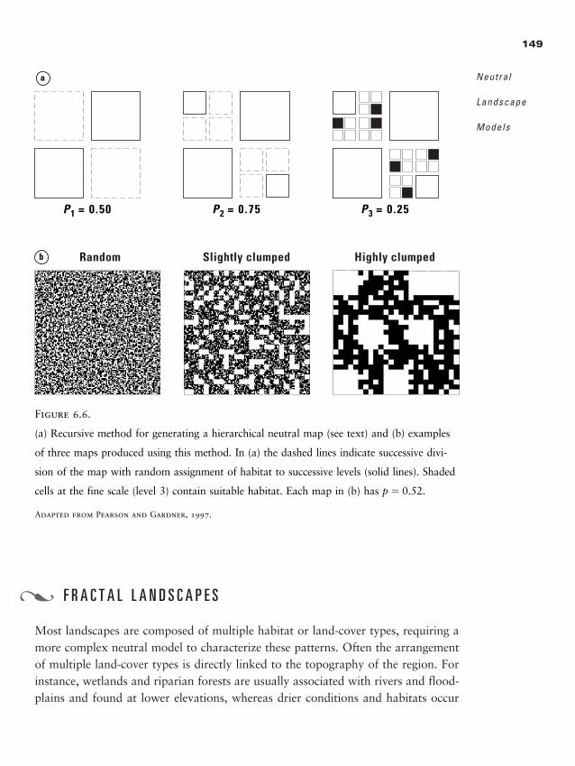
F R A C T A L L A N D S C A P E S

Most landscapes are composed of multiple habitat or land-cover types, requiring amore complex neutral model to characterize these patterns. Often the arrangementof multiple land-cover types is directly linked to the topography of the region. Forinstance, wetlands and riparian forests are usually associated with rivers and flood-plains and found at lower elevations, whereas drier conditions and habitats occur

149

Neutra l

Landscape

Models

�

P1 = 0.50 P2 = 0 .75 P3 = 0 .25

a

Random Slightly clumped Highly clumpedb

Figure 6.6.

(a) Recursive method for generating a hierarchical neutral map (see text) and (b) examples

of three maps produced using this method. In (a) the dashed lines indicate successive divi-

sion of the map with random assignment of habitat to successive levels (solid lines). Shaded

cells at the fine scale (level 3) contain suitable habitat. Each map in (b) has p � 0.52.

Adapted from Pearson and Gardner, 1997.

2888_e06_p135-156 2/27/01 1:42 PM Page 149

along ridge tops. Conditions between these extremes are intermediate in elevationand usually intermediate in soil moisture and temperature levels. Because habitatcharacteristics (land-cover types) vary with these elevational gradients, many land-scapes with multiple cover types are characterized by a strong autocorrelation be-tween habitat types. Methods that can generate patterns of continuous changewould provide a useful neutral model for landscapes with multiple land-covertypes.

One method for representing continuous, autocorrelated variation of patternsis the generation of maps by fractal Brownian motion. A fractal Brownian mo-tion in one dimension is produced by creating a series of steps, Xt, whose distancefrom the previous step (Xt1 � Xt) is randomly determined from a Gaussian dis-tribution. A three-dimensional map may be produced by allowing steps to occurin both the X and Y directions, with the random displacements recorded as ele-vation (the Z direction). The midpoint displacement method (MPDM) for creat-ing fractal surfaces has been extensively used to model three-dimensional patterns(Barnsley et al., 1988). The fractal of fractal Brownian motion is controlled bytwo parameters: the variance of displacement of points, �2 (usually set to 1.0),and H, which controls the correlation between successive steps (Saupe, 1988; Plot-nick and Prestegaard, 1993). Because the successive displacement of points resultsin an expected difference between any two points equal to (E[X1 � (X1 � d)] dH

(Plotnick and Prestegaard, 1993), the difference between two points will be pro-portional to the square of the distance, d, and the correlation, C(d), between thepoints [C(d) � 22H�1 � 1] (Mandelbrot, 1983; Feder, 1988). The fractal dimen-sion, D, of maps generated by the MPDM is equal to D � 3.0 � H (Saupe, 1988).When H � 0.5, successive displacements in the Brownian walk are not correlated;when H � 0.5, successive displacements are negatively correlated and maps ap-pear to have a very rough surface; and when H � 0.5, steps are positively corre-lated and the maps have a smooth surface (Figure 6.7). Habitat maps may be gen-erated from the continuous numbers produced by the MPDM by scaling the realnumbers and assigning ordinal values to each grid square proportional to the frac-tion of the map, pi, occupied by each habitat type (Gardner, 1999). This processof generating a neutral model with fractal maps is summarized in three steps: (1)generation of a topographic map with roughness controlled by H, (2) slicing thetopography into contours with the area of each contour equal to the proportionof the map occupied by that habitat type, and (3) assigning ordinal habitat (landcover) values to sites within each contour.

The realistic nature of the fractal maps is the direct result of the autocorrelated

150

L A N D S C A P E

E C O L O G Y I N

T H E O R Y A N D

P R A C T I C E

2888_e06_p135-156 2/27/01 1:42 PM Page 150

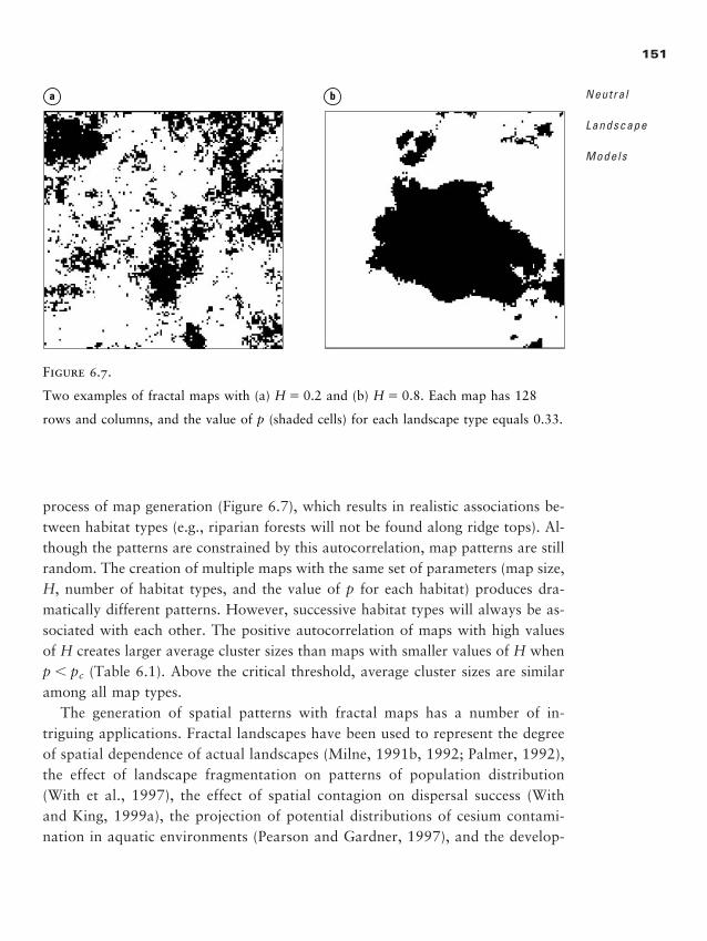
process of map generation (Figure 6.7), which results in realistic associations be-tween habitat types (e.g., riparian forests will not be found along ridge tops). Al-though the patterns are constrained by this autocorrelation, map patterns are stillrandom. The creation of multiple maps with the same set of parameters (map size,H, number of habitat types, and the value of p for each habitat) produces dra-matically different patterns. However, successive habitat types will always be as-sociated with each other. The positive autocorrelation of maps with high valuesof H creates larger average cluster sizes than maps with smaller values of H whenp � pc (Table 6.1). Above the critical threshold, average cluster sizes are similaramong all map types.

The generation of spatial patterns with fractal maps has a number of in-triguing applications. Fractal landscapes have been used to represent the degreeof spatial dependence of actual landscapes (Milne, 1991b, 1992; Palmer, 1992),the effect of landscape fragmentation on patterns of population distribution(With et al., 1997), the effect of spatial contagion on dispersal success (Withand King, 1999a), the projection of potential distributions of cesium contami-nation in aquatic environments (Pearson and Gardner, 1997), and the develop-

151

Neutra l

Landscape

Models

ba

Figure 6.7.

Two examples of fractal maps with (a) H � 0.2 and (b) H � 0.8. Each map has 128

rows and columns, and the value of p (shaded cells) for each landscape type equals 0.33.

2888_e06_p135-156 2/27/01 1:43 PM Page 151

ment of experimental systems to measure the effect of habitat connectivity oninsect movement patterns (With et al., 1999). In most of these examples, the ef-fect of structure on habitat arrangement was quantified by comparison of frac-tal maps with simple (nonstructured) random maps. For instance, the objectiveof With et al. (1997) was to examine how landscape structure affected the pat-terns of population dispersion of mobile organisms. Variation in landscape struc-ture was created by generating maps that differed in the number and propor-tion of habitat types and the methods used to generate the spatial patterns. Simplerandom maps created pattern without an underlying structure, whereas fractalmaps with different values of H created differently structured maps. The resultsshowed that landscape structure had a large effect on the distribution of simu-lated patterns of species distributions. Although population size remained fairlyconstant over all simulations, patterns of distribution shifted owing to the ag-gregation of individuals within specific habitat types. The control of landscapestructure created by the comparison of neutral models allowed the effect of pat-tern and scale to be evaluated.

Pearson and Gardner (1997) used randomly generated fractal landscapes foran entirely different purpose: to determine the consequences of spatial variationin the patterns of 137Cs contamination in a Tennessee reservoir. The spatial pat-tern of contamination was important because sites within the reservoir with highcontaminant levels (hot spots) could affect cleanup strategies. It was believed thatcontaminant hot spots should be spatially correlated, but the degree of correla-tion was not known. Fractal maps with varying levels of H were produced to as-sess the effectiveness of various sediment sampling schemes on the detection ofthese hot spots. The results showed that spatial patterns could be detected accu-rately in maps with a large degree of spatial autocorrelation using relatively fewsamples. However, as autocorrelation declined, the number of samples requiredto achieve the same degree of accuracy increased dramatically. A comparison offractal maps with 137Cs distributions estimated by a sedimentation model showedthat contaminant levels were positively correlated within deposition zones (areaswith similar hydrodynamics), but uncorrelated across different deposition zones.

Other applications of fractal landscapes as neutral models, including the ex-ploration of edge effects (With 1997a, b) and source–sink relationships (Milne,1992; With, 1997a), have been suggested. Because multiple realizations of theseneutral models can be generated, systematic application allows the effect of onecomponent of landscape structure, the autocorrelation among habitat types, to bedetermined.

152

L A N D S C A P E

E C O L O G Y I N

T H E O R Y A N D

P R A C T I C E

2888_e06_p135-156 2/27/01 1:43 PM Page 152

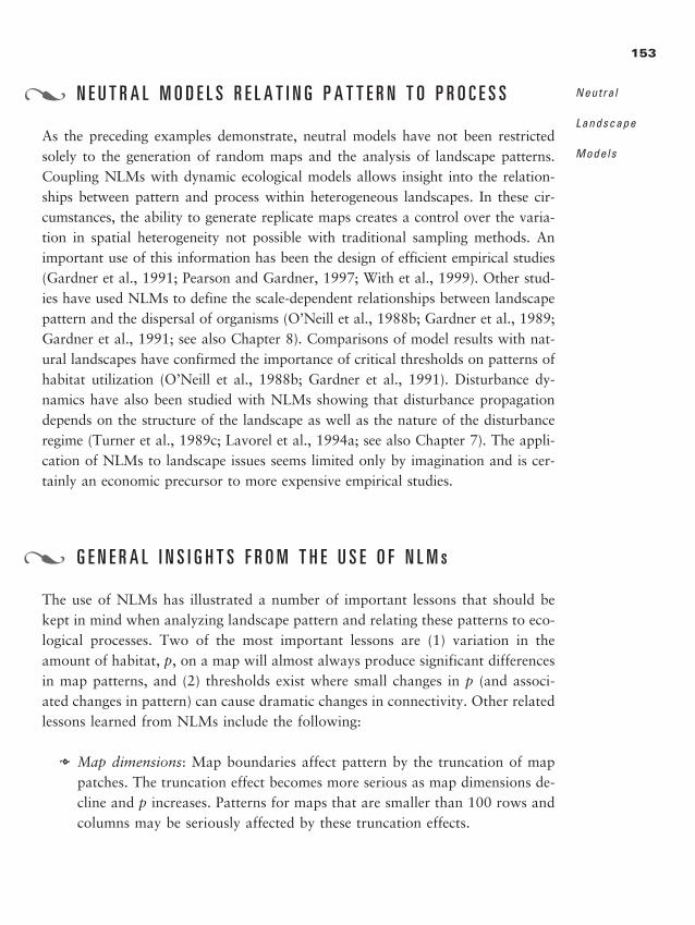
N E U T R A L M O D E L S R E L A T I N G P A T T E R N T O P R O C E S S

As the preceding examples demonstrate, neutral models have not been restrictedsolely to the generation of random maps and the analysis of landscape patterns.Coupling NLMs with dynamic ecological models allows insight into the relation-ships between pattern and process within heterogeneous landscapes. In these cir-cumstances, the ability to generate replicate maps creates a control over the varia-tion in spatial heterogeneity not possible with traditional sampling methods. Animportant use of this information has been the design of efficient empirical studies(Gardner et al., 1991; Pearson and Gardner, 1997; With et al., 1999). Other stud-ies have used NLMs to define the scale-dependent relationships between landscapepattern and the dispersal of organisms (O’Neill et al., 1988b; Gardner et al., 1989;Gardner et al., 1991; see also Chapter 8). Comparisons of model results with nat-ural landscapes have confirmed the importance of critical thresholds on patterns ofhabitat utilization (O’Neill et al., 1988b; Gardner et al., 1991). Disturbance dy-namics have also been studied with NLMs showing that disturbance propagationdepends on the structure of the landscape as well as the nature of the disturbanceregime (Turner et al., 1989c; Lavorel et al., 1994a; see also Chapter 7). The appli-cation of NLMs to landscape issues seems limited only by imagination and is cer-tainly an economic precursor to more expensive empirical studies.

G E N E R A L I N S I G H T S F R O M T H E U S E O F N L M s

The use of NLMs has illustrated a number of important lessons that should bekept in mind when analyzing landscape pattern and relating these patterns to eco-logical processes. Two of the most important lessons are (1) variation in theamount of habitat, p, on a map will almost always produce significant differencesin map patterns, and (2) thresholds exist where small changes in p (and associ-ated changes in pattern) can cause dramatic changes in connectivity. Other relatedlessons learned from NLMs include the following:

� Map dimensions: Map boundaries affect pattern by the truncation of mappatches. The truncation effect becomes more serious as map dimensions de-cline and p increases. Patterns for maps that are smaller than 100 rows andcolumns may be seriously affected by these truncation effects.

153

Neutra l

Landscape

Models

�

�

2888_e06_p135-156 2/27/01 1:43 PM Page 153

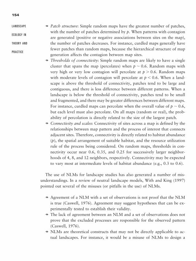
� Patch structure: Simple random maps have the greatest number of patches,with the number of patches determined by p. When patterns with contagionare generated (positive or negative associations between sites on the map),the number of patches decreases. For instance, curdled maps generally havefewer patches than random maps, because the hierarchical structure of mapgeneration affects the contagion between map sites.

� Thresholds of connectivity: Simple random maps are likely to have a singlecluster that spans the map (percolates) when p � 0.6. Random maps withvery high or very low contagion will percolate at p � 0.6. Random mapswith moderate levels of contagion will percolate at p � 0.6. When a land-scape is above the threshold of connectivity, patches tend to be large andcontiguous, and there is less difference between different patterns. When alandscape is below the threshold of connectivity, patches tend to be smalland fragmented, and there may be greater differences between different maps.For instance, curdled maps can percolate when the overall value of p � 0.6,but each level must also percolate. On all maps (random or real), the prob-ability of percolation is directly related to the size of the largest patch.

� Connectivity and scales: Connectivity of sites across a map is defined by therelationships between map pattern and the process of interest that connectsadjacent sites. Therefore, connectivity is directly related to habitat abundance(p), the spatial arrangement of suitable habitat, and the resource utilizationrule of the process being considered. On random maps, thresholds in con-nectivity occur near 0.6, 0.35, and 0.25 for successively larger neighbor-hoods of 4, 8, and 12 neighbors, respectively. Connectivity may be expectedto vary most at intermediate levels of habitat abundance (e.g., 0.3 to 0.6).

The use of NLMs for landscape studies has also generated a number of mis-understandings. In a review of neutral landscape models, With and King (1997)pointed out several of the misuses (or pitfalls in the use) of NLMs.

� Agreement of a NLM with a set of observations is not proof that the NLMis true (Caswell, 1976). Agreement may suggest hypotheses that can be ex-perimentally tested to establish their validity.

� The lack of agreement between an NLM and a set of observations does notprove that the excluded processes are responsible for the observed pattern(Caswell, 1976).

� NLMs are theoretical constructs that may not be directly applicable to ac-tual landscapes. For instance, it would be a misuse of NLMs to design a

154

L A N D S C A P E

E C O L O G Y I N

T H E O R Y A N D

P R A C T I C E

2888_e06_p135-156 2/27/01 1:43 PM Page 154

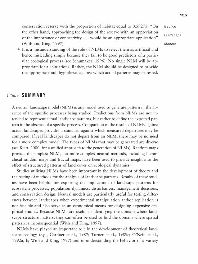
conservation reserve with the proportion of habitat equal to 0.59275. “Onthe other hand, approaching the design of the reserve with an appreciationof the importance of connectivity . . . would be an appropriate application”(With and King, 1997).

� It is a misunderstanding of the role of NLMs to reject them as artificial andhence misleading simply because they fail to be good predictors of a partic-ular ecological process (see Schumaker, 1996). No single NLM will be ap-propriate for all situations. Rather, the NLM should be designed to providethe appropriate null hypotheses against which actual patterns may be tested.

S U M M A R Y

A neutral landscape model (NLM) is any model used to generate pattern in the ab-sence of the specific processes being studied. Predictions from NLMs are not in-tended to represent actual landscape patterns, but rather to define the expected pat-tern in the absence of a specific process. Comparison of the results of NLMs againstactual landscapes provides a standard against which measured departures may becompared. If real landscapes do not depart from an NLM, there may be no needfor a more complex model. The types of NLMs that may be generated are diverse(see Keitt, 2000, for a unified approach to the generation of NLMs). Random mapsprovide the simplest NLM, but more complex neutral methods, including hierar-chical random maps and fractal maps, have been used to provide insight into theeffect of structured patterns of land cover on ecological dynamics.

Studies utilizing NLMs have been important in the development of theory andthe testing of methods for the analysis of landscape patterns. Results of these stud-ies have been helpful for exploring the implications of landscape patterns forecosystem processes, population dynamics, disturbances, management decisions,and conservation design. Neutral models are particularly useful for testing differ-ences between landscapes when experimental manipulation and/or replication isnot feasible and also serve as an economical means for designing expensive em-pirical studies. Because NLMs are useful in identifying the domain where land-scape structure matters, they can often be used to find the domain where spatialpattern is inconsequential (With and King, 1997).

NLMs have played an important role in the development of theoretical land-scape ecology (e.g., Gardner et al., 1987; Turner et al., 1989c; O’Neill et al.,1992a, b; With and King, 1997) and in understanding the behavior of a variety

155

Neutra l

Landscape

Models

�

2888_e06_p135-156 2/27/01 1:43 PM Page 155

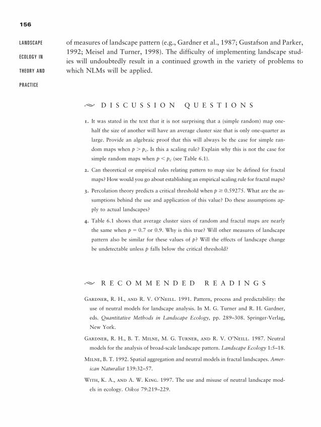
of measures of landscape pattern (e.g., Gardner et al., 1987; Gustafson and Parker,1992; Meisel and Turner, 1998). The difficulty of implementing landscape stud-ies will undoubtedly result in a continued growth in the variety of problems towhich NLMs will be applied.


1. It was stated in the text that it is not surprising that a (simple random) map one-

half the size of another will have an average cluster size that is only one-quarter as

large. Provide an algebraic proof that this will always be the case for simple ran-

dom maps when p � pc. Is this a scaling rule? Explain why this is not the case for

simple random maps when p � pc (see Table 6.1).

2. Can theoretical or empirical rules relating pattern to map size be defined for fractal

maps? How would you go about establishing an empirical scaling rule for fractal maps?

3. Percolation theory predicts a critical threshold when p � 0.59275. What are the as-

sumptions behind the use and application of this value? Do these assumptions ap-

ply to actual landscapes?

4. Table 6.1 shows that average cluster sizes of random and fractal maps are nearly

the same when p � 0.7 or 0.9. Why is this true? Will other measures of landscape

pattern also be similar for these values of p? Will the effects of landscape change

be undetectable unless p falls below the critical threshold?


Gardner, R. H., and R. V. O’Neill. 1991. Pattern, process and predictability: the

use of neutral models for landscape analysis. In M. G. Turner and R. H. Gardner,

eds. Quantitative Methods in Landscape Ecology, pp. 289–308. Springer-Verlag,

New York.

Gardner, R. H., B. T. Milne, M. G. Turner, and R. V. O’Neill. 1987. Neutral

models for the analysis of broad-scale landscape pattern. Landscape Ecology 1:5–18.

Milne, B. T. 1992. Spatial aggregation and neutral models in fractal landscapes. Amer-

ican Naturalist 139:32–57.

With, K. A., and A. W. King. 1997. The use and misuse of neutral landscape mod-

els in ecology. Oikos 79:219–229.

156

L A N D S C A P E

E C O L O G Y I N

T H E O R Y A N D

P R A C T I C E

2888_e06_p135-156 2/27/01 1:43 PM Page 156

C H A P T E R

Landscape Disturbance Dynamics

Disturbance is an important and integral part of many ecosystemsand landscapes. Disturbances create patterns in vegetation by producing

a mosaic of seral stages (Figure 7.1) that ecologists have long recognized as im-portant to landscape-level patch mosaics (e.g., Cooper, 1913; Leopold, 1933; Watt,1947; Reiners and Lang, 1979; White, 1979). The causes, patterns, dynamics, andconsequences of disturbances are major research topics in landscape ecology(Romme and Knight, 1982; Risser et al., 1984; Turner, 1987b, 1989; Baker, 1989a,1989c; Turner and Dale, 1998). Indeed, disturbances may even be required forthe maintenance of community structure and ecosystem function (White, 1979;Mooney and Godron, 1983; Sousa, 1984; Glenn and Collins, 1992; Collins et al.,1998). For example, hurricanes contribute to the maintenance of species diversityin many tropical forests, and regular fires may maintain some landscapes, likeprairies. Disturbance has been increasingly recognized by ecologists as a naturalprocess and source of heterogeneity within ecological communities, reflecting areal shift in perception during the latter half of the 20th century from an equi-librial to nonequilibrial view of the natural world (Wu and Loucks, 1995).

7

2888_e07_p157-200 2/27/01 1:48 PM Page 157

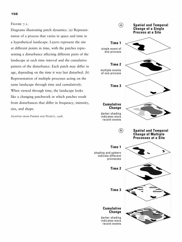
158

Spatial and TemporalChange of MultipleProcesses at a Site

Time 1

single event ofone process

Time 2

multiple eventsof one process

Time 3

CumulativeChange

darker shadingindicates more

recent events

Time 1

shading and patternindicate different

processes

Time 2

Time 3

CumulativeChange

darker shadingindicates more

recent events

Spatial and Temporal Change of a Single Process at a Site

a

b

Figure 7.1.

Diagrams illustrating patch dynamics. (a) Represen-

tation of a process that varies in space and time in

a hypothetical landscape. Layers represent the site

at different points in time, with the patches repre-

senting a disturbance affecting different parts of the

landscape at each time interval and the cumulative

pattern of the disturbance. Each patch may differ in

age, depending on the time it was last disturbed. (b)

Representation of multiple processes acting on the

same landscape through time and cumulatively.

When viewed through time, the landscape looks

like a changing patchwork in which patches result

from disturbances that differ in frequency, intensity,

size, and shape.

Adapted from Parker and Pickett, 1998.

2888_e07_p157-200 2/27/01 1:48 PM Page 158

There are several reasons for considering landscape disturbance dynamics in aseparate chapter. Disturbances are unusual in that they both create and respond tolandscape pattern. Disturbances usually result in open space, such as gaps in other-wise continuous forest, and they often alter levels of resources such as light and nu-trients. By creating these open spaces, disturbances create patchiness in a landscape.However, the effects of disturbance on the biota often depend on the state of thesystem before it was disturbed. For example, tree height influences the extent of up-rooting and stem snapping that occurs in a forest affected by catastrophic wind. Thesuccessional stage of a community when it is disturbed may control the availabilityof propagules that determine, in part, the composition of the postdisturbance com-munity. Disturbances are also of tremendous importance in land and resource man-agement. Fire is a prominent example, but managers must consider a wide range ofnatural disturbances. Managing human disturbances so that they mimic the spatialand temporal patterns of natural disturbances and reduce undesirable deleterious ef-fects has also been widely discussed (e.g., Hunter, 1993; Attiwill, 1994; Delong andTanner, 1996). Of course, meeting such an objective requires understanding the dy-namics of the natural disturbance regime in a given landscape. Finally, in landscapessubject to large, infrequent disturbances, the spatial pattern imposed by a distur-bance event will structure the landscape until the next disturbance occurs. The erup-tion of Mount St. Helens in 1980 and the Yellowstone fires of 1988 are exampleswhere the large disturbance established the template for species and ecosystemprocesses in those landscapes for decades or centuries to come.

In this chapter, we focus on how disturbances interact reciprocally with land-scape pattern. We begin by providing common terminology and then consider howlandscape pattern influences the susceptibility of sites to disturbance and how thepatterns of disturbance spread. We next discuss the spatial mosaic created by dis-turbance, how this spatial heterogeneity influences succession, and the effects ofchanging disturbance regimes on landscape pattern. Finally, we consider conceptsof equilibrium as applied to disturbance-prone landscapes.

D I S T U R B A N C E A N D D I S T U R B A N C E R E G I M E S

A disturbance is defined as a relatively discrete event that disrupts the structureof an ecosystem, community, or population and changes resource availability orthe physical environment (White and Pickett, 1985). Disturbances happen overrelatively short intervals of time: hurricanes or windstorms occur over hours to

159

Landscape

Disturbance

Dynamics

�

2888_e07_p157-200 2/27/01 1:48 PM Page 159

days, fires occur over hours to months, and volcanoes erupt over periods of daysor weeks. In origin, disturbances may be abiotic (e.g., hurricanes, tornadoes, orvolcanic eruptions), biotic (e.g., the spread of an exotic pest or pathogen), or somecombination of the two (e.g., fires require conditions suitable for ignition andburning, which are abiotic, as well as a source of adequate fuel, which is biotic).Ecologists distinguish between a particular disturbance event, like an individualstorm or fire, and the disturbance regime that characterizes a landscape. The dis-turbance regime of a landscape refers to the spatial and temporal dynamics of dis-turbances over a longer time period. It includes characteristics such as spatial dis-tribution of the disturbances; disturbance frequency, return interval, and rotationperiod; and disturbance size, intensity, and severity (Table 7.1).

The literature on patch dynamics (Watt, 1947; Levin and Paine, 1974b; Whit-taker and Levin, 1977; Pickett and Thompson, 1978; Pickett and White, 1985;Levin et al., 1993), in which ecological systems are conceptualized as mosaics ofpatches generated by disturbance, was an important precursor to the explicit treat-ment of disturbance in landscape ecology and offered a useful conceptual frame-work; a concise overview of patch dynamics can be found in Wu and Levin (1994).Patch dynamics implies a relatively distinct spatial pattern (Figure 7.1), but it doesnot establish constraints on patch size, persistence, composition, or geographic lo-cation, which may shift through time (Levin and Paine, 1974a, b). In addition, itimplies spatial relationships among patches and between disturbed patches andthe surrounding matrix or interspersed undisturbed areas (Figure 7.1). Finally,patch dynamics emphasize change. Disturbance dynamics and succession are in-tertwined in their effects on landscape patterns and change, and the successionalchanges that follow disturbance are main components of our understanding ofdisturbance in a landscape context.

It is important to recognize that the definition of disturbance is scale depen-dent (Allen and Starr, 1982; Pickett et al., 1989; Turner et al., 1993b; Wu andLoucks, 1995). Allen and Starr (1982) laid this out nicely in their book, Hierar-chy. They argued that a disturbance can only affect a holon, or particular levelwithin a hierarchy, if the scales of both the disturbance and the holon are similar(see Chapter 2). If the disturbance is small and ephemeral relative to the entity ofinterest, it passes unnoticed. If the disturbance is large and long in duration or re-turn time, two alternatives may occur. First, the holon may live out its entire lifein the presence of the disturbance. Second, the holon may never experience thecycle of the disturbance at all. If, however, the holon and the disturbance are char-acterized by almost identical scales, then the holon will indeed be perturbed bythe transition from the undisturbed to the disturbed state.

160

L A N D S C A P E

E C O L O G Y I N

T H E O R Y A N D

P R A C T I C E

2888_e07_p157-200 2/27/01 1:48 PM Page 160

What is especially interesting about this hierarchical framework is that a par-ticular disturbance observed at one scale may be a disruptive force, whereas itmay be a stabilizing force when observed at a different scale. Consider the phe-nomenon of forest fire. A tree burns to death once in its lifetime, and if the holonis the tree, then fire is a major perturbation, and the fact that other trees burn atother times is beside the point (Allen and Starr, 1982). If we move from the single-tree holon to the forest holon, however, the components might be speciesrather than individuals, and the forest integrates multiple fires. Species may beadapted to survive within the forest as a mosaic of patches of differing ages andcompositions, such that fire may even be required for maintenance of forest di-

161

Landscape

Disturbance

Dynamics

Table 7.1.Definitions of components of a disturbance regime.

Term Definition

Frequency Mean or median number of events occurring at an average point pertime period, or decimal fraction of events per year; often used forprobability of disturbance when expressed as the decimal fraction ofevents per year.

Intensity Physical energy of the event per area per time (e.g., heat released per area per time period for fire or wind speed for storms); characteris-tic of the disturbance, rather than the ecological effect.

Residuals Organisms or propagules that survive a disturbance event; also referred to as biotic legacies. Residuals are measures of severity andthus (at least within one disturbance) an index of intensity.

Return interval Mean or median time between disturbances; the inverse of frequency; variance may also be important, because this influences pre-dictability.

Rotation period Mean time needed to disturb an area equivalent to some study area, which must be explicitly defined.

Severity Effect of the disturbance event on the organism, community, orecosystem; closely related to intensity, because more intense distur-bances generally are more severe.

Size Area disturbed, which can be expressed as mean area per event, area per time period, or percent of some study area per time period.

Adapted from White and Pickett, 1985, and Turner et al., 1998b.

2888_e07_p157-200 2/27/01 1:48 PM Page 161

versity (Allen and Starr, 1982). Thus, as with other aspects of landscape ecology,we must be cognizant of the spatial and temporal scales of the phenomenon un-der consideration.

I N F L U E N C E O F T H E L A N D S C A P E O N D I S T U R B A N C E P A T T E R N

L a n d s c a p e P o s i t i o n a n d S u s c e p t i b i l i t y o f S i t e s t o D i s t u r b a n c e

The term landscape position typically refers to the topographic position of a siteor group of sites, including relative elevation, landform, slope, and aspect (seeChapter 4). Are various spatial locations in the landscape differentially suscepti-ble to disturbance? If so, can we predict which areas are more or less susceptibleto particular types of disturbance? Susceptibility to disturbance of sites located atparticular landscape positions can be evaluated by comparing the probability orfrequency of occurrence of a particular disturbance at many places in a landscape.A variety of field studies has addressed these questions in different types of ecosys-tems.

Runkle (1985) studied the disturbance regime in cove forests of the SouthernAppalachian Mountains and found it to be determined by regional and local topo-graphic position. Cove forests occur in sheltered areas at middle elevations andare dominated by mesophytic species (e.g., sugar maple, Acer saccharum; yellowbuckeye, Aesculus sylvatica; yellow birch, Betula lutea; American beech, Fagusgrandifolia; silverbell, Halesia carolina; white basswood, Tillia heterophylla; andeastern hemlock, Tsuga canadensis). Regionally, Runkle (1985) found that the oc-currence of fire was lower in the mountains of eastern Tennessee and westernNorth Carolina compared to the piedmont farther to the east. Within the moun-tains, fires occurred primarily on south-facing slopes near ridgetops, especially onridges at lower elevations. North-facing slopes and sheltered ravines had the low-est incidence of fire. Wind-related disturbances were found to be dominated bysmall disturbance events, resulting in the deaths of one or a few canopy trees (aforest gap) at any given location; interestingly, the rate of repeat disturbance washigh. Having initially sampled vegetation in 273 gaps, Runkle revisited these gaps6 to 7 years later. He found that new gaps often were forming close to the oldgaps such that the changed environmental conditions (e.g., greater sunlight) weremaintained, and the process of gap closure was slowed. Thus, landscape position

162

L A N D S C A P E

E C O L O G Y I N

T H E O R Y A N D

P R A C T I C E

�

2888_e07_p157-200 2/27/01 1:48 PM Page 162

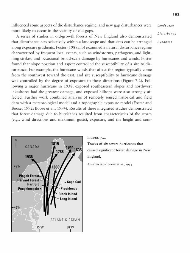
influenced some aspects of the disturbance regime, and new gap disturbances weremore likely to occur in the vicinity of old gaps.

A series of studies in old-growth forests of New England also demonstratedthat disturbance acts selectively within a landscape and that sites can be arrangedalong exposure gradients. Foster (1988a, b) examined a natural disturbance regimecharacterized by frequent local events, such as windstorms, pathogens, and light-ning strikes, and occasional broad-scale damage by hurricanes and winds. Fosterfound that slope position and aspect controlled the susceptibility of a site to dis-turbance. For example, the hurricane winds that affect the region typically comefrom the southwest toward the east, and site susceptibility to hurricane damagewas controlled by the degree of exposure to these directions (Figure 7.2). Fol-lowing a major hurricane in 1938, exposed southeastern slopes and northwestlakeshores had the greatest damage, and exposed hilltops were also strongly af-fected. Further work combined analysis of remotely sensed historical and fielddata with a meteorological model and a topographic exposure model (Foster andBoose, 1992; Boose et al., 1994). Results of these integrated studies demonstratedthat forest damage due to hurricanes resulted from characteristics of the storm(e.g., wind directions and maximum gusts), exposure, and the height and com-

163

Landscape

Disturbance

Dynamics

N

45°N

10

1938

1815

1788

1869

1944 1635

A T L A N T I C O C E A N

C A N A D A

40°N

75°W 70°W

Harvard ForestHartford

Poughkeepsie

Pisgah Forest

Providence

Block IslandLong Island

Cape Cod

Figure 7.2.

Tracks of six severe hurricanes that

caused significant forest damage in New

England.

Adapted from Boose et al., 1994.

2888_e07_p157-200 2/27/01 1:48 PM Page 163

position of the vegetation. Other studies have observed similar effects. For exam-ple, levels of hurricane damage in Hawaii varied substantially along an elevationalgradient (Harrington et al., 1997), and forest stands of similar composition inMinnesota suffered different amounts of windstorm damage based on their loca-tion (Dyer and Baird, 1997). After the eruption of Mount St. Helens, topographicpositions where snow accumulated and protected the meristems of plants revege-tated more quickly than other areas (Dale, 1991; del Moral and Bliss, 1993).

In contrast to the observations of Runkle, Foster, and others, a study address-ing these questions in Upper Michigan found no evidence for significant effects oflandscape position on disturbance susceptibility. Frelich and Lorimer (1991) stud-ied three tracts of old-growth forest in which the disturbance regime included ef-fects of fire, wind, drought, insects, disease, ice storms, and lightning strikes. Theytested for differences in the disturbance regime between upland and lowland sites,aspect classes, slope classes, and the hemlock zone along Lake Superior and theinterior forests dominated by sugar maple. Extensive field sampling was conducted,but no significant effects of these factors were observed. The upper Midwest hasrelatively little topographic relief, and Frelich and Lorimer (1991) suggested thatthe lack of topographical influence on the disturbance regime in this landscapemay reflect the types of windstorms that occur in the Upper Great Lakes Regionas compared to those that occur in the eastern United States. The windstorms thatdo the greatest damage in the Upper Great Lakes have strong downward compo-nents, compared to the horizontal winds of hurricanes; even the Southern Ap-palachians, where Runkle conducted his work, are influenced by hurricanes, al-beit infrequently. Studies of the spatial pattern of tornadoes have also demonstratedan absence of physiographic control (Peterson and Pickett, 1995). Downbursts(strong downdrafts of air from a thunderstorm or large cumulus cloud that gen-erate an outflow of wind that travels away from the point where it hits the ground)and tornadoes can hit any position in the landscape, resulting in little differenti-ation among topographic positions.

The extensive 1988 fires in Yellowstone National Park provide another exam-ple in which topographic position exerted little influence on susceptibility of sitesto disturbance. Topography can influence fire spread: flames burn more readilyuphill than downhill because of the tendency for hot air to move upward. There-fore, leeward slopes often burn with less intensity than windward slopes (Hein-selman, 1996). In addition, areas with less fuel or less flammable fuel can func-tion as firebreaks. However, the burning conditions that occurred in Yellowstoneduring 1988 were so extreme that slope position, fuel, and natural firebreaks (e.g.,streams, rivers, and even the Grand Canyon of the Yellowstone River) did not im-

164

L A N D S C A P E

E C O L O G Y I N

T H E O R Y A N D

P R A C T I C E

2888_e07_p157-200 2/27/01 1:48 PM Page 164

pede the fire. Thus, landscape position had little influence on susceptibility to fireunder the extreme drought and wind that occurred in Yellowstone during the sum-mer of 1988 (Turner and Romme, 1994).

In landscapes subject to periodic burning, the probability of ignition may varyspatially (e.g., Burgan and Hartford, 1988; Chou et al., 1993). In Glacier NationalPark, there is a high frequency of lightning ignitions on ridgelines and south-facing slopes (Habeck and Mutch, 1973). Topographic position does indeed in-fluence fire ignitions, but human influences in the landscape may also producespatial variability in fires. In the upper midwestern United States, Cardille (1998;Cardille et al., 2001) investigated the relationship between wildfire origin loca-tions and environmental and social factors for �18,000 fires between 1985 and1995. Results revealed that fires were more likely to occur in locations havinghigher human population density and higher road density and less likely to occurat greater distances from interior forests. Studies in Alaska, USA, have also demon-strated a strong relationship between fire occurrence and nearness to roads (F. S.Chapin III, personal communication).

Landscape position appears to influence susceptibility to disturbance when thedisturbance itself has a distinct directionality (e.g., hurricane tracks) such thatsome locations are usually more exposed than others. In addition, landscape po-sition may influence susceptibility if the disturbance is of moderate intensity, suchthat its spread is influenced by subtle differences in the landscape. However, if thedisturbance itself has no spatial directionality (e.g., downbursts) or is sufficientlyintense that its spread is unaffected by differences in the landscape (e.g., high-intensity crown fire), then landscape position does not influence susceptibility tothe disturbance.

E f f e c t o f L a n d s c a p e P a t t e r n o n t h e S p r e a d o f D i s t u r b a n c e

Understanding the effect of landscape heterogeneity on the spread of disturbancewas identified by Risser et al. (1984) as a fundamental question in landscape ecol-ogy, and this was the theme of the first U.S. Landscape Ecology Symposium, heldat the University of Georgia in January 1986 (Turner, 1987b). Risser et al. (1984)noted that spatial homogeneity often enhances the spread of a disturbance; con-sider the spread of pests through agroecosystems, the perpetuation of wildfire, orepidemics such as Dutch elm disease. They also noted that other disturbances maybe enhanced by landscape heterogeneity; for example, fragmented forests harborlarger populations of deer that disturb surrounding crops or overbrowse nativeforest species. But landscape heterogeneity enhances the rate of recovery by pro-

165

Landscape

Disturbance

Dynamics

2888_e07_p157-200 2/27/01 1:48 PM Page 165

viding refuges for organisms that recolonize disturbed areas. A variety of studiessuggests an interaction between landscape heterogeneity and the spread of dis-turbance, although its direction (e.g., whether it enhances or retards spread) dif-fers among disturbance types (Turner and Bratton, 1987; Castello et al., 1995).We will consider several examples that illustrate different aspects of this impor-tant interaction.

Theoretical DevelopmentAn influential conceptual study by Franklin and Forman (1987) examined the prob-ability of disturbance (e.g., wildfire, windthrow, and pests) as a function of thespatial heterogeneity imposed on a forested landscape by clear-cutting. Indeed, nu-merous subsequent studies have focused on the mosaic that results from alterna-tive spatial arrangements of clear-cuts in landscapes (e.g., Li et al., 1993; Wallinet al., 1994; Gustafson and Crow, 1996). Franklin and Forman (1987) exploredthe consequences of forest cutting along a gradient of forest conditions fromprimeval to a completely clear-cut landscape. They used simple geometric models(Figure 7.3) to evaluate how patch size, number of patches, and lengths of edgechanged under different cutting patterns; temporal dynamics (e.g., succession) werenot considered. Next, the implications of these alternative arrangements of forestand cutover lands for disturbances were evaluated. Windthrow susceptibility wasassumed to increase with the amount of edge, the isolation of forest in small patches,and increasing wind fetch. Results of the model demonstrated that windthrow po-tential would increase initially with forest cutting and continue to increase as for-est patches became isolated on all sides (Figure 7.4a). Wind fetches then progres-sively increase, especially after half the landscape is cut over; after 80% of theoriginal forest is cleared, windthrow risk to all remaining patches was consideredto be maximal. Predictions were also made for susceptibility to both fire ignitionand spread, along with risk of particular pest and pathogen outbreaks (Figure 7.4band c). Results suggested a striking influence of landscape heterogeneity on a va-riety of disturbances, although the specific effects varied by disturbance type.

Another conceptual framework for studying the effects of landscape hetero-geneity on disturbance was developed by Turner et al. (1989c) based on the neu-tral model approach (see Chapter 6). In this model, the landscape was representedas a grid of 10,000 cells containing habitat that either was or was not suscepti-ble to a given disturbance. Susceptible habitat was distributed at random and oc-cupied different proportions, p, of the landscape ranging from 0.1 to 0.9. Distur-bance was then simulated by two simple parameters: f, the probability of initiationof a new disturbance in a susceptible site, and i the probability that the distur-

166

L A N D S C A P E

E C O L O G Y I N

T H E O R Y A N D

P R A C T I C E

2888_e07_p157-200 2/27/01 1:48 PM Page 166

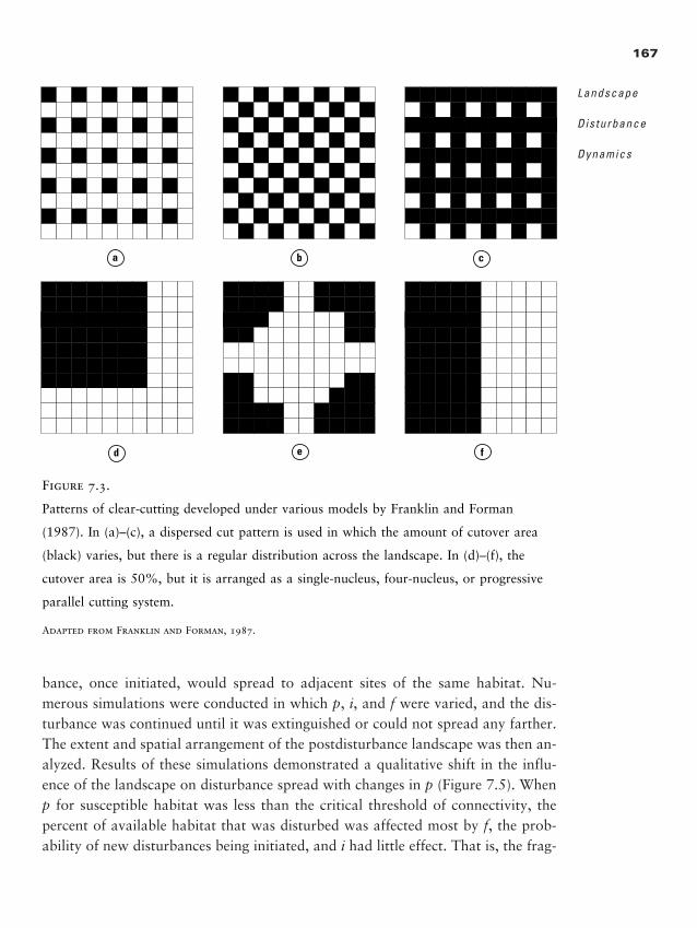
bance, once initiated, would spread to adjacent sites of the same habitat. Nu-merous simulations were conducted in which p, i, and f were varied, and the dis-turbance was continued until it was extinguished or could not spread any farther.The extent and spatial arrangement of the postdisturbance landscape was then an-alyzed. Results of these simulations demonstrated a qualitative shift in the influ-ence of the landscape on disturbance spread with changes in p (Figure 7.5). Whenp for susceptible habitat was less than the critical threshold of connectivity, thepercent of available habitat that was disturbed was affected most by f, the prob-ability of new disturbances being initiated, and i had little effect. That is, the frag-

167

Landscape

Disturbance

Dynamics

a b c

d e f

Figure 7.3.

Patterns of clear-cutting developed under various models by Franklin and Forman

(1987). In (a)–(c), a dispersed cut pattern is used in which the amount of cutover area

(black) varies, but there is a regular distribution across the landscape. In (d)–(f), the

cutover area is 50%, but it is arranged as a single-nucleus, four-nucleus, or progressive

parallel cutting system.

Adapted from Franklin and Forman, 1987.

2888_e07_p157-200 2/27/01 1:48 PM Page 167

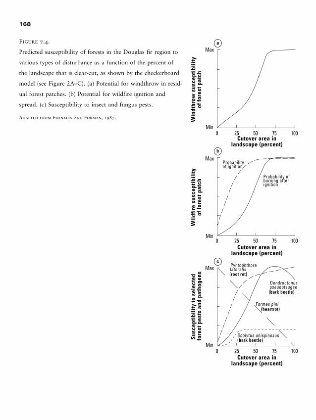
168

Susc

epti

bili

ty to

sel

ecte

d fo

rest

pes

ts a

nd p

atho

gens

Cutover area in landscape (percent)

Probability of ignition

Probability ofburning after ignition

Scolytus unispinosus

Dendroctonuspseudotsugae

Pyhtophthoralateralis

Formes pini

0Min

Max

Wil

dfir

e su

scep

tibi

lity

of fo

rest

pat

ch

Min

Max

Win

dthr

ow s

usce

ptib

ilit

yof

fore

st p

atch

Min

Max

25 50 75 100


0 25 50 75 100


0 25 50 75 100

(root rot)

(bark beetle)

(heartrot)

(bark beetle)

a

b

c

Figure 7.4.

Predicted susceptibility of forests in the Douglas fir region to

various types of disturbance as a function of the percent of

the landscape that is clear-cut, as shown by the checkerboard

model (see Figure 2A–C). (a) Potential for windthrow in resid-

ual forest patches. (b) Potential for wildfire ignition and

spread. (c) Susceptibility to insect and fungus pests.

Adapted from Franklin and Forman, 1987.

2888_e07_p157-200 2/27/01 1:48 PM Page 168

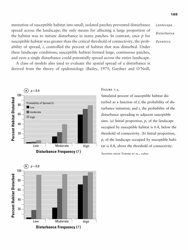
mentation of susceptible habitat into small, isolated patches prevented disturbancespread across the landscape; the only means for affecting a large proportion ofthe habitat was to initiate disturbance in many patches. In contrast, once p forsusceptible habitat was greater than the critical threshold of connectivity, the prob-ability of spread, i, controlled the percent of habitat that was disturbed. Underthese landscape conditions, susceptible habitat formed large, continuous patches,and even a single disturbance could potentially spread across the entire landscape.

A class of models also used to evaluate the spatial spread of a disturbance isderived from the theory of epidemiology (Bailey, 1975; Gardner and O’Neill,

169

Landscape

Disturbance

Dynamics

Low Moderate High

Perc

ent H

abit

at D

istu

rbed

Perc

ent H

abit

at D

istu

rbed

Disturbance Frequency (f )

20

40

60

80

100p = 0.4

Probability of Spread (i)

low

moderate

high

Low Moderate High

Disturbance Frequency (f )

20

40

60

80

100p = 0.8

a

b

Figure 7.5.

Simulated percent of susceptible habitat dis-

turbed as a function of f, the probability of dis-

turbance initiation, and i, the probability of the

disturbance spreading to adjacent susceptible

sites. (a) Initial proportion, p, of the landscape

occupied by susceptible habitat is 0.4, below the

threshold of connectivity. (b) Initial proportion,

p, of the landscape occupied by susceptible habi-

tat is 0.8, above the threshold of connectivity.

Adapted from Turner et al., 1989c.

2888_e07_p157-200 2/27/01 1:48 PM Page 169

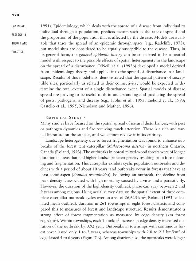
1991). Epidemiology, which deals with the spread of a disease from individual toindividual through a population, predicts factors such as the rate of spread andthe proportion of the population that is affected by the disease. Models are avail-able that trace the spread of an epidemic through space (e.g., Radcliffe, 1973),but model sites are considered to be equally susceptible to the disease. Thus, inits general form, the general epidemic theory can be considered to be a neutralmodel with respect to the possible effects of spatial heterogeneity in the landscapeon the spread of a disturbance. O’Neill et al. (1992b) developed a model derivedfrom epidemiology theory and applied it to the spread of disturbance in a land-scape. Results of this model also demonstrated that the spatial pattern of suscep-tible sites, particularly as related to their connectivity, would be expected to de-termine the total extent of a single disturbance event. Spatial models of diseasespread are proving to be useful tools in understanding and predicting the spreadof pests, pathogens, and disease (e.g., Hohn et al., 1993; Liebold et al., 1993;Castello et al., 1995; Nicholson and Mather, 1996).

Empirical StudiesMany studies have focused on the spatial spread of natural disturbances, with pestor pathogen dynamics and fire receiving much attention. There is a rich and var-ied literature on the subject, and we cannot review it in its entirety.

Landscape heterogeneity due to forest fragmentation was found to enhance out-breaks of the forest tent caterpillar (Malacosoma disstria) in northern Ontario,Canada (Roland, 1993). The outbreaks in boreal mixed-wood forests were of longerduration in areas that had higher landscape heterogeneity resulting from forest clear-ing and fragmentation. This caterpillar exhibits cyclic population outbreaks and de-clines with a period of about 10 years, and outbreaks occur in forests that have atleast some aspen (Populus tremuloides). Following an outbreak, the decline frompeak density is associated with high mortality caused by a virus and a parasitic fly.However, the duration of the high-density outbreak phase can vary between 2 and9 years among regions. Using aerial survey data on the spatial extent of three com-plete caterpillar outbreak cycles over an area of 26,623 km2, Roland (1993) calcu-lated mean outbreak duration in 261 townships in eight forest districts and com-pared this to measures of forest and landscape structure. Results demonstrated astrong effect of forest fragmentation as measured by edge density (km forestedge/km2). Within townships, each 1 km/km2 increase in edge density increased du-ration of the outbreak by 0.92 year. Outbreaks in townships with continuous for-est cover lasted only 1 to 2 years, whereas townships with 2.0 to 2.5 km/km2 ofedge lasted 4 to 6 years (Figure 7.6). Among districts also, the outbreaks were longer

170

L A N D S C A P E

E C O L O G Y I N

T H E O R Y A N D

P R A C T I C E

2888_e07_p157-200 2/27/01 1:48 PM Page 170

171

Year

s of

out

brea

k

Heterogeneity (km forest edge per km2 )

6

5

4

3

2

1

0 0.5 1.0 1.5 2.0 2.5 3.00

Sudbury

Kirkland Lake

Fort Frances

Thunder Bay

Blind River

Espanola

Sault Ste. Marie

NorthBay

Com

pone

nt e

ffect

on

dura

tion

(yea

rs)

0.00

0.25

0.50

0.75

1.00

1.25

-0.25

-0.50

-0.75

-1.00

0.50 0.75 1.00 1.25Heterogeneity (km edge per km 2 )

1 Fort Frances2 Thunder Bay3 Sault Ste. Marie4 Blind River

5 Espanola6 Sudbury7 North Bay8 Kirkland Lake

54 88

52

50

48

46

44

42

54

52

50

48

46

44

42

86 84 82 80 78

86 84 82 80 78

0 100 200

kilometers

300 400

1

2

3 4

5

6

7

8

0 1 2 3 4 5

kilometers

a

b

c d

Figure 7.6.

(a) Areas of Ontario, Canada, in which duration of forest tent caterpillar outbreaks was related to forest and

landscape structure. (b) Example from one township (MacPherson Township, North Bay District) showing the

distribution of forest (green) and nonforested (white) land. (c) Mean duration of forest tent caterpillar out-

break for 261 townships as a function of edge density for all townships. (d) Effect of mean habitat hetero-

geneity on outbreak duration within the eight forest districts.

Redrawn from Roland, 1993.

2888_e07_p157-200 2/27/01 1:48 PM Page 171

in those districts that had high average fragmentation (Figure 7.6). At both levels,the amount or proportion of aspen was not significant. Roland (1993) suggestedseveral explanations for these results. Broad-scale fragmentation of the forest mayaffect the interaction between the natural predators on the caterpillar, in that dis-persal of the pathogens may be limited by forest fragmentation. In addition, manyspecies of Lepidoptera lay more eggs along the edges of host-plant patches thanwithin the interior, so the forest tent caterpillar abundances may also be greater ini-tially along the forest edges. Warmer microclimatic conditions along the patch edgesmay also lead to more rapid development of the insect.

Reconstructions of regional outbreaks of western spruce budworm (Choris-toneura occidentalis) in the western United States during the past three centuriessuggest that landscape heterogeneity decreases the spread of this pest. Swetnamand Lynch (1993) found that the 20th century had the longest intervals of reducedbudworm activity, and the most recent outbreak that occurred through the 1970sand 1980s was unusually severe. Also, budworm infestations and epidemic peri-ods appeared to be most synchronous during the 20th century, meaning that theywere likely to occur simultaneously in many different geographic locations. Bud-worm infestations develop and spread under conditions of high tree density andconnectivity among forest stands, and this was pointed out by interesting varia-tion in the chronologies. For example, a widespread outbreak that occurred be-tween 1900 and 1920 was missing from the Colorado Front Range and the San-gre de Cristo Mountains. Swetnam and Lynch (1993) attributed this absence tothe rapid changes that had occurred in the Southern Rocky Mountain mixedconifer forests during this period. Extensive logging and previous fires had reducedconifer densities substantially, and the resulting landscape heterogeneity, in whichforests were sparser and less connected, retarded spread of the budworm. Subse-quent fire suppression, reduced sheep grazing, and favorable climatic conditionsallowed host-tree seedlings to become established, setting the stage for a dramaticfuture increase in tree density and forest connectivity. During the first part of thecentury (including the period of the widespread outbreak), these developing forestswere less susceptible to budworm outbreaks because they contained few maturetrees, and the open stand structure limited dispersal of the budworm. By the 1940s,however, these mixed conifer forests had greater canopy closure, the mature hosttrees became an important component of stand composition, and the forests weremore spatially continuous across the landscape than they had been in presettle-ment times. Budworm outbreaks subsequently became more widespread and moresevere than in earlier periods. Thus, decreased landscape heterogeneity, inducedby human activities, resulted in increased spread and synchrony of spruce bud-

172

L A N D S C A P E

E C O L O G Y I N

T H E O R Y A N D

P R A C T I C E

2888_e07_p157-200 2/27/01 1:48 PM Page 172

worm outbreaks. Swetnam and Lynch (1993) suggested that regional patterns ofbudworm outbreak, observed as synchrony among widely dispersed stands, wererelated to climate control on budworm dynamics, primarily through spring rain-fall. However, differences in local patterns resulted especially from land-use his-tory in which stand density, stand age, and landscape pattern may override theeffects of broad-scale climatic influences.

The role of landscape heterogeneity in controlling patterns of fire spread hasbeen explored in a variety of systems, both through modeling and empirical study.In some coniferous forests, heterogeneity in the pattern of different forest ageclasses tends to retard the spread of fires (e.g., Givnish, 1981; Foster, 1983; Fos-ter and King, 1986). If flammability is related to stand age (e.g., through standdensity and the dead woody fuel mass), the spatial distribution of old and youngstands may constrain or enhance fire spread. In California, for example, fires inchaparral were observed to burn well in old stands and become diminished as theyspread toward patches of younger vegetation (Minnich, 1983). There may be crit-ical thresholds in environmental constraints that determine whether landscape het-erogeneity will influence the spread of crown fire (Renkin and Despain, 1992;Turner and Romme, 1994). Landscape pattern may have little influence on crownfire behavior when burning conditions are extreme (Turner and Romme, 1994)(Figure 7.7). Under conditions of extreme drought and high winds, all fuels acrossthe landscape become highly susceptible to burning and may render the occur-rence of large stand-replacing fires inevitable (Fryer and Johnson, 1988; Johnson,1992; Bessie and Johnson, 1995).

SynthesisGiven the wide range of studies on the subject, can we generalize about whetherlandscape heterogeneity does or does not enhance the spread of disturbance? Turneret al. (1989c) suggested that the answer depends on whether the disturbance spreadswithin the same cover type, such as the spread of a species-specific parasite througha forest, or whether it crosses boundaries and spreads between different cover types.If the disturbance spreads within the same cover type, then greater landscape het-erogeneity should retard the spread of disturbance. This is observed in the sprucebudworm example (Swetnam and Lynch, 1993) and the spread of fires under mod-erate burning conditions (Turner and Romme, 1994). If the disturbance spreads be-tween cover types or is otherwise enhanced by edge effects, then increased landscapeheterogeneity should enhance the spread of the disturbance. This was observed inthe forest tent caterpillar example (Roland, 1993) and windthrow (Franklin and For-man, 1987). Recent results also suggest that there are circumstances in which land-

173

Landscape

Disturbance

Dynamics

2888_e07_p157-200 2/27/01 1:48 PM Page 173

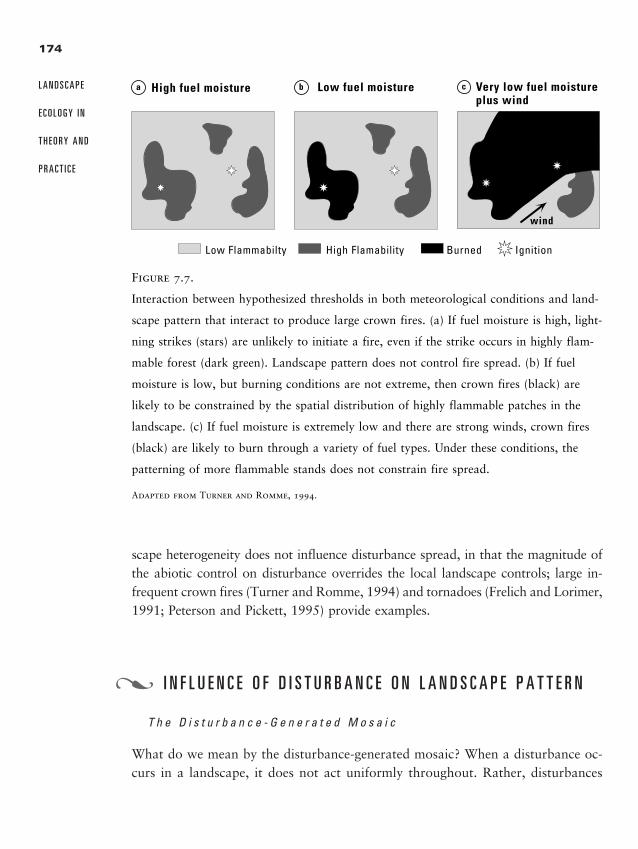
scape heterogeneity does not influence disturbance spread, in that the magnitude ofthe abiotic control on disturbance overrides the local landscape controls; large in-frequent crown fires (Turner and Romme, 1994) and tornadoes (Frelich and Lorimer,1991; Peterson and Pickett, 1995) provide examples.

I N F L U E N C E O F D I S T U R B A N C E O N L A N D S C A P E P A T T E R N

T h e D i s t u r b a n c e - G e n e r a t e d M o s a i c

What do we mean by the disturbance-generated mosaic? When a disturbance oc-curs in a landscape, it does not act uniformly throughout. Rather, disturbances

174

L A N D S C A P E

E C O L O G Y I N

T H E O R Y A N D

P R A C T I C E

Low Flammabilty High Flamability Burned Ignition

wind

a b cHigh fuel moisture Low fuel moisture Very low fuel moistureplus wind

Figure 7.7.

Interaction between hypothesized thresholds in both meteorological conditions and land-

scape pattern that interact to produce large crown fires. (a) If fuel moisture is high, light-

ning strikes (stars) are unlikely to initiate a fire, even if the strike occurs in highly flam-

mable forest (dark green). Landscape pattern does not control fire spread. (b) If fuel

moisture is low, but burning conditions are not extreme, then crown fires (black) are

likely to be constrained by the spatial distribution of highly flammable patches in the

landscape. (c) If fuel moisture is extremely low and there are strong winds, crown fires

(black) are likely to burn through a variety of fuel types. Under these conditions, the

patterning of more flammable stands does not constrain fire spread.

Adapted from Turner and Romme, 1994.

�

2888_e07_p157-200 2/27/01 1:48 PM Page 174

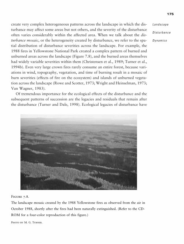
create very complex heterogeneous patterns across the landscape in which the dis-turbance may affect some areas but not others, and the severity of the disturbanceoften varies considerably within the affected area. When we talk about the dis-turbance mosaic, or the heterogeneity created by disturbance, we refer to the spa-tial distribution of disturbance severities across the landscape. For example, the1988 fires in Yellowstone National Park created a complex pattern of burned andunburned areas across the landscape (Figure 7.8), and the burned areas themselveshad widely variable severities within them (Christensen et al., 1989; Turner et al.,1994b). Even very large crown fires rarely consume an entire forest, because vari-ations in wind, topography, vegetation, and time of burning result in a mosaic ofburn severities (effects of fire on the ecosystem) and islands of unburned vegeta-tion across the landscape (Rowe and Scotter, 1973; Wright and Heinselman, 1973;Van Wagner, 1983).

Of tremendous importance for the ecological effects of the disturbance and thesubsequent patterns of succession are the legacies and residuals that remain afterthe disturbance (Turner and Dale, 1998). Ecological legacies of disturbance have

175

Landscape

Disturbance

Dynamics

Figure 7.8.

The landscape mosaic created by the 1988 Yellowstone fires as observed from the air in

October 1988, shortly after the fires had been naturally extinguished. (Refer to the CD-

ROM for a four-color reproduction of this figure.)

Photo by M. G. Turner.

2888_e07_p157-200 2/27/01 1:48 PM Page 175

both biological and physical components. Biotic legacies, or residuals, refer to thetypes, quantities, and patterns of organisms and biotic structures that persist fromthe predisturbance ecosystem. For example, residuals may include surviving indi-viduals, standing dead trees, vegetative tissue that can regenerate, seed banks, lit-ter, carcasses, and microbial and fungal soil organisms. Abiotic legacies are phys-ical modifications of the environment that may result from the disturbance, suchas mudslides or slope failures, lava flows, or movements of rocks or boulders instreams. Understanding the nature of the disturbance mosaic and the factors con-trolling these landscape patterns is essential for predicting ecosystem dynamics andvegetation development in disturbance-prone landscapes.

Foster et al. (1998) examined the landscape patterns and legacies that developfrom several types of large, infrequent disturbances that influence forests (Figure7.9). There has been considerable recent interest in the role of large, infrequentdisturbances (Turner et al., 1997a; Turner and Dale, 1998) following a numberof natural disturbances that received considerable attention from both the eco-logical research community and the general public (e.g., the eruption of MountSt. Helens in 1980, the 1988 Yellowstone fires, the 1993 floods in the midwest-ern United States, and hurricanes Hugo in 1989 and Andrew in 1992). Here, wedraw on the synthesis by Foster et al. (1998) to illustrate the variety of landscapepatterns generated by catastrophic wind, fires, and floods.

Hurricanes produce a patchwork of forest age and height structure, uprootmounds and downed boles, standing broken snags, and leaning and damaged trees(Figure 7.9) (Foster, 1988a; Foster et al., 1998). The survival, releafing and sprout-ing of windthrown and damaged trees may influence subsequent ecosystem de-velopment. In addition, increased accumulations of fine woody debris and leavesmay increase the likelihood of fire occurring in the same area (Patterson and Fos-ter, 1990; Paine et al., 1998). In contrast to hurricanes, tornadoes are relativelysmall and short-lived, although they are violent and unpredictable. A grouping oftornadoes that affected Pennsylvania, Ohio, New York, and Ontario in 1985 il-lustrates the landscape pattern of severe tornadoes (Peterson and Pickett, 1995).Tracks of the tornadoes were oriented eastward and northeastward, resulting inmore than 800 km of tornado damage. Path widths averaged 500 m and rangedfrom �200 to �2750 m. The damage patterns of tornadoes are remarkable forthe sharpness of the edges between intact forest and completely windthrown ar-eas (Peterson and Pickett, 1995). Hurricanes, tornadoes, and downbursts are ex-tremes in the gradient of size and severity of wind damage; however, all stormtypes have a gradient of intensities and severities and vary in the spatial extent ofdamage (Foster et al., 1998).

176

L A N D S C A P E

E C O L O G Y I N

T H E O R Y A N D

P R A C T I C E

2888_e07_p157-200 2/27/01 1:48 PM Page 176

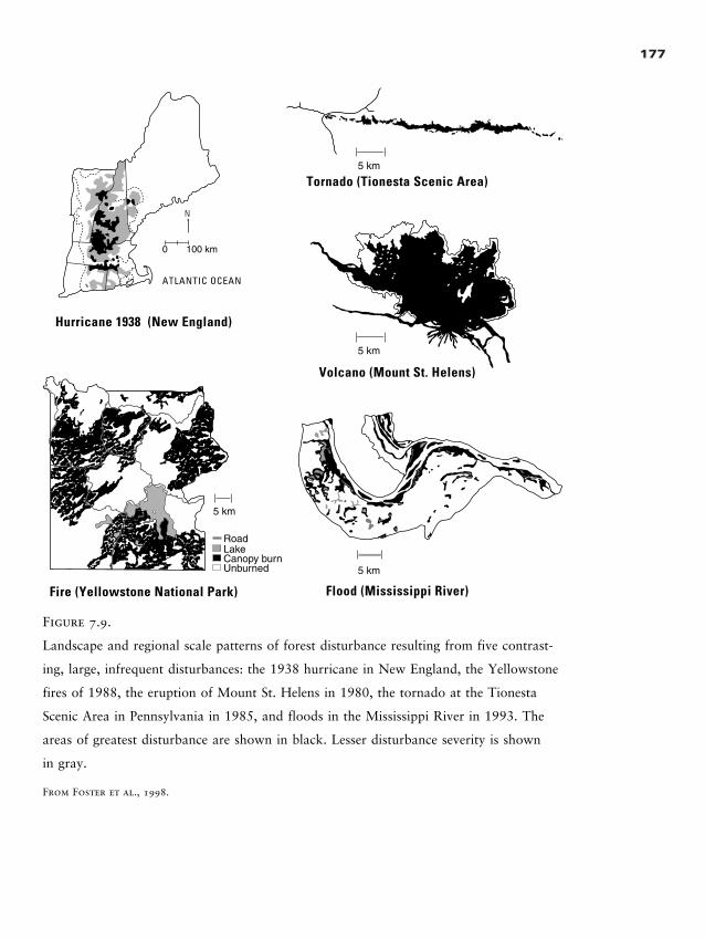
177

Volcano (Mount St. Helens)

0 100 km

N

ATLANTIC OCEAN

Hurricane 1938 (New England)

Fire (Yellowstone National Park)

Tornado (Tionesta Scenic Area)5 km

5 km

Road

Flood (Mississippi River)

5 km

5 km

LakeCanopy burnUnburned

Figure 7.9.

Landscape and regional scale patterns of forest disturbance resulting from five contrast-

ing, large, infrequent disturbances: the 1938 hurricane in New England, the Yellowstone

fires of 1988, the eruption of Mount St. Helens in 1980, the tornado at the Tionesta

Scenic Area in Pennsylvania in 1985, and floods in the Mississippi River in 1993. The

areas of greatest disturbance are shown in black. Lesser disturbance severity is shown

in gray.

From Foster et al., 1998.

2888_e07_p157-200 2/27/01 1:48 PM Page 177

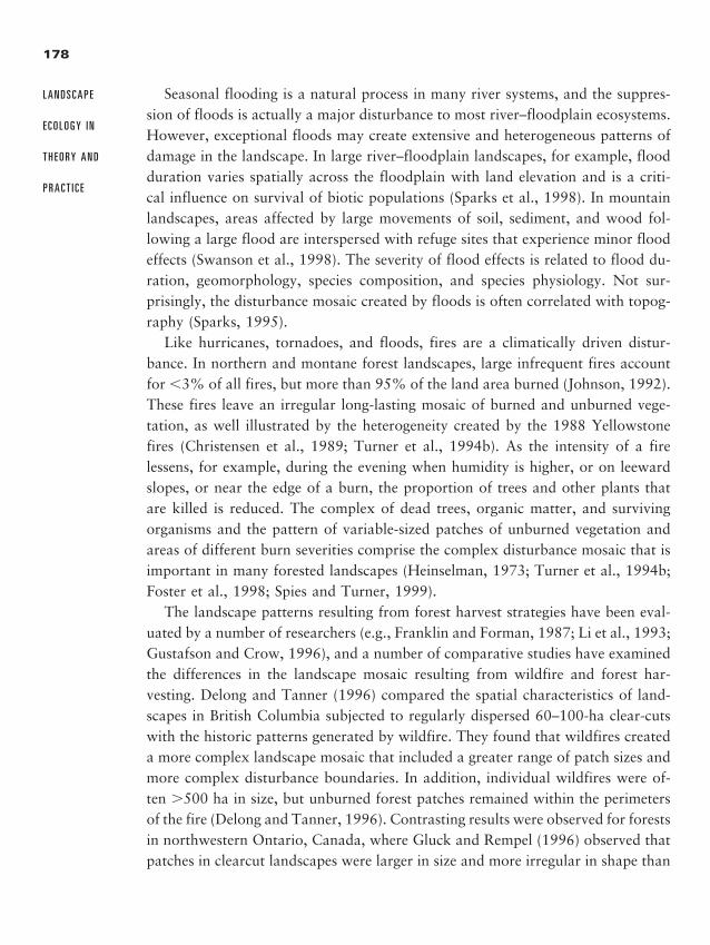
Seasonal flooding is a natural process in many river systems, and the suppres-sion of floods is actually a major disturbance to most river–floodplain ecosystems.However, exceptional floods may create extensive and heterogeneous patterns ofdamage in the landscape. In large river–floodplain landscapes, for example, floodduration varies spatially across the floodplain with land elevation and is a criti-cal influence on survival of biotic populations (Sparks et al., 1998). In mountainlandscapes, areas affected by large movements of soil, sediment, and wood fol-lowing a large flood are interspersed with refuge sites that experience minor floodeffects (Swanson et al., 1998). The severity of flood effects is related to flood du-ration, geomorphology, species composition, and species physiology. Not sur-prisingly, the disturbance mosaic created by floods is often correlated with topog-raphy (Sparks, 1995).

Like hurricanes, tornadoes, and floods, fires are a climatically driven distur-bance. In northern and montane forest landscapes, large infrequent fires accountfor �3% of all fires, but more than 95% of the land area burned (Johnson, 1992).These fires leave an irregular long-lasting mosaic of burned and unburned vege-tation, as well illustrated by the heterogeneity created by the 1988 Yellowstonefires (Christensen et al., 1989; Turner et al., 1994b). As the intensity of a firelessens, for example, during the evening when humidity is higher, or on leewardslopes, or near the edge of a burn, the proportion of trees and other plants thatare killed is reduced. The complex of dead trees, organic matter, and survivingorganisms and the pattern of variable-sized patches of unburned vegetation andareas of different burn severities comprise the complex disturbance mosaic that isimportant in many forested landscapes (Heinselman, 1973; Turner et al., 1994b;Foster et al., 1998; Spies and Turner, 1999).

The landscape patterns resulting from forest harvest strategies have been eval-uated by a number of researchers (e.g., Franklin and Forman, 1987; Li et al., 1993;Gustafson and Crow, 1996), and a number of comparative studies have examinedthe differences in the landscape mosaic resulting from wildfire and forest har-vesting. Delong and Tanner (1996) compared the spatial characteristics of land-scapes in British Columbia subjected to regularly dispersed 60–100-ha clear-cutswith the historic patterns generated by wildfire. They found that wildfires createda more complex landscape mosaic that included a greater range of patch sizes andmore complex disturbance boundaries. In addition, individual wildfires were of-ten �500 ha in size, but unburned forest patches remained within the perimetersof the fire (Delong and Tanner, 1996). Contrasting results were observed for forestsin northwestern Ontario, Canada, where Gluck and Rempel (1996) observed thatpatches in clearcut landscapes were larger in size and more irregular in shape than

178

L A N D S C A P E

E C O L O G Y I N

T H E O R Y A N D

P R A C T I C E

2888_e07_p157-200 2/27/01 1:48 PM Page 178

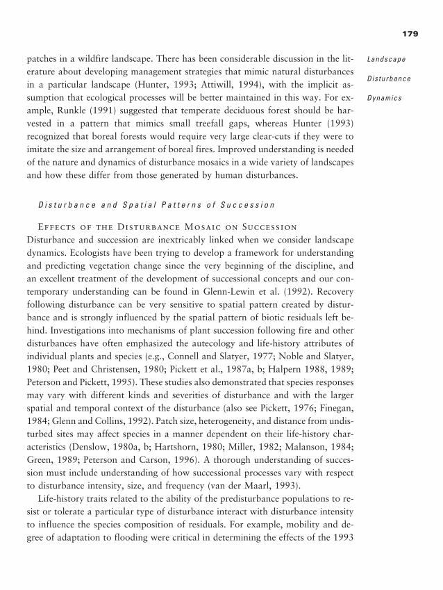
patches in a wildfire landscape. There has been considerable discussion in the lit-erature about developing management strategies that mimic natural disturbancesin a particular landscape (Hunter, 1993; Attiwill, 1994), with the implicit as-sumption that ecological processes will be better maintained in this way. For ex-ample, Runkle (1991) suggested that temperate deciduous forest should be har-vested in a pattern that mimics small treefall gaps, whereas Hunter (1993)recognized that boreal forests would require very large clear-cuts if they were toimitate the size and arrangement of boreal fires. Improved understanding is neededof the nature and dynamics of disturbance mosaics in a wide variety of landscapesand how these differ from those generated by human disturbances.

D i s t u r b a n c e a n d S p a t i a l P a t t e r n s o f S u c c e s s i o n

Effects of the Disturbance Mosaic on SuccessionDisturbance and succession are inextricably linked when we consider landscapedynamics. Ecologists have been trying to develop a framework for understandingand predicting vegetation change since the very beginning of the discipline, andan excellent treatment of the development of successional concepts and our con-temporary understanding can be found in Glenn-Lewin et al. (1992). Recoveryfollowing disturbance can be very sensitive to spatial pattern created by distur-bance and is strongly influenced by the spatial pattern of biotic residuals left be-hind. Investigations into mechanisms of plant succession following fire and otherdisturbances have often emphasized the autecology and life-history attributes ofindividual plants and species (e.g., Connell and Slatyer, 1977; Noble and Slatyer,1980; Peet and Christensen, 1980; Pickett et al., 1987a, b; Halpern 1988, 1989;Peterson and Pickett, 1995). These studies also demonstrated that species responsesmay vary with different kinds and severities of disturbance and with the largerspatial and temporal context of the disturbance (also see Pickett, 1976; Finegan,1984; Glenn and Collins, 1992). Patch size, heterogeneity, and distance from undis-turbed sites may affect species in a manner dependent on their life-history char-acteristics (Denslow, 1980a, b; Hartshorn, 1980; Miller, 1982; Malanson, 1984;Green, 1989; Peterson and Carson, 1996). A thorough understanding of succes-sion must include understanding of how successional processes vary with respectto disturbance intensity, size, and frequency (van der Maarl, 1993).

Life-history traits related to the ability of the predisturbance populations to re-sist or tolerate a particular type of disturbance interact with disturbance intensityto influence the species composition of residuals. For example, mobility and de-gree of adaptation to flooding were critical in determining the effects of the 1993

179

Landscape

Disturbance

Dynamics

2888_e07_p157-200 2/27/01 1:48 PM Page 179

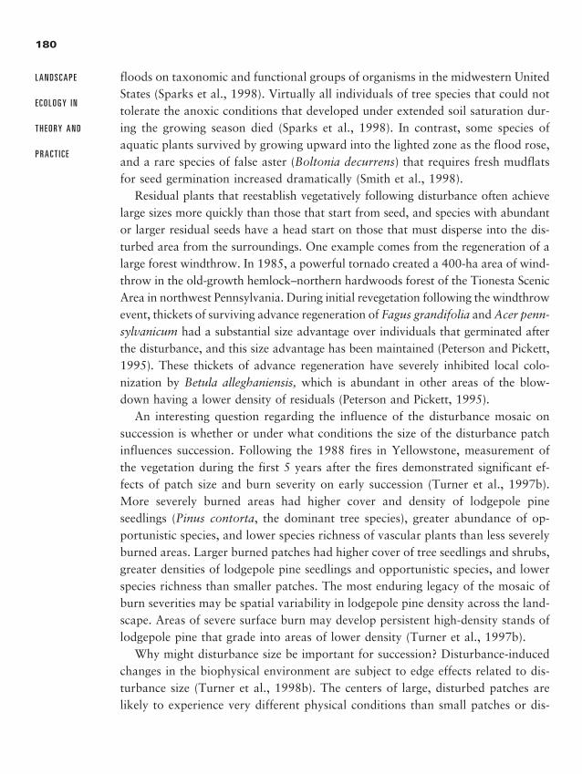
floods on taxonomic and functional groups of organisms in the midwestern UnitedStates (Sparks et al., 1998). Virtually all individuals of tree species that could nottolerate the anoxic conditions that developed under extended soil saturation dur-ing the growing season died (Sparks et al., 1998). In contrast, some species ofaquatic plants survived by growing upward into the lighted zone as the flood rose,and a rare species of false aster (Boltonia decurrens) that requires fresh mudflatsfor seed germination increased dramatically (Smith et al., 1998).

Residual plants that reestablish vegetatively following disturbance often achievelarge sizes more quickly than those that start from seed, and species with abundantor larger residual seeds have a head start on those that must disperse into the dis-turbed area from the surroundings. One example comes from the regeneration of alarge forest windthrow. In 1985, a powerful tornado created a 400-ha area of wind-throw in the old-growth hemlock–northern hardwoods forest of the Tionesta ScenicArea in northwest Pennsylvania. During initial revegetation following the windthrowevent, thickets of surviving advance regeneration of Fagus grandifolia and Acer penn-sylvanicum had a substantial size advantage over individuals that germinated afterthe disturbance, and this size advantage has been maintained (Peterson and Pickett,1995). These thickets of advance regeneration have severely inhibited local colo-nization by Betula alleghaniensis, which is abundant in other areas of the blow-down having a lower density of residuals (Peterson and Pickett, 1995).

An interesting question regarding the influence of the disturbance mosaic onsuccession is whether or under what conditions the size of the disturbance patchinfluences succession. Following the 1988 fires in Yellowstone, measurement ofthe vegetation during the first 5 years after the fires demonstrated significant ef-fects of patch size and burn severity on early succession (Turner et al., 1997b).More severely burned areas had higher cover and density of lodgepole pineseedlings (Pinus contorta, the dominant tree species), greater abundance of op-portunistic species, and lower species richness of vascular plants than less severelyburned areas. Larger burned patches had higher cover of tree seedlings and shrubs,greater densities of lodgepole pine seedlings and opportunistic species, and lowerspecies richness than smaller patches. The most enduring legacy of the mosaic ofburn severities may be spatial variability in lodgepole pine density across the land-scape. Areas of severe surface burn may develop persistent high-density stands oflodgepole pine that grade into areas of lower density (Turner et al., 1997b).

Why might disturbance size be important for succession? Disturbance-inducedchanges in the biophysical environment are subject to edge effects related to dis-turbance size (Turner et al., 1998b). The centers of large, disturbed patches arelikely to experience very different physical conditions than small patches or dis-

180

L A N D S C A P E

E C O L O G Y I N

T H E O R Y A N D

P R A C T I C E

2888_e07_p157-200 2/27/01 1:48 PM Page 180

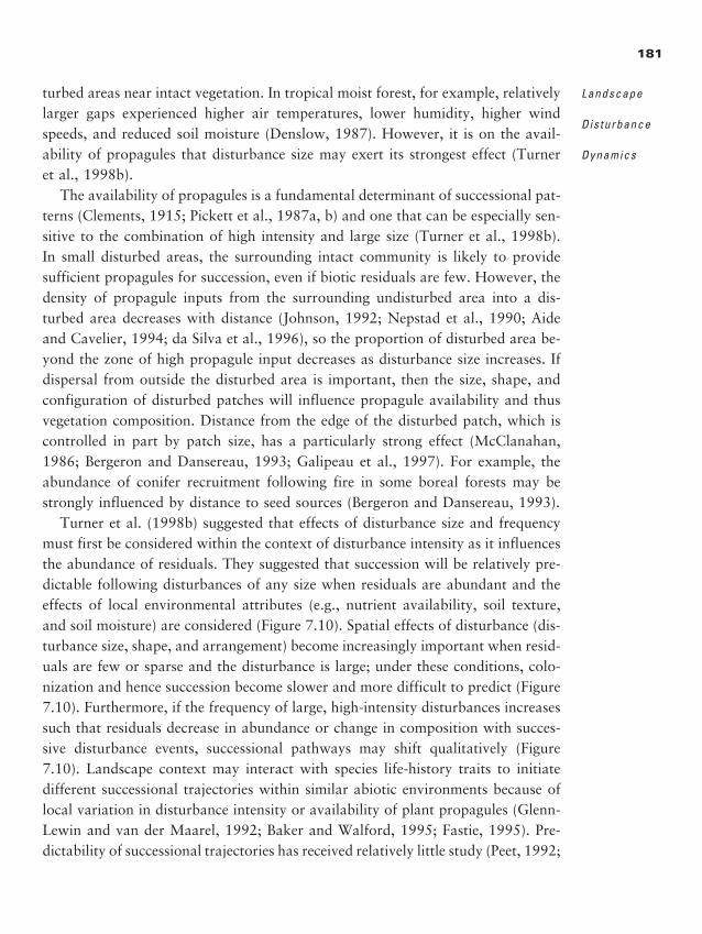
turbed areas near intact vegetation. In tropical moist forest, for example, relativelylarger gaps experienced higher air temperatures, lower humidity, higher windspeeds, and reduced soil moisture (Denslow, 1987). However, it is on the avail-ability of propagules that disturbance size may exert its strongest effect (Turneret al., 1998b).

The availability of propagules is a fundamental determinant of successional pat-terns (Clements, 1915; Pickett et al., 1987a, b) and one that can be especially sen-sitive to the combination of high intensity and large size (Turner et al., 1998b).In small disturbed areas, the surrounding intact community is likely to providesufficient propagules for succession, even if biotic residuals are few. However, thedensity of propagule inputs from the surrounding undisturbed area into a dis-turbed area decreases with distance (Johnson, 1992; Nepstad et al., 1990; Aideand Cavelier, 1994; da Silva et al., 1996), so the proportion of disturbed area be-yond the zone of high propagule input decreases as disturbance size increases. Ifdispersal from outside the disturbed area is important, then the size, shape, andconfiguration of disturbed patches will influence propagule availability and thusvegetation composition. Distance from the edge of the disturbed patch, which iscontrolled in part by patch size, has a particularly strong effect (McClanahan,1986; Bergeron and Dansereau, 1993; Galipeau et al., 1997). For example, theabundance of conifer recruitment following fire in some boreal forests may bestrongly influenced by distance to seed sources (Bergeron and Dansereau, 1993).

Turner et al. (1998b) suggested that effects of disturbance size and frequencymust first be considered within the context of disturbance intensity as it influencesthe abundance of residuals. They suggested that succession will be relatively pre-dictable following disturbances of any size when residuals are abundant and theeffects of local environmental attributes (e.g., nutrient availability, soil texture,and soil moisture) are considered (Figure 7.10). Spatial effects of disturbance (dis-turbance size, shape, and arrangement) become increasingly important when resid-uals are few or sparse and the disturbance is large; under these conditions, colo-nization and hence succession become slower and more difficult to predict (Figure7.10). Furthermore, if the frequency of large, high-intensity disturbances increasessuch that residuals decrease in abundance or change in composition with succes-sive disturbance events, successional pathways may shift qualitatively (Figure7.10). Landscape context may interact with species life-history traits to initiatedifferent successional trajectories within similar abiotic environments because oflocal variation in disturbance intensity or availability of plant propagules (Glenn-Lewin and van der Maarel, 1992; Baker and Walford, 1995; Fastie, 1995). Pre-dictability of successional trajectories has received relatively little study (Peet, 1992;

181

Landscape

Disturbance

Dynamics

2888_e07_p157-200 2/27/01 1:48 PM Page 181

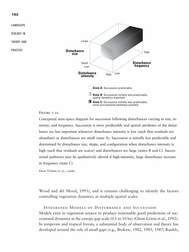
182

L A N D S C A P E

E C O L O G Y I N

T H E O R Y A N D

P R A C T I C E

Wood and del Moral, 1993), and it remains challenging to identify the factorscontrolling vegetation dynamics at multiple spatial scales.

Integrated Models of Disturbance and SuccessionModels exist in vegetation science to produce reasonably good predictions of suc-cessional dynamics at the canopy gap scale (0.1 to 10 ha) (Glenn-Lewin et al., 1992).In temperate and tropical forests, a substantial body of observation and theory hasdeveloped around the role of small gaps (e.g., Brokaw, 1982, 1985, 1987; Runkle,

Large

SmallLow

High

High

Low

Disturbancesize

Disturbanceintensity

State A: Succession predictable

Disturbancefrequency

State B: Succession initially less predictable,spatial dynamics important

State C: Succession initially less predictable,novel successional pathways possible

Figure 7.10.

Conceptual state-space diagram for succession following disturbances varying in size, in-

tensity, and frequency. Succession is more predictable and spatial attributes of the distur-

bance are less important whenever disturbance intensity is low (such that residuals are

abundant) or disturbances are small (state A). Succession is initially less predictable and

determined by disturbance size, shape, and configuration when disturbance intensity is

high (such that residuals are scarce) and disturbances are large (states B and C). Succes-

sional pathways may be qualitatively altered if high-intensity, large disturbance increase

in frequency (state C).

From Turner et al., 1998b.

2888_e07_p157-200 2/27/01 1:48 PM Page 182

1982, 1985; Lertzman, 1992). In the small-gap paradigm, differences in vegetationdynamics are primarily attributed to gap size, whereas shade tolerance differenti-ates tree species into early-successional and late-successional species (Swaine andWhitmore, 1988). The forest gap models (Botkin et al., 1972; Shugart and West,1981) have been applied to a broad spectrum of community types, extrapolatinglandscape-scale effects from multiple simulations of small (0.1 ha) forest plots. Al-though simulation of disturbance effects has been included in the gap models(Shugart and Noble, 1981; Bonan and Shugart, 1989), inclusion of spatial effectsof dispersal and fire has been accomplished by linking multiple plots (replicate mod-els) within a spatial network (Urban et al., 1991; Acevedo et al., 1996).

Applying the theoretical and empirical advances in understanding of how dis-turbance and succession interact with large, heterogeneous landscapes is challeng-ing because of the spatial interactions and the long time scales involved (He andMladenoff, 1999; Mladenoff and Baker, 1999). Integrated models of disturbanceand succession can reveal trends and dynamics in landscapes that cannot be easilyobserved empirically, and such models may be particularly useful for addressingquestions of broad-scale disturbances or global change. Extrapolating models acrossspatial scales, however, remains difficult (McKenzie et al., 1996). An example of anintegrated model of disturbance and succession is LANDIS, developed for a 500,000-ha landscape in northern Wisconsin, USA (Mladenoff et al., 1996; He and Mlade-noff, 1999; Mladenoff and He, 1999). The study landscape is located in the tran-sitional zone between boreal forest to the north and temperate forest to the south;the region was glaciated, has little topographic relief, and is largely forested. Themodel represents landscape heterogeneity caused by spatial variation in environ-mental conditions and disturbance rates, as well as the effects of past human usesin the landscape. Multiple disturbance types are simulated, including fire, wind-throw, and forest harvest, and succession is represented at the species level. Suc-cessional dynamics are based on life-history attributes (e.g., shade tolerance, dis-turbance susceptibility, vegetative reproduction, time to sexual maturity, longevity)of up to 30 species, and spatial processes such as seed dispersal are included.

LANDIS was initialized with the current landscape pattern and used to simu-late landscape dynamics for 500 yr, with fire as the only disturbance (He andMladenoff, 1999). Results demonstrated that, even when the presettlement dis-turbance regime was reestablished, some species, such as hemlock, yellow birch,oak, and pine, did not recover their presettlement proportions of the forest com-munity for 100 to 500 yr. They also found that landscape recovery could be de-tected at broad spatial scales as the composition of the forest communities dif-ferentiated on different land types. Interestingly, the landscape showed greater

183

Landscape

Disturbance

Dynamics

2888_e07_p157-200 2/27/01 1:48 PM Page 183

alteration on the more mesic landforms in which disturbances were infrequent butsevere, as compared to the more xeric landforms in which disturbance was morefrequent but less severe. Similar results have been observed in other systems (Gard-ner et al., 1996; Turner et al., 1998b). It is important to remember that these mod-eling approaches are not used deterministically to predict what will happen withspecific individual events. Models such as LANDIS and Fire-BGC (Keane et al.,1996a, b) can incorporate feedbacks among species, disturbance, and environ-mental variability and are valuable tools for examining complex interactions ofspecies and disturbance over large areas and long time periods.

E f f e c t s o f C h a n g i n g D i s t u r b a n c e R e g i m e s o n L a n d s c a p e P a t t e r n

Because disturbances can be such a strong source of landscape structure, intentionalor unintentional shifts in the disturbance regime may dramatically alter the land-scape. For example, past climatic changes of small magnitude have caused signifi-cant changes in fire regimes in forested landscapes (Green, 1982; Hemstrom andFranklin, 1982; Clark, 1988, 1990; Bergeron, 1991; Campbell and McAndrews,1993), and fire suppression during the past century has lengthened the fire returninterval and altered successional pathways in many regions (e.g., Glitzenstein et al.,1995; Linder et al., 1997). Changes in the frequency and extent of flooding haveresulted in ecological responses in many river–floodplain systems. However, en-hancing our quantitative understanding and ability to predict the effects of chang-ing disturbance regimes on landscape structure remains a current topic of active re-search (Graham et al., 1990; Miller and Urban, 1999). In particular, little is knownregarding which components of landscape structure are most sensitive to change orhow directional changes in landscape structure can be detected.

Spatial models have proved valuable in exploring the sensitivity of landscapepatterns to changes in disturbance regime. Using a GIS-based spatial model anddata on historical changes in fire sizes, Baker (1992) simulated the effects of set-tlement and fire suppression on landscape structure in the Boundary Waters Ca-noe Area of northern Minnesota, an area in which fire dynamics have been wellstudied (Heinselman, 1996). Prior to European settlement, fires were relativelylarge and infrequent. As the upper Midwest was settled by Europeans, fire fre-quency increased substantially because of indiscriminate burning by early settlers,land speculators, and prospectors. Subsequently, there was an extensive period ofactive human fire suppression. The periods of settlement and fire suppression,which represented substantial shifts from the presettlement disturbance regime,produced significant effects on landscape structure (Figure 7.11). Settlement pro-duced immediate effects on some metrics of landscape pattern, including patch

184

L A N D S C A P E

E C O L O G Y I N

T H E O R Y A N D

P R A C T I C E

2888_e07_p157-200 2/27/01 1:48 PM Page 184

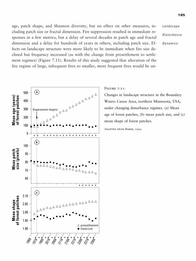
age, patch shape, and Shannon diversity, but no effect on other measures, in-cluding patch size or fractal dimension. Fire suppression resulted in immediate re-sponses in a few metrics, but a delay of several decades in patch age and fractaldimension and a delay for hundreds of years in others, including patch size. Ef-fects on landscape structure were more likely to be immediate when fire size de-clined but frequency increased (as with the change from presettlement to settle-ment regimes) (Figure 7.11). Results of this study suggested that alteration of thefire regime of large, infrequent fires to smaller, more frequent fires would be un-

185

Landscape

Disturbance

Dynamics

Mea

n ag

e (y

ears

)of

fore

st p

atch

esM

ean

patc

h si

ze (p

ixel

s)M

ean

shap

eof

fore

st p

atch

es

500

400

300

200

100

0

105

95

85

75

65

2.10

2.05

2.00

1.95

1.90

1868

19

18*

1968

*20

18*

2068

*21

18*

2168

*22

18*

2268

*23

18*

2368

*

Suppression begins

presettlementhistorical

* * * * * * * * *

* * * * * * * * * ** * * * * * * * *

* * ** * *

a

b

c

Figure 7.11.

Changes in landscape structure in the Boundary

Waters Canoe Area, northern Minnesota, USA,

under changing disturbance regimes. (a) Mean

age of forest patches, (b) mean patch size, and (c)

mean shape of forest patches.

Adapted from Baker, 1992.

2888_e07_p157-200 2/27/01 1:48 PM Page 185

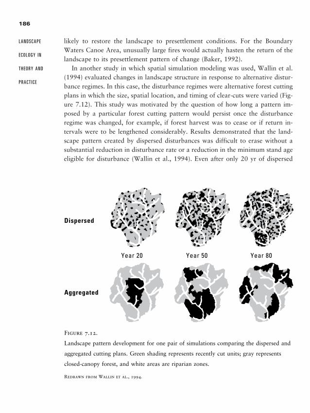
likely to restore the landscape to presettlement conditions. For the Boundary Waters Canoe Area, unusually large fires would actually hasten the return of thelandscape to its presettlement pattern of change (Baker, 1992).

In another study in which spatial simulation modeling was used, Wallin et al.(1994) evaluated changes in landscape structure in response to alternative distur-bance regimes. In this case, the disturbance regimes were alternative forest cuttingplans in which the size, spatial location, and timing of clear-cuts were varied (Fig-ure 7.12). This study was motivated by the question of how long a pattern im-posed by a particular forest cutting pattern would persist once the disturbanceregime was changed, for example, if forest harvest was to cease or if return in-tervals were to be lengthened considerably. Results demonstrated that the land-scape pattern created by dispersed disturbances was difficult to erase without asubstantial reduction in disturbance rate or a reduction in the minimum stand ageeligible for disturbance (Wallin et al., 1994). Even after only 20 yr of dispersed

186

L A N D S C A P E

E C O L O G Y I N

T H E O R Y A N D

P R A C T I C E

Year 20 Year 50 Year 80

Dispersed

Aggregated

Figure 7.12.

Landscape pattern development for one pair of simulations comparing the dispersed and

aggregated cutting plans. Green shading represents recently cut units; gray represents

closed-canopy forest, and white areas are riparian zones.

Redrawn from Wallin et al., 1994.

2888_e07_p157-200 2/27/01 1:48 PM Page 186

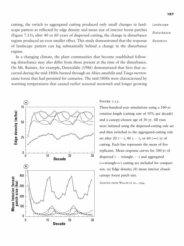
187

Landscape

Disturbance

Dynamics

cutting, the switch to aggregated cutting produced only small changes in land-scape pattern as reflected by edge density and mean size of interior forest patches(Figure 7.13); after 40 or 60 years of dispersed cutting, the change in disturbanceregime produced an even smaller effect. This study demonstrated that the responseof landscape pattern can lag substantially behind a change in the disturbanceregime.

In a changing climate, the plant communities that become established follow-ing disturbance may also differ from those present at the time of the disturbance.On Mt. Rainier, for example, Dunwiddie (1986) demonstrated that fires that oc-curred during the mid-1800s burned through an Abies amabilis and Tsuga merten-siana forest that had persisted for centuries. The mid-1800s were characterized bywarming temperatures that caused earlier seasonal snowmelt and longer growing

Decade

Decade

Mea

n In

teri

or fo

rest

pa

tch

size

(ha)

Edge

den

sity

(m/h

a)

0

25

75

50

0

100

300

400

200

0 10 20 30

0 10 20 30

a

b

Figure 7.13.

Three-hundred-year simulations using a 100-yr

rotation length (cutting rate of 10% per decade)

and a canopy-closure age of 30 yr. All runs

were initiated using the dispersed-cutting rule set

and then switched to the aggregated-cutting rule

set after 20 (��), 40 (- - -), or 60 (——) yr of

cutting. Each line represents the mean of five

replicates. Mean response curves for 300-yr of

dispersed (- - -triangle- - -) and aggregated

(——triangle——) cutting are included for compari-

son. (a) Edge density; (b) mean interior closed-

canopy forest patch size.

Adapted from Wallin et al., 1994.

2888_e07_p157-200 2/27/01 1:48 PM Page 187

seasons. These climatic conditions allowed Tsuga heterophylla to become abun-dant briefly after the fires, and T. heterophylla was then replaced by Abies lasio-carpa. Because long-lived mature trees may survive short-term climatic fluctua-tions, species that are best adapted to the current climate may only be able toenter the forest in open habitats following severe fires, and forest compositionmay respond to climatic changes primarily after disturbance (Dunwiddie, 1986).A study by Cwynar (1987) also suggests that, although the ultimate cause of post-glacial vegetation change in the Pacific Northwest was climate change, the prox-imate cause of some postglacial vegetation changes was an altered fire regime. Asmall change to a drier climate probably triggered a relatively large change in thedisturbance regime by increasing fire frequency (Cwynar, 1987). Potential cli-matically induced alterations in crown fire regimes may therefore lead to sub-stantial landscape changes, in terms of both the characteristic vegetation mosaicand the species composition of particular regions. Understanding the sensitivity of disturbance regimes to climate change remains an important topic of currentresearch.

One general result to emerge from these studies is the importance of using avariety of metrics of landscape pattern to detect changes resulting from alterationsof disturbance regimes. Some aspects of pattern are likely to be affected more thanothers or to respond more quickly, yet we presently do not have sufficient datafrom which to recommend a narrow set of metrics sufficient to characterize orpredict disturbance effects. The paucity of data and the impossibility of experi-mental manipulation at landscape scales make the development and testing of hy-potheses problematic.

C O N C E P T S O F L A N D S C A P E E Q U I L I B R I U M

The notion of equilibrium in ecological systems has inspired a long history of in-terest and controversy in ecology (e.g., Egerton, 1973; Bormann and Likens, 1979;Connell and Sousa, 1983; Wiens, 1984; DeAngelis and Waterhouse, 1987). Pick-ett et al. (1994:159) identified equilibrium as one of few overarching paradigmsin ecology, and one of the oldest and most pervasive, that affect the dialog be-tween observable phenomena and conceptual constructs in all the more special-ized areas of ecology. Six tenets of this paradigm were identified (Pickett et al.1994), in which ecological systems were considered: (1) to be essentially closed,(2) to be self-regulating, (3) to possess stable point or stable cycle equilibria, (4)

188

L A N D S C A P E

E C O L O G Y I N

T H E O R Y A N D

P R A C T I C E

�

2888_e07_p157-200 2/27/01 1:48 PM Page 188

to have deterministic dynamics, (5) to be essentially free of disturbance, and (6)to be independent of human influences. The shift in ecology from an equilibriumview of nature to the nonequilibrium paradigm occurred gradually throughout the20th century. In the nonequilibrium paradigm, ecological systems are thought tobe open, to be regulated by both intrinsic and extrinsic factors, to lack a stablepoint equilibrium, to be nondeterministic, to incorporate disturbance, and to ad-mit human influence. If equilibrium is observed, it may only appear at certain spa-tial and temporal scales (Pickett et al., 1994). Because these ideas represent sucha fundamental shift in ecological thinking and because they are so relevant forboth basic and applied ecology, we review the development of the concepts asthey apply to landscape ecology in some depth.

Questions of whether equilibrium could be detected on landscapes subject todisturbance and how large a landscape must be to incorporate a given disturbanceregime have been important themes in landscape ecology (Shugart and West, 1981;Romme, 1982; Baker, 1989a). The controversy regarding equilibrium has stemmedin part from inconsistent definitions and criteria used by investigators and in partfrom disagreement about whether it is valid to define the existence of an equilib-rium state at all (Turner et al., 1993b). DeAngelis and Waterhouse (1987) pro-vide an excellent review of the treatment of these concepts in ecological models.The critical issue is that concepts of equilibrium are confounded by problems ofscale, and landscapes can exhibit a suite of dynamics of which equilibrium is butone (Turner et al., 1993b).

Equilibrium points can be precisely defined mathematically, but equilibriumand stability are not well defined when applied to real ecological systems (DeAn-gelis and Waterhouse, 1987). Properties used to evaluate equilibrium fall into twogeneral categories: persistence (nonextinction or presence) and constancy (nochange or minimal fluctuation in numbers, densities, or relative proportions). Per-sistence can be applied to all species, as is often done in many population-orientedmodels (e.g., DeAngelis and Waterhouse, 1987), or to the presence of all standage classes or successional stages in a landscape (e.g., Romme, 1982). Constancymay refer to the number of species (e.g., MacArthur and Wilson, 1967), the den-sity of individual species (e.g., May, 1973), the standing crop of biomass (e.g.,Bormann and Likens, 1979; Sprugel, 1985), or the relative proportions of seralstages on a landscape (e.g., Romme, 1982; Baker, 1989a, c). There are funda-mental differences in considering species composition versus structural attributessuch as biomass, age classes, and seral stages. Seral stages or age classes do notbecome extinct because they can be regenerated by disturbances, provided thespecies comprising each stage do not become extinct.

189

Landscape

Disturbance

Dynamics

2888_e07_p157-200 2/27/01 1:48 PM Page 189

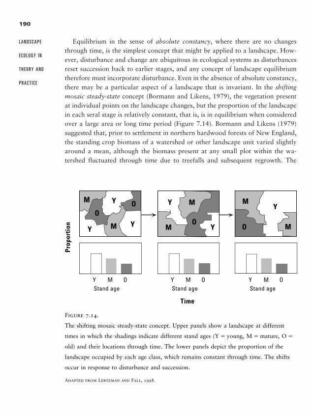
Equilibrium in the sense of absolute constancy, where there are no changesthrough time, is the simplest concept that might be applied to a landscape. How-ever, disturbance and change are ubiquitous in ecological systems as disturbancesreset succession back to earlier stages, and any concept of landscape equilibriumtherefore must incorporate disturbance. Even in the absence of absolute constancy,there may be a particular aspect of a landscape that is invariant. In the shiftingmosaic steady-state concept (Bormann and Likens, 1979), the vegetation presentat individual points on the landscape changes, but the proportion of the landscapein each seral stage is relatively constant, that is, is in equilibrium when consideredover a large area or long time period (Figure 7.14). Bormann and Likens (1979)suggested that, prior to settlement in northern hardwood forests of New England,the standing crop biomass of a watershed or other landscape unit varied slightlyaround a mean, although the biomass present at any small plot within the wa-tershed fluctuated through time due to treefalls and subsequent regrowth. The

190

L A N D S C A P E

E C O L O G Y I N

T H E O R Y A N D

P R A C T I C E

Time

Prop

orti

on

Stand ageY M O

Stand ageY M O

Stand ageY M O

M

MM

MY Y

YO

O

Y

YY

OO

O

M

M

Figure 7.14.

The shifting mosaic steady-state concept. Upper panels show a landscape at different

times in which the shadings indicate different stand ages (Y � young, M � mature, O �

old) and their locations through time. The lower panels depict the proportion of the

landscape occupied by each age class, which remains constant through time. The shifts

occur in response to disturbance and succession.

Adapted from Lertzman and Fall, 1998.

2888_e07_p157-200 2/27/01 1:48 PM Page 190

shifting mosaic steady-state concept has been difficult to test empirically, but ithas been suggested to apply to other systems. Studies of wave-generated fir forestsin the northeastern United States have suggested a steady-state condition over theentire system despite widespread local patterns of community degradation and re-generation (Sprugel, 1976; Sprugel and Bormann, 1981). Zackrisson (1977) sug-gested that the forest mosaic in a boreal forest in northern Sweden remains un-changed, even though the spatial distribution of postfire succession is alwayschanging. The concept applies best when disturbances are small and frequent ina large area of homogeneous habitat (Pickett and White, 1985). Large areas maybe more likely than small areas to exhibit a stable mosaic (Zedler and Goff, 1973;Connell and Sousa, 1983; DeAngelis and Waterhouse, 1987). Shugart and West(1981) suggested that a quasi-steady-state landscape was likely only where thelandscape was at least 50 times the average size of a disturbance, although Baker(1989a) failed to find equilibrium in the Boundary Waters Canoe Area even at ascale 87 times the mean disturbance patch size.

Another concept considers landscape equilibrium to be a stationary process (astochastic process that does not change in distribution over time or space) withepisodic perturbation (Loucks, 1970). Loucks (1970) suggested that communitiesmay appear unstable at any particular time because community composition ischanging, but that the entire long-term sequence of changes constitutes a stablesystem, because the same sequence recurs after every disturbance. In fire-domi-nated landscapes, for example, the statistical distribution of seral stages, time in-tervals between successive fires, or similar parameters can be determined (e.g., VanWagner, 1978; Johnson, 1979; Yarie, 1981; Johnson and Van Wagner, 1985;Johnson and Gutsell, 1994). This concept explicitly acknowledges the stochasticnature of disturbance, but assumes that the distribution of disturbance intervalsand the proportion of the landscape occupied by different seral stages remainsmore or less constant through time. However, the distribution of intervals betweendisturbances may not be the same, and the probability of disturbance may changewith time since last disturbance (Clark, 1989).

A concept related to the stationary process is that of stochastic or relative con-stancy through time. Botkin and Sobel (1975) suggested that a system that changesbut remains within bounds is a stochastic analog of equilibrium that is applica-ble to ecological systems. Harrison (1979) also suggested that the concept of asystem remaining within acceptable ranges in spite of environmental uncertaintywas most relevant to ecology. However, even this concept is scale dependent. Forexample, long-term directional changes in climate due to global warming or glacialcycles would eventually move a landscape out of preset bounds.

191

Landscape

Disturbance

Dynamics

2888_e07_p157-200 2/27/01 1:48 PM Page 191

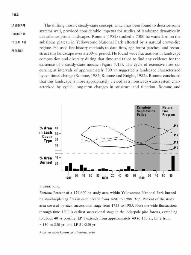
The shifting mosaic steady-state concept, which has been found to describe somesystems well, provided considerable impetus for studies of landscape dynamics indisturbance-prone landscapes. Romme (1982) studied a 7300-ha watershed on thesubalpine plateau in Yellowstone National Park affected by a natural crown-fireregime. He used fire history methods to date fires, age forest patches, and recon-struct this landscape over a 200-yr period. He found wide fluctuations in landscapecomposition and diversity during that time and failed to find any evidence for theexistence of a steady-state mosaic (Figure 7.15). The cycle of extensive fires oc-curring at intervals of approximately 300 yr suggested a landscape characterizedby continual change (Romme, 1982; Romme and Knight, 1982). Romme concludedthat this landscape is more appropriately viewed as a nonsteady-state system char-acterized by cyclic, long-term changes in structure and function. Romme and

192

L A N D S C A P E

E C O L O G Y I N

T H E O R Y A N D

P R A C T I C E

% Areain Each

CoverType

CompleteSuppressionPolicy

NaturalFireProgram

% AreaBurned

LP 0

LP 1

LP 2

LP 3

10

40

20

20

3040

20 40 60 801700

20 40 60 801800

20 40 60 801900

Figure 7.15.

Bottom: Percent of a 129,600-ha study area within Yellowstone National Park burned

by stand-replacing fires in each decade from 1690 to 1988. Top: Percent of the study

area covered by each successional stage from 1735 to 1985. Note the wide fluctuations

through time. LP 0 is earliest successional stage in the lodgepole pine forests, extending

to about 40 yr postfire; LP 1 extends from approximately 40 to 150 yr, LP 2 from

�150 to 250 yr, and LP 3 �250 yr.

Adapted from Romme and Despain, 1989.

2888_e07_p157-200 2/27/01 1:48 PM Page 192

Despain (1989) expanded this study to an area of 129,600 ha, but still found con-stant fluctuation in the patch mosaic during the past 250 yr.

Similarly, Baker (1989a, c) tested for a stable patch mosaic in the 404,000-hafire-influenced Boundary Waters Canoe Area (BWCA), but did not find a stablepatch mosaic at any of five spatial scales. Baker (1989a) used a Markov chain ap-proach to examine potential long-term trends in the vegetation mosaic in theBoundary Waters Canoe Area, Minnesota, based on fire-year maps published byHeinselman (1973). The model was developed for heuristic purposes and assumedthat the fire regime that occurred during the 141-yr study period (1727–1868) re-mained constant into the future. Transitions occurred between forest age classes.Baker used the model to compare the final distribution of age classes at five spa-tial scales and to evaluate the presence of a stable mosaic and the minimum areaneeded for a stable mosaic to be observed. Similarity between the simulated finaldistributions of age classes and the steady-state final distribution was gener-ally low across all spatial scales. He suggested that the lack of a steady-state mo-saic was due to (1) spatial heterogeneity in the fire regime, whereby ignitionsources, drought severity, fuel load, and fire spread probability would vary acrossthe landscape and (2) a difference in the scales of fire patches and environmentalheterogeneity. Baker (1989a) concluded that the Boundary Waters Canoe Arealandscape was a “mosaic of different non-steady-state mosaics.” Indeed, crown-fire-dominated systems may generally be considered as nonequilibrium landscapes(Turner and Romme, 1994; Boychuk et al., 1997).

Turner et al. (1993b) used a simple spatial model to develop a view of land-scape dynamics that considered the spatial–temporal scales of disturbance and theresultant landscape dynamics and that could be applied across a range of scales.A simple spatial model was developed that incorporated four major factors char-acterizing landscape dynamics: disturbance frequency, recovery time, spatial ex-tent of disturbance events, and size of the landscape of interest. These four fac-tors were reduced to two key parameters representing ratios of time and space.The use of ratios in both parameters permits comparison of landscapes across arange of spatial and temporal scales.

The temporal parameter (T) was defined by the ratio of the disturbance inter-val (the time between successive disturbances) to the recovery time (the time re-quired for a disturbed site to achieve recovery to a mature stage). Defining thetemporal parameter as a ratio permitted three qualitatively different states to beconsidered, regardless of the type or time scale of the disturbance: (1) the distur-bance interval is longer than the recovery time (T � 1), so the system can recoverbefore being disturbed again; (2) the disturbance interval and recovery time are

193

Landscape

Disturbance

Dynamics

2888_e07_p157-200 2/27/01 1:48 PM Page 193

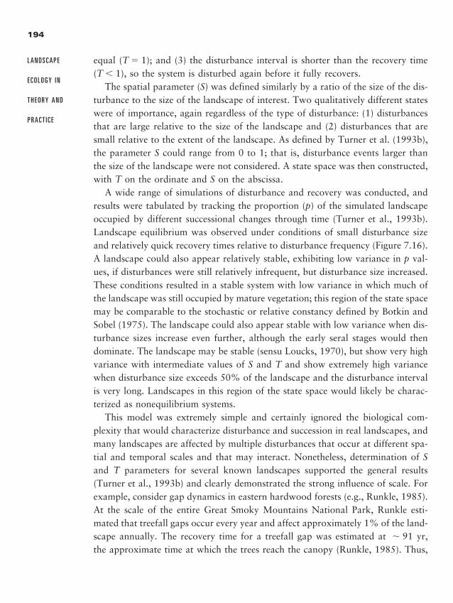
equal (T � 1); and (3) the disturbance interval is shorter than the recovery time(T � 1), so the system is disturbed again before it fully recovers.

The spatial parameter (S) was defined similarly by a ratio of the size of the dis-turbance to the size of the landscape of interest. Two qualitatively different stateswere of importance, again regardless of the type of disturbance: (1) disturbancesthat are large relative to the size of the landscape and (2) disturbances that aresmall relative to the extent of the landscape. As defined by Turner et al. (1993b),the parameter S could range from 0 to 1; that is, disturbance events larger thanthe size of the landscape were not considered. A state space was then constructed,with T on the ordinate and S on the abscissa.

A wide range of simulations of disturbance and recovery was conducted, andresults were tabulated by tracking the proportion (p) of the simulated landscapeoccupied by different successional changes through time (Turner et al., 1993b).Landscape equilibrium was observed under conditions of small disturbance sizeand relatively quick recovery times relative to disturbance frequency (Figure 7.16).A landscape could also appear relatively stable, exhibiting low variance in p val-ues, if disturbances were still relatively infrequent, but disturbance size increased.These conditions resulted in a stable system with low variance in which much ofthe landscape was still occupied by mature vegetation; this region of the state spacemay be comparable to the stochastic or relative constancy defined by Botkin andSobel (1975). The landscape could also appear stable with low variance when dis-turbance sizes increase even further, although the early seral stages would thendominate. The landscape may be stable (sensu Loucks, 1970), but show very highvariance with intermediate values of S and T and show extremely high variancewhen disturbance size exceeds 50% of the landscape and the disturbance intervalis very long. Landscapes in this region of the state space would likely be charac-terized as nonequilibrium systems.

This model was extremely simple and certainly ignored the biological com-plexity that would characterize disturbance and succession in real landscapes, andmany landscapes are affected by multiple disturbances that occur at different spa-tial and temporal scales and that may interact. Nonetheless, determination of Sand T parameters for several known landscapes supported the general results(Turner et al., 1993b) and clearly demonstrated the strong influence of scale. Forexample, consider gap dynamics in eastern hardwood forests (e.g., Runkle, 1985).At the scale of the entire Great Smoky Mountains National Park, Runkle esti-mated that treefall gaps occur every year and affect approximately 1% of the land-scape annually. The recovery time for a treefall gap was estimated at � 91 yr,the approximate time at which the trees reach the canopy (Runkle, 1985). Thus,

194

L A N D S C A P E

E C O L O G Y I N

T H E O R Y A N D

P R A C T I C E

2888_e07_p157-200 2/27/01 1:48 PM Page 194

195

Landscape

Disturbance

Dynamics

for treefall gaps in the Great Smokies, the temporal parameter T � 0.01 and thespatial parameter S � 0.01. This disturbance regime occurs in the extreme lower-left corner of the diagram in the equilibrium region (Figure 7.16). Consider nowwhat happens when the spatial scale is altered such that we consider treefall gapsonly within a 100-m2 plot within the park. The median gap size is �75 m2 (Run-kle, 1982), and we can estimate that a treefall occurs within a 100-m2 plot every100 years or so. Recovery time is still �50 yr. Under these conditions, the tem-poral parameter T � 2.0, and the spatial parameter S � 0.75, bringing this dis-turbance regime into the region of a stable system with very high variance. Thisexample illustrates nicely the dependence of our observations of landscape dy-namics on the spatial extent that is considered.

Stable,Low Variance

Stable,Low

Variance

Stable,High Variance

Equilibrium orSteady State

Unstable:System Bifurcation or Crash

Stable,Very HighVariance

Dis

turb

ance

inte

rval

/Rec

over

y in

terv

al

0.010.25

0.05

0.10

0.50

1.00

5.00

10.00

0.50 0.75

Disturbance extent /Landscape extent

E

A

B

C

D

F

Figure 7.16.

State-space diagram of the temporal and spatial parameters that illustrates regions that

display qualitatively different landscape dynamics.

Redrawn from Turner et al., 1993b.

2888_e07_p157-200 2/27/01 1:48 PM Page 195

Much of the disagreement surrounding equilibrium versus nonequilibrium andstability versus instability can be attributed to several factors: the ambiguity invarious definitions, different views of spatial heterogeneity and its effects, the lackof explicit specification of scales, and differences in theoretical foundations (Wuand Loucks, 1995). Landscapes can exhibit a variety of behaviors under differentdisturbance regimes, and the same landscape may shift among different regions ofbehavior. Landscapes that traditionally are considered as being in equilibrium arecharacterized by small and infrequent disturbance and rapid recovery. Stable sys-tems with high variance are characterized by intermediate size and frequency ofdisturbance and intermediate rates of recovery. Potentially unstable systems arecharacterized by large and frequent disturbance and slow recovery. In these land-scapes, a system crash or bifurcation to a qualitatively different system is possi-ble (Paine et al., 1998; Romme et al., 1998). Conclusions regarding landscapeequilibrium are appropriate only for a specified spatial and temporal scale. Fail-ure to recognize this dependence can lead to sharply different interpretations ofthe same dynamics.

S U M M A R Y

Disturbance creates patterns and is an important and integral part of many ecosys-tems and landscapes. The causes, patterns, dynamics, and consequences of dis-turbances have been major research topics in landscape ecology. Disturbance anddisturbance regime are characterized by a variety of attributes, including size, frequency, intensity, severity, and shape. The definition of disturbance is scale dependent.

Are various spatial locations in the landscape differentially susceptible to dis-turbance? If so, can we predict which areas are more or less susceptible to par-ticular types of disturbance? Susceptibility to disturbance of sites located at par-ticular landscape positions is evaluated by comparing the probability or frequencyof occurrence of a particular disturbance at many places in a landscape. Resultsfrom a variety of studies suggest that landscape position appears to influence sus-ceptibility to disturbance when the disturbance has a distinct directionality (e.g.,hurricane tracks) such that some locations are usually exposed more than others.In addition, landscape position may influence susceptibility if the disturbance isof moderate intensity, such that its spread is influenced by subtle differences inthe landscape. However, if the disturbance itself has no spatial directionality (e.g.,

196

L A N D S C A P E

E C O L O G Y I N

T H E O R Y A N D

P R A C T I C E

�

2888_e07_p157-200 2/27/01 1:48 PM Page 196

downbursts) or is sufficiently intense that its spread is unaffected by differencesin the landscape (e.g., high-intensity crown fire), then landscape position does notinfluence susceptibility to the disturbance.

Understanding how landscape heterogeneity can influence the spatial spread ofdisturbance has been a focus of landscape ecological research. Research from the-oretical and empirical studies suggests that we cannot generalize as to whetherlandscape pattern always enhances or retards disturbance spread, but that its po-tential effects on disturbance spread may be substantial. If the disturbance spreadswithin the same cover type, then greater landscape heterogeneity may retard thespread of disturbance. If the disturbance spreads between cover types or is other-wise enhanced by edge effects, then increased greater landscape heterogeneityshould enhance the spread of the disturbance. However, there may also be thresh-olds in environmental conditions beyond which landscape pattern will not affectthe spread of a disturbance.

Disturbance is an important agent of pattern creation in landscapes. Distur-bances create very complex heterogeneous patterns across the landscape, becausethe disturbance may affect some areas but not others, and severity of the distur-bance often varies considerably within the affected area. These resulting mosaicsmay show considerable persistence through time. Recovery following disturbancecan be very sensitive to spatial pattern created by disturbance and is strongly in-fluenced by the spatial pattern of biotic residuals left behind. Disturbance and suc-cession are inextricably linked when we consider landscape dynamics.

A thorough understanding of succession must include an understanding of howsuccessional processes vary with respect to disturbance intensity, size, and fre-quency. The availability of propagules is a fundamental determinant of succes-sional patterns and can be especially sensitive to the combination of high inten-sity and large size. If dispersal from outside the disturbed area is important, thenthe size, shape, and configuration of disturbed patches will influence propaguleavailability and thus vegetation composition. Spatial effects of disturbance (dis-turbance size, shape, and arrangement) become increasingly important when resid-uals are few or sparse and the disturbance is large; under these conditions, colo-nization and hence succession become slower and more difficult to predict.

Applying the theoretical and empirical advances in understanding of how dis-turbance and succession interact to large, heterogeneous landscapes is challengingbecause of the spatial interactions and the long time scales involved. Integrated mod-els of disturbance and succession can reveal trends and dynamics in landscapes thatcannot be easily observed empirically, and such models may be particularly usefulfor addressing questions of broad-scale disturbances or global change.

197

Landscape

Disturbance

Dynamics

2888_e07_p157-200 2/27/01 1:48 PM Page 197

Because disturbances can be such a strong source of landscape structure, in-tentional or unintentional shifts in the disturbance regime may dramatically alterthe landscape. For example, past climatic changes of small magnitude have causedsignificant changes in fire regimes in forested landscapes. Shifts in disturbanceregime will lead to shifts in landscape structure, with varying time lags; the re-sponse of landscape pattern can lag substantially behind a change in the distur-bance regime.

Questions of whether equilibrium can be detected on landscapes subject to dis-turbance and how large a landscape must be to incorporate a given disturbanceregime have been important themes in landscape ecology. Much of the disagree-ment surrounding equilibrium versus nonequilibrium and stability versus insta-bility can be attributed to several factors: the ambiguity in various definitions, dif-ferent views of spatial heterogeneity and its effects, the lack of explicit specificationof scales, and differences in theoretical foundations. Landscapes can exhibit a va-riety of behaviors under different disturbance regimes, and the same landscapemay shift among different regions of behavior. Landscapes that traditionally areconsidered as being in equilibrium are characterized by small and infrequent dis-turbance and rapid recovery. Stable systems with high variance are characterizedby intermediate size and frequency of disturbance and intermediate rates of re-covery. Potentially unstable systems are characterized by large and frequent dis-turbance and slow recovery. In these landscapes, a system crash or bifurcation toa qualitatively different system is possible. Conclusions regarding landscape equi-librium are appropriate only for a specified spatial and temporal scale. Failure torecognize this dependence can lead to sharply different interpretations of the samedynamics.


1. How can a disturbance both create landscape pattern and respond to landscape pat-

tern? Use at least one example of a natural disturbance to illustrate your answer.

2. Succession is generally defined as change in vegetation through time; thus, tempo-

ral dynamics are explicit. Is succession also spatial? Why or why not? Under what

conditions will the spatial pattern of disturbance influence succession?

3. How would you compare a natural and human-driven disturbance regime? What

criteria would you suggest for determining whether a human-driven disturbance is

comparable to a natural disturbance for a given landscape?

198

L A N D S C A P E

E C O L O G Y I N

T H E O R Y A N D

P R A C T I C E

2888_e07_p157-200 2/27/01 1:48 PM Page 198

4. Explain how scale dependence is important in understanding disturbance dynamics

and the effects of disturbances on a landscape. Consider both spatial and temporal

scale.

5. You are charged with developing a strategy for monitoring the effects of distur-

bance on landscape structure for a large region over the coming century. What

would you measure and why? How could you determine the sensitivity of your in-

dicators to changes in the disturbance regime?

6. Are disturbance-driven landscapes stable? Justify your answer.


Boose, E. R., D. R. Foster, and M. Fluet. 1994. Hurricane impacts to tropical and

temperate forest landscapes. Ecological Monographs 64:369–400.

Franklin, J. F., and R. T. T. Forman. 1987. Creating landscape patterns by forest

cutting: ecological consequences and principles. Landscape Ecology 1:5–18.

Hunter, M. L., Jr. 1993. Natural fire regimes as spatial models for managing boreal

forests. Biological Conservation 65:115–120.

Knight, D. H., and L. L. Wallace. 1989. The Yellowstone fires: issues in landscape

ecology. BioScience 39:700–706.

Pickett, S. T. A., S. C. Collins, and J. J. Armesto. 1987b. A hierarchical consid-

eration of causes and mechanisms of succession. Vegetatio 69:109–114.

Romme, W. H., and D. H. Knight. 1982. Landscape diversity: the concept applied

to Yellowstone Park. BioScience 32:664–670.

Turner, M. G., W. H. Romme, R. H. Gardner, R. V. O’Neill, and T. K. Kratz.

1993. A revised concept of landscape equilibrium: disturbance and stability on scaled

landscapes. Landscape Ecology 8:213–227.

199

Landscape

Disturbance

Dynamics

2888_e07_p157-200 2/27/01 1:48 PM Page 199

C H A P T E R

Organisms andLandscape Pattern

The spatial distribution of resources in heterogeneous landscapes canhave important effects on the growth, reproduction, and dispersal of or-

ganisms. The changing distribution of resources due to land-use change is a crit-ical issue for conservation design and management (Hobbs, 1993; Fahrig and Mer-riam, 1994; Noble and Dirzo, 1997). Development of the science in this area hascertainly been encouraged by environmental questions that demanded answersgrounded in basic understanding. For example, issues associated with habitat frag-mentation, in which the amount of habitat is reduced and the remaining habitatapportioned into smaller, more isolated patches (Figure 8.1), have come to theforefront (Wilcove et al., 1986; Saunders et al., 1991; Meffe and Carroll, 1994;Opdam et al., 1996). Ecologists have been pressed to understand and to predictthe prognosis for a variety of organisms that face increasingly fragmented habi-tat. It is now recognized that the maintenance of biodiversity (the abundance, va-riety, and genetic constitution of native animals and plants) requires a landscapeperspective (Franklin, 1993) that complements population, community, andecosystem considerations. In addition, there has been increasing recognition of theimportance of animals (e.g., their movement and foraging patterns) affecting the

8

2888_e08_p201-248 3/2/01 2:57 PM Page 201

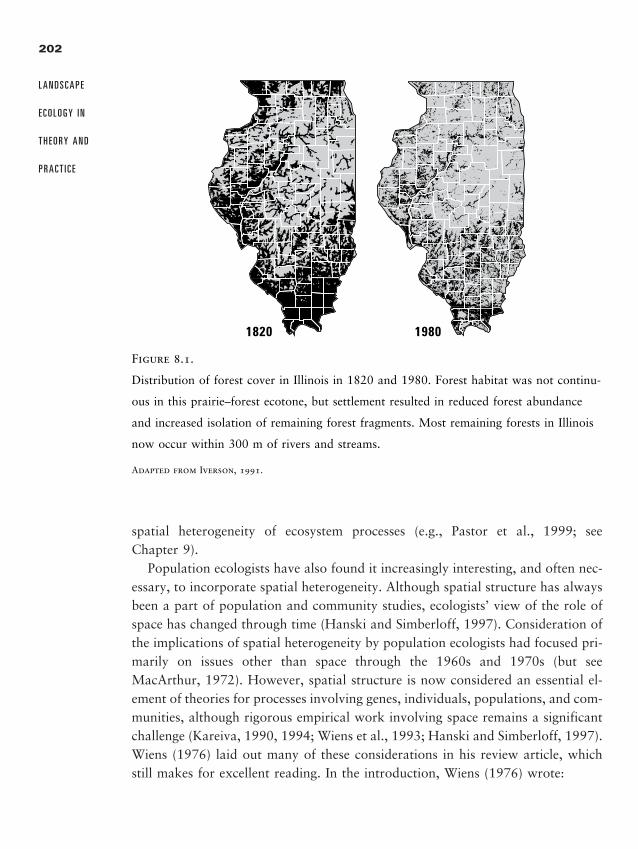
202

L A N D S C A P E

E C O L O G Y I N

T H E O R Y A N D

P R A C T I C E

spatial heterogeneity of ecosystem processes (e.g., Pastor et al., 1999; see Chapter 9).

Population ecologists have also found it increasingly interesting, and often nec-essary, to incorporate spatial heterogeneity. Although spatial structure has alwaysbeen a part of population and community studies, ecologists’ view of the role ofspace has changed through time (Hanski and Simberloff, 1997). Consideration ofthe implications of spatial heterogeneity by population ecologists had focused pri-marily on issues other than space through the 1960s and 1970s (but seeMacArthur, 1972). However, spatial structure is now considered an essential el-ement of theories for processes involving genes, individuals, populations, and com-munities, although rigorous empirical work involving space remains a significantchallenge (Kareiva, 1990, 1994; Wiens et al., 1993; Hanski and Simberloff, 1997).Wiens (1976) laid out many of these considerations in his review article, whichstill makes for excellent reading. In the introduction, Wiens (1976) wrote:

1820 1980

Figure 8.1.

Distribution of forest cover in Illinois in 1820 and 1980. Forest habitat was not continu-

ous in this prairie–forest ecotone, but settlement resulted in reduced forest abundance

and increased isolation of remaining forest fragments. Most remaining forests in Illinois

now occur within 300 m of rivers and streams.

Adapted from Iverson, 1991.

2888_e08_p201-248 3/2/01 2:57 PM Page 202

In the real world, environments are patchy. Factors influencing the proximate

physiological or behavioral state or the ultimate fitness of individuals exhibit

discontinuities on many scales in time and space. The patterns of these dis-

continuities produce an environmental patchwork which exerts powerful in-

fluences on the distributions of organisms, their interactions, and their adap-

tations. (Wiens, 1976:81)

Obviously, interactions between spatial heterogeneity and organisms is a sub-ject for which there is tremendous overlap among population ecology, landscapeecology, and conservation biology; even so, the needed synthesis among thesefields has yet to emerge. The traditional cultures in these subdisciplines are verydifferent and have often resulted in different emphases (see Ives et al., 1998).For instance, research in population ecology typically addresses how interactionswithin and among populations (e.g., competition and predation) generate spa-tial patterns and how these patterns then influence the outcomes of subsequentinteractions. Unlike landscape ecologists, population ecologists usually do notbegin with a map describing spatial patterns of resources, and more frequentlyemploy more theoretical and analytical models that are not directly oriented to-ward a particular organism or management issue (Ives et al., 1998). In contrast,research in landscape ecology on populations typically addresses the effects ofhabitat abundance and spatial configuration on a population of interest and be-gins with an explicit map, which might also change through time. Questions ofmanagement relevance for specific plants or animals are often addressed. Rela-tively complex simulation models of organisms acting on real (or realisticallycomplex) maps are more frequently used. Conservation biology may employ ei-ther of the two approaches described above, but the focus is often on threat-ened or endangered species whose long-term persistence in a given landscape isof concern.

In this chapter, we begin with a brief review of conceptual developments of in-teractions of organisms and spatial dynamics, focusing especially on the shift fromthe paradigm of island biogeography to that of metapopulation biology, and thendiscuss the scale-dependent nature of interactions between organisms and space.We next present a series of insights about the effect of spatial pattern on organ-isms that have emerged from landscape ecological studies, that is, a summary ofcurrent understanding, and suggest the conditions under which spatial pattern isimportant for organisms. Finally, we discuss the use of spatially explicit popula-tion models.

203

Organisms

and Landscape

Pat tern

2888_e08_p201-248 3/2/01 2:57 PM Page 203

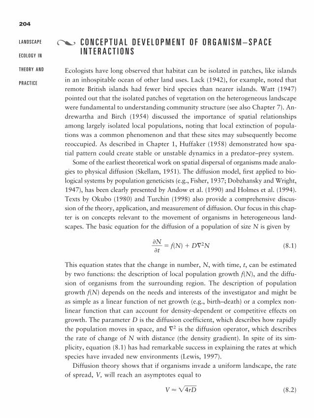
C O N C E P T U A L D E V E L O P M E N T O F O R G A N I S M – S P A C E I N T E R A C T I O N S

Ecologists have long observed that habitat can be isolated in patches, like islandsin an inhospitable ocean of other land uses. Lack (1942), for example, noted thatremote British islands had fewer bird species than nearer islands. Watt (1947)pointed out that the isolated patches of vegetation on the heterogeneous landscapewere fundamental to understanding community structure (see also Chapter 7). An-drewartha and Birch (1954) discussed the importance of spatial relationshipsamong largely isolated local populations, noting that local extinction of popula-tions was a common phenomenon and that these sites may subsequently becomereoccupied. As described in Chapter 1, Huffaker (1958) demonstrated how spa-tial pattern could create stable or unstable dynamics in a predator–prey system.

Some of the earliest theoretical work on spatial dispersal of organisms made analo-gies to physical diffusion (Skellam, 1951). The diffusion model, first applied to bio-logical systems by population geneticists (e.g., Fisher, 1937; Dobzhansky and Wright,1947), has been clearly presented by Andow et al. (1990) and Holmes et al. (1994).Texts by Okubo (1980) and Turchin (1998) also provide a comprehensive discus-sion of the theory, application, and measurement of diffusion. Our focus in this chap-ter is on concepts relevant to the movement of organisms in heterogeneous land-scapes. The basic equation for the diffusion of a population of size N is given by

��

�

Nt� � f(N) � D�2N (8.1)

This equation states that the change in number, N, with time, t, can be estimatedby two functions: the description of local population growth f(N), and the diffu-sion of organisms from the surrounding region. The description of populationgrowth f(N) depends on the needs and interests of the investigator and might beas simple as a linear function of net growth (e.g., birth–death) or a complex non-linear function that can account for density-dependent or competitive effects ongrowth. The parameter D is the diffusion coefficient, which describes how rapidlythe population moves in space, and �2 is the diffusion operator, which describesthe rate of change of N with distance (the density gradient). In spite of its sim-plicity, equation (8.1) has had remarkable success in explaining the rates at whichspecies have invaded new environments (Lewis, 1997).

Diffusion theory shows that if organisms invade a uniform landscape, the rateof spread, V, will reach an asymptotes equal to

V � �4rD� (8.2)

204

L A N D S C A P E

E C O L O G Y I N

T H E O R Y A N D

P R A C T I C E

�

2888_e08_p201-248 3/2/01 2:57 PM Page 204

where r is the intrinsic rate of population growth. Andow et al. (1990) tested theadequacy of equation (8.2) against observed rates of spread for three differentspecies. The results showed that equation (8.2) adequately explained the invasionprocess of muskrats in Europe and the cabbage white butterfly in North America.However, in the third case, movements of the cereal leaf beetle, the estimation ofD was made by observing fine-scale patterns of movements. These data were be-lieved to produce an underestimation of the real value of D and a biased predictionof V. Thus, equation (8.2) gives a good approximation to spread across the land-scape, provided that the data are gathered at sufficiently broad scales. The com-plexities of actual landscapes are included as the average value of D and, as longas spatial patterns remain relatively constant, provide an adequate description of in-vasion at landscape scales. When landscape patterns change dramatically, the val-ues of D may need to be reestimated or alternative dispersal models considered.

I s l a n d B i o g e o g r a p h y

The theory of island biogeography (MacArthur and Wilson, 1963, 1967; MacArthur,1972) was an important influence on how ecologists think about organisms and spa-tial pattern, and for some time it was the prevailing paradigm guiding the design ofconservation reserves. Island biogeography was developed as a general theory to pre-dict the number of species found on oceanic islands. The theory predicts that thenumber of species on an island will reach an equilibrium that is positively related toisland size (larger islands would contain more species) and negatively related to dis-tance from the mainland (fewer species on islands far from the mainland and thesource of new colonists). The number of species on an island depends on the immi-gration rate of species to the island and the extinction rate of species from the is-land. Immigration to the island is assumed to be a linear function of distance, d, andalso depends on the size of the mainland source community, such that

I � d(P � R)k

where P is the number of species in the mainland pool, R is the number of specieson the island, and k is a parameter that would differ with communities of differ-ent organisms. The value of k is determined by fitting data to a specific island sys-tem. Once a species finds its way to the island, its rate of extinction depends onthe available resources. If all islands are similar, the available resources should beproportional to island size.

E � nSm

205

Organisms

and Landscape

Pat tern

2888_e08_p201-248 3/2/01 2:57 PM Page 205

where S is island size and n and m are parameters fitted by regression from data.Early field studies provided empirical support for the theory (Simberloff and

Wilson, 1969, 1970). The basic concept was expanded to include alpine zones(Vuilleumier, 1970), which have communities isolated on the tops of mountainsmuch like oceanic islands. The theory was also applied to cave communities (Cul-ver, 1970; Vuilleumier, 1973). For these communities, the aboveground landscapeseparating the cave mouths functions very much like an inhospitable ocean.

With growing concern about habitat fragmentation, drawing the analogy be-tween habitat fragments and islands was easy, and island biogeography theorywas readily embraced by ecologists. The theory was applied to the design of na-ture preserves in terrestrial landscapes, generating a long debate among ecologistsabout whether a single large preserve would be better than having several smallerpreserves spaced such that organisms could move among them. The argument cen-tered on the fact that a single preserve might hold more total species, but it couldbe wiped out with a single catastrophic event. In contrast, the smaller preserveswould each contain fewer species, but some preserves would be likely to surviveany particular catastrophic event. If even a single small reserve escaped the cata-strophe, it would provide a source for recolonization of the damaged areas (Burkey,1989; Soule and Simberloff, 1986).

Island biogeography theory was subjected to a number of criticisms (Carlquist,1974; Gilbert, 1980), and many modifications have been suggested. Perhaps the pri-mary criticism has been the assumption of equilibrium (Diamond, 1972; Terborgh,1975). An island system would require a very long period of time to reach such anequilibrium number of species (Simpson, 1974), perhaps best measured in geologictime units during which climate and many other factors change. In many ecosystems,chronic disturbance (Villa et al., 1992) would also invalidate the assumption, be-cause the next disturbance would occur long before the system reached equilibrium.It has also been pointed out that islands close to the shore will experience very largeimmigration rates (Brown and Kodric-Brown, 1977). The immigration could over-whelm the extinction rate so that effects of island size would not be evident, althoughsome models incorporated size-dependent immigration. In addition, island size anddistance become less important as dispersal ability increases (Roff, 1974b).

Other studies have identified factors in addition to those considered in islandbiogeography theory that influence species richness in habitat fragments. Webband Vermaat (1990) documented species diversity in isolated heathland remnantsthat form islands in an ocean of other vegetation. Counter to the prediction, theyfound that small islands had higher species diversity because they could not resistinvasion by surrounding vegetation. Large islands, in contrast, had lower species

206

L A N D S C A P E

E C O L O G Y I N

T H E O R Y A N D

P R A C T I C E

2888_e08_p201-248 3/2/01 2:57 PM Page 206

diversity because they resisted the invaders. Habitat quality (Murphy et al., 1990)or interspecific competition (Hanski, 1981, 1983) on an island may sometimes bemore important than size. Some island systems are dominated by catastrophic dis-turbances, such as hurricanes, that may cause extinction, irrespective of island size(Ehrlich et al., 1980). In disturbance-driven systems, population size and com-munity diversity may be dominated by reinvasion processes. In fact, when naturaldisturbances are common, persistence may be higher on a landscape with severalpatches, because this spreads the risk of the entire population being wiped out(Goodman, 1987). Other ecosystem processes, such as trophic dynamics, that in-fluence community composition must also be considered. Spiders on Bahamian is-lands largely followed island biogeography theory except when predatory lizardswere present (Toft and Schoener, 1983). Then the relationships changed signifi-cantly, and predation tended to dominate the extinction rates.

The theory of island biogeography clearly dominated much of conservation bi-ology through the 1970s and 1980s. Despite the criticisms, island biogeographytheory has been important in highlighting effects of the size and isolation of nat-ural areas on their effectiveness in meeting conservation objectives; indeed, thesefactors remain important considerations in conservation planning. There is over-whelming evidence that species richness increases with area, whether on islandsor on the mainland. However, metapopulation models emerged in the late 1980sas a way of thinking about fragmented habitats and heterogeneous terrestrial en-vironments in general; some authors have referred to this as a paradigm shift (Han-ski, 1989; Merriam, 1991), but it can also be considered as a switch to questionsat finer spatial scales than those considered by island biogeography.

M e t a p o p u l a t i o n B i o l o g y

Levins (1969, 1970) observed that most populations have a finite probability ofextinction, m, that is measurably greater than zero, implying that populations willeventually go extinct. However, if the population is fragmented into a patchworkof subpopulations and the probability of extinction of the subpopulations remainssmall, local extinctions may be balanced by recolonization from neighboring pop-ulations. When these conditions exist, the process of extinction and colonizationis locally dynamic but may be regionally stable. A simple equation summarizesthis concept:

�ddpt� � cp(1 � p) � mp (8.3)

207

Organisms

and Landscape

Pat tern

2888_e08_p201-248 3/2/01 2:57 PM Page 207

where c and m are the probabilities of colonization and extinction, respectively,and p is the proportion of available locations (patches) colonized at any point intime. The equilibrium solution to equation (8.3) provides an estimate of the ex-pected proportion of colonized sites, p�.

p� � 1 � �mc�

Populations persist regionally (p� is greater than zero) only if the probability ofextinction, m, is less than the probability of colonization, c. It is a simple matterto rearrange the terms to calculate the expected number of empty sites, s�.

S� � 1 � p� � �mc�

The interconnected set of subpopulations that function as a demographic unitwas termed a metapopulation by Levins (1969). The concepts and terms used inmetapopulation theory (Table 8.1) have been readily incorporated into landscapeecology, in part because metapopulation concepts seem to be an apt descriptionof population dynamics in natural or artificially fragmented landscapes.

One interesting application of metapopulation theory has been the assessmentof the effect of habitat destruction on regional population dynamics. Habitat de-struction, in terms of metapopulations, is equivalent to the destruction of a habi-tat patch and the elimination of a site that may support a single subpopulation ofthe metapopulation. If the fraction of occupied sites, p, is assumed to decrease lin-early as the fraction of potentially occupied sites destroyed increases, then equa-tion (8.3) becomes

�ddpt� � cp(1 � D � p) � mp (8.4)

where D is the proportion of sites that have been destroyed. The equilibrium so-lution for equation (8.4) is

p� � 1 � D � �mc�

This equilibrium equation predicts that the threshold for extinction of the entiremetapopulation (p� � 0) will occur when the fraction of available sites, (1 � D),

208

L A N D S C A P E

E C O L O G Y I N

T H E O R Y A N D

P R A C T I C E

2888_e08_p201-248 3/2/01 2:57 PM Page 208

is less than or equal to m/c. This relationship, illustrated in Figure 8.2, shows thata metapopulation within a region will disappear long before the final patches havebeen destroyed (in fact, for the parameters used in Figure 8.2, approximately one-third of the habitat patches still remain when the population goes extinct). Thereare many reasons to believe that the potential relationship between D and p� maynot be linear. For instance, nonlinear relationships may occur when habitat de-struction is nonrandom (spatially correlated) or when progeny must traverse in-creasingly hostile terrain to find unoccupied habitat sites. Under these circum-stances, the linear relationship in Figure 8.2 becomes nonlinear, and precipitousdeclines in the survival of the metapopulations occur with even small amounts ofhabitat destruction near the extinction threshold (Lande, 1987). Tilman and col-leagues (Tilman, 1994; Tilman et al., 1994; Tilman et al., 1997), in an interest-ing series of papers, have extended these concepts to the problem of predictingthe combined effect of habitat destruction and competition between sympatricspecies. Time lags induced by competitive displacement and life-history charac-teristics result in a delay in the eventual extinction of species due to habitat loss.This effect, termed extinction debt, implies that a precipitous decline in speciesabundance and diversity may be the inevitable consequence of habitat loss butwill not be observed until many years after the disturbances have occurred.

The Levins model of metapopulations is spatially implicit; that is, the processof colonization and extinction of suitable habitat patches is independent of theirspatial locations. Sites that are a long distance from neighbors have the same prob-ability of colonization and extinction as sites closer to neighbors, implying that

209

Organisms

and Landscape

Pat tern

0.8

0.6

0.4

0.2

0.00.0 0.2 0.4 0.6 0.8 1.0

Site

s oc

cupi

ed (p

' )

Habitat destroyed (D )

Extinctionthreshold

Figure 8.2.

Equilibrium percentage of occupied sites (p� � 1 � D �

m/c) as a function of the fraction of habitat destroyed

(D). Here m � 0.2 and c � 0.6. The extinction threshold

occurs when the fraction of habitat destroyed is equal to

1 � m/c � 0.666.

Adapted from Bascompte and Sole, 1996.

2888_e08_p201-248 3/2/01 2:57 PM Page 209

210

Table 8.1.Definitions and synonyms of terms used in metapopulation studies.

Term Synonyms Definition

Levins meta- Classical metapopulation Metapopulation structure assumed in the Levins model: a population large network of similar small patches, with local dynamics

occurring at a much faster time scale than metapopulation dynamics.

Local population Population, subpopulation, deme Set of individuals that live in the same habitat patch and thereforeinteract with each other; most naturally applied to populations livingin such small patches that all individuals practically share a commonenvironment.

Metapopulation Composite, population, assemblage (of Set of local populations within some larger area, where typically populations, when local populations migration from one local population to at least some other patches are called subpopulations) is possible.

Patch Habitat patch, habitat island, site, A continuous area of space with all necessary resources for the locality persistence of a local population and separated by unsuitable habitat

from other patches (at any given time a patch may be occupied orempty).

Patch model Occupancy model, presence–absence A metapopulation model in which local population size is ignored model and the number (or fraction) of occupied habitat patches is modeled.

2888_e08_p201-248 3

/2/01 2

:57 PM P

age 210

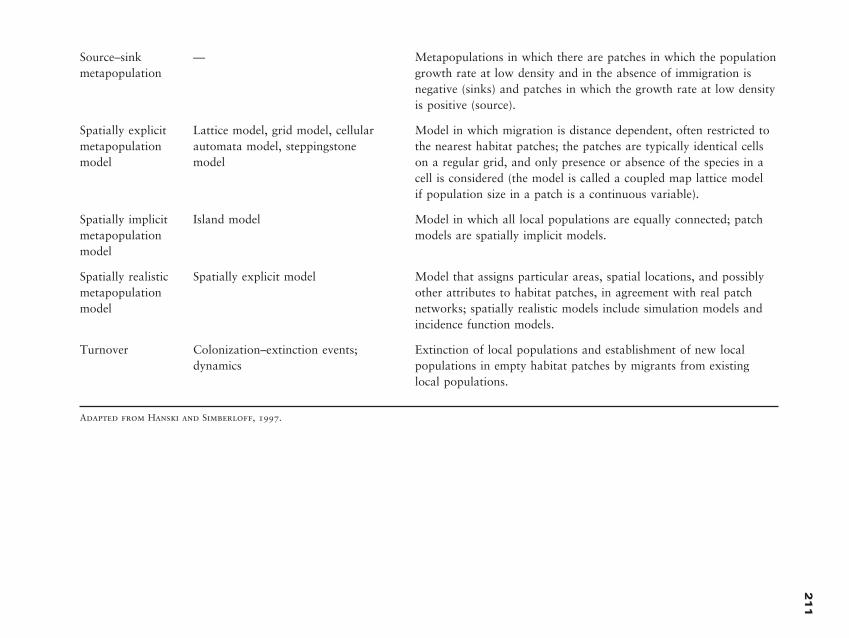
21

1Source–sink — Metapopulations in which there are patches in which the population metapopulation growth rate at low density and in the absence of immigration is

negative (sinks) and patches in which the growth rate at low densityis positive (source).

Spatially explicit Lattice model, grid model, cellular Model in which migration is distance dependent, often restricted to metapopulation automata model, steppingstone the nearest habitat patches; the patches are typically identical cells model model on a regular grid, and only presence or absence of the species in a

cell is considered (the model is called a coupled map lattice model if population size in a patch is a continuous variable).

Spatially implicit Island model Model in which all local populations are equally connected; patch metapopulation models are spatially implicit models.model

Spatially realistic Spatially explicit model Model that assigns particular areas, spatial locations, and possibly metapopulation other attributes to habitat patches, in agreement with real patch model networks; spatially realistic models include simulation models and

incidence function models.

Turnover Colonization–extinction events; Extinction of local populations and establishment of new local dynamics populations in empty habitat patches by migrants from existing

local populations.

Adapted from Hanski and Simberloff, 1997.

2888_e08_p201-248 3

/2/01 2

:57 PM P

age 211

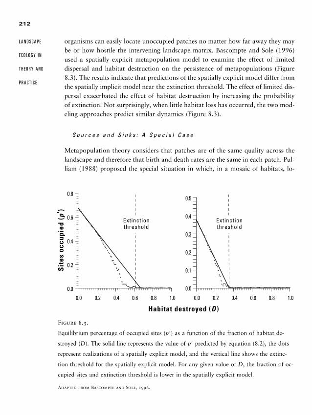
212

L A N D S C A P E

E C O L O G Y I N

T H E O R Y A N D

P R A C T I C E

0.8

0.6

0.4

0.2

0.00.0 0.2 0.4 0.6 0.8 1.0

Sit

es o

ccup

ied

(p' )

Habitat destroyed (D )

Extinctionthreshold

0.5

0.4

0.3

0.2

0.1

0.0

0.0 0.2 0.4 0.6 0.8 1.0

Extinctionthreshold

Figure 8.3.

Equilibrium percentage of occupied sites (p�) as a function of the fraction of habitat de-

stroyed (D). The solid line represents the value of p� predicted by equation (8.2), the dots

represent realizations of a spatially explicit model, and the vertical line shows the extinc-

tion threshold for the spatially explicit model. For any given value of D, the fraction of oc-

cupied sites and extinction threshold is lower in the spatially explicit model.

Adapted from Bascompte and Sole, 1996.

organisms can easily locate unoccupied patches no matter how far away they maybe or how hostile the intervening landscape matrix. Bascompte and Sole (1996)used a spatially explicit metapopulation model to examine the effect of limiteddispersal and habitat destruction on the persistence of metapopulations (Figure8.3). The results indicate that predictions of the spatially explicit model differ fromthe spatially implicit model near the extinction threshold. The effect of limited dis-persal exacerbated the effect of habitat destruction by increasing the probabilityof extinction. Not surprisingly, when little habitat loss has occurred, the two mod-eling approaches predict similar dynamics (Figure 8.3).

S o u r c e s a n d S i n k s : A S p e c i a l C a s e

Metapopulation theory considers that patches are of the same quality across thelandscape and therefore that birth and death rates are the same in each patch. Pul-liam (1988) proposed the special situation in which, in a mosaic of habitats, lo-

2888_e08_p201-248 3/2/01 2:57 PM Page 212

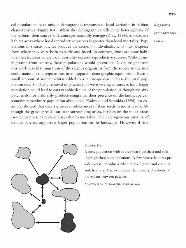
cal populations have unique demographic responses to local variation in habitatcharacteristics (Figure 8.4). When the demographics reflect the heterogeneity ofthe habitat, then source–sink concepts naturally emerge (Dias, 1996). Sources arehabitat areas where local reproductive success is greater than local mortality. Pop-ulations in source patches produce an excess of individuals, who must dispersefrom where they were born to settle and breed. In contrast, sinks are poor habi-tats, that is, areas where local mortality exceeds reproductive success. Without im-migration from sources, these populations would go extinct. A key insight fromthis work was that migration of the surplus organisms from the source to the sinkcould maintain the populations in an apparent demographic equilibrium. Even asmall amount of source habitat added to a landscape can increase the total pop-ulation size. Similarly, removal of patches that were serving as sources for a largerpopulation could lead to catastrophic decline of the population. Although the sinkpatches do not ordinarily produce emigrants, their presence on the landscape cansometimes maximize population abundance. Kadmon and Schmida (1990), for ex-ample, showed that desert grasses produce most of their seeds in moist wadis. Al-though the grass spreads out over surrounding areas, it relies on the moist areas(source patches) to replace losses due to mortality. The heterogeneous mixture ofhabitat patches supports a larger population on the landscape. However, if sink

213

Organisms

and Landscape

Pat tern

Figure 8.4.

A metapopulation with source (dark patches) and sink

(light patches) subpopulations. A few source habitats pro-

vide excess individuals when they emigrate and colonize

sink habitats. Arrows indicate the primary directions of

movement between patches.

Adapted from Pulliam and Dunning, 1994.

2888_e08_p201-248 3/2/01 2:57 PM Page 213

habitat is too abundant relative to source habitat, organisms with limited disper-sal will be unable to find source habitat, and the landscape will be unable to sup-port a viable population (Pulliam and Danielson, 1991). The maintenance of high-quality habitat on a landscape is important, and the effects of habitat loss cannotbe mitigated by the preservation of sink habitat. In addition, a patch that is asource for one species may be a sink for other species (Danielson, 1991, 1992).

I d e n t i f i c a t i o n o f S u i t a b l e H a b i t a t

Our discussion thus far has implicitly assumed that suitable habitat for a popu-lation is known and that its spatial distribution has been described. In a standardecological metapopulation study, a key initial task is to distinguish between suit-able and unsuitable habitat and delimit the patches of suitable habitat in a studyarea (Hanski and Simberloff, 1997). Suitable habitat includes those areas that havebeen defined as having the conditions required for a given species to meet its needsfor resources, shelter, and reproduction. A variety of methods can be employedfor identifying suitable habitat (Hansen et al., 1993), ranging from associationswith seral stage or stand structure (Hansen et al., 1995), habitat suitability mod-els (Van Horne and Wiens, 1991), logistic regression (Mladenoff et al., 1995;Mladenoff and Sickley, 1998), Bayesian rules (Miller et al., 1997), and multi-variate statistical methods (e.g., Hansen et al., 1995; Knick and Dyer, 1997). How-ever, it is important to recognize the complexities inherent in this task, and that itis difficult to distinguish among source, sink, and unsuitable habitats. In particu-lar, population density is not a means of identifying suitable habitat, because poorhabitats may be population sinks that have a temporary surplus of individuals rel-ative to source habitats (e.g., following juvenile dispersal) (Van Horne, 1983).

In some instances, the simplifying binary assumption of suitable and unsuitablehabitat, which is necessary to keep the models reasonably simple, is very clear. How-ever, in other cases, it may be difficult to partition the landscape into patches em-bedded in an unsuitable matrix. Consider habitat perceived as suitable or favorableby eastern timber wolves (Canis lupus lycaon) in the upper midwestern United States.Although driven nearly to extinction during the early part of the century, wolves havebeen gradually expanding their range during the past 15 years, moving eastward fromMinnesota into northern Wisconsin and the Upper Peninsula of Michigan. Analysesof data from radio-collared wolves revealed that suitable habitat was a function notonly of vegetation type and deer density (deer are commonly preyed on by the wolves),but also of land ownership, road density, and human population density across thelandscape (Mladenoff et al., 1995). Wolves were moving throughout the landscape

214

L A N D S C A P E

E C O L O G Y I N

T H E O R Y A N D

P R A C T I C E

2888_e08_p201-248 3/2/01 2:57 PM Page 214

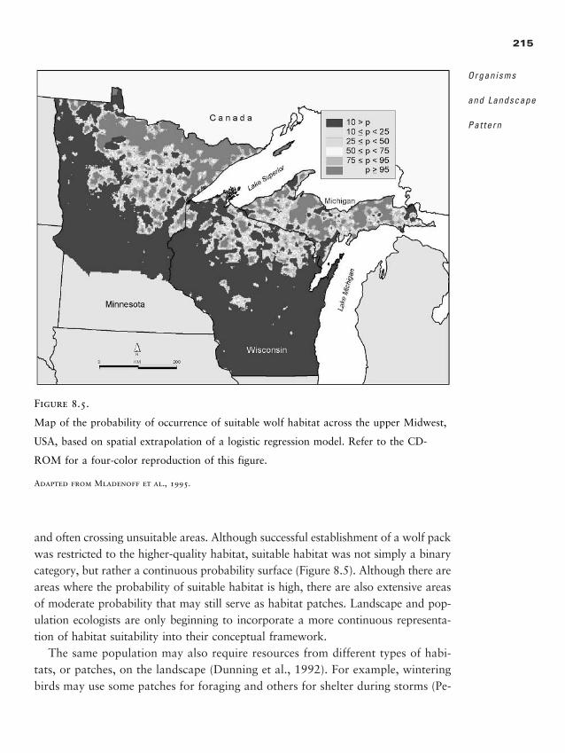
and often crossing unsuitable areas. Although successful establishment of a wolf packwas restricted to the higher-quality habitat, suitable habitat was not simply a binarycategory, but rather a continuous probability surface (Figure 8.5). Although there areareas where the probability of suitable habitat is high, there are also extensive areasof moderate probability that may still serve as habitat patches. Landscape and pop-ulation ecologists are only beginning to incorporate a more continuous representa-tion of habitat suitability into their conceptual framework.

The same population may also require resources from different types of habi-tats, or patches, on the landscape (Dunning et al., 1992). For example, winteringbirds may use some patches for foraging and others for shelter during storms (Pe-

215

Organisms

and Landscape

Pat tern

Figure 8.5.

Map of the probability of occurrence of suitable wolf habitat across the upper Midwest,

USA, based on spatial extrapolation of a logistic regression model. Refer to the CD-

ROM for a four-color reproduction of this figure.

Adapted from Mladenoff et al., 1995.

2888_e08_p201-248 3/2/01 2:57 PM Page 215

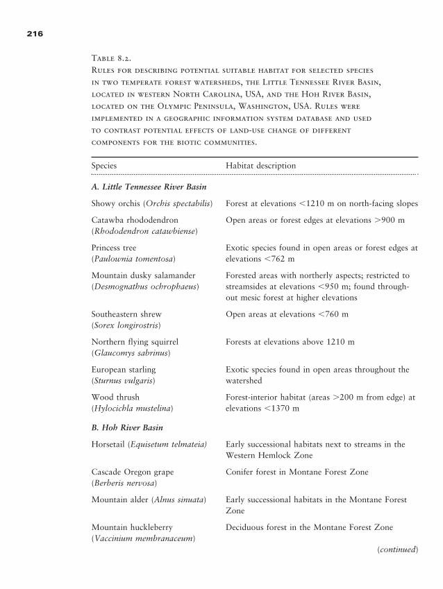
216

Table 8.2.Rules for describing potential suitable habitat for selected species in two temperate forest watersheds, the Little Tennessee River Basin,located in western North Carolina, USA, and the Hoh River Basin, located on the Olympic Peninsula, Washington, USA. Rules were implemented in a geographic information system database and used to contrast potential effects of land-use change of different components for the biotic communities.

Species Habitat description

A. Little Tennessee River Basin

Showy orchis (Orchis spectabilis) Forest at elevations 1210 m on north-facing slopes

Catawba rhododendron Open areas or forest edges at elevations 900 m(Rhododendron catawbiense)

Princess tree Exotic species found in open areas or forest edges at (Paulownia tomentosa) elevations 762 m

Mountain dusky salamander Forested areas with northerly aspects; restricted to (Desmognathus ochrophaeus) streamsides at elevations 950 m; found through-

out mesic forest at higher elevations

Southeastern shrew Open areas at elevations 760 m(Sorex longirostris)

Northern flying squirrel Forests at elevations above 1210 m(Glaucomys sabrinus)

European starling Exotic species found in open areas throughout the (Sturnus vulgaris) watershed

Wood thrush Forest-interior habitat (areas 200 m from edge) at (Hylocichla mustelina) elevations 1370 m

B. Hoh River Basin

Horsetail (Equisetum telmateia) Early successional habitats next to streams in the Western Hemlock Zone

Cascade Oregon grape Conifer forest in Montane Forest Zone(Berberis nervosa)

Mountain alder (Alnus sinuata) Early successional habitats in the Montane Forest Zone

Mountain huckleberry Deciduous forest in the Montane Forest Zone(Vaccinium membranaceum)

(continued)

2888_e08_p201-248 3/2/01 2:57 PM Page 216

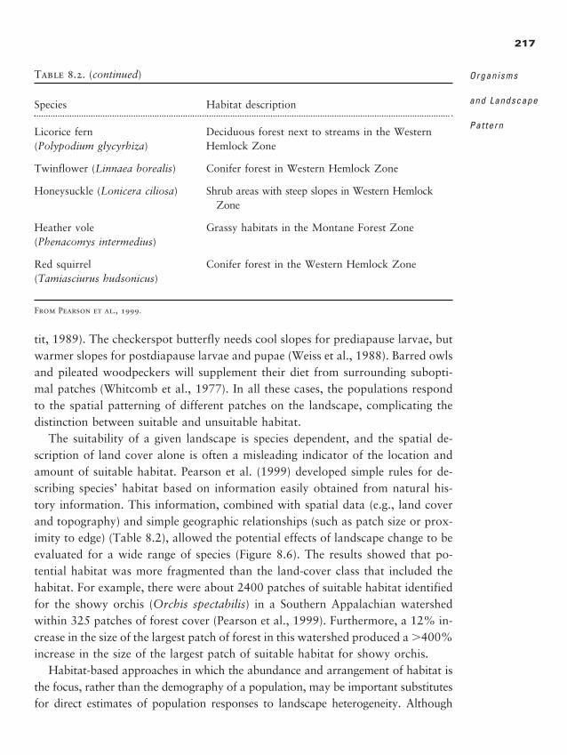
tit, 1989). The checkerspot butterfly needs cool slopes for prediapause larvae, butwarmer slopes for postdiapause larvae and pupae (Weiss et al., 1988). Barred owlsand pileated woodpeckers will supplement their diet from surrounding subopti-mal patches (Whitcomb et al., 1977). In all these cases, the populations respondto the spatial patterning of different patches on the landscape, complicating thedistinction between suitable and unsuitable habitat.

The suitability of a given landscape is species dependent, and the spatial de-scription of land cover alone is often a misleading indicator of the location andamount of suitable habitat. Pearson et al. (1999) developed simple rules for de-scribing species’ habitat based on information easily obtained from natural his-tory information. This information, combined with spatial data (e.g., land coverand topography) and simple geographic relationships (such as patch size or prox-imity to edge) (Table 8.2), allowed the potential effects of landscape change to beevaluated for a wide range of species (Figure 8.6). The results showed that po-tential habitat was more fragmented than the land-cover class that included thehabitat. For example, there were about 2400 patches of suitable habitat identifiedfor the showy orchis (Orchis spectabilis) in a Southern Appalachian watershedwithin 325 patches of forest cover (Pearson et al., 1999). Furthermore, a 12% in-crease in the size of the largest patch of forest in this watershed produced a 400%increase in the size of the largest patch of suitable habitat for showy orchis.

Habitat-based approaches in which the abundance and arrangement of habitat isthe focus, rather than the demography of a population, may be important substitutesfor direct estimates of population responses to landscape heterogeneity. Although

217

Organisms

and Landscape

Pat tern

Table 8.2. (continued)

Species Habitat description

Licorice fern Deciduous forest next to streams in the Western (Polypodium glycyrhiza) Hemlock Zone

Twinflower (Linnaea borealis) Conifer forest in Western Hemlock Zone

Honeysuckle (Lonicera ciliosa) Shrub areas with steep slopes in Western Hemlock Zone

Heather vole Grassy habitats in the Montane Forest Zone(Phenacomys intermedius)

Red squirrel Conifer forest in the Western Hemlock Zone(Tamiasciurus hudsonicus)

From Pearson et al., 1999.

2888_e08_p201-248 3/2/01 2:57 PM Page 217

maintenance of biodiversity is often desired in land planning and resource manage-ment, it is impossible to manage simultaneously for all species present at a site. Iden-tification of suitable habitat for species and tracking changes in habitat abundanceand pattern through time allow the modeling of risks of biodiversity changes at land-scape scales and are a first step to anticipate potential effects of land-use changes (Ri-itters et al., 1997; White et al., 1997). Hansen et al. (1993) recommended that habi-tat suitability and life-history attributes be used as surrogates for detailed demographicdata for vertebrate species, an approach that they believe is intermediate between thecoarse-filter and fine-filter approaches described by Noss (1987) and Hunter (1991).Associating target species with specific habitat configurations and evaluating alter-native management prescriptions using simulation models were among the key stepsof their approach. If habitat is well defined, the method can be used to monitor habi-tat change through time, compare habitats among areas, or examine the effect ofscale by developing GIS-based signatures (spatial pattern analyses) for varying scalessurrounding the locations (Knick and Dyer, 1997; Riitters et al., 1997).

Habitat-based approaches have already offered insight into understanding theimplications of variation in landscape pattern for a variety of taxa. A rule-basedprobabilistic model linked with land cover and physiographic data was used topredict the suitability of a landscape in northeast England for three species of birds

218

L A N D S C A P E

E C O L O G Y I N

T H E O R Y A N D

P R A C T I C E

Woodthrush

Europeanstarling

1975–1986 Historical No forest lossa b

Figure 8.6.

Maps of suitable habitat for two bird species,

European starling and wood thrush, in the Little

Tennessee River Basin, western North Carolina,

at the end of a 100-yr simulation using transi-

tion probabilities (a) extrapolated from the

1975–1986 historical period and (b) with no

loss of forest permitted.

Adapted from Pearson et al., 1999.

2888_e08_p201-248 3/2/01 2:57 PM Page 218

(Tucker et al., 1997). In low- to mid-elevation forests in the Pacific Northwest,risk to bird species under four different management scenarios was evaluated byquantifying suitable habitat for each species using habitat maps, species–habitatassociations, and other life-history requirements (Hansen et al., 1995). Recently,White et al. (1997) used habitat and area requirements for a large sample of ver-tebrate species in Monroe County, Pennsylvania, to assess risks to biodiversity as-sociated with land development. Six possible alternative versions of MonroeCounty that differed in the extent and spatial distribution of human impact weredeveloped for the year 2020 based on projected current rates of population growth.Results demonstrated little variation in species richness among the six alternatives(extinction of species was not prevalent), although loss of habitat might have beensubstantial. The Gap Analysis approach (Scott et al., 1987, 1993), which analyzesexisting preserves and land cover types to identify regions with high species di-versity that remain unprotected, has been useful for allocating conservation re-sources to protect diversity over broad state-level scales. Riitters et al. (1997) de-rived habitat maps from digital land-cover maps by using a spatial filteringalgorithm at various scales; results demonstrated that the amount and arrange-ment of suitable habitat changed with the home-range size of the organism. Col-lectively, these studies suggest that analyzing species habitat requirements may serveas a suitable starting point for relating land-use change to biodiversity. In such ap-plications, however, it is important to remember that the availability of habitatimplies potential rather than actual use of the habitat by the species of interest.

In sum, landscape ecologists tend to view the complex mosaic structure of reallandscapes as the template on which populations operate. Patches of the samehabitat may vary in quality, yet many studies simplify nature’s complexity by de-scribing habitat as either suitable or unsuitable and assuming a featureless back-ground matrix (Wiens, 1997). Although empirical and modeling studies all requiresimplification, we must remember that the issue of how to identify suitable habi-tat is an important one, and its implementation influences the observations or pre-dictions for a given landscape. The same landscape may be very different for dif-ferent species, and an organism-centered view of the landscape is required tounderstand the response of populations to spatial patterning.

C o n t r a s t b e t w e e n M e t a p o p u l a t i o n T h e o r y a n d

L a n d s c a p e E c o l o g y

There is clearly much common ground between metapopulation biology and land-scape ecology, yet Wiens (1997) identified several important differences. As we

219

Organisms

and Landscape

Pat tern

2888_e08_p201-248 3/2/01 2:57 PM Page 219

have seen, metapopulation models are typically focused on idealized habitatpatches in a featureless landscape and emphasize local extinction, interpatch move-ment, and recolonization. Four features that characterize landscape ecology arelargely missing from metapopulation models: (1) variation in patch quality, (2) variation in the quality of the surrounding environment, (3) boundary effects,and (4) how the landscape influences connectivity among patches (Wiens, 1997).The interpatch matrix becomes important in landscape ecology because dispersalbetween patches depends on the quality of the matrix. If the matrix is inhospitable,like the ocean, isolation becomes more important. For example, Bolger et al.(1997a) found that the urban matrix is essentially impervious to native rodents insouthern California, because animals did not cross even short distances betweenremnant habitat fragments. If the matrix has relatively low contrast with the habi-tat patches, isolation may be much less important. Metapopulation models alsoimplicitly assume a landscape in which the suitable habitat patches occupy a rel-atively low proportion of the landscape, whereas landscape ecologists are oftenfocusing on a wide range of proportions of availability of suitable habitat. Onlandscapes, it is also important to keep in mind that the matrix and the edges ofthe patches are themselves habitat for other species (McCollin, 1993).

The main difference between the metapopulation view of nature and that em-braced by landscape ecologists revolves around the degree of complexity that isconsidered: the metapopulation view of nature, complex as it is, seems much sim-pler in comparison to how landscape ecologists view reality (Hanski and Gilpin,1997, Preface). As noted by several authors, we do not yet have a conceptual andpractical synthesis of metapopulation biology and landscape ecology, yet estab-lishing more common ground between these lines of inquiry is imperative (Turneret al., 1995b; Hanski and Gilpin, 1997; Preface; Wiens, 1997; With, 1997a). Workby With and King (1999b) in which a generalized metapopulation model is cou-pled with fractal neutral landscape models is an example of a step toward a the-oretical synthesis between metapopulation and landscape ecology.

S y n t h e s i s : C o n c e p t u a l D e v e l o p m e n t

In spite of the simplifying assumptions of the theories of island biogeography andmetapopulation biology, an impressive body of literature has confirmed the impor-tance of patch isolation and patch size. The evidence ranges from pika on talus slopes(Smith, 1980), to birds in forest patches (Opdam et al, 1984, 1985; Whitcomb, 1977;Verboom et al., 1991), to frogs (Gulve, 1994) and snails (Aho, 1978) in freshwaterponds. Some studies stress the importance of isolation of the habitat islands (Helli-

220

L A N D S C A P E

E C O L O G Y I N

T H E O R Y A N D

P R A C T I C E

2888_e08_p201-248 3/2/01 2:57 PM Page 220

well, 1976; Hayden et al, 1985). Others stress island size (Williams, 1964; Freemarkand Merriam, 1986) or effective island size in the presence of nest predators (Wilcoveet al., 1986; Small and Hunter, 1988). Even with the complexities of the terrestriallandscape, basic theory explains a great deal of the variance in the spatial distribu-tion of the biotic community (Saunders et al., 1991), as long as the assumptions arereasonably valid. Thus, many studies generally confirm insights expressed in islandbiogeography and metapopulation theory, and, along with population genetics, thesemodels provide much of the theoretical foundation for conservation (With, 1997b).Landscape ecology introduces more spatial complexity than is considered in eithertheory. As ecologists continue to grapple with issues regarding how organisms re-spond to spatial pattern, there will be many opportunities for synthesis among pop-ulation ecology, conservation biology, and landscape ecology.

S C A L E - D E P E N D E N T N A T U R E O F O R G A N I S M R E S P O N S E S

Important concepts relating to scale arise when the interactions between diverse or-ganisms and the spatial pattern of suitable habitat are considered (Wiens, 1989a). Abeetle does not relate to its environment on the same scales as a vulture, even thoughboth are scavengers. Similarly, a resource patch for one species is not necessarily aresource patch for another, which implies that descriptions of patchiness are speciesand process specific (Figure 8.7). Furthermore, conclusions about how species respondto pattern at one scale are difficult to translate to another species at another scale.Returning once again to Wiens’ (1976) review article, we read, “First, it is essentialthat the fabric of spatial scales on which patchiness is expressed be unraveled, andthe structure of spatial heterogeneity be related to the variations in environmentalstates on diverse time scales. The key to achieving this is in shedding our own con-ceptions of environmental scale and instead concentrating on the perceptions of theorganisms, attempting to view environmental structure through their senses” (Wiens,1976:110). Thus, there is a strong imperative to focus on the scales that are appro-priate for the organism, recognizing that our human-based perception of scale andpattern may not be the right one. So, why do appropriate scales differ among taxa?

Some differences in appropriate scales are due to various attributes of the species.For example, vagile species may be less sensitive to fine-scale patterns of adjacencythan sedentary species or those that have very limited dispersal distances. In thespecies-rich mesic forests of the Southern Appalachians, studies of forest herbs havedemonstrated that native herbaceous species with good dispersal (e.g., maidenhair

221

Organisms

and Landscape

Pat tern

�

2888_e08_p201-248 3/2/01 2:57 PM Page 221

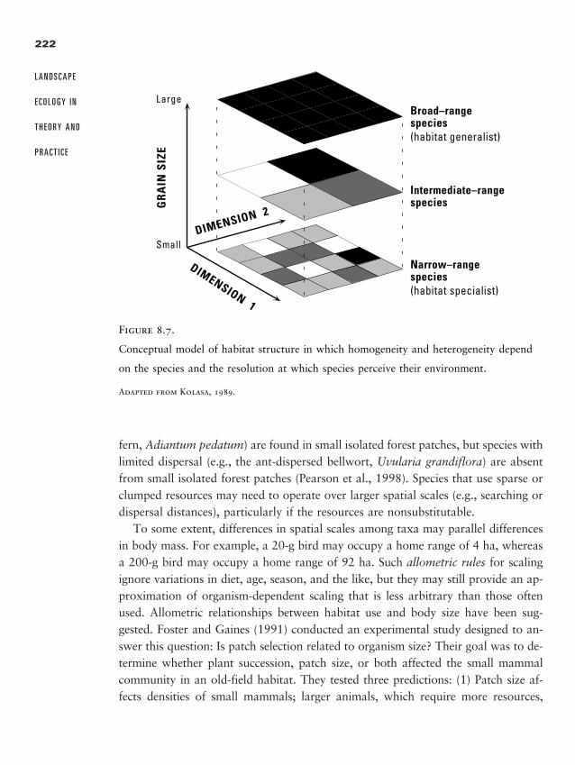
fern, Adiantum pedatum) are found in small isolated forest patches, but species withlimited dispersal (e.g., the ant-dispersed bellwort, Uvularia grandiflora) are absentfrom small isolated forest patches (Pearson et al., 1998). Species that use sparse orclumped resources may need to operate over larger spatial scales (e.g., searching ordispersal distances), particularly if the resources are nonsubstitutable.

To some extent, differences in spatial scales among taxa may parallel differencesin body mass. For example, a 20-g bird may occupy a home range of 4 ha, whereasa 200-g bird may occupy a home range of 92 ha. Such allometric rules for scalingignore variations in diet, age, season, and the like, but they may still provide an ap-proximation of organism-dependent scaling that is less arbitrary than those oftenused. Allometric relationships between habitat use and body size have been sug-gested. Foster and Gaines (1991) conducted an experimental study designed to an-swer this question: Is patch selection related to organism size? Their goal was to de-termine whether plant succession, patch size, or both affected the small mammalcommunity in an old-field habitat. They tested three predictions: (1) Patch size af-fects densities of small mammals; larger animals, which require more resources,

222

L A N D S C A P E

E C O L O G Y I N

T H E O R Y A N D

P R A C T I C E

Large

Small

GR

AIN

SIZ

E

DIMENSION 1

DIMENSION 2

Broad–range species(habitat generalist)

Intermediate–range species

Narrow–range species(habitat specialist)

Figure 8.7.

Conceptual model of habitat structure in which homogeneity and heterogeneity depend

on the species and the resolution at which species perceive their environment.

Adapted from Kolasa, 1989.

2888_e08_p201-248 3/2/01 2:57 PM Page 222

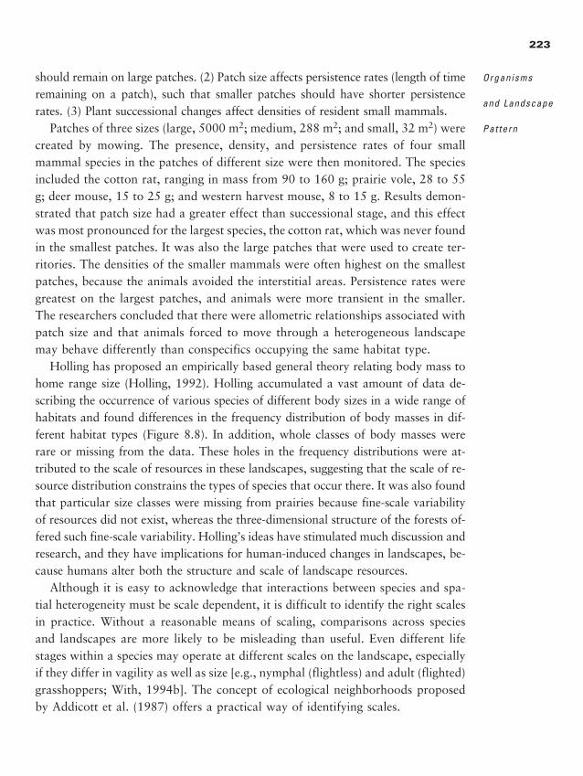
should remain on large patches. (2) Patch size affects persistence rates (length of timeremaining on a patch), such that smaller patches should have shorter persistencerates. (3) Plant successional changes affect densities of resident small mammals.

Patches of three sizes (large, 5000 m2; medium, 288 m2; and small, 32 m2) werecreated by mowing. The presence, density, and persistence rates of four smallmammal species in the patches of different size were then monitored. The speciesincluded the cotton rat, ranging in mass from 90 to 160 g; prairie vole, 28 to 55g; deer mouse, 15 to 25 g; and western harvest mouse, 8 to 15 g. Results demon-strated that patch size had a greater effect than successional stage, and this effectwas most pronounced for the largest species, the cotton rat, which was never foundin the smallest patches. It was also the large patches that were used to create ter-ritories. The densities of the smaller mammals were often highest on the smallestpatches, because the animals avoided the interstitial areas. Persistence rates weregreatest on the largest patches, and animals were more transient in the smaller.The researchers concluded that there were allometric relationships associated withpatch size and that animals forced to move through a heterogeneous landscapemay behave differently than conspecifics occupying the same habitat type.

Holling has proposed an empirically based general theory relating body mass tohome range size (Holling, 1992). Holling accumulated a vast amount of data de-scribing the occurrence of various species of different body sizes in a wide range ofhabitats and found differences in the frequency distribution of body masses in dif-ferent habitat types (Figure 8.8). In addition, whole classes of body masses wererare or missing from the data. These holes in the frequency distributions were at-tributed to the scale of resources in these landscapes, suggesting that the scale of re-source distribution constrains the types of species that occur there. It was also foundthat particular size classes were missing from prairies because fine-scale variabilityof resources did not exist, whereas the three-dimensional structure of the forests of-fered such fine-scale variability. Holling’s ideas have stimulated much discussion andresearch, and they have implications for human-induced changes in landscapes, be-cause humans alter both the structure and scale of landscape resources.

Although it is easy to acknowledge that interactions between species and spa-tial heterogeneity must be scale dependent, it is difficult to identify the right scalesin practice. Without a reasonable means of scaling, comparisons across speciesand landscapes are more likely to be misleading than useful. Even different lifestages within a species may operate at different scales on the landscape, especiallyif they differ in vagility as well as size [e.g., nymphal (flightless) and adult (flighted)grasshoppers; With, 1994b]. The concept of ecological neighborhoods proposedby Addicott et al. (1987) offers a practical way of identifying scales.

223

Organisms

and Landscape

Pat tern

2888_e08_p201-248 3/2/01 2:57 PM Page 223

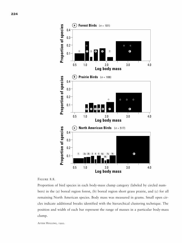
Figure 8.8.

Proportion of bird species in each body-mass clump category (labeled by circled num-

bers) in the (a) boreal region forest, (b) boreal region short grass prairie, and (c) for all

remaining North American species. Body mass was measured in grams. Small open cir-

cles indicate additional breaks identified with the hierarchical clustering technique. The

position and width of each bar represent the range of masses in a particular body-mass

clump.

After Holling, 1992.

224

Prop

orti

on o

f spe

cies

Prop

orti

on o

f spe

cies

Prop

orti

on o

f spe

cies

Log body mass

1 2 3 4 6 7 8

Forest Birds (n = 101)

0.1

0.2

0.3

0.4

2 3 44 5 6 7 8

Prairie Birds (n = 108)

0.1

0.2

0.3

0.4

1 3 4 5 8

North American Birds (n = 517)

0.1

0.2

0.3

0.4

0.5 1.0 2.0 3.0 4.0

2b 6a 7a 7b2a6b

Log body mass0.5 1.0 2.0 3.0 4.0

Log body mass0.5 1.0 2.0 3.0 4.0

a

b

c

2888_e08_p201-248 3/2/01 2:57 PM Page 224

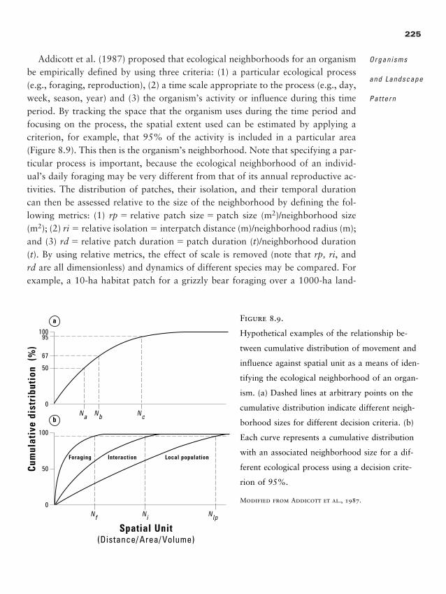
Addicott et al. (1987) proposed that ecological neighborhoods for an organismbe empirically defined by using three criteria: (1) a particular ecological process(e.g., foraging, reproduction), (2) a time scale appropriate to the process (e.g., day,week, season, year) and (3) the organism’s activity or influence during this timeperiod. By tracking the space that the organism uses during the time period andfocusing on the process, the spatial extent used can be estimated by applying acriterion, for example, that 95% of the activity is included in a particular area(Figure 8.9). This then is the organism’s neighborhood. Note that specifying a par-ticular process is important, because the ecological neighborhood of an individ-ual’s daily foraging may be very different from that of its annual reproductive ac-tivities. The distribution of patches, their isolation, and their temporal durationcan then be assessed relative to the size of the neighborhood by defining the fol-lowing metrics: (1) rp � relative patch size � patch size (m2)/neighborhood size(m2); (2) ri � relative isolation � interpatch distance (m)/neighborhood radius (m);and (3) rd � relative patch duration � patch duration (t)/neighborhood duration(t). By using relative metrics, the effect of scale is removed (note that rp, ri, andrd are all dimensionless) and dynamics of different species may be compared. Forexample, a 10-ha habitat patch for a grizzly bear foraging over a 1000-ha land-

225

Organisms

and Landscape

Pat tern

Spatial Unit(Distance/ Area/ Volume)

Cum

ulat

ive

dist

ribu

tion

(%

)

10095

67

50

0

100

50

0Nf

Na Nb Nc

Ni Nlp

Foraging Interaction Local population

a

b

Figure 8.9.

Hypothetical examples of the relationship be-

tween cumulative distribution of movement and

influence against spatial unit as a means of iden-

tifying the ecological neighborhood of an organ-

ism. (a) Dashed lines at arbitrary points on the

cumulative distribution indicate different neigh-

borhood sizes for different decision criteria. (b)

Each curve represents a cumulative distribution

with an associated neighborhood size for a dif-

ferent ecological process using a decision crite-

rion of 95%.

Modified from Addicott et al., 1987.

2888_e08_p201-248 3/2/01 2:57 PM Page 225

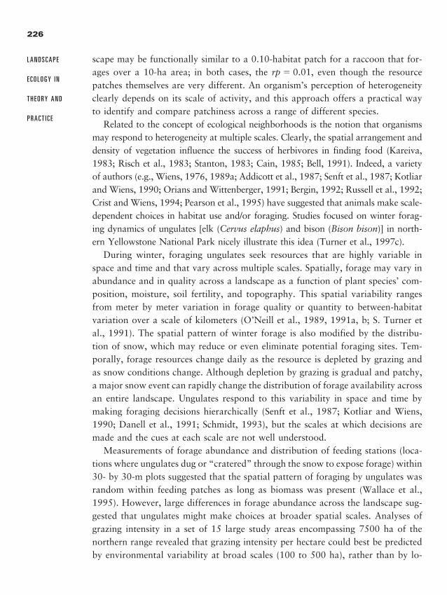
scape may be functionally similar to a 0.10-habitat patch for a raccoon that for-ages over a 10-ha area; in both cases, the rp � 0.01, even though the resourcepatches themselves are very different. An organism’s perception of heterogeneityclearly depends on its scale of activity, and this approach offers a practical wayto identify and compare patchiness across a range of different species.

Related to the concept of ecological neighborhoods is the notion that organismsmay respond to heterogeneity at multiple scales. Clearly, the spatial arrangement anddensity of vegetation influence the success of herbivores in finding food (Kareiva,1983; Risch et al., 1983; Stanton, 1983; Cain, 1985; Bell, 1991). Indeed, a varietyof authors (e.g., Wiens, 1976, 1989a; Addicott et al., 1987; Senft et al., 1987; Kotliarand Wiens, 1990; Orians and Wittenberger, 1991; Bergin, 1992; Russell et al., 1992;Crist and Wiens, 1994; Pearson et al., 1995) have suggested that animals make scale-dependent choices in habitat use and/or foraging. Studies focused on winter forag-ing dynamics of ungulates [elk (Cervus elaphus) and bison (Bison bison)] in north-ern Yellowstone National Park nicely illustrate this idea (Turner et al., 1997c).

During winter, foraging ungulates seek resources that are highly variable inspace and time and that vary across multiple scales. Spatially, forage may vary inabundance and in quality across a landscape as a function of plant species’ com-position, moisture, soil fertility, and topography. This spatial variability rangesfrom meter by meter variation in forage quality or quantity to between-habitatvariation over a scale of kilometers (O’Neill et al., 1989, 1991a, b; S. Turner etal., 1991). The spatial pattern of winter forage is also modified by the distribu-tion of snow, which may reduce or even eliminate potential foraging sites. Tem-porally, forage resources change daily as the resource is depleted by grazing andas snow conditions change. Although depletion by grazing is gradual and patchy,a major snow event can rapidly change the distribution of forage availability acrossan entire landscape. Ungulates respond to this variability in space and time bymaking foraging decisions hierarchically (Senft et al., 1987; Kotliar and Wiens,1990; Danell et al., 1991; Schmidt, 1993), but the scales at which decisions aremade and the cues at each scale are not well understood.

Measurements of forage abundance and distribution of feeding stations (loca-tions where ungulates dug or “cratered” through the snow to expose forage) within30- by 30-m plots suggested that the spatial pattern of foraging by ungulates wasrandom within feeding patches as long as biomass was present (Wallace et al.,1995). However, large differences in forage abundance across the landscape sug-gested that ungulates might make choices at broader spatial scales. Analyses ofgrazing intensity in a set of 15 large study areas encompassing 7500 ha of thenorthern range revealed that grazing intensity per hectare could best be predictedby environmental variability at broad scales (100 to 500 ha), rather than by lo-

226

L A N D S C A P E

E C O L O G Y I N

T H E O R Y A N D

P R A C T I C E

2888_e08_p201-248 3/2/01 2:57 PM Page 226

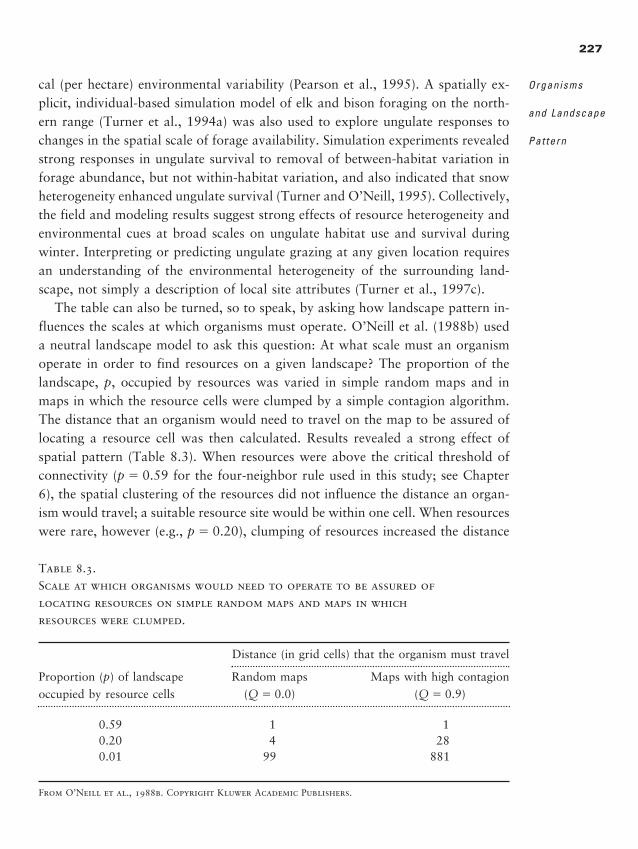
cal (per hectare) environmental variability (Pearson et al., 1995). A spatially ex-plicit, individual-based simulation model of elk and bison foraging on the north-ern range (Turner et al., 1994a) was also used to explore ungulate responses tochanges in the spatial scale of forage availability. Simulation experiments revealedstrong responses in ungulate survival to removal of between-habitat variation inforage abundance, but not within-habitat variation, and also indicated that snowheterogeneity enhanced ungulate survival (Turner and O’Neill, 1995). Collectively,the field and modeling results suggest strong effects of resource heterogeneity andenvironmental cues at broad scales on ungulate habitat use and survival duringwinter. Interpreting or predicting ungulate grazing at any given location requiresan understanding of the environmental heterogeneity of the surrounding land-scape, not simply a description of local site attributes (Turner et al., 1997c).

The table can also be turned, so to speak, by asking how landscape pattern in-fluences the scales at which organisms must operate. O’Neill et al. (1988b) useda neutral landscape model to ask this question: At what scale must an organismoperate in order to find resources on a given landscape? The proportion of thelandscape, p, occupied by resources was varied in simple random maps and inmaps in which the resource cells were clumped by a simple contagion algorithm.The distance that an organism would need to travel on the map to be assured oflocating a resource cell was then calculated. Results revealed a strong effect ofspatial pattern (Table 8.3). When resources were above the critical threshold ofconnectivity (p � 0.59 for the four-neighbor rule used in this study; see Chapter6), the spatial clustering of the resources did not influence the distance an organ-ism would travel; a suitable resource site would be within one cell. When resourceswere rare, however (e.g., p � 0.20), clumping of resources increased the distance

227

Organisms

and Landscape

Pat tern

Table 8.3.Scale at which organisms would need to operate to be assured of locating resources on simple random maps and maps in which resources were clumped.

Distance (in grid cells) that the organism must travel

Proportion (p) of landscape Random maps Maps with high contagionoccupied by resource cells (Q � 0.0) (Q � 0.9)

0.59 1 10.20 4 280.01 99 881

From O’Neill et al., 1988b. Copyright Kluwer Academic Publishers.

2888_e08_p201-248 3/2/01 2:57 PM Page 227

the organism must search by a factor of 7. When resources were very rare (p �

0.01), the organism needed to search a distance nearly nine times greater whenresources were clumped than when they were distributed at random. Thus, thestructure of the landscape itself may dictate the scales at which organisms mustoperate. In addition, the effectiveness of different foraging tactics may vary withthe spatial distribution of resources (e.g., Cain, 1985; Roese et al., 1991).

To test empirically for different scales of interaction with patch structure amongdifferent species, With (1994b) studied three grasshopper species using experimen-tal microlandscapes (Wiens and Milne, 1989; Johnson et al., 1992a). The study wasconducted in grassland habitat, and 25-m2 microlandscapes were established inwhich the heterogeneity of shortgrass cover was varied. With (1994b) recorded themovement patterns of the grasshopper species in different landscape mosaics andapplied fractal analysis to compare the landscape perceptions of the different speciesin the same environments. Results demonstrated that the largest of the grasshopperspecies moved up to six times faster than the two smaller species, and the speciesresponded differently to microlandscape structure in the 25-m2 plots. The twosmaller species also had more complex movement patterns than the larger species,suggesting that these species were interacting with patch structure at a finer scaleof resolution than the larger species (With, 1994b). With concluded from these stud-ies that the grasshopper species were scaling the landscape differently and suggestedthat the scale independence of fractal analysis provides a useful tool for identifyingsuch differences among taxa. Thus, the scale of pattern will interact with the scaleat which an organism operates to determine its dynamics on a given landscape.

S y n t h e s i s : S c a l e D e p e n d e n c e

Just as our ability to detect pattern depends on the scale at which we make measure-ments, the ability of organisms to detect and respond to heterogeneity depends on howthey scale the environment (Wiens, 1989a). The multiple scales at which species per-ceive their environment and the fact that these scales often differ from our own mustbe recognized in any attempt to understand or predict the response of organisms tospatial heterogeneity. Because species differ in the scales at which they use resourcesor perceive the environment (their ecological neighborhoods), studies of the interac-tions among species may be particularly sensitive to scale (Wiens, 1989a). However,understanding the responses of organisms to spatial pattern at multiple scales is in itsinfancy (Kareiva, 1990; Kotliar and Wiens, 1990; Hyman et al., 1991; Ward and Saltz,1994) and remains a high priority for ecology (Lubchenco et al., 1991; Levin, 1992).

228

L A N D S C A P E

E C O L O G Y I N

T H E O R Y A N D

P R A C T I C E

2888_e08_p201-248 3/2/01 2:57 PM Page 228

E F F E C T S O F S P A T I A L P A T T E R N O N O R G A N I S M S

We now summarize a number of insights that have emerged from landscape eco-logical studies about organisms and space. Examples selected are illustrative ratherthan comprehensive. The focus is on effects of patch size and heterogeneity, eco-tones and boundary shape, habitat connectivity and the role of corridors, andlandscape context. This section ends with a synthesis, suggesting the conditionsfor which spatial pattern will be important for organisms.

P a t c h S i z e a n d H e t e r o g e n e i t y

In general, larger, more heterogeneous patches support more species. A well-studied aspect of population responses to habitat arrangement is the effect ofpatch size. In general, larger patches of habitat contain more species and oftena greater number of individuals than smaller patches of the same habitat. Thisis not at all surprising based on the well-documented relationship between speciesand area, and it occurs for several reasons. First, the larger the habitat patch isthe more local environmental variability is contained within it, such as differ-ences in microclimate, structural variation in plants, and diversity of topographicpositions. Even a seemingly uniform expanse of habitat such as forest or grass-land is, at some scale, a mosaic of different habitats (Wilcove et al., 1986). Thisvariability provides more opportunities for organisms with different require-ments and tolerances to find suitable sites within the patch. In addition, theedges and interiors of patches may have different conditions that favor somespecies but not others, and the relative abundance of edge versus interior habi-tats varies with patch size. Smaller patches have a greater perimeter-to-area ra-tio than larger patches, which means that smaller patches will have a greaterproportion of edge habitat and the larger patch will have a greater proportionof interior habitat.

Consider these differences for forested patches. At the edge of a forestedpatch, there is generally more light, a warmer, drier microclimate, and greateraccess for organisms that frequent open habitats (Chen et al., 1992, 1995,1996). In contrast, the interior of the patch tends to be more shady, cooler andmore moist, and often off limits to the organisms of open habitat (Ranney etal., 1981). When a patch gets sufficiently small or elongated in shape, all inte-rior habitat is lost, leading to a loss of interior species and dominance by edgespecies. Large patches typically include both edge and interior species. An im-

229

Organisms

and Landscape

Pat tern

�

2888_e08_p201-248 3/2/01 2:57 PM Page 229

portant point to keep in mind is that fragmentation may actually increase to-tal species diversity (Opdam, 1991); although the fragmentation decreases thehabitat of forest-interior species, the resulting heterogeneity increases opportu-nities for forest-edge and open-field populations. However, this increase inspecies diversity that may result from habitat fragmentation may not be desir-able from a conservation perspective.

Many studies have examined the effects of patch size on bird communities (e.g.,Van Dorp and Opdam, 1987; Verboom et al., 1991; McGarigal and McComb,1995). Freemark and Merriam (1986) found that larger forest patches in Canadahad more species than smaller forest patches, with forest interior birds showingthe strongest effect. In addition, forest patches that had greater within-patch het-erogeneity in terms of habitat structure and microenvironmental conditions alsohad more bird species and more total numbers of birds, with edge-related speciesshowing the greatest effect. However, forest-edge birds may be nest predators anddecrease the effective size of the patch for other species (Andren, 1992).

In Amazonian forests, a long-term study initiated by Tom Lovejoy of the Smith-sonian Institution has examined the effects of patch size on a wide range of trop-ical biota. The biota of continuous unfragmented forest in the Amazon regionwere sampled during 1983 and 1984, after which time the forest was cut exper-imentally to create fragments of 1 and 10 ha. Responses of the biota were thenmeasured during the subsequent 9 years following fragmentation. Results for in-sectivorous birds (Stouffer and Bierregaard, 1995) demonstrated that bird abun-dance and species richness within the forest fragments declined dramatically fol-lowing isolation, despite the fact that the fragments were separated fromcontinuous forest by only 70 to 650 m. Army ant colonies were eliminated soonfollowing fragmentation. The bird species that were obligate army ant followersdropped out first; of the non-army ant obligates, only two species of edge spe-cialists were not affected by fragmentation. The bird communities in the 1-ha frag-ments diverged from the preisolation community more than did the communi-ties in the 10-ha fragments, indicating an effect of patch size. Interestingly, assecondary succession proceeded in the cleared areas, communities in the larger(10-ha) fragments became more like the preisolation communities, although com-munities in the smaller fragments continued to diverge.

In sum, there is overwhelming evidence from many taxa and geographic loca-tions that larger patches support a greater number of species, and that an increasein within-patch heterogeneity (e.g., vertical complexity, microsite variety) will gen-erally increase species richness.

230

L A N D S C A P E

E C O L O G Y I N

T H E O R Y A N D

P R A C T I C E

2888_e08_p201-248 3/2/01 2:57 PM Page 230

E c o t o n e s a n d E f f e c t s o f B o u n d a r y S h a p e

Shape of boundary can influence species’ relative abundances. Closely related toissues associated with patch size are those relating to the shape of the boundaries,or ecotone, between two cover types. Patch shape refers to the two-dimensionalform of a given area as determined by its perimeter (edge or boundary may beused synonymously). Some of the effects of patch shape on organisms result fromthe relative amounts of interior and edge habitat that are provided by a givenshape. For a given area, a circular shape will have the least edge habitat, whereasa very long narrow shape will have much more, and perhaps only, edge habitat,depending on the width. Because some organisms specialize on edges while oth-ers require interior habitats, patch shape has important implications for the bioticcommunity.

Boundary shape can influence ecological processes, yet there is not a largeamount of literature on the effects of varying edge shapes (Forman, 1995). Hu-man activities often simplify boundary shapes, changing complex shapes thatmay follow topographic variability or result from natural disturbance intostraight lines (Krummel et al., 1987). A study of revegetation on disturbed mineareas examined the influence of different shapes of the boundary between theundisturbed forest, which is a source of propagules for succession, and the re-claimed mine area. Hardt and Forman (1989) compared boundaries of threeshapes, convex, concave, and straight, and found that the density of colonizingtrees was 2.5 times greater in areas with concave boundaries. In addition, therewas greater evidence of browsing on the vegetation adjacent to convex bound-aries. These results suggested that the convex boundary shape would result inmore rapid rates of succession. Another interesting consideration related to patchshape is the orientation, or general directionality, of a patch. Patch orientationinfluences bird species richness in forest fragments, presumably because patchesthat are oriented perpendicular to migratory pathways are more likely to attractbirds than patches that are aligned with migratory pathways (Gutzwiller andAnderson, 1992).

Forman has been conducting an interesting long-term study of the effects of theshape of the boundary between pinyon–juniper (Pinus–Juniperus) and grassland(Bouteloua–Artemisia) in northern New Mexico on wildlife usage in and acrossthe boundary. Results have demonstrated that use of the edge by both elk (Cervuselaphus) and deer (Odocoileus hemionus) increases with curvilinearity of the edgeand movement along the boundaries decreases (Forman, 1995:106–107). Whereas

231

Organisms

and Landscape

Pat tern

2888_e08_p201-248 3/2/01 2:57 PM Page 231

movement across boundaries increases with curvilinearity, straight boundaries ap-pear to act as partial boundaries. However, the influence of boundary shape onorganisms remains a topic for which more research is needed.

The particular type of edge that surrounds a given habitat patch may also bean important influence on the species found within the habitat patch. For exam-ple, Watts (1996) determined that the species richness and total abundance of win-tering sparrows in habitat patches were affected by the type of adjacent edge veg-etation. Habitat patches supported more species and individuals when they wereadjacent to dense edges (privet and brambles) than when adjacent to sparse edges(e.g., deciduous forest). Watts (1996) suggests that the occurrence of individualspecies may be independent of resource availability if there is a strong effect ofedge quality on the species.

A review of theoretical and empirical studies of species interactions with habi-tat edges (Fagan et al., 1999) suggested four general classes of effects: (1) edges thatmay be barriers or filters to movement; (2) agents that alter mortality rates; (3) ar-eas providing energetic subsidies or refuge; and (4) regions where novel interspeciesinteractions may occur. The wide differences in response of different species to edgescan result in dramatically different effects. Fagan et al. (1999) have noted that ourknowledge of “edge-mediated dynamics place(s) severe limitations” on our under-standing of processes leading to species colonization or extinction, which comprisesthe conceptual core of island biogeography and species–area relations.

H a b i t a t C o n n e c t i v i t y

Connectivity is a scale-dependent threshold phenomenon. The connectivity of suit-able habitat can constrain the spatial distribution of a species by making some ar-eas accessible and others inaccessible. Plants and animals need suitable areas inwhich movement and dispersal can occur to maintain the populations. Both plantsand animals have varying degrees of mobility, although plants, of course, usuallymove at the seed stage rather than as mature organisms. Once suitable habitat fora species of interest is characterized, determining whether the habitat is or is notspatially connected is often of interest.

A series of studies of small mammals in an agricultural landscape mosaic inCanada conducted by Merriam and his colleagues nicely illustrates important ef-fects of habitat connectivity on small mammals, as well as the integration of fieldstudies and modeling. Their study area is a landscape containing crop fields alongwith scattered woodlands. These woodlands are sometimes isolated from one an-other by being completely surrounded by crop fields, and sometimes the wood-

232

L A N D S C A P E

E C O L O G Y I N

T H E O R Y A N D

P R A C T I C E

2888_e08_p201-248 3/2/01 2:57 PM Page 232

lands are connected by fencerows—narrow corridors of trees and shrubs that growup along the borders of the crop fields. Early studies of this landscape demon-strated that chipmunks and white-footed mice traveled frequently along thefencerows, but seldom moved between the wood and the field or across open fields(Wegner and Merriam, 1979). Birds also seldom flew directly over the open fieldsbetween the woods and preferred to fly along the fencerows. Similar results havebeen observed in many locations in Europe, where fencerows between woodlandshave developed over many centuries (Forman and Baudry, 1984).

Merriam and colleagues next explored what happened to the small mammal pop-ulations if they were extirpated within the woodlands (Henderson et al., 1985). Lo-cal extinctions are a frequent natural occurrence each year because relatively smallnumbers of animals survive the winter. Chipmunks were live-trapped and removedfrom woodland patches, and the rate of recolonization of these patches depended ontheir connectivity to other woods; that is, recolonization depended on whether thepatches were joined or linked to one another. Recolonization occurred more rapidlyin patches that were connected to other wooded areas by fencerows than in the iso-lated woodlands. This study also suggested that an area of at least 4 km2 and con-taining at least five woodlands and interconnecting fencerows would be required forthe populations in this mosaic to persist through the years (Henderson et al., 1985).

A simulation modeling study was used to explore further the effects of alter-native patterns of connectivity among patches (Lefkovitch and Fahrig, 1985).Thirty-four different arrangements of connections among five patches were simu-lated to determine which spatial characteristics of groups of habitat patches wereimportant predictors of the survival of a resident animal population, like the chip-munks or white-footed mice. Results indicated that populations in isolated patchesdied out much earlier and had lower population sizes than did the populations inthe connected patches. These results were supported by field data in which fourinterconnected woodlands had higher mean population sizes of white-footed micethan two isolated woodlands of similar size. New organisms could disperse intothe connected woodlands and augment or replenish the local populations, whereasthe isolated woodland received fewer new mice.

Connectivity also influences the use of suitable habitat by larger organisms.Milne et al. (1989) examined the effects of habitat fragmentation on winteringwhite-tailed deer. Using a GIS-based model including 12 landscape variables, deerhabitat was predicted independently at each of 22,750 contiguous 0.4-ha grid cells.When predicted habitat use was compared with empirical data, results demon-strated that deer did not use sites of suitable habitat that were isolated from othersuitable sites.

233

Organisms

and Landscape

Pat tern

2888_e08_p201-248 3/2/01 2:57 PM Page 233

Whether habitat is connected or not is a threshold phenomenon that depends onboth the abundance and spatial arrangement of the habitat, as well as the move-ment or dispersal characteristics of the organism. A threshold refers to there beinga point at which the habitat suddenly becomes either connected or disconnected.Recall from Chapter 6 how the use of neutral landscape models demonstrated con-nectivity across simple random or structured landscapes. When a four-neighbor ruleis employed, suitable habitat is distributed in a number of relatively small discon-nected patches when it occupies less than �60% of a landscape; however, whensuitable habitat occupies more than 60% of the landscape, the habitat is distributedin a few, large, well-connected patches. Under these conditions, the threshold ofconnectivity is �60%. If the habitat is not distributed at random, but has a greaterdegree of clumping as observed in most landscapes, the threshold of connectivityusually moves down. In other words, the habitat would be connected at some lowerfraction of occupancy on the landscape. Consider next the different movement abil-ities of an organism on a set of landscapes where the suitable habitat is again dis-tributed at random. If the organism is a bit better at getting around, say it can moveto its eight nearest neighbors, the adjacent and diagonal neighbors, then the thresh-old of connectivity decreases to about 40%. If the organism can jump across a sin-gle cell of unsuitable habitat and essentially ignore this interruption (albeit, a verysimple view of the matrix), the threshold of connectivity decreases again, and a land-scape containing only 25% suitable habitat could be traversed by the organism.Changes in the clumping of the habitat will also interact with the movement capa-bility of the organism to determine the threshold of connectivity. Thus, connectiv-ity is greatly influenced by the behavior of the organism.

The important idea about habitat connectivity is that habitat is either connectedor disconnected and the change between these two states occurs at a threshold ofhabitat abundance. For an organism, this means the qualitative difference betweenbeing able to move about the landscape to locate suitable sites for foraging, nest-ing, and dispersal and being unable to do so. This has important implications forconservation, because suitable habitat might be lost for a while with no apparentnegative effect on a plant or animal of interest until this threshold is passed. Thennegative effects may occur suddenly as the organisms can no longer meet theirneeds on the fragmented landscape. Exactly where the threshold is depends on theorganism, the amount of habitat, the spatial clustering of the habitat, and the na-ture of the matrix; different species might perceive different thresholds in the samelandscape (Pearson et al., 1996; With, 1997a).

Do such thresholds in connectivity exist in real landscapes? Andren (1994) re-viewed the empirical evidence for birds and mammals that could be used to test pre-

234

L A N D S C A P E

E C O L O G Y I N

T H E O R Y A N D

P R A C T I C E

2888_e08_p201-248 3/2/01 2:57 PM Page 234

dictions derived from a neutral landscape model regarding habitat connectivity. Heexamined the process of habitat fragmentation, with its loss of habitat, reductionsin patch sizes, and increased distances between patches. His results lead to the con-clusion that the relative importance of these three aspects of fragmentation differsdepending on abundance of suitable habitat in a landscape. When landscapes have30% suitable habitat the primary effect of habitat fragmentation is habitat loss.This is because in landscapes with relatively high proportions of suitable habitat thehabitat is reasonably well connected, and the configuration of habitat is less impor-tant. In experimental landscapes designed to study beetle movement, Wiens et al.(1997) found threshold effects when grassy habitat was less than 20%. Simulationsconducted by Fahrig (1997) also demonstrated that the effects of habitat loss couldoutweigh the effects of habitat fragmentation on population extinction. In landscapeswith low proportions of suitable habitat (10% to 30%), the spatial arrangement ofpatches is very important. Further reduction in habitat results in an exponential in-crease in distances between patches, that is, rapid decreases in connectivity; With andKing (1999a) found evidence for a strong effect of gap structure on dispersal suc-cess. Moreover, the effect of patch size and isolation will not only depend on theproportion of original habitat in the landscape, but also on the suitability of the sur-rounding habitats (e.g., the matrix, areas between patches) for movement. Note thatthe results from both the theory and empirical studies suggest that conservation ac-tions, such as adding habitat or protecting key locations, are most likely to have sub-stantial effects on habitat connectivity when the suitable habitat is relatively low inabundance (Andren, 1994; Pearson et al., 1996; Fahrig, 1997). It is in this rangewhere small changes in habitat abundance are likely to cause the threshold of con-nectivity to be passed. However, it is also important to recognize that the effects ofhabitat loss cannot be mitigated simply by connecting remaining habitat fragments.

What Is the Role of Corridors?Corridors, narrow patches of land that connect similar patches but that differ fromthe surrounding matrix, have been proposed in conservation plans as a means ofmaintaining connectivity between otherwise isolated patches of habitat. As notedby With (1997a), corridors are appealing in a patch-based view of the world inwhich habitat is either suitable or unsuitable and corridors provide a physicalbridge linking islands of habitat. The presence of corridors is assumed to increasepopulation persistence by providing for an exchange of individuals among a pop-ulation that was previously connected but that is now fragmented. However, therehas been much controversy regarding their effectiveness (e.g., Simberloff and Cox,1987; Saunders and Hobbs, 1991; Hobbs, 1992; Beier and Noss, 1998).

235

Organisms

and Landscape

Pat tern

2888_e08_p201-248 3/2/01 2:57 PM Page 235

Functional corridors may not be discrete structures. Gustafson and Gardner(1996) simulated dispersal and patch colonization on heterogeneous landscapesand identified the regions of the landscape in which flows were funneled and that,therefore, functioned effectively as corridors. They found that these “corridors”were diffuse and difficult to identify. Reduced contrast between habitat patchesand the intervening matrix may enhance connectivity more than would a discretecorridor. Although protecting naturally existing corridors probably benefits re-gional and local biodiversity, the creation of linear patches may not provide suchbenefits (Rosenberg et al., 1997).

Rosenberg et al. (1997) provided a useful distinction between two functions oflinear landscape features: (1) they may themselves provide habitat, containing theresources needed for survival, reproduction, and movement; or (2) they may serveas biological corridors that provide for movement between habitat patches, butnot necessarily for reproduction. Because corridors may be heavily influenced byedge effects, their interior habitat is reduced and may even be absent completely.By examining the literature on the use of corridors, Rosenberg et al. (1997) thensynthesized a set of common patterns regarding the effectiveness of corridors. First,individual animals are likely to select pathways for movement that include com-ponents of their habitat when confronted by a choice, and this behavior is mostpronounced for individuals moving within their home range. Second, the relativeuse of the matrix as movement habitat depends on its contrast with the organ-ism’s suitable habitat. Third, the behavior of animals may change in areas of lessfavorable habitat; for example, animals may move more rapidly when traversinglow-quality habitat than in high-quality habitat. Evaluating the effectiveness of alinear habitat patch as a corridor requires a three-step evaluation of whether or-ganisms can find, select, and successfully move through the patch; more empiri-cal study is needed of a wider range of species in conditions that represent thecomplexity of real landscapes (Lidicker and Koenig, 1996; Rosenberg et al., 1997).Enhancing our understanding of how organisms move through heterogeneouslandscapes (along corridors or through the matrix) is a key component of under-standing the responses of organisms to spatial pattern.

E f f e c t s o f L a n d s c a p e C o n t e x t

Characteristics of the surrounding landscape can strongly influence local pop-ulations. Whether the presence or abundance of organisms at a given location orsampling point is explained by characteristics of the immediate locale or by at-tributes of the surrounding landscape is an interesting question. Pearson (1993)

236

L A N D S C A P E

E C O L O G Y I N

T H E O R Y A N D

P R A C T I C E

2888_e08_p201-248 3/2/01 2:57 PM Page 236

studied wintering birds in powerline rights-of-way (ROW) in the Georgia pied-mont. These ROWs are corridors in which the vegetation is maintained in an openstate, usually by mowing, so that shrubs and herbaceous plants dominate. The ar-eas surrounding the ROW may also be open, forested, or in cultivation. Pearsonrecorded the abundance of different bird species and the characteristics of the veg-etation (such as height, density, and species composition) within each ROW andquantified the types of habitats in the surrounding landscape based on aerial pho-tography (Figure 8.10). He found that variability in the presence and abundanceof certain wintering birds [e.g., Parids (titmice) and Rufous-Sided Towhee (Pipiloerythrophthalmus)] was best explained by the habitats in the surrounding land-scape (Table 8.4). Other species [e.g., Northern Cardinal (Pyrrhuloxia cardinalis)and White-Throated Sparrow (Zonotrichia albicollis)] responded only to the char-acteristics of the local habitat, and yet other species [e.g., Carolina Wren (Thryotho-

237

Organisms

and Landscape

Pat tern

300-m radius

200-m radius

100-m radius

Study Plot

Landscape Matrix Habitats

300 m Right-of-way corridor 45 m

Figure 8.10.

Different spatial extents at which landscape patterns were characterized by Pearson

(1993) and used in statistical models of bird species presence and abundance in power-

line right-of-way sample plots.

Adapted from Pearson, 1993.

2888_e08_p201-248 3/2/01 2:57 PM Page 237

rus ludovicianus)] responded both to local conditions and to the landscape con-text (Table 8.4).

In a study that considered an even greater spatial extent, Flather and Sauer(1996) used data from the Breeding Bird Survey (BBS), annual censuses takenalong fixed routes that are 39.4 km in length, and analyzed land-cover patternsin a circular scene of 19.7-km radius centered along each route, an area of 1200km2. They then tested the null hypothesis of no relation between landscape struc-ture and neotropical migrant abundance by correlating the measures of landscape

238

L A N D S C A P E

E C O L O G Y I N

T H E O R Y A N D

P R A C T I C E

Table 8.4.Results of stepwise regression models of bird response variables as explained by within-habitat variables and characteristics of the surrounding landscape.

Response variable Matrix r2 Model r2

Community measures

Total number of birds 0.24 0.73Species richness 0.74 0.74Shannon diversity 0.82 0.82

Functional groups

Forest species 0.57 0.84Early successional species 0.18 0.18Generalists 0.13 0.73Parids 0.65 0.76

Selected species

Carolina wren 0.48 0.83Field sparrow 0.24 0.24Dark-eyed junco 0.24 0.24Northern cardinal 0.31 0.83Rufous-sided towhee 0.54 0.83Song sparrow 0.19 0.19White-throated sparrow 0.00 0.83

From Pearson, 1993. Copyright Kluwer Academic Publishers.

Matrix r2 reflects the amount of variation explained only by the landscape matrix variables.

Model r2 is the coefficient of determination for the entire regression equation. Amount of varia-

tion explained only by within-habitat variables can be computed by difference.

2888_e08_p201-248 3/2/01 2:57 PM Page 238

structure with breeding-bird abundance. Results demonstrated that neotropicalmigrants were more abundant in landscapes with a greater proportion of forestand wetland habitats, fewer edge habitats, larger forest patches, and forest habi-tats well dispersed throughout the scene. Landscapes with high proportions of human-dominated land uses (e.g., agriculture and urban) supported lower relativeabundances of neotropical migrants. Neotropical migrants were also low in abun-dance where landscape diversity and edge were high and forest edges were morecomplex (as measured by fractal dimension). However, species that were perma-nent residents showed few correlations with landscape structure, and temperatemigrants were associated with habitat diversity and edge attributes, rather thanwith the amount, size, and dispersion of forest habitats.

A number of other examples of the importance of landscape context can befound in the literature. Lindenmayer and Nix (1993) found that the occupancy ofcorridors by arboreal marsupials in Australia could not be predicted by habitatfeatures within the corridor; information on the composition of the surroundinglandscape was required. The winter foraging patterns of elk and bison in north-ern Yellowstone National Park, discussed earlier in this chapter, clearly differedwith spatial scale and provide another example of the importance of landscapecontext (Pearson et al., 1995). Models explaining breeding-bird abundance in anurban southern California landscape were significantly improved when landscapevariables were added (Bolger et al., 1997b).

Collectively, these examples demonstrate that it is often important to considerlandscape context along with local site attributes when trying to explain local eco-logical processes. This insight has substantial implications for land management,because it suggests that what happens in small local areas may be influenced con-siderably by the surrounding landscape. Ecologists are conducting research to un-derstand better when and over what scales the overall landscape influences are im-portant or may even dominate and when the local conditions are more important.

S y n t h e s i s : W h e n I s S p a t i a l P a t t e r n I m p o r t a n t ?

The influence of spatial heterogeneity on organisms, while interesting in its ownright, certainly adds a substantial degree of complexity to population or commu-nity dynamics. But when is space really important, and when might spatial rela-tionships be prudently ignored? Although the answer to this question depends onspecific objectives and circumstances, there are instances where space (size, shape,and arrangement of habitat across the landscape) matters, and the answers to thisquestion are clear. These include (1) when habitat is rare or fragmented, because

239

Organisms

and Landscape

Pat tern

2888_e08_p201-248 3/2/01 2:57 PM Page 239

theory and empirical data both point to the strong influence of spatial pattern inconnecting or fragmenting habitat when it occupies 20% to 30% of a landscape,(2) if edge effects are important components of the process being studied, and (3)if dispersal limits movement between patches and metapopulation dynamics arelikely to affect habitat use. Following from this, spatial considerations may notbe needed if habitat is very abundant, because most suitable sites will likely bewell connected and edge effects will be small; or if edge effects are unimportantfor the process or species being studied; or if movement is relatively unlimited andorganisms can reach all or most areas containing suitable habitat.

It is also important to recognize the limitations of a patch-based view of the worldand to know when a more continuous or complex view of spatial heterogeneity isneeded. Franklin (1993) argues that conservation considerations should include botha patch-based component, such as the design (size and spacing) of nature reserves,and the condition and management of the matrix, that is, the intervening areas be-tween patches or reserves. Landscape context may be quite important for the organ-isms living in a given patch, and reducing the contrast across the edges of patchesmay enhance the suitability of the patches for organisms. The processes of movementand dispersal are also strongly influenced by the characteristics of the landscape be-tween patches, yet quantitative data on this are sparse (and difficult to obtain).

S P A T I A L L Y E X P L I C I T P O P U L A T I O N M O D E L S

The representation of spatial heterogeneity in population ecology varies consider-ably, ranging from assumptions that the world is subdivided into a large collec-tion of patches that are all equally accessible to one another, to steppingstonemodels in which the patches have fixed locations in space (and so dispersal dis-tances between patches will vary), to continuum models in which there is a con-tinuous coordinate system in which populations interact and disperse (Kareiva,1990). Landscape ecologists, however, typically utilize spatially explicit popula-tion models (SEPMs) to address questions about organisms in landscapes. SEPMshave a structure that specifies the location of each object of interest (e.g., organ-ism, population, cell, or habitat patch) within a heterogeneous landscape, andtherefore the spatial relationships among habitat patches and other landscape fea-tures are explicitly represented (Dunning et al., 1995). The models typically rep-resent a landscape as a grid of cells and simulate the birth, death, foraging, andmovement patterns of animals or plants across the landscape. Thus, SEPMs can

240

L A N D S C A P E

E C O L O G Y I N

T H E O R Y A N D

P R A C T I C E

�

2888_e08_p201-248 3/2/01 2:57 PM Page 240

be used to address questions of changing resource distributions, habitat fragmen-tation, isolation, habitat shape, and patch size on populations of interest. Themodels may be individual-based models, in which the attributes and movementsof every individual in the population are represented in the model, or they maybe cell-based models in which the occupancy of a cell, or site, is the focus (thesemodels are also called cellular automata models). SEPMs have yielded interestinginsights into the interactions between single populations and their habitats.

BACHMAP is an example of an individual-based SEPM model designed to elu-cidate the effects of habitat arrangement on the size and extinction probability ofa Bachman’s sparrow (Aimophila aestivalis) population in a region managed fortimber production (Pulliam et al., 1992). Bachman’s sparrow is a small bird foundin pine woods of the southeastern United States, and the species is of concern toland managers because its population has declined since the 1930s over much ofits range. The BACHMAP model includes life-history characteristics (such as dis-persal, survivorship, and reproductive success) of Bachman’s sparrow and the land-scape characteristics of the Savannah River Site, South Carolina. An interestingaspect of the population is that the sparrows occur primarily in very young pinestands (10 yr after planting) and in mature pine stands (50 yr old), but theyrarely use stands of intermediate age. Thus, as trees are harvested and regrow, thedistribution of suitable habitat for Bachman’s sparrow across the landscapechanges. Simulations indicated that the demographic parameters (having to dowith birth and death rates) had a greater impact on population size than the dis-persal parameters (having to do with moving across the landscape to find suitablehabitat); but many of the simulated population sizes were small, much less thanthe amount of suitable habitat might theoretically support. An extension ofBACHMAP developed by Liu (1993) and called ECOLECON integrated economicconsiderations and harvesting scenarios, allowing future landscape patterns, eco-nomic returns, and sparrow population dynamics to be considered together.

Individual-based SEPMs have been developed for a variety of other species. Inindividual-based models, the location of each individual across the landscape ismonitored, and the state of individuals (e.g., weight) may be tracked separately.An individual-based model for moose foraging in a boreal landscape (Moen et al.,1997, 1998) is discussed in Chapter 9, and individual-based models serve as com-ponents of a multilevel spatial model of the Everglades (DeAngelis et al., 1998),also discussed in Chapter 9. The spotted owl model (Noon and McKelvey, 1996a)used to assess the implications of old-growth forest harvesting in the Pacific North-west and discussed in Chapter 10 also falls into this category, as does the elk andbison simulation model for northern Yellowstone National Park (Turner et al.,

241

Organisms

and Landscape

Pat tern

2888_e08_p201-248 3/2/01 2:57 PM Page 241

1994a), discussed earlier in this chapter. Individual-based models represent a bottom-up approach to modeling population dynamics in space, but some re-searchers are interested in developing more formal protocols for linking these mod-els with classical population ecology approaches (Fahse et al., 1998).

SEPMs may also be population based, in which each cell contains a popula-tion (Dunning et al., 1995). In these cell-based models, occupancy and evenabundance are tracked on cells representing the landscape, but the fate of indi-viduals is not tracked. These models have also yielded a variety of useful in-sights. With and Crist (1995) projected the dispersion patterns of grasshoppersacross a larger landscape mosaic using a cell-based model. Lavorel et al. (1994b)used a spatially explicit simulation model to examine the interaction among dis-persal strategies, seed dormancy, and disturbances on the pattern of coexistence.The results showed that when species differed only in mean dispersal distancethe species with the shorter-range dispersal would always displace the other.When disturbances prevented reproduction, but activated dormant seeds, dif-ferences in dormancy strategy could result in coexistence of species with differ-ent dispersal capabilities. The predicted patterns of coexistence were consistentwith conclusions of a field study, in species-rich Mediterranean old-fields, wherecoexistence of annual and perennial forbs depends on the interactions amongdispersal and dormancy strategies, spatial heterogeneity, and small-scale distur-bances (Lavorel et al., 1994a).

SEPMs can be used to address a wide range of questions in landscape ecol-ogy, population ecology, and conservation biology. They are particularly usefultools when questions require consideration of the amount, geometry, and ratesof change in habitat. For management questions, SEPMs may be used to developa robust relative ranking of management alternatives (Turner et al., 1995a).However, it is important to remember that these models are data hungry, andthe lack of data for the scales or area of interest may limit their application.Validation and interpretation of the simulations can also be difficult. In addi-tion, few SEPMs have been developed in which multiple species or interactionsamong species are considered. For example, Liu et al. (1995) demonstrated howthe Bachman’s Sparrow, described earlier, was affected by forest-managementscenarios developed for the federally listed Red-Cockaded Woodpecker (Picoidesborealis). Although the two species overlap in habitat requirements in these long-leaf pine forests of the Southeast, the woodpecker requires stands older than 70yr, whereas Bachman’s Sparrow also occurs in younger stands. Thus, a shift tomanagement of old-growth stands would actually reduce the habitat availablefor Bachman’s sparrow. Management plans based on SEPMs developed for a

242

L A N D S C A P E

E C O L O G Y I N

T H E O R Y A N D

P R A C T I C E

2888_e08_p201-248 3/2/01 2:57 PM Page 242

single species may be insufficient for management of other species on the land-scape, even those having similar habitat requirements. Again, a multispecies man-agement perspective is sorely needed.

S U M M A R Y

Organisms exist in spatially heterogeneous landscapes. Landscape ecologists areparticularly interested in how organisms utilize resources that are distributed acrossa heterogeneous landscape and how they live, reproduce, disperse, and interactwith each other in space. Studies in population ecology have always been cog-nizant of spatial issues, but explicit consideration of spatial factors influencingpopulations has become much more prominent in the past three decades. Earlystudies focused on the diffusion of organisms across homogeneous landscapes, pre-dicting rates of spread and number of sites that would be occupied under variousconditions. However, the development of island biogeography and metapopula-tion theory fueled much research on the dynamics of populations in heterogeneouslandscapes. Island biogeography was developed as a general theory to predict thenumber of species found on oceanic islands based on two attributes of an island:its size and its distance from the mainland. Island biogeography theory was sub-jected to a number of criticisms, one of which was its assumption of an equilib-rium number of species. Despite the criticisms, island biogeography theory hasbeen important in highlighting the effects of the size and isolation of natural ar-eas on their effectiveness in meeting conservation objectives.

In the late 1980s, interest in Levins’s metapopulation model revised and re-placed equilibrium island biogeography as a way of thinking about fragmentedhabitats and heterogeneous terrestrial environments in general. A metapopulationwas considered as a collection of subpopulations, each occupying a suitable patchof habitat in a landscape of otherwise unsuitable habitat, forming an intercon-nected set of subpopulations that function together as a demographic unit. Thetwo key premises in the metapopulation approach are that (1) populations arespatially structured into assemblages of local breeding subpopulations and (2) mi-gration among subpopulations results in a recolonization following local extinc-tion, producing regionally stable metapopulation dynamics. The development ofsource–sink models resulted when differences between patches were considered.Patches with excess reproduction are source patches, and sink patches occur whenlocal mortality exceeds reproductive success. Source–sink dynamics allow migra-

243

Organisms

and Landscape

Pat tern

�

2888_e08_p201-248 3/2/01 2:57 PM Page 243

tion of the surplus organisms from the source to the sink patches, maintainingpopulations in an apparent demographic equilibrium.

Many approaches to studying populations in heterogeneous space require iden-tification of suitable and unsuitable habitat. In some instances this simplifying isclear, but in other cases it is difficult to partition the landscape into patches em-bedded in an unsuitable matrix. Landscape and population ecologists are only be-ginning to incorporate a more continuous representation of habitat suitability intotheir conceptual framework. The same landscape will look very different to dif-ferent organisms, and the spatial description of land cover alone may be misleadingas a surrogate for suitable habitat. Thus, it is important to recognize the com-plexities inherent in habitat definition. However, habitat-based approaches mayalso be important surrogates for some estimates of population responses to land-scape heterogeneity. Identification of suitable habitat for species and trackingchanges in habitat abundance and pattern through time can contribute to model-ing risks to biodiversity at landscape scales and serve as a first step toward an-ticipating potential ecological effects of land-use changes.

Landscape ecology adds several features to the consideration of how popula-tions interact with spatial pattern: (1) variation in patch quality, (2) variation inthe quality of the surrounding environment, (3) boundary effects, and (4) how thelandscape influences connectivity among patches. The main difference between themetapopulation view of nature and that embraced by landscape ecologists revolvesaround the degree of complexity that is considered. We do not yet have a con-ceptual and practical synthesis of metapopulation biology and landscape ecology,yet establishing more common ground between these lines of inquiry is imperative.

There are important concepts relating to scale when the interactions betweenorganisms and spatial pattern are considered, because the appropriate scales varyamong taxa—and among questions. There is a strong imperative to focus on thescales that are appropriate for the organism, recognizing that our human-basedperception of scale and pattern may not be the right one. Some differences in ap-propriate scales are due to various attributes of the organisms, such as differencesin body mass. It is easy to acknowledge that interactions between organisms andspatial heterogeneity must be scale dependent, but it is difficult to identify theright scales in practice. The concept of ecological neighborhoods offers one prac-tical approach to this thorny issue. Related to the concept of ecological neigh-borhoods is the notion that organisms may respond to heterogeneity at multiplescales. In addition, the structure of the landscape itself may dictate the scales atwhich organisms must operate.

244

L A N D S C A P E

E C O L O G Y I N

T H E O R Y A N D

P R A C T I C E

2888_e08_p201-248 3/2/01 2:57 PM Page 244

A number of insights that have emerged from landscape ecological studies aboutorganisms and space are presented, with examples:

� Patch size and heterogeneity: In general, larger more heterogeneous patchessupport more species.

� Ecotones and effects of boundary shape: Shape of boundary can influencespecies’ relative abundances.

� Habitat connectivity: Connectivity is a scale-dependent, threshold phenom-enon.

� Effects of landscape context: Characteristics of the surrounding landscapecan strongly influence local populations.

The influence of spatial heterogeneity on organisms adds a substantial degreeof complexity to any study of a population or community, and there remains theimportant question of when space really must be considered and when it mightbe prudently ignored. Instances where space (size, shape, and arrangement of habi-tat across the landscape) simply must be considered include (1) when habitat israre or fragmented, especially when suitable habitat is 20% to 30%; (2) if edgeeffects are important to the process being studied; and (3) if dispersal limits move-ment between patches and metapopulation dynamics are likely to occur.

The representation of spatial heterogeneity in population ecology models variesconsiderably. Landscape ecologists typically utilize spatially explicit population mod-els (SEPMs) to address questions about organisms in landscapes. SEPMs have astructure that specifies the location of each object of interest (e.g., organism, pop-ulation, cell, or habitat patch) within a heterogeneous landscape, and therefore thespatial relationships between habitat patches and other landscape features are ex-plicitly represented. SEPMs can be used to address a wide range of questions inlandscape ecology, population ecology, and conservation biology. They are partic-ularly useful tools when questions require consideration of the amount, geometry,and rates of change in habitat. Note, however, that while SEPMs are powerful toolsthey lack generality. In contrast, the patch-based models of island biogeography andmetapopulation theory are general, but they often lack applicability to specific man-agement questions. What is needed is a general, spatially explicit theory.

Field studies, experiments, and theory development have clearly demonstratedthe important effects of spatial patterning on a variety of organisms. Patch size,shape, and arrangement; habitat connectivity; and landscape context may all havestrong influences on the abundance and persistence of populations. When appliedto conservation issues, landscape ecology encourages a broad-scale perspective that

245

Organisms

and Landscape

Pat tern

2888_e08_p201-248 3/2/01 2:57 PM Page 245

recognizes spatial complexity and dynamics. However, there remains both the op-portunity and need for much greater synthesis among landscape ecology, popula-tion ecology, and conservation biology. A landscape perspective may also fostergreater integration in approaches and understanding of the linkages betweenspecies and ecosystem function; this topic is covered in Chapter 9.


1. Equation (8.2) predicts a rate of spread due to dependence on the estimate of the

diffusion coefficient, D. Discuss the assumptions necessary to estimate the diffusion

coefficient and the problems that may arise when comparing rates of spread

among species within the same landscape or for the same species in different land-

scapes.

2. Discuss the concepts and principles of conservation design that have been affected

by island biogeography theory. Are these concepts and principles dependent on the

assumptions of the theory? Discuss how recent changes in our view of the applica-

bility of island biogeography theory have affected the principles and practice of con-

servation design.

3. It is a simple process to convert equation (8.3) to its discrete form and produce a

graph of the growth of a metapopulation. [Hint: the discrete form equation (8.3)

will estimate the net change from one generation to the next.] Set m � 0.2, c � 0.6,

and the initial value of p � 0.2 and graph the response of the system over 25 gen-

erations. What is this equilibrium value? Was equilibrium reached in 25 genera-

tions? What happens after 25 additional generations if m � 0.62?

4. Most source–sink metapopulation models are spatially explicit. How might equa-

tion (8.3) be modified to represent a spatially implicit source–sink metapopulation?

Speculate on the conditions that would allow a spatially implicit model to accu-

rately reflect source–sink dynamics in a heterogeneous landscape. What conditions

will cause a spatially explicit model to fail?

5. What species attributes determine the spatial and temporal scales needed to char-

acterize species abundance and distribution at landscape scales? Can allometric rules

be derived for relationships among species groups or between diverse taxa?

6. Habitat connectivity is usually measured as a function of the geometry of land cover.

Discuss the limitations and uncertainties that these methods pose for diverse species

groups. How might measures of connectivity be improved?

246

L A N D S C A P E

E C O L O G Y I N

T H E O R Y A N D

P R A C T I C E

2888_e08_p201-248 3/2/01 2:57 PM Page 246


Andren, H. 1994. Effects of habitat fragmentation on birds and mammals in land-

scapes with different proportions of suitable habitat. Oikos 71:355–366.

Den Boer, P. J. 1981. On the survival of populations in a heterogeneous and variable

environment. Oecologia 50:39–53.

Dunning, J. B., D. J. Stewart, B. J. Danielson, B. R. Noon, T. L. Root, R. H. Lam-

berson, and E. E. Stevens. 1995. Spatially explicit population models: current forms

and future uses. Ecological Applications 5:3–11.

Franklin, J. F. 1993. Preserving biodiversity: species, ecosystems, or landscapes? Eco-

logical Applications 3:202–205.

Hanski, I., and M. E. Gilpin, editors. 1997. Metapopulation Biology. Academic Press,

New York.

Kareiva, P. 1990. Population dynamics in spatially complex environments: theory and

data. Philosophical Transactions of the Royal Society of London B 330:175–190.

McGarigal, K., and W. C. McComb. 1995. Relationship between landscape structure

and breeding birds in the Oregon Coast Range. Ecological Monographs 65:235–260.

Verboom, J. A., P. Schotman, P. Opdam, and J. A. J. Metz. 1991. European nuthatch

metapopulations in a fragmented agricultural landscape. Oikos 61:149–156.

Wiens, J. A. 1976. Population responses to patchy environments. Annual Review of

Ecology and Systematics 7:81–120.

247

Organisms

and Landscape

Pat tern

2888_e08_p201-248 3/2/01 2:57 PM Page 247

C H A P T E R

EcosystemProcesses in the Landscape

Determining the patterns, causes, and effects of ecosystem functionacross landscapes remains an important current topic in ecosystem and

landscape ecology. Indeed, the interface between science and the management ofecosystems is one of the most dynamic fields of contemporary ecology (Chris-tensen et al., 1996; Carpenter and Turner, 1998). The term ecosystem was firstintroduced by Tansley (1935) and refers to a spatially explicit unit of Earth thatincludes all the organisms, along with all components of the abiotic environmentwithin its boundaries (Likens, 1995). Ecosystem ecology focuses on the flow ofenergy and matter through organisms and their environment. Ecosystem studiesaddress questions about the capture of light energy by plants, its conversion intoorganic matter, and its transfer to other organisms and questions about nutrientcycling, in which essential elements such as phosphorus and nitrogen cycle re-peatedly between the living and nonliving parts of ecosystems (Golley, 1993; Car-penter, 1998). Spatially, ecosystem science encompasses bounded systems like wa-tersheds, spatially complex landscapes, and even the biosphere itself; temporally,ecosystem science crosses scales ranging from seconds to millennia (Carpenter andTurner, 1998). Ecosystem ecology is a well-developed field and will not be ex-

9

2888_e09_p249-288 2/27/01 1:56 PM Page 249

250

L A N D S C A P E

E C O L O G Y I N

T H E O R Y A N D

P R A C T I C E

haustively reviewed here; interested readers are referred to Golley’s review of thehistory of ecosystem research (1993), and the recent synthesis by Pace and Groff-man (1998).

During the past several decades, studies of the effects of forest disturbances onbiogeochemical processes produced a wealth of information about watershed dy-namics, energy flow, and nutrient cycling in natural and managed systems in theUnited States. Watershed studies during the past several decades at a variety ofresearch sites, including Hubbard Brook (New Hampshire), H. J. Andrews (Ore-gon), Coweeta (North Carolina), and Walker Branch Watershed (Tennessee), pro-vided ecologists with new insights into the interactions between terrestrial andaquatic systems (e.g., Bormann and Likens, 1979; Swank and Crossley, 1988;Johnson and Van Hook, 1989; Likens and Bormann, 1995). Nutrient budgetswere developed for whole watersheds, and the effects of experimental manipula-tions, especially forest clear-cutting, on rates of nutrient cycling, storage, and losswere determined. More recently, ecosystem-level research has expanded to con-sider spatial heterogeneity, for example, topographic or regional variation in nu-trient cycling processes (e.g., Zak et al., 1987, 1989; Groffman et al., 1993; Ben-ning and Seastedt, 1995; Burke et al., 1995; Gross et al., 1995; C. L. Turner etal., 1997); spatial variation across landscapes in evapotranspiration leaf area (Run-ning et al., 1987; Running et al., 1989; Spanner et al., 1990; Band et al., 1991;Nemani et al., 1993; Pierce et al., 1994), biomass and productivity (Host et al.,1988; Sala et al., 1988); the transport of materials between ecosystems (Peterjohnand Correll, 1984; Shaver et al., 1991; Soranno et al., 1996); and spatial inter-actions among the plant community, large herbivores, and nutrient cycling(Coughenour, 1991; Pastor and Naiman, 1992; Pastor and Cohen, 1997). Un-derstanding the implications of landscape heterogeneity and disturbance dynam-ics for ecosystem processes is among the most important challenges facing con-temporary ecosystem ecologists (Schimel et al., 1997).

When landscape ecologists study ecosystem processes, they emphasize the causesand consequences of spatial heterogeneity in the rates of ecosystem processes (e.g.,net primary productivity, nitrogen mineralization), the influence of landscape po-sition on ecosystem function; and the horizontal movement of materials (such aswater, nutrients, or sediments) and how these movements might differ with al-ternative spatial arrangements of land cover. We consider each of these topicshere. We include land–water interactions in this chapter because many importantquestions and land-management issues revolve around functional interactions be-tween terrestrial and aquatic systems, especially the transport of sediment and ex-cess nutrients to streams, lakes, estuaries, and coastal oceans. When a watershed

2888_e09_p249-288 2/27/01 1:56 PM Page 250

is considered homogeneous and point measurements are made at the outflow, spa-tial heterogeneity is not relevant. However, when different watersheds are com-pared or the heterogeneity within a watershed is of interest, such studies overlapwith landscape ecology. Finally, the landscape provides an ideal template for de-veloping much needed linkages between populations and ecosystem processes(Jones and Lawton, 1995), and we consider these interactions in this chapter.

S P A T I A L H E T E R O G E N E I T Y I N E C O S Y S T E M P R O C E S S E S

Ecosystem processes vary spatially in response to many factors. For example, tem-perature gradients, precipitation patterns, and topographic variation produce dif-ferences in the rates of processes such as productivity, decomposition, and nitro-gen cycling across landscapes. Soils and topography exert a powerful influenceover ecosystem processes, and this is a common theme throughout this chapter.Another common theme is that relevant spatial and temporal scales, and the ap-propriate model formulations, vary considerably with the process and question ofinterest. For example, the relevant landscape for studying microbial processes inthe soil will be much smaller than the landscape used to study regional patternsof primary production. Similarly, a very detailed process model may work wellfor a relatively small extent, but a simpler model may be needed for large regions(see also Chapter 3).

P a t t e r n s o f B i o m a s s , P r o d u c t i v i t y , a n d C a r b o n

Global and regional patterns of variation in net primary production in terrestrialand aquatic systems have been recognized by biologists for many decades (Leithand Whittaker, 1975; Box, 1978). More recently, ecologists have gained tremen-dous insights into the spatial and temporal dynamics of net primary production(NPP) with the advent of remote imagery from which rates of NPP can be in-ferred. Since the first Landsat satellite was launched in 1972, estimation of ter-restrial plant production has been one of the most important applications of satel-lite remote sensing (Running, 1990). Understanding and predicting such patternsbecame more urgent as scientists worked to understand the global carbon cycle,tried to quantify carbon sinks, sources, and fluxes; and began to grapple with pre-dicting possible consequences of global warming (Bolin, 1977; Emmanuel et al.,1984).

251

Ecosystem

Processes in

the Landscape

�

2888_e09_p249-288 2/27/01 1:56 PM Page 251

New views of spatiotemporal patterns of vegetation and NPP that were pro-duced in the 1980s by remote sensing scientists caught the attention of ecologists.Data from the AVHRR (advanced very high resolution radiometer) satellite, whichprovides daily images of Earth at a resolution of 1.1 km, were used to generatevegetation maps for Africa (Tucker et al., 1985), North America (Goward et al.,1985), and the globe (Justice et al., 1985). These maps relied on the dimension-less normalized difference vegetation index (NDVI), a ratio of the difference be-tween near-infrared (NIR, 0.725 to 1.1 �m) and red (RED, 0.58 to 0.68 �m) por-tions of the spectrum: NDVI � (NIR � RED)/(NIR � RED). The value of theNDVI is directly related to the presence of photosynthesizing vegetation, provid-ing an indirect measure of the health and growth of vegetation (Jensen, 1996).Recent global change research has validated the importance of coarse-scale NDVImeasurements as inputs into global climate models (Los et al., 1994). In fact, themeasurement of NDVI represents a critical input for general circulation modelsof the atmosphere by providing regional- to global-scale land surface parameterssuch as LAI (leaf area index), albedo, and FPAR (fraction of absorbed photosyn-thetically active radiation) (Sellers et al., 1994).

NDVI has proved to be quite useful, as it relates well to leaf area index (LAI)(Sellers, 1985, 1987) and, in turn, to NPP (Goward et al., 1987). LAI, the ratioof leaf area to ground area, usually reported as m2/m2, is a useful index for a va-riety of ecosystem processes, including the interception of light and water by thevegetation, attenuation of light through the canopy, transpiration, photosynthe-sis, and nitrogen content. Ecologists estimating ecosystem processes across land-scapes now routinely measure LAI, in part because it can be well estimated forlarge areas by satellite imagery (Running, 1990).

Vegetation indexes derived from satellite data offer new ways of exploring spa-tial variation in ecosystem structure and function at broad scales. Riera et al. (1998)hypothesized that variability in vegetation cover and biomass should be related totopographic relief and to land use–land cover at the spatial extent of full LandsatThematic Mapper (TM) images (�185-km swath). The simple ratio vegetation in-dex (SR) [defined as the ratio between TM3 (the reflectance in band 3, 0.63 to 0.69�m, corresponding to the red portion of the spectrum) and TM4 (the reflectance inband 4, 0.76 to 0.90 �m, the near-infrared) of the Landsat TM sensor] and theNDVI were compared across 13 study sites representing a wide range of biomes inNorth America. Marked differences in landscape heterogeneity were observed amongthe landscapes. Desert and grassland landscapes had low mean NDVI and low over-all heterogeneity, whereas forested landscapes had high mean NDVI, but also lowoverall heterogeneity. Spatial heterogeneity was greatest for those landscapes that

252

L A N D S C A P E

E C O L O G Y I N

T H E O R Y A N D

P R A C T I C E

2888_e09_p249-288 2/27/01 1:56 PM Page 252

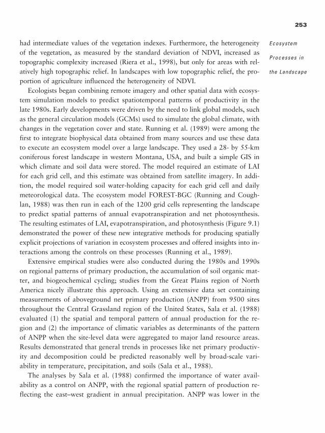
had intermediate values of the vegetation indexes. Furthermore, the heterogeneityof the vegetation, as measured by the standard deviation of NDVI, increased astopographic complexity increased (Riera et al., 1998), but only for areas with rel-atively high topographic relief. In landscapes with low topographic relief, the pro-portion of agriculture influenced the heterogeneity of NDVI.

Ecologists began combining remote imagery and other spatial data with ecosys-tem simulation models to predict spatiotemporal patterns of productivity in thelate 1980s. Early developments were driven by the need to link global models, suchas the general circulation models (GCMs) used to simulate the global climate, withchanges in the vegetation cover and state. Running et al. (1989) were among thefirst to integrate biophysical data obtained from many sources and use these datato execute an ecosystem model over a large landscape. They used a 28- by 55-kmconiferous forest landscape in western Montana, USA, and built a simple GIS inwhich climate and soil data were stored. The model required an estimate of LAIfor each grid cell, and this estimate was obtained from satellite imagery. In addi-tion, the model required soil water-holding capacity for each grid cell and dailymeteorological data. The ecosystem model FOREST-BGC (Running and Cough-lan, 1988) was then run in each of the 1200 grid cells representing the landscapeto predict spatial patterns of annual evapotranspiration and net photosynthesis.The resulting estimates of LAI, evapotranspiration, and photosynthesis (Figure 9.1)demonstrated the power of these new integrative methods for producing spatiallyexplicit projections of variation in ecosystem processes and offered insights into in-teractions among the controls on these processes (Running et al., 1989).

Extensive empirical studies were also conducted during the 1980s and 1990son regional patterns of primary production, the accumulation of soil organic mat-ter, and biogeochemical cycling; studies from the Great Plains region of NorthAmerica nicely illustrate this approach. Using an extensive data set containingmeasurements of aboveground net primary production (ANPP) from 9500 sitesthroughout the Central Grassland region of the United States, Sala et al. (1988)evaluated (1) the spatial and temporal pattern of annual production for the re-gion and (2) the importance of climatic variables as determinants of the patternof ANPP when the site-level data were aggregated to major land resource areas.Results demonstrated that general trends in processes like net primary productiv-ity and decomposition could be predicted reasonably well by broad-scale vari-ability in temperature, precipitation, and soils (Sala et al., 1988).

The analyses by Sala et al. (1988) confirmed the importance of water avail-ability as a control on ANPP, with the regional spatial pattern of production re-flecting the east–west gradient in annual precipitation. ANPP was lower in the

253

Ecosystem

Processes in

the Landscape

2888_e09_p249-288 2/27/01 1:56 PM Page 253

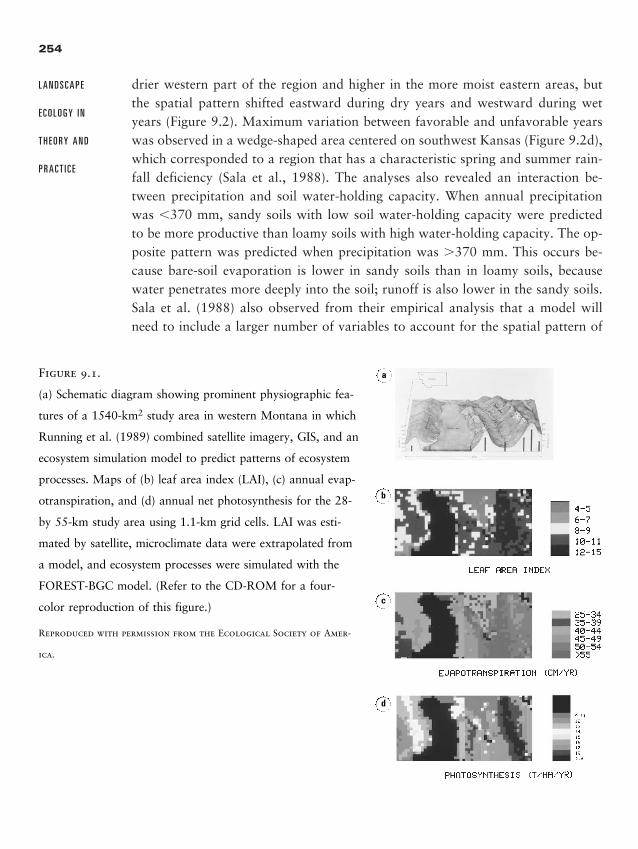
drier western part of the region and higher in the more moist eastern areas, butthe spatial pattern shifted eastward during dry years and westward during wetyears (Figure 9.2). Maximum variation between favorable and unfavorable yearswas observed in a wedge-shaped area centered on southwest Kansas (Figure 9.2d),which corresponded to a region that has a characteristic spring and summer rain-fall deficiency (Sala et al., 1988). The analyses also revealed an interaction be-tween precipitation and soil water-holding capacity. When annual precipitationwas �370 mm, sandy soils with low soil water-holding capacity were predictedto be more productive than loamy soils with high water-holding capacity. The op-posite pattern was predicted when precipitation was �370 mm. This occurs be-cause bare-soil evaporation is lower in sandy soils than in loamy soils, becausewater penetrates more deeply into the soil; runoff is also lower in the sandy soils.Sala et al. (1988) also observed from their empirical analysis that a model willneed to include a larger number of variables to account for the spatial pattern of

254

L A N D S C A P E

E C O L O G Y I N

T H E O R Y A N D

P R A C T I C E

Figure 9.1.

(a) Schematic diagram showing prominent physiographic fea-

tures of a 1540-km2 study area in western Montana in which

Running et al. (1989) combined satellite imagery, GIS, and an

ecosystem simulation model to predict patterns of ecosystem

processes. Maps of (b) leaf area index (LAI), (c) annual evap-

otranspiration, and (d) annual net photosynthesis for the 28-

by 55-km study area using 1.1-km grid cells. LAI was esti-

mated by satellite, microclimate data were extrapolated from

a model, and ecosystem processes were simulated with the

FOREST-BGC model. (Refer to the CD-ROM for a four-

color reproduction of this figure.)

Reproduced with permission from the Ecological Society of Amer-

ica.

a

b

c

d

2888_e09_p249-288 2/27/01 1:56 PM Page 254

the same process as the scale of analysis becomes finer. The pattern of the processat the coarse scale constrained the pattern at the finer scale; thus, variability atthe finer scale will be accounted for by factors at that scale plus the factors thatdetermine the pattern at the coarse scale.

Spatial variation in soil organic matter and carbon has also been studied in theGreat Plains region, where the accumulation of organic matter in soils dependson temperature, moisture, soil texture, and plant lignin content (Parton et al.,1987). Lignin is a structural compound that is difficult for most microbes to de-compose, and thus plant tissues with higher lignin content tend to decomposemore slowly. Across the dry landscape of the Great Plains, soil carbon increasesfrom southwest to northeast and, additionally, is greater on fine-textured soilsthan on sandy soils. General patterns across the landscape are reasonably wellknown, but additional variables like plant species composition, past land use, and

255

Ecosystem

Processes in

the Landscape

150

150

200

200

300

300

400

400

500

500

600

600

0.5 0.3

0.7

0.9

0.9

0.7 0.5

0.3

200

200

300

300

400

400

500

500

600 700

600

700

100

100

200

200

300

300

400

400

500

500

a b

c d

Figure 9.2.

Isopleths of aboveground net primary pro-

duction (ANPP, g/m2) for the Central

Grassland region of the United States (a)

during years of average precipition, (b)

during relatively dry years, and (c) during

relatively wet years. (d) Isopleths show the

relative variability in production between

favoral and unfavorable years, estimated

as (ANPPwet � ANPPdry)/ANPPaverage.

Adapted from Sala et al., 1988.

2888_e09_p249-288 2/27/01 1:56 PM Page 255

landscape position are required to predict ecosystem processes at finer scales. Amore recent study conducted in agroecosystems illustrates some of these patterns.

Burke et al. (1995) studied the patterns of soil organic matter (SOM), micro-bial biomass, and the availability of carbon (C) and nitrogen (N) in soils in twogeographic locations, then at different landscape positions (at the bottom, or toe,of a slope; on a slope; or at the top of a ridge), and under different types of landmanagement. They found that these indicators of ecosystem functioning (SOM,microbial biomass, and soil C and N) were highest at the more northern of twostudy sites in eastern Colorado, and at toeslope landscape positions, the bases ofslopes where materials tend to accumulate. The geographic differences betweensites reflected broad-scale influences of temperature and soil texture on the accu-mulation of organic matter; the northern site had cooler temperatures and finersoils. The effects of landscape position reflected the long-term transport of fineorganic matter downslope, as well as gradients in available moisture and pro-duction. Ridgetops tend to be exposed and dry, toeslopes more sheltered and moist.Thus, there are natural gradients in soil organic matter and nutrient supply ca-pacity across the landscape. Nutrient fluxes by litter redistribution can also be ex-tensive in other landscapes. For example, redistribution of leaf litter in a topo-graphically and edaphically complex landscape on the Allegheny Plateau in Ohiowas found to be substantial, with some landscape positions (e.g., ridgetops andupper slopes) serving as a net source of litter and others (side and lower slopes)serving as a net sink (Boerner and Kooser, 1989).

While abiotic gradients exert a powerful influence, rates and spatial patternsof NPP can also vary with changes in land use and with natural disturbances. Ex-amining land-use changes and NPP in Georgia, USA, Turner (1987c) found anoverall increase in annual NPP from 2.5 to 6.4 tonnes/ha from 1935 to 1982.These changes were associated with a period of widespread abandonment of crop-lands, followed by natural succession to pine and increased urbanization in someareas. Production of croplands varied widely among physiographic regions in thestate. Low NPP through the 1960s reflected persistent effects of poor agriculturalpractices that had caused the fertility of the land to decline; in the piedmont re-gion, nearly all the topsoil had been lost from nearly half of the land area. HigherNPP after the 1960s was due, in part, to improvements in agriculture and silvi-culture, as well as large increases in irrigated area and inputs of nitrogen fertiliz-ers. By 1982, the average NPP of forests in Georgia was 8.3 tonnes/ha, approxi-mately two-thirds of the predicted natural rate.

Spatial and temporal variation in NPP has important implications for regionaland global patterns of carbon dynamics. Secondary forests in regions that expe-

256

L A N D S C A P E

E C O L O G Y I N

T H E O R Y A N D

P R A C T I C E

2888_e09_p249-288 2/27/01 1:56 PM Page 256

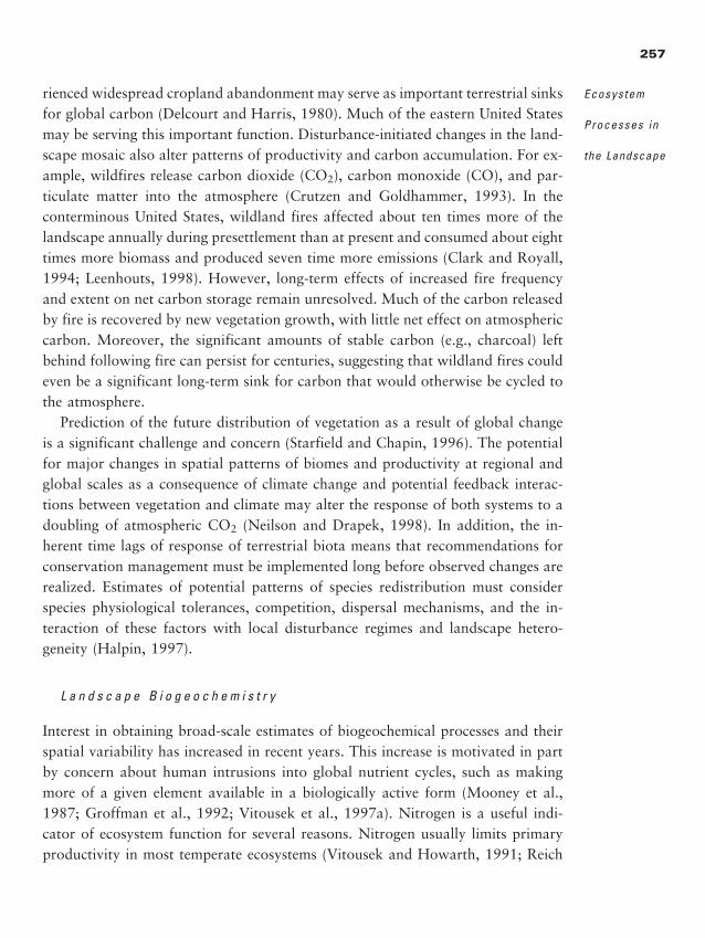
rienced widespread cropland abandonment may serve as important terrestrial sinksfor global carbon (Delcourt and Harris, 1980). Much of the eastern United Statesmay be serving this important function. Disturbance-initiated changes in the land-scape mosaic also alter patterns of productivity and carbon accumulation. For ex-ample, wildfires release carbon dioxide (CO2), carbon monoxide (CO), and par-ticulate matter into the atmosphere (Crutzen and Goldhammer, 1993). In theconterminous United States, wildland fires affected about ten times more of thelandscape annually during presettlement than at present and consumed about eighttimes more biomass and produced seven time more emissions (Clark and Royall,1994; Leenhouts, 1998). However, long-term effects of increased fire frequencyand extent on net carbon storage remain unresolved. Much of the carbon releasedby fire is recovered by new vegetation growth, with little net effect on atmosphericcarbon. Moreover, the significant amounts of stable carbon (e.g., charcoal) leftbehind following fire can persist for centuries, suggesting that wildland fires couldeven be a significant long-term sink for carbon that would otherwise be cycled tothe atmosphere.

Prediction of the future distribution of vegetation as a result of global changeis a significant challenge and concern (Starfield and Chapin, 1996). The potentialfor major changes in spatial patterns of biomes and productivity at regional andglobal scales as a consequence of climate change and potential feedback interac-tions between vegetation and climate may alter the response of both systems to adoubling of atmospheric CO2 (Neilson and Drapek, 1998). In addition, the in-herent time lags of response of terrestrial biota means that recommendations forconservation management must be implemented long before observed changes arerealized. Estimates of potential patterns of species redistribution must considerspecies physiological tolerances, competition, dispersal mechanisms, and the in-teraction of these factors with local disturbance regimes and landscape hetero-geneity (Halpin, 1997).

L a n d s c a p e B i o g e o c h e m i s t r y

Interest in obtaining broad-scale estimates of biogeochemical processes and theirspatial variability has increased in recent years. This increase is motivated in partby concern about human intrusions into global nutrient cycles, such as makingmore of a given element available in a biologically active form (Mooney et al.,1987; Groffman et al., 1992; Vitousek et al., 1997a). Nitrogen is a useful indi-cator of ecosystem function for several reasons. Nitrogen usually limits primaryproductivity in most temperate ecosystems (Vitousek and Howarth, 1991; Reich

257

Ecosystem

Processes in

the Landscape

2888_e09_p249-288 2/27/01 1:56 PM Page 257

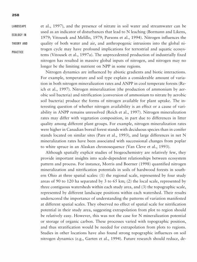
et al., 1997), and the presence of nitrate in soil water and streamwater can beused as an indicator of disturbances that lead to N leaching (Bormann and Likens,1979; Vitousek and Melillo, 1979; Parsons et al., 1994). Nitrogen influences thequality of both water and air, and anthropogenic intrusions into the global ni-trogen cycle may have profound implications for terrestrial and aquatic ecosys-tems (Vitousek et al., 1997a). The unprecedented production of industrially fixednitrogen has resulted in massive global inputs of nitrogen, and nitrogen may nolonger be the limiting nutrient on NPP in some regions.

Nitrogen dynamics are influenced by abiotic gradients and biotic interactions.For example, temperature and soil type explain a considerable amount of varia-tion in both nitrogen mineralization rates and ANPP in cool temperate forests (Re-ich et al., 1997). Nitrogen mineralization (the production of ammonium by aer-obic soil bacteria) and nitrification (conversion of ammonium to nitrate by aerobicsoil bacteria) produce the forms of nitrogen available for plant uptake. The in-teresting question of whether nitrogen availability is an effect or a cause of vari-ability in ANPP remains unresolved (Reich et al., 1997). Nitrogen mineralizationrates may differ with vegetation composition, in part due to differences in litterquality among different plant groups. For example, nitrogen mineralization rateswere higher in Canadian boreal forest stands with deciduous species than in coniferstands located on similar sites (Pare et al., 1993), and large differences in net Nmineralization rates have been associated with successional changes from poplarto white spruce in an Alaskan chronosequence (Van Cleve et al., 1993).

Although spatially explicit studies of biogeochemistry are relatively few, theyprovide important insights into scale-dependent relationships between ecosystempattern and process. For instance, Morris and Boerner (1998) quantified nitrogenmineralization and nitrification potentials in soils of hardwood forests in south-ern Ohio at three spatial scales: (1) the regional scale, represented by four studyareas of 90 to 120 ha separated by 3 to 65 km; (2) the local scale, represented bythree contiguous watersheds within each study area, and (3) the topographic scale,represented by different landscape positions within each watershed. Their resultsunderscored the importance of understanding the patterns of variation manifestedat different spatial scales. They observed no effect of spatial scale for nitrificationpotential in their study area, suggesting extrapolation from plot to region shouldbe relatively easy. However, this was not the case for N mineralization potentialor storage of organic carbon. These processes varied with topographic position,and thus stratification would be needed for extrapolation from plots to regions.Studies in other locations have also found strong topographic influences on soilnitrogen dynamics (e.g., Garten et al., 1994). Future research should reduce, de-

258

L A N D S C A P E

E C O L O G Y I N

T H E O R Y A N D

P R A C T I C E

2888_e09_p249-288 2/27/01 1:56 PM Page 258

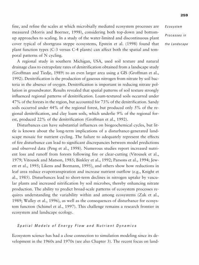
fine, and refine the scales at which microbially mediated ecosystem processes aremeasured (Morris and Boerner, 1998), considering both top-down and bottom-up approaches to scaling. In a study of the water-limited and discontinuous plantcover typical of shortgrass steppe ecosystems, Epstein et al. (1998) found thatplant function types (C-3 versus C-4 plants) can affect both the spatial and tem-poral patterns of N cycling.

A regional study in southern Michigan, USA, used soil texture and naturaldrainage class to extrapolate rates of denitrification obtained from a landscape study(Groffman and Tiedje, 1989) to an even larger area using a GIS (Groffman et al.,1992). Denitrification is the production of gaseous nitrogen from nitrate by soil bac-teria in the absence of oxygen. Denitrification is important in reducing nitrate pol-lution in groundwater. Results revealed that spatial patterns of soil texture stronglyinfluenced regional patterns of denitrification. Loam-textured soils occurred under47% of the forests in the region, but accounted for 73% of the denitrification. Sandysoils occurred under 44% of the regional forest, but produced only 5% of the re-gional denitrification, and clay loam soils, which underlie 9% of the regional for-est, produced 22% of the denitrification (Groffman et al., 1992).

Disturbances can have substantial influences on biogeochemical cycles, but lit-tle is known about the long-term implications of a disturbance-generated land-scape mosaic for nutrient cycling. The failure to adequately represent the effectsof fire disturbance can lead to significant discrepancies between model predictionsand observed data (Peng et al., 1998). Numerous studies report increased nutri-ent loss and runoff from forests following fire or clear-cutting (Vitousek et al.,1979; Vitousek and Matson, 1985; Binkley et al., 1992; Parsons et al., 1994; Jew-ett et al., 1995; Likens and Bormann, 1995), and others show how reductions inleaf area reduce evapotranspiration and increase nutrient outflow (e.g., Knight etal., 1985). Disturbances lead to short-term declines in nitrogen uptake by vascu-lar plants and increased nitrification by soil microbes, thereby enhancing nitrateproduction. The ability to predict broad-scale patterns of ecosystem processes re-quires understanding the variability within and among ecosystems (Zak et al.,1989; Walley et al., 1996), as well as the consequences of disturbance for ecosys-tem function (Schimel et al., 1997). This challenge remains a research frontier inecosystem and landscape ecology.

S p a t i a l M o d e l s o f E n e r g y F l o w a n d N u t r i e n t D y n a m i c s

Ecosystem science has had a close connection to simulation modeling since its de-velopment in the 1960s and 1970s (see also Chapter 3). The recent focus on land-

259

Ecosystem

Processes in

the Landscape

2888_e09_p249-288 2/27/01 1:56 PM Page 259

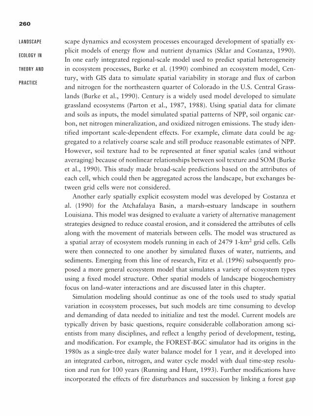
scape dynamics and ecosystem processes encouraged development of spatially ex-plicit models of energy flow and nutrient dynamics (Sklar and Costanza, 1990).In one early integrated regional-scale model used to predict spatial heterogeneityin ecosystem processes, Burke et al. (1990) combined an ecosystem model, Cen-tury, with GIS data to simulate spatial variability in storage and flux of carbonand nitrogen for the northeastern quarter of Colorado in the U.S. Central Grass-lands (Burke et al., 1990). Century is a widely used model developed to simulategrassland ecosystems (Parton et al., 1987, 1988). Using spatial data for climateand soils as inputs, the model simulated spatial patterns of NPP, soil organic car-bon, net nitrogen mineralization, and oxidized nitrogen emissions. The study iden-tified important scale-dependent effects. For example, climate data could be ag-gregated to a relatively coarse scale and still produce reasonable estimates of NPP.However, soil texture had to be represented at finer spatial scales (and withoutaveraging) because of nonlinear relationships between soil texture and SOM (Burkeet al., 1990). This study made broad-scale predictions based on the attributes ofeach cell, which could then be aggregated across the landscape, but exchanges be-tween grid cells were not considered.

Another early spatially explicit ecosystem model was developed by Costanza etal. (1990) for the Atchafalaya Basin, a marsh–estuary landscape in southernLouisiana. This model was designed to evaluate a variety of alternative managementstrategies designed to reduce coastal erosion, and it considered the attributes of cellsalong with the movement of materials between cells. The model was structured asa spatial array of ecosystem models running in each of 2479 1-km2 grid cells. Cellswere then connected to one another by simulated fluxes of water, nutrients, andsediments. Emerging from this line of research, Fitz et al. (1996) subsequently pro-posed a more general ecosystem model that simulates a variety of ecosystem typesusing a fixed model structure. Other spatial models of landscape biogeochemistryfocus on land–water interactions and are discussed later in this chapter.

Simulation modeling should continue as one of the tools used to study spatialvariation in ecosystem processes, but such models are time consuming to developand demanding of data needed to initialize and test the model. Current models aretypically driven by basic questions, require considerable collaboration among sci-entists from many disciplines, and reflect a lengthy period of development, testing,and modification. For example, the FOREST-BGC simulator had its origins in the1980s as a single-tree daily water balance model for 1 year, and it developed intoan integrated carbon, nitrogen, and water cycle model with dual time-step resolu-tion and run for 100 years (Running and Hunt, 1993). Further modifications haveincorporated the effects of fire disturbances and succession by linking a forest gap

260

L A N D S C A P E

E C O L O G Y I N

T H E O R Y A N D

P R A C T I C E

2888_e09_p249-288 2/27/01 1:56 PM Page 260

model with BGC (FIRE-BGC, Keane et al., 1996a, b). The spatial FOREST-BGCmodel that predicts photosynthesis, respiration, evapotranspiration, decomposition,and nitrogen mineralization over broad landscapes is then used to calibrate simplemodels for implementation at the global scale (Hunt et al., 1991; Running, 1994).The calibration of simple ecosystem models for use on larger spatial and temporalscales also offers a powerful approach for scaling (Running and Hunt, 1993) thatremains a topic of active research. The suggestion first made by Overton (1975) touse multiscale models that contain submodels operating at different scales and de-grees of complexity now promises new insight into simulating ecosystem patternand process (e.g., DeAngelis et al., 1998, discussed later in this chapter).

S y n t h e s i s

Empirical and modeling studies of the spatial heterogeneity in ecosystem processeshave demonstrated several important points. First, spatial variations in abioticvariables (temperature, precipitation, soils, and topographic position) often pro-duce substantial spatial variation in ecosystem processes. Thus, as ecosystem ecol-ogists have long recognized, the abiotic template is a powerful constraint on ecosys-tem function. Second, abiotic factors vary over multiple spatial scales, andecologists are still striving to determine the scales that are appropriate for devel-oping predictive relationships. Considering these factors hierarchically may en-hance our understanding of how they vary. Third, understanding the implicationsof the dynamic landscape mosaic for ecosystem processes remains a frontier inecosystem and landscape ecology. We simply do not have a well-developed the-ory of ecosystem function that is spatially explicit, nor do we have a wealth ofempirical studies from which to infer general conclusions.

E F F E C T S O F L A N D S C A P E P O S I T I O N O N L A K E E C O S Y S T E M S

Our focus on the spatial variability in ecosystem processes has, thus far, empha-sized processes in terrestrial systems. However, spatial variability is also observedin the aquatic systems embedded in landscapes. Limnologists have long consid-ered lakes as discrete units of study, owing in part to the natural boundary of thelake shoreline (Forbes, 1887). Understanding the spatial patterns within individ-ual lakes (e.g., patterns and processes in stratified lakes) occupied early limnolo-

261

Ecosystem

Processes in

the Landscape

�

2888_e09_p249-288 2/27/01 1:56 PM Page 261

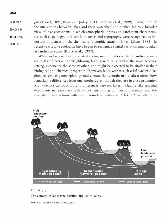
gists (Forel, 1892; Birge and Juday, 1911; Soranno et al., 1999). Recognition ofthe interactions between lakes and their watershed and airshed led to a broaderview of lake ecosystems in which atmospheric inputs and catchment characteris-tics such as geology, land use–land cover, and topography were recognized as im-portant influences on the chemical and trophic status of lakes (Likens, 1985). Inrecent years, lake ecologists have begun to recognize spatial variation among lakesat landscape scales (Kratz et al., 1997).

When and where does the spatial arrangement of lakes within a landscape mat-ter to lake functioning? Neighboring lakes generally lie within the same geologicsetting, experience the same weather, and might be expected to be similar in theirbiological and chemical properties. However, lakes within such a lake district (re-gions of similar geomorphology and climate that contain many lakes) often showremarkable differences from one another, even though they are in close proximity.Many factors can contribute to differences between lakes, including lake size anddepth, internal processes such as nutrient cycling or trophic dynamics, and thestrength of interactions with the surrounding landscape. A lake’s landscape posi-

262

L A N D S C A P E

E C O L O G Y I N

T H E O R Y A N D

P R A C T I C E

HydraulicallyMounded Lakes

Groundwater flowWater table Surface water flow

Lowlandscape position

Highlandscape position

GroundwaterFlowthrough Lakes

DrainageLakes

Figure 9.3.

The concept of landscape position applied to lakes.

Modified from Webster et al., 1996.

2888_e09_p249-288 2/27/01 1:56 PM Page 262

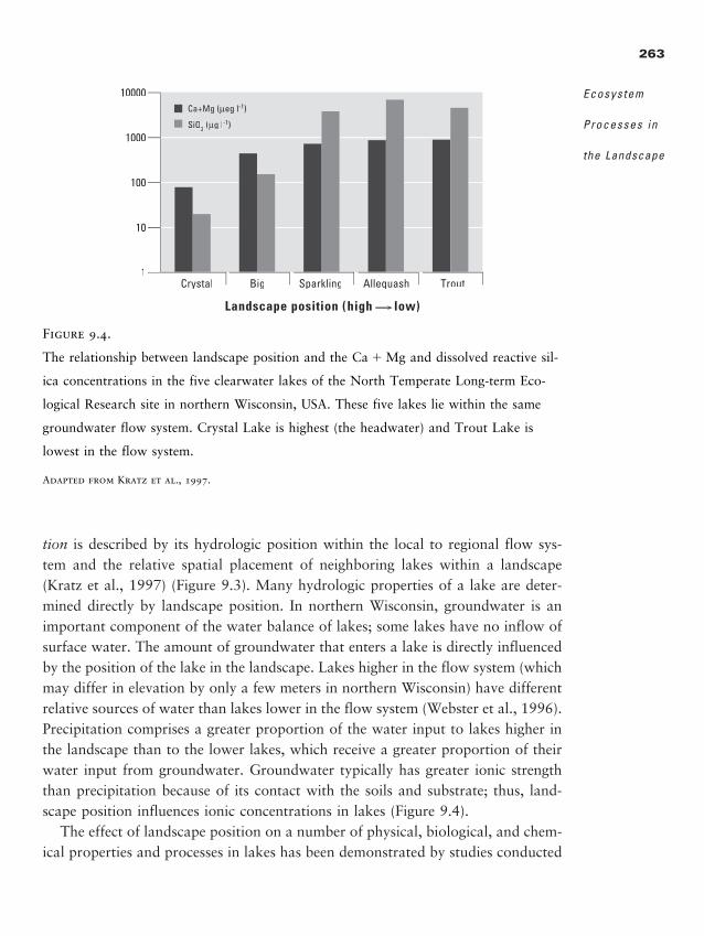
263

Ecosystem

Processes in

the Landscape

tion is described by its hydrologic position within the local to regional flow sys-tem and the relative spatial placement of neighboring lakes within a landscape(Kratz et al., 1997) (Figure 9.3). Many hydrologic properties of a lake are deter-mined directly by landscape position. In northern Wisconsin, groundwater is animportant component of the water balance of lakes; some lakes have no inflow ofsurface water. The amount of groundwater that enters a lake is directly influencedby the position of the lake in the landscape. Lakes higher in the flow system (whichmay differ in elevation by only a few meters in northern Wisconsin) have differentrelative sources of water than lakes lower in the flow system (Webster et al., 1996).Precipitation comprises a greater proportion of the water input to lakes higher inthe landscape than to the lower lakes, which receive a greater proportion of theirwater input from groundwater. Groundwater typically has greater ionic strengththan precipitation because of its contact with the soils and substrate; thus, land-scape position influences ionic concentrations in lakes (Figure 9.4).

The effect of landscape position on a number of physical, biological, and chem-ical properties and processes in lakes has been demonstrated by studies conducted

Landscape position (high low)

Crystal

µeg l-1)

SiO2 ( g l-1)

Big Sparkling Allequash Trout

10

100

1000

10000

1

Figure 9.4.

The relationship between landscape position and the Ca � Mg and dissolved reactive sil-

ica concentrations in the five clearwater lakes of the North Temperate Long-term Eco-

logical Research site in northern Wisconsin, USA. These five lakes lie within the same

groundwater flow system. Crystal Lake is highest (the headwater) and Trout Lake is

lowest in the flow system.

Adapted from Kratz et al., 1997.

2888_e09_p249-288 2/27/01 1:56 PM Page 263

in the Northern Highlands Lake District of northern Wisconsin, an area contain-ing about 2500 lakes (Magnuson and Kratz, in press). The response of lake chem-istry to drought differs by lake position (Webster et al., 1996). There is a com-mon tendency for lakes to increase in cation concentration during drought periodsbecause chemical concentrations increase as water evaporates. However, lakes lowin the landscape tended to increase in the total mass of cations in the lake, whereaslakes high in the landscape tended to have no change in mass, or even a decreasein cation mass in the lake (Webster et al., 1996). Changes in cation concentra-tions can also lead to changes in the biota; for example, crayfish and snails occuronly in lakes with adequate calcium, and a 10% increase or decrease in calciumconcentration would add or remove about 5% of the lakes above 4 ha in area ascrayfish and snail habitat (Kratz et al., 1997). Silica concentrations, which varywith landscape position and are much higher in lakes with more groundwater in-put, may influence the robustness of freshwater sponges in the littoral zone oflakes and, in turn, influence the rest of the littoral zone food web.

Landscape processes that influence the amount of dissolved organic carbon(DOC) entering a lake can affect the magnitude and vertical distribution of pri-mary production within the lake. Lakes with high concentrations of DOC tend tobe tea colored, and the brown color reduces the clarity of the water and hencethe light penetration. Colored DOC is derived mainly from the soils or wetlandsin the landscape surrounding a lake. Therefore, the position of the lake relativeto sources of allochthonous (from external sources) DOC inputs can influence netprimary productivity within the lake (Kratz et al., 1997; Gergel et al., 1999).

An extensive analysis of 556 lakes in northern Wisconsin demonstrated thatlandscape position explained a significant fraction of the variance in 21 of 25 vari-ables tested (Riera et al., 2000). Variables most strongly related to landscape po-sition were measures of lake size and shape, concentrations of major ions (exceptfor sulfate) and silica, biological variables (chlorophyll concentration, crayfishabundance, and fish species richness), and human variables (density of cottages).Lake depth, water optical properties, and concentrations of nutrients other thansilica were poorly explained by lake order (Riera et al., 2000).

Recent work has extended these analysis to other lake districts. Soranno et al.(1999) analyzed long-term data from nine lake chains (lakes in a series, connectedthrough surface or groundwater flow) from seven lake districts of diverse hydro-geomorphic setting in North America. The study asked (1) if there were predictablespatial patterns in chemical, algal, and water quality variables along lake chainsand (2) if lakes that are closer together in a chain behave more similarly throughtime. Results indicated that spatial and temporal patterns of lakes within a lake

264

L A N D S C A P E

E C O L O G Y I N

T H E O R Y A N D

P R A C T I C E

2888_e09_p249-288 2/27/01 1:56 PM Page 264

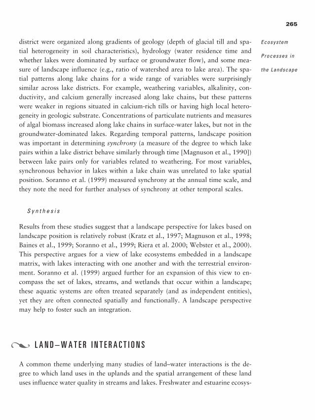
district were organized along gradients of geology (depth of glacial till and spa-tial heterogeneity in soil characteristics), hydrology (water residence time andwhether lakes were dominated by surface or groundwater flow), and some mea-sure of landscape influence (e.g., ratio of watershed area to lake area). The spa-tial patterns along lake chains for a wide range of variables were surprisingly similar across lake districts. For example, weathering variables, alkalinity, con-ductivity, and calcium generally increased along lake chains, but these patternswere weaker in regions situated in calcium-rich tills or having high local hetero-geneity in geologic substrate. Concentrations of particulate nutrients and measuresof algal biomass increased along lake chains in surface-water lakes, but not in thegroundwater-dominated lakes. Regarding temporal patterns, landscape positionwas important in determining synchrony (a measure of the degree to which lakepairs within a lake district behave similarly through time [Magnuson et al., 1990])between lake pairs only for variables related to weathering. For most variables,synchronous behavior in lakes within a lake chain was unrelated to lake spatialposition. Soranno et al. (1999) measured synchrony at the annual time scale, andthey note the need for further analyses of synchrony at other temporal scales.

S y n t h e s i s

Results from these studies suggest that a landscape perspective for lakes based onlandscape position is relatively robust (Kratz et al., 1997; Magnuson et al., 1998;Baines et al., 1999; Soranno et al., 1999; Riera et al. 2000; Webster et al., 2000).This perspective argues for a view of lake ecosystems embedded in a landscapematrix, with lakes interacting with one another and with the terrestrial environ-ment. Soranno et al. (1999) argued further for an expansion of this view to en-compass the set of lakes, streams, and wetlands that occur within a landscape;these aquatic systems are often treated separately (and as independent entities),yet they are often connected spatially and functionally. A landscape perspectivemay help to foster such an integration.

L A N D – W A T E R I N T E R A C T I O N S

A common theme underlying many studies of land–water interactions is the de-gree to which land uses in the uplands and the spatial arrangement of these landuses influence water quality in streams and lakes. Freshwater and estuarine ecosys-

265

Ecosystem

Processes in

the Landscape

�

2888_e09_p249-288 2/27/01 1:56 PM Page 265

tems act as integrators and centers of organization within the landscape, touch-ing nearly all aspects of the natural environment and human culture (Correll etal., 1992; Boynton et al., 1995; Naiman et al., 1995; Naiman, 1996). Hynes,widely regarded as the father of modern stream ecology, stated, “We must not di-vorce the stream from its valley in our thoughts at any time. If we do, we losetouch with reality” (Hynes, 1975). As demonstrated by the effect of landscape po-sition on lake characteristics, land–water interactions are apparent even in rela-tively undisturbed landscapes. In another example, studies along a toposequenceof tundra, sedge, and shrub communities along a slope in Alaska have revealedthe importance of ecosystem adjacencies to nutrient transformation and move-ment. Shaver et al. (1991) addressed the question of how heterogeneity amongecosystems influenced the outputs of nutrients into surface waters in an undis-turbed tundra landscape (Figure 9.5). The entire sequence of community types oc-curred along a few hundred meters, but large differences were observed in therates of plant uptake, mineralization, and transport between ecosystems.

Improving our understanding of the complex relationships between the landand water is an important goal of both basic and applied research in landscapeecology. Freshwaters are degraded by increasing inputs of silt, nutrients, and pol-lutants from agriculture, forest harvest, and cities (Carpenter et al., 1995, 1998).Consider a watershed containing croplands or pastures. Farmers often apply fer-

266

L A N D S C A P E

E C O L O G Y I N

T H E O R Y A N D

P R A C T I C E

Figure 9.5.

(a) Toposequence studied by Shaver et al. (1991) in the Sagavanirktok River valley in northern Alaska.

Six ecosystem types extend from the uplands down to a series of floodplain terraces and to the river. The

entire toposequence is underlain by permafrost, and soil water flows downslope over the permafrost dur-

ing summer. Total vertical drop is �10 m, and horizontal distance ranges from 100 to 200 m. (b) Con-

ceptual model of element cycling along the toposequence at the study site. The sequence is viewed in one

dimension as a series of individual square meters linked by element transport in soil water. (c) The

processes represented within and between cells. In each square meter, there may be internal recycling of

elements by plant and soil (A and B), exchange between plants and soil through uptake or litterfall (C),

and exchange with the atmosphere through processes such as nitrogen fixation or denitrification (D). Ele-

ments may also be weathered from parent materials (E). Transport of elements downslope in soil water is

indicated by (F).

Adapted from Shaver et al., 1991.

2888_e09_p249-288 2/27/01 1:56 PM Page 266

tilizers high in nitrogen and phosphorus (P) to their fields, but not all the addedN and P is taken up by the plants. When it rains, some of these nutrients areleached from the soil and transported through the watershed and into the streamby both surface and subsurface water flow. Like agricultural areas, cities and sub-urbs are important contributors to such nonpoint source pollution, that is, pollutionthat does not come from a single source, like a pipe, but rather is delivered from

267

Ecosystem

Processes in

the Landscape

Water table Permafrost

Wet sedge tundra

Footslopeequisetum

Hillslopeshrub–lupine

Hilltop heath

Tussock tundra

Riverside willow

?

Plants

Soils

D

AC

E

F

B

Ecosystem1

Ecosystem2

(x meters wide)

Ecosystem3

(y meters wide)

Ecosystem4

12

x

12

y

x - 1

y - 1

a

b c

2888_e09_p249-288 2/27/01 1:56 PM Page 267

widespread areas of the landscape. Homeowners often apply as much fertilizer andpesticides per unit area to their lawns as farmers do to their crop fields, and a por-tion of these nutrients ends up in nearby aquatic systems. Lakes and reservoirs fillmore rapidly with mud from agricultural and urban land uses, and the growth ofnuisance plants, including toxic blue-green algae, is promoted by the increased siltand nutrients. Regional changes in land use cause widespread eutrophication of manylakes on the landscape. Eutrophication makes lakes more similar, because the lakesare all dominated by the same set of species that can tolerate eutrophic conditions.Therefore, the diversity of lake types within a landscape is reduced as all lakes be-come eutrophic and converge to have similar species (Carpenter et al., 1995).

The nutrients most often considered in studies of land–water interactions are ni-trogen and phosphorus. Economic and health concerns about excess nitrogen inputsinto aquatic ecosystems are growing throughout the world (e.g., Cole et al., 1993;Mueller and Helsel, 1996; Vitousek et al., 1997a). In rivers, nitrogen biogeochem-istry is sensitive to land-use patterns, the structure of the riparian zone, and riverflow regimes (Cirmo and McDonnell, 1997). Accumulation of excess phosphorus inlake and stream systems has long been recognized as a driver of eutrophication (e.g.,Carpenter et al., 1998). However, understanding the effects of land-use patterns onwater quality and the spatial scales over which these effects are manifest has becomean important goal of landscape ecological studies, particularly since the mid 1980s.

Osborne and Wiley (1988) analyzed the nitrogen and phosphorus concentra-tion of streams in the Salt River Basin, Illinois, and used regression analysis to de-termine whether there was a relationship to land-use patterns mapped from aer-ial photos. Results demonstrated that the amount of urban land cover and itsdistance from the stream were the most important variables in predicting nutri-ent concentrations in the stream water. In the Saginaw River, Michigan, water-shed, 62 catchments were studied to relate seasonal stream-water chemistry tolandscape characteristics (Johnson et al., 1997). Results demonstrated a strong in-fluence of landscape characteristics, but the predictive power of particular vari-ables differed among seasons (Table 9.1). For example, land use and the interac-tion of land use and geology were the best predictors of variance in nitrogen duringsummer, but geology and the interaction between land use and geology were thebest predictors during autumn. Other studies have also found significant rela-tionships between land use and concentrations of nutrients in lakes and streams(e.g., Geier et al., 1994; Hunsaker and Levine, 1995; Johnes et al., 1996; Sorannoet al., 1996; Bolstad and Swank, 1997; Lowrance, 1998; Bennett et al., 1999).

Landscape patterns are also important in urban areas, as illustrated for Min-

268

L A N D S C A P E

E C O L O G Y I N

T H E O R Y A N D

P R A C T I C E

2888_e09_p249-288 2/27/01 1:56 PM Page 268

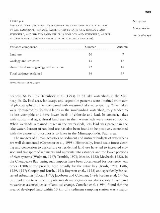
neapolis–St. Paul by Detenbeck et al. (1993). In 33 lake watersheds in the Min-neapolis–St. Paul area, landscape and vegetation patterns were obtained from aer-ial photographs and then compared with measured lake water quality. When lakeswere dominated by forested lands in the surrounding watershed, they tended tobe less eutrophic and have lower levels of chloride and lead. In contrast, lakeswith substantial agricultural land uses in their watersheds were more eutrophic.When wetlands remained intact in the watersheds, less lead was present in thelake water. Percent urban land use has also been found to be positively correlatedwith the export of phosphorus to lakes in the Minneapolis–St. Paul area.

The impacts of human activities on sediment and nutrient budgets of watershedsare well-documented (Carpenter et al., 1998). Historically, broad-scale forest clear-ing and conversion to agriculture or residential land use have led to increased ero-sion and transport of sediments and nutrients into estuaries and the lower portionsof river systems (Wolman, 1967; Trimble, 1974; Meade, 1982; Meybeck, 1982). Inthe Chesapeake Bay basin, such impacts have been documented for postsettlementtimes (1700s to the present) both broadly for the entire bay (Brush, 1984, 1986,1989, 1997; Cooper and Brush, 1991; Boynton et al., 1995) and specifically for se-lected tributaries (Costa, 1975; Jacobson and Coleman, 1986; Jordan et al, 1997a,b). In addition to sediment inputs, metals and organics are also exported from landto water as a consequence of land-use change. Comeleo et al. (1996) found that thearea of developed land within 10 km of a sediment sampling station was a major

269

Ecosystem

Processes in

the Landscape

Table 9.1.Percentage of variance in stream-water chemistry accounted for by all landscape factors, partitioned by land use, geology and structure, and shared land use plus geology and structure, as well as unexplained variance (based on redundancy analysis).

Variance component Summer Autumn

Land use 20 7

Geology and structure 15 17

Shared: land use � geology and structure 22 16

Total variance explained 56 39

From Johnson et al., 1997.

2888_e09_p249-288 2/27/01 1:56 PM Page 269

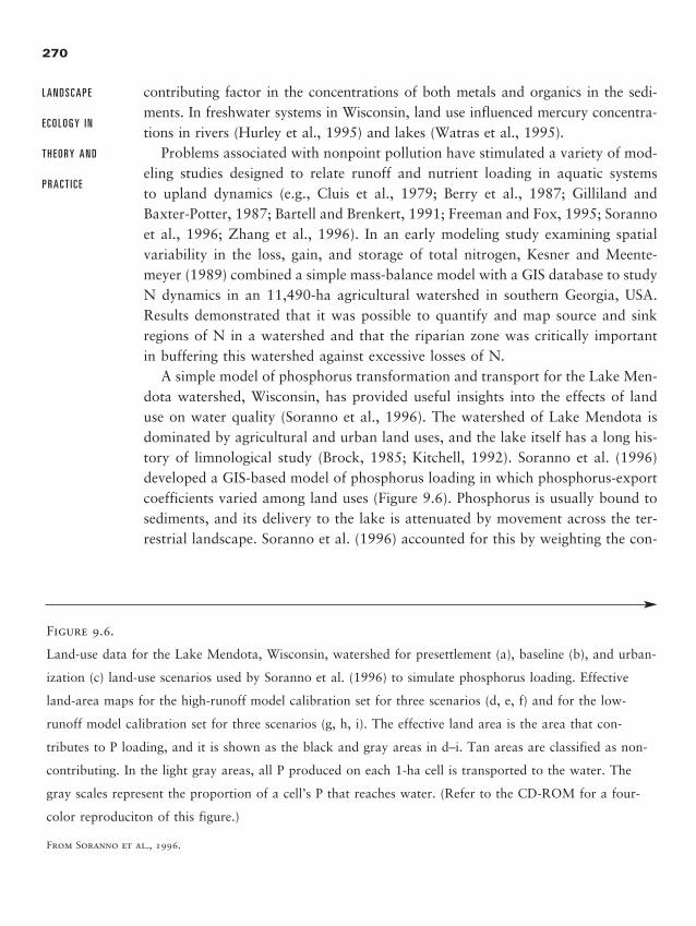
contributing factor in the concentrations of both metals and organics in the sedi-ments. In freshwater systems in Wisconsin, land use influenced mercury concentra-tions in rivers (Hurley et al., 1995) and lakes (Watras et al., 1995).

Problems associated with nonpoint pollution have stimulated a variety of mod-eling studies designed to relate runoff and nutrient loading in aquatic systems to upland dynamics (e.g., Cluis et al., 1979; Berry et al., 1987; Gilliland and Baxter-Potter, 1987; Bartell and Brenkert, 1991; Freeman and Fox, 1995; Sorannoet al., 1996; Zhang et al., 1996). In an early modeling study examining spatialvariability in the loss, gain, and storage of total nitrogen, Kesner and Meente-meyer (1989) combined a simple mass-balance model with a GIS database to studyN dynamics in an 11,490-ha agricultural watershed in southern Georgia, USA.Results demonstrated that it was possible to quantify and map source and sinkregions of N in a watershed and that the riparian zone was critically importantin buffering this watershed against excessive losses of N.

A simple model of phosphorus transformation and transport for the Lake Men-dota watershed, Wisconsin, has provided useful insights into the effects of landuse on water quality (Soranno et al., 1996). The watershed of Lake Mendota isdominated by agricultural and urban land uses, and the lake itself has a long his-tory of limnological study (Brock, 1985; Kitchell, 1992). Soranno et al. (1996)developed a GIS-based model of phosphorus loading in which phosphorus-exportcoefficients varied among land uses (Figure 9.6). Phosphorus is usually bound tosediments, and its delivery to the lake is attenuated by movement across the ter-restrial landscape. Soranno et al. (1996) accounted for this by weighting the con-

270

L A N D S C A P E

E C O L O G Y I N

T H E O R Y A N D

P R A C T I C E

Figure 9.6.

Land-use data for the Lake Mendota, Wisconsin, watershed for presettlement (a), baseline (b), and urban-

ization (c) land-use scenarios used by Soranno et al. (1996) to simulate phosphorus loading. Effective

land-area maps for the high-runoff model calibration set for three scenarios (d, e, f) and for the low-

runoff model calibration set for three scenarios (g, h, i). The effective land area is the area that con-

tributes to P loading, and it is shown as the black and gray areas in d–i. Tan areas are classified as non-

contributing. In the light gray areas, all P produced on each 1-ha cell is transported to the water. The

gray scales represent the proportion of a cell’s P that reaches water. (Refer to the CD-ROM for a four-

color reproduciton of this figure.)

From Soranno et al., 1996.

2888_e09_p249-288 2/27/01 1:56 PM Page 270

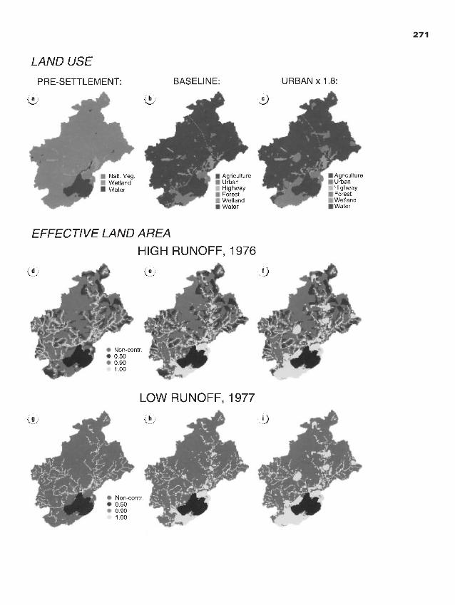
271

g h i

fed

a b c

2888_e09_p249-288 2/27/01 1:56 PM Page 271

tribution of phosphorus to the lake by a given grid cell by its distance from the lake.Because of the network of storm sewers serving the urban areas of Madison, Wis-consin, and surrounding communities, urban areas were treated as though they wereadjacent to streams. The model was then used to compare phosphorus loadings inLake Mendota under current patterns of land use, presettlement land use, and pro-jected future land use in which the urban area increased nearly twofold. Because rain-fall events drive runoff, simulations were conducted for both high- and low-precip-itation years. Results demonstrated that most of the watershed did not contributephosphorus loading to the lake; most P came from a relatively small proportion ofthe watershed, ranging from 17% of the watershed contributing during low-precip-itation years to 50% during high-precipitation years. A sixfold increase in phospho-rus loading was estimated to have occurred since settlement. Results also demon-strated the importance of riparian vegetation in attenuating phosphorus runoff.

R o l e o f R i p a r i a n B u f f e r s

Riparian vegetation zones, including wetlands and floodplain forests, are con-spicuous elements of many landscapes and important mediators of land–water in-teractions (Naiman and DeCamps, 1997). Freshwaters are especially sensitive tochanges in these adjacent lands (Correll et al., 1992, Osborne and Kovacic, 1993;Correll, 1997; Lowrance et al., 1997). Riparian buffers, areas of relatively undis-turbed vegetation along streams or adjacent to lakes, influence transport of nu-trients and sediments from upland agricultural–urban areas to aquatic ecosystems.Riparian vegetation and microbial communities can take up large amounts of wa-ter, sediment, and nutrients from surfacewater and groundwater draining agri-cultural areas within a catchment, often substantially reducing the discharges ofnutrients to aquatic ecosystems. The increased surface roughness created by veg-etation can also trap particles. Therefore, landscape ecologists have taken partic-ular interest in characterizing and understanding the function of patches or cor-ridors of riparian vegetation, because their functional importance is large relativeto their size.

Wetlands, floodplains, and riparian vegetation zones have often been alteredby agricultural and urban development (Turner et al., 1998a) (Figure 9.7). Woodyriparian vegetation once covered an estimated 30 to 40 million ha in the con-tiguous United States (Swift, 1974). At least two-thirds of that area has been con-verted to nonforest land uses, and only 10 to 14 million ha remained in the early1970s. Floodplain clearing for agriculture, urbanization, and water resource de-velopment has been responsible for much of the loss of riparian forests. Riparian

272

L A N D S C A P E

E C O L O G Y I N

T H E O R Y A N D

P R A C T I C E

2888_e09_p249-288 2/27/01 1:56 PM Page 272

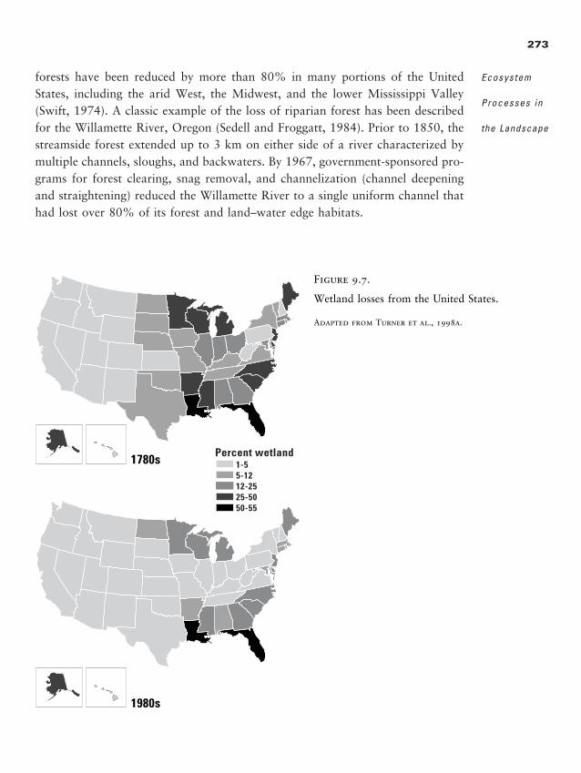
forests have been reduced by more than 80% in many portions of the UnitedStates, including the arid West, the Midwest, and the lower Mississippi Valley(Swift, 1974). A classic example of the loss of riparian forest has been describedfor the Willamette River, Oregon (Sedell and Froggatt, 1984). Prior to 1850, thestreamside forest extended up to 3 km on either side of a river characterized bymultiple channels, sloughs, and backwaters. By 1967, government-sponsored pro-grams for forest clearing, snag removal, and channelization (channel deepeningand straightening) reduced the Willamette River to a single uniform channel thathad lost over 80% of its forest and land–water edge habitats.

273

Ecosystem

Processes in

the Landscape

1780s

1980s

1-55-1212-2525-5050-55

Percent wetland

Figure 9.7.

Wetland losses from the United States.

Adapted from Turner et al., 1998a.

2888_e09_p249-288 2/27/01 1:56 PM Page 273

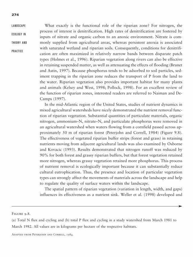
What exactly is the functional role of the riparian zone? For nitrogen, theprocess of interest is denitrification. High rates of denitrification are fostered byinputs of nitrate and organic carbon to an anoxic environment. Nitrate is com-monly supplied from agricultural areas, whereas persistent anoxia is associatedwith saturated wetland and riparian soils. Consequently, conditions for denitrifi-cation are often maximized in relatively narrow bands between disparate patchtypes (Holmes et al., 1996). Riparian vegetation along rivers can also be effectivein retaining suspended matter, as well as attenuating the effects of flooding (Brunetand Astin, 1997). Because phosphorus tends to be adsorbed to soil particles, sed-iment trapping in the riparian zone reduces the transport of P from the land tothe water. Riparian vegetation also provides important habitat for many plantsand animals (Kelsey and West, 1998; Pollock, 1998). For an excellent review ofthe function of riparian zones, interested readers are referred to Naiman and De-Camps (1997).

In the mid-Atlantic region of the United States, studies of nutrient dynamics inmixed agricultural watersheds have nicely demonstrated the nutrient removal func-tion of riparian vegetation. Substantial quantities of particulate materials, organicnitrogen, ammonium–N, nitrate–N, and particulate phosphorus were removed inan agricultural watershed when waters flowing from a cornfield passed across ap-proximately 50 m of riparian forest (Peterjohn and Correll, 1984) (Figure 9.8).The effectiveness of vegetated riparian buffer strips (forest and grass) in retainingnutrients moving from adjacent agricultural lands was also examined by Osborneand Kovacic (1993). Results demonstrated that nitrogen runoff was reduced by90% for both forest and grassy riparian buffers, but that forest vegetation retainedmore nitrogen, whereas grassy vegetation retained more phosphorus. This processof nutrient removal is ecologically important because it can substantially reducecultural eutrophication. Thus, the presence and location of particular vegetationtypes can strongly affect the movements of materials across the landscape and helpto regulate the quality of surface waters within the landscape.

The spatial pattern of riparian vegetation (variation in length, width, and gaps)influences its effectiveness as a nutrient sink. Weller et al. (1998) developed and

274

L A N D S C A P E

E C O L O G Y I N

T H E O R Y A N D

P R A C T I C E

Figure 9.8.

(a) Total N flux and cycling and (b) total P flux and cycling in a study watershed from March 1981 to

March 1982. All values are in kilograms per hectare of the respective habitats.

Adapted from Peterjohn and Correll, 1984.

2888_e09_p249-288 2/27/01 1:56 PM Page 274

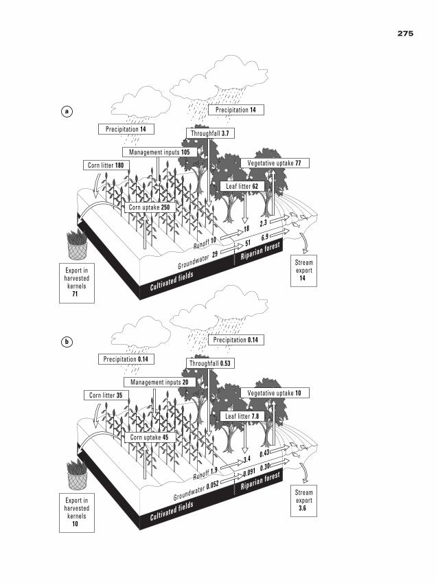
275

Export inharvested

kernels71

Streamexport

14

Riparian forest

Cultivated fieldsGroundwater 29

51 6.9

Runoff 10 1

8 2.3

Throughfall 3.7Precipitation 14

Precipitation 14

Corn uptake 250

Corn litter 180

Leaf litter 62

Management inputs 105Vegetative uptake 77

Export inharvested

kernels10

Streamexport

3.6

Riparian forest

Cultivated fieldsGroundwater 0.052

0.091 0.30

Runoff 1.9 3.4 0.43

Throughfall 0.53Precipitation 0.14

Precipitation 0.14

Corn uptake 45

Corn litter 35

Leaf litter 7.8

Management inputs 20Vegetative uptake 10

a

b

2888_e09_p249-288 2/27/01 1:56 PM Page 275

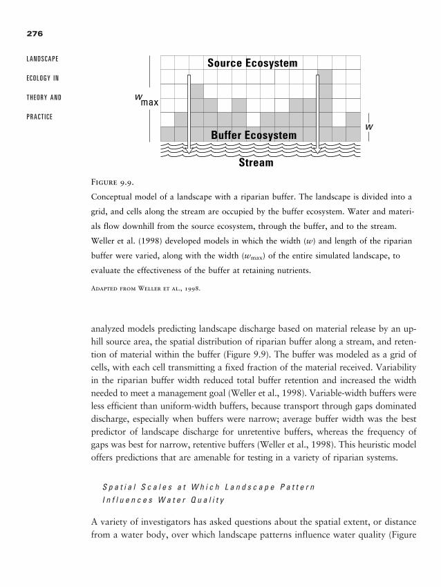
analyzed models predicting landscape discharge based on material release by an up-hill source area, the spatial distribution of riparian buffer along a stream, and reten-tion of material within the buffer (Figure 9.9). The buffer was modeled as a grid ofcells, with each cell transmitting a fixed fraction of the material received. Variabilityin the riparian buffer width reduced total buffer retention and increased the widthneeded to meet a management goal (Weller et al., 1998). Variable-width buffers wereless efficient than uniform-width buffers, because transport through gaps dominateddischarge, especially when buffers were narrow; average buffer width was the bestpredictor of landscape discharge for unretentive buffers, whereas the frequency ofgaps was best for narrow, retentive buffers (Weller et al., 1998). This heuristic modeloffers predictions that are amenable for testing in a variety of riparian systems.

S p a t i a l S c a l e s a t W h i c h L a n d s c a p e P a t t e r n

I n f l u e n c e s W a t e r Q u a l i t y

A variety of investigators has asked questions about the spatial extent, or distancefrom a water body, over which landscape patterns influence water quality (Figure

276

L A N D S C A P E

E C O L O G Y I N

T H E O R Y A N D

P R A C T I C E

Source Ecosystem

Buffer Ecosystem

Stream

w

wmax

Figure 9.9.

Conceptual model of a landscape with a riparian buffer. The landscape is divided into a

grid, and cells along the stream are occupied by the buffer ecosystem. Water and materi-

als flow downhill from the source ecosystem, through the buffer, and to the stream.

Weller et al. (1998) developed models in which the width (w) and length of the riparian

buffer were varied, along with the width (wmax) of the entire simulated landscape, to

evaluate the effectiveness of the buffer at retaining nutrients.

Adapted from Weller et al., 1998.

2888_e09_p249-288 2/27/01 1:56 PM Page 276

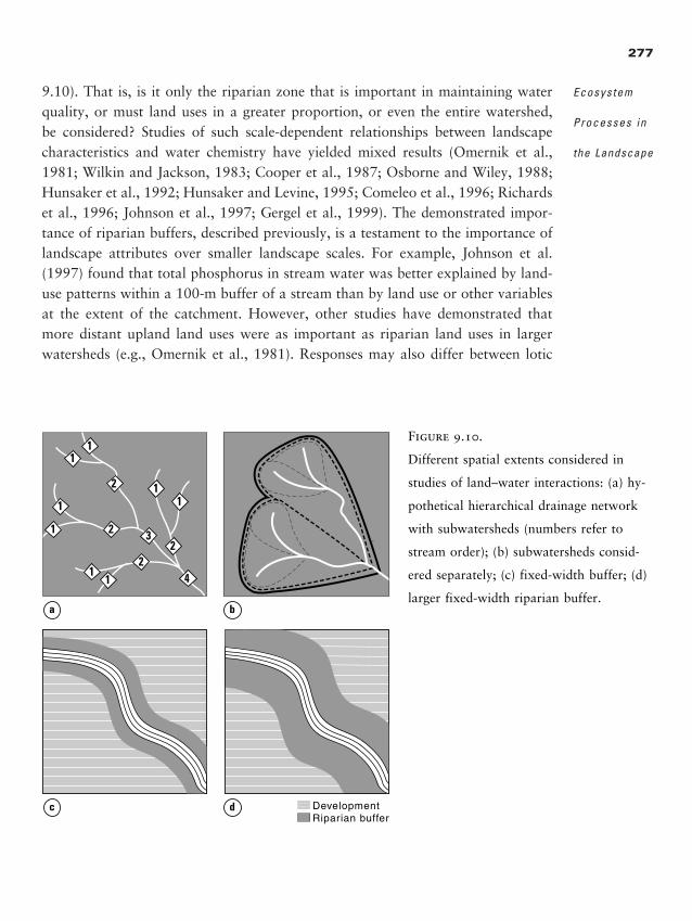
9.10). That is, is it only the riparian zone that is important in maintaining waterquality, or must land uses in a greater proportion, or even the entire watershed,be considered? Studies of such scale-dependent relationships between landscapecharacteristics and water chemistry have yielded mixed results (Omernik et al.,1981; Wilkin and Jackson, 1983; Cooper et al., 1987; Osborne and Wiley, 1988;Hunsaker et al., 1992; Hunsaker and Levine, 1995; Comeleo et al., 1996; Richardset al., 1996; Johnson et al., 1997; Gergel et al., 1999). The demonstrated impor-tance of riparian buffers, described previously, is a testament to the importance oflandscape attributes over smaller landscape scales. For example, Johnson et al.(1997) found that total phosphorus in stream water was better explained by land-use patterns within a 100-m buffer of a stream than by land use or other variablesat the extent of the catchment. However, other studies have demonstrated thatmore distant upland land uses were as important as riparian land uses in largerwatersheds (e.g., Omernik et al., 1981). Responses may also differ between lotic

277

Ecosystem

Processes in

the Landscape

Riparian bufferDevelopment

1

1

1

1

11

11

2

2

2

23

4

a

c

b

d

Figure 9.10.

Different spatial extents considered in

studies of land–water interactions: (a) hy-

pothetical hierarchical drainage network

with subwatersheds (numbers refer to

stream order); (b) subwatersheds consid-

ered separately; (c) fixed-width buffer; (d)

larger fixed-width riparian buffer.

2888_e09_p249-288 2/27/01 1:56 PM Page 277

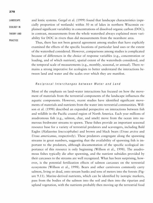
and lentic systems. Gergel et al. (1999) found that landscape characteristics (espe-cially proportion of wetlands) within 50 m of lakes in northern Wisconsin ex-plained significant variability in concentrations of dissolved organic carbon (DOC);in contrast, measurements from the whole watershed always explained more vari-ability for DOC in rivers than did measurements from the nearshore area.

Thus, there has not been general agreement among studies that have explicitlyexamined the effects of the specific locations of particular land uses or the extentof the watershed considered. However, comparisons among studies is complicatedbecause of differences in the choice of response variables (e.g., concentration orloading, and of which nutrient), spatial extent of the watersheds considered, andthe temporal scale of measurements (e.g., monthly, seasonal, or annual). There re-mains a strong imperative for ecologists to better understand the interactions be-tween land and water and the scales over which they are manifest.

R e c i p r o c a l I n t e r c h a n g e s b e t w e e n W a t e r a n d L a n d

Most of the emphasis on land–water interactions has focused on how the move-ment of materials from the terrestrial components of the landscape influences theaquatic components. However, recent studies have identified significant move-ments of materials and nutrients from the water into terrestrial communities. Will-son et al. (1998) described an expanded perspective on interactions between fishand wildlife in the Pacific coastal region of North America. Each year millions ofanadromous fish (e.g., salmon, char, and smelt) move from the ocean into nu-merous freshwater streams to spawn. These fishes provide an important seasonalresource base for a variety of terrestrial predators and scavengers, including BaldEagles (Haliaeetus leucocephalus) and brown and black bears (Ursus arctos andUrsus americanus, respectively). These predators congregate along the spawningstreams in great numbers, suggesting that the availability of spawning fish is im-portant to the predators, although documentation of the specific ecological im-portance of this resource is only beginning (Willson et al., 1998). The anadro-mous fishes typically die after spawning, and the nutrient subsidies provided bytheir carcasses to the streams are well recognized. What has been surprising, how-ever, is the potential fertilization effects of salmon carcasses on the terrestrialecosystems (Willson et al., 1998). Bears and other carnivores commonly carrysalmon, living or dead, onto stream banks and tens of meters into the forests (Fig-ure 9.11). Marine-derived nutrients, which can be identified by isotopic markers,pass from the bodies of the salmon into the soil and then into the riparian andupland vegetation, with the nutrients probably then moving up the terrestrial food

278

L A N D S C A P E

E C O L O G Y I N

T H E O R Y A N D

P R A C T I C E

2888_e09_p249-288 2/27/01 1:56 PM Page 278

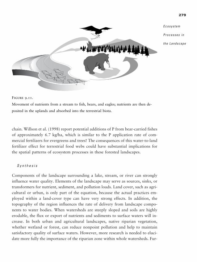
chain. Willson et al. (1998) report potential additions of P from bear-carried fishesof approximately 6.7 kg/ha, which is similar to the P application rate of com-mercial fertilizers for evergreens and trees! The consequences of this water-to-landfertilizer effect for terrestrial food webs could have substantial implications forthe spatial patterns of ecosystem processes in these forested landscapes.

S y n t h e s i s

Components of the landscape surrounding a lake, stream, or river can stronglyinfluence water quality. Elements of the landscape may serve as sources, sinks, ortransformers for nutrient, sediment, and pollution loads. Land cover, such as agri-cultural or urban, is only part of the equation, because the actual practices em-ployed within a land-cover type can have very strong effects. In addition, thetopography of the region influences the rate of delivery from landscape compo-nents to water bodies. When watersheds are steeply sloped and soils are highlyerodable, the flux or export of nutrients and sediments to surface waters will in-crease. In both urban and agricultural landscapes, native riparian vegetation,whether wetland or forest, can reduce nonpoint pollution and help to maintainsatisfactory quality of surface waters. However, more research is needed to eluci-date more fully the importance of the riparian zone within whole watersheds. Fur-

279

Ecosystem

Processes in

the Landscape

Figure 9.11.

Movement of nutrients from a stream to fish, bears, and eagles; nutrients are then de-

posited in the uplands and absorbed into the terrestrial biota.

2888_e09_p249-288 2/27/01 1:56 PM Page 279

thermore, recently identified movements of nutrients from the water into someupland communities point to important reciprocal interchanges between water andland that may have substantial implications for spatial heterogeneity in ecosystemprocesses in terrestrial landscapes.

L I N K I N G S P E C I E S A N D E C O S Y S T E M S

When we seek to understand the functional dynamics of entire landscapes, inter-actions between species and ecosystem processes must often be considered. Graz-ers, for example, can enhance mineral availability by increasing nutrient cyclingin patches of their waste (McNaughton et al., 1988; Day and Detling, 1990; Hol-land et al., 1992). In dealing with the management or restoration of landscapes,it is again important to account for both species and ecosystem processes. Land-scape ecology offers both a conceptual framework and methods for making sub-stantial progress in this area and may perhaps help to dissolve some fences be-tween the traditionally distinct subdisciplines of population and ecosystem ecologies.In an introductory chapter in the book Linking Species and Ecosystems (Jonesand Lawton, 1995), Grimm (1995) writes:

Interactions between population/community and ecosystem ecologists would

be facilitated by adopting, as a starting point, a spatially based conception of

units of study. . . . Whatever the scale of the investigation, a spatially based

perspective places species interactions (the traditional focus of community ecol-

ogy) into a context in which their effect on ecosystem processes may be as-

sessed. Interactions between patches may be critical to larger-scale processes

and include biotic interactions that occur within component subsystems.

Species and ecosystems are inherently linked, but population ecology and ecosys-tem ecology often break this linkage conceptually. In this section, we highlighttwo studies that illustrate insights from and approaches for considering species–ecosystem interactions in a landscape context.

V e g e t a t i o n , L a r g e H e r b i v o r e s , a n d N u t r i e n t C y c l i n g

Studies in the boreal forest landscape have demonstrated fascinating links amongspatial patterns of plant species distributions and biomass, the foraging dynamics

280

L A N D S C A P E

E C O L O G Y I N

T H E O R Y A N D

P R A C T I C E

�

2888_e09_p249-288 2/27/01 1:56 PM Page 280

of moose (Alces alces), and rates of nutrient cycling (McInnes et al., 1992; Jeffrieset al., 1994; Pastor et al., 1997). Studies on Isle Royale, an island located in LakeSuperior and well known for long-term studies of moose and wolves, demonstratedhow selective foraging by moose on hardwood species allows unbrowsed or lightlybrowsed conifers to dominate the boreal landscape (McInnes et al., 1992). Mooseprefer to browse upon deciduous tree species such as birch (Betula lutea) and as-pen (Populus tremuloides), as well as balsam fir (Abies balsamea), rather than onwhite spruce (Picea glauca). In areas of Isle Royale where fences (exclosures) werebuilt to prevent moose from browsing, the deciduous trees have persisted andgrown larger. However, outside the exclosures, where moose were allowed tobrowse, white spruce was the only tree species that could grow above the brows-ing height of a moose. Moose browsing on balsam fir and the deciduous trees pre-vented saplings of these preferred forage species from growing into full-sized trees.The browsing of moose also opens up the forest canopy and reduces tree biomass,allowing more light to reach the forest floor and stimulating more production ofshrubs and herbaceous species.

Understanding the spatial heterogeneity of ecosystem processes in this boreallandscape requires forging a linkage between the feeding ecology and populationdynamics of moose and the function of the ecosystem, all within the context of alandscape. By selectively foraging on specific plant species, moose and other largeherbivores influence ecosystem dynamics, changing plant community composition,biomass, production, and nutrient cycling (McInnes et al., 1992). Soils in areasdominated by spruce received less litter, and the nutritional quality of the litter,especially its nitrogen content, declined for the decomposers. This decrease in lit-ter quantity and quality leads to a decline in microbial processes that in turn de-termine nitrogen availability for the living plants. Conifer litter depresses the avail-ability of soil nitrogen, which limits net primary production in boreal forests.

Moen et al. (1997, 1998) developed a simulation model to predict how alter-native moose foraging strategies affect the net annual energy balance and densityof moose and the spatial distribution of browse across the landscape. Simulationswere conducted at fine resolution (grid cells of 1 m2 over an 8-ha landscape), andresults have demonstrated how moose create their own landscape by their pat-terns of foraging and the feedbacks of these patterns on vegetation structure andcomposition. Because moose are highly mobile and can forage all around the land-scape, interactions between moose and vegetation create a mosaic of nutrient cy-cling regimes in these boreal forests, resulting in complex spatial and temporalpatterns of browsing, conifer density, and soil nitrogen distribution across thelandscape (Pastor et al., 1999).

281

Ecosystem

Processes in

the Landscape

2888_e09_p249-288 2/27/01 1:56 PM Page 281

S p e c i e s a n d E c o s y s t e m D y n a m i c s i n t h e E v e r g l a d e s

The basic and applied issues associated with restoration of the Everglades, Florida,provide an excellent example of the benefit gained by linking species and ecosys-tems in a landscape context (Davis and Ogden, 1994; DeAngelis et al., 1998). TheEverglades is a huge freshwater marsh that extends from Lake Okeechobee in cen-tral Florida southward toward Florida Bay and the Gulf of Mexico. Water is theprevailing abiotic influence on this landscape, flowing south and southwest fromLake Okeechobee at a very slow rate across this flat region. Human modificationof the natural flow began early in the 20th century and involved levees, canals,pumping stations, and water-control structures to drain large areas of the Ever-glades. Agriculture and urban land uses quickly occupied these former wetlands.Water flow to the southern Everglades, which was protected as a national parkin 1947, is delivered through water-control structures, and both the volume andtiming of flow have been altered. The net effects of these hydrological changeswere (1) a loss of uninterrupted sheet flow, (2) pronounced fluctuations in waterlevels, (3) a higher frequency of major drydown events, and (4) a disproportion-ate loss of high-elevation short-hydroperiod wetlands (DeAngelis et al., 1998).

Before these modifications occurred, a broad area (up to 90 km wide) of theEverglades was inundated up to a depth of 0.5 m during part of the year, creat-ing a continuous spectrum of hydroperiods (average annual inundation time fora particular area), which has important ecological consequences. During flooding,populations of small fish, crayfish, and the like, are nourished by detritus and al-gae growth, are relatively protected from large predatory fish, and reach high pop-ulation sizes. During the dry period, the fishes are concentrated by the recedingwaters into pools and depressions. Wading birds then rely on this concentratedresource base to provide food for their young during the nesting period (Fleminget al., 1994). Wading bird populations have declined by �90% since the 1940s,and a variety of other species (e.g., Cape Sable Seaside Sparrow, Ammodramusmaritimus; American alligator, Alligator mississipiensis) have also suffered nega-tive consequences from the modification of the natural hydrology and disruptionof trophic dynamics across the landscape (DeAngelis et al., 1998). Recent coop-erative efforts by an array of federal and state agencies are striving to restore theEverglades and other ecosystems in southern Florida.

DeAngelis et al. (1998) developed a spatial model (Across Trophic Level Sys-tem Simulation, or ATLSS) of the Everglades that explores the effects of changesin hydrology on a variety of species, including those at the top of the food web.The species differ in their use of the landscape and resources and include the

282

L A N D S C A P E

E C O L O G Y I N

T H E O R Y A N D

P R A C T I C E

2888_e09_p249-288 2/27/01 1:56 PM Page 282

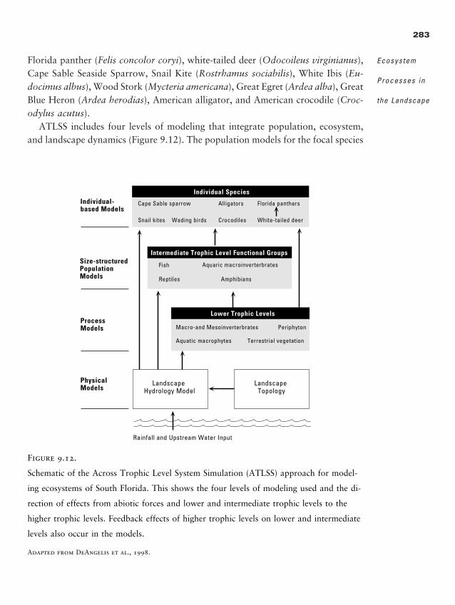
Florida panther (Felis concolor coryi), white-tailed deer (Odocoileus virginianus),Cape Sable Seaside Sparrow, Snail Kite (Rostrhamus sociabilis), White Ibis (Eu-docimus albus), Wood Stork (Mycteria americana), Great Egret (Ardea alba), GreatBlue Heron (Ardea herodias), American alligator, and American crocodile (Croc-odylus acutus).

ATLSS includes four levels of modeling that integrate population, ecosystem,and landscape dynamics (Figure 9.12). The population models for the focal species

283

Ecosystem

Processes in

the Landscape

Rainfall and Upstream Water Input

Individual-based Models

Landscape Hydrology Model

Landscape Topology

Size-structuredPopulationModels

ProcessModels

Physical Models

Intermediate Trophic Level Functional Groups

Individual Species

Lower Trophic Levels

Cape Sable sparrow

Fish

Reptiles Amphibians

Aquaric macroinverterbrates

Macro-and Mesoinverterbrates Periphyton

Aquatic macrophytes Terrestrial vegetation

Alligators Florida panthers

Snail kites Wading birds Crocodiles White-tailed deer

Figure 9.12.

Schematic of the Across Trophic Level System Simulation (ATLSS) approach for model-

ing ecosystems of South Florida. This shows the four levels of modeling used and the di-

rection of effects from abiotic forces and lower and intermediate trophic levels to the

higher trophic levels. Feedback effects of higher trophic levels on lower and intermediate

levels also occur in the models.

Adapted from DeAngelis et al., 1998.

2888_e09_p249-288 2/27/01 1:56 PM Page 283

are individual-based models and include the characteristics of each organism (age,size, spatial location, sex, health, social status, etc.). Immediately below the indi-vidual-based models are the intermediate trophic levels (fish, aquatic macroinver-tebrates, and several groups of reptiles and amphibians), which are modeled assize-structured populations. Below this level and driving their biomass are thelower trophic levels, simulated by process models and consisting of macrophytes,periphyton, aquatic mesofauna, and macroinvertebrates. The macrophytes includeboth aquatic and terrestrial plants that provide forage for the white-tailed deer.Finally, there is a landscape structure level that includes the standard static datalayers (e.g., surface elevation, vegetation types, soil types, road networks), as wellas dynamic layers, such as changing water levels across the landscape.

The ATLSS modeling approach thus uses the spatially explicit view of the land-scape to simulate effects of the ecosystem directly on individuals. The output fromthis model is expected to provide information to managers that would help themto rank the effectiveness of various water-management options against specific cri-teria for indicator species. DeAngelis et al. (1998) also used the Everglades restora-tion and modeling effort to highlight two important theoretical issues that are cur-rent challenges to ecologists: (1) uniting or at least connecting population ecologywith the behavioral and physiological condition of individuals and (2) uniting pop-ulation ecology with ecosystem ecology.

S E A R C H I N G F O R G E N E R A L P R I N C I P L E S

Modeling will continue to be an important tool for understanding the causes andconsequences of variation in ecosystem processes, although the logistics of inten-sively measuring such processes at fine resolution but broad spatial extent aredaunting (not to mention very, very expensive). Many spatial models of ecosys-tem processes have focused on management issues, particularly nonpoint-sourcepollution (identifying critical source areas, relating land use to sediment and nu-trient loads, predicting movements of materials during storm events, and mitigat-ing contamination). Basic questions addressed by spatial ecosystem models focuson the problem of what happens when you consider space. For example, how doesspatial variability in climate or soils affect ecosystem processes such as NPP orevapotranspiration? In general, modeling studies have elucidated the controls onecosystem processes of spatial variation in the environment, served as informativetools for exploring effects of alternative landscape patterns on aquatic ecosystems,

284

L A N D S C A P E

E C O L O G Y I N

T H E O R Y A N D

P R A C T I C E

�

2888_e09_p249-288 2/27/01 1:56 PM Page 284

and are just beginning to delve into the spatial interactions between species andecosystem processes. Modelers continue to grapple with a number of fundamen-tal issues associated with spatial models of ecosystem processes. Parameterizationof spatial models is difficult and can be highly uncertain, and highly parameter-ized models are less portable from one system to another. Therefore, it is not sur-prising that investigators continue to experiment with techniques for incorporat-ing spatial dynamics while keeping the data demands of the model reasonable.

Furthering our knowledge of the patterns and causes of spatial heterogeneity inecosystem function remains at the frontier of ecosystem and landscape ecology. Thelibrary of empirical data from a variety of landscapes is slowly building, yet we haveno general answers to such questions as these: Just how spatially variable are ecosys-tem processes? How do the controls on processes and rates operate across space?Are there critical thresholds in spatial variability that are important for ecosystemprocesses? Despite tremendous advances in understanding ecosystem processes overrelatively small spatial extents, there exists very little theory for predicting variabil-ity in ecosystem processes across larger areas. A more synthetic understanding ofspatial heterogeneity in ecosystem processes remains an important research need,one that should include both theoretical development and empirical study.

S U M M A R Y

Determining the patterns, causes, and effects of ecosystem function across land-scapes is an important current topic in ecosystem and landscape ecology. Whenlandscape ecologists study ecosystem processes, they emphasize the causes andconsequences of spatial heterogeneity in the rates of ecosystem processes (e.g., netprimary productivity, nitrogen mineralization); the influence of landscape positionon ecosystem function, and the horizontal movement of materials (such as water,nutrients, or sediments) and how these movements might differ with alternativespatial arrangements of land cover.

Spatial variation in abiotic variables (temperature, precipitation, soils, and topo-graphic position) often produces substantial spatial variation in ecosystem processes(e.g., productivity, decomposition, and nitrogen cycling) across landscapes. For example, nutrient accumulation and cycling may vary between ridgetops, whichtend to be exposed and dry, and the more sheltered and moist bases of slopes.Thus, as ecosystem ecologists have long recognized, the abiotic template is a pow-erful constraint on ecosystem function. However, changes in land-use patterns and

285

Ecosystem

Processes in

the Landscape

�

2888_e09_p249-288 2/27/01 1:56 PM Page 285

natural disturbances also influence the rates and patterns of ecosystem processes.Disturbances can have substantial influences on biogeochemical cycles, but littleis known about the long-term implications of a disturbance-generated landscapemosaic for nutrient cycling.

Abiotic factors vary over multiple spatial scales, and ecologists are still strivingto determine the scales that are appropriate for developing predictive relationships.Empirical studies of ecosystem processes have demonstrated that a model will needto include a larger number of variables to account for the spatial pattern of the sameprocess as the scale of analysis (either extent or grain) becomes finer.

The recent focus on landscape dynamics and ecosystem processes encourageddevelopment of spatially explicit models of energy flow and nutrient dynamics.Simulation modeling should continue as one of the tools used to study spatial vari-ation in ecosystem processes, but such models are time consuming to develop anddemanding of data with which to initialize and test the model.

Aquatic ecologists have been exploring landscape-level characteristics that de-scribe the state of lake ecosystems. Many hydrologic properties of a lake are de-termined directly by landscape position—its hydrologic position within the localto regional flow system and the relative spatial placement of neighboring lakeswithin a landscape. Results from a variety of studies suggest that a landscape per-spective for lakes based on landscape position is relatively robust. This perspec-tive argues for a view of lake ecosystems embedded in a landscape matrix, withlakes interacting with one another and with the terrestrial environment. A land-scape perspective also may help to foster a view of land–water interactions thatencompasses the set of lakes, streams, and wetlands that occur within a landscape.

Components of the landscape surrounding a lake, stream, or river can stronglyinfluence water quality. Elements of the landscape may serve as sources, sinks, ortransformers for nutrient, sediment, and pollution loads. A common theme un-derlying many studies of land–water interactions is the degree to which land usesin the uplands and the spatial arrangement of these land uses influence water qual-ity in streams and lakes. Riparian vegetation zones, including wetlands and flood-plain forests, are conspicuous elements of many landscapes and important medi-ators of land–water interactions. Most of the emphasis on land–water interactionshas focused on how the movement of materials from the terrestrial componentsof the landscape influences the aquatic components. However, recent studies havealso identified significant movements of materials and nutrients from the waterinto terrestrial communities. There remains a strong imperative for ecologists tobetter understand the reciprocal interactions between land and water and the scalesover which they are manifest.

286

L A N D S C A P E

E C O L O G Y I N

T H E O R Y A N D

P R A C T I C E

2888_e09_p249-288 2/27/01 1:56 PM Page 286

Understanding the implications of the dynamic landscape mosaic for ecosystemprocesses remains a frontier in ecosystem and landscape ecology. We simply donot have a well-developed theory of ecosystem function that is spatially explicit,nor do we have a wealth of empirical studies from which to infer general con-clusions. Landscape ecology also offers promise as a conceptual framework withinwhich interactions between species and ecosystem processes can be linked.


1. A daunting challenge in studying the spatial variation in ecosystem function and the

factors that control the rates of ecosystem processes is to balance data needs (e.g.,

spatial extent of the study and the number of measurements needed) with logistical

difficulties and actual cost (e.g., person-hours required for collecting and process-

ing samples and the costs of running laboratory analyses). Consider an extensive

landscape of your choice. Develop a field sampling design that attempts to describe

the spatial variation of an ecosystem attribute or process rate (e.g., NPP, LAI, ni-

trogen mineralization, denitrification, phosphorus accumulation) of your choice.

a. Did you need to stratify sampling in your design? Why or why not? If yes, by

what variables did you stratify, and why?

b. How did you consider issues of spatial autocorrelation in your design?

c. Estimate the cost of implementing your design in terms of person-hours and lab-

oratory costs (if any). Could this cost be reduced by combining remote sensing

with field measurements? Why or why not?

2. Describe how the processes associated with the release, uptake, and storage of car-

bon would change in the following scenarios over a period of 100 years (graphical

representations may be helpful):

a. A temperate deciduous forest is affected by small-gap disturbances that affect 1%

of the landscape each year and initiate succession within the gaps.

b. A temperate deciduous forest is cleared for agriculture and farmed continuously

for 50 years. Farming is then abandoned, and the land undergoes natural suc-

cession for the next 50 years.

c. A mature boreal forest landscape experiences wildfire that burns 60% of the

landscape and initiates forest succession. Ten years later, a second fire burns 50%

of the previously burned area and eliminates the newly established trees, result-

ing in the area of double-burn being dominated by herbaceous vegetation for the

next 80 years.

287

Ecosystem

Processes in

the Landscape

2888_e09_p249-288 2/27/01 1:56 PM Page 287

3. Consider an agricultural watershed in which fertilizers are applied to upland crop

fields. A management goal for this watershed is to maintain acceptable water qual-

ity while producing agricultural products. Under what conditions might you expect

a riparian buffer to be effective at maintaining water quality? Under what condi-

tions would a reduction in the source of nutrients (e.g., reduce or eliminate some

fertilizer inputs) be needed to maintain water quality?

4. How do you expect the statistical relationships between a measurement of ecosys-

tem function and a variable that controls that function to change with spatial scale?

Are the changes with scale linear? Why or why not?


Burke, I. C., D. S. Schimel, C. M. Yonker, W. J. Parton, L. A. Joyce, and W. K.

Lauenroth. 1990. Regional modeling of grassland biogeochemistry using GIS.

Landscape Ecology 4:45–54.

DeAngelis, D. L., L. J. Gross, M. A. Huston, W. F. Wolff, D. M. Fleming, E. J.

Comiskey, and S. M. Sylvester. 1998. Landscape modeling for Everglades ecosys-

tem restoration. Ecosystems 1:64–75.

Kratz, T. K., K. E. Webster, C. J. Bowser, J. J. Magnuson, and B. J. Benson.

1997. The influence of landscape position on lakes in northern Wisconsin. Fresh-

water Biology 37:209–217.

Naiman, R. J., and H. Decamps. 1997. The ecology of interfaces: riparian zones. An-

nual Review of Ecology and Systematics 28:621–658.

Pastor, J., Y. Cohen, and R. Moen. 1999. Generation of spatial patterns in boreal

forest landscapes. Ecosystems 2:439–450.

Peterjohn, W. T., and D. L. Correll. 1984. Nutrient dynamics in an agricultural

watershed: observations on the role of a riparian forest. Ecology 65:1466–75.

Running, S. W., R. R. Nemani, D. L. Peterson, L. E. Band, D. F. Potts, L. L.

Pierce, and M. A. Spanner. 1989. Mapping regional forest evapotranspiration and

photosynthesis by coupling satellite data with ecosystem simulation. Ecology 70:

1090–1101.

Soranno, P. A., S. L. Hubler, S. R. Carpenter, and R. C. Lathrop. 1996. Phos-

phorus loads to surface waters: a simple model to account for spatial pattern of land

use. Ecological Applications 6:865–878.

288

L A N D S C A P E

E C O L O G Y I N

T H E O R Y A N D

P R A C T I C E

2888_e09_p249-288 2/27/01 1:56 PM Page 288

C H A P T E R

Applied Landscape Ecology

The practical application of landscape ecology is an exciting and rapidlyexpanding field. Landscape ecology contributes to many different aspects

of applied ecology and is playing a significant role in the development and appli-cation of methods of ecosystem management (Agee and Johnson, 1988; Slocombe,1993; Grumbine, 1994; Christensen et al., 1996). The challenges facing naturalresource managers increasingly occur over entire landscapes and involve spatialinterdependencies among landscape components at many scales. Demand for thescientific underpinnings of managing landscapes and incorporating the conse-quences of spatial heterogeneity into land-management decisions is substantial.Consequently, many resource managers are shifting their management from anapproach that focuses on specific resources, such as fish, wildlife, and water, toone focused on the integrity of entire systems. An awareness is growing that eco-logical effects of resource management are sensitive to the temporal scales andspatial configuration of the activity (e.g., timber harvesting or land development).Indeed, nearly all land-management agencies in the United States have recognizedthat informed resource-management decisions cannot be made exclusively at thelevel of habitat units or local sites. This shift has caused an increased demand for

10

2888_e10_p289-326 2/27/01 1:52 PM Page 289

290

L A N D S C A P E

E C O L O G Y I N

T H E O R Y A N D

P R A C T I C E

applications and management recommendations that often outpaces the basic sci-ence (Turner et al., in press).

Applications of landscape ecology require integration and synthesis of the manyfacets of the discipline that have been considered separately in this book. For ex-ample, in managing a particular landscape, consideration must be given to theconfiguration of the landscape mosaic and its change with time, the disturbanceregime and its likely consequences for patterns and processes, the responses ofmany different species that operate at a variety of scales, and the effects of changeon ecosystem function. Many applications of landscape ecology depend on es-tablishing a cause–effect relationship between landscape pattern and an environ-mental variable of interest. These relationships can then be used to plan the spa-tial configuration of landscape mosaics to minimize undesirable impacts.Ultimately, analyses of changes in landscape pattern may prove to be a practicaland efficient approach to broad-scale environmental analysis (O’Neill et al., 1997).

Applied problems and resource management were instrumental in catalyzingthe development and emergence of landscape ecology, and they continue to stim-ulate both basic and applied research in landscape ecology. For example, under-standing the effects of landscape pattern on stream and lake ecosystems has beendriven by the practical problem of how to maintain healthy aquatic ecosystems.Similarly, the need for forest managers to schedule timber harvests in space andtime across landscapes stimulated much basic research on the effects of alterna-tive harvesting regimes for landscape patterns and processes. In fact, the distinc-tion between basic and applied research is often arbitrary; most applied problemshave basic components. The theory and methods of landscape ecology clearly haveimplications for many applied problems and resource-management questions,which in turn will continue to promote research that contributes to our basic un-derstanding of the interaction between pattern and process. In this chapter, wesurvey how principles of landscape ecology have proved useful and where the chal-lenges lie for land-use decisions, forest management, regional impact assessment,and broad-scale environmental monitoring.

L A N D U S E

Understanding land-use changes and their ecological implications presents a fun-damental challenge to ecologists, one in which landscape ecology clearly must playa role. Throughout the world, land cover today is altered principally by direct hu-

�

2888_e10_p289-326 2/27/01 1:52 PM Page 290

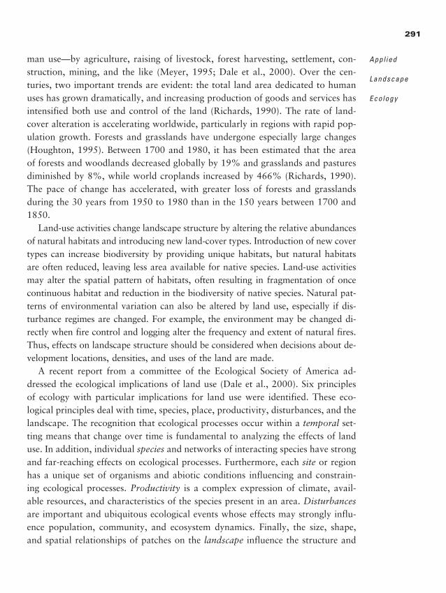
man use—by agriculture, raising of livestock, forest harvesting, settlement, con-struction, mining, and the like (Meyer, 1995; Dale et al., 2000). Over the cen-turies, two important trends are evident: the total land area dedicated to humanuses has grown dramatically, and increasing production of goods and services hasintensified both use and control of the land (Richards, 1990). The rate of land-cover alteration is accelerating worldwide, particularly in regions with rapid pop-ulation growth. Forests and grasslands have undergone especially large changes(Houghton, 1995). Between 1700 and 1980, it has been estimated that the areaof forests and woodlands decreased globally by 19% and grasslands and pasturesdiminished by 8%, while world croplands increased by 466% (Richards, 1990).The pace of change has accelerated, with greater loss of forests and grasslandsduring the 30 years from 1950 to 1980 than in the 150 years between 1700 and1850.

Land-use activities change landscape structure by altering the relative abundancesof natural habitats and introducing new land-cover types. Introduction of new covertypes can increase biodiversity by providing unique habitats, but natural habitatsare often reduced, leaving less area available for native species. Land-use activitiesmay alter the spatial pattern of habitats, often resulting in fragmentation of oncecontinuous habitat and reduction in the biodiversity of native species. Natural pat-terns of environmental variation can also be altered by land use, especially if dis-turbance regimes are changed. For example, the environment may be changed di-rectly when fire control and logging alter the frequency and extent of natural fires.Thus, effects on landscape structure should be considered when decisions about de-velopment locations, densities, and uses of the land are made.

A recent report from a committee of the Ecological Society of America ad-dressed the ecological implications of land use (Dale et al., 2000). Six principlesof ecology with particular implications for land use were identified. These eco-logical principles deal with time, species, place, productivity, disturbances, and thelandscape. The recognition that ecological processes occur within a temporal set-ting means that change over time is fundamental to analyzing the effects of landuse. In addition, individual species and networks of interacting species have strongand far-reaching effects on ecological processes. Furthermore, each site or regionhas a unique set of organisms and abiotic conditions influencing and constrain-ing ecological processes. Productivity is a complex expression of climate, avail-able resources, and characteristics of the species present in an area. Disturbancesare important and ubiquitous ecological events whose effects may strongly influ-ence population, community, and ecosystem dynamics. Finally, the size, shape,and spatial relationships of patches on the landscape influence the structure and

291

Appl ied

Landscape

Ecology

2888_e10_p289-326 2/27/01 1:52 PM Page 291

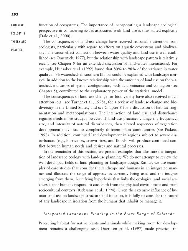
function of ecosystems. The importance of incorporating a landscape ecologicalperspective in considering issues associated with land use is thus stated explicitly(Dale et al., 2000).

The consequences of land-use change have received reasonable attention fromecologists, particularly with regard to effects on aquatic ecosystems and biodiver-sity. The cause–effect connection between water quality and land use is well estab-lished (see Omernick, 1977), but the relationship with landscape pattern is relativelyrecent (see Chapter 9 for an extended discussion of land–water interactions). Forexample, Hunsaker et al. (1992) found that 80% to 90% of the variance in waterquality in 36 watersheds in southern Illinois could be explained with landscape met-rics. In addition to the known relationship with the amounts of land use on the wa-tershed, indicators of spatial configuration, such as dominance and contagion (seeChapter 5), contributed to the explanatory power of the statistical model.

The consequences of land-use change for biodiversity have also received muchattention (e.g., see Turner et al., 1998a, for a review of land-use change and bio-diversity in the United States, and see Chapter 8 for a discussion of habitat frag-mentation and metapopulations). The interaction of land use and disturbanceregimes needs more study, however. If land-use practices change the frequency,size, and intensity of natural disturbances, then altered sequences of vegetationdevelopment may lead to completely different plant communities (see Pickett,1998). In addition, continued land development in regions subject to severe dis-turbances (e.g., hurricanes, crown fires, and floods) will produce continued con-flict between human needs and desires and natural processes.

In the remainder of this section, we present examples that illustrate the integra-tion of landscape ecology with land-use planning. We do not attempt to review thewell-developed fields of land planning or landscape design. Rather, we use exam-ples of case studies that consider the landscape and humans in an integrated man-ner and illustrate the range of approaches currently being used and the insightsemerging from them. A unifying hypothesis that links the ecological and social sci-ences is that humans respond to cues both from the physical environment and fromsociocultural contexts (Riebsame et al., 1994). Given the extensive influence of hu-man land use on landscape structure and function, it is folly to consider the futureof any landscape in isolation from the humans that inhabit or manage it.

I n t e g r a t e d L a n d s c a p e P l a n n i n g i n t h e F r o n t R a n g e o f C o l o r a d o

Protecting habitat for native plants and animals while making room for develop-ment remains a challenging task. Duerksen et al. (1997) made practical re-

292

L A N D S C A P E

E C O L O G Y I N

T H E O R Y A N D

P R A C T I C E

2888_e10_p289-326 2/27/01 1:52 PM Page 292

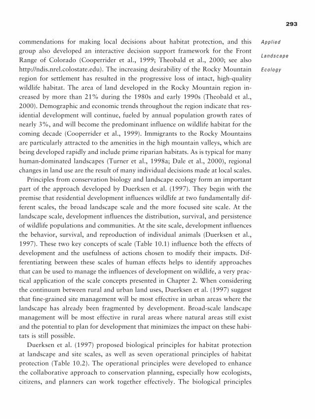
commendations for making local decisions about habitat protection, and this group also developed an interactive decision support framework for the FrontRange of Colorado (Cooperrider et al., 1999; Theobald et al., 2000; see alsohttp://ndis.nrel.colostate.edu). The increasing desirability of the Rocky Mountainregion for settlement has resulted in the progressive loss of intact, high-qualitywildlife habitat. The area of land developed in the Rocky Mountain region in-creased by more than 21% during the 1980s and early 1990s (Theobald et al.,2000). Demographic and economic trends throughout the region indicate that res-idential development will continue, fueled by annual population growth rates ofnearly 3%, and will become the predominant influence on wildlife habitat for thecoming decade (Cooperrider et al., 1999). Immigrants to the Rocky Mountainsare particularly attracted to the amenities in the high mountain valleys, which arebeing developed rapidly and include prime riparian habitats. As is typical for manyhuman-dominated landscapes (Turner et al., 1998a; Dale et al., 2000), regionalchanges in land use are the result of many individual decisions made at local scales.

Principles from conservation biology and landscape ecology form an importantpart of the approach developed by Duerksen et al. (1997). They begin with thepremise that residential development influences wildlife at two fundamentally dif-ferent scales, the broad landscape scale and the more focused site scale. At thelandscape scale, development influences the distribution, survival, and persistenceof wildlife populations and communities. At the site scale, development influencesthe behavior, survival, and reproduction of individual animals (Duerksen et al.,1997). These two key concepts of scale (Table 10.1) influence both the effects ofdevelopment and the usefulness of actions chosen to modify their impacts. Dif-ferentiating between these scales of human effects helps to identify approachesthat can be used to manage the influences of development on wildlife, a very prac-tical application of the scale concepts presented in Chapter 2. When consideringthe continuum between rural and urban land uses, Duerksen et al. (1997) suggestthat fine-grained site management will be most effective in urban areas where thelandscape has already been fragmented by development. Broad-scale landscapemanagement will be most effective in rural areas where natural areas still existand the potential to plan for development that minimizes the impact on these habi-tats is still possible.

Duerksen et al. (1997) proposed biological principles for habitat protectionat landscape and site scales, as well as seven operational principles of habitatprotection (Table 10.2). The operational principles were developed to enhancethe collaborative approach to conservation planning, especially how ecologists,citizens, and planners can work together effectively. The biological principles

293

Appl ied

Landscape

Ecology

2888_e10_p289-326 2/27/01 1:52 PM Page 293

294

Table 10.1.Comparison of the landscape and site scales characterized by Duerksen et al. (1997) with regard to the effects of residential development on wildlife and the appropriate management actions that might mitigate impacts.

Scale of effects Examples of effects Type of Examples of of development of development protection protection tools

Landscape Conversion of habitat Landscape Zoningscale patches to residential management Clustering

development Transportation planning

Fragmentation of Transfer of developmenthabitat patches rightsby roads Conservation easements

Site scale Increased predation Site Control of petsby domestic pets management Buffer requirements

Increased disturbance Maintenance of nativefrom human activity plants in landscaping

Reduced cover of Sensitive lands overlaysnative vegetation

Table 10.2.Principles for habitat protection at the landscape scale

Biological principles for habitat protection at landscape scales

Principle 1 Maintain large, intact patches of native vegetation by preventing fragmentation of these patches by development

Principle 2 Establish priorities for species protection and protect habitats that constrain the distribution and abundance of these species

Principle 3 Protect rare landscape elements. Guide development toward areas of landscape containing common features

Principle 4 Maintain connections among wildlife habitats by identifying and protecting corridors for movement

(continued)

2888_e10_p289-326 2/27/01 1:52 PM Page 294

295

Table 10.2. (continued)

Biological principles for habitat protection at landscape scales

Principles 5 Maintain significant ecological processes such as fires and floods in protected areas

Principle 6 Contribute to the regional persistence of rare species by protecting some of their habitat locally

Principle 7 Balance the opportunity for recreation by the public with the habitat needs of wildlife

Principles for wildlife conservation at the site scale

Principle 1 Maintain buffers between areas dominated by human activities and core areas of wildlife habitat

Principle 2 Facilitate wildlife movement across areas dominated by human activities

Principle 3 Minimize human contact with large native predators

Principle 4 Control numbers of mid-size predators, such as some pets and other species associated with human-dominated areas

Principle 5 Mimic features of the natural local landscape in developed areas

Operational principles

Principle 1 Be willing to use rules of thumb based on scientific findings that may someday prove to be false.

Principle 2 Understand that complex environmental problems do not have a single, scientific solution founded on “truth.”

Principle 3 Begin all conservation plans with clearly stated, specific goals for wildlifeprotection.

Principle 4 Insist that the analysis used for setting conservation priorities can be understood by everyone who is affected by it.

Principle 5 Realize that all models are wrong, but some are useful.

Principle 6 Make plans adaptive by evaluating the consequences of actions. Learn bydoing.

Principle 7 Seize opportunities to enhance wildlife habitat by intelligent design ofdevelopments.

From Duerksen et al., 1997.

2888_e10_p289-326 2/27/01 1:52 PM Page 295

summarized the findings of conservation biology that are most relevant to habi-tat protection in rapidly developing areas, while acknowledging that such knowl-edge may be imperfect. These principles are very much in accord with our un-derstanding of the interactions between organisms and landscape pattern (seeChapter 8), addressing issues of patch size, edge effects, habitat connectivity,and the role of natural disturbances in maintaining ecological processes (seeChapter 7).

Implementation of the principles proposed by Duerksen et al. (1997) has beenundertaken by the Colorado Natural Diversity Information Source (NDIS). NDISsupports planning by local communities by providing readily accessible informa-tion on the impacts of development on wildlife (Cooperrider et al., 1999;Theobald et al., 2000). A pilot project for Summit County, Colorado, a rapidlygrowing area located in a high mountain valley �100 km west of Denver, re-sulted in a decision support system through a collaborative process involving bothexperts (e.g., programmer, geographer, ecologist, GIS analyst, land-use attorney)and users (landowners, environmental advocates, developers, and planners). Im-plementation of the system took advantage of existing data (e.g., distributionmaps for 30 species of vertebrates) linked to vegetation mapped from satelliteimagery and habitat maps for all vertebrate species that occurred in the county.Five indexes were used to assess habitat value: (1) local diversity, (2) neighbor-hood diversity, (3) user-defined local diversity, (4) corridors, and (5) patch value.Habitat value, in turn, was linked with a stochastic model to forecast the distri-bution of building units across the county, and the potential impacts of devel-opment at a particular location can be assessed (Cooperrider et al., 1999).Through the World Wide Web (see http://ndis.nrel.colostate.edu), users can in-teractively specify an area to be developed in the future and assess potential im-pacts on wildlife (Figure 10.1). Many developers are enthusiastic about the sys-tem, because it is much to their advantage to make their plans as ecologicallysensitive as possible and to identify potentially serious problems before proceed-ing too far along in the design process (N. T. Hobbs, Colorado Division ofWildlife, personal communication).

296

L A N D S C A P E

E C O L O G Y I N

T H E O R Y A N D

P R A C T I C E

Figure 10.1.

The home page (a) and an example of the habitat distribution for a selected species (b) from the Colorado

Natural Diversity Information Source (NDIS) (http://ndis.nrel.colostate.edu).

2888_e10_p289-326 2/27/01 1:52 PM Page 296

a

b

2888_e10_p289-326 2/27/01 1:52 PM Page 297

L a n d - U s e A l t e r n a t i v e s i n t h e A g r i c u l t u r a l M i d w e s t , U S A

Further illustration of the value of using spatial models that compare alternative fu-ture scenarios of landscape change to help decision makers to visualize and evaluatealternative choices for a particular region is provided in an ongoing study in the agri-cultural Midwest, USA (Santelmann et al., in press). In contrast to the Rocky Moun-tain region, the Midwest has been subjected to extensive land conversion, largely tointensive agriculture, since the mid 1800s. A variety of ecological problems have en-sued, including severe fragmentation of remaining natural habitat (e.g., Curtis, 1959;Burgess and Sharpe, 1981) and deteriorating water quality (e.g., Kitchell, 1992; Car-penter et al., 1998). Land-use patterns that minimize deleterious effects on both ter-restrial and aquatic ecosystems while maintaining agricultural productivity are desired.

Three alternative future scenarios were designed for two different agriculturalwatersheds in Iowa to represent their potential landscape composition �25 yearsinto the future (Figure 10.2). In consultation with a range of disciplinary experts, ateam of landscape architects led the development of the scenarios (J. Nassauer, Uni-versity of Michigan, personal communication; http://www.snre.umich.edu/faculty-research/nassauer/Webpage3.html). Scenarios included (1) continuation of presenttrends in which food production and economic profit receive highest priority, (2)an effort to preserve biodiversity and improve water quality using conventionalmethods; and (3) incorporation of a greater range of innovative agricultural prac-tices, coupled with effort to preserve and restore native biodiversity and improvewater quality. The future landscapes are then linked with a constellation of differ-ent modeling approaches to explore the consequences for water quality; aquatic,wetland, and terrestrial biodiversity; and economic impact on farmers (Santelmannet al., in press; see also http://www.iastate.edu/�codi/Watershed/). In addition, farmplanning is addressed to incorporate input from local farmers and decision makersand to explore how socioeconomic constraints translate into land-use and land-man-agement decisions. The long-term significance of this approach rests in its ability toinform landowners and policy makers (e.g., those crafting legislation that affectsagricultural policy) about the ecological and social effects of land-use and land-man-agement in agricultural landscapes like those in the Western Corn Belt Region.

F o r e c a s t i n g L a n d - U s e C h a n g e s i n S o u t h e r n

A p p a l a c h i a n L a n d s c a p e s

In the Southern Appalachian Mountains in the southeast United States, studiesduring the past 10 years have quantified land-cover changes (e.g., Turner et al.,

298

L A N D S C A P E

E C O L O G Y I N

T H E O R Y A N D

P R A C T I C E

2888_e10_p289-326 2/27/01 1:52 PM Page 298

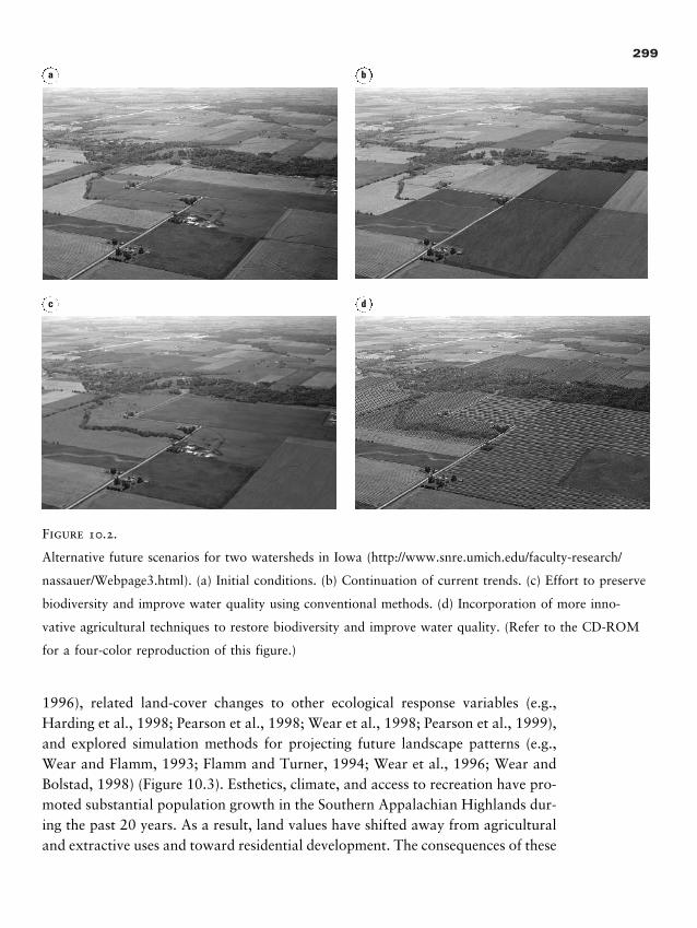
299

Figure 10.2.

Alternative future scenarios for two watersheds in Iowa (http://www.snre.umich.edu/faculty-research/

nassauer/Webpage3.html). (a) Initial conditions. (b) Continuation of current trends. (c) Effort to preserve

biodiversity and improve water quality using conventional methods. (d) Incorporation of more inno-

vative agricultural techniques to restore biodiversity and improve water quality. (Refer to the CD-ROM

for a four-color reproduction of this figure.)

1996), related land-cover changes to other ecological response variables (e.g.,Harding et al., 1998; Pearson et al., 1998; Wear et al., 1998; Pearson et al., 1999),and explored simulation methods for projecting future landscape patterns (e.g.,Wear and Flamm, 1993; Flamm and Turner, 1994; Wear et al., 1996; Wear andBolstad, 1998) (Figure 10.3). Esthetics, climate, and access to recreation have pro-moted substantial population growth in the Southern Appalachian Highlands dur-ing the past 20 years. As a result, land values have shifted away from agriculturaland extractive uses and toward residential development. The consequences of these

a b

c d

2888_e10_p289-326 2/27/01 1:52 PM Page 299

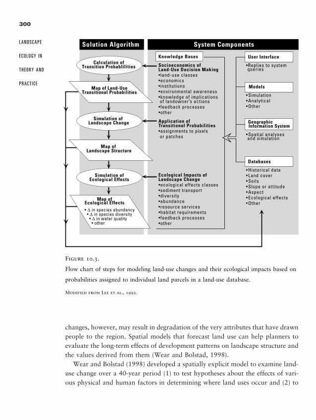
changes, however, may result in degradation of the very attributes that have drawnpeople to the region. Spatial models that forecast land use can help planners toevaluate the long-term effects of development patterns on landscape structure andthe values derived from them (Wear and Bolstad, 1998).

Wear and Bolstad (1998) developed a spatially explicit model to examine land-use change over a 40-year period (1) to test hypotheses about the effects of vari-ous physical and human factors in determining where land uses occur and (2) to

300

L A N D S C A P E

E C O L O G Y I N

T H E O R Y A N D

P R A C T I C E

Solution Algorithm System Components

Calculation ofTransition Probablilities

Map of Land-UseTransitional Probabilities

Simulation of Landscape Change

Map of Landscape Structure

Simulation ofEcological Effects

Map ofEcological Effects

Knowledge Bases

Socioeconomics of Land-Use Decision Making•land-use classes•economics•institutions•environmental awareness•knowledge of implications of landowner’s actions•feedback processes•other

Application ofTransitional Probabilities•assignments to pixels or patches

Ecological Impacts ofLandscape Change•ecological effects classes•sediment transport•diversity•abundance•resource services •habitat requirements•feedback processes•other

Models

• Simulation• Analytical• Other

Geographic Information System

• Spatial analyses and simulation

Databases

• Historical data• Land cover• Soils• Slope or attitude• Aspect• Ecological effects• Other

User Interface

•Replies to system queries

• ∆ in species abundancy • ∆ in species diversity • ∆ in water quality • other

Figure 10.3.

Flow chart of steps for modeling land-use changes and their ecological impacts based on

probabilities assigned to individual land parcels in a land-use database.

Modified from Lee et al., 1992.

2888_e10_p289-326 2/27/01 1:52 PM Page 300

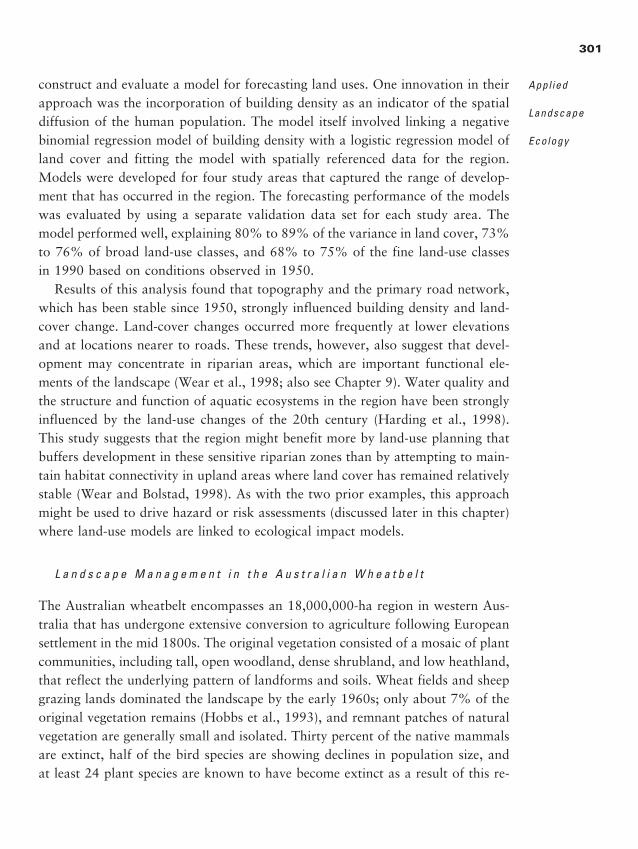
construct and evaluate a model for forecasting land uses. One innovation in theirapproach was the incorporation of building density as an indicator of the spatialdiffusion of the human population. The model itself involved linking a negativebinomial regression model of building density with a logistic regression model ofland cover and fitting the model with spatially referenced data for the region.Models were developed for four study areas that captured the range of develop-ment that has occurred in the region. The forecasting performance of the modelswas evaluated by using a separate validation data set for each study area. Themodel performed well, explaining 80% to 89% of the variance in land cover, 73%to 76% of broad land-use classes, and 68% to 75% of the fine land-use classesin 1990 based on conditions observed in 1950.

Results of this analysis found that topography and the primary road network,which has been stable since 1950, strongly influenced building density and land-cover change. Land-cover changes occurred more frequently at lower elevationsand at locations nearer to roads. These trends, however, also suggest that devel-opment may concentrate in riparian areas, which are important functional ele-ments of the landscape (Wear et al., 1998; also see Chapter 9). Water quality andthe structure and function of aquatic ecosystems in the region have been stronglyinfluenced by the land-use changes of the 20th century (Harding et al., 1998).This study suggests that the region might benefit more by land-use planning thatbuffers development in these sensitive riparian zones than by attempting to main-tain habitat connectivity in upland areas where land cover has remained relativelystable (Wear and Bolstad, 1998). As with the two prior examples, this approachmight be used to drive hazard or risk assessments (discussed later in this chapter)where land-use models are linked to ecological impact models.

L a n d s c a p e M a n a g e m e n t i n t h e A u s t r a l i a n W h e a t b e l t

The Australian wheatbelt encompasses an 18,000,000-ha region in western Aus-tralia that has undergone extensive conversion to agriculture following Europeansettlement in the mid 1800s. The original vegetation consisted of a mosaic of plantcommunities, including tall, open woodland, dense shrubland, and low heathland,that reflect the underlying pattern of landforms and soils. Wheat fields and sheepgrazing lands dominated the landscape by the early 1960s; only about 7% of theoriginal vegetation remains (Hobbs et al., 1993), and remnant patches of naturalvegetation are generally small and isolated. Thirty percent of the native mammalsare extinct, half of the bird species are showing declines in population size, andat least 24 plant species are known to have become extinct as a result of this re-

301

Appl ied

Landscape

Ecology

2888_e10_p289-326 2/27/01 1:52 PM Page 301

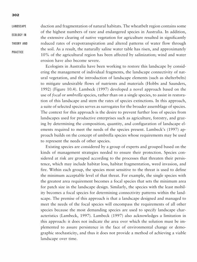
duction and fragmentation of natural habitats. The wheatbelt region contains someof the highest numbers of rare and endangered species in Australia. In addition,the extensive clearing of native vegetation for agriculture resulted in significantlyreduced rates of evapotranspiration and altered patterns of water flow throughthe soil. As a result, the naturally saline water table has risen, and approximately10% of the agricultural region has been affected by salinization; wind and watererosion have also become severe.

Ecologists in Australia have been working to restore this landscape by consid-ering the management of individual fragments, the landscape connectivity of nat-ural vegetation, and the introduction of landscape elements (such as shelterbelts)to mitigate undesirable flows of nutrients and materials (Hobbs and Saunders,1992) (Figure 10.4). Lambeck (1997) developed a novel approach based on theuse of focal or umbrella species, rather than on a single species, to assist in restora-tion of this landscape and stem the rates of species extinctions. In this approach,a suite of selected species serves as surrogates for the broader assemblage of species.The context for this approach is the desire to prevent further loss of species fromlandscapes used for productive enterprises such as agriculture, forestry, and graz-ing by determining the composition, quantity, and configuration of landscape el-ements required to meet the needs of the species present. Lambeck’s (1997) ap-proach builds on the concept of umbrella species whose requirements may be usedto represent the needs of other species.

Existing species are considered by a group of experts and grouped based on thekinds of management strategies needed to ensure their protection. Species con-sidered at risk are grouped according to the processes that threaten their persis-tence, which may include habitat loss, habitat fragmentation, weed invasion, andfire. Within each group, the species most sensitive to the threat is used to definethe minimum acceptable level of that threat. For example, the single species withthe greatest area requirement becomes a focal species that sets the minimum areafor patch size in the landscape design. Similarly, the species with the least mobil-ity becomes a focal species for determining connectivity patterns within the land-scape. The premise of this approach is that a landscape designed and managed tomeet the needs of the focal species will encompass the requirements of all otherspecies because the most demanding species are used to specify landscape char-acteristics (Lambeck, 1997). Lambeck (1997) also acknowledges a limitation inthis approach: it does not indicate the area over which the solution must be im-plemented to assure persistence in the face of environmental change or demo-graphic stochasticity, and thus it does not provide a method of achieving a viablelandscape over time.

302

L A N D S C A P E

E C O L O G Y I N

T H E O R Y A N D

P R A C T I C E

2888_e10_p289-326 2/27/01 1:52 PM Page 302

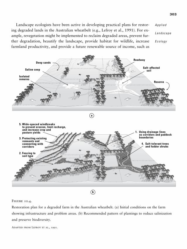
303

Appl ied

Landscape

Ecology

2. Fencing to soil type

5. Wide-spaced windbreaks to prevent erosion, limit recharge, and increase crop and pasture yields

3. Protecting existing remnants and connecting with corridors

4. Salt-tolerant trees and fodder shrubs

1. Using drainage lines as corridors and paddock boundaries

b

Saline seep

Isolated remains

Salt–affected soil

Reserve

RoadwayDeep sands

a

Figure 10.4.

Restoration plan for a degraded farm in the Australian wheatbelt. (a) Initial conditions on the farm

showing infrastructure and problem areas. (b) Recommended pattern of plantings to reduce salinization

and preserve biodiversity.

Adapted from Lefroy et al., 1991.

Landscape ecologists have been active in developing practical plans for restor-ing degraded lands in the Australian wheatbelt (e.g., Lefroy et al., 1991). For ex-ample, revegetation might be implemented to reclaim degraded areas, prevent fur-ther degradation, beautify the landscape, provide habitat for wildlife, increasefarmland productivity, and provide a future renewable source of income, such as

2888_e10_p289-326 2/27/01 1:53 PM Page 303

firewood, honey, or wildflowers (Lefroy et al., 1991). An example of the spatialimplementation of such a revegetation plan is shown in Figure 10.4. These typesof revegetation plans are developed and implemented at the scale of the farm, but they may eventually produce a connected mosaic across the whole landscape.Landscape restoration can help to mitigate problems of salinization and loss ofbiodiversity.

T r o p i c a l S l a s h - a n d - B u r n A g r i c u l t u r e

Agricultural land use is of particular concern in the tropics, where soils are oftenlow in organic matter and nutrients (Dixon et al., 1994). The carbon and nutri-ents are incorporated into the massive tree boles. As a result, a traditional agri-cultural practice known as slash and burn has been employed (Southworth et al.,1991). The tropical forest is cut and burned, and crops are then planted on theburned site. The burning transfers the nutrients from the trees back into the soil,permitting a few years of relatively high crop production. After the fertilizing ef-fect of the burning is exhausted, the farmer moves to a new plot and repeats theprocess.

The landscape impacts of these practices were studied in Rondonia, Brazil, anarea where development is being encouraged as a means of easing population pres-sures in the major cities (Southworth et al., 1991). A spatially explicit simulationmodel (Dale et al., 1993) was developed that included socioeconomic and eco-logical factors involved in the colonization process. The region was first dividedinto individual plots available to colonists and each simulated colonist was thenallowed to choose a lot based on local site conditions and distance to market.Colonists then decided on the percentage of the lot to clear, crops to plant, and,eventually, duration of occupancy. As colonization continued, the model calcu-lated the carbon lost to the atmosphere as a result of both combustion and de-composition, changes to landscape structure, and the potential impacts on wildlife.In the worst-case scenario, the rate of land clearing was rapid and the naturalhabitat was quickly fragmented. In the best-case scenario, more sustainable land-use practices were implemented and less land was cleared. The worst-case scenarioproduced about three times more carbon released to the atmosphere than the best-case scenario (Dale et al., 1994a).

The impacts of slash-and-burn agriculture on biodiversity were assessed by con-sideration of the habitat requirements for more than 100 individual species (Of-ferman et al., 1995). In tropical forests, many species, such as primates and treefrogs, never descend from the canopy and are therefore unable to disperse across

304

L A N D S C A P E

E C O L O G Y I N

T H E O R Y A N D

P R A C T I C E

2888_e10_p289-326 2/27/01 1:53 PM Page 304

305

Appl ied

Landscape

Ecology

gaps. Other species, such as bees that pollinate rare orchids, will not cross gapsgreater than 100 m. Therefore, fragmentation in these ecosystems would appearto have a drastic impact on the animal community, particularly those species thathave large area requirements and low gap-crossing ability (Figure 10.5). For ex-ample, under the worst-case scenario of land use, 40% of the area is unusable bythe tree frogs within 7 years (Dale et al., 1994b).

The Rondonia project required an interdisciplinary approach to address com-plex problems in agricultural land-use management. The results showed that in-dividual decisions made by the colonists based on socioeconomic considerations,such as the cost to transport their product to the marketplace, have serious con-sequences for land-use change in this region. However, collective decisions by the

Are

a (

103 h

a)A

rea

(10

3 ha)

TypicalWorstSustainable

1 3 5 7 9 11 13 15 17 20 25 30 35 40 0

50

100

150

200

250

1 3 5 7 9 11 13 15 17 20 25 30 35 40 0

50

100

150

200

250

Year

Year

Agriculturalscenario

a

b

Figure 10.5.

Area of suitable habitat available to fauna (a)

with area requirements proportional to gap-

crossing ability and (b) with large area require-

ments and low gap-crossing ability under alter-

native scenarios of deforestation in Rondonia,

Brazil. The simulation model predicted patterns

of forest clearing under the typical scenario, in

which farmers clear �3 ha per year; the worst-

case scenario, based on the most extreme land-

use practices of colonists who settled along the

Transamazon highway; and the best-case sce-

nario, based on an ecologically innovative farm-

ing system in which burning is rare, there is no

income from cattle, and a variety of perennial

crops are grown.

From Dale et al., 1994b.

2888_e10_p289-326 2/27/01 1:53 PM Page 305

community can either enhance or mitigate these effects; for instance, higher taxeson properties nearer to market result in distant lots being more attractive eco-nomically, and colonists then disperse over a wider region. Thus, an integratedlandscape model makes it possible to extrapolate the management practices andland-use pattern to determine potential environmental impacts.

L a n d U s e : S y n t h e s i s

The question about land use is not whether we should or should not use land, butrather how we can best use the land (Turner et al., 1998a). The answer, however,is complex; there are no “cook book” approaches for identifying the optimalarrangement. Landscape ecology contributes principles and techniques for con-sidering how to arrange human structures spatially and identify potential ecolog-ical implications of alternative arrangements. This has been illustrated in the pre-ceding examples, although models that truly integrate a wide range of ecologicalimpacts (e.g., habitat for various species, water quality, biogeochemistry) havebeen rare, and they reflect an area of active current research.

Santelmann et al. (in press) identified five conditions that must be met for prac-tical application of ecological principles in land-use decision making.

1. Decision makers must understand the need and share the goal.2. Abstract principles must be translated into specific land-use decisions.3. Responsibility for associated costs and labor (which tend to occur up front

and are specific to place) must be assigned and accepted (made economi-cally feasible).

4. Benefits (which tend to be realized in the longer term and diffuse in space)must be understood and shown to have value.

5. Practices must be culturally acceptable (this includes respect for the rightsof property owners).

Land-use models that truly integrate social, economic, and ecological consid-erations are in their infancy, and no consensus has yet been reached about whatapproaches are best for this task (Dale et al., 2000). Although recent models ofland-use change often seem simplistic, they are at the forefront of landscape inte-gration (e.g., Wilkie and Finn, 1988; Southworth et al., 1991; Baker, 1992; Leeet al., 1992; Dale et al., 1993, 1994a, b; Riebsame et al., 1994; Gilruth et al.,1995; Turner et al., 1996; Wear et al., 1996; Wear and Bolstad, 1998). Althoughthe many diverse factors [including human perceptions, economic systems, mar-

306

L A N D S C A P E

E C O L O G Y I N

T H E O R Y A N D

P R A C T I C E

2888_e10_p289-326 2/27/01 1:53 PM Page 306

ket and resource demands, foreign relations (e.g., trade agreements), fluctuationsin interest rates, and pressure for environmental conservation and maintenance ofecosystem goods and services] that interact to determine patterns of land use arerecognized conceptually, the quantitative relationships among these variables arepoorly known. This interface is a key challenge facing the scientific community inthe coming decades.

Interdisciplinary studies are often complex (e.g., Naiman, 1999; Pickett et al.,1999; Turner and Carpenter, 1999; Wear, 1999), but there should be strong en-couragement to develop the required integration. Riebsame et al. (1994) make sev-eral suggestions for improved, integrated land-use, land-cover modeling: (1) im-proved methods and approaches for integrating sociocultural factors, becausesocial driving forces must be coupled with their ecological effects and feedbacksto society; (2) modeling interactions among multiple resources, not just one ortwo; (3) modeling cumulative effects, particularly when a threshold response (e.g.,sudden disconnection of habitat) may be likely; (4) dealing with surprise, such asunusual conditions, rapid change, and others that may come from the environ-ment or society. It is important to reiterate the sentiments expressed by Riebsameet al. (1994), who wrote, “Our limited ability to simulate realistic land-use pat-terns is not just a modeling problem, but a reflection of the real world.” We con-cur with this evaluation and suggest that this area of applied research presents acompelling challenge to landscape ecology that will persist for the coming years.

F O R E S T M A N A G E M E N T

Forest management practices have an immediate impact on the spatial pattern on thelandscape. Natural disturbance regimes create openings that vary in size, shape, andlocation (see Chapter 7). Harvesting creates clear-cut patches of distinct size andarrangement, and different harvesting strategies produce different landscape patterns(Franklin and Forman, 1987). Landscape ecological research in forest managementhas focused on (1) establishing the relationship between harvesting strategy and theresultant spatial pattern on the landscape and (2) determining how to minimize ad-verse effects such as habitat fragmentation and loss of old-growth forest. Spatial mod-els have been important tools in studies evaluating the implications of alternative har-vest strategies (e.g., Franklin and Forman, 1987; Li et al., 1993; Gustafson and Crow,1996; Mladenoff and Baker, 1999). We have discussed many issues of forest man-agement in the preceding chapters. In this section, we highlight two real-world ex-

307

Appl ied

Landscape

Ecology

�

2888_e10_p289-326 2/27/01 1:53 PM Page 307

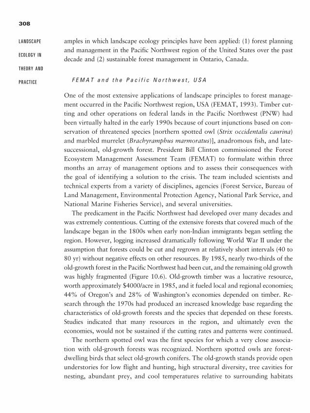
amples in which landscape ecology principles have been applied: (1) forest planningand management in the Pacific Northwest region of the United States over the pastdecade and (2) sustainable forest management in Ontario, Canada.

F E M A T a n d t h e P a c i f i c N o r t h w e s t , U S A

One of the most extensive applications of landscape principles to forest manage-ment occurred in the Pacific Northwest region, USA (FEMAT, 1993). Timber cut-ting and other operations on federal lands in the Pacific Northwest (PNW) hadbeen virtually halted in the early 1990s because of court injunctions based on con-servation of threatened species [northern spotted owl (Strix occidentalis caurina)and marbled murrelet (Brachyramphus marmoratus)], anadromous fish, and late-successional, old-growth forest. President Bill Clinton commissioned the ForestEcosystem Management Assessment Team (FEMAT) to formulate within threemonths an array of management options and to assess their consequences withthe goal of identifying a solution to the crisis. The team included scientists andtechnical experts from a variety of disciplines, agencies (Forest Service, Bureau ofLand Management, Environmental Protection Agency, National Park Service, andNational Marine Fisheries Service), and several universities.

The predicament in the Pacific Northwest had developed over many decades andwas extremely contentious. Cutting of the extensive forests that covered much of thelandscape began in the 1800s when early non-Indian immigrants began settling theregion. However, logging increased dramatically following World War II under theassumption that forests could be cut and regrown at relatively short intervals (40 to80 yr) without negative effects on other resources. By 1985, nearly two-thirds of theold-growth forest in the Pacific Northwest had been cut, and the remaining old growthwas highly fragmented (Figure 10.6). Old-growth timber was a lucrative resource,worth approximately $4000/acre in 1985, and it fueled local and regional economies;44% of Oregon’s and 28% of Washington’s economies depended on timber. Re-search through the 1970s had produced an increased knowledge base regarding thecharacteristics of old-growth forests and the species that depended on these forests.Studies indicated that many resources in the region, and ultimately even theeconomies, would not be sustained if the cutting rates and patterns were continued.

The northern spotted owl was the first species for which a very close associa-tion with old-growth forests was recognized. Northern spotted owls are forest-dwelling birds that select old-growth conifers. The old-growth stands provide openunderstories for low flight and hunting, high structural diversity, tree cavities fornesting, abundant prey, and cool temperatures relative to surrounding habitats

308

L A N D S C A P E

E C O L O G Y I N

T H E O R Y A N D

P R A C T I C E

2888_e10_p289-326 2/27/01 1:53 PM Page 308

888262

20

1940sYear

Old

-gro

wth

fore

st (t

hous

ands

of h

ecta

res)

Tota

ls in

pat

ch-s

ize

cate

gori

es (t

hous

ands

of h

ecta

res)

0–4 4–40 40–400

400–4,000

4,000 –40,000

Over40,000

Patch size category (hectares)

1940s

1988

Oldgrowth

Maturewithold

trees

Youngwithold

trees

High- elevation

oldforest

Stuntedold

forest

Mature forest

Forest–type category

Forest in 114-meter edge zone

Interior forest

8

16

24

32

40

48

56

64

72

40

60

80

100

120

140

160

0

Fore

sted

are

a (t

hous

ands

of h

ecta

res)

8

16

24

32

40

48

56

64

a

b

c

Figure 10.6.

Recent and historical changes in the abundance

of old-growth forest and its spatial pattern on

the Olympic Peninsula, Washington: (a) area of

old-growth forest through time; (b) frequency

distribution of old-growth by patch size in the

1940s and 1980s showing the dramatic decline

in the number of large patches; (c) area of dif-

ferent forest types considered to constitute inte-

rior forest, located more than 114 m from the

edge of a patch in 1988.

After Morrison et al., 1991.

2888_e10_p289-326 2/27/01 1:53 PM Page 309

(the owls have a narrow thermal-neutral zone with makes them susceptible to heatstress). Historically, the owls ranged between southern California and the SierraNevada Mountains to British Columbia. Pairs form long-term bonds and occupylarge home ranges (�800 ha). The owls are also long-lived, with high annual adultsurvival rates (0.8 to 0.95) and low reproductive rates (�1 fledgling/yr with vari-able nesting frequencies). Juveniles fledge in the autumn and disperse over longdistance (up to 150 km), even over unsuitable habitat, in their search for territo-ries and mates. The spotted owl population was estimated to have declined by50% from historical numbers, with metapopulation structure having been pro-duced by human-induced habitat changes. Forest harvest was primarily clear-cutting, which eliminated suitable habitat completely.

Although the owl was the focus of much attention (and legal action), FEMATwas given a broader charge—to develop long-term management alternatives formaintaining biological diversity that met the following objectives (FEMAT, 1993):maintenance and/or restoration of habitat conditions for the northern spotted owland the marbled murrelet that will provide for viability of each species; mainte-nance and/or restoration of habitat conditions to support viable populations, welldistributed across their current range, of species known to be associated with old-growth forest conditions; maintenance and/or restoration of spawning and rear-ing habitat on federal lands to support recovery and maintenance of viable pop-ulations of anadromous fish species and other at-risk fish species and stocks; andmaintenance and/or creation of a connected or interactive old-growth forest ecosys-tem on the federal lands within the region. In addition, management options forhabitat adjacent to streams were developed to conserve aquatic, riparian, and wet-land habitats, and stream corridors were to be protected.

In addition to consideration of the ecological effects of management options,FEMAT was charged with addressing a broad range of forest resource outputsand their economic implications. The economic assessments were designed to eval-uate resource yields and values, local and regional economic conditions (e.g., em-ployment), National Forest product markets, and other policy considerations.Commodity products considered included timber, special forest products (e.g.,mushrooms, boughs, ferns), livestock grazing, commercial fisheries, and minerals.Noncommodity outputs such as recreation, scenic quality, water and air quality,and other public goods were also considered. Social assessment of the options wasalso conducted to provide policy makers with an understanding of how potentialpolicy options might affect important social values and activities.

FEMAT eventually developed and compared a total of ten options, which var-ied in four principal respects: the quantity and location of land placed in some

310

L A N D S C A P E

E C O L O G Y I N

T H E O R Y A N D

P R A C T I C E

2888_e10_p289-326 2/27/01 1:53 PM Page 310

form of reserve; the activities permitted within the reserve area; the delineation ofthe matrix, or the areas outside the reserves; and the activities allowed within thematrix. Reserves were of two types, either old growth or riparian. Buffers of vary-ing widths around permanent and intermittent streams were considered in all op-tions. For timber harvesting in the matrix, guidelines were established to reducecontrast between the reserves and the matrix and facilitate movement of juvenileand spotted owls across the landscape. For example, the 50–11–40 rule called for50% of the federal forested land within each quarter-township to be in forestedcondition with trees averaging at least 11 inches in diameter at breast height andwith a canopy closure of at least 40%. In addition, guidelines that varied the re-tention of live or green trees within cut areas were considered.

Landscape and metapopulation concepts both played an important role in the FE-MAT assessment. Shaffer (1985) had first suggested the application of metapopula-tion concepts to owl management. Shaffer (1985) considered the arrangement ofhabitat, recommending maintenance of the same spatial distribution of average sizeand spacing of present-day patches and moving away from population viability analy-sis, which focused only on population size. Lande (1987, 1988) developed the firstmodels, and his results demonstrated that populations of territorial animals wouldcollapse when habitat abundance declines below a threshold (he suggested 20%).These models were not spatially explicit, assuming that every patch or territory wasequally accessible to all others. The spatially explicit models developed by KevinMcKelvey, Roland Lamberson, and Barry Noon were first introduced in the ThomasReport (Thomas et al., 1990; Noon and McKelvey, 1996b). Results suggested thata viable metapopulation could be maintained by a network of habitat conservationareas greater than 20 territories and spaced �19.2 km apart. Results also highlighteda time lag between habitat fragmentation and population decline.

The importance of landscape structure and landscape context was evidentthroughout the FEMAT process and in the development of the owl recovery plan.Analysis of landscape structure, especially the amount and spatial arrangement ofold growth, was fundamental to the assessment process, as were the spatial pro-jections of the alternatives. The effects of landscape context were reflected in the50–11–40 rule for management of the matrix surrounding habitat conservationareas. This acknowledged that landscape surroundings may be more importantthan narrow habitat corridors in promoting movements and linkages among sub-populations. The plan set aside 7.4 million acres as a reserve for species that de-pend on old-growth forest and 2.6 million acres as riparian reserves; harvestingis not permitted in these reserves. An additional 1.5 million acres was set asidefor experimentation with new harvesting approaches designed to avoid habitat

311

Appl ied

Landscape

Ecology

2888_e10_p289-326 2/27/01 1:53 PM Page 311

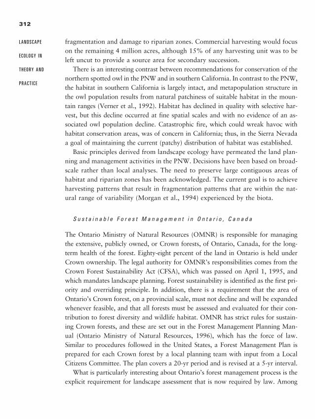
fragmentation and damage to riparian zones. Commercial harvesting would focuson the remaining 4 million acres, although 15% of any harvesting unit was to beleft uncut to provide a source area for secondary succession.

There is an interesting contrast between recommendations for conservation of thenorthern spotted owl in the PNW and in southern California. In contrast to the PNW,the habitat in southern California is largely intact, and metapopulation structure inthe owl population results from natural patchiness of suitable habitat in the moun-tain ranges (Verner et al., 1992). Habitat has declined in quality with selective har-vest, but this decline occurred at fine spatial scales and with no evidence of an as-sociated owl population decline. Catastrophic fire, which could wreak havoc withhabitat conservation areas, was of concern in California; thus, in the Sierra Nevadaa goal of maintaining the current (patchy) distribution of habitat was established.

Basic principles derived from landscape ecology have permeated the land plan-ning and management activities in the PNW. Decisions have been based on broad-scale rather than local analyses. The need to preserve large contiguous areas ofhabitat and riparian zones has been acknowledged. The current goal is to achieveharvesting patterns that result in fragmentation patterns that are within the nat-ural range of variability (Morgan et al., 1994) experienced by the biota.

S u s t a i n a b l e F o r e s t M a n a g e m e n t i n O n t a r i o , C a n a d a

The Ontario Ministry of Natural Resources (OMNR) is responsible for managingthe extensive, publicly owned, or Crown forests, of Ontario, Canada, for the long-term health of the forest. Eighty-eight percent of the land in Ontario is held underCrown ownership. The legal authority for OMNR’s responsibilities comes from theCrown Forest Sustainability Act (CFSA), which was passed on April 1, 1995, andwhich mandates landscape planning. Forest sustainability is identified as the first pri-ority and overriding principle. In addition, there is a requirement that the area ofOntario’s Crown forest, on a provincial scale, must not decline and will be expandedwhenever feasible, and that all forests must be assessed and evaluated for their con-tribution to forest diversity and wildlife habitat. OMNR has strict rules for sustain-ing Crown forests, and these are set out in the Forest Management Planning Man-ual (Ontario Ministry of Natural Resources, 1996), which has the force of law.Similar to procedures followed in the United States, a Forest Management Plan isprepared for each Crown forest by a local planning team with input from a LocalCitizens Committee. The plan covers a 20-yr period and is revised at a 5-yr interval.

What is particularly interesting about Ontario’s forest management process is theexplicit requirement for landscape assessment that is now required by law. Among

312

L A N D S C A P E

E C O L O G Y I N

T H E O R Y A N D

P R A C T I C E

2888_e10_p289-326 2/27/01 1:53 PM Page 312

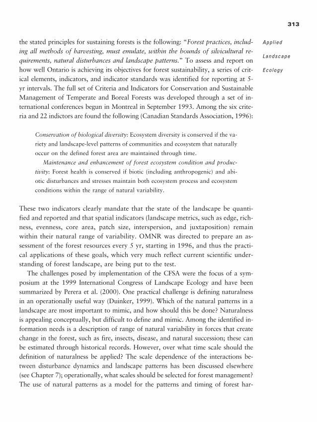
the stated principles for sustaining forests is the following: “Forest practices, includ-ing all methods of harvesting, must emulate, within the bounds of silvicultural re-quirements, natural disturbances and landscape patterns.” To assess and report onhow well Ontario is achieving its objectives for forest sustainability, a series of crit-ical elements, indicators, and indicator standards was identified for reporting at 5-yr intervals. The full set of Criteria and Indicators for Conservation and SustainableManagement of Temperate and Boreal Forests was developed through a set of in-ternational conferences begun in Montreal in September 1993. Among the six crite-ria and 22 indictors are found the following (Canadian Standards Association, 1996):

Conservation of biological diversity: Ecosystem diversity is conserved if the va-

riety and landscape-level patterns of communities and ecosystem that naturally

occur on the defined forest area are maintained through time.

Maintenance and enhancement of forest ecosystem condition and produc-

tivity: Forest health is conserved if biotic (including anthropogenic) and abi-

otic disturbances and stresses maintain both ecosystem process and ecosystem

conditions within the range of natural variability.

These two indicators clearly mandate that the state of the landscape be quanti-fied and reported and that spatial indicators (landscape metrics, such as edge, rich-ness, evenness, core area, patch size, interspersion, and juxtaposition) remainwithin their natural range of variability. OMNR was directed to prepare an as-sessment of the forest resources every 5 yr, starting in 1996, and thus the practi-cal applications of these goals, which very much reflect current scientific under-standing of forest landscape, are being put to the test.

The challenges posed by implementation of the CFSA were the focus of a sym-posium at the 1999 International Congress of Landscape Ecology and have beensummarized by Perera et al. (2000). One practical challenge is defining naturalnessin an operationally useful way (Duinker, 1999). Which of the natural patterns in alandscape are most important to mimic, and how should this be done? Naturalnessis appealing conceptually, but difficult to define and mimic. Among the identified in-formation needs is a description of range of natural variability in forces that createchange in the forest, such as fire, insects, disease, and natural succession; these canbe estimated through historical records. However, over what time scale should thedefinition of naturalness be applied? The scale dependence of the interactions be-tween disturbance dynamics and landscape patterns has been discussed elsewhere(see Chapter 7); operationally, what scales should be selected for forest management?The use of natural patterns as a model for the patterns and timing of forest har-

313

Appl ied

Landscape

Ecology

2888_e10_p289-326 2/27/01 1:53 PM Page 313

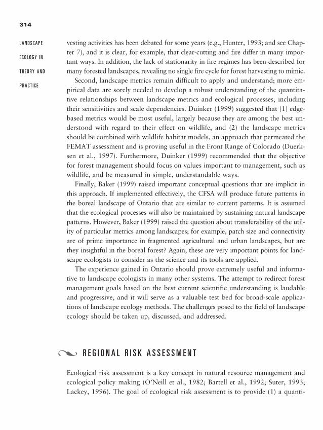
vesting activities has been debated for some years (e.g., Hunter, 1993; and see Chap-ter 7), and it is clear, for example, that clear-cutting and fire differ in many impor-tant ways. In addition, the lack of stationarity in fire regimes has been described formany forested landscapes, revealing no single fire cycle for forest harvesting to mimic.

Second, landscape metrics remain difficult to apply and understand; more em-pirical data are sorely needed to develop a robust understanding of the quantita-tive relationships between landscape metrics and ecological processes, includingtheir sensitivities and scale dependencies. Duinker (1999) suggested that (1) edge-based metrics would be most useful, largely because they are among the best un-derstood with regard to their effect on wildlife, and (2) the landscape metricsshould be combined with wildlife habitat models, an approach that permeated theFEMAT assessment and is proving useful in the Front Range of Colorado (Duerk-sen et al., 1997). Furthermore, Duinker (1999) recommended that the objectivefor forest management should focus on values important to management, such aswildlife, and be measured in simple, understandable ways.

Finally, Baker (1999) raised important conceptual questions that are implicit inthis approach. If implemented effectively, the CFSA will produce future patterns inthe boreal landscape of Ontario that are similar to current patterns. It is assumedthat the ecological processes will also be maintained by sustaining natural landscapepatterns. However, Baker (1999) raised the question about transferability of the util-ity of particular metrics among landscapes; for example, patch size and connectivityare of prime importance in fragmented agricultural and urban landscapes, but arethey insightful in the boreal forest? Again, these are very important points for land-scape ecologists to consider as the science and its tools are applied.

The experience gained in Ontario should prove extremely useful and informa-tive to landscape ecologists in many other systems. The attempt to redirect forestmanagement goals based on the best current scientific understanding is laudableand progressive, and it will serve as a valuable test bed for broad-scale applica-tions of landscape ecology methods. The challenges posed to the field of landscapeecology should be taken up, discussed, and addressed.

R E G I O N A L R I S K A S S E S S M E N T

Ecological risk assessment is a key concept in natural resource management andecological policy making (O’Neill et al., 1982; Bartell et al., 1992; Suter, 1993;Lackey, 1996). The goal of ecological risk assessment is to provide (1) a quanti-

314

L A N D S C A P E

E C O L O G Y I N

T H E O R Y A N D

P R A C T I C E

�

2888_e10_p289-326 2/27/01 1:53 PM Page 314

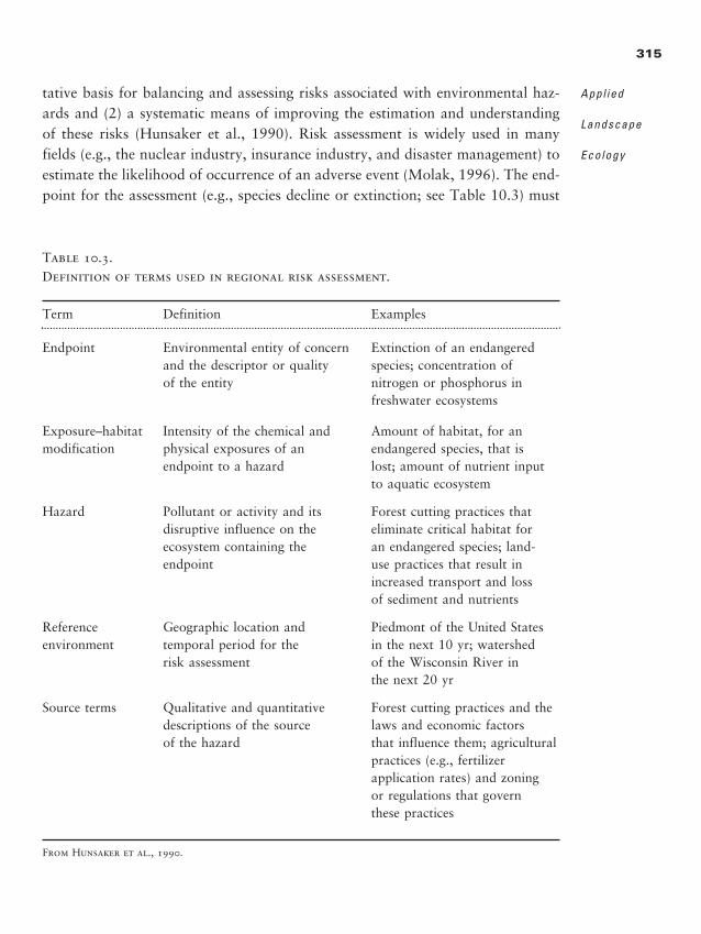
tative basis for balancing and assessing risks associated with environmental haz-ards and (2) a systematic means of improving the estimation and understandingof these risks (Hunsaker et al., 1990). Risk assessment is widely used in manyfields (e.g., the nuclear industry, insurance industry, and disaster management) toestimate the likelihood of occurrence of an adverse event (Molak, 1996). The end-point for the assessment (e.g., species decline or extinction; see Table 10.3) must

315

Appl ied

Landscape

Ecology

Table 10.3.Definition of terms used in regional risk assessment.

Term Definition Examples

Endpoint Environmental entity of concern Extinction of an endangeredand the descriptor or quality species; concentration of of the entity nitrogen or phosphorus in

freshwater ecosystems

Exposure–habitat Intensity of the chemical and Amount of habitat, for anmodification physical exposures of an endangered species, that is

endpoint to a hazard lost; amount of nutrient input to aquatic ecosystem

Hazard Pollutant or activity and its Forest cutting practices thatdisruptive influence on the eliminate critical habitat for ecosystem containing the an endangered species; land-endpoint use practices that result in

increased transport and loss of sediment and nutrients

Reference Geographic location and Piedmont of the United States environment temporal period for the in the next 10 yr; watershed

risk assessment of the Wisconsin River in the next 20 yr

Source terms Qualitative and quantitative Forest cutting practices and thedescriptions of the source laws and economic factors of the hazard that influence them; agricultural

practices (e.g., fertilizerapplication rates) and zoning or regulations that govern these practices

From Hunsaker et al., 1990.

2888_e10_p289-326 2/27/01 1:53 PM Page 315

be defined a priori and the probability of observing the endpoint is estimated,given all the stochastic effects and uncertainties involved (O’Neill et al., 1982).

Concepts of landscape ecology have been particularly useful in developing riskassessment approaches that can address questions of long-term management of re-sources over larger areas (Hunsaker et al., 1990; Graham et al., 1991). Environ-mental hazards occur over a wide range of spatial and temporal scales. Some haz-ards affect large regions (e.g., acid deposition, global climatic warming, nitrogensaturation) and some are clearly influenced by landscape configuration (e.g., non-point pollution; see Chapter 9). Regional risk assessment was developed for situ-ations in which either the cause or the consequence of the environmental hazardwas regional in its extent (Hunsaker et al., 1990). Note that a local phenomenoncan have a regional consequence (e.g., single-source pollutants that become widelydispersed or loss of a species’ critical source habitat, which results in a broad-scalepopulation decline), or multiple, local factors can combine to create a regionalhazard to a population, species, or ecosystem that is widely dispersed.

Regional (and local) risk assessments have two distinct phases. The first phasefocuses on a hazard definition that establishes the endpoints, source terms, andreference environment of the problem being studied. In essence, this is the con-ceptualization of the problem, and much discussion often surrounds this aspect ofrisk assessment (Lackey, 1996). In the second phase, or problem solution, the ex-posures and effects are assessed, and the exposure levels are related to the effectslevels to determine risk. A variety of specialized techniques is employed to deter-mine the probability of occurrence of the adverse endpoint. In a regional risk as-sessment, the spatial characteristics of the regional landscape and any spatial char-acteristics associated with exposure or effects of exposure are included (Grahamet al., 1991).

A prototype regional risk assessment was developed by Graham et al. (1991)for the Adirondack Mountains, located in north central New York. The Adiron-dack Mountains have been studied extensively with regard to acid deposition, andthe region has experienced increased atmospheric concentrations of ozone. Ele-vated ozone concentrations result in physiological stress on trees, particularlyconifers (Heck et al., 1986), and stressed trees are more susceptible to bark bee-tle infestations that, in turn, result in tree-killed patches that range in size from afew trees to �25 ha. The bark beetle attacks reduce interior forest habitat and in-crease forest-edge habitat. The loss of conifers with their acidic needle litter canalso change the pH of small mountain lakes that receive runoff from the affectedwatershed.

316

L A N D S C A P E

E C O L O G Y I N

T H E O R Y A N D

P R A C T I C E

2888_e10_p289-326 2/27/01 1:53 PM Page 316

Graham et al. (1991) used regional risk assessment to examine the ozone–beetle complex. They began with a map of land use for a 300,000-ha area in theAdirondacks that contained 66 small lakes. A simulation model was used to im-pose an ozone stress (low or high) across the study region, which then increasedthe probability of beetle infestation. The location and size of bark beetle attackswere selected at random, and the resulting change in landscape pattern (e.g., for-est edge) was determined. Most bark beetle infestations produced patches thatwere one grid cell (4 ha) in size. However, the high-ozone concentration resultedin more and larger patches of beetle-induced conifer mortality than did the low-ozone concentration scenario. The model was run 100 times for two scenarios ofelevated ozone concentrations. Each altered landscape then was used as input ina second model that related land cover to lake water quality (Hunsaker et al.,1986). To calculate the risk of a significant impact, the percentage of the 100model runs that showed a significant (�25%) change in pH was calculated. Ifthere was a 25% change in 50% of the runs, then the risk, or probability, of theozone–beetle complex causing a significant impact on water acidity was 0.5.

Simulation results revealed that forest edge increased in all cases (risk � 1.00for both ozone concentration levels) and that significant shifts in lake pH werelikely (risk � 0.89). A variety of pattern-sensitive endpoints (e.g., forest-edgelengths, contagion) was computed in the assessment, and most of these were in-fluenced by the ozone scenarios. Thus, this regional risk assessment approach com-bined existing information on land cover, ozone, and beetle attacks to estimatealterations in the landscape pattern and then to translate this change in patterninto the probability of an ecological impact. Methods employed included land-scape pattern analysis and spatial and stochastic modeling, with existing empiri-cal data used for parameterization.

An example of a regional risk assessment is provided by Riitters et al. (1997).Land-cover data for a region around the Chesapeake Bay, located in the mid-Atlantic region of the United States, were used to assess habitat suitability for avariety of organisms. Within a square window of grid cells (for which size wasdetermined based on the home range of the organism) on the land-cover map,simple rule-based algorithms were used to determine whether all habitat require-ments for the organism could be met within that window. The window was thenmoved over the entire region to determine the percentage of the area that pro-vides adequate habitat. Riitters et al. (1997) used home ranges of 5, 45, and 410ha and asked whether 90% of the window was forested. More complex habitatrequirements could be implemented. Risk to different species because of habitat

317

Appl ied

Landscape

Ecology

2888_e10_p289-326 2/27/01 1:53 PM Page 317

loss under alternative land-cover change scenarios could then be assessed for a va-riety of species. Although not called regional risk assessment by the authors, Whiteet al. (1997; see Chapter 8) employed this type of approach with alternative land-use scenarios and potential consequences on biodiversity in the Pocono Moun-tains, Pennsylvania.

A similar approach was also used by Hansen et al. (1993) to evaluate man-agement strategies in the Willamette National Forest in the Cascade Mountains,Oregon. Habitat data, including forest type, territory size, and sensitivity to edges,were collected for 51 species of birds. Using a land-cover map of the area, 140years of land-cover changes were simulated under a variety of management op-tions, such as intense forestry, no forestry, and a modified multiple-use harvestoption. Thus, this study linked spatial and temporal dynamics of the study region.Each management strategy was evaluated in terms of how it changed the per-centage of the area suitable for habitat for each of the 51 species, and the result-ing change in biodiversity as habitat was lost was estimated. This permitted a di-rect connection to be made between management strategies and risk to biodiversity.

The Gap Analysis Program of the U.S. Geological Survey, Biological ResourcesDivision (Scott et al., 1996) also utilizes a landscape approach for assessing re-gional risk to biodiversity. The greatest risk comes from the appropriation andfragmentation of natural cover for human use. At the scale of the ecoregion (a ge-ographic region with a characteristic set of integrated ecosystems, such as tundraor temperate desert; Bailey, 1998), remote imagery, aerial photography, andground surveys are combined in a geographic information system to produce land-cover maps. Existing land cover is compared to maps of potential vegetation coverto identify subregions in which impacts to ecological communities may be great-est. Maps of ownership are also examined to determine whether current owner-ship patterns offer appropriate levels of protection to biodiversity or whether pro-tected areas miss some critical subregions.

One example of the application of gap analysis is in the Mojave Desert, Cali-fornia (Thomas and Davis, 1996). A vegetation map recognized 32 natural vege-tation types, such as desert grassland and holly scrub. A land management mapwas superimposed on the vegetation map that distinguished (1) public ownershipwith well-developed preservation plans, (2) public ownership with a variety ofland uses, and (3) private ownership. The overlays permitted each vegetation typeto be characterized as adequately represented, poorly represented, or critically un-derrepresented in protected areas. Thus, gap analysis identifies subregions whereecosystem types are threatened; that is, there are gaps in regional protection. Ratherthan focusing on lists of individual endangered species, gap analysis recognizes

318

L A N D S C A P E

E C O L O G Y I N

T H E O R Y A N D

P R A C T I C E

2888_e10_p289-326 2/27/01 1:53 PM Page 318

that preservation of the intact ecosystem is of primary importance. Taking a broadlandscape approach may be the most practical approach to identifying threats andprioritizing policy decisions at the regional scale (Franklin, 1993).

C O N T I N E N T A L - S C A L E M O N I T O R I N G

An important application of landscape ecology is in the area of broad-scale mon-itoring. Satellite imagery of Earth’s surface is now collected routinely and is widelyavailable. Classification of repeated imagery can be analyzed over time to quantifychanges in land cover and landscape pattern. Landscape ecology provides a keystep in the process, making it possible to relate changes in surface patterns to eco-logical impacts, such as the loss of wildlife habitat and changes in water quality.

The Environmental Protection Agency’s Landscape Ecology Program is designedto establish the feasibility of this approach to monitoring and assessment (O’Neillet al., 1994). The program combines available data sets, such as land cover, ma-jor roads, topography, and population density, to quantify landscape changesthrough time. These changes are then related to ecological variables of interest todetermine the potential impact or risk. An example of this broad-scale monitor-ing is provided for watersheds in the Chesapeake Bay region (Riitters and Wick-ham, 1995). Streams that run through agricultural fields receive nutrients and siltfrom erosion. The effect is intensified if slopes are steep, since gravity acceleratesthe erosion process. Information on land cover and topography are then combinedto assess the risk to water quality. Figure 10.7 shows the watersheds in the regionthat are at the highest risk of impact on water quality when farming is adjacentto streams on slopes of �3%.

The concept of continental-scale monitoring has been expanded to the entireUnited States (O’Neill et al., 1997). In one analysis, the potential vegetation, de-termined by climate and topography (Kuchler, 1964), was compared to actual veg-etation, determined by satellite imagery (Loveland et al., 1991). The comparisonswere summarized by ecoregion (Omernick, 1987) to identify the areas with thegreatest risk to biodiversity that might occur as a consequence of habitat loss. Inanother analysis, land cover in major water resource regions (Seaber et al., 1984)was used to estimate nitrogen concentrations in surface waters using empirical re-lationships established by Omernick (1977). As time series of higher-resolutionimagery become available, it will be possible to monitor the risk to dozens of en-vironmental variables across the continent on an annual basis. However, the abil-

319

Appl ied

Landscape

Ecology

�

2888_e10_p289-326 2/27/01 1:53 PM Page 319

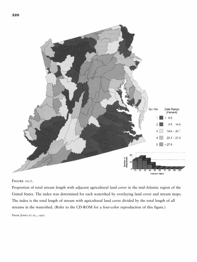
320

Figure 10.7.

Proportion of total stream length with adjacent agricultural land cover in the mid-Atlantic region of the

United States. The index was determined for each watershed by overlaying land cover and stream maps.

The index is the total length of stream with agricultural land cover divided by the total length of all

streams in the watershed. (Refer to the CD-ROM for a four-color reproduction of this figure.)

From Jones et al., 1997.

2888_e10_p289-326 2/27/01 1:53 PM Page 320

ity of scientists to quantify spatial patterns in numerous ways (see Chapter 5) stillexceeds our ability to relate these spatial patterns to ecological processes; furtherdevelopment of empirical data demonstrating linkages between landscape patternand ecological indicators remains a critical need. We suggest that the potential forlandscape monitoring to be truly effective depends on development of a muchstronger and more extensive library of case studies that relate the broad-scale land-scape metrics to measured ecological processes.

S U M M A R Y

Landscape ecology contributes to many different aspects of applied ecology. Resource managers have shifted their emphasis from management of separate re-sources to management focused on the integrity of entire ecosystems and land-scapes. Challenges facing resource managers often involve spatial interdependen-cies among landscape components, and demand for the scientific underpinningsof managing landscapes is high. Despite the acknowledged importance of a land-scape perspective by both scientists and resources managers, determining how toimplement management at broader scales is very much a work in progress (Turneret al., in press). Thus far, landscape ecology has contributed to a variety of ap-plications, including land use, forest management, risk assessment, and broad-scale monitoring. The demand for input from landscape ecologists to resourcemanagement decisions at all scales is very high.

Can lessons be extracted thus far from applications of landscape ecology? Wethink so. First, determining what is optimal for any given landscape is not straight-forward. Optimal is a value judgment, and the development of a consensus opin-ion is often an arduous process. It is difficult to balance the multiple criteria bywhich a landscape may be considered—economic output, persistence of biodiver-sity, maintenance of water quality, and adequate land for human development.Even when naturalness is identified as a goal for landscape condition, implementingsuch an objective is not straightforward. The landscape ecologist can provide arigorous analysis of alternative landscapes, including the potential implications forvarious ecological processes. However, the science still stumbles when an optimaltarget condition must be unambiguously identified, in part because such a deci-sion requires more than science.

Second, applied landscape ecology often requires a team approach; indeed, noneof the examples that we have highlighted in this chapter have resulted from sin-

321

Appl ied

Landscape

Ecology

�

2888_e10_p289-326 2/27/01 1:53 PM Page 321

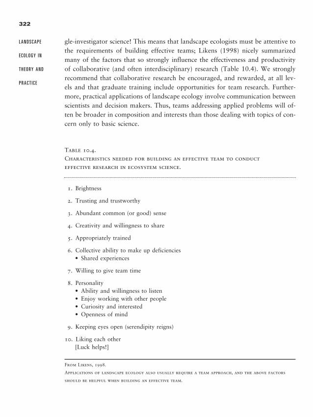
gle-investigator science! This means that landscape ecologists must be attentive tothe requirements of building effective teams; Likens (1998) nicely summarizedmany of the factors that so strongly influence the effectiveness and productivityof collaborative (and often interdisciplinary) research (Table 10.4). We stronglyrecommend that collaborative research be encouraged, and rewarded, at all lev-els and that graduate training include opportunities for team research. Further-more, practical applications of landscape ecology involve communication betweenscientists and decision makers. Thus, teams addressing applied problems will of-ten be broader in composition and interests than those dealing with topics of con-cern only to basic science.

322

L A N D S C A P E

E C O L O G Y I N

T H E O R Y A N D

P R A C T I C E

Table 10.4.Characteristics needed for building an effective team to conduct effective research in ecosystem science.

1. Brightness

2. Trusting and trustworthy

3. Abundant common (or good) sense

4. Creativity and willingness to share

5. Appropriately trained

6. Collective ability to make up deficiencies• Shared experiences

7. Willing to give team time

8. Personality• Ability and willingness to listen• Enjoy working with other people• Curiosity and interested• Openness of mind

9. Keeping eyes open (serendipity reigns)

10. Liking each other[Luck helps!]

From Likens, 1998.

Applications of landscape ecology also usually require a team approach, and the above factors

should be helpful when building an effective team.

2888_e10_p289-326 2/27/01 1:53 PM Page 322

Third, there are still basic research needs that have direct implications for ap-plications of landscape ecology. For example, the insufficient development of clearprinciples for development and analysis of spatial data and models to estimateboth the causes and consequences of landscape pattern and change remain a se-rious limiting factor. The effectiveness of broad-scale landscape monitoring is stilllimited by uncertainty in what the changes in landscape metrics really mean forecological processes. Progress in these arenas is clearly needed, and results willtransfer quickly to applied landscape ecology.

Fourth, there is an urgent need for training in advanced analytical methods,including modeling, spatial statistics, and remote sensing. Modeling offers ameans for exploring the causes and consequences of alternative spatial patterns.But the integration of models and their evaluation is a technologically challengingprocess. Greater exposure to the development, parameterization, and interpre-tation of models should be required in the training of landscape ecologists. Land-scape ecologists must have more than a passing familiarity with model devel-opment and interpretation, as well as with techniques for quantitative spatialanalysis.

Fifth, there will never be enough data upon which to base management rec-ommendations. As GIS databases become more and more common in land andresource management, some of the tedious work required to build databases forlandscape analysis and applications has been reduced. However, there is still neverenough data—for species occurrence, demography, or dispersal; water quality;productivity or nutrient dynamics; and the like. As is true for other areas of ecol-ogy, landscape ecologists should recognize that decisions must and will be madein the face of uncertainty, and that the data represent only one of the inputs tothe decision-making process. The best current science and data must be broughtto bear on applied questions, with full recognition that our understanding maywell change in the future.

Finally, applications of landscape ecology require integration and synthesis.Throughout this book, and as students are typically taught, concepts are sepa-rated into seemingly discrete units, for example, species responses to landscapepatterns, disturbance dynamics, or spatial patterns of nutrient cycling. In land-scape ecology applications, however, these separate concepts must be consideredsynthetically. Therefore, thinking across traditional boundaries must be encour-aged. We are optimistic that applications of landscape ecology will continue todevelop and that applied problems will continue to stimulate progress in our ba-sic understanding of the relationship between pattern and process at multiplescales.

323

Appl ied

Landscape

Ecology

2888_e10_p289-326 2/27/01 1:53 PM Page 323


1. Disturbance regimes can alter landscape structure and, in turn, influence the per-

sistence and abundance of organisms across a landscape. For each of the three

“species” listed below, (a) evaluate its ability to persist under the disturbance regime

and the expected trend of its population during the coming 200 yr, and (b) describe

how you might manage the landscape under the specified disturbance regime to

maximize and minimize the species’ population.

Species:

iii. The odd-looking purple bird is an old-growth forest obligate that requires large

patches of suitable habitat.

iii. The small-eared hoary vole requires forested habitat (not meadows) and dis-

perses only along forested corridors.

iii. The dominant-tree root rot fungus invades �100 m into the edges of the forest

and can also be transported downhill by water.

Disturbance regimes:

iii. Forest fire affects 30% of a landscape at approximately 100-yr intervals; vege-

tation takes 125 yr to regrow following disturbance.

iii. Road length in a forested landscape increases by 20% during each decade for

100 yr.

iii. Each year, about 2% of a forested landscape is affected by small disturbances;

vegetation regrows within 75 yr.

2. You have been named the director of the newly created Agency for Monitoring

Landscape Change (AMLC). Your charge is to develop a set of metrics that can be

used to detect change through time and differences between regions in the south-

eastern United States (or a regional landscape of your choice). Describe a set of at

least five landscape metrics that will constitute your initial monitoring plan for the

AMLC. For each index, describe (a) what attributes of the pattern and process of

the landscape the index measures and (b) the advantage and limitations affecting

its use. Explain why the set that you have selected will best meet the needs of the

AMLC; that is, justify your choices based on what the set will accomplish in toto.

3. Describe the procedures that you would use to incorporate landscape ecological

principles and techniques in development of a 20-yr land-use plan for a county of

your choice.

4. Compare and contrast basic and applied research in landscape ecology. Do you

think the distinction is useful? Why or why not?

324

L A N D S C A P E

E C O L O G Y I N

T H E O R Y A N D

P R A C T I C E

2888_e10_p289-326 2/27/01 1:53 PM Page 324


Dale, V. H., S. M. Pearson, H. L. Offerman, and R. V. O’Neill. 1994. Relating

patterns of land-use change to faunal biodiversity in the Central Amazon. Conser-

vation Biology 8:1027–1036.

Duerksen, C. J., D. L. Elliott, N. T. Hobbs, E. Johnson, and J. R. Miller. 1997.

Habitat Protection Planning: Where the Wild Things Are. American Planning Asso-

ciation, Planning Advisory Service, Report 470/471.

Franklin, J. F., and R. T. T. Forman. 1987. Creating landscape pattern by forest

cutting: ecological consequences and principles. Landscape Ecology 1:5–18.

O’Neill, R. V., C. T. Hunsaker, K. B. Jones, K. H. Riitters, J. D. Wickham, P.

M. Schwartz, I. A. Goodman, B. L. Jackson, and W. S. Baillargeon. 1997.

Monitoring environmental quality at the landscape scale. BioScience 47:513–519.

Wear, D. N., and P. Bolstad. 1998. Land-use changes in southern Appalachian land-

scapes: spatial analysis and forecast evaluation. Ecosystems 1:575–594.

325

Appl ied

Landscape

Ecology

2888_e10_p289-326 2/27/01 1:53 PM Page 325

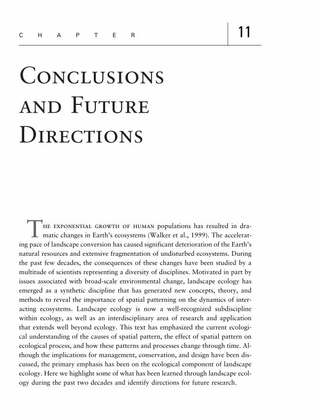
C H A P T E R

Conclusions and Future Directions

The exponential growth of human populations has resulted in dra-matic changes in Earth’s ecosystems (Walker et al., 1999). The accelerat-

ing pace of landscape conversion has caused significant deterioration of the Earth’snatural resources and extensive fragmentation of undisturbed ecosystems. Duringthe past few decades, the consequences of these changes have been studied by amultitude of scientists representing a diversity of disciplines. Motivated in part byissues associated with broad-scale environmental change, landscape ecology hasemerged as a synthetic discipline that has generated new concepts, theory, andmethods to reveal the importance of spatial patterning on the dynamics of inter-acting ecosystems. Landscape ecology is now a well-recognized subdisciplinewithin ecology, as well as an interdisciplinary area of research and applicationthat extends well beyond ecology. This text has emphasized the current ecologi-cal understanding of the causes of spatial pattern, the effect of spatial pattern onecological process, and how these patterns and processes change through time. Al-though the implications for management, conservation, and design have been dis-cussed, the primary emphasis has been on the ecological component of landscapeecology. Here we highlight some of what has been learned through landscape ecol-ogy during the past two decades and identify directions for future research.

11

2888_e11_p327-332 2/27/01 11:43 AM Page 327

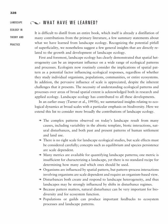
328

L A N D S C A P E

E C O L O G Y I N

T H E O R Y A N D

P R A C T I C E

W H A T H A V E W E L E A R N E D ?

It is difficult to distill from an entire book, which itself is already a distillation ofmany contributions from the primary literature, a few summary statements aboutwhat we have learned from landscape ecology. Recognizing the potential pitfallof superficiality, we nonetheless suggest a few general insights that are directly re-lated to the growth and development of landscape ecology.

First and foremost, landscape ecology has clearly demonstrated that spatial het-erogeneity can be an important influence on a wide range of ecological patternsand processes. Ecologists now routinely consider the implications of spatial pat-tern as a potential factor influencing ecological responses, regardless of whetherthey study individual organisms, populations, communities, or entire ecosystems.In addition, the pervasive influence of scale is appreciated, despite the inherentchallenges that it presents. The necessity of understanding ecological patterns andprocesses over areas of broad spatial extent is acknowledged both in research andapplied ecology. Landscape ecology has contributed to all these developments.

In an earlier essay (Turner et al., 1995b), we summarized insights relating to eco-logical dynamics at broad scales with a particular emphasis on biodiversity. Here weextend this list to consider more broadly the contributions of landscape ecology.

� The complex patterns observed on today’s landscape result from manycauses, including variability in the abiotic template, biotic interactions, nat-ural disturbances, and both past and present patterns of human settlementand land use.

� There is no right scale for landscape ecological studies, but scale effects mustbe considered carefully; concepts such as equilibrium and species persistenceare scale dependent.

� Many metrics are available for quantifying landscape patterns; one metric isinsufficient for characterizing a landscape, yet there is no standard recipe fordetermining how many and which ones should be used.

� Organisms are influenced by spatial pattern, but pattern–process interactionsinvolving organisms are scale dependent and require an organism-based view.

� Disturbances both create and respond to landscape heterogeneity, and thuslandscapes may be strongly influenced by shifts in disturbance regimes.

� Because pattern matters, natural disturbance can be very important for bio-diversity and for ecosystem function.

� Populations or guilds can produce important feedbacks to ecosystemprocesses and landscape patterns.

�

2888_e11_p327-332 2/27/01 11:43 AM Page 328

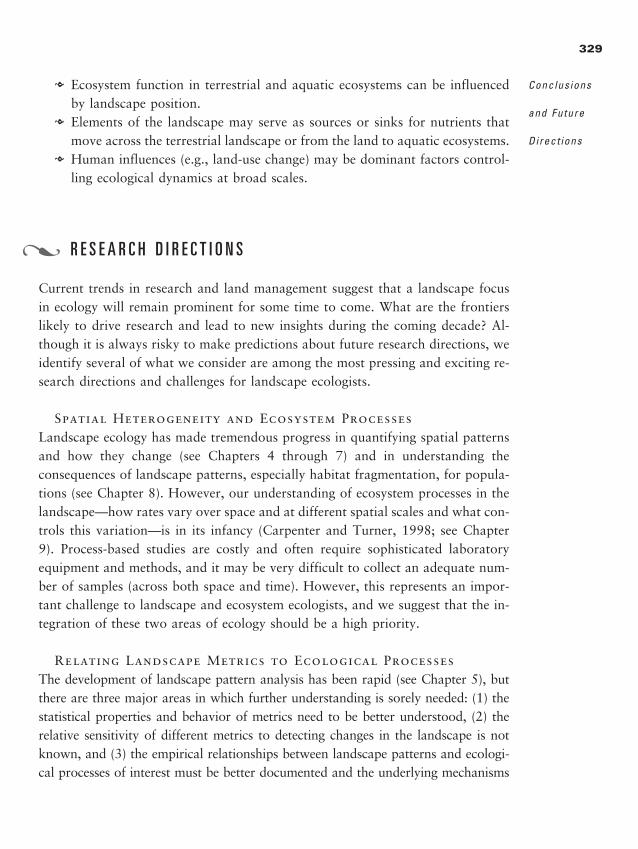
� Ecosystem function in terrestrial and aquatic ecosystems can be influencedby landscape position.

� Elements of the landscape may serve as sources or sinks for nutrients thatmove across the terrestrial landscape or from the land to aquatic ecosystems.

� Human influences (e.g., land-use change) may be dominant factors control-ling ecological dynamics at broad scales.

R E S E A R C H D I R E C T I O N S

Current trends in research and land management suggest that a landscape focusin ecology will remain prominent for some time to come. What are the frontierslikely to drive research and lead to new insights during the coming decade? Al-though it is always risky to make predictions about future research directions, weidentify several of what we consider are among the most pressing and exciting re-search directions and challenges for landscape ecologists.

Spatial Heterogeneity and Ecosystem ProcessesLandscape ecology has made tremendous progress in quantifying spatial patternsand how they change (see Chapters 4 through 7) and in understanding the consequences of landscape patterns, especially habitat fragmentation, for popula-tions (see Chapter 8). However, our understanding of ecosystem processes in thelandscape—how rates vary over space and at different spatial scales and what con-trols this variation—is in its infancy (Carpenter and Turner, 1998; see Chapter9). Process-based studies are costly and often require sophisticated laboratoryequipment and methods, and it may be very difficult to collect an adequate num-ber of samples (across both space and time). However, this represents an impor-tant challenge to landscape and ecosystem ecologists, and we suggest that the in-tegration of these two areas of ecology should be a high priority.

Relating Landscape Metrics to Ecological ProcessesThe development of landscape pattern analysis has been rapid (see Chapter 5), butthere are three major areas in which further understanding is sorely needed: (1) thestatistical properties and behavior of metrics need to be better understood, (2) therelative sensitivity of different metrics to detecting changes in the landscape is notknown, and (3) the empirical relationships between landscape patterns and ecologi-cal processes of interest must be better documented and the underlying mechanisms

329

Conclus ions

and Future

Direct ions

�

2888_e11_p327-332 2/27/01 11:43 AM Page 329

understood. Collectively, progress in these three research areas will help ecologistsdetermine what is worth measuring and why and when a change in a metric is sig-nificant both statistically and ecologically. It remains a critical research task to de-termine what constitutes a significant change, both statistically and ecologically, inspatial metrics and to relate such changes to ecologically relevant responses. Appli-cations of landscape ecology depend heavily on such understanding (see Chapter 10).

Thresholds, Nonlinearities, and Rules for ScalingCritical thresholds in landscape pattern (see Chapter 6) provide an example of anonlinearity with important implications for understanding the relationship betweenpattern and process. Identifying and understanding the nonlinearities associated withchanges in spatial and temporal scale provide exciting opportunities for researchand very practical applied challenges. The effects of scale are now well recognized,but the need for improved quantitative understanding remains critical. Ecologistsstill struggle with identifying the right scale(s) for studying and understanding par-ticular patterns and processes and extrapolating the knowledge gained at one scaleto other scales. The rules of thumb that have been suggested for scaling (see Chap-ters 2 and 5) need to be tested more widely, and the qualitative differences associ-ated with changes in spatial pattern (e.g., critical thresholds; see Chapter 6) need tobe considered in actual landscapes. Many of the ideas developing in the realm ofcomplex adaptive systems (e.g., Milne, 1998), in which emphasis is frequently placedon slow and fast variables, may also shed light on issues associated with spatial scal-ing. We see nonlinear dynamics and scaling as topics that will continue to motivatea considerable volume of basic and applied research in landscape ecology.

Feedbacks between Organisms and Ecosystems in SpaceIdentifying the interactions and feedbacks between organisms and ecosystemprocesses in a spatial context remains an important goal. A large body of litera-ture describes the effects of spatial pattern on the presence or abundance of pop-ulations, but there is relatively little research on the relationship between speciesdynamics and ecosystem processes in a spatial context. The potential feedbacksof populations to ecosystem and landscape dynamics remain poorly understood.

Causes and Consequences of Land-use ChangeThe size of the human population on Earth reached 6 billion during the fall of1999, and it will continue to increase. The human population is already trans-forming much of the surface of Earth and co-opting much of the world’s resources(Vitousek et al., 1997b). Increases in the extent and intensity of human land uses

330

L A N D S C A P E

E C O L O G Y I N

T H E O R Y A N D

P R A C T I C E

2888_e11_p327-332 2/27/01 11:43 AM Page 330

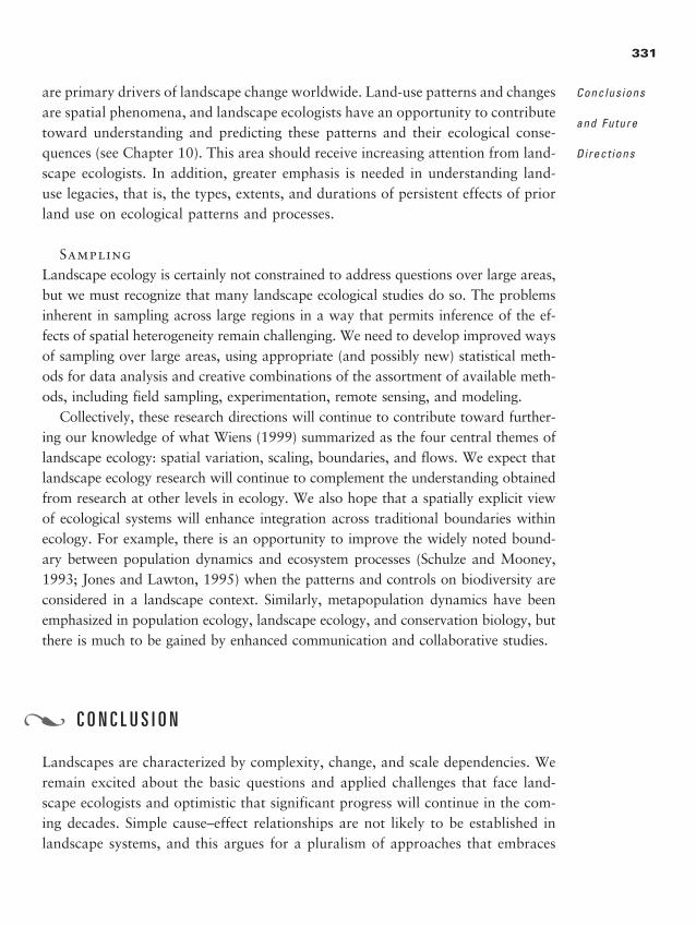
are primary drivers of landscape change worldwide. Land-use patterns and changesare spatial phenomena, and landscape ecologists have an opportunity to contributetoward understanding and predicting these patterns and their ecological conse-quences (see Chapter 10). This area should receive increasing attention from land-scape ecologists. In addition, greater emphasis is needed in understanding land-use legacies, that is, the types, extents, and durations of persistent effects of priorland use on ecological patterns and processes.

SamplingLandscape ecology is certainly not constrained to address questions over large areas,but we must recognize that many landscape ecological studies do so. The problemsinherent in sampling across large regions in a way that permits inference of the ef-fects of spatial heterogeneity remain challenging. We need to develop improved waysof sampling over large areas, using appropriate (and possibly new) statistical meth-ods for data analysis and creative combinations of the assortment of available meth-ods, including field sampling, experimentation, remote sensing, and modeling.

Collectively, these research directions will continue to contribute toward further-ing our knowledge of what Wiens (1999) summarized as the four central themes oflandscape ecology: spatial variation, scaling, boundaries, and flows. We expect thatlandscape ecology research will continue to complement the understanding obtainedfrom research at other levels in ecology. We also hope that a spatially explicit viewof ecological systems will enhance integration across traditional boundaries withinecology. For example, there is an opportunity to improve the widely noted bound-ary between population dynamics and ecosystem processes (Schulze and Mooney,1993; Jones and Lawton, 1995) when the patterns and controls on biodiversity areconsidered in a landscape context. Similarly, metapopulation dynamics have beenemphasized in population ecology, landscape ecology, and conservation biology, butthere is much to be gained by enhanced communication and collaborative studies.

C O N C L U S I O N

Landscapes are characterized by complexity, change, and scale dependencies. Weremain excited about the basic questions and applied challenges that face land-scape ecologists and optimistic that significant progress will continue in the com-ing decades. Simple cause–effect relationships are not likely to be established inlandscape systems, and this argues for a pluralism of approaches that embraces

331

Conclus ions

and Future

Direct ions

�

2888_e11_p327-332 2/27/01 11:43 AM Page 331

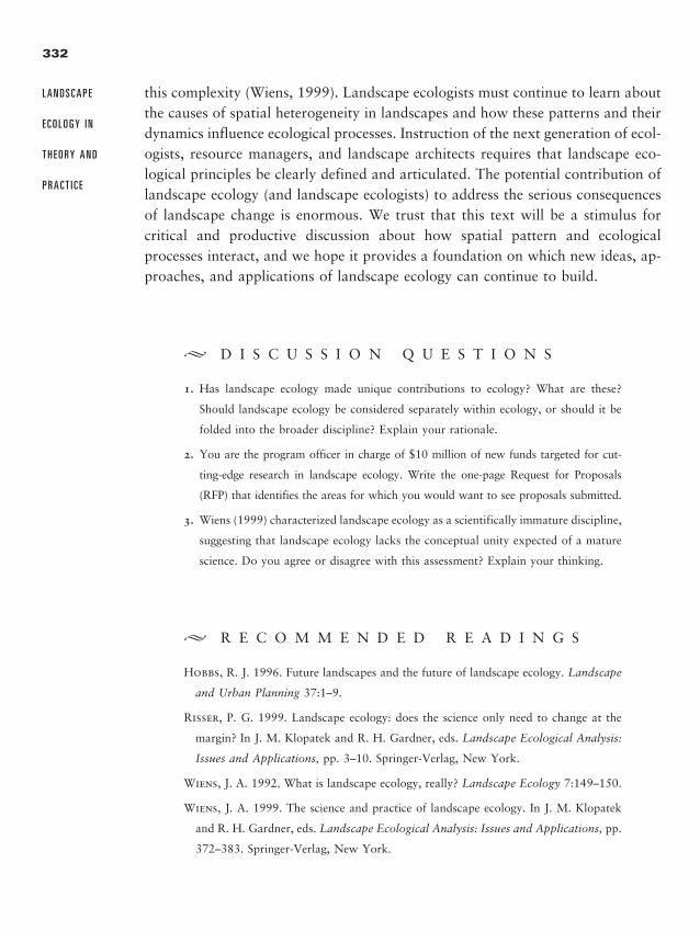
this complexity (Wiens, 1999). Landscape ecologists must continue to learn aboutthe causes of spatial heterogeneity in landscapes and how these patterns and theirdynamics influence ecological processes. Instruction of the next generation of ecol-ogists, resource managers, and landscape architects requires that landscape eco-logical principles be clearly defined and articulated. The potential contribution oflandscape ecology (and landscape ecologists) to address the serious consequencesof landscape change is enormous. We trust that this text will be a stimulus forcritical and productive discussion about how spatial pattern and ecologicalprocesses interact, and we hope it provides a foundation on which new ideas, ap-proaches, and applications of landscape ecology can continue to build.


1. Has landscape ecology made unique contributions to ecology? What are these?

Should landscape ecology be considered separately within ecology, or should it be

folded into the broader discipline? Explain your rationale.

2. You are the program officer in charge of $10 million of new funds targeted for cut-

ting-edge research in landscape ecology. Write the one-page Request for Proposals

(RFP) that identifies the areas for which you would want to see proposals submitted.

3. Wiens (1999) characterized landscape ecology as a scientifically immature discipline,

suggesting that landscape ecology lacks the conceptual unity expected of a mature

science. Do you agree or disagree with this assessment? Explain your thinking.


Hobbs, R. J. 1996. Future landscapes and the future of landscape ecology. Landscape

and Urban Planning 37:1–9.

Risser, P. G. 1999. Landscape ecology: does the science only need to change at the

margin? In J. M. Klopatek and R. H. Gardner, eds. Landscape Ecological Analysis:

Issues and Applications, pp. 3–10. Springer-Verlag, New York.

Wiens, J. A. 1992. What is landscape ecology, really? Landscape Ecology 7:149–150.

Wiens, J. A. 1999. The science and practice of landscape ecology. In J. M. Klopatek

and R. H. Gardner, eds. Landscape Ecological Analysis: Issues and Applications, pp.

372–383. Springer-Verlag, New York.

332

L A N D S C A P E

E C O L O G Y I N

T H E O R Y A N D

P R A C T I C E

2888_e11_p327-332 2/27/01 11:43 AM Page 332

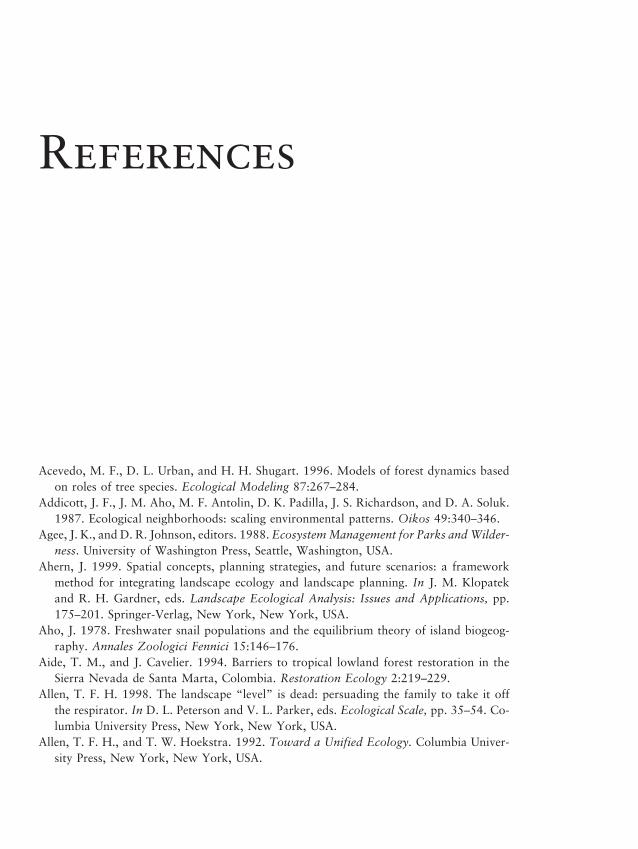
References

Acevedo, M. F., D. L. Urban, and H. H. Shugart. 1996. Models of forest dynamics basedon roles of tree species. Ecological Modeling 87:267–284.

Addicott, J. F., J. M. Aho, M. F. Antolin, D. K. Padilla, J. S. Richardson, and D. A. Soluk.1987. Ecological neighborhoods: scaling environmental patterns. Oikos 49:340–346.

Agee, J. K., and D. R. Johnson, editors. 1988. Ecosystem Management for Parks and Wilder-ness. University of Washington Press, Seattle, Washington, USA.

Ahern, J. 1999. Spatial concepts, planning strategies, and future scenarios: a frameworkmethod for integrating landscape ecology and landscape planning. In J. M. Klopatekand R. H. Gardner, eds. Landscape Ecological Analysis: Issues and Applications, pp.175–201. Springer-Verlag, New York, New York, USA.

Aho, J. 1978. Freshwater snail populations and the equilibrium theory of island biogeog-raphy. Annales Zoologici Fennici 15:146–176.

Aide, T. M., and J. Cavelier. 1994. Barriers to tropical lowland forest restoration in theSierra Nevada de Santa Marta, Colombia. Restoration Ecology 2:219–229.

Allen, T. F. H. 1998. The landscape “level” is dead: persuading the family to take it offthe respirator. In D. L. Peterson and V. L. Parker, eds. Ecological Scale, pp. 35–54. Co-lumbia University Press, New York, New York, USA.

Allen, T. F. H., and T. W. Hoekstra. 1992. Toward a Unified Ecology. Columbia Univer-sity Press, New York, New York, USA.

2888_e12_p333-388 2/27/01 1:55 PM Page 333

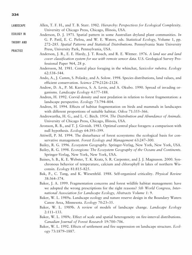
334

L A N D S C A P E

E C O L O G Y I N

T H E O R Y A N D

P R A C T I C E

Allen, T. F. H., and T. B. Starr. 1982. Hierarchy: Perspectives for Ecological Complexity.University of Chicago Press, Chicago, Illinois, USA.

Anderson, D. J. 1971. Spatial pattern in some Australian dryland plant communities. InG. P. Patil, E. C. Pielou, and W. E. Waters, eds. Statistical Ecology, Volume 1, pp.272–285. Spatial Patterns and Statistical Distributions. Pennsylvania State UniversityPress, University Park, Pennsylvania, USA.

Anderson, J. R., E. E. Hardy, J. T. Roach, and R. E. Witmer. 1976. A land use and landcover classification system for use with remote sensor data. U.S. Geological Survey Pro-fessional Paper 964, 28 p.

Andersson, M. 1981. Central place foraging in the whinchat, Saxicolor rubetra. Ecology62:538–544.

Ando, A., J. Camm, S. Polasky, and A. Solow. 1998. Species distributions, land values, andefficient conservation. Science 279:2126–2128.

Andow, D. A., P. M. Kareiva, S. A. Levin, and A. Okubo. 1990. Spread of invading or-ganisms. Landscape Ecology 4:177–188.

Andren, H. 1992. Corvid density and nest predation in relation to forest fragmentation: alandscape perspective. Ecology 73:794–804.

Andren, H. 1994. Effects of habitat fragmentation on birds and mammals in landscapeswith different proportions of suitable habitat. Oikos 71:355–366.

Andrewartha, H. G., and L. C. Birch. 1954. The Distribution and Abundance of Animals.University of Chicago Press, Chicago, Illinois, USA.

Aronson, R. B., and T. J. Givnish. 1983. Optimal central place foragers: a comparison withnull hypothesis. Ecology 64:395–399.

Attiwill, P. M. 1994. The disturbance of forest ecosystems: the ecological basis for con-servative management. Forest Ecology and Management 63:247–300.

Bailey, R. G. 1996. Ecosystem Geography. Springer-Verlag, New York, New York, USA.Bailey, R. G. 1998. Ecoregions: The Ecosystem Geography of the Oceans and Continents.

Springer-Verlag, New York, New York, USA.Baines, S. B., K. E. Webster, T. K. Kratz, S. R. Carpenter, and J. J. Magnuson. 2000. Syn-

chronous behavior of temperature, calcium and chlorophyll in lakes of northern Wis-consin. Ecology 81:815–825.

Bak, P., C. Tang, and K. Wiesenfeld. 1988. Self-organized criticality. Physical Review38:364–374.

Baker, J. A. 1999. Fragmentation concerns and forest wildlife habitat management: havewe adopted the wrong prescriptions for the right reasons? 5th World Congress, Inter-national Association for Landscape Ecology, Abstracts Volume 1: 9.

Baker, W. L. 1989a. Landscape ecology and nature reserve design in the Boundary WatersCanoe Area, Minnesota. Ecology 70:23–35.

Baker, W. L. 1989b. A review of models of landscape change. Landscape Ecology2:111–133.

Baker, W. L. 1989c. Effect of scale and spatial heterogeneity on fire-interval distributions.Canadian Journal of Forest Research 19:700–706.

Baker, W. L. 1992. Effects of settlement and fire suppression on landscape structure. Ecol-ogy 73:1879–1887.

2888_e12_p333-388 2/27/01 1:55 PM Page 334

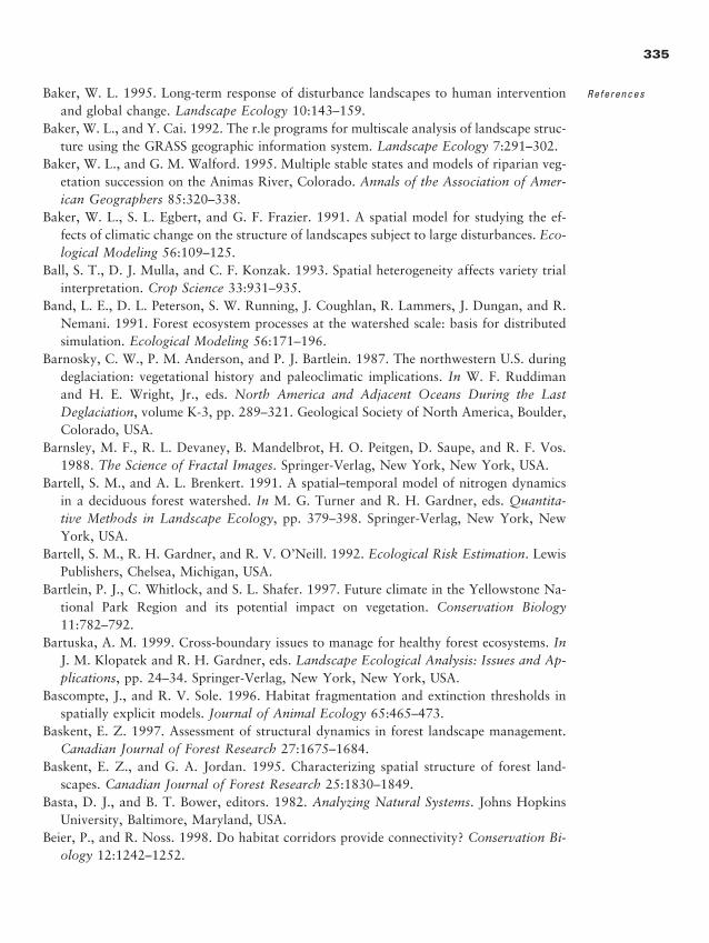
Baker, W. L. 1995. Long-term response of disturbance landscapes to human interventionand global change. Landscape Ecology 10:143–159.

Baker, W. L., and Y. Cai. 1992. The r.le programs for multiscale analysis of landscape struc-ture using the GRASS geographic information system. Landscape Ecology 7:291–302.

Baker, W. L., and G. M. Walford. 1995. Multiple stable states and models of riparian veg-etation succession on the Animas River, Colorado. Annals of the Association of Amer-ican Geographers 85:320–338.

Baker, W. L., S. L. Egbert, and G. F. Frazier. 1991. A spatial model for studying the ef-fects of climatic change on the structure of landscapes subject to large disturbances. Eco-logical Modeling 56:109–125.

Ball, S. T., D. J. Mulla, and C. F. Konzak. 1993. Spatial heterogeneity affects variety trialinterpretation. Crop Science 33:931–935.

Band, L. E., D. L. Peterson, S. W. Running, J. Coughlan, R. Lammers, J. Dungan, and R.Nemani. 1991. Forest ecosystem processes at the watershed scale: basis for distributedsimulation. Ecological Modeling 56:171–196.

Barnosky, C. W., P. M. Anderson, and P. J. Bartlein. 1987. The northwestern U.S. duringdeglaciation: vegetational history and paleoclimatic implications. In W. F. Ruddimanand H. E. Wright, Jr., eds. North America and Adjacent Oceans During the LastDeglaciation, volume K-3, pp. 289–321. Geological Society of North America, Boulder,Colorado, USA.

Barnsley, M. F., R. L. Devaney, B. Mandelbrot, H. O. Peitgen, D. Saupe, and R. F. Vos.1988. The Science of Fractal Images. Springer-Verlag, New York, New York, USA.

Bartell, S. M., and A. L. Brenkert. 1991. A spatial–temporal model of nitrogen dynamicsin a deciduous forest watershed. In M. G. Turner and R. H. Gardner, eds. Quantita-tive Methods in Landscape Ecology, pp. 379–398. Springer-Verlag, New York, NewYork, USA.

Bartell, S. M., R. H. Gardner, and R. V. O’Neill. 1992. Ecological Risk Estimation. LewisPublishers, Chelsea, Michigan, USA.

Bartlein, P. J., C. Whitlock, and S. L. Shafer. 1997. Future climate in the Yellowstone Na-tional Park Region and its potential impact on vegetation. Conservation Biology11:782–792.

Bartuska, A. M. 1999. Cross-boundary issues to manage for healthy forest ecosystems. InJ. M. Klopatek and R. H. Gardner, eds. Landscape Ecological Analysis: Issues and Ap-plications, pp. 24–34. Springer-Verlag, New York, New York, USA.

Bascompte, J., and R. V. Sole. 1996. Habitat fragmentation and extinction thresholds inspatially explicit models. Journal of Animal Ecology 65:465–473.

Baskent, E. Z. 1997. Assessment of structural dynamics in forest landscape management.Canadian Journal of Forest Research 27:1675–1684.

Baskent, E. Z., and G. A. Jordan. 1995. Characterizing spatial structure of forest land-scapes. Canadian Journal of Forest Research 25:1830–1849.

Basta, D. J., and B. T. Bower, editors. 1982. Analyzing Natural Systems. Johns HopkinsUniversity, Baltimore, Maryland, USA.

Beier, P., and R. Noss. 1998. Do habitat corridors provide connectivity? Conservation Bi-ology 12:1242–1252.

335

References

2888_e12_p333-388 2/27/01 1:55 PM Page 335

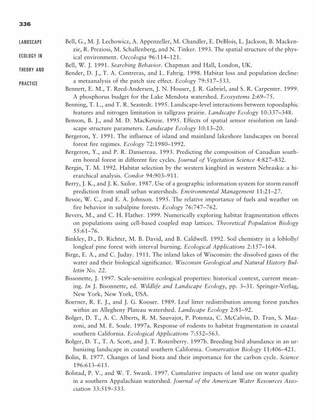
Bell, G., M. J. Lechowicz, A. Appenzeller, M. Chandler, E. DeBlois, L. Jackson, B. Macken-zie, R. Preziosi, M. Schallenberg, and N. Tinker. 1993. The spatial structure of the phys-ical environment. Oecologia 96:114–121.

Bell, W. J. 1991. Searching Behavior. Chapman and Hall, London, UK.Bender, D. J., T. A. Contreras, and L. Fahrig. 1998. Habitat loss and population decline:

a metaanalysis of the patch size effect. Ecology 79:517–533.Bennett, E. M., T. Reed-Andersen, J. N. Houser, J. R. Gabriel, and S. R. Carpenter. 1999.

A phosphorus budget for the Lake Mendota watershed. Ecosystems 2:69–75.Benning, T. L., and T. R. Seastedt. 1995. Landscape-level interactions between topoedaphic

features and nitrogen limitation in tallgrass prairie. Landscape Ecology 10:337–348.Benson, B. J., and M. D. MacKenzie. 1995. Effects of spatial sensor resolution on land-

scape structure parameters. Landscape Ecology 10:13–20.Bergeron, Y. 1991. The influence of island and mainland lakeshore landscapes on boreal

forest fire regimes. Ecology 72:1980–1992.Bergeron, Y., and P. R. Dansereau. 1993. Predicting the composition of Canadian south-

ern boreal forest in different fire cycles. Journal of Vegetation Science 4:827–832.Bergin, T. M. 1992. Habitat selection by the western kingbird in western Nebraska: a hi-

erarchical analysis. Condor 94:903–911.Berry, J. K., and J. K. Sailor. 1987. Use of a geographic information system for storm runoff

prediction from small urban watersheds. Environmental Management 11:21–27.Bessie, W. C., and E. A. Johnson. 1995. The relative importance of fuels and weather on

fire behavior in subalpine forests. Ecology 76:747–762.Bevers, M., and C. H. Flather. 1999. Numerically exploring habitat fragmentation effects

on populations using cell-based coupled map lattices. Theoretical Population Biology55:61–76.

Binkley, D., D. Richter, M. B. David, and B. Caldwell. 1992. Soil chemistry in a loblolly/longleaf pine forest with interval burning. Ecological Applications 2:157–164.

Birge, E. A., and C. Juday. 1911. The inland lakes of Wisconsin: the dissolved gases of thewater and their biological significance. Wisconsin Geological and Natural History Bul-letin No. 22.

Bissonette, J. 1997. Scale-sensitive ecological properties: historical context, current mean-ing. In J. Bisonnette, ed. Wildlife and Landscape Ecology, pp. 3–31. Springer-Verlag,New York, New York, USA.

Boerner, R. E. J., and J. G. Kooser. 1989. Leaf litter redistribution among forest patcheswithin an Allegheny Plateau watershed. Landscape Ecology 2:81–92.

Bolger, D. T., A. C. Alberts, R. M. Sauvajot, P. Potenza, C. McCalvin, D. Tran, S. Maz-zoni, and M. E. Soule. 1997a. Response of rodents to habitat fragmentation in coastalsouthern California. Ecological Applications 7:552–563.

Bolger, D. T., T. A. Scott, and J. T. Rotenberry. 1997b. Breeding bird abundance in an ur-banizing landscape in coastal southern California. Conservation Biology 11:406–421.

Bolin, B. 1977. Changes of land biota and their importance for the carbon cycle. Science196:613–615.

Bolstad, P. V., and W. T. Swank. 1997. Cumulative impacts of land use on water qualityin a southern Appalachian watershed. Journal of the American Water Resources Asso-ciation 33:519–533.

336

L A N D S C A P E

E C O L O G Y I N

T H E O R Y A N D

P R A C T I C E

2888_e12_p333-388 2/27/01 1:55 PM Page 336

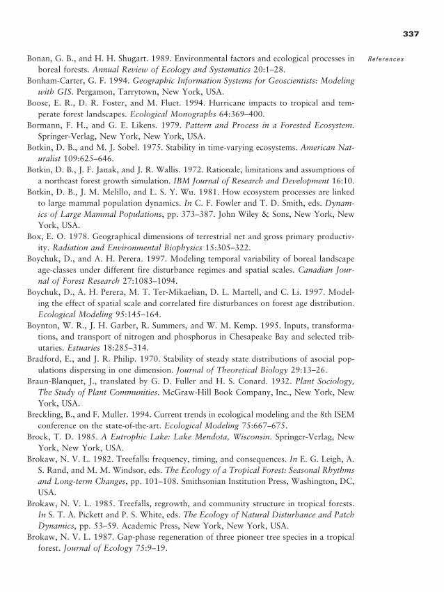
Bonan, G. B., and H. H. Shugart. 1989. Environmental factors and ecological processes inboreal forests. Annual Review of Ecology and Systematics 20:1–28.

Bonham-Carter, G. F. 1994. Geographic Information Systems for Geoscientists: Modelingwith GIS. Pergamon, Tarrytown, New York, USA.

Boose, E. R., D. R. Foster, and M. Fluet. 1994. Hurricane impacts to tropical and tem-perate forest landscapes. Ecological Monographs 64:369–400.

Bormann, F. H., and G. E. Likens. 1979. Pattern and Process in a Forested Ecosystem.Springer-Verlag, New York, New York, USA.

Botkin, D. B., and M. J. Sobel. 1975. Stability in time-varying ecosystems. American Nat-uralist 109:625–646.

Botkin, D. B., J. F. Janak, and J. R. Wallis. 1972. Rationale, limitations and assumptions ofa northeast forest growth simulation. IBM Journal of Research and Development 16:10.

Botkin, D. B., J. M. Melillo, and L. S. Y. Wu. 1981. How ecosystem processes are linkedto large mammal population dynamics. In C. F. Fowler and T. D. Smith, eds. Dynam-ics of Large Mammal Populations, pp. 373–387. John Wiley & Sons, New York, NewYork, USA.

Box, E. O. 1978. Geographical dimensions of terrestrial net and gross primary productiv-ity. Radiation and Environmental Biophysics 15:305–322.

Boychuk, D., and A. H. Perera. 1997. Modeling temporal variability of boreal landscapeage-classes under different fire disturbance regimes and spatial scales. Canadian Jour-nal of Forest Research 27:1083–1094.

Boychuk, D., A. H. Perera, M. T. Ter-Mikaelian, D. L. Martell, and C. Li. 1997. Model-ing the effect of spatial scale and correlated fire disturbances on forest age distribution.Ecological Modeling 95:145–164.

Boynton, W. R., J. H. Garber, R. Summers, and W. M. Kemp. 1995. Inputs, transforma-tions, and transport of nitrogen and phosphorus in Chesapeake Bay and selected trib-utaries. Estuaries 18:285–314.

Bradford, E., and J. R. Philip. 1970. Stability of steady state distributions of asocial pop-ulations dispersing in one dimension. Journal of Theoretical Biology 29:13–26.

Braun-Blanquet, J., translated by G. D. Fuller and H. S. Conard. 1932. Plant Sociology,The Study of Plant Communities. McGraw-Hill Book Company, Inc., New York, NewYork, USA.

Breckling, B., and F. Muller. 1994. Current trends in ecological modeling and the 8th ISEMconference on the state-of-the-art. Ecological Modeling 75:667–675.

Brock, T. D. 1985. A Eutrophic Lake: Lake Mendota, Wisconsin. Springer-Verlag, NewYork, New York, USA.

Brokaw, N. V. L. 1982. Treefalls: frequency, timing, and consequences. In E. G. Leigh, A.S. Rand, and M. M. Windsor, eds. The Ecology of a Tropical Forest: Seasonal Rhythmsand Long-term Changes, pp. 101–108. Smithsonian Institution Press, Washington, DC,USA.

Brokaw, N. V. L. 1985. Treefalls, regrowth, and community structure in tropical forests.In S. T. A. Pickett and P. S. White, eds. The Ecology of Natural Disturbance and PatchDynamics, pp. 53–59. Academic Press, New York, New York, USA.

Brokaw, N. V. L. 1987. Gap-phase regeneration of three pioneer tree species in a tropicalforest. Journal of Ecology 75:9–19.

337

References

2888_e12_p333-388 2/27/01 1:55 PM Page 337

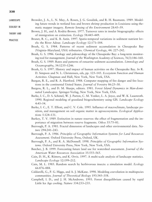
Browder, J. A., L. N. May, A. Rosen, J. G. Gosslink, and R. H. Baumann. 1989. Model-ing future trends in wetland loss and brown shrimp production in Louisiana using the-matic mapper imagery. Remote Sensing of the Environment 28:45–59.

Brown, J. H., and A. Kodric-Brown. 1977. Turnover rates in insular biogeography: effectsof immigration on extinction. Ecology 58:445–449.

Brunet, R. C., and K. B. Astin. 1997. Spatio-temporal variations in sediment nutrient lev-els: the River Adour. Landscape Ecology 12:171–184.

Brush, G. S. 1984. Patterns of recent sediment accumulation in Chesapeake Bay (Virginia–Maryland, USA) tributaries. Chemical Geology, 44: 227–242.

Brush, G. S. 1986. Geology and paleoecology of the Chesapeake Bay: a long-term monitor-ing tool for management. Journal of the Washington Academy of Sciences, 76(3):146–160.

Brush, G. S. 1989. Rates and patterns of estuarine sediment accumulation. Limnology andOceanography, 34:1235–1246.

Brush, G. S. 1997. History and impact of human activities on the Chesapeake Bay. In R.D. Simpson and N. L. Christensen, eds, pp. 125–145. Ecosystem Function and HumanActivities. Chapman and Hall, New York, New York, USA.

Burgan, R. E., and R. A. Hartford. 1988. Computer mapping of fire danger and fire loca-tions in the continental United States. Journal of Forestry 86:25–30.

Burgess, R. L., and D. M. Sharpe, editors. 1981. Forest Island Dynamics in Man-domi-nated Landscapes. Springer-Verlag, New York, New York, USA.

Burke, I. C., D. S. Schimel, W. J. Parton, C. M. Yonker, L. A. Joyce, and W. K. Lauenroth.1990. Regional modeling of grassland biogeochemistry using GIS. Landscape Ecology4:45–54.

Burke, I. C., E. T. Elliott, and C. V. Cole. 1995. Influence of macroclimate, landscape po-sition, and management on soil organic matter in agroecosystems. Ecological Applica-tions 5:124–131.

Burkey, T. V. 1989. Extinction in nature reserves: the effect of fragmentation and the im-portance of migration between reserve fragments. Oikos 55:75–81.

Burrough, P. A. 1981. Fractal dimension of landscapes and other environmental data. Na-ture 294:241–243.

Burrough, P. A. 1986. Principles of Geographic Information Systems for Land ResourcesAssessment. Oxford University Press, Oxford, UK.

Burrough, P. A., and R. A. McDonnell. 1998. Principles of Geographic Information Sys-tems. Oxford University Press, New York, New York, USA.

Butcher, J. B. 1999. Forecasting future land use for watershed assessment. Journal of theAmerican Water Resources Association 35:555–565.

Cain, D. H., K. Riitters, and K. Orvis. 1997. A multi-scale analysis of landscape statistics.Landscape Ecology 12:199–212.

Cain, M. L. 1985. Random search by herbivorous insects: a simulation model. Ecology66:876–888.

Caldarelli, G., P. G. Higgs, and A. J. McKane. 1998. Modeling coevolution in multispeciescommunities. Journal of Theoretical Biology 193:345–358.

Campbell, I. D., and J. H. McAndrews. 1993. Forest disequilibrium caused by rapid Little Ice Age cooling. Nature 334:233–235.

338

L A N D S C A P E

E C O L O G Y I N

T H E O R Y A N D

P R A C T I C E

2888_e12_p333-388 2/27/01 1:55 PM Page 338

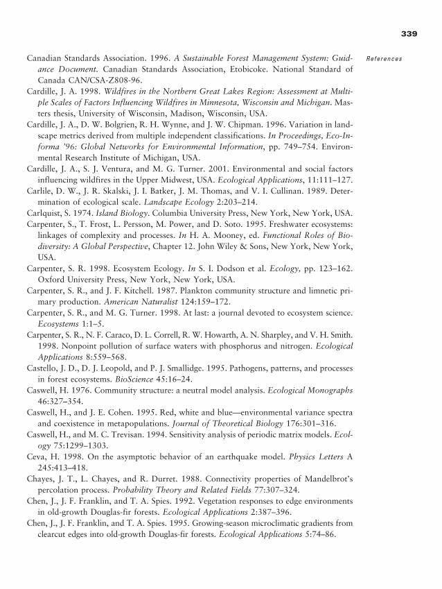
Canadian Standards Association. 1996. A Sustainable Forest Management System: Guid-ance Document. Canadian Standards Association, Etobicoke. National Standard ofCanada CAN/CSA-Z808-96.

Cardille, J. A. 1998. Wildfires in the Northern Great Lakes Region: Assessment at Multi-ple Scales of Factors Influencing Wildfires in Minnesota, Wisconsin and Michigan. Mas-ters thesis, University of Wisconsin, Madison, Wisconsin, USA.

Cardille, J. A., D. W. Bolgrien, R. H. Wynne, and J. W. Chipman. 1996. Variation in land-scape metrics derived from multiple independent classifications. In Proceedings, Eco-In-forma ’96: Global Networks for Environmental Information, pp. 749–754. Environ-mental Research Institute of Michigan, USA.

Cardille, J. A., S. J. Ventura, and M. G. Turner. 2001. Environmental and social factorsinfluencing wildfires in the Upper Midwest, USA. Ecological Applications, 11:111–127.

Carlile, D. W., J. R. Skalski, J. I. Batker, J. M. Thomas, and V. I. Cullinan. 1989. Deter-mination of ecological scale. Landscape Ecology 2:203–214.

Carlquist, S. 1974. Island Biology. Columbia University Press, New York, New York, USA.Carpenter, S., T. Frost, L. Persson, M. Power, and D. Soto. 1995. Freshwater ecosystems:

linkages of complexity and processes. In H. A. Mooney, ed. Functional Roles of Bio-diversity: A Global Perspective, Chapter 12. John Wiley & Sons, New York, New York,USA.

Carpenter, S. R. 1998. Ecosystem Ecology. In S. I. Dodson et al. Ecology, pp. 123–162.Oxford University Press, New York, New York, USA.

Carpenter, S. R., and J. F. Kitchell. 1987. Plankton community structure and limnetic pri-mary production. American Naturalist 124:159–172.

Carpenter, S. R., and M. G. Turner. 1998. At last: a journal devoted to ecosystem science.Ecosystems 1:1–5.

Carpenter, S. R., N. F. Caraco, D. L. Correll, R. W. Howarth, A. N. Sharpley, and V. H. Smith.1998. Nonpoint pollution of surface waters with phosphorus and nitrogen. EcologicalApplications 8:559–568.

Castello, J. D., D. J. Leopold, and P. J. Smallidge. 1995. Pathogens, patterns, and processesin forest ecosystems. BioScience 45:16–24.

Caswell, H. 1976. Community structure: a neutral model analysis. Ecological Monographs46:327–354.

Caswell, H., and J. E. Cohen. 1995. Red, white and blue—environmental variance spectraand coexistence in metapopulations. Journal of Theoretical Biology 176:301–316.

Caswell, H., and M. C. Trevisan. 1994. Sensitivity analysis of periodic matrix models. Ecol-ogy 75:1299–1303.

Ceva, H. 1998. On the asymptotic behavior of an earthquake model. Physics Letters A245:413–418.

Chayes, J. T., L. Chayes, and R. Durret. 1988. Connectivity properties of Mandelbrot’spercolation process. Probability Theory and Related Fields 77:307–324.

Chen, J., J. F. Franklin, and T. A. Spies. 1992. Vegetation responses to edge environmentsin old-growth Douglas-fir forests. Ecological Applications 2:387–396.

Chen, J., J. F. Franklin, and T. A. Spies. 1995. Growing-season microclimatic gradients fromclearcut edges into old-growth Douglas-fir forests. Ecological Applications 5:74–86.

339

References

2888_e12_p333-388 2/27/01 1:55 PM Page 339

Chen, J., J. F. Franklin, and J. S. Lowe. 1996. Comparison of abiotic and structurally de-fined patch patterns in a hypothetical forest landscape. Conservation Biology10:854–862.

Cherrill, A., and C. McClean. 1995. An investigation of uncertainty in field habitat map-ping and the implications for detecting land-cover change. Landscape Ecology 10:5–21.

Chou, Y. H., R. A. Minnich, and R. A. Chase. 1993. Mapping probability of fire occur-rence in San Jacinto Mountains, California, USA. Environmental Management 17:129–140.

Christensen, N. L., J. K. Agee, P. F. Brussard, J. Hughes, D. H. Knight, G. W. Minshall,J. M. Peek, S. J. Pyne, F. J. Swanson, J. W. Thomas, S. Wells, S. E. Williams, and H. A. Wright. 1989. Interpreting the Yellowstone fires of 1988. BioScience 39:678–685.

Christensen, N. L., A. M. Bartuska, J. H. Brown, S. R. Carpenter, C. D’Antonio, R. Fran-cis, J. F. Franklin, J. A. MacMahon, R. F. Noss, D. J. Parsons, C. H. Peterson, M. G. Turner, and R. G. Woodmansee. 1996. The scientific basis for ecosystem man-agement. Ecological Applications 6:665–691.

Cirmo, C. P., and J .J. McDonnell. 1997. Linking the hydrologic and biogeochemical con-trols of nitrogen transport in near-stream zones of temperate forested catchments: a re-view. Journal of Hydrology 199:88–120.

Clark, J. S. 1988. Effect of climate change on fire regimes in northwestern Minnesota. Nature 334:233–235.

Clark, J. S. 1989. Ecological disturbance as a renewal process: theory and application tofire history. Oikos 56:17–30.

Clark, J. S. 1990. Fire and climate change during the last 750 years in northwestern Min-nesota. Ecological Monographs 60:135–159.

Clark, J. S., and P. R. Royall. 1994. Pre-industrial particulate emissions and carbon se-questration from biomass burning in North America. Biogeochemistry 23:35–51.

Clark, W. C. 1980. Witches, Floods, and Wonder Drugs. Institute of Resource Ecology,R-22. University of British Columbia, Vancouver, British Columbia, Canada.

Clark, W. C., D. D. Jones, and C. S. Holling. 1978. Patches, movements, and populationdynamics in ecological systems: a terrestrial perspective. In J. S. Steele, ed. Spatial Pat-tern in Plankton Communities, pp. 105–126. Plenum Press, New York, New York, USA.

Clark, W. C., D. D. Jones, and C. S. Holling. 1979. Lessons for ecological policy design:a case study of ecosystem management. Ecological Modeling 7:1–53.

Clements, F. E. 1915. Plant Succession: An Analysis of the Development of Vegetation.Carnegie Institute Publication No. 242, Washington, D.C. 512 p.

Cluis, D. A., D. Couillarg, and L. Potvin. 1979. A square grid transport model relatingland use exports to nutrient loads in rivers. Water Resources Research 15:630–636.

Cody, M. L. 1983. The land birds. In T. J. Case and M. L. Cody, eds. Island Biogeogra-phy in the Sea of Cortez, pp. 210–245. University of California Press, Berkeley, Cali-fornia, USA.

Cohen, A. E., A. Gonzalez, J. H. Lawton, O. L. Petchey, D. Wildman, and J. E. Cohen.1998. A novel experimental apparatus to study the impact of white noise and 1/f noiseon animal populations. Proceedings of the Royal Society of London Series B—Biolog-ical Sciences 265:11–15.

340

L A N D S C A P E

E C O L O G Y I N

T H E O R Y A N D

P R A C T I C E

2888_e12_p333-388 2/27/01 1:55 PM Page 340

Cohen, D., and S. A. Levin. 1991. Dispersal in patchy environments: the effects of tem-poral and spatial structure. Theoretical Population Biology 39:63–99.

Cole, J. J., C. L. Peierls, N. F. Caraco, and M. L. Pace. 1993. Nitrogen loading of riversas a human-driven process. In M. J. McDonnell and S. T. A. Pickett, eds. Humans asComponents of Ecosystems, pp. 141–157. Springer-Verlag, New York, New York, USA.

Cole, L. C. 1951. Population cycles and random oscillations. Journal of Wildlife Manage-ment 15:233–252.

Cole, L. C. 1954. Some features of random cycles. Journal of Wildlife Management18:107–109.

Collins, S. L., A. K. Knapp, J. M. Briggs, J. M. Blair, and E. M. Steinhauer. 1998. Mod-ulation of diversity by grazing and mowing in native tallgrass prairie. Science 280:745–747.

Comeleo, R. L., J. F. Paul, P. V. August, J. Copeland, C. Baker, S. S. Hale, and R. W. La-timer. 1996. Relationships between watershed stressors and sediment contamination inChesapeake Bay estuaries. Landscape Ecology 11:307–319.

Comins, H. N., and D. W. E. Blatt. 1974. Pre-predation models in spatially heterogeneousenvironments. Journal of Theoretical Biology 48:75–83.

Connell, J. H., and R. O. Slatyer. 1977. Mechanisms of succession in natural communitiesand their role in community stability and organization. American Naturalist 111:1119–1144.

Connell, J. H., and W. P. Sousa. 1983. On the evidence needed to judge ecological stabil-ity or persistence. American Naturalist 121:789–824.

Cooper, J. R., J. W. Gilliam, R. B. Daniels, and W. P. Robarge. 1987. Riparian areas asfilters for agricultural sediment. Soil Science Society of America Journal 51:416–420.

Cooper, S. R., and G. S. Brush. 1991. Long-term history of Chesapeake Bay anoxia. Sci-ence, 254:992–996.

Cooper, W. S. 1913. The climax forest of Isle Royale, Lake Superior, and its development.I. Botanical Gazette 55:1–44.

Cooperrider, A., L. R. Garrett, and N. T. Hobbs. 1999. Data collection, management, andinventory. In N. C. Johnson, A. J. Malk, W. T. Sexton, and R. Szaro, eds. EcologicalStewardship: A Common Reference for Ecosystem Management, pp. 604–627. ElsevierScience Limited, Oxford, UK.

Correll, D. L. 1997. Buffer zones and water quality protection: general principles. InN. E. Haycock, T. P. Burt, K. W. T. Goulding, and G. Pinay, eds. Buffer Zones: TheirProcesses and Potential in Water Protection, pp. 7–20. Quest Environmental, Harpenden,UK.

Correll, D. L., T. E. Jordan, and D. E. Weller. 1992. Nutrient flux in a landscape: effectsof coastal land use and terrestrial community mosaic on nutrient transport to coastalwaters. Estuaries 15:431–442.

Costa, J .E. 1975. Effects of agriculture on erosion and sedimentation in the Piedmontprovince, Maryland. Geological Society of America Bulletin 86: 1281–1286.

Costanza, R., and T. Maxwell. 1994. Resolution and predictability: an approach to thescaling problem. Landscape Ecology 9:47–57.

Costanza, R., F. H. Sklar, and M. L. White. 1990. Modeling coastal landscape dynamics:

341

References

2888_e12_p333-388 2/27/01 1:55 PM Page 341

process-based dynamic spatial ecosystem simulation can examine long-term naturalchanges and human impacts. Bioscience 40:91–107.

Costanza, R., D. Duplisea, and U. Kautsky. 1998. Ecological modeling and economic sys-tems with STELLA—Introduction. Ecological Modeling 110:1–4.

Coughenour, M. B. 1991. Spatial components of plant–herbivore interactions in pastoral,ranching, and native ungulate ecosystems. Journal of Range Management 44:530–542.

Coulson, R. N., C. N. Lovelady, R. O. Flamm, S. L. Spradling, and M. C. Saunders. 1991.In: M. G. Turner and R. H. Gardner, eds. Quantitative Methods in Landscape Ecol-ogy, pp. 153–172. Springer-Verlag, New York.

Cressie, N. A. C. 1991. Statistics for Spatial Data. John Wiley & Sons, New York, NewYork, USA.

Criminale, W. O., and D. F. Winter. 1974. The stability of steady-state depth distributionsof marine phytoplankton. American Naturalist 108:679–687.

Crist, T. O., and J. A. Wiens. 1994. Scale effects of vegetation on forager movement andseed harvesting by ants. Oikos 69:37–46.

Cronin, T. M., and C. E. Schneider. 1990. Climatic influences on species: evidence fromthe fossil record. Trends in Ecology and Evolution 5:275–279.

Crowley, T. J., and K. Y. Kim. 1994. Milankovitch forcing of the last interglacial sea level.Science 265:1566–1568.

Crutzen, P. J., and J. G. Goldhammer, editors. 1993. Fire in the Environment: The Eco-logical, Atmospheric, and Climatic Importance of Vegetation Fires. John Wiley & Sons,New York, New York, USA.

Cullinan, V. I., and J. M. Thomas. 1992. A comparison of quantitative methods for ex-amining landscape pattern and scale. Landscape Ecology 7:211–227.

Culver, D. C. 1970. Analysis of simple cave communities. I. Caves as islands. Evolution29:463–474.

Curtis, J. T. 1956. The modification of mid-latitude grasslands and forests by man. InW. L. Thomas, ed. Man’s Role in Changing the Face of the Earth, pp. 721–736. Uni-versity of Chicago Press, Chicago, Illinois, USA.

Curtis, J. T. 1959. The Vegetation of Wisconsin. University of Wisconsin Press, Madison,Wisconsin, USA.

Cwynar, L.C. 1987. Fire and the forest history of the North Cascade Range. Ecology68:791–802.

da Silva, J. M., C. Uhl, and G. Murray. 1996. Plant succession, landscape management,and the ecology of frugivorous birds in abandoned Amazonian pastures. ConservationBiology 10:491–503.

Dale, V. H. 1991. The debris avalanche at Mount St. Helens: vegetation establishment in theten years since the eruption. National Geographic Research and Exploration 7(3):328–341.

Dale, V. H., F. Southworth, R. V. O’Neill, A. Rosen, and R. Frohn. 1993. Simulating spa-tial patterns of land-use change in Rondonia, Brazil. Lectures on Mathematics in theLife Sciences 23:29–55.

Dale, V. H., R. V. O’Neill, F. Southworth, and M. Pedlowski. 1994a. Modeling effects ofland management in the Brazilian Amazonian settlement of Rondonia. Conservation Bi-ology 8:196–206.

342

L A N D S C A P E

E C O L O G Y I N

T H E O R Y A N D

P R A C T I C E

2888_e12_p333-388 2/27/01 1:55 PM Page 342

Dale, V. H., S. M. Pearson, H. L. Offerman, and R. V. O’Neill. 1994b. Relating patternsof land-use change to faunal biodiversity in the Central Amazon. Conservation Biology8:1027–1036.

Dale, V. H., A. E. Lugo, J. A. MacMahon, and S. T. A. Pickett. 1998. Ecosystem man-agement in the context of large, infrequent disturbances. Ecosystems 1:546–557.

Dale, V. H., S. Brown, R. A. Haeuber, N. T. Hobbs, N. Huntly, R. J. Naiman, W. E. Rieb-same, M. G. Turner, and T. J. Valone. 2000. Ecological principles and guidelines formanaging the use of land: a report from the Ecological Society of America. EcologicalApplications 10:639–670.

Danielson, B. J. 1991. Communities on a landscape: the influence of habitat heterogeneityon the interactions between species. American Naturalist 138:1105–1120.

Danielson, B. J. 1992. Habitat selection, interspecific interactions and landscape composi-tion. Evolutionary Ecology 6:399–411.

Dannell, K., L. Edenius, and P. Lundberg. 1991. Herbivory and tree stand composition:moose patch use in winter. Ecology 72:1350–1357.

Darwen, P. J., and D. G. Green. 1996. Viability of populations in a landscape. EcologicalModeling 85:165–171.

Davis, M. B. 1983. Quaternary history of deciduous forests of eastern North America andEurope. Annals Missouri Botanical Garden 70:550–563.

Davis, S. M., and J. C. Ogden, editors. 1994. Everglades: The Ecosystem and Its Restora-tion. St. Lucie Press, Delray Beach, Florida, USA.

Day, T. A., and J. K. Detling. 1990. Grassland patch dynamics and herbivore grazing pref-erence following urine deposition. Ecology 71:180–188.

DeAngelis, D. L., and J. C. Waterhouse. 1987. Equilibrium and nonequilibrium conceptsin ecological models. Ecological Monographs 57:1–21.

DeAngelis, D. L., L. J. Gross, M. A. Huston, W. F. Wolff, D. M. Fleming, E. J. Comiskey,and S. M. Sylvester. 1998. Landscape modeling for Everglades ecosystem restoration.Ecosystems 1:64–75.

Delcourt, H. R. 1987. The impact of prehistoric agriculture and land occupation on nat-ural vegetation. Trends in Ecology and Evolution 2:39–44.

Delcourt, H. R., and P. A. Delcourt. 1987. Long-term Forest Dynamics of the TemperateZone. Springer-Verlag, New York, New York, USA.

Delcourt, H. R., and P. A. Delcourt. 1991. Quaternary Ecology: A Paleoecological Per-spective. Chapman and Hall, New York, New York, USA.

Delcourt, H. R., and P. A. Delcourt. 1996. Presettlement landscape heterogeneity: evaluatinggrain of resolution using General Land Office Survey data. Landscape Ecology 11:363–381.

Delcourt, H. R., and W. F. Harris. 1980. Carbon budget of the southeastern US biota:analysis of historical change in trend from source to sink. Science 210:321–323.

Delcourt, H. R., P. A. Delcourt, and T. Webb. 1983. Dynamic plant ecology: the spectrumof vegetational change in space and time. Quaternary Science Review 1:153–175.

Del Moral, R., and L. C. Bliss. 1993. Mechanisms of primary succession: insights result-ing from the eruption of Mount St. Helens. Advances in Ecological Research 24:1–66.

Delong, S. C., and D. Tanner. 1996. Managing the pattern of forest harvest: lessons fromwildfire. Biodiversity and Conservation 5:1191–1205.

343

References

2888_e12_p333-388 2/27/01 1:55 PM Page 343

Denevan, W. M. 1992. The pristine myth: the landscape of the Americas in 1492. Annalsof the Association of American Geographers 82:369–385.

Denslow, J. D. 1980a. Gap partitioning among tropical trees. Biotropica 12 (Supple-ment):47–55.

Denslow, J. D. 1980b. Patterns of plant species diversity during succession under differentdisturbance regimes. Oecologia 46:18–21.

Denslow, J. S. 1987. Tropical rain forest gaps and tree species diversity. Annual Review ofEcology and Systematics 18:431–451.

Detenbeck, N., C. A. Johnston, and G. Niemi. 1993. Wetland effects on lake water qual-ity in the Minneapolis/St. Paul metropolitan area. Landscape Ecology 8:39–61.

Deutsch, C. V., and A. G. Journel. 1992. GSLIB: Geostatistical Software Library and User’sGuide. Oxford University Press, New York, New York, USA.

Diamond, J. M. 1972. Biogeographic kinetics: estimation of relaxation times for avifaunaof southwestern Pacific Islands. Proceedings National Academy of Sciences USA 69:3199–3203.

Diamond, J. M., and R. M. May. 1976. Island biogeography and the design of natural re-serves. In J. Diamond and T. J. Case, eds. Theoretical Ecology: Principles and Appli-cations, pp. 163–186. Harper & Row, New York, New York, USA.

Diamond., J. M., and E. Mayr. 1976. Species–area relations for birds of the Solomon arch-ipelago. Proceedings of the National Academy of Sciences, USA 73:262–266.

Dias, P. C. 1996. Sources and sinks in population biology. Tree 11:326–329.Dixon, R. K., S. Brown, R. A. Houghton, A. M. Solomon, M. C. Trexler, and J. Wis-

niewski. 1994. Carbon pools and flux of global forest ecosystems. Science 263:185–190.

Dobzhansky, T., and S. Wright. 1947. Genetics of natural populations. XV. Rate of dif-fusion of a mutant gene through a population of Drosophila pseudoobscura. Genetics31:303–324.

Dubois, D. M. 1975. A model of patchiness for prey–predator plankton populations. Eco-logical Modeling 1:67–80.

Duerksen, C. J., D. L. Elliott, N. T. Hobbs, E. Johnson, and J. R. Miller. 1997. HabitatProtection Planning: Where the Wild Things Are. American Planning Association, Plan-ning Advisory Service, Report number 470/471.

Duinker, P. N. 1999. Landscape ecology in forest management and policy: are reality andexpectations diverging? 5th World Congress, International Association for LandscapeEcology, Abstracts Volume 1:38–39.

Dunn, C. P., D. M. Sharpe, G. R. Guntenspergen, F. Stearns, and Z. Yang. 1991. Methods for analyzing temporal changes in landscape pattern. In M. G. Turner and R. H. Gardner, eds. Quantitative Methods in Landscape Ecology, pp. 173–198. Springer-Verlag, New York, New York, USA.

Dunning, J. B., B. J. Danielson, and H. R. Pulliam. 1992. Ecological processes that affectpopulations in complex landscapes. Oikos 65:169–175.

Dunning, J. B., D. J. Steware, B. J. Danielson, B. R. Noon, T. L. Root, R. H. Lamberson,and E. E. Stevens. 1995. Spatially explicit population models: current forms and futureuses. Ecological Applications 5:3–11.

344

L A N D S C A P E

E C O L O G Y I N

T H E O R Y A N D

P R A C T I C E

2888_e12_p333-388 2/27/01 1:55 PM Page 344

Dunwiddie, P.W. 1986. A 6000-year record of forest history on Mount Rainier, Wash-ington. Ecology 67:58–68.

Durrett, R., and S. A. Levin. 1994. Stochastic spatial models: a user’s guide to ecologicalapplications. Philosophical Transactions of the Royal Society of London B 343:329–350.

Dyer, J. M., and P. R. Baird. 1997. Wind disturbance in remnant forest stands along theprairie–forest ecotone, Minnesota, USA. Plant Ecology 129:121–134.

Dyer, M. I., D. L. DeAngelis, and W. M. Post. 1986. A model of herbivore feedback onplant productivity. Mathematical Biosciences 79:171–184.

Edelstein-Keshet, L. 1986. Mathematical Models in Biology. Random House, New York,New York, USA.

Egerton, F. N. 1973. Changing concepts of the balance of nature. Quarterly Review of Bi-ology 48:322–350.

Ehrlich, P. R., D. D. Murphy, M. C. Singer, C. B. Sherwood, R. R. White, and I. L. Brown.1980. Extinction, reduction, stability and increase: the responses of the checkerspot but-terfly (Euphydryas) populations to the California drought. Oecologia 46:101–105.

Elliott, N. C., R. W. Kieckhefer, J. H. Lee, and B. W. French. 1999. Influence of within-field and landscape factors on aphid predator populations in wheat. Landscape Ecol-ogy 14:239–252.

Emanuel, W. R. 1996. Modeling carbon cycling on disturbed landscapes. Ecological Mod-elling 89:1–12.

Emanuel, W. R., G. G. Killough, W. M. Post, and H. H. Shugart. 1984. Modeling terres-trial ecosystems in the global carbon cycle with shifts in carbon storage capacity by land-use change. Ecology 65:970–983.

Epperson, B. K. 1994. Spatial and space–time correlations in systems of subpopulationswith stochastic migration. Theoretical Population Biology 46:160–197.

Epstein, H. E., I. C. Burke, and A. R. Mosier. 1998. Plant effects on spatial and temporalpatterns of nitrogen cycling in shortgrass steppe. Ecosystems 1:374–385.

Estades, C. F., and S. A. Temple. 1999. Deciduous-forest bird communities in a fragmentedlandscape dominated by exotic pine plantations. Ecological Applications 9:573–585.

Fabos, J. G. 1985. Land-use Planning: From Global to Local Challenge. Chapman andHall, New York, New York, USA.

Fagan, W. E., R. S. Cantrell, and C. Cosner. 1999. How habitat edges change species in-teractions. American Naturalist 153:165–182.

Fahrig, L. 1997. Relative effects of habitat loss and fragmentation on population extinc-tion. Journal of Wildlife Management 61:603–610.

Fahrig, L., and G. Merriam. 1994. Conservation of fragmented populations. ConservationBiology 8:50–59.

Fahse, L., C. Wissel, and V. Grimm. 1998. Reconciling classical and individual-based ap-proaches in theoretical population ecology: a protocol for extracting population para-meters from individual-based models. American Naturalist 152:838–852.

Fall, A., and J. Fall. 1996. A Hierarchical Organization of Landscape Models. Simon FraserUniversity CSS/LCCR Technical Report TR96–01.

Farina, A. 1998. Principles and Methods in Landscape Ecology. Chapman and Hall, London, UK.

345

References

2888_e12_p333-388 2/27/01 1:55 PM Page 345

Fastie, C. L. 1995. Causes and ecosystem consequences of multiple pathways of primarysuccession at Glacier Bay, Alaska. Ecology 76:1899–1916.

Feder, J. 1988. Fractals. Plenum Press, New York, New York, USA.FEMAT (Forest Ecosystem Management Assessment Team). 1993. Forest Ecosystem Man-

agement: An Ecological, Economic, and Social Assessment. Report of the Forest Ecosys-tem Management Assessment Team, July 1993. U. S. Government Printing Office: Wash-ington, DC.

Finegan, B. 1984. Forest succession. Nature 312:109–114.Fisher, R. A. 1935. The Design of Experiments. Oliver and Boyd, London, UK.Fisher, R. A. 1937. The wave of advance of advantageous genes. Annals of Eugenics (Lon-

don) 7:355–369.Fitz, H. C., E. B. DeBellevue, R. Costanza, R. Boumans, T. Maxwell, L. Wainger, and

F. H. Sklar. 1996. Development of a general ecosystem model for a range of scales andecosystems. Ecological Modeling 88:263–295.

Flamm, R. O., and M. G. Turner. 1994. Alternative model formulations of a stochasticmodel of landscape change. Landscape Ecology 9:37–46.

Flather, C. H., and J. R. Sauer. 1996. Using landscape ecology to test hypotheses aboutlarge-scale abundance patterns in migratory birds. Ecology 77:28–35.

Fleming, D. M., W. F. Wolff, and D. L. DeAngelis. 1994. Importance of landscape hetero-geneity to wood storks in Florida Everglades. Environmental Management 18:743–757.

Fonseca, M. S., S. S. Bell, M. O. Hall, and D. L. Meyer. 1996. Evidence for Threshold Effects of Seagrass Landscape Structure on Associated Fauna. 24th Annual Benthic Ecol-ogy Meeting, Columbia, South Carolina, USA.

Forbes, S. A. 1887. The lake as a microcosm. Bulletin Science Association of Peoria, Illi-nois, 1887, pp. 77–87.

Forel, F. A. 1892. Lac Leman: Monographie Limnologique. Lausanne, Rouge, France.Forester, J. W. 1969. Urban Dynamics. Massachusetts Institute of Technology Press, Cam-

bridge, Massachusetts, USA.Forman, R. T. T. 1983. An ecology of the landscape. BioScience 33:535.Forman, R. T. T. 1990. The beginnings of landscape ecology in America. In I. S. Zonn-

eveld and R. T. T. Forman, eds. Changing Landscapes: An Ecological Perspective, pp.35–41. Springer-Verlag, New York, New York, USA.

Forman, R. T. T. 1995. Land Mosaics. Cambridge University Press, Cambridge, UK.Forman, R. T. T., and J. Baudry. 1984. Hedgerows and hedgerow networks in landscape

ecology. Environmental Management 8:495–510.Forman, R. T. T., and M. Godron. 1981. Patches and structural components for a land-

scape ecology. Bioscience 31:733–740.Forman, R. T. T., and M. Godron. 1986. Landscape Ecology. John Wiley & Sons, New

York, New York, USA.Foster, D. R. 1983. Fire history and landscape patterns in southeastern Labrador. Cana-

dian Journal of Botany 61:2459–2471.Foster, D. R. 1988a. Disturbance history, community organization and vegetation dynam-

ics of the old-growth Pisgah Forest, southwestern New Hampshire, USA. Journal ofEcology 76:105–134.

346

L A N D S C A P E

E C O L O G Y I N

T H E O R Y A N D

P R A C T I C E

2888_e12_p333-388 2/27/01 1:55 PM Page 346

Foster, D. R. 1988b. Species and stand response to catastrophic wind in central New Eng-land, USA. Journal of Ecology 76:135–151.

Foster, D. R. 1992. Land-use history (1730–1990) and vegetation dynamics in central NewEngland, USA. Journal of Ecology 80:753–772.

Foster, D. R., and E. R. Boose. 1992. Patterns of forest damage resulting from catastrophicwind in central New England, USA. Journal of Ecology 80:79–98.

Foster, D. R., and G. A. King. 1986. Vegetation pattern and diversity in S. E. Labrador,Canada: Betula papyrifera (birch) forest development in relation to fire history and phys-iography. Journal of Ecology 74:465–483.

Foster, D. R., D. H. Knight, and J. F. Franklin. 1998. Landscape patterns and legacies re-sulting from large infrequent forest disturbances. Ecosystems 1:497–510.

Foster, J., and M. S. Gaines. 1991. The effects of a successional habitat mosaic on a smallmammal community. Ecology 72:1358–1373.

Fotheringham, S., and P. Rogerson. 1994. Spatial Analysis and GIS. Taylor and Francis,Bristol, Pennsylvania, USA.

Franklin, J. F. 1993. Preserving biodiversity: species, ecosystems, or landscapes? Ecologi-cal Applications 3:202–205.

Franklin, J. F,. and R. T. T. Forman. 1987. Creating landscape patterns by forest cutting:ecological consequences and principles. Landscape Ecology 1:5–18.

Freeman, W., and J. Fox. 1995. ALAWAT: A spatially allocated watershed model for ap-proximating stream, sediment and pollutant flows in Hawaii, USA. Environmental Man-agement 19:567–577.

Freemark, K. E., and H. G. Merriam. 1986. Importance of area and habitat heterogeneityto bird assemblages in temperate forest fragments. Biological Conservation 36:115–141.

Frelich, L. E., and C. G. Lorimer. 1991. Natural disturbance regimes in hemlock–hardwoodforests of the Upper Great Lakes region. Ecological Monographs 61:145–164.

Fries, C., M. Carlsson, B. Dahlin, T. Lamas, and O. Sallnas. 1998. A review of conceptuallandscape planning models for multiobjective forestry in Sweden. Canadian Journal ofForest Research 28:159–167.

Fryer, G. I., and E. A. Johnson. 1988. Reconstructing fire behavior and effects in a sub-alpine forest. Journal of Applied Ecology 25:1063–1072.

Galipeau, C., D. Kneeshaw, and Y. Bergeron. 1997. White spruce and balsam fir colo-nization of a site in the southeastern boreal forest as observed 68 years after fire. Cana-dian Journal of Forest Research 27:139–147.

Gardner, R. H. 1999. RULE: A program for the generation of random maps and the analy-sis of spatial patterns. In J. M. Klopatek and R. H. Gardner, eds. Landscape Ecologi-cal Analysis: Issues and Applications, pp. 280–303. Springer-Verlag, New York, NewYork, USA.

Gardner, R. H. 1998. Pattern, process, and the analysis of spatial scales. In E. L. Petersonand V. T. Parker, eds. Ecological Scale, Theory and Applications, pp. 17–34. Colum-bia University Press, New York, New York, USA.

Gardner, R. H., and R. V. O’Neill. 1991. Pattern, process and predictability: the use ofneutral models for landscape analysis. In M. G. Turner and R. H. Gardner, eds. Quan-

347

References

2888_e12_p333-388 2/27/01 1:55 PM Page 347

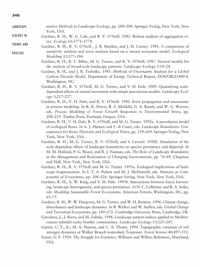
titative Methods in Landscape Ecology, pp. 289–308. Springer-Verlag, New York, NewYork, USA.

Gardner, R. H., W. G. Cale, and R. V. O’Neill. 1982. Robust analysis of aggregation er-ror. Ecology 63:1771–1779.

Gardner, R. H., R. V. O’Neill , J. B. Mankin, and J. H. Carney. 1981. A comparison ofsensitivity analysis and error analysis based on a stream ecosystem model. EcologicalModeling 12:177–194.

Gardner, R. H., B. T. Milne, M. G. Turner, and R. V. O’Neill. 1987. Neutral models forthe analysis of broad-scale landscape patterns. Landscape Ecology 1:19–28.

Gardner, R. H., and J. R. Trabalka. 1985. Methods of Uncertainty Analysis for a GlobalCarbon Dioxide Model. Department of Energy Technical Report. DOE/OR/21400-4.Washington, DC.

Gardner, R. H., R. V. O’Neill, M. G. Turner, and V. H. Dale. 1989. Quantifying scale-dependent effects of animal movement with simple percolation models. Landscape Ecol-ogy 3:217–227.

Gardner, R. H., V. H. Dale, and R. V. O’Neill. 1990. Error propagation and uncertaintyin process modeling. In R. K. Dixon, R. S. Meldahl, G. A. Ruark, and W. G. Warren,eds. Process Modeling of Forest Growth Responses to Environmental Stress, pp.208–219. Timber Press, Portland, Oregon, USA.

Gardner, R. H., V. H. Dale, R. V. O’Neill, and M. G. Turner. 1992a. A percolation modelof ecological flows. In A. J. Hansen and F. di Castri, eds. Landscape Boundaries: Con-sequences for Biotic Diversity and Ecological Flows, pp. 259–269. Springer-Verlag, NewYork, New York, USA.

Gardner, R. H., M. G. Turner, R. V. O’Neill, and S. Lavorel. 1992b. Simulation of thescale-dependent effects of landscape boundaries on species persistence and dispersal. InM. M. Holland, P. G. Risser, and R. J. Naiman, eds. The Role of Landscape Boundariesin the Management and Restoration of Changing Environments, pp. 76–89. Chapmanand Hall, New York, New York, USA.

Gardner, R. H., R. V. O’Neill and M. G. Turner. 1993a. Ecological implications of land-scape fragmentation. In S. T. A. Pickett and M. J. McDonnell, eds. Humans as Com-ponents of Ecosystems, pp. 208–226. Springer-Verlag, New York, New York, USA.

Gardner, R. H., A. W. King, and V. H. Dale. 1993b. Interactions between forest harvest-ing, landscape heterogeneity, and species persistence. In D. C. LeMaster and R. A. Sedjo,eds. Modeling Sustainable Forest Ecosystems, American Forests, Washington, DC, pp.65–75.

Gardner, R. H., W. W. Hargrove, M. G. Turner, and W. H. Romme. 1996. Climate change,disturbances and landscape dynamics. In B. Walker and W. Steffen, eds. Global Changeand Terrestrial Ecosystems, pp. 149–172. Cambridge University Press, Cambridge, UK.

Garrabou, J., J. Riera, and M. Zabala. 1998. Landscape pattern indices applied to Mediter-ranean subtidal rocky benthic communities. Landscape Ecology 13:225–247.

Garten, C. T., Jr., M. A. Huston, and C. A. Thoms. 1994. Topographic variation of soilnitrogen dynamics at Walker Branch watershed, Tennessee. Forest Science 40:497–512.

Gause, G. F. 1934. The Struggle for Existence. Williams and Wilkin, Baltimore, Maryland,USA.

348

L A N D S C A P E

E C O L O G Y I N

T H E O R Y A N D

P R A C T I C E

2888_e12_p333-388 2/27/01 1:55 PM Page 348

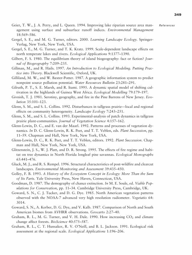
Geier, T. W., J. A. Perry, and L. Queen. 1994. Improving lake riparian source area man-agement using surface and subsurface runoff indices. Environmental Management18:569–586.

Gergel, S. E., and M. G. Turner, editors. 2000. Learning Landscape Ecology. Springer-Verlag, New York, New York, USA.

Gergel, S. E., M. G. Turner, and T. K. Kratz. 1999. Scale-dependent landscape effects onnorth temperate lakes and rivers. Ecological Applications 9:1377–1390.

Gilbert, F. S. 1980. The equilibrium theory of island biogeography: fact or fiction? Jour-nal of Biogeography 7:209–235.

Gillman, M., and R. Hails. 1997. An Introduction to Ecological Modeling. Putting Prac-tice into Theory. Blackwell Scientific, Oxford, UK.

Gilliland, M. W., and W. Baxter-Potter. 1987. A geographic information system to predictnonpoint source pollution potential. Water Resources Bulletin 23:281–291.

Gilruth, P. T., S. E. Marsh, and R. Itami. 1995. A dynamic spatial model of shifting cul-tivation in the highlands of Guinea West Africa. Ecological Modelling 79:179–197.

Givnish, T. J. 1981. Serotiny, geography, and fire in the Pine Barrens of New Jersey. Evo-lution 35:101–123.

Glenn, S. M., and S. L. Collins. 1992. Disturbances in tallgrass prairie—local and regionaleffects on community heterogeneity. Landscape Ecology 7:243–251.

Glenn, S. M., and S. L. Collins. 1993. Experimental-analysis of patch dynamics in tallgrassprairie plant-communities. Journal of Vegetation Science 4:157–162.

Glenn-Lewin, D. C., and E. van der Maarl. 1992. Patterns and processes of vegetation dy-namics. In D. C. Glenn-Lewin, R. K. Peet, and T. T. Veblen, eds. Plant Succession, pp.11–59. Chapman and Hall, New York, New York, USA.

Glenn-Lewin, D. C., R. K. Peet, and T. T. Veblen, editors. 1992. Plant Succession. Chap-man and Hall, New York, New York, USA.

Glitzenstein, J. S., W. J. Platt, and D. R. Strong. 1995. The effects of fire regime and habi-tat on tree dynamics in North Florida longleaf pine savannas. Ecological Monographs65:441–476.

Gluck, M. J., and R. S. Rempel. 1996. Structural characteristics of post-wildfire and clearcutlandscapes. Environmental Monitoring and Assessment 39:435–450.

Golley, F. B. 1993. A History of the Ecosystem Concept in Ecology: More Than the Sumof Its Parts. Yale University Press, New Haven, Connecticut, USA.

Goodman, D. 1987. The demography of chance extinction. In M. E. Soule, ed. Viable Pop-ulations for Conservation, pp. 11–34. Cambridge University Press, Cambridge, UK.

Goward, S. N., C. J. Tucker, and D. G. Dye. 1985. North American vegetation patternsobserved with the NOAA-7 advanced very high resolution radiometer. Vegetatio 64:3014.

Goward, S. N., A. Kerber, D. G. Dye, and V. Kalb. 1987. Comparison of North and SouthAmerican biomes from AVHRR observations. Geocarto 2:27–40.

Graham, R. L., M. G. Turner, and V. H. Dale. 1990. How increasing CO2 and climatechange affect forests. BioScience 40:575–587.

Graham, R. L., C. T. Hunsaker, R. V. O’Neill, and B. L. Jackson. 1991. Ecological riskassessment at the regional scale. Ecological Applications 1:196–206.

349

References

2888_e12_p333-388 2/27/01 1:55 PM Page 349

Grant, W. E., E. K. Pedersen, and S. L. Marin. 1997. Ecology and Natural Resource Man-agement. Systems Analysis and Simulation. John Wiley & Sons, Inc., New York, NewYork, USA.

Green, D. G. 1982. Fire and stability in the postglacial forests of southwest Nova Scotia.Journal of Biogeography 9:29–40.

Green, D. G. 1989. Simulated effects of fire, dispersal and spatial pattern on competitionwithin forest mosaics. Vegetatio 82:139–153.

Green, D. G. 1994. Simulation studies of connectivity and complexity in landscapes andecosystems. Pacific Conservation Biology 3:194–200.

Greig-Smith, P. 1952. The use of random and contiguous quadrants in the study of thestructure of plant communities. Annals of Botany 16:293–316.

Greig-Smith, P. 1979. Pattern in vegetation. Journal of Ecology 67:755–779.Greig-Smith, P. 1983. Quantitative Plant Ecology. University of California Press, Berkeley,

California, USA.Grimm, N. B. 1995. Why link species and ecosystems? In C. G. Jones and J. H. Lawton,

eds. Linking Species and Ecosystems, pp. 5–15. Chapman and Hall, New York, NewYork, USA.

Groffman, P. M., and J. M. Tiedje. 1989. Denitrification in north temperate forest soils:spatial and temporal patterns at the landscape and seasonal scales. Soil Biology and Bio-chemistry 21:613–620.

Groffman, P. M., J. M. Tiedje, D. L. Mokma, and S. Simkins. 1992. Regional scale analy-sis of denitrification in north temperate forest soils. Landscape Ecology 7:45–53.

Groffman, P. M., D. R. Zak, S. Christensen, A. Mosier, and J. M. Tiedje. 1993. Earlyspring nitrogen dynamics in a temperate forest landscape. Ecology 74:1579–1585.

Gross, K. L., K. S. Pregitzer, and A. J. Burton. 1995. Spatial variation in nitrogen avail-ability in three successional plant communities. Journal of Ecology 83:357–367.

Grumbacher, S. K., K. M. McEwen, D. A. Halverson, D. T. Jacobs, and J. Lindner. 1993.Self-organized criticality—an experiment with sandpiles. American Journal of Physics61:329–335.

Grumbine, R. E. 1994. What is ecosystem management? Conservation Biology 8:27–38.Gulve, P. S. 1994. Distribution and extinction patterns within a northern metapopulation

of the pond frog, Rana lessonae. Ecology 75:1357–1367.Gustafson, E. J. 1998. Quantifying landscape spatial pattern: What is the state of the art?

Ecosystems 1:143–156.Gustafson, E. J., and T. R. Crow. 1994. Modeling the effects of forest harvesting on land-

scape structure and the spatial distribution of cowbird brood parasitism. LandscapeEcology 9:237–248.

Gustafson, E. J., and T. R. Crow. 1996. Simulating the effects of alternative forest man-agement strategies on landscape structure. Journal of Environmental Management46:77–94.

Gustafson, E. J., and R. H. Gardner. 1996. The effect of landscape heterogeneity on theprobability of patch colonization. Ecology 77:94–107.

Gustafson, E. J., and G. R. Parker. 1992. Relationships between landcover proportion andindices of landscape spatial pattern. Landscape Ecology, 7:101–110.

350

L A N D S C A P E

E C O L O G Y I N

T H E O R Y A N D

P R A C T I C E

2888_e12_p333-388 2/27/01 1:55 PM Page 350

Gutzwiller, K. J., and S. H. Anderson. 1992. Interception of moving organisms: influences ofpatch shape, size, and orientation on community structure. Landscape Ecology 6:293–303.

Habeck, J. R., and R. W. Mutch. 1973. Fire-dependent forests in the northern Rockies.Quaternary Research 3:408–424.

Haber, W. 1990. Using landscape ecology in planning and management. In I. S. Zonneveldand R. T. T. Forman, eds. Changing Landscapes: An Ecological Perspective, pp.217–232. Springer-Verlag, New York, New York, USA.

Haefner, J. W. 1988a. Niche shifts in Greater Antillean Anolis communities: effects of nichemetric and biological resolution on null model tests. Oecologia 77:107–117.

Haefner, J. W. 1988b. Assembly rules for Greater Antillean Anolis lizards: competition andrandom models compared. Oecologia 74:551–565.

Hagget, P. 1963. Scale components in geographical problems. In R. J. Chorley and P. Haggett, eds. Frontiers in Geographical Teaching, pp. 164–185. Methuen & Com-pany Limited, London, UK.

Haines-Young, R., and M. Chopping. 1996. Quantifying landscape structure: a review oflandscape indices and their application to forested landscapes. Progress in Physical Ge-ography 20:418–445.

Haines-Young, R., D. R. Green, and S. Cousins, editors. 1993. Landscape Ecology andGeographic Information Systems. Taylor & Francis, Bristol, Pennsylvania, USA.

Halpern, C. B. 1988. Early successional pathways and the resistance and resilience of for-est communities. Ecology 69:1703–1715.

Halpern, C. B. 1989. Early successional patterns of forest species: interactions of life his-tory traits and disturbance. Ecology 70:704–720.

Halpin, P. N. 1997. Global climate change and natural-area protection: management re-sponses and research directions. Ecological Applications 7:828–843.

Hamilton, H. R., S. E. Goldstone, J. W. Milliman, A. L. Pugh, E. B. Roberts, and Z. Zeller.1969. Systems Simulation for Regional Analysis: An Application to River-basin Plan-ning. Massachusetts Institute of Technology Press, Cambridge, Massachusetts, USA.

Hamilton, W. D., and R. M. May. 1977. Dispersal in stable habitats. Nature 269:578–581.Hansen, A. J., S. L. Garman, B. Marks, and D. L. Urban. 1993. An approach for manag-

ing vertebrate diversity across multiple-use landscapes. Ecological Applications3:481–496.

Hansen, A. J., W. C. McComb, R. Vega, M. G. Raphael, and M. Hunter. 1995. Bird habi-tat relationships in natural and managed forests in the West Cascades of Oregon. Eco-logical Applications 5:555–569.

Hanski, I. 1981. Coexistence of competitors in patchy environments with and without pre-dation. Oikos 37:306–312.

Hanski, I. 1983. Coexistence of competitors in patchy environments. Ecology 64:493–500.

Hanski, I. 1989. Metapopulation dynamics: does it help to have more of the same? Trendsin Ecology and Evolution 4:113–114.

Hanski, I. 1998. Metapopulation dynamics. Nature 396:41–49.Hanski, I. A., and M. E. Gilpin, editors. 1997. Metapopulation Biology. Academic Press,

New York, New York, USA.

351

References

2888_e12_p333-388 2/27/01 1:55 PM Page 351

Hanski, I., and D. Simberloff. 1997. The metapopulation approach, its history, conceptualdomain, and application to conservation. In I. A. Hanski and M. E. Gilpin, eds. Metapop-ulation Biology, pp. 5–26. Academic Press, New York, New York, USA.

Hansson, L., L. Fahrig, and G. Merriam, editors. 1995. Mosaic Landscapes and Ecologi-cal Processes. Chapman and Hall, London, UK.

Harding, J. S., E. F. Benfield, P. V. Bolstad, G. S. Helfman, and E. B. D. Jones, III. 1998.Stream biodiversity: the ghost of land use past. Proceedings of the National Academyof Sciences 95:14843–14847.

Hardt, R. A., and R. T. T. Forman. 1989. Boundary form effects on woody colonizationof reclaimed surface mines. Ecology 70:1252–1260.

Hargrove, W. W., and J. Pickering. 1992. Pseudoreplication: a sine qua non for regionalecology. Landscape Ecology, 6: 251–258.

Harkness, R. D., and N. G. Maroudas. 1985. Central place foraging by an ant (Cataglyphisbicolor Fab.): a model of searching. Animal Behavior 33:916–928.

Harrington, R. A., J. H. Fownes, P. G. Scowcroft, and C. S. Vann. 1997. Impact of Hur-ricane Iniki on native Hawaiian Acacia koa forests: damage and two-year recovery. Jour-nal of Tropical Ecology 13:539–558.

Harris, G. P. 1998. Predictive models in spatially and temporally variable freshwater sys-tems. Australian Journal of Ecology 23:80–94.

Harris, L. D. 1984. The Fragmented Forest. University of Chicago Press, Chicago, Illinois,USA.

Harrison, G. W. 1979. Stability under environmental stress: resistance, resilience, persis-tence and variability. American Naturalist 113:659–669.

Harrison, S. 1994. Metapopulations and conservation. In P. J. Edwards, R. M. May, andN. R. Webb, eds. Large-scale Ecology and Conservation Biology, pp. 111–128. Black-well Scientific Publications, Oxford, UK.

Harton, J. C., and N. O. E. Smart. 1984. The effect of long-term exclusion of large her-bivores on soil nutrient status in Murchison Falls National Park, Uganda. African Jour-nal of Ecology 22:20–23.

Hartshorn, G. S. 1980. Neotropical forest dynamics. Biotropica 12 (Supplement):23–30.

Hartway, C., M. Ruckelshaus, and P. Kareiva. 1998. The challenge of applying spatiallyexplicit models to a world of sparse and messy data. In J. Bascompte and R. V. Sole,eds. Modeling Spatiotemporal Dynamics in Ecology, pp. 215–223. Springer-Verlag,Berlin, Germany.

Hastings, A. 1977. Spatial heterogeneity and the stability of predator–prey systems. Theo-retical Population Biology 12:37–48.

Hastings, A. 1996a. Models of spatial spread: is the theory complete? Ecology 77:1675–1679.

Hastings, A. 1996b. Population Biology: Concepts and Models. Springer-Verlag, New York,New York, USA.

Hastings, H. M., and G. Sugihara. 1993. Fractals: A User’s Guide for the Natural Sciences.Oxford University Press, New York, New York, USA.

Hayden, I. J., J. Faaborg, and R. L. Clawson. 1985. Estimates of minimal area require-

352

L A N D S C A P E

E C O L O G Y I N

T H E O R Y A N D

P R A C T I C E

2888_e12_p333-388 2/27/01 1:55 PM Page 352

ments for Missouri forest birds. Transactions of the Missouri Academy of Science19:11–22.

He, H. S., and D. J. Mladenoff. 1999. Spatially explicit and stochastic simulation of for-est-landscape fire disturbance and succession. Ecology 80:81–99.

He, H. S., D. J. Mladenoff, and T. R. Crow. 1999. Linking an ecosystem model and alandscape model to study forest species response to climate warming. Ecological Mod-eling 114:213–233.

Heck, W. W., A. S. Heagle, and D. S. Shriner. 1986. Effects on vegetation: native, crops,forest. In A. Stern, ed. Air Pollution, Volume 6, pp. 247–350. Academic Press, NewYork, New York, USA.

Heinselman, M. L. 1973. Fire in the virgin forests of the Boundary Waters Canoe Area,Minnesota. Quaternary Research 3:329–382.

Heinselman, M. L. 1996. The Boundary Waters Wilderness Ecosystem. University of Min-nesota Press, Minneapolis, Minnesota, USA.

Helliwell, D. R. 1976. The effects of size and isolation on the conservation value of woodedsites in Britain. Journal of Biogeography 3:407–416.

Hemens, G. C. 1970. Analysis and simulation of urban activity patterns. Socio-economicPlanning Science 4:53–66.

Hemstrom, M. A., and J. F. Franklin. 1982. Fire and other disturbances of the forests inMount Rainier National Park. Quaternary Research 18:32–51.

Henderson, M. T., G. Merriam, and J. Wegner. 1985. Patchy environments and speciessurvival: chipmunks in an agricultural mosaic. Biological Conservation 31:95–105.

Henderson-Sellers, A., M. F. Wilson, and G. Thomas. 1985. The effect of spatial resolu-tion on archives of land cover type. Climate Change 7:391–402.

Henebry, G. M. 1995. Spatial model error analysis using autocorrelation indices. Ecolog-ical Modeling 82:75–91.

Herbert, J., and B. J. Stevens. 1960. A model for the distribution of residential activities inurban areas. Journal of Regional Science 2:21–36.

Hett, J. M. 1971. Land Use Changes in East Tennessee and a Simulation Model Which Describes These Changes for Three Counties. ORNL/IBP-71/8. Oak Ridge NationalLaboratory, Oak Ridge, Tennessee, USA.

Heuvelink, G. B. M. 1998. Uncertainty analysis in environmental modeling under a changeof spatial scale. Nutrient Cycling in Agroecosystems 50:255–264.

Higgins, S. I., and D. M. Richardson. 1999. Predicting plant migration rates in a chang-ing world: the role of long-distance dispersal. American Naturalist 153:464–475.

Hilborn, R. 1975. The effect of spatial heterogeneity on the persistence of predator–preyinteractions. Theoretical Population Biology 8:346–355.

Hobbs, R. J. 1992. The role of corridors in conservation: solution or bandwagon? Trendsin Ecology and Evolution 7:389–392.

Hobbs, R. J. 1993. Effects of landscape fragmentation on ecosystem processes in the west-ern-Australian wheat-belt. Biological Conservation 64:193–201.

Hobbs, R. J., and D. A. Saunders, eds. 1992. Reintegrating Fragmented Landscapes.Springer-Verlag, New York, New York, USA.

Hobbs, R. J., D. A. Saunders, L. A. Lobry de Bruyn, and A. R. Main. 1993. Changes in

353

References

2888_e12_p333-388 2/27/01 1:55 PM Page 353

biota. In R. J. Hobbs and D. A. Saunders, eds. Reintegrating Fragmented Landscapes,pp. 65–106. Springer-Verlag, New York, New York, USA.

Hogeweg, P. 1988. Cellular automata as a paradigm for ecological modeling. Applicationsin Mathematics and Computation 27:81–100.

Hohn, M. E., A. M. Liebhold, and L. S. Gribko. 1993. Geostatistical model for forecast-ing spatial dynamics of defoliation caused by the gypsy moth (Lepidoptera: Lymantri-idae). Environmental Entomology 22:1066–1075.

Holland, E. A., W. J. Parton, J. K. Detling, and D. L. Coppock. 1992. Physiological re-sponses of plant populations to herbivory and other consequences of ecosystem nutri-ent flow. American Naturalist 140:685–706.

Holling, C. S. 1978. Adaptive Environmental Assessment and Management. John Wiley &Sons, New York, New York, USA.

Holling, C. S. 1992. Cross-scale morphology, geometry and dynamics of ecosystems. Eco-logical Monographs 62:447–502.

Holmes, E. E., M. A. Lewis, J. E. Banks, and R. R. Veit. 1994. Partial differential equa-tions in ecology: spatial interactions and population dynamics. Ecology 75:17–29.

Holmes, R. M., J. B. Jones, Jr., S. G. Fisher, and N. B. Grimm. 1996. Denitrification in anitrogen-limited stream ecosystem. Biogeochemistry 33:125–146.

Host, G. E., K. S. Pregitzer, C. W. Ramm, J. B. Hart, and D. T. Cleland. 1987. Landform-mediated differences in successional pathways among upland forest ecosystems in north-western Lower Michigan. Forest Science 33:445–457.

Host, G. E., K. S. Pregitzer, C. W. Ramm, D. P. Lusch, and D. T. Cleland. 1988. Varia-tion in overstory biomass among glacial landforms and ecological land units in north-western Lower Michigan. Canadian Journal of Forest Research 18:659–668.

Houghton, R. A. 1995. Land-use change and the carbon cycle. Global Change Biology1:275–287.

Huffaker, C. B. 1958. Experimental studies on predation: dispersion factors and preda-tor–prey oscillations. Hilgardia 27:343–383.

Huffaker, C. B., K. P. Shea, and S. G. Herman. 1963. Experimental studies on predation:complex dispersion and levels of food in an acarine predator–prey interaction. Hilgardia34:305–330.

Hunsaker, C. T., and D. A. Levine. 1995. Hierarchical approaches to the study of waterquality in rivers. Bioscience 45:193–203.

Hunsaker, C. T., S. W. Christensen, J. J. Beauchamp, R. J. Olson, R. S. Turner, and J. L. Malenchuk. 1986. Empirical Relationships Between Watershed Attributes andHeadwater Chemistry in the Adirondack Region. ORNL/TM-9838. Oak Ridge Na-tional Laboratory, Oak Ridge, Tennessee, USA.

Hunsaker, C. T., R. L. Graham, L. W. Barnthouse, R. H. Gardner, R. V. O’Neill, and G. W. Suter III. 1990. Assessing ecological risk on a regional scale. Environmental Man-agement 14:325–332.

Hunsaker, C. T., D. A. Levine, S. P. Timmons, B. L. Jackson, and R. V. O’Neill. 1992.Landscape characterization for assessing regional water quality. In D. H. McKenzie, D. E. Hyatt, and V. J. McDonald, eds. Ecological Indicators, Volume 2, pp. 997–1006.Elsevier Applied Science, New York, New York, USA.

354

L A N D S C A P E

E C O L O G Y I N

T H E O R Y A N D

P R A C T I C E

2888_e12_p333-388 2/27/01 1:55 PM Page 354

Hunt, E. R., Jr., F. C. Martin, and S. W. Running. 1991. Simulating the effects of climaticvariation on stem carbon accumulation of a ponderosa pine stand: comparison with an-nual growth increment data. Tree Physiology 9:161–171.

Hunter, M. L., Jr. 1991. Coping with ignorance: the coarse-filter strategy for maintainingbiodiversity. In K. A. Kohm, ed. Balancing on the Brink of Extinction, pp. 266–281.Island Press, Washington, DC, USA.

Hunter, M. L., Jr. 1993. Natural fire regimes as spatial models for managing boreal forests.Biological Conservation 65:115–120.

Hurlbert, S. H. 1984. Pseudoreplication and the design of ecological field experiments. Eco-logical Monographs 54:187–211.

Hurley, J. P., J. M. Benoit, C. L. Babiarz, M. M. Shafer, A. W. Andre, J. R. Sullivan, R. Hammond, and D. A. Webb. 1995. Influence of watershed characteristics on mer-cury levels in Wisconsin rivers. Environmental Science and Technology 29:1867–1875.

Hyman, J. B., J. B. McAninch, and D. L. DeAngelis. 1991. An individual-based simulationmodel of herbivory in a heterogeneous landscape. In M. G. Turner and R. H. Gardner,eds. Quantitative Methods in Landscape Ecology, pp. 443–475. Springer-Verlag, NewYork, New York, USA.

Hynes, H. B. N. 1975. The stream and its valley. Verhandlungren der Internationalen Vere-iningung fuer Theoretische und Angewandte Limnologie 19:1–15.

Imes, R. A., J. Rolstad, and P. Wegge. 1993. Predicting space use responses to habitat frag-mentation: can voles Microtus oeconomus serve as an experimental model system (EMS)for capercaille grouse in boreal forest? Biological Conservation 63:261–268.

Isard, W. 1960. Methods of Regional Analysis: An Introduction to Regional Science. Mass-achusetts Institute of Technology Press, Cambridge, Massachusetts, USA.

Isard, W. 1972. Ecologic–economic Analysis for Regional Development. The Free Press,New York, New York, USA.

Isard, W. 1975. Introduction to Regional Science. Prentice Hall, Upper Saddle River, NewJersey, USA.

ISI. 1999. The Web of Science (http//webofscience.com), the Web interface providing ac-cess to the Science Citation Index Expanded (TM), Institute for Scientific Information,3501 Market Street, Philadelphia, Pennsylvania, 19104, USA.

Istock, C. A., and S. M. Scheiner. 1987. Affinities and high-order diversity within land-scape mosaics. Evolutionary Ecology 1:11–29.

Istok, J. D., J. D. Smythe, and A. L. Flint. 1993. Multivariate geostatistical analysis ofgroundwater contamination: a case history. Ground Water 31: 63–74.

Iverson, L. R. 1988. Land-use changes in Illinois, USA: the influence of landscape attrib-utes on current and historic land use. Landscape Ecology 2:45–62.

Iverson, L. R. 1991. Forest resources of Illinois: What do we have and what are they do-ing for us? Illinois Natural History Survey Bulletin 34:361–374.

Ives, A. R., M. G. Turner, and S. M. Pearson. 1998. Local explanations of landscape pat-terns: can analytical approaches approximate simulation models of spatial processes?Ecosystems 1:35–51.

Jackson, D. A., K. M. Somers, and H. H. Harvey. 1992. Null models and fish communi-ties: evidence of nonrandom patterns. American Naturalist 139:930–951.

355

References

2888_e12_p333-388 2/27/01 1:55 PM Page 355

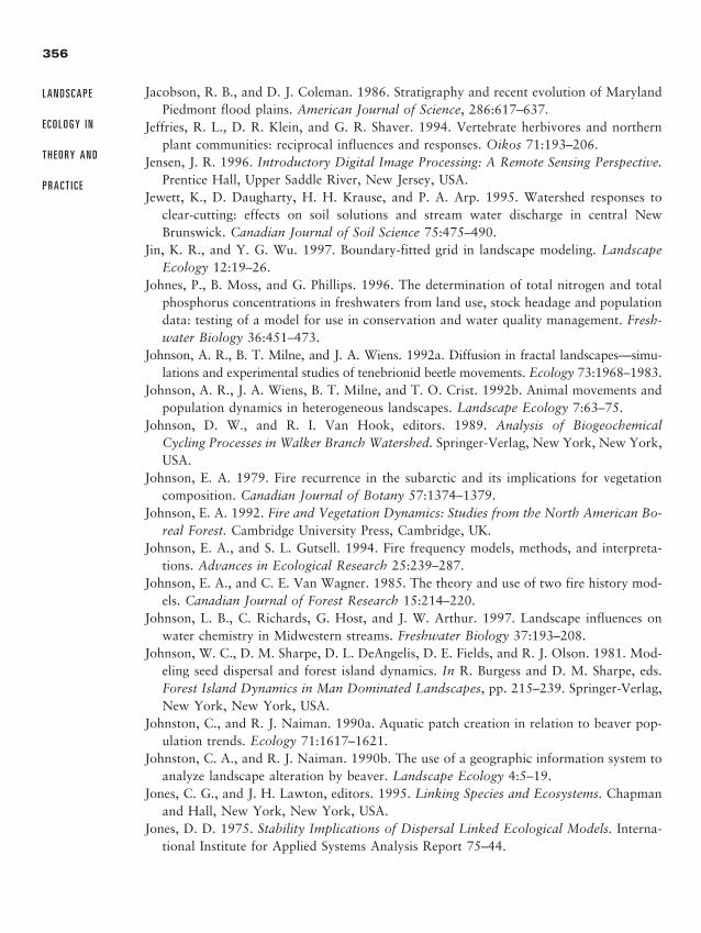
Jacobson, R. B., and D. J. Coleman. 1986. Stratigraphy and recent evolution of MarylandPiedmont flood plains. American Journal of Science, 286:617–637.

Jeffries, R. L., D. R. Klein, and G. R. Shaver. 1994. Vertebrate herbivores and northernplant communities: reciprocal influences and responses. Oikos 71:193–206.

Jensen, J. R. 1996. Introductory Digital Image Processing: A Remote Sensing Perspective.Prentice Hall, Upper Saddle River, New Jersey, USA.

Jewett, K., D. Daugharty, H. H. Krause, and P. A. Arp. 1995. Watershed responses toclear-cutting: effects on soil solutions and stream water discharge in central NewBrunswick. Canadian Journal of Soil Science 75:475–490.

Jin, K. R., and Y. G. Wu. 1997. Boundary-fitted grid in landscape modeling. LandscapeEcology 12:19–26.

Johnes, P., B. Moss, and G. Phillips. 1996. The determination of total nitrogen and totalphosphorus concentrations in freshwaters from land use, stock headage and populationdata: testing of a model for use in conservation and water quality management. Fresh-water Biology 36:451–473.

Johnson, A. R., B. T. Milne, and J. A. Wiens. 1992a. Diffusion in fractal landscapes—simu-lations and experimental studies of tenebrionid beetle movements. Ecology 73:1968–1983.

Johnson, A. R., J. A. Wiens, B. T. Milne, and T. O. Crist. 1992b. Animal movements andpopulation dynamics in heterogeneous landscapes. Landscape Ecology 7:63–75.

Johnson, D. W., and R. I. Van Hook, editors. 1989. Analysis of Biogeochemical Cycling Processes in Walker Branch Watershed. Springer-Verlag, New York, New York,USA.

Johnson, E. A. 1979. Fire recurrence in the subarctic and its implications for vegetationcomposition. Canadian Journal of Botany 57:1374–1379.

Johnson, E. A. 1992. Fire and Vegetation Dynamics: Studies from the North American Bo-real Forest. Cambridge University Press, Cambridge, UK.

Johnson, E. A., and S. L. Gutsell. 1994. Fire frequency models, methods, and interpreta-tions. Advances in Ecological Research 25:239–287.

Johnson, E. A., and C. E. Van Wagner. 1985. The theory and use of two fire history mod-els. Canadian Journal of Forest Research 15:214–220.

Johnson, L. B., C. Richards, G. Host, and J. W. Arthur. 1997. Landscape influences onwater chemistry in Midwestern streams. Freshwater Biology 37:193–208.

Johnson, W. C., D. M. Sharpe, D. L. DeAngelis, D. E. Fields, and R. J. Olson. 1981. Mod-eling seed dispersal and forest island dynamics. In R. Burgess and D. M. Sharpe, eds.Forest Island Dynamics in Man Dominated Landscapes, pp. 215–239. Springer-Verlag,New York, New York, USA.

Johnston, C., and R. J. Naiman. 1990a. Aquatic patch creation in relation to beaver pop-ulation trends. Ecology 71:1617–1621.

Johnston, C. A., and R. J. Naiman. 1990b. The use of a geographic information system toanalyze landscape alteration by beaver. Landscape Ecology 4:5–19.

Jones, C. G., and J. H. Lawton, editors. 1995. Linking Species and Ecosystems. Chapmanand Hall, New York, New York, USA.

Jones, D. D. 1975. Stability Implications of Dispersal Linked Ecological Models. Interna-tional Institute for Applied Systems Analysis Report 75–44.

356

L A N D S C A P E

E C O L O G Y I N

T H E O R Y A N D

P R A C T I C E

2888_e12_p333-388 2/27/01 1:55 PM Page 356

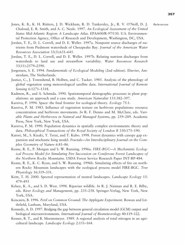
Jones, K. B., K. H. Riitters, J. D. Wickham, R. D. Tankersley, Jr., R. V. O’Neill, D. J.Chaloud, E. R. Smith, and A. C. Neale. 1997. An Ecological Assessment of the UnitedStates Mid-Atlantic Region: A Landscape Atlas. EPA/600/R-97/130. U.S. Environmen-tal Protection Agency, Office of Research and Development, Washington, DC, USA.

Jordan, T. E., D. L. Correll, and D. E. Weller. 1997a. Nonpoint source discharges of nu-trients from Piedmont watersheds of Chesapeake Bay. Journal of the American WaterResources Association 33(3):631–645.

Jordan, T. E., D. L. Correll, and D. E. Weller. 1997b. Relating nutrient discharges fromwatersheds to land use and streamflow variability. Water Resources Research33(11):2579–2590.

Jorgensen, S. E. 1994. Fundamentals of Ecological Modeling (2nd edition). Elsevier, Am-sterdam, The Netherlands.

Justice, C., J. Townshend, B. Holben, and C. Tucker. 1985. Analysis of the phenology ofglobal vegetation using meteorological satellite data. International Journal of RemoteSensing 6:1271–1318.

Kadmon, R., and A. Schmida. 1990. Spatiotemporal demographic processes in plant pop-ulations: an approach and a case study. American Naturalist 135:382–397.

Kareiva, P. 1994. Space: the final frontier for ecological theory. Ecology 75:1.Kareiva, P. M. 1983. Influence of vegetation texture on herbivore populations: resource

concentration and herbivore movements. In R. F. Denno and M. McClure, eds. Vari-able Plants and Herbivores in Natural and Managed Systems, pp. 259–289. AcademicPress, New York, New York, USA.

Kareiva, P. M. 1990. Population dynamics in spatially complex environments: theory anddata. Philosophical Transactions of the Royal Society of London B 330:175–190.

Katori, M., S. Kizaki, Y. Terui, and T. Kubo. 1998. Forest dynamics with canopy gap ex-pansion and stochastic Ising model. Fractals—An Interdisciplinary Journal on the Com-plex Geometry of Nature 6:81–86.

Keane, R. E., P. Morgan and S. W. Running. 1996a. FIRE-BGC—A Mechanistic Ecolog-ical Process Model for Simulating Fire Succession on Coniferous Forest Landscapes ofthe Northern Rocky Mountains. USDA Forest Service Research Paper INT-RP-484.

Keane, R. E., K. C. Ryan, and S. W. Running. 1996b. Simulating effects of fire on north-ern Rocky Mountain landscapes with the ecological process model FIRE-BGC. TreePhysiology 16:319–331.

Keitt, T. H. 2000. Spectral representation of neutral landscapes. Landscape Ecology 15:479–493

Kelsey, K. A., and S. D. West. 1998. Riparian wildlife. In R. J. Naiman and R. E. Bilby,eds. River Ecology and Management, pp. 235–258. Springer-Verlag, New York, NewYork, USA.

Kencairn, B. 1996. Peril on Common Ground: The Applegate Experiment. Rowan and Lit-tlefield, Lanham, Maryland, USA.

Kennedy, A. D. 1997. Bridging the gap between general circulation model (GCM) output andbiological microenvironments. International Journal of Biometeorology 40:119–122.

Kesner, B. T., and B. Meentemeyer. 1989. A regional analysis of total nitrogen in an agri-cultural landscape. Landscape Ecology 2:151–164.

357

References

2888_e12_p333-388 2/27/01 1:55 PM Page 357

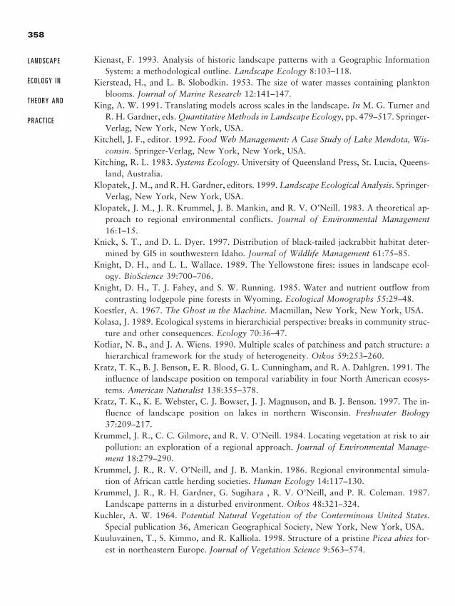
Kienast, F. 1993. Analysis of historic landscape patterns with a Geographic InformationSystem: a methodological outline. Landscape Ecology 8:103–118.

Kierstead, H., and L. B. Slobodkin. 1953. The size of water masses containing planktonblooms. Journal of Marine Research 12:141–147.

King, A. W. 1991. Translating models across scales in the landscape. In M. G. Turner andR. H. Gardner, eds. Quantitative Methods in Landscape Ecology, pp. 479–517. Springer-Verlag, New York, New York, USA.

Kitchell, J. F., editor. 1992. Food Web Management: A Case Study of Lake Mendota, Wis-consin. Springer-Verlag, New York, New York, USA.

Kitching, R. L. 1983. Systems Ecology. University of Queensland Press, St. Lucia, Queens-land, Australia.

Klopatek, J. M., and R. H. Gardner, editors. 1999. Landscape Ecological Analysis. Springer-Verlag, New York, New York, USA.

Klopatek, J. M., J. R. Krummel, J. B. Mankin, and R. V. O’Neill. 1983. A theoretical ap-proach to regional environmental conflicts. Journal of Environmental Management16:1–15.

Knick, S. T., and D. L. Dyer. 1997. Distribution of black-tailed jackrabbit habitat deter-mined by GIS in southwestern Idaho. Journal of Wildlife Management 61:75–85.

Knight, D. H., and L. L. Wallace. 1989. The Yellowstone fires: issues in landscape ecol-ogy. BioScience 39:700–706.

Knight, D. H., T. J. Fahey, and S. W. Running. 1985. Water and nutrient outflow fromcontrasting lodgepole pine forests in Wyoming. Ecological Monographs 55:29–48.

Koestler, A. 1967. The Ghost in the Machine. Macmillan, New York, New York, USA.Kolasa, J. 1989. Ecological systems in hierarchicial perspective: breaks in community struc-

ture and other consequences. Ecology 70:36–47.Kotliar, N. B., and J. A. Wiens. 1990. Multiple scales of patchiness and patch structure: a

hierarchical framework for the study of heterogeneity. Oikos 59:253–260.Kratz, T. K., B. J. Benson, E. R. Blood, G. L. Cunningham, and R. A. Dahlgren. 1991. The

influence of landscape position on temporal variability in four North American ecosys-tems. American Naturalist 138:355–378.

Kratz, T. K., K. E. Webster, C. J. Bowser, J. J. Magnuson, and B. J. Benson. 1997. The in-fluence of landscape position on lakes in northern Wisconsin. Freshwater Biology37:209–217.

Krummel, J. R., C. C. Gilmore, and R. V. O’Neill. 1984. Locating vegetation at risk to airpollution: an exploration of a regional approach. Journal of Environmental Manage-ment 18:279–290.

Krummel, J. R., R. V. O’Neill, and J. B. Mankin. 1986. Regional environmental simula-tion of African cattle herding societies. Human Ecology 14:117–130.

Krummel, J. R., R. H. Gardner, G. Sugihara , R. V. O’Neill, and P. R. Coleman. 1987.Landscape patterns in a disturbed environment. Oikos 48:321–324.

Kuchler, A. W. 1964. Potential Natural Vegetation of the Conterminous United States.Special publication 36, American Geographical Society, New York, New York, USA.

Kuuluvainen, T., S. Kimmo, and R. Kalliola. 1998. Structure of a pristine Picea abies for-est in northeastern Europe. Journal of Vegetation Science 9:563–574.

358

L A N D S C A P E

E C O L O G Y I N

T H E O R Y A N D

P R A C T I C E

2888_e12_p333-388 2/27/01 1:55 PM Page 358

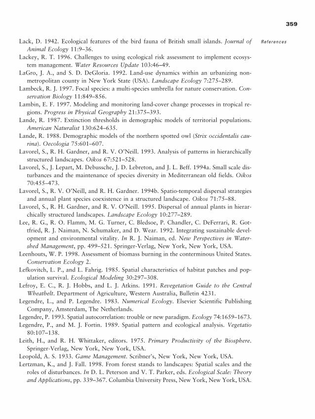
Lack, D. 1942. Ecological features of the bird fauna of British small islands. Journal ofAnimal Ecology 11:9–36.

Lackey, R. T. 1996. Challenges to using ecological risk assessment to implement ecosys-tem management. Water Resources Update 103:46–49.

LaGro, J. A., and S. D. DeGloria. 1992. Land-use dynamics within an urbanizing non-metropolitan county in New York State (USA). Landscape Ecology 7:275–289.

Lambeck, R. J. 1997. Focal species: a multi-species umbrella for nature conservation. Con-servation Biology 11:849–856.

Lambin, E. F. 1997. Modeling and monitoring land-cover change processes in tropical re-gions. Progress in Physical Geography 21:375–393.

Lande, R. 1987. Extinction thresholds in demographic models of territorial populations.American Naturalist 130:624–635.

Lande, R. 1988. Demographic models of the northern spotted owl (Strix occidentalis cau-rina). Oecologia 75:601–607.

Lavorel, S., R. H. Gardner, and R. V. O’Neill. 1993. Analysis of patterns in hierarchicallystructured landscapes. Oikos 67:521–528.

Lavorel, S., J. Lepart, M. Debussche, J. D. Lebreton, and J. L. Beff. 1994a. Small scale dis-turbances and the maintenance of species diversity in Mediterranean old fields. Oikos70:455–473.

Lavorel, S., R. V. O’Neill, and R. H. Gardner. 1994b. Spatio-temporal dispersal strategiesand annual plant species coexistence in a structured landscape. Oikos 71:75–88.

Lavorel, S., R. H. Gardner, and R. V. O’Neill. 1995. Dispersal of annual plants in hierar-chically structured landscapes. Landscape Ecology 10:277–289.

Lee, R. G., R. O. Flamm, M. G. Turner, C. Bledsoe, P. Chandler, C. DeFerrari, R. Got-tfried, R. J. Naiman, N. Schumaker, and D. Wear. 1992. Integrating sustainable devel-opment and environmental vitality. In R. J. Naiman, ed. New Perspectives in Water-shed Management, pp. 499–521. Springer-Verlag, New York, New York, USA.

Leenhouts, W. P. 1998. Assessment of biomass burning in the conterminous United States.Conservation Ecology 2.

Lefkovitch, L. P., and L. Fahrig. 1985. Spatial characteristics of habitat patches and pop-ulation survival. Ecological Modeling 30:297–308.

Lefroy, E. C., R. J. Hobbs, and L. J. Atkins. 1991. Revegetation Guide to the CentralWheatbelt. Department of Agriculture, Western Australia, Bulletin 4231.

Legendre, L., and P. Legendre. 1983. Numerical Ecology. Elsevier Scientific PublishingCompany, Amsterdam, The Netherlands.

Legendre, P. 1993. Spatial autocorrelation: trouble or new paradigm. Ecology 74:1659–1673.Legendre, P., and M. J. Fortin. 1989. Spatial pattern and ecological analysis. Vegetatio

80:107–138.Leith, H., and R. H. Whittaker, editors. 1975. Primary Productivity of the Biosphere.

Springer-Verlag, New York, New York, USA.Leopold, A. S. 1933. Game Management. Scribner’s, New York, New York, USA.Lertzman, K., and J. Fall. 1998. From forest stands to landscapes: Spatial scales and the

roles of disturbances. In D. L. Peterson and V. T. Parker, eds. Ecological Scale: Theoryand Applications, pp. 339–367. Columbia University Press, New York, New York, USA.

359

References

2888_e12_p333-388 2/27/01 1:55 PM Page 359

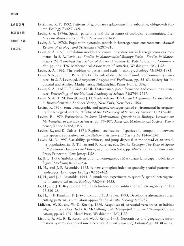
Lertzman, K. P. 1992. Patterns of gap-phase replacement in a subalpine, old-growth for-est. Ecology 73:657–669.

Levin, S. A. 1976a. Spatial patterning and the structure of ecological communities. Lec-tures on Mathematics in the Life Science 8:1–35.

Levin, S. A. 1976b. Population dynamics models in heterogeneous environments. AnnualReview of Ecology and Systematics 7:287–310.

Levin, S. A. 1978. Population models and community structure in heterogeneous environ-ments. In S. A. Levin, ed. Studies in Mathematical Biology Series—Studies in Mathe-matics (Mathematical Association of America) Volume II. Populations and Communi-ties, pp. 439–476. Mathematical Association of America, Washington, DC, USA.

Levin, S. A. 1992. The problem of pattern and scale in ecology. Ecology 73:1943–1983.Levin, S. A., and R. T. Paine. 1974a. The role of disturbance in models of community struc-

ture. In S. A Levin, ed. Ecosystem Analysis and Prediction, pp. 55–63. Society for In-dustrial and Applied Mathematics, Philadelphia, Pennsylvania, USA.

Levin, S. A., and R. T. Paine. 1974b. Disturbance, patch formation and community struc-ture. Proceedings of the National Academy of Science 71:2744–2747.

Levin, S. A., T. M. Powell, and J. H. Steele, editors. 1993. Patch Dynamics. Lecture Notesin Biomathematics. Springer-Verlag, New York, New York, USA.

Levins, R. 1969. Some demographic and genetic consequences of environmental heterogene-ity for biological control. Bulletin of the Entomological Society of America 15:237–240.

Levins, R. 1970. Extinctions. In Some Mathematical Questions in Biology. Lectures onMathematics in the Life Sciences, pp. 77–107. American Mathematical Society, Provi-dence, Rhode Island, USA.

Levins, R., and D. Culver. 1971. Regional coexistence of species and competition betweenrare species. Proceedings of the National Academy of Science 68:1246–1248.

Lewis, M. A. 1997. Variability, patchiness, and jump dispersal in the spread of an invad-ing population. In D. Tilman and P. Kareiva, eds. Spatial Ecology: The Role of Spacein Population Dynamics and Interspecific Interactions, pp. 46–69. Princeton UniversityPress, Princeton, New Jersey, USA.

Li, B. L. 1995. Stability analysis of a nonhomogeneous Markovian landscape model. Eco-logical Modeling 82:247–256.

Li, H., and J. F. Reynolds. 1993. A new contagion index to quantify spatial patterns oflandscapes. Landscape Ecology 8:155–162.

Li, H., and J. F. Reynolds. 1994. A simulation experiment to quantify spatial heterogene-ity in categorical maps. Ecology 75:2446–2455.

Li, H., and J. F. Reynolds. 1995. On definition and quantification of heterogeneity. Oikos73:280–284.

Li, H., J. F. Franklin, F. J. Swanson, and T. A. Spies. 1993. Developing alternative forestcutting patterns: a simulation approach. Landscape Ecology 8:63–75.

Lidicker, W. Z., and W. D. Koenig. 1996. Responses of terrestrial vertebrates to habitatedges and corridors. In D. R. McCullough, ed. Metapopulations and Wildlife Conser-vation, pp. 85–109. Island Press, Washington, DC, USA.

Liebold, A. M., R. E. Rossi, and W. P. Kemp. 1993. Geostatistics and geographic infor-mation systems in applied insect ecology. Annual Review of Entomology 38:303–327.

360

L A N D S C A P E

E C O L O G Y I N

T H E O R Y A N D

P R A C T I C E

2888_e12_p333-388 2/27/01 1:55 PM Page 360

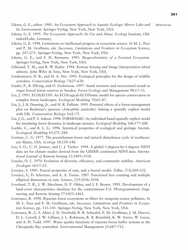
Likens, G. E., editor. 1985. An Ecosystem Approach to Aquatic Ecology: Mirror Lake andIts Environment. Springer-Verlag, New York, New York, USA.

Likens, G. E. 1995. The Ecosystem Approach: Its Use and Abuse. Ecology Institute, Old-endorf/Luhe, Germany.

Likens, G. E. 1998. Limitations to intellectual progress in ecosystem science. In M. L. Paceand P. M. Groffman, eds. Successes, Limitations and Frontiers in Ecosystem Science,pp. 247–271. Springer-Verlag, New York, New York, USA.

Likens, G. E., and F. H. Bormann. 1995. Biogeochemistry of a Forested Ecosystem.Springer-Verlag, New York, New York, USA.

Lillesand, T. M., and R. W. Kiefer. 1994. Remote Sensing and Image Interpretation (thirdedition). John Wiley & Sons, New York, New York, USA.

Lindenmayer, D. B., and H. A. Nix. 1993. Ecological principles for the design of wildlifecorridors. Conservation Biology 7:627–630.

Linder, P., B. Elfving, and O. Zackrisson. 1997. Stand structure and successional trends invirgin boreal forest reserves in Sweden. Forest Ecology and Management 98:17–33.

Liu, J. 1993. ECOLECON: An ECOLogical–ECONomic model for species conservation incomplex forest landscapes. Ecological Modeling 70:63–87.

Liu, J., J. B. Dunning, Jr., and H. R. Pulliam. 1995. Potential effects of a forest-managementplan on Bachman’s sparrow (Aimophila aestivalis): linking a spatially explicit modelwith GIS. Conservation Biology 9:62–75.

Liu, J. G., and P. S. Ashton. 1998. FORMOSAIC: An individual-based spatially explicit modelfor simulating forest dynamics in landscape mosaics. Ecological Modeling 106:177–200.

Loehle, C., and B. L. Li. 1996. Statistical properties of ecological and geologic fractals.Ecological Modeling 85:271–284.

Lorimer, C. G. 1977. The presettlement forest and natural disturbance cycle of northeast-ern Maine, USA. Ecology 58:139–148.

Los, S. O., C. O. Justace, and C. J. Tucker. 1994. A global 1-degrees-by-1-degrees NDVIdata set for climate studies derived from the GIMMS continental NDVI data. Interna-tional Journal of Remote Sensing 15:3493–3518.

Loucks, O. L. 1970. Evolution of diversity, efficiency, and community stability. AmericanZoologist 10:17–25.

Lovejoy, S. 1985. Fractal properties of rain, and a fractal model. Tellus, 37A:209–232.Lovejoy, S., D. Schertzer, and A. A. Tsonis. 1987. Functional box counting and multiple

elliptical dimensions in rain. Science, 235:1036–1038.Loveland, T. R., J. W. Merchant, D. P. Ohlen, and J. F. Brown. 1991. Development of a

land-cover characteristics database for the conterminous U.S. Photogrammetric Engi-neering and Remote Sensing 57:1453–1463.

Lowrance, R. 1998. Riparian forest ecosystems as filters for nonpoint-source pollution. InM. L. Pace and P. M. Groffman, eds. Successes, Limitations and Frontiers in Ecosys-tem Science, pp. 113–141. Springer-Verlag, New York, New York, USA.

Lowrance, R., L. S. Altier, J. D. Newbold, R. R. Schnabel, P. M. Groffman, J. M. Denver,D. L. Correll, J. W. Gilliam, J. L. Robinson, R. B. Brinsfield, K. W. Staver, W. Lucas,and A. H. Todd. 1997. Water quality functions of riparian forest buffer systems in theChesapeake Bay watershed. Environmental Management 21:687–712.

361

References

2888_e12_p333-388 2/27/01 1:55 PM Page 361

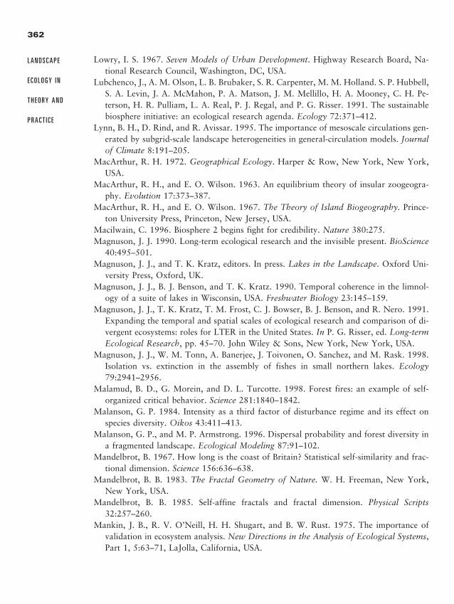
Lowry, I. S. 1967. Seven Models of Urban Development. Highway Research Board, Na-tional Research Council, Washington, DC, USA.

Lubchenco, J., A. M. Olson, L. B. Brubaker, S. R. Carpenter, M. M. Holland. S. P. Hubbell,S. A. Levin, J. A. McMahon, P. A. Matson, J. M. Mellillo, H. A. Mooney, C. H. Pe-terson, H. R. Pulliam, L. A. Real, P. J. Regal, and P. G. Risser. 1991. The sustainablebiosphere initiative: an ecological research agenda. Ecology 72:371–412.

Lynn, B. H., D. Rind, and R. Avissar. 1995. The importance of mesoscale circulations gen-erated by subgrid-scale landscape heterogeneities in general-circulation models. Journalof Climate 8:191–205.

MacArthur, R. H. 1972. Geographical Ecology. Harper & Row, New York, New York,USA.

MacArthur, R. H., and E. O. Wilson. 1963. An equilibrium theory of insular zoogeogra-phy. Evolution 17:373–387.

MacArthur, R. H., and E. O. Wilson. 1967. The Theory of Island Biogeography. Prince-ton University Press, Princeton, New Jersey, USA.

Macilwain, C. 1996. Biosphere 2 begins fight for credibility. Nature 380:275.Magnuson, J. J. 1990. Long-term ecological research and the invisible present. BioScience

40:495–501.Magnuson, J. J., and T. K. Kratz, editors. In press. Lakes in the Landscape. Oxford Uni-

versity Press, Oxford, UK.Magnuson, J. J., B. J. Benson, and T. K. Kratz. 1990. Temporal coherence in the limnol-

ogy of a suite of lakes in Wisconsin, USA. Freshwater Biology 23:145–159.Magnuson, J. J., T. K. Kratz, T. M. Frost, C. J. Bowser, B. J. Benson, and R. Nero. 1991.

Expanding the temporal and spatial scales of ecological research and comparison of di-vergent ecosystems: roles for LTER in the United States. In P. G. Risser, ed. Long-termEcological Research, pp. 45–70. John Wiley & Sons, New York, New York, USA.

Magnuson, J. J., W. M. Tonn, A. Banerjee, J. Toivonen, O. Sanchez, and M. Rask. 1998.Isolation vs. extinction in the assembly of fishes in small northern lakes. Ecology79:2941–2956.

Malamud, B. D., G. Morein, and D. L. Turcotte. 1998. Forest fires: an example of self-organized critical behavior. Science 281:1840–1842.

Malanson, G. P. 1984. Intensity as a third factor of disturbance regime and its effect onspecies diversity. Oikos 43:411–413.

Malanson, G. P., and M. P. Armstrong. 1996. Dispersal probability and forest diversity ina fragmented landscape. Ecological Modeling 87:91–102.

Mandelbrot, B. 1967. How long is the coast of Britain? Statistical self-similarity and frac-tional dimension. Science 156:636–638.

Mandelbrot, B. B. 1983. The Fractal Geometry of Nature. W. H. Freeman, New York,New York, USA.

Mandelbrot, B. B. 1985. Self-affine fractals and fractal dimension. Physical Scripts32:257–260.

Mankin, J. B., R. V. O’Neill, H. H. Shugart, and B. W. Rust. 1975. The importance ofvalidation in ecosystem analysis. New Directions in the Analysis of Ecological Systems,Part 1, 5:63–71, LaJolla, California, USA.

362

L A N D S C A P E

E C O L O G Y I N

T H E O R Y A N D

P R A C T I C E

2888_e12_p333-388 2/27/01 1:55 PM Page 362

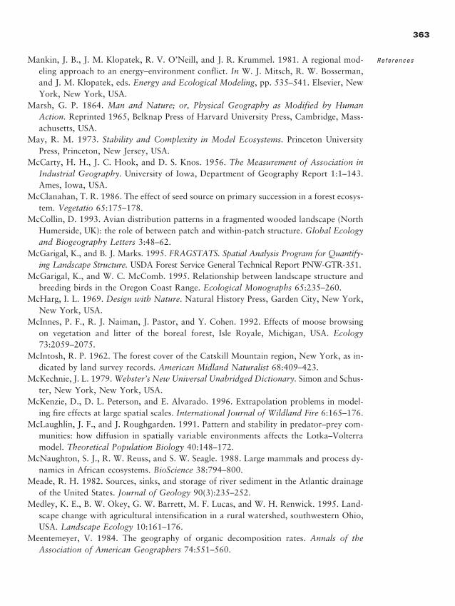
Mankin, J. B., J. M. Klopatek, R. V. O’Neill, and J. R. Krummel. 1981. A regional mod-eling approach to an energy–environment conflict. In W. J. Mitsch, R. W. Bosserman,and J. M. Klopatek, eds. Energy and Ecological Modeling, pp. 535–541. Elsevier, NewYork, New York, USA.

Marsh, G. P. 1864. Man and Nature; or, Physical Geography as Modified by Human Action. Reprinted 1965, Belknap Press of Harvard University Press, Cambridge, Mass-achusetts, USA.

May, R. M. 1973. Stability and Complexity in Model Ecosystems. Princeton UniversityPress, Princeton, New Jersey, USA.

McCarty, H. H., J. C. Hook, and D. S. Knos. 1956. The Measurement of Association inIndustrial Geography. University of Iowa, Department of Geography Report 1:1–143.Ames, Iowa, USA.

McClanahan, T. R. 1986. The effect of seed source on primary succession in a forest ecosys-tem. Vegetatio 65:175–178.

McCollin, D. 1993. Avian distribution patterns in a fragmented wooded landscape (NorthHumerside, UK): the role of between patch and within-patch structure. Global Ecologyand Biogeography Letters 3:48–62.

McGarigal, K., and B. J. Marks. 1995. FRAGSTATS. Spatial Analysis Program for Quantify-ing Landscape Structure. USDA Forest Service General Technical Report PNW-GTR-351.

McGarigal, K., and W. C. McComb. 1995. Relationship between landscape structure andbreeding birds in the Oregon Coast Range. Ecological Monographs 65:235–260.

McHarg, I. L. 1969. Design with Nature. Natural History Press, Garden City, New York,New York, USA.

McInnes, P. F., R. J. Naiman, J. Pastor, and Y. Cohen. 1992. Effects of moose browsingon vegetation and litter of the boreal forest, Isle Royale, Michigan, USA. Ecology73:2059–2075.

McIntosh, R. P. 1962. The forest cover of the Catskill Mountain region, New York, as in-dicated by land survey records. American Midland Naturalist 68:409–423.

McKechnie, J. L. 1979. Webster’s New Universal Unabridged Dictionary. Simon and Schus-ter, New York, New York, USA.

McKenzie, D., D. L. Peterson, and E. Alvarado. 1996. Extrapolation problems in model-ing fire effects at large spatial scales. International Journal of Wildland Fire 6:165–176.

McLaughlin, J. F., and J. Roughgarden. 1991. Pattern and stability in predator–prey com-munities: how diffusion in spatially variable environments affects the Lotka–Volterramodel. Theoretical Population Biology 40:148–172.

McNaughton, S. J., R. W. Reuss, and S. W. Seagle. 1988. Large mammals and process dy-namics in African ecosystems. BioScience 38:794–800.

Meade, R. H. 1982. Sources, sinks, and storage of river sediment in the Atlantic drainageof the United States. Journal of Geology 90(3):235–252.

Medley, K. E., B. W. Okey, G. W. Barrett, M. F. Lucas, and W. H. Renwick. 1995. Land-scape change with agricultural intensification in a rural watershed, southwestern Ohio,USA. Landscape Ecology 10:161–176.

Meentemeyer, V. 1984. The geography of organic decomposition rates. Annals of the Association of American Geographers 74:551–560.

363

References

2888_e12_p333-388 2/27/01 1:55 PM Page 363

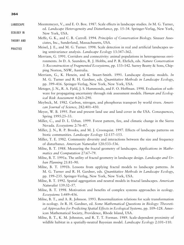
Meentemeyer, V., and E. O. Box. 1987. Scale effects in landscape studies. In M. G. Turner,ed. Landscape Heterogeneity and Disturbance, pp. 15–34. Springer-Verlag, New York,New York, USA.

Meffe, G. K., and C. R. Carroll. 1994. Principles of Conservation Biology. Sinauer Asso-ciates, Inc., Sunderland, Massachusetts, USA.

Meisel, J. E., and M. G. Turner. 1998. Scale detection in real and artificial landscapes us-ing semivariance analysis. Landscape Ecology 13:347–362.

Merriam, G. 1991. Corridors and connectivity: animal populations in heterogeneous envi-ronments. In D. A. Saunders, R. J. Hobbs, and P. R. Ehrlich, eds. Nature Conservation3: Reconstruction of Fragmented Ecosystems, pp. 133–142. Surrey Beatty & Sons, Chip-ping Norton, NSW, Australia.

Merriam, G., K. Henein, and K. Stuart-Smith. 1991. Landscape dynamic models. InM. G. Turner and R. H. Gardner, eds. Quantitative Methods in Landscape Ecology,pp. 399–416. Springer-Verlag, New York, New York, USA.

Metzger, J. N., R. A. Fjeld, J. S. Hammonds, and F. O. Hoffman. 1998. Evaluation of soft-ware for propagating uncertainty through risk assessment models. Human and Ecolog-ical Risk Assessment 4:263–290.

Meybeck, M. 1982. Carbon, nitrogen, and phosphorus transport by world rivers. Ameri-can Journal of Science, 282:401–450.

Meyer, W. B. 1995. Past and present land use and land cover in the USA. Consequences,Spring 1995:25–33.

Miller, C., and D. L. Urban. 1999. Forest pattern, fire, and climatic change in the SierraNevada. Ecosystems 2:76–87.

Miller, J. N., R. P. Brooks, and M. J. Croonquist. 1997. Effects of landscape patterns onbiotic communities. Landscape Ecology 12:137–153.

Miller, T. E. 1982. Community diversity and interactions between the size and frequencyof disturbance. American Naturalist 120:533–536.

Milne, B. T. 1988. Measuring the fractal geometry of landscapes. Applications in Mathe-matics and Computation 27:67–79.

Milne, B. T. 1991a. The utility of fractal geometry in landscape design. Landscape and Ur-ban Planning 21:81–90.

Milne, B. T. 1991b. Lessons from applying fractal models to landscape patterns. InM. G. Turner and R. H. Gardner, eds. Quantitative Methods in Landscape Ecology,pp. 199–235. Springer-Verlag, New York, New York, USA.

Milne, B. T. 1992. Spatial aggregation and neutral models in fractal landscapes. AmericanNaturalist 139:32–57.

Milne, B. T. 1998. Motivation and benefits of complex systems approaches in ecology.Ecosystems 1:449–456.

Milne, B. T., and A. R. Johnson. 1993. Renormalization relations for scale transformationin ecology. In R. H. Gardner, ed. Some Mathematical Questions in Biology: Theoreti-cal Approaches for Predicting Spatial Effects in Ecological Systems, pp. 109–128. Amer-ican Mathematical Society, Providence, Rhode Island, USA.

Milne, B. T., K. M. Johnston, and R. T. T. Forman. 1989. Scale-dependent proximity ofwildlife habitat in a spatially-neutral Bayesian model. Landscape Ecology 2:101–110.

364

L A N D S C A P E

E C O L O G Y I N

T H E O R Y A N D

P R A C T I C E

2888_e12_p333-388 2/27/01 1:55 PM Page 364

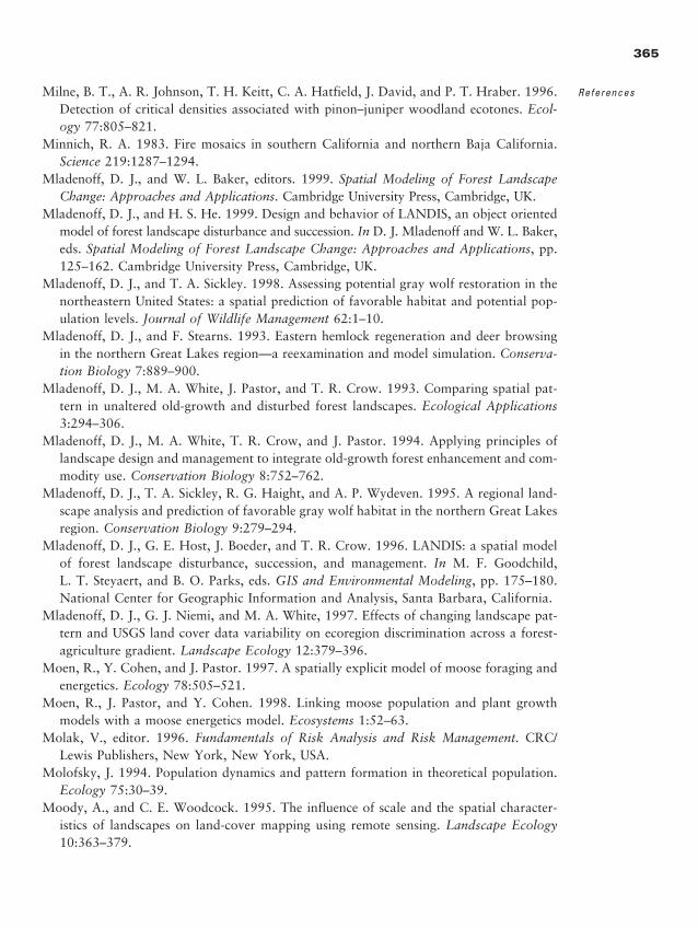
Milne, B. T., A. R. Johnson, T. H. Keitt, C. A. Hatfield, J. David, and P. T. Hraber. 1996.Detection of critical densities associated with pinon–juniper woodland ecotones. Ecol-ogy 77:805–821.

Minnich, R. A. 1983. Fire mosaics in southern California and northern Baja California.Science 219:1287–1294.

Mladenoff, D. J., and W. L. Baker, editors. 1999. Spatial Modeling of Forest LandscapeChange: Approaches and Applications. Cambridge University Press, Cambridge, UK.

Mladenoff, D. J., and H. S. He. 1999. Design and behavior of LANDIS, an object orientedmodel of forest landscape disturbance and succession. In D. J. Mladenoff and W. L. Baker,eds. Spatial Modeling of Forest Landscape Change: Approaches and Applications, pp.125–162. Cambridge University Press, Cambridge, UK.

Mladenoff, D. J., and T. A. Sickley. 1998. Assessing potential gray wolf restoration in thenortheastern United States: a spatial prediction of favorable habitat and potential pop-ulation levels. Journal of Wildlife Management 62:1–10.

Mladenoff, D. J., and F. Stearns. 1993. Eastern hemlock regeneration and deer browsingin the northern Great Lakes region—a reexamination and model simulation. Conserva-tion Biology 7:889–900.

Mladenoff, D. J., M. A. White, J. Pastor, and T. R. Crow. 1993. Comparing spatial pat-tern in unaltered old-growth and disturbed forest landscapes. Ecological Applications3:294–306.

Mladenoff, D. J., M. A. White, T. R. Crow, and J. Pastor. 1994. Applying principles oflandscape design and management to integrate old-growth forest enhancement and com-modity use. Conservation Biology 8:752–762.

Mladenoff, D. J., T. A. Sickley, R. G. Haight, and A. P. Wydeven. 1995. A regional land-scape analysis and prediction of favorable gray wolf habitat in the northern Great Lakesregion. Conservation Biology 9:279–294.

Mladenoff, D. J., G. E. Host, J. Boeder, and T. R. Crow. 1996. LANDIS: a spatial modelof forest landscape disturbance, succession, and management. In M. F. Goodchild, L. T. Steyaert, and B. O. Parks, eds. GIS and Environmental Modeling, pp. 175–180.National Center for Geographic Information and Analysis, Santa Barbara, California.

Mladenoff, D. J., G. J. Niemi, and M. A. White, 1997. Effects of changing landscape pat-tern and USGS land cover data variability on ecoregion discrimination across a forest-agriculture gradient. Landscape Ecology 12:379–396.

Moen, R., Y. Cohen, and J. Pastor. 1997. A spatially explicit model of moose foraging andenergetics. Ecology 78:505–521.

Moen, R., J. Pastor, and Y. Cohen. 1998. Linking moose population and plant growthmodels with a moose energetics model. Ecosystems 1:52–63.

Molak, V., editor. 1996. Fundamentals of Risk Analysis and Risk Management. CRC/Lewis Publishers, New York, New York, USA.

Molofsky, J. 1994. Population dynamics and pattern formation in theoretical population.Ecology 75:30–39.

Moody, A., and C. E. Woodcock. 1995. The influence of scale and the spatial character-istics of landscapes on land-cover mapping using remote sensing. Landscape Ecology10:363–379.

365

References

2888_e12_p333-388 2/27/01 1:55 PM Page 365

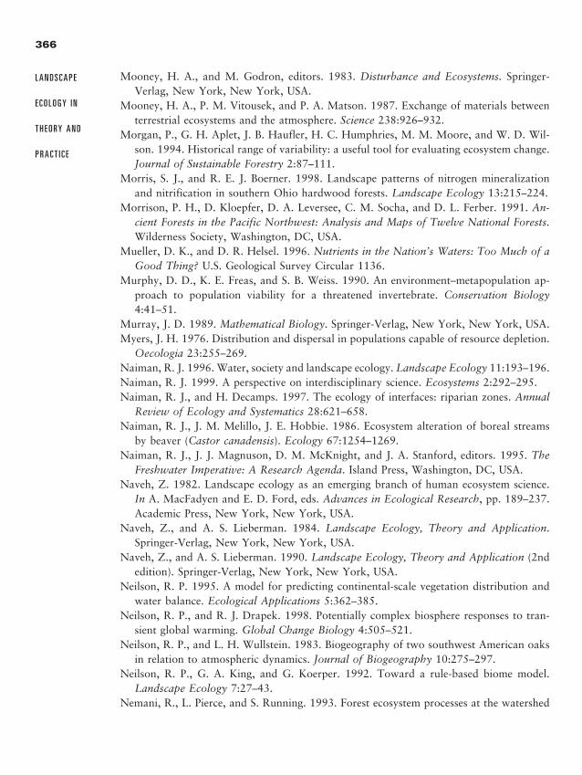
Mooney, H. A., and M. Godron, editors. 1983. Disturbance and Ecosystems. Springer-Verlag, New York, New York, USA.

Mooney, H. A., P. M. Vitousek, and P. A. Matson. 1987. Exchange of materials betweenterrestrial ecosystems and the atmosphere. Science 238:926–932.

Morgan, P., G. H. Aplet, J. B. Haufler, H. C. Humphries, M. M. Moore, and W. D. Wil-son. 1994. Historical range of variability: a useful tool for evaluating ecosystem change.Journal of Sustainable Forestry 2:87–111.

Morris, S. J., and R. E. J. Boerner. 1998. Landscape patterns of nitrogen mineralizationand nitrification in southern Ohio hardwood forests. Landscape Ecology 13:215–224.

Morrison, P. H., D. Kloepfer, D. A. Leversee, C. M. Socha, and D. L. Ferber. 1991. An-cient Forests in the Pacific Northwest: Analysis and Maps of Twelve National Forests.Wilderness Society, Washington, DC, USA.

Mueller, D. K., and D. R. Helsel. 1996. Nutrients in the Nation’s Waters: Too Much of aGood Thing? U.S. Geological Survey Circular 1136.

Murphy, D. D., K. E. Freas, and S. B. Weiss. 1990. An environment–metapopulation ap-proach to population viability for a threatened invertebrate. Conservation Biology4:41–51.

Murray, J. D. 1989. Mathematical Biology. Springer-Verlag, New York, New York, USA.Myers, J. H. 1976. Distribution and dispersal in populations capable of resource depletion.

Oecologia 23:255–269.Naiman, R. J. 1996. Water, society and landscape ecology. Landscape Ecology 11:193–196.Naiman, R. J. 1999. A perspective on interdisciplinary science. Ecosystems 2:292–295.Naiman, R. J., and H. Decamps. 1997. The ecology of interfaces: riparian zones. Annual

Review of Ecology and Systematics 28:621–658.Naiman, R. J., J. M. Melillo, J. E. Hobbie. 1986. Ecosystem alteration of boreal streams

by beaver (Castor canadensis). Ecology 67:1254–1269.Naiman, R. J., J. J. Magnuson, D. M. McKnight, and J. A. Stanford, editors. 1995. The

Freshwater Imperative: A Research Agenda. Island Press, Washington, DC, USA.Naveh, Z. 1982. Landscape ecology as an emerging branch of human ecosystem science.

In A. MacFadyen and E. D. Ford, eds. Advances in Ecological Research, pp. 189–237.Academic Press, New York, New York, USA.

Naveh, Z., and A. S. Lieberman. 1984. Landscape Ecology, Theory and Application.Springer-Verlag, New York, New York, USA.

Naveh, Z., and A. S. Lieberman. 1990. Landscape Ecology, Theory and Application (2ndedition). Springer-Verlag, New York, New York, USA.

Neilson, R. P. 1995. A model for predicting continental-scale vegetation distribution andwater balance. Ecological Applications 5:362–385.

Neilson, R. P., and R. J. Drapek. 1998. Potentially complex biosphere responses to tran-sient global warming. Global Change Biology 4:505–521.

Neilson, R. P., and L. H. Wullstein. 1983. Biogeography of two southwest American oaksin relation to atmospheric dynamics. Journal of Biogeography 10:275–297.

Neilson, R. P., G. A. King, and G. Koerper. 1992. Toward a rule-based biome model.Landscape Ecology 7:27–43.

Nemani, R., L. Pierce, and S. Running. 1993. Forest ecosystem processes at the watershed

366

L A N D S C A P E

E C O L O G Y I N

T H E O R Y A N D

P R A C T I C E

2888_e12_p333-388 2/27/01 1:55 PM Page 366

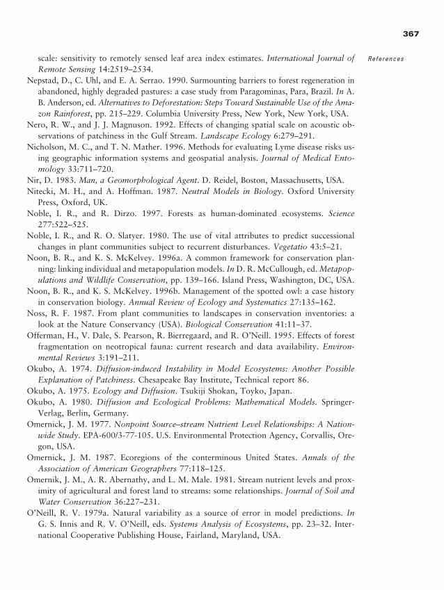
scale: sensitivity to remotely sensed leaf area index estimates. International Journal ofRemote Sensing 14:2519–2534.

Nepstad, D., C. Uhl, and E. A. Serrao. 1990. Surmounting barriers to forest regeneration inabandoned, highly degraded pastures: a case study from Paragominas, Para, Brazil. In A.B. Anderson, ed. Alternatives to Deforestation: Steps Toward Sustainable Use of the Ama-zon Rainforest, pp. 215–229. Columbia University Press, New York, New York, USA.

Nero, R. W., and J. J. Magnuson. 1992. Effects of changing spatial scale on acoustic ob-servations of patchiness in the Gulf Stream. Landscape Ecology 6:279–291.

Nicholson, M. C., and T. N. Mather. 1996. Methods for evaluating Lyme disease risks us-ing geographic information systems and geospatial analysis. Journal of Medical Ento-mology 33:711–720.

Nir, D. 1983. Man, a Geomorphological Agent. D. Reidel, Boston, Massachusetts, USA.Nitecki, M. H., and A. Hoffman. 1987. Neutral Models in Biology. Oxford University

Press, Oxford, UK.Noble, I. R., and R. Dirzo. 1997. Forests as human-dominated ecosystems. Science

277:522–525.Noble, I. R., and R. O. Slatyer. 1980. The use of vital attributes to predict successional

changes in plant communities subject to recurrent disturbances. Vegetatio 43:5–21.Noon, B. R., and K. S. McKelvey. 1996a. A common framework for conservation plan-

ning: linking individual and metapopulation models. In D. R. McCullough, ed. Metapop-ulations and Wildlife Conservation, pp. 139–166. Island Press, Washington, DC, USA.

Noon, B. R., and K. S. McKelvey. 1996b. Management of the spotted owl: a case historyin conservation biology. Annual Review of Ecology and Systematics 27:135–162.

Noss, R. F. 1987. From plant communities to landscapes in conservation inventories: alook at the Nature Conservancy (USA). Biological Conservation 41:11–37.

Offerman, H., V. Dale, S. Pearson, R. Bierregaard, and R. O’Neill. 1995. Effects of forestfragmentation on neotropical fauna: current research and data availability. Environ-mental Reviews 3:191–211.

Okubo, A. 1974. Diffusion-induced Instability in Model Ecosystems: Another Possible Explanation of Patchiness. Chesapeake Bay Institute, Technical report 86.

Okubo, A. 1975. Ecology and Diffusion. Tsukiji Shokan, Toyko, Japan.Okubo, A. 1980. Diffusion and Ecological Problems: Mathematical Models. Springer-

Verlag, Berlin, Germany.Omernick, J. M. 1977. Nonpoint Source–stream Nutrient Level Relationships: A Nation-

wide Study. EPA-600/3-77-105. U.S. Environmental Protection Agency, Corvallis, Ore-gon, USA.

Omernick, J. M. 1987. Ecoregions of the conterminous United States. Annals of the Association of American Geographers 77:118–125.

Omernik, J. M., A. R. Abernathy, and L. M. Male. 1981. Stream nutrient levels and prox-imity of agricultural and forest land to streams: some relationships. Journal of Soil andWater Conservation 36:227–231.

O’Neill, R. V. 1979a. Natural variability as a source of error in model predictions. InG. S. Innis and R. V. O’Neill, eds. Systems Analysis of Ecosystems, pp. 23–32. Inter-national Cooperative Publishing House, Fairland, Maryland, USA.

367

References

2888_e12_p333-388 2/27/01 1:55 PM Page 367

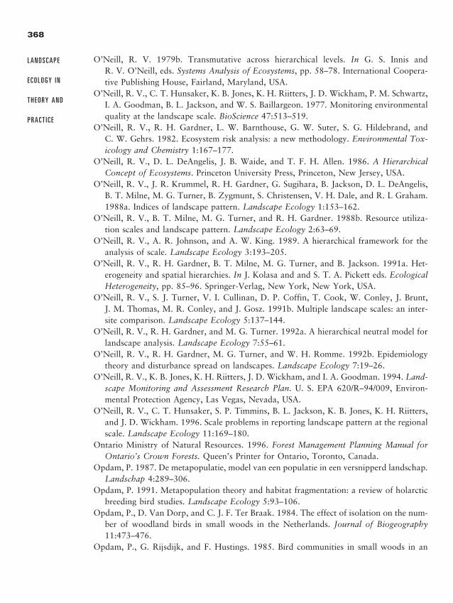
O’Neill, R. V. 1979b. Transmutative across hierarchical levels. In G. S. Innis and R. V. O’Neill, eds. Systems Analysis of Ecosystems, pp. 58–78. International Coopera-tive Publishing House, Fairland, Maryland, USA.

O’Neill, R. V., C. T. Hunsaker, K. B. Jones, K. H. Riitters, J. D. Wickham, P. M. Schwartz,I. A. Goodman, B. L. Jackson, and W. S. Baillargeon. 1977. Monitoring environmentalquality at the landscape scale. BioScience 47:513–519.

O’Neill, R. V., R. H. Gardner, L. W. Barnthouse, G. W. Suter, S. G. Hildebrand, and C. W. Gehrs. 1982. Ecosystem risk analysis: a new methodology. Environmental Tox-icology and Chemistry 1:167–177.

O’Neill, R. V., D. L. DeAngelis, J. B. Waide, and T. F. H. Allen. 1986. A HierarchicalConcept of Ecosystems. Princeton University Press, Princeton, New Jersey, USA.

O’Neill, R. V., J. R. Krummel, R. H. Gardner, G. Sugihara, B. Jackson, D. L. DeAngelis,B. T. Milne, M. G. Turner, B. Zygmunt, S. Christensen, V. H. Dale, and R. L Graham.1988a. Indices of landscape pattern. Landscape Ecology 1:153–162.

O’Neill, R. V., B. T. Milne, M. G. Turner, and R. H. Gardner. 1988b. Resource utiliza-tion scales and landscape pattern. Landscape Ecology 2:63–69.

O’Neill, R. V., A. R. Johnson, and A. W. King. 1989. A hierarchical framework for theanalysis of scale. Landscape Ecology 3:193–205.

O’Neill, R. V., R. H. Gardner, B. T. Milne, M. G. Turner, and B. Jackson. 1991a. Het-erogeneity and spatial hierarchies. In J. Kolasa and and S. T. A. Pickett eds. EcologicalHeterogeneity, pp. 85–96. Springer-Verlag, New York, New York, USA.

O’Neill, R. V., S. J. Turner, V. I. Cullinan, D. P. Coffin, T. Cook, W. Conley, J. Brunt, J. M. Thomas, M. R. Conley, and J. Gosz. 1991b. Multiple landscape scales: an inter-site comparison. Landscape Ecology 5:137–144.

O’Neill, R. V., R. H. Gardner, and M. G. Turner. 1992a. A hierarchical neutral model forlandscape analysis. Landscape Ecology 7:55–61.

O’Neill, R. V., R. H. Gardner, M. G. Turner, and W. H. Romme. 1992b. Epidemiologytheory and disturbance spread on landscapes. Landscape Ecology 7:19–26.

O’Neill, R. V., K. B. Jones, K. H. Riitters, J. D. Wickham, and I. A. Goodman. 1994. Land-scape Monitoring and Assessment Research Plan. U. S. EPA 620/R–94/009, Environ-mental Protection Agency, Las Vegas, Nevada, USA.

O’Neill, R. V., C. T. Hunsaker, S. P. Timmins, B. L. Jackson, K. B. Jones, K. H. Riitters,and J. D. Wickham. 1996. Scale problems in reporting landscape pattern at the regionalscale. Landscape Ecology 11:169–180.

Ontario Ministry of Natural Resources. 1996. Forest Management Planning Manual forOntario’s Crown Forests. Queen’s Printer for Ontario, Toronto, Canada.

Opdam, P. 1987. De metapopulatie, model van een populatie in een versnipperd landschap.Landschap 4:289–306.

Opdam, P. 1991. Metapopulation theory and habitat fragmentation: a review of holarcticbreeding bird studies. Landscape Ecology 5:93–106.

Opdam, P., D. Van Dorp, and C. J. F. Ter Braak. 1984. The effect of isolation on the num-ber of woodland birds in small woods in the Netherlands. Journal of Biogeography11:473–476.

Opdam, P., G. Rijsdijk, and F. Hustings. 1985. Bird communities in small woods in an

368

L A N D S C A P E

E C O L O G Y I N

T H E O R Y A N D

P R A C T I C E

2888_e12_p333-388 2/27/01 1:55 PM Page 368

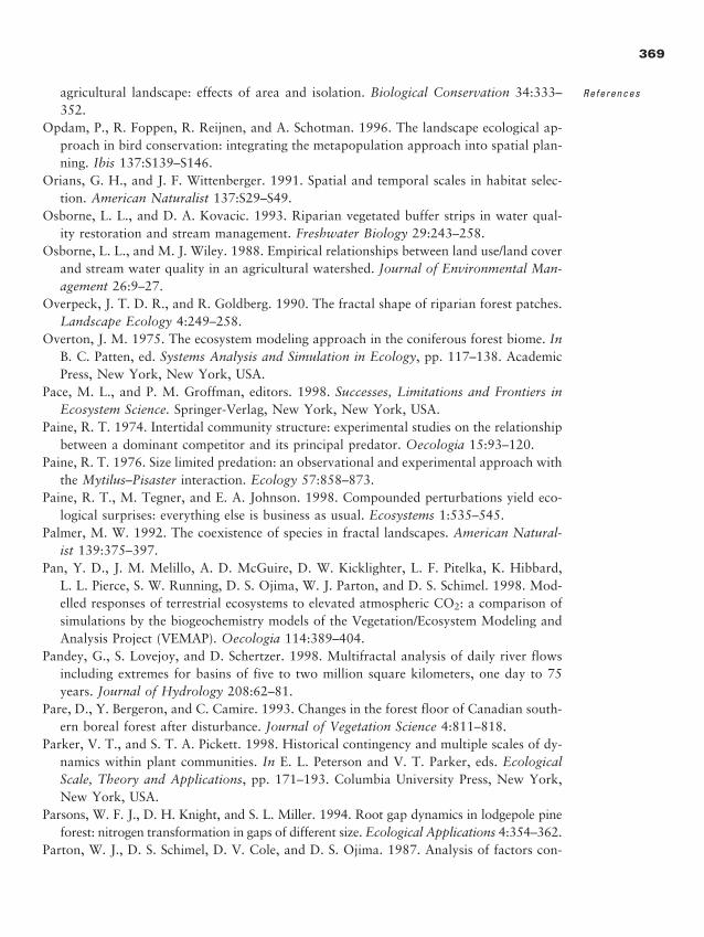
agricultural landscape: effects of area and isolation. Biological Conservation 34:333–352.

Opdam, P., R. Foppen, R. Reijnen, and A. Schotman. 1996. The landscape ecological ap-proach in bird conservation: integrating the metapopulation approach into spatial plan-ning. Ibis 137:S139–S146.

Orians, G. H., and J. F. Wittenberger. 1991. Spatial and temporal scales in habitat selec-tion. American Naturalist 137:S29–S49.

Osborne, L. L., and D. A. Kovacic. 1993. Riparian vegetated buffer strips in water qual-ity restoration and stream management. Freshwater Biology 29:243–258.

Osborne, L. L., and M. J. Wiley. 1988. Empirical relationships between land use/land coverand stream water quality in an agricultural watershed. Journal of Environmental Man-agement 26:9–27.

Overpeck, J. T. D. R., and R. Goldberg. 1990. The fractal shape of riparian forest patches.Landscape Ecology 4:249–258.

Overton, J. M. 1975. The ecosystem modeling approach in the coniferous forest biome. InB. C. Patten, ed. Systems Analysis and Simulation in Ecology, pp. 117–138. AcademicPress, New York, New York, USA.

Pace, M. L., and P. M. Groffman, editors. 1998. Successes, Limitations and Frontiers inEcosystem Science. Springer-Verlag, New York, New York, USA.

Paine, R. T. 1974. Intertidal community structure: experimental studies on the relationshipbetween a dominant competitor and its principal predator. Oecologia 15:93–120.

Paine, R. T. 1976. Size limited predation: an observational and experimental approach withthe Mytilus–Pisaster interaction. Ecology 57:858–873.

Paine, R. T., M. Tegner, and E. A. Johnson. 1998. Compounded perturbations yield eco-logical surprises: everything else is business as usual. Ecosystems 1:535–545.

Palmer, M. W. 1992. The coexistence of species in fractal landscapes. American Natural-ist 139:375–397.

Pan, Y. D., J. M. Melillo, A. D. McGuire, D. W. Kicklighter, L. F. Pitelka, K. Hibbard, L. L. Pierce, S. W. Running, D. S. Ojima, W. J. Parton, and D. S. Schimel. 1998. Mod-elled responses of terrestrial ecosystems to elevated atmospheric CO2: a comparison ofsimulations by the biogeochemistry models of the Vegetation/Ecosystem Modeling andAnalysis Project (VEMAP). Oecologia 114:389–404.

Pandey, G., S. Lovejoy, and D. Schertzer. 1998. Multifractal analysis of daily river flowsincluding extremes for basins of five to two million square kilometers, one day to 75years. Journal of Hydrology 208:62–81.

Pare, D., Y. Bergeron, and C. Camire. 1993. Changes in the forest floor of Canadian south-ern boreal forest after disturbance. Journal of Vegetation Science 4:811–818.

Parker, V. T., and S. T. A. Pickett. 1998. Historical contingency and multiple scales of dy-namics within plant communities. In E. L. Peterson and V. T. Parker, eds. EcologicalScale, Theory and Applications, pp. 171–193. Columbia University Press, New York,New York, USA.

Parsons, W. F. J., D. H. Knight, and S. L. Miller. 1994. Root gap dynamics in lodgepole pineforest: nitrogen transformation in gaps of different size. Ecological Applications 4:354–362.

Parton, W. J., D. S. Schimel, D. V. Cole, and D. S. Ojima. 1987. Analysis of factors con-

369

References

2888_e12_p333-388 2/27/01 1:55 PM Page 369

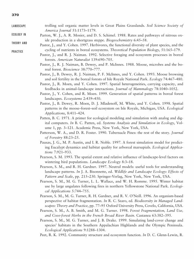
trolling soil organic matter levels in Great Plains Grasslands. Soil Science Society ofAmerica Journal 51:1173–1179.

Parton, W. J., A. R. Mosier, and D. S. Schimel. 1988. Rates and pathways of nitrous ox-ide production in a shortgrass steppe. Biogeochemistry 6:45–58.

Pastor, J., and Y. Cohen. 1997. Herbivores, the functional diversity of plant species, and thecycling of nutrients in boreal ecosystems. Theoretical Population Biology, 51:165–179.

Pastor, J., and R. J. Naiman. 1992. Selective foraging and ecosystem processes in borealforests. American Naturalist 139:690–705.

Pastor, J., R. J. Naiman, B. Dewey, and P. McInnes. 1988. Moose, microbes and the bo-real forest. Bioscience 38:770–777.

Pastor, J., B. Dewey, R. J. Naiman, P. F. McInnes, and Y. Cohen. 1993. Moose browsingand soil fertility in the boreal forests of Isle Royale National Park. Ecology 74:467–480.

Pastor, J., R. Moen, and Y. Cohen. 1997. Spatial heterogeneities, carrying capacity, andfeedbacks in animal–landscape interactions. Journal of Mammalogy 78:1040–1052.

Pastor, J., Y. Cohen, and R. Moen. 1999. Generation of spatial patterns in boreal forestlandscapes. Ecosystems 2:439–450.

Pastor, J., B. Dewey, R. Moen, D. J. Mladenoff, M. White, and Y. Cohen. 1998. Spatialpatterns in the moose–forest–soil ecosystem on Isle Royale, Michigan, USA. EcologicalApplications, 8:411–424.

Patten, B. C. 1971. A primer for ecological modeling and simulation with analog and dig-ital computers. In B. C. Patten, ed. Systems Analysis and Simulation in Ecology, Vol-ume 1, pp. 3–121. Academic Press, New York, New York, USA.

Patterson, W. A., and D. R. Foster. 1990. Tabernacle Pines: the rest of the story. Journalof Forestry 88:23–25.

Pausas, J. G., M. P. Austin, and I. R. Noble. 1997. A forest simulation model for predict-ing Eucalypt dynamics and habitat quality for arboreal marsupials. Ecological Applica-tions 7:921–933.

Pearson, S. M. 1993. The spatial extent and relative influence of landscape-level factors onwintering bird populations. Landscape Ecology 8:3–18.

Pearson, S. M., and R. H. Gardner. 1997. Neutral models: useful tools for understandinglandscape patterns. In J. A. Bisonnette, ed. Wildlife and Landscape Ecology: Effects ofPattern and Scale, pp. 215–230. Springer-Verlag, New York, New York, USA.

Pearson, S. M., M. G. Turner, L. L. Wallace, and W. H. Romme. 1995. Winter habitatuse by large ungulates following fires in northern Yellowstone National Park. Ecologi-cal Applications 5:744–755.

Pearson, S. M., M. G. Turner, R. H. Gardner, and R. V. O’Neill. 1996. An organism-basedperspective of habitat fragmentation. In R. C. Szaro, ed. Biodiversity in Managed Land-scapes: Theory and Practice, pp. 77–95 Oxford University Press, Covelo, California, USA.

Pearson, S. M., A. B. Smith, and M. G. Turner. 1998. Forest Fragmentation, Land Use,and Cove-forest Herbs in the French Broad River Basin. Castanea 63:382–395.

Pearson, S. M., M. G. Turner, and J. B. Drake. 1999. Simulating land-cover change andspecies’ habitats in the Southern Appalachian Highlands and the Olympic Peninsula.Ecological Applications 9:1288–1304.

Peet, R. K. 1992. Community structure and ecosystem function. In D. C. Glenn-Lewin, R.

370

L A N D S C A P E

E C O L O G Y I N

T H E O R Y A N D

P R A C T I C E

2888_e12_p333-388 2/27/01 1:55 PM Page 370

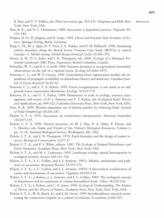
K. Peet, and T. T. Veblen, eds. Plant Succession, pp. 103–151. Chapman and Hall, NewYork, New York, USA.

Peet, R. K., and N. L. Christensen. 1980. Succession: a population process. Vegetatio 43:131–140.

Peitgen, H. O., H. Jurgens, and D. Saupe. 1992. Chaos and Fractals: New Frontiers of Sci-ence. Springer-Verlag, Berlin, Germany.

Peng, C. H., M. J. Apps, D. T. Price, I. A. Nalder, and D. H. Halliwell. 1998. Simulatingcarbon dynamics along the Boreal Forest Transect Case Study (BFTCS) in centralCanada—1. Model testing. Global Biogeochemical Cycles 12:381–392.

Perera, A. H., D. L. Euler, and I. D. Thompson, eds. 2000. Ecology of a Managed Ter-restrial Landscape. UBC Press, Vancouver, British Columbia, Canada.

Peterjohn, W. T., and D. L. Correll. 1984. Nutrient dynamics in an agricultural watershed:observations on the role of a riparian forest. Ecology 65:1466–1475.

Peterson, C. J., and W. P. Carson. 1996. Generalizing forest regeneration models: the de-pendence of propagule availability on disturbance history and stand size. Canadian Jour-nal of Forest Research 26:45–52.

Peterson, C. J., and S. T. A. Pickett. 1995. Forest reorganization: a case study in an old-growth forest catastrophic blowdown. Ecology 76:763–774.

Peterson, D. L., and V. T. Parker. 1998. Dimensions of scale in ecology, resource man-agement, and society. In D. L. Peterson and V. T. Parker, eds. Ecological Scale: Theoryand Applications, pp. 499–522. Columbia University Press, New York, New York, USA.

Petit, D. R. 1989. Weather-dependent use of habitat patches by wintering birds. Journalof Field Ornithology 60:241–247.

Pickett, S. T. A. 1976. Succession: an evolutionary interpretation. American Naturalist110:107–119.

Pickett, S. T. A. 1998. Natural processes. In M. J. Mac, P. A. Opler, P. Doran, and C. Haecker, eds. Status and Trends of Our Nation’s Biological Resources, Volume 1,pp. 11–36. National Biological Service, Washington, DC, USA.

Pickett, S. T. A., and J. N. Thompson. 1978. Patch dynamics and the design of nature re-serves. Biological Conservation 13:27–37.

Pickett, S. T. A., and P. S. White, editors. 1985. The Ecology of Natural Disturbance andPatch Dynamics. Academic Press, New York, New York, USA.

Pickett, S. T. A., and M. L. Cadenasso. 1995. Landscape ecology: spatial heterogeneity inecological systems. Science 269:331–334.

Pickett, S. T. A., S. C. Collins, and J. J. Armesto. 1987a. Models, mechanisms and path-ways of succession. Botanical Review 53:335–371.

Pickett, S. T. A., S. C. Collins, and J. J. Armesto. 1987b. A hierarchical consideration ofcauses and mechanisms of succession. Vegetatio 69:109–114.

Pickett, S. T. A., J. Kolasa, J. J. Armesto, and S. L. Collins. 1989. The ecological conceptof disturbance and its expression at various hierarchical levels. Oikos 54:129–136.

Pickett, S. T. A., J. Kolasa, and C. G. Jones. 1994. Ecological Understanding. The Natureof Theory and the Theory of Nature. Academic Press, New York, New York, USA.

Pickett, S. T. A., W. R. Burch, Jr., and J. M. Grove. 1999. Interdisciplinary research: main-taining the constructive impulse in a culture of criticism. Ecosystems 2:302–307.

371

References

2888_e12_p333-388 2/27/01 1:55 PM Page 371

Pierce, L. L., and S. W. Running. 1995. The effects of aggregating sub-grid land surfacevariation on large-scale estimates of net primary production. Landscape Ecology10:239–253.

Pierce, L. L., S. W. Running, and J. Walker. 1994. Regional-scale relationships of leaf areaindex to specific leaf area and leaf nitrogen. Ecological Applications 4:313–321.

Pittsburgh Community Renewal Project. 1962. Employment, Income, and Population Sub-models. Progress Report No. 4. Department of City Planning, Pittsburgh, Pennsylvania,USA.

Platt, J. R. 1964. Strong inference. Science 146:347–353.Platt, T., and K. L. Denman. 1975. Spectral analysis in ecology. Annual Review of Ecol-

ogy and Systematics 6:189–210.Platt, W. J., and I. M. Weis. 1985. An experimental study of competition among fugitive

prairie plants. Ecology 66:708–720.Plotnick, R. E., and R. H. Gardner. 1993. Lattices and landscapes. In R. H. Gardner, ed.

Lectures on Mathematics in the Life Sciences: Predicting Spatial Effects in EcologicalSystems, pp. 129–157. American Mathematical Society, Providence, Rhode Island, USA.

Plotnick, R. E., and K. L. Prestegaard. 1993. Fractal analysis of geologic time series. InN. Lam and L. DeCola, eds. Fractals in Geography, pp. 207–224. Prentice Hill, UpperSaddle River, New Jersey, USA.

Plotnick, R. E., R. H. Gardner, and R. V. O’Neill. 1993. Lacunarity indices as measuresof landscape texture. Landscape Ecology 8:201–211.

Pollock, M. M. 1998. Biodiversity. In R. J. Naiman and R. E. Bilby, eds. River Ecologyand Management, pp. 430–452. Springer-Verlag, New York, New York, USA.

Powell, T. M., P. J. Richerson, T. M. Dillon, B. A. Agee, B. J. Dozier, D. A. Godden, andL. O. Myrup. 1975. Spatial scales of current speed and phytoplankton biomass fluctu-ations in Lake Tahoe. Science 189:1088–1090.

Pulliam, H. R. 1988. Sources, sinks and population regulation. American Naturalist132:652–661.

Pulliam, H. R., and B. J. Danielson. 1991. Sources, sinks, and habitat selection: a land-scape perspective on population dynamics. American Naturalist 132:S50–S66.

Pulliam, H. R., and J. B. Dunning. 1994. Demographic processes: population dynamics onheterogeneous landscapes. In G. K. Meffe and C. R. Carroll, eds. Principles of Conser-vation Biology, pp. 179–205. Sinauer Associates, Inc., Sunderland, Massachusetts.

Pulliam, H. R., J. B. Dunning, and J. Liu. 1992. Population dynamics in complex land-scapes: a case study. Ecological Applications 2:165–177.

Quinn, J. F., and A. E. Dunham. 1983. On hypothesis testing in ecology and evolution.American Naturalist 122:602–617.

Radcliffe, J. 1973. The initial geographical spread of host–vector and carrier-borne epi-demics. Journal of Applied Probability 10:703–717.

Ranney, J. W., M. C. Bruner, and J. B. Levenson. 1981. The importance of edge in thestructure and dynamics of forest islands. In R. L. Burgess and D. M. Sharpe, eds. For-est Island Dynamics in Man-dominated Landscapes, pp. 67–95. Springer-Verlag, NewYork, New York, USA.

Rastetter, E. B., A. W. King, B. J. Cosby, G. M. Hornberger, R. B. O’Neill, and J. E. Hob-

372

L A N D S C A P E

E C O L O G Y I N

T H E O R Y A N D

P R A C T I C E

2888_e12_p333-388 2/27/01 1:55 PM Page 372

bie. 1992. Aggregating fine-scale ecological knowledge to model coarser-scale attributesof ecosystems. Ecological Applications 2:55–70.

Reddingius, J., and P. J. Den Boer. 1970. Simulation experiments illustrating stabilizationof animal numbers by spreading of risk. Oecologia 5:240–284.

Reibsame, W. E., W. J. Parton, K. A. Galvin, I. C. Burke, L. Bohren, R. Young, and E. Knop. 1994. Integrated modeling of land use and cover change. BioScience 44:350–356.

Reich, P. B., D. F. Grigal, J. D. Aber, and S. T. Gower. 1997. Nitrogen mineralization andproductivity in 50 hardwood and conifer stands on diverse soils. Ecology 78:335–347.

Reiners, W. A., and G. E. Lang. 1979. Vegetational patterns and processes in the balsamfir zone, White Mountains, New Hampshire. Ecology 60:403–417.

Remillard, M. M., G. K. Gruendling, and D. J. Bogucki. 1987. Disturbance by beaver (Cas-tor canadensis Kuhl) and increased landscape heterogeneity. In M. G. Turner, ed. Land-scape Heterogeneity and Disturbance, pp. 103–123. Springer-Verlag, New York, NewYork, USA.

Renkin, R. A., and D. G. Despain. 1992. Fuel moisture, forest type and lightning-causedfire in Yellowstone National Park. Canadian Journal of Forest Research 22:37–45.

Rescia, A. J., M. F. Schmitz, P. M. deAgar, C. L. dePablo, and F. D. Pineda. 1997. A frag-mented landscape in northern Spain analyzed at different spatial scales: implications formanagement. Journal of Vegetation Science 8:343–352.

Richards, D., L. B. Johnson, and G. Host. 1996. Landscape-scale influences on stream habi-tats and biota. Canadian Journal of Fisheries and Aquatic Science 53 (Suppl. 1):295–311.

Richards, J. F. 1990. Land transformation. In B. L. Turner III et al., eds. The Earth asTransformed by Human Action, pp. 163–178. Cambridge University Press, Cambridge,UK.

Ricotti, M. E., and E. Zio. 1999. Neural network approach to sensitivity and uncertaintyanalysis. Reliability Engineering and System Safety 64:59–71.

Riebsame, W. E., W. B. Meyer, and B. L. Turner II. 1994. Modeling land use and coveras part of global environmental change. Climatic Change 28:45–64.

Riera, J. L., J. J. Magnuson, J. R. Vande Castle, and M. D. MacKenzie. 1998. Analysis oflarge-scale spatial heterogeneity in vegetation indices among North American landscapes.Ecosystems 1:268–282.

Riera, J. L., J. J. Magnuson, T. K. Kratz, and K. E. Webster. 2000. A geomorphic templatefor the analysis of lake district applied to the Northern Highland Lake District, Wis-consin, USA. Freshwater Biology, 43:301–318.

Riitters, K. H., and J. D. Wickham. 1995. A Landscape Atlas of the Chesapeake Bay Wa-tershed. Environmental Research Center, Tennessee Valley Authority, Norris, Tennessee,USA.

Riitters, K. H., R. V. O’Neill, C. T. Hunsaker, J. D. Wickham, D. H. Yankee, S. P. Tim-mons, K. B. Jones, and B. L. Jackson. 1995. A factor analysis of landscape pattern andstructure metrics. Landscape Ecology 10:23–40.

Riitters, K. H., R. V. O’Neill, and K. B. Jones. 1997. Assessing habitat suitability at mul-tiple scales: a landscape-level approach. Biological Conservation 61:191–202.

Ripley, B. D. 1978. Spectral analysis and the analysis of pattern in plant communities. Jour-nal of Ecology 66:965–981.

373

References

2888_e12_p333-388 2/27/01 1:55 PM Page 373

Ripley, B. D. 1981. Spatial Statistics. John Wiley & Sons, New York, New York, USA.Risch, S. J., D. Andow, and M. A. Altieri. 1983. Agro-ecosystem diversity and pest con-

trol: data, tentative conclusions and new research directions. Environmental Entomol-ogy 12:625–629.

Risser, P. G., J. R. Karr, and R. T. T. Forman. 1984. Landscape Ecology: Directions andApproaches. Special Publication Number 2. Illinois Natural History Survey, Champaign,Illinois, USA.

Roberts, D. W. 1996. Landscape vegetation modeling with vital attributes and fuzzy sys-tems theory. Ecological Modeling 90:175–184.

Roberts, M. R., and F. S. Gilliam. 1995. Patterns and mechanisms of plant diversity inforested ecosystems—implications for forest management. Ecological Applications5:969–977.

Roe, F. G. 1951. The North American Buffalo. University of Toronto Press, Toronto,Canada.

Roese, J. H., K. L. Risenhoover, and L. J. Folse. 1991. Habitat heterogeneity and foragingefficiency: an individual-based model. Ecological Modeling 57:133–143.

Roff, D. A. 1974a. Spatial heterogeneity and the persistence of populations. Oecologia15:240–258.

Roff, D. A. 1974b. The analysis of a population model demonstrating the importance ofdispersal in a heterogeneous environment. Oecologia 15:259–275.

Roland, J. 1993. Large-scale forest fragmentation increases the duration of tent caterpillaroutbreak. Oecologia 93:25–30.

Romme, W. H. 1982. Fire and landscape diversity in subalpine forests of Yellowstone Na-tional Park. Ecological Monographs 52:199–221.

Romme, W. H., and D. G. Despain. 1989. Historical perspective on the Yellowstone firesof 1988. BioScience 39:695–699.

Romme, W. H., and D. H. Knight. 1982. Landscape diversity: the concept applied to Yel-lowstone Park. BioScience 32:664–670.

Romme, W. H., E. E. Everham, L. E. Frelich, M. A. Moritz, and R. E. Sparks. 1998. Arelarge, infrequent disturbances qualitatively different from small, frequent disturbances?Ecosystems 1:524–534.

Rose, K. A., A. L. Brenkert, R. B. Cook, R. H. Gardner, and J. P. Hettelingh. 1991a. Sys-tematic comparison of ILWAS, MAGIC, and ETD watershed acidification models: 1.Mapping among model inputs and deterministic results. Water Resources Research27:2577–2598.

Rose, K. A., A. L. Brenkert, R. B. Cook, R. H. Gardner, and J. P. Hettelingh. 1991b. Sys-tematic comparison of ILWAS, MAGIC, and ETD watershed acidification models: 2.Monte Carlo analysis under regional variability. Water Resources Research 27:2591–2603.

Rose, K. A., E. P. Smith, R. H. Gardner, A. L. Brenkert, and S. M. Bartell. 1991c. Para-meter sensitivities, Monte Carlo filtering, and model forecasting under uncertainty. Jour-nal of Forecasting 10:117–133.

Rosenberg, D. K., B. R. Noon, and E. C. Meslow. 1997. Biological corridors: form, func-tion, and efficacy. BioScience 47:677–687.

374

L A N D S C A P E

E C O L O G Y I N

T H E O R Y A N D

P R A C T I C E

2888_e12_p333-388 2/27/01 1:55 PM Page 374

Rossi, R. E., D. J. Mulla, A. G. Journel, and E. H. Franz. 1992. Geostatistical tools formodeling and interpreting ecological spatial dependence. Ecological Monographs62:277–314.

Rowan, R., N. Knowlton, A. Baker, and J. Jara. 1997. Landscape ecology of algal sym-bionts creates variation in episodes of coral bleaching. Nature 388:265–269.

Rowe, J. S. 1961. The level-of-integration concept and ecology. Ecology 42:420–427.Rowe, J. S., and G. W. Scotter. 1973. Fire in the boreal forest. Quaternary Research

3:444–464.Runkle, J. R. 1982. Patterns of disturbance in some old-growth mesic forests of eastern

North America. Ecology 63:1533–1546.Runkle, J. R. 1985. Disturbance regimes in temperate forests. In S. T. A. Pickett and

P. S. White, eds. The Ecology of Natural Disturbance and Patch Dynamics, pp. 17–34.Academic Press, New York, New York, USA.

Runkle, J. R. 1991. Gap dynamics of old-growth eastern forests: management implications.Natural Areas Journal 11:19–25.

Running, S. W. 1990. Remote sensing of terrestrial primary productivity. In R. J. Hobbsand H. A. Mooney, eds. Remote sensing of biosphere functioning, pp. 65–85. Springer-Verlag, New York, New York, USA.

Running, S. W. 1994. Testing forest-BGC ecosystem process simulations across a climaticgradient in Oregon. Ecological Applications 4:238–247.

Running, S. W., and J. C. Coughlan. 1988. A general model of forest ecosystem processesfor regional applications. I. Hydrologic balance, canopy gas exchange and primary pro-duction processes. Ecological Modeling 42:125–154.

Running, S. W., and E. R. Hunt, Jr. 1993. Generalization of a forest ecosystem processmodel for other biomes, BIOME-BGC, and an application for global-scale models. InJ. R. Ehlinger and C. Field, eds. Scaling Physiological Processes: Leaf to Globe, pp.141–157. Academic Press, San Diego, California, USA.

Running, S. W., R. R. Nemani, and R. D. Hungerford. 1987. Extrapolation of synopticmeterological data in mountainous terrain, and its use for simulating forest evapotran-spiration and photosynthesis. Canadian Journal of Forest Research 17:472–483.

Running, S. W., R. R. Nemani, D. L. Peterson, L. E. Band, D. F. Potts, L. L. Pierce, andM. A. Spanner. 1989. Mapping regional forest evapotranspiration and photosynthesisby coupling satellite data with ecosystem simulation. Ecology 70:1090–1101.

Russell, R. W., G. L. Hunt, Jr., K. O. Coyle, and R. T. Cooney. 1992. Foraging in a frac-tal environment: spatial patterns in a marine predator–prey system. Landscape Ecology7:195–209.

Russo, J. M., and J. W. Zack. 1997. Downscaling GCM output with a mesoscale model.Journal of Environmental Management 49:19–29.

Ruzicka, M., and L. Miklos. 1990. Basic premises and methods in landscape ecological plan-ning and optimization. In I. S. Zonneveld and R. T. T. Forman, eds. Changing Landscapes:An Ecological Perspective, pp. 233–260. Springer-Verlag, New York, New York, USA.

Rykiel, E. J. 1996. Testing ecological models: the meaning of validation. Ecological Mod-eling 90:229–244.

Rykiel, E. J., R. N. Coulson, P. J. H. Sharpe, T. F. H. Allen, and R. O. Flamm. 1988. Dis-

375

References

2888_e12_p333-388 2/27/01 1:55 PM Page 375

turbance propagation by bark beetles as an episodic landscape phenomenon. LandscapeEcology 1:129–139.

Sala, O. E., W. J. Parton, L. A. Joyce, and W. K. Lauenroth. 1988. Primary production ofthe central grassland region of the United States. Ecology 69:40–45.

Santelmann, M., K. Freemark, D. White, J. Nassauer, M. Clark, B. Danielson, J. Eilers, R. Cruse, S. Galatowitsch, S. Polasky, K. Vache, and J. Wu. In press. Applying ecolog-ical principles to land-use decision making in agricultural watersheds. In V. H. Dale andR. Haeuber, eds. Applying Ecological Principles to Land Management. Springer-Verlag,New York, New York, USA.

Saunders, D. and R. J. Hobbs, editors. 1991. Nature Conservation 2: The Role of Corri-dors. Surrey Beatty & Sons, Chipping Norton, N.S.W., Australia.

Saunders, D., R. J. Hobbs, and C. R. Margules. 1991. Biological consequences of ecosys-tem fragmentation: a review. Conservation Biology 5:18–32.

Saupe, D. 1988. Algorithms for random fractals. In H. O. Peitgen and D. Saupe, eds. TheScience of Fractal Images, pp. 71–133. Springer-Verlag, New York, New York, USA.

Scheffer, M., and R. J. D. Boer. 1995. Implications of spatial heterogeneity for the para-dox of enrichment. Ecology 76:2270–2277.

Schimel, D. S., VEMAP Participants, and B. H. Braswell. 1997. Continental scale variabilityin ecosystem processes: models, data, and the role of disturbance. Ecological Mono-graphs 67:251–271.

Schippers, P., J. Verboom, J. P. Knaapen, and R. C. van Apeldoorn. 1996. Dispersal andhabitat connectivity in complex heterogeneous landscapes: an analysis with a GIS-basedrandom walk model. Ecography 19:97–106.

Schmidt, K. 1993. Winter ecology of nonmigratory Alpine red deer. Oecologia 95:226–233.Schneider, D. C. 1994. Quantitative Ecology: Spatial and Temporal Scaling. Academic

Press, San Diego, California, USA.Schneider, D. C. 1998. Applied scaling theory. In D. L. Peterson and V. L. Parker, eds.

Ecological Scale, pp. 253–269. Columbia University Press, New York, New York, USA.Schneider, D. C., and Piatt, J. F. 1986. Scale-dependent correlation of seabirds with school-

ing fish in a coastal ecosystem. Marine Ecology—Progress Series 32:237–246.Schreiber, K. F. 1990. The history of landscape ecology in Europe. In I. S. Zonneveld and

R. T. T. Forman, eds. Changing Landscapes: An Ecological Perspective, pp. 21–33.Springer-Verlag, New York, New York, USA.

Schulze, E.-D., and H. A. Mooney, editors. 1993. Biodiversity and Ecosystem Function.Springer-Verlag, New York, New York, USA.

Schumaker, N. H. 1996. Using landscape indices to predict habitat connectivity. Ecology77:1210–1225.

Scott, J. M., J. J. Jacobi, and J. E. Estes. 1987. Species richness: a geographic approach toprotecting future biological diversity. BioScience 37:782–788.

Scott, J. M., F. Davis, B. Csuti, R. Noss, B. Butterfield, C. Groves, H. Anderson, S. Caicco,F. D’Erchia, T. C. Edwards, Jr., J. Ulliman, and R. G. Wright. 1993. Gap analysis: ageographic approach to protection of biodiversity. Wildlife Monographs No. 123.

Scott, J. M., T. H. Tear, and F. W. Davis, editors. 1996. Gap Analysis: A Landscape Ap-proach to Biodiversity Planning. American Society for Photogrammetry and RemoteSensing. Bethesda, Maryland, USA.

376

L A N D S C A P E

E C O L O G Y I N

T H E O R Y A N D

P R A C T I C E

2888_e12_p333-388 2/27/01 1:55 PM Page 376

Seaber, P. R., F. P. Kapinos, and G. L. Knapp. 1984. State Hydrologic Unit Maps. U.S.Geological Survey, Denver, Colorado, USA.

Sedell, J. R., and J. L. Froggatt. 1984. Importance of streamside forests to large rivers: theisolation of the Willamette River, Oregon, USA, from its floodplain by snagging andstreamside forest removal. Verhandlungen des Internationalen Vereins der Limnologie22:1824–1834.

Segal, L. A, and S. A. Levin. 1976. Applications of nonlinear stability theory to the studyof the effects of diffusion on predator–prey interactions. Topics in Statistical Mechan-ics and Biophysics. Proceedings of the AIP Conference 27:123–152.

Sellers, P. J. 1985. Canopy reflectance, photosynthesis and transpiration. International Jour-nal of Remote Sensing 6:1335–1372.

Sellers, P. J. 1987. Canopy reflectance, photosynthesis and transpiration. II. The role ofbiophysics in the linearity of their interdependence. Remote Sensing and Environment21:143–183.

Sellers, P. J. 1994. A global 1-degrees-by-1-degrees NDVI data set for climate studies. 2.The generation of global fields of terrestrial biophysical parameters from the NDVI. In-ternational Journal of Remote Sensing 15: 3519–3545.

Senft, R. L., M. B. Coughenour, D. W. Bailey, L. R. Rittenhouse, O. E. Sala, and D. M.Swift. 1987. Large herbivore foraging and ecological hierarchies. BioScience 37:789–799.

Shafer, M. L. 1985. The metapopulation and species conservation: the special case of theNorthern Spotted Owl. In R. J. Gutierrez and A. B. Carey, eds. Ecology and Manage-ment of the Spotted Owl in the Pacific Northwest, pp. 86–99. United States Forest Ser-vice Technical Report PNW-185.

Shaver, G. R., K. J. Knadelhoffer, and A. E. Giblin. 1991. Biogeochemical diversity and el-ement transport in a heterogeneous landscape, the north slope of Alaska. In M. G.Turner and R. H. Gardner, eds. Quantitative Methods in Landscape Ecology, pp.105–125. Springer-Verlag, New York, New York, USA.

Shugart, H. H., and I. R. Noble. 1981. A computer model of succession and fire responseof the high altitude Eucalyptus forest of the Brindabella Range, Australian Capital Ter-ritory. Australian Journal of Ecology 6:149–164.

Shugart, H. H., Jr., and D. C. West. 1981. Long-term dynamics of forest ecosystems. Amer-ican Scientist 69:647–652.

Siemann, E., and J. H. Brown. 1999. Gaps in mammalian body size distributions reexam-ined. Ecology 80:2788–2792.

Silbernagel, J., S. R. Martin, M. R. Gale, and J. Chen. 1997. Prehistoric, historic, and pre-sent settlement patterns related to ecological hierarchy in the Eastern Upper Peninsulaof Michigan, USA. Landscape Ecology 12:223–240.

Simberloff, D. S. 1974. Equilibrium theory of island biogeography and ecology. AnnualReview of Ecology and Systematics 5:161–182.

Simberloff, D. S. 1978. Using island biogeographic distributions to determine if coloniza-tion is stochastic. American Naturalist 112:713–719.

Simberloff, D., and J. Cox. 1987. Consequences and costs of conservation corridors. Con-servation Biology 1:63–71.

Simberloff, D., and E. O. Wilson. 1969. Experimental zoogeography of islands. The colo-nization of empty islands. Ecology 50:278–296.

377

References

2888_e12_p333-388 2/27/01 1:55 PM Page 377

Simberloff, D., and E. O. Wilson. 1970. Experimental zoogeography of islands. A two-yearrecord of colonization. Ecology 50:278–316.

Simpson, J. B. 1974. Glacial migration of plants: island biogeography evidence. Science185:698–700.

Sisk, T. D., N. M. Haddad, and P. R. Ehrlich. 1997. Bird assemblages in patchy wood-lands: modeling the effects of edge and matrix habitats. Ecological Applications7:1170–1180.

Skellam, J. G. 1951. Random dispersal in theoretical populations. Biometrika 38:196–218.Skinner, C. N. 1995. Change in spatial characteristics of forest openings in the Klamath

Mountains of northwestern California, USA. Landscape Ecology 10:219–228.Sklar, F. H., and R. Costanza. 1990. The development of dynamic spatial models for land-

scape ecology: a review and prognosis. In M. G. Turner and R. H. Gardner, eds. Quan-titative Methods in Landscape Ecology, pp. 239–288. Springer-Verlag, New York, NewYork, USA.

Slocombe, D. S. 1993. Implementing ecosystem-based management. BioScience 43:612–622.

Slud, P. 1976. Geographic and climatic relationships of avifaunas with special reference tocomparative distribution in the Neotropics. Smithsonian Contributions in Zoology212:1–149.

Small, M. F., and M. L. Hunter. 1988. Forest fragmentation and avian nest predation inforested landscapes. Oecologia 76:62–64.

Smith, A. T. 1980. Temporal changes in insular populations of the pika (Ochotona prin-ceps). Ecology 61:8–13.

Smith, C. A., editor. 1976. Regional Analysis. Academic Press, New York, New York, USA.Smith, M., T. Keevin, P. Mettler-McClure, and R. Barkau. 1998. Effect of the flood of

1993 on Boltonia decurrens, a rare floodplain plant. Regulated Rivers Research Man-agement 14:191–202.

Smuts, J. 1926. Holism and Evolution. Macmillan, London, UK.Sollins, P., G. Spycher, and C. Topik. 1983. Processes of soil organic matter accretion at

a mudflow chronosequence, Mt. Shasta, California. Ecology 64:1273–1282.Soranno, P. A., S. L. Hubler, S. R. Carpenter, and R. C. Lathrop. 1996. Phosphorus loads

to surface waters: a simple model to account for spatial pattern of land use. EcologicalApplications 6:865–878.

Soranno, P. A., K. E. Webster, J. L. Riera, T. K. Kratz, J. S. Baron, P. A. Bukaveckas, G. W. Kling, D. S. White, N. Caine, R. C. Lathrop, and P. R. Leavitt. 1999. Spatialvariation among lakes within landscapes: ecological organization along lake chains.Ecosystems 2:395–410.

Soule, M. E., and D. Simberloff. 1986. What do genetics and ecology tell use about thedesign of nature reserves? Biological Conservation 2:75–92.

Sousa, W. P. 1984. The role of disturbance in natural communities. Annual Review of Ecol-ogy and Systematics 15:353–391.

Southworth, F., V. H. Dale, and R. V. O’Neill. 1991. Contrasting patterns of land use inRondonia, Brazil: simulating the effects on carbon release. International Social ScienceJournal 43:681–698.

378

L A N D S C A P E

E C O L O G Y I N

T H E O R Y A N D

P R A C T I C E

2888_e12_p333-388 2/27/01 1:55 PM Page 378

Spanner, M. A., L. L. Pierce, and S. W. Running. 1990. The seasonality of AVHRR dataof temperate coniferous forests: relationship with leaf area index. Remote Sensing ofEnvironment 33:97–112.

Sparks, R. E. 1995. Need for ecosystem management of large rivers and floodplains. Bio-Science 45:168–182.

Sparks, R. E., J. C. Nelson, and Y. Yin. 1998. Naturalization of the flood regime in regu-lated rivers. BioScience 48:706–720.

Spies, T. A., W. J. Ripple, and G. A. Bradshaw. 1994. Dynamics and pattern of a man-aged coniferous forest landscape in Oregon. Ecological Applications 4:555–568.

Spies, T. A., and M. G. Turner. 1999. Dynamic forest mosaics. In M. Hunter, ed. Main-taining Biodiversity in Forest Ecosystems, pp. 95–160. Cambridge University Press, NewYork, New York, USA.

Sprugel, D. G. 1976. Dynamic structure of wave-generated Abies balsamea forests in thenortheastern United States. Journal of Ecology 64:889–911.

Sprugel, D. G. 1985. Natural disturbance and ecosystem energetics. In S. T. A. Pickett andP. S. White, eds. The Ecology of Natural Disturbance and Patch Dynamics, pp. 335–352.Academic Press, New York, New York, USA.

Sprugel, D. G., and F. H. Bormann. 1981. Natural disturbance and the steady state in high-altitude balsam fir forests. Science 211:390–393.

Stanton, M. L. 1983. Spatial patterns in the plant community and their effects upon insectsearch. In S. Ahmad, ed. Herbivore Insects: Host-seeking Behavior and Mechanisms,pp. 125–157. Academic Press, New York, New York, USA.

Starfield, A. M., and A. L. Bleloch. 1986. Building Models for Conservation and Man-agement. Macmillan Publishing Company, New York, New York, USA.

Starfield, A. M., and F. S. Chapin III. 1996. Model of transient changes in arctic and borealvegetation in response to climate and land use change. Ecological Applications 6:842–864.

Stauffer, D. 1985. Introduction to Percolation Theory. Taylor and Francis, London, UK.Stauffer, D., and A. Aharony. 1992. Introduction to Percolation Theory (2nd edition). Tay-

lor & Francis, London, UK.Steele, J. S. 1974a. Stability of plankton ecosystems. In M. B. Usher and M. H. Williamson,

eds. Ecological Stability, pp. 179–191. Chapman and Hall, London, UK.Steele, J. S. 1974b. Spatial heterogeneity and population stability. Nature 248:83.Steele, J. S. 1989. The ocean “landscape.” Landscape Ecology 3:185–195.Steger, W. A. 1964. Pittsburgh urban renewal simulation model. Journal of the Institute

of Planners 30:51–54.Stouffer, P. C., and R. O. Bierregaard, Jr. 1995. Use of Amazonian forest fragments by un-

derstory insectivorous birds. Ecology 76:2429–2445.Strong, D. R. 1980. Null hypotheses in ecology. Synthese 43:271–285.Sugihara, G., and R. M. May. 1990. Applications of fractals in ecology. Trends in Ecol-

ogy and Evolution 5:79–86.Sukachef, V. N. 1944. Principles of genetical classification in biogeocoenology (Russ). Zh.

Obshch. Biol. (USSR) 6.Sukachef, V. N. 1945. Biogeocoenology and phytocoenology. Readings of the Academy of

Sciences USSR 4:g. (Russ.)

379

References

2888_e12_p333-388 2/27/01 1:55 PM Page 379

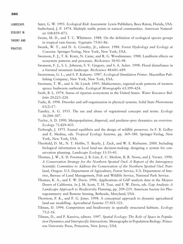
Suter, G. W. 1993. Ecological Risk Assessment. Lewis Publishers, Boca Raton, Florida, USA.Sutherland, J. P. 1974. Multiple stable points in natural communities. American Natural-

ist 108:859–873.Swain, M. D., and T. C. Whitmore. 1988. On the definition of ecological species groups

in tropical rain forests. Vegetatio 75:81–86.Swank, W. T., and D. A. Crossley, Jr., editors. 1988. Forest Hydrology and Ecology at

Coweeta. Springer-Verlag, New York, New York, USA.Swanson, F. J., T. K. Kratz, N. Caine, and R. G. Woodmansee. 1988. Landform effects on

ecosystem patterns and processes. BioScience 38:92–98.Swanson, F. J., S. L. Johnson, S. V. Gregory, and S. A. Acker. 1998. Flood disturbance in

a forested mountain landscape. BioScience 48:681–689.Swartzman, G. L., and S. P. Kaluzny. 1987. Ecological Simulation Primer. Macmillan Pub-

lishing Company, New York, New York, USA.Swetnam, T. W., and A. M. Lynch. 1993. Multicentury, regional-scale patterns of western

spruce budworm outbreaks. Ecological Monographs 63:399–424.Swift, B. L. 1974. Status of riparian ecosystems in the United States. Water Resource Bul-

letin 20:223–228.Tadic, B. 1998. Disorder and self-organization in physical systems. Solid State Phenomena

61(2):17.Tansley, A. G. 1935. The use and abuse of vegetational concepts and terms. Ecology

16:284–307.Taylor, A. D. 1990. Metapopulation, dispersal, and predator–prey dynamics: an overview.

Ecology 71:429–433.Terborgh, J. 1975. Faunal equilibria and the design of wildlife preserves. In F. B. Golley

and E. Medina, eds. Tropical Ecology Systems, pp. 369–380. Springer-Verlag, NewYork, New York, USA.

Theobald, D. M., N. T. Hobbs, T. Bearly, J. Zack, and W. E. Riebsame. 2000. Includingbiological information in local land-use decision-making: designing a system for con-servation planning. Landscape Ecology 15:35–45.

Thomas, J. W., E. D. Forsman, J. B. Lint, E. C. Meslow, B. R. Noon, and J. Verner. 1990.A Conservation Strategy for the Northern Spotted Owl: A Report of the InteragencyScientific Committee to Address the Conservation of the Northern Spotted Owl. Port-land, Oregon. U.S. Department of Agriculture, Forest Service, U.S. Department of Inte-rior, Bureau of Land Management, Fish and Wildlife Service, National Park Service.

Thomas, K. A., and F. W. Davis. 1996. Applications of GAP analysis data in the MojaveDesert of California. In J. M. Scott, T. H. Tear, and F. W. Davis, eds. Gap Analysis: ALandscape Approach to Biodiversity Planning, pp. 209–219. American Society for Pho-togrammetry and Remote Sensing, Bethesda, Maryland, USA.

Thornton, P. K., and P. G. Jones. 1998. A conceptual approach to dynamic agriculturalland-use modelling. Agricultural Systems 57:505–521.

Tilman, D. 1994. Competition and biodiversity in spatially structured habitats. Ecology75:2–16.

Tilman, D., and P. Kareiva, editors. 1997. Spatial Ecology: The Role of Space in Popula-tion Dynamics and Interspecific Interactions. Monographs in Population Biology. Prince-ton University Press, Princeton, New Jersey, USA.

380

L A N D S C A P E

E C O L O G Y I N

T H E O R Y A N D

P R A C T I C E

2888_e12_p333-388 2/27/01 1:55 PM Page 380

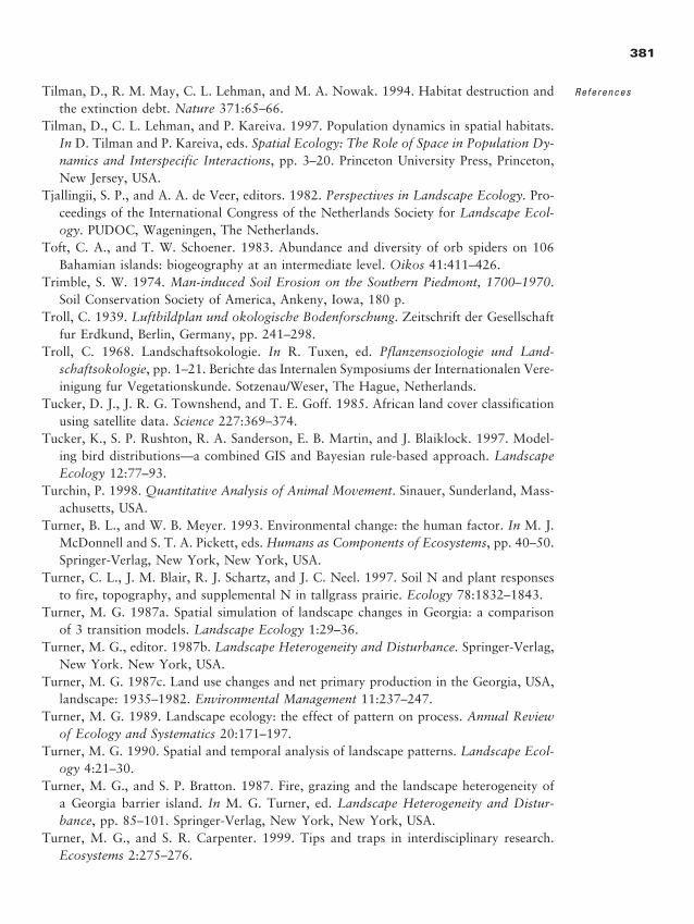
Tilman, D., R. M. May, C. L. Lehman, and M. A. Nowak. 1994. Habitat destruction andthe extinction debt. Nature 371:65–66.

Tilman, D., C. L. Lehman, and P. Kareiva. 1997. Population dynamics in spatial habitats.In D. Tilman and P. Kareiva, eds. Spatial Ecology: The Role of Space in Population Dy-namics and Interspecific Interactions, pp. 3–20. Princeton University Press, Princeton,New Jersey, USA.

Tjallingii, S. P., and A. A. de Veer, editors. 1982. Perspectives in Landscape Ecology. Pro-ceedings of the International Congress of the Netherlands Society for Landscape Ecol-ogy. PUDOC, Wageningen, The Netherlands.

Toft, C. A., and T. W. Schoener. 1983. Abundance and diversity of orb spiders on 106Bahamian islands: biogeography at an intermediate level. Oikos 41:411–426.

Trimble, S. W. 1974. Man-induced Soil Erosion on the Southern Piedmont, 1700–1970.Soil Conservation Society of America, Ankeny, Iowa, 180 p.

Troll, C. 1939. Luftbildplan und okologische Bodenforschung. Zeitschrift der Gesellschaftfur Erdkund, Berlin, Germany, pp. 241–298.

Troll, C. 1968. Landschaftsokologie. In R. Tuxen, ed. Pflanzensoziologie und Land-schaftsokologie, pp. 1–21. Berichte das Internalen Symposiums der Internationalen Vere-inigung fur Vegetationskunde. Sotzenau/Weser, The Hague, Netherlands.

Tucker, D. J., J. R. G. Townshend, and T. E. Goff. 1985. African land cover classificationusing satellite data. Science 227:369–374.

Tucker, K., S. P. Rushton, R. A. Sanderson, E. B. Martin, and J. Blaiklock. 1997. Model-ing bird distributions—a combined GIS and Bayesian rule-based approach. LandscapeEcology 12:77–93.

Turchin, P. 1998. Quantitative Analysis of Animal Movement. Sinauer, Sunderland, Mass-achusetts, USA.

Turner, B. L., and W. B. Meyer. 1993. Environmental change: the human factor. In M. J.McDonnell and S. T. A. Pickett, eds. Humans as Components of Ecosystems, pp. 40–50.Springer-Verlag, New York, New York, USA.

Turner, C. L., J. M. Blair, R. J. Schartz, and J. C. Neel. 1997. Soil N and plant responsesto fire, topography, and supplemental N in tallgrass prairie. Ecology 78:1832–1843.

Turner, M. G. 1987a. Spatial simulation of landscape changes in Georgia: a comparisonof 3 transition models. Landscape Ecology 1:29–36.

Turner, M. G., editor. 1987b. Landscape Heterogeneity and Disturbance. Springer-Verlag,New York. New York, USA.

Turner, M. G. 1987c. Land use changes and net primary production in the Georgia, USA,landscape: 1935–1982. Environmental Management 11:237–247.

Turner, M. G. 1989. Landscape ecology: the effect of pattern on process. Annual Reviewof Ecology and Systematics 20:171–197.

Turner, M. G. 1990. Spatial and temporal analysis of landscape patterns. Landscape Ecol-ogy 4:21–30.

Turner, M. G., and S. P. Bratton. 1987. Fire, grazing and the landscape heterogeneity ofa Georgia barrier island. In M. G. Turner, ed. Landscape Heterogeneity and Distur-bance, pp. 85–101. Springer-Verlag, New York, New York, USA.

Turner, M. G., and S. R. Carpenter. 1999. Tips and traps in interdisciplinary research.Ecosystems 2:275–276.

381

References

2888_e12_p333-388 2/27/01 1:55 PM Page 381

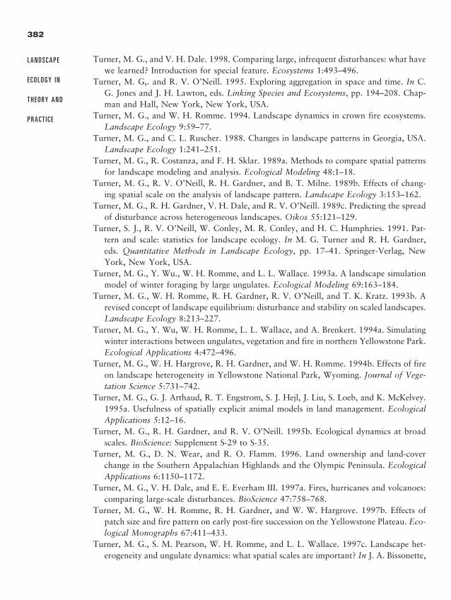
Turner, M. G., and V. H. Dale. 1998. Comparing large, infrequent disturbances: what havewe learned? Introduction for special feature. Ecosystems 1:493–496.

Turner, M. G,. and R. V. O’Neill. 1995. Exploring aggregation in space and time. In C.G. Jones and J. H. Lawton, eds. Linking Species and Ecosystems, pp. 194–208. Chap-man and Hall, New York, New York, USA.

Turner, M. G., and W. H. Romme. 1994. Landscape dynamics in crown fire ecosystems.Landscape Ecology 9:59–77.

Turner, M. G., and C. L. Ruscher. 1988. Changes in landscape patterns in Georgia, USA.Landscape Ecology 1:241–251.

Turner, M. G., R. Costanza, and F. H. Sklar. 1989a. Methods to compare spatial patternsfor landscape modeling and analysis. Ecological Modeling 48:1–18.

Turner, M. G., R. V. O’Neill, R. H. Gardner, and B. T. Milne. 1989b. Effects of chang-ing spatial scale on the analysis of landscape pattern. Landscape Ecology 3:153–162.

Turner, M. G., R. H. Gardner, V. H. Dale, and R. V. O’Neill. 1989c. Predicting the spreadof disturbance across heterogeneous landscapes. Oikos 55:121–129.

Turner, S. J., R. V. O’Neill, W. Conley, M. R. Conley, and H. C. Humphries. 1991. Pat-tern and scale: statistics for landscape ecology. In M. G. Turner and R. H. Gardner,eds. Quantitative Methods in Landscape Ecology, pp. 17–41. Springer-Verlag, NewYork, New York, USA.

Turner, M. G., Y. Wu., W. H. Romme, and L. L. Wallace. 1993a. A landscape simulationmodel of winter foraging by large ungulates. Ecological Modeling 69:163–184.

Turner, M. G., W. H. Romme, R. H. Gardner, R. V. O’Neill, and T. K. Kratz. 1993b. Arevised concept of landscape equilibrium: disturbance and stability on scaled landscapes.Landscape Ecology 8:213–227.

Turner, M. G., Y. Wu, W. H. Romme, L. L. Wallace, and A. Brenkert. 1994a. Simulatingwinter interactions between ungulates, vegetation and fire in northern Yellowstone Park.Ecological Applications 4:472–496.

Turner, M. G., W. H. Hargrove, R. H. Gardner, and W. H. Romme. 1994b. Effects of fireon landscape heterogeneity in Yellowstone National Park, Wyoming. Journal of Vege-tation Science 5:731–742.

Turner, M. G., G. J. Arthaud, R. T. Engstrom, S. J. Hejl, J. Liu, S. Loeb, and K. McKelvey.1995a. Usefulness of spatially explicit animal models in land management. EcologicalApplications 5:12–16.

Turner, M. G., R. H. Gardner, and R. V. O’Neill. 1995b. Ecological dynamics at broadscales. BioScience: Supplement S-29 to S-35.

Turner, M. G., D. N. Wear, and R. O. Flamm. 1996. Land ownership and land-coverchange in the Southern Appalachian Highlands and the Olympic Peninsula. EcologicalApplications 6:1150–1172.

Turner, M. G., V. H. Dale, and E. E. Everham III. 1997a. Fires, hurricanes and volcanoes:comparing large-scale disturbances. BioScience 47:758–768.

Turner, M. G., W. H. Romme, R. H. Gardner, and W. W. Hargrove. 1997b. Effects ofpatch size and fire pattern on early post-fire succession on the Yellowstone Plateau. Eco-logical Monographs 67:411–433.

Turner, M. G., S. M. Pearson, W. H. Romme, and L. L. Wallace. 1997c. Landscape het-erogeneity and ungulate dynamics: what spatial scales are important? In J. A. Bissonette,

382

L A N D S C A P E

E C O L O G Y I N

T H E O R Y A N D

P R A C T I C E

2888_e12_p333-388 2/27/01 1:55 PM Page 382

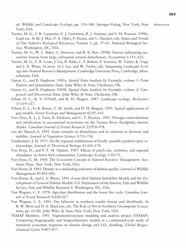
ed. Wildlife and Landscape Ecology, pp. 331–348. Springer-Verlag, New York, NewYork, USA.

Turner, M. G., S. R. Carpenter, E. J. Gustafson, R. J. Naiman, and S. M. Pearson. 1998a.Land use. In M. J. Mac, P. A. Opler, P. Doran, and C. Haecker, eds. Status and Trendsof Our Nation’s Biological Resources, Volume 1, pp. 37–61. National Biological Ser-vice, Washington, DC, USA.

Turner, M. G., W. L. Baker, C. Peterson, and R. K. Peet. 1998b. Factors influencing suc-cession: lessons from large, infrequent natural disturbances. Ecosystems 1:511–523.

Turner, M. G., T. R. Crow, J. Liu, D. Rabe, C. F. Rabeni, P. Soranno, W. Taylor, K. Vogt,and J. A. Wiens. In press. In J. Liu. and W. Taylor, eds. Integrating Landscape Ecol-ogy into Natural Resource Management. Cambridge University Press, Cambridge, Mass-achusetts, USA.

Upton, G., and B. Fingleton. 1985a. Spatial Data Analysis by Example, volume 1: PointPattern and Quantitative Data. John Wiley & Sons, Chichester, UK.

Upton, G., and B. Fingleton. 1985b. Spatial Data Analysis by Example, volume 2: Cate-gorical and Directional Data. John Wiley & Sons, Chichester, UK.

Urban, D. L., R. V. O’Neill, and H. H. Shugart. 1987. Landscape ecology. BioScience37:119–127.

Urban, D. L., G. B. Bonan, T. M. Smith, and H. H. Shugart. 1991. Spatial applications ofgap models. Forest Ecology and Management 42:95–110.

Van Cleve, K. J., J. Yarie, R. Erickson, and C. T. Dryness. 1993. Nitrogen mineralizationand nitrification in successional ecosystems on the Tanana River floodplain, interiorAlaska. Canadian Journal of Forest Research 23:970–978.

van der Maarel, E. 1993. Some remarks on disturbance and its relations to diversity andstability. Journal of Vegetation Science 3:733–736.

Vandermeer, J. H. 1973. On the regional stabilization of locally unstable predator–prey re-lationships. Journal of Theoretical Biology 41:161–170.

Van Dorp, D., and P. F. M. Opdam. 1987. Effects of patch size, isolation, and regionalabundance on forest bird communities. Landscape Ecology 1:59–73.

Van Dyne, G. M. 1969. The Ecosystem Concept in Natural Resource Management. Aca-demic Press, New York, New York, USA.

Van Horne, B. 1983. Density as a misleading indicator of habitat quality. Journal of WildlifeManagement 47:893–901.

Van Horne, B., and J. A. Wiens. 1991. Forest Bird Habitat Suitability Models and the De-velopment of General Habitat Models. U.S. Department of the Interior, Fish and WildlifeService, Fish and Wildlife Research 8. Washington, DC, USA.

Van Wagner, C. E. 1978. Age-class distribution and the forest fire cycle. Canadian Jour-nal of Forest Research 8:220–227.

Van Wagner, C. E. 1983. Fire behavior in northern conifer forests and shrublands. InR. W. Wein and D. A. MacLean, eds. The Role of Fire in Northern Circumpolar Ecosys-tems, pp. 65–80. John Wiley & Sons, New York, New York, USA.

VEMAP Members. 1995. Vegetation/ecosystem modeling and analysis project (VEMAP):Comparing biogeography and biogeochemistry models in a continental-scale study ofterrestrial ecosystem responses to climate change and CO2 doubling. Global Biogeo-chemical Cycles 9:407–437.

383

References

2888_e12_p333-388 2/27/01 1:55 PM Page 383

Verboom, J. A., P. Schotman, P. Opdam, and J. A. J. Metz. 1991. European nuthatchmetapopulations in a fragmented agricultural landscape. Oikos 61:149–156.

Verner, J., K. S. McKelvey, B. R. Noon, R. J. Gutierrez, G. I. Gould, Jr., and T. W. Beck.1992. The California Spotted Owl: A Technical Assessment of Its Current Status. U.S.Forest Service General Technical Report PSW-GTR-133. Pacific Southwest Research Sta-tion, Albany, California, USA.

Villa, F., O. Rossi, and F. Sartore. 1992. Understanding the role of chronic environmentaldisturbance in the context of island biogeographic theory. Environmental Management16:653–666.

Vitousek, P. M., and R. W. Howarth. 1991. Nitrogen limitation on land and in the sea:how can it occur? Biogeochemistry 13:87–115.

Vitousek, P. M., and P. A. Matson. 1985. Disturbance, nitrogen availability, and nitrogenlosses in an intensively managed loblolly pine plantation. Ecology 66: 1360–1376.

Vitousek, P. M., and J. M. Melillo. 1979. Nitrate losses from disturbed forests: patternsand mechanisms. Forest Science 25:605–619.

Vitousek, P. M., H. A. Mooney, J. Lubchenco, and J. M. Melillo. 1997b. Human domi-nation of Earth’s ecosystems. Science 277:494–499.

Vitousek, P. M., J. R. Gosz, C. C. Grier, J. M. Melillo, W. A. Reiners, and R. L. Todd.1979. Nitrate losses from disturbed ecosystems. Science 204:469–474.

Vitousek, P. M., J. D. Aber, R. W. Howarth, G. E. Likens, P. A. Matson, D. W. Schindler,W. H. Schlesinger, and D. G. Tilman. 1997a. Human alteration of the global nitrogencycles: sources and consequences. Ecological Applications 7:737–750.

Von Bertalanffy, L. 1968. General System Theory, Foundations, Development and Appli-cations. George Braziller, New York, New York, USA.

Von Bertalanffy, L. 1969. Change or law. In A. Koestler and J. R. Smythies, eds. BeyondReductionism: The Alpbach Symposium, pp. 56–84. George Braziller, New York, NewYork, USA.

Von Humboldt, A. 1807. Ideen zu Einer Geographie der Pflanzen Nebst Einem Gemaldeder Tropenlaender. Tubingen, Germany.

Vos, C. C., and P. Opdam. 1993. Landscape Ecology of a Stressed Environment. Chap-man & Hall, London, UK.

Vuilleumier, F. 1970. Insular biogeography in continental regions. I. The northern Andesof South America. American Naturalist 104:373–388.

Vuilleumier, F. 1973. Insular biogeography in continental regions. II. Cave faunas fromTesin, southern Switzerland. Systematic Zoology 22:64–76.

Walker, B., W. Steffen, J. Canadell, and J. Ingram. 1999. The Terrestrial Biosphere andGlobal Change: Implications for Natural and Managed Ecosystems. Cambridge Uni-versity Press, Cambridge, UK.

Wallace, L. L., M. G. Turner, W. H. Romme, R. V. O’Neill, and Y. Wu. 1995. Scale ofheterogeneity of forage production and winter foraging by elk and bison. LandscapeEcology 10:75–83.

Wallach, D., and M. Genard. 1998. Effect of uncertainty in input and parameter values onmodel prediction error. Ecological Modeling 105:337–345.

Walley, F. L., C. Van Kessel, and D. J. Pennock. 1996. Landscape-scale variability of N mineralization in forest soils. Soil Biology and Biochemistry 28:383–391.

384

L A N D S C A P E

E C O L O G Y I N

T H E O R Y A N D

P R A C T I C E

2888_e12_p333-388 2/27/01 1:55 PM Page 384

Wallin, D. O., F. J. Swanson, and B. Marks. 1994. Landscape pattern response to changesin pattern generation rules: land-use legacies in forestry. Ecological Applications 4:569–580.

Ward, D., and D. Saltz. 1994. Foraging at different spatial scales: dorcas gazelles foragingfor lilies in the Negev desert. Ecology 75:45–58.

Warming, E. 1925. Oecology of Plants; An Introduction to the Study of Plant-communi-ties. Oxford, London, UK.

Watras, C. J., K. A. Morrison, and J. S. Host. 1995. Concentration of mercury species inrelationship to other site-specific factors in the surface waters of northern Wisconsinlakes. Limnology and Oceanography 40:556–565.

Watt, A. S. 1947. Pattern and process in the plant community. Journal of Ecology 35:1–22.Watt, K. E. F. 1968. Ecology and Resource Management. McGraw-Hill, New York, New

York, USA.Watts, B. D. 1996. Landscape configuration and diversity hotspots in wintering sparrows.

Oecologia 108:512–517.Wear, D. N. 1999. Challenges to interdisciplinary discourse. Ecosystems 2:299–301.Wear, D. N., and P. Bolstad. 1998. Land-use changes in southern Appalachian landscapes:

spatial analysis and forecast evaluation. Ecosystems 1:575–594.Wear, D. N., and R. O. Flamm. 1993. Public and private disturbance regimes in the South-

ern Appalachians. Natural Resource Modeling 7:379–397.Wear, D. N., M. G. Turner, and R. O. Flamm. 1996. Ecosystem management with multi-

ple owners: landscape dynamics in a Southern Appalachian watershed. Ecological Ap-plications 6:1173–1188.

Wear, D. N., M. G. Turner, and R. J. Naiman. 1998. Institutional imprints on a developingforested landscape: implications for water quality. Ecological Applications 8:619–630.

Webb, N. R., and A. H. Vermaat. 1990. Changes in vegetational diversity on remnantheathland fragments. Biological Conservation 53:253–264.

Webster, K. E., T. K. Kratz, C. J. Bowser, J. J. Magnuson, and W. J. Rose. 1996. The in-fluence of landscape position on lake chemical response to drought in northern Wis-consin, USA. Limnology and Oceanography 41:977–984.

Webster, K. E., P. A. Soranno, S. B. Baines, T. K. Kratz, C. J. Bowser, P. J. Dillon, P. Campbell, E. J. Fee, and R. E. Hecky. 2000. Structuring features of lake districts: ge-omorphic and landscape controls on lake chemical responses to drought. Freshwater Bi-ology 43:499–515.

Wegner, J., and G. Merriam. 1979. Movements by birds and small mammals between awood and adjoining farm habitats. Journal of Applied Ecology 16:349–357.

Weiss, S. B., D. D. Murphy, and R. R. White. 1988. Sun, slope, and butterflies: topographicdeterminants of habitat quality for Euphydryas editha. Ecology 69:1486–1496.

Weller, D. E., T. E. Jordan, and D. L. Correll. 1998. Heuristic models for material dis-charge from landscapes with riparian buffers. Ecological Applications 8:1156–1169.

Whitcomb, B. L., R. F. Whitcomb, and D. Bystrak. 1977. Island biogeography and “habi-tat islands” of eastern forests: III. Long-term turnover and effects of selective loggingon the avifauna of forest fragments. American Birds 31:17–23.

Whitcomb, R. F. 1977. Island biogeography and habitat islands of eastern forests. Amer-ican Birds 31:3–5.

385

References

2888_e12_p333-388 2/27/01 1:55 PM Page 385

White, D., P. G. Minotti, M. J. Barczak, J. C. Sifneos, K. E. Freemark, M. V. Santelmann,C. F. Steinitz, A. R. Kiester, and E. M. Preston. 1997. Assessing risks to biodiversityfrom future landscape change. Conservation Biology 11:349–360.

White, M. A., and D. J. Mladenoff. 1994. Old-growth forest landscape transitions frompre-European settlement to present. Landscape Ecology 9:191–206.

White, P. S. 1979. Pattern, process, and natural disturbance in vegetation. Botanical Re-view 45:229–299.

White, P. S., and S. T. A. Pickett. 1985. Natural disturbance and patch dynamics: an in-troduction. In S. T. A. Pickett and P. S. White, eds. The Ecology of Natural Distur-bance and Patch Dynamics, pp. 3–13. Academic Press, New York, New York, USA.

Whitney, G. G. 1986. Relation of Michigan’s presettlement pine forests to substrate anddisturbance history. Ecology 67:1548–1559.

Whitney, G. G., and W. J. Somerlot. 1985. A case study of woodland continuity and changein the American Midwest. Biological Conservation 31:265–287.

Whittaker, R. H. 1952. A study of summer foliage insect communities in the Great SmokyMountains. Ecological Monographs 22:1–44.

Whittaker, R. H. 1956. Vegetation of the Great Smoky Mountains. Ecological Monographs26:1–80.

Whittaker, R. H., and S. A. Levin. 1977. The role of mosaic phenomena in natural com-munities. Theoretical Population Biology 12:117–139.

Wickham, J. D., and K. H. Riitters. 1995. Sensitivity of landscape metrics to pixel size. In-ternational Journal of Remote Sensing 16:3585–3594.

Wickham, J. D., R. V. O’Neill, K. H. Riitters, T. G. Wade, and K. B. Jones. 1997. Sensi-tivity of selected landscape pattern metrics to land-cover misclassification and differ-ences in land-cover composition. Photogrammetric Engineering and Remote Sensing63:397–402.

Wiens, J. A. 1976. Population responses to patchy environments. Annual Review of Ecol-ogy and Systematics 7:81–120.

Wiens, J. A. 1984. On understanding a nonequilibrium world: myth and reality in com-munity patterns and processes. In D. R. Strong, Jr., D. Simberloff, L. G. Abele, and A. B. Thistle, eds. Ecological Communities: Conceptual Issues and the Evidence, pp. 439–457. Princeton University Press, Princeton, New Jersey, USA.

Wiens, J. A. 1989a. Spatial scaling in ecology. Functional Ecology 3:385–397.Wiens, J. A. 1989b. The Ecology of Bird Communities. Volume 1. Foundations and Pat-

terns. Cambridge University Press, Cambridge, UK.Wiens, J. A. 1995. Landscape mosaics and ecological theory. In L. Hansson, L. Fahrig, and

G. Merriam, eds. Mosaic Landscapes and Ecological Processes, pp. 1–26. Chapman &Hall, London, UK.

Wiens, J. A. 1997. Metapopulation dynamics and landscape ecology. In I. Hanski and M. E. Gilpin, eds. Metapopulation Biology, pp. 43–62. Academic Press, New York, NewYork, USA.

Wiens, J. A. 1999. The science and practice of landscape ecology. In J. M. Klopatek andR. H. Gardner, eds. Landscape Ecological Analysis: Issues and Applications, pp.372–383. Springer-Verlag, New York, New York, USA.

386

L A N D S C A P E

E C O L O G Y I N

T H E O R Y A N D

P R A C T I C E

2888_e12_p333-388 2/27/01 1:55 PM Page 386

Wiens, J. A., and B. T. Milne. 1989. Scaling of “landscapes” in landscape ecology, or land-scape ecology from a beetle’s perspective. Landscape Ecology 3:87–96.

Wiens, J. A., N. C. Stenseth, B. Van Horne, and R. A. Ims. 1993. Ecological mechanismsand landscape ecology. Oikos 66:369–380.

Wiens, J. A., T. O. Crist, K. A. With, and B. T. Milne. 1995. Fractal patterns of insectmovement in microlandscape mosaics. Ecology 76:663–666.

Wiens, J. A., R. L. Schooley, and R. D. Weeks. 1997. Patchy landscapes and animal move-ments: do beetles percolate? Oikos 78:257–264.

Wienstein, D. A., and H. H. Shugart. 1983. Ecological modeling of landscape dynamics.In H. A. Mooney and M. Godron, eds. Disturbance and Ecosystems, pp. 29–45.Springer-Verlag, New York, New York, USA.

Wilcove, D. S., C. H. McLellan, and A. P. Dobson. 1986. Habitat fragmentation in thetemperate zone. In M. E. Soule, ed. Conservation Biology: The Science of Scarcity andDiversity, pp. 237–256. Sinauer Assocication, Sunderland, Massachusetts, USA.

Wilkin, D. C., and R. W. Jackson. 1983. Non-point water quality contributions from landuse. Journal of Environmental Systems 13(22):127–136.

Williams, C. B. 1964. Patterns in the Balance of Nature. Academic Press, New York, NewYork, USA.

Williams, M. 1989. Americans and Their Forests: A Historical Geography. Cambridge Uni-versity Press, New York, New York, USA.

Williamson, M. 1981. Island Populations. Oxford University Press, Oxford, UK.Willson, M. F., S. M. Gende, and B. H. Marston. 1998. Fishes and the forest. BioScience

48:455–462.Wilson, J. B., M. T. Sykes, and R. K. Peet. 1995. Time and space in the community struc-

ture of a species-rich limestone grassland. Journal of Vegetation Science 6:729–740.With, K. A. 1994a. Using fractal analysis to assess how species perceive landscape struc-

ture. Landscape Ecology 9:25–36.With, K. A. 1994b. Onogenetic shifts in how grasshoppers interact with landscape struc-

ture: an analysis of movement patterns. Functional Ecology 8:477–485.With, K. A. 1997a. The application of neutral landscape models in conservation biology.

Conservation Biology 11:1069–1080.With, K. A. 1997b. The theory of conservation biology. Conservation Biology 11:1436–1440.With, K. A., and T. O. Crist. 1995. Critical thresholds in species’ responses to landscape

pattern. Ecology 76:2446–2459.With, K. A., and A. W. King. 1997. The use and misuse of neutral landscape models in

ecology. Oikos 97:219–229.With, K. A., and A. W. King. 1999a. Dispersal success on fractal landscapes: a consequence

of lacunarity thresholds. Landscape Ecology 14:73–82.With, K. A., and A. W. King. 1999b. Extinction thresholds for species in fractal landscapes.

Conservation Biology 13:314–326.With, K. A., R. H. Gardner, and M. G. Turner. 1997. Landscape connectivity and popu-

lation distributions in heterogeneous environments. Oikos 78:151–169.With, K. A., S. J. Cadaret, and C. Davis. 1999. Movement responses to patch structure in

experimental fractal landscapes. Ecology 80:1340–1353.

387

References

2888_e12_p333-388 2/27/01 1:55 PM Page 387

Wohl, D. L., J. B. Wallace, and J. L. Meyer. 1995. Benthic macroinvertebrate communitystructure, function and production with respect to habitat type, reach and drainage basinin the southern Appalachians (USA). Freshwater Biology 34:447–464.

Wolfram, S. 1984. Cellular automata as models of complexity. Nature 311:419–424.Wolman, M. G. 1967. Cycle of sedimentation and erosion in urban river channels. Ge-

ografiska Annaler, 49A:385–395.Wood, D. M., and R. del Moral. 1993. Colonizing plants on the pumice plains, Mount

St. Helens, Washington. American Journal of Botany 75:1228–1237.Wright, H. E., Jr., and M. L. Heinselman. 1973. Introduction to symposium on the eco-

logical role of fire in natural coniferous forests of western and northern America. Qua-ternary Research 3:319–328.

Wu, J., and S. A. Levin. 1994. A spatial patch dynamic modeling approach to pattern andprocess in an annual grassland. Ecological Monographs 64:447–464.

Wu., J., and O. L. Loucks. 1995. From balance of nature to hierarchical patch dynamics:a paradigm shift in ecology. Quarterly Review of Biology 70:439–466.

Yamamura, N. 1976. A mathematical approach to spatial distribution and temporal suc-cession in plant communities. Bulletin of Mathematical Biology 38:517–526.

Yarie, J. 1981. Forest fire cycles and life tables: a case study from interior Alaska. Cana-dian Journal of Forest Research 11:554–562.

Zackrisson, O. 1977. Influence of forest fires on the North Swedish boreal forest. Oikos29:22–32.

Zak, D. R., K. S. Pregitzer, and G. E. Host. 1987. Landscape variation in nitrogen miner-alization and nitrification. Canadian Journal of Forest Research 16:1258–1263.

Zak, D. R., G. E. Host, and K. S. Pregitzer. 1989. Regional variability in nitrogen miner-alization, nitrification, and overstory biomass in northern Lower Michigan. CanadianJournal of Forest Research 19:1521–1526.

Zedler, P. H., and F. G. Goff. 1973. Size-association analysis of forest successional trendsin Wisconsin. Ecological Monographs 43:79–94.

Zhang, R., J. D. Hamerlinck, S. P. Gloss, and L. Munn. 1996. Determination of nonpoint-source pollution using GIS and numerical models. Environmental Quality 25:411–418.

Zhou, G., and A. M. Liebhold. 1995. Forecasting the spatial dynamics of gypsy moth out-breaks using cellular transition models. Landscape Ecology 10:177–189.

Ziegler, B. P. 1977. Persistence and patchiness of predator–prey systems induced by discreteevent population exchange mechanisms. Journal of Theoretical Biology 67:687–713.

Zonneveld, I. S. 1982. Land(scape) ecology, a science or a state of mind. In S. P. Tjallingiiand A. A. de Veer, eds. Perspectives in Landscape Ecology, pp. 9–15. Proceedings ofthe International Congress of The Netherlands Society of Landscape Ecology. PUDOC,Wageningen, The Netherlands.

Zonneveld, I. S. 1990. Scope and concepts of landscape ecology as an emerging science. InI. S. Zonneveld and R. T. T. Forman, eds. Changing Landscapes: An Ecological Per-spective, pp. 1–20. Springer-Verlag, New York, New York, USA.

Zonneveld, I. S. 1995. Land Ecology. SPB Academic Publishing, Amsterdam, The Nether-lands.

388

L A N D S C A P E

E C O L O G Y I N

T H E O R Y A N D

P R A C T I C E

2888_e12_p333-388 2/27/01 1:55 PM Page 388

Index

Abies, 82Abies amabilis, 187Abies balsamea, 281Abies lasiocarpa, 78, 188Abiotic legacies, definition, 176Aboveground net primary production

(ANPP), 253, 255Acer pennsylvanicum, 180Acer saccharum, 87, 121, 162Acid deposition, 26, 316Adaptive management, 15Adeiges picea, 85Adiantum pedatum, 222Adirondack Mountains, New York,

316–317Advanced very high resolution radiometer

(AVHRR), 251Aerial photography, 10, 48, 85, 95, 144,

318Aerial survey, 170Aesculus sylvatica, 162

Africa, 16, 251Aggregation errors, 103Agroecosystem, 5, 165, 256Aimophilia aestivalis, 241Alaska, USA, 5, 258, 266Albedo, 251Alces alces, 281Alder, mountain, 216Allegheny Plateau, Ohio, 256Allerton Park, Illinois, workshop, 12Alligator mississippiensis, 282Allometric rules, 222Alnus sinuate, 216Amazonian forests, 230American alligator, 282American crocodile, 283Ammodramus maritimus, 282Anadramous fish, 278, 308Anderson classification system, 97Anisotropy, 111Anolis communities, 138

2888_e13_p389-402 2/27/01 1:55 PM Page 389

390

L A N D S C A P E

E C O L O G Y I N

T H E O R Y A N D

P R A C T I C E

Anoxia, 180, 274APACK, 109Aphis sambuci, 55Appalachian Mountains, 4, 121, 298–299Applied ecology, 321Ardea alba, 283Ardea herodias, 283Army ants, 230Artemesia, 78Arthropod, 5, 37Aspen, 78, 170, 172, 281Atchafalaya Basin, Louisiana, 260ATLSS, 282–284Australia, 239Australian dry-land communities, 147Australian wheatbelt, 302–304Autecology, 179Autocorrelation, 126, 138, 150, 152

Bachman’s Sparrow, 241–242Badger, 72Bahamian islands, 207Bald Cyprus, 88Bald Eagle, 278Balsam fir, 281Balsam wooly adelgid, 85Bark beetle, 85Bayesian model, 61Bears, 278–279Beaver, 85Beech, 87Beetle, 221, 235Beetle, cereal leaf, 205Bellwort, 222Berberis nervosa, 216Betula alleghaniensis, 121, 180Betula lutea, 162, 281Betula papyrifera, 82Biodiversity, 201, 218–219, 291, 303

definition, 201Biogeocenology, 10Biogeochemical cycling, 253, 257Biogeography, 12, 13Biomass, 250–251Biome, 73Biotic interactions, influence on landscape

pattern, 83–86Biotic legacies, definition, 176

Biotic residuals, 179–181Birch, 82, 121, 281Bird assemblages, 138Birds, 230, 233Bison, 85, 226–227, 239Bison bison, 85, 226Body mass, frequency distribution,

223–224Border Lakes, Michigan, 122Boreal forest, 71, 183, 191, 224, 280–281Boundary effects, 244Boundary shape, 231, 245Boundary Waters Canoe Area, 185–186,

191–193Bouteloua gracilis, 5Bouteloua-Artemisia, 231Brachyramphus marmoratus, 308Brazil, 4, 304–305Breeding Bird Survey (BBS), 238Britain, 42British Columbia, Canada, 178, 310Buchloe dactyloides, 5Budworm outbreaks, 172Butterfly

cabbage, 205checkerspot, 217

Cadiz Township, Wisconsin, 94Calcium, 263–264California, USA, 173, 220, 310, 312, 318Canada, 232, 258Canis lupus lycaon, 214Canopy gaps, 19Cape Sable Seaside Sparrow, 282, 283Carbon, 251, 255–257, 264, 304Carbon dioxide, 75–76, 79, 257Carbon monoxide, 257Cascade Mountains, Oregon, 318Castor Canadensis, 85Cellular automata models, 65Central place theory, 16Century model, 260Cervus elaphus, 226, 231Cesium contamination, 151–152Chesapeake Bay, 104, 269, 317–318Chile, 6China, 6Chipmunks, 233

2888_e13_p389-402 2/27/01 1:55 PM Page 390

Chlorophyll, 264Choristoneura fumiferana, 85Choristoneura occidentalis, 172Climate

definition, 72influence on landscape pattern, 72–74,

91Climate change, 72–80, 188

responses of biota to, 75–80Clusters, 139–140, 148

formation, 141number, 144size, 142

Coevolution, 19Colorado Front Range, USA, 172Colorado Natural Diversity Information

Source (NDIS), 296–297Colorado, USA, 5, 6, 292–294, 256, 260Community formation, 137Community structure, 137Competition, 18, 72, 83–84, 91, 207Complex adaptive systems, 329Complex systems, 19Configuration, definition of, 3Connectivity (also see Habitat

connectivity), 138, 146, 153–154,167, 244

and percolation, 19definition, 3

Conservation, 26, 234–235design, 205, 246planning, 207

Conservation biology, 20, 203, 221, 246,293, 331

Constancy, 189–190Contagion, 147, 227Coral bleaching, 20Correlogram, 127–129, 131Corridor, 3, 12, 229, 233, 235–237, 239

definition of, 3Cotton rat, 223Cover type, definition, 3Coweeta, North Carolina, 250Critical threshold, 29, 31, 141–143, 146,

153, 167, 173–174, 227definition of, 29, 31

Crocodylus acutus, 283Cropland abandonment, 256

Crown Forest Sustainability Act (CFSA),312

Curdled maps, 154Curdled systems, 148

Deciduous forest, 71, 232Decomposition, 261Deer, 231Deer mouse, 223Deforestation, 87, 291

in the USA, 89Deme, definition, 210Denitrification, 259, 274Denver, Colorado, 296Desert grasses, 213Desmognathus ochrophaeus, 216Differential equations, 51Diffusion coefficient, 204, 246Diffusion, physical, 204Diffusive instability, 84Dimensional analysis, 58Dispersal, 18, 181

as cause of spatial pattern, 72–73in response to climate change, 77interaction with spatial heterogeneity,

17Dissolved organic carbon (DOC), 264,

278Disturbance, 49, 65, 72, 82, 91, 155,

157–199, 250, 286, 291, 296, 328and biogeochemical cycling, 259and nitrogen leaching, 258chronic, 206clear-cuts, 166definition of, 90, 159disease, 170downbursts, 164–165dynamics, 153effects, 146epidemics, 165, 170, 172fire (also see Fire), 160, 172, 175, 178,

183floods, 176, 178, 180forest harvest, 183frequency, 179, 181frequency, definition, 161human, 159, 165hurricanes, 163–165, 176–178

391

Index

2888_e13_p389-402 2/27/01 1:55 PM Page 391

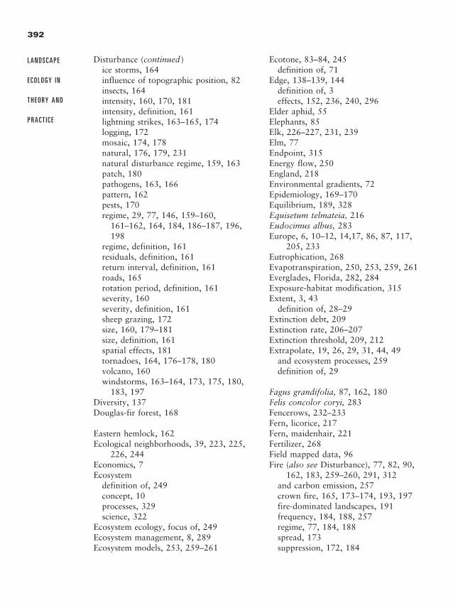
Disturbance (continued )ice storms, 164influence of topographic position, 82insects, 164intensity, 160, 170, 181intensity, definition, 161lightning strikes, 163–165, 174logging, 172mosaic, 174, 178natural, 176, 179, 231natural disturbance regime, 159, 163patch, 180pathogens, 163, 166pattern, 162pests, 170regime, 29, 77, 146, 159–160,

161–162, 164, 184, 186–187, 196,198

regime, definition, 161residuals, definition, 161return interval, definition, 161roads, 165rotation period, definition, 161severity, 160severity, definition, 161sheep grazing, 172size, 160, 179–181size, definition, 161spatial effects, 181tornadoes, 164, 176–178, 180volcano, 160windstorms, 163–164, 173, 175, 180,

183, 197Diversity, 137Douglas-fir forest, 168

Eastern hemlock, 162Ecological neighborhoods, 39, 223, 225,

226, 244Economics, 7Ecosystem

definition of, 249concept, 10processes, 329science, 322

Ecosystem ecology, focus of, 249Ecosystem management, 8, 289Ecosystem models, 253, 259–261

Ecotone, 83–84, 245definition of, 71

Edge, 138–139, 144definition of, 3effects, 152, 236, 240, 296

Elder aphid, 55Elephants, 85Elk, 226–227, 231, 239Elm, 77Endpoint, 315Energy flow, 250England, 218Environmental gradients, 72Epidemiology, 169–170Equilibrium, 189, 328Equisetum telmateia, 216Eudocimus albus, 283Europe, 6, 10–12, 14,17, 86, 87, 117,

205, 233Eutrophication, 268Evapotranspiration, 250, 253, 259, 261Everglades, Florida, 282, 284Exposure-habitat modification, 315Extent, 3, 43

definition of, 28–29Extinction debt, 209Extinction rate, 206–207Extinction threshold, 209, 212Extrapolate, 19, 26, 29, 31, 44, 49

and ecosystem processes, 259definition of, 29

Fagus grandifolia, 87, 162, 180Felis concolor coryi, 283Fencerows, 232–233Fern, licorice, 217Fern, maidenhair, 221Fertilizer, 268Field mapped data, 96Fire (also see Disturbance), 77, 82, 90,

162, 183, 259–260, 291, 312and carbon emission, 257crown fire, 165, 173–174, 193, 197fire-dominated landscapes, 191frequency, 184, 188, 257regime, 77, 184, 188spread, 173suppression, 172, 184

392

L A N D S C A P E

E C O L O G Y I N

T H E O R Y A N D

P R A C T I C E

2888_e13_p389-402 2/27/01 1:55 PM Page 392

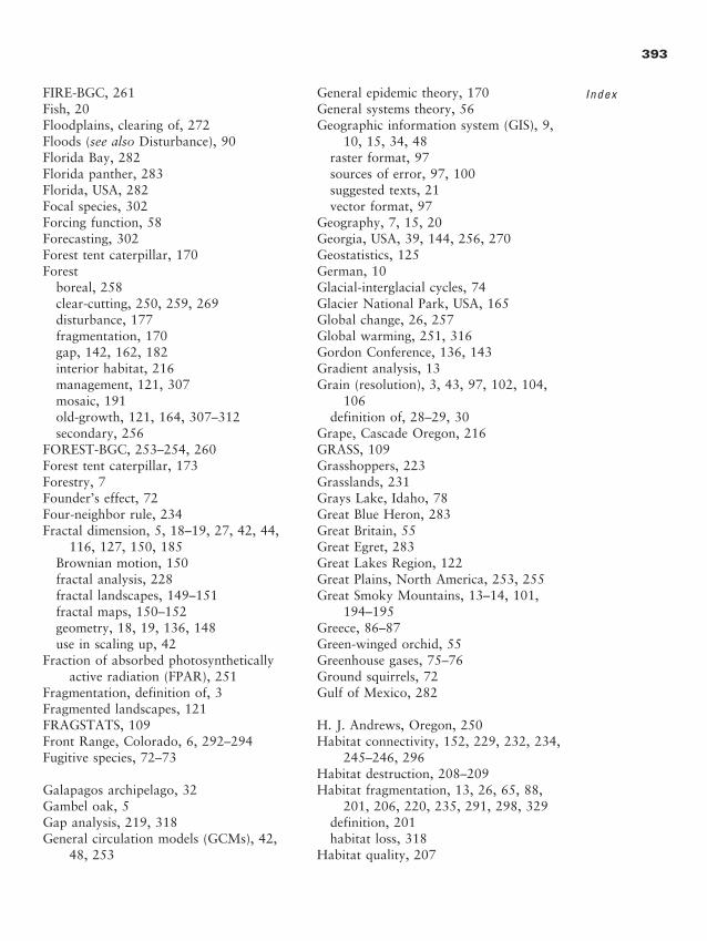
FIRE-BGC, 261Fish, 20Floodplains, clearing of, 272Floods (see also Disturbance), 90Florida Bay, 282Florida panther, 283Florida, USA, 282Focal species, 302Forcing function, 58Forecasting, 302Forest tent caterpillar, 170Forest

boreal, 258clear-cutting, 250, 259, 269disturbance, 177fragmentation, 170gap, 142, 162, 182interior habitat, 216management, 121, 307mosaic, 191old-growth, 121, 164, 307–312secondary, 256

FOREST-BGC, 253–254, 260Forest tent caterpillar, 173Forestry, 7Founder’s effect, 72Four-neighbor rule, 234Fractal dimension, 5, 18–19, 27, 42, 44,

116, 127, 150, 185Brownian motion, 150fractal analysis, 228fractal landscapes, 149–151fractal maps, 150–152geometry, 18, 19, 136, 148use in scaling up, 42

Fraction of absorbed photosyntheticallyactive radiation (FPAR), 251

Fragmentation, definition of, 3Fragmented landscapes, 121FRAGSTATS, 109Front Range, Colorado, 6, 292–294Fugitive species, 72–73

Galapagos archipelago, 32Gambel oak, 5Gap analysis, 219, 318General circulation models (GCMs), 42,

48, 253

General epidemic theory, 170General systems theory, 56Geographic information system (GIS), 9,

10, 15, 34, 48raster format, 97sources of error, 97, 100suggested texts, 21vector format, 97

Geography, 7, 15, 20Georgia, USA, 39, 144, 256, 270Geostatistics, 125German, 10Glacial-interglacial cycles, 74Glacier National Park, USA, 165Global change, 26, 257Global warming, 251, 316Gordon Conference, 136, 143Gradient analysis, 13Grain (resolution), 3, 43, 97, 102, 104,

106definition of, 28–29, 30

Grape, Cascade Oregon, 216GRASS, 109Grasshoppers, 223Grasslands, 231Grays Lake, Idaho, 78Great Blue Heron, 283Great Britain, 55Great Egret, 283Great Lakes Region, 122Great Plains, North America, 253, 255Great Smoky Mountains, 13–14, 101,

194–195Greece, 86–87Green-winged orchid, 55Greenhouse gases, 75–76Ground squirrels, 72Gulf of Mexico, 282

H. J. Andrews, Oregon, 250Habitat connectivity, 152, 229, 232, 234,

245–246, 296Habitat destruction, 208–209Habitat fragmentation, 13, 26, 65, 88,

201, 206, 220, 235, 291, 298, 329definition, 201habitat loss, 318

Habitat quality, 207

393

Index

2888_e13_p389-402 2/27/01 1:55 PM Page 393

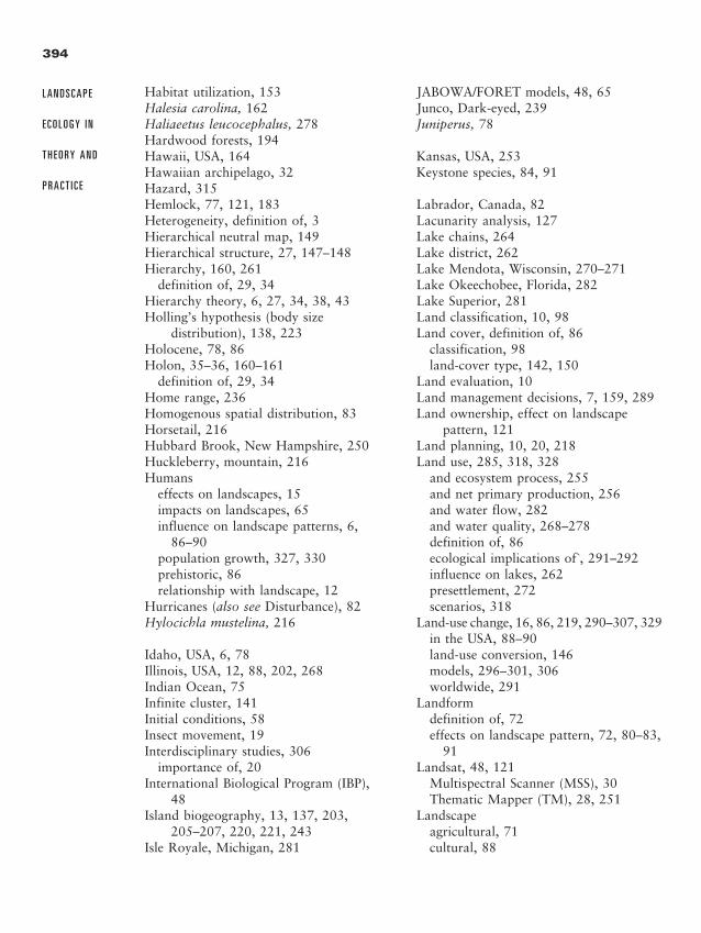
Habitat utilization, 153Halesia carolina, 162Haliaeetus leucocephalus, 278Hardwood forests, 194Hawaii, USA, 164Hawaiian archipelago, 32Hazard, 315Hemlock, 77, 121, 183Heterogeneity, definition of, 3Hierarchical neutral map, 149Hierarchical structure, 27, 147–148Hierarchy, 160, 261

definition of, 29, 34Hierarchy theory, 6, 27, 34, 38, 43Holling’s hypothesis (body size

distribution), 138, 223Holocene, 78, 86Holon, 35–36, 160–161

definition of, 29, 34Home range, 236Homogenous spatial distribution, 83Horsetail, 216Hubbard Brook, New Hampshire, 250Huckleberry, mountain, 216Humans

effects on landscapes, 15impacts on landscapes, 65influence on landscape patterns, 6,

86–90population growth, 327, 330prehistoric, 86relationship with landscape, 12

Hurricanes (also see Disturbance), 82Hylocichla mustelina, 216

Idaho, USA, 6, 78Illinois, USA, 12, 88, 202, 268Indian Ocean, 75Infinite cluster, 141Initial conditions, 58Insect movement, 19Interdisciplinary studies, 306

importance of, 20International Biological Program (IBP),

48Island biogeography, 13, 137, 203,

205–207, 220, 221, 243Isle Royale, Michigan, 281

JABOWA/FORET models, 48, 65Junco, Dark-eyed, 239Juniperus, 78

Kansas, USA, 253Keystone species, 84, 91

Labrador, Canada, 82Lacunarity analysis, 127Lake chains, 264Lake district, 262Lake Mendota, Wisconsin, 270–271Lake Okeechobee, Florida, 282Lake Superior, 281Land classification, 10, 98Land cover, definition of, 86

classification, 98land-cover type, 142, 150

Land evaluation, 10Land management decisions, 7, 159, 289Land ownership, effect on landscape

pattern, 121Land planning, 10, 20, 218Land use, 285, 318, 328

and ecosystem process, 255and net primary production, 256and water flow, 282and water quality, 268–278definition of, 86ecological implications of`, 291–292influence on lakes, 262presettlement, 272scenarios, 318

Land-use change, 16, 86, 219, 290–307, 329in the USA, 88–90land-use conversion, 146models, 296–301, 306worldwide, 291

Landformdefinition of, 72effects on landscape pattern, 72, 80–83,

91Landsat, 48, 121

Multispectral Scanner (MSS), 30Thematic Mapper (TM), 28, 251

Landscapeagricultural, 71cultural, 88

394

L A N D S C A P E

E C O L O G Y I N

T H E O R Y A N D

P R A C T I C E

2888_e13_p389-402 2/27/01 1:55 PM Page 394

definition of, 7intuitive sense, 1organism’s perspective, 1

Landscape architecture, 7, 10, 20Landscape composition, 71

metrics of, 108Landscape context, 236, 245Landscape design, 15Landscape diversity, 104, 192Landscape ecology

as a viewpoint, 10central themes, 331coining of term, 10conceptual basis of, 12definition of, 2–4, 21–22 difference from other areas of ecology, 4influence of scale theory on, 9influence of systems ecology on, 56influence of technology on, 9roots of, 10society for, 11terminology, 3, 12

Landscape equilibrium, 188–196Landscape fragmentation, 142, 151Landscape heterogeneity, 165–166Landscape management, 15, 289Landscape metrics (see Metrics), 147,

313–314Landscape models (also see Models), 64–66Landscape mosaic, 88, 175, 178Landscape pattern, 94, 174, 186, 188,

146, 147, 155causes of, 18, 91measurement (see Metrics)mechanisms to explain, 18state space for, 123

Landscape planning, 15Landscape position, 165

and ecosystem process, 256definition, 162influence on lakes, 261–265

Landscape restoration, 302–303Landscape structure, 155Landscape texture, 19Landslides, 83Larix occidentalis, 80Latitude, 73–74LCmax, 144

Leaf area index (LAI), 251, 253, 254Lepidoptera, 172Leslie matrix models, 48Level of organization, 27, 29, 34

definition, 27, 29Life-history, 179Lightning (also see Disturbance), 82, 85Limnologists, 261Little Ice Age, 75, 77Little Tennessee River Basin, 216, 218Local extinction, 220Lodgepole pine, 6, 78, 102, 104–105,

180, 192Lotka-Volterra models, 48Louisiana, USA, 260

MacArthur Award Address, 25MacPherson Township, Ontario, 171Madison, Wisconsin, 272Magnesium, 263Malacosoma disstra, 170Map

boundaries, 153dimensions, 153extent, 105, 140map overlay techniques, 15

Mapping, 10Marbled Murrelet, 308Markov chain, 61Marsupials, 239Matrix, 3, 12, 220

definition of, 3Mechanism, definition of, 52Mediterranean, 4, 6, 12, 86, 87Mercury, 270Mesic forests, 221Mesic landforms, 184Metapopulation, 65, 203, 208–209, 220,

311, 331definition, 210dynamics, 146frogs, 220models, 13, 219, 221, 243snails, 220

Metricaverage patch size, 114, 122connectivity, 111, 113, 123contagion, 111–112, 122, 124

395

Index

2888_e13_p389-402 2/27/01 1:55 PM Page 395

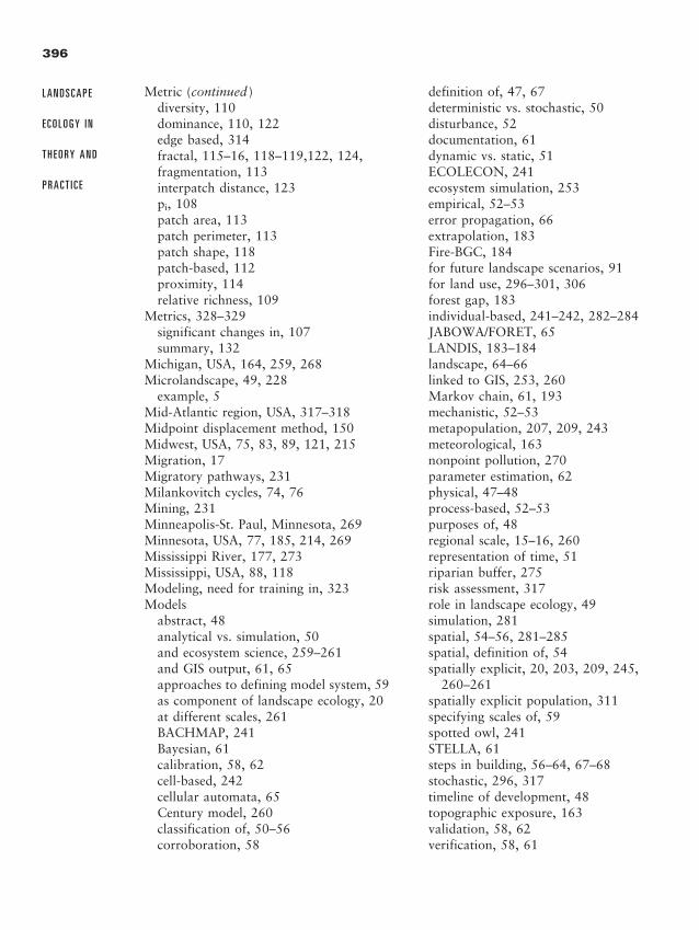
Metric (continued )diversity, 110dominance, 110, 122edge based, 314fractal, 115–16, 118–119,122, 124,fragmentation, 113interpatch distance, 123pi, 108patch area, 113patch perimeter, 113patch shape, 118patch-based, 112proximity, 114relative richness, 109

Metrics, 328–329significant changes in, 107summary, 132

Michigan, USA, 164, 259, 268Microlandscape, 49, 228

example, 5Mid-Atlantic region, USA, 317–318Midpoint displacement method, 150Midwest, USA, 75, 83, 89, 121, 215Migration, 17Migratory pathways, 231Milankovitch cycles, 74, 76Mining, 231Minneapolis-St. Paul, Minnesota, 269Minnesota, USA, 77, 185, 214, 269Mississippi River, 177, 273Mississippi, USA, 88, 118Modeling, need for training in, 323Models

abstract, 48analytical vs. simulation, 50and ecosystem science, 259–261and GIS output, 61, 65approaches to defining model system, 59as component of landscape ecology, 20at different scales, 261BACHMAP, 241Bayesian, 61calibration, 58, 62cell-based, 242cellular automata, 65Century model, 260classification of, 50–56corroboration, 58

definition of, 47, 67deterministic vs. stochastic, 50disturbance, 52documentation, 61dynamic vs. static, 51ECOLECON, 241ecosystem simulation, 253empirical, 52–53error propagation, 66extrapolation, 183Fire-BGC, 184for future landscape scenarios, 91for land use, 296–301, 306forest gap, 183individual-based, 241–242, 282–284JABOWA/FORET, 65LANDIS, 183–184landscape, 64–66linked to GIS, 253, 260Markov chain, 61, 193mechanistic, 52–53metapopulation, 207, 209, 243meteorological, 163nonpoint pollution, 270parameter estimation, 62physical, 47–48process-based, 52–53purposes of, 48regional scale, 15–16, 260representation of time, 51riparian buffer, 275risk assessment, 317role in landscape ecology, 49simulation, 281spatial, 54–56, 281–285spatial, definition of, 54spatially explicit, 20, 203, 209, 245,

260–261spatially explicit population, 311specifying scales of, 59spotted owl, 241STELLA, 61steps in building, 56–64, 67–68stochastic, 296, 317timeline of development, 48topographic exposure, 163validation, 58, 62verification, 58, 61

396

L A N D S C A P E

E C O L O G Y I N

T H E O R Y A N D

P R A C T I C E

2888_e13_p389-402 2/27/01 1:55 PM Page 396

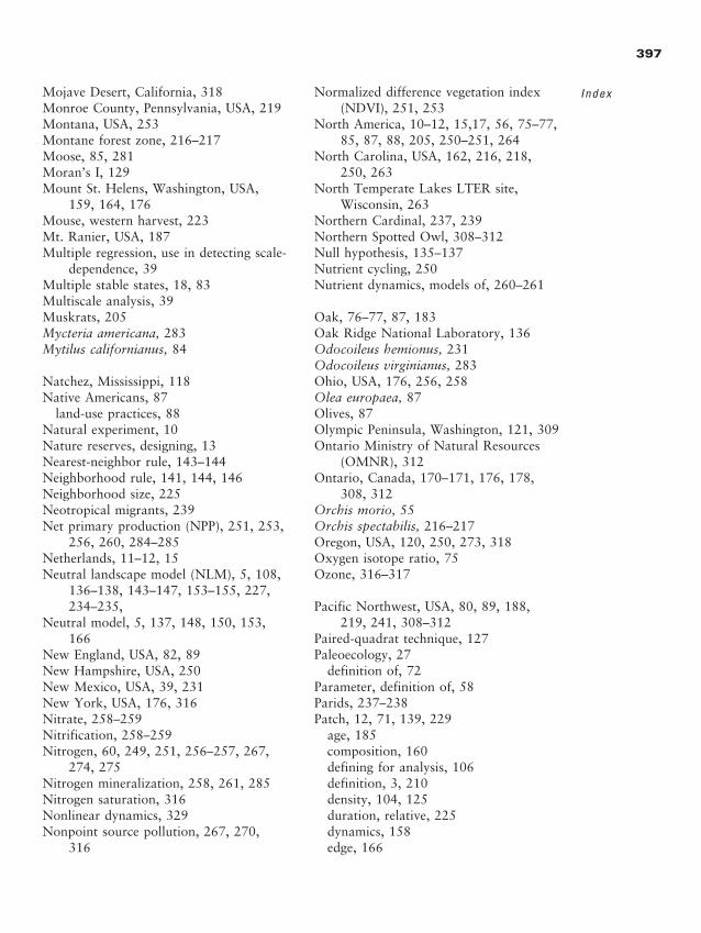
Mojave Desert, California, 318Monroe County, Pennsylvania, USA, 219Montana, USA, 253Montane forest zone, 216–217Moose, 85, 281Moran’s I, 129Mount St. Helens, Washington, USA,

159, 164, 176Mouse, western harvest, 223Mt. Ranier, USA, 187Multiple regression, use in detecting scale-

dependence, 39Multiple stable states, 18, 83Multiscale analysis, 39Muskrats, 205Mycteria americana, 283Mytilus californianus, 84

Natchez, Mississippi, 118Native Americans, 87

land-use practices, 88Natural experiment, 10Nature reserves, designing, 13Nearest-neighbor rule, 143–144Neighborhood rule, 141, 144, 146Neighborhood size, 225Neotropical migrants, 239Net primary production (NPP), 251, 253,

256, 260, 284–285Netherlands, 11–12, 15Neutral landscape model (NLM), 5, 108,

136–138, 143–147, 153–155, 227,234–235,

Neutral model, 5, 137, 148, 150, 153,166

New England, USA, 82, 89New Hampshire, USA, 250New Mexico, USA, 39, 231New York, USA, 176, 316Nitrate, 258–259Nitrification, 258–259Nitrogen, 60, 249, 251, 256–257, 267,

274, 275Nitrogen mineralization, 258, 261, 285Nitrogen saturation, 316Nonlinear dynamics, 329Nonpoint source pollution, 267, 270,

316

Normalized difference vegetation index(NDVI), 251, 253

North America, 10–12, 15,17, 56, 75–77,85, 87, 88, 205, 250–251, 264

North Carolina, USA, 162, 216, 218,250, 263

North Temperate Lakes LTER site,Wisconsin, 263

Northern Cardinal, 237, 239Northern Spotted Owl, 308–312Null hypothesis, 135–137Nutrient cycling, 250Nutrient dynamics, models of, 260–261

Oak, 76–77, 87, 183Oak Ridge National Laboratory, 136Odocoileus hemionus, 231Odocoileus virginianus, 283Ohio, USA, 176, 256, 258Olea europaea, 87Olives, 87Olympic Peninsula, Washington, 121, 309Ontario Ministry of Natural Resources

(OMNR), 312Ontario, Canada, 170–171, 176, 178,

308, 312Orchis morio, 55Orchis spectabilis, 216–217Oregon, USA, 120, 250, 273, 318Oxygen isotope ratio, 75Ozone, 316–317

Pacific Northwest, USA, 80, 89, 188,219, 241, 308–312

Paired-quadrat technique, 127Paleoecology, 27

definition of, 72Parameter, definition of, 58Parids, 237–238Patch, 12, 71, 139, 229

age, 185composition, 160defining for analysis, 106definition, 3, 210density, 104, 125duration, relative, 225dynamics, 158edge, 166

397

Index

2888_e13_p389-402 2/27/01 1:55 PM Page 397

Patch (continued )heterogeneity, 179, 245identification, 106isolation, 220isolation, relative, 225model, 210mosaic, stable, 193number, 139, 148, 166persistence, 160shape, 138, 148, 231size, 104, 125, 138, 140, 148, 160,

166, 179–181, 220, 223, 229, 225,245, 296, 309

size, relative, 225source, 13structure, 15, 154, 228structure, definition of, 3

Pattern analysis, 97Pattern, multiple scales of, 38Paulownia tomentosa, 216pc, 141–142, 148Pennsylvania, USA, 176–177, 180, 318Percolating cluster, 141Percolation theory, 18–19, 136, 141, 143,

146Percolation threshold, 141Perimeter-area ratio, 124, 229Pesticide, 268Phase difference, 72Phenacomys intermedius, 217Phosphorus, 249, 267, 274–275, 279Photosynthesis, 53, 253–254, 261Phytosociology, 12–13Picea, 82Picea engelmannii, 78Picea glauca, 281Pink noise, 41Pinus albicaulis, 79Pinus contorta, 6, 78, 180Pinus flexilis, 78Pinus ponderosa, 80Pinus strobus, 87Pinus-Juniperus, 231Pinyon-juniper, 231Pioides borealis, 242Pipilo erythrophthalmus, 237Pisaster ochraceous, 84

Plankton, 84Pleistocene, 78Pocono Mountains, Pennsylvania, 318Pollen analysis, 78Polypodium glycyhiza, 217Population

colonization, 207extinction, 205, 207models, spatially explicit, 240–243population growth models, 50–52population growth, intrinsic rate,

205population viability analysis, 311sink, 213–214source, 213–214stability of, 18theory, 17

Populus tremuloides, 78, 170, 281Predation, 83, 91, 278Predator-prey interactions, 17, 204Predator-prey models, 84Princess tree, 216Pseudo-replication, 32, 101Pseudotsuga menziessii, 78Pyrrhuloxia cardinalis, 237

Quasi-steady-state landscape, 191Quaternary, 77Quercus, 76Quercus gambelii, 5, 80Quercus rubra, 87

r.le, 109Raccoon, 226Random landscape, 129Random maps, 19, 136, 152Range of natural variability, 313Reaction-diffusion models, 84Red noise, 41Reference environment, 315Refuges, from predators, 17Regional planning, 7Regional risk assessment, 314–319Regional science, 16Relative constancy, 191Relative patch area, 124Remote imagery, 10, 28, 95, 253, 318

398

L A N D S C A P E

E C O L O G Y I N

T H E O R Y A N D

P R A C T I C E

2888_e13_p389-402 2/27/01 1:55 PM Page 398

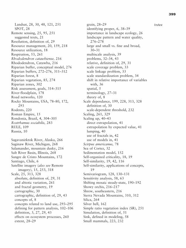
Landsat, 28, 30, 48, 121, 251SPOT, 28

Remote sensing, 25, 95, 251suggested texts, 21

Resolution, definition of, 29Resource management, 20, 159, 218Resource utilization, 18Respiration, 53, 261Rhododendron catawbiense, 216Rhododendron, Catawba, 216Riparian buffer, conceptual model, 276Riparian buffers, 272–276, 311–312Riparian forest, 8Riparian vegetation, 85, 274Riparian zones, 302Risk assessment, goals, 314–315River-floodplain, 178Road networks, 120Rocky Mountains, USA, 78–80, 172,

293Rodents, 220Roman Empire, 15Rondonia, Brazil, 4, 304–305Rostrhamus sociabilis, 283RULE, 109Russia, 10

Sagavanirktok River, Alaska, 266Saginaw River, Michigan, 268Salamander, mountain dusky, 216Salt River Basin, Illinois, 268Sangre de Cristo Mountains, 172Santiago, Chile, 6Satellite imagery (also see Remote

imagery), 15, 253, 318Scale, 25, 313, 328

absolute, definition of, 29, 31and abiotic variation, 261and fractal geometry, 19cartographic, 30cartographic, definition of, 29, 43concepts of, 8concepts related to land use, 293–295defining for pattern analysis, 102–106definition, 3, 27, 29, 43effects on ecosystem processes, 260extent, 28–29

grain, 28–29identifying proper, 6, 38–39importance in landscape ecology, 26landscape pattern and water quality,

276–278large and small vs. fine and broad,

30–31multiscale analysis, 39problems, 32–34, 43relative, definition of, 29, 31scale coverage problem, 33scale linkage problem, 33scale standardization problem, 34shift in relative importance of variables

with, 36spatial, 5terminology, 27–31theory of, 8

Scale dependance, 199, 228, 313, 328definition of, 30scale-dependent threshold, 232

Scaling, 261, 329Scaling up, 40–43

direct extrapolation, 41extrapolation by expected value, 41lumping, 40use of fractals in, 42use of models in, 41

Scirpus americanus, 78Sea of Cortez, 32Sedimentation model, 152Self-organized criticality, 18, 19Self-similarity, 19, 42, 116Self-similarity, applications of concepts,

19Semivariogram, 128, 130–131Sensitivity analysis, 58, 63Shifting mosaic steady-state, 190–192Showy orchis, 216–217Shrew, southeastern, 216Sierra Nevada Mountains, 310, 312Silica, 264Silver bell, 162Simple ratio vegetation index (SR), 251Simulation, definition of, 51Sink, defined in modeling, 58Small mammals, 223, 232

399

Index

2888_e13_p389-402 2/27/01 1:55 PM Page 399

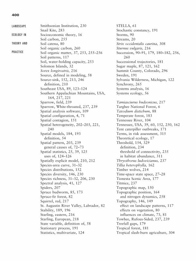
Smithsonian Institution, 230Snail Kite, 283Socioeconomic theory, 16Soil carbon, 255Soil catena, 80Soil organic carbon, 260Soil organic matter, 37, 253, 255–256Soil patterns, 117Soil, water-holding capacity, 253Solomon Islands, 32Sorex longirostris, 216Source, defined in modeling, 58Source-sink, 152, 213, 246

definition, 210Southeast USA, 89, 123–124Southern Appalachian Mountains, USA,

164, 217, 221Sparrow, field, 239Sparrow, White-throated, 237, 239Spatial analysis software, 109Spatial configuration, 4, 71Spatial contagion, 151Spatial heterogeneity, 202–203, 221,

240Spatial models, 184, 193

definition, 54Spatial pattern, 203, 239

general causes of, 72–73Spatial statistics, 25, 39, 125

uses of, 124–126Spatially explicit model, 210, 212Species-area curve, 31–32Species distributions, 152Species diversity, 146, 230Species richness, 31–32, 206, 230Spectral analysis, 41, 127Spiders, 207Spruce budworm, 85, 173Spruce-fir forest, 82Squirrel, red, 217St. Augustin River Valley, Labrador, 82Stability, 189, 196Starling, eastern, 216Starling, European, 218State variable, definition of, 58Stationary process, 191Statistics, multivariate, 124

STELLA, 61Stochastic constancy, 191Storms, 90Streams, 20Strix occidentalis caurina, 308Sturnus vulgaris, 216Succession, 90–91, 179, 180–182, 256,

260Successional trajectories, 181Sugar maple, 87, 121, 162Summit County, Colorado, 296Sweden, 191Sylvania Wilderness, Michigan, 122Synchrony, 265Systems analysis, 16Systems ecology, 56

Tamiasciurus hudsonicus, 217Targhee National Forest, 6Taxodium distichum, 88Temperate forest, 183Tennessee River, 104Tennessee, USA, 39, 60, 152, 250, 162Tent caterpiller outbreaks, 171Terms, in risk assessment, 315Theoretical ecology, 17Threshold, 154, 329

definition, 234threshold of connectivity, 235in habitat abundance, 311

Thryothorus ludovicianus, 237Tillia heterophylla, 162Timber wolves, 214Time-space state space, 27–28Tionesta Scenic Area, 177Titmice, 237Topographic map, 150Topographic position, 164

and nitrogen dynamics, 258Topography, 146, 149

effect on landscape patterns, 117effects on vegetation, 80influences on climate, 73, 81

Towhee, Rufous-Sided, 237, 239Treefall gaps, 179Tropical forest, 181Tropical slash-burn agriculture, 304

400

L A N D S C A P E

E C O L O G Y I N

T H E O R Y A N D

P R A C T I C E

2888_e13_p389-402 2/27/01 1:55 PM Page 400

Truncation effect, 140–141, 153Truncation error, 105Tsuga canadensis, 121, 162Tsuga heterophylla, 188Tsuga mertensiana, 187

Umbrella species, 302Uncertainty analysis, 63Ungulate, 39, 50, 226–227United States, 12, 13, 16, 36, 83, 89–90,

101, 122, 124, 253, 273, 274, 289,298, 312, 318

Upper Great Lakes Region, USA, 164Upper Peninsula, Michigan, USA, 214Urban development, 16Urban dynamics, 16Urbanization, 256, 269, 282Ursus americanus, 278Ursus arctos, 278US Bureau of Land Management, 8,

308US Environmental Protection Agency,

308, 318US Forest Service, 8, 308US General Land Office Survey, 96US Geological Survey, 97, 318US National Marine Fisheries Service,

308US National Park Service, 8, 308Uvularia grandiflora, 222

Vaccinium membranaceum, 216Variable

definition, 58driving, 58, 59external, 58output, 58

Vegetation patterns, determinants of, 13Volcanic eruption (see Disturbance), 90Vole, heather, 217Vulture, 221

Wadis, 213Walker Branch Watershed, Tennessee, 60,

250Washington, USA, 39Water quality, 250, 265–278, 292, 318Watershed dynamics, 250Western hemlock zone, 216–217Western spruce budworm, 172Wetlands, 8Wetlands, losses of, 272–273White basswood, 162White Ibis, 283White pine, 77, 87White-footed mice, 233White-tailed deer, 233, 283Whitebark pine, 102, 104–105Wildlife ecology, 7Wildlife habitat models, 314Willamette National Forest, 318Willamette River, Oregon, 273Wintering birds, 215Wisconsin, USA, 94, 101, 124, 214,

263–264, 270, 272, 278Wolf pack, 215Wood Stork, 283Wood Thrush, 216Woodpecker, pileated, 217Woodpecker, red-cockaded, 242Wren, Carolina, 237–238Wyoming, USA, 79

Xeric landforms, 184

Yellow birch, 162, 183Yellow buckeye, 162Yellowstone fires, 159, 176, 178, 180Yellowstone National Park, 4, 12, 50, 79,

94, 105, 110, 164, 175, 192, 226,239, 241

Zonotrichia albicollis, 237

401

Index

2888_e13_p389-402 2/27/01 1:55 PM Page 401

About the Authors

Monica G. Turner is a Professor in the Department of Zoology, Univer-sity of Wisconsin-Madison. She received her B.S. in Biology from Fordham Uni-versity, Bronx, New York, in 1980, and her Ph.D. in Ecology from the Univer-sity of Georgia under the direction of Frank B. Golley in 1985. Following atwo-year postdoc at Georgia with Eugene P. Odum, she was a research scientistat Oak Ridge National Laboratory for seven years before joining the Universityof Wisconsin faculty in 1994. Her research interests focus on the causes and ef-fects of natural disturbances, particularly fire in Yellowstone National Park; move-ment and habitat use patterns of large ungulates; the causes of land-use changeand its ecological legacies; the intersection between ecosystem and landscape ecol-ogy; and interactions between terrestrial and aquatic systems. Her work is char-acterized by the use of field studies as well as modeling and theory. Turner co-organized the first U.S. landscape ecology symposium in 1986 and served the U.S.chapter of the International Association of Landscape Ecology (US-IALE) as Pro-gram Chair from 1986–1989, Councilor-at-Large from 1990–1992, Local Meet-ing Host in 1993, and President from 1994–1996. She is also active in the Eco-logical Society of America and has served on advisory committees for numerousorganizations, including the National Science Foundation and National Research

2888_e14_p403-404 2/27/01 1:55 PM Page 403

Council. She is co-editor-in-chief of the journal Ecosystems and serves on the ed-itorial board of Ecological Applications, BioScience, and Landscape Ecology.

Robert H. Gardner is a Professor at the Appalachian Laboratory of theUniversity of Maryland Center for Environmental Science. He received a B.A. inBiology from Taylor University, an M.A. in Biology from William and Mary, anda Ph.D. in Zoology from North Carolina State University. His research interestsand publications are varied, including topics related to the statistical analysis ofmodel simulations, risk analysis, and issues of scale. Of special interest have beentheoretical and empirical studies of landscape disturbances. Gardner has servedon the editorial board of several journals, including editor-in-chief of LandscapeEcology from 1996–1999; has been an active participant in the Global Changeand Terrestrial Ecosystems research of the International Geosphere-Biosphere Pro-gram (IGBP); and has served on a variety of committees for the Ecological Soci-ety of America and US-IALE.

Robert V. O’Neill has recently retired as Corporate Fellow in the Environ-mental Sciences Division at Oak Ridge National Laboratory. He remains an adjunctProfessor at the University of Tennessee. He received his Ph.D. from the Universityof Illinois in 1967. His interest in landscape ecology dates back to the late 1970sand has resulted in over 75 publications. He was a participant in the workshop atAllerton Park, Illinois, that catalyzed the development of landscape ecology in theUnited States and served as Councilor-at-Large for US-IALE from 1989–1994. Heis a Fellow of the American Association for the Advancement of Science and hasserved on the editorial boards of Ecology, Columbia University Press, Ecosystems,and Conservation Ecology. He has received a number of awards, including the Tech-nical Achievement Award, Martin Marietta Corporation 1987; Distinguished Sta-tistical Ecologist, International Association for Statistical Ecology, 1994; Robert H.MacArthur Award, Ecological Society of America, 1998; Bronze Medal, EPA-ORD1999; Twentieth Century Distinguished Service Award, 1999, Ninth Lukacs Sym-posium, Bowling Green State University. He is currently President of the U.S. Chap-ter of the International Society for Ecological Economics.

Each of the authors has been honored to receive the Distinguished Landscape Ecol-ogist award from US-IALE: Gardner in 1994, O’Neill in 1995, and Turner in1998. We believe that this recognition derived largely from having been part ofsuch a rewarding and productive long-term collaboration.

2888_e14_p403-404 2/27/01 1:55 PM Page 404

landscape ecology

Documents