Copyright � 2009 by the Genetics Society of AmericaDOI: 10.1534/genetics.108.093153

Linkage Disequilibrium Between Loci With Unknown Phase

Alan R. Rogers*,1 and Chad Huff†

*Department of Anthropology and †Department of Human Genetics, University of Utah, Salt Lake City, Utah 84112

Manuscript received June 26, 2008Accepted for publication May 3, 2009

ABSTRACT

Linkage disequilibrium is often measured by two statistics, D and r, which can be interpreted as thecovariance and the correlation between loci and across gametes. When data consist of diploid genotypes,however, gametes cannot be identified. A variety of iterative statistical methods are used in such cases, allof which assume random mating. Previous work has shown that D and r can be expressed as covariancesand correlations across diploid genotypes, provided that mating is random. We show here that this resultalso holds approximately when mating is nonrandom. This provides a means of estimating theseparameters without iteration and without assuming random mating. This estimator is nearly as accurate asthe widely used EM estimator and is many times faster.

IN diploid species, it is much easier to determinegenotypes than haplotypes. Consequently, we are

often ignorant about which nucleotides reside togetheron individual chromosomes. We are ignorant, in otherwords, about ‘‘gametic phase.’’ This makes it hard tomeasure statistical associations (‘‘linkage disequilib-rium,’’ LD) among loci. These associations are ofinterest for many reasons. They help us map diseaseloci, infer the histories of populations, and detect theeffects of natural selection. The power of such studieshas grown enormously as genome-scale databases, suchas the HapMap (2007), have become available. On theother hand, their power is also limited by ambiguityabout gametic phase.

The methods currently used to estimate LD (Hill 1974;Weir 1977; Excoffier and Slatkin 1995; Stephens

et al. 2001) simplify the problem by assuming that pop-ulations mate at random. In most cases, some iterativealgorithm is then used to converge gradually on a solu-tion. In this article we introduce an approximate methodthat involves no iteration and allows for nonrandommating. It is nearly as accurate as the widely used EMalgorithm (Excoffier and Slatkin 1995) but muchfaster.

The approximation works with pairs of biallelic loci.In recent years, attention has shifted toward methodsthat reconstruct entire haplotypes involving many sites(Clark 1990; Excoffier and Slatkin 1995; Stephens

et al. 2001). Yet pairwise methods remain important.They underlie several graphical methods in wide use(Ding et al. 2003; Barrett et al. 2005), they provide thebackbone of descriptive studies of LD on genomic scales

(HapMap 2005), they are used in mapping diseasegenes (Jorde 2000), and they are used to search forthe effects of positive selection (Wang et al. 2006).

METHODS

Theory: Several standard measures of LD can beexpressed in terms of covariances across gametes. In thissection, we derive analogous formulas in terms ofcovariances across diploid genotypes.

Consider two genetic loci, one with alleles A and a andthe other with alleles B and b. In this system, there arefour gamete types, AB, Ab, aB, and ab, with relativefrequencies PAB, PAb, PaB, and Pab. Lewontin andKojima (1960) introduced

D ¼ PABPab � PAbPaB ð1Þ

as a measure of LD. A few years later, Hill andRobertson (1968) introduced an alternative measure,

r ¼ D=ffiffiffiffiffiffiffiffiffiffiffiffiffiffiffiffiffiffiffiffiffiffiffiffiffiffiffiffiffiffiffiffiffiffiffiffiffiffiffiffiffiffiffiffipAð1� pAÞpBð1� pBÞ

p; ð2Þ

where pA and pB are the relative frequencies of A and B.If the two loci are statistically independent, D and r bothequal zero. Both are positive if A tends to appeartogether with B. Both are easy to estimate from gametefrequencies, i.e., when gametic phase is known, andboth are in wide use today. Our goal is to estimate themfrom data with unknown phase.

Eight parameters are needed to describe the com-plete distribution of genotypes at two biallelic loci(Weir 1996, pp. 125–127). We eliminate several of thesedimensions by imposing the following constraints. First,we assume that PAB, PAb, PaB, and Pab have the samevalues among male and female gametes. This impliesfour constraints, three of which are independent.

1Corresponding author: Department of Anthropology, 270 S. 1400 E.,University of Utah, Salt Lake City, UT 84112.E-mail: rogers@anthro.utah.edu

Genetics 182: 839–844 ( July 2009)

Another constraint involves the inbreeding coefficient,f—the probability that two homologous genes within arandom individual are identical by descent (IBD). Weassume that this probability is the same at each locus,thus imposing a fourth independent constraint. Withthese constraints, the original eight dimensions collapseto four. Thus, our model requires four parameters. Wedescribe it in terms of pA, pB, f, and D.

We also introduce two sets of variables, one describinggametes and the other describing diploid individuals.For gametes, let y ¼ 1 on A-bearing gametes and 0 on a-bearing gametes. Similarly, let z ¼ 1 and 0 on B-bearingand b-bearing gametes. The means of y and z are pA andpB, and their variances are pA(1� pA) and pB(1� pB). Fordiploids, let Y¼ 2, 1, and 0 in genotypes AA, Aa, and aa,and let Z ¼ 2, 1, and 0 in genotypes BB, Bb, and bb.Taking the two loci together, (yi, zi) represents the stateof gamete i, where i ¼ 1 or 2 within any diploid indi-vidual. Such an individual has state (Y, Z), where Y¼ y1 1

y2 and Z ¼ z1 1 z2. If gametic phase is unknown, thenwe can observe Y and Z but not yi and zi. We refer to y andz as ‘‘genic values’’ and to Y and Z as ‘‘genotypic values.’’It is well known that D is the covariance and r thecorrelation between y and z. In what follows, we in-troduce an approximation that extends these results toY and Z.

We use the words ‘‘variance,’’ ‘‘covariance,’’ and ‘‘cor-relation’’ in two different ways: as functions of prob-ability distributions and as functions of data. Thesewords refer in the first sense to parameters and in thesecond to statistics. Where the meaning is not clear fromcontext, we refer to ‘‘theoretical’’ or ‘‘sample’’ variances,covariances, and correlations.

The theoretical covariance between Y and Z can beexpanded as a sum,

CðY ; ZÞ ¼ Cðy1; z1Þ1 Cðy1; z2Þ1 Cðy2; z1Þ1 Cðy2; z2Þ:

Two of these pairs, (y1, z1) and (y2, z2), lie on individualchromosomes and thus have covariance D. The othertwo depend in a complex way on the association be-tween uniting gametes. For individual loci, it is conven-tional to describe this association in terms of theprobability, f, that two uniting gametes are IBD. Com-plications arise, however, in applying this machinery totwo-locus haplotypes. Because of recombination, thetwo genes at one locus may be IBD even if those at theother locus are not. Nonetheless, consider the case inwhich recombination is absent. In that case, (y1, z1) and(y2, z2) are IBD with probability f and independent withprobability 1� f. When they are IBD, C(y1, z2)¼C(y1, z1)¼D. Otherwise, y1 and z2 are independent and their co-variance is zero. Thus,

CðY ; ZÞ ¼ 2Dð1 1 f Þ: ð3Þ

We propose to use this formula as an approximation,even when recombination does occur. To get a sense

of the resulting error, consider a monoecious sexualpopulation—one with sex but no sexes. Recombinationoccurs at rate c, and f measures the inbreeding of thecurrent generation relative to its parents. To simplifythings, we assume that the genotypes of the parentalgeneration were formed by random mating. We do allowfor nonrandom mating, however, when these parentsmated to form the current generation. With this setup,C(y1, z2) is nonzero only if both gametes are non-recombinants, an event with probability (1 � c)2 � 1 �2c. In that case, the argument of the previous paragraphapplies. Thus, C(y1, z2)� fD(1� 2c), and the same is trueof C(y2, z1). This gives

CðY ; ZÞ � 2Dð1 1 f Þ � 4fcD;

ignoring terms of order c2. Had we used Equation 3 as anapproximation, that approximation would have in-volved an error of �4fcD. This error is large only if f, c,and D are all large. Yet a large value of c nearly alwaysimplies a small value of D—unlinked loci are unlikelyto be in strong LD. Thus, we are unlikely to makea substantial error by using using Equation 3 as anapproximation.

The variances of Y and Z can be derived withoutrecourse to this approximation. That of Y is

VY ¼ 2pAð1� pAÞð1 1 f Þ ð4Þ

and a similar expression holds for VZ (Weir 2008, p.136). The correlation between Y and Z is defined asrYZ ¼ CðY ; ZÞ=

ffiffiffiffiffiffiffiffiffiffiffiVY VZ

p. In view of Equations 2–4, this

reduces to

rYZ � r : ð5Þ

In other words, the correlation between genotypicvalues is approximately equal to that between genicvalues.

Weir (2008) has derived similar formulas. Like us, hederives formulas for C(Y, Z). In the special case ofrandom mating, he also shows that rYZ ¼ r (Weir 2008,p. 132). Equation 5 suggests that Weir’s result maybe useful as an approximation even when mating isnonrandom.

These formulas suggest a simple way to estimate LDfrom unphased data. It is easy to estimate the samplecorrelation between genotypic values. Equation 5 im-plies that such estimates can be interpreted as estimatesof r. These in turn can be transformed into estimates ofD by inverting Equation 2. The statistical properties ofthese estimates are investigated below by computersimulation.

Computer simulations: We used two types of com-puter simulation. The direct sampling algorithm (de-scribed in the appendix) specifies all parameter values,uses these to sample from the distribution of gametes,and then joins gametes to form diploid individuals.We use this approach to evaluate the approximation

840 A. R. Rogers and C. Huff

discussed above. This approach is flexible but requiresarbitrary assumptions about the values of pA, pB, and r.

To avoid these arbitrary assumptions, we also examinethe estimators using data generated by a coalescentsimulation with recombination (Hudson 1990). In thissimulation, the parameters we specify are those de-scribing evolutionary history. We take the results ofSchaffner et al. (2005) as a reasonable model of humanevolutionary history, and their publication should beconsulted for details. Briefly, their model holds thatEurope and Asia were colonized from Africa, withbottlenecks at the time of colonization. Our programassumed random mating, a mutation rate of 2.2 3 10�8,and a recombination rate of 1 cm/Mb. It generated asimulated sample of 50 diploid ‘‘African’’ individuals,each with 1000 chromosomes. Chromosomes were 1 Mblong, and the average chromosome varied at 2979 poly-morphic sites (SNPs) within the sample. Our programcrawled along each chromosome, comparing each pair ofSNPs within a moving 1600-SNP window, but excludingpairs .500 kb apart. Each comparison involved estimat-ing r using the derived alleles at each of the two SNPs.

Both types of computer simulation generated sam-ples of haploid gametes, which were used to calculatethe ‘‘true value’’ of r2. True value is in quotation marksbecause there are really two versions of ‘‘truth’’: (1) thevalue within the population as a whole and (2) the valuewithin our sample of gametes with known phase. Wemeasure deviations from the latter value because weare interested in the error resulting from unknowngametic phase.

Each simulation also combined gametes to formdiploid genotypes with unknown gametic phase. Theprograms then used these data to estimate r2 by twomethods: (1) the EM method introduced by Excoffier

and Slatkin (1995) and (2) the method introducedhere, which we refer to by our own initials (Rogers andHuff, RH). The EM algorithm is designed to reconstructhaplotypes involving many polymorphic loci. We codeda reduced version, which deals only with a pair ofbiallelic loci. This ensures that execution speed is notreduced by unnecessarily compex code. The EM algo-rithm works with a vector of haplotype frequencies,which it improves iteratively until some tolerancecriterion is reached. Following Excoffier and Slatkin

(1995), we set the tolerance parameter to 10�7. (In ourversion, this means that the sum of absolute differencesbetween two successive frequency vectors is ,10�7.)

RESULTS

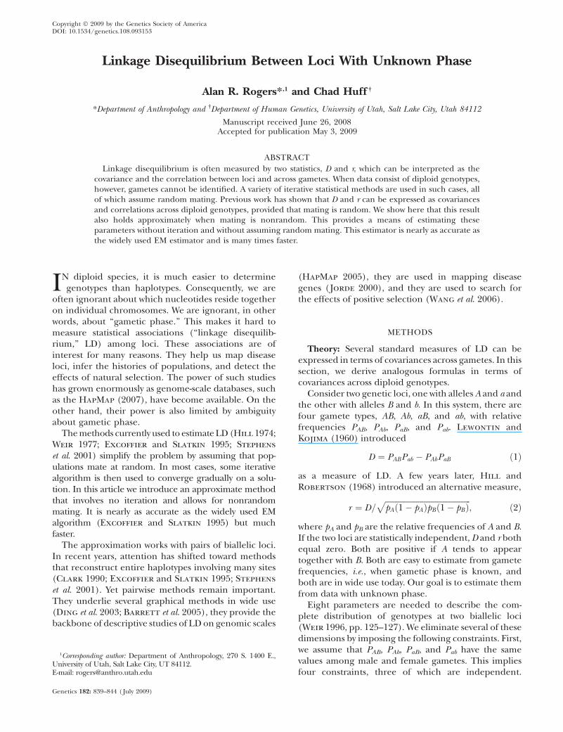
The RH method is based on an approximation that isexact under complete linkage (c¼ 0) or when mating israndom ( f ¼ 0). At larger values of c and f, approxima-tion error generates bias, which should inflate thestandard error (SE) of our estimates. For this reason,we expect SE to increase with c whenever f . 0. Thelarger the approximation error is, the steeper thisrate of increase should be. Figure 1 uses this idea toevaluate approximation error. In Figure 1’s top leftpanel, the curve for random mating ( f ¼ 0) appears to

Figure 1.—The effect of recombination rate(c) on the standard error (SE) of the RH estima-tor. Each point is based on 100,000 data sets sim-ulated by direct sampling.

Linkage Disequilibrium 841

be completely flat, as expected in the absence ofapproximation error. In the other curves in that panel,f . 0 and error does increase with c, especially wheninbreeding is strong. Yet even then, the approximationerror is minor until c . 10�2. Even under stronginbreeding, therefore, the approximation is excellentfor sites that are separated by ,1 cM.

These conclusions depend on the particular values ofpA, pB, and D9 that are assumed in the top left panel ofFigure 1. The other panels of Figure 1 carry out the sameanalysis for different sets of parameter values. In thebottom two panels of Figure 1, D9 is near zero, and all ofthe curves are essentially flat, irrespective of the value off. This suggests that there is little approximation errorunder weak LD, even if inbreeding is strong. This isconsistent with our analytical error analysis (see above),in which the error was proportional to D. The top rightpanel of Figure 1 considers the case in which LD isvery strong. In this case, strong inbreeding leads to asubstantial approximation error, but as before this erroris important only for loci separated by .1 cM. This is theonly situation we have found in which the approxima-tion error is large, and it refers to a situation—strongLD between essentially unlinked loci—that is unlikely tohappen often in nature.

Each panel of Figure 1 also shows that SE declineswith f. This makes sense because ambiguity aboutgametic phase arises from individuals who are hetero-zygous at both loci. In inbred samples, there are fewsuch individuals and it is therefore easy to estimate LD(Fallin and Schork 2000).

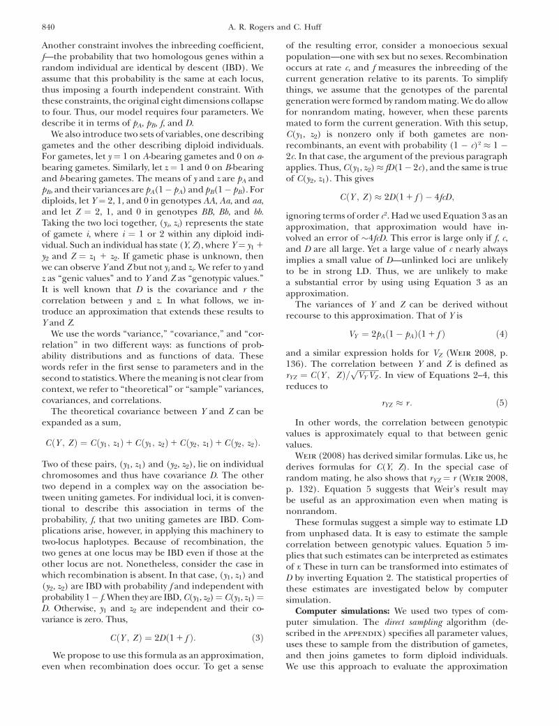
The results just presented pertain to only one of thefactors that contribute to statistical error. To study theothers, we turn next to coalescent simulations. Figure 2summarizes estimates of r2 based on 601,778,210 pairs ofSNPs, which were generated by coalescent simulation.The EM method failed to converge in a small fraction(0.04%) of the comparisons. The pairs were sorted into20 bins, on the basis of the physical distance separatingthe two SNPs. The left panel of Figure 2 shows the meanestimate of r2 within each bin. Both estimators show theexpected pattern, with r2 declining as distance increases.X’s indicate the means of the ‘‘true’’ values of r2. Themeans of both estimators are larger than the true values,

indicating a small upward bias. This bias is a little largerfor the RH method than for EM.

The right panel of Figure 2 shows the standard errors(SE) of both estimators. (Note that these are the stan-dard errors of individual estimates, not of the meansdisplayed in the left panel.) The two estimators differonly a little. The EM algorithm has a small advantage(smaller SE), especially for tightly linked loci. For theRH estimator, the bias in estimates of r2 does not arisefrom any bias in the underlying estimates of r. On thecontrary, these latter estimates are essentially unbiased(data not shown). Instead, the larger bias in the RHmethod reflects a larger sampling variance in estimatesof r.

The smaller sampling variance of EM is not surpris-ing, as EM is a maximum-likelihood estimator andshould therefore have near-optimal statistical proper-ties, at least in large samples. Nonetheless, this advan-tage appears to be small and should be weighed againstother considerations.

One such consideration involves the assumption ofrandom mating. EM makes this assumption, but the RHmethod does not. Consequently, one might supposethat inbreeding would introduce bias into EM estimatesor elevate their standard errors. This, however, is not thecase. As mentioned above, inbreeding makes it easier toestimate LD. Both estimators of r2 have smaller standarderrors under inbreeding than under random mating.The bias and standard error of EM are consistentlysmaller than those of the RH method, even underinbreeding (data not shown).

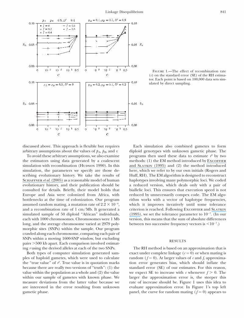
Another consideration has to do with executionspeed (Figure 3). Sample size affects the speed of bothalgorithms, but not in the same way. Both begin withthe same initial step: a single pass through the datato construct a 3 3 3 table of genotype counts. Bothalgorithms then use this table in a second stage that doesnot depend on sample size. In the RH algorithm, thissecond stage is very fast, so the algorithm is dominatedby the initial tabulation. Its execution time thus in-creases linearly with sample size. The second stage of theEM algorithm involves a series of iterations. This processis relatively costly and dominates when sample size issmall. Execution time is thus insensitive to sample size

Figure 2.—Performance of estimators of r2.Left, mean estimates of r2; right, standard errors(SE) of estimates.

842 A. R. Rogers and C. Huff

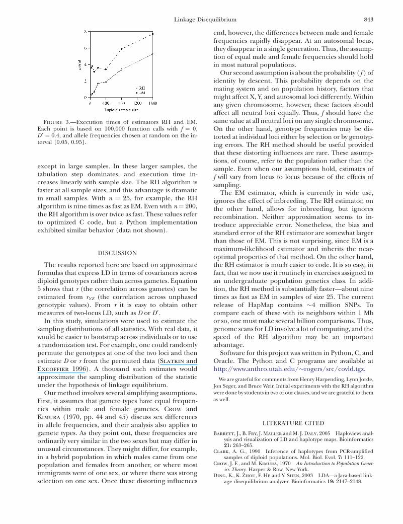
except in large samples. In these larger samples, thetabulation step dominates, and execution time in-creases linearly with sample size. The RH algorithm isfaster at all sample sizes, and this advantage is dramaticin small samples. With n ¼ 25, for example, the RHalgorithm is nine times as fast as EM. Even with n¼ 200,the RH algorithm is over twice as fast. These values referto optimized C code, but a Python implementationexhibited similar behavior (data not shown).

DISCUSSION

The results reported here are based on approximateformulas that express LD in terms of covariances acrossdiploid genotypes rather than across gametes. Equation5 shows that r (the correlation across gametes) can beestimated from rYZ (the correlation across unphasedgenotypic values). From r it is easy to obtain othermeasures of two-locus LD, such as D or D9.

In this study, simulations were used to estimate thesampling distributions of all statistics. With real data, itwould be easier to bootstrap across individuals or to usea randomization test. For example, one could randomlypermute the genotypes at one of the two loci and thenestimate D or r from the permuted data (Slatkin andExcoffier 1996). A thousand such estimates wouldapproximate the sampling distribution of the statisticunder the hypothesis of linkage equilibrium.

Our method involves several simplifying assumptions.First, it assumes that gamete types have equal frequen-cies within male and female gametes. Crow andKimura (1970, pp. 44 and 45) discuss sex differencesin allele frequencies, and their analysis also applies togamete types. As they point out, these frequencies areordinarily very similar in the two sexes but may differ inunusual circumstances. They might differ, for example,in a hybrid population in which males came from onepopulation and females from another, or where mostimmigrants were of one sex, or where there was strongselection on one sex. Once these distorting influences

end, however, the differences between male and femalefrequencies rapidly disappear. At an autosomal locus,they disappear in a single generation. Thus, the assump-tion of equal male and female frequencies should holdin most natural populations.

Our second assumption is about the probability ( f ) ofidentity by descent. This probability depends on themating system and on population history, factors thatmight affect X, Y, and autosomal loci differently. Withinany given chromosome, however, these factors shouldaffect all neutral loci equally. Thus, f should have thesame value at all neutral loci on any single chromosome.On the other hand, genotype frequencies may be dis-torted at individual loci either by selection or by genotyp-ing errors. The RH method should be useful providedthat these distorting influences are rare. These assump-tions, of course, refer to the population rather than thesample. Even when our assumptions hold, estimates off will vary from locus to locus because of the effects ofsampling.

The EM estimator, which is currently in wide use,ignores the effect of inbreeding. The RH estimator, onthe other hand, allows for inbreeding, but ignoresrecombination. Neither approximation seems to in-troduce appreciable error. Nonetheless, the bias andstandard error of the RH estimator are somewhat largerthan those of EM. This is not surprising, since EM is amaximum-likelihood estimator and inherits the near-optimal properties of that method. On the other hand,the RH estimator is much easier to code. It is so easy, infact, that we now use it routinely in exercises assigned toan undergraduate population genetics class. In addi-tion, the RH method is substantially faster—about ninetimes as fast as EM in samples of size 25. The currentrelease of HapMap contains �4 million SNPs. Tocompare each of these with its neighbors within 1 Mbor so, one must make several billion comparisons. Thus,genome scans for LD involve a lot of computing, and thespeed of the RH algorithm may be an importantadvantage.

Software for this project was written in Python, C, andOracle. The Python and C programs are available athttp://www.anthro.utah.edu/�rogers/src/covld.tgz.

We are grateful for comments from Henry Harpending, Lynn Jorde,Jon Seger, and Bruce Weir. Initial experiments with the RH algorithmwere done by students in two of our classes, and we are grateful to themas well.

LITERATURE CITED

Barrett, J., B. Fry, J. Maller and M. J. Daly, 2005 Haploview: anal-ysis and visualization of LD and haplotype maps. Bioinformatics21: 263–265.

Clark, A. G., 1990 Inference of haplotypes from PCR-amplifiedsamples of diploid populations. Mol. Biol. Evol. 7: 111–122.

Crow, J. F., and M. Kimura, 1970 An Introduction to Population Genet-ics Theory. Harper & Row, New York.

Ding, K., K. Zhou, F. He and Y. Shen, 2003 LDA—a Java-based link-age disequilibrium analyzer. Bioinformatics 19: 2147–2148.

Figure 3.—Execution times of estimators RH and EM.Each point is based on 100,000 function calls with f ¼ 0,D9 ¼ 0.4, and allele frequencies chosen at random on the in-terval [0.05, 0.95].

Linkage Disequilibrium 843

Excoffier, L., and M. Slatkin, 1995 Maximum likelihood estima-tion of molecular haplotype frequencies in a diploid population.Mol. Biol. Evol. 12: 921–927.

Fallin, D., and N. J. Schork, 2000 Accuracy of haplotype frequencyestimation for biallelic loci, via the expectation-maximization algo-rithmforunphasedgenotypedata. Am.J.Hum.Genet. 67:947–959.

HapMap, 2005 A haplotype map of the human genome. Nature 437:1299–1320.

HapMap, 2007 A second generation human haplotype map of over3.1 million SNPs. Nature 449: 851–862.

Hedrick, P. W., 2004 Genetics of Populations, Ed. 3. Jones & Bartlett,Boston.

Hill, W. G., 1974 Estimation of linkage disequilibrium in randomlymating populations. Heredity 33: 229–239.

Hill, W. G., and A. Robertson, 1968 Linkage diseqilibrium infinite populations. Theor. Appl. Genet. 38: 226–231.

Hudson, R. R., 1990 Gene genealogies and the coalescent process,pp. 1–44 in Oxford Surveys in Evolutionary Biology, Vol. 7, edited byD. Futuyma and J. Antonovics. Oxford University Press,Oxford.

Jorde, L. B., 2000 Linkage disequilibrium and the search for com-plex diseases. Genome Res. 10: 1435–1444.

Lewontin, R. C., and K.-i. Kojima, 1960 The evolutionary dynamicsof complex polymorphisms. Evolution 14: 458–472.

Schaffner, S. F., C. Foo, S. Gabriel, D. Reich, M. J. Daly et al.,2005 Calibrating a coalescent simulation of human genomesequence variation. Genome Res. 15: 1576–1583.

Slatkin, M., and L. Excoffier, 1996 Testing for linkage disequilib-rium in genotypic data using the expectation-maximization algo-rithm. Heredity 76: 377–383.

Stephens, M., N. Smith and P. Donnelly, 2001 A new statisticalmethod for haplotype reconstruction from population data.Am. J. Hum. Genet. 68: 978–989.

Wang, E. T., G. Kodama, P. Baldi and R. K. Moyzis, 2006 Globallandscape of recent inferred Darwinian selection for Homosapiens. Proc. Natl. Acad. Sci. USA 103: 135–140.

Weir, B. S., 1977 Estimation of linkage disequilibrium in randomlymating populations. Heredity 42: 105–111.

Weir, B. S., 1996 Genetic Data Analysis II: Methods for Discrete Popula-tion Genetic Data. Sinauer Associates, Sunderland, MA.

Weir, B. S., 2008 Linkage disequilibrium and association mapping.Annu. Rev. Genomics Hum. Genet. 9: 129–142.

Communicating editor: L. Excoffier

APPENDIX: DIRECT SAMPLING ALGORITHM FORGENERATING DIPLOID GENOTYPES

In the generation of the parents, the four types ofgametes have probabilities

ðy; zÞ Probabilityð1; 1Þ pApB 1 Dð1; 0Þ pAð1� pBÞ � Dð0; 1Þ ð1� pAÞpB � Dð0; 0Þ ð1� pAÞð1� pBÞ1 D

9>>>>=>>>>;

ðA1Þ

(Hedrick 2004, Equation 10.1).In this probability distribution, gametes are classified

by their state at the two loci. We also need to classifythem in terms of identity by descent. In sexual specieswith separate sexes, homologous genes cannot be IBDfrom the generation of their parents. To avoid this issue,we model a population of monoecious sexuals. Theinbreeding coefficient f represents the probability thattwo homologous genes are IBD from the generation oftheir parents.

A two-locus gamete is ‘‘recombinant’’ if an odd numberof crossover events occurred between the two loci. Thishappens with probability c, the recombination rate.Within recombinant gametes, the two loci are indepen-dent provided that the parents mated at random. Incomparing two-locus gametes, there are three cases toconsider:

Case 1: Neither gamete is a recombinant, an event withprobability (1 � c)2. In this case, the two gametes areIBD with probability f. Thus, we generate the firstgamete by sampling from (A1). Then, with probabil-ity f, we duplicate the first gamete to obtain thesecond. Otherwise (with probability 1� f ), we sampleonce again from (A1).

Case 2: One gamete is a recombinant, an event withprobability 2c(1 � c). In this case, the nonrecombi-nant gamete may be (i) IBD with the A/a locus of therecombinant (probability f ), (ii) IBD with B/b (prob-ability f ), or (iii) IBD with neither locus (probability1� 2f ). The nonrecombinant gamete cannot be IBDwith both loci of the recombinant. To deal with thesecases, our algorithm takes the following steps: (i)generate the nonrecombinant gamete by sam-pling from (A1); (ii) with probability f, obtain theA/a locus of the second gamete by copying thefirst; otherwise sample from Bernoulli(pA); and (iii)obtain the B/b locus of the second gamete in ananalogous fashion.

Case 3: Both gametes are recombinants, an event withprobability c2. At each locus, the two genes are IBDwith independent probability f. In that case, the twogenes at each locus are generated by independentsamples from the appropriate Bernoulli distribution.Otherwise (with probability 1� f ), they are two copiesof a single Bernoulli variate.

844 A. R. Rogers and C. Huff