linkage disequilibrium maps constructed with common snps are useful for first-pass disease...

www.elsevier.com/locate/ygeno

Genomics 84 (20

Linkage disequilibrium maps constructed with common SNPs

are useful for first-pass disease association screens

P. Taillon-Millera,1, S.F. Sacconeb,1, N.L. Sacconec,1, S. Duana, E.F. Klossa,

E.G. Lovinsd, R. Donaldsona, A. Phongd, C. Had, L. Flagstada, S. Millera,

A. Drendela, D. Lindd, R.D. Millera, J.P. Riceb, P-Y. Kwokd,e,*

aDepartment of Dermatology, Washington University School of Medicine, St. Louis, MO 63110, USAbDepartment of Psychiatry, Washington University School of Medicine, St. Louis, MO 63110, USAcDepartment of Genetics, Washington University School of Medicine, St. Louis, MO 63110, USA

dCardiovascular Research Institute, University of California at San Francisco, Long 1332A, San Francisco, CA 94143, USAeDepartment of Dermatology, University of California at San Francisco, Long 1332A, San Francisco, CA 94143, USA

Received 10 August 2004; accepted 10 August 2004

Available online 17 September 2004

Abstract

To develop an efficient strategy for mapping genetic factors associated with common diseases, we constructed linkage disequilibrium

(LD) maps of human chromosomes 5, 7, 17, and X. These maps consist of common single nucleotide polymorphisms at an average

intermarker distance of 100 kb. The genotype data from these markers in a panel of American samples of European descent were analyzed to

produce blocks of markers in strong pair-wise LD. Power calculations were used to guide block definitions and predicted that high-level LD

maps would be useful in initial genome scans for susceptibility alleles in case-control association studies of complex diseases. As anticipated,

LD blocks on the X chromosome were larger and covered more of the chromosome than those found on the autosomes.

D 2004 Elsevier Inc. All rights reserved.

Keywords: Polymorphism; Single nucleotide; Linkage disequilibrium; Genomics; Sample size

Introduction

With the finished reference human genome sequence

available and haplotype maps for human panels from three

continents being constructed [1], there is intense discussion

and debate on how to take advantage of the genomic

information to study common diseases with a genetic

approach. In an ideal world, the functions of all the genes

and their regulatory elements would be known and the

entire genome of an individual could be sequenced quickly

and inexpensively. Therefore, one could obtain the com-

plete genome sequences of a group of patients suffering

0888-7543/$ - see front matter D 2004 Elsevier Inc. All rights reserved.

doi:10.1016/j.ygeno.2004.08.009

* Corresponding author. Fax: (415) 476 2283.

E-mail address: [email protected] (P-Y. Kwok).1 These authors contributed equally to this publication.

from a disease and compare them to those of a group of

appropriately selected control individuals and identify genes

or regulatory elements with functional differences between

the two groups. But until this level of biological under-

standing and technical capability is reached, one has to rely

on indirect tools in the search for disease-predisposing

alleles. While genetic linkage studies of families have been

very successful in identifying genes responsible for simple

traits, it has been proposed that association studies using

single nucleotide polymorphisms (SNPs) will be most

useful to identify genes involved in complex diseases [2].

Association testing relies on the principle that nearby SNPs

are often in linkage disequilibrium (LD); however, LD is

not a simple function of the distance between markers.

Instead, one observes a complicated pattern of regions of

extensive LD punctuated by regions of no LD across the

genome [3–9]. This pattern of LD is a result of many

04) 899–912

http:\\snp.wustl.edu\snp%1Eresearch\ld%1Eblocks\tables\

P. Taillon-Miller et al. / Genomics 84 (2004) 899–912900

factors, including genetic drift, admixture, migration,

population structure, variable mutation rates, variable

recombination rates, gene conversion, and natural selection

[10].

Defining the patterns of LD and the underlying haplotype

structure across the human genome is expected to aid in

elucidating the causes of complex human diseases by

helping researchers design association studies that make

efficient use of SNP markers [11]. Several groups have

demonstrated that the haplotype structures are complex,

requiring many markers to define the major haplotypes

found in even small regions of the genome (10 to 20 kb)

[4,6,8,9,12,13]. What is often overlooked, however, is the

fact that many contiguous bhaplotype blocksQ are highly

correlated and that markers in neighboring haplotype blocks

are often in strong LD with each other [5,9]. These

observations prompted us to evaluate whether high-level

LD maps would capture useful long-range LD structure and

allow selection of representative btagQ SNPs in regions of

strong LD. A hierarchical strategy of performing initial

genome scans with reduced-density maps in case-control

association studies could then provide an efficient way to

identify genetic factors associated with common diseases. In

this strategy a secondary screen would likely be required to

localize a disease variant to a specific gene once a region of

association has been detected. Variants in regions with no

LD could be missed in the initial pass, as would those with

very low frequency or multiple alleles, but these cases will

be difficult with any screening strategy. For such cases a

second pass with increased density in regions of low LD

might be necessary. However, a whole genome scan

following this approach could potentially use many fewer

SNPs than has been previously proposed, thus making such

studies practical. The approach could also be used to study

genetic effects that have been localized to chromosomal

regions in prior family studies, or to survey candidate genes

of special interest, as it provides a means for prioritization of

SNPs for follow-up genotyping.

To develop this approach, we present the LD maps of

human chromosomes 5, 7, 17, and X (covering ~20% of the

human genome) consisting of common SNPs chosen

according to allele frequency data generated from three

panels of 42 individuals (European, Asian, and African

American) and genotyped in a panel of 94 American

samples of European descent. LD block definitions were

guided by power calculations, which predict that reduced-

Table 1

Characteristics of SNPs analyzed

Chromosome Chromosome

length (Mb)

SNPs

genotyped

5 179.7 1442

7 156.4 1753

17 82.3 662

X 149.5 1487

density maps will be useful in genetic analyses of common

diseases.

Results

We selected 5344 common SNPs (each with previ-

ously estimated minor allele frequencies of z10%) in

each of three panels of individuals of European, Asian,

and African descent (a list of SNPs is provided in

Supplemental Tables S1a-S1d) across human chromosomes

5, 7, 17, and X. These SNPs were genotyped in 94

genetically unrelated samples from the CEPH collection

(Supplemental Tables S2a and S2b) using a primer

extension assay with fluorescence polarization detection

[14]. On the X chromosome, only males were genotyped so

we were able to determine complete haplotypes across the

chromosome (Supplemental Table S3). The genotypes

generated from the autosomal SNPs are given in Supple-

mental Tables S4a–S4c.

For each chromosome, pair-wise linkage disequilibrium

between all markers with minor allele frequencies (MAF)

z10%was measured usingD,DV, and r2. Because the resultswere very similar between SNPs with MAFz10% and those

with MAF z20%, only the data from the SNPs with MAF

z20% will be presented. The LD results from all pair-wise

comparisons with SNPs with MAFz10% are not given with

this publication but are available at http://snp.wustl.edu/

snp_research/ld_blocks; edited results for markers withMAF

z20% are also available at this Web site.

Table 1 summarizes the statistics of the SNPs genotyped

in this study. As predicted, 5098 (N95%) of the SNPs

genotyped were indeed common in the CEPH panel we

studied, with MAF z10%. In fact, 4405 (83%) of the

SNPs had a MAF z20% in the CEPH panel. The mean

intermarker distance between the SNPs with MAF z20%

was found to be 151, 106, 148, and 124 kb in

chromosomes 5, 7, 17, and X, respectively. But the mean

intermarker distance can be skewed by large gaps between

sequencing contigs, the centromeric region, and regions in

which very few SNPs were available at the time of this

study. Fig. 4c shows that for the complete marker set 15%

were closer than 5 kb, about 50% were closer than 25 kb,

and more than 70% (3130 SNPs, MAF z20%,) were

within 100 kb of their nearest neighbor. When only these

3130 SNPs are considered, in fact the mean intermarker

SNPs with

MAF z10%

SNPs with

MAF z20%

Mean intermarke

distance (kb)

MAF z20%

1389 1188 151

1659 1470 106

638 550 148

1412 1197 125

r


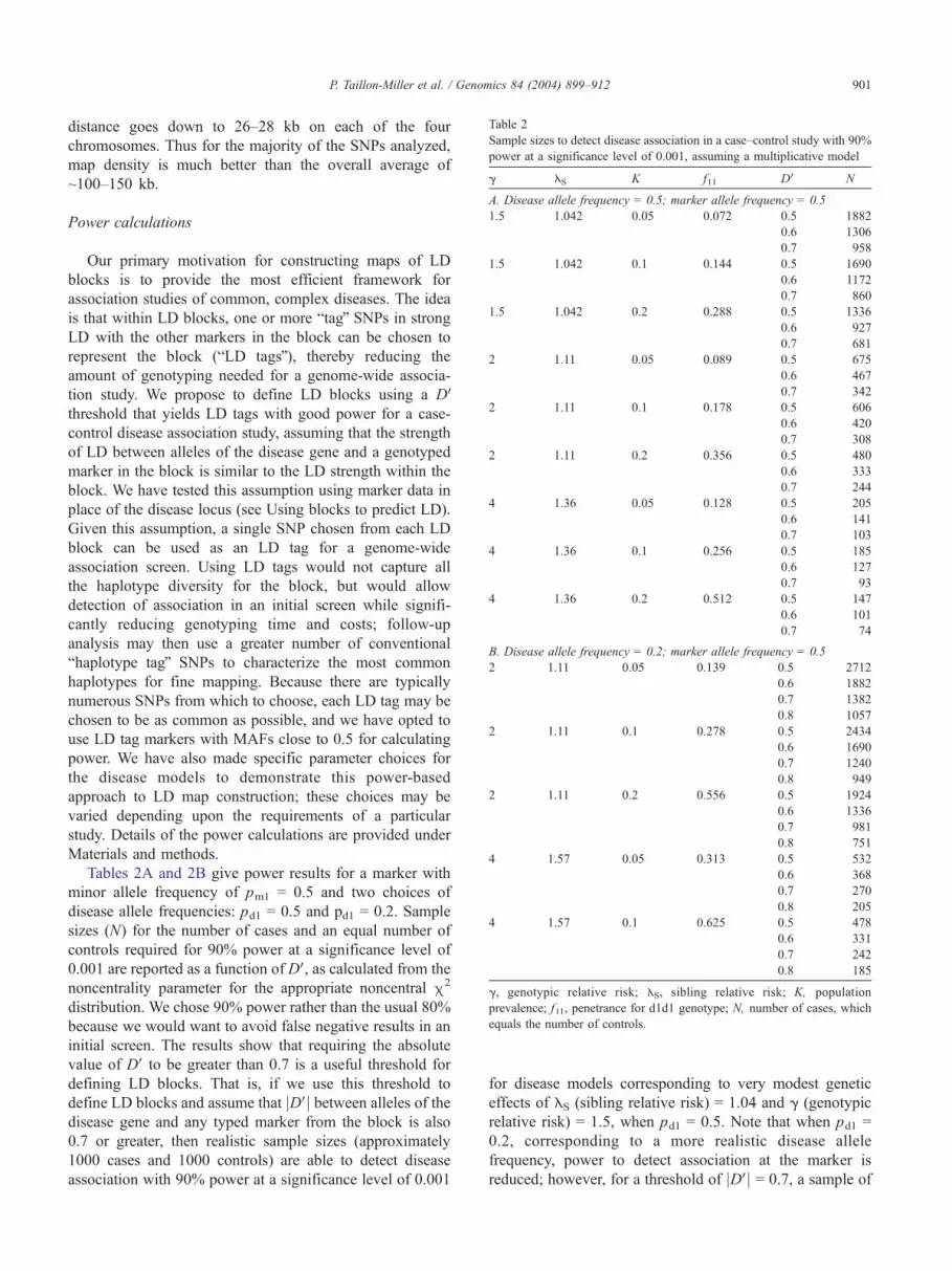
Table 2

Sample sizes to detect disease association in a case–control study with 90%

power at a significance level of 0.001, assuming a multiplicative model

g ES K f11 DV N

A. Disease allele frequency = 0.5; marker allele frequency = 0.5

1.5 1.042 0.05 0.072 0.5 1882

0.6 1306

0.7 958

1.5 1.042 0.1 0.144 0.5 1690

0.6 1172

0.7 860

1.5 1.042 0.2 0.288 0.5 1336

0.6 927

0.7 681

2 1.11 0.05 0.089 0.5 675

0.6 467

0.7 342

2 1.11 0.1 0.178 0.5 606

0.6 420

0.7 308

2 1.11 0.2 0.356 0.5 480

0.6 333

0.7 244

4 1.36 0.05 0.128 0.5 205

0.6 141

0.7 103

4 1.36 0.1 0.256 0.5 185

0.6 127

0.7 93

4 1.36 0.2 0.512 0.5 147

0.6 101

0.7 74

B. Disease allele frequency = 0.2; marker allele frequency = 0.5

2 1.11 0.05 0.139 0.5 2712

0.6 1882

0.7 1382

0.8 1057

2 1.11 0.1 0.278 0.5 2434

0.6 1690

0.7 1240

0.8 949

2 1.11 0.2 0.556 0.5 1924

0.6 1336

0.7 981

0.8 751

4 1.57 0.05 0.313 0.5 532

0.6 368

0.7 270

0.8 205

4 1.57 0.1 0.625 0.5 478

0.6 331

0.7 242

0.8 185

g, genotypic relative risk; ES, sibling relative risk; K, population

prevalence; f11, penetrance for d1d1 genotype; N, number of cases, which

equals the number of controls.

P. Taillon-Miller et al. / Genomics 84 (2004) 899–912 901

distance goes down to 26–28 kb on each of the four

chromosomes. Thus for the majority of the SNPs analyzed,

map density is much better than the overall average of

~100–150 kb.

Power calculations

Our primary motivation for constructing maps of LD

blocks is to provide the most efficient framework for

association studies of common, complex diseases. The idea

is that within LD blocks, one or more btagQ SNPs in strong

LD with the other markers in the block can be chosen to

represent the block (bLD tagsQ), thereby reducing the

amount of genotyping needed for a genome-wide associa-

tion study. We propose to define LD blocks using a DVthreshold that yields LD tags with good power for a case-

control disease association study, assuming that the strength

of LD between alleles of the disease gene and a genotyped

marker in the block is similar to the LD strength within the

block. We have tested this assumption using marker data in

place of the disease locus (see Using blocks to predict LD).

Given this assumption, a single SNP chosen from each LD

block can be used as an LD tag for a genome-wide

association screen. Using LD tags would not capture all

the haplotype diversity for the block, but would allow

detection of association in an initial screen while signifi-

cantly reducing genotyping time and costs; follow-up

analysis may then use a greater number of conventional

bhaplotype tagQ SNPs to characterize the most common

haplotypes for fine mapping. Because there are typically

numerous SNPs from which to choose, each LD tag may be

chosen to be as common as possible, and we have opted to

use LD tag markers with MAFs close to 0.5 for calculating

power. We have also made specific parameter choices for

the disease models to demonstrate this power-based

approach to LD map construction; these choices may be

varied depending upon the requirements of a particular

study. Details of the power calculations are provided under

Materials and methods.

Tables 2A and 2B give power results for a marker with

minor allele frequency of pm1 = 0.5 and two choices of

disease allele frequencies: pd1 = 0.5 and pd1 = 0.2. Sample

sizes (N) for the number of cases and an equal number of

controls required for 90% power at a significance level of

0.001 are reported as a function of DV, as calculated from the

noncentrality parameter for the appropriate noncentral m2

distribution. We chose 90% power rather than the usual 80%

because we would want to avoid false negative results in an

initial screen. The results show that requiring the absolute

value of DV to be greater than 0.7 is a useful threshold for

defining LD blocks. That is, if we use this threshold to

define LD blocks and assume that jDVj between alleles of thedisease gene and any typed marker from the block is also

0.7 or greater, then realistic sample sizes (approximately

1000 cases and 1000 controls) are able to detect disease

association with 90% power at a significance level of 0.001

for disease models corresponding to very modest genetic

effects of ES (sibling relative risk) = 1.04 and g (genotypic

relative risk) = 1.5, when pd1 = 0.5. Note that when pd1 =

0.2, corresponding to a more realistic disease allele

frequency, power to detect association at the marker is

reduced; however, for a threshold of jDVj = 0.7, a sample of


approximately 1000 cases and 1000 controls still gives 90%

power at a significance level of 0.001 for disease models

corresponding to a slightly larger sibling relative risk of 1.11

and g = 2.

Needless to say, for disease genes with stronger genetic

effects, smaller sample sizes are sufficient; alternatively,

larger sample sizes will yield comparable power even if

smaller thresholds for jDVj are chosen (cf. the table entries

for g = 4). Additional power calculations indicate that with a

threshold of jDVj = 0.7, reasonable power to detect genetic

effects for a common disease is maintained for small

departures of the marker allele frequency from 0.5. For

example, consider a disease with prevalence of 0.2 and g

ranging from 2 to 3. If pm1 = 0.4 and pd1 = 0.2, and

considering both possible phases of co-occurrence of the

alleles, the range of sample sizes runs from N = 229 to N =

1451. If the prevalence is lowered to 0.1, sample sizes are

still under 2000 cases and 2000 controls. Thus as long as

LD block tags can be chosen to have allele frequency close

to 0.5, reasonable power is maintained.

We therefore chose a jDVj threshold of 0.7 to define our

primary blocks, described below, to maximize the LD block

size while minimizing the sample size needed for a useful

range of disease models. We also report LD block results for

jDVj thresholds of 0.6, 0.8, 0.9, and 1.0.

Linkage disequilibrium blocks

We define a linkage disequilibrium block to be a

consecutive set of at least three markers along with a

threshold T and a disequilibrium coefficient L (DV or r2)

such that all pairs of markers in the block satisfy jLj z T. By

a weak linkage disequilibrium block we mean a set of at

least three consecutive markers along with three parameters

Tl, Tu, and F and a disequilibrium coefficient L such that all

pairs of markers in the block satisfy jLj z Tl (the lower

threshold) and at least F% of the pairs of markers satisfy

jLj z Tu (the upper threshold). Guided by our power

analyses, we will focus on LD blocks constructed using a

threshold T = 0.7. Although our power calculations were

based on DV, they may be reformulated to correspond to r2

levels via the formula r ¼ Dffiffiffiffiffiffiffiffiffiffiffiffiffip1p2q1q2

p .

Tables 3A and 3B contain summary statistics for the

average and maximum number of the LD blocks as well

as the average and maximum size of the blocks on each

chromosome as found by our algorithm for the coefficients

DV and r2, respectively. To indicate the extent of these

blocks, Table 3 also gives the percentage of the total

number of SNP markers that fall within blocks, and also

statistics Rmax, Rhap, and bcoverage,Q defined as follows.

From the point of view of reducing genotyping, the best

case scenario would be when a single SNP can be chosen

to represent each LD block; note that for SNPs not lying

within any block, no breductionQ takes place and each

such SNP must still be included in the genotyping. The

original number of SNPs is then reduced by a percentage

we call Rmax. For our chromosome X data, if there exists

a subset of SNPs in a block that determines all possible

haplotypes observed, we may choose to use this subset to

represent the block. We then obtain a set of SNPs

consisting of these representatives for every block together

with all SNPs not in blocks, and the original number of

SNPs is then reduced by a percentage we call Rhap. An

example of an LD block with significant haplotype

reduction is given in Fig. 1, in which all the haplotypes

found in the males we genotyped are unambiguously

defined by only 3 SNPs in an LD block consisting of 13

SNPs. We define the coverage to be the percentage of the

chromosome covered by blocks while ignoring gaps

greater than 100 kb. This definition allows us to account

for variable spacing of markers and focus on the parts of

the chromosomes that are most densely covered by our

SNP map. See Fig. 2 for a graph of the coverage by DVthreshold. Additional details on coverage are provided

under Materials and methods.

Chromosomal coverage

At the jDVj threshold of 0.7 the autosomes exhibit block

coverage of roughly 25%, while the coverage on the X

chromosome is substantially higher at 43%. Our definition

of coverage is in fact conservative compared to the

percentage of markers that occur within blocks, as the

latter measure is uniformly higher than our measure of

coverage (Table 3). While the percentage of markers in

blocks does not account for the variable spacing of our

SNP markers, it still provides a useful measure and reveals

that blocks are extensive across the chromosomes in these

data. With a jDVj threshold of 0.7, roughly 40% of

autosomal SNPs and 60% of chromosome X SNPs fall

within blocks. A graphical representation of the LD block

structure of all four chromosomes is given in Fig. 3. It is

clear from this figure that LD blocks are found across the

entire length of all four chromosomes and in some cases

can be extensive. The markers included in each LD block

are in Supplemental Table S5.

The reduction (Rmax) in the total number of SNPs,

obtained by taking one tag SNP per block while still

including every SNP that does not lie in a block, is

approximately 29% on the autosomes and 44% on X.

Hence, in theory, we can genotype just 71% of our markers

and still retain a significant amount of power in a genome-

wide association screen. On the X chromosome, only 53%

of the SNPs have to be genotyped in a genome-wide

association study instead of 73% of the SNPs needed to

define all the common haplotypes (e.g., for a threshold of

0.7, Rmax = 47% versus Rhap = 27%).

Overall, the coverage results were similar for the

autosomes while the coverage on chromosome X was

nearly twice as much. Indeed, even when we require that

jDVj = 1 the coverage on X is still 22%; roughly three times

that of the autosomes (Fig. 2). These observations confirm

Table 3

|DV| threshold Number

of blocks

Mean size of

blocks (SNPs)

Max size

(SNPs)

Mean

width (kb)

Max

width (kb)

% of markers

within blocks

Rmax

(%)

Rhap

(%)

Coverage

(%)

A. LD blocks using DV

Chromosome X

0.6 148 4.9 14 129.3 2410 60.65 48.3 21.6 47.4

0.7 145 4.7 13 104.7 987 56.47 44.4 20.5 43.2

0.8 137 4.5 13 91.2 987 51.13 39.7 19.9 36.5

0.9 124 4.3 13 76.3 689 44.11 33.8 18.2 28.4

1 107 4.1 12 67 689 36.51 27.6 16 21.7

Chromosome 5

0.6 111 4.3 15 92.6 536 40.49 31.1 - 28.4

0.7 106 4.3 13 82.3 536 38.13 29.2 - 25.4

0.8 101 4.1 11 69 536 34.51 26 - 22.1

0.9 87 3.8 11 47 323 28.11 20.8 - 15.8

1 64 3.5 7 26.8 171 18.69 13.3 - 6.5

Chromosome 7

0.6 158 4.1 10 79.3 636 43.61 32.9 - 27.1

0.7 149 4 11 74.1 471 40.48 30.3 - 23.4

0.8 138 3.9 10 63.5 446 36.67 27.3 - 19.9

0.9 115 3.8 11 51.7 446 30.07 22.2 - 14.9

1 76 3.4 10 40.3 446 17.76 12.6 - 8.3

Chromosome 17

0.6 58 3.9 6 71.8 426 40.91 30.4 - 29.9

0.7 53 3.8 6 90.8 963 36.55 26.9 - 26.9

0.8 45 3.6 6 52.6 339 29.45 21.3 - 19.1

0.9 39 3.5 6 47.7 339 24.73 17.6 - 15.8

1 25 3.2 4 18 74 14.36 9.8 - 5

B. LD blocks using r2

Chromosome X

0.6 98 4.2 13 73.3 700 34.5 26.3 16 21.4

0.7 91 4.1 13 72.4 689 31.08 23.5 14.9 19.3

0.8 71 4.2 11 76.5 689 24.64 18.7 13.2 15

0.9 61 3.9 9 56.3 527 19.8 14.7 11.8 10.6

1 39 3.5 8 36.2 169 11.53 8.3 8.3 5.4

Chromosome 5

0.6 61 3.9 10 59.9 525 19.78 14.7 - 11.7

0.7 52 3.6 10 46.4 366 15.91 11.5 - 8.6

0.8 39 3.6 8 42.8 366 11.7 8.4 - 5.7

0.9 28 3.2 4 28.8 222 7.58 5.2 - 3.2

1 7 3.1 4 23.1 67 1.85 1.3 - 0.8

Chromosome 7

0.6 76 3.5 8 49.6 357 17.96 12.8 - 8.6

0.7 63 3.3 6 35.1 189 14.35 10.1 - 6.7

0.8 46 3.3 6 29 189 10.41 7.3 - 3.8

0.9 33 3.2 6 17 62 7.07 4.8 - 1.8

1 8 3.2 4 7.1 20 1.7 1.2 - 0.2

Chromosome 17

0.6 28 3.2 4 38.1 163 16.18 11.1 - 10.7

0.7 23 3.2 4 39.3 163 13.45 9.3 - 8.9

0.8 15 3.2 4 24.7 148 8.73 6 - 3

0.9 11 3.2 4 24.8 148 6.55 4.6 - 1.9

1 5 3.2 4 8.8 21 2.91 2 - 0.4

Rmax is the reduction, expressed as a percentage, in the total number of markers if one SNP from each block is selected and all remaining SNPs not in blocks are

also selected. Rhap is the reduction if SNPs are selected on the basis of complete haplotype determination within blocks. The coverage is the percentage of the

chromosome covered by blocks if gaps larger than 100 kb are ignored.


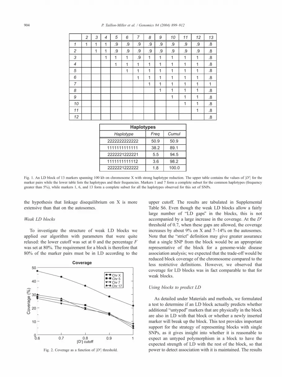
Fig. 1. An LD block of 13 markers spanning 100 kb on chromosome X with strong haplotype reduction. The upper table contains the values of jDVj for themarker pairs while the lower table lists the haplotypes and their frequencies. Markers 1 and 7 form a complete subset for the common haplotypes (frequency

greater than 5%), while markers 1, 6, and 13 form a complete subset for all the haplotypes observed for this set of SNPs.


the hypothesis that linkage disequilibrium on X is more

extensive than that on the autosomes.

Weak LD blocks

To investigate the structure of weak LD blocks we

applied our algorithm with parameters that were quite

relaxed: the lower cutoff was set at 0 and the percentage F

was set at 80%. The requirement for a block is therefore that

80% of the marker pairs must be in LD according to the

Fig. 2. Coverage as a function of jDVj threshold.

upper cutoff. The results are tabulated in Supplemental

Table S6. Even though the weak LD blocks allow a fairly

large number of bLD gapsQ in the blocks, this is not

accompanied by a large increase in the coverage. At the DVthreshold of 0.7, when these gaps are allowed, the coverage

increases by about 9% on X and 7–14% on the autosomes.

Note that the bstrictQ definition may give greater assurance

that a single SNP from the block would be an appropriate

representative of the block for a genome-wide disease

association analysis; we expected that the trade-off would be

reduced block coverage of the chromosome compared to the

less restrictive definitions. However, we observed that

coverage for LD blocks was in fact comparable to that for

weak blocks.

Using blocks to predict LD

As detailed under Materials and methods, we formulated

a test to determine if an LD block actually predicts whether

additional buntypedQ markers that are physically in the block

are also in LD with that block or whether a newly inserted

marker will break up the block. This test provides important

support for the strategy of representing blocks with single

SNPs, as it gives insight into whether it is reasonable to

expect an untyped polymorphism in a block to have the

expected strength of LD with the rest of the block, so that

power to detect association with it is maintained. The results

Fig. 3. A blue diamond indicates the location and size of each LD block. The scale of the size of the LD block is located on the left y axis. The location on the

chromosome in kilobases is on the x axis. At the bottom of each graph represented by a black square is the location of each marker with a minor allele

frequency N20%. A red circle indicates the number of markers in each LD block with the scale on the right x axis. For the markers included in each LD block

and their locations on the chromosome please refer to Table S5 in the supplemental materials.


Table 4

Results of test to determine if LD blocks predict LD

T1 T2 p

X 5 7 17

0.7 0.7 96.1 94.1 94.3 92.8

0.8 0.7 98.2 97.1 96.1 91.9

0.8 0.8 96.7 95.5 94.1 86.2

T1, the jDVj threshold for all pairs in the computed block of SNPs, A1, . . .,

An; T2, the jDVj threshold required for pairings with the additional SNP, B;

p, the empirical conditional probability that each pairing of B with Ai

satisfies jDVj z T2.


of our test are summarized in Table 4. We see that indeed,

LD blocks are excellent predictors of the strength of LD

with other SNPs in our data. For example, on chromosome

5, if a collection of markers A1, A2, . . ., An is an LD block

with jDVj z 0.8 (the first threshold T1), then any other

marker B that is physically in this block will be, with 97.1%

certainty, in LD with A1, A2, . . ., An with jDVj z 0.7 (the

second threshold T2).

Discussion

The results of our study show that regions of strong LD

are commonly found on both autosomes and the X

chromosome with the X more extensively covered by

longer LD blocks. In fact, blocks of strong LD are easily

found with high-level SNP maps on chromosomes 5, 7,

17, and X consisting of common SNPs at ~100 kb density.

Power calculations predict that these LD blocks can be

represented by LD tag SNPs in genome-wide association

studies to identify alleles associated with common diseases

within LD blocks. As the number of common genotyped

SNPs continues to increase, we will be able to cover the

genome with LD blocks. Our results further predict that

from an overall map of 30,000 to 50,000 SNPs with minor

allele frequencies of z20% in each of the major

populations in the world, a subset of LD tag SNPs will

be useful in the initial genome-wide scanning for common

disease alleles.

The common SNPs selected for our study were identified

prior to the completion of the human genome sequence and

the launching of the International HapMap Project. Large

gaps therefore were found between contigs and the coverage

of common SNPs was incomplete. Despite these limitations,

LD blocks, defined by the DVstatistic, covered about 25% of

the autosomes and 40% of chromosome X where there was

sufficient SNP density. On average the blocks spanned

about 80 kb on the autosomes and 100 kb on X.

We designed an algorithm that reveals a block structure

whose usefulness is measured both by sharp reduction of the

number of SNPs needed in a genetic association study and

by the extent to which the LD blocks cover a chromosome.

In addition, our block definitions have the advantage of

being linked directly to the goal of using LD blocks to aid

disease association studies. As the motivation for our block

definitions differs from other important motivations such as

representation of haplotypes or study of possible evolu-

tionary models, the resulting block characteristics may differ

from those of other studies without detracting from our

conclusions. Our use of power calculations to guide block

definitions directly does rely on the assumption that the

strength of LD among the markers in the block is similar to

that of the LD that would be observed between those

markers and a disease gene if the disease gene occurred in

the block, but was untyped. We tested this assumption

directly within our data using genotyped markers in place of

the disease gene and found that for jDVj thresholds of 0.7 to

0.8, if an additional marker physically within an existing LD

block was introduced, it would satisfy the same jDVjthreshold with every block marker in the great majority of

cases. Note also that when this assumption is satisfied,

selecting a single LD tag SNP to represent the block, rather

than the more conventional approach of representing all

common haplotypes with a group of tag SNPs, may be

sufficient to detect a disease association in an initial screen,

provided appropriate parameters are chosen for the power

calculations. Further investigations that will use dense

marker data to help determine the most appropriate

strategies for SNP reduction are under way.

The above findings about the predictive ability of these

LD blocks are also consistent with our observations about

weak LD blocks. LD structure is complex and it is well

known that runs of SNPs in LD can be interrupted by SNPs

not in LD with the others [12,13]. To test this effect, we also

studied weak LD blocks, which allowed LD gaps within

blocks. Interestingly, we found that although the weak

definition would be expected to allow for larger blocks

encompassing more of the chromosome, in fact chromoso-

mal coverage increased only minimally.

The power analyses reported here considered only certain

disease models and thus should be viewed as only a guide to

selecting LD thresholds for block definition. We chose

marker allele frequencies of 0.5 for simplicity to illustrate

our approach; however, it is important to note that power is

affected by the frequency of the marker allele that tends to

co-occur with the disease allele as others have pointed out as

well [15,16]. Our overall approach provides a template

strategy to define LD blocks and prioritize SNPs for a given

disease association study; appropriate disease models and

the desired level of power may be chosen depending on the

particular study. Our report has focused on LD blocks for DVthresholds of 0.7 and above since these thresholds corre-

spond to power to detect common disease genes of modest

effect for the selected models. However, for disease genes of

stronger effects, smaller sample sizes or reduced jDVjthresholds (and therefore LD blocks having greater chro-

mosomal coverage) can yield sufficient power (Table 2).

Thus a given association genome screen can be designed

according to whether a project wishes to constrain recruiting

costs or genotyping costs.


Our hierarchical association mapping strategy is geared

toward detection of common disease alleles. The debate

about the bcommon disease, common geneQ hypothesis is

important and may be resolved by further study and

successful identification of such genes. Larger sample sizes,

stronger LD thresholds, or alternative strategies may be

necessary to allow the approach proposed here to move

beyond detecting common susceptibility alleles. Never-

theless, for detecting common alleles, a hierarchical

approach using an initial reduced-density SNP map offers

an efficient and economical alternative to large-scale

genotype studies.

In the initial phase of genetic association studies, it is

important to identify regions of the human genome

associated with a disease quickly and cost effectively.

Equally important is the ability to exclude large regions of

the genome not associated with the disease alleles. If N is

the number of individuals, M the number of markers being

genotyped, Cg the cost of genotyping a single marker for a

single individual, and CT the total cost, then CT = NMCg. N

is determined by our power calculations and M is

determined by the block structure for a given DV cutoff.Although our maps are not populated with enough SNPs to

determine M accurately, efforts such as the International

HapMap Project [1] are providing genotyping data for an

extremely dense set of SNPs across the genome. An

important next step for our approach will be to apply it to

these data to construct high-level, reduced-density associa-

tion screen maps, which can be compared to the full-density

data. Our present results strongly suggest that for the initial

genome-wide association studies of common disease,

screening maps of common SNPs at a modest density can

maintain power to detect disease association while reducing

genotyping costs compared to the approach of constructing

haplotype maps to define the common haplotypes.

Materials and methods

SNP markers

All SNPs used in this study had known frequencies,

mapped to a unique location according to the dbSNP map

(build 112), and met our criteria for primer design

(discussed below).

All SNP markers were selected from public databases or

selected and characterized for allele frequencies by our

group. They were then submitted to the SNP Consortium

(TSC) and dbSNP databases (dbSNP, http://www.ncbi.nlm.

nih.gov/SNP/; TSC, http://snp.cshl.org/).

SNPs with allele frequencies from 10 to 90% in all three

population samples of 42 individuals each (European

American, African American, and Asian American-bTheTSC setQ) were selected for genotyping. We also included a

small number of SNPs in which the allele frequencies were

between 10 and 90% in two of the three samples but the

information was not available for the third sample. In a

small number of cases from dbSNP, if the frequencies from

an equivalent set of samples met the criteria the SNP was

included.

We tracked the progress of this field by first discovering

SNPs, then characterizing SNPs, and finally taking advant-

age of the wealth of characterized SNPs available in the

public databases. We used a top-down hierarchical approach

to covering the chromosome with SNPs. SNPs were picked

across the chromosome at specific intervals without regard

for gene densities or gene locations. The first pick was

characterizing for frequency of one SNP every 25 kb across

the entire human genome with the SNPs and maps available

at that time. The SNPs with the desired frequencies were

then funneled into the genotyping project for chromosomes

X and 7. A second pick for characterization was done for

both chromosomes X and 7 at 10 kb, and chromosome X

went through a third round of characterizing SNPs at 5-kb

intervals. We also picked SNPs for chromosomes X and 7

from public databases when more characterized SNPs

became available. This study began with chromosomes X

and 7 and then later expanded to 20% of the genome with

the addition of chromosomes 5 and 17. Chromosome 5 and

17 SNPs were picked entirely from public databases that

included our own submissions. A list of the SNPs used in

this study is in supplemental Tables S1a–S1d.

SNP marker quality

All 5344 SNP assays used in this study (supplemental

Tables S1a-S1d) had a sample genotyping success rate

greater than 80%. Chromosome 7 had the best chromosome

coverage with 1753 SNPs for an average intermarker

distance of 89 kb and chromosome 5 had the least coverage

with 1442 markers and an average consecutive intermarker

distance of 125 kb. A breakdown of the number of SNPs at

10 and 20% MAF and 20% with intermarker distances b100

kb is shown in Table 1.

Fig. 4A shows the distribution of the MAF and Fig. 4B

shows the observed heterozygosity for all the SNP markers

used in this study. SNPs for this study were picked to have

a MAF of 10–50%. Although individual SNPs could have

different genotype frequencies from the predicted frequen-

cies, N95% of the SNP assays had a MAF N10% after

genotyping and N80% of the SNPs had a MAF N20% after

genotyping (Table 1). The estimate of heterozygosity

provided by dbSNP was also a good predictor of the

SNP frequency and was on average within 5% for each

bin. Between 5 and 6% of all SNPs genotyped had

heterozygosities less than 0.2 with the remaining 94–95%

being N0.2.

The distance from one SNP marker to the next is shown

in Fig. 4C. Approximately 50% of the markers are closer

than 25 kb and 70–80% of the markers are closer than 100

kb. The inset bar graph shows the 0–25,000 bp range. All

distances used were from dbSNP, build 112.

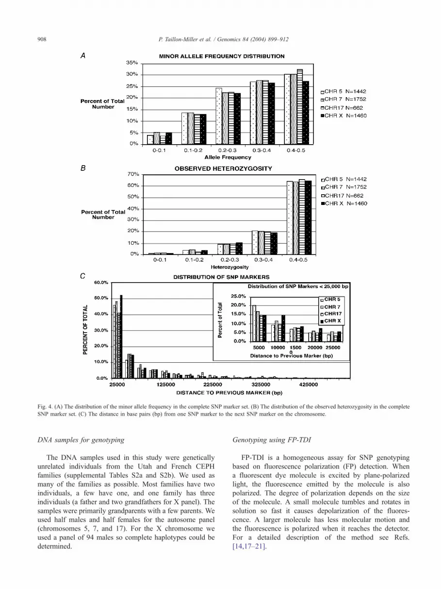
http:\\www.ncbi.nlm.nih.gov\SNP\%3B%20TSC

http:\\snp.cshl.org\

Fig. 4. (A) The distribution of the minor allele frequency in the complete SNP marker set. (B) The distribution of the observed heterozygosity in the complete

SNP marker set. (C) The distance in base pairs (bp) from one SNP marker to the next SNP marker on the chromosome.


DNA samples for genotyping

The DNA samples used in this study were genetically

unrelated individuals from the Utah and French CEPH

families (supplemental Tables S2a and S2b). We used as

many of the families as possible. Most families have two

individuals, a few have one, and one family has three

individuals (a father and two grandfathers for X panel). The

samples were primarily grandparents with a few parents. We

used half males and half females for the autosome panel

(chromosomes 5, 7, and 17). For the X chromosome we

used a panel of 94 males so complete haplotypes could be

determined.

Genotyping using FP-TDI

FP-TDI is a homogeneous assay for SNP genotyping

based on fluorescence polarization (FP) detection. When

a fluorescent dye molecule is excited by plane-polarized

light, the fluorescence emitted by the molecule is also

polarized. The degree of polarization depends on the size

of the molecule. A small molecule tumbles and rotates in

solution so fast it causes depolarization of the fluores-

cence. A larger molecule has less molecular motion and

the fluorescence is polarized when it reaches the detector.

For a detailed description of the method see Refs.

[14,17–21].


The FP-TDI assay requires three unlabeled oligonu-

cleotides for each SNP. Two serve as PCR primers and

the third is a SNP probe that is complementary to the

template sequence with its 3V end annealed to the target

one base before the polymorphic site. The entire reaction

is done in one reaction tube without separation or

purification.

Because of this simplicity the FP-TDI assay is

extremely flexible and can be adapted to any number of

assays and to all levels of throughput. To meet the needs

of the project outlined here we increased our throughput to

a level that was capable of producing 4 million genotypes/

year. This was accomplished by creating a modular

approach to genotyping. Each equipment portion of the

module consisted of a Perkin-Elmer (Boston, MA, USA)

Evolution P3 liquid handling machine with a b96 well-

head,Q 24 384-well thermocycler blocks, one Perkin-Elmer

fluorescence polarization 384-well plate reader, and two

low-speed centrifuges with deep well buckets. With

efficient use of time and equipment up to two runs of

24 � 384 samples or 18,432 genotypes can be accom-

plished in a 10-h day with three people working staggered

schedules.

Genotyping procedure

All pipetting steps were done by hand with a Rainin

electronic multichannel pipettor, the Perkin-Elmer Apricot

personnel pipettor, the Robbins Hydra, or preferably with

the Perkin-Elmer Evolution P3 depending on the stage of

the project.

All PCRs and SNP detection reactions were designed

for standard melting temperature (Tm) and used standard

cycling conditions. The two PCR primers and the one SNP

detection primer were ordered arrayed in a 96-well tray at

a standard concentration for ease of handling. Primers were

ordered as 6 nmol lyophilized in a 96-well plate and then

150 Al water was added to each well to make a 40 AMstock solution.

We also prepared in advance the DNA template. To make

dried DNA plates 3 Al (0.8 ng/Al) of DNA from a 96-well

DNA plate was dispensed to all four quadrants of 384-well

black plates with the Perkin–Elmer Evolution P3 using a 96-

tip head. The plates were spun down and air-dried at room

temperature overnight. The plates were stacked and wrap-

ped with plastic film and kept desiccated at room tempe-

rature until needed. One allele combination per day was

genotyped whenever possible.

PCR

Volumes are for one reaction. Samples contained

genomic DNA dried previously, 0.5 Al 10� PCR buffer

(200 mM Tris-HCl (pH 8.4) and 500 mM KCl), 0.25 AlMgCl2 (50 mM), 0.1 Al dNTPs (2.5 mM), 0.02 Al any Hot

Start Taq (5 U/Al), 2.13 Al water, final volume 3.0 Al. Then 3Al of primers (40 AM) was added.

PCR thermocycling program

The cycling program was 1 cycle of 958C for 2 min; 35

cycles of 928C for 10 s, 588C for 20 s, 688C for 30 s; and 1

cycle of 688C for 10 min. The temperature of the

thermocycler was reduced to 48C until samples were

removed for the next step.

SNP detection reactions

For remaining the steps we used the AcycloPrime-FP

SNP Detection System Kit (Perkin–Elmer Life Sciences).

EXO-SAP reaction to remove excess primers and

unincorporated dNTPs

The 10� PCR clean-up reagent was diluted with PCR

clean-up buffer provided by the kit. Of this, 2 Al was addedto each well, and the plates was spun down.

EXO-SAP cycling program

The cycling program was 378C for 60 min, 808C for 15

min, and the temperature of the thermocycler was reduced to

48C until samples were removed for the next step.

TDI reaction mix for SNP detection

For one reaction, the volumes were 2.0 Al 10� buffer,

0.05 Al AcycloPol, 1.0 Al terminator mix, and 4.95 Al water,for a total volume of 8.00 Al.

Pipetting steps for TDI (SNP detection)

Five microliters of 1 AM SNP primers was dispensed into

the relevant quadrants of a 384-well plate, and the plate was

spun down. Eight microliters of TDI mix was dispensed into

the plate, and again the plate was spun down.

TDI cycling program

The cycling program was 1 cycle of 958C for 2 min and

10–40 cycles of 958C for 15 s, 558C for 30 s (20 cycles are

standard). The temperature of the thermocycler was reduced

to 48C until samples were removed for the next step.

Reading plates

To read the plates, they were spun down and stacked in

the Perkin-Elmer Victor or Perkin-Elmer EnVision stacker.

Plates were read for both dyes. Analysis of the data was

accomplished with the Excel Macro software provided by

the manufacturer. Data were then saved as a tab-delimited

text document that could be imported into the linkage

disequilibrium analysis software. Our lab currently uses the

SNPScorer software, which outputs results directly into a

database.

Primer design for FP-TDI

To achieve the high throughput needed for this project

all primers were designed with a strict criterion for Tm

and all reactions were run under a single set of

parameters.


PCR primer design

PCR primers were designed using Primer3, release 0.9

(with code available at http://www.genome.wi.mit.edu/

genome_software/other/primer3.html Ref. [22]) using the

parameters previously described [23]. Minor changes for

this application follow: TARGET = SNP_Position-20 bases,

20 bases; PRIMER_OPT_TM = 55, PRIMER_MAX_TM =

56, PRIMER_MIN_TM = 54; PRIMER_PRODUCT_

SIZE_RANGE = 80–400; PRIMER_PRODUCT_OPT_

SIZE = 250.

SNP primer design

The shortest primer with a Tm of 50–558C and a minimum

length of 16 bp and a maximum length of 40 bp was picked

on both the forward and the reverse strand. The SNP primer

is complementary to the sequence and ends with the base

adjacent to the SNP site. The Allawi and Santa-Lucia nearest

neighbor sequence-dependent thermodynamic parameters

[24] were used to determine Tm.

If both a forward and a reverse SNP primer could be

chosen in the first step, one was selected by assigning

penalties to various types of repeated sequences. This

minimized failures due to repeated sequences near the SNP.

If the penalties were equal the shortest primer was chosen

because it was the least expensive. If there was no clear

preference the default was the forward primer. Sometimes

SNP primers could not be chosen because of the melting

temperature and length criteria. This could be due to extreme

GC content, a neighboring SNP within the potential primer

site, or a reported SNP that was not a single-base biallelic

polymorphism.

In our experience, FP-TDI assays can be developed for

all SNPs found in unique sequence. Because of the stringent

design of our PCR conditions, 95% of them are successful

[25] and 80% of the FP-TDI genotyping assays work the

first time. Sixty percent of the failed assays work when

repeated with the SNP primer from the other strand, which

gives a final assay success rate of N90%. Our genotyping

error rate is b0.02%.

We periodically develop FP-TDI genotyping assays for

all uniquely mapped SNPs found in public databases. These

assays and the expanded protocols for the methods outlined

above are available at http://snp.wustl.edu.

Linkage disequilibrium analysis

Pair-wise linkage disequilibrium was computed for all

possible two-way comparisons of SNPs, with significance

levels determined by them2 statistic for the corresponding 2�2 table (1 degree of freedom). Haplotype frequencies for

autosomes were estimated using the E-M algorithm of

Excoffier and Slatkin [26] as implemented for pairs of

markers in the LDMAX program of the GOLD software

package [27]. For the X chromosome, haplotypes were

directly observable. SAS (SAS Institute, Cary, NC, USA)

together with LDMAX was used to compute m2 statistics and

linkage disequilibrium measures D, DV, and r2, defined as

follows. For two loci L1 and L2, each with two alleles 1 and 2,

let pi be the frequency of allele 1 and qi = 1 � pi be the

frequency of allele 2, at locus i (i = 1, 2). Assume pi V qi, that

is, allele 1 is the minor allele. Let pjk be the frequency of the

jk haplotype. The coefficient of disequilibrium is D = p11 �p1p2. The labeling of the alleles may affect the sign of D but

not its absolute value. The normalized disequilibrium

coefficient is obtained by dividing D by its maximum

possible (absolute) value given p1 and p2: DV= D/|D|max,

where |D|max = max ( p1p2, q1q2) if D b 0 and |D|max =

min ( q1p2, p1q2) if D N 0. The correlation coefficient

is r ¼ D=ffiffiffiffiffiffiffiffiffiffiffiffiffiffiffiffiffiffip1q1p2q2

p(if we define the random variable Xi on

individuals to be 1 if the individual has allele 1 at loci i and

0 otherwise, then D = cov(X1,X2) and var(Xi) = piqi so r is

the usual correlation coefficient of these two random

variables). SNP heterozygosities were computed. Hetero-

zygosity for a biallelic marker with allele frequencies p and

q = 1 � p is given by H = 1 � p2 � q2 = 2p(1 � p).

Power calculations and linkage disequilibrium blocks

We chose to define LD blocks using threshold values for

DVthat correspond to good power for a case-control disease

association study of realistic sample size. The assumption is

that the strength of LD between alleles of the disease gene

and a genotyped marker in the block is similar to the LD

strength within the block. For such a case-control study, the

Pearson m2 test statistic for a 2 � 2 contingency table may

be used to test for allelic association. To calculate the

expected power for particular values of DV, we assumed a

range of disease models specified by disease gene frequen-

cies at a biallelic disease gene and penetrances for the three

genotype classes. To aid interpretation, we also parame-

terized each model in terms of the population prevalence (K)

of the disease, the disease gene frequency, and two of the

three penetrances. We considered both multiplicative

models and more general models, but will focus on the

multiplicative models here. Hence we assume that if d1 is

the disease allele, the penetrances for the genotype classes

are fd1d2 = g fd2d2 and fd1d1 = g2 fd2d2, where g is the

bgenotypic relative risk.Q For each multiplicative model we

computed the corresponding sibling relative risk (ES) usingcorrected formulas derived as in Risch and Merikangas [2].

We assumed marker allele frequencies to be 0.5 and

considered two cases for disease allele frequency pd1: pd1 =

0.5 (which would result in the maximum power for this

marker allele frequency) and pd1 = 0.2, corresponding to a

more realistic, common disease allele frequency. While

these are specific choices and of course do not represent the

full range of scenarios that may occur in an actual disease

association study, they provide a reasonable setting to guide

our LD block definitions. We propose this overall approach

as a general strategy for defining LD blocks for disease

http:\\www.genome.wi.mit.edu\genome_software\other\primer3.html

http:\\snp.wustl.edu


association studies; the range of models and desired power

level may then be chosen depending on the specific study.

The power calculations rely on determining the expected

marker allele frequencies in cases versus controls given a

particular disease model (penetrances), disease and marker

allele frequencies, andDVvalue (which determines haplotype

frequencies). Sham [28] derives the necessary formulas for

case and control allele frequencies in terms of haplotype

frequencies (chapter 4, section 4.6). We then used noncentral

m2 distributions to calculate sample sizes to detect associ-

ation between disease and marker in a m2 test, with specified

power and significance level. That is, for a given significance

level a, asymptotically, the m2 statistic follows a m2

distribution with 1 df under the null hypothesis and follows

a noncentral m2 with 1 df under the alternative hypothesis.

The noncentrality parameter is given by the m2 statistic

computed with parameters taking on the values correspond-

ing to the alternative hypothesis and is proportional to the

sample size2. Weir [29] discusses further details of the use of

the noncentral m2 for power in an analogous context; the

Web-interface power calculator of Purcell et al. [30] also

uses the noncentral m2 in the same way as our calculations.

After useful DV threshold values were determined from

our power calculations, LD blocks were defined using all

SNPs having a minor allele frequency of 20% or greater.

Our primary LD blocks were defined by requiring all

marker pairs in a given block to have jDVj greater than or

equal to the chosen threshold. We also studied weak LD

blocks with less restrictive definitions described below.

Algorithms for finding linkage disequilibrium blocks

Our power calculations suggest the following strategy for

reducing the number of markers genotyped for an associ-

ation study. If jDVj z T for a pair of SNPs then select only

one of them for genotyping, where T is a threshold of LD

strength to be determined from the power calculations. If the

same level of LD existed between a given SNP and several

other SNPs, then one might select that single SNP to

represent the entire group. However, by requiring the more

stringent criterion that all pairs of markers within the group

satisfy the LD threshold T, we allow ourselves more choices

for tag SNP selection and also increase our confidence that a

chosen tag SNP is likely to be a good representative, not

2 The noncentrality parameter Enc for the noncentral m2 distribution

corresponding to the alternative hypothesis, computed from the appropriate

2 � 2 table, is

knc ¼ 2N

"P M1 j caseð Þ � P M1 j controlð Þð Þ2

P M1 j caseð Þ þ P M1 j controlð Þ

þ P M2 j caseð Þ � P M2 j controlð Þð Þ2

P M2 j caseð Þ þ P M2 j controlð Þ

#

where N is the number of cases, which equals the number of controls;

P(Mi j case) is the allele frequency of Mi in cases, and P(Mi j case) is theallele frequency of Mi in controls.

only for other markers in the block but also for potentially

untyped markers in the region of the block.

We therefore define a linkage disequilibrium block to be

a consecutive (relative to the map in use) set of at least three

markers along with a cutoff threshold T and a disequilibrium

coefficient L (DVor r2) such that all pairs of markers in the

block satisfy jLj z T. Furthermore, in the interest of relaxing

the threshold requirement potentially to increase chromoso-

mal coverage and reduce the number of tag SNPs required

for a genome screen, we also examine weak LD blocks. By

a weak linkage disequilibrium block we mean a set of at

least three consecutive markers along with three parameters

Tl, Tu, and F and a disequilibrium coefficient L such that all

pairs of markers in the block satisfy jLj z Tl (the lower

threshold), and least F% of the pairs of markers satisfy jLjzTu (the upper threshold).

Once a set of nonoverlapping LD blocks has been

determined we would like to know what proportion of the

chromosome is covered by LD blocks. We could divide the

sum of the widths of the blocks by the width of the

chromosome but this would be in some sense misleading

since the denominator includes blarge gapsQ such as the

centromere and gaps between contigs. Therefore, we omit

these regions and consider only that portion of the chromo-

some where the SNPs are suitably dense. More precisely,

define the densely covered region of the chromosome to be the

union of all the intervals between consecutive SNPs that are

within some distance W of each other. In other words, every

part of the densely covered region must lie between two SNPs

that are withinW.We then define the coverageC by taking the

intersection of blocks with the densely covered region and

divide the total size of this region by the size of the densely

covered region. In our analysis, we chose W to be 100 kb.

We have designed an algorithm that takes ordered

markers and produces a set of nonoverlapping blocks and

attempts to maximize the block coverage. This is consistent

with our goal of using blocks as a tool for reducing SNP

density while retaining power in an initial association

screen. We therefore wish block coverage to be as extensive

as possible to allow for maximum genotyping reduction

according to our strategy, but are not necessarily interested

in block size or blocks as indicators of haplotype diversity.

Beginning with the first marker and then proceeding, in

order, to the following markers, we find the largest block

containing each marker (these blocks may include markers

that either precede or follow the current marker). A block is

ignored if it is contained in the block previously discovered

by the algorithm. If a block overlaps with the previous block

but is not contained in it we consider the following four

options: (1) truncate the previous block by removing a

minimal number of markers so that it no longer overlaps

with the current block, (2) truncate the current block in the

same way, (3) discard the previous block, or (4) discard the

current block. The option that produces the greatest amount

of coverage is chosen, with ties yielding to the order of the

options.


When haplotypes are known we are interested in finding

subsets of SNPs that determine all observed haplotypes

within blocks. We call these complete subsets, and our

algorithm for finding them consists of testing all subsets of

size 1, 2, 3, and so on, and reporting the first complete

subset found. Since for the autosomes only the genotypes

are known, this algorithm is applied only to chromosome X.

Using blocks to predict LD

One of the applications of determining LD blocks is to

reduce the number of markers required for an association

study by selecting LD tag SNPs from the blocks. An

underlying assumption is that if the disease gene is physically

in the block then it can be expected to be in LDwith a tag SNP

from the block. We have designed a test to determine if LD

blocks work as predictors this way.

Suppose A1, A2, . . ., An are SNPs that form an LD block.

If B is an additional SNP that lies physically between A1 and

An we expect that B would be part of the block; that is, B is in

linkage disequilibrium with A1, A2, . . .., An. More precisely,

we assume that jDVj z T1 for each of pairs in the set A1, A2,

. . ., An. We then determine the empirical conditional

probability P that jDVj z T2, the lower cutoff, for each of

the pairings of B with A1, A2, . . ., An. If this probability is

high then we conclude that LD blocks are good predictors of

LD with additional markers in the region. In other words, if

we already have a block, then the block structure will most

likely be preserved after new markers are added to it. We use

two cutoffs to allow for some flexibility in our test.

Acknowledgment

Some of this work was supported by grants from the

National Institutes of Health: HG01720 (P.Y.K.), DA15129

(N.L.S.), and AA07580 (S.F.S.).

Appendix A. Supplementary data

Supplementary data for this article may be found on

ScienceDirect or at http://snp.wustl.edu/snp_research/

ld_blocks.

References

[1] The International HapMap Consortium, The International HapMap

project, Nature 426 (2003) 789.

[2] N. Risch, K. Merikangas, The future of genetic studies of complex

human diseases, Science 273 (1996) 1516–1517.

[3] P. Taillon-Miller, et al., Juxtaposed regions of extensive and minimal

linkage disequilibrium in human Xq25 and Xq28, Nat. Genet. 25

(2000) 324.

[4] M.J. Daly, J.D. Rioux, S.F. Schaffner, T.J. Hudson, E.S. Lander, High-

resolution haplotype structure in the human genome, Nat. Genet. 29

(2001) 229–232.

[5] D.E. Reich, et al., Linkage disequilibrium in the human genome,

Nature 411 (2001) 199–204.

[6] S.B. Gabriel, et al., The structure of haplotype blocks in the human

genome, Science 296 (2002) 2225–2229.

[7] N. Patil, et al., Blocks of limited haplotype diversity revealed by high-

resolution scanning of human chromosome 21, Science 294 (2001)

1719.

[8] E. Dawson, et al., A first-generation linkage disequilibrium map of

human chromosome 22, Nature 418 (2002) 544.

[9] M.S. Phillips, et al., Chromosome-wide distribution of haplotype

blocks and the role of recombination hot spots, Nat. Genet. 33 (2003)

382.

[10] K.G. Ardlie, L. Kruglyak, M. Seielstad, Patterns of linkage

disequilibrium in the human genome, Nat. Rev. Genet. 3 (2002)

299–309.

[11] A.G. Clark, et al., Linkage disequilibrium and inference of ancestral

recombination in 538 single-nucleotide polymorphism clusters across

the human genome, Am. J. Hum. Genet. 73 (2003) 285–300.

[12] C.S. Carlson, et al., Additional SNPs and linkage-disequilibrium

analyses are necessary for whole-genome association studies in

humans, Nat. Genet. 33 (2003) 518–521.

[13] D.C. Crawford, et al., Evidence for substantial fine-scale variation in

recombination rates across the human genome, Nat. Genet. 36 (2004)

700–706.

[14] T.M. Hsu, P.-Y. Kwok, Homogeneous Primer Extension Assay with

Fluorescence Polarization Detection, in Single Nucleotide Poly-

morphisms: Method And Protocols, Humana Press, Totowa, NJ,

2002, pp. 177–188.

[15] K.T. Zondervan, L.R. Cardon, The complex interplay among

factors that influence allelic association, Nat. Rev. Genet. 5 (2004)

89–100.

[16] R.M. Pfeiffer, M.H. Gail, Sample size calculations for population and

family-based case-control association studies on marker genotypes,

Genet. Epidemiol. 25 (2003) 136–148.

[17] X. Chen, L. Levine, P.-Y. Kwok, Fluorescence polarization in

homogeneous nucleic acid analysis, Genome Res. 9 (1999) 492.

[18] T.M. Hsu, P.-Y. Kwok, Homogeneous primer extension assay with

fluorescence polarization detection, Methods Mol. Biol. 212 (2003)

177.

[19] T.M. Hsu, X. Chen, S. Duan, R.D. Miller, P.-Y. Kwok, Universal SNP

genotyping assay with fluorescence polarization detection, Biotechni-

ques 31 (2001) 560.

[20] P.-Y. Kwok, SNP genotyping with fluorescence polarization detection,

Hum. Mutat. 19 (2002) 315.

[21] R.A. Greene, et al., A Novel Method for SNP Analysis Using

Fluorescence Polarization. P10131, Perkin-Elmer Life Sciences,

Boston, 2001.

[22] S. Rozen, H. Skaletsky, Primer3 on the WWW for general users

and for biologist programmers, Methods Mol. Biol. 132 (2000)

365.

[23] E.F. Vieux, P.-Y. Kwok, R.D. Miller, Primer design for PCR and

sequencing in high-throughput analysis of SNPs, Biotechniques 32

(2002) S28.

[24] R. Owczarzy, et al., Predicting sequence-dependent melting stability of

short duplex DNA oligomers, Biopolymers 44 (1997) 217.

[25] R.D. Miller, S. Duan, E.G. Lovins, E.F. Kloss, P.-Y. Kwok, Efficient

high-throughput resequencing of genomic DNA, Genome Res. 13

(2003) 717.

[26] L. Excoffier, M. Slatkin, Maximum-likelihood estimation of molec-

ular haplotype frequencies in a diploid population, Mol. Biol. Evol. 12

(1995) 921.

[27] G.R. Abecasis, W.O.C. Cookson, GOLD-graphical overview of

linkage disequilibrium, Bioinformatics 16 (2000) 182.

[28] P. Sham, Statistics in Human Genetics, Arnold, London, 1998.

[29] B.S. Weir, Genetic Data Analysis II, Sinauer, Sunderland, MA,

1996.

[30] S. Purcell, S.S. Cherny, P.C. Sham, Genetic power calculator: design

of linkage and association genetic mapping studies of complex traits,

Bioinformatics 19 (2003) 149.


linkage disequilibrium maps constructed with common snps are useful for first-pass disease...

Documents