International Journal of Innovation and Applied Studies ISSN 2028-9324 Vol. 9 No. 4 Dec. 2014, pp. 1869-1877 © 2014 Innovative Space of Scientific Research Journals http://www.ijias.issr-journals.org/

Corresponding Author: Fayrouz DKHICHI 1869

Levenberg-Marquardt and Conjugate Gradient Training Algorithms of Neural Network for Parameter Determination of Solar Cell

Fayrouz DKHICHI and Benyounes OUKARFI

Department of Electrical Engineering, EEA&TI laboratory,

Faculty of Sciences and Techniques, Hassan II University, Mohammedia, Morocco

Copyright © 2014 ISSR Journals. This is an open access article distributed under the Creative Commons Attribution License, which permits unrestricted use, distribution, and reproduction in any medium, provided the original work is properly cited.

ABSTRACT: This present paper deals with the parameter determination of solar cell under different values of irradiance and

temperature by using an artificial neural network. This latter is trained by an optimization algorithm based on gradient descent. In this work we used two distinguished algorithms from different order of gradient descent: Levenberg-Marquardt and conjugate gradient. The use of these two algorithms is to conduct a comparative study on their performances. The results revealed that the Levenberg-Marquardt algorithm presents the best potential in providing accurate electrical parameters values compared to conjugate gradient algorithm. Moreover, the trends of electrical parameters according to irradiance and temperature show the effect of each of these two meteorological factors on the values of the intrinsic parameters of solar cell.

KEYWORDS: Artificial neural network, Conjugate gradient, Electrical parameters, Levenberg-Marquardt, Solar cell.

1 INTRODUCTION

The continuous exhibition to irradiance (G), temperature (T) and aging leads to prevent the photovoltaic (PV) module to achieve its optimal performances. In order to study the impact of these handicapping factors on the produced electrical energy, we therefore need to know the behavior of the smallest unit of a PV module which is the solar cell, and thus by determining its intrinsic electrical parameters.

Under the lack of a direct mathematical equation between [G, T] and the electrical parameters, the Artificial Neural Network (ANN) seems to be an adequate method to model this implicit non-linear relationship. The feature of this method is presented in its ability to predict result from exploitation of the acquired data. Hence, the information is carried by weights, representing the connections values between neurons. The functioning of ANN requires her learning by a training algorithm, ensuring the minimization of the error generated at the network output.

In this study we used two gradient descent optimization algorithms that allow separately the training of ANN: Conjugate gradient of first order of gradient and the Levenberg-Marquardt of second order. We firstly determined the electrical parameters values of solar cell according to different values of G and T, then we compared between the potentials of the two algorithms opted for training of ANN. In addition, plotted curves of the electrical parameters values are provided in order to show the impact of G and T on these parameters during the production of the electrical energy by a solar cell.

Levenberg-Marquardt and Conjugate Gradient Training Algorithms of Neural Network for Parameter Determination of Solar Cell

ISSN : 2028-9324 Vol. 9 No. 4, Dec. 2014 1870

2 SOLAR CELL MODEL

2.1 SINGLE DIODE EQUIVALENT MODEL

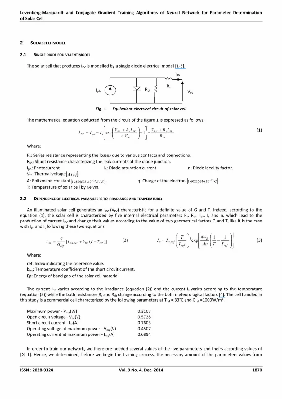
The solar cell that produces IPV is modelled by a single diode electrical model [1-3].

Fig. 1. Equivalent electrical circuit of solar cell

The mathematical equation deducted from the circuit of the figure 1 is expressed as follows:

1expsh

PVsPV

th

PVsPVsphPV

R

IRV

Vn

IRVIII

(1)

Where:

Rs: Series resistance representing the losses due to various contacts and connections.

Rsh: Shunt resistance characterizing the leak currents of the diode junction.

Iph: Photocurrent. Is: Diode saturation current. n: Diode ideality factor.

Vth: Thermal voltage qAT .

A: Boltzmann constant KJ /10.3806503.1 23 . q: Charge of the electron C1910.60217646.1 .

T: Temperature of solar cell by Kelvin.

2.2 DEPENDENCE OF ELECTRICAL PARAMETERS TO IRRADIANCE AND TEMPERATURE:

An illuminated solar cell generates an IPV (VPV) characteristic for a definite value of G and T. Indeed, according to the equation (1), the solar cell is characterized by five internal electrical parameters Rs, Rsh, Iph, Is and n, which lead to the production of current IPV and change their values according to the value of two geometrical factors G and T, like it is the case with Iph and Is following these two equations:

)]([ , refIscrefphref

ph TTbIG

GI

(2) 11

exp3,

ref

g

refrefss

TTAn

qE

T

TII (3)

Where:

ref: Index indicating the reference value. bIsc: Temperature coefficient of the short circuit current.

Eg: Energy of band gap of the solar cell material.

The current Iph varies according to the irradiance (equation (2)) and the current Is varies according to the temperature (equation (3)) while the both resistances Rs and Rsh change according to the both meteorological factors [4]. The cell handled in this study is a commercial cell characterized by the following parameters at Tref = 33°C and Gref =1000W/m²:

Maximum power - Pmp(W) 0.3107 Open circuit voltage - Voc(V) 0.5728 Short circuit current - Isc(A) 0.7603 Operating voltage at maximum power - Vmp(V) 0.4507 Operating current at maximum power - Imp(A) 0.6894

In order to train our network, we therefore needed several values of the five parameters and theirs according values of [G, T]. Hence, we determined, before we begin the training process, the necessary amount of the parameters values from

Rs Rsh Iph VPV

IPV

Fayrouz DKHICHI and Benyounes OUKARFI

ISSN : 2028-9324 Vol. 9 No. 4, Dec. 2014 1871

several characteristics IPV(VPV). We considered different characteristics for a margin of solar irradiance values between 100W/m² and 1000W/m² and for a cellular temperature values going from 15°C to 45°C. These IPV(VPV) are obtained from the schematization of a simulation model of the solar cell under MATLAB/SIMULINK software.

Fig. 2. Solar cell model

The block “cell model” of Fig. 2 includes a subsystem, modeling the mathematical equation (1).

Fig. 3. Internal cell structure inside the block “Solar cell model”

The block of Iph in figure 3 models the equation (2), while the block of Voc and Is in the same figure models successively the both following equations for current Ipv= 0 :

)]([ , refvocrefocref

oc TTbVG

GV (4)

1exp

ocph

s V

thVocV

II

(5)

bvoc: Temperature coefficient of the open circuit voltage.

3 THE USED ARTIFICIAL NEURAL NETWORK

The determination of the five internal electrical parameters of solar cell for various values of T and G are ensured by an ANN made in [4]. The architecture includes an entrance layer, a hidden layer and an output layer as shown below:

f

T

G

Ipv

P

Vpv

PV module (V)cell model

V

33

T

P-V characteristic

I-V characteristic

1000

G

f(z) zSolve

f(z) = 0Algebraic Constraint

Ipv

Ipv

IpvVth

Vpv

Ipv

2Vpv

1Ppv

n

n

n

TVt

Vth

T Voc

Voc

Rs

Rs

Product3

Product2

Product1

Product

Iph

Voc

Vt

Is

Is

T

GIph

Iph

exp(u)

Fcn1

1/u

Fcn

f(z) zSolvef(z) = 0

Algebraic Constraint

1

1

3Ipv

2G

1T

Levenberg-Marquardt and Conjugate Gradient Training Algorithms of Neural Network for Parameter Determination of Solar Cell

ISSN : 2028-9324 Vol. 9 No. 4, Dec. 2014 1872

Fig. 4. The used topology of ANN

The entrance layer contains two inputs [T, G], the hidden layer contains twenty hidden neurons and that of the output includes five neurons of output corresponding to the five parameters [Rs, Rsh, Iph, Is, n] whose we want to predict the values. The entrance and the output of the network are connected by the following equations:

hjf Activation function « hyperbolic tangent » of the hidden neurons, o

sf Activation function « linear » of the output

neurons.

Equations of input Equations of output

(6) 2

1jiji

iiji bwxz

(7) )( jihjsj zfy

(8) 20

1sjsj

jsjsj bwyz

(9) )( sj

os zfy

4 TRAINING ALGORITHMS OF THE NETWORK

The training of the ANN is characterized by three stages: learning, validation and test. In order to obtain a good training, the error generated by the output of ANN during the learning stage must be minimized. This error is known under the name of “Mean Squared Error”

)( learningmeanF , which is expressed by the following equation:

(10) ),(),(1

2

1 1)(

p

t

v

mlearninglearninglearningmean mtymtS

pF

Where: p: Number of examples {input, output}. v: Number of network output. S: Desired values of the network output. t: Index pointing out the number of examples. m: Index pointing out the number of output. y: Matrix values of the network output y = [Rs, Rsh, Iph, Is, n].

The minimization of the error )( learningmeanF is ensured by the adjustment of the ANN’s weights (w), using one

optimization algorithm among the both: Levenberg-Marquardt or conjugate gradient.

4.1 LEVENBERG-MARQUARDT ALGORITHM

Levenberg-Marquardt algorithm (LM) is well known for its combination between the steepest descent method and Gauss-Newton method, which explain its low sensitivity toward initial points and its fast convergence around the optimum [5]. The LM algorithm adjusts the weights (w) of the network by following the expression:

Fayrouz DKHICHI and Benyounes OUKARFI

ISSN : 2028-9324 Vol. 9 No. 4, Dec. 2014 1873

'1

IJJ

eJww

kk

kkkk

(11)

Where: J: Jacobian matrix of the error function .)( learningmeanF

e: Error between the desired and calculated network output. k: Number of iterations. I: Matrix identity.

Regulation strategy of the damping factor of Levenberg-Marquardt algorithm is made according to the following principle:

If the calculated error )( learningmeanF for wk+1, decreases then:

10/

Else 10* and wk+1 = wk

4.2 CONJUGATE GRADIENT ALGORITHM

Conjugate gradient algorithm (CG) is of the same family as the steepest descent algorithm, but it is more efficient. At the first iteration, the direction of gradient descent "d" is defined as follows:

kkold eJd '2

From the second iteration

kkkk

oldold

eJeJ

dd'''

'

)(

and oldkknew deJd '2

newkk dww 1 (12)

5 RESULTS

Training of the network is made with 130 inputs-outputs examples distributed in three sets (learning, validation and

test).

5.1 MEAN SQUARED ERROR

LM algorithm allows a good training of the ANN compared with CG algorithm; the latter converges slowly as it is shown in figure 5.

Fig. 5. Evolution of the mean squared error at learning stage of the ANN trained by LM and CG

Levenberg-Marquardt and Conjugate Gradient Training Algorithms of Neural Network for Parameter Determination of Solar Cell

ISSN : 2028-9324 Vol. 9 No. 4, Dec. 2014 1874

5.2 EVOLUTION OF ELECTRICAL PARAMETERS ACCORDING TO TEMPERATURE

Electrical parameters values of solar cell are determined in margin of T = [15°C, 45°C]. In order to well observe their evolution, we have chosen to present their curves for two values of G (150W/m² and 350W/m²) (figures 6, 10).

Fig. 6. Series resistance Rs according to temperature

Fig. 7. Shunt resistance Rsh according to temperature

Fig. 8. Photocurrent Iph according to temperature

Fig. 9. Saturation current Is according to temperature

Fig. 10. Diode ideality factor n according to temperature

Fayrouz DKHICHI and Benyounes OUKARFI

ISSN : 2028-9324 Vol. 9 No. 4, Dec. 2014 1875

5.3 EVOLUTION OF ELECTRICAL PARAMETERS ACCORDING TO IRRADIANCE

Electrical parameters values of solar cell are determined in margin of G = [100W/m², 1000W/m²]. Since the curves are crowded, we have chosen two values of T (15°C and 35°C) to observe well the evolution of these parameters (figures 11,15).

Fig. 11. Series resistance Rs according to irradiance

Fig. 12. Shunt resistance Rsh according to irradiance

Fig. 13. Photocurrent Iph according to irradiance

Fig. 14. Saturation current Is according to irradiance

Fig. 15. Diode ideality factor n according to irradiance

Levenberg-Marquardt and Conjugate Gradient Training Algorithms of Neural Network for Parameter Determination of Solar Cell

ISSN : 2028-9324 Vol. 9 No. 4, Dec. 2014 1876

6 DISCUSSIONS

As it is shown in fig. 5, the LM algorithm converges quickly and presents a minimal value of )( learningmeanF compared to the

error generated by the CG algorithm. This ability of LM to reach lower value of the mean squared error better than CG is explained by the features that LM inherits from Gauss-Newton. This algorithm becomes fast and effective when the network weights are well refined by the steepest descent algorithm. In other hand the CG which behaves like steepest descent, it had a slow convergence around the optimal network weighs, which explain the behavior of the algorithm that does not achieve a minimal error like it is the case with LM.

The obtained curves of the electrical parameters of the solar cell according to temperature and irradiance (fig. 6 to fig. 15), shows clearly that the network trained by LM gives values near to desired values than those obtained by ANN trained by CG. The temperature and the irradiance apply different effects on the five parameters Rs, Rsh, Iph, Is and n. As it is clearly seen in fig. 6 and in fig. 11, the values of Rs increase when T and/or G increase too, while in the two fig. 7 and fig. 12, the values of Rsh decrease with the variation of G, then they remain almost the same although the variation of T. The photocurrent Iph as its name indicates, it is more affected by the change of G than by T, so this is obvious in fig. 8 and fig. 13. The values of Is decrease with G and increase with T (fig. 9 and fig. 14), this evolution is also observed in the values of the diode ideality factor n (fig. 10 and fig. 15).

Table 1. Percentage of error of electrical parameters obtained par the ANN trained par LM and CG algorithms.

Meteorological Conditions

Conventional model [6] Proposed ANN trained by LM Proposed ANN trained by CG

G [W/m²] T [°C] Rs [%] Rsh [%] Iph [%] Is [%] n [%] Rs [%] Rsh [%] Iph [%] Is [%] n [%] Rs [%] Rsh [%] Iph [%] Is [%] n [%]

200

15

0.0336 0.0115 0.0005 1.9764 0.0171 0.0000 0.0007 0.0005 0.0112 0.0000 0.0002 0.0222 0.1556 0.0965 0.0007

400 0.0292 0.0077 0.0006 0.4265 0.0237 0.0002 0.0001 0.0005 0.0124 0.0000 0.0002 0.0891 0.0194 0.0202 0.0001

600 0.0270 0.0059 0.0005 0.5636 0.0288 0.0000 0.0034 0.0005 0.0036 0.0012 0.0003 0.0556 0.0083 0.1163 0.0054

800 0.0248 0.0041 0.0004 0.7100 0.0339 0.0001 0.0013 0.0004 0.0144 0.0000 0.0062 0.1898 0.0071 0.2419 0.0070

1000 0.0246 0.0012 0.0002 0.0488 0.0251 0.0000 0.0011 0.0002 0.0267 0.0003 0.0003 0.1594 0.0445 0.0816 0.0049

200

45

0.0337 0.0104 0.0006 0.8324 0.0168 0.0000 0.0005 0.0006 0.0004 0.0001 0.0002 0.0034 0.0193 0.0023 0.0015

400 0.0294 0.0065 0.0006 0.8639 0.0219 0.0002 0.0053 0.0006 0.0891 0.0033 0.0003 0.1660 0.0506 0.0831 0.0041

600 0.0271 0.0050 0.0004 0.8541 0.0312 0.0000 0.0021 0.0004 0.0419 0.0034 0.0005 0.0121 0.0207 0.0512 0.0093

800 0.0024 0.0030 0.0003 0.0002 0.0304 0.0000 0.0027 0.0000 0.0002 0.0000 0.0001 0.0643 0.0011 0.1795 0.0079

1000 0.0011 0.0029 0.0002 0.0011 0.0361 0.0000 0.0018 0.0002 0.0162 0.0005 0.0001 0.1831 0.0111 0.0778 0.0052

In a previous work [6], we identified the electrical parameters of the mathematical model equation (1) by a conventional

method. We therefore adjusted numerically the sum of squared error in order to determine these parameters by using one characteristic IPV (VPV). This characteristic is taken for a determined value of T and G. The determination of the corresponding values of the electrical parameters makes the identification issue a little bit slow and heavy to implement. Consequently the ANN method resolves this problem and presents an adapted determination platform, which establish a relationship between [T, G] and [Rs, Rsh, Iph, Is, n].

As it is shown in Table 1, we observe that the ANN trained by LM and CG presents the error percentages of electrical parameters minimum compared to that supplied by the conventional method, except for the percentages of error concerning the parameters Rsh et Iph supplied by the CG algorithm which had important values compared to those presented by the conventional method. When we compare between ANN trained by LM and that trained by CG, we noteworthy that the first one presents the most minimal errors.

7 CONCLUSIONS

Levenberg-Marquardt algorithm provides the best performances in the training of the artificial neural network compared to the conjugate gradient algorithm. The determined values of the five electrical parameters of solar cell obtained by the network trained by the Levenberg-Marquardt algorithm are so close to the desired values, due to the ability of this algorithm to combine between the characteristics of steepest descent algorithm and the Gauss-Newton algorithm which ensure a maximal minimization of the mean squared error.

Fayrouz DKHICHI and Benyounes OUKARFI

ISSN : 2028-9324 Vol. 9 No. 4, Dec. 2014 1877

REFERENCES

[1] A. Jain, A. Kapoor, “Exact analytical solutions of the parameters of real solar cells using Lambert W-function”, Solar Energy Materials & Solar Cells, vol. 81, pp. 269-277, 2004.

[2] H. Qin, J. W. Kimball, “Parameter Determination of Photovoltaic Cells from Field Testing Data using Particle Swarm Optimization”, IEEE, 2011.

[3] T. Ikegami, T. Maezono, F. Nakanishi, Y. Yamagata, K. Ebihara, “Estimation of equivalent circuit parameters of PV module and its application to optimal operation of PV system”, Solar Energy Materials & Solar Cells, vol. 67 pp. 389-395, 2011.

[4] E. Karatepe, M. Boztepe, M. Colak, “Neural network based solar cell model”, Energy Conversion and Management, vol. 47, pp. 1159-1178, 2006.

[5] B. G. Kermani, S. S. Schiffmanb, H. T. Nagle, “Performance of the Levenberg–Marquardt neural network training method in electronic nose applications”, Sensors and Actuators, vol. 110, pp. 13–22, 2005.

[6] B. Oukarfi, F. Dkhichi, A. Fakkar, “Parametric identification by minimizing the squared residuals (Application to a photovoltaic cell)”, Proc. 1th IEEE Conf. on Renewable and sustainable energy conference, Ouarzazate, IEEE Explore, (March 7-9 2013).