application of galerkin method to conjugate heat transfer calculation
TRANSCRIPT
APPLICATION OF GALERKIN METHOD TO CONJUGATEHEAT TRANSFER CALCULATION
Andrej HorvatReactor Engineering Division, ‘‘Jozef Stefan’’ Institute,Ljubljana, Slovenia
Ivan CattonThe Henry Samueli School of Engineering and Applied Science,Mechanical and Aerospace Engineering Department,University of California, Los Angeles,California, USA
A fast-running computational algorithm based on the volume averaging technique (VAT) is
developed and solutions are obtained using the Galerkin method (GM). The goal is to extend
applicability of the GM to the area of heat exchangers in order to provide a reliable
benchmark for numerical calculations of conjugate heat transfer problems. Using the VAT,
the computational algorithm is fast-running, but still able to present a detailed picture of
temperature fields in air flow as well as in the solid structure of the heat sink. The calculated
whole-section drag coefficient Cd and Nusselt number Nu were compared with finite-volume
method (FVM) results and with experimental data to verify the computational model. The
comparison shows good agreement. The present results demonstrate that the selected
Galerkin approach is capable to perform heat exchanger calculations where the thermal
conductivity of the solid structure has to be taken into account.
1. INTRODUCTION
Cross-flow through the solid structure is found in a number of differentapplications, especially in heat exchanging devices. Although the problem has beenwidely studied, there are still unresolved issues, which deserve researchers’ attention.
The widespread use of heat exchangers in many industrial sectors caused theirdevelopment to take place in a number of rather unrelated areas. Furthermore, designsolutions were based solely on experimental work because of the absence of today’spowerful computers and lack of suitable numerical methods (Antonopoulos [1],
Received 4 October 2002; accepted 12 May 2003.
A. Horvat gratefully acknowledges the financial support received from the Kerze-Cheyovich scho-
larship and the Ministry of Education, Science and Sport of the Republic of Slovenia. The efforts of I.
Catton were the result of support by DARPA as part of the HERETIC program (DAAD19-99-1-0157).
A. Horvat is currently at ANSYS CFX Didcot, United Kingdom.
Address correspondence to A. Horvat, ‘‘Jozef Stefan’’ Institute, Reactor Engineering Division,
Jamova 39, SI 1001, Ljubljana, Slovenia. E-mail: [email protected]
Numerical Heat Transfer, Part B, 44: 509–531, 2003
Copyright # Taylor & Francis Inc.
ISSN: 1040-7790 print/1521-0626 online
DOI: 10.1080/10407790390231752
509
Barsamian and Hassan [2]). The nature of experimental work limited researchers tostudy only a few heat exchanger geometries and a few variations in their geometryparameters. Furthermore, the flow conditions were often limited by availableexperimental setups. These disadvantages, compared to numerical modeling, did notallow researchers to explore a wide range of parameters in order to find an optimalgeometry. Rather, they limited the engineer’s choices to well-tested and provendesigns.
On the other hand, direct numerical simulation of transport phenomena in eachmaterial phase (or component) is theoretically possible, but it demands enormouscomputational resources even for simple geometries. This is the reason why directapproaches are rarely seen in practical engineering applications. In order to resolvemost of the flow features and at the same time keep the model simple enough to serveas an engineering tool, an averaging of fluid and heat flow variables has to be per-formed. Recently, a unified approach based on the volume averaging technique
NOMENCLATURE
Ac flow contact area of the test section
Ag heat sink ground area
Ao interface area
A1 ¼ 7M4={M3[1þ exp(g)]}A2 ¼ 7A17M4=M3
A? channel flow area
c specific heat
Cd whole-section drag coefficient
Cl local drag coefficient
d pin-fin diameter
dh hydraulic diameter¼ (4Vf=Ao)
D1 ¼ uF1
D2 ¼F4S1=S2
D3 ¼F5S1=S2þF4
D4 ¼ uF1S1=S2
F1 ¼ af Pr Res(dh=L)
F4 ¼af(dh2=H2)
F5 ¼Nus(dhS)
FVM finite-volume method
GM Galerkin method
h arbitrary function, heat transfer coeffi-
cient
H height
K linearized drag coefficient ¼ (M3u)
M2 ¼ af=Res(dh2=H2)
M3 ¼ 1=2Cl(dhS)
M4 ¼ dh=L
L length of the test section
Nu whole-section Nusselt number
Nus pore Nusselt number (¼ hdh=lf)p pressure
Dp whole-section pressure drop
px pitch between pin-fins in x direction
py pitch between pin-fins in y direction
Pr Prandtl number
Q heat flow
Reh Reynolds number ¼ (udh=vf)
Res pore Reynolds number ¼ (Udh=vf)
S specific surface¼ (Ao=V)
S1 ¼as (dh2=H2)
S2 ¼Nus(lf=ls)(dhS)T temperature
Tg temperature at bottom, z¼ 0 position
Tin temperature at inflow, x¼ 0 position
u velocity in streamwise direction
U velocity scale
v velocity vector
V representative elementary volume
W mechanical work
x general spatial coordinate, streamwise
coordinate
z vertical spanwise coordinate
a volume fraction
l thermal conductivity
L area of integration
m dynamic viscosity
n kinematic viscosity
r density
Subscript=Superscript
f fluid phase
s solid phase
Symbols
� phase average variables
^ dimensional variables
½ � whole-section average variables
510 A. HORVAT AND I. CATTON
(VAT) has been developed and utilized for calculations of heat exchangers withisothermal (Horvat and Catton [3]) and heat conducting structures (Horvat et al. [4]).
In applying the VAT to a system of equations, transport processes in a heatexchanger are modeled as porous media flow. This generalization allows us to unifythe heat transfer calculation techniques for different kinds of heat exchangers andtheir structures. The case-specific geometric arrangements, material properties, andfluid flow conditions enter the computational algorithm only as precalculatedcoefficients, which require additional modeling. This clear separation between themodel and the case-specific coefficients simplifies the computational algorithm.Therefore, the algorithm is fast-running, but still able to present a detailed picture oftemperature fields in air flow as well as in a solid structure of a heat sink.
In the present article, the VAT is used to model heat transfer processes in anelectronic device heat sink. The geometry and boundary conditions closely follow theheat sink configuration studied experimentally in the Morrin-Martinelli-GierMemorial Heat Transfer Laboratory at the University of California, Los Angeles.The system of porous media flow equations is solved semianalytically using theGalerkin method (GM). To demonstrate the capability and accuracy of the selectedmethod, the results are compared with experimental data as well as with othernumerical results obtained with the finite–volume method (FVM). Despite simpli-fications, which are needed to solve the problem semianalytically, the comparisonshows good agreement.
In the past, the Galerkin solution technique was widely used for transportphenomena-related problems (Catton [5] and [6], McDonough and Catton [7],Howle [8]). It should be mentioned that the Galerkin approach is not the optimalmethod for this kind of calculation, due to serious limitations in the methodapplicability to more realistic geometries and boundary conditions. Nevertheless, thecase presented here is an important benchmark on which other numerical results canbe tested.
2. GOVERNING EQUATIONS FOR UNIFORM FLOW THROUGH HEAT SINK
The VAT was initially proposed in the 1960 s by Anderson and Jackson [9],Slattery [10], Marle [11], Whitaker [12], and Zolotarev and Redushkevich [13]. As themain intention of this article is to present the Galerkin solution procedure forthe heat sink cross-flow, detailed description of the VAT will be omitted. Many ofthe important details and examples of applications can be also found in Dullien [14],Kheifets and Neimark [15], Adler [16], and Horvat [17].
To describe fluid and heat flow in an electronic device heat sink, momentumand energy transport equations for fluid flow, as well as an additional energyequations for the solid structure are needed. Applying the VAT, the transportequations are averaged over a representative elementary volume (REV), whichproduces porous media flow equations.
2.1. Momentum Transport
The derivation of the momentum transport equation for porous media flowstarts from the momentum equation for steady-state incompressible flow, where the
GALERKIN METHOD FOR CONJUGATE HEAT TRANSFER 511

effect of gravity is neglected. For uniform porous media (af is a constant), themomentum equation can be written as
afrf�vvjq�vviqxj
¼ �afq�ppfqxi
þ afmfq2�vviqx2j
� 1
V
ZAo
pdLi þmfV
ZAo
qviqxj
dLj ð1Þ
The integrals in Eq. (1) are a consequence of the volumetric averaging. They capturethe momentum transport on the fluid–solid interface. Similar to turbulent flow, aseparate model in the form of a closure relation is needed. In the present case, theintegrals are replaced with the following empirical drag relation:
1
2Clrf�vv
2i Ao ¼ �
ZAo
pdLi þ mf
ZAo
qviqxj
dLj ð2Þ
where Cl is the local value of the drag coefficient, which depends on the localReynolds number. Reliable empirical data for the local drag coefficient Cl werefound in Launder and Massey [18] and in Kays and London [19].
Inserting the empirical correlation (2) into Eq. (1), the momentum equation forporous media flow is given as
afrf�vvjq�vviqxj
¼ �afq�ppfqxi
þ af mfq2�vviqx2j
þ 1
2Clrf�vv
2i S ð3Þ
It is additionally assumed that the volume average velocity through the heat sink isunidirectional v¼ {u,0,0}, and changes only in the vertical direction. This means thatthe pressure force across the entire simulation domain is balanced with shear forces.Therefore, the momentum transport equation is reduced to
� afmfq2�uuqz2
þ 1
2Clrf�uu
2S ¼ DpL
ð4Þ
2.2. Energy Transport in Fluid
The energy transport equation for fluid flow is developed from the energytransport equation for steady-state incompressible flow. For uniform porous mediait is written as
afrf cf�vvjq �TTf
qxj¼ aflf
q2 �TTf
qx2jþ lf
V
ZAo
qTqxj
dLj ð5Þ
The integral in Eq. (5) represents the interphase heat exchange between fluid flowand the solid structure, and it requires additional modeling. In the present case anempirical linear relation between the fluid and the solid temperature is taken as anappropriate model for the interphase heat flow:
hð �TTf � �TTsÞAo ¼ �lf
ZAo
qTqxj
dLj ð6Þ
512 A. HORVAT AND I. CATTON
where h is the local value of the heat transfer coefficient, which depends on the localReynolds number. The data for the local heat transfer coefficient h were takenfrom Zukauskas and Ulinskas [20] for low Reynolds numbers, whereas for higherReynolds numbers, the experimental data from Kays and London [19] were moreappropriate.
Inserting the relation (6) into Eq. (5) the energy transport equation for fluidflow can be written as
afrf cf�vvjq �TTf
qxj¼ aflf
q2 �TTf
qx2j� hð �TTf � �TTsÞS ð7Þ
The energy transport equation for fluid flow (7) is further simplified with the velocityunidirectional assumption. Therefore, the temperature field in the fluid is formed as abalance between thermal convection in the streamwise direction, thermal diffusion,and the heat, which is transferred from the solid structure to fluid flow. Thus, thedifferential form of the energy equation for the fluid is
afrf cf �uuq �TTf
qx¼ aflf
q2 �TTf
qz2� hð �TTf � �TTsÞS ð8Þ
2.3. Energy Transport in Solid
In a solid phase, thermal diffusion is the only mechanism of heat transport.Therefore, the energy transport equation for the solid structure is reduced to thesimple diffusion equation
0 ¼ aslsq2 �TTs
qx2jþ ls
V
ZAo
qTqxj
dLj ð9Þ
where the integral captures the interphase heat exchange. Closure is obtained bysubstituting the linear relation
hð �TTf � �TTsÞAo ¼ ls
ZAo
qTqxj
dLj ð10Þ
in Eq. (9). The VAT energy transport equation for the solid structure is nowwritten as
0 ¼ aslsq2 �TTs
qx2jþ hð �TTf � �TTsÞS ð11Þ
The heat sink structure in each REV is only loosely connected in horizontal direc-tions (see Figure 1). As a consequence, only the thermal diffusion in the verticaldirection is in balance with the heat leaving the structure through the fluid–solidinterface, whereas the thermal diffusion in the horizontal directions can be neglected.This simplifies the energy equation for the solid structure to
0 ¼ aslsq2 �TTs
qz2þ hð �TTf � �TTsÞS ð12Þ
GALERKIN METHOD FOR CONJUGATE HEAT TRANSFER 513
3. SIMULATION SETUP
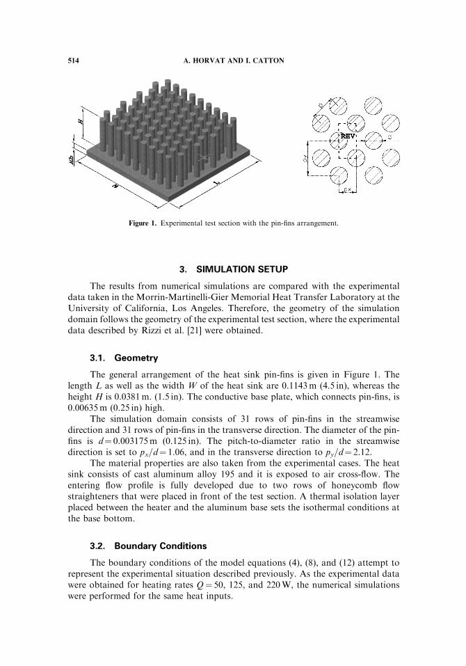
The results from numerical simulations are compared with the experimentaldata taken in the Morrin-Martinelli-Gier Memorial Heat Transfer Laboratory at theUniversity of California, Los Angeles. Therefore, the geometry of the simulationdomain follows the geometry of the experimental test section, where the experimentaldata described by Rizzi et al. [21] were obtained.
3.1. Geometry
The general arrangement of the heat sink pin-fins is given in Figure 1. Thelength L as well as the width W of the heat sink are 0.1143m (4.5 in), whereas theheight H is 0.0381m. (1.5 in). The conductive base plate, which connects pin-fins, is0.00635m (0.25 in) high.
The simulation domain consists of 31 rows of pin-fins in the streamwisedirection and 31 rows of pin-fins in the transverse direction. The diameter of the pin-fins is d¼ 0.003175m (0.125 in). The pitch-to-diameter ratio in the streamwisedirection is set to px=d¼ 1.06, and in the transverse direction to py=d¼ 2.12.
The material properties are also taken from the experimental cases. The heatsink consists of cast aluminum alloy 195 and it is exposed to air cross-flow. Theentering flow profile is fully developed due to two rows of honeycomb flowstraighteners that were placed in front of the test section. A thermal isolation layerplaced between the heater and the aluminum base sets the isothermal conditions atthe base bottom.
3.2. Boundary Conditions
The boundary conditions of the model equations (4), (8), and (12) attempt torepresent the experimental situation described previously. As the experimental datawere obtained for heating rates Q¼ 50, 125, and 220W, the numerical simulationswere performed for the same heat inputs.
Figure 1. Experimental test section with the pin-fins arrangement.
514 A. HORVAT AND I. CATTON
For the momentum transport equation (4), the no-slip boundary conditions areimplemented for both walls that are parallel with the flow direction:
�uuð0Þ ¼ 0 �uuðHÞ ¼ 0 ð13Þ
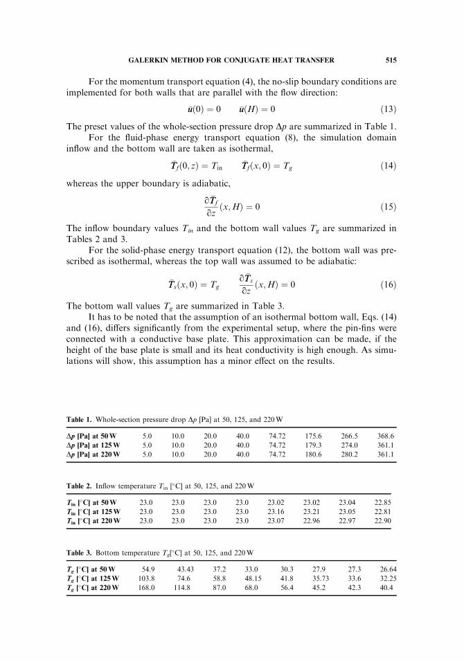
The preset values of the whole-section pressure drop Dp are summarized in Table 1.For the fluid-phase energy transport equation (8), the simulation domain
inflow and the bottom wall are taken as isothermal,
�TTfð0; zÞ ¼ Tin�TTfðx; 0Þ ¼ Tg ð14Þ
whereas the upper boundary is adiabatic,
q �TTf
qzðx;HÞ ¼ 0 ð15Þ
The inflow boundary values Tin and the bottom wall values Tg are summarized inTables 2 and 3.
For the solid-phase energy transport equation (12), the bottom wall was pre-scribed as isothermal, whereas the top wall was assumed to be adiabatic:
�TTsðx; 0Þ ¼ Tgq �TTs
qzðx;HÞ ¼ 0 ð16Þ
The bottom wall values Tg are summarized in Table 3.It has to be noted that the assumption of an isothermal bottom wall, Eqs. (14)
and (16), differs significantly from the experimental setup, where the pin-fins wereconnected with a conductive base plate. This approximation can be made, if theheight of the base plate is small and its heat conductivity is high enough. As simu-lations will show, this assumption has a minor effect on the results.
Table 1. Whole-section pressure drop Dp [Pa] at 50, 125, and 220W
Dp [Pa] at 50W 5.0 10.0 20.0 40.0 74.72 175.6 266.5 368.6
Dp [Pa] at 125W 5.0 10.0 20.0 40.0 74.72 179.3 274.0 361.1
Dp [Pa] at 220W 5.0 10.0 20.0 40.0 74.72 180.6 280.2 361.1
Table 2. Inflow temperature Tin [�C] at 50, 125, and 220W
Tin [�C] at 50W 23.0 23.0 23.0 23.0 23.02 23.02 23.04 22.85
Tin [�C] at 125W 23.0 23.0 23.0 23.0 23.16 23.21 23.05 22.81
Tin [�C] at 220W 23.0 23.0 23.0 23.0 23.07 22.96 22.97 22.90
Table 3. Bottom temperature Tg[�C] at 50, 125, and 220W
Tg [�C] at 50W 54.9 43.43 37.2 33.0 30.3 27.9 27.3 26.64
Tg [�C] at 125W 103.8 74.6 58.8 48.15 41.8 35.73 33.6 32.25
Tg [�C] at 220W 168.0 114.8 87.0 68.0 56.4 45.2 42.3 40.4
GALERKIN METHOD FOR CONJUGATE HEAT TRANSFER 515
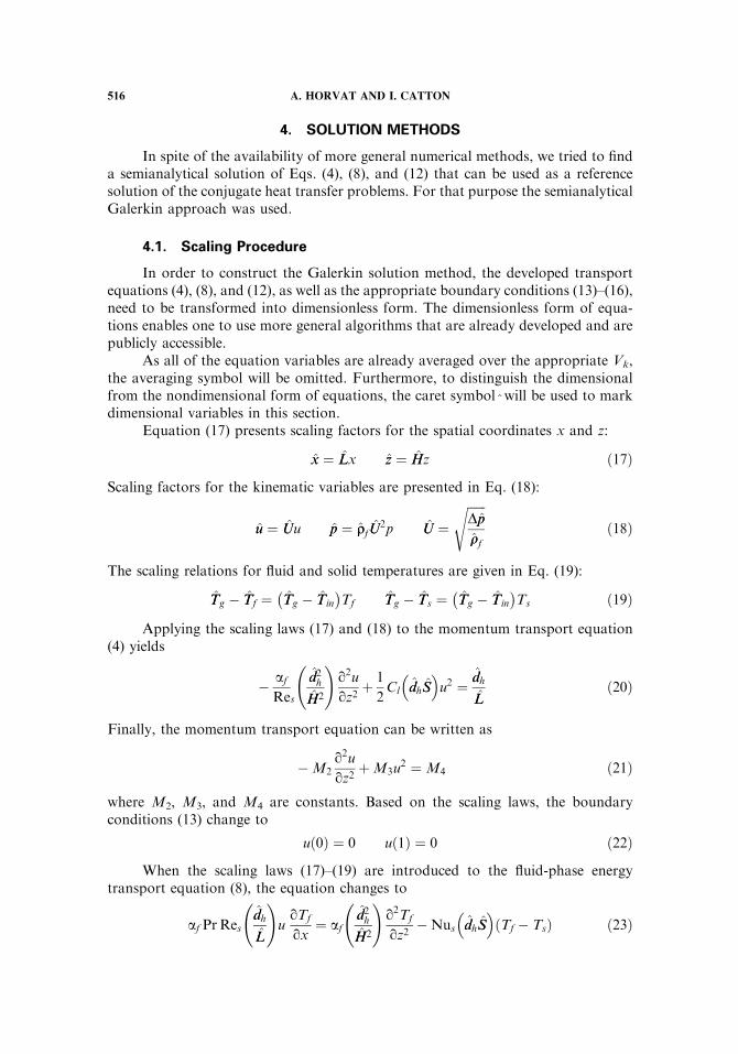
4. SOLUTION METHODS
In spite of the availability of more general numerical methods, we tried to finda semianalytical solution of Eqs. (4), (8), and (12) that can be used as a referencesolution of the conjugate heat transfer problems. For that purpose the semianalyticalGalerkin approach was used.
4.1. Scaling Procedure
In order to construct the Galerkin solution method, the developed transportequations (4), (8), and (12), as well as the appropriate boundary conditions (13)–(16),need to be transformed into dimensionless form. The dimensionless form of equa-tions enables one to use more general algorithms that are already developed and arepublicly accessible.
As all of the equation variables are already averaged over the appropriate Vk,the averaging symbol will be omitted. Furthermore, to distinguish the dimensionalfrom the nondimensional form of equations, the caret symbol^will be used to markdimensional variables in this section.
Equation (17) presents scaling factors for the spatial coordinates x and z:
xx ¼ LLx zz ¼ HHz ð17Þ
Scaling factors for the kinematic variables are presented in Eq. (18):
uu ¼ UUu pp ¼ rrfUU2p UU ¼
ffiffiffiffiffiffiDpprrf
sð18Þ
The scaling relations for fluid and solid temperatures are given in Eq. (19):
TTg � TTf ¼ TTg � TTin
� �Tf TTg � TTs ¼ TTg � TTin
� �Ts ð19Þ
Applying the scaling laws (17) and (18) to the momentum transport equation(4) yields
� afRes
dd2hHH2
!q2uqz2
þ 1
2Cl ddhSS� �
u2 ¼ ddh
LLð20Þ
Finally, the momentum transport equation can be written as
�M2q2uqz2
þM3u2 ¼ M4 ð21Þ
where M2, M3, and M4 are constants. Based on the scaling laws, the boundaryconditions (13) change to
uð0Þ ¼ 0 uð1Þ ¼ 0 ð22Þ
When the scaling laws (17)–(19) are introduced to the fluid-phase energytransport equation (8), the equation changes to
af PrResddh
LL
!uqTf
qx¼ af
dd2hHH2
!q2Tf
qz2�Nus ddhSS
� �ðTf � TsÞ ð23Þ
516 A. HORVAT AND I. CATTON
Equation (23) can be further simplified to
F1uqTf
qx¼ F4
q2Tf
qz2� F5ðTf � TsÞ ð24Þ
where F1, F4, and F5 are constants. Based on the scaling laws, the boundary con-ditions (14) and (15) change to
Tfð0; zÞ ¼ 1 Tfðx; 0Þ ¼ 0qTf
qzðx; 1Þ ¼ 0 ð25Þ
As in the previous case, inserting the scaling laws (17)–(19) to the solid-phaseenergy transport equation (12) gives the following form:
0 ¼ asdd2hHH2
!q2Ts
qz2þNus
llflls
!ddhSS� �
ðTf � TsÞ ð26Þ
Next, the solid-phase energy transport equation (26) is reduced to
0 ¼ S1q2Ts
qz2þ S2ðTf � TsÞ ð27Þ
where S1 and S2 are constants. The solid structure boundary conditions (16) alsochange to
Tsðx; 0Þ ¼ 0qTs
qzðx; 1Þ ¼ 0 ð28Þ
4.2. Galerkin Solution Procedure
The momentum transport equation (21) is first linearized to
�M2q2uqz2
þ Ku ¼ M4 ð29Þ
with K¼M3u being a constant. The solution of the linearized momentum transportequation (29) is expected to be of the form
u � expðgzÞ ð30Þ
where g is a constant. Taking into account the boundary conditions given byEq. (22), the fluid velocity is
u ¼ A1 expðgzÞ þ A2 expð�gzÞ þM4
Kð31Þ
where g, A1, and A2 are constants defined from boundary conditions.To find the solution to the system of energy transport equations (24) and (27),
both equations are combined into the single expression
uF1qTs
qxþ F4
S1
S2
q4Ts
qz4� F5
S1
S2þ F4
� �q2Ts
qz2� uF1
S1
S2
q3Ts
qx qz2¼ 0 ð32Þ
GALERKIN METHOD FOR CONJUGATE HEAT TRANSFER 517
which can be written in a more compact form as
D1qTs
qxþD2
q4Ts
qz4�D3
q2Ts
qz2�D4
q3Ts
qx qz2¼ 0 ð33Þ
where D2, D3 are constants and D1, D4 are functions of z.Next, separation of variables in the following form is used to find the solution
of Eq. (33):
Ts ¼ XðxÞZðzÞ ð34Þ
with the boundary conditions
Xð0Þ ¼ 1 Zð0Þ ¼ 0qZqz
ð1Þ ¼ 0 ð35Þ
When Eq. (34) is inserted in Eq. (33), the following differential equation is obtained:
D1ZXI þD2Z
IVX�D3ZIIX�D4Z
IIXI ¼ 0 ð36Þ
The solution in the z direction of Eq. (36) is anticipated to be a finite set of ortho-gonal functions,
Z ¼ AnZn Zn ¼ sinðgnzÞ gn ¼2n� 1
2p ð37Þ
which satisfy the boundary conditions (35). Introducing Eq. (37) into Eq. (36) bringsus to
D1XIðAnZnÞ þD2XðAng4nZnÞ þD3XðAng2nZnÞ þD4X
IðAng2nZnÞ ¼ error ð38Þ
and in a more compact form to
XIAn D1 þ g2nD4
� �Zn þ XAn g4nD2 þ g2nD3
� �Zn ¼ error ð39Þ
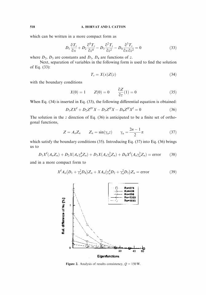
Figure 2. Analysis of results consistency, Q ¼ 150W.
518 A. HORVAT AND I. CATTON
As the series is finite, there is a certain discrepancy associated with the expansion.This error is orthogonal to the set of functions used for the expansion and can bereduced with multiplication by Zm (m¼ 1, N) and further integration from 0 to 1:
XIAn
Z1
0
D1 þ g2nD4
� �ZnZm dzþ XAn
Z1
0
g4nD2 þ g2nD3
� �ZnZm dz ¼ 0 ð40Þ
In matrix form, Eq. (40) is written as
XIAnInm þ XAnJnm ¼ 0 ð41Þ
where Inm and Jnm are z-dependent integrals. As the x- and z-dependent parts ofEq. (41) can be separated,
b ¼ �XIm
Xm¼ AnJnm
AnInmð42Þ
separate equations are written for the x direction,
XIm þ bmXm ¼ 0 ð43Þ
and for the z direction,
AnJnm � bmAnInm ¼ 0 ð44Þ
The solution of Eq. (43) is obtained by integration:
Xm ¼ C expð�bmxÞ ð45Þ
where C and bm are arbitrary constants. Rearranging Eq. (44), an extended eigen-value problem can be formed as
ðJnm � bmInmÞAn ¼ 0 ð46Þ
The system of Eq. (46) has a nontrivial solution if
DetðJnm � bmInmÞ ¼ 0 ð47Þ
From this condition the system eigenvalues bm are determined. Furthermore, eacheigenvalue bm corresponds to a specific m vector of An.
Using the solutions of Eq. (43) and the matrix system (47), one can constructthe solid structure temperature field:
Ts ¼ CiXiAinZn ð48Þ
Reintroducing Eq. (27), the fluid temperature field is then given by
Tf ¼ CiXiAin 1þ S1
S2g2n
� �Zn ð49Þ
The coefficients Ci are found from the initial condition Tfð0; zÞ ¼ 1:
CiAin 1þ S1
S2g2n
� �Zn ¼ 1 ð50Þ
GALERKIN METHOD FOR CONJUGATE HEAT TRANSFER 519
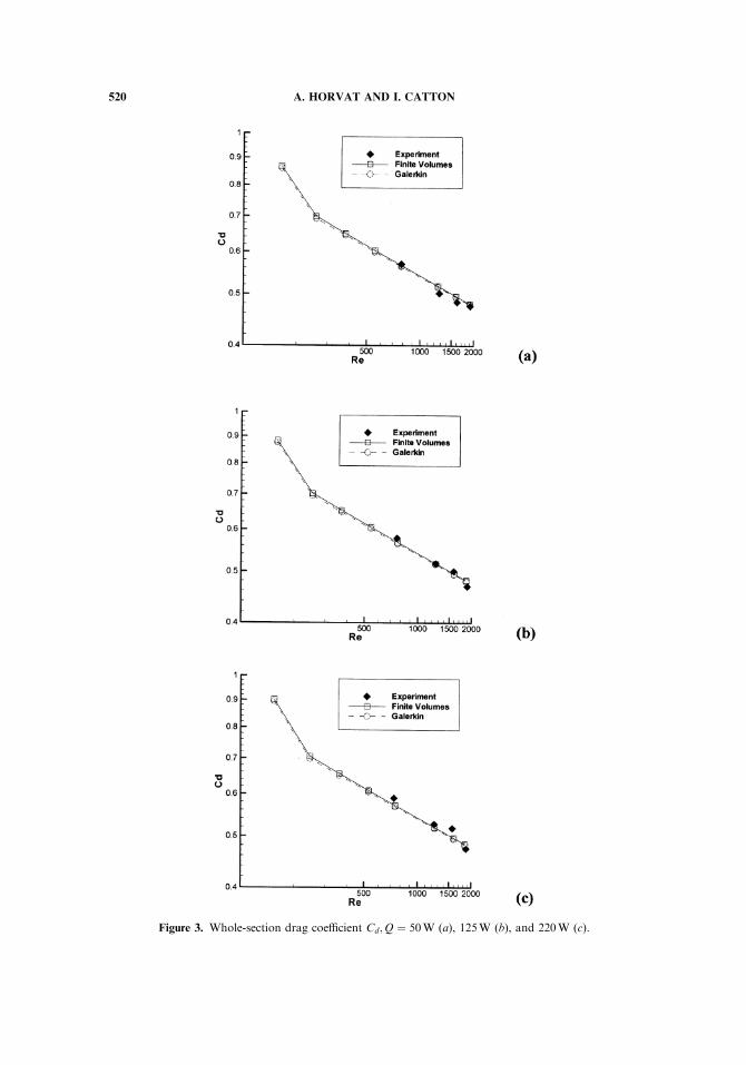
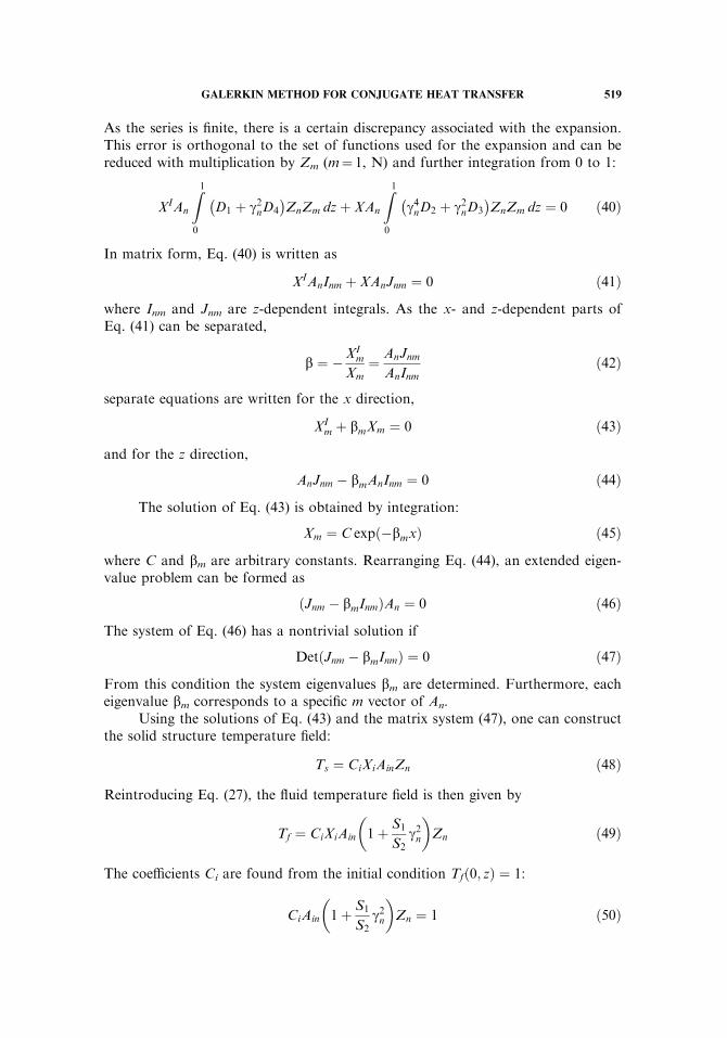
Figure 3. Whole-section drag coefficient Cd;Q ¼ 50W (a), 125W (b), and 220W (c).
520 A. HORVAT AND I. CATTON
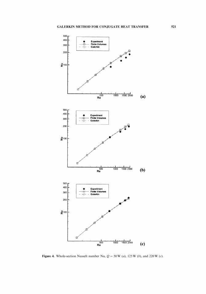
Figure 4. Whole-section Nusselt number Nu, Q ¼ 50W (a), 125W (b), and 220W (c).
GALERKIN METHOD FOR CONJUGATE HEAT TRANSFER 521
Again, using the same procedure by multiplying Eq. (50) with Zm (m¼ 1, N) andintegrating it from 0 to 1,
CiAin 1þ S1
S2g2n
� �Z1
0
ZnZm dz ¼Z1
0
Zmdz ð51Þ
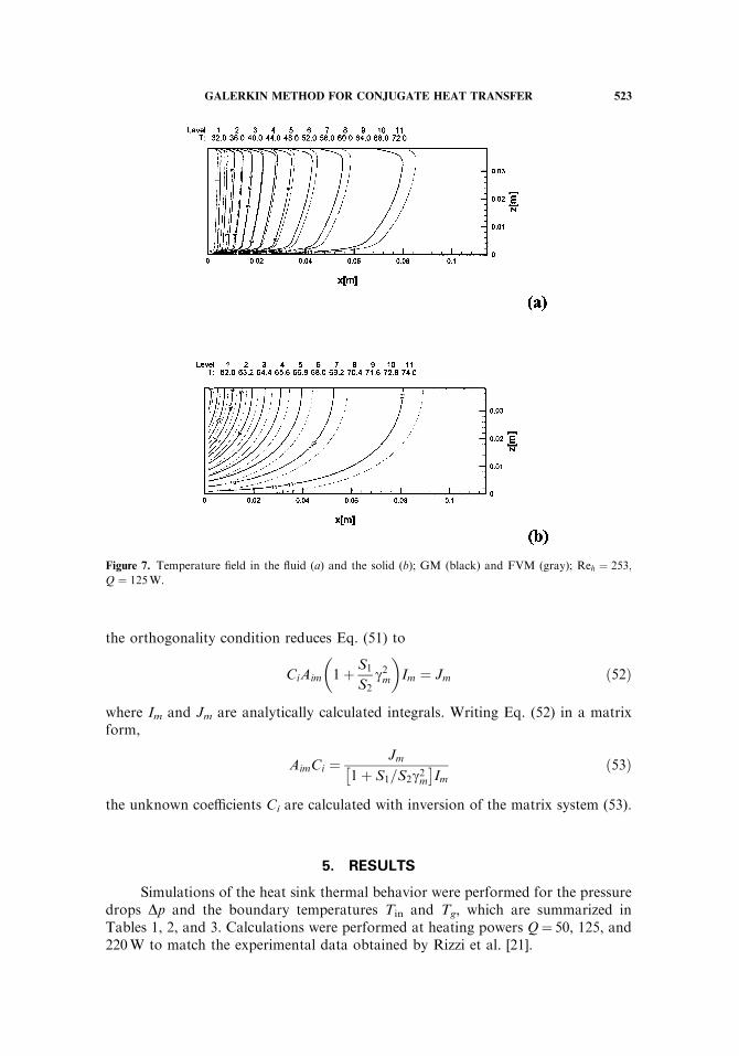
Figure 6. Temperature field in the fluid (a) and the solid (b); GM (black) and FVM (gray); Reh¼ 159,
Q¼ 125W.
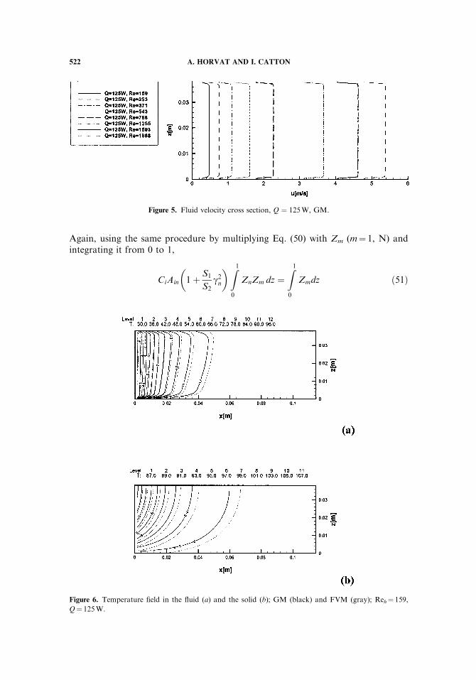
Figure 5. Fluid velocity cross section, Q ¼ 125W, GM.
522 A. HORVAT AND I. CATTON
the orthogonality condition reduces Eq. (51) to
CiAim 1þ S1
S2g2m
� �Im ¼ Jm ð52Þ
where Im and Jm are analytically calculated integrals. Writing Eq. (52) in a matrixform,
AimCi ¼Jm
1þ S1=S2g2m�
Imð53Þ
the unknown coefficients Ci are calculated with inversion of the matrix system (53).
5. RESULTS
Simulations of the heat sink thermal behavior were performed for the pressuredrops Dp and the boundary temperatures Tin and Tg, which are summarized inTables 1, 2, and 3. Calculations were performed at heating powers Q¼ 50, 125, and220W to match the experimental data obtained by Rizzi et al. [21].
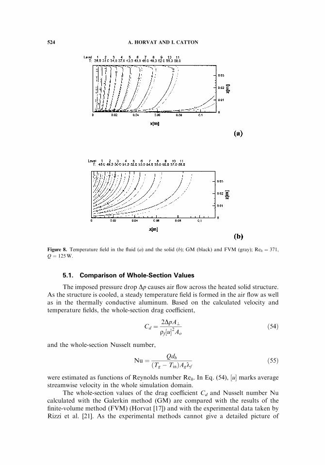
Figure 7. Temperature field in the fluid (a) and the solid (b); GM (black) and FVM (gray); Reh ¼ 253;
Q ¼ 125W.
GALERKIN METHOD FOR CONJUGATE HEAT TRANSFER 523
5.1. Comparison of Whole-Section Values
The imposed pressure drop Dp causes air flow across the heated solid structure.As the structure is cooled, a steady temperature field is formed in the air flow as wellas in the thermally conductive aluminum. Based on the calculated velocity andtemperature fields, the whole-section drag coefficient,
Cd ¼2DpA?
rf½u�2Ao
ð54Þ
and the whole-section Nusselt number,
Nu ¼ QdhðTg � TinÞAglf
ð55Þ
were estimated as functions of Reynolds number Reh. In Eq. (54), ½u� marks averagestreamwise velocity in the whole simulation domain.
The whole-section values of the drag coefficient Cd and Nusselt number Nucalculated with the Galerkin method (GM) are compared with the results of thefinite-volume method (FVM) (Horvat [17]) and with the experimental data taken byRizzi et al. [21]. As the experimental methods cannot give a detailed picture of
Figure 8. Temperature field in the fluid (a) and the solid (b); GM (black) and FVM (gray); Reh ¼ 371;
Q ¼ 125W.
524 A. HORVAT AND I. CATTON

velocity and temperature fields, the comparisons of these whole-section values serveas the verification of the constructed physical model and validate the developednumerical code.
The consistency analysis was also performed. For this purpose the simulationswere done with N¼ 2, 4, 8, 16, 32, and 64 eigenfunctions (37), and the whole-sectionNusselt number Nu was calculated for different Reynolds numbers. Figure 2 presentsonly a part of the results, in order to prove consistency of the developed procedure.It is evident that for Reynolds number Reh¼ 1993, the whole-section Nusseltnumber Nu calculated with only 2 eigenfunctions differs for 1.4% from the onecalculated with 64 eigenfunctions. As the number of eigenfunctions used increases,the difference decreases even further.
Figures 3 show the whole-section drag coefficient Cd [Eq. (54)] as a function ofReynolds number Reh at thermal powers Q¼ 50, 125, and 220W. The results cal-culated with the GM (marked with Galerkin) are close to the results obtained by theFVM (marked with finite volumes) as well as to the experimental data (marked withExperiment). Slight discrepancy from the experimental data at higher Reynoldsnumber is due to transition to turbulence, which is evident in the experimentalresults, but is not captured by the model. For thermal power Q¼ 125 W, Figure 3bshows good agreement between the GM results, the FVM results, and theexperimental data. The difference is visible only at the last experimental point
Figure 9. Temperature field in the fluid (a) and the solid (b); GM (black) and FVM (gray); Reh ¼ 543;
Q ¼ 125W.
GALERKIN METHOD FOR CONJUGATE HEAT TRANSFER 525
(Reh¼ 1912), where the transition effects are already present. Although Figure 3cstill shows good agreement between both models and experimental data, largerdiscrepancies are already visible. Namely, at thermal power Q¼ 220W the air flowthrough the heat sink is strongly influenced by thermal stratification, due to intensiveheating at the bottom. The resulting buoyancy effects cause model deficiencies aswell as problems with the representation of collected experimental data.
Figures 4 show the whole-section Nusselt number Nu [Eq. (55)], as a functionof Reynolds number Reh at thermal powers Q¼ 50, 125, and 220W. The Nusseltnumber distributions at thermal power Q¼ 50W are presented in Figure 4a. Theyshow a larger difference between the GM and FVM results on one side and theexperimental data on the other. The difference of approximately 10% is steadythroughout the whole range of tested Reynolds numbers Reh, which is believed to bea consequence of systematic modeling or experimental error. Figure 4b, which showsthe whole-section Nusselt number Nu at thermal power Q¼ 125W, displays only aminor difference of approximately 5% as the Reynolds number increases fromReh¼ 762 to Reh¼ 1,893. At thermal power Q¼ 220W (Figure 4c), the differencebetween calculated values and experimental data becomes negligible.
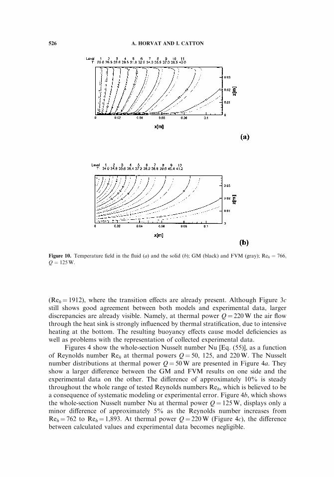
Figure 10. Temperature field in the fluid (a) and the solid (b); GM (black) and FVM (gray); Reh ¼ 766;
Q ¼ 125W.
526 A. HORVAT AND I. CATTON
5.2. Temperature Distribution in Heat Sink
The detailed temperature fields at different Reynolds number Reh give aninsight into the heat transfer conditions in the studied heat sink. For calculationsperformed by the GM, 346140 mesh points in the x and z directions were used tosimulate heat transfer processes in the fluid and solid phases. As the accuracy of thesemianalytical GM is essentially connected with the number of orthogonal functionsused for expansion, Eq. (37), 45 basis functions are used in all cases presented. Basedon the consistency analysis performed, we are convinced that the maximum asso-ciated error can reach up to 1% for the highest tested Reynolds number Reh.
It should be also noted that although different heating power Q is used at thebottom, there exists a similarity in forced–convection heat removal from the heatsink structure. Namely, higher heat input causes higher absolute temperature levels,whereas the form of isotherms changes only slightly, due to modification in airmaterial properties. Therefore, this article presents the velocity profiles and tem-perature fields only for thermal power Q¼ 125W.
Figure 5 gives velocity profiles of the air flow at different Reynolds numbersReh. The core of the simulation domain has a flat velocity profile due to dragassociated with the submerged pin-fins. As the drag is smaller at lower Reynoldsnumbers Reh, the boundary layers close to the bottom and the top are much better
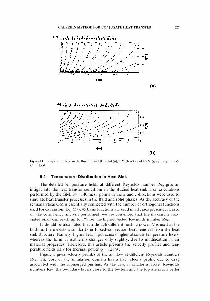
Figure 11. Temperature field in the fluid (a) and the solid (b); GM (black) and FVM (gray); Reh ¼ 1255;
Q ¼ 125W.
GALERKIN METHOD FOR CONJUGATE HEAT TRANSFER 527
resolved. Nevertheless, the GM cannot resolve the boundary layer correctly. Com-pared to the FVM it overpredicts the boundary-layer thickness and therefore reducesthe wall friction (Horvat [17]).
Figures 6–13 show the temperature field cross sections at different Reynoldsnumbers Reh. The temperatures are in degrees Celsius. Figures marked (a) presentthe temperature field in fluid flow, whereas figures marked (b) reveal the temperaturefield in the solid structure; black lines mark isotherms calculated with the GM,whereas gray lines mark isotherms calculated with the FVM. Comparisons show thatthe form of isotherms as well as the absolute temperatures are close together.Larger differences occur close to the bottom due to different thermal boundaryconditions.
It is evident that the lowest temperature in the air flow is at the beginning of theheat sink; this is on the left side. Temperature raises as the air passes through theheat-exchanging structure. Therefore, the highest temperatures are expected at theexit; this is on the right side. The temperature field in the solid structure is morevertically stratified as the heat enters the structure from the bottom. As a con-sequence, the lowest temperature in the solid phase is in the upper left corner and thehighest at the bottom.
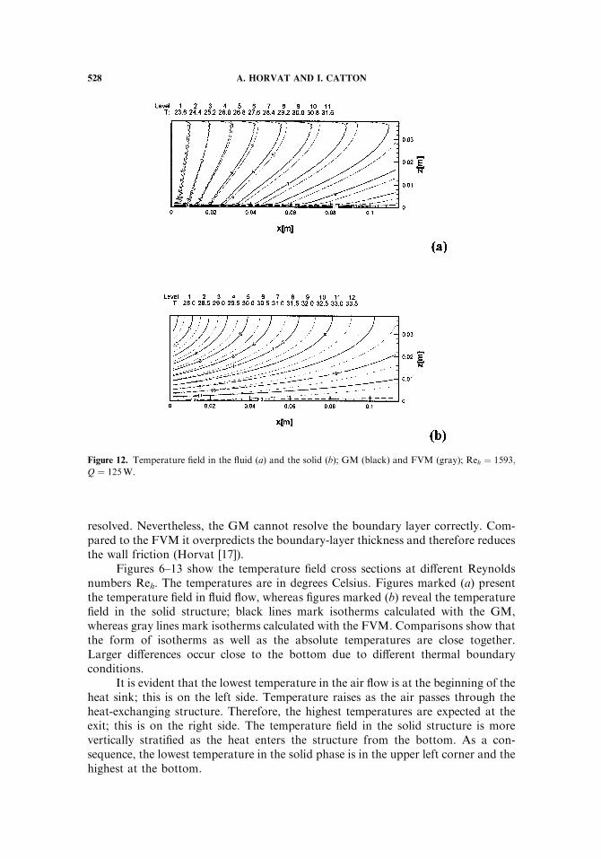
Figure 12. Temperature field in the fluid (a) and the solid (b); GM (black) and FVM (gray); Reh ¼ 1593;
Q ¼ 125W.
528 A. HORVAT AND I. CATTON
The heat flux is a vector perpendicular to the isotherms and therefore a qua-litative picture of heat flow can be extracted from the calculated temperature fields. Itcan be seen from Figure 8 that most of the heat is transferred from the solid to fluidin the first half of the test section. The highest heat fluxes appear in the lower leftcorner, where the temperature gradients are the largest. Figures 6–9 reveal that atlow Reynolds numbers, the temperature field is not fully developed. This means thatthe air which enters the test section is quickly heated due to its low velocity andleaves the heat sink at the temperature of the solid phase, unable to receive addi-tional heat from the source. With increasing Reynolds number Reh, the state ofthermal saturation diminishes (Figure 10).
The coolant flow lowers the temperature of the heat-conducting structureunequally. This directly changes the form of isotherms. The effect is not so evident atlow Reynolds numbers (Figures 6–8). On the contrary, when the Reynolds numberReh increases (Figures 9–11), the isotherms become tilted, showing the increasingvertical thermal stratification of the coolant flow.
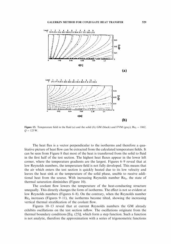
Figures 10–13 reveal that at current Reynolds numbers the GM alreadyexhibits oscillations on the test section inflow. The oscillations originate from thethermal boundary conditions [Eq. (25)], which form a step function. Such a functionis not analytic, therefore the approximation with a series of trigonometric functions
Figure 13. Temperature field in the fluid (a) and the solid (b); GM (black) and FVM (gray); Reh ¼ 1862;
Q ¼ 125W.
GALERKIN METHOD FOR CONJUGATE HEAT TRANSFER 529
produces oscillations. As the GM still predicts the temperature field with the sameaccuracy as the FVM in the first half of the simulation domain, the increasingReynolds number Reh causes differences between both solutions toward the end ofthe test section. Nevertheless, the differences for the tested range of Reynoldsnumbers Reh were not higher than 5% of the whole-section temperature increaseTg7Tin.
6. CONCLUSIONS
The article represents a contribution to conjugate heat transfer modeling. Inthis work the volume averaging technique (VAT) was tested and applied to thesimulation of air flow through an aluminum (Al) chip heat sink. The constructedcomputational algorithm enables prediction of cooling capabilities for the selectedgeometry. Using the VAT, the computational algorithm is fast-running, but still ableto present a detailed picture of temperature fields in air flow as well as in the solidstructure of the heat sink.
In the frame of the work performed, the VAT basic rules were used to developa specific form of the porous media flow model. As the flow variables were averagedover the representative elementary volume (REV), local momentum and thermalinteractions between phases had to be replaced with additional models. To close thesystem of transport equations, reliable data for interphase transfer coefficients werefound in Launder and Massey [18], Zukauskas and Ulinskas [20], and Kays andLondon [19].
The geometry of the simulation domain and the boundary conditions followedthe geometry of the experimental test section used in the Morrin-Martinelli-GierMemorial Heat Transfer Laboratory at the University of California, Los Angeles.The calculations were performed at three different heating powers, Q¼ 50, 125, and220W, and eight different pressure drops Dp. The imposed pressure drop achievescoolant flow of Reynolds number Reh from 159 to 1,862. The semianalyticalGalerkin method (GM) was developed for solving the equations. Although the GMis a well-established technique, it has not been used for conjugate heat transferproblems in heat exchanger geometries.
The calculated whole-section drag coefficient Cd and Nusselt number Nu werecompared with FVM results and with the experimental data of Rizzi et al. [21] toverify the computational model. The comparison shows good agreement betweenGM and FVM results. The experimental data exhibit up to 10% difference throughthe whole computational range of Reynolds numbers Reh, which is believed to be aconsequence of systematic modeling or experimental error.
The detailed temperature fields in the coolant flow as well as in the heat-conducting structure were also calculated and compared with FVM results. Thecalculated temperature fields in the fluid and the solid reveal up to 5% discrepancybetween the two methods, although different thermal boundary conditions at thebottom were used.
The present results demonstrate that the selected Galerkin approach is capableof performing heat exchanger calculations where the thermal conductivity of thesolid structure has to be taken into account.
530 A. HORVAT AND I. CATTON
REFERENCES
1. K. A. Antonopoulos, Prediction of Flow and Heat Transfer in Rod Bundles: Results,
Ph.D. thesis, Mechanical Engineering Department, Imperial College, London, UK, 1979.2. H. R. Barsamian and Y. A. Hassan, Large Eddy Simulation of Turbulent Crossflow in
Tube Bundles, Nuclear Eng. Design J., vol. 172, pp. 103–122, 1997.
3. A. Horvat and I. Catton, Development of an Integral Computer Code for Simulation ofHeat Exchangers, Proc. 8th Regional Meeting, Nuclear Energy in Central Europe,Portoroz, Slovenia, no. 213, 2001.
4. A. Horvat, M. Rizzi, and I. Catton, Numerical Investigation of Chip Cooling UsingVolume Averaging Technique (VAT), in B. Sunden and C. A. Brebbia (eds.), AdvancedComputational Methods in Heat Transfer VII, pp. 373–382, WIT Press, Southampton,UK, 2002.
5. I. Catton, Convection in a Closed Rectangular Region: The Onset of Motion, Trans.ASME, Feb., pp. 186–188, 1970.
6. I. Catton, Effect of Wall Conduction on the Stability of a Fluid in a Rectangular Region
Heated from Below, Trans. ASME, Nov., pp. 446–452, 1972.7. J. M. McDonough and I. Catton, A Mixed Finite Difference-Galerkin Procedure for 2D
Convection in a Square Box, Int. J. Heat Mass Transfer, vol 25, pp. 1137–1146, 1982.
8. L. A. Howle, A Comparison of the Reduced Galerkin and Pseudo-Spectral Methods forSimulation of Steady Rayleigh-Benard Convection, Int. J. Heat Mass Transfer, vol. 39,no. 12, pp. 2401–2407, 1996.
9. T. B. Anderson and R. Jackson, A Fluid Mechanical Description of Fluidized Beds, Int.Eng. Chem. Fund., 6, pp. 527–538, 1967.
10. J. C. Slattery, Flow of Viscoelastic Fluids through Porous Media, AIChE J., vol 13,pp. 1066–1071, 1967.
11. C. M. Marle, Ecoulements monophasiques en milineu poreux, Rev. Inst. Francais duPetrole, vol. 22, pp. 1471–1509, 1967.
12. S. Whitaker, Diffusion and Dispersion in Porous Media, AIChE J., vol. 13, pp. 420–427,
1967.13. P. P. Zolotarev and L. V. Redushkevich, The Equations for Dynamic Sorption in an
Undeformed Porous Medium, Dok. Phys. Chem., vol. 182, pp. 643–646, 1968.
14. F. A. L. Dullien, Porous Media Fluid Transport and Pore Structure, Academic Press, NewYork, 1979.
15. L. L. Kheifets and A. V. Neimark, Multiphase Processes in Porous Media, Nadra,Moscow, 1982.
16. P. M. Adler, Porous Media: Geometry and Transport, Butterworth-Heinemann, Stone-ham, MA, 1992.
17. A. Horvat, Calculation of Conjugate Heat Transfer in a Heat Sink Using Volume
Averaging Technique (VAT), M.Sc. thesis, University of California, Los Angeles, 2002.18. B. E. Launder and T. H. Massey, The Numerical Prediction of Viscous Flow and Heat
Transfer in Tube Banks, J. Heat Transfer, vol. 100, pp. 565–571, 1978.
19. W. S. Kays and A. L. London, Compact Heat Exchangers, 3d ed., Krieger, Malabar, FL,pp. 152–155, 1998.
20. A. Zukauskas and A. Ulinskas, Efficiency Parameters for Heat Transfer in Tube Banks,
J. Heat Transfer Eng., vol. 5, no. 1, pp. 19–25, 1985.21. M. Rizzi, M. Canino, K. Hu, S. Jones, V. Travkin, and I. Catton, Experimental Inves-
tigation of Pin Fin Heat Sink Effectiveness, Proc. 35th Natl. Heat Transfer Conf.,Anaheim, CA, 2001.
GALERKIN METHOD FOR CONJUGATE HEAT TRANSFER 531