AN EXPERIMENTAL AND ANALYTICAL STUDY OF

PANTOGRAPH DYNAMICS

by

Steven Daniel Eppinger

Bachelor of ScienceMassachusetts Institute of Technology

(February 1983)

SUBMITTED TO THE DEPARTMENT OF MECHAINICALENGINEERING IN PARTIAL FULFILLMENT OF THE

REQUIREMENTS FOR THE DEGREE OF

MASTER OF SCIENCE

at the

MASSACHUSETTS INSTITUTE OF TECHNOLOGY

May 1984

Copyright @ 1984 Massachusetts Institute of Technology

Signature of Author

Certified by

'- vnp'-1crmP

Department of Mechanical EngineeringMay 23, 1984

Thesis Supervisor

Accepted b;Warren M. Rohsenow

msiesuso el arman, Department Thesis CommitteeOFTEaGLG

JUL 1 7 1984Li F ;: p Archives

-2-

AN EXPERIMENTAL AND ANALYTICAL STUDY OF

PANTOGRAPH DYNAMICS

bySteven Daniel Eppinger

Submitted to the Department of Mechanical Engineeringon May 23, 1984 in partial fulfillment of therequirements for the degree of Master of Science.

Abstract

A study has been conducted of the performance of pantograph/catenary

systems for electrified, high-speed rail vehicles. In this thesis, a general

pantograph model is developed and augmented with specific elbow and

suspension models which represent characteristics of a particular high-speed,

intercity pantograph. The model is verified through dynamic tests conducted

on the actual device, instrumented in the laboratory. A comparison confirms

that the nonlinear model, with the proper choice of parameters, can accurately

predict pantograph dynamics for frequencies past the pantograph's second

modelled resonance. The model is to be used in computer simulations of

pantograph/catenary interactions to study overall system performance under

various conditions.

Thesis Supervisor: David N. WormleyTitle: Professor of Mechanical Engineering

Thesis Supervisor: Warren P. SeeringTitle: Associate Professor of Mechanical Engineering

-3-

Acknowledgments

Over the course of a research project and during the production of athesis, one receives the help of many friends and associates. Some of thesesupporters deserve special recognition.

This project was funded by the U.S. Department of Transportation,Office of University Research, under Grant Number DT-RS-56-81-C-00020.George Neat at the Transportation Systems Center provided the laboratoryspace for the experimental work. The technical assistance of DanDeChristoforo, of T.S.C., has been greatly appreciated. Amtrak kindly loaneda pantograph for the testing. Mike Bitsura, of The Ringsdorff Corporation,advised in the setup and operation of the pantograph.

Professor Wormley has guided this project with foresight in researchdirections. Professor Seering's generous advice and encouragement allowed therough spots to pass, eventually. His extra efforts have been deeplyappreciated. Working with these two fine researchers has been an invaluableexperience for me. Kurt Armbruster and Cal Vesely did the groundwork inthe early model development, while Dave O'Connor later finished up thecatenary work. Dave's help with the experiment and companionshipthroughout the project have been enjoyed. Gary Drlik assisted in the equationderivation and data processing.

Thanks are due to Bonnie Walters, of The Writing Program, whocommented upon previous versions of this document. Weekly technicaldiscussions with Pat Turner have helped me to gain the proper perspective onresearch issues. The kinship among the members of The Vehicle DynamicsLaboratory (Mike, Ademola, Gus, Long Chain, Dave, John, Dan, Mark, Kurt,Fort, Alex, Pat, Neal, Roberto, also "honorary members" - Joan and Leslie)has aided in the completion of many Master's Theses.

Special thanks are owed to my family: to my parents, who showed mehow to take a challenge; and to my wife, Julie, whose loving support made itpossible.

Table of Contents

Abstract 2

Acknowledgments 3

Table of Contents 4

List of Figures 5

List of Tables 5

1. Introduction 6

1.1 Background 61.2 Pantograph/Catenary Systems 71.3 Pantograph Modelling 131.4 Scope of Research 15

2. Literature Survey 17

3. Analytical Models 20

3.1 General Pantograph Model 203.2 Elbow Model 293.3 Cylinder Models 313.4 Solution Technique 363.5 Choice of Parameters 39

4. Experimental Model 44

4.1 Laboratory Setup 444.2 Experimental Procedure 474.3 Data Processing 48

5. Results 505.1 Simulation Output 505.2 Experimental Data 575.3 Model Verification 62

6. Conclusions and Recommendations 656.1 Dynamic Model Development 656.2 Recommendations for Use 66

References 68

Appendix A. Derivation of Governing Equations 71

Appendix B. Lower Arm Kinematics 80

Appendix C. Simulation Program 83

-5-

List of Figures

Figure 1-1: Common Catenary Configurations 8Figure 1-2: Common Pantograph Configurations 10Figure 1-3: Pantograph/Catenary Interaction 12Figure 1-4: Pantograph Models 14Figure 3-1: Brecknell-Willis Pantograph 21Figure 3-2: Brecknell-Willis Pantograph Mechanism 22Figure 3-3: Nonlinear Pantograph Model 24Figure 3-4: Brecknell-Willis Elbow Model 30Figure 3-5: Nonlinear Cylinder Model 32Figure 3-6: Linear Cylinder Model 32Figure 4-1: Experimental Pantograph Setup 45Figure 5-1: 2.0 Hz Simulation Time Response 52Figure 5-2: 3.5 Hz Simulation Time Response 52Figure 5-3: 4.5 Hz Simulation Time Response 53Figure 5-4: 6.5 Hz Simulation Time Response 53Figure 5-5: 8.5 Hz Simulation Time Response 54Figure 5-6: 10.0 Hz Simulation Time Response 54Figure 5-7: Frequency Response of the Nonlinear Model 56Figure 5-8: 2.0 Hz Experimental Data 59Figure 5-9: 3.5 Hz Experimental Data 59Figure 5-10: 4.0 Hz Experimental Data 60Figure 5-11: 6.0 Hz Experimental Data 60Figure 5-12: 8.0 Hz Experimental Data 61Figure 5-13: 10.0 Hz Experimental Data 61Figure 5-14: Frequency Response of the Experimental Pantograph 63Figure A-1: General Pantograph Model 72Figure B-1: Brecknell-Willis Lower Arm Linkage 81

List of Tables

Parameters for the Nonlinear Pantograph ModelTable 3-I:.

-6-

Chapter 1

Introduction

1.1 Background

Electrification of rail transport provides increased efficiency of power

conversion over conventional fossil-fuel-based rail propulsion. Some diesel

locomotives, for example, use internal combustion engines to generate power for

the electric motors which turn the wheels. It is better, however, to generate

electricity from petroleum on a much larger scale. Modern electric trains,

therefore, use power generated at large plants and thus are more efficient and

more reliable than their predecessors. The problem is then to pass the

electricity to the train as it travels.

Usually, the power is transferred to the moving train by one of two

simple means. The first lays a conducting member directly onto the rail bed,

parallel to the two main rails. Current flows through this "third rail" and is

collected by a pick-up roller on the train. This very reliable method is used

for the shorter, intracity systems where access to the underground rail area is

strictly limited.

The longer, intercity routes must use a more complex scheme, the

pantograph/catenary system. The catenary is a structure of overhead current-

carrying wires, suspended by supporting towers. A mechanical arm, known as

a pantograph, is mounted atop the train and contacts the wire, passing the

current to the train below. This scheme is favored for the longer installations

-7-

where safe access to the rail bed must be guaranteed.

1.2 Pantograph/Catenary Systems

Major sections of track have been electrified in both Europe and Japan,

and more extensive conversions are planned. Pantograph/catenary systems are

currently being used by the Japanese Shinkansen and Tokiado systems, the

TGV and SNCF lines in France, and of course, in the United States along

most of Amtrak's Northeast Corridor (Boston/New York/Washington). These

rail systems have been extremely expensive to construct. Over half of their

high capital cost can be charged to the construction of the overhead catenary

system. Great interest has been expressed in understanding how to build less-

expensive, better-performing systems and how to cheaply alter our present

systems to more closely resemble the state-of-the-art.

Catenary Styles

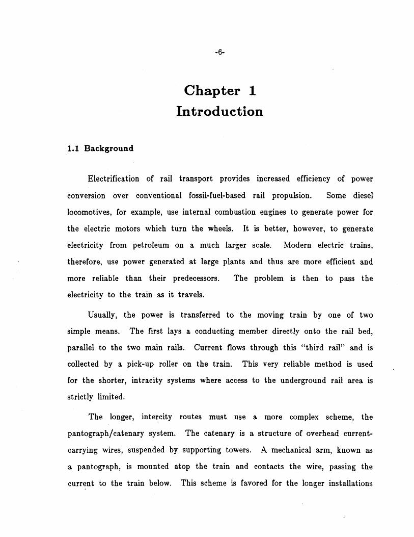
The catenary is a compliant structure of wires which sags under its own

weight and displaces upward with the contact force from the pantograph. The

support towers are quite stiff and constrain the catenary displacement at the

beginning and end of each span. Some typical catenary configurations are

shown in Figure 1-1.

The simplest catenary, a single tensioned cable suspended between towers,

is known as a trolley wire. The trolley wire, Figure 1-1a, is typically found in

low-speed systems such as Boston's MBTA green-line.

The simple catenary, Figure 1-1b, provides more uniform compliance

-8-

TOWER

(a) Trolley Wire

T--.<MESSENGER WIRE

(b) Simple Catenary

~TThrmmDROPPER

(c) Stitched Catenary

AUXILIARY WIRE

(d) Compound Catenary

Figure 1-1: Common Catenary Configurations

-9-

along the length of a span. It consists of two tensioned wires. The upper, or

messenger wire, is suspended between the towers and supports a number of

droppers from which the contact wire hangs. In this configuration the

catenary stiffness is still many times greater at the towers than elsewhere

along the span.

The stitched catenary, Figure 1-1c, employs auxiliary wires which bypass

the towers to gain more uniform stiffness. An even more complex design, the

compound catenary, shown in Figure 1-1d, uses three tensioned wires with

droppers to achieve the desired stiffness. All of the catenaries, however, have

one common deficiency: they lack uniform compliance, so the pantograph

cannot maintain a constant contact force as it travels along.

Pantograph Styles

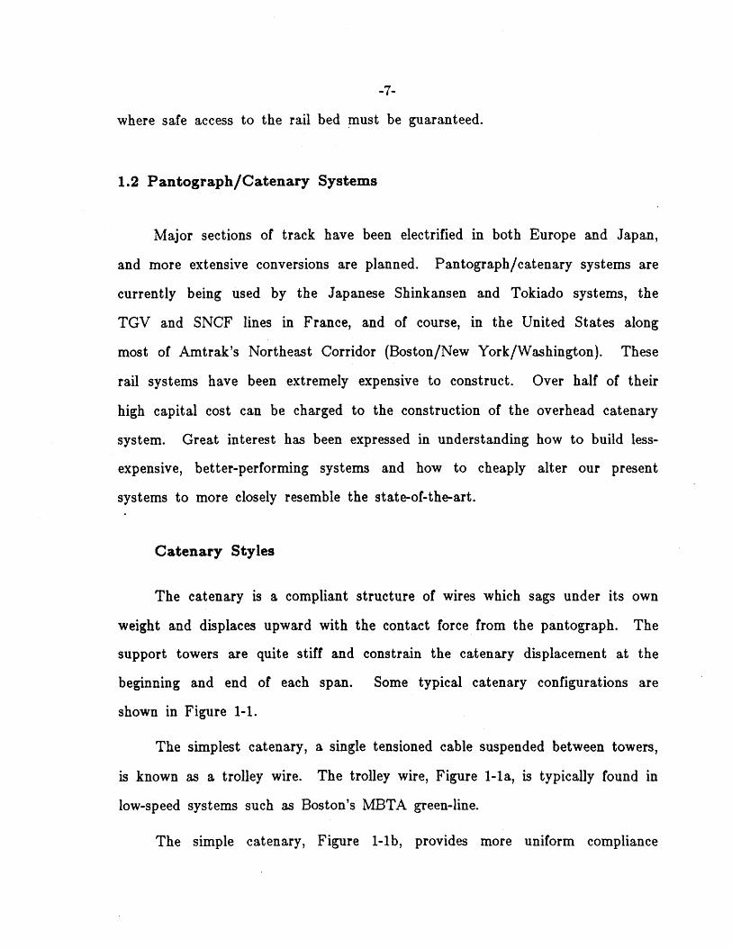
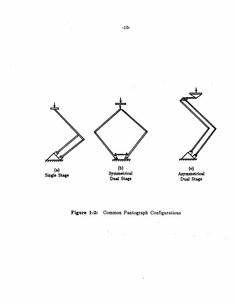
There are many different pantograph designs. Figure 1-2 displays two

common types. A simple pantograph might consist of a four-bar linkage

designed to move the contacting shoe up and down in a nearly-straight line.

Some sort of suspension, usually a spring or pneumatic cylinder, provides an

uplift force. This single-stage pantograph is sketched in Figure 1-2a. The

mass of the large frame necessary to span a broad range of operating heights

can make the pantograph clumsy and unable to respond quickly to the

changing catenary shape.

A dual-stage pantograph generally includes a large frame linkage similar

to the single-stage pantograph and a relatively light and stiff head link

designed to respond to the higher-frequency components of the catenary shape.

Again, a suspension of some kind provides the uplift force. This pantograph

-10-

(a)Single Stage

(b)SymmetricalDual Stage

(c)Asymmetrical

Dual Stage

Figure 1-2: Common Pantograph Configurations

-11-

configuration is commonly found on long-distance, high-speed trains, while the

simpler version typifies the slower, urban trolley systems. Figure 1-2b

represents a dual-stage pantograph, the August-Stemman. It is of the

symmetrical type, a five-bar linkage which requires a kinematic constraint to

insure straight-line (vertical) motion. A light head with a stiff suspension are

mounted above the symmetrical frame.

Figure 1-2c represents an asymmetrical dual-stage pantograph, such as the

Faively or Brecknell-Willis models. The lower and upper frame arms can be

considered four-bar linkages, and a head link supports the contacting shoe.

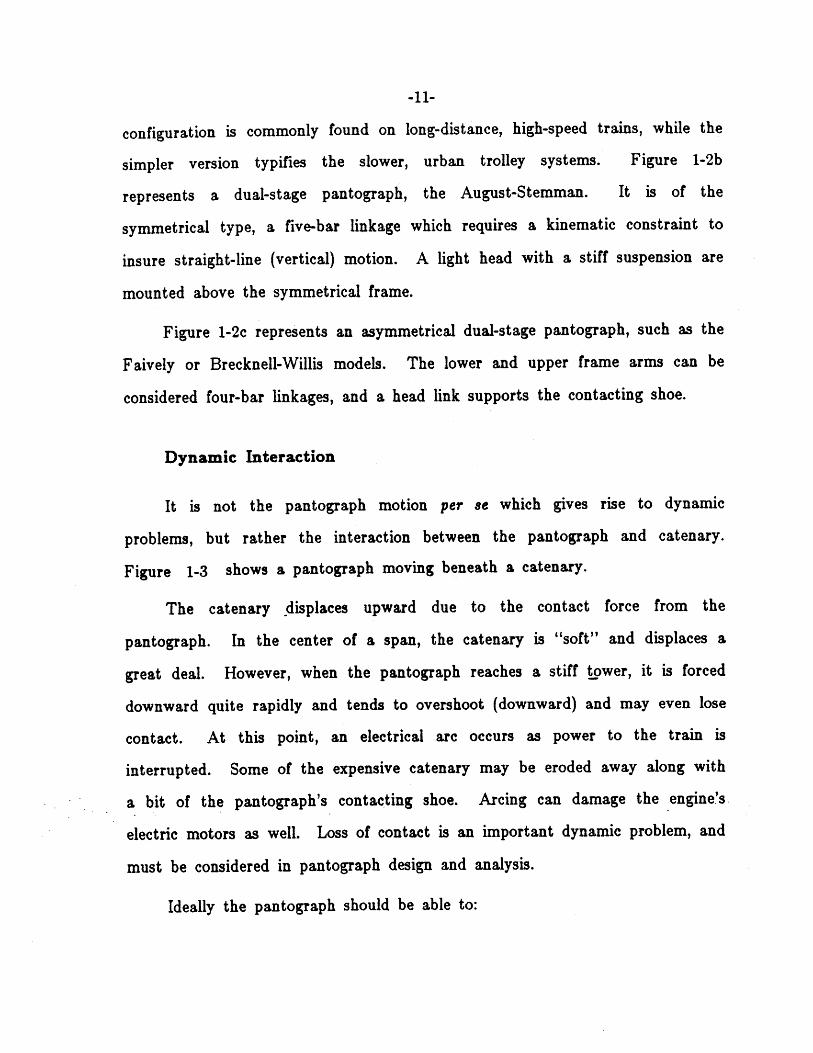
Dynamic Interaction

It is not the pantograph motion per se which gives rise to dynamic

problems, but rather the interaction between the pantograph and catenary.

Figure 1-3 shows a pantograph moving beneath a catenary.

The catenary .displaces upward due to the contact force from the

pantograph. In the center of a span, the catenary is "soft" and displaces a

great deal. However, when the pantograph reaches a stiff tower, it is forced

downward quite rapidly and tends to overshoot (downward) and may even lose

contact. At this point, an electrical are occurs as power to the train is

interrupted. Some of the expensive catenary may be eroded away along with

a bit of the pantograph's contacting shoe. Arcing can damage the engine's

electric motors as well. Loss of contact is an important dynamic problem, and

must be considered in pantograph design and analysis.

Ideally the pantograph should be able to:

-12-

CATENARY

Figure 1-3: Pantograph/Catenary Interaction

-13-

. operate at a broad range of speeds and wire heights. (The catenaryheight may be low through tunnels and high in open areas.)

" operate with a minimum of contact force (to reduce wear of thecatenary).

. never lose contact with the wire.

Since no pantograph posesses these characteristics, all are limited in operating

speed.

1.3 Pantograph Modelling

In an effort to better understand the dynamic interaction of these

systems, researchers have developed mathematical models which are used to

predict performance. While the catenary models are generally quite complex,

most pantograph models have been simple, lumped-mass representations.

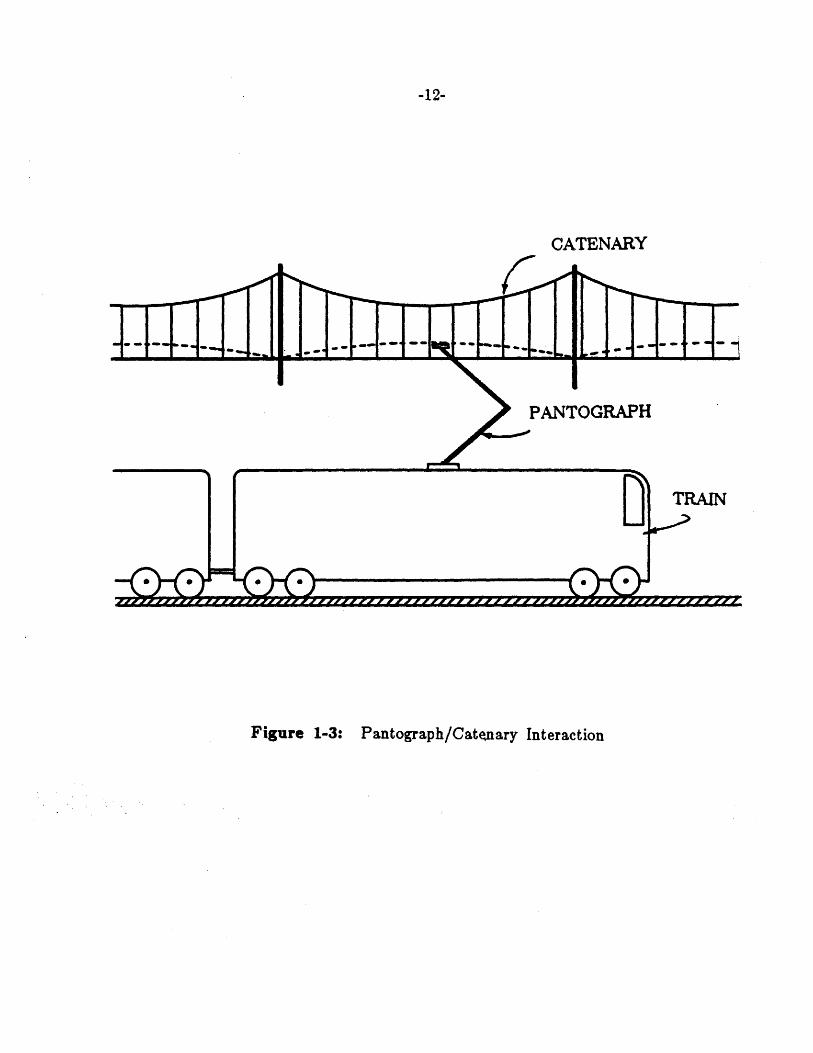
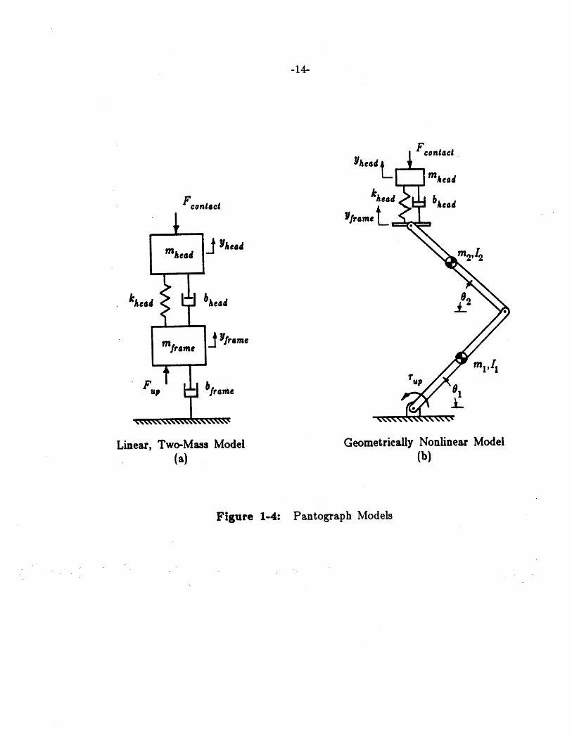
Figure 1-4a shows a typical two-mass pantograph model. The system

includes lumped masses for the pantograph frame and head, as well as

suspensions between the two masses, and from the frame to ground. Simple

nonlinearities, such as coulomb friction and nonlinear springs and dampers, can

be easily added to this type of model. However, the lumped-mass

representation does not model geometric nonlinearities of the frame, since the

masses can only move vertically.

The geometrically nonlinear model of Figure 1-4b more closely depicts an

actual pantograph. This type of model can be tailored to describe many

different system configurations, also including coulomb friction, or nonlinear

springs and dampers. A nonlinear model such as this is necessary to predict

some of the special characteristics of the pantograph response.

-14-

Yhead t -mkead

b L '

Yframe

Linear, Two-Mass Model(a)

Yframe t

m2

Tup

Geometrically Nonlinear Model(b)

Figure 1-4: Pantograph Models

-15-

Many studies of pantograph/catenary system dynamics have been

conducted using lumped-mass pantograph representations. This research

investigates the use of a nonlinear model to better predict dynamic interaction.

1.4 Scope of Research

This research is part of a broader project, sponsored by the U.S.

Department of Transportation, which aims to "understand pantograph/catenary

systems in order to determine the design parameters which significantly affect

their performance." The cost of a pantograph is quite small compared to that

of the catenary system. If a better-performing pantograph could be developed

for use with existing catenary systems in the U.S., an increase in operating

speed could be achieved. In this project, both pantograph and catenary

models have been developed to simulate dynamic interaction and study

performance.

First, a modal catenary simulation was developed which is capable of

predicting catenary response to a time-varying contact force input from a

model pantograph. For the most part, a linear, two-mass pantograph model is

used in simulating the dynamic interaction.

In parallel with the catenary work, a nonlinear pantograph model has

been developed and tested. This model considers the geometric nonlinearities

of the frame linkages, the coupling among the various links, and the nonlinear

suspension characteristics as well.

The pantograph model has been verified by correctly predicting the

dynamics of a Brecknell-Willis pantograph, which has been instrumented and

tested in the laboratory. The nonlinear pantograph model is then used in

-16-

place of the two-mass pantograph model in conjunction with the catenary

model to best predict the response of the coupled system. Finally, these

models are used both separately and together in design parameter studies

aimed at understanding the performance of various systems configurations.

This thesis presents the development and use of the nonlinear pantograph

model and the associated experimental work. The next chapter reviews recent

work in related areas. In Chapter Three, the pantograph model and

simulation are developed. The following chapter discusses the laboratory

testing of a high-speed pantograph. Chapter Five presents the results of the

two studies and their correlation. The final chapter draws some conclusions

from this project and makes recommendations concerning future research in the

area.

-17-

Chapter 2

Literature Survey

In the past twenty-five years, much research has been conducted to

understand and improve pantograph/catenary systems. Some of the more

important pantograph studies are reviewed here, while many of the catenary

works have been discussed by O'Connor [12] and Armbruster [1]. A more

complete survey of the recent literature in these areas is included in the first

annual report of this project [20].

Studies of Pantograph Dynamics

Research has concentrated on improving pantograph dynamics, since -a

better-performing pantograph makes possible the construction of less-expensive

catenaries and allows higher-speed operation under existing catenaries. Many

authors [4, 6, 7, 8, 11] suggest that reducing head mass is a key element in

improving performance. A lighter head, with less inertia, is better able to

track the high-frequency components of the wire shape. Gostling and Hobbs

[11] support this recommendation, but further suggest that the head

suspension be kept soft.

Belyaev, et al., [21 tested two Soviet pantographs and found that the

lighter of them performed better at high speeds; however, the authors were

concerned with its sturdiness. They also added viscous damping to the heads

and found that this change resulted in a more uniform contact force history in

both cases. Boissonnade [4] tested the Faiveley high-speed pantograph on the

-18-

French SNCF line. He advocates both the reduction of head mass and the

increase of head damping on all pantographs. Further he suggests that "one-

way" damping could decrease loss of contact. This nonlinear damper, resisting

only the downward motion of the head, was not tested.

Peters [131 performed tests on both the single- and dual-stage Faiveley

pantographs. He used loss-of-contact duration as the performance criterion.

Peters reports that short separations, less than 5 ms, result in small, low-

temperature, electric arcs that cause no damage to the pantograph head or

contact wire. Separations of medium duration, 5 to 20 ms, are the most

damaging to the catenary and contact shoe. For durations of greater than 20

ms, the forward motion of the train extinguishes the are. This causes loss of

power to the train, but no additional damage. Peters reports that significant

improvements were observed by increasing the uplift force and reducing the

head mass.

Recently, British rail's Research and Development Division and Brecknell-

Willis & Co., Ltd. completed the development of the "BR-BW Highspeed

Pantograph". Coxen et al., [81 report that this simple, high-performance

pantograph allows train speeds to be increased significantly for given standards

of contact loss. This asymmetrical pantograph features a light head link with

a torsional spring suspension. Flow to a pneumatic cylinder, which provides

the uplift force, passes through a small orifice, adding both stiffness and

damping to the frame at high frequencies. Airfoils are used to overcome

aerodynamic asymmetries.

At M.I.T., Vesely [171 developed a nonlinear dynamic pantograph model,

describing the August-Stemman (symmetrical) pantograph. He performed

frequency response tests in the laboratory to confirm that the model

-19-

predictions correlated well with the experimental data up to a 13 Hz excitation

frequency, above which unmodelled structural effects became important. Vesely

suggests that the two-mass model may be a suitable representation of the

actual system for displacements less than 20 cm.

Several researchers have studied the use of active elements to improve

pantograph performance. Wann [19] compared passive and several classically-

controlled active designs. He showed that active elements have the potential

to significantly improve pantograph performance. Sikorsky Aircraft [14]

mounted hydraulic actuators to the frame of an August-Stemman pantograph.

A suitable control system was not found. Belyaev, et al., [2] considered using

an active pneumatic cylinder on a TS-IM pantograph to stabilize the contact

force against the catenary. Vinayagalingam [18] simulated two active

pantograph designs, a frame-actuated controller and his own "panhead inertia

compensated" controller. Neither design showed any significant reduction in

contact force variation.

Most of the pantograph models used are geometrically linear, lumped-

mass models, such as the two-mass model shown in Figure 1-4. Both Coxen

[8] and Vesely (171 developed nonlinear pantograph models which showed good

agreement with the physical systems. The evolution of a more accurate,

generic pantograph model should aid in the further development of

pantograph/catenary systems.

This thesis presents the development of a general nonlinear pantograph

model, which is augmented with specific elbow and cylinder models to describe

the Brecknell-Willis pantograph. The model is verified through comparison

with results from laboratory testing of the actual device.

-20-

Chapter 3

Analytical Models

Several dynamic models are developed in order to study pantograph

performance. A nonlinear model, while fairly complex, is best able to predict

the pantograph behavior. First the general pantograph model is discussed, and

then the necessary elbow and cylinder models are developed to form a

nonlinear model which describes the Brecknell-Willis pantograph.

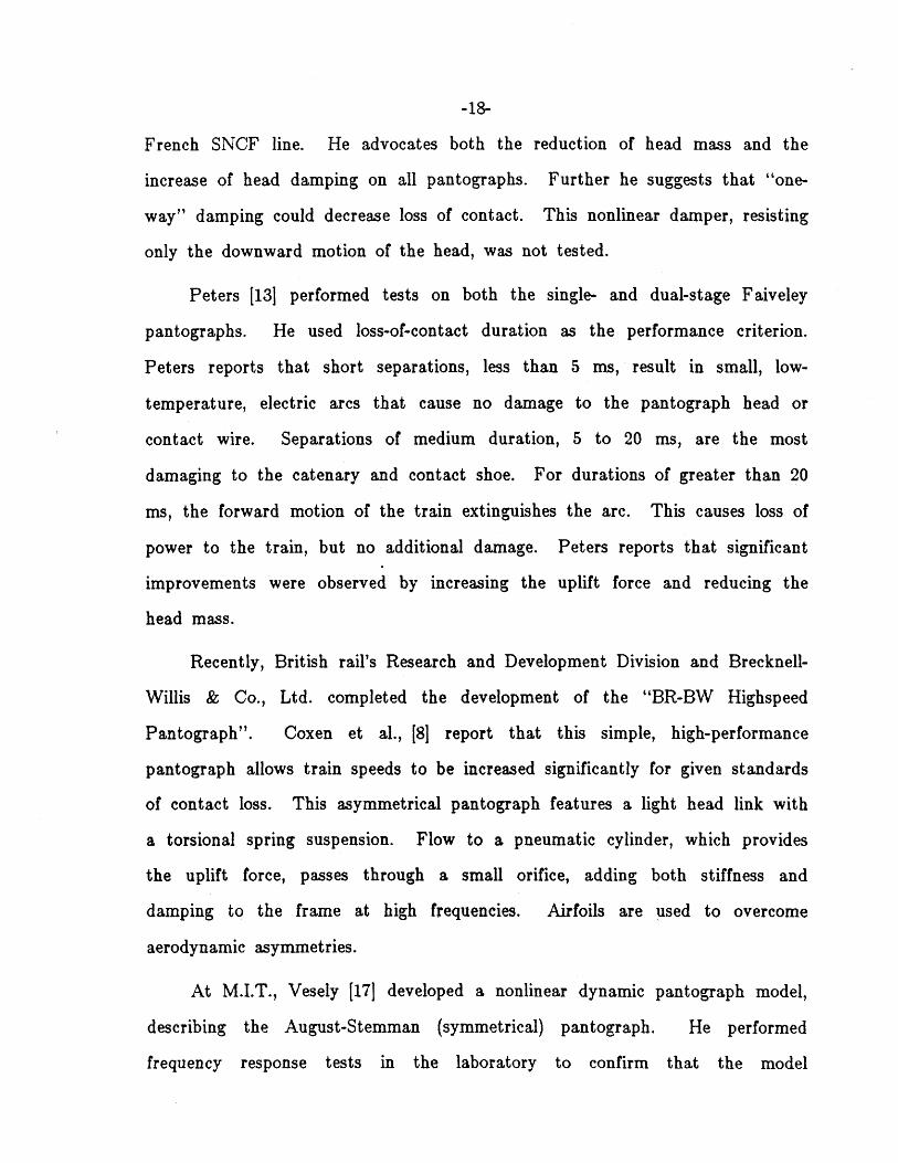
The Brecknell-Willis pantograph is of the asymmetrical type described in

Chapter 1. It consists of two frame arms which raise a head link to support

the contacting shoe. This pantograph, designed for high-speed, intercity use, is

sketched in Figure 3-1. The lower arm of the frame is actually a linkage

designed to raise the upper arm with the lower. The upper arm, a simple

four-bar linkage, provides a "datum" angle with respect to which the head link

rotates. A pneumatic cylinder gives an uplift force to the frame. As air

rushes in and out of the cylinder, it passes through a small orifice to add

damping to the system. A sketch of the Brecknell-Willis pantograph

configuration is shown in Figure 3-2.

3.1 General Pantograph Model

While the general pantograph model developed, with the proper choice of

parameters, can represent many pantograph configurations, it is presented here

to describe an asymmetrical pantograph such as the Brecknell-Willis. The

-21-

Figure 3-1: Brecknell-Willis Pantograph

Sketch Courtesy of the Ringsdorff Corporation

-22-

DATUM BAR CONTACTING SHOE

UPPER LINK

FIFTH BAR

PINION

OR

RACK

LOWER

FOURTH BAR

BASE PIVOT

ORIFICE

Figure 3-2: Brecknell-Willis Pantograph Mechanism

-23-

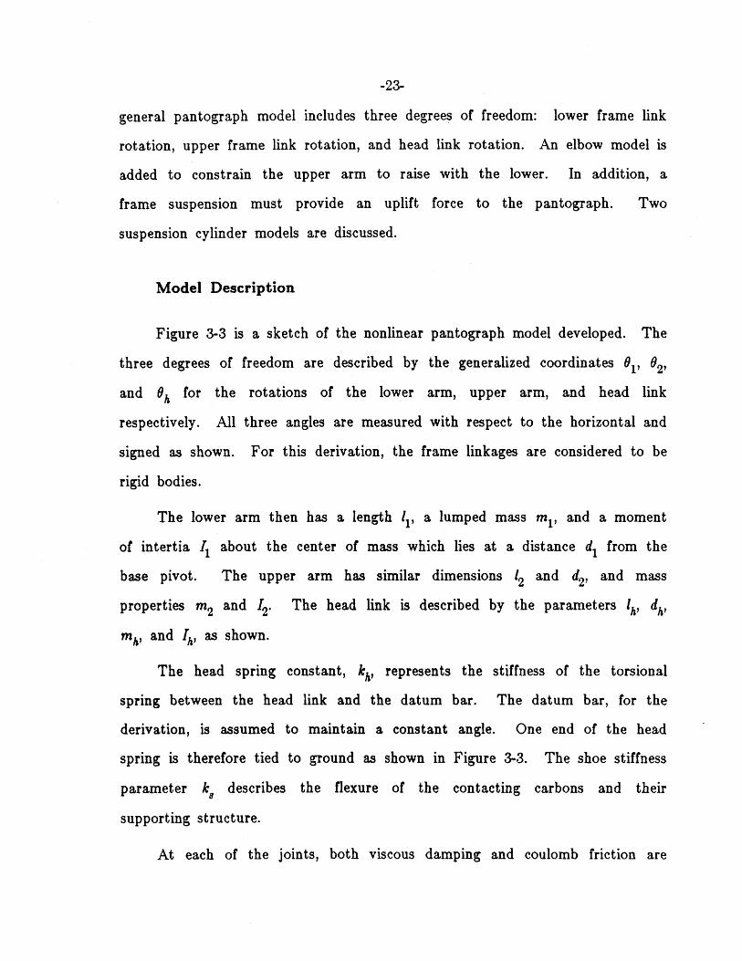
general pantograph model includes three degrees of freedom: lower frame link

rotation, upper frame link rotation, and head link rotation. An elbow model is

added to constrain the upper arm to raise with the lower. In addition, a

frame suspension must provide an uplift force to the pantograph. Two

suspension cylinder models are discussed.

Model Description

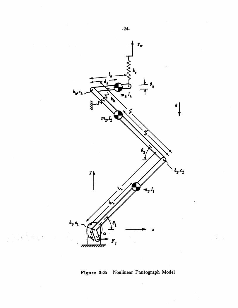
Figure 3-3 is a sketch of the nonlinear pantograph model developed. The

three degrees of freedom are described by the generalized coordinates 01, 02>

and 6h for the rotations of the lower arm, upper arm, and head link

respectively. All three angles are measured with respect to the horizontal and

signed as shown. For this derivation, the frame linkages are considered to be

rigid bodies.

The lower arm then has a length 11, a lumped mass mi, and a moment

of intertia I1 about the center of mass which lies at a distance d, from the

base pivot. The upper arm has similar dimensions 12 and d2, and mass

properties m2 and 12. The head link is described by the parameters 1h, dh,

mh, and Ih, as shown.

The head spring constant, kh, represents the stiffness of the torsional

spring between the head link and the datum bar. The datum bar, for the

derivation, is assumed to maintain a constant angle. One end of the head

spring is therefore tied to ground as shown in Figure 3-3. The shoe stiffness

parameter k, describes the flexure of the contacting carbons and their

supporting structure.

At each of the joints, both viscous damping and coulomb friction are

-24-

lh

L9 h

M2A)

1

on

Figure 3-3: Nonlinear Pantograph Model

blip Cis

I 4

-25-

included. These parameters are assigned the values b1, b2, bh, C1, c2, and ch

and are applied as shown in the sketch.

A displacement input y, models the time-varying catenary height. The

input force, F,, from the pneumatic cylinder suspension is applied at a fixed

angle a from the lower link and through a moment arm of length 1b as shown

in the sketch. This input force, which may also vary with time, not only

must overcome the weight of the links due to gravity but also must provide

an uplift force against the wire.

The elbow and suspension models are discussed below in sections 3.2 and

3.3 respectively.

Equation Derivation

The governing equations for the nonlinear model described above are

derived using Lagrange's (energy-based) method, discussed in [9]. While only a

summary of the equation derivation is presented here, the details are given in

Appendix A.

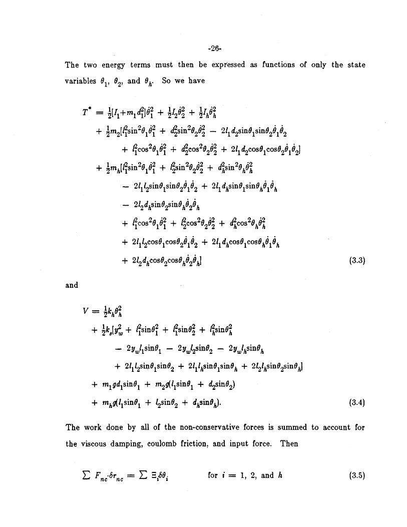
First the kinetic coenergy 20 is written as a sum of simple terms which

account for the motions of the three links.

T = (I+mid) + I2O2 + Im 2(22+y 2 ) + 2 + imh("2+i' ) (3.1)

The potential energy V is then written to include the effects of gravity and

the two springs.

V = 1kh02 + 1 k(y-yd) 2 + m gyi + m292 + mh9h (3.2)

-26-

The two energy terms must then be expressed as functions of only the state

variables 01, 02, and 6h. So we have

T ' + I22 + 7Ik

+ 2m2[ 2 61 51 + d sin2 2 - 2l 1d2sinosnO2 1O2

+ lPcos 201 2 + d4cos 225 + 2l1 d2coso cos 2O1O2J

+ {mh~lisin 26o 5 + lPsin 22 + d sin 2

- 21112sin0 1sin02 1662 + 2 lldhsinolsinohd6 k6

- 212 dhsinO2snBh2h

+ lPcos 201 5 + lPcos 2025 + d cos 20h62

+ 211 2cos 0cosO2 1 2 + 2lldhcosOlcosOl6 h

+ 212 dhcosO2cosOhO2Ohj (3.3)

and

V = k2

+ zk,[y2, + lsin02 + (fsin6 + lRsin02

- 2y~lgsin01 - 2yl 2sin02 - 2y.lhsinOh

+ 2l1, 2sinO1sin02 + 2IllhsinOjsinOh + 2l2lhsino 2sinOhl

+ migdjsin0j + m29I1sinO 1 + d2sin02)

+ mhgI1sinO1 + 12sin02 + dhsiOh)- (3.4)

The work done by all of the non-conservative forces is summed to account for

the viscous damping, coulomb friction, and input force. Then

ZFn62r- = E =A66 for i = 1, 2, and h (3.5)

-27-

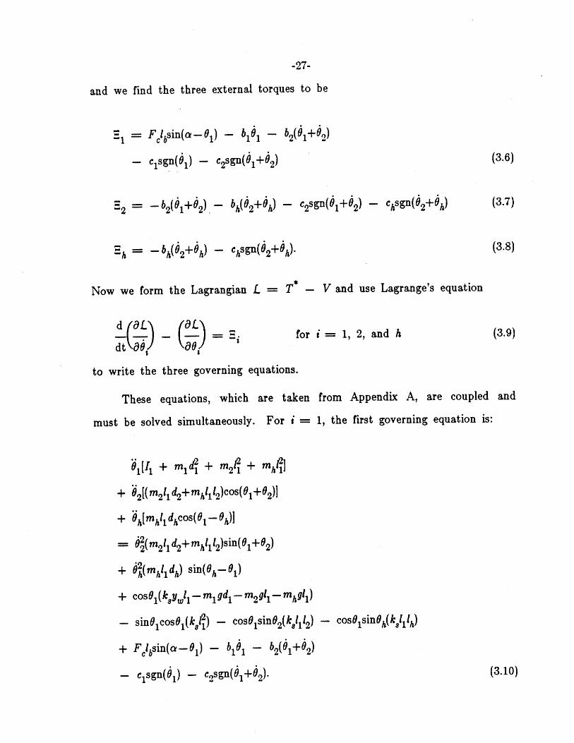
and we find the three external torques to be

= Flbsin(a -61) - - 2(

- cisgn(#1) - c2sgn(41+42) (3.6)

2= -b 2( 1+6 2). h2+6h) - c2sgn(#1+#2) ~ chsgn(#2 +#h) (3.7)

h= -0bh2+6h) - chsgn(62+#h). (3.8)

Now we form the Lagrangian L = T* - V and use Lagrange's equation

d aL foL. -. for i = 1, 2, and h (3.9)

dt a6

to write the three governing equations.

These equations, which are taken from Appendix A, are coupled and

must be solved simultaneously. For i = 1, the first governing equation is:

11+ m1 d. + m2( + mh

+ 2[(m 211 d2+ mhl12)cos(O1+02)]

+ Oh[mhIl dhcos(Ol - h)]

= 62(m 2ild2 +mhl112)sin(Ol+ 2

+ 62(mhlidh) sin(Oh-01)

+ cosO1(k,ywlI - m, gd, - m2 91 - mhg 1)

- sinO coso1(k,R) - cos61sinO2(k, 2) - cosOlsin~h(k~lilh)

+ FClbsin(a -61) -b16 b2(61+62)

- clsgn(#1 ) - c2sgn(# 1+42)' (3.10)

-28-

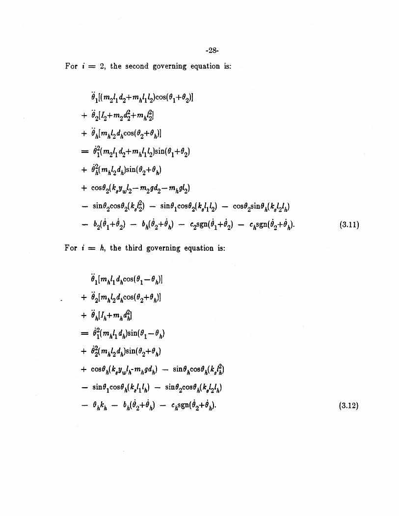
For i = 2, the second governing equation is:

Ol[(m 21ld 2+mh1l 2)cos(Ol+ 82)3

+ 2tI2+ m2d2+mh2

+ Oh[mhl2dhcos(02+ h)]

S(m 2 1 d2+mhll+ 2)sin(61+02)

+ $(hmhl 2dh)sin(02+Oh)

+ cos02(k8yw 2- m2gd2 - mhI 2)

- sinO2coso2(kl2) - sinO1cosO2(k,112) - cosO2sinoh(kl 2lh)

- b2(01+0 2) - bh( 0 2+oh) - c2sgn(01A 2 ) - chsgn(O2+h). (3.11)

For i = h, the third governing equation is:

Gllmhlldhcos(- 0h)l

+ 92[mhl 2dhcos( 0

2+Oh)I

+ OhlIh+mhdjl

= $(mh1 d h)sin(Ol - Oh)

+ j2( m 2dh)sin(02+ 0 h)

+ cosoh(k8 ywlk-mhgdh) - sinOhcosph(k1 )

- sinolcosOh(kIl1 lh) - sinO2 cosoh(k12

1h)

- Ohkh - bh(0 2 h) - chsgn(0 2+6h). (3.12)

-29-

3.2 Elbow Model

In order to provide that the upper arm generally rises with the lower,

the actual linkage sketched in Figure 3-4a must be considered. The lower arm

mechanism consists of two long links pinned a fixed distance apart at their

base ends. At the elbow ends of these links are a rack and pinion. (This

arrangement more closely resembles a sprocket and chain.) The upper arm is

attached to the pinion.

This elbow, however, is not infinitely stiff. While 62 increases with 01

for the slow motion of the pantograph, at higher excitation frequencies, the

angular velocities 01 and 62 may be of opposite sign. An elbow model must

be included to establish static and dynamic properties of 62.

An elbow link, with angle 6, measured with respect to the horizontal as

shown, represents the part of the elbow which moves with the lower arm. A

torsional spring and damper are placed between this elbow link and an

extension of the upper arm. The elbow is modelled as shown in Figure 3-4b.

The parameters k, and be are chosen to represent the torsional stiffness and

viscous damping of the transmission at the elbow. The kinematic relation

between 6, and 61 is derived for the true configuration of Figure 3-4a instead

of the four-bar linkage sketched.

To incorporate this elbow model into the general pantograph model, we

must add the potential energy term

V = k,(6, - 62)2 (3.13)

and the non-conservative work term

-30-

Brecknell-Willis Elbow ModelFigure 3-4:

-31-

F= -- b(#e - #2)(86e - 62). (3.14)

Of course, we do not change the kinetic coenergy term T* since no mass or

inertia has been added.

Now 6 e and 6. must be expressed as functions of the state variables 6166e

and #1. We will also need - as a function of 01. These kinematic relations66~

are derived in Appendix B, although not in closed form. For the governing66

equations, we will continue to use the symbols, 6, e, and -o as necessary.601

Using Lagrange's equation, Equation (3.9), we simply add the two torque6 6

terms ke(6e-62)-- and -b,(O,-52)-e to the left- and right-hand sides of66, 6

Equation (3.10) respectively. Also we add the terms k,(02-0,) and -be(O6 2)

to the left- and right-hand sides of Equation (3.11).

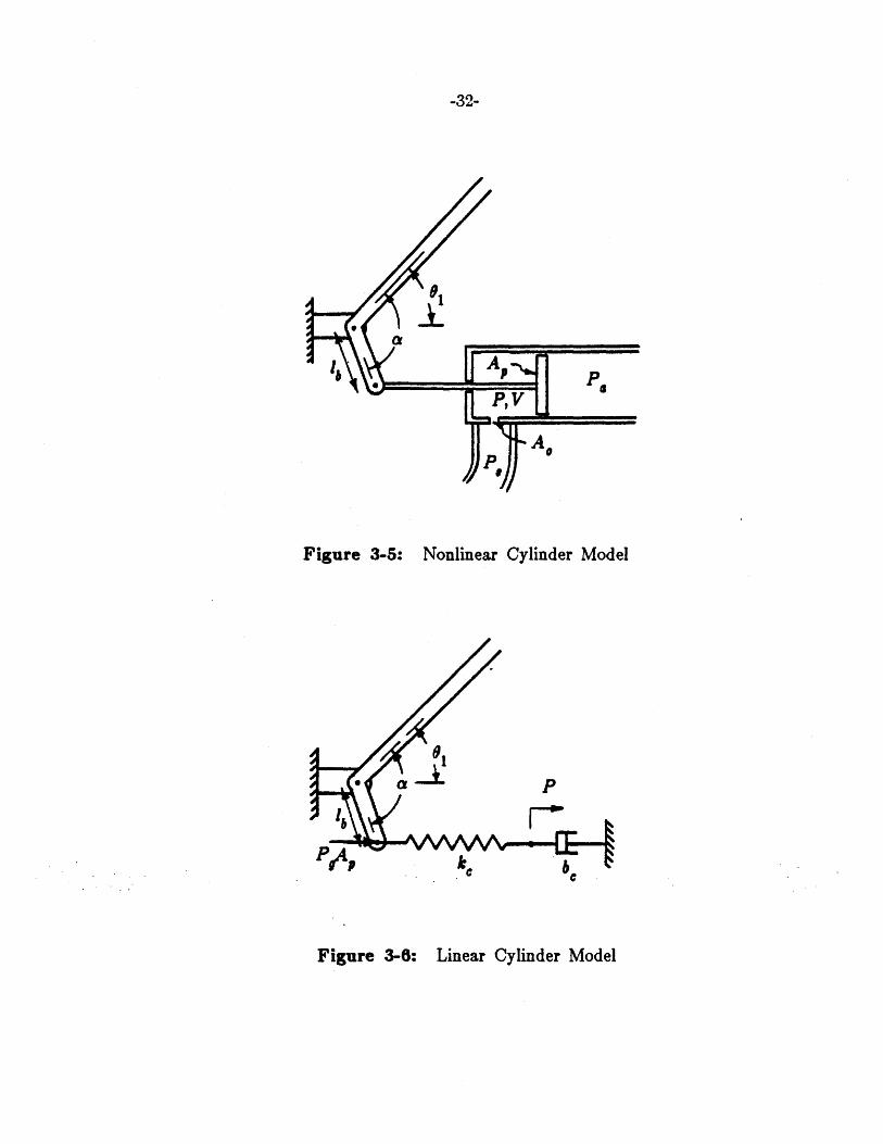
3.3 Cylinder Models

Two different models for the pneumatic suspension were developed. The

nonlinear cylinder model Figure 3-5, considers the air to be an ideal gas which

compresses reversibly. The flow is resisted as it passes through the small

orifice to or from the constant supply pressure. The linear cylinder model,

Figure 3-6, treats the compressible fluid as a simple spring and the orifice as a

viscous damper in series.

Either cylinder model adds a new state variable, P, to the list of

generalized coordinates used in the pantograph model. Therefore, for each

case, we must derive a differential equation for the new state of the form

P= f (61 01, P) and then couple the two systems by defining the input force

F,= f (61, P).

-32-

A,

Figure 3-5: Nonlinear Cylinder Model

P

P0A

Figure 3-6: Linear Cylinder Model

-33-

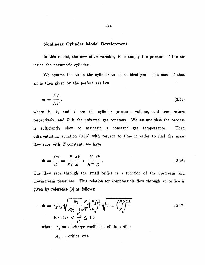
Nonlinear Cylinder Model Development

In this model, the new state variable, P, is simply the pressure of the air

inside the pneumatic cylinder.

We assume the air in the cylinder to be an ideal gas. The mass of that

air is then given by the perfect gas law,

PVm = - . (3.15)

RT

where P, V, and T are the cylinder pressure, volume, and temperature

respectively, and R is the universal gas constant. We assume that the process

is sufficiently slow to maintain a constant gas temperature. Then

differentiating equation (3.15) with respect to time in order to find the mass

flow rate with T constant, we have

dm P dV V dP- = - - + (3.16)dt RT dt RT dt

The flow rate through the small orifice is a function of the upstream and

downstream pressures. This relation for compressible flow through an orifice is

given by reference [3] as follows:

27 P, Pg P1-T = CdA, - 1 - -r (3.17)

R(3-I1)V T P, PUP U

for .528 < d < 1.0PU

where c = discharge coefficient of the orifice

A, = orifice area

-34-

7 = ratio of specific heats for the gas

PU = upstream pressure

Pd = downstream pressure.

Equating the mass flow rates through the orifice and into the cylinder,

we eliminate rh and have the differential equation for the pressure.

dP R TcdAO 2-y P P P P dV- -~( 1 - - - (3.18)dt V R(-1)Vr P, PU V dt

where Pd = P and PU =P, for P < P,

and Pd = P, and Pu = P for P > P8.

To implement this cylinder model, the differential equation for the

pressure is integrated along with the governing equations for the paitograph.

To couple the differential equations, we solve for the. cylinder volume as a

function of the lower frame link position, 61, and substitute into Equation

(3.18)

V = V* + Aplbcos(ac-Ol) (3.19)

and

dV.- = A,6 1sin(a - 1) (3.20)dt

where V0 is the cylinder volume when (a- 1)= ir and A, is the piston surface

area. Now we have

RTcdA. 2" - P P 1 - P

V*+APIos(a -6 1) R(--1) v T Pk P

-35-

PA,6 1sin(a -0 1) (3.21)

V*+Aplbcos(a - 1)

Finally, to couple the cylinder force to the pantograph, we substitute into

the first pantograph differential equation

FC = (P - Pa)AP (3.22)

where Pa is the atmospheric pressure. Note that under static conditions,

61=0 and for P to be zero, Pd=P,, so the pressure, P, must equal the

absolute supply pressure, P,. So

Fetatic = (Ps~Pa)A* (3.23)

Linear Cylinder Model Development

In the linear model, the new state is the displacement P of the point

between the spring and damper, as shown in Figure 3-6.

The differential equation governing the motion of P can be obtained by

summing the two forces which act on the point.

kc[P - lcos(a--1)] + bP = 0. (3.24)

Now, solving for P

kP = -[lcos(a-61) - P1. (3.25)

bc

-36-

The force applied to the lower link is found by adding the spring tension to

the external force

F = PA, + k0[P - lbcos(a-01)] (3.26)

where P is the supply gage pressure, Pg=P,-Pa-

To implement this linear cylinder model, the differential equation for the

motion of the point P, Equation (3.25), is integrated along with the governing

equations of the pantograph. To couple the cylinder model to the pantograph,

we substitute the input force given by Equation (3.26) into the first

pantograph equation. Note that under static conditions, the force applied to

the lower link is

Ftatic =P gAp (3.27)

as in the nonlinear case.

3.4 Solution Technique

The governing equations for the general pantograph model are a set of

three coupled, second-order differential equations. Before integrating, the

second derivative terms are decoupled by their simultaneous solution.

We first write Equations (3.10), (3.11), and (3.12) in a convenient form.

A0 + B02 + COh = D

E61 + F2 + Gh = H (3.28)

I + 02 + KOA = L

-37-

where

B = (m 211d2+mhllI2)cos(01+02)

C = mhll dhcos(Ol- Oh)

DO( 2 I2ld 2+mhlI2)sn(01+02)

± O(m lldh) Sjn( 0h- 01)

+ coso l(k 8 yI, 1- mlgd1- m2g11- mfgl1)

-sinolcoso l(k1) -cos9 1sino 2( k8!1!2) -cssih(k,! k

+ FC1sin(a-Ol) - l 611 - b2 (01A0)

- cs sgn(0 1) - c2sgn( 1 +0)

E = (m 2 1 d2 ±mhlll2)cos(01±02)

F = 12+m 2d22+mhp~l

GC mhl 2dhcos(02+oh)

H = 02(m 2 lid2+mftlil2)sin(01+0 2)

+ 0(m mh2 df)sin( 02± 0h)

+ cos02 (kSYWl 2 - m2gd 2- Mhgl 2)

-sin 2 coso 2 ( k8P2) - sin01 coso2( k8!1!2) - coso 2sinoh( k82!f)

- 2(61+0) - bh( 02+ 6) - c2sgn(0 1±0) - chsgn(O 2 +Ok)

I = mhlldhcos(l-oh)

J = mhl2dhcos( 02+0h)

K = Ih+mhd~h

L = 62(m 11dh)sin(l - h)

+ 02( mh!2dh)sin(6+ )

-38-

+ cos~hwk-mhgdh) - sin0hcos0h(kl)

- sinOlcoso0sllh) ~ sino 2cosoh(k12

1h)

- Ohkh - bh(i2+ih) - csgn(O2+ih). (3.29)

Using any suitable means (Cramer's rule, matrix inversion, or Gaussian

elimination and back-substitution [161), we can find decoupled expressions for

the three accelerations.

DFK + BGL + CHJ - LFC - HBK - DJG

AFK + BGI + CEJ - IFC - EBK -AJG

AHK + DGI + CEL - IHC - EDK -ALG

02 AFK + BGI + CEJ - IFC - EBK - AJG (3.30)

AFL + BHI + DEJ - IFD- EBL- AJH

6 h AFK + BGI + CEJ - IFC- EBK- AJG

A numerical integration routine, based on the fourth-order Runge-Kutta

method [15], is used to solve the differential equations for the time response.

This integrator only works with first-order equations, so to the three

acceleration equations, we add three (trivial) equations defining the velocity

states. Finally, we choose one of the two cylinder equations and have seven

first-order equations to determine the solution for the states

O, 0 , 02, 0 h ih, and P.

The equations of motion are coded into a FORTRAN subroutine, EQSIM,

included in Appendix C The software package DYSYS, used at M.I.T.'s Joint

Computer Facility, provides the Runge-Kutta integrator and the necessary

plotting routines.

-39-

3.5 Choice of Parameters

The many parameters for the nonlinear pantograph model, Figure 3-3, are

listed in Table 3-I along with the values chosen to describe the Brecknell-Willis

pantograph tested.

The physical dimensions 11, 12, and 1h representing the three link lengths

were taken from the pantograph set up in the laboratory, and then verified

with dimensions extracted from a set of assembly drawings, supplied by The

Ringsdorff Corporation.

The masses mi, M2, and m., the moments of inertia I, 12, and Ih, and

the distances to link centers of mass d1, d2, and dh, were estimated from

known link properties.

The input spring constant, k,, corresponds to the stiffness of the

contacting shoe and its supporting structure. Its value was determined by

removing the head, supporting it rigidly at the points where the apex frame

attaches, and measuring both applied force and deflection of the carbons in a

series of tests.

The head spring rate, kh is a nonlinear function of the angle, 0 h. The

spring includes the effects of the stop which limits the head rotation. The

torques necessary to deflect the head link in both directions were recorded,

along with the induced rotations.

The stop was found to be less than five times as stiff as the torsional

spring designed to provide the stiffness kh. Furthermore, the torsion bar is

preloaded in such a way that for the small deflections of Oh encountered in the

laboratory testing, the head spring is always in the region governed by the

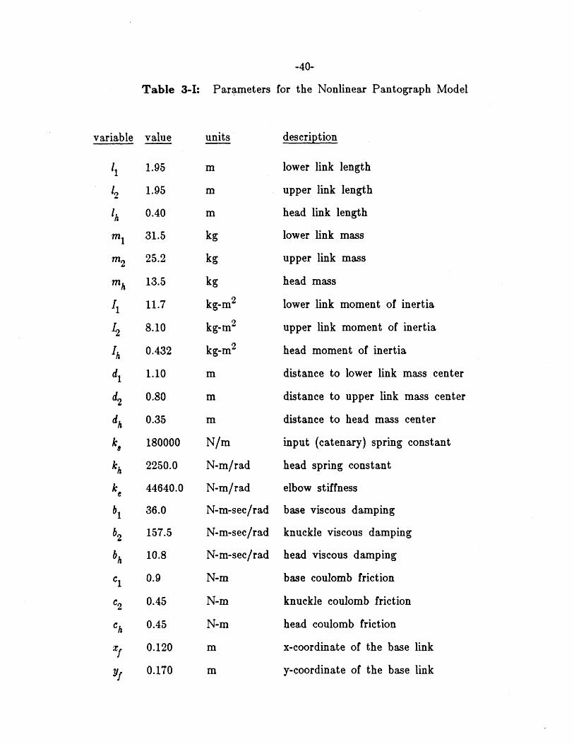
Table 3-I: Parameters

variable value units

11

12

1h

m2

mh

I,

12

Ik

di

d2

dh

k e

kh

k,

bi

C2

Ch

x,yf

1.95

1.95

0.40

31.5

25.2

13.5

11.7

8.10

0.432

1.10

0.80

0.35

180000

2250.0

44640.0

36.0

157.5

10.8

0.9

0.45

0.45

0.120

0.170

m

m

m

kg

kg

kg

kg-m2

kg-m2

kg-m2

m

m

m

N/m

N-m/rad

N-m/rad

N-m-sec/rad

N-m-sec/rad

N-m-sec/rad

N-m

N-m

N-m

m

m

-40-

for the Nonlinear Pantograph Model

description

lower link length

upper link length

head link length

lower link mass

upper link mass

head mass

lower link moment of inertia

upper link moment of inertia

head moment of inertia

distance to lower link mass center

distance to upper link mass center

distance to head mass center

input (catenary) spring constant

head spring constant

elbow stiffness

base viscous damping

knuckle viscous damping

head viscous damping

base coulomb friction

knuckle coulomb friction

head coulomb friction

x-coordinate of the base link

y-coordinate of the base link

-41-

Table 3-I,

le

00

lb

a

A,

AO

V*0

Pg

R

17

Cd

P,

T

k9

b,

g

0.082

-0.164

0.235

1.82

0.0123

0.00000314

0.000996

710185.0

287.0

1.40

0.60

101000.0

293.0

162000.0

90000.0

9.80665

continued

m length of the elbow link (pinion radius)

rad initial value of Oe (for 01=0)

m moment arm length for cylinder

rad angle between lower link and moment arm

m2 piston surface area

m2 orifice area

m3 cylinder volume when (a-6) r

N/m 2 supply gage pressure

m2/sec 2-K universal gas constant

(dimensionless) specific heat ratio

(dimensionless) discharge coefficient

N/m 2 atmospheric pressure

K cylinder temperature

N/m simple cylinder spring

N-sec/m simple cylinder damper

m/sec2 gravitational acceleration

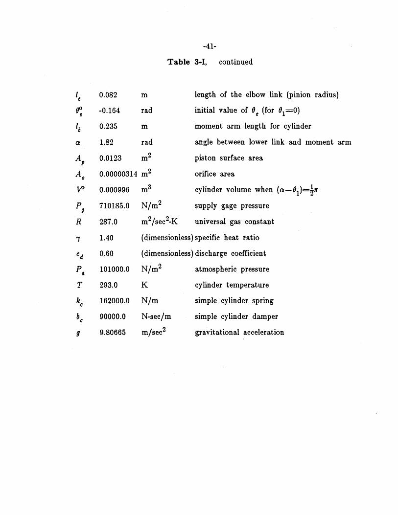
-42-

stop stiffness. Therefore, the constant chosen for kh, given in the table,

represents only the stiffness of the stop.

The elbow stiffness, ke, was found by measuring force and deflection at

the top of the upper arm with the lower arm fixed. The relation was

observed to be linear within the accuracy of the measurements made, and the

calculated value for k. appears in the table.

The viscous damping constants, b1, b2, and bh, for the three joints were

estimated by matching the peak amplitudes predicted by the simulation output

at the resonant frequencies with those observed in the experimental data at

the same frequencies.

The coulomb friction observed in the pantograph was very low so the

values cl, c2, and ch were set to small values in the absence of a suitable

model for the stiction which may have a greater effect.

The dimensions x. y. 1,, and e which affect the elbow linkage

kinematics were measured on the pantograph. The dimensions t b and a,

describing the short arm through which input torque is applied, were also

measured in the laboratory and confirmed by the assembly drawings.

The piston area A , and orifice area A, were measured by removing the

necessary parts from the cylinder. The cylinder initial volume V* was

calculated from the known cylinder dimensions. The supply gage pressure, P,,

was found from the regulator setpoint.

The values for the gas properties R and 7 were found in tables. The

discharge coefficient cd describes a sharp orifice. The ambient pressure and

temperature were used for Pa and T. For the simple cylinder model, the

stiffness kc describes the compression of the gas that would be trapped in the

-43-

cylinder if the orifice were blocked. A value for kc was chosen by linearizing

the compression of the ideal gas about the static pressure operating point.

The value for the cylinder damping, be, was chosen by matching the linear

cylinder pressure output to the experimental pressure data.

The usual value for the gravitational acceleration, g, was used.

-44-

Chapter 4

Experimental Model

An experiment was performed in the laboratory to verify that the

nonlinear model is an accurate representation of a real pantograph. A

Brecknell-Willis pantograph was instrumented, and its dynamic response to a

range of displacement input recorded for analysis. This chapter discusses the

dynamic testing conducted at the U.S. Department of Transportation's

Transportation System Center (TSC) in Cambridge, Massachusetts.

4.1 Laboratory Setup

A Brecknell-Willis "high-speed" pantograph was obtained from Amtrak

and set up in the TSC laboratory. The pantograph was fixed to a steel base

plate, and a structure of steel beams erected to support a hydraulic input ram

and instrumentation. A supply of compressed gas (nitrogen) was provided to

operate the pneumatic system which raises the pantograph. Figure 4-1 depicts

this laboratory setup.

The servo-controlled hydraulic ram simulated a sinusoidal catenary over a

range of frequency. The ram, mounted above the pantograph, excited the

system with a displacement input at the contacting carbons. A function

generator provided the time-varying input signal to the servo controller. An

LVDT measured the ram's position output for feedback and for reference.

In some tests, the ram was rigidly attached to the center of the carbons.

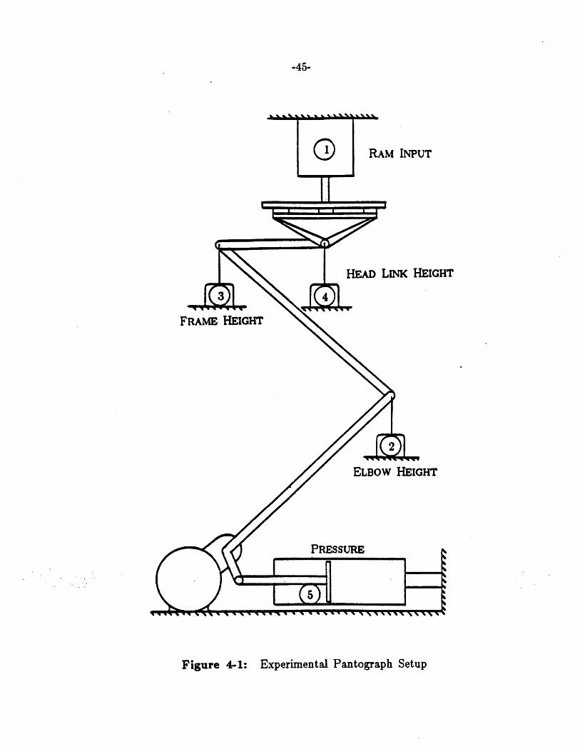
-45-

FRAME HEIGHT

RAM INPUT

HEAD LINK HEIGHT

2

ELBOW HEIGHT

PRESSURE

Figure 4-1: Experimental Pantograph Setup

-46-

This configuration corresponds to the simulated test case in which the catenary

spring, k, can both push down and pull up on the head. Further tests were

run in which the ram was not attached, and could only push down, which is

case is more representative of the pantograph operating under a catenary.

Three position displacement transducers, by Celesco Transducers

Products, measured the response of the three rotational state variables. These

transducers, called stringpots, simply consist of precision conductive-plastic,

rotary potentiometers that have cable wrapped around their input shafts with

light return springs.

One stringpot, attached at the pantograph "elbow", measured the lower

link position. The second stringpot, attached to a point at the top of the

pantograph frame, recorded the overall motion. The remaining one measured

the height of the end of the head link. The difference between the first two

stringpot signals gave the upper frame link motion, while the difference

between the second and third signals gave the head link motion. The

potentiometers allowed the use of a simple voltage divider circuit to output a

voltage proportional to linear displacement. The input voltage to each

transducer was "tuned" to attain zero output at the static operating point.

A differential pressure transducer, by Validyne Engineering Corporation,

measured the pneumatic cylinder pressure. One side of the diaphragm was

maintained at the supply pressure, while the other side contained the cylinder

pressure. In this configuration, the transducer output represents the pressure

drop across the small orifice at the cylinder input. The transducer was of the

variable-reluctance type, so it required an AC carrier signal and a demodulator

to produce the desired DC output. A Tektronix differential amplifier was used

to subtract the DC offset from the pressure signal.

-47-

A Racal FM data recorder was used to store the transducer outputs on

magnetic tape for later analysis. Five channels of data were recorded:

1. ram LVDT output

2. elbow stringpot output

3. top-of-frame stringpot output

4. head stringpot output

5. pressure transducer output

The first signal records the time-varying input height, while the

remaining four channels represent the response of the pantograph's four degrees

of freedom, 01, 02, 64, and P.

4.2 Experimental Procedure

A summary of the experimental procedure follows.

After the pantograph and instrumentation were set up as described,

pressure was applied to the pneumatic cylinder. To avoid the transient

associated with filling the system to operating pressure, supply pressure was

temporarily routed to both sides of the differential pressure transducer. This

prevented damage to the diaphragm before the operating point was reached.

Next, the hydraulic pump and cooling system were started. With a low-

frequency, zero-amplitude input signal, the servo controller was turned on.

The input voltage was applied to the stringpots, and the carrier signal to

the pressure transducer. All five circuits, including the ram setpoint, were

then tuned to achieve zero output at the static operating point. To maximize

-48-

the dynamic range of data stored on the tape recorder.

Then, with the desired frequency and amplitude set, the five channels of

data were recorded onto the tape.

Data were taken at 0.5 Hz intervals from 1.0 to 15.0 Hz. Data were

obtained for the cases with the head both rigidly attached to, and detached

from the ram. Many input amplitudes were applied, and frequency was swept

both up and down to observe various nonlinear effects.

The five (analog) channels of experimental data were digitized wtih an

analog-to-digital (A/D) converter. The data were then processed digitally to

obtain the desired output states.

4.3 Data Processing

The analog data were transported on magnetic tape to the Machine

Dynamics Laboratory at M.I.T. The five channels were played back

simultaneously with the Racal tape recorder into a Datel A/D converter on the

Digital PDP 11/44 minicomputer in the laboratory. Each channel was sampled

every 2 ms (500 Hz) for two seconds. The digital data were ouput to files for

processing.

The raw data files were transferred on disk to M.I.T.'s Joint Computer

Facility, where the processing was to be completed. The data arrays were

scaled, first by the recording levels to obtain the recorder input voltage

amplitudes, and then by the instrumentation sensitivities to find the actual

pressure and displacement information. Next, the elbow column was

subtracted from the top-of-frame column to obtain the displacements of the

-49-

upper link with respect to the lower link. The top-of-frame column was then

subtracted from the head column to yield the head displacements with respect

to the top of the frame. Finally, the five columns of data were slightly offset

for plotting.

Of the 20 seconds of data recorded at each frequency of excitation, only

1.6 seconds were digitized, and only one second of data actually plotted.

-50-

Chapter 5

Results

A comparison is made of the two pantograph representations discussed in

the previous chapters. The simulation output is compared with the processed

experimental data to verify that the analytical model can be used to

accurately predict the actual pantograph dynamics.

5.1 Simulation Output

The general pantograph model developed in Chapter Three was

augmented with the linear cylinder and elbow models in order to describe the

Brecknell-Willis pantograph tested.

The input height, y,, was a sinusoidal displacement of peak-to-peak

amplitude 3.7 mm added to the static operating height of 1.58 m. Input

frequency ranged from 1.0 to 30.0 Hz.

In these simulations, the top spring, k,, was able to apply forces both up

and down to the head, modelling the case in which the ram was attached

rigidly to the contacting carbons.

For the modelled system, which acts somewhat like a three-mass, four-

spring system, we expect to observe three second-order resonances, and one

first-order lag. In fact, we do see just that. The system resonances are at

roughly 4.25 Hz, 8.75 Hz, and 19.5 Hz. The first-order cylinder state, P,

always follows the lower frame link state 61, as expected. The time constant

-51-

bedescribing the cylinder response is r = -.

kc

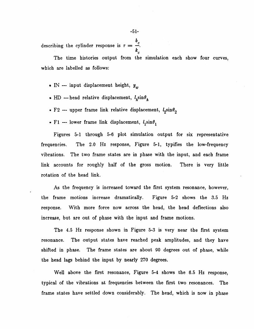
The time histories output from the simulation each show four curves,

which are labelled as follows:

* IN --- input displacement height, y.

* HD --- head relative displacement, ihsinh

* F2 --- upper frame link relative displacement, l2sin 2

* F1 --- lower frame link displacement, lisinol

Figures 5-1 through 5-6 plot simulation output for six representative

frequencies. The 2.0 Hz response, Figure 5-1, typifies the low-frequency

vibrations. The two frame states are in phase with the input, and each frame

link accounts for roughly half of the gross motion. There is very little

rotation of the head link.

As the frequency is increased toward the first system resonance, however,

the frame motions increase dramatically. Figure 5-2 shows the 3.5 Hz

response. With more force now across the head, the head deflections also

increase, but are out of phase with the input and frame motions.

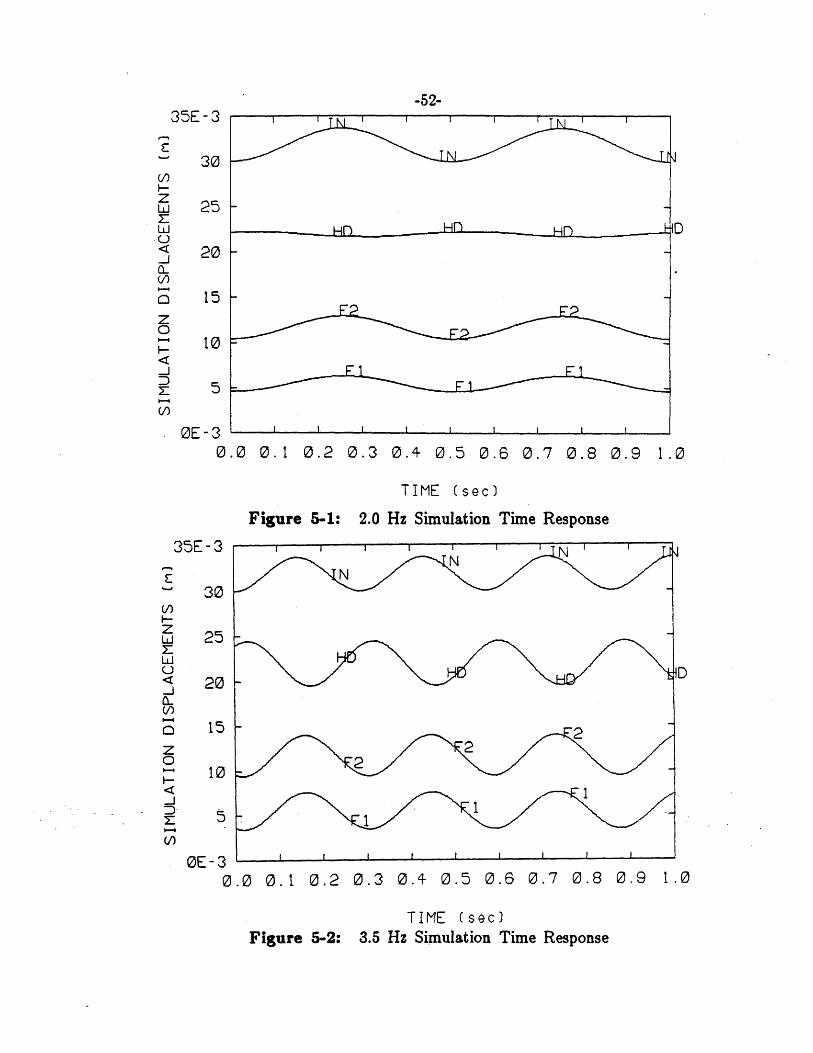
The 4.5 Hz response shown in Figure 5-3 is very near the first system

resonance. The output states have reached peak amplitudes, and they have

shifted in phase. The frame states are about 90 degrees out of phase, while

the head lags behind the input by nearly 270 degrees.

Well above the first resonance, Figure 5-4 shows the 6.5 Hz response,

typical of the vibrations at frequencies between the first two resonances. The

frame states have settled down considerably. The head, which is now in phase

35E-3

OE-30.0 0.1 0.2 0.3 0.4 0.5 0.6 0.7 0.8 0.9 1.0

TIME (sec)Figure 5-2: 3.5 Hz Simulation Time Response

30

25

20

15

10

5

-52-

.0 0.1 0.2 0.3 0.4 0.5 0.6 0.7 0.8 0.9 1.0

TIME (sec)

Figure 5-1: 2.0 Hz Simulation Time Response

0E-30

35E- 3

30

25

20

15

10

5

(1)

zLd

LU

C-)

0-4

0

z0N-4

VI)

-53-35E -3

30 D

D25

D

20

15

10

5

0E -30.0 0.1 0.2 0.3 0.4 0.5 0.6 0.7 0.8 0.9 1.0

TIME (sec)

Figure 5-3: 4.5 Hz Simulation Time Response

0.0 0.1 0.2 0.3 0.4 0.5 0.6 0.7 0.8 0.9 1.0

TIME (sec)

6.5 Hz Simulation Time Response

35E -3

30

25

20

15

10

5

OE-3

- -N

-N

Figure 5-4:

-54-35E -3

30

25

20

15

10

5

0E-3 I I

0.0 0.1 0.2 0.3 0.4

Figure 5-5:

35E-3

30

25

20

15

10

5

0.5 0.6 0.7 0.8 0.9 1.0

TIME (sec)

8.5 Hz Simulation Time Response

OE -3 ' ' . ' I I I I

0.0 0.1 0.2 0.3 0.4 0.5 0.6 0.7 0.8 0.9 1.0

TIME (sec)Figure 5-6: 10.0 Hz Simulation Time Response

U

0..

0

-55-

with the input displacement, dominates the response. The two frame states

have split in phase. The upper frame link is again in phase with the input,

while the lower link is now almost 180 degrees out of phase.

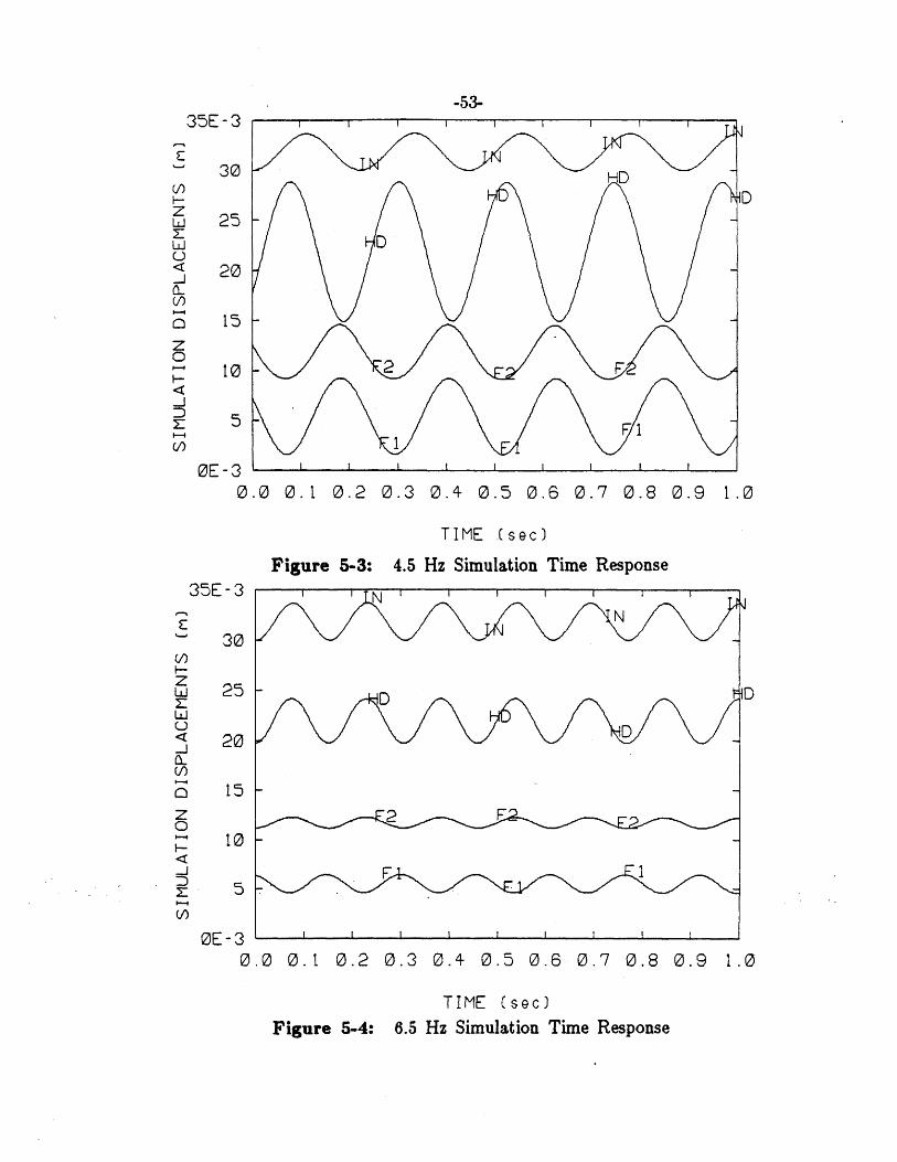
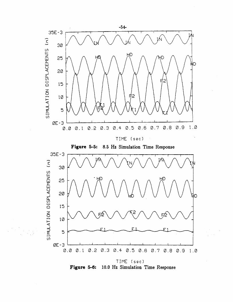
The 8.5 Hz response, Figure 5-5, is very near the second system

resonance. The states have again shifted by 90 degrees and reached peak

amplitudes.

Figure 5-6 shows the 10.0 Hz response which typifies the system response

to input frequencies above the second resonance. The head rotation is again

in phase with the input displacement. However, with its amplitude greater

than that of the input, the head motion causes the frame to be out of phase

(the opposite of the situation just below the first resonance).

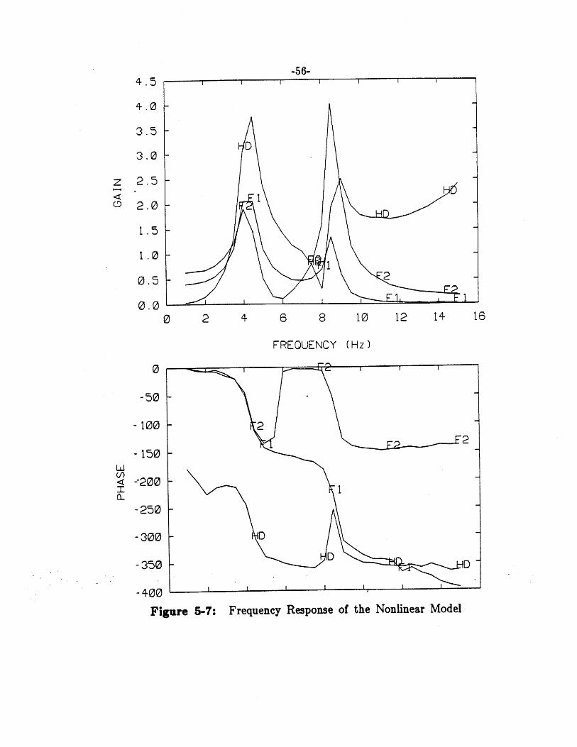
Since only a few frequencies are plotted here for brevity, while many

more cases were simulated, a graphic aid is used to visualize the system's total

frequency response. If the system were linear, we could make a Bode plot to

show the frequency response. For the nonlinear pantograph model simulated,

at low amplitudes of excitation and small levels of coulomb friction, the

vibrations about an operating point would be nearly linear. For comparison

with the experimental results only, we can make a frequency response plot in

the style of a Bode plot. The plot is valid only for the specific operating

height and input amplitude for which it is drawn. Figure 5-7 shows this

frequency repsonse plot for the simulation output discussed.

The actual simulated response, of course, is nonlinear. Each point on the

amplitude plot was then determined by considering only the component at the

forcing frequency, and evaluating the output amplitude and phase with respect

to the input.

-56-4.5

4.0

3.5D

3.0

z 2.51-1

2.0 -

1.5 -

1.0 -

110.5 -2-

0.00 2 4 6 8 10 12 14 16

FREQUENCY (Hz)

0

-50

-100 - 22

-150 -

-200 -

- 250 -

-300 - D

- 350 D D

- 400

Frequency Response of the Nonlinear ModelFigure 5-7:

-57-

5.2 Experimental Data

The test pantograph was set up in the laboratory, instrumented, and

tested as described in Chapter Four. The experimental data were processed

and are presented here for comparison with the simulation output.

The static operating height of 1.58 m and the sinusoidal input

displacement amplitude of 3.7 mm peak-to-peak compare to those used in the

model implementation. However, unlike the digital simulation's constant-

amplitude input displacement, the servo-controlled hydraulic ram cannot

maintain the desired response for all situations. The experimental input

displacement is therefore neither purely sinusoidal, nor of constant amplitude.

Again, while many tests were conducted, only a few sample results are

reproduced here for comparison. Input frequencies ranged from 1.0 Hz to 15.0

Hz. In the cases presented below, the contacting shoe was rigidly attached to

the ram.

Insight gained from the modelling has led us to expect to observe three

system resonances and to find the pressure state responding only to the lower

frame link motions. The first two resonances appear near 4.0 Hz and 8.25 Hz.

The third resonance falls at a frequency above the test range. The cylinder

pressure response was as expected and, for clarity, is not included in the plots

below.

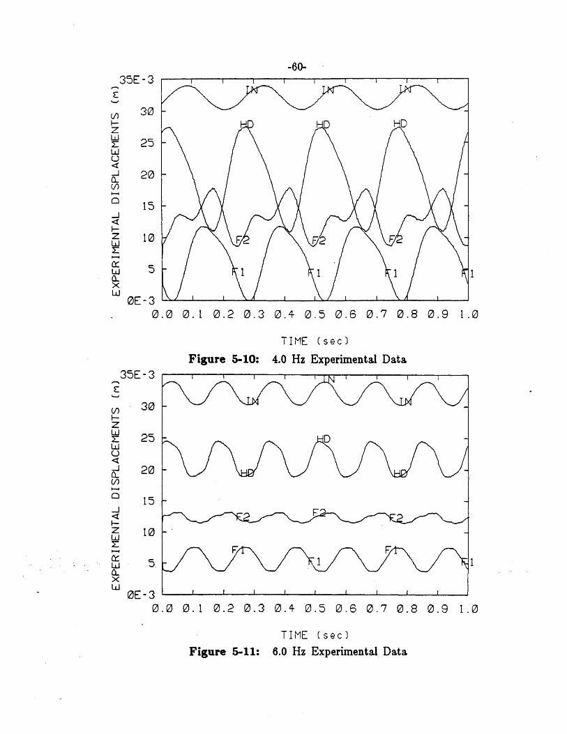
The time histories obtained from the experimental data are each

presented as four curves. The states represent the same ones output from the

simulation, and are labelled as follows:

* IN --- input displacement

-58-

. HD ---head displacement with respect to top of frame

. F2 upper frame link displacement with respect to elbow

. F1 lower frame link displacement

Figures 5-8 through 5-13 contain experimental data plotted for six

representative frequencies.

Figure 5-8 shows the 2.0 Hz response. The two frame states dominate

the response, each taking roughly half the input amplitude. The amount of

head rotation is small at low frequency and out of phase, as expected.

The system response at 3.5 Hz, shown in Figure 5-9, shows the frame

states increasing in amplitude as the first resonance is approached. The

greater frame response induces large head motions 180 degrees out of phase

with the input.

Figure 5-10 shows the 4.0 Hz response, very near the first system

resonance. All three of the states now lag almost 90 degrees from their low-

frequency phase relations. The large-amplitude motions display one of the

nonlinear effects not shown in the smaller vibrations. The model does not

predict this harmonic response at double the input frequency.

Past the first resonance, the 6.0 Hz response plotted in Figure

5-11 shows the head with an amplitude greater than that of the input

displacement, and in phase. The two frame states have split phase as

predicted, with the upper link back in phase with the input, and the lower

link 180 degrees out of phase.

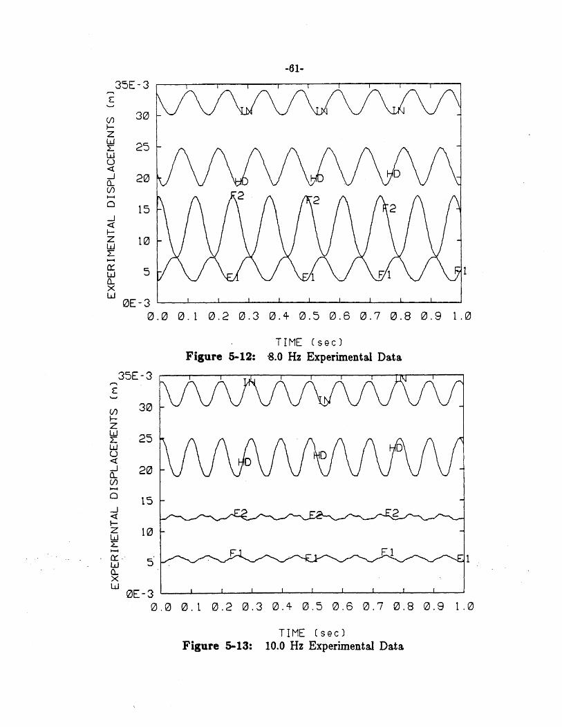
Figure 5-12 shows the system response at 8.0 Hz, very near the second

resonance. All the states are approaching peak amplitudes and are again

-59-

35E-3

30

25

20

15

10

5

OE -3

35E-3

30

25

20

15

10

5

OE -3

0.0 0.1 0.2 0.3 0.4 0.5 0.6 0.7 0.8 0.9 1.0

TIME (sec)Figure 5-8: 2.0 Hz Experimental Data

0.0 0.1 0.2 0.3 0.4 0.5 0.6 0.7 0.8 0.9 1.0

TIME (sec)Figure 5-9: 3.5 Hz Experimental Data

H

I I I I I I I I

-............

-. .........- -- --- D H -- Jd

-60-

30

25

20

15

10

5

0E-30.0

Figure 5-10:35E-3

TIME (sec)

4.0 Hz Experimental Data

30-

25D

20

15

10

5 1

0E-30.0 0.1 0.2 0.3 0.4 0.5 0.6 0.7 0.8 0.9 1.0

TIME (sec)

Figure 5-11: 6.0 Hz Experimental Data

35E-3

0. 1 0.2 0.3 0.4 0.5 0.6 0.7 0.8 0.9 1.0

-61-35E-3

30

z

-20L

2 215 - 2

.J

z 10 -

5 F

xOE-3

0.0 0.1 0.2 0.3 0.4 0.5 0.6 0.7 0.8 0.9 1.0

TIME (sec)

Figure 5-12: -8.0 Hz Experimental Data

35E-3

30z

< 25C-)

0

15 -

15

Z 1L

OE-3

0.0 0.1 0.2 0.3 0.4 0.5 0.6 0.7 0.8 0.9 1.0

TIME (sec)Figure 5-13: 10.0 Hz Experimental Data

-62-

shifting in phase.

Above the second resonance, Figure 5-13 shows the 10.0 Hz response.

The head is now in phase with the input and dominates the response. The

two frame states are out of phase with the input and have a lower amplitude,

as expected.

As with the simulation output, we will again attempt to summarize the

frequency response graphically as if the system were linear. Taking only the

peak amplitude of the response at each input frequency, we can make a

frequency response plot which approximates the system performance only at

the specific operating point and input amplitude tested. Figure 5-14 shows

this plot for the experimental data discussed.

5.3 Model Verification

The frequency response plots for the simulated and actual pantographs

are sketched in Figures 5-7 and 5-14, respectively. The two systems share

many common traits yet there are some distinct differences. For comparison,

these two plots which represent the system responses under similar conditions

are discussed.

At low frequency, the model correctly predicts both the amplitude and

phase of the head state. The model shows the lower frame link taking less

than half the input amplitude, and the upper link having correspondingly more.

This is the effect of the kinematic elbow relation, which must be slightly off.

The experimental data plotted suggest that -0 is near 1.0, while the model6e 60,

shows that - is much higher, perhaps 1.4, since the upper link moves more6tt

than the lower link in the quasi-static case.

4.5

4.0 -D

3.5 -1

3.0

z 2.5 -

0 2.0 -

1.5

1.0

0.5

0.00 2 4 6 8 10 12 14 16

FREQUENCY (Hz)

0

-50 2

-100 21

-150

)-200C.

-250 -

-300 -D D

-350 - D

- 400

Frequency Response of the Experimental PantographFigure 5-14:

-64-

The frequency of and peak amplitudes at the first resonance are well

shown by the model (considering the resolution along the frequency axis). The

phase shifts and splitting of the frame states are also remarkably well

predicted.

At 6.5 Hz, the experimental data displays a definite jump in head

amplitude and a temporary shift in the upper link phase. The model shows

no such changes. These phenomena suggest another resonance, perhaps

structural, which is not modelled in the simulation.

The frequency of the second resonance is slightly off; however, the

relative amplitudes of the states are fairly well predicted by the model. There

is some discrepancy in the phase shifts at this resonance.

Above 10 Hz, the model correctly predicts the amplitudes of the states,

including the rise before the next resonance. Frame phase relationships, on

the other hand, are wrong above the second resonance; however, with the very

low amplitudes of frame motion at these frequencies, the consequence of this

divergence may be small. Failure of the model to accurately represent this

phase information may be attributable to inaccuracies caused by the limitations

of the simple, linear cylinder model.

In conclusion, the nonlinear model describing the Brecknell-Willis

pantograph accurately predicts the fundamental response amplitudes through 15

Hz, and phases through the second resonance, near 9 Hz.

The model developed can now be used to study many new configurations

of high-speed pantographs. The model can be used in conjunction with

catenary simulations developed in order to study the pantograph/catenary

interaction.

-65-

Chapter 6

Conclusions and Recommendations

6.1 Dynamic Model Development

A nonlinear model was developed to predict the response of a

pantograph. The model was used to describe a Brecknell-Willis Pantograph.

The actual device was instrumented and tested in the laboratory. The

experimental data were compared with the simulation output in order to

confirm the validity of the model.

The results, presented in the previous chapter, show that the simulation

is able to produce the system response for input frequencies through the

second modelled resonance. The pantograph's resonant frequencies near 4.25

and 8.25 Hz were closely predicted by the model. The proper amplitudes and

phase shifts are shown by the simulation results both before and after the first

resonance. However, at 6.5 Hz there is an unmodelled resonance, one which

shows up in the experimental data and not in the simulation output causing a

discrepancy only in the response amplitudes very near 6.5 Hz. At the higher

frequencies, above 9 Hz, the model predicts the amplitudes of motions

correctly, but not the phase.

In general, the model developed has proven to be quite robust. The

nonlinear model well predicted the dynamics of the physical system, including

some features of the response which could not have been matched by a linear

model.

-66-

The model assumes all of the links to be rigid; however, in the physical

system these members can flex, so there are many more resonances than

actually modelled. If the system response must be predicted with more

accuracy or at higher frequencies, adequate models of structural effects would

have to be included.

Elbow modelling has a great effect on system performance. One cannot

assume the knuckle of an asymmetrical pantograph to be infinitely stiff.

O'Connor [12] showed that frame motions are a very important factor in

dynamic performance, and the results presented here show that the two frame

links do not always move together, so an accurate elbow model is essential.

The cylinder model may also significantly influence overall performance.

Its effect should be studied in more depth. In addition, the kinematics of the

upper arm could be included in the model to provide a more accurate "datum

angle" to reference the head link's torsional spring.

6.2 Recommendations for Use

The successful nonlinear pantograph model development warrants its

implementation into a complete pantograph/catenary dynamic simulation. The

pantograph model is ready for use with any catenary model that can interface

through a contact spring.

The catenary model developed as part of this research [1], [12], and [201,

accepts contact force from the pantograph in each timestep and returns the

new wire height to the pantograph [211, while the two systems are integrated

simultaneously.

-67-

Finally, both the complete pantograph/catenary simulation and the

nonlinear pantograph model itself will be very useful in parameter studies

aimed at determining the parameters which seriously affect. overall system

performance.

-68-

References

[1] Armbruster, K.Modelling and Dynamics of Pantograph-Catenary Systems for High Speed

Trains.Master's thesis, Massachusetts Institute of Technology, 1983.

[21 Belyaev, I. A., Vologine, V. A., and Freifeld, A. V.Improvement of Pantograph and Catenary and Method of Calculating

Their Mutual Interactions at High Speeds.Rail International , June, 1977.

[3] Blackburn, John F., Reethof, Gerhard, and Shearer, J. Lowen.Fluid Power Control.MIT Press, Cambridge, Massachusetts, 1960.

[41 Boissonnade, Pierre.Catenary Design for High Speeds.Rail International , March, 1975.

[51 Boissonnade, Pierre, and Dupont, Robert.SNCF Tests Collection Systems for High Speeds.International Railway Journal , October, 1975.

[6] Boissonnade, Pierre, and Dupont, Robert.Current Collection With Two-Stage Pantographs on the New Paris-Lyon

Line.Railway Gazette International , October, 1977.

[7] Communications of the 0. R. E.Behavior of Pantographs and Overhead Equipment at Speeds Above 160

km/hr.Rail International , January, 1972.

[8] Coxen, D. J., Gostling, R. J., and Whitehead, K. M.Evolution of a Simple High-Performance Pantograph.Railway Gazette , January, 1980.

-69-

[9] Crandall, Stephen H., et al.,Dynamics of Mechanical and Electromechanical Systems.McGraw Hill, New York, New York, 1968.

[101 Faux, I. D. and Pratt, M. J.Computational Geometry for Design and Manufacture.Ellis Horwood, Chichester, West Sussex, England, 1981.

[11] Gostling, R. J. and Hobbs, A. E. W.The Interactions of Pantographs and Overhead Equipment: Practical

Applications of a New Theoretical Method.Technical Report, Institute of Mechanical Engineers, Derby Branch,

February, 1981.

[12] O'Connor, D.Modelling and Simulation of Pantograph-Catenary Systems.Master's thesis, Massachusetts Institute of Technology, 1984.

[131 Peters, John.Dead Line Testing of the Faiveley Single and Dual Stage Pantographs on

the R TT Catenary Systems.Technical Report FRA/TCC-81/01, U.S. Department of Transportation,

1981.

[14] Sikorsky Aircraft.Design and Development of a Servo-Operated Pantograph for High Speed

Trains.Final Report Contract Number 7-35415, U.S. Department of

Transportation, July, 1970.

[151 Simmons, George F.Differential Equations with Applications and Historical Notes.McGraw-Hill, New York, New York, 1972.

[16] Strang, Gilbert.Linear Algebra and Its Applications.Academic Press, New York, New York, 1980.

[17] Vesely, G. C.Modelling and Experimentation of Pantograph Dynamics.Master's thesis, Massachusetts Institute of Technology, 1983.

-70-

[18] Vinayagalingam, T.Computer Evaluation of Controlled Pantographs for Current Collection

From Simple Catenary Overhead Equipment at High Speed.Journal of Dynamic Systems, Measurement, and Control , December,

1983.

[19] Wann, L. M.Improvement of a Pantograph for High Speed Train.Master's thesis, Massachusetts Institute of Technology, 1980.

[20] Wormley, D. N., Seering, W. P., Armbruster, K., and Vesely, G. C.Dynamic Performance Characteristics of New Configuration Pantograph-

Catenary Systems.First Annual Report, Grant Number DT-RS-56-81-C-00020, U.S.

Department of Transportation, December, 1982.

[211 Wormley, D. N., Seering, W. P., Eppinger, S. D., and O'Connor, D. N.Dynamic Performance Characteristics of New Configuration Pantograph-

Catenary Systems.Final Report, Grant Number DT-RS-56-81-C-00020, U.S. Department of

Transportation, May, 1984.

-71-

Appendix ADerivation of Governing Equations

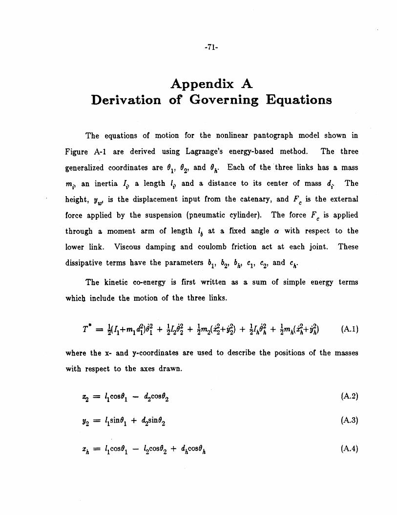
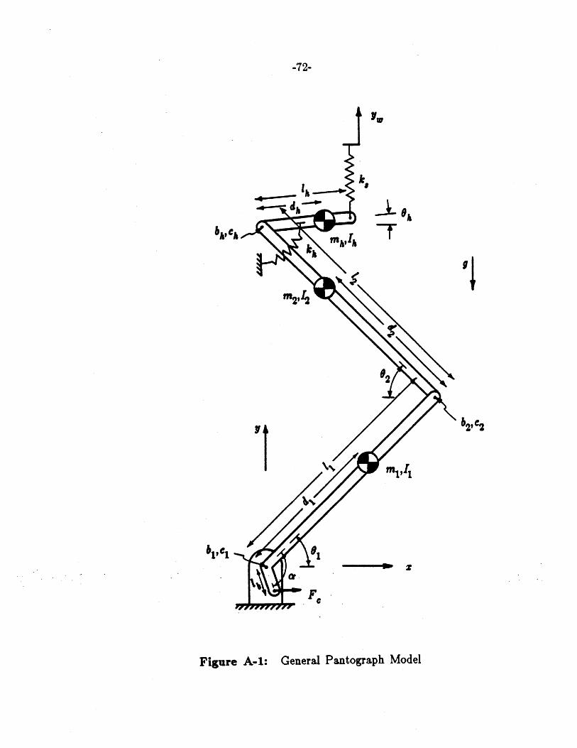
The equations of motion for the nonlinear pantograph model shown in

Figure A-1 are derived using Lagrange's energy-based method. The three

generalized coordinates are 01, 02, and Oh. Each of the three links has a mass

Mg, an inertia I, a length l, and a distance to its center of mass dg. The

height, y, is the displacement input from the catenary, and Fc is the external

force applied by the suspension (pneumatic cylinder). The force FC is applied

through a moment arm of length 1b at a fixed angle a with respect to the

lower link. Viscous damping and coulomb friction act at each joint. These

dissipative terms have the parameters bl, b2, bh, C1' C2, and ch.

The kinetic co-energy is first written as a sum of simple energy terms

which include the motion of the three links.

- + 2 2 + jm( i~'(I+m d?)# + i2 2 + i I + m(+) (A.1)

where the x- and y-coordinates are used to describe the positions of the masses

with respect to the axes drawn.

2 = IlcosOl - d2cos02 (A.2)

y2 = lisin06 + d2sin02 (A.3)

Zh = 11coso 1 - l2cosO2 + dhcosoh (A.4)

-72-

ill

bA, C%

r 2';

Yt

ie &

T

b2, C2

mi

--------- *

F,

General Pantograph ModelFigure A-1:

-73-

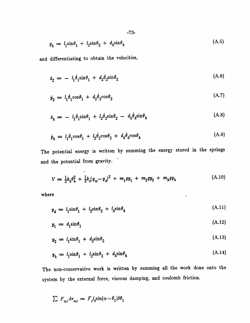
(A.5)h 1 sinO1 + 12sin0 2 + dhsinoh

and differentiating to obtain the velocities,

:2 1 1 sin01 + d2e 2sinO2

2 1101cos61 + d2O2cosO2

(A.6)

(A.7)

(A.8)

(A.9)

'h - 1 1isinO1 + l2 2Sin0 2 - dhihsinh

h 1 161cos + 12A 2cosO2 + dh~cosOh

The potential energy is written by summing the energy stored in the springs

and the potential from gravity.

(A.10)V = 6kh02 + k,( y,-yd) 2 + m gy/ + m2 992 + mhgyh

where

Yd = l1sinG1 + 12sin62 + Ihsin6h(A. 11)

(A.12)

(A.13)

(A.14)

y2 = 11sinG1 + d2sin62

yh = l1sinO1 + l2sin02 + dhsinoh

The non-conservative work is written by summing all the work done onto the

system by the external force, viscous damping, and coulomb friction.

E Fnc-6rn = Fclsin(a- 69)6 61

yJ = disin6,

-74-

- b1 61 60 - b2(61+6 2)(60 1+60 2) - bh(62+6h 2+6A)

- clsgn(01)601 - c2sgn(61+02 )(6 1+602)

- chsgn(02 h)(6 2+6 h) (A.15)

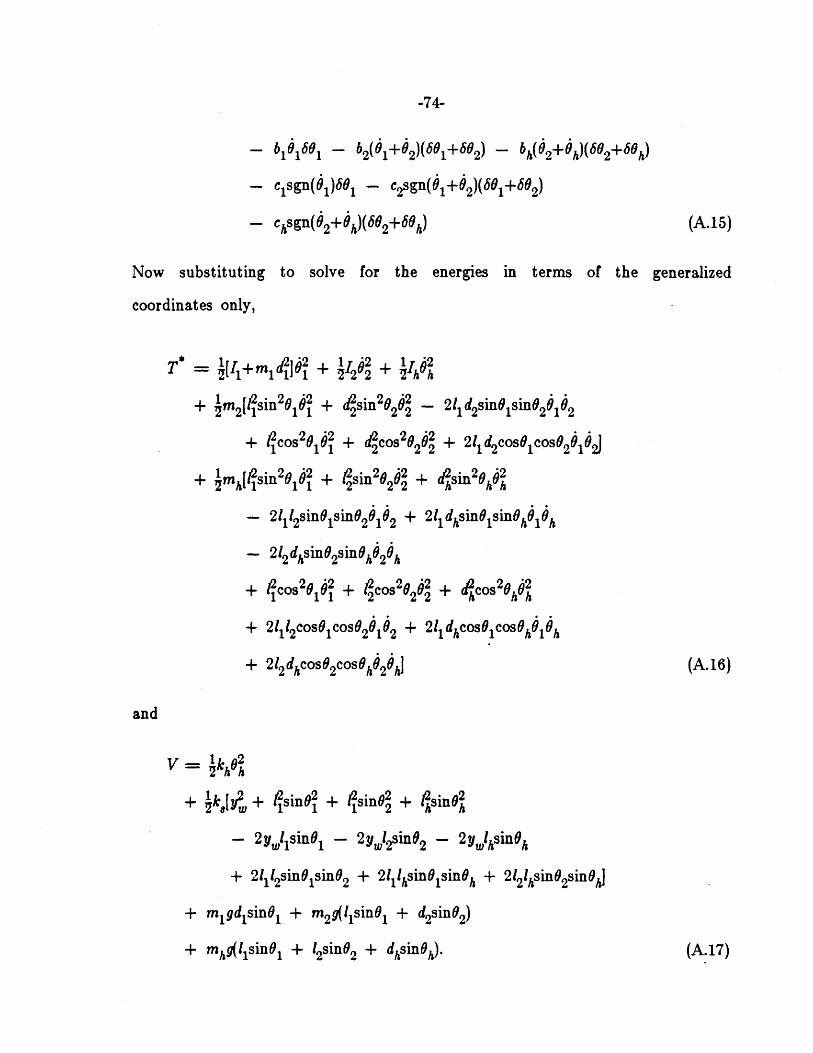
Now substituting to solve for the energies in terms of the generalized

coordinates only,

T = [41+m dij0 + I 25 + 1Ih2

+ {m 2[ s 201 + d sin 2O25 - 2l d2sinO1sinO2 1O2

+ l cos201 $ + d cos2025 + 211d2cos01cos020102

+ {mh[1psin 20 52 + p'sin 2025 + d sin20k02

- 211 2sin01sin020162 + 2 ldhsinOjsinOh0,il

- 2 l2dohin 2sin0h626h

+ lpcos 20151 + cos 220 + d cos20

+ 21,12cos0 1cos820102 + 21 dhcosOjcosOh616h

+ 212dhcoso2cosohO 26h (A.16)

and

V = 1kh0212h

+ {kay2 + Pjsin02 + P sin02 + Phsin02

- 2y.l 1 sin01 - 2yl 2sin0 2 - 2 y.lksinOh

+ 2l1 l2sinO1sino 2 + 21llhsinOlsin0h + 2Ilksno2sinO

+ migdjsin01 + m29(l 1sino1 + d2sin02)

+ mhgllsinol + l2sin02 + dhsinOh). (A.17)

-75-

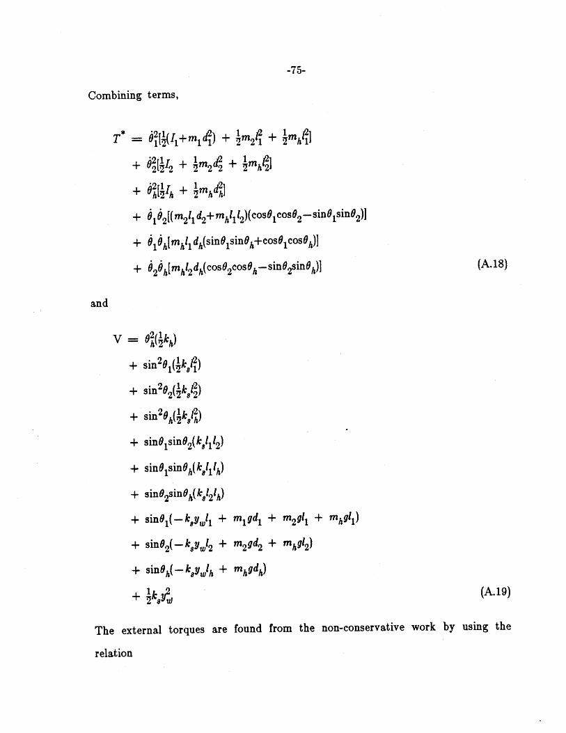
Combining terms,

T* = 6'[ (I +m d2) + 'm2lP + 'mh(P.

+ 62 + dnh + 1in

+ Ih + -mhd/j

+ e02[( m2 d2+mhl1 2)(cosOlcos 2 - sinO1sino2)

+ 5ShImhIl dh(sinOlsinh+cosOIcosOh)l

+ $2 8hfmhl2 dh(coso2cosoh- sinO2Sinh) (A.18)

and

V = 02(1k

+ sin261 (1k,j)

+ sin2o2(2k8122)

+ sin26h(kkA)

+ sinO6sin 2(ko1 1l2)

+ sindlsinOh(klll)

+ sin02sin ( k, 12

1h)

+ sinO (-kIyj 1 + mIgd1 + n291 + nhgl 1)

+ sinO2(~k 8 ywl2 + m2gd2 + mh912)

+ sin0h(-kywlh + mgdh)

+ ik.y (A.19)

The external torques are found from the non-conservative work by using the

relation

-76-

E ,,87,,= E ;6; for i = 1, 2, and h.

The external torques are found to be

= F lbsin(a -01) - b10 - 2

- clsgn(#1 ) - c2sgn(#1+62 )

21= - - bh(62+ h) - c2sgn(#16

2 ) - csgn(#2+h)

I= - bh(6 2 + h) - chsgn(#2+#h)'

Now we form the Lagrangian,

L = T -V

and use Lagrange's equation to write the governing equations:

d aL/

dt 85,

8L

I,

for i = 1, 2, and h.

For i = 1, we find the first governing equation by differentiating.

d (L)

dt 86i

aL\

--9=0i

i~~l2 + M P. + +Mh

+ 2[(rn2 1 d2+mh1l 2)(cosOlcos62- sinOlsin6 2)]

+ #[ mhil dh(sinOlsinOh+cosolcosoh)]

- 02(01+02)(sinOcosO2+cosO1sin6O2(m 2!1d2+ mhl1I2)

(A.20)

(A.21)

(A.22)

(A.23)

(A.24)

(A.25)

(A.26)

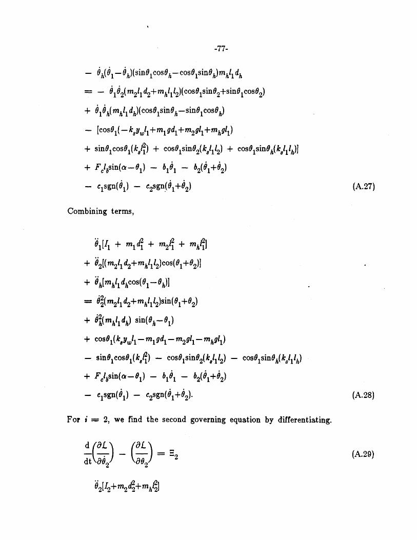
-77-

-- O h)(sinOcosoh-cosOlsinoh)mh l dh

= - 0162(m 211 d2+ mhll12 )(cosOjsinO2+sinOjcos0 2)

+ 610 h( mhIl dh)(cosOlsinh- sinO1cos0h)

- [cosO 1( -k,ywll + m gd 1+m 2gl1+mhgl 1)

+ sinO coso 1 (kRl ) + coso1sin 2(k!1112) + cosolsinohk(k 8ll)l

+ Fclbsin(ca-6l) - -- 62(1+ )

- clsgn(61 ) - c2sgn(01+02)

Combining terms,

1(/1 + m d + m21 + h Il

+ 02[(m 21d2+mhl1l 2)cos(01+6 2)1

+ Oh[mhld hcos(Ol- 6h)-

(m2 1d 2+mhfl 1 2)sin(91+02)

+ h (mh 1 h) sin(o-01)

+ cosOj(k,ywlj--mjgdj- m29 1- hli)

- sino coso 1(k/l) - cosO1sino2(k,1112) - cosolsinoh~skilh)

+ Fclbsin(ca-91) - 5j61 - 2(+6)

- c1sgn(6 1) - c2 sgn(01+62 ).

For i = 2, we find the second governing equation by differentiating.

d (aL\ (OL\=+md22

(A.27)

(A.28)

(A.29)

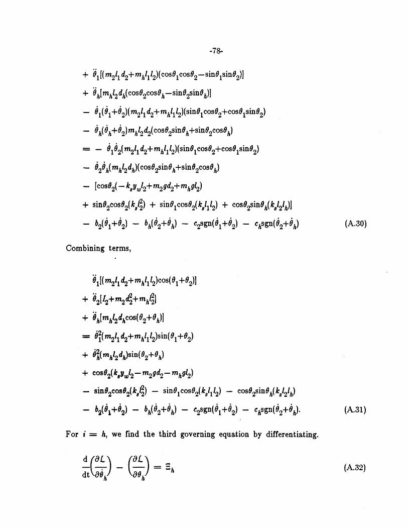
-78-

+ Ol[(m 2 1 d2+mhl 1l2)(cosOlcosO2- sinO1sinO2)l

+ h[ mhl2dh(cos 02cosoh-sin 2sinoh)1

- 1 (i1+62)(m2 11 d2+ mhll12)(sinOlCos02+cosOlsin02)

- h(6h+ 2)mhl2d2 (coso2Sinoh+sino2 cosOh)

= - 6162(m 2 1 d2+mhJl 2)(sinBlcoso 2+cosolsino 2)

-2 6h(mhl2dh)(cosO2Sinoh+sino2cosoh)

- [cos 2(- k-yal 2 +m2gd2+mh9l2 )

+ sin02coso2( kl ) + sinOlcos0 2(k)l112) + cosO2sinoh(kI 2Ihll

- b20 1 +2) - bh(02+ h) - c2sg(i 1 +6 2) ~ chO 2+h) (A.30)

Combining terms,

6 1[(m2 1 d2+mhk 1l2)cos(Ol+6 2)l

+ 02 [I2+m2d2+mhp1~

+ Ohlmkl2 dhcos(02+oh)1

S(m2 1d2+mh12)sin(Ol+ 2)

+ $62(mh2 d h)sin(0 2+6h

+ coso2(kyw2- m29d2 - mhg 2)

- sinO2 cos92(k,2) - sinolcosO2(k,1112) - cosO2sinoh e(k121h)

- b2 ( 1+'2) - bh(62+h) - c2 sg( 1 2 ) Csgn(6 2+6h). (A.31)

For i = h, we find the third governing equation by differentiating.

d ( (L\

)- ( ) = " (A.32)

-79-

Oh[Ih+ mftdl

+ ollmhll dh(sinOlsinoh+cosolcosoh)l

+ 02 [mhl12 dh(cosO2cosoh- sino2sinOh)l

- l - h) mhll dh(sinOlcos 0h-cosOlsinoh)

- 022+ h) in 12 dh(sino2cos Oh+ Cos O2 sinoh)

-l 61h( ikl dh)(sinOlcosoh- cosOls1iI~h)

-020h( ink2 d4)(sin0 2cosOh+cosO2sinOh)

(0 [hkh + cosoh( - k.3ywl+mhgdh)

+ sin~hcos~(k1Ph) + sinolcosoh(khIllh) + sinO2coso(k! 2 h)1

- bh(0 2+G) - c0sgn( 2+O) (A.33)

Combining terms,

l ld hcos(O - 0h)l

+ 0h[Ih+mhY h

- O(m m1 1 d h)sin(Ol- h

+62(m mldh)sin(8 2+oh)

+ cosoh(k8ywlh-tmhgdh) - sinohcoso(k.Ph)

- sin~lOk( k8, 1 Ift) - sino 2cos~h(k,,l2Ih)

- Ohkh - b 0 h) - C-sgn( 2+O). (A.34)

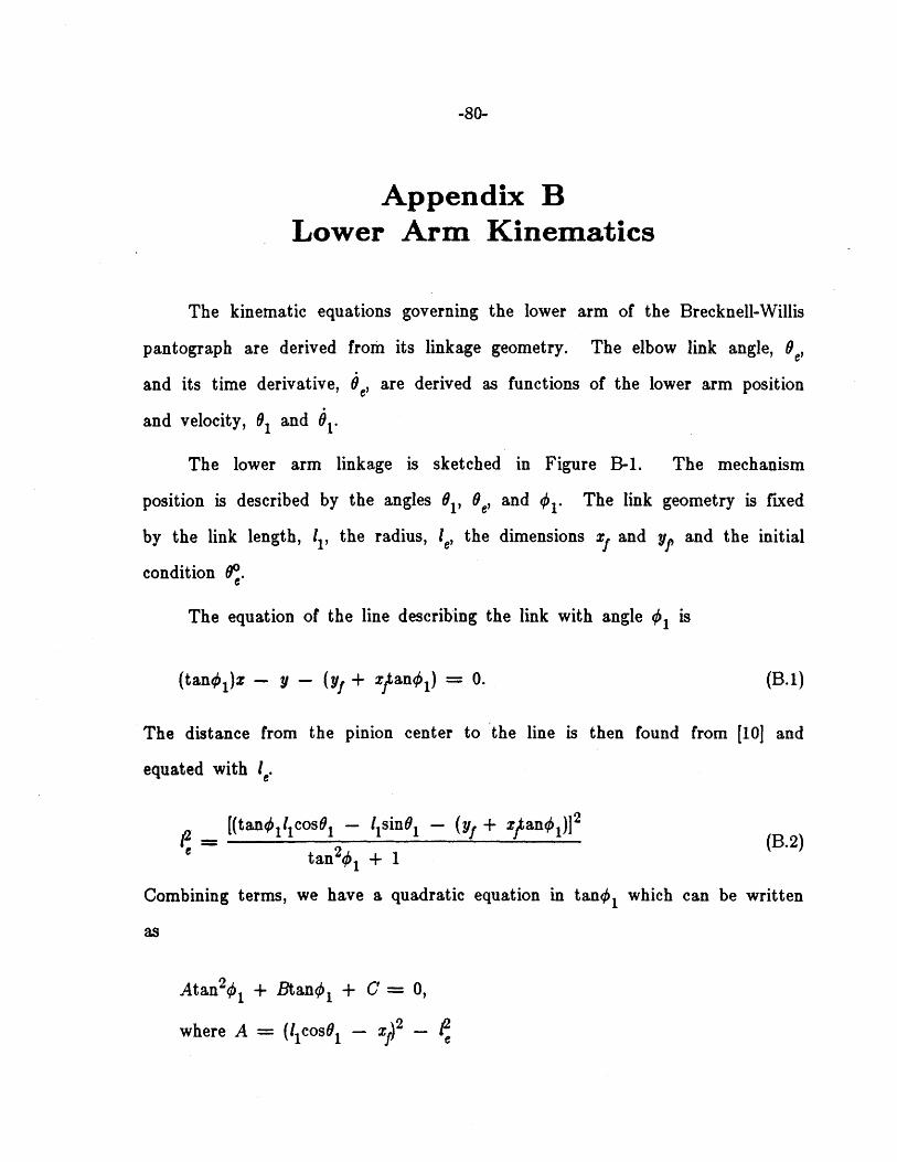
-80-

Appendix BLower Arm Kinematics

The kinematic equations governing the lower arm of the Brecknell-Willis

pantograph are derived from its linkage geometry. The elbow link angle, 6 ,

and its time derivative, 6,, are derived as functions of the lower arm position

and velocity, 61 and 1.

The lower arm linkage is sketched in Figure B-1. The mechanism

position is described by the angles 61, 6, and 41. The link geometry is fixed

by the link length, 11, the radius, I,, the dimensions zf and y. and the initial

condition 6*.

The equation of the line describing the link with angle 41 is

(tan4 1)x - y - (yf + xzank 1) = 0. (B.1)

The distance from the pinion center to the line is then found from [10] and

equated with .-

[(tan 1 1cos6, - l1sinO, - (y1 + zpan.01)12 (B.2)

e tan24 1 + 1

Combining terms, we have a quadratic equation in tan4, which can be written

as

Atan241 + Btano1 + C = 0,

where A = (l1 cosO, - -

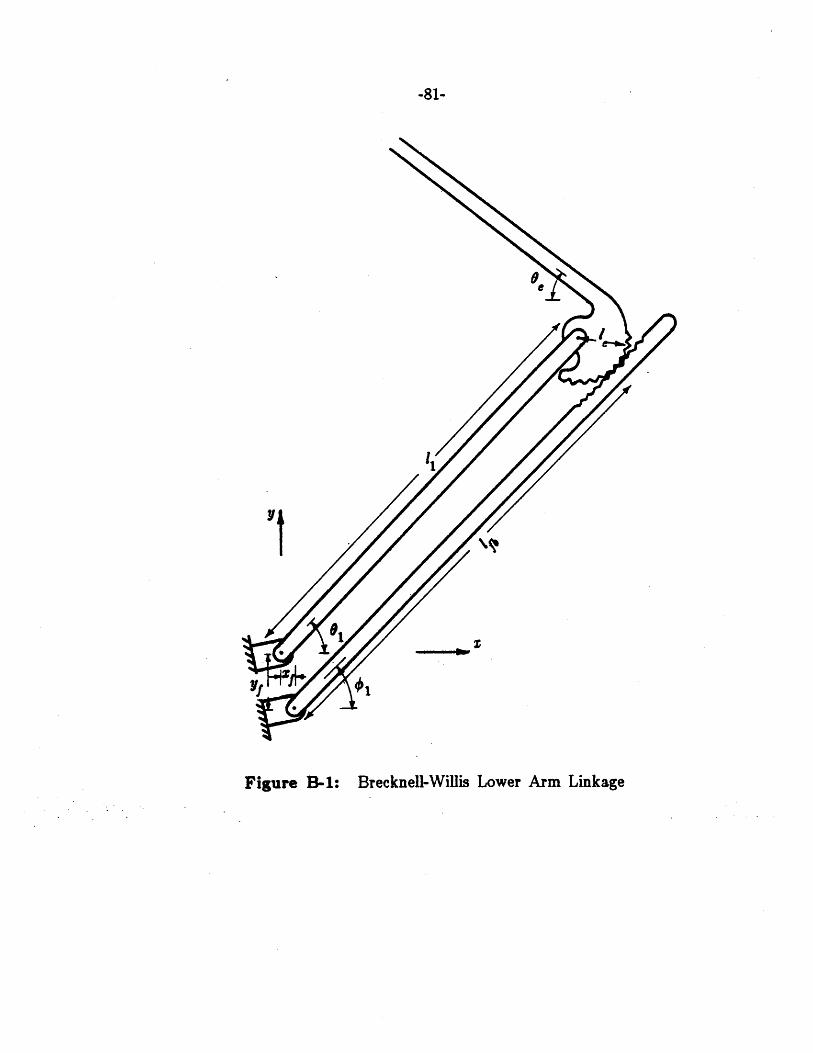
-81-

Brecknell-Willis Lower Arm LinkageFigure B-1:

-82-

B = -2( 1 cosO, - xf)(l 1sin61 + yf)

and C = (lisinO1 + yf)2- . (B.3)

The solution to this equation is found from the quadratic formula where the

negative root is taken.

(B.4)=B

-aB2 -Q4AC4 =arctan

2A

Now the length of the "fourth bar" is written in terms of the angles 01 and

(B.5)lb = /(lcosO + - )2 + (l1 sinO, - Iecoskj + 2

Finally, the rotation of the pinion is found to be

6,~ ~ 0 =1*- + 1Oe e

where the initial conditions . and 6* are the values of and 6, respectively

when 01=0.

(B.6)

-83-

Appendix CSimulation Program

The following is the FORTRAN code of the simulation subroutine

EQSIM, used in conjunction with the software package DYSYS.

SIMULATION OF BRECKNELL-WILLIS PANTOGRAPH DYNAMICS

By Steven D. Eppinger June 1983 through May 1984

SUBROUTINE EQSIM

COMMON T,DT,Y(30) ,FY(30) ,STIME,FTIME,NEWDT,NEWRUN,N& IPR, ICD, ICN, TBREAK,PNEXT,TBACK,CONSTANT (30)

REAL L1,L2,LH,M1,M2,MH,I1,I2,IH,KS,KH,NIA,LMARM,NA,& IK1,JK1,KK1,LK1,LK2,LK3,LK4,LK5,LK6,LK7,LY3,& I,J,K,L,KE,JAIB,KAIC,LAID,LE,LC1MXF,LS1PYF,KCYL

CC Equate state and auxilliary variables to array elements.

EQUIVALENCEEQUIVALENCEEQUIVALENCEEQUIVALENCEEQUIVALENCEEQUIVALENCEEQUIVALENCEEQUIVALENCEEQUIVALENCEEQUIVALENCEEQUIVALENCEEQUIVALENCEEQUIVALENCEEQUIVALENCEEQUIVALENCEEQUIVALENCEEQUIVALENCEEQUIVALENCE

(Y (1) ,TH1)(Y (2) ,TH1D)(Y(3) ,TH2)(Y (4) ,TH2D)(Y (5) ,THH)(Y (6) ,TOHD)(Y (7) ,P)(Y(8) ,HDHT)(Y (9) ,YW)(Y(10) ,FCONT)(Y(11) ,FINPUT)(Y (12) , EKIN)(Y(13) ,EPOT)(Y(14) ,ENERGY)(Y (15) ,F1OUT)(Y(16) ,F2OUT)(Y(17) ,HDOUT)(Y(18) ,RINOUT)

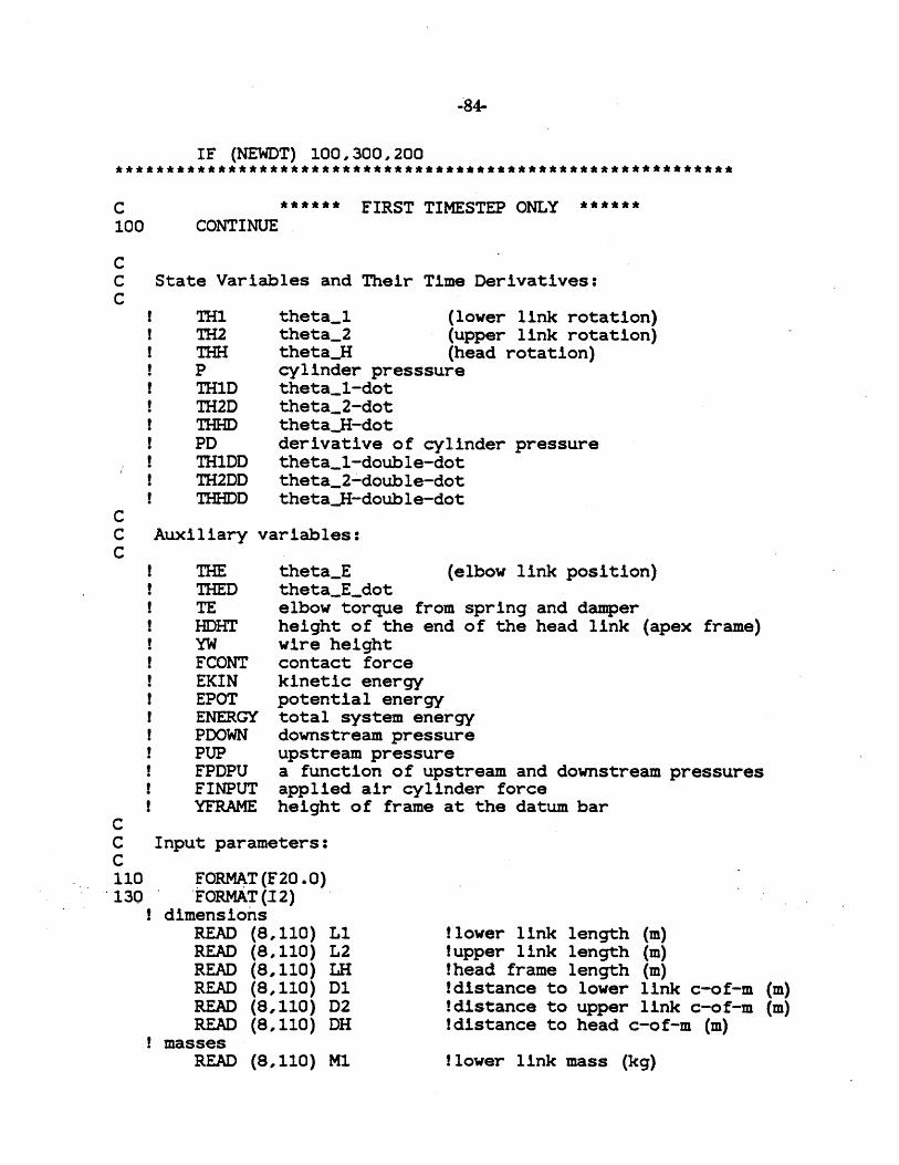
-84-

IF (NEWDT) 100,300,200

****** FIRST TIMESTEP ONLY ******CONTINUE

CC State Variables and Their Time Derivatives:C

TH1TH2THHPTH1DTH2D

PDTH1DDTH2DDTHHDD

theta_1 (lower link rotation)theta_2 (upper link rotation)thetaH (head rotation)cylinder presssuretheta_1-dottheta_2-dotthetaH-dotderivative of cylinder pressuretheta_1-double-dottheta_2-double-dotthetaji-double-dot

C Auxiliary variables:

THETHEDTEHDHTYWFCONTEKINEPOTENERGYPDOWNPUPFPDPUFINPUTYFRAME

thetaE (elbow link position)theta_E_dotelbow torque from spring and damperheight of the end of the head link (apex frame)wire heightcontact forcekinetic energypotential energytotal system energydownstream pressureupstream pressurea function of upstream and downstream pressuresapplied air cylinder forceheight of frame at the datum bar

C Input parameters:C110 FORMAT (F20. 0)130 FORMAT (.12)

I dimensionsREAD (8,110) LiREAD (8,110) L2READ (8,110) LHREAD (8,110) D1READ (8,110) D2READ (8,110) DH

I massesREAD (8,110) M1

!lower link length (m)I upper link length (m)!head frame length (m)Idistance to lower link c-of-m (m)!distance to upper link c-of-m (m)!distance to head c-of-m (m)

!lower link mass (kg)

C100

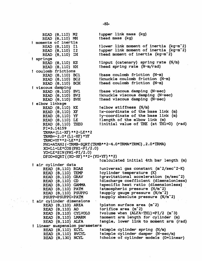
-85-

READ (8,110) M2 !upper ink mass (Ig)READ (8,110) MH !head mass (kg)

moments of inertiaREAD (8,110) Il !lower link moment of inertia (kg-m^2)READ (8,110) 12 !upper link moment of inertia (kg-m^2)READ (8,110) IH !head moment of inertia (kg-m"2)

! springsREAD (8,110) KS !nput (catenary) spring rate (N/i)READ (8,110) KH !head spring rate (N-r/rad)

! coulomb frictionsREAD (8,110) BC1 !base coulomb friction (N-r)READ (8,110) BC2 !knuckle coulomb friction (N-i)READ (8,110) BCH !head coulomb friction (N-r)

! viscous dampingREAD (8,110) BV1 !base viscousdamping (N-sec)READ (8,110) BV2 !knuckle viscous damping (N-sec)READ (8,110) BVH !head viscous damping (N-sec)

! elbow linkageREAD (8,110) KE !elbow stiffness (N/i)READ (8,110) XF !x-coordinate of the base link (i)READ (8,110) YF !y-coordinate of the base link (i)READ (8,110) LE !length of the elbow link (i)READ (8,110) THEO initial value of THE (at TH1=0) (rad)PI=3.14159TRMA= (Li-XF) **2-LE**2TRMB=-2.0 * (Li-XF) *YFTRMC=YE'*F**L**2PI{1=ATAN2 (-ThMB-SQRT(TRMB**2-4.0*TRMA*TRMC) .2.0*TRMA)XG=L+LE*COSp(PHp-PI/2.0)YG=LE*hSINe(PH1-PI/2.)DeGOaSQRT((XG-Xd)o**2+(YG+YF) **2)

!calculated initial 4th bar length (m)

I air cylinder dataREAD (8,110) RGASREAD (8,110) TEMPREAD (8,110) CRAVREAD (8,110) CDREAD (8,110) GAMMAREAD (8,110) PATMREAD (8,110) PSUPPGPSUPP=PSUPPG+PATM

I. air cylinder dimensionsREAD (8,110) AREAREAD (8,110) AO IREAD (8,110) CYLVOLOREAD (8,110) LMARMREAD (8,110) ALFA

Ilinear suspension parametersREAD (8,110) ICCYL IREAD (8,110) BVCYLREAD (8,130) NCYL I

universal gas constant (m^2/sec^2-K)cylinder temperature (K)gravitational acceleration (m/sec^A2)discharge coefficient (dimensionless)specific heat ratio (dimensionless)atmospheric pressure (N/m^2)supply gauge pressure (N/m^2)supply absolute pressure (N/m^2)

piston surface area (m^2)orifice area (m^2)volume when (ALFA-TH1)=PI/2 (m^3)moment arm length for cylinder (m)angle, lower link to moment arm (rad)

simple cylinder spring (N/m)simple cylinder damper (N-sec/m)choice of cylinder models (O=linear)

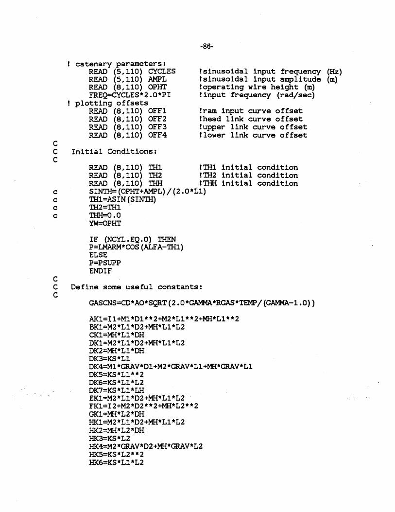
-86-

catenary parameters:READ (5,110) CYCLESREAD (5,110) AMPLREAD (8,110) OPHTFREQ=CYCLES*2.0*PI

! plotting offsetsREAD (8,110) OFF1READ (8,110) OFF2READ (8,110) OFF3READ (8,110) OFF4

CC Initial Conditions:

!sinusoidal input frequency (Hz)!sinusoidal input amplitude (m)t operating wire height (m)input frequency (rad/sec)

!ram input curve offset!head link curve offset!upper link curve offset!lower link curve offset

READ (8,110) TH1 !TH1 initialREAD (8,110) TH2 !TH2 initialREAD (8,110) THH !TH initialSINTH= (OPHT+AMPL) / (2 .0*L1)TH1=ASIN (SINTH)TH2=TH1THH=0.0YW=OPHT

conditionconditioncondition

IF (NCYL.EQ.0) THENP=LMARM*COS (ALFA-TH1)ELSEP=PSUPPENDIF

CC Define some useful constants:C

GASCNS=CD*AO*SQRT(2.0*GAMMA*RGAS*TEMP/(GAMMA-1.0))

AK1=I1+M1*D1**2+M2*L1**2+MH*L1**2BK1=M2*L1*D2+MH*L1*L2CK1=MH*L1*DHDK1=M2*L1*D2+MH*L1*L2DK2=MH*L1*DHDK3=KS*L1DK4=M1*GRAV*D1+M2*GRAV*L+MH*GRAV*L1DK5=KS*L1**2DK6=KS*L1*L2DK7=KS*L1*LHEK1=M2*L1*D2+MH*L1*L2FK1=12+M2*D2**2+MH*L2**2GK1=MH*L2*DHHK1=M2*L1*D2+MH*L1*L2HK2=MH*L2*DHHK3=KS*L2HK4=M2*GRAV*D2+MH*GRAV*L2HK5=KS*L2**2HK6=KS*L1*L2

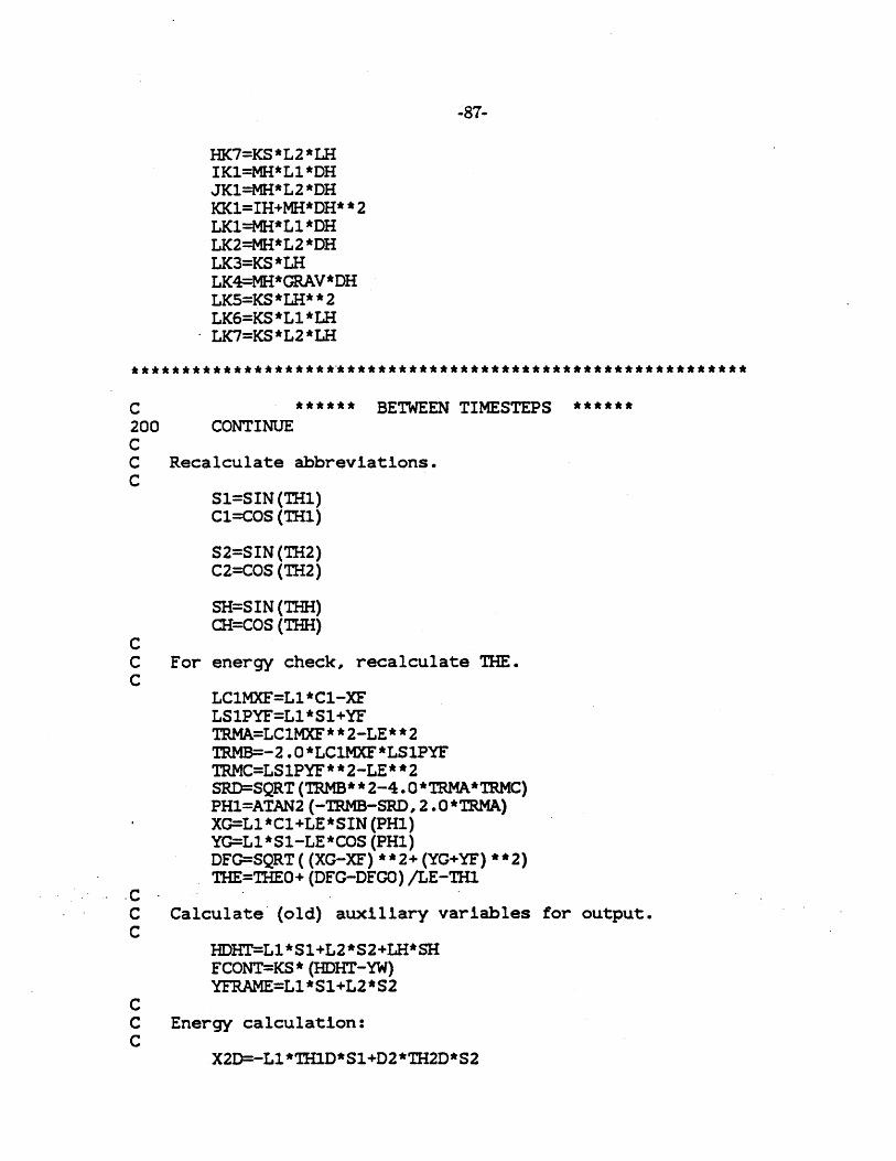
-87-

HK7=KS*L2*LHIK1=MH*L1*DHJK1=MH*L2*DHKK1=IH+MH*DH**2LK1=MH*L1*DHLK2=MH*L2*DHLK3=KS*LHLK4=MH*GRAV*DHLK5=KS*LH**2LK6=KS*L1*LHLK7=KS*L2*LH

C ****** BETWEEN TIMESTEPS *200 CONTINUECC Recalculate abbreviations.C

S1=SIN (TH1)C1=COS (TH1)

S2=SIN (TH2)C2=COS (TH2)

SH=SIN (THH)CH=COS (THH)

CC For energy check, recalculate THE.C

LC1MXF=L1*C1-XFLS1PYF=L1*S1+YFTRMA=LC1MXF**2-LE**2TRMB=-2.0*LC1MXF*LS1PYFTRMC=LS1PYF**2-LE**2SRD=SQRT (TRMB* * 2-4.0 *TRMA*TRMC)PH1=ATAN2 (-TRMB-SRD, 2.0*TRMA)XG=L1*C1+LE*SIN (PH1)YG=L1*S1-LE*COS (PH1)DFG=SQRT( (XG-XF) **2+ (YG+YF) **2)THE=THE0+ (DFG-DFGO) /LE-TH1

CC Calculate (old) auxiliary variables for output.C

HDHT=L1*S1+L2*S2+LH*SHFCONT=KS* (HDHT-YW)YFRAME=L1*S1+L2*S2

CC Energy calculation:C

X2D=-L1*TH1D*S1+D2*TH2D*S2

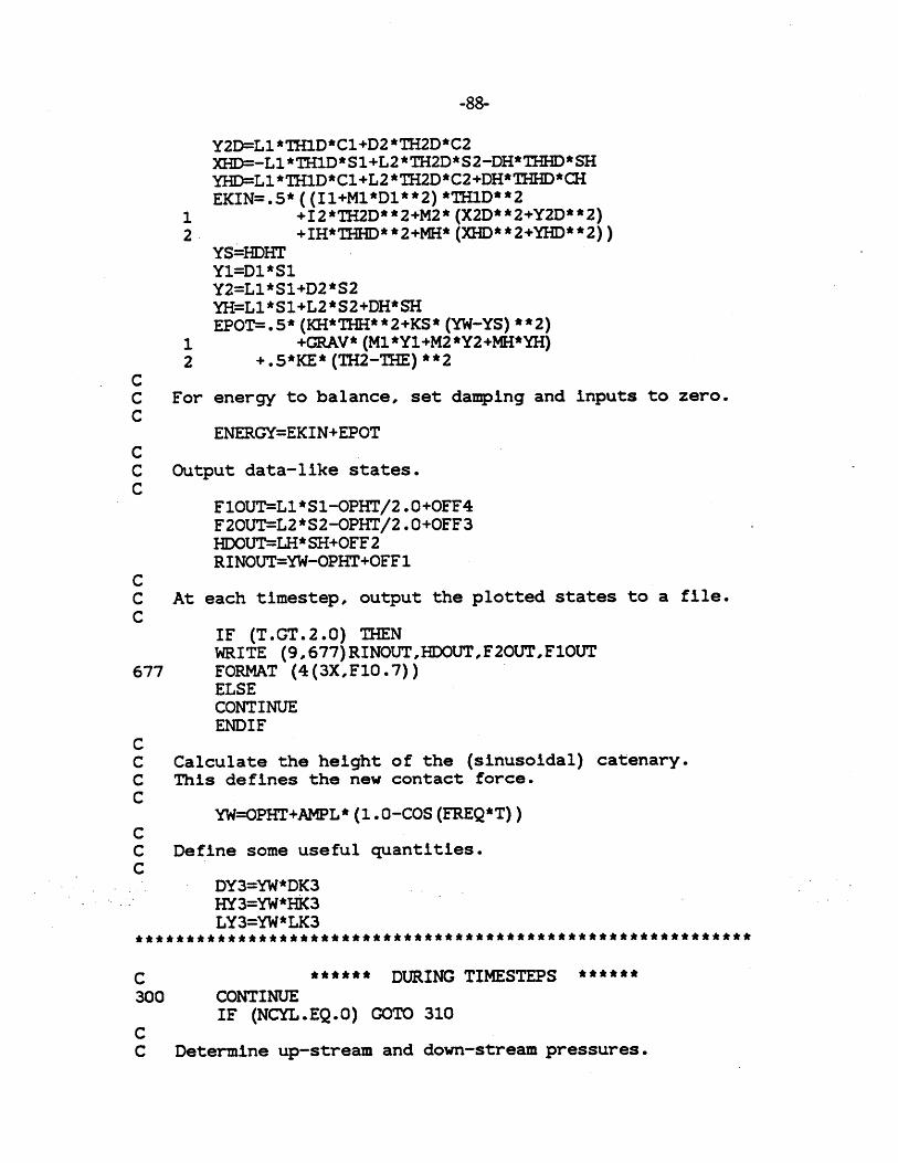
-88-

Y2D=L1*TH1D*C1+D2*TH2D*C2XHD=-L1*THlD*S1+L2*TH2D*S2-DH*THH*SHYHD=L1*THl1D*C1+L2*TH2D*C2+DH*THHD*CHEKIN=.5* ((I1+M1*D1**2) *TH1D**2

1 +12*TH2D**2+M2* (X2D**2+Y2D**2)2 +IH*THHD**2+MH* (XHD**2+YHD**2))

YS=HDHTY1=D1*S1Y2=L1*S1+D2*S2YH=L1*S1+L2*S2+DH*SHEPOT=.5* (KH*THH**2+KS* (YW-YS) **2)

1 +GRAV* (Ml*Y1+M2*Y2+MHi*YH)2 +.5*KE* (TH2-THE) **2

CC For energy to balance, set damping and inputs to zero.C

ENERGY=EKIN+EPOTCC Output data-like states.C

F1OUT=L1*S1-OPHT/2.0+OFF4F2OUT=L2*S2-OPHT/2.0+OFF3HDOUT=-LH*SH+0FF2RINOUT=YW-OPHT+OFF1

CC At each timestep, output the plotted states to a file.C

IF (T.GT.2.0) THENWRITE (9,677)RINOUT,HDOUT,F2OUT,F1OUT

677 FORMAT (4(3XF10.7))ELSECONTINUEENDIF

CC Calculate the height of the (sinusoidal) catenary.C This defines the new contact force.C

YW=OPHT+AMPL* (1.0-COS (FREQ*T))CC Define some useful quantities.C

DY3=YW*DK3HY3=YW*HK3LY3=YW*LK3

C DURING TIMESTEPS *300 CONTINUE

IF (NCYL.EQ.0) COTO 310CC Determine up-stream and down-stream pressures.

-89-

CIF (P.GT.PSUPP) THEN

PUP=PPDOWN=PSUPP

ELSEPUP=PSUPPPDOWN=P

ENDIF

CYLVOL=CYLVOLO+AREA*LMARM*COS (ALFA-TH1)CYLVOLD=AREA*THl1D* SIN (ALFA-TH1)

PDPU=PDOWN/PUPPD=GASCNS/CYLVOL*PUP* (PDPU) ** (1.0/GAMMA)

& *SQRT (1.0-PDPU** (GAMMA-1.0/GAMMA))& -P*CYLVOLD/CYLVOL

FINPUT= (P-PATM) *AREAGOTO 320

CC Simple (linear) cylinder equations.C310 XCYL=LMARM*COS (ALFA-TH1) -P

PD=KCYL*XCYL/BVCYLFINPUT=PSUPPG*AREA-KCYL*XCYL

320 CONTINUECC Abbreviations:C

S1=SIN (TH1)C1=COS (TH1)

S2=SIN(TH2)C2=COS (TH2)

SH=SIN (THH)CH=COS (THH)

S12=SIN (TH1+TH2)C12=COS (TH1+TH2)

S2H=SIN (TH2+THH)C2H=COS (TH2+THH)

S1H=SIN (TH1-THH)C1H=COS (TH1-THH)

SH1=SIN (THH-TH1)CC Calculate the elbow link position and the elbow torque.C

LC1MXF=L1*C1-XF

-90-

LS1PYF=L1*S1+YFTRMA=LC1MXF**2-LE**2TRMB=-2.0 *LC1MXF*LS1PYFTRMC=LS1PYF**2-LE**2SRD=SQRT (TRMB**2-4.0*TRMA*TRMC)PH1=ATAN2 (-TRMB-SRD, 2.0*TRMA)XG=L1*C1+LE*SIN (PHi)YG=L1*S1-LE*COS (PHi)DFG=SQRT( (XG-XF) **2+ (YG+YF) **2)THE=THEO+ (DFG-DFGO) /LE-TH1

CC Calculate DTHEDTH1.C

DCDTH1=2.0*LS1PYF*L1*C1DBDTH1=-2.0* (LC1MXF*L1*C1-LS1PYF*L1*S1)DADTH1=-2.0*LC1MXF*L1*S1DPH1DTH1= (-TRMA**2/ (2.0*TRMA**2+TRMB**2-

1 2.0*TRMA*TRMC+TRMB*SRD)) *2 (DBDTH1/TRMA-TRMB*DADTH1/TRMA**2+3 (TRMB*DBDTH1-2.0* (TRMA*DCDTH1+4 TRMC*DADTHl1) ) / (TRMA* SRD) -5 SRD*DADTH1/TRMA**2)

DYGDTH1=L1*C1+LE*SIN (PHi) *DPH1DTH1DXGDTH1=-L1*S1+LE*COS (PH1) *DPH1DTH1DFGDTH1= ((XG-XF) *DXGDTH1+ (YG+YF) *DYGDTH1l)

& /SQRT( (XG-XF) **2+ (YG+YF) **2)DTHEDTH1=DFGDTH1/LE-1.0

CC The equations of motion are as follows:C A*THl1DD + B*TH2DD + C*THDD = DC E*TH1DD + F*TH2DD + G*THHDD = HC I*TH1DD + J*TH2DD + K*THHDD = LC where A,B,C,DE,FG,H,I,J,K,L are functions of the threeC rotational state variables, their first time derivatives,C the state variable P, the input YW, and the system parameters.C

A=AK1B=BK1*C12C=CK1*C1HD=TH2D**2*S12*DK1

1 +THHD**2*SH1*DK22 +C1* (DY3-DK4)3 -S1*C1*DK5-C1*S2*DK6-C1*SH*DK74 +FINPUT*LMARM*SIN (ALFA-TH1) -KE* (THE-TH2) *DTHEDTH15 -SIGN (BC1, TH1D) -SIGN (BC2,TH1D+TH2D)6 -BV1*TH1D-BV2* (TH1D+TH2D)

E=EK1*C12F=FK1G=GK1*C2HH=TH1D**2*HK1*S12

-91-

1 +THHD**2*HK2*S2H2 +C2* (HY3-HK4)3 -S2*C2*HK5-S1*C2*HK6-C2*SH*HK74 -KE*(TH2-THE)5 -SIGN (BC2, THlD+TH2D) -SIGN (BCH, TH2D+THHD)6 -BV2* (TH1D+TH2D) -BVH* (TH2D+THHD)

I=IK1*C1HJ=JK1*C2HK=KK1L=TH1D**2*LK1*S1H

1 +TH2D**2*LK2*S2H2 +CH* (LY3-LK4)3 -SH*CH*LK5-S1*CH*LK6-S2*CH*LK74 -THH* KH-SIGN (BCH, TH2D+THHD)5 -BVH* (TH2D+THHD)

CC Define some abbreviations.C

FAEB=F*A-E*BGAEC=G*A-E*CHAED=H*A-E*DJAIB=J*A-I*BKAIC=K*A-I*CLAID=L*A-I*D

CC Equations to be integrated:C

THHDD=(FAEB*LAID-JAIB*HAED)/(FAEB*KAIC-JAIB*CAEC)TH2DD=(HAED-GAEC*THHDD)/FAEBTH1DD= (D-B*TH2DD-C*THHDD) /A

CC Derivitives of state variables:C

FY (1)=TH1DFY (2)=TH1DDFY (3),=TH2DFY (4)=TH2DDFY (5) =THHDFY (6) =THHDDFY(7)=PD

RETURNEND