ORIGINAL ARTICLE

Investigation of water depth and basin wall effects on KVLCC2in manoeuvring motion using viscous-flow calculations

S. L. Toxopeus • C. D. Simonsen • E. Guilmineau •

M. Visonneau • T. Xing • F. Stern

Received: 2 October 2012 / Accepted: 31 March 2013

� JASNAOE 2013

Abstract The objective of the NATO AVT-161 working

group is to assess the capability of computational tools to

aid in the design of air, land and sea vehicles. For sea

vehicles, a study has been initiated to validate tools that can

be used to simulate the manoeuvrability or seakeeping

characteristics of ships. This article is part of the work

concentrating on manoeuvring in shallow water. As

benchmark case for the work, the KVLCC2 tanker from

MOERI was selected. At INSEAN, captive PMM

manoeuvring tests were conducted with a scale model of

the vessel for various water depths. Several partners in the

AVT group have conducted RANS calculations for a

selected set of manoeuvring conditions and water depths

for the bare hull. Each partner was asked to use their best

practice and own tools to prepare the computations and run

their flow codes. Specific instructions on the post-pro-

cessing were given such that the results could be compared

easily. The present article discusses these results. Detailed

descriptions of the approach, assumptions, and verification

and validation studies are given. Comparisons are made

between the computational results and with the experi-

ments. Furthermore, flow features are discussed.

Keywords KVLCC2 � Viscous flow � Manoeuvring �Shallow water � Wall effects

1 Introduction

The NATO Specialist Team in Naval Ship Manoeuvrability

(ST-NSM) is developing a Standardization Agreement

(STANAG) regarding common manoeuvring capabilities

for NATO warships for specific missions. The naval ships

are subject to more strict criteria than imposed by IMO

resolutions for commercial vessels, as explained by Ornfelt

[1]. To verify compliance with the STANAG, high-fidelity

predictions of the ship’s manoeuvring characteristics are

required. In Quadvlieg et al. [2] it was concluded that

modern empiric prediction tools have not been validated

thoroughly for all possible manoeuvres or missions

described in the STANAG and therefore further validation

and improvements are required. The objective of the NATO

AVT-161 working group is to assess the capability of

computational tools to aid in the design of air, land and sea

vehicles. If these tools prove to be accurate in prediction of

these characteristics, they can be used to obtain more

accurate assessments of compliance with the STANAG. For

sea vehicles, a study has been initiated to validate tools that

can be used to simulate the manoeuvrability or seakeeping

S. L. Toxopeus (&)

Maritime Research Institute Netherlands (MARIN)/Delft

University of Technology, Wageningen, The Netherlands

e-mail: s.l.toxopeus@marin.nl

C. D. Simonsen

FORCE Technology, Lyngby, Denmark

e-mail: cds@force.dk

E. Guilmineau � M. Visonneau

ECN-Ecole Centrale de Nantes, Nantes, France

e-mail: Emmanuel.Guilmineau@ec-nantes.fr

M. Visonneau

e-mail: Michel.Visonneau@ec-nantes.fr

T. Xing

University of Idaho, Moscow, ID, USA

e-mail: xing@uidaho.edu

F. Stern

IIHR-Hydroscience and Engineering, The University of Iowa,

Iowa City, IA, USA

e-mail: frstern@engineering.uiowa.edu

123

J Mar Sci Technol

DOI 10.1007/s00773-013-0221-6

characteristics of ships. This article is part of the work

concentrating on manoeuvring in shallow water. In the

present study, the capability to predict the influence of the

water depth on the forces and moments on a ship will be

investigated. In Simonsen et al. [3], the importance of the

domain width for shallow water conditions was already

stressed and it was suggested that blockage may contribute

to the scatter in the results from different towing tanks for

the Esso Osaka. Therefore, special attention will be paid to

the effect of the blockage on the results.

As benchmark case for the work, the KVLCC2 tanker

from MOERI was selected. At INSEAN, captive PMM

manoeuvring tests were conducted in 2005/2006 with a

7 m scale model of the vessel (scale: 1:45.714) for various

water depths. The main particulars of the KVLCC2 are

given in Table 1. Several partners in the AVT group have

conducted RANS calculations for a selected set of

manoeuvring conditions and water depths for the bare hull.

Each partner was asked to use their best practice and own

tools to prepare the computations and run their flow codes.

Specific instructions on the post-processing were given

such that the results could be compared easily. The present

article discusses these results. Detailed descriptions of the

approach, assumptions, and verification and validation

studies are given. Comparisons are made between the

computational results and with the experiments. Further-

more, flow features are discussed.

2 Coordinate system

The origin of the right-handed system of axes used in this

study is located at the intersection of the water plane,

midship and centre-plane, with x directed forward, y to

starboard and z vertically downward. The forces and

moments are also given according to this coordinate sys-

tem. Sinkage is positive for the ship moving deeper into the

water and trim is positive for bow up.

In the present calculations, a positive drift angle b cor-

responds to the flow coming from port side (i.e. b = arctan

-v/u, with u the ship-fixed velocity in x direction and v the

ship-fixed velocity in y direction). The non-dimensional

yaw rate c is calculated with c = r 9 Lpp/V and is positive

for a turning rate r to starboard when sailing at positive

forward speed V.

3 KVLCC2 model tests

The KVLCC2 (KRISO Very Large Crude Carrier) hull

form was one of the subjects of study during the CFD

Workshops Gothenburg 2000 [4] and 2010 [5] and the

SIMMAN 2008 Workshop [6]. For straight ahead condi-

tions, the flow features and resistance values were mea-

sured, see Lee et al. [7] and Kim et al. [8].

Captive model tests for the bare hull KVLCC2 were

conducted by INSEAN in 2005/2006 in preparation for the

SIMMAN 2008 Workshop [6], see also Fabbri et al.

[9–11]. The scale of the ship model, INSEAN model no

C2487, was 1:45.71. A set of PMM tests comprising

amongst others the measurement of the forces and

moments for steady drift motion and oscillatory yaw

motion was performed. During the tests, the model was

free to heave and pitch. For the present work, only the tests

with the bare hull form and a model speed of 0.533 m/s, or

Fn = 0.0642 are considered.

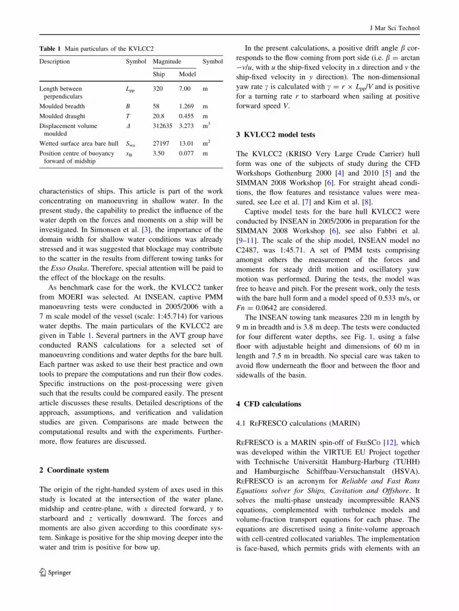
The INSEAN towing tank measures 220 m in length by

9 m in breadth and is 3.8 m deep. The tests were conducted

for four different water depths, see Fig. 1, using a false

floor with adjustable height and dimensions of 60 m in

length and 7.5 m in breadth. No special care was taken to

avoid flow underneath the floor and between the floor and

sidewalls of the basin.

4 CFD calculations

4.1 REFRESCO calculations (MARIN)

REFRESCO is a MARIN spin-off of FRESCO [12], which

was developed within the VIRTUE EU Project together

with Technische Universitat Hamburg-Harburg (TUHH)

and Hamburgische Schiffbau-Versuchanstalt (HSVA).

REFRESCO is an acronym for Reliable and Fast Rans

Equations solver for Ships, Cavitation and Offshore. It

solves the multi-phase unsteady incompressible RANS

equations, complemented with turbulence models and

volume-fraction transport equations for each phase. The

equations are discretised using a finite-volume approach

with cell-centred collocated variables. The implementation

is face-based, which permits grids with elements with an

Table 1 Main particulars of the KVLCC2

Description Symbol Magnitude Symbol

Ship Model

Length between

perpendiculars

Lpp 320 7.00 m

Moulded breadth B 58 1.269 m

Moulded draught T 20.8 0.455 m

Displacement volume

moulded

D 312635 3.273 m3

Wetted surface area bare hull Swa 27197 13.01 m2

Position centre of buoyancy

forward of midship

xB 3.50 0.077 m

J Mar Sci Technol

123

arbitrary number of faces (hexahedrals, tetrahedrals,

prisms, pyramids, etc.). The code is targeted, optimized

and highly validated for hydrodynamic applications, in

particular for obtaining current, wind and manoeuvring

coefficients of ships, submersibles and semi-submersibles

[13–16].

Several different turbulence closure models are avail-

able in REFRESCO. In this study, the Menter’s 1994 ver-

sion of the SST model [17] of the two-equation k–xturbulence model is used. In the turbulence model, the

Spalart correction (proposed by Dacles-Mariani et al. [18])

of the stream-wise vorticity can be activated.

For ship manoeuvres, not only oblique flow is of inter-

est, but also the flow around the ship when it performs a

rotational (yaw) motion. In RANS, the rotational motion

can be modelled in several ways, such as moving the grid

in a rotational motion through a stationary flow (inertial

reference system), or by letting the flow rotate around the

stationary ship (non-inertial reference system). For this

work a non-inertial reference system is chosen. Centrifugal

and Coriolis forces to account for the rotation of the

coordinate system are added to the momentum equation as

source terms. More information about the implementation

can be found in Toxopeus [16].

4.1.1 Computational domain and grids

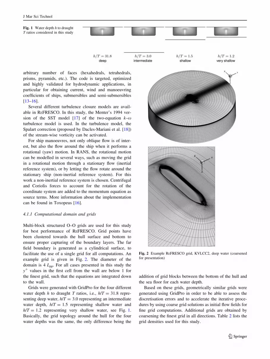
Multi-block structured O–O grids are used for this study

for best performance of REFRESCO. Grid points have

been clustered towards the hull surface and bottom to

ensure proper capturing of the boundary layers. The far

field boundary is generated as a cylindrical surface, to

facilitate the use of a single grid for all computations. An

example grid is given in Fig. 2. The diameter of the

domain is 4 Lpp. For all cases presented in this study the

y? values in the first cell from the wall are below 1 for

the finest grid, such that the equations are integrated down

to the wall.

Grids were generated with GridPro for the four different

water depth h to draught T ratios, i.e., h/T = 31.8 repre-

senting deep water, h/T = 3.0 representing an intermediate

water depth, h/T = 1.5 representing shallow water and

h/T = 1.2 representing very shallow water, see Fig. 1.

Basically, the grid topology around the hull for the four

water depths was the same, the only difference being the

addition of grid blocks between the bottom of the hull and

the sea floor for each water depth.

Based on these grids, geometrically similar grids were

generated using GridPro in order to be able to assess the

discretisation errors and to accelerate the iterative proce-

dures by using coarse grid solutions as initial flow fields for

fine grid computations. Additional grids are obtained by

coarsening the finest grid in all directions. Table 2 lists the

grid densities used for this study.

Fig. 1 Water depth h to draught

T ratios considered in this study

Fig. 2 Example REFRESCO grid, KVLCC2, deep water (coarsened

for presentation)

J Mar Sci Technol

123

4.1.2 Case setup

The calculations presented in this study were all conducted

without incorporating free-surface deformation and

assuming steady flow. Based on the speeds used during the

tests and the range of drift angles or yaw rates studied, the

effects of Froude number and free-surface deformation on

the forces on the manoeuvring ship were expected to be

reasonably small and assumed to be smaller than the

uncertainties due to, e.g., discretisation errors or errors in

the experimental results. To simplify the calculations,

symmetry boundary conditions were therefore applied on

the undisturbed water surface and dynamic sinkage and

trim was neglected. On the hull surface, no-slip and

impermeability boundary conditions are used (�u ¼ 0). For

all calculations, even for deep water, the boundary condi-

tion on the bottom surface is set to moving-wall/fixed slip

(�u ¼ �V1, with �V1 the inflow velocity). All calculations

were conducted with a Reynolds number of Re = 3.7 9

106.

Additionally, a calculation for deep water with the finest

grid was conducted with Re = 4.6 9 106, in order to be

able to compare the flow field with measurements in a wind

tunnel by Lee et al. [7].

Calculations for ships at drift angles or yaw rates are

conducted by setting the boundary conditions at the exte-

rior to the proper inflow velocities. This is done using the

so-called BCAUTODETECT boundary condition, which

automatically applies inflow conditions (�u ¼ �V1) or out-

flow (Neumann, o/o�n ¼ 0) conditions on the cell faces,

depending on the normal velocity at each cell face on the

boundary. Therefore, the computational domain does not

need to be changed for each new calculation and a single

grid for different manoeuvring conditions can be used.

Details about BCAUTODETECT can be found in Toxopeus

[16].

In order to efficiently generate results for many drift

angles, a routine was used to automatically increment the

drift angle during a single simulation. Simulations begin

with a pre-set drift angle, until a specified number of

iterations is reached, or when the maximum change in the

residuals is less than a specified convergence criterion.

Next, the drift angle is incremented by Db, by changing the

inflow conditions, and the solution is continued from the

solution from the previous drift angle. Starting the calcu-

lations from a converged solution at a slightly different

drift angle saves time compared to performing each cal-

culation separately from undisturbed flow. This procedure

is repeated until the desired maximum inflow angle is

reached. In Toxopeus [16], it is demonstrated that this

approach provides the same results as those obtained with

multiple single-drift angle calculations.

This procedure was designated drift sweep and the

application has already been presented in, e.g., Toxopeus

[16], Vaz et al. [14] and Bettle et al. [19].

4.2 STAR-CCM ? calculations (FORCE)

The computations are performed with the Reynolds aver-

aged Navier–Stokes (RANS) solver STAR-CCM ? from

CD-adapco. The code solves the RANS and continuity

equations on integral form on an unstructured mesh by

means of the finite volume technique. For the present

calculations the temporal discretisation is based on a first

order Euler difference, while spatial discretisation is per-

formed with second order schemes for both convective and

viscous terms. The pressure and the velocities are coupled

by means of the SIMPLE method. Closure of the Reynolds

stress problem is achieved by means of the isotropic

blended k–e/k–x SST turbulence model with an all y? wall

treatment, which based on the y? value automatically,

selects the proper near wall model. The free surface is

modelled with the two phase volume of fluid technique

(VOF). In case squat is included in the simulation, the

6DOF module in the CFD code is applied. The heave and

pitch motions are found by solving the equations of

motions on each time step based on the hydrodynamic

forces computed with the flow solver. The motion of the

ship in the flow model is handled by mesh morphing, i.e.,

by stretching the computational grid locally around the ship

as it moves. In the present approach the computation with

squat is done in two steps. First dynamic sinkage and trim

are determined with the morphing technique on a coarse

grid and next the model is positioned and locked in the fine

grid simulation for calculation of the hydrodynamic forces.

Further details about the code can be found in the Star-

CCM ? User’s Manual [20].

4.2.1 Computational domain and grids

The applied grid is an unstructured hexa-dominant poly-

hedral mesh, which is generated in STAR-CCM ? by

means of the trimmed mesh approach. The idea is to apply

an orthogonal hexahedral background grid and use the

shape of the ship to cut out a hole with the same geometry

as the hull form. When this is done, prism layers are grown

Table 2 Grid densities used for verification and validation in

REFRESCO

h/T Grid cells (10-3)

31.8 (deep) 12721, 8455, 5388, 3340, 2270, 1590, 121

3.0 (intermediate) 13005, 8597, 5573, 3446, 2374, 1604, 137

1.5 (shallow) 11659, 7688, 4936, 3106, 2112, 1437, 119

1.2 (very shallow) 11031, 7270, 4664, 2899, 1999, 1351

J Mar Sci Technol

123

on the geometry to resolve the boundary layer on the hull.

Finally, zones with local grid refinement are used around

the ship, in the gap between ship and seabed and in the free

surface region. Since static drift conditions are simulated,

both sides of the hull are considered instead of exploiting

the centre plane symmetry. The grid near wall spacing on

no-slip surfaces are in the range from y? = 1 to y? = 30.

Different grids are applied for each water depth, but in

order to minimize the influence of the grid fineness when

the pressure and shear forces are integrated to obtain the

hydrodynamic loads, the same cell size is used on the hull

surface for all grids. The location of the outer boundaries is

described in the case setup section below. On the seabed,

prism layers are applied to resolve the bottom boundary

layer in shallow water, but not in the deep water case,

where this effect is negligible. Concerning mesh size, the

grids used for free surface simulations contain around 7.5

million cells, while the grids applied for simulations

without free surface only contains app. 5.0 million cells,

since the mesh above the still water surface can be

removed. Examples on the applied grids can be seen in

Fig. 3. As mentioned earlier the squat is computed an a

coarse grid, which in this case consist of approximately 1

million cells. Forces are calculated with 7.5 million cells.

In cases with small under keel clearance and mesh morp-

hing there is a risk of deforming the mesh too much when

the ship squats and the under keel clearance is reduced.

Figure 4 shows a cross section below the ship located

0.071L aft of the forward perpendicular plane where the

larger deformations occur due to bow down trim. As seen

in the figure the deformed mesh looks fine after morphing.

Further, no negative cell volumes were detected during the

computation.

4.2.2 Case setup

The influence of tank width, free surface effects and squat

is investigated in the present computations. Except for the

case where squat is included, all simulations are performed

with the ship fixed at design draught and even keel. Two

domain widths are considered. The narrow domain has the

same width as the towing tank, where the experiments were

conducted, i.e., 1.29Lpp, while the wide domain has a width

of 3.00Lpp. For all cases the inlet boundary is located

2.36Lpp in front of the ship, while the outlet boundary is

located 3.79Lpp downstream of the ship. The bottom of the

domain is located according to the considered water depth.

A no-slip condition is used on the hull itself. Below the

ship two different boundary conditions are applied

depending on the water depth. In deep water, i.e.,

h/T = 8.3, the effect of the boundary layer on the seabed is

negligible, so a slip-wall condition is applied. In shallow

water, i.e. h/T = 1.5 and 1.2, a boundary layer builds up on

the seabed below the ship, which influences the flow in the

gap between the bottom of the ship and the seabed.

Therefore, a moving no-slip condition is applied on the

seabed, so the bottom moves with the free stream speed. It

should be noted that the bottom is modelled with a standard

Fig. 3 Example STAR-CCM ? grid applied for shallow water

simulation with free surface

Fig. 4 Grid in gap between ship and seabed after morphing during

computation of squat

J Mar Sci Technol

123

fully turbulent boundary layer, i.e. the roughness is not

adjusted to reflect the bottom in the towing tank.

For simulations without free surface the top of the

domain is placed on the still water surface, where a sym-

metry condition is applied. On the inlet boundary the free

stream speed prescribed, while the outlet boundary is

modelled with a pressure condition, p = 0. On the sides of

the domain a slip-wall boundary condition is used. When

simulations with free surface and with and without squat

are conducted, the domain is extended 0.65Lpp into the air

above the still water level to capture the free surface

deformation and a slip condition is applied as boundary

condition. Further, the volume fraction is prescribed on the

inlet boundary to model the still water level and the

hydrostatic pressure is applied on the outlet boundary. All

other boundary conditions are the same as above.

Only straight-ahead, b = 0�, and static drift, b = 4�, are

simulated. In both cases the same outer domain and

boundary conditions are applied and the drift angle is

obtained by turning the ship 4 degrees relative to the

domain and flow direction, similar to a towing tank PMM

test.

4.3 ISIS-CFD calculations (ECN)

ISIS-CFD, developed by the CFD group of the Fluid

Mechanics Laboratory and available as a part of the

FINETM/Marine computing suite, is an incompressible

unsteady Reynolds-averaged Navier–Stokes (URANS)

method. The solver is based on the finite volume method

to build the spatial discretisation of the transport equa-

tions. The unstructured discretisation is face-based, which

means that cells with an arbitrary number of arbitrarily

shaped faces are accepted. A detailed description of the

solver is given in Queutey and Visonneau [21] and Du-

vigneau et al. [22]. The velocity field is obtained from the

momentum conservation equations and the pressure field

is extracted from the mass conservation constraint, or

continuity equation, transformed into a pressure equation.

In the case of turbulent flows, transport equations for the

variables in the turbulence model are added to the dis-

cretisation. Free-surface flow is simulated with a multi-

phase flow approach: the water surface is captured with a

conservation equation for the volume fraction of water,

discretised with specific compressive discretisation

schemes discussed in Queutey and Visonneau [21]. The

method features sophisticated turbulence models: apart

from the classical two-equation k–x and k–e models, the

anisotropic two-equation explicit algebraic stress model

(EASM), as well as Reynolds stress transport models are

available, see Duvigneau et al. [22] and Deng and

Visonneau [23]. The technique included for the 6 degree

of freedom simulation of ship motion is described by

Leroyer and Visonneau [24]. Time-integration of New-

ton’s laws for the ship motion is combined with analytical

weighted or elastic analogy grid deformation to adapt the

fluid mesh to the moving ship. Furthermore, the code has

the possibility to model more than two phases. For

brevity, these options are not further described here.

4.3.1 Computational domain and grids

The computational domain takes into account the size of

the tank, i.e., the width is 9 m and the water depth varies

between 0.546 to 3.777 m. All computational domains

start 2.5Lpp before the hull and extend 4Lpp after the hull.

The top of the mesh for the simulation with free surface is

located 0.143Lpp above the still water level. Grids were

generated with Hexpress. For all test-cases, the hull is

described with the same number of faces, and for the

‘‘straight-ahead’’ cases, the mesh contains between 1.5

and 1.7 million cells, while for the ‘‘static drift’’ cases, the

mesh is comprised of 9.2–10 million cells. For the

straight-ahead case, only one side of the ship is computed.

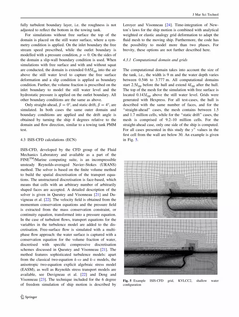
For all cases presented in this study the y? values in the

first cell from the wall are below 30. An example is given

in Fig. 5.

Fig. 5 Example ISIS-CFD grid, KVLCC2, shallow water

configuration

J Mar Sci Technol

123

4.3.2 Case setup

The calculations presented in this article were made with or

without taking the free surface into account. Three water

depth h to draught T ratios were studied: h/T = 8.3 rep-

resenting deep water, h/T = 1.5 representing shallow water

and h/T = 1.2 representing very shallow water and two

conditions were considered: ‘‘straight-ahead’’, and ‘‘static

drift’’ with a drift angle of 4�. All the computations were

performed with wall function on the ship hull and free-slip

on side wall and tank bottom. Since the ship is moving at

model speed in the ISIS-CFD computations, the velocity at

the inlet is set to zero. The turbulence model used for all

test cases is the non-linear anisotropic Explicit Algebraic

Stress Model (EASM). When the ship is free to sink and

trim, the hull motion is computed using Newton’s laws and

the mesh is adapted to the movement of the ship with the

analytical weighted grid deformation of ISIS-CFD, see

Leroyer and Visonneau [24].

4.4 CFDShip-Iowa calculations (IIHR)

These results are a portion of those of a more compre-

hensive study that uses DES on a 13M grid to investigate

vortical and turbulent structures for KVLCC2 tanker hull

form at large drift angles with analogy to delta wings, see

Xing et al. [25]. The general-purpose solver CFDShip-

Iowa-V.4 (see Carrica et al. [26]) solves the unsteady

RANS (URANS) or DES equations in the liquid phase of a

free surface flow. The free surface is captured using a

single-phase level set method and the turbulence is mod-

elled by isotropic or anisotropic turbulence models.

Numerical methods include advanced iterative solvers,

second and higher order finite difference schemes with

conservative formulations, parallelization based on a

domain decomposition approach using the message-pass-

ing interface (MPI), and dynamic overset grids for local

grid refinement and large-amplitude motions.

4.4.1 Computational domain and grids

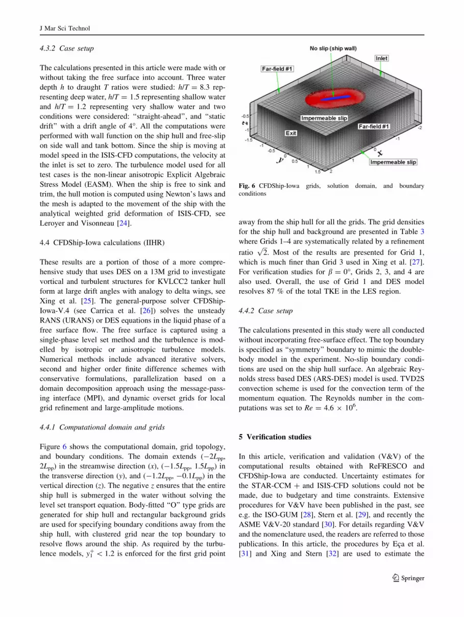
Figure 6 shows the computational domain, grid topology,

and boundary conditions. The domain extends (-2Lpp,

2Lpp) in the streamwise direction (x), (-1.5Lpp, 1.5Lpp) in

the transverse direction (y), and (-1.2Lpp, -0.1Lpp) in the

vertical direction (z). The negative z ensures that the entire

ship hull is submerged in the water without solving the

level set transport equation. Body-fitted ‘‘O’’ type grids are

generated for ship hull and rectangular background grids

are used for specifying boundary conditions away from the

ship hull, with clustered grid near the top boundary to

resolve flows around the ship. As required by the turbu-

lence models, y1? \ 1.2 is enforced for the first grid point

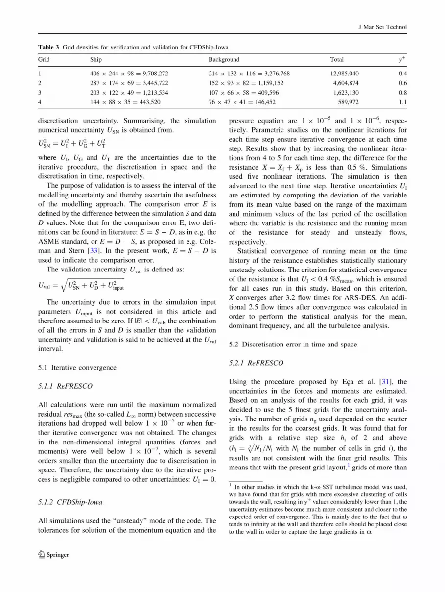
away from the ship hull for all the grids. The grid densities

for the ship hull and background are presented in Table 3

where Grids 1–4 are systematically related by a refinement

ratioffiffiffi

2p

. Most of the results are presented for Grid 1,

which is much finer than Grid 3 used in Xing et al. [27].

For verification studies for b = 0�, Grids 2, 3, and 4 are

also used. Overall, the use of Grid 1 and DES model

resolves 87 % of the total TKE in the LES region.

4.4.2 Case setup

The calculations presented in this study were all conducted

without incorporating free-surface effect. The top boundary

is specified as ‘‘symmetry’’ boundary to mimic the double-

body model in the experiment. No-slip boundary condi-

tions are used on the ship hull surface. An algebraic Rey-

nolds stress based DES (ARS-DES) model is used. TVD2S

convection scheme is used for the convection term of the

momentum equation. The Reynolds number in the com-

putations was set to Re = 4.6 9 106.

5 Verification studies

In this article, verification and validation (V&V) of the

computational results obtained with ReFRESCO and

CFDShip-Iowa are conducted. Uncertainty estimates for

the STAR-CCM ? and ISIS-CFD solutions could not be

made, due to budgetary and time constraints. Extensive

procedures for V&V have been published in the past, see

e.g. the ISO-GUM [28], Stern et al. [29], and recently the

ASME V&V-20 standard [30]. For details regarding V&V

and the nomenclature used, the readers are referred to those

publications. In this article, the procedures by Eca et al.

[31] and Xing and Stern [32] are used to estimate the

Fig. 6 CFDShip-Iowa grids, solution domain, and boundary

conditions

J Mar Sci Technol

123

discretisation uncertainty. Summarising, the simulation

numerical uncertainty USN is obtained from.

U2SN ¼ U2

I þ U2G þ U2

T

where UI, UG and UT are the uncertainties due to the

iterative procedure, the discretisation in space and the

discretisation in time, respectively.

The purpose of validation is to assess the interval of the

modelling uncertainty and thereby ascertain the usefulness

of the modelling approach. The comparison error E is

defined by the difference between the simulation S and data

D values. Note that for the comparison error E, two defi-

nitions can be found in literature: E = S - D, as in e.g. the

ASME standard, or E = D - S, as proposed in e.g. Cole-

man and Stern [33]. In the present work, E = S - D is

used to indicate the comparison error.

The validation uncertainty Uval is defined as:

Uval ¼ffiffiffiffiffiffiffiffiffiffiffiffiffiffiffiffiffiffiffiffiffiffiffiffiffiffiffiffiffiffiffiffiffiffiffiffiffi

U2SN þ U2

D þ U2input

q

The uncertainty due to errors in the simulation input

parameters Uinput is not considered in this article and

therefore assumed to be zero. If |E| \ Uval, the combination

of all the errors in S and D is smaller than the validation

uncertainty and validation is said to be achieved at the Uval

interval.

5.1 Iterative convergence

5.1.1 REFRESCO

All calculations were run until the maximum normalized

residual resmax (the so-called L? norm) between successive

iterations had dropped well below 1 9 10-5 or when fur-

ther iterative convergence was not obtained. The changes

in the non-dimensional integral quantities (forces and

moments) were well below 1 9 10-7, which is several

orders smaller than the uncertainty due to discretisation in

space. Therefore, the uncertainty due to the iterative pro-

cess is negligible compared to other uncertainties: UI = 0.

5.1.2 CFDShip-Iowa

All simulations used the ‘‘unsteady’’ mode of the code. The

tolerances for solution of the momentum equation and the

pressure equation are 1 9 10-5 and 1 9 10-6, respec-

tively. Parametric studies on the nonlinear iterations for

each time step ensure iterative convergence at each time

step. Results show that by increasing the nonlinear itera-

tions from 4 to 5 for each time step, the difference for the

resistance X = Xf ? Xp is less than 0.5 %. Simulations

used five nonlinear iterations. The simulation is then

advanced to the next time step. Iterative uncertainties UI

are estimated by computing the deviation of the variable

from its mean value based on the range of the maximum

and minimum values of the last period of the oscillation

where the variable is the resistance and the running mean

of the resistance for steady and unsteady flows,

respectively.

Statistical convergence of running mean on the time

history of the resistance establishes statistically stationary

unsteady solutions. The criterion for statistical convergence

of the resistance is that UI \ 0.4 %Smean, which is ensured

for all cases run in this study. Based on this criterion,

X converges after 3.2 flow times for ARS-DES. An addi-

tional 2.5 flow times after convergence was calculated in

order to perform the statistical analysis for the mean,

dominant frequency, and all the turbulence analysis.

5.2 Discretisation error in time and space

5.2.1 ReFRESCO

Using the procedure proposed by Eca et al. [31], the

uncertainties in the forces and moments are estimated.

Based on an analysis of the results for each grid, it was

decided to use the 5 finest grids for the uncertainty anal-

ysis. The number of grids ng used depended on the scatter

in the results for the coarsest grids. It was found that for

grids with a relative step size hi of 2 and above

(hi ¼ffiffiffiffiffiffiffiffiffiffiffiffi

N1=Ni3p

with Ni the number of cells in grid i), the

results are not consistent with the finer grid results. This

means that with the present grid layout,1 grids of more than

Table 3 Grid densities for verification and validation for CFDShip-Iowa

Grid Ship Background Total y?

1 406 9 244 9 98 = 9,708,272 214 9 132 9 116 = 3,276,768 12,985,040 0.4

2 287 9 174 9 69 = 3,445,722 152 9 93 9 82 = 1,159,152 4,604,874 0.6

3 203 9 122 9 49 = 1,213,534 107 9 66 9 58 = 409,596 1,623,130 0.8

4 144 9 88 9 35 = 443,520 76 9 47 9 41 = 146,452 589,972 1.1

1 In other studies in which the k-x SST turbulence model was used,

we have found that for grids with more excessive clustering of cells

towards the wall, resulting in y? values considerably lower than 1, the

uncertainty estimates become much more consistent and closer to the

expected order of convergence. This is mainly due to the fact that xtends to infinity at the wall and therefore cells should be placed close

to the wall in order to capture the large gradients in x.

J Mar Sci Technol

123

about 1.6 9 106 cells are required to obtain a reliable

solution of the forces and moments. Table 4 presents the

estimated discretisation uncertainties for b = 0� in deep,

shallow and very shallow water. In this table, S indicates

the value of the solution on the finest grid, US the uncer-

tainty in the solution and p the observed order of conver-

gence. In Tables 5 and 6 the uncertainties for b = 4� and

c = 0.4 are shown.

In deep water, monotonic convergence for X is not

found for b = 0� and b = 4�. In that case, the data range is

used to estimate the uncertainty, combined with a factor of

safety of 3. Due to the small difference of X on the different

grids, the estimated uncertainty is however small, i.e.,

UX = 1.3 %S. For Xp and apparent order of convergence

much larger than the theoretical order of 2 is found. This

indicates irregular behaviour of the solution upon grid

refinement and therefore a factor of safety of 3 is adopted

as well.

For the shallow water depth cases of h/T = 1.5 and

h/T = 1.2, larger uncertainties are found, up to

UX = 11.8 %S, which is mainly caused by slow conver-

gence (p \ 1) The cases with yaw rates show the largest

uncertainties, also due to slow convergence and still large

changes between the solutions on the different grids.

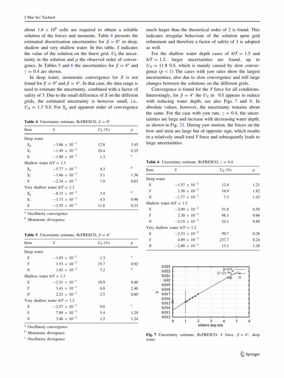
Convergence is found for the Y force for all conditions.

Interestingly, for b = 4� the UY in %S appears to reduce

with reducing water depth, see also Figs. 7 and 8. In

absolute values, however, the uncertainty remains about

the same. For the case with yaw rate, c = 0.4, the uncer-

tainties are large and increase with decreasing water depth,

as shown in Fig. 21. During yaw motion, the forces on the

bow and stern are large but of opposite sign, which results

in a relatively small total Y force and subsequently leads to

large uncertainties.

Table 4 Uncertainty estimate, REFRESCO, b = 0�

Item S US (%) p

Deep water

Xp -3.06 9 10-3 12.8 3.45

Xf -1.49 9 10-2 10.4 0.25

X -1.80 9 10-2 1.3 a

Shallow water h/T = 1.5

Xp -5.77 9 10-3 4.3 b

Xf -1.66 9 10-2 3.1 1.38

X -2.24 9 10-2 7.0 0.63

Very shallow water h/T = 1.2

Xp -8.15 9 10-3 3.4 b

Xf -1.73 9 10-2 4.5 0.96

X -2.55 9 10-2 11.8 0.23

a Oscillatory convergenceb Monotonic divergence

Table 5 Uncertainty estimate, REFRESCO, b = 4�

Item S US (%) p

Deep water

X -1.83 9 10-2 1.3 a

Y 1.53 9 10-2 15.7 0.92

N 1.02 9 10-2 7.2 b

Shallow water h/T = 1.5

X -2.31 9 10-2 10.9 0.40

Y 3.41 9 10-2 6.8 2.46

N 2.23 9 10-2 2.5 0.80

Very shallow water h/T = 1.2

X -2.57 9 10-2 9.0 c

Y 7.89 9 10-2 5.4 1.29

N 3.46 9 10-2 1.2 1.24

a Oscillatory convergenceb Monotonic divergencec Oscillatory divergence

Table 6 Uncertainty estimate, REFRESCO, c = 0.4

Item S US (%) p

Deep water

X -1.57 9 10-2 12.4 1.21

Y 1.58 9 10-2 16.9 1.82

N -1.77 9 10-2 7.3 1.43

Shallow water h/T = 1.5

X -2.09 9 10-2 51.8 0.50

Y 2.30 9 10-2 98.3 0.66

N -2.15 9 10-2 24.1 0.88

Very shallow water h/T = 1.2

X -2.53 9 10-2 99.7 0.26

Y 4.89 9 10-2 237.7 0.24

N -2.89 9 10-2 13.1 1.36

Fig. 7 Uncertainty estimate, REFRESCO, Y force, b = 4�, deep

water

J Mar Sci Technol

123

The uncertainties in the N moment are found to be more

reasonable than the uncertainties in X or Y, see Figs. 9 and

10. This is probably caused by the fact that during pure

yaw motion, the yaw moment (sum of contributions) is

better defined than the longitudinal force or side force

(difference between contributions). However, for c = 0.4,

the uncertainty is judged to be too high. Especially for

shallow water with h/T = 1.5, the uncertainty is high, due

to a low apparent order of convergence and large grid

dependency, see Fig. 9.

The theoretical order of convergence should be 2 for

ReFRESCO. However, due to flux limiters, discretisation

of the boundary conditions and other factors, the apparent

order of convergence is expected to be between 1 and 2 for

geometrically similar grids in the asymptotic range. Con-

sidering uncertainty estimates for the various water depths

and conditions, the apparent orders do not always follow

this expectation. This indicates that either even finer grids

are required, or that scatter in the results spoils the

uncertainty estimate.

5.2.2 CFDShip-Iowa

Quantitative verification is conducted for the grids fol-

lowing the factor of safety method, see Xing and Stern

[32]. The design of the grids enables two grid-triplet

studies with grid refinement ratio r ¼ffiffiffi

2p

(1, 2, 3 and 2, 3,

4). Larger r is not used since the coarse grids will be too

coarse such that different flow physics are predicted on

different grids as shown by the use of r ¼ffiffiffi

2p

at b = 0�,

i.e., steady vs. unsteady. The use of finer grids than Grid 1

may help as shown by the monotonic convergence for 5415

test case with grids up to 276 M (see Bhushan et al. [34]),

but simulations are too expensive and beyond the scope of

the current study. Smaller r is not used either since solution

changes will be small and the sensitivity to grid-spacing

may be difficult to identify compared with iterative errors.

Quantitative evaluation for time-step was not possible

since large time-step leads to unstable solutions for

ARS-DES on Grid 1 and simulations using smaller time-

step are too expensive. Nonetheless, the current time-step

(dt = 0.002) is only 20 % of the typical dt for CFD sim-

ulations in ship hydrodynamics and it is sufficiently small

to resolve all the unsteadiness of the vortical structures and

turbulent structures.

Previous simulation using ARS-DES on Grid 3 showed

that flow at b = 0� for KVLCC2 is steady and thus BKW

or ARS model was used (Xing et al. [27]). On Grid 1, ARS

shows steady flow, whereas ARS-DES predicts unsteady

flow. Table 7 shows V&V for the resistance. The experi-

mental data used to obtain the comparison errors is pre-

sented in Table 11. For b = 0�, monotonic convergence is

only achieved on (2, 3, 4) for X and on (2, 3, 4) and (1, 2, 3)

for Xf. The estimated orders of accuracy show large

oscillations as PG has values from 1.16 to 4.09. Xp shows

oscillatory divergence on the two grid triplets.

Overall the solutions are not in the asymptotic range,

which was attributed to several causes. At b = 0�, ARS-

DES on Grid 1 shows unsteady flow, whereas all other

grids predict steady flows and thus they are resolving dif-

ferent flow physics. Further refinement of the grids may

help but subject to the problem of separating iterative

errors and grid solution changes on fine grids. Furthermore,

grid refinement for DES changes the numerical errors and

the sub-grid scaling modelling errors simultaneously,

which was not considered for all available solution

Fig. 8 Uncertainty estimate, REFRESCO, Y force, b = 4�, very

shallow water

Fig. 9 Uncertainty estimate, REFRESCO, N moment, c = 0.4,

shallow water

Table 7 Verification for CFDShip-Iowa, ARS-DES

Variables Grids RG PG UG d/E UV UD

X 2, 3, 4 0.125 3.00 1.716 2.1 3.70 3.3

Xf 1, 2, 3 0.059 4.09 0.228 1.4 – –

Xf 2, 3, 4 0.447 1.16 4.07 1.3 – –

Xp 1, 2, 3 -1.1 Oscillatory divergence – –

Xp 2, 3, 4 -1.1 Oscillatory divergence – –

UG is %Sfine, d is %Xf,ITTC for Xf, E, UV, and UD is %D

J Mar Sci Technol

123

verification methods. It should be also noted that all grid-

triplet studies except Xf for (2, 3, 4) estimate PG [ 2, which

cause unreasonably small uncertainties due to a small error

estimate. Recently, an alternative form of the FS method (FS1

method) was developed and evaluated using the same dataset

as the FS method but using pth instead of pRE in the error

estimate for PG [ 1 (Xing and Stern [35]). The FS1 and FS

methods are the same for PG \ 1. For pth = 2 and grid

refinement ratio r = 2, the FS1 method is less and more

conservative than the FS method for 1 \ PG B 1.235 and

PG [ 1.235, respectively. As a result, the FS1 method may

have an advantage for uncertainty estimates when PG [ 2

where the FS and other verification methods likely predict

unreasonably small uncertainties due to small error estimate.

The use of FS1 method will increase UG from 1.716 %Sfine

to 19.485 %Sfine and thus UV from 3.70 %D to

19.4 %D. However, since the dataset to derive/validate the

FS and FS1 methods is restricted to PG \ 2, the pros/cons of

using the FS or FS1 method cannot be validated.

6 Validation

In this section, the CFD results will be compared to the

available measurements. First, flow features will be qualita-

tively compared to wind tunnel test results presented by Lee

et al. [7]. Second, the predicted forces and moments will be

validated using the measurements conducted by INSEAN.

Additionally, the results obtained at the higher Reynolds

number (Re = 4.6 9 106) will be validated. The validation

will mostly focus on the ReFRESCO and CFDShip-Iowa

results, since for these solutions uncertainty estimates are

available. A more general comparison between the results

from the different solvers is given in Sect. 6.

6.1 Flow features

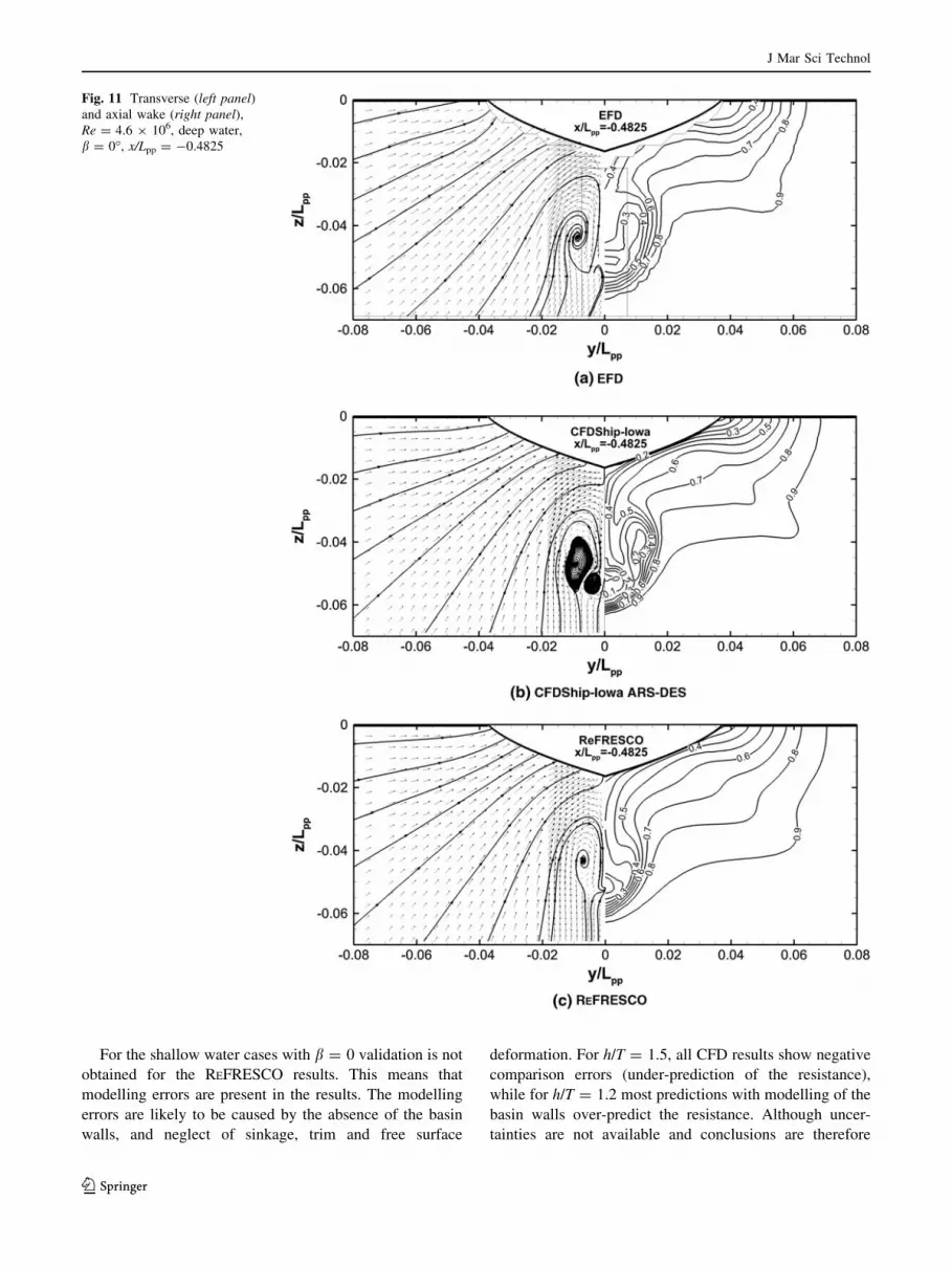
Figure 11 shows the comparison of the experimental data

and CFD for the averaged axial velocity at the propeller

plane. The experiment clearly shows hook-shape pattern of

the axial velocity. As explained by Larsson et al. [36] in the

CFD Workshop Gothenburg 2010, this pattern was caused

by an intense stern bilge vortex and a secondary counter-

rotating vortex close to the vertical plane of symmetry. The

secondary vortex cannot be seen clearly in the experiment

due to limitation of the resolution. CFDShip-Iowa ARS on

grid 1 under-estimates the size of the main vortex and

predicts steady flow. CFDShip-Iowa ARS-DES on grid 1

shows significant improvements on estimating the size of

the main vortex and prediction of the hook-shape pattern.

The REFRESCO result contains the stern bilge vortex and

counter-rotating secondary vortex, but the hook shape is

not well resolved. In Toxopeus [37], it was shown that by

activating the Spalart correction of the stream-wise vor-

ticity the hook shape could be resolved, indicating the

sensitivity of the results to the turbulence model.

Figure 12 shows the total turbulent kinetic energy k,

which shows the similar trend as that for axial velocity

distributions shown in Fig. 11, but with the peak value of

k (*2.1 %U02) over-predicted by 35 % in the CFDShip-

Iowa result. In the ReFRESCO results, the hook-shape is

less developed and only one peak is clearly visible, but the

peak value is quite close to the measurements (3.5 %

underprediction).

6.2 Forces and moments

Tables 8, 9, 10 present the EFD and CFD results for the

different water depths and manoeuvring conditions. The

comparison errors E, numerical and data uncertainties USN

and UD and the validation uncertainties Uval are given if

available. For b = 0�, UD is assumed to be the same as for

b = 4�. For c = 0.4, UD is estimated based on repeat tests,

or taken from the b = 4� condition. This is done to have at

least the possibility to obtain Uval, although it is ques-

tionable whether single observations have the same

uncertainties as the average value from multiple runs (for

which outliers in the data are less significant). Note: after

careful analysis of the results for c = 0.4 in shallow water,

it was found that the transverse force Y obtained from the

EFD could not be used for validation of the CFD results for

these conditions.

6.2.1 Straight ahead sailing

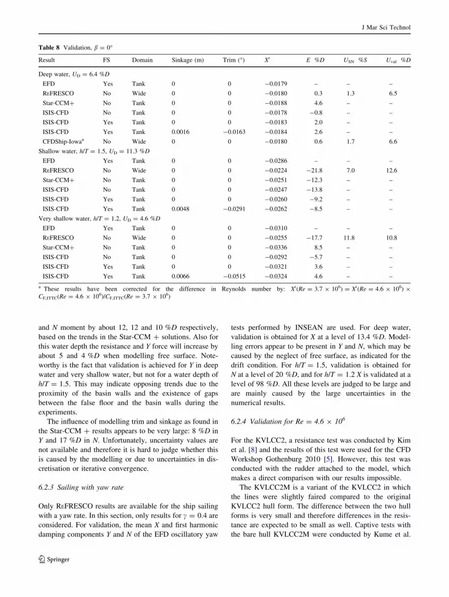
For b = 0� in deep water, see Table 8, uncertainties are

available for the REFRESCO and CFDShip-Iowa results. In

both cases validation of the solution is obtained

(|E| \ Uval), at levels of 6.5 %D and 6.6 %D respectively.

The comparison errors for all computations are reasonably

small, i.e., 4.6 %D or less.Fig. 10 Uncertainty estimate, REFRESCO, N moment, c = 0.4, very

shallow water

J Mar Sci Technol

123

For the shallow water cases with b = 0 validation is not

obtained for the REFRESCO results. This means that

modelling errors are present in the results. The modelling

errors are likely to be caused by the absence of the basin

walls, and neglect of sinkage, trim and free surface

deformation. For h/T = 1.5, all CFD results show negative

comparison errors (under-prediction of the resistance),

while for h/T = 1.2 most predictions with modelling of the

basin walls over-predict the resistance. Although uncer-

tainties are not available and conclusions are therefore

Fig. 11 Transverse (left panel)and axial wake (right panel),Re = 4.6 9 106, deep water,

b = 0�, x/Lpp = -0.4825

J Mar Sci Technol

123

difficult to draw, this might be caused by the existence of a

gap between the false bottom and the basin walls during the

experiments. Such a gap will effectively reduce the

blockage in the basin, which will be most pronounced in

the most extreme shallow water conditions.

As expected, all b = 0� results indicate that modelling

the basin walls will increase the resistance compared to

using a wide domain (about 10 %D, see also below). The

ISIS-CFD results show that modelling the free surface will

increase the resistance further, i.e. by about 3 %D in deep

water, 5 %D for h/T = 1.5 and 9 %D for h/T = 1.2. An

additional increase is found when the dynamic trim and

sinkage is considered as well: about 1 %D.

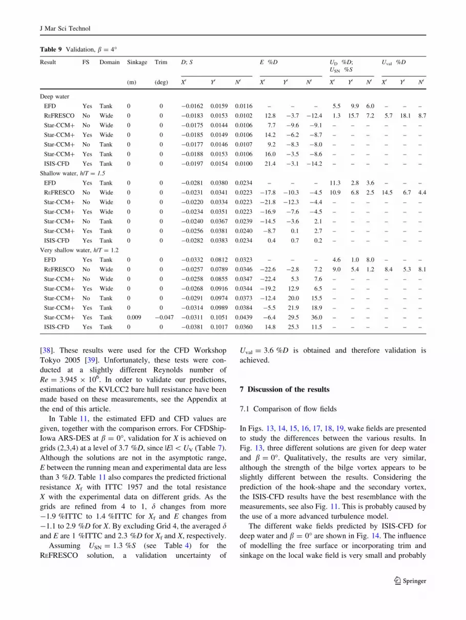
6.2.2 Sailing at a drift angle

For a drift angle of b = 4�, the largest number of results

are available. Uncertainties are available for the

REFRESCO results, and validation for Y is obtained for

deep water at a level of 18.1 %D, see Table 9. Validation

for X and N is not obtained (|E| [ Uval), indicating mod-

elling errors. Considering all CFD results, the scatter in

Y and N is judged to be small, i.e., rS = 3 %S, and much

smaller than the comparison error. All CFD results con-

sistently over-predict the X force and under-predict both

the Y force and the N moment. For deep water, the influ-

ence of modelling the basin walls on the results is judged to

be negligible. There seems to be a slight influence of

modelling free surface deformation on the resistance, but

without uncertainty estimates, the difference cannot be

validated.

For a shallow water depth of h/T = 1.5, no validation is

achieved, although |EN| is close to Uval for N. Based on the

different results, it is expected that the modelling error is

mainly caused by the neglect of the basin walls. Judging

from the trends in the Star-CCM ? results, using a tank

domain instead of a wide domain will on average increase

the resistance, the Y force and N moment by about 8, 8 and

7 %D, respectively. Modelling free surface will increase

the resistance and Y force by about 5 and 4 %D.

In very shallow water, validation is achieved for Y and

N, at levels of 5.3 and 8.1 %D respectively. For X, a

modelling error is present, which is probably caused by the

neglect of the basin walls, free surface deformation and

sinkage and trim. On average, using a tank domain instead

of a wide domain will increase the resistance, the Y force

Fig. 12 Turbulent kinetic

energy contours,

Re = 4.6 9 106, deep water,

b = 0�, x/Lpp = -0.4825

J Mar Sci Technol

123

and N moment by about 12, 12 and 10 %D respectively,

based on the trends in the Star-CCM ? solutions. Also for

this water depth the resistance and Y force will increase by

about 5 and 4 %D when modelling free surface. Note-

worthy is the fact that validation is achieved for Y in deep

water and very shallow water, but not for a water depth of

h/T = 1.5. This may indicate opposing trends due to the

proximity of the basin walls and the existence of gaps

between the false floor and the basin walls during the

experiments.

The influence of modelling trim and sinkage as found in

the Star-CCM ? results appears to be very large: 8 %D in

Y and 17 %D in N. Unfortunately, uncertainty values are

not available and therefore it is hard to judge whether this

is caused by the modelling or due to uncertainties in dis-

cretisation or iterative convergence.

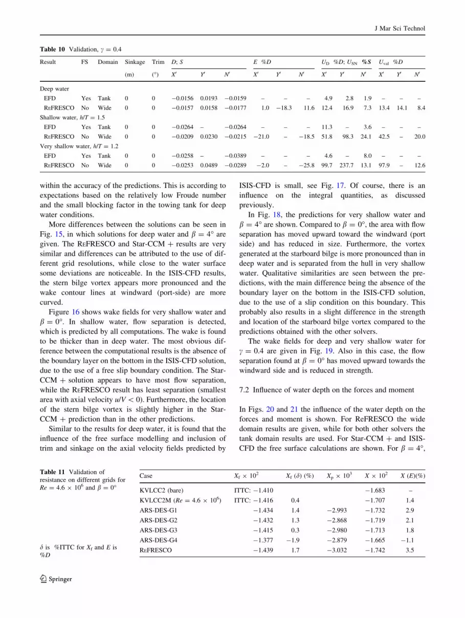
6.2.3 Sailing with yaw rate

Only REFRESCO results are available for the ship sailing

with a yaw rate. In this section, only results for c = 0.4 are

considered. For validation, the mean X and first harmonic

damping components Y and N of the EFD oscillatory yaw

tests performed by INSEAN are used. For deep water,

validation is obtained for X at a level of 13.4 %D. Model-

ling errors appear to be present in Y and N, which may be

caused by the neglect of free surface, as indicated for the

drift condition. For h/T = 1.5, validation is obtained for

N at a level of 20 %D, and for h/T = 1.2 X is validated at a

level of 98 %D. All these levels are judged to be large and

are mainly caused by the large uncertainties in the

numerical results.

6.2.4 Validation for Re = 4.6 9 106

For the KVLCC2, a resistance test was conducted by Kim

et al. [8] and the results of this test were used for the CFD

Workshop Gothenburg 2010 [5]. However, this test was

conducted with the rudder attached to the model, which

makes a direct comparison with our results impossible.

The KVLCC2M is a variant of the KVLCC2 in which

the lines were slightly faired compared to the original

KVLCC2 hull form. The difference between the two hull

forms is very small and therefore differences in the resis-

tance are expected to be small as well. Captive tests with

the bare hull KVLCC2M were conducted by Kume et al.

Table 8 Validation, b = 0�

Result FS Domain Sinkage (m) Trim (�) X0 E %D USN %S Uval %D

Deep water, UD = 6.4 %D

EFD Yes Tank 0 0 -0.0179 – – –

REFRESCO No Wide 0 0 -0.0180 0.3 1.3 6.5

Star-CCM? No Tank 0 0 -0.0188 4.6 – –

ISIS-CFD No Tank 0 0 -0.0178 -0.8 – –

ISIS-CFD Yes Tank 0 0 -0.0183 2.0 – –

ISIS-CFD Yes Tank 0.0016 -0.0163 -0.0184 2.6 – –

CFDShip-Iowaa No Wide 0 0 -0.0180 0.6 1.7 6.6

Shallow water, h/T = 1.5, UD = 11.3 %D

EFD Yes Tank 0 0 -0.0286 – – –

REFRESCO No Wide 0 0 -0.0224 -21.8 7.0 12.6

Star-CCM? No Tank 0 0 -0.0251 -12.3 – –

ISIS-CFD No Tank 0 0 -0.0247 -13.8 – –

ISIS-CFD Yes Tank 0 0 -0.0260 -9.2 – –

ISIS-CFD Yes Tank 0.0048 -0.0291 -0.0262 -8.5 – –

Very shallow water, h/T = 1.2, UD = 4.6 %D

EFD Yes Tank 0 0 -0.0310 – – –

REFRESCO No Wide 0 0 -0.0255 -17.7 11.8 10.8

Star-CCM? No Tank 0 0 -0.0336 8.5 – –

ISIS-CFD No Tank 0 0 -0.0292 -5.7 – –

ISIS-CFD Yes Tank 0 0 -0.0321 3.6 – –

ISIS-CFD Yes Tank 0.0066 -0.0515 -0.0324 4.6 – –

a These results have been corrected for the difference in Reynolds number by: X0(Re = 3.7 9 106) = X0(Re = 4.6 9 106) 9

CF,ITTC(Re = 4.6 9 106)/CF,ITTC(Re = 3.7 9 106)

J Mar Sci Technol

123

[38]. These results were used for the CFD Workshop

Tokyo 2005 [39]. Unfortunately, these tests were con-

ducted at a slightly different Reynolds number of

Re = 3.945 9 106. In order to validate our predictions,

estimations of the KVLCC2 bare hull resistance have been

made based on these measurements, see the Appendix at

the end of this article.

In Table 11, the estimated EFD and CFD values are

given, together with the comparison errors. For CFDShip-

Iowa ARS-DES at b = 0�, validation for X is achieved on

grids (2,3,4) at a level of 3.7 %D, since |E| \ UV (Table 7).

Although the solutions are not in the asymptotic range,

E between the running mean and experimental data are less

than 3 %D. Table 11 also compares the predicted frictional

resistance Xf with ITTC 1957 and the total resistance

X with the experimental data on different grids. As the

grids are refined from 4 to 1, d changes from more

-1.9 %ITTC to 1.4 %ITTC for Xf and E changes from

-1.1 to 2.9 %D for X. By excluding Grid 4, the averaged dand E are 1 %ITTC and 2.3 %D for Xf and X, respectively.

Assuming USN = 1.3 %S (see Table 4) for the

REFRESCO solution, a validation uncertainty of

Uval = 3.6 %D is obtained and therefore validation is

achieved.

7 Discussion of the results

7.1 Comparison of flow fields

In Figs. 13, 14, 15, 16, 17, 18, 19, wake fields are presented

to study the differences between the various results. In

Fig. 13, three different solutions are given for deep water

and b = 0�. Qualitatively, the results are very similar,

although the strength of the bilge vortex appears to be

slightly different between the results. Considering the

prediction of the hook-shape and the secondary vortex,

the ISIS-CFD results have the best resemblance with the

measurements, see also Fig. 11. This is probably caused by

the use of a more advanced turbulence model.

The different wake fields predicted by ISIS-CFD for

deep water and b = 0� are shown in Fig. 14. The influence

of modelling the free surface or incorporating trim and

sinkage on the local wake field is very small and probably

Table 9 Validation, b = 4�

Result FS Domain Sinkage Trim D; S E %D UD %D;

USN %SUval %D

(m) (deg) X0 Y0 N0 X0 Y0 N0 X0 Y0 N0 X0 Y0 N0

Deep water

EFD Yes Tank 0 0 -0.0162 0.0159 0.0116 – – – 5.5 9.9 6.0 – – –

REFRESCO No Wide 0 0 -0.0183 0.0153 0.0102 12.8 -3.7 -12.4 1.3 15.7 7.2 5.7 18.1 8.7

Star-CCM? No Wide 0 0 -0.0175 0.0144 0.0106 7.7 -9.6 -9.1 – – – – – –

Star-CCM? Yes Wide 0 0 -0.0185 0.0149 0.0106 14.2 -6.2 -8.7 – – – – – –

Star-CCM? No Tank 0 0 -0.0177 0.0146 0.0107 9.2 -8.3 -8.0 – – – – – –

Star-CCM? Yes Tank 0 0 -0.0188 0.0153 0.0106 16.0 -3.5 -8.6 – – – – – –

ISIS-CFD Yes Tank 0 0 -0.0197 0.0154 0.0100 21.4 -3.1 -14.2 – – – – – –

Shallow water, h/T = 1.5

EFD Yes Tank 0 0 -0.0281 0.0380 0.0234 – – – 11.3 2.8 3.6 – – –

REFRESCO No Wide 0 0 -0.0231 0.0341 0.0223 -17.8 -10.3 -4.5 10.9 6.8 2.5 14.5 6.7 4.4

Star-CCM? No Wide 0 0 -0.0220 0.0334 0.0223 -21.8 -12.3 -4.4 – – – – – –

Star-CCM? Yes Wide 0 0 -0.0234 0.0351 0.0223 -16.9 -7.6 -4.5 – – – – – –

Star-CCM? No Tank 0 0 -0.0240 0.0367 0.0239 -14.5 -3.6 2.1 – – – – – –

Star-CCM? Yes Tank 0 0 -0.0256 0.0381 0.0240 -8.7 0.1 2.7 – – – – – –

ISIS-CFD Yes Tank 0 0 -0.0282 0.0383 0.0234 0.4 0.7 0.2 – – – – – –

Very shallow water, h/T = 1.2

EFD Yes Tank 0 0 -0.0332 0.0812 0.0323 – – – 4.6 1.0 8.0 – – –

REFRESCO No Wide 0 0 -0.0257 0.0789 0.0346 -22.6 -2.8 7.2 9.0 5.4 1.2 8.4 5.3 8.1

Star-CCM? No Wide 0 0 -0.0258 0.0855 0.0347 -22.4 5.3 7.6 – – – – – –

Star-CCM? Yes Wide 0 0 -0.0268 0.0916 0.0344 -19.2 12.9 6.5 – – – – – –

Star-CCM? No Tank 0 0 -0.0291 0.0974 0.0373 -12.4 20.0 15.5 – – – – – –

Star-CCM? Yes Tank 0 0 -0.0314 0.0989 0.0384 -5.5 21.9 18.9 – – – – – –

Star-CCM? Yes Tank 0.009 -0.047 -0.0311 0.1051 0.0439 -6.4 29.5 36.0 – – – – – –

ISIS-CFD Yes Tank 0 0 -0.0381 0.1017 0.0360 14.8 25.3 11.5 – – – – – –

J Mar Sci Technol

123

within the accuracy of the predictions. This is according to

expectations based on the relatively low Froude number

and the small blocking factor in the towing tank for deep

water conditions.

More differences between the solutions can be seen in

Fig. 15, in which solutions for deep water and b = 4� are

given. The REFRESCO and Star-CCM ? results are very

similar and differences can be attributed to the use of dif-

ferent grid resolutions, while close to the water surface

some deviations are noticeable. In the ISIS-CFD results,

the stern bilge vortex appears more pronounced and the

wake contour lines at windward (port-side) are more

curved.

Figure 16 shows wake fields for very shallow water and

b = 0�. In shallow water, flow separation is detected,

which is predicted by all computations. The wake is found

to be thicker than in deep water. The most obvious dif-

ference between the computational results is the absence of

the boundary layer on the bottom in the ISIS-CFD solution,

due to the use of a free slip boundary condition. The Star-

CCM ? solution appears to have most flow separation,

while the REFRESCO result has least separation (smallest

area with axial velocity u/V \ 0). Furthermore, the location

of the stern bilge vortex is slightly higher in the Star-

CCM ? prediction than in the other predictions.

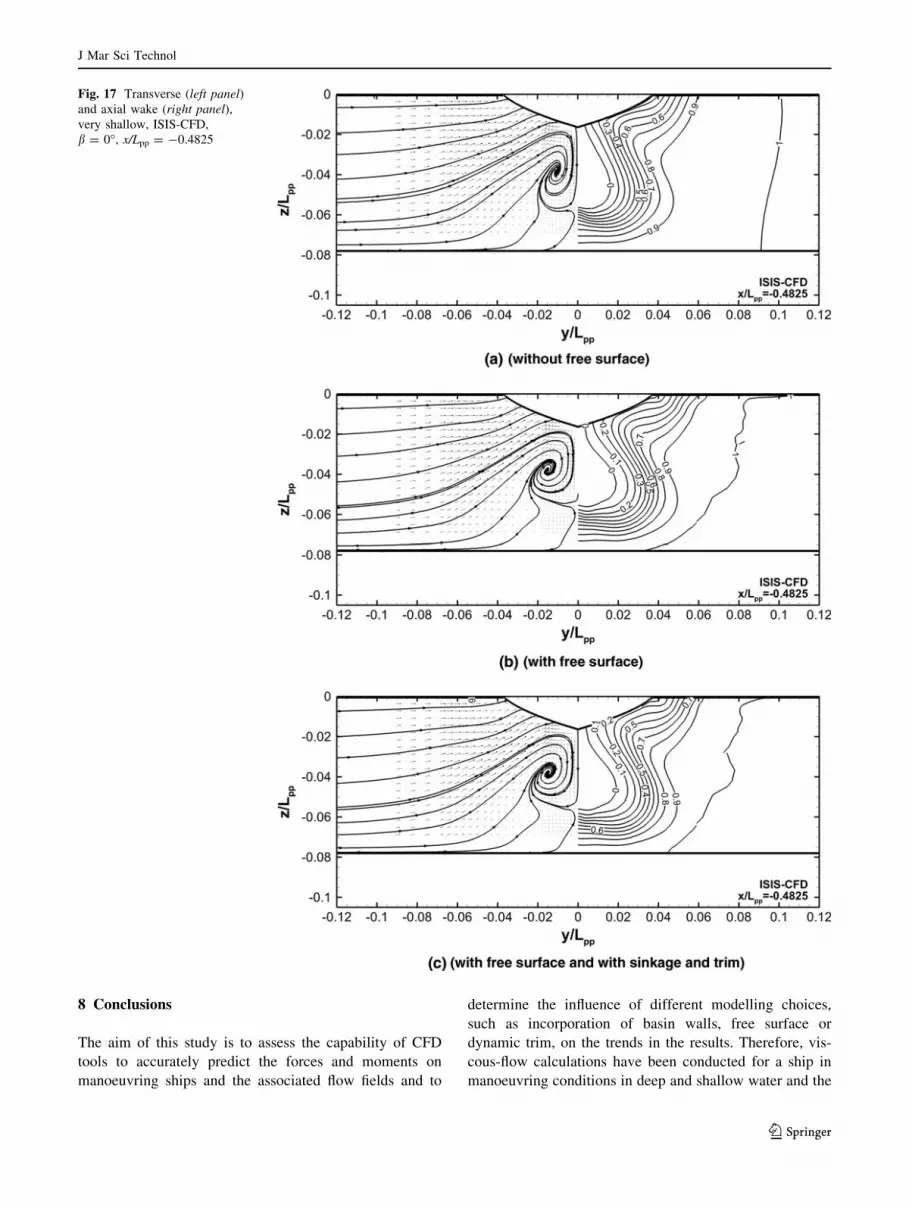
Similar to the results for deep water, it is found that the

influence of the free surface modelling and inclusion of

trim and sinkage on the axial velocity fields predicted by

ISIS-CFD is small, see Fig. 17. Of course, there is an

influence on the integral quantities, as discussed

previously.

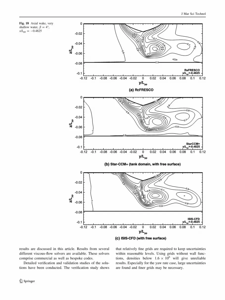
In Fig. 18, the predictions for very shallow water and

b = 4� are shown. Compared to b = 0�, the area with flow

separation has moved upward toward the windward (port

side) and has reduced in size. Furthermore, the vortex

generated at the starboard bilge is more pronounced than in

deep water and is separated from the hull in very shallow

water. Qualitative similarities are seen between the pre-

dictions, with the main difference being the absence of the

boundary layer on the bottom in the ISIS-CFD solution,

due to the use of a slip condition on this boundary. This

probably also results in a slight difference in the strength

and location of the starboard bilge vortex compared to the

predictions obtained with the other solvers.

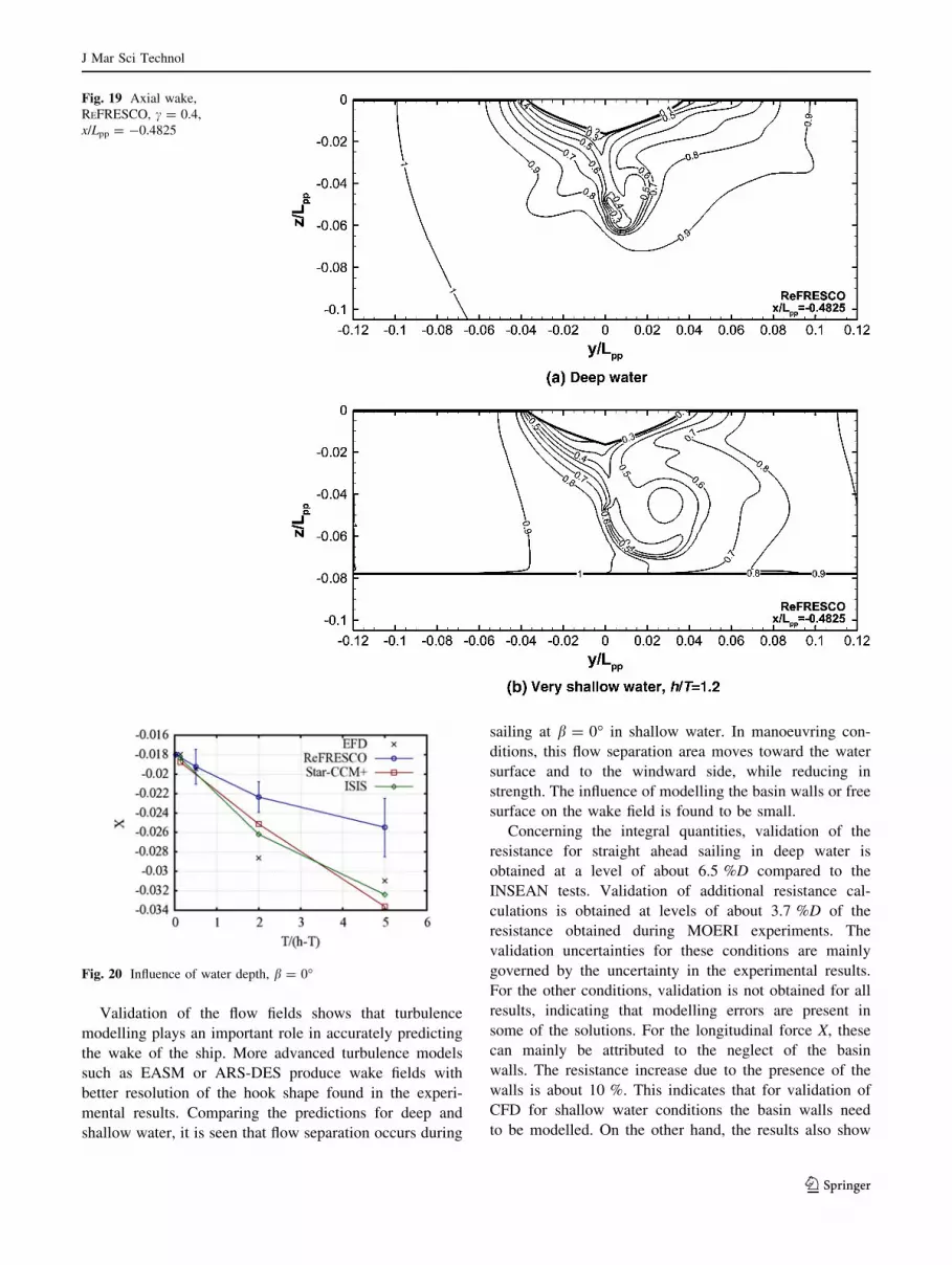
The wake fields for deep and very shallow water for

c = 0.4 are given in Fig. 19. Also in this case, the flow

separation found at b = 0� has moved upward towards the

windward side and is reduced in strength.

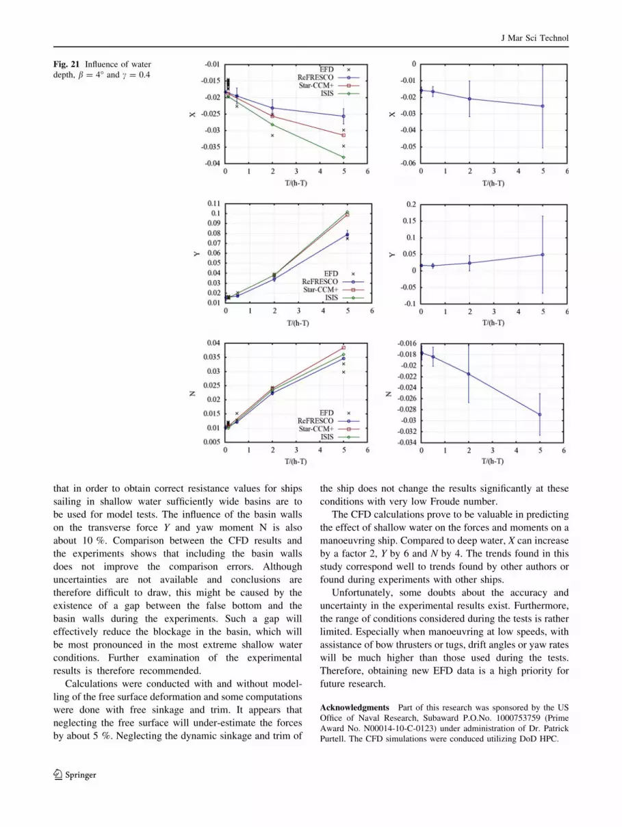
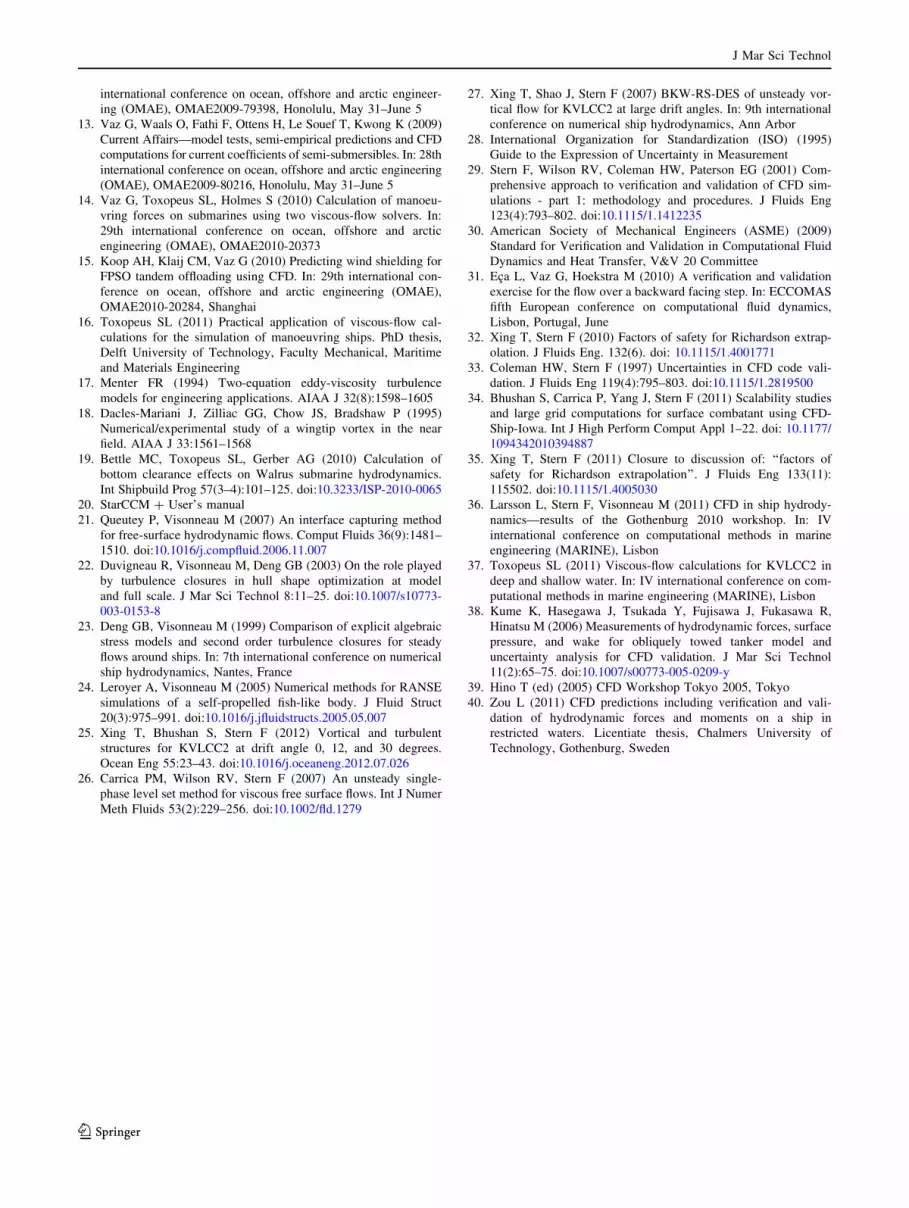
7.2 Influence of water depth on the forces and moment

In Figs. 20 and 21 the influence of the water depth on the

forces and moment is shown. For ReFRESCO the wide

domain results are given, while for both other solvers the

tank domain results are used. For Star-CCM ? and ISIS-

CFD the free surface calculations are shown. For b = 4�,

Table 10 Validation, c = 0.4

Result FS Domain Sinkage Trim D; S E %D UD %D; USN %S Uval %D

(m) (�) X0 Y0 N0 X0 Y0 N0 X0 Y0 N0 X0 Y0 N0

Deep water

EFD Yes Tank 0 0 -0.0156 0.0193 -0.0159 – – – 4.9 2.8 1.9 – – –

REFRESCO No Wide 0 0 -0.0157 0.0158 -0.0177 1.0 -18.3 11.6 12.4 16.9 7.3 13.4 14.1 8.4

Shallow water, h/T = 1.5

EFD Yes Tank 0 0 -0.0264 – -0.0264 – – – 11.3 – 3.6 – – –

REFRESCO No Wide 0 0 -0.0209 0.0230 -0.0215 -21.0 – -18.5 51.8 98.3 24.1 42.5 – 20.0

Very shallow water, h/T = 1.2

EFD Yes Tank 0 0 -0.0258 – -0.0389 – – – 4.6 – 8.0 – – –

REFRESCO No Wide 0 0 -0.0253 0.0489 -0.0289 -2.0 – -25.8 99.7 237.7 13.1 97.9 – 12.6

Table 11 Validation of

resistance on different grids for

Re = 4.6 9 106 and b = 0�

d is %ITTC for Xf and E is

%D

Case Xf 9 102 Xf (d) (%) Xp 9 103 X 9 102 X (E)(%)

KVLCC2 (bare) ITTC: -1.410 -1.683 –

KVLCC2M (Re = 4.6 9 106) ITTC: -1.416 0.4 -1.707 1.4

ARS-DES-G1 -1.434 1.4 -2.993 -1.732 2.9

ARS-DES-G2 -1.432 1.3 -2.868 -1.719 2.1

ARS-DES-G3 -1.415 0.3 -2.980 -1.713 1.8

ARS-DES-G4 -1.377 -1.9 -2.879 -1.665 -1.1

REFRESCO -1.439 1.7 -3.032 -1.742 3.5

J Mar Sci Technol

123

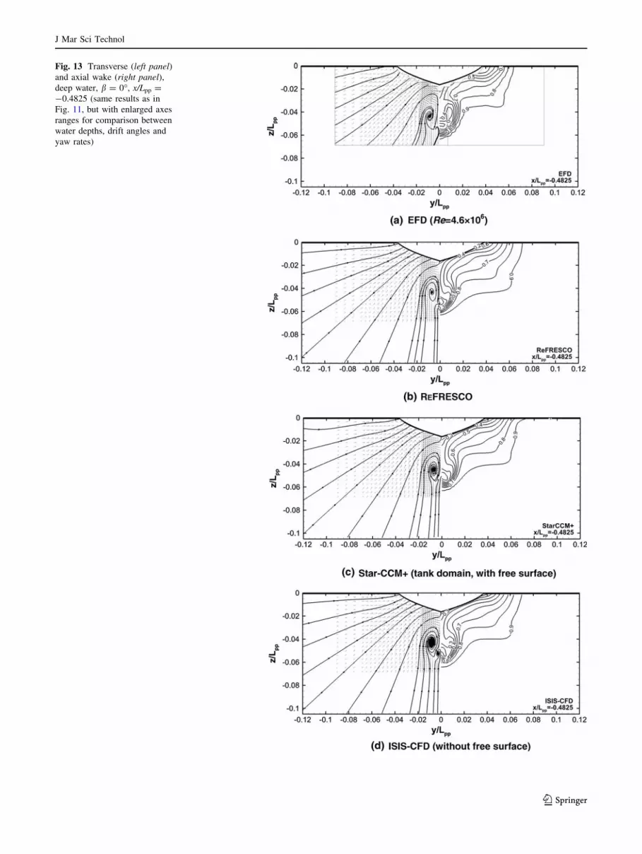
Fig. 13 Transverse (left panel)and axial wake (right panel),deep water, b = 0�, x/Lpp =

-0.4825 (same results as in

Fig. 11, but with enlarged axes

ranges for comparison between

water depths, drift angles and

yaw rates)

J Mar Sci Technol

123

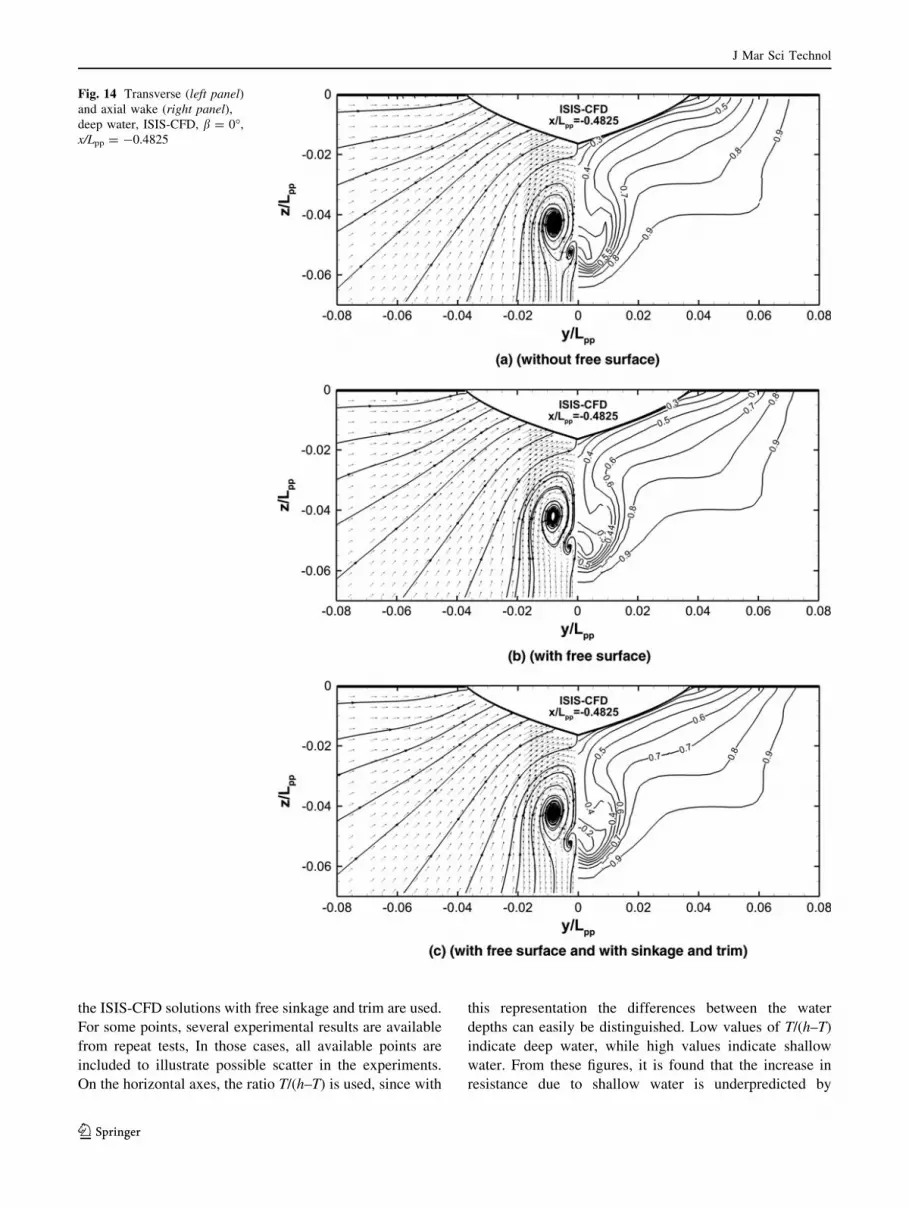
the ISIS-CFD solutions with free sinkage and trim are used.

For some points, several experimental results are available

from repeat tests, In those cases, all available points are

included to illustrate possible scatter in the experiments.

On the horizontal axes, the ratio T/(h–T) is used, since with

this representation the differences between the water

depths can easily be distinguished. Low values of T/(h–T)

indicate deep water, while high values indicate shallow

water. From these figures, it is found that the increase in

resistance due to shallow water is underpredicted by

Fig. 14 Transverse (left panel)and axial wake (right panel),deep water, ISIS-CFD, b = 0�,

x/Lpp = -0.4825

J Mar Sci Technol

123

REFRESCO compared to Star-CCM ? and ISIS-CFD, due

to the neglect of the basin walls and the free surface.

Generally, the predictions from Star-CCM ? and ISIS-

CFD are of the same order of magnitude, but the trends

are not completely similar. This may be caused by

uncertainties in the results or by the inclusion of sinkage

and trim in the ISIS-CFD calculations.

The increase of the forces and moment in shallow

water is considerable. For b = 4�, X increases by a factor

of about 1.7, Y by about 6 and N by about 4. These values

Fig. 15 Axial wake, deep

water, b = 4�,

x/Lpp = -0.4825

J Mar Sci Technol

123

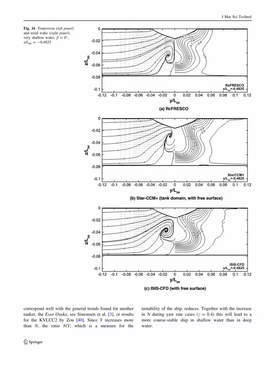
correspond well with the general trends found for another

tanker, the Esso Osaka, see Simonsen et al. [3], or results

for the KVLCC2 by Zou [40]. Since Y increases more

than N, the ratio N/Y, which is a measure for the

instability of the ship, reduces. Together with the increase

in N during yaw rate cases (c = 0.4) this will lead to a

more course-stable ship in shallow water than in deep

water.

Fig. 16 Transverse (left panel)and axial wake (right panel),very shallow water, b = 0�,

x/Lpp = -0.4825

J Mar Sci Technol

123

8 Conclusions

The aim of this study is to assess the capability of CFD

tools to accurately predict the forces and moments on

manoeuvring ships and the associated flow fields and to

determine the influence of different modelling choices,

such as incorporation of basin walls, free surface or

dynamic trim, on the trends in the results. Therefore, vis-

cous-flow calculations have been conducted for a ship in

manoeuvring conditions in deep and shallow water and the

Fig. 17 Transverse (left panel)and axial wake (right panel),very shallow, ISIS-CFD,

b = 0�, x/Lpp = -0.4825

J Mar Sci Technol

123

results are discussed in this article. Results from several

different viscous-flow solvers are available. These solvers

comprise commercial as well as bespoke codes.

Detailed verification and validation studies of the solu-

tions have been conducted. The verification study shows

that relatively fine grids are required to keep uncertainties

within reasonable levels. Using grids without wall func-

tions, densities below 1.6 9 106 will give unreliable

results. Especially for the yaw rate case, large uncertainties

are found and finer grids may be necessary.

Fig. 18 Axial wake, very

shallow water, b = 4�,

x/Lpp = -0.4825

J Mar Sci Technol

123

Validation of the flow fields shows that turbulence

modelling plays an important role in accurately predicting

the wake of the ship. More advanced turbulence models

such as EASM or ARS-DES produce wake fields with

better resolution of the hook shape found in the experi-

mental results. Comparing the predictions for deep and

shallow water, it is seen that flow separation occurs during

sailing at b = 0� in shallow water. In manoeuvring con-

ditions, this flow separation area moves toward the water

surface and to the windward side, while reducing in

strength. The influence of modelling the basin walls or free

surface on the wake field is found to be small.

Concerning the integral quantities, validation of the

resistance for straight ahead sailing in deep water is

obtained at a level of about 6.5 %D compared to the

INSEAN tests. Validation of additional resistance cal-

culations is obtained at levels of about 3.7 %D of the

resistance obtained during MOERI experiments. The

validation uncertainties for these conditions are mainly

governed by the uncertainty in the experimental results.

For the other conditions, validation is not obtained for all

results, indicating that modelling errors are present in

some of the solutions. For the longitudinal force X, these

can mainly be attributed to the neglect of the basin

walls. The resistance increase due to the presence of the

walls is about 10 %. This indicates that for validation of

CFD for shallow water conditions the basin walls need

to be modelled. On the other hand, the results also show

Fig. 19 Axial wake,

REFRESCO, c = 0.4,

x/Lpp = -0.4825

Fig. 20 Influence of water depth, b = 0�

J Mar Sci Technol

123

that in order to obtain correct resistance values for ships

sailing in shallow water sufficiently wide basins are to

be used for model tests. The influence of the basin walls

on the transverse force Y and yaw moment N is also

about 10 %. Comparison between the CFD results and

the experiments shows that including the basin walls

does not improve the comparison errors. Although

uncertainties are not available and conclusions are

therefore difficult to draw, this might be caused by the

existence of a gap between the false bottom and the

basin walls during the experiments. Such a gap will

effectively reduce the blockage in the basin, which will

be most pronounced in the most extreme shallow water

conditions. Further examination of the experimental

results is therefore recommended.

Calculations were conducted with and without model-

ling of the free surface deformation and some computations

were done with free sinkage and trim. It appears that

neglecting the free surface will under-estimate the forces

by about 5 %. Neglecting the dynamic sinkage and trim of

the ship does not change the results significantly at these

conditions with very low Froude number.

The CFD calculations prove to be valuable in predicting

the effect of shallow water on the forces and moments on a

manoeuvring ship. Compared to deep water, X can increase

by a factor 2, Y by 6 and N by 4. The trends found in this

study correspond well to trends found by other authors or

found during experiments with other ships.

Unfortunately, some doubts about the accuracy and

uncertainty in the experimental results exist. Furthermore,

the range of conditions considered during the tests is rather

limited. Especially when manoeuvring at low speeds, with

assistance of bow thrusters or tugs, drift angles or yaw rates

will be much higher than those used during the tests.

Therefore, obtaining new EFD data is a high priority for

future research.

Acknowledgments Part of this research was sponsored by the US

Office of Naval Research, Subaward P.O.No. 1000753759 (Prime

Award No. N00014-10-C-0123) under administration of Dr. Patrick

Purtell. The CFD simulations were conduced utilizing DoD HPC.

Fig. 21 Influence of water

depth, b = 4� and c = 0.4

J Mar Sci Technol

123

Appendix

Estimation of KVLCC2 bare hull resistance

from experimental results

To estimate the resistance of the bare hull KVLCC2 at

Re = 4.6 9 106, the KVLCC2 with rudder data is cor-

rected for the estimated resistance of the rudder. For this,

the following steps are made:

First, the resistance R of the model is calculated (resistance

coefficient based on wetted surface area CT = 4.11 9 10-3

[5], with a specified uncertainty of UD = 1 % [8]; wetted area

with rudder Swa = 0.2682 9 Lpp2 [5]; model speed

V = 1.047 m/s [8]):

R ¼ CT � 1=2� q� V2 � Swa

¼ �4:11� 10�3 � 0:5� 998� 1:0472 � 0:2682� L2pp

¼ 18:36 N

Then, the resistance of the rudder is estimated. For this,

the average velocity at the rudder location is calculated,

using a wake fraction of w = 0.44 [8]: Vrud = (1 - w)

V = 0.586 m/s. The Reynolds number for the rudder with

average chord c = 0.149 m follows from (m = 1.256 9

10-6 m2/s based on the Reynolds number and model

speed during the tests): Rerud = Vrud c/m = 6.96 9 104.

Additionally, the rudder resistance coefficient is needed to

calculate the rudder resistance. An estimate is made with

the ITTC friction line, using an assumed form factor

(1 ? k) of 1.1, which is reasonable for lifting surfaces:

CT;rud

0:075

log Rerudð Þ � 2ð Þ21þ kð Þ ¼ 10:21� 10�3

The rudder wetted area follows from the difference

between the wetted area with rudder and without rudder

(Swa,bare = 0.2656 9 Lpp2 [39]), such that the rudder

resistance is found:

Rrud ¼ CT;rud � 1=2� q� V2rud � Swa;rud

¼ �10:21� 10�3 � 0:5� 998� 0:5862

� 0:2682� 0:2656ð Þ � L2pp

¼ 0:14 N

The non-dimensional longitudinal force X for the

KVLCC2 without rudder is now estimated by:

X ¼ � R� Rrudð Þ= 1=2qV2LppT� �

¼ �1:683� 10�2

Estimation of KVLCC2M bare hull resistance

at Re = 4.6 9 106 from experimental results

The resistance of the KVLCC2M can be scaled to a dif-

ferent Reynolds number using the form factor method. For

this, the form factor is required, see also, e.g., Toxopeus

[37]. In the Tokyo workshop, the form factor was specified

to be: (1 ? k) = 1.2 [39]. The total longitudinal force

measured was given by Kume et al. [38]: X =

-1.756 9 10-2, with UD = 3.3 %. The friction coefficient

for Re = 3.945 9 106 leads to Xf = -1.457 9 10-2,

using a wetted surface area of Swa = 0.2668 9 Lpp2 [39].

The residual resistance is therefore found as follows:

Xres = X - (1 ? k)�Xf = 0.76 9 10-4. Taking the friction

coefficient for Re = 4.6 9 106, and combining this with

the form factor and the residual resistance, the following

longitudinal force is estimated for the KVLCC2M:

X ¼ 1þ kð Þ � Xf Re ¼ 4:6� 106� �

þ Xres

¼ 1:2��1:416� 10�2 þ 0:76� 10�4

¼ �1:707� 10�2

This value is about 1.4 % larger in magnitude than the

estimated value for the KVLCC2 bare hull, which is within

the uncertainty of the experiments.

References

1. Ornfelt M (2009) Naval mission and task driven manoeuvrability

requirements for naval ships. In: 10th international conference on

fast sea transportation (FAST). Athens, pp 505–518

2. Quadvlieg FHHA, Armaoglu E, Eggers R, Coevorden P van

(2010) Prediction and verification of the manoeuvrability of naval

surface ships. In: SNAME Annual Meeting and Expo, Seattle/

Bellevue, Washington

3. Simonsen CD, Stern F, Agdrup K (2006) CFD with PMM test

validation for manoeuvring VLCC2 tanker in deep and shallow

water. In: International conference on marine simulation and ship

manoeuvring (MARSIM), Terschelling, The Netherlands

4. Larsson L, Stern F, Bertram V (2003) Benchmarking of com-

putational fluid dynamics for ship flows: The Gothenburg 2000

workshop. J Ship Res 47(1):63–81

5. Larsson L, Stern F, Visonneau M (eds) (2010) Gothenburg 2010:

a workshop on numerical ship hydrodynamics, Gothenburg

6. Stern F, Agdrup K (eds) (2008) SIMMAN workshop on verifi-

cation and validation of ship manoeuvring simulation methods,

Copenhagen

7. Lee S-J, Kim H-R, Kim W-J, Van S-H (2003) Wind tunnel tests

on flow characteristics of the KRISO 3,600 TEU containership

and 300k VLCC double-deck ship models. J Ship Res 47(1):

24–38

8. Kim W-J, Van S-H, Kim DH (2001) Measurement of flows

around modern commercial ship models. Exp Fluids 31(5):567–

578

9. Fabbri L, Benedetti L, Bouscasse B, Gala FL, Lugni C (2006) An

experimental study of the manoeuvrability of a blunt ship: the

effect of the water depth. In: International conference on ship and

shipping research (NAV)

10. Fabbri L, Benedetti L, Bouscasse B, Gala FL, Lugni C (2006) An

experimental study of the manoeuvrability of a blunt ship: the

effect of the water depth. In: 9th numerical towing tank sympo-

sium (NuTTS)

11. Fabbri L, Campana E, Simonsen C (2011) An experimental study

of the water depth effects on the KVLCC2 tanker. AVT-189

Specialists’ Meeting, Portsdown West, UK, pp 12–14 October

12. Vaz G, Jaouen FAP, Hoekstra M (2009) Free-surface viscous

flow computations. Validation of URANS code FRESCO. In: 28th

J Mar Sci Technol

123

international conference on ocean, offshore and arctic engineer-

ing (OMAE), OMAE2009-79398, Honolulu, May 31–June 5

13. Vaz G, Waals O, Fathi F, Ottens H, Le Souef T, Kwong K (2009)

Current Affairs—model tests, semi-empirical predictions and CFD

computations for current coefficients of semi-submersibles. In: 28th

international conference on ocean, offshore and arctic engineering

(OMAE), OMAE2009-80216, Honolulu, May 31–June 5

14. Vaz G, Toxopeus SL, Holmes S (2010) Calculation of manoeu-

vring forces on submarines using two viscous-flow solvers. In:

29th international conference on ocean, offshore and arctic

engineering (OMAE), OMAE2010-20373

15. Koop AH, Klaij CM, Vaz G (2010) Predicting wind shielding for

FPSO tandem offloading using CFD. In: 29th international con-

ference on ocean, offshore and arctic engineering (OMAE),

OMAE2010-20284, Shanghai

16. Toxopeus SL (2011) Practical application of viscous-flow cal-

culations for the simulation of manoeuvring ships. PhD thesis,

Delft University of Technology, Faculty Mechanical, Maritime

and Materials Engineering

17. Menter FR (1994) Two-equation eddy-viscosity turbulence

models for engineering applications. AIAA J 32(8):1598–1605

18. Dacles-Mariani J, Zilliac GG, Chow JS, Bradshaw P (1995)

Numerical/experimental study of a wingtip vortex in the near

field. AIAA J 33:1561–1568

19. Bettle MC, Toxopeus SL, Gerber AG (2010) Calculation of

bottom clearance effects on Walrus submarine hydrodynamics.

Int Shipbuild Prog 57(3–4):101–125. doi:10.3233/ISP-2010-0065

20. StarCCM ? User’s manual

21. Queutey P, Visonneau M (2007) An interface capturing method

for free-surface hydrodynamic flows. Comput Fluids 36(9):1481–

1510. doi:10.1016/j.compfluid.2006.11.007

22. Duvigneau R, Visonneau M, Deng GB (2003) On the role played

by turbulence closures in hull shape optimization at model

and full scale. J Mar Sci Technol 8:11–25. doi:10.1007/s10773-

003-0153-8

23. Deng GB, Visonneau M (1999) Comparison of explicit algebraic

stress models and second order turbulence closures for steady

flows around ships. In: 7th international conference on numerical

ship hydrodynamics, Nantes, France

24. Leroyer A, Visonneau M (2005) Numerical methods for RANSE

simulations of a self-propelled fish-like body. J Fluid Struct

20(3):975–991. doi:10.1016/j.jfluidstructs.2005.05.007

25. Xing T, Bhushan S, Stern F (2012) Vortical and turbulent

structures for KVLCC2 at drift angle 0, 12, and 30 degrees.

Ocean Eng 55:23–43. doi:10.1016/j.oceaneng.2012.07.026

26. Carrica PM, Wilson RV, Stern F (2007) An unsteady single-

phase level set method for viscous free surface flows. Int J Numer

Meth Fluids 53(2):229–256. doi:10.1002/fld.1279

27. Xing T, Shao J, Stern F (2007) BKW-RS-DES of unsteady vor-

tical flow for KVLCC2 at large drift angles. In: 9th international

conference on numerical ship hydrodynamics, Ann Arbor

28. International Organization for Standardization (ISO) (1995)

Guide to the Expression of Uncertainty in Measurement

29. Stern F, Wilson RV, Coleman HW, Paterson EG (2001) Com-

prehensive approach to verification and validation of CFD sim-

ulations - part 1: methodology and procedures. J Fluids Eng

123(4):793–802. doi:10.1115/1.1412235

30. American Society of Mechanical Engineers (ASME) (2009)

Standard for Verification and Validation in Computational Fluid

Dynamics and Heat Transfer, V&V 20 Committee

31. Eca L, Vaz G, Hoekstra M (2010) A verification and validation

exercise for the flow over a backward facing step. In: ECCOMAS

fifth European conference on computational fluid dynamics,

Lisbon, Portugal, June

32. Xing T, Stern F (2010) Factors of safety for Richardson extrap-

olation. J Fluids Eng. 132(6). doi: 10.1115/1.4001771

33. Coleman HW, Stern F (1997) Uncertainties in CFD code vali-

dation. J Fluids Eng 119(4):795–803. doi:10.1115/1.2819500

34. Bhushan S, Carrica P, Yang J, Stern F (2011) Scalability studies

and large grid computations for surface combatant using CFD-

Ship-Iowa. Int J High Perform Comput Appl 1–22. doi: 10.1177/

1094342010394887

35. Xing T, Stern F (2011) Closure to discussion of: ‘‘factors of

safety for Richardson extrapolation’’. J Fluids Eng 133(11):

115502. doi:10.1115/1.4005030

36. Larsson L, Stern F, Visonneau M (2011) CFD in ship hydrody-

namics—results of the Gothenburg 2010 workshop. In: IV

international conference on computational methods in marine

engineering (MARINE), Lisbon

37. Toxopeus SL (2011) Viscous-flow calculations for KVLCC2 in

deep and shallow water. In: IV international conference on com-

putational methods in marine engineering (MARINE), Lisbon

38. Kume K, Hasegawa J, Tsukada Y, Fujisawa J, Fukasawa R,

Hinatsu M (2006) Measurements of hydrodynamic forces, surface

pressure, and wake for obliquely towed tanker model and

uncertainty analysis for CFD validation. J Mar Sci Technol

11(2):65–75. doi:10.1007/s00773-005-0209-y

39. Hino T (ed) (2005) CFD Workshop Tokyo 2005, Tokyo

40. Zou L (2011) CFD predictions including verification and vali-

dation of hydrodynamic forces and moments on a ship in

restricted waters. Licentiate thesis, Chalmers University of

Technology, Gothenburg, Sweden

J Mar Sci Technol

123