r Human Brain Mapping 000:00–00 (2012) r

Inverse Modeling in Magnetic Source Imaging:Comparison of MUSIC, SAM(g2), and sLORETA to

Interictal Intracranial EEG

Karin L. de Gooijer-van de Groep,1,2 Frans S.S. Leijten,1

Cyrille H. Ferrier,1 and Geertjan J.M. Huiskamp1*

1Department of Neurology and Clinical Neurophysiology, Rudolf Magnus Institute of Neuroscience,University Medical Centre Utrecht, Utrecht, The Netherlands

2MIRA Institute for Biomedical Technology and Technical Medicine, Twente University, Enschede,The Netherlands

r r

Abstract: Magnetoencephalography (MEG) is used in the presurgical work-up of patients with focalepilepsy. In particular, localization of MEG interictal spikes may guide or replace invasive electroence-phalography monitoring that is required in difficult cases. From literature, it is not clear which MEGsource localization method performs best in this clinical setting. Therefore, we applied three sourcelocalization methods to the same data from a large patient group for which a gold standard, interictalspikes as identified in electrocorticography (ECoG), was available. The methods used were multiplesignal classification (MUSIC), Synthetic Aperture Magnetometry kurtosis [SAM(g2)], and standardizedlow-resolution electromagnetic tomography. MEG and ECoG data from 38 patients with refractoryfocal epilepsy were obtained. Results of the three source localization methods applied to the interictalMEG data were assigned to predefined anatomical regions. Interictal spikes as identified in ECoGwere also assigned to these regions. Identified regions by each MEG method were compared to ECoG.Sensitivity and positive predictive value (PPV) of each MEG method were calculated. All three MEGmethods showed a similar overall correlate with ECoG spikes, but the methods differ in which regionsthey detect. The choice of the inverse model thus has an unexpected influence on the results of mag-netic source imaging. Combining inverse methods and seeking consensus can be used to improve spec-ificity at the cost of some sensitivity. Combining MUSIC with SAM(g2) gives the best results(sensitivity ¼ 38% and PPV ¼ 82%). Hum Brain Mapp 00:000–000, 2012. VC 2012 Wiley Periodicals, Inc.

Keywords: interictal; magnetoencephalography; intracranial EEG monitoring; source localization;inverse modeling; irritative zone

r r

INTRODUCTION

Magnetoencephalography (MEG) is used in the presur-gical work-up of patients with focal epilepsy. With MEG,interictal data can be recorded and mapped, which helpsto localize the irritative zone: the area of cortical tissuethat generates interictal spikes and encompasses the epi-leptogenic zone [Rosenow and Luders, 2001]. The goldstandard for delineating these zones is chronic intracranialelectroencephalography (EEG), with electrodes placed ei-ther into the brain (depth-EEG) or over the cortical surface(electrocorticography, ECoG). Chronic intracranial EEG,

*Correspondence to: Dr. Geertjan J.M. Huiskamp, Department ofNeurology and Clinical Neurophysiology, hp F02.230, UniversityMedical Centre Utrecht, PO Box 85500, 3508 GA Utrecht, TheNetherlands. E-mail: g.j.m.huiskamp@umcutrecht.nl

Received for publication 22 November 2010; Revised 30 December2011; Accepted 2 January 2012

DOI: 10.1002/hbm.22049Published online in Wiley Online Library (wileyonlinelibrary.com).

VC 2012 Wiley Periodicals, Inc.

however, is invasive, inconvenient, and costly. InterictalMEG may help to substitute ECoG in some cases or at leastto guide placement of electrodes and minimize their number.In a recent study [Agirre-Arrizubieta et al., 2009], we com-pared interictal ECoG and interictal MEG to see how interic-tal MEG reflects interictal ECoG. We concluded that MEGsource imaging reliably localizes interictal ECoG spikes. AllMEG spikes were associated with an interictal ECoG spike.Fifty-six percent of all regions with interictal ECoG spikeswere identified by interictal MEG. MEG is, however, not anall-comprehensive substitute. Its lack of sensitivity could beexplained by the stochastics of spike occurrence and limitedacquisition time, the radial orientation of spike sources orsource depth—factors that cannot easily be influenced. How-ever, the choice of the inverse model necessary for sourceimaging may also play a role. If so, better clinical resultsmight be obtained using different models.

Different source localization models have given rise to dif-ferent solutions to the inverse problem [Baillet et al., 2001;Grech et al., 2008; Michel et al., 2004]. They can be dividedinto three families [Leijten and Huiskamp, 2008]. Most clini-cal studies have used only the first family: classical single ormultiple dipole modeling in which a current dipole sourcemodel is fitted to the EEG or MEG data. Parameters that haveto be estimated are the dipole position and strength. The sec-ond and third families have been used much less. In the sec-ond family, a source is found by scanning all possiblepositions in the brain. These methods require assumptionsabout which part of the measured data is signal and which isbackground or noise. The third family consists of linearinverse methods in which the data are modeled with onlythe source strengths as parameters for a distributed set ofdipoles at fixed, known locations. Assumptions about or con-straints on source strength are required for these methods.

In this study, we will compare three source imagingpackages with inverse methods of the last two families ofinverse solutions, i.e., multiple signal classification(MUSIC) [Mosher et al., 1992], Synthetic Aperture Magne-tometry kurtosis [SAM(g2)] [Kirsch et al., 2006; Robinsonet al., 2002], and standardized low-resolution electromag-netic tomography (sLORETA) [Pascual-Marqui, 2002].SAM(g2) transforms MEG data into a functional image ofspike-like activity and provides source time courses invoxels exhibiting high excess kurtosis [Kirsch et al., 2006;Robinson et al., 2002]. sLORETA is a weighted minimumnorm inverse solution for EEG or MEG. It is a nonadaptivespatial filter dependent on sensor configuration. MUSICand SAM(g2) belong to the second group of inverse solu-tions and sLORETA to the third group.

SAM(g2) and sLORETA are spatial filters. They make anestimation of noise covariance where MUSIC assumes thenoise to be white. MUSIC and SAM(g2) presume the sourceto be focal and of dipolar origin. They are sensitive only tothe dipolar portion of the source activity. They cannot detectactivity that has spread over a significant cortical area. Pitfallscan be expected with extended sources and when sources arestrongly correlated. With sLORETA simultaneously active

sources can be separated, but only if their fields are distinctenough and of similar strength. With low signal-to-noise ra-tio, sLORETA reconstructions may have some source loca-tion bias and give blurred results. sLORETA and MUSICneed preselection of spikes. SAM(g2) avoids the human sub-jectivity in detecting spikes [Baillet et al., 2001; Kobayashiet al., 2005; Mosher and Leahy, 1998; Robinson et al., 2002;Sekihara et al., 2005; Wagner et al., 2004].

In the clinical context mentioned above, it should beclear that the issue is not the millimeter accuracy of MEGlocalizations but rather the sensitivity and specificity ofMEG when it comes to identifying sublobar regions thatshow interictal activity. The source of the epileptic activityis unknown and can be complex, which makes fine tuningof inverse methods for each particular patient difficult.More often ready-to-use software packages with a specificinverse method are used. From literature, it is not yet clearwhich source localization method performs best in thisclinical setting. Simulation studies using EEG have sug-gested that in the analysis of real interictal spikes resultsfrom different methods should always be taken intoaccount [Grova et al., 2006]. Therefore, we compared soft-ware packages with the often used MUSIC, SAM(g2), andsLORETA modeling in MEG source imaging of focal epi-lepsy, by applying the three methods to the same datafrom a large patient group for whom a gold standard ofECoG was available. This study gives more insight in thedifference in results of methods used in clinical practice.

MATERIALS AND METHODS

Patients

Data were obtained from 38 patients with refractoryfocal epilepsy who underwent chronic intracranial EEGmonitoring (subdural ECoG) and MEG registration as partof their presurgical work-up between 1998 and 2008. MEGresults using the MUSIC inverse algorithm were availableand used for implantation strategy. All patients weretreated in the University Medical Centre in Utrecht as partof the national Collaborative Dutch Epilepsy Surgery Pro-gram. Approval for the MEG studies was given by theMedical Ethics Committee of the hospital.

MRI

As part of a dedicated MRI epilepsy protocol, preopera-tive whole-head high-resolution 3D T1 sequences at 1.5and 3 T (Philips Achieva, Best, The Netherlands) wereavailable, allowing accurate segmentation of the corticalgray matter at a resolution of 1.5 mm.

Chronic ECoG

Chronic ECoG was performed with subdural electrodes(Ad-Tech, Racine, WI) that were introduced through a

r de Gooijer-van de Groep et al. r

r 2 r

craniotomy, 80–120 electrodes per patient. Interelectrodedistance was 1 cm. Data were acquired at a sampling rateof 400 or 512 Hz at a resolution of 12 or 16 bits. Appropri-ate antialiasing filters and a hardware high-pass filter of0.16 Hz were used. ECoG was continuously recorded 24 ha day for an average of 7 (range: 3–10) days. In onepatient, a single depth electrode was also placed, whichwas not used in the data comparison. The electrodes werelocalized by comparing digital photographs during and af-ter implantation and by a postimplantation CT scan thatwas matched to a MRI volume acquired preoperatively[Noordmans et al., 2001]. The electrode positions from var-ious viewpoints were projected on the preimplantationMRI cortex rendering.

MEG

MEG recordings were obtained in a 151-channel whole-head MEG system (Omega 151; CTF Systems, Port Coqui-tlam, British Columbia, Canada) at the MEG Centre of theFree University Medical Centre in Amsterdam. The MEGsystem consisted of axial gradiometers distributed in a hel-met-shaped array inside a Dewar filled with liquid helium.Spontaneous activity was recorded at a sample rate of 625or 1,250 Hz with a 32-bit resolution. Antialiasing filterswere used (208 or 416 Hz). At least 60 min of MEG datawas obtained from each patient. Head position was meas-ured before and after each session of around 10 min.Head-shape information was acquired by marking up to100 anatomic landmarks on the skull using a fourth coilfor more accurate MRI coregistration [de Munck et al.,2001].

MEG Spike Identification for MUSIC and

sLORETA

Two clinical neurophysiologist independently markedinterictal transients in MEG datasets. High- and low-passfilters were set at 0.7 and 70 Hz, respectively. A total of60–90 min of interictal MEG data was analyzed for eachpatient. Kappa statistics were calculated between the inter-ictal epileptiform transients marked by the two independ-ent observers for each MEG recording. Only MEGrecordings for which there was sufficient agreement (inter-observer kappa > 0.4) were accepted. For these, consensusinterictal epileptiform transients were then defined asinterictal epileptiform spikes. An automated clusteringalgorithm [van ’t Ent et al., 2003] was performed to segre-gate different interictal epileptiform spikes. In this algo-rithm, MEG data centered on selected spikes werenormalized, and Euclidean distances between spike repre-sentations were input to a Ward’s hierarchical clusteringalgorithm. With this method, a reliable categorization ofepileptiform spikes can be obtained. The spikes from eachcluster were averaged and tested for homogeneity by plot-ting the averaged spikes and their standard deviations.

When the standard deviation of the cluster was largerthan one-third of the spike maximum, the cluster wasrejected. Clusters of spikes that were part of physiologicalrhythms were discarded.

MEG Spike Modeling: sLORETA and MUSIC

The averaged clusters of spikes were modeled usingCurry 3.0 software (Philips Medical Systems, Hamburg,Germany) for MUSIC and NUTMEG 1.0 [Dalal et al., 2004]for sLORETA. For both methods, a single-shell sphericalhead model was used as forward model. MRI anatomicallandmarks were matched to those recorded during theMEG session. MUSIC resolution was 3 mm and sLORETAwas 5 mm. For both methods, the region of interest wasthe whole brain. The interval from the beginning of therising slope of the spike to the spike maximum was usedfor MUSIC analysis [Leijten and Huiskamp, 2008]. Princi-pal component analysis determined the separationbetween noise and signal subspace. Locations for whichthe resulting MUSIC metric exceeded two-thirds of theoverall maximum were displayed on a cortical renderingfrom MRI. The same clusters of spikes were also used forsLORETA analysis. For sLORETA an additional high-passfilter of 1 Hz was applied. Also, data were selected suchthat it had the peak of interest in it but also a largeenough time window around this peak to further ensurethat the sensor covariance matrix was not too singular(mean length ¼ 141 ms and standard deviation ¼ 23 ms).For regularization, Tikhonov regularization was used. Afixed regularization parameter was used, which was set atthe safe side, avoiding spurious results. The time aroundthe spike maximum showing the highest estimated localcurrent density was used. A threshold was set at 90% ofthe current density and voxels exceeding this thresholdwere displayed in a 3D MRI.

SAM(g2)

The SAM(g2) analysis [Kirsch et al., 2006; Robinson et al.,2002] was performed using software tools provided by VSMMedTech/CTF Systems (Port Coquitlam, British Columbia,Canada). In SAM, a scalar beamformer is used that isobtained by optimizing the source moment vector directionfrom the data. Multiple local spheres were used as forwardmodel. To eliminate the background activity and contrastthe interictal spike activity, SAM(g2) analysis was per-formed with a bandpass filter of 20–70/200 Hz. A total of20–70 Hz is used in several studies [Ishii et al., 2008; Kirschet al., 2006] and is outside the range of alpha-band activitythat would tend to drive the excess kurtosis negative.SAM(g2) was performed on raw datasets with lengthsbetween 100 and 900 s without visible artifacts. In somepatients two datasets were used. Segments with muscle arti-facts were avoided. MEG data were transformed in virtualsensor waveforms for every voxel in the region of interest,

r MEG Evaluation in Epilepsy r

r 3 r

which was again the whole brain, at steps of 5 mm. For eachcoordinate in the head, the excess kurtosis (g2) was com-puted for its virtual sensor waveform. Excess kurtosis is ameasure of the statistical distribution of sample amplitudesand is independent of absolute amplitude or the order inwhich samples are selected. Excess kurtosis was computedfrom each source waveform as g2 ¼ 1

Kr4

PKk¼1½Sk � S�4 � 3,

where k is the sample index, K is the total number of sam-ples, and r is the standard deviation of the time series SðkÞ.The excess kurtosis is unitless. The presence of spikesimplies statistical outliers from a normal distribution func-tion. Normal brain source activity can have a small positivekurtosis of <0.5.

An image was made up of the g2 values correspondingto each voxel. The threshold to detect peaks in the volu-metric image and the peak-to-root mean square ratio todetect spikes in the virtual sensors were set to 1.0 and 6.0,respectively. Virtual sensors and the marked spikes wereused to recognize muscle activity and other artifacts. Setsthat still contained muscle activity or artifacts were reana-lyzed without the trials containing these artifacts. The finalvirtual sensors that showed excess kurtosis of half themaximum (but higher than 1.0) were displayed on the 3DMRI. For SAM(g2), the maximum of the virtual sensor waslocalized and its surrounding area that had kurtosis ofabout half the maximum.

ECoG Spikes

For each patient, two clinical neurophysiologists selectedup to 60 min of representative samples of awake interictalECoG spikes. These samples included all different interictalECoG spikes observed during the recording period. Theserepresentative interictal ECoG data were analyzed by con-sensus. Data were rereferenced to an indifferent intracranialelectrode for review. High- and low-pass filters were set to0.53 and 70 Hz, respectively. The different spikes wereidentified and averaged in the interictal ECoG data set. Forscalp and intracranial EEG, the relevance of taking synchro-nous surface area into consideration has been emphasizedby several authors [Alarcon et al., 1994; Mikuni et al., 1997;Oishi et al., 2002; Shigeto et al., 2002; Tao et al., 2005, 2007].This is because compound EEG/MEG activity can be con-sidered as the sum of multiple potential fields generated ina synchronously activated surface area. For ECoG no accu-rate source model is available for this yet. Therefore, weused the method described by Agirre-Arrizubieta et al.[2009]: for each averaged ECoG spike, a combined ampli-tude and synchronous surface-area measure was calculatedto characterize the data. Spikes were related to the back-ground. The comparison with the background for each elec-trode indicated whether the spatial extent of the averagedspike could be estimated reliably. Only spikes where atleast one of the electrodes met the background criteria wereplotted on the CT-MRI rendering by marking each electrodethat met these criteria.

Brain Anatomical Regions

Anatomical landmarks such as central sulcus and theSylvian fissure and the electrocortical stimulation functionmapping results were used, in the neurosurgical sense, todefine specific anatomical cortical brain regions, asdescribed in the article by Agirre-Arrizubieta et al. [2009].These regions are the central, parietal, and occipital lobes.The frontal lobe was divided in the frontal superior,medial, inferior, and fronto-orbital regions; the temporallobe into the lateral and mesial regions, the latter compris-ing the amygdale, the hippocampus, the parahippocampalgyrus, and the temporal-basal area. The interhemisphericregion, finally, consisted of the mesial surface of the fron-tal, parietal, and occipital lobes.

Association Method and Interpretation of the

Results

Two specialists, independently, in random order andblinded for patient name, allocated the results of MEGsource imaging using MUSIC, SAM(g2), and sLORETAand each interictal ECoG spike to its predefined anatomi-cal region(s). In case of discrepancy, consensus wassought. Anatomical regions found by each MEG methodwere compared to the ECoG. MEG results were classifiedas ‘‘match,’’ ‘‘indecisive" or ‘‘false positive" (Fig. 1). Whenthere was overlap within the same anatomical regionbetween ECoG and MEG, we called this a ‘‘match.’’ WhenMEG results were outside the area covered by electrodegrids, outside the brain cortex, or were localized over avery large area, this was an ‘‘indecisive" result. ‘‘False pos-itives" were MEG results in a region covered by grids, buthaving no ECoG counterpart (Fig. 2A). A false positivecould be partial, as shown in Figure 2B where an MEGresult localizes in the lateral temporal and in the centrallobe (the precentral and postcentral gyrus). There is, how-ever, only a corresponding ECoG result in the temporal

Figure 1.

Classification of MEG results. An MEG result is accorded to pre-

defined anatomical region(s) (single or multiple). For anatomical

region A, the possible comparison categories with ECoG are

shown. This is repeated for all regions covering the cortex.

r de Gooijer-van de Groep et al. r

r 4 r

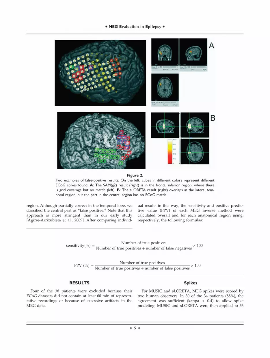
region. Although partially correct in the temporal lobe, weclassified the central part as ‘‘false positive.’’ Note that thisapproach is more stringent than in our early study[Agirre-Arrizubieta et al., 2009]. After comparing individ-

ual results in this way, the sensitivity and positive predic-tive value (PPV) of each MEG inverse method werecalculated overall and for each anatomical region using,respectively, the following formulas:

sensitivityð%Þ ¼ Number of true positives

Number of true positivesþ number of false negatives� 100

PPV ð%Þ ¼ Number of true positives

Number of true positivesþ number of false positives� 100

RESULTS

Four of the 38 patients were excluded because theirECoG datasets did not contain at least 60 min of represen-tative recordings or because of excessive artifacts in theMEG data.

Spikes

For MUSIC and sLORETA, MEG spikes were scored bytwo human observers. In 30 of the 34 patients (88%), theagreement was sufficient (kappa > 0.4) to allow spikemodeling. MUSIC and sLORETA were then applied to 53

Figure 2.

Two examples of false-positive results. On the left: cubes in different colors represent different

ECoG spikes found. A: The SAM(g2) result (right) is in the frontal inferior region, where there

is grid coverage but no match (left). B: The sLORETA result (right) overlaps in the lateral tem-

poral region, but the part in the central region has no ECoG match.

r MEG Evaluation in Epilepsy r

r 5 r

averaged clusters of spikes in these 30 patients. sLORETAgave one result located outside the cortex, which wasmarked as indecisive.

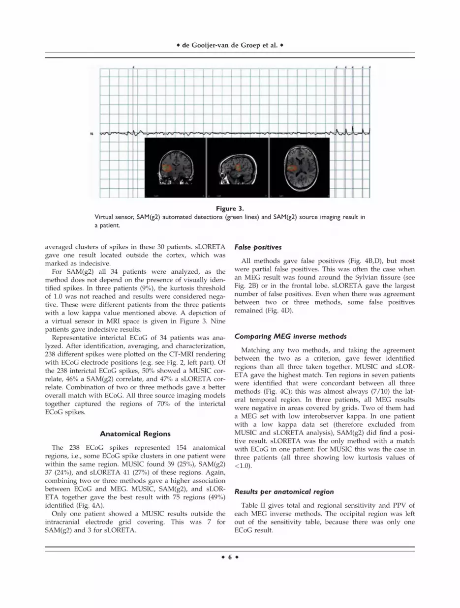
For SAM(g2) all 34 patients were analyzed, as themethod does not depend on the presence of visually iden-tified spikes. In three patients (9%), the kurtosis thresholdof 1.0 was not reached and results were considered nega-tive. These were different patients from the three patientswith a low kappa value mentioned above. A depiction ofa virtual sensor in MRI space is given in Figure 3. Ninepatients gave indecisive results.

Representative interictal ECoG of 34 patients was ana-lyzed. After identification, averaging, and characterization,238 different spikes were plotted on the CT-MRI renderingwith ECoG electrode positions (e.g. see Fig. 2, left part). Ofthe 238 interictal ECoG spikes, 50% showed a MUSIC cor-relate, 46% a SAM(g2) correlate, and 47% a sLORETA cor-relate. Combination of two or three methods gave a betteroverall match with ECoG. All three source imaging modelstogether captured the regions of 70% of the interictalECoG spikes.

Anatomical Regions

The 238 ECoG spikes represented 154 anatomicalregions, i.e., some ECoG spike clusters in one patient werewithin the same region. MUSIC found 39 (25%), SAM(g2)37 (24%), and sLORETA 41 (27%) of these regions. Again,combining two or three methods gave a higher associationbetween ECoG and MEG. MUSIC, SAM(g2), and sLOR-ETA together gave the best result with 75 regions (49%)identified (Fig. 4A).

Only one patient showed a MUSIC results outside theintracranial electrode grid covering. This was 7 forSAM(g2) and 3 for sLORETA.

False positives

All methods gave false positives (Fig. 4B,D), but mostwere partial false positives. This was often the case whenan MEG result was found around the Sylvian fissure (seeFig. 2B) or in the frontal lobe. sLORETA gave the largestnumber of false positives. Even when there was agreementbetween two or three methods, some false positivesremained (Fig. 4D).

Comparing MEG inverse methods

Matching any two methods, and taking the agreementbetween the two as a criterion, gave fewer identifiedregions than all three taken together. MUSIC and sLOR-ETA gave the highest match. Ten regions in seven patientswere identified that were concordant between all threemethods (Fig. 4C); this was almost always (7/10) the lat-eral temporal region. In three patients, all MEG resultswere negative in areas covered by grids. Two of them hada MEG set with low interobserver kappa. In one patientwith a low kappa data set (therefore excluded fromMUSIC and sLORETA analysis), SAM(g2) did find a posi-tive result. sLORETA was the only method with a matchwith ECoG in one patient. For MUSIC this was the case inthree patients (all three showing low kurtosis values of<1.0).

Results per anatomical region

Table II gives total and regional sensitivity and PPV ofeach MEG inverse methods. The occipital region was leftout of the sensitivity table, because there was only oneECoG result.

Figure 3.

Virtual sensor, SAM(g2) automated detections (green lines) and SAM(g2) source imaging result in

a patient.

r de Gooijer-van de Groep et al. r

r 6 r

DISCUSSION

Clinical Conclusions

At first sight, the sensitivity of MEG source imagingmethods looks similar (Table II). In fact, if the three meth-ods would have been evaluated independently on the ba-sis of the same data, the conclusion would have been thattheir performance is similar, and no recommendation for a

particular method would have been given. However, themethods do differ in what they detect. Thus, the choice ofinverse models has a remarkable influence on the yield ofmagnetic source imaging. As can be seen from the table,the number of detected regions with spikes in the ECoGdoubles from around 25% using any inverse model alone(Table II) to almost 50% when results from all three mod-els are combined (Table III). This comes at a cost of an

TABLE I. Positive predictive value for each single method, combination of methods, and concordance of methods

Positive predictive value MUSIC SAM(g2) sLORETAMUSIC þSAM(g2)

MUSIC þsLORETA

SAM(g2) þsLORETA

MUSIC þSAM(g2) þ sLORETA

Single methods 83% 84% 72% — — — —Combination of methods — — — 82% 74% 76% 75%Concordance of methods — — — 90% 87% 82% 83%

Figure 4.

A: Cumulative number of ECoG regions found with one, two, or three MEG inverse methods.

B: Cumulative number of false positives found using one, two, or three MEG methods. C: Num-

ber of ECoG regions found using one MEG method (underlined) and concordances (overlap). D:

Number of false positives found using one MEG method (underlined) and concordances

(overlap).

r MEG Evaluation in Epilepsy r

r 7 r

equal doubling in false-positive MEG results from 5–10%to 16%. Most of the false positives are due to sLORETA.Running MUSIC and SAM(g2) algorithms on the sameMEG data improves the identification of spike regions inthe ECoG by almost 15% with only a small increase of 3%in false positives (Table III). This may help to guide elec-trode placement in patients planned for intracranial EEG,as such an approach upholds the high reliability of MEGsource imaging while improving its relatively low sensitiv-ity, based on the very same MEG data.

Combining inverse methods and seeking consensus canalso be used to further improve specificity of the results toalmost 100% (Table I). Unfortunately, if overlap betweenmethods is thus used, the number of results drops sub-stantially. Again, sLORETA seems least helpful. Concord-ance between MUSIC and SAM(g2) gives the maximumspecificity with at least some sensitivity left. All threemethods are most consistent in localizing sources in thetemporal lobe (Table IV). Least regions are found in thefrontal lobe. MUSIC and sLORETA are better in localizingin the interhemispheric region compared with SAM(g2).

Before we will come to a practical advice, we will try toanswer the question why these inverse methods may havesuch a surprising complementariness and discuss some ofthe limitations of our study.

Reasons for Complementariness

MUSIC and sLORETA were applied to the same, visuallyscored MEG spikes. Our expectation, therefore, was thatexactly the same anatomical regions would be found in themajority of cases. However, this was actually the case inonly three patients. The explanation could be that mostspikes are complex and originate from different anatomicalregions, a situation for which each method has a differentsensitivity, or that bias occurred in one or either method.Relative bias in MUSIC and SAM compared with sLORETAcan be expected in sources that are highly correlated.Another bias of MUSIC and SAM is the constraint that asource should be dipolar. Methods also perform differentlywhen not both the maximum and minimum of the MEGfield are covered by the MEG helmet. Figure 5 shows theeffect of a source in the tip of the temporal lobe. Only whenthe head is surrounded completely by a MEG helmet, thewhole magnetic field would be detected. In this example,the assumption of dipolarity of MUSIC and SAM may workout differently in the resulting solution than for the distrib-uted model underlying sLORETA. Model simulations doneby our group confirmed this (unpublished results).

Because we are dealing with nonsimultaneous data, notall bias and attendant wrong localization will end up as a

TABLE II. Sensitivity and false-positive results of the MEG source imaging methods alone for each anatomical

region and overall

ECoG spikeregions

MUSIC SAM(g2) sLORETA

Match withECoG

Falsepositives Match with ECoG False positives Match with ECoG False positives

Frontal 60 3 (5%) 2 (3%) 13 (22%) 6 (10%) 12 (20%) 8 (13%)Temporal 47 18 (38%) 0 (0%) 13 (28%) 0 (0%) 9 (19%) 1 (2%)Central 17 4 (24%) 3 (18%) 4 (24%) 1 (6%) 8 (47%) 5 (29%)Parietal 16 4 (25%) 2 (13%) 5 (31%) 0 (0%) 5 (31%) 2 (13%)Interhemispherical 13 9 (69%) 1 (8%) 1 (8%) 0 (0%) 6 (46%) 0 (0%)(Occipital) (1) (1) (0) (1) (0) (1) (0)Overall 154 39 (25%) 8 (5%) 37 (24%) 7 (5%) 41 (27%) 16 (10%)

TABLE III. Sensitivity and false-positive results of the MEG source imaging methods in combination for each

anatomical region and overall

ECoG spikeregions

MUSIC þ SAM(g2) MUSIC þ sLORETA SAM(g2) þ sLORETAMUSIC þ SAM(g2) þ

sLORETA

Match withECoG

Falsepositives

Match withECoG

Falsepositives

Match withECoG

Falsepositives

Match withECoG

Falsepositives

Frontal 60 15 7 14 9 23 12 24 13Temporal 47 19 0 19 1 15 1 20 1Central 17 6 3 10 6 10 5 11 6Parietal 16 8 2 6 4 8 2 9 4Interhemispherical 13 9 1 10 1 7 0 10 1(Occipital) (1) (1) (0) (1) (0) (1) (0) (1) (0)Overall 154 58 (38%) 13 (8%) 60 (39%) 21 (14%) 64 (42%) 20 (13%) 75 (49%) 25 (16%)

r de Gooijer-van de Groep et al. r

r 8 r

false-positive result. A wrongly modeled result may stillcoincide with another ECoG spike localization. Figure 6shows the cluster and its dipole field that MUSIC localizedpurely in the temporal lobe and sLORETA more centro-parietally. This patient did show central and parietal inter-ictal ECoG activity, but the question is whether sLORETAlocalized this or actually mislocalized the temporal spike.The low amplitude of the negative flux in channel MLT35compared with the large flux in MLT22 and the fact thatthere is negative flux contralaterally supports the assump-tion that the MEG helmet did not cover the negative maxi-mum. In the same patient, source imaging ofsomatosensory evoked field data, where the whole mag-netic dipole field is covered by the MEG helmet, showedno difference between MUSIC and sLORETA results.

Blurred results can occur due to the regularization thatis required in sLORETA. This could also be an explanationfor different results between MUSIC and sLORETA. Weused a fixed regularization parameter, set at the safe side,

so with a bias toward more smooth results. We did check,in a number of cases, a data-dependent parameter, butresults did not differ much. More importantly, a highthreshold was used for sLORETA, but even then mostsLORETA results cover more than one contiguous anatom-ical region, probably resulting in a high number of (par-tial) false positives. Some sLORETA results projected overboth sides of the Sylvian fissure and had to be allocated toboth the lateral temporal and the central regions. In clini-cal terms, this ambiguity is definitively unwanted, as theseareas require a very different surgical approach and havea different surgical prognosis. Other false positives werefound in the central and frontal lobes. This could be an ar-tifact of our classification method because the predefinedfrontal regions are close to each other, just as the relativelysmall central region is neighboring various other brainregions.

Simultaneously active sources can be seperated bysLORETA, but only if their fields are distinct enough and

TABLE IV. Sensitivity and false-positive results of the MEG source imaging methods using only concordant results

for each anatomical region and overall

ECoG spikeregions

MUSIC þ SAM(g2) MUSIC þ sLORETA SAM(g2) þ sLORETAMUSIC þ SAM(g2) þ

sLORETA

Match withECoG

Falsepositives

Match withECoG

Falsepositives

Match withECoG

Falsepositives

Match withECoG

Falsepositives

Frontal 60 1 1 1 1 2 2 0 1Temporal 47 12 0 8 0 7 0 7 0Central 17 2 1 2 2 2 1 1 1Parietal 16 1 0 3 0 2 0 1 0Interhemispherical 13 1 0 5 0 0 0 0 0(Occipital) (1) (1) (0) (1) (0) (1) (0) (1) (0)Overall 154 18 (12%) 2 (1%) 20 (13%) 3 (2%) 14 (9%) 3 (2%) 10 (6%) 2 (1%)

Figure 5.

Dipole field detected in the real MEG helmet (left) and in an imaginary sphere surrounding the

whole head (right).

r MEG Evaluation in Epilepsy r

r 9 r

of similar strength. In the context of a strong or superficialsource, week or deep sources remain invisible and nearbysources of similar orientation tend not to be separated butinterpreted as one source located in between [Sekiharaet al., 2005; Wagner et al., 2004].

Spikes for MUSIC and sLORETA analysis were markedvisually. This might give a bias toward superficial sources,ignoring the interictal spikes that are difficult to detect inMEG, which can originate from deep source. As a conse-quence, results by MUSIC and sLORETA that are deep arelikely false localizations. In the mesial temporal region,e.g., many high amplitudes were seen in the ECoG in ourpatient population, but few results were found there byMEG. Because ECoG and MEG were not recorded simulta-

neously, it remains difficult to establish which interictalspikes seen in ECoG are invisible in MEG. In general,source location, orientation, extent, and curvature canexplain the sensitivity of MEG for interictal spikes [Huis-kamp et al., 2010].

SAM(g2) uses the ‘‘spikiness" of the data, i.e., it favorsestimated source waveforms with a high kurtosis value.Instances of high ‘‘spikiness" in the virtual sensors, how-ever, do not always equal what human observers see asspikes. This makes SAM(g2) from the outset a truly inde-pendent method from the other two. Sometimes not evena single spike of the human observers was found bySAM(g2), or markers were placed where nothing wasidentified by visual inspection. Of course, this could be

Figure 6.

Averaged spike cluster (top left) with corresponding dipole field (top right) and source imaging

results using MUSIC on a rendered brain (bottom left) and sLORETA (bottom right).

r de Gooijer-van de Groep et al. r

r 10 r

due to SAM(g2)’s optimal spatial filter for the virtual sen-sors. The virtual signal in this sensor may reveal spikeshidden in the MEG signal itself. SAM(g2) would thusseem especially attractive when the MEG data show no orsparse spikes. Indeed, SAM(g2) gave good results in onesuch patient (four of five ECoG regions found). Interest-ingly, no results were found in the hippocampus. Yet,more research is necessary. Optimal settings are not wellestablished. In some patients, we tried a high-pass filterdifferent from the suggested 20 Hz, leading to results withhigher kurtosis and better concordance with ECoG data. Inother patients, this had no effect or an adverse effect. Fig-ure 7 shows the results in one patient. Using a high-passfilter of 20 Hz, two not very clear results were found (onesource outside the brain) with a kurtosis value around 1.0.The region found was frontal. Setting the high-pass filterat 10 Hz, the kurtosis value was much higher (8.4) and aclear region was identified, which was temporal. TheECoG showed that only the latter result was true. Similareffects for different low-pass filter setting may beexpected.

LIMITATIONS

Although interictal ECoG is the gold standard for inter-ictal MEG, a disadvantage is its limited coverage of thebrain. Especially, SAM(g2) gave a lot of results outside thearea covered by grids (seven patients). There is a bias inthe placement of the grids, as MEG MUSIC results wereavailable before electrode placement. As a result, fewer

source localizations outside the grids were to be expectedusing MUSIC. sLORETA, based on the same spikes asMUSIC, found fewer results outside the grids thanSAM(g2). As a consequence of our approach to use ready-to-use software packages different forward models wereused: multiple spheres for SAM(g2) and a single spherefor sLORETA and MUSIC. It has been shown that theeffect of this on localization of interictal spikes for MEG isnegligible, even when using realistic models [Scheler et al.,2007]. Volume conductor effects can influence estimateddipole orientation [Huiskamp, 2004]. This can have aninfluence when orientation is used as a constraint, whichis not the case in our study.

RECOMMENDATIONS

In difficult cases for epilepsy surgery, especially whenintracranial investigations seem warranted, MEG is aworthwhile noninvasive study. Interictal MEG sourceimaging results are extremely reliable using sophisticatedinverse models, in that MEG will localize areas with inter-ictal spikes in the ECoG. Thus, when available, MEGresults should always be taken into account in placingelectrode grids. Unfortunately, MEG results reveal only aminority of interictally active regions and, therefore, donot substitute the ECoG. Surprisingly, without the needfor ancillary MEG recordings, the relatively low sensitivityof MEG can be improved by combining different inversesource models. We, therefore, advise to incorporate twosuch models, MUSIC and SAM(g2), into the routine of

Figure 7.

SAM(g2) results for the same dataset using different high-pass filters. Left: high-pass filter of 20

Hz (first virtual sensor in ventricle); right: high-pass filter of 10 Hz.

r MEG Evaluation in Epilepsy r

r 11 r

presurgical magnetic source imaging. Both methods can beseen as complementary.

Future Directions

Subsequent research may take many forms. The per-formance of other advanced source localization methodsmust be tested (e.g., R-MUSIC [Mosher and Leahy, 1998],which deals with some disadvantages of MUSIC). Prepro-cessing algorithms may be developed to assist in choosingan inverse method for a particular dataset instead of ourproposed combining. However, optimizing combinedmethods by using model averaging can be considered[Trujillo-Barreto et al., 2004]. More research has to be doneon the optimal filter settings for SAM(g2). Virtual sensorsof SAM(g2) data have to be studied thoroughly and com-pared to amplitude distributions in corresponding ECoGelectrodes or kurtosis of source amplitude distributions asderived from sLORETA. A big challenge will be to dealwith the effect of noise on the size of the MEG result.MEG results can be compared to EEG-fMRI findings, andthese may also complement each other. Finally, it shouldbe investigated if interictal MEG has a bias toward regionsof ictal onset. If so, its relatively low sensitivity may evenbe a selective advantage. A reason to believe that thismight be so is the fact that probably the regions with thelargest synchronous surface area produce visible spikes.These may be the property that predisposes toward ictalepileptogenicity.

ACKNOWLEDGMENTS

The authors thank the MEG Centre of the Free Univer-sity Medical Centre in Amsterdam, The Netherlands, fortheir support and Epilepsy Centre Kempenhaeghe, Heeze,The Netherlands, for sharing MEG data.

REFERENCES

Agirre-Arrizubieta Z, Huiskamp GJ, Ferrier CH, van Huffelen AC,Leijten FS (2009): Interictal magnetoencephalography and theirritative zone in the electrocorticogram. Brain 132:3060–3071.

Alarcon G, Guy CN, Binnie CD, Walker SR, Elwes RD, Polkey CE(1994): Intracerebral propagation of interictal activity in partialepilepsy: Implications for source localisation. J Neurol Neuro-surg Psychiatry 57:435–449.

Baillet S, Mosher JC, Leahy RM (2001): Electromagnetic brainmapping. IEEE Signal Process Mag 18:14–30.

Dalal SS, Zumer JM, Agrawal V, Hild KE, Sekihara K, NagarajanSS (2004): NUTMEG: A neuromagnetic source reconstructiontoolbox. Neurol Clin Neurophysiol 2004:52.

Dalal SS, Zumer JM, Guggisberg AG, Trumpis M, Wong DD, Seki-hara K, Nagarajan SS (2011): MEG/EEG source reconstruction,statistical evaluation, and visualization with NUTMEG. Com-put Intell Neurosci 2011:758973.

de Munck JC, Verbunt JP, van ’t Ent D, van Dijk BW (2001): Theuse of an MEG device as 3D digitizer and motion monitoringsystem. Phys Med Biol 46:2041–2052.

Grech R, Cassar T, Muscat J, Camilleri KP, Fabri SG, Zervakis M,Xanthopoulos P, Sakkalis V, Vanrumste B (2008): Review onsolving the inverse problem in EEG source analysis. J Neuro-eng Rehabil 5:25.

Grova C, Daunizeau J, Lina JM, Benar CG, Benali H, Gotman J(2006): Evaluation of EEG localization methods using realisticsimulations of interictal spikes. Neuroimage 29:734–753.

Huiskamp G (2004): EEG-MEG source characterization in postsurgical epilepsy: The influence of large cerebrospinal fluidcompartments. Conf Proc IEEE Eng Med Biol Soc 6:4401–4404.

Huiskamp G, Agirre-Arrizubieta Z, Leijten F (2010): Regional dif-ferences in the sensitivity of MEG for interictal spikes in epi-lepsy. Brain Topogr 23:159–164.

Ishii R, Canuet L, Ochi A, Xiang J, Imai K, Chan D, Iwase M,Takeda M, Snead OC III, Otsubo H (2008): Spatially filteredmagnetoencephalography compared with electrocorticographyto identify intrinsically epileptogenic focal cortical dysplasia.Epilepsy Res 81:228–232.

Kirsch HE, Robinson SE, Mantle M, Nagarajan S (2006): Auto-mated localization of magnetoencephalographic interictalspikes by adaptive spatial filtering. Clin Neurophysiol117:2264–2271.

Kobayashi K, Yoshinaga H, Ohtsuka Y, Gotman J (2005): Dipolemodeling of epileptic spikes can be accurate or misleading.Epilepsia 46:397–408.

Leijten FS, Huiskamp G (2008): Interictal electromagnetic sourceimaging in focal epilepsy: Practices, results and recommenda-tions. Curr Opin Neurol 21:437–445.

Michel CM, Murray MM, Lantz G, Gonzalez S, Spinelli L, Gravede Peralta R (2004): EEG source imaging. Clin Neurophysiol115:2195–2222.

Mikuni N, Nagamine T, Ikeda A, Terada K, Taki W, Kimura J,Kikuchi H, Shibasaki H (1997): Simultaneous recording of epi-leptiform discharges by MEG and subdural electrodes in tem-poral lobe epilepsy. Neuroimage 5:298–306.

Mosher JC, Leahy RM.Recursive MUSIC (1998): A framework forEEG and MEG source localization. IEEE Trans Biomed Eng45:1342–1354.

Mosher JC, Lewis PS, Leahy RM (1992): Multiple dipole modelingand localization from spatiotemporal Meg data. IEEE TransBiomed Eng 39:541–557.

Noordmans HJ, van Rijen PC, van Veelen CW, Viergever MA, Hoe-kema R (2001): Localization of implanted EEG electrodes in avirtual-reality environment. Comput Aided Surg 6:241–258.

Oishi M, Otsubo H, Kameyama S, Morota N, Masuda H,Kitayama M, Tanaka R (2002): Epileptic spikes: Magnetoence-phalography versus simultaneous electrocorticography. Epilep-sia 43:1390–1395.

Pascual-Marqui RD (2002): Standardized low-resolution brain elec-tromagnetic tomography (sLORETA): Technical details. Meth-ods Find Exp Clin Pharmacol 24:5–12.

Robinson SE, Vrba J, Otsubo H, Ishii R (2002): Finding epilepticloci by nonlinear parametrization of source waveforms. In:Nowak H, Haueisein J, Giessler F, Huonker R, editors. Pro-ceedings of the 13th International Conference on Biomagnet-ism. VDE Verlag GMBH, Jena, Germany. pp 220–222.

Rosenow F, Luders H (2001): Presurgical evaluation of epilepsy.Brain 124:1683–1700.

Scheler G, Fischer MJ, Genow A, Hummel C, Rampp S, Paulini A,Hopfengartner R, Kaltenhauser M, Stefan H (2007): Spatialrelationship of source localizations in patients with focal epi-lepsy: Comparison of MEG and EEG with a three spherical

r de Gooijer-van de Groep et al. r

r 12 r

shells and a boundary element volume conductor model. HumBrain Mapp 28:315–322.

Sekihara K, Sahani M, Nagarajan SS (2005): Localization bias andspatial resolution of adaptive and non-adaptive spatial filtersfor MEG source reconstruction. Neuroimage 25:1056–1067.

Shigeto H, Morioka T, Hisada K, Nishio S, Ishibashi H, Kira D,Tobimatsu S, Kato M (2002): Feasibility and limitations of mag-netoencephalographic detection of epileptic discharges: Simul-taneous recording of magnetic fields and electrocorticography.Neurol Res 24:531–536.

Tao JX, Ray A, Hawes-Ebersole S, Ebersole JS (2005): IntracranialEEG substrates of scalp EEG interictal spikes. Epilepsia 46:669–676.

Tao JX, Baldwin M, Hawes-Ebersole S, Ebersole JS (2007): Corticalsubstrates of scalp EEG epileptiform discharges. J Clin Neuro-physiol 24:96–100.

Trujillo-Barreto NJ, Aubert-Vazquez E, Valdes-Sosa PA (2004):Bayesian model averaging in EEG/MEG imaging. Neuroimage21:1300–1319.

van ’t Ent D, Manshanden I, Ossenblok P, Velis DN, de MunckJC, Verbunt JP, Lopes da Silva FH (2003): Spike cluster anal-ysis in neocortical localization related epilepsy yields clini-cally significant equivalent source localization results inmagnetoencephalogram (MEG). Clin Neurophysiol 114:1948–1962.

Vrba J, Robinson SE (2001): Signal processing in magnetoencepha-lography. Methods 25:249–271.

Wagner M, Fuchs M, Kastner J (2004): Evaluation of sLORETA inthe presence of noise and multiple sources. Brain Topogr16:277–280.

APPENDIX

Details of the following can be found in Mosher et al.[1992] (MUSIC), Pascual-Marqui [2002] and Dalal et al.[2011] (sLORETA), and Vrba and Robinson [2001] (SAM).

THE FORWARD MODEL

The forward model is defined by:

~bðtÞ ¼ L~sðtÞ þ ~nðtÞ (A1)

where ~bðtÞ is the axial gradiometer data at timet biðtÞ i ¼ 1;Ng; ~nðtÞ, ~nðtÞ is the noise in axial gradiometerat time t niðtÞ i ¼ 1;Ng the number of sensors, ~sðtÞ is thesource strength at time t of unit dipoles sjðtÞ j ¼ 1;Ns thenumber of source points, and L is the lead field matrixLij i ¼ 1;Ng j ¼ 1;Ns.

The source~s (and corresponding lead field matrix L) canbe either defined for each of three orthogonal elementarydipoles in Cartesian x; y; z directions (as is the case in thesLORETA implementation) or optimized for a certaindipole orientation y as is the case for MUSIC andSAM(g2). L is computed using a single- (MUSIC andsLORETA) or multiple-sphere (SAM) head model. Thespatial data covariance matrix R and corresponding noisecovariance N, both of size Ng �Ng, for a given time inter-val T are as follows:

R ¼ZT

~bðtÞ~btðtÞdt (A2)

N ¼ZT

~nðtÞ~ntdt (A3)

MUSIC

In MUSIC, the metric MUSj in source points j ¼ 1;Ns isdefined as follows:

MUSj ¼ 1

kminðLtjENEtNLj;L

tjLjÞ

(A4)

where EN is a matrix of eigenvectors~ei of~~R i ¼ r:::Ng with

1 < r <¼ Ng separating signal from noise subspace andkmin is the minimum generalized eigenvector of the matrixpair parenthesis. Lj (size Ng � 3) is the lead field submatrixfor the three elementary dipoles at source location j.

sLORETA

In sLORETA (power of) source strength ~sðtÞ withsjðtÞ j ¼ 1;Ns, the number of source points is calculated:

~sðtÞ ¼ LtðLLt þ cIÞ�1~bðtÞ (A5)

where I is the identity matrix of dimension Ns �Ns andc > 0 a scalar regularization parameter to be chosen allow-ing inversion of the matrix in parenthesis (Tikhonov regu-larization). ~sðtÞ is normalized by its estimated variance rassuming independence of source activity and uniformsensor noise N ¼ kI, with prior source variance rprior ¼ I:

r ¼ LtðLLt þ cIÞ�1L (A6)

leading to the sLORETA metric sLORj for source location j:

sLORj ¼~sjðtÞtr�1j ~sjðtÞ (A7)

where the vector ~sj now refers to the three-dimensionalsubvector for the elementary dipoles and rj is the corre-sponding 3� 3 submatrix.

SAM(g2)

SAM uses a scalar linearly constrained minimum var-iance beamformer optimized for unit dipole direction h:

~sðtÞ ¼ LtR�1

LtR�1L~bðtÞ (A8)

The SAM(g2) metric computes for ~sðtÞ the excess kurto-sis ~g2 of the amplitude distribution over the time intervalT containing K samples:

~g2 ¼PK

k¼1ð~sðtkÞ� <~s >Þ4Kr4

~s

� 3 (A9)

where <~s > and r~s are the average and standard devia-tion of estimated source function amplitude for K samplesof each source point sj j ¼ 1;Ns.

r MEG Evaluation in Epilepsy r

r 13 r