arX

iv:1

303.

6665

v1 [

mat

h.A

P] 2

6 M

ar 2

013 Inverse anisotropic conductivity from internal current densities

Guillaume Bal∗ Chenxi Guo† Francois Monard‡

March 28, 2013

Abstract

This paper concerns the reconstruction of an anisotropic conductivity tensor γ frominternal current densities of the form J = γ∇u, where u solves a second-order elliptic equation∇ · (γ∇u) = 0 on a bounded domain X with prescribed boundary conditions. A minimumnumber of such functionals equal to n+ 2, where n is the spatial dimension, is sufficient toguarantee a local reconstruction. We show that γ can be uniquely reconstructed with a lossof one derivative compared to errors in the measurement of J . In the special case where γis scalar, it can be reconstructed with no loss of derivatives. We provide a precise statementof what components may be reconstructed with a loss of zero or one derivatives.

1 Introduction

Hybrid medical imaging modalities are extensively studied in the bio-engineering community.Such methods aim to combine high-contrast, such as the one found in the modalities ElectricalImpedance Tomography (EIT) or Optical Tomography (OT), with high-resolution, as is observedin the modalities Magnetic Resonance Imaging (MRI) or ultrasound. The high-contrast modalityEIT aims to locate unhealthy tissues by reconstructing their electrical conductivity γ fromcurrent boundary measurements. This leads to an inverse problem known as Calderon’s problem.Extensive studies have been made on uniqueness properties and reconstruction methods for thisinverse problem [33]. Unfortunately, the problem is severely ill-posed and yields images withpoor resolution.

It is sometimes possible to leverage a physical coupling between a high-contrast, low-resolutionmodality and a high-resolution, low-contrast modality. Such a coupling typically provides in-ternal functionals of the unknown coefficients of interest and greatly improve its resolution

∗Department of Applied Physics and Applied Mathematics, Columbia University, New York NY, 10027;

gb2030@columbia.edu†Department of Applied Physics and Applied Mathematics, Columbia University, New York NY, 10027;

cg2597@columbia.edu‡Department of Mathematics, University of Washington, Seattle WA, 98195; fmonard@uw.edu

1

[1, 2, 3, 6, 7, 22, 29, 32]. Different types of internal functionals, such as current densitiesand power densities, corresponding to different physical couplings have been analyzed to re-cover the unknown conductivity. In the case of power densities, we refer the reader to, e.g.,[4, 5, 9, 16, 17, 22, 23, 24, 25].

In this paper, we consider the Current Density Impedance Imaging problem (CDII), alsocalled Magnetic Resonance Electrical Impedance Tomography (MREIT) of reconstructing ananisotropic conductivity tensor in the second-order elliptic equation,

∇ · (γ∇u) =n∑

i,j=1

∂i(γij∂ju) = 0 (X), u|∂X = g, (1)

from knowledge of internal current densities of the form H = γ∇u, where u solves (1). Tobe consistent with earlier publications, where the notation H is used systematically to denoteinternal functionals, we use H to denote current densities rather than the more customarynotation J . Here X is an open bounded domain with a C2,α or smoother boundary ∂X. Theabove equation has real-valued coefficients and γ is a symmetric tensor satisfying the uniformellipticity condition

κ−1‖ξ‖2 ≤ ξ · γξ ≤ κ‖ξ‖2, ξ ∈ Rn, for some κ ≥ 1, (2)

so that (1) admits a unique solution in H1(X) for g ∈ H 1

2 (∂X).Internal current density functionals H can be obtained by the technique of current density

imaging. The idea is to use Magnetic Resonance Imaging (MRI) to determine the magneticfield B induced by an input current I. The current density is then defined by H = ∇×B. Wethus need to measure all components of B to calculate H, which may create some difficulties inpractice, but this is the starting point of this paper. See [11, 30] for details.

A perturbation method to reconstruct the unknown conductivity in the linearized case waspresented in [12]. In dimension n = 2, a numerical reconstruction algorithm based on theconstruction of equipotential lines was given in [18]. Kwon et al [19] proposed a J -substitutionalgorithm, which is an iterative algorithm. Assuming knowledge of only the magnitude ofonly one current density |H| = |γ∇u|, the problem was studied in [26, 27, 28] (see the latterreference for a review) in the isotropic case and more recently in [10, 21] in the anisotropic casewith anisotropy known. In [14, 20], Nachman et al. and Lee independently found a explicitreconstruction formula for visualizing log γ at each point in a domain. The reconstruction withfunctionals of the form γt∇u is shown in [15] in the isotropic case. For t = 0, the functionalsare given by solutions of (1), then a more general complex-valued tensor in the anisotropic casewas presented in [8]. In [31], assuming that the magnetic field B is measurable, Seo et al. gavea reconstruction for a complex-valued coefficient in the isotropic case.

In the present work, we study the inverse problem in the anisotropic setting with a set ofcurrent densities Hj = γ∇uj for 1 ≤ j ≤ m, where uj solves (1) with prescribed boundary

2

conditions gj . We propose sufficient conditions on m and the choice of gj≤j≤m such that thereconstruction of γ is unique and satisfies elliptic stability estimates.

2 Statement of the main results

For X ⊂ Rn, we denote by Σ(X) the set of conductivity tensors with bounded components

satisfying the uniform ellipticity condition (2). Then for k ≥ 1 an integer and 0 < α < 1, wedenote

Ck,αΣ (X) := γ ∈ Σ(X)| γpq ∈ Ck,α(X), 1 ≤ p ≤ q ≤ n.

In what follows, by “solution of (1)” we may refer to the solution itself or the boundary condition

that generates it, i.e. g = u|∂X ∈ H1

2 (∂X). We will consider collections of measurements of theform

Hi : γ 7→ Hi(γ) = γ∇ui, 1 ≤ i ≤ m, (3)

where ui solves (1) with boundary condition gi. We decompose γ into the product of a scalarfactor β with an anisotropic structure γ

γ := βγ, β = (det γ)1

n , det γ = 1. (4)

Since γ satisfies the uniform elliptic condition (2), β is bounded away from zero.From knowledge of a sufficiently large number of current densities, the reconstruction formu-

las for β and γ can be locally established in terms of the current densities and their derivativesup to first order.

2.1 Main hypotheses

We begin with the main hypotheses that allow us to setup a few reconstruction procedures.The first hypothesis aims at making the scalar factor β in (4) locally reconstructible via a

gradient equation.

Hypothesis 2.1. There exist two solutions (u1, u2) of (1) and X0 ⊂ X convex satisfying

infx∈X0

F1(u1, u2) ≥ c0 > 0 where F1(u1, u2) := |∇u1|2|∇u2|2 − (∇u1 · ∇u2)2. (5)

On to the hypotheses for local reconstructibility of γ, we first need to have, locally, a basisof gradients of solutions of (1).

Hypothesis 2.2. There exist n solutions (u1, . . . , un) of (1) and X0 ⊂ X satisfying

infx∈X0

F2(u1, . . . , un) ≥ c0 > 0, where F2(u1, . . . , un) := det(∇u1, . . . ,∇un). (6)

3

Let us now pick u1, · · · , un satisfying Hyp. 2.2 and consider additional solutions un+kmk=1.Each additional solution decomposes in the basis (∇u1, . . . ,∇un) as

∇un+k =n∑

i=1

µik∇ui, 1 ≤ k ≤ m, (7)

where, as shown in [5] for instance, the coefficients µik take the expression

µik = −det(∇u1, . . . ,i

︷ ︸︸ ︷

∇un+k, . . . ,∇un)det(∇u1, . . . ,∇un)

= −det(H1, . . . ,

i︷ ︸︸ ︷

Hn+k, . . . ,Hn)

det(H1, . . . ,Hn),

in particular, these coefficients are accessible from current densities. The subsequent algorithmswill make extensive use of the matrix-valued quantities

Zk = [Zk,1| · · · |Zk,n] , where Zk,i := ∇µik, 1 ≤ k ≤ m (8)

In particular, the next hypothesis, formulating a sufficient condition for local reconstructibilityof the anisotropic part of γ is that, locally, a certain number of matrices Zk (at least two) satisfiessome rank maximality condition.

Hypothesis 2.3. Assume that Hypothesis 2.2 holds for some (u1, . . . , un) over X0 ⊂ X anddenote by H the matrix with columns H1, . . . ,Hn. Then there exist un+1, . . . , un+m solutions of(1) and some X ′ ⊆ X0 such that the x-dependent space

W := span(ZkH

TΩ)sym, Ω ∈ An(R), 1 ≤ k ≤ m⊂ Sn(R) (9)

has codimension one in Sn(R) throughout X′.

An alternate approach to reconstruct γ is to set up a coupled system for u1, . . . , un satisfyingHyp. 2.2 globally. This system of PDEs can be derived under the following hypothesis (part A).From this system and under an additional hypothesis (part B), we can derive an elliptic systemfrom which to reconstruct u1, . . . , un.

Hypothesis 2.4. A. Suppose that Hypothesis 2.2 is satisfied over X0 = X for some solutions(u1, . . . , un). There exists an additional solution un+1 of (1) whose matrix Z1 defined by(8) is uniformly invertible over X, i.e.

infx∈X

detZ1 ≥ c0 > 0, (10)

for some positive constant c0.

4

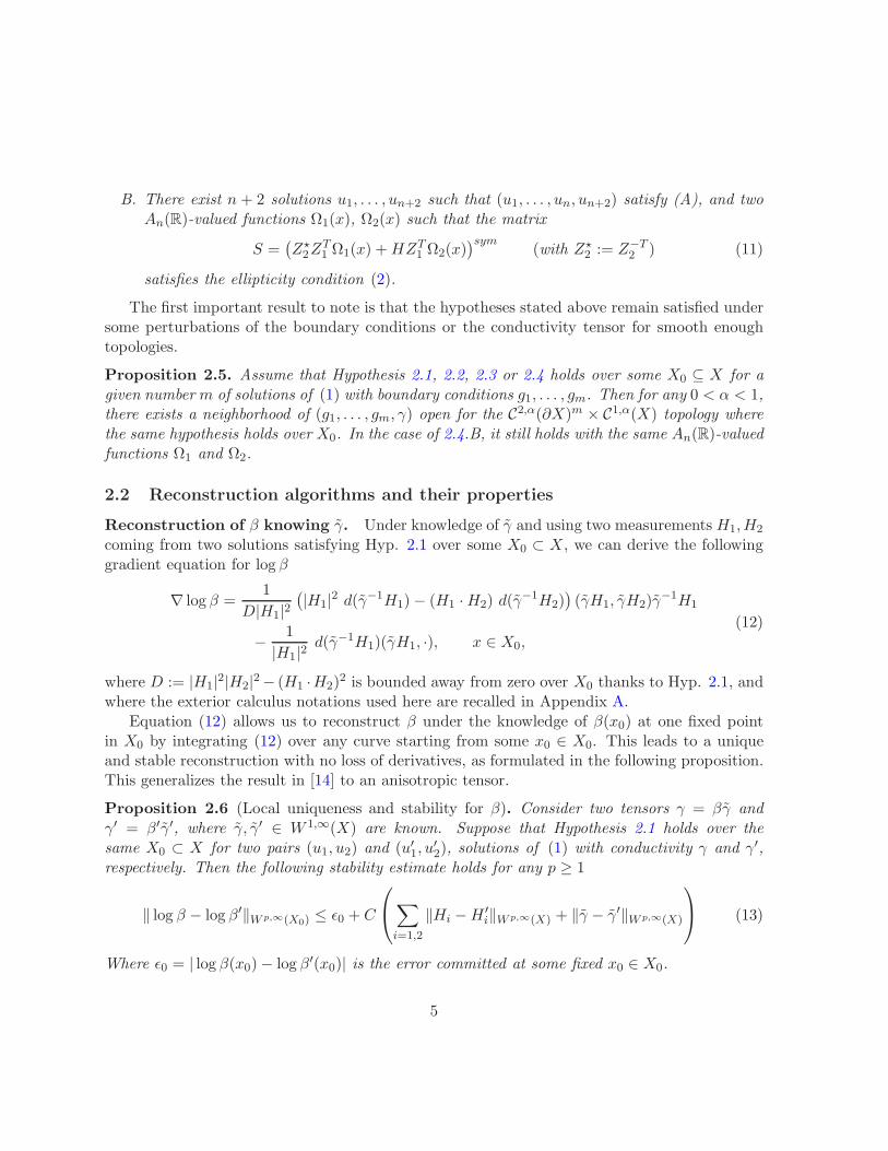
B. There exist n + 2 solutions u1, . . . , un+2 such that (u1, . . . , un, un+2) satisfy (A), and twoAn(R)-valued functions Ω1(x), Ω2(x) such that the matrix

S =(Z⋆2Z

T1 Ω1(x) +HZT

1 Ω2(x))sym

(with Z⋆2 := Z−T

2 ) (11)

satisfies the ellipticity condition (2).

The first important result to note is that the hypotheses stated above remain satisfied undersome perturbations of the boundary conditions or the conductivity tensor for smooth enoughtopologies.

Proposition 2.5. Assume that Hypothesis 2.1, 2.2, 2.3 or 2.4 holds over some X0 ⊆ X for agiven numberm of solutions of (1) with boundary conditions g1, . . . , gm. Then for any 0 < α < 1,there exists a neighborhood of (g1, . . . , gm, γ) open for the C2,α(∂X)m × C1,α(X) topology wherethe same hypothesis holds over X0. In the case of 2.4.B, it still holds with the same An(R)-valuedfunctions Ω1 and Ω2.

2.2 Reconstruction algorithms and their properties

Reconstruction of β knowing γ. Under knowledge of γ and using two measurements H1,H2

coming from two solutions satisfying Hyp. 2.1 over some X0 ⊂ X, we can derive the followinggradient equation for log β

∇ log β =1

D|H1|2(|H1|2 d(γ−1H1)− (H1 ·H2) d(γ

−1H2))(γH1, γH2)γ

−1H1

− 1

|H1|2d(γ−1H1)(γH1, ·), x ∈ X0,

(12)

where D := |H1|2|H2|2− (H1 ·H2)2 is bounded away from zero over X0 thanks to Hyp. 2.1, and

where the exterior calculus notations used here are recalled in Appendix A.Equation (12) allows us to reconstruct β under the knowledge of β(x0) at one fixed point

in X0 by integrating (12) over any curve starting from some x0 ∈ X0. This leads to a uniqueand stable reconstruction with no loss of derivatives, as formulated in the following proposition.This generalizes the result in [14] to an anisotropic tensor.

Proposition 2.6 (Local uniqueness and stability for β). Consider two tensors γ = βγ andγ′ = β′γ′, where γ, γ′ ∈ W 1,∞(X) are known. Suppose that Hypothesis 2.1 holds over thesame X0 ⊂ X for two pairs (u1, u2) and (u′1, u

′2), solutions of (1) with conductivity γ and γ′,

respectively. Then the following stability estimate holds for any p ≥ 1

‖ log β − log β′‖W p,∞(X0) ≤ ǫ0 + C

∑

i=1,2

‖Hi −H ′i‖W p,∞(X) + ‖γ − γ′‖W p,∞(X)

(13)

Where ǫ0 = | log β(x0)− log β′(x0)| is the error committed at some fixed x0 ∈ X0.

5

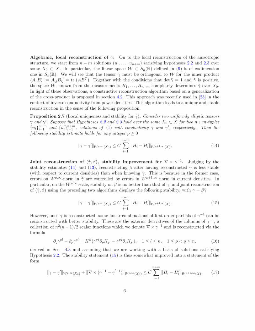
Algebraic, local reconstruction of γ: On to the local reconstruction of the anisotropicstructure, we start from n +m solutions (u1, . . . , un+m) satisfying hypotheses 2.2 and 2.3 oversome X0 ⊂ X. In particular, the linear space W ⊂ Sn(R) defined in (9) is of codimensionone in Sn(R). We will see that the tensor γ must be orthogonal to W for the inner product〈A,B〉 := AijBij = tr (ABT ). Together with the conditions that det γ = 1 and γ is positive,the space W, known from the measurements H1, . . . ,Hn+m completely determines γ over X0.In light of these observations, a constructive reconstruction algorithm based on a generalizationof the cross-product is proposed in section 4.2. This approach was recently used in [23] in thecontext of inverse conductivity from power densities. This algorithm leads to a unique and stablereconstruction in the sense of the following proposition.

Proposition 2.7 (Local uniqueness and stability for γ). Consider two uniformly elliptic tensorsγ and γ′. Suppose that Hypotheses 2.2 and 2.3 hold over the same X0 ⊂ X for two n+m-tuplesuin+m

i=1 and u′in+mi=1 , solutions of (1) with conductivity γ and γ′, respectively. Then the

following stability estimate holds for any integer p ≥ 0

‖γ − γ′‖W p,∞(X0) ≤ C

n+m∑

i=1

‖Hi −H ′i‖W p+1,∞(X). (14)

Joint reconstruction of (γ, β), stability improvement for ∇ × γ−1. Judging by thestability estimates (14) and (13), reconstructing β after having reconstructed γ is less stable(with respect to current densities) than when knowing γ. This is because in the former case,errors on W p,∞-norm in γ are controlled by errors in W p+1,∞ norm in current densities. Inparticular, on theW p,∞ scale, stability on β is no better than that of γ, and joint reconstructionof (γ, β) using the preceding two algorithms displays the following stability, with γ = βγ

‖γ − γ′‖W p,∞(X0) ≤ C

n+m∑

i=1

‖Hi −H ′i‖W p+1,∞(X). (15)

However, once γ is reconstructed, some linear combinations of first-order partials of γ−1 can bereconstructed with better stability. These are the exterior derivatives of the columns of γ−1, acollection of n2(n− 1)/2 scalar functions which we denote ∇× γ−1 and is reconstructed via theformula

∂qγpl − ∂pγ

ql = H il(γqj∂pHji − γpj∂qHji), 1 ≤ l ≤ n, 1 ≤ p < q ≤ n, (16)

derived in Sec. 4.3 and assuming that we are working with a basis of solutions satisfyingHypothesis 2.2. The stability statement (15) is thus somewhat improved into a statement of theform

‖γ − γ′‖W p,∞(X0) + ‖∇ × (γ−1 − γ′−1)‖W p,∞(X0) ≤ C

n+m∑

i=1

‖Hi −H ′i‖W p+1,∞(X), (17)

6

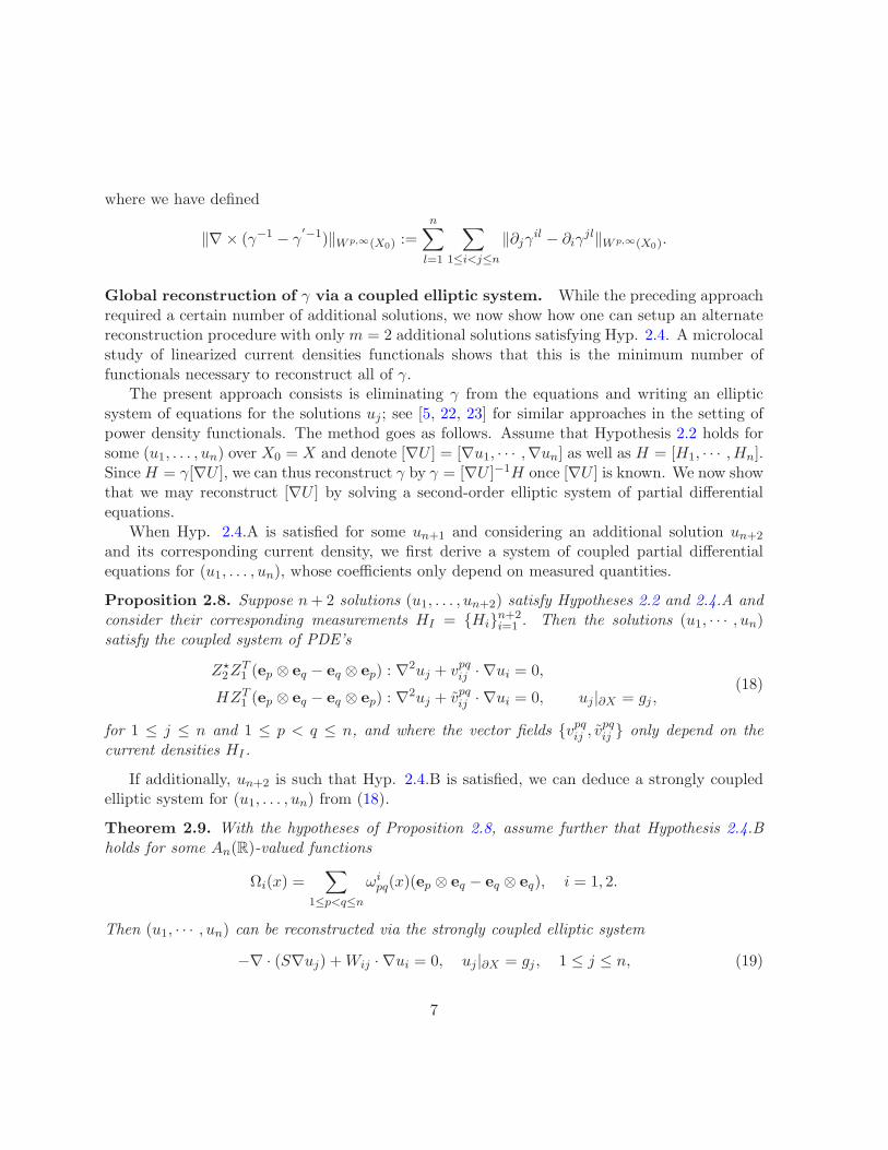
where we have defined

‖∇ × (γ−1 − γ′−1)‖W p,∞(X0) :=

n∑

l=1

∑

1≤i<j≤n

‖∂jγil − ∂iγjl‖W p,∞(X0).

Global reconstruction of γ via a coupled elliptic system. While the preceding approachrequired a certain number of additional solutions, we now show how one can setup an alternatereconstruction procedure with only m = 2 additional solutions satisfying Hyp. 2.4. A microlocalstudy of linearized current densities functionals shows that this is the minimum number offunctionals necessary to reconstruct all of γ.

The present approach consists is eliminating γ from the equations and writing an ellipticsystem of equations for the solutions uj; see [5, 22, 23] for similar approaches in the setting ofpower density functionals. The method goes as follows. Assume that Hypothesis 2.2 holds forsome (u1, . . . , un) over X0 = X and denote [∇U ] = [∇u1, · · · ,∇un] as well as H = [H1, · · · ,Hn].SinceH = γ[∇U ], we can thus reconstruct γ by γ = [∇U ]−1H once [∇U ] is known. We now showthat we may reconstruct [∇U ] by solving a second-order elliptic system of partial differentialequations.

When Hyp. 2.4.A is satisfied for some un+1 and considering an additional solution un+2

and its corresponding current density, we first derive a system of coupled partial differentialequations for (u1, . . . , un), whose coefficients only depend on measured quantities.

Proposition 2.8. Suppose n+ 2 solutions (u1, . . . , un+2) satisfy Hypotheses 2.2 and 2.4.A andconsider their corresponding measurements HI = Hin+2

i=1 . Then the solutions (u1, · · · , un)satisfy the coupled system of PDE’s

Z⋆2Z

T1 (ep ⊗ eq − eq ⊗ ep) : ∇2uj + vpqij · ∇ui = 0,

HZT1 (ep ⊗ eq − eq ⊗ ep) : ∇2uj + vpqij · ∇ui = 0, uj|∂X = gj ,

(18)

for 1 ≤ j ≤ n and 1 ≤ p < q ≤ n, and where the vector fields vpqij , vpqij only depend on the

current densities HI .

If additionally, un+2 is such that Hyp. 2.4.B is satisfied, we can deduce a strongly coupledelliptic system for (u1, . . . , un) from (18).

Theorem 2.9. With the hypotheses of Proposition 2.8, assume further that Hypothesis 2.4.Bholds for some An(R)-valued functions

Ωi(x) =∑

1≤p<q≤n

ωipq(x)(ep ⊗ eq − eq ⊗ eq), i = 1, 2.

Then (u1, · · · , un) can be reconstructed via the strongly coupled elliptic system

−∇ · (S∇uj) +Wij · ∇ui = 0, uj|∂X = gj , 1 ≤ j ≤ n, (19)

7

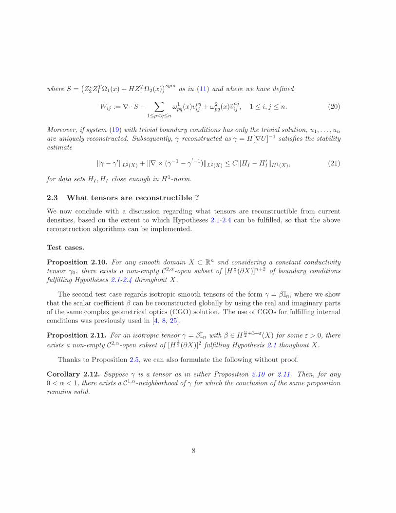
where S =(Z⋆2Z

T1 Ω1(x) +HZT

1 Ω2(x))sym

as in (11) and where we have defined

Wij := ∇ · S −∑

1≤p<q≤n

ω1pq(x)v

pqij + ω2

pq(x)vpqij , 1 ≤ i, j ≤ n. (20)

Moreover, if system (19) with trivial boundary conditions has only the trivial solution, u1, . . . , unare uniquely reconstructed. Subsequently, γ reconstructed as γ = H[∇U ]−1 satisfies the stabilityestimate

‖γ − γ′‖L2(X) + ‖∇ × (γ−1 − γ′−1)‖L2(X) ≤ C‖HI −H ′

I‖H1(X), (21)

for data sets HI ,HI close enough in H1-norm.

2.3 What tensors are reconstructible ?

We now conclude with a discussion regarding what tensors are reconstructible from currentdensities, based on the extent to which Hypotheses 2.1-2.4 can be fulfilled, so that the abovereconstruction algorithms can be implemented.

Test cases.

Proposition 2.10. For any smooth domain X ⊂ Rn and considering a constant conductivity

tensor γ0, there exists a non-empty C2,α-open subset of [H1

2 (∂X)]n+2 of boundary conditionsfulfilling Hypotheses 2.1-2.4 throughout X.

The second test case regards isotropic smooth tensors of the form γ = βIn, where we showthat the scalar coefficient β can be reconstructed globally by using the real and imaginary partsof the same complex geometrical optics (CGO) solution. The use of CGOs for fulfilling internalconditions was previously used in [4, 8, 25].

Proposition 2.11. For an isotropic tensor γ = βIn with β ∈ H n2+3+ε(X) for some ε > 0, there

exists a non-empty C2,α-open subset of [H1

2 (∂X)]2 fulfilling Hypothesis 2.1 thoughout X.

Thanks to Proposition 2.5, we can also formulate the following without proof.

Corollary 2.12. Suppose γ is a tensor as in either Proposition 2.10 or 2.11. Then, for any0 < α < 1, there exists a C1,α-neighborhood of γ for which the conclusion of the same propositionremains valid.

8

Push-forwards by diffeomorphisms Recall that for Ψ : X → Ψ(X) aW 1,2-diffeomorphismand γ ∈ Σ(X), we define Ψ⋆γ the conductivity tensor push-forwarded by Ψ from γ defined overΨ(X), by

Ψ⋆γ := (|JΨ|−1DΨ · γ ·DΨ) Ψ−1, JΨ := detDΨ. (22)

We now show that, whenever a tensor is being push-forwarded from another by a diffeormor-phism, then the local or global reconstructibility of one is equivalent to that of the other, in thesense of the Proposition below. While the existence of Ψ⋆γ in Σ(Ψ(X)) merely requires that Ψbe aW 1,2-diffeomorphism, our results below will require that Ψ be smoother and that it satisfiesthe following uniform condition over X

C−1Ψ ≤ |JΨ| ≤ CΨ for some CΨ ≥ 1. (23)

Proposition 2.13. Assume that Hypothesis 2.1, 2.2, 2.3 or 2.4 holds over some X0 ⊆ X fora given number m of solutions of (1) with boundary conditions g1, . . . , gm. For Ψ : X → Ψ(X)a smooth diffeomorphism satisfying (23), the same hypothesis holds true over Ψ(X0) for theconductivity tensor Ψ⋆γ with boundary conditions (g1 Ψ−1, . . . , gm Ψ−1). In the case of Hyp.2.4.B, it holds with the following An(R)-valued functions defined over Ψ(X):

Ψ⋆Ω1 := [DΨ · Ω1 ·DΨt] Ψ−1 and Ψ⋆Ω2 := [|JΨ|DΨ · Ω2 ·DΨt] Ψ−1. (24)

In contrast to inverse conductivity problems from boundary data, where the diffeomorphismsabove are a well-known obstruction to injectivity, Proposition 2.13 precisely states the opposite:if a given tensor γ is reconstructible in some sense, then so is Ψ⋆γ, and the boundary conditionsmaking the inversion valid are explicitely given in terms of the ones that allow to reconstruct γ.

Corollary 2.14. Suppose γ is a tensor as in either Proposition 2.10 or 2.11 and Ψ : X → Ψ(X)is a diffeomorphism satisfying (23). Then the conclusion of the same proposition holds for thetensor Ψ⋆γ over Ψ(X) and boundary conditions defined over ∂(Ψ(X)).

Generic reconstructibility. We finally state that any C1,α smooth tensor is, in principle,reconstructible from current densities in the sense of the following proposition. This result usesthe Runge approximation property, a property equivalent to the unique continuation principle,valid for Lipschitz-continuous tensors.

Proposition 2.15. Let X ⊂ Rn a C2,α domain and γ ∈ C1,α

Σ (X). Then for any x0 ∈ X, thereexists a neighborhood X0 ⊂ X of x0 and n+ 2 solutions of (1) fulfilling hypotheses 2.2 and 2.3over X0.

9

Outline: The rest of the paper is structured as follows. Section 3 covers the preliminaries,including the proof of Proposition 2.5. Section 4 presents the derivations of the local recon-struction algorithms: Sec. 4.1 covers the local reconstruction of β and proves Proposition 2.6;Sec. 4.2 covers the local reconstruction of γ and the proof of Proposition 2.7; Sec. 4.3 justifiesequation (16); Sec. 4.4 discusses the global reconstruction of γ via an elliptic system, with aproof of Propositions 2.8 and 2.9. Finally, Section 5 discusses the question of reconstructibilityfrom current densities, with the proofs of Propositions 2.10, 2.11, 2.13 and 2.15.

3 Preliminaries

In this section, we briefly recall elliptic regularity results, the mapping properties of the currentdensity operator and we conclude with the proof of Proposition 2.5.

Properties of the forward mapping. In the following, we will make use of the followingresult, based on Schauder estimates for elliptic equations. It is for instance stated in [13].

Proposition 3.1. For k ≥ 2 an integer and 0 < α < 1, if X is a Ck+1,α-smooth domain, thenthe mapping (g, γ) 7→ u, solution of (1), is continuous in the functional setting

Ck,α(∂X) × Ck−1,αΣ (X) → Ck,α(X).

As a consequence, we can claim that, with the same k, α as above, the current densityoperator (g, γ) 7→ γ∇u is continuous in the functional setting

Ck,α(∂X) × Ck−1,αΣ (X) → Ck−1,α(X).

Moreover, this fact allows us to prove Proposition 2.5.

Proof of Proposition 2.5. Fixing some domain X0 ⊂ X and using Proposition 3.1, it is clearthat the mappings

f1 : (C2,α(∂X))2 × C1,αΣ (X) ∋ (g1, g2, γ) 7→ inf

X0

F1(u1, u2),

f2 : (C2,α(∂X))n × C1,αΣ (X) ∋ (g1, . . . , gn, γ) 7→ inf

X0

F2(u1, . . . , un),

with F1,F2 defined in (5),(6), are continuous, so f−11

((0,∞)

)and f−1

2

((0,∞)

)are open, which

takes care of Hypotheses 2.1 and 2.2. Further, Hypothesis 2.3 is fulfilled if and only if condition 31holds. Again, using Prop. 3.1, the mapping f3 := infX0

B with B defined in (31) is a continuousfunction of (g1, . . . , gn+m, γ) ∈ (C2,α(∂X))n+m × C1,α

Σ (X) so that f−13

((0,∞)

)is open.

10

Along the same lines, Hypothesis 2.4.A is stable under such perturbations because the map-ping

(C2,α(∂X))n+1 × C1,αΣ (X) ∋ (g1, . . . , gn+1, γ) 7→ inf

XdetZ1,

is continuous whenever u1, . . . , un satisfy (6) over X. Finally, fixing two An(R)-valued functionsΩ1(x) and Ω2(x), Hypothesis 2.4.B is fulfilled whenever

(g1, . . . , gn+2, γ) ∈n⋂

i=1

s−1i

((0,∞)

), (25)

where we have defined the functionals, for 1 ≤ i ≤ n

si : (C2,α(∂X))n+2 × C1,αΣ (X) ∋ (g1, . . . , gn+2, γ) 7→ inf

XdetSpq1≤p,q≤i,

with S = Sp,q1≤p,q≤n defined as in (11). Such functionals are, again, continuous, in particularthe set in the right-hand side of (25) is open. This concludes the proof.

4 Reconstruction approaches

4.1 Local reconstruction of β

In this section, we assume that γ is known and with W 1,∞ components. Assuming Hypothesis2.1 is fulfilled for two solutions u1, u2 over an open set X0 ⊂ X, we now prove equation (12).

Proof of equation (12). Rewriting (3) as 1βγ−1Hj = ∇uj and applying the operator d(·). Using

identities (49) and (50), we arrive at the following equation for log β:

∇ log β ∧ (γ−1Hj) = d(γ−1Hj), j = 1, 2. (26)

Let us first notice the following equality of vector fields

∇ log β ∧ (γ−1)H1(γH1, ·) = (∇ log β · γH1)(γ−1H1)− |H1|2∇ log β,

so that

∇ log β =1

|H1|2(∇ log β · γH1)γ

−1H1 −1

|H1|2∇ log β ∧ (γ−1H1)(γH1, ·)

=1

|H1|2(∇ log β · γH1)γ

−1H1 −1

|H1|2d(γ−1H1)(γH1, ·).

It remains thus to prove that

(∇ log β · γH1) =1

D

(|H1|2d(γ−1H1)− (H1 ·H2)d(γ

−1H2))(γH1, γH2),

11

which may be checked directly by computing, for j = 1, 2

d(γ−1Hj)(γH1, γH2) = d log β ∧ (γ−1Hj)(γH1, γH2)

= (∇ log β · γH1)Hj ·H2 − (∇ log β · γH2)(Hj ·H1).

Taking the appropriate weighted sum of the above equations allows to extract (∇ log β · γH1),and hence (12).

Reconstruction procedures for β, uniqueness and stability. Suppose equation (12)holds over some convex set X0 ⊂ X and fix x0 ∈ X0. Equation (12) is a gradient equation∇ log β = F with known right-hand side F . For any x ∈ X0, one may thus construct β(x) byintegrating (12) over the segment [x0, x], leading to one possible formula

β(x) = β(x0) exp

(∫ 1

0(x− x0) · F ((1− t)x0 + tx) dt

)

, x ∈ X0. (27)

Proof of Proposition 2.6. Since det γ = 1, the entries of γ−1 are polynomials of the entries of γ,so that the entries of the right-hand side of (12) are polynomials of the entries of H1,H2, γ andtheir derivatives, with bounded coefficients. It is thus straightforward to establish that

‖∇ log β −∇ log β′‖L∞(X0) ≤ C(‖H −H ′‖W 1,∞(X) + ‖γ − γ′‖W 1,∞(X)) (28)

for some constant C. Estimate (13) then follows from the fact that

‖ log β − log β′‖L∞(X0) ≤ | log β(x0)− log β′(x0)|+∆(X)‖∇ log β −∇ log β′‖L∞(X0),

where ∆(X) denotes the diameter of X.

One could use another integration curve than the segment [x0, x] to compute β(x). In orderfor this integration to not depend on the choice of curve, the right-hand side F of (12) shouldsatisfy the integrability condition dF = 0, a condition on the measurements which characterizespartially the range of the measurement operator.

When measurements are noisy, said right-hand side may no longer satisfy this requirement,in which case the solution to (12) no longer exists. One way to remedy this issue is to solvethe normal equation to (12) over X0 (whose boundary can be made smooth) with, for instance,Neuman boundary conditions:

−∆ log β = −∇ · F (X0), ∂ν log β|∂X0= F · ν,

where ν denotes the outward unit normal to X0. This approach salvages existence while pro-jecting the data onto the range of the measurement operator, with a stability estimate similarto (13) on the Hs Sobolev scale instead of the W s,∞ one.

12

4.2 Local reconstruction of γ

We now turn to the local reconstruction algorithm of γ. In this case, the reconstruction isalgebraic, i.e. no longer involves integration of a gradient equation. In the sequel, we work withn+m solutions of (1) denoted uin+m

i=1 , whose current densities Hi = γ∇uin+mi=1 are assumed

to be measured.

Derivation of the space of linear constraints (9). Apply the operator d(γ−1·) to therelation of linear dependence

Hn+k = µikHi, where µik := −det(H1, . . . ,

i︷ ︸︸ ︷

Hn+k, . . . ,Hn)

det(H1, . . . ,Hn), 1 ≤ i ≤ n.

Using the fact that d(γ−1Hi) = d(∇ui) = 0, we arrive at the following relation,

Zk,i ∧ γ−1Hi = 0, where Zk,i := ∇µik, k = 1, 2, . . .

Since the 2-form vanishes, by applying two vector fields γep, γep, 1 ≤ p < q ≤ n, we obtain,

HqiZk,i · γep = HpiZk,i · γeq,

Notice that the above equation means (γZk)piHqi = (γZk)qiHpi, which amounts to the fact thatγZkH

T is symmetric. This means in particular that γZkHT is orthogonal to An(R), and for

any Ω ∈ An(R), we can rewrite this orthogonality condition as

0 = tr (γZkHTΩ) = tr (γTZkH

TΩ) = γ : ZkHTΩ = γ : (ZkH

TΩ)sym, (29)

where the last part comes from the fact that γ is itself symmetric. Each matrix Zk thus generatesa subspace of Sn(R) of linear contraints for γ. Considering m additional solutions, we arrive atthe space of constraints defined in (9).

Algebraic inversion of γ via cross-product. We now show how to reconstruct γ explicitelyat any point where the space W defined in (9) has codimension one. We define the generalizedcross product as follows. Over an N -dimensional space V with a basis (e1, · · · , eN ), we definethe alternating N − 1-linear mapping N : VN−1 → V as the formal vector-valued determinantbelow, to be expanded along the last row

N (V1, · · · , VN−1) :=1

det(e1, · · · , eN )

∣∣∣∣∣∣∣∣∣

〈V1, e1〉 . . . 〈V1, eN 〉...

. . ....

〈VN−1, e1〉 . . . 〈VN−1, eN 〉e1 . . . eN

∣∣∣∣∣∣∣∣∣

(30)

13

N (V1, · · · , VN−1) is orthogonal to V1, · · · , VN−1. Moreover, N (V1, · · · , VN−1) vanishes if andonly if (V1, · · · , VN−1) are linearly dependent.

With this notion of cross-product in the case V ≡ Sn(R), we derive the following reconstruc-tion algorithm for γ. Adding m additional solutions, we find that W can be spanned by ♯W :=n(n−1)

2 mmatrices whose expressions are given in (9), picking for instance ei⊗ej−ej⊗ei1≤i<j≤n

as a basis for An(R). The condition that W is of codimension one over X0 can be formulatedas:

infx∈X0

B(x) > c1 > 0, B :=∑

I∈σ(nS−1,♯W)

|detN (I)| 1n , (31)

where σ(nS − 1, ♯W) denotes the sets of increasing injections from [1, nS − 1] to [1, ♯W], andwhere we have definedN (I) = N (MI1 , · · · ,MInS−1

), whereN is defined by (30) with V ≡ Sn(R).Then under condition (31), W is of rank nS − 1 in Sn(R).

Whenever (M1, . . . ,MnS−1) are picked in W, their cross-product must be proportional to γ.The constant of proportionality can be deduced, up to sign, from the condition det γ = 1 so wearrive at ±|detN (M1, · · · ,MnS−1)|

1

n γ = N (M1, · · · ,MnS−1). The sign ambiguity is removedby ensuring that γ must be symmetric definite positive, in particular its first coefficient on thediagonal should be positive. As a conclusion, we obtain the relation

|detN (I)| 1n γ = sign(N11(I))N (I), I ∈ σ(nS − 1, ♯W). (32)

This relation is nontrivial (and allows to reconstruct γ) only if (M1, . . . ,MnS−1) are linearlyindependent. When codim W = 1 but ♯W > nS − 1, we do not know a priori which nS − 1-subfamily of W has maximal rank, so we sum over all possibilities. Equation (32) then becomes

∑

I∈σ(nS−1,♯W)

sign(N11(I))N (I) = Bγ, (33)

with B defined in (31). Since B > c1 > 0 over X0, γ can be algebraically reconstructed on X0

by formula (33), where N is defined by (30) with V = Sn(R).

Uniqueness and stability. Formula (33) has no ambiguity provided condition (31), hencethe uniqueness. Regarding stability, we briefly justify Proposition 2.7.

Proof of Proposition 2.7. In formula (33), the components of the cross-productsN (I) are smooth(polynomial) functions of the components of the matrices ZkH, which in turn are smooth func-tions of the components of Hin+m

i=1 and their first derivatives, and where the only term appear-ing as denominator is det(H1, . . . ,Hn), which is bounded away from zero by virtue of Hypothesis2.2. Thus (14) holds for p = 0. That it holds for any p ≥ 1 is obtained by taking partial deriva-tives of the reconstruction formula of order p and bounding accordingly.

14

4.3 Joint reconstruction of (γ, β) and stability improvement

In this section, we justify equation (16), which allows to justify the stability claim (17). Start-ing from n solutions satisfying Hypothesis 2.2 over X0 ⊆ X and denote H = Hijni,j=1 =

[H1| . . . |Hn] as well as Hpq := (H−1)pq. Applying the operator d(γ−1·) to both sides of (3)yields d(γ−1Hj) = d(∇uj) = 0 due to (49). Rewritten in scalar components for 1 ≤ j ≤ n and1 ≤ p < q ≤ n

0 = ∂q(γplHlj)− ∂p(γ

qlHlj) = (∂qγpl − ∂pγ

ql)Hlj + γpl∂qHlj − γql∂pHlj.

Thus (16) is obtained after multiplying the last right-hand side by Hji, summing over j andusing the property that

∑nj=1HljH

ji = δil.

4.4 Reconstruction of γ via an elliptic system

In this section, we will construct a second order system for (u1, · · · , un) with n+2 measurements,assuming Hypotheses 2.2 and 2.4.A hold with X0 = X. For the proof below, we shall recall thedefinition of the Lie Bracket of two vector fields in the euclidean setting:

[X,Y ] := (X · ∇)Y − (Y · ∇)X = (Xi∂i)Yjej − (Y i∂i)X

jej.

Proof of Proposition 2.8. As is shown by (29), γZkHT is symmetric. Multiplying both sides by

γ−1 and using γ−1H = ∇U , we see that Zk[∇U ]T is symmetric. More explicitly, we have

Zk,pi∂qui = Zk,qi∂pui, k = 1, 2, (34)

or simply Zk[∇U ]T = [∇U ]ZTk . Assume Hypothesis 2.4.A holds with Z2 invertible so that

(Z2,1, · · · , Z2,n) form a basis in Rn. We define its dual frame such that Z⋆

2,j · Z2,i = δij . Denote

Z⋆2 = [Z⋆

2,1, · · · , Z⋆2,n] and Z

⋆2 = Z−T

2 . Then the symmetry of Z2[∇U ]T reads,

Z⋆2,j · ∇ui = Z⋆

2,i · ∇uj, 1 ≤ i ≤ j ≤ n. (35)

Pick v a scalar function, we have the following commutation relation:

(X · ∇)(Y · ∇)v = (Y · ∇)(X · ∇)v + [X,Y ] · ∇v

Rewrite Z1,pi∂q = Z1,pieq · ∇ and apply Z⋆2,j · ∇ to both sides of (34), we have the following

equation by the above relations in Lie Bracket,

[Z⋆2,j, Z1,pieq

]· ∇ui + (Z1,pieq · ∇)(Z⋆

2,j · ∇)ui =[Z⋆2,j , Z1,qiep

]· ∇ui + (Z1,qiep · ∇)(Z⋆

2,j · ∇)ui(36)

15

where Zk,ij = Zk : ei ⊗ ej . Plugging (35) to the above equation gives,

(Z1,pieq · ∇)(Z⋆2,i · ∇)uj +

[Z⋆2,j , Z1,pieq

]· ∇ui = (Z1,qiep · ∇)(Z⋆

2,i · ∇)uj +[Z⋆2,j, Z1,qiep

]· ∇ui

Looking at the principal part, the first term of the LHS reads

(Z1,pieq · ∇)(Z⋆2,i · ∇)uj = (Z⋆

2ZT1 ep ⊗ eq) : ∇2uj + (Z1,pieq · ∇)Z⋆

2,i · ∇uj .

Therefore, (36) amounts to the following coupled system,

Z⋆2Z

T1 (ep ⊗ eq − eq ⊗ ep) : ∇2uj + vpqij · ∇ui = 0, uj|∂X = gj , 1 ≤ p ≤ q ≤ n (37)

where

vpqij := δij [(Z1,pleq − Z1,qlep) · ∇]Z⋆2,l +

[Z⋆2,j , Z1,pieq − Z1,qiep

]. (38)

Notice that H = γ[∇U ] implies that H−T [∇U ]T is symmetric. Compared with equation (34),we can see that the same proof holds if we replace Z2 by H−T . In this case, the dual frame ofH−T is simply H. So (37) and (38) hold by replacing Z⋆

2 by H and defining vpqij accordingly.

We now suppose that Hypothesis 2.4.B is satisfied and proceed to the proof of Theorem 2.9.

Proof. Starting from Hypothesis 2.4.B with An(R)-valued functions of the form

Ωi(x) =∑

1≤p<q≤n

ωipq(x)(ep ⊗ eq − eq ⊗ eq), i = 1, 2,

we take the weighted sum of equations (18) with weights ω1pq, ω

2pq. The principal part becomes

S : ∇2ui, which upon rewritting it as ∇ · (S∇ui)− (∇ · S) · ∇ui yields system (19).On to the proof of stability, pick another set of data H ′

I := H ′in+2

i=1 close enough to HI inW 1,∞ norm, and write the corresponding system for u′1, . . . , u

′n

−∇ · S′∇u′j +W ′ij · ∇u′i = 0, 1 ≤ j ≤ n, (39)

where S′ and W ′ij are defined by replacing HI in (20) by H ′

I . Subtracting (39) from (19), wehave the following coupled elliptic system for vj = uj − u′j :

−∇ · S∇vj +Wij · ∇vi = ∇ · (S − S′)∇u′j + (W ′ij −Wij) · ∇u′i, vj |∂X = 0 (40)

The proof is now a consequence of the Fredholm alternative (as in [5, Theorem 2.9]). We recast(40) as an integral equation. Denote the operator L0 = −∇ · (S∇) and define L−1

0 : H−1(X) ∋f 7→ v ∈ H1

0 (X), where v is the unique solution to the equation

−∇ · (S∇v) = f (X), v|∂X = 0.

16

By the Lax-Milgram theorem, we have ‖v‖H10(X) ≤ C‖f‖H−1(X), where C only depends on

X and S. Thus L−10 : H−1(X) → H1

0 (X) is continuous, and by Rellich imbedding, L−10 :

L2(X) → H10 (X) is compact. Define the vector space H = (H1

0 (X))n, v = (v1, . . . , vn), h =(L−1

0 f1, . . . , L−10 fn), where fj = ∇·(S−S′)∇u′j+(W ′

ij−Wij) ·∇u′i, and the operator P : H → Hby,

P : H ∋ v → Pv := (L−10 (Wi1 · ∇vi), · · · , L−1

0 (Win · ∇vi)) ∈ H.

Since theWij are bounded, the differential operatorsWij ·∇ : H10 → L2 are continuous. Together

with the fact that L−10 : L2 → H1

0 is compact, we get that P : H → H is compact. After applyingthe operator L−1

0 to (19), the elliptic system is reduced to the following Fredholm equation:

(I+P)v = h.

By the Fredholm alternative, if −1 is not an eigenvalue of P, then I+P is invertible and bounded‖v‖H ≤ ‖(I +P)−1‖L(H)‖h‖H. Since L−1

0 : H−1(X) → H10 (X) is continuous, h in (H1

0 (X))n isbounded by f = (f1, · · · , fn) in (H−1(X))n.

‖h‖H ≤ ‖L−10 ‖L(H−1,H1

0)‖f‖H−1(X).

Then we have the estimate,

‖v‖H ≤ ‖(I +P)−1‖L(H)‖L−10 ‖L(H−1,H1

0)‖f‖H−1(X)

Noting that L−10 is continuous and the RHS of (40) is expressed by HI−H ′

I and their derivativesup to second order, we have the stability estimate

‖u− u′‖H10(X) ≤ C‖HI −H ′

I‖H1(X)

where C depends on HI but can be chosen uniform for HI and H ′I sufficiently close. Then γ is

reconstructed by γ = H[∇U ]−1 and ∇× γ−1 by (16), with a stability of the form

‖γ − γ′‖L2(X) + ‖∇ × (γ−1 − γ′−1))‖L2(X) ≤ C‖HI −H ′I‖H1(X).

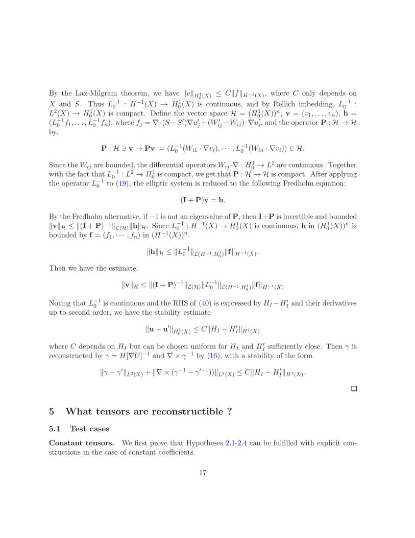
5 What tensors are reconstructible ?

5.1 Test cases

Constant tensors. We first prove that Hypotheses 2.1-2.4 can be fulfilled with explicit con-structions in the case of constant coefficients.

17

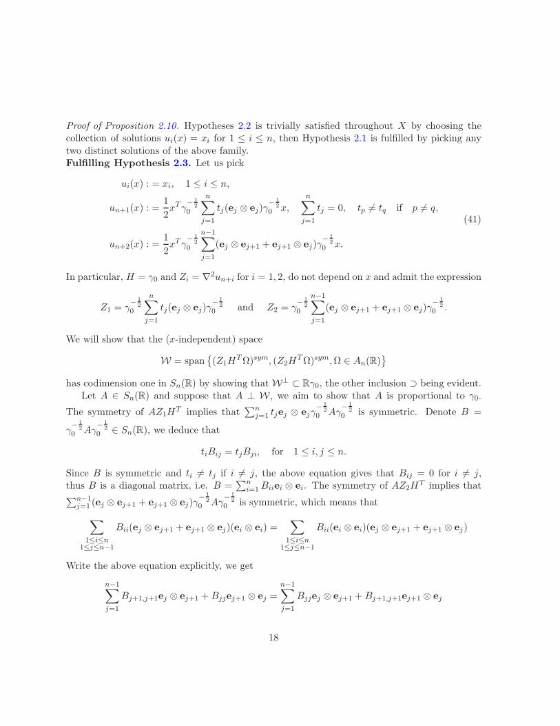
Proof of Proposition 2.10. Hypotheses 2.2 is trivially satisfied throughout X by choosing thecollection of solutions ui(x) = xi for 1 ≤ i ≤ n, then Hypothesis 2.1 is fulfilled by picking anytwo distinct solutions of the above family.Fulfilling Hypothesis 2.3. Let us pick

ui(x) : = xi, 1 ≤ i ≤ n,

un+1(x) : =1

2xTγ

− 1

2

0

n∑

j=1

tj(ej ⊗ ej)γ− 1

2

0 x,

n∑

j=1

tj = 0, tp 6= tq if p 6= q,

un+2(x) : =1

2xTγ

− 1

2

0

n−1∑

j=1

(ej ⊗ ej+1 + ej+1 ⊗ ej)γ− 1

2

0 x.

(41)

In particular, H = γ0 and Zi = ∇2un+i for i = 1, 2, do not depend on x and admit the expression

Z1 = γ− 1

2

0

n∑

j=1

tj(ej ⊗ ej)γ− 1

2

0 and Z2 = γ− 1

2

0

n−1∑

j=1

(ej ⊗ ej+1 + ej+1 ⊗ ej)γ− 1

2

0 .

We will show that the (x-independent) space

W = span(Z1H

TΩ)sym, (Z2HTΩ)sym,Ω ∈ An(R)

has codimension one in Sn(R) by showing that W⊥ ⊂ Rγ0, the other inclusion ⊃ being evident.Let A ∈ Sn(R) and suppose that A ⊥ W, we aim to show that A is proportional to γ0.

The symmetry of AZ1HT implies that

∑nj=1 tjej ⊗ ejγ

− 1

2

0 Aγ− 1

2

0 is symmetric. Denote B =

γ− 1

2

0 Aγ− 1

2

0 ∈ Sn(R), we deduce that

tiBij = tjBji, for 1 ≤ i, j ≤ n.

Since B is symmetric and ti 6= tj if i 6= j, the above equation gives that Bij = 0 for i 6= j,thus B is a diagonal matrix, i.e. B =

∑ni=1Biiei ⊗ ei. The symmetry of AZ2H

T implies that∑n−1

j=1 (ej ⊗ ej+1 + ej+1 ⊗ ej)γ− 1

2

0 Aγ− 1

2

0 is symmetric, which means that

∑

1≤i≤n1≤j≤n−1

Bii(ej ⊗ ej+1 + ej+1 ⊗ ej)(ei ⊗ ei) =∑

1≤i≤n1≤j≤n−1

Bii(ei ⊗ ei)(ej ⊗ ej+1 + ej+1 ⊗ ej)

Write the above equation explicitly, we get

n−1∑

j=1

Bj+1,j+1ej ⊗ ej+1 +Bjjej+1 ⊗ ej =n−1∑

j=1

Bjjej ⊗ ej+1 +Bj+1,j+1ej+1 ⊗ ej

18

Which amounts to

n−1∑

j=1

(Bj+1,j+1 −Bjj)(ej+1 ⊗ ej − ej+1 ⊗ ej) = 0

Notice that ej+1⊗ej−ej+1⊗ej1≤j≤n−1 are linearly independent in An(R), so Bj+1,j+1 = Bjj

for 1 ≤ j ≤ n − 1, i.e. B is proportional to the identity matrix. This means that A must beproportional to γ0 and thus W⊥ ⊂ Rγ0. Hypothesis 2.3 is fulfilled throughout X.

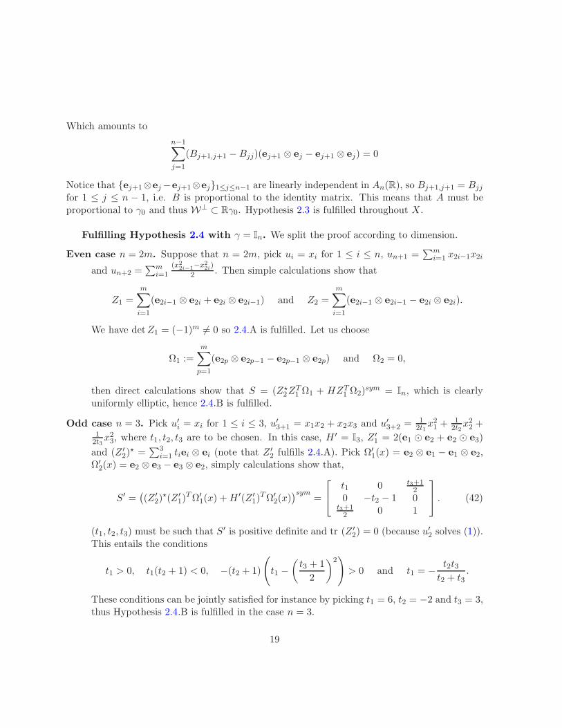
Fulfilling Hypothesis 2.4 with γ = In. We split the proof according to dimension.

Even case n = 2m. Suppose that n = 2m, pick ui = xi for 1 ≤ i ≤ n, un+1 =∑m

i=1 x2i−1x2i

and un+2 =∑m

i=1

(x22i−1

−x22i)

2 . Then simple calculations show that

Z1 =m∑

i=1

(e2i−1 ⊗ e2i + e2i ⊗ e2i−1) and Z2 =m∑

i=1

(e2i−1 ⊗ e2i−1 − e2i ⊗ e2i).

We have detZ1 = (−1)m 6= 0 so 2.4.A is fulfilled. Let us choose

Ω1 :=m∑

p=1

(e2p ⊗ e2p−1 − e2p−1 ⊗ e2p) and Ω2 = 0,

then direct calculations show that S = (Z⋆2Z

T1 Ω1 + HZT

1 Ω2)sym = In, which is clearly

uniformly elliptic, hence 2.4.B is fulfilled.

Odd case n = 3. Pick u′i = xi for 1 ≤ i ≤ 3, u′3+1 = x1x2 + x2x3 and u′3+2 = 12t1x21 +

12t2x22 +

12t3x23, where t1, t2, t3 are to be chosen. In this case, H ′ = I3, Z

′1 = 2(e1 ⊙ e2 + e2 ⊙ e3)

and (Z ′2)

⋆ =∑3

i=1 tiei ⊗ ei (note that Z ′2 fulfills 2.4.A). Pick Ω′

1(x) = e2 ⊗ e1 − e1 ⊗ e2,Ω′2(x) = e2 ⊗ e3 − e3 ⊗ e2, simply calculations show that,

S′ =((Z ′

2)⋆(Z ′

1)TΩ′

1(x) +H ′(Z ′1)

TΩ′2(x)

)sym=

t1 0 t3+12

0 −t2 − 1 0t3+12 0 1

. (42)

(t1, t2, t3) must be such that S′ is positive definite and tr (Z ′2) = 0 (because u′2 solves (1)).

This entails the conditions

t1 > 0, t1(t2 + 1) < 0, −(t2 + 1)

(

t1 −(t3 + 1

2

)2)

> 0 and t1 = − t2t3t2 + t3

.

These conditions can be jointly satisfied for instance by picking t1 = 6, t2 = −2 and t3 = 3,thus Hypothesis 2.4.B is fulfilled in the case n = 3.

19

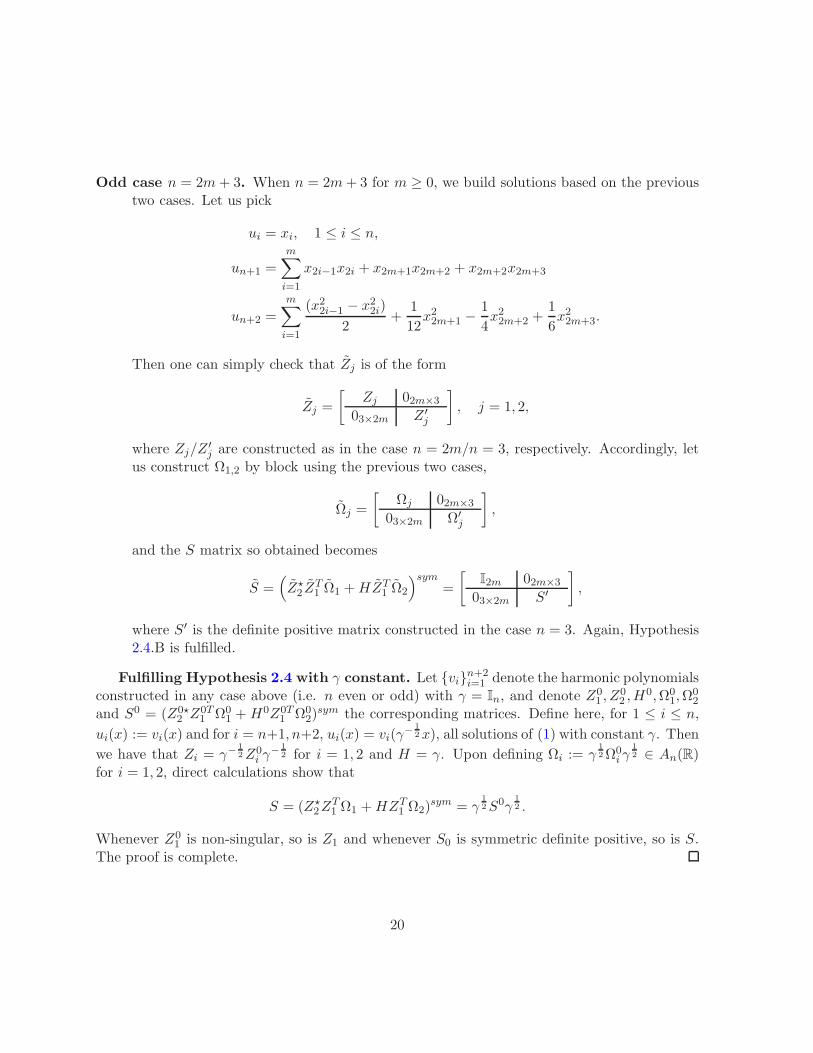
Odd case n = 2m+ 3. When n = 2m+ 3 for m ≥ 0, we build solutions based on the previoustwo cases. Let us pick

ui = xi, 1 ≤ i ≤ n,

un+1 =m∑

i=1

x2i−1x2i + x2m+1x2m+2 + x2m+2x2m+3

un+2 =

m∑

i=1

(x22i−1 − x22i)

2+

1

12x22m+1 −

1

4x22m+2 +

1

6x22m+3.

Then one can simply check that Zj is of the form

Zj =

[Zj 02m×3

03×2m Z ′j

]

, j = 1, 2,

where Zj/Z′j are constructed as in the case n = 2m/n = 3, respectively. Accordingly, let

us construct Ω1,2 by block using the previous two cases,

Ωj =

[Ωj 02m×3

03×2m Ω′j

]

,

and the S matrix so obtained becomes

S =(

Z⋆2 Z

T1 Ω1 +HZT

1 Ω2

)sym

=

[I2m 02m×3

03×2m S′

]

,

where S′ is the definite positive matrix constructed in the case n = 3. Again, Hypothesis2.4.B is fulfilled.

Fulfilling Hypothesis 2.4 with γ constant. Let vin+2i=1 denote the harmonic polynomials

constructed in any case above (i.e. n even or odd) with γ = In, and denote Z01 , Z

02 ,H

0,Ω01,Ω

02

and S0 = (Z0⋆2 Z

0T1 Ω0

1 +H0Z0T1 Ω0

2)sym the corresponding matrices. Define here, for 1 ≤ i ≤ n,

ui(x) := vi(x) and for i = n+1, n+2, ui(x) = vi(γ− 1

2x), all solutions of (1) with constant γ. Then

we have that Zi = γ−1

2Z0i γ

− 1

2 for i = 1, 2 and H = γ. Upon defining Ωi := γ1

2Ω0i γ

1

2 ∈ An(R)for i = 1, 2, direct calculations show that

S = (Z⋆2Z

T1 Ω1 +HZT

1 Ω2)sym = γ

1

2S0γ1

2 .

Whenever Z01 is non-singular, so is Z1 and whenever S0 is symmetric definite positive, so is S.

The proof is complete.

20

Isotropic tensors. As a second test case, we show that, based on the construction of complexgeometrical optics (CGO) solutions, Hypothesis 2.1 can be satisfied globally for an isotropictensor γ = βIn when β is smooth enough. CGO solutions find many applications in inverseconductivity/diffusion problems, and more recently in problems with internal functionals [4, 25,8]. As established in [7], when β ∈ H

n2+3+ε(X), one is able to construct a complex-valued

solution of (1) of the form

uρ =1√βeρ·x(1 + ψρ), (43)

where ρ ∈ Cn is a complex frequency satisfying ρ · ρ = 0, which is equivalent to taking ρ =

ρ(k + ik⊥) for some unit orthogonal vectors k,k⊥ and ρ = |ρ|/√2 > 0. The remainder ψρ

satisfies an estimate of the form ρψρ = O(1) in C1(X). The real and imaginary parts of ∇uρare almost orthogonal, modulo an error term that is small (uniformly over X) when ρ is large.We use this property here to fulfill Hypothesis 2.1.

Proof of Proposition 2.11. Pick two unit orthogonal vectors k and k⊥, and consider the CGOsolution uρ as in (43) with ρ = ρ(k + ik⊥) for some ρ > 0 which will be chosen large enoughlater. Computing the gradient of uρ, we arrive at

∇uρ = eρ·x(ρ+ϕρ), with ϕρ := ∇ψρ − ψρ∇ log√

β,

with supX |ϕρ| ≤ C independent of ρ. Splitting into real and imaginary parts, each of which isa real-valued solution of (1), we obtain the expression

∇uℜρ =ρeρk·x√

β

(

(k+ ρ−1ϕ

ℜρ ) cos(ρk

⊥ · x)− (k⊥ + ρ−1ϕ

ℑρ ) sin(ρk

⊥ · x))

,

∇uℑρ =ρeρk·x√

β

(

(k⊥ + ρ−1ϕ

ℑρ ) cos(ρk

⊥ · x) + (k+ ρ−1ϕ

ℜρ ) sin(ρk

⊥ · x))

,

from which we compute directly that

|∇uℜρ|2|∇uℑ

ρ|2 − (∇uℜ

ρ· ∇uℑ

ρ)2 =

ρ2e2ρk·x

β(1 + o(ρ−1)).

Therefore, for ρ large enough, the quantity in the left-hand side above remains bounded awayfrom zero throughout X, and the proof is complete.

5.2 Push-forward by diffeomorphism

Let Ψ : X → Ψ(X) be a W 1,2-diffeomorphism where X has smooth boundary. Then forγ ∈ Σ(X), the push-forwarded tensor Ψ⋆γ defined in (22) belongs to Σ(Ψ(X)) and Ψ pushesforward a solution u of (1) to a function v = u Ψ−1 satisfying the conductivity equation

−∇y · (Ψ⋆γ∇yv) = 0 (Ψ(X)), v|∂(Ψ(X)) = g Ψ−1,

21

moreover Ψ and Ψ|∂X induce respective isomorphisms of H1(X) and H1

2 (∂X) onto H1(Ψ(X))

and H1

2 (∂(Ψ(X))).

Proof of Proposition 2.13. The hypotheses of interest all fomulate the linear independence ofsome functionals in some sense. We must see first how these functionals are push-forwardedvia the diffeomorphism Ψ. For 1 ≤ i ≤ m, we denote vi := Ψ⋆ui = ui Ψ−1 as well asΨ⋆Hi := [Ψ⋆γ]∇yvi where y denotes the variable in Ψ(X). Direct use of the chain rule allowsto establish the following properties, true for any x ∈ X:

∇ui(x) = [DΨ]T (x)∇yvi(Ψ(x)),

Hi(x) = γ∇ui(x) = |JΨ|(x)[DΨ]−1Ψ⋆H(Ψ(x)),

Zi(x) = [DΨ]T (x)Ψ⋆Zi(Ψ(x)),

(44)

where we have defined Ψ⋆Zi the matrix with columns

[Ψ⋆Zi],j = −∇ydet(∇yv1, . . . ,

j︷ ︸︸ ︷

∇yvn+i, . . . ,∇yvn)

det(∇yv1, . . . ,∇yvn), 1 ≤ j ≤ n.

Hypotheses 2.1 and 2.2. Since [DΨ] is never singular over X, relations (44) show thatfor any 1 ≤ k ≤ n, the vectors fields (∇u1, . . . ,∇uk) are linearly dependent at x if and only ifthe vectors fields (∇yv1, . . . ,∇yvk) are linearly dependent at Ψ(x). The case k = 2 takes careof Hyp. 2.1 while the case k = n takes care of Hyp. 2.2.

Hypothesis 2.3. If we denote

Ψ⋆W(Ψ(x)) = span(Ψ⋆Zk(Ψ⋆H)TΩ)sym, Ω ∈ An(R), 1 ≤ k ≤ m

,

direct computations show that

W(x) = [DΨ(x)]T ·Ψ⋆W(Ψ(x)) · [DΨ(x)],

thus since DΨ(x) is non-singular, we have that dimW(x) = dimΨ⋆W(Ψ(x)), so the statementof Proposition holds for Hyp. 2.3.

Hypothesis 2.4. The transformation rules (44) show that Z1 is nonsingular at x iff Ψ⋆Z1

is nonsingular at Ψ(x), so the statement of the proposition holds for Hyp. 2.4.A.Second, for two An(R)-valued functions Ω1(x) and Ω2(x), and upon defining Ψ⋆Ω1, Ψ⋆Ω2 as

in (24), as well as

Ψ⋆S :=([Ψ⋆Z2]

−T [Ψ⋆Z1]TΨ⋆Ω1 + [Ψ⋆H][Ψ⋆Z1]

TΨ⋆Ω2

)sym,

direct use of relations (44) yield the relation

S(x) = [DΨ(x)]−1 ·Ψ⋆S(Ψ(x)) · [DΨ(x)]−T , x ∈ X,

and since DΨ is uniformly non-singular, S is uniformly elliptic if and only if Ψ⋆S is, so thestatement of the proposition holds for Hyp. 2.4.B.

22

5.3 Generic reconstructibility

We now show that, in principle, any C1,α-smooth conductivity tensor is locally reconstructiblefrom current densities. The proof relies on the Runge approximation for elliptic equations,which is equivalent to the unique continuation principle, valid for conductivity tensors withLipschitz-continuous components.

This scheme of proof was recently used in the context of other inverse problems with internalfunctionals [8, 23], and the interested reader is invited to find more detailed proofs there.

Proof of Proposition 2.15. Let x0 ∈ X and denote γ0 := γ(x0). We first construct solutions ofthe constant-coefficient problem by picking the functions defined in (41) (call them v1, . . . , vn+2)and by defining, for 1 ≤ i ≤ n+2, u0i (x) := vi(x)−vi(x0). These solutions satisfy ∇·(γ0∇ui) = 0everywhere and fulfill Hypotheses 2.2 and 2.3 globally.

Second, from solutions u0i n+2i=1 , we construct a second family of solutions uri n+2

i=1 via thefollowing equation

∇ · (γ∇uri ) = 0 (B3r), uri |∂B3r= u0i , 1 ≤ i ≤ n+ 2, (45)

where B3r is the ball centered at x0 and of radius 3r, r being tuned at the end. The maximumprinciple as well as interior regularity results for elliptic equations allow to deduce the fact that

limr→0

max1≤i≤n+2

‖uri − u0i ‖C2(B3r) = 0. (46)

Third, assuming that r has been fixed at this stage, the Runge approximation propertyallows to claim that for every ε > 0 and 1 ≤ i ≤ n+ 2, there exists gεi ∈ H

1

2 (∂X) such that

‖uεi − uri ‖L2(B3r) ≤ ε, where uεi solves (1) with uεi |∂X = gεi , (47)

which, combined with interior elliptic estimates, yields the estimate

‖uεi − uri ‖C2(Br)≤ C

r2‖uεi − uri ‖L∞(B2r) ≤

C

r2ε,

Since r is fixed at this stage, we deduce that

limε→0

max1≤i≤n+2

‖uεi − uri ‖C2(Br) = 0. (48)

Completing the argument, we recall that Hypotheses 2.2 and 2.3 are characterized by contin-uous functionals (say f2 and f3) in the topology of C2,α boundary conditions. While the first stepestablished that f2 > 0 and f3 > 0 for the constant-coefficient solutions, limits (46) and (48) tellus that there exists a small r > 0, then a small ε > 0 such that max1≤i≤n+2 ‖uεi − u0i ‖C2(Br(x0))

is so small that, by the continuity of f2 and f3, these functionals remain positive. Hypotheses2.2 and 2.3 are thus satisfied over Br by the family uεi n+2

i=1 which is controlled by boundaryconditions. The proof is complete.

23

Remark 5.1 (On generic global reconstructibility). Let us mention that from the local recon-structibility statement above, one can establish a global reconstructibility one. Heuristically, bycompactness of X, one can cover the domain with a finite number of either neighborhoods asabove or subdomains diffeomorphic to a half-ball if the point x0 is close to ∂X, over each of whichγ is reconstructible. One can then patch together the local reconstructions using for instance apartition of unity, and obtain a globally reconstructed γ. The additional technicalities that thisproof incurs may be found in [8].

As a conclusion, for any C1,α-smooth tensor γ, there exists a finite N and non-empty openset O ⊂ (C2,α(∂X))N such that any giNi=1 ∈ O generates current densities that reconstruct γuniquely and stably (in the sense of estimate (17)) throughout X.

A Exterior calculus and notations

Throughout this paper, we use the following convention regarding exterior calculus. Because weare in the Euclidean setting, we will avoid the flat operator notation by identifying vector fieldswith one-forms via the identification ei ≡ ei where eini=1 and eini=1 denote bases of Rn andits dual, respectively. In this setting, if V = V iei is a vector field, dV denotes the two-vectorfield

dV =∑

1≤i<j≤n

(∂iVj − ∂jV

i)ei ∧ ej.

A two-vector field can be paired with two other vector fields via the formula

A ∧B(C,D) = (A · C)(B ·D)− (A ·D)(B · C),

which allows to make sense of expressions of the form

dV (A, ·) =∑

1≤i<j≤n

(∂iVj − ∂jV

i)((A · ei)ej − (A · ej)ei).

Note also the following well-known identities for f a smooth function and V a smooth vectorfield, rewritten with the notation above:

d(∇f) = 0, f ∈ C2(X), (49)

d(fV ) = ∇f ∧ V + fdV. (50)

Acknowledgments

This work was supported in part by NSF grant DMS-1108608 and AFOSR Grant NSSEFFFA9550-10-1-0194. FM is partially supported by NSF grant DMS-1025372.

24

References

[1] H. Ammari, E. Bonnetier, Y. Capdeboscq, M. Tanter, and M. Fink, ElectricalImpedance Tomography by elastic deformation, SIAM J. Appl. Math., 68 (2008), pp. 1557–1573. 1

[2] S. R. Arridge and O. Scherzer, Imaging from coupled physics, Inverse Problems, 28(2012), p. 080201. 1

[3] G. Bal, Inside Out, Cambridge University Press, 2012, ch. Hybrid inverse problems andinternal functionals. 1

[4] G. Bal, E. Bonnetier, F. Monard, and F. Triki, Inverse diffusion from knowledgeof power densities, to appear in Inverse Problems and Imaging, (2013). arXiv:1110.4577. 2,8, 21

[5] G. Bal, C. Guo, and F. Monard, Linearized internal functionals for anisotropic con-ductivities, submitted, (2013). 2, 4, 7, 16

[6] G. Bal and J. C. Schotland, Inverse scattering and acousto-optic imaging, Phys. Rev.Letters, 104 (2010), p. 043902. 1

[7] G. Bal and G. Uhlmann, Inverse diffusion theory of photoacoustics, Inverse Problems,26 (2010). 1, 21

[8] , Reconstruction of coefficients in scalar second-order elliptic equations from knowledgeof their solutions, to appear in C.P.A.M., (2012). arXiv:1111.5051. 2, 8, 21, 23, 24

[9] Y. Capdeboscq, J. Fehrenbach, F. de Gournay, and O. Kavian, Imaging by modi-fication: Numerical reconstruction of local conductivities from corresponding power densitymeasurements, SIAM Journal on Imaging Sciences, 2 (2009), pp. 1003–1030. 2

[10] N. Hoell and A. Moradifam and A. Nachman, Current density impedance imagingof an anisotropic conductivity in a known conformal class, submitted (2013). 2

[11] Y. Ider and L. Muftuler,Measurement of AC magnetic field distribution using magneticresonance imaging, IEEE Transactions on Medical Imaging, 16 (1997), pp. 617–622. 2

[12] Y. Ider and Ozlem Birgul, Use of the magnetic field generated by the internal distribu-tion of injected currents for electrical impedance tomography (MR-EIT), Elektrik, 6 (1998),pp. 215–225. 2

[13] V. Isakov, Inverse Problems for Partial Differential Equations, no. 127 in Applied Math-ematical Science, Springer, 2 ed., 2006. 10

25

[14] M. Joy, A. Nachman, K. Hasanov, R. Yoon, and A. Ma, A new approach to CurrentDensity Impedance Imaging (CDII), in Proc. 12th Annu. ISMRM Int. Conf., Kyoto, 2004.2, 5

[15] I. Kocyigit, Acousto-electric tomography and cgo solutions with internal data, InverseProblems, 28 (2012), p. 125004. 2

[16] P. Kuchment and L. Kunyansky, 2D and 3D reconstructions in acousto-electric tomog-raphy, Inverse Problems, 27 (2011). 2

[17] P. Kuchment and D. Steinhauer, Stabilizing inverse problems by internal data, InverseProblems, 28 (2012), p. 4007. arXiv:1110.1819. 2

[18] O. Kwon, J.-Y. Lee, and J.-R. Yoon, Equipotential line method for magnetic resonanceelectrical impedance tomography, Inverse Problems, 18 (2002), pp. 1089–1100. 2

[19] O. Kwon, E. Woo, J. Yoon, and J. Seo, Magnetic resonance electrical impedancetomography (MREIT): simulation study of J-substitution algorithm., IEEE Trans. Biomed.Eng., 49 (2002), pp. 160–7. 2

[20] J.-Y. Lee, A reconstruction formula and uniqueness of conductivity in mreit using twointernal current distributions, Inverse Problems, 20 (2004), pp. 847–58. 2

[21] W. Ma and T.P. DeMonte and A.I. Nachman and N. Elsaid and M.L.G. Joy,Experimental implementation f a new method of imaging anisotropic electric conductivities,submitted (2013). 2

[22] F. Monard, Taming unstable inverse problems. Mathematical routes toward high-resolutionmedical imaging modalities, PhD thesis, Columbia University, 2012. 1, 2, 7

[23] F. Monard and G. Bal, Inverse anisotropic conductivity from power densities in dimen-sion n ≥ 3, to appear in CPDE, (2012). submitted to CPDE. 2, 6, 7, 23

[24] , Inverse anisotropic diffusion from power density measurements in two dimensions,Inverse Problems, 28 (2012), p. 084001. arXiv:1110.4606. 2

[25] , Inverse diffusion problems with redundant internal information, Inv. Probl. Imaging,6 (2012), pp. 289–313. arXiv:1106.4277. 2, 8, 21

[26] A. Nachman, A. Tamasan, and A. Timonov, Conductivity imaging with a single mea-surement of boundary and interior data., Inverse Problems, 23 (2007), pp. 2551–63. 2

[27] A. Nachman, A. Tamasan, and A. Timonov, Recovering the conductivity from a singlemeasurement of interior data, Inverse Problems, 25 (2009), p. 035014. 2

26

[28] , Current Density Impedance Imaging, Tomography and Inverse Transport Theory.Contemporary Mathematics (G. Bal, D. Finch, P. Kuchment, P. Stefanov, G. Uhlmann,Editors) (2011) 2

[29] O. Scherzer, Handbook of Mathematical Methods in Imaging, Springer Verlag, New York,2011. 1

[30] G. Scott, M. Joy, R. Armstrong, and R. Henkelman, Measurement of nonuniformcurrent density by magnetic resonance, IEEE Transactions on Medical Imaging, 10 (1991),pp. 362–374. 2

[31] J. K. Seo, D.-H. Kim, J. Lee, O. I. Kwon, S. Z. K. Sajib, and E. J. Woo, Electricaltissue property imaging using MRI at dc and larmor frequency, Inverse Problems, 28 (2012),p. 084002. 2

[32] P. Stefanov and G. Uhlmann, Inside Out, Cambridge University Press, 2012, ch. Multi-wave methods via ultrasound. 1

[33] G. Uhlmann, Developments in inverse problems since Calderon’s foundational paper, Har-monic analysis and partial differential equations, Chicago Lectures in Math., Univ. ChicagoPress, Chicago, IL, (1999), pp. 295–345. 1

27