introduction to loop quantum cosmology

Symmetry, Integrability and Geometry: Methods and Applications SIGMA * (201*), ***, 94 pages

Introduction to loop quantum cosmology

Kinjal BANERJEE †, Gianluca CALCAGNI ‡ and Mercedes MARTÍN-BENITO ‡

† Beijing Normal UniversityE-mail: [email protected]‡ Max Planck Institute for Gravitational Physics (Albert Einstein Institute),Am Mühlenberg 1, D-14476 Golm, GermanyE-mail: [email protected], [email protected]

Abstract. This is an introduction to loop quantum cosmology (LQC) reviewing mini- andmidisuperspace models as well as homogeneous and inhomogeneous effective dynamics.

Key words: Loop quantum cosmology; Loop quantum gravity

2010 Mathematics Subject Classification: 83C45; 83C75; 83F05

Contents

Introduction 3

1 Loop quantization 41.1 Ashtekar–Barbero formalism . . . . . . . . . . . . . . . . . . . . . . . . . . . 41.2 Kinematic Hilbert space . . . . . . . . . . . . . . . . . . . . . . . . . . . . . 6

2 Plan of the review 8

I Minisuperspaces in loop quantum cosmology 9

3 Friedmann–Robertson–Walker models 93.1 Classical phase space description . . . . . . . . . . . . . . . . . . . . . . . . 103.2 Kinematical structure . . . . . . . . . . . . . . . . . . . . . . . . . . . . . . 113.3 Hamiltonian constraint operator . . . . . . . . . . . . . . . . . . . . . . . . . 123.4 Analysis of the constraint operator . . . . . . . . . . . . . . . . . . . . . . . 173.5 Physical structure . . . . . . . . . . . . . . . . . . . . . . . . . . . . . . . . 203.6 Dynamical singularity resolution: quantum bounce . . . . . . . . . . . . . . 223.7 FRW models with curvature or cosmological constant . . . . . . . . . . . . . 25

arX

iv:1

109.

6801

v1 [

gr-q

c] 3

0 Se

p 20

11

2 K. Banerjee, G. Calcagni and M. Martín-Benito

4 Bianchi I model 274.1 Classical formulation in Ashtekar–Barbero variables . . . . . . . . . . . . . . 274.2 Quantum representation . . . . . . . . . . . . . . . . . . . . . . . . . . . . . 284.3 Improved dynamics . . . . . . . . . . . . . . . . . . . . . . . . . . . . . . . . 284.4 Hamiltonian constraint operator . . . . . . . . . . . . . . . . . . . . . . . . . 294.5 Superselection sectors . . . . . . . . . . . . . . . . . . . . . . . . . . . . . . 324.6 Physical Hilbert space . . . . . . . . . . . . . . . . . . . . . . . . . . . . . . 324.7 Loop quantization of other Bianchi models . . . . . . . . . . . . . . . . . . . 35

II Midisuperspace models in loop quantum gravity 37

5 Hybrid quantization of the polarized Gowdy T 3 model 405.1 Classical description of the Gowdy T 3 model . . . . . . . . . . . . . . . . . 405.2 Fock quantization of the inhomogeneous sector . . . . . . . . . . . . . . . . 425.3 Hamiltonian constraint operator . . . . . . . . . . . . . . . . . . . . . . . . . 435.4 Physical Hilbert space . . . . . . . . . . . . . . . . . . . . . . . . . . . . . . 445.5 The Gowdy T 3 model coupled to a massless scalar field . . . . . . . . . . . . 47

6 Polymer quantization of the polarized Gowdy T 3 model 496.1 Classical theory . . . . . . . . . . . . . . . . . . . . . . . . . . . . . . . . . . 496.2 Quantum theory . . . . . . . . . . . . . . . . . . . . . . . . . . . . . . . . . 53

7 Comparison with the hybrid quantization 66

III Effective dynamics 68

8 Homogeneous effective dynamics 688.1 Parametrization of the Hamiltonian constraint . . . . . . . . . . . . . . . . . 688.2 Minisuperspace parametrization . . . . . . . . . . . . . . . . . . . . . . . . . 708.3 Effective equations of motion . . . . . . . . . . . . . . . . . . . . . . . . . . 718.4 Inverse-volume corrections in minisuperspace models . . . . . . . . . . . . . 748.5 Models with k 6= 0 and Λ 6= 0 . . . . . . . . . . . . . . . . . . . . . . . . . . 76

9 Inhomogeneous models 789.1 Lattice refinement . . . . . . . . . . . . . . . . . . . . . . . . . . . . . . . . 78

10 Conclusions 84

Introduction to LQC 3

Introduction

General relativity (GR) and quantum mechanics are two of the best verified theories ofmodern physics. While general relativity has been spectacularly successful in explainingthe universe at astronomical and cosmological scales, quantum mechanics gives an equallycoherent physical picture on small scales. However, one of the biggest unfulfilled challengesin physics remains to incorporate the two theories in the same framework. Ordinary quan-tum field theories, which have managed to describe the three other fundamental forces(electromagnetic, weak and strong), have failed for general relativity because it is not per-turbatively renormalizable.

Loop quantum gravity (LQG) [1, 2, 3] is an attempt to construct a mathematically rigor-ous, non-perturbative, background independent formulation of quantum general relativity.GR is reformulated in terms of Ashtekar–Barbero variables, namely the densitized triadand the Ashtekar connection. The basic classical variables are taken to be the holonomiesof the connection and the fluxes of the triads and these are then promoted to basic quantumoperators. The quantization is not the standard Schrödinger quantization but an unitar-ily inequivalent choice known as loop/polymer quantization. The kinematic structure ofLQG has been well developed. A robust feature of LQG, not imposed but emergent, is theunderlying discreteness of space.

With the aim of obtaining physical implications from LQG, in the last years the ap-plication of loop quantization techniques to cosmological models has undergone a notabledevelopment. This field of research is known under the name of loop quantum cosmol-ogy (LQC). The models analyzed in LQC are mini- and midisuperspace models. Thesemodels have Killing vectors which reduce the degrees of freedom of full GR. In the caseof minisuperspaces, the reduced theories have no field-theory degrees of freedom remain-ing. Although there are field-theory degrees of freedom in the midisuperspace models, theirnumber is smaller than in the full theory. Therefore, these are simplified systems whichprovide toy models suitable for studying some aspects of the full quantum gravity theory.Moreover, classical solutions are well known (in fact, we are aware of very few systemswhich have closed-form solutions of Einstein equations with no Killing vectors) and it isrelatively easy to study the effects of the quantization.

LQC cannot be considered the cosmological sector of LQG because the symmetry re-duction is carried out before quantizing, and the results so obtained may not be the sameif the reduction is done after quantization. However by adapting the techniques used inthe full theory to the symmetry-reduced cosmological models we may hope to capture someof the crucial features of the full theory, as well as to obtain hints about how to tacklethem. Indeed, one of the generic characteristics of LQC is the avoidance of the classicalsingularity. In the present absence of recognized experimental and observational signaturesof quantum gravity, this novel and robust result has been increasing the hope that LQGmay indeed be the correct theory of quantum gravity.

In this article we will review the progress made in the various cosmological models


studied in LQC in the last few years. A recent review [4] emphasizes aspects that areonly briefly mentioned here, such as the “simplified” or “solvable” LQC framework, thedetails of effective dynamics for FRW models with non-zero curvature and/or cosmologicalconstant, and inflationary perturbation theory in LQC. On the other hand, here we focusmore on midisuperspaces and discuss lattice refinement parametrizations at some length.Before starting, we shall briefly recall the main features in the kinematic structures of LQG.Similar ingredients are used in the kinematic structure of the LQC models to be discussedlater.

1 Loop quantization

1.1 Ashtekar–Barbero formalism

In the Hamiltonian formulation, the four-dimensional spacetime metric is described by athree-metric qab induced in the spatial sections Σ that foliate the spacetime manifold, thelapse function N and the shift vector Na [5, 6].1 Both the lapse N and the shift vectorNa are Lagrange multipliers accompanying the constraints that encoded the general co-variance of general relativity. These constraints are, respectively, the scalar or Hamiltonianconstraint and the diffeomorphisms constraint (which is a three-vector). Therefore, thephysically relevant information is encoded in the spatial three-metric and in its canonicallyconjugate momentum, or equivalently, in the extrinsic curvature Kab = Lnqab/2, where nis the unit normal to Σ and Ln is the Lie derivative along n [7].

LQG is based in a formulation of general relativity as a gauge theory [8, 9, 10, 11, 12],in which the phase space is described by a su(2) gauge connection, the Ashtekar–Barberoconnection Aia, and its canonically conjugate momentum, the densitized triad2 Eai , thatplays the role of an “electric field”. To define these objects, first one introduces the co-triadeia, defined as qab = eiae

jbδij , where δij stands for the Kronecker delta in three dimensions,

and then one defines the triad, eai , as its inverse eai ejb = δji δ

ab . The densitized triad then

reads Eai =√qeai , where q stands for the determinant of the spatial three-metric. In

turn, the Ashtekar–Barbero connection reads [13] Aia = Γia + γKia, where γ is an arbitrary

real and non-vanishing parameter, called the Immirzi parameter [14, 15], Kia = Kabe

bjδij

is the extrinsic curvature in triadic form, and Γia is the spin connection compatible withthe densitized triad. Namely, it verifies ∇bEai + εijkΓ

jbE

ak = 0, where εijk is the totallyantisymmetric symbol and ∇b is the usual spatial covariant derivative [7]. The canonicalpair (A,E) has the following Poisson bracket:

Aai (x), Ejb (y) = 8πGγδab δji δ(x− y) , (1.1)

1Latin indices from the beginning of the alphabet, a, b, ..., denote spatial indices.2Latin indices from the middle of the alphabet, i, j, . . . are SU(2) indices and label new degrees of

freedom introduced when passing to the triad formulation.


where G is Newton constant and δ(x− y) denotes the three-dimensional Dirac delta distri-bution on the hypersurface Σ.

Since the internal Euclidean metric δij is invariant under SU(2) rotations, the internalSU(2) degrees of freedom are gauge. Therefore, in this formulation of general relativity,besides the diffeomorphisms constraint Ca and the scalar (or Hamiltonian) constraint C,there is a gauge (or Gauss) constraint Gi fixing the rotation freedom that we have justintroduced. In the variables (Aai , E

jb ), those constraints have the following expression (in

vacuum)3 [1],

Gi = ∂aEai + εijkΓ

jaE

ak = 0, (1.2a)

Ca = F iabEbi = 0, (1.2b)

C =1√

|det(E)|εijk

[F iab − (1 + γ2)εimnK

ma K

nb

]EajEbk = 0, (1.2c)

where F iab is the curvature tensor of the Ashtekar–Barbero connection,

F iab = ∂aAib − ∂bAia + εijkA

jaA

kb . (1.3)

1.1.1 Holonomy-flux algebra

The next step is to define the holonomies and fluxes which will later be promoted to basicquantum variables.

The configuration variables chosen are the holonomies of Aia. They are more convenientthan the connection itself thanks to their properties under gauge transformation. Theholonomy of the connection A along the edge e is given by

he(A) = Pe∫e dx

aAia(x)τi , (1.4)

where P denotes path ordering and τi are the generators of SU(2), such that [τi, τj ] = εijkτk.

The momentum conjugate to the holonomy is given by the flux of Eai over surfaces Sand smeared with a su(2)-valued function f i:

E(S, f) =

∫Sf iEai εabcdx

bdxc. (1.5)

The description of the phase space in terms of holonomies and fluxes is not only suit-able for its transformation properties, but also because these objects are diffeomorphisminvariant and their definition is background independent. Moreover, their Poisson bracketis divergence-free

E(S, f), he(A) = 2πGγε(e, S)f iτihe(A), (1.6)

where ε(e, S) represents the regularization of the Dirac delta: it vanishes if e does notintersect S, as well as if e ⊂ S, and |ε(e, S)| = 1 if e and S intersect in one point, the signdepending on the relative orientation between e and S [3].

3In the presence of matter coupled to the geometry, there is a matter term contributing to each constraint.


1.2 Kinematic Hilbert space

In LQG, the holonomy-flux algebra is represented over a kinematical Hilbert space that isdifferent from the more familiar Schrödinger-type Hilbert space. It is given by the comple-tion of the space of cylindrical functions (defined on the space of generalized connections)with respect to the so-called Ashtekar–Lewandowski measure [16, 17, 18, 19]. We give avery brief description of this kinematical Hilbert space below, while the details can be foundin [1, 2, 3] (and references therein).

A generalized connection he(A) ≡ Ae is an assignment of A ∈ SU(2) to any analyticpath e ⊂ Σ. A graph Γ is a collection of analytic paths e ⊂ Σ meeting at most at theirendpoints. We will consider only closed graphs. The point at which two edges meet iscalled a vertex. Let n be the number of edges in Γ. A function cylindrical with respect toΓ is given by

ψΓ(A) := fΓ

(Ae1 , . . . Aen

), (1.7)

where fΓ is a smooth function on SU(2)n such that ψΓ(A) is gauge invariant. The spaceof states cylindrical with respect to Γ are denoted by CylΓ. The space of all functionscylindrical with respect to some Γ ∈ Σ is denoted by Cyl and is given by

Cyl =⋃Γ

CylΓ (1.8)

Given a cylindrical function ψΓ(A) ∈ Cyl, the Ashtekar–Lewandowski measure, denotedby µ0, is defined by∫

A/Gdµ0[ψΓ(A)] :=

∫SU(2)n

∏e⊂Γ

dhefΓ

(Ae1 , . . . Aen

), ∀ ψΓ(A) , (1.9)

where dh is the normalized Haar measure on SU(2). Using this measure we can define aninner product on Cyl:

〈ψΓ, ψ′Γ〉 := 〈fΓ

(Ae1 , . . . Aen

), gΓ′

(Ae1 , . . . Aem

)〉

=

∫SU(2)n

∏e⊂ΞΓΓ′

dhefΓ

(Ae1 , . . . Aen

)gΓ′(Ae1 , . . . Aem

), (1.10)

where ΞΓΓ′ is any graph such that Γ ⊂ ΞΓΓ′ and Γ′ ⊂ ΞΓΓ′ . Then, the kinematicalHilbert space of LQG is the Cauchy completion of Cyl in the Ashtekar–Lewandowski norm:Hkin = L2(A/G, dµ0).

A basis on this Hilbert space is provided by spin network states, which are constructed asfollows. Given a graph Γ, each edge e is colored by a non-trivial irreducible representationπje of SU(2), and associated to each vertex v there is a contraction tensor cv (calledintertwiner) which contracts the matrices πje for all edges incident at the vertex in a gauge


invariant way. Spin network states are cylindrical functions with respect to this colouredgraph. They are denoted by Ts := TΓ,~j,~c(A) where ~j = je and ~c = cv. Then, everycylindrical function can be expanded in the basis of spin network states.

On CylΓ the operators representing the corresponding holonomies act by multiplication,while the operator representing the flux is given by

EΓ(S, f) = i2πG~∑e⊂Γ

ε(e, S)Tr(f iτiAe

∂

∂Ae

). (1.11)

To obtain the quantum version of the more general operators, they have to be firstrewritten in terms of the basic holonomy-flux operators. Note that the quantum configu-ration space is not the space of smooth connections but rather the space of holonomies (orgeneralized connections). Since the Ashtekar–Lewandowski measure is discontinuous in theconnection, there is no well-defined operator for the connection on Hkin. Consequently, thecurvature must be defined in terms of holonomies before it can be promoted to a quantumoperator. The strategy in the full theory is to define any general quantum operator viaregularization as follows (see [1, 3] for details):

• The spatial manifold Σ is triangulated into elementary tetrahedra;

• the integral over Σ is replaced by a Riemann sum over the cells;

• for each cell, we define a regularized expression in terms of the basic operators, suchthat we get the correct classical expression in the limit the cell is shrunk to zero;

• this is promoted to a quantum operator provided it is densely defined on Hkin.

In the subsequent sections we shall see how the same strategy is applied for defining thequantum operators in LQC. One significant difference is that in the full theory the finalexpressions are independent of the regularization, while in the symmetry-reduced modelsthe regularization (i.e., the size of the cells) cannot be removed and has to be treated asan ambiguity. However, we can fix the form of the ambiguity by taking hints from the fulltheory.

One of the most interesting features of LQG is that the spectra of the operators rep-resenting geometrical quantities like area and volume are discrete. Discrete eigenvaluesimply that the underlying spatial manifold is also discrete at least when we are close to thequantum gravity scale. This is a feature of the quantization scheme and it also plays andimportant role in the singularity avoidance in LQC minisuperspace models.

This is the kinematical structure of LQG. As we shall see later, the programme of LQCtries to closely follow the same steps as far as possible. The procedure is obviously muchsimpler than in the full theory, and in the case of minisuperspace models it is possible to gobeyond the kinematics and construct the physical Hilbert space. Another useful proceduredeveloped to study the effect of the underlying discreteness is the use of effective equationsto study homogeneous cosmologies and perturbations therein. This has opened up a largenumber of systems to semiclassical analyses.


2 Plan of the review

Significant progress has been made in the study of a number of cosmologies in LQC. Here, weshall give an overall account of various facets of LQC, outlining technical aspects, reviewingthe results achieved and indicating the directions of further research. The rest of the paperis divided into three parts.

In part I we discuss LQC minisuperspace models. The simplest cases of minisuperspaceare Friedmann–Robertson–Walker (FRW) models, which are homogeneous and isotropic.The kinematical quantization programme followed for these models will be discussed indetail, using the example of flat FRW. We also describe the results obtained in the physicalHilbert space including the dynamical singularity resolution and the bounce. Open andclosed FRW models, with and without a cosmological constant, are briefly discussed. Thenext level of complication, Bianchi models, consists in removing the assumption of isotropy.In this case, our illustrative example will be the Bianchi I model but we also indicate thework done so far for Bianchi II and Bianchi IX cases.

Then, part II focusses on the LQC of midisuperspace models which are neither homoge-neous nor isotropic. We describe the only case whose loop quantization has been studiedin some detail, the linearly polarized Gowdy T 3 model. Two contrasting approaches havebeen taken in the study of this model. In the first approach, the degrees of freedom havebeen separated into homogeneous and inhomogeneous sectors. The homogeneous sectoris quantized using the tools developed in LQC, while the inhomogeneous sector is Fockquantized. In the second approach, the model is studied as a whole mimicking the steps ofLQG. We describe and compare both procedures.

Finally, in part III we discuss the programme of effective dynamics developed in LQC.In contrast to the previous two parts, this approach aims to incorporate the effects of thediscrete geometry as corrections to the classical equations. In this way it may be possibleto link LQC to phenomenological evidence.

In the end we summarize the current directions of ongoing research.


Part I

Minisuperspaces in loop quantum cosmologyLQC [20, 21, 22, 23] adapts the techniques developed in loop quantum gravity [1, 2, 3] to thequantization of simpler models than the full theory, as minisuperspace models. Minisuper-space models are solutions of Einstein’s equations with a high degree of symmetry, so muchso that there are no field theory degrees of freedom remaining. They lead to homogeneouscosmological solutions all of which suffer from a singularity where the classical equationsof motion break down. Since, after quantization, these are essentially quantum mechanicalsystems, they serve as good toy models for testing the predictions of LQG.

In LQC, we start from the classically symmetry-reduced phase space and then try toapply the steps followed in LQG to these systems. Owing to simplifications due to classicalsymmetry reduction, many technical complications typical of LQG can be avoided, and thequantization programme can be carried out beyond what has been achieved so far in the fulltheory. The fact that there is a well-defined full theory which tells us that the underlyingspatial geometry is discrete is a crucial ingredient in the formulation of LQC. A significantachievement of LQC is the development of a well-defined quantum theory for cosmologicalmodels where the classical singularity is absent. This resolution of the classical singularityis a robust feature of LQC as it is seen in all the minisuperspace models studied so far, aswell as under various choices made in addressing the ambiguities arising in quantization. Inthis part we shall review the LQC of various known minisuperspace cosmological scenarios.

3 Friedmann–Robertson–Walker models

LQC started with the pioneering works by Bojowald [24, 25, 26, 27, 28], that showed thefirst attempts of implementing the methods of LQG to the quantization of the simplestcosmological model: the flat Friedmann–Robertson–Walker (FRW) model (homogeneousand isotropic with flat spatial sections), whose geometry is described by a single degree offreedom, the scale factor. This system, even if very simple, is physically interesting since,at large scales, our universe is approximately homogeneous and isotropic. In addition,cosmological observations are compatible with a spatially flat geometry.

After the early papers by Bojowald, the kinematic structure of LQC was revised andmore rigorously established [29], which made it possible to complete the quantization ofthe model in presence of a homogeneous massless scalar field minimally coupled to thegeometry, as well as to study the resulting quantum evolution [30, 31, 32, 33]. Classically,this model represents expanding universes with an initial big bang singularity, where certainphysical observables, such as the matter density, diverge. Remarkably, the quantum dy-namics resolves the singularity replacing it with a quantum bounce, while for semiclassicalstates it agrees with the classical dynamics far away form the singularity. Therefore, even


though this is the simplest cosmological model, its loop quantization, also called polymericquantization, already leads to relevant results, the most important one being the avoidanceof the singularity.

Using the example of the flat FRWmodel coupled to a massless scalar, we shall discuss indetail the basics and the mathematical structure of LQC., adopting the so-called improveddynamics prescription [32].

3.1 Classical phase space description

3.1.1 Ashtekar–Barbero formalism

The classical phase space in the presence of homogeneity is much simpler than the generalsituation described in the introduction. In homogeneous cosmology, the gauge and dif-feomorphisms constraints are trivially satisfied, the Hamiltonian constraint being the onlysurvivor in the model. Moreover, for flat FRW the spin connection vanishes. In this case,the geometry part of the scalar constraint in its integral version is4 Cgrav(N) = NCgrav,with

Cgrav =

∫Σd3x C = − 1

γ2

∫Σd3x

εijkFiabE

ajEbk√|det(E)|

. (3.1)

Since flat FRW spatial sections Σ are non-compact, and the variables that describe it arespatially homogeneous, integrals such as (3.1) diverge. To avoid that, one usually restrictsthe analysis to a finite cell V. Owing to homogeneity, the study of this cell reproduces whathappens in the whole universe. When imposing also isotropy, the connection and the triadcan be described (in a convenient gauge) by a single parameter c and p, respectively, in theform [29]

Aia = c V −1/3o

oeia, Eai = p V −2/3o

√oq oeai . (3.2)

Here we have introduced a fiducial co-triad oeia that we will choose to be diagonal, oeia = δia,and the determinant

√oq of the corresponding fiducial metric. The results do not depend

on the fiducial choice. With the above definitions, the symplectic structure is defined via,

c, p =8πGγ

3. (3.3)

The variable p is related to the scale factor a commonly employed in geometrodynamicsthrough the expression a(t) =

√|p(t)|V −1/3

o . Note that p is positive (negative) if physicaland fiducial triads have the same (opposite) orientation.

On the other hand, a (homogeneous) massless scalar field φ, together with its momen-tum Pφ, provide the canonical pair describing the matter content, with Poisson bracket

4The lapse function N goes out of the integral due to the homogeneity.


φ, Pφ = 1. Then, the total Hamiltonian constraint contains a matter contribution besidethe geometry one, given in Eq. (3.1), and reads

C = Cgrav + Cmat = − 6

γ2c2√|p|+ 8πG

P 2φ

V= 0, (3.4)

where V = |p|3/2 is the physical volume of the cell V.

3.1.2 Holonomy-flux algebra

When defining holonomies and fluxes in LQC, and in the particular case of isotropic FRWmodels, owing to the homogeneity it is sufficient to consider straight edges oriented alongthe fiducial directions, and with oriented length equal to µV 1/3

o , where µ is an arbitraryreal number. Therefore, the holonomy along one such edge, in the i-th direction, is givenby

hµi (c) = eµcτi = cos(µc

2

)1 + 2 sin

(µc2

)τi. (3.5)

Then, the gravitational part of the configuration algebra is the algebra generated by thematrix elements of the holonomies, namely, the algebra of quasi-periodic functions of c,that are the complex exponentials

Nµ(c) = ei2µc. (3.6)

In analogy with the terminology employed in LQG [1, 3], the vector space of these quasi-periodic functions is called the space of cylindrical functions defined over symmetric con-nections, and it is denoted by CylS.

In turn, the flux is given by

E(S, f) = pV −2/3o AS,f , (3.7)

where AS,f is the fiducial area of S times an orientation factor (that depends on f). Then,the flux is essentially described by p.

In summary, in isotropic and homogeneous LQC the phase space is described by thevariables Nµ(c) and p, whose Poisson bracket is

Nµ(c), p = i4πGγ

3µNµ(c). (3.8)

3.2 Kinematical structure

Mimicking the quantization implemented in LQG, in LQC we adopt a representation ofthe algebra generated by the phase space variables Nµ(c) and p that is not continuous in


the connection, and therefore there is no operator representing c [29]. More concretely, thequantum configuration space is the Bohr compactification of the real line, RBohr, and thecorresponding Haar measure that characterizes the kinematical Hilbert space is the so-calledBohr measure [34]. It is simpler to work in momentum representation. In fact, such Hilbertspace is isomorphic to the space of functions of µ ∈ R that are square summable withrespect to the discrete measure [34], known as polymeric space. In other words, employingthe kets |µ〉 to denote the quantum states Nµ(c), whose linear span is the space CylS (densein RBohr), the kinematical Hilbert space is the completion of CylS with respect to the innerproduct 〈µ|µ′〉 = δµµ′ . We will denote this Hilbert space by Hgrav. Note that Hgrav isnon-separable, since the states |µ〉 form a non-countable orthogonal basis.

Obviously, the action of Nµ on the basis states is

Nµ′ |µ〉 = |µ+ µ′〉. (3.9)

On the other hand, the Dirac rule [Nµ, p] = i~ Nµ(c), p implies that

p|µ〉 = p(µ)|µ〉, p(µ) =4πl2Plγ

3µ, (3.10)

where lPl =√G~ is the Planck length. As we see, the spectrum of this operator is dis-

crete, as a consequence of the representation not being continuous in µ. Due to this lackof continuity, the Stone-von Neumann theorem about the uniqueness of the representa-tion in quantum mechanics [35, 36] is not applicable in this context. Therefore, the loopquantization of this model is inequivalent to the standard Wheeler–DeWitt (WDW) quan-tization [37, 38], where operators have a typical Schrödinger-like representation. In fact,while the WDW quantization fails in solving the problem of the big bang singularity, theloop quantization is singularity free [31, 32], as we will see later.

For the matter field, we adopt a standard Schrödinger-like representation, with φ actingby multiplication and Pφ = −i~∂φ as derivative, being both operators defined on theHilbert space L2(R, dφ). As domain, we take the Schwartz space S(R) of rapidly decreasingfunctions, which is dense in L2(R, dφ). The total kinematical Hilbert space is then Hkin =Hgrav ⊗ L2(R, dφ).5

3.3 Hamiltonian constraint operator

3.3.1 Curvature operator and improved dynamics

Since the connection is not well defined in the quantum theory, the classical expression ofthe Hamiltonian constraint, given in Eq. (3.4), cannot be promoted directly to an operator.

5Note that the basic operators defined above are in the tensor product of both sectors (geometry andmatter), acting as the identity in the sector where they do not have dependence. For instance, the operatorp defined on CylS ⊗ S(R) really means p ⊗ 1. Nonetheless, for the sake of simplicity we will ignore thetensor product by the identity.


In order to obtain the quantum analogue of the gravitational part, we follow the proce-dure adopted in the full theory. We start from the general expression (3.1) and expressthe curvature tensor in terms of the holonomies, which do have a well-defined quantumcounterpart.

Following LQG, we take a closed square loop with holonomy

hµij = hµi hµj (hµi )−1(hµj )−1, (3.11)

that encloses a fiducial area A = µ2V2/3o . The curvature tensor then reads [29]

F iab = −2 limA→0

tr

(hµjk − δjk

Aτ i

)oeja

oekb . (3.12)

This limit is classically well defined. However, in the quantum theory we cannot contractthe area to zero because that limit does not converge.

Since we have a well defined full theory (unlike WDW quantization), we can appeal to thediscretization of geometry coming from it. In LQG, geometric area has a discrete spectrumwith a non-vanishing minimum eigenvalue ∆ [39, 40]. This suggests that we should not takethe null area limit, but consider only areas larger than ∆. Then, we contract the area ofthe loop till a minimum value Amin = µ2V

2/3o , such that the geometric area corresponding

to this fiducial area, given by the flux E(min, f = 1) = pµ2, is equal to ∆. In short, thecurvature is defined as

F iab = −2 tr

(hµjk − δjk

µ2V2/3o

τ i

)oeja

oekb , (3.13)

where µ, characterizing the minimum area of the loop, is given by the Ansatz

1

µ=

√|p|∆. (3.14)

This choice of µ is usually called improved dynamics in the LQC literature [32]. Finally,expression (3.13) is promoted to an operator.

Note that terms of the kind Nµ = eiµc/2 contribute to hµij . In order to define the

operator Nµ = eiµc/2, it is assumed that this operator generates unit translations overthe affine parameter associated with the vector field µ[p(µ)]∂µ [32]. In other words, weintroduce a canonical transformation in the geometry sector of the phase space, such thatit is described by the variable b = ~µc/2 and its canonically conjugate variable v(p) =(2πγl2Pl

√∆)−1sgn(p)|p|3/2 (sgn denotes the sign), with b, v = 1. The variable v(µ) =

v[p(µ)] indeed verifies ∂v = µ(µ)∂µ. Then, we relabel the basis states of Hgrav with thisnew parameter v that, unlike µ, is adapted to the action of Nµ. In fact, introducing the


operator v with action v|v〉 = v|v〉, it is straightforward to show that Nµ|v〉 = |v + 1〉, sothat the Dirac rule [eib/~, v]|v〉 = i~ eib/~, v|v〉 is satisfied. On the other hand, we obtainp|v〉 = (2πγl2Pl

√∆)2/3sgn(v)|v|2/3|v〉.

It is worth mentioning that the parameter v has a geometrical interpretation: its absolutevalue is proportional to the physical volume of the cell V, given by

V = |p|3/2, V |v〉 = 2πγl2Pl

√∆|v||v〉. (3.15)

The quantization within the prescription (3.14) meant an important improvement forLQC [32]. Earlier, it was assumed that the minimum fiducial length was just some constantµo related to ∆ [29]. However, the resulting quantum dynamics was not successful, inas-much as the quantum effects of the geometry could be important at scales where the matterdensity was not necessarily high. In that case, in the semiclassical regime the physical re-sults deviated significantly from the predictions made by general relativity [31]. Improveddynamics solves this problem. Furthermore, it has been proved that it is the only min-isuperspace quantization (among a certain family of possibilities) yielding to a physicallyadmissible model [41], independent of the fiducial structures, with a well-defined classicallimit in agreement with GR, and giving rise to a scale of Planck order where quantumeffects are important and solve the singularity problem.

3.3.2 Representation of the Hamiltonian constraint

When trying to promote the gravitational part of the scalar constraint (3.1) to an operator,we find an additional difficulty concerning the inverse of the volume,

1

V=

√oq√

|det(E)|Vo. (3.16)

The volume operator has a discrete spectrum with the eigenvalue zero included, so itsinverse (obtained by using the spectral theorem) is not well defined in zero. Nonetheless,following LQG [42, 43], from the classical identity

εijkEajEbk√

| det(E)|=

3∑k=1

sgn(p)

2πγGV1/3o

1

loekc

oεabc tr(hlk(c)

[hlk(c)]

−1, Vτi

), (3.17)

we can obtain an operator for the left-hand side of this expression by promoting the func-tions on the right-hand side to the corresponding operators, and by making the replacement , → −(i/~)[ˆ, ˆ]. Note that the parameter l labels a quantization ambiguity. In ordernot to introduce new scales in the theory, we take for l the value µ =

√∆/|p| [32].

Plugging this result into the Hamiltonian constraint (3.1), as well as the curvature givenin Eq. (3.13), we obtain that the geometry (or gravitational) contribution to the Hamilto-


nian constraint operator is [32]

Cgrav = i3sgn(p)

2πγ3l2Pl∆3/2

V [ sin (µc)sgn(p)]2(NµV N−µ − N−µV Nµ

), (3.18)

with

sin(µc) =N2µ − N−2µ

2i. (3.19)

Let us now deal with the representation of the matter contribution, given in the secondterm of Eq. (3.4). To represent the inverse of the volume, we follow the same strategy asbefore, now starting with the classical identity

sgn(p)

|p|1−s=

1

s4πγG

1

ltr

(∑i

τ ihli(c)

[hli(c)]−1, |p|s

), (3.20)

and again choosing l equal to µ in the quantum theory. To fix the ambiguity in the constants > 0, we choose for simplicity s = 1/2. We obtain

[1√|p|

]=

3

4πγl2Pl

√∆sgn(p)

√|p|(N−µ

√|p|Nµ − Nµ

√|p|N−µ

). (3.21)

The action of this operator on the basis states is diagonal and given by

[1√|p|

]|v〉 = b(v)|v〉, b(v) =

3

2

1

(2πγl2Pl

√∆)1/3

|v|1/3∣∣|v + 1|1/3 − |v − 1|1/3

∣∣.(3.22)

While, for large values of v, b(v) is well approximated by the classical value 1/√|p|, for

small values of v they differ considerably. In fact, the above operator is bounded from aboveand annihilates the zero-volume states.

The matter contribution to the constraint is then given by the operator

Cmat = −8πl2Pl~[

1

V

]∂2φ,

[1

V

]=

[1√|p|

]3

. (3.23)

In order for the Hamiltonian constraint operator C = Cgrav + Cmat to be (essentially)self-adjoint, we need to symmetrize the gravitational term (3.18). There is an ambiguityin the chosen symmetric factor ordering and several possibilities have been studied in theliterature [32, 33, 44, 45, 46] (see [46] for a detailed comparison between them). Due toits suitable properties, here we will adopt the prescription called sMMO in [46],6 that is asimplified version of the prescription of [45]. Its two main features are:

6The acronym “MMO” refers to the model of [45], by Martín-Benito, Mena Marugán, and Olmedo.


i) decoupling of the zero-volume state |v = 0〉;

ii) decoupling of states with opposite orientation of the densitized triad, namely states|v < 0〉 are decoupled from states |v > 0〉.

As we will see, this will give rise to simple superselection sectors with nice properties.Remarkably, the behavior of the resulting eigenstates of the gravitational part of the con-straint already shows the occurrence of a generic quantum bounce dynamically resolvingthe singularity. Therefore, this prescription ensures that the quantum bounce mechanism isan intrinsic feature of the theory, independent of the particular physical state considered.7

Then, following [45, 46], we take

C =

[1

V

]1/2(− 6

γ2Ω2 + 8πGP 2

φ

) [1

V

]1/2

. (3.24)

where the operator Ω is defined as

Ω =1

4i√

∆|p|

3/4 [(N2µ − N−2µ

)sgn(p) + sgn(p)

(N2µ − N−2µ

)]|p|

3/4. (3.25)

The action of sgn(p) on the state |v = 0〉 can be defined arbitrarily, since the final actionof Ω is independent of that choice, provided that Ω|0〉 = 0.

Thanks to the splitting of powers of p on the left and on the right, C annihilates thesubspace of zero-volume states and leaves invariant its orthogonal complement, thus decou-pling the zero-volume states as desired. We can then remove the state |0〉 and define theoperators acting on the geometry sector on the Hilbert space Hgrav defined as the Cauchycompletion (with respect to the discrete measure) of the dense domain

CylS = span|v〉; v ∈ R \ 0. (3.26)

As a consequence, the big bang is resolved already at the kinematical level, in the sensethat the quantum equivalent of the classical singularity (namely, the eigenstate of vanishingphysical volume) has been entirely removed from the kinematical Hilbert space (see also[47]).

In view of the operator (3.24), it is more convenient to work with its densitized version,defined as

C =

[1

V

]−1/2

C

[1

V

]−1/2

= − 6

γ2Ω2 + 8πGP 2

φ , (3.27)

7In [32], the quantum bounce was shown just for particular semiclassical states. Then, with the factorordering adopted in [33], it was shown that the quantum bounce is generic, but the result is only obtainedfor a specific superselection sector. The results of [45] are instead completely general.


since the operators Ω2 and P 2φ = −~2∂2

φ become Dirac observables that commute with thedensitized constraint operator C. Note that, if we had not decoupled the zero-volume states,

zero would be in the discrete spectrum of [1/V ] and the operator [1/V ]−1/2

(obtained viaspectral theorem) would be ill defined. Nonetheless, in Hgrav (with domain CylS) it iswell defined. Both the densitized and original constraints are equivalent, inasmuch as theirsolutions are bijectively related [45].

3.4 Analysis of the Hamiltonian constraint operator

With the aim of diagonalizing the Hamiltonian constraint operator C, let us characterizethe spectral properties of the operators entering its definition. As it is well known, theoperator P 2

φ = −~2∂2φ is essentially self-adjoint in its domain S(R), with double degenerate

absolutely continuous spectrum, its generalized eigenfunctions of eigenvalue (~ν)2 being theplane waves e±i|ν|φ. The gravitational operator Ω2 is more complicated and we analyze itin detail in the following.

3.4.1 Superselection sectors

The action of Ω2 on the basis states |v〉 of the kinematical sector Hgrav is

Ω2|v〉 = −f+(v)f+(v + 2)|v + 4〉+[f2

+(v) + f2−(v)

]|v〉 − f−(v)f−(v − 2)|v − 4〉,

(3.28)

where

f±(v) =πγl2Pl

2

√|v ± 2|

√|v|s±(v), s±(v) = sgn(v ± 2) + sgn(v), (3.29)

so that Ω2 is a difference operator of step four. In addition, note that f−(v)f−(v − 2) = 0if v ∈ (0, 4] and f+(v)f+(v + 2) = 0 if v ∈ [−4, 0). In consequence, the operator Ω2 onlyrelates states |v〉 with support in a particular semilattice of step four of the form

L±ε = v = ±(ε+ 4n), n ∈ N, ε ∈ (0, 4]. (3.30)

Then, Ω2 is well defined in any of the Hilbert subspaces H±ε obtained as the closure of therespective domains Cyl±ε = lin|v〉, v ∈ L±ε , with respect to the discrete inner product.The non-separable kinematical Hilbert space Hgrav can be thus written as a direct sum ofseparable subspaces Hgrav = ⊕ε(H+

ε ⊕H−ε ).The action of the Hamiltonian constraint (and that of the physical observables, as we

will see) preserves the spaces H±ε ⊗ L2(R, dφ), which then provide superselection sectors.Therefore, we can restrict the analysis to any of them, e.g., to H+

ε ⊗ L2(R, dφ), for anarbitrary value of ε ∈ (0, 4].


The fact that the gravitational part of the Hamiltonian constraint is a difference operatoris due to the discreteness of the geometry representation, and therefore it is a genericfeature of the theory. Actually, the different factor orderings analyzed within the improveddynamics prescription (e.g., [32, 33, 45]) display superselection sectors having support inlattices of step four. The difference between the superselection sectors considered here [45]and those of [32, 33] is that the formers have support contained in a semiaxis of the realline, whereas the support of the latters is contained in the whole real line.

3.4.2 Self-adjointness and spectral properties

Though the gravitational part of the Hamiltonian constraint operator is not a usual differ-ential operator but a difference operator, there exists a rigorous proof showing that it isessentially self-adjoint [48]. Here we sketch that proof for the operator that we are consid-ering, Ω2, but indeed the proof can be extended for the different orderings explored in theliterature (e.g., [32, 33]).8

In [48] the authors define certain operator H ′APS,9 which is a difference operator of step

four, and they show that H ′APS is unitarily related, through a Fourier transformation, tothe Hamiltonian of a point particle in a one-dimensional Pöschl–Teller potential, which isa well-known differential operator. In particular, it is essentially self-adjoint, and then sois H ′APS as well.

In our notation, H ′APS is defined on the Hilbert spaces:

• H+ε ⊕H−4−ε, with domain Cyl+ε ∪ Cyl−4−ε, if ε 6= 4;

• H+4 ⊕H

−4 ⊕H0, (H0 being the one-dimensional Hilbert space generated by |v = 0〉),

with domain Cyl+4 ∪ Cyl−−4 ∪ lin|0〉, if ε = 4.

Now, one can show that Ω2 and [4/(3πG)]H ′APS (defined on the same Hilbert space) differ ina trace class symmetric operator [45, 46]. Then, a theorem by Kato and Rellich [49] ensuresthat Ω2, defined in the same Hilbert space as H ′APS, is essentially self-adjoint. From thisresult, it is not difficult to prove also that the restriction of Ω2 to H+

ε (the subspace wherewe have restricted the analysis) is also essentially self-adjoint [45], just by analyzing itsdeficiency index equation [50].

On the other hand, it was shown in [48] that the essential and the absolutely continuousspectra of the operator H ′APS are both [0,∞). Once again, Kato’s perturbation theory[49] allows one to extend these results to the operator Ω2 defined in H+

ε ⊕ H−4−ε. Inaddition, taking into account the symmetry of Ω2 under a flip of sign in v and assuming theindependence of the spectrum from the label ε, we conclude that the essential and absolutelycontinuous spectra of Ω2 defined in H+

ε are [0,∞) as well. Besides, as we will see in next

8Ω2 is analog to the operator Θ of [32].9The acronym “APS” refers to the model of [32] by Ashtekar, Pawłowski and Singh.


subsection, the (generalized) eigenfunctions of Ω2 converge for large v to eigenfunctionsof the WDW counterpart of the operator. This fact, together with the continuity of thespectrum in geometrodynamics, suffices to conclude that the discrete and singular spectraare empty.

In summary, the operator Ω2 defined on H+ε is a positive and essentially self-adjoint

operator, whose spectrum is absolutely continuous and given by R+.

3.4.3 Generalized eigenfunctions

Let us denote by |eελ〉 =∑

v∈L+εeελ(v)|v〉 the generalized eigenstates of Ω2, corresponding

to the eigenvalue (in generalized sense) λ ∈ [0,∞). The analysis of the eigenvalue equationΩ2|eελ〉 = λ|eελ〉 shows that the initial datum eελ(ε) completely determines the rest of eigen-function coefficients eελ(ε+ 4n), n ∈ N+ [45]. Therefore, the spectrum of Ω2, besides beingpositive and absolutely continuous, is also non-degenerate. We choose a basis of states|eελ〉 normalized to the Dirac delta such that 〈eελ|eελ′〉 = δ(λ− λ′). This condition fixes thecomplex norm of eελ(ε). The only remaining freedom in the choice of this initial datum isthen its phase, that we fix by taking eελ(ε) positive. The generalized eigenfunctions thatform the basis are then real, a consequence of the fact that the difference operator Ω2 hasreal coefficients. In short, the spectral resolution of the identity in the kinematical Hilbertspace H+

ε associated with Ω2 can be expressed as

1 =

∫R+

dλ|eελ〉〈eελ|. (3.31)

The behavior of the eigenfunctions eελ(ε) in the limit v → ∞ allows us to understandthe relation between the quantization of the model within LQC and that of the standardWDW theory, where a Schrödinger-like representation is employed in the geometry sector,instead of polymeric. Let us study this limit.

In the WDW theory the analog to the operator Ω2 is simply given by [45]

Ω2

= −α2

4

[1 + 4v∂v + 4(v∂v)

2], (3.32)

where α = 4πγl2Pl. Ω2is well defined on the Hilbert space L2(R+, dv). Moreover, it is

essentially self-adjoint, and its spectrum is absolutely continuous with double degeneracy.The generalized eigenfunctions corresponding to the eigenvalue λ ∈ [0,∞) will be labeledwith ω = ±

√λ ∈ R and are given by

eω(v) =1√

2πα|v|exp

(−iω ln |v|

α

). (3.33)

These eigenfunctions provide an orthogonal basis (in a generalized sense) for L2(R+, dv),with normalization 〈eω|eω′〉 = δ(ω − ω′).


Using the results of [51], one can show that the loop basis eigenfunctions eελ(v) convergefor large v to an eigenfunction of the WDW analog Ω

2. The WDW limit is explicitly given

by [45]

eελ(v)v1−−−→ r

exp [iφε(ω)] eω(v) + exp [−iφε(ω)] e−ω(v)

, (3.34)

where r is a normalization factor. In turn, the phase φε(ω) behaves as [46, 51]

φε(ω) = T (|ω|) + cε +Rε(|ω|), (3.35)

where T is a certain function of |ω|, cε is a constant, and limω→0Rε(|ω|) = 0.

3.5 Physical structure

3.5.1 Physical Hilbert space

We are now in a position to complete the quantization of the model. In order to do that,we can follow two alternative strategies:

• We can apply the group averaging procedure [52, 53, 54, 55, 56]. The physical statesare the states invariant under the action of the group generated by the self-adjointextension of the constraint operator, and we can obtain them by averaging over thatgroup. In addition, this averaging determines a natural inner product that endowsthe physical states with a Hilbert structure.

• We can solve the constraint in the space(CylS ⊗ S(R)

)∗, dual to the domain of

definition of the Hamiltonian constraint operator.10 Namely, we can look for theelements (ψ| ∈

(CylS ⊗ S(R)

)∗that verify (ψ|C† = 0. Then, in order to endow them

with a Hilbert space structure, we can impose self-adjointness in a complete set ofobservables. This determines the physical inner product [57, 58].

Both methods give the same result (up to unitary equivalence): the physical solutionsare given by11

Ψ(v, φ) =

∫ ∞0

dλ eελ(v)[ψ+(λ)eiν(λ)φ + ψ−(λ)e−iν(λ)φ

], (3.36)

10We do not expect the solutions of the constraint to live in the kinematical Hilbert space H±ε ⊗L2(R, dφ),which is quite restricted, but rather in the larger space(

CylS ⊗ S(R))∗⊃ H±ε ⊗ L2(R, dφ) ⊃ CylS ⊗ S(R).

11See, e.g., [32] for the application of the group averaging method, or [45] as an example of the secondmethod.


where

ν(λ) :=

√3λ

4πl2Pl~γ2. (3.37)

In addition, the physical inner product is

〈Ψ1|Ψ2〉phys =

∫ ∞0

dλ[ψ∗1+(λ)ψ2+(λ) + ψ∗1−(λ)ψ2−(λ)

]. (3.38)

Therefore, the physical Hilbert space, where the spectral profiles ψ±(λ) live, is

Hεphys = L2(R+, dλ

). (3.39)

3.5.2 Evolution picture and physical observables

In any gravitational system, as the one considered here, the Hamiltonian is a linear combi-nation of constraints, and thus it vanishes. In other words, the time coordinate of the metricis not a physical time, and provides a notion of “frozen” evolution, unlike what happens intheories, such as usual QFT, in which the metric is a static background structure. Withthe aim of interpreting the results in a time evolution picture, we need to define what thisconcept of evolution is. To do that, we choose a suitable variable or a function of the phasespace, and regard it as internal time [59].

In the model that we are describing, it is natural to choose φ as the physical time. Inthis way, we can regard the Hamiltonian constraint as an evolution equation φ. In turn, νplays the role of frequency associated to that time. As we see in Eq. (3.36), the solutionsto the constraint can be decomposed in positive and negative frequency components

Ψ±(v, φ) =

∫ ∞0

dλ eελ(v)ψ±(λ)e±iν(λ)φ, (3.40)

that, moreover, are determined by the initial data Ψ±(v, φ0) via the unitary evolution

Ψ±(v, φ) = U±(φ− φ0)Ψ±(v, φ0) , (3.41a)

U±(φ− φ0) = exp

[±i√

3

4πl2Pl~γ2Ω2(φ− φ0)

]. (3.41b)

This allows us to define Dirac observables “in evolution”, namely relational observables[60, 61, 62], and in turn, to interpret the physical results. Let us note first that, in theclassical theory, although v is not a constant of motion, v(φ) turns out to be a single-valuedfunction of φ in each dynamical trajectory [32], and then v|φ=φ0 is a well-defined observablefor each fixed value φ0. It measures the volume at time φ0. The quantum analogue of thatobservable is the operator

v|φ0Ψ(v, φ) = U+(φ− φ0)vΨ+(v, φ0) + U−(φ− φ0)vΨ−(v, φ0). (3.42)

We see that, given a physical solution Ψ(v, φ), the action of this operator consists in:


i) decomposing the solution in its positive and negative frequency components,

ii) freezing them at the initial time φ = φ0,

iii) multiplying its initial datum by v, and

iv) evolving through Eq. (3.41).

The result is again a physical solution, and then the operator v|φ0 constructed in this wayis indeed a Dirac observable.

Then, the constant of motion Pφ = −i~∂φ and the operator v|φ form a complete set ofDirac (and then physical) observables. Note that both the physical observables and thephysical inner product preserve not only the superselection sectors, but also the subspacesof positive and negative frequency. Therefore, any of these subspaces provide an irreduciblerepresentation of the observables algebra, and the analysis can be restricted, for instance,to the positive frequency sector.

The operator v|φ allows to analyze the physical results in evolution. Namely, one cancompute the expectation value of that observable on physical states at different times. Wewill carry out that analysis in the next section for semiclassical states, and see graphicallythe occurrence of the quantum bounce.

3.6 Dynamical singularity resolution: quantum bounce

In the classical theory, when the volume of the universe vanishes, the energy density di-verges, leading to a big bang singularity. Now, in the quantum theory, the structure of thesuperselection sectors, and more specifically the form of the eigenfunctions eελ(v), ensuresthat the classical big bang singularity is replaced by a quantum bounce. Actually, thisresult is a consequence of the following properties:

• Exact standing-wave behavior:As we have seen, the eigenfunctions eελ(v) converge in the large v limit to a com-bination of two eigenfunctions of the WDW theory. These eigenfunctions, given inEq. (3.33), contract and expand in v, respectively, and can be interpreted as incomingand outgoing waves. These components contribute with the same amplitude to thelimit, and in this sense the limit is an exact standing-wave.

• No-boundary description:On the other hand, the eigenfunctions eελ(v) have support in a single semiaxis that,moreover, does not contain the putative singularity v = 0. This feature is due justto the functional properties of the gravitational operator Ω2, and not derived fromimposing any particular boundary condition. In that sense, the eigenfunctions verifya no-boundary description.12

12In quantum cosmology, the concept of no-boundary has been employed in a different sense of the onediscussed here [63, 64, 65].


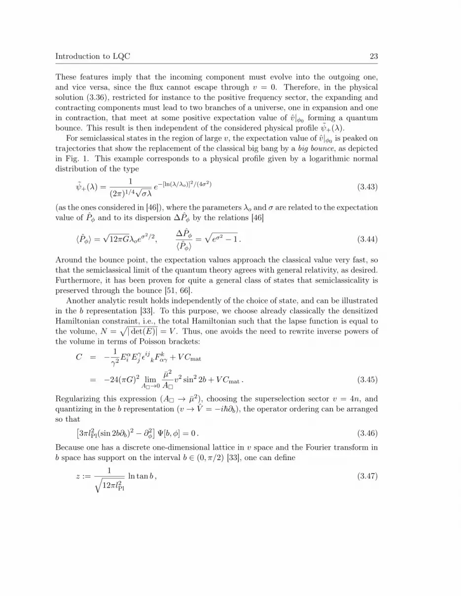
These features imply that the incoming component must evolve into the outgoing one,and vice versa, since the flux cannot escape through v = 0. Therefore, in the physicalsolution (3.36), restricted for instance to the positive frequency sector, the expanding andcontracting components must lead to two branches of a universe, one in expansion and onein contraction, that meet at some positive expectation value of v|φ0 forming a quantumbounce. This result is then independent of the considered physical profile ψ+(λ).

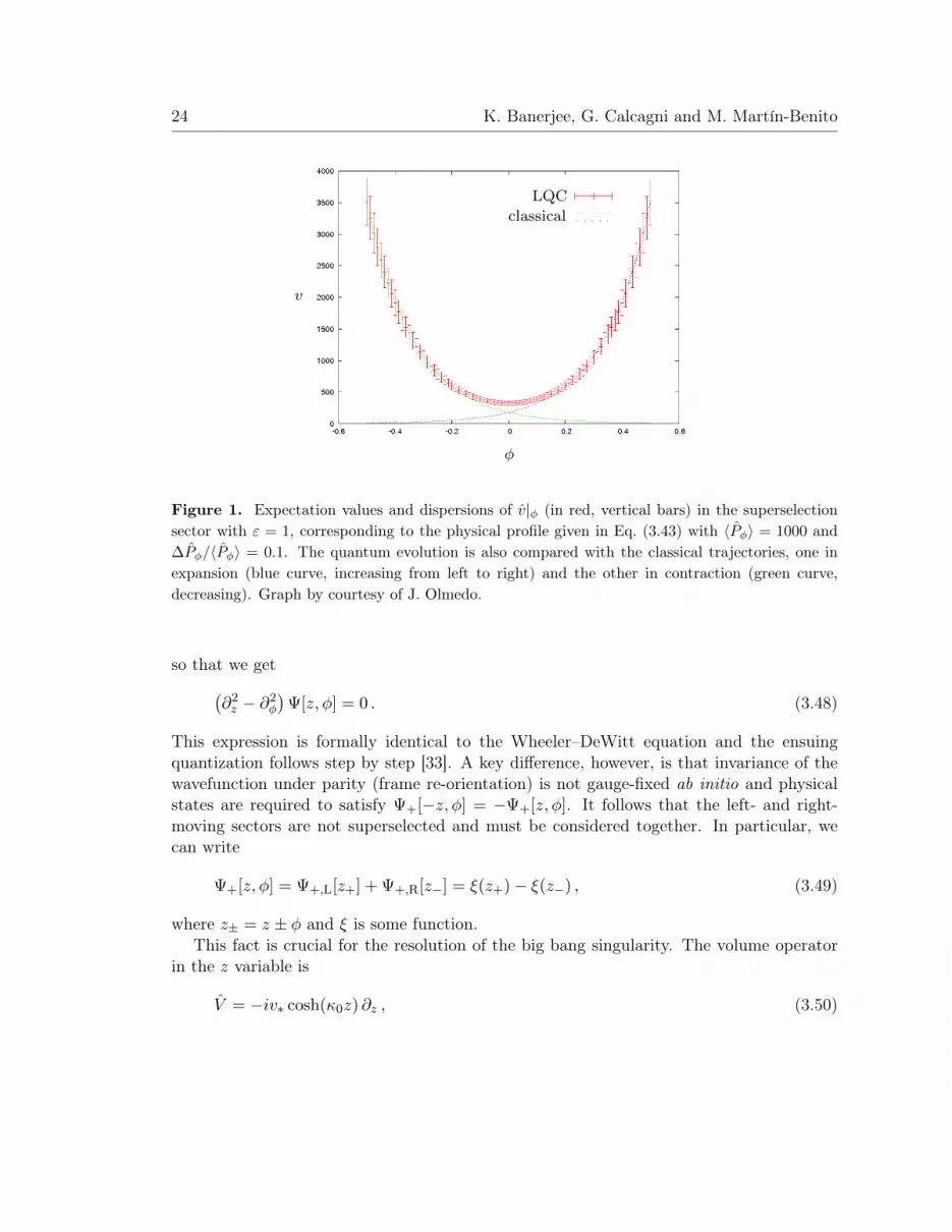
For semiclassical states in the region of large v, the expectation value of v|φ0 is peaked ontrajectories that show the replacement of the classical big bang by a big bounce, as depictedin Fig. 1. This example corresponds to a physical profile given by a logarithmic normaldistribution of the type

ψ+(λ) =1

(2π)1/4√σλ

e−[ln(λ/λo)]2/(4σ2) (3.43)

(as the ones considered in [46]), where the parameters λo and σ are related to the expectationvalue of Pφ and to its dispersion ∆Pφ by the relations [46]

〈Pφ〉 =√

12πGλoeσ2/2,

∆Pφ

〈Pφ〉=√eσ2 − 1 . (3.44)

Around the bounce point, the expectation values approach the classical value very fast, sothat the semiclassical limit of the quantum theory agrees with general relativity, as desired.Furthermore, it has been proven for quite a general class of states that semiclassicality ispreserved through the bounce [51, 66].

Another analytic result holds independently of the choice of state, and can be illustratedin the b representation [33]. To this purpose, we choose already classically the densitizedHamiltonian constraint, i.e., the total Hamiltonian such that the lapse function is equal tothe volume, N =

√| det(E)| = V . Thus, one avoids the need to rewrite inverse powers of

the volume in terms of Poisson brackets:

C = − 1

γ2Eαi E

γj εijkF

kαγ + V Cmat

= −24(πG)2 limA→0

µ2

Av2 sin2 2b+ V Cmat . (3.45)

Regularizing this expression (A → µ2), choosing the superselection sector v = 4n, andquantizing in the b representation (v → V = −i~∂b), the operator ordering can be arrangedso that[

3πl2Pl(sin 2b∂b)2 − ∂2

φ

]Ψ[b, φ] = 0 . (3.46)

Because one has a discrete one-dimensional lattice in v space and the Fourier transform inb space has support on the interval b ∈ (0, π/2) [33], one can define

z :=1√

12πl2Pl

ln tan b , (3.47)


φ

v

LQC

classical

Figure 1. Expectation values and dispersions of v|φ (in red, vertical bars) in the superselectionsector with ε = 1, corresponding to the physical profile given in Eq. (3.43) with 〈Pφ〉 = 1000 and∆Pφ/〈Pφ〉 = 0.1. The quantum evolution is also compared with the classical trajectories, one inexpansion (blue curve, increasing from left to right) and the other in contraction (green curve,decreasing). Graph by courtesy of J. Olmedo.

so that we get(∂2z − ∂2

φ

)Ψ[z, φ] = 0 . (3.48)

This expression is formally identical to the Wheeler–DeWitt equation and the ensuingquantization follows step by step [33]. A key difference, however, is that invariance of thewavefunction under parity (frame re-orientation) is not gauge-fixed ab initio and physicalstates are required to satisfy Ψ+[−z, φ] = −Ψ+[z, φ]. It follows that the left- and right-moving sectors are not superselected and must be considered together. In particular, wecan write

Ψ+[z, φ] = Ψ+,L[z+] + Ψ+,R[z−] = ξ(z+)− ξ(z−) , (3.49)

where z± = z ± φ and ξ is some function.This fact is crucial for the resolution of the big bang singularity. The volume operator

in the z variable is

V = −iv∗ cosh(κ0z) ∂z , (3.50)


where v∗ is a positive constant and κ0 =√

12πl2Pl. At any time φ and on any physicalstate, one can show that the expectation value of the volume is

〈|V |〉 = 〈Ψ+| |V | |Ψ+〉 = V∗ cosh(κ0φ) , (3.51)

where V∗ > 0 is the minimal volume at the bounce. Equation (3.51) completes the proofthat the big bang singularity is avoided in minisuperspace LQC. Further evidence comesfrom noticing that matter energy density has an absolute upper bound (approximatelyequal to 0.41 times the Planck density) on the whole physical Hilbert space [33]. We canreach the same quantitative conclusion, albeit not as robustly, when looking at the effectivedynamics on semiclassical states (section 8).

3.7 FRW models with curvature or cosmological constant

In the previous sections, we ignored the contribution both of the intrinsic curvature Γia =(k/2)δia and of a cosmological constant Λ. Here, we sketch scenarios where the universe isnot flat (k = ±1) and/or Λ 6= 0. For more details, consult [4].

3.7.1 Closed universe

The case of a universe with positive-definite spin connection, k = 1, was studied in [67, 68,69, 70, 71, 72, 73, 74]. Due to the extra term in the connection, the form of the classicalHamiltonian constraint (3.4) as a function of c (related to metric variables as c = γa + k,—a dot denotes derivative with respect to synchronous time) is modified by the replacementc2 → c(c− V 1/3

o ) + (1 + γ2)V2/3o /4. In the classical Friedmann equation, this replacement

corresponds to H2 → H2 + k/a2 with k = 1, where H := a/a is the Hubble parameter.The quantum constraint and the resulting difference equation are modified accordingly.There is no arbitrariness in the fiducial volume Vo, since it can be identified with the totalvolume of the universe, which is finite and well defined. Then, the choice of elementaryholonomy is more natural than in the flat case and, locally, one can distinguish betweenthe group structure of SU(2) and SO(3) [70]. As in the flat case, the constraint operatoris essentially self-adjoint [70] and the singularity at v = 0 is removed from the quantumevolution [67, 70, 71]. However, instead of a single-bounce event one now has a cyclic model[71]. This can be traced back to the fact that the classical and quantum scalar constrainthave both contracting and expanding branches coexisting in closed-universe solutions, whilethese branches correspond to distinct solutions in the flat case.

3.7.2 Open universe

Loop quantum cosmology of an open universe [74, 75, 76] is slightly more delicate to dealwith. In contrast with the flat and closed cases k = 0, 1, the spin connection is non-diagonal, so that also the connection is non-diagonal and it has two (rather than one)


dynamical components c(t) and c2(t). The Gauss constraint fixes c2 = 1 and one endsup with the same number of degrees of freedom as usual. The volume of the universe isinfinite as in the flat case, and a fiducial volume must be defined. The classical Hamiltonianconstraint is Eq. (3.4) with c2 → c2−V 2/3

o γ2. The quantum constraint is constructed afterdefining a suitable holonomy loop; the bounce still takes place and the v = 0 big-bang statefactors out of the dynamics.

3.7.3 Λ 6= 0

Another generalization is to add a cosmological constant term, positive [67, 73, 77] ornegative [48, 72, 76, 78]. At the level of the difference equation, these models have beenstudied in relation to the self-adjoint property.

For Λ > 0, below a critical value Λ∗ (of order of the Planck energy), the Hamiltonianconstraint operator admits many self-adjoint extensions, each with a discrete spectrum.Above Λ∗, the operator is essentially self-adjoint but there are no physically interestingstates in the Hilbert space of the model [77].

For Λ < 0, the scalar constraint is essentially self-adjoint and its spectrum is discrete[48] (while, we recall, for Λ = 0 it is continuous and with support on the positive real line),also when k = −1 [76]. As in the Λ = 0, k = 1 case, the universe undergoes cycles ofbounces [78].


4 Bianchi I model

The next step in extending loop quantum cosmology to more general situations consistsin the consideration of (still homogeneous but) anisotropic cosmologies. The simplestanisotropic spacetime is the Bianchi I model, since it has flat spatial sections. This modelhas been extensively studied, owing to its simplicity and applications in cosmology. In fact,prior to the development of loop quantum cosmology, its quantization employing Ashtekarvariables was already analyzed [79, 80, 81]. The first attempts of constructing a kinemat-ical Hilbert space and the Hamiltonian constraint operator within a polymeric formalismwere done in [47]. Then, soon after the quantization of the flat FRW model was completedwithin the improved dynamics scheme [32], the same programme was applied to Bianchi I,which we shall review now.

4.1 Classical formulation in Ashtekar–Barbero variables

For simplicity, we will consider the model in vacuo. Unlike the FRW universe, which isstatic in vacuo, the vacuum Bianchi I model has non-trivial dynamics. Its solutions areof Kasner type [82], with two expanding scale factors and the third in contraction, or viceversa.

Moreover, for later convenience, we will consider a spatial three-torus topology. There-fore, it will not be necessary to introduce any fiducial cell, since the model already providesa natural finite cell, that of the three-torus, described with angular coordinates θ, σ, δrunning from 0 to 2π.

Like in the isotropic case, we fix the gauge and choose a diagonal flat co-triad oeia = δia.The presence of three different directions requires three variables to describe the Ashtekar–Barbero connection and three more for the densitized triad, that is13

Aia =ci

2πδia, Eai =

pi4π2

δai√oq, i = θ, σ, δ. (4.1)

The Poisson brackets defining the phase space are then ci, pj = 8πGγδij . The spacetimemetric in these variables reads

ds2 = −N2dt2 +|pθpσpδ|

4π2

(dθ2

p2θ

+dσ2

p2σ

+dδ2

p2δ

). (4.2)

In turn, the phase space is constrained by the Hamiltonian constraint

CBI = − 2

γ2

cθpθcσpσ + cθpθc

δpδ + cσpσcδpδ

V= 0. (4.3)

In this expression, V =√|pθpσpδ| is the physical volume of the universe.

13In the following, we will not use the Einstein summation convention, unless specified otherwise.


4.2 Quantum representation

In order to polymerically represent this system, we follow the approach described in section3.2 [83]. Holonomies hµii (ci) = eµic

iτi are defined along straight edges of fiducial length2πµi ∈ R and oriented in the fiducial directions, here labeled by i = θ, σ, δ. The fluxesof the densitized triad through rectangular surfaces of fiducial area Ai and orthogonal tothe i-th direction, given by E(Ai, f = 1) = [pi/(4π

2)]Ai, complete the description of thephase space before quantization. The configuration algebra is the tensor product of thealgebras of quasi-periodic functions of the connection for each fiducial direction: CylS =⊗iCyliS = lin|µθ, µσ, µδ〉, where the kets |µi〉 denote the quantum states correspondingto the matrix elements of the holonomies Nµi(ci) = eiµic

i/2 in momentum representation.Hence, the kinematical Hilbert space is the tensor product Hgrav = ⊗iHigrav, where Higrav isthe Cauchy completion of CyliS with respect to the discrete inner product 〈µi|µ′i〉 = δµiµ′i .

The basic operators are pi and Nµ′i . Their action on the basis states |µi〉 is

pi|µi〉 = pi(µi)|µi〉, pi(µi) = 4πγl2Plµi, (4.4a)

Nµ′i |µi〉 = |µi + µ′i〉, (4.4b)

such that [Nµi , pj ] = i~ Nµi(ci), pj.

4.3 Improved dynamics

The most involved aspect that one encounters when trying to adapt the quantization ofthe isotropic case to the anisotropic case lies in the implementation of the improved dy-namics, explained in section 3.3. In the presence of anisotropies, we need to introducethree minimum fiducial lengths µi, when defining the curvature tensor in terms of a loopof holonomies.

Originally, a naive Ansatz was chosen, given by

1

µ′i=

√|pi|√∆. (4.5)

This is the simplest generalization of the ansatz of the isotropic case, Eq. (3.14). As aconsequence, the operators entering the Hamiltonian constraint have the same form asthose of the flat FRW model. Furthermore, operators corresponding to different directionscommute among one another. This allows to complete the quantization obtaining thephysical Hilbert space [84], in the same way as for the FRW model. However, when thetopology is non-compact and then a finite fiducial cell is introduced, the physical resultsdepend on this fiducial choice [85]. This drawback led to the revision of the definition of


µi, and another Ansatz free of these problems was proposed, this time given by14

1

µi=

1√∆

√∣∣∣∣pjpkpi∣∣∣∣. (4.6)

This choice is geometrically better justified (for a discussion about its derivation see [86]).Furthermore, this prescription is the only one verifying a remarkable property: For all thefiducial directions, the exponents µici of the matrix elements Nµi(ci) have a constant andfixed (up to a sign) Poisson bracket with the variable

v = sgn(pθpσpδ)

√|pθpσpδ|

2πγl2Pl

√∆, (4.7)

which is proportional to the volume. Note that it coincides with the parameter v(p) ofthe isotropic case if we identify the three fiducial directions. As a consequence, as we willsee, the volume will suffer constant shifts in the quantum theory, as in the isotropic case.Thanks to this property, the improved dynamics prescription (4.6) nicely implements theinterplay between the anisotropies and the volume. Instead, within the naive prescriptiongiven by Eq. (4.5), there is no interplay between the degrees of freedom associated withdifferent directions, because of the commutation between the operators acting on differentfiducial directions. Thus, apart from giving dependencies on fiducial choices, it also seemsless physically motivated.

Because of these reasons, today it is generally accepted that the more correct improveddynamics prescription is Eq. (4.6), which we shall consider in this paper.


As in the isotropic case, in order to obtain the Hamiltonian constraint operator we cannotrepresent directly its classical form (4.3), but its expression in terms of the curvature tensor.For homogeneous models with vanishing spin connection, as Bianchi I, this expression wasgiven in Eq. (3.1).

For simplicity, we will densitize the Hamiltonian constraint classically, by simply multi-plying it by the volume V . In this way we avoid the appearance of inverse powers of thevolume that make the quantum theory complicated. In any case, as seen in the flat FRWmodel, the densitization could be carried out with no problem in the quantum theory.

In analogy with the isotropic case, but now taking into consideration that the threefiducial directions are different, the curvature operator is the quantum counterpart of theclassical expression

F iab = −2∑j,k

tr

(hµjk − δjk4π2µjµk

τ i

)δjaδ

kb , hµjk = h

µjj h

µkk (h

µjj )−1(hµkk )−1. (4.8)

14Whenever the three indices i, j, k appear in the same expression, we will consider εijk 6= 0, so that theyare different.


Taking into account Eq. (4.8), the expression of the densitized triad and the definition ofµi, the densitized Hamiltonian constraint for the Bianchi I model reads

CBI =2

γ2∆V 2∑i,j,k

εijk sgn (pj)sgn(pk)tr(τih

µjk

). (4.9)

In order to represent this constraint as an operator, we first need to define the operatorsNµi , which represent the matrix elements of the holonomies hµii . To define them we followa similar strategy to that adopted in the isotropic case. We start by reparametrizing pi(µi)with a parameter λi(pi) such that the vectorial field µi∂µi produces constant translations inλi. The solution is λi(pi) = sgn(pi)

√|pi|/(4πγl2Pl

√∆)1/3 [86]. The difference with respect

to the isotropic case is that the translations produced by µi∂µi , being constant with respectto the dependence on λi, do depend on the parameters λj and λk associated with the othertwo directions. In fact, we have µi∂µi = (2|λjλk|)−1∂λi .

As in the isotropic case, we define the operator Nµi such that its action on the basisstates |λi〉 is the same as the transformation generated by µi∂µi on the parameter λi, thatis

N±µθ |λθ, λσ, λδ〉 =

∣∣∣∣λθ ± 1

2|λσλδ|, λσ, λδ

⟩, (4.10)

and similarly for N±µσ and N±µδ . Moreover, inverting the change of variable, we obtain

pi|λθ, λσ, λδ〉 = (4πγl2Pl√

∆)2/3sgn(λi)λ2i |λθ, λσ, λδ〉. (4.11)

As explained in the flat FRW case, one can always choose a suitable factor ordering for theHamiltonian constraint that allows to remove the kernel of the volume operator, generatedby the states with λθλσλδ = 0. This is what we will consider. Therefore, the operators Nµiare well defined.

The action of N±µi can be slightly simplified by introducing the variable v defined inEq. (4.7), that in terms of λ’s is given by v = 2λθλσλδ. Indeed, making the change from,e.g., the states |λθ, λσ, λδ〉 to the states |v, λσ, λδ〉, one can check that, under the actionof Nµi , v suffers a constant shift equal to 1 or −1 depending on the orientation of thedensitized triad coefficients. On the other hand, the variables λσ and λδ suffer a dilatationor contraction that only depends on their own sign and on v (see [86] for the details).

The variable v is proportional to the volume

V =√|pθpσpδ|, V |v, λσ, λδ〉 = 2πγl2Pl

√∆|v||v, λσ, λδ〉. (4.12)

Therefore, as happened in the isotropic case, in this scheme the volume undergoes constanttranslations. The other two variables measure the degree of anisotropy of the system.

Once we know how to represent the matrix elements of the holonomies, we can promotethe Hamiltonian constraint to an operator. When symmetrizing it, we will adopt the


prescription of [87], whose factor ordering is analog to that considered in section 3 (seeEq. (3.25)). Explicitly, it is given by [87, 88]

CBI = − 1

γ2(ΩθΩσ + ΩσΩθ + ΩθΩδ + ΩδΩθ + ΩσΩδ + ΩδΩσ), (4.13)

where

Ωi =1

4i√

∆

√V[(N2µi − N−2µi

)sgn(pi) + sgn(pi)

(N2µi − N−2µi

)] √V . (4.14)

This operator differs from that of [86] in the treatment applied to the signs of pi when sym-metrizing. Then, CBI not only decouples the zero-volume states, but also it does not relatestates with opposite orientation of any of the triad coefficients, namely, states |v, λσ, λδ〉with opposite sign in any of their quantum numbers. Therefore, CBI leaves invariant allthe octants in the tridimensional space defined by v, λσ and λδ. Hence, we can restrict thestudy to any of them. We will restrict ourselves to the subspace of positive densitized triadcoefficients, given by

Cyl+S = lin|v, λσ, λδ〉; v, λσ, λδ > 0. (4.15)

The action of CBI on the states of Cyl+S turns out to be

CBI|v, λσ, λδ〉 =(πl2Pl)

2

4

[x−(v)|v − 4, λσ, λδ〉− − x−0 (v)|v, λσ, λδ〉−

− x+0 (v)|v, λσ, λδ〉+ + x+(v)|v + 4, λσ, λδ〉+

], (4.16)

where we have introduced the coefficients

x−(v) = 2√v(v − 2)

√v − 4[1 + sgn(v − 4)], x+(v) = x−(v + 4), (4.17a)

x−0 (v) = 2(v − 2)v[1 + sgn(v − 2)], x+0 (v) = x−0 (v + 2), (4.17b)

and the following linear combination of states

|v ± n, λσ, λδ〉± =

∣∣∣∣v ± n, λσ, v ± nv ± 2λδ

⟩+

∣∣∣∣v ± n, v ± nv ± 2λσ, λδ

⟩+

∣∣∣∣v ± n, v ± 2

vλσ, λδ

⟩+

∣∣∣∣v ± n, λσ, v ± 2

vλδ

⟩+

∣∣∣∣v ± n, v ± 2

vλσ,

v ± nv ± 2

λδ

⟩+

∣∣∣∣v ± n, v ± nv ± 2λσ,

v ± 2

vλδ

⟩. (4.18)

Note that, in fact, the operator CBI is well defined in Cyl+S , since x−(v) = 0 if v ≤ 4, andx−0 (v) = 0 if v ≤ 2. Since there is no v = 0 state, the singularity has no longer analog inthe kinematical Hilbert space, and then is resolved already kinematically.


4.5 Superselection sectors

The analysis of the action of CBI on a generic basis state |v, λ?σ, λ?δ〉 shows that:

i) Concerning the variable v, it suffers a constant shift equal to 4 or −4, the latest onlyif v > 4. Therefore, CBI preserves the subspace of states whose quantum number vbelongs to any of the semilattices of step four

L+ε = ε+ 4k, k = 0, 1, 2..., ε ∈ (0, 4]. (4.19)

ii) Concerning the anisotropy variables, λσ and λδ, the effect upon them does not dependon the initial quantum numbers λ?σ and λ?δ , but only on v = ε + 4k. Moreover, thisdependence occurs via fractions whose denominator is two units bigger or smallerthan the numerator. As a consequence, the iterative action of the constraint operatoron |v, λ?σ, λ?δ〉, only relates this state with states whose quantum numbers λσ and λδare of the form λa = ωελ

?a, with ωε belonging to the set

Wε =

(ε− 2

ε

)z ∏m,n∈N

(ε+ 2m

ε+ 2n

)kmn; kmn ∈ N, z ∈ Z if ε > 2, z = 0 if ε < 2

.

(4.20)

The set Wε is infinite and, moreover, one can prove that it is dense in the positive realline [87]. Nonetheless, it is countable. Therefore, while the variable v has support in simplesemilattices of constant step, the variables λa take values belonging to complicated sets,but they also provide separable subspaces. As a concrete example, we see that, if both εand λ?a are integers, then λa take values in the positive rational numbers.

In conclusion, the operator CBI leaves invariant the Hilbert subspaces H+ε,λ?σ ,λ

?δ, defined

as the Cauchy completion of

Cyl+ε,λ?σ ,λ?δ = lin|v, λσ, λδ〉; v ∈ L+ε , λa = ωελ

?a, ωε ∈ Wε, λ

?a ∈ R+, (4.21)

with respect to the discrete inner product 〈v, λσ, λδ|v′, λ′σ, λ′δ〉 = δvv′δλσλ′σδλδλ′δ . As we willsee, physical observables also preserve these separable subspaces H+

ε,λ?σ ,λ?δ, and therefore

they provide sectors of superselection, and we can restrict the study to any of them.

4.6 Physical Hilbert space

The Hamiltonian constraint operator CBI is quite complicated and, unlike the isotropiccase (and unlike previous quantizations of the model [84]), its spectral properties have notbeen determined. Consequently, it has not been diagonalized either. Therefore, the groupaveraging approach is not useful in this situation, and to analyze the physical solutions one


has to impose the constraint directly on the dual space (Cyl+ε,λ?σ ,λ?δ )∗. The elements (ψ| of

that space have the formal expansion

(ψ| =∑v∈L+

ε

∑ωε∈Wε

∑ωε∈Wε

ψ(v, ωελ?σ, ωελ

?δ)⟨v, ωελ

?σ, ωελ

?δ

∣∣. (4.22)

From the action of CBI, one obtain that the constraint(ψ∣∣CB

BI† = 0 leads to the following

recurrence relation,

ψ+(v + 4, λσ, λδ) =1

x+(v)

[x−0 (v)ψ−(v, λσ, λδ) + x+

0 (v)ψ+(v, λσ, λδ)

− x−(v)ψ−(v − 4, λσ, λδ)

]. (4.23)

In this expression, in order to simplify the notation, we have introduced the projections of(ψ| on the linear combinations of six states defined in Eq. (4.18), namely,

ψ±(v ± n, λσ, λδ) = (ψ|v ± n, λσ, λδ〉± . (4.24)

Owing to the property x−(ε) = 0, the above recurrence relation, that is of order 2 in thevariable v, becomes a first-order equation if v = ε:

ψ+(ε+ 4, λσ, λδ) =1

x+(ε)

[x−0 (ε)ψ−(ε, λσ, λδ) + x+

0 (ε)ψ+(ε, λσ, λδ)

]. (4.25)

Therefore, if we know all the data in the initial section v = ε, we obtain all the combinationsof six terms given by

ψ+(ε+ 4, λσ, λδ) = ψ

(ε+ 4, λσ,

ε+ 4

ε+ 2λδ

)+ ψ

(ε+ 4,

ε+ 4

ε+ 2λσ, λδ

)+ ψ

(ε+ 4, λσ,

ε+ 2

ελδ

)+ ψ

(ε+ 4,

ε+ 2

ελσ, λδ

)+ ψ

(ε+ 4,

ε+ 2

ελσ,

ε+ 4

ε+ 2λδ

)+ ψ

(ε+ 4,

ε+ 4

ε+ 2λσ,

ε+ 2

ελδ

).

(4.26)

From the combinations ψ+(ε+4, λσ, λδ), it is possible to determine any of the individualterms ψ(ε + 4, λσ, λδ) that compose them, since it has been shown that the system ofequations that relate the formers with the latters is formally invertible [88]. This has beenproven not only for v = ε+ 4 but also for all v ∈ L+

ε . In conclusion, the physical solutionsof the Hamiltonian constraint are completely determined by the set of initial data

ψ(ε, λσ, λδ) = ψ(ε, ωελ?σ, ωελ

?δ), ωε, ωε ∈ Wε, λ?σ, λ

?δ ∈ R+, (4.27)


and we can identify solutions with this set. We can also characterize the physical Hilbertspace as the Hilbert space of the initial data. In order to endow the set of initial datawith a Hilbert structure, one can take a complete set of observables forming a closedalgebra, and impose that the quantum counterpart of their complex conjugation relationsbecome adjointness relations between operators. This determines a unique (up to unitaryequivalence) inner product.

Before doing that, it is suitable to change the notation. Following [88], let us introducethe variables xa = ln(λa) = ln(λ?a) + ρε. Note that ρε takes values in a dense set of the realline, given by the logarithm of the points in the setWε. We will denote that set by Zε. Foreach direction a = σ or δ, we consider the linear span Cylλ?a of the states whose support isjust one point xa of the superselection sector defined by taking the product of λ?a with allthe points in the set Zε. We call Hλ?a the Hilbert completion of this vector space with thediscrete inner product.

Then, a set of observables acting on the initial data ψ(xσ, xδ) := ψ(ε, xσ, xδ) is thatformed by the operators eixa and Uρaa , with ρa ∈ Zε and a = σ, δ, defined as

eixσ ψ(xσ, xδ) = eixσ ψ(xσ, xδ), (4.28a)

Uρσσ ψ(xσ, xδ) = ψ(xσ + ρσ, xδ), (4.28b)

and similarly for eixδ and Uρδδ . These operators provide an overcomplete set of observablesand are unitary in Hλ?σ ⊗Hλ?δ , according with their reality conditions. Therefore, we con-clude that this Hilbert space is precisely the physical Hilbert space of the vacuum BianchiI model.

Owing to the complicated form of the solutions, together with the fact that a basis ofeigenfunctions of the Hamiltonian constraint operator is not known, the evolution pictureof this model has not been studied yet. It is expected that, as in the isotropic models, aquantum bounce solves dynamically the big bang singularity. Indeed, this has been alreadychecked using an effective dynamics [89], in the case of the model coupled to a masslessscalar field, as in the FRW case. In this respect, it is worth commenting that in analyseswhere a massless scalar field is introduced, the latter serves as internal time to describethe notion of evolution, as seen in section 3.5.2. This field (unlike the geometric degreesof freedom) is quantized adopting a standard Schrödinger-like representation, which makesstraightforward the construction of a family of unitarily related observables parametrizedby the internal time. However, in vacuum cases such as the Bianchi I model we havejust described, where a suitable matter field is not at hand, it would be interesting todescribe the evolution regarding as internal time one of the geometry degrees of freedom.There is a complication because of the fact that such internal time is polymeric, since thegeometry degrees of freedom are polymerically quantized. Although such description hasnot been carried out for the Bianchi I model within the current improved dynamics, it hasbeen nonetheless constructed for the vacuum Bianchi I model quantized within the naive


improved dynamics given in Eq. (4.5). That was done in [90], and an analog constructioncould just as well serve to describe the evolution of the current vacuum Bianchi I model(quantized within the scheme given in Eq. (4.6)), using either the volume variable v or itsmomentum as internal time.

4.7 Loop quantization of other Bianchi models

Bianchi models are characterized by possessing three spatial Killing fields. In the case ofthe Bianchi I model, the Killing fields commute and, then, it is the simplest of the Bianchimodels. This is the reason why it has been extensively studied in the literature, and inparticular in the framework of LQC. Nevertheless, loop quantization has been also extendedto other Bianchi models (with non-commuting Killing fields), in particular to Bianchi IIand Bianchi IX. A preliminary loop quantization of these models was already consideredjust after the birth of LQC [47, 91]. More recently, their quantization has been achievedimplementing the improved dynamics developed for Bianchi I, in [92] for Bianchi II and in[93] for Bianchi IX. In the following we summarize the main characteristics of these works.We refer the reader to those references for further details.

Both the Bianchi II and the Bianchi IX models possess non-commuting Killing fields.As a consequence, the fiducial triad and co-triad cannot be chosen to be diagonal, a firstfeature that complicates the analysis in comparison with Bianchi I. Moreover, the spinconnection of those models is non-trivial. After choosing a suitable gauge and appropriateparameterizations for the Ashtekar–Barbero variables, the Hamiltonian constraint of bothBianchi II and Bianchi IX consists in that of the (analog) Bianchi I model plus an extraterm, of course different for each model, but that in both cases involves components of theconnection and inverses of the densitized triad coefficients.

The kinematical Hilbert space of the Bianchi II and IX models is identical to that ofBianchi I. The main difficulty lies in the representation of the components of the connec-tion that appear in the extra term of the Hamiltonian constraint.15 To tackle this issue,the strategy adopted is to define an operator representing the connection [92], choosing asuitable loop of holonomies and implementing the ideas employed when constructing thecurvature operator for Bianchi I. As a result, the components ci of the connection turn outto be represented by the polymeric operator

ci =sin µiciµi

, (4.29)

where µi is the minimum length defined in Eq. (4.6).Once the above operator is defined, the representation of the Hamiltonian constraint

as a symmetric operator follows straightforwardly, in the same way as for the Bianchi I15The inverse of the components of the densitized triad can be regularized using commutators with

holonomies, in an analog way as that employed in the FRW model.


model. Once again, classical singularities are avoided in both models, since the kernel ofthe volume operator can be removed from their quantum theories.


Part II

Midisuperspace models in loop quantumgravityIn the previous part we have discussed the loop quantization of several homogeneous cosmo-logical models. In all of them the classical cosmological singularity is avoided. Nonetheless,it is natural to ask whether the resolution of the singularity is an intrinsic feature of theloop quantization or, on the contrary, if it is a result due to the high symmetry of the ho-mogeneous models. In order to answer this question, it seems inevitable to extend the loopquantization to inhomogeneous systems. Furthermore, it is essential to make this step inorder to develop a realistic theory of quantum cosmology. Indeed, as the results obtained inmodern cosmology indicate, in the early universe the inhomogeneities played a fundamentalrole in the formation of the cosmic structures that we observe today.

The quantization of inhomogeneous models is technically more complicated than that ofminisuperspaces, since they possess field degrees of freedom, as the full theory. Hopefully,facing the loop quantization of midisuperspaces we will get insights about the open problemspresent in loop quantum gravity.

In this section we will review the status of loop quantization of midisuperspace models.Classically, these models have Killing vectors which reduce the degrees of freedom of themetric but the number of Killing vectors are low enough to ensure that the remainingdegrees of freedom are local. The metrics are therefore parametrized by functions of timeand spatial coordinate(s). Thus, unlike minisuperspace scenarios, midisuperspace modelsare field theories (for a comprehensive review, see [94]). Questions beyond the reach ofminisuperspace models can be addressed in the study of midisuperspaces both classicallyas well as in the context of a particular quantization scheme. In the context of LQG, theseissues may include the construction of Dirac observables or of quasilocal observables, theclosure of the quantum constraint algebra and, most importantly, whether the singularityresolution mechanism of LQC continues to be valid in the field theory context.

There exist a number of midisuperspace models but the loop quantization procedure hasbeen attempted only in a few of them so far. One important class of models is obtained bysymmetry reduction of GR.

• Spherical symmetry.In 3 + 1 dimensions, a spacetime is called spherically symmetric if its isometry groupcontains a subgroup isomorphic to SO(3), and the orbits of this subgroup are 2-spheres such that the induced metric thereon is Riemannian and proportional to theunit round metric on S2. These are, in a sense, midway between the minisuperspacemodels and models with an infinite number of physical degrees of freedom. Sphericallysymmetric spacetime metrics depend on the radial coordinate, and therefore these


models have to be treated as field theories. However, in vacuum, the physical solutionsare characterized by only a single parameter according to Birkhoff’s theorem. In thatrespect they are dynamically trivial, although the gauge-fixing procedure is extremelynon-trivial. To make them into physical field theories, we need to add matter in theform of dust shells.

Here we are mainly interested in cosmological models while the spherical symmet-ric models are mostly black hole solutions, in particular the Schwarzschild solution.Hence, we will briefly mention the progress made in the context of LQG for complete-ness.

In [95] the kinematical framework for studying spherically symmetric models in LQGwas introduced. The volume operator was constructed in [96] and it was shown thatthe volume eigenstates are not eigenstates of the flux operator. Consequently, thestandard prescription of constructing the Hamiltonian operator cannot be used. Thisproblem was circumvented in [97], where the Hamiltonian constraint operator wasconstructed in terms of non-standard variables which mix the connection and the ex-trinsic curvature. This formulation was extended to explore the question of singularityresolution of Schwarzschild black holes in [98] and the Lemaître–Toleman–Bondi col-lapse of a spherical inhomogeneous dust cloud in [99]. The choice of variables made inthe above programme is similar to the polymer quantization of the Gowdy T 3 model,which will be described in detail later. Since the basic quantum variables used in theseconstructions are different from the basic quantum variables of the full theory, an-other approach in loop quantization of the spherically symmetric models was exploredin [100]. In this approach, the diffeomorphism constraint is fixed leaving the Gaussand the Hamiltonian constraints. The latter is then applied to the Schwarzschildsolution. The exterior solutions agree with the ones obtained in geometrodynamics.The interior solution was studied in [101] where it was shown that, after a partialgauge fixing, it can be mapped to the minisuperspace Kantowski–Sachs model. Af-ter loop quantization, the singularity is replaced by a bounce. In [102] the issue ofthe residual diffeomorphism invariance of loop-quantized spherical symmetric modelshas been investigated. Although the quantization programme is still incomplete, thestudies done so far indicate that the singularity resolution mechanism described inthe previous section may be a robust feature of loop quantization.

Another class of midisuperspace models can be roughly classified on the isometry groupof the metric. In most cases, this is equivalent to a classification based on the number ofKilling vectors of the metric.

• Spacetimes with one Killing vector.

These models are obtained by symmetry reduction corresponding to one-dimensionalspatial isometry groups taken to be R or U(1). Some of the important features of


GR are retained, such as diffeomorphism invariance and the field-theoretic non-linearnature of the physical degrees of freedom. It was shown in [103] that, locally, it ispossible to interpret these 3 + 1 dimensional models as 2 + 1 dimensional general rel-ativity coupled to two matter fields, a scalar field and a one-form field corresponding,respectively, to the norm and the twist of the four-dimensional Killing vector field.However, not much work has been done so far in loop quantizing this reduced systemapart from the preliminary analysis carried out in [104] in terms of complex Ashtekarvariables.

• Spacetimes with two Killing vectors.

The next level of simplification is to consider two-dimensional spacelike isometrygroups. Two types of group action and spatial topologies have been studied in LQG:

– Isometry group of R×U(1) with the spatial topology being R3. These correspondto Einstein–Rosen cylindrical waves. An preliminary attempt has been made toconstruct the kinematic Hilbert space and define the volume operator (see section5.11 of [20]), although there has not been much progress so far.

– Isometry group of U(1) × U(1) with the spatial topology being T 3. These cor-respond to Gowdy models.

If we impose the additional condition that the Killing vectors are mutually orthogonal,we obtain polarized models. These are the simplest midisuperspace models with onlyone field theory degree of freedom. An example is the polarized Gowdy T 3 model.This has been studied in some detail in LQG from two different perspectives, both ofwhich will be described in detail in the next two sections.


5 Hybrid quantization of the polarized Gowdy T 3 model

Gowdy models are among the best known inhomogeneous cosmologies [105, 106]. Theyrepresent globally hyperbolic vacuum spacetimes, with compact spatial sections and withtwo spatial Killing fields. The simplest example is the linearly polarized Gowdy T 3 model.Indeed, its classical solutions are exactly known [107, 108, 109]. They represent gravita-tional waves propagating in a closed expanding universe. Its standard quantization wasalready considered since the 70’s [110, 111, 112, 113, 114, 115, 116, 117]. Moreover, a Fockquantization of the model, in which the dynamics is implemented unitarily, was achieved[118, 119], and it has been shown that this quantization is essentially unique [120, 121] (ina sense that we will explain later).

In order to apply the quantization employed in LQC to this model, the simplest possibil-ity is to carry out a hybrid quantization, that combines the polymeric quantization of thedegrees of freedom that parametrize the homogeneous solutions, with the Fock quantizationfor the inhomogeneities. This hybrid quantization was developed in Refs. [87, 122, 123].Here we summarize its construction and main results.

5.1 Classical description of the Gowdy T 3 model

The Gowdy T 3 model represents vacuum solutions to the Einstein equations, with twospatial Killing fields that commute, and with spatial hypersurfaces homeomorphic to athree-torus. As said before, we will consider the linearly polarized model, that possesses anadditional symmetry: the Killing vectors are orthogonal to hypersurfaces and, therefore,are mutually orthogonal everywhere. Letting ∂σ and ∂δ be the Killing vectors, the modeladmits global coordinates t, θ, σ, δ adapted to the symmetries, with θ, σ, δ ∈ S1.

After a 3+1 decomposition, we can describe the spacetime metric in terms of the three-metric qab induced in the spatial sections foliating the four-dimensional manifold, the den-sitized lapse N∼ = N/

√q, and the shift vector Na, with a, b ∈ θ, σ, δ. Owing to the

isometries ∂σ and ∂δ, the Gowdy model verifies qθσ = 0 = qθδ. This condition fixes thegauge freedom associated with the momentum constraint in those directions, and impliesNσ = 0 = N δ [124]. As a consequence, the metric components only depend on t and θand are periodic in the latter. This periodicity allows us to decompose the metric compo-nents in Fourier modes.16 On the other hand, the condition of linear polarization imposesqσδ = 0. Therefore, the three-metric is diagonal and can be described by three fields (τ, ξ, γ),that essentially characterize the area of the isometry group orbits, the norm of one of theKilling vectors, and the scale factor of the metric induced on the set of group orbits. The

16We adopt the following convention to define the Fourier modes φm of a generic field φ(θ):

φ(θ) =∑m∈Z

1√2πφme

imθ, φm =1√2π

∮dθφ(θ)e−imθ. (5.1)


phase space is then parametrized by those fields and by their momenta (Pτ , Pξ, Pγ), andconstrained by the θ-momentum constraint and by the Hamiltonian constraint [119].

In order to prepare the model for its quantization, the gauge is further reduced. Oneimposes that the generator of the conformal transformations, Pγ , and the area of the isom-etry group orbits, τ , are homogeneous functions. These conditions fix the gauge freedomassociated with the non-zero Fourier modes of the θ-momentum constraint and of the den-sitized Hamiltonian constraint, and imply that the functions Nθ and N∼ are homogeneous[119, 122, 123]. Then, two global constraints remain in the model, the spatial average ofthe θ-momentum constraint, generating rigid rotations in the circle, and the spatial averageof the densitized Hamiltonian constraint. We will denote them by Cθ and CG, respectively.

The classically reduced phase space can be split into homogeneous and inhomogeneoussectors. The homogeneous sector coincides with the phase space of the Bianchi I space-time with three-torus topology. This sector will be quantized à la LQC, and therefore isparametrized by the variables (ci, pi), i = θ, σ, δ, with Poisson bracket ci, pj = 8πGγδij ,as described in section 4. The inhomogeneous sector is given by the non-zero (inhomoge-neous) modes of the fields unaffected by the gauge fixing, namely (ξm , Pξm ),m ∈ Z \ 0.This sector will be quantized employing the Fock quantization of [119]. To employ thisFock representation, the above inhomogeneous modes are in turn described by annihilationand creation variables (am, a

∗m), defined as those related to a free massless scalar field. This

quantization is preferred as long as is the only Fock quantization of the deparametrized sys-tem in which the dynamics is unitary and with a vacuum invariant under the S1 translations(the remaining symmetry after gauge fixing) [120, 121].

The three-metric in terms of the chosen variables reads [87]

ds2 = −qθθ(|pθ|4π2

)2

N∼2dt2 + qθθdθ

2 + qσσdσ2 + qδδdδ

2,

qθθ =1

4π2

∣∣∣∣pσpδpθ

∣∣∣∣ exp

2π√|pθ|

cδpδ − cσpσcσpσ + cδpδ

ξ(θ)− π2

|pθ|[ξ(θ)]2 − 8πGγ

cσpσ + cδpδζ(θ)

,

qσσ =1

4π2

∣∣∣∣pθpδpσ

∣∣∣∣ exp

− 2π√|pθ|

ξ(θ)

,

qδδ =1

4π2

∣∣∣∣pθpσpδ∣∣∣∣ exp

2π√|pθ|

ξ(θ)

, (5.2)

where the inhomogeneities are encoded in the terms

ξ(θ) =1

π

∑m6=0

√G

|m|(am + a∗−m)eimθ,

ζ(θ) = i∑m 6=0

∑m6=0

sgn(m+ m)

√|m+ m||m||m|

(a−m − a∗m)(am+m + a∗−(m+m)

)eimθ.


On the other hand, the remaining constraints have the following form:

Cθ =

∞∑m=1

m(a∗mam − a∗−ma−m) = 0, (5.3)

CG = CBI + Cξ = 0, Cξ = G

[(cσpσ + cδpδ)

2

γ2|pθ|Hξ

int + 32π2|pθ|Hξ0

]. (5.4)

In the above expression,

Hξint =

∑m 6=0

1

2|m|[2a∗mam + ama−m + a∗ma

∗−m], Hξ

0 =∑m 6=0

|m|a∗mam, (5.5)

and CBI is the (densitized) Hamiltonian constraint of the Bianchi I model given in Eq.(4.9). In the Hamiltonian constraint, the inhomogeneities appear in the term Hξ

0 , thatcorresponds to the Hamiltonian of a free massless scalar field, and in the term Hξ

int, thatrepresents an interaction term. The inhomogeneities are coupled to the homogeneous sectorin a non-trivial way, so that the feasibility of the hybrid quantization is not straightforwarda priori.

5.2 Fock quantization of the inhomogeneous sector

Once the inhomogeneous sector is described with the appropriate annihilation and creationlike variables, am and a∗m, it is straightforward to get its Fock quantization. With that aim,we promote the variables am and a∗m to annihilation and creation operators, am and a†mrespectively, such that [am, a

†m] = δmm. From the vacuum state |0〉, characterized by the

equations

am|0〉 = 0, ∀m ∈ Z, (5.6)

we construct the one-particle Hilbert space, and the associated symmetric Fock space F[125]. The annihilation and creation operators are densely defined in the subspace of Fgiven by finite linear combinations of n-particle states

|n〉 := |..., n−2, n−1, n1, n2, ...〉, (5.7)

such that∑

m nm < ∞, being nm ∈ N the occupation number (or number of particles) ofthe m-th mode. We will denote that space by S. Note that the n-particle states provide abasis for the Fock space, orthonormal with respect to the inner product 〈n′|n〉 = δn′n. Theaction of am and a†m on these states is

am| . . . , nm, . . . 〉 =√nm| . . . , nm − 1, . . . 〉 , (5.8a)

a†m| . . . , nm, . . . 〉 =√nm + 1| . . . , nm + 1, . . . 〉 . (5.8b)


5.2.1 Generator of translations in the circle

The constraint that generates translations in the circle, Cθ, does not affect the homogeneoussector, and then it is represented on the above Fock space. Taking normal ordering, thecorresponding operator is

Cθ = ~∞∑m>0

m(a†mam − a†−ma−m). (5.9)

This operator is self-adjoint in the Fock space F .The n-particle states annihilated by Cθ are those that satisfy the condition

∞∑m>0

mXm = 0, Xm = nm − n−m. (5.10)

They provide a basis for a proper subspace of the Fock space, that we will denote by Ff .


Physical states must be annihilated as well by the quantum counterpart of the Hamiltonianconstraint CG, given in Eq. (5.4), which involves both homogeneous and inhomogeneoussectors.

In the previous section, we have already described the representation of the inhomo-geneous sector, with basic operators am and a†m acting on the Fock space F , which thusconstitutes the inhomogeneous sector of the kinematical Hilbert space. On the other hand,the homogeneous sector is quantized following LQC, namely, it is given by the loop quan-tization of the Bianchi I model. As we discussed in section 4, in the literature two differentimplementations of the improved dynamics has been applied to the Bianchi I model. There-fore, there exist also two different descriptions for the hybrid Gowdy model, one adoptingthe naive Ansatz (4.5) [87, 122, 123], and another adopting the improved Ansatz (4.6)[87, 88]. Here we will just explain the second description, which adopts the quantizationof the Bianchi I model described in section 4 when representing the homogeneous sector.This sector of the kinematical Hilbert space will be the kinematical Hilbert space H+

ε,λ?σ ,λ?δ,

defined in subsection 4.5.The first term of the Hamiltonian constraint operator, CG = CBI+Cξ, is thus the Bianchi

I operator (4.13). We just need to construct the operator Cξ that couples homogeneousand inhomogeneous sector.

Let us first focus on the inhomogeneous terms. In order to represent the free HamiltonianHξ

0 and the interaction term Hξint, defined in Eq. (5.5), we choose normal ordering. Then,


their quantum analogs are given by

Hξ0 =

∞∑m>0

mNm, Nm = a†mam + a†−ma−m, (5.11)

Hξint =

∞∑m>0

Nm + Ymm

, Ym = ama−m + a†ma†−m, (5.12)

both densely defined in the space S of n-particle states. The operator Hξ0 acts diagonally on

the n-particle states, and then it is well-defined in the Fock space F . On the contrary, Hξint

does not leave invariant the domain S. Indeed, the operator Ym annihilates and createspairs of particles in modes with the same wavenumber |m|, and then Hξ

int creates an infinitenumber of particles. However, one can prove [87] that the norm of Hξ

int|n〉 is finite for alln ∈ S, and therefore this operator, with domain S, is also well defined in the Fock space F .

For the homogeneous terms, we recall that the operator Ωi, defined in Eq. (4.14), is theloop quantum analogue of the classical term cipi, and that the inverse powers of |pi| can beregularized taking commutators of pi with holonomies. In view of these prescriptions, Cξcan be represented by the symmetric operator [87, 88]

Cξ = l2Pl

[ 1

|pθ|14

]2(Ωσ + Ωδ)

2

γ2

[ 1

|pθ|14

]2

Hξint + 32π2 |pθ|Hξ

0

, (5.13)

where

[1

|pθ|14

]|v, λσ, λδ〉 =

b?θ(v, λσ, λδ)

(4πγl2Pl

√∆)

16

|v, λσ, λδ〉, (5.14)

b?θ(v, λσ, λδ) =√

2|λσλδ|∣∣∣√|v + 1| −

√|v − 1|

∣∣∣ . (5.15)

The operator Cξ, so constructed, leaves the sectors of superselection of the Bianchi Imodel invariant, and then it is in fact well defined on the separable kinematical Hilbertspace H+

ε,λ?σ ,λ?δ⊗F .

5.4 Physical Hilbert space

In order to impose the Hamiltonian constraint(ψ∣∣CB

G† = 0, we expand a general state (ψ|

in the basis of states |v, ωελ?σ, ωελ?δ〉 of the homogeneous sector. That is,

(ψ| =∑v∈Lε

∑ωε∈Wε

∑ωε∈Wε

〈v, ωελ?σ, ωελ?δ | ⊗ (ψ(v, ωελ?σ, ωελ

?δ)| , (5.16)


where, let us recall, Wε is the set (4.20). In the above expression,

(ψ(v, λσ, λδ)| = (ψ(v, ωελ?σ, ωελ

?δ)|

is the projection of (ψ| on the state |v, λσ, λδ〉 = |v, ωελ?σ, ωελ?δ〉 of the homogeneous sectorand, in principle, it must belong to the dual space of some appropriate dense domain of theFock space F .

If we substitute the above expansion in the constraint, and take into account the action ofthe operators affecting the homogeneous sector, we obtain that the projections (ψ(v, λσ, λδ)|satisfy difference equations in v that, generically, relate data on the section v+ 4 with dataon the sections v and v − 4, as it happened in the Bianchi I model. Following Ref. [87],to simplify the notation of the resulting equation, we introduce the projections of (ψ| onthe linear combinations given in Eq. (4.18). Namely, we define (ψ±(v ± n, λσ, λδ)| =(ψ|v ± n, λσ, λδ〉±. Similarly, it is convenient to introduce the combinations of states

|v ± n, λσ, λδ〉′± =

∣∣∣∣v ± n, λσ, v ± nv λδ

⟩+

∣∣∣∣v ± n, v ± nv ± 2λσ,

v ± 2

vλδ

⟩+

∣∣∣∣v ± n, v ± nv λσ, λδ

⟩+

∣∣∣∣v ± n, v ± 2

vλσ,

v ± nv ± 2

λδ

⟩, (5.17)

and to define the projections of (ψ| on them: (ψ′±(v±n, λσ, λδ)| = (ψ|v±n, λσ, λδ〉′±. Withthis notation, the solutions of the Hamiltonian constraint satisfy the explicit relation

(ψ+(v + 4, λσ, λδ)| − η[b?θ(v, λσ, λδ)b?θ(v + 4, λσ, λδ)]

2 v + 4

v(ψ′+(v + 4, λσ, λδ)|Hξ

int

= −1

η

32v2

λ2σλ

2δx+(v)

(ψ(v, λσ, λδ)|Hξ0 +

x−0 (v)

x+(v)(ψ−(v, λσ, λδ)|+

x+0 (v)

x+(v)(ψ+(v, λσ, λδ)|

− x−(v)

x+(v)(ψ−(v − 4, λσ, λδ)|+ η[b?θ(v, λσ, λδ)]

4

[b?θ(v − 4, λσ, λδ)

b?θ(v, λσ, λδ)

]2 v − 4

v

x−(v)

x+(v)

× (ψ′−(v − 4, λσ, λδ)| −[x−0 (v)

x+(v)(ψ′−(v, λσ, λδ)|+

x+0 (v)

x+(v)(ψ′+(v, λσ, λδ)|

]Hξ

int,

(5.18)

where η =(

lPl4πγ√

∆

)2/3is a dimensionless parameter, b?θ(v, λσ, λδ) is the function (5.15),

and the coefficients x±(v) and x±0 (v) were defined in Eq. (4.17).Similarly to the analysis done in the Bianchi I model, it has been investigated whether

the solution is totally determined (at least formally) by the data in the initial section v = ε.The presence of the interaction term in the left-hand side of Eq. (5.18) complicates a directdemonstration of the above statement. However, it is possible to obtain such result in termsof an asymptotic analysis of the solutions. Note that the model provides a dimensionlessparameter η that can be used to develop an asymptotic procedure, without the need to


introduce any external parameter by hand. This analysis was carried out in [87], and werefer to it for the details. The main result of this analysis is that, in fact, the initialdata (ψ(ε, λσ, λδ)| (where λσ and λδ run over all possible values in their correspondingsuperselection sectors) completely determine the solution. The solutions turn out to beformal, in the sense that the states (ψ(v + 4, λσ, λδ)| do not belong in general to the dualspace of S, owing to the presence of Hξ

int in their expression.The physical Hilbert space can be characterized, even though the solutions are formal.

Indeed, once we justify that the set of initial data (ψ(ε, ωελ?σ, ωελ

?δ)| ; ωε, ωε ∈ Wε spec-

ifies the solution, we can identify solutions with their corresponding initial data, and thephysical Hilbert space with the Hilbert space of such initial data, exactly as we proceededwith the Bianchi I model.

Once again, the reality conditions over a complete set of observables, acting on the initialdata, univocally determines the inner product that provides the Hilbert structure. Suchobservables are given, for instance, by the overcomplete set of observables of the BianchiI model, given in Eq. (4.28), together with a suitable complete set of observables for theinhomogeneous sector, given by [87]

(am + a†m)± (a−m + a†−m), i[(am − a†m)± (a−m − a†−m)]; m ∈ N+. (5.19)

These operators represent the real Fourier coefficients of the non-zero modes of the fieldξ(θ) and of its momentum Pξ(θ), and in fact they are self-adjoint in the Fock space F .

Finally, imposing the remaining symmetry of translations on S1, the result is that thephysical Hilbert space of the Gowdy model is [87]

Hphys = Hλ?σ ,λ?δ ⊗Ff . (5.20)

Namely, it is the tensor product of the physical Hilbert space of the Bianchi I model timesthe physical Fock space for the inhomogeneities (defined in section 5.2). We note that Ffis unitarily equivalent to the physical space of the Fock quantization of the deparametrizedsystem [118, 119]. Therefore, the standard quantum field theory for the inhomogeneities isrecovered, and they can be seen as propagating over a polymerically quantized Bianchi Ibackground. This result supports the validity of the hybrid quantization, since this shouldlead to the standard quantization of the system in the limit in which the effects coming fromthe discreteness of the geometry are negligible. This result is not trivial, since the hybridquantization is introduced in the kinematical setting, and the relation between kinematicaland physical structures cannot be anticipated before the quantization is completed.

5.4.1 Singularity resolution

The classical solutions of the linearly polarized Gowdy T 3 model generically display acosmological singularity [108]. In the parametrization employed for the hybrid quantizationof the model, this classical singularity corresponds to vanishing values of the coefficients pi.


In the quantum theory, the kernel of the operators pi is removed and, as a consequence,there is no analog of the classical singularity. This resolution of the singularity is kinematicaland, therefore, independent of the dynamics. It persists in the Hilbert space of the physicalstates since they do not have projection on the kernel of the operators pi. Moreover, theyonly have support in a sector with positive orientation of the coefficients pi and, then,they do not cross the singularity towards other branches of the universe corresponding todifferent orientations.

A description of the evolution picture of the model is missing, owing to its high com-plication. It is worthy to note that, at least for the choice of the original naive improveddynamics, the effective dynamics of the model has been thoroughly analyzed [126]. In par-ticular, it has been studied how the inhomogeneities affect the dynamics of the Bianchi Ibackground. Numerical simulations show that the effect of the inhomogeneities does notdestroy the bounce. For the improved dynamics discussed here, a similar analysis has notbeen done yet, but we can expect similar results, since the bounce mechanism appears forboth improved schemes.

5.5 The Gowdy T 3 model coupled to a massless scalar field

So far we have discussed the hybrid quantization of the linearly polarized Gowdy modelin vacuo. This model allows, almost straightforwardly, for the introduction of a minimallycoupled free massless scalar field with the same symmetries as the metric [127]. Indeed,after a suitable rescaling of matter modes, these contribute to the constraints Cθ and CGexactly in the same manner as the gravitational field ξ. Also, the Fock quantization ofthat system (after a complete deparametrization) enjoys the same uniqueness results asthat of the model in vacuo and, hence, there is a preferred Fock description also for theinhomogeneities of the matter field. Therefore, the hybrid approach follows exactly in thesame way as for the vacuum case.

The interest in considering the model filled with matter lies in the fact that FRW-typesolutions are then allowed. Indeed, as we saw before, the vacuum Gowdy model can beseen as a vacuum Bianchi I background filled with inhomogeneities propagating in onedirection, and the subclass of isotropic solutions of the vacuum Bianchi I model representtrivial Minkowski spacetimes rather than flat FRW universes. Nonetheless, in the presenceof matter, the flat-FRW becomes the isotropic sector of the Bianchi I model. In that sense,there is a subclass of solutions of the Gowdy model coupled to matter that can be regarded asa flat FRW background filled with inhomogeneities propagating in one direction. Therefore,the linearly polarized Gowdy T 3 model coupled to a massless scalar field provides a simplelaboratory where to study, at the quantum level (by means of the hybrid quantization),interesting physical phenomena such as the backreaction of the (quantum) inhomogeneitieson (polymerically quantized) flat FRW cosmologies or, vice versa, the effect of the quantumbackground geometry on the propagation of the inhomogeneities [128]. This analysis isintended to be a first step towards a quantum theory of FRW plus inhomogeneities. Its


character is quite preliminary, since the inhomogeneities of Gowdy are just a subclassof the inhomogeneities that one would introduce in the FRW model to account for theinhomogeneities that we observe in our universe. Nonetheless, a complete quantization ofsuch a system has not been yet achieved, and the hybrid Gowdy model offers a suitablesetting to start with. Actually, by employing the same hybrid procedure, the flat FRWmodel plus perturbations is being analyzed [129]. The hybrid quantization also applies inthis more realistic system as long as a unique Fock quantization for the inhomogeneities isat hand as well [130, 131, 132].


6 Polymer quantization of the polarized Gowdy T 3 model

In the previous section, we saw a successful quantization scheme of the linearly polarizedGowdy T 3 model where the degrees of freedom were split into homogeneous and inhomoge-neous sectors. The homogeneous sector was quantized using the LQC techniques, while theinhomogeneous part was Fock quantized. One of the significant advantages of the hybridquantization is that the calculations are tractable and the tools developed and studied inLQC can be used to address questions even in the midisuperspace context. While it is anextremely useful first step in quantization of midisuperspace models, it crucially dependson the fact that the inhomogeneous degrees of freedom can be treated perturbatively, and itis assumed that there exits a regime in which the most important effects emerging from thediscretization of the geometry are those that affect the homogeneous subsystem. Ideally,we would like to loop quantize the full polarized Gowdy T 3 model without separating thedegrees of freedom. In this section we review the work that has been done so far in thatdirection, which has been carried out in [133, 134].

6.1 Classical theory

The variables chosen in this section are significantly different from the ones used in therest of the review so far. We shall therefore indicate the steps followed in obtaining thesevariables.

6.1.1 Gowdy T 3 model in Ashtekar variables

In order to loop quantize, we first need to rewrite the Gowdy T 3 model in terms of realAshtekar variables. Canonical quantization of the unpolarized Gowdy T 3 model in termsof the complex Ashtekar variables has been given in [135, 136] which we will briefly sketchbelow in terms of the real Ashtekar variables.

Recall that, owing to global hyperbolicity, spacetime can be decomposed asM = Σt⊗R,where Σt is homeomorphic to a three-tours. As in the previous section, let the angularcoordinates of Σt be (θ, σ, δ), and the two commuting Killing vectors be ξa1 = ∂σ andξa2 = ∂δ. These isometries imply that the Lie derivatives along these two Killing vectorsvanish i.e.

Lξ1Aia = 0 = Lξ1EaiLξ2Aia = 0 = Lξ2Eai .

The phase-space variables are therefore only functions of θ. The Gauss and the diffeomor-phism constraint reduce to

Gi = ∂θEθi + εkijA

jaE

ak , (6.1)

Va = (∂aAib)E

bi − (∂θA

ia)E

θi + εijkA

jaA

kbE

bi . (6.2)


The vector constraint given by Ca = AiaGi − Va generates spatial diffeomorphisms.We now impose the following gauge-fixing conditions:

EθI = 0 = Eρ3 , ρ = σ, δ , I = 1, 2 . (6.3)

The constraints GI and Cρ are then solved by AIθ = 0 = A3ρ.

Thus, only one component of the Gauss constraint (G3) and one of the diffeomorphismconstraint along the θ direction (Cθ =: C) survive together with the Hamiltonian constraint.Since none of the quantities depend on σ or δ, we can integrate over the torus T 2 and writethe symplectic structure as17

Ω =4π2

κγ

∫dθ(dA3

θ ∧ dEθ3 + dAIρ ∧ dEρI

)(6.4)

This is the classical phase phase in terms of real Ashtekar variables. One important ob-servation is that this is basically a one-dimensional theory. This is useful because in onedimension, under orientation-preserving coordinate transformations, a tensor density ofcontravariant rank p, covariant rank q and weight w, can be thought of as a scalar densityof weight = w + q − p. Hence, under a θ coordinate transformation, Eθ3 transforms as ascalar, EρI ’s transform as scalar densities of weight 1, A3

θ transforms as a scalar density ofweight 1, and AIρ’s transform as scalars.

6.1.2 Choice of new variables

It turns out that these variables are not suitable for loop quantization and we need to makecanonical transformations similar to those performed for the spherical symmetric case in[95]. Note that, for each ρ, the AIρ and EρI rotate among themselves under the U(1) gaugetransformations generated by the Gauss constraint. These suggest that we can performcanonical transformations to define the following variables:

Eσ1 = Eσ cosβ , Eσ2 = Eσ sinβ , (6.5)Eδ1 = −Eδ sin β , Eδ2 = Eδ cos β , (6.6)A1σ = Aσ cos(α+ β) , A2

σ = Aσ sin(α+ β) , (6.7)A1δ = −Aδ sin(α+ β) , A2

δ = Aδ cos(α+ β) . (6.8)

The angles for the connection components are introduced in a particular fashion for laterconvenience.

The radial coordinates, Eσ, Eδ, Aσ, Aδ, are gauge invariant and always strictly positive(vanishing radial coordinates correspond to a trivial symmetry orbit which is ignored).

17In this section, sum over repeated indices is understood.


In terms of these variables, the symplectic structure (6.4) gets expressed as

Ω =4π2

κγ

∫dθ[dA3

θ ∧ dEθ3 + dX ∧ dEσ + dY ∧ dEδ + dβ ∧ dP β + dβ ∧ dP β],

(6.9)

where:

X := Aσ cos(α) , Y := Aδ cos(α) , (6.10)P β := −EσAσ sin(α) , P β := −EδAδ sin(α) . (6.11)

It is convenient to make a further canonical transformation:

ξ = β − β , η = β + β , (6.12)

P ξ =P β − P β

2, P η =

P β + P β

2. (6.13)

The constraints are greatly simplified and their detailed expressions can be found in [133].This completes the description of the unpolarized Gowdy T 3 model in the variables we havedefined. The number of canonical field variables is 10 while there is a threefold infinity offirst-class constraints. There are therefore 2 field degrees of freedom. We now need toimpose two second-class constraints such that the number of field degrees of freedom arereduced from two to one (as it should be in the polarized case).

6.1.3 Reduction to polarized model

In terms of the variables defined above, the spatial three-metric is given by

ds2 = cos ξEσEδ

Eθ3dθ2 +

Eθ3cos ξ

Eδ

Eσdσ2 +

Eθ3cos ξ

Eσ

Eδdδ2 − 2

Eθ3cos ξ

sin ξ dσdδ . (6.14)

For the Killing vectors ∂σ and ∂δ to be orthogonal to each other, the dσdδ term inthe metric should be zero. This implies that the polarization condition is implemented byrestricting to the ξ = 0 sub-manifold of the phase space of the unpolarized model.18 Inorder to get a non-degenerate symplectic structure, we need one more condition. We expectthe two conditions to reduce a field degree of freedom. This turns out to be

χ(θ) := 2P ξ + Eθ3∂θ lnEδ

Eσ≈ 0 . (6.15)

Thus, the reduction to the polarized model is obtained by imposing the two polarizationconstraints

ξ ≈ 0 , χ ≈ 0 , ξ(θ), χ(θ′) = 2κγδ(θ − θ′) . (6.16)18Actually there are two possible choices, ξ = 0 and ξ = π. We shall take the constraint to be ξ = 0,

which implies Eθ3 > 0.


We can solve the polarization constraints strongly and use Dirac brackets. Since the polar-ization constraints weakly commute with all the other constraints, the constraint algebrain terms of Dirac brackets is same as that in terms of the Poisson brackets and remainsunaffected. Furthermore, equations of motions for all the variables other than ξ, Pξ alsoremain unaffected. We can thus set the polarization constraints strongly equal to zero inall the expressions and continue to use the original Poisson brackets. It also turns outthat the basic variables X,Y , unlike in the full theory, are actually the extrinsic curvaturecomponents in the σ and δ direction, respectively.

The above construction can be carried out equivalently using SU(2) variables by usingη-dependent τ matrices:

τσ(θ) := cos η(θ) τ1 + sin η(θ) τ2 , (6.17)τδ(θ) := − sin η(θ) τ1 + cos η(θ) τ2 , (6.18)τ3(θ) := τ3 . (6.19)

The SU(2) formulation is useful in the quantum theory especially while constructing theHamiltonian constraint operator.

Let us review the classical phase space we have constructed. For convenience of notationwe rename Eθ3 := E and A3

θ := A. The basic configuration variables are X,Y,A, η andthe momentum variables are Eσ, Eδ, E , P η, with Poisson brackets of the form X,Eσ =(2G/π)γδ(θ − θ′).19 The spatial metric is given by

ds2 =EσEδ

Edθ2 + E E

δ

Eσdσ2 + EE

σ

Eδdδ2 . (6.20)

The expressions of the constraints are greatly simplified:

G3 =1

κ′γ[∂θE + P η] , (6.21)

Cθ =1

κ′γ

[Eσ∂θX + Eδ∂θY −A∂θE + P η∂θη

], (6.22)

H = − 1

κ′1√E

[1

γ2

(XEσY Eδ +AE(XEσ + Y Eδ) + E∂θη(XEσ + Y Eδ)

)−EσΓσE

δΓδ

]+

1

2κ′∂θ

2E (∂θE)√

E

− κ′

4

G2

√E− γ

2∂θ

(G√E

), (6.23)

where E = |E|EσEδ.

It is obvious from these definitions that X,Y, E , η are scalars while Eσ, Eδ,A, P η arescalar densities of weight 1. The Gauss constraint shows that A transforms as a U(1)connection, while η is translated by the gauge parameter. All other variables are gaugeinvariant.

19Only in this section we will absorb the 4π2 and use κ′ := 2G/π.


This completes the process of symmetry reduction from the unpolarized to the polarizedcase. This is a consistent symmetry reduction as can be checked by verifying the constraintalgebra. It is also possible to show that the solutions of the equations of motion are equiv-alent to the standard Gowdy solutions. In this construction, the goal has been to expressthe polarized Gowdy T 3 in terms of variables which are suitable for loop quantization. Inparticular, they allow a simpler choice of edge and point holonomies, a simpler form forthe volume operator, and also a more tractable expression for the Hamiltonian constraint.Although it may not be possible to make the same choice of variables for other midisuper-space models, similar variables have been used in the preliminary steps of loop quantizationof another midisuperspace model which we describe in brief below.

Plane gravitational waves

The difference between the polarized Gowdy T 3 model and the plane polarized (pp)gravitational waves is in the global topology. While the Gowdy model has a compacttopology, pp waves have the global topology of Minkowski space. The coordinates are nolonger angular but due to the homogeneity it is possible to choose an arbitrary finite areafrom the plane wavefronts and consider only finite wave packets. The classical phase spacein Ashtekar variables is constructed in [137] in a similar way as done for the polarizedGowdy T 3 model described above.

Waves travelling only in one direction are considered to avoid the problem of wavecollision. Finite pulses of pp waves travelling in the positive or in the negative z directionare characterized by a null Killing vector kµ satisfying ∇(µkν) = 0. This gives rise to twonew constraints:

U+ = EσKσ + EδKδ − ∂zE , (6.24)

U− = EσKσ − EδKδ − E lnEδ

Eσ. (6.25)

It can be also shown that the constraint U− is identically zero on the constraint surfaceand has weakly vanishing Poisson brackets with all the other constraints i.e. it is gaugeinvariant and conserved under spatial diffeomorphisms and time evolutions. The constraintU+ Poisson commutes with the Gauss, diffeomorphism and Hamiltonian constraints. Thisconstraint can be added as a new first-class constraint and the standard constraint algebracan be enlarged. This is an additional ingredient in the analysis of pp waves and the systemcan now be loop quantized.

6.2 Quantum theory

In this section, we review the loop quantization of the Gowdy model [134]. The methodsand steps used here closely follow those used in LQG and are to be viewed as first stepstowards constructing a quantum theory of the Gowdy model where all the gravitationaldegrees of freedom are loop quantized.


6.2.1 Basic states

Since this is a one-dimensional theory, the graphs are just n arcs with n vertices. Theconfiguration variable A is a U(1) connection 1-form, so we integrate it along an edge (anarc along S1) and by taking its exponential we define the (edge) holonomy variable valuedin U(1):

h(k)e (A) := exp

(ik

2

∫eA), k ∈ Z . (6.26)

The configuration variables X,Y ∈ R and η ∈ R/Z are scalars and hence no smearing isneeded. For these we define the point holonomies (at points v)

h(µ)v (X) := exp

[iµ

2X(v)

], (6.27)

h(ν)v (Y ) := exp

[iν

2Y (v)

], (6.28)

hλv (η) := exp [iλη(v)] , (6.29)

where µ, ν ∈ R and λ ∈ Z. The X,Y point holonomies are interpreted as unitary repre-sentations of the compact Abelian group RBohr, which is the Bohr compactification of theadditive group of real numbers R.

The kinematical Hilbert space is thus a tensor product of the Hilbert spaces constructedfor A, X, Y, η variables. For A, the Hilbert space can be constructed using U(1) holonomiesin a procedure similar to full LQG. For X, Y and η, we can use the point holonomies asin minisuperspace LQC, where the quantum configuration space is taken to be the Bohrcompactification RBohr. By contrast, η is an angle variable, so the corresponding pointholonomy is valued in U(1).

An orthonormal basis on the tensor-product Hilbert space is provided by the “chargenetwork functions”. They are labelled by a close, oriented graph Γ with n edges e and nvertices v, a U(1) representation ke for each edge, a U(1) representation λv ∈ Z for eachvertex, and RBohr representations µv, νv for each vertex:

TΓ,~k,~µ,~ν,~λ

(A, X, Y, η) :=∏e∈Γ

ke[h(e)]

∏v∈V (Γ)

µv[hv(X)]νv[hv(Y )]λv[hv(η)]

=∏e∈Γ

exp

(ike2

∫eA) ∏v∈V (Γ)

×[

exp(iµv2X)

exp(iνv2Y)

exp (iλvη)], (6.30)

where V (Γ) represents the set of vertices belonging to the graph Γ. Functions where any ofthe labels are different are orthogonal —in particular, two graphs must coincide for non-zero


inner product. These basis states provide an orthogonal decomposition for the kinematicalHilbert space when all the representation labels are non-zero.

Note that, unlike in the full theory, in this model we have both point and edge holonomies.This construction is also significantly different from the hybrid quantization of the previoussection. There, the loop Hilbert space has only the homogeneous part represented by pointholonomies similar to LQC, while the inhomogeneous part is Fock quantized. In that case,the full Hilbert space is a tensor product of the two.

6.2.2 Flux operators

The conjugate variables are represented as

Eσ(θ) ∼ −iγl2Pl

δhθ(X)

δX(θ)

∂

∂hθ(X), (6.31)

where l2Pl := κ′~.The flux variables corresponding to Eσ, Eδ, P η are defined by integrating these densities

on an interval I of the circle, eg Fσ,I :=∫I E

σ,Fδ,I :=∫I E

δ. E , being a scalar, is alreadya suitable variable. Their actions on the basis functions (6.30) are

E(θ)TΓ,~k,~µ,~ν,~λ

=γl2Pl

2

ke+(θ) + ke−(θ)

2T

Γ,~k,~µ,~ν,~λ, (6.32)∫

IEσT

Γ,~k,~µ,~ν,~λ=

γl2Pl

2

∑v∈V (Γ)∩I

µvTΓ,~k,~µ,~ν,~λ, (6.33)

∫IEδT

Γ,~k,~µ,~ν,~λ=

γl2Pl

2

∑v∈V (Γ)∩I

νvTΓ,~k,~µ,~ν,~λ, (6.34)

∫IP ηT

Γ,~k,~µ,~ν,~λ= γl2Pl

∑v∈V (Γ)∩I

λvTΓ,~k,~µ,~ν,~λ, (6.35)

where I is an interval on S1. The symbols e±(θ) either refer to the two oriented edges ofthe graph Γ, meeting at θ if there is a vertex at θ, or they denote two parts of the sameedge if there is no vertex at θ. In such a case, the k labels are the same. In case a vertexis an end-point of the interval, there is an additional factor of 1/2 for its contribution tothe sum. 20 Note that classically the triad components Eσ and Eδ are positive. Fluxes,however, can take both signs since they involve integrals which depend on the orientation.We have thus constructed the kinematical Hilbert space together with the representationof the basic variables. Next, we turn to the construction of composite operators.

20This follows from∫ b

a

dx δ(x− x0) =

1 if x0 ∈ (a, b) ;12

if x0 = a or x0 = b;0 if x0 /∈ [a, b].


6.2.3 Construction of more general operators

The diffeomorphism covariance requires that all operators of interest are integrals of expres-sions in terms of the basic operators. They also involve products of elementary operators atthe same point (same θ) and thus need a “regularization”. As in LQG, the general strategyto define such operators is:

1. replace the integral by a Riemann sum using a “cell-decomposition” (or partition) ofS1;

2. for each cell, define a regulated expression choosing suitable ordering of the basicoperators, and evaluate the action on basis states;

3. check “cylindrical consistency” of this action so that the (regulated) operator can bedensely defined on the kinematical Hilbert space via projective limit;

4. finally, one would like to remove the regulator.

Since our model is one-dimensional, both the cell-decomposition and the graphs under-lying the basis states are characterized by finitely many points and the arcs connecting theconsecutive points. Adapting the techniques used in LQG [1, 3], the products of elementaryvariables are regulated by using a point splitting and then expressing the fields in terms ofthe appropriate holonomies and fluxes.

A regulator, for each given graph Γ, then consists of a family of partitions ΠΓε such

that, for each ε, each vertex of Γ is contained in exactly one cell. There is also a choiceof representation labels k0, µ0, ν0, λ0 which can be taken to be the same for all ε. Sinceeach ΠΓ can also be thought of as being defined by a set of points such that each ver-tex is flanked by two points, any orientation-preserving diffeomorphism will automaticallypreserve the order of the vertices and cell boundaries. Every sufficiently refined partitionthen automatically becomes a diffeomorphism-covariant regulator. We shall assume thatthe parameter ε denoting a family of partitions are sufficiently refined and also plays therole of a diffeo-covariant regulator. The regulated expressions depend on ε and we recoverthe classical expressions as ε→ 0.

As in LQG, the issue of cylindrical consistency is automatically sorted out by referringto the orthogonal decomposition of Hkin, i.e., by specifying the action of the operatorson basis states with all representation labels being non-zero. A few comments about thesubsequent construction:

1. We have assumed the “length of the intervals” to be same and equal to ε. Thiscorresponds to a “cubic” partition and is chosen for convenience only.

2. The charges µv, νv can take both signs depending on the orientation of the interval.However, the eigenvalues of the volume operator must have explicit absolute values.


3. Ii denotes the i-th cell of the partition. For a given graph, the partition is so chosenthat each vertex is included in one and only one interval Ii. The intervals which donot contain any vertex of the graph, do not contribute to the summation owing tothe property of flux operators. Hence, the sum collapses to contributions only fromthe vertices, independent of the partition. The action is manifestly independent of εand even though the number of intervals go to infinity as ε → 0, the action remainsfinite and well defined.

4. Because of this property of the fluxes, we can choose the θi point in a cell to coincidewith a vertex of a graph if Ii contains a vertex, or with an arbitrary point if Ii doesnot contain a vertex.

5. The measure of the integrals in this section is sometimes suppressed for brevity ofnotation but can be clearly understood from the context.

Volume operator

In the classical expression for the Hamiltonian constraint, powers of E := |E|EσEδ occurin the same manner as in the full theory. It is therefore natural to consider the expressionfor the volume of a region I × T 2 and construct the corresponding operator. The classicalvolume operator written in terms of basic variables is

V(I × T 2) =

∫I×T 2

d3x√g = 4π2

∫Idθ√|E|EσEδ . (6.36)

To obtain the quantum operator, we first rewrite Eq. (6.36) as a Riemann sum of volumeof the cells, which we denote as

Vε(I) ≈n∑i=1

∫ θi+ε

θi

dθ√|E|EσEδ .

This has to be written in terms of the flux variables:

Vε(I) ≈n∑i=1

ε√|E(θi)|

√Eσ(θi)

√Eδ(θi)

≈n∑i=1

√|E|√εEσ√εEδ

≈n∑i=1

√|E|(θi)

√∣∣∣∣∫ θi+ε

θi

dθEσ∣∣∣∣√∣∣∣∣∫ θi+ε

θi

dθEδ∣∣∣∣ . (6.37)

The right-hand side is now expressed in terms of flux variables. The regulated volumeoperator can be defined as:

Vε(I) :=n∑i=1

√ˆ|E|(θi)

√√√√ ∣∣∣∣∫IiEσ∣∣∣∣√√√√ ∣∣∣∣∫

IiEδ∣∣∣∣ . (6.38)


Clearly, this is diagonal in the basis states and its action on a basis state TΓ,~k,~µ,~ν,~λ

yieldsthe eigenvalue

V~k,~µ,~ν,~λ =1√2

(γl2Pl

2

)3/2 ∑v∈I∩V (Γ)

[|µv| |νv| |ke+(v) + ke−(v)|

] 12

. (6.39)

Thanks to our choice of basic variables, the eigenstates of the flux operators are also volumeeigenstates.

Gauss constraint

Consider the Gauss constraint (6.21):

G3 =

∫S1

dθ(∂θE + P η)

≈n∑i=1

[∫IiP η + E(θi + ε)− E(θi)

], (6.40)

Gε3 :=n∑i=1

[∫IiP η + E(θi + ε)− E(θi)

]. (6.41)

Again, this is easily quantized with its action on a basis state TΓ,~k,~µ,~ν,~λ

, giving the eigenvalue

γl2Pl

∑v∈V (Γ)

[λv +

ke+(v)− ke−(v)

2

]. (6.42)

Notice that in the limit of infinitely fine partitions, for a given graph, if there is a vertexv ∈ Ii, then there is no vertex in the adjacent cells. As a result, E(θi+1) gives ke+(v)/2 and−E(θi) gives −ke−(v)/2, since θi divides the same edge and so does θi+1.

Once again, the eigenvalues are manifestly independent of ε and the action is diffeo-invariant. Imposition of the Gauss constraint can be done simply by restricting to basisstates with labels satisfying λv = −(ke+(v) − ke−(v))/2, ∀v ∈ V (Γ). Since λv ∈ Z, thedifference in the k labels at each vertex must be an even integer. We will assume theserestrictions on the representation labels and from now on deal with gauge-invariant basisstates. Explicitly,

TΓ,~k,~µ,~ν

=∏e∈Γ

exp

ike2

∫e

[A(θ)− ∂θη]

∏v∈V (Γ)

exp

[iµv2X(v)

]exp

[iνv2Y (v)

].

(6.43)

We have also used η(v+(e))− η(v−(e)) =∫e ∂θη, where v

±(e) denote the tip and tail of theedge e.


6.2.4 Hamiltonian constraint

Preliminaries

The Hamiltonian constraint is much more complicated. After some manipulation, wecan write (6.23) as a sum of a kinetic and a potential term,

H := − 1

κ′[HK +HP ] , (6.44)

HK :=1

γ2

∫S1

dθN(θ)1√E

[XEσY Eδ + (A+ ∂θη) E(XEσ + Y Eδ)

], (6.45)

HP := −∫S1

dθN(θ)1√E

[−1

4(∂θE)2 +

(E)2

4

(∂θE

σ

Eσ− ∂θE

δ

Eδ

)2]

−∫S1

dθN(θ)1

2∂θ

[2E (∂θE)√

E

]. (6.46)

Here it is more convenient to use SU(2)-valued holonomies using the η-dependent τ matricesdefined Eq. (6.17):

hθ(I) := exp

[τ3

∫Idθ′A(θ′)

]= cos

(1

2

∫IA)

+ 2τ3 sin

(1

2

∫IA),

hσ(θ) := exp [µ0X(θ) τσ(θ)] = cos[µ0

2X(θ)

]+ 2τσ(θ) sin

[µ0

2X(θ)

], (6.47)

hδ(θ) := exp [ν0Y (θ) τδ(θ)] = cos[ν0

2Y (θ)

]+ 2τδ(θ) sin

[ν0

2Y (θ)

].

Each of the SU(2)-valued holonomies, as well as the sine and cosine, are well defined on thekinematical Hilbert space. The interval I will typically be a cell of a partition, (θi, θi + ε).The parameters µ0, ν0 are the chosen and fixed representations of RBohr, k0 = 1 is the fixedrepresentation of the U(1). As before the parameter ε which denotes a family of partitions,also plays the role of a diffeo-covariant regulator. We briefly describe the steps in obtaininga well-defined quantum operator; the details can be found in [134].

Consider an expression of the form Tr(hihjh−1i h−1

j hkh−1k ,√E), for distinct i, j, k tak-

ing values θ, σ, δ. For small values of X,Y,∫I A, we can make the following approximations:

hσ(θ)hσ(θ)−1, V (I) = −κ′γ

2µ0τσ

E(θ)∫I E

δ

V (I)≈ − κ′γ

2µ0τσ

Eδ(θ)E(θ)√E(θ)

,

hδ(θ)hδ(θ)−1, V (I) = −κ′γ

2ν0τδE(θ)

∫I E

σ

V (I)≈ − κ′γ

2ν0τδ

Eσ(θ)E(θ)√E(θ)

,

hθh−1θ , V (I) = −κ

′γ

2τ3

∫I E

σ∫I E

δ

V (I)≈ − κ′γ

2ετ3

Eσ(θ)Eδ(θ)√E(θ)

, (6.48)∫IA ≈ εA(θ) ,

∫IEσ ≈ εEσ(θ) ,

∫IEδ ≈ εEδ(θ) , (6.49)


where V (I) is the volume of the interval I.Then, the holonomies can be expanded in a power series. Because of the trace, it is

enough to expand each holonomy up to first order. The surviving terms are quadraticterms arising from products of the linear ones and a linear term coming from hk. If oneinterchanges the i ↔ j holonomies, the linear term retains the sign while the quadraticone changes the sign. Thus, taking the difference of the two traces leaves us only with thequadratic terms, which are exactly of the form needed in HK . There are derivatives of ηwhich arise from the position dependence of the τσ, τδ matrices:

τσ(θ + ε)− τσ(θ) ≈ ε∂θτσ = ε∂θη τδ(θ) ,

τδ(θ + ε)− τδ(θ) ≈ ε∂θτδ = − ε∂θη τσ(θ) . (6.50)

In the quantization of the HP , we also need to use the following identities repeatedly (inthe form LHS/RHS = 1):

Z(I) := εabcTr[hah−1

a , V (I) hbh−1b , V (I) hch−1

c , V (I)]

=3

2

(κ′γ

2

)3

µ0ν0V (I) , (6.51)

Zα(I) := εabcTr[hah−1

a , (V (I))α hbh−1b , (V (I))α hch−1

c , (V (I))α]

=3

2

(κ′γ

2

)3

µ0ν0 α3[V (I)]3α−2

= α3[V (I)]3(α−1) Z(I) . (6.52)

These are essentially versions of the identity 1 = (|det(eia)|/√E)n [138].

It is also convenient to define the following families of operators:

Oσα(I, θ) :=

cos

[1

2µ0X(θ)

]V α(I) sin

[1

2µ0X(θ)

]−

sin

[1

2µ0X(θ)

]V α(I) cos

[1

2µ0X(θ)

],

Oδα(I, θ) :=

cos

[1

2µ0Y (θ)

]V α(I) sin

[1

2µ0Y (θ)

]−

sin

[1

2µ0Y (θ)

]V α(I) cos

[1

2µ0Y (θ)

],

Oθα(I, θ) :=

[cos

(1

2

∫IA)V α(I) sin

(1

2

∫IA)−

sin

(1

2

∫IA)V α(I) cos

(1

2

∫IA)]

. (6.53)

Above, θ is a point in the interval I and α > 0 is the power of the volume operator. Again,for simplicity of notation we will suppress the θ labels in the above operators.


The operators Oaα := [cos(· · · )V α sin(· · · ) − sin(· · · )V α cos(· · · )], a = θ, σ, δ appear inall the terms and are functions of both holonomies and fluxes. To see that this is actuallydiagonal in the charge network basis, write the cos and sin operators as sums and differencesof the exponentials (i.e., holonomies). It then follows that

cos(· · · )V α sin(· · · )− sin(· · · )V α cos(· · · ) =1

2i

[e−i(··· )V e+i(··· ) − e+i(··· )V e−i(··· )

].

(6.54)

It is now obvious that the operators are diagonal and thus commute with all the fluxoperators. Finally, the operator form of Zα(I) can be obtained as

Zα(I) := εabcTrha [ h−1

a , V (I)α

] hb [ h−1b , V (I)

α] hc [ h−1

c , V (I)α

]

= −12 Oσα(I) Oδα(I) Oθα(I) . (6.55)

Having noted the ingredients common to the quantization of the different pieces of theHamiltonian constraint, we turn to each one in some detail.

Quantization of HK

Choosing a partition of S1 with a sufficiently large number of n points at θi, i =1, · · · , n, θn = 2π, ε = θi+1 − θi, we write the integral as a sum,

HK ≈ 1

γ2

n∑i=1

εN(θi)1√E(θi)

[XEσY Eδ + (A+ ∂θη) E(XEσ + Y Eδ)

](θi)

=1

γ2

n∑i=1

N(θi)1

V (Ii)

X(θi)

(∫IiEσ)Y (θi)

(∫IiEδ)

+ (6.56)(∫IiA+ ∂θη

)E(θi)

[X(θi)

∫IiEσ + Y (θi)

∫IiEδ]

.

For small values of the extrinsic curvature components (∼ X,Y , classical regime) andsufficiently refined partition (ε 1, continuum limit), the i-th term in the sum can bewritten in terms of the traces of the SU(2)-valued holonomies. The expression in terms ofholonomies and fluxes goes over to the classical expression in the classical regime. It canbe promoted to an operator by putting hats on the holonomies and fluxes and replacingPoisson brackets by (i~)−1 times the commutators. Here, the standard choice of puttingthe holonomies on the left is made. Then, we use the expressions for the holonomies interms of the trigonometric operators given in Eq. (6.47), and evaluating the traces we get


the quantum operator as

HregK = −i 4

l2Plγ3

1

µ0ν0

n∑i=1

N(θi)

(sin[µ0X(θi)

]sin[ν0Y (θi)

] ×Oθ1(Ii) +

2 sin

[1

2ν0Y (θi + ε)

]cos

[1

2ν0Y (θi)

]sin

(∫IiA−∆i

)×Ox1 (Ii) +

2 sin

[1

2µ0X(θi + ε)

]cos

[1

2µ0X(θi)

]sin

(∫IiA−∆i

)×Oy1(Ii)

),

where ∆i := η(θi)− η(θi + ε) is outside the integrals.

Quantization of HP

All the three terms of HP are functions only of the momenta, but there are a couple ofobstacles in a straightforward transcription of HP . These have to be expressed in termsof basic variables, i.e., in terms of fluxes and holonomies. Also, the power(s) of momentain the denominators will make the action on some states singular. The first part is easyto take care of thanks to the density weight 1. For the second part, we use the identities(6.51) and (6.52).21

The common strategy followed for these terms is:

1. introduce a sufficiently large number k > 0 of positive powers of1 = 16[3(κ′γ)3µ0ν0]−1Z(I)/V (I),and express Z in terms of Zα. This introduces further powers of the volume;

2. choose α(k) such that explicit multiplicative factors of the volume become 1 andfurther choose k.

Now the expression can be promoted to an operator.

First term of HP :

We first rewrite this in terms of the basic variables:

−∫S1

dθN(θ)1√E(θ)

[−1

4(∂θE)2

]≈ 1

4

n∑i=1

N(θi)

[E(θi + ε)− E(θi)

]2√E(θi)

∫Ii E

σ∫Ii E

δ. (6.57)

We now follow the strategy mentioned for the terms in the denominator. After somemanipulation, the right-hand side becomes

1

4

[16

3(κ′γ)3µ0ν0α3

]k n∑i=1

N(θi)[E(θi + ε)− E(θi)

]2[Zα(Ii)]k

∣∣∣∣∣α:= 2

3− 1

3k

. (6.58)

21In this one-dimensional model, this procedure is equivalent to the point-splitting procedure of [138].


The choice α := 2/3 − 1/(3k) removes explicit factors of the volume. The choice of k > 0is limited by α > 0 (being it a power of the volume appearing in Zα). Some convenientchoices would be k = 1 (α = 1/3), k = 2 (α = 1/2), and so on. For all of them, the aboveexpression can be promoted to a well-defined operator.

Second term of HP :

To begin with, one observes that Eδ/Eσ is a scalar and ∂θ ln(Eδ/Eσ) is a scalar density.This term is then manipulated as:

−1

4

∫S1

N(θ)[E(θ)]2√E(θ)

(∂θE

σ

Eσ− ∂θE

δ

Eδ

)2

= −1

4

∫S1

N(θ)[E(θ)]2√E(θ)

(∂θ ln

Eδ

Eσ

)2

.

(6.59)

We write the right-hand side in terms of flux variables as

RHS = −1

4

n∑i=1

N(θi)[E(θi)]

2

V (Ii)

[∫Ii E

σ∫Ii E

δ

(∫Ii+1

Eδ∫Ii+1

Eσ−∫Ii E

δ∫Ii E

σ

)]2

. (6.60)

Now we have the fluxes in the denominator which can be defined exactly as the inversetriad operators of LQC. Denoting the fluxes as Fσ,I :=

∫I E

σ,Fδ,I :=∫I E

δ,

F−1σ,I =

(1

κ′γl

) 11−l

X(v),F lσ,I 1

1−l, l ∈ (0, 1)

=

(2i

κ′γlµ0

) 11−l(h(µ0/2)v (X)

h(−µ0/2)v (X),F lσ,I

) 11−l

, (6.61)

and similarly for F−1δ,I . These can be promoted to well-defined operators. Then, following

our strategy for the inverse volume factors, we get

RHS = −1

4

n∑i=1

N(θi)[E(θi)]

2

V (Ii)

[F−1δ,IiFσ,Ii

(F−1σ,Ii+1

Fδ,Ii+1−F−1

σ,IiFδ,Ii

)]2

= −1

4

[16

3(κ′γ)3µ0ν0α3

]k n∑i=1

N(θi)[E(θi)]2 (6.62)

×

[F−1δ,IiFσ,Ii

(F−1σ,Ii+1

Fδ,Ii+1−F−1

σ,IiFδ,Ii

)]2

[Zα(Ii)]k∣∣∣α= 2

3− 1

3k

.

The choice of α would be same as that in the first term.


Third term of HP :We can rewrite

HT = −∫S1

N(θ)∂θ

[E∂θE√E(θ)

]≈ −

n∑i=1

N(θi)ε∂θ

[E(θi)∂θE√E(θi)

]as

RHS = −[

16

3(κ′γ)3µ0ν0α3

]k×

n∑i=1

N(θi)E(θi + ε)

[E(θi + 2ε)− E(θi + ε)

][ Zα(Ii+1) ]k

− E(θi)[E(θi + ε)− E(θi)

][ Zα(Ii) ]k

∣∣∣α= 2

3− 1

3k

, (6.63)

where the choice of α is as before.We have expressed HP in terms of the holonomy-flux variables. Quantization can be

carried out simply via the replacement (Zα)k → (−i/~)3k(Zα)k.We have thus managed to write the Hamiltonian constraint as a well-defined operator

on the kinematic Hilbert space. Obviously, there are operator ordering ambiguities in thequantization of HK . However, because of Eq. (6.54), there are no ordering ambiguities inHP . It is also straightforward to verify that the action of the operator is well defined onthe states in the Hilbert space [134].

6.2.5 Ambiguities in the quantization scheme

In the course of the above construction, there have been obvious issues of quantization am-biguities. These are in fact ambiguities in the ordering of the operators, in the transcriptionin terms of basic quantum variables as well as in the choice of partitions.

Let us review them and the choices we made.

1. In HK we chose to keep the holonomies to the left. Then, the term containing thevolume operator acts first on the states and the pieces which do not have any verticesgive zero.

2. In the regularization of HK we used the inverse volume and plaquette holonomies.We could have introduced inverse flux operators and E operators to replace 1/

√E

and also replaced the X,Y,∫Ii A by sin(µ0X)/µ0, and similarly for the others. Such a

replacement would still give the classical expression back in the limit of small X,Y, ε.The quantum operator, however, would be different.

3. The second term in the HP could be manipulated in terms of inverse powers of√E

instead of introducing inverse flux operators (e.g., by replacing 1/Eσ = EEδ/(√E)2).


This would lead to E2(Fσ,IiFδ,Ii+1

−Fδ,IiFσ,Ii+1

)2 and α(k) = 2/3− 5/(3k). In thelimit of infinite refinement, each cell would contain at most one vertex and the cellsadjacent to such a cell would always be empty. Consequently, the second term of HP ,regulated in the above manner, would always give a zero action.

4. Over and above these different transcriptions, we also have the ambiguities introducedby the arbitrary positive power k (and α(k)) and by the arbitrary power l ∈ (0, 1) inthe definition of inverse flux operators, which is similar to the one in the minisuper-space models described before.

There are also issues related to the choice of partitions, the subsequent ε→ 0 limit, andthe presence/absence of local degrees of freedom. This is most dramatically brought out bythe second term of HP . Classically, this is the term which reveals spatial correlations in asolution spacetime through ∂θ ln(Eδ/Eσ) [133] and reflects the presence of infinitely manyphysical solutions. In the (vacuum) spherically-symmetric case, such a term is absent andso are local physical degrees of freedom. We would like to see if there is a quantization ofthis term which reflects these correlations. This can only be ensured if we chose a partitionsuch that every cell has exactly one vertex. Then, the contributions will explicitly dependupon µ, ν labels of adjacent vertices and, in this sense, spatial correlations will survive inthe constraint operator. However, the price to pay for that is that we cannot take infiniterefinement (ε→ 0).

An even more restrictive choice would be to pick the partition defined by the graphitself —cells defined by the edges and the boundary points of cells as vertices. In this case,the new vertices created by HK would be the already present vertices and the constraintequation would lead to a (partial) difference equation among the labels. The ε → 0 limitmay then be thought to be relevant when states have support on graphs with a very large(but finite) number of vertices; heuristically, for semiclassical states. However, more workneeds to be done to determine the validity of this proposal.

This completes the kinematic framework of the polymer quantization of this model. Dueto the complicated nature of the expressions, not much progress has been made beyond thatso far. A few directions in which there is ongoing further research are:

• verification of the quantum constraint algebra,

• obtaining the spectrum and checking the self-adjointness of the Hamiltonian con-straint operator,

• construction of Dirac and quasi-local energy observables, at least on the kinematicHilbert space,

• exploring the possibility of µ-type quantizations in the homogeneous directions,

• checking whether the Bianchi I cosmological model can be viewed as a sector of thismodel.


7 Comparison with the hybrid quantization

As we have seen in the previous two sections, the polarized Gowdy T 3 model has beenquantized in two different ways within the framework of LQG. While it would be good tohave a procedure to compare the physical results of the two frameworks, it is not possiblecurrently. Although both quantization schemes start from the classically-reduced phasespace of the model, there are significant differences in the treatment, both in the classicaland the quantum theory.

The motivation of the hybrid quantization programme is to utilize the tools of LQC onmidisuperspace models. It tries to determine whether the singularity resolution in LQCis a feature of the quantization scheme or an artifact of the high degree of symmetryof minisuperspace. Moreover, it provides a suitable arena to analyze the back-reactionbetween inhomogeneities and quantum background geometry. On the other hand, thepolymer approach tries to construct a loop-quantized theory ab initio, trying to mimic theprocedures of the full theory. In addition to the fate of the classical singularity in polymerquantization, its aim is to provide a toy model where some problems of the full theory, suchas the verification of the quantum constraint algebra and the construction of observables,can be explored.

Let us review the progress made in the two quantization schemes so far.

• The hybrid quantization scheme employs the machinery developed in minisuperspaceLQC described before, in order to study the midisuperspace model. After a partialgauge fixing, it can be easily seen that the polarized Gowdy T 3 model can be thoughtof as a Bianchi I model filled with inhomogeneities propagating in one direction. Thisfact is exploited to break up the degrees of freedom into a homogeneous Bianchi I partand an inhomogeneous scalar field. In addition, as a consequence of the partial gaugefixing, only two global constraints remain in the model. The polymer quantizationprogramme, on the other hand, aims to implement the loop quantization programmeby defining suitable Ashtekar variables for the entire model. Unlike in the hybridapproach, the system is symmetry reduced, but no further gauge is fixed at theclassical level, so that the constraints are not global but depend on the point.

The difference between the two approaches can be seen, on the one hand, in thedifferent way the spatial metric is parametrized, by comparing Eqs. (5.2) and (6.20)22

and, on the other hand, in the different constraints surviving in the classically-reducedmodel.

• The quantization that is subsequently carried out is also different. In hybrid quantiza-tion, the homogeneous Bianchi I is loop quantized while the inhomogeneous scalar fieldis Fock quantized using creation/annihilation operators. The full kinematic Hilbertspace is a tensor product of the two. There is a non-trivial interaction term in the

22Note that there is no relation between the scalar field ξ in (5.2) and the angle ξ in (6.20).


Hamiltonian which couples the homogeneous and inhomogeneous modes. However,all the constraints can be expressed as densely defined operators on the tensor prod-uct Hilbert space. In the polymer quantization, all the degrees of freedom are loopquantized but, unlike the full theory, there are both point and edge holonomies. Thetechniques of full LQG are used to define the kinematic polymer Hilbert space. Subse-quently, more general operators are constructed including the Hamiltonian constraintoperator and it can be shown that they are well defined on the kinematic Hilbertspace and do not depend on the regulator.

Thus, we have two different quantum theories of the same classical system, both ofwhich have a well-defined action of the constraint operators. However, these operatorsare defined on very different Hilbert spaces, and the quantum theories may not beunitarily equivalent. While the polymer quantization scheme is closer in spirit toLQG, progress has stalled beyond this point because of the extremely complicatednature of the expressions. On the other hand, significant progress has been made inthe hybrid quantization programme.

• The construction of the physical Hilbert space has not been carried out so far in thepolymer scheme. On the other hand, in the hybrid approach the physical Hilbert spacehas been constructed, which turns out to be tensor product of the physical Hilbertspace of the Bianchi I model and the physical Fock space for the inhomogeneities,which are not neglected in this model. Rather, it is possible to view this systemas some inhomogeneous scalar field on a polymer-quantized Bianchi I space. Theclassical singularity is absent in the physical Hilbert space even in the presence ofinhomogeneities.


Part III

Effective dynamicsIn the last part, we discuss two aspects of loop quantum cosmology which play an importantrole in the connection between theory and phenomenology. Section 8 presents the effectiveFRW dynamics obtained by evaluating the scalar constraint on semiclassical states. Thechoice of parametrization in minisuperspace is determined by rather robust arguments, butthe latters undergo several modifications in the context of inhomogeneous models; this isthe subject of section 9, where the lattice refinement framework is introduced.

8 Homogeneous effective dynamics

The exact and numerical discrete dynamics stemming from the quantum Hamiltonian con-straint provides important information about the singularity resolution in LQC, but it doesnot yield itself to manipulations suitable for the extraction of inflationary dynamics andobservables in a semiclassical limit. This can be achieved by evaluating the Hamiltonianconstraint on semiclassical states, resulting in continuous Friedmann equations correctedby quantum terms. At this point, standard analysis techniques developed in classical FRWcosmology can be applied to these equations. The study of linear perturbations (whichshall not be reviewed here) requires, however, some extra effort.

Effective cosmological equations of motion are derived from the expression of the Hamil-tonian constraint on a semiclassical state. The latter is typically decomposed into a grav-itational and matter sector, |Ψsc〉 =

∑A,B |grav〉A ⊗ |mat〉B. In general, geometrical and

matter operators do not act separately on physical states because solutions to the Hamilto-nian constraint already incorporate correlations between the two sectors. So operators onsuch states are in general complicated, entangled observables. However, on a semiclassicalstate geometrical and matter operators commute and they can be treated separately.

Before discussing how semiclassical states determine an effective dynamics, it is conve-nient to generalize the Hamiltonian constraint and introduce some ambiguity parameterswhich were previously kept fixed. This is done in order to accommodate results which willbe later obtained in an inhomogeneous setting. In this part we set ~ = 1.

8.1 Parametrization of the Hamiltonian constraint

Let κ2 = 8πG. As before, we define a pair of variables

b :=µc

2, v :=

6

(1 + n)γκ2

p

µ, (8.1)


where µ, however, is now an arbitrary dimensionless function of the densitized triad:

µ =

(p∗p

)n=(a∗a

)2n, (8.2)

where n ∈ R (until now it was fixed to n = 1/2) and p∗ and a∗ are, respectively, constantsof dimension [p∗] = −2 and [a∗] = 0. Then,

b, v = 1 . (8.3)

In a purely homogeneous model, there is no reason in favour of (and, in fact, there are someagainst) taking n 6= 1/2, but for the time being we do not attempt to justify this gener-alization. Another ambiguity parameter q ∈ R can arise when writing down Thiemann’sidentity

εijkEai E

bj√

| detE|= 2εabc

V 1−q

q

δV q

δEck. (8.4)

Denote with `20 = A the area of an elementary plaquette. For a flat homogeneous back-ground, the classical scalar constraint becomes [139]

C = − 1

γ2

Eai Ebj√

|detE|εijkF

kab + Cmat

=8(1 + n)

γ2q

[(1 + n)γκ2

3

] 1−2n2(1+n)

lim`0→0

1

`30

(pn∗2

) 32(1+n)

v3(1−q)2(1+n) sin2 2b

×[sin b cos b, v3q

2(1+n) − cos b sin b, v3q

2(1+n) ] + Cmat . (8.5)

The gravitational sector is only a function of b and v. The scalar field part (with potentialU(φ)) only contains volume factors,

Cmat = κ2Π2φ

p3/2+ p3/2U(φ) . (8.6)

As before, the quantum constraint is regularized by assuming that holonomy plaquettescannot be shrunk indefinitely, replacing the limit `0 → 0 in Eq. (8.5) with `0 → V

1/3o µ.

With this substitution, the quantum Hamiltonian operator corresponding to Eq. (8.5) iswell defined:

C = −4 sin 2b A sin 2b+ Cmat , (8.7)


where

A =i(1 + n)

4qVoγ2

[(1 + n)γκ2

3

] 1+4n2(1+n)

(pn∗2

)− 32(1+n)

×

|v|3(1+2n−q)

2(1+n)

[cos b

|v|

3q2(1+n) sin b− sin b

|v|

3q2(1+n) cos b

]

=1 + n

8qVoγ2

[(1 + n)γκ2

3

] 1+4n2(1+n)

(pn∗2

)− 32(1+n)

×

|v|3(1+2n−q)

2(1+n)

[e−ib

|v|

3q2(1+n) eib − eib

|v|

3q2(1+n) e−ib

]. (8.8)

We continue to use the notation |v〉 as the eigenstates of v upon which holonomies act astranslations,

v|v〉 = v|v〉 , eiv′b|v〉 = |v + v′〉 . (8.9)

These states are also eigenstates of A,

A|v〉 = Av|v〉 , (8.10)

with eigenvalues

Av =1 + n

8qVoγ2

(pn∗2

)− 32(1+n)

[(1 + n)γκ2

3

] 1+4n2(1+n)

|v|3(1+2n−q)

2(1+n)

(|v + 1|

3q2(1+n) − |v − 1|

3q2(1+n)

).

(8.11)

8.2 Minisuperspace parametrization

While in LQG the area spectrum is bounded from below by the minimum area ∆, dueto the symmetry reduction the same property is not shared by loop quantum cosmology.Nonetheless, we have seen that one may draw inspiration from the full theory and assumethat the kinematical area of any loop inside the comoving volume Vo is bounded by thearea gap for the gauge invariant states which are likely to be realized in a homogeneouscontext. This value is (twice) the LQG area gap [86],

∆ = 4√

3πγl2Pl , (8.12)

so that

(a`0)2 ≥ ∆ . (8.13)


This step is rather speculative inasmuch as it borrows a result of the background-independentframework and forces it into the symmetry-reduced model. It is necessary, however, be-cause the quantum scalar constraint in minisuperspace would be singular if one maintainedthe limit `0 → 0. Moreover, the semiclassical limit and the Wheeler–DeWitt equation arereproduced correctly.

If the inequality (8.13) is saturated (smallest possible holonomy path), the comoving cellarea is also the comoving area gap, that is, the smallest non-vanishing eigenvalue of thearea operator measuring comoving surfaces. In particular,

`20

V2/3o

=∆

p=(p∗

∆µ)1/n

. (8.14)

One has µ = `0/V1/3o if p∗ = ∆ and

n =1

2, (8.15)

a choice corresponding to the improved quantization scheme [32, 33, 71]. The set |v〉becomes the eigenstate basis of the volume operator, v ∝ p3/2 = V . As the Universeexpands, the comoving area gap shrinks to zero and the geometry is better and betterdescribed by classical general relativity, while near the big bang quantum effects becomeimportant.

Originally, the variables p and c were used instead of v and b, corresponding to µ = 1(n = 0). In this “old quantization scheme,” the states |v〉 = |µ〉 coincide with the basiseigenstates of the momentum operator p, with eigenvalues v ∝ p [29, 140]. This case leadsto severe restrictions of the matter sector if the wavefunctions solving the Hamiltonianconstraint are required to be normalizable and to reproduce the classical limit at largescales [141]. Also for such reason, the improved quantization scheme seems to be the mostnatural and, as we have already seen, the most reasonable in a purely homogeneous context.However, later motivations lead us to keep n, p∗ and the other free parameters of the modelas general as possible. In this case, p∗ is some physical squared length determined by thetheory which may differ from the mass gap ∆.

8.3 Effective equations of motion

A semiclassical state |Ψsc〉 is peaked around some point (v, b) in the classical phase space.One can compute the expectation value of the Hamiltonian constraint operator thereon,using an appropriate inner product. Accordingly, for the gravitational part of the Hamil-tonian operator (8.7) we approximate its expectation value as 〈Ψsc|sin µc A sin µc|Ψsc〉 ≈Av sin2 µc, and we may write

〈Ψsc|C|Ψsc〉 ≈ −6

γ2α√p

sin2 µc

µ2+ 2κ2p3/2ρ , (8.16)


where the scalar field energy density is

2κ2ρ := 〈v|Cmat|λ〉 =νP 2

φ

2p3/2+ p3/2V . (8.17)

We have two correction functions, α and ν. The first is

α =σ

12qv

(∣∣∣∣1 +1

v

∣∣∣∣ 6qσ

−∣∣∣∣1− 1

v

∣∣∣∣ 6qσ

), (8.18)

where

σ = 4(1 + n) ,1

3< q ≤ 1 . (8.19)

The matter correction function is

ν := (〈v|v1−lvl−1|v〉)6

(1−l)σ

=

[v

2l

(∣∣∣∣1 +1

v

∣∣∣∣l − ∣∣∣∣1− 1

v

∣∣∣∣l)] 6

(1−l)σ, (8.20)

where the ambiguity l lies in the range [138, 142]

1

2≤ l < 1 . (8.21)

When α = 1 and the matter sector is a massless free scalar field, Eq. (8.16) is exact[143]. In general, however, the evolution of a finitely-spread semiclassical state will producequantum fluctuations leading to additional corrections to Eq. (8.16) [144, 145]. Assumingthat the semiclassical wave-packet of the Universe does not spread appreciably, we can stickwith Eq. (8.16) also in the presence of a nontrivial scalar potential. Then, the matter energydensity ρ is given by Eq. (8.17).

The Hamilton equation of motion for the densitized triad gives the Hubble parameter

H = αsin 2µc

2γaµ. (8.22)

In the classical limit, c→ γa and the right-hand side tends to a/a for small µc. CombiningEqs. (8.16) and (8.22), one gets the Friedmann equation

H2 =κ2

3ρ

(α− ρ

ρ∗

), (8.23)

where

ρ∗ ≡3

γ2κ2µ2p. (8.24)


The equation of motion of the scalar field is

Pφ = p3/2 φ

Nν, (8.25)

while the equation for Pφ leads to the effective Klein–Gordon equation

φ+

(3H − ν

ν

)φ+ νU,φ = 0 . (8.26)

As ν ≥ 0 has a maximum at v = 1 and then decreases down to unity for large v, the frictionterm in Eq. (8.26) changes sign during the evolution of the universe, the first stage beingof superacceleration.

Setting α = 1 = ν in the equations of motion (8.23) and (8.26), one ignores inverse-volume corrections. On the other hand, in the limit sin 2µc → 2µc one neglects holonomycorrections and the second term in Eq. (8.23) is dropped.

The left-hand side of Eq. (8.23) is positive definite and, if ρ > 0 (α > 0 if n > −1), theenergy density is bounded from above:

ρ ≤ αρ∗ . (8.27)

When ρ∗ ∝ a2(2n−1) varies with time, there is no constant absolute upper bound. This isavoided in the improved quantization (8.15), where the critical density is constant:

ρ∗ =3

γ2κ2p∗.

For the particular choice p∗ = ∆, the critical density is less than half the Planck density,

ρ∗ =

√3

32π2γ3ρPl ≈ 0.41 ρPl . (8.28)

The numerical prefactor depends on Eqs. (8.12) and (8.13) and it could change in a morecomplete formulation of the model, but not in a way leading to qualitative differences.

If the ambiguity q is set equal to 1, α = 1 and the lower bound (8.27) is the fixedconstant (8.28) [32, 146, 147]. Thus, the avoidance of the big bang singularity in LQC isconfirmed at the kinematical level (via the spectrum of the inverse volume operator), by thefull quantum Hamiltonian dynamics and through the effective dynamical equations. Thebig bang is replaced by a bounce at H = 0, where the energy density is about half thePlanck energy.

These results are encouraging but, of course, insufficient to establish a solid solutionof the big bang issue. First, the minisuperspace quantization is a toy model. Second,even choosing the improved quantization scheme, the critical density αρ∗ may be non-constant if q 6= 1, in which case one might think that the neat bounce interpretation is lost.Nevertheless, we have seen how loop quantum gravity could resolve the big bang singularityon one hand, and how far we are from a complete understanding of the full theory from theother.


8.4 Inverse-volume corrections in minisuperspace models

We discuss now the correction functions α and ν from the point of view of their asymptoticlimits, later stressing an interpretational issue.

On a semiclassical state the eigenvalues of |v|l−1 are approximated by the classical vari-able vl−1 itself. Consistently, the classical limit corresponds to a large-volume approxi-mation where v 1, while in the near-Planck regime (“small volumes”; the reason forquotation marks will be soon clear) v 1. Since the momentum operator is v = 2p/µ, thetotal p-dependence of v is effectively

v =12√

3

σ

p∗∆

(p

p∗

)σ4

. (8.29)

“Near the Planck scale” (v 1), the correction functions read

α ≈ v2− 6qσ =: α1δ

−qαPl , (8.30)

ν ≈ v6(2−l)(1−l)σ =: ν1δ

−qνPl , (8.31)

where

qα = 1− 3q

σ, α1 =

(12√

3

σ

p∗∆

)2qα

, (8.32)

qν =3(2− l)(1− l)σ

, ν1 =

(12√

3

σ

p∗∆

)2qν

(8.33)

and

δPl :=

(p∗p

)σ2

=(a∗a

)σ. (8.34)

From the calculation leading to α and ν, one can argue that the “natural” choice of theambiguities l and q can be set at the middle of their range:

l =3

4, q =

1

2. (8.35)

In the minisuperspace parametrization, the old quantization scheme corresponds to σ = 4and

qα =5

8, α1 = 3

158 = O(10) , (8.36)

qν =15

4, ν1 = 3

454 = O(105) , (8.37)


while the improved scheme has

σ = 6 (8.38)

and

qα =3

4, α1 = 23/233/4 ≈ 6 , (8.39)

qν =5

2, ν1 = 2535/2 ≈ 500 . (8.40)

In homogeneous models with n = 0, the duration of this regime depends on the spinrepresentation of the holonomies, small j implying a very short super-inflationary periodand, actually, almost no intermediate stage between the discrete quantum regime and thecontinuum classical limit [142]. Since small-j representations are theoretically favoured,this constitutes a problem. It will be relaxed in a different parametrization when inhomo-geneities are taken into account.

In the quasi-classical limit (large volumes), Eqs. (8.18) and (8.20) can be approximatedas

α ≈ 1 + α0δPl , (8.41)ν ≈ 1 + ν0δPl , (8.42)

where

α0 =(3q − σ)(6q − σ)

64

(∆

p∗

)2

, (8.43)

ν0 =σ(2− l)

63

(∆

p∗

)2

. (8.44)

For the natural choice (8.35), the old and improved quantization schemes in minisuperspaceparametrization correspond, respectively, to

σ = 4 , α0 = 52534 ≈ 0.002 , ν0 = 5

63 ≈ 0.02 , (8.45)

and

σ = 6 , α0 = 196 ≈ 0.01 , ν0 = 5

144 ≈ 0.03 . (8.46)

Taking q = 1 instead, one gets a negative α0 = −1/648 for σ = 4 and α0 = 0 for σ = 6.Although one can resort to different quantization schemes, Eqs. (8.41), (8.30), (8.42) and

(8.31) maintain the same structure, where the coefficients σ, qα, and qν are robust in thechoice of the parameters, inasmuch as their order of magnitude does not change appreciably[148]. All these parameters can be set to their “natural” values, which are dictated by theform of the Hamiltonian or other considerations.


Now we examine an interpretational issue, already mentioned earlier, related to anyparametrization in pure minisuperspace. On an ideal FRW background, open and flatuniverses have infinite spatial volume and the super-Hamiltonian constraint is formally illdefined because it entails a divergent integration of a spatially constant quantity over acomoving spatial slice Σ,∫

Σd3x = +∞ .

To make the integral finite, it is customary to define the constraint on a freely chosen finiteregion of size V = a3Vo, where Vo is the corresponding comoving volume:∫

Σd3x→

∫Σ(Vo)

d3x = Vo < +∞ .

The volume appears in the correction function (8.34) as δPl ∼ a−σ ∼ V −σ/3. To make δPl

adimensional, one can use the Planck length lPl to write

δPl ∼(l3PlVo

)σ3

a−σ . (8.47)

Physically, the parameter σ is related to how the number of plaquettes of an underlyingdiscrete state changes with respect to the volume as the universe expands. The latter is aphenomenological prescription for the area of holonomy plaquettes, but ideally it should bean input from the full theory [149]. For phenomenology at the current level of precision,the most significant parameter among α0, ν0, σ is σ, which is not as much affected bydifferent choices of the minisuperspace scheme.

Since δPl is Vo-dependent, inverse-volume corrections cannot strictly be made sense ofin a pure minisuperspace treatment. To cast the problem in other words, the conformalinvariance of the scale factor a in a non-closed universe make statements such as a∗/a 1independent of any physical length scale. One could interpret Vo as a regulator and sendVo →∞ at the end of calculations, so that in the quasi-classical limit there are no inverse-volume corrections at all. However, the full theory does contain these corrections, and oneshould explain why they do not appear in a cosmological setting. At best, this highlightssome tension in the theoretical construction of the homogeneous LQC effective dynamics.To get a clearer picture, we should include inhomogeneities already at the fundamentallevel. The study of midisuperspace models, mentioned in the previous part, is a step inthat direction.

8.5 Models with k 6= 0 and Λ 6= 0

The flat effective dynamical model has been extended to cases with curvature and a cos-mological constant.


For a closed universe, k = 1, there is no fiducial volume problem, as mentioned insection 3.7, and inverse-volume corrections are meaningful also in a pure homogeneous andisotropic setting. The cyclic bounces appearing in the dynamics of the difference evolutionequation [71] exist also at the effective level [69, 72, 73]; in particular, the big crunch ofclassical closed universes can be avoided [68]. The bounce persists in an open universe,k = −1 [75]. In general, all past and future strong curvature singularities are resolved ink = ±1 isotropic models; for the closed model, weak singularities in the past evolution mayalso be resolved [74].

There is evidence that a cosmological constant, if suitably tuned, does not spoil thesingularity resolution. When Λ > 0 and k = 1 [73], the bounce is preserved if the cos-mological constant is sufficiently small. Above a certain critical value, however, periodicoscillations take place. When Λ < 0, recollapse of the universe is possible, even cyclically[72, 78]. Whatever the sign of the cosmological constant, the effective Friedmann equationis Eq. (8.23), with the critical density ρ∗ shifted by a constant, Λ-dependent term.


9 Inhomogeneous models

So far we have not given any motivation for taking µ ∝ p−n. This is the next subject and itresides in a framework which does not enjoy the symmetries of a purely FRW background.

9.1 Lattice refinement

In loop quantum gravity, the classical continuum of general relativity is replaced by the ap-pearance of discrete spatial structures. It is often expected that the scale of the discretenessis determined by the Planck length lPl, but if discreteness is fundamental, its scale must beset by the dynamical parameters of some underlying state. Such states are spin networks,graphs in an embedding space whose edges e are labeled by spin quantum numbers je.The quantum number determines the area of an elementary plaquette intersecting only oneedge e, given by A = γl2Pl

√je(je + 1). The geometrical size of the plaquette changes only

when the latter intersects another edge, thus increasing in quantum jumps. The scale isdetermined by the Planck length for dimensional reasons, but the actual size is given by thespin quantum number. Its values in a specific physical situation have to be derived fromthe LQG dynamical equations, a task which remains extremely difficult. However, giventhe form in which je appears in the dynamical equations, its implications for physics can beunderstood in certain phenomenological situations, such as cosmological scenarios. Then,instead of using the spin labels je, it is useful to refer to an elementary quantum-gravitylength scale L, which needs not be exactly the Planck length.

The scale L naturally arises if translation invariance is broken, e.g., by clustering matteror inhomogeneous perturbations. The comoving volume Vo of the system can be discretizedas a lattice whose N cells or patches are nearly isotropic, have characteristic comoving size`30, and correspond to the vertices of the spin network associated with Vo. The proper sizeof a cell is

L3 := a3`0 =V

N. (9.1)

To calculate the curvature at the lattice sites within Vo, we need to specify closed holonomypaths around such points. A generic holonomy plaquette is given by the compositionof elementary holonomies over individual plaquettes. Therefore we set the length of theelementary holonomy to be that of the characteristic lattice cell. In other words, theelementary loops of comoving size `0 we have talked about until now define the cells’ walls,while in a pure FRW background there is only one cell of volume Vo (the number N isarbitrary). We naturally identify the previously ad-hoc function µ(p) as the ratio of thecell-to-lattice size, under the requirement that the lattice be refined in time:

µ = N−1/3 . (9.2)

The patch size `30 is independent of the size of the fiducial region, since both Vo and N scalein the same way when the size of the region is changed. Physical predictions should not


feature the region one chooses unless one is specifically asking region-dependent questions(such as: What is the number of vertices in a given volume?). This addresses the issueof conformal invariance briefly mentioned above in minisuperspace. In the presence ofinhomogeneities there is no conformal freedom and, on the other hand, fluxes are determinedby the inhomogeneous spin-network quantum state of the full theory associated with a givenpatch [150]. This implies that to change the fiducial volume a3Vo would change the numberof vertices of the underlying physical state. Therefore, there is no scaling ambiguity in theequations of motion [150, 151], although the physical observables will depend on the choiceof spin-network state.

The spin-network state described by the lattice can be (and usually is) excited by the ac-tion of the Hamiltonian operator on the spin vertices, increasing their number and changingtheir edge labels [43, 152]. This process has not yet been established univocally in the fulltheory, so it is convenient to parametrize the number of vertices as in Eq. (9.1) [149], wherethe length L(t) is state dependent and, by assumption, coordinate independent; its timedependence is inherited from the state itself. As the kinematical Hilbert space is usuallyfactorized into gravitational and matter sectors, the problem here emerges of how to definea natural clock when matter does not enter in the definition of a (purely geometrical) spinnetwork. This issue will require a much deeper understanding of the theory. So, as unsat-isfactory as Eq. (9.1) may be, we take it as a phenomenological ingredient in the presentformulation of inhomogeneous LQC.

The general form (8.2) of µ(p) is obtained if L(t) scales as

L ∼ a3(1−2n) . (9.3)

Homogeneous models adopting Eq. (8.14) feature holonomies which depend on triad vari-ables; in other words, curvature components are constrained by the area operator althoughthis does not appear in the full constraint. On the other hand, in inhomogeneous modelsthe dependence of the parameter µ on p is implemented at state (rather than operatorial)level, in closer conformity with the full theory [149].

As a side remark, the patches of volume L3 find a most natural classical analoguein inhomogeneous cosmologies, in particular within the separate universe picture [153].For quantum corrections, the regions of size L3 are provided by an underlying discretestate and thus correspond to quantum degrees of freedom absent classically. However, thediscrete nature of the state implies that inhomogeneities are unavoidable and no perfectlyhomogeneous geometry can exist. Given these inhomogeneities and their scale providedby the state, one can reinterpret them in a classical context, making use of the separateuniverse picture. There, the volume V can be regarded as a region of the universe whereinhomogeneities are non-zero but small. This region is coarse grained into smaller regionsof volume L3, each centered at some point x, wherein the universe is FRW and described bya “local” scale factor a(t,x) = ax(t). The difference between scale factors separated by thetypical perturbation wavelength |x′−x| ∼ λ V 1/3 defines a spatial gradient interpreted asa metric perturbation. In a perfectly homogeneous context, L3 ∼ V and there is no sensible


notion of cell subdivision of V ; this is tantamount to stating that only the fiducial volumewill enter the quantum corrections and the observables, N = N0. On the other hand,in an inhomogeneous universe the quantity L3 carries a time dependence which, in turn,translates into a momentum dependence. The details of the cell subdivision (number ofcells per unit volume) are intimately related to the structure of the small perturbations andtheir spectrum. Thus, lattice refinement is better suitable in the cosmological perturbationanalysis. As long as perturbations are linear and almost scale invariant, the size of thevolume within which the study is conducted is totally irrelevant.

9.1.1 Critical density and quantum corrections

From Eqs. (8.24), (9.2) and (9.1), the critical density is

ρ∗ =3

γ2κ2

(NV

)2/3

=3

γ2κ2L2. (9.4)

In all quantization schemes but the improved one (n = 1/2), ρ∗ is not constant and dependson the dynamical patch size L. In any case, the critical density is a number density whichdepends neither on the size of the fiducial volume nor on coordinates, so it is physicallywell defined even outside the improved quantization scheme.

Similar considerations hold for the quantum correction δPl. In a purely homogeneousuniverse, the only way to write down Eq. (8.34) is δPl ∝ (lPl/V

1/3)σ, which is volumedependent. On the other hand, in the lattice interpretation

δPl =

(`Pl

L

)σ, (9.5)

and the same quantity is determined by the inhomogeneous state through the patch sizeL. Notice that σ > 0 is not the parameter σ determined by Eq. (8.19); n = 1/2 will notimply σ = 6. The inverse-volume corrections (9.5) do not depend on holonomies due tothe use of Thiemann’s trick (such as Eq. (3.17)) [154]. Another reason to understand thisfact is that L2 is nothing but the expectation value of the flux operator FS =

∫S d

2y Eai na(through a surface S with co-normal na) on a semiclassical state [154]. In inverse-volumeas well as holonomy corrections, one refers to elementary building blocks of a discrete state,respectively, the plaquette areas and the edge lengths. A pure minisuperspace quantizationmakes use of macroscopic parameters such as the volume of some fiducial region, and fluxesare calculated on comoving areas ∼ V

2/3o . On the other hand, in the lattice-refinement

formulation of loop quantum cosmology one uses the microscopic volume of a cell, and fluxesare defined on comoving areas ∼ `20. This leads to Eq. (9.5), with some phenomenologicalparameter σ.

Intuitively, holonomy corrections become large when the Hubble scale H−1 = a/a ∼γL is of the size of the discreteness scale, an extreme regime in cosmology. In terms of


the classical energy density ρ = 3H2/κ2, holonomy corrections can be quantified by theparameter

δhol :=ρ

ρ∗= (γHL)2 . (9.6)

These are small when δhol 1. In order to compare inverse-volume with holonomy correc-tions, we notice that

δPl =(γlPlHδ

−1/2hol

)σ. (9.7)

For a universe of causal size H−1 ∼ lPl, inverse-volume corrections are considerable andbehave very differently from what is normally expected for quantum gravity. For smalldensities, holonomy corrections are small, but inverse-volume corrections may still be largebecause they are magnified by an inverse power of δhol. As the energy density decreasesin an expanding universe, holonomy corrections fall to small values, while inverse-volumecorrections increase. For instance, in an inflationary regime with a typical energy scaleof ρ ∼ 10−10ρPl, we can use Eq. (9.7) with σ = 4 to write δhol ∼ 10−9/

√δPl. Small

holonomy corrections of size δhol < 10−6 then require inverse-volume correction largerthan δPl > 10−6. This interplay of holonomy and inverse-volume corrections can makeloop quantum cosmology testable, because it leaves only a finite window for consistentparameter values, rather than just providing Planckian upper bounds. It also shows thatinverse-volume corrections become dominant for sufficiently small densities (eventually, ofcourse, they are suppressed as the densities further decrease).

9.1.2 Lattice parametrization

The lattice refinement picture allows us to reinterpret minisuperspace quantization schemesin a different language. Equation (9.5) replaces the total lattice fiducial volume V as the“patch” (i.e., cell) volume L3 [155]. This means that one makes the formal replacementV → V/N everywhere in minisuperspace expressions, which can be also justified as follows.At the kinematical level, internal time is taken at a fixed value but the geometry still varieson the whole phase space. In this setting, we must keep N fixed to some constant N0

while formulating the constraint as a composite operator. Since the vertex density does notdepend on the choice of fiducial volume, it is physically reasonable to expect the N0 factorto be hidden in the kinematical quantity a∗ (or p∗). The net result is the Hamiltonianconstraint operator of the previous sections.

However, when one solves the constraint or uses it for effective equations, one has tobring in the dynamical nature of N from an underlying full state. This is the motivationfor promoting N to a time-dependent quantity. For some stretches of time, one can chooseto use the scale factor a as the time variable and represent N (a) as a power law (Eq. (9.2)),

N = N0a6n . (9.8)


Overall, quantum corrections are of the form (9.5),

δPl =

(`3PlNV

) σ3

=

(`3PlN0

Vo

) σ3

a(2n−1)σ , (9.9)

where σ > 0. This equation cannot be obtained in a pure minisuperspace setting.The parameter a plays two roles, one as a dynamical geometric quantity and the other as

internal time. While writing down the semiclassical Hamiltonian with inverse-volume (andholonomy) corrections, one is at a non-dynamical quantum-geometric level. Then, internaltime is taken at a fixed value but the geometry still varies on the whole phase space.In this setting, we must keep N fixed while formulating the constraint as a compositeoperator. The net result is the Hamiltonian constraint operator of the basic formulation ofloop quantum cosmology [28, 140] not taking into account any refinement, corresponding ton = 0 and σ = σ. On the other hand, Eq. (9.8) captures operator as well as state propertiesof the effective dynamics. The parametrization of N as a power law of the scale factor issimply a way to encode the qualitative (yet robust) phenomenology of the theory. Thegeneral viewpoint is similar to mean-field approximations which model effects of underlyingdegrees of freedom by a single, physically motivated function.

Comparing with the earlier minisuperspace parameterization, Eq. (9.9) gives σ = (1 −2n)σ. Since ∂N/∂V ≥ 0, one has n ≥ 0: the number of vertices N must not decrease withthe volume, and it is constant for n = 0. Also, `0 ∼ a1−2n is the geometry as determinedby the state; in a discrete geometrical setting, this has a lower non-zero bound whichrequires n ≤ 1/2. In particular, for n = 1/2 we have a constant patch volume as in theimproved minisuperspace quantization scheme [32]. In contrast with the minisuperspaceparametrization (8.19), in the effective parametrization of Eq. (9.9) we have σ = 0 for theimproved quantization scheme n = 1/2. The range of n is then

0 < n ≤ 1

2. (9.10)

The critical density ρ∗ ∝ a6(2n−1), Eq. (9.4), is still constant for n = 1/2.The exponent σ in Eq. (9.8) can be taken as a small positive integer. In fact, the correc-

tion function δPl depends on flux values, corresponding to p for the isotropic background.Since p changes sign under orientation reversal but the operators are parity invariant, onlyeven powers of p can appear, giving σ = 4 as the smallest value. Therefore we set σ ≥ 4.

To summarize, σ is a time-independent parameter given by the quasi-classical theoryand with range

σ ≥ 0 . (9.11)

σ may be different in α and ν for an inhomogeneous model, but we assume that thebackground equations (8.41) and (8.42) are valid also in the perturbed case. The coefficientsα0 and ν0 become arbitrary but positive parameters. In fact, from the explicit calculations of


inverse-volume operators and their spectra in exactly isotropic models and for regular latticestates in the presence of inhomogeneities [148, 156, 157], correction functions implementinginverse-volume corrections approach the classical value always from above. This impliesthat

α0 ≥ 0 , ν0 ≥ 0 . (9.12)

The lattice parametrization replaces the one for homogeneous LQC. In fact, strictly speak-ing, the use of one parametrization instead of the other is not a matter of choice. A perfectlyhomogeneous FRW background is an idealization of reality which, in most applications,turns out to be untenable. The study of cosmological perturbations with inverse volumecorrections [151, 154, 158, 159, 160, 161, 162, 163] is an example in this respect. In thatcase, therefore, the lattice refinement parametrization is not only useful, but also requiredfor consistency. Effective linearized equations in the presence of holonomy corrections areunder development, but we do not have complete control over them yet. For vector andtensor modes a class of consistent constraints with a closed algebra is known [151, 158, 164],and therefore inspections of cosmological holonomy effects have been analyzed for gravita-tional waves [165, 166, 167, 168, 169]. On the other hand, anomaly cancellation is moredifficult to work out in the scalar sector, and here only some preliminary study has beencarried out [170].

We conclude with some comments on the superinflationary phase of loop quantum cos-mology. In the near-Planckian regime, the small-j problem in the homogeneous parametriza-tion is reinterpreted and relaxed in terms of the lattice embedding. The volume spectrumdepends on the quadratic Casimir in j representation: µ−n ∼ V 2/3 ∼

√C2(j) ∼ j. A

higher-j effect can be obtained as a refinement of the lattice (smaller µ) [171], thus al-lowing for long enough superacceleration. A change in µ(p) can be achieved by varyingthe comoving volume Vo. This is an arbitrary operation in pure FRW, while in inhomoge-neous models µ is a physical quantity related to the number of vertices of the underlyingreduced spin-network state. As long as a calculation of this effect from the full theoryis lacking, we will not be able to predict the duration of the small-volume regime. Moreimportantly, the closure of the constrained algebra is a wide open issue outside the ap-proximation (8.41)-(8.42), and early works on superinflationary cosmological perturbations[172, 173, 174, 175, 176, 177] have not received a rigorous confirmation.


10 Conclusions

The kinematical structure of LQG is well defined although there are some technical diffi-culties in the construction of the physical theory. One way of increasing our understandingof loop quantization is to apply it to simple systems. Here we look at applications to cos-mological systems, also with the hope of making progress in developing a realistic theoryof quantum cosmology.

Owing to the presence of an underlying full theory, this procedure has been much moresuccessful than the earlier WDW quantization. Trying to follow the steps of LQG, using thefact that the underlying geometry is discrete and making physically well-motivated Ansätzeabout the size of the fiducial cells, we have obtained a quantization scheme which ensuresthe resolution of the classical singularity as well as the correct semiclassical limit. This is ageneric feature of LQC of all minisuperspace models. We have described two examples ofminisuperspace LQC in detail:

• The flat FRW model is the simplest and the most rigorously studied model in LQC.We have used it to explain the kinematic structure of LQC, and to describe the con-struction of the physical Hilbert space and of observables. These provide an evolutionpicture of the universe with respect to a massless scalar field playing the role of a clockvariable, which in turn serves to illustrate the mechanism of singularity resolution.

• Bianchi I model serves as an example for the complications which arise in LQC,from the correct choice of the quantization scheme to the construction of the physicalHilbert space. In this model the evolution picture is not complete yet as long as a basisof states diagonalizing the Hamiltonian constraint remains unknown. The Bianchi Imodel also plays a crucial role in the hybrid quantization of Gowdy T 3 model.

Once we have got some handle on the construction of quantum theories of minisuperspacemodels, we need to consider models with field theory degrees of freedom, i.e., midisuperspacemodels. They can serve as good toy models for testing the field-theoretical features of thefull theory. Also a study of the fate of the classical singularity in these models is neededto ensure that the singularity resolution mechanism in LQC is generic and not an artifactof the symmetry reduction. However, only one model, the polarized Gowdy T 3 model,has been studied so far in LQC. We have described and compared two approaches, thehybrid quantization and the polymer quantization procedures. The hybrid quantizationscheme, although very successful, quantizes a part of the geometry in the Fock way, whilethe polymer quantization scheme is still incomplete. We feel the need to study a completeloop quantization of this and other midisuperspace models for a better understanding ofLQG/LQC.

The path we have followed in the first two parts is to bring more and more complicatedsystems under the ambit of loop quantization. We have started with flat FRW, which ishomogeneous and isotropic. Then we have removed the isotropy condition and studied


Bianchi I. Finally, we have tried to lift even the homogeneity condition (although retainingsome other symmetries) and studied the Gowdy T 3 model.

Instead of looking at various models, one can take another path and look at the genericfeatures of the theory and try to incorporate these as corrections to the classical equations.This effective equation approach, presented in part III, is a setting where the effects ofLQC can be incorporated in a way suitable for phenomenology and observations. Wehave described the progress made in both homogeneous and inhomogeneous contexts. Inthe latter, the main complication is the closure of the effective constraint algebra, whosestudy has been completed for inverse-volume corrections but is still ongoing when holonomycorrections are switched on. While verifying this property, we have to ensure that we retainthe features which resolve the singularity while giving the correct large-scale behaviour.Once this is satisfied, we can use this framework to make predictions and constrain theparameters of the model, at least in the semiclassical regime.

The purpose of this review was to show the different facets of LQC and to describe thework done in various directions. These indicate that, as we move towards studying theLQC of models with lesser degrees of symmetry, a more holistic understanding of all thesedevelopments is needed. This is essential for further improving our hold on this quantumtheory of gravity.


References[1] Thiemann T., Modern canonical quantum general relativity, Cambridge University Press, Cambridge,

2007.

[2] Rovelli C., Quantum gravity, Cambridge University Press, Cambridge, 2004.

[3] Ashtekar A. and Lewandowski J., Background independent quantum gravity: a status report, ClassicalQuantum Gravity 21 (2004), R53 [arXiv:gr-qc/0404018].

[4] Ashtekar A. and Singh P., Loop quantum cosmology: a status report, arXiv:1108.0893.

[5] Arnowitt R., Deser S. and Misner C.W., The dynamics of general relativity, in Gravitation: anintroduction to current research, Editor L. Witten, Wiley, New York, 1962.

[6] Misner C.W., Thorne K.S. and Wheeler J.A., Gravitation, Freeman, San Francisco, 1973.

[7] Wald R.M., General relativity, University of Chicago Press, Chicago, 1984.

[8] Ashtekar A., New variables for classical and quantum gravity, Phys. Rev. Lett. 57 (1986), 2244.

[9] Ashtekar A., New Hamiltonian formulation of general relativity, Phys. Rev. D 36 (1987), 1587.

[10] Rovelli C. and Smolin L., Knot theory and quantum gravity, Phys. Rev. Lett. 61 (1988), 1155.

[11] Rovelli C. and Smolin L., Loop representation for quantum general relativity, Nucl. Phys. B 331(1990), 80.

[12] Ashtekar A., Lectures on non-perturbative canonical gravity, World Scientific, Singapore, 1991.

[13] Barbero J.F., Real Ashtekar variables for Lorentzian signature space times, Phys. Rev. D 51 (1995),5507 [arXiv:gr-qc/9410014].

[14] Immirzi G., Quantum gravity and Regge calculus, Nucl. Phys. B (Proc. Suppl.) 57 (1997), 65 [arXiv:gr-qc/9701052].

[15] Immirzi G., Real and complex connections for canonical gravity, Classical Quantum Gravity 14 (1997),L177 [arXiv:gr-qc/9612030].

[16] Ashtekar A. and Isham C.J., Representations of the holonomy algebras of gravity and non-Abeliangauge theories, Classical Quantum Gravity 9 (1992), 1433.

[17] Ashtekar A. and Lewandowski J., Representation theory of analytic holonomy C∗-algebras, in Knotsand quantum gravity, Editor J.C. Baez, Oxford University Press, Oxford, 1994 [arXiv:gr-qc/9311010].

[18] Baez J.C., Generalized measures in gauge theory, Lett. Math. Phys. 31 (1994), 213 [arXiv:hep-th/9310201].

[19] Ashtekar A. and Lewandowski J., Projective techniques and functional integration for gauge theories,J. Math. Phys. 36 (1995), 2170 [arXiv:gr-qc/9411046].

[20] Bojowald M., Loop quantum cosmology, Living Rev. Rel. 11 (2008), 4.

[21] Ashtekar A., An introduction to loop quantum gravity through cosmology, Nuovo Cim. 122B (2007),135 [arXiv:gr-qc/0702030].

[22] Ashtekar A., Loop quantum cosmology: an overview, Gen. Rel. Grav. 41 (2009), 707[arXiv:0812.0177].

[23] Mena Marugán G.A., A brief introduction to loop quantum cosmology, AIP Conf. Proc. 1130 (2009),89 [arXiv:0907.5160].

[24] Bojowald M., Loop quantum cosmology I: kinematics, Classical Quantum Gravity 17 (2000), 1489[arXiv:gr-qc/9910103].


[25] Bojowald M., Loop quantum cosmology II: volume operators, Classical Quantum Gravity 17 (2000),1509 [arXiv:gr-qc/9910104].

[26] Bojowald M., Loop quantum cosmology III: Wheeler–DeWitt operators, Classical Quantum Gravity18 (2001), 1055 [arXiv:gr-qc/0008052].

[27] Bojowald M., Loop quantum cosmology IV: discrete time evolution, Classical Quantum Gravity 18(2001), 1701 [arXiv:gr-qc/0008053].

[28] Bojowald M., Absence of singularity in loop quantum cosmology, Phys. Rev. Lett. 86 (2001), 5227[arXiv:gr-qc/0102069].

[29] Ashtekar A., Bojowald M. and Lewandowski J., Mathematical structure of loop quantum cosmology,Adv. Theor. Math. Phys. 7 (2003), 233 [gr-qc/0304074].

[30] Ashtekar A., Pawłowski T. and Singh P., Quantum nature of the big bang, Phys. Rev. Lett. 96 (2006),141301 [arXiv:gr-qc/0602086].

[31] Ashtekar A., Pawłowski T. and Singh P., Quantum nature of the big bang: an analytical and numericalinvestigation. I, Phys. Rev. D 73 (2006), 124038 [arXiv:gr-qc/0604013].

[32] Ashtekar A., Pawłowski T. and Singh P., Quantum nature of the big bang: improved dynamics, Phys.Rev. D 74 (2006), 084003 [arXiv:gr-qc/0607039].

[33] Ashtekar A., Corichi A. and Singh P., Robustness of key features of loop quantum cosmology, Phys.Rev. D 77 (2008), 024046 [arXiv:0710.3565].

[34] Velhinho J.M., The quantum configuration space of loop quantum cosmology, Classical QuantumGravity 24 (2007), 3745 [arXiv:0704.2397].

[35] Stone M.H., Linear transformations in Hilbert space, III: operational methods and group theory, Proc.Nat. Acad. Sci. U.S.A. 16 (1930), 172.

[36] von Neumann J., Die Eindeutigkeit der Schrödingerschen Operatoren (The uniqueness of theSchrödinger operators), Math. Ann. 104 (1931), 570.

[37] J. A. Wheeler, Superspace and the Nature of Quantum Geometrodynamics, in Batelle Rencontres,edited by C. M. DeWitt and J. A. Wheeler (W. A. Benjamin, New York, 1972).

[38] DeWitt B.S., Quantum theory of gravity I. The canonical theory, Phys. Rev. 160 (1967), 1113.

[39] Rovelli C. and Smolin L., Discreteness of area and volume in quantum gravity, Nucl. Phys. B 442(1995), 593; Erratum, Nucl. Phys. B 456 (1995), 753 [arXiv:gr-qc/9411005].

[40] Ashtekar A. and Lewandowski J., Quantum theory of gravity 1: area operators, Classical QuantumGravity 14 (1997), A55 [arXiv:gr-qc/9602046].

[41] Corichi A. and Singh P., Is loop quantization in cosmology unique?, Phys. Rev. D 78 (2008), 024034[arXiv:0805.0136].

[42] Thiemann T., Anomaly-free formulation of non-perturbative four-dimensional Lorentzian quantumgravity, Phys. Lett. B 380 (1996), 257 [arXiv:gr-qc/9606088].

[43] Thiemann T., Quantum spin dynamics (QSD), Classical Quantum Gravity 15 (1998), 839 [arXiv:gr-qc/9606089].

[44] Kamiński W., Lewandowski J. and Pawłowski T., Physical time and other conceptual issues of QGon the example of LQC, Classical Quantum Gravity 26 (2009), 035012 [arXiv:0809.2590].

[45] Martín-Benito M., Mena Marugán G.A. and Olmedo J., Further improvements in the understandingof isotropic loop quantum cosmology, Phys. Rev. D 80 (2009), 104015 [arXiv:0909.2829].


[46] Mena Marugán G.A., Olmedo J. and Pawłowski T., Prescriptions in loop quantum cosmology: acomparative analysis, arXiv:1108.0829.

[47] Bojowald M., Homogeneous loop quantum cosmology, Classical Quantum Gravity 20 (2003), 2595[arXiv:gr-qc/0303073].

[48] Kamiński W. and Lewandowski J., The flat FRW model in LQC: the self-adjointness, Classical Quan-tum Gravity 25 (2008), 35001 [arXiv:0709.3120].

[49] Kato T., Perturbation theory for linear operators, Springer-Verlag, Berlin, 1980.

[50] Reed M. and Simon B., Methods of modern mathematical physics I: functional analysis, AcademicPress, San Diego, 1980.

[51] Kamiński W. and Pawłowski T., Cosmic recall and the scattering picture of loop quantum cosmology,Phys. Rev. D 81 (2010), 084027 [arXiv:1001.2663].

[52] Marolf D., Refined algebraic quantization: systems with a single constraint, arXiv:gr-qc/9508015.

[53] Marolf D., Quantum observables and recollapsing dynamics, Classical Quantum Gravity 12 (1995),1199 [arXiv:gr-qc/9404053].

[54] Marolf D., Observables and a Hilbert space for Bianchi IX, Classical Quantum Gravity 12 (1995),1441 [arXiv:gr-qc/9409049].

[55] Marolf D., Almost ideal clocks in quantum cosmology: a brief derivation of time, Classical QuantumGravity 12 (1995), 2469 [arXiv:gr-qc/9412016].

[56] Ashtekar A., Lewandowski J., Marolf D., Mourão J. and Thiemann T., Quantization of diffeomor-phism invariant theories of connections with local degrees of freedom, J. Math. Phys. 36 (1995), 6456[arXiv:gr-qc/9504018].

[57] Rendall A.D., Unique determination of an inner product by adjointness relations in the algebra ofquantum observables, Classical Quantum Gravity 10 (1993), 2261 [arXiv:gr-qc/9303026].

[58] Rendall A.D., Adjointness relations as a criterion for choosing an inner product, gr-qc/9403001.

[59] Kuchař K., Canonical quantization of cylindrical gravitational waves, Phys. Rev. D 4 (1971), 955.

[60] Rovelli C., Partial Observables, Phys. Rev. D 65 (2002), 124013 [gr-qc/0110035.

[61] Dittrich B., Partial and Complete Observables for Canonical General Relativity, Classical QuantumGravity 23 (2006), 6155 [gr-qc/0507106].

[62] Dittrich B., Partial and Complete Observables for Hamiltonian Constrained Systems, Gen. Relativ.Gravit. 39 (2007), 1891.

[63] Hawking S.W., The boundary conditions of the universe, Pont. Acad. Sci. Varia 48 (1982), 563.

[64] Hartle J.B. and Hawking S.W., Wave function of the universe, Phys. Rev. D 28 (1983), 2960.

[65] Hawking S.W., The quantum state of the universe, Nucl. Phys. B 239 (1984), 257.

[66] Corichi A. and Singh P., Quantum bounce and cosmic recall, Phys. Rev. Lett. 100 (2008), 161302[arXiv:0710.4543].

[67] Bojowald M. and Vandersloot K., Loop quantum cosmology, boundary proposals, and inflation, Phys.Rev. D 67 (2003), 124023 [gr-qc/0303072].

[68] Singh P. and Toporensky A., Big crunch avoidance in k = 1 semiclassical loop quantum cosmology,Phys. Rev. D 69 (2004), 104008 [gr-qc/0312110].

[69] Lidsey J.E., Mulryne D.J., Nunes N.J. and Tavakol R., Oscillatory universes in loop quantum cosmol-ogy and initial conditions for inflation, Phys. Rev. D 70 (2004), 063521 [gr-qc/0406042].


[70] Szulc Ł., Kamiński W. and Lewandowski J., Closed FRW model in loop quantum cosmology, ClassicalQuantum Gravity 24 (2007), 2621 [gr-qc/0612101].

[71] Ashtekar A., Pawłowski T., Singh P. and Vandersloot K., Loop quantum cosmology of k = 1 FRWmodels, Phys. Rev. D 75 (2007), 024035 [gr-qc/0612104].

[72] Bojowald M. and Tavakol R., Recollapsing quantum cosmologies and the question of entropy, Phys.Rev. D 78 (2008), 023515 [arXiv:0803.4484].

[73] Mielczarek J., Hrycyna O. and Szydłowski M., Effective dynamics of the closed loop quantum cos-mology, JCAP 0911 (2009), 014 [arXiv:0906.2503].

[74] Singh P. and Vidotto F., Exotic singularities and spatially curved loop quantum cosmology, Phys.Rev. D 83 (2011), 064027 [arXiv:1012.1307].

[75] Vandersloot K., Loop quantum cosmology and the k = −1 RW model, Phys. Rev. D 75 (2007),023523 [gr-qc/0612070].

[76] Szulc Ł., Open FRW model in loop quantum cosmology, Classical Quantum Gravity 24 (2007), 6191-6200 [arXiv:0707.1816].

[77] Kamiński W. and Pawłowski T., The LQC evolution operator of FRW universe with positive cosmo-logical constant, Phys. Rev. D 81 (2010), 024014 [arXiv:0912.0162].

[78] Bentivegna E. and Pawlowski T., Anti-de Sitter universe dynamics in LQC, Phys. Rev. D 77 (2008),124025 [arXiv:0803.4446].

[79] Ashtekar A. and Pullin J., Bianchi cosmologies: a new description, Ann. Israel Phys. Soc. 9 (1990),65.

[80] Manojlović N. and Mikovic A., Canonical analysis of the Bianchi models in an Ashtekar formulation,Classical Quantum Gravity 10 (1993), 559.

[81] Manojlović N. and Mena Marugán G.A., Nonperturbative canonical quantization of minisuperspacemodels: Bianchi types I and II, Phys. Rev. D 48 (1993), 3704 [arXiv:gr-qc/9304041].

[82] Kasner E., Geometrical theorems on Einstein’s cosmological equations, Amer. J. Math. 43 (1921),217.

[83] Chiou D.W., Loop quantum cosmology in Bianchi type I models: analytical investigation, Phys. Rev.D 75 (2007), 024029 [arXiv:gr-qc/0609029].

[84] Martín-Benito M., Mena Marugán G.A. and Pawłowski T., Loop quantization of vacuum Bianchi Icosmology, Phys. Rev. D 78 (2008), 064008 [arXiv:0804.3157].

[85] Szulc Ł., Loop quantum cosmology of diagonal Bianchi Type I model: simplifications and scalingproblems, Phys. Rev. D 78 (2008), 064035 [arXiv:0803.3559].

[86] Ashtekar A. and Wilson-Ewing E., Loop quantum cosmology of Bianchi I models, Phys. Rev. D 79(2009), 083535 [arXiv:0903.3397].

[87] Garay L.J., Martín-Benito M. and Mena Marugán G.A., Inhomogeneous loop quantum cosmology:Hybrid quantization of the Gowdy model, Phys. Rev. D 82 (2010), 044048 [arXiv:1005.5654].

[88] Martín-Benito M., Mena Marugán G.A. and Wilson-Ewing E., Hybrid quantization: from Bianchi Ito the Gowdy model, Phys. Rev. D 82 (2010), 084012 [arXiv:1006.2369].

[89] Chiou D.W., Effective dynamics, big bounces and scaling symmetry in Bianchi Type I loop quantumcosmology, Phys. Rev. D 76 (2007), 124037 [arXiv:0710.0416].

[90] Martín-Benito M., Mena Marugán G.A. and Pawłowski T., Physical evolution in loop quantum cos-mology: the example of vacuum Bianchi I, Phys. Rev. D 80 (2009), 084038 [arXiv:0906.3751].


[91] Bojowald M., Date G., and Vandersloot K., Homogeneous Loop Quantum Cosmology: The Role ofthe Spin Connection, Class. Quant. Grav. 21 (2004), 1253 [gr-qc/0311004].

[92] Ashtekar A. and Wilson-Ewing E., Loop quantum cosmology of Bianchi type II models, Phys. Rev.D 80 (2009), 123532 [arXiv:0910.1278].

[93] Wilson-Ewing E., Loop quantum cosmology of Bianchi type IX models, Phys. Rev. D 82 (2010),043508 [arXiv:1005.5565].

[94] Barbero J.F. and Villaseñor E.J.S., Quantization of midisuperspace models, Living Rev. Rel. 13(2010), 6 [arXiv:1010.1637].

[95] Bojowald M., Spherically symmetric quantum geometry: states and basic operators, Classical Quan-tum Gravity 21 (2004), 3733 [gr-qc/0407017].

[96] Bojowald M. and Swiderski R., The volume operator in spherically symmetric quantum geometry,Classical Quantum Gravity 21 (2004), 4881 [gr-qc/0407018].

[97] Bojowald M. and Swiderski R., Spherically symmetric quantum geometry: Hamiltonian constraint,Classical Quantum Gravity 23 (2006), 2129 [gr-qc/0511108].

[98] Bojowald M., Nonsingular black holes and degrees of freedom in quantum gravity, Phys. Rev. Lett.95 (2005), 061301 [gr-qc/0506128].

[99] Bojowald M., Harada T. and Tibrewala R., Lemaître–Tolman–Bondi collapse from the perspective ofloop quantum gravity, Phys. Rev. D 78 (2008), 064057 [arXiv:0806.2593].

[100] Campiglia M., Gambini R. and Pullin J., Loop quantization of spherically symmetric midi-superspaces, Classical Quantum Gravity 24 (2007), 3649, [gr-qc/0703135].

[101] Campiglia M., Gambini R. and Pullin J., Loop quantization of spherically symmetric midi-superspaces: the interior problem, AIP Conf. Proc. 977 (2008), 52, [arXiv:0712.0817].

[102] Gambini R. and Pullin J., Diffeomorphism invariance in spherically symmetric loop quantum gravity,Adv. Sci. Lett. 2 (2009), 251, [arXiv:0807.4748].

[103] Geroch R.P., A method for generating solutions of Einstein’s equations, J. Math. Phys. 12 (1971),918.

[104] Husain V. and Pullin J., Quantum theory of space-times with one Killing field, Mod. Phys. Lett. A5 (1990), 733.

[105] Gowdy R.H., Gravitational waves in closed universes, Phys. Rev. Lett. 27 (1971), 826.

[106] Gowdy R.H., Vacuum spacetimes with two-parameter spacelike isometry groups and compact invari-ant hypersurfaces: topologies and boundary conditions, Ann. Phys. 83 (1974), 203.

[107] Moncrief V., Global properties of Gowdy spacetimes with T 3 × R topology, Ann. Phys. 132 (1981),87.

[108] Moncrief V., Infinite-dimensional family of vacuum cosmological models with Taub-NUT (Newman-Unti-Tamburino)-type extensions, Phys. Rev. D 23 (1981), 312.

[109] Isenberg J. and Moncrief V., Asymptotic behavior of the gravitational field and the nature of singu-larities in Gowdy spacetimes, Ann. Phys. 199 (1990), 84.

[110] Misner C.W., A minisuperspace example: the Gowdy T 3 cosmology, Phys. Rev. D 8 (1973), 3271.

[111] Berger B.K., Quantum graviton creation in a model universe, Ann. Phys. 83 (1974), 458.

[112] Berger B.K., Quantum cosmology: exact solution for the Gowdy T 3 model, Phys. Rev. D 11 (1975),2770.

[113] Berger B.K., Quantum effects in the Gowdy T 3 cosmology, Ann. Phys. 156 (1984), 155.


[114] Pierri M., Probing quantum general relativity through exactly soluble midi-superspaces. II: PolarizedGowdy models, Int. J. Mod. Phys. D 11 (2002), 135 [gr-qc/0101013].

[115] Corichi A., Cortez J., and Quevedo H., On unitary time evolution in Gowdy T 3 cosmologies, Int. J.Mod. Phys. D 11 (2002), 1451 [gr-qc/0204053].

[116] Torre C.G., Quantum dynamics of the polarized Gowdy T 3 model, Phys. Rev. D 66 (2002), 084017[gr-qc/0206083].

[117] Cortez J. and Mena Marugán G.A., Feasibility of a unitary quantum dynamics in the Gowdy T 3

cosmological model, Phys. Rev. D 72 (2005), 064020 [gr-qc/0507139].

[118] Corichi A., Cortez J. and Mena Marugán G.A., Unitary evolution in Gowdy cosmology, Phys. Rev.D 73 (2006), 041502 [gr-qc/0510109].

[119] Corichi A., Cortez J. and Mena Marugán G.A., Quantum Gowdy T 3 model: a unitary description,Phys. Rev. D 73 (2006), 084020 [gr-qc/0603006].

[120] Corichi A., Cortez J., Mena Marugán G.A., and Velhinho J.M., Quantum Gowdy T 3 model: auniqueness result, Classical Quantum Gravity 23 (2006), 6301 [gr-qc/0607136].

[121] Cortez J., Mena Marugán G.A., and Velhinho J.M., Uniqueness of the Fock quantization of theGowdy T 3 model, Phys. Rev. D 75 (2007), 084027 [gr-qc/0702117].

[122] Martín-Benito M., Garay L.J., and Mena Marugán G.A., Hybrid quantum Gowdy cosmology: com-bining loop and Fock quantizations, Phys. Rev. D 78 (2008), 083516 [arXiv:0804.1098].

[123] Mena Marugán G.A. and Martín-Benito M., Hybrid quantum cosmology: combining loop and Fockquantizations, Int. J. Mod. Phys. A 24 (2009), 2820 [arXiv:0907.3797].

[124] Mena Marugán G.A. and Montejo M., Quantization of pure gravitational plane waves, Phys. Rev. D58 (1998), 104017 [gr-qc/9806105].

[125] Wald R.M., Quantum Field Theory in Curved Spacetime and Black Hole Thermodynamics (Universityof Chicago Press, Chicago, 1994).

[126] Brizuela D., Mena Marugán G.A. and Pawłowski T., Big Bounce and Inhomogeneities, ClassicalQuantum Gravity 27 (2010), 052001 [arXiv:0902.0697]; Effective dynamics of the hybrid quantizationof the Gowdy T 3 universe, [arXiv:1106.3793].

[127] Martín-Benito M., Martín-de Blas D., and Mena Marugán G.A., Matter in inhomogeneous loopquantum cosmology: the Gowdy T 3 model , Phys. Rev. D 83 (2011), 084050 [arXiv:1012.2324].

[128] Martín-Benito M., Martín-de Blas D., and Mena Marugán G.A., From the hybrid Gowdy modeltowards inhomogeneous Friedmann-Robertson-Walker quantum cosmologies, in preparation.

[129] Mena Marugán G.A. and Olmedo J., Inhomogeneities and inflation in Loop Quantum Cosmology: Ahybrid approach, in preparation.

[130] Cortez J., Mena Marugan G.A., and Velhinho J.M., Fock quantization of a scalar field with timedependent mass on the three-sphere: unitarity and uniqueness, Phys. Rev. D 81 (2010), 044037[arXiv:1001.0946].

[131] Cortez J., Mena Marugan G.A., Olmedo J., and Velhinho J.M., A unique Fock quantization for fieldsin non-stationary spacetimes , JCAP 1010 (2010), 030 [arXiv:1004.5320].

[132] Cortez J., Mena Marugan G.A., Olmedo J., and Velhinho J.M., Uniqueness of the Fock quantiza-tion of fields with unitary dynamics in nonstationary spacetimes , Phys. Rev. D 83 (2011), 025002[arXiv:1101.2397].

[133] Banerjee K. and Date G., Loop quantization of polarized Gowdy model on T 3: classical theory,Classical Quantum Gravity 25 (2008), 105014 [arXiv:0712.0683].


[134] Banerjee K. and Date G., Loop quantization of polarized Gowdy model on T 3: kinematical statesand constraint operators, Classical Quantum Gravity 25 (2008), 145004 [arXiv:0712.0687].

[135] Husain V. and Smolin L., Exactly soluble quantum cosmologies from two Killing field reductions ofgeneral relativity, Nucl. Phys. B 327 (1989), 205.

[136] Mena Marugán G.A., Canonical quantization of the Gowdy model, Phys. Rev. D 56 (1997), 908[gr-qc/9704041].

[137] Hinterleitner F. and Major S., On plane gravitational waves in real connection variables, Phys. Rev.D 83 (2011), 044034, [arXiv:1006.4146];Hinterleitner F. and Major S., Towards loop quantization of plane gravitational waves,[arXiv:1106.1448].

[138] Thiemann T., QSD 5: quantum gravity as the natural regulator of matter quantum field theories,Classical Quantum Gravity 15 (1998), 1281 [gr-qc/9705019].

[139] Calcagni G., Classical and Quantum Cosmology, preprint.

[140] Bojowald M., Isotropic loop quantum cosmology, Classical Quantum Gravity 19 (2002), 2717 [gr-qc/0202077].

[141] Nelson W. and Sakellariadou M., Lattice refining LQC and the matter Hamiltonian, Phys. Rev. D76 (2007), 104003 [arXiv:0707.0588].

[142] Bojowald M., Lidsey J.E., Mulryne D.J., Singh P. and Tavakol R., Inflationary cosmology and quan-tization ambiguities in semiclassical loop quantum gravity, Phys. Rev. D 70 (2004), 043530 [gr-qc/0403106].

[143] Bojowald M., Large scale effective theory for cosmological bounces, Phys. Rev. D 75 (2007),081301(R) [gr-qc/0608100].

[144] Bojowald M., Hernández H. and Skirzewski A., Effective equations for isotropic quantum cosmologyincluding matter, Phys. Rev. D 76 (2007), 063511 [arXiv:0706.1057].

[145] Bojowald M., Quantum nature of cosmological bounces, Gen. Rel. Grav. 40 (2008), 2659[arXiv:0801.4001].

[146] Singh P., Loop cosmological dynamics and dualities with Randall–Sundrum braneworlds, Phys. Rev.D 73 (2006), 063508 [arXiv:gr-qc/0603043].

[147] Singh P., Vandersloot K. and Vereshchagin G.V., Nonsingular bouncing universes in loop quantumcosmology, Phys. Rev. D 74 (2006), 043510 [arXiv:gr-qc/0606032].

[148] Bojowald M., Hernández H.H., Kagan M. and Skirzewski A., Effective constraints of loop quantumgravity, Phys. Rev. D 75 (2007), 064022 [gr-qc/0611112].

[149] Bojowald M., Loop quantum cosmology and inhomogeneities, Gen. Rel. Grav. 38 (2006), 1771 [gr-qc/0609034].

[150] Bojowald M., Loop quantum cosmology: recent progress, Pramana 63 (2004), 765 [gr-qc/0402053].

[151] Bojowald M. and Hossain G.M., Loop quantum gravity corrections to gravitational wave dispersion,Phys. Rev. D 77 (2008), 023508 [arXiv:0709.2365].

[152] Rovelli C. and Smolin L., The physical Hamiltonian in nonperturbative quantum gravity, Phys. Rev.Lett. 72 (1994), 446 [gr-qc/9308002].

[153] Wands D., Malik K.A., Lyth D.H. and Liddle A.R., A new approach to the evolution of cosmologicalperturbations on large scales, Phys. Rev. D 62 (2000), 043527 [astro-ph/0003278].

[154] Bojowald M., Calcagni G. and Tsujikawa S., Observational test of inflation in loop quantum cosmol-ogy, arXiv:1107.1540.


[155] Bojowald M., Consistent loop quantum cosmology, Classical Quantum Gravity 26 (2009), 075020[arXiv:0811.4129].

[156] Bojowald M., The inverse scale factor in isotropic quantum geometry, Phys. Rev. D 64 (2001), 084018[gr-qc/0105067].

[157] Bojowald M., Quantization ambiguities in isotropic quantum geometry, Classical Quantum Gravity19 (2002), 5113 [gr-qc/0206053].

[158] Bojowald M. and Hossain G.M., Cosmological vector modes and quantum gravity effects, ClassicalQuantum Gravity 24 (2007), 4801 [arXiv:0709.0872].

[159] Bojowald M. Hossain G.M., Kagan M. and Shankaranarayanan S., Anomaly freedom in perturbativeloop quantum gravity, Phys. Rev. D 78 (2008), 063547 [arXiv:0806.3929].

[160] Calcagni G. and Hossain G.M., Loop quantum cosmology and tensor perturbations in the earlyuniverse, Adv. Sci. Lett. 2 (2009), 184 [arXiv:0810.4330].

[161] Bojowald M. Hossain G.M., Kagan M. and Shankaranarayanan S., Gauge invariant cosmologicalperturbation equations with corrections from loop quantum gravity, Phys. Rev. D 79 (2009), 043505[arXiv:0811.1572]; Erratum-ibid: D 82 (2010), 109903(E).

[162] Bojowald M. and Calcagni G., Inflationary observables in loop quantum cosmology, JCAP 03 (2011),032 [arXiv:1011.2779].

[163] Bojowald M., Calcagni G. and Tsujikawa S., Observational constraints on loop quantum cosmology[arXiv:1101.5391].

[164] Mielczarek J., Cailleteau T., Barrau A. and Grain J., Anomaly-free vector perturbations with holon-omy corrections in loop quantum cosmology, arXiv:1106.3744.

[165] Mielczarek J., Gravitational waves from the Big Bounce, JCAP 11 (2008), 011 [arXiv:0807.0712].

[166] Copeland E.J., Mulryne D.J., Nunes N.J. and Shaeri M., The gravitational wave background fromsuper-inflation in loop quantum cosmology, Phys. Rev. D 79 (2009), 023508 [arXiv:0810.0104].

[167] Grain J. and Barrau A., Cosmological footprints of loop quantum gravity, Phys. Rev. Lett. 102 (2009),081301 [arXiv:0902.0145].

[168] Mielczarek J., Cailleteau T., Grain J. and Barrau A., Inflation in loop quantum cosmology: dynamicsand spectrum of gravitational waves, Phys. Rev. D 81 (2010), 104049 [arXiv:1003.4660].

[169] Grain J., Barrau A., Cailleteau T. and Mielczarek J., Observing the big bounce with tensor modesin the cosmic microwave background: phenomenology and fundamental LQC parameters, Phys. Rev.D 82 (2010), 123520 [arXiv:1011.1811].

[170] Wilson-Ewing E., Holonomy corrections in the effective equations for scalar mode perturbations inloop quantum cosmology, arXiv:1108.6265.

[171] Bojowald M., Cartin D. and Khanna G., Lattice refining loop quantum cosmology, anisotropic modelsand stability, Phys. Rev. D 76 (2007), 064018 [arXiv:0704.1137].

[172] Tsujikawa S., Singh P. and Maartens R., Loop quantum gravity effects on inflation and the CMBClassical Quantum Gravity 21 (2004), 5767 [astro-ph/0311015].

[173] Bojowald M., Lidsey J.E., Mulryne D.J., Singh P. and Tavakol R., Inflationary cosmology and quan-tization ambiguities in semiclassical loop quantum gravity, Phys. Rev. D 70 (2004), 043530 [gr-qc/0403106].

[174] Hossain G.M., Primordial density perturbation in effective loop quantum cosmology, Classical Quan-tum Gravity 22 (2005), 2511 [gr-qc/0411012].


[175] Calcagni G. and Cortês M., Inflationary scalar spectrum in loop quantum cosmology, Classical Quan-tum Gravity 24 (2007), 829 [gr-qc/0607059].

[176] Copeland E.J., Mulryne D.J., Nunes N.J. and Shaeri M., Super-inflation in loop quantum cosmology,Phys. Rev. D 77 (2008), 023510 [arXiv:0708.1261].

[177] Shimano M. and Harada T., Observational constraints on a power spectrum from super-inflation inloop quantum cosmology, Phys. Rev. D 80 (2009), 063538 [arXiv:0909.0334].

introduction to loop quantum cosmology

Documents