internal flows | mcgraw-hill education - access engineering

7. Internal Flows

7.1. INTRODUCTION

The material in this chapter is focused on the influence of viscosity on the flows internal to boundaries, such as flow in a pipe orbetween rotating cylinders. Chapter 8 will focus on flows that are external to a boundary, such as an airfoil. The parameter thatis of primary interest in an internal flow is the Reynolds number:

(7.1)

where L is the primary characteristic length (e.g., the diameter of a pipe) in the problem of interest and V is usually the averagevelocity in a flow.

If viscous effects dominate the flow (this requires a relatively large wall area), as in a long length of pipe, the Reynolds numberis important; if inertial effects dominate, as in a sudden bend or a pipe entrance, then the viscous effects can often be ignoredsince they do not have a sufficiently large area upon which to act thereby making the Reynolds number less influential.

We will consider internal flows in pipes, between parallel plates and rotating cylinders, and in open channels in some detail. Ifthe Reynolds number is relatively low, the flow is laminar (see Sec. 3.3.3); if it is relatively high, then the flow is turbulent. Forpipe flows, the flow is assumed to be laminar if R < 2000; for flow between wide parallel plates, it is laminar if Re < 1500; forflow between rotating concentric cylinders, it is laminar and flows in a circular motion below Re < 1700; and in the openchannels of interest, it is assumed to be turbulent. The characteristic lengths and velocities will be defined later.

7.2. ENTRANCE FLOW

The comments and Reynolds numbers mentioned above refer to developed flows, flows in which the velocity profiles do notchange in the stream-wise direction. In the region near a geometry change, such as an elbow or a valve or near an entrance, thevelocity profile changes in the flow direction. Let us consider the changes in the entrance region for a laminar flow in a pipe orbetween parallel plates. The entrance length L is sketched in Fig. 7.1. The velocity profile very near the entrance is essentiallyuniform, the viscous wall layer grows until it permeates the entire cross section over the inviscid core length L ; the profilecontinues to develop into a developed flow at the end of the profile development region.

Figure 7.1 The laminar-flow entrance region in a pipe or between parallel plates.

For a laminar flow in a pipe with a uniform velocity profile at the entrance,

E

i

© McGraw-Hill Education. All rights reserved. Any use is subject to the Terms of Use, Privacy Notice and copyright information.

https://www.accessengineeringlibrary.com/mhe-lookup/atom-id/a348950fc6af93fd

https://www.accessengineeringlibrary.com/mhe-lookup/atom-id/68d9c6fbf1dd308e#c9780071487818ch03lev2sec07

(7.2)

where V is the average velocity and D is the diameter. The inviscid core is about half of the entrance length. It should bementioned that laminar flows in pipes have been observed at Reynolds numbers as high as 40 000 in extremely controlledflows in smooth pipes in a building free of vibrations; for a conventional pipe with a rough wall, we use 2000 as the limit for alaminar flow.

For flow between wide parallel plates with a uniform profile at the entrance,

(7.3)

where h is the distance between the plates and V is the average velocity. A laminar flow cannot exist for Re > 7700; a value of1500 is used as the limit for a conventional flow.

The entrance region for a developed turbulent flow is displayed in Fig. 7.2. The velocity profile is developed at the length L , butthe characteristics of the turbulence in the flow require the additional length. For large Reynolds numbers exceeding 10 in apipe, we use

(7.4)

Figure 7.2 The turbulent-flow entrance region in a pipe.

For a flow with Re = 4000, the development lengths are possibly five times those listed in Eq. (7.4) due to the initial laminardevelopment followed by the development of turbulence. (Research has not been reported for flows in which Re < 10 ).

The pressure variation is sketched in Fig. 7.3. The initial transition to turbulence from the wall of the pipe is noted in the figure.The pressure variation for the laminar flow is higher in the entrance region than in the fully developed region due to the largerwall shear and the increasing momentum flux.

d5

5


Figure 7.3 Pressure variation in a pipe for both laminar and turbulent flows.

7.3. LAMINAR FLOW IN A PIPE

Steady, developed laminar flow in a pipe will be derived applying Newton's second law to the element of Fig. 7.4 in Sec. 7.3.1 orusing the appropriate Navier-Stokes equation of Chap. 5 in Sec. 7.3.2. Either derivation can be used since we arrive at the sameequation using both approaches.

Figure 7.4 Steady, developed flow in a pipe.

7.3.1. The Elemental Approach

The element of fluid shown in Fig. 7.4 can be considered a control volume into and from which the fluid flows or it can beconsidered a mass of fluid at a particular moment. Considering it to be an instantaneous mass of fluid that is not acceleratingin this steady, developed flow, Newton's second law takes the form

(7.5)

where τ is the shear on the wall of the element and γ is the specific weight of the fluid. The above equation simplifies to

(7.6)

using dh = –sin θ dx with h measured in the vertical direction. Note that this equation can be applied to either a laminar or aturbulent flow. For a laminar flow, the shear stress is related to the velocity gradient by Eq. (1.13):[1]


https://www.accessengineeringlibrary.com/mhe-lookup/atom-id/e7d1a605aa9fbb2a

https://www.accessengineeringlibrary.com/mhe-lookup/atom-id/db781d79cc9c894c#ch01eqn13

(7.7)

Because we assume a developed flow (no change of the velocity profile in the flow direction), the left-hand side is a function ofr only and so d(p + γh)/dx must be at most a constant (it cannot depend on r since there is no radial acceleration and since weassume the pipe is relatively small, there is no variation of pressure with r); hence, we can write

(7.8)

This is integrated to provide the velocity profile

(7.9)

where the constant of integration C can be evaluated using u(r ) = 0 so that

(7.10)

For a horizontal pipe for which dh/dx = 0, the velocity profile becomes

(7.11)

The above velocity profile is a parabolic profile; the flow is sometimes referred to as a Poiseuille flow.

The same result can be obtained by solving the appropriate Navier-Stokes equation; if that is not of interest, go directly to Sec.7.3.3.

7.3.2. Applying the Navier–Stokes Equations

The z-component differential momentum equation using cylindrical coordinates from Table 5.1 is applied to a steady,developed flow in a circular pipe. For the present situation, we wish to refer to the coordinate in the flow direction as x and thevelocity component in the x-direction as u(x); so, let us replace the z with x and the v with u. Then, the differential equationtakes the form

(7.12)

0

z


https://www.accessengineeringlibrary.com/mhe-lookup/atom-id/e7d1a605aa9fbb2a#ch05table01

Observe that the left-hand side is zero, i.e., the fluid particles are not accelerating. Using ρg = γ sinθ = –γdh/dx the aboveequation simplifies to

(7.13)

where the first two terms in the parentheses on the right-hand side of Eq. (7.12) have been combined, i.e.,

Now, we see that the left-hand side of Eq. (7.13) is at most a function of x and the right-hand side is a function of r. This meansthat each side is at most a constant, say λ, since x and r can be varied independently of each other. So, we replace the partialderivatives with ordinary derivatives and write Eq. (7.13) as

(7.14)

This is integrated to provide

(7.15)

Multiply by dr/r and integrate again. We have

(7.16)

Refer to Fig. 7.4: the two boundary conditions are u is finite at r = 0 and u = 0 at r = r . Thus, A = 0 and . Since λis the left-hand side of Eq. (7.13), we can write Eq. (7.16) as

(7.17)

This is the parabolic velocity distribution of a developed laminar flow in a pipe, sometimes called a Poiseuille flow. For ahorizontal pipe, dh/dx = 0 and

(7.18)

7.3.3. Quantities of Interest

x

0


The first quantity of interest in the flow in a horizontal pipe is the average velocity V. If we express the constant pressuregradient as dp/dx = – Δp/L, where Δp is the pressure drop (a positive number) over the length of pipe L, there results

(7.19)

The maximum velocity occurs at r = 0 and is, using Eq. 7.11 or Eq. 7.18,

(7.20)

The pressure drop, rewriting Eq. (7.19), is [for a sloped pipe replace p with (p + γh)]

(7.21)

The shear stress at the wall can be found by considering a control volume of length L in the pipe. For a horizontal pipe, thepressure force balances the shear force so that the control volume yields

(7.22)

Sometimes a dimensionless wall shear, called the friction factor f, is used. It is defined to be

(7.23)

We also refer to a head loss h defined as Δp/γ. By combining the above equations, it can be expressed as

(7.24)

This is sometimes referred to as the Darcy-Weisbach equation; it is valid for both a laminar and a turbulent flow in a pipe. Interms of the Reynolds number, the friction factor for a laminar flow is (combine Eqs. (7.21) and (7.24))

(7.25)

L


where Re = VD/v. If this is substituted into Eq. (7.24), we see that the head loss is directly proportional to the average velocity ina laminar flow, a fact that is also applied to a laminar flow in a conduit of any cross section.

EXAMPLE 7.1 The pressure drop over a 30-m length of 1-cm-diameter horizontal pipe transporting water at 20°C is measured to be 2 kPa. Alaminar flow is assumed. Determine (a) the maximum velocity in the pipe, ( b) the Reynolds number, ( c) the wall shear stress, and ( d) the frictionfactor.

Solution: (a) The maximum velocity is found to be

Note: The pressure must be in pascals in order for the units to check. It is wise to make sure the units check when equations are used for the firsttime. The above units are checked as follows:

(b) The Reynolds number, a dimensionless quantity, is

This exceeds 2000 but a laminar flow can exist at higher Reynolds numbers if a smooth pipe is used and care is taken to provide a flow free ofdisturbances. But, note how low the velocity is in this relatively small pipe. Laminar flows are rare in most engineering applications unless the fluidis extremely viscous or the dimensions are quite small.

(c) The wall shear stress due to the viscous effects is found to be

If we had used the pressure in kPa, the stress would have had units of kPa.

(d) Finally, the friction factor, a dimensionless quantity, is

7.4. LAMINAR FLOW BETWEEN PARALLEL PLATES

Steady, developed laminar flow between parallel plates (one plate is moving with velocity U) will be derived in Sec. 7.4.1applying Newton's second law to the element of Fig. 7.5 or using the appropriate Navier-Stokes equation of Chap. 5 in Sec.7.4.2. Either derivation can be used since we arrive at the same equation using both approaches.

Figure 7.5 Steady, developed flow between parallel plates.



https://www.accessengineeringlibrary.com/mhe-lookup/atom-id/e7d1a605aa9fbb2a


The element of fluid shown in Fig. 7.5 can be considered a control volume into and from which the fluid flows or it can beconsidered a mass of fluid at a particular moment. Considering it to be an instantaneous mass of fluid that is not acceleratingin this steady, developed flow, Newton's second law takes the form

(7.26)

where τ is the shear on the wall of the element and γ is the specific weight of the fluid. We have assumed a unit length into thepaper (in the z-direction). To simplify, divide by dx dy and use dh = –sin θ dx with h measured in the vertical direction:

(7.27)

For this laminar flow, the shear stress is related to the velocity gradient by τ = μ du/dy so that Eq. (7.27) becomes

(7.28)

The left-hand side is a function of y only for this developed flow (we assume a wide channel with an aspect ratio in excess of 8)and the right-hand side is a function of x only. So, we can integrate twice on y to obtain

(7.29)

Using the boundary conditions u(0) = 0 and u(b) = U, the constants of integration are evaluated and a parabolic profile results:

(7.30)

If the plates are horizontal and U = 0, the velocity profile simplifies to

(7.31)

where we have let d(p + γh)/dx = – Δp/L for the horizontal plates where Δp is the pressure drop, a positive quantity.

If the flow is due only to the top plate moving, with zero pressure gradient, it is a Couette flow so that u(y) = Uy/b. If both platesare stationary and the flow is due only to a pressure gradient, it is a Poiseuille flow.


The same result can be obtained by solving the appropriate Navier–Stokes equation; if that is not of interest, go directly to Sec.7.4.3.


The x-component differential momentum equation in rectangular coordinates (see Eq. (5.18)) is selected for this steady,developed flow with streamlines parallel to the walls in a wide channel (at least an 8:1 aspect ratio):

(7.32)

where the channel makes an angle of θ with the horizontal. Using dh = –dx sin θ, the above partial differential equationsimplifies to

(7.33)

where the partial derivatives have been replaced by ordinary derivatives since u depends on y only and p is a function of x only.

Because the left-hand side is a function of y and the right-hand side is a function of x, both of which can be varied independentof each other, the two sides can be at most a constant, say λ, so that

(7.34)

Integrating twice provides

(7.35)

Refer to Fig. 7.5: the boundary conditions are u(0) = 0 and u(b) = U provided

(7.36)

The velocity profile is thus

(7.37)


https://www.accessengineeringlibrary.com/mhe-lookup/atom-id/e7d1a605aa9fbb2a#ch05eqn18

where λ has been used as the right-hand side of Eq. (7.33).

In a horizontal channel, we can write d(p + γh)/dx = –Δp/L. If U = 0, the velocity profile is

(7.38)

This is the Poiseuille flow. If the pressure gradient is zero and the motion of the top plate causes the flow, it is a Couette flowwith u(y) = Uy/b.


Let us consider several quantities of interest for the case of two fixed horizontal plates with U = 0. The first quantity of interestin the flow is the average velocity V. The average velocity is, assuming unit width of the plates,

(7.39)

The maximum velocity occurs at y = b/2 and is

(7.40)

The pressure drop, rewriting Eq. (7.39), is for this horizontal channel,

(7.41)

The shear stress at either wall can be found by considering a free body of length L in the channel. For a horizontal channel, thepressure force balances the shear force:

(7.42)

In terms of the friction factor f, defined by

(7.43)

[2]


the head loss for the horizontal channel is

(7.44)

Several of the above equations can be combined to find

(7.45)

where Re = bV/v. If this is substituted into Eq. (7.44), we see that the head loss is directly proportional to the average velocity ina laminar flow.

The above equations were derived for a channel with aspect ratio > 8. For lower aspect-ratio channels, the sides would requireadditional terms since the shear acting on the side walls would influence the central part of the flow.

If interest is in a horizontal channel flow where the top plate is moving and there is no pressure gradient, then the velocityprofile would be the linear profile

(7.46)

EXAMPLE 7.2 The thin layer of rain at 20°C flows down a parking lot at a relatively constant depth of 4 mm. The area is 40 m wide with a slopeof 8 cm over 60 m of length. Estimate (a) the flow rate, (b) shear at the solid surface, and ( c) the Reynolds number.

Solution: (a) The velocity profile can be assumed to be one-half of the profile shown in Fig. 7.5, assuming a laminar flow. The average velocitywould remain as given by Eq. (7.39) , i.e.,

where Δp has been replaced with γh. The flow rate is

(b) The shear stress at the solid wall is

(c) The Reynolds number is

The Reynolds number is below 1500, so the assumption of laminar flow is acceptable.

7.5. LAMINAR FLOW BETWEEN ROTATING CYLINDERS


7.5. LAMINAR FLOW BETWEEN ROTATING CYLINDERS

Steady flow between concentric cylinders, as sketched in Fig. 7.6, is another relatively simple example of a laminar flow that wecan solve analytically. Such a flow exists below a Reynolds number of 1700. Above 1700, the flow might be a different laminarflow or a turbulent flow. This flow has application in lubrication in which the outer shaft is stationary. We will again solve thisproblem using a fluid element in Sec. 7.5.1 and using the appropriate Navier-Stokes equation in Sec. 7.5.2; either method maybe used.

Figure 7.6 Flow between concentric cylinders.


The two rotating concentric cylinders are displayed in Fig. 7.6. We will assume vertical cylinders, so body forces will act normalto the circular flow in the θ-direction with the only nonzero velocity component v . The element of fluid selected, shown in Fig.7.6, has no angular acceleration in this steady-flow condition. Consequently, the summation of torques acting on the element iszero:

(7.47)

where τ(r) is the shear stress and L is the length of the cylinders, which must be large when compared with the gap width ∂ = r -r . Equation (7.47) simplifies to

(7.48)

The last two terms of Eq. (7.47) are higher-order terms that are negligible when compared with the first two terms, so that thesimplified equation is

(7.49)

Now we must recognize that the τ of Eq. (7.49) is –τ of Table 5.1 with entry under "Stresses." For this simplified application,the shear stress is related to the velocity gradient by

[3]

θ

2

1

[4]rθ



(7.50)

This allows Eq. (7.49) to be written, writing the partial derivatives as ordinary derivatives since v depends on r only, as

(7.51)

Multiply by dr, divide by μr, and integrate:

(7.52)

or, since rd(v /r)/dr = dv /dr – v /r, this can be written as

(7.53)

Now integrate again and obtain

(7.54)

Using the boundary conditions v = r ω at r = r and v = r ω at r = r , the constants are found to be

(7.55)

The same result can be obtained by solving the appropriate Navier-Stokes equation; if that is not of interest, go directly to Sec.7.5.3.


θ

θ θ θ

θ 1 1 1 θ 2 2 2



The θ-component differential momentum equation of Table 5.1 is selected for this circular motion with v = 0 and v = 0:

(7.56)

Replace the partial derivatives with ordinary derivatives since v depends on θ only and the equation becomes

(7.57)

which can be written in the form

(7.58)

Multiply by dr and integrate:

(7.59)

Integrate once again:

(7.60)

The boundary conditions v (r ) = rω and v (r ) = rω allow

(7.61)


r z

θ

θ 1 1 θ 2 2



Many applications of rotating cylinders involve the outer cylinder being fixed, that is, ω = 0. The velocity distribution, found inthe preceding two sections, with A and B simplified, becomes

(7.62)

The shear stress τ (–τ from Table 5.1) acts on the inner cylinder. It is

(7.63)

The torque T needed to rotate the inner cylinder is

(7.64)

The power Ẇ required to rotate the inner cylinder with rotational speed ω is then

(7.65)

This power, required because of the viscous effects in between the two cylinders, heats up the fluid in bearings and oftendemands cooling to control the temperature.

For a small gap δ between the cylinders, as occurs in lubrication problems, it is acceptable to approximate the velocitydistribution as a linear profile, a Couette flo. Using the variable y of Fig. 7.6 the velocity distribution is

(7.66)

where y is measured from the outer cylinder in towards the center.

2

1 rθ

1



EXAMPLE 7.3 The viscosity is to be determined by rotating a long 6-cm-diameter, 30-cm-long cylinder inside a 6.2-cm-diameter cylinder. Thetorque is measured to be 0.22 N·m and the rotational speed is measured to be 3000 rpm. Use Eqs. (7.62) and (7.66) to estimate the viscosity.Assume that S = 0.86.

Solution: The torque is found from Eq. (7.64) based on the velocity distribution of Eq. (7.62) :

Using Eq. (7.66) , the torque is found to be

The error assuming the linear profile is 5.3 percent.

The Reynolds number is, using v = μ/ρ,

The laminar flow assumption is acceptable since Re < 1700.

7.6. TURBULENT FLOW IN A PIPE

The Reynolds numbers for most flows of interest in conduits exceed those at which laminar flows cease to exist. If a flowstarts from rest, it rather quickly undergoes transition to a turbulent flow. The objective of this section is to express the velocitydistribution in a turbulent flow in a pipe and to determine quantities associated with such a flow.

A turbulent flow is a flow in which all three velocity components are nonzero and exhibit random behavior. In addition, theremust be a correlation between the randomness of at least two of the velocity components; if there is no correlation, it is simplya fluctuating flow. For example, turbulent boundary layer usually exists near the surface of an airfoil but the flow outside theboundary layer is not referred to as "turbulent" even though there are fluctuations in the flow; it is the free stream.

Let us present one way of describing a turbulent flow. The three velocity components at some point are written as

(7.67)

where ū denotes a time-average part of the x-component velocity and u′ denotes the fluctuating random part. The time averageof u is

(7.68)


where T is sufficiently large when compared with the fluctuation time. For a developed turbulent pipe flow, the three velocitycomponents would appear as in Fig. 7.7. The only time-average component would be ū in the flow direction. Yet there mustexist a correlation between at least two of the random velocity fluctuations, e.g., such velocity correlations result in

turbulent shear.

Figure 7.7 The three velocity components in a turbulent flow at a point where the flow is in the x-direction so that v = w = 0 and u ≠ 0.

We can derive an equation that relates and the time-average velocity component ū in the flow direction of a turbulent flow,but we cannot solve the equation even for the simplest case of steady flow in a pipe. So, we will present experimental datafor the velocity profile and define some quantities of interest for a turbulent flow in a pipe.

First, let us describe what we mean by a "smooth" wall. Sketched in Fig. 7.8 is a "smooth" wall and a "rough" wall. The viscouswall layer is a thin layer near the pipe wall in which the viscous effects are significant. If this viscous layer covers the wallroughness elements, the wall is "smooth," as in Fig. 7.8(a); if the roughness elements protrude out from the viscous layer, thewall is "rough," as in Fig. 7.8(b).

Figure 7.8 A smooth wall and a rough wall.

There are two methods commonly used to describe the turbulent velocity profile in a pipe. These are presented in the followingsections.

7.6.1. The Semi-Log Profile

The time-average velocity profile in a pipe is presented for a smooth pipe as a semi-log plot in Fig. 7.9 with empiricalrelationships near the wall and centerline that allow ū(0) = 0 and dū/dy = 0 at y = r . In the wall region, the characteristic velocityis the shear velocity and the characteristic length is the viscous length v/u ; the profiles are

(7.69)

(7.70)

[5]

0[6]

τ


Figure 7.9 Experimental data for a smooth wall in a developed pipe flow.

The interval 5 < u y/v < 30 is buffer zone in which the experimental data do not fit either of the curves. The outer edge of the wallregion may be as low as u y/v = 3000 for a low-Reynolds-number flow.

The viscous wall layer plays no role for a rough pipe. The characteristic length is the average roughness height e and the wallregion is represented by

(7.71)

The outer region is independent of the wall effects and thus is normalized for both smooth and rough walls using the radius asthe characteristic length and is given by

(7.72)

An additional empirical relationship h(y/r ) is needed to complete the profile for y > 0.15r . Most relationships that satisfy dū/dy= 0 at y = r will do.

The wall region of Fig. 7.9(a) and the outer region of Fig. 7.9(b) overlap as displayed in Fig. 7.9(a). For smooth and rough pipesrespectively

τ

τ

0 0

0


(7.73)

(7.74)

We do not often desire the velocity at a particular location, but if we do, before u can be found u must be known. To find uwe must know τ . To find τ we can use (see Eq. (7.6))

(7.75)

The friction factor f can be estimated using the power-law profile that follows if the pressure drop is not known.

7.6.2. The Power-Law Profile

Another approach, although not quite as accurate, involves using the power-law profile given by

(7.76)

where n is between 5 and 10, usually an integer. This can be integrated to yield the average velocity

(7.77)

The value of n in Eq. (7.76) is related empirically to f by

(7.78)

For smooth pipes, n is related to the Reynolds number as shown in Table 7.1.

Table 7.1 Exponent n for Smooth Pipes

Re = VD/v 4 × 10 10 10 > 2 × 10

n 6 7 9 10

The power-law profile cannot be used to estimate the wall shear since it has an infinite slope at the wall for all values of n. Italso does not have a zero slope at the pipe centerline, so it is not valid near the centerline. It is used to estimate the energy fluxand momentum flux of pipe flows.

max τ τ

0 0

3 5 6 6


Finally, it should be noted that the kinetic-energy correction factor is 1.03 for n = 7; hence, it is often taken as unity for turbulentflows.

EXAMPLE 7.4 Water at 20°C flows in a 4-cm-diameter horizontal pipe with a flow rate of 0.002 m /s. Estimate (a) the wall shear stress, ( b) themaximum velocity, (c) the pressure drop over 20 m, ( d) the viscous layer thickness, and (e) determine if the wall is smooth or rough assuming theroughness elements to have a height of 0.0015 mm. Use the power-law profile.

Solution: First, the average velocity and Reynolds number are

(a) To find the wall shear stress, first let us find the friction factor. From Table 7.1, the value n = 6.8 is selected and from Eq. (7.78)

The wall shear stress is, see Eq. (7.75) ,

(b) The maximum velocity is found using Eq. (7.77) :

(c) The pressure drop is

(d) The friction velocity is

and the viscous layer thickness is

(e) The height of the roughness elements is given as 0.0015 mm (drawn tubing), which is less than the viscous layer thickness. Hence, the wall issmooth. Note: If the height of the wall elements was 0.046 mm (wrought iron), the wall would be rough.

7.6.3. Losses in Pipe Flow

The head loss is of considerable interest in pipe flows. It was presented in Eqs. (7.24) and (4.23) and is

(7.79)

3


https://www.accessengineeringlibrary.com/mhe-lookup/atom-id/11be4d17319b8f0e#ch04eqn23

So, once the friction factor is known, the head loss and pressure drop can be determined. The friction factor depends on anumber of properties of the fluid and the pipe:

(7.80)

where the roughness height e accounts for the turbulence generated by the roughness elements. A dimensional analysis allowsEq. (7.80) to be written as

(7.81)

where e/D is termed the relative roughness.

Experimental data has been collected and presented in the form of the Moody diagram, displayed in Fig. 7.10 for developedflow in a conventional pipe. The roughness heights are also included in the diagram. There are several features of this diagramthat should be emphasized. They follow:

A laminar flow exists up to Re ≅ 2000 after which there is a critical zone in which the flow is undergoing transition to aturbulent flow. This may involve transitory flow that alternates between laminar and turbulent flows.

The friction factor in the transition zone, which begins at about Re = 4000 and decreases with increasing Reynolds numbers,becomes constant at the end of the zone as signified by the light line in Fig. 7.10.

The friction factor in the completely turbulent regime is constant and depends on the relative roughness e/D. Viscouseffects, and thus the Reynolds number, do not affect the friction factor.

The height e of the roughness elements in the Moody diagram is for new pipes. Pipes become fouled with age changingboth e and the diameter D resulting in an increased friction factor. Designs of piping systems should include such agingeffects.

Figure 7.10 The Moody diagram.

An alternate to using the Moody diagram is to use formulas developed by Swamee and Jain for pipe flow; the particularformula selected depends on the information given. The formulas to determine quantities in long reaches of developed pipeflow (these formulas are not used in short lengths or in pipes with numerous fittings and geometry changes) are as follows:

[7]


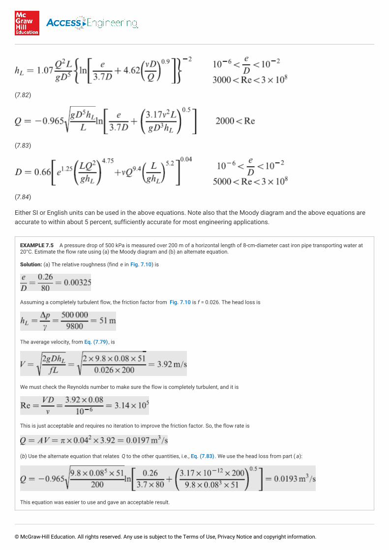
(7.82)

(7.83)

(7.84)

Either SI or English units can be used in the above equations. Note also that the Moody diagram and the above equations areaccurate to within about 5 percent, sufficiently accurate for most engineering applications.

EXAMPLE 7.5 A pressure drop of 500 kPa is measured over 200 m of a horizontal length of 8-cm-diameter cast iron pipe transporting water at20°C. Estimate the flow rate using (a) the Moody diagram and (b) an alternate equation.

Solution: (a) The relative roughness (find e in Fig. 7.10) is

Assuming a completely turbulent flow, the friction factor from Fig. 7.10 is f = 0.026. The head loss is

The average velocity, from Eq. (7.79) , is

We must check the Reynolds number to make sure the flow is completely turbulent, and it is

This is just acceptable and requires no iteration to improve the friction factor. So, the flow rate is

(b) Use the alternate equation that relates Q to the other quantities, i.e., Eq. (7.83) . We use the head loss from part ( a):

This equation was easier to use and gave an acceptable result.


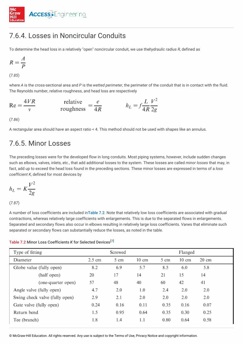
7.6.4. Losses in Noncircular Conduits

To determine the head loss in a relatively "open" noncircular conduit, we use the hydraulic radius R, defined as

(7.85)

where A is the cross-sectional area and P is the wetted perimeter, the perimeter of the conduit that is in contact with the fluid.The Reynolds number, relative roughness, and head loss are respectively

(7.86)

A rectangular area should have an aspect ratio < 4. This method should not be used with shapes like an annulus.

7.6.5. Minor Losses

The preceding losses were for the developed flow in long conduits. Most piping systems, however, include sudden changessuch as elbows, valves, inlets, etc., that add additional losses to the system. These losses are called minor losses that may, infact, add up to exceed the head loss found in the preceding sections. These minor losses are expressed in terms of a losscoefficient K, defined for most devices by

(7.87)

A number of loss coefficients are included in Table 7.2. Note that relatively low loss coefficients are associated with gradualcontractions, whereas relatively large coefficients with enlargements. This is due to the separated flows in enlargements.Separated and secondary flows also occur in elbows resulting in relatively large loss coefficients. Vanes that eliminate suchseparated or secondary flows can substantially reduce the losses, as noted in the table.

Table 7.2 Minor Loss Coefficients K for Selected Devices[7]


values for other geometries can be found in Technical Paper 410 . the cranecompany, 1957.

based on exit velocityV .

based on entrancevelocity V .

We often equate the losses in a device to an equivalent length of pipe, i.e.,

(7.88)

This provides the relationship

[7]

2 1


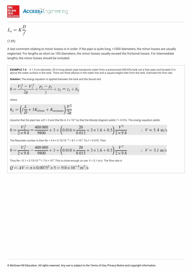
(7.89)

A last comment relating to minor losses is in order: if the pipe is quite long, >1000 diameters, the minor losses are usuallyneglected. For lengths as short as 100 diameters, the minor losses usually exceed the frictional losses. For intermediatelengths, the minor losses should be included.

EXAMPLE 7.6 A 1.5-cm-diameter, 20-m-long plastic pipe transports water from a pressurized 400-kPa tank out a free open end located 3 mabove the water surface in the tank. There are three elbows in the water line and a square-edged inlet from the tank. Estimate the flow rate.

Solution: The energy equation is applied between the tank and the faucet exit:

where

Assume that the pipe has e/D = 0 and that Re ≅ 2 × 10 so that the Moody diagram yields f = 0.016. The energy equation yields

The Reynolds number is then Re = 5.4 × 0.15/10 = 8.1 × 10 . Try f = 0.018. Then

Thus Re = 5.1 × 0.15/10 = 7.6 × 10 . This is close enough so use V = 5.1 m/s. The flow rate is

7.6.6. Hydraulic and Energy Grade Lines

5

−6 4

–6 4


7.6.6. Hydraulic and Energy Grade Lines

The energy equation is most often written so that each term has dimensions of length, i.e.,

(7.90)

In piping systems, it is often conventional to refer to the hydraulic grade line (HGL) and the energy grade line (EGL). The HGL, thedashed line in Fig. 7.11, is the locus of points located a distance p/γ above the centerline of a pipe. The EGL, the solid line in Fig.7.11, is the locus of points located a distance V /2 above the HGL. The following observations relate to the HGL and the EGL.

The EGL approaches the HGL as the velocity goes to zero. They are identical on the surface of a reservoir.

Both the EGL and the HGL slope downward in the direction of the flow due to the losses in the pipe. The greater the losses,the greater the slope.

A sudden drop occurs in the EGL and the HGL equal to the loss due to a sudden geometry change, such as an entrance, anenlargement, or a valve.

A jump occurs in the EGL and the HGL due to a pump and a drop due to a turbine.

If the HGL is below the pipe, there is a vacuum in the pipe, a condition that is most often avoided in the design of pipingsystems because of possible contamination.

Figure 7.11 The hydraulic grade line (HGL) and the energy grade line (EGL) for a piping system.

7.7. OPEN CHANNEL FLOW

Consider the developed turbulent flow in an open channel, sketched in Fig. 7.12. The water flows at a depth y of and thechannel is on a slope S, which is assumed to be small so that sin θ = S. The cross section could be trapezoidal, as shown, or itcould be circular, rectangular, or triangular. Let us apply the energy equation between the two sections:

(7.91)

2


Figure 7.12 Flow in an open channel.

The head loss is the elevation change, i.e.,

(7.92)

where L is the distance between the two selected sections. Using the head loss expressed by Eq. (7.86), we have

(7.93)

The Reynolds number of the flow in an open channel is invariably large and the channel is rough so that the friction factor is aconstant independent of the velocity (see the Moody diagram of Fig. 7.10) for a particular channel. Consequently, the velocity isrelated to the slope and hydraulic radius by

(7.94)

where C is a dimensional constant called the Chezy coefficient; it has been related experimentally to the channel roughness andthe hydraulic radius by

(7.95)

The dimensionless constant n is a measure of the wall roughness and is called the Manning n. Values for a variety of wallmaterials are listed in Table 7.3.

[7]


Table 7.3 Values of the Manning n

Wall material Manning n

Brick 0.016

Cast or wrought iron 0.015

Concrete pipe 0.015

Corrugated metal 0.025

Earth 0.022

Earth with stones and weeds 0.035

Finished concrete 0.012

Mountain streams 0.05

Planed wood 0.012

Sewer pipe 0.013

Riveted steel 0.017

Rubble 0.03

Unfinished concrete 0.014

Rough wood 0.013

The values in this table result in flow rates too large for R>3 m. The manning n should be increased by 10 to 15 percent for thelarger channels.

The flow rate in an open channel follows from Q = AV and is

(7.96)

This is referred to as the Chezy-Manning equation. It can be applied using English units by replacing the "1" in the numeratorwith "1.49."

If the channel surface is smooth, e.g., glass or plastic, Eq. (7.96) should not be used since it assumes a rough surface. Forchannels with smooth surfaces, the Darcy-Weisbach equation, Eq. (7.86), along with the Moody diagram should be used.

[7]

[7]


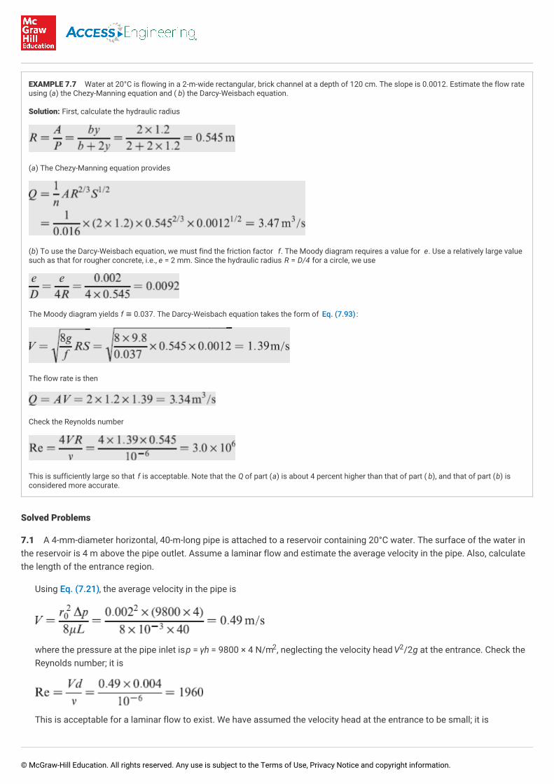
EXAMPLE 7.7 Water at 20°C is flowing in a 2-m-wide rectangular, brick channel at a depth of 120 cm. The slope is 0.0012. Estimate the flow rateusing (a) the Chezy-Manning equation and ( b) the Darcy-Weisbach equation.

Solution: First, calculate the hydraulic radius

(a) The Chezy-Manning equation provides

(b) To use the Darcy-Weisbach equation, we must find the friction factor f. The Moody diagram requires a value for e. Use a relatively large valuesuch as that for rougher concrete, i.e., e = 2 mm. Since the hydraulic radius R = D/4 for a circle, we use

The Moody diagram yields f ≅ 0.037. The Darcy-Weisbach equation takes the form of Eq. (7.93) :

The flow rate is then

Check the Reynolds number

This is sufficiently large so that f is acceptable. Note that the Q of part (a) is about 4 percent higher than that of part ( b), and that of part (b) isconsidered more accurate.

Solved Problems

7.1 A 4-mm-diameter horizontal, 40-m-long pipe is attached to a reservoir containing 20°C water. The surface of the water inthe reservoir is 4 m above the pipe outlet. Assume a laminar flow and estimate the average velocity in the pipe. Also, calculatethe length of the entrance region.

Using Eq. (7.21), the average velocity in the pipe is

where the pressure at the pipe inlet is p = γh = 9800 × 4 N/m , neglecting the velocity head V /2g at the entrance. Check theReynolds number; it is

This is acceptable for a laminar flow to exist. We have assumed the velocity head at the entrance to be small; it is

2 2


This is quite small compared with the pressure head of 4 m. So, the calculations are acceptable provided the entranceregion is not very long.

We have neglected the effects of the entrance region's non-parabolic velocity profile (see Fig. 7.1). The entrance region'slength is

so the effect of the entrance region is negligible.

7.2 A developed, steady laminar flow exists between horizontal concentric pipes. The flow is in the direction of the axis of thepipes. Derive the differential equations and solve for the velocity profile.

The element selected, upon which the forces would be placed, would be a hollow cylindrical shell (a sketch may be helpfulfor visualization purposes), that would appear as a ring from an end view, with length dx. The ring would have an inner radiusr and an outer radius r + dr. The net pressure force acting on the two ends would be

The shear stress forces on the inner and the outer cylinder sum as follows (the shear stress is assumed to oppose the flow):

For a steady flow, the pressure and shear stress forces must balance. This provides

Substitute the constitutive equation τ = –μdu/dr (see footnote associated with Eq. (7.7) assuming the element is near theouter pipe) and obtain

This can now be integrated to yield

Integrate once more to find the velocity profile to be

The constants A and B can be evaluated by using u(r ) = 0 and u(r ) = 0.

7.3 What pressure gradient would provide a zero shear stress on the stationary lower plate in Fig. 7.5 assuming horizontalplates with the top plate moving to the right with velocity U.

The shear stress is τ = –μdu/dy so that the boundary conditions are du/dy (0) = 0, u(0)= 0, and u(b) = U. These are applied toEq. (7.29) or Eq. (7.35) to provide the following:

1 2


Now, u(b) = U, resulting in

This is a positive pressure gradient, so the pressure increases in the direction of U

7.4 Show that the velocity distribution given by Eq. (7.62) approximates a straight line when the gap between the two cylindersis small relative to the radii of the cylinders.

Since the gap is small relative to the two radii, we can let R ≅ r ≅ r . Also, let θ = r – r and y = r – r) (refer to Fig. 7.6) inthe velocity distribution of Eq. (7.62). The velocity distribution takes the form

where we have used the approximation

since y is small compared with R and 2R. The above velocity distribution is a straight-line distribution with slope ω R/δ.

7.5 Water at 15°C is transported in a 6-cm-diameter wrought iron pipe at a flow rate of 0.004 m /s. Estimate the pressuredrop over 300 m of horizontal pipe using (a) the Moody diagram and (b) an alternate equation.

The average velocity and Reynolds number are

(a) The value of e is found on the Moody diagram so that

The friction factor is found from the Moody diagram to be

The pressure drop is then

(b) Using Eq. (7.82), the pressure drop is

1 2 2 1 2

1

3


These two results are within 2 percent and are essentially the same.

7.6 A pressure drop of 200 kPa is measured over a 400-m length of 8-cm-diameter horizontal cast iron pipe that transports20°C water. Determine the flow rate using (a) the Moody diagram and (b) an alternate equation.

The relative roughness is

and the head loss is

(a) Assuming a completely turbulent flow, Moody's diagram yields

The average velocity in the pipe is found, using Eq. (7.79), to be

resulting in a Reynolds number of

At this Reynolds number and e/D = 0.0325, Moody's diagram provides f ≅ 0.026, so the friction factor does not have to beadjusted. The flow rate is then expected to be

(b) Since the head loss was calculated using the pressure drop, Eq. (7.83) can be used to find the flow rate:

These two results are within 3 percent and either is acceptable.

7.7 A farmer needs to provide a volume of 500 L every minute of 20°C water from a lake through a wrought iron siphon adistance of 800 m to a field 4 m below the surface of the lake. Determine the diameter of pipe that should be selected. Use (a)the Moody diagram and (b) an alternate equation.

(a) The average velocity is related to the unknown diameter D by

2


The head loss is 4 m (the energy equation from the lake surface to the pipe exit provides this. We assume that V /2g isnegligible at the pipe exit), so

The Reynolds number and relative roughness are

This requires a trial-and-error solution. We can select a value for f and check to see if the equations and the Moody diagramagree with that selection. Select / = 0.02. Then, the above equations yield

The above match very well on the Moody diagram. Usually, another selection for/and a recalculation of the diameter,Reynolds number, and relative roughness are required. (b) Since the diameter is unknown, Eq. (7.84) is used which provides

The two results are within 2 percent, so are essentially the same.

7.8 A smooth rectangular duct that measures 10×20 cm transports 0.4 m /s of air at standard conditions horizontal distanceof 200 m. Estimate the pressure drop in the duct.

The hydraulic radius is

The average velocity and Reynolds number in the duct are

The Moody diagram provides f = 0.016. The pressure drop is then

7.9 Sketch the hydraulic grade line for the piping system of Example 7.6 if the three elbows are spaced equally between thepressurized tank and the exit of the pipe.

The hydraulic grade line is a distance p/γ above the surface of the water in the tank at the beginning of the pipe. Thehydraulic grade line is sketched in Fig. 7.13.

2

3


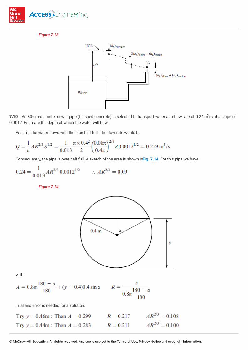
Figure 7.13

7.10 An 80-cm-diameter sewer pipe (finished concrete) is selected to transport water at a flow rate of 0.24 m /s at a slope of0.0012. Estimate the depth at which the water will flow.

Assume the water flows with the pipe half full. The flow rate would be

Consequently, the pipe is over half full. A sketch of the area is shown in Fig. 7.14. For this pipe we have

Figure 7.14

with

Trial and error is needed for a solution.

3


Hence, y = 0.42 m is an acceptable result.

Supplementary Problems

Laminar or Turbulent Flow

7.11 Calculate the maximum average velocity in a 2-cm-diameter pipe for a laminar flow using a critical Reynolds number of2000 if the fluid is (a) water at 20°C, (b) water at 80°C, (c) SAE-30 oil at 80°C, and (d) atmospheric air at 20°C.

7.12 The Red Cedar River flows placidly through MSU's campus at a depth of 80 cm. A leaf is observed to travel about 1 m in4 s. Decide if the flow is laminar or turbulent. Make any assumptions needed.

7.13 A drinking fountain has an opening of 4 mm in diameter. The water rises a distance of about 20 cm in the air. Is the flowlaminar or turbulent as it leaves the opening? Make any assumptions needed.

7.14 SAE-30 oil at 80°C occupies the space between two cylinders, 2 and 2.2 cm in diameter. The outer cylinder is stationaryand the inner cylinder rotates at 100 rpm. Is the oil in a laminar or turbulent state if Re = 1700? Use Re = ωr δ/v, where δ = r– r .

Entrance Flow

7.15 Water is flowing in a 2-cm-diameter pipe with a flow rate of 0.0002 m /s. For an entrance that provides a uniformvelocity profile, estimate inviscid core length and the entrance length if the water temperature is (a) 20, (b) 40, (c) 60, and (d)80°C.

7.16 A parabolic velocity profile is desired at the end of a 10-m-long, 8-mm-diameter tube attached to a tank filled with 20°Cwater. An experiment is run during which 60 L is collected in 90 min. Is the laminar flow assumption reasonable? If so, wouldthe tube be sufficiently long?

7.17 A parabolic profile is desired in 20°C air as it passes between two parallel plates that are 80 mm a part in a universitylaboratory. If the Reynolds number Vh/v = 1500, how long would the channel need to be to observe a fully developed flow, i.e., aparabolic velocity profile? What would be the average velocity?

7.18 The flow of 20°C water in a 2-cm-diameter pipe oscillates between being laminar and turbulent as it flows through thepipe from a reservoir. Estimate the inviscid core and the entrance lengths (a) if the flow is laminar and the average velocity is0.15 m/s, and (b) if the flow is turbulent and the average velocity is 0.6 m/s (use the results of Eq. (7.4)).

7.19 Argue that the pressure gradient Δp/Δx in the entrance region is greater than the pressure gradient in the developed flowregion of a pipe. Use a fluid increment of length Δx and cross-sectional area πr in the entrance region and in the developed-flow region.

7.20 Explain why the pressure distribution in the entrance region of a pipe for the relatively low-Reynolds-number turbulentflow (Re ≈ 10 000) is below the extended straight-line distribution of developed flow. Refer to Fig. 7.3.

Laminar Flow in a Pipe

7.21 Show that the right-hand side of Eq. (7.19) does indeed follow from the integration.

7.22 Show that f = 64/Re for a laminar flow in a pipe.

7.23 Show that the head loss in a laminar flow in a pipe is directly proportional to the average velocity in the pipe.

7.24 The pressure drop over a 15-m length of 8-mm-diameter horizontal pipe transporting water at 40°C is measured to be1200 Pa. A laminar flow is assumed. Determine (a) the maximum velocity in the pipe, (b) the Reynolds number, (c) the wallshear stress, and (d) the friction factor.

crit 1 2

1

3

02


7.25 A liquid flows through a 2-cm-diameter pipe at a rate of 20 L every minute. Assume a laminar flow and estimate thepressure drop over 20 m of length in the horizontal pipe for (a) water at 40°C, (b) SAE-10 oil at 20°C, and (c) glycerin at 40°C.Decide if a laminar flow is a reasonable assumption.

7.26 Water at 20°C flows through a 12-mm-diameter pipe on a downward slope so that Re = 2000. What angle would result ina zero pressure drop?

7.27 Water at 40°C flows in a vertical 8-mm-diameter pipe at 2 L/min. Assuming a laminar flow, calculate the pressure dropover a length of 20 m if the flow is (a) upwards and (b) downwards.

7.28 Atmospheric air at 25°C flows in a 2-cm-diameter horizontal pipe at Re = 1600. Calculate the wall shear stress, thefriction factor, the head loss, and the pressure drop over 20 m of pipe.

7.29 A liquid flows in a 4-cm-diameter pipe. At what radius does the velocity equal the average velocity assuming a laminarflow? At what radius is the shear stress equal to one-half the wall shear stress?

7.30 Find an expression for the angle θ that a pipeline would require such that the pressure is constant assuming a laminarflow. Then, find the angle of a 10-mm-diameter pipe transporting 20°C water at Re = 2000 so that a constant pressure occurs.

7.31 Solve for the constants A and B in Solved Problem 7.2 using cylinder radii of r = 4 cm and r = 5 cmassuming that 20°Cwater has a pressure drop of 40 Pa over a 10-m length. Also find the flow rate. Assume laminar flow.

7.32 SAE-10 oil at 20°C flows between two concentric cylinders parallel to the axes of the horizontal cylinders having radii of 2and 4 cm. The pressure drop is 60 Pa over a length of 20 m. Assume laminar flow. What is the shear stress on the innercylinder?

Laminar Flow Between Parallel Plates

7.33 What pressure gradient would provide a zero shear stress on the stationary lower plate in Fig. 7.5 for horizontal plateswith the top plate moving to the right with velocity U. Assume a laminar flow.

7.34 What pressure gradient is needed so that the flow rate is zero for laminar flow between horizontal parallel plates if thelower plate is stationary and the top plate moves with velocity U. See Fig. 7.5.

7.35 Fluid flows in a horizontal channel that measures 1×40 cm. If Re = 1500 calculate the flow rate and the pressure dropover a length of 10 m if the fluid is (a) water at 20°C, (b) air at 25°C, and (c) SAE-10 oil at 40°C. Assume laminar flow.

7.36 Water at 20°C flows down an 80-m-wide parking lot at a constant depth of 5 mm. The slope of the parking lot is 0.0002.Estimate the flow rate and the maximum shear stress. Is a laminar flow assumption reasonable?

7.37 Water at 20°C flows between two parallel horizontal plates separated by a distance of 8 mm. The lower plate isstationary and the upper plate moves at 4 m/s to the right (see Fig. 7.5). Assuming a laminar flow, what pressure gradient isneeded such that:

(a) The shear stress at the upper plate is zero

(b) The shear stress at the lower plate is zero

(c) The flow rate is zero

(d) The velocity at y = 4 mm is 4 m/s

7.38 Atmospheric air at 40°C flows between two parallel horizontal plates separated by a distance of 6 mm. The lower plateis stationary and the pressure gradient is –3 Pa/m. Assuming a laminar flow, what velocity of the upper plate (see Fig. 7.5) isneeded such that:

1 2


(a) The shear stress at the upper plate is zero

(b) The shear stress at the lower plate is zero

(c) The flow rate is zero

(d) The velocity at y = 4 mm is 2 m/s

7.39 SAE-30 oil at 40°C fills the gap between the stationary plate and the 20-cm-diameter rotating plate shown in Fig. 7.15.Estimate the torque needed assuming a linear velocity profile if Ω = 100 rad/s.

Figure 7.15

7.40 SAE-10 oil at 20°C fills the gap between the moving 120-cm-long cylinder and the fixed outer surface. Assuming a zeropressure gradient, estimate the force needed to move the cylinder at 10 m/s. Assume a laminar flow.

Laminar Flow Between Rotating Cylinders

7.41 Assuming a Couette flow between a stationary and a rotating cylinder, determine the expression for the power needed torotate the inner rotating cylinder. Refer to Fig. 7.6.

Figure 7.16

7.42 SAE-10 oil at 20°C fills the gap between the rotating cylinder and the fixed outer cylinder shown in Fig. 7.17. Estimate thetorque needed to rotate the 20-cm-long cylinder at 40 rad/s (a) using the profile of Eq. (7.62) and (b) assuming a Couette flow.

Figure 7.17

7.43 A 3-cm-diameter cylinder rotates inside a fixed 4-cm-diameter cylinder with 40°C SAE-30 oil filling the space between the30-cm-long concentric cylinders. Write the velocity profile and calculate the torque and the power required to rotate the innercylinder at 2000 rpm assuming a laminar flow.

7.44 Determine the expressions for the torque and the power required to rotate the outer cylinder if the inner cylinder of Fig.7.6 is fixed. Assume a laminar flow.


Turbulent Flow in a Pipe

7.45 Time average the differential continuity equation for an incompressible flow and prove that two continuity equationsresult:

7.46 A 12-cm-diameter pipe transports water at 25°C in a pipe with roughness elements averaging 0.26 mm in height. Decideif the pipe is smooth or rough if the flow rate is (a) 0.0004, (b) 0.004, and (c) 0.04 m /s.

7.47 Estimate the maximum velocity in the pipe of (a) Prob. 7.46a, (b) Prob. 7.46b, and (c) Prob. 7.46c.

7.48 Draw a cylindrical control volume of length L and radius r in a horizontal section of pipe and show that the shear stressvaries linearly with r, that is, τ = rΔp/(2L). The wall shear is then given by τ = r Δp/(2L) (see Eq. (7.75)).

7.49 Estimate the velocity gradient at the wall, the pressure drop, and the head loss over 20 m of length for the water flow of(a) Prob. 7.46a, (b) Prob. 7.46b, and (c) Prob. 7.46c. Note: Since turbulence must be zero at the wall, the wall shear stress isgiven by .

7.50 Water at 20°C flows in a 10-cm-diameter smooth horizontal pipe at the rate of 0.004 m /s. Estimate the maximumvelocity in the pipe and the head loss over 40 m of length. Use the power-law velocity distribution.

7.51 SAE-30 oil at 20°C is transported in a smooth 40-cm-diameter pipe with an average velocity of 10 m /s. Using the power-law velocity profile, estimate (a) the friction factor, (b) the pressure drop over 100 m of pipe, (c) the maximum velocity, and (d)the viscous wall layer thickness.

7.52 Rework Prob. 7.51 using the semi-log velocity profile.

7.53 If the pipe of Prob. 7.51 is a cast iron pipe, rework the problem using the semi-log velocity profile.

Losses in Pipe Flow

7.54 Water at 20°C flows at 0.02 m /s in an 8-cm-diameter galvanized iron pipe. Calculate the head loss over 40 m ofhorizontal pipe using (a) the Moody diagram and (b) the alternate equation.

7.55 Rework Prob. 7.54 using (a) SAE-10 oil at 80°C, (b) glycerin at 70°C, and (c) SAE-30 oil at 40°C.

7.56 Water at 30°C flows down a 30° incline in a smooth 6-cm-diameter pipe at a flow rate of 0.006 m /s. Find the pressuredrop and the head loss over an 80-m length of pipe.

7.57 If the pressure drop in a 100-m section of horizontal 10-cm-diameter galvanized iron pipe is 200 kPa, estimate the flowrate if the liquid flowing is (a) water at 20°C, (b) SAE-10 oil at 80°C, (c) glycerin at 70°C, and (d) SAE-30 oil at 20°C. Because theMoody diagram requires a trial-and-error solution, one of the alternate equations is recommended.

7.58 Air at 40°C and 200 kPa enters a 300-m section of 10-cm-diameter galvanized iron pipe. If a pressure drop of 200 Pa ismeasured over the section, estimate the mass flux and the flow rate. Because the Moody diagram requires a trial-and-errorsolution, one of the alternate equations is recommended. Assume the air to be incompressible.

7.59 A pressure drop of 100 kPa is desired in 80 m of smooth pipe transporting 20°C water at a flow rate of 0.0016 m/s.What diameter pipe should be used? Because the Moody diagram requires a trial-and-error solution, one of the alternateequations is recommended.

7.60 Rework Prob. 7.59 using (a) SAE-10 oil at 80°C, (b) glycerin at 70°C, and (c) SAE-30 oil at 20°C.

3

0 0

3

3

3

3

3


7.61 A farmer wishes to siphon 20°C water from a lake, the surface of which is 4 m above the plastic tube exit. If the totaldistance is 400 m and 300 L of water is desired per minute, what size tubing should be selected? Because the Moody diagramrequires a trial-and-error solution, one of the alternate equations is recommended.

7.62 Air at 35°C and 120 kPa enters a 20×50 cm sheet metal conduit at a rate of 6 m /s. What pressure drop is to be expectedover a length of 120 m?

7.63 A pressure drop of 6000 Pa is measured over a 20 m length as water at 30°C flows through the 2×6 cm smooth conduit.Estimate the flow rate.

Minor Losses

7.64 The loss coefficient of the standard elbow listed in Table 7.2 appears quite large compared with several of the other losscoefficients. Explain why the elbow has such a relatively large loss coefficient by inferring a secondary flow after the bend.Refer to Eq. (3.31).

7.65 Water at 20°C flows from a reservoir out a 100-m-long, 4-cm-diameter galvanized iron pipe to the atmosphere. The outletis 20 m below the surface of the reservoir. What is the exit velocity (a) assuming no losses in the pipe and (b) including thelosses? There is a square-edged entrance. Sketch the EGL and the HGL for both (a) and (b).

7.66 Add a nozzle with a 2-cm-diameter outlet to the pipe of Prob. 7.65. Calculate the exit velocity.

7.67 The horizontal pipe of Prob. 7.65 is fitted with three standard screwed elbows equally spaced. Calculate the flowincluding all losses. Sketch the HGL.

7.68 A 4-cm-diameter cast iron pipe connects two reservoirs with the surface of one reservoir 10 m below the surface of theother. There are two standard screwed elbows and one wide-open angle valve in the 50-m-long pipe. Assuming a square-edgedentrance, estimate the flow rate between the reservoirs. Assume a temperature of 20°C.

7.69 An 88% efficient pump is used to transport 30°C water from a lower reservoir through an 8-cm-diameter galvanized ironpipe to a higher reservoir whose surface is 40 m above the surface of the lower one. The pipe has a total length of 200 m.Estimate the power required for a flow rate of 0.04 m /s. What is the maximum distance from the lower reservoir that the pumpcan be located if the horizontal pipe is 10 m below the surface of the lower reservoir?

7.70 A 90% efficient turbine operates between two reservoirs connected by a 200-m length of 40-cm-diameter cast iron pipethat transports 0.8 m s of 20°C water. Estimate the power output of the turbine if the elevation difference between the surfacesof the reservoirs is 40 m.

7.71 The pump characteristic curves, shown in Fig. 7.18, relate the efficiency and the pump head (see Eq. (4.25)) for the pumpof this problem to the flow rate. If the pump is used to move 20°C water from a lower reservoir at elevation 20 m to a higherreservoir at elevation 60 m through 200 m of 16-cm-diameter cast iron pipe, estimate the flow rate and the power required.

3

3

3/


https://www.accessengineeringlibrary.com/mhe-lookup/atom-id/68d9c6fbf1dd308e#ch03eqn31

https://www.accessengineeringlibrary.com/mhe-lookup/atom-id/11be4d17319b8f0e#ch04eqn25

Figure 7.18

Open Channel Flow

7.72 Water flows at a depth of 80 cm in an open channel on a slope of 0.0012. Find the average shear stress acting on thechannel walls if the channel cross section is (a) a 140-cm-wide rectangle and (b) a 3.2-m-diameter circle. (Draw a controlvolume and sum forces.)

7.73 Water flows in a 2-m-wide rectangular finished concrete channel with a slope of 0.001 at a depth of 80 cm. Estimate theflow rate using (a) the Chezy–Manning equation and (b) the Moody diagram.

7.74 Water is not to exceed a depth of 120 cm in a 2-m-wide finished rectangular concrete channel on a slope of 0.001. Whatwould the flow rate be at that depth? (a) Use the Chezy–Manning equation and (b) the Moody diagram.

7.75 Estimate the flow rate in the channel shown in Fig. 7.19 if the slope is 0.0014. The sides are on a slope of 45° (a) Use theChezy–Manning equation and (b) the Darcy–Weisbach equation. (c) Also, calculate the average shear stress on the walls.

Figure 7.19

7.76 Water flows in a 2-m-diameter sewer (finished concrete) with S = 0.0016. Estimate the flow rate if the depth is (a) 50, (b)100, (c) 150, and (d) 199 cm.

7.77 Water flows in a 120-cm-diameter sewer (finished concrete) with S = 0.001 at a flow rate of 0.4 m /s. What is theexpected depth of flow?

Answers to Supplementary Problems

7.11 (a) 0.1007 m/s (b) 0.0367 m/s (c) 1.8 m/s (d) 1.51 m/s

7.12 Highly turbulent

7.13 Turbulent

3


7.14 Laminar

7.15 (a) 16.4 m, 8.2 m (b) 25.1 m, 12.5 m (c) 34.7 m, 17.4 m (d) 45.1 m, 22.6 m

7.16 Yes, yes

7.17 4.8 m, 0.283 m/s

7.18 (a) 1.94 m, 3.87 m (b) 0.2 m, 2.4 m

7.19 See problem statement





7.24 (a) 0.448 m/s (b) 2950 (c) 0.16 Pa (d) 0.0217

7.25 (a) 1114 Pa, not laminar (b) 153 kPa, laminar (c) 594 kPa, laminar

7.26 0.219° downward

7.27 (a) 200.6 kPa (b) –191.8 kPa

7.28 0.0091 Pa, 0.04, 3.13 m, 36.4 Pa

7.29 1.414 cm, 1 cm

7.30 sin (8µV/γr ), 0.376 °

7.31 4.1, 14.8, 0.0117 m /s

7.32 0.035 N/m

7.33 2U/b

7.34 6µU/b

7.35 (a) 0.0006 m /s, 180 Pa (b) 0.0093 m /s, 51.5 Pa (c) 0.0024 m /s, 264 kPa

7.36 0.00653 m /s, 0.0098 N/m

7.37 (a) –125Pa/m (b) 125 Pa/m (c) 375 Pa/m (d) –0.25 Pa/m

7.38 (a) 2.83 m/s (b) –2.83m/s (c) –0.942 m/s (d) 1.37 m/s

7.39 12.6 N-m

7.40 565 N

7.41

7.42 (a) 0.346 N.m (b) 0.339 N.m

7.43 539(0.0016/r – r), 0.325 m, 136 W

–l 20

3

2

2

2

3 3 3

3 2


7.44


7.46 (a) smooth (b) rough (c) rough

7.47 (a) 0.047 m/s (b) 0.474 m/s (c) 4.6 m/s


7.49 (a) 7.3 s , 4.4 Pa, 0.00045 m (b) 490 s , 290 Pa, 0.03 m (c) 45,200 s , 27 kPa, 2.7 m

7.50 0.63m/s, 0.125 m

7.51 (a) 0.024 (b) 275 kP (c) 12.4 m/s (d) 1.82 mm

7.52 (a) 0.0255 (b) 292 kP (c) 11.9 m/s (d) 1.77 mm

7.53 (a) 0.0275 (b) 315 kP (c) 12.5 m/s (d) 1.71 mm

7.54 (a) 9.7 m (b) 9.55

7.55 (a) 11.3 m, 11.1 m (b) 15.1 m, 15.2 m (c) 16.1 m, 16.5 m

7.56 – 343 kPa, 4.98 m

7.57 (a) 0.033 m /s (b) 0.032 m /s (c) 0.022 m /s (d) 0.022 m /s

7.58 0.0093 m /s, 0.031 kg/s

7.59 5.6 cm

7.60 (a) 3.5 cm (b) 3.9 cm (c) 3.9 cm

7.61 8.4 cm

7.62 18.8 kPa

7.63 0.00063 m /s


7.65 (a) 19.8 m/s (b) 2.01 m/s

7.66 0.995 m/s

7.67 1.56 m/s

7.68 1.125 m/s

7.69 138 hp, 6.7 m

7.70 173 hp

7.71 0.3 m /s, 290 hp

7.72 (a) 4.39 Pa (b) 4.92 Pa

7.73 (a) 2.45 m /s (b) 2.57 m /s

–1 –1 –1

3 3 3 3

3

3

3

3 3

3 3


7.74 (a) 0.422 m /s (b) 0.435 m /s

7.75 (a) 1.99 m /s (b) 2.09 m /s (c) 5.32 Pa

7.76 (a) 0.747 /s (b) 3.30 /s (c) 6.27 /s (d) 6.59 /s

7.77 0.45 m

The minus sign is required since the stress is a postive quantity and du/dr is negative near the lower wall.

For a sloped channel simply replace p with (p + γh).

The Reynolds number is defined as Re = ω r δ/v where δ = r – r .

The minus sign results from the shear stress in Fig. 7.6 being on a negative face in the positive direction, the sign convention for astress component.

Steady turbulent flow means the time-average quantities are independent of time.

The shear velocity is a fictitious velocity that allows experimental data to be presented in dimensionless form that is valid for allturbulent pipe flows. The viscous length is also a fictitious length.

3 3

3 3

3 3 3 3

[1]

[2]

[3] 1 1 2 1

[4]

[5]

[6]


internal flows | mcgraw-hill education - access engineering

Documents