inter-hemispheric linkages in climate change: paleo-perspectives for

Clim. Past, 2, 167–185, 2006www.clim-past.net/2/167/2006/© Author(s) 2006. This work is licensedunder a Creative Commons License.

Climateof the Past

Inter-hemispheric linkages in climate change: paleo-perspectives forfuture climate change

J. Shulmeister1, D. T. Rodbell2, M. K. Gagan3, and G. O. Seltzer4†

1Department of Geological Sciences, University of Canterbury, Private Bag 4800, Christchurch, New Zealand2Department of Geology, Union College, Schenectady, NY 12308, USA3Research School of Earth Sciences, The Australian National University, Canberra 2000, ACT, Australia4Department of Earth Sciences, Heroy Geology Lab, University of Syracuse, Syracuse NY 13244, USA†deceased

Received: 20 December 2005 – Published in Clim. Past Discuss.: 22 February 2006Revised: 31 August 2006 – Accepted: 16 October 2006 – Published: 26 October 2006

Abstract. The Pole-Equator-Pole (PEP) projects of thePANASH (Paleoclimates of the Northern and SouthernHemisphere) programme have significantly advanced our un-derstanding of past climate change on a global basis andhelped to integrate paleo-science across regions and researchdisciplines. PANASH science allows us to constrain predic-tions for future climate change and to contribute to the man-agement of consequent environmental changes. We identifythree broad areas where PEP science makes key contribu-tions.

1. The pattern of global changes. Knowing the exacttiming of glacial advances (synchronous or otherwise) dur-ing the last glaciation is critical to understanding inter-hemispheric links in climate. Work in PEPI demonstratedthat the tropical Andes in South America were deglaciatedearlier than the Northern Hemisphere (NH) and that an ex-tended warming began there ca. 21 000 cal years BP. Thegeneral pattern is consistent with Antarctica and has nowbeen replicated from studies in Southern Hemisphere (SH)regions of the PEPII transect. That significant deglaciationof SH alpine systems and Antarctica led deglaciation of NHice sheets may reflect either i) faster response times in alpinesystems and Antarctica, ii) regional moisture patterns that in-fluenced glacier mass balance, or iii) a SH temperature forc-ing that led changes in the NH. This highlights the limitationsof current understanding and the need for further fundamen-tal paleoclimate research.

2. Changes in modes of operation of oscillatory climatesystems.Work across all the PEP transects has led to therecognition that the El Nino Southern Oscillation (ENSO)phenomenon has changed markedly through time. It now ap-pears that ENSO operated during the last glacial termination

Correspondence to:J. Shulmeister([email protected])

and during the early Holocene, but that precipitation tele-connections even within the Pacific Basin were turned down,or off. In the modern ENSO phenomenon both inter-annualand seven year periodicities are present, with the inter-annualsignal dominant. Paleo-data demonstrate that the relative im-portance of the two periodicities changes through time, withlonger periodicities dominant in the early Holocene.

3. The recognition of climate modulation of oscillatorysystems by climate events. We examine the relationship ofENSO to a SH climate event, the Antarctic cold reversal(ACR), in the New Zealand region. We demonstrate that theonset of the ACR was associated with the apparent switchingon of an ENSO signal in New Zealand. We infer that this re-lated to enhanced zonal SW winds with the amplification ofthe pressure fields allowing an existing but weak ENSO sig-nal to manifest itself. Teleconnections of this nature wouldbe difficult to predict for future abrupt change as boundaryconditions cannot readily be specified. Paleo-data are criticalto predicting the teleconnections of future changes.

1 Introduction

1.1 Background to the Pole-Equator-Pole projects ofPANASH

The aim of all PANASH science is to understand the modesof climate and environmental variability. This work is prob-lem/project focused. The ENSO climate system, for exam-ple, has been a particular focus for research. These researchproblems are tackled through multi-proxy climate and envi-ronmental reconstructions and paleo-climate modeling.

Within PANASH, the largest projects have been the threePEP transects. PEP I covers the Americas, PEPII covers

Published by Copernicus GmbH on behalf of the European Geosciences Union.

168 J. Shulmeister et al.: PEP overview

the East Asia to Australasia region, and PEPIII extends fromNorthern Europe to Southern Africa. Under the auspices ofthe PEPs hundreds of scientists have been involved in dozensof projects. The PEPs have played a major role in bringingtogether disparate regions and research disciplines into co-hesive science programmes and numerous, substantive out-puts have been achieved (e.g. Markgraf, 2001; Battarbee etal., 2004; Dodson et al., 2004). Given the scale of the PEPprojects, it is not feasible to attempt to summarise the wholeof the science programme in a single paper. Instead thispaper identifies three general areas of research where PEPprojects have significantly contributed to the understandingof past and present climate systems. In order to further focusthe paper we have chosen to review progress in one region,the South Pacific Basin, using a case study approach.

We highlight how the understanding derived from “paleo”work can assist in the understanding of future change. We fo-cus on the need to work on high-resolution records that willallow paleoclimate science to interface with climate mod-elling and management but we also emphasise the need foron-going fundamental research into past environments andclimates. Despite many decades of paleoenvironmental re-search we do not have adequate understanding of the patternsof change over huge swathes of the globe’s surface, notablyAfrica, the SH in general and much of the world’s oceans.

The three topics we have chosen to highlight are: 1) Pat-terns of global change, 2) Changes in the modes of oscil-latory climate systems, and 3) Climatic teleconnections ofclimate events. The latter two topics deal with the uniquepower of ‘paleo’ science to deal with longer-term changesand extreme events. The first topic, however, highlights acautionary note about the limits of our knowledge.

2 Contribution 1: The pattern of global changes: Casestudy – The Last Glacial Maximum (LGM) and thetiming of deglaciation in the Southern tropics andmid-latitudes

One of the longest standing debates in global climate changehas been on the mechanism of climate signal transfer fromthe region of climate forcing to the rest of the globe. Thelargest climate changes of the recent geological past are theice ages. On a glacial-interglacial timescale, the timing ofglacial advances in the mid-latitude SH appears to be broadlysynchronous with those of the main northern ice advances(e.g. Nelson et al., 1985). This is unexpected, as SH con-ditions based on orbital (Milankovitch) forcing of solar in-solation, should be out of phase with the Northern Hemi-sphere (Mercer, 1984; Berger, 1992). The apparent syn-chrony requires rapid transfer of cooling from the North-ern Hemisphere (NH). The main candidates for this forcingare changes in greenhouse gas concentration in the atmo-sphere (e.g. Petit et al., 1999; Indermuhle et al., 2000) and/or

changes in heat transport through ocean (thermohaline) cir-culation (e.g. Broecker, 2000; Stocker, 2000).

The focus for much of this work has centred on the ter-mination of the last ice-age. The primary reason for this isthat the warming associated with this termination is of simi-lar or even larger magnitude than the human-induced climatemodification expected under future greenhouse-gas scenar-ios (Watson et al., 2001) although the rate of change wasmuch slower. A second reason is that numerous climatearchives that span the last deglaciation are both available andwell dated. Emerging from these well dated archives havebeen the observations of offset timing between late glacial-interglacial transition (LGIT) cooling events, such as the SHAntarctic Cold Reversal and NH Younger Dryas. These ob-servations have lead to the idea of the so-called climate “see-saw” where one hemisphere leads the climate in the other.This, in turn, appears to support an ocean thermohaline cir-culation mechanism of global climate transmission.

Though the thermohaline circulation mechanism is notuniversally accepted, there is little doubt that there is an inter-hemispheric offset in climate change. It is not, however, easyto resolve whether the North leads the South, or vice-versa(e.g. Steig and Alley, 2002). Antarctica started to warm at∼17 000 calendar years ago and is a widespread view thatthe warming which is associated with a glacial termination inGreenland did not occur until∼14 700 years ago (e.g. Ras-mussen et al., 2006). In contrast, Alley et al. (2002) amongothers, suggest that NH cooling peaked much earlier, near24 000 years ago, and that the real trend to warming in theNH was established soon after this point. Following thislogic NH warming leads SH warming. The differences inages from the different viewpoints reflect different ways ofdetermining the onset of events (warming) rather than differ-ent data sets.

The whole debate has proceeded without much referenceto either the tropics or the mid-latitude SH. Here we presenta cautionary note, wherein we summarise evidence for anearly “LGM” and an early start to deglaciation in the tropicsand southern mid-latitudes. These data can be interpreted toimply that deglaciation started in the tropics and propagatedfirstly to low mid-latitudes before extending to either Antarc-tica or Greenland.

2.1 Timing of the LGM and deglaciation in the SH tropicsand mid-latitudes

2.1.1 Tropical South America

Recent work (Smith et al., 2005a) has highlighted evidencefor the relative unimportance of the globally defined LGM(23 000–19 000 years ago, Mix et al., 2001) in the Andes ofPeru and Bolivia. There, moraines from six valleys (3 valleysystems), previously attributed to LGM advances, proved tobe much older (Fig. 1). The moraines that date to the globalLGM advance are located significantly up valley from their

Clim. Past, 2, 167–185, 2006 www.clim-past.net/2/167/2006/

J. Shulmeister et al.: PEP overview 169

Fig. 1. Exposure ages of moraines in the Junin Valleys (Peru;A) and Milluni and Zongo Valleys (Bolivia;B) based on cosmogenic datingwith 10Be. Thin gray lines are contour lines, with altitudes in m a.s.l.; contour inteverals are 200 m (A) and 500 m (B). Many of the morainesof Group D, once thought to be correlative with the LGM, are more than 100 000 yr old. The LGM corresponds with moraines (labelled B)from a relatively minor advance. The most extensive glaciation of the last glacial cycle occurred between 34 and 22 kcal yr BP. Reprintedwith permission from Smith et al., Early Local Last Glacial Maximum in the Tropical Andes, Science, 308, 678–681, 2005. Copyright 2005AAAS.

originally inferred LGM ice positions. In addition, a late lastglaciation (OIS 3) advance, dating to between 34 000 and28 000 years ago, was significantly bigger than the subse-quent OIS 2 LGM advances in all these systems. Ice mayhave remained in an advanced position until about 23 000years ago, after which it retreated rapidly up valley. There-fore, it appears that the global LGM was marked by a minorre-advance during the local deglaciation of the tropical An-des.

A major strength of the recent work of Smith et al. (2005a)is the scale of the dating. Several hundred10Be ages weredetermined of which 106 ages relate to late last glaciationadvances. The general pattern of the ages is compelling.

One long-standing climate inference regarding globalcooling, based on estimates of equilibrium line altitude(ELA) depression during the global LGM, is also challengedby the Smith et al. (2005a) findings. With the dramatic re-duction in the revised extent of the LGM comes a new cal-culation of the ELA depression during the LGM (Smith etal., 2005b). ELA depressions of only 300–600 m are esti-mated for the western side of the tropical Andes, indicatingLGM cooling of only 2–4◦C. This is much closer to the trop-ical ocean cooling inferred for the Pacific than the changesderived from the Atlantic Basin.

The Smith et al. (2005a) conclusion of relatively minor iceextent during the LGM in the Peruvian Andes is consistent

with several other studies from the tropical Andes. Seltzer(1994) reported basal radiocarbon dates from a moraine-dammed lake in a cirque in the Cordillera Quimsa Cruz Bo-livia of ∼20,000 cal yr BP. These dates require deglacia-tion before this time, and a maximum glacial ELA lower-ing of <500 m, far less than the purported global average of∼1000 m for the LGM (Broecker and Denton, 1989; Porter,2001). Likewise, Mark et al. (2002) report a maximum ELAdepression of 500 m for LGM paleoglaciers in the QuelccayaIce Cap region of southern Peru. In contrast, in the Andes ofnorthern Peru, Ecuador, and Colombia workers have reportedconsiderably higher (up to∼1500 m) estimates of the mag-nitude of ELA depression during the LGM (e.g., Clapperton,1986; Rodbell, 1992; Mark and Helmens, 2005), with univer-sally more ELA depression on the eastern side of the Andesthan on the western side. This latter was echoed in the find-ings of Smith et al. (2005b). These differences raise two sig-nificant questions: 1) Does the apparent northward increasein ELA depression for purported LGM paleoglaciers reflecta real paleoclimatic gradient or is it the product of poor agecontrol in northern regions? 2) Do the apparent increasesin ELA depression from west to east across the Andes re-flect real paleoclimatic gradients or are they the product ofdifferent glaciological conditions on the eastern side of theAndes than on the western side. These latter could includethe positive feedback set up by paleoglaciers advancing into

www.clim-past.net/2/167/2006/ Clim. Past, 2, 167–185, 2006


300 kmSouth

ern

Alps

New Zealand

Mapourika

LGM

34-28ka

300 kmSouth

ern

Alps

New Zealand

Rakaia Valley

LakeColeridge

Rakaia River

Tui Creek -late OIS3

Moraineposition

Bayfields - LGM

Fig. 2. LGM vs OIS 3 limits in New Zealand.(a) displays the Rakaia Valley in Canterbury, in the eastern South Island, where recent work(Shulmeister et al., unpublished data) has dated a presumed OIS 4 advance in late OIS 3. This makes OIS 3 advances significantly biggerthan LGM advances in this eastern system.(b) demonstrates that a late OIS 3 advance is larger than the LGM advance in this west coastsystem (Suggate and Almond, 2005). A similar age advance, also larger than the LGM advance, is noted at Mt Kosciusko, in SE Australia(Barrows et al., 2001). The LGM is defined as 23 000–19 000 years ago, following Mix et al. (2001). (b) is reprinted from Suggate, R. P.and Almond, P., The Last Glacial Maximum (LGM) in western South Island, New Zealand: Implications for the global LGM and MIS 2,Quaternary Science Reviews, 24, 1923–1940, 2005, with permission from Elsevier.

regions of increasing mean annual precipitation, or higherdebris cover on glaciers on the eastern side of the Andes,which generally flowed down deeply incised bedrock val-leys, whereas those on the western side were mostly pied-mont glaciers that expanded out onto Inter-Adean plateaus at∼4000 m a.s.l., such as the Altiplano of southern Peru andBolivia.

2.1.2 Temperate Australasia

During the peak of the last ice age at least discontinu-ous glaciation extended from Antarctica as far north as theSnowy Mountains in southeastern Australia (36◦45′ S) in theSW Pacific region. Here again a traditional view of lastglacial maxima coinciding with the global LGM has requiredrevision as new age control data have come to light.

The classic glacial sequence in New Zealand comes fromthe Kumara-Moana area in Westland (Suggate, 1990). TheLGM is defined by the Larrikins-2 advance in north West-land and the M52 advance in south Westland (Suggate andAlmond, 2005). These date to 24 500 to 21 500 years ago.They are not, however, the largest advances during the lat-ter part of the last ice age. Instead the Larrikins-1/M51 ad-vance between 34 000 and 28 000 years ago extended furtherand is volumetrically bigger (Fig. 2). The main LGM ad-vance on the eastern side of the Alps is poorly dated exceptin the Rakaia Valley in Canterbury. Here the Bayfield ad-

vances (Soons and Gullentops, 1973), which may representtwo Last Glacial maxima yield a mean age of less than 23 500years ago roughly co-eval with moraines on the west coast.Recent luminescence dating (Shulmeister et al., unpublisheddata) of outwash deposits previously mapped as OIS 4 in-dicates that late OIS 3 advances (provisionally post 37 000years ago) are also recorded (Fig. 2). These OIS 3 ice limitsare significantly greater than the true LGM limits. While thetiming of relationships between the eastern and western ad-vances requires further work, one conclusion is that the LGMis not the major glacial advance in the latter part of the lastglaciation in New Zealand.

The New Zealand pattern is partially confirmed by discon-tinuous data from Australia. On the eastern highlands at MtKosciusko (36◦45′ S) Barrows et al. (2001) recognised a sig-nificant glacial advance at about 32 000 cal yr ago. A pseudo-LGM advance dating to between 24 and 22 000 cal yr ago isalso noted but is significantly smaller than the late MIS 3advance. In contrast, glacial advances in Tasmania duringthe latter half of the last glaciation are limited to small scalecirque readvances (e.g. Barrows et al., 2002; Kiernan et al.,2004). The LGM moraines were constructed around 20 000–17 000 years ago. They may, or may not, have reoccupiedlate OIS 3 positions.

A further notable feature of New Zealand paleoclimate isthe apparent lack of cooling at the LGM. Traditional proxies



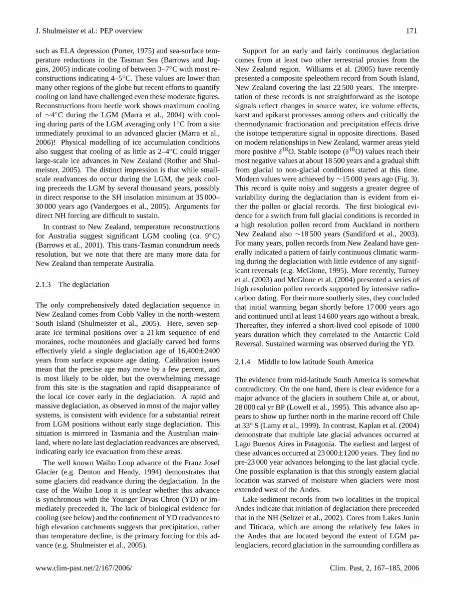
such as ELA depression (Porter, 1975) and sea-surface tem-perature reductions in the Tasman Sea (Barrows and Jug-gins, 2005) indicate cooling of between 3–7◦C with most re-constructions indicating 4–5◦C. These values are lower thanmany other regions of the globe but recent efforts to quantifycooling on land have challenged even these moderate figures.Reconstructions from beetle work shows maximum coolingof ∼4◦C during the LGM (Marra et al., 2004) with cool-ing during parts of the LGM averaging only 1◦C from a siteimmediately proximal to an advanced glacier (Marra et al.,2006)! Physical modelling of ice accumulation conditionsalso suggest that cooling of as little as 2–4◦C could triggerlarge-scale ice advances in New Zealand (Rother and Shul-meister, 2005). The distinct impression is that while small-scale readvances do occur during the LGM, the peak cool-ing preceeds the LGM by several thouasand years, possiblyin direct response to the SH insolation minimum at 35 000–30 000 years ago (Vandergoes et al., 2005). Arguments fordirect NH forcing are difficult to sustain.

In contrast to New Zealand, temperature reconstructionsfor Australia suggest significant LGM cooling (ca. 9◦C)(Barrows et al., 2001). This trans-Tasman conundrum needsresolution, but we note that there are many more data forNew Zealand than temperate Australia.

2.1.3 The deglaciation

The only comprehensively dated deglaciation sequence inNew Zealand comes from Cobb Valley in the north-westernSouth Island (Shulmeister et al., 2005). Here, seven sep-arate ice terminal positions over a 21 km sequence of endmoraines, roche moutonees and glacially carved bed formseffectively yield a single deglaciation age of 16,400±2400years from surface exposure age dating. Calibration issuesmean that the precise age may move by a few percent, andis most likely to be older, but the overwhelming messagefrom this site is the stagnation and rapid disappearance ofthe local ice cover early in the deglaciation. A rapid andmassive deglaciation, as observed in most of the major valleysystems, is consistent with evidence for a substantial retreatfrom LGM positions without early stage deglaciation. Thissituation is mirrored in Tasmania and the Australian main-land, where no late last deglaciation readvances are observed,indicating early ice evacuation from these areas.

The well known Waiho Loop advance of the Franz JosefGlacier (e.g. Denton and Hendy, 1994) demonstrates thatsome glaciers did readvance during the deglaciation. In thecase of the Waiho Loop it is unclear whether this advanceis synchronous with the Younger Dryas Chron (YD) or im-mediately preceeded it. The lack of biological evidence forcooling (see below) and the confinement of YD readvances tohigh elevation catchments suggests that precipitation, ratherthan temperature decline, is the primary forcing for this ad-vance (e.g. Shulmeister et al., 2005).

Support for an early and fairly continuous deglaciationcomes from at least two other terrestrial proxies from theNew Zealand region. Williams et al. (2005) have recentlypresented a composite speleothem record from South Island,New Zealand covering the last 22 500 years. The interpre-tation of these records is not straightforward as the isotopesignals reflect changes in source water, ice volume effects,karst and epikarst processes among others and critically thethermodynamic fractionation and precipitation effects drivethe isotope temperature signal in opposite directions. Basedon modern relationships in New Zealand, warmer areas yieldmore positiveδ18O. Stable isotope (δ18O) values reach theirmost negative values at about 18 500 years and a gradual shiftfrom glacial to non-glacial conditions started at this time.Modern values were achieved by∼15 000 years ago (Fig. 3).This record is quite noisy and suggests a greater degree ofvariability during the deglaciation than is evident from ei-ther the pollen or glacial records. The first biological evi-dence for a switch from full glacial conditions is recorded ina high resolution pollen record from Auckland in northernNew Zealand also∼18 500 years (Sandiford et al., 2003).For many years, pollen records from New Zealand have gen-erally indicated a pattern of fairly continuous climatic warm-ing during the deglaciation with little evidence of any signif-icant reversals (e.g. McGlone, 1995). More recently, Turneyet al. (2003) and McGlone et al. (2004) presented a series ofhigh resolution pollen records supported by intensive radio-carbon dating. For their more southerly sites, they concludedthat initial warming began shortly before 17 000 years agoand continued until at least 14 600 years ago without a break.Thereafter, they inferred a short-lived cool episode of 1000years duration which they correlated to the Antarctic ColdReversal. Sustained warming was observed during the YD.

2.1.4 Middle to low latitude South America

The evidence from mid-latitude South America is somewhatcontradictory. On the one hand, there is clear evidence for amajor advance of the glaciers in southern Chile at, or about,28 000 cal yr BP (Lowell et al., 1995). This advance also ap-pears to show up further north in the marine record off Chileat 33◦ S (Lamy et al., 1999). In contrast, Kaplan et al. (2004)demonstrate that multiple late glacial advances occurred atLago Buenos Aires in Patagonia. The earliest and largest ofthese advances occurred at 23 000±1200 years. They find nopre-23 000 year advances belonging to the last glacial cycle.One possible explanation is that this strongly eastern glaciallocation was starved of moisture when glaciers were mostextended west of the Andes.

Lake sediment records from two localities in the tropicalAndes indicate that initiation of deglaciation there preceededthat in the NH (Seltzer et al., 2002). Cores from Lakes Juninand Titicaca, which are among the relatively few lakes inthe Andes that are located beyond the extent of LGM pa-leoglaciers, record glaciation in the surrounding cordillera as



10,0

00

11,0

00

12,0

00

13,0

00

14,0

00

15,0

00

16,0

00

17,0

00

18,0

00

19,0

00

20,0

00

21,0

00

- 430

- 440

- 450

- 460

- 470

- 480

(delta D)

VostokDeuterium

- 3.30

- 3.10

- 2.90

- 3.50

- 3.70

NW SISpeleothem

(delta O)18

GISP IIO

18

(delta O)18

- 3.50

- 3.60

- 3.70

- 3.80

0

- 1

1

S-America(glacial flour

flux)

(Petit et al. 1999)

(Williams et al. 2005)

(Grootes ans Stuiver 1997)

(Rodbell, unpub data)

Pukaki CraterPollen

- 1

0

1

2

(Log podocarp /grasses)

?

Max. ice extent

Min. ice extent

Glacial records(New Zealand)

Westland

?

YoungerDryas

Antarctic ColdReversal

Years BP

Deglaciation goesglobal

Antarctic deglaciationstarts

Southern mid-latitudesstart to deglaciate

Main

Degla

cia

tion

com

ple

te

*

3 2 1

Greenland

Antarctica

New Zealand

New Zealand

TropicalSth America

Fig. 3. Interhemispheric timing of post-glacial warming: An alternative view. Here we summarise rock flour records from tropical SouthAmerica (Rodbell, unpublished data) and pollen (Sandiford et al., 2003), glacial (Suggate, 1990) and speleothem records (Williams et al.,2005) from New Zealand and compare them to standard deuterium records from Vostok in Antarctica (Petit et al., 1999) and the oxygenisotope ice core record from GISP II (Grootes and Stuiver, 1997). We highlight shifts in climate (Bands 1–3). Band 1 shows a shift towardswarm (interglacial) conditions in New Zealand and tropical South America at about 18 500 calibrated years ago. Band 2 marks the onsetof continuous warming in the Antarctic at about 17 000 calibrated years ago and Band 3 marks a second warming phase in South Americaand New Zealand and the first indication of warming in Greenland. In summary, these data suggest that warming initiates in the tropicsand southern mid-latitudes and is transmitted to the Antarctic before warming initiates in northern high latitudes. It is recognised that someworkers place NH warming much earlier (e.g. Alley et al., 2002, see text).

increases in the abundance of glacial flour. These recordsclearly show the initial reduction in glacial flour flux begin-ning prior to 20 000 cal yr BP, and cessation by∼19 000 calyr BP. Sediment records from lakes within the LGM icelimits record a late glacial readvance that was underway by14 000 cal yr BP, and rapid ice retreat that began∼13 000 calyr BP (Rodbell and Seltzer, 2000). Most paleoglaciers re-treated to nearly modern (∼1950 AD) limits by 12 500 calyr BP, but some actually disappeared for several thousand

years before reforming in the mid-late Holocene (Abbott etal., 2003).

There has been considerable disagreement over themoraine evidence for an ice advance synchronous with theYD advance of the NH (reviewed in Rodbell and Seltzer,2000). In general, there is neither the necessary age con-trol nor the unambiguous stratigraphic evidence to providecompelling evidence for a significant ice advance during theYD in the tropical Andes. The aforementioned lake sediment



evidence, which is both well-dated and continuous, providessolid evidence for rapid ice retreat during the YD. The YD,however, was apparently cold in the tropical Andes as evi-denced by the Huascaran Peru ice core record (Thompson etal., 1995). Thus it appears that conditions must have becomesuddenly drier during this time in order to drive significantice retreat.

2.1.5 Summary

The timing of the maximum glaciation in the latter part ofthe last ice age in the Andean tropics of South America pre-ceded the LGM by 5–10 kyr. There is widespread evidenceof late OIS 3 advances in the tropics and mid-latitudes of theSH. These advances are bigger and more pervasive than theLGM advance, at least in the South American Andean trop-ics and in Australasia. A reasonable case can be made thatthe first step towards an interglacial climate occurred at about18 500 cal yr BP in the southern mid-latitudes.

The available paleo-records suggest that the sequence ofevents for the last deglaciationcouldbe re-interpreted as fol-lows (see Fig. 3): Tropical (and mid-latitude SH) glacialmaxima were achieved 5–10 000 years before the LGM.The deglaciation in both regions effectively starts soon af-ter 28 000 years ago but is interrupted by smaller-scale re-advances during the LGM. This is some 4000 years beforethe maximum cooling in the NH as defined by Alley etal. (2002). In short, something caused deglaciation to start inthe tropics and mid-latitude SH well before the NH reachedmaximum cooling (Mix et al., 2002). Alternatively, if step-wise warming is taken as the marker for the onset of deglacia-tion, SH tropical and mid-latitude regions started a drift tointerglacial conditions about 18 500 years ago. This is 1500years before the inferred warming of Antarctica at∼17 000years ago and more than 3000 years ahead of Greenland,which warmed abruptly after 14 700 years ago (e.g. Ras-mussen et al., 2006). In both Australasia and tropical AndeanSouth America there are glacial fluctuations around 14 000years ago though it is unclear whether their timing coincides.

The significance of these observations is that they chal-lenge the basic assumptions of climate change on which webase our predictions of global climate response. The recordscould be interpreted to demonstrate that the Andean trop-ics and mid-latitude SH lead the polar regions, or they maybe compatible with an NH climate lead. Our purpose, how-ever, is not to directly dispute the understanding of patternsof global change. It is to emphasise the extent of the un-certainty, given the limitations of the available paleoclimaterecords. It is imperative, therefore, that fundamental researchinto the basic patterns of long-term global change continuesto be supported. There are large areas of the planet, notablyAfrica, the SH and large sections of the oceans where our un-derstanding of long-term climate and environmental changeis inadequate. We will not be successful in predicting future

responses to climate modification if we cannot even specifythe patterns of past changes.

3 Contribution 2. The recognition and definition oflonger-term changes in modes of operation of climatephenomena. Case study: the Holocene evolution ofENSO and change from long frequency to biennial os-cillation ENSO dominance

The ENSO phenomenon contributes a large portion of theinterannual (2–7 yr) variability in the modern climate sys-tem (Gagan et al., 2004). Work across all the PEP transectshas led to the recognition that ENSO has changed markedlythrough time. In particular, a mid-Holocene shift or driftin ENSO activity by∼5000 yr BP has been postulated fromboth modelling studies (e.g. Clement et al., 1999) and paleo-ENSO records (e.g. Shulmeister and Lees, 1995; Shulmeis-ter, 1999; Rodbell et al., 1999; Moy et al., 2002). A fur-ther intensification of ENSO is often invoked at around 3000yr BP (e.g. Sandweiss et al., 2001; Woodroffe et al., 2003;Gagan et al., 2004). Understanding ENSO variations un-der mid-late Holocene conditions is particularly importantbecause global sea-level and ice cover are effectively mod-ern, leaving potential forcings such as extra-tropical forcing,changes in mean temperature and the like to be examined(Diaz and Markgraf, 1992).

The following brief review of the ENSO phenomenon fol-lows Cane (2005) (Fig. 4). ENSO is an ocean-atmospherecirculation pattern in the Pacific set up by 2–7 year oscil-lations in the temperature contrast between the western andeastern tropical Pacific. This zonal temperature contrast isdue to upwelling of cold water in the eastern equatorial Pa-cific, while warm surface waters in the tropical western Pa-cific are maintained by inflow from the equatorial regionsunder the prevailing easterly trade wind systems. The tem-perature contrast maintains the trade wind flow and pro-vides a positive feedback, the so-called “Bjerknes mecha-nism” (Cane, 2005). If the trade winds weaken, the flowcollapses and ultimately reverses. The mechanism explainswhy the circulation breaks down (to an El Nino) once coolinghas started in the western Pacific but it does not provide thetrigger for the switch to an El Nino state. This is most proba-bly provided by wave propagation in the tropical ocean ther-mocline which is described as the delayed oscillator (Cane,2005).

The bandwidth for modern ENSO oscillations is 2-7 years.Changes in the dominant period of ENSO variability can beidentified from the analyses of instrumental records (e.g. Se-toh et al., 1999; An and Wang, 2000) as well as predictedconceptually from modelling (Lau and Sheu, 1988). Itshould be noted that some climatologists and oceanogra-phers (e.g. Federov and Philander, 2000) sound a warningon the existence of multiple modes of ENSO periodicities,pointing out that they may indicate changes in longer term



Figure 4. ENSO pattern (from Cane, 2005). (a) During normal conditions trade winds

drive upwelling off the South American coast and force warm surface waters from the

eastern tropical Pacific to the western Pacific. The deep pool of warm water in the

western tropical Pacific (a.k.a. West Pacific Warm Pool –WPWP) causes intense

convection over the WPWP. Rising air circulates eastward and subsides in the eastern

Pacific over the cooler upwelling water, closing the circulation loop. (b) During El Niño

events, the trade winds decline and warm water flows from the WPWP to the eastern

Pacific. The shoaling of the WPWP causes a decline in convection in the western Pacific

and a convective cell migrates eastward. This causes widespread modification of global

weather patterns. Reprinted from Earth and Planetary Science Letters, 230, M.A. Cane,

The evolution of El Niño, past and future, 227-240, 2005, with permission from

Elsevier

Fig. 4. ENSO pattern (from Cane, 2005).(a) During normal conditions trade winds drive upwelling off the South American coast and forcewarm surface waters from the eastern tropical Pacific to the western Pacific. The deep pool of warm water in the western tropical Pacific(a.k.a. West Pacific Warm Pool – WPWP) causes intense convection over the WPWP. Rising air circulates eastward and subsides in theeastern Pacific over the cooler upwelling water, closing the circulation loop.(b) During El Nino events, the trade winds decline and warmwater flows from the WPWP to the eastern Pacific. The shoaling of the WPWP causes a decline in convection in the western Pacific anda convective cell migrates eastward. This causes widespread modification of global weather patterns. Reprinted from Cane, M. A., Theevolution of El Nino, past and future, Earth Planet. Sci. Lett., 230, 227–240, 2005, with permission from Elsevier.

background climatology modifying the apparent expressionof ENSO rather than the phenomenon itself.

Tomita and Yasunari (1993) identified two types of ENSO;a long-frequency ENSO with a mean duration of 57 monthsand a biennial-oscillation ENSO with a duration of 30months. This bi-modal ENSO of Tomita and Yasunari hasnot been widely recognised and the example is provided asa case study of how variable ENSO periodicitiescould im-pact regional climates. According to the authors the biennial-oscillation ENSO causes a sea surface temperature (SST)anomaly for only one year in the eastern tropical Pacific butis associated with a clockwise eddy of wind-stress anoma-lies in the western tropical Pacific during the “mature” ElNino phase (Tomita and Yasunari, 1993). This wind stressanomaly assists in terminating the El Nino phase of theENSO phenomenon and forms part of a teleconnection to theEast Asian winter monsoon. Long-frequency ENSO causesSST anomalies in the eastern equatorial Pacific for three suc-cessive years but has no wind-stress anomaly in the westerntropical Pacific.

ENSO has very significant climatic impacts within the Pa-cific basin, and through teleconnections to other parts of theglobe. Substantial progress has been made in understandingthe modern phenomenon, but ENSO has proved very variablein both temporal and spatial impacts, and modern ocean andatmosphere records are not long enough to decipher long-term changes in ENSO behaviour. Here we present a seriesof ENSO records from across the South Pacific Basin. Cu-mulatively these records clearly indicate that the frequencyof ENSO events has increased through the course of theHolocene and that the mean strength of El Nino events hasalso increased. The records do not, however, imply that theENSO system has ever switched off.

3.1 ENSO in South America

The impact of ENSO on the western margin of South Amer-ica has been documented for the past several centuries (e.g.,Quinn et al., 1987). During non-El Nino years in the trop-ical eastern Pacific, tradewind circulation dominates, SSTs



are cool, and the∼75 km wide onshore coastal belt below3000 m a.s.l. is very dry. During El Nino events tradewindsslacken, the thermocline in the eastern Pacific deepens, andrainfall increases dramatically along the coast. During strongEl Nino years, rising motions occur in parts of the easternPacific troposphere that are normally characterized by subsi-dence and inversion. Under these conditions, rainfall alongthe coast can be extreme, driven by intraseasonal bursts ofdeep convection and torrential rainfall.

The inland extent of precipitation events is limited, and,generally, east of the crest of the Andes the climatic responseto El Nino events is muted, and in some regions the responseis opposite of that noted along the coastal belt. One regionwhere the latter is especially true is on the Peruvian-BolivianAltiplano. In this region, El Nino events are marked by asignificantreductionin precipitation.

The best known record from the high Andes is the LagunaPallcacocha (Ecuador) record (Rodbell et al., 1999; Moy etal., 2002). Here a 15 000-year record of clastic sediment in-flux to a lake marks precipitation driven run-off events ina normally semi-arid setting. Spectral analysis of colourchanges in the sediments related to the influx events showsthat for the last 150 years the colour banding contains signifi-cant spectral variance in the 2–7 year ENSO bandwidth. Theinflux bands are associated with warm SST excursions offthe coast of Ecuador during El Nino events. Modern ENSOband variance, along with decadal to centennial scale vari-ance, appears after about 6000 years ago.

The Laguna Pallcacocha record demonstrates a long-termdrift from long period variability to shorter period variability(Fig. 5). During the early Holocene, all the spectral variabil-ity occurs at long time periods dissimilar to modern ENSOsignals. From 6000 to about 3000 years ago the period ofvariability shortens and a ca. 7 yr ENSO signal becomes vis-ible. In the last 3000 years the signal frequency has been in-creasing and 3–4 year period signals have become important.In short ENSO frequency appears to have increased throughthe Holocene at this site.

A limitation of the Lake Pallcacocha record is that thebanding is non-annual and the bands reflect individual sed-imentation (precipitation) events. Consequently, there isa minimum threshold that needs to be exceeded before aband will be deposited. Changes in the amplitude of ENSOevents could mimic the effect of changes in periodicity, if thechanges in amplitude fluctuate around the threshold value.Changes in amplitude are interpreted to be present in therecord.

Over the last 6000 years, where ENSO has been visiblein this record, it is not consistently strongly “on”. Instead atleast three phases of enhanced ENSO events centred around5000, 3000 and 1000 years ago can be recognised. This wasinferred by Moy et al. (2002) to represent a roughly 2100year cyclicity. This repetitive pattern may be forced by inso-lation (solar activity).

0

2000

4000

6000

8000

10000

12000

0 10 20 30

El Niño Events

(events per 100-yr window)

Ag

e(c

aly

rB

P)

Fig. 5. Number of strong El Nino events recorded in Laguna Pall-cacocha Ecuador per 100 year overlapping window (from Moy etal., 2002). The early Holocene was marked by fewer events andthe frequency of events increased through the Holocene beginning∼6000 cal yr BP and peaked several times in the last 2000 yr.

Recently, the first nearly-continuous 20,000-year longarchive of past El Nino activity has been obtained from ma-rine sediments off the coast of Peru (Rein et al., 2005).This record shows significant El Nino activity as early as17 000 cal yr BP, strong activity during the late glacial, anda marked reduction in El Nino activity from 9–5000 yearsBP. The Holocene portion of this record agrees well with the



Fig. 6. From McGregor and Gagan (2004)(a) Changes in El Ninofrequency given by coralδ18O records from Muschu Island, Koil Is-land, and Madang, PNG (Tudhope et al., 2001), lacustrine storm de-posits (Moy et al., 2002), and model results (Clement et al., 2000).Data are scaled to events/century to facilitate direct comparison.(b)Changes in El Nino amplitude given by coralδ18O records in panel(a), the standard deviation of coralδ18O in microatolls from the cen-tral equatorial Pacific (Woodroffe et al., 2003), and model results(Clement et al., 2000; Liu et al., 2000). The threshold amplitudeanalysis of the Tudhope et al. (2001) coral records is restricted to ElNino events to facilitate comparison with other records. Error barfor the modern Muschu Island coral record is the standard error ofthe mean for all El Nino events recorded for 1950–1997. Errors forfossil coral percentage changes include the standard errors for boththe modern and fossil corals. Reprinted with permission from Mc-Gregor, H. V. and Gagan, M. K., Western Pacific coralδ18O recordsof anomalous Holocene variability in the El Nino-Southern Oscilla-tion, Geophys. Res. Lett., 31, L11204, 1–4, 2004, Copyright 2004AGU.

aforementioned Pallcacocha record, however this is the firstevidence of strong El Nino activity during MIS 2 from theeastern tropical Pacific.

3.2 Coral records of ENSO in the West Pacific Warm Pool

Viewed as an oceanic system, the Western Pacific Warm Pool(WPWP) and Indonesia form the “down-drift” core regionfor ENSO. Under normal conditions, the surface waters ofthe WPWP are very warm (>28◦C) and provide vast quan-tities of atmospheric water vapour and latent heat that drivethe world’s climate. The resulting high levels of convectiverainfall make the surface waters of the WPWP less salinethan average tropical seawater. This low density warm poolwater is displaced eastward during El Nino events and SSTsin the WPWP decline by about 1◦C, mainly in response to

the thinning of the surface mixed layer and greater mixingwith underlying, cooler water. Consequently, atmosphericconvection in the WPWP region is disrupted during El Ninoevents (Rasmusson and Carpenter, 1982) causing droughtconditions in the WPWP region (Ropelewski and Halpert,1987).

El Nino events are recorded by massive, long-lived coralsin the WPWP region through changes in theδ18O values intheir skeletons. These changes in skeletalδ18O reflect thecombined effect of cooler SSTs and the reduction in18O-depleted rainfall during El Ninos. Analysis of fossil coralsfrom northern Papua New Guinea dating to 7600–5400 yearsyears ago suggests that ENSO amplitude was reduced to 85–40% of modern (Tudhope et al., 2001; McGregor and Gagan,2004; Fig. 6). Records from Christmas Island in the centralequatorial Pacific also contain a strong ENSO signal indi-cating ENSO amplitudes 80–60% of modern from∼4000 to3300 years ago (Woodroffe and Gagan, 2000; Woodroffe etal., 2003). In contrast, large and protracted El Nino events areidentified for 2500–1700 years ago (McGregor and Gagan,2004) and remained above modern until the last 1000 years(Moy et al., 2002).

Analysis of individual ENSO events reveals that the pre-cipitation response to El Nino temperature anomalies wassubdued in the mid-Holocene (Gagan et al., 2004). There-fore, while ENSO strength may be reduced in the earlyHolocene, there is no suggestion from coral records for theWPWP that ENSO is eliminated. In fact, coral records doc-umenting the early Holocene climate in Indonesia (Gagan etal., unpublished data) show clear seasonal ENSO SST sig-nals, and in terms of temperature, mid-Holocene El Ninos onthe Great Barrier Reef were similar in amplitude to recentevents (Gagan et al., 2004). Unlike recent events, however,summer rainfall was only marginally reduced, producing arecord with much less interannual rainfall variability.

The relative failure of the precipitation anomaly to de-velop in these WPWP records may explain the absence ofENSO signals in Ecuador during the early Holocene. Withstrong convection still occurring over the WPWP, the Walkerand Hadley circulations were probably still operating intheir usual meridional positions, even if somewhat reduced.Therefore, the opportunity for a strong convective cell to de-velop in the eastern Pacific may have been reduced. Alter-natively, El Nino-driven precipitation only reaches Lake Pal-cacocha during strong-very strong events when convectionreaches∼4000 m and the absence of El Nino signals at thissite during the early Holocene may indicate the absence ofsuch strong events.

Just as the amplitude of ENSO varied through theHolocene, so too did the frequency. Unlike Laguna Pallca-cocha, where ENSO bandwidths are effectively absent untilabout 6000 years ago, ENSO-like phenomena are in placeat 12 000 years ago elsewhere in the tropics (Rein et al.,2005). By 10 000 years ago the spectral signal shows strongforcing at 1.5–3 year bandwidths. During the peak ENSO



frequency period (about 2000 to 1000 years ago) the fre-quency of events becomes nearly annual before droppingback to a 1.5 yr bandwidth in the last millennium. The over-all frequency of events observed in coral records from theWPWP is much greater than in Ecuador, but the trend to-wards high frequency oscillation is similar. The differencebetween the records may again be that the Ecuador lakesediments only record El Nino events when they are strongenough to trigger a rainfall anomaly in western tropical SouthAmerica.

3.3 ENSO teleconnections in the SW Pacific (NewZealand)

ENSO is the principle EOF in most analyses of the NewZealand inter-annual climate. The climatic effects of ENSOwere mapped in some detail by Gordon (1985) who demon-strated that the impacts in New Zealand vary by season andlocality. Also, Mullan (1995) demonstrated that the effectswere partially non-stationary and consequently impacts mayvary through time. Despite these riders, the strong topo-graphic division of New Zealand makes regional precipita-tion signals highly sensitive to small-scale synoptic changesand these are what allow us to recognise ENSO effects. Theprimary ENSO impacts in New Zealand are related to thewaxing and waning of surface pressure over eastern Aus-tralia in response to El Nino events. During El Nino events,anomalous high pressure over eastern Australia causes anacceleration of the regional southwest air-flow over NewZealand. By contrast, reduced zonal flow and more frequentdevelopment of blocking highs over the country occurs dur-ing La Ninas. Within New Zealand the northern part of NorthIsland is particularly responsive to changes in the South-ern Oscillation (SO). Auckland and the surrounding regionshave significant SO correlations (p<0.05) for temperature inSpring, Summer and Winter and for rainfall in Spring andSummer (Gordon, 1986). It just misses significance in Win-ter. The regional climate of Auckland is dominated by SWflows and the pressure anomaly maps (Fig. 11 in Gordon,1986) highlight the susceptibility of this flow to SO varia-tions.

In the following sections we examine the impact of ENSOon the Holocene glacial records in New Zealand and on pale-oclimate records from a maar in the Auckland region. Thesedata are then compared to the recently developed regionalcomposite speleothem record of Williams et al. (2005).

3.3.1 Records of glacial activity and speleothems

It has been demonstrated that the strength and pattern ofwesterly wind flow and concomitant precipitation and cloudcover are critical to modern glacier mass balance in NewZealand (Fitzharris et al., 1992; Tyson et al., 1997; Hookerand Fitzharris, 1999). Changes in westerly air-flow can bedirectly correlated with ENSO and, at least for the west coast

glaciers, a prima facie relationship between a westerly indexand glacier fluctuation has been established. Specifically, themodern west coast glaciers respond with a 5–7 year lag toaverage seasonal synoptic conditions, with advances occur-ring after years of positive zonal (southwesterly) flow and re-treats associated with years of meridional (northerly) anoma-lies. East coast glaciers, on the other hand, have longer re-sponse times and respond to longer period (decadal) forc-ing. Millennial-scale changes in the westerlies will be con-trolled by the pole-equator temperature gradient, which ismost likely driven by orbital forcing through modification ofinsolation derived seasonality (e.g. Dodson, 1998; Shulmeis-ter, 1999; Shulmeister et al., 2004).

The long-term records from these glaciers indicate a re-markable absence of evidence for glacial advances from9000 to 5000 years ago. After 5000 years the glacial sys-tems switched on. The best-studied Holocene glacial recordcomes from the west coast, Franz Josef Glacier, which ad-vanced at 5000, 2500, 1500 years ago and during the LittleIce Age (Wardle, 1973). This suggests ENSO activity hasstepped-up in the latter half of the Holocene.

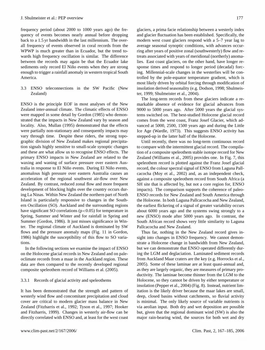
Until recently, there was no long-term continuous recordto compare with the intermittent glacial record. The compila-tion of a composite speleothem stable isotope record for NewZealand (Williams et al., 2005) provides one. In Fig. 7, thisspeleothem record is plotted against the Franz Josef glacialrecord, the colour spectral signal of ENSO from Laguna Pall-cacocha (Moy et al., 2002) and, as an independent check,against a composite speleothem record from South Africa (aSH site that is affected by, but not a core region for, ENSOimpacts). The comparison supports the coherence of paleo-ENSO records for New Zealand and South America throughthe Holocene. In both Laguna Pallcacocha and New Zealand,the earliest flickering of a signal of greater variability occursabout 6000 years ago and the systems swing strongly to anew (ENSO) mode after 5000 years ago. In contrast, theSouth African record shows very little similarity to LagunaPallcacocha and New Zealand.

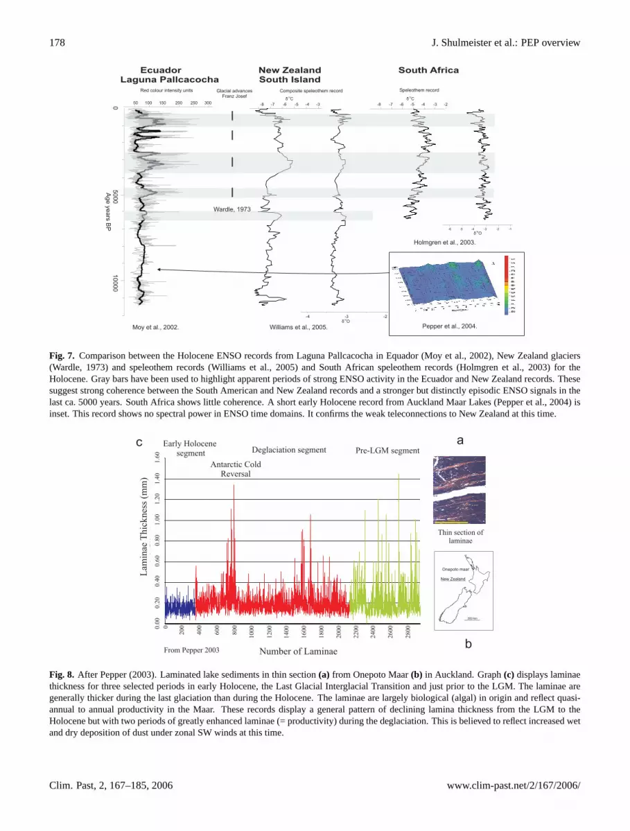
Thus far, nothing in the New Zealand record gives in-sight into changes in ENSO frequency. We cannot demon-strate a Holocene change in bandwidth from New Zealand,but we can demonstrate that ENSO operated differently dur-ing the LGM and deglaciation. Laminated sediment recordsfrom Auckland Maar craters are the key (e.g. Horrocks et al.,2005). Some of these laminae are at least quasi-annual and,as they are largely organic, they are measures of primary pro-ductivity. The laminae become thinner from the LGM to theHolocene, so they cannot be driven by either temperature orinsolation (Pepper et al., 2004) (Fig. 8). Instead, nutrient lim-itation is the likely driver because the maar lakes are small,deep, closed basins without catchments, so fluvial activityis minimal. The only likely source of variable nutrients isvia aeolian input. Both dry and wet deposition are possiblebut, given that the regional dominant wind (SW) is also themajor rain-bearing wind, the sources for both wet and dry



0A

ge

ye

ars

BP

50

00

10

00

0

-8 -7 -6 -5 -4 -3 -8 -7 -6 -5 -4 -3 -2

Ecuador New Zealand South AfricaLaguna Pallcacocha South Island

-6 -5 -4 -3 -2 -1

ä O18

-4 -3 -2ä O

18

ä C13

ä C13

50 100 150 200 250 300

Red colour intensity units Composite speleothem recordGlacial advancesFranz Josef

Speleothem record

Holmgren et al., 2003.

Pepper et al., 2004.Williams et al., 2005.

Wardle, 1973

Moy et al., 2002.

Fig. 7. Comparison between the Holocene ENSO records from Laguna Pallcacocha in Equador (Moy et al., 2002), New Zealand glaciers(Wardle, 1973) and speleothem records (Williams et al., 2005) and South African speleothem records (Holmgren et al., 2003) for theHolocene. Gray bars have been used to highlight apparent periods of strong ENSO activity in the Ecuador and New Zealand records. Thesesuggest strong coherence between the South American and New Zealand records and a stronger but distinctly episodic ENSO signals in thelast ca. 5000 years. South Africa shows little coherence. A short early Holocene record from Auckland Maar Lakes (Pepper et al., 2004) isinset. This record shows no spectral power in ENSO time domains. It confirms the weak teleconnections to New Zealand at this time.

Va ria t ion of la mina e down c ore

0.0

00

.20

0.4

00

.60

0.8

01

.00

1.2

01

.40

1.6

0

Lam

inae

Thic

knes

s(m

m)

0

20

0

40

0

80

0

10

00

12

00

14

00

16

00

18

00

20

00

22

00

24

00

26

00

28

00

60

0

Number of Laminae

Thin section oflaminae

Deglaciation segment Pre-LGM segment

Antarctic ColdReversal

Early Holocenesegment

1 mm

From Pepper 2003

300 km

New Zealand

Onepoto maar

b

ac

Fig. 8. After Pepper (2003). Laminated lake sediments in thin section(a) from Onepoto Maar(b) in Auckland. Graph(c) displays laminaethickness for three selected periods in early Holocene, the Last Glacial Interglacial Transition and just prior to the LGM. The laminae aregenerally thicker during the last glaciation than during the Holocene. The laminae are largely biological (algal) in origin and reflect quasi-annual to annual productivity in the Maar. These records display a general pattern of declining lamina thickness from the LGM to theHolocene but with two periods of greatly enhanced laminae (= productivity) during the deglaciation. This is believed to reflect increased wetand dry deposition of dust under zonal SW winds at this time.



0

0.2

0.4

0.6

0.8

1

Period (years)2 2.5 3 4 5 7 10 20 100

B

A

Cen

tralW

ind

ow

Ag

e(y

rB

P)

No

rmalized

PS

D

No

rma

lize

dP

ow

er

Sp

ec

tra

lD

en

sit

y

Period (years)2 2.5 3 4 5 7 10 20 100

Cen

tralW

ind

ow

Ag

eC

No

rmalized

PS

D

Period (years)2 2.5 3 4 5 7 10 20 100

Cen

tralW

ind

ow

Ag

e(y

rB

P)

25870

25998

26126

26254

26382

26510

Antarctic Cold Reversal

Early deglaciation event

Near Glacial Maximum

Interannual ENSO

Seven year ENSO mode

Early Holocene

Fig. 9. Spectral analyses of lamina thickness from Onepoto Maar during parts of(a) immediately prior to the LGM(b) the deglaciation and(c) the early Holocene. The deglacial section displays a 7 year ENSO like periodicity during two distinct episodes, which coincide with thesections of thickened laminae in Fig. 7. The younger of these matches the onset of the Antarctic Cold Reversal (ACR). The ACR appears tobe reflected in New Zealand by a strengthening of the regional SW flow which amplifies the ENSO signal enough for it to be reflected in therecord. Reprinted with permission from Pepper, A. C., Shulmeister, J., Nobes, D. C., and Augustinus, P. C., Possible ENSO signals prior tothe last Glacial Maximum, during the deglaciation and the early Holocene from New Zealand, Geophys. Res. Lett., 31, L15206 1–4, 2004,Copyright 2004 AGU.

deposition coincide. Therefore, we interpret these records toshow variability in the southwest wind which, in the Auck-land region, is strongly related to ENSO variability (Gordon,1985). The Auckland Maar record shows strong coherenceat a 2–3 year bandwidth near the LGM. There is no visibleENSO signal in the early Holocene, but during the deglacia-tion there are two brief periods showing strong spectral forc-ing at a 7 year bandwidth (Fig. 9).

3.4 Discussion/Summary: Changes in the amplitude andfrequency of ENSO events

ENSO switches up and down (rather than on and off) dur-ing the Holocene. Clearly, there are important changesin paleo-ENSO dynamics in the middle Holocene. To in-terpret the Holocene evolution of ENSO, we lean towardsthe hypothesis of Haug et al. (2001) who suggested thatthe ITCZ was located further north during the early-middleHolocene. This may have strengthened the links betweenENSO and the NH monsoonal systems but weakened the



Significant Peaks in PSD

0.0E+00

5.0E-04

1.0E-03

1.5E-03

2.0E-03

2.5E-03

110100

Period (years)

Po

we

rS

pe

ctr

al

De

ns

ity

(no

rmali

se

du

nit

s)

Power spectral density

95 % confidence

99 % confidence

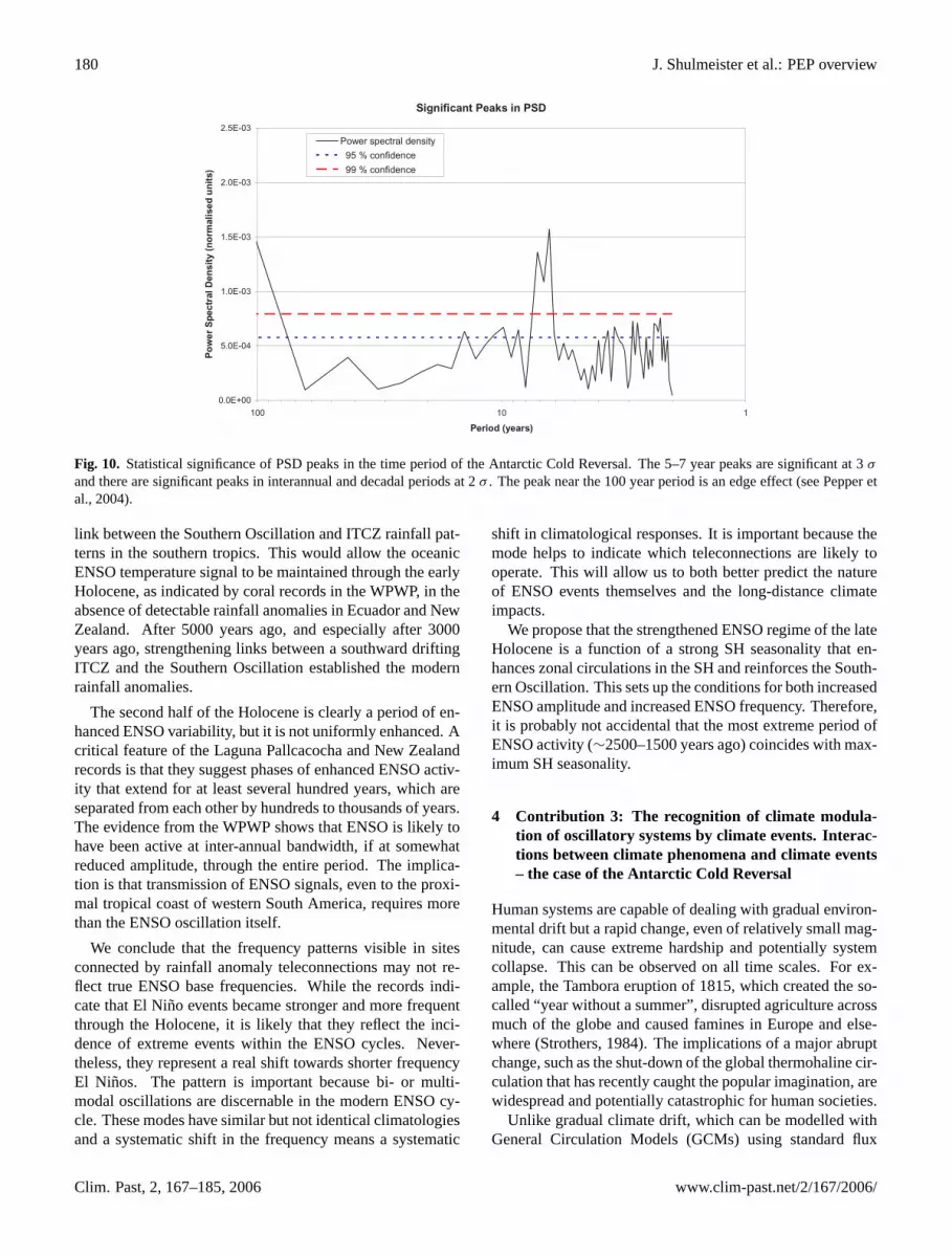
Fig. 10. Statistical significance of PSD peaks in the time period of the Antarctic Cold Reversal. The 5–7 year peaks are significant at 3σ

and there are significant peaks in interannual and decadal periods at 2σ . The peak near the 100 year period is an edge effect (see Pepper etal., 2004).

link between the Southern Oscillation and ITCZ rainfall pat-terns in the southern tropics. This would allow the oceanicENSO temperature signal to be maintained through the earlyHolocene, as indicated by coral records in the WPWP, in theabsence of detectable rainfall anomalies in Ecuador and NewZealand. After 5000 years ago, and especially after 3000years ago, strengthening links between a southward driftingITCZ and the Southern Oscillation established the modernrainfall anomalies.

The second half of the Holocene is clearly a period of en-hanced ENSO variability, but it is not uniformly enhanced. Acritical feature of the Laguna Pallcacocha and New Zealandrecords is that they suggest phases of enhanced ENSO activ-ity that extend for at least several hundred years, which areseparated from each other by hundreds to thousands of years.The evidence from the WPWP shows that ENSO is likely tohave been active at inter-annual bandwidth, if at somewhatreduced amplitude, through the entire period. The implica-tion is that transmission of ENSO signals, even to the proxi-mal tropical coast of western South America, requires morethan the ENSO oscillation itself.

We conclude that the frequency patterns visible in sitesconnected by rainfall anomaly teleconnections may not re-flect true ENSO base frequencies. While the records indi-cate that El Nino events became stronger and more frequentthrough the Holocene, it is likely that they reflect the inci-dence of extreme events within the ENSO cycles. Never-theless, they represent a real shift towards shorter frequencyEl Ninos. The pattern is important because bi- or multi-modal oscillations are discernable in the modern ENSO cy-cle. These modes have similar but not identical climatologiesand a systematic shift in the frequency means a systematic

shift in climatological responses. It is important because themode helps to indicate which teleconnections are likely tooperate. This will allow us to both better predict the natureof ENSO events themselves and the long-distance climateimpacts.

We propose that the strengthened ENSO regime of the lateHolocene is a function of a strong SH seasonality that en-hances zonal circulations in the SH and reinforces the South-ern Oscillation. This sets up the conditions for both increasedENSO amplitude and increased ENSO frequency. Therefore,it is probably not accidental that the most extreme period ofENSO activity (∼2500–1500 years ago) coincides with max-imum SH seasonality.

4 Contribution 3: The recognition of climate modula-tion of oscillatory systems by climate events. Interac-tions between climate phenomena and climate events– the case of the Antarctic Cold Reversal

Human systems are capable of dealing with gradual environ-mental drift but a rapid change, even of relatively small mag-nitude, can cause extreme hardship and potentially systemcollapse. This can be observed on all time scales. For ex-ample, the Tambora eruption of 1815, which created the so-called “year without a summer”, disrupted agriculture acrossmuch of the globe and caused famines in Europe and else-where (Strothers, 1984). The implications of a major abruptchange, such as the shut-down of the global thermohaline cir-culation that has recently caught the popular imagination, arewidespread and potentially catastrophic for human societies.

Unlike gradual climate drift, which can be modelled withGeneral Circulation Models (GCMs) using standard flux



equations and modern boundary conditions, changes in sys-tem mode will not (normally) fall out of climate models.The only real strategy to predict mode changes is to examinethe history of climate systems from the paleo-record, to seewhether and how the system has behaved in the recent geo-logical past. Some syatem changes over the last 20 000 yearsare now becoming well recognized, in particular the late-last glaciation abrupt cooling known as the Younger Dryas,and oscillatory changes such as Dansgaard-Oescher events.Recognition of these events allows us to estimate the direc-tion and extent of change possible in climate systems. It alsomay allow us to identify the trigger, which gives us the po-tential for managing some of the changes. As the quality anddensity of paleo-records improves we are also beginning torecognise the global teleconnections linked to climate changeevents and can make useful, if still unquantified statementsabout far-field effects of change. Here we present one ex-ample, the Antarctic Cold Reversal (ACR) where the climatelink between a change in one region (coastal Antarctica) andits effect in another (New Zealand) can be demonstrated.

4.1 The Antarctic Cold Reversal in the New Zealand record

In Sect. 2.3.2 we highlighted a maar lake record from theAuckland region, New Zealand, that demonstrates strongENSO-like periodicities (Pepper et al., 2004). Within thatrecord the transition from the last glaciation to the present in-terglaciation presents a clear story. For most of the deglacia-tion, there is no evidence of strong inter-annual variabilityin the Auckland region. During two brief interludes, how-ever, strong inter-annual variability at a 7 year ENSO pe-riodicity is observed and is statistically significant (Fig. 10).The younger of these two events aligns well with the onset ofthe Antarctic Cold Reversal between 14 800 and 14 500 yearsago (Jouzel et al., 1995; Blunier et al., 1997). The durationof the event is much shorter than the ACR, lasting about 150years as opposed to the 1700 years of the ACR. Neverthe-less the coincidence of the timing of initiation is compelling.Furthermore, there is a strong ACR record from the oceanoff New Zealand (Carter et al., 2003) and it shows up interrestrial paleoecological records (e.g. Turney et al., 2003;McGlone et al., 2004).

The ACR manifests itself in Antarctica as a cool anomalyrecorded in the oxygen isotope ratios of ice formed at∼14 800 years ago. Simplistically, a decrease in tempera-tures in the Antarctic margin would be expected to increasethe speed of the zonal westerlies to the north by increasingthe thermal (pressure) contrast between the polar region andthe surrounding ocean. A general increase in westerly cir-culation at southern mid-latitudes would be expected. Thisis observed from the Auckland record. The individual lami-nae in the maar records are interpreted as annual and reflectaeolian flux to the maar under zonal south-westerly flows.During the ACR event the laminae are significantly thickerthan at any other time since the LGM (Fig. 8). In short the

general pattern of the Auckland record is compatible with asimplistic predicted change in westerly wind strength underAntarctic cooling.

The additional factor is the apparent enhancement of anENSO signal in the New Zealand region during this event.ENSO has been identified as an important driver of Antarcticclimate change on inter-annual to decadal scales (e.g. Kwokand Comiso, 2002). Under modern conditions, ENSO tele-connections exist between New Zealand and the Antarc-tic. Links between ENSO warm events in the South Pa-cific and impacts in Antarctica have been recognised, partlythrough the mechanism of blocking highs hindering migra-tion of the Amundsen Sea Low (Renwick, 1998; Bertler etal., 2004). The connections are also interlinked with vari-ability in the Antarctic Oscillation (e.g. Fogt and Bromwich,2006; L’Heureux and Thompson, 2006). The position (or ab-sence) of blocking systems in the South Pacific and easternAustralia, in turn, control the zonal flows over New Zealandduring ENSO events (and at other times). This relationshipis, however, both seasonal and non-stationary. In the RossSea, the regional climate shows a significant positive ENSOcorrelation during the last decade whereas no significant cor-relation is observed in the decade from 1971–1980 (Bertleret al., 2004).

Since the Antarctic is not the source area for ENSO, we donot suggest that ENSO actually switches on during the ACR.Rather, we infer that circulation changes associated with theACR event amplified an existing ENSO signal in the NewZealand region. This occurred through an enhancement ofzonal wind flows that magnified the signal sufficiently for itto become visible through primary production in the Auck-land maar.

This type of study provides insight into the climatology ofa teleconnection for a climate change event. The El Nino-style anomaly can be projected out of the NZ region usingmodern climatologies to provide a testable prediction of re-gional responses to the ACR. These predictions can be testedby further paleoclimate studies in other regions. However, itis likely that only high temporal resolution paleoclimate re-search will be capable of providing insights into how globalclimate change is transmitted.

5 Conclusions

The PEP projects of PANASH have extended our understand-ing of past climate change. The main messages from thispaper are:

1) Low resolution records provide information on chang-ing background states on which ENSO, the monsoons andother climate phenomena are superimposed. This is a criti-cal underpinning for the higher resolution studies. In addi-tion, as we move towards higher precision, numerical, recon-structions of climate parameters we need the verification thatbroad reconstructions provide. Many of these low resolution



records provide a higher reliability than the numerical re-constructions. The presence of tree stumps in growth po-sition, for example, guarantees that local conditions werefavourable enough for trees to grow. Such high reliabilityindicators greatly reinforce the inferences from numerical re-constructions.

The need for ongoing basic research is highlighted by thefact that although very significant advances have been madein the understanding of past climate systems, we cannot yetdefine the basic patterns of past climate change accurately.We cannot even hope to reconstruct global impacts of cli-mate change if we have very intermittent coverage of theglobe. We note particular data deficiencies over much of theSH, the oceans and Africa. We have highlighted this predica-ment by demonstrating that one of the better studied periods,the transition from the Last Glaciation Maximum to the cur-rent Interglaciation can be re-interpreted in the light of recentpaleo-climate finds. We cannot even specify with confidencewhether the post LGM warming initiates at one of the Polesor the equator.

2) There is a real need for annually resolved paleoclimaterecords. This paper has highlighted the rapid growth in ourunderstanding of the geological history of ENSO. The stud-ies that have provided this insight are annual in resolution,or higher, because only these studies can examine the phe-nomenon. In fact, the increase in understanding reduces ourability to make simple statements about the phenomenon. Itis our view that the core ENSO system probably operatescontinuously through the Holocene but that teleconnectionsthrough precipitation and other anomalies are non-stationaryon centennial and millennial scales. Major changes in cli-mate can occur without ENSO switching on or off. Thechange in frequency and the possible relationship of thischange to insolation forcing is also important, both becauseit affects regional climate responses and because the geo-logical observations allow models of climate change to betested against real data. The better we know the history ofthe climate systems, the better our hope of predicting cli-mate change and subsequently managing environmental con-sequences.

With respect to annual records, bioturbation of sea-floorsediments is a particular problem. While in earlier stud-ies the relatively high resolution (centennial scale) from ma-rine cores gave a comparative advantage over the availablediscontinuous terrestrial records, the situation is slowly re-versing. Ice core, laminated lake, dendro- and speleothemrecords all allow quasi-annual resolution on land. We needannual resolution to examine climatic phenomena, such asENSO, which cannot be examined in centennial resolutionrecords. There is an urgent need to identify higher resolu-tion marine records that can actually see these signals. Otherthan coral proxies, only a handful of records from anoxicsites (e.g. Rein et al., 2005) can actually be used to examinethese types of change.

3) “Rates of change” is one of the critical pieces of the jig-saw that paleoclimate studies can provide. The risk of abruptclimate change is recognised as very important and inher-ently difficult for future climate change prediction (Watsonet al., 2001). Human systems are quite adaptable to changeso long as it is gradual and predictable. The same systemsmay collapse under even moderate change scenarios if therate of change is too great. Paleoclimate work is the onlyreliable tool to evaluate how fast natural systems can change.

The observation of interactions between abrupt climatephenomena and oscillatory systems requires well-dated highresolution paleoclimatic records. Thus far paleoclimate workhas allowed us to recognise that abrupt climate changes haveoccurred and to specify some aspects of the change in thecore affected regions. Paleoclimate work needs to extendto examining the teleconnections between the abrupt phe-nomena and distal climates. The importance of distal re-sponses to abrupt change has been recognised for some time(e.g. Broecker, 2000) but it is only with the proliferation ofquasi-annual resolution records that we can start to recognisethe climatic processes involved in the teleconnections them-selves.

4) Modelling work provides the global view and improvesour understanding by giving insights into the processes con-trolling climate change. Paleo-data provide both verificationfor model runs and in some instances the data and ideas togenerate the model scenarios. Modelling provide us with thedynamic reconstructions of past climates and the ability toexamine teleconnections. It gives us the ability to turn re-constructions of local climates into powerful tools for pre-dicting future climate change and managing environmentalconsequences.

Acknowledgements.We dedicate this paper to the memory ourcolleague and friend G. O. Seltzer, long-time leader of the PEPIproject and a major player in much of the science presented inthis paper. J. Shulmeister acknowledges Marsden Grant UOC301and University of Canterbury internal grant U6508 for supportof glacial work and PGSF grant VIC-009 for paleolimnologicalinvestigations. He thanks the Department of Geosciences, IdahoState University and the RMAP programme RSPAS, AustralianNational University for hospitality and facilities while writing thispaper during a sabbatical visit. D. Rodbell acknowledges NSFgrants EAR9418886 and ATM-9809229 for support of his workin the tropical Andes. M. K. Gagan acknowledges AustralianResearch Council grant DP0342917 for support of his work inthe west Pacific Warm Pool region. We thank D. Nobes for helpwith the Onepoto spectral analyses and the anonymous referees fortheir comments that have resulted in a significantly tightened finalmanuscript.

Edited by: T. Kiefer

References

Abbott, M. B., Wolfe, B. B., Wolfe, A. P., Seltzer, G. O., Ar-avena, R., Mark, B. G., Polissar, P. J., Rodbell, D. T., Rowe,



H. D., and Vuille, M.: Holocene Paleohydrology and glacial his-tory of the central Andes using multiproxy lake sediment studies,Palaeogeography, Palaeoclimatology, Palaeoecology, 194, 123–138, 2003.

Alley, R. B., Brook, E. J., and Anandakrishna, S.: A northern leadin the orbital band: North-south phasing of Ice-Age events, Qua-ternary Science Reviews, 21, 431–441, 2002.

An, S.-I. and Wang, B.: Interdecadal change of the structure ofENSO mode and its impact on ENSO frequency, J. Clim., 13,2044–2055, 2000.

Barrows, T. T. and Juggins, S.: Sea-surface temperatures aroundthe Australian margin and Indian Ocean during the Last GlacialMaximum, Quaternary Science Reviews, 24, 1017–1047, 2005.

Barrows, T. T., Stone, J. O., Fifield, L. K., and Cresswell, R.G.: Late Pleistocene glaciation of the Kosciusko Massif, SnowyMountains, Australia, Quaternary Research, 55, 179–189, 2001.

Barrows, T. T., Stone, J. O., Fifield, L. K., and Cresswell, R. G.:The timing of the last glacial maximum in Australia. QuaternaryScience Reviews, 21, 159–173, 2002.

Battarbee, R., Gasse, F., and Stickley, C.: Past Climate Variabilitythrough Europe and Africa, Kluwer, 610p., 2004.

Berger, A.: IGBP PAGES/World Data Center-A for Paleoclimatol-ogy Data Contribution Series # 92-007, 1992.

Bertler, N. A. N., Barrett, P. J., Mayewski, P. A., Fogt, R. L., Kreutz,K. J., and Shulmeister, J.: El Nino suppresses Antarctic warming,Geophys. Res. Lett., 31, L15207, doi:10.1029/2004GL020749,2004.

Blunier, T., Schwander, J., Stauffer, B., Stocker, T., Dallenbach,A., Indermuhle, A., Tschumi, J., Chappelaz, J., Raynaud, D.,and Barnola, J.-M.: Timing of the Antarctic Cold Reversal andthe atmospheric CO2 increase with respect to the Younger Dryasevent, Geophys. Res. Lett., 24, 2683–2686, 1997.

Broecker, W. S.: Abrupt climate change:causal constraints providedby the paleoclimate record, Earth Sci. Rev., 51, 137–154, 2000.

Broecker, W. S. and Denton, G. H.: The role of ocean-atmospherereorganizations in glacial cycles, Geochim. Cosmochim. Acta,53, 2465–2501, 1989.

Cane, M. A.: The evolution of El Nino, past and future, EarthPlanet. Sci. Lett., 230, 227–240, 2005.

Carter, L., Manighetti, B., and Neil, H.: From icebergs to pon-gas: Antarctica’s ocean link with New Zealand, Water and At-mosphere online, 11, 30–31, 2003.

Clapperton, C. M.: Glacial Geomorphology, Quaternary glacial se-quence and paleoclimatic inferences in the Ecuadoran Andes, In-ternational Geomorphology, Proceedings 1st conference 2, 843–870, 1986.

Clement, A. C., Seager, R., and Cane, M. A.: Orbital controls onthe El Nino/Southern Oscillation and the tropical climate, Pale-ooceanography, 14, 441–456, 1999.

Denton, G. H. and Hendy, C. H.: Younger Dryas age advance ofFranz Josef Glacier in the Southern Alps of New Zealand, Sci-ence, 264, 1434–1437, 1994.

Diaz, H. F. and Markgraf, V.: El Nino, Historical and Paleoclimateaspects of the Southern Oscillation, Cambridge University Press,1992.

Dodson, J. R.: Timing and response of vegetation change to Mi-nankovitch forcing in temperate Australia and New Zealand,Global Planet. Change, 18, 161–174, 1998.

Dodson, J., Taylor, D., Ono, Y., and Wang, P.: Climate, Human

and Natural Systems of the PEP II Transect, Quaternary Interna-tional, 118–119, 1–203, 2004.

Federov, A. V. and Philander, S. G.: Is El Nino changing?, Science,288, 1997–2002, 2000.

Fitzharris, B. B., Hay, J. E., and Jones, P. D.: Behaviour of NewZealand glaciers and atmospheric circulation changes over thepast 130 years, Holocene, 2, 97–106, 1992.

Fogt, R. L. and Bromwich, D. H.: Decadal variability of the ENSOteleconnection to the High-Latitude South Pacific Governed byCoupling with the Southern Annular Mode, J. Clim., 19, 979–997, 2006.

Gagan, M. K., Hendy, E. J., Haberle, S. G., and Hantoro, W. S.:Post-glacial evolution of the Indo-Pacific Warm Pool and ElNino-Southern Oscillation, Quaternary International, 118–119,127–143, 2004.

Gordon, N. D.: The Southern Oscillation: A New Zealand perspec-tive, Journal of the Royal Society of New Zealand, 15, 137–155,1985.

Grootes, P. M. and Stuiver, M.: Oxygen 18/16 variability in Green-land snow and ice with 10-3- to 105-year time resolution, J. Geo-phys. Res., 102(C12), 26 455–26 470, 1997.

Hendy, E. J., Gagan, M. K., and Lough, J. M.: Chronological con-trol of coral records using luminescent lines and evidence fornon-stationary ENSO teleconnections in northeast Australia, TheHolocene, 13, 187–199, 2003.

Holmgren, K., Lee-Thorp, J. A., Cooper, G. R. J., Lundblad, K.,Partridge, T. C., Scott, L., Sithaldeen, R., Siep Talma, A., andTyson, P. D.: Persistent millennial-scale climatic variability overthe past 25,000 years in Southern Africa, Quaternary Science Re-views, 22, 2311–2326, 2003.

Hooker, B. L. and Fitzharris, B. B.: The correlation between cli-matic parameters and the retreat and advance of Franz JosefGlacier, New Zealand, Global Planet. Change, 22, 39–48, 1999.

Horrocks, M., Augustinus, P., Deng, Y., Shane, P., and Anderson,S.: Holocene vegetation, environment and tephra recorded fromLake Pupuke, Auckland, New Zealand, New Zealand Journal ofGeology and Geophysics, 48, 85–94, 2005.

Haug, G. H., Hughen, K. A., Sigman, D. M., Peterson, L. C., andRohl, U.: Southward migration of the intertropical convergencezone through the Holocene, Science, 293, 1304–1308, 2001.

Indermuhle, A., Monnin, E., Stauffer, B., and Stocker, T. F.: Atmo-spheric CO2 concentration from 60 to 20 kyr BP from the TaylorDome ice core, Antarctica, Geophys. Res. Lett., 27, 735–738,2000.

Jouzel, J., Vaikmae, R., Petit, J. R., et al.: The two step shape andtiming of the last deglaciation in Antarctica, Climate Dynamics,11, 151–161, 1995.

Kaplan, M. R., Ackert Jr., R. P., Singer, B. S., Douglass, D. C.,and Kurz, M. D.: Cosmogenic nuclide chronology of millennial-scale glacial advances during O-isotope stage 2 in Patagonia,GSA Bulletin, 116, 308–321, 2004.

Kiernan, K., Fifield, L. K., and Chappell, J.: Cosmogenic nu-clide ages for Last Glacial Maximum moraine at Schnells Ridge,Southwest Tasmania, Quaternary Research, 61, 335–338, 2004.

Kwok, R. and Comiso, J. C.: Southern Ocean climate and sea iceanomalies associated with the Southern Oscillation, J. Clim., 15,487–501, 2002.

Lamy, F., Hebbeln, D., and Wefer, G.: High resolution marinerecord of climatic change in mid-latitude Chile during the last



28,000 years based on terrigenous sediment parameters, Quater-nary Research, 51, 83–93, 1999.

Lau, K.-M. and Sheu, P. J.: Annual cycle, quasi-biennial oscilla-tion, and Southern Oscillation in global precipitation, J. Geo-phys. Res., 93, 10 975–10 988, 1988.

L’Heureux, M. L. and Thompson, D. W. J.: Observed Relationshipsbetween the El Nino-Southern Oscillation and the ExtratropicalZonal-Mean Circulation, J. Clim., 19, 276–287, 2006.

Liu, Z., Kutzbach, J., and Wu, L.: Modeling climatic shift of ElNino variability in the Holocene, Geophys. Res. Lett., 27, 2265–2268, 2000.

Lowell, T. V., Heusser, C. J., Andersen, B. G., Moreno, P. I., Hauser,A., Heusser, L. E., Schluchter, C., Marchant, D. R., and Denton,G. H.: Interhemispheric correlation of Late Pleistocene glacialevents, Science, 269, 1541–1549, 1995.

Mark, B., Seltzer, G., Rodbell, D., and Goodman, A.: Rates ofDeglaciation during the Last Glaciation and Holocene in theCordillera Vilcanota-Quelccaya Ice Cap Region, Southeastern,Peru, Quaternary Research, 57, 287–298, 2002.

Mark, B. G. and Helmens, K. F.: Reconstruction of glacierequilibrium-line altitudes for the last glacial maximum on theHigh Plain of Bagota region, eastern cordillera, Colombia: To-pographic and Climatic Implications, Journal of Quaternary Sci-ence, 20, 789–800, 2005.

Markgraf, V.: Interhemispheric Climate Linkages, Academic Press,454 p., 2001.

Marra, M. J., Smith, E. G. C., Shulmeister, J., and Leschen, R.:Late Quaternary climate change from the Awatere Valley, SouthIsland, New Zealand using the maximum likelihood envelopemethod, Quaternary Science Reviews, 23, 1637–1650, 2004.

Marra, M. J., Shulmeister, J., and Smith, E. C. G.: Reconstruct-ing temperature during the Last Glacial Maximum from LyndonStream, South Island, New Zealand using beetle fossils and max-imum likelihood envelopes, Quaternary Science Reviews, 25,1841–1849, 2006.

McGlone, M. S.: Late glacial landscape and vegetation change andthe Younger Dryas climatic oscillations in New Zealand, Quater-nary Science Reviews, 14, 867–881, 1995.

McGlone, M. S., Turney, C. S. M., and Wilmshurst, J. M.: Late-glacial and Holocene vegetation and climatic history of the CassBasin, central South Island, New Zealand, Quaternary Research,62, 267–279, 2004.

McGregor, H. V. and Gagan, M. K.: Western Pacific coralδ18O records of anomalous Holocene variability in the ElNino-Southern Oscillation, Geophys. Res. Lett., 31, L11204,doi:10.1029/2004GL019972, 1–4, 2004.

Mercer, J. H.: Simultaneous climatic change in both hemispheresand similar bipolar interglacial warming: Evidence and implica-tions, in: Climate Processes and Climate Sensitivity, edited by:Hansen, H. and Takahashi, T., American Geophysical Union, pp.307–313, 1984.

Mix, A. C., Bard, E., and Schneider, R.: Environmental processesof the ice age: land, oceans, glaciers (EPILOG), Quaternary Sci-ence Reviews, 20, 627–657, 2001.

Moy, C. M., Seltzer, G. O., Rodbell, D. T., and Anderson, D. M.:Variability of El Nino/Southern Oscillation activity at millennialtimescales during the Holocene epoch, Nature, 420, 162–165,2002.

Mullan, A. B.: On the linearity and stability of southern oscillation-

climate relationships for New Zealand, Int. J. Climatol., 15,1365–1386, 1995.

Nelson, C. S., Hendy, C. H., Jarrett, G. R., and Cuthbertson, A.M.: Near-synchroneity of New Zealand alpine glaciations andNorthern Hemisphere continental glaciations during the past 750kyr, Nature, 318, 361–363, 1985.

Ono, Y., Shulmeister, J., Lemkuhle, F., Asahi, K., and Aoki, T.:Timing and causes of glacial advances in the PEP 2 transect (EastAsia to Antarctica) during the last glaciation cycle, QuaternaryInternational, 118/119, 55–68, 2004.

Pepper, A. C.: Late Quaternary climate records using laminatedlake sediments from an Auckland Maar Crater (Onepoto Maar),New Zealand, unpublished MSc thesis University of Canterbury,2003.

Pepper, A. C., Shulmeister, J., Nobes, D. C., and Augustinus, P. C.:Possible ENSO signals prior to the last Glacial Maximum, duringthe deglaciation and the early Holocene from New Zealand, Geo-phys. Res. Lett., 31, L15206, 1–4, doi:10.1029/2004GL020236,2004.

Petit, J. R., Jouzel, J., Raynaud, D., Barkov, N. I., Barnola, J.-M.,Basile, I., Benders, M., Chappelaz, J., Davis, M., Delaygue, G.,Delmotte, M., Kotlyakov, V. M., Legrand, M., Lipenkov, V. Y.,Lorius, C., Pepin, L., Ritz, C., Satzman, E., and Stievenard, M.:Climate and atmospheric history of the past 420,000 years fromthe Vostok ice core, Antarctica, Nature, 3999, 429–436, 1999.

Porter, S. C.: Equilibrium-Line altitudes of Late QuaternaryGlaciers in the Southern Alps, New Zealand, Quaternary Re-search, 5, 27–47, 1975.

Porter, S. C.: Snowline depression in the tropics durning the LastGlaciation, Quaternary Science Reviews, 20, 1067–1091, 2001.

Quinn, W. H., Neal, V. T., and Antinez de Mayolo, S.: El Ninooccurrences over the past four and a half centuries, J. Geophys.Res., 92, 14 449–14 461, 1987.

Rasmussen, S. O., Andersen, K. K., Svensson, A. M., Steffensen,J. P., Vinther, B. M., Clausen, H. B., Siggaard-Andersen, M.-L., Johnsen, S. J., Larsen, L. B., Dahl-Jensen, D., Bigler,M., Rothlisberger, R., Fischer, H., Goto-Azuma, K., Hans-son, M. E., and Ruth, U.: A new Greenland ice core chronol-ogy for the last termination, J. Geophys. Res., 111, D06102,doi:10.1029/2005JD006079, 2006.

Rasmussen, E. M. and Carpenter, T. H.: Variations in tropical seasurface temperature and surface wind fields associated with theEl Nino/Southern Oscillation, Monthly Weather Review, 110,354–384, 1982.

Rein, B., Luckge, A., Reinhardt, L., Sirocko, F., Wolf, A., andDullo, W.-C.: El Nino variability off Peru during the last 20,000years, Paleooceanography, 20, doi:10.1029/2004PA001099,2005.

Renwick, J. A.: ENSO-related variability in the frequency of SouthPacific blocking, Monthly Weather Review, 126, 3117–3123,1998.

Rodbell, D. T.: Late Pleistocene equilibrium-line altitude recon-structions in the northern Peruvian Andes, Boreas, 21, 43–52,1992.

Rodbell, D. T., Seltzer, G. O., Anderson, D. M., Abbott, M. B.,Enfield, D. B., and Newman, J. H.: An∼15,000-year record of ElNino-driven alluviation in southwestern Ecuador, Science, 283,516–520, 1999.

Rodbell, D. T. and Seltzer, G. O.: Rapid Ice Margin Fluctuations



During the Younger Dryas in the Tropical Andes, Quaternary Re-search, 54, 328–338, 2000.

Ropelewski, C. F. and Halpert, M. S.: Global and regional scaleprecipitation patterns associated with the El Nino/Southern Os-cillation, Monthly Weather Review, 115, 1606–1626, 1987.

Rother, H. and Shulmeister, J.: Synoptic climate change as a driverof late Quaternary glaciations in the mid-latitudes of the South-ern Hemisphere, Clim. Past, 2, 11–19, 2006,http://www.clim-past.net/2/11/2006/.

Sandiford, A., Newnham, R. M., Alloway, B. V., and Ogden, J.: A28 000 – 7600 cal yr BP pollen record of vegetation and climatechange from Pukaki Crater, northern New Zealand, Palaeogeog-raphy, Palaeoclimatology, Palaeoecology, 201, 235–247, 2003.

Sandweiss, D. H., Maasch, K. A., Burger, R. L., Richardson III, J.B., Rollins, H. B., and Clement, A.: Variation in Holocene ElNino frequencies: Climate records and cultural consequences inancient Peru, Geology, 29, 603–606, 2001.

Scott, L.: A Late Quaternary pollen record from the Transvaalbushveld, South Africa, Quaternary Research, 17, 339–370,1982.

Seltzer, G. O.: A lacustrine record of late-Pleistocene climaticchange in the subtropical Andes, Boreas, 23, 105–111, 1994.

Seltzer, G. O., Rodbell, D. T., Baker, P. A., Fritz, S. C., Tapia, P.M., Rowe, H. D., and Dunbar, R. B.: Early warming of tropicalSouth America at the last glacial-interglacial transition, Science,296, 1685–1686, 2002.

Setoh, T., Imawaki, S., Ostrovskii, A., and Umatani, S.-I.: Inter-decadal variations of ENSO signals and annual cycles revealedby wavelet analysis. Journal of Oceanography, 55, 385–394,1999.

Shulmeister, J.: Australasian evidence for mid-Holocene climatechange implies precessional control of Walker Circulation in thePacific, Quaternary International, 57/58, 81–91, 1999.

Shulmeister, J. and Dodson, J. (Eds.): Late Quaternary climatechange in the New Zealand Region, Special Issue Global Planet.Change, 33(3–4), 205–362, 2002.

Shulmeister, J. and Lees, B. G.: Pollen evidence from tropical Aus-tralia for the onset of an ENSO-dominated climate at c. 4000 BP,The Holocene, 5, 10–18, 1995.

Shulmeister, J., Goodwin, I., Renwick, J., Harle, K., Armand, L.,McGlone, M. S., Cook, E., Dodson, J., Hesse, P. P, Mayewski,P., and Curran, M.: The Southern Hemisphere Westerlies in theAustralasian sector during the last glaciation cycle: A synthesis,Quaternary International, 118/119, 23–53, 2004.

Shulmeister, J., Fink, D., and Augustinus, P. C.: A cosmogenic nu-clide chronology of the last glacial transition in North-West Nel-son, New Zealand – new insights in Southern Hemisphere cli-mate forcing during the last deglaciation, Earth Planet. Sci. Lett.,233, 455–466, 2005.

Smith, J. A., Seltzer, G. O., Farber, D. L., Rodbell, D. T., and Finkel,R. C.: Early local last glacial maximum in the tropical Andes,Science, 308, 678–680, 2005a.

Smith, J. A., Seltzer, G. O., Rodbell, D. T. and Kline, A. G.: Re-gional synthesis of last glacial maximum snowlines in the trop-ical Andes, South America, Quaternary International, 138–139,145–167, 2005b.

Soons, J. M. and Gullentops, F. W.: Glacial advances in the RakaiaValley, New Zealand, New Zealand Journal of Geology and Geo-physics, 16, 425–438, 1973.

Steig, E. J. and Alley, R. B.: Phase relationships between Antarcticand Greenland climate records, Annals of Glaciology, 35, 451–456, 2002.

Strothers, R. B.: The great Tambora eruption of 1815 AD and itsaftermath, Science, 224, 1191–1198, 1984.

Stocker, T. F.: Past and future reorganisations in the Climate Sys-tem, Quaternary Science Reviews, 19, 301–319, 2000.

Suggate, R. P.: Late Pliocene and Quaternary glaciations of NewZealand, Quaternary Science Reviews, 9, 175–194, 1990.

Suggate, R. P. and Almond, P. C.: The Last Glacial Maximum(LGM) in western South Island, New Zealand: Implications forthe global LGM and MIS 2, Quaternary Science Reviews, 24,1923–1940, 2005.

Tomita, T. and Yasunari, T.: On the two types of ENSO, Journal ofthe Meteorological Society of Japan, 71, 273–283, 1993.

Thompson, L. G., Mosley-Thompson, E., Davis, M. E., Lin, P. -N.,Henderson, K. A., Cole-Dai, J., Bolzan, J. F., and Liu, K.-B.:Late glacial stage and Holocene tropical ice core records fromHuascaran, Peru, Science, 269, 46–50, 1995.

Tudhope, A. W., Chilcott, C. P., McCulloch, M. T., Cook, E., Chap-pell, J., Ellam, R. M., Lea, D. W., Lough, J. M., and Shimmield,G. B.: Variability in the El Nino-Southern Oscillation through aglacial-interglacial cycle, Science, 291, 1511–1517, 2001.

Turney, C. S. M., McGlone, M. S., and Wilmshurst, J. M.: Asyn-chronous climate change between New Zealand and the NorthAtlantic during the last deglaciation, Geology, 31, 223–226,2003.

Tyson, P. D., Sturman, A. P., Fitzharris, B. B., Mason, S. J., andOwens, I. F.: Circulation changes and teleconnections betweenglacial advances on the west coast of New Zealand and extendedspells of drought years in South Africa, Int. J. Climatol., 17,1499–1512, 1997.

Vandergoes, M. J., Newnham, R. M., Preusser, F., Hendy, C. H.,Lowell, T. V., Fitzsimons, S. J., Hogg, A. G., Kasper, H. U., andSchluchter, C.: Regional insolation forcing of late Quaternaryclimate change in the Southern Hemisphere, Nature, 436, 242–246, 2005.

Wardle, P. W.: Variations of glaciers of Westland National Parkand the Hooker Range, New Zealand, New Zealand Journal ofBotany, 11, 349–388, 1973

Watson, R. T. and the Core Writing Team (Eds.): Climate Change2001: Synthesis Report, IPCC, Geneva, 184 p., 2001.

Williams, P. W.: A 230 ka record of glacial and interglacial eventsfrom Aurora Cave, Fiordland, New Zealand, New Zealand Jour-nal of Geology and Geophysics, 39, 225–241, 1996.

Williams, P. W., King, D. N. T., Zhao, J.-X., and Collerson, K.D.: Late Pleistocene to Holocene composite speleothem18O and13C chronologies from South Island, New Zealand-did a globalYounger Dryas really exist?, Earth Planet. Sci. Lett., 230, 301–317, 2005.

Woodroffe, C. D. and Gagan, M. K.: Coral microatolls from thecentral Pacific record late Holocene El Nino, Geophys. Res.Lett., 27, 1511–1514, 2000.

Woodroffe, C. D., Beech, M. R., and Gagan, M. K.: Mid-late Holocene El Nino variability in the equatorial Pa-cific from coral microatolls, Geophys. Res. Lett., 30, 1358,doi:10.1029/2002GL015868, 2002.


http://www.clim-past.net/2/11/2006/

inter-hemispheric linkages in climate change: paleo-perspectives for

Documents