INSTITUTE FOR PRIVATE CAPITAL WORKING PAPER

December, 2016

Finding Fortune: How Do Institutional Investors Pick Asset Managers?

Finding Fortune: How Do Institutional Investors Pick Asset Managers?I

Gregory W. Brown∗, Oleg Gredil∗∗, Preetesh Kantak∗

Abstract

This paper studies how professional asset allocators such as endowments, fund-of-funds, or pension fundsselect fund managers for investments. We develop a simple model of their due-diligence process to motivatepredictions about the timing of investment decisions. We then test these predictions using a unique datasetwith detailed information on the interactions between a large institutional investor and 1,093 hedge fundsover the course of 8 years. Soft information conveyed during the meetings with fund managers stronglyinfluences the decisions. A one standard deviation increase in our proxy for positive soft information doublesthe probability of fund selection and reduces the due-diligence time by 20%. Contrary to prior research, wefind no evidence that relying on these subjective judgements is wasteful. Instead, in a matched sample,conditioned on the fund characteristics and past performance, the 12-month average peer-adjusted returnsare 1.5% higher for the selected funds.

Keywords: Asset Management, Institutional Investors, Hedge Funds, Portfolio Choice

JEL Classification: G11, G23

IFirst version: November 18, 2015; This version: March 15, 2016∗University of North Carolina at Chapel Hill, Kenan-Flagler Business School, gregwbrown@unc.edu, (919) 962-9250 and

preetesh kantak@unc.edu∗∗Tulane University, Freeman School of Business, ogredil@tulane.edu, (504) 314-7567

Helpful comments and suggestions were provided by Diego Garcia and Yasser Boualam. All errors are our own.

Finding Fortune: How Do Institutional Investors Pick Asset Managers?

Abstract

This paper studies how professional asset allocators such as endowments, fund-of-funds, or pension fundsselect fund managers for investments. We develop a simple model of their due-diligence process to motivatepredictions about the timing of investment decisions. We then test these predictions using a unique datasetwith detailed information on the interactions between a large institutional investor and 1,093 hedge fundsover the course of 8 years. Soft information conveyed during the meetings with fund managers stronglyinfluences the decisions. A one standard deviation increase in our proxy for positive soft information doublesthe probability of fund selection and reduces the due-diligence time by 20%. Contrary to prior research, wefind no evidence that relying on these subjective judgements is wasteful. Instead, in a matched sample,conditioned on the fund characteristics and past performance, the 12-month average peer-adjusted returnsare 1.5% higher for the selected funds.

1. Introduction

In the U.S. alone, over $15 trillion in assets are allocated by institutional asset managers such as pensions

funds, insurance companies, endowments, funds-of-funds, and foundations. Investment of their assets is

delegated to managers of traditional long-only investment strategies in equity and fixed income markets.

But, increasingly allocations include ‘alternatives’ such as hedge funds and private equity funds which are

allowed substantial discretion in determining specific investments. Overall, the vast majority of delegated

asset management involves active investment strategies.1 The past 20 years has seen substantial growth in

all types of delegated asset management (including traditional “40-Act” mutual funds in the U.S.), but the

growth in delegated asset management by institutional investors has been more than twice as large.2 Despite

the enormous size of the market for delegated asset management among institutional investors, often referred

to as “allocators”, relatively little is known about the process by which these institutions make decisions.

This paper seeks to provide a framework for better understanding the allocator’s problem and investigates

the specific process for choosing funds of a long-short equity portfolio for a large institutional investor.

While there is a mature literature examining the optimal contract between investment principal and asset

manager, few papers examine how the principals allocate capital among investment managers (henceforth

“fund managers“) in less abstract settings. Institutional allocators appear to hire and fire managers based on

1 See, for example, Standard and Poors’ Money Market Directories.2 The Investment Company Institute, 2005 and 2015 Fact Books.

1

past excess returns (Goyal and Wahal, 2008) and also appear to monitor managers better than retail investors

(Evans and Fahlenbrach, 2012). However, little is documented about the due diligence process these asset

allocators undertake and how additional information, acquired through substantial expenditures on in-house

research and consultants, guides their choices. The investors problem can be framed as a tension between

acting quickly using widely available “hard information” that is fairly cheap to obtain but of relatively low

quality versus expending resources (time, labor, and fees) to obtain additional “soft information” that will

better allow the allocator to identify the quality of the fund manager. That is, the allocator may earn greater

excess return (i.e., alpha) by informing their choice with soft information, but the costs of collection will

also lower net returns.

The allocator’s problem stems from the same type of asymmetric information condition present in many

principal-agent relationships. With the limited information available to them, allocators are unable to de-

termine “good” from “bad” fund managers, which all have an incentive to represent themselves as good

managers to attract investments in their funds. For example, Korteweg and Sorensen (2014) show that lim-

ited partners in private equity firms need a sequence of about 25 funds to identify top quartile firms (only 3%

of managers have such extensive track records) while Pastor et al. (2015) find that performance deteriorates

over a typical mutual fund’s lifetime.3 Another consideration for allocators is that waiting to learn a fund’s

type through collection of only hard information increases the chance that other asset allocators may iden-

tify the skilled managers first and the opportunity to invest will no longer be available (e.g., the hedge fund

closes to new investors after an influx of capital or a successful venture capital firm only provides allocations

to its previous fund investors). Berk and Green (2004) suggests that this is the equilibrium when there exists

a declining return to scale to a fund’s investment strategy.4

We develop a model for their investment decision; our objective is to model the allocator’s “hazard”

functions, i.e., P(investment | non-investment in previous periods). The model is similar to ones used to

characterize the industry diffusion of new technologies, e.g., characterization of adoption curves or optimal

3 Pooling of good and bad managers can arise for a variety of intuitive reasons, e.g., costly effort induces sub-optimal investmentdecisions by a delegated investor (Bhattacharya et al. (1985), Admati et al. (1997)) or transparency compromises a fund managers’ability to add value inducing them to withhold information on their investment process (Gervais and Strobl (2015)).

4 Empirical evidence provides support for declining returns to scale. See, for example, Chen et al. (2004) and Pastor et al.(2015).

2

contracts to incentivize technology development.5. It can also be viewed as an infinite-period extension

of Hermalin et al.’s (1998) work on governance and CEO monitoring. The intuition developed through

the model results in four testable predictions. First, better “hard” (or auditable) information leads to faster

investment decisions. Second, more precise auditable information also leads to faster investment decisions.

Third, better “soft” (or private) information leads to faster investment decisions. And fourth, more precise

private information leads to faster decisions.

Our empirical tests involve a proprietary dataset obtained from a large institutional investor that allocates

to a portfolio of long-short equity hedge funds. We document in detail the process by which the allocator

identifies prospective mangers, interviews representatives of the funds (typically multiple times), and ana-

lyze the resulting information. We investigate how the hard and soft information produced by the allocator

on 1,093 funds impacts manager selection decisions over a 7-year period from 2005-2012. Our unique

dataset allows us to observe how the research staff of the allocator conducts internal analysis of hedge fund

managers’ pitchbooks and manager meetings via notes made in an internal research system. We use these

notes to construct proxies for soft information by conducting textual analysis of all the entries related to

each fund in our sample. Additionally, we test whether the use of soft information has a positive effect on

realized excess returns.

Our empirical results suggest that both the level and uncertainty of soft information are strong predictors

of the probability of selecting a fund (also called “admitting” or “accepting” a fund, a concept we formalize

later). A one standard deviation higher level of our soft information proxy leads to almost a doubling of the

chance of admitting a fund at any point in time. Given our empirical specification, this leads directly to a

shorter time for a recommendation (i.e., a lower due-diligence time). A one standard deviation decrease in

our proxy for soft information uncertainty leads to an almost 20% (8 month) drop in due-diligence time. As

predicted, the uncertainty around hard information is a significant predictor of the time to admission as well.

A one standard deviation increase in hard information uncertainty leads to roughly an 11 month increase

in the due-diligence period. Interestingly, the level of hard information, while statistically significant, is

not as strong a predictor of fund selection as soft information and realized return uncertainty. We also

5See McCardle (1985); Bergemann and Hegge (2005); Schivardi and Schneider (2008); Ulu and Smith (2009); Young (2009);and Manso (2011)

3

find evidence that these recommendations add pecuniary value to the allocator. In the 12 months following

admission, gross alpha is approximately 1.5% higher for admitted than non-admitted funds. Interestingly,

in keeping with Berk and Green (2004), this alpha decays to an insignificant level in the second year after

admission.

The context of hedge fund manager selection is attractive for testing our hypotheses because the incen-

tives are strong for both a bad (but lucky) fund to hide its type and for the allocator to act quickly in identi-

fying exceptional fund managers. While the model suggests that similar forces are at work in fund manager

selection more broadly, by focusing our analysis to a specific allocator we limit unobserved heterogeneity,

for example, in the funds’ investment strategies or the allocator’s investment philosophies. Consequently,

our empirical strategy yields more power in estimating the effects of soft and hard information on outcomes

(albeit just for our specific allocator). In addition, we mitigate concerns about time-variation in performance

by normalizing fund returns using the performance of peer funds (as in Jagannathan et al., 2010). While we

cannot draw firm conclusions about the full range of allocators and funds, our discussions with institutional

investors suggest that our framework represents a good first approximation to the process followed by many

large institutional investors.

There is an established literature that looks at the utility of ratings and recommendations from various

sources for retail mutual funds.6 Institutional asset management decisions, however, have been examined

less. Recent work has focused more on new product performance or the relationship between manager

turnover and performance.7 Our results relate most closely to the work of Jenkinson, et al. (2015), who

focus on elucidating how consulting firms, which provide mutual fund recommendations to institutional

investors, form their opinions. Similar to our work, they find a prominent role for soft information in the

“formation, impact and accuracy” of their recommendations. On the other hand, they also show a negative

post-recommendation alpha; implied in their finding is that the soft information results in little pecuniary

benefit to the end investor. As we are able to explore the time to and probability of a recommendation,

our data allows us to explore this question more deeply. Given the results of Berk and Green (2004) and

subsequent work, we think the question of timing is critical in assessing the benefits of this information.

6 For example, see Blake et al. (2000), Bergstresser, et al. (2009), Gennaioli et al. (2015).7See Busse, et al (2010) or Goyal, et al (2008)

4

Finally, our work in this area focuses on less explored but rapidly growing part of the investment advisory

industry, the alternative investment space.

The remainder of the paper is organized as follows. In section 2, we present a framework and develop

hypotheses. In section 3 we walk through a stylized version of the allocator’s due-diligence process and

describe our data. Section 4 reports the main empirical results and additional tests. Section 5 concludes.

2. A Framework for the Institutional Investor’s Problem

Institutional investors have a difficult job when it comes to selecting asset managers. A typical asset

allocator in an endowment-style portfolio will create a portfolio by choosing a few dozen fund managers

among thousands of alternatives in the traditional long-only strategies as well as hedge, buyout, venture

capital, real estate, energy, infrastructure, and other strategies. The problem is challenging because all man-

agers will claim to have skill (i.e. be of the “good” type) even though empirical evidence suggests that many

funds are unable to generate positive excess returns. For most alternative fund managers, historical returns

are at best available at a monthly frequency (and these are typically unaudited) and at worst, completely un-

available (e.g., for new commitments in private equity or real estate funds). Asset allocators must often rely

on performance track records of other funds operated by the same management firm, or the same managers

at other firms (e.g., in the case of a new hedge fund or private equity firm). These track records will typi-

cally provide a very incomplete and statistically unreliable estimate of a fund managers ability to generate

excess returns. As a consequence, institutional investors, without fail, undertake additional research on fund

managers in an attempt to determine their investment acumen. This research process can take a variety of

forms but typically is done either by an in-house staff of investment professionals that specialize in evaluat-

ing managers or through the use of external consultants that serve as an outsourced research solution (or in

many cases both). Here we characterize the process by which this research leads to an investment decision

by an allocator’s in-house staff only. Given that our data are generated internal to the institutional investors,

our problem is fundamentally different than that of Jenkinson, et al. (2015) in that we can abstract from the

additional agency issues related to hiring consultants.

The typical process for evaluating managers involves several steps. First, the allocator meets the fund

manager and typically has a short meeting (e.g., 30-60 minutes) in which representatives of the fund give

5

an overview of their strategy with a 20-30 page pitchbook presentation. If the staff is sufficiently interested,

a series of follow-up meetings will allow for increasingly in-depth information to be collected by the allo-

cator. During this time, the allocator will often also observe additional “hard” information such as a fund’s

returns, specific transactions in portfolio securities, and updated assets under management (or commitments

from other investors in the case of a private equity or real estate fund). However, most of the information

collected and evaluated is “soft” information that will characterize such things as the fund manager’s style,

idea generation process, risk management strategy, organizational structure, etcetera. This information is

typically summarized and aggregated in a qualitative way by the allocators investment staff through inter-

nal reporting systems and memos. When the staff is sufficiently confident in the quality of a manager, it

will make a recommendation to an investment committee to undertake an allocation to the fund (or accept

the fund into a universe of investable funds). From our discussions with various asset allocators, it is not

uncommon to have 5 or more meetings before a recommendation is made to commit funds to a manager.

However, asset allocators also have incentives not to wait too long in making a decision. Consider the

case of a fund-of-funds manager or endowment-style manager. In these cases, the asset allocators are charg-

ing a fee for the service of selecting superior asset managers. This fee is typically based on the total assets

the allocator has under management not just those invested in funds. Thus, if a fund-of-funds manager is not

fully invested (e.g., holding cash or zero-alpha assets), then fees serve as a notable drag on the performance

of the manager. This might result in lower performance bonuses for the allocator or lower chances of new

business (since FoFs also are evaluated on track records). There is also evidence, as well as a widely held

belief, that identifying highly skilled managers early in their careers results in superior returns because of

decreasing returns to scale of AUM (e.g., in hedge funds) and preferred access to subsequent opportunities

(e.g., follow-on funds in the case of venture capital funds). Consequently, the allocators would like to find

high alpha investments as quickly as possible.

Thus, a very natural tension arises in the allocator’s problem. Allocators must identify and invest with

managers with positive alpha in a timely manner in order to justify their existence. However, this identifi-

cation process is quite unreliable given the incentives of managers to obfuscate their true abilities and all

claim that they are of high quality. The process of doing research and collecting soft information effec-

tively increases the probability of identifying high quality managers as well as reducing the time required if

6

allocators were to rely on just hard information.

In order to formalize this intuition, we develop an infinite-period model of the allocator’s decision. We

assume an allocator is looking for a fund that can generate net positive alpha. At inception of due-diligence,

the allocator assumes a certain prior belief about the distribution of alpha, α ∼ N (0,1/τ0).8 As noted, the

allocator faces a tradeoff between having meetings and the costs. In addition, we assume the allocator is risk

neutral so that the profit function of the allocator can be written as

π0 (α) =−K +Aα. (1)

K and A can be interpreted as an expected fixed cost associated with portfolio monitoring and as leverage

on an underlying alpha generating ability, respectively.

We use a normal-normal Bayes updating process for new information. Every period of new information

is an amalgamation of “hard” and “soft” information. Hard information (HI) has a realization of an estimate

of alpha, H, with fixed precision h. A meeting occurrence (SI) has a realization of an estimate of alpha, S,

with fixed precision, s. Thus, if no meeting occurs at period j,

α j =H jh+ατ

h+ τ

τ j = h+ τ.

If there is a meeting then,

α j =S js+H jh+ατ

s+h+ τ(2)

τ j = s+h+ τ. (3)

Note that given equation 1, for a single period problem, the allocator will only invest if α j > α0 =KA . For a

multi-period problem, the allocator extends this two-choice decision by following the dynamic programming

8Empirically, this approach can be motivated by Jones and Shanken (2005), where a mutual fund’s expected alpha is “shrunk”using Bayesian methods by information in the cross-section of mutual fund alphas.

7

problem,

V (α) = max{0,π0 (α) ,−c+βE(V ′ (M (α))

)}, (4)

where c is the cost of having a meeting and V ′ (M (α)) is the continuation value of waiting. That is, defining

a piecemeal function π(α) = max{0,π0 (α)}, the allocator will forgo the single period decision if and only

if −c+βE (V ′ (M (α)))> π(α). M (α) is the pre-posterior expected value of α j+1 and follows simply from

equations 2 and 3. This model motivates three primary results:

LEMMA 1. The value of collecting one more piece of information is non-increasing in j (time).

PROOF. See Appendix A.

This result is due to the lower riskiness of the M as time proceeds. Although new information, in ex-

pectations, does not provide a different signal, it is expected to tighten the confidence interval of our current

alpha estimate. As one would expect, if the value of an additional piece of information decreases over time,

the expected benefit of waiting another period will eventually not cover the cost of an additional meeting,

which is our next result.

THEOREM 1. There exists N ≤∞ that signifies an optimal stopping rule such that V(αn)= π

(αn)∀ n≥ N.

That is, there are no more meetings after this point in due-diligence.

PROOF. See Appendix A.

Intuitively, it makes sense that as time progresses the estimated alpha producing abilities of the fund

become more “entrenched” in the eyes of the allocator. This leads to less value given to each new piece of

information. The final relevant result is that thresholds for investing or rejecting a fund are created endoge-

nously due to the decreasing (in time) value of additional information.

THEOREM 2. For each stage j ∃(α j,α j

)such that 0≤ α j ≤ α0 ≤ α j, where the allocator continues to con-

duct due-diligence on the fund if α j ≤ α≤ α j, accepts the fund if α≥ α j and rejects the fund if α j ≥ α.

8

PROOF. See Appendix A.

The key intuition from the model and its results are that the “kink” in π(α) causes the continuation

component of the value function, i.e., −c+βE (V ′ (M (α))), to be convex. Due to its convexity, at certain

points of time and values of α, the continuation value may have values greater than π(α), which means the

allocator will delay an investment decision and continue to assess the fund. Furthermore, due to its convexity,

Jensen’s inequality applies, i.e., the higher the precision (lower the variance) of the soft information signal,

the faster the continuation value falls, and the lower N (time to investment decision) is in expectation. This

is similar to how American-style call options are evaluated. The investment option’s effective “strike” is α0

and the “expiration” is a function of the cost (c) and variance ( 1s and 1

h ) of the signal of alpha.

To convey further intuition, Figure 1 illustrates the allocator’s problem. Panel A shows a fund that was

not accepted and Panel B shows a fund that was accepted. Recall, the designations “accepted” and “not

accepted” represent whether the fund has passed or not passed, respectively, a due-diligence hurdle required

by the allocator to be included in an universe of possible investments. This hurdle, which would directly

map to an expected alpha, is represented in Figure 1 by the dotted lines. We refer to the accepted and not-

accepted funds as “xyz” and “abc”, respectively. Each graph has three regions, similar to those developed

in our model. In our database the average alpha of funds the allocator accepted was about 6% annualized,

which we assume is the allocator’s endogenous threshold α. Likewise, if estimates of alpha are less than

−6% annualized, the allocator rejects the fund. The large region in the middle is the allocator’s continuation

region.

At the time of the first meeting the allocator has no hard information; the prior of a fund’s alpha is

assumed to be distributed as the alpha of all funds in our database. For our data the monthly prior is

α0 ∼ N(0.0017,0.01072

). As time goes by and the allocator collects and assesses information on the fund,

the allocator’s estimate of the mean of the fund’s alpha-generating process sharpens. Both Panels A and B

show a gradual tightening of the confidence intervals around the alpha estimates as time progresses. The

rate at which this occurs, however, is very different depending on the set of conditioning information that

we include.

The cyan line and fill is the expected alpha and its uncertainty at any time in the due diligence process,

9

conditioned only on the fund’s previous returns. Assume Bayesian-normal updating, as in our model, the

allocator will only be 95% confident in making an immediate investment at time 0 if the expected alpha is

greater than an annualized 12%. As Panel A illustrates, given our idealized filtering process and limited

information set (returns only), the allocator would have accepted fund abc in November 2008. Alternatively,

Panel B shows that the allocator would have never accepted fund xyz during the period illustrated. In our

framework, other information clearly must have influenced the allocator’s decision.

The red line and fill is the expected alpha and its uncertainty at time t conditioned on both the fund’s

returns and information acquired during meetings. The occurrences of these meeting-months are designated

by the vertical shading. For simplicity, the distribution of information acquired during these meetings (i.e.

S j ∼ N (αS,s)) are estimated from the full sample of a fund’s returns (i.e. from inception to June 2012).

Additionally, the realization, S j, for each meeting is just assumed to be the mean. Given the information

received during the meetings, fund abc is now not accepted and fund xyz is accepted. Of particular interest

for fund abc is the second meeting in October 2008. Hard information during that month would have

compelled the allocator to accept the fund; however, the meeting shrunk the expected alpha back into the

research, or non-acceptance, zone.

Intuitively, while the hard information (in our example, return data only) increases the ability of the

allocator to determine if the fund manager is of a good type, the bar is still too high for possibly “unlucky”

funds and not high enough for possibly “lucky” funds. Because it is not possible to collect much public

information about fund managers, the due-diligence process typically involves collecting private informa-

tion through individual meetings. The information acquired during these meetings allows the allocator to

“shrink” their assessment towards the true long-run alpha generating capabilities of the fund. Additionally,

as long as the fund manager is not obviously of a bad type the allocator will continue to want to evaluate

the manager’s track record. Consequently, there is a large “no-decision” region around an expected alpha of

zero where the allocator decides to keep observing information.

Using this intuition it is clear that the allocator would decide to invest in a fund with an expected alpha

greater or less than the threshold much sooner or later, respectively, then if they had not collected proprietary

soft information. In our case, fund xyz would not have been accepted until December 2011 and our allocator

would have lost nearly 6% on the capital they invested. Whereas, fund abc would have been accepted in

10

November 2010 and the allocator would have realized negative alpha in subsequent months as the fund

under-performed.

The model and illustration motivate a series of hypotheses that we will test in section 4. A decision

can be induced by a level AND precision motive. Higher soft information should decrease the time to

admission. Given that our primary empirical model is proportional in time, this should also lead to an

increase in probability of admission at any point in time. Higher precision (i.e., lower uncertainty) of soft

information should also lead to a shorter time to admission and higher probability of admission at any point

in time. The same hypothesis applies to hard information. More formally,

H01: the level of soft information will have no impact on the time to admission,

H02: the precision of soft information will have no impact on the time to admission,

H03: the level of hard information will have no impact on the time to admission,

H04: the precision of hard information will have no impact on the time to admission.

Finally, we also test if the acquisition of this soft information has any bearing on post-admission results. We

do all our analysis gross of allocator fees; given the allocator is compensated for the alpha generated by their

investments, we believe this is an appropriate choice.

3. Hard Data, Soft Data and the Allocator’s Process

Our empirical analysis considers a single large institutional investor acting as a financial fiduciary to

make investments in a long-short equity hedge fund portfolio. Our data covers the period since the portfolio’s

inception in 2005 to June 2012. The institutional investor managed more than $15 billion in assets and more

than $2 billion in the portfolio under consideration. As part of our analysis, we entered into non-disclosure

agreements with the allocator that prevent us from disclosing any fund-level information. However, we

have access to all fund-level data and internal notes stored in the investor’s research databases including

information provided by the funds as well as internal notes generated by the investment research team and

senior management. As noted, the investment process typically involves a series of meetings with managers,

independent research by the allocator’s team, and analysis of the information collected in both meetings and

separately.

11

After each meeting a member of the allocator’s investment team writes a summary note (on average

<500 words) about the topics discussed. While these notes give a largely objective picture of the topics

explored during each meeting, they typically do not express an outright opinion about whether the fund

should be accepted or rejected for an investment. For many of the funds we examine there are more than 5

pre-investment decision notes in the internal database. When the investment team feels that it has collected

enough information about a fund to reach a favorable decision, it makes a recommendation to the investment

committee to “accept” or “admit” the fund into the investable universe of funds for the allocator’s portfolio.

This may or may not result in an eventual investment based on the current strategy and cash-flows of the

allocator.

3.1. Understanding the Allocator’s Process

We begin our analysis by documenting the research and due-diligence process undertaken by the insti-

tutional investor. This section presents details on the ‘how’ and ‘why’ behind the collection of proprietary

research. To further illustrate the role that this additional information plays, consider Figure 2 which com-

pares rolling window abnormal return estimates (alphas) for funds that were accepted for possible invest-

ment by the allocator with those that never passed that hurdle. We create matched samples based on calendar

time, AUM, age, and an additional dimension (details in the figure’s caption). Panels A and B show his-

tograms for the periods immediately preceding the decision while the bottom panels (C and D) report such

comparisons for the 5-12 month periods before the investment decision was made. Table 2 provides the

non-parametric summary test statistics for each histogram. The means are significantly different and the

Kolmogorov-Smirnov test show the sample of returns are statistically coming from different distributions.

Although different, the overlap in the distributions is still substantial. Clearly, the allocator is not admitting

funds based on return statistics alone.

We conduct a similar analysis comparing information ratios (IRs) for funds that are admitted and not

admitted as the allocator may be admitting funds based on a risk-adjusted rather than raw excess return

basis. Figure 3 and table 2 shows a similar dynamic. As was the case for excess returns in Figure 2, the

IRs for funds admitted and not admitted are largely overlapping, again indicating that the allocator is using

something in addition to return-based statistics when admitting funds.

In the following paragraphs we describe how the interactions between a fund manager and the alloca-

12

tor inform the allocator’s due-diligence process. We describe both how the allocator sources fund manager

introductions, and how they collect and document details of their interactions. Intermixed with these descrip-

tions are quotes from our interviews with senior partners at the allocator and snippets from the notes written

immediately after their interactions with fund managers. Albeit suggestive, the hope is that this context will

add further evidence to the importance of proprietary research in the fund admission process. To narrow

the scope of this exercise, we focus on the interactions between the allocator and fund “xyz” from section

2. In the first meeting, this fund was actually pre-seed and thus actively looking for outside investors. The

interactions with fund xyz were generally positive; after a series of seven meetings, our allocator decided to

admit the fund into their investment universe.

This case study approach helps us connect our data to the process described in Section 2 and tested

in Section 4. As we will detail below, this incremental approach serves two purposes. First, it allows the

allocator to optimize the trade-off between expected alpha and information acquisitions costs by spending

less time with ‘bad’ funds. Second, it allows the allocator to assess how consistent the manager is with their

investment approach. As the allocator’s CIO points out, “consistency is important for us. Do managers do

what they say they do?”

The allocator casts a wide net when it comes to sourcing funds in which it might invest. Initial contact

with fund managers comes through a variety of channels. First, many new funds are founded by managers

which have spun out from a fund with which the allocator has an existing or previous relationship. The

introduction to xyz was the result of such a relationship; xyz’s CIO left a fund in which the allocator had

previously invested. Second, the investment community has a large set of interwoven relationships that

can serve as introduction points (for example, professional colleagues from previous employment, college

classmates or social relationships). Both “warm” introductions channels may serve as a win-win for the

allocator and fund because of a reputation or certification effect that is important to the allocator. Thus, the

due-diligence period should shrink; the allocator is already familiar with some workings of the fund, while

the fund has to worry less about further dissemination of possibly sensitive information. As one senior

manager at the allocator stated, “most often the introduction is through people that we know.” Stressing the

importance of the fund manager’s network, the manager added, “in evaluating new managers, [he] want(s)

to know who they worked with and in what capacity.”

13

A third, and very common, introduction mechanism is through a fund’s prime broker. Prime brokers are

the financial institutions through which a fund executes most transactions and secures funding for leveraged

positions. Institutional quality funds looking to raise money almost always have a marketing relationship

with their prime broker(s). This relationship benefits the fund by bringing in new assets for the fund to

manage and benefits the prime broker due to the eventual fees those assets will generate. From the prime

brokers perspective, high fixed costs to initiate lending facilities are overcome by helping the fund grow

larger. As a consequence, the prime brokers have dedicated “capital introduction” functions that directly

reach out to asset allocators on behalf of the fund and often organize events (e.g., seminars in desirable

locations) to introduce funds to potential investors. A fourth way the allocator meets new managers is at

industry conferences. These conferences serve a variety of purposes, perhaps the most important being fund

marketing. For some of the larger conferences, it is common for our allocator to have initial meetings with

more than 15 funds.

In general the initial meeting between the allocator and fund, regardless of channel, is short, lasting just

30 to 60 minutes. The initial meeting usually occurs at a conference, on a video-conference call, or in a

conference room at the allocator’s office. This is in contrast to later meetings as highlighted in section 3.3.

After an initial meeting, a file is opened on a fund which includes any materials provided by the fund (e.g.,

a pitch-book). In addition an internal database entry is created that includes notes and analysis of the fund

by the allocator’s investment professional that conducted the interview. This database typically includes the

historical returns provided by the fund.

As noted already, a crucial and almost universal first piece of soft information about a fund comes in the

form of the pitch-book. The fund usually presents the pitch-book as a physical set of presentation slides in

the first 15-20 minutes of the initial meeting. Pitch-books follow a fairly standard format. As an example,

the first few slides of fund xyz’s pitchbook highlights historical milestones of the fund, organizational charts,

and the backgrounds of the portfolio managers. The next 10 slides discusses the fund’s investment process

from idea generation, to portfolio construction, and trade execution. Risk management, or more generally,

how the fund weighs an investment’s opportunity against its risk, is also discussed in this section. The

general theme of this second section is ‘differentiation’, i.e., what makes the fund’s process different and

how does this translate into an investment edge. The final section provides big-picture snapshots of the

14

fund’s portfolio (e.g., historical returns, country or sectoral allocations, etc.). The pitch-book also includes

appendices with further details on background, historic trade ideas, and lessons learned in different market

environments. The goal of the appendices is to satisfy compliance requirements, provide boilerplate fund

investment terms, and highlight the fund’s ‘investment process’ in action.

For our allocator, the decision to meet with a fund is deliberately NOT algorithmic. For example, there

is no screening on fund size (AUM), returns, or track-record length.9 In general, our allocator views the

fund sourcing process as an opportunity to have their “ears-to-the-ground.” By meeting new managers, the

allocator keeps an open mind which helps identify interesting new strategies and develop broad investment

themes for their portfolio. It is important to highlight that even at the first meeting, much of the information

recorded by the allocator is inherently “soft” in nature.

The initial interaction tends to focus heavily on the backgrounds of the fund managers; specifically

focusing on funds or managers under which the investment officers under consideration trained. As the

allocator’s CIO states, ”no one is born with pure investment talent; it takes deliberate practice under a good

coach to become a good investor.” The allocator thus starts with an in-depth analysis of why the fund

managers left (or is seeking to leave) their previous fund. The first set of notes for fund xyz, for example,

reflect candid conversations on why their CIO thinks his previous fund was unsuccessful: “[he] believes

[that the previous fund] grew too big too fast... and [that] the bulk of people that invested in [the previous

fund] had an asset/liability mismatch, resulting in our inability to hold positions during the crunch times.”

He also elaborates on what he’ll do similarly and differently having learned from that experience: “[our]

objective is the same - to pick businesses that are fundamentally performing well. This way [we’ll] do

fine through the cycles... [we are targeting] initial assets between $250-400mm with a steady growth of

committed investors over the long run; this is the zone that makes sense in [our] space.” In addition, he’ll

manage the portfolio differently versus his former fund: “there’s no reason to use financial leverage when

investing in emerging markets” and ”you cannot play in size when you’re investing in emerging markets;

it’s important to be nimble.” As the allocator ends up being an early investor in xyz, it’s telling that the

context facilitated by conversations such as this clearly enhanced the desirability of investing in a spin-out

from what on the surface was an unsuccessful parent fund.

9Note that this not only mitigates sample selection bias, but also our use of a prior from the cross-section of alphas in section 2.

15

The initial meetings also tend to address broader issues of team and teamwork. The allocator’s CIO in

particular “wants managers with confidence in their people and process. We appreciate the importance of

how [various support functions] enhance the investment process.” Although teamwork is rarely discussed

directly in the notes, its importance is implied in discussions on how much credit and/or blame the fund

manager places on others for past success and failures. As one manager at the allocator puts it, “clear

negatives are for a manager to exaggerate experience and not give credit to the team or mentors.” In the

initial meeting for xyz, the fund manager describes his former boss as the “best stock picker [he] has ever

met in [his] life; [we] got 70-80% of our portfolio right thanks to [former boss’] insight.” He also repeatedly

implies that this experience will be invaluable as he builds out his own fund.

According to our allocator, whether subsequent meetings are scheduled is primarily determined by the

quality of information received in the initial meeting. If the allocator is sufficiently impressed, it will ini-

tiate a research or due-diligence process. The second and third meetings tend to shift from background to

infrastructure and economic specifics of the fund. The second meeting note of xyz, for example, points out

that “[the CIO] has put in about 1/3 of his personal net worth to fund operations for about 2 years. In his

words, enough for him to care about, but not enough to lose sleep over.” Additionally, “[the CIO] has the

wealth and contacts to hire the right people and the [current] team seems impressive at first blush.” These

statement highlights the importance the allocator places on incentives when choosing a fund. Is the manager

still hungry for success? Is there too much or too little personal skin in the game? And how would these

incentives influence the day-to-day operations of the fund.

Given the amount of time and resources involved in meeting a fund, the initial meetings are also pre-

dominantly “soft” vs. “hard” in nature. Any discussion of returns, for example, serves to add context to the

managers mindset rather than to explicitly understand what generated past performance. As a manager at the

allocator mentions, “there are a lot of subtleties in discussions around performance. We want to know the

basic premise for how they make money. How does a manager’s story compare to historical results? Is the

manager realistic in their own assessment of performance?” In these early stages this “soft” information is

used to efficiently weed-out managers. The same manager at the allocator states that “[they] prefer to have

shorter meetings to digest what [they’ve] learned and to determine if there’s another meeting; [meetings]

take a large amount of our time and resources.” Although the second meeting note is generally positive for

16

fund xyz, there are a few concerns (motivation for future meetings) raised by the allocator, e.g., “[CIO of

allocator] is not necessarily convinced about their Pan-Asia approach and [he] doesn’t understand what their

edge in China is for example.”

As the research progresses, the interactions with fund managers focus more on how investments are

made. As one partner at the allocator points out, “for me the key themes of people, philosophy, and process

are essential.” Having covered the people component in the first few meetings the allocator shifts to the

other pillars of their process. Philosophy covers biases (e.g., value versus growth, momentum versus mean

reversion) and long-run themes (e.g., macroeconomic, sectoral or position-specific issues) that inform their

portfolio. Process covers limitations of their specific strategy, how risk management is interwoven in their

allocations, and generally how the funds institutional infrastructure is used in idea generation and thesis

formation.

For fund xyz, meetings 3 and 4 tended to focus more on philosophy. Discussions on how investments

are chosen for the portfolio were common, e.g., “[CIO] separates himself from [previous fund] as more of

a stock-picker versus one that would call markets” or ”longs for [xyz] need the proper balance-sheet and

working capital for the business as it looks to shift from low to high margin business lines.” In addition, big

picture themes are discussed, e.g., xyz sees their main long themes as “power generation in India with the

country having a power deficit of 15% while the economy is growing steadily” and ”consumer durables in

China with the government pushing incentives to go out and spend”. On the short side their main themes

are “telecom in India due to stretched valuations” and “LCD companies in Taiwan due to lower global

discretionary spending.” Fund xyz’s CIO provides further details on companies and allocations in their

portfolio, reflecting how they are positioned to take advantage of these broad themes. In this context, the

allocator also seeks to understand a fund’s edge and if this edge is sustainable or due to special market

conditions. In the case of fund xyz, “[their CIO] considers his edge to be ‘duration arbitrage,’ i.e., most of

the Street is focused on the next 1-3 months; volatility and market dislocations frequently create attractive

entry points for our long-term strategy.”

On the process side, risk management was a key theme in meeting 4. For example, limits on position

sizes and risk are discussed, e.g., “the target is 40-50 stocks long and short; gross exposure will always be net

long” as well as expectations for the portfolio during difficult times, e.g., “you should expect [the CIO] to be

17

shrinking the balance sheet; summing initial drawdown and costs to take the risk out, [the CIO] estimates a

20-25% max downside.” The senior managers at the allocator also stressed that this hypothetical ‘scenario’

analysis was a big part of the their due-diligence process. The allocator’s CIO points out that “in evaluating

the manager’s process, we want to understand what types of risks they are comfortable with and how they

define and measure risk. How is this expressed in manager actions in a variety of market scenarios?”

The scope of teamwork and analyst involvement in the research process is also thoroughly addressed

in the notes, e.g., “every analyst at [xyz] has a list of 50 names to cover, but are given the task of covering

only 25 names extremely well; it’s their job to find the market leaders in their industries.” Additionally, “the

analysts are very engaged with management of firms they invest with; this aids in deciding tactical trading

and position sizing in terms of short-term earnings expectations.” Another important area of discussion was

fund xyz’s allocation to cash and how this matches with the their presentation of the immediate opportunity

set available. The allocator sees asset accumulation without commensurate expansion in investments along

the lines of the “misrepresentation” issues highlighted in section 1.

For fund xyz, meetings 5-7 reflect many of the same discussion points described in the last few para-

graphs. As already pointed out, these meetings are used to tease out the “consistency” of a fund’s philosophy

and process; these meetings address shifts in portfolio concentration and turnover in analysts. Given one

of the suggestions from meeting 4 to buy shares in a mining company, the allocator discusses how “[xyz]

is considering selling the name as exploration has been held up by slow approval for one of the company’s

mines; this mine is critical for [company’s] expected cost savings and is baked into [xyz’s] numbers.” It is

through these conversations that the allocator really begins to understand the relationship between the phi-

losophy, process (i.e. gleaned from soft information) and subsequent returns (i.e. hard information). In these

later meetings the basic premise seems to be that the allocator now has a firm understanding of how fund

xyz wants to project itself, but does this conform to the realized returns being generated. As the allocator’s

CIO mentions, “we work to get past ‘anecdotalism’ where managers make selective disclosures about trades

and performances; it impresses us when a manager volunteers a discussion about a losing trade. This really

helps us understand the investment process and how the manager learns.” Ultimately, the allocator wants to

know if the investments made are consistent with the philosophy and process they have shared.

Given this anecdotal evidence, the key insight is that the decision to invest with a particular fund is

18

made in a very uncertain, dynamic environment. A great deal of time, money and effort is expended by the

allocator to discern skill from luck when quantitative information is limited. The allocator’s organizational

structure itself reflects this reality. “The quantitative side is easy and we typically delegate this analysis to

an analyst. The more senior people focus almost all of their efforts on understanding the people, process,

and philosophy of the manager.” The allocator thus sees proprietary research as a crucial piece to better

understanding (and forecasting) the return-generating ability of a fund.

3.2. Hard Information

Our analysis is built around a detailed proprietary dataset documenting the history of interactions be-

tween the allocator and potential funds for investment. Our dataset includes information on 1,093 hedge

funds pursuing an Equity Long-short strategy from January 2005 though June 2012.10 Each interaction

(henceforth, meeting) is characterized by a date, type (e.g. call, conference, on-site, etc.), list of partici-

pants, and related documents. The documents typically include a pitch-book prepared by the fund and/or a

meeting report (henceforth, note) written by the allocator’s employees.

Besides the contents of the pitch-books and notes, we also observe time-invariant characteristics for each

fund such as management experience, education, previous professional affiliations, as well as returns and

AUM history. Where possible, we supplement and cross-verify the data against our combined database of

public information on funds. The names are hand-matched; when multiple funds are associated with a given

firm name across databases, monthly returns and AUM are an equal-weighted average.

From the allocator, we also obtain a complete and dated history of due diligence stages for each fund

as well as amounts invested. Importantly, the stage code ‘admission to investment universe’ (henceforth,

admitted) allows us to decouple the admission process from the actual investment decision. This is critical

because not all admitted funds receive immediate investment allocations. This generally has little to do with

the perceived quality of the fund, but instead occurs because the allocator is already fully invested or above

its desired risk levels. Thus, an additional investment is not desirable. For example, if the allocator is wanting

to make redemptions in the long-short hedge fund portfolio, it may not want to make new investments in a

given month. So, a just-admitted fund will not be invested in, but has still passed muster from a research

10 A combined database of funds available in the CISDM, HFN, HFR, Lipper-TASS databases over a longer time span (1990sthrough present) has about 6,000 equity long-short funds depending on what types of screens are applied.

19

and due-diligence perspective.11 Consequently, for our purposes the admission stage, rather than the actual

investment stage, provides the better signal of the due-diligence activity associated with a fund decision.

The allocator admitted 214 funds over our 7-year examination period of which 114 received invest-

ments. Pre-crisis (2005-2008) the allocator had a steadily increasing allocation to the portfolio allowing it to

disseminate capital immediately after completing due-diligence. Post-crisis (2009-2012), monthly outflows

from the portfolio were more frequent, binding the funding constraint discussed above. The allocator’s in-

flows were on average 13% higher in months when the allocator invested, whereas inflows were on average

2% lower on months where the allocator admitted (but did not invest). Table 1 presents the summary statis-

tics for various “hard information” variables. Table 3 presents and tests differences in summary statistics

between admitted and non-admitted funds. Given that we have panel data, the statistics are computed using

the average over the first 12 months of the allocator’s due-diligence period for each fund. Unsurprisingly,

funds admitted had on average larger assets-under-management (AUM) and excess returns than those that

were not-admitted.

3.3. Meetings

The information about the meetings is stored in a propitiatory SQL database maintained by the allocator.

Each meeting is given an interaction and stage code. The interaction codes describe the type of meeting that

takes place, e.g., a phone call, an on-site meeting, an electronic communication, etc. The stage code de-

scribes the interaction’s role in the due diligence process, e.g., screening, first step, next step, due diligence,

admission to investment universe, investment. To simplify exposition, we code meetings into informal (e.g.

‘conference’ or ‘email’), semi-formal (‘call’ or ‘face-to-face meeting’), and formal (’on-site visit’). Table 4

presents and tests differences in summary statistic in soft information between admitted and non-admitted

funds. Numbers are averaged over all meetings pre-admission decision. There is a clear difference in the

quantity (by number and type of meetings and number of words) and quality of information extracted during

the meetings.

Figure 5, panel A graphically captures the information shown in Table 4. Admitted funds have a larger

proportion of formal meetings (verses semi-formal or informal meetings) than do non-admitted funds. Un-

11 As another example, due to lock-ups at similar funds in the portfolio, an admitted fund might not be invested in until the fundit is replacing can be liquidated.

20

surprisingly, the formality of the meetings increases much more rapidly for the admitted versus non-admitted

funds during the due-diligence process. While not significant for the first meeting, the difference in means

of meeting type and period (by admitted versus not) is statistically significant over the entire due-diligence

period (i.e. pre-admission). In addition, conditional on eventual admissions (no admission), the respective

averages are 3.9 (2.7) meetings with a meeting every 6.8 (8.3) months. Conditional on at least 4 meetings

occurring, the differences in meetings’ period between admitted and non-admitted funds remains significant

economically and statistically: on average 6.6 and 7.8 month respectively.

Figure 5, Panel B conveys these facts in calendar time. The figure reports the average number of meet-

ings per month during the first and last 9 months of due-diligence for both admitted and non-admitted funds

on a three month rolling basis. As one would expect, the meetings are more frequent early in the due-

diligence period. For example, for admitted and non-admitted funds it is roughly 0.4 meetings per month,

for the first three months of due-diligence. These frequencies are not statistically different from one another.

The frequency of meetings falls for both sets of funds as time progresses, but at varying rates. Although

we are not controlling for other time-varying characteristics such as returns which likely correlate with the

interest that the allocator shows towards a fund, by even the 6th month the meeting frequencies tell us some-

thing statistically about whether or not the fund will be admitted. The bifurcation of frequencies between

admitted and non-admitted funds increases substantially as we move closer to the admission decision date.

For example, at nine months before the admission decision is made, non-admitted funds have nearly 0.2

fewer meetings per month than admitted funds. Although not formally tested in a multi-variate context, this

finding matches a result from a simple extension (proven in Appendix B) of our model.

While it appears that the very occurrence of meetings is a relevant proxy for the information the allocator

acquires, the quality of information, although more challenging to identify, is also of interest. We use the

text in the meeting notes to measure the quality of each meeting. Because meeting notes are written by the

allocator, they are likely to reflect their assessment of meeting proceedings. We assess the content of notes

using the financial word lists of Laughran and McDonald, focusing on positive, negative, and uncertain

proportions.12 It is important to note that these word lists were originally generated from companies’ filing

12 This follows work done by Loughran, et al (2011), Garica (2013), and others. In addition, we expand the uncertain word listwith CONSTRUED, HEDGE, HEDGING, LIQUIDITY, CASH, LEVERAGE, COMPLIANCE, BETA.

21

with the SEC. Although our context is likely very different, as the use of these word lists has been extended

to capture behavioral or sentimental characteristics we thus feel comfortable in using them for our analysis.13

We examine the text in a sample of 2,689 meeting notes. On average each note has 304 words, but

we only consider notes with more than 50 words. This corresponds to 73% of the the sample and 99% of

words in the full notes sample.14 Table 5 lists the most commonly cited words in the notes (in order of

frequency) from each of the 3 lists. This “unconditional” lists and reading through the notes reveal some

thematic patterns in the text related to the classification of words in these three groups. Both positive and

negative words reflect discussions about specific portfolio themes or positions. However, positive words

tend to be associated with descriptions of long positions/themes, while negative words are associated with

both past portfolio losses’ and short positions’ description. Negative words also result from discussions of

how the fund determines value, manages risk and learns from mistakes. Uncertain words appear the most

sentiment-driven. They tend to feature discussions about inconsistencies in the pitches, lack of investment

ideas, and decisiveness to deploy capital (asset hoarding).

3.4. Pitchbooks

Unlike the meeting notes, the pitch-books are written by the hedge fund managers. Because the pitch-

books are largely marketing materials, the content is clearly biased toward a favorable portrayal of the fund.

Our sample includes pitchbooks from 677 funds. In a few cases where more than one pitch-book is available

for a fund, we examine the most recent one. On average, there are 3,375 words per pitch-book (ignoring

numbers). As noted in section 3.1, the pitch-books are dedicated to a managers’ experience, fund history,

investment philosophy, current themes or positions, and risk management. However, there is still significant

variation in content, lengths and degree of ‘polish.’ Some Pitchbooks have a very thorough discussion of

recent trade examples, whereas some feature just management biographies, fund terms and performance

summaries. Table 4 shows that with pitchbooks positive and negative words positively associate with the

allocators admission outcome. In addition, pitchbooks feature a somewhat lower fraction of positive and

negative words than is observed for meeting notes. The fraction of uncertain words on the other hand is

significantly higher in pitchbooks than those of meetings notes (1.90% versus 1.77%).

13 See Garcia (2013), etcetera.14 Our results are robust to picking a different cut-off point for inclusion.

22

We repeat the textual analysis done for the meeting notes with the text from the pitch-books. Table 5

also lists the most commonly cited words in the pitchbooks in order of frequency from the three word lists.

Positive words seem to reflect positive outcomes of returns or honors associated with the managers’ back-

grounds (e.g. “x was the highest ranked analyst at y”). We associate many of these words with ‘bragging’.

From discussions with the allocator investment staff, pitch-books that rely heavily on past performance or

accolades are generally considered uninformative. The negative words in pitch-books tend to be associated

with the strategic focus of the fund. For example, a fund might discuss the growth of emerging market juxta-

posed with the malaise in developed markets. The uncertain words in pitch-books are often associated with

discussions of the risk management process and examples. As pointed out in section 3.1, if there is a ‘must

have’ topic in a hedge fund pitch it would likely be risk management. Hence, the context for uncertainty

words in pitch-books tends to be very different than in the meeting notes where they appear to pick-up the

allocator’s negative sentiment.

3.5. Soft Information Metrics

Using our word count data, we seek to quantify the information available in the notes and pitchbooks

for use in our analysis. As pointed out, the word lists seem to reflect information content discussed in these

meetings. Table 4 provides statistical evidence that these lists may capture important differences between

admitted and non-admitted funds along the lines of our anecdotal evidence. Going forward, we thus combine

frequencies into indices to both increase the power of these counts and for the sake of brevity. We define

Notes-index as:

NIit = posit +negit −uncit , (5)

where posit , negit , and uncit are the standardized proportions of positive, negative and uncertain words in

Meeting notes for fund-month it.15 Figure 6A compares the pre-admission path of average NIt over the first

3 meetings and the last three meetings during the due-diligence process - i.e. #1 and #-1 denote the first and

last (after which the fund is either admitted or drops from our database) meetings, respectively. To illustrate

the effect of content on the admission outcome rather than just the occurrence of another meeting, we only

15 For each word list, we subtract the calendar-year mean and divide by standard deviation.

23

include observations where there is a subsequent meeting.16 In addition, we exclude overlapping meetings.

We see that NIt is higher for admitted funds, in particular, for the first and and last meeting.

As with the meeting notes, we combine the standardized fractions of positive, negative and uncertain

words in an index, PI. Given our anecdotal discussion in section 3.4, we include positive and uncertain word

counts with a negative and positive sign, respectively. The index is defined as:

PIi =−pospi +negpi +uncpi, (6)

where pospi, negpi, and uncpi are the standardized proportions of positive, negative and uncertain words

in fund i’s pitchbook. While, PIi does not vary with time, its impact may have differential effects on the

allocator’s decision depending on the meeting count.17 Figure 6B compares the average PI by meeting

number conditioned on whether the fund was eventually admitted or not. As with NIt , meeting #1 and #-1

refers to the first meeting conditional on their being a second meeting and the last meeting, respectively. In

addition, we exclude overlapping meetings in this analysis. As with meeting notes, our simple pitchbook

word counts correlates with due diligence outcomes. Figure 6B suggests that the role of pitchbook content

is more important early in the due-diligence process. As the model suggested, the difference between PI

for admitted and non-admitted funds shrinks as the due diligence progresses. The main takeaway from this

word lists analysis is that there are systematic differences in content for the admitted versus non-admitted

fund notes and pitchbooks.

In addition, Table 4 includes summary statistics and test information on start-up funds. This subset of

funds illustrates how important soft information can be to the due-diligence outcome given that very little

(if any) hard information is available. Of the 1,093 funds about only 10% are start-ups. Of these start-ups

roughly 26% were admitted. This is not statistically different from the admission rate in the rest of the

sample. However, if we condition on whether there was a prior investment relationship with the manager

(e.g. a spin-off from a fund already invested in), the probability of admission jumps to a statistically different

16 As shown earlier, the meeting frequency strongly predicts admission decisions. This approach also mitigates the potentialendogeneity of the due diligence outcome and the last meeting content.

17E.g., given that these marketing material are distributed during the first or second meeting, we assume the pitchbook would bemore important in the beginning versus the end of due-diligence process

24

50%. In the next section we formalize our findings in a time-varying, multivariate setting.

4. Empirical Tests

4.1. Framework

The data description supports the idea that information is acquired sequentially over the due diligence

process. Our empirical analysis focuses on how information gleaned from meeting notes and pitch-books

is used in the decision making process. Consequently, we appeal to a multi-variate analysis to test for

the presence and the effects of soft information through time. As illustrated in Figure 1 and motivated in

Section 2, our empirical settings must capture the idea of passage of time to an event. This alpha-filtering,

path-dependent process naturally fits into the suite of survival analysis tools. Another benefit of using a

hazard-type models is the possibility for a proper handling of censored or incomplete data.

In the case of right-censoring, we observe a time series of data (auditable and not) until some time C. It

is, however, difficult to ascertain precisely why the data stops at C. In our data it could be that the allocator

has lost interest in maintaining the data after they decided not to admit or invest.18 We address this issue by

first limiting our primary analysis to the pre-admission period thus shortening the amount of data we need

for analysis. To not have an implication for estimates’ consistency, such censoring in hazard estimation is

allowed only if it is independent of the actual admission decision. We thus append data on funds from the

public databases, of which upwards of 60% of our funds are part. The left-censoring problem pertains to

difficultly in determining the beginning of due-diligence period. Since the majority of allocator’s employees

were engaged in asset allocation business before joining the allocator, this could be critical in our analysis.

We control for this aspect by limiting analysis to only managers admitted after the first 6 months of data.

4.1.1. Time-invariant Hazard Model

Our hazard-event is a successful passage of the due diligence process by a fund as denoted by the

status of ‘admission to investment universe.’ To further clarify the need for a more flexible hazard- rather

than linear-type model, we first conducted some analysis of our primary hypothesis using simple OLS. The

beginning of the spell begins at the first meeting, when a pitchbook is sent or presented. The end of a spell

18Alternatively, the fund shuts down because the primary manager retired.

25

is either an admission to the investment universe or dropping out (censoring) of a fund, which we assume is

random. We define the due-diligence period, T, as the difference in months between the end and beginning

of spell. Our OLS specification for fund i is thus,

lnTi = µ+βhiHIi +βsiSIi + εi, (7)

where HIi is hard or auditable information and SIi is soft or private information for fund i. Our regressors

capture both auditable and private information along the quality and precision dimensions. Additionally,

given that the due-diligence period is only defined relative to the first meeting and the admission date,

the OLS regression requires us to collapse the data by fund (i.e. each fund in these regression is a single

observation). For the time-invariant analysis, our private information proxies are the mean excess-return

(quality) and excess-return volatility (1/precision) over the due-diligence period. Our private information

proxies are the number of meetings (quality) and mean number of meeting note words (precision). While

we embed these proxies into “indices” for the time-varying model in section 4.1.2, we keep them separate

for the time-invariant analysis.

Table 6, panel A reports our estimates for the full-sample of funds (i.e. all admitted and non-admitted

funds). All variables are standardized so that coefficients reflect changes from a one standard deviation

difference in the regressor. The results are intuitive - the probability of admission is higher in mean excess

return, lower in excess return volatility, higher in better soft information and higher in more precise soft

information. We therefore can reject all formal hypothesis from section 2.

However, there are several limitations to this full sample analysis. Firstly, it ignores that our data gen-

erating process is sequential; examining the full panel of overlapping data should help get a clear picture

of the due-diligence process. Secondly, there fraction of admitted with and non-admitted funds may not

be fixed over time. Our allocator’s decision would most likely involve comparing like funds rather than all

funds when making their admission decision. Similar in motivation to the analysis presented in Figure 2,

we estimate an OLS model where each admitted fund is matched to 3 non-admitted funds using the Maha-

lanobis distance based on a fund’s log(AUM), age and past alpha. The OLS specification is then run on this

reduced sample panel. As Panel B of Table 6 shows, our results are robust to this possibility.

Finally, model (7) ignores that the passage of time per se, regardless of covariate values, may impact

26

the probability of admission. A vector representation of this model is Ti = exp(x′iβ)T0, where T0 is the

exponentiated error and constant terms. This implies proportionality in time to admission with respect to

the covariates; that is at any point in time the difference in due-diligence is only due to differences in the

covariates. For example, if exp(x′iβ) = 2, fund i is twice as likely to be admitted than the baseline or average

fund at time t. In other words, conditional on any time t the probability that the average fund remains in

the “research zone” (see section 2), is twice as high as that for fund i. If we denote this probability as

Si (t) = S0 (t/2), we have a direct link to a “survival” function, where survival in our case is non-admission.

This definition of survival is that of an “accelerated” hazard; in other words, our OLS specification is forcing

us to analyze our data using a very specific common, covariate-independent time dynamic. Our motivation

from section 2 and anecdotal evidence from 3.1 tells that all else equal (i.e. maintaining time proportionality)

acquiring enough auditable and private information to make a decision takes time. This implies that at

a short time-horizon the conditional probability (hazard) of admission independent of covariates should

be positively related to time and that this relationship will eventually decreases in magnitude as the due-

diligence period increases. This describes not an accelerated, but a possibly hump shaped common hazard

component. Next, we explain how we aggregate some of our variables for exposition. Then, in section 4.1.3,

we tackle these misspecification issues by using a richer empirical hazard model.

4.1.2. Variable Construction

Our main variable of interest is our Soft Information index, SIit , which is an amalgamation of past

meeting occurrences and the information transmitted during these meetings as measured by the word lists’

frequencies from the pitchbooks and/or meeting notes. We define the variable as follows:

SIit =

SIit−1 if no meeting at t,

SIit−1 + Imeet,it +B(NIit) if meeting occurs at t,

B(PIi)+ Imeet,it +B(NIit) on date t = 1.

(8)

Our construction method assumes for all funds i that (1) there is no soft information at t=0 so SIi0 = 0, (2)

the allocator receives the pitchbook and analyzes it at date t=1, and (3) the meetings convey information at

date t and this information remains relevant until the end of due-diligence. Given (3), it is important to note

that we are attempting to model the decision to admit the fund as an approved investment not to meet. Thus,

27

we construct Soft Information such that meeting events and respective word counts are stock rather than flow

variables and embed no time-decay into the variable to avoid any spurious correlation with the due-diligence

spell and our hazard function.19 Imeet,it is an indicator function denoting if a meeting occurred at time t for

fund i. B(·) is a binary function that is +1 if the value of the arguments is one standard deviation higher than

the mean or -1 if is is one standard deviation lower than the mean.20 Both arguments, the pitchbook, PIi,

or meeting note, NIit , indices are standardized across calendar years and defined in section 3.5 as a linear

combinations of standardized fractions of positive, negative and uncertain words lists from Laughran et al

(2011).21

Figure 7 plots the Soft Information index in due diligence time for eventually admitted versus non-

admitted funds. In the figure, we pool the index values at 3, 6, and 9-months and similarly over the last

9 months of due diligence. The cross-sectional mean values are always significantly higher for admitted

funds, but also increase substantially over time. Similar to the other univariate results in section 3, however,

it’s important to note that this figure does not control for other covariates, which likely explain a significant

portion of the difference in SIit between admitted and non-admitted funds, especially early in the due-

diligence period. Properly assessing the effects of soft information on the admission decision necessitates a

multi-variate analysis, which we present in the next section.

We control for the fund managers’ education and network by dummy variables denoting whether they

attended an elite university or have had a prior relationship with allocator’s employees.22 If we do not have

information of the funds college or allocator’s employee affiliation from either allocator’s database or the

fund’s pitchbook these variables take a value of zero.

As illustrated in section 4.1.1, both a fund’s excess return and standard deviation are important covari-

ates. In our matched OLS regressions we matched on AUM; this seemed to affect some of the regression

results. Our proxies of past performance (i.e. the auditable information) are thus abnormal Sharpe-ratio

19 All results continue to hold if we introduce a wide range of decay/deprecation rates for Soft Information to model that infor-mation may become stale over time. Our examinations of PI and NI pre-admission dynamics are in section 3.1, which suggestsvery little decay if any.

20 One standard deviation seemed like a natural threshold although results are robust to a wide range of different thresholds.21The word lists’ fractions are Winsorized at 2.5% from each side, separately for pitchbooks and meeting notes.22 Cohen et al (2008) find that managers who have better social networks with company managers take larger positions in these

companies and overall outperform peers. Chevalier et al (1999) and Grinblatt, et al (2012) find that managers who graduate fromcolleges with higher average SATs or who have higher IQ’s outperform peers on average.

28

and log(AUM) of the fund. Following Jagannathan, et al (2010), we compute a 24 months rolling average

excess return of the fund versus peers. In addition, our database flags sectoral and regional characteristics

of the fund. Using this information we match an appropriate HFR long-short index. We then scale these

rolling returns by the rolling idiosyncratic volatility of the fund to obtain a 24-month rolling abnormal Infor-

mation or Sharpe-ratio. If the fund happen to have less that 24 months of returns, we compute the abnormal

Sharpe-ratio using all the available data and impute 0 if there is none exists (e.g. a startup fund). If fund’s

AUM information is missing we use the firm’s assets or a single, time-invariant estimate from the allocator

database.

4.1.3. Time-varying Hazard Model

We seek to model the hazard function as the admission rate at time T conditional on non-admission

until time T or later , λt = lim∆t→0Pr[t≤T<t+∆t|T≥t]

∆t . We utilize a discrete-time hazard model, specifically, a

proportional-odds logistic model for our estimation.23 The link between the porportional hazard model and

proportional odds logistic model is illustrated with a simple example. Let’s assume there are three funds;

the first is admitted in period 1, the second in period 2 and the third is not admitted and censored in period

3. Appealing to the hazard formulations above, the odds of each outcome for fund i is thus,

ln[

P(Ait = 1|Ait−1 = 0)P(Ait = 0|Ait−1 = 0)

]= Xitβ+ f (t)

Inverting this general expression and computing the joint probabilities of our three funds we obtain,

P(A11 = 1) =eX11β+ f1

1+ eX11β+ f1

P(A22 = 1,A21 = 0) = P(A22 = 1|A21 = 0)P(A21 = 0) =eX22β+ f2

1+ eX22β+ f2

11+ eX21β+ f1

,

P(A33 = 0,A32 = 0,A31 = 0) =1

1+ eX33β+ f3

11+ eX32β+ f2

11+ eX31β+ f1

.

The maximum likelihood estimation of this system is a panel logistics model where funds are dropped from

the sample after they are either admitted or censored. This choice of model enables us to account for the

23 In doing so, we follow recent finance literature, e.g. Demyanyk and Van Hembert (2011) use a proportional-odds model toestimate various characteristics of the mortgage market.

29

discrete arrival of our auditable information, the monthly frequency of the due diligence status update and a

more flexibly common (i.e. covariate-invariant portion) hazard or duration pattern.

Given the additional data we should thus be able to isolate the common duration and the covariate

components of the hazard. As a first pass, we estimate the following on a panel of 45,714 fund-months:

λ(t|Xit) = P(T = ti|T ≥ ti) = log(

p1− p

)= ηi j +βXit + f (t) , (9)

where ηi j includes fixed effects and time-invariant information about the fund manager, such as education

or prior relationship with the allocator. f (t) is a parametric function of time and captures the separable

common time effects. We use a function that captures our intuition and anecdotal evidence from section 2,

f (t) = β1t+β2 log t.24 Xit is time-varying as both soft and hard information proxies are updated each month.

In addition, we assume that a subset of X , XA, depends on auditable information only (i.e. past excess return

and risk) while the complement subset, X\A, depends on soft information only (e.g. Meeting notes). Given

this specification, testing whether the βs corresponding to X\A are not equal is equivalent to testing whether

non-auditable information affects the admission rate.25

4.2. Results

Table 7 reports estimates of our discrete time-varying hazard model (9) where XA includes the Informa-

tion ratio and log(AUM) as of the respective month while X\A include Soft index as well as dummy variables

denoting whether the fund managers attended an elite university or have had a prior relationship with the

allocator’s employees. The common component of the hazard function is parametrized by the coefficients

on log(Duration) and Duration. Duration measures the number of months elapsed since the due-diligence

start (i.e. beginning of spell) for the respective fund to time t, as long as t is less than the end of spell (i.e.

admission or censoring). Thus for admitted, funds the panel ends at the admission month while for never

admitted funds the empirical specification assumes the data runs until July 2012 unless censored. Censoring

24 That is the conditional probability of investment is concave in time with it rapidly increasing early and then decreasing slowlyas time proceeds, capturing how all immediate sources of information are tapped and new information acquisition is slower after apoint.

25 This assumes that we do not omit auditable information relevant for the allocator decision, with which X\A happens to correlate.

30

occurs if either the either allocator’s proprietary records or combined CISDM-HFN-HFR-TASS database

stops. Market variables are controls used to absorb variation in the overall information set and include mar-

ket returns (current and lags), rolling volatilities of Fama-French 4 factors, and predicted capital flows to the

allocator.26

We begin with specification (1) which omits X\A and demonstrates the importance of a fund’s measurable

past performance and AUM to the allocator’s admission decision. Specification (2) adds fund-strategy fixed-

effects; our allocator may have preferences towards certain types of themes (e.g. emerging markets, natural

resources, healthcare) or there may be residual heterogeneity by strategy in the hedge fund universe. The

coefficients on Information ratio and log(AUM) are still significant and positive in specification (2). In

fact, adding the strategy fixed effects seems to strengthen the positive effects of log(AUM). Just as with

the coefficient on the fund characteristics, adding strategy fixed effects makes virtually no difference to the

common hazard function parameters as measured by the coefficients on Log(Duration) and Duration. The

significantly negative (positive) sign of the latter (former) suggests that the hazard function is concave in

time, i.e. the probability of investments increases initially as the allocator monitors the fund, but begins to

fall over time.

In specification (3) and (4), we expand the aggregate information set by Soft Information, X\A. All

three variables, Affiliated fund, Affiliated college and Soft index significantly relate to the due-diligence

outcome. Note that, unlike the other two variables, Soft index is continuous and varies within the life

of a given fund. Except for dummies-variables, columns dy/dx report marginal effects on the probability

of admission estimated at zero for the other covariates (remember all covariates are standardized). Thus,

from specifications (3) and (4) it follows that a one standard deviation increase in Soft index improves the

probability of a positive admission decision (0.47% unconditionally) by 80 to 90 basis points which is 1.3-

to-1.5 times greater than a unit increase in Information ratio. Overall these results and those of section 4.1.1

are strongly consistent with our predictions in section 2. Namely, we can reject the hypotheses that the level

and precision of hard and soft information level have no relationship to the time and probability of admission

the allocator’s investment universe.

26 Albeit most of these variables load significantly, they contribute less than 3% to the explanatory power and dropping themleave the main results largely unchanged qualitatively and quantitatively.

31

As mentioned in section 2 and illustrated in section 3, the acquisition of this information requires a

tremendous commitment of resources. The hope is therefore that it leads to an enhanced investment choice

set. We thus look at how much pecuniary value is added by the soft information, by conducting an analysis

similar to that shown in figures 2 and 3. For each fund-month, we create matched samples based on calendar

time, AUM, age and past rolling alpha estimates. Calendar time is chosen to make sure our analysis controls

for market environment, e.g., outperforming in 2008 is much more telling than outperforming in 2006. Berk

and Green (2004) suggest decaying alpha for larger funds when there exists a declining returns to scale;

AUM is used control for this dynamic. As mentioned in section 3.1, many of these allocators (including

ours) pride themselves on identifying new managers of “potential”; one would assume our allocator would

also thus compare funds of like age.

Rather than comparing past alpha as in figure 2 we now compare future (forward) rolling alphas between

admitted and non-admitted funds. These histograms are presented in Figure 4 and the statistical analysis is

presented in Table 2. The most relevant histograms are those in Panels A and B. Panel A shows the rolling

forward alpha comparison versus the closest 3 peers for the first 12 months after admission. Panel B is

relative to the closest Bay, the closest peer for the first 12 months after admission. While the means are

not dissimilar, the medians are significantly different, reflecting the non-normality of the distributions. The

median admitted fund outperforms the median non-admitted fund by nearly 1.5% over the first year. This is

significant at the 5% level for the 3-way matching and 10% level for the best match. Given these results it

seems that the allocator work is able identify higher alpha producing funds to some degree.

Interestingly, Panels C and D show possible evidence of the dynamics consistent with Berk and Green

(2004) model; that is, funds that are outperforming have capital inflows that retard their ability to generate

returns going forward. The histograms are of forward 12-month rolling alphas one year out from admission.

Although the medians are not statistically different from one another the means are; admitted funds on

average now underperform non-admitted funds. This is generated from the fatter tails of admitted funds in

the histograms.

32

5. Conclusion

This paper studies the fund manager selection problem from the standpoint of professional asset allo-

cators such as pension funds, endowments and funds-of-funds. We first develop a simple model for un-

derstanding the due-diligence process and the fund selection decision. In part, the allocator’s objective is

to minimize the noise on their signal of the fund manager’s skill, subject to the costs of due diligence and

the risk that competing investors identify the opportunity first (and erode the opportunity for a profitable

investment). That is, the allocator benefits from inferring manager skill before other investors because this

may impede the manager’s ability to deliver positive abnormal returns.

Building on a detailed accord of a large institutional investor’s interactions with 1,093 hedge funds

during 8 years, we find their process consistent with our framework. There is prominent role for “soft

information” - i.e. information not contained in past returns - in determining the direction and timing of

the due-diligence outcomes empirically. A one standard deviation increase in a proxy of soft information

quality doubles the probability of the fund selection and leads to a 20% drop in the time taken for due-

diligence. This is about the same magnitude of effect as after a one standard deviation increase in the

fund’s peer-adjusted information ratio. Furthermore, we find no evidence that relying on soft information,

which is potentially prone to poor subjective judgments, degrades the allocator’s performance. Instead, we

find that peer-adjusted excess returns are 1.5% higher for the accepted funds over the next 12 months (in a

matched sample conditioning on the fund characteristics and past performance). The abnormal performance

dissipates about one year after the fund acceptance date, highlighting the importance of the speed of due-

diligence and early access to new managers.

One notable difference in our settings from previous studies is that we examine the in-house recommen-

dations rather than those made by external advisers and consultants. Hence, different agency aspects are

likely to be involved. Our data also allow us to disentangle manager selection from portfolio constraints,

accurately determine decisions’ timing, and measure the quality and quantity of the events preceding invest-

ment decisions. However, the cost of our exceptionally detailed information on the due-diligence process is

that we are able to study just one investor. Thus, our results may not generalize to the broader set of asset

allocators.

33

References

Admati, Anat R, and Paul Pfleiderer, 1997, Does it all add up? benchmarks and the compensation of active

portfolio managers, The Journal of Business 70, 323–350.

Bergstresser, Daniel, John MR Chalmers, and Peter Tufano, 2009, Assessing the costs and benefits of bro-

kers in the mutual fund industry, Review of Financial Studies 22, 4129–4156.

Berk, Jonathan B, and Richard C Green, 2004, Mutual fund flows and performance in rational markets,

Journal of Political Economy 112, 1269–1295.

Berk, Jonathan B, and Jules H Van Binsbergen, 2015, Measuring skill in the mutual fund industry, Journal

of Financial Economics.

Bhattacharya, Sudipto, and Paul Pfleiderer, 1985, Delegated portfolio management, Journal of Economic

Theory 36, 1–25.

Binsbergen, Van, H Jules, Michael W Brandt, and Ralph SJ Koijen, 2008, Optimal decentralized investment

management, The Journal of Finance 63, 1849–1895.

Blake, Christopher R, and Matthew R Morey, 2000, Morningstar ratings and mutual fund performance,

Journal of financial and Quantitative Analysis 35, 451–483.

Busse, Jeffrey A, Amit Goyal, and Sunil Wahal, 2010, Performance and persistence in institutional invest-

ment management, The Journal of Finance 65, 765–790.

Chen, Hsiu-lang, and George G Pennacchi, 2009, Does prior performance affect a mutual fund’s choice of

risk? theory and further empirical evidence, Journal of Financial and Quantitative Analysis 44, 745–775.

Chen, Joseph, Harrison Hong, Ming Huang, and Jeffrey D Kubik, 2004, Does fund size erode mutual fund

performance? the role of liquidity and organization, American Economic Review 94, 1276–1302.

Chevalier, Judith, and Glenn Ellison, 1999, Career concerns of mutual fund managers, Quarterly Journal of

Economics pp. 389–432.

34

Cohen, Lauren, Andrea Frazzini, and Christopher Malloy, 2008, The small world of investing: Board con-

nections and mutual fund returns, Journal of Political Economy 116, 951–979.

Demyanyk, Yuliya, and Otto Van Hemert, 2011, Understanding the subprime mortgage crisis, Review of

Financial Studies 24, 1848–1880.

Dybvig, Philip H, Heber Farnsworth, and Jennifer N Carpenter, 1999, Portfolio performance and agency,

NYU Working Paper No. S-AM-99-01.

Fung, William, David A Hsieh, Narayan Y Naik, and Tarun Ramadorai, 2008, Hedge funds: Performance,

risk, and capital formation, The Journal of Finance 63, 1777–1803.

Garcıa, Diego, and Branko Urosevic, 2013, Noise and aggregation of information in large markets, Journal

of Financial Markets 16, 526–549.

Gennaioli, Nicola, Andrei Shleifer, and Robert Vishny, 2015, Money doctors, The Journal of Finance 70,

91–114.

Gervais, Simon, and Gunter Strobl, 2012, The industrial organization of money management, Duke Univer-

sity Working Paper.

Goyal, Amit, and Sunil Wahal, 2008, The selection and termination of investment management firms by

plan sponsors, The Journal of Finance 63, 1805–1847.

Griffin, John M, and Jin Xu, 2009, How smart are the smart guys? a unique view from hedge fund stock

holdings, Review of Financial Studies 22, 2531–2570.

Grinblatt, Mark, Matti Keloharju, and Juhani T Linnainmaa, 2012, Iq, trading behavior, and performance,

Journal of Financial Economics 104, 339–362.

Hendricks, Darryll, Jayendu Patel, and Richard Zeckhauser, 1993, Hot hands in mutual funds: Short-run

persistence of relative performance, 1974-1988, Journal of finance pp. 93–130.

Jagannathan, Ravi, Alexey Malakhov, and Dmitry Novikov, 2010, Do hot hands exist among hedge fund

managers? an empirical evaluation, The Journal of Finance 65, 217–255.

35

Jenkinson, Tim, Howard Jones, and Jose Vicente Martinez, 2015, Picking winners? investment consultants’

recommendations of fund managers, The Journal of Finance.

Jones, Christopher S, and Jay Shanken, 2005, Mutual fund performance with learning across funds, Journal

of Financial Economics 78, 507–552.

Korteweg, Arthur G, and Morten Sorensen, 2014, Skill and luck in private equity performance, University

of California Working Paper.

Kosowski, Robert, Narayan Y Naik, and Melvyn Teo, 2007, Do hedge funds deliver alpha? a bayesian and

bootstrap analysis, Journal of Financial Economics 84, 229–264.

Lakonishok, Josef, Andrei Shleifer, Robert W Vishny, Oliver Hart, and George L Perry, 1992, The structure

and performance of the money management industry, Brookings Papers on Economic Activity. Microeco-

nomics pp. 339–391.

Lim, Jongha, Berk A Sensoy, and Michael S Weisbach, 2013, Indirect incentives of hedge fund managers,

National Bureau of Economic Research Working Paper.

Loughran, Tim, and Bill McDonald, 2011, When is a liability not a liability? textual analysis, dictionaries,

and 10-ks, The Journal of Finance 66, 35–65.

Lynch, Anthony W, and David K Musto, 2003, How investors interpret past fund returns, The Journal of

Finance 58, 2033–2058.

McCardle, Kevin F, 1985, Information acquisition and the adoption of new technology, Management science

31, 1372–1389.

Pastor, L’ubos, Robert F Stambaugh, and Lucian A Taylor, 2015, Scale and skill in active management,

Journal of Financial Economics 116, 23–45.

Titman, Sheridan, and Cristian Tiu, 2011, Do the best hedge funds hedge?, Review of Financial Studies 24,

123–168.

Ulu, Canan, and James E Smith, 2009, Uncertainty, information acquisition, and technology adoption, Op-

erations Research 57, 740–752.

36

Yan, Xuemin Sterling, 2008, Liquidity, investment style, and the relation between fund size and fund per-

formance, Journal of Financial and Quantitative Analysis 43, 741–767.

37

Figure 1: Alpha-filtering Process: An Example

This figure provides two examples of funds in our sample and the filtering process we suggest the allocator is usingto identify ability. Panel A represents the due-diligence period of fund “abc” which was not accepted by the allocator.Panel B represents the due-diligence period of fund “xyz” which was accepted by the allocator. The shaded barsindicates months where the allocator interacted with the fund. For both panels, the cyan line and fill are the expectedalpha estimated from a prior and then sequentially updated with fund returns only (using Bayesian normal updating).The red line is the expected alpha updated with BOTH fund returns AND soft information obtained from the allocator’smeeting with funds. The prior α is distributed N

(0.0017,0.01072

), which is the sample mean and standard deviation

over all fund-months in our database. This prior is then updated (using Bayesian normal updating) with the realizationand standard error from the 12-month rolling Jensen’s alpha estimates. Soft information from meetings are assumed tobe normally distributed with mean and standard error estimated using the full sample of return data from the respectivefunds, i.e. from inception to June 2012.

A: Panel A: Not-accepted Fund “abc”

Date01/07 01/08 01/09 01/10 01/11

Ann

ualiz

ed A

lpha

-0.15

-0.1

-0.05

0

0.05

0.1

0.15

Research Zone

Reject Zone

Accept ZoneE

t(, | R

t, I

meet)

Et(, | R

t)

B: Panel B: Accepted Fund “xyz”

Date04/09 07/09 10/09 01/10 04/10 07/10 10/10

Ann

ualiz

ed A

lpha

-0.15

-0.1

-0.05

0

0.05

0.1

0.15

Research Zone

Reject Zone

Accept ZoneE

t(, | R

t, I

meet)

Et(, | R

t)

Figure 2: Fund Selection and Past Alphas

This figure reports frequency distributions of a 12-month rolling Jensen’s α-estimates (winsorized at 1.25% from eachside) for funds that the allocator admitted for possible investments versus a matched group of peer funds that werenever admitted. In all panels, the peer funds are matched according to the Mahalanobis distance based on a fund’slog(AUM), age and an additional variable (“observables”), which is the information ratios for panels A and C andthe due-diligence month for panels B and D. In addition, for panels A and C, the control group for each fund is the 3closest peers within a calendar month whereas for panels B and D it is a single peer within past performance tercile andcalendar month. Panels A and B pool monthly α estimates over 3 months before the allocator’s decision date, Panels Cand D pool earlier months (up to 12). Summary stats and tests of differences between the admitted and non-admittedsamples are provided in table 2.

Panel A: Closest 3 peers by performance; 1-4 monthsbefore decision

020

4060

Den

sity

-.04 -.02 0 .02 .04

Admitted Not Admitted

Panel B: Closest peer by due-diligence spell; 1-4months before decision

020

4060

Den

sity

-.04 -.02 0 .02 .04

Admitted Not Admitted

Panel C: Closest 3 peers by performance; 5-12 monthsbefore decision

020

4060

Den

sity

-.04 -.02 0 .02 .04

Admitted Not Admitted

Panel D: Closest peer by due-diligence spell; 5-12months before decision

020

4060

Den

sity

-.04 -.02 0 .02 .04

Admitted Not Admitted

Figure 3: Fund Selection and Past Information Ratios

The analysis represented in this figure is identical to that of figure 2, but using estimates of the information ratio, i.e.rolling excess return divided by it’s respective idiosyncratic volatility. The excess return is the fund return minus thepeer benchmark returns. Our allocator flags each fund as either a global long-short, an emerging market specialist,a market neutral, or a relative value fund. Our peer benchmarks are thus the HFRI equity hedge (HFRIEHI), HFRIemerging market (HFRIEM), HFRI equity market neutral (HFRIEMNI) and HFRI relative value (HFRIRVA) indices,respectively. The expected excess returns and idiosyncratic volatility are computed as a 12-month rolling average ofthese excess returns. The matching is done as above, but the information ratios rather than the Jensen’s rolling alphasare presented. Summary stats and tests of differences between the admitted and not admitted samples are given intable 2.

Panel A: Closest 3 peers by performance; 1-4 monthsbefore decision

02

46

8D

ensi

ty

-.2 -.1 0 .1 .2

Admitted Not Admitted

Panel B: Closest peer by due-diligence spell; 1-4months before decision

02

46

8D

ensi

ty

-.2 -.1 0 .1 .2

Admitted Not Admitted

Panel C: Closest 3 peers by performance; 5-12 monthsbefore decision

02

46

Den

sity

-.2 -.1 0 .1 .2

Admitted Not Admitted

Panel D: Closest peer by due-diligence spell; 5-12months before decision

02

46

8D

ensi

ty

-.2 -.1 0 .1 .2

Admitted Not Admitted

Figure 4: Fund Selection and Future Alphas

This figure reports frequency distributions of a 12-month forward rolling Jensen’s α-estimates (winsorized at 1.25%from each side) for funds that the allocator admitted for possible investments versus a matched group of peer fundsthat were never admitted. As in figure 2, peer funds are matched according to the Mahalanobis distance based on afund’s log(AUM), age and an additional variable (“observables”), which is the information ratios for panels A and Cand the due-diligence month for panels B and D. For panels A and C, the control group for each fund is the 3 closestpeers within a calendar month whereas for panels B and D it is a single peer within past performance tercile andcalendar month. The histograms below represent the forward rolling alpha of these matched fund-months. That is, the“admitted” group is matched after their admission date and αs are computed using future (at time t “unobservable”)returns. We do this to compare returns of admitted versus not admitted funds beyond the admission date. Panels Aand B pool monthly α estimates over the 12 months post decision, where as Panels C and D pool estimates between13 and 24 months post decision. Summary stats and tests of differences between the samples are given in table 2.

Panel A: Closest 3 peers by performance; 1-12 monthsafter decision

020

4060

Den

sity

-.06 -.04 -.02 0 .02 .04

Admitted Not Admitted

Panel B: Closest peer by due-diligence spell; 1-12months after decision

010

2030

40D

ensi

ty

-.06 -.04 -.02 0 .02 .04

Admitted Not Admitted

Panel C: Closest 3 peers by performance; 13-24 monthsafter decision

020

4060

Den

sity

-.06 -.04 -.02 0 .02 .04

Admitted Not Admitted

Panel D: Closest peer by due-diligence spell; 13-24months after decision

010

2030

4050

Den

sity

-.06 -.04 -.02 0 .02 .04

Admitted Not Admitted

Figure 5: Fund Selection and Manager Meetings

This figure compares meeting frequency and composition between admitted and not admitted funds during the due-diligence process. To simplify exposition, we code meetings into informal (‘conference’ or ‘email’), semi-formal(‘call’ or ‘face-to-face meeting’), and formal (’on-site visit’). Panel A shows the average change in composition ofadmitted and not admitted funds as the allocator holds progressively more meetings with the fund. Panel B reportsthe frequency of meeting during the first and last nine months of due-diligence at three month intervals. The unit onthe x-axis is month where 1 and -1 denote the first and last month of due-diligence, respectively. We split the analysisinto into the first and last 9 months in order to enhance the comparability of meeting frequencies across differentdue-diligence durations.

A: Panel A. Meeting composition

0.5

1

0 2 4 6 0 2 4 6

Not Admitted Admitted

Informal Semi-formal Formal

Perc

enta

ge

Meeting number

B: Panel B. Meeting frequency

0.1

.2.3

.4M

eetin

gs p

er m

onth

3 6 91=First Due-Diligence Month

-9 -6 -3-1=Last Due-diligence Month

Not Admitted Admitted

Figure 6: Fund Selection and Word Counts

The figure compares word-count patterns over due-diligence between admitted and not admitted funds. Panel A plotsde-meaned by meeting number values of Notes-index, NIit = posit + negit − uncit , while Panel B plots de-meanedPitchbooks-index, PIi = −pospi + negpi + uncpi. For Meeting notes, posit , negit , and uncit are the standardized pro-portions of positive, negative and uncertain words for fund-month it. That is for each word list, we subtract thecalendar-year mean and divide by the calendar-year standard deviation over our panel. The Pitchbook index doesn’tinclude the “t” subscript as the counts are invariant to time, i.e. we only have one pitch book per fund. Both panelscompare the pre-admission path of average index value over the first and last three meetings. Thus, ‘1’ and ‘-1’ denotethe first and last meeting (before admission or censoring), respectively. Similar to figure 5B, this enhances the com-parability of meeting frequencies across funds with different due-diligence durations. In addition, to isolate effects ofcontent on the admission outcome rather than the decision to meet again, we include only observations where thereis a subsequent meeting and exclude overlapping meetings. We discuss the rationale behind the differences in theconstruction PIi and NIit in the text.

A: Panel A. Notes-index by meeting number

-.1-.0

50

.05

.1N

ote

inde

x

1 2 31=First Meeting

-3 -2 -1-1=Last Meeting

Not Admitted Admitted

B: Panel B. Pitchbooks-index by meeting number

-.2-.1

0.1

.2PB

inde

x

1 2 31=First Meeting

-3 -2 -1-1=Last Meeting

Not Admitted Admitted

Figure 7: Fund Selection and Soft Information

Soft Information index, SIit is an amalgamation of past meeting occurrences and the information transmitted duringthese meetings as measured by the word lists’ frequencies in the pitch books and meeting notes. The index at date tis a function of its past month value, SIit−1, and the information acquired on date t. This information can come fromeither the pitch book (summarized by the pitch book index, PIi) or notes (summarized by meeting note index, NIit ).The exact formulaic description of the index is available in section 4. The figure plots the Soft Information index indue diligence time for eventually admitted versus non-admitted funds. We pool the index values at 3, 6, 9-monthsand similarly over the last 3, 6, and 9 months of due diligence. As in figures 5B and 6, we do this to enhance thecomparability of meeting frequencies across funds with different due-diligence durations.

12

34

Soft

inde

x

3 6 91=First Due-Diligence Month

-9 -6 -3-1=Last Due-diligence Month

Not Admitted Admitted

Table 1: Summary Statistics

This table reports summary statistics for hard or auditable (panel A), and soft or private information (panel B) mea-sures that we use in our analysis. For panel B our primary source is an up-to-date database of monthly returns andfund AUM estimates maintained by the allocator; this data already integrates data from HFR and HedgeFund.net. Wealso match our fund names to funds in the CISDM and Lipper-TASS database; this data is only used in our analysiswhen information is missing from our primary source. For panel B, meeting number is the maximum number ofmeetings our allocator has had with a fund pre-admission. Informal and formal meeting is the number of informal (i.e.‘conference’ or ‘email’) or formal (’on-site visit’) interactions each fund has had over the course of the due diligence(pre-admission). The word count frequencies are generated using the Laughran and McDonald (2011) positive, nega-tive and uncertain word lists applied to each pre-admission note and pitch book for each fund. The additional wordsCONSTRUED, HEDGE, HEDGING, LIQUIDITY, CASH, LEVERAGE, COMPLIANCE, BETA are appended to theuncertain list.

Panel A: “Hard” information

count mean sd skewness p5 p25 p50 p75 p95

Fund AUM (USD mln) 45861 496.4 3241.4 39.8 7.10 53 292.8 555.3 1095.3Fund age (months) 38217 73.1 86.7 9.48 9 33 59 94 167Raw return (R t) 30666 0.0039 0.035 -0.62 -0.057 -0.014 0.0068 0.026 0.054E t(R− peers) 30666 0.0020 0.014 -0.40 -0.018 -0.0043 0.0020 0.0084 0.022Rolling Alpha 30122 0.0044 0.012 -0.78 -0.012 -0.00077 0.0044 0.0095 0.022Rolling Beta 30122 0.47 0.53 1.13 -0.17 0.13 0.37 0.73 1.41Idiosync. Volatility 30122 0.15 0.10 2.18 0.041 0.079 0.12 0.19 0.35Idiosync. Skewness 30081 3.23 40.8 3.27 -16.1 -1.13 -0.044 1.22 32.2σ t(R− peers) 30666 0.13 0.081 2.43 0.045 0.078 0.11 0.16 0.28

ˆSkew t(R− peers) 30390 -0.15 1.19 -0.86 -2.17 -0.77 -0.068 0.60 1.56

Panel B: “Soft” information

count mean sd skewness p5 p25 p50 p75 p95

Meeting number (All) 2803 2.96 3.06 4.58 1 1 2 4 8Formal meetings 215 1.34 0.62 1.84 1 1 1 2 3Informal meetings 383 1.45 0.96 3.00 1 1 1 2 3Notes:Words per Document 1783 400.5 240.3 1.46 120 231 348 507 885Percent Positive 1783 0.90 0.68 1.01 0 0.41 0.81 1.29 2.12Percent Negative 1783 1.16 0.84 1.08 0 0.56 1.03 1.62 2.66Percent Uncertain 1783 1.77 1.23 1.48 0 0.93 1.57 2.38 4.02

Pitchbooks:Words per Document 619 3758.3 2773.7 2.69 756 2068 3141 4782 8471Percent Positive 614 0.90 0.50 1.24 0.29 0.56 0.81 1.17 1.78Percent Negative 614 1.01 0.57 2.72 0.32 0.62 0.93 1.28 1.94Percent Uncertain 614 1.97 1.00 3.47 0.71 1.39 1.85 2.43 3.45

Table 2: Matched Histogram Statistics

This table reports means, medians and test statistics for admitted and matched non-admitted funds from figures 2, 3,and 4. For each of these figures, admitted funds are matched to peers according to the Mahalanobis distance basedon a fund’s log(AUM), age and an additional variable (“observables”), which is the information ratios for panels Aand C and the due-diligence month for panels B and D. For panels A and C, the control group for each fund is the 3closest peers within a calendar month whereas for panels B and D it is a single peer within past performance tercileand calendar month. Figures 2 and 3 are backwards looking, i.e. the histograms are of rolling Jensen’s α-estimatesand information ratios from months past. This information is available to the allocator when making his admissiondecision. Figure 4 represents the rolling Jensen’s α-estimate going forward, i.e. the information is the realized alphapost admission, and is not available to the allocator when making his decision.

Admitted Matched, Not Admitted PvaluesN Mean Median N Mean Median Ranksum KS-test

Fig 2, Rolling Alpha:Panel A 570 0.00970 0.00866 570 0.00815 0.00807 0.00776 0.04149Panel B 561 0.00963 0.00854 561 0.00845 0.00752 0.01512 0.06343Panel C 751 0.00799 0.00750 751 0.00669 0.00666 0.00675 0.00507Panel D 742 0.00794 0.00744 742 0.00688 0.00686 0.03826 0.03392

Fig 3, Information Ratio:Panel A 570 0.05639 0.04719 570 0.04641 0.04531 0.10586 0.18098Panel B 561 0.05425 0.04638 561 0.04219 0.04852 0.14735 0.02321Panel C 751 0.05106 0.04682 751 0.04579 0.04481 0.20507 0.17041Panel D 742 0.05031 0.04541 742 0.04022 0.04234 0.09623 0.00673

Fig 4, Forward Rolling Alpha:Panel A 1405 -0.00041 0.00183 1405 -0.00046 0.00054 0.00051 0.00000Panel B 1382 -0.00055 0.00163 1382 -0.00112 0.00071 0.07853 0.03804Panel C 1378 -0.00186 0.00145 1378 0.00039 0.00132 0.51120 0.00000Panel D 1378 -0.00186 0.00145 1378 -0.00020 0.00110 0.42092 0.00725

Table 3: Univariate Tests: Returns and AUMs

This table reports difference tests on various hard information measures 12 months from the beginning of due-diligencebetween admitted and non-admitted funds. Excess return, ˆE (R− peer), is the fund return minus a peer benchmarkreturn. Our allocator flags long-short funds as either a global long-short, emerging market, market neutral, or relativevalue fund. Our peer benchmarks are thus the HFRI equity hedge, HFRI emerging market, HFRI equity marketneutral and HFRI relative value indices, respectively. The expected level and higher moments of excess return are thencomputed as a 12-month rolling average. Alpha is the 12-month rolling Jensen’s rolling α-estimate using the marketreturn as the benchmark. The higher order moments of its residuals are denoted as “idiosyncratic” below. We test thedifference in means using a t- and Wilcoxon rank-sum test.

Admitted Not Admitted PvaluesN Mean Median N Mean Median T-test Ranksum

Fund AUM (USD mln) 113 1517 384 790 433 304 0.001 0.026Fund age (months) 110 64.3 33.5 648 59.2 40.5 0.580 0.215Raw return (E(R)) 109 0.014 0.014 561 0.005 0.010 0.009 0.020E(R− peers) 109 0.008 0.007 561 0.003 0.002 0.001 0.002Rolling Alpha 109 0.010 0.009 558 0.006 0.006 0.000 0.000Rolling Beta 109 0.602 0.446 558 0.493 0.386 0.063 0.043Idiosync. Volatility 109 0.141 0.117 558 0.128 0.107 0.167 0.139Idiosync. Skewness 109 2.677 -0.014 557 5.041 -0.062 0.507 0.928σ(R− peers) 109 0.124 0.103 561 0.118 0.101 0.395 0.762

ˆSkew(R− peers) 109 -0.156 -0.151 560 -0.117 -0.049 0.724 0.584Sharpe ratio (months) 109 0.096 0.075 560 0.061 0.054 0.000 0.000Information ratio (months) 113 0.053 0.061 790 0.017 0.000 0.000 0.000

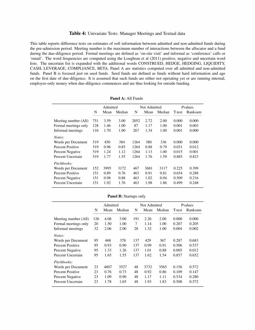
Table 4: Univariate Tests: Manager Meetings and Textual data

This table reports difference tests on estimates of soft information between admitted and non-admitted funds duringthe pre-admission period. Meeting number is the maximum number of interactions between the allocator and a fundduring the due-diligence period. Formal meetings are defined as ’on-site visit’ and informal as ‘conference’ calls or‘email’. The word frequencies are computed using the Loughran et al (2011) positive, negative and uncertain wordlists. The uncertain list is expanded with the additional words CONSTRUED, HEDGE, HEDGING, LIQUIDITY,CASH, LEVERAGE, COMPLIANCE, BETA. Panel A are statistics computed over all admitted and non-admittedfunds. Panel B is focused just on seed funds. Seed funds are defined as funds without hard information and ageon the first date of due-diligence. It is assumed that such funds are either not operating yet or are running internal,employee-only money when due-diligence commences and are thus looking for outside funding.

Panel A: All Funds

Admitted Not Admitted PvaluesN Mean Median N Mean Median T-test Ranksum

Meeting number (All) 751 3.59 3.00 2052 2.72 2.00 0.000 0.000Formal meetings only 128 1.46 1.00 87 1.17 1.00 0.001 0.003Informal meetings 116 1.70 1.00 267 1.34 1.00 0.001 0.000

Notes:Words per Document 519 450 384 1264 380 336 0.000 0.000Percent Positive 519 0.96 0.85 1264 0.88 0.79 0.031 0.012Percent Negative 519 1.24 1.12 1264 1.13 1.00 0.015 0.001Percent Uncertain 519 1.77 1.55 1264 1.76 1.59 0.885 0.823

Pitchbooks:Words per Document 152 3995 3172 467 3681 3117 0.225 0.399Percent Positive 151 0.89 0.76 463 0.91 0.81 0.654 0.288Percent Negative 151 0.98 0.88 463 1.02 0.94 0.509 0.216Percent Uncertain 151 1.92 1.76 463 1.98 1.86 0.499 0.248

Panel B: Startups only

Admitted Not Admitted PvaluesN Mean Median N Mean Median T-test Ranksum

Meeting number (All) 126 4.08 3.00 191 2.26 2.00 0.000 0.000Formal meetings only 20 1.50 1.00 7 1.14 1.00 0.207 0.205Informal meetings 32 2.06 2.00 28 1.32 1.00 0.004 0.002

Notes:Words per Document 95 468 378 137 429 367 0.287 0.683Percent Positive 95 0.93 0.90 137 0.99 0.91 0.506 0.537Percent Negative 95 1.33 1.26 137 1.01 0.88 0.005 0.012Percent Uncertain 95 1.65 1.55 137 1.62 1.54 0.857 0.652

Pitchbooks:Words per Document 23 4607 3527 48 3732 3565 0.156 0.572Percent Positive 23 0.76 0.73 48 0.92 0.86 0.109 0.147Percent Negative 23 1.09 0.90 48 1.17 1.11 0.534 0.280Percent Uncertain 23 1.78 1.65 48 1.93 1.83 0.508 0.572

Table 5: Top Words: Meeting Notes and Pitchbooks

This table reports the top words from the three words lists (positive, negative and uncertain) of Loughran, et al (2011)applied to our meeting notes and pitch books. The uncertain list is expanded with the additional words CONSTRUED,HEDGE, HEDGING, LIQUIDITY, CASH, LEVERAGE, COMPLIANCE, BETA. The two sources of soft informationare listed separately to show differences in their content and motivate our construction of their information proxies,i.e. Notes-index, NIit = posit + negit − uncit , and Pitchbooks-index, PIi = −pospi + negpi + uncpi, which is formallydiscussed in text.

Rank Positive Negative Uncertain

Pbook Notes Pbook Notes Pbook Notes

1 Opportunities Good Volatility Volatility Exposure Exposure2 Strong Opportunities Loss Cut Risk Risk3 Opportunity Strong Losses Negative Hedge Liquidity4 Attractive Great Conviction Closed Liquidity Cash5 Positive Better Negative Against Volatility Hedge6 Greater Positive Distressed Bad Cash Could7 Reward Able Deviation Conviction Leverage Believes8 Advantage Opportunity Opportunistic Losses Risks Exposures9 Leading Attractive Disclaimer Late Compliance Volatility10 Superior Greater Restructuring Lost Exposures Beta11 Achieved Despite Against Difficult Beta Leverage12 Good Advantage Poor Hurt Hedging Believe13 Achieve Benefit Volatile Claims Approximately Risks14 Gains Excited Stress Loss Could Roughly15 Successful Reward Closed Crisis Believe Hedging16 Better Winners Lack Poor Vary Approximately17 Highest Gains Lose Distressed Deviation Might18 Benefit Strength Construed Wrong Assumptions Almost19 Honors Highest Decline Decline Speculative Seems20 Success Stable Illiquid Lose Believed Cautious21 Able Leading Critical Illiquid Differ Possible22 Transparency Constructive Bankruptcy Problem Volatile Probably23 Profitable Outperformed Ill Problems Believes Volatile24 Gain Improving Crisis Weak Possible Assuming25 Profitability Gain Late Concerns Assumed Depending26 Great Profitable Disclosed Restructuring Depending Uncertainty27 Enhanced Successful Worst Worst Preliminary Dependent28 Stable Confident Weak Lack Anticipated Compliance29 Improving Outperform Inefficiencies Forced Assuming Anticipates30 Advantages Happy Declining Volatile Probability Somewhat31 Effective Success Conflicts Concerned Assume Anticipate32 Favorable Improve Exposed Defensive Assumes Anticipated33 Despite Favorable Claims Slowing Almost Apparently34 Strength Easy Bad Correction Nearly Probability35 Efficient Winner Limitations Slowdown Dependent Sometimes36 Excellent Strengths Force Slow Might Occasionally37 Outstanding Improvement Breakdown Tightening Hidden Maybe38 Outperformed Transparency Unlawful Missed Approximate Perhaps39 Improved Optimistic Difficult Exposed Variant Possibility40 Distinction Rebound Deteriorating Recession Anticipate Risky

Table 6: Time-invariant Hazard Model

This table reports estimates of a log-linear model of the due diligence spell as a function of auditable and private infor-mation. We split our proxy of soft information into its level ( ˆE (R− peer)) and volatility ( ˆσt (R− peer)). Observationsare by fund averages over the pre-admission period for admitted funds and over all available data for non-admittedfunds. All variables are standardized so that the coefficients reflect the effects of a one standard deviation move in theunderlying regressor. Panel A reports results for the full-sample of funds whereas Panel B - for the matched samplewhere each admitted fund is matched to a set of 3 peer funds according to the Mahalanobis distance based on thefunds’ average log(AUM), age, excess return and idiosyncratic volatility. Reported t-statistics (in parenthesis) arerobust to heteroskedasticity.

Panel A: All Funds

(1) (2) (3) (4) (5)β

(t-stat)β

(t-stat)β

(t-stat)β

(t-stat)β

(t-stat)

Hard information:E t(R− peers) −0.101∗∗∗ −0.079∗∗∗

(−4.04) (−2.86)σ t(R− peers) 0.252∗∗∗ 0.219∗∗∗

(8.60) (7.74)

Soft information:Meeting number (All) 0.087∗∗∗ 0.126∗∗∗

(5.28) (7.54)Words per Document −0.230∗∗∗ −0.179∗∗∗

(−11.00) (−7.47)

Observations 749 747 985 979 744R2 0.0222 0.1386 0.0156 0.1098 0.2372

Panel B: Matched Sample

(1) (2) (3) (4) (5)β

(t-stat)β

(t-stat)β

(t-stat)β

(t-stat)β

(t-stat)

Hard information:E t(R− peers) −0.043 −0.034

(−1.36) (−1.13)σ t(R− peers) 0.285∗∗∗ 0.242∗∗∗

(10.14) (8.63)

Soft information:Meeting number (All) 0.166∗∗∗ 0.146∗∗∗

(6.87) (6.54)Words per Document −0.149∗∗∗ −0.131∗∗∗

(−4.86) (−4.28)

Observations 557 556 564 556 548R2 0.0036 0.1586 0.0523 0.0426 0.2254

Table 7: Time-varying Hazard Model

This table reports logistic hazard model estimates of positive due-diligence outcome (fund admission to investableuniverse) as function of (1) fund and market observables, (2) due-diligence duration, and (3) proxy of soft (i.e. non-auditable) information disseminated during the allocator’s interaction with the funds’ managers. The main variablesof interest are Information ratio, measuring for auditable information about the fund, and Soft index, measuring forsubjective information conveyed over the meeting interaction with the fund managers. Both variables are defined inthe text (section 4.1.2). Except for dummies-variables (denoted with D), columns dy/dx report marginal effects on theprobability of admission estimated at the mean levels of other covariates. Duration measures the number of monthselapsed since the due-diligence start for the respective fund until the current month. Thus for admitted funds the panelends at the admission month, for never admitted it lasts through July 2012 unless censored. Market variables includemarket returns (current and lags), rolling volatilities of Fama-French 4 factors, and predicted capital inflows to theallocator. Reported t-statistics (in parenthesis) are robust to heteroskedasticity and autocorrelation.

(1) (2) (3) (4)β

(t-stat)dy/dx β

(t-stat)dy/dx β

(t-stat)dy/dx β

(t-stat)dy/dx

Hard information:Information ratio 0.445∗∗∗ 0.0009 0.456∗∗∗ 0.0008 0.400∗∗∗ 0.0006 0.423∗∗∗ 0.0006

(6.64) (6.89) (6.07) (6.41)Log(AUM) 0.385∗∗∗ 0.0008 0.467∗∗∗ 0.0009 0.376∗∗∗ 0.0006 0.465∗∗∗ 0.0006

(4.35) (5.11) (3.78) (4.53)

Soft information:Affiliated fund (D) 0.453∗∗∗ 0.0007 0.371∗∗ 0.0005

(2.85) (2.29)Affiliated college (D) 0.497∗∗∗ 0.0007 0.561∗∗∗ 0.0008

(3.44) (3.78)Soft index (lagged) 0.612∗∗∗ 0.0009 0.612∗∗∗ 0.0008

(9.84) (10.61)

Due-diligence spell:Log(Duration) 0.543∗∗∗ 0.0011 0.538∗∗∗ 0.0010 0.344∗∗ 0.0005 0.336∗∗ 0.0005

(3.77) (3.70) (2.36) (2.27)Duration −0.040∗∗∗ −0.0001 −0.039∗∗∗ −0.0001 −0.045∗∗∗ −0.0001 −0.044∗∗∗ −0.0001

(−4.40) (−4.29) (−4.99) (−4.94)

Market variables Yes Yes Yes YesYear FE Yes Yes Yes YesStrategy FE No Yes No Yes

Observations 45,714 45,714 45,714 45,714Pseudo R2 0.1271 0.1391 0.1768 0.1874Baseline probability 0.0047 0.0047 0.0047 0.0047BIC 2,591 2,591 2,488 2,492

Appendix A. Model Analysis

These results are from McCardle (1985) and Ulu and Smith (2009) using a normal-normal framework.

LEMMA 1. The value of collecting one more piece of information is non-increasing in j (time).

PROOF. The expected change in value of one more piece of information can be defined as

E(∆α j

)=−c+βE

(π(M(α j)))−π(α j−1

)≥−c+βE

(π(M(α j+1

)))−π(α j)

As Eπ(M(α j))

is convex, Jensen’s inequality gives us LEMMA 1.

THEOREM 1. There exists N ≤∞ that signifies an optimal stopping rule such that V(αn)= π

(αn)∀ n≥ N.

That is, there are no more meetings after this point in due-diligence.

PROOF. Note, as π(α) is convex and non-decreasing, and also

0 = 0 · ∂M (α)

∂α≤ ∂Eπ(M (α))

∂α= E{π′ (M (α))

∂M (α)

∂α} ≤ A · ∂M (α)

∂α= A,

the maximum of Eπ(M (α)) is achieved at α0. Therefore, if E(∆α0

)< 0 then E

(∆α j

)< 0. Furthermore, as

Eπ(M(α0))

approaches π(α0)= 0 as j approaches ∞, for any ε > 0,∃ an N such that Eπ

(MN+1

(α0))

<

ε = c then E(∆α0

)< 0. That is, accepting or rejecting is optimal versus continuing for all estimates of α.

THEOREM 2. For each stage j ∃(α j,α j

)such that 0 ≤ α j ≤ α0 ≤ α j, where the allocator continues to

conduct due-diligence on the fund if α j ≤ α≤ α j, accepts the fund if α≥ α j and rejects the fund if α j ≥ α.

PROOF. It is obvious that M (α) increases in α and from THEOREM 1 that E (V ′ (M (α))) is at most A.

Assuming that j < N, that is the continuation area is non-empty, given that π(α) is piecewise linear then it

i

will intersect the continuation value, −c+βE (V ′ (M (α))), exactly twice -

α j = α js.t.− c+βE (Vj+1 (M j+1 (α))) = π0(α j)

α j = α js.t.− c+βE (Vj+1 (M j+1 (α))) = 0.

Appendix B. Model Extension

This result is directly from McCardle (1985). In the previous derivations the frequency (governed by

λ below) of meetings is fixed at every period. In reality this could be a choice variable of the allocator.

In other words, the allocator chooses to monitor the fund more intensely or have more frequent meetings.

The trade-off is between more intense due-diligence and higher costs. The intensity can be thought of

as the probability of having a meeting, which factors into the timing of proprietary-information arrival or

hazard, T. Let’s assume T ∼ λe−λt , that is the arrival of information is also a stochastic process that follows

an exponential distribution. Thus the expected discounted cost of one additional piece of information and

discount rate is, accordingly,

E∫ T

0cλe−rtdt = cλ

1r

E(1− e−rt)= cλ

λ+ r= c (B.1)

Ee−rt =∫

∞

0λe−rte−λtdt =

λ

λ+ r= β (B.2)

Previously, we just use c and β. The allocator can now choose λ∗ = λ∗j (α) in order to maximize the contin-

uation value. With LEMMA 2 below, we obtain an interesting result regarding the frequency of meetings in

THEOREM 4.

LEMMA 2. The anticipated return, V (α), is non-increasing in j.

PROOF. Given that accept-reject decision is only dependent on time j decision, we can focus on the contin-

uation component of the dynamic program. Thus,

EVj (M j (α))≥ EVj (M j+1 (α))≥ EVj+1 (M j+1 (α)) .

The first inequality is because M j+1 is less risky and mirrors the discussion at the end of section 2. The

ii

second inequality is by induction. That is, if we start at j = N, the convexity of VN−1 (α) maximization

allows that for any M (α) this would hold true.

THEOREM 3. α j and α j are non-decreasing and non-increasing, respectively, in j.

PROOF. From LEMMA 2, if accepting or rejecting is optimal at j then it is also at j+1. That is the accepting

and rejection zones are convex and increasing.

THEOREM 4. If cλ is twice difference in λ and c′λ> 0 and c′′

λ> 0 then λ∗ is non-decreasing in α and non-

increasing in j.

PROOF. First, we note that the continuation value, −cλ+λEV ′(α)λ+r , is initially increasing and then decreasing.

This means a maximum exists. Thus,

maxλ

−cλ +λEV ′ (α)λ+ r

=⇒ ∂

∂λ

−cλ +λEV ′ (α)λ+ r

=−c′

λ+EV ′ (α)λ+ r

− −cλ +λEV ′ (α)

(λ+ r)2 = 0

This simplifies to rEV ′ (M (α)) = c′λ(λ+ r)− cλ. As α rises the LHS rises. Also from LEMMA 2 as j rises

the LHS falls. In equilibrium this must be mirrored by the RHS. Given that ∂RHS/∂λ = c′′λ(λ+ r)> 0 then

λ∗ must rise in α and fall in j.

iii