• . ' V -

iNIS-mf—8645

NUCLEAR CARDIOLOGY

:•?

I NUCLEAR CARDIOLOGY I

Fourier functional images in leftventricular wall motion analysis

and

an investigation into lesion detectabilityin myocardial perfusion scintigraphy

PROEFSCHRIFT

TER VERKRIJGING VAN DE GRAAD VAN DOCTOR IN DE GENEESKUNDEAAN DE RIJKSUNIVERSITEIT TE LEIDEN,

OP GEZAG VAN DE RECTOR MAGNIFICUS DR. A. A. H. KASSENAAR,HOOGLERAAR IN DE FACULTEIT DER GENEESKUNDE,VOLGENS BESLUIT VAN HET COLLEGE VAN DEKANEN

TE VERDEDIGEN OP DONDERDAG 3 JUNI 1982TE KLOKKE 16.15 UUR

door

PIETER HERMAN VOSgeboren te Leiden in I9S2

Promotor: Prof. Dr. A. R. Bakker

Co-promotor: Dr. E. K. J. Pauwels

Referenten: Prof. H. de JongeDr. J. J. Schipperheyn

ISBN 90-9000312-6

This work has been done in co-operation with Drs. A. M. Vossepoel(Department of Biomedical Information Processing, University Medical Center, Leiden).

This study was supported by a grant from the Dutch Heart Foundation.

f*

r

Contents

General introduction

1. Data acquisition and processing in nuclear medicine

1.1 Data acquisition and processing - current practice1.2 Requirements for a nuclear medicine computer system1.3 Description of the computer system

References

2. Use of Fourier amplitude/phase images for quantification of leftventricular wall motion abnormalities

2.1 Introduction2.2 Anatomy and physiology of the heart2.3 Detection of abnormal left ventricular wall motion with radiographic

angiography2.4 Gated blood pool studies2.5 Characterization of the left ventricular time-activity curve with the first

harmonic in the Fourier spectrum2.6 Patient studies2.7 Results2.8 Discussion

List of relevant symbols and abbreviations

References

3. Detection of non-perfused lesions in myocardiai peifusion scintigraphywith thallium-201 and the influence of count density on lesiondetectability

3.1 Introduction3.2 Materials and methods

4

1

I 3.3 Results! 3.4 Discussion

AppendixA. Description of the model for the myocardium and the image generationA-l IntroductionA-2 Heart modelA-3 Generation of images

List of relevant symbols and abbreviations

B. Determination of the point spread function of the detecting/ imagingsystem

B-l Point spread function without attenuationB-2 Point spread function with attenuationB-3 Experimental determination of line spread functionB-4 Derivation of coefficients of the point spread function from the line

spread function

List of relevant symbols and abbreviations

References

4. Influence of tracer distribution, scatter and photon energy on lesiondetectability

4.1 Introduction4.2, Influence of tracer distribution on lesion detectability4.3 Influence of scatter on lesion detectability4.4 Influence of photon energy on lesion detectability

References

Summary

Samenvatting

Curriculum vitae

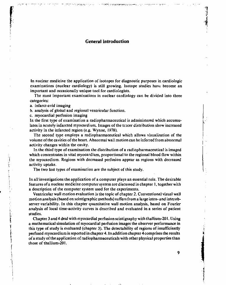
Genera] introduction

In nuclear medicine the application of isotopes for diagnostic purposes in cardiologieexaminations (nuclear cardiology) is still growing. Isotope studies have become animportant and occasionally unique tool for cardiologists.

The most important examinations in nuclear cardiology can be divided into threecategories:a. infarct-avid imagingb. analysis of global and regional ventricular function.c. myocardial perfusion imagingIn the first type of examination a radiopharmaceutical is administered which accumu-lates in acutely infarcted myocardium. Images of the tracer distribution show increasedactivity in the infarcted region (e.g. Wynne, 1978).

The second type employs a radiopharmaceutical which allows visualization of thevolume of the cavities of the heart. Abnormal wall motion can be inferred from abnormalactivity changes within the cavity.

In the third type of examination the distribution of a radiopharmaceutical is imagedwhich concentrates in vital myocardium, proportional to the regional blood flow withinthe myocardium. Regions with decreased perfusion appear as regions with decreasedactivity uptake.

The two last types of examination are the subject of this study.

In all investigations the application of a computer plays an essential role. The desirablefeatures of a nuclear medicine computer system are discussed in chapter 1, together witha description of the computer system used for the experiments.

Ventricular wall motion evaluation is the topic of chapter 2. Conventional visual wallmotion analysis (based on scintigraphic methods) suffers from a large intra-and interob-server -variability. In this chapter quantitative wall motion analysis, based on Fourieranalysis of local time-activity curves is described and evaluated in a series of patientstudies.

Chapter 3 and 4 deal with myocardial perfusion scintigraphy with thallium-201. Usinga mathematical simulation of myocardial perfusion images the observer performance inthis type of study is evaluated (chapter 3). The detectability of regions of insufficientlyperfused myocardium is reported in chapter 4. In addition chapter 4 comprises the resultsof a study of the application of radiopharmaceuticals with other physical properties thanthose of thallium-201.

i

iV

4

Chapter 1

Data acquisition and processing in nuclear medicine

1.1 Data acquisition and processing - current practice

1.1. l GammacameraNuclear medicine examinations involve the registration of the distribution of a radio-pharmaceutical in the human body. The registration is usually performed with a gammacamera.

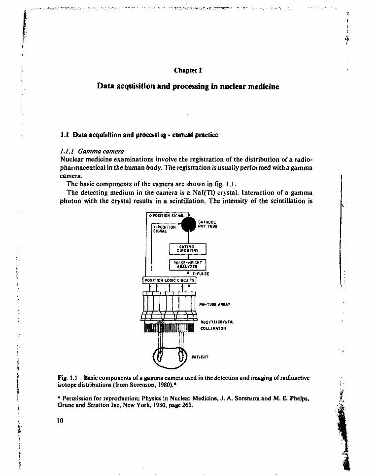
The basic components of the camera are shown in fig. 1.1.The detecting medium in the camera is a Nal(Tl) crystal. Interaction of a gamma

photon with the crystal results in a scintillation. The intensity of the scintillation is

| POSITION LOGIC CIRCUITS |

t I Ï t tPM-TUBE ARRAY

N o I I T i ) CRYSTAL

COLLI MATOR

MTIENT

Fig. 1.1 Basic components of a gamma camera used in the detection and imaging of radioactiveisotope distributions (from Sorenson, 1980).*

• Permission for reproduction; Physics in Nuclear Medicine, J. A. Sorenson and M. E. Phelps,Grune and Stratton Jnc, New York, 1980, page 265.

10

proportional to the energy of the incident photon. If the interaction leads to a Comptonprocess, a secundary photon with lower energy than the initial incident photon will beemitted, which may cause a second scintillation with less intensity. Currently usedradiopharmaceuticals employ gamma emitting isotopes with photon energies rangingfrom about 80 to 300 ke V. These photons interact with the crystal mainly by photoelect-ric absorption.

In order to determine the site of the photon emission a collimator is placed before thecamera crystal. Special collimators for high sensitivity, high resolution, high or lowenergy photons etc. are available.

A direct photographic image of the distribution of the scintillations could be obtainedif their intensity was sufficient. However, the intensity cf the light emitted by the cameracrystal is too low for this purpose and besides, no energy discrimination (for instance toseparate Compton and primary photons) would be possible in that case.

To obtain an image of the scintillations their location and intensity are converted toelectrical pulses by an array of photomultiplier tubes (PMT). From the outputs of thesetubes an X and Y signal is derived which represents the location of a scintillation. TheZ-signal is the sum of all PMT outputs, and its magnitude represents the intensity of thescintillation, which is proportional to the incident photon energy. With the Z-signalphotons of the desired energy can be selected for imaging with a pulse height analyzer. If ascintillation meets the energy criteria of the pulse height analyzer the X and Y pulses areused for the positioning of a dot on a cathode ray tube screen and subsequent exposure ofa film. Usually images are generated for a predefined exposure time or until a predefinednumber of scintillations ('counts') is collected in the image.

1.1.2 Acquisition and processing of gamma camera data by computerIn the past ten years the use of digital computers in nuclear medicine has increased in anattempt to improve data acquisition and image quality. Application of computers alsoinitiated the use of new techniques, such as quantification of (regional) activity uptake,gated blood pool scintigraphy (chapter 2) and tomography. The X and Y position signalsof the events, selected by pulse height analysis can be stored in the computer after analogto digital conversion.

Two ways of data acquisition are in common use: list-mode and frame-mode.List mode. All X and Y coordinate pairs are recorded directly in the computer

memory; time markers and physiologic signals (such as ECG trigger pulses) are added.Pairs of digitized co-ordinates are sequentially stored in the memory. Afterwards datacan be arranged in a matrix, which can be presented as an image. The major advantage ofthe method is its flexibility to produce curves, images etc. in the form that the observerneeds since all raw data are available. However, processing afterwards entails that imagesare not readily available immediately after acquisition. Since storage capacity is propor-tional to the total number of counts in the study a large storage capacity may be neededfor storage of studies employing high count rates and a long acquisition time.

Frame mode. Images are formed within the computer memory during acquisition.The field of view is represented by an array of image elements (pixels). A separatememory location is assigned to each picture element. If an event is detected in the area of

11

a distinct pixel, the number of counts in the corresponding memory location is incre-mented with one. When acquisition has ended the image is immediately available forstorage or display. However, the data are only available in the spatial and temporalresolution defined at the start of acquisition.

The storage capacity assigned to each pixel should be large enough to accomodate themaximum number of counts that can be expected. Usually before acquisition the storagecapacity per pixel can be specified to some extent. For instance, for a large number ofcounts two bytes and for a small number of counts only one byte can be assigned to eachpixel (one byte contains 8 bits).

1.2 Requirements for a nuclear medicine computer system

!n this paragraph the desirable properties of a nuclear medicine computer system will bediscussed, specified from the nuclear medicine point of view. The specifications will bederived from the present 'state of the art' of gamma cameras and radiopharmaceuticals,in such a way that the computer is not the limiting factor for spatial resolution, maximalcount rate etc. and that all studies can be performed without restrictions concerning theincoming data. If possible, new developments expected in the near future will be includedin the discussion.

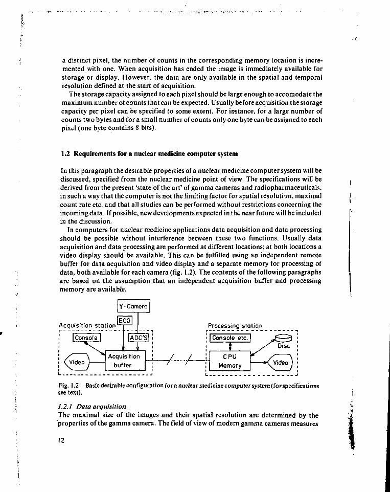
In computers for nuclear medicine applications data acquisition and data processingshould be possible without interference between these two functions. Usually dataacquisition and data processing are performed at different locations; at both locations avideo display should be available. This can be fulfilled using an independent remotebuffer for data acquisition and video display and a separate memory for processing ofdata, both available for each camera (fig. 1.2). The contents of the following paragraphsare based on the assumption that an independent acquisition buffer and processingmemory are available.

Y-Camera

Acquisition stationr

Processing stationr

; | Console etc.; |

/ / ;

' \

CPUMemory

/ Disc

*C Video J

Fig. 1.2 Basic desirable configuration fora nuclear medicine computer system (for specificationssee text).

1.2.1 Data acquisition-The maximal size of the images and their spatial resolution are determined by the'properties of the gamma camera. The field of view of modern gamma cameras measures

12

about 0.35 m in diameter maximally; the system's spatial resolution (measured with aparallel hole, high resolution collimator and a bar phantom) is maximally 2.8-3.0 mm.Following Shannon's sampling theorem (which states that the sampling frequencyshould be at least double the highest frequency in the signal; Shannon, 1949) the spatialsampling frequency should be at least 0.7 mnr' in order to prevent loss of information.This means that for the large field of view camera images should contain at least in theorder of 256x256 pixels for adequate spatial resolution over the whole field of view.

Two bytes per pixel allow for accumulation of images with a maximal count density upto 16 kcount/ mm2, which is certainly sufficient for nuclear medicine procedures present-ly in use. Using these specifications frame mode acquisition of a 256x256 (2 bytes/ pixel)image requires 128 kbytes.

Acquisition of the (analog) position signals from the camera with the (digital) compu-ter requires digitization of these signals. This is performed with analog-to-digital conver-ters (ADC's). Both the resolution and the (related) conversion speed of the ADC's maylimit the acquisition of data from the gamma camera. The gamma camera's dead time isabout 5 /us, which limits the count rate to 200 kcounts/s. The dead time for the ADC'sshould therefore meet this limit. Presently used ADC's actually require a total conversiontime of about 2 jus for 8-bit precision, i.e. a 256x256 pixel image.

The data acquisition in multiple gated (MUGA) heart studies imposes special require-ments on the acquisition buffer. In MUGA heart studies a series of images of the activitydistribution of a radiopharmacvutical in the heart cavities is acquired, covering a com-plete cardiac cycle.

This type of study is usually performed to calculate ejection fraction and to assessventricular wall motion abnormalities. In addition parameters such as peak ejection andpeak filling rate can be determined (the parameters are calculated from the time-activitycurve over one ventricle; wall motion is assessed by display of subsequent images in realtime). The study can be performed both at rest and under stress conditions (see alsochapter 2).

The addition of counts is performed in the buffer immediately after registration, whichmeans that the results of the acquisition are directly available when the acquisition hasended. The memory should be large enough to contain images from one complete cardiaccycle.

Four parameters have to be spec:fied for the acquisition format: image size, spatialresolution, temporal resolution and average count density in the heart region.

Image size and spatial resolution. The maximal spatial resolution is determined by thesystem spatial resolution: about 0.19 m field of view is sufficient for imaging the heart soimaging with optimal spatial resolution requires 128x128 pixels/image. In practice,however, the high spatial resolution in MUGA studies is useless, because of motionartifacts (e.g. patient movement, respiration). The spatial resolution of the images cantherefore be reduced without affecting the quality of the study. About 4-5 mm spatialresolution (Bacharach, 1979b; Burow, 1977; Adam, 1980) is found to be adequate for thistype of study. This means that acquisition in 64x64 pixel images is sufficient to cover thefield of view required.

13

Temporal resolution. The required temporal resolution depends on the purpose of thestudy. For visual wall motion assessment 12-16 frames/ cycle is considered to be suffi-cient. For ejection fraction calculation and calculation of the peak ejection and fillingrate during resting conditions about 25 frames/ s are required. Assuming a minimal heartrate of 40 beats/min, about 40 frames/cycle are maximally required for parametercalculation under resting conditions. 25 frames/ s are also sufficient for calculation of theejection fraction during exercise but for calculation of peak ejection and filling rate SOframes/ s are required. The number of frames that has to be acquired within one cycle willnever exceed 75 (Bacharach, 1979a; Aswegen, 1980; this work § 2.4.4).

Average count density in the heart region. The average count rate in MUG A acquisi-tion is about 12 kcounts/s (for 555 MBq (15 mCi) of radiopharmaceutical). Using 300kcounts/ frame the aquisition time is about 10 minutes (1 cycle/s, 25 frames/s, 12kcounts/s, which results in 480 counts/(framexcycle)), which appears to be a reasonablecompromise between the imaging time, radiation burden and the noise in the images(during resting conditions). In practice, two bytes/pixel in the images is adequate to meetthe count rate requirement, therefore the buffer size for MUGA acquisition should beabout 320 kbyte ((64x64)x2x40).

During exercise imaging time is limited to about 200 s. Because of the short acquisitiontime and the high frame rate only 1 byte/ pixel is required, and a 320 kbyte acquisitionbuffer is sufficient.

During data acquisition in a MUGA study the possibility should exist to exclude beats ofwhich the cycle length exceeds predefined limits (chapter 2, § 2.4.2). Therefore the datafrom one cycle have to be buffered, at least during the subsequent cycle. During thefollowing cycle the length of the previous cycle can be checked and data can be discardedif necessary. When a high sensitivity collimator is used, the count rate in MUGA studiesmay go up to 30 kcounts/s and buffering one cycle in the memory requires about2x1.5x30=90 kbyte (assuming 1.5 s/cycle; 2 bytes/count). Double buffering is neces-sary: during acquisition in one buffer the contents of the other buffer are stored: thereforebuffering requires a 180 kbyte memory.

In summary, about a 500 kbyte direct addressable memory is needed for versatile dataacquisition in MUGA heart studies.

List mode acquisition should also be available. In addition to direct transfer of data to astorage medium the memory should be able to buffer some disc blocks of data which maybe necessary for acquisition at peak count rates. Also in this process, double buffering ofdata is required. The memory requirements are easily fulfilled by the memory sizepreviously specified.

The real time clock frequency should be high enough for proper measurement of theMUGA time intervals and adequate synchronization of the clock with the trigger signal.Assuming a high frame rate (50 frames/ s for exercise studies) each imaging interval takes20 ms. Application of a 1000 Hz clock (which is used in most present-day nuclearmedicine computers) introduces an error of 5% in the determination of the first interval

14

of each cycle. Moreover, a low clock frequency only allows for a rough selection ofinterval lengths.

Application of a high frequency clock (for instance 10000 Hz) would reduce theseerrors to a negligible level.

1.2.2 Display of imagesDisplay on data on a video screen requires a refresh of the data from the memory: anumber of memory locations are used for the storage of data to be displayed at the screen.Each location corresponds to one element on the video screen. Most video screenscomprise 512x512 elements; the same number of memory locations is needed for displayover the full screen. Display of 256 intensity levels is more than sufficient to meetdiscrimination of the human visual system. This number of intensity levels can berepresented by assigning 1 byte to each display element. As a result the use of the fullscreen requires a 256 kbyte memory to refresh the video screen.

For display purposes interpolation of images can be useful. Using the aforementionedmemory size an image with 256x256 pixels in the computer can be interpolated to512x512 elements on the video screen.

A 256 kbyte memory is also sufficient for buffering 4 MUGA studies with 16frames/cycle (64x64 byte/frame). By means of a microprocessor the images can besequentially selected for display in real time, allowing the CPU to perform other tasks.This feature can be used for instance to display a rest and exercise MUGA acquisition intwo views.

If the acquisition buffer is large enough, it can be used to refresh the video screen. Usingthe buffer size specified in § 1.2.1 (500 kbyte) all video display functions can be performedusing the acquisition buffer.

1.2.3 Processing of dataFor complete storage of a M U G A study maximally 320 kbytes are necessary (cf. § 1.2.1).A larger storage capacity is useful for the calculation of functional images. (A functionalimage comprises a parameter value in each pixel, usually calculated from a localtime-activity curve for the corresponding pixel in each image sequence, (cf. § 2.4.5)).Additional storage capacity for functional images, curves, operating system, programsetc. should be available. The amount of memory required for MUGA studies should alsoallow storage of two static images with maximal spatial resolution and maximal field ofview (256x 256 pixels), which is necessary for convolutional filter procedures. About 400

' kbyte for the central memory therefore appears to be the desirable minimal directaddressable memory size needed for MUGA data processing. In addition memory foracquisition and video display should be available.

; The processing of images can be speeded up greatly by parallel processing of arrays.

; 1.2.4 Storage of data; Most presently used gamma cameras allow for acquisition at a rate of up to 200: kcounts/s. A system claiming a maximal count rate up to 500 kcounts/s has been

f 15

presented (however, in this system all corrections for non-linearity etc. have beendisabled to obtain the high acquisition rate). A count rate of 200 kcounts/s requires adata rate of 400 kbytes/s.

The storage capacity should be large enough to store large amounts of list mode data(a MUG A heart study requires maximally 24 Mbyte storage capacity in list mode).

Modern nuclear medicine computers all apply 80-120 Mbyte discs which have suffi-ciently large capacity to meet these requirements.

1.2.5 SoftwareOperation of nuclear medicine computers often requires a compromise between simplici-ty in operation and flexibility. Physicians and technologists should be able to identify andstart the acquisition protocols. A menu structure of the software, leading the userstepwise through the various possibilities for data acquisition and (predefined) dataprocessing is an attractive feature.

Using the menu the user should be allowed to construct strings of modules (each withits own function) without limitations of data transfer between subsequent modules. Alsosomeone unfamiliar with computer programming should be able to construct his or herown acquisition and processing sequences, thus allowing easy integration of the compu-ter into the daily routine.

The modules ought to perform fast execution of their function. Therefore it is attrac-tive to use them in combination with user written programs: it should be possible toinclude user written programs in strings of modules via the menu without restrictions ofdata transfer. In particular, modules should be available that allow processing of incom-ing data during acquisition using user-written programs, allowing for quality control onincoming data.

During all acquisition and processing data should be automatically and uniquelyidentified on display and hard copy. If a central hospital information system is availablethe nuclear medicine computer system should be linked to it, to obtain the patientidentification directly. To this end, using the nuclear medicine computer it should bepossible to store and to retrieve information to and from patient files in the centralsystem, instead of using keyboard operations.

With the central information system coupled to the computer patient identificationnumber is sufficient to automatically add other patient identification data to the dataobtained in the scintigraphic examinations, thus preventing mismatch between thepatient study and the patient identification.

1.3 Description of computer system

The computer system used for the work presented in this thesis was supplied by MedicalData Systems, Ann Arbor, Michigan, U.S.A., (MODUMED TRINARY system).

In the following paragraphs the hardware and software are described.

1.3.1 HardwareThe basic configuration of the computer system is shown in fig. 1.3a.

16

(A)

Discs3x3 Mbyte

IB) 28 kbyteProgr./processing

16 kbyteCamera 1

16 kbyteCamera 2

Monitor

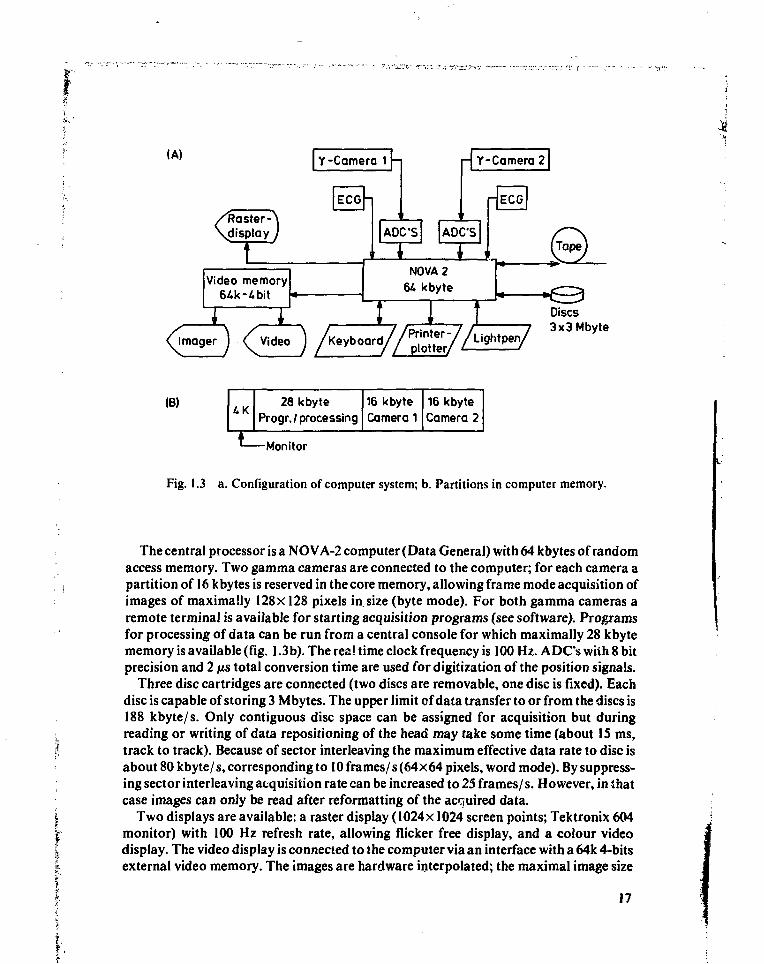
Fig. 1.3 a. Configuration of computer system; b. Partitions in computer memory.

The central processor is a NOVA-2 computer (Data General) with 64 kbytes of randomaccess memory. Two gamma cameras are connected to the computer; for each camera apartition of 16 kbytes is reserved in the core memory, allowing frame mode acquisition ofimages of maximally 128x 128 pixels in. size (byte mode). For both gamma cameras aremote terminal is available for starting acquisition programs (see software). Programsfor processing of data can be run from a central console for which maximally 28 kbytememory is available (fig. 1.3b). The real time clock frequency is 100 Hz. A DCs with 8 bitprecision and 2 us total conversion time are used for digitization of the position signals.

Three disc cartridges are connected (two discs are removable, one disc is fixed). Eachdisc is capable of storing 3 Mbytes. The upper limit of data transfer to or from the discs is188 kbyte/ s. Only contiguous disc space can be assigned for acquisition but duringreading or writing of data repositioning of the head may take some time (about 15 ms,track to track). Because of sector interleaving the maximum effective data rate to disc isabout 80 kbyte/s, corresponding to 10 frames/s (64x64 pixels, word mode). By suppress-ing sector interleaving acquisition rate can be increased to 25 frames/ s. However, in thatcase images can only be read after reformatting of the acquired data.

Two displays are available: a raster display (1024x 1024 screen points; Tektronix 604monitor) with 100 Hz refresh rate, allowing flicker free display, and a colour videodisplay. The video display is connected to the computer via an interface with a 64k 4-bitsexternal video memory. The images are hardware interpolated; the maximal image size

17

I .«•-••—. -

available is 128x128 pixels. The depth of the elements in the video memory allowsdisplay of 16 intensity levels. The colour of each pixel can be specified with a translationtable. For dynamic display of MUGA studies in real time the video memory is refreshedfrom the central core memory, thereby locking all other tasks performed by the compu-ter.

A video imager (MATRIX) is connected to the video image memory for hard copydisplay on transparent nuclear medicine film. Further devices connected to the computerare a line printer, a tape unit and a light pen; an ECG trigger (Brattle) is available for bothcameras. (ECG triggering is used for acquisition of gated heart studies).

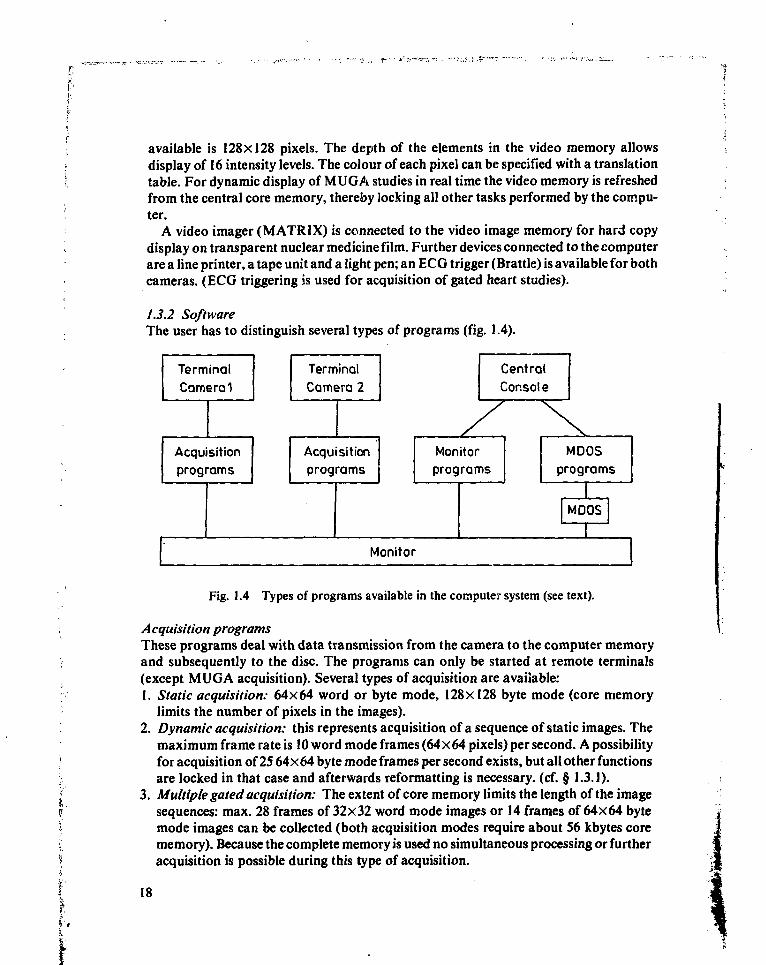
1.3.2 SoftwareThe user has to distinguish several types of programs (fig. 1.4).

TerminalCamera 1

Acquisitionprograms

TerminalCamera 2

Acquisitionprograms

y

CentralConsole

Monitorprograms

\\

MDOSprograms

MDOS

Monitor

Fig. 1.4 Types of programs available in the compute:* system (see text).

Acquisition programsThese programs deal with data transmission from the camera to the computer memoryand subsequently to the disc. The programs can only be started at remote terminals(except MUGA acquisition). Several types of acquisition are available:1. Static acquisition: 64x64 word or byte mode, 128x128 byte mode (core memory

limits the number of pixels in the images).2. Dynamic acquisition: this represents acquisition of a sequence of static images. The

maximum frame rate is 10 word mode frames (64x64 pixels) per second. A possibilityfor acquisition of 25 64x64 byte mode frames per second exists, but all other functionsare locked in that case and afterwards reformatting is necessary, (cf. § 1.3.]).

3. Multiple gated acquisition: The extent of core memory limits the length of the imagesequences: max. 28 frames of 32x32 word mode images or 14 frames of 64x64 bytemode images can be collected (both acquisition modes require about 56 kbytes corememory). Because the complete memory is used no simultaneous processing or furtheracquisition is possible during this type of acquisition.

18

A hardware zoom (2x) is available on the gamma camera. Therefore a central portionof the field of view (0.175 X 0.175 m) can be digitized with 32 X 32 pixels, resulting in5.5 mm pixel resolution, thus approaching the requirements previously mentioned (cf.§ 1.2.1). The maximal number of frames per cardiae cycle is 28, allowing calculation ofthe ejection fraction in patients with a heart rate as low as 44 beats/ min.

4. List mode acquisition: This type of acquisition is possible to a very limited extent,only if all possible disc space is used (partitions with user written programs areoverwritten) about 7.5 Mbyte data can be stored. Reconstruction of images turned outto take a considerable amount of time. For these reasons list mode acquisition was notused.

All acquisition programs require manual input of patient data such as patient name andnumber, type of study, mode of acquisition etc. These data are stored in a specialdirectory and are not uniquely coupled to the patient study.

Monitor programsThese programs can only be executed from the central console. They include utilities,simple image processing (smooth, contrast enhancement), region of interest selection,curve generation, display functions, MDOS (see next section) etc. All programs aredelivered by the manufacturer.

MDOSMDOS is a program that extends the capabilities of the monitor to include functionsnecessary for programming (FORTRAN IV). The maximum core space for data anduser program is about 28 kbytes.

MDOS offers only limited use of available functions as present in monitor programs.. Important functions such as definition of region of interests cannot be performed byi subroutines in the MDOS library. Therefore processing (often requiring region of

interest selection) usually cannot be performed in one user written program sequence,seriously limiting the routine use of the computer.

References

: Adam, W.E., Bitter, F. (1980), Advances in heart imaging, Proc. Int. Symp. Med. Radionuclideimaging, Heidelberg, september 1-5, IAEA.

Aswegen, A.V., Alderson, P.O., Nickoloff, E.L. et al. (1980), Temporal resolution requirementsfor left ventricular time-activity curves, Radiology 135: 165-170.

Bacharach, S.L., Green, M.V., Borer, J.S. et al. (1979a), Left ventricular peak ejection rate, fillingrate and ejection fraction -frame rate requirementsat rest and exercise, J.Nucl. Med. 20:189-193.

f Bacharach, S.L., Green, M.V., Borer, J.S. (1979b). Instrumentation and data processing in cardio-jV vascular nuclear medicine: evaluation of ventricular function, Sem.Nucl.Med. 9:257-274.f Burow, R.D., Strauss, H. W., Singleton, R. et al. (1977), Analysis of left ventricular function from: multiple gated acquisition cardiac blood pool imaging, Circulation 56:1024-1028.| Sorenson, J. A., Phelps, M.E. (1980), Physics in nuclear medicine, Gruneand Stratton, New York.! Wynne, J., Holman, B.L., Lesch, M.(1978), Myocardialscintigraphybyinfarct-avidradiotracers,' Pinciples of cardiovascular nuclear medicine, Holman, B.L., Sonnenblick, E.H. and Lesch, M.f (eds), Grune and Stratton, New York.>,H1* 1 9# • '

V,f-

Chapter 2

Use of Fourier amplitude/phase images for quantificationof left ventricular wall motion abnormalities

2.1 Introduction

Analysis of wall motion of the left ventricle of the heart, both by radiographic angio-graphy and by scintigraphy is usually performed by visual interpretation of the dynamicdisplay of the geometry of the left ventricular cavity during the cardiac cycle. Bothmethods suffer from an important inter- and intra-observer variability. Therefore severalmethods for quantification of regional activity changes have been proposed.

One of the quantitative scintigraphic methods developed recently is based on charac-terization of (regional) activity changes in time by fhe first harmonic in the Fourierspectrum of regional time-activity curves. Parameters of the first harmonic can be used tocharacterize wall motion abnormalities. In this chapter the fundamentals of the methodare described; its usefulness in the assessment of wall motion abnormalities will bediscussed following a comparison of the Fourier parameter characterization with visualinterpretation of wall motion by three observers.

In paragraph 2.2 a description of the anatomy and physiology of the heart (in particularof the left ventricle) is given. Conventional radiographic angiography analysis of wallmotion abnormalities is described in paragraph 2.3. Gated blood pool studies areintroduced in paragraph 2.4, the application of the first harmonic approximation ofregional time-activity curves is discussed in paragraph 2.5, the experimental methodsused for wall motion assessment are presented in paragraph 2.6 and the results of theexperiments are given in paragraph 2.7. Paragraph 2.8 contains the conclusion.

2.2 Anatomy and physiology of the heart

The heart is a hollow muscular organ divided into two parts: the left and the right heart,separated by an atrio-ventricular septum. Both parts of the heart comprise two cavities(atrium and ventricle) which are separated by a valve, called the tricuspid valve at theright side and the mitral valve at the left side. Both parts of the heart pump blood from alow pressure, venous side to a high pressure, arterial side of the circulation. The rightheart pumps deoxygenated blood from the systemic veins to the pulmonary artery, theleft heart pumps oxygenated blood from the pulmonary veins to the systemic arteries.Pulmonary and systemic circulation are normally almost completely separated and are

21

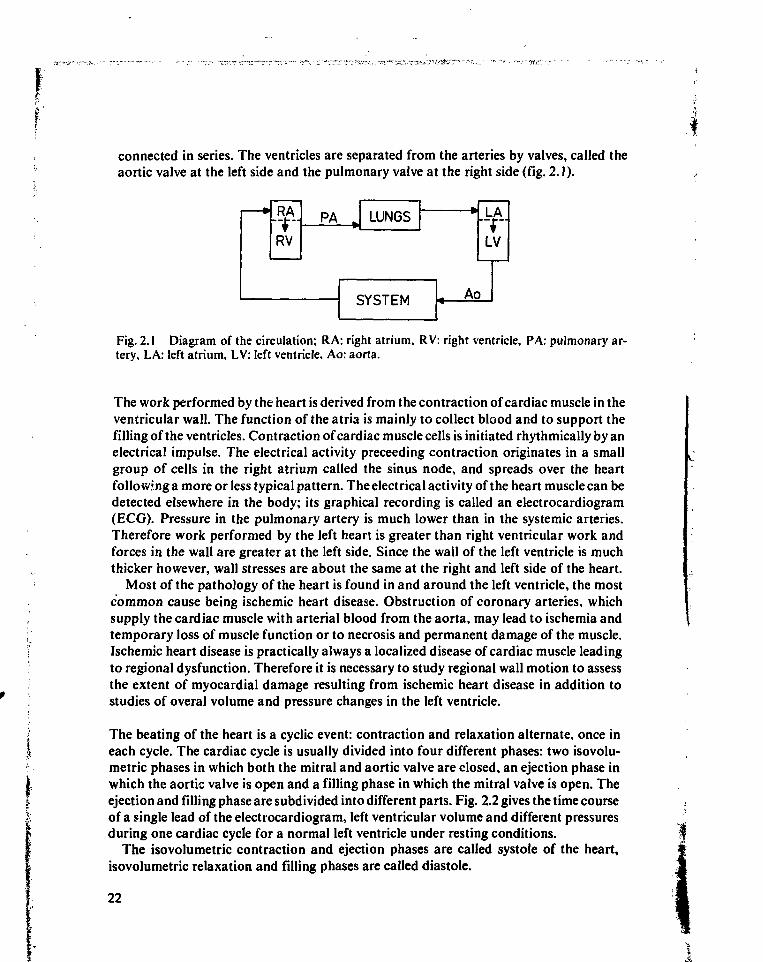
connected in series. The ventricles are separated from the arteries by valves, called theaortic valve at the left side and the pulmonary valve at the right side (fig. 2.1).

4*..RV

PA „ LUNGS

SYSTEM i A c

.LA.

LV

>

Fig. 2.1 Diagram of the circulation; RA: right atrium, RV: right ventricle, PA: pulmonary ar-tery, LA: left atrium, LV: left ventricle, Ao: aorta.

.1

The work performed by the heart is derived from the contraction of cardiac muscle in theventricular wall. The function of the atria is mainly to collect blood and to support thefilling of the ventricles. Contraction of cardiac muscle cells is initiated rhythmically by anelectrical impulse. The electrical activity preceeding contraction originates in a smallgroup of cells in the right atrium called the sinus node, and spreads over the heartfollowing a more or less typical pattern. The electrical activity of the heart muscle can bedetected elsewhere in the body; its graphical recording is called an electrocardiogram(ECG). Pressure in the pulmonary artery is much lower than in the systemic arteries.Therefore work performed by the left heart is greater than right ventricular work andforces in the wall are greater at the left side. Since the wall of the left ventricle is muchthicker however, wall stresses are about the same at the right and left side of the heart.

Most of the pathology of the heart is found in and around the left ventricle, the mostcommon cause being ischemic heart disease. Obstruction of coronary arteries, whichsupply the cardiac muscle with arterial blood from the aorta, may lead to ischemia andtemporary loss of muscle function or to necrosis and permanent damage of the muscle.Ischemic heart disease is practically always a localized disease of cardiac muscle leadingto regional dysfunction. Therefore it is necessary to study regional wall motion to assessthe extent of myocardial damage resulting from ischemic heart disease in addition tostudies of overal volume and pressure changes in the left ventricle.

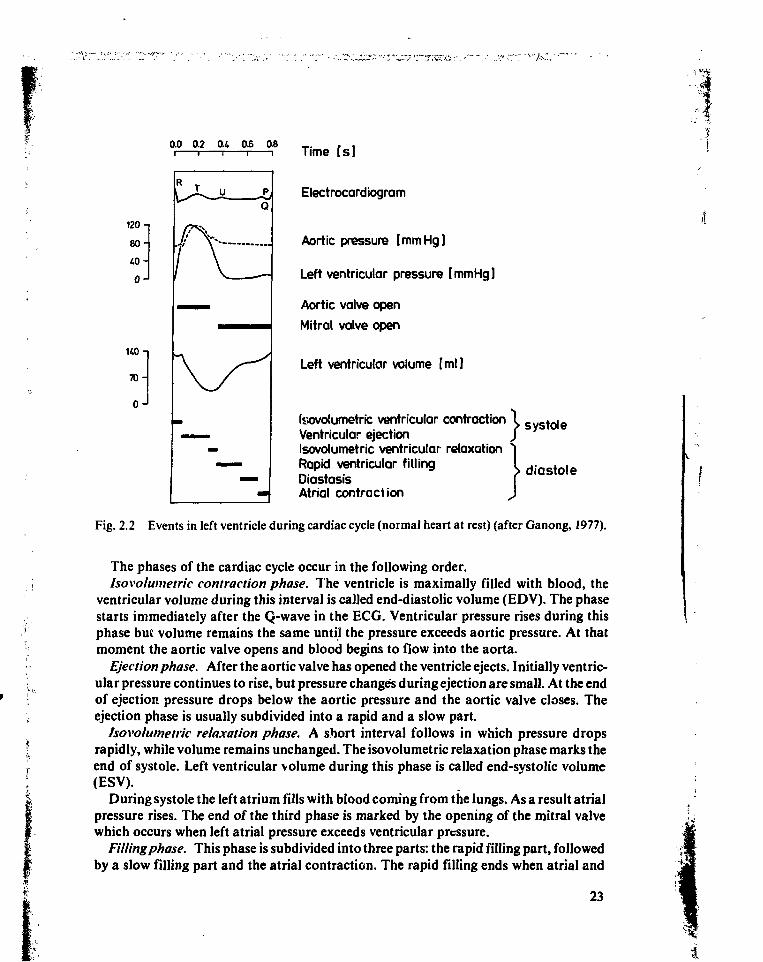
The beating of the heart is a cyclic event: contraction and relaxation alternate, once ineach cycle. The cardiac cycle is usually divided into four different phases: two isovolu-metric phases in which both the mitral and aortic valve are closed, an ejection phase inwhich the aortic valve is open and a filling phase in which the mitral valve is open. Theejection and filling phase are subdivided into different parts. Fig. 2.2 gives the time courseof a single lead of the electrocardiogram, left ventricular volume and different pressuresduring one cardiac cycle for a normal left ventricle under resting conditions.

The isovolumetric contraction and ejection phases are called systole of the heart,isovolumetric relaxation and filling phases are called diastole.

22

0.0 0.2 0.4 0.6 08Time Is ]

Electrocardiogram

Aortic pressure [mmHg]

Left ventricular pressure [mmHg]

Aortic valve open

Mitral valve open

Left ventricular volume [ml]

Isovotumetric ventricular contraction X SyS toie

Ventricular ejection ƒIsovolumetric ventricular relaxation 1Rapid ventricular filling I d i a s t o l e

Oiastasis [Atrial contraction J

Fig. 2.2 Events in left ventricle during cardiac cycle (normal heart at rest) (after Ganong, 1977).

120

80

40

0

140

70

0-

The phases of the cardiac cycle occur in the following order.Isovolumetric contraction phase. The ventricle is maximally filled with blood, the

ventricular volume during this interval is called end-diastolic volume (EDV). The phasestarts immediately after the Q-wave in the ECG. Ventricular pressure rises during thisphase but volume remains the same until the pressure exceeds aortic pressure. At thatmoment the aortic valve opens and blood begins to flow into the aorta.

Ejection phase. After the aortic valve has opened the ventricle ejects. Initially ventric-ular pressure continues to rise, but pressure changes during ejection are small. At the endof ejection pressure drops below the aortic pressure and the aortic valve closes. Theejection phase is usually subdivided into a rapid and a slow part.

Isovolumetric relaxation phase. A short interval follows in which pressure dropsrapidly, while volume remains unchanged. The isovolumetric relaxation phase marks theend of systole. Left ventricular volume during this phase is called end-systolic volume(ESV).

During systole the left atrium fills with blood coming from the lungs. As a result atrialpressure rises. The end of the third phase is marked by the opening of the mitral valvewhich occurs when left atrial pressure exceeds ventricular pressure.

Filling phase. This phase is subdivided into three parts: the rapid filling part, followedby a slow filling part and the atrial contraction. The rapid filling ends when atrial and

23

t

ventricular pressure have equilized. During the slow filling period or diastasis the flowfrom atrium to ventricle almost stops and the mitral valve closes partially. The ventricle'waits' for the atrial contraction to occur. During atrial contraction additional blood ispumped into the ventricle and the mitral valve again opens widely. The filling phase endswhen ventricular contraction increases pressure inside the ventricle, closing the mitralvalve.

Commonly used parameters related to the different phases in the cycle are:LVET: left ventricular ejection time (duration of the ejection phase).LVFT: left ventricular rapid filling time (duration of rapid filling phase).DIAS: duration of diastasis.PEP: pre-ejection period; a short period between onset of the QRS complex of the

ECG and opening of the aortic valve.TCYC: length of the cardiac cycle; using TCYC the heart rate is defined as 60/ TCYC,

(number of beats per minute; TCYC in seconds).Literature: Ganong(1977), Hammermeister(1974), Lewis (1976).

2.3 Detection of abnormal left ventricular wall motion with radiographic angiography

Since most diseases of the heart, especially ischemic heart disease, lead to necrosis ofmuscle cells and subsequent loss of contractile properties much effort has been spent toquantify the amount of damage and to determine its localization by measuring pressureand volume changes during the cardiac cycle. Loss of muscle cells in the heart reduces theamount of fibre shortening and can therefore be expected to reduce stroke volume (SV).Compensatory mechanisms in the body react to stroke volume reduction by graduallyincreasing end-diastolic volume. As a result stroke volume increases to about normalvalues while fibre shortening remains reduced. Any increase of end-diastolic volumeincreases wall stress, which leads to an increase of wall thickness caused by a process ofhypertrophy in the still healthy parts of the heart.

The extent of myocardial damage can be assessed from measurements of pressure andvolume and related parameters, the localization can only be found if regional changes ofvolume or wall motion are analyzed.

The most important index of muscle cell loss is the ejection fraction (EF), which isdefined as:

E F

EDV EDV

Ejection fraction is initially reduced when, due to muscle cell loss, stroke volume is lower.; When the end-diastolic size of the heart has increased and stroke volume has returned tof normal, ejection fraction is still reduced. Normal values of EF are 0.67±0.08 if measured: by radiographic angiography (Kennedy, 1966). Loss of contractile functions can also be

; 24

assessed from parameters related to rate of force or pressure development. The rate ofpressure development (dP/dt) is an estimate of peak systolic pressure. Peak systolicpressure itself measured in a sufficiently filled heart directly reflects the number ofcontractile elements, but it can only be measured in experimental situations when theventricle contracts against a closed aortic valve. However, peak dP/dt and the ratio ofpre-ejection period and ejection time (PEP/ LVET) are both indirect measures of peaksystolic pressure, and can therefore be used to indirectly estimate the extent ofmyocardial damage (normal value for PEP/LVET: 0.34±0.02, (Lewis, 1976)).

It is known that relaxation of heart muscle is slowed down if the fibers contractisometrically. In dilated, partly damaged hearts, fibre shortening is reduced and relaxa-tion is usually prolonged. Peak filling rate can therefore also be used as an estimate ofmyocardial damage and compensatory end-diastolic dilatation (normal value of peakfilling rate: 500±170 ml/s, (Hammermeister, 1974)).

All so-called parameters of contractility derived from pressure or volume measure-ments of the whole heart are sensitive to haemodynamic changes, not directly related tothe extent of damage of the heart muscle. Ejection fraction can increase if the inputimpedance of the aorta is lowered, especially in damaged hearts; dP/dt and PEP/ LVETare sensitive to changes of end-diastolic volume and heart rate. This complicates theinterpretation of the data. A perhaps more important limitation of the contractilityparameters is the absence of spatial information. Especially in coronary artery diseaseinformation on the extent of damage should be completed by adding data on thelocalization of the tissue necrosis or ischemia.

The conventional detection method for regional myocardial damage is radiographicangiography: through a catheter threaded into the left ventricle, contrast material isinjected. The ventricular volume can be visualized by radiographic analysis, after mixingof the contrast material with blood in the cavity. From the study of contrast displacementwall movement can be reconstructed.

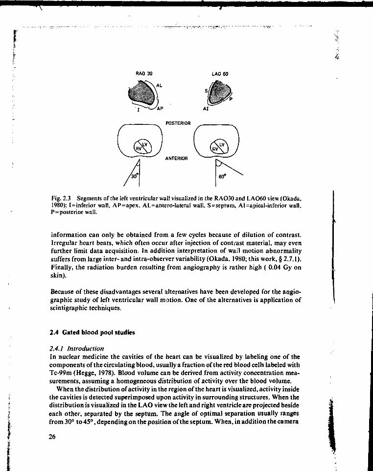
For analysis of wall motion usually two projections are used: RAO30 and LAO60(RAO: right anterior oblique view, the angle between the X-ray tube and a plane that canbe imagined to pass through the spinal chord and perpendicular to the thorax equals 30degrees; LAO: left anterior oblique). The RAO30 view allows visualization of themovement of the antero-lateral, apical and inferior wall of the left ventricle, the LAO60view of the septal, apical-inferior and posterior wall movement (Okada, 1980; fig. 2.3).Roughly four types of wall motion can be distinguished: normal movement (normo-kine-sia), decreased movement (hypo-kinesia), no movement (a-kinesia) and paradoxalmovement (dys-kinesia). In the last case the wall moves outwards during systole andinward early in diastole under the influence of pressure changes within the ventricle,instead of inwards during systole as in normally contracting parts of the ventricle.

Volume related parameters can all be obtained from radiographic angiograms in theRAO30 view or from a combination of images in the RAO30 and LAO60 view (Dodge,1960), using an ellipsoid approximation of the left ventricular shape.

The approximation may be quite poor, particularly in normal hearts at end-diastoleand in hearts with severe regional disorders. Another disadvantage of the method is that

25

4L

RAO 30 LAO 60

POSTERIOR

ANTERIOR

Fig. 2.3 Segments of the left ventricular wall visualized in the RAO30 and LAO60 view (Okada.1980); I=inferior wall, AP=apex, AL=antero-lateral wall, S=septum, AI=apical-inferior wall,P=posterior wall.

information can only be obtained from a few cycles because of dilution of contrast.Irregular heart beats, which often occur after injection of contrast material, may evenfurther limit data acquisition. In addition interpretation of wail motion abnormalitysuffers from large inter- and intra-observer variability (Okada, 1980; this work, § 2,7.1).Finally, the radiation burden resulting from angiography is rather high ( 0.04 Gy onskin).

Because of these disadvantages several alternatives have been developed for the angio-graphic study of left ventricular wall motion. One of the alternatives is application ofscintigraphic techniques.

2.4 Gated blood pool studies

2.4.1 IntroductionIn nuclear medicine the cavities of the heart can be visualized by labeling one of thecomponents of the circulating blood, usually a fraction of the red blood cells labeled withTc-99m (Hegge, 1978). Blood volume can be derived from activity concentration mea-surements, assuming a homogeneous distribution of activity over the blood volume.

When the distribution of activity in the region of the heart is visualized, activity insidethe cavities is detected superimposed upon activity in surrounding structures. When thedistribution is visualized in the LAO view the left and right ventricle are projected besideeach other, separated by the septum. The angle of optimal separation usually rangesfrom 30° to 45°, depending on the position of the septum. When, in addition the camera

26

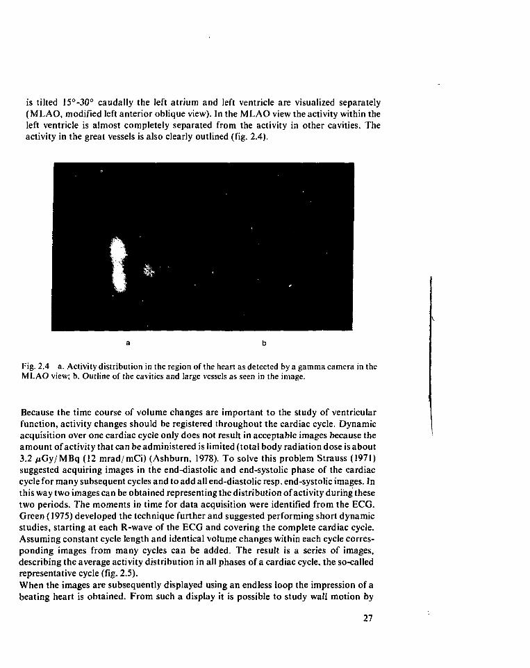
is tilted 15°-30° caudally the left atrium and left ventricle are visualized separately(MLAO, modified left anterior oblique view). In the MLAO view the activity within theleft ventricle is almost completely separated from the activity in other cavities. Theactivity in the great vessels is also clearly outlined (fig. 2.4).

Fig. 2.4 a. Activity distribution in the region of the heart as detected by a gamma camera in theMLAO view; b. Outline of the cavities and large vessels as seen in the image.

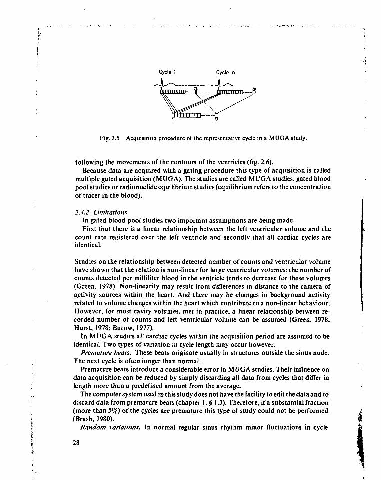
Because the time course of volume changes are important to the study of ventricularfunction, activity changes should be registered throughout the cardiac cycle. Dynamicacquisition over one cardiac cycle only does not result in acceptable images because theamount of activity that can be administered is limited (total body radiation dose is about3.2 juGy/MBq (12 mrad/mCi) (Ashburn, 1978). To solve this problem Strauss (1971)suggested acquiring images in the end-diastolic and end-systolic phase of the cardiaccycle for many subsequent cycles and to add all end-diastolic resp. end-systolic images. Inthis way two images can be obtained representing the distribution of activity during thesetwo periods. The moments in time for data acquisition were identified from the ECG.Green (1975) developed the technique further and suggested performing short dynamicstudies, starting at each R-wave of the ECG and covering the complete cardiac cycle.Assuming constant cycle length and identical volume changes within each cycle corres-ponding images from many cycles can be added. The result is a series of images,describing the average activity distribution in all phases of a cardiac cycle, the so-calledrepresentative cycle (fig. 2.5).

When the images are subsequently displayed using an endless loop the impression of abeating heart is obtained. From such a display it is possible to study wall motion by

27

Cycle 1 Cycle n

Fig. 2.5 Acquisition procedure of the representative cycle in a MUG A study.

following the movements of the contours of the ventricles (fig. 2.6).Because data are acquired with a gating procedure this type of acquisition is called

multiple gated acquisition (MUGA). The studies are called MUGA studies, gated bloodpool studies or radionuclide equilibrium studies (equilibrium refers to the concentrationof tracer in the blood).

2.4.2 LimitationsIn gated blood pool studies two important assumptions are being made.First that there is a linear relationship between the left ventricular volume and the

count rate registered over the left ventricle and secondly that all cardiac cycles areidentical.

Studies on the relationship between detected number of counts and ventricular volumehave shown that the relation is non-linear for large ventricular volumes: the number ofcounts detected per milliliter blood in the ventricle tends to decrease for these volumes(Green, 1978). Non-linearity may result from differences in distance to the camera ofactivity sources within the heart. And there may be changes in background activityrelated to volume changes within the heart which contribute to a non-linear behaviour.However, for most cavity volumes, met in practice, a linear relationship between re-corded number of counts and left ventricular volume can be assumed (Green. 1978;Hurst, 1978; Burow, 1977).

In MUGA studies all cardiac cycles within the acquisition period are assumed to beidentical. Two types of variation in cycle length may occur however.

Premature beats. These beats originate usually in structures outside the sinus node.The next cycle is often longer than normal.

;-s Premature beats introduce a considerable error in MUGA studies. Their influence on' data acquisition can be reduced by simply discarding all data from cycles that differ in; length more than a predefined amount from the average.

The computer system used in this study does not have the facility to edit the data and todiscard data from premature beats (chapter 1, § 1.3). Therefore, if a substantial fraction(more than 5%) of the cycles are premature this type of study could not be performed

i (Brash, 1980).f Random variations. In normal regular sinus rhythm minor fluctuations in cycle

I 28f

utt* * t

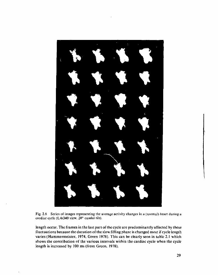
Fig. 2.6 Series of images representing the average activity changes in a (normal) heart during acardiac cycle (LAO40 view, 20° caudal tilt).

length occur. The frames in the last part of the cycle are predominantly affected by thesefluctuations because the duration of the slow filling phase is changed most if cycle lengthvaries (Hammermeister, 1974, Green 1978). This can be clearly seen in table 2.1 whichshows the contribution of the various intervals within the cardiac cycle when the cyclelength is increased by 100 ms (from Green, 1978).

29

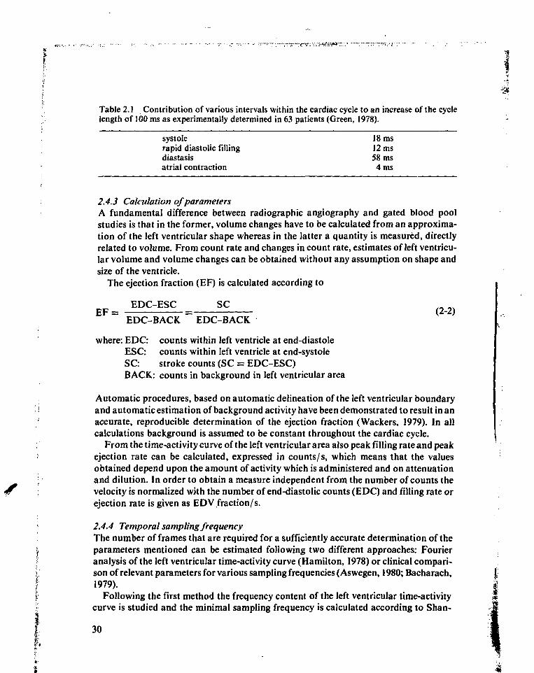
Table 2.1 Contribution of various intervals within the cardiac cycle to an increase of the cyclelength of 100 ms as experimentally determined in 63 patients (Green, 1978).

systolerapid diastolic fillingdiastasisatrial contraction

18 ms12 ms58 ms4 ms

• 2.4.3 Calculation of parametersA fundamental difference between radiographic angiography and gated blood poolstudies is that in the former, volume changes have to be calculated from an approxima-tion of the left ventricular shape whereas in the latter a quantity is measured, directlyrelated to volume. From count rate and changes in count rate, estimates of left ventricu-lar volume and volume changes can be obtained without any assumption on shape andsize of the ventricle.

The ejection fraction (EF) is calculated according to

EDC-ESC SCE F = = (2-2)

EDC-BACK EDC-BACKwhere: EDC: counts within left ventricle at end-diastole

ESC: counts within left ventricle at end-systoleSC: stroke counts (SC = EDC-ESC)BACK: counts in background in left ventricular area

Automatic procedures, based on automatic delineation of the left ventricular boundary• and automatic estimation of background activity have been demonstrated to result in an

accurate, reproducible determination of the ejection fraction (Wackers, 1979). In all. calculations background is assumed to be constant throughout the cardiac cycle.; From the time-activity curve of the left ventricular area also peak filling rate and peak; ejection rate can be calculated, expressed in counts/s, which means that the values

obtained depend upon the amount of activity which is administered and on attenuationi and dilution. In order to obtain a measure independent from the number of counts the

velocity is normalized with the number of end-diastolic counts (EDC) and filling rate orejection rate is given as EDV fraction/s.

' 2.4.4 Temporal sampling frequencyi The number of frames that are required for a sufficiently accurate determination of the| parameters mentioned can be estimated following two different approaches: FourierI analysis of the left ventricular time-activity curve (Hamilton, 1978) or clinical compari-; son of relevant parameters for various sampling frequencies (Aswegen, 1980; Bacharach,f 1979).f Following the first method the frequency content of the left ventricular time-activity

curve is studied and the minimal sampling frequency is calculated according to Shan-

30

non's sampling theorem (Shannon, 1949). According to the second method the values ofclinical parameters are determined for various sampling frequencies and differences inthe values of the parameters are studied.

Both methods indicate that the sampling frequency should be about 20-25 frames/ s,which means that for normal heart rates (about 0.85 s/cardiac cycle) each cycle shouldbe sampled by at least 17-21 frames for both wall motion and ejection fraction analysis, atrest and during exercise.

2.4.5 Functional imagesLargest activity changes in the left ventricular area are seen near the edges of the ventricle,if the cavity is approximated with a spherical, contracting model and imaged with highspatial resolution.

In practice, however, in normally contracting ventricles local time-activity curvesclosely resemble each other. Adam (1977) found that in these ventricles local time-activi-ty curves correlate well with the global time-activity curve: if for each pixel a time-activitycurve is calculated, the correlation coefficient with total left ventricular time-activitycurve is greater than 0.9 in 78% of the pixels within the left ventricle. Only for pixels nearthe border of the left ventricular area does the correlation coefficient drop to zero.Probably the theoretically expected activity changes are masked by the point spreadfunction of the detecting/ imaging system, patient movement, respiration, background,irregular shape of the cavity and noise. In case of regional wall motion abnormality,regional volume changes are altered and local time-activity curves are affected; as a resultthe correlation of local curves with the global curve decreases (Adam, 1977).

For each regional time-activity curve function parameters can be calculated in thesame way as for the global curve. Because of the large number of pixels within the leftventricular area (normally about 300-400) the results of parametric analysis for eachpixel are best presented in images, using colour coding of the parameter values. This typeof image is called functional image. A well known example is the regional ejectionfraction image which shows the regional ejection fraction for each pixel (Maddox, 1978;fig. 2.7).

2.5 Characterization of the left ventricular time-activity curve with the first harmonic inthe Fourier spectrum

2.5.1 IntroductionAlthough regional time-activity curves give a reliable description of local activity changesthis may not necessarily be true for single curve points. For instance, calculation of theregional ejection fraction only requires two curve points which may be subject tosignificant errors, even if the curve as a whole correlates well with the total time-activitycurve.

In general, it can be expected that parameters, derived from single points in the curveare sensitive to noise. In the case of the regional ejection fraction the background mayalso vary regionally, causing errors in regional background determination. Also changes

31

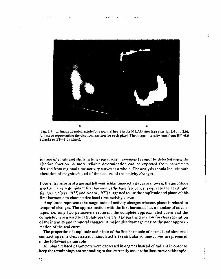
Fig. 2.7 a. Image at end-diastole for a normal heart in the M LAO view (see also fig. 2.4 and 2.6);b. Image representing the ejection fraction for each pixel. The image intensity runs from EF=0.0(black) to EF=1.0 (white).

in time intervals and shifts in time (paradoxal movement) cannot be detected using theejection fraction. A more reliable determination can be expected from parametersderived from regional time-activity curves as a whole. The analysis should include bothalteration of magnitude and of time course of the activity changes.

Fourier transform of a normal left ventricular time-activity curve shows in the amplitudespectrum a very dominant first harmonic (the base frequency is equal to the heart rate;fig. 2.8). Geffers (1977) and Adam (1977) suggested to use the amplitude and phase of thisfirst harmonic to characterize local time-activity curves.

Amplitude represents the magnitude of activity changes whereas phase is related totemporal changes. The approximation with the first harmonic has a number of advan-tages: i.e. only two parameters represent the complete approximated curve and thecomplete curve is used to calculate parameters. The parameters allow for clear separationof the intensity and temporal changes. A major disadvantage may be the poor approxi-mation of the real curve.

The properties of amplitude and phase of the first harmonic of normal and abnormalcontracting ventricles, assessed in simulated left ventricular volume curves, are presentedin the following paragraphs.

All phase related parameters were expressed in degrees instead of radians in order tokeep the terminology corresponding to that currently used in the literature on this topic.

32

WW

nMp

\

if

ri

f ,

•

•

•

* W 1

L

n

ïccEïT?

• « . « • FKBUENCY CHZ1 I2.S * . M TlfC ATTEK K-WWE (SI t .89

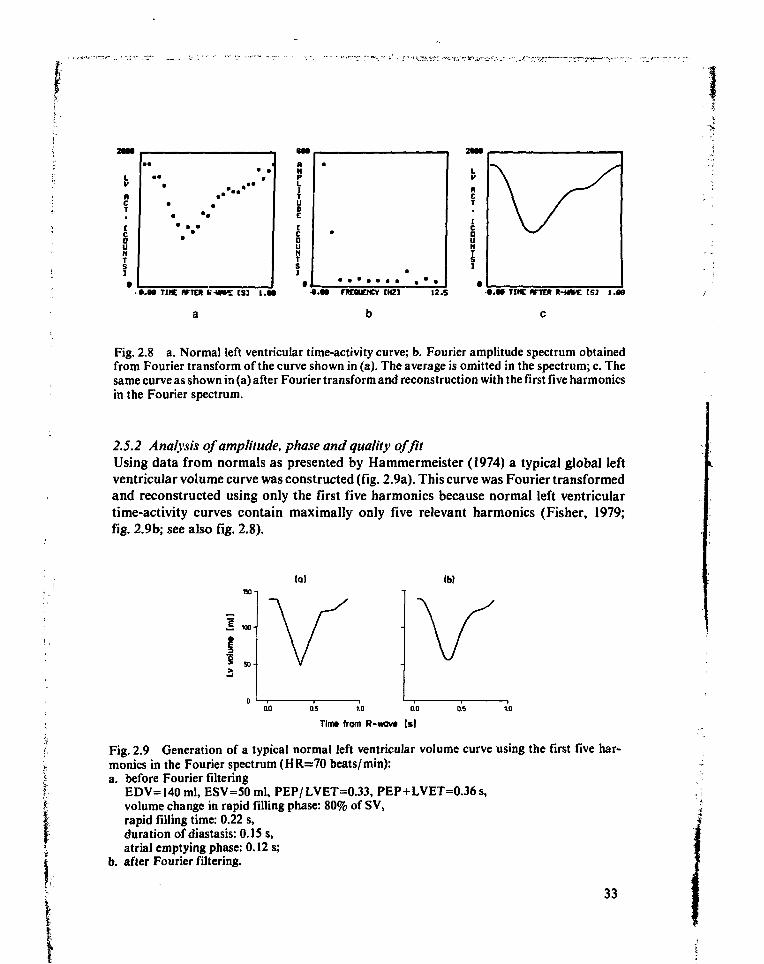
Fig. 2.8 a. Normal left ventricular time-activity curve; b. Fourier amplitude spectrum obtainedfrom Fourier transform of the curve shown in (a). The average is omitted in the spectrum; c. Thesame curve as shown in (a) after Fourier transform and reconstruction with the first five harmonicsin the Fourier spectrum.

2.5.2 Analysis of amplitude, phase and quality of fitUsing data from normals as presented by Hammermeister (1974) a typical global leftventricular volume curve was constructed (fig. 2.9a). This curve was Fourier transformedand reconstructed using only the first five harmonics because normal left ventriculartime-activity curves contain maximally only five relevant harmonics (Fisher, 1979;fig. 2.9b; see also fig. 2.8).

(a) (b)

1 «.

OU} 0.5 1.0 0.0 05 1.0

Tim» from R-wav* (s)

Fig. 2.9 Generation of a typical normal left ventricular volume curve using the first five har-monics in the Fourier spectrum (HR=70 beats/min):a. before Fourier filtering

EDV=l40 ml, ESV=50 ml, PEP/LVET=0.33, PEP+LVET=0.36s,volume change in rapid filling phase: 80% of S V,rapid filling time: 0.22 s,duration of diastasis: 0.15 s,atrial emptying phase: 0.12 s;

b. after Fourier filtering.

33

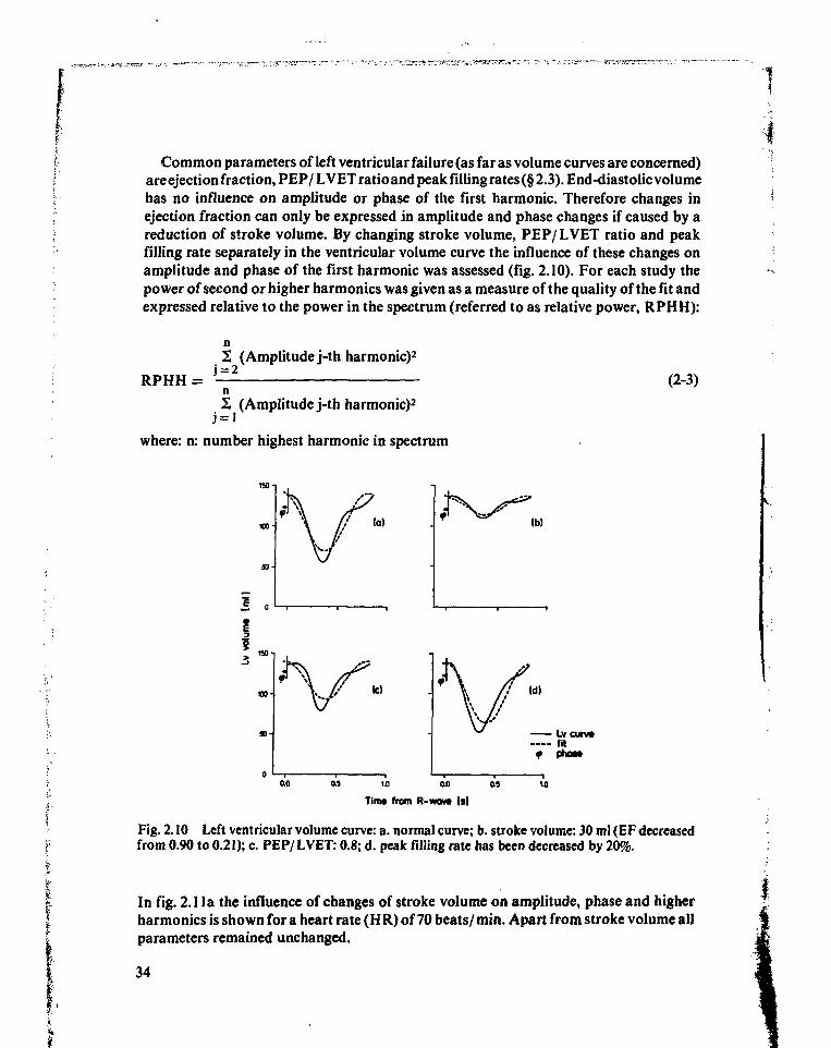
Common parameters of left ventricular failure (as far as volume curves are concerned)are ejection fraction, PEP/ LVET ratio and peak filling rates (§ 2.3). End-diastolic volumehas no influence on amplitude or phase of the first harmonic. Therefore changes inejection fraction can only be expressed in amplitude and phase changes if caused by areduction of stroke volume. By changing stroke volume, PEP/ LVET ratio and peakfilling rate separately in the ventricular volume curve the influence of these changes onamplitude and phase of the first harmonic was assessed (fig. 2.10). For each study thepower of second or higher harmonics was given as a measure of the quality of the fit andexpressed relative to the power in the spectrum (referred to as relative power, RPHH):

(Amplitude j-th harmonic)2

RPHH = (2-3)

2 (Amplitude j-th harmonic)2

where: n: number highest harmonie in spectrum

Ib)

«o

as 1.0 ao as

Tim* from R-wav» Is)

Fig. 2.10 Left ventricular volume curve: a. normal curve; b. stroke volume: 30 ml (EF decreasedfrom 0.90 to 0.21); c. PEP/LVET: 0.8; d. peak filling rate has been decreased by 20%.

In fig. 2.1 la the influence of changes of stroke volume on amplitude, phase and higherharmonics is shown for a heart rate (HR) of 70 beats/min. Apart from stroke volume allparameters remained unchanged.

34

I

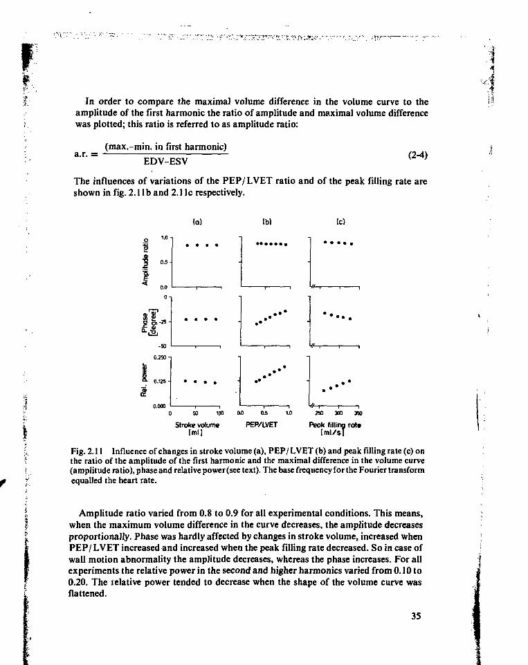
I: In order to compare the maximal volume difference in the volume curve to theamplitude of the first harmonic the ratio of amplitude and maximal volume differencewas plotted; this ratio is referred to as amplitude ratio:

a.r. =(max.-min. in first harmonic)

EDV-ESV (2-4)

The influences of variations of the PEP/ LVET ratio and of the peak filling rate areshown in fig. 2.1 lb and 2.1 Ic respectively.

(a) (b) (c)

0.000

50 100 0.0 250 300 390

Stroke volume[ml]

PEP/LVET Peak filling rate[tnl/s]

Fig. 2.11 Influence of changes in stroke volume (a), PEP/ LVET (b) and peak filling rate (c) onthe ratio of the amplitude of the first harmonic and the maximal difference in the volume curve(amplitude ratio), phase and relative power (see text). The base frequency for the Fourier transformequalled the heart rate.

Amplitude ratio varied from 0.8 to 0.9 for all experimental conditions. This means,when the maximum volume difference in the curve decreases, the amplitude decreasesproportionally. Phase was hardly affected by changes in stroke volume, increased whenPEP/ LVET increased and increased when the peak filling rate decreased. So in case ofwall motion abnormality the amplitude decreases, whereas the phase increases. For allexperiments the relative power in the second and higher harmonics varied from 0.10 to0.20. The relative power tended to decrease when the shape of the volume curve wasflattened.

35

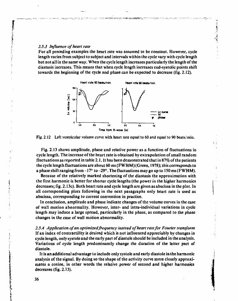
2.5.3 Influence of heart rateFor all preceding examples the heart rate was assumed to be constant. However, cyclelength varies from subject to subject and intervals within the cycle vary with cycle lengthbut not all in the same way. When the cycle length increases particularly the length of thediastasis increases. This means that when cycle length increases end-systolic points shifttowards the beginning of the cycle and phase can be expected to decrease (fig. 2.12).

Heart rat* 60 baats/min Haart rat» 90 baats/min

1 IOOH

iLvcurv*fit

f

3.0 0.5 1.0 0.0 0.S 10

Tim* from R-wovt Is'i

Fig. 2.12 Left ventricular volume curve with heart rate equal to 60 and equal to 90 beats/ min.

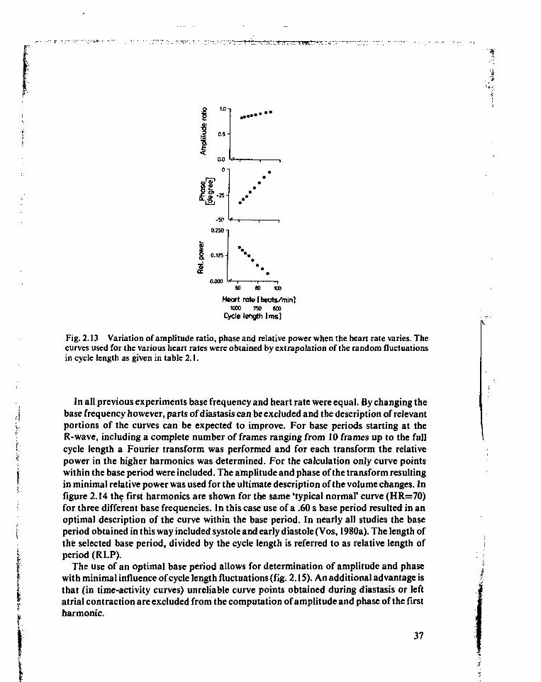
Fig. 2.13 shows amplitude, phase and relative power as a function of fluctuations incycle length. The increase of the heart rate is obtained by extrapolation of small randomfluctuations as reported in table 2.1. It has been demonstrated that in 87% of the patientsthe cycle length fluctuations are about 60 ms (FWHM) (Green, 1978); this corresponds toa phase shift ranging from -17° to -29°. The fluctuations may go up to 150 ms (F W H M).

Because of the relatively marked shortening of the diastasis the approximation withthe first harmonic is better for shorter cycle lengths (the power in the higher harmonicsdecreases; fig. 2.13c). Both heart rate and cycle length are given as abscissa in the plot. Inall corresponding plots following in the next paragraphs only heart rate is used asabscissa, corresponding to current convention in practice.

In conclusion, amplitude and phase indicate changes of the volume curves in the caseof wall motion abnormality. However, inter- and intra-individual variations in cyclelength may induce a large spread, particularly in the phase, as compared to the phasechanges in the case of wall motion abnormality.

2.5.4 Application of an optimized frequency instead of heart rate for Fourier transformIf an index of contractility is desired which is not influenced appreciably by changes incycle length, only systole and the early part of diastole should be included in the analysis.Variations of cycle length predominantly change the duration of the latter part ofdiastole.

It is an additional advantage to include only systole and early diastole in the harmonicanalysis of the signal. By doing so the shape of the activity curve more closely approxi-mates a cosine, in other words the relative power of second and higher harmonicsdecreases (fig. 2.13).

''4

36

1.0-

3 0.5-

0.0

On

«f-25-

-50

0.250-

0.125-

0.00060 10

Heart rate (beats/miniWOO 750 600

Cycle length [ms]

Fig. 2.13 Variation of amplitude ratio, phase and relative power when the heart rate varies. Thecurves used for the various heart rates were obtained by extrapolation of the random fluctuationsin cycle length as given in table 2.1.

In all previous experiments base frequency and heart rate were equal. By changing thebase frequency however, parts of diastasis can be excluded and the description of relevantportions of the curves can be expected to improve. For base periods starting at theR-wave, including a complete number of frames ranging from 10 frames up to the fullcycle length a Fourier transform was performed and for each transform the relativepower in the higher harmonics was determined. For the calculation only curve pointswithin the base period were included. The amplitude and phase of the transform resultingin minimal relative power was used for the ultimate description of the volume changes. Infigure 2.14 the first harmonics are shown for the same 'typical normal' curve (HR=70)for three different base frequencies. In this case use of a .60 s base period resulted in anoptimal description of the curve within the base period. In nearly all studies the baseperiod obtained in this way included systole and early diastole (Vos, 1980a). The length ofthé selected base period, divided by the cycle length is referred to as relative length ofperiod (RLP).

The use of an optimal base period allows for determination of amplitude and phasewith minimal influence of cycle length fluctuations (fig. 2.1S). An additional advantage isthat (in time-activity curves) unreliable curve points obtained during diastasis or leftatrial contraction are excluded from the computation of amplitude and phase of the firstharmonic.

37

4(a) Ib) (O

Lv curv»fit

f Phos»

00 0.5 10 0-0 0.5 1.0 0.0 05 1X1

Tim* from R-wavt Is)

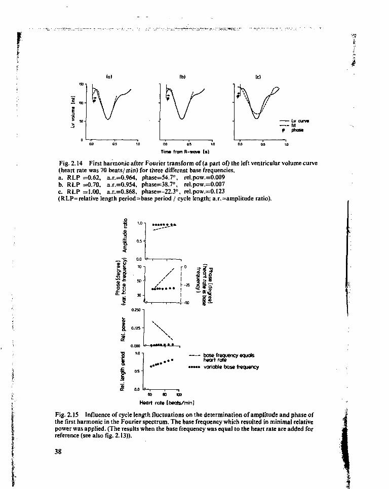
Fig. 2.14 First harmonie after Fourier transform of (a part of) the left ventricular volume curve(heart rate was 70 beats/ min) for three different base frequencies.a. RLP =0.62, a.r.=0.964, phase=54.7°, rel.pow.=0.009b. RLP =0.70, a.r.=0.954, phase=38.7<\ rel.pow.=0.007c. RLP =1.00, a.r.=0.868, phase=-22.3°, rel.pow.=0.I23(RLP= relative length period = base period / cycle length; a.r. =amplitude ratio).

1.0

„•> . o.o w—r-• £ 70 -i

50 -

30-

h-25

r-5B0.J50 -i

0.125 -

0.000

1.0

0.5-

8. 0.0

base frequency equalsheart rate

• • • • • variable base frequency

CO W X»

Heart rate tbeats/minj

Fig. 2. IS Influence of cycle length fluctuations on the determination of amplitude and phase ofthe first harmonic in the Fourier spectrum. The base frequency which resulted in minimal relativepower was applied. (The resplts when the base frequency was equal to the heart rate are added forreference (see also fig. 2.13)).

38

For the same values of stroke volume, PEP/ LVET and peak filling rate as in theprevious paragraph amplitude, phase and relative power were calculated using a variablefrequency for the Fourier transform: for each experiment the frequency resulting inminimal relative power was used for the calculations (fig. 2.16; fig. 2.17).

Ib)

(cl (d)

Lvcurvtfit

f Phott

i.o onTin» from R-wov» Is)

0.5

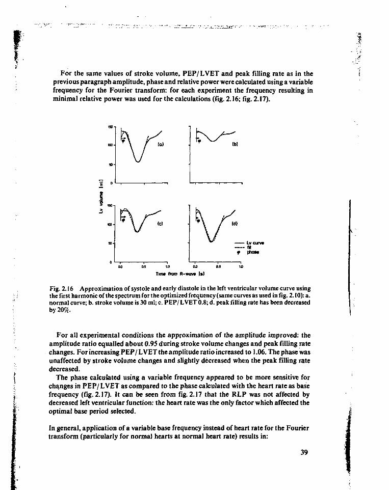
Fig. 2.16 Approximation of systole and early diastole in the left ventricular volume curve usingthe first harmonic of the spectrum for the optimized frequency (same curves as used in fig. 2.10): a.normal curve; b. stroke volume is 30 ml; c. PEP/ LVET 0.8; d. peak filling rate has been decreasedby 20%.

For all experimental conditions the approximation of the amplitude improved: theamplitude ratio equalled about 0.95 during stroke volume changes and peak filling ratechanges. For increasing PEP/ LVET the amplitude ratio increased to 1.06. The phase wasunaffected by stroke volume changes and slightly decreased when the peak filling ratedecreased.

The phase calculated using a variable frequency appeared to be more sensitive forchanges in PEP/ LVET as compared to the phase calculated with the heart rate as basefrequency (fig. 2.17). It can be seen from fig. 2.17 that the RLP was not affected bydecreased left ventricular function: the heart rate was the only factor which affected theoptimal base period selected.

In general, application of a variable base frequency instead of heart rate for the Fouriertransform (particularly for normal hearts at normal heart rate) results in:

39

base frequencyequals heart rate

• • • • • variable basefrequency

0 50 100

Stroke volume [ml]

0.5

PEP/LVET

250 300 350

Peak filling rate (ml/sl

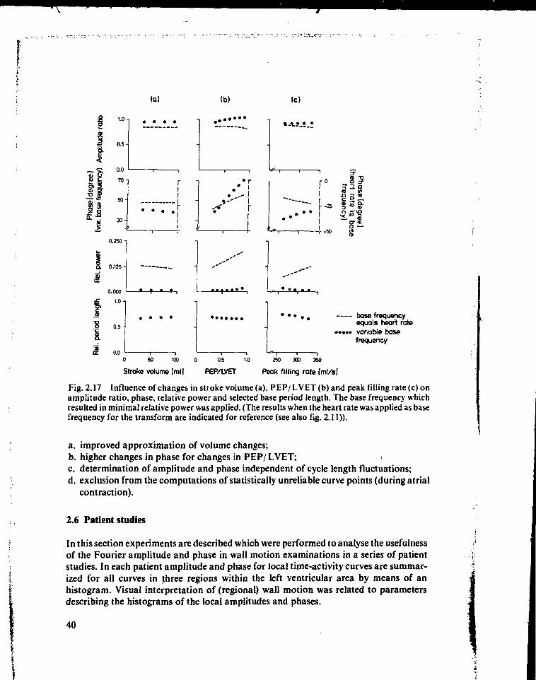
Fig. 2.17 Influence of changes in stroke volume (a), PEP/ LVET (b) and peak filling rate (c) onamplitude ratio, phase, relative power and selected base period length. The base frequency whichresulted in minimal relative power was applied. (The results when the heart rate was applied as basefrequency for the transform are indicated for reference (see also fig. 2.11)).

a. improved approximation of volume changes;b. higher changes in phase for changes in PEP/ LVET;c. determination of amplitude and phase independent of cycle length fluctuations;d. exclusion from the computations of statistically unreliable curve points (during atrial

contraction).

2.6 Patient studies

In this section experiments are described which were performed to analyse the usefulnessof the Fourier amplitude and phase in wall motion examinations in a series of patientstudies. In each patient amplitude and phase for local time-activity curves are summar-ized for all curves in three regions within the left ventricular area by means of anhistogram. Visual interpretation of (regional) wall motion was related to parametersdescribing the histograms of the local amplitudes and phases.

• i -

40

-s*

2.6.1 Data acquisitionSeventy-five consecutive patients, referred to the Division of Nuclear Medicine (Univer-sity Hospital Leiden, The Netherlands) for evaluation of left ventricular function werechosen. Patients with severe arrhythmia, bundle branch block or other conductiondisorders were excluded from this study (§ 2.4.2). Also patients with severe valvularregurgitation were excluded.

The labeling of red blood cells was performed in vivo. An intravenous (i.v.) injection ofabout 0.4 mg stannous chloride and 2.0 mg pyrophosphate dissolved in 0.5 ml of a salinesolution was administered, followed about 30 minutes later by an i.v. injection of 555MBq (15 mCi) Tc-99m pertechnetate. According to the experiments performed by Hegge(1978) after five minutes an homogenous distribution of radiopharmaceutical over theblood volume is reached and the study can start.

A gamma camera with a large field of view (equipped with a general purpose, parallelhole collimator) was placed in the LAO position. The obliquity was adjusted for eachpatient in order to obtain a good separation of left and right ventricle. Without change ofthe obliquity the camera was tilted 30° caudally in order to avoid overlap of left atriumand left ventricle.

Multiple gated acquisition was performed at rest using a commercially availableacquisition program (MDS-MUGA). Before data acquisition started the average cyclelength was determined and divided into 28 equal intervals. Corresponding to theseintervals 28 frames were acquired per cycle, offering sufficient temporal resolution(§ 2.4.4). To save space in the memory of the computer and to maintain spatial resolutiononly the central portion of the camera's field of view was digitized, offering a maximalspatial resolution of about 5 mm (32x 32 pixels, zoomed into the heart region, 16 cm fieldof view). Although this is less than the spatial resolution of the camera system, severalauthors have shown that this spatial sampling frequency is adequate for wall motionanalysis (Burow, 1977; Bacharach, 1978). Afterwards the image was interpolated to64x64 pixels for display purposes, (see also chapter 1, § 1.2.1). Using the MUGAprinciple a representative cycle was obtained. Each frame contained at least 300k counts,usually obtained in 10-15 minutes acquisition time. After acquisition and interpolationthe images were stored on disc. At the time of acquisition data such as heart rate, time perframe, number of frames collected etc. were registered on a standard information sheet.

During acquisition a small source of 1.5 MBq (40 juCi) Tc-99m was placed in one of thecorners of the field of view of the camera. After data acquisition a curve was generatedtaking the source in a region of interest (ROI). The calibrated source was used to correctfor the effect of variation of cycle length on the average number of counts in end-diastolicframes (Taylor, 1979). All studies were corrected in this way.

Visual interpretation of left ventricular wall motion was performed independently bythree cardiologists. After a nine point smoothing the images were displayed in an endlessloop on the television monitor in real time (black/white). The left ventricle was dividedinto three regions (postero-lateral, infero-apical, antero-septal). Wall motion in each

41

region was reported using the same (ordinal) scale as usually applied for the descriptionof wall motion in radiographic angiography:

0 = normokinesia1 = hypokinesia2 = akinesia3 = dyskinesia

For 37 of the 75 patients a radiographic angiogram (R AO30 and L AO60) was available,obtained within three months before or after the MUG A study. In none of these patientsdid the condition of the heart seriously change within this period. All angiograms(LAO60 view) were interpreted by the same observers using the same scores. All ob-servers interpreted the corresponding 37 M UG A studies twice. Observer 3 interpreted allangiograms twice. The repeated interpretations were used to assess the amount ofinter-and intra-observer variability. A comparison of wall motion analysis using thesetwo methods was not performed because the angle of view was different, so it wasimpossible to compare the same segments of the ventricular wall.

2.6.2 Data analysisFor each study the optimal frequency for Fourier transform of the regional time-activitycurves was derived from the total left ventricular time-activity curve using the relativepower criterion as described in § 2.5.2. All parameters related to the Fourier transformthat could be derived from the total curve were calculated both for optimized basefrequency and for heart rate as base frequency (amplitude ratio, phase, relative power).The relative length of the base period was derived from the selected base period and theaverage cycle length.

Using the optimized base frequency, amplitude and phase were calculated for all pixelswith an odd reference number within the images only. This restriction was used to limitexecution time for analysis during the daily routine. A typical execution time for a baseperiod of 20 frames was about 2 minutes. After the calculation local amplitude and phasevalues were interpolated for display purposes resulting in two 64x64 pixel frames.

The amplitudes indicate absolute activity changes, which may vary from patient topatient because of differences in attenuation and dilution. In order to normalize ampli-tudes of local activity curves of the left ventricle the amplitude frame was divided by theaverage value of the local amplitude and multiplied by the ejection fraction (Adam,1980). In this way the amplitudes of the local activity curves within the left ventriculararea were related to the left ventricular ejection fraction; the scale factor used was

EF(2-5)1/n

where: Ay: amplitude detected in pixel i, j |SAjj.' sum of all amplitudes within left ventricular area fn: total number of pixels within left ventricular area *

42

Using the local, scaled amplitude and the local phase two functional images can becreated describing the local time-activity changes and temporal differences in the activitychanges.

2.6.3 Generation of histograms describing values of local amplitude and phaseTo relate the amplitude and phase of the activity curves obtained in certain regions of theventricle to regional wall motion, the left ventricular area must be divided into threeregions pertaining to the antero-lateral, the postero-lateral and the infero-apical part ofthe wall. However, a large number of local amplitudes and phases was available withineach region so some form of summarizing the information within the regions had to beperformed. For example, if the apex was determined to be hypokinetic the amplitudesand phases in a collection of pixels within the apical region has to be related to the wallmotion score.

The subdividing into three regions of interest (ROI's) was done by hand using a lightpen (fig. 2.18). The contours of the free wall were (visually) derived from the amplitudeimage, the location of the interventricular septum was marked out in the end-diastolicimage.

^ — ^ postero-lateral

JCVAantero-septal \T / " " ]

\ / ~~T—infero-apical

Fig. 2.18 Regions of interest over the three regions within the left ventricular area for which theamplitude and phase histogram was calculated (MLAO view).

For each of the ROI's an histogram was formed containing all values of the amplitudeswithin that region; a similar histogram was created for the phase distribution. In additionan amplitude and phase histogram was generated of the total left ventricular area. Theprograms for calculation of the histograms included a 3-point smooth. The followingparameters calculated from these histograms were related to wall motion score:

mean: x = 2 Xj/n (2-6)standard deviation: SD = ^(Xj-x^/n 1 (2-7)skewness: 2 (x; - x)3/(n SD*) (2-8)kurtosis: 2 (x; - x)4/(n SD4) - 3 (2-9)

where: x{: local value of amplitude or phasex: average value of xn: number of points in the histogramSD: standard deviation

43

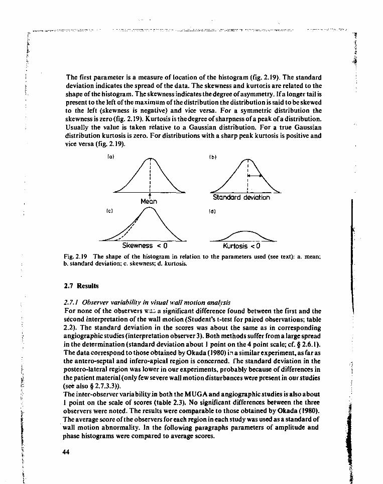
The first parameter is a measure of location of the histogram (fig. 2.19). The standarddeviation indicates the spread of the data. The skewness and kurtoris are related to theshape of the histogram. The skewness indicates the degree of asymmetry. If a longer tail ispresent to the left of the maximum of the distribution the distribution is said to be skewedto the left (skewness is negative) and vice versa. For a symmetric distribution theskewness is zero (fig. 2.19). Kurtosis is the degree of sharpness of a peak of a distribution.Usually the value is taken relative to a Gaussian distribution. For a true Gaussiandistribution kurtosis is zero. For distributions with a sharp peak kurtosis is positive andvice versa (fig. 2.19).

(c)

Skewness < 0

Standard deviation

Id)

Kurtosis <0Fig. 2.19 The shape of the histogram in relation to the parameters used (see text): a. mean:b. standard deviation; c. skewness; d. kurtosis.

2.7 Results

2.7.1 Observer variability in visual wall motion analysisFor none of the observers wi- a significant difference found between the first and thesecond interpretation of the wall motion (Student's t-test for paired observations; table2.2). The standard deviation in the scores was about the same as in correspondingangiographic studies (interpretation observer 3). Both methods suffer from a large spreadin the determination (standard deviation about 1 point on the 4 point scale; cf. § 2.6.1).The data correspond to those obtained by Okada (1980) in a si milar experiment, as far asthe antero-septal and infero-apical region is concerned. The standard deviation in thepostero-lateral region was lower in our experiments, probably because of differences inthe patient material (only few severe wall motion disturbances were present in our studies(see also § 2.7.3.3)).The inter-observer variability in both the M UG A and angiographic studies is also about1 point on the scale of scores (table 2.3). No significant differences between the threeobservers were noted. The results were comparable to those obtained by Okada (1980).The average score of the observers for each region in each study was used as a standard ofwall motion abnormality. In the following paragraphs parameters of amplitude andphase histograms were compared to average scores.

44

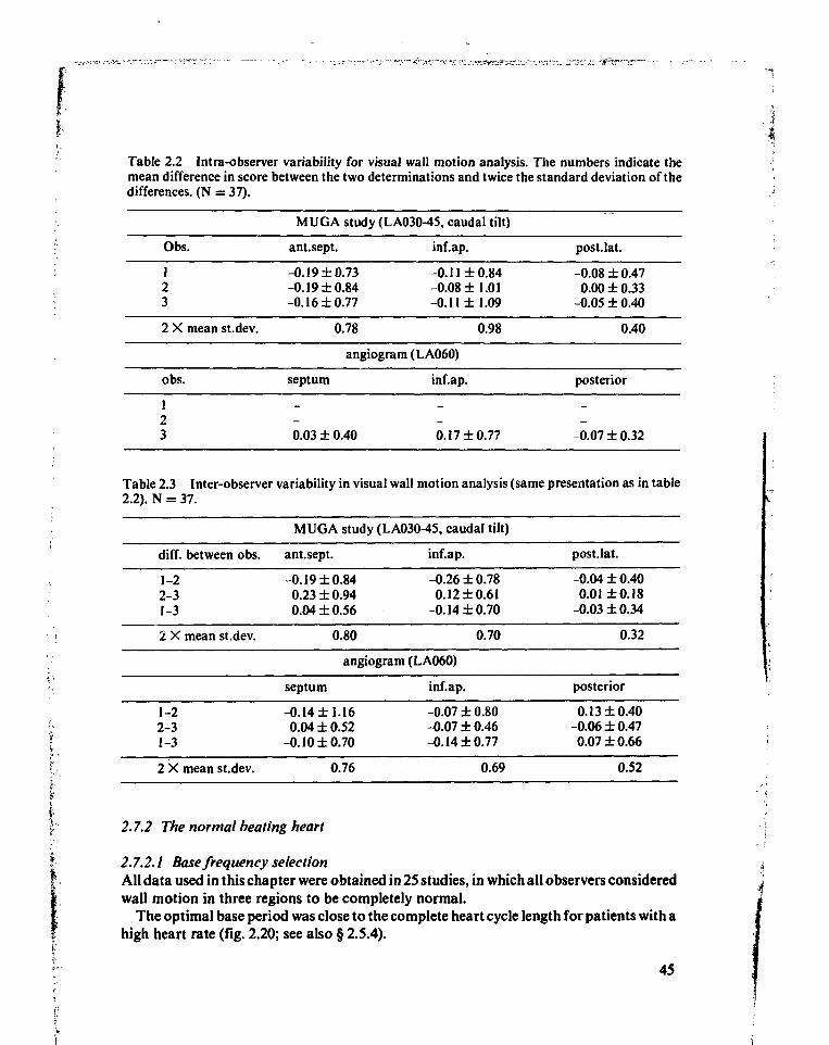
Table 2.2 Intra-observer variability for visual wall motion analysis. The numbers indicate themean difference in score between the two determinations and twice the standard deviation of thedifferences. (N = 37).

Obs.

123

2 X mean st.dev.

obs.

123

MUG A study (LA030-45, caudal tilt)

ant.sept.

-0.19 ±0.73-0.19 ±0.84-0.16 ±0.77

0.78

inf.ap.

-0.11 ±0.84-0.08 ±1.01-0.11 ±1.09

0.98

angiogram (LA060)

septum

0.03 ± 0.40

inf.ap.

0.17 ±0.77

post.Iat.

-0.08 ±0.470.00 ±0.33

-0.05 ±0.40

0.40

posterior

-0.07 ±0.32

Table 2.3 Inter-observer variability in visual wall motion analysis (same presentation as in table2.2). N = 37.

diff. between obs.

1-22-31-3

2 X mean st.dev.

1-22-31-3

2 X mean st.dev.

MUG A study (LA030-45, caudal tilt)

ant.sept.

-0.19 ±0.840.23 ±0.940.04 ±0.56

0.80

inf.ap.

-0.26 ±0.780.12 ±0.61

-0.14 ±0.70

0.70

angiogram (LA060)

septum

-0.14 ±1.160.04 ±0.52

-0.10 ±0.70

0.76

inf.ap.

-0.07 ±0.80-0.07 ±0.46-0.14 ±0.77

0.69

post.Iat.

-0.04 ± 0.400.01 ±0.18

-0.03 ±0.34

0.32

posterior

0.13 ±0.40-0.06 ±0.470.07 ±0.66

0.52

2.7.2 The normal beating heart

2.7.2.1 Base frequency selectionAll data used in this chapter were obtained in 25 studies, in which all observers consideredwall motion in three regions to be completely normal.

The optimal base period was close to the complete heart cycle length for patients with ahigh heart rate (fig. 2.20; see also § 2.5.4).

45

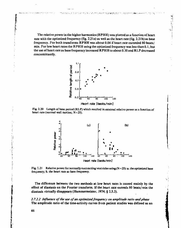
The relative power in the higher harmonics (RPH H) was plotted as a function of heartrate with the optimized frequency (fig. 2.21a) as well as the heart rate (fig. 2.21b) as basefrequency. For both transforms RPHH was about 0.04 if heart rate exceeded 80 beats/min. For low heart rates the RPH H using the optimized frequency was less than 0.1, butthe use of heart rate as base frequency increased RPH H to about 0.30 and RLP decreasedconcomittantly.

1.1

I o.0.7

0.5 H"

10.3

* *

U0 60 80 100 120

Heart rate [beats/min]

Fig. 2.20 Length of base period (RLP) which resulted in minimal relative power as a function ofheart rate (normal wall motion; N=25).

(a)

• 1,

(b)

•

•w

I I

uo 60 eo 100 ISO 10 60 B0 • 100 120

Heart rate [beats/min]

Fig. 2.21 Relative power for normally contracting ventricles using (N=25): a. the optimized basefrequency; b. the heart rate as base frequency.

The difference between the two methods at low heart rates is caused mainly by theeffect of diastasis on the Fourier transform. If the heart rate exceeds 80 beats/min thediastasis virtually disappears (Hammermeister, 1974; § 2.S.3).

2.7.2.2 Influence of the use of an optimized frequency on amplitude ratio and phaseThe amplitude ratio of the time-activity curves from patient studies was defined as an

46

I

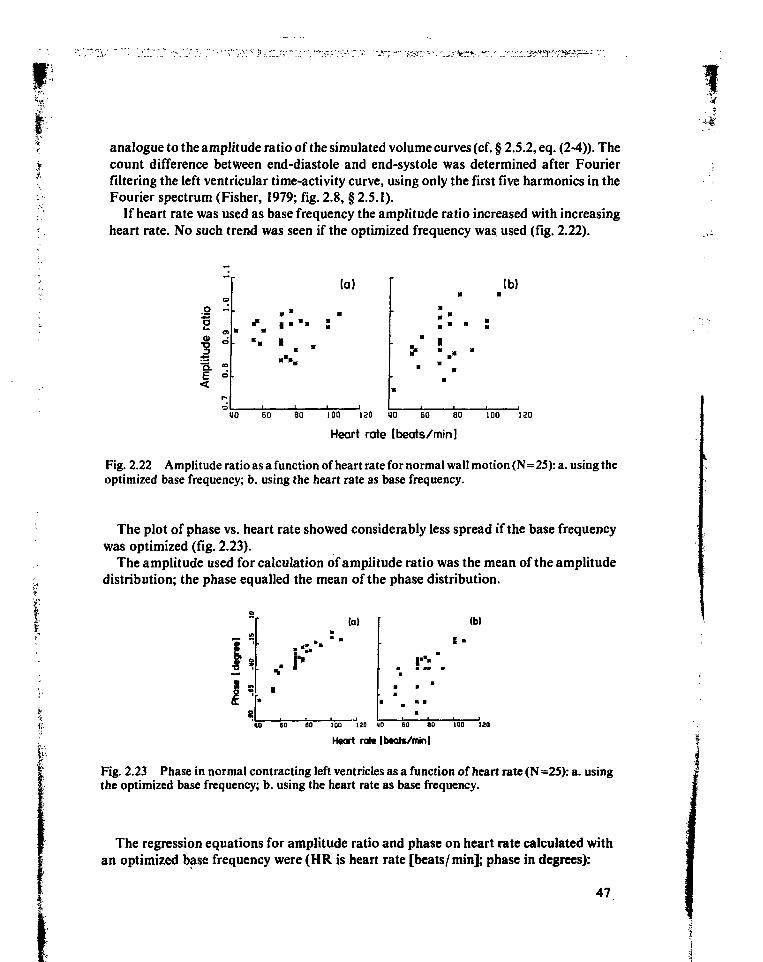
I' ~ ; ' " " ; . . ' • : " - • ; • _ - -

analogue to the amplitude ratio of the simulated volume curves (cf. § 2.5.2, eq. (2-4)). Thecount difference between end-diastole and end-systole was determined after Fourierfiltering the left ventricular time-activity curve, using only the first five harmonics in theFourier spectrum (Fisher, 1979; fig. 2.8, § 2.5.1).

If heart rate was used as base frequency the amplitude ratio increased with increasingheart rate. No such trend was seen if the optimized frequency was used (fig. 2.22).

o «

1

•s. -E °

(a) (b)

• . •

40 60 80 100 130 HO EO 80 100 120

Heart rate [beats/min]

Fig. 2.22 Amplitude ratio as a function of heart rate for normal wall motion (N=25): a. using theoptimized base frequency; b. using the heart rate as base frequency.

The plot of phase vs. heart rate showed considerably less spread if the base frequencywas optimized (fig. 2.23).

The amplitude used for calculation of amplitude ratio was the mean of the amplitudedistribution; the phase equalled the mean of the phase distribution.

i;(a)

• '

.. i"

(b)

S •

«0 60 80 100 120 110 60 80 100 120

Heart rait [btats/tnin]

Fig. 2.23 Phase in normal contracting left ventricles as a function of heart rate (N =25): a. usingthe optimized base frequency; b. using the heart rate as base frequency.

The regression equations for amplitude ratio and phase on heart rate calculated withan optimized base frequency were (HR is heart rate [beats/min]; phase in degrees):

47

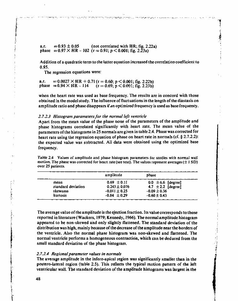
a.r. = 0.93 ± 0.05 (not correlated with HR; fig. 2.22a)phase =0.97 X HR - 102 (r = 0.91; p < 0.001; fig. 2.23a)

Addition of a quadratic term to the latter equation increased the correlation coefficient to0.95.

The regression equations were:

a.r. = 0.0027 X HR + 0.71 (r = 0.60; p < 0.001; fig. 2.22b)phase = 0.94 X HR - 114 (r = 0.69; p < 0.00!; fig. 2.23b)

when the heart rate was used as base frequency. The results are in concord with thoseobtained in the model study. The influence of fluctuations in the length of the diastasis onamplitude ratio and phase disappears if an optimized frequency is used as base frequency.

2.7.2.3 Histogram parameters for the normal left ventricleApart from the mean value of the phase none of the parameters of the amplitude andphase histograms correlated significantly with heart rate. The mean value of theparameters of the histograms in 25 normals are given in table 2.4. Phase was corrected forheart rate using the regression equation of phase on heart rate in normals (cf. § 2.7.2.2):the expected value was subtracted. All data were obtained using the optimized basefrequency.

Table 2.4 Values of amplitude and phase histogram parameters for studies with normal wallmotion. The phase was corrected for heart rate (see text). The values represent averages (± 1 SD)over 25 patients.

amplitude phase

mean 0.69 ±0.11 0.0 ±6.6 [degree]standard deviation 0.243 ±0.076 4.7 ±2.2 [degree]skewness -0.011 ± 0.25 -0.09 ± 0.36kurtosis -0.84 ±0.29 -0.60 ±0.43

The average value of the amplitude is the ejection fraction. Its value corresponds to thosereported in literature (Wackers, 1979; Kennedy, 1966). The normal amplitude histogramappeared to be non-skewed and only slightly flattened. The standard deviation of thedistribution was high, mainly because of the decrease of the amplitude near the borders ofthe ventricle. Also the normal phase histogram was non-skewed and flattened. Thenormal ventricle performs a homogeneous contraction, which can be deduced from thesmall standard deviation of the phase histogram.

2.7.2A Regional parameter values in normalsThe average amplitude in the infero-apical region was significantly smaller than in thepostero-lateral region (table 2.5). This reflects the typical motion pattern of the leftventricular wall. The standard deviation of the amplitude histograms was largest in the

48

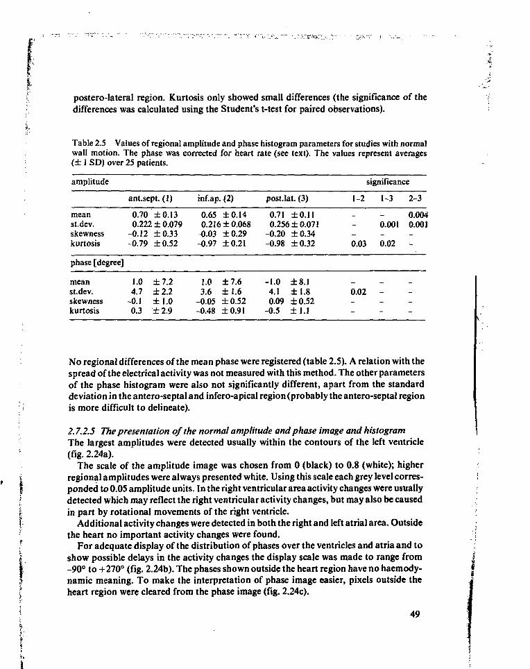
postero-lateral region. Kurtosis only showed small differences (the significance of thedifferences was calculated using the Student's t-test for paired observations).

Table 2.5 Values of regional amplitude and phase histogram parameters for studies with normalwall motion. The phase was corrected for heart rate (see text). The values represent averages(± 1 SD) over 25 patients.

amplitude

meanst.dev.skewnesskurtosis

phase [degree]

meanst.dev.skewnesskurtosis

ant.sept. (1)

0.70 ±0.130.222 ± 0.079

-0.12 ±0.33-0.79 ±0.52

1.0 ±7.24.7 ±2.2

-0.1 ±1.00.3 ± 2.9

inf.ap. (2)

0.65 ±0.140.216 ±0.068

-0.03 ±0.29-0.97 ±0.21

1.0 ±7.63.6 ±1.6

-0.05 ±0.52-0.48 ±0.91

postJat. (3)

0.71 ±0.110.256 ±0.071

-0.20 ±0.34-0.98 ±0.32

-1.04.10.09

-0.5

±8.1±1.8±0.52±1.1

1-2

0.03

0.02

significance

1-3

0.001

0.02

-

2-3

0.0040.001

-

No regional differences of the mean phase were registered (table 2.5). A relation with thespread of the electrical activity was not measured with this method. The other parametersof the phase histogram were also not significantly different, apart from the standarddeviation in the antero-septal and infero-apical region (probably the antero-septal regionis more difficult to delineate).

2.7.2.5 The presentation of the normal amplitude and phase image and histogramThe largest amplitudes were detected usually within the contours of the left ventricle(fig. 2.24a).

The scale of the amplitude image was chosen from 0 (black) to 0.8 (white); higherregional amplitudes were always presented white. Using this scale each grey level corres-ponded to 0.05 amplitude units. In the right ventricular area activity changes were usuallydetected which may reflect the right ventricular activity changes, but may also be causedin part by rotational movements of the right ventricle.

Additional activity changes were detected in both the right and left atrial area. Outsidethe heart no important activity changes were found.

For adequate display of the distribution of phases over the ventricles and atria and toshow possible delays in the activity changes the display scale was made to range from-90° to +270° (fig. 2.24b). The phases shown outside the heart region have no haemody-namic meaning. To make the interpretation of phase image easier, pixels outside theheart region were cleared from the phase image (fig. 2.24c).

49

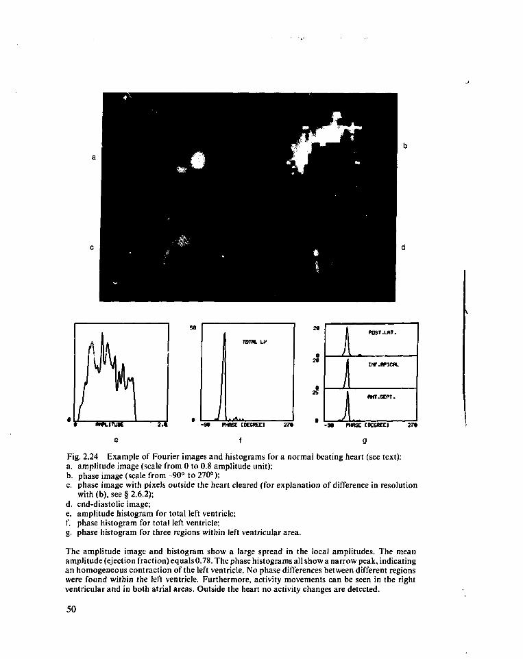
- 9 t PHASE CKCKC) 27*

f

1 POST .LAT.

I INF.flPICM.

1 (MT.SEPT.

- M PHBSE CDCCftEC] 27»

Fig. 2.24 Example of Fourier images and histograms for a normal beating heart (see text):a. amplitude image (scale from 0 to 0.8 amplitude unit);b. phase image (scale from -90° to 270°);c. phase image with pixels outside the heart cleared (for explanation of difference in resolution

with (b), see § 2.6.2);d. end-diastolic image;e. amplitude histogram for total left ventricle;f. phase histogram for total left ventricle;g. phase histogram for three regions within left ventricular area.

The amplitude image and histogram show a large spread in the local amplitudes. The meanamplitude (ejection fraction) equals 0.78. The phase histograms all show a narrow peak, indicatingan homogeneous contraction of the left ventricle. No phase differences between different regionswere found within the left ventricle. Furthermore, activity movements can be seen in the rightventricular and in both atrial areas. Outside the heart no activity changes are detected.

50

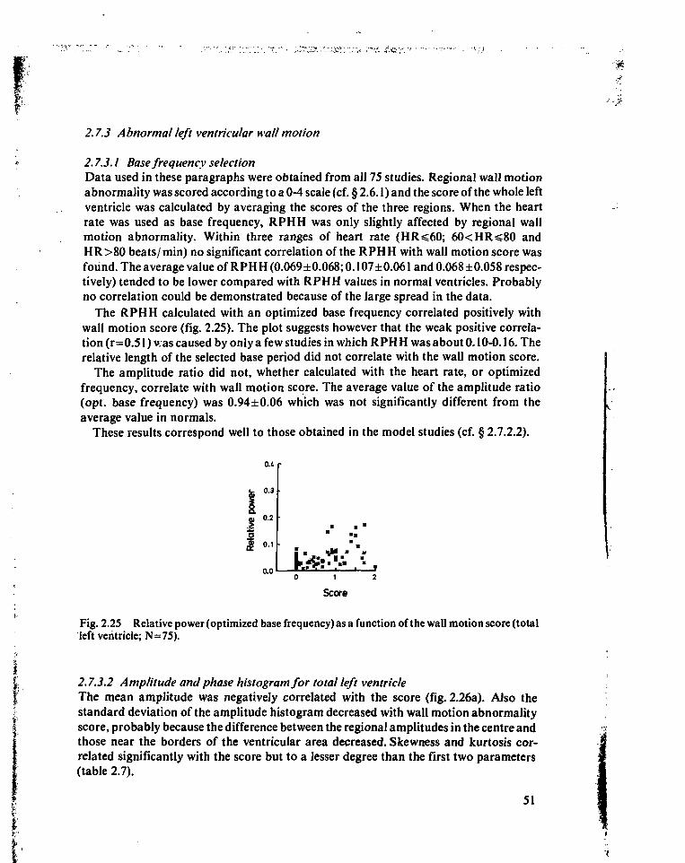
2.7.3 Abnormal left ventricular wall motion

2.7.3.1 Base frequency selectionData used in these paragraphs were obtained from all 75 studies. Regional wall motionabnormality was scored according to a 0-4 scale (cf. § 2.6.1) and the score of the whole leftventricle was calculated by averaging the scores of the three regions. When the heartrate was used as base frequency, RPHH was only slightly affected by regional wallmotion abnormality. Within three ranges of heart rate (HR^60; 60<HR<80 andHR>80 beats/min) no significant correlation of the RPHH with wall motion score wasfound. The average value of RPHH (0.069±0.068; 0.107±0.061 and 0.068 ±0.058 respec-tively) tended to be lower compared with RPHH values in normal ventricles. Probablyno correlation could be demonstrated because of the large spread in the data.

The RPHH calculated with an optimized base frequency correlated positively withwall motion score (fig. 2.25). The plot suggests however that the weak positive correla-tion (r=0.51) v.as caused by only a few studies in which RPH H was about 0.10-0.16. Therelative length of the selected base period did not correlate with the wall motion score.

The amplitude ratio did not, whether calculated with the heart rate, or optimizedfrequency, correlate with wall motion score. The average value of the amplitude ratio(opt. base frequency) was 0.94±0.06 which was not significantly different from theaverage value in normals.

These results correspond well to those obtained in the model studies (cf. § 2.7.2.2).

0.1

0.3

0.2

0.1

0.01 2

Score

Fig. 2.25 Relative power (optimized base frequency) as a function of the wall motion score (totalleft ventricle; N=75).

2.7.3.2 Amplitude and phase histogram for total left ventricleThe mean amplitude was negatively correlated with the score (fig. 2.26a). Also thestandard deviation of the amplitude histogram decreased with wall motion abnormalityscore, probably because the difference between the regional amplitudes in the centre andthose near the borders of the ventricular area decreased. Skewness and kurtosis cor-related significantly with the score but to a lesser degree than the first two parameters(table 2.7).

51

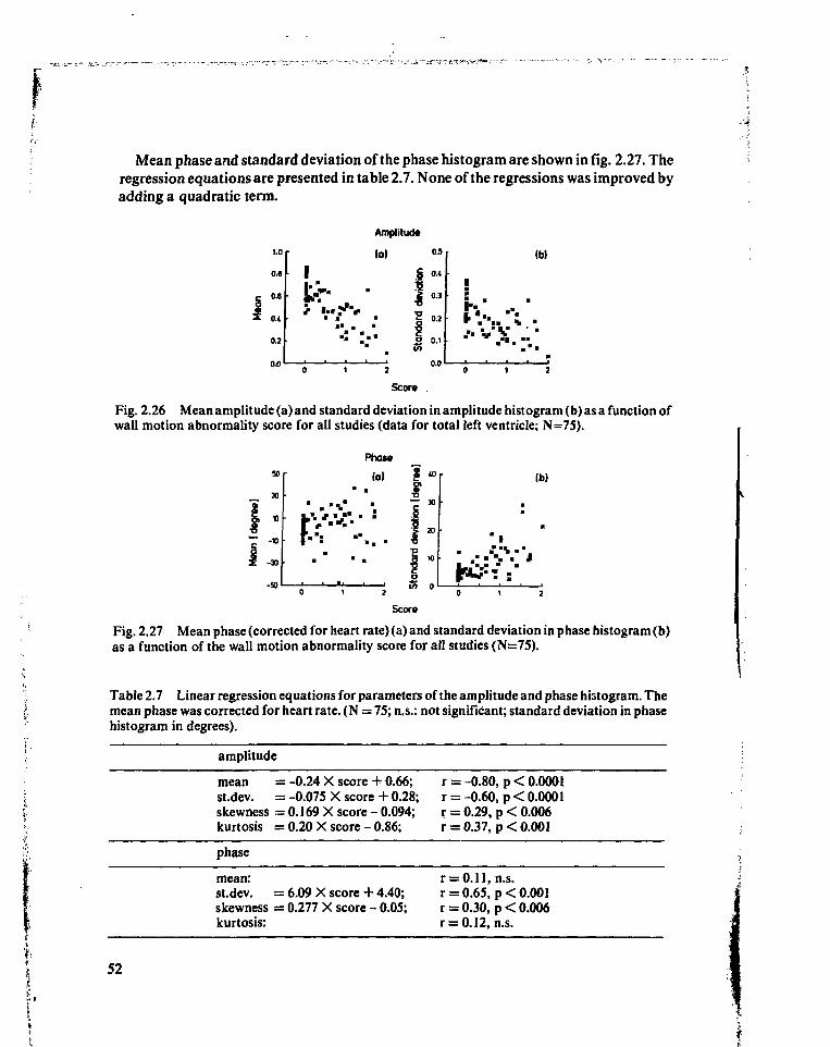
Mean phase and standard deviation of the phase histogram are shown in fig. 2.27. Theregression equations are presented in table 2.7. None of the regressions was improved byadding a quadratic term.

1.C

0.6

0.6

O.t

0.2

tr-

Amplitude

(o) ° 5

s «£ 0.3

I "211 1 0.1

(b)

i. '

* •

•

Score .

Fig. 2.26 Mean amplitude (a) and standard deviation in amplitude histogram (b) as a function ofwall motion abnormality score for all studies (data for total left ventricle; N=75).

Phase

(a)

tn o

Ib)

Score

Fig. 2.27 Mean phase (corrected for heart rate) (a) and standard deviation in phase histogram (b)as a function of the wall motion abnormality score for all studies (N=75).

Table 2.7 Linear regression equations for parameters of the amplitude and phase histogram. Themean phase was corrected for heart rate. (N = 75; n.s.: not significant; standard deviation in phasehistogram in degrees).

amplitude

mean = -0.24 X score + 0.66;st.dev. = -0.075 X score + 0.28;skewness - 0.169 X score - 0.094;kurtosis = 0.20 X score - 0.86;

phase

mean:stdev. = 6.09 X score + 4.40;skewness = 0.277 X score - 0.05;kurtosis:

r = -0.80, p < 0.0001r = -0.60, p<0.000lr = 0.29, p < 0.006r = 0.37, p < 0.001

r = 0.11, n.s.r = 0.65, p < 0.001r = 0.30, p < 0.006r = 0.12, n.s.

52

It could be expected that the mean phase was not significantly correlated with the wallmotion score: the score may include several types of wall motion abnormalities. Aparadoxally moving region causes a local phase shift, while the other regions shownormal wall motion. For instance: apex is dyskinetic (score=3), the other regions arenormal (score=0), resulting in an average score 1. In case of hypokinetic movement of allregions a different motion pattern exists whereas the average score may be equal: score is1 in all regions, average score is 1. A meaningful use of the mean phase can therefore onlybe expected if a regional analysis is used.

The standard deviation in the phase histogram appeared to be a specific indicator forwall motion abnormalities. If a large standard deviation was found it was likely that someform of wall motion abnormality was present (the normal range for the standarddeviation was quite small; table 2.4).

2.7.3.3 Regional analysis of amplitude and phase histogramLinear and quadratic regression analysis was performed for each parameter of amplitudeand phase histogram of all three regions, relating regional parameters to average regionalwall motion scores.

None of the quadratic regressions resulted in a significantly higher correlation ascompared to linear regression. Therefore only linear regression analysis will be discussedin the following.

Generally speaking the mean amplitude, the standard deviation of the regional ampli-tude histogram and the standard deviation of the regional phase histogram correlatedsignificantly with the regional wall motion score (table 2.8; fig 2.28). The mean phasestayed in the normal range for hypokinetic movements. However, the mean phaseappeared to be sensitive for detection of paradoxal movements (14 segments withscore>2 were included, 11 of these showed a shift in phase). Skewness and kurtosisappeared to be of little value for wall motion analysis.

The results presented in this and in the previous paragraphs clearly show that the meanamplitude contains most information regarding (regional) wall motion abnormality.However, from this single regression analysis it cannot be excluded that other parametersmay give additional information, as compared to the use of the mean amplitude only.

Therefore multiple regression analysis was performed including the means and thestandard deviations. Skewness and kurtosis were not used because of the poor correla-tions obtained.

' 2.7.3.4 Multiple regression analysis] The squared correlation coefficient used in this paragraph indicates to which proportion '; the variability of the score is explained by the (combination of) parameters under study.

The parameter which explains the highest proportion was selected first, next the parame-• ter that adds most information etc. The resulting correlation coefficients and the squaredf correlation coefficients are shown in table 2.9. Only linear regressions were used.I Total left ventricle. The mean amplitude was the first parameter selected for the total| score (64% of the score was explained by the mean amplitude). Addition of the standard: deviation in the phase histogram resulted in 7% more information. The mean phó^e and

I 53

i%

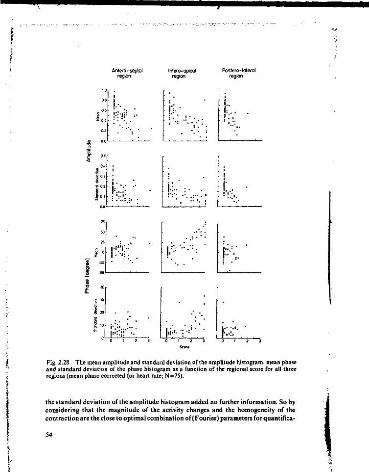
Antero-septalregion

Infero-apicalregion

Postero-lateralregion

1.0

0.6

.0 .6

\o,

0.2

0.0

0.5 r

0.3

0.2

0.0

i.-.•

•

ï * •• •

•

••

i-:..•

" • • *

! . •

• . . . . i

• • ' . •

•I! - .

1:.. . .: i ••

!•

k •

75

50

25

0

-25

-50

! " • • : .

to

I 3 0

'S

I»

r. . . • •0 1 2 3 0 ( 2 3

Scort

Fig. 2.28 The mean amplitude and standard deviation of the amplitude histogram, mean phaseand standard deviation of the phase histogram as a function of the regional score for all threeregions (mean phase corrected for heart rate; N=75).

the standard deviation of the amplitude histogram added no further information. So byconsidering that the magnitude of the activity changes and the homogeneity of thecontraction are the close to optimal combination of (Fourier) parameters for quantifica-

54

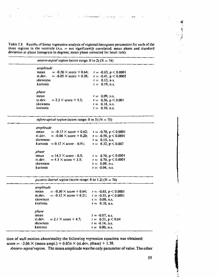
Table 2.8 Results of linear regression analysis of regional histogram parameters for each of thethree regions in the ventricle (n.s. = not significantly correlated; mean phase and standarddeviation in phase histogram in degrees; mean phase corrected for heart rate).

antero-septal region (score range: 0 to 2) (N =

amplitudemean =st.dev. =skewnesskurtosis

phasemeanst.dev. =skewnesskurtosis

= -0.20 X score= -0.05 X score

- 2.3 X score +

infero-apical region (score

amplitudemean =st.dev. =skewnesskurtosis =

:-0.13 X score: -0.04 X score

: 0.12 X score-

+ 0.64;+ 0.28;

5.5;

r =r =r =r =

r =r =r =r =

-0.65,-0.41,0.13,0.19,

0.09,0.36,0.18,0.10,

74)

p < 0.0001p < 0.0002n.s.n.s.

n.s.p < 0.001n.s.n.s.

range: 0to3)(N = 75)

+ 0.62;+ 0.20;

0.91;

r =r =r =r =

-0.70,-0.59,0.15,0.32,

p < 0.0001p < 0.0001n.s.p < 0.002

phasemean = 14.3 X score - 0.5; r = 0.70, p < 0.0001st.dev. = 4.3 X score + 3.5; r = 0.70, p < 0.0001skewness r = 0.09, n.s.kurtosis r = -0.04, n.s.

postero-lateral region (score range: 0 to 1.2) (N = 74)

amplitudemean =-0.30 X score + 0.64; r =-0.65, p < 0.0001st.dev. = -0.12 X score + 0.21; r = -0.55, p < 0.0001skewness r = 0.00, n.s.kurtosis r = 0.10, n.s.

phasemean r = -0.07, n.s.st.dev. =2.1 X score+ 4.7; r = 0.21, p < 0.04skewness r = -0.14, n.s.kurtosis r = 0.00, n.s.

tion of wall motion abnormality the following regression equation was obtained:score = -2.06 X (mean ampl.) + 0.034 X (st.dev. phase) + 1.38.

A ntero-septal region. The mean amplitude was the only parameter of value. The other

55

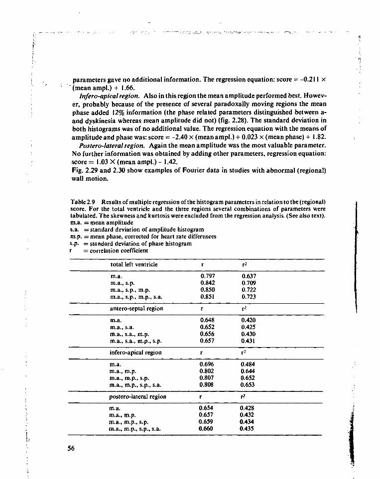
parameters gave no additional information. The regression equation: score = -0.211 x" (mean ampl.) + 1.66.

Infero-apical region. Also in this region the mean amplitude performed best. Howev-er, probably because of the presence of several paradoxally moving regions the meanphase added 12% information (the phase related parameters distinguished between a-and dyskinesia whereas mean amplitude did not) (fig. 2.28). The standard deviation inboth histograms was of no additional value. The regression equation with the means ofamplitude and phase was: score = -2.40 x (mean ampl.)+ 0.023 x (mean phase) + 1.82.

Postero-lateral region. Again the mean amplitude was the most valuable parameter.No further information was obtained by adding other parameters, regression equation:score = 1.03 X (mean ampl.) - 1.42.Fig. 2.29 and 2.30 show examples of Fourier data in studies with abnormal (regional)wall motion.

Table 2.9 Results of multiple regression of the histogram parameters in relation to the (regional)score. For the total ventricle and the three regions several combinations of parameters weretabulated. The skewness and kurtosis were excluded from the regression analysis. (See also text).m.a. = mean amplitudes.a. = standard deviation of amplitude histogramm.p. = mean phase, corrected for heart rate differencess.p. = standard deviation of phase histogramr = correlation coefficient

total left ventricle

m.a.m.a., s.p.m.a., s.p., m.p.m.a., s.p., m.p., s.a.

antero-septal region

m.a.m.a., s.a.m.a., s.a., m.p.m.a., s.a., m.p., s.p.

infero-apical region

m.a.m.a., m.p.m.a., m.p., s.p.m.a., m.p., s.p., s.a.

postero-lateral region

m.a.m.a., m.p.m.a., m.p., s.p.m.a., m.p., s.p., s.a.

r

0.7970.8420.8500.851

r

0.6480.6520.6560.657

r

0.6960.8020.8070.808

r

0.6540.6570.6590.660

r2

0.6370.7090.7220.723

r-'

0.4200.4250.4300.431

r2

0.4840.6440.6520.653

r2

0.4280.4320.4340.435

56

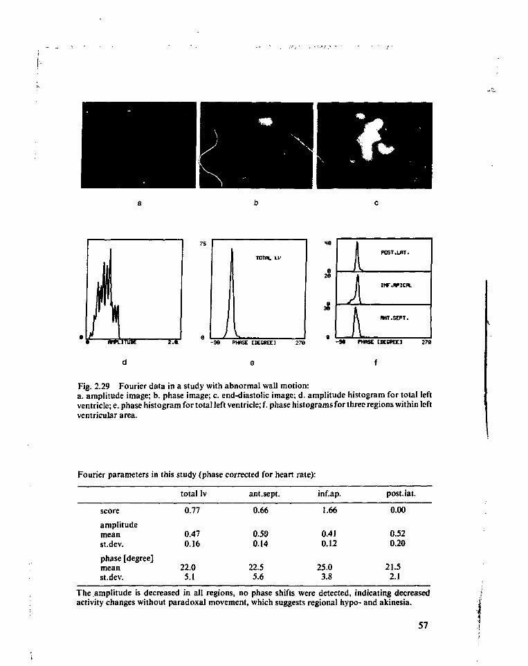
2e

L

POST.LHT.

RNT.SEPT.

- 3 6 PHRSE tBECKE] 276

Fig. 2.29 Fourier data in a study with abnormal wall motion:a. amplitude image; b. phase image; c. end-diastolic image; d. amplitude histogram for total leftventricle; e. phase histogram for total left ventricle; f. phase histograms for three regions within leftventricular area.

Fourier parameters in this study (phase corrected for heart rate):

score

amplitudemeanst.dev.

phase [degree]meanst.dev.

totallv

0.77

0.470.16

22.05.1

ant.sept.

0.66

0.500.14

22.55.6

inf.ap.

1.66

0.410.12

25.03.8

post. lat.

0.00

0.520.20

21.52J

The amplitude is decreased in all regions, no phase shifts were detected, indicating decreasedactivity changes without paradoxal movement, which suggests regional hypo- and akinesia.

57

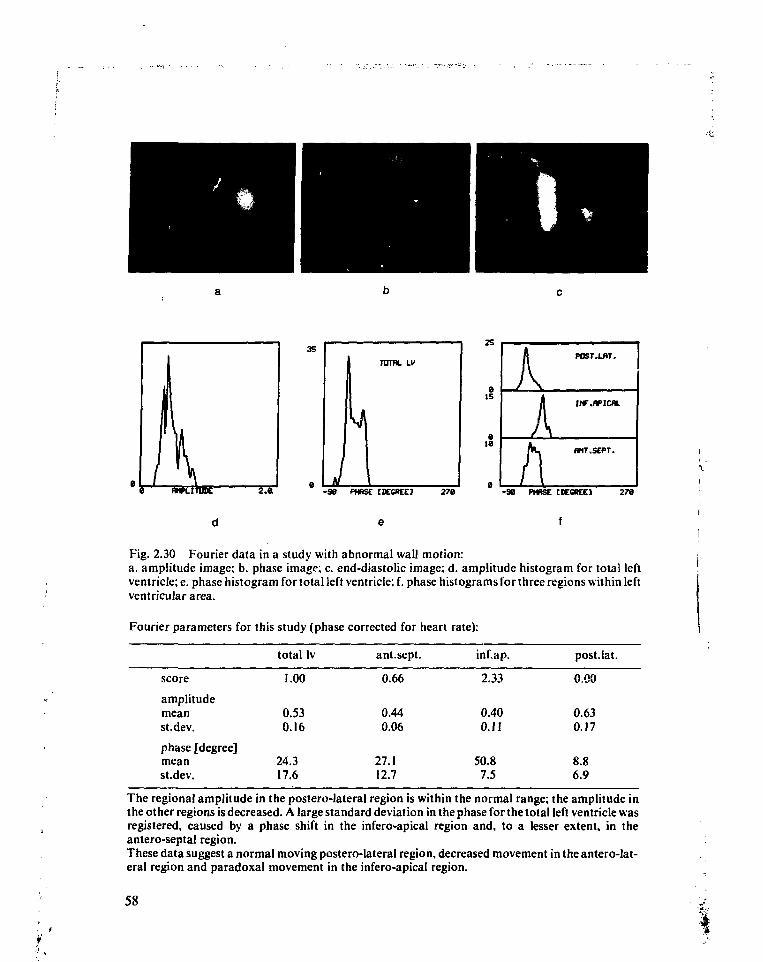
15

ie

POST.LBT.

PUT.SEPT.

- 9 8 PHASE HECREEJ 270 -90 PHRSE tKOtCE] 278

Fig. 2.30 Fourier data in a study with abnormal wall motion:a. amplitude image; b. phase image; c. end-diastolic image; d. amplitude histogram for total leftventricle; e. phase histogram for total left ventricle; f. phase histograms for three regions within leftventricular area.

Fourier parameters for this study (phase corrected for heart rate):

score

amplitudemeanst.dev.

phase [degree]meanst.dev.

total Iv

1.00

0.530.16

24.317.6

ant.sept.

0.66

0.440.06

27.112.7

inf.ap.

2.33

0.400.11

50.87.5

post.lat.

0.00

0.630.17

8.86.9

The regional amplitude in the postero-lateral region is within the normal range; the amplitude inthe other regions is decreased. A large standard deviation in the phase for the total left ventricle wasregistered, caused by a phase shift in the infero-apical region and, to a lesser extent, in theantero-septal region.These data suggest a normal moving postero-lateral region, decreased movement in the antero-lat-eral region and paradoxal movement in the infero-apical region.

58

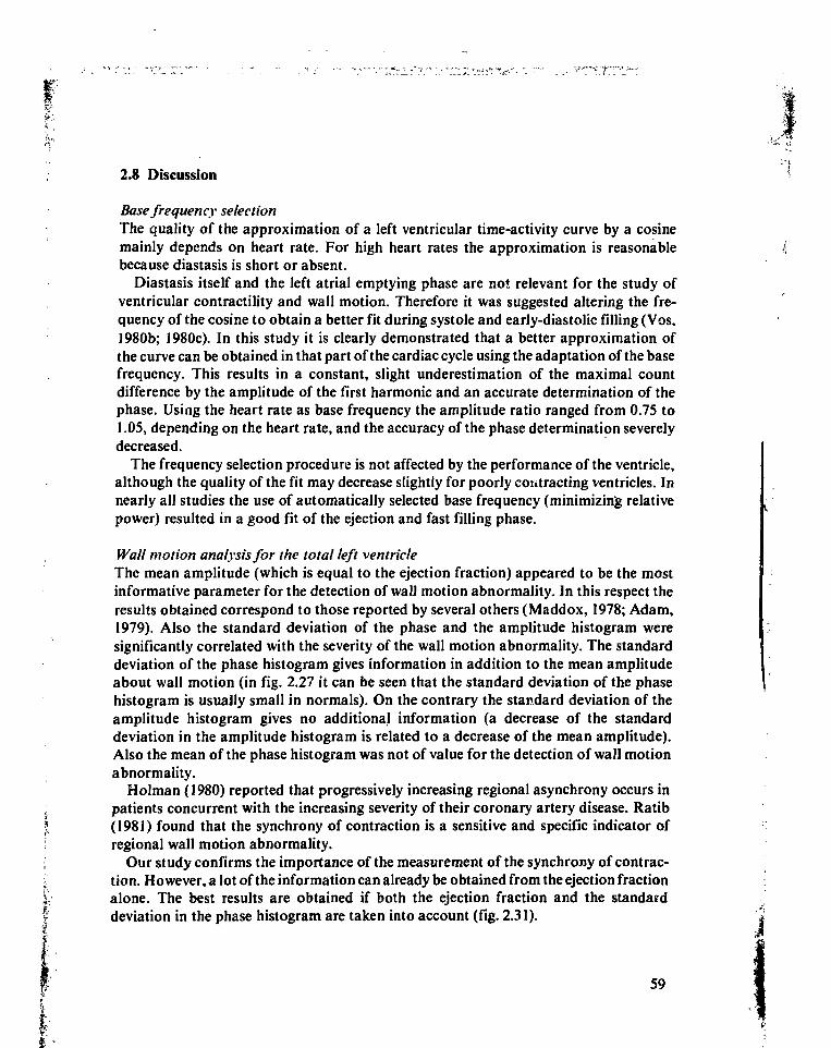
2.8 Discussion

Base frequency selectionThe quality of the approximation of a left ventricular time-activity curve by a cosinemainly depends on heart rate. For high heart rates the approximation is reasonablebecause diastasis is short or absent.

Diastasis itself and the left atrial emptying phase are not relevant for the study ofventricular contractility and wall motion. Therefore it was suggested altering the fre-quency of the cosine to obtain a better fit during systole and early-diastolic filling (Vos,1980b; 1980c). In this study it is clearly demonstrated that a better approximation ofthe curve can be obtained in that part of the cardiac cycle using the adaptation of the basefrequency. This results in a constant, slight underestimation of the maximal countdifference by the amplitude of the first harmonic and an accurate determination of thephase. Using the heart rate as base frequency the amplitude ratio ranged from 0.75 to1.05, depending on the heart rate, and the accuracy of the phase determination severelydecreased.

The frequency selection procedure is not affected by the performance of the ventricle,although the quality of the fit may decrease slightly for poorly contracting ventricles. Innearly all studies the use of automatically selected base frequency (minimizing relativepower) resulted in a good fit of the ejection and fast filling phase.

Wall motion analysis for the total left ventricleThe mean amplitude (which is equal to the ejection fraction) appeared to be the mostinformative parameter for the detection of wall motion abnormality. In this respect theresults obtained correspond to those reported by several others (Maddox, 1978; Adam,1979). Also the standard deviation of the phase and the amplitude histogram weresignificantly correlated with the severity of the wall motion abnormality. The standarddeviation of the phase histogram gives information in addition to the mean amplitudeabout wall motion (in fig. 2.27 it can be seen that the standard deviation of the phasehistogram is usually small in normals). On the contrary the standard deviation of theamplitude histogram gives no additional information (a decrease of the standarddeviation in the amplitude histogram is related to a decrease of the mean amplitude).Also the mean of the phase histogram was not of value for the detection of wall motionabnormality.

Holman (1980) reported that progressively increasing regional asynchrony occurs inpatients concurrent with the increasing severity of their coronary artery disease. Ratib(1981) found that the synchrony of contraction is a sensitive and specific indicator ofregional wall motion abnormality.

Our study confirms the importance of the measurement of the synchrony of contrac-tion. However, a lot of the information can already be obtained from the ejection fractionalone. The best results are obtained if both the ejection fraction and the standarddeviation in the phase histogram are taken into account (fig. 2.31).

59

II,-

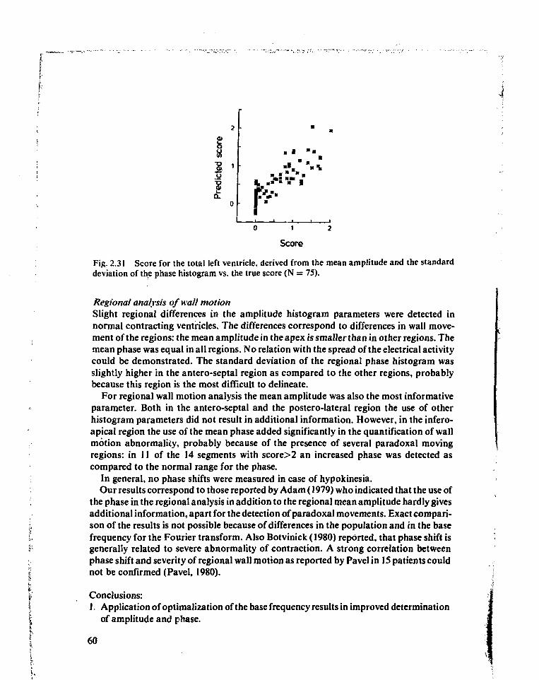
Q)

s1Q.

Score

Fig. 2.31 Score for the total left ventricle, derived from the mean amplitude and the standarddeviation of the phase histogram vs. the true score (N = 75).

Regional analysis of wall motionSlight regional differences in the amplitude histogram parameters were detected innormal contracting ventricles. The differences correspond to differences in wall move-ment of the regions: the mean amplitude in the apex is smaller than in other regions. Themean phase was equal in all regions. No relation with the spread of the electrical activitycould be demonstrated. The standard deviation of the regional phase histogram wasslightly higher in the antero-septal region as compared to the other regions, probablybecause this region is the most difficult to delineate.

For regional wall motion analysis the mean amplitude was also the most informativeparameter. Both in the antero-septal and the postero-lateral region the use of otherhistogram parameters did not result in additional information. However, in the infero-apical region the use of the mean phase added significantly in the quantification of wallmotion abnormality, probably because of the presence of several paradoxal movingregions: in 11 of the 14 segments with score>2 an increased phase was detected ascompared to the normal range for the phase.

In general, no phase shifts were measured in case of hypokinesia.Our results correspond to those reported by Adam (1979) who indicated that the use of

the phase in the regional analysis in addition to the regional mean amplitude hardly givesadditional information, apart for the detection of paradoxal movements. Exact compari-son of the results is not possible because of differences in the population and in the basefrequency for the Fourier transform. Also Botvinick (1980) reported, that phase shift isgenerally related to severe abnormality of contraction. A strong correlation betweenphase shift and severity of regional wall motion as reported by Pavel in 15 patients couldnot be confirmed (Pavel, 1980).

Conclusions:1. Application of optimalization of the base frequency results in improved determination

of amplitude and phase.

60

2. The mean amplitude (that is, the ejection fraction) is the major parameter for quantifi-cation of wall motion abnormalities.

3. The heart rate should be taken into account in phase analysis.4. The phase is sensitive for paradoxally moving wall regions.5. The phase is of no value for the quantification of hypokinetic wall segments.6. The standard deviation of the phase histogram for the total left ventricle is a specific

parameter in the detection of regional wall motion abnormalities and therefore addsinformation to the results as obtained from the mean amplitude.

7. Skewness and kurtosis of the amplitude and phase histogram are of no additionalvalue for wall motion analysis.

List of relevant symbol and abbreviations

a.r.AoBACKEDCEDVEFESCESVFWHMHRLALAOD1ASLVLVETLVFTMUGAMLAOPAPEPRARAORLPROIRPHH

RVSCsvTCYC

amplitude ratioaortabackgroundnumber of counts detected in left ventricle at end-diastoleend-diastolic volume of left ventricleleft ventricular ejection fractionnumber of counts detected in left ventricle at end-systoleend-systolic volume of left ventricleFull width half maximumheart rateleft atriumleft anterior obliqueduration of diastasis in left ventricleleft ventricleleft ventricular ejection timeleft ventricular rapid filling timemultiple gated (acquisition)modified left anterior obliquepulmonary arterypre-ejection period of left ventricleright atriumright anterior obliquerelative length of period (for Fourier transform)region of interestrelative power in second and higher harmonics in the Fourier spectrum of aleft ventricular time-activity curveright ventriclestroke counts in left ventriclestroke volume of left ventriclelength of cardiac cycle

61

I

f. References

; Adam, W.E., Bitter, F. (1980), Advances in heart imaging, Proc. Int. Symp. Med. Radionuclidei Imaging, Heidelberg.;; Adam, W.E., Geffers, H., Sigel, H. et al. (1977), Evaluation of left ventricular function by

radionuclide angiography, Herz 2: 195-199.:. Adam, W.E., Tarkowska, A., Bitter, F. et al. (1979), Equilibrium (gated) radionuclide ventriculo-

graphy, Cardiovasc. Radio!. 2: 161-173.Ashburn, W.L., Schelbert, H.R., Verba, J. W. (1978), Left ventricular ejection fraction - a review of

several radionuclide angiographic approaches using the scintillation camera, Prog. Card. Dis.20: 267-284.

Aswegen, A.v., Alderson, P.O., Nickoloff, E.L. et al. (1980), Temporal resolution requirements forleft ventricular time-activity curves, Radiology 135: 165-170.

Bacharach, S.L., Green, M. V., Borer, J.S. et al. (1979), Left ventricular peak ejection rate, fillingrate, and ejection fraction - frame rate requirements at rest and exercise: concise communica-tion, J.Nucl.Med. 20: 189-193.

Bodenheimer, M.M., Banka, V.S., Fooskee, C M . et al. (1979), Comparison of wall motion andregional ejection fraction at rest and during isometric exercise, J.Nucl.Med. 20: 724-732.

Borer, J.S., Bacharach, S.L., Green, M.V. etal. (1977), Real-time radionuclidecine-angiographyin the noninvasive evaluation of global and regional left ventricular function at rest and duringexercise in patients with coronary artery disease, New.Engl.J.Med. 296:839-844.

Botvinick, E., Dunn, R., O'Connell, W. et al. (I980), The phase image - its relationship to patternsof contraction and conduction, Circ. 62: p. III-148 (abstract).

Brash, H.M., Wraith, P.K., Hannan, W.J. et al. (1980), The influence of ectopic heart beats ingated ventricular blood pool studies, J.Nucl.Med. 21:391-393.

Burrow, R.D., Strauss, H.W., Singleton, R.S. et al. (1977), Analysis of left ventricular functionfrom gated acquisition, cardiac blood pool imaging, Circ. 56: 1024-1028.

Dodge, H.T., Sandier, H.S., Ballew, D.W. etal. (1960), The use of bi-plane angiocardiography forthe measurement of the left ventricular volume in man, Am. Heart. J. 60: 762-776.

Fisher, P., Knopp, R., Breuel, H.-P. (1979), Zur anwendung der Harmonischen Analyse bei derFunktionsszintigraphie des Herzens, Nucl.-Med. Band XVIII/Heft4: 167-171.

Ganong, W.F. (1977), Medical physiology. Lange Medical Publications, Los Altos, California,; 8th ed.

Geffers, H., Adam, W.A., Bitter, F. et al. (1977), Data processing and functional imaging in: radionuclide ventriculography. IVth Int. Conf. Data Proc. and Med. Imaging, Nashville,

Tenn., U.S.A.Green, M.V., Bacharach, S.L., Douglas, M.A. et al. (1978), Sources of virtual background in

• multi-image blood pool studies, in: Nuclear Cardiology, Symposium Proceedings SNM Com-puter Council, J.A. Sorenson (ed), Atlanta, Georgia, U.S.A., pp. 97-106.

Green, M.V., Ostrow, H.G., Douglas, M.A et al. (1975), High temporal resolution ECG-gatedscintigraphic angiography, J.Nucl.Med. 16:95-98.

! Hamilton, G.W., Williams, D.L., Caldwell, J.H. (1978), Frame-rate requirements for recordingtime-activity curves by radionuclide angiography, in: Nuclear Cardiology, Symposium Pro-

• ceedings SNM, J.A.Sorenson (ed), Atlanta, Georgia, U.S.A., pp. 75-84.Hammermeister, K.E., Warbasse, J.R. (1974), The rate of change of left ventricular volume in man,

v Circ. 49:739-747.i Hegge, F.N., Hamilton, G.W., Larson, S.M. et al. (1978), Cardiac chamber imaging: a comparison< of red blood cells labeled with Tc-99m in vitro and in vivo, J.Nucl.Med. 19:129-134.i Holman, B.L., Wynne, J., Idione, J., et al. (1980), Disruption in the temporal sequence of regional|f ventricular contraction, Circ. 61:1075-1083.I Hurst, R.R., Logan, K.W. (1978), A simulated heart model using computer image analysis forf validating cardiovascular nuclear medicine parameters. Nuclear Cardiology, Symposium Pro-| ceedings SNM, J.A.Sorenson (ed), Atlanta, Georgia, U.S.A., pp. 55-62.

I 62

Kennedy, J.W., Baxley, W. A., Figley, M.M. et al. (1966), Quantitative Angiocardiography I, Thenormal left ventricle in man, Circ. 43: 272-278.

Lewis, R.P., Boudoulas, H., Welch, T.G. et al. (1976), Usefulness of systolic time intervals incoronary artery disease, Am.J.Card. 37: 787-796.

Maddox, D.E., Holman, B.L., Wynne, J. et al. (1978), Ejection fraction image: a noninvasive indexof regional left ventricular wall motion, Am.J.Card. 41: 1230-1238.

Okada, R.D., Kirshenbaum, H.D., Kushner, F.G. et al. (1980), Observer variance in the qualitativeevaluation of left ventricular wall motion and the quantitation of left ventricular ejectionfraction using rest and exercise multigated blood pool imaging, Circ. 61: 128-136.

Pavel, D., Swiryn, S., Lam, W. (1980), Ventricular phase analysis of radionuclide gated studies,Am.J.Card. 45: 398 (abstract).

Ratib, O., Henze, E., Schoen, H. et al. (1981), Phase analysis of radionuclide angiograms: a newtool for detection of coronary artery disease, Circ, 64: p IV-143 (abstract).

Shannon, C.E. (1949), Communication in the presence of noise, Proc.Ire 37: 10-21.Strauss, H.W., Zaret, B.L., Hurley, P.J. et al. (1971), A scintigraphic method for measuring left

ventricular ejection fraction in man without cardiac catheterization, Am.J.Card. 28: 575-580.Taylor, D.N., Hawkes, D.J., Goddard, B.A. et al. (1979), A simple method for correcting left

ventricular equilibrium radionuclide angiography for the effects of arrhythmias, Phys.Med.Biol. 24: I)62-1/67.

Vos, P.H., Vossepoel, A.M., Beekhuis, H. et al. (1980a), Characterization of the ventricularfunction by temporal Fourier transform, Nucl.Med.Comm. 1: 10-18.

Vos, P.H., Vossepoel, A.M. (1980b), Improved evaluation of left ventricular contractility in gatedblood pool studies by temporal Fourier transform, Proc 10th Ann. Symp. of the SNM Comp.Council, Miami Beach, U.S.A.

Vos, P.H., Vossepoel, A.M. (1980c), Functional images to describe the contractility of the heart ingated blood pool studies, Proc. Third World Conf. Medical Informatics (MEDINFO), Tokyo,Japan.

Wackers, F.J.Th., Berger, H.J., Johnstone, D.E. et al. (1979), Multiple gated cardiac blood poolimaging for left ventricular ejection fraction: validation of the technique and assessment ofvariability, Am.J.Card. 43: 1139-1166.

63

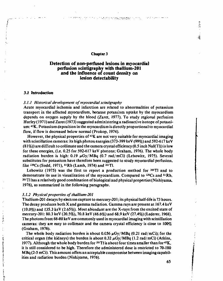
Chapter 3

Detection of non-perfused lesions in myocardialperfusion scintigraphy with thallium-201

and the influence of count density onlesion detectability

3.1 Introduction

3.1.1 Historical development of myocardial scintigraphyAcute myocardial ischemia and infarction are related to abnormalities of potassiumtransport in the affected myocardium, because potassium uptake by the myocardiumdepends on oxygen supply by the blood (Zaret, 1977). To study regional perfusionHurley (1971) and Zaret (1973) suggested administering a radioactive isotope of potassi-um: 43K. Potassium deposition in the myocardium is directly proportional to myocardialflow, if flow is decreased below normal (Prokop, 1974).

However, the physical properties of 43K are not very suitable for myocardial imagingwith scintillation cameras: its high photon energies (373-399 keV (99%) and 592-617 keV(81 %)) are difficult to collimate and the camera crystal efficiency (0.5 inch Nal(Tl)) is lowfor these energies, (i.e. 0.25 for 592-617 keV photons; Graham, 1976). The whole bodyradiation burden is high: 0.19 /uGy/MBq (0.7 rad/mCi) (Lebowitz, 1975). Severalsubstitutes for potassium have therefore been suggested to study myocardial perfusion,like '2»Cs (Sodd, 1971), »'Rb (Lamb, 1974) and 2OIT1.

Lebowitz (1975) was the first to report a production method for 2OIT1 and todemonstrate its use in visualization of the myocardium. Compared to 129Cs and 81Rb,20'Tl has a relatively good combination of biological and physical properties (Nishiyama,1976), as summarized in the following paragraphs.

3.1.2 Physical properties of thallium-201Thallium-201 decays by electron capture to mercury-201; its physical half-life is 73 hours.The decay produces both X and gamma radiation. Gamma rays are present at 167.4 keV(10.0%) and 135.3 keV (2.65%). Most abundant are the X-rays from the excited state ofmercury-201: 80.3 keV (20.5%), 70.8 keV (46.6%) and 68.9 keV (27.4%) (Lederer, 1968).The photons from 68-80 keV are commonly used in myocardial imaging with scintillationcameras: they are easy to collimate and the camera crystal efficiency is close to 100%(Graham, 1976).

The whole body radiation burden is about 0.056 ftGyl MBq (0.21 rad/mCi); for the \critical organ (the kidneys) the burden is about 0.32 fiGyj MBq (1.2 rad/ mCi) (Atkins, '1977). Although the whole body burden for 2OIT1 is about four times smaller than for 43K, 'iit is still considered to be high. Therefore the administered dose is restricted to 70-180MBq (2-5 mCi). This amount offers an acceptable compromise between imaging capabil-ities and radiation burden (Nishiyama, 1976).

65

3.1.3 Biological properties of thalliumAlthough there is still some controversy about the biological properties of thallium withrespect to the mechanism of thallium uptake into muscle cells, most authors state that themuscle cell cannot differentiate between K+ and Tl+ (Ritchie and Hamilton (1978)published a clear summary of the experiments on this topic). Both ions rapidly disappearfrom the blood: 90-95% within five minutes after intravenous admistration (Atkins,1977). The extraction of thallium during its first passage through the coronary circula-tion (following a bolus injection) is about 88%(Weich, 1978). However, thallium appearsto concentrate in the myocardium to a greater degree than potassium (Strauss, 1975) andsubsequent clearing of thallium from the myocardium is considerably slower than that ofpotassium (Hamilton, 1978c). The concentration of thallium-20! in parts of the bodyother than the myocardium is low, compared with potassium-43 (Nishiyama, 1976); the(whole body) effective half-life of thallium is 57 hours. The data show that thallium is auseful myocardial imaging agent, although its uptake in living cells is not the same asfound for potassium.

3.1.4 Imaging of the myocardiumThallium scintigraphy of the heart can be used to detect myocardial infarction as well asstress-induced regional myocardial ischemia (Cook, 1976; Ritchie, 1977; Lenears, 1977;Hamilton, 1977; Pohost, 1978; Hamilton, 1978b). Thallium does not accumulate ininfarcted regions of the myocardium; in images of thallium distribution in myocardiumobtained during resting conditions infarcted regions appear as 'cold' spots.

The detection of stress-induced regional myocardial ischemia requires a comparisonbetween thallium distribution obtained at rest and during exercise. Cold spots in 'exer-cise' images, not found in images obtained at rest indicate areas of stress inducedischemia. Thallium is administered at maximal exercise or when anginal pain or ECG-changes indicating ischemia have developed. Because of redistribution effects imaging ofthe tracer distribution obtained under stress or under ischemic conditions should befinished within 45 minutes. In this period images in at least three, but preferably fiveviews should be depicted (anterior, LAO30, LAO45, LAO60 and left lateral). Two tofour hours after exercise, thallium is completely redistributed and has perfused in theischemic regions. At that time imaging should be repeated.

3.1.5 Image quality in thallium-201 scintigraphyThallium images are of poor quality in comparison with other types of scintigrams.

Several factors that may have a degrading effect on image quality have been reportedin literature:

High level of background activity. Only a small fraction of the administered amountof isotope (about 3%) accumulates in the myocardium. The remaining isotope is extract-ed from the blood mainly by liver, spleen, lungs and skeletal muscle; the ratio betweenactivity in the myocardium and background activity as measured in images acquired atrest, is about 2:1 (Hamilton, 1977; Bradley-Moore, 1975).

Poor signal-to-noise ratio. Images of the thallium distribution in the myocardiumsuffer from a poor signal-to-noise ratio because:

66

i~

a. only a small dose of thallium can be administered due to the radiation burden for thebody (cf. §3.1.2).

b. only a limited period of time is available for imaging (particularly during exercisebecause of redistribution effects (cf. § 3.1.4)).

c. the energy of 80 keV photons is greatly attenuated in human tissue: for a normaldistribution of thallium in the thorax only about 25% of the emitted photons will bedetected (cf. chapter 4; Budinger, 1977).Contamination with thallium-202. Thallium-201 is contaminated with small

amounts of thallium-202. In our experiments the fraction of thallium-202 is less than0.5% (Byck-Mallinckrodt). Thallium-202 produces high energy photons (439 keV, 95%).Photons with such high energy penetrate the septa of the low energy collimator andproduce secondary photons because of Compton interactions in the camera crystal,which may be detected within the energy window (chapter 4).

Motion artifacts. Images of the myocardial distribution of thallium are accumulatedover a period of several minutes. Movements of the heart within this period causeblurring of the images. Reduction of motion artifacts is possible using ECG-synchron-ized data acquisition. However, this technique greatly increases the time needed toaccumulate images with sufficient count density. Therefore the advantage of synchroniz-ing is doubtful. (Hamilton, 1978d)

3.1.6 Aim of the studyBy using a mathematical model of myocardium and imaging process a good flexibili-ty can be obtained in creating lesions of any size at any location with any degree ofperfusion in combination with the ability to simulate imaginary imaging conditions. Thisapproach is chosen to study factors that may affect lesion detectability in thallium-201myocardial perfusion scintigraphy.

Usually results of myocardial perfusion scintigraphy are compared with angiographicorelectro-cardiographicfindings. (Ritchie, 1977; Lenears, 1977; Hamilton, 1977). How-ever, in these types of studies the extent, location and perfusion density of ischemicregions cannot be accurately determined. The same difficulties occur in animal studies onmyocardial perfusion (Strauss, 1975; Mueller, 1976). Therefore none of these approachesis suitable for experiments that require a large flexibility in the experimental conditions.

Phantom studies (Mueller, 1976; Cook, 1976) may partially overcome this problem.: However, in physical phantoms it is difficult to simulate the complicated changes in

shape of the myocardial wall and the movements of the ventricles. Besides, in all physicalexperiments not all physical factors that influence image interpretation can be variedindependently. For instance, Compton scatter cannot be excluded without affecting theattenuation of photons.

In this chapter the detection of lesions in thallium-201 scintigraphy will be described; inaddition the influence of count density upon lesion detectability is reported. The modelitself, the experimental method as well as the data analysis, will be extensively described.

i The same type of experiments and the same way of data analysis will be applied in chapter| 4 where the influence of scatter and photon energy on lesion detectability will be* reported.I 67

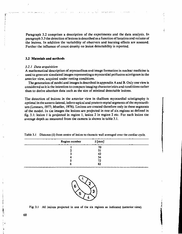
Paragraph 3.2 comprises a description of the experiments and the data analysis. Inparagraph 3.3 the detection of lesions is described as a function of location and volume ofthe lesions. In addition the variability of observers and learning effects are assessed.Further the influence of count density on lesion detectability is reported.

3.2 Materials and methods

3.2.1 Data acquisitionA mathematical description of myocardium and image formation in nuclear medicine isused to generate simulated images representing a myocardial perfusion scintigram in theanterior view, acquired under resting conditions.

The generation of model and images is described in appendix A and B. Only one view isconsidered as it is the intention to compare imaging characteristics and conditions ratherthan to derive absolute data such as the size of minimal detectable lesions.

The detection of lesions in the anterior view in thallium myocardial scintigraphy isoptimal in the antero-lateral, infero-apical and postero-septal segments of the myocardi-um (Lenears, 1977; Mueller, 1976). Lesions are created therefore only in these segmentsof the model. In the images the lesions are projected in one of six regions as defined infig. 3.1: lesion I is projected in region 1, lesion 2 in region 2 etc. For each lesion theaverage depth as measured from the camera is shown in table 3.1.

Table 3.1 Distance (z) from centre of lesion to thoracic wall averaged over the cardiac cycle.

Region number z [mm]

123456

70SI42547282

Fig. 3.1 All lesions projected in one of the six regions as indicated (anterior view).

68

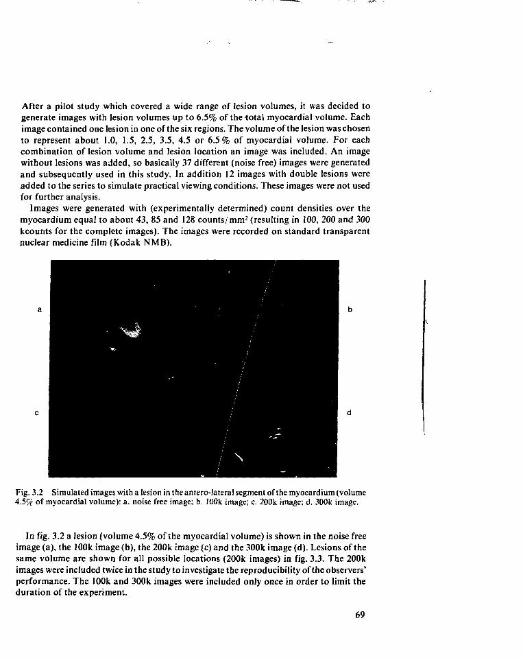
After a pilot study which covered a wide range of lesion volumes, it was decided togenerate images with lesion volumes up to 6.5% of the total myocardial volume. Eachimage contained one lesion in one of the six regions. The volume of the lesion was chosento represent about 1.0, 1.5, 2.5, 3.5, 4.5 or 6.5% of myocardial volume. For eachcombination of lesion volume and lesion location an image was included. An imagewithout lesions was added, so basically 37 different (noise free) images were generatedand subsequently used in this study. In addition 12 images with double lesions wereadded to the series to simulate practical viewing conditions. These images were not usedfor further analysis.

Images were generated with (experimentally determined) count densities over themyocardium equal to about 43, 85 and 128 counts/mm2 (resulting in 100, 200 and 300kcounts for the complete images). The images were recorded on standard transparentnuclear medicine film (Kodak NMB).

Fig. 3.2 Simulated images with a lesion in the antero-Jateral segment of the myocardium (volume4.5% of myocardial volume): a. noise free image; b. 100k image; c. 200k image; d. 300k image.

In fig. 3.2 a lesion (volume 4.5% of the myocardial volume) is shown in the noise freeimage (a), the 100k image (b), the 200k image (c) and the 300k image (d). Lesions of thesame volume are shown for all possible locations (200k images) in fig. 3.3. The 200kimages were included twice in the study to investigate the reproducibility of the observers'performance. The 100k and 300k images were included only once in order to limit theduration of the experiment.

69

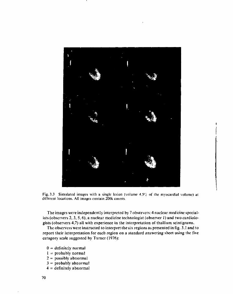
Fig. 3.3 Simulated images with a single lesion (volume 4.5r( of the myocardial volume) atdifferent locations. All images contain 200k counts.

The images were independently interpreted by 7 observers: 4 nuclear medicine special-ists (observers 2, 3, 5, 6), a nuclear medicine technologist (observer 1) and two cardiolo-gists (observers 4,7) all with experience in the interpretation of thallium scintigrams.

The observers were instructed to interpret the six regions as presented in fig. 3.1 and toreport their interpretation for each region on a standard answering sheet using the fivecatagory scale suggested by Turner (1976):

0 = definitely normal1 = probably normal2 = possibly abnormal3 = probably abnormal4 = definitely abnormal

70

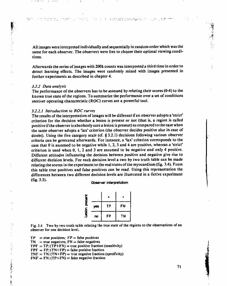
All images were interpreted individually and sequentially in random order which was thesame for each observer. The observers were free to choose their optimal viewing condi-tions.

Afterwards the series of images with 200k counts was interpreted a third time in order todetect learning effects. The images were randomly mixed with images presented infurther experiments as described in chapter 4.

3.2.2 Data analysisThe performance of the observers has to be assessed by relating their scores (0-4) to theknown true state of the regions. To summarize the performance over a set of conditionsreceiver operating characteristic (ROC) curves are a powerful tool.

3.2.2.1 Introduction to ROC curvesThe results of the interpretation of images will be different if an observer adopts a'strict'criterion for the decision whether a lesion is present or not (that is, a region is calledpositive if the observer is absolutely sure a lesion is present) as compared to the case whenthe same observer adopts a 'lax' criterion (the observer decides positive also in case ofdoubt). Using the five category scale (cf. § 3.2.1) decisions following various observercriteria can be generated afterwards. For instance, a 'lax' criterion corresponds to thecase that 0 is assumed to be negative while 1, 2, 3 and 4 are positive, whereas a 'strict'criterion is used when 0, 1, 2 and 3 are assumed to be negative and only 4 positive.Different attitudes influencing the decision between positive and negative give rise todifferent decision levels. For each decision level a two by two truth table can be maderelating the scores in the experiment to the real states of the myocardium (fig. 3.4). Fromthis table true positives and false positives can be read. Using this representation thedifferences between two different decision levels are illustrated in a fictive experiment

Observer interpretation

yes

no

•

TP

FP

-

FN

TN

Fig. 3.4 Two by two truth table relating the true state of the regions to the observations of anobserver for one decision level.

TP — true positives; FP = false positivesTN = true negatives; FN = false negativesTPF = TP/(TP+FN) = true positive fraction (sensitivity)FPF = FP/(TN+FP) = false positive fractionTNF = TN/(TN+FP) = true negative fraction (specificity)FNF = FN/(TP+FN) = false negative fraction

71

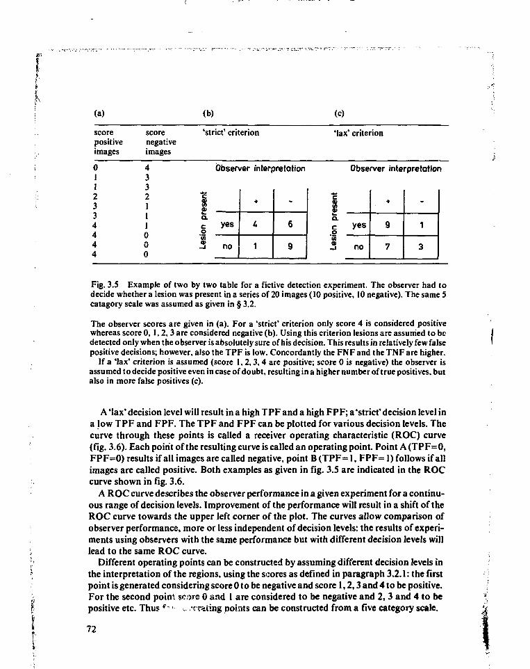
i(a)

scorepositiveimages

scorenegativeimages

(b)

'strict' criterion

(c)

Max' criterion

0112334444

4332111000

Observer interpretation Observer interpretation

1ffa. yes

no 1

-

6

9

o'Ci

yes

no

•

9

7

-

1

3

Fig. 3.5 Example of t w o by two table for a fictive detection experiment. The observer had todecide whether a lesion was present in a series o f 20 images (10 posit ive, 10 negative). The same Scatagory scale was assumed as given in § 3.2.

The observer scores are given in (a). For a 'strict* criterion only score 4 is considered posit ivewhereas score 0, 1 , 2 , 3 are considered negative (b) . Using this criterion lesions are assumed to bedetected only when the observer is absolutely sure of his decis ion. This results in relatively few falseposit ive decis ions; however, a l so the T P F is low. Concordant ly the F N F and the T N F are higher.

If a 'lax' criterion is assumed (score 1 , 2 , 3 , 4 are positive; score 0 is negative) the observer isassumed to decide positive even in case of doubt , resulting in a higher number of true posit ives, butalso in more false posit ives (c).

A 'lax' decision level will result in a high TPF and a high FPF; a 'strict' decision level ina low TPF and FPF. The TPF and FPF can be plotted for various decision levels. Thecurve through these points is called a receiver operating characteristic (ROC) curve(fig. 3.6). Each point of the resulting curve is called an operating point. Point A(TPF=0,FPF=0) results if all images are called negative, point B (TPF= 1, FPF= 1) follows if allimages are called positive. Both examples as given in fig. 3.5 are indicated in the ROCcurve shown in fig. 3.6.

A ROC curve describes the observer performance in a given experiment for a continu-ous range of decision levels. Improvement of the performance will result in a shift of theROC curve towards the upper left corner of the plot. The curves allow comparison ofobserver performance, more or less independent of decision levels: the results of experi-ments using observers with the same performance but with different decision levels willlead to the same ROC curve.

Different operating points can be constructed by assuming different decision levels inthe interpretation of the regions, using the scores as defined in paragraph 3.2.1: the firstpoint is generated considering score 0 to be negative and score 1,2,3 and 4 to be positive.For the second point score 0 and 1 are considered to be negative and 2,3 and 4 to bepositive etc. Thus f-•' •:. ''rating points can be constructed from a five category scale.

72

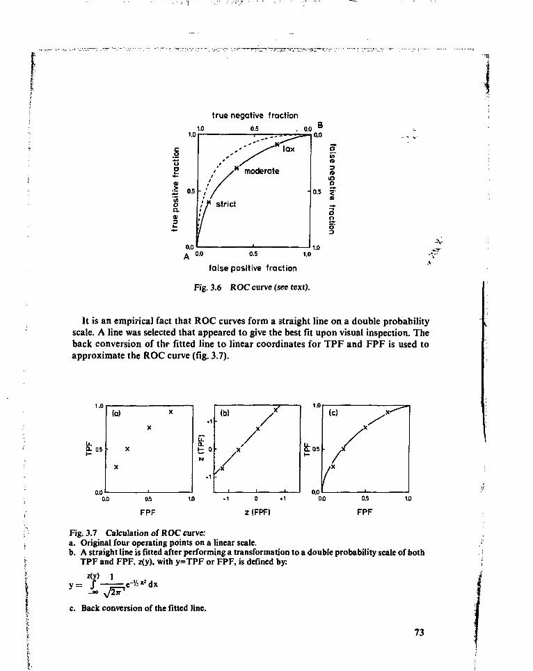
true negative fraction

1.0

0.5 1.0

false positive fraction

Fig. 3.6 ROC curve (see text).

•>,-

It is an empirical fact that ROC curves form a straight line on a double probabilityscale. A line was selected that appeared to give the best fit upon visual inspection. Theback conversion of thf fitted line to linear coordinates for TPF and FPF is used toapproximate the ROC curve (fig. 3.7).

0- 0.5

0.0

Fig. 3.7 Calculation of ROC curve:a. Original four operating points on a linear scale.b. A straight line is fitted after performing a transformation to a double probability scale of both

TPF and FPF. z(y), with y=TPF or FPF, is defined by:

z(y) 1

c. Back conversion of the fitted line.

73

. / •

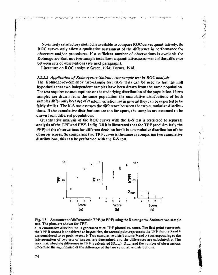
No entirely satisfactory method is available to compare ROC curves quantitatively. SoROC curves only allow a qualitative assessment of the difference in performance forobservers and/or procedures. If a sufficient number of observations is available theKolmogorov-Smirnov two-sample test allows a quantitative assessment of the differencebetween sets of observations (see next paragraph).

Literature on ROC analysis: Green, 1974; Turner, 1978.

3.2.2.2 Application of Kolmogorov-Smirnov two-sample test in ROC analysisThe Kolmogorov-Smirnov two-sample test (K-S test) can be used to test the nullhypothesis that two independent samples have been drawn from the same population.The test requires no assumptions on the underlying distribution of the population. If twosamples are drawn from the same population the cumulative distributions of bothsamples differ only because of random variation, so in general they can be expected to befairly similar. The K-S test assesses the difference between the two cumulative distribu-tions. If the cumulative distributions are too far apart, the samples are assumed to bedrawn from different populations.

Quantitative analysis of the ROC curves with the K-S test is restricted to separateanalysis of the TPF and FPF. In fig. 3.8 it is illustrated that the TPF (and similarly theFPF) of the observations for different decision levels is a cumulative distribution of theobserver scores. So comparing two TPF curves is the same as comparing two cumulativedistributions; this can be performed with the K-S test.

1.0 n

Ü- 0 .5-

1.0 n

LLQ. 0 .5 -

1.0-

4-Score

(a)Score(b)

- ! T4 3 2 1

Score(c)

Fig. 3.8 Assessment of differences in TPF(or FPF) using the Kolmogorov-Smirnov two-sampletest. The plots are shown for TPF.a. A cumulative distribution is generated with TPF plotted vs. score. The first point representsthe TPF if score 4 is considered to be positive, the second point represents the TPF if score 3 and 4are considered to be positive etc.; b. Two cumulative distributions (• and x) corresponding to theinterpretation of two sets of images, are determined and the differences are calculated; c. Themaximal, absolute difference in TPF is calculated (Dmax). Dmax and the number of observationsdetermine the significance of the difference of the two cumulative distributions.

74

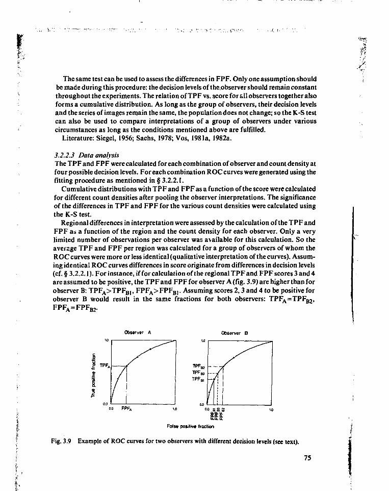
The same test can be used to assess the differences in FPF. Only one assumption shouldbe made during this procedure: the decision levels of the.observer should remain constantthroughout the experiments. The relation of TPF vs. score for all observers together alsoforms a cumulative distribution. As long as the group of observers, their decision levelsand the series of images remain the same, the population does not change; so the K-S testcan also be used to compare interpretations of a group of observers under variouscircumstances as long as the conditions mentioned above are fulfilled.

Literature: Siegel, 1956; Sachs, 1978; Vos, 1981a, 1982a.

3.2.2.3 Data analysisThe TPF and FPF were calculated for each combination of observer and count density atfour possible decision levels. For each combination ROC curves were generated using thefitting procedure as mentioned in § 3.2.2.1.

Cumulative distributions with TPF and FPF as a function of the score were calculatedfor different count densities after pooling the observer interpretations. The significanceof the differences in TPF and FPF for the various count densities were calculated usingthe K-S test.

Regional differences in interpretation were assessed by the calculation of the TPF andFPF as a function of the region and the count density for each observer. Only a verylimited number of observations per observer was available for this calculation. So theaverage TPF and FPF per region was calculated for a group of observers of whom theROC curves were more or less identical (qualitative interpretation of the curves). Assum-ing identical ROC curves differences in score originate from differences in decision levels(cf. § 3.2.2.1). For instance, if for calculation of the regional TPF and FPF scores 3 and 4are assumed to be positive, the TPF and FPF for observer A (fig. 3.9) are higher than forobserver B: TPFA>TPFBJ, FPFA> FPFB(. Assuming scores 2,3 and 4 to be positive forobserver B would result in the same fractions for both observers: TPFA=TPFB2,FPFA=FPFB2.

Observer A Observer B

|

0.0 FPF.

IEFalse positive fraction

Fig. 3.9 Example of ROC curves for two observers with different decision levels (see text).

75

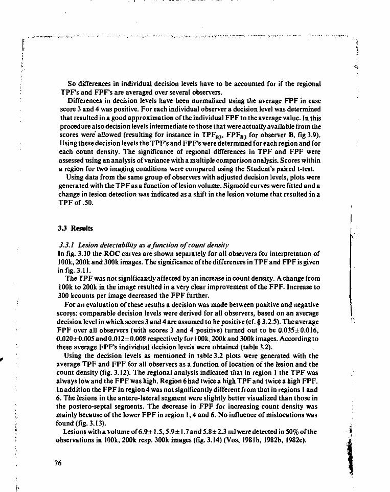
So differences in individual decision levels have to be accounted for if the regionalTPFs and FPF's are averaged over several observers.

Differences in decision levels have been normalized using the average FPF in casescore 3 and 4 was positive. For each individual observer a decision level was determinedthat resulted in a good approximation of the individual FPF to the average value. In thisprocedure also decision levels intermediate to those that were actually available from thescores were' allowed (resulting for instance in TPFB3, FPFB3 for observer B, fig 3.9).Using these decision levels the TPFs and FPFs were determined for each region and foreach count density. The significance of regional differences in TPF and FPF wereassessed using an analysis of variance with a multiple comparison analysis. Scores withina region for two imaging conditions were compared using the Student's paired t-test.

Using data from the same group of observers with adjusted decision levels, plots weregenerated with the TPF as a function of lesion volume. Sigmoid curves were fitted and achange in lesion detection was indicated as a shift in the lesion volume that resulted in aTPF of .50.

3.3 Results

3.3.1 Lesion detectability as a function of count densityIn fig. 3.10 the ROC curves are shown separately for all observers for interpretation of100k, 200k and 300k images. The significance of the differences in TPF and FPF is givenin fig. 3.11.

The TPF was not significantly affected by an increase in count density. A change from100k to 200k in the image resulted in a very clear improvement of the FPF. Increase to300 kcounts per image decreased the FPF further.

For an evaluation of these results a decision was made between positive and negativescores: comparable decision levels were derived for all observers, based on an averagedecision level in which scores 3 and 4 are assumed to be positive (cf. § 3.2.S). The averageFPF over all observers (with scores 3 and 4 positive) turned out to be 0.035±0.0I6,0.020± 0.005 and 0.012± 0.008 respectively for 100k, 200k and 300k images. According tothese average FPFs individual decision levels were obtained (table 3.2).

Using the decision levels as mentioned in table 3.2 plots were generated with theaverage TPF and FPF for all observers as a function of location of the lesion and thecount density (fig. 3.12). The regional analysis indicated that in region 1 the TPF wasalways low and the FPF was high. Region 6 had twice a high TPF and twice a high FPF.In addition the FPF in region 4 was not significantly different from that in regions 1 and6. The lesions in the antero-lateral segment were slightly better visualized than those inthe postero-septal segments. The decrease in FPF for increasing count density wasmainly because of the lower FPF in region 1,4 and 6. No influence of mislocations wasfound (fig. 3.13).

Lesions with a volume of 6.9± 1.5,5.9± 1.7 and 5.8±2.3 ml were detected in 50% of theobservations in 100k, 200k resp. 300k images (fig. 3.14) (Vos, 1981b, 1982b, 1982c).

76

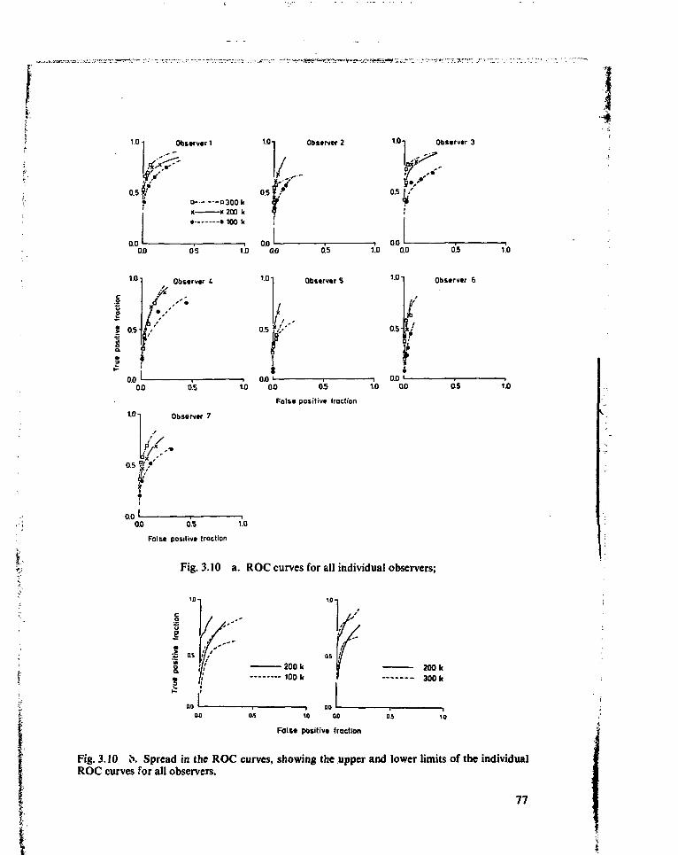
1.0

0.5

0.0

Obstrvtr1

o O300kx x 200 k• • 100 k

1.0 Observer 2

ir0.0 os

Obscrvtr

os

1.0-1 Observtr 7

—i 0.0 >—1.0 0.0

1.01 Obstrvtr S

'f0.0 "-

10-j Observtr 3

—i 0.01.0 0.0

1.01

0.5-

0.5

Obstrvtr 6

i

- i 0.0 '1.0 0.0 0.5 1.0 0.0 05

Foist positivt fraction

1.0

1.0

0.00.0 0.5 1.0

False positive traction

Fig. 3.10 a. ROC curves for all individual observers;

I as«&s

/

•200 k- 100 k

200 k300 k

- i ao i

Fait* positivt fraction

Fig. 3.10 b. Spread in the ROC curves, showing the upper and lower limits of the individualROC curves for all observers.

77

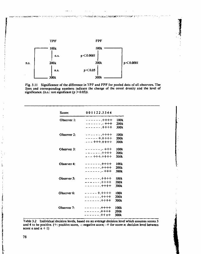
TPF

100k

FPF

n.s.

p < 0.0001

p<0.05

p < 0.0001

Fig. 3.11 Significance of the difference in TPF and FPF for pooled data of all observers. Thelines and corresponding numbers indicate the change of the count density and the level ofsignificance, (n.s.: not significant (p > 0.05)).

Score: 00 1 1 2 2 . 3 3 4 4

Observer 1: .++++ 100k.- +++ 200k.++++ 300k

Observer 2: .++++ 100k+.++++ 200k

+++.++++ 300k

Observer 3: . - + + + 100k.++++ 200k

+++.++++ 300k

Observer 4: .++++ 100k.++++ 200k.- + + + 300k

Observer 5: .++++ 1.00k.++++ 200k.++++ 300k

Observer 6: + .++++ 100k.++++ 200k.++++ 300k

Observer 7: .++++ 100k.++++ 200k.++ -H- 300k

Table 3.2 Individual decision levels, based on an average decision level which assumes scores 3and 4 to be positive. (+: positive score, -: negative score; - + for score n: decision level betweenscore n and n + 1)

78

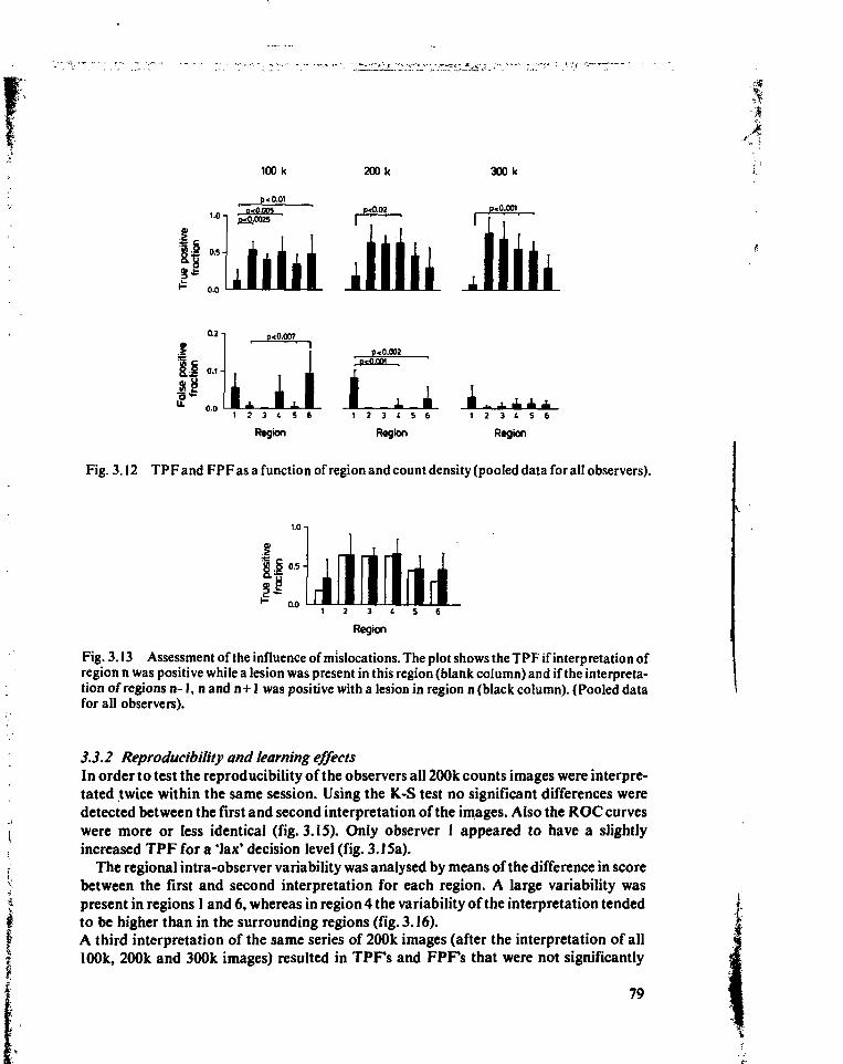
'Jt

300 k

p<0.001

0.2 -|

0.0

p< 0.007

I p< 0.003; 0*0.001 '

1 2 3 ( 5 6

Region Region

1 2 3 1 5 6

Region

Fig. 3.12 TPF and FPF as a function of region and count density (pooled data for all observers).

1.0-,

1 2 3 ( 5 6

Region

Fig. 3.13 Assessment of the influence of mislocations. The plot shows the TPF if interpretation ofregion n was positive while a lesion was present in this region (blank column) and if the interpreta-tion of regions n-1, nand n+I was positive with a lesion in region n (black column). (Pooled datafor all observers).

3.3.2 Reproducibility and learning effectsIn order to test the reproducibility of the observers all 200k counts images were interpre-tated twice within the same session. Using the K.-S test no significant differences weredetected between the first and second interpretation of the images. Also the ROC curveswere more or less identical (fig. 3.15). Only observer 1 appeared to have a slightlyincreased TPF for a 'lax' decision level (fig. 3.15a).

The regional intra-observer variability was analysed by means of the difference in scorebetween the first and second interpretation for each region. A large variability waspresent in regions 1 and 6, whereas in region 4 the variability of the interpretation tendedto be higher than in the surrounding regions (fig. 3.16).A third interpretation of the same series of 200k images (after the interpretation of all100k, 200k and 300k images) resulted in TPFs and FPFs that were not significantly

79

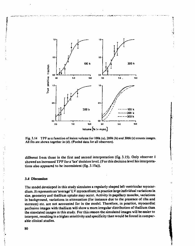
1.0-

0.5

so.o

1.0 n

100 k

100 so . 100

1.0

0.5-

0.0

100 k200 k300 k

ao 5.0 100

Volume [% Iv myocj

Fig. 3.14 TPF as a function of lesion volume for 100k (a), 200k (b) and 300k (c) counts images.All fits are shown together in (d). (Pooled data for all observers).

different from those in the first and second interpretation (fig. 3.15). Only observer Ishowed an increased TPF for a 'lax' desision level. (For this decision level his interpreta-tions also appeared to be inconsistent (fig. 3.15a)).

3.4 Discussion

The model developed in this study simulates a regularly shaped left ventricular myocar-dium. It represents an 'average' L V myocardium; in practice large individual variations insize, geometry and thallium uptake may occur. Activity in papillary muscles, variationsin background, variations in attenuation (for instance due to the presence of ribs andsternum) etc. are not accounted for in the model. Therefore, in practice, myocardialperfusion images with thallium will show a more irregular distribution of thallium thanthe simulated images in this study. For this reason the simulated images will be easier tointerpret, resulting in a higher sensitivity and specificity than would be found in compar-able clinical studies.

80

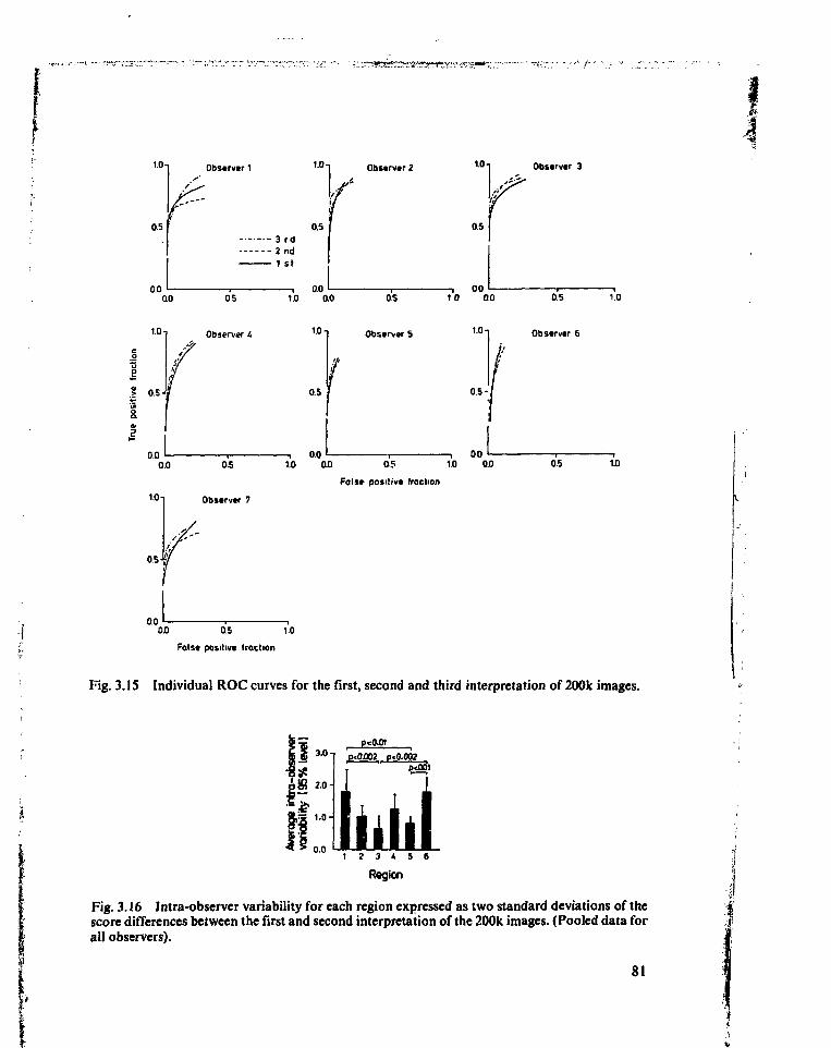
1.0

0.5

0.0

Observer1 1 0 1

0.53 rd2nd1 st

00

1.0

•ss» 0.5 J5

0.0

0.5

Observer L

0.01.0 0.0

10 -i

0.5

, 0.0

Observer 21<>T Observer 3

0.5

, , 000.5 10 0.0 0.5 1.0

Observers 1 " i Observer 6

0.5-/

0.00.0 0.5 1.0 0.0 0.5 1.0 0.0

False positive fraction

1 ° 1 Observer 7

0.0 0.5 1.0

False positive traction

OS 1.0

Fig. 3.IS Individual ROC curves for the first, second and third interpretation of 200k images.

3.0 np<0.01

•8*pffi 20-Is

0.0

p«0.002 p-0.002

1 2 3 4 5 6

Rsgion

Fig. 3.16 Intra-observer variability for each region expressed as two standard deviations of thescore differences between the first and second interpretation of the 200k images. (Pooled data forall observers).

81

f-

I-

However, it is intended to compare various imaging conditions rather than to extrapo-late data on biological characteristics from the model to clinical routine. Therefore theregularity of the model does not interfere with the aim of this study.

The use of the K-S test appears to be useful for quantitative assessment of differences inperformance in rating experiments: the results of both visual inspection of the ROCcurves and analysis of regional and size effects are in agreement with the results asobtained with this test.

The count density does not affect the sensitivity of the detection of lesions. Although nosignificant differences were detected between the interpretation of the antero-lateralsegment and the infero-apical (and partly postero-septal) segment the lesions in the firstmentioned segment tend to be better visualized. The same result was reported in a clinicalsetting (Okada, 1980; Atwood, 1981).

The FPF is severely affected by the count density. Region I and 6 have high FPF's forlow count densities; increase of the count density diminishes the regional differences. Theregions with a high FPF also show a high intra-observer variability. The difficultinterpretation of the regions near the base of the left ventricle can be expected: theborders of the myocardium are quite vague in these regions.

Clinical studies indicated that the observer variability (Okada, 1980; Atwood, 1981)and the FPF (Lenears, !977) are higher in the apical region as compared to that in thesurrounding regions. This difference is usually attributed to the biological variations inthis region (Cook, 1976). However, this study reveals that also in the absence of biologi-cal variations this region appears to be difficult for the observers to judge. As thegeometry is the only changing factor in this study it is likely that observer variability inthe apical region is at least partially caused by geometrical factors.

The lesion volume which is detected in 50% of the interpretations (about 6 ml) iscomparable to that reported by Mueller (1976) from physical phantom measurements(about 4 ml).

In conclusion, the results of the detection experiments as obtained with the mathematicalmodel are comparable to those reported for clinical and physical experiments. Therefore,the model can be used to test the influence of various image characteristics, although theabsolute values on lesion detectability may not be comparable to those obtained clin-ically.

82

Appendix A: Description of the model for the myocardium and the image generation

A-l Introduction

An image can be described as a convolution of an object and the point spread function(PSF) of the detection/imaging system (Beck, 1975; Brown, 1971; Metz, 1974).

Assuming shift invariancy for the PSF in planes parallel to the collimator, it followsthat:

TI(x„ y„ T) = 5 SSS A(x, y, z, t) • PSF(x-x„ y-y„ z) . dxdydzdt (A-l)

t = Oxyz

where: I(Xj, y t, T): count density in image point (xj, yj) at t = T.(x, y): coordinates in planes parallel to the collimatorz: distance between source and collimatorA(x, y, z, t): count rate from (point) source at location (x, y, z) at time t.PSF: point spread function

The PSF depends on:1. collimator and camera system;2. the radio-nuclide used;3. the medium between source and detector;4. the distance from source to the detector;5. the energy window of the pulse height analyser.

In appendix B a description is given of the PSF for the imaging configuration formyocardial perfusion scintigraphy with thallium-201 as used at the Division of NuclearMedicine, University Hospital Leiden, The Netherlands. This PSF is used in the experi-ments described in this thesis, in cases where thallium-201 is applied.

The count rate from a radioactive source is a Poisson distributed variable (Evans, 1955).The count density in nuclear medicine images will also obey a Poisson probabilityfunction because of the additive properties of these types of variables (Metz, 1974;Papoulis, 1964).

83

Equation (A-l) can be rewritten in (Metz, 1969):

I(x„ y„ T) = SSS A'(x, y, z, T) . PSF(x-x„ y-y„ z) dxdydz ± N (x„ y„ T) (A-2)xyz v

where: A'(x, y, z, T): Expectation of A(x, y, z, t)Np(X(, y(, T): Poisson noise resulting from the finite number of photons that

contribute to image point (x,, Vj) within time interval T (Beck,1975).

Because of the Poisson statistics N_ (x,, y (, T) equals -N/I(xI,yj,T). (Instrumental noise isusually very low and has therefore been omitted in equation (A-2)).

From equation (A-2) it can be concluded that it is allowed to calculate an image in twosubsequent steps. First the response of the detection/imaging system to the objectdistribution can be calculated using expectation values for the local count rates. Once this(noise free) image is calculated, noise can be added to each image element depending onthe intensity of the image element.

A-2 Heart model

A-2.1 Geometric model of the left ventricular wallTwo assumptions have been made in the development of the heart model.a. Because the right ventricle is hardly visualized due to its thin wall, its small tissue mass

and its limited blood supply (Cook, 1976), activity of the left ventricular wall only istaken into account. Thallium in the other parts of the heart is assumed to contribute tobackground activity.

b. The wall of the thorax is supposed to be flat. No variations in attenuation areintroduced to simulate mammae. Therefore all physiological data used applies tomales.

The concentration <.•.; thallium in healthy myocardial tissue is approximately constant(Wackers, 1978; Bradley-Moore, 1975). Therefore it is sufficient to describe only thegeometry of the LV myocardium throughout the cardiac cycle. Afterwards this geometrycan be 'filled in' with evenly distributed thallium.

In radiographic angiography several symmetrical figures have been used to approxi-mate the LV contours for estimation of the LV volume throughout the cardiac cycle.Davila (1968) has compared several of these figures, including a cylinder, a combinationof several cylinders and several types of ellipsoids. An ellipsoid of revolution (prolatespheroid) as originally suggested by Dodge (1960, 1961) proved to be a reliable andaccurate reference figure to estimate LV volume. Since the ellipsoid is simple to treatmathematically it is chosen for the description of the inner contour of the L V myocardi-um. An ellipsoid of revolution can also be used for the desciption of the outer wallgeometry (Rackley, 1974). Therefore the shape of the left ventricle is approximated witha thick walled ellipsoid of revolution.

84

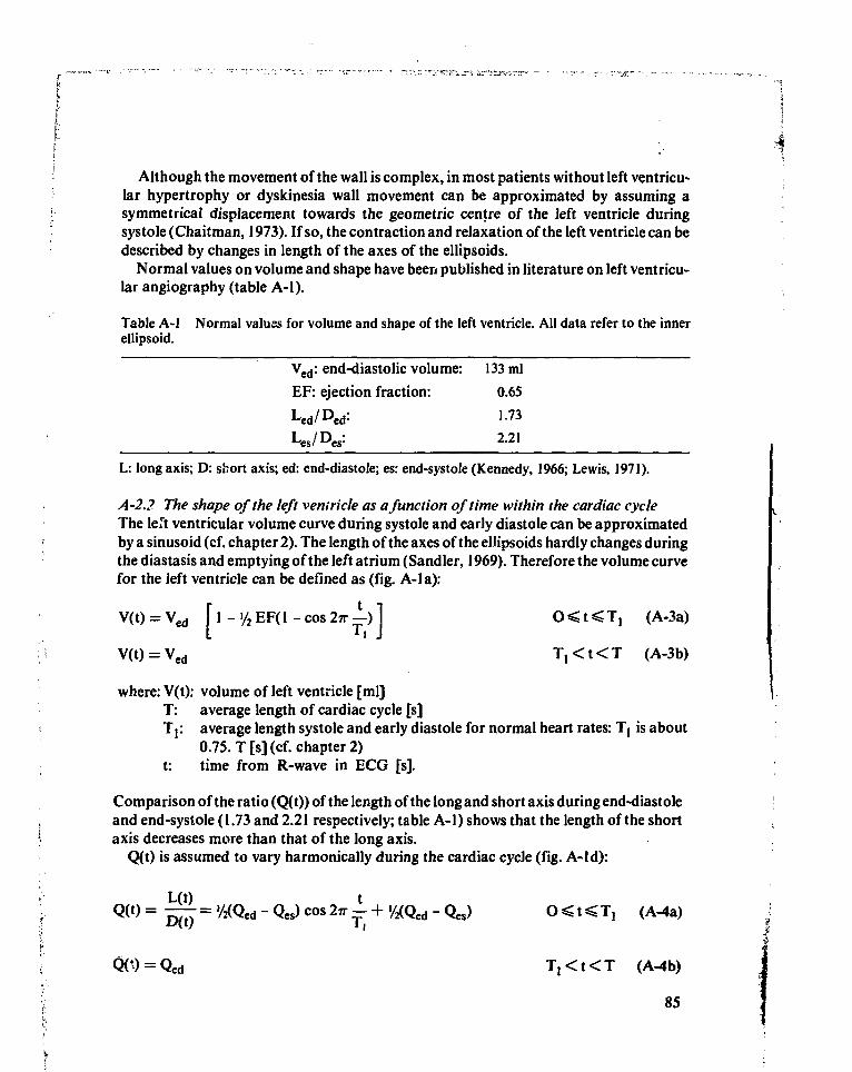
k " ' ' ' ' "\

\ \

Although the movement of the wall is complex, in most patients without left ventricu-lar hypertrophy or dyskinesia wall movement can be approximated by assuming asymmetrical displacement towards the geometric centre of the left ventricle duringsystole (Chaitman, 1973). If so, the contraction and relaxation of the left ventricle can bedescribed by changes in length of the axes of the ellipsoids.

Normal values on volume and shape have been published in literature on left ventricu-lar angiography (table A-l).

Table A-l Normal values for volume and shape of the left ventricle. All data refer to the innerellipsoid.

Ved: end-diastolic volume: 133 ml

EF: ejection fraction: 0.65

Led/Ded: 1.73

L: long axis; D: short axis; ed: end-diastole; es: end-systole (Kennedy, 1966; Lewis, 1971).

A-2.2 The shape of the left ventricle as a function of time within the cardiac cycleThe left ventricular volume curve during systole and early diastole can be approximatedby a sinusoid (cf. chapter 2). The length of the axes of the ellipsoids hardly changes duringthe diastasis and emptying of the left atrium (Sandier, 1969). Therefore the volume curvefor the left ventricle can be defined as (fig. A-la):

V(t) = Ved f 1 - >/2 EF( 1 - cos 2TT —) 1 O < t < T, (A-3a)

V(t) = Ved T , < t < T (A-3b)

where: V(t): volume of left ventricle [ml]T: average length of cardiac cycle [s]T]: average length systole and early diastole for normal heart rates: T, is about

0.75. T [s] (cf. chapter 2)t: time from R-wave in ECG [s].

Comparison of the ratio (Q(t)) of the length of the long and short axis during end-diastoleand end-systole (1.73 and 2.21 respectively; table A-l) shows that the length of the shortaxis decreases more than that of the long axis.

Q(t) is assumed to vary harmonically during the cardiac cycle (fig. A-ld):

L(t) tQ(t) = — = '/«Qed - Qes) cos 2TT - + '/2(Qed - Qes) O < t < T, (A-4a)

T,<t<T (

85

where: L(t): length of long axis as a function of time [m]D(t): length of short axis as a function of time [m]

As the ventricular volume is approximated by an ellipsoid, it follows that

4(A-5)

3 -l \ I )

Substitution of eq. (A-3) and (A-4) in eq. (A-5) results in

D ( t ) = [ (>/2 V e d E F c o s 2n 1 + V e d (1 - '/2 E F ) ) - £ — ] V i O ̂ t ̂ T , ( A - 6 a )L 11 "vlw J

FurtherL(t) = Q(t) D(t) O ̂ t < T, (A-6b)D(t) = Ded T,<t<T (A-6c)

= L e d T , < t < T (A-6d)

Figure A-lb and A-lc show the functions L(t) and D(t).

Within a coordinate system which describes the movement of the ventricle as a whole, themovement of the inner wall can be described by

x' \ / D(t) \I + y'2 + z'2 = I I (A-7)

Q(t) ƒ \ 2 ƒ

where: x', y', z' are coordinates within the moving coordinate system. (The x' axis'corresponds to the long axis of the ventricle).

Tne volume of the left ventricular cavity is represented by eq. (A-5). Likewise, the outerwall movement within the moving coordinate system can be described by an ellipsoid:

x'2 (v'2 "t" z'2)

['/2L(t) + W(t)p + Ü4D(t) + W(t)p = l ( A ' 8 )

where: W(t): thickness of left ventricular wall as measured along the axes of the ellipsoid.

The volume of the myocardium and cavity together is equal to

f = 1 „ | — + W ( t ) I I ̂ + W(tt I (A-9)

86

I.

From eq. (A-5) and (A-9) it follows that (ignoring the time index)

= Vout - Vin = A-n [ W*D (>/2Q + 1) + '/2WD* ('/2 + Q) + W3] (A-10)

where: VwaJ|: volume of left ventricular myocardium [ml].

Vwal| is approximately constant during the cardiac cycle: 179 ml (Kennedy, 1966). As theaverage wall thickness is approximately 12 mm (at end-diastole; Kennedy, 1966), it

4follows that - IT W3 < Vwall. Therefore eq. (A-10) can be rewritten in

D(1+2Q) 3(V in-Vout)W + W + = O

2(Q + 2) 2TTD(Q + 2 )

Because Q(t) > 0 and W(t) > 0 it can be concluded that

W(t) = '/2 t-W,(t) + VW,(t)2 - 4W2(t) ]

D(t)(l+2Q(t))where: W,(t) = — ^ ^^- (A-12a)1 W 2(2 + Q(t))

W,(t) = wa" (A-12b)2 W 27rD(t)(2 + Q(t))

A-2.3 Movement of the left ventricle within the thorax during the cardiac cycleIn a supine position and during resting conditions the movement of the heart due torespiration is very small. And since the geometric centre of the left ventricle hardly moves(1.4±0.8% of the end-diastolic long axis (Meester, 1980) during contraction of the leftventricle under conditions as mentioned before), translations of the ventricle duringcontraction can also be ignored. However, the left ventricle performs a rotationalmovement: the base moves inferiorly and the apex superiorly. Besides, a small front toback rotation of the apex is present (Sandier, 1968; McDonald, 1970). The rotation of thelong axis can be defined in a fixed coordinate system within the thorax. The origin of thissystem is located in the centre of the left ventricle. The z-axis points to the camera, they-axis to the head and the x-axis to the left lateral side. The movement of the long axis canbe described by angles <p and 6 (fig. A-2).ip represents the angle between the long axis and the xy plane (AP-plane) and 6 the anglebetween the projection of the long axis at the plane with z = 0 and the (negative) y-axis.The z'-axis is located in the xz-plane throughout the cycle.

Average values for these angles at end-diastole are: <p=20.3° and 0=39.8°. Therotation can be defined by specification of the change in these angles. Assuming aharmonic change of<p and 6 throughout the cardiac cycle the movement can be defined

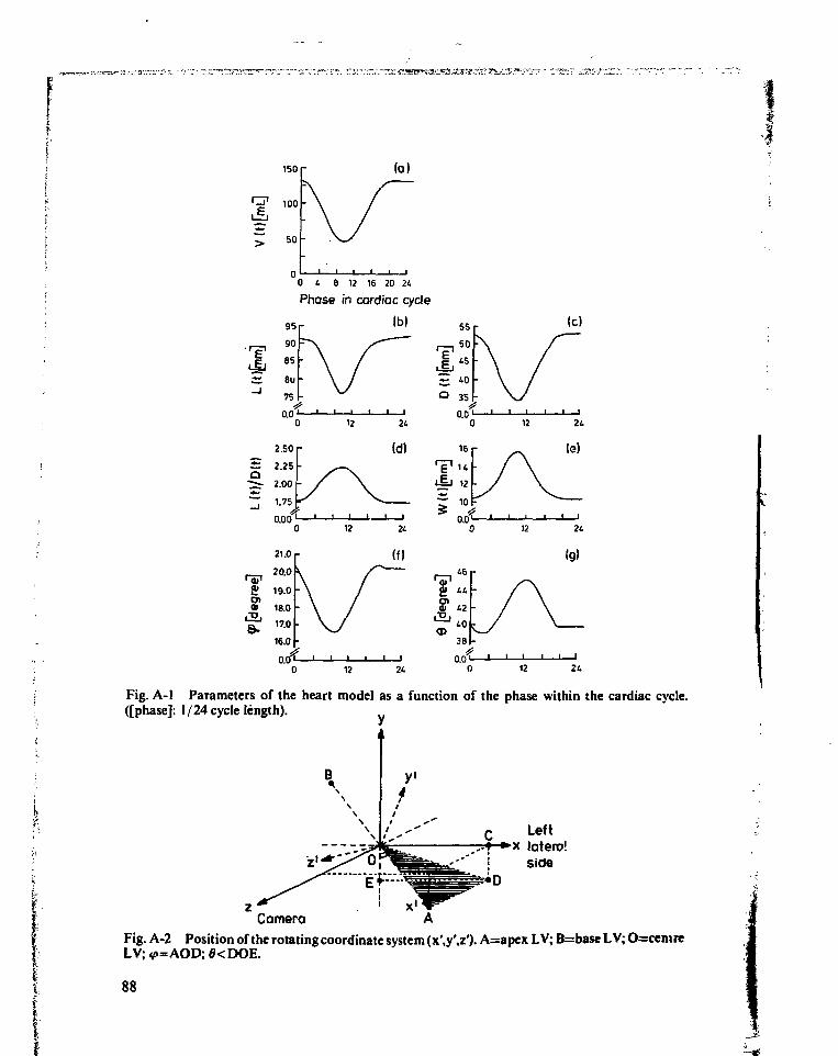
150 r

100

50

0 4 6 12 16 20 24

Phase in cardiac cycle

Ib)

Fig. A-l Parameters of the heart model as a function of the phase within the cardiac cycle,([phase]: 1/24 cycle length).

Left.-f »x latero!

side

CameraFig. A-2 Position of the rotating coordinate system (x\y\z'). A=apex LV; B=base L V; O=cemreLV; v»=AOD; fl<DOE.

88

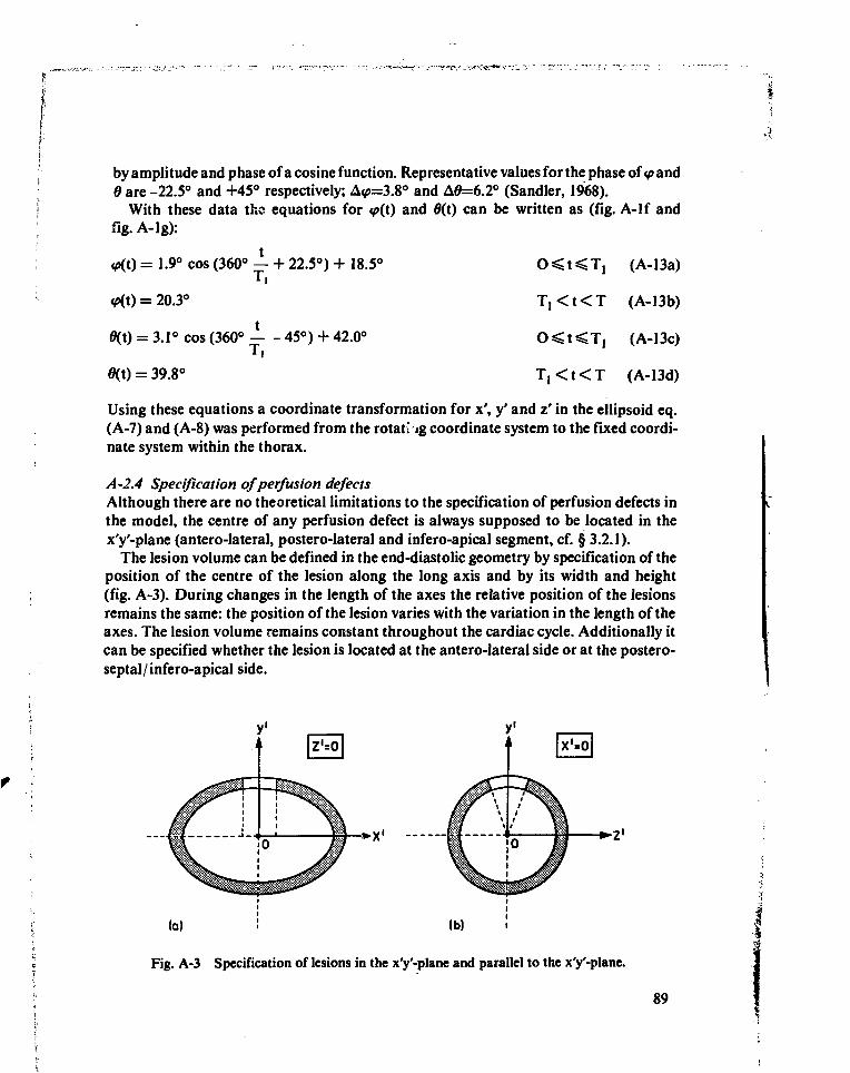
by amplitude and phase of a cosine function. Representative values for the phase of <p and6 are -22.5° and +45° respectively; A<p=3.8° and A0=6.2° (Sandier, 1968).

With these data the equations for <p(i) and 0(t) can be written as (fig. A-lf andfig. A-lg):

(A-13a)

(A-13b)

(A-13c)

(A-13d)

= 1.9° cos (360° — + 22.5°) + 18.5C

ifi(t) = 20.3°

0(t) = 3.1° cos (360° 45°) + 42.0°

0(t) = 39.8°

T , < t < T

T , < t < T

Using these equations a coordinate transformation for x', y' and z' in the ellipsoid eq.(A-7) and (A-8) was performed from the rotating coordinate system to the fixed coordi-nate system within the thorax.

A-2.4 Specification of perfusion defectsAlthough there are no theoretical limitations to the specification of perfusion defects inthe model, the centre of any perfusion defect is always supposed to be located in thex'y'-plane (antero-lateral, postero-lateral and infero-apical segment, cf. § 3.2.1).

The lesion volume can be defined in the end-diastolic geometry by specification of theposition of the centre of the lesion along the long axis and by its width and height(fig. A-3). During changes in the length of the axes the relative position of the lesionsremains the same: the position of the lesion varies with the variation in the length of theaxes. The lesion volume remains constant throughout the cardiac cycle. Additionally itcan be specified whether the lesion is located at the antero-lateral side or at the postero-septal/infero-apical side.

• x '

Fig. A-3 Specification of lesions in the x'y'-plane and parallel to the x'y'-plane.

89

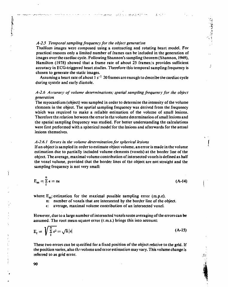
/4-2.5 Temporal sampling frequency for the object generationThallium images were composed using a contracting and rotating heart model. Forpractical reasons only a limited number of frames can be included in the generation ofimages over the cardiac cycle. Following Shannon's sampling theorem (Shannon, 1949),Hamilton (1978) showed that a frame rate of about 25 frames/s provides sufficientaccuracy in ECG-triggered heart studies. Therefore this temporal sampling frequency ischosen to generate the static images.

Assuming a heart rate of about 1 s~' 20 frames are enough to describe the cardiac cycleduring systole and early diastole.

A-2.6 Accuracy of volume determinations; spatial sampling frequency for the objectgenerationThe myocardium (object) was sampled in order to determine the intensity of the volumeelements in the object. The spatial sampling frequency was derived from the frequencywhich was required to make a reliable estimation of the volume of small lesions.Therefore the relation between the error in the volume determination of small lesions andthe spatial sampling frequency was studied. For better understanding the calculationswere first performed with a spherical model for the lesions and afterwards for the actuallesions themselves.

A-2.6.1 Errors in the volume determination for spherical lesionsIf an object is sampled in order to estimate object volume, an error is made in the volumeestimation due to partially included volume elements (voxels) at the border line of theobject. The average, maximal volume contribution of intersected voxels is defined as halfthe voxel volume, provided that the border lines of the object are not straight and thesampling frequency is not very small:

Em = I € = ne (A-14)

where: Em: estimation for the maximal possible sampling error (m.p.e).n: number of voxels that are intersected by the border line of the object,e: average, maximal volume contribution of an intersected voxel.

However, due to a large number of intersected voxels some averaging of the errors can beassumed. The root mean square error (r.m.s.) brings this into account:

E r =

These two errors can be specified for a fixed position of the object relative to the grid. Ifthe position varies, also ths volume and error estimation may vary. This volume change isreferred to as grid error.

90

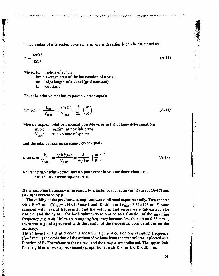
The number of intersected voxels in a sphere with radius R can be estimated as:

nkm2

where: R: radius of spherekm2: average area of the intersection of a voxelm: edge length of a voxel (grid constant)k: constant

Thus the relative maximum possible error equals

mV V ?k \ RMrue Mrue A A "•

where: r.m.p.e.: relative maximal possible error in the volume determinationsm.p.e.: maximum possible errorVtrue: true volume of sphere

and the relative root mean square error equals

Er Vnr.r.m.s. =

Mrue( m

-

where: r.r.m.s.: relative root mean square error in volume determinations,r.m.s.: root mean square error.

If the sampling frequency is increased by a factor p, the factor (m/ R) in eq. (A-17) and(A-18) is decreased by p.

The validity of the previous assumptions was confirmed experimentally. Two sphereswith R=7 mm (V t r u e=1.44xl03mm3) and R=20 mm (Vtrue=3.35xlO< mm3) weresampled with several frequencies and the volumes and errors were calculated. Ther.m.p.e. and the r.r.m.s. for both spheres were plotted as a function of the samplingfrequency (fig. A-4). Unless the sampling frequency becomes less than about 0.55 mm~',there was a good agreement with the results of the theoretical considerations on theaccuracy.The influence of the grid error is shown in figure A-5. For one sampling frequency(fs = 1 mm-1) the deviation of the estimated volume from the true volume is plotted as afunction of R. For reference the r.r.m.s. and the r.m.p.e. are indicated. The upper limitfor the grid error was approximately proportional with R~2 for 2 < R < 50 mm.

91

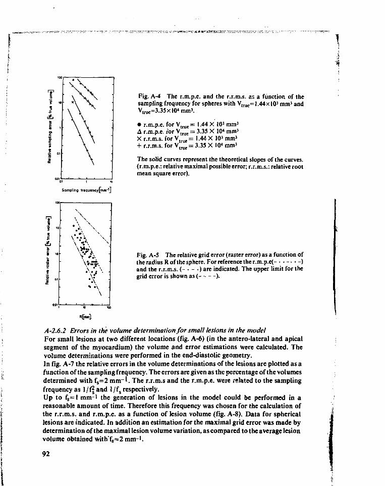
Sampling tftqutncy[mnr\j

Fig. A-4 The r.m.p.e. and the r.r.m.s. as a function of thesampling frequency for spheres with Vtrue= J.44xlO3 mm3 andV,rue=3.35xlO«mm3.

• r.m.p.e. for Vtrue = 1.44 X 10' mm3

A r.m.p.e. for VtrueX r.r.m.s. for Vtrue

= 3.35 X 10* mm3

= 1.44 X 103mm3

+ r.r.m.s. for V, r u e = 3.35 X 10* mm3

The solid curves represent the theoretical slopes of the curves,(r.m.p.e.: relative maximal possible error; r.r.m.s.: relative rootmean square error).

Fig. A-5 The relative grid error (raster error) as a function ofthe radius R of the sphere. For reference the r.m.p.e(- . . - . . - )and the r.r.m.s. ( - • - • ) are indicated. The upper limit for thegrid error is shown as ( ).

A-2.6.2 Errors in the volume determination for small lesions in the modelFor small lesions at two different locations (fig. A-6) (in the antero-lateral and apicalsegment of the myocardium) the volume and error estimations were calculated. Thevolume determinations were performed in the end-diastolic geometry.In fig. A-7 the relative errors in the volume determinations of the lesions are plotted as afunction of the sampling frequency. The errors are given as the percentage of the volumesdetermined with fs=2 m r ' . The r.r.m.s and the r.m.p.e. were related to the samplingfrequency as 1/ff and l/fs respectively.Up to fs=l mm-1 the generation of lesions in the model could be performed in areasonable amount of time. Therefore this frequency was chosen for the calculation ofthe r.r.m.s. and r.m.p.e. as a function of lesion volume (fig. A-8). Data for sphericallesions are indicated. In addition an estimation for the maximal grid error was made bydetermination of the maximal lesion volume variation, as compared to the average lesionvolume obtained with"fs=2 mm-'.

92

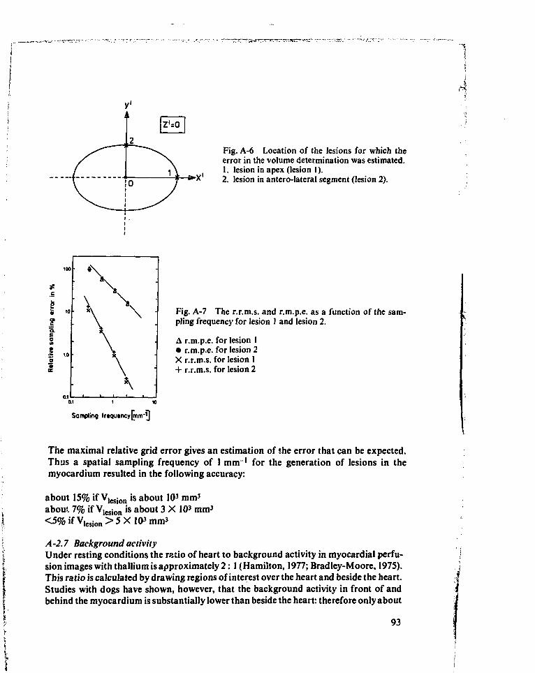
Pig. A-6 Location of the lesions for which theerror in the volume determination was estimated.1. lesion in apex (lesion 1).2. lesion in antero-Iateral segment (lesion 2).

I*

I3»a.

Fig. A-7 The r.r.m.s. and r.m.p.e. as a function of the sam-pling frequency for lesion 1 and lesion 2.

A r.m.p.e. for lesion 1• r.m.p.e. for lesion 2X r.r.m.s. for lesion 1+ r.r.m.s. for lesion 2

Sampling fr»qutncy[rnm-^]

The maximal relative grid error gives an estimation of the error that can be expected.Thus a spatial sampling frequency of 1 mm' for the generation of lesions in themyocardium resulted in the following accuracy:

about 15% if V,esion is about 103 mm3

about 7% if Vlesion is about 3 X 103 mm3

<5%ifV l e s i o n>5X103mm3

A -2.7 Background activityUnder resting conditions the ratio of heart to background activity in myocardial perfu-sion images with thallium is approximately 2: 1 (Hamilton, 1977; Bradley-Moore, I97S).This ratio is calculated by drawing regions of interest over the heart and beside the heart.Studies with dogs have shown, however, that the background activity in front of andbehind the myocardium is substantially lower than beside the heart: therefore only about

93

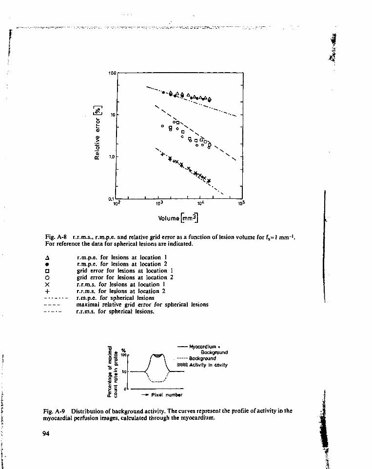
100

10* 103

Volume [mm3]

10=

Fig. A-8 r.r.m.s., r.m.p.e. and relative grid error as a function of lesion volume for fs=l mm-1.For reference the data for spherical lesions are indicated.

A r.m.p.e. for lesions at location 1• r.m.p.e. for lesions at location 2D grid error for lesions at location 1O grid error for lesions at location 2X r.r.m.s. for lesions at location 1+ r.r.m.s. for lesions at location 2- • • r.m.p.e. for spherical lesions

maximal relative grid error for spherical lesionsr.r.m.s. for spherical lesions.

° C8 , |If|

Myocardium •Background

Backgroundy/s?//,. Activity in cavity

—•> Pixel numbar

Fig. A-9 Distribution of background activity. The curves represent the profile of activity in themyocardial perfusion images, calculated through the myocardium.

94

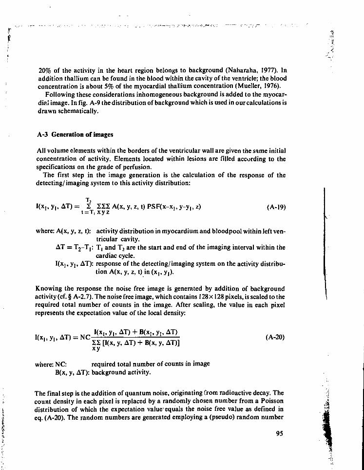
rr •

20% of the activity in the heart region belongs to background (Naharaha, 1977). Inaddition thallium can be found in the blood within the cavity of the ventricle; the bloodconcentration is about 5% of the myocardial thallium concentration (Mueller, 1976).

Following these considerations inhomogeneous background is added to the myocar-diai image. In fig. A-9 the distribution of background which is used in our calculations isdrawn schematically.

A-3 Generation of images

All volume elements within the borders of the ventricular wall are given the same initialconcentration of activity. Elements located within lesions are filled according to thespecifications on the grade of perfusion.

The first step in the image generation is the calculation of the response of thedetecting/imaging system to this activity distribution:

T2

I(x,, y,, AT) = J, 222 A(x, y, z, t) PSF(x-x„ y-y,, z) (A-19)

where: A(x, y, z, t): activity distribution in myocardium and bloodpool within left ven-tricular cavity.

AT = T2-Tj: T, and T2 are the start and end of the imaging interval within thecardiac cycle.

I(Xj, y,, AT): response of the detecting/ imaging system on the activity distribu-tion A(x, y, z, t) in (x,, y,).

Knowing the response the noise free image is generated by addition of backgroundactivity (cf. § A-2.7). The noise free image, which contains 128 x 128 pixels, is scaled to therequired total number of counts in the image. After scaling, the value in each pixelrepresents the expectation value of the local density:

I(x,, y., AT) + B(x,, y,, AT)I(x,, y,, AT) = NC-i-Hiii '- l±Jll L ( A .2 O)

" y " 22[I(x,y,AT) + B(x,y,AT)]xy

where: NC: required total number of counts in imageB(x, y, AT): background activity.

The final step is the addition of quantum noise, originating from radioactive decay. Thecount density in each pixel is replaced by a randomly chosen number from a Poissondistribution of which the expectation value-equals the noise free value as defined ineq. (A-20). The random numbers are generated employing a (pseudo) random number

95

generator based on a multiplicative congruential method as described e.g. by Naylor(1968). Variation of the total number of counts in the image can be easily performed byrescaling the noise free image and the generation of noise based on the new local countdensities.

List of relevant symbols and abbreviations

A Activity distributionB Background activityD Length of short axis of the ellipsoid describing the inner contour of the left

ventricular (LV) myocardium.D o u t Idem for outer contourE m Maximum possible error in volume determinationEr Root mean square error in volume determinationEF Ejection fractione Maximum error in volume determination of one volume elementfs Spatial sampling frequency for objectI Intensity in imageL Length of long axis of the ellipsoid describing the inner contour of the LV

myocardiumLout Idem for outer contourm Grid constantn Number of voxels intersected by border line of objectNC Total number of counts in imageNp Poisson noise originating from radioactive decayPS F Point spread functiontp Angle between long axis and xy planeQ Quotient of L and DR Radius of spherical lesionr.m.p.e. Relative maximal possible errorr.r.m.s. Relative root mean square errorT Average cardiac cycle lengtht Time within cardiac cycle measured from start of R-wave6 Angle between projection of long axis in anterior-posterior plane and neg-

ative y-axisV Volume of LV cavityVwaii Volume of LV myocardiumW Thickness of LV myocardial wall as measured along the axis of the ellip-

soidsWn Coefficient in equation for Wx,y,z Spatial cartesian coordinates (resting co-ordinate system)x',y',z' Spatial cartesian coordinates (moving co-ordinate system)

96

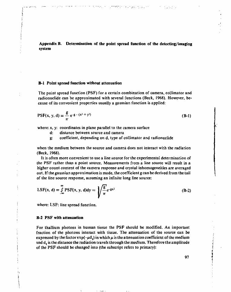
Appendix B. Determination of the point spread function of the detecting/imagingsystem

B-l Point spread function without attenuation

The point spread function (PSF) for a certain combination of camera, collimator andradionuclide can be approximated with several functions (Beck, 1968). However, be-cause of its convenient properties usually a gaussian function is applied:

PSF(x, y, d) = — e-e • <*2 + v2) (B-l)

where: x, y: coordinates in plane parallel to the camera surfaced: distance between source and camerag: coefficient, depending on d, type of collimator and radionuclide

when the medium between the source and camera does not interact with the radiation(Beck, 1968).

It is often more convenient to use a line source for the experimental determination ofthe PSF rather than a point source. Measurements from a line source will result in ahigher count content of the camera response and crystal inhomogeneities are averagedout. If the gaussian approximation is made, the coefficient g can be derived from the tailof the line source response, assuming an infinite long line source:

LSF(x, d) = ƒ PSF(x, y, d)dy = I / ? e - s x 2 (B-2)•frwhere: LSF: line spread function.

B-2 PSF with attenuation

For thallium photons in human tissue the PSF should be modified. An importantfraction of the photons interact with tissue. The attenuation of the source can beexpressed by the factor exp(-/udt) in which ju is the attenuation coefficient of the mediumand dt is the distance the radiation travels through the medium. Therefore the amplitudeof the PSF should be changed into (the subscript refers to primary):

97

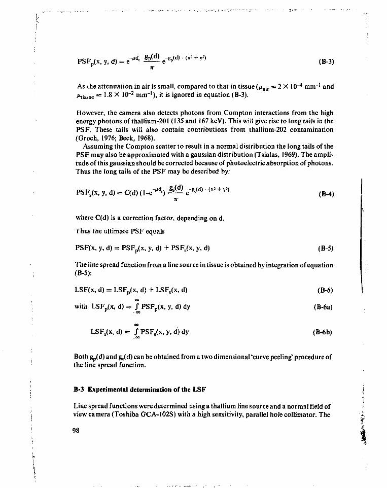
p (B-3)

As ihe attenuation in air is small, compared to that in tissue (/tair = 2 X 10~4 m m ' andt̂issue = 1-8 X 10~2 mm"1), it is ignored in equation (B-3).

However, the camera also detects photons from Compton interactions from the highenergy photons of thaIlium-201 (135 and 167 keV). This will give rise to long tails in thePSF. These tails will also contain contributions from thallium-202 contamination(Groch, 1976; Beck, 1968).

Assuming the Compton scatter to result in a normal distribution the long tails of thePSF may also be approximated with a gaussian distribution (Tsialas, 1969). The ampli-tude of this gaussian should be corrected because of photoelectric absorption of photons.Thus the long tails of the PSF may be described by:

PSFs(x, y. d) = C(d) (I-e""".) S&- e* ( d )" ^ + ^ (B-4)

where C(d) is a correction factor, depending on d.

Thus the ultimate PSF equals

PSF(x, y, d) = PSFp(x, y, d) + PSFs(x, y, d) (B-5)

The line spread function from a line source in tissue is obtained by integration of equation(B-5):

LSF(x, d) = LSFp(x, d) + LSFs(x, d) (B-6)

with LSF (x, d) = ƒ PSF_(x, y, d) dy (B-6a)V -00 V

so

LSFs(x, d ) = S PSFs(x, y, d') dy (B-6b)

Both g„(d) and g/d) can be obtained from a two dimensional 'curve peeling1 procedure ofthe line spread function.

B-3 Experimental determination of the LSF

Line spread functions were determined using a thallium line source and a normal field ofview camera (Toshiba GCA-I02S) with a high sensitivity, parallel hole collimator. The

98

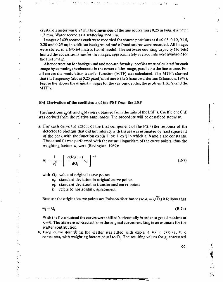
crystal diameter was 0.25 m, the dimensions of the line source were 0.25 m long, diameter1.2 mm. Water served as a scattering medium.

Images of 400 seconds each were recorded for source positions at d=0.05,0.10,0.15,0.20 and 0.25 m; in addition background and a flood source were recorded. All imageswere stored in a 64x64 matrix (word mode). The software counting capacity (16 bits)limited the acquisition time for the images; approximately 882 kcounts were available forthe first image.

After correction for background and non-uniformity, profiles were calculated for eachimage by summing the elements in the center of the image, parallel to the line source. Forall curves the modulation transfer function (MTF) was calculated. The MTF's showedthat the frequency (about 0.25 pixel/ mm) meets the Shannon criterium (Shannon, 1949).Figure B-1 shows the original images for the various depths, the profiles (LSF's)and theMTF's.

B-4 Derivation of the coefficients of the PS F from the LSF

The functions gp(d) and gs(d) were obtained from the tails of the LSF's. Coefficient C(d)was derived from the relative amplitudes. The procedure will be described stepwise.

a. For each curve the extent of the first component of the PSF (the response of thedetector to photqns that did not interact with tissue) was estimated by least square fitof the peak with the function exp(a + bx + ex2) in which a, b and c are constants.The actual fit was performed with the natural logarithm of the curve points, thus theweighting factors w; were (Bevington, 1969):

1 f d(log O:) 1 ~2

wi = TT= ^ °i (B-7)

with O;: value of original curve pointso-y standard deviation in original curve pointsa[: standard deviation in transformed curve pointsi: refers to horizontal displacement

Because the original curve points are Poisson distributed (so ax = VÖj) it follows that

w; = Oi (B-7a)

With the fits obtained the curves were shifted horizontally in order to get all maxima atx = 0. The fits were subtracted from the original curves resulting in an estimate for thescatter contribution.

b. Each curve describing the scatter was fitted with exp(a + bx + ex2) (a, b, cconstants), with weighting factors equal to O;. The resulting values for gs correlated

99

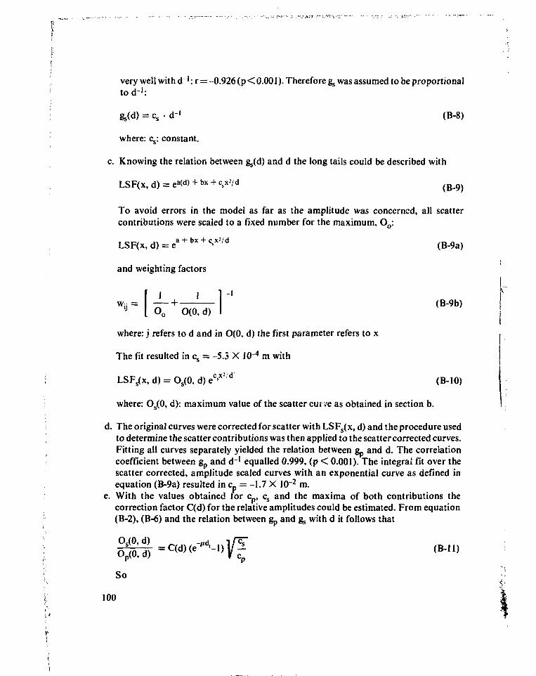
very well with d~': r = -0.926 (p < 0.001). Therefore gg. was assumed to be proportionaltod"1:

= c s - d ' (B-8)

where: cs: constant.

c. Knowing the relation between g/d) and d the long tails could be described with

LSF(x, d) = ea<d> + bx + c.x2/d ( B , 9 )

To avoid errors in the model as far as the amplitude was concerned, all scattercontributions were scaled to a fixed number for the maximum, Oo:

(B-9a)

and weighting factors

f 1 1 1 'W::= + (B-9b)U I O o O(0, d) I

where: j refers to d and in O(0, d) the first parameter refers to x

The fit resulted in cs = -5.3 X 104 m with

LSFs(x, d) = Os(0, d) eCsX: d (B-10)

where: Os(0, d): maximum value of the scatter curve as obtained in section b.

d. The original curves were corrected for scatter with LSFs(x, d) and the procedure usedto determine the scatter contributions was then applied to the scatter corrected curves.Fitting all curves separately yielded the relation between gp and d. The correlationcoefficient between gp and d~' equalled 0.999, (p < 0.001). The integral fit over thescatter corrected, amplitude scaled curves with an exponential curve as defined inequation (B-9a) resulted in cp = -1.7 X 10~2 m.

e. With the values obtained for cp, cs and the maxima of both contributions thecorrection factor C(d) for the relative amplitudes could be estimated. From equation(B-2), (B-6) and the relation between gp and gs with d it follows that

( B . M )

So

100

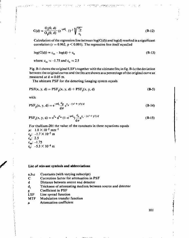
Calculation of the regression line between log(C(d)) and log(d) resulted in a significantcorrelation (r = 0.962, p < 0.001). The regression line itself equalled

log(C(d)) = cra • log(d) + cn (B-13)

where: cm = -1.75 and cn = 2.5

Fig. B-1 shows the original LSF's together with the ultimate fits; in fig. B-lc the deviationbetween the original curves and the fits are shown as a percentage of the original curve asmeasured at d = 0.05 m.

The ultimate PSF for the detecting/ imaging system equals

PSF(x, y, d) = PSFp(x, y, d) + PSFs(x, y, d) (B-5)

with:

> c ' ^ + y2)/dPSF_(x, y, d) = e-"d' ->

PSFs(x, y, d) = ec" dc™ (l-e"d ' ) ^ " ( x ' + y2)/d

djr

For thallium-201 the value of the constants in these equations equalsfx: 1.8X10-2 mm 1

cp: -1.7 X 10-2 m

cn: 2.5cm: -1.75cs: -5.3 X 10~4 m

List of relevant symbols and abbreviations

a,b,c Constants (with varying subscript)C Correction factor for attenuation in PSFd Distance between source and detectordt Thickness of attenuating medium between source and detectorg Coefficient in PSFLSF Line spread functionMTF Modulation transfer functiona Attenuation coefficient

101

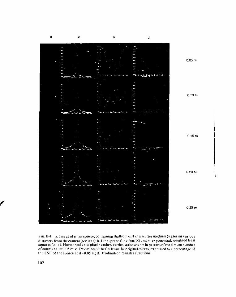
0.05 m

0.10 m

0 15 m

0.20 m

0 25 m

Fig. B-l a. Image of a line source, containing thallium-201 in a scatter medium (water) at variousdistances from the camera (see text); b. Line spread function (X) and bi-exponential. weighted leastsquares fit (+). Horizontal axis: pixel number, vertical axis: counts in peicent of maximum numberof counts at d =0.05 m; c. Deviation of the fits from the original curves, expressed as a percentage ofthe LSF of the source at d = 0.05 m; d. Modulation transfer functions.

102

O Point of original LSFPS F Point spread functiona Possible error in O originating radioactive decaya' Value of a after logarithm transformw Weighting factorx,y Cartesian coordinates in plane parallel to camera surface.

References

Atkins, H.L., Budinger, T.F., Lebowitz, E. et ul. (1977), Thallium for medical use. Part 3: Humandistribution and physical imaging properties, J.Nucl.Med.: 18,133-140.

Atwood, J.E., Jensen, D., Froelicher, V. et al. (1981), Agreement in human interpretation ofanalog thallium myocardial perfusion images, Circ.: 64,601-609.

Beck, R.N. (1968), The scanning system as a whole, in: "Fundamental problems in scanning",Gottschalk, A. and Beck, R.N. (eds), C.C.Thomas, Springfield, U.S.A.

Beck, R.N. (1975), Fundamental aspects of imaging, in: "Proc. XIII Ann. Meeting Int. SNM,Copenhagen, Denmark, sept. 10-13.

Bevington, P.R. (1969), Data reduction and error analysis in physical sciences, McGraw-Hill.Bradley-Moore, P.R., Lebowitz, E., Green, M.W. et al. (1975), Thallium for medical use. Part 2:

Biological behavior, J.Nucl.Med. 16, 156-160.Brown, D.W., Kirch, D.L., Ryerson, T.W., et al. (1971), Computer processing of scans using

Fourier and other transformations, J.Nucl.Med. 12:287-291.Budinger, T.F., Rollo, F.D. (1978), Physics and instrumentation in nuclear medicine, in: Principles

of cardiovascular nuclear medicine, Holman, B.L. (ed), Grune and Stratton Inc, New York.Chaitman, B.R., Bristow, J.D. (1973), Rahimtoola, S.H., Left ventricular wall motion assessed by

using fixed external reference systems, Circ.: 58,1043-1054.Cook, D.J., Bailey, 1., Strauss, H.W. et al. (I976), Thallium-201 for myocardial imaging: appear-

ance of the normal heart, J.Nucl.Med.: 17,583-589.Davila, J.C.. Sanmarco, M.E. (1966), An analysis of the fit of mathematical models applicable to

the measurement of the left ventricular volume, Am.J.Card.: 18,31-42.Dodge, H.T., Sandier, H.S., Ballew, D.W. et al. (1960), The use of biplane angiocardiography for

the measurement of the left ventricular volume in man, Am.Heart.J.: 60, 762-776.Dodge. H.T.. Sandier, H.S., Baxley, W. A. et al. (1966), Usefulness and limitations of radiographic

methods for determining left ventricular volume, Am.J.Card.: 18,10-24.Evans. R.D. (1955), The statistics of nuclear particles, in; "The atomic nucleus", McGraw-Hill Inc.,

New York Graham, L.S., Poe, N.D., Robinson, G.F. (1976), Collimation for imaging themyocardium 2, J.Nucl.Med.: 17,719-723.

Green. D.M., Swets, J.A. (1974), Signal detection theory and .psychophysics, Robert KriegerPublishing Company, New York.

Groch. M.W., Lewis, G.K. (1976), Thallium-201: Scintillation camera imaging considerations,J.Nucl.Med.: 17,142-145.

Hamilton, G.W., Trobaugh, G.B., Ritchie, J.L. et al. (1977), Myocardial imaging with intraven-ously injected thallium-201 in patients with suspected coronary artery disease, Am.J.Card.: 38,347-354.

Hamilton G.W., Williams, D.L., Caldwell, J.H. (1978a), Frame rate requirements for recordingtime-activity curves by radionuclide angiocardiography, in: "Nuclear Cardiology", Symposiumproceedings, Sorenson, J.A. (ed), SNM.

Hamilton. G.W., Ritchie, J.L., Coleman, A. et al. (1978b), Myocardial imaging: equipment andtechniques, in: "Thallium-201 myocardial imaging", Ritchie, J.L., Hamilton, G.W., Wackers,FJ.Th. (eds), Raven Press, New York.

103

Hamilton, G.W., Narahara, K.A., Yee, H.etal. (1978c), Myocardial imaging with thallium-201:effect of cardiac drugs on myocardial images and absolute tissue distribution, J.Nucl.Med.:19, 10-16.

Hamilton, G.W., Narahara, K.A., Trobaugh, G.B. etal. (1978d), Thallium-201 myocardial imag-ing: characterization of the ECG-synchronized images, J.Nucl.Med.: 19, 1103-1110.

Hurley, P.J., Cooper, M., Reba, R.C. et al. (197I),43KC1: a new radiopharmaceutical for imagingthe heart, J.Nucl.Med.: 12,516-519.

Kennedy, J.W., Baxley, W.A., Figley, M.M. etal. (I966), Quantitative angiocardiography 1, Thenormal left ventricle in man, Circ: 34,272-278.

Lamb, J.F., Baker, G.A., Khentigan, A. et al. (1974), Rubidii:m-81 for myocardial imaging, in:Proc. First World Congress Nucl. Med., Japan Radio-isoiupe Association, Tokyo, pp. 1051-1053.

Lebowitz, E., Greene, M.W., Fairchild, R. et al. (1975), Thallium-201 for medica! use. Part 1.J.Nucl.Med.: 16, 151-155.

Lederer, CM., Hollander, J.M., Perlman, I. (1968), Table of isotopes, 6th ed., John Wiley andSons.

Lenaers, A., Block, P., Thiel, E. van, et al. (1977). Segmental analysis of TI-201 stress myocardialscintigraphy, J.Nucl.Med.: 18,509-516.

Lewis, R.P., Sandier, H. (1971), Relationship between changes in left ventricular dimensions andthe ejection fraction in man, Circ: 44,548-557.

McDonald, I.G. (1970), The shape and movements of the human left ventricle during systole.Am.J.Card.: 26,221-230.

Meester, G.T. (1980), Computer analysis of cardiac catheterization data. Ph.D. Thesis. ErasmusUniversity Rotterdam, The Netherlands.

Metz, C.E. (1969), A mathematical investigation of radioisotope scan image processing. Ph.D.Thesis, University of Pennsylvania, U.S.A.

Metz, C.E., Beck, R.N. (I974), Quantitative effects of stationary linear image processing on noiseand resolution of structure in radionuclide images. J.Nucl.Med: 15. 164-170.

Mueller, T.M., Marcus, M.L., Ehrhardt, J.C. etal. (1976), Limitations of thallium-201 myocardialperfusion scintigrams, Circ.: 54,640-646.

Narahara, K.A., Hamilton, G.W., Williams, D.L. etal. (1977). Myocardial imaging with thallium-201: an experimental model for the analysis of the true myocardial and background imagecomponents, J.Nucl.Med.: 18,781-786.

Naylor, T.H., Balintfy, J.L, Burdick, D.S. et al. (1966), Computer simulation techniques. JohnWiley-and Sons, Inc., New York.

Nishiyama, H., Sodd, V.J., Adolph, R.J. et al. (J976), Intercomparison of myocardial imagingagents: Tl-201, Cs-129, K-43 and Rb-81, J.Nucl.Med.: 17,880-889.

Okada, R.D., Boucher, C.A., Kirshenbaum, H.K. et al. (1980), Improved diagnostic accuracy ofthallium-201 stress test using multiple observers and criteria derived from interobserver analysisof variance, Am.J.Card.: 46,619-624.

Papoulis, A. (1964), Probalility, Random variables and stochastic processes, McGraw-Hill, inc..New York.

Pohost, G.M., Zir, L.M., Moore, R.H. et al. (1977), Differentiation of transiently ischemic frominfarcted myocardium by serial imaging after a single dose of thallium-201, Circ.: 55.294-302.

Prokop, E.K., Strauss, H. W., Shaw, J. et al. (1974), Comparison of regional myocardial perfusiondetermined by ionic potassium-43 to that determined by microspheres, Circ.: 50.978-984.

Rackley, C.E., Hood, W.P. (1974), Measurements of ventricular volume, mass and ejectionfraction, in: "Cardiac catherization and angiography", Grossman, W. (ed). Lea and Febiger.Philadelphia, 1974.

Ritchie, J.L., Trobaugh, G.B., Hamilton, G.W. et al. (I977), Myocardial imaging with thallium-201 at rest and during exercise, Circ.: 56,66-71.

104

Ritchie, J.L., Hamilton, G.W. (1978), Biologic properties of thallium, in: "Thallium-201 myocar-dial imaging", Ritchie, J.L., Hamilton, G.W., Wackers, F.J.Th, (eds), Raven Press, New York.

Sachs, L. (1978), Angewandte Statistik, Springer Verlag, Berlin.Sandier, H.S., Ghista, D.N. (1969), Mechanical and dynamic implications of dimensional mea-

surements of the left ventricle, Fed.Proc: 28, 1344-1350.Sandier, H., Dodge, H.T. (1968), The use of single plane angiocardiograms for the calculation of

the left ventricular volume in man, Am.J.Card.: 75,325-334.Shannon, C.E. (1949), Communication in the presence of noise, Proc.IRE: 37, 10-21.Siegel, S. (1956), Nonparametric statistics for the behavioral sciences, McGraw-Hill, Inc., New

York.Sodd, V.J., Blue, J.W., Scholz, K.L. (1971), Cs-129 Production via the 1-127 (alpha,2n) Cs-129

reaction and its preparation as a radiopharmaceutical, Phys.Med.Biol.: 16, 587-598.Strauss, H.W., Harrison, K., Langan, J.K. et al. (1975), Thallium for medical imaging, Circ.:

51,641-645.Tsialas, S.P., Hine, G.J. (1969), Collimator characteristics for radio-isotope scanning, J.Nucl.-

Med.: 19, 100-106.Turner, D.A., Fordham, E.W., Pagano, J.V. et al. (1976), Brain scanning with the Anger multi-

plane scanner as a second examination. Evaluation by the ROC method, Radiology: 121,115-124.

Turner, D.A. (1978), An intuitive approach to receiver operating characteristic curve analysis,J.Nucl.Med.: 19,218-220.

Vos, P.H., Vossepoel, A.M., Hermans, J., Pauwels, E.KJ.(1981a), Evaluation of lesion detectabil-ity in thallium-201 scintigraphy using a mathematical model for the heart, Proc. 2nd IEEEConf. Medical Imaging and Psychophysics, Brussel, July 2-3.

Vos. P.H., Vossepoel, A.M., Pauwels, E.K.J. (1981b), Evaluation of thallium-201 myocardialscintigraphy using a mathematical model, Proc. Fh-st Int. Symp. Nucl. Card., Tel Aviv, Israel,Sept. 6-10, (abstract).

Vos. P.H., Hermans, J. (1982a), Simple image processing techniques in thallium-201 myocaidialperfusion scintigraphy, Letter to the editor, Radiology, submitted.

Vos, P.H., Vossepoel, A.M., Hermans, J., Pauwels, E.K.J. (1982b), Detection of lesions inthallium-201 myocardial scintigraphy, Eur.J.Nucl.Med.: 7, 174-180.

Vos. P.H.. Vossepoel, A.M., Pauwels, E.K.J. (1982c), Detection of lesions in thallium-20! my-ocardial perfusion scintigraphy, Proc. World Fed. Nucl. Med. Biol. (third conf.), Paris,Aug. 29-Sept. 2, accepted for publication.

Wackers. F.J.Th., Sokole, E.B., Samson, G. et al. (1978), Anaiomy of the normal myocardialimage, in: "Thallium-201 myocardial imaging", Ritchie, J.L., Hamilton, G.W., Wackers,F.J.Th, (eds). Raven Press, New York.

Weich. H.F., Strauss, H.W., Pitt, B.(I976), Myocardial extraction fraction of thallium-201, Circ:54.11-218. (abstract).

Zaret. B.L. (1977). Myocardial imaging with radioactive potassium and its analogs, Prog.Card.Dis.: 20. 81-94.

Zaret, B.L., Strauss, H.W., Martin, N.D. et al. (1973), Non-invasive regional myocardial perfusionwith radioactive potassium, New.Engl.J.Med.: 288,809-812.

105

Chapter 4

Influence of tracer distribution, scatter andphoton energy on lesion detectability

4.1 Introduction

A physical model for the generation of thallium myocardial perfusion scintigrams allowscreation of a series of images, generated under various realistic imaging conditions. Amathematical model allows also the creation of images under various imaginary imagingconditions. Observation of these images may indicate in which way generation of imagesin a realistic environment can be improved.

In this chapter several imaging factors potentially affecting lesion detectability inthallium scintigrams (lesion perfusion, scatter and photon energy) will be considered and v

their influence on lesion detectability will be reported, using the same basic series of ; jimages as in chapter 3, except for variation of the parameter under study. Also the samemethod of data analysis is applied.

In paragraph 4.2 the influence of lesion thallium concentration on lesion detectability isreported. The influence of scatter is described in paragraph 4.3. The results of myocardialperfusion imaging with isotopes, other than thallium-201 (as far as the physical charac-teristics is concerned), are contained in paragraph 4.4.

Images used for the experiments described in paragraph 4.2 were randomly mixed withimages containing non-perfused lesions (chapter 3). Images for the other experiments(paragraph 4.3 and 4.4) were interpreted in a second session, together with the thirdinterpretation of 200k images with non-perfused lesions (chapter 3).

4.2 Influence of tracer distribution on lesion detectability

4.2.1 IntroductionActivity within lesions will clearly decrease their detectability The severity of coronarystenosis and collateral circulation will affect the detection of lesions (Mueller, 1976;Massie, 1979; Hamilton, 1977) and in cases of subendocardial lesions also a worsedetection rate can be expected.

In this paragraph the influence of activity within lesions is described, and it is reportedwhether an increase of count density may compensate for the decrease of lesion detection.

107 r ;

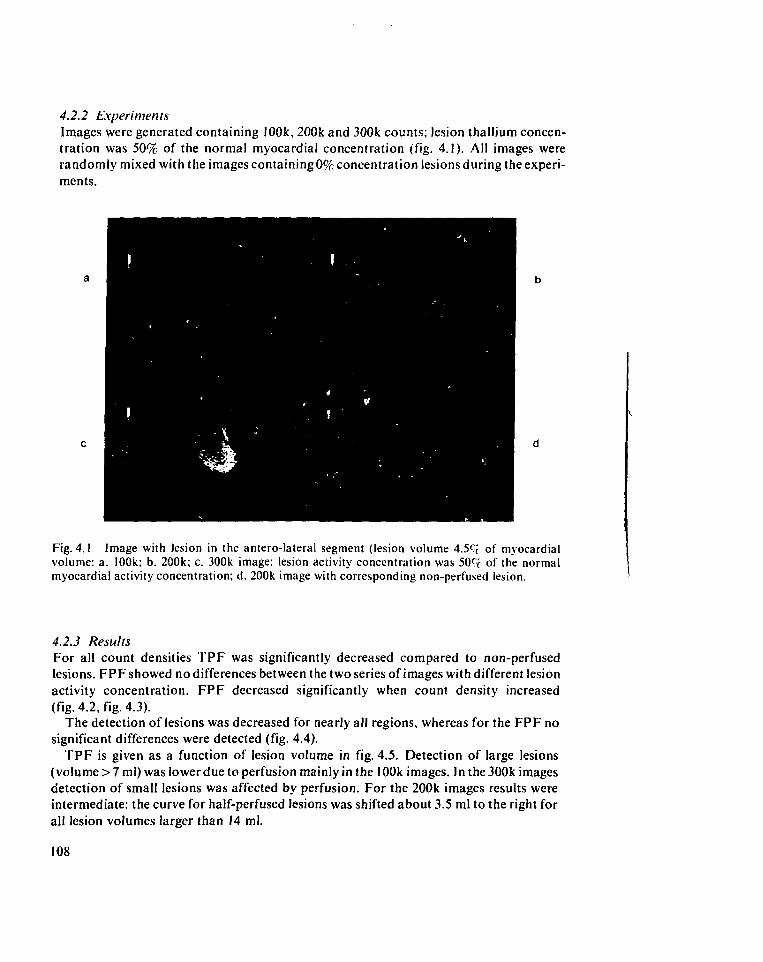
4.2.2 ExperimentsImages were generated containing 100k, 200k and 300k counts; lesion thallium concen-tration was 50% of the normal myocardial concentration (fig. 4.1). All images wererandomly mixed with the images containing 0% concentration lesions during the experi-ments.

Fig. 4.1 Image with lesion in the antero-lateral segment (lesion volume 4.5C( of myocardialvolume: a. 100k; b. 200k; c. 300k image: lesion activity concentration was 509r of the normalmyocardial activity concentration; d. 200k image with corresponding non-perfused lesion.

4.2.3 ResultsFor all count densities TPF was significantly decreased compared to non-perfusedlesions. FPF showed no differences between the two series of images with different lesionactivity concentration. FPF decreased significantly when count density increased(fig. 4.2, fig. 4.3).

The detection of lesions was decreased for nearly all regions, whereas for the FPF nosignificant differences were detected (fig. 4.4).

TPF is given as a function of lesion volume in fig. 4.5. Detection of large lesions(volume > 7 ml) was lower due to perfusion mainly in the 100k images. In the 300k imagesdetection of small lesions was affected by perfusion. For the 200k images results wereintermediate: the curve for half-perfused lesions was shifted about 3.5 ml to the right forall lesion volumes larger than 14 ml.

108

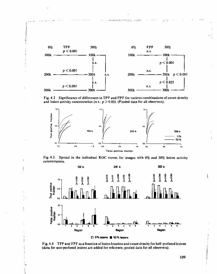
0%

100k -

200k -

300k -

TPFp < 0.001

p < 0.001

p < 0.001

50%

100k-

In.s.

• 200k n.s.

n.s.

300k

0%

100k •

200k

300k

FPFn.s.

n.s.

n.s.

50%

— 100k —I

p < 0.001

— 200k p < 0.001I

p < 0.025

300k

Fig. 4.2 Significance of differences in TPF and FPF for various combinations of count densityand lesion activity concentration (n.s.: p >0.05). (Pooled data for all observers).

100 k 200 k

1 0 0 0 0-5 10 Q.0

False positive fraction

300 k

0%50%

Fig. 4.3. Spread in the individual ROC curves for images with 0% and 50% lesion activityconcentration.

100 k 200 k 300 k

i f UH

r•" 00

V v

q 8S 5^ ^ «3 «3 «30 . 0 . 0 . 0 . 0 .

Uu81

0.2 -i

II3 ( 5 6

Region

nl PL3 ( 5 6

Region

O 0% lesions • 50% lesions

_ — • r-U- ~ l

3 1 5

Region

Fig. 4.4 TPF and FPF as a function of lesion location and count density for half-perfused lesions(data for non-perfused lesions are added for reference; pooled data for all observers).

109

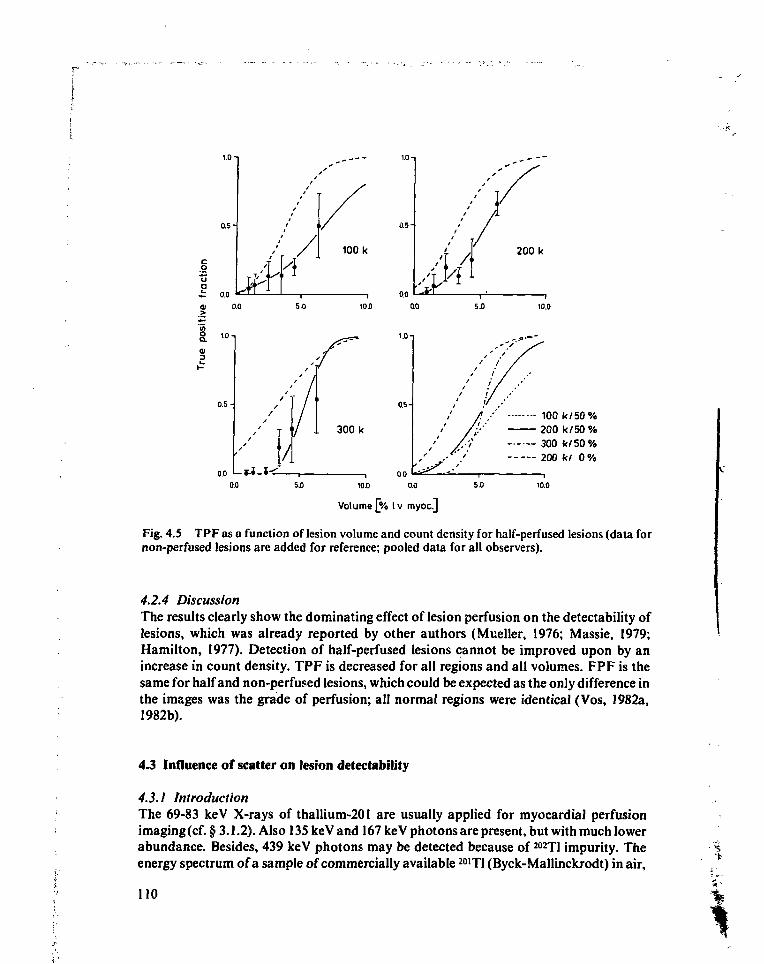
0.5-

a o.oÉ

lYl5.0

100 k

10.00.0

5.0

200 k

10.0

a.o L$.I_l0.0

300 k

i.o

0.5-

00

100 k/50%200 k/50%300 k/50%200 k/ 0%

5.0 10.0 0.0 5.0 10.0

Volume [% Iv myoc]

Fig. 4.5 TPF as a function of lesion volume and count density for half-perfused lesions (data fornon-perfused lesions are added for reference; pooled data for all observers).

4.2.4 DiscussionThe results clearly show the dominating effect of lesion perfusion on the detectability oflesions, which was already reported by other authors (Mueller, 1976; Massie, 1979;Hamilton, 1977). Detection of half-perfused lesions cannot be improved upon by anincrease in count density. TPF is decreased for all regions and all volumes. FPF is thesame for half and non-perfused lesions, which could be expected as the only difference inthe images was the grade of perfusion; all normal regions were identical (Vos, 1982a,1982b).

4.3 Influence of scatter on lesion detectability

4.3.1 IntroductionThe 69-83 keV X-rays of thallium-201 are usually applied for myocardial perfusionimaging (cf. §3.1.2). Also 135 keV and 167 ke V photons are present, but with much lowerabundance. Besides, 439 keV photons may be detected because of 202Tl impurity. Theenergy spectrum of a sample of commercially available 2O1T1 (Byck-Mallinckrodt) in air,

110

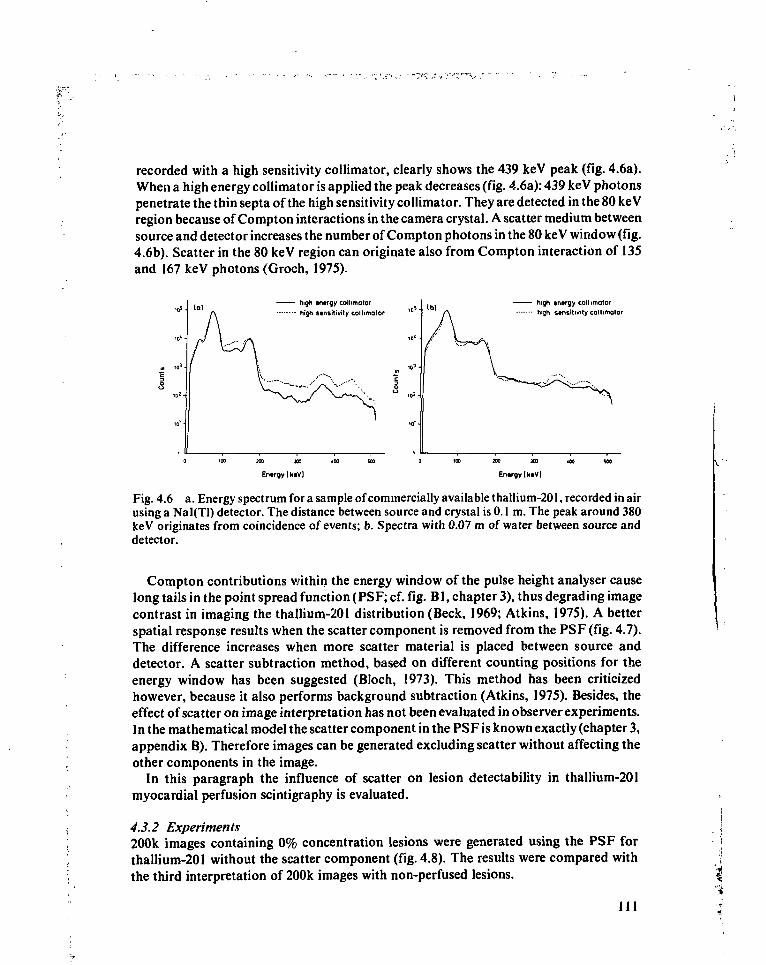
recorded with a high sensitivity collimator, clearly shows the 439 keV peak (fig. 4.6a).When a high energy collimator is applied the peak decreases (fig. 4.6a): 439 keV photonspenetrate the thin septa of the high sensitivity collimator. They are detected in the 80 keVregion because of Compton interactions in the camera crystal. A scatter medium betweensource and detector increases the number of Compton photons in the 80 keV window (fig.4.6b). Scatter in the 80 keV region can originate also from Compton interaction of 135and 167 keV photons (Groch, 1975).

high «ntrgy collimator

high stnsitivity collimatorhigh inirgy collimatorhigh stnsitivity collimotor

En.rgylktV] EntrgylktV)

Fig. 4.6 a. Energy spectrum for a sample of commercially available thallium-201, recorded in airusing a Nal(Tl) detector. The distance between source and crystal is 0.1 m. The peak around 380keV originates from coincidence of events; b. Spectra with 0.07 m of water between source anddetector.

Compton contributions within the energy window of the pulse height analyser causelong tails in the point spread function (PSF; cf. fig. Bl, chapter 3), thus degrading imagecontrast in imaging the thallium-201 distribution (Beck, 1969; Atkins, 1975). A betterspatial response results when the scatter component is removed from the PSF (fig. 4.7).The difference increases when more scatter material is placed between source anddetector. A scatter subtraction method, based on different counting positions for theenergy window has been suggested (Bloch, !973). This method has been criticizedhowever, because it also performs background subtraction (Atkins, 1975). Besides, theeffect of scatter on image interpretation has not been evaluated in observer experiments.In the mathematical model the scatter component in the PSF is known exactly (chapter 3,appendix B). Therefore images can be generated excluding scatter without affecting theother components in the image.

In this paragraph the influence of scatter on lesion detectability in thallium-201myocardial perfusion scintigraphy is evaluated.

4.3.2 Experiments200k images containing 0% concentration lesions were generated using the PSF forthallium-201 without the scatter component (fig. 4.8). The results were compared withthe third interpretation of 200k images with non-perfused lesions.

I l l

I"i

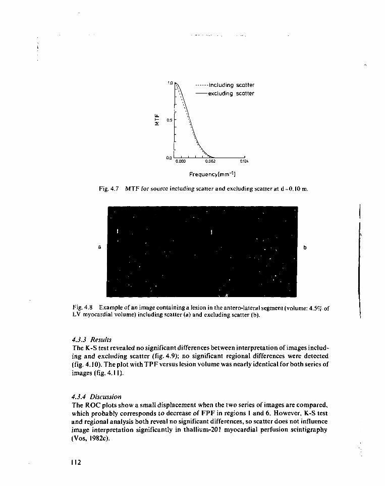
including scatterexcluding scatter

0.000 0.062 O.W

Frequencylmm""1)

Fig. 4.7 MTF for source including scatter and excluding scatter at d=0.10 m.

Fig. 4.8 Example of an image containing a lesion in the antero-lateral segment (volume: 4.5% ofLV myocardial volume) including scatter (a) and excluding scatter (b).

4.3.3 ResultsThe K-S test revealed no significant differences between interpretation of images includ-ing and excluding scatter (fig. 4.9); no significant regional differences were detected(fig. 4.10). The plot with TPF versus lesion volume was nearly identical for both series ofimages (fig. 4.11).

4.3.4 DiscussionThe ROC plots show a small displacement when the two series of images are compared,which probably corresponds to decrease of FPF in regions 1 and 6. However, K-S testand regional analysis both reveal no significant differences, so scatter does not influenceimage interpretation significantly in thallium-201 myocardial perfusion scintigraphy(Vos, 1982c).

112

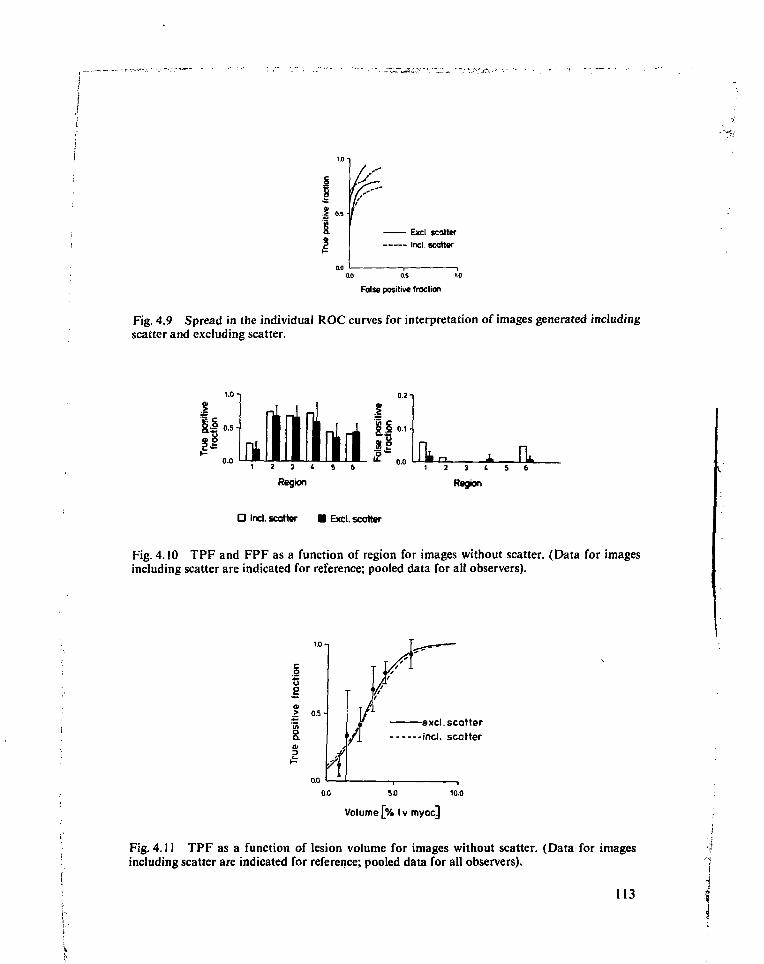
1.2

Exd scatter

Inel. scatter

0.0 0.S

Talse positive fraction

Fig. 4.9 Spread in the individual ROC curves for interpretation of images generated includingscatter and excluding scatter.

1.0

0.0in..

1 2 3 ( 5 6

Region

IS 0.1-

53-0.0 Ik». JL

1 2 3 t S 6

Region

O Incl. scatter • Excl. scatter

Fig. 4.10 TPF and FPF as a function of region for images without scatter. (Data for imagesincluding scatter are indicated for reference; pooled data for all observers).

o

s> 0.5 -

0.04

excl. scatter

yl incl. scatter

10.0

Volume [% Iv myocj

Fig. 4.11 TPF as a function of lesion volume for images without scatter. (Data for imagesincluding scatter are indicated for reference; pooled data for all observers).

113

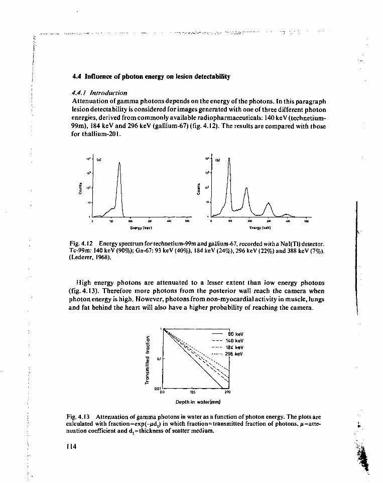
4.4 Influence of photon energy on lesion detectability

4.4.1 IntroductionAttenuation of gamma photons depends on the energy of the photons. In this paragraphlesion detectability is considered for images generated with one of three different photonenergies, derived from commonly available radiopharmaceuticals: 140 keV (technetium-99m), 184 keV and 296 keV (gallium-67) (fig. 4.12). The results are compared with thoseforthallium-201.

I ,0

(a)

wo xo

Entrgylkiv)

10'

300 HO

Entrgy [IciVI

Fig. 4.12 Energy spectrum for technetium-99m and gallium-67, recorded with a Nal(Tl) detector.Tc-99m: 140 keV (90%); Ga-67: 93 keV (40%), 184 keV (24%), 296 keV (22%) and 388 keV (7%).(Lederer, 1968).

High energy photons are attenuated to a lesser extent than low energy photons(fig. 4.13). Therefore more photons from the posterior wall reach the camera whenphoton energy is high. However, photons from non-myocardial activity in muscle, lungsand fat behind the heart will also have a higher probability of reaching the camera.

0.01

80 keV140 keV184 keV296 keV

0.0 135 270

Depth in waterlmm]

Fig. 4.13 Attenuation of gamma photons in water as a function of photon energy. The plots arecalculated with fraction=exp(-jidt) in which fraction=transmitted fraction of photons, p=atte-

coefficient and d,=thickness of scatter medium.

114

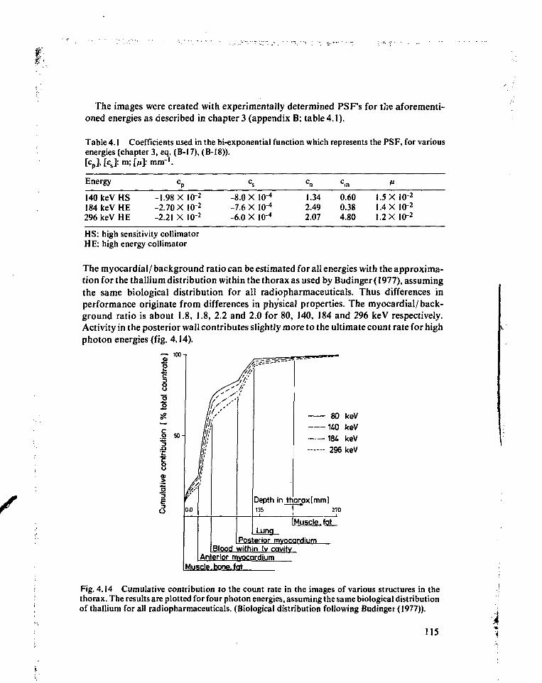
The images were created with experimentally determined PSF's for the aforementi-oned energies as described in chapter 3 (appendix B; table 4.1).

Table 4.1 Coefficients used in the bi-exponential function which represents the PSF, for variousenergies (chapter 3, eq. (B-17), (B-I8)).[cD],[cs]:m;[/tt]:niin-1.

Energy cp

140keVHS -1.98 X I 0 2

184keVHE -2.70XI0"2

296 keV HE -2.21 X I0"2

HS: high sensitivity collimatorH E: high energy collimator

cs

-8.0 X-7.6 X-6.0 X

10"4

lo-4

IO"4

1.342.492.07

c,n

0.600.384.80

1.51.41.2

XX

X

10-210-2IQ"2

The myocardial/ background ratio can be estimated for all energies with the approxima-tion for the thallium distribution within the thorax as used by Budinger (1977), assumingthe same biological distribution for all radiopharmaceuticals. Thus differences inperformance originate from differences in physical properties. The myocardial/back-ground ratio is about 1.8, 1.8, 2.2 and 2.0 for 80, 140, 184 and 296 keV respectively.Activity in the posterior wall contributes slightly more to the ultimate count rate for highphoton energies (fig. 4.14).

80 keV

140 keV184 keV296 keV

Depth in thoroxtmml135 ! 270

I Muscle .fatI Luna

Posterior myocardiumBlood within Iv cavity

Anterior myocardiumduscle. bone, fat

Fig. 4.14 Cumulative contribution to the count rate in the images of various structures in thethorax. The results are plotted for four photon energies, assuming the same biological distributionof thallium for all radiopharmaceuticals. (Biological distribution following Budinger (1977)).

US *

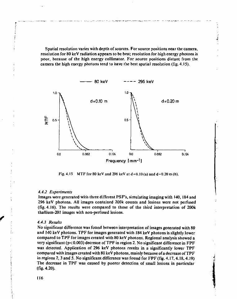
Spatial resolution varies with depth of sources. For source positions near the camera,resolution for 80 keV radiation appears to be best; resolution for high energy photons ispoor, because of the high energy collimator. For source positions distant from thecamera the high energy photons tend to have the best spatial resolution (fig. 4.15).

80keV 296 keV

1-0-»

I - 0.5-

d=0.10 m

0.5-

0.062

d = 0.20 m

0.124. 0.0

Frequency [mm-1]

0.062 0.124

Fig. 4.15 MTF for 80 keV and 296 keV at d=0.!0 (a) and d=0.20 m (b).

4.4.2 ExperimentsImages were generated with three different PSF's, simulating imaging with 140, 184 and296 keV photons. All images contained 200k counts and lesions were not perfused(fig. 4.16). The results were compared to those of the third interpretation of 200kthallium-201 images with non-perfused lesions.

4.4.3 ResultsNo significant difference was found between interpretation of images generated with 80and 140 keV photons. TPF for images generated with 184 keV photons is slightly lowercompared to TPF for images created with 80 keV photons. Regional analysis showed avery significant (p< 0.003) decrease of TPF in region 2. No significant difference in FPFwas detected. Application of 296 keV photons results in a significantly lower TPFcompared with images created with 80 keV photons, mainly because of a decrease of TPFin regions 2, 3 and 5. No significant difference was found for FPF (fig. 4.17,4.18,4.19)The decrease in TPF was caused by poorer detection of small lesions in particular(fig. 4.20).

116

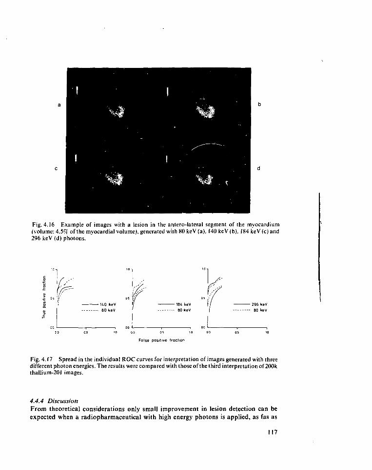
Fig. 4.16 Example of images with a lesion in the antero-lateral segment of the myocardium(volume: 4.59t of the myocardial volume), generated with 80keV(a), 140 keV(b), I84keV(c)and296 keV (d) photons.

"̂ u' I'• 184 keV• 80 keV

False positive fraction

- 296 keV• 80 kev

Fig. 4.17 Spread in the individual ROC curves for interpretation of images generated with threedifferent photon energies. The results were compared with those of the third interpretation of 200kthaIlium-201 images.

4.4.4 DiscussionFrom theoretical considerations only small improvement in lesion detection can beexpected when a radiopharmaceutical with high energy photons is applied, as fas as

117

. > •

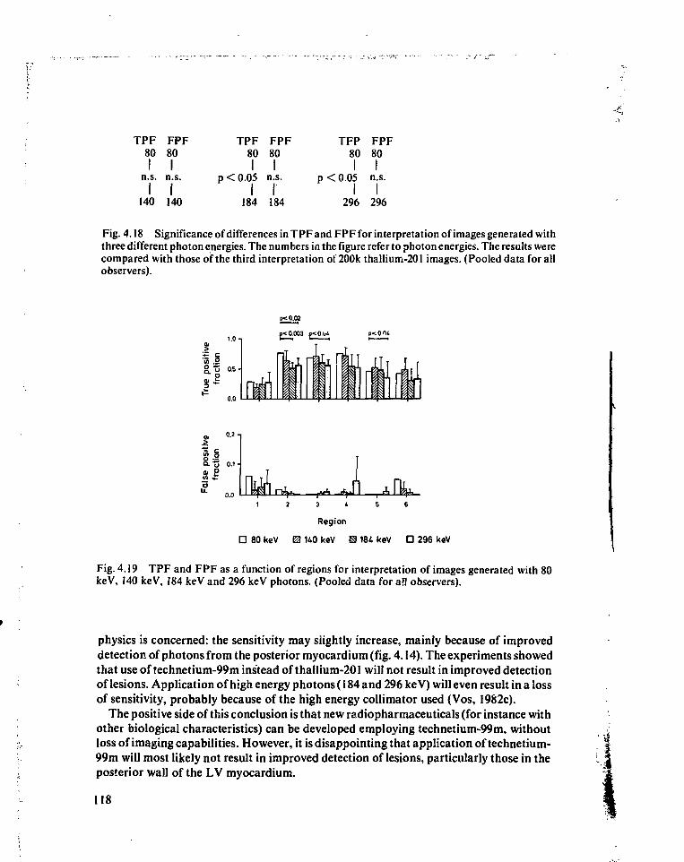
TPF FPF80 80

I In.s. n.s.

I I140 140

TPF FPF80 80

I Ip<0.05 n.s.

184 184

TFP FPF80 80

I Ip < 0.05 n.s.

296 296

Fig. 4.18 Significance of differences in TPF and FPF for interpretation of images generated withthree different photon energies. The numbers in the figure refer to photon energies. The results werecompared with those of the third interpretation of 200k thallium-201 images. (Pooled data for allobservers).

11.0

0.0

ix amp< 0.003 p<0.u4

ai Oin i:

0.1-

3 4 5 6

Region

D 80 keV 0 140 keV H 184 keV O 296 keV

Fig. 4.19 TPF and FPF as a function of regions for interpretation of images generated with 80keV, 140 keV, 184 keV and 296 keV photons. (Pooled data for a'l observers).

physics is concerned: the sensitivity may slightly increase, mainly because of improveddetection of photons from the posterior myocardium (fig. 4.14). The experiments showedthat use of technetium-99m instead of thallium-201 will not result in improved detectionof lesions. Application of high energy photons (184 and 296 keV) will even result in a lossof sensitivity, probably because of the high energy collimator used (Vos, 1982c).

The positive side of this conclusion is that new radiopharmaceuticals (for instance withother biological characteristics) can be developed employing technetium-99m, withoutloss of imaging capabilities. However, it is disappointing that application of technetium-99m will most likely not result in improved detection of lesions, particularly those in theposterior wall of the LV myocardium.

118

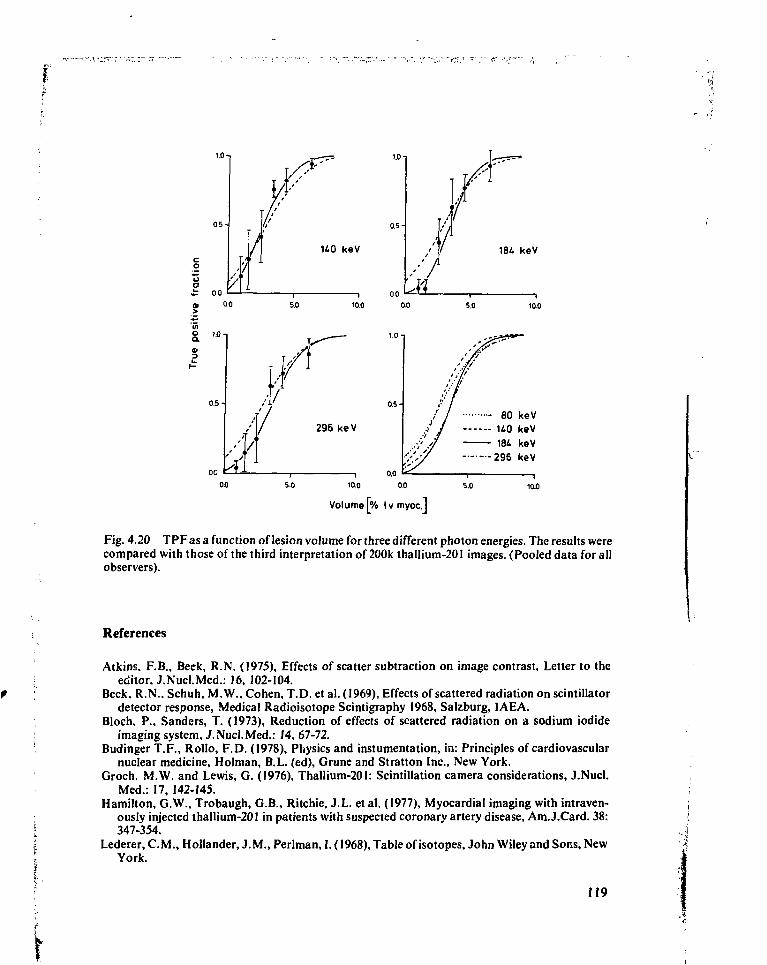
1.01

.fc 00O, 0.0

1.0

10.0 0.0

10S

296 keV80 keV

140 keV184 keV

296 keV

011 50 10.0 5.0

Volume [% Ivmyoc.J

Fig. 4.20 TPF as a function of lesion volume for three different photon energies. The results werecompared with those of the third interpretation of 200k thaIlium-201 images. (Pooled data for allobservers).

References

Atkins. F.B., Beck, R.N. (1975), Effects of scatter subtraction on image contrast. Letter to theeditor. J.Nucl.Med.: 16, 102-104.

Beck. R.N., Schuh, M.W.. Cohen, T.D. et al. (1969), Effects of scattered radiation on scintillatordetector response, Medical Radioisotope Scintigraphy 1968, Salzburg, IAEA.

Bloch, P., Sanders, T. (1973), Reduction of effects of scattered radiation on a sodium iodideimaging system, J.Nucl.Med.: 14, 67-72.

Budinger T.F., Rollo, F.D. (1978), Physics and instumentation, in: Principles of cardiovascularnuclear medicine. Holman, B.L. (ed), Grune and Stratton Inc., New York.

Groch. M.W. and Lewis, G. (1976), Thallium-201: Scintillation camera considerations, J.Nucl.Med.: 17, 142-145.

Hamilton, G.W., Trobaugh, G.B., Ritchie, J.L. et al. (1977), Myocardial imaging with intraven-ously injected thallium-201 in patients with suspected coronary artery disease, Am.J.Card. 38:347-354.

Lederer, CM. , Hollander, J.M., Perlman, 1.(1968), Table of isotopes, John Wiley and Sons, NewYork.

119

fI

Massie, B.M., Botvinnick, E., Arnold, S. et al. (1979), Effect of contrast enhancement on thesensitivity and specificity of Tl-201 scintigraphy, Am.J.CardioL: 43, 357, (Abstract).

Massie, B.M., Botvinnick, E.H., Brundage, B.H. (1979), Correlation of thaIIium-201 scintigramswith coronary anatomy: Factors affecting region by region sensitivity, Am.J.Cardiol.: 44,616-622.

Mueller, T.M., Marcus, M.L., Ehrhardt, J.C. et al. (1976), Limitations of thallium-201 myocardialperfusion scintigrams, Circulation: 54, 640-646.

Vos, P.H., Vossepoel, A.M., Pauwels, E.K.J. (1982a), Detection of lesions in thallium-201 my-ocardial perfusion scintigraphy, Eur.J.Nucl.Med.: 7, 174-180.

Vos, P.H., Vossepoel, A.M., Pauwels, E.K.J. (1982b), Detection of lesions in thallium-201 my-ocardial perfusion scintigraphy, Proc. World Fed. Nucl. Med. Biol. (third conf.), Paris,Aug. 29-Sept. 2, accepted for publication.

Vos, P.H., Pauwels, E.K.J., Vossepoel, A.M. (1982c), Influence of scatter and photon energy onlesion detectability in myocardial scintigraphy, Proc. World Fed. Nucl. Med. Biol. (third conf.),Paris, Aug. 29-Sept. 2, accepted for publication.

i120 I

Summary

This thesis deals with two topics in nuclear cardiology. In the first left ventricular wallmotion assessment using Fourier transform of local left ventricular time-activity curvesin gated blood pool studies is evaluated. In the second the interpretation of myocardialperfusion scintigrams is assessed which are obtained with thallium-201 or with anotherradiopharmaceutical with different physical, but identical biological properties.

In all these investigations data acquisition and analysis by computer played an essen-tial role.

In chapter 1 the desirable properties of a nuclear medicine computer system are given andthe computer system used for this work is described.

Data acquisition and processing should be possible without interference between thesetwo functions. Acquisition and processing of data are usually performed at differentlocations; at both locations a video display unit should be available. These requirementscan be fulfilled with an independent buffer for data acquisition and display (500 kbyte)for each remote station, near the gamma camera and a centrally located memory for dataprocessing (400 kbyte) complete with a display buffer (256 kbyte). These specificationsallow for versatile acquisition and processing of multiple gated heart studies, includingarrhythmia filtering during acquisition.

Software in a menu structure, including the possibility to integrate user writtenprograms with manufacturer supplied modules, should allow for easy data acquisitionand processing. If a hospital information system is available the nuclear medicinecomputer should be connected to it in order to obtain patient data from the centralsystem which should be automatically included in the scintigraphic studies.

Wall motion analysis of the left ventricle using Fourier transform of local time-activitycurves in the left ventricular region in gated blood pool studies is described in chapter 2.

To develop the method a series of volume curves was simulated to represent a widevariety of left ventricular volume curves. The differences between the curves includeddifferent heart rates, stroke volumes, pre-ejection to ejection time ratio's, and peak fillingrates. Amplitude and phase of the first harmonic in the Fourier spectrum were studied inrelation to changes of the parameters of the curves.

Fourier transform with the heart rate as base frequency resulted in a dominant firstharmonic in the spectrum; higher harmonics were present particularly at low heart ratesbecause of the longer duration of diastasis. When the base frequency was increased (at

121

least ejection and rapid filling phase were included in the transform) the power in thehigher harmonics could be decreased in these studies. A reduction of the base periodlength therefore leads to a better approximation of the relevant contractility parametersof the left ventricle by amplitude and phase of the first harmonic in the Fourier spectrum.

The usefulness of the method was evaluated in a series of 75 patient studies. The resultsof harmonic analysis were related to observations of three cardiologists, who interpretedwall motion in three regions of the left ventricle (antero-septal, infero-apical, postero-lat-eral), and reported their interpretation using a 4 point score (normo-, hypo-, a- anddyskinesia). Within these regions local time-activity curves (over 1 pixel) were generatedand for each curve amplitude and phase of the first harmonic were calculated, using anadjusted base frequency for each study.

Histograms were obtained representing the distribution of amplitudes and phases ofthe first harmonic of the local time-activity curves in the left ventricular area and in thethree separate regions within that area. Apart from the mean value of the phase histo-gram none of the histogram parameters was correlated with heart rate. In all furtherpresentations the mean value of the phase histogram was corrected for heart rate.

For the total left ventricle all parameters, except mean and kurtosis of the phasehistograms, showed a significant (linear) correlation with the average wall motion score.Regionally, only the mean value and the standard deviation of the amplitude histogramcorrelated significantly with the wall motion score in all regions; the mean value of thephase correlated with the score only in the infero-apical region.

In order to determine to what extent various parameters showed overlapping informa-tion a multiple linear regression analysis was performed including mean and standarddeviation of both histograms. For the total left ventricle mean amplitude and standarddeviation of the phase are the most informative parameters; the use of the combination ofthese two parameters results in r2 = 0.71 with the score.

In all three regions of the left ventricular area the mean of the amplitude histogram wasthe most informative. Other parameters added no information except in the infero-apicalregion for the mean of the phase histogram, probably because of paradoxal movement inthis region in a number of studies (r2 = 0.64 for combination of mean amplitude andmean phase in the infero-apical region; r2 = 0.42 resp. 0.43 for mean amplitude only in theantero-septal and the postero-lateral region).

In chapter 3 detection of non-perfused lesions in myocardial perfusion scintigraphy withthalliurn-201 is described.

Using a mathematical model of myocardium and image formation a series of imageswas generated, simulating myocardial perfusion scans obtained at rest in the anteriorview. An image comprised a lesion in one of six regions; the size of the lesions was variedin six steps. One image was generated for each possible combination of lesion locationand lesion volume. One image without lesions was added. The whole series comprised 37images. This series of images was displayed with 100k, 200k and 300k counts per image.

The images were presented in random order to seven experienced observers. Theobservers were instructed to interpret each of the six regions in each image and to reportwhether a lesion was seen using a 5 point scale, ranging from 0 (definitely normal) to 4

122

(definitely abnormal). Differences in interpretation of the 100k, 200k and 200k imagesfor the complete group of observers were assessed using the Kolmogorov-Smirnovtwo-sample test for the true positive fraction (TPF) and false positive fraction (FPF)separately. In addition TPF and FPF were analysed as a function of location of theregions and TPF as a function of lesion volume. The series of 200k images was includedtwice to assess the intra-observer variability.

No significant differences were found between the TPF for the three different countdensities. In general region 1 (top of the horseshoe shaped myocardial representation inthe antero-lateral segment) showed lowest regional TPF. FPF was significantly de-creased when count density increased, mainly because of a lower FPF in regions 1 and 6(both tops of the horseshoe) and, to a lesser extent, in region 4 (infero-apical segment).The observer variability was largest in regions in which FPF depended on count density.No effect of mislocation could be demonstrated. TPF as a function of lesion volumeshowed no clear differences between the three count densities.

Detection of partly perfused lesions and the influence of scatter and photon energy onmyocardial perfusion scintigraphy is described in chapter 4. The same technique wasused as reported in chapter 3.

A series of images was generated in which the activity within the lesion was reduced tohalf the normal myocardial activity concentration of thallium. The amount of activitywithin lesions severely affected the TPF; detection could not be improved by increasingcount density.

In order to evaluate the influence of scatter on image interpretation images weregenerated using the point spread function for thallium-201, in which the scatter compo-nent was removed. No significant differences were found in TPF and FPF, comparedwith images including scatter.

By alteration of the PSF images were obtained, generated for various photon energiesother than used in scintigraphy with thallium-201: 140 keV, 184 keV and 296 keV. Thebiological distribution of the radiopharmaceutical was not changed. Results of imageinterpretation were compared with those for thallium-201. No differences were found forimages generated with 140 keV photons. For images obtained with 184 keV and 296 keVphotons TPF was significantly lower. This was caused mainly by poorer detection ofsmall lesions, probably resulting from the application of a high energy collimator forthese energies. The experiments indicate that no improvement in the interpretation ofmyocardial perfusion scans can be expected if photon energies which are higher than 80keV are applied.

123

Samenvatting

Dit proefschrift behandelt twee onderwerpen uit de nucleaire cardiologie. Het eerstebetreft de analyse van de linker ventrikel wandbeweging in ECG-gesynchroniseerdebloedpoel studies m.b.v. Fouriertransformatie van lokale tijd-aktiviteitskurves in hetlinker ventrikel. Het tweede onderwerp omvat de interpretatie van perfusiescintigram-men van het myocardium, vervaardigd met thallium-201 of met een radiofarmakon metandere fysische, maar gelijke biologische eigenschappen.

Acquisitie en analyse van data m.b.v. een computer spelen bij beide onderwerpen eenbelangrijke rol.

De gewenste eigenschappen van een computersysteem t.b.v. nucleaire geneeskunde zijnbeschreven in hoofdstuk 1; verder bevat dit hoofdstuk een beschrijving van het gebruiktecomputersysteem.

Data-acquisitie en -verwerking moeten onafhankelijk van elkaar kunnen geschieden.Deze taken worden meestal op verschillende plaatsen uitgevoerd; op beide plaatsen isgebruik van een video beeldscherm gewenst. Dit kan gerealiseerd worden m.b.v. eenonafhankelijk buffer bij de kamera voor data-acquisitie en beeldweergave (500 kbyte) eneen geheugen voor gegevensverwerking (400 kbyte) waaraan een geheugen voor beeld-weergave (256 kbyte) gekoppeld is. Deze specificiaties maken een flexibele acquisitie enverwerking van gesynchroniseerde hartstudies mogelijk, inclusief een filter voor arit-mieen tijdens de acquisitie.

Voor de applikatie programmatuur is een menustruktuur wenselijk. De gebruikermoet daarin verschillende zowel door de fabrikant geleverde modules als zelf geschrevenprogramma's kunnen integreren om een gemakkelijke data-acquisitie en -verwerking tekunnen realiseren. Als een ziekenhuis informatiesysteem aanwezig is moet het computer-systeem voor de nucleaire geneeskunde hieraan gekoppeld kunnen worden, zodat patiën-tengegevens uit het centrale systeem automatisch bij de scintigrafische studies gevoegdkunnen worden.

In hoofdstuk 2 wordt de analyse van de linker ventrikel wandbeweging m.b.v. Fouriertransformatie van lokale tijd-aktiviteitskurves beschreven.

De methode werd ontwikkeld m.b.v. gesimuleerde volumekurves, waarin hartfre-kwentie, slagvolume, ratio van pre-ejektietijd en ejektietijd, en maximale vullingssnel-heid gevarieerd werden (de drie laatst genoemde grootheden zijn gerelateerd aan deventrikelfunktie). Amplitude en fase van de eerste harmonische in het Fourierspektrum

124

werden hierbij gerelateerd aan veranderingen van genoemde grootheden in de kurves.Fourier transformatie met de hartfrekwentie als basisfrekwentie resulteerde in een

dominante eerste harmonische in het spektrum; hogere harmonischen ontstonden vooralbij lagere hartfrekwentie als gevolg van de langere duur van de diastase. Bij toename vande basisfrekwentie (waarbij de ejektiefase en snelle vullingsfase altijd binnen debasisperiode vielen) nam het vermogen in de hogere harmonischen af in deze studies.Wijziging van de basisperiode leidt daarom tot een betere benadering van de relevantekontraktiliteitsparameters in het linker ventrikel m.b.v. amplitude en fase van de eersteharmonische in het Fourierspektrum.

De methode werd in de praktijk geëvalueerd in 75 patiëntstudies. De amplitude en fasewerden daarbij gerelateerd aan de waarnemingen van drie cardiologen, die de wand-beweging in drie gebieden in het linker ventrikel beoordeelden (antero-septaal, infero-apicaal, postero-lateraal). Hun bevindingen werden weergegeven m.b.v. een 4 punts-schaal (normo-, hypo-, a- en dyskinesie). Binnen de genoemde gebieden werd eentijd-aktiviteitskurve gegenereerd voor elk beeldelement. Voor elke kurve werd deamplitude en fase van de eerste harmonische berekend, gebruikmakend van een perstudie aangepaste basisfrekwentie.

Van de amplitudes en fases binnen het linker ventrikelgebied en binnen elk van de driegekozen gebieden in het linker ventrikel werd een histogram berekend. Behalve hetgemiddelde in het fasehistogram was geen van de parameters gekorreleerd met dehartfrekwentie. In de volgende resultaten is het gemiddelde in het fasehistogramgekorrigeerd voor de hartfrekwentie.

Voor het gehele linker ventrikel werd voor alle parameters (behalve gemiddelde enkurtosis van het fasehistogram) een signifikante lineaire korrelatie gevonden met degemiddelde wandbewegingsscore. Regionaal korreleerde alleen het gemiddelde en destandaard deviatie in het amplitude histogram met de wandbewegingsscore in elk van degebieden. Het gemiddelde in het fasehistogram korreleerde alleen met de score in hetinfero-apicale gebied.

Vervolgens werd een meervoudige lineaire regressie analyse verricht op de gemiddel-den en standaard deviaties van beide histogrammen om na te gaan in hoeverre deinformatie verkregen uit de verschillende parameters elkaar overlappen. Voor het gehelelinker ventrikel leverde de kombinatie van gemiddelde amplitude en standaard deviatiein het fasehistogram nagenoeg alle informatie (r2 = 0.71 met de wandbewegingsscore).

In de drie onderzochte gebieden in het linker ventrikel was de gemiddelde amplitude demeest informatieve grootheid. Andere parameters leverden nauwelijks extra informatiebehalve in het infero-apicale gebied waar toevoeging van de gemiddelde fase dekorrelatiekoefficient deed toenemen: r2 = 0.64 voor de kombinatie van gemiddeldeamplitude en fase in het infero-apicale gebied, r2 = 0.42 eu r2 = 0.43 voor de gemiddeldeamplitude alleen in het antero-septale resp. postero-laterale gebied).

In hoofdstuk 3 is de detektie van niet-geperfundeerde delen van het myocardium inperfusiescintigrafie met thallium-201 beschreven.

Een serie myocardium perfusiescintigrammen (in rust, anterior opname) werdvervaardigd m.b.v. een mathematische beschrijving van het myocardium en de beeld-

125

vorming. In het beeld werd het myocardium onderverdeeld in zes gebieden; er werdenperfusiedefecten gekreëerd in het myocardium, welke in een van deze zes gebiedenaanwezig waren. Per gebied werden zes verschillende volumina voor de defektengekreëerd. Er werd een beeld gegenereerd voor elke mogelijke kombinatie van plaats envolume van het defekt. Aan deze serie werd een normaal beeld toegevoegd zodat inprincipe 37 verschillende beelden beschikbaar waren. Deze serie beelden werd afgebeeldmet 100k, 200k en 300k counts per beeld.

Zeven ervaren waarnemers interpreteerden deze beelden welke in een willekeurigevolgorde getoond werden. Hun oordeel of er wel of geen defekt zichtbaar was werd voorelk gebied in elk beeld weergegeven m.b.v. een 5 puntsschaal, variërend van 0 (zekernormaal) tot 4 (zeker abnormaal). Verschillen in interpretatie van de 100k, 200k en 300kbeelden werden geëvalueerd met de Kolmogorov-Smirnov toets voor twee steekproeven,afzonderlijk voor de terecht positief beoordeelde gebieden (uitgedrukt als fraktie van hettotale aantal positief beoordeelde gebieden: true positive fraction, TPF) en de tenonrechte positief beoordeelde gebieden (false positive fraction, FPF). Daarnaast werdenTPF en FPF voor elk gebied apart geanalyseerd; de TPF werd ook beschouwd als funktievan het volume van het defekt. De 200k beelden werden tweemaal geïnterpreteerd om devariabiliteit van de waarnemers te onderzoeken.

Er zijn geen signifikante verschillen gevonden in de TPF voor beelden gegenereerd met100k, 200k of 300k counts. In het algemeen was de TPF laag in gebied 1 (top van hetantero-laterale segment in het hoefijzervormig beeld van het myocardium). De FPF werdsignifikant lager bij toenemend aantal counts in het beeld, vooral omdat de FPF afnam ingebied I en 6 (beide toppen van het myocardium in het beeld), en, in mindere mate,in gebied 4 (infero-apicale gebied). In gebieden waarin de FPF het sterkst afhing van hetaantal counts was de variabiliteit van elke waarnemer het grootst. Mislokaties haddengeen waarneembaar effect op de resultaten. De TPF als funktie van het volume van dedefekten toonde geen duidelijk verschil bij verschillende aantallen counts per beeld.

De detektie van geperfundeerde defekten is beschreven in hoofdstuk 4. In dit hoofdstukwordt verder de invloed van scatter en fotonenergie in myocardium perfusiescintigrafiebeschreven. Hierbij werd dezelfde techniek gebruikt als beschreven in hoofdstuk 3.

Er werd een serie beelden gegenereerd waarvoor de concentratie van aktiviteit in dedefekten de helft bedroeg van dat in normaal myocardium. Deze defekten werdenslechter gedetekteerd dan niet-geperfundeerde defekten; dit verbeterde niet doorverhoging van het aantal counts in het beeld.

Om de invloed van scatter op de detektie van niet-geperfundeerd myocardium na tegaan werden beelden gegenereerd waaruit de scatterkomponent was verwijderd. Deinterpretatie van deze beelden was gelijk aan die van de originele scintigrammen.

Door de puntspreidingsfunktie te veranderen konden beelden gegenereerd wordenvoor andere fotonenergieën dan gebruikt in thallium-201 scintigrafie: 140 keV, 184 keV,296 keV. Hierbij werd de biologische verdeling van het radiofarmakon hetzelfdeverondersteld. De resultaten van de beeidinterpretatie werden vergeleken met die van deoriginele beelden voor thallium-201. Er werd geen verschil in interpretatie gevondenwanneer de beelden met 140 keV fotonen waren gegenereerd. Echter bij toepassing van

126

184 en 296 keV fotonen werd de TPF signifikant lager, vooral door verminderde detektievan kleine defekten. De toepassing van een hoge-energie kollimator is hiervanwaarschijnlijk de oorzaak. Op grond van deze experimenten kan gekonkludeerd wordendat toepassing van fotonen met hogere energie dan 80 keV waarschijnlijk geen verbeterdeinterpretatie van myocardium perfusiescintigrammen mogelijk maakt.

127

Ii

k

Curriculum vitae

De schrijver van dit proefschrift werd in 1952 geboren te Leiden.1971 Eindexamen Atheneum-B aan het Christelijk Lyceum Delft1971-1978 Studie Technische Natuurkunde aan de Technische Hogeschool Delft

Vakgroep Systemen en Signalen, Subgroep Signaalverwerking(voorzitter: Prof. Ir. B. P. Th. Veltman)

1975-1978 Student-assistent op de afdeling Biologische Natuurkundevan de Erasmus Universiteit Rotterdam

2975-1976 Medewerker Research Rekencentrum Gist-Brocades N.V. te Delft1978-1982 Als fysicus verbonden aan de afdeling Isotopendiagnostiek van de afdeling

Radiodiagnostiek (hoofd: Prof. Dr. A. E. van Voorthuisen) van hetAcademisch Ziekenhuis Leiden

Vanaf 1 augustus 1982 als klinisch fysicus verbonden aan het Dr. Bernard VerbeetenInstituut in Tilburg.

128

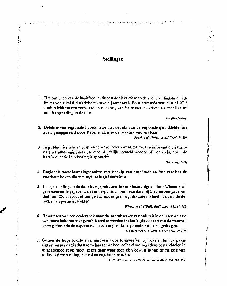
Stellingen

1. Het ontlenen van de basisfrequentie aart de ejektiefase en de snelle vullingsfase in delinker ventrikel tijd-aktiviteitskurve bij temporale Fouriertransformatie in MUG Astudies leidt tot een verbeterde benadering van het te meten aktiviteitsverschil en totminder spreiding in de fase.

Dit proefschrift

2. Detektie van regionale hypokinesie met behulp van de regionale gemiddelde fasezoals gesuggereerd door Pavel et al. is in de praktijk onbruikbaar.

Pavel et al. (19X0). Am.JXanl. 45:39H

3. In publikaties waarin gesproken wordt over kwantitatieve faseinformatie bij regio-nale wand bewegingsanalyse moet duidelijk vermeld worden of en zo ja, hoe dehartfrequentie in rekening is gebracht.

Dit proefschrift

4. Regionale wand bewegingsanalyse met behulp van amplitude en fase verdient devoorkeur boven die met regionale ejektiefraktie.

5. In tegenstelling tot de door hun gepubliceerde konklusie volgt uit door Wiener et al.gepresenteerde gegevens, dat een 9-punts smooth van data bij kleurenweergave vanthallium-201 mycocardium perfusiescans geen signifikante invloed heeft op de de-tektie van perfusiedefekten.

Wiener et al. (19X0). Radiology 136:1X1 1X5

6. Resultaten van een onderzoek naar de interobserver variabiliteit in de interpretatievan scans behoren niet gepubliceerd te worden indien blijkt dat een van de waarne-mers gedurende de experimenten een onjuist korrigerende bril heeft gedragen.

A. Cuaran et al. (1980). J.Nucl.Med. 21:1-9

7. Gezien de hoge lokale stralingsdosis voor longweefsel bij rokers (bij I.S pakjesigaretten per dag is dat 8 rem/ jaar) en de hoeveelheid radio-aktieve bestanddelen inuitgeademde rook moet, zeker daar waar men zich bewust is van de risiko's vanradio-aktieve straling, het roken nagelaten worden.

T. H Winters et al. (1982). IV.EngU.Afee/. 306:364-365

8. Uit het feit dat verschillende deskundigen van de Franse opwerkingsfabriek Cogémaop het symposium 'Verworvenheden bij opwerking en opslag van kernsplijtingsafval'spraken over de technische aspecten van splijtstofverwerking, dient gekonkludeerdte worden, dat een veilige verwerking van dit afval (nog) niet mogelijk is.

Symposium op 20 september 1981. georganiseerd door KIVI. ECN en KEMA

9. Binnen de bebouwde kom verdient een 'groene golf voor het fietsverkeer de voor-keur boven een 'groene golf voor het autoverkeer.

10. Het verkeersreglement dient zodanig veranderd te worden, dat fietsers geen rekeninghoeven te houden met verbodsborden, behalve daar waar de toevoeging 'ook voorfietsers' geplaatst is.

P. H. Vos,juni 1982.