Information in the Revision Process of Real-Time Datasets∗

Valentina Corradi1, Andres Fernandez2, and Norman R. Swanson21University of Warwick2Rutgers University

July 2007

Abstract

In this paper we first develop two statistical tests of the null hypothesis that early release data are rational. The

tests are consistent against generic nonlinear alternatives, and are conditional moment type tests, in the spirit of

Bierens (1982,1990), Chao, Corradi and Swanson (2001) and Corradi and Swanson (2002). We then use this test,

in conjunction with standard regression analysis in order to individually and jointly analyze a real-time dataset for

money, output, prices and interest rates. All of our empirical analysis is carried out using various variable/vintage

combinations, allowing us to comment not only on rationality, but also on a number of other related issues. For

example, we discuss and illustrate the importance of the choice between using first, later, or mixed vintages of data

in prediction. Interestingly, it turns out that early release data are generally best predicted using first releases. The

standard practice of using “mixed vintages” of data appears to always yield poorer predictions, regardless of what

we term “definitional change problems” associated with using only first releases for prediction. Furthermore, we note

that our tests of first release rationality based on ex ante prediction find no evidence that the data rationality null

hypothesis is rejected for a variety of variables (i.e. we find strong evidence in favor of the “news” hypothesis). Thus,

it appears that there is little benefit to using later releases of data for prediction and policy analysis, for example.

Additionally, we argue that the notion of final data is misleading, and that definitional and other methodologicalchanges that pepper real-time datasets are important. Finally, we carry out an empirical example, where little

evidence that money has marginal predictive content for output is found, regardless of whether various revision error

variables are added to standard vector autoregression models of money, output, prices and interest rates.

Keywords: bias; efficiency; generically comprehensive tests; rationality; preliminary, final, andreal-time data.JEL classification: C32, C53, E01, E37, E47.

∗ Valentina Corradi, Department of Economics, University of Warwick, Coventry, CV4 7AL, UK, v.corradi@warwick.ac.uk.Andres Fernandez, Department of Economics, Rutgers University, 75 Hamilton Street, New Brunswick, NJ 08901,

USA, afernandez@fas-econ.rutgers.edu . Norman R. Swanson, Department of Economics, Rutgers University, 75

Hamilton Street, New Brunswick, NJ 08901, USA, nswanson@econ.rutgers.edu. The paper has been prepared for

the conference entitled “Real-Time Data Analysis and Methods in Economics”, held at the Federal Reserve Bank of

Philadelphia, and the authors are grateful to seminar participants for many useful comments on early versions of this

paper. Corradi gratefully acknowledges ESRC grant RES-062-23-0311, and Swanson acknowledges financial support

from a Rutgers University Research Council grant.

1 Introduction

The literature on testing for and assessing the rationality of early release economic data is rich

and deep. A very few of the most recent papers on the subject include Howrey (1978), Mankiw,

Runkle, and Shapiro (1984), Mankiw and Shapiro (1986), Milbourne and Smith (1989), Keane

and Runkle (1989,1990), Kennedy (1993), Kavajecz and Collins (1995), Faust, Rogers, and Wright

(2005), Swanson and van Dijk (2006), and the papers cited therein.1 In recent years, in large part

due to the notable work of Diebold and Rudebusch (1991), many agencies have begun to collect

and disseminate real-time data that are useful for examining data rationality, and more generally

for examining the entire revision history of a variable. This has led to much renewed interest in the

area of real-time data analysis. However, relatively few papers have examined issues such as data

rationality using tests other than ones based on fairly simplistic models such linear regressions.2

In this paper, we add to the literature on whether preliminary (and later releases) of a given

variable are rational by outlining two consistent out-of-sample tests for nonlinear rationality that

are consistent against generic (non)linear alternatives. One test can be used to determine whether

preliminary data are rational, in the sense that subsequent data releases simply take “news” into

account that are not available at the time of initial release (see Mankiw and Shapiro (1986) and

Faust, Rogers and Wright (2005) for further explanation of the “news” hypothesis). In this case, we

have evidence that the first release data are those that should be used in out-of-sample prediction.

If this test fails, then two additional testing procedures are proposed. The first involves simply

using later release data in the same test to estimate the timing of data rationality (e.g. to estimate

how many months it takes before data are rational). The second involves carrying out a different

test which is designed to determine whether the data irrationality arises (i) simply because of

a bias in the preliminary estimate, in which case the preliminary data should be adjusted by

including an estimate of the bias prior to its use in out of sample prediction; or (ii) because

available information has been used inefficiently when constructing first release data. The tests

are related to the conditional moment tests of Bierens (1982,1990), de Jong (1996), and Corradi

and Swanson (2002); and we provide asymptotic theory necessary for the valid implementation

1A small subset of other papers that examine data rationality, either explicitly, or implicitly via the analysis ofreal-time predictions, include Burns and Mitchell (1946), Muth (1961), Morgenstern (1963), Stekler (1967), Pierce(1981), Shapiro and Watson (1988), Diebold and Rudebusch (1991), Neftci and Theodossiou (1991), Brodsky andNewbold (1994), Mariano and Tanizaki (1995), Hamilton and Perez-Quiros (1991), Robertson and Tallman (1998),Gallo and Marcellino (1999), Swanson, Ghysels, and Callan (1999), McConnell and Perez-Quiros (2000), Amato andSwanson (2001), Croushore and Stark (2001,2003), Ghysels, Swanson and Callan (2002), and Bernanke and Boivin(2003).

2For a discussion of nonlinearity and data rationality, the reader is referred to Brodsky and Newbold (1994),Rathjens and Robins (1995), and Swanson and van Dijk (2006).

1

of the statistics using critical values constructed via a block (likelihood) bootstrap related to the

bootstrap procedures discussed in Corradi and Iglesis (2007) and Corradi and Swanson (2007). Of

final note is that in addition to being based on linear models, many of the regression based tests

used to examine rationality in the literature are actually “in-sample”, in the sense that “true”

prediction experiments are not carried out when testing rationality. We feel that this is a crucial

issue, and is analogous to the issue of whether the “correct” way to test for Granger causality is to

use in-sample tests or ex ante out-of-sample predictive accuracy assessments. Our tests are truly

out-of-sample; and hence quite different from prior tests of rationality such as those discussed and

implemented in the keynote paper written by Mankiw and Shapiro (1986), and subsequent related

papers.

In addition to outlining and implementing new rationality tests, we carry out a series of predic-

tion experiments in this paper. One feature that ties together our prediction experiments and our

data rationality tests is that we take no stand on what constitutes final data, as we argue that the

very notion of using so-called final data in such analyses is fraught with problems. In particular,

data are never truly final, as they are subject to an indefinite number of revisions. More impor-

tantly, it is not clear that financial market participants, government policy setters, and generic

economic agents use final data in day to day decision making. For example, financial markets cer-

tainly react to first release data, and also to a small number of subsequent data revisions. However,

they pretty clearly do not react to revisions to data from 10 or 20 years ago, say. Similarly, policy

setters base their decisions to some extent on predictions of near-term early release target variables

such as inflation, unemployment, and output growth. They clearly do not base their decisions

upon predictions of final versions of these data. The reason for this is that early release data are

revised not only because of the collection of additional information relevant to the time period in

question, but also because of “definitional changes”. Indeed, distant revisions are due primarily to

definitional and other structural data collection methodology changes; and it goes without saying

that policy setters, for example, have very little premonition of definitional changes that will occur

10 or 20 years in the future, and indeed do not care about such. Of course, one might argue, and

perhaps in certain contexts should argue that there exists some “true underlying” final definition

of a variable; and definitional changes represent incremental efforts made by statistical agencies to

converge to this definition. Moreover, it is not clear that empirical analysts should simply make

level adjustments to series in order to allow for definitional changes - this is at best a crude solution

to the problem (even if the raw data are transformed to growth rates). Instead, one might argue

2

that a whole new series should be formed after each definitional change.

The above arguments, taken in concert, imply that the variable that one cares about predicting

may in many cases be a near-term vintage; and if one cares about final data, one may have a

very difficult time, as one would need then to predict unknowable future definitional and other

methodological changes implicit to the data construction process. Regardless of one’s view on this

matter, though, there are clearly instances where one may be interested in predicting first release

data, and one of the objectives of this paper is to address how best to do this. Furthermore, it

is pretty clear that much caution needs to be used when analyzing real-time data. For example,

application of simple level shifts to datasets in order to deal with “definitional changes” may be

grossly inadequate in some cases, as the entire dynamic structure of a series might have changed

after a “definitional change”, so that the current “definition” of GDP, say, may result in an entirely

different time series that based on an earlier definition. This issue is examined in the sequel via

discussion of a simple graphical method for determining “definitional changes”, and via careful

examination of the statistical properties of money, output, and prices for different sample periods

corresponding to “definitional changes”.

The preceding arguments are not meant to suggest that the standard approach in prediction

exercises of using all available information when parameterizing models and subsequently when

constructing predictions is invalid. Indeed, given that definitional changes may indeed make early

releases of data from the distant past unreliable, when viewed in concert with early releases of very

recent data, it still makes sense to use the most recently available data (as opposed to only using

preliminary data, say) in prediction. However, it should nevertheless be stressed that the most

recent data that are available for a particular variable consist of a series of observations, each of

which is a different vintage. Thus, the standard econometric approach is to use a mixture of different

vintages. This in turn poses a different sort of potential problem. Namely, if the objective is to

construct predictions of early data vintages, then why use an arbitrarily large number of different

data vintages when parameterizing prediction models? This is one of the issues addressed in the

empirical part of this paper, where real-time prediction experiments are carried out using various

vintages of data as the target variable to be predicted, and using various vintages and combinations

of vintages, and revision errors in the information set from which the model is parameterized.

For example, we investigate whether kth available data are better predicted using all available

information (i.e. using the latest real-time data), or using only past kth available observations.

This approach allows us to answer the following sort of question. If the objective is prediction

3

of preliminary data, then do any advantages associated with using only past first release data to

make such predictions outweigh the costs associated with the fact that distant first release data

are clearly subject to the “definitional change” problems discussed above; when compared with

predictions constructed using real-time data which are subject to the criticism that noise is added

to the regression because many different vintages are used in model parameterization? As might

be expected, the answer to the above question in part depends upon how severe the definitional

changes are, and in part on how much history is used in our experiments; and hence how many

definitional changes are allowed to contaminate our first release time series.

We also investigate whether revision errors can be used to improve predictions. Furthermore,

we carry out a real-time assessment of the marginal predictive content of money for income using

various vintage/variable combinations of output, money, prices, and interest rates.

Interestingly, it turns out that early release data are best predicted using first releases for all of

the variables we examine, even though we ignore definitional changes in our preliminary data series.

This suggests that the standard practice of using “mixed vintages” of data when constructing early

release predictions is not optimal, in a predictive accuracy sense. Moreover, there appears to be no

evidence of early release data irrationality, when our truly ex ante rationality tests are implemented;

further supporting the notion that first release data should be used for forming predictions of early

release data, and hence in subsequent policy analysis based upon such predictions. In support of

the above findings, evidence is presented supporting the conclusion that adding revisions to simple

autoregressive type prediction models does not lead to improved predictive performance. Finally,

we find that there appears to be little marginal predictive content of money for output. This result

holds for standard real-time vector autoregressions (VARs), and for VARs that are augmented with

various revision error variables.

The rest of the paper is organized as follows. In Section 2, we outline some notation, and

briefly explain the ideas behind testing for data rationality. In Section 3, we outline our nonlinear

rationality tests, and in Section 4 we outline the empirical methodology used in our prediction

experiments. Section 5 contains a discussion of the data used, and empirical results are gathered

in Section 6. Concluding remarks are given in Section 7. All proofs are gathered in an appendix.

2 Setup

Let t+kXt denote a variable (reported as an annualized growth rate) for which real-time data are

available, where the subscript t denotes the time period to which the datum pertains, and the

4

subscript t+ k denotes the time period during which the datum becomes available. In this setup,

if we assume a one month reporting lag, then first release or “preliminary” data are denoted by

t+1Xt. In addition, we denote fully revised or “final” data, which is obtained as k → ∞, by fXt.

Finally, data are grouped into so-called vintages, where the first vintage is preliminary data, the

second release is 2nd available data, and so on.

The topic of testing rationality of preliminary data announcements is discussed in detail by

Mankiw and Shapiro (1986), Keane and Runkle (1989,1990), Swanson and van Dijk (2006), and

many others.3 The notion of rationality can most easily be explained by considering Muth’s (1961)

definition of rational expectations, where the preliminary release t+1Xt is a rational forecast of the

final data fXt if and only if:

t+1Xt = E[fXt|F t+1t ], (1)

where F t+1t contains all information available at the time of release of t+1Xt (see below for further

discussion). This equation can be examined via use of the following regression model:

fXt = α+ t+1Xt β + t+1W0tγ + εt+1, (2)

where t+1Wt is an m× 1 vector of variables representing the conditioning information set availableat time period t+ 1 and εt+1 is an error term assumed to be uncorrelated with t+1Xt and t+1Wt.

The null hypothesis of interest (i.e. that of rationality) in this model is that α = 0, β = 1, and

γ = 0, and corresponds to the idea of testing for the rationality of t+1Xt for fXt by finding out

whether the conditioning information in t+1Wt, available in real-time to the data issuing agency

could have been used to construct better conditional predictions of final data.

Based on regressions in the spirit of the above model, and on an examination of preliminary

and final money stock data, Mankiw, Runkle, and Shapiro (1984) find evidence against the null

that α = 0, β = 1, and γ = 0 in (2), suggesting that preliminary money stock announcements

are not rational. On the other hand, Kavajecz and Collins (1995) find that seasonally unadjusted

money announcements are rational while adjusted ones are not. For GDP data, Mankiw and

Shapiro (1986) find little evidence against the null hypothesis of rationality, while Mork (1987) and

Rathjens and Robins (1995) find evidence of irrationality, particularly in the form of prediction bias

(i.e. α 6= 0 in (2)). Keane and Runkle (1990) examine the rationality of survey price forecasts ratherthan preliminary (or real-time) data, using the novel approach of constructing panels of real-time

survey predictions. This allows them to avoid aggregation bias, for example, and may be one of the3For a very clear discussion of some approaches used to test for rationality, see also Faust, Rogers, and Wright

(2005), where the errors-in-variables and rational forecast models are used to discuss the notions of “noise” and“news”, respectively.

5

reasons why they find evidence supporting rationality, even though previous studies focusing on

price forecasts had found evidence to the contrary. Swanson and van Dijk (2006) consider the entire

revision history for each variable, and hence discuss the “timing” of data rationality by generalizing

(2) as follows:

fXt − t+kXt = α+ t+kXt β + t+kW0t+k−1γ + εt+k (3)

and

t+kXt − t+1Xt = α+ t+1Xt β + t+1W0tγ + εt+k, (4)

where k = 1, 2, . . . defines the release (or vintage) of data (that is, for k = 1 we are looking at

preliminary data, for k = 2 the data have been revised once, etc.). The primary objective of fitting

the second of these two regression models is to assess whether there is information in the revision

error between periods t + k and t + 1 that could have been predicted when the initial estimate,

t+1Xt, was formed. Using this approach, Swanson and van Dijk find that data rationality is most

prevalent after 3 to 4 months, for unadjusted industrial production and producer prices.

In the sequel, we consider questions of data rationality similar to those discussed above. How-

ever, we do not assume linearity, as is implicit in the tests carried out in all of the papers discussed

above. Additionally, we examine a number of empirical prediction models in order to assess the

relative merits of using various vintages of real-time data, in the context of predicting a variety of

different variable/vintage combinations (see above for further discussion).

3 Consistent Out of Sample Tests for Rationality

3.1 The Framework

As mentioned above, a common approach in the literature has been to use linear regressions in

order to test for rationality. Therefore, failure to reject the null equates with an absence of linear

correlation between the revision error and information available at the time of the first data release.

It follows that these tests do not necessarily detect nonlinear dependence. Our objective in this

section is to provide a test for rationality which is consistent against generic nonlinear alternatives.

In other words, we propose a test that is able to detect any form of dependence between the

revision error and information available at the time of the first data release. This is accomplished

by constructing conditional moment tests which employ an infinite number of moment conditions

(see e.g. Bierens (1982,1990), Bierens and Ploberger (1997), de Jong (1996), Hansen (1996a), Lee,

Granger and White (1993) and Stinchcombe and White (1998), Corradi and Swanson (2002)).

6

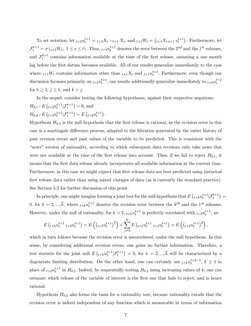
To set notation, let t+2ut+1t = t+2Xt −t+1 Xt, and t+1Wt =

¡t+1Xt,t+1 u

t+1t

¢. Furthermore, let

F t+1t = σ (s+1Ws; 1 ≤ s ≤ t) . Thus, t+2ut+1t denotes the error between the 2nd and the 1st releases,

and F t+1t contains information available at the time of the first release, assuming a one month

lag before the first datum becomes available. All of our results generalize immediately to the case

where t+1Wt contains information other than t+1Xt and t+1ut+1t . Furthermore, even though our

discussion focusses primarily on t+2ut+1t , our results additionally generalize immediately to t+ku

t+jt

for k ≥ 2, j ≥ 1, and k > j.In the sequel, consider testing the following hypotheses, against their respective negations:

H0,1 : E¡t+2u

t+1t |F t+1t

¢= 0, and

H0,2 : E¡t+2u

t+1t |F t+1t

¢= E

¡t+2u

t+1t

¢.

Hypothesis H0,1 is the null hypothesis that the first release is rational, as the revision error in this

case is a martingale difference process, adapted to the filtration generated by the entire history of

past revision errors and past values of the variable to be predicted. This is consistent with the

“news” version of rationality, according to which subsequent data revisions only take news that

were not available at the time of the first release into account. Thus, if we fail to reject H0,1, it

means that the first data release already incorporates all available information at the current time.

Furthermore, in this case we might expect that first release data are best predicted using historical

first release data rather than using mixed vintages of data (as is currently the standard practice).

See Section 5.2 for further discussion of this point.

In principle, one might imagine forming a joint test for the null hypothesis thatE¡t+ku

t+1t |F t+1t

¢=

0, for k = 2, ..., k, where t+kut+1t denotes the revision error between the kth and the 1st releases.

However, under the null of rationality, for k > 2, t+kut+1t is perfectly correlated with t+2u

t+1t , as:

E¡t+ku

t+1t t+2u

t+1t

¢= E

³¡t+2u

t+1t

¢2´+

kXj=3

E¡t+ju

t+1t t+2u

t+1t

¢= E

³¡t+2u

t+1t

¢2´,

which in turn follows because the revision error is uncorrelated, under the null hypothesis. In this

sense, by considering additional revision errors, one gains no further information. Therefore, a

test statistic for the joint null E¡t+ku

t+1t |F t+1t

¢= 0, for k = 2, ..., k will be characterized by a

degenerate limiting distribution. On the other hand, one can certainly use t+kut+k−1t , k ≥ 1 in

place of t+2ut+1t in H0,1. Indeed, by sequentially testing H0,1 using increasing values of k, one can

estimate which release of the variable of interest is the first one that fails to reject, and is hence

rational.

Hypothesis H0,2 also forms the basis for a rationality test, because rationality entails that the

revision error is indeed independent of any function which is measurable in terms of information

7

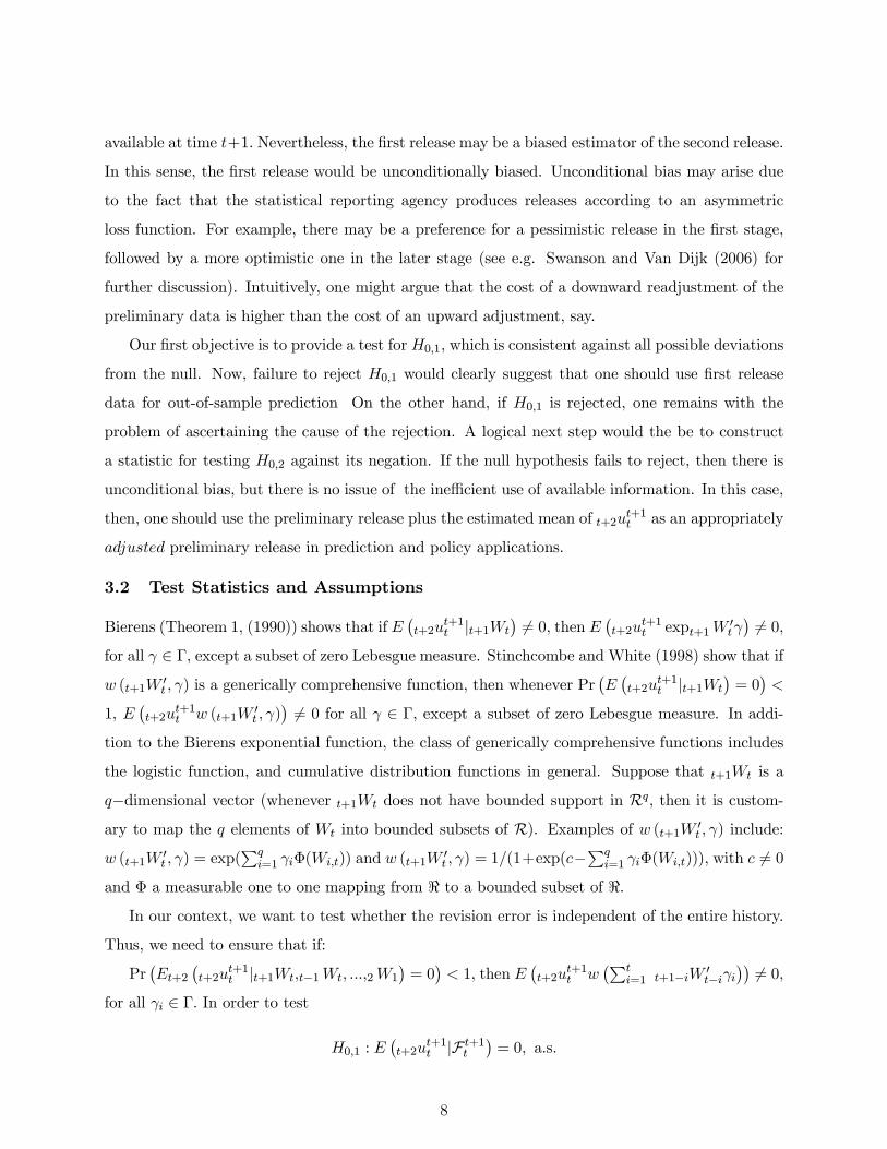
available at time t+1. Nevertheless, the first release may be a biased estimator of the second release.

In this sense, the first release would be unconditionally biased. Unconditional bias may arise due

to the fact that the statistical reporting agency produces releases according to an asymmetric

loss function. For example, there may be a preference for a pessimistic release in the first stage,

followed by a more optimistic one in the later stage (see e.g. Swanson and Van Dijk (2006) for

further discussion). Intuitively, one might argue that the cost of a downward readjustment of the

preliminary data is higher than the cost of an upward adjustment, say.

Our first objective is to provide a test for H0,1, which is consistent against all possible deviations

from the null. Now, failure to reject H0,1 would clearly suggest that one should use first release

data for out-of-sample prediction On the other hand, if H0,1 is rejected, one remains with the

problem of ascertaining the cause of the rejection. A logical next step would the be to construct

a statistic for testing H0,2 against its negation. If the null hypothesis fails to reject, then there is

unconditional bias, but there is no issue of the inefficient use of available information. In this case,

then, one should use the preliminary release plus the estimated mean of t+2ut+1t as an appropriately

adjusted preliminary release in prediction and policy applications.

3.2 Test Statistics and Assumptions

Bierens (Theorem 1, (1990)) shows that if E¡t+2u

t+1t |t+1Wt

¢ 6= 0, then E ¡t+2ut+1t expt+1W0tγ¢ 6= 0,

for all γ ∈ Γ, except a subset of zero Lebesgue measure. Stinchcombe and White (1998) show that ifw (t+1W 0

t , γ) is a generically comprehensive function, then whenever Pr¡E¡t+2u

t+1t |t+1Wt

¢= 0

¢<

1, E¡t+2u

t+1t w (t+1W

0t , γ)

¢ 6= 0 for all γ ∈ Γ, except a subset of zero Lebesgue measure. In addi-tion to the Bierens exponential function, the class of generically comprehensive functions includes

the logistic function, and cumulative distribution functions in general. Suppose that t+1Wt is a

q−dimensional vector (whenever t+1Wt does not have bounded support in Rq, then it is custom-ary to map the q elements of Wt into bounded subsets of R). Examples of w (t+1W 0

t , γ) include:

w (t+1W0t , γ) = exp(

Pqi=1 γiΦ(Wi,t)) and w (t+1W

0t , γ) = 1/(1+exp(c−

Pqi=1 γiΦ(Wi,t))), with c 6= 0

and Φ a measurable one to one mapping from < to a bounded subset of <.In our context, we want to test whether the revision error is independent of the entire history.

Thus, we need to ensure that if:

Pr¡Et+2

¡t+2u

t+1t |t+1Wt,t−1Wt, ...,2W1

¢= 0

¢< 1, then E

¡t+2u

t+1t w

¡Pti=1 t+1−iW 0

t−iγi¢¢ 6= 0,

for all γi ∈ Γ. In order to test

H0,1 : E¡t+2u

t+1t |F t+1t

¢= 0, a.s.

8

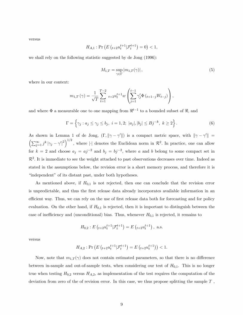
versus

HA,1 : Pr¡E¡t+2u

t+1t |F t+1t

¢= 0

¢< 1,

we shall rely on the following statistic suggested by de Jong (1996):

M1,T = supγ∈Γ

|m1,T (γ)| , (5)

where in our context:

m1,T (γ) =1√T

T−2Xt=1

t+2ut+1t w

⎛⎝t−1Xj=1

γ0jΦ (t+1−jWt−j)

⎞⎠ ,and where Φ a measurable one to one mapping from <t−1 to a bounded subset of <, and

Γ =nγj : aj ≤ γj ≤ bj , i = 1, 2; |aj |, |bj| ≤ Bj−k, k ≥ 2

o. (6)

As shown in Lemma 1 of de Jong, (Γ, kγ − γ0k) is a compact metric space, with kγ − γ0k =³P∞j=1 j

k |γj − γ0|2´1/2

, where |·| denotes the Euclidean norm in R2. In practice, one can allowfor k = 2 and choose aj = aj−2 and bj = bj−2, where a and b belong to some compact set in

R2. It is immediate to see the weight attached to past observations decreases over time. Indeed asstated in the assumptions below, the revision error is a short memory process, and therefore it is

“independent” of its distant past, under both hypotheses.

As mentioned above, if H0,1 is not rejected, then one can conclude that the revision error

is unpredictable, and thus the first release data already incorporates available information in an

efficient way. Thus, we can rely on the use of first release data both for forecasting and for policy

evaluation. On the other hand, if H0,1 is rejected, then it is important to distinguish between the

case of inefficiency and (unconditional) bias. Thus, whenever H0,1 is rejected, it remains to

H0,2 : E¡t+2u

t+1t |F t+1t

¢= E

¡t+2u

t+1t

¢, a.s.

versus

HA,2 : Pr¡E¡t+2u

t+1t |F t+1t

¢= E

¡t+2u

t+1t

¢¢< 1.

Now, note that m1,T (γ) does not contain estimated parameters, so that there is no difference

between in-sample and out-of-sample tests, when considering our test of H0,1. This is no longer

true when testing H0,2 versus HA,2, as implementation of the test requires the computation of the

deviation from zero of the of revision error. In this case, we thus propose splitting the sample T ,

9

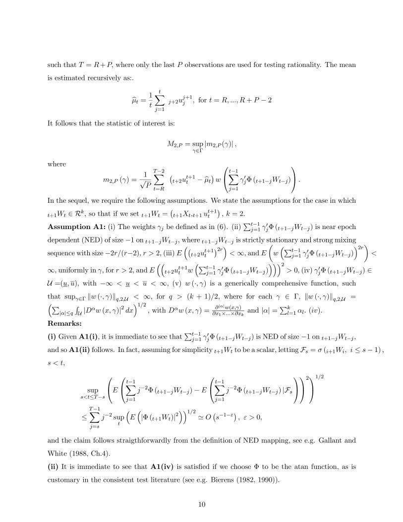
such that T = R+P, where only the last P observations are used for testing rationality. The mean

is estimated recursively as:.

bμt = 1

t

tXj=1

j+2uj+1j , for t = R, ...,R+ P − 2

It follows that the statistic of interest is:

M2,P = supγ∈Γ

|m2,P (γ)| ,

where

m2,P (γ) =1√P

T−2Xt=R

¡t+2u

t+1t − bμt¢w

⎛⎝t−1Xj=1

γ0jΦ (t+1−jWt−j)

⎞⎠ .In the sequel, we require the following assumptions. We state the assumptions for the case in which

t+1Wt ∈ Rk, so that if we set t+1Wt =¡t+1Xt,t+1 u

t+1t

¢, k = 2.

Assumption A1: (i) The weights γj be defined as in (6). (ii)Pt−1j=1 γ

0jΦ (t+1−jWt−j) is near epoch

dependent (NED) of size −1 on t+1−jWt−j, where t+1−jWt−j is strictly stationary and strong mixing

sequence with size−2r/(r−2), r > 2, (iii)E³¡t+2u

t+1t

¢2r´<∞, andE

µw³Pt−1

j=1 γ0jΦ (t+1−jWt−j)

´2r¶<

∞, uniformly in γ, for r > 2, andE³³

t+2ut+1t w

³Pt−1j=1 γ

0jΦ (t+1−jWt−j)

´´´2> 0, (iv) γ0jΦ (t+1−jWt−j) ∈

U =(u, u), with −∞ < u < u < ∞, (v) w (·, γ) is a generically comprehensive function, suchthat supγ∈Γ kw (·, γ)kq,2,U < ∞, for q > (k + 1)/2, where for each γ ∈ Γ, kw (·, γ)kq,2,U =³P

|α|≤qRU |Dαw (x, γ)|2 dx

´1/2, with Dαw (x, γ) = ∂|α|w(x,γ)

∂x1×...×∂xk and |α| =Pkl=1 αl. (iv).

Remarks:

(i) GivenA1(i), it is immediate to see thatPt−1j=1 γ

0jΦ (t+1−jWt−j) is NED of size −1 on t+1−jWt−j ,

and soA1(ii) follows. In fact, assuming for simplicity t+1Wt to be a scalar, letting Fs = σ (i+1Wi, i ≤ s− 1) ,s < t,

sups<t≤T−s

⎛⎝E⎛⎝t−1Xj=1

j−2Φ (t+1−jWt−j)−E⎛⎝t−1Xj=1

j−2Φ (t+1−jWt−j) |Fs⎞⎠⎞⎠2⎞⎠1/2

≤T−1Xj=s

j−2 supt

³E³|Φ (t+1Wt)|2

´´1/2 ' O ¡s−1−ε¢ , ε > 0,and the claim follows straigthforwardly from the definition of NED mapping, see e.g. Gallant and

White (1988, Ch.4).

(ii) It is immediate to see that A1(iv) is satisfied if we choose Φ to be the atan function, as is

customary in the consistent test literature (see e.g. Bierens (1982, 1990)).

10

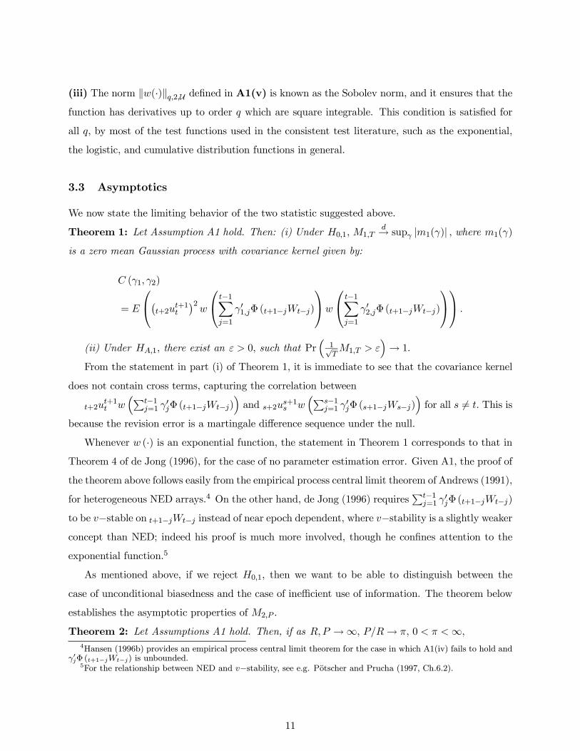
(iii) The norm kw(·)kq,2,U defined in A1(v) is known as the Sobolev norm, and it ensures that thefunction has derivatives up to order q which are square integrable. This condition is satisfied for

all q, by most of the test functions used in the consistent test literature, such as the exponential,

the logistic, and cumulative distribution functions in general.

3.3 Asymptotics

We now state the limiting behavior of the two statistic suggested above.

Theorem 1: Let Assumption A1 hold. Then: (i) Under H0,1, M1,Td→ supγ |m1(γ)| , where m1(γ)

is a zero mean Gaussian process with covariance kernel given by:

C (γ1, γ2)

= E

⎛⎝¡t+2ut+1t

¢2w

⎛⎝t−1Xj=1

γ01,jΦ (t+1−jWt−j)

⎞⎠w⎛⎝t−1Xj=1

γ02,jΦ (t+1−jWt−j)

⎞⎠⎞⎠ .(ii) Under HA,1, there exist an ε > 0, such that Pr

³1√TM1,T > ε

´→ 1.

From the statement in part (i) of Theorem 1, it is immediate to see that the covariance kernel

does not contain cross terms, capturing the correlation between

t+2ut+1t w

³Pt−1j=1 γ

0jΦ (t+1−jWt−j)

´and s+2us+1s w

³Ps−1j=1 γ

0jΦ (s+1−jWs−j)

´for all s 6= t. This is

because the revision error is a martingale difference sequence under the null.

Whenever w (·) is an exponential function, the statement in Theorem 1 corresponds to that in

Theorem 4 of de Jong (1996), for the case of no parameter estimation error. Given A1, the proof of

the theorem above follows easily from the empirical process central limit theorem of Andrews (1991),

for heterogeneous NED arrays.4 On the other hand, de Jong (1996) requiresPt−1j=1 γ

0jΦ (t+1−jWt−j)

to be v−stable on t+1−jWt−j instead of near epoch dependent, where v−stability is a slightly weakerconcept than NED; indeed his proof is much more involved, though he confines attention to the

exponential function.5

As mentioned above, if we reject H0,1, then we want to be able to distinguish between the

case of unconditional biasedness and the case of inefficient use of information. The theorem below

establishes the asymptotic properties of M2,P .

Theorem 2: Let Assumptions A1 hold. Then, if as R,P →∞, P/R→ π, 0 < π <∞,4Hansen (1996b) provides an empirical process central limit theorem for the case in which A1(iv) fails to hold and

γ0jΦ (t+1−jWt−j) is unbounded.5For the relationship between NED and v−stability, see e.g. Potscher and Prucha (1997, Ch.6.2).

11

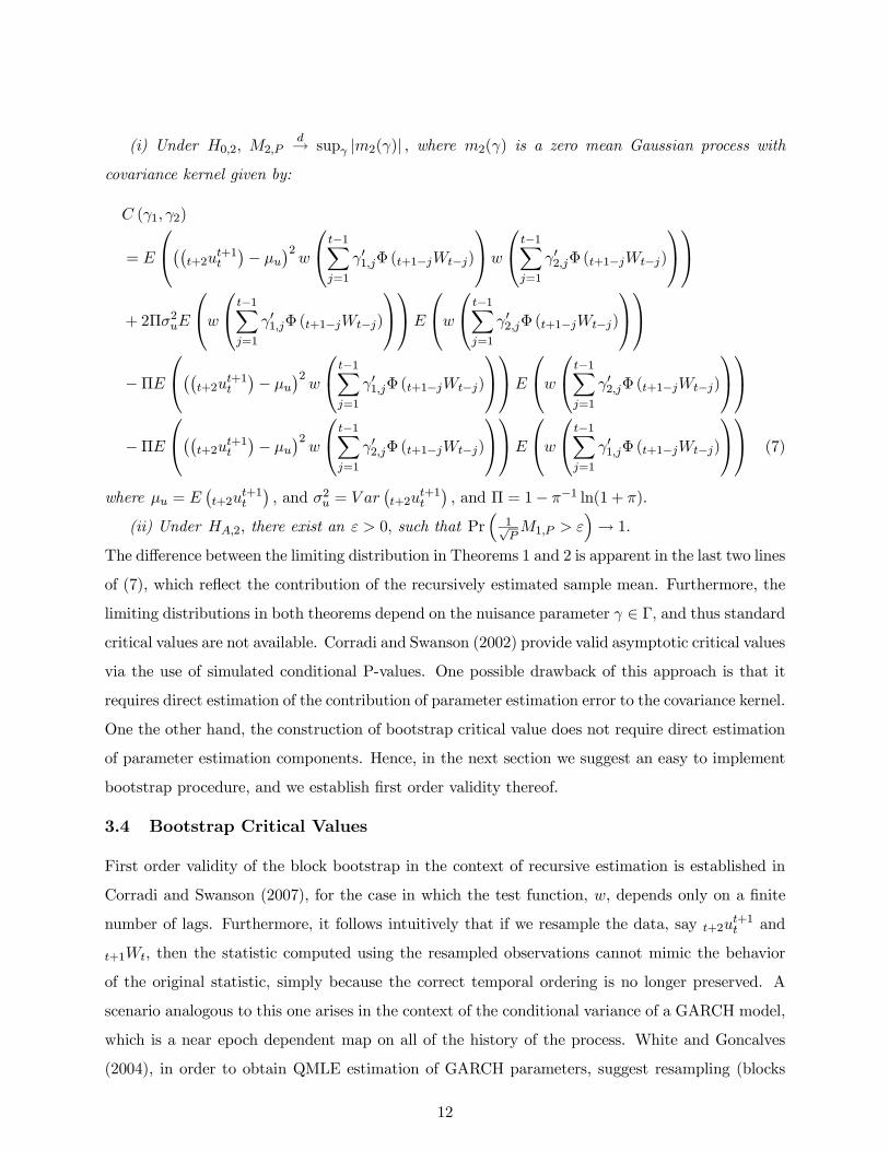
(i) Under H0,2, M2,Pd→ supγ |m2(γ)| , where m2(γ) is a zero mean Gaussian process with

covariance kernel given by:

C (γ1, γ2)

= E

⎛⎝¡¡t+2ut+1t

¢− μu¢2w

⎛⎝t−1Xj=1

γ01,jΦ (t+1−jWt−j)

⎞⎠w⎛⎝t−1Xj=1

γ02,jΦ (t+1−jWt−j)

⎞⎠⎞⎠+ 2Πσ2uE

⎛⎝w⎛⎝t−1Xj=1

γ01,jΦ (t+1−jWt−j)

⎞⎠⎞⎠E⎛⎝w

⎛⎝t−1Xj=1

γ02,jΦ (t+1−jWt−j)

⎞⎠⎞⎠−ΠE

⎛⎝¡¡t+2ut+1t

¢− μu¢2w

⎛⎝t−1Xj=1

γ01,jΦ (t+1−jWt−j)

⎞⎠⎞⎠E⎛⎝w

⎛⎝t−1Xj=1

γ02,jΦ (t+1−jWt−j)

⎞⎠⎞⎠−ΠE

⎛⎝¡¡t+2ut+1t

¢− μu¢2w

⎛⎝t−1Xj=1

γ02,jΦ (t+1−jWt−j)

⎞⎠⎞⎠E⎛⎝w

⎛⎝t−1Xj=1

γ01,jΦ (t+1−jWt−j)

⎞⎠⎞⎠ (7)

where μu = E¡t+2u

t+1t

¢, and σ2u = V ar

¡t+2u

t+1t

¢, and Π = 1− π−1 ln(1 + π).

(ii) Under HA,2, there exist an ε > 0, such that Pr³

1√PM1,P > ε

´→ 1.

The difference between the limiting distribution in Theorems 1 and 2 is apparent in the last two lines

of (7), which reflect the contribution of the recursively estimated sample mean. Furthermore, the

limiting distributions in both theorems depend on the nuisance parameter γ ∈ Γ, and thus standardcritical values are not available. Corradi and Swanson (2002) provide valid asymptotic critical values

via the use of simulated conditional P-values. One possible drawback of this approach is that it

requires direct estimation of the contribution of parameter estimation error to the covariance kernel.

One the other hand, the construction of bootstrap critical value does not require direct estimation

of parameter estimation components. Hence, in the next section we suggest an easy to implement

bootstrap procedure, and we establish first order validity thereof.

3.4 Bootstrap Critical Values

First order validity of the block bootstrap in the context of recursive estimation is established in

Corradi and Swanson (2007), for the case in which the test function, w, depends only on a finite

number of lags. Furthermore, it follows intuitively that if we resample the data, say t+2ut+1t and

t+1Wt, then the statistic computed using the resampled observations cannot mimic the behavior

of the original statistic, simply because the correct temporal ordering is no longer preserved. A

scenario analogous to this one arises in the context of the conditional variance of a GARCH model,

which is a near epoch dependent map on all of the history of the process. White and Goncalves

(2004), in order to obtain QMLE estimation of GARCH parameters, suggest resampling (blocks

12

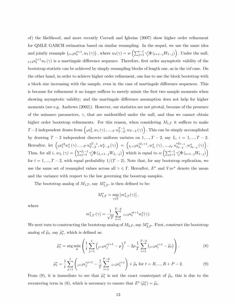
of) the likelihood, and more recently Corradi and Iglesias (2007) show higher order refinement

for QMLE GARCH estimation based on similar resampling. In the sequel, we use the same idea

and jointly resample¡t+2u

t+1t , wt (γ)

¢, where wt(γ) = w

³Pt−1j=1 γ

0jΦ (t+1−jWt−j)

´. Under the null,

t+2ut+1t wt (γ) is a martingale difference sequence. Therefore, first order asymptotic validity of the

bootstrap statistic can be achieved by simply resampling blocks of length one, as in the iid case. On

the other hand, in order to achieve higher order refinement, one has to use the block bootstrap with

a block size increasing with the sample, even in the case of martingale difference sequences. This

is because for refinement it no longer suffices to merely mimic the first two sample moments when

showing asymptotic validity; and the martingale difference assumption does not help for higher

moments (see e.g. Andrews (2002)). However, our statistics are not pivotal, because of the presence

of the nuisance parameters, γ, that are unidentified under the null, and thus we cannot obtain

higher order bootstrap refinements. For this reason, when considering M1,T it suffices to make

T −2 independent draws from³3u21, w1 (γ) , ...,T u

T−1T−2, wT−2 (γ)

´. This can be simply accomplished

by drawing T − 2 independent discrete uniform variates on 1, ..., T − 2, say Ii, i = 1, ..., T − 2.Hereafter, let

³3u∗21 w

∗1 (γ) , ...,T u

∗T−1T−2 , w

∗T−2 (γ)

´=³I1+2u

∗I1+1I1

, w∗I1 (γ) , ...,IT u∗IT−1IT−2 , w

∗IT−2 (γ)

´.

Thus, for all i, wIi (γ) =³PIi−1

j=1 γ0jΦ (Ii+1−jWIi−j)´which is equal to w

³Pt−1j=1 γ

0jΦ (t+1−jWt−j)

´for t = 1, ..., T − 2, with equal probability 1/(T − 2). Note that, for any bootstrap replication, weuse the same set of resampled values across all γ ∈ Γ. Hereafter, E∗ and V ar∗ denote the meanand the variance with respect to the law governing the boostrap samples.

The bootstrap analog of M1,T , say M∗1,T , is then defined to be:

M∗1,T = sup

γ∈Γ

¯m∗1,T (γ)

¯,

where

m∗1,T (γ) =1√T

T−2Xt=1

t+2u∗t+1t w∗t (γ).

We next turn to constructing the bootstrap analog ofM2,P , sayM∗2,P . First, construct the bootstrap

analog of bμt, say bμ∗t , which is defined as:bμ∗t = argminμ

⎛⎝1t

tXj=1

³j+2u

∗j+1j − μ

´2 − 2μ 1T

T−2Xi=1

¡i+2u

i+1i − bμt¢

⎞⎠ . (8)

bμ∗t = 1

t

tXj=1

Ãj+2u

∗j+1j − 1

T

T−2Xi=1

i+2ui+1i

!+ bμt for t = R, ...,R+ P − 2. (9)

From (9), it is immediate to see that bμ∗t is not the exact counterpart of bμt, this is due to therecentering term in (8), which is necessary to ensure that E∗ (bμ∗t ) = bμt.

13

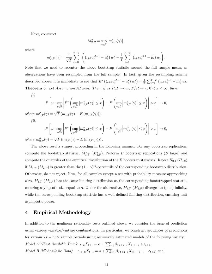
Next, construct:

M∗2,P = sup

γ∈Γ

¯m∗2,P (γ)

¯,

where

m∗2,P (γ) =1√P

T−2Xt=R

át+2u

∗t+1t − bμ∗t ¢w∗t − 1

T

T−2Xi=1

¡i+2u

i+1t − bμt¢wt! .

Note that we need to recenter the above bootstrap statistic around the full sample mean, as

observations have been resampled from the full sample. In fact, given the resampling scheme

described above, it is immediate to see that E∗¡¡t+2u

∗t+1t − bμ∗t ¢w∗t ¢ = 1

T

PT−2t=1

¡t+2u

t+1t − bμt¢wt.

Theorem 3: Let Assumption A1 hold. Then, if as R,P →∞, P/R→ π, 0 < π <∞, then:(i)

P

"ω : sup

x∈<

¯¯P ∗

Ãsupγ∈Γ

¯m∗1,T (γ)

¯ ≤ x!− P Ãsupγ∈Γ

¯mμ1,T (γ)

¯≤ x

!¯¯ > ε

#→ 0,

where mμ1,T (γ) =

√T (m1,T (γ)−E (m1,T (γ))) .

(ii)

P

"ω : sup

x∈<

¯¯P ∗

Ãsupγ∈Γ

¯m∗2,P (γ)

¯ ≤ x!− P Ãsupγ∈Γ

¯mμ2,P (γ)

¯≤ x

!¯¯ > ε

#→ 0,

where mμ2,P (γ) =

√P (m2,P (γ)−E (m2,P (γ))) .

The above results suggest proceeding in the following manner. For any bootstrap replication,

compute the bootstrap statistic, M∗1,T (M

∗2,P ). Perform B bootstrap replications (B large) and

compute the quantiles of the empirical distribution of the B bootstrap statistics. Reject H0,1 (H0,2)

if M1,T (M2,P ) is greater than the (1−α)th-percentile of the corresponding bootstrap distribution.

Otherwise, do not reject. Now, for all samples except a set with probability measure approaching

zero, M1,T (M2,P ) has the same limiting distribution as the corresponding bootstrapped statistic,

ensuring asymptotic size equal to α. Under the alternative, M1,T (M2,P ) diverges to (plus) infinity,

while the corresponding bootstrap statistic has a well defined limiting distribution, ensuring unit

asymptotic power.

4 Empirical Methodology

In addition to the nonlinear rationality tests outlined above, we consider the issue of prediction

using various variable/vintage combinations. In particular, we construct sequences of predictions

for various ex − ante sample periods using recursively estimated models of the following variety:Model A (First Available Data): t+kXt+1 = α+

Ppi=1 βi t+2−iXt+1−i + εt+k;

Model B (k thAvailable Data) : t+kXt+1 = α+Ppi=1 βi t+2−iXt+3−k−i + εt+k; and

14

Model C (Real-Time Data) : t+kXt+1 = α+Ppi=1 βi t+1Xt+1−i + εt+k

By comparing the ex−ante predictive performance of the above three models for various valuesof k, we can directly examine various properties of the revision process and hence various features

pertaining to the rationality of early data releases. The first regression model has explanatory

variables that are formed using only 1st available data, while the second regression model has

explanatory variables that are available k−1 months ahead, corresponding (k−1)st available data.Thus, the first model corresponds to the approach of simply using first available data and ignoring

all later vintages, regardless of which vintage of data is being forecasted. On the other hand, the

second model only uses data that have been revised k−1 times in order to predict data that likewisehave been revised k−1 times. This sort of prediction model might be useful, for example, if it turnsout that data are found to be “rational” after 3 releases using the above rationality tests, and if it

is thus decided that only 3rd release data is “trustworthy” enough to be used in policy analysis, say.

It follows immediately upon inspection of the models that Models A and B are the same for k = 2,

regardless of p. In Model C, the latest vintage of each observation is used in prediction, so that the

dataset is fully updated prior to each new prediction being made. We refer to this model as our

“real-time” model, as policy makers and others who construct new predictions each period, after

updating their datasets and re-estimating their models, generally use this type of model. Note also

that it follows that for p = 1, Models A and C are the same for all k, while Models A, B, and C

are the same for k = 2. Finally, Models A and B are identical for all p if k = 2.

Now, if useful information accrues via the revision process, then one might expect that using

real-time data (Model C) would yield a better predictor of t+kXt than when only “stale” 1st release

data are used (Model B), for example. Of course, the last statement has a caveat. Namely, it

is possible that 1st vintage data are best predicted using only 1st vintage regressors, 2nd vintage

using 2nd vintage regressors, etc.. This might arise if the use of real-time data as in Model C

results in an “informational mix-up”, due to the fact that every observation used to estimate the

model is a different vintage, and only one of these vintages can possibly correspond to the vintage

being predicted at any point in time (see discussion in the introduction for further details). This

eventuality would be consistent with a finding that Model B yields the “best” predictions. However,

the problem with using Model B is that we are ignoring more recent vintages of some variables,

and so the model is in some sense “out of date”. This is a substantial disadvantage, and may well

be expected to result in Model C yielding the best predictions for values of k great than 2. Our

approach in the empirical application is to set: (i) p = 1; (ii) p = SIC; (iii) p = AIC; (iv) p = 0.

15

Additionally, we set k ={1, 2, 3, 6, 12, 24}. Furthermore, for Type C regressions, in addition tothe basic regression model, we consider models where we include additional regressors of the form:

(i) t+1W0t = t+1u

tt−k, for each of k = 1, 2, ..., 24; (ii) t+1W

0t = ( t+1u

tt−1, t+1utt−2,t+1 utt−3)0; and (iii)

t+1W0t = t+1u

t+2−kt+1−k, for each of k = 3, 4, ..., 24.

Additionally, we estimate multivariate versions of all of the models described above, where we

include (i) money, income, prices, and interest rates; and (ii) income, prices, and interest rates.

In these models it is assumed that the target variable of interest is output growth. Thus, we are

examining, in real-time, the marginal predictive content of money for output, using regressions

including various data vintages, various revision errors, and for a target variable which consist of

various releases of output growth.

All of our prediction experiments are based on the examination of the mean square forecast

errors associated with predictions constructed using recursively estimated models; and MSFEs are

in turn examined via the use of Diebold and Mariano (1995) and Clark and McCracken (2001)

type predictive accuracy tests (see also Clark and McCracken (2005), McCracken (2006), and West

(1996)).

5 Empirical Results

5.1 Data

The variables used in the empirical part of this paper are real GDP (seasonally adjusted), the GDP

chain-weighted price index (seasonally adjusted), the money stock (measured as M1, seasonally

adjusted) and the real interest rate (measured as the rate on 3-month Treasury bills).6 All series

have a quarterly frequency and our real time data sets for each of the four variables were obtained

from the Philadelphia Reserve System’s real time data set for Macroeconomists (RTDSM).7

The first vintage in our sample is 1965.Q4, for which the first calendar observation is 1959.Q3.

This means that the first observation in our dataset is the observation that was available to re-

searchers in the fourth quarter of 1965, corresponding to calendar dated data for the third quarter

of 1953. The datasets range up to the 2006.Q4 vintage and the corresponding 2006.Q3 calendar

date, allowing us to keep track of the exact data that were available at each vintage for every pos-

6Results based on the use of M2 in place of M1 in all empirical exercises are available upon request, and arequalitatively the same as those reported for M1.

7The RTDSM can be accessed on-line at http://www.phil.frb.org/econ/forecast/readow.html. The series wereobtained from the “By-Variable” files of the “Core Variables/Quarterly Observations/Quarterly Vintages” dataset.The data we use are discussed in detail in Croushore and Stark (2001). Note also that interest rates are not revised,and hence our interest rate dataset is a vector rather than a matrix (see Ghysels, Swanson, and Callan (2002) for adetailed discussion of the calendar date/vintage structure of real-time datasets).

16

sible calendar dated observation up to one quarter before the vintage date. This makes it possible

to trace the entire series of revisions for each observation across vintages. We use log-differences

throughout our analysis (except for interest rates); and the log-differences of all the variables, except

the interest rate, are plotted in Figures 1-3. The figures also exhibit the first and second revision

errors measured as the difference between the first vintage (e.g. first available) of a calendar ob-

servation and the second and third vintages, respectively. As can readily be seen upon inspection

of the distributions of the revision errors, as well as via examination of the summary statistics

reported in Table 1, the first revision (i.e. the difference between the first and second vintages)

is fairly close to normally distributed. On the other hand, the distribution of the second revision

errors is mostly concentrated in the zero interval, implying that much of the revision process has

already taken place in the first revision. Indeed, the distributional shape of revision errors beyond

the first revision is very much the same as that reported for the second revision in these plots,

with the exception of revision errors associated with definitional and other structural changes to

the series. This is one of the reasons why much of our analysis focuses only on the impact of first

and second revision errors - later revision errors offer little useful information, other than signalling

the presence of definition and related methodological changes. Indeed, an important property of

real-time datasets like the RTDSM is the possibility that calendar observations may vary across

vintages for reasons other than because of “pure” revisions. This is illustrated in Figure 4 where

we have plotted four early calendar dates (1959.Q4; 1960.Q4; 1961.Q4; and 1962.Q4) across all

available vintages in our sample, for output (GDP) and money (both in log-differences). Of note is

that the data varies significantly across the vintages. For instance, looking at the 1959.Q4 calendar

observation for output across all vintages, one can observe several discrete movements driving the

value of that particular observation from a monthly growth of 1% for the earlier vintages to 0.5%

for the late vintages. It seems reasonable to argue that most (if not all) of the discrete variations in

that particular calendar observation are not due to “pure revisions”, but are solely a consequence of

“definitional breaks” in the measurement of output. To verify this claim, we plotted and compared

several other calendar observations across all vintages and we could identify nine clear breaks in

the following dates: 1976.Q1; 1981.Q1; 1986.Q1; 1992.Q1; 1996.Q1; 1997.Q2; 1999.Q4; 2000.Q2;

and, 2004.Q1. (These are the breaks that define the sample periods for which summary statistics

are reported in Table 2). This can be graphically illustrated by noticing that in Figure 4, for out-

put, the four calendar dates plotted exhibit abrupt changes in the same vintages, corresponding to

these dates. Not surprisingly, the same nine breaks were identified in our measure of prices, since

17

our measure is a composite measure of GDP prices. However, it should be noted that the same

procedure for the money series does not yield such well defined ”definitional breaks”, as some of

the breaks do not apply to all vintages. This can be observed in the lower graph in Figure 4. This

suggests a need for great caution when analyzing real time data, particularly money stock.

In the introduction of this paper, we argued that the variable that one cares about predicting

is likely to be a near-term vintage, and if one cares about final data, one may have a very difficult

time, as one would need then to predict unknowable future definitional and other methodological

changes implicit to the data construction process. The above discussion supports this argument.

Namely, “pure revision” appears to occur in the near-term, “definitional change” occurs in the long

term, and little occurs between. Furthermore, and as argued in the introduction, application of

simple level shifts to datasets in order to address the “definitional change” issue may be grossly

inadequate in some cases, as the entire dynamic structure of a series might have changed after

a “definitional change”, so that the current definition of GDP may define an entirely different

time series that based on an earlier definition, say. However, it should be noted that although

our summary statistics reported in Table 2 suggest that there are indeed significant differences

between the means and other measures associated with series in different “definitional change”

sub-samples, our other empirical evidence suggests that the “definitional change” issue may not be

very damaging. This issue is discussed in the next sub-section.

5.2 Basic Predictive Regression Results

As discussed in Section 4, we carried out three types of simple autoregressive prediction experiments,

where the objective was to forecast output. The methods involved fitting regression Models A, B,

and C. Given the discussion of the previous sub-section, it is quite apparent that Models A and

B are, strictly speaking, invalid. This follows because the models are estimated recursively, using

all data available prior to the construction of each new prediction (see footnote to Table 3 for

further details). This in turn means that the structure of Models A and B ensures that data

from different “definitional periods” will be used in the estimation of the models, for many of the

predictions made; and hence parameter estimates will in principle be corrupted. However, Model

C does not have this feature, as one always uses currently available data for model estimation and

prediction construction. Indeed, Model C is arguably the type of model that the Federal Reserve

uses to construct predictions. Namely, data are updated at each point in time, as they become

available, and prior to re-estimation of models and prediction construction. The other models use

what might be called “stale data”. However, the other models might have a certain advantage

18

over Model C. For example, Model A only uses first available data to predict first available data.

Indeed, Model A also uses first available data for cases where we are interested in predicting second

and later vintages of data (i.e. when we are predicting t+kXt+1, for k > 2). Model B, on the other

hand, uses only kth vintage data for predicting kth vintages. Thus, Models B and C do not suffer

from the “mixed vintages” problem that Model A does. They do not use explanatory datasets for

which each and every observation corresponds to a different vintage. One aspect of our prediction

experiments is that we are able to shed light upon the following trade-off: What is worse: using

“mixed vintage” datasets that are not subject to “definitional change” problems, or using datasets

containing only the vintage corresponding to the desired prediction vintage, but with “definitional

change” problems?

The answer to the preceding question is immediately apparent upon inspection of Table 3,

where results for basic autoregressive versions of Models A, B, and C are presented for various

prediction periods, various values of k, and for models both with and without included revision

error regressors.8 Model C never yield the lowest mean square forecast error (MSFE), regardless of

what vintage of data is being predicted, and regardless of the variable being predicted.9 In particular,

for output, prices, and money, Models A and B always “win”, and for most cases where Model B

“wins”, it is simply because it is for a case where Models A and B yield identical results (see Section

4 for a discussion of these cases). Thus, it indeed appears to be the case that Model A “wins” in

virtually every case considered across all variables, and regardless of whether revision errors are

added as additional regressors or not. Thus, we have surprising evidence that preliminary data are

useful even for predicting later data releases. While this is pretty strong evidence against Model

C, one must keep in mind that Model B uses “stale data” when predicting vintages for k > 2, and

hence it might not be viewed as too surprising that Model A dominates Model B. In summary, we

have interesting evidence suggesting that real-time datasets are crucial, but perhaps not always in

the way people have though, as the “mixed vintage” problem appears to be sufficiently important

as to cause Model C to “lose” every one of our prediction competitions. This findings holds even

though Model A is subject to the “definitional change” problem, suggesting that the “definitional

8In Model C, additional “revision error” regressors include: (i) t+1W0t = t+1u

tt−k; (ii) t+1W

0t = ( t+1u

tt−1, t+1u

tt−2)

0;and (iii) t+1W

0t = t+1u

t+2−kt+1−k. Note that results are only reported for k = 2, 3, and 4. Other values of k were considered,

but results are not reported here as they are qualitatively the same as those that are reported, and because “purerevisions” appear to die out extremely quickly in the data (see above discussion). Finally, note that although modelswere estimated using lags selected with the AIC and the SIC, and for lags set equal to unity, results are only reportedfor lags selected using the SIC. The reason for this is that models with lags selected using the SIC uniformly yieldedthe lowest MSFEs across all cases reported.

9Note also that the random walk model does not yield the lowest MSFE for any cases considered. The onlyexception is output for k = 2, when the forecasting period starting date is1983:01, in which case Model C beatsModels A and B, and the random walk model beats Models A, B, and C.

19

change” problem is not too severe.10

It is also apparent from inspection of Table 3 that adding revision errors to the prediction

models does not result in lower MSFEs, at least for the cases that we have considered. This

finding, coupled with our finding that Model A yields the lowest MSFEs across all cases, suggests

that all of our data are to some extent efficient. Of course, this result is based upon autoregression

type models, and one would need to include additional regressors, both linearly and nonlinearly, to

properly examine the issue of efficiency. In the next section this is done via examination of vector

autoregressive predictive models for output. In the subsequent section, we examine the issue using

the tests discussed in Section 3 of this paper.

5.3 Rationality Tests

We now turn to an illustration of how one might empirically implement the rationality tests dis-

cussed above. Note that in-depth empirical research of the series, however, is left to future research.

We begin by testing the following hypothesis:

H0,1 : E¡t+2u

t+1t |F t+1t

¢= 0, a.s.

This is done for the three variables (X 0s) in our dataset (i.e. real GDP (seasonally adjusted), the

GDP chain-weighted price index (seasonally adjusted), and the money stock (measured as M1,

seasonally adjusted). Recall that the relevant test statistic is:

M1,T = supγ∈Γ

|m1,T (γ)| ,

where

m1,T (γ) =1√T

T−2Xt=1

t+2ut+1t w

⎛⎝t−1Xj=1

γ0jΦ (t+1−jWt−j)

⎞⎠ ,We will distinguish two cases for t+1−jWt−j : (i) t+1−jWt−j is a scalar,

t+1−jWt−j = t+1−jXt−j ; j = 0, 1, ..., t− 1,10Diebold Mariano (1995) test statistics were constructed for all of the results reported in the tables discussed

in this subsection, and all test statistic values were far below standard normal critical values, in absolute value,suggesting that there is actually little to choose between the models (tabulated values are available upon requestfrom the authors). However, we note that it remains an interesting result of our experiments that Model A virtuallyalways yields lower MSFEs, when comparing point values; whereas in a truly experimental setting one might expectan equal number of “wins” based on point MSFEs for each of the different models, under the null hypothesis. Forthis reason, we conjecture that more refined testig with bigger samples of data, for example, might be expected toyield test statistics that are significantly different from zero.For further discussion of valid test critical value construction when applying Diebold Mariano statistics in the

current context, refer to Clark and McCracken (2007).

20

and, (ii) t+1−jWt−j is a vector,

t+1−jWt−j =ht+1−jXt−j , t+1−jut−jt−1−j

i0j = 0, 1, ..., t− 1.

Following Corradi and Swanson (2002) we set w as the exponential function, and Φ the inverse

tangent function. Finally, we set γj ≡ γ · j−k, where γ is defined over a fine grid; γ ∈ [0, 3], for thescalar case; and

γ =

µγ1γ2

¶∈ [0, 3]x[0, 3]

for the vector case. We report results for k = 2, 3 and 4. To sum-up, the test statistic, under the

scalar case (i), is computed as the supremum of

m1,T (γ) =1√T

T−2Xt=1

t+2ut+1t exp

⎛⎝t−1Xj=1

³γ1j

−k tan−1 (Xt−j)´⎞⎠ ,

and, under the vector case (ii), is the supremum of

m1,T (γ) =1√T

T−2Xt=1

t+2ut+1t exp

⎛⎝t−1Xj=1

³γ1j

−k tan−1 (t+1−jXt−j) + γ2j−k tan−1

³t+1−jut−jt−1−j

´´⎞⎠ ,When forming bootstrap samples for M1,T , it suffices to make T − 2 independent draws from³3u21, w1 (γ) , ...,T u

T−1T−2, wT−2 (γ)

´. This can be simply accomplished by drawing T −2 independent

discrete uniform variates on 1, ..., T − 2, say Ii, i = 1, ..., T − 2. Note that for implementation ofthe bootstrap in the current context, we select observations in which we can “back-fill” as much

as T − 3 observations in order to construct w(·). In our case, since our full sample consists of 164observations, we choose the first observation of the summation to be the 81st. Finally, note that

for any k/variable combination, we also form a test of H0,2, if H0,1 is rejected.

Results are gathered in Table 5, were it is immediately apparent that the null hypothesis fails to

reject for all k/variable combinations, using critical values taken from the 90th and 95th percentiles

of the bootstrap distributions. This suggests two things. First, when viewed in a truly ex ante

context, there is no evidence of data irrationality for any of the series examined here. In particular,

recall that H0,1 is the null hypothesis that the first release is rational, as the revision error in

this case is a martingale difference process, at least when adapted to the filtrations used for the

results reported in Panels A and B of the table. This is consistent with the “news” version of

rationality, according to which subsequent data revisions only take news that were not available

at the time of the first release into account. Thus, we have evidence that first, second and third

data releases already incorporate “all” available information at their time of release. This also

21

implies, for example, that first release data might be expected to be best predicted using historical

first release data rather than using mixed vintages of data (as is currently the standard practice).

Indeed, this is what was found based upon our simple regression experiments reported in the

previous subsection. Second, bias adjustment to preliminary releases may not be useful, in an ex

ante forecasting context. Indeed, given that H0,1 fails to reject, we did not even test H0,2.

5.4 Marginal Predictive Content of Money for Output

In this subsection, we implement Models A,B, and C to examine whether additional variables and

their respective revision errors improve predictive performance. Results are gathered in Table 4,

and correspond to those reported in Table 3, except that vector autoregressions are estimated

rather than autoregressions, and the target variable to be predicted is output. Note that models

with and without money are included, so that we can additionally assess the marginal predictive

content of money for output.11 As a benchmark, the autoregressive and random walk prediction

model results from Table 3 are included.

Interestingly, the vector autoregression models yield lower MSFEs than their autoregressive

counterparts for prediction periods beginning in 1970:1 and 1983:1; but not for the recent very

stable period beginning in 1990:1. Furthermore, it is always the case that (regardless of sample

period, model, and vintage) the models with money yield higher MSFEs than the models without

money. This result holds regardless of whether we add revision errors as additional regressors or

not. Thus, we have evidence that including money in linear output prediction models does not

improve predictive performance. Additionally, models with revision errors never outperform their

counterparts that do not contain revision errors. This is further evidence that our preliminary data

are efficient.

6 Concluding Remarks

We outline two new tests for data rationality, both of which are designed to assess rationality from

an ex ante forecasting perspective. An illustrative empirical implementation of the tests yields

support for the “news” hypothesis, in the sense that early data revisions to U.S. output, price,

and money variables appear to only take news that were not available at the time of data release

into account. Furthermore, and consistent with this finding, we carry out a series of prediction

experiments lending support to the notion that first available data are best predicted with datasets

11Amato and Swanson (2001) also use real-time data to assess the marginal preditive content of money for output.However, they do not consider models that additionally include various types of revision errors as predictors, as isdone in this paper.

22

constructed using only past first available data, and not using mixed vintages of data, as is the

usual approach. Finally, we find little real-time marginal predictive content of money for output,

both when past historical data as well as past revision errors are used as explanatory variables.

Many problems in this literature reamin unsolved. For example, from an empirical perspective it

remains to extend the analysis that we carry out to later vintages (only the first three vintages were

examined in our empirical analysis), and to further examine the important problem of definitional

change that is addressed in the paper. From a theoretical perspective, it remains to extend many

of the standard predictive accuracy and related tests to the case of real-time data, including those

that have been hithertofor carried out using “in-sample” regression approaches.

23

7 References

Amato, J. and N.R. Swanson (2001), The Real-Time Predictive Content of Money for Output,

Journal of Monetary Economics 48, 3—24.

Andrews, D.W.K. (1991), An Empirical Process Central Limit Theorem for Dependent Non-

Identically Distributed Random Variables, Journal of Multivariate Analysis, 38, 187-203.

Andrews, D.W. K. (2002), Higher-Order Improvements of a Computationally Attractive k−StepBootstrap for Extremum Estimators, Econometrica 70, 119-162.

Bernanke, B.S. and J. Boivin (2003), Monetary Policy in a Data-Rich Environment, Journal of

Monetary Economics 50, 525—546.

Bierens, H.B. (1982), Consistent Model Specification Tests, Journal of Econometrics, 20, 105-

134.

Bierens, H.B. (1990), A Conditional Moment Test of Functional Form, Econometrica , 58,

1443-1458

Bierens, H.J. and W. Ploberger, (1997): Asymptotic Theory of Integrated Conditional Moment

Tests, Econometrica, 65, 1129-1152.

Brodsky, N. and P. Newbold (1994), Late Forecasts and Early Revisions of United States GNP,

International Journal of Forecasting 10, 455—460.

Burns, A.F. and W.C. Mitchell (1946), Measuring Business Cycles, New York: NBER.

Chao, J., V. Corradi and N.R. Swanson (2001), An Out of Sample Test for Granger Causality,

Macroeconomic Dynamics 5, 598-620.

Clark, T. E. and M.W. McCracken (2001), Tests of Equal Forecast Accuracy and Encompassing

for Nested Models, Journal of Econometrics 105, 85-110.

Clark, T. E. and M.W. McCracken (2005), Evaluating Direct Multi-Step Forecasts, Econometric

Reviews 24, 369-404.

Clark, T. E. and M.W. McCracken (2007), Tests of Equal Predictive Ability with Real-Time

Data, Working Paper, Federal Reserve Board.

Corradi, V. and E.M. Iglesias (2007), Bootstrap Refinements for QML Estimators of the

GARCH(1,1) Parameters, Working Paper, Warwick University.

Corradi, V. and N.R. Swanson (2002), A Consistent Test for Nonlinear Out of Sample Predictive

Accuracy, Journal of Econometrics 110, 353-381.

Corradi, V. and N.R. Swanson (2006a), Predictive Density Evaluation, in: Handbook of

Economic Forecasting, eds. Clive W.J. Granger, Graham Elliot and Allan Timmerman, Elsevier,

24

Amsterdam, pp. 197-284.

Corradi, V. and N.R. Swanson (2006b), Predictive Density and Conditional Confidence Interval

Accuracy Tests, Journal of Econometrics 135, 187-228.

Corradi, V. and N.R. Swanson (2007), Nonparametric Bootstrap Procedures for Predictive

Inference Based on Recursive Estimation Schemes, International Economic Review, 48, 67-109.

Croushore, D. and T. Stark (2001), A Real-Time Dataset for Macroeconomists, Journal of

Econometrics 105, 111—130.

Croushore, D. and T. Stark (2003), A Real-Time Dataset for Macroeconomists: Does Data

Vintage Matter?, Review of Economics and Statistics 85, 605—617.

de Jong, R.M., (1996), The Bierens Test Under Data Dependence, Journal of Econometrics,

72, 1-32.

Diebold, F. X. and R.S. Mariano (1995), Comparing Predictive Accuracy, Journal of Business

and Economic Statistics 13, 253-263.

Diebold, F.X. and G.D. Rudebusch (1991), Forecasting Output with the Composite Leading

Index: A Real-Time Analysis, Journal of the American Statistical Association 86, 603—610.

Diebold, F.X. and G.D. Rudebusch (1996), Measuring Business Cycles: A Modern Perspective,

Review of Economics and Statistics 78, 67—77.

Faust, J., J.H. Rogers and J.H. Wright (2003), Exchange Rate Forecasting: The Errors We’ve

Really Made, Journal of International Economics 60, 35—59.

Faust, J., J.H. Rogers and J.H. Wright (2005), News and Noise in G-7 GDP Announcements,

Journal of Money, Credit and Banking, 37, 403-417

Gallant, A.R., and H. White, (1988), A Unified Theory of Estimation and Inference for Non-

linear Dynamic Models, Blackwell, Oxford.

Gallo, G.M. and M. Marcellino (1999), Ex Post and Ex Ante Analysis of Provisional Data,

Journal of Forecasting 18, 421—433.

Ghysels, E., N.R. Swanson and M. Callan (2002), Monetary Policy Rules with Model and Data

Uncertainty, Southern Economic Journal 69, 239-265.

Goncalves, S. and H. White (2004), Maximum Likelihood and the Bootstrap for Nonlinear

Dynamic Models, Journal of Econometrics 119, 199-219.

Granger, C.W.J. (2001), An Overview of Nonlinear Macroeconometric Empirical Models,Macroe-

conomic Dynamics 5, 466—481.

Hamilton, J.D. and G. Perez-Quiros (1996), What Do the Leading Indicators Lead?, Journal

25

of Business 69, 27—49.

Hansen, B.E. (1996a), Inference When a Nuisance Parameter is not Identified Under the Null

Hypothesis, Econometrica, 64, 413-430.

Hansen, B.E., (1996b), Stochastic Equicontinuity for Unbounded Dependent Heterogeneous

Arrays, Econometric Theory, 12, 347-359.

Howrey, E.P. (1978), The Use of Preliminary Data in Econometric Forecasting, Review of

Economics and Statistics 66, 386—393.

Kavajecz, K.A. and S. Collins (1995), Rationality of Preliminary Money Stock Estimates, Re-

view of Economics and Statistics 77, 32—41.

Keane, M.P. and D.E. Runkle (1989), Are Economic Forecasts Rational?, Federal Reserve Bank

of Minneapolis Quarterly Review 13 (Spring), 26—33.

Keane, M.P. and D.E. Runkle (1990), Testing the Rationality of Price Forecasts: New Evidence

from Panel Data, American Economic Review 80, 714—735.

Kennedy, J. (1993), An Analysis of Revisions to the Industrial Production Index, Applied Eco-

nomics 25, 213—219.

Lee, T.-H., H. White and C.W.J. Granger, (1993), Testing for Neglected Nonlinearity in Time

Series Models: A Comparison of Neural Network Methods and Alternative Tests, Journal of Econo-

metrics, 56, 269-290.

Mankiw, N.G., D.E. Runkle and M.D. Shapiro (1984), Are Preliminary Announcements of the

Money Stock Rational Forecasts?, Journal of Monetary Economics 14, 15—27.

Mankiw, N.G. and M.D. Shapiro (1986), News or Noise: an Analysis of GNP Revisions, Survey

of Current Business 66, 20—25.

Mariano, R.S. and H. Tanizaki (1995), Prediction of Final Data with Use of Preliminary and/or

Revised Data, Journal of Forecasting 14, 351—380.

McConnell, M.M. and G. Perez Quiros (2000), Output Fluctuations in the United States: What

Has Changed Since the Early 1980s?, American Economic Review 90, 1464—1476.

McCracken, M. W. (2006), Asymptotics for Out—of—Sample Tests of Causality, Journal of

Econometrics, forthcoming.

Milbourne, R.D. and G.W. Smith (1989), How Informative Are Preliminary Announcements of

the Money Stock in Canada?, Canadian Journal of Economics, 22, 595—606.

Morgenstern, O. (1963), On The Accuracy of Economic Observations, 2nd. ed., Princeton:

Princeton University Press.

26

Mork, K.A. (1987), Ain’t Behavin’: Forecast Errors and Measurement Errors in Early GNP

Estimates, Journal of Business & Economic Statistics 5, 165—175.

Muth J.F. (1961), Rational Expectations and the Theory of Price Movements, Econometrica

29, 315—335.

Neftci, S.N. and Theodossiou (1991), Properties and Stochastic Nature of BEA’s Early Esti-

mates of GNP, Journal of Economics and Business 43, 231—239.

Pierce, D.A. (1981), Sources of Error in Economic Time Series, Journal of Econometrics 17,

305—321.

Potscher, B.M., and I.R. Prucha, (1997), Dynamic Nonlinear Econometric Models, Springer,

Berlin.

Ratjens, P. and R.P Robins (1995), Do Goverment Agencies Use Public Data: the Case of GNP,

Review of Economics and Statistics, 77, 170-172.

Robertson, J.C. and E.W. Tallman (1998), Data Vintages and Measuring Forecast Performance,

Federal Reserve Bank of Atlanta Economic Review 83 (Fourth Quarter), 4—20.

Runkle, D.E. (1998), Revisionist History: How Data Revisions Distort Economic Policy Re-

search, Federal Reserve Bank of Minneapolis Quarterly Review 22 (Fall), 3—12.

Shapiro, M.D. andM.W.Watson (1988), Sources of Business-Cycle Fluctuations, NBER Macroe-

conomics Annual 3, 111—148.

Stekler, H.O. (1967), Data Revisions and Economic Forecasting, Journal of the American Sta-

tistical Association 62, 470—483.

Stinchcombe, M.B. and H. White, (1998), Consistent Specification Testing with Nuisance Pa-

rameters Present Only Under the Alternative, Econometric Theory, 14, 3, 295-325.

Stock, J.H. and M.W. Watson (1996), Evidence on Structural Instability in Macroeconomic

Time Series Relations, Journal of Business & Economic Statistics 14, 11—30.

Stock, J.H. and M.W. Watson (1999), Business Cycle Fluctuations in US Macroeconomic Time

Series, in J.B. Taylor and M. Woodford (eds.), Handbook of Macroeconomics Vol. 1A, Amsterdam:

Elsevier Science, pp. 3—64.

Swanson, N.R., E. Ghysels and M. Callan (1999), A Multivariate Time Series Analysis of the

Data Revision Process for Industrial Production and the Composite Leading Indicator, in R.F.

Engle and H. White (eds.), Cointegration, Causality, and Forecasting: A Festschrift in Honour of

Clive W.J. Granger, Oxford: Oxford University Press, pp. 45-75.

Swanson, N.R. and D. van Dijk (2006), Are Statistical Reporting Agencies Getting It Right?

27

Data Rationality and Business Cycle Asymmetry, Journal of Business & Economic Statistics 24,

24—42.

West, K. D. (1996), Asymptotic Inference About Predictive Ability, Econometrica 64, 1067-

1084.

Zarnowitz, V. (1978), Accuracy and Properties of Recent Macroeconomic Forecasts, American

Economic Review 68, 313—319.

28

Appendix

Proof of Theorem 1:

(i) Given A1(iv)-(v), for each γ ∈ Γ, t+2ut+1t w³Pt−1

j=1 γ0jΦ (t+1−jWt−j)

´is Lipschitz of or-

der 1 on U . Thus, given A1(ii), from Theorem 4.2 in Gallant and White (1988), it follows that

t+2ut+1t w

³Pt−1j=1 γ

0jΦ (t+1−jWt−j)

´is NED of size −1 on the strong mixing base Φ (t+1−jWt−j)

of size −2r/(r − 2). Given A1(ii)-(iii), it follows from Lemma 2 in Andrews (1991) that for any

γ, γ0 ∈ Γ, Cov (mT (γ),mT (γ0)) exists. Straightforward calculation, show that Cov (mT (γ),mT (γ0))is as defined in the statement of the Theorem. Thus, Assumption C in Andrews (1991) is satisfied,

and the statement follows from his Theorem 4, recalling that given A1(i), Γ ⊆ Rk.

(ii)

m1,T (γ)

=1√T

T−2Xt=1

⎛⎝t+2ut+1t w

⎛⎝t−1Xj=1

γ0jΦ (t+1−jWt−j)

⎞⎠−E⎛⎝t+2ut+1t w

⎛⎝t−1Xj=1

γ0jΦ (t+1−jWt−j)

⎞⎠⎞⎠⎞⎠+

1√T

T−2Xt=1

E

⎛⎝t+2ut+1t w

⎛⎝t−1Xj=1

γ0jΦ (t+1−jWt−j)

⎞⎠⎞⎠ .The first term on the RHS above is OP (1) as it convergence in distribution by part (i). As w (·, γ) isgenerically comprehensive, E

³t+2u

t+1t w

³Pt−1j=1 γ

0jΦ (t+1−jWt−j)

´´6= 0 for all γ ∈ Γ. The statement

then follows.

Proof of Theorem 2:

(i) For any given γ, let μu = E¡t+2u

t+1t

¢and μ (γ) = E

³w³Pt−1

j=1 γ0jΦ (t+1−jWt−j)

´´,

m2,P (γ) =1√P

T−2Xt=R

¡t+2u

t+1t − μ

¢w

⎛⎝t−1Xj=1

γ0jΦ (t+1−jWt−j)

⎞⎠− 1√

P

T−2Xt=R

Ã1

t

tXi=1

¡i+2u

i+1i − μu

¢!w

⎛⎝t−1Xj=1

γ0jΦ (t+1−jWt−j)

⎞⎠=

1√P

T−2Xt=R

¡t+2u

t+1t − μu

¢w

⎛⎝t−1Xj=1

γ0jΦ (t+1−jWt−j)

⎞⎠− 1√

P

T−2Xt=R

Ã1

t

tXi=1

¡i+2u

i+1i − μu

¢!μ (γ) + oP (1) (10)

where the oP (1) term holds uniformly in γ, because of the uniform law of large numbers for NED

processes on a strong mixing base (e.g. Gallant and White, 1988, Ch.3). As for first term on

29

the RHS of (10), (m2,P (γ) ,m2,P (γ0)) converges in distribution for each for any γ, γ0 ∈ Γ and is

stochastic equicontinuous on Γ, by Theorem 4 in Andrews (2001). As for second term on the RHS

of (10), it can be treated by a similar argument as in the proof of Theorem 1 in Corradi and

Swanson (2002).

(ii) As in Part (ii) of Theorem 1.

Proof of Theorem 3:

(i) First note that, as Ii are identically and independently distributed, and thus w∗t (γ) is iid

conditionally on the sample. Now,

E∗Ã1√T

T−2Xt=1

t+2u∗t+1t w∗t

!=√TE∗

¡t+2u

∗t+1t w∗t

¢=

1√T

T−2Xt=1

t+2ut+1t wt

and thus for all γ, E∗³m∗1,T (γ)

´= m1,T (γ) . Also,

V ar∗Ã1√T

T−2Xt=1

t+2u∗t+1t w∗t

!

= E∗Ã1√T

T−2Xt=1

Ãt+2u

∗t+1t w∗t −

1

T

T−2Xt=1

t+2ut+1t wt

!!2

=1

T

T−2Xt=1

Ãt+2u

t+1t wt − 1

T

T−2Xt=1

t+2ut+1t wt

!2

= E

⎛⎝¡t+2ut+1t

¢2w

⎛⎝t−1Xj=1

γ0jΦ (t+1−jWt−j)

⎞⎠2⎞⎠+ op(1)Then, by Theorem 3.5 in Kunsch (1989), pointwise in γ,

√T¡m∗1,T (γ)−E∗

¡m∗1,T (γ)

¢¢ d∗→ N¡0, V ar∗

¡m∗1,T (γ)

¢¢,

conditional on the sample, and for all samples except for a subset of probability measure approaching

zero. Joint convergence of³√T³m∗1,T (γ)−E∗

³m∗1,T (γ)

´´,√T³m∗1,T (γ

0)−E∗³m∗1,T (γ

0)´´´

follows immediately as a consequence of theWold device. Given A1(iv)-(v),m∗1,T (γ)−E∗³m∗1,T (γ)

´has a series expansion with smooth (first order Lipschitz) coefficients, as described in equations

(3.3) and (3.4) in Andrews (1991). Thus, stochastic equicontinuity on Γ follows from Theorem 1

in Andrews (1991). The statement in part (i), then follows by noting that for each γ1, γ2 ∈ Γ,

Cov∗Ã1√T

T−2Xt=1

t+2u∗t+1t w∗t (γ1) ,

1√T

T−2Xt=1

t+2u∗t+1t w∗t (γ1)

!

30

= E

⎛⎝¡t+2ut+1t

¢2w

⎛⎝t−1Xj=1

γ01,jΦ (t+1−jWt−j)

⎞⎠w⎛⎝t−1Xj=1

γ02,jΦ (t+1−jWt−j)

⎞⎠⎞⎠+ op(1).(ii) Let wt (γ) = w

³Pt−1j=1 γ

0jΦ (t+1−jWt−j)

´, μ(γ) = E(wt (γ)), and μu = E

¡t+2u

t+1t

¢.

m∗2,P (γ) =1√P

T−2Xt=R

át+2u

∗t+1t − bμ∗t ¢w∗t (γ)− 1

T

T−2Xi=1

¡i+2u

i+1i − bμt¢wi (γ)!

=1√P

T−2Xt=R

át+2u

∗t+1t − bμt¢w∗t (γ)− 1

T

T−2Xi=1

¡i+2u

i+1i − bμt¢wi (γ)!

− 1√P

T−2Xt=R

(bμ∗t − bμt)w∗t (γ)=

1√P

T−2Xt=R

át+2u

∗t+1t − bμt¢w∗t (γ)− 1

T

T−2Xi=1

¡i+2u

i+1i − bμt¢wi (γ)!

− 1√P

T−2Xt=R

(bμ∗t − bμt)μ(γ)− 1√P

T−2Xt=R

(bμ∗t − μu) (w∗t (γ)− μ(γ))

= IP (γ)− IIP (γ)− IIIP (γ)

We need to show that, conditional on the sample, and for all samples except for a subset of

probability measure approaching zero, IP (γ) has the same limiting distribution as in the statement

in (i), IIP (γ) has the same limiting distribution as1√P

PT−2t=R

¡1t

Pti=1

¡i+2u

i+1i − μu

¢¢μ (γ) , and

that IIIP (γ) is oP (1). Now,

E∗Ã1√P

T−2Xt=R

¡¡t+2u

∗t+1t − bμt¢w∗t (γ)¢

!

=1√P

T−2Xt=R

1

T

T−2Xi=1

¡i+2u

i+1t wt (γ)− bμt¢wi (γ) ,

and

V ar∗Ã1√P

T−2Xt=R

¡t+2u

∗t+1t − bμt¢w∗t (γ)

!

=1

P

T−2Xt=R

1

T

T−2Xi=1

ái+2u

t+1i − bμt¢wi (γ)− 1

T

T−2Xi=1

¡i+2u

i+1t wt (γ)− bμt¢wi (γ)!2

Thus, IP (γ) can be treated along the same lines as in Part (i).

Recalling the definition of bμ∗t , given in (9),− IIP (γ) = 1√

P

T−2Xt=R

(bμ∗t − bμt)μ(γ)31

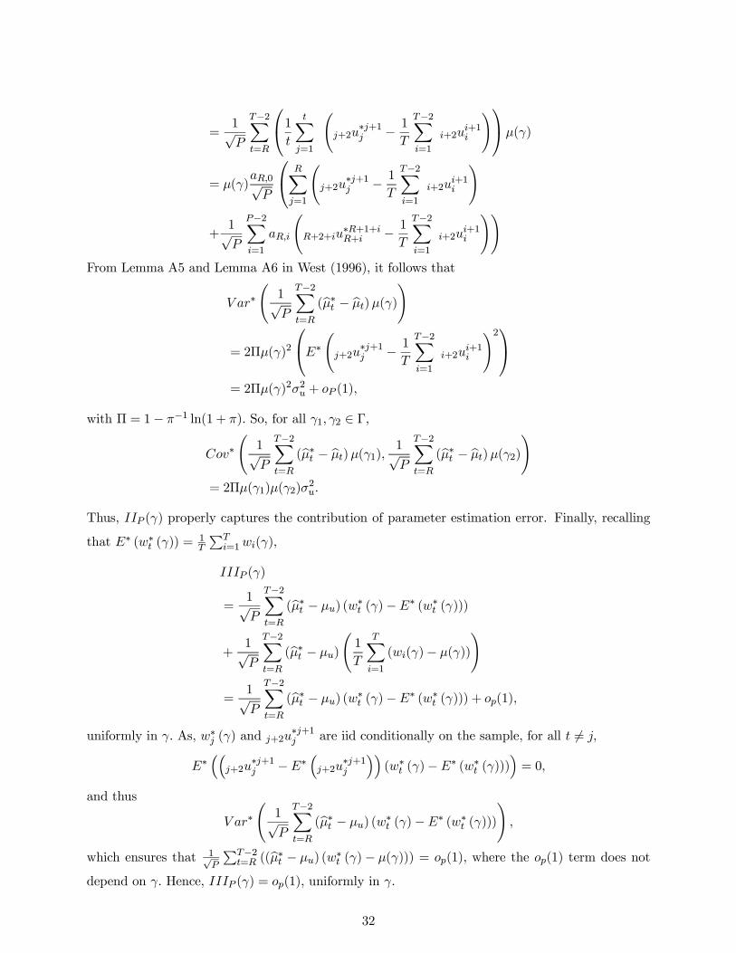
=1√P

T−2Xt=R

⎛⎝1t

tXj=1

Ãj+2u

∗j+1j − 1

T

T−2Xi=1

i+2ui+1i

!⎞⎠μ(γ)

= μ(γ)aR,0√P

⎛⎝ RXj=1

Ãj+2u

∗j+1j − 1

T

T−2Xi=1

i+2ui+1i

!

+1√P

P−2Xi=1

aR,i

ÃR+2+iu

∗R+1+iR+i − 1

T

T−2Xi=1

i+2ui+1i

!!From Lemma A5 and Lemma A6 in West (1996), it follows that

V ar∗Ã1√P

T−2Xt=R

(bμ∗t − bμt)μ(γ)!

= 2Πμ(γ)2

⎛⎝E∗Ãj+2u∗j+1j − 1

T

T−2Xi=1

i+2ui+1i

!2⎞⎠= 2Πμ(γ)2σ2u + oP (1),

with Π = 1− π−1 ln(1 + π). So, for all γ1, γ2 ∈ Γ,

Cov∗Ã1√P

T−2Xt=R

(bμ∗t − bμt)μ(γ1), 1√P

T−2Xt=R

(bμ∗t − bμt)μ(γ2)!

= 2Πμ(γ1)μ(γ2)σ2u.

Thus, IIP (γ) properly captures the contribution of parameter estimation error. Finally, recalling

that E∗ (w∗t (γ)) = 1T

PTi=1wi(γ),

IIIP (γ)

=1√P

T−2Xt=R

(bμ∗t − μu) (w∗t (γ)−E∗ (w∗t (γ)))

+1√P

T−2Xt=R

(bμ∗t − μu)

Ã1

T

TXi=1

(wi(γ)− μ(γ))

!

=1√P

T−2Xt=R

(bμ∗t − μu) (w∗t (γ)−E∗ (w∗t (γ))) + op(1),

uniformly in γ. As, w∗j (γ) and j+2u∗j+1j are iid conditionally on the sample, for all t 6= j,

E∗³³

j+2u∗j+1j −E∗

³j+2u

∗j+1j

´´(w∗t (γ)−E∗ (w∗t (γ)))

´= 0,

and thus

V ar∗Ã1√P

T−2Xt=R

(bμ∗t − μu) (w∗t (γ)−E∗ (w∗t (γ)))

!,

which ensures that 1√P

PT−2t=R ((bμ∗t − μu) (w∗t (γ)− μ(γ))) = op(1), where the op(1) term does not

depend on γ. Hence, IIIP (γ) = op(1), uniformly in γ.

32

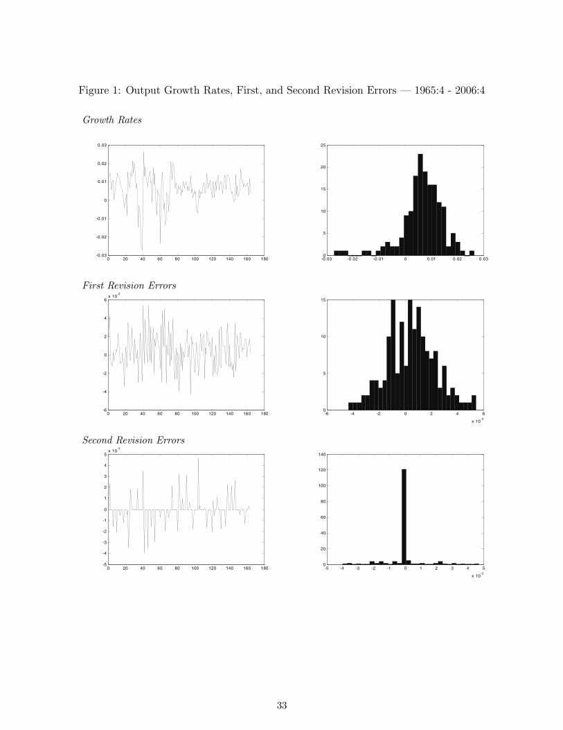
Figure 1: Output Growth Rates, First, and Second Revision Errors – 1965:4 - 2006:4

Growth Rates

0 20 40 60 80 100 120 140 160 180-0.03

-0.02

-0.01

0

0.01

0.02

0.03

-0.03 -0.02 -0.01 0 0.01 0.02 0.030

5

10

15

20

25

First Revision Errors

0 20 40 60 80 100 120 140 160 180-6

-4

-2

0

2

4

6x 10

-3

-6 -4 -2 0 2 4 6

x 10-3

0

5

10

15

Second Revision Errors

0 20 40 60 80 100 120 140 160 180-5

-4

-3

-2

-1

0

1

2

3

4

5x 10

-3

-5 -4 -3 -2 -1 0 1 2 3 4 5

x 10-3

0

20

40

60

80

100

120

140

33

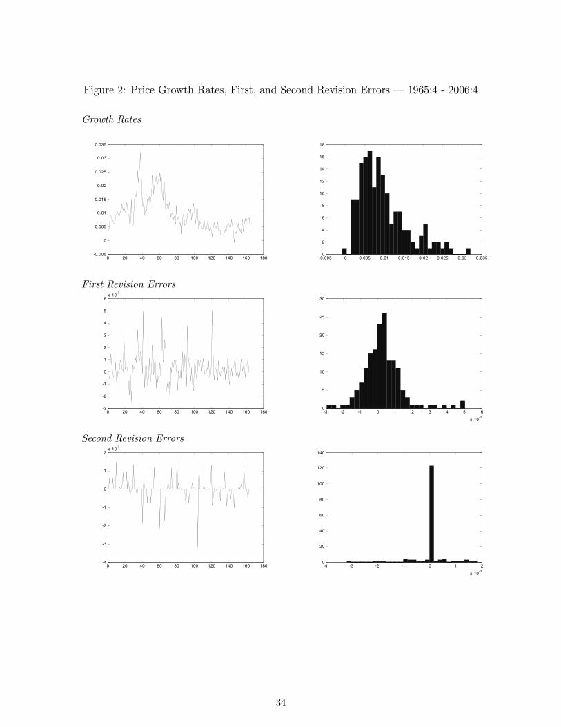
Figure 2: Price Growth Rates, First, and Second Revision Errors – 1965:4 - 2006:4

Growth Rates

0 20 40 60 80 100 120 140 160 180-0.005

0

0.005

0.01

0.015

0.02

0.025

0.03

0.035

-0.005 0 0.005 0.01 0.015 0.02 0.025 0.03 0.0350

2

4

6

8

10

12

14

16

18

First Revision Errors

0 20 40 60 80 100 120 140 160 180-3

-2

-1

0

1

2

3

4

5

6x 10

-3

-3 -2 -1 0 1 2 3 4 5 6

x 10-3

0

5

10

15

20

25

30

Second Revision Errors

0 20 40 60 80 100 120 140 160 180-4

-3

-2

-1

0

1

2x 10

-3

-4 -3 -2 -1 0 1 2

x 10-3

0

20

40

60

80

100

120

140

34

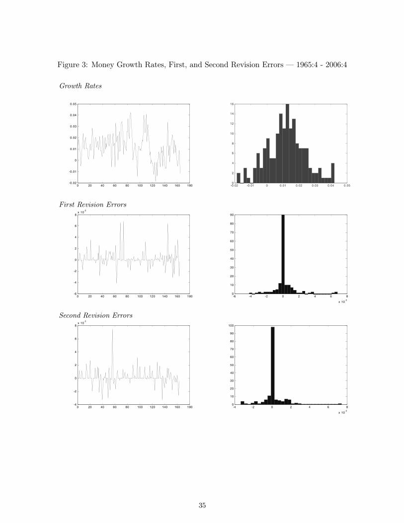
Figure 3: Money Growth Rates, First, and Second Revision Errors – 1965:4 - 2006:4

Growth Rates

0 20 40 60 80 100 120 140 160 180-0.02

-0.01

0

0.01

0.02

0.03

0.04

0.05

-0.02 -0.01 0 0.01 0.02 0.03 0.04 0.050

2

4

6

8

10

12

14

16

First Revision Errors

0 20 40 60 80 100 120 140 160 180-6

-4

-2

0

2

4

6

8x 10

-3

-6 -4 -2 0 2 4 6 8

x 10-3

0

10

20

30

40

50

60

70

80

90

Second Revision Errors

0 20 40 60 80 100 120 140 160 180-4

-2

0

2

4

6

8x 10

-3

-4 -2 0 2 4 6 8

x 10-3

0

10

20

30

40

50

60

70

80

90

100

35

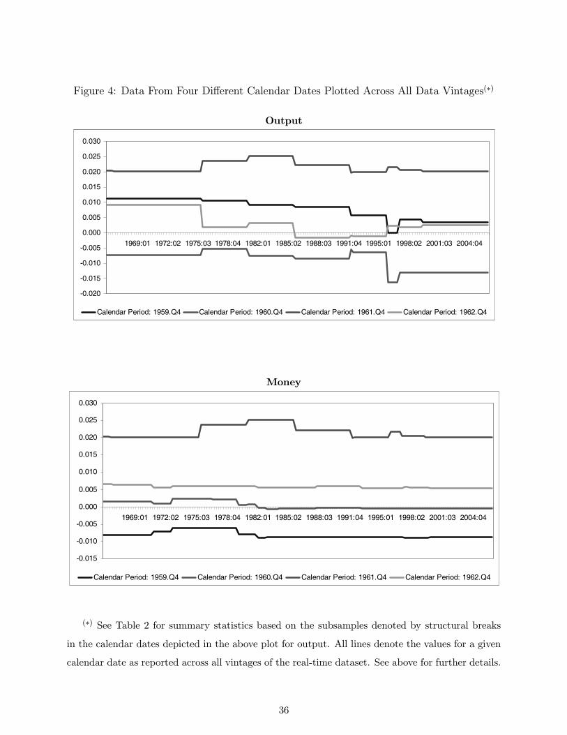
Figure 4: Data From Four Different Calendar Dates Plotted Across All Data Vintages(∗)

Output

-0.020

-0.015

-0.010

-0.005

0.000

0.005

0.010

0.015

0.020

0.025

0.030

1969:01 1972:02 1975:03 1978:04 1982:01 1985:02 1988:03 1991:04 1995:01 1998:02 2001:03 2004:04

Calendar Period: 1959.Q4 Calendar Period: 1960.Q4 Calendar Period: 1961.Q4 Calendar Period: 1962.Q4

Money

-0.015

-0.010

-0.005

0.000

0.005

0.010

0.015

0.020

0.025

0.030

1969:01 1972:02 1975:03 1978:04 1982:01 1985:02 1988:03 1991:04 1995:01 1998:02 2001:03 2004:04

Calendar Period: 1959.Q4 Calendar Period: 1960.Q4 Calendar Period: 1961.Q4 Calendar Period: 1962.Q4

(∗) See Table 2 for summary statistics based on the subsamples denoted by structural breaks

in the calendar dates depicted in the above plot for output. All lines denote the values for a given

calendar date as reported across all vintages of the real-time dataset. See above for further details.

36

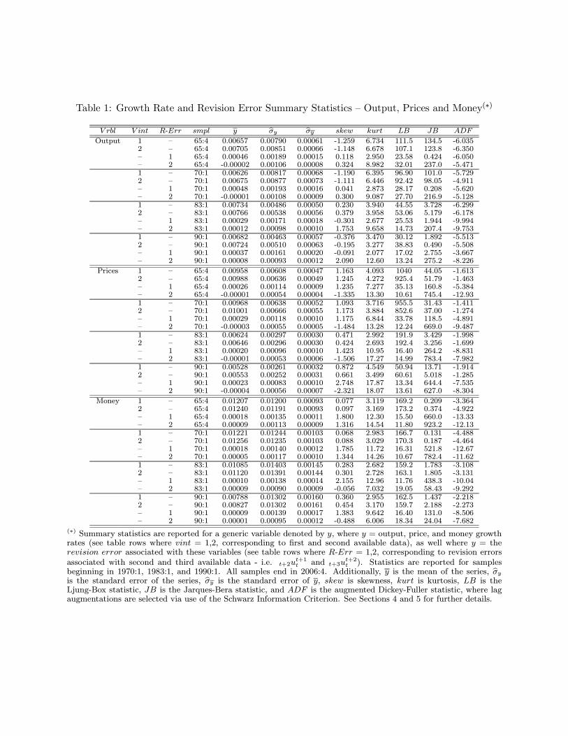
Table 1: Growth Rate and Revision Error Summary Statistics — Output, Prices and Money(∗)

V rbl V int R-Err smpl y bσy bσy skew kurt LB JB ADF

Output 1 — 65:4 0.00657 0.00790 0.00061 -1.259 6.734 111.5 134.5 -6.0352 — 65:4 0.00705 0.00851 0.00066 -1.148 6.678 107.1 123.8 -6.350— 1 65:4 0.00046 0.00189 0.00015 0.118 2.950 23.58 0.424 -6.050— 2 65:4 -0.00002 0.00106 0.00008 0.324 8.982 32.01 237.0 -5.4711 — 70:1 0.00626 0.00817 0.00068 -1.190 6.395 96.90 101.0 -5.7292 — 70:1 0.00675 0.00877 0.00073 -1.111 6.446 92.42 98.05 -4.911— 1 70:1 0.00048 0.00193 0.00016 0.041 2.873 28.17 0.208 -5.620— 2 70:1 -0.00001 0.00108 0.00009 0.300 9.087 27.70 216.9 -5.1281 — 83:1 0.00734 0.00486 0.00050 0.230 3.940 44.55 3.728 -6.2992 — 83:1 0.00766 0.00538 0.00056 0.379 3.958 53.06 5.179 -6.178— 1 83:1 0.00029 0.00171 0.00018 -0.301 2.677 25.53 1.944 -9.994— 2 83:1 0.00012 0.00098 0.00010 1.753 9.658 14.73 207.4 -9.7531 — 90:1 0.00682 0.00463 0.00057 -0.376 3.470 30.12 1.892 -5.5132 — 90:1 0.00724 0.00510 0.00063 -0.195 3.277 38.83 0.490 -5.508— 1 90:1 0.00037 0.00161 0.00020 -0.091 2.077 17.02 2.755 -3.667— 2 90:1 0.00008 0.00093 0.00012 2.090 12.60 13.24 275.2 -8.226

Prices 1 — 65:4 0.00958 0.00608 0.00047 1.163 4.093 1040 44.05 -1.6132 — 65:4 0.00988 0.00636 0.00049 1.245 4.272 925.4 51.79 -1.463— 1 65:4 0.00026 0.00114 0.00009 1.235 7.277 35.13 160.8 -5.384— 2 65:4 -0.00001 0.00054 0.00004 -1.335 13.30 10.61 745.4 -12.931 — 70:1 0.00968 0.00638 0.00052 1.093 3.716 955.5 31.43 -1.4112 — 70:1 0.01001 0.00666 0.00055 1.173 3.884 852.6 37.00 -1.274— 1 70:1 0.00029 0.00118 0.00010 1.175 6.844 33.78 118.5 -4.891— 2 70:1 -0.00003 0.00055 0.00005 -1.484 13.28 12.24 669.0 -9.4871 — 83:1 0.00624 0.00297 0.00030 0.471 2.992 191.9 3.429 -1.9982 — 83:1 0.00646 0.00296 0.00030 0.424 2.693 192.4 3.256 -1.699— 1 83:1 0.00020 0.00096 0.00010 1.423 10.95 16.40 264.2 -8.831— 2 83:1 -0.00001 0.00053 0.00006 -1.506 17.27 14.99 783.4 -7.9821 — 90:1 0.00528 0.00261 0.00032 0.872 4.549 50.94 13.71 -1.9142 — 90:1 0.00553 0.00252 0.00031 0.661 3.499 60.61 5.018 -1.285— 1 90:1 0.00023 0.00083 0.00010 2.748 17.87 13.34 644.4 -7.535— 2 90:1 -0.00004 0.00056 0.00007 -2.321 18.07 13.61 627.0 -8.304

Money 1 — 65:4 0.01207 0.01200 0.00093 0.077 3.119 169.2 0.209 -3.3642 — 65:4 0.01240 0.01191 0.00093 0.097 3.169 173.2 0.374 -4.922— 1 65:4 0.00018 0.00135 0.00011 1.800 12.30 15.50 660.0 -13.33— 2 65:4 0.00009 0.00113 0.00009 1.316 14.54 11.80 923.2 -12.131 — 70:1 0.01221 0.01244 0.00103 0.068 2.983 166.7 0.131 -4.4882 — 70:1 0.01256 0.01235 0.00103 0.088 3.029 170.3 0.187 -4.464— 1 70:1 0.00018 0.00140 0.00012 1.785 11.72 16.31 521.8 -12.67— 2 70:1 0.00005 0.00117 0.00010 1.344 14.26 10.67 782.4 -11.621 — 83:1 0.01085 0.01403 0.00145 0.283 2.682 159.2 1.783 -3.1082 — 83:1 0.01120 0.01391 0.00144 0.301 2.728 163.1 1.805 -3.131— 1 83:1 0.00010 0.00138 0.00014 2.155 12.96 11.76 438.3 -10.04— 2 83:1 0.00009 0.00090 0.00009 -0.056 7.032 19.05 58.43 -9.2921 — 90:1 0.00788 0.01302 0.00160 0.360 2.955 162.5 1.437 -2.2182 — 90:1 0.00827 0.01302 0.00161 0.454 3.170 159.7 2.188 -2.273— 1 90:1 0.00009 0.00139 0.00017 1.383 9.642 16.40 131.0 -8.506— 2 90:1 0.00001 0.00095 0.00012 -0.488 6.006 18.34 24.04 -7.682

(∗) Summary statistics are reported for a generic variable denoted by y, where y = output, price, and money growthrates (see table rows where vint = 1,2, corresponding to first and second available data), as well where y = therevision error associated with these variables (see table rows where R-Err = 1,2, corresponding to revision errorsassociated with second and third available data - i.e. t+2u

t+1t and t+3u

t+2t ). Statistics are reported for samples

beginning in 1970:1, 1983:1, and 1990:1. All samples end in 2006:4. Additionally, y is the mean of the series, bσyis the standard error of the series, bσy is the standard error of y, skew is skewness, kurt is kurtosis, LB is theLjung-Box statistic, JB is the Jarques-Bera statistic, and ADF is the augmented Dickey-Fuller statistic, where lagaugmentations are selected via use of the Schwarz Information Criterion. See Sections 4 and 5 for further details.

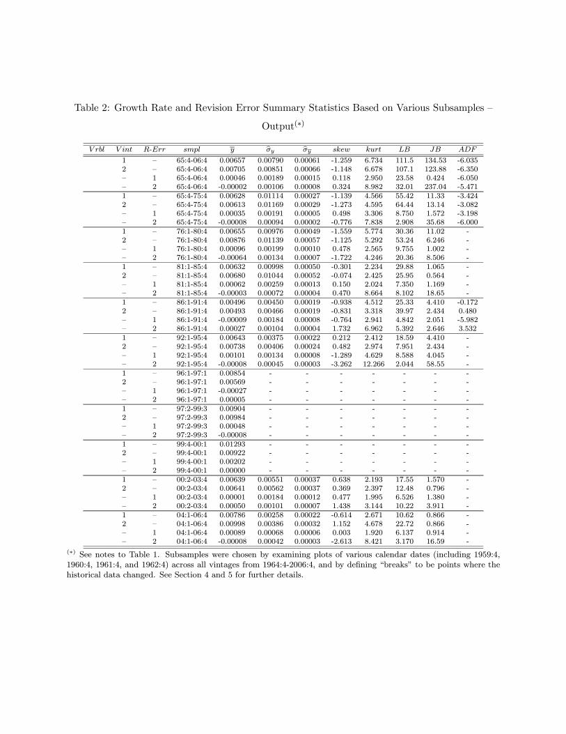
Table 2: Growth Rate and Revision Error Summary Statistics Based on Various Subsamples —

Output(∗)

V rbl V int R-Err smpl y bσy bσy skew kurt LB JB ADF

1 — 65:4-06:4 0.00657 0.00790 0.00061 -1.259 6.734 111.5 134.53 -6.0352 — 65:4-06:4 0.00705 0.00851 0.00066 -1.148 6.678 107.1 123.88 -6.350— 1 65:4-06:4 0.00046 0.00189 0.00015 0.118 2.950 23.58 0.424 -6.050— 2 65:4-06:4 -0.00002 0.00106 0.00008 0.324 8.982 32.01 237.04 -5.4711 — 65:4-75:4 0.00628 0.01114 0.00027 -1.139 4.566 55.42 11.33 -3.4242 — 65:4-75:4 0.00613 0.01169 0.00029 -1.273 4.595 64.44 13.14 -3.082— 1 65:4-75:4 0.00035 0.00191 0.00005 0.498 3.306 8.750 1.572 -3.198— 2 65:4-75:4 -0.00008 0.00094 0.00002 -0.776 7.838 2.908 35.68 -6.0001 — 76:1-80:4 0.00655 0.00976 0.00049 -1.559 5.774 30.36 11.02 -2 — 76:1-80:4 0.00876 0.01139 0.00057 -1.125 5.292 53.24 6.246 -— 1 76:1-80:4 0.00096 0.00199 0.00010 0.478 2.565 9.755 1.002 -— 2 76:1-80:4 -0.00064 0.00134 0.00007 -1.722 4.246 20.36 8.506 -1 — 81:1-85:4 0.00632 0.00998 0.00050 -0.301 2.234 29.88 1.065 -2 — 81:1-85:4 0.00680 0.01044 0.00052 -0.074 2.425 25.95 0.564 -— 1 81:1-85:4 0.00062 0.00259 0.00013 0.150 2.024 7.350 1.169 -— 2 81:1-85:4 -0.00003 0.00072 0.00004 0.470 8.664 8.102 18.65 -1 — 86:1-91:4 0.00496 0.00450 0.00019 -0.938 4.512 25.33 4.410 -0.1722 — 86:1-91:4 0.00493 0.00466 0.00019 -0.831 3.318 39.97 2.434 0.480— 1 86:1-91:4 -0.00009 0.00184 0.00008 -0.764 2.941 4.842 2.051 -5.982— 2 86:1-91:4 0.00027 0.00104 0.00004 1.732 6.962 5.392 2.646 3.5321 — 92:1-95:4 0.00643 0.00375 0.00022 0.212 2.412 18.59 4.410 -2 — 92:1-95:4 0.00738 0.00406 0.00024 0.482 2.974 7.951 2.434 -— 1 92:1-95:4 0.00101 0.00134 0.00008 -1.289 4.629 8.588 4.045 -— 2 92:1-95:4 -0.00008 0.00045 0.00003 -3.262 12.266 2.044 58.55 -1 — 96:1-97:1 0.00854 - - - - - - -2 — 96:1-97:1 0.00569 - - - - - - -— 1 96:1-97:1 -0.00027 - - - - - - -— 2 96:1-97:1 0.00005 - - - - - - -1 — 97:2-99:3 0.00904 - - - - - - -2 — 97:2-99:3 0.00984 - - - - - - -— 1 97:2-99:3 0.00048 - - - - - - -— 2 97:2-99:3 -0.00008 - - - - - - -1 — 99:4-00:1 0.01293 - - - - - - -2 — 99:4-00:1 0.00922 - - - - - - -— 1 99:4-00:1 0.00202 - - - - - - -— 2 99:4-00:1 0.00000 - - - - - - -1 — 00:2-03:4 0.00639 0.00551 0.00037 0.638 2.193 17.55 1.570 -2 — 00:2-03:4 0.00641 0.00562 0.00037 0.369 2.397 12.48 0.796 -— 1 00:2-03:4 0.00001 0.00184 0.00012 0.477 1.995 6.526 1.380 -— 2 00:2-03:4 0.00050 0.00101 0.00007 1.438 3.144 10.22 3.911 -1 — 04:1-06:4 0.00786 0.00258 0.00022 -0.614 2.671 10.62 0.866 -2 — 04:1-06:4 0.00998 0.00386 0.00032 1.152 4.678 22.72 0.866 -— 1 04:1-06:4 0.00089 0.00068 0.00006 0.003 1.920 6.137 0.914 -— 2 04:1-06:4 -0.00008 0.00042 0.00003 -2.613 8.421 3.170 16.59 -

(∗) See notes to Table 1. Subsamples were chosen by examining plots of various calendar dates (including 1959:4,1960:4, 1961:4, and 1962:4) across all vintages from 1964:4-2006:4, and by defining “breaks” to be points where thehistorical data changed. See Section 4 and 5 for further details.

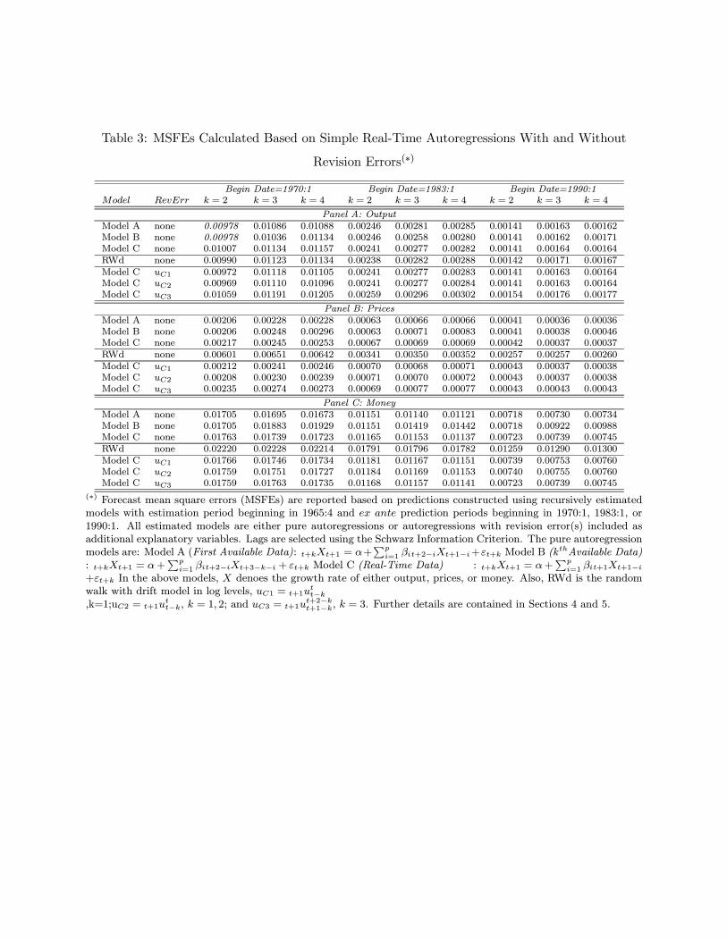
Table 3: MSFEs Calculated Based on Simple Real-Time Autoregressions With and Without

Revision Errors(∗)

Begin Date=1970:1 Begin Date=1983:1 Begin Date=1990:1Model RevErr k = 2 k = 3 k = 4 k = 2 k = 3 k = 4 k = 2 k = 3 k = 4

Panel A: OutputModel A none 0.00978 0.01086 0.01088 0.00246 0.00281 0.00285 0.00141 0.00163 0.00162Model B none 0.00978 0.01036 0.01134 0.00246 0.00258 0.00280 0.00141 0.00162 0.00171Model C none 0.01007 0.01134 0.01157 0.00241 0.00277 0.00282 0.00141 0.00164 0.00164RWd none 0.00990 0.01123 0.01134 0.00238 0.00282 0.00288 0.00142 0.00171 0.00167Model C uC1 0.00972 0.01118 0.01105 0.00241 0.00277 0.00283 0.00141 0.00163 0.00164Model C uC2 0.00969 0.01110 0.01096 0.00241 0.00277 0.00284 0.00141 0.00163 0.00164Model C uC3 0.01059 0.01191 0.01205 0.00259 0.00296 0.00302 0.00154 0.00176 0.00177

Panel B: PricesModel A none 0.00206 0.00228 0.00228 0.00063 0.00066 0.00066 0.00041 0.00036 0.00036Model B none 0.00206 0.00248 0.00296 0.00063 0.00071 0.00083 0.00041 0.00038 0.00046Model C none 0.00217 0.00245 0.00253 0.00067 0.00069 0.00069 0.00042 0.00037 0.00037RWd none 0.00601 0.00651 0.00642 0.00341 0.00350 0.00352 0.00257 0.00257 0.00260Model C uC1 0.00212 0.00241 0.00246 0.00070 0.00068 0.00071 0.00043 0.00037 0.00038Model C uC2 0.00208 0.00230 0.00239 0.00071 0.00070 0.00072 0.00043 0.00037 0.00038Model C uC3 0.00235 0.00274 0.00273 0.00069 0.00077 0.00077 0.00043 0.00043 0.00043

Panel C: MoneyModel A none 0.01705 0.01695 0.01673 0.01151 0.01140 0.01121 0.00718 0.00730 0.00734Model B none 0.01705 0.01883 0.01929 0.01151 0.01419 0.01442 0.00718 0.00922 0.00988Model C none 0.01763 0.01739 0.01723 0.01165 0.01153 0.01137 0.00723 0.00739 0.00745RWd none 0.02220 0.02228 0.02214 0.01791 0.01796 0.01782 0.01259 0.01290 0.01300Model C uC1 0.01766 0.01746 0.01734 0.01181 0.01167 0.01151 0.00739 0.00753 0.00760Model C uC2 0.01759 0.01751 0.01727 0.01184 0.01169 0.01153 0.00740 0.00755 0.00760Model C uC3 0.01759 0.01763 0.01735 0.01168 0.01157 0.01141 0.00723 0.00739 0.00745

(∗) Forecast mean square errors (MSFEs) are reported based on predictions constructed using recursively estimatedmodels with estimation period beginning in 1965:4 and ex ante prediction periods beginning in 1970:1, 1983:1, or1990:1. All estimated models are either pure autoregressions or autoregressions with revision error(s) included asadditional explanatory variables. Lags are selected using the Schwarz Information Criterion. The pure autoregressionmodels are: Model A (First Available Data): t+kXt+1 = α+

Ppi=1 βit+2−iXt+1−i+εt+k Model B (k

thAvailable Data): t+kXt+1 = α+

Ppi=1 βit+2−iXt+3−k−i + εt+k Model C (Real-Time Data) : t+kXt+1 = α+

Ppi=1 βit+1Xt+1−i

+εt+k In the above models, X denoes the growth rate of either output, prices, or money. Also, RWd is the randomwalk with drift model in log levels, uC1 = t+1u

tt−k

,k=1;uC2 = t+1utt−k, k = 1, 2; and uC3 = t+1u

t+2−kt+1−k, k = 3. Further details are contained in Sections 4 and 5.

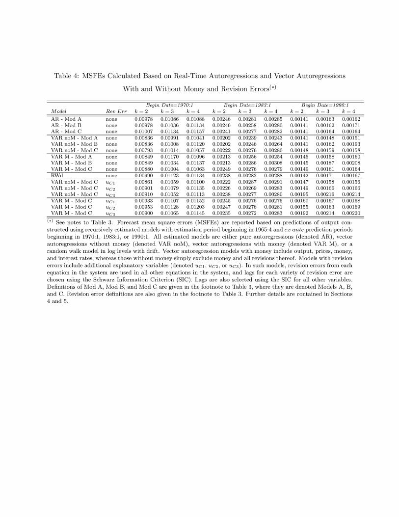
Table 4: MSFEs Calculated Based on Real-Time Autoregressions and Vector Autoregressions

With and Without Money and Revision Errors(∗)

Begin Date=1970:1 Begin Date=1983:1 Begin Date=1990:1Model Rev Err k = 2 k = 3 k = 4 k = 2 k = 3 k = 4 k = 2 k = 3 k = 4

AR - Mod A none 0.00978 0.01086 0.01088 0.00246 0.00281 0.00285 0.00141 0.00163 0.00162AR - Mod B none 0.00978 0.01036 0.01134 0.00246 0.00258 0.00280 0.00141 0.00162 0.00171AR - Mod C none 0.01007 0.01134 0.01157 0.00241 0.00277 0.00282 0.00141 0.00164 0.00164VAR noM - Mod A none 0.00836 0.00991 0.01041 0.00202 0.00239 0.00243 0.00141 0.00148 0.00151VAR noM - Mod B none 0.00836 0.01008 0.01120 0.00202 0.00246 0.00264 0.00141 0.00162 0.00193VAR noM - Mod C none 0.00793 0.01014 0.01057 0.00222 0.00276 0.00280 0.00148 0.00159 0.00158VAR M - Mod A none 0.00849 0.01170 0.01096 0.00213 0.00256 0.00254 0.00145 0.00158 0.00160VAR M - Mod B none 0.00849 0.01034 0.01137 0.00213 0.00286 0.00308 0.00145 0.00187 0.00208VAR M - Mod C none 0.00880 0.01004 0.01063 0.00249 0.00276 0.00279 0.00149 0.00161 0.00164RWd none 0.00990 0.01123 0.01134 0.00238 0.00282 0.00288 0.00142 0.00171 0.00167VAR noM - Mod C uC1 0.00861 0.01059 0.01100 0.00222 0.00287 0.00291 0.00147 0.00158 0.00156VAR noM - Mod C uC2 0.00901 0.01079 0.01135 0.00226 0.00269 0.00283 0.00149 0.00166 0.00166VAR noM - Mod C uC3 0.00910 0.01052 0.01113 0.00238 0.00277 0.00280 0.00195 0.00216 0.00214VAR M - Mod C uC1 0.00933 0.01107 0.01152 0.00245 0.00276 0.00275 0.00160 0.00167 0.00168VAR M - Mod C uC2 0.00953 0.01128 0.01203 0.00247 0.00276 0.00281 0.00155 0.00163 0.00169VAR M - Mod C uC3 0.00900 0.01065 0.01145 0.00235 0.00272 0.00283 0.00192 0.00214 0.00220

(∗) See notes to Table 3. Forecast mean square errors (MSFEs) are reported based on predictions of output con-structed using recursively estimated models with estimation period beginning in 1965:4 and ex ante prediction periodsbeginning in 1970:1, 1983:1, or 1990:1. All estimated models are either pure autoregressions (denoted AR), vectorautoregressions without money (denoted VAR noM), vector autoregressions with money (denoted VAR M), or arandom walk model in log levels with drift. Vector autoregression models with money include output, prices, money,and interest rates, whereas those without money simply exclude money and all revisions thereof. Models with revisionerrors include additional explanatory variables (denoted uC1, uC2, or uC3). In such models, revision errors from eachequation in the system are used in all other equations in the system, and lags for each variety of revision error arechosen using the Schwarz Information Criterion (SIC). Lags are also selected using the SIC for all other variables.Definitions of Mod A, Mod B, and Mod C are given in the footnote to Table 3, where they are denoted Models A, B,and C. Revision error definitions are also given in the footnote to Table 3. Further details are contained in Sections4 and 5.

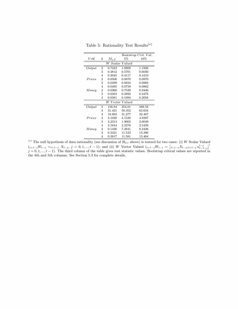
Table 5: Rationality Test Results(∗)

Bootstrap Crit. V al.V rbl k M1,T 5% 10%

W Scalar V alued

Output 2 0.7243 1.0808 1.19263 0.3812 0.5701 0.60304 0.3045 0.4117 0.4410

Prices 2 0.0506 0.0870 0.09703 0.0499 0.0824 0.08684 0.0495 0.0759 0.0862

Money 2 0.0366 0.7539 0.94463 0.0283 0.2893 0.34784 0.0381 0.1894 0.2058

W V ector V alued

Output 2 156.84 354.01 388.583 31.431 58.352 63.6344 19.863 31.277 32.487

Prices 2 3.1020 4.1520 4.93973 3.2314 1.9002 2.00494 3.1644 2.2276 2.5439

Money 2 0.1436 7.2841 8.24263 0.3421 11.533 13.3964 0.3817 11.581 13.464

(∗) The null hypothesis of data rationality (see discussion of H0,1 above) is testsed for two cases: (i) W Scalar Valued

(t+1−jWt−j =t+1−j Xt−j , j = 0, 1, ..., t − 1); and (ii) W Vector Valued (t+1−jWt−j =£t+1−jXt−j ,t+1−j u

t−jt−1−j

¤0j = 0, 1, ..., t− 1). The third column of the table gives test statistic values. Bootstrap critical values are reported inthe 4th and 5th columns. See Section 5.3 for complete details.