information compliance officer - whatdotheyknow
TRANSCRIPT

Dr James Knapton
Information Compliance Officer
Peter Alexander
By email
Reference: FOI-2018-272
1 May 2018
Dear Mr Alexander,
Your request was received on 12 April 2018 and I am dealing with it under the terms of the Freedom of
Information Act 2000 (‘the Act’).
You asked:
Could you please release the exam papers for the core and optional modules offered in MPhil
Economics and MPhil Economic Research, for the academic years 2015-2016 and 2016-2017?
The requested information is attached. Please note that the attached documentation should not be
copied, reproduced or used except in accordance with the law of copyright.
If you are unhappy with the service you have received in relation to your request and wish to make a
complaint or request an internal review of this decision, you should write to Dr Kirsty Allen, Head of the
Registrary’s Office, quoting the reference above, at The Old Schools, Trinity Lane, Cambridge, CB2
1TN or send an email marked for her attention to [email protected]. The University would normally
expect to receive your request for an internal review within 40 working days of the date of this letter and
reserves the right not to review a decision where there has been undue delay in raising a complaint. If
you are not content with the outcome of your review, you may apply directly to the Information
Commissioner for a decision. Generally, the Information Commissioner cannot make a decision unless
you have exhausted the complaints procedure provided by the University. The Information
Commissioner may be contacted at: The Information Commissioner’s Office, Wycliffe House, Water
Lane, Wilmslow, Cheshire, SK9 5AF (https://ico.org.uk/).
The Old Schools
Trinity Lane
Cambridge, CB2 1TN
Tel: +44 (0) 1223 764142
Fax: +44 (0) 1223 332332
Email: [email protected]
www.cam.ac.uk

Yours sincerely,
James Knapton

ECM9/ECM10/ECM11/MGM3MPhil in EconomicsMPhil in Economic ResearchMPhil in Finance and EconomicsMPhil Finance
Wednesday 11 January 2017 10:00-12:00
M100MICROECONOMICS I
Candidates are required to answer three out of four questions
Write your candidate number (not your name) on the cover of each booklet.
Write legibly.
If you identify an error in this paper, please alert the Invigilator, who will notifythe Examiner. A general announcement will be made if the error is validated.
STATIONERY REQUIREMENTS20 Page booklet x 1Rough work pads
SPECIAL REQUIREMENTS TO BE SUPPLIED FOR THISEXAMINATIONCalculator - students are permitted to bring an approved calculator
You may not start to read the questions printedon the subsequent pages of this question paper
until instructed that you may do so by the Invigilator.
1 of 3

1. Consider an agent with initial wealth w who plans to bid in a first price sealed bid auction (i.e., anauction in which everyone submits a bid simultaneously and the highest bid wins). The value sheassigns to the item being auctioned is v. She believes that if she submits a bid b, she will win withprobability G(b), where G is continuous, differentiable, and strictly increasing function. The agent’swealth will be either w + v − b if she wins or w if she loses. Her (Bernouli) utility over final wealthis u(x), where u is continuous and differentiable with u′(0) > 0 and u′′(0) < 0. You can assume thatlogG(b) is concave in b and that optimal bids are always interior.
(i) Write down the agent’s expected utility.
(ii) Set up the agent’s problem and show that optimal bid b∗ is characterized by:
u′(w + v − b∗)
u(w + v − b∗) − u(w)=G′(b∗)
G(b∗).
(iii) Using implicit differentiation and the log concavity of G, show that the agent bids strictly morefor an object she values more (higher v). [Note: This is the hardest part of this question. You donot need to answer this part to be able to answer the remaining parts of the question].
(iv) Suppose G(b) = b(0.5) and the agent is risk neutral. Find an expression for the amount the agentoptimally bids in terms of just v.
(v) Continuing to let G(b) = b(0.5) suppose the agent is risk averse. Does the agent bid more or lessthan when risk neutral?
2. Consider an economy with two agents and two goods: a numeraire good and houses. Agents i = 1, 2are endowed with ei units of the numeraire. We will assume that e1 ≥ e2. There is a single house andthe agents initially own equal shares of it. However, the house must be owned in full by an agent foran agent to consume it (and derive any utility from it). The agents have identical preferences. Agenti’s utility from consuming ci units of the numeraire and si = 1, 0 units of houses is u(ci, si), wheredu(ci,si)
dci> 0, d2u(ci,si)
dc2i< 0, u(c, 1) − u(c, 0) > 0 and du(c,1)
dc > du(c,0)dc . Negative consumption of the
numeraire good is permitted and you can normalise its price to 1. Let p be the price of a house.
(i) Write down agent i’s constrained optimisation problem.
(ii) Given the house can only be consumed as a whole, what does it mean for houses to be a normalgood?
(iii) Show that houses are a normal good.
(iv) Hence argue that if e1 > e2, agent 1 will own the house in a Walrasian equilibrium.
(v) Find a Walrasian equilibrium of the economy.
(vi) Are there are multiple Walrasian equilibria? If so, show that there exist multiple Walrasianequilibria, if not, show that there is a unique Walrasian equilibrium. Then provide some intuitionfor your answer.
2 of 3

(i) In the context of the two-good economy define (a) complete preferences, (b) transitive preferences,(c) continuous preferences and (d) monotonic preferences.
(ii) Identify graphically the set of consumption bundles that the consumer must weakly prefer to x.
(iii) If the consumer’s preferences are also convex, how does your answer to (ii) change?
(iv) Suppose that in addition to the two marketed goods, there is also a third good whose level is fixedin the short run. If the consumer’s choices between the first two goods are not affected by thefixed level x3 of the third good, what can be inferred about the utility function u(x1, x2, x3).
4. There are three goods labeled 1, 2 and 3. Consider the following three possible consumption bundlesxA = (1, 3, 2), xB = (2, 2, 2) and xC = (2, 2, 1).
(i) Suppose Consumer A is rational. At prices pA = (2, 1, 1), you observe him choose xA. Atprices pB = (1, 2, 1), you observe him choose xB . Now he has wealth w = 7 and faces pricesp = (1, 1.5, 1). Can you say for certain if any of the bundles will or will not be chosen? What ifA’s preferences are also locally non-satiated?
(ii) Suppose Consumer B has the following indirect utility function
v(p1, p2, w) =
(w
p1
) 14(w
p2
) 34
.
(a) Calculate the expenditure function e(p1, p2, u).
(b) Calculate the Hicksian demand functions h1(p1, p2, u) and h2(p1, p2, u).
(iii) Suppose Consumer C has rational, continuous and locally non-satiated preferences, and that herpreferences are also homothetic, (i.e. if x ∼ x′ then αx ∼ αx′). What can you conclude abouthow Consumer C’s Marshallian demand x(p, w) will vary with w?
3 of 3
3. Consider a two-good economy and a consumer with complete, transitive, continuous, and monotonicpreferences. Prices in this economy are always strictly positive. Suppose the consumer has wealthw = 9. You know that at prices p = (2, 1), the consumer’s unique preferred bundle is x = (3, 3) and atprices p′ = (1, 2), the consumer’s unique preferred bundle is x′ = (5, 2).
END OF PAPER

ECM9/ECM10/ECM11/MGM3MPhil in EconomicsMPhil in Economic ResearchMPhil in Finance and EconomicsMPhil Finance
Monday 8 May 2017 02:00pm - 04:00pm
M100MICROECONOMICS I
Candidates are required to answer three out of four questions
Write your candidate number (not your name) on the cover of each booklet.
Write legibly.
STATIONERY REQUIREMENTS20 Page booklet x 1Rough work pads
SPECIAL REQUIREMENTS TO BE SUPPLIED FOR THISEXAMINATIONCalculator - students are permitted to bring an approved calculator
You may not start to read the questions printed on the subsequentpages of this question paper until instructed that you may do so by theInvigilator.
1 of 3
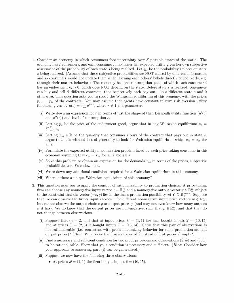
1. Consider an economy in which consumers face uncertainty over S possible states of the world. Theeconomy has I consumers, and each consumer i maximizes her expected utility given her own subjectiveassessment of the probability of each state s being realized. Let qis be the probability i places on states being realized. (Assume that these subjective probabilities are NOT caused by different informationand so consumers would not update them when learning each others’ beliefs directly or indirectly, e.g.through their market behavior.) The economy has one consumption good, of which each consumer ihas an endowment ei > 0, which does NOT depend on the state. Before state s is realized, consumerscan buy and sell S different contracts, that respectively each pay out 1 in a different state s and 0otherwise. This question asks you to study the Walrasian equilibrium of this economy, with the pricesp1, . . . , pS of the contracts. You may assume that agents have constant relative risk aversion utilityfunctions given by u(c) = 1
1−r c1−r, where r 6= 1 is a parameter.
(i) Write down an expression for r in terms of just the shape of then Bernoulli utility function (u′(c)and u′′(c)) and level of consumption c.
(ii) Letting pe be the price of the endowment good, argue that in any Walrasian equilibrium pe =∑Ss=1 ps.
(iii) Letting xis ∈ R be the quantity that consumer i buys of the contract that pays out in state s,argue that it is without loss of generality to look for Walrasian equilibria in which cis = xis forall s.
(iv) Formulate the expected utility maximization problem faced by each price-taking consumer in this economy assuming that cis = xis for all i and all s.
(v) Solve this problem to obtain an expression for the demands xis in terms of the prices, subjectiveprobabilities and i’s endowment.
(vi) Write down any additional conditions required for a Walrasian equilibrium in this economy.
(vii) When is there a unique Walrasian equilibrium of this economy?
2. This question asks you to apply the concept of rationalizability to production choices. A price-takingfirm can choose any nonnegative input vector z ∈ Rm
+ and a nonnegative output vector y ∈ Rn+ subject
to the constraint that the vector (−z, y) lies in the firm’s production possibility set Y ⊆ Rm+n+ . Suppose
that we can observe the firm’s input choices z for different nonnegative input price vectors w ∈ Rm+ ,
but cannot observe the output choices y or output prices p (and may not even know how many outputsn it has). We do know that the output prices are non-negative, such that p ∈ Rn
+, and that they donot change between observations.
(i) Suppose that m = 2, and that at input prices w = (1, 1) the firm bought inputs z = (10, 15)and at prices w = (2, 3) it bought inputs z = (13, 14). Show that this pair of observations isnot rationalizable (i.e. consistent with profit-maximizing behavior for some production set andoutput prices)? (Hint: What does the firm’s choices of z instead of z at prices w imply?)
(ii) Find a necessary and sufficient condition for two input price-demand observations (z, w) and (z, w)to be rationalizable. Show that your condition is necessary and sufficient. (Hint: Consider howyour approach to answering part (i) can be generalized.)
(iii) Suppose we now have the following three observations:
• At prices w = (1, 1) the firm bought inputs z = (10, 15).
2 of 3
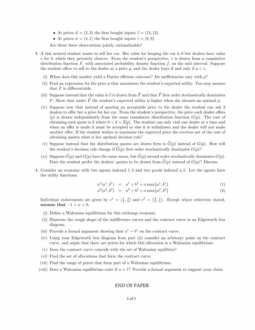
• At prices w = (2, 3) the firm bought inputs z = (13, 13).
• At prices w = (4, 1) the firm bought inputs z = (8, 9).
Are these three observations jointly rationalizable?
3. A risk neutral student wants to sell her car. Her value for keeping the car is 0 but dealers have valuev for it which they privately observe. From the student’s perspective, v is drawn from a cumulativedistribution function F , with associated probability density function f , on the unit interval. Supposethe student offers to sell to the dealer at a price p, and the dealer buys if and only if p < v.
(i) When does this market yield a Pareto efficient outcome? Do inefficiencies vary with p?
(ii) Find an expression for the price p that maximizes the student’s expected utility. You may assumethat F is differentiable.
(iii) Suppose instead that the value is v is drawn from F and that F first order stochastically dominates
F . Show that under F the student’s expected utility is higher when she chooses an optimal p.
(iv) Suppose now that instead of quoting an acceptable price to the dealer the student can ask 2dealers to offer her a price for her car. From the student’s perspective, the price each dealer offers(p) is drawn independently from the same cumulative distribution function G(p). The cost ofobtaining each quote is k where 0 < k < E[p]. The student can only visit one dealer at a time andwhen an offer is made it must be accepted or else it is withdrawn and the dealer will not makeanother offer. If the student wishes to maximize the expected price she receives net of the cost ofobtaining quotes what is her optimal decision rule?
(v) Suppose instead that the distribution quotes are drawn form is G(p) instead of G(p). How will
the student’s decision rule change if G(p) first order stochastically dominates G(p)?
(vi) Suppose G(p) and G(p) have the same mean, but G(p) second order stochastically dominates G(p).
Does the student prefer the dealers’ quotes to be drawn from G(p) instead of G(p)? Discuss.
4. Consider an economy with two agents indexed 1, 2 and two goods indexed a, b. Let the agents havethe utility functions:
u1(a1, b1) = a1 + b1 + αmaxa1, b1 (1)
u2(a2, b2) = a2 + b2 + αmaxa2, b2 (2)
Individual endowments are given by e1 = (15 ,
45 ) and e2 = (4
5 ,15 ). Except where otherwise stated,
assume that −1 < α < 0.
(i) Define a Walrasian equilibrium for this exchange economy.
(ii) Illustrate the rough shape of the indifference curves and the contract curve in an Edgeworth boxdiagram.
(iii) Provide a formal argument showing that a1 = b1 on the contract curve.
(iv) Using your Edgeworth box diagram from part (ii) consider an arbitrary point on the contractcurve, and argue that there are prices for which this allocation is a Walrasian equilibrium.
(v) Does the contract curve coincide with the set of Walrasian equilibria?
(vi) Find the set of allocations that form the contract curve.
(vii) Find the range of prices that form part of a Walrasian equilibrium.
(viii) Does a Walrasian equilibrium exist if α = 1? Provide a formal argument to support your claim.
3 of 3
END OF PAPER

ECM9/ECM10/ECM11MPhil in EconomicsMPhil in Finance & EconomicsMPhil in Economic Research
Tuesday 23 May 2017 9:00am - 11:00am
M110MICROECONOMICS II
Candidates are required to answer three out of four questions.
Write your candidate number (not your name) on the cover of each booklet.
Write legibly.
If you identify an error in this paper, please alert the Invigilator, who will notifythe Examiner. A general announcement will be made if the error is validated.
STATIONERY REQUIREMENTS20 Page booklet x 1Rough work pads
SPECIAL REQUIREMENTS TO BE SUPPLIED FOR THISEXAMINATIONCalculator - students are permitted to bring an approved calculator
You may not start to read the questions printedon the subsequent pages of this question paper
until instructed that you may do so by the Invigilator.
1 of 5

1. (a) Consider the following two-player game
1/2 A B C
A a, b 1,1 c, dB 1,1 0,0 1,1
C e, f 1,1 g, h
where a, b, c, d, e, f, g, h are arbitrary payoffs such that a+ e > 2, c+ g > 2, b+3d > 4and f + 3h > 4.
i. Show that for each player strategy B is strictly dominated by another strategy
(possibly a mixed one).
ii. Show that the above game has a pure or a mixed strategy Nash equilibrium.
(Hint: First, consider cases in which at least one player has a dominant strategy. Then
consider the case in which no player has a dominant strategy.)
(b) Consider a game in which each player i = 1, .., n chooses a real number si in the
interval [0, 1] once and simultaneously. Let πi(s1, .., sn) be the payoff of player i if the
players choose a strategy profile (s1, ..., sn). Suppose πi(s1, .., sn) is differentiable.
Explain why, in general, any non-interior Nash equilibrium of this game is Pareto
inefficient.
(c) By means of an example or otherwise show that rational players do not necessarily
choose a Nash equilibrium in complete information normal form games.
(d) Discuss the assumptions needed to justify the concept of Nash equilibrium (both pure
and mixed) in games of complete information.
2 of 5
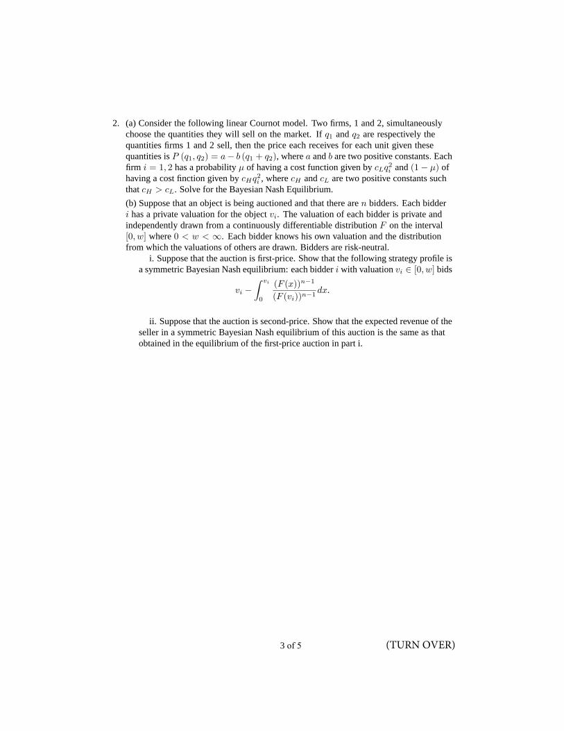
2. (a) Consider the following linear Cournot model. Two firms, 1 and 2, simultaneously
choose the quantities they will sell on the market. If q1 and q2 are respectively the
quantities firms 1 and 2 sell, then the price each receives for each unit given these
quantities is P (q1, q2) = a− b (q1 + q2), where a and b are two positive constants. Each
firm i = 1, 2 has a probability µ of having a cost function given by cLq2i and (1− µ) of
having a cost finction given by cHq2i , where cH and cL are two positive constants such
that cH > cL. Solve for the Bayesian Nash Equilibrium.
(b) Suppose that an object is being auctioned and that there are n bidders. Each bidder
i has a private valuation for the object vi. The valuation of each bidder is private and
independently drawn from a continuously differentiable distribution F on the interval
[0, w] where 0 < w < ∞. Each bidder knows his own valuation and the distribution
from which the valuations of others are drawn. Bidders are risk-neutral.
i. Suppose that the auction is first-price. Show that the following strategy profile is
a symmetric Bayesian Nash equilibrium: each bidder i with valuation vi ∈ [0, w] bids
vi −∫ vi
0
(F (x))n−1
(F (vi))n−1dx.
ii. Suppose that the auction is second-price. Show that the expected revenue of the
seller in a symmetric Bayesian Nash equilibrium of this auction is the same as that
obtained in the equilibrium of the first-price auction in part i.
3 of 5 (TURN OVER)

3. (a) Show that any game with a finite number of pure strategies has a mixed Nash
equilibrium. (You may assume the following result: any normal form game has a Nash
equilibrium if the set of strategies for every player is convex and compact and the payoff
function for each player i is quasi-concave in i′s strategy and continuous in the strategies
of all players). Hence, explain briefly why every finite extensive form game has a mixed
subgame perfect equilibrium strategy.
(b) Consider a 2-player game G described by the following payoff matrix:
A B CA 3, 3 0, 4 3, 0B 4, 0 0, 0 c, dC 0, 3 a, b 0, 0
for some paramters a, b, c and d. Assume that the players are restricted to using pure
strategies.
i. Assume that a > c + 1 , c > 3, b > 3 and 1 > d > 0. Compute the set of
Nash equilibria of G. Suppose that G in part (b) is played twice, the players do not
discount the future and there is perfect monitoring. Show that there exists a subgame
perfect equilibrium such that both players choose A in period 1. Are there any
subgame perfect equilibrium that results in outcome (B,A) or (A,B) in period 1 for
these paramater values?
ii. Assume that a = d = 1 and b = c = 4. Compute the set of Nash equilibrium
of G. Suppose that G is infinitely repeated and the players discount the future by a
factor δ < 1. Show that there exists a subgame perfect equilibrium that induces the
outcome (A,A) at every period on the equilibrium path if δ is sufficiently close to
1. Are there any subgame perfect equilibrium that results in the following cyclical
equilibrium path: play (B,A) at odd periods and (A,B) at even periods?
iii. Assume that a = d = 1 and b = c = 2. Does the game G have a Nash
equilibrium? What are the minmax payoffs for each player? Suppose that G is
infinitely repeated and the players discount the future by a factor δ < 1. Does there
exist a subgame perfect equilibrium that induces the outcome (A,A) at every period
on the equilibrium path for δ sufficiently close to 1? Explain your answer.
4 of 5

4. (a) Consider the following ultimatum 2-player bargaining game over a pie of size 2.
First, Player 1 makes an offer of 0, 1 or 2. Next player 2 responds to the offer of player
1 by either accepting or rejecting the offer. If an offer x = 0, 1, 2 is made and Player 2
accepts then the game ends and the payoffs of 1 and 2 are respectively x and 2 − x. If
Player 2 rejects an offer the game ends and each players payoff will be zero.
Describe both the extensive and the normal form representations of the above game.
What are the Nash equilibria and the subgame perfect equilibria of this game? Is there a
Nash equilibrium that is not credible? If so, explain why this is the case.
(b) Consider the following extensive form game.
i. Show that there does not exist a pure-strategy perfect Bayesian equilibrium in
this extensive form game.
ii. Describe the mixed-strategy perfect Bayesian equilibria of the game.
(c) Explain why perfect Bayesian equilibrium may not be always a reasonable solution
concept in dynamic games of imperfect information. Discuss briefly how one may
refine the concept of perfect Baysian equilibrium to make it a more reasonable solution
concept.
5 of 5
END OF PAPER

ECM9/ECM10/ECM11MPhil in EconomicsMPhil in Finance & EconomicsMPhil in Economic Research
Thursday 1 June 2017 1:30pm - 3:30pm
M120TOPICS IN ECONOMIC THEORY
Candidates are required to answer three out of four questions
Write your candidate number (not your name) on the cover of each booklet.
Write legibly.
If you identify an error in this paper, please alert the Invigilator, who will notifythe Examiner. A general announcement will be made if the error is validated.
STATIONERY REQUIREMENTS20 Page booklet x 1Rough work pads
SPECIAL REQUIREMENTS TO BE SUPPLIED FOR THISEXAMINATIONCalculator - students are permitted to bring an approved calculator
You may not start to read the questions printedon the subsequent pages of this question paper
until instructed that you may do so by the Invigilator.
1 of 5

1. a. Consider the infinite horizon alternating bargaining game with 2 players (Rubinstein
model). The size of the pie is 1. The rules are in odd periods player 1 makes an offer
of a split x ∈ [0, 1] to player 2, which player 2 may accept or reject and in even
periods player 2 makes an offer of a split to player 1, which player 1 may accept or
reject. If at any period a player accepts an offer, the proposed split is immediately
implemented and the game ends. If she rejects, nothing happens until the next period.
Assume that each player i discounts future payoffs by a common factor δ < 1.
i. Show there exists a subgame perfect equilibrium with the following outcome:
there is agreement at the first date and the players receive a unique payoff
described by the following split: player 1 receives 11+δ and player 2 receives δ
1+δ .
ii. Explain why the equilibrium payoff described in part (a) is the unique subgame
perfect equilibrium outcome (A sketch of the arguments will suffice).
iii. Modify the above bargaining game by giving player 2 the following option: at
the end of any even period player 2 can opt out and obtain a payoff of s ∈ R+after rejecting the offer of player 1. Assume that s ≤ δ
1+δ . Describe the subgame
perfect equilibrium of this modified game.
b. Consider the set of 2-person bargaining problems B where the set of possible
utility agreements is some subset of R2+ and disagreement results in a payoff vector
d = (d1, d2) ∈ R2+. Thus B = (U, d) | U ⊆ R2+ and d ∈ U. Let f : B → R2be the bargaining solution. Thus, f(U, d) ∈ U describes the utility vector the
players will receive if U ⊆ R2+ is the set of possible utility agreements and d is the
disagreement payoff vector.
i. Suppose that f is such that, for any positive real numbers a, b and c,f(U, d) = ( c
2a ,c2b ) if U = (u1, u2) ∈ R2+ | au1 + bu2 ≤ c and if d = 0.
Assume that f satisfies Independent of irrelvant alternatives. Show that
f(U, d) = arg max(u1,u2)∈U u1u2 if U is convex, d = 0.
ii. Suppose that f is egalitarian; that is f(U, d) = arg max(u1,u2)∈U mini=1,2 ui.Show that f satisfies Pareto and independence of irrelevant alternatives axioms
but it violates independent of utility units.
2 of 5

2. a. Suppose that there exists a mechanism that implements the social choice function
f(·) in Bayesian Nash equilibrium. Show that f(·) is truthfully implementable in
Bayesian Nash equilibrium.
b. Consider the following mechanism design problem of implementing a project. There
is a finite number of agents I and a finite set of projects denoted by K. An alternative
is given by a vector x = (k, t1, ..., tI) where k ∈ K is the project choice and ti ∈ Ris a transfer to agent i. Denote the set of private signals each agent i receives by Θi.
Assume Θi is finite. Agent i’s utility is given by
ui(x, θi) = wi(vi(k, θi) + ti)
where vi : K × Θi → R+ and wi : R → R. Assume that wi(.) is an increasing
function. For any θ = (θ1, ..., θI) ∈ ×Ii=1Θi, let k∗(θ) be an expost efficient project;
thusI∑i=1
vi(k∗(θ), θi) ≥
I∑i=1
vi(k, θi) for all k ∈ K (1)
Show that the social choice function f(·) = (k∗(·), t1(·), ..., tI(·)) is truthfully
implementable in dominant strategies if, for all i = 1, ..., I and all θ = (θi, θ−i) ∈×Ii=1Θi,
ti(θ) =
∑j 6=i
vj(k∗(θ), θj)
+ hi(θ−i),
where hi(·) is an arbitrary function of θ−i.
c. Consider the mechanism design problem described in part b. Suppose that wi(.) is
the identity function for all i; thus each agent i’s utility is given by
ui(x, θi) = vi(k, θi) + ti.
Also assume that each agent i’s signal θi ∈ Θi is independently distributed according
to some probability distribution.Show that for any expost efficient project k∗(.),
there exists transfer functions (t1(·), ..., tI(·)) such that∑Ii=1 ti(θ) = 0 and the
social choice function f(·) = (k∗(·), t1(·), ..., tI(·)) is truthfully implementable in
Bayesian Nash equilibrium.
3 of 5 (TURN OVER)

3. Consider the Crawford-Sobel model of strategic information transmission. An expert
privately observes the state θ ∈ Θ = [0, 1] and then sends a message m ∈ M = [0, 1]to a decision maker. The decision maker does not observe θ but (possibly) obtains
information about it from the expert’s message. Before receiving a message from the
expert, the decision maker has a prior belief about the state θ that is uniformly distributed
on [0, 1]. The decision maker observes the message and then chooses an action y ∈ R.
The expert’s payoff function is uS(y, θ) = − (y − (θ + b))2, where b is some positive
constant, and that of the decision maker is uR(y, θ) = − (y − θ)2.
a. Define a pure strategy perfect Bayesian equilibrium in this setup. Explain why the
restriction to pure strategy equilibria is without loss of generality in this context.
b. Describe a “babbling” equilibrium of this game and explain why this kind of
equilibrium always exists.
c. Find a three-message perfect Bayesian equilibrium for this game in which there is
information transmission.
d. Compute the decision maker’s ex ante expected payoff in the three-message perfect
Bayesian equilibrium.
4 of 5

4. Two agents (i = 1, 2) are engaged in a productive relationship. There are two physical
assets, a1 and a2. There are two stages. At stage 1 each simultaneously chooses a level
of investment, i’s investment being ei ∈ [0,∞). At stage 2 the owner of asset j (j = 1, 2)
chooses an action yj ∈ h, l. The two actions y1 and y2 are chosen simultaneously. The
agents can also make money transfers to each other. The payoff for agent i (i = 1, 2) is
Vi(e1, e2, y1, y2, ti) = (e1 + e2)φi(y1, y2) + ti − e2i ,where ti is the net money transfer to i and φi is given by the following matrix, in which
the row corresponds to y1, the column to y2, and the first entry in a cell gives φ1(y1, y2)and the second entry gives φ2(y1, y2)
h lh 2,2 -1,4
l 4,-1 0,0
At the outset, before stage 1, the agents contract. The only contracts permitted are
ownership contracts. At stage 2 they engage in Nash bargaining and can negotiate a
binding contract on (y1, y2, t1, t2). It is not possible to leave the relationship.
a. Find the first-best investments and the maximum total surplus.
b. Solve for the subgame-perfect equilibrium in the case (i) in which 1 owns both assets,
and (ii) in which 1 owns asset 1 and 2 owns asset 2. Which ownership structure is
better? Is either structure efficient? If not, discuss the intuition for this.
c. If agent 1 initially owns both assets and initially has all the bargaining power, what
would you expect to happen at the initial contracting stage (i) if both are already
committed to the relationship, and (ii) if they are not?
d. Do the two assets satisfy Grossman and Hart’s definitions of complementary and
independent assets?
5 of 5
END OF PAPER

ECM9/ECM10/ECM11MPhil in EconomicsMPhil in Finance & EconomicsMPhil in Economic Research
Wednesday 31 May 2017 9:00am - 11:00am
M130APPLIED MICROECONOMICS
This paper is in two sections. Candidates are required to answer four outof six questions in Section A; and the one compulsory question in SectionB.
Questions within Section A carry equal weight. Each section carries equalweighting.
Write your candidate number (not your name) on the cover of each booklet.
Write legibly.
If you identify an error in this paper, please alert the Invigilator, who will notifythe Examiner. A general announcement will be made if the error is validated.
STATIONERY REQUIREMENTS20 Page booklet x 1Rough work pads
SPECIAL REQUIREMENTS TO BE SUPPLIED FOR THISEXAMINATIONCalculator - students are permitted to bring an approved calculator
You may not start to read the questions printedon the subsequent pages of this question paper
until instructed that you may do so by the Invigilator.
1 of 4

Section A
1. Consider an economy with only two individuals who differ in terms of their ability. Howdoes cutting the marginal tax rate of the lower ability person affect the possible incentivecompatible tax rates for the high ability?
2. Suppose there is one input, labour z, and one output, y, in th economy. The governmentwants to raise revenue, R, but there are no lump sum taxes. What prices should the producersface? What prices should consumers face?
3. What is the difference between the Marshallian and Hicksian wage elasticity of labour supply?What is the Firsch elasticity? If wages are known to be high this year, but falling next year,how would you evaluate the labour supply response?
4. Assuming preferences are quadratic,
u(c) = −1
2(b− c)
2
what would the effect on consumption be of (i) a permanent increase in income and (ii) atransitory increase in income? How would your answer change if preferences had the CRRAform:
u(c) =c1−γ
1 − γ
5. The government believes uncertainty about the economic situation after Brexit will causeindividuals to spend less for the next two years. It is considering announcing now that VATwill be cut to 15% when Brexit actually happens. Evaluate this policy.
6. An econometrician observes that 30% of recipients of disability insurance are not actually limited in how much work they can do. She also observes that only 43% of those who are work limited are in receipt of disability insurance. What can be infered from these observations about the disability insurance program?
2 of 4

Section B
1. A researcher estimates a demand system by OLS with each budget share regression given by:
wih = αi0 + αiadadultsh + αikidskidsh +7∑j=1
γij ln pj,h + βi lnxhPh
+ uih
where wih is the budget share on good i for household h; the price index Ph is the Stone price index for household h. There are seven goods in this demand system: food at home (fath); food in restaurants (rest); transport (tranall); services (serv); recreation (recr); alcohol and tobacco (vice); and clothing (clth). The coefficient estimates from each OLS regression are given in the columns in Figure 1 (overleaf).
(a) What conditions have to hold for the adding-up condition to hold? What would it meanif the adding up condition were violated?
(b) Calculate the Hicksian, Marshallian and Income elasticities for services (serv), clothing(clth) and food in restaurants (rest). The budget share on services is 17%, on clothingis 10.5% and on food in restaurants is 9%.
(c) Explain whether the estimates are consistent with a utility function of the form:
u =(qα1
fath · qα2rest · q
α3
tranall · qα4serv · qα5
recr · qα6vice · q
α7
clth
)where αi are preference parameters.
(d) Two concepts that can be used to measure the change in welfare assoicated with a pricechange are the equivalent variation and compensating variation. How do these measuresdiffer? When are the two measures going to give identical answers?
(e) Using either the compensating variation or the equivalent variation, calculate the dead-weight loss of imposing a 5% tax on each of the three goods: clothing, food in restau-rants, services.
(f) Assume that initially there is no VAT on clothing but food in restaurants and servicesare both subject to a 20% rate of VAT. Is there a way to change the tax schedule tomake it more efficient at raising a given amount of revenue?
3 of 4 TURN OVER

Figure 1: Estimated Demand System
4 of 4
END OF PAPER

ECM9/ECM10/ECM11MPhil in EconomicsMPhil in Finance & EconomicsMPhil in Economic Research
Thursday 25 May 2017 1:30pm - 3:30pm
M150ECONOMICS OF NETWORKS
Candidates are required to answer three out of four questions.
Each question carries equal weight
Write your candidate number (not your name) on the cover of each booklet.
Write legibly.
If you identify an error in this paper, please alert the Invigilator, who will notifythe Examiner. A general announcement will be made if the error is validated.
STATIONERY REQUIREMENTS20 Page booklet x 1Rough work pads
SPECIAL REQUIREMENTS TO BE SUPPLIED FOR THISEXAMINATIONCalculator - students are permitted to bring an approved calculator
You may not start to read the questions printedon the subsequent pages of this question paper
until instructed that you may do so by the Invigilator.
1 of 4

Question 1: Consider a n player network formation game. Suppose that two players i and j canform a link if they both agree, and pay a cost c > 0. The network created by this bilateral linkingis denoted by g. The payoffs to player i under network g are
Πi(g) = 1 +∑j 6=i
δd(i,j;g) − ηdi (g)c, (1)
where d(i, j;g) is the (geodesic) distance between i and j in network g and δ ∈ (0, 1) is the decayfactor.
a. Define a pairwise stable network. Provide the range of parameter values, c and δ, for whichthe empty, the complete and star network are pairwise stable.
b. Now consider a variant of the model in which link creation and benefit flow are both directed(in the spirit of Twitter). So only directed paths matter for flow of benefits. Suppose thatthere is no decay. Write out the payoffs carefully. Show that the cycle containing all nodes isthe unique strict (non-empty) Nash network.
Question 2: Consider a n player network formation game. Link formation is two-sided. Everyevery pair of players who have a path between them create a total surplus of 1. Assume that eachplayer pays c > 0 for every link he forms. Suppose that the surplus is independent of the length ofthe path. The payoffs are shared with players who are critical for the exchange. Define player i tobe critical for players j and k if she lies on every path between them in the network. Let Cjk(g) bethe set of critical players for j and k in network g. The surplus of 1 is equally divided between jand k and all the critical players Cjk(g).
a. Consider a game with 5 players and write down all the critical players in a cycle and the starnetwork.
b. Write down the strategies of linking and the payoffs. Discuss the different incentives to createlinks.
c. Show that a star and a cycle containing all players are both pairwise stable.
d. Discuss the strategic robustness of the cycle and the star network. In particular, examine thepossibility of sustaining large intermediation rents if pairs of players are able to coordinatetheir linking activity.
2 of 4

Question 3: Consider a n player game on a network g. Players simultaneously chooses a networkaction xi ∈ 0, 1 and a market action yi ∈ 0, 1. Define ai = (xi, yi). Suppose that in a networkg faced with a action profile a = (a1, a2, .., an), the payoff function for player i is given by
Φi(a|g) = (1 + θyi)xiχi(a|g) + yi − xipx − yipy (2)
where χi(a|g) is the number of neighbors in network g who choose the network action, and px ≥ 0and py ≥ 0, respectively, are the prices of actions x and y. We say that the actions x and y aresubstitutes if θ ∈ [−1, 0] and complements if θ ≥ 0. A Nash equilibrium is said to be maximal ifthere does not exist another equilibrium that Pareto dominates it.
a. Suppose that θ = −1, px = 4 and py = 0.5. Describe how the network shapes behavior in themaximal equilibrium.
b. Suppose that θ = 1, px = 7 and py = 2. Describe how the network shapes behavior in themaximal equilibrium.
c. Assess the impact of markets on aggregate welfare (measured as the sum of individual payoffs)and inequality (measured as a ratio of highest versus the lowest income) in the two abovesettings.
Question 4: Consider a four-region economy, with regional liquidity demands in state Si, i = 1, 2,as specified in the table below. Each state takes place with equal probability.
Regional liquidity demandRegion
State A B C D
S1 0.75 0.25 0.75 0.25S2 0.25 0.75 0.25 0.75
There is a liquid asset which represents a storage technology. Investment in a long asset is availableat t = 0. Per unit invested in the long asset, the yield is of r = 0.4 at t = 1 (premature liquidation),and of R > 1 at t = 2. Assume that the period utility function is of the form u(ct) = ln(ct).
a. Denote as y and x the per capita amounts that the social planner invests in the short andlong assets, respectively. The feasibility constraint is thus y+x ≤ 1. Noting that at t = 0 theprobability of being an early or a late consumer equals 0.5, derive the first-best allocation.
b. Describe the combination of investment decisions and interbank deposits that achieve the first-best allocation when (i) the representative bank of a region holds deposits in the representativebanks of all other regions (complete structure); and (ii) the representative bank of region Adeposits in the representative bank of region B, the latter deposits in the representative bankof region C, and so on (a cycle network). For each case, explain the sequence of withdrawalsif state S1 takes place.
3 of 4 (TURN OVER)

c. Next suppose that an unanticipated state S (assigned zero probability at t = 0), takes place.In this state, regions B, C andD have a liquidity demand of 0.5, but regionA faces a demandof 0.5 + ε. Consider the cycle network and set ε = 0.1 and R = 1.5. Show that there is nocontagion. Would your results change if ε was larger?
4 of 4
END OF PAPER

ECM9/ECM10/ECM11MPhil in EconomicsMPhil in Finance & EconomicsMPhil in Economic Research
Tuesday 30 May 2017 9:00am - 11:00am
M170INDUSTRIAL ORGANISATION
Candidates are required to answer 3 compulsory questions
Write your candidate number (not your name) on the cover of each booklet.
Write legibly.
If you identify an error in this paper, please alert the Invigilator, who will notifythe Examiner. A general announcement will be made if the error is validated.
STATIONERY REQUIREMENTS20 Page booklet x 1Rough work pads
SPECIAL REQUIREMENTS TO BE SUPPLIED FOR THISEXAMINATIONCalculator - students are permitted to bring an approved calculator
You may not start to read the questions printedon the subsequent pages of this question paper
until instructed that you may do so by the Invigilator.
1 of 4

Question 1Consider three firms i = 1, 2, 3 located on a circular city with distance 1 between them (so
the total length of the city is 3). Consumers with unit demand for a product are uniformly
distributed on the circle with density one. Firms produce at constant and symmetric marginal
costs c > 0 and offer uniform prices to consumers. A consumer’s utility is given by
u(x, p) =
s− d− p if p ≤ s− d
0 if p > s− d
where d ≥ 0 denotes the distance of the consumer’s location to that of the firm and p is the
price charged for the product. Assume throughout that there is full market coverage.
a. Consider the case in which all firms remain independent and compete non-cooperatively
in prices. Find the equilibrium prices p∗i , quantities q∗i and profits π
∗i , i = 1, 2, 3.
b. Now consider a merger between firms 1 and 2 to form. This merged company retains
the product varieties (locations) of firms 1 and 2 and competes against the remaining
independent firm 3. You may assume that the two firms that merge behave symmetrically,
so that p1 = p2 = p , q1 = q2 = q and π1 = π2 = π. Find the equilibrium prices p∗ and
p∗3, quantities q∗ and q∗3 and profits π
∗ and π∗3, noting that quantities and profits for the
merged firm are 2q∗ and 2π∗, respectively.
c. Compare the equilibrium prices, quantities and profits before and after the merger. Who
benefits/loses from the merger, in absolute and in relative term?
2 of 4
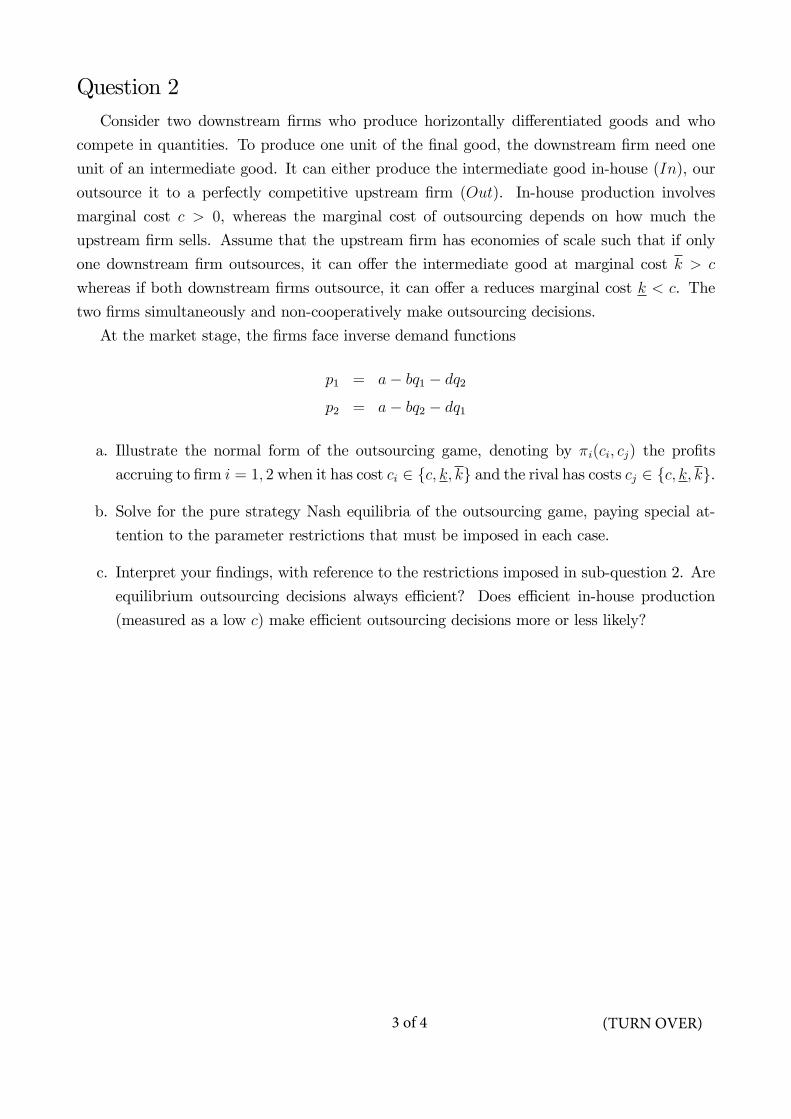
Question 2Consider two downstream firms who produce horizontally differentiated goods and who
compete in quantities. To produce one unit of the final good, the downstream firm need one
unit of an intermediate good. It can either produce the intermediate good in-house (In), our
outsource it to a perfectly competitive upstream firm (Out). In-house production involves
marginal cost c > 0, whereas the marginal cost of outsourcing depends on how much the
upstream firm sells. Assume that the upstream firm has economies of scale such that if only
one downstream firm outsources, it can offer the intermediate good at marginal cost k > c
whereas if both downstream firms outsource, it can offer a reduces marginal cost k < c. The
two firms simultaneously and non-cooperatively make outsourcing decisions.
At the market stage, the firms face inverse demand functions
p1 = a− bq1 − dq2p2 = a− bq2 − dq1
a. Illustrate the normal form of the outsourcing game, denoting by πi(ci, cj) the profits
accruing to firm i = 1, 2 when it has cost ci ∈ c, k, k and the rival has costs cj ∈ c, k, k.
b. Solve for the pure strategy Nash equilibria of the outsourcing game, paying special at-
tention to the parameter restrictions that must be imposed in each case.
c. Interpret your findings, with reference to the restrictions imposed in sub-question 2. Are
equilibrium outsourcing decisions always effi cient? Does effi cient in-house production
(measured as a low c) make effi cient outsourcing decisions more or less likely?
3 of 4 (TURN OVER)

Question 3Consider two firms producing horizontally differentiated goods. The firms are located at
the end-points of a linear city of unit length. Consumers have unit demand and are uniformly
distributed along the city with density one. Firms produce at constant and symmetric marginal
costs c > 0 and offer uniform prices to consumers. A consumer’s utility is given by
u(x, p) =
s− τd− p if p ≤ s− τd
0 if p > s− τd
where d ≥ 0 denotes the distance of the consumer’s location to that of the firm and p is the
price charged for the product. The constant τ > 0 is the travel cost borne by the consumers.
Assume throughout that there is full market coverage.
a. Consider an infinite period game in which the firms play the market game in each period
t = 1, 2, .... The future is discounted by a factor δ ∈ (0, 1). Carefully define grim trigger
strategies in this setting.
b. Derive explicit expressions πC , πD and πN , i.e. for the payoffs to cooperating, deviating
and playing according to the (stage-game) Nash equilibrium respectively. Derive a con-
dition on the discount factor δ that determines whether tacit collusion in grim trigger
strategies is feasible.
c. Carefully determine how πC , πD and πN vary with the transport cost τ . Explain the
tradeoffs involved and discuss how these findings influence the sustainability of tacit
collusion via grim trigger strategies.
END OF PAPER
4 of 4

ECM9/ECM10MPhil in EconomicsMPhil in Economic Research
Friday 26 May 2017 1:30pm - 3:30pm
M180LABOUR: SEARCH, MATCHING AND AGGLOMERATION
Candidates are required to answer three out of four questions. Each questioncarries equal weight.
Write your candidate number (not your name) on the cover of each booklet.
Write legibly.
If you identify an error in this paper, please alert the Invigilator, who will notifythe Examiner. A general announcement will be made if the error is validated.
STATIONERY REQUIREMENTS20 Page booklet x 1Rough work pads
SPECIAL REQUIREMENTS TO BE SUPPLIED FOR THISEXAMINATIONCalculator - students are permitted to bring an approved calculator
You may not start to read the questions printedon the subsequent pages of this question paper
until instructed that you may do so by the Invigilator.
1 of 3

1. Consider the Postel-Vinay & Robin (2002) model. We assume that workersand firms are homogeneous. The productivity of a match is p. Parametersare as they were in the lecture notice that is: ρ is the discount rate, b is theflow value of unemployment, λ0 is the arrival rate of jobs to unemployed, λ1is the arrival rate of jobs to employed, δ is the job destruction rate. Let U bethe value of unemployment and W (w) the value of employment at a wage w.(a) Write the Bellman equation for the value of unemployment.(b) Let w0 be the wage that makes a worker indifferent between remaining
in unemployment and beginning work (U = W (w0)). Use this relation tosimplify the expression under (a) and provide an intuition for the result.
(c) What wage offer will an employed worker get when receiving an outsideoffer from another employer? Is there any indeterminacy about whetherhe will move/stay?
(d) Write the Bellman equation for a worker at his maximum wage andsimplify this expression to obtain the maximum value a worker can get.
(e) Show that
w0 = b− λ1ρ+ δ
(p− b)
(f) What happens to w0 if (i) as λ1 → 0 and (ii) as ρ → ∞? Explain yourresults.
(g) What is the distribution of wages amongst employed?(h) Derive the mean wage paid in the economy.(i) What is the mean wage wage when workers don’t discount future earn-
ings? Give intuition for your answer and discuss the implications forfirms vacancy posting decisions.
2. Minimum wages and job search models(a) Give a short overview of the stylized facts regarding the introduction of
a minimum wage.(b) David Lee regresses the 10-50% log wage differential on inter-state varia-
tion in minimum wages. He finds a strong negative effect: the higher theminimum wage, the smaller the 10-50% differential. Can this result beinterpreted as evidence that the wage differentials between workers withdifferent human capital are compressed by an increase in the minimumwage?
(c) To what extend can these facts be explained by job search models?(d) Some studies find that a higher minimum wage might increase employ-
ment. What do you have to assume on wage setting, labour supply,vacancy creation, and the matching function to explain this outcome?
2 of 3

3. Public transport in cities(a) Consider a circular city as in Lucas & Rossi Hansberg (2002). Suppose
that the city would develop a public transport railsystem with a stopat the city center that extends from there in all directions with a singlestop at all locations at distance R from the center (so every point on thering R has a stop that connects it to the city center). Assume that thecity autorities have chosen a proper location for these stops such thatthe system is useful for commuting. Furthermore, this city turns outto have a mixed neighbourhood where residential and commercial use ofland coincide. Commuting cost by any other mode of transport are κ perunit of distance, commuting by public transport occurs at cost ψ < κ perunit of distance. Depict a possible profile of land rents and depict thelocations of the various zones (residential, commercial, mixed). Explainyour answer, in particular the location of the zones and the wage functionthat goes with this pattern.
(b) Consider the density of land use in the neighbourhood of the stations,both at the center and at location R. Is this density is lower or higherthan at locations further away from the station? Is this effi cient?
(c) Public transport is a means of transport with high fixed cost (construc-tion of tracks etc.) and low variable cost per trip. Suppose you arethe mayor of the city. Design an effi cient system for funding the pub-lic transport system. Explain your design. What are the drawbacks ofalternative designs?
4. Agglomeration of human capital(a) The agglomeration of people in cities has played an important role in
the evolution of the world economy since the rise of agriculture. Give ashort historical overview in at most 10 sentences.
(b) Gennaio et.al. (2013) provide a model for the agglomeration of humancapital within countries. Describe the main features of that model inat most 10 sentences. Pay attention to the role of economies of scale,knowledge spill-overs, and entrepreneurship. Are there externalities intheir model?
(c) Is the equilibrium effi cient in their model? Why or why not? If not,what policies could help to alleviate the problem?
(d) Who captures the benefits of agglomeration in their model?(e) Teulings & Van Rens (2008) show that an increase in the average level
of education in a country reduces the return to human capital. Is thisconsistent with the analysis of Gennaio et.al.? Explain your answer.
3 of 3
END OF PAPER

ECM9/ECM10/ECM11MPhil in EconomicsMPhil in Finance & EconomicsMPhil in Economic Research
Thursday 12 January 2017 10:00-12:00
M200MACROECONOMICS I
The paper is in two sections: You should answer all four questions in Section A and one question from Section B. Each Section carries equal weight.
Write your candidate number (not your name) on the cover of each booklet.
Write legibly.
If you identify an error in this paper, please alert the Invigilator, who will notifythe Examiner. A general announcement will be made if the error is validated.
STATIONERY REQUIREMENTS20 Page booklet x 1Rough work pads
SPECIAL REQUIREMENTS TO BE SUPPLIED FOR THISEXAMINATIONCalculator - students are permitted to bring an approved calculator
You may not start to read the questions printedon the subsequent pages of this question paper
until instructed that you may do so by the Invigilator.
1 of 5
SECTION A
A.1 Solow growth model
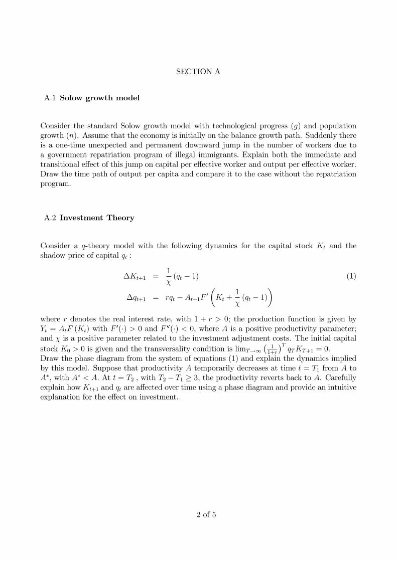
Consider the standard Solow growth model with technological progress (g) and populationgrowth (n). Assume that the economy is initially on the balance growth path. Suddenly thereis a one-time unexpected and permanent downward jump in the number of workers due toa government repatriation program of illegal immigrants. Explain both the immediate andtransitional effect of this jump on capital per effective worker and output per effective worker.Draw the time path of output per capita and compare it to the case without the repatriationprogram.
A.2 Investment Theory
Consider a q-theory model with the following dynamics for the capital stock Kt and theshadow price of capital qt :
∆Kt+1 =1
χ(qt − 1) (1)
∆qt+1 = rqt − At+1F ′(Kt +
1
χ(qt − 1)
)where r denotes the real interest rate, with 1 + r > 0; the production function is given byYt = AtF (Kt) with F ′(·) > 0 and F
′′(·) < 0, where A is a positive productivity parameter;and χ is a positive parameter related to the investment adjustment costs. The initial capitalstock K0 > 0 is given and the transversality condition is limT→∞
(11+r
)TqTKT+1 = 0.
Draw the phase diagram from the system of equations (1) and explain the dynamics impliedby this model. Suppose that productivity A temporarily decreases at time t = T1 from A toA∗, with A∗ < A. At t = T2 , with T2 − T1 ≥ 3, the productivity reverts back to A. Carefullyexplain how Kt+1 and qt are affected over time using a phase diagram and provide an intuitiveexplanation for the effect on investment.
2 of 5

A.3 Equilibrium with Imperfect CompetitionSuppose a representative firm i ∈ [0, 1] maximizes real profits
Πi =PiPQi −
W
PLi
where Qi denotes the production of good i, Pi the price of good i, P ≡∫ 10Pidi the aggre-
gate price level, W the nominal wage, and Li the firm’s labour input. The productiontechnology is described by
Qi = ALi
where A denotes productivity. The firm operates under monopolistic competition andfaces demand
Qi = Y
(PiP
)−ηwhere Y ≡
∫ 10Qidi denotes aggregate output and the parameter η > 1. In the labour
market, the firm faces the following real wage function:
W
P= BLβ
where L ≡∫ 10Lidi denotes aggregate employment, and B and β are positive parameters.
The aggregate demand relation is described by
Y =M
P
where M denotes aggregate demand.Derive the level of the real wage W
P, aggregate employment L and aggregate output Y
in the flexible price equilibrium. Explain how they are affected by an increase in B.
A.4 Anticipated Positive Aggregate Demand Shock in Dornbusch ModelSuppose the economy of Americana can be described by a Dornbusch model with thefollowing short-run dynamics for the (log) nominal exchange rate s (defined as thedomestic price of foreign currency) and the (log) aggregate price level p:
s = 4 (s− s) − 2 (p− p)p = (s− s) − (p− p)
where the steady state (indicated by an upper bar) equals s = q + k and p = p∗ + k,with (log) real exchange rate q = 1
2(y − u) and macroeconomic fundamentals k ≡
(m− m∗) − (y − y∗). In addition, m denotes the money supply, y the natural rateof output and u is a measure of exogenous aggregate demand. Foreign variables areindicated by an asterisk.Suppose the new President of Americana suddenly announces fiscal policy measuresthat will lead to a permanent increase in u in one year. Explain how this affects thenominal exchange rate s and aggregate price level p over time, and carefully illustratethe dynamics in a phase diagram. Does the nominal exchange rate s ‘overshoot’thenew steady state s′ at any time?
3 of 5
SECTION B
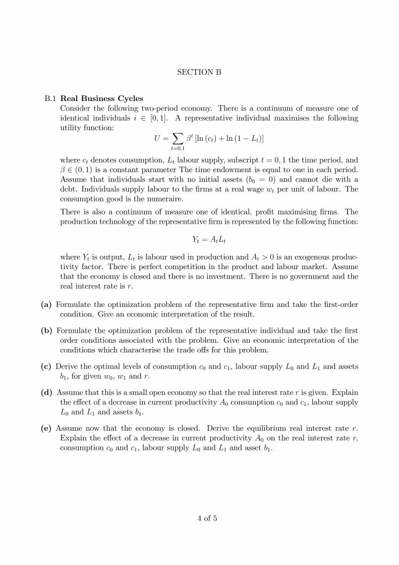
B.1 Real Business CyclesConsider the following two-period economy. There is a continuum of measure one ofidentical individuals i ∈ [0, 1]. A representative individual maximises the followingutility function:
U =∑t=0,1
βt [ln (ct) + ln (1− Lt)]
where ct denotes consumption, Lt labour supply, subscript t = 0, 1 the time period, andβ ∈ (0, 1) is a constant parameter The time endowment is equal to one in each period.Assume that individuals start with no initial assets (b0 = 0) and cannot die with adebt. Individuals supply labour to the firms at a real wage wt per unit of labour. Theconsumption good is the numeraire.
There is also a continuum of measure one of identical, profit maximising firms. Theproduction technology of the representative firm is represented by the following function:
Yt = AtLt
where Yt is output, Lt is labour used in production and At > 0 is an exogenous produc-tivity factor. There is perfect competition in the product and labour market. Assumethat the economy is closed and there is no investment. There is no government and thereal interest rate is r.
(a) Formulate the optimization problem of the representative firm and take the first-ordercondition. Give an economic interpretation of the result.
(b) Formulate the optimization problem of the representative individual and take the firstorder conditions associated with the problem. Give an economic interpretation of theconditions which characterise the trade offs for this problem.
(c) Derive the optimal levels of consumption c0 and c1, labour supply L0 and L1 and assetsb1, for given w0, w1 and r.
(d) Assume that this is a small open economy so that the real interest rate r is given. Explainthe effect of a decrease in current productivity A0 consumption c0 and c1, labour supplyL0 and L1 and assets b1.
(e) Assume now that the economy is closed. Derive the equilibrium real interest rate r.Explain the effect of a decrease in current productivity A0 on the real interest rate r,consumption c0 and c1, labour supply L0 and L1 and asset b1.
4 of 5
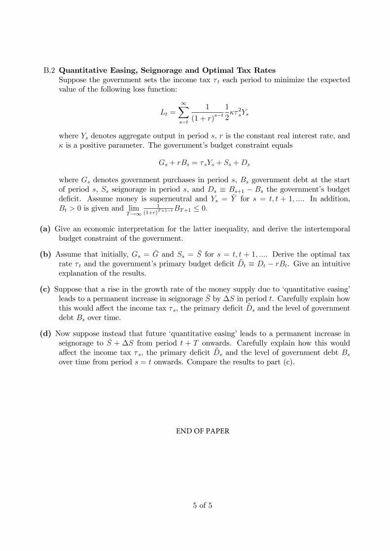
B.2 Quantitative Easing, Seignorage and Optimal Tax RatesSuppose the government sets the income tax τ t each period to minimize the expectedvalue of the following loss function:
Lt =
∞∑s=t
1
(1 + r)s−t1
2κτ 2sYs
where Ys denotes aggregate output in period s, r is the constant real interest rate, andκ is a positive parameter. The government’s budget constraint equals
Gs + rBs = τ sYs + Ss +Ds
where Gs denotes government purchases in period s, Bs government debt at the startof period s, Ss seignorage in period s, and Ds ≡ Bs+1 − Bs the government’s budgetdeficit. Assume money is superneutral and Ys = Y for s = t, t + 1, .... In addition,Bt > 0 is given and lim
T→∞1
(1+r)T+1−tBT+1 ≤ 0.
(a) Give an economic interpretation for the latter inequality, and derive the intertemporalbudget constraint of the government.
(b) Assume that initially, Gs = G and Ss = S for s = t, t + 1, .... Derive the optimal taxrate τ t and the government’s primary budget deficit Dt ≡ Dt − rBt. Give an intuitiveexplanation of the results.
(c) Suppose that a rise in the growth rate of the money supply due to ‘quantitative easing’leads to a permanent increase in seignorage S by ∆S in period t. Carefully explain howthis would affect the income tax τ s, the primary deficit Ds and the level of governmentdebt Bs over time.
(d) Now suppose instead that future ‘quantitative easing’leads to a permanent increase inseignorage to S + ∆S from period t + T onwards. Carefully explain how this wouldaffect the income tax τ s, the primary deficit Ds and the level of government debt Bs
over time from period s = t onwards. Compare the results to part (c).
5 of 5
END OF PAPER

ECM9/ECM10/ECM11MPhil in EconomicsMPhil in Finance & EconomicsMPhil in Economic Research
Wednesday 10 May 2017 2:00pm - 4:00pm
M200MACROECONOMICS I
The paper is in two sections: You should answer all four questions in Section Aand one question from Section B. Each Section carries equal weight.
Write your candidate number (not your name) on the cover of each booklet.
Write legibly.
If you identify an error in this paper, please alert the Invigilator, who will notifythe Examiner. A general announcement will be made if the error is validated.
STATIONERY REQUIREMENTS20 Page booklet x 1Rough work pads
SPECIAL REQUIREMENTS TO BE SUPPLIED FOR THISEXAMINATIONCalculator - students are permitted to bring an approved calculator
You may not start to read the questions printedon the subsequent pages of this question paper
until instructed that you may do so by the Invigilator.
1 of 5
A.1 Solow Growth Model
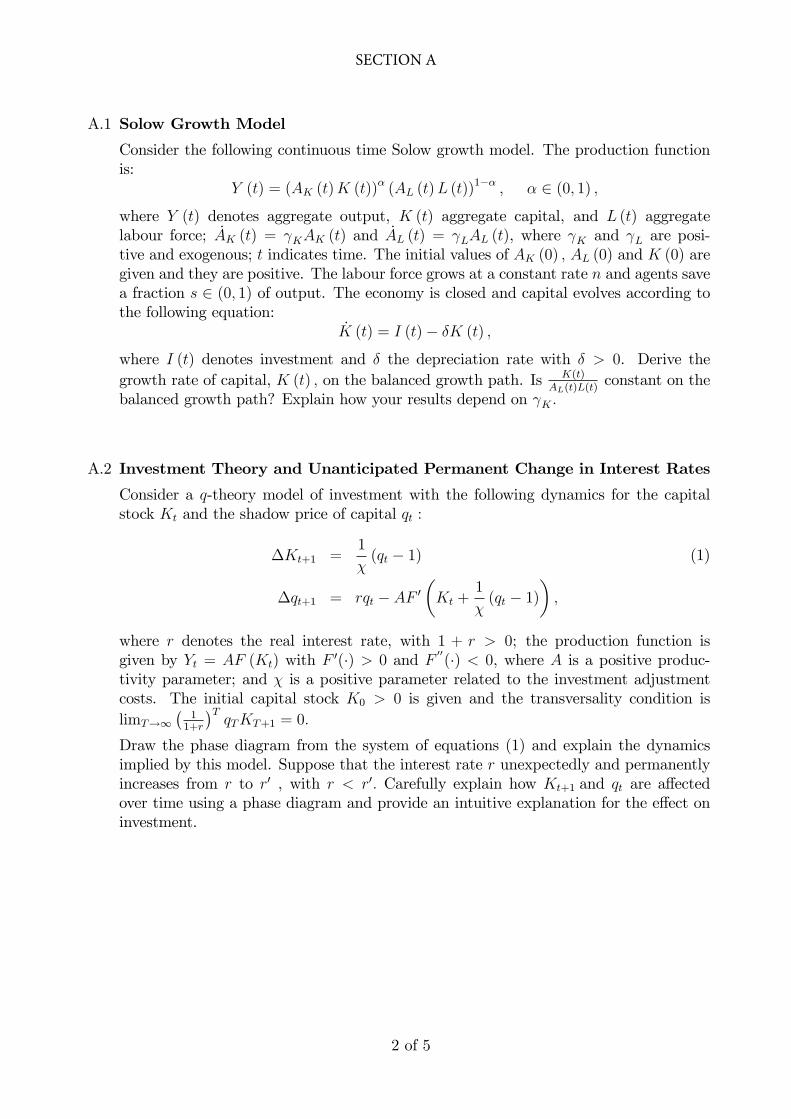
Consider the following continuous time Solow growth model. The production functionis:
Y (t) = (AK (t)K (t))α (AL (t)L (t))1−α , α ∈ (0, 1) ,
where Y (t) denotes aggregate output, K (t) aggregate capital, and L (t) aggregatelabour force; AK (t) = γKAK (t) and AL (t) = γLAL (t), where γK and γL are posi-tive and exogenous; t indicates time. The initial values of AK (0) , AL (0) and K (0) aregiven and they are positive. The labour force grows at a constant rate n and agents savea fraction s ∈ (0, 1) of output. The economy is closed and capital evolves according tothe following equation:
K (t) = I (t)− δK (t) ,
where I (t) denotes investment and δ the depreciation rate with δ > 0. Derive thegrowth rate of capital, K (t) , on the balanced growth path. Is K(t)
AL(t)L(t)constant on the
balanced growth path? Explain how your results depend on γK .
A.2 Investment Theory and Unanticipated Permanent Change in Interest Rates
Consider a q-theory model of investment with the following dynamics for the capitalstock Kt and the shadow price of capital qt :
∆Kt+1 =1
χ(qt − 1) (1)
∆qt+1 = rqt − AF ′(Kt +
1
χ(qt − 1)
),
where r denotes the real interest rate, with 1 + r > 0; the production function isgiven by Yt = AF (Kt) with F ′(·) > 0 and F
′′(·) < 0, where A is a positive produc-
tivity parameter; and χ is a positive parameter related to the investment adjustmentcosts. The initial capital stock K0 > 0 is given and the transversality condition islimT→∞
(1
1+r
)TqTKT+1 = 0.
Draw the phase diagram from the system of equations (1) and explain the dynamicsimplied by this model. Suppose that the interest rate r unexpectedly and permanentlyincreases from r to r′ , with r < r′. Carefully explain how Kt+1 and qt are affectedover time using a phase diagram and provide an intuitive explanation for the effect oninvestment.
2 of 5
SECTION A
A.3 Central Bank Contract with Output Growth Bonus
Suppose the economy of Americana is described by the following Phillips equation:
π = πe + (gY − gY ) + ε,
where π denotes inflation, gY the growth rate of real output, gY the long run growth rateof real output, and ε a white noise cost push shock. Private sector inflation expectationsπe are formed using rational expectations at the beginning of the period, before theshock ε has been realized. Monetary policy is delegated to a central banker who setsreal output growth gY after the shock ε has been observed. The central banker minimizesthe following loss function:
L =1
2(π − π∗)2 +
1
2(gY − g∗Y )2 − β (gY − g∗Y ) ,
where π∗ denotes the central banker’s inflation target, g∗Y the central banker’s real outputgrowth target, and β a non-negative parameter. Suppose that before the beginning ofthe period, the new president of Americana appoints a central banker with an inflationtarget of 2% and a real output growth target of 4%, while long run real output growthequals 2%. In addition, the president decides to provide the central banker a personalincentive to achieve the real output growth target through a ‘bonus’payment that isincreasing in real output growth gY , so that β > 0.Derive the equilibrium outcome of private sector inflation expectations πe, real outputgrowth gY and inflation π. Explain intuitively how these outcomes are affected by thereal output growth bonus.
A.4 Anticipated Negative Aggregate Demand Shock in Dornbusch Model
Suppose the economy of Britannia can be described by a Dornbusch model with thefollowing short-run dynamics for the (log) nominal exchange rate s (defined as thedomestic price of foreign currency) and the (log) aggregate price level p:
s = (s− s) + (p− p) ,p = (s− s) − (p− p) ,
where the steady state (indicated by an upper bar) equals s = q + k and p = p∗ + k,with macroeconomic fundamentals k ≡ (m− m∗) − 1
2(y − y∗) and (log) real exchange
rate q = y − u. In addition, m denotes the (log) money supply, y the (log) natural rateof output, and u is a measure of exogenous aggregate demand. Foreign variables areindicated by an asterisk.Suppose the government of Britannia suddenly announces that it will abandon a singlemarket with Europia in T years, which will increase barriers to international trade andlead to a permanent decrease in u in T years. Explain how this affects the nominal ex-change rate s and aggregate price level p over time, and carefully illustrate the dynamicsin a phase diagram. How do the effects on the nominal exchange rate s and aggregateprice level p depend on T?
3 of 5 (TURN OVER)
B.1 Consumption Theory and a Risky Asset
Consider a household whose preferences are described by:
U = Et
∞∑s=t
u (Cs)
(1 + r)s,
where C is consumption and u′ (C) > 0 and u′′ (C) < 0 and r > 0 is the discount rate.
Assume that the household’s unique source of income is the dividends, Dt, and capitalgains from holding equity At which has price Pt. Assume that equity holdings could besold after dividends have been paid. Moreover assume A0 > 0. The budget constraintof the household is:
Ct + PtAt+1 = (Pt +Dt)At.
(a) Provide an economic interpretation of the household’s budget constraint.
(b) Set up the household’s optimization problem, derive the intertemporal Euler equationfor consumption and interpret it.
For the remainder of the question assume that u (Ct) = Ct.
(c) Using the Euler equation obtained in part (b) derive Pt in terms of future dividends.Which condition do you have to impose? Give an economic intuition.
(d) How does an increase of dividends in period t+s, Dt+s, affect the equity price in periodt? How is this price affected as s increases? How does a permanent increase of allfuture dividends by ε > 0 from period t onwards affect the price in t? Give an economicintuition of your findings.
(e) Assume that u (Ct) = Ct and Pt equals the expression derived in part (c) plus a deter-ministic bubble, (1 + r)t b, and b > 0. Carefully show whether the intertemporal Eulerequation for consumption derived in part (b) is still satisfied. Could b be negative? Givean economic intuition.
4 of 5
SECTION B
B.2 Optimal Tax Rates, Seignorage and Inflation TargetSuppose social welfare losses are described by
Lt =∞∑s=t
1
(1 + r)s−t
1
2κτ 2
sYs +1
2π2s
,
where τ s denotes the income tax rate, Ys aggregate output, πs inflation, and the sub-script s indicates the time period. The real interest rate r is constant and κ is a positiveparameter. The government sets the income tax rate τ t in each period to minimizesocial welfare losses Lt. The government’s intertemporal budget constraint equals
(1 + r)Bt +∞∑s=t
Gs
(1 + r)s−t=∞∑s=t
τ sYs
(1 + r)s−t+∞∑s=t
Ss
(1 + r)s−t,
where Bt > 0 is government debt at the start of period t and Gs government purchases,which equal Gs = G for s = t, t + 1, .... In addition, seignorage Ss is determined bySs = µs
Ms
Ps, where Ms denotes the money supply, µs the (approximate) growth rate of
Ms, and Ps the aggregate price level. Real money demand is described by
Ms
Ps= e−θisYs,
where is is the nominal interest rate, which satisfies is = r+πes, where πes denotes inflation
expectations and θ is a positive parameter. Assume that money is superneutral, withYs = Y for s = t, t+1, ..., and that perfect foresight holds, so that πes = πs. Also assumethat the economy is in a steady state with constant real money balancesMs/Ps, so thatµs = πs. The money growth rate µs is set in each period by an independent centralbank that minimizes the loss function
LCBt =∞∑s=t
1
(1 + r)s−t1
2(πs − π∗)2 ,
where π∗ denotes the central bank’s inflation target.
(a) Compute the money growth rate µs that the central bank sets to minimize itsloss function LCBt . In addition, compute the resulting inflation expectations πes,nominal interest rate is, real money holdings Ms/Ps and seignorage Ss in terms ofthe central bank’s inflation target π∗.
(b) Derive the money growth rate µ that maximizes steady-state seignorage S. Com-pute the corresponding level of seignorage Smax. What level of the inflation targetπ∗ would generate the maximum steady-state seignorage Smax?
(c) For a given level of πs and Ss = S for s = t, t+ 1, ..., derive the optimal tax rate τ tset by the government in terms of Bt, G, Y and S. Give an intuitive explanationof the results.
(d) Use the results from parts (a) and (c) to write social welfare losses Lt in terms ofthe inflation target π∗, and derive the optimality condition for the socially optimalinflation target π∗SO that minimizes social welfare losses Lt. Determine how π∗SOcompares to π∗ = 0 and to the inflation target derived in part (b). Provide anintuitive explanation for the results.
5 of 5
END OF PAPER

ECM9/ECM10MPhil in EconomicsMPhil in Economic Research
Monday 5 June 2017 1:30pm - 3:30pm
M210MACROECONOMICS II
This paper is in two sections. Section A: Candidates are required to answerthree out of four questions. Section B: Candidates are required to answerone compulsory question.
Each section carries equal weighting.
Write your candidate number (not your name) on the cover of each booklet.
Write legibly.
If you identify an error in this paper, please alert the Invigilator, who will notifythe Examiner. A general announcement will be made if the error is validated.
STATIONERY REQUIREMENTS20 Page booklet x 2Rough work pads
SPECIAL REQUIREMENTS TO BE SUPPLIED FOR THISEXAMINATIONCalculator - students are permitted to bring an approved calculator
You may not start to read the questions printedon the subsequent pages of this question paper
until instructed that you may do so by the Invigilator.
1 of 5
SECTION A
A.1 Neoclassical Growth ModelConsider an economy with aggregate production function
Y (t) = K(t)αE(t)β(A(t)N(t))1−α−β, α, β ∈ (0, 1) and β + α < 1.
Y is output, K is capital, N is labour, E is energy, and A is labour pro-ductivity. Technological progress grows at rate g and the initial technology,A(0) > 0, is given. Capital evolves according to:
K(t) = I(t)− δK(t),
where I corresponds to investment and δ > 0 is the depreciation rate, andK(0) is given. There is a continuum of measure one of households who areinfinite lived, with preferences
U =
∫ ∞0
e−ρtL(t)u(c(t))dt, ρ > 0, u(c) =c1−θ − 1
1− θ, θ > 0,
where c(t) denotes consumption of each household member. L(t) is thenumber of household members, which grows at rate n. Assume that L(0) = 1and each household member has one unit of productive time. Suppose thereis a fixed stock of nonrenewable resources, R(0), and that energy use depletesthis stock, so that
R(t) = −sR(t)R(t),
where sR(t) ∈ (0, 1) is the endogenously determined extraction rate. Set upthe Social Planner’s problem for this economy and derive the optimal growthrate of output per capita along the balanced growth path equilibrium. Wouldoutput per capita be growing along the balanced growth path equilibrium?
A.2 Search Model with Probability of DyingAn agent receives every period an offer to work forever at a wage w, wherew is drawn from the distribution F (w) with support [0, B] where B is finite.Offers are independently and identically distributed. The objective of theagent is to maximise Et=0
∑∞t=0(β(1 − s))tyt, where yt = w if the worker
has accepted a job that pays w, and yt = b if the agent remains unemployed,β ∈ (0, 1) is a subjective discount factor, and s ∈ (0, 1) is the probabilitythat the agent will die in each period. Assume that 0 < b < B <∞.
(i) Write down Bellman’s Functional Equation for an unemployed agentand argue (intuitively) that the optimal policy function is a reservationwage w such that the agent will accept a job offer if w > w.
(ii) Suppose that there is now a continuum 1 of identical individuals sam-pling jobs from the same stationary distribution F (w). There is a massof s workers born every period, so that population is constant, andthese workers start out as unemployed. What would be the steady-state unemployment rate for this economy?
2 of 5

A3. Contraction MappingConsider the following cake-eating problem with infinite horizon: an agenthas an initial cake of size x0. She can eat away ct ≥ 0 from the cake eachperiod, so xt+1 = xt − ct. The size of the cake can never become negative.The agent has per-period utility u(ct) =
√ct and discount factor β. Write the
Bellman equation for this problem. Is this Bellman equation a Contraction?Explain.
A.4 Asset PricingConsider an economy populated by a continuum of measure one of identicalhouseholds, each with preferences given by E0[
∑∞t=0 β
tu(ct)] where ct is con-
sumption at period t, u(ct) =c1−θt −11−θ with θ ≥ 0, and β ∈ (0, 1) corresponds
to the subjective discount factor. There is a single asset tree which yieldsperishable dividends dt (fruits). Households are initially endowed with somenumber of shares of the tree: s0. Assume that dt is a random variable takingvalues from the set D ≡ d1, ..., dN and is distributed according to a first-order Markov chain with constant transition probability matrix. Householdscan trade the share of the tree. The price of the tree when the current real-ization of dt is d is given by the function p : D → R+. There are no otherassets in this economy. State the problem of the representative householdin recursive form and assuming that the value function is differentiable, de-rive the the optimal price of share of the tree as a function of present andfuture dividends. Does ‘good news’ about future output (dividends) alwaysproduce an increase in stock prices? Explain.
3 of 5 TURN OVER
SECTION B
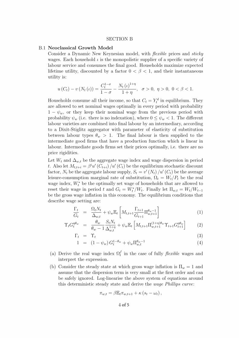
B.1 Neoclassical Growth ModelConsider a Dynamic New Keynesian model, with flexible prices and stickywages. Each household ι is the monopolistic supplier of a specific variety oflabour service and consumes the final good. Households maximize expectedlifetime utility, discounted by a factor 0 < β < 1, and their instantaneousutility is:
u (Ct)− v (Nt (ι)) =C1−σt
1− σ− Nt (ι)1+η
1 + η, σ > 0, η > 0, 0 < β < 1.
Households consume all their income, so that Ct = Y dt in equilibrium. They
are allowed to set nominal wages optimally in every period with probability1 − ψw, or they keep their nominal wage from the previous period withprobability ψw (i.e. there is no indexation), where 0 ≤ ψw < 1. The differentlabour varieties are combined into final labour by an intermediary, accordingto a Dixit-Stiglitz aggregator with parameter of elasticity of substitutionbetween labour types θw > 1. The final labour is then supplied to theintermediate good firms that have a production function which is linear inlabour. Intermediate goods firms set their prices optimally, i.e. there are noprice rigidities.
Let Wt and ∆w,t be the aggregate wage index and wage dispersion in periodt. Also let Mt,t+i = βiu′ (Ct+i) /u
′ (Ct) be the equilibrium stochastic discountfactor, Nt be the aggregate labour supply, St = v′ (Nt) /u
′ (Ct) be the averageleisure-consumption marginal rate of substitution, Ωt = Wt/Pt be the realwage index, W ∗
t be the optimally set wage of households that are allowed toreset their wage in period t and Gt = W ∗
t /Wt. Finally let Πw,t = Wt/Wt−1be the gross wage inflation in this economy. The equilibrium conditions thatdescribe wage setting are:
ΓtGt
=ΩtNt
∆w,t
+ ψwEt[Mt,t+1
Γt+1
Gt+1
Πθw−1w,t+1
](1)
ΥtGηθwt =
θwθw − 1
StNt
∆1+ηw,t
+ ψwEt[Mt,t+1Π
(1+η)θww,t+1 Υt+1G
ηθwt+1
](2)
Γt = Υt (3)
1 = (1− ψw)G1−θwt + ψwΠθw−1
w,t (4)
(a) Derive the real wage index Ωft in the case of fully flexible wages and
interpret the expression.
(b) Consider the steady state at which gross wage inflation is Πw = 1 andassume that the dispersion term is very small at the first order and canbe safely ignored. Log-linearise the above system of equations aroundthis deterministic steady state and derive the wage Phillips curve:
πw,t = βEtπw,t+1 + κ (st − ωt) ,
4 of 5

where κ > 0 depends on the model’s parameters and lower case lettersdenote log-deviations of variables from their steady state. Provide aninterpretation of the wage Phillips curve.
(c) Explain how the slope of the wage Phillips curve κ changes as
i. households become more patient,
ii. wages become less sticky,
iii. the labour supply becomes more inelastic and
iv. as different types of labour become more substitutable.
END OF PAPER
5 of 5

ECM9/ECM10MPhil in EconomicsMPhil in Economic Research
Wednesday 24 May 9:00am - 11:00am
M220MACROECONOMICS III
This paper is in two sections:Section A - candidates are required to answer three out of four questions.Section B —candidates are required to answer one compulsory question.
Each section carries equal weight.
Write your candidate number (not your name) on the cover of each booklet.
Write legibly.
If you identify an error in this paper, please alert the Invigilator, who will notifythe Examiner. A general announcement will be made if the error is validated.
STATIONERY REQUIREMENTS20 Page booklet x 1Rough work pads
SPECIAL REQUIREMENTS TO BE SUPPLIED FOR THISEXAMINATIONCalculator - students are permitted to bring an approved calculator
You may not start to read the questions printedon the subsequent pages of this question paper
until instructed that you may do so by the Invigilator.
1 of 6

Section A
QUESTION 1: The current account
Suppose the world economy consists of two countries, Europia and Americana(indicated by an asterisk), that are initially completely identical, and onlyoperates for two period (t = 1, 2). In each country, the representative agentmaximizes lifetime utility
U = lnC1 + β lnC2
where Ct denotes consumption, the subscript t the time period, and 0 < β < 1.The agent’s budget constraint is
Bt+1 = Yt + (1 + r)Bt − It − Tt − Ct
where Yt denotes output, It investment, Tt lump sum taxes, r the world realinterest rate, and Bt+1 net foreign assets at the end of period t, with B1 = B3 = 0.Output Yt is produced according to
Yt = 2√Kt
where Kt denotes capital, which satisfies
Kt+1 = Kt + It
where It ∈ R, Kt ≥ 0 and K1 = 1. The government’s budget constraint is
Gt = Tt
where government purchases Gt are given by G1 = G and G2 = 0. Assume freetrade between Europia and Americana, and no international capital marketimperfections.Solve for optimal investment I1, consumption C1, national saving S1 and thecurrent account CA1 in terms of β, G and r. Explain the effect of an increase inAmericana’s government purchases G∗ in period 1 on the equilibrium world realinterest rate rW and on investment I1, consumption C1, national saving S1 andthe current account CA1 in period 1 in Europia and in Americana.
2 of 6

QUESTION 2: Risk sharing without trade in assets
Consider a two-country (H and F ) endowment economy. Each country has astochastic endowment of a country-specific good, YH and YF . Also, preferences aresubject to country-specific taste shocks $ and $∗. The social planner problem is:
Max µ $
(CγHC
1−γF
1− σ
)1−σ+ (1− µ) $∗
(C∗γH C
∗1−γF
1− σ
)1−σ
s.t. : CH + C∗H = YH
: CF + C∗F = YF
where CH and C∗H denote the consumption of the H good at Home and in Foreign,CF and C∗F denote consumption of the F good at Home and in Foreign, µ denotesthe social planner weight attributed to the Home country.(a) Solve for the social planner allocation.(b) For the same economy, work out the market equilibrium under financial au-
tarky. Under what conditions is perfect risk sharing achievable without tradein assets across borders?
(c) How does you answer to (b) changes if shocks are anticipated to occur in thefuture? Explain.
3 of 6 (TURN OVER)
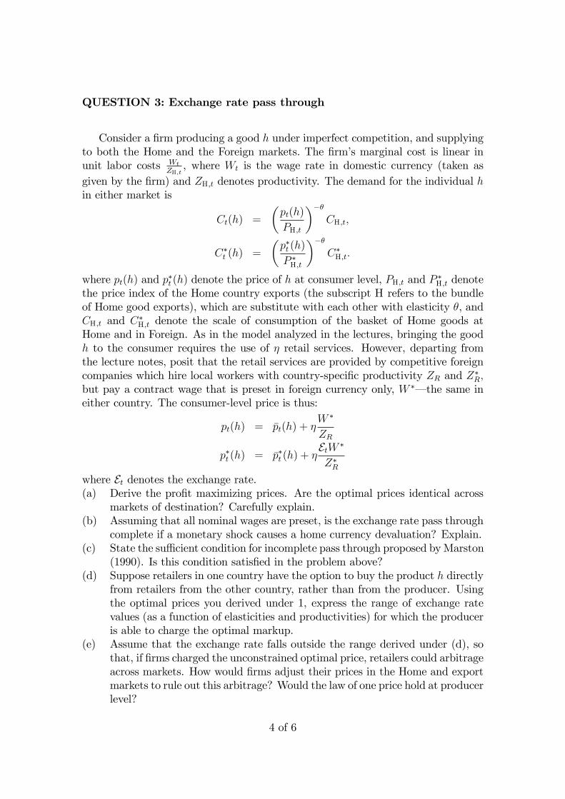
QUESTION 3: Exchange rate pass through
Consider a firm producing a good h under imperfect competition, and supplyingto both the Home and the Foreign markets. The firm’s marginal cost is linear inunit labor costs Wt
ZH,t, where Wt is the wage rate in domestic currency (taken as
given by the firm) and ZH,t denotes productivity. The demand for the individual hin either market is
Ct(h) =
(pt(h)
PH,t
)−θCH,t,
C∗t (h) =
(p∗t (h)
P ∗H,t
)−θC∗H,t.
where pt(h) and p∗t (h) denote the price of h at consumer level, PH,t and P ∗H,t denotethe price index of the Home country exports (the subscript H refers to the bundleof Home good exports), which are substitute with each other with elasticity θ, andCH,t and C∗H,t denote the scale of consumption of the basket of Home goods atHome and in Foreign. As in the model analyzed in the lectures, bringing the goodh to the consumer requires the use of η retail services. However, departing fromthe lecture notes, posit that the retail services are provided by competitive foreigncompanies which hire local workers with country-specific productivity ZR and Z∗R,but pay a contract wage that is preset in foreign currency only, W ∗– the same ineither country. The consumer-level price is thus:
pt(h) = pt(h) + ηW ∗
ZR
p∗t (h) = p∗t (h) + ηEtW ∗
Z∗Rwhere Et denotes the exchange rate.(a) Derive the profit maximizing prices. Are the optimal prices identical across
markets of destination? Carefully explain.(b) Assuming that all nominal wages are preset, is the exchange rate pass through
complete if a monetary shock causes a home currency devaluation? Explain.(c) State the suffi cient condition for incomplete pass through proposed byMarston
(1990). Is this condition satisfied in the problem above?(d) Suppose retailers in one country have the option to buy the product h directly
from retailers from the other country, rather than from the producer. Usingthe optimal prices you derived under 1, express the range of exchange ratevalues (as a function of elasticities and productivities) for which the produceris able to charge the optimal markup.
(e) Assume that the exchange rate falls outside the range derived under (d), sothat, if firms charged the unconstrained optimal price, retailers could arbitrageacross markets. How would firms adjust their prices in the Home and exportmarkets to rule out this arbitrage? Would the law of one price hold at producerlevel?
4 of 6

QUESTION 4: Empirical tests of risk sharing
Consider a two-country model. Use the following notation: U (U∗) denotesutility, C (C∗) consumption at Home (abroad), Pt (P∗t ) the price level at Home(abroad), ζC,t (ζ
∗C,t) country-specific taste shocks, and Et is the exchange rate (units
of Home currency per unit of Foreign currency).(a) State and explain the condition for effi cient risk sharing.(b) Show how to derive a regression model to test of “market completeness”at
international level. In doing so, posit that the instantaneous utility is
U = ζC,tC1−σ
1− σ , and U∗ = ζ∗C,t(C∗)1−σ
1− σ
Carefully write down the null hypothesis.(c) Would the regression model be valid if markets are not complete? Explain.
5 of 6 (TURN OVER)

Section B
QUESTION 5: Global monetary stabilization with “dollar pricing”
Consider the model of monetary policy stabilization after Corsetti-Pesenti 2005discussed in the lecture notes. The Home country welfare function can be written
Et−1 lnCt − constant=Et−1 lnµtPt− constant
where µt is the monetary stance of the country, controlled by monetary authorities,and the CPI is defined as
Pt = 2P1/2H P
1/2F
with PH denoting the price index of domestically produced goods (each sold atthe individual price p (h)), PF the price index of imported goods (each sold atp (f)), all denominated in Home currency. Foreign welfare, consumption, monetarystance and prices are similarly defined, with a star referring to foreign variables andforeign-currency denominated prices.Assume that Home firms preset the price of their product variety h in own
currency (according to the hypothesis of Producer Currency Pricing, or PCP):
Etp∗t (h) = pt (h) = mkp · Et−1(Wt
ZHt
)while Foreign preset their export prices of their good variety f in Home currency(according to Local Currency Pricing, or LCP).
pt (f) = mkp · Et−1(EtW ∗
t
ZFt
)and p∗t (f) = mkp · Et−1
(W ∗t
ZFt
).
Above: Wt and W ∗t denote wages, denominated in Home and Foreign currency,
respectively; ZHt and ZFt denote productivities, mkp denote constant markup; andEt denote the exchange rate (units of Home currency per unit of Foreign currency).Assume that risk sharing is perfect, such that Et = µt
µ∗t, and that countries chooses
µt and µ∗t under commitment, i.e., they solve the optimal policy problem ex ante,
at t− 1.(a) Derive and discuss the optimal policy rules:
(a.1) under Nash, i.e. assuming that each country sets its monetary stancetaking the stance abroad as given;
(a.2) under policy cooperation.(b) Contrast the optimal response to a positive productivity shock in the foreign
country under Nash and Cooperation.
END OF PAPER
6 of 6

ECM9/ECM10MPhil in EconomicsMPhil in Economic Research
Tuesday 6 June 2017 9:00am - 11:00am
M230APPLIED MACROECONOMICS
Candidates are required to answer three out of seven questions.
Write your candidate number (not your name) on the cover of each booklet.
Write legibly.
If you identify an error in this paper, please alert the Invigilator, who will notifythe Examiner. A general announcement will be made if the error is validated.
STATIONERY REQUIREMENTS20 Page booklet x 2Metric Graph PaperRough work pads
SPECIAL REQUIREMENTS TO BE SUPPLIED FOR THISEXAMINATIONCalculator - students are permitted to bring an approved calculator
You may not start to read the questions printedon the subsequent pages of this question paper
until instructed that you may do so by the Invigilator.
1 of 8
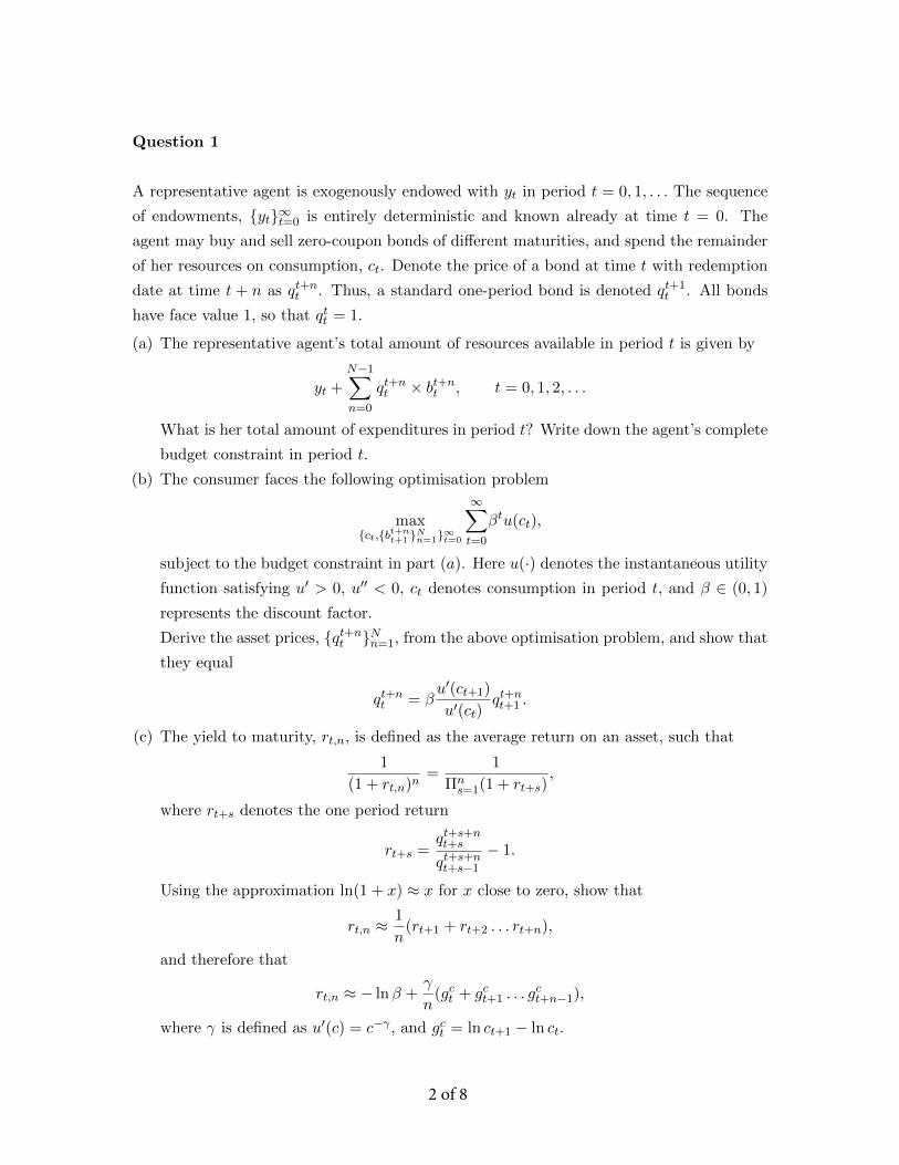
Question 1
A representative agent is exogenously endowed with yt in period t = 0, 1, . . . The sequence
of endowments, yt∞t=0 is entirely deterministic and known already at time t = 0. The
agent may buy and sell zero-coupon bonds of different maturities, and spend the remainder
of her resources on consumption, ct. Denote the price of a bond at time t with redemption
date at time t + n as qt+nt . Thus, a standard one-period bond is denoted qt+1t . All bonds
have face value 1, so that qtt = 1.
(a) The representative agent’s total amount of resources available in period t is given by
yt +
N−1∑n=0
qt+nt × bt+nt , t = 0, 1, 2, . . .
What is her total amount of expenditures in period t? Write down the agent’s complete
budget constraint in period t.
(b) The consumer faces the following optimisation problem
maxct,bt+nt+1 Nn=1∞t=0
∞∑t=0
βtu(ct),
subject to the budget constraint in part (a). Here u(·) denotes the instantaneous utility
function satisfying u′ > 0, u′′ < 0, ct denotes consumption in period t, and β ∈ (0, 1)
represents the discount factor.
Derive the asset prices, qt+nt Nn=1, from the above optimisation problem, and show that
they equal
qt+nt = βu′(ct+1)
u′(ct)qt+nt+1 .
(c) The yield to maturity, rt,n, is defined as the average return on an asset, such that
1
(1 + rt,n)n=
1
Πns=1(1 + rt+s)
,
where rt+s denotes the one period return
rt+s =qt+s+nt+s
qt+s+nt+s−1− 1.
Using the approximation ln(1 + x) ≈ x for x close to zero, show that
rt,n ≈1
n(rt+1 + rt+2 . . . rt+n),
and therefore that
rt,n ≈ − lnβ +γ
n(gct + gct+1 . . . g
ct+n−1),
where γ is defined as u′(c) = c−γ , and gct = ln ct+1 − ln ct.
2 of 8

Question 2
A representative agent solves the following optimisation problem
maxct,bt+1∞t=0
∞∑t=0
βtu(ct),
subject to bt + wt−1 − Tt = ptct + qtbt+1, t = 0, 1, 2, . . .
where bt denotes nominal bond holdings, wt−1 nominal income, ct real consumption, pt the
price level, qt the nominal bond price, Tt nominal lump-sum taxes, and β ∈ (0, 1) represents
the discount factor. The utility function, u(·), satisfies u′ > 0, u′′ < 0. It is assumed that
wt = ptyt, where yt is exogenous.
(a) Derive the Euler equation associated with the above optimisation problem.
(b) The public sector’s budget constraint is given by
dt = qtdt+1 + Tt + (mt −mt−1), t = 0, 1, 2, . . .
where dt denotes nominal debt, and mt denotes the monetary base. Use the fact that
mt = ptyt, and that dt = bt and derive the economy’s real resource constraint (i.e. the
GDP identity).
(c) Now assume that the central bank targets inflation such that
µt = (1− ρ)µ+ ρµt−1,
with mt+1 = µtmt. Assume further that output is constant over time, yt = yt+1 = . . . =
y. Derive a similar law of motion for the bond price, qt.
3 of 8 (TURN OVER)

Question 3
In period t, a representative agent is in possession of xt units of cash and bt units of a
riskless bond. She receives wt−1 units of labour income, and interest payments on bond
holdings are denoted it. These (nominal) resources may be spent on (real) consumption,
ct; purchases of new bonds, bt+1; and future excess cash holdings, xt+1. The price level is
denoted pt. The budget constraint is therefore
xt + bt + yt − Tt = ptct + bt+1 + xt+1,
where yt denotes total income, yt = wt−1+btit, and Tt denotes some lump-sum taxes. Given
a sequence of prices, it, pt, and taxes, Tt, the agent’s optimisation problem is given as
maxct,bt+1,xt+1∞t=0
∞∑t=0
βtu(ct),
subject to the budget constraint above. The utility function, u(·), satisfies u′ > 0, u′′ < 0,
and β ∈ (0, 1) represents the discount factor.
The government’s sequence of (nominal) debt, dt, taxes, Tt, and real government spend-
ing, gt, satisfies
dt+1 + Tt = dt(1 + it) + ptgt, t = 0, 1, 2, . . .
Money supply is constant and equals m. The sequence of aggregate real output, Yt, is
treated as given.
(a) Derive the Euler equations associated with the household’s problem. Given an intuitive
explanation.
(b) Define a competitive equilibrium and derive the equation of exchange. Do prices, pt,
succumb to the monetarist view?
(c) Now suppose that a fraction of the contemporaneous labour income, γtwt, is received
already in period t, but that the reminder, (1 − γt)wt, is still only received in period
t+ 1. The sequence γt is treated as given.
Under these new conditions derive the household’s budget constraint, and derive the
equation of exchange. How is the velocity of money related to γ? Explain intuitively.
4 of 8

Question 4
A government’s period-by-period budget constraint is given by
ptgt + dt = qtdt+1 + Tt + (mt −mt−1), t = 0, 1, 2, . . .
where gt denotes real government spending, dt nominal debt, Tt nominal lump-sum taxes,
and mt the stock of money. Here qt denotes the price of a one period riskless bond which
pays out one unit of nominal resources in period t + 1. The implied nominal interest rate
is given by qt = 11+it+1
. Denote real taxes as τt = Tt/pt, and the real interest rate as
1 + rt+1 = (1 + it+1)ptpt+1
.
(a) Derive the government’s budget constraint in real terms.
(b) The equation of exchange states that ptyt = vtmt. Assume that yt = y, and vt = 1, and
rt = r, for t = 0, 1, . . . Show that real government debt can be written as a function of
the net present value of real government spending, real taxes, real output, and inflation,
πt = pt−pt−1
pt−1. (Hint: Impose the “no-Ponzi condition” lims→∞
1(1+r)sdt+s = 0)
(c) In addition to the assumption imposed in part (c) above, assume that taxes follow the
autoregressive law of motion
τt+1 = (1− ρ)τ + ρτt,
and that real government debt as well as spending are constant over time, dt = dt/pt = d
and gt = g, t = 0, 1, . . .
Derive an expression for inflation from the government budget constraint and show that
inflation must follow an autoregressive law of motion. What is the long-run inflation rate
in this economy? Why did Sargent and Wallace call this “some unpleasant monetarist
arithmetics”?
5 of 8 (TURN OVER)
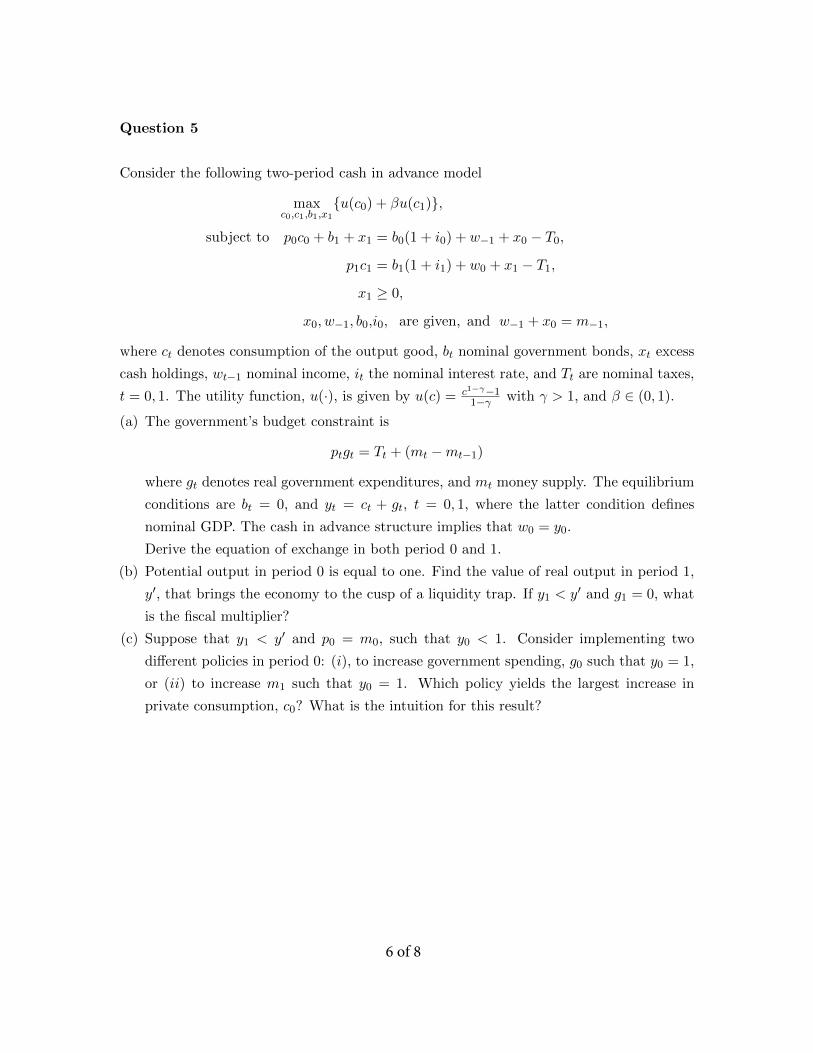
Question 5
Consider the following two-period cash in advance model
maxc0,c1,b1,x1
u(c0) + βu(c1),
subject to p0c0 + b1 + x1 = b0(1 + i0) + w−1 + x0 − T0,
p1c1 = b1(1 + i1) + w0 + x1 − T1,
x1 ≥ 0,
x0, w−1, b0,i0, are given, and w−1 + x0 = m−1,
where ct denotes consumption of the output good, bt nominal government bonds, xt excess
cash holdings, wt−1 nominal income, it the nominal interest rate, and Tt are nominal taxes,
t = 0, 1. The utility function, u(·), is given by u(c) = c1−γ−11−γ with γ > 1, and β ∈ (0, 1).
(a) The government’s budget constraint is
ptgt = Tt + (mt −mt−1)
where gt denotes real government expenditures, and mt money supply. The equilibrium
conditions are bt = 0, and yt = ct + gt, t = 0, 1, where the latter condition defines
nominal GDP. The cash in advance structure implies that w0 = y0.
Derive the equation of exchange in both period 0 and 1.
(b) Potential output in period 0 is equal to one. Find the value of real output in period 1,
y′, that brings the economy to the cusp of a liquidity trap. If y1 < y′ and g1 = 0, what
is the fiscal multiplier?
(c) Suppose that y1 < y′ and p0 = m0, such that y0 < 1. Consider implementing two
different policies in period 0: (i), to increase government spending, g0 such that y0 = 1,
or (ii) to increase m1 such that y0 = 1. Which policy yields the largest increase in
private consumption, c0? What is the intuition for this result?
6 of 8

Question 6
Consider the cash-in-advance model,
maxct,bt+1∞t=0
∞∑t=0
βtu(ct),
s.t. ptct + bt+1 + xt+1 = (1 + it)bt + wt−1 + xt − Tt,
where yt is a given sequence of endowments, ct denotes real consumption, bt nominal
government bonds, xt excess cash holdings, wt−1 nominal income, it the nominal interest
rate, and Tt are nominal taxes. The utility function, u(·), is given by u(c) = c1−γ−11−γ with
γ > 1, and β ∈ (0, 1).
The government’s budget constraint is given by
ptgt + itdt = (dt+1 − dt) + Tt + (mt −mt−1),
where gt denotes real government expenditures, dt nominal debt, and mt money supply.
Assume that mt = m ∀t, and gt = 0 ∀t. Potential output in period t is equal to one.
Suppose that agents unexpectedly receive news in period t that output in period t+1 will
decline and equal y′ < 1. In addition, assume throughout this exercise that the economy is
not in a liquidity trap in period t+ 1.
(a) If the fall in period t + 1 output is not sufficient to bring the economy to a liquidity
trap in period t, how do these news affect pt+1, pt, and it+1? How is the real interest
rate, rt+1, affected? What is the intuition for these price movements?
(b) How big must the fall in output be for the economy to fall into a liquidity trap in period
t? Suppose that yt is still equal to 1, what is the effect on period t prices, velocity of
money, vt, and excess cash holdings, xt+1?
(c) Assume that the price level in period t, pt, is pre-set and equal to m.
How is output in period t related to output in period t+ 1? Illustrate this relationship
both mathematically and graphically.
7 of 8 (TURN OVER)

Question 7
A government’s budget constraint in nominal terms is given by
ptgt + itdt = (dt+1 − dt) + Tt + (mt −mt−1),
where gt denotes real government expenditures, dt nominal debt, it the nominal interest
rate, Tt nominal tax revenue, and mt money supply.
(a) What is the government’s budget constraint in real terms?
(b) Explain intuitively why the real debt is defined as dt/pt−1 instead of dt/pt.
(c) Government budgets often report the nominal gross of interest deficit defined as
ptgt − Tt + itdt
and also the ratio to nominal GDP
ptgt − Tt + itdtptyt
. (1)
However, the gross of interest deficit in real terms as a fraction of real GDP is instead
given by
gt − τt + rtdtyt
,
where dt denotes real government debt.
How come the definition in equation (1) may overstate the government’s “deficit prob-
lem”? How does this bias change with the rate of inflation, πt?
END OF PAPER
8 of 8

ECM9/ECM10/ECM11/MGM3MPhil in EconomicsMPhil in Economic ResearchMPhil in Finance and EconomicsMPhil Finance
Friday 13 January 2017 10:00-12:00
M300ECONOMETRIC METHODS
You should answer eight questions in total. Answer all six questions from Section A and two questions from Section B. Part A is 60% of total marks.
Write your candidate number (not your name) on the cover of each booklet.
Write legibly.
STATIONERY REQUIREMENTS20 Page booklet x 1Rough work padsNew Cambridge Elementary Statistical Tables
SPECIAL REQUIREMENTS TO BE SUPPLIED FOR THIS EXAMINATIONCalculator - students are permitted to bring an approved calculator
You may not start to read the questions printed on the subsequentpages of this question paper until instructed that you may do so by
the Invigilator.
1 of 6
If you identify an error in this paper, please alert the Invigilator, who will notify the Examiner. A general announcement will be made if the error is validated.

A1 You have data on the height Yi, i = 1, ..., n, of n individuals, n1 of whichare men and the rest are women. You run the following regression
Yi = β1Dmi + β2Dwi + β3Xi + εi,
where Dmi is the dummy variable for men, Dwi is the dummy variablefor women, and Xi is the weight of individual i. Note that the constant isnot included in the regression. Show that the sum of the OLS residuals,∑n
i=1εi, equals zero.
A2 Consider the following regression
lwagei = β0 + β1educi + β2tenurei + εi, (1)
. reg resid2 educ tenure
Source SS df MS Number of obs = 526F(2, 523) = 4.83
Model 1.10887555 2 .554437776 Prob > F = 0.0083Residual 60.0010537 523 .114724768 R-squared = 0.0181
Adj R-squared = 0.0144Total 61.1099293 525 .116399865 Root MSE = .33871
resid2 Coef. Std. Err. t P>|t| [95% Conf. Interval]
educ .0021394 .005347 0.40 0.689 -.0083648 .0126436tenure .0063546 .0020494 3.10 0.002 .0023285 .0103807_cons .1356805 .0701332 1.93 0.054 -.0020969 .273458
2 of 6
where lwagei is the log wage of individual i, educi is the education, andtenurei is the number of years with current employer. The following arethe results of the OLS regression of the squared residuals from the above regression on educ
and
tenurei. Use these results to conduct the Breusch-
P agan test the homoskedasticity of the original regression (1).
SECTION A

. reg lwage educ exper resid
Source SS 722F(3, 718) 44.87
Model 20.022858 3 6.67428601 Prob > F 0.0000Residual 106.789058 718 .148731278 R-squared 0.1579
Adj R-squared 0.1544Total 126.811916 721 .175883378 Root MSE .38566
lwage Coef.
educ .142298 .018011 7.90 0.000 .1069375 .1776585exper .0376059 .005374 7.00 0.000 .0270552 .0481565resid -.0769213 .0196251 -3.92 0.000 -.1154509 -.0383918_cons 4.429426 .2962819 14.95 0.000 3.847744 5.011108
A4 Consider a panel regression
yit = cit + βxit + εit,
where cit is unobserved, but it is known that cit = ci,t+2 for any i andt. Propose a consistent estimator of β. Show its consistency, stating anyadditional assumptions that you need.
A5 A process yt satisfies the following regression
yt = β0 + β1xt + εt,
where xt and εt are two independent AR(1) processes
xt = 0.5xt−1 + ut, and
εt = 0.1εt−1 + wt
with i.i.d. standard normal ut and wt. Find the autocorrelation functionof yt.
A6 You have n i.i.d. observations yi, i = 1, ..., n, with density function
f (y, θ) =1√2πθ
exp
−y
2
2θ
.
Find the maximum likelihood estimator of θ. Approximate its variancefor large n.
3 of 6
A3 You would like to run a regression of log wage (lwagei), on constant, educ-tation (educi), and experience (experi). However, you suspect that educimight be endogenous. You have two instruments: mother’s education(meduci), and father’s education, (feduci). Let residi be the OLS residu-als from the regression of educi on constant, meduci, feduci, and experi.The OLS regression of lwagei, on constant, educi, experi, and residi givesthe following results. Using these results, test the endogeneity of educi.Argue that the reported coeffi cients on educi and experi are numericallyequal to the 2SLS estimates.
Please turn over
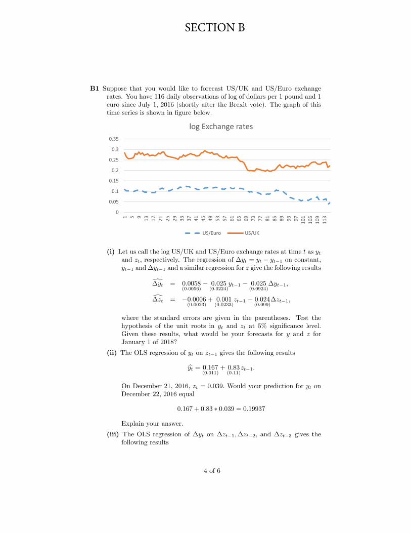
B1 Suppose that you would like to forecast US/UK and US/Euro exchangerates. You have 116 daily observations of log of dollars per 1 pound and 1euro since July 1, 2016 (shortly after the Brexit vote). The graph of thistime series is shown in figure below.
0
0.05
0.1
0.15
0.2
0.25
0.3
0.35
1 5 9 13 17 21 25 29 33 37 41 45 49 53 57 61 65 69 73 77 81 85 89 93 97 101
105
109
113
log Exchange rates
US/Euro US/UK
(i) Let us call the log US/UK and US/Euro exchange rates at time t as ytand zt, respectively. The regression of ∆yt = yt − yt−1 on constant,yt−1 and∆yt−1 and a similar regression for z give the following results
∆yt = 0.0058(0.0056)
− 0.025(0.0224)
yt−1 − 0.025(0.0924)
∆yt−1,
∆zt = −0.0006(0.0023)
+ 0.001(0.0233)
zt−1 − 0.024(0.099)
∆zt−1,
where the standard errors are given in the parentheses. Test thehypothesis of the unit roots in yt and zt at 5% significance level.Given these results, what would be your forecasts for y and z forJanuary 1 of 2018?
(ii) The OLS regression of yt on zt−1 gives the following results
yt = 0.167(0.011)
+ 0.83(0.11)
zt−1.
On December 21, 2016, zt = 0.039. Would your prediction for yt onDecember 22, 2016 equal
0.167 + 0.83 ∗ 0.039 = 0.19937
Explain your answer.
(iii) The OLS regression of ∆yt on ∆zt−1,∆zt−2, and ∆zt−3 gives thefollowing results
4 of 6
SECTION B

. reg dy L1.dz L2.dz L3.dz
Source SS 112F(3, 108) 0.30
Model .000045452 3 .000015151 Prob > F = 0.8240Residual .005420629 108 .000050191 R-squared = 0.0083
Adj R-squared = -0.0192Total .005466081 111 .000049244 Root MSE = .00708
dy Coef. Std. Err. t P>|t| [95% Conf. Interval]
dzL1. -.039442 .1389438 -0.28 0.777 -.3148527 .2359688L2. .1110407 .161019 0.69 0.492 -.2081268 .4302083L3. -.1026289 .1610944 -0.64 0.525 -.421946 .2166882
_cons -.0003422 .000678 -0.50 0.615 -.0016862 .0010018
.What is the estimate of the long run multiplier in the effect of ∆zton ∆yt? Test the hypothesis that the coeffi cients on ∆zt−1,∆zt−2,and ∆zt−3 are equal to zero. Discuss the validity of your test.
(iv) How would you test for no serial correlation in the errors of theregression from (iii)?
B2 Consider a regression model
yi = β0 + β1xi + εi,
where (xi, εi) , i = 1, ..., n, are i.i.d. with Exi = Eεi = 0, but Cov (xi, εi) 6=0. Suppose that vi is a valid instrument for xi. Assume that vi, i = 1, ..., n,are i.i.d., and Evi = 0. A friend suggests that you can use an extra in-strument wi = vi + ηi, where ηi, i = 1, ..., n, are i.i.d., independent fromvj , xj and εj , for all j = 1, ..., n, and have zero mean.
(i) Let zi = (1, vi, wi)′. Show that the rank condition holds for zi.
(ii) Recall that under homoskedasticity,
√n(β2SLS − β
)d→ N
(0, σ2
(Exiz
′i (Eziz
′i)−1Ezix
′i
)−1)where β2SLS is the 2SLS estimator of β = (β0, β1)
′ that uses zi asinstruments. Verify that the homoskedasticity holds, assuming thatE(ε2i |vi
)= σ2.
(iii) Compute the variance covariance matrix of the asymptotic distribu-tion of
√n(β2SLS − β
), assuming that σ2 = Ev2i = Eη2i = Evixi =
1.
(iv) Compare the variance covariance matrix computed in (iii) with thevariance covariance matrix of the asymptotic distribution of
√n(β2SLS − β
),
where β2SLS is the 2SLS estimator of β that uses only (1, vi) as in-struments. Briefly comment on your comparison.
5 of 6
Please turn over

B3 A researcher studies the effect of water pollution on the mortality rate in afish population. He runs extensive laboratory experiments and determinesthat the 0.1% and 0.05% concentrations of a pollutant in water lead to50% and 23% mortality rate, respectively.
(i) Assuming that the probability of death is described by a probit model,determine the mortality rate of fish in absolutely clean water.
(ii) What would your answer to (i) be had you assumed that the proba-bility of death is described by a linear probability model? Comment.
(iii) In fact, to establish the 50% and 23% mortality rates, the researchersimply computed the proportion of fish in two large tanks of wa-ter with the concentration of a pollutant equal to 0.1% and 0.05%,respectively. Argue that the researcher’s method is equivalent to amaximum likelihood procedure.
(iv) Assume that each of the tanks of water had 1000 fish. Find thestandard errors of the 50% and 23% estimates.
B4 Consider the following regression model
yi = β0 + β1xi + εi,
where (yi, xi) , i = 1, ..., n are i.i.d. and εi = xi × ui with ui distributedas a standard normal conditionally on xi.
(i) Show that εi, i = 1, ..., n are i.i.d.
(ii) Which Gauss-Markov assumptions hold for this model and which fail?What does this imply for the OLS estimator of β1?
(iii) Suppose that n = 3, and
i 1 2 3yi 1 0 -1xi 1 2 4
Find the GLS estimate β1,GLS .
(iv) What is the finite sample distribution of βGLS =(β0,GLS , β1,GLS
)′conditional on x1, x2, and x3?
6 of 6
END OF PAPER

ECM9/ECM10/ECM11/MGM3MPhil in EconomicsMPhil in Economic ResearchMPhil in Finance and EconomicsMPhil Finance
Friday 12th, May, 2017 2:00pm - 4:00pm
M300ECONOMETRIC METHODS
Answer all six questions from Section A and two questions from Section B. PartA is 60% of total marks.
All questions in Section A carry equal weight.
Write your candidate number (not your name) on the cover of each booklet.
Write legibly. Credit will be given for clear presentation of relevant statistics.
If you identify an error in this paper, please alert the Invigilator, who will notifythe Examiner. A general announcement will be made if the error is validated.
STATIONERY REQUIREMENTS20 Page booklet x 1Rough work pads
SPECIAL REQUIREMENTS TO BE SUPPLIED FOR THISEXAMINATIONCalculator - students are permitted to bring an approved calculatorDickey-Fuller TablesNew Cambridge Statistical TablesEngle-Granger Tables
You may not start to read the questions printedon the subsequent pages of this question paper
until instructed that you may do so by the Invigilator.
1 of 6
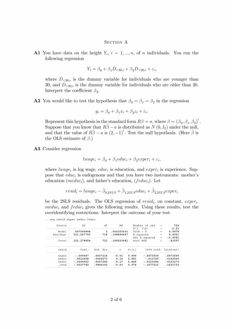
Section A
A1 You have data on the height Yi, i = 1, ..., n, of n individuals. You run thefollowing regression
Yi = β0 + β1D<30,i + β2D>20,i + εi,
where D<30,i is the dummy variable for individuals who are younger than30, and D>20,i is the dummy variable for individuals who are older than 20.Interpret the coeffi cient β2.
A2 You would like to test the hypothesis that β0 = β1 = β2 in the regression
yi = β0 + β1xi + β2zi + εi.
Represent this hypothesis in the standard formRβ = a, where β = (β0, β1, β2)′ .
Suppose that you know that Rβ− a is distributed as N (0, I2) under the null,and that the value of Rβ − a is (2,−1)′ . Test the null hypothesis. (Here β isthe OLS estimate of β.)
A3 Consider regression
lwagei = β0 + β1educi + β2experi + εi,
where lwagei is log wage, educi is education, and experi is experience. Sup-pose that educi is endogenous and that you have two instruments: mother’seducation (meduci), and father’s education, (feduci). Let
residi = lwagei − β0,2SLS + β1,2SLSeduci + β2,2SLSexperi
be the 2SLS residuals. The OLS regression of residi, on constant, experi,meduci and feduci gives the following results. Using these results, test theoveridentifying restrictions. Interpret the outcome of your test.
opened on: 20 Dec 2016, 15:36:01 name: <unnamed> log: C:\Users\ao319\Documents\MPhil\2016\A3a.smcl log type: smcl opened on: 20 Dec 2016, 15:36:01
. reg resid exper meduc feduc
Source SS df MS Number of obs = 722 F(3, 718) = 0.01
Model .007060894 3 .002353631 Prob > F = 0.9978 Residual 121.267793 718 .168896647 R-squared = 0.0001
Adj R-squared = -0.0041 Total 121.274854 721 .168203681 Root MSE = .41097
resid Coef. Std. Err. t P>|t| [95% Conf. Interval]
exper -.000047 .0037216 -0.01 0.990 -.0073536 .0072596 meduc .0012458 .0066271 0.19 0.851 -.011765 .0142566 feduc -.0009902 .0057649 -0.17 0.864 -.0123084 .0103279 _cons -.0027745 .0840162 -0.03 0.974 -.1677212 .1621723
2 of 6

A4 Consider a very simple fixed effects regression
yit = ci + εit, i = 1, ..., n; t = 1, ..., T, (1)
where εit are i.i.d. N (0, σ2) variables and there are no explanatory variables.A colleague proposes to estimate σ2 as 1
nTtimes the SSR from the dummy
variables regression. Find the bias of such an estimate.
A5 A time series yt satisfies the following AR(3) equation
yt = α + ρ1yt−1 + ρ2yt−2 + ρ3yt−3 + εt, t = 1, ..., T.
For which values of ρ1, ρ2 and ρ3 does yt have a unit root? How would youtest for the unit root in yt?
A6 You have n i.i.d. observations yi, i = 1, ..., n that equal −1 with probability p,+1 with probability q, and 0 with probability 1 − p − q. Find the maximumlikelihood estimator of θ = (p, q)′ and the Fisher information matrix.
3 of 6 (TURN OVER)
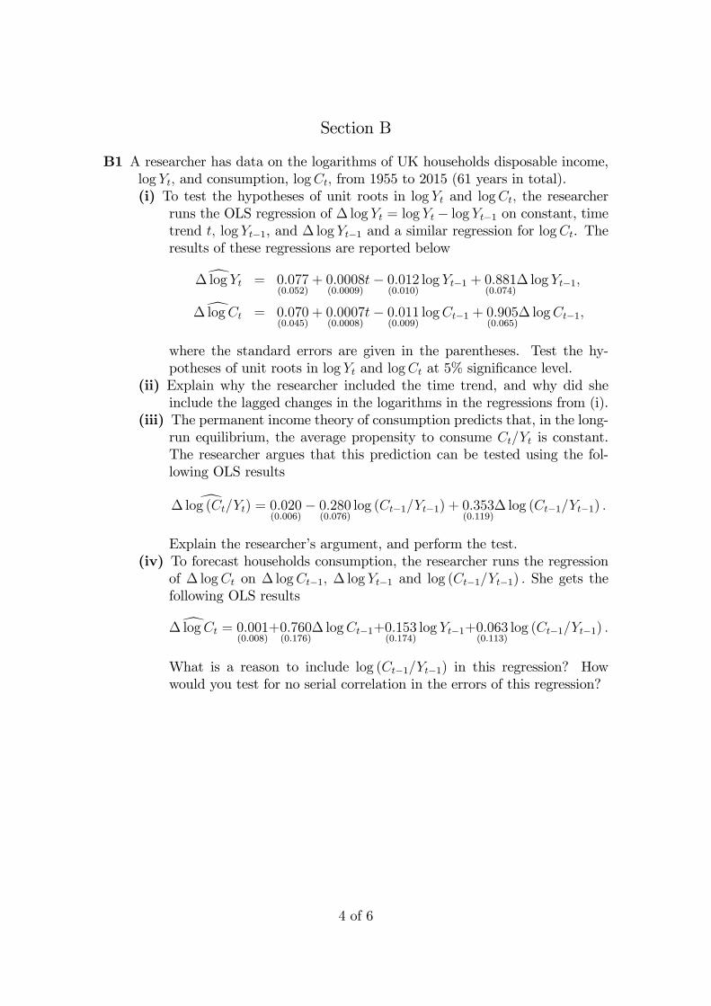
Section B
B1 A researcher has data on the logarithms of UK households disposable income,log Yt, and consumption, logCt, from 1955 to 2015 (61 years in total).(i) To test the hypotheses of unit roots in log Yt and logCt, the researcher
runs the OLS regression of ∆ log Yt = log Yt − log Yt−1 on constant, timetrend t, log Yt−1, and ∆ log Yt−1 and a similar regression for logCt. Theresults of these regressions are reported below
∆ log Yt = 0.077(0.052)
+ 0.0008(0.0009)
t− 0.012(0.010)
log Yt−1 + 0.881(0.074)
∆ log Yt−1,
∆ logCt = 0.070(0.045)
+ 0.0007(0.0008)
t− 0.011(0.009)
logCt−1 + 0.905(0.065)
∆ logCt−1,
where the standard errors are given in the parentheses. Test the hy-potheses of unit roots in log Yt and logCt at 5% significance level.
(ii) Explain why the researcher included the time trend, and why did sheinclude the lagged changes in the logarithms in the regressions from (i).
(iii) The permanent income theory of consumption predicts that, in the long-run equilibrium, the average propensity to consume Ct/Yt is constant.The researcher argues that this prediction can be tested using the fol-lowing OLS results
∆ log (Ct/Yt) = 0.020(0.006)
− 0.280(0.076)
log (Ct−1/Yt−1) + 0.353(0.119)
∆ log (Ct−1/Yt−1) .
Explain the researcher’s argument, and perform the test.(iv) To forecast households consumption, the researcher runs the regression
of ∆ logCt on ∆ logCt−1, ∆ log Yt−1 and log (Ct−1/Yt−1) . She gets thefollowing OLS results
∆ logCt = 0.001(0.008)
+0.760(0.176)
∆ logCt−1+0.153(0.174)
log Yt−1+0.063(0.113)
log (Ct−1/Yt−1) .
What is a reason to include log (Ct−1/Yt−1) in this regression? Howwould you test for no serial correlation in the errors of this regression?
4 of 6
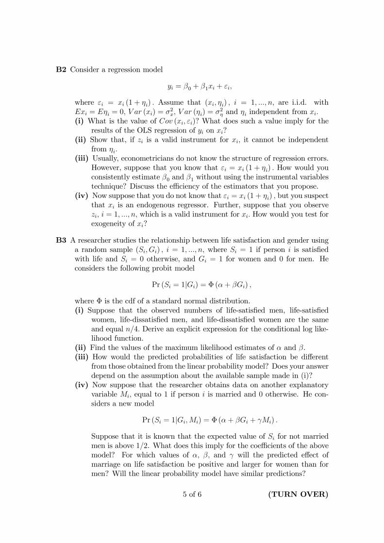
B2 Consider a regression model
yi = β0 + β1xi + εi,
where εi = xi (1 + ηi) . Assume that (xi, ηi) , i = 1, ..., n, are i.i.d. withExi = Eηi = 0, V ar (xi) = σ2x, V ar (ηi) = σ2η and ηi independent from xi.(i) What is the value of Cov (xi, εi)? What does such a value imply for the
results of the OLS regression of yi on xi?(ii) Show that, if zi is a valid instrument for xi, it cannot be independent
from ηi.(iii) Usually, econometricians do not know the structure of regression errors.
However, suppose that you know that εi = xi (1 + ηi) . How would youconsistently estimate β0 and β1 without using the instrumental variablestechnique? Discuss the effi ciency of the estimators that you propose.
(iv) Now suppose that you do not know that εi = xi (1 + ηi) , but you suspectthat xi is an endogenous regressor. Further, suppose that you observezi, i = 1, ..., n, which is a valid instrument for xi. How would you test forexogeneity of xi?
B3 A researcher studies the relationship between life satisfaction and gender usinga random sample (Si, Gi) , i = 1, ..., n, where Si = 1 if person i is satisfiedwith life and Si = 0 otherwise, and Gi = 1 for women and 0 for men. Heconsiders the following probit model
Pr (Si = 1|Gi) = Φ (α + βGi) ,
where Φ is the cdf of a standard normal distribution.(i) Suppose that the observed numbers of life-satisfied men, life-satisfied
women, life-dissatisfied men, and life-dissatisfied women are the sameand equal n/4. Derive an explicit expression for the conditional log like-lihood function.
(ii) Find the values of the maximum likelihood estimates of α and β.(iii) How would the predicted probabilities of life satisfaction be different
from those obtained from the linear probability model? Does your answerdepend on the assumption about the available sample made in (i)?
(iv) Now suppose that the researcher obtains data on another explanatoryvariable Mi, equal to 1 if person i is married and 0 otherwise. He con-siders a new model
Pr (Si = 1|Gi,Mi) = Φ (α + βGi + γMi) .
Suppose that it is known that the expected value of Si for not marriedmen is above 1/2. What does this imply for the coeffi cients of the abovemodel? For which values of α, β, and γ will the predicted effect ofmarriage on life satisfaction be positive and larger for women than formen? Will the linear probability model have similar predictions?
5 of 6 (TURN OVER)

B4 Consider the following two-period panel regression model
yit = αi + βxit + εit, i = 1, ..., n, t = 1, 2.
where (yi1, yi2, xi1, xi2, αi) , i = 1, ..., n are i.i.d., εi1 = 0, i = 1, ..., n, that is, inthe first period εi1 is identically zero, and εi2 is independent from (xi1, xi2, αi),Eεi2 = 0, and V ar (εi2) = 1.(i) Which Gauss-Markov assumptions hold for this model and which may
fail?(ii) Will the fixed effects estimator of β be unbiased? Will it be consistent?
Explain your answers.(iii) Propose a consistent estimator of the fixed effects αi and show its con-
sistency.(iv) Suppose that αi = ηi, where ηi is independent from (xi1, xi2) , Eηi = 0
and V ar (ηi) = 1. Let wit = ηi + εit and
w = (w11, w12, w21, w22, ..., wn1, wn2)′ .
Find Ω = V ar (w) and its inverse Ω−1. Using your findings, describe theGLS estimator of β in the regression yit = βxit + wit.
END OF PAPER
6 of 6

ECM9/ECM10/ECM11MPhil in EconomicsMPhil in Finance & EconomicsMPhil in Economic Research
Friday 2nd June 2017 1:30pm to 3:30pm
M310TIME SERIES
Candidates are required to answer five questions from Section A andone question from Section B.
Section A is weighted as 60% and Section B as 40%.
Write your candidate number (not your name) on the cover of each booklet.
Write legibly.
If you identify an error in this paper, please alert the Invigilator, who will notifythe Examiner. A general announcement will be made if the error is validated.
STATIONERY REQUIREMENTS20 Page booklet x 1Rough work pads
SPECIAL REQUIREMENTS TO BE SUPPLIED FOR THISEXAMINATIONCalculator - students are permitted to bring an approved calculator
You may not start to read the questions printedon the subsequent pages of this question paper
until instructed that you may do so by the Invigilator.
1 of 4
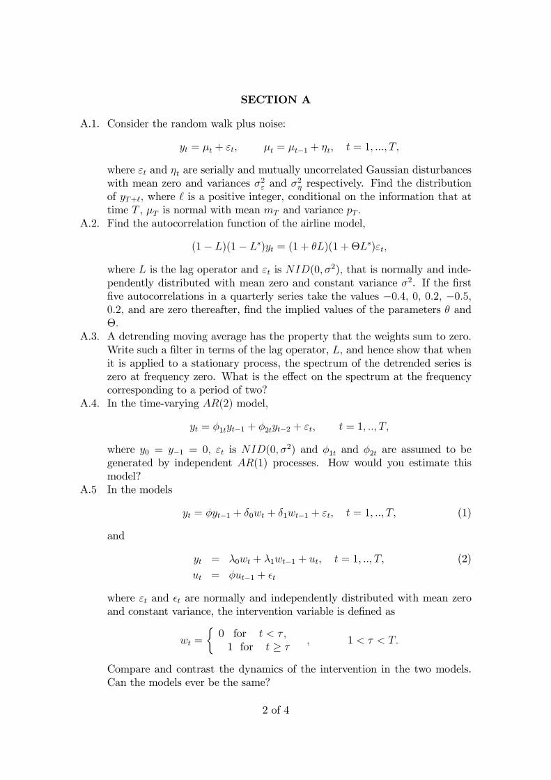
SECTION A
A.1. Consider the random walk plus noise:
yt = µt + εt, µt = µt−1 + ηt, t = 1, ..., T,
where εt and ηt are serially and mutually uncorrelated Gaussian disturbanceswith mean zero and variances σ2ε and σ
2η respectively. Find the distribution
of yT+`, where ` is a positive integer, conditional on the information that attime T , µT is normal with mean mT and variance pT .
A.2. Find the autocorrelation function of the airline model,
(1− L)(1− Ls)yt = (1 + θL)(1 + ΘLs)εt,
where L is the lag operator and εt is NID(0, σ2), that is normally and inde-pendently distributed with mean zero and constant variance σ2. If the firstfive autocorrelations in a quarterly series take the values −0.4, 0, 0.2, −0.5,0.2, and are zero thereafter, find the implied values of the parameters θ andΘ.
A.3. A detrending moving average has the property that the weights sum to zero.Write such a filter in terms of the lag operator, L, and hence show that whenit is applied to a stationary process, the spectrum of the detrended series iszero at frequency zero. What is the effect on the spectrum at the frequencycorresponding to a period of two?
A.4. In the time-varying AR(2) model,
yt = φ1tyt−1 + φ2tyt−2 + εt, t = 1, .., T,
where y0 = y−1 = 0, εt is NID(0, σ2) and φ1t and φ2t are assumed to begenerated by independent AR(1) processes. How would you estimate thismodel?
A.5 In the models
yt = φyt−1 + δ0wt + δ1wt−1 + εt, t = 1, .., T, (1)
and
yt = λ0wt + λ1wt−1 + ut, t = 1, .., T, (2)
ut = φut−1 + εt
where εt and εt are normally and independently distributed with mean zeroand constant variance, the intervention variable is defined as
wt =
0 for t < τ,
1 for t ≥ τ, 1 < τ < T.
Compare and contrast the dynamics of the intervention in the two models.Can the models ever be the same?
2 of 4

A.6. Consider the model
yt = εt + βεt−1εt−2, εt ∼ NID(0, σ2), t = 1, ..., T,
where NID(0, σ2) denotes normally and independently distributed with meanzero and constant variance σ2, and ε0 and ε−1 are fixed and known. Find theminimum mean square error estimator (MMSE) of yT+1 and compare its MSEwith that of the best linear predictor. How would you estimate β?
A.7. The Clayton copula is defined as
C(u1, u2) =
(u−θ1 + u−θ2 − 1)−1/θ, θ > 0u1u2, θ = 0.
Explain what is meant by tail dependence and obtain expressions for taildependence in a Clayton copula when θ > 0 and when θ = 0. Define the coef-ficient of lower tail dependence (the lower tail index) and derive this coeffi cientfor the Clayton copula.
3 of 4 (TURN OVER)
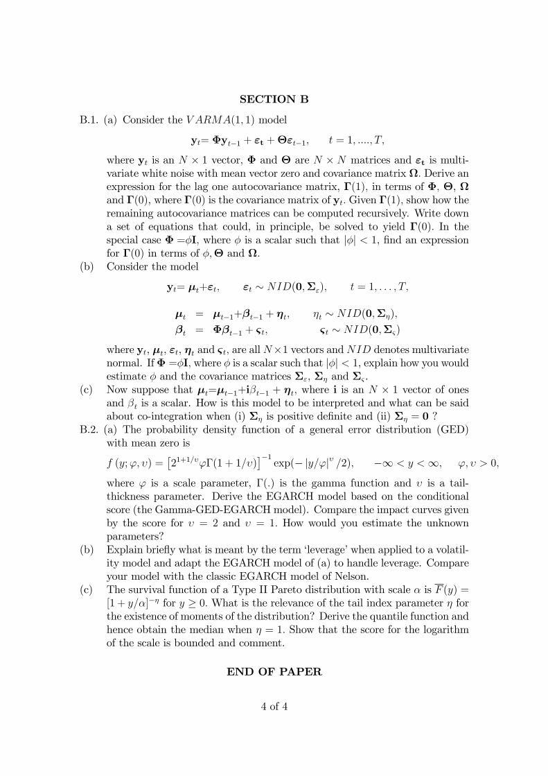
SECTION B
B.1. (a) Consider the V ARMA(1, 1) model
yt= Φyt−1 + εt + Θεt−1, t = 1, ...., T,
where yt is an N × 1 vector, Φ and Θ are N × N matrices and εt is multi-variate white noise with mean vector zero and covariance matrix Ω. Derive anexpression for the lag one autocovariance matrix, Γ(1), in terms of Φ, Θ, Ωand Γ(0), where Γ(0) is the covariance matrix of yt. Given Γ(1), show how theremaining autocovariance matrices can be computed recursively. Write downa set of equations that could, in principle, be solved to yield Γ(0). In thespecial case Φ =φI, where φ is a scalar such that |φ| < 1, find an expressionfor Γ(0) in terms of φ,Θ and Ω.
(b) Consider the model
yt= µt+εt, εt ∼ NID(0,Σε), t = 1, . . . , T,
µt = µt−1+βt−1 + ηt, ηt ∼ NID(0,Ση),
βt = Φβt−1 + ς t, ς t ∼ NID(0,Σς)
where yt, µt, εt, ηt and ς t, are all N×1 vectors andNID denotes multivariatenormal. IfΦ =φI, where φ is a scalar such that |φ| < 1, explain how you wouldestimate φ and the covariance matrices Σε, Ση and Σς .
(c) Now suppose that µt=µt−1+iβt−1 + ηt, where i is an N × 1 vector of onesand βt is a scalar. How is this model to be interpreted and what can be saidabout co-integration when (i) Ση is positive definite and (ii) Ση = 0 ?
B.2. (a) The probability density function of a general error distribution (GED)with mean zero is
f (y;ϕ, υ) =[21+1/υϕΓ(1 + 1/υ)
]−1exp(− |y/ϕ|υ /2), −∞ < y <∞, ϕ, υ > 0,
where ϕ is a scale parameter, Γ(.) is the gamma function and υ is a tail-thickness parameter. Derive the EGARCH model based on the conditionalscore (the Gamma-GED-EGARCH model). Compare the impact curves givenby the score for υ = 2 and υ = 1. How would you estimate the unknownparameters?
(b) Explain briefly what is meant by the term ‘leverage’when applied to a volatil-ity model and adapt the EGARCH model of (a) to handle leverage. Compareyour model with the classic EGARCH model of Nelson.
(c) The survival function of a Type II Pareto distribution with scale α is F (y) =[1 + y/α]−η for y ≥ 0. What is the relevance of the tail index parameter η forthe existence of moments of the distribution? Derive the quantile function andhence obtain the median when η = 1. Show that the score for the logarithmof the scale is bounded and comment.
END OF PAPER
4 of 4

ECM9/ECM10/ECM11/MGM3MPhil in EconomicsMPhil in Finance & EconomicsMPhil in Economic ResearchMPhil in Finance
Wednesday 7 May 2017 9:00am-11:00am
M320CROSS SECTION AND PANEL DATA ECONOMETRICS
Candidates are required to answer three questions from Section A and onequestion from Section B.
Section A is weighted as 60% and Section B as 40%
Write your candidate number (not your name) on the cover of each booklet.
Write legibly.
If you identify an error in this paper, please alert the Invigilator, who will notifythe Examiner. A general announcement will be made if the error is validated.
STATIONERY REQUIREMENTS20 Page booklet x 1Rough work pads
SPECIAL REQUIREMENTS TO BE SUPPLIED FOR THIS EXAMINATIONDurbin-Watson and Dickey-Fuller TablesNew Cambridge Elementary Statistical TablesCalculator - students are permitted to bring an approved calculator
You may not start to read the questions printedon the subsequent pages of this question paper
until instructed that you may do so by the Invigilator.
1 of 8
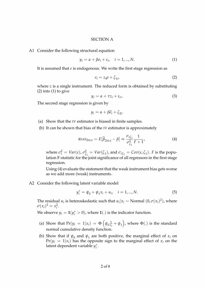
2 of 8
SECTION A
A1 Consider the following structural equation
yi = α + βei + εi, i = 1, ..., N. (1)
It is assumed that e is endogenous. We write the first stage regression as
ei = ziρ + ζ1i, (2)
where z is a single instrument. The reduced form is obtained by substituting(2) into (1) to give
yi = α + τzi + εri. (3)
The second stage regression is given by
yi = α + βei + ζ2i.
(a) Show that the IV estimator is biased in finite samples.
(b) It can be shown that bias of the IV estimator is approximately
BIAS2SLS = E[β2SLS − β] ≈σεζ1
σ2ζ1
1F + 1
, (4)
where σ2ε = Var(ε), σ2
ζ1= Var(ζ1), and σεζ1
= Cov(ε, ζ1). F is the popu-lation F-statistic for the joint significance of all regressors in the first stageregression.Using (4) evaluate the statement that the weak instrument bias gets worseas we add more (weak) instruments.
A2 Consider the following latent variable model
y∗i = ψ0 + ψ1xi + ui, i = 1, ..., N. (5)
The residual ui is heteroskedastic such that ui|xi ∼ Normal (0, σ(xi)2), where
σ(xi)2 = x2
i .
We observe yi = 1(y∗i > 0), where 1(.) is the indicator function.
(a) Show that Pr(yi = 1|xi) = Φ(
ψ01xi+ ψ1
), where Φ(.) is the standard
normal cumulative density function.
(b) Show that if ψ0 and ψ1 are both positive, the marginal effect of xi onPr(yi = 1|xi) has the opposite sign to the marginal effect of xi on thelatent dependent variable y∗i .
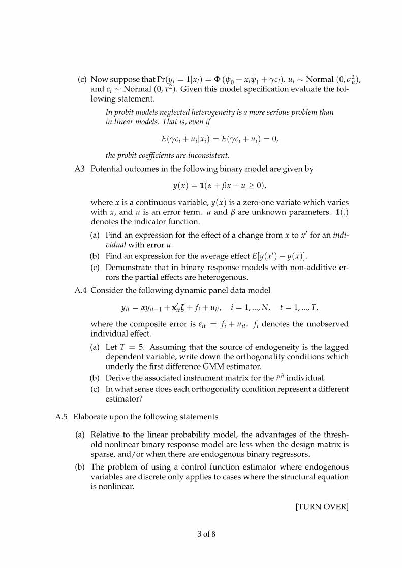
3 of 8
(c) Now suppose that Pr(yi = 1|xi) = Φ (ψ0 + xiψ1 + γci). ui ∼ Normal (0, σ2u),
and ci ∼ Normal (0, τ2). Given this model specification evaluate the fol-lowing statement.
In probit models neglected heterogeneity is a more serious problem thanin linear models. That is, even if
E(γci + ui|xi) = E(γci + ui) = 0,
the probit coefficients are inconsistent.
A3 Potential outcomes in the following binary model are given by
y(x) = 1(α + βx + u ≥ 0),
where x is a continuous variable, y(x) is a zero-one variate which varieswith x, and u is an error term. α and β are unknown parameters. 1(.)denotes the indicator function.
(a) Find an expression for the effect of a change from x to x′ for an indi-vidual with error u.
(b) Find an expression for the average effect E[y(x′)− y(x)].(c) Demonstrate that in binary response models with non-additive er-
rors the partial effects are heterogenous.
A.4 Consider the following dynamic panel data model
yit = αyit−1 + x′itζ + fi + uit, i = 1, ..., N, t = 1, ..., T,
where the composite error is εit = fi + uit. fi denotes the unobservedindividual effect.
(a) Let T = 5. Assuming that the source of endogeneity is the laggeddependent variable, write down the orthogonality conditions whichunderly the first difference GMM estimator.
(b) Derive the associated instrument matrix for the ith individual.(c) In what sense does each orthogonality condition represent a different
estimator?
A.5 Elaborate upon the following statements
(a) Relative to the linear probability model, the advantages of the thresh-old nonlinear binary response model are less when the design matrix issparse, and/or when there are endogenous binary regressors.
(b) The problem of using a control function estimator where endogenousvariables are discrete only applies to cases where the structural equationis nonlinear.
[TURN OVER]

(c) The error components representation of a mixed logit model and the ran-dom effects panel data estimator both generate non-iid covariance matri-ces which may be exploited to solve different problems.
(d) Explain how to construct an estimator from a set of population momentconditions using the generalised method of moments.
4 of 8

SECTION B
B.1 The relationship between female labour force participation (y) and fertility(d1) is written as
yit = 1(α + δ1d1,it + δ2d2,it + x′iβ + ξ it > 0), i = 1, ..., N and t = 1, ..., T,
where 1(.) denotes the indicator function, yit is a binary indicator of partici-pation in year t (defined as positive annual hours of work), fertility (d1,it) is adummy variable which takes the value one if the age of the youngest child attime t + 1 is 1, and d2,it is a dummy indicator equal to one if the woman has achild between the ages of 2 and 6. xi is vector of additional controls.
In addition ξ it = αi + uit is a standard composite panel data error term inwhich αi represents an individual-specific effect and uit denotes time varyingerrors including idiosyncratic labour market shocks.
a) Briefly discuss why fertility is most likely an endogenous variable. Pro-vide justification for the use of an indicator of whether a woman has twochildren of the same sex as an external instrument for fertility.
b) In Table 1 we report results based on the application of a number of linearestimators. Columns 2, 3, and 4, report, respectively, results based uponthe use of an OLS, 2SLS and within-group (WG) estimator.
Columns 5 and 6 present results for two first-difference GMM estimators,that exploit, respectively, strict and weak exogeneity assumptions.
i) For each estimator outline the identification assumptions and in par-ticular discuss how each estimator accounts for the endogeneity offertility.
ii) In what sense does the use of the WG estimator represent a tradeoffbetween accounting for unobserved heterogeneity and bias?
c) Write down the moment equations which underly the results for theGMM-1 and GMM-2 estimators.
For each estimator state the degree of overidentification.
d) Using the results in columns 5 and 6 test for strict exogeneity. What doyou conclude?
[TURN OVER]5 of 8

Table 1: Female Labour Force Participation
Linear Probability Models (N=1442, 1986-1989)
Variable OLS 2SLS1 WG GMM-12 GMM-23
Fertility −0.15 −1.01 −0.06 −0.08 −0.13(8.2) (2.1) (3.8) (2.8) (2.2)
Kids2-6 −0.08 −0.24 0.001 −0.005 −0.09(5.2) (2.6) (0.04) (0.4) (2.7)
Sargan 48.0 18.0(d.f.) (22) (10)
Notes- Heteroskedasticity robust t-ratios shown in parentheses
- 1 External instrument: whether a woman has two children of the same sex.
- The variable Kids2-6 is equal to one if a woman has a child between 2 and 6.
- 2 Treats fertility as endogenous and uses all lags and leads ofKids2-6 and the external instrument same sex.
- 3 Treats fertility as endogenous and uses lags of Kids 2-6 and same sex up to t-1.
- Estimators which do not account for individual effects also include a constant,age, race, and education dummies (not reported).- Sargan denotes the Sargan test for overidentifying restrictions.
The sample consists of 1442 women aged between 18-55 in 1986.
6 of 8
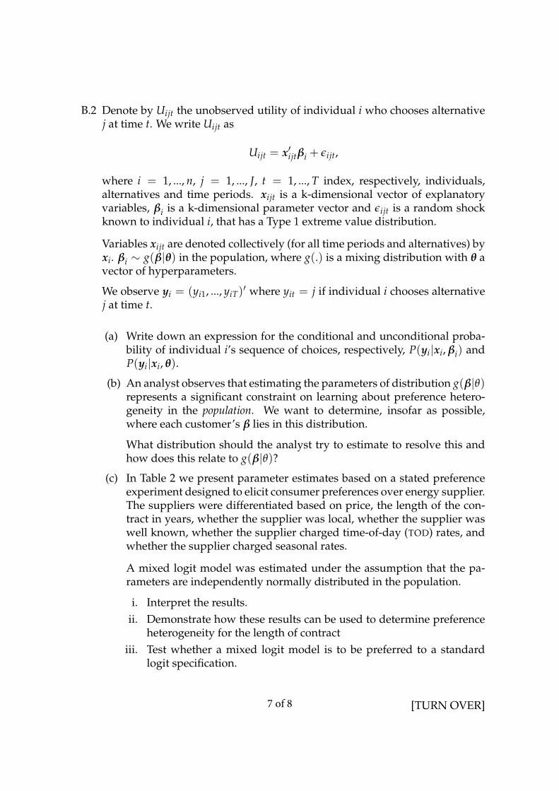
B.2 Denote by Uijt the unobserved utility of individual i who chooses alternativej at time t. We write Uijt as
Uijt = x′ijtβi + εijt,
where i = 1, ..., n, j = 1, ..., J, t = 1, ..., T index, respectively, individuals,alternatives and time periods. xijt is a k-dimensional vector of explanatoryvariables, βi is a k-dimensional parameter vector and εijt is a random shockknown to individual i, that has a Type 1 extreme value distribution.
Variables xijt are denoted collectively (for all time periods and alternatives) byxi. βi ∼ g(β|θ) in the population, where g(.) is a mixing distribution with θ avector of hyperparameters.
We observe yi = (yi1, ..., yiT)′ where yit = j if individual i chooses alternative
j at time t.
(a) Write down an expression for the conditional and unconditional proba-bility of individual i’s sequence of choices, respectively, P(yi|xi, βi) andP(yi|xi, θ).
(b) An analyst observes that estimating the parameters of distribution g(β|θ)represents a significant constraint on learning about preference hetero-geneity in the population. We want to determine, insofar as possible,where each customer’s β lies in this distribution.
What distribution should the analyst try to estimate to resolve this andhow does this relate to g(β|θ)?
(c) In Table 2 we present parameter estimates based on a stated preferenceexperiment designed to elicit consumer preferences over energy supplier.The suppliers were differentiated based on price, the length of the con-tract in years, whether the supplier was local, whether the supplier waswell known, whether the supplier charged time-of-day (TOD) rates, andwhether the supplier charged seasonal rates.
A mixed logit model was estimated under the assumption that the pa-rameters are independently normally distributed in the population.
i. Interpret the results.ii. Demonstrate how these results can be used to determine preference
heterogeneity for the length of contractiii. Test whether a mixed logit model is to be preferred to a standard
logit specification.
[TURN OVER]7 of 8

Table 2: Mixed logit model of choice among energy suppliers
θ σθ
Price coeff.−0.8827(0.050)
−
Contract−0.2125(0.026)
0.3865(0.028)
Local2.2277(0.127)
1.7514(.137)
Well-known1.5906(0.100)
0.9621(0.098)
TOD2.1328(0.054)
0.4113(0.040)
Seasonal2.1577(0.051)
0.2812(0.022)
Log Likelihood Logit: −4959Log Likelihood Mixed Logit −3619
Standard errors in parenthesis
θ denotes the mean and σθ the standard deviation of each parameter estimated.
END OF PAPER
9 of 9

ECM9/ECM10MPhil in EconomicsMPhil in Economic Research
Monday 22 May 2017 09:00 - 11:0000am - 11:00am
M330APPLIED ECONOMETRICS
The paper is in two sections: Candidate are require to answer from Section A twocompulsory questions and section B two out of four questions.
Each question carries equal weight.
Write your candidate number (not your name) on the cover of each booklet.
Write legibly.
If you identify an error in this paper, please alert the Invigilator, who will notifythe Examiner. A general announcement will be made if the error is validated.
STATIONERY REQUIREMENTS20 Page booklet x 1Rough work pads
SPECIAL REQUIREMENTS TO BE SUPPLIED FOR THISEXAMINATIONCalculator - students are permitted to bring an approved calculator
You may not start to read the questions printedon the subsequent pages of this question paper
until instructed that you may do so by the Invigilator.
1 of 10
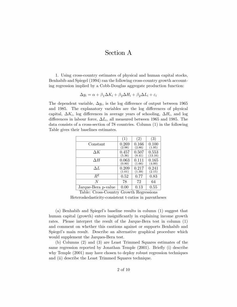
Section A
1. Using cross-country estimates of physical and human capital stocks,Benhabib and Spiegel (1994) ran the following cross-country growth account-ing regression implied by a Cobb-Douglas aggregate production function:
∆yi = α+ β1∆Ki + β2∆Hi + β2∆Li + εi
The dependent variable, ∆yi, is the log difference of output between 1965and 1985. The explanatory variables are the log differences of physicalcapital, ∆Ki, log differences in average years of schooling, ∆Hi, and logdifferences in labour force, ∆Li, all measured between 1965 and 1985. Thedata consists of a cross-section of 78 countries. Column (1) in the followingTable gives their baselines estimates.
(1) (2) (3)Constant 0.269
(2.98)0.166(2.86)
0.100(1.95)
∆K 0.457(5.36)
0.507(8.41)
0.553(13.16)
∆H 0.063(0.80)
0.111(1.66)
0.165(4.00)
∆L 0.209(1.01)
0.217(1.39)
0.241(2.15)
R2 0.52 0.77 0.83
N 78 72 64
Jarque-Bera p-value 0.00 0.13 0.55Table: Cross-Country Growth Regressions
Heteroskedasticity-consistent t-ratios in parentheses
(a) Benhabib and Spiegel’s baseline results in column (1) suggest thathuman capital (growth) enters insignificantly in explaining income growthrates. Please interpret the result of the Jarque-Bera test in column (1)and comment on whether this cautions against or supports Benhabib andSpiegel’s main result. Describe an alternative graphical procedure whichwould supplement the Jarques-Bera test.
(b) Columns (2) and (3) are Least Trimmed Squares estimates of thesame regression reported by Jonathan Temple (2001). Briefly (i) describewhy Temple (2001) may have chosen to deploy robust regression techniquesand (ii) describe the Least Trimmed Squares technique.
2 of 10

(c) In column (3) the Least Trimmed Squares procedure is dropping 14observations. Upon inspection, we learn that these observations stand outfrom the rest of the sample in that they experienced very little (or evennegative) human capital growth relative to the rest of the world during thistwenty year period. Does this alone justify the change in point estimatesand statistical significance observed when we go from column (1) to column(3)? Explain your answer.
3 of 10 (TURN OVER)

2. Besley and Burgess (2004) consider the following model for outcomesin Indian states (indexed by s) at time t,
yst = αs + βt + µrst + ξxst + εst, (1)
where αs and βt are fixed effects, rst is a “labor reform”variable, and xstare other exogenous variables.1
(a) Explain how µ defines a “difference-in-difference”(DD) effect. Out-line the necessary conditions for the identification of DD effects on the spec-ification (1).
(b) Assume that the econometrician Rob is told by a political scientistfriend that there are some states where the labour reforms would be a pro-forma reform only —that is, even though there formally is a reform (and itis recorded in the data as such), it could never be enforced in practice.
• (i) Explain the danger of just recoding these observations as if therewere no reforms to begin with.
• (ii) Outline how you could use the information on these problematicstates to better formulate a regression model to estimate the effect oflabour reforms.
(c) Explain what the DD effects are using Table 5.2.3 of Angrist andPischke (2009). Discuss what assumption underlying the specification inequation (1) seems to be violated. Explain your reasoning. The Table ofAngrist and Pischke is reproduced at the end of the exam (see Figure 1).
1 In their paper, labour reforms are measured with a time lag, but this is not central.
4 of 10
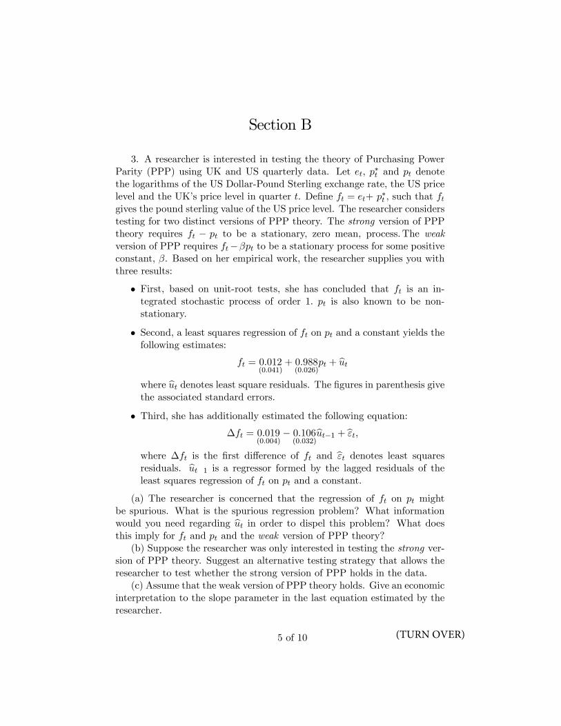
Section B
3. A researcher is interested in testing the theory of Purchasing PowerParity (PPP) using UK and US quarterly data. Let et, p∗t and pt denotethe logarithms of the US Dollar-Pound Sterling exchange rate, the US pricelevel and the UK’s price level in quarter t. Define ft = et+ p∗t , such that ftgives the pound sterling value of the US price level. The researcher considerstesting for two distinct versions of PPP theory. The strong version of PPPtheory requires ft − pt to be a stationary, zero mean, process.The weakversion of PPP requires ft−βpt to be a stationary process for some positiveconstant, β. Based on her empirical work, the researcher supplies you withthree results:
• First, based on unit-root tests, she has concluded that ft is an in-tegrated stochastic process of order 1. pt is also known to be non-stationary.
• Second, a least squares regression of ft on pt and a constant yields thefollowing estimates:
ft = 0.012(0.041)
+ 0.988(0.026)
pt + ut
where ut denotes least square residuals. The figures in parenthesis givethe associated standard errors.
• Third, she has additionally estimated the following equation:∆ft = 0.019
(0.004)− 0.106(0.032)
ut−1 + εt,
where ∆ft is the first difference of ft and εt denotes least squaresresiduals. ut 1 is a regressor formed by the lagged residuals of theleast squares regression of ft on pt and a constant.
(a) The researcher is concerned that the regression of ft on pt mightbe spurious. What is the spurious regression problem? What informationwould you need regarding ut in order to dispel this problem? What doesthis imply for ft and pt and the weak version of PPP theory?
(b) Suppose the researcher was only interested in testing the strong ver-sion of PPP theory. Suggest an alternative testing strategy that allows theresearcher to test whether the strong version of PPP holds in the data.
(c) Assume that the weak version of PPP theory holds. Give an economicinterpretation to the slope parameter in the last equation estimated by theresearcher.
5 of 10 (TURN OVER)
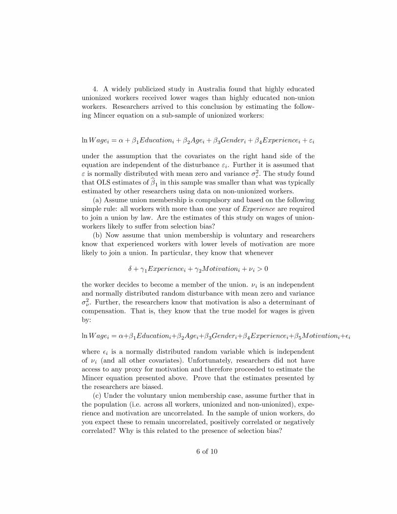
4. A widely publicized study in Australia found that highly educatedunionized workers received lower wages than highly educated non-unionworkers. Researchers arrived to this conclusion by estimating the follow-ing Mincer equation on a sub-sample of unionized workers:
lnWagei = α+ β1Educationi + β2Agei + β3Genderi + β4Experiencei + εi
under the assumption that the covariates on the right hand side of theequation are independent of the disturbance εi. Further it is assumed thatε is normally distributed with mean zero and variance σ2ε. The study foundthat OLS estimates of β1 in this sample was smaller than what was typicallyestimated by other researchers using data on non-unionized workers.
(a) Assume union membership is compulsory and based on the followingsimple rule: all workers with more than one year of Experience are requiredto join a union by law. Are the estimates of this study on wages of union-workers likely to suffer from selection bias?
(b) Now assume that union membership is voluntary and researchersknow that experienced workers with lower levels of motivation are morelikely to join a union. In particular, they know that whenever
δ + γ1Experiencei + γ2Motivationi + νi > 0
the worker decides to become a member of the union. νi is an independentand normally distributed random disturbance with mean zero and varianceσ2ν . Further, the researchers know that motivation is also a determinant ofcompensation. That is, they know that the true model for wages is givenby:
lnWagei = α+β1Educationi+β2Agei+β3Genderi+β4Experiencei+β5Motivationi+εi
where εi is a normally distributed random variable which is independentof νi (and all other covariates). Unfortunately, researchers did not haveaccess to any proxy for motivation and therefore proceeded to estimate theMincer equation presented above. Prove that the estimates presented bythe researchers are biased.
(c) Under the voluntary union membership case, assume further that inthe population (i.e. across all workers, unionized and non-unionized), expe-rience and motivation are uncorrelated. In the sample of union workers, doyou expect these to remain uncorrelated, positively correlated or negativelycorrelated? Why is this related to the presence of selection bias?
6 of 10

(d) The arguments in (b) and (c) were noted to the researchers, whowere advised to address them with Heckman’s two-step procedure. In theirreply they indicate that, in the absence of exclusion restrictions, they areskeptical the procedure would be able to deliver unbiased estimates. Discussthe researchers’reply.
7 of 10 (TURN OVER)
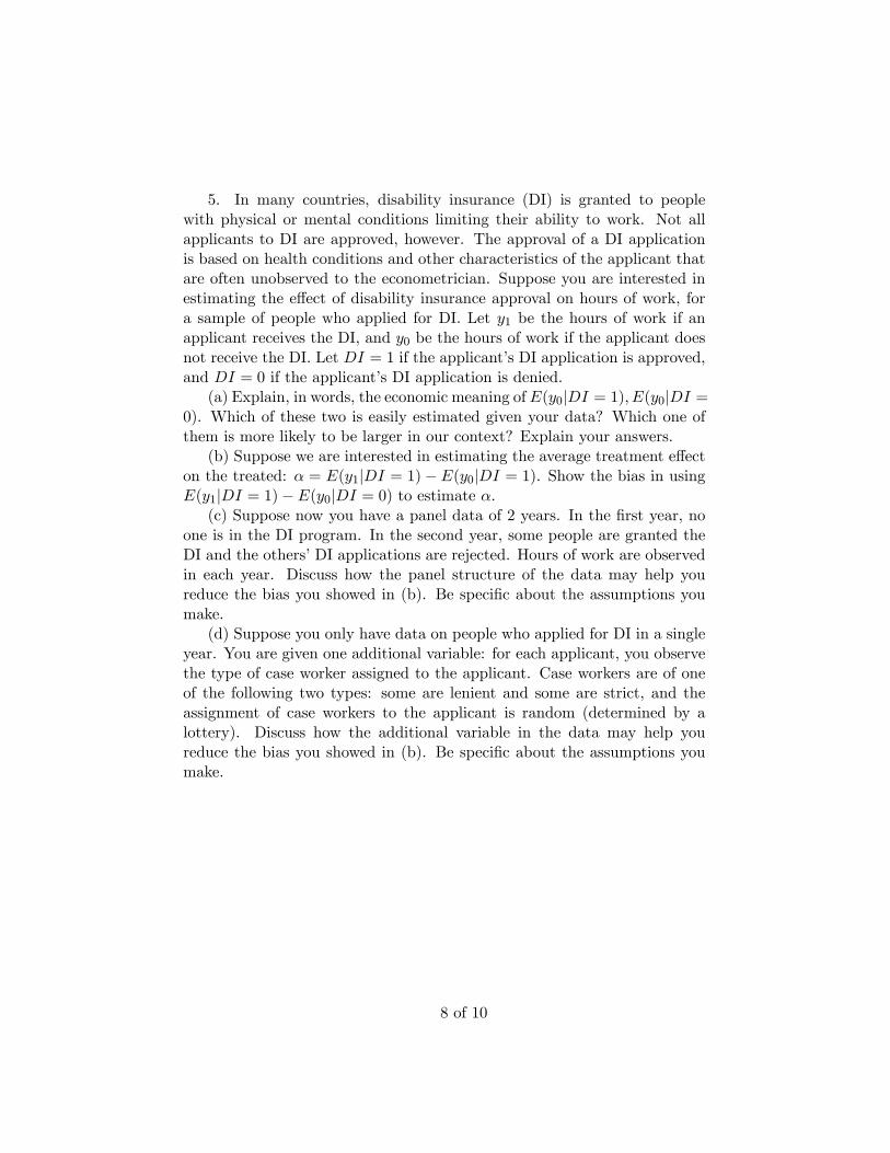
5. In many countries, disability insurance (DI) is granted to peoplewith physical or mental conditions limiting their ability to work. Not allapplicants to DI are approved, however. The approval of a DI applicationis based on health conditions and other characteristics of the applicant thatare often unobserved to the econometrician. Suppose you are interested inestimating the effect of disability insurance approval on hours of work, fora sample of people who applied for DI. Let y1 be the hours of work if anapplicant receives the DI, and y0 be the hours of work if the applicant doesnot receive the DI. Let DI = 1 if the applicant’s DI application is approved,and DI = 0 if the applicant’s DI application is denied.
(a) Explain, in words, the economic meaning of E(y0|DI = 1), E(y0|DI =0). Which of these two is easily estimated given your data? Which one ofthem is more likely to be larger in our context? Explain your answers.
(b) Suppose we are interested in estimating the average treatment effecton the treated: α = E(y1|DI = 1)− E(y0|DI = 1). Show the bias in usingE(y1|DI = 1)− E(y0|DI = 0) to estimate α.
(c) Suppose now you have a panel data of 2 years. In the first year, noone is in the DI program. In the second year, some people are granted theDI and the others’DI applications are rejected. Hours of work are observedin each year. Discuss how the panel structure of the data may help youreduce the bias you showed in (b). Be specific about the assumptions youmake.
(d) Suppose you only have data on people who applied for DI in a singleyear. You are given one additional variable: for each applicant, you observethe type of case worker assigned to the applicant. Case workers are of oneof the following two types: some are lenient and some are strict, and theassignment of case workers to the applicant is random (determined by alottery). Discuss how the additional variable in the data may help youreduce the bias you showed in (b). Be specific about the assumptions youmake.
8 of 10

6. An econometrician, Robert, collects data containing total employment(L) and average wages (W) for all the counties in the UK. Robert considersthe following model of supply and demand for labor:
Di = α0 + α1Wi + εi, (2)
Si = β0 + β1Wi + µi (3)
where Di, Si and Wi are labor demand, labor supply and wages in county i.The parameters of interest are α1. Robert assumes that the labor market ineach county is independent and competitive, so labor market clears (Di =Si) for any county i and εi, µi are i.i.d..
(a) Draw a simple labor demand and supply diagram for a given countyi and derive its equilibrium wage, Wi.
(b) To estimate labor demand (equation (2)), Robert regresses Li on Wi
and obtains the least square estimator (α1) for α1. Is α1 unbiased? If so,provide a proof. If not, derive the bias of the least square estimator for α1.
(c) Suppose that, in addition to variables on employment and wages,Robert observes the number of new migrants in a county (Mi) in his data.Assume that E(µi|Mi) = E(εi|Mi) = 0. Can Robert use the additionalvariable on migrants to improve the previous estimates of α1, and if so,how? Please explain your answers carefully.
(d) Is it possible to identify β1 with Robert’s dataset containing informa-tion on Mi, Li, and Wi? Why? How would you advise Robert to estimateβ1? Be clear on any assumptions you are making.
9 of 10 (TURN OVER)

Figure 1:180 CHAPTER 5. FIXED EFFECTS, DD, AND PANEL DATA
Table 5.2.3: E¤ect of labor regulation on the performance of rms in Indian states(1) (2) (3) (4)
Labor regulation (lagged) -0.186 -0.185 -0.104 0.0002(.0641) (.0507) (.039) (.02)
Log development 0.240 0.184 0.241expenditure per capita (.1277) (.1187) (.1057)
Log installed electricity 0.089 0.082 0.023capacity per capita (.0605) (.0543) (.0333)
Log state population 0.720 0.310 -1.419(.96) (1.1923) (2.3262)
Congress majority -0.0009 0.020(.01) (.0096)
Hard left majority -0.050 -0.007(.0168) (.0091)
Janata majority 0.008 -0.020(.0235) (.0333)
Regional majority 0.006 0.026(.0086) (.0234)
State-specic trends NO NO NO YESAdjusted R-squared 0.93 0.93 0.94 0.95
Notes: Adapted from Besley and Burgess (2004), Table IV. The table reports
regression-DD estimates of the e¤ects of labor regulation on productivity. The
dependent variable is log manufacturing output per capita. All models include
state and year e¤ects. Robust standard errors clustered at the state level are
reported in parentheses. State amendments to the Industrial Disputes Act are
coded 1=pro-worker, 0 = neutral, -1 = pro-employer and then cumulated over
the period to generate the labor regulation measure. Log of installed electrical
capacity is measured in kilowatts, and log development expenditure is real per
capita state spending on social and economic services. Congress, hard left, Janata,
and regional majority are counts of the number of years for which these political
groupings held a majority of the seats in the state legislatures. The data are for
the sixteen main states for the period 1958-1992. There are 552 observations.
wage study. The addition of controls a¤ects the Besley and Burgess estimates little. But the addition
of state-specic trends kills the labor-regulation e¤ect, as can be seen in column 4. Apparently, labor
regulation in India increases in states where output is declining anyway. Control for this trend therefore
drives the estimated regulation e¤ect to zero.
Picking Controls
Weve labeled the two dimensions in the DD set-up states and time because this is the archetypical
DD example in applied econometrics. But the DD idea is much more general. Instead of states, the
subscript s might denote demographic groups, some of which are a¤ected by a policy and others are not.
For example, Kugler, Jimeno, and Hernanz (2005) look at the e¤ects of age-specic employment protection
END OF PAPER
10 of 10

ECM9/ECM10 MPhil in EconomicsMPhil in Economic Research
Thursday 8 June 2017 1.30pm - 3.30pm
M500DEVELOPMENT ECONOMICS
Answer two out of three questions. Each question carries equal weight.
Write your candidate number (not your name) on the cover of each booklet.
Write legibly.
If you identify an error in this paper, please alert the Invigilator, who will notifythe Examiner. A general announcement will be made if the error is validated.
STATIONERY REQUIREMENTS20 Page booklet x 1Rough work pads
SPECIAL REQUIREMENTS TO BE SUPPLIED FOR THISEXAMINATIONCalculator - students are permitted to bring an approved calculator
You may not start to read the questions printedon the subsequent pages of this question paper
until instructed that you may do so by the Invigilator.
1 of 3

1(a) Ethnic migrant networks drawn from different European origin countries his-torically competed with each other in the U.S. labor market. There is apositive relationship between ethnic-network competition in 1850 and par-ticipation in ethnic churches in 1860 at the county level. The relationshipbetween ethnic-network competition in 1850 and church participation growsstronger as we move forward in time, over the course of the twentieth century,long after the ethnic networks themselves had ceased to be relevant. Providean explanation for this observation.
(b) A cohort of high school seniors (aged 18) in a representative sample of U.S.counties were surveyed in 1980 and subsequently followed over their workinglives. What relationship would you expect between historical ethnic competi-tion in their birth county and their occupational and migration choices? Whatare the consequences of these choices for economic effi ciency and inequality?
2(a) There is a positive relationship between the population density of rural coun-ties in the Punjab in 1931 and the number of individuals that migrated fromthose counties to the U.K. in the 1950’s (when there were no governmen-tal restrictions on immigration). Social connectedness is increasing in spatialproximity, which is increasing in the population density of a rural population.Can we conclude from the observed relationship between population densityand migration that migrant networks are active?
(b) Closer inspection of the data indicates that the positive relationship betweenpopulation density in the origin county and migration is only obtained forcounties with population densities that exceed a threshold level. Below thethreshold, there is no relationship between population density and migration.Explain this observation with the help of a repeated-game model of migrantnetworks. How would you use the observed discontinuity to provide additionalsupport for the claim that migrant networks are active?
3(a) Individuals born in rural Chinese counties can either choose a wage occupationin their birth county or move to one of two available urban destinations andset up a business. It is observed that individuals born in higher populationdensity counties are more likely to select into business. Population densityis positively associated with spatial proximity, which, in turn, is positivelyassociated with social connectedness. One explanation for the observed oc-cupational choice is thus that higher population density gives rise to strongerbusiness networks. Develop a test based on the relationship between popu-lation density in the birth county and the distribution of businesses acrossthe two urban destinations to provide additional support for this claim, beingcareful to make precise the assumptions underlying the test that you propose.
(b) Hsieh and Klenow in a series of well known papers provide empirical evidencethat there is greater dispersion in firms size within industries in China than
2 of 3

in the United States. They also show that in the same industry, firms aresmaller in China than in the United States. They argue that this evidenceis indicative of a misallocation of resources in China and that output wouldincrease if these distortions were eliminated. Comment on this argumentin light of the fact that business networks, organized around different birthcounties, are active in China.
END OF PAPER
3 of 3

ECM11MPhil in Finance and Economics
Tuesday 10 January 2017 10:00-12:00
F100/F200FINANCE I/II
You should answer all four questions
Write your candidate number (not your name) on the cover of each booklet.
Write legibly.
If you identify an error in this paper, please alert the Invigilator, who will notifythe Examiner. A general announcement will be made if the error is validated.
STATIONERY REQUIREMENTS20 Page booklet x 1Rough work pads
SPECIAL REQUIREMENTS TO BE SUPPLIED FOR THISEXAMINATIONCalculator - students are permitted to bring an approved calculator
You may not start to read the questions printedon the subsequent pages of this question paper
until instructed that you may do so by the Invigilator.
1 of 2

Question 1. The common stock of General Dynamics is currently selling for $94.50 pershare. The stock’s current dividend is $2.40 per share (assume that this will be paid inone year). The firm’s Price-to-Earnings (P/E) Ratio is 8. Assume that the appropriatediscount rate, or opportunity cost of capital, for General Dynamics is 12%.
1. Using the Gordon Growth model, what is the growth rate, g, implied by GeneralDynamic’s stock and the above information?
2. What is the return on equity (ROE) implied by this value of g and the aboveinformation?
Question 2. The standard deviation of returns on the market portfolio is σm = 20%.Consider a portfolio p which is (i) well-diversified and (ii) has a beta equal to βp = 1.5.Calculate the standard deviation of returns on this portfolio σp, explaining how you deriveyour result.
Question 3. A firm has no debt in its capital structure and the expected return on itsequity is 10%. The rate of return on government bonds is 4% and the expected marketrisk premium is 8%. Ignore corporate taxes.
The firm is considering a new capital structure with 60 percent debt. The debt wouldbecome risky so that the beta of the debt would equal 0.15. What would be the beta ofthe equity?
Question 4. The United Construction Co. (UCC) currently has a capital structure of20% debt to total assets, based on current market values. The current debt is riskless andmore debt can be taken on, up to a limit of 35% debt, without making the debt risky andlosing the firm’s ability to borrow at 7%, the risk free rate. The expected return on themarket is 15% and the beta of UCC’s equity is 0.8 (at the current debt level).
1. According to the security market line, what is the expected rate of return on UCCequity?
2. What is the beta of UCC assets?
3. What will be the expected return on UCC equity if the company increases its lever-age so that debt represents 35% of total assets?
END OF PAPER
2 of 2

ECM11MPhil in Finance & Economics
Tuesday 9 May 2017 2:00pm - 4:00pm
F100FINANCE I
Candidates are required to answer all four questions.
Write your candidate number (not your name) on the cover of each booklet.
Write legibly.
If you identify an error in this paper, please alert the Invigilator, who will notifythe Examiner. A general announcement will be made if the error is validated.
STATIONERY REQUIREMENTS20 Page booklet x 1Rough work pads
SPECIAL REQUIREMENTS TO BE SUPPLIED FOR THISEXAMINATIONCalculator - students are permitted to bring an approved calculator
You may not start to read the questions printedon the subsequent pages of this question paper
until instructed that you may do so by the Invigilator.
1 of 2

Question 1. A 4 percent coupon paying bond with maturity of 10 years has a price of$855 whereas a 8 percent coupon paying bond with same maturity has a price of $1, 150.Coupon payments are semi-annual. What is the semi-annually compounded 10 year spotrate?
Question 2. Blast-Rock Corporation has a capital structure consisting (only) of commonstock and corporate debt. The market value of Blast-Rock Corporation’s common stockis $40 million and the market value of its debt is $60 million. The probability of defaulton debt obligations is essentially zero. The beta of the company’s common stock is 0.8,the expected market risk premium is 10 percent and the Treasury bill rate is 6 percent.Ignoring corporate taxes, what is the firm’s cost of capital?
Question 3. Today is Fabio’s 5th birthday. His father intends to start saving a fixedamount every month for his university. He will start saving at the end of this month. Hewill each time place these savings in a bank account that pays an interest of 4 percentper annum with monthly compounding. Will there be 200 times as much as one monthlypayment accumulated on the bank account by Fabio’s 18th birthday?
Question 4. The CAPM provides the expected return on an asset:
E [ri] = rf + βi,m (E [rm] − rf ) .
Formally derive that the expression of βi,m is
βi,m =σi,mσ2m
.
END OF PAPER
2 of 2

ECM11MPhil in Finance & Economics
Wednesday 24 May 2017 1:30pm - 3:30pm
F200FINANCE II
Candidates are required to answer all four questions..
Write your candidate number (not your name) on the cover of each booklet.
Write legibly.
If you identify an error in this paper, please alert the Invigilator, who will notifythe Examiner. A general announcement will be made if the error is validated.
STATIONERY REQUIREMENTS20 Page booklet x 1Rough work pads
SPECIAL REQUIREMENTS TO BE SUPPLIED FOR THISEXAMINATIONCalculator - students are permitted to bring an approved calculator
You may not start to read the questions printedon the subsequent pages of this question paper
until instructed that you may do so by the Invigilator.
1 of 3

Question 1. A stock price is currently 50. Over each of the next two three-month periodsit is expected to go up by 6% or down by 5%. The risk-free interest rate is 5% per annumwith continuous compounding.
(a) What is the value of a six-month European call option with a strike price of 51?
(b) What is the value of a six-month European put option with a strike price of 51?
(c) Verify that the European call and European put satisfy put-call parity.
(d) If the put option were American, would it ever be optimal to exercise it early at anyof the nodes on the tree.
Question 2. The standard deviation of annual returns on the market portfolio is σm =0.25. Consider a rather risky asset i with a beta equal to βp = 1.3 and a standarddeviation of annual returns which is double that of the market portfolio, i.e. σi = 0.5.What percentage of the total risk of the risky asset i is diversifiable?
Question 3. Consider two firms, U and L:– The unlevered firm U is financed by equity only. Denote EU the market value of firmU ’s equity. The market value of firm U is VU = EU .– The levered firm L is financed by debt and equity. It maintains a debt level DL andpays a perpetual expected interest rate r on this debt. Denote DL and EL the marketvalue of firm L’s debt and equity. The market value of firm L is VL = DL + EL.– At date t = 0, the two firms only differ in their capital structure, and are expected togenerate an identical series of cash flows Ct in year t, for t ≥ 1.
Provide a formal arbitrage proof of the Miller-Modigliani Proposition, which statesthat VU = VL.
Question 4. Consider a firm whose balance sheet is as follows:
Assets Liabilities
Liquid Assets: X0
Fixed Assets: A
Bank Debt: B0 due at t = 0Public Debt: λP due at t = 0Public Debt: (1− λ)P due at t = 1
A fraction φ0 of the public debt is as senior as the bank. The other (1− φ0) is junior tothe bank.
2 of 3
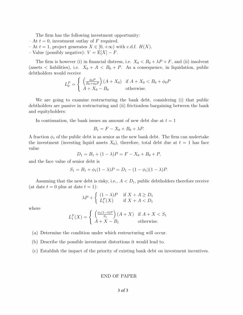
The firm has the following investment opportunity:– At t = 0, investment outlay of F required.– At t = 1, project generates X ∈ [0,+∞) with c.d.f. H(X).– Value (possibly negative): V = E[X]− F .
The firm is however (i) in financial distress, i.e. X0 < B0 + λP +F , and (ii) insolvent(assets < liabilities), i.e. X0 + A < B0 + P . As a consequence, in liquidation, publicdebtholders would receive
LP0 =
(φ0P
B0+φ0P
)(A+X0) if A+X0 < B0 + φ0P
A+X0 −B0 otherwise.
We are going to examine restructuring the bank debt, considering (i) that publicdebtholders are passive in restructuring and (ii) frictionless bargaining between the bankand equityholders:
In continuation, the bank issues an amount of new debt due at t = 1
B1 = F −X0 +B0 + λP.
A fraction φ1 of the public debt is as senior as the new bank debt. The firm can undertakethe investment (investing liquid assets X0), therefore, total debt due at t = 1 has facevalue
D1 = B1 + (1− λ)P = F −X0 +B0 + P,
and the face value of senior debt is
S1 = B1 + φ1(1− λ)P = D1 − (1− φ1)(1− λ)P.
Assuming that the new debt is risky, i.e., A < D1, public debtholders therefore receive(at date t = 0 plus at date t = 1):
λP +
(1− λ)P if X + A ≥ D1
LP1 (X) if X + A < D1
where
LP1 (X) =
(φ1(1−λ)P
S1
)(A+X) if A+X < S1
A+X −B1 otherwise.
(a) Determine the condition under which restructuring will occur.
(b) Describe the possible investment distortions it would lead to.
(c) Establish the impact of the priority of existing bank debt on investment incentives.
END OF PAPER
3 of 3

ECM9/ECM10/ECM11MPhil in EconomicsMPhil in Finance & EconomicsMPhil in Economic Research
Thursday 25 May 2017 9:00am -11:00am
F300CORPORATE FINANCE
Candidates are required to answer all four questions.
Write your candidate number (not your name) on the cover of each booklet.
Write legibly.
If you identify an error in this paper, please alert the Invigilator, who will notifythe Examiner. A general announcement will be made if the error is validated.
STATIONERY REQUIREMENTS20 Page booklet x 1Rough work pads
SPECIAL REQUIREMENTS TO BE SUPPLIED FOR THISEXAMINATIONCalculator - students are permitted to bring an approved calculator
You may not start to read the questions printedon the subsequent pages of this question paper
until instructed that you may do so by the Invigilator.
1 of 3

Question 1A company maintains a constant debt to value ratio of 1/2 and faces equity cost of capital rE =
10%, debt cost of capital of rD = 6% and pays corporate taxes at rate τC = 40%. The company isconsidering an investment that requires an initial outlay of $100 million. The investment will increasethe company’s free cash flow by $5 million the first year, and this contribution is expected to grow ata rate of 3% every year thereafter. The company will maintain a constant debt to value ratio for thisinvestment.
a. Using the WACC method, calculate the net present value of this investment.
b. How much additional debt must the company issue to finance the investment and maintain adebt to value ratio of 1/2 and how much equity must it issue? Explain your reasoning.
c. Assume that to finance the investment, the company issues new debt of $65.8 million. Usingthe APV method, calculate the net present value of this investment.
Question 2An entrepreneur has a project that can either succeed or fail, with each outcome being equally
likely. If it succeeds, the project is worth $150m while if it fails, it is worth only $80m. The project’scash flows are unrelated to those of the economy (so the risk is diversifiable) and the risk-free rate is5%. The company has 10m shares outstanding.
a. Calculate the value of the firm’s securities at the start of the year if it is (i) all equity financedand (ii) financed by $100m in debt. Compare the values of the firm under these capital structuresand briefly comment.
b. Now assume that in case of default, financial distress costs reduce the value of the firm by $20m.Compute the value of the firm when it is (i) all equity financed and (ii) financed by $100m indebt. Compare the values of the firm under these capital structures and briefly comment.
c. Briefly discuss who bears the costs of financial distress and what the implications for the optimalcapital structure are if there are no other market imperfections.
2 of 3
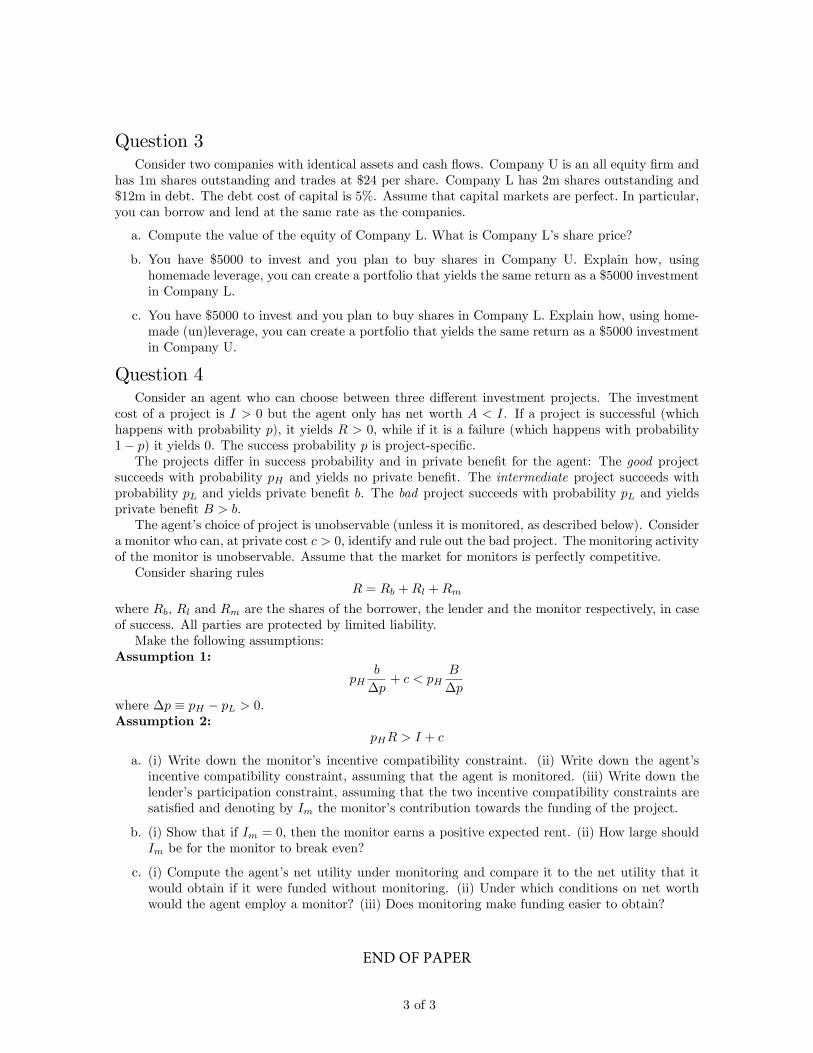
Question 3Consider two companies with identical assets and cash flows. Company U is an all equity firm and
has 1m shares outstanding and trades at $24 per share. Company L has 2m shares outstanding and$12m in debt. The debt cost of capital is 5%. Assume that capital markets are perfect. In particular,you can borrow and lend at the same rate as the companies.
a. Compute the value of the equity of Company L. What is Company L’s share price?
b. You have $5000 to invest and you plan to buy shares in Company U. Explain how, usinghomemade leverage, you can create a portfolio that yields the same return as a $5000 investmentin Company L.
c. You have $5000 to invest and you plan to buy shares in Company L. Explain how, using home-made (un)leverage, you can create a portfolio that yields the same return as a $5000 investmentin Company U.
Question 4Consider an agent who can choose between three different investment projects. The investment
cost of a project is I > 0 but the agent only has net worth A < I. If a project is successful (whichhappens with probability p), it yields R > 0, while if it is a failure (which happens with probability1− p) it yields 0. The success probability p is project-specific.The projects differ in success probability and in private benefit for the agent: The good project
succeeds with probability pH and yields no private benefit. The intermediate project succeeds withprobability pL and yields private benefit b. The bad project succeeds with probability pL and yieldsprivate benefit B > b.The agent’s choice of project is unobservable (unless it is monitored, as described below). Consider
a monitor who can, at private cost c > 0, identify and rule out the bad project. The monitoring activityof the monitor is unobservable. Assume that the market for monitors is perfectly competitive.Consider sharing rules
R = Rb +Rl +Rm
where Rb, Rl and Rm are the shares of the borrower, the lender and the monitor respectively, in caseof success. All parties are protected by limited liability.Make the following assumptions:
Assumption 1:
pHb
∆p+ c < pH
B
∆p
where ∆p ≡ pH − pL > 0.Assumption 2:
pHR > I + c
a. (i) Write down the monitor’s incentive compatibility constraint. (ii) Write down the agent’sincentive compatibility constraint, assuming that the agent is monitored. (iii) Write down thelender’s participation constraint, assuming that the two incentive compatibility constraints aresatisfied and denoting by Im the monitor’s contribution towards the funding of the project.
b. (i) Show that if Im = 0, then the monitor earns a positive expected rent. (ii) How large shouldIm be for the monitor to break even?
c. (i) Compute the agent’s net utility under monitoring and compare it to the net utility that itwould obtain if it were funded without monitoring. (ii) Under which conditions on net worthwould the agent employ a monitor? (iii) Does monitoring make funding easier to obtain?
3 of 3
END OF PAPER

ECM9/ECM10/ECM11/MGM3MPhil in EconomicsMPhil in Finance & EconomicsMPhil in Economic ResearchMPhil in Finance
Tuesday 23 May 2017 1:30pm - 3:30pm
F400ASSET PRICING
Candidates are required to answer all four questions.
Write your candidate number (not your name) on the cover of each booklet.
Write legibly.
If you identify an error in this paper, please alert the Invigilator, who will notifythe Examiner. A general announcement will be made if the error is validated.
STATIONERY REQUIREMENTS20 Page booklet x 1Rough work pads
SPECIAL REQUIREMENTS TO BE SUPPLIED FOR THISEXAMINATIONCalculator - students are permitted to bring an approved calculator
You may not start to read the questions printedon the subsequent pages of this question paper
until instructed that you may do so by the Invigilator.
1 of 3

1. Suppose that there are several investors and several assets. Suppose furtherthat investors have constant absolute risk aversion, and that the returns on theassets are jointly normally distributed.
(a) Find a formula for the asset demands of an individual investor.
(b) Explain the main features of this formula.
(c) Taking the formula from part (a) as your starting point, derive the security-market line (SML).
(d) Explain the main features of the SML.
2. Suppose that there are two risky assets: a safe asset and a risky asset. Theinitial price of the risky asset is 20. In each period there is a shock s ∈ d, u.If s = d then the price falls by 10%. If s = u then the price rises by 10%. Theinitial price of the safe asset is 1. In each period the price rises by 5%.
(a) What is meant by a put option with strike price 22 and maturity 2 in thissetting?
(b) Assuming that there is no arbitrage, what is the price of this option attime 0?
3. (a) Write down a model of the dynamics of spot rates. Explain carefully themeaning of the various elements of the model.
(b) In the context of your model, what does it means to say that the termstructure of bond prices is affine? Why is it considered to be “affine”?
(c) Assuming that the term structure of bond prices is indeed affine in thissense, find the stochastic differential equation followed by the price of aT -bond.
2 of 3

4. There are three assets: a safe asset and two risky assets. The prices B, R andS of the safe asset, risky asset 1 and risky asset 2 evolve according to the s.d.e.s
dB = r B dt,
dR = µRRdt+ σRRdZ,
dS = µS S dt+ σS S dZ
respectively, where Z is a one-dimensional standard Wiener process. There isalso a derivative written on the first asset that pays Φ(RT ) at maturity T > 0.There is no arbitrage.
(a) Find the equation satisfied by the price of the derivative. Be careful toexplain any assumptions that you make, and to set out the main steps ofyour derivation carefully.
(b) What conditions must µR, µS, σR and σS satisfy? Explain carefully howyour arrived at these conditions.
END OF PAPER
3 of 3

ECM9/ECM10/ECM11MPhil in EconomicsMPhil in Finance & EconomicsMPhil in Economic Research
Monday 29 May 2017 1:30pm - 3.30pm
F500EMPIRICAL FINANCE
This paper is in two sections. Section A: Candidates are required to answerall four questions. Section B: Candidates are required to answer two outof three questions.
Each section carries equal weight.
Write your candidate number (not your name) on the cover of each booklet.
Write legibly.
If you identify an error in this paper, please alert the Invigilator, who will notifythe Examiner. A general announcement will be made if the error is validated.
STATIONERY REQUIREMENTS20 Page booklet x 1Rough work pads
SPECIAL REQUIREMENTS TO BE SUPPLIED FOR THISEXAMINATIONCalculator - students are permitted to bring an approved calculator
You may not start to read the questions printedon the subsequent pages of this question paper
until instructed that you may do so by the Invigilator.
1 of 4

Section A
1. Suppose that observed closing (log) stock prices follow the random walk
pt = µ+ pt−1 + ut
ut = εt + θεt−1
where εt ∼ N(0, σ2ε).(a) For what values of θ is this model consistent with the Effi cient Market
Hypothesis?(b) For what values of θ is this model consistent with the empirical evidence
on daily returns as presented in Table 2.4 of Campbell, Lo andMackinlay,attached?
(c) What are some market microstructure explanations for this finding?(d) Define the variance ratio
V R(k) =var(pt+k − pt)
k × var(pt+1 − pt).
What is V R(k) as a function of θ?2. True, False, Explain
(a) A portfolio hedged against factor risk always has zero risk(b) In the absence of noise traders, bid ask spreads would be narrower, and
so markets would be more effi cient.(c) The long run risks model says that at plausible values for the preference
parameters (IES and RRA), a reduction in economic uncertainty or bet-ter long-run growth prospects leads to a rise in the wealth—consumptionand the price—dividend ratios.
(d) Stock returns are more volatile during Wednesdays than Mondays. Thisis incompatible with market effi ciency
3. Assume that fundamental price P ∗ is a random walk unrelated to order flow
P ∗t = P ∗t−1 + εt.
Suppose that buy and sell orders arrive randomly each period, and let Itdenote the trade direction indicator, +1 for buy and -1 if customer is selling.Assume that It is iid with equal probability of +1 and -1 and unrelated toP ∗t . Suppose that the bid ask spread is s so that the transaction price eachperiod Pt satisfies
Pt = P ∗t + Its
2.
Then derive an expression for cov [∆Pt−1,∆Pt] in terms of s.What is Bid askbounce? How could one obtain an estimate of the bid ask spread based ontransactions data only?
2 of 4
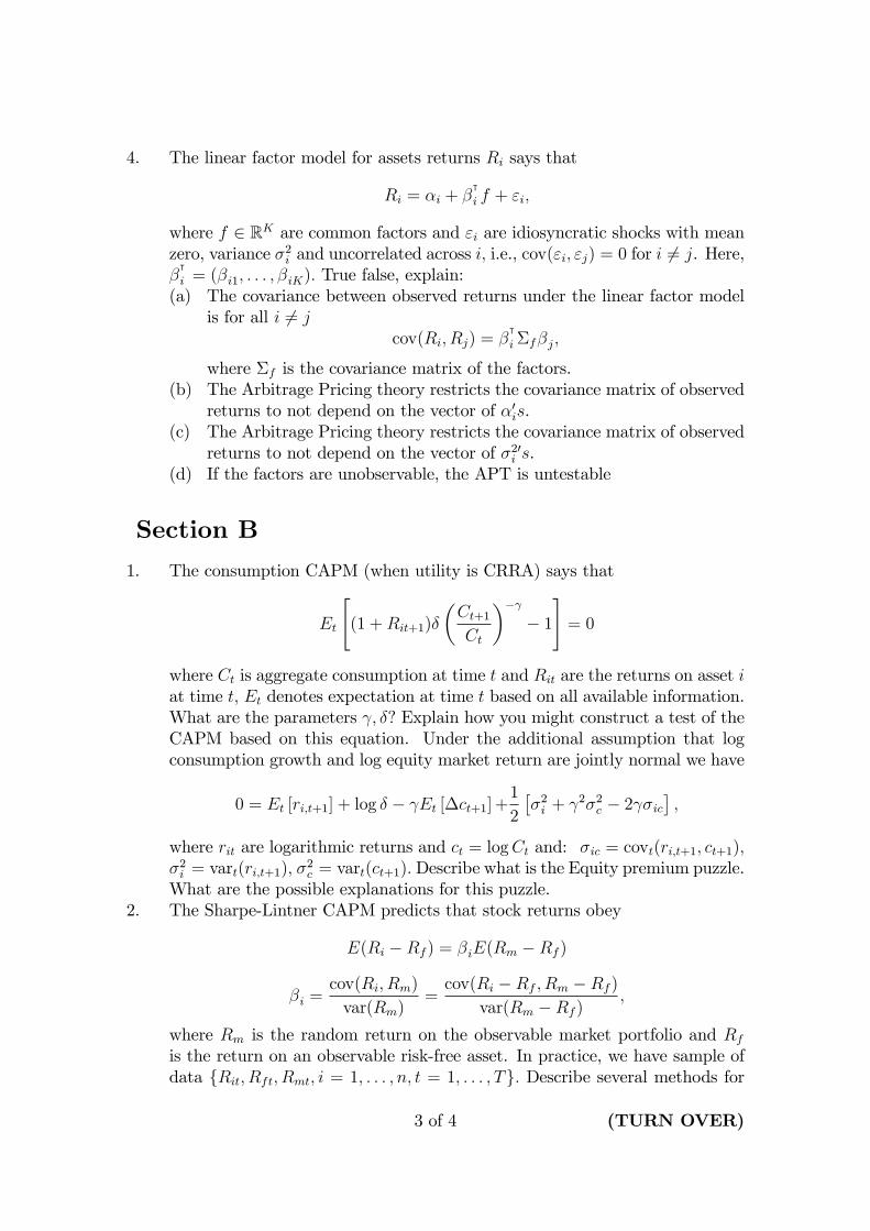
4. The linear factor model for assets returns Ri says that
Ri = αi + βᵀi f + εi,
where f ∈ RK are common factors and εi are idiosyncratic shocks with meanzero, variance σ2i and uncorrelated across i, i.e., cov(εi, εj) = 0 for i 6= j. Here,βᵀi = (βi1, . . . , βiK). True false, explain:(a) The covariance between observed returns under the linear factor model
is for all i 6= jcov(Ri, Rj) = β
ᵀi Σfβj,
where Σf is the covariance matrix of the factors.(b) The Arbitrage Pricing theory restricts the covariance matrix of observed
returns to not depend on the vector of α′is.(c) The Arbitrage Pricing theory restricts the covariance matrix of observed
returns to not depend on the vector of σ2′i s.(d) If the factors are unobservable, the APT is untestable
Section B
1. The consumption CAPM (when utility is CRRA) says that
Et
[(1 +Rit+1)δ
(Ct+1Ct
)−γ− 1
]= 0
where Ct is aggregate consumption at time t and Rit are the returns on asset iat time t, Et denotes expectation at time t based on all available information.What are the parameters γ, δ? Explain how you might construct a test of theCAPM based on this equation. Under the additional assumption that logconsumption growth and log equity market return are jointly normal we have
0 = Et [ri,t+1] + log δ − γEt [∆ct+1] +1
2
[σ2i + γ2σ2c − 2γσic
],
where rit are logarithmic returns and ct = logCt and: σic = covt(ri,t+1, ct+1),σ2i = vart(ri,t+1), σ
2c = vart(ct+1).Describe what is the Equity premium puzzle.
What are the possible explanations for this puzzle.2. The Sharpe-Lintner CAPM predicts that stock returns obey
E(Ri −Rf ) = βiE(Rm −Rf )
βi =cov(Ri, Rm)
var(Rm)=
cov(Ri −Rf , Rm −Rf )
var(Rm −Rf ),
where Rm is the random return on the observable market portfolio and Rf
is the return on an observable risk-free asset. In practice, we have sample ofdata Rit, Rft, Rmt, i = 1, . . . , n, t = 1, . . . , T. Describe several methods for
3 of 4 (TURN OVER)

testing this model. In your account be careful to say whether you are workingwith individual stocks or portfolios, what the null and alternative hypothesesare, and what are the test statistics. How is this model useful in conductingevent studies?
3. Suppose that daily stock returns satisfy
rt = µ+ σtεt
σ2t = ω + βσ2t−1 + γr2t−1,
where εt is iid standard normal and independent of all past information. Whatproperties of daily stock returns does the GARCH model capture? Describehow you would estimate the parameters µ, ω, β, γ given a sample of datar1, . . . , rT. Compare the resulting estimate of volatility σ2t with the realizedvolatility estimator and with the implied volatility estimator. Describe ineach case how the estimates are constructed, their interpretations, and theirproperties.
END OF PAPER
4 of 4

ECM9/ECM10/ECM11MPhil in EconomicsMPhil in Finance & EconomicsMPhil in Economic Research
Wednesday 7 June 2017 1:30pm - 3:30pm
F510INTERNATIONAL FINANCE
Candidates are required to answer four out of five questions.
Write your candidate number (not your name) on the cover of each booklet.
Write legibly.
If you identify an error in this paper, please alert the Invigilator, who will notifythe Examiner. A general announcement will be made if the error is validated.
STATIONERY REQUIREMENTS20 Page booklet x 1Rough work pads
SPECIAL REQUIREMENTS TO BE SUPPLIED FOR THISEXAMINATIONCalculator - students are permitted to bring an approved calculator
You may not start to read the questions printedon the subsequent pages of this question paper
until instructed that you may do so by the Invigilator.
1 of 5

QUESTION 1 Uncovered Interest Parity(a) Define the “Uncovered Interest Parity”(UIP). State briefly but precisely how
it is tested using regression models, and in which way it fails to hold empiri-cally.
(b) The empirical failure of the UIP is often referred to as the “UIP puzzle”.Consider the hypothesis that this puzzle can be attributed entirely to omittinga risk-premium from the regression model.• Under what conditions would the risk premium help explain the UIP
puzzle? Discuss the results by Fama 1984.• If Fama 1984 is right, what other empirical puzzle would arise? Explain
carefully.
QUESTION 2 Covered Interest ParitySuppose that international investors attribute a small probability to the event
of another large global crisis. They also believe that, if and when this new globalcrisis occurs, the US would tax interest income on US financial assets owned byforeigners, at a constant tax rate τ .(a) Define the cross-currency basis of a foreign currency vis-à-vis the dollar. De-
rive and discuss the implications of the prospective taxation for the cross-currency basis. In answering this question, make use of the asset pricingequation analyzed in class and explain carefully your results.
(b) Would anticipation of solvency problems (credit risk) among US financialintermediaries make a difference to your answer? (Hint: in addressing thisquestion, it is analytically convenient to ignore the prospective tax discussedin (a)).
QUESTION 3 The Peso problemExplain briefly but rigorously the “peso problem” and its applications to the
main puzzles in international finance.
2 of 5

QUESTION 4 Risk sharing and sovereign riskConsider a stylized two-period model of a small open economy populated by
many individuals i, each with life-time utility and endowments
ln (ci,0) + E ln (ci,1) ,
yi,0 = 0.5, and yi,1 =
1.80 with probability 1/2,1.20 with probability 1/2.
Individuals are ex-ante identical, but face individual income risk ex-post. In period0, all individuals have the same income yi,0 = 0.5; in period 1, an individual i canbe ‘lucky’and get yi,1 = 1.80, or ‘unlucky’and get yi,1 = 1.20, each with probability1/2.In period 0, individuals are able to issue liabilities bi,0 promising a cash flow that iscontingent on the realization of their income. Namely, an individual debt contractstipulates that, in period 1, she will have to pay back either xHi if she turns outto be lucky or xLi if she turns out to be unlucky. International investors are riskneutral and do not discount the future, so that bi,0 will be equal to the expectedpayoff:
bi,0 = E0 (xi) .
Answer the following:(a) Define the real rate in financial autarky and compare it with the world market
rate: will the country be a net importer or a net exporter of financial assetsin period 0?
(b) Write down the individual i consumption-saving problem. What debt con-tracts would you expect to observe in equilibrium if(i) international contracts are enforceable by some supranational authority,
and individual incomes are verifiable?(ii) international contracts are not enforceable but incomes are verifiable.
However, if an individual defaults she/he has to endure costs for k = 0.5.(iii) contracts are not enforceable and income not verifiable, so that interna-
tional investors are not willing to lend against contingent payment (hint,set xHi = xLi ).
For each case (i) (ii) (iii) above, calculate bi,0, the cash flow xHi andxLi and the allocation of consumption. Explain you answer discussingbriefly the effi ciency of the consumption allocation.
(d) Suppose individuals residing in the country revise their income expectationsin the future–←→y i,1 will be a mean preserving spread of yi,1
←→y i,1 =
2 with probability 1/2,1 with probability 1/2.
Compare the cases (i) and (iii) above: In which case will agents change theamount of liabilities they issue in period 0? Carefully explain your answer.
(e) How would you answer to b(ii) above change if k = 0.4?
3 of 5 (TURN OVER)

QUESTION 5 US Monetary Tightening, Financial Fragility and Cur-rency CrisesSuppose a small open emerging economy is described by the following Aghion, Bac-chetta and Banerjee (2000) model. Money market equilibrium is given by
Mt
Pt= L (Yt, it)
where Mt denotes the nominal money supply, Pt the aggregate price level, Yt thelevel of aggregate real output, it the nominal interest rate, and the subscript tthe time period. Real money demand L (.) satisfies ∂L/∂Y > 0, ∂L/∂i < 0 andL (0, i) > 0. Equilibrium in the foreign exchange market is determined by uncoveredinterest parity:
1 + it = (1 + i∗)Et [St+1]
St
where i∗ is the US nominal interest rate, and St the nominal exchange rate, definedas the domestic price of US dollars. The aggregate price level Pt is preset at theend of period t− 1. Purchasing power parity holds ex ante so that
Pt = Et−1 [St]
where the foreign price level has been normalized to P ∗ = 1.Output is produced with capital Kt according to the linear production technology
Yt = AKt
where A > 0 denotes productivity. Capital accumulation is determined by
Kt = Bt + Ft
where Bt is the domestic firm’s short term debt, and Ft retained cash flow. Thefirm faces external financing constraints in the form of a borrowing limit
Bt = e−βit−1Ft
where β > 0. Furthermore, the size of the domestic credit market is limited toB > 0 and any additional borrowing has to take place in US dollars. Assume thatB1 > B. Retained cash flow depends on past real profits and equals
Ft = max 0, (1− α) Πt−1/Pt−1
where 0 < α < 1 and Πt denotes nominal profits after debt repayments:
Πt = PtYt − (1 + it−1)Pt−1B − (1 + i∗)StSt−1
Pt−1
(Bt − B
)The economy starts from a long run equilibrium in period t = 0. Assume thatinitially, 1+i∗
1+i1
M2
L(0,i2)< P1AK1−(1+i0)P0B
(1+i∗)(B1−B).
4 of 5

(a) Show that asset market equilibrium implies
S1 =1 + i∗
1 + i1
M2
L (Y2, i2)(IPLM)
Explain intuitively how the domestic nominal interest i1, US nominalinterest rate i∗ and future domestic output Y2 affect the nominal exchangerate S1.
(b) Show that future output Y2 satisfies
Y2 = max
0, A
(e−βi1 + 1
)(1− α)
[AK1 − (1 + i0)
P0
P1
B − (1 + i∗)S1
P1
(B1 − B
)](FC)
Give an intuitive explanation for the effect of the domestic nominal in-terest rate i1, US nominal interest rate i∗ and the nominal exchange rateS1 on future output Y2.
(c) Suppose the economy faces a higher US nominal interest rate i∗. Showgraphically and explain intuitively how this affects the nominal exchangerate S1 and future output Y2. Could the higher US interest rate lead toa currency crisis in the emerging economy?
END OF PAPER
5 of 5

ECM9/ECM10/ECM11MPhil in EconomicsMPhil in Finance & EconomicsMPhil in Economic Research
Tuesday 30 May 2017 1:30pm - 3:30pm
F520BEHAVIOURAL FINANCE
Candidates are required to answer two out of three questions
Write your candidate number (not your name) on the cover of each booklet.
Write legibly.
If you identify an error in this paper, please alert the Invigilator, who will notifythe Examiner. A general announcement will be made if the error is validated.
STATIONERY REQUIREMENTS20 Page booklet x 1Rough work pads
SPECIAL REQUIREMENTS TO BE SUPPLIED FOR THISEXAMINATIONCalculator - students are permitted to bring an approved calculator
You may not start to read the questions printedon the subsequent pages of this question paper
until instructed that you may do so by the Invigilator.
1 of 3

QUESTION 1
a. Describe differences and similarities of decision making under Expected utility model andProspect Theory.
b. Explain what are the main theoretical challenges in testing the Market EfficiencyHypothesis? Fully elaborate your answer.
c. Describe the concept of Adaptive Market Hypothesis.
QUESTION 2
a. Can herding behaviour be rational? Discuss. Provide some examples to support your answer.
b. Describe main intuition why herding can lead to market inefficiency. Provide some examplesto support your answer.
c. Explain how risk-shifting behavior could cause occurrences and subsequently bursts offinancial bubbles. Fully justify your arguments. Provide some examples that support yourarguments.
2 of 3

QUESTION 3
a. Large uninformed trades in the stock market typically cause large price impacts (an exampleof uninformed trades would be fire sales or trades of index tracing fund due to inclusion of anew stock into a stock index). Explain the role of limits to arbitrage in existence of thoseprice impacts. Should we observe the price impacts in markets with active arbitrageurs whoface no constraints or risks in executing arbitrage strategies?
b. The closed-end fund discount is typically used as a proxy for noise traders’ risk. Provide therationale and intuition for this argument. Given that we typically observe closed-end funddiscounts rather than premiums, does it mean that noise traders are mostly pessimistic?
c. Demonstrate how ambiguity aversion can lead to excess volatility. Consider a case of the
model developed in Dow and Werlang (1992) (Excess volatility of stock prices and Knightian
uncertainty, European Economic Review). Specifically, consider a two-period model with a
single stock traded in the market and risk-free rate is equal to zero. At the end of the second
period, the stock pays a liquidating dividends V. There are there are 3 states of nature; the
value of V in states 1, 2 and 3 are 1, 0.5 or 0 respectively. All agents are identical and risk
neutral and makes the decisions according to the multiple prior model (Choquet Expected
utility). In period t = 1 agents receive public information about the value of the asset
represented by a partition I = 1,2; 3 of the set of states. Assume that the true objective
probability on the space of states is P(1)=0.5 and P(2)=P(3)=0.25. Assume agents do not
know the exact probability and their beliefs and attitudes towards uncertainty are
represented by the lower envelope of the following three probability measures: P, Q and O,
where Q(1)=Q(2)=0.25 and Q(3)=0.5 and O(1)=O(3)=0.25 and O(2)=0.5. Provide
necessary analysis.
3 of 3
END OF PAPER

ECM9/ECM10/ECM11MPhil in EconomicsMPhil in Finance & EconomicsMPhil in Economic Research
Friday 9 June 2017 1:30pm - 3:30pm
F540TOPICS IN APPLIED ASSET MANAGEMENT
This paper is in two sections:Section A: candidates are required to answer one compulsory question.Section B: Candidates are required to answer two out of four questions.
Section A is weighted at 40% and section B is weighted at 60%.
Write your candidate number (not your name) on the cover of each booklet.
Write legibly.
If you identify an error in this paper, please alert the Invigilator, who will notifythe Examiner. A general announcement will be made if the error is validated.
STATIONERY REQUIREMENTS20 Page booklet x 1Rough work pads
SPECIAL REQUIREMENTS TO BE SUPPLIED FOR THISEXAMINATIONCalculator - students are permitted to bring an approved calculator
You may not start to read the questions printedon the subsequent pages of this question paper
until instructed that you may do so by the Invigilator.
1 of 4

SECTION A
1. General Question
(a) What is the minimal number of assets you would require in a 1N
port-folio in which each asset has identical statistical properties and theaverage covariance with other assets is 0.1 and the average variance is0.5, in order to achieve a portfolio vol of 0.10 ? Provide a mathematicaljustification for your answer.
(b) Ferson and Siegel(2001) have shown how the optimal weight functionis changed when you take into account the fact that you can exploit apredictive model (conditional information) rather than use the uncon-ditional moments in mean variance optimisation. Derive and explainthe rationale behind their formula.
(c) Explain briefly how mean variance portfolio weights can be computedusing an Ordinary Least Squares Regression. The computational prob-lems involved with MV weights in practice may be overcome through theuse of relaxation methods such as used for resolving multicollinearity inregression; in particular explain what is meant by RIDGE regression,LASSO and ELASTIC NET.
(d) Show that Long Horizon predictive regressions ( with a positive coeffi-cient) where the predictor variable is persistent will necessarily implythe regression coefficient grows with the horizon. Similarly show, evenif returns are independent, that the R2and Sharpe Ratio will also nec-essarily grow with the horizon.
(e) Examine whether portfolio volatility ( with two assets) is sub-additiveand translation invariant ( or monotonic) and hence decide whethervolatility is a coherent risk measure or not.
(f) The case for regular portfolio rebalancing rather than adopting a buyand hold strategy is complicated in general but one argument for rebal-ancing back to constant weights is based on what is known as volatilityharvesting. Explain this result, the assumptions on which it is basedand potential limitations.
2 of 4

SECTION B
2. Mean Variance and Predictability
(a) Discuss the conditions DeMiguel, Garlappi and Uppal(2009) derivedanalytically and by simulation to show when Mean Variance could dom-inate 1
N? What further condition became apparent in their empirical
results?
(b) What principal critiques ( with justification) can you make of theirstudy and hence its relevance?
(c) Explain briefly how Volatility Timing and Parametric Portfolios at-tempt to resolve the well known problems with implementing MeanVariance in practice
(d) Forecast combination, Shrinkage ( relaxation) methods and factor mod-els have all recently been shown to deliver clear evidence of out of samplepredictability unlike the results of Goyal and Welch(2008);
i. Campbell and Thompson discuss the relationship between the R2
in a predictive regression and the Sharpe Ratio from the result-ing investment strategy- derive this relationship and discuss how itrelates to the more general theoretical results we have consideredwhich relate the predictive R2 to the stochastic discount factor ofan asset pricing model.
ii. Why should Forecast Combination, Shrinkage or Factor methodstherefore be expected to deliver greater profitability.
iii. Describe why the Kitchen Sink regressions of Goyal and Welchfailed and why forecast combination may effectively recover pre-dictability and hence profitability in a mean variance certaintyequivalent sense.
3. CAPM and APT
(a) Compare and contrast the relative theoretical and practical advantagesand disadvantages of APT and CAPM.
(b) Outline the derivation of APT using a no-arbitrage argument or in someother way you have studied.
(c) Compare the three basic types of factor models commonly employed.
(d) Describe the Partial Least Squares (PLS) approach to factor construc-tion and compare this with Principal Components as a means of con-structing factors.
4. Trend Following and Betting against Beta
(a) Describe the theoretical argument made to explain the Low Beta anomalyby Frazzini and Pedersen(2103) including why the Security Market Linepivots.
(b) When and why does low beta investing not deliver abnormal returns?
3 of 4 TURN OVER

(c) Discriminate between Time Series and Cross Section Momentum andderive the relationship between the expected returns to cross sectionmomentum and time series momentum and hence why cross sectionmomentum might need to be reconsidered as a strategy
(d) Explain the standard form a trend following strategy (Time Series Mo-mentum) takes including how you would ensure a target annualisedvolatility through appropriate position sizing (Constant Volatility TrendFollowing); secondly explain why this strategy failed to perform inthe period 2009-2013 and describe the steps through which perfor-mance was recovered by incorporating risk parity as suggested by Bal-tas(2015)UBS.
5. Risk Management
(a) Define and explain the relationship and relatives properties of Value atRisk, Expected Shortfall and Expectiles.
(b) Define the Information Ratio, Calmar Ratio, a CARE model and Max-imum Drawdown
(c) What are the principle advantages and disadvantages of Historical Sim-ulation when used as a method of computing Value at Risk and describeone method that may be used to overcome its deficiencies.
(d) Consider 100 independent defaultable bonds each with a current priceof 100 and a default probability of 2% for each bond. When they don’tdefault they deliver 105 at the end of the year. Now consider twoportfolios, the first , portfolio A, is concentrated and made up of 100units of only the first bond and the second portfolio, portfolio B, iscompletely diversified containing one unit of each bond. Examine therisk capital required when using a 95% VaR level for each portfolio anddiscuss the result you find. Explain your results and why they comeabout? In general, under what situations are you likely to find VaRfails to satisfy the conditions for coherency?
END OF PAPER
4 of 4

Faculty of Economics
MPhil/MRes/MPhil Finance and Economics
Preparatory Course Exam
29 September 2016
You have TWO hours
Answer ALL FOUR questions
Each question will carry equal weight.
Write your candidate number (not your name) on the cover of your answerbooklet.
If you identify an error in this paper, please alert the invigilator.
Write legibly.
You may not start to read the questions printed on the subsequent
pages of this question paper until instructed that you may do so by
the invigilator

1.
(a) Let
A =
1 0 01 1 00 0 1
and B =
1 0 00 1 00 −2 1
Compute AB, and BA.
(b)
i. Prove that for a square matrix An×n the following holds:
tr(AA′) = tr(A′A) =∑ij
a2ij
ii. Find the eigenvalues of matrix A
A =
1 3 00 1 02 1 5
iii. Determine the rank of matrix C below:
C =
3 0 1 26 1 0 012 1 2 46 0 2 49 0 1 2
iv. Prove that rank(A)=rank(A′).
(c) Consider the following sequence
xk =√2xk−1 +
3
8xk−2 −
3√2
8xk−3
check whether the eect of x0, the initial value of this sequence,becomes arbitrarily small as k → ∞.
page 1 of 3

2.Random variable X takes values in −1, 1. Random variable Y takesvalues in −1, 0, 1 . Their joint probability mass function is given par-tially in the Table below. The marginal distributions of both X and Yare (discrete) uniform.
X
-1 1
-1 14
Y 0
1 16
(a) Calculate the remaining values for the joint probability mass func-tion.
(b) Are X and Y independent?
(c) Deneη = Y − α− βX
and where α and β are xed coecients. Show that it is possible tochoose values for α and β such that
i. E (η) = 0
ii. Cov (X, η) = 0
(d) Calculate the required values of α and β for the distribution obtainedin (a).
(e) Given a random sample of observationsxi, yi; i = 1, . . . , N fromthis joint distribution denote the ordinary least squares estimators ofthe intercept and slope in a linear regression of yi on xi as α and β.Will these estimators be
i. Unbiasedii. Ecient
for the coecients α and β calculated in (d)? Justify your answer.
page 2 of 3

3.
(a) Consider the following dierence equation:
xt+2 − 3xt+1 + 2xt = 3t
Solve the equation with initial condition x0 = 0 and x1 = 0.
(b) Consider the following system of dierential equations:.x = 2x+ 3y.y = 3x− 6y
i. Sketch the dynamic solution in a phase diagram and explain thedynamics.
ii. Find the analytical solution of the system. If the initial conditionof the system is x(0) = 1 and y(0) = −3 is the system going toconverge to the steady state? Justify your answer?
4.
(a) Answer and explain briey
i. Is the set A = [0, 2)∪(2, 4] bounded? Is it convex? Is it compact?
ii. Sketch the set of points (x, y) described by the equation x2 +y2 − 25 = 0. Call this set B. Is B bounded? Is it convex? Is itcompact?
iii. State Brouwer's xed point theorem.
iv. Consider the set A above. Does Brouwer's theorem apply? Ifnot, give an example of a function f : A → A which does nothave a xed point.
v. Consider the set B above. Does Brouwer's theorem apply? Ifnot, give an example of a function f : B → B which does nothave a xed point.
(b) Consider the problem of maximising f(a, b) = a exp(b) subject to theconstraint a +Kb ≤ M , where K and M are positive constant realnumbers, whereas a and b are real variables with b ≥ 0.
i. For which values of K and M , does the optimal solution implyb = 0?
ii. What is the solution when f is known to attain its maximumwhen a and b are positive?
END OF PAPER
page 3 of 3

Faculty of Economics
MPhil/MRes Pre-Course Exam
September 2016
ANSWERS
1

1.
(a)
AB =
1 0 01 1 00 −2 1
and BA =
1 0 01 1 0−2 −2 1
(b)
i.
tr(AA′) =∑i
(AA′)ii =∑i
∑j
a2ij =∑j
∑i
a2ij =∑j
(AA)jj = tr(A′A)
ii. λ1 = 1 (twice),λ2 = 5.
iii. rank(C) = 3.
iv. Since the column rank of A is the row rank of A′ and sincewe know that the column and row ranks are equal, the resultimmediately follows.
(c) The sequence satises:uk = Auk−1,
where
uk =
xkxk−1xk−2
and A =
√2 38 − 3
√2
81 0 00 1 0
The eigenvalues of A are
|A− λI3| =
∣∣∣∣∣∣√
2− λ 38 − 3
√2
81 −λ 00 1 −λ
∣∣∣∣∣∣ = (√
2− λ)(λ2 − 3
8)
the eigenvalues are λ1 =√
2 > 1, λ2 =√
38 < 1, λ3 = −
√38 < 1.
For the eect of the initial value to have an arbitrarily small eect ask →∞, all eigenvalues should be smaller than one in absolute value,which is not the case in our example, therefore the eect of the initialvalue x0 does not become arbitrarily small.
2. Note in this question it is very important to be clear about popula-tion values and sample values. Thus the (population) variance of X is
V ar(X) = E (X − µ)2and the sample variance is 1
N−1∑
(xi − x)2. Con-
fusion between x and µ (or between β and β) will lose marks.
2

(a) The joint pmf is
X
-1 1
-1 14
112
Y 0 112
14
1 16
16
(b) They are not independent as eg P (X = 1, Y = −1) = 112 but P (X = 1)P (Y = −1) =
12 ×
13
(c) We have E (η) = E (Y − α− βX) = µY−α−βµX . Also Cov (η,X) =Cov (Y − α− βX,X) = Cov (X,Y ) − βV ar (X) so choosing β =Cov(X,Y )V ar(X) and α = µY − βµX will do.
(d) For the given distribution we have µY = µX = 0. Trivially V ar(X) =1 and Cov (X,Y ) =
∑(x− µX) (y − µY ) p (x, y) which is
(−1) . (−1) .1
4+ (−1) . (1) .
1
12+ (0) . (−1) .
1
12+ (0) . (1) .
1
4+ (1) . (−1) .
1
6+ (1) . (1) .
1
6
=1
4− 1
12=
1
6
Using these values we get α = 0 and β = 16 .
(e) There are some subtle issues here and I'm not looking for elaborateproofs (or calculation of CRLB) not least because there's a time con-straint. For unbiasedness and eciency we'd need something likeGauss Markov to apply. The errors η are not normally distributed(they take on only six values) so we won't get eciency. For unbiased-ness we need E (η | X) = 0. We have Cov (η,X) = 0 by constructionbut conditional independence is dierent. You can write out thejoint pmf of η and X quite easily and verify this is true. So the leastsquares estimator will be unbiased for α and β but not ecient.
3.
(a) Solution of the homogeneous part is:
λ2 − 3λ+ 2 = 0
λ1 = 2 and λ2 = 1
xc,t = c12t + c2
3

Solution of the non homogeneous part using the method of undeter-mined coecients. We try the solution xp,t = A3t
A3t+2 − 3A3t+1 + 2A3t − 3t = 0
3t (9A− 9A− 2A− 1) = 0
we set the expression in brackets equal to 0
9A− 9A− 2A− 1 = 0
A = −1
2
then the general solution is:
xg,t = xc,t + xp,t = c12t + c2 −1
23t.
Using the initial condition x0 = 0 and x1 = 0 the constant c1 and c2can be pinned down solving the following system:
c120 + c2 − 12 = 0 t = 0
c121 + c2 − 32 = 0 t = 1
and c1 = 1 and c2 = − 12 . The solution is nally
xg,t = 2t − 1
23t − 1
2
(b)
i. The phase diagram of the system is:
where.x = 0 is y = − 2
3x and.y = 0 is y = 1
2x.
ii. The eigenvalues of the matrix
(2 33 −6
)are r1 = −7 and
r2 = 3 and the corresponding eigenvectors are v1 =
(−13
)
4

and v2 =
(31
). The general solution of the system is:
x (t) = −A1e−7t + 3A2e
3t
y (t) = 3A1e−7t +A2e
3t
If the initial condition is x(0) = 1 and y(0) = −3, we can pindown the constants A1 and A2 such that
x (0) = 1 = −A1 + 3A2
y (0) = 3 = 3A1 +A2
then A1 = −1 and A2 = 0. Only the stable part of the solutionsurvives. The system will converge.The solution will converge to the steady state only if the initialcondition is on the stable arm. The equation of the stable armis given by:
x (t)− x∗
y (t)− y∗= −1
3
however, given x∗ = y∗ = 0
x (0)
y (0)= −1
3
that is on the stable arm.
4.
(a)
i. Bounded, not convex (a hole in the middle), not compact (be-cause it is not closed, it is missing a limit point, namely 2).
ii. It is a circle with centre at the origin, and radius 5. Bounded,compact, but not convex.
iii. Let S be a non-empty, compact, convex subset of Rn . If f :S → S is continuous, then f has a xed point, i.e., there mustbe a point c ∈ S such that f(c) = c.
iv. No, the theorem doesn't apply as A is not convex (nor compact).A function f : A→ A without a xed point maps [0, 2) to (2, 4],and maps (2, 4] to [0, 2) by sending x to its mirror image with 2being the ipping point.
v. No, the theorem doesn't apply as B is not convex. Consider anyfunction with rotates the points in B around the origin by anangle other than a multiple of 360 degrees.
(b) To simplify, let's instead work with the natural log of f , that is
maxa,b
ln a+ b s.t.a
K+ b ≤ M
Kand − b ≤ 0
5

The Kuhn-Tucker Lagrangean is
L = ln a+ b+ λ
(M
K− a
K− b)
FOCs are
La = a−1 − λ
K= 0
andLb = 1− λ
Complementary slackness:
i. Lb ≤ 0 and b = 0. In this case a = M . Holds when λ = K/M ≥1. That is, when M ≤ K, the optimal solution implies b = 0.
ii. Lb = 0 and b > 0, in which case λ = 1 and a = K; b = M/K− 1.When M > K, we have this solution.
6