influence of rotational diffusion on the electric field induced effect on the fluorescence spectrum...

'Chemical Physics E L S E V I E R Chemical Physics 214 (1997) 383-407

Influence of rotational diffusion on the electric field induced effect on the fluorescence spectrum of diluted solutions

I. Theory and numerical simulations Heribert Reis, Wolfram Baumann

Institute of Physical Chemistry, Johannes Gutenberg University of Mainz, D-55099 Mainz, Germany

Received 3 June 1996

Abstract

The theory for the calculation of excited state dipole moments from electrooptical emission measurements, developed by Baumann and Deckers (Ber. Bunsenges. Phys. Chem. 81 (1977) 786) presupposes a Boltzmann distribution for the emitting molecules. Using the anisotropic rotational diffusion model and taking into account all important electric field induced effects, we derive equations that describe quantitatively the electric field effect on the fluorescence of an ensemble of solute rigid molecules which are not yet equilibrated with respect to their orientation when emitting. Numerical simulations are performed to compare the general case and the limiting case of a prevailing Boltzmann distribution and to examine the influence of "slip" and "stick" boundary conditions, as well as the assumption of isotropic diffusion.

1. Introduct ion

Electrooptical absorption and emission measurements provide information about dipole moments and polarizabilities o f solute molecules in their electronic ground and excited states as well as the relative directions of the transition dipole moments between the states involved. For the case of emission, Baumann and Deckers [ 1 ] developed a theory for two limiting cases concerning the ratio of the fluorescence lifetime ~'a and the rotational diffusion relaxation time ~'Or:

( 1 ) "ror/~'a >> 1 ; no rotational relaxation occurs prior to emission and the orientational distribution function relevant for emission is determined by the distribution function of the molecules in their ground state before excitation. The resulting expression for the relative change of the fluorescence intensity is quite lengthy and has not been verified so far.

(2) 7"Or/~',, << 1; the ensemble of emitting molecules can be described by a Boltzmann distribution function. Up to now, most measurements have been interpreted according to this model. Usually a small absolute value of the degree of anisotropy of the fluorescence r was considered as sufficient to apply the model, provided that the transition dipole moments of the absorption and emission were nearly parallel or perpendicular. However, as the dynamic process of reorientation was not taken into account in the development of the electric field effect model, it was not possible to estimate the error introduced by small but nonvanishing values of r, It seemed thus necessary to develop a generalization of the theory for any possible ratio 7"or/T~, also in view of

0301-0104/97/$17.00 Copyright (~) 1997 Elsevier Science B.V. All rights reserved. PII S0301-0104(96) 00324-2

384 H. Reis, W. Baumann/Chemical Physics 214 (1997) 383-407

the increasing number of interesting molecules with high fluorescence quantum yield and small fluorescence life time. To describe the process of rotational relaxation, we choose the theory of rotational diffusion, which has been shown [2,3] to be a quite successful model for medium-sized molecules in nonpolar solvents. A further advantage of this model compared to other, possibly more elaborate ones, is the possibility to treat it in an analytical form.

There have been some earlier attempts to include the finite rotational relaxation time into the theoretical description of the electric field effect on the degree of anisotropy of the fluorescence [4-6,8]. Weber [4], Hornick and Weil [5] and Rolinski [6] did not take into account the electric field induced band shift effect, which has been shown to make an appreciable contribution to the considered effect [7] and thus oversimplified the problem. Liptay [8] on the other hand used a simple jump model to describe the rotational relaxation process which presumably is too crude to model the real process.

In this article, we develop a generalized theory taking into account all relevant spectral field effects, using the anisotropic rotational diffusion model and give the results of some numerical simulations, from which we shall conclude that there may be a chance to check the new theory experimentally.

Some remarks about the notation of tensors used: Tensors of rank k are denoted by k-fold underlining. A superscript T on second-rank tensors denotes transposition. Contractions of two tensors are denoted by dots and

follow the nesting convention, e.g. A = BiC ¢~ Aij = ~'~klm BiklmCmlkj" The tensorial product of two tensors of

rank nl and n2, respectively, resulting in a tensor of rank nl + n2 will be denoted without product sign, e.g. C = AB ¢~ Cij k = AiBjk.

2. Theory

2.1. Assumptions and fundamental equations

The molar decadic absorption coefficient x of a dilute solution, irradiated by linear polarized light with polarization unit vector e a and wavenumber ~a for an electronic transition ]a t) *-- Ig), assuming the dipole, Born-Oppenheimer and Condon approximations, can be given by (e.g. [9] )

/~" r:'l 2 l ~A = lk a]d,a,g J d f2 f g ( f2) ( e_a " m_a, g)2Sa,g( ~A) , ( l )

where K~ = 2~'2NA/ln lOhcoeo, NA is the Avogadro constant, h is the Planck constant, co is the velocity of light, e0 is the permittivity of free space, m_~,g = ~_~,g/]IZa'gl, ~ , g = (a'l/z[g) is the electronic transition dipole

moment and Sa,g is given by

Sa,g = Z Wgi(i[f)Zsa'f gi' (2) i f

where i, f denote the vibrational quantum numbers of the initial and final vibronic state, respectively, Wg i is the probability to find a molecule in the initial vibronic state, ( i l f ) 2 is the Franck-Condon factor and Sa,fg i is the corresponding band shape function, normalized to 1 with respect to integration over wavenumber PA. We assume a homogeneous superposition, i.e. dipole moments, polarizabilities and transition dipole moment directions are equal for all vibronic levels involved. All state functions are assumed to be real. The orientation of a coordinate system fixed in the molecule with respect to the laboratory fixed coordinate system is described by the set of variables /2, e.g. the Euler angles {~b0~O} with dO = (1/87r2)d~bsinOdOd~, and fg(S2) is the corresponding orientational distribution function.

The photon density current of the spontaneous emission q~(~E,_e E, t) as a function of wavenumber ~E, unit vector of the analyzing polarizer e_ e and time t can be represented by [ 1 ]

H. Reis, W. Baumann/Chemical Physics 214 (1997) 383-407 385

qb = Kelx2g,ana(t ) f da fa(a,t)(ee, mg,a)2s~,,(~e,t) , (3) ~,E 3

where KE = 27r2/heo and na denotes the population number in the excited state la). The remaining quantities are analogous defined to Eq. (1), except that they refer to the transition la) ---, Ig'). Again, we assume a homogeneous superposition and being concerned mainly with nonpolar solvents we additionally assume the state dependent quantities to be time-independent after relaxation to state la).

We shall assume that the relaxation time for the process la') ~ la) is much smaller than the reorientational relaxation time of the solute molecules. Then the molecules do not change their orientation appreciably during this process. We assume further that the molecules in the state la> are rigid; any nuclear rearrangement due to the change of the electronic state will have taken place during the relaxation la'> ---' la).

2.2. Electric field effects on the absorption and emission processes

The relative electric field-induced change of the quantities appearing in Eqs. ( 1 ), (3) is usually small for the conditions applied in electrooptical measurements (dipole moments of the solutes 0-100 × 10 -30 Cm, applied electric field strength up to 107 V m - l , T = 298 K). Thus the electric field dependence of the quantities can be approximated by series expansions truncated after the term proportional to E~. Consequently, the effect of a homogeneous external electric field on the molar decadic absorption coefficient x and the photon current density q~ can be described by the quantities L and X, respectively, defined by [ 10,11 ]

K(Es) _ K(O)

L - K(0)Es 2 , (4)

(p(ED _ qb(O) x - ¢,(o)~ (5)

The superscripts (Es) and (0) denote with and without field, respectively. The following individual effects have to be taken into account:

(i) Change of the transition dipole moment,

/'z~ :') = ~---~t + ~kZ" Es' (6)

where akZ is the transition polarizability (for a definition, see e.g. [12] ). Transition hyperpolarizabilities will be neglected.

(ii) Band shift. The band shape function in an electric field s~e')(P) is given by

.(2) 47= 4°)+ (7) where

S ~ ' = S[~'( mkl~_.~ " " E , ) , ( 8 )

si~) - "t '1½ ( "k, - - " A k t Z " Es ) + S[k 21 (A,~t~ • Es) 2 , ( 9 )

and

1 dSkl sL~l - hco d r ' ' (10)

1 d2Skt ( 11 ) s[21- 2(hc0) 2 d~ 2 "

The quantities Akl__a, Akt~ are the effective changes of the polarizability and the dipole moment during the considered process, see [ 13] Eqs. (13) - (16) .


(iii) Orienting effect. The orientational distribution function of the molecules in the electronic ground state fg~S) (/2) is given by the Boltzmann distribution function. Its expansion up to terms proportional to E~ yields

f~ge*'(s2)=l+/3p.__a.Es+l/313Es.g_g.E,-sp(a=g)E:]+~/3213(~_~g.Es)2-(#gEs)2], (12)

where/3 = 1 / k T , k is the Boltzmann constant and T the temperature. The orientational distribution function in the excited state f~&) (g2, t) is yet to be calculated. Since the

limiting case of f~&) is given by the Boltzmann-distribution function, we can express the field dependence of f~{<) by a series,

f(a&)(O,t) = f a (0) + f a (I) + f a (2), (13)

with f~i) o< E~ (i = 0, 1,2) and

f dO f{a 0 ( 1"2, t) = 8io. ( 14)

12

(iv) Change of the excited state population number and of the fluorescence lifetime. The time dependence of the population number na(t) of an ensemble of molecules excited at t = 0 is given by

n.(t) = n~(O) exp{- t /ra}. (15)

The electric field effect on the absorption coefficient leads to a change of na(O). In the case of spectrally broad excitation it is [ 14]

n~a&)(O) = n~ °) + n (2) = n a" {°)(1 + (L)E2), (16)

with

(L) = f o d~A Ic(O) L N o f ~ d~'a t<(°)N0 ' (17)

where No is the number of photons impinging on the solution. The quantity k,, = 1/7" a is equal to the sum of all radiationless and radiative relaxation rates for the

processes which depopulate the excited state. Its electric field dependence can be expressed by the general expansion

k~E~ k{aO~ + k~al)Es (2) 2 = + k a E s. (18)

We assume the radiationless relaxation rates to be orientationally isotropic in absence of the electric field. The same holds for the radiative relaxation rates. Then they cannot depend on the direction of the electric field and the expansion term k~ l) must vanish. Thus we can express the field dependence of the fluorescence lifetime as

(1 / ra ) {E*) 1/r~ °) + k(2)F 2 = --a - s . (19)

The field dependence of the exponential function in Eq. (15) can be found by inserting Eq. (19) and expanding

exp{_t(1/ra){Es)} exp{_t/rCaO)}[1 - C2) 2 = tk a E s ] . (20)

The relationship of k~ 2) with molecular quantities is quite complex [15], but its influence on the experimental quantity X is usually considered to be small.


The quantity L, defined in Eq. (4) , may be expressed as [ 10,11 ]

L = I O a r a "t- l E a S m + [FAra q'- GASA]tA -t'- [HArA + IASA]UA, (21)

where ra and SA are functions of the angle 0 A between the electric field E s and the polarization vector of the incident light e A, namely

ra(Oa) = 3(2 -- cos 20a) , (22)

sa(Oa) = 3 ( 3 COS 20a -- 1). (23)

Furthermore,

15hcoI ( ~ A ) - I d ( K / f ' A ) (24) t A ( ~'A ) -- dr'----7-'

( ) - I d2(K/f'm) 1 K

UA(~A) -- 30(hc0) ~ ~a d172 a , (25)

and

DA = t~RA1 " ].£__g ~- SAI,

Ea = f12 [3(m_m_a,g -/.t g) 2 --/z~] -+- f l[3 m__a,g .~g • m__a,g -- sp(~g) ] -+- 3fl/a.g. RA2 Jr- 3SA2,

F A = ~[&g • Aa,g~__ - -'~ l sp(Aa,g~) -k- RAI • Aa,g~.,

1 1 • __ " __ " . -.~ -[-gAa,gld~ • RA2 , GA =fl(m___a,g I.tg)(m___a,g Aa,gl.Z) + ~m___a,g Aa,gOl m_~,g

HA = ( A a'g~) 2,

I A = ( ~ , g " Aa,gl,,) 2.

(26)

(27)

(28)

(29)

(30)

(31)

The quantities RAI , RA2, SAt, SA2 are connected with the transition polarizability, see [12], In the case of emission we get a similar equation for the steady state if we assume a Boltzmann distribution for the ensemble of emitting molecules [ 11 ],

with

X = ~ D ~ r E + l E, s e e + [FErE + GEse]tE + [HEre + IESE]Ue, (32)

1 (~3E) - I d(qS/~3) tE( f~E) = 15hc----~o df,-------~ ' (33)

l ( ~ ) - ' d 2 ( ¢ / ~ 3 ) UE(¢E) = 30(hc0)2 d ~ ' (34)

DIE( ~A) = D E -~ 3 ( ( t ( O A ,~A) ) - k(a2)Ta), (35)

ElE( ~a) = E E "~ 6 ( ( t ( Oa, ~A) ) -- k(2)Ta) , (36)

The coefficients De-In are given by Eqs. ( 2 6 ) - ( 3 1 ) , if we replace the simple index g by a, the double index a'g by g'a and finally Aa, u by Aag,. The functions re, se are given by Eqs. (22) , (23) as functions of the angle 0e between the electric field E~ and the unit vector e E of the analyzing polarizer.


2.3. Calculation o f the general orientation distribution function

As already mentioned, Eq. (32) with the modified Eqs. (26) - (31) is valid only if the ensemble of emitting molecules can be described approximately by the Boltzmann distribution. Now we shall show how these equations change if we consider the effects of the nonvanishing rotational relaxation times. The primary problem is the calculation of the orientational distribution function f~, Eq. (13), which we shall accomplish within the framework of the rotational diffusion theory.

2.3. l. The differential equation fo r the orientational distribution function To start with, we treat the case of excitation with a short light pulse at time t = 0, No(ea , f 'A , t ) =

~(t)No(e_a, PA). If Ra,or denotes the operator describing the rotational motion and r~ the fluorescence lifetime, then the rate

equation for f~(S2, t )na( t ) may be written as

dfana _ fan a + n~ka,Orfa. (37) dt r~

If Kcsd << 1, where Cs is the concentration of the solute and d the optical path, then the initial condition is given by the expression

f a ( g2, O)na(O) = KAfg (12 ) ( e A " ~a,g)Z(Sa,g), (38)

with K A = ( 2 zr2 N A / hCoeo ) c sd and

O ~ t ~

/ d~'A f'A s~,gNo. (39) (Sa, ) d

o

We define a new function F~ (/2, t) by

F~( s2, t) = f~( s2, t)n~(O). (40)

The ansatz

f~( S2, t ) n , ( t ) = Fa( S2, t) exp{- t / r~} (41)

in Eq. (37) then yields

dFa _ Ra,orFa. (42) dt

The initial condition Fa(S2,0) is given by Eq. (38). Using the function F~ instead of )ca avoids the necessity to calculate the initial condition fa(s2, 0) from Eq. (38).

In the case of steady state excitation, No(t) = No, we have

G( 0 o

Both excitation conditions are experimentally realizable. However, it will turn out in the course of further derivation that the temporal behaviour of the experimental signal in the case of a short pulse excitation is far too complicated to make an experimental verification possible.

For the function F~ e') defined in Eq. (40) in an electric field we get from Eqs. (40), (13) and (16),

H. Reis, W. Baumann/Chemical Physics 214 (1997) 383 -407

r,(2) F(aED = F(a °) + Fa (I) + r a ,

F,}i) = na-(°) f ( i ) , i = 0, 1.

15(2) ~(0) .c(2) _(2) 4"(0) = na J a + h a da "

389

(44)

(45)

(46)

The anisotropic rotational diffusion equation for the distribution function in an external reorienting potential V~(/2) = V~ O) + V. (2) with

V~ 1) =-~_~_~ .Es, (47)

V (2) = - ½ E s.~_~. E s, (48)

is given by [ 16,17]

OF(~E') - I~,, o.r(ff A 3t

= _ [/_/o + / 3 L •/:) • ( L V . ) ] F~ (E'), ( 4 9 )

where H ° = L. D. L, _L is the quantum mechanical angular momentum operator, and D is the rotational diffusion tensor. We omitted any state-identifying subscript on D and H °, because they always refer to the state la). It should be kept in mind, however, that the rotational diffusion tensor may be different for different electronic states.

2.3.2. Transformation of the differential equation for the orientational distribution function The solution of Eq. (49) is complicated by the expression LF (Es) appearing in this equation. Introducing a

new function G(ff ') by the transformation

cf,) = exp {½Va#} ( 5 0 )

we get an equation for G(f ") which is more convenient for solution. Solving Eq. (50) for F, (E~), inserting into Eq. (49) and rearrangement yields

aG~f ,) Ot =exP{½V~fl} ~.,o~exp {-½V.fl} O(J ")

= - + ½#( vo) - , : ~/3 (LVa) .D . (LVa)] a(ff '). (51)

We can expand G (E') in a series,

G (E') =G(a °) + G(a 1) + G (2) , G(a i) ~ E~.. (52)

In order to find the connection between the expansion terms G (i) and F(~ i), we use Eq. (44) and V, from Eq. (47), (48) in Eq. (50), expand the exponential in a series and compare with Eq. (52). We obtain

G (°) = F (°), (53)

G(at)=F (1) F(0) lRt7 - . ~ t - - ~ s "~_.~, ( 5 4 )

G(.2)=F(. 2 ) -F ( ' ) ' t ~F 'a p--~-, ~ F~o) [~/32(Es ~_~)2 ~,SE_, + . - ~ • . E q . ( 5 5 ) ]

Substituting Eq. (52) in Eq. (51) and equating terms of equal order in Es generates three differential equations for the G(a i), namely


( ~ + H°) Ga(0) =0, (56'

(o) ~" " F H ° G(2) - - -~ IR(7" ( I ) ( H 0 v ( l ) t - - , ~ a ) - 1-Rt'T'(°)[(H°V~} 2 ) 2 t ' ' v a ) - I / ~ ( L V ( I ) ) -_.D ( L V ( I ) ) ] . (58)

Eq. (56) can be solved analytically. Together with the initial condition equations (59) and (62) it constitutes the starting point for the calculation of the degree of anisotropy of the fluorescence [ 18-20]. The functions G(a i), i > 0, can be determined by substituting the solutions ~(i-1)-~(°) into the differential equation for G~ ° [21].

Neglecting all transition polarizabilities, the initial conditions G (i) (0) may be calculated by first substituting /.(e,)\ Eq. (39) with Eqs. (7)-(11) into F~ E') (0), Eq. (38) and subsequently substituting fg(E,), Eq. (12) and \%,u /,

F, li)(O) into Eqs. (53)-(55) ,

G(a °) (0 ) = Fa (°) (0 ) = (_e A _e A ) : m_.(0), (59 )

G~))(O) = (--£A eA DEs)iB(0), (60)

Ga (2) (0) = (e A e A E s Es ) : C ( 0 ) , (61 )

with

A(0) 2 = = KA].Za,g(Sa,g)ma,gm_m_a,g, (62) 2 , (1) B ( O, .= Ka].Za,g<Sa g>d_.~a,gma,gm_a,g, (63)

2 [ ( _ l s p a g l + f l [ ~ . g / z u , 2 , ) ~ , L + ~_Ua~ , ~U_~] -- ½~, gAtZo,g<Sa,g> ½t~ Gg = = __ --

-~-~-(ta> (fl(2Ao'g[.l~]..Lg--Aa'g#[-£a)"}-Aa'g~.)-}-15(l.ta>Aa'g[..£Aa'gl.L]m_~_a,gm_~a,g,

denotes the trace of cr and ~...~_g

C_(0) =

where sp ~g

(64)

d_da( 1 ) _ 1 ) 15(tA)Aa,glZ ' .,~ = / 3 ( ~ ~ + _ (65)

(~[i]\ %,gl (66)

( t A ) - 15(Sa'g)'

^12]\ Jatg ] (UA>- 15(So,g)' (67)

o~

f _ [i] - / . [ i ] \ d ~ A P A S a , g ( b , A , N O ( e A , P A , t ) " (68) \aa,g ] =

o

The laboratory fixed tensors (e a e a), ( e A e m Es) and (e a e a E s E s) are not time dependent and the operator H ° is defined in the molecular fixed coordinate system. Therefore we can make the following ansatz for G(a °) (t) -G~2) ( t):


G~°)(t) = (eA eA) : A ( t ) , (69)

G~a l) ( t) = ( e A e A E s ) i n ( / ' ) , (70)

G~a2)(t) = (~A eA Es E s ) : C ( t ) , ( 7 1 )

where the unknown functions A( t ) , B( t ) and C( t ) are fixed in the molecular coordinate system.

It is always possible to find a coordinate system that diagonalizes the rotational diffusion tensor D [22] and we will define this as the molecular coordinate system. We denote the principal diagonal elements by Di (i = 1,2, 3). In the principal axes system of D the eigenwert equation of H ° can be solved exactly [ 16],

HOgetrm = Elr~lr.,, (72)

In general, the Tl~., (1 = 0, 1,2 .... ), ( r ,m = - l , - I + 1 ..... l - 1,I) can be given in terms of the Wigner rotation matrices with elements t Dmn(S2), as defined by Lindner [23] J,

l

~ttlrm 2 1 V / ~ ~ l = btr.D.m, (73) n = - I

The b I are unitary matrices of dimension (21 + 1 ) Q ( 2 / + 1 ). Thus

l

D'.,,, = Z r=-I

(74)

The functions qq~m are orthonormal with respect to the variables s2 while the functions D[, m are orthogonal according to

f 8t~t28m,m2 G,.2. ( ) I* 1 12 75 dO Dm,n~ (,O) Dm2n2 ( g'2) = 21 + 1

s2

The quantities Et; and btrn can be expressed in terms of the diffusion coefficients Di. They are given in Appendix A for l = 0, 1,2, 3.

In the case of isotropic diffusion, the eigenvalues Fit s" of H ° are given by

E ~ ° = l ( I + 1)D. (76)

In order to calculate the effect of the angular momentum operators on the quantities in Eqs. (56) - (58) we express the different tensors in their spherical irreducible forms. The procedure is explained in Appendix B.

We find from Eqs. (B.5) and (74),

G~a°)(t) = Z ( e A e A ) l * m a l n ( t ) blr*n ~lrm, ( 7 7 )

lmnr

bt*" ~'l~m, ( 78) G~l)(t) = Z (--l)l+l+a(eaeaEs)*atmBaln(t) Mmnr

l~t+a'+&~e e E E ~* C rt) bt*n ~Fl .... (79) G ( 2 ) ( t ) = Z ( - ) ~ a a s s),tla21m a2hllnt klk2lmnr

I Different definitions of D~ m and ~trm can be found in the literature. It is t • = / (Dmn) Rose (D,~)Lindner for the often used definition of M.E. Rose, Elementary Theory of Angular Momentum (New York, 1957).


Similarly we can express the G(a i) (0) in terms of the qttCm. The case of stationary excitation conditions is found by replacing all the time dependent quantities in

Eqs. (77)-(79) by integrals similar to Eq. (43), i.e., by

2 =/dt Z(t) exp{- t / r . } ,

0

where Z = At,, Bath, Ca2a,tn, G(a i), (i = 0, 1,2).

(80)

2.3.3. Solution of the differential equations for the expansion terms of the orientational distribution function Those tensors which carry only angular information, i.e. the tensors eEe E, eAe A, m,z,~mdg and mg,~mg~,

will be represented in their spherical irreducible form expressed with the renormalized spherical harmonics C/ti, according to Eq. (B.7). Ail other tensors will be expressed in their Cartesian form. Both representations can easily be transformed into each other by means of Eqs. (B.1), (B.3) and the inversions thereof, respectively.

We assume the external electric field E s to be directed along the laboratory z-axis. Then the spherical irreducible components of E s are given by

(Es) lm = Es6mO. ( 81 )

Solution of the differential equation for G~ °). Substituting G~a°)(t) in the form of Eq. (77) into Eq. (56) together with the initial condition Eq. (59) results with the use of Eq. (72) and the unitarity of the bl~il in a linear homogeneous differential equation for the expansion coefficients Atn(t). Its solution is

Atil(t) = Zbl¢ilbt*~n, exp{-EtTt}Atn,(O), l= 0,2, (82) tIIT

where

(,0 Atn, (0) = KA (Sa'g)/-l,2,g 0 0 Clnl ( f~a+g)"

The last equation results from Eq. (62) withEq. (B.7). The quantity ( ' i i ) denotes

coefficient in the notation of [23]. For stationary excitation conditions we find from Eq. (80),

At, = S (1) ~--~ Ftrnn, 0 0 Cln'(~Qa'g)' Till

where we introduced the abbreviations

S(I) 2 = KaT"a].%a,g(Sa+g),

b* blrn l'rnl Flrnnl = Et~.7"a + 1"

(83)

the Clebsch-Gordan

(84)

(85)

(86)

Solution of the differential equation for G~a l ). Eq. (69) in Eq. (57) yields

( 0 ) G~al) A(t)HO(E, ~a)" ~'~ -~" n 0 ( t ) = I t ~ ( e A e A ) : _ _ • (87)


For a product of the form 9_" E~, where a is a body fixed vector, we have from Eqs. (B.5), (74), (81) and with U = bl T,

1

~. _E~ = ~ ~ ~e,,0a,, (88) 7"=-- 1

with (ax,ay,az)= (al,a-l,ao). Then we can write

hrO(E, ~) Es (89)

where E 1 is a diagonal matrix with elements

[ E l , , EI22, E133 ] = JEl l , E l - 1 , El0] = [Elx, Ely, E l z ]. (90)

With the aid of Eq. (90) we can treat the eigenvalues El~ like the Cartesian components Eli of a vector. The /za, are accordingly the components of ~ in the space of the eigenfunctions ~t~m and should not be confused with the spherical components/xa,,.

With Eqs. (89), (B.5) and (74) the right-hand side of Eq. (87) can be written as

=~1 ~ [(eae.)aEs]tm* ~bt~*~ ( _ ) ( a + t + l ) [ ( E l . # a ) A a ( t ) ] t n~t~m. (91) Mmnr

We substitute Eq. (78) into Eq. (87) using Eq. (91), multiply the resulting equation with bmtCam(S2A)Tttrm(~2), integrate over S2A and /2 and sum over T. The resulting linear, inhomogeneous differential equation for the coefficients Bat. (t) can be solved to give

t

Bat~(t) = ~ bl,~bt*~, , { ½l~ / dt' e x p { - E t ~ ( t - t ')} [ (E , . Ixa)Aa(t') ]l,~ +exp{-Et,t}Bat,~ (0)}, nit 0

A = 0 , 2 , 1=1 ,2 ,3 . (92)

If we express the components [ (El •/Za) Aa] l., according to Eq. (B.3) by the individual components using Eq. (82), the following time integrals arise:

' I texp{-El, t}, if Ir = Azi, exp{-El , t} f d t ' exp{(El, - Ea,,)t '} = ~ exp{-Ear, t} - exp{-Et, t} if lr =~ Arl. (93)

0 E l f -- E,~r I '

We see from Eqs. (93) and (92) that two terms with different temporal behavior contribute to exp{-t/Za}Batn(t). The first one represents the exponential decaying initial conditions, the second contains ~_~, and disappears both at t = 0 and t = ec.

In the case of stationary excitation we get with Eq. (80) for/~atn,

[ ' 1 Uni (1) _1._ Tagt~Eli[Ll~ai (94) = -- daatg i , J~Oln S(l) Z E l i r a + 1 i

394 H. Reis, W. Baumann/ Chemical Physics 214 (1997) 383-407

B21n = ~/~s(l) ~flr,nnl ~-'~ ( llz n22 ll ) ~i glzi Izn2

x[C2n2(~a'g)d(l)gi+Ta½~Eli[d'aiZF2r2n2n3C2n3(~a'g) ] • T2n3

We used Eq. (65), Eq. (90) and U = _b T in the derivation of Eqs. (94) and (95).

(95)

Solution of the differential equation for G (2). With Eqs. (69) and (70), we find from Eq. (58),

+ H ° G(a2)(t) = --½fl(eAeAEs)iB(t ) (H°V~} 1))

--l~(eAeA) : A(t)[(H°V~ 2)) -/~(LV (1)) .g- (LV~I))]. (96 )

The tensors of rank 4 occurring in Eq. (79) are conveniently coupled according to Eq. (B.4). In order to determine the coefficients C&a,l,, the first term on the right-hand side of Eq. (96) must be coupled the same way. After coupling of the known components (El • #~) l,, and Ba~ a3,2 to [ (El •/xa) Bala3 ] l, (A3 = 1,2, 3), we recouple to [ (Ej •/xa)B]a2a~tn (.~2 = 0,2) according to (compare [24], p. 100, Eqs. (3)-(240), (3)-(241))

3 { 1 1 A2} [ ( E l ' l z a ) B a t a 3 ] t ' ' A l I A3 (97) [(El "t~a)B]&a,ln = (- ) t+a ' Z X/(2h2 + 1)(2A3 + 1) a3=l

where the expression in braces denotes a 6j-symbol in the notation of Lindner [ 23 ]. Using the identities

(LV~(')).D.(LV~(I))=½[H°(Es.~__~)2-(E~Es):((E1.~__~)~__~+~__a(E,.~,))], (98)

and

H°(E,E, : d) = E,E, : D a, (99)

where d stands for ~_~_~ or ~ and

BIT [~1] IJ

we find after some manipulations a linear, inhomogeneous differential equation for Ca.~ad, (t), with the solution

t

Ca2a,ln(t)=ZblrnbTrn,[f dt'exp{-El~(t-t')}Kaza,ln(t')+exp{-Elrt}Ca2a,tn(O) ] , rnl 0

a t , & = 0 , 2 , l = o, 1 , 2 , 3 , 4 , (101)

where

3 { 1 1 A2}[(El.tZa),Ba,a3(t)]l n K&a,tn(t)=Z~/(2A2+ 1)(2A3+ 1) A1 1 A3 A3=l

[fiD= 1 (D~2 [(El" IZo)]&)}Aal(t)]t n (102) +LK2 a~+~3 - /za)/Za +/za(El •

D~ and D~ are given by Eq. (100) with d i j = tZal/Zaj and d i j = tea o, respectively.


Substituting A(t), Eq. (82), and B(t) , Eq. (92), into Ka2a~tn and evaluating the time integrals, we find again two contributions to Ca2all?1 exp{- t / ra} , one of them expressing the exponential decaying initial conditions, while the second, disappearing at t = 0 and t = oo, contains ~--~--a' ~--.a/Xg and =a°t.

In the case of stationary excitation, we have with Eq. (80),

d(3) - C (1) "-t-C (2) -'l- (103) CA2AIIn -- A2Alln ~ A2AIIn A2.~lln'

(A2 hl l ) ~ ( l / z 1 12 ) e (l, =s(l) E Ftrnnl E n2 n3 nl

a2Al/?1 rnl n2713 P n2

X E S l x i U v j [ L a , g i j "~ 11~2].~ai ~1~]iZaiAa,gl,~j ] 1 1~1 q O 0 -

~(2) =TaS(, , (A2 A, / 1 ) r~n~ (10 l A1) aaal,. EFt'n"1 E n2 n3 0 0 "/'711 712713

xF'tmn~?14Caln'(d'2a'g) ZUuiUvJ{rE2n.~ ( l l~ ')t2 IxvU

B 2 x ba2rzn2b.&r2?1E&~2 [¼fla~ij + _.~tZai#aj ] f12 - - 8 ( 1 n2 (104)

{ 1 1 a2}EFlrnn 1 C(3)a :a l / .=½fl raSt l )EV/(2a2+l) (2A3+l) At l A3 .h 3 7"711

X E E S l ~ i g v j ( E l i [ . . ~ a i ) ( 1 t~3 l ) EfA3r2712n 3 bryn2 /j ~ n2 nl r2n3

1 AI A3) (10 1 A' ) [ ,,4(') . . _ Ela,g)] ~n4 ( tx n4 n3 r3n5 O 0 / _ CAln4(t°A X .-a'gl--aa,gj -'~ ½1~EljTa~1"aj E FAlr'?14nsCAIns (

(lO5)

where

, ( ) L ¢&) =Sa22~fl(fl~glzg +a=g) + 15(tA) ~ g A a , g l Z - b IAa'gOl + 15(ua)Aa'gtzAa, Iz ...~_.a~ g __ ~ __ g " (106)

2.4. The relative field induced shift of the photon current density for a general orientation distribution

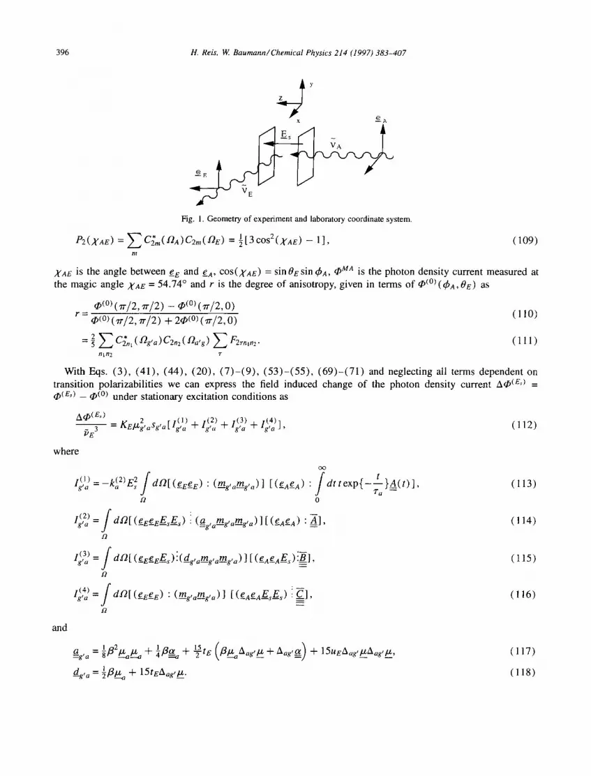
In the following we confine ourselves to the geometrical conditions sketched in Fig. 1. Then we can describe eA, ~E by the angles f~a = (~)A, Om) = ( ~ a , 7r/2) and/-/e = (~be, 0e) = (7r/2, 0e), respectively, where 0 is the angle to the z-axis and ~b is the azimuthal angle, measured with respect to the x-axis.

The photon density current without electric field q0 (°) for stationary excitation conditions can be found from Eqs. (3), (45), (77), (84) and (B.8). We write it in the form

~(0) 1 I," . (2), ¢'(1)[1 "~- 4p2(,~AE ) E C2%1 (~'~g'a)f2n2(~'~atg) E f2rnln2] (107) ~E 3 = -~lXEl,~g, aag,aO 711 tl2 J"

~MA = [1 + 2P2(XAE)r] (108)

tTe3 •

where

396 H. Reis. W. Baumann/ Chemical Physics 214 (1997) 383-407

y

x ~,~

Fig. 1. Geometry of experiment and laboratory coordinate system.

P2(XAE) = ~ C~m( OA)C2m(J"2E) = 1 [3 COS2(XAE) -- 1] , ( 1 0 9 ) m

XAE i s the angle between e E and e A, COS(XAE) = sin 0E sin (ha, (I)MA i s the photon density current measured at the magic angle XAe = 54.74° and r is the degree of anisotropy, given in terms of qs(o)(~ba, 0e) as

@(o) (rr/2, rr/2) - qs(o)(rr/2, O) r = q~(o)(7r/2, rr/2) + 2qo(o)(7r/2, O) (110)

2 Z C~n~ (l2g'a)Czn2(Oa'*:) Z Fzrn,n2. (111) = 5 Bin 2 7"

With Eqs. ( 3 ) , (41 ) , (44 ) , (20 ) , ( 7 ) - ( 9 ) , ( 5 3 ) - ( 5 5 ) , ( 6 9 ) - ( 7 1 ) and neglecting all terms dependent on transition polarizabilities we can express the field induced change of the photon density current AqS(e,) = 45(e,) _ q)(0) under stationary excitation conditions as

A@(e,) 2 [ l ( l ) + I(2) + I(3) I(4)], (112) ~E 3 -- KEll~g'aSg'a L g'a g a "g'a + "g'a

where

oo

/ t ( l ) =-k~ E s d~-2[(eEe__E) " (mg, amg,a) ] [ ( e A e A ) " d t t e x p { - }A(t)] (113) agla - - '

12 0

ig(2) f dO[ (gEeEEsEs) : (ag,amg,am_g,a) l [ (e_-AeA) : ~ ] ( 1 14)

12

g(3) = f dO[ ( e e e e E s)i (dg,amg,am_g,a) ] [ (eAeAE s )iB-] ( 1 15 ) ta ~

12

lg(4) f dO[(e_eee) : (mg,amg,a)] [ ( eaeaEsEs ) i-C], ( 1 1 6 ) t a ~ . . . . . .

12

and

1 2 1 a,o + + + +

_ 1 d_g, a - g[t~ + 15teAag/~.

(117)

(118)


We define a new function X MA by

qo(Es) _ 4(0) X MA - - [1 + 2 P z ( X A e ) r ] X . (119)

~MAE~ss

There exist five positions of the vectors e e, e A and E s to each other, which are linear independent [8]. With the equations derived above we are able to calculate X MA for all positions, but we will confine ourselves here to the special case sketched in Fig. 1, in addition with excitation light unpolarized. Such a geometry can easily be achieved in an experimental setup and is used in the laboratory of the authors [25] 2. Then we have ~('2 a :--- (7r/4, 7r/2) and only the emission polarizer angle 0e is variable.

Expressing the scalar products in Eqs. ( 113)-(116) in the spherical irreducible forms according to Eq. (B.5), l using the orthogonality of the Dm~, Eq. (75), and Eqs. (103)-(105) , (94), (95), (84), (65), (117), (118),

Eq. (112) and finally Eq. (119) yields after lengthy calculations an expression for X MA, which can be written in the same form like the equation for X in the case of a Boltzmann distribution, Eq. (32). The coefficients DE to 1E of Eqs. (32), (35) and (36) are given by

D e = 0 , (120)

2 E(4) E E = k(2)"r"a -a~eP(°) + spL~(O~E~,) + ~L(2):'g E~ 2) + /3 ~__~_~ :

-q-fl~_~, ( f l ~ -k- 15(ta)Aa'g/Z) : E(E3)+ fla=~ : E(5)=E ' (121)

• 1 r / ( l ) ( 1 2 2 ) FE '> + + 15(tA)Ao, _) : + ,

G E - ~ t ~ a A a g ' ~ : G (I) + Aag'l.l.(t~l~g "~- 15(IA)Aa'g~___) : G(E2) q- ~Aag'~_~ : (123)

H (1) (124) H e = Aag ' t zAag ' tZ : ._e_* E ,

(1) l e =Aag'l-LAag'~___ : I E • (125)

The coefficients E(e i) to l(e 1) depend on the diffusion coefficients Dk, the fluorescence lifetime ra and the angles Oa,g and ~g'a, describing the transition moment directions. They are listed in Appendix C. The Boltzmann distribution limit, Eqs. (27) - (31) with the replacements mentioned after Eq. (36), results correctly, as can be seen by using the isotropic diffusion model, Eq. (76), setting Dra --+ oo and using the rule of de l'H6pital in Eqs. (C.15)-(C.34) in Appendix C.

Comparing with the relatively simple equations in the case of a Boltzmann distribution, Eq. (32) with Eqs. (27 ) - (31 ) , we see that the generalization of the theory leads to equations complicated enough to possibly prevent any meaningful evaluation of experimental data. Much more parameters are needed for an evaluation; some may be obtained from electrooptical absorption measurements, while others, i.e. the diffusion constants Dk in the excited state, are not experimentally accessible in general but are to be calculated by assuming some suitable model for the rotational motion. To get some idea about the most sensitive parameters of the equations we performed some numerical calculations.

3. N u m e r i c a l s i m u l a t i o n s

We performed calculations for 3 differently shaped "molecules", fitting into ellipsoidal cavities with volume V = 250 × 10 -3o m 3 and half-axes ( a l , a z , a 3 ) given in Table 1.

In the hydrodynamic Stokes-Einstein-Debye (SED) model for molecular rotation, the diffusion constants Oi may be calculated assuming either "stick" or "slip" boundary conditions. "Stick" conditions should be

2 The complete theory is available on request from the authors.


Table 1 Half-axis and diffusion constants for the ellipsoids used in the simulations

Nr. ( a~, a2, a3 ) / n m ( D l, D2, D3 )Slip / n s - I ( D l, D2, D3 )Stick / n s - I

1 (0.22,0.631,0.43) ( 19.3,10.1,3.51 ) ( 1.63,2.74,1.71 ) 2 (0.2,0.35,0.853) (3.13,1.48,14.1) (1.07,1.01,3.18) 3 (0.8,0.4,0.1865) (7.94,1.59,5.12) (2.77,1.10,1.16)

applicable for solute molecules much bigger than the solvent molecules, while "slip" conditions are thought to be more appropriate for smaller solutes [26]. Recently, a comprehensive comparison of experimental results with the predictions of different models for reorientational relaxation by Ben-Amotz et al. [2,3] revealed the remarkable, although not completely comprehensible success of the SED-theory for predicting diffusion coefficients, especially with "slip" boundary conditions for medium-sized molecules in alkanes.

The diffusion coefficients are given by

kT Di = (126)

"qW(i'

where r/ is the viscosity of the solution and the ~i incorporate the effects of the boundary conditions, they are given by Perrin [27] for "stick" and by Youngren and Acrivos [28] for "slip" (see [29] for a correction to Ref. [28]) . Assuming 7/ = 10 -3 Pa s (corresponding roughly to cyclohexane at room temperature) and T = 298 K we get for the ellipsoids the values listed in Table l. It can be seen that the diffusion coefficients for "slip" conditions are very sensitive to the shape, much more than for "stick" conditions.

If the molecules are modeled as spheres, "slip" conditions predict ~:i = 0 and only the "stick"-model is applicable, with ~:i = 6 for i = 1,2,3. Then it is D = 2.7427 × 109 s -1 for all "molecules".

In a typical electrooptical emission measurement, the quantity X(0E) is measured for two values of 0, namely 0 = 0 and 0 = zr/2. In favorable cases, X(~E, 0e) can be measured for several wavenumbers of the emission band (spectrally resolved electrooptically emission measurement). A multilinear regression according to Eq. (32) then yields the coefficients D~E-Ie [ 1,11 ]. Combining with an electrooptical absorption measurement, a value for the coefficient Ee can be determined [ 11 ].

We assume that all dipole and transition dipole moments are parallel to each other and to the molecular 3-axis. For molecules with high dipole moments, the contribution of the polarizabilities usually can be neglected. We furthermore neglect the quantity k~ (2). Then, in the limit of the Boltzmann distribution, the value of the excited state dipole moment/za can be calculated from the coefficient Ee, which is given by (compare Eq. (27) with the substitutions stated after Eq. (36))

1 ,-,2 2 EE = ~p /-%. (127)

In the general case, the coefficient EE is given by the more complex expression (see Eqs. (121), (106)) ,

1 ,-,2 2 E ( 2 ) ,-,2 E (3 ) ..a_ f . / 2 2 E ( 4 ) EE= 2P [~g E33 - [ - P ]J~a["l'g E33 ~t--" t-"a E33' (128)

where we further neglected the quantities (ta) and (UA) in order to reduce the number of variable parameters for the numerical simulations. E (k~ denotes the ( i j ) th component of the tensor E(Ek~. While the quantity/zg is Eij accessible from electrooptical absorption measurements, the coefficients E (k) (k = 2, 3,4) have to be calculated E33 with the diffusion coefficients Di and the fluorescence lifetime ra as input parameters.

First, we want to examine the influence of the different boundary and shape conditions on the coefficients E (i) ( i = 2, 3,4). The calculations were performed for ~'a = 0 to 5 ns in steps of 0.02 ns. Figs. 2 and 3 show the E33 coefficients E (3) and ~7'(4) respectively, which determine the contribution of [J.aJd.g and /z] to Ee, respectively, E33 Jr" E33 ,

for the three "molecules". The coefficients were normalized to E(e4~ = 1 in the Boltzmann distribution limit. As

H. Reis, W. Baumann/ Chemical Physics 214 (1997) 383-407 399

0.35

0.3

0.25

0.2

0.15

0.1

0.05

0

(3) (EE)33

• MOl. 1, skip ~ MOt. 2, slip I o Mol. 1, stick ---~--Mol. 2, stick I o Mol. 3, slip ~ S p h e r e | " Mol. 3, stick I

1 2 3 4 5

"~ / ns a

0.8

0.6

0.4

0.2 ........

0 0 1

(4) ( E E ) 3 3

2 3 "~ / ns

a

4 5

Fig. 2. Fig. 3.

Fig. 2. The coefficient E (3) occurring in Eq. (128), calculated as a function of ra for the molecules specified in Table 1 and normalized E33,

to E (4) = 1 in the B o l t z m a n n - l i m i t . E33

~(4) Fig. 3. The coefficient t~E3a, occurring in Eq. (128), calculated as a function of ra. Legend and normalization as in Fig. 2.

( F(4)~

1 " - - E ~33

0.8

0.6

0.4

0.2

0

E(3)) 33 0.35 I ~

0.3 . . . . . . . .

0.25

0.2

0.15

0.1

0.05

0 0 0.05 0.1 0.15 0.2 0.25 0.3 0.35 0.4

r

0 0.05 0.1 0.15 0.2 0.25 0.3 0.35 0.4

Fig. 4. Fig. 5.

Fig. 4. The coefficient E (3) occurring in Eq. (128), plotted as a function of r. Legend and normalization as in Fig. 2. E33,

Fig. 5. The coefficient E (4) occurring in Eq. (128), plotted as a function of r. Legend and normalization as in Fig. 2. E33 '

expected, different boundary and shape condi t ions lead to different funct ional dependencies on ~-,. The same

holds also for the coefficient ,~(2) (no t shown) . ~t-' E3 3

In Figs. 4 and 5, the plot of the same coefficients as a funct ion of the degree of anisotropy r are shown. For E (4) ( and E (2)x e33 e3~ ), the curves for the different boundary and shape condi t ions are very similar, indicat ing that

the funct ional dependencies of r and E (4) on the differences of the diffusion coefficients for the three diffusion E33 models are roughly the same (note that e.g. for "molecule" 3, D1/D2 = 5 for "slip", 2.5 for "stick", 1 for isotropic d i f fus ion) . The coefficient E (3) on the other hand is more sensit ive to the different diffusion models , E33

but its cont r ibut ion to Ee is usual ly smaller than that o f E(e4~. In Fig. 6 the coefficient Ee, normal ized for lim~,--.oo Ee = 1, is plotted as a funct ion of r in the region

400 H. Reis, V~ Baumann/Chemical Physics 214 (1997) 383-407

, E / norm. • k=3 /2 / E

1 , 6 o k=l - - F ~ , ~ . . . . ~ . . . . ' . . . . ,=k

• k= / 4 ~ o;, '. " 1 , 4 o k=O I .,,.~ *" " " ' ~ % 8 " • • "

1 , 2 [ . . ~.;,..~,~.."¢ .... . . . . . . ......

o,8 .~t ~ ° o % ~ o ~ o ~ . e o ~ o o o ~. ~ o0~: 0 , 6

: ' < : : . . ; : ° - o , . . . . i

0 . . . . I , I . . . . i . . . . i l l i ~ l A i ~ ~, ~ , ~

0 0 , 0 5 0 , 1 0 , 1 5 0 , 2 0 , 2 5 0 , 3

r

Fig. 6. EE as a function of r and of the ratio k = /Zg//Za for "molecule" 2 with "slip", "stick" and isotropic diffusion conditions (not separately labeled); normalized to Ee = 1 in the Boltzmann limit.

r = 0 to 0.3 for different ratios k = IZg/tXa for "molecule" 2, for which the deviations in E~33~ for the different diffusion models are highest.

It can be seen that the different boundary and shape conditions manifest themselves only in some scatter around distinguishable curves. In general, the differences caused by applying different diffusion models will be buried in the statistical experimental error. In the most common case p,g~_,~ > 0 and/Zg < / za , the value of

/za, calculated from Eq. (127), i.e. assuming Boltzmann distribution, would be smaller compared to the result for the general distribution. Furthermore, we see that a correction for rotational relaxation can be necessary already for quite small values of r. For a solution of molecules with the shape specified and with tzg/JZa = 1/2 , showing a value for the degree of the anisotropy of r = 0.03, the measured value of E e amounts to only 80% of the value expected in the case of a Boltzmann distribution. The evaluation according to Eq. (127) would thus lead to a value for/z~, which is 10% too low.

Often it is not possible to perform a spectrally resolved measurement because of a low signal to noise ratio. Then the quantities X(0e ) may be measured by an optical integration over the whole fluorescence band (integral electrooptical emission measurement). In the Boltzmann distribution limit the further evaluation proceeds via suitable linear combinations of X(0) and X(Tr/2), if the angle between ~ and the transition dipole moment

of emission mag, is known [ 11,30,31]. For the case ~ II mau, considered here, this combination is

X3 = 6 [xMA(o) - - 3 x M A ( T r / 2 ) + 2(L(7"r/2))]. (129)

In the Boltzmann distribution limit, X3 equals Ee - 6 D e and is thus independent of te, uE. In the case of a general distribution, X3 is no longer independent of te and ue. To get an idea about their influence on X3, we assumed te = 0.02 × 102° J-~ and ue = 0.02 × 1040 j - 2 and calculated their contribution to X3 for the same ratios [,Za//Zg a s for Fig. 6 for "molecule" 1. We found that the deviations were highest for k = 0 and vanished for k = 1, but even for the quite high values of te , uE chosen, the deviations never exceeded 5% for r < 0.1. Taking into consideration that for integral measurements the value of uE is usually at least one order of magnitude smaller, and the generally quite high experimental uncertainties, it may be considered acceptable to neglect the contributions of the derivative terms to X3 up to r = 0.2.

4. Conclusions

We have shown that the inclusion of the finite rotational relaxation time into the theoretical interpretation of electrooptical emission measurements leads to lengthy expressions with a lot of parameters, of which the


diffusion coefficients depend much on the model used to describe the motion. The simulations in Section 3 on the other hand suggest that the evaluations according to different models may lead to very similar results, if only the degree of anisotropy r is modeled correctly.

In the anisotropic diffusion models, the rotational diffusion coefficients Dk can be calculated by approximating the shape of the molecule by an ellipsoid. If the fluorescence lifetime and the directions of the transition dipole moments of absorption and of emission in the molecular fixed coordinate system are known, then the viscosity r/ occurring in Eq. (126) may be used as an adjustable parameter to fit the degree of anisotropy of the fluorescence. This treatment may compensate for some of the imperfections that are clearly involved when approximating the molecular rotational motion by the motion of an ellipsoid in the hydrodynamic limit. The quantity r/ in Eq. (126) has often been interpreted as a "microviscosity", differing from the macroscopic measurable viscosity [ 32,35].

The relative directions of the transition dipole moments in absorption and emission can be inferred from time-dependent fluorescence depolarization measurements (TDFDM) or from fluorescence depolarization measurements in rigid media. If the excited electronic state involved in the absorption and emission processes is the same, the transition dipole moment directions of absorption and emission should be parallel and the limiting value of the degree of anisotropy ( r ( t = 0) in the case of TDFDM) should reach the value 0.4. Often, this is not the case [36] and the possible reasons must be considered very carefully in view of the conditions to be fulfilled for the application of the theory presented here (Section 2.1). For example, if there is an overlap of transitions of different moment directions of the emission band and/or the absorption band in the region of excitation, the theory cannot be applied without modification.

TDFDM may sometimes provide additional information. In principle, the temporal decay of r( t ) in the anisotropic model is described by a sum of at least two exponential functions with the eigenvalues E2~ as relaxation rates. If they could be determined unambiguously, the diffusion coefficients D~ or at least two ratios Di/Dj could be calculated. However, usually only a mean relaxation rate can be determined, due to the low signal to noise ratio of the data [36].

In the anisotropic models, the absolute direction of the transition moments in the molecular fixed system must be known, too. For molecules of low symmetry, it may be very difficult to get this information experimentally, usually one has to resort to the results of semiempirical calculations.

The evaluation procedure becomes much easier if the isotropic diffusion model can be applied. Then for the calculation of the coefficients E~ i~, etc., only the relative direction of the two transition moments and the parameter D~'a must be known (compare the remarks at the end of Appendix C). The main question is if this simplified model can be applied. The simulations in Section 3 suggest that it is possible, at least for the cases investigated. Of course, only experimental tests can finally answer this question. The results of an evaluation program on measurements of selected molecules will be reported in a forthcoming paper.

We also have shown that already small values of the degree of anisotropy of the fluorescence may lead to quite large errors in the excited state dipole moments when calculated assuming the limiting case of a Boltzmann distribution. It should be mentioned that this was already pointed out by Weber [4] in 1965, who used the isotropic diffusion model to describe the influence of the finite rotational relaxation time on the electric field effect on the degree of anisotropy of the fluorescence.

Appendix A. Eigenvalues and eigenfunctions of the asymmetric diffusor

The notation of the Ezr and the b2rn follows Wegener et al. [37]. For I = 1 we used the representation given by Huntress [38], using the free choice of the phase for blrn to get the relation U x = b I mentioned in Appendix C. For b3rn w e were unable to find a representation in the literature, so we calculated them according to the procedure given in Landau and Lifshitz [39], p. 400.


1 r \n btrn Err - 3 - 2 -1 0 1 2 3

0 0 1 0

1 - I ~ 2 0 -'~22 D 2 + D 3

0 0 1 0 DI + D 2

1 --~2 0 ---~2 D , + D 3

i 0 0 0 i 3 ( D + D3) 2 - 2 v2 ~ - - 1 0 - ' ~ 0 ~ 0 3 ( D + D2

b 0 c 6D - 2A o - o

i 0 3 ( D + DI ) 1 o ~ o b 0 c__' 0 b 6D + 2A

2 vSM M v~M

- 3 - a 3 0 - b 3 0 b3 0 a 3 15D - 3D~ - 2&l

- 2 c3 0 d3 0 d3 0 c3 15D - 3D2 - 262

- 1 0 e3 0 v ~ f 3 0 e 3 0 15D - 3D 3 - 263 l 0 0 0 l 0 12D o o - ~

1 0 f3 0 -V '2e3 0 f3 0 15D -- 3D3 + 261 2 d3 0 - c 3 0 - c 3 0 d3 15D - 3D2 + 262

3 - b 3 0 a3 0 - a 3 0 b3 15D - 3DI + 261

1 D='~(D,+D2+D3), A=~/D~ +D2+D~--D1D2--D2D3--DID3,

b=3(D3-D)+2A, c=x/~(Dl --D2), M= b2~/-~"~,

1 ¢ +DI+TD2--SD ] 1 / DI+TD2--8D 3 a3='~ 1 ~ l , b3=~ V I -- ~1 '

1 / 7ot+oZ-So ~ _1_ / DZ+D2--20~ d 3 = 2 v l - - ~2 ' e3-2 V 1+ :~3 '

SI=~/4( D2--D3)2 +( D1--D2) ( DI--D3),

~2=~/4 ( D1- D3 ) 2 + ( D2-- DI ) ( D2 - D3 ) ,

63=X/4(D1 -D2)2+( D3--D2)( D3-DO.

1 / . 7D 1 +D 2 --8D 3 C3=2 V I + 4~ 2 •

f 3 = 1 ¢ 1 - D' 4 02 3

(A.1)

Appendix B. Spherical irreducible tensors

Let Tik ] be a tensor of rank k with the Cartesian components T/z...i* with il . . . . . ik = x, y, z . The determination of the spherical irreducible components 7),,, is accomplished in two steps [40] . First the spherical components T,~....,~ k with a l . . . . . ak = - -1 ,0 , 1 are calculated by the transformation

Tm .. . . k = Z Ua, i~ "'" U,~kik Ti~...ik, (B . 1 ) il...&

with


o

U = 0 .

1 i

(B.2)

It is U = b ~ , if i = ( x , y , z ) is replaced by 7-= ( - 1 , 0 , !) (compare Appendix B). For the second step the following equation is important: if Ait~l, Bllz] are irreducible spherical tensors, the

products At~m~ Btzm2 are reducible according to

( l] 12 lm ) At~m, Btzm2" (AB)Im = y ~ ml m2 m l rtt2

(B.3)

We can imagine any Cartesian tensor Tik I as build up of k tensors of rank 1, which in turn are irreducible in the spherical basis. Thus any Cartesian tensor of rank k > 1 can be successively reduced with the help of Eq. (B.3).

As an example, we take a tensor of rank 4 with spherical components Tu~,p. If the tensor is symmetric in/z, u and in ~, p, it is advantageous to couple first {#u} to A]a and {(p} to A2/3 and then to couple ( . t l a , A2fl} to Im,

a,,a2 E {0,2}, / E {0,1,2,3,4}.

1 a2" p ;3 /

(B.4)

The spherical irreducible tensors transform under rotations in the same way as the spherical harmonics Yr,,. Let Atk I be a tensor defined in the laboratory coordinate system (LS) and Z[kl a tensor defined in the molecular coordinate system (MS). The rotation R(.O) rotates LS into MS. Then the scalar product of Alk ] and Z Ikl can be given by

( 1 -~ ~-'] a;+/+kA* t Al~l[k]ZIk] = Z ' - ' aJ tm(Ls)zajtn(Ms)Dmn(g2)" a j l m n

(B.5)

This equation is valid for the relevant tensors in our context, which can be imagined as build up of k tensors of rank 1.

Because the renormalized spherical functions Clu are irreducible, we can use them to express the spherical components au, (aa)t,, of a and (aa), respectively, in the following way:

a;, = aClz,( S2a), (B.6)

= a 2 ( 1 1 l)Cl,,,(g2a) (B.7) (aa)lm 0 0 0 "

With these equations, together with Eq. (B.5) and Eq. (74), it is possible to reproduce all relevant products of molecule fixed and laboratory fixed tensors. For example, we have ( I = A; E)

= ~tzag 1 + 2 C2,7(g2,~g)C2m(12;)gt2 . . . . (B.8) ?t int


Appendix C. The coefficients E(ff to/(~) of Eqs. (121)-(125)

E7 ) = V" C f C; nln2

g~ I) = - 5 r , (C.2)

E(E2) ---- Z (Te* O(2) + V ~ 1"Te*ca 9()(2) --r/ --~-'6,/1 ~ii--/.tl--R2--~ii_.S,Rlgt2 , (C.3) n I/i//2

E(E3) = Z Ce*O(12)+ ~-~ Ce*Ca(O(123)-nl n2 +O(13) - - 0 ( 2 ) ) + - ~ r l , (C.4) n ~-4,n "~I-"2.nxnl :::zO,n2nl ~5,n2nl

I1 nln 2

E(4) =~ce*o( '2) +Z('Te*ca fO(123)-n l n2 ,. 0 (123) +O__~(2) n +0(12) + 0 (12) } (0.5) =E =1 ,n / = l ,n2nj + ~I3,n2.l , . =2,n2nl =3,n2nl '

D DID2

g(ES' = Z Ce 'O(2 , + --n, n2 [[20(2'~2,n2n, +O(2'~,n2.1 ] , ( 0 . 6 ) 11 Din2

F{EI) =O(1 l) + ~ Cff£~12), ( 0 . 7 ) n

G(I) IF(I) e* (1) c e * c a [ 2 0 ( 1 2 3 ) T + 4 0 ( 2 ) ] - - S r l , (0.8) =E =-~=E + Z Cn ~O2,n + ~ nl n2 m ~-----3,n2ni ~,n2nlJ

It DID 2

F(2) I (1) ~7"~ ('~acQ( 1 ) *T = e - 0 3 - 53- Z_.#-"--~--4,, ' (C.9) /I

~(2, ,~(2) V ' c r o(,) ~* , , (~3, = '5~ E + ~ /I ~ , / I + Z C g I I Cn220=Q=~,.2. ,, (C. IO) 11 RIR 2

E l " = 1 - 3 }--~ Cn~42 ~* , ( C . ' I ) n

/( ,) ,H(l) ~* (o) = g--~e + Z C. O,,n + Z Ce;Ca280(2'=2,n2È, - S r l ' (C.12) n nln2

where we introduced the abbreviations

C,~ = C2n(n~, , , ) , (O.13)

C a = C2n(~'2a'g). (C. 14)

The O-tensors depend only on the rotational diffusion coefficients Dk and on the fluorescence lifetime z,,. In Cartesian coordinates, they are given by

O(0'1,nj~ = v~su[ i , J ,n] , (c.15)

o( l, El iTa l,ji = •iJ EliT a + 1 (C.16)

O(1, ~ U [ i , j , n ] E1d'a 2,nji = El iTa + 1 ' (C.17)

~ij (C .18) O ( l ) _ 3 , j i Eliq-a + 1 '

H. Reis, W. Baumann/Chemical Physics 214 (1997) 383-407

[3(1 ) . f i . . . l = v 3 U [ l , y , n ] E l i T . a + l ~4,nji

b2rnl b~rn 2 Vl.n,n2F}(2) = 6 Z (1 q- E2TTa) 2 '

2,nln,.ji = 2V/- ff Z U[i'j'n3] n4 n2 n3n 4 T

(2) v ~ Z U[i,j, nl] Z F2rnnIE2rTa ' 3,nji = n I T

405

(C.19)

(C.20)

(C.21)

(C.22)

0(2) V ~ f f E s [ i ' j ' n 5 ] E FRTB2i76[~F2T2B3BIbRT3B4b~T3n5E2T3Ta--~I73tIla11417S]Q 2 23 :6 ) 4,n2nl.ji = - - 12 4 ' n5 Tn3n4ll6 (C.23)

V/-~VE ( 2 2 2)ZF2rn2n,, (C.24) 0~221172.]i =2 U[i,j, nB] n3 121 n4 B3B4 T

O~2~.ji = 2x/-6 Z U[i,j, nl] E F2,,,,, (C.25) 711 T

, { ,,,:,= --d- ~-~U[i,j,n'] k ~ _ i G,, q- Z F2rnn, I + ( E 2 r - E l i - E I j ) T a n 1 T

0(~2~ v~ 2 ,B2n l j i - 2v / -~ Z U[i'J 'nsl

tl 5 Z V~Tn2n 6

TB3t/4n6

o~l:2)nlji = F2"rnznl E21.T a -~ 1 ' ' T

U [ i , j , n l ] [ann ' + { ( E l i - E l j ) 7 " a - l } Z F2rnnl t"}(12) V/-'6 Z El jTa + 1 V4,nj i = n 1 T

5,nji = ~ E EliZa + 1 B 1 T

t"}(123) = 3 F2rn2n6K[i,J , n3 ,n6] El iEl j , r a F2r,n~nl _ anln ~ (E l i l j )Ta V l ,nznlji . - ' Tn3?t 6 TI

O(123) = 6 E F2rn2n3 EliTa K [ i, j, nl 123 ] 2,n2nlji ' ' Tn3

3,n2nlji I13

-~-E].j) Ta] ~'-a,,14n5 ~gt i/73 ) ( n24:3 1226/ ,

(C.26)

(C.27)

(c.28)

(C.29)

(c.3o)

(C.31)

(C.32)

(C.33)

406 H. Reis, W Baumann/Chemical Physics 214 (1997) 383-407

o(13) ..=6K[i,j,nl,n2], O,WUJI

(C.34)

(C.35)

(C.36)

The equations simplify considerably in the case of isotropic diffusion. Then we have from Eqs. (86), (76) and

the unitarity of b/711,

c FIT,,, = l T 1 + 1(1+ 1)07,’

(C.37)

and all summations over Ti vanish, as well as a considerable number of the summations over ni.

References

[ 1 1 W. Baumann and H. Deckers, Ber. Bunsenges. Phys. Chem. 81 ( 1977) 786.

[ 21 A.M. Williams, Y. Jiang and D. Ben-Amotz, Chem. Phys. 180 ( 1994) 119.

[3] R. Ravi and D. Ben-Amotz, Chem. Phys. 183 ( 1994) 385. ]4] G. Weber, J. Chem. Phys. 43 (1965) 521.

[5] C. Homick and G. Weill, Biopol. 10 (1971) 2345.

[ 61 0. Rolinski, A. Baiter and A. Kowalczyk, Chem. Phys. 141 (1990) 265.

[ 71 J. Czekalla, W. Liptay, K.-O. Meyer, Ber. Bunsenges. Phys. Chem. 67 ( 1963) 465 [ 81 W. Lintav, Z. Naturforsch. 18a ( 1963) 705.

[91

[lOI

1111

[I21

[I31

I141

[I51

[ 161 I171

1181

[I91

1201

1211

1221 1231

1241

1251

1261 1271 [I81 [291 [301

R. Wortmann, K. Elich, S. Lebus and W. Liptay, J. Chem. Phys. 95 ( 1991) 6371.

W. Liptay, Dipole moments and polarizabilities of molecules in excited electronic states, in: Excited States, Vol. 1, ed. E.C. Lim

(Academic Press, New York, 1974) p. 128.

W. Baumann, Determination of dipole moments in ground and excited states, in: Physical Methods of Chemistry, Vol. 38,

Determination of Chemical Composition and Molecular Structure 2E, eds. B.W. Rossiter and J.F. Hamilton (Wiley, New York,

1989) p. 45. W. Liptay, B. Dumbacher and H. Weisenberger, Z. Naturforsch. 23a ( 1968) 1601.

W. Liptay, R. Wortmann, H. Schaffrin, 0. Burkhard, W. Reitinger and N. Detzer, Chem. Phys. 120 ( 1988) 429. R. Wortmann, K. Elich and W. Liptay, Chem. Phys. 124 (1988) 395.

S.H. Lin, J. Chem. Phys. 62 (1975) 4500.

L.D. Favro, Phys. Rev. 119 (1960) 53. H. Risken, The Fokker-Planck-equation (Springer Berlin 1984).

T.J. Chuang and K.B. Eisenthal, J. Chem. Phys. 57 (1972) 5094.

M. Ehrenberg and R. Rigler, Chem. Phys. Lett. 14 (1972) 539.

G.G. Belford, R.L. Belford and G. Weber, Proc. Natl. Acad. Sci. US 69 (1972) 1392.

W.A. Wegener, J. Chem. Phys. 84 ( 1986) 5989.

W.A. Wegener, Biopol. 23 (1984) 2243. A. Lindner, Drehimpulse in der Quantenmechanik (Teubner, Stuttgart, 1984)

L.C. Biedenham and J.D. Louck, Angular Momentum in Quantum Physics, Encyclopedia of Mathematics and its Applications, Vol.

8 (Addison-Wesley, Reading, MA, 198 I ). H. Deckers and W. Baumann, Ber. Bunsenges. Phys. Chem. 81 (1977) 795.

C.-M. Hu and R. Zwanzig, J. Chem. Phys. 60 ( 1974) 4354.

P.F. Perrin, J. Phys. Radium 5 ( 1934) 497. G.K. Youngren and A. Acrivos, J. Chem. Phys. 63 ( 1975) 3846. R.J. Sension and R. Hochstrasser, J. Chem. Phys. 98 (1993) 2490. W. Baumann and H. Bischof, J. Mol. Struct. 129 (1985) 125.


[31] W. Baumann, Z. Nagy, H. Reis and N. Detzer, Chem. Phys. Lett. 224 (1994) 517. [32] D. Ben-Amotz and J.M. Drake, J. Chem. Phys. 89 (1988) 1019. 133] S. Canonica, A.A. Schmid and U.P. Wild, Chem. Phys. Lett. 122 (1985) 529. 1341 A. Gierer and K. Wirtz, Z. Naturforsch. Teil A 8 (1953) 532. 1351 E. Akesson, A. Hakkarainen, E. Laitinen, V. Helenius, T. Gillbro, J. Korppi-Tommola and V. SundstrOm, J. Chem. Phys. 95 (1991)

6508. 136] G.R. Fleming, Chemical Applications of Ultrafast Spectroscopy (Oxford Univ. Press, Oxford, 1986). 137] W.A. Wegener, R.M. Dowben and V.J. Koester, J. Chem. Phys. 70 (1979) 622. 1381 W.T. Huntress, J. Chem. Phys. 48 (1968) 3524. 1391 L.D. Landau and E.M. Lifschitz, Lehrbuch der theoretischen Physik, Band lII: Quantenmechanik, 7. Aufl. (Akademie-Verlag, Berlin,

1984). 140 ] C.G. Gray and K.E. Gubbins, Theory of Molecular Fluids (New York, Oxford, 1984).

influence of rotational diffusion on the electric field induced effect on the fluorescence spectrum...

Documents