Independent EEG Sources Are DipolarArnaud Delorme1,2,4*, Jason Palmer1, Julie Onton1,5, Robert Oostenveld3, Scott Makeig1

1 Swartz Center for Computational Neuroscience, University of California San Diego, La Jolla, California, United States of America, 2 Centre de recherche Cerveau et

Cognition, Paul Sabatier University, Toulouse, France, 3 Donders Institute for Brain, Cognition and Behaviour, Radboud University, Nijmegen, The Netherlands, 4 CERCO,

CNRS, Toulouse, France, 5 Naval Health Research Center, San Diego, California, United States of America

Abstract

Independent component analysis (ICA) and blind source separation (BSS) methods are increasingly used to separateindividual brain and non-brain source signals mixed by volume conduction in electroencephalographic (EEG) and otherelectrophysiological recordings. We compared results of decomposing thirteen 71-channel human scalp EEG datasets by 22ICA and BSS algorithms, assessing the pairwise mutual information (PMI) in scalp channel pairs, the remaining PMI incomponent pairs, the overall mutual information reduction (MIR) effected by each decomposition, and decomposition‘dipolarity’ defined as the number of component scalp maps matching the projection of a single equivalent dipole with lessthan a given residual variance. The least well-performing algorithm was principal component analysis (PCA); bestperforming were AMICA and other likelihood/mutual information based ICA methods. Though these and other commonly-used decomposition methods returned many similar components, across 18 ICA/BSS algorithms mean dipolarity variedlinearly with both MIR and with PMI remaining between the resulting component time courses, a result compatible with aninterpretation of many maximally independent EEG components as being volume-conducted projections of partially-synchronous local cortical field activity within single compact cortical domains. To encourage further method comparisons,the data and software used to prepare the results have been made available (http://sccn.ucsd.edu/wiki/BSSComparison).

Citation: Delorme A, Palmer J, Onton J, Oostenveld R, Makeig S (2012) Independent EEG Sources Are Dipolar. PLoS ONE 7(2): e30135. doi:10.1371/journal.pone.0030135

Editor: Lawrence M. Ward, University of British Columbia, Canada

Received July 29, 2011; Accepted December 9, 2011; Published February 15, 2012

Copyright: � 2012 Delorme et al. This is an open-access article distributed under the terms of the Creative Commons Attribution License, which permitsunrestricted use, distribution, and reproduction in any medium, provided the original author and source are credited.

Funding: This work was supported by a gift from the Swartz Foundation (Old Field NY) and by grants from the National Institute of Mental Health USA (RO1-NS047293-01A1) and the National Science Foundation USA (NSF IIS-0613595). The funders had no role in study design, data collection and analysis, decision topublish, or preparation of the manuscript.

Competing Interests: The authors have declared that no competing interests exist.

* E-mail: arno@ucsd.edu

Introduction

Brain-generated EEG data are generally considered to index

synchronous aspects of local field potentials surrounding radially-

arrayed cortical pyramidal cells [1,2]. There are strong biological

reasons to believe that under favorable circumstances ICA should

separate signals arising from local field activities in physically

distinct, compact cortical source areas: First, short-range (,100 mm)

lateral connections between cortical neurons are vastly more dense

than longer-range connections [3,4], while inhibitory and glial cell

networks have no long-range processes [3]. Also, thalamocortical

connections that also play a strong role in cortical field dynamics

[5,6] are predominantly radial. For these reasons, synchronization

of cortical field activities within sparsely connected distributed

domains should be much weaker than whole or partial synchroni-

zation of field activity within compact domains supported by short-

range anatomic connections. Thus, cortical field potentials contrib-

uting to scalp EEG should arise largely from near-synchronous field

activities within cortical ‘patches’ whose net far-field signals are near-

instantaneously volume conducted to and linearly summed at EEG

scalp electrodes.

Emergence of near-synchronous field activity within small

cortical domains has been observed and modeled in vivo (‘phase

cones’) [7], in vitro (‘neuronal avalanches’) [8,9] and in silico [10].

The net far-field projection of such a cortical patch will nearly

equal that of a single ‘equivalent’ current dipole located near and

typically beneath the center of the generating patch [11,12]. In

practice, we have observed that linear decomposition of high-

density scalp EEG data by Independent Component Analysis

(ICA) may return up to dozens of maximally independent com-

ponent processes whose scalp maps are generally compatible with

their generation in such a cortical patch [13,14,15,16,17]. This

suggests an approach to comparing the relative biological plau-

sibility and utility for EEG source separation of the many ICA and

other blind source separation (BSS) algorithms that have been

introduced in the last two decades.

BSS/ICA sourcesBSS and, in particular, ICA methods are now widely used for

separating artifacts from scalp-recorded electroencephalographic

(EEG) and related data [18,19,20,21,22] and, increasingly, to

separate and study brain source activities [13,14,23,24,25,26].

ICA identifies signals in recorded multi-channel data mixtures

whose time courses are maximally independent of one other and

in this sense contribute maximally distinct information to the

recorded data. Instead of directly addressing the general EEG

inverse problem of determining the time courses and spatial dis-

tributions of cortical (and other) source areas of recorded scalp

signals using an electrical forward head model (estimating the

projection weights of all possible sources to the scalp sensors), ICA

directly models What distinct signals are contained in the volume-

conducted scalp data, and returns the relative projection strength

PLoS ONE | www.plosone.org 1 February 2012 | Volume 7 | Issue 2 | e30135

of each maximally independent source to the scalp sensors,

thereby also greatly simplifying the problem of determining Where

in the brain each EEG source signal is generated [12,24].

Non-brain sourcesScalp-recorded EEG data also include non-brain or ‘artifact’

signals that are linearly mixed with brain EEG source activities

at the scalp electrodes. ICA has been found to efficiently separate

out several classes of spatially stereotyped non-brain signals: scalp

and neck muscle electromyographic (EMG) activities, electro-

oculographic (EOG) activities associated with eye blinks [20],

saccades, and ocular motor tremor [15] as well as electrocardio-

graphic (ECG) signal and single-channel noise produced by

occasional loose connections between electrodes and scalp. Spa-

tially non-stereotyped artifacts associated with irregular scalp maps

(for example, artifacts produced by extreme participant move-

ments) cannot be parsed by ICA into one (or a few) component(s),

so these are best removed from the data before decomposition.

Decomposition differencesThough ICA algorithms all have the same root goal [27] and

generally produce similar results when used to unmix idealized

source mixtures, since EEG brain and non-brain source signals

are likely not perfectly independent and different algorithmic

approaches to maximizing independence differ, different ICA alg-

orithms may return somewhat different results when applied

to the same EEG data. Unlike most ICA algorithms that attempt

to minimize instantaneous dependence, some BSS algorithms att-

empt to reduce redundancy between lagged versions of the data.

To date, the three ICA/BSS algorithms applied most often to

EEG data are likely extended Infomax ICA [27,28], so-called

FastICA [29], and Second-Order Blind Identification (SOBI) [30].

Computer code for these and a variety of other proposed ICA and

BSS algorithms are readily available, making of interest a com-

parison of their effectiveness for EEG data decomposition.

Comparing decompositionsTo date, however, suitable measures have not been dem-

onstrated for comparing the components returned by different

ICA/BSS algorithms applied to actual (as opposed to simulated)

EEG data for which ‘ground truth’ source signals and scalp

projections are not available. In particular, components produced

by ICA decompositions that minimize mutual information be-

tween simultaneously recorded signal values have not been much

compared to components produced by BSS algorithms that sim-

ultaneously minimize component signal redundancy at multiple

time delays [16,21].

Here, we use three measures – the amount of mutual information

reduction (MIR) between the recovered component time courses

relative to the recorded data channels (in kbits/sec), the mean

remaining pairwise mutual information (PMI) between pairs of

component time courses (in kbits/sec) [31], and the ‘dipolarity’ of

the decomposition defined as the number of returned components

whose scalp maps can be fit to the scalp projection of a single

equivalent dipole with less than a specified error threshold (specified

as percent residual variance). We applied these measures to 71-

channel EEG data we had collected from 14 subjects (roughly

300,000 time points for each) as they performed a modified

Sternberg visual working memory task [25] (see Methods).

The motivation for the first two measures (MIR and PMI) is

clear; they test how well the results of the decomposition approach

the instantaneous independence objective. MIR, introduced here,

is a direct (and as we show, easily computed) measure of the

statistical distinctness of the activities of the resulting components,

the absence of dependency entailing, in particular, suppressing the

strong linear mixing of EEG signal source signals by common

volume conduction to the electrodes. PMI is a partial measure of

MIR that can also be directly (though less efficiently) computed

from the data. MIR takes into account multi-component de-

pendencies whereas PMI only considers pairwise dependencies.

Both can be said to index the relative success of ICA/BSS in

finding component processes with fixed scalp projection patterns

and near-independent time courses whose projections sum to

the data.

The motivation for the third measure (dipolarity) is the

assumption that brain and non-brain EEG sources have spatially

fixed source locations and orientations, as well as temporally

distinct, independently varying time courses. This assumption is

reasonable at least for scalp muscle, ocular, and electrode artifact

signals and, as described above, for many cortical source processes

as well, whose volume-conducted potentials recorded at the scalp

represent far-field projections of signals each generated within a

compact patch of coherent cortical field activity (e.g., within a

cortical ‘phase cone’ [32] or ‘neuronal avalanche’ sequence [8,9]).

While this may not perfectly describe all brain EEG sources, the

total numbers of such sources separated by these decompositions is

of interest since they allow interpretation as locally synchronous

field signals from distinct (and more simply localizable) cortical

areas.

Here, we show that these three rather different measures, the

first two considering only the component time courses and the

third only the component scalp maps, are redundant, as they

similarly rank-order decomposition differences for a large subset of

available ICA/BSS methods applied to actual high-density EEG

data. This result is compatible with a model of many EEG signal

sources as originating in partially synchronous local field activity

across a cortical patch or spatially fixed non-brain artifact gen-

erator and, we believe, further supports the utility of ICA deco-

mposition for identifying physiologically and functionally distinct

sources of high-density EEG data.

Results

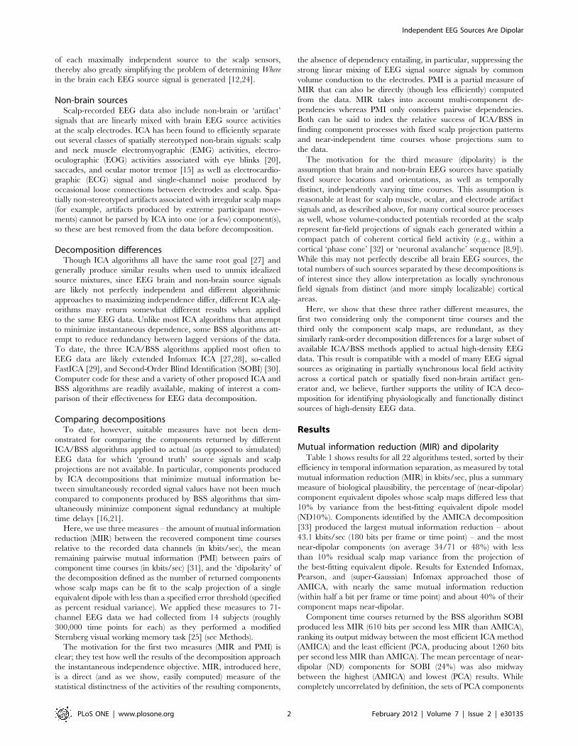
Mutual information reduction (MIR) and dipolarityTable 1 shows results for all 22 algorithms tested, sorted by their

efficiency in temporal information separation, as measured by total

mutual information reduction (MIR) in kbits/sec, plus a summary

measure of biological plausibility, the percentage of (near-dipolar)

component equivalent dipoles whose scalp maps differed less that

10% by variance from the best-fitting equivalent dipole model

(ND10%). Components identified by the AMICA decomposition

[33] produced the largest mutual information reduction – about

43.1 kbits/sec (180 bits per frame or time point) – and the most

near-dipolar components (on average 34/71 or 48%) with less

than 10% residual scalp map variance from the projection of

the best-fitting equivalent dipole. Results for Extended Infomax,

Pearson, and (super-Gaussian) Infomax approached those of

AMICA, with nearly the same mutual information reduction

(within half a bit per frame or time point) and about 40% of their

component maps near-dipolar.

Component time courses returned by the BSS algorithm SOBI

produced less MIR (610 bits per second less MIR than AMICA),

ranking its output midway between the most efficient ICA method

(AMICA) and the least efficient (PCA, producing about 1260 bits

per second less MIR than AMICA). The mean percentage of near-

dipolar (ND) components for SOBI (24%) was also midway

between the highest (AMICA) and lowest (PCA) results. While

completely uncorrelated by definition, the sets of PCA components

Independent EEG Sources Are Dipolar

PLoS ONE | www.plosone.org 2 February 2012 | Volume 7 | Issue 2 | e30135

were not as highly independent, retaining higher-order depen-

dencies.

Figure 1A shows exemplar scalp maps for seven (AMICA)

components with successively higher amounts of equivalent dipole

residual variance (from 1% to 64%), plus one component (lower

right, a typical PCA high-order ‘checkerboard’-like map with

still higher r.v. = 84%) clearly incompatible with the projection

of single brain equivalent dipole. Figure 1B shows, for four

decomposition algorithms, the mean density (in dipoles per mm3)

of equivalent dipoles for components with near-dipolar (r.v.,5%)

scalp maps in two brain slices. The figure reflects the fact that

applied to these data sets AMICA returned a larger number of

near-dipolar components than extended infomax ICA, FastICA,

or SOBI. For this reason, we used AMICA as a standard for

exploration of the similarities and differences between components

returned by the other decompositions. Source densities for PCA

and sphering decompositions are not shown: Very few of the PCA

component scalp maps were near-dipolar – for example on

average only 3 of 71 at the 10% residual variance (r.v.) cutoff, and

those mainly dominated by large eye artifacts. A much larger

number of ‘sphering’ components (87%) had near-dipolar scalp

maps, as is guaranteed by the nature of the sphering decompo-

sition (see Methods). However, as the best-fitting single-dipole

models for these sphering component maps are near-radial to

the scalp surface and located below each of the scalp channels,

respectively, rather than indicating the location and orientation of

an actual EEG source.

General component similarityNext, we made a preliminary assessment of whether the best-

known ICA and BSS algorithms generally returned similar

components. To do this, we first selected from the AMICA de-

composition of one participant’s data, by visual inspection of scalp

maps, time courses, and power spectra, representative components of

seven types – central occipital alpha band (near 10-Hz) activity,

frontal midline theta band (near 5-Hz) activity, eye blink artifacts,

left and right mu rhythm activities (near 10 Hz, with prominent

harmonics), lateral saccade artifacts, and electromyographic (EMG)

Table 1. Mean mutual information reduction and ‘dipolarity’measures for each algorithm across 13 data sets.

Algorithm (MATLABfunction) MIR (kbits/s) ND 10% Origin1

AMICA 43.12 48.6 EEGLAB 6.1

Infomax (runica) 43.07 41.6 EEGLAB 4.515

Extended Infomax (runica) 43.02 43.8 EEGLAB 4.515

Pearson 43.01 42.6 ICAcentral (6)

SHIBBS 42.74 34.1 ICAcentral (5)

JADE 42.74 33.9 EEGLAB 4.515

FastICA2 42.71 35.5 ICAcentral (2)

TICA 42.68 34.1 ICALAB 1.5.2

JADE_OPT. (jade_op) 42.64 31.0 ICALAB 1.5.2

SOBI4 42.51 24.5 EEGLAB 4.515

JADE_TD (jade_td) 42.47 28.9 ICALAB 1.5.2

SOBIRO4 (acsobiro) 42.44 26.4 EEGLAB 4.515

Sphering 42.34 87.0 EEGLAB 4.515

FOBI 42.31 26.5 ICALAB 1.5.2

EVD24 42.30 25.4 ICALAB 1.5.2

EVD 42.19 23.7 ICALAB 1.5.2

icaMS3 42.18 14.0 ICA DTU Tbox

AMUSE 42.14 11.9 ICALAB 1.5.2

PCA 41.86 4.4 EEGLAB 4.515

SONS 41.76 37.5 ICALAB 1.5.2

eeA 39.98 27.4 ICAcentral (8)

ERICA 38.78 39.7 ICALAB 1.5.2

1EEGLAB (sccn.ucsd.edu/eeglab); ICAcentral (tsi.enst.fr/icacentral); ICALAB(bsp.brain.riken.go.jp/ICALAB); ICA DTU Toolbox (mole.imm.dtu.dk.toolbox/ica). Numbers in parentheses to the right of the ICAcentral source labelindicate the entry in the ICACentral.org database; other numbers in thisposition give the toolbox version used.

2A symmetric approach to optimizing the FastICA weights returned similarresults.

3By default not using pre-whitening.4The time lag used was 100 samples, which is supposed to be optimal for EEGdata.

The leftmost column gives the algorithm used (and when ambiguous, theMATLAB function in parentheses). The second column (Mutual InformationReduction, MIR, in kilobits per second) indicates the excess mutual informationremaining among the component time courses, compared to the componenttime courses of the most efficient algorithm tested (AMICA). The third column(near-dipolar percentage, ND10%) indicates the percentage of returnedcomponents whose scalp maps had less than 10% residual variance from thescalp projection of the best-fitting single equivalent dipole model. The fourthcolumn (Origin) indicates the online source repository from which the MATLABsource code was obtained (see footnotes).doi:10.1371/journal.pone.0030135.t001

Figure 1. Component dipolarity and equivalent dipole density.A. Example component scalp maps more (top) to less (bottom)resembling the projection of a single equivalent dipole. Eightinterpolated independent component (IC) scalp maps with progres-sively more difference from the projection of the best-fitting equivalentdipole (ED) (percent of residual variance (r.v.) indicated for each map).All but the bottom-right component scalp map are from AMICAdecompositions. 1st row: (left) frontal midline IC with prominent thetaband activity; (right) right parietal IC with a more tangentially orientedED model and prominent alpha band peak. 2nd row: (left) centralparietal IC likely reflecting coupled field activity in adjacent left andright medial cortex; (right) more anterior midline IC. 3rd row: (left) ICaccounting for EMG activity of a right post-auricular muscle; (right) IC ofuncertain origin. 4th row: (left) IC accounting for electrode noise at themost affected (red) scalp electrode; (right) high-order PCA componentwith a characteristic ‘checkerboard’ scalp map unlike the projection ofany single ED. B. Mean (left) medial sagittal and (right) axial (z = 40 mm)densities of near-dipolar (r.v., = 5%) component equivalent dipolesacross all data sets, from four (indicated) decomposition methods.doi:10.1371/journal.pone.0030135.g001

Independent EEG Sources Are Dipolar

PLoS ONE | www.plosone.org 3 February 2012 | Volume 7 | Issue 2 | e30135

activity from a right forehead muscle. We then found the components

from four other decompositions of the same data set (Infomax ICA,

FastICA, SOBI, and sphering) whose scalp maps were most cor-

related to the seven representative AMICA component maps.

Results in Figure 2A show the scalp maps of these ‘best-

matching components’ strongly resembled those returned by

AMICA. Note, however, the relative inability of sphering (bottom

row, two rightmost columns) to find component maps with tan-

gentially-oriented equivalent dipole models (lateral eye movement

artifacts and right frontal scalp muscle activity). Also, as expected

the eye blink artifacts (third column) clearly separated by all but

the sphering decomposition (bottom) clearly could be better fit

with dual-symmetric equivalent dipole models (one dipole for each

eye), though here for simplicity we chose to ignore the presence of

such components in defining decomposition ‘dipolarity.’ These

representative components are present in most datasets.

Next, we found clusters of AMICA components from the other

data sets most similar in location and dynamics to each of the

original seven components; the four component clusters account-

ing for non-artifact brain sources are shown in Figure 2B. To

further quantify relationships between components returned by

the different decompositions, we computed the mean absolute

correlations between scalp maps and activity time courses of com-

ponents from all the algorithms that best matched the seven

selected AMICA components shown in Figure 2A. Results are

shown in Figure 3.

For all of the twelve algorithms that reduced average pairwise

mutual information more than sphering (the highlighted algorithm

labels in Figure 3A), absolute correlations between the AMICA

component scalp maps and the best-matching component scalp

maps were mostly above 0.9 (Figure 3B), as were most of the time

course correlations (Figure 3C). For comparison, Figure 3Ashows the MIR (red) and difference in MIR from AMICA (blue)

for each algorithm. For unknown reasons, on this particular type

of high dimensional EEG data, three ICA algorithms (SONS, eeA,

and ERICA, rightmost columns) were markedly less efficient in

reducing mutual information overall, although the scalp maps of

their best-matching components also generally resembled (r.0.9)

those of the seven selected AMICA components (see Discussion).

As the time courses of the best map-correlated sphering com-

ponents (Figure 3, middle column) were not well correlated with

those returned by the ICA algorithms, we omitted sphering from

further method comparisons.

Decomposition dipolarityNext, we computed the resemblance of the scalp maps of each

component returned by the remaining decomposition methods

to the scalp projection of a best-fitting single equivalent dipole.

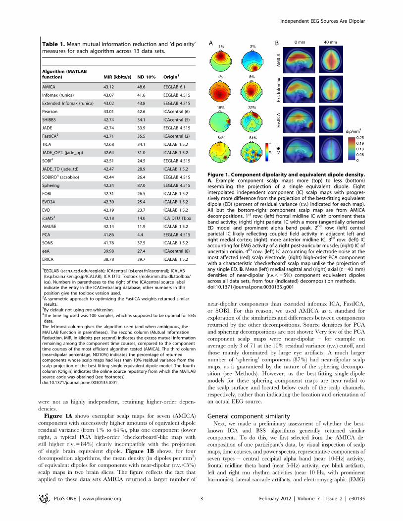
Figure 4A shows the cumulative distributions of percent residual

scalp map variance left unaccounted for by the equivalent dipole

model for all components returned by the remaining 18 ICA/BSS

algorithms. The cumulative percentage of near-dipolar components

can be read from the ordinate for each residual variance cutoff on

the abscissa. The three black/grey dashed traces allow comparison

with quite different results of sphering (top), of PCA whitening

(bottom), and of attempting to fit equal numbers of randomly

selected raw, single time-point EEG data scalp maps with a single

equivalent dipole model (center). Note the largely increased number

of ‘near-dipolar’ ICA component maps compared to the raw

channel EEG data. SOBI and the other time-dependent algorithms

did not return as many near-dipolar components as the natural

gradient-based ICA algorithms, which were led by AMICA, which

returned on average 34 (of 71) such components at an (arbitrary)

10% residual variance dipolarity threshold.

Mutual information reduction (MIR) versus dipolarityNext, we asked whether the algorithms that better reduced the

mutual information present in the raw scalp channel time courses

also returned more components with near-dipolar scalp maps.

Figure 2. ICA algorithms return similar dipolar components. A.The top rows show activity spectra and scalp maps for seven AMICAcomponents from one subject accounting respectively for eye blinks,lateral eye movements (EOG), and right frontal scalp muscle activity aswell as posterior alpha band, central mu rhythm, and frontal midlinetheta activity. Lower four rows show scalp maps of best-matchingcomponents by Extended Infomax ICA, FastICA, SOBI, and spheringdecompositions of the same subject data, e.g., those with highestabsolute scalp map correlations to the respective AMICA components.Note the resemblance of the scalp maps in each case for AMICA andExtended Infomax, and the differences between the AMICA andsphering component maps. B. Scalp maps and mean activity spectraof four clusters of similar AMICA components from 6–10 different datasets from different subjects, isolated by visual inspection of componentscalp maps and mean activity spectra and accounting respectively forcentral occipital alpha, frontal midline theta, and left and right murhythm activities.doi:10.1371/journal.pone.0030135.g002

Independent EEG Sources Are Dipolar

PLoS ONE | www.plosone.org 4 February 2012 | Volume 7 | Issue 2 | e30135

Figure 4B plots, for the remaining 18 decompositions, the rela-

tionship between mean algorithm MIR and algorithm dipolarity,

here defined as number of components with single equivalent

dipole model residual variance below a stricter threshold (r.v.#

5%). The figure reveals a surprisingly strong and highly signifi-

cant linear relationship (r2 = 0.96) between the mean increase in

the independence of the component time courses (in MIR kbits/

second) and the number of returned components with near-dipolar

scalp maps.

The inset to Figure 4B shows the r2 and probability (by t-test)

of the regression line for residual variance dipolarity thresholds

between 2% to 99%. The inset shows that the positive slope of the

regression line in the main figure is significant by t-test (at p,1024)

at residual variance (r.v.) thresholds from 2% to over 20%, with

the linear fit accounting for more than 96% of algorithm variance

at its peak (r.v., = 6%). The 6% r.v. threshold might not be far

above the minimum r.v. error compatible with our use, here, of

a simple best-fitting spherical head model and standardized

electrode locations to compute the scalp map projections of the

equivalent dipoles; using a best-fitting spherical head model

instead of an individual head model built from a subject MR head

image adds on average a 3% r.v. error (Z. Akalin Acar, personal

communication). Components with scalp map r.v., = 6% may

thus be quite consistent with the projection of a single equivalent

dipole (though this fact alone does not necessarily rule out source

geometries other than a single compact cortical patch domain). In

brief, Figure 4B indicates that more independent linear EEGdecompositions include more near-dipolar components,

and that this monotonic relationship is on average nearlylinear across a large number of ICA and BSS algorithmsfrom PCA to Infomax ICA and AMICA.

Pairwise mutual information (PMI) and dipolarityPlotting algorithm dipolarity, defined as the mean number of

returned components with near-dipolar (here, r.v.,5%) scalp

maps, against the mean percentage of mutual information re-

maining between pairs of component time courses, compared to

pairwise mutual information between EEG scalp channels

(Figure 4C), revealed a similar linear trend. The more completely

the decomposition eliminates pairwise mutual information, the

more near-dipolar components are separated by the decomposi-

tion. However, the converse is not true; pairwise mutual in-

formation measures only account for a portion of total mutual

information, which may also obtain exclusively within subspaces of

more than two signals. Though linear trend (r2 = 0.71) for PMI is not

as strong as for total MIR, the residual variance cutoff at which

this linear trend is maximum is near equivalent (cf. Figure 4B).

Mutual information and equivalent dipole locationFor the four brain component types shown in Figure 2B, we

found the component returned by each of the 18 algorithms for each

of the 13 datasets whose scalp map most closely resembled that of the

exemplar AMICA component (Figure 2A, top row). We defined

the mean cluster ‘tightness’ of the cluster of these 13 components as

the mean distance from each cluster component equivalent dipole

model to the location of the dipole cluster centroid. The resulting

mean cluster tightness for each decomposition algorithm is shown in

Figure 4D plotted against its mean MIR. As expected, cluster

tightness was smallest for AMICA since the clustered components

from the other decompositions were those with best (but imperfect)

scalp map correlations to the exemplar AMICA components.

However, the relationship between component cluster tightness (in

root mean square mm) and the mutual information reduction (MIR)

achieved by the other algorithms again had a strong linear trend

(r2 = 0.74). Thus, on average algorithms that returned more near-

dipolar components (Figures 3 and 4) also returned components

(of the four selected types) whose equivalent dipole locations, across

participants, were more consistent.

To confirm the consistency of these findings, Figure 5A plots,

for each data set and decomposition algorithm, the number of

near-dipolar components (r.v., = 5%) returned versus mutual

information reduction (MIR) produced by the decomposition.

Here colors group results for each dataset. Dipolarity is positively

related to MIR for 12 of the 13 data sets. The mean r2 value of the

linear fit, across all datasets, is r2 = 0.6460.29 (p,0.00001 by two-

tailed unpaired t-test, df = 12).

Figure 5B plots decomposition dipolarity for each data set

versus MIR and total scalp-channel PMI before decomposition.

Results for the 18 algorithms (plus sphering) are connected by

line segments in the same order as in the mean results shown

in Figure 4A (i.e., from PCA to AMICA), with dashed lines

connecting the AMICA results (crossed circles) and ‘sphering’

(open circle) results. Figure 5B again shows that one of the 13

data sets (colored light green) is an outlier for which pre-

decomposition PMI is relatively high, and that MIR has no strong

relation to the ‘dipolarity’ of the decompositions. The (vertical)

orders of the decomposition results for the other 12 data sets

consistently resemble the mean results shown in Figure 4B. The

Figure 3. Correlations of component scalp maps and timecourses across algorithms for the seven identified componenttypes. A. (Blue trace) Mean (6std. deviation across all data sets)additional mutual information remaining in the time courses ofcomponents returned by each of the 22 decomposition algorithmsrelative to AMICA decompositions of the same data, sorted left to rightby overall degree of mutual information reduction (MIR, red trace).Names of the 12 algorithms returning components with more mutualinformation reduction (MIR) than simple sphering (bottom left) arelettered in black. B. Mean correlations between seven representativeAMICA component scalp maps from one participant (same as top rowin Figure 2) and the seven components with best absolute scalp mapcorrelations to these returned by the other decompositions of thissubject’s data. C. Mean correlations between the independentcomponent activation time courses for the same component pairs asin B. Although the time course correlations are generally lower thanscalp map correlations, the two patterns of results are similar, with(leftmost) decompositions effecting the most mutual informationreduction returning components whose scalp maps and activitiesgenerally strongly resemble the selected AMICA components.doi:10.1371/journal.pone.0030135.g003

Independent EEG Sources Are Dipolar

PLoS ONE | www.plosone.org 5 February 2012 | Volume 7 | Issue 2 | e30135

panel also shows that, as might be expected, the amount of mutual

information reduction for each data set is roughly proportional to

the original amount of channel-pair PMI in the data (as indicated

by the linear trend plotted on the ‘floor’ of the plotting box). Note

that the total mutual information in the channel data, though itself

infeasible to compute and not shown here, can be expected to be

smaller than the total PMI (here about 300 kbits/s) since much of

the mutual information between different channel pairs may

actually reflect common higher-order dependencies that are

counted multiple times in calculating total PMI. In turn, total

mutual information in the channel data must be larger than the

MIR (here near 40 kbits/s).

Figure 4. Decompositions that reduce total mutual information in the component time courses also return more components withnear-dipolar scalp maps. A. Cumulative mean percentage of components returned by each blind source separation algorithm sorted by percentscalp map residual variance (r.v.) remaining after subtracting the best-fitting single equivalent dipole model. The key lists the decomposition methodsin order of their mean number of near-dipolar components (e.g, having scalp map r.v., = 10%). Note the topmost yellow dashed trace (sphering), thebottommost trace (PCA, principal component analysis), and the black dashed trace (mean cumulative dipolarity of 71 sample EEG scalp mapsrandomly selected from each dataset). B. (Ordinate) percentage of components with strongly dipolar scalp maps (r.v., = 5%), plotted against(abscissa) mean mutual information reduction (MIR) for 18 of the algorithms. The dashed line shows the linear regression (R2 = 0.96, p,10212). Figureinset: (red trace) Probability that MIR varies linearly with the proportion of near-dipolar components, and (blue) proportion of variance accounted forby the linear fit, as functions of ‘near-dipolar’ r.v. threshold. Both variables peak at a ‘dipolar’ residual variance cutoff of 6%. The 18 decompositionmethods form four groups (colored oval highlights added manually to group algorithms by type; see Methods). The computed standard deviations ofthese MI values are too small to be represented. C. Percentage near-dipolar components (with scalp map r.v., = 5%) as a function of meanpercentage of channel pairwise mutual information (PMI) remaining between component time courses. Ellipses around each data point indicate, onthe horizontal axis, 3-std. dev. confidence bounds for each component PMI calculation. Note: the PMI standard error of the mean (SEM) confidenceregion is ,180 times more narrow. The heights of the ovals show the range of decomposition ‘dipolarity’ values for neighborhood r.v. cutoff valuesbetween 4.5% and 5.5% ; other details as in B. D. For the seven identified component clusters for each decomposition method (as in Figure 2),component cluster tightness (CCT) was defined as mean distance from each component equivalent dipole to the method cluster dipole centroid. Asexpected, mean CCT was smallest for AMICA. Across all decomposition methods, the relationship between cluster tightness and MIR again had a nearlinear trend (r2 = 0.74). Thus, in general decompositions producing more MIR also returned components of seven identified types with moreconsistent equivalent dipole locations across subjects.doi:10.1371/journal.pone.0030135.g004

Independent EEG Sources Are Dipolar

PLoS ONE | www.plosone.org 6 February 2012 | Volume 7 | Issue 2 | e30135

Discussion

Use of ICA to remove distinct sources of artifact data from

EEG and other neuroimaging data is increasingly widely

accepted [19,20,21,22] and its use to isolate and characterize

cortical sources increasing [13,14,16,17,24,34]. Although many

researchers may have been curious about the relative advan-

tages and underlying validity of applying one or other ICA or

BSS decomposition to their EEG data, to date there has been little

head-to-head comparison of the results of these algorithms,

principally because ‘ground truth’ knowledge of the sources of

EEG data is not yet available (e.g., from high-definition reco-

rdings), and their statistics are thus also difficult to simulate

accurately.

Physiologically, EEG signals originating within the brain are

assumed mainly to be associated with near-synchronous field

activities within a connected patch (or two densely connected

patches) of cortical pyramidal cells sharing a common alignment

near-perpendicular to the cortical surface [1]. In the absence of

local coherence in cortical neural field activity, potentials from the

countless cortical field microdomains must tend to cancel each

other at the scalp – in this case no far-field cortical signals can be

recorded at the scalp. Local cortical field activity that is partly or

wholly coherent across a compact cortical patch, on the other

hand, is volume-conducted to the scalp electrodes as far-field

potential.

While spatiotemporal dynamics of local cortical field synchro-

nies have not yet been fully observed, investigations using small

electrode grids have modeled such field patterns as ‘phase cones’

[32] or as ‘neuronal avalanche’ events [8,9] and mathematical

cortical models have pointed to the possible importance of

stochastic network resonance in producing measurable local field

potentials [35,36]. Each scalp EEG channel represents the time

course of potential difference between an electrode pair (often

transformed post hoc into the ‘average reference’ potential dif-

ference between each scalp electrode signal and the average

potential across all the electrodes). Scalp EEG channels record

differently weighted sums of the far-field signals that reach them

from all brain and non-brain sources, plus any near-field electrode

noise generated at the electrode/skin interface.

The high anatomic bias in cortical connectivity toward local

(,100 mm) connections, as well as the primarily radial connectiv-

ity between cortex and thalamus, support the concept that the far-

field signal emerging from one domain (island, patch) of local

spatiotemporal field synchrony should be typically predominantly

or nearly independent from any other such signal arising elsewhere

in cortex (with exceptions discussed below). Therefore, decom-

posing scalp EEG data into component processes with maximally

independent time courses should recover component processes

whose scalp projection patterns should strongly resemble a single

equivalent dipole [12,13]. Here we show, for the first time, that

linear blind source decomposition methods returning components

with more independent time courses (ICA decompositions in

particular) do in fact also return components with more nearly

dipolar scalp maps, even though none of the ICA/BSS algorithms we tested

here either incorporate or take advantage of any biophysical or topographical

information about electrode locations or source conduction patterns.

ICA and BSS algorithmsIn the idealized case in which the source signals whose far field

projections are mixed at the electrodes are truly independent –

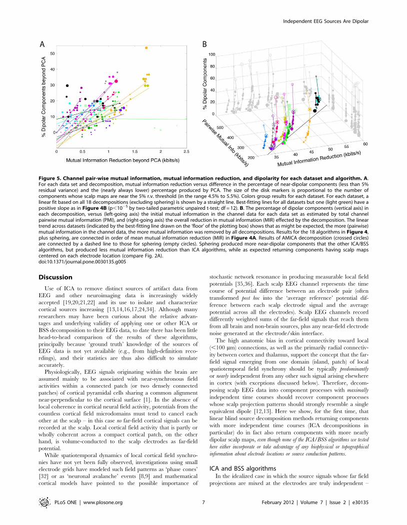
Figure 5. Channel pair-wise mutual information, mutual information reduction, and dipolarity for each dataset and algorithm. A.For each data set and decomposition, mutual information reduction versus difference in the percentage of near-dipolar components (less than 5%residual variance) and the (nearly always lower) percentage produced by PCA. The size of the disk markers is proportional to the number ofcomponents whose scalp maps are near the 5% r.v. threshold (in the range 4.5% to 5.5%). Colors group results for each dataset. For each dataset, alinear fit based on all 18 decompositions (excluding sphering) is shown by a straight line. Best-fitting lines for all datasets but one (light green) have apositive slope as in Figure 4B (p,1025 by two-tailed parametric unpaired t-test; df = 12). B. The percentage of dipolar components (vertical axis) ineach decomposition, versus (left-going axis) the initial mutual information in the channel data for each data set as estimated by total channelpairwise mutual information (PMI), and (right-going axis) the overall reduction in mutual information (MIR) effected by the decomposition. The lineartrend across datasets (indicated by the best-fitting line drawn on the ‘floor’ of the plotting box) shows that as might be expected, the more (pairwise)mutual information in the channel data, the more mutual information was removed by all decompositions. Results for the 18 algorithms in Figure 4,plus sphering, are connected in order of mean mutual information reduction (MIR) in Figure 4A. Results of AMICA decomposition (crossed circles)are connected by a dashed line to those for sphering (empty circles). Sphering produced more near-dipolar components that the other ICA/BSSalgorithms, but produced less mutual information reduction than ICA algorithms, while as expected returning components having scalp mapscentered on each electrode location (compare Fig. 2A).doi:10.1371/journal.pone.0030135.g005

Independent EEG Sources Are Dipolar

PLoS ONE | www.plosone.org 7 February 2012 | Volume 7 | Issue 2 | e30135

e.g., in decompositions of synthetic model data of unlimited length

– many ICA algorithms may be expected to give equivalent results

[27]. The most commonly reported algorithms to date (e.g., In-

fomax ICA, SOBI, and FastICA) are all able to extract several

classes of non-brain artifacts [21]. Here, these algorithms extracted

similar sources in several recognized brain and non-brain source

categories (Figures 2, 3). Nevertheless, our results show that the

method used to separate ICA components does indeed affect the

degree of temporal independence of the obtained components, as

well as the number of such (near-dipolar) components that can be

plausibly interpreted as representing the projection of a single

cortical patch of near-synchronous field activity.

Figure 4 shows that 18 of the 22 decomposition approaches we

tested differed principally in only one dimension (not two) that

tightly linked their degree of mutual information reduction and

the number (or percentage) of their returned components with

near-dipolar scalp maps that could represent the projection of

locally synchronous field activity across a single cortical patch [11].

Our finding of a direct relationship between mutual informa-

tion reduction and decomposition dipolarity is quite compatible

with such a model of maximally independent EEG sources. The

strongly linearity of this relationship across the 18 decompositions

(from PCA to Infomax and AMICA) in Figures 4 and 5 seems

more difficult to predict. This result seems the more remarkable

since the spatial relationships of the electrodes to each other or to

the head were not entered into these algorithms but were, in effect,

learned by them from the higher-order statistics of the temporal

EEG dynamics.

We suggest that the linear relationship of mutual information

reduction and dipolarity may only be explained by a direct

physiological connection between the nature of source processes

themselves and single equivalent dipole scalp projections. For the

many component processes that originate in cortex, this may

indeed reflect synchronous field activity across a cortical patch,

while many non-brain (‘artifact’) EEG component projections may

also resemble the projection of a single equivalent dipole within

or at the surface of the head (e.g., scalp muscle activities, ocular

artifacts, single-channel noise, electrocardiographic artifact). Dis-

tinguishing between near-dipolar brain and non-brain sources is

typically straightforward based on their time courses, spectra, and

the position of their equivalent dipole.

Infomax ICA and AMICAInterestingly, the five most efficient algorithms in our compar-

ison all use natural gradient descent on approximations of the

instantaneous data likelihood. Thus, it appears that this approach

may indeed be optimal for efficient separation of component

source processes from high-density EEG data [37]. The superior

performance of the AMICA algorithm on these data may be

explained by the fact that, in contrast to other infomax-related

algorithms, AMICA attempts to model and use, for further re-

finement, each component’s time course probability density

function (PDF) as well as its spatial projection. By modeling the

PDF of each component flexibly as a sum of extended Gaussians,

AMICA may obtain better component separation than algorithms

that assume one (or one of two) fixed parametric templates for

each component PDF, as do standard or Extended Infomax [33].

When enough data are available, AMICA decomposition also

scales well to high dimensions (e.g., to as many as 360 channels in

our experience).

Delay-dependent decompositionsDelay-dependent BSS algorithms SOBI, SOBIRO, SONS,

AMUSE, icaMS, FOBI, EVD, and EVD-24 performed less well

here, both in terms of mutual information reduction and dipolarity.

Most of these algorithms rely on joint minimization of second-order

correlations at multiple lags. Users of these algorithms may point out

that their goal is not temporal independence per se, and thus the

components these algorithms return may have other features of

interest relevant to their individual objectives. Nevertheless, the

components returned by the most tested of these algorithms, SOBI,

tended to resemble components returned by instantaneous ICA

(Figures 1 and 2).

Second-order decompositionsThe failure of PCA to return more than a very few near-dipolar

components was not unexpected. The objective of Principal

Component Analysis (PCA) is to lump together as much variance

as possible into each successive principal component, whose scalp

maps must then be orthogonal to all the others and therefore are not

free to model a scalp source projection resembling a single dipole.

The necessary orthogonality of principal component scalp maps

guarantees that higher-order component scalp maps resemble

checkerboards of various densities, while lowest-order principal

components may be dominated by single large artifacts (e.g., eye

blink artifacts) [38]. PCA components may thus be said to ‘lump’

together activity from many physiologically distinct, near-indepen-

dent EEG sources so as to each contribute as much distinct variance

to the data as possible. ICA algorithms, by contrast, attempt to

‘split’ the raw data into maximally independent processes that each

contribute as much distinct information to the mixed scalp channel

signals as possible.

Sphering components, in particular, most often have stereo-

typed scalp maps consisting of a focal projection peaking at each

respective data channel and thus resembling the projection of

a radial equivalent dipole located beneath the central scalp

channel (see Methods). This could possibly represent physiolog-

ically plausible projections of cortical EEG sources only if the

cortex were smooth and unfolded, whereas the largest portion

of the human cortex lies in its many sulci. Therefore, ICA de-

composition approaches (including AMICA and infomax) that

typically begin by sphering the data must progressively reduce the

number of quasi-dipolar component maps they return (as may be

seen in Figure 3), as the components adapt to the actual spatial

projections of the actual still-more independent brain and non-

brain sources in the data and as mutual independence among

their time courses increases. Principal components themselves, as

discussed above, are constrained to have orthogonal scalp maps

and hence in general cannot be expected to resemble the output of

a single cortical area. Yet in our assay PCA participated in the

same linear trade-off between independence and near-dipolarity as

17 other BSS and ICA algorithms (Figure 4A), likely in part

because the few largest components returned by all algorithms

accounted for eye activity artifacts, whose projections to the scalp

are approximately dipolar.

Caveats and further comparisonsOur measure of overall decomposition ‘dipolarity,’ while clearly

useful and informative (Figure 4), is also rather crude for at least

two reasons. First, here we used only a spherical head model and

common electrode coordinates to estimate best-fitting equivalent

dipole models for the component maps and to estimate their

residual variance from the actual component scalp maps. Better

dipole fitting results should be obtained using boundary element

method (BEM) or other anatomically more exact head models and

more precisely co-registered electrode locations. More advanced

(and complex) inverse approaches might estimate the location of

the cortical source patches directly by building participant-specific

Independent EEG Sources Are Dipolar

PLoS ONE | www.plosone.org 8 February 2012 | Volume 7 | Issue 2 | e30135

electrical forward head models from participant magnetic re-

sonance (MR) head images, which were not available for our

participants [39]. Second, a more sensitive measure of physiolog-

ical plausibility might explicitly model scalp muscles, ocular

artifacts, and electrocardiographic artifact more precisely, and

should allow for the possibility that a few independent sources are

generated by synchronized activity from two strongly coupled

cortical patches (or the two eyeballs). We do not see how our result

should be expected to be compromised by such methodological

improvements, though it does seem possible that the dipolarity

threshold yielding the strongest linear relationship to MIR (6%

residual variance, see Figure 4B and C insets) might be lower if

more accurately individualized forward head models were used to

compute it [39].

There might be multiple reasons for the inefficient results of the

three ICA/BSS algorithms we did not include in Figures 4B and

4C since they returned decompositions with less total mutual

information reduction than second-order sphering. These include

possible mismatches between our data and the default algorithm

parameters we used. In particular, these parameters may have been

optimized by their authors for decomposition of a few channels of

idealized data rather than for realistic high-dimensional data. For

this reason and for possible other future interest, we are making

available (at http://sccn.ucsd.edu/eeglab/BSSComparison/) both

the anonymized EEG datasets and the custom MATLAB (The

Mathworks, Inc.) scripts we used to obtain the results in Figure 4B,

with a hope that others may wish to run comparisons of optimized

versions of these or other ICA/BSS algorithms to compare against

the results presented here. Others may wish to propose figures of

merit other than independence and dipolarity that bring out

different types of utility for, e.g., decomposition methods that take

into account dependence over time.

Dependence remaining between maximally independentcomponents

ICA decomposition has proven to be a highly useful approach

for EEG data analysis, and our results here, as well as relevant

reports on invasively acquired data [40], suggest that it may have

substantial biological support. However, modeling cortical source

activities as arising from exact synchrony across a cortical patch or

phase-cone (as underlies decompositions such as AMICA) may

have only first-order physiological model validity. Frequency-

domain complex ICA decomposition methods may be able to

more accurately model stereotyped radially expanding or

contracting islands of synchronous activity (e.g., ‘phase cones’ or

‘avalanches’) associated with rhythmic EEG source activities, even

when these have relatively small time-varying effects on the

component process scalp projections [31,41].

Our results show that other portions of the remaining mutual

information between ICA components might reflect the still

imperfect decomposition performance of even the best current

ICA methods. Step-like changes in spatial source structure and/or

transient or sustained periods of spatiotemporal dependence within

one or more component subspaces are other possible sources

of residual dependence. Spatiotemporal non-stationarities may

include source processes that appear to travel long distances across

cortex, such as sleep slow waves [42], K-complexes, and spindles

[43] and some forms of epileptic seizures [40]. Still other changes in

spatial source structure may accompany changes in subject

cognitive state, task, or engagement. Thus, ICA methods that allow

for modeling of spatial non-stationarity of the source configuration

[31,44], and/or more general convolutive process demixing [45],

are of interest and might be tested in a manner resembling the

present investigation. Although the PMI measure used here does

not allow inference of causal relationships between component

processes that exhibit residual dependence, methods based on

Granger causality and transfer entropy might be used to examine

this [46].

Comparison to source isolation by response averagingThe ICA approach to EEG source identification contrasts

with the long (and still) predominant approach of attempting

to identify (only) those EEG sources active during peaks in

averaged evoked potential epochs following abrupt onsets of

experimentally presented sensory signals, on the assumption that

these scalp maps sum the projection(s) of one or at most very few

cortical source areas. Unfortunately, effects of sensory signals

on the statistics of cortical field activities spread quite rapidly,

concurrent with neural cross-talk and feedback between early

sensory areas beginning about 30 ms [4,47]. This makes it less

likely that later peaks in average evoked potential waveforms

represent the projection of activity from a single cortical source

area, making spatial source filtering by response averaging and

then ‘peak picking’ a relatively inefficient approach to isolating

and locating individual EEG source signals.

Reduction of the EEG data by response averaging has the

additional liability of discarding the large majority of the data, thus

not allowing identification of the sources of the great majority of

ongoing EEG activity that is not captured in ERP averages. The

ICA approach by contrast, when favorably applied to suitable and

sufficient data, allows identification of up to dozens of individual

cortical source projections, both their maps and activity time

courses, and their individual contributions to the ongoing (or trial

averaged) data, making available a wider range of source and

network level analyses while avoiding severe confounds produced

by the unavoidable summation of their signals being broadly

volume conducted from each brain and non-brain source to most

of the scalp electrodes.

ConclusionOur results confirm that ICA and other BSS algorithms

are capable of separating high-density EEG data into as many

as dozens of processes with maximally independent time courses

and near-dipolar scalp projections. Each unmixed maximally

independent component process can be said to be a concurrently

active source of information contributing to the data. Component

processes with near-dipolar scalp projections may also represent

physiologically distinct brain sources when and if they can be

associated with field activity partially or fully synchronized across a

cortical patch (or possibly across and between two anatomically

well-connected patches). The tight connection between temporal

independence and dipolarity demonstrated by our results is

compatible with the hypothesis that cortical contributions to scalp

EEG in large part sum far-field potentials from emergent islands or

patches of near-synchronous cortical field activity. The activities of

other (and sometimes many) maximally independent component

processes are clearly generated, at least in large part, by non-brain

sources typically identifiable as arising predominantly from

eye blinks or saccades, scalp or neck muscle electromyographic

activity, electrocardiographic contamination, line noise, single

electrode noise, etc.

ICA decomposition transforms the problem of EEG analysis

from analysis of the locally highly-correlated source signal mixtures

recorded at the two-dimensional scalp surface to analysis of the time

courses and spatial 3-D source distributions of maximally

temporally independent data sources whose separate patterns of

projection via volume conduction to the scalp sensors are given

by the decomposition. More importantly for neuroscience, the

Independent EEG Sources Are Dipolar

PLoS ONE | www.plosone.org 9 February 2012 | Volume 7 | Issue 2 | e30135

enhanced signal-to-noise ratio of the unmixed independent source

time courses of both brain and non-brain component processes

allow study of relationships between multiple EEG source processes,

behavior, and subject experience through a collection of single trials

and/or in the continuous data record. Further, the separated

component scalp maps greatly simplify the process of identifying

the cortical patch (or non-brain source) involved in generating

each identified source activity using a suitable biophysical inverse

method.

Here we have shown, first, that although some ICA and BSS

algorithms return larger numbers of EEG components with more

nearly dipolar scalp maps than others, they appear to identify

similar, biologically plausible brain and non-brain component

processes. Further, we have shown that for many ICA and BSS

algorithms applied to our data, their degree of efficiency in re-

ducing mutual information among the resulting component time

courses is positively correlated with the number of biologically

plausible near-dipolar components they return. Moreover, for 18

such algorithms (including algorithms as diverse as PCA, SOBI,

FastICA, JADE, infomax ICA, and AMICA), this relationship

appears to be, on average, linear, a result that invites deeper study

since the methods used by these algorithms appear on the surface

diverse and dipolarity and MIR would seem to have no inherently

simple numerical relationship.

To invite comparisons of the methods tested with other linear

decomposition techniques, we are making the anonymized EEG

data and custom MATLAB analysis and plotting scripts available

for this purpose (see Methods). We hope these results may serve

to increase the acceptance of the utility of ICA methods for (a)

separating the statistical question of what EEG source activity time

courses compose the data record from the biophysical inverse

problem of finding where these source activities take place, and (b)

separating the spatial source projection pattern for each identified

source signal, thus simplifying the biophysical inverse problem for

sources in the whole data, rather than only in limited response

averages drawn from it. We hope that extracting source-level in-

formation from high-density EEG data by ICA decomposition

brings closer the goal of developing high-density EEG imaging

into a true functional 3-D cortical imaging modality, with high

temporal resolution and spatial resolution adequate for studying

distributed macroscopic cortical brain processes supporting both

normal and abnormal behavior and experience.

Methods

Ethics StatementHuman subject data presented in this article have been acquired

under an experimental protocol approved by an Institutional

Review Board of University of California San Diego. Written con-

sent was obtained from each subject.

Participant taskFourteen volunteer participants performed a visual working

memory task [25]. At the beginning of each trial a central fixation

symbol was presented for 5 sec. A series of eight single letters, 3–7

of which were black (to be memorized) and the rest green (to

be ignored), were then presented for 1.2 s with 200-ms gaps. Foll-

owing these, a dash appeared on the screen for 2–4 s to signal a

memory maintenance period during which the participant was to

retain the sequence of memorized letters until a (red) probe letter

was presented. The participant then had to press one of two

buttons with their dominant hand (index finger or thumb) to

indicate whether or not the probe letter was part of the memorized

letter set. Auditory feedback 400 ms after the button press

informed the participant whether their answer was correct or

not. The next trial began when the participant pressed another

button. Each participant performed 100–150 task trials - see

Onton et al. [25] for additional details and event-related analyses.

We did not consider event-related analysis of the data in the

present study.

EEG dataEEG data were collected from 71 channels (69 scalp and 2

periocular electrodes, all referred to right mastoid) at a sampling

rate of 250 Hz with an analog pass band of 0.01 to 100 Hz (SA

Instrumentation, San Diego). Input impedances were brought

under 5 kV by careful scalp preparation. We initially selected data

from 14 out of 23 participants based on the perceived quality of

the original ICA decompositions under visual inspection (7 males,

7 females, mean age 2566.5 years). Of these, we informally judged

seven to give ‘better’ extended infomax ICA decompositions

(defined by a relatively large number of component scalp maps

that resembled the projection of a single dipole), and seven to

give ‘poorer’ ICA decompositions (with fewer such component

maps). For one of the participants with an unusually ‘poor’ ICA

decomposition, for unknown reasons all ICA/BSS algorithms

failed to substantially reduce mutual information from the level

of the raw scalp channels. Results for this data set were also

unreliable across algorithms, so data from this participant were

excluded, leaving data sets from 13 participants to be used in the

comparisons.

Data analysisData were analyzed by custom MATLAB scripts built on the

open source EEGLAB toolbox [48]. Continuous data were first

high-pass filtered above 0.5 Hz using a FIR filter. Data epochs

were then selected from 700 ms before to 700 ms after each letter

presentation. The mean channel values were removed from each

epoch, and between 1 and 16 noisy data epochs were removed by

visual inspection before ICA decomposition. Criteria for epoch

removal were the presence of high-amplitude, high-frequency

abnormalities (such as those accompanying occasional coughs,

sneezes, jaw clenching, etc.). The total number of data samples in

each dataset was between 296,000 and 315,000.

Algorithm selectionWe tested a total of 22 linear decomposition algorithms, 20 ICA

or BSS algorithms plus principal component analysis (PCA) and

PCA-related data whitening or sphering. MATLAB code for the

ICA algorithms we used can be downloaded from the Internet (see

Table 1). The selected algorithms all perform complete decom-

positions in which the number of returned components is equal to

the number of channels:

WA~S ð1Þ

where A is the data matrix of size (number of channels by number of time

points), W is an unmixing matrix of size (number of ICA components by

number of channels), and S is the ICA component activation time

courses of size (number of ICA components by number of time points).

Natural gradient approachICA and BSS algorithms learn the unmixing weight matrix that

makes the resulting component time courses or activations as

temporally independent from each other as possible. However, the

approach of each algorithm to estimating and/or approaching this

independence is different. AMICA [33], Extended Infomax [27],

Independent EEG Sources Are Dipolar

PLoS ONE | www.plosone.org 10 February 2012 | Volume 7 | Issue 2 | e30135

Infomax [28], Pearson ICA [49], and ERICA [50] belong to the

class of natural gradient ICA algorithms [37], differing only in the

way they estimate the component probability distributions. These

algorithms are highlighted in yellow in Figure 4.

Second-order time-delay approachSOBI [30] is a second-order BSS method that attempts to sim-

ultaneously reduce a large number of time-delay correlations (by

default, 100) between the source activities. SOBIRO (a variant of

SOBI using a robust orthogonalization method), SONS, AMUSE,

icaMS, FOBI, EVD, and EVD 24 all use time-delay covariance

matrices [51]. For all these algorithms, we selected the default time

delays as implemented in the downloaded software implementa-

tions. These algorithms are highlighted in blue in Figure 4.

Other methodsOther algorithms including (so-called) FastICA maximize the

negentropy of their component distributions or their fourth-order

cumulants (e.g., JADE; JADE optimized) [29,52]. Extensive

documentation of these algorithms is available (e.g., [28,29,51]).

We used the software default parameters; it is possible that better

ICA decompositions might have been obtained in some cases

using other parameter choices. These algorithms are highlighted in

pink in Figure 4.

Principal Component Analysis (PCA)ICA and BSS algorithms differ from principal component

analysis (PCA) in that they identify sources of distinct information in

the data instead of, like PCA, characterizing orthogonal directions

of maximal variance in the data. Thereby ICA can bypass PCA’s

spatial orthogonality constraint that invariably gives a complex

checkerboard appearance to scalp topographies of high-order

PCA components [38]. We included PCA in our assay because

it has been used to decompose EEG and ERP data [53], and

because of its relation to sphering, which is often used to pre-

process data before applying ICA decomposition. PCA is high-

lighted in green in Figure 4.

SpheringSphering decorrelates the component pair time courses while

leaving each component scalp map centered on an original scalp

channel. It is equivalent to rotating the data into their principal

component basis, equating data variance along all principal axes

(thus ‘whitening’ the data), and then rotating the data back to their

original channel basis [28]. Any rotation of the whitened data by a

rotation matrix R will retain unit variance in all directions.

Choosing R~U , we get V~UD{1=2UT . Since U is orthonor-

mal, we have U{1~UT . Thus transforming by U reverses or

undoes the initial rotation UT in which the data were projected

onto the eigenvectors. The whitened data (VX ) transformed by

V~UD{1=2UT then are not the same as the original data; in

particular, the data now have unit variance in all directions. Since

sphering is a linear spatial transform of the data, the columns of

the inverse sphering ‘mixing’ matrix (V -1) contain the sphering

component topographies (see examples in Figure 1, bottom row).

Note that these are centered on successive single channels in the

submitted channel list.

Measuring entropy and mutual informationIndependence of a set of random variables can be measured by

the mutual information. Mutual information is defined in terms

of the entropy (a measure of the degree of randomness or un-

predictability) of the data, which for a continuous random vector

x, is called the differential entropy, and is defined by

h(x)~E {log p(x)f g ð2Þ

where p(x) is the probability density function of the random vector

x.

The mutual information between two random variables X and Ycan be defined as the difference between the sum of the individual

(marginal) entropies of X and Y , and the joint entropy of X and

Y , h(X ,Y )

I(X ; Y )~h(X )zh(Y ){h(X ,Y ) ð3Þ

Similarly the mutual information in, or among, the components of

a random vector y~½y1; :::; yn� is defined by

I(y1; :::; yn)~h(y1)z:::zh(yn){h(y) ð4Þ

The mutual information is always non-negative since the joint

entropy of a random vector is always less than or equal to the sum of

the marginal entropies, with equality only if the components of

the random vector are independent. Larger mutual information

indicates that the entropy or ‘‘uncertainty’’ in the joint distribution

of y~½y1; :::; yn� is significantly lower than the entropy in the

factorial distribution (the product of the marginals that would result

if the random variables were independent). That is, there is some

dependence in the component time courses that makes the value of

the vector y less uncertain when considered as a multi-dimensional

whole than when each of its components are considered separately

(e.g., ignoring any dependence-derived information in the multi-

dimensional distribution about which combinations of component

values are more or less likely than the individual component values

would in themselves dictate).

Mutual information and linear transformsFor ICA analysis, the observed EEG data are modeled as an

independent and identically distributed (i.i.d.) realization of a

vector time series x(t), the observed linear mixture of a set of nsources si(t) activating the corresponding component projection

topographies ai, i~1, :::, n, so that

x(t)~As(t), t~1, :::, N ð5Þ

ICA decomposition attempts to estimate the sources by learning

the un-mixing matrix W~A{1 such that

y(t)~Wx(t), t~1, :::, N ð6Þ

where y(t) is equivalent to s(t) except for permutation and scaling

of the components – operations that do not change the degree of

dependence or mutual information among the components. The

strategy used by many ICA algorithms involves estimating W so

as to minimize the mutual information I(y) of the resulting

component signals. The actual cost function employed depends on

how the component joint density function is approximated.

In cumulant ICA methods, the source densities are expanded

in terms of cumulants (e.g., mean, variance, kurtosis) that are

estimated empirically from the partially unmixed data as the un-

mixing matrix is optimized [54,55]. The source densities are

generally taken to be members of a parametric family of dis-

tributions (or a quasi-parametric family in the case of mixture

Independent EEG Sources Are Dipolar

PLoS ONE | www.plosone.org 11 February 2012 | Volume 7 | Issue 2 | e30135

models), and the density parameters are optimized along with the

un-mixing matrix to maximize the likelihood [33]. In the quasi-

parametric case, with the optimization being viewed as over all

possible source densities, this amounts to minimization of the

mutual information itself.

Component Mutual InformationFor the linear transformation y~Wx, the entropy of the con-

tinuous vector variable y is given by

h(y)~log det Wj jzh(x) ð7Þ

By (3), the mutual information of the transformed data, I(y), is

then

I(y)~h(y1)z:::zh(yn){log det Wj j{h(x) ð8Þ

Since h(x), the joint entropy of the data, x, is independent of W ,

the minimization of the mutual information over W (and possibly

over parameters of the source density models q(yi), i~1, :::, nessentially consists of minimizing the sum of the marginal en-

tropies, yi, minus a term involving the determinant of W . Thus

ICA algorithms following this approach must model only one-

dimensional densities, either parametrically from the data [33] or

using cumulant expressions [28,29]. Most of the algorithms we use

here also apply sphering (or some more general whitening

procedure) as a pre-processing step to remove second-order de-

pendency (correlations) between the (sphered) channel signals.

Details on the entropy calculations are provided in the following

section.

Pairwise Mutual Information (PMI)The pairwise mutual information matrix M for the set of time

series xi(t), i~1, :::, n, considered as N samples of the random

variables xi, i~1, :::, n, is defined by

½M�ij~I(xi; xj)~h(xi)zh(xj){h(xi, xj) ð9Þ

We estimate the entropy using the usual binning method, where

histograms and a simple Riemann approximation to the integrals

are used to compute the entropies. This approach is generally

suitable for large sample sizes like those encountered in EEG.

Approximate asymptotic variance of the estimate is also available

in terms of number of bins and number of samples, allowing us to

assess the statistical significance of the results.

We choose a fixed number of bins, B, for all univariate random

variables, and construct the 2-D histograms using B2 bins, using

the same marginal bin endpoints as used for the one-dimensional

histograms. Specifically, let the one-dimensional histogram of data

xi be denoted bi(k), k~1, :::, B, where bi(k) is the number of

time points t for which the value of xi(t) is in the kth bin. The

estimate of the continuous one-dimensional density p(xi) is taken

to be bi(k)=(NDk) over the kth bin, where Dk is the size of the kth

bin, and N is the total number of time points. This makes the

continuous density integrate to one in the Riemann approxima-

tion,

Xk

p(x)Dk~X

k(bi(k)=(NDk))Dk~1 ð10Þ

Since we use B bins distributed over the maximum and minimum

values of the time series, the bin size Dk is 1=B for all k. The

estimate of the one-dimensional marginal entropy is then given by,

Xk{p(x)log p(x)Dk~{

Xk

(bi(k)=(NDk)) log

bi(k)=ð (NDk)ÞDk~Hi{log B ð11Þ

where Hi is the discrete entropy of the B-dimensional discrete

probability distribution defined by bi(k)=N, k~1, :::, B.

The two dimensional joint entropy is estimated similarly, with

the joint density of xi and xj taken to have the constant value

bij(k,l)=(NDkDl) over the (k,l) bin, where bij(k,l) is the number of

time points for which xi(t) is in the kth bin and xj(t) is in the lth

bin. The estimate of the joint entropy is then,

Xk

Xl{p(xi,xj) log p(xi,xj)DkDl~

-X

k

Xl

bij(k,l)=N� �

log bij(k,l)=N� �

{2 log Bð12Þ

We define the discrete joint ‘‘bin entropy’’ as,

Hij~{X

k

Xl(bij(k,l)=N) log(bij(k,l)=N)

Now, for the estimate of the mutual information between xi and xj,

we have,

Mij~(Hi{log B)z(Hj{log B){(Hij{2 log B)~HizHj{Hijð14Þ

Thus the estimate of the mutual information does not depend on

the bin size, only on the bin entropies. This result does not depend

on the fact that equal bin sizes were used. Even with arbitrary bin

sizes, the bin size terms cancel. Note that total PMI (the sum of

PMI for all xi,xj pairs) may be larger than MI when higher-order

dependencies are present in the data.

The approximate entropy estimator bias is given by

(B{1)=(2N) ð15Þ

where B is the number of bins and N is the number of samples

[56]. If we define pi,k~bi(k)=N , and Hi0~P

k {pi,k log pi,k,

then the approximate variance of the bias corrected entropy

estimate for source i is

Xk{pi,k (log pi,k)2

h i{H2

i0

� �=N ð16Þ

Since the PMI and MIR estimates are expressed in terms of sums

of entropies, their variances can be calculated by summing the

appropriate entropy variances. Note that mutual information

estimates were bias corrected. Error bars are not shown in any of

the figures because they were not visible at the scale of the plots. A

caveat to the validity of the estimates is that they assume

stationarity of data, which does not necessarily hold in the case

of EEG data. However the measures can still be used to assess

relative performance of unmixing matrices, as well as to assess the

co-variation of dipolarity and other measures with mutual

information reduction (MIR).

Mutual Information Reduction (MIR)The reduction in mutual information achieved by a potential

ICA matrix W can be calculated using only one-dimensional

density models. Specifically, the mutual information reduction (MIR),

Independent EEG Sources Are Dipolar

PLoS ONE | www.plosone.org 12 February 2012 | Volume 7 | Issue 2 | e30135

i.e. the amount of mutual information removed from set of

channels, is given by,

MIR~I(x){I(y)~½h(x1)z:::zh(xn)�{½h(y1)z:::zh(yn)�{

h(x)zlog det Wj jzh(x)

~log det Wj jz½h(x1)z:::zh(xn)�{½h(y1)z:::zh(yn)�

ð17Þ

The MIR thus depends only on the difference between the sums

of the marginal entropies of x and y and on the (log) determinant

of W . The marginal entropies involved are readily estimated

using histograms of the channel and estimated source data (as in

the preceding section on direct estimation of pairwise mutual

information). ICA attempts to minimize mutual information in the

estimated sources, I(y), and thus to maximize MIR. Thus, MIR

for an ICA algorithm is expected to be positive for a given dataset,

and algorithms reducing the mutual information more, thereby

producing more independent sources, will have higher MIR.

Equivalent dipole modelingAfter computing all 22 decompositions for each of the 13 EEG

datasets, we localized a best-fitting single equivalent dipole cor-

responding to each returned component using a single equivalent

dipole in a best-fitting spherical four-shell model head (radius: 71,

72, 79, 85 mm; shell conductances: 0.33, 0.0042, 1, 0.33 mS) using

the DIPFIT plug-in (version 1.02) in the EEGLAB toolbox (version

4.515) [48]. To avoid errors based on the simplistic head model we

used in the computations, scalp map values for two electrodes sited

near the eyes were excluded from dipole fitting. Note that modeling

each component map with a single dipole is somewhat idealistic,

since in particular some ICA components represent apparently

bilateral synchronous source activities (e.g., the component maps in

the third column of Figure 1). However, brain components clearly

warranting a dual-dipole model appeared to be rare (approximately

one per decomposition), as we typically find in other decompositions

of more than 32 data channels. Components accounting for most

electro-oculographic (EOG) artifacts should also be modeled using

two (peri-ocular) dipoles, but as the eyes are relatively close together

and accurate forward modeling the front of the skull is difficult, the

additional errors introduced by using single dipole models for EOG

components is not large.

Data and methods availableThe 13 anonymized data sets used in the analysis are available for

download (http://sccn.ucsd.edu/wiki/BSSComparison) together

with a ‘README’ file and MATLAB scripts using EEGLAB

functions (http://sccn.ucsd.edu/eeglab) that perform the algorithm

comparisons including computation of mutual information reduc-

tion (MIR) and dipolarity (dipole fitting). Plotting scripts are also

included for reconstructing Figure 4B and adding a new data point

for a new decomposition algorithm. Using these scripts and the

referenced EEGLAB functions (http://sccn.ucsd.edu/eeglab), in-

terested readers may compare MIR and dipolarity of any other

linear decompositions of these data, and may compare results of

an algorithm of their choice with our results as applied to the same

data sets. The authors invite readers to send us results of these

comparisons for inclusion on the web page above, following

instructions contained in the README file.

Acknowledgments

We wish to thank Anthony Bell, Tzyy-Ping Jung, Te-Won Lee, and

Terrence Sejnowski for their early and important collaborations with the

senior author to discover how to apply ICA to biological data. Thanks also

to Jean-Francois Cardoso for his JADE code (available, with many other

ICA algorithms at http://www.tsi.enst.fr/icacentral/algos.html), to An-

drejz Chichocki for allowing us to use the source code for the several

ICALAB (http://www.bsp.brain.riken.jp/ICALAB/) algorithms, and to

Zeynep Akalin Acar for clarifications on dipole fitting.

Author Contributions

Conceived and designed the experiments: AD JP SM. Performed the

experiments: AD JP. Analyzed the data: AD. Contributed reagents/

materials/analysis tools: JO RO. Wrote the paper: AD JP SM.

References

1. Nunez P (1974) The brain wave equation: a model for the EEG. Mathematical

Biosciences 21: 279–297.

2. Varela F, Lachaux J, Rodriguez E, Martinerie J (2001) The brainweb: phase

synchronization and large-scale integration. Nat Rev Neurosci 2: 229–239.

3. Stepanyants A, Martinez LM, Ferecsko AS, Kisvarday ZF (2009) The fractions

of short- and long-range connections in the visual cortex. Proc Natl Acad

Sci U S A 106: 3555–3560.

4. Stettler DD, Das A, Bennett J, Gilbert CD (2002) Lateral connectivity and

contextual interactions in macaque primary visual cortex. Neuron 36: 739–750.

5. Sarnthein J, Morel A, von Stein A, Jeanmonod D (2005) Thalamocortical theta

coherence in neurological patients at rest and during a working memory task.

Int J Psychophysiol 57: 87–96.

6. Dehghani N, Cash SS, Rossetti AO, Chen CC, Halgren E (2011) Magneto-

encephalography demonstrates multiple asynchronous generators during human

sleep spindles. J Neurophysiol 104: 179–188.

7. Freeman WJ (1975) Mass Action in the Nervous System. New York: Academic

Press.

8. Beggs JM, Plenz D (2003) Neuronal avalanches in neocortical circuits. J Neurosci

23: 11167–11177.

9. Gireesh ED, Plenz D (2008) Neuronal avalanches organize as nested theta- and

beta/gamma-oscillations during development of cortical layer 2/3. Proc Natl

Acad Sci U S A 105: 7576–7581.

10. Benayoun M, Cowan JD, van Drongelen W, Wallace E (2010) Avalanches in a

stochastic model of spiking neurons. PLoS Comput Biol 6: e1000846.

11. Scherg M, Berg P (1991) Use of prior knowledge in brain electromagnetic source

analysis. Brain Topogr 4: 143–150.

12. Akalin Acar Z, Makeig S (2011) Neuroelectromagnetic forward head modeling

toolbox. J of Neuroscience Methods; in press.

13. Makeig S, Debener S, Onton J, Delorme A (2004) Mining event-related brain

dynamics. Trends Cogn Sci 8: 204–210.

14. Delorme A, Westerfield M, Makeig S (2007) Medial prefrontal theta bursts

precede rapid motor responses during visual selective attention. Journal of

Neuroscience 27: 11949–11959.

15. Onton J, Makeig S (2009) High-frequency Broadband Modulations of

Electroencephalographic Spectra. Front Hum Neurosci 3: 61.

16. Crespo-Garcia M, Atienza M, Cantero JL (2008) Muscle artifact removal from

human sleep EEG by using independent component analysis. Ann Biomed Eng

36: 467–475.

17. Chen Y, Akutagawa M, Katayama M, Zhang Q, Kinouchi Y (2008) ICA based

multiple brain sources localization. Conf Proc IEEE Eng Med Biol Soc 2008:

1879–1882.

18. Makeig S, Bell AJ, Jung TP, Sejnowski TJ (1996) Independent component analysis

of electroencephalographic data. In: Touretzky D, Mozer M, Hasselmo M, eds.

Advances in Neural Information Processing Systems. pp 145–151.

19. Jung TP, Makeig S, Humphries C, Lee TW, McKeown MJ, et al. (2000)

Removing electroencephalographic artifacts by blind source separation.

Psychophysiology 37: 163–178.

20. Jung TP, Makeig S, Westerfield M, Townsend J, Courchesne E, et al. (2000)

Removal of eye activity artifacts from visual event-related potentials in normal

and clinical subjects. Clin Neurophysiol 111: 1745–1758.

21. Delorme A, Sejnowski T, Makeig S (2007) Enhanced detection of artifacts in

EEG data using higher-order statistics and independent component analysis.

Neuroimage 34: 1443–1449.

22. Hoffmann S, Falkenstein M (2008) The correction of eye blink artefacts in the

EEG: a comparison of two prominent methods. PLoS ONE 3.

23. Makeig S, Jung TP, Bell AJ, Ghahremani D, Sejnowski TJ (1997) Blind

separation of auditory event-related brain responses into independent compo-

nents. Proc Natl Acad Sci U S A 94: 10979–10984.

24. Makeig S, Westerfield M, Jung TP, Enghoff S, Townsend J, et al. (2002)

Dynamic brain sources of visual evoked responses. Science 295: 690–694.

Independent EEG Sources Are Dipolar

PLoS ONE | www.plosone.org 13 February 2012 | Volume 7 | Issue 2 | e30135

25. Onton J, Delorme A, Makeig S (2005) Frontal midline EEG dynamics during

working memory. Neuroimage 27: 341–356.

26. Gomez-Herrero G, Atienza M, Egiazarian K, Cantero J (2008) Gomez-Herrero

G, Atienza M, Egiazarian K, Cantero JL. Neuroimage 43(3): 497–508.

27. Lee TW, Girolami M, Bell AJ, Sejnowski TJ (2000) A Unifying Information-

theoretic Framework for Independent Component Analysis. Comput Math Appl

31: 1–21.

28. Bell AJ, Sejnowski TJ (1995) An information-maximization approach to blind

separation and blind deconvolution. Neural Comput 7: 1129–1159.

29. Hyvarinen A, Oja E (2000) Independent component analysis: algorithms and

applications. Neural Netw 13: 411–430.

30. Belouchrani A, Cichocki A (2000) Robust whitening procedure in blind source

separation context. Electronics Letters 36: 2050–2053.

31. Palmer JA, Makeig S, Kreutz-Delgado K, Rao B (2008) Newton Method for the

ICA Mixture Model, in Proceedings of the 33rd IEEE International Conference

on Acoustics and Signal Processing (ICASSP 2008). Las Vegas, NV, pp. 1805–

1808, March 31 2008–April 4 2008.

32. Freeman WJ, Barrie JM (2000) Analysis of spatial patterns of phase in

neocortical gamma EEGs in rabbit. J Neurophysiol 84: 1266–1278.

33. Palmer JA, Kreutz-Delgado K, Rao BD, Makeig S (2007) Modeling and

Estimation of Dependent Subspaces with Non-Radially Symmetric and Skewed

Densities. Proceedings of the 7th International Symposium on Independent

Component Analysis, Edited by Mike E. Davies, Christopher J. James, Samer A.

Abdallah and Mark D Plumbley, Lecture Notes in Computer Science, Springer.

34. Grau C, Fuentemilla L, Marco-Pallares J (2007) Functional neural dynamics

underlying auditory event-related N1 and N1 suppression response. Neuroimage

36: 522–531.

35. Kang K, Shelley M, Henrie JA, Shapley R (2011) LFP spectral peaks in V1

cortex: network resonance and cortico-cortical feedback. J Comput Neurosci 29:

495–507.

36. Robinson PA (2006) Patch propagators, brain dynamics, and the generation of

spatially structured gamma oscillation. Phys Rev E 73: 041904.

37. Amari S (1999) Natural gradient learning for over- and under-complete bases In

ICA. Neural Comput 11: 1875–1883.

38. Mocks J, Verleger R (1986) Principal component analysis of event- related

potentials: a note on misallocation of variance. Electroencephalogr Clin Neur-

ophysiol 65: 393–398.

39. Akalin Acar Z, Worrell G, Makeig S (2009) Patch basis electrocortical source

imaging in epilepsy. IEEE Engineer Med Biol Soc 2009: Minneapolis, Minnesota.

40. Akalin Acar Z, Palmer J, Worrell G, Makeig S (2011) Adaptive mixture independent

component analysis and source localization in epilepsy. IEEE EMBC;Boston MA.41. Anemuller J, Sejnowski TJ, Makeig S (2003) Complex independent component

analysis of frequency-domain electroencephalographic data. Neural Netw 16:

1311–1323.42. Massimini M, Huber R, Ferrarelli F, Hill S, Tononi G (2004) The sleep slow

oscillation as a traveling wave. J Neurosci 24: 6862–6870.43. Poe GR, Walsh CM, Bjorness TE (2010) Cognitive neuroscience of sleep. Prog

Brain Res 185: 1–19.

44. Lee TW, Girolami M, Sejnowski TJ (1999) Independent component analysisusing an extended infomax algorithm for mixed subgaussian and supergaussian

sources. Neural Comput 11: 417–441.45. Dyrholm M, Makeig S, Hansen LK (2007) Model selection for convolutive ICA

with an application to spatiotemporal analysis of EEG. Neural Comput 19:934–955.

46. Mullen T, Akalin Acar Z, Worrell G, Makeig S (2011) Modeling cortical source

dynamics and interactions during seizure. IEEE Engineering in Medicine andBiology Society. Boston MA.

47. Hupe JM, James AC, Girard P, Lomber SG, Payne BR, et al. (2001) Feedbackconnections act on the early part of the responses in monkey visual cortex.

J Neurophysiol 85: 134–145.

48. Delorme A, Makeig S (2004) EEGLAB: an open source toolbox for analysis ofsingle-trial EEG dynamics including independent component analysis. J Neurosci

Methods 134: 9–21.49. Karvanen J, Koivunen V (2002) Blind separation methods based on Pearson

system and its extensions. Signal Processing 82: 663–673.50. Cruces S, Castedo L, Cichocki A (2002) Robust blind source separation using

cumulants. Neurocomputing 49: 87–117.

51. Cichocki A, Amari S (2002) Adaptive Blind Signal Processing: Wiley.52. Cardoso JF (1999) Higer-order contrasts for independent component analysis.

Neural Comput 11: 157–192.53. Dien J, Khoe W, Mangun GR (2006) Evaluation of PCA and ICA of simulated

ERPs: Promax vs. infomax rotations. Hum Brain Mapp.

54. Comon P (1994) Independent Component Analysis: a new concept? SignalProcessing 36: 287–314.

55. Pham DT, Garat P (1997) Blind separation of mixture of independent sourcesthrough a Quasi-Maximum Likelihood approach. IEEE Trans Signal Processing

45: 1712–1725.56. Moddemeijer R (1989) On Estimation of Entropy and Mutual Information of

Continuous Distributions. Signal Processing 16: 233–248.

Independent EEG Sources Are Dipolar

PLoS ONE | www.plosone.org 14 February 2012 | Volume 7 | Issue 2 | e30135