Improving the Performance of the Instantaneous BlindAudio Source Separation Algorithms

Amr E. MahmoudFaculty of Engineering

Helwan UniversityHelwan, Egypt

amr@engr.uconn.edu

Reda A. AmmarCSE Dept.

University of ConnecticutStorrs, CT, USA

Reda@engr. uconn.edu

Mohamed I. EladawyFaculty of Engineering

Helwan UniversityHelwan, Egypt

mohamed@eladawy.com

Medhat HussienFaculty ofEngineering

Helwan UniversityHelwan, Egypt

awadalla_medhat@yahoo.co.uk

Abstract

Several algorithms for instantaneous BlindSource Separation (BSS) have been introduced in thepast years. The performance of these algorithmsneeds to be evaluated and assessed to study theirmerits and choose the best of them for a givenapplication. In this paper, a new adaptive approach ispresented to evaluate different blind sourceseparation algorithms. In this new approach, threenew evaluation metrics are added. The first metric isthe minimum number of samples required for asuccessful separation process. The second metric isthe time needed to complete the separation process.The third metric is the number of sources that theBSS algorithm can separate from their mixtures.

The new approach is used to compare threedifferent Blind Source Separation algorithms. Thesealgorithms are: kurtosis [1-3], Negentropy [4, 5], andthe Maximum Likelihood [6, 7]. Since the evaluationof a BSS technique is application-dependent, we areusing the same application (separation of audiosources) to evaluate each of these BSS algorithms.

The comparison, between the threealgorithms, shows that the Maximum Likelihood hasthe best performance and the kurtosis is the faster.This motivates us to develop a new hybrid approachthat combines the two algorithms to gain the benefitsfrom both algorithms. In this new algorithm we startwith the Maximum Likelihood (ML) algorithm tofmd the separation matrix and then tune this matrixby the kurtosis algorithm.

1. Introduction

Blind source separation (BSS) refers to the problemof recovering source signals from several observedmixtures. In many cases, a priori knowledge aboutthe characteristics of the source signals and the wayin which they are mixed together are eitherinaccessible (unknown) or very expensive to acquire.Consequently, the separation is carried out only onthe basis of the available mixtures with theassumption of mutual statistical independence amongsources' signals [8].

978-1-4244-5950-6/09/$26.00 ©2009 IEEE

The Blind Source Separation was initiallyproposed by Herault et ale [10, 11] to study somebiological phenomena [9, 12]. But the BSS has anumber of interesting applications not only onmedical signal processing, but also incommunications, and many other fields. In recentyears, this research area attracts large attention inaudio signal processing due to various applicationssuch as crosstalk removal in multi-microphonerecordings, speech enhancement, beam-forming,direction of arrival estimation, etc. A typicalapplication example is the so-called cocktail partyproblem in which individual speeches should beextracted from mixtures of several speakers recordedin a common acoustic environment [13].

In this paper, we address the blindseparation of audio sources by means of IndependentComponent Analysis (ICA) [13]. ICA is a popularmethod for BSS using the assumption that originalsources are mutually independent. In this technique, aset of original source signals are retrieved from theirmixtures. We applied three different ICA algorithms(Kurtosis, Negentropy, and Maximum likelihood) toseparate the original source from the mixtures. Then,the new evaluation approach was used to compare theperformance among these three ICA algorithms.

Section 2 gives the basic notations for mixing anddemixing of the BSS. Section 3 explains thefundamental concepts of the selected ICA algorithmsthat will be used in this paper. Section 4 discussesexisting performance evaluation metrics. Section 5describes the new evaluation algorithm. Section 6 isfor the comparing among the three algorithms usingthe new evaluation metrics. Section 7 shows theresults of the performance of the selected algorithms.Finally, section 8 gives the conclusion of the work inthis paper.

2. leA Model

The simplest case for ICA is the instantaneous linearnoiseless mixing model. In this case, the mixingprocess can be expressed as

519

The basic ICA problem, its extensions andapplications have been studied widely and manyalgorithms have been developed. Examples of thesealgorithms are the instantaneous BSS methods suchas kurtosis, Negentropy, and ML.

3.1. Nongaussianity Algorithms

Nongaussianity is of paramount importance in ICAestimation [16]. According to central limit theorem,sum of two independent random variables results inanother random variable that has distribution closerto the independent components. We can consider alinear combination of the x/s as follows:

3. leA Algorithms

There are two ideas commonly used for theIndependent Component Analysis (ICA). These arenongaussianity sources' signals and independentsources' signals. Based on these two ideas manyapproaches were introduced. Kurtosis andNegentropy approaches are based on thenongaussianity idea whereas the maximum likelihoodapproach is based on the idea that components areindependent.

(8)

The nongaussianity can be measured by the absolutevalue of Kurtosis [10-12]. Kurtosis can be estimatedby fourth order moment of the sample data. Thekurtosis of y, denoted by Kurt(y), for a zero meanvariable is defmed by

Absolute or mean values of kurtosis are zero for agaussian variable, and greater than zero for mostnongaussian random variables. to maximize theabsolute value of kurtosis, we would start from somevector w which is the optimized vector forreconstruction filter, compute the direction in whichthe absolute value of the kurtosis of y = wT Z isgrowing most strongly, based on the variable samplez, where z is the whitened data obtained from x, andthen move the vector w in that direction.

Thus denoting y = wT z, the gradient of theabsolute value of kurtosis of wT z can be simplycomputed as

olkurt(wTz) I = 4 sign (kurt(wTz))[E{z(wTz)2 - 3wllwll 2 (9)ow

For the whitened w, IIwll 2 =1, thus the numericaloptimization problem reduces to the following updateequation for kurtosis maximization

aw oc (kurt(wT z) )E{z(wTZ)3} (10)

w ~ w/llwll (11)

bT A would be actually equal to one of theindependent components. The question is now: howcould we use the central limit theorem to determine bso that it would be equal to one of the rows of theinverse ofA? In practice, we cannot determine such ab exactly, because we have no knowledge of thematrix A, but we can fmd an estimator that gives agood approximation [13].

Let us vary the coefficients in q, and seehow the distribution of y = qT S changes. Thefundamental idea here is that since a sum of twoindependent random variables is more Gaussian thanthe original variables. y is usually more Gaussianthan any of the Si and becomes least Gaussian when itin fact equals to one of s; In this case, obviously onlyone of the elements qj of q is nonzero. The Gaussianmeasure is based on two ideas: one is the kurtosis andthe other is the Negentropy.

3.1.1. Kurtosis

(2)

(1)X=AS

s=wx

where X is an d*N data matrix. The rows ofX are theobserved mixed signals, d is the number of mixedsignals and N is their length or the number of samplesin each signal. Similarly, the unknown matrix Sincludes samples of the original source signals. S is adxN matrix. A is an unknown regular d*d mixingmatrix. The mixing matrix is assumed to be square,for simplicity.

A basic assumption in ICA is that theelements ofS, denoted sij, are mutually Independentlyand Identically Distributed (lID) random variableswith probability density functions (pdt) p;{sij) i=I, ... ,d. The row variables sij for allj=I, ... , N, having thesame density, are thus an i.i.d. sample of one of theindependent sources denoted by s; The keyassumptions for the identifiability of the model(equation #1) are all but at most one of the densitiesPi are non-Gaussian, and the unknown matrix A hasfull rank. In the following, W denote the demixingmatrix, W= A-i. Then the estimated source signals Sare

(7)y = bT X =bT AS = qT S

where vector b has to be determined. If b were one ofthe rows of the inverse of A, this linear combination

3.1.2. Negentropy

Another measure for the nongaussianity is theNegentropy, which is based on the differential

978-1-4244-5950-6/09/$26.00 ©2009 IEEE 520

(13)

(14)

(15)

(16)

entropy [13, 14]. The differential entropy of arandom vector y with the density p(y) defmed as:

H(y) = - Jp(y)logp(y)dy (12)

Entropy is closely related to the code length of therandom vector. So the entropy values for thevariables with Gaussian distribution are maximum,while they are minimum for the nongaussianvariables. A normalized version of entropy is givenby Negentropy J, which is defmed as follows

JCy) = H(Ygaussian) - HCy)

Where Ygaussian is a Gaussian random vector of thesame covariance (or Correlation) matrix as y. TheNegentropy is always non-negative. It is zero only forthe Gaussian random vectors and positive fornongaussian variables. To maximize the value ofNegentropy, we will start from some vector w, whichis the optimized vector for reconstruction filter,compute the direction in which the value of theNegentropyof Y = wTz is growing most strongly,and fmally move the vector w in this growingdirection based on the variable sample z, where z isthe whitened data obtained from x.

The gradient of the value of Negentropy of w Tz canbe computed as

a}(w) a[E{G(wTz) - E{G(V)}]2w - -- - ---------- aw - aw

For the whitened w, llwll' =1, thus the numericaloptimization problem is reduced to the followingequation for Negentropy maximization

aw ~ E{zg(wTz)}

w s--w/llw]

The new w replaces the old value of wand theprocess is repeated until aw is very small (zero).

might know their pdfs and we know that these signalsare independent. Therefore, based on this knowledgewe can separate the source signals from theirmixtures.

4. Performance Evaluation Metrics

Due to wide variety of BSS algorithms and widevariety of the separation problem defmition, it hasbeen hard to evaluate an algorithm or to compareseveral algorithms because of the lack of appropriateperformance metrics and standard tests, even in thevery simple case of linear instantaneous mixtures.Some researchers introduced numerical performancecriteria that can help in evaluating and comparingalgorithms when applied to usual BSS problems. Anexample of these research results is the PerformanceMeasurement in Blind Audio Source Separation [15].This research introduces a performance criterion thatbased on the estimated source decomposition byorthogonal projection. When A is a time-invariantinstantaneous matrix and the mixture is separated byapplying a time-invariant instantaneous matrix W,Scan be decomposed as

m

Sj = (WA)jjSj + L(WA)jj'Sj' + L~ini (13)i'*i i=l

Since (WA)u is considered as time-invariantgain. Therefore, the equation can be seen as a sumthree terms Stragert , einterference , and enoise, respectively.There is another term which can be called the artifactof the algorithm, but it doesnot appear in the equation(eartif = 0 here). However, the above equation cannotbe used as a defmition of Stragert, einterference, enoise, andeartif, since the mixing and demixing systems areunknown. Also, the two first terms of the equationmay not be perceived as separate sound objects whenan unwanted source is highly correlated with thewanted source.

Let us denote II {yhY2, ••• ,Yk} theorthogonal projector onto the subspace spanned bythe vectors yl,y2, ... ,yk. The projector is a T*Tmatrix, where T is the length of these vectors. Weconsider the three orthogonal projectors

3.2. Maximum Likelihood Estimation

Maximum likelihood estimation (MLE) is a standardstatistical tool for finding parameter values (e.g., theunmixing matrix W) that provide the best fit of somedata (e.g., the extracted signals y) to a given model(e.g., the assumed joint pdfp(s) of source signals).

The ML includes a specification of a pdf,which is in this case the pdf p(s) of the unknownsource signals s. Using the ML ICA, the objective isto fmd an unmixing matrix that yields extractedsignals Y = WX with a joint pdf as similar as possibleto the original joint pdfp(s). It is worth to mentionthat although the source signals are not known, we

978-1-4244-5950-6/09/$26.00 ©2009 IEEE

PSj = n{Sj}

Ps = n{(Sj1)lSj1sn}

(14)

521

5. New Performance Metrics

The computation of einterference is a bit more complex.If the sources are mutually orthogonal, then

The computation of Stragert is straight forward since itinvolves only a simple inner product:

(21)

(22)SAR - 101 IIStarget + einterf + enoise 11

2

- 0910 2

Ileartifil

These four measures cover all types of distortionsthat can appear is the estimated sources. But thesemeasures are not sufficient. There are a number ofproblems that can affect the evaluation and may givea wrong result. These problems are:

1. The number of sources that is used in theevaluation technique. Since one BSS methodmay appear to be good over the othermethods at a specific number of sources, itis necessary to evaluate the target methodsfor different numbers of sources.

2. The number of samples per source. Sinceone BSS method may appear to be goodover the other methods at a specific numberof samples, it is necessary to evaluate thetarget methods for different numbers ofsources.

3. The time that the algorithm can take forseparating the given source signals. Since, insome applications, the little difference inSDR and other parameters can be neglectedwith respect to the time consume.

Due to the above concerns, we introduce additionalperformance metrics:

1- The effect of the number of sources.2- The effect of the number of samples per

signal.3- The ratio between the SDR and the

separation time.

the source-to-noise ratio (SNR)

SNR - 101 IIStarget + einterfl12

- 0910 II 2enoisell

the source-to-artifacts ratio(SAR)(15)

(16)

In summary research results in [15] can be used inevaluating the BSS performance. We will enhancethis approach and add three new metrics: the first isthe number of sources, the second is the number ofsamples in each mixture, and the last one is the timethat the algorithm takes to separate the sources.

to evaluate each of Stragerb einterference, enoise and asfollows:

Starget = PSjSj

einterf = PsSj - PSjSj

enoise = Ps,nSj - PsSj

eartif = s, - Ps,nSj

In this section, we propose new performance criteriathat can be used for all BSS methods. Currentnumerical performance criteria were introduced in[15]. These are:

einterf = I (Sj,Sj,)Sj,/IISj,1I2

(17)j'*j

The computation ofPs,n proceeds in a similarfashion; however, most of the time we can make theassumption that the noise signals are mutuallyorthogonal and orthogonal to each source, so that

the source-to-distortion ratio (SDR)

SDR = lOl091O IIStargetl12

Ileinterf + enoise + eartifl12

the source-to-interference ratio (SIR)

SIR - 101 II Stargetl12

- 0910 2

II einterf II

(19)

(20)

6. The Comparison Approach

In order to compare among instantaneous BSSMethods, a 15 speech signals will be used. Thesignals are 8-bit with 2.5sec, sampled at 8khz andnormalized. But the length of the data is changedmany times during the simulation to test thealgorithms for different data lengths.

The instantaneous mixing matrix is a squarefull rank random matrix. Different mixing matricesare generated. Then we apply all algorithms to eachmatrix. Finally we take the average of the results foreach algorithm for all mixing matrices.

978-1-4244-5950-6/09/$26.00 ©2009 IEEE 522

The BSS methods [Kurtosis, Negentropy, ML] andthe performance measure GUI-program areimplemented using MATLAB 2006. The simulationis running on Pentium4, 3GHZ Computer. Thesimulation is done by testing each algorithm with thesame random mixing matrices, and at several datalengths (16000, 12000, 8000, 4000, 2000, and 1000sample per source). For each mixture and eachalgorithm, the (nonquantized) estimated sources aredecomposed using different allowed distortions andthe performance measures are computed. Also thealgorithm is run for different number of sourcesstarting from 2 sources till 15 sources.

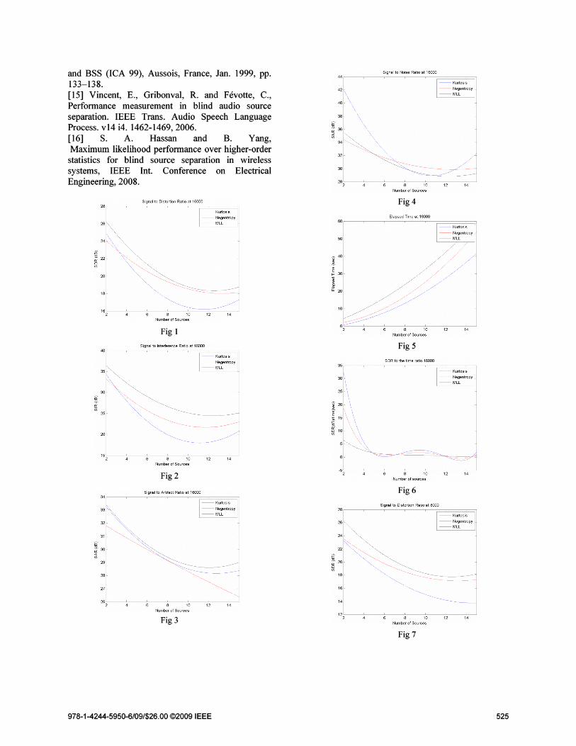
The results are summarized in Figures (1-6)the curves for the performance at 16000sample/source and Figures (7-12) the curves for theperformance at 8000 sample/source.

7. Results

The performance of the selected three algorithmsshows that:

a) When the number of samples per source is large

1. The ML algorithm has a better SDR thanNegentropy, which is better than Kurtosis.

2. The ML algorithm has a better SIR thanNegentropy, which is better than Kurtosis.

3. The ML algorithm has a better SAR thanNegentropy, which is better than Kurtosis.

b) When the number of samples per source is small

1. The Negentropy algorithm has a better SDRthan ML, which is better than Kurtosis.

2. The Negentropy algorithm has a better SIRthan ML, which is better than Kurtosis.

3. The Negentropy algorithm has a better SARthan ML, which is better than Kurtosis.

While

4. For the SNR the three algorithms areapproximately the same and in some casethe kurtosis shows a better performance.

5. The Kurtosis algorithm takes a less timewith respect to the other two algorithms andthe ML algorithm is the slower one.

6. The Kurtosis has the best SDR/Time ratiofor all case at small number of sources,while the Negentropy is better than ML. Butin high number of sources the threeapproximately has close performance.

7. All algorithms failed in separating thesources if the number of samples is 1000 orless.

978-1-4244-5950-6/09/$26.00 ©2009 IEEE

The algorithms were tested for other types of signals(stationary signals e.g. sawtooth, sin wave, squarewav, ... ). They succeeded in separating sourcesignals of stationary pdf if the number of samples persignals is less than 1000 samples. This means that thetype of data plays a fundamental role in theevaluation ofBSS.

8. The Hybrid Algorithm

Our previous study showed that the Kurtosisalgorithm is the fastest algorithm (its conversion tothe solution is faster than the other algorithms). Onthe other hand it has the worst accuracy among all ofthe algorithms. On the contrary, the searching for thesolution in the ML algorithm takes more time toconverge and produce the highest accuracy among allof the algorithms.

This motivates us to think about developinga hybrid approach that combine both of the ML withits accuracy and Kurtosis with its speed. The newhybrid algorithm will start the search for theunmixing matrix using the ML to put the searchprocess in its right direction. This means that the MLalgorithm will run for a fmite number of iterations.Then the kurtosis will complete the search to fme thefmal solution.

9. The Hybrid Algorithm's Performance

In order to evaluate the Hybrid, a 15 speech signalswere used. The signals are 8-bit with 2.5sec, sampledat 8khz and normalized. The instantaneous mixingmatrix is a square full rank random matrix. Differentmixing matrices are generated. Then we applied allalgorithms to each matrix. Finally we took theaverage of the results for each algorithm for allmixing matrices.

The BSS methods [Kurtosis, ML, and thehybrid] and the performance measure GUI-programare implemented using MATLAB 2006. Thesimulation is running on Pentium4, 3GHZ Computer.For each mixture and each algorithm, the(nonquantized) estimated sources were decomposedusing different allowed distortions and theperformance measures are computed. Also thealgorithm was run for different number of sourcesstarting from 2 sources till 15 sources. The hybridapproach started with the ML loop which runs for 15iterations then the kurtosis started to complete thesearching process.

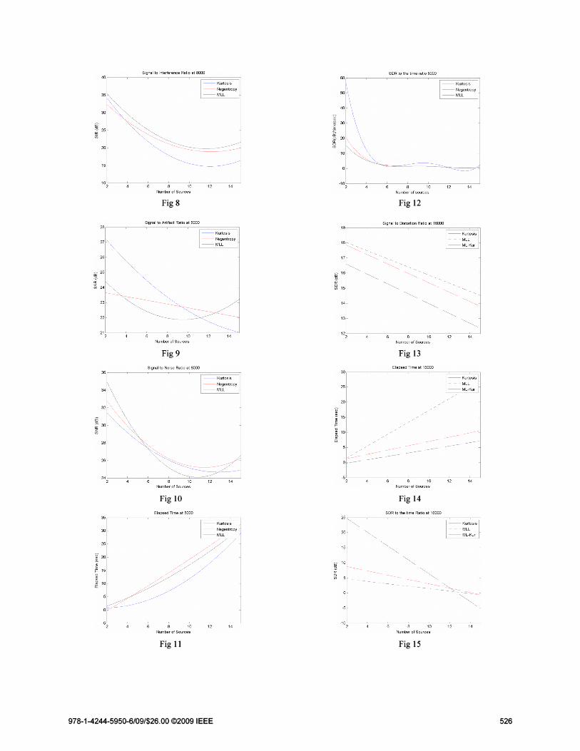
The results are summarized in Figures (13­15) the curves for the performance at 16000samples/source.

523

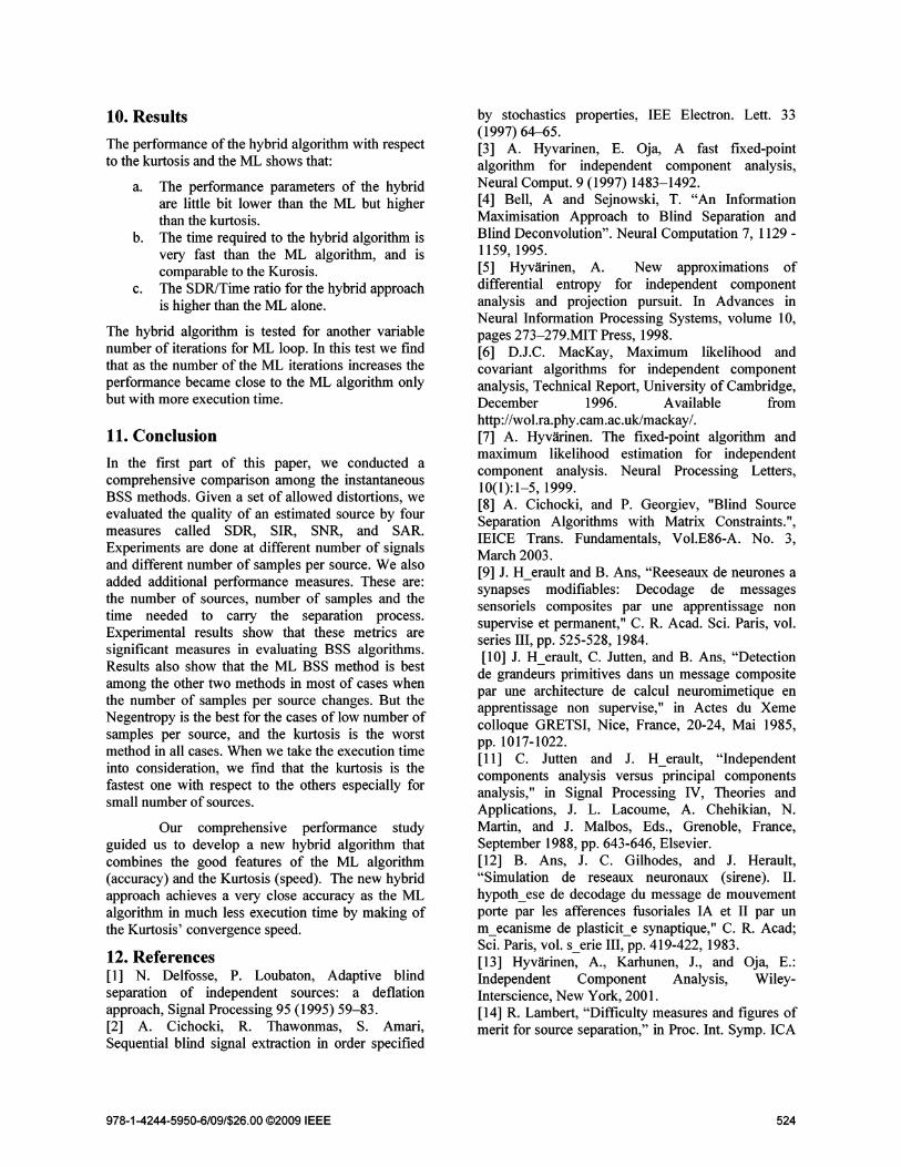
10. Results

The performance of the hybrid algorithm with respectto the kurtosis and the ML shows that:

a. The performance parameters of the hybridare little bit lower than the ML but higherthan the kurtosis.

b. The time required to the hybrid algorithm isvery fast than the ML algorithm, and iscomparable to the Kurosis.

c. The SDR/Time ratio for the hybrid approachis higher than the ML alone.

The hybrid algorithm is tested for another variablenumber of iterations for ML loop. In this test we findthat as the number of the ML iterations increases theperformance became close to the ML algorithm onlybut with more execution time.

11. Conclusion

In the first part of this paper, we conducted acomprehensive comparison among the instantaneousBSS methods. Given a set of allowed distortions, weevaluated the quality of an estimated source by fourmeasures called SDR, SIR, SNR, and SAR.Experiments are done at different number of signalsand different number of samples per source. We alsoadded additional performance measures. These are:the number of sources, number of samples and thetime needed to carry the separation process.Experimental results show that these metrics aresignificant measures in evaluating BSS algorithms.Results also show that the ML BSS method is bestamong the other two methods in most of cases whenthe number of samples per source changes. But theNegentropy is the best for the cases of low number ofsamples per source, and the kurtosis is the worstmethod in all cases. When we take the execution timeinto consideration, we fmd that the kurtosis is thefastest one with respect to the others especially forsmall number of sources.

Our comprehensive performance studyguided us to develop a new hybrid algorithm thatcombines the good features of the ML algorithm(accuracy) and the Kurtosis (speed). The new hybridapproach achieves a very close accuracy as the MLalgorithm in much less execution time by making ofthe Kurtosis' convergence speed.

12. References[1] N. Delfosse, P. Loubaton, Adaptive blindseparation of independent sources: a deflationapproach, Signal Processing 95 (1995) 59-83.[2] A. Cichocki, R. Thawonmas, S. Amari,Sequential blind signal extraction in order specified

978-1-4244-5950-6/09/$26.00 ©2009 IEEE

by stochastics properties, lEE Electron. Lett. 33(1997) 64-65.[3] A. Hyvarinen, E. OJa, A fast fixed-pointalgorithm for independent component analysis,Neural Comput. 9 (1997) 1483-1492.[4] Bell, A and Sejnowski, T. "An InformationMaximisation Approach to Blind Separation andBlind Deconvolution". Neural Computation 7, 1129 ­1159, 1995.[5] Hyvarinen, A. New approximations ofdifferential entropy for independent componentanalysis and projection pursuit. In Advances inNeural Information Processing Systems, volume 10,pages 273-279.MIT Press, 1998.[6] D.J.C. MacKay, Maximum likelihood andcovariant algorithms for independent componentanalysis, Technical Report, University of Cambridge,December 1996. Available fromhttp://wol.ra.phy.cam.ac.uk/mackay/.[7] A. Hyvarinen, The fixed-point algorithm andmaximum likelihood estimation for independentcomponent analysis. Neural Processing Letters,10(1):1-5, 1999.[8] A. Cichocki, and P. Georgiev, "Blind SourceSeparation Algorithms with Matrix Constraints.",IEICE Trans. Fundamentals, VoI.E86-A. No.3,March 2003.[9] J. H_erault and B. Ans, "Reeseaux de neurones asynapses modifiables: Decodage de messagessensoriels composites par une apprentissage nonsupervise et permanent," C. R. Acad. Sci. Paris, vol.series III, pp. 525-528, 1984.[10] J. H_erault, C. Jutten, and B. Ans, "Detection

de grandeurs primitives dans un message compositepar une architecture de calcul neuromimetique enapprentissage non supervise," in Actes du Xemecolloque GRETSI, Nice, France, 20-24, Mai 1985,pp. 1017-1022.[11] C. Jutten and J. H_erault, "Independentcomponents analysis versus principal componentsanalysis," in Signal Processing IV, Theories andApplications, J. L. Lacoume, A. Chehikian, N.Martin, and J. Malbos, Eds., Grenoble, France,September 1988, pp. 643-646, Elsevier.[12] B. Ans, J. C. Gilhodes, and J. Herault,"Simulation de reseaux neuronaux (sirene). II.hypoth_ese de decodage du message de mouvementporte par les afferences fusoriales IA et II par unmecanisme de plasticit_e synaptique," C. R. Acad;sci. Paris, vol. s erie III, pp. 419-422, 1983.[13] Hyvarinen. A., Karhunen, J., and OJa, E.:Independent Component Analysis, Wiley­Interscience, New York, 2001.[14] R. Lambert, "Difficulty measures and figures ofmerit for source separation," in Proc. Int. Symp. ICA

524

36

38

40

12 14

-- Kurtosis

-- Negentropy-- MLL

8 10Number of Sources

282:-----';---:-----';--_____,~-__;':_-_____,c_:_-.J

30

32

44,-~--~-~--~r=====il

42

Signal to Noise Ratio at 16000

34

and BSS (lCA 99), Aussois, France, Jan. 1999, pp.133-138.[15] Vincent, E., Gribonval, R. and Fevotte, C.,Performance measurement in blind audio sourceseparation. IEEE Trans. Audio Speech LanguageProcess. v14 i4. 1462-1469,2006.[16] S. A. Hassan and B. Yang,Maximum likelihood performance over higher-orderstatistics for blind source separation in wirelesssystems, IEEE Int. Conference on ElectricalEngineering, 2008.

Signal to Distortion Ratio at 16000

28,-~--~-~--~r====r::::::;lFig 4

26

-- Kurtosis

-- Negentropy--MLL

50

40

Elapsed Time at 16000

-- Kurtosis

-- Negentropy

-- MLL

20 30

1820

8 10Number of Sources

Fig 1

12 14

8 10Number of Sources

12 14

1412

-- Kurtosis

-- Negentropy

-- MLL

8 10Number of sources

Fig 5

SDR to the time ratio 16000

-5:-2--:-----';---:----;':-------,~----;-;-----'

30

35,-~-~-~--~r====::::;l

1412

-- Kurtosis

-- Negentropy--MLL

Fig 2

8 10Number of Sources

Signal to Interference Ratio at 16000

20

25

30

35

-- Kurtosis--Negentropy

-- MLL

Signal to Distortion Ratio at 8000

20

22

24

26

28,-~-~--~-~r===='il

Fig 6

18

--Kurtosis

-- Negentropy--MLL

Signal to Artifact Ratio at 16000

341-~-~----r=======il

27 16

14128 10Number of Sources

14

122L--~--~-~--~-~--~-.J

14128 10Number of Sources

262';-----:--_____,:-----';--_____;~-__;':_-_____;C;_____'

Fig 3

Fig 7

978-1-4244-5950-6/09/$26.00 ©2009 IEEE 525

Signal to Interference Ratio at 8000 SDR to the time ratio 8000

20

30

-- Kurtosis

-- Negentropy-- MLL

601-~-~-~-~r===='il-- Kurtosis

-- Negentropy-- MLL

401-~-~-~--~r====:::;l

35

15

141210Number of sources

-102!c-- --c- - -:;-- - -:c-- - -:;;-- ---,;';;-- --;':--'

14128 10Number of Sources

Fig 8 Fig 12

Signal to Artifact Ratio at 8000 Signal to Distortion Ratio at 16000

1412

I

Kurtosis- - - MLL

-- ML-Kur

8 10Number of Sources

191-~-~--~-~-r===_==='il

::112

2',---~--~--o_-~o_-___,L--~---'

12 14

-- Kurtosis

-- Negentropy-- MLL

8 10Number of Sources

26

22

23

27

CD 25

"c:;':.i 24

Fig 9 Fig 13

Signal to Noise Ratio at 8000 Elapsed Time at 16000

-- Kurtosis

-- Negentropy-- MLL 1

- - KurtosiS

- - - MLL

-- ML-Kur

14128 10Number of Sources

25

20

14128 10Number of Sources

36

34

32

0;

~,i 30

28

26

242

Fig 10 Fig 14

I

Kurtosis- - - MLL

-- ML-Kur

SDR to the time Ratio at 16000

25~

20 "<,-- Kurtosis

-- Negentropy-- MLL

Elapsed Time at 8000

30

35,-~-~-~-~r====~

-5

1525

~ 15

ii~ 10W

141210Number of Sources

-102o---~--~--_c_---'-:---7---,--~-'141210

Number of Sources

-52L--~--~--~--_7_--7--~-,--..J

Fig 11 Fig 15

978-1-4244-5950-6/09/$26.00 ©2009 IEEE 526