implementation of pipelined fft processor on fpga
TRANSCRIPT
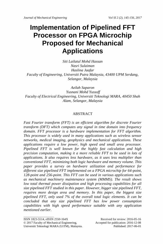
Journal of Mechanical Engineering Vol SI 2 (2), 145-156, 2017
____________________ ISSN 1823-5514, eISSN 2550-164X Received for review: 2016-05-16
© 2017 Faculty of Mechanical Engineering, Accepted for publication: 2016-12-08
Universiti Teknologi MARA (UiTM), Malaysia. Published: 2017-06-01
Implementation of Pipelined FFT Processor on FPGA Microchip
Proposed for Mechanical Applications
Siti Lailatul Mohd Hassan
Nasri Sulaiman
Haslina Jaafar
Faculty of Engineering, Universiti Putra Malaysia, 43400 UPM Serdang,
Selangor, Malaysia
Azilah Saparon
Yusnani Mohd Yussoff
Faculty of Electrical Engineering, Universiti Teknologi MARA, 40450 Shah
Alam, Selangor, Malaysia
ABSTRACT
Fast Fourier transform (FFT) is an efficient algorithm for discrete Fourier
transform (DFT) which computes any signal in time domain into frequency
domain. FFT processor is a hardware implementation for FFT algorithm.
This processor is widely used in many applications such as wireless sensor
networks, medical imaging, geophysics and mechanical applications. These
applications require a low power, high speed and small area processor.
Pipelined FFT is well known for the highly fast calculation and high
precision computation, making it a more reliable FFT to be used in lots of
applications. It also requires less hardware, as it uses less multiplier than
conventional FFT, minimizing both logic hardware and memory volume. This
paper provides a survey on hardware utilization and performance for
different size pipelined FFT implemented on a FPGA microchip for 64-point,
128-point and 256-point. This FFT can be used in various applications such
as mechanical machinery maintenance system (MMMS). The result shows
low total thermal power dissipation and high processing capabilities for all
size pipelined FFT studied in this paper. However, bigger size pipelined FFT,
requires more design area and memory. In this paper, the biggest size
pipelined FFT, only used 7% of the overall total logic elements. It can be
concluded that any size pipelined FFT has low power consumption
capabilities with high speed performance suitable with any application
mentioned earlier.
Siti Lailatul Mohd Hassan et. al.
146
Keywords: DFT, Pipelined FFT, FPGA, Low Power Dissipation
Introduction
In 1965, Cooley and Tukey published a more general version of FFT
algorithm, which had become a popular algorithm, used up till now. In 1960s,
the algorithm was only based on software. It is almost impossible to do the
hardware implementation. However, as semiconductor technology flourishes,
other technology such as System-on-Chip (SoC) also evolves, making it
possible to perform the FFT algorithms in hardware forms. Recently,
applications on portable systems such as the wireless sensor networks,
portable hand-held medical and mechanical sensors, had pushed the FFT
processor power consumption to be the most critical design requirements.
Generally, FFT processor can be classified into three main categories;
column FFT, fully parallel FFT and pipelined FFT [3-4]. Pipelined FFT is
more widely used because of the low power consumption and also high
throughput [5].
This paper proposed a pipelined FFT processor implemented on
FPGA microchip for various applications including mechanical system. A
mechanical machinery maintenance system (MMMS) is an example of
mechanical application using FFT. This system is used in maintenance of
machinery. In the past, when talking about maintenance, it usually involves
breakdown maintenance or post-maintenance. These types of maintenances
reduced the revenue and production reliability, more downtime, and higher
repair costs. However, if early detection of faults can be monitored, it will
help to schedule related activities, reducing downtime and losses. One of the
most common used predictive maintenances is vibration analysis. By
studying the vibration of a machine, it is possible to predict the machine
failure in advance. Faulty machine produces characteristic vibration at
different frequencies, indicating specific machine fault conditions. Some
typical faults in machine are unbalance, misalignment, and looseness [6-8].
Figure 1 shows the basic flow diagram of the vibration sensing used in
this system. Basically it has two parts, the instrumentation system for
vibration signal acquisition such as accelerometer and the processing unit,
where FFT is the main component to identify natural frequencies of
mechanical system. [9] Usually, accelerometer is used as sensor. It converts
mechanical motion into voltage which corresponds to the surface
acceleration. Voltage from the accelerometer is then sampled and analysed in
time domain. Using FFT in the processing unit, signal in time domain is
converted to frequency domain. This is to get more understanding on the
vibration characteristics, between normal and faulty operation modes. [6]

Implementation of Pipelined FFT Processor on FPGA Microchip
147
Depending on the application, data from his vibration sensing is analyzed to
get the output diagnostic algorithm and be alarm when there are changes.
Data
AnalysisAccelerometer
Processing
FFT
Time-
Frequency
AnalysisVibration
Acceleration
Figure 1: Basic flow diagram of the vibration sensing used in MMMS
The acceleration data from accelerometer is collected in time domain
signal and it is represented in sine wave form, with all the frequencies and
amplitude combined. However, it is difficult to study the vibration fault in a
mechanical structure in time domain form. It is necessary to process the data
in time domain and then to convert it to the frequency domain for spectrum
analysis. This is simply done by applying an FFT. In FFT, each individual
amplitude and frequency can be displayed, making it easier to study and
analyze a repetitive signal. [9]
This paper presents an analysis on hardware utilization and
performance of different points ranging from 16 to 256 pipelined FFT
processor.
Implementation of Pipelined FFT on FPGA Chip
This section explains the design features and implementation of pipelined
FFT on FPGA microchip.
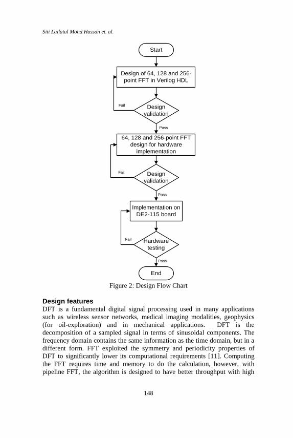
Design flow chart In general, the project design can be divided into two phases. The first phase
is to design 64, 128 and 256-point pipelined FFT in Verilog HDL. For design
validation, the design synthesis and functionality are checked. If the
validation failed, modifications are performed on the FFTs. The second phase
of the project is the hardware implementation. All the modules in pipelined
FFTs are compiled and the performance analysis is checked. Once there is no
error in the design, the pipelined FFTs are downloaded into the DE2-115
board for hardware testing.
Siti Lailatul Mohd Hassan et. al.
148
Start
Design of 64, 128 and 256-
point FFT in Verilog HDL
Design
validation
64, 128 and 256-point FFT
design for hardware
implementation
Design
validation
Implementation on
DE2-115 board
Hardware
testing
End
Pass
Fail
Fail
Pass
Pass
Fail
Figure 2: Design Flow Chart
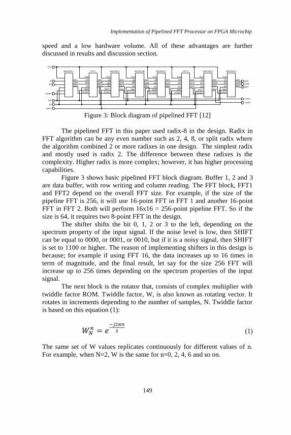
Design features DFT is a fundamental digital signal processing used in many applications
such as wireless sensor networks, medical imaging modalities, geophysics
(for oil-exploration) and in mechanical applications. DFT is the
decomposition of a sampled signal in terms of sinusoidal components. The
frequency domain contains the same information as the time domain, but in a
different form. FFT exploited the symmetry and periodicity properties of
DFT to significantly lower its computational requirements [11]. Computing
the FFT requires time and memory to do the calculation, however, with
pipeline FFT, the algorithm is designed to have better throughput with high
Implementation of Pipelined FFT Processor on FPGA Microchip
149
speed and a low hardware volume. All of these advantages are further
discussed in results and discussion section.
DOI
DOR
RDY
BUFFER 1
CLK
DII
DIR
ED
RST
START
DOI
DOR
RDY
FFT 1
CLK
DI
DR
ED
SHIFT
START
DOI
DOR
RDY
SHIFTER 1
CLK
DI
ED
RST
START
DOI
DOR
RDY
ROTATOR
DR
CLK
DI
DR
ED
RST
START
DOI
DOR
RDY
BUFFER 2
CLK
DII
DIR
ED
RST
START
DOI
DOR
RDY
FFT 2
CLK
DI
DR
ED
SHIFT
START
DOI
DOR
RDY
SHIFTER 2
CLK
DI
DR
ED
RST
START
DOI
DOR
RDY
BUFFER 3
OVF OVF
CLK
DI
DR
ED
RSTOVF1
OVF2
DOI
DOR
RDY
START
SHIFT Figure 3: Block diagram of pipelined FFT [12]
The pipelined FFT in this paper used radix-8 in the design. Radix in
FFT algorithm can be any even number such as 2, 4, 8, or split radix where
the algorithm combined 2 or more radixes in one design. The simplest radix
and mostly used is radix 2. The difference between these radixes is the
complexity. Higher radix is more complex; however, it has higher processing
capabilities.
Figure 3 shows basic pipelined FFT block diagram. Buffer 1, 2 and 3
are data buffer, with row writing and column reading. The FFT block, FFT1
and FFT2 depend on the overall FFT size. For example, if the size of the
pipeline FFT is 256, it will use 16-point FFT in FFT 1 and another 16-point
FFT in FFT 2. Both will perform 16x16 = 256-point pipeline FFT. So if the
size is 64, it requires two 8-point FFT in the design.
The shifter shifts the bit 0, 1, 2 or 3 to the left, depending on the
spectrum property of the input signal. If the noise level is low, then SHIFT
can be equal to 0000, or 0001, or 0010, but if it is a noisy signal, then SHIFT
is set to 1100 or higher. The reason of implementing shifters in this design is
because; for example if using FFT 16, the data increases up to 16 times in
term of magnitude, and the final result, let say for the size 256 FFT will
increase up to 256 times depending on the spectrum properties of the input
signal.
The next block is the rotator that, consists of complex multiplier with
twiddle factor ROM. Twiddle factor, W, is also known as rotating vector. It
rotates in increments depending to the number of samples, N. Twiddle factor
is based on this equation (1):
𝑊𝑁𝑛 = 𝑒
−𝑗2𝜋𝑛
2 (1)
The same set of W values replicates continuously for different values of n.
For example, when N=2, W is the same for n=0, 2, 4, 6 and so on.
Siti Lailatul Mohd Hassan et. al.
150
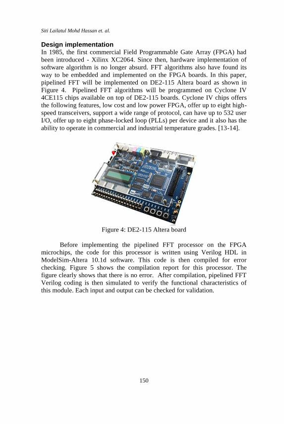
Design implementation In 1985, the first commercial Field Programmable Gate Array (FPGA) had
been introduced - Xilinx XC2064. Since then, hardware implementation of
software algorithm is no longer absurd. FFT algorithms also have found its
way to be embedded and implemented on the FPGA boards. In this paper,
pipelined FFT will be implemented on DE2-115 Altera board as shown in
Figure 4. Pipelined FFT algorithms will be programmed on Cyclone IV
4CE115 chips available on top of DE2-115 boards. Cyclone IV chips offers
the following features, low cost and low power FPGA, offer up to eight high-
speed transceivers, support a wide range of protocol, can have up to 532 user
I/O, offer up to eight phase-locked loop (PLLs) per device and it also has the
ability to operate in commercial and industrial temperature grades. [13-14].
Figure 4: DE2-115 Altera board
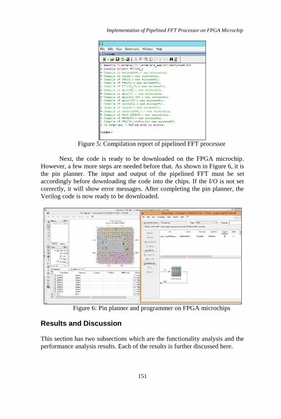
Before implementing the pipelined FFT processor on the FPGA
microchips, the code for this processor is written using Verilog HDL in
ModelSim-Altera 10.1d software. This code is then compiled for error
checking. Figure 5 shows the compilation report for this processor. The
figure clearly shows that there is no error. After compilation, pipelined FFT
Verilog coding is then simulated to verify the functional characteristics of
this module. Each input and output can be checked for validation.
Implementation of Pipelined FFT Processor on FPGA Microchip
151
Figure 5: Compilation report of pipelined FFT processor
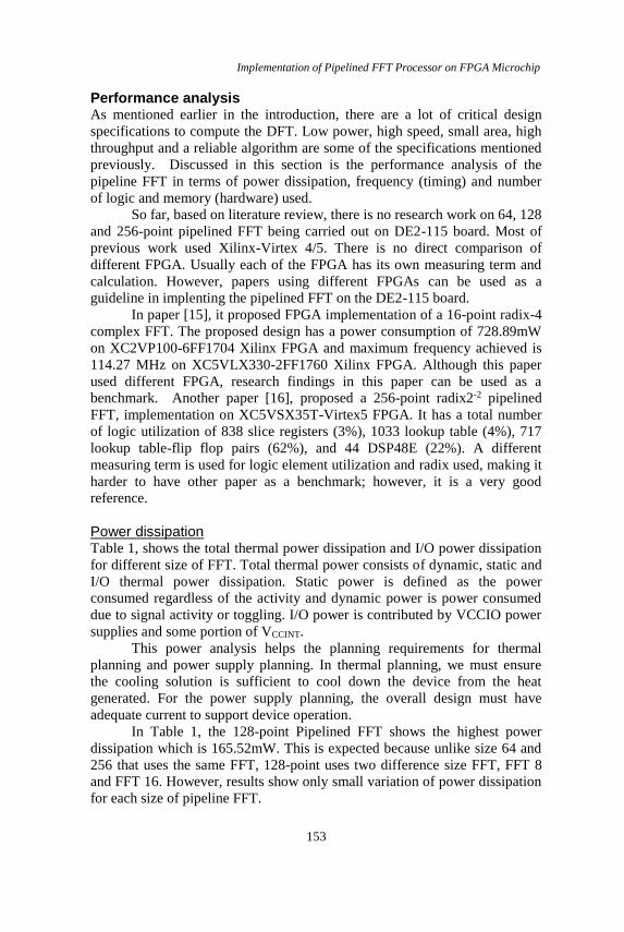
Next, the code is ready to be downloaded on the FPGA microchip.
However, a few more steps are needed before that. As shown in Figure 6, it is
the pin planner. The input and output of the pipelined FFT must be set
accordingly before downloading the code into the chips. If the I/O is not set
correctly, it will show error messages. After completing the pin planner, the
Verilog code is now ready to be downloaded.
Figure 6: Pin planner and programmer on FPGA microchips
Results and Discussion
This section has two subsections which are the functionality analysis and the
performance analysis results. Each of the results is further discussed here.

Siti Lailatul Mohd Hassan et. al.
152
Functionality analysis Each of the inputs data and outputs data are monitored and investigated.
Figure 7 shows the example of input data (DR and DI) and output data (DOR
and DOI) of 256-point pipelined FFT. The figure also shows the other input
signals for the system such as the clock (CLK), start (START), reset (RST),
and enable (ED). Clock signal used in this analysis is global clock, and each
result is synthesized in one clock cycle. START can be generated once before
the operation for global synchronization. The input data starts after the falling
edge of START signal. The RST signal will restart the whole pipelined FFT
operation when set to ‘high’. Lastly, the ED signal controls the throughput of
the pipelined FFT. The input data are sampled when ED is ‘high’ and on the
rising clock edge.
Figure 7: Example of 256-point pipelined FFT input and output
The inputs data (DR and DI) are generated using the Matlab. These
generated input data are then transformed using a defined FFT function in the
Matlab, producing the FFT output. The inputs data is then given to the
pipelined FFT processor written in Verilog code. These outputs (DOR and
DOI) obtained from the Verilog simulation is then compared to the Matlab
output. For example, from the result obtained from Matlab simulation, DOR
is equal to F87C and DOI is F8C9. Both are negative numbers. The output of
Verilog simulation from the same input is DOR equal to FEF9 and DOI equal
to FEFE. Both of these values are also negative values. Although the value is
not similar, it is the correct output based on the polarity (negative or positive)
values of the results, confirming the functionality of this FFT processor
module. This is expected in Verilog as, the data will go through several
modules; however, in Matlab, the data will only pass through one big
module.
Implementation of Pipelined FFT Processor on FPGA Microchip
153
Performance analysis As mentioned earlier in the introduction, there are a lot of critical design
specifications to compute the DFT. Low power, high speed, small area, high
throughput and a reliable algorithm are some of the specifications mentioned
previously. Discussed in this section is the performance analysis of the
pipeline FFT in terms of power dissipation, frequency (timing) and number
of logic and memory (hardware) used.
So far, based on literature review, there is no research work on 64, 128
and 256-point pipelined FFT being carried out on DE2-115 board. Most of
previous work used Xilinx-Virtex 4/5. There is no direct comparison of
different FPGA. Usually each of the FPGA has its own measuring term and
calculation. However, papers using different FPGAs can be used as a
guideline in implenting the pipelined FFT on the DE2-115 board.
In paper [15], it proposed FPGA implementation of a 16-point radix-4
complex FFT. The proposed design has a power consumption of 728.89mW
on XC2VP100-6FF1704 Xilinx FPGA and maximum frequency achieved is
114.27 MHz on XC5VLX330-2FF1760 Xilinx FPGA. Although this paper
used different FPGA, research findings in this paper can be used as a
benchmark. Another paper [16], proposed a 256-point radix2-2 pipelined
FFT, implementation on XC5VSX35T-Virtex5 FPGA. It has a total number
of logic utilization of 838 slice registers (3%), 1033 lookup table (4%), 717
lookup table-flip flop pairs (62%), and 44 DSP48E (22%). A different
measuring term is used for logic element utilization and radix used, making it
harder to have other paper as a benchmark; however, it is a very good
reference.
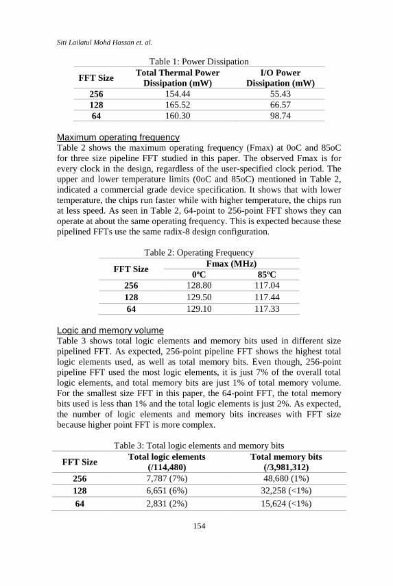
Power dissipation Table 1, shows the total thermal power dissipation and I/O power dissipation
for different size of FFT. Total thermal power consists of dynamic, static and
I/O thermal power dissipation. Static power is defined as the power
consumed regardless of the activity and dynamic power is power consumed
due to signal activity or toggling. I/O power is contributed by VCCIO power
supplies and some portion of VCCINT.
This power analysis helps the planning requirements for thermal
planning and power supply planning. In thermal planning, we must ensure
the cooling solution is sufficient to cool down the device from the heat
generated. For the power supply planning, the overall design must have
adequate current to support device operation.
In Table 1, the 128-point Pipelined FFT shows the highest power
dissipation which is 165.52mW. This is expected because unlike size 64 and
256 that uses the same FFT, 128-point uses two difference size FFT, FFT 8
and FFT 16. However, results show only small variation of power dissipation
for each size of pipeline FFT.
Siti Lailatul Mohd Hassan et. al.
154
Table 1: Power Dissipation
FFT Size Total Thermal Power
Dissipation (mW)
I/O Power
Dissipation (mW)
256 154.44 55.43
128 165.52 66.57
64 160.30 98.74
Maximum operating frequency Table 2 shows the maximum operating frequency (Fmax) at 0oC and 85oC
for three size pipeline FFT studied in this paper. The observed Fmax is for
every clock in the design, regardless of the user-specified clock period. The
upper and lower temperature limits (0oC and 85oC) mentioned in Table 2,
indicated a commercial grade device specification. It shows that with lower
temperature, the chips run faster while with higher temperature, the chips run
at less speed. As seen in Table 2, 64-point to 256-point FFT shows they can
operate at about the same operating frequency. This is expected because these
pipelined FFTs use the same radix-8 design configuration.
Table 2: Operating Frequency
FFT Size Fmax (MHz)
0oC 85oC
256 128.80 117.04
128 129.50 117.44
64 129.10 117.33
Logic and memory volume Table 3 shows total logic elements and memory bits used in different size
pipelined FFT. As expected, 256-point pipeline FFT shows the highest total
logic elements used, as well as total memory bits. Even though, 256-point
pipeline FFT used the most logic elements, it is just 7% of the overall total
logic elements, and total memory bits are just 1% of total memory volume.
For the smallest size FFT in this paper, the 64-point FFT, the total memory
bits used is less than 1% and the total logic elements is just 2%. As expected,
the number of logic elements and memory bits increases with FFT size
because higher point FFT is more complex.
Table 3: Total logic elements and memory bits
FFT Size Total logic elements
(/114,480)
Total memory bits
(/3,981,312)
256 7,787 (7%) 48,680 (1%)
128 6,651 (6%) 32,258 (<1%)
64 2,831 (2%) 15,624 (<1%)
Implementation of Pipelined FFT Processor on FPGA Microchip
155
Conclusion
In conclusion, pipelined FFT processor implementation on microchip FPGA
is a promising solution to any portable applications using FFT. This is
because FPGA is a programmable chip which can be programmed to be 64,
128, 256 and any other higher point. The results show low thermal power
dissipation, good operating frequency for low and high temperature limit and
total logic elements and memory bits used are small.
References
[1] P. Augusta Sophy, “Analysis and design of low power radix-4 FFT
processor using pipelined architecture,” International Conference on
Computing and Communication Technologies (Feb 2015).
[2] Swanpnil Badar et al., “High speed FFT processor design using radix -
4 pipelined architecture,” International Conference on Industrial
Instrumentation and Control (May 2015).
[3] T. Arslan et al., “Low Power Commutator for Pipelined FFT
Processors,” IEEE International Symposium on Circuits and Systems
(2005).
[4] P. J Hong et al., “Design of a reconfigureble FFT processor using
multi-objective genetic algorithm,” International Conference on
Intelegent and Advance Systems (2010).
[5] Zhuo Qian et al., “Low-Power Split-Radix FFT Processors Using
Radix-2 Butterfly Units,” IEEE Transactions on Very Large Scale
Integration (VLSI) Systems (Apr 2016).
[6] Giovanni Betta et Aal., “A DSP-based FFT-analyzer for the Fault
Diagnosis of Rotating Machine Based on Vibration Analysis,” IEEE
Instrumentation and Measurement Technology Conference (Budapest
Hungary, May 2001).
[7] A.M. Patil et al., “Vibration Analysis of Bearing Using FFT
Analyzer,” International Journal of Advanced Technology in
Engineering and Science, Vol. 02, Issue No. 04 (April 2014).
[8] S.S. Mahadik et al., “Equipment Performance Improvement using
Condition Based Maintenance through Vibration Analysis in Sugar
Plant,” International Journal of Advanced Engineering Technology,
134-136, (2012).
[9] J P A mezquita-Sanchez et al., “Determination of system frequencies
in mechanical systems during shutdown transient,” Journal of
Scientific & Industrial Research, Vol. 69, pp. 415-421 (June 2010).
[10] Vinay Kumar M et al., “Area and Frequency optimized 1024-point
Radix-2 FFT Processor on FPGA,” International Conference on VLSI
Systems, Architecture, Technology and Applications (2015).
Siti Lailatul Mohd Hassan et. al.
156
[11] Senthil Sivakumar M et al., “Design of low power FFT processors
using multiplier less architecture,” ARPN Journal of Engineering and
Applied Sciences, Vol.10, No.11 (June 2015).
[12] Oleg Uzenkov et al., “Pipelined FFT/IFFT 256 points processor:
Overview,” OpenCores.org (2014).
[13] M. Khalil et al, “Design and Implementation of FFT/IFFT System
Using Embedded Design Techniques,” International Journal of
Engineering and Innovative Technology (IJEIT), Vol. 3, Issue 6 (Dec
2013).
[14] Z. Qian et al., “A novel low-power and in-place split-radix FFT
processor,” Proceedings of the @4th edition of the great lakes
symposium on VLSI – GLSVLSI’14 (2014).
[15] Abhishek Mankar et al., “FPGA Impelmentation of 16-Point Radix-4
Complex FFT Core using NEDA” 2013 Students Conference on
Engineering and Systems (2013).
[16] Ahmed Saeed et al., “FPGA implementation of Radix-22 Pipelined
FFT Processor”, Proceedings of the 8th WSEAS International
Conference on Signal Processing FPGA (2009).